FIL COR LL UIAD AD-A22 4 249 DE006

Technical Report ARFSD-TR-90003

IP-POSITION CONTROL OF A FLEXIBLE BEAM: MODELINGAPPROACHES AND EXPERIMENTAL VERIFICATION

M. MatticeN. Coleman

rLECTPtiject Engineers

qJUL 10 1990AREsco K. Craig-Department of Mechanical Engineering

J Aeronautical Engineering and MechanicsRensselaer Polytechnic Institute

Troy, NY 12180-3590

June 1990

U.S. ARMY ARMAMENT RESEARCH, DEVELOPMENT AND

ENGINEERING CENTER

Fire Support Armaments Center

ARM"MTMU~MONS PctnyArsenal, N~ew Jersey

Approved for public release; distribution unlimited.

07gO0O1

I INCI ARIFIFf'SECURITY CLASSIFICATION OF THIS PAGE

REPORT DOCUMENTATION PAGEla. REPORT SECURITY CLASSIFICATION 1b. RESTRICTIVE MARKINGS

UNCLASSIFIED2. SECURITY CLASSIFICATION AUTHORITY 3. DISTRIBUTION/AVAILABILITY OF REPORT

2h. DECLASSIFICATION/DOWNGRADING SCHEDULE Approved for public release; distribution is unlimited.

4. PERFORMING ORGANIZATION REPORT NUMBER 5. MONITORING ORGANIZATION REPORT NUMBERTechnical Report ARFSD-TR-90003

6a. NAME OF PERFORMING ORGANIZATION 6b. OFFICE SYMBOL 7a. NAME OF MONITORING ORGANIZATIONARDEC, FSAC (cont) SMCAR-FSF-RC

6c. ADDRESS (CITY, STATE, AND ZIP CODE) 7b. ADDRESS (CITY, STATE, AND ZIP CODE)Fire Control DivisionPicatinny Arsenal, NJ 07806-5000 (cont)

Bs. NAME OF FUNDING/SPONSORING 8b. OFFICE SYMBOL 9. PROCUREMENT INSTRUMENT IDENTIFICATION NUMBERORGANIZATION ARDEC, IMDSTINFO Br. I SMCAR-IMI-I

Sc. ADDRESS (CITY, STATE, AND ZIP CODE) 10. SOURCE OF FUNDING NUMBERSPROGRAM PROJECT NO. ITASK NO. WORK UNIT

Picatinny Arsenal, NJ 07806-5000 ELEMENT NO. ACCESSION NO.

11. TITLE (INCLUDE SECURITY CLASSIFICATION)

TIP-POSITION CONTROL OF A FLEXIBLE BEAM: MODELING APPROACHES AND EXPERIMENTALVERIFICATION

12. PERSONAL AUTHOR(S)K. Craig, Rensselaer Polytechnic Institute and M. Matlice and N. Coleman, Project Engineers, ARDEC

13s. TYPE OF REPORT 13b. TIME COVERED 14. DATE OF REPORT (YEAR, MONTH, DAY 15. PAGE COUNT

Interim FROM .Sp8& TO Sp. June 1990 6316. SUPPLEMENTARY NOTATION

17. COSATI CODES 18. SUBJECT TERMS (CONTINUE ON REVERSE IF NECESSARY AND IDENTIFY BY BLOCK NUMBER)FIELD GROUP SUB-GROUP. , Equations of motion, Finite element analysis Open oop transfer functions,I jReduced order model Lumped parameter model,

19. ABSTRACT (CONTINUE ON REVERSE IF NECESSARY AND IDENTIFY BY BLOCK NUMBER)- This report represents the dynamic modeling part of an experimental/theoretical effort to develop and test

pointing and tracking control techniques for a mechanical system containing both rigid and flexible bodies.Recently much work has been done to model open-oop chains of rigid and elastic bodies with applicationto kinematic linkages, spacecraft, and manipulators.

/

20. DISTRIBUTION/AVAILABILITY OF ABSTRACT 21. ABSTRACT SECURITY CLASSIFICATION

[Q] UNCLASSIFIED/UNLIMITED [] SAME AS RPT. DTIC USERS UNCLASSIFIED22.. NAME OF RESPONSIBLE INDIVIDUAL 22b. TELEPHONE (INCLUDE AREA CODE) 22c. OFFICE SYMBOL

I. HAZNEDARI (201) 724-3316 SMCAR-IMI-l

DD FORM 1473, 84 MARUNCLASSIFIED

SECURITY CLASSIFICATION OF THIS PAGE

6a. (cont)

Department of Mechanical Engineering

6c. (cont)

Aeronautical Engineering and MechanicsRensselaer Polytechnic InstituteTroy, NY 12180-3590

ACCesio! For

NTIS CRA&

DIIC TAB 0UlvJ'nno ' ,celJ1JStlfiC3t: -:f,

Distribtion !

Av-0a;Iiiry C'des \

Dist Special

X-1

CONTENTS

Page

Introduction 1

Experimental Apparatus 2

Dynamic Modelling 2

Model Description and Derivation of Equations of Motion 2Exact Solution and Open-Loop Transfer Functions 5Reduced-Order Model with Cantilevered Modes 8Finite Element Analysis 11Lumped Parameter Model 12Reduced-Order Model with System Modes A13Complete Model of Electromechanical System and 15

Experimental VerificationConclusions :16

Appendixes

A Rigid Disk and Flexible Beam: Exact Open-Loop Transfer Functions 27and Reduced-Order Models of the Open-Loop Transfer Functions

B Reduced-Order Model of Rigid Disk/Flexible Beam System 35with Cantilevered Modes

C Finite Element Analysis of Rigid Disk/Flexible Beam System 39

D Reduced-Order Model of Rigid Disk - Flexible Beam with 43System Modes

E State-Space Formulation of Equations of Motion for Reduced-Order 49Model of Rigid Disk - Flexible Beam System with System Modes

F Complete Equations of Motion in State-Space Form for the Electro- 53mechanical System

Distribution List 59

THIS DOCUMENT CONTAINEDBLANK PAGES THAT HAVE

BEEN DELETED

FIGURES

Page

1 Experimental apparatus 19

2 Dynamic analysis of a flexible beam attached to a rigid rotor with variable 20radius

3 Dynamic analysis of a flexible beam attached to a rigid rotor with variable 21inertia

4 Results from exact analysis 22

5 Results from reduced-order model with cantilevered modes 23

6 Results from finite element analysis model 24

7 Results from reduced-order model with system modes 25

8 Open loop response to sine input 26

9 Open loop response to triangle input 26

10 Triangle input 26

11 MATRIX model for simulation 26

ii

INTRODUCTION

The dynamic modeling part of an experimental/theoretical effort to develop andtest pointing and tracking control techniques for a mechanical system containing bothrigid and flexible bodies is presented in this report. Recently, much work was done tomodel open-loop chains of ridig and elastic bodies with application to kinematiclinkages, spacecraft, and manipulators.

In this modelling effort, the work of Schmitz1 was used as a guide. The mechani-cal system consisted of a flexible beam fixed to a rigid disk and rotating in the horizontalplane. The new contributions that result from this work are: (1) the inclusion of the size(the radius of the rigid disk) as well as the mass properties of the rigid moving base inderiving the equations of motion, (2) the study of the effect of the size of the movingrigid base on the dynamic response of the system, and (3) the development and com-parison of several modelling approaches which can be used for control design: areduced-order model with cantilever modes, a reduced-order model with system modes,a model based on finite element analysis, and a lumped parameter model.

The computer software used for this work was: MSC Pal2 (finite elementanalysis), MATRIXx (dynamic analysis and control design), and MathCAD(multipurpose engineering software). The book of Meirovitch 2 was referred to oftenduring the course of this work.

Work currently engaged in is: (1) completion of model validation, including studyof the effects of Coulomb and viscous damping; (2) development and testing of several

control algorithms: PID, LQG/LTR, adaptive and HO; and (3) addition of an end-pointposition sensor to the experimental apparatus to allow for end-point position feedbackcontrol.

'Schmitz, E., "Experiments on the End-Point Position Control of a Very Flexible One-Link Manipulator," Ph.D. Thesis, Stanford University, Guidance and Control Laboratory,Department of Aeronautics and Astronautics, Stanford, CA, 1985.

2Meirovitch, L., Analytical Methods in Vibrations, The Macmillan Company, New York,1967.

EXPERIMENTAL APPARATUS

An experimental apparatus (fig 1) was built to demonstrate pointing and trackingcontrol strategies for fast-moving, lightweight, flexible appendages to rigid bodies. Itconsists of a one degree of freedom rigid disk, rotating about a vertical axis, with a long,thin, flexible beam fixed to it in the horizontal plane. Two dc torque motors, one usedfor disturbance input and one used for control, cause the disk to rotate about the verticalaxis. A resolver is used to measure disk angle, which is the only sensor on the systemat the present time. A beam end-point position sensor is presently being added to thesystem.

DYNAMIC MODELLING

Dynamic equations were developed for a mechanical system consisting of aflexible beam fixed to a rigid disk. Goals were to understand the fundamental charac-teristics of the system and to develop a model of the system which can be used to testnew control algorithms.

Model Description and Derivation of Equations of Motion

Consider a uniform flexible beam of length L, fixed to a rigid disk of radius R, andmoving in the horizontal plane, as shown in the figure below.

- Fixed Reference Line

u(t) J,R

- - --- -------------- - X

R i DFlexibleRigid Disk Fixed Attachment E,I,A,L,p Beam

u(t) = externally applied torqueJ = mass moment of inertia of rigid disk about axis of rotationR = radius of rigid diskE = modulus of elasticity of beam materialI = area moment of inertia of beam cross section about neutral axisA = cross-sectional area of beamp = density of beam material a = p.A = mass per unit lengthL = length of beam

2

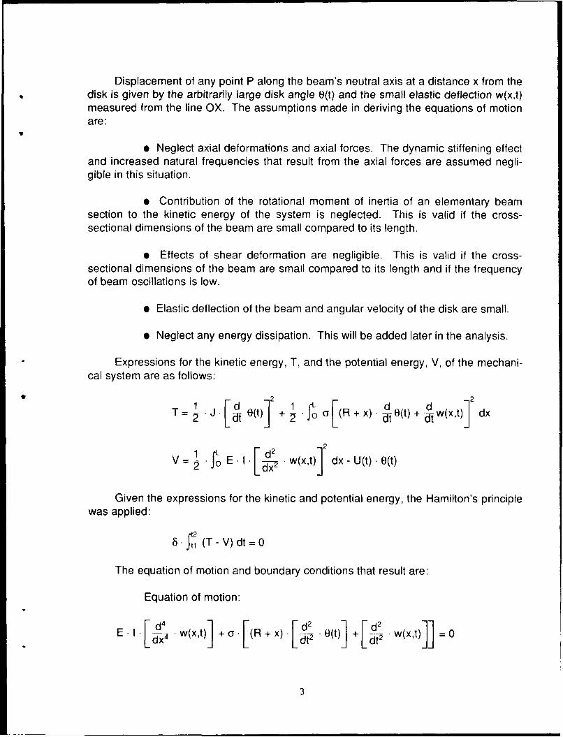
Displacement of any point P along the beam's neutral axis at a distance x from thedisk is given by the arbitrarily large disk angle 0(t) and the small elastic deflection w(x,t)measured from the line OX. The assumptions made in deriving the equations of motionare:

9 Neglect axial deformations and axial forces. The dynamic stiffening effectand increased natural frequencies that result from the axial forces are assumed negli-gible in this situation.

e Contribution of the rotational moment of inertia of an elementary beamsection to the kinetic energy of the system is neglected. This is valid if the cross-sectional dimensions of the beam are small compared to its length.

9 Effects of shear deformation are negligible. This is valid if the cross-sectional dimensions of the beam are small compared to its length and if the frequencyof beam oscillations is low.

* Elastic deflection of the beam and angular velocity of the disk are small.

* Neglect any energy dissipation. This will be added later in the analysis.

Expressions for the kinetic energy, T, and the potential energy, V, of the mechani-cal system are as follows:

1 (() 2 +2

T = a J e(t) + [ c (R + x). d O(t) + d w(x t)] dx-2~ E dt od tv = 1 L E. 2. w(x,t) ]2dx -Ut), O(t)

Given the expressions for the kinetic and potential energy, the Hamilton's principle

was applied:

f2 (T- V) dt = O

The equation of motion and boundary conditions that result are:

Equation of motion:

E-I. d .w(xt) +0. (R+x)- d[ .O(t)] +[ d .w(xt)]] =0

3

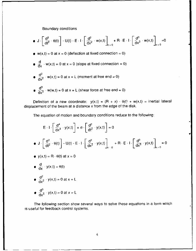
Boundary conditions

O . (t) -U(t) - E l I w(x,t) + R E .I w(xt) =01x=O --x x=O=

* w(x,t) = 0 at x = 0 (deflection at fixed connection = 0)

ddx& w(x,t) = O at x = 0 (slope at fixed connection =0)

* d-X •w(x,t) = 0 at x =L (moment at free end = 0)

d3

* a-ij w(w,t) = 0 at x = L (shear force at free end = 0)

Definition of a new coordinate: y(x,t) = (R + x) 0 0(t) + w(x,t) = inertial lateraldisplacement of the beam at a distance x from the edge of the disk.

The equation of motion and boundary conditions reduce to the following:

E.I. d-x .Y(X,t) +0. d y(xt) =0

S. J[d.O(t) U(t) - EI d. Y(xt) + R E I . Y(xt) =0

* y(x,t) = R • O(t) at x = 0

d• dil- 'y(x,t) =OMt

d 2

0 dx- .y(x,t)=0atx=L

d3

* cd-. y(xt)=0atx=L

The following section show several ways to solve these equations in a form whichis useful for feedback control systems.

4

Exact Solution and Open-Loop Transfer Functions

The variables y(x,s), u(s), and 0(s) are defined as the Laplace transforms of thevariables y(x,t), u(t), and 0(t), respectively. Taking the Laplace transform of the equa-tion of motion and boundary conditions, the following is obtained:

Equation of Motion

Boundary Conditions:

9 J.s 2 (s) .yxs) +R E.l.[sL EY(XS) =0xdX =0 d X (' 1=0 0

@ y(x,s) = R - (s)at x=0

d* d x "y(x,s) = (s) at x = 0

0 -x y(x,s)=0atx=L

d3* dx-.y(x,s)=0atx=L

The following dimensionless ratios are defined:

R JR= 8 L1 = 0

Note that o L = (o- L) -L2 = m. L2 where m is the total mass of the beam. The dimen-sionless complex number X related to the Laplace variable s is defined by:

The general solution of the equation of motion is:

y(x,s) = A. sin(P - x) + B • sinh(P • x) + C cos(, -x)

5

With this equation and the boundary conditions stated above, the following isfound:

M(1 L . 0]] -1 D R -CE.I1 ( B= -A

[-sin(X) - sinh(k)] [-cos(X) - cosh(X)] R cosh(X) + sinh(k)

[-cos(X) - cosh(X)] [sin(X) - sinh(k)] cosh(X) + R. sinh(k) = M(k)13 3

2. 6. -2 kL + R

Solving for A, C, and 0:

1 f"-U(s 1 [1 + sin(X) sinh(k) + cos(k) cosh(k)]K 1 2

LE .I 13. h + (-R) [cos(k)- sinh(k) + sin(X) cosh(k)]

C=1 R [1 + cos(X) cosh(k) - sin(X), sinh(k)].K ~ 2.

LE -1-1 [cos(X) sinh(4) - sin(?) cosh(k)]J

= 2 u(s) [1 + cos(X) cosh(k)]K 2

E -I 3.

-22K= - [1 + cos(k) cosh(k)] •X + sin(k) cosh(k) 6l+

L+ 2. k. 6 sin(k)- sinh(X) + cos(X). sinh(o) • • 2 j

L

The following open-loop transfer functions are of interest:

Os)O(s,) Disk angle sensor colocated with the actuator.

6

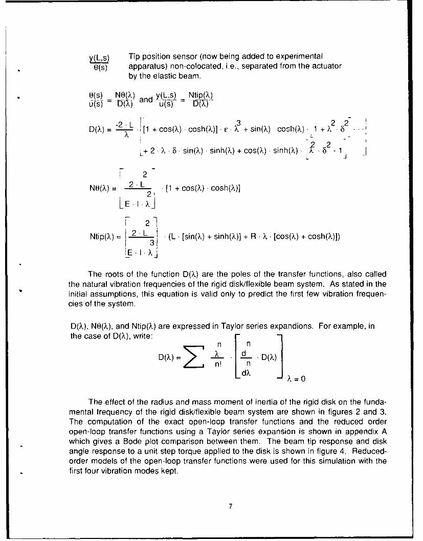
y(L,s) Tip position sensor (now being added to experimental0(s) apparatus) non-colocated, i.e., separated from the actuator

by the elastic beam.

O(s) NO(X) y(L,s) Ntip(X)u(s) andu(s)

-v cs(A)]c3 2 2D(X)= -2.L 1 +cos() -cosh()].c. +sin(X) cosh(X). 1 +? .8

L+2 . 8 sinQ) sinh(k) + cos(X) .sinh(X) . - 1J

2

NO(X) 2 L 2 [1 + cos(X) • cosh(X)]

1 2]

Ntip(X) (L [sinQ) + sinh(X)] + R. X [cos(X) + cosh(X)])IL3I

The roots of the function D(X) are the poles of the transfer functions, also calledthe natural vibration frequencies of the rigid disk/flexible beam system. As stated in theinitial assumptions, this equation is valid only to predict the first few vibration frequen-cies of the system.

D(X), N0(X), and Ntip(X) are expressed in Taylor series expandions. For example, inthe case of D(X), write: -

n nD(k)= X' d D l . (k)

nD n

LdX J?

The effect of the radius and mass moment of inertia of the rigid disk on the funda-mental frequency of the rigid disk/flexible beam system are shown in figures 2 and 3.The computation of the exact open-loop transfer functions and the reduced orderopen-loop transfer functions using a Taylor series expansion is shown in appendix Awhich gives a Bode plot comparison between them. The beam tip response and diskangle response to a unit step torque applied to the disk is shown in figure 4. Reduced-order models of the open-loop transfer functions were used for this simulation with thefirst four vibration modes kept.

7

The roots of NO(X) are the same as the roots of D(X) for r = 0, i.e., for an infinitelylarge disk moment of inertia. Therefore, the colocated zeros (the roots of NO(X)] cor-respond to the natural vibration frequencies of a cantilevered beam. These frequenciesare also called antresonance frequencies. If the actuator is driven with a sinusoidalcommand at one of these frequencies, the rigid disk will not move and the elastic beamvibrates according to the selected cantilevered mode shape.

The tip position transfer function has zeros with a positive real part; therefore, thesystem is a nnnminimum phase system. The initial time response of the beam tip to aunit step torque input to the disk is a short quasi-stationary period (approximately0.0066 seconds) followed by motion of the tip in the opposite direction to that of the rigiddisk (fig. 4). The contributions to the tip position of the rigid body mode and the firstflexible modes. This type of initial response presents a difficult contrcl problem.

Reduced-Order Model with Cantilevered Modes

It is common to use the constrained mode shapes (cantilevered modes) ratherthan the unconstrained mode shapes of the system in order to attempt to describe thedynamic behavior of an elastic structure. Although the system modes lead to a verysimple formulation for the dynamic equations, they are difficult to use for a multilinkflexible manipulator because of their dependence on the relative orientation of the links.Formulation in terms of the cantilevered modes does not have this drawback.

The elastic deflection w(x,t) is expressed in terms of the following series:

w(x,t) =(x) q(t)ii

The mode shapes for a cantilever beam have been previously derived in various

reference books and textbooks and can be expressed as follows:

O(x) = A [cos(Pi• x) + cosh(P • x)] + B. [cos(P • x) - cosh( • x)...

+ C. [sin(3 x) + sinh(. • x) + D. [sin(3 x) - sinh(13• x)]

The boundary conditions are:

atx=0: O(x)=0

2 3

atxL: d d d (x) = 0dx d3

dx dx

8

Therefore,

A=C-0and D F cos(l .L) + cosh(13. L)-] sin(P - L)_- sinh(P . L) 1Aii -0ad si([3. L) + siii(13 L)j L cos (1-L) + cosh(-31) j

Therefore, the mode shapes can be expressed as:

O(x) = -L. cos(Y, x) - cosh(3, x) - Lcish(X) -+ (c_9 [sin(P3 x) - sinh([3• x]

where X = PL is a root of the equation [1 + cos(X)cosh(X)] = 0. The first four roots of thisequation are 1.8751, 4.6941, 7.8548, and 10.9955, and the values of D/B correspond-ing to these values of X are -0.7341, -1.0185, -0.9992, and -1.0000, respectively. Thecantilevered frequencies are related to the values of X by the following equation:

;)2 - E I .X4,a. L4

In the expressions for kinetic energy, t, and potential energy, V, in w(x,t) is re-placed with its series representation. The result is:

T= . [(j + Fl) -02 + 0 .1 F2, + F3j I .. + ,i 12. F4]

1 1

1 2 F5 - u(t)-1

F2. = 2. R..[Lo . (X)i dx

F3 = 2. fo .x.O(x)i dx

F41 = o a I O(x), 2 dx

F51 = J E .I. d- • .4(x)i dx

O n dl9

Lagrange's equations was applied:

d [ dd.] dT+ d dV=•t "qj dq---j " d qj

An infinite set of coupled ordinary differential equations was obtained. Using thefirst three mode shapes of the cantilever beam, the equations of motion that result areas follows:

(j + Fl). + F2j + F3j I = u(t)

11 .jF2 +F3jJ .0+F4.i +F5j q =0 i=1 ,2,3

There are four equations and four unknowns: 0 q, q2 q3 These equations cannow be put in state-space form where the state variables are:

x, =0 x3 =ql x5 = q 2 x7 = q3

x2 = x 4 = 6I x6 = C12 x 8 = q 3

The state-variable equations that result are as follows:

2 .-1 = x 2 -i i = 1,2, 3, 4

1;K2: .[~t) -"F5, F2j + F3j

1 I I _F2, +F3j 2 i F4, 2 .x 2 ,1

1FJ + F 1 4 F4i

x2 [F2i + F3i] J + 1

2 1IF2j + F312

J+F1 4.F4,

2u(t) +• F5L FZ + F3, X2 j, ] -[ Li] x2 i+1 i =1,2, 3

10

The computation of the stare-variable equations and the equations of motion instate-space matrix form are shown in appendix B. Bode plots of magnitude (dB) versusfrequency (rad/sec) for disk angle motion and beam tip motion are shown in figure 5.Also shown in this figure are the beam tip response and disk angle response to a unitstep torque applied to the disk.

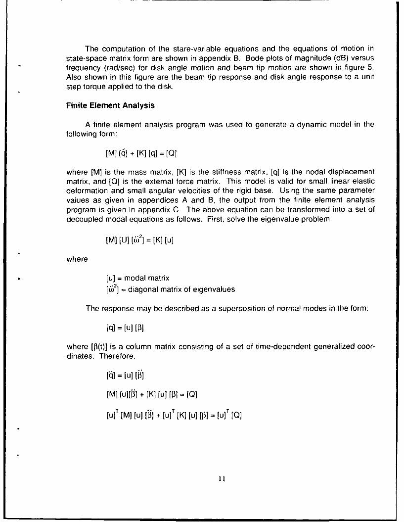
Finite Element Analysis

A finite element analysis program was used to generate a dynamic model in thefollowing form:

[M] (q + [K] [q] = [0]

where [M] is the mass matrix, [K] is the stiffness matrix, [q] is the nodal displacementmatrix, and [Q] is the external force matrix. This model is valid for small linear elasticdeformation and small angular velocities of the rigid base. Using the same parametervalues as given in appendices A and B, the output from the finite element analysisprogram is given in appendix C. The above equation can be transformed into a set ofdecoupled modal equations as follows. First, solve the eigenvalue problem

[M] [U] [632] = [K] [u]

where

[u] = modal matrix

[6;2] = diagonal matrix of eigenvalues

The response may be described as a superposition of normal modes in the form:

[q] = [u] [P]

where [[P(t)] is a column matrix consisting of a set of time-dependent generalized coor-dinates. Therefore,

[ = [u] [[3]

[M] [u( j] + [K] [u] [1] = [01

[u]T [M] [u] [] + [u]T [K] [u] [13] = [u]T [Q]

11

But normal modes are such that

[u] T [Mu]u = [I]

[u]T [K] [ul = [ 2]

In addition, a column matrix of generalized forces N(t)O was introduced associatedwith the generalized coordinates 3(t) and related to the forces Q(t) by

[N] = [u]T [0]

therefore,

[I] + [i2] [13] = [N]

This represents a set of n uncoupled differential equations of the type

P (t) r + (e62. 1P(t), = N(t)r r = 1, 2,.. n

Therefore, modal analysis consists of uncoupling the equations of motion bymeans of a linear coordinate transformation; the transformation matrix is just the modalmatrix [u]. Details of this procedure are given in appendix C. Using the results of thisanalysis, bode plots of magnitude (dB) versus frequency (rad/sec) for disk angle motionand beam tip response and the beam tip response and disk angle response to a unitstep torque are shown in figure 6.

Lumped Parameter Model

P. Sheth and K. Craig have developed a rigid disk, 2 rigid link, 2 torsional springmodel of the rigid disk/flexible beam dynamic system that preserves the followingcharacteristics of the continuous system:

1. Natural frequencies of the first two modes of vibration

2. Mode shapes of the first two modes of vibration

This lumped model is a first approximation of the real structure, although it may bean excellent approximation for specific situations. A diagram of the lumped model alongwith its parameters is shown below.

12

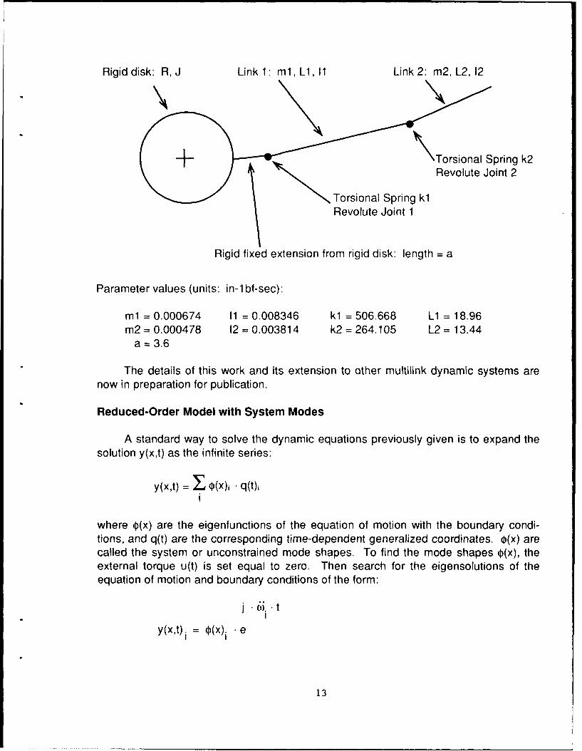
Rigid disk: R, J Link 1: ml, L1, I1 Link 2: m2, L2, 12

+ \Torsional Spring k

1' ~Torsional Spring k1ieoue on

Revolute Joint 1

Rigid fixed extension from rigid disk: length = a

Parameter values (units: in-i bf-sec):

ml = 0.000674 I1 = 0.008346 k1 = 506.668 Li = 18.96m2 = 0.000478 12 = 0.003814 k2 = 264.105 L2 = 13.44

a = 3.6

The details of this work and its extension to other multilink dynamic systems arenow in preparation for publication.

Reduced-Order Model with System Modes

A standard way to solve the dynamic equations previously given is to expand thesolution y(x,t) as the infinite series:

y(x,t) = , (x)i • q(t)

where O(x) are the eigenfunctions of the equation of motion with the boundary condi-tions, and q(t) are the corresponding time-dependent generalized coordinates. O(x) arecalled the system or unconstrained mode shapes. To find the mode shapes O(x), theexternal torque u(t) is set equal to zero. Then search for the eigensolutions of theequation of motion and boundary conditions of the form:

y(x,t) i = O(x)i • e

13

We obtained a fourth order ordinary differential equation in the variable x whose

general solution is:

)(x) = A. sin(13, x) + B. sinh(3 • x) + C cos(P , x) + D . cosh(P • x)

This equation has already been studied. The solution to the following system ofequation is given in appendix D.

-sin(X) - sinh(k) -cos(X) - cosh(? ) R • cosh(?) + L snh(X)

coh()A 0-cos(X) - cosh(k) sin() - sinh(k) L csh(X) + R. sinh(X) C = 0

2 6. X -2 L - X 30L + R

D=R0e-CD R=a J

B=- -A =-B - L L 3

In the previously given expressions for kinetic energy, T, and potential energy, V,y(x,t) = (R + x) 0(t) + w(x,t) with its series representation was replaced. The result is:

[ [j ] (0)i + T . (x)2 dx

V = - q"f E I .2 (x)i dx - u(t). [([O(0)] qj]

The modes were normalized so that the expression2 L

J .d-x.()] +i a (x)2dx] equals one for each mode shape.

When this is done, the expressions for T and V reduce to the following:

T= 2 2 V=. q2 (,.u.q. e d 0)

L1i

14

The summation is over the range 0 to 3 where the value i = 0 corresponds to therigid body mode for which the frequency of vibration is 0. Lagrange's equations werethen applied, and a set of decoupled ordinary differential equations of the following formwere obtained:

q+q =u(t) (0), i = 0, 1,2, 3

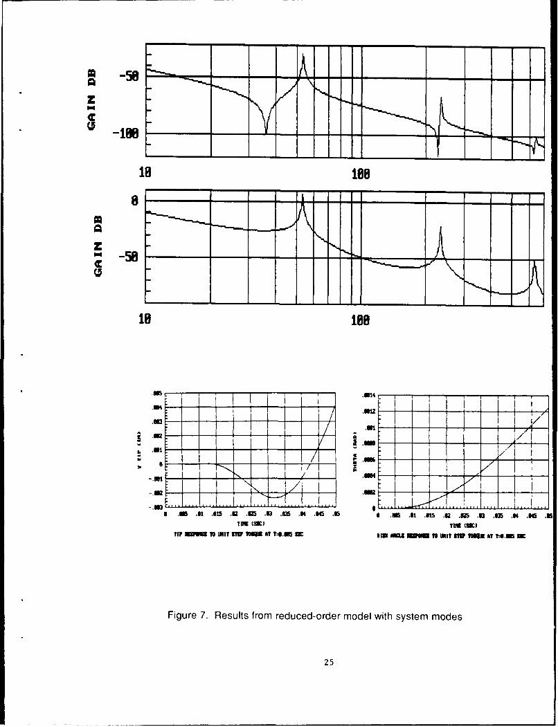
These equations are easily put in state-space form and are shown in appendix E.The Bode plots of magnitude (dB) versus frequency (rad/sec) for disk angle motion andbeam tip response and the beam tip response and disk angle response to a unit steptorque are shown in figure 7. These results are slightly different from previous modelsas slightly different values of the parameters J,R,L and d were used to match actualexperimental parameters.

Complete Model of Electromechanical System and Experimental Verification

The reduced-order model with system modes derived in the previous section wasused as the model for the mechanical part of the system. The following equations ofmotion for the electrical part of the system must be added.

State variables: i1 and i2

1il = [ [-R1 il - Kbl * 0 + Kal • e(t)l]

1i = [ [-R2 i2 - Kb2. 0 + Ka2. e(t) 2]

The torque on the disk from the motors is given by:

Torque from motors = Ktl .ii + Kt2 .i2

R1 = electrical resistance of motor 1R2 = electrical resistance of motor 2Li = electrical inductance of motor 1L2 = electrical inductance of motor 2Kal = amplifier gain for motor 1 (amplifier 1 was linear in the range -1 < 0 < 1 input

volts)Ka2 = amplifier gain for motor 2 (amplifier 2 was linear in the range -1 < 0 < 1 input

volts)Kbl = back emf constant for motor 1Kb2 = back emf constant for motor 2e(t), = input voltage to motor 1

e(t), = input voltage to motor 215

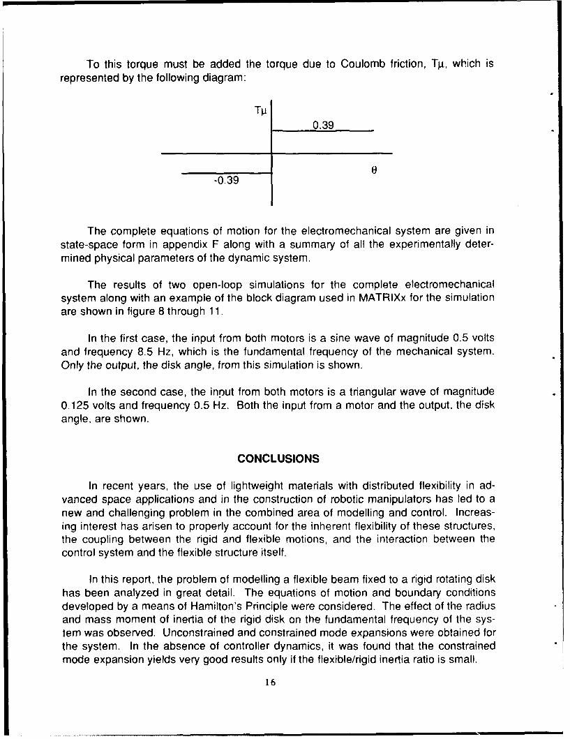
To this torque must be added the torque due to Coulomb friction, TA, which isrepresented by the following diagram:

Tp0.39

e-0.39

The complete equations of motion for the electromechanical system are given instate-space form in appendix F along with a summary of all the experimentally deter-mined physical parameters of the dynamic system.

The results of two open-loop simulations for the complete electromechanicalsystem along with an example of the block diagram used in MATRIXx for the simulationare shown in figure 8 through 11.

In the first case, the input from both motors is a sine wave of magnitude 0.5 voltsand frequency 8.5 Hz, which is the fundamental frequency of the mechanical system.Only the output, the disk angle, from this simulation is shown.

In the second case, the input from both motors is a triangular wave of magnitude0.125 volts and frequency 0.5 Hz. Both the input from a motor and the output, the diskangle, are shown.

CONCLUSIONS

In recent years, the use of lightweight materials with distributed flexibility in ad-vanced space applications and in the construction of robotic manipulators has led to anew and challenging problem in the combined area of modelling and control. Increas-ing interest has arisen to properly account for the inherent flexibility of these structures,the coupling between the rigid and flexible motions, and the interaction between thecontrol system and the flexible structure itself.

In this report, the problem of modelling a flexible beam fixed to a rigid rotating diskhas been analyzed in great detail. The equations of motion and boundary conditionsdeveloped by a means of Hamilton's Principle were considered. The effect of the radiusand mass moment of inertia of the rigid disk on the fundamental frequency of the sys-tem was observed. Unconstrained and constrained mode expansions were obtained forthe system. In the absence of controller dynamics, it was found that the constrainedmode expansion yields very good results only if the flexible/rigid inertia ratio is small.

16

Finite element and lumped parameter models of the system were also derived. Themotor dynamics were integrated into the structural model considering a specific labora-tory setup. This experiment was also used to validate the model.

Mu!tiple-link robot arms with motors at the joints can be considered to satisfy thecondition of small flexible/rigid inertia ratio so that constrained expansions are expectedto perform well. However, a question which requires further research effort is whetherconstrained mode expansions together with controller dynamics are suitable for cur-rently projected space structures that have very large flexible/rigid inertia ratios.

17

C

ILD

19

UQ)V,)

004NL000 0000 i

a

0n T

ca

U

0 a'

-0 ('3V

CT)_

E< a'

70

o0 0 0 0 0 0o 0 0) 0 00

(ZA) IKDNinoC~LI ]VINjIVGN2J

20

(FC)

CN000 s

0 C v

0- -0

L-

OCC.

a

W n

O ciaoc

(fEca

Ci

o 0 o o Co ao 00C 06r 6l

N(zvi) )I3NONoC5JA 7ViN3A'VG]Nn-

21

.004

z .6

- .ee ----

-- . 8 4 -I I 1 1 1 I I I I I I I I i I I I I I It i 1 1 1 1 1 I I I I I

8 .885 .81 .815 .82 .85 .83 835 ,.84 .845 .85

TIRE (SEC)

TIP RESPONSE TO LIT STEP TORQUE AT T=:.885 SEC

.8816

.0014 -

.8812

€ .881 /

. MW

S, .9U /

8 .885 ,81 .815 .2 .825 .83 .835 .84 M845 .85TIME (SEC)

DISX uAE RESPOMSE TO UIuT STEP TORQUE AT T.885 SEC

Figure 4. Results from exact analysis

22

8_

S -58 "'-.

-15816] 188

58

-I9

18 1In~ 56

- lee

'M

8 M .1 .815 . . 83 .83 .4 ., .1 8 A 1m , 0 .1 2 ,5 .83 Am .84 .86 .15

IN (Me) i (SIC)

TiP U TO IT 3I3 TOE T 4.1M MC IM 3 T tll MR NI TI 4 1

Figure 5. Results from reduced-order model with cantilevered modes

23

IMMMM

~-50

toto

-'Nib

-501

SUIC

rU1

Lm

t /r~,1Z .8

ip M 10 A tN? SIU 7 US A? T4.0 3C a " i m ow gI ? Sf nw AT M -1101

Figure 6. Rescults from finite element analysis model

24

-50

I LA I I

mje

o . --- -l -1 - t

T ii TI

Tilp IIIMIII TI IQ M IT S.I "a A 4M einl I I I " l MITI If "M T 1,411111 M

Figure 7. Results from reduced-order model with system modes

25

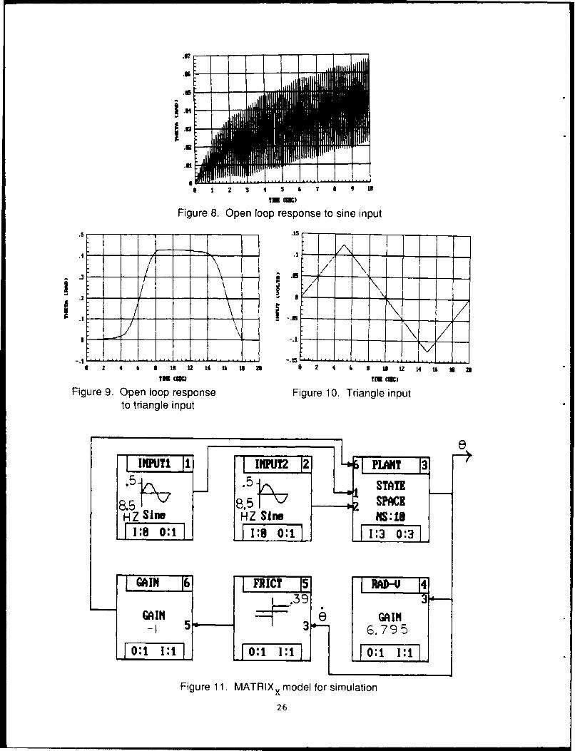
Figure 8. Open loop response to sine input

.1-- .15

I 2 4 6 8 L 2 14 5 1 8 21 6 2 4 6 e Ml 12 14 Ui 1

TIn (wc Mu ()

Figure 9. Open loop response Figure 10. Triangle inputto triangle input

eINPUTi I1 INPUT22 PLANT 3

I STATE8.5 102 SPACE

HZ SIM HZ Sine NS: I@1 :8 o:i 1 :@ o:ij L 1:3 0,:73

GAI Tf FRCT RD-V 4.39 3

- 1 6.795__ __ __ _________: 0:1 1:1

Figure 11. MATRIXX model for simulation

26

APPENDIX A

RIGID DISK AND FLEXIBLE BEAM: EXACT OPEN-LOOP TRANSFERFUNCTIONS AND REDUCED-ORDER MODELS OF THE OPEN-LOOP

TRANSFER FUNCTIONS

27

Parameter values (units: inch-lbf-sec)

E:=3.0 107 L:=36.0 d:=0.25

R d4 d48(R): - - -- =) 0 .0 0 0 7 2 5 A : =r .64 I t= -6

L:0OO 2 64 1.i 6 4

a 1) A C(j) ._ 1 - E_ 1I .2o -L 3 f( ' 2.E '.L 4

6 2(X) :=2•f(Q,) R :=5.625 J:= 0.416

N(X) := 1 + cos(.) -cosh(X)

NTIP(X, R) := L [sin(k) + sinh(X)] + R • k (cos(X) + cosh(?)]

D(XR,J) : c(J) X3 . [1 + cos(k) • cosh(k)] + I1 + 6(R)21 • sin(X) • cosh(X)...

+ 2 .X 6(R). sin(X), sinh(X) + 1k2 6(R) 2 - 11 . cos(k), sInh(k)

TF(K,R,J) : = -L N(K) TFTIP(k,R,J) " - -I NTIP(,R)

V. DQ(XA E . -,-, , RJ

X := 1.8 root[N(k),k] = 1.875 f(1.875) = 5.489

6(1.875) = 34.488

K: 4.6 root[N(k),K] = 4.694 f(4.694) = 34.401

6(4.694) = 216.149

K: 7.8 root[N(k),k) = 7.855 f(7.855) = 96.334

6 (7.855) = 605.284

K:= 10.9 root[N(X),K] = 10.996 f(10.996) = 188.78

6i(10.996) = 1.186. 103

X := 2.3 root[D(k,R,J),K] = 2.3993 f(2.393) = 8.941

6 (2.393) = 56.176

29

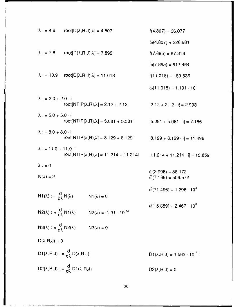
S= 4.8 root[D(,R,J),.] = 4.807 f(4.807) = 36.077

6(4.807) = 226.681

= 7.8 root[D(X.,R,J), ] = 7.895 f(7.895) = 97.318

6;(7.895) = 611.464

X:= 10.9 root[D(k,R,J),.j = 11.018 f(11.018)= 189.536

6(11.018) = 1. 191 10 3

X = 2.0 + 2.0. iroot[NTIP(X,R),X,] = 2.12 + 2.12i 12.12 + 2.12 • il = 2.998

? = 5.0 + 5.0. iroot[NTIP( ,R),?L] = 5.081 + 5.081i 15.081 + 5.081 • il = 7.186

k 8.0 + 8.0. iroot[NTIP(X,R),X] = 8.129 + 8.129i 18.129 + 8.129. il = 11.496

= 11.0 + 11.0.iroot[NTIP(X,R),X] = 11.214 + 11.214i 111.214 + 11.214. il = 15.859

X:=06i(2.998) = 88.172

N(X) = 2 6(7.186) = 506.572

(*(11.496) = 1.296 .103N1N,(,),0Nl(X) •=d N(k.) N1 (?,) = 0

6(15.859) = 2.467 • 103

N2(k) d N1.) N2(k) =-1.91 1012

N3(k) d N2(X) N3(.) = 0

D(X.,R,J) = 0

D1(X,R,J) = .D(X,R,J) D1(kXR,J) = 1.563- 1011

dX

D2(.,R,J) D= D1 (.,R,J) D2(X,R,J) = 0

30

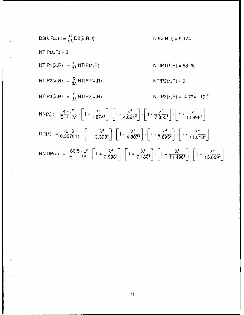
D3(4,R,J) = D2(4,R,J) D3(X,R,J) = 9.174

NTIPXR =

NTIP(X,R) 0

NI1 ,,R) dX NTIPQ(.,R) NTIP1 (X,R) = 83.25

NTIP2(X,R) =d NTIP1 (X,R) NTIP2(?X,R) = 0dX

NTP() dX NTIP2(X,R) NTIP3(X,R) = -4.734. 10

-L 1 X2- [1 X4 ] F 41 .41DD(X) .032701' L .93- 4.0jL- 9 iL-_ _

ENI() =166 . + 2.9984] 7 186 4][+ 114964] [i 15.8594]

31

TTF(X): NN() FTIP(X)' NTPX Bode Plot Comparison: Exact

versus Reduced Order

X: 1,1.01 ..20

1. 11 -71

1. 1000

1 II 1 000

.12

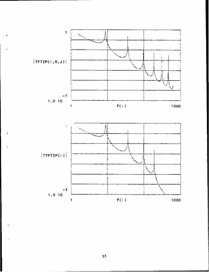
*1 I

"TFTIP( ,,RJ)I

-71.0110 -_ _ _ _ _ _ _ _ _ _ _ _ _ _

S .... 1000I "--'.... ___',,____....-

TTFTIP(, ) I

-7 ,1 .010

1 fG. 1000

33

APPENDIX B

REDUCED-ORDER MODEL OF RIGID DISK/FLEXIBLEBEAM SYSTEM WITH CANTILEVERED MODES

35

Parameter values (units: inch-lbf-sec)

E: = 3.0 • 107 L: = 36.0 d: = 0.25

R & ' d 2

8(r): = p: = 0. 0 0 072 5 I: = n - 64 A: x 4

J 1 __E._

E(a): F(X)=2. L

(1)X):= 2 f(X)

R: = 5.625 J: = 0.416

Mode shape of a cantilever beam: O(x) Origin =1

X1:= 1.8751X2: = 4.69409X3: = 7.85476

cosh(X) + cos(X)F(k)" = -si nh(X) + in(R) F(,1) = 0.734096

F(X2) = 1.018467F(X3) = 0.999224

(x,X): [CS LL x}. cosh[E .x]. F(X) [sin[~ L x]sinh [ - . x]]]

¢(L,X1) = 71,999785 O(L,X2) = -71.999917 o(L,X3) = 72.000184

Fl:= a L.[ R2 + R L + L] F2() =2 R.J fL(x,X) -adx

F3(X): = 2-Jo x. (XX), adx F4(X): = - (T-_[0(XX)] 2 dx

F5k:= ddOx,k] ]2 xF1 = 0.853447

F21 := F2(X1) F21 = 0.406276

37

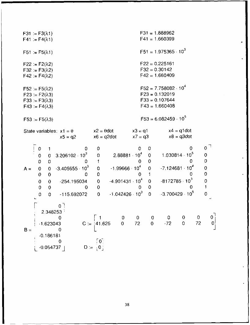
F31 := F3(X1) F31 = 1.888962F41 :=F4(X1) F41 = 1.660399

F51 :=F5(X1) F51 = 1.975365. 10

F22 := F2(X2) F22 = 0.225161F32 := F3(.2) F32 = 0.30142F42 := F4(X2) F42 = 1.660409

F52 := F5Q(2) F52 = 7.758082 104

F23 := F2(.3) F23 = 0.132019F33 := F3(?,3) F33 = 0.107644F43 := F4(Q3) F43 = 1.660408

F53 := F5(R3) F53 = 6.082459 105

State variables: xl = e x2 = Odot x3 = q1 x4 = qldotx5 = q2 x6 = q2dot x7 = q3 x8 =q3dot

7 -

0 1 0 0 0 0 0 0

0 0 3.206102 103 0 2.88881 104 0 1.030814 105 00 0 0 1 0 0 0 0

A= 0 0 -3.405655 103 0 -1.99666.104 0 -7.124681 -104 00 0 0 00 1 0 0

0 0 -254.195034 0 -4.901431 104 0 -8172785 103 00 0 0 0 0 00 1

0 0 -115.692072 0 -1.042426 103 0 -3.700429 105 0

0-012.348253

0 c; 0 0 0 0 0 0o

-1.623043 C = 4 1.6 2 5 0 72 0 -72 0 72 01B 0 L

-0.1861810 O

-0.054737j D := L

38

APPENDIX C

FINITE ELEMENT ANALYSIS OF RIGID DISK/FLEXIBLE BEAM SYSTEM

39

Using six beam elements to represent the flexible beam offset from the center of

rotation of the disk and a lumped inertia to represent the rigid disk, the mass matrix, [M],and stiffness matrix, [K], are:

4.201 •10 14.94 -8.729 3.662 -1.321 0.4059 -0.105517.52 2.644 -1.361 0.5450 -0.1762 0.04927

18.52 2.207 -1.185 0.4371 -0.1429

18.70 2.099 -1.009 0.4293 10 =[M]18.88 1.662 -1.227

19.88 3.345

L 5.992

r1.722. 102 -24.85 9.041 -2.413 0.6413 -0.1599 0.02659)4.997 -3.159 1.271 -0.3376 0.08415 -0.01400'

3.895 -2.863 1.186 -0.2957 0.04918

3.811 -2.821 1.102 -0.1833 .102 =[K]3.727 -2.525 0.6863

2.625 -0.9692

L 0.4275

0y1 Torque

y 02 0

y 0 =[0]3 =[q] 0 external force vector

y nodal displacement vector 04 0y5y6

Solution to the eigenvalue problem: [K] [u] = [(j)] [M] [u]

('J2= 1; = 3.1938.- 103 2 { 5.1292- 104 0)3 3.7616. 10s

i,2 =065466

(,42 1.4584 10 4.1546 106 1; 9.0099 10

41

2.469 -2.535 0.8549 -0.3914 0.2364 -0.1620 0.138928.68 -20.82 -15.69 46.52 -67.04 73.36 -77.3743.34 -12.27 -54.78 72.19 -19.63 -48.45 89.9857.74 7.786 -71.04 3.162 69.07 -0.9024 -94.63 .10 . =[u]71.91 35.43 -44.11 -63.90 -16.45 50.69 87.3985.97 67.07 20.09 -21.95 -52.03 -64.88 -66.79100 100 100 100 100 100 100

Normal modes must be normalized so that: [u] T[M] [U] = [I][u]T[K] [U] = [C2]

The result is.

0.8985 -1.1314 0.4669 -0.2201 0.1388 -0.1002 0.066010.4357 -9.2940 -8.5689 26.1614 -39.3613 45.3776 -36.746215.7682 -5.4752 -29.9182 40.5986 -11.5230 -29.9682 42.7346121.0086 3.4755 -38.7995 1.7785 40.5556 -0.5582 -44.9412 = [u]26.1672 15.8138 -24.0894 -35.9363 -9.6564 31.3545 41.5060131.2821 29.9402 10.9742 -12.3428 -30.5504 -40.1319 -31.7223

'L.36.3838 44.6376 54.6172 56.2393 58.7158 61.8603 47.4935]

The equations of motion become: [f] + [i2] [1 ] = [ulT[Q ]

0.8985 [Torque]-1.13140.4669

-0.22010.1388

-0.1002_-0.0660_

The output equations are: [q] = [u] [1]

These equations are uncoupled and it is straightforward to put them in state variableform.

42

APPENDIX D

REDUCED-ORDER MODEL OF RIGID DISK - FLEXIBLE BEAMWITH SYSTEM MODES

43

NOTE: Parameter values for L, d, R, and J are different here than in previous simula-tions. These are the actual parameters for the apparatus on which experiments wereperformed.

E := 3.0. 10' L =35.125 d := 0.249

R d 2 d 4

8(R) := L p =0.000725 AREA . := t 6 4

5:=pAREA C(J) :- J) 1 - E I

6(X) := 2 • • f(QX) J := 0.57301

D 1 (.,R,J) := E(J) - .3. [1 + cos(X ) • cosh(k)] + I1 + X 2 5(R) 2 1 sin(k) • cosh(3)...

+ 2 k X. 6(R). sin(X) • sinh(X) + 1X2 6(.) 2 - 11 cos(?,) • sinh(X)

D)X,RJ)= k2 D1(XR,J)

X =2.3 X1 := root[d(X,R,J),,] Xl = 2.281132052f(k1) = 8.500007313

6,;(;1) = 53.407121063

k := 4.8 2 := root[D(k,R,J),K] ?2 = 4.777449767f(2,2) = 37.2829874116(2) = 234.255918709

X := 7.8 3 := root[D(.,R,J), X] L3 = 7.884939741f(X3) = 101.5582486746(?K3) = 638.109295891

.:= 10.9 .4 := root[d(Q,R,J),3.j .4 = 11.012274831f(?,4) = 198.094550571

i (X 4) = 1.24466477 103

Xl1 (K) := -sin(?,) - sinh(k) X21 (k) := -cos(X) - cosh(K)X1 2(K) := -cos(k) - cosh(K) X22(K) := sin(?.) - sinh(k)

L- sinh(k) L cosh(K)X13(X) := R cosh(k) + X23() X + R. sinh(Xk)

45

X31 (X,R) := 2- 6(R)X32 :=-2

X33(X,J,R) := L . E(J) - L* 5(R) + R

x11(X) x12(X) X13(X)-X(X,R,J) : X21(X, X22,) X23(X,

[X31(X,R) X32 X33RJR)j

4 := X1 .= 2.281132052

7-5.600935951 -4.2928731 104.548427761]X(X,R,J) = -4.2928731 -4.084649959 105.502227379

,_ 0.787437043 -2 68.454784401J

jX(X,R,J)I = 1.37069393510-5

X2 = 4.777449767

,-58.398403556 -59.469720184 796.837320401-'x(X,R,J) =.-59.469720184 -60.394172143 796.848176783,

_ 1.649155258 -2 300.258431662j

Ix(X.,R,J)l = -6.553719071 • 10-'

.:= X3 = 7.884939741

F-1.329481791 103 -1.328451693 103 1.397190909 10 4

X(A.,R,J) =j1.328451693. 103 -1.327482749 103 1.397190849 104

L 2.721847526 -2 817.899062996 .1

IX( ,R,J)I = -4.009991272. 107

The solution to the set of homogeneous equation with 0i = 1 is given by the following:

ORIGIN = 1i= 1, 2..3 - 31.938591]1.3= t2 C :=i 87.7208561

LX3j "179.353947J

46

- -5.813294- 21.2113511 r-25.876091-A:= -75.685245 B 83.0374941 D -81.658356,

L-168.705692] L1 73.160387j L-1 73.291447J

The modes of vibration are:

1(x) :=A si A, x] + B, sinhI_ .x +C, .+cosI-L x]+D, .cosh[ x]

02(x) :=A 2 sin -x] + B2 sinh[ x] +C2 C2 x] +D2 cosh[ k 2 ]03(x) :: A3 sin[ . x] + B3 sinh[X + C3 cosL x] + D3 cosh[3 X]

00(x) := R + x This is the RIGID BODY mode.

47

APPENDIX E

STATE-SPACE FORMULATION OF EQUATIONS OF MOTION FORREDUCED-ORDER MODEL OF RIGID DISK - FLEXIBI _ BEAM

SYSTEM WITH SYSTEM MODES

49

x =Ax + Bu y =Cx + Du

0 1 0 0 0 0 0 0

~d0 0 0 0 0 0 0 0 d-- p(0)o

0 0 0 1 0 0 0 0 0

(4)2 0 0 0 0 0 [A] d

0 0 0 0 02 1 0 0 0

0 0 0 0 46 0 0 0 dx 0(0)2

0 0 0 0 0 0 02 1 0

S00 0 dx (0)31

3() 7-- O(L)o O (L), o(L) 2 o (L)3

0 0 0 0 =[C] F 0d 0d d d i D

dx O(O)o 0 dx(0) 1 0 &0(0)2 0 x0(0)3 0 = [D]_- -J

Output 1: absolute beam tip position (inches)Output 2: disk angle (radians)Input: Torque u(t) to disk

51

APPENDIX F

COMPLETE EQUATIONS OF MOTION IN STATE-SPACE FORM FOR THEELECTROMECHANICAL SYSTEM

53

State of variable equations: x = Ax + Bu y = Cx + Du

0 1 0 0 00 0 0 0 0

0 0 0 00 0 -2.. l)c 01o

0 0 0 0 020 0 0 0 -0)2 columns 1 through 5 of [A]

0 0 0 0 00 0 0 0 0

-Kbi d -Kbl d0 L dx.(0)0 0 -- 0

o i- a10) L d-Kb2d.(0) 0 -Kb2 d 0

0 -0L2 d-0x --L2 20 0

o 0 0 Kti. .(0)o Kt2. -(0)o

0 0 0 0 0d 00) t d

0 0 0 K. .(), Kt20 0.(O),

0 0 0 0 0 =columns 6through 10

-2.12.0)2 0 0 Kt1. ---0(0)2 Kt2 "d 'x 0)2 of [A]

0 02 1 0 0

d 0 Kt2-d0

0 "o3 -2"q3")3 Ktl.-.(0)3 "ax(0)3

-Kbi d -Kbi d -R1 0BEl &'(0)2 0 -L_- - .0(0 -Ui-

-Kb2 d -Kb2 d -R2

L2 -d- . 0 L2- (0)3 05L2

55

d70 0 0 O(L)o dx-.(O)o 0

d d0 0 .(0)o 0 0 d .(0)o

d0 0 0 O(L)I dx 0(0)1 0

0 0 dd O(O)0

S[B]= [C] T

d d0 0 d x.(0)2 O(L) 2 & .P(0)2 0

d dx0 0 , (0)3 0 0 ,()

Kal dL1 0 0 O(L) 3 0(0)3 0

Ka2 d0 L2 0 0 0 & 0(0)3

0 0 00 0 0

70 0 01'0 0 0 =[D]LO 0 oJ

Inputs: 1 - el (t) = voltage input to motor 12 - e2(t) = voltage input to motor 23 - Tp = Coulomb friction torque on disk

Outputs: 1 - beam tip position (inches)2 - disk angular position (rad)3 - disk angular velocity (rad/sec)

Summary of parameter values: (units: in-lbf-sec)

E := 3.0. 10' L =35.125 p : 0.000725

R := 6.0625 J := 0.573 d := 0.249

56

R1 :=29 Q :=55Q Li :=0.0125 H

L2 := 0.025 H Kal 17.84 Ka2 := 17.92

Ktl := 4.204 in-lbf/A Kt2 := 5.511 in-lbf/A

Kbl := 0.473 V-sec/rad Kb2 0.620 V-sec/rad

ll .01 112 := .01 3 01

Tp :0.39 in-lbf

E = modulus ot elasticity of beam materialL = length of beam1) = mass density of beam materialR = radius of rigid diskJ mass moment of inertia of rigid diskd = diameter of uniform beamR1 = electrical resistiance of motor 1R2 = electrical resistance of motor 2Li = electrical inductance of motor 1L2 = electrical inductance of motor 2Kal = amplifier gain for motor 1Ka2 = amplifier gain for motor 2Ktl = motor 1 torque constantKt2 = motor 2 torque constantKbl = motor 1 back emf constantKb2 = motor 2 back emf constant11 = damping coefficient associated with each modeTp = Coulomb friction torque acting on disk6i =frequency in rad/sec

O(L)o := 34.9017 O(L)1 := -46.5615 O(L) 2 := 55.7653 O(L) 3 .= -56.5945

d d d ddx .(0)o := 0.8474 d .(0)l := 0.9226 ai .(0)2 0.3433 .0P(0)3 := 0.1625

I6 := 53.4071 (62 := 234.2559 6 3 := 638.1093

57

DISTRIBUTION LIST

CommanderArmament Research, Development and Engineering CenterU.S. Army Armament, Munitions and Chemical CommandATTN: SMCAR-IMI-I (2)

SMCAR-FSF-RC (6)Picatinny Arsenal, NJ 07806-5000

CommanderU.S. Army Armament, Munitions and Chemical CommandATTN: AMSMC-GCL(D)Picatinny Arsenal, NJ 07806-5000

AdministratorDefense Technical Information CenterATTN: Accessions Division (12)Cameron StationAlexandria, VA 22304-6145

DirectorU.S. Army Materiel Systems Analysis ActivityATTN: AMXSY-MPAberdeen Proving Ground, MD 21005-5066

CommanderChemical Research, Development and Engineering CenterU.S. Army Armament, Munitions and Chemical CommandATTN: SMCCR-MSIAberdeen Proving Ground,, MD 21010-5423

CommanderChemical Research, Development and Engineering CenterU.S. Army Armament, Munitions and Chemical CommandATTN: SMCCR-RSP-AAberdeen Proving Ground, MD 21010-5423

DirectorBallistic Research LaboratoryATTN: AMXBR-OD-STAberdeen Proving Ground, MD 21005-5066

5

59

ChiefBenet Weapons Laboratory, CCACArmament Research, Development and Engineering CenterU.S. Army Armament, Munitions and Chemical CommandATTN: SMCAR-CCB-TLWatervliet, NY 12189-5000

CommanderU.S. Army Armament, Munitions and Chemical CommandATTN: SMCAR-ESP-LRock Island, IL 61299-6000

DirectorU.S. Army TRADOC Systems Analysis ActivityATTN: ATAA-SLWhite Sands Missile Range, NM 88002

60