IP land, FP6-2002-SPACE-1 geoland · Integrated Project geoland ... 2.3 OFM requirements ... OLF...

IP geoland, FP6-2002-SPACE-1

Date Issued: 27.09.2004 Issue: I1.00

geoland

Integrated Project geoland

GMES products & services, integrating EO monitoring capacities to support the implementation of European directives and policies

related to “land cover and vegetation”

CSP – Algorithm Theoretical Basis Document (ATBD)

WP 8312 – Customisation for LAI, fAPAR, fcover and albedo

CSP-0350-RP-0008-ATBDWP8312

Issue 1.00

EC Proposal Reference No. FP-6-502871

Book Captain: Roselyne Lacaze (MEDIAS-France)

Contributing Authors:

EC Proposal Reference No.: FP6-502871

CSP Methods compendium (ATBD) WP8312 geoland

Document-No. CSP-0350-RP-0008-ATBDWP8312 © geoland consortium Issue: I1.00 Date: 27.09.2004 Page: 2 of 26

Document Release Sheet

Book captain: Roselyne Lacaze (MEDIAS-France) Sign Date

Approval Marc Leroy (CSP Task Manager) Sign Date

Endorsement: Co-ordinator (ITD) Sign Date

Distribution: CSP Partners

Global Observatories Task Managers




Change Record

Issue/Rev Date Page(s) Description of Change Release

1.00 27-09-2004 All Description of algorithms and customisation methods to reply to the Global Observatories requirements.




TABLE OF CONTENTS

1 Background of the document ............................................................................................6

1.1 Executive Summary..............................................................................................................6

1.2 Scope and Objectives...........................................................................................................6

1.3 Content of the document ......................................................................................................6

1.4 Related documents...............................................................................................................6

1.4.1 Input..................................................................................................................................6

1.4.2 Output...............................................................................................................................7

2 Review of users requirements...........................................................................................7

2.1 ONC requirements................................................................................................................7

2.2 OLF requirements.................................................................................................................7

2.3 OFM requirements................................................................................................................8

3 Methodology description ...................................................................................................8

3.1 Overview ..............................................................................................................................8

3.2 The retrieval algorithm..........................................................................................................9

3.2.1 The CYCLOPES algorithms............................................................................................10

3.2.2 The GLOBCARBON algorithms ......................................................................................13

3.3 The product quality .............................................................................................................18

3.4 The validation procedure ....................................................................................................18

3.5 Risk of failure and mitigation measures ..............................................................................18

4 Customisation methods...................................................................................................18

4.1 Customisation for ONC.......................................................................................................18

4.2 Customisation for OLF........................................................................................................21

4.3 Customisation for OFM.......................................................................................................22

5 References........................................................................................................................23

6 Pseudo-Code ....................................................................................................................25




List of Tables

Table 1: Narrow to broadband conversion coefficients for the VEGETATION channels. ...............12

Table 2: Grouping of IGBP land cover classes into seven functional types and cover-dependent clumping index values for LAI/fAPAR algorithms....................................................................15

List of Figures

Figure 1: Land cover map with 8 vegetation types provided by CNRM/Météo-France for ONC customisation.........................................................................................................................19

Figure 2: Example of mean LAI maps of the different vegetation types. ........................................20

Figure 3: Fcover over Boreal Eurasia, 15th July 2002. ...................................................................21

Figure 4: Fcover time profiles for pixels located on bare soil (15° N: orange), sahelian wooded grassland (10° N: red), sahelian woodland (5° N: magenta) in northern hemisphere along the 25° East meridian across Africa..............................................................................................21

Figure 5: Fcover time profiles for pixels located on equatorial forest (0° S: green), woodland (15° S: blue), and bushland (25° S: cyan) in southern hemisphere along the 25° East meridian across Africa. ....................................................................................................................................21

Figure 6: FAPAR over Poland from the beginning of May to the end of June, 2002, at 10-day frequency. ..............................................................................................................................22




1 BACKGROUND OF THE DOCUMENT

1.1 EXECUTIVE SUMMARY

The LAI, fAPAR, fcover and albedo are bio-geophysical parameters characterizing the land surface. They are used to describe the vegetation and soil in the surface-atmosphere interaction schemes, in the crop models, and to investigate the land cover changes.

On one hand, these parameters are produced in the frame of existing project: FP5/CYCLOPES for LAI, fAPAR, fcover and albedo; ESA/GLOBCARBON for LAI and fAPAR. The final products are technical properties (spatial and temporal resolution, spectral characteristics, thematic accuracy, etc …) that depend on the input data, and the retrieval algorithms. On the other hand, global observatories need these parameters with specific formats adapted to their own applications. Then, the CYCLOPES and GLOBCARBON products require customisation before to be used by OLF, ONC and OFM.

This document presents the retrieval algorithms, and the customisation processes applied to each parameter to satisfy the users’ needs.

1.2 SCOPE AND OBJECTIVES

As the LAI, fAPAR, fcover and albedo are outputs of CYCLOPES and GLOBCARBON projects, it is first necessary to describe the retrieval algorithms, their hypothesis, their advantages and drawbacks. (A complete inter-comparison of CYCLOPES and GLOBCARBON LAI and fAPAR are foreseen in WP8311.) Then, this document presents the customisation methods developed to fit the Observatories requirements. This ATBD is the physical baseline for coding a customisation module that will be applied to the outputs of CYCLOPES and GLOBCARBON processing lines in order to generate the CSP products in the specific formats required by users.

1.3 CONTENT OF THE DOCUMENT

The users’ requirements are reviewed in Chapter 2, product per product and Observatory per Observatory. The CYCLOPES and GLOBCARBON algorithms are presented in Chapter 3 and the customisation methods in Chapter 4.

1.4 RELATED DOCUMENTS

1.4.1 Input

Overview of former deliverables acting as inputs to this document.

Document ID Descriptor

CSP-0350-RP-0005 Service Portfolio




1.4.2 Output

Overview of other deliverables for which this document is an input.

Document ID Descriptor

CSP-0350-RP-0010 Test and Benchmarks report

CSP-0350-RP-0012 The input and output data sets used for tests and benchmarks

CSP-0350-COD-0009 The customisation processing line

CSP-0350-RP-0011 The processing line test report

CSP-0350-PRD-0000 CSP Product WP8321

2 REVIEW OF USERS REQUIREMENTS

The service portfolio indicates that LAI, fAPAR, fcover and albedo from CYCLOPES and GLOBCARBON are derived from VEGETATION/SPOT sensor (space resolution: 1km) with a 10-day time step (CSP-0350-RP-005-ServicePortfolioWP8210). These products cover the period from 1998 to 2003.

2.1 ONC REQUIREMENTS

LAI represents the foliage amount on the surface and the albedo allows to estimate the radiation available at the surface level. They are used in Soil-Vegetation-Atmosphere Transfer (SVAT) scheme, and they are the first priority products for assimilation experiment in a carbon cycle model. ONC needs visible and near-infrared bi-hemispherical (integrated over the whole illumination directions and the whole observations configurations) albedos. FAPAR translates the photosynthesis activity of vegetation. It will be used in validation process, and also for assimilation experiment over test areas. ONC needs a daily fAPAR, i.e. characterizing the radiation absorption over the whole day.

ONC needs tiled averages (mean and standard deviation) maps at 0.5° of space resolution for 8 vegetation classes (Grassland C3; Grassland C4; Cropland C3; Cropland C4; Bare ground; Broadleaf evergreen forest; Deciduous forest; Conifer forest). The number of valid pixels for each class in the 0.5° cell is also required. The distribution of the 8 vegetation types relies on the ECOCLIMAP land cover map (Masson et al., 2003). Maps have to be projected in a regular latitude/longitude grid. Files have to be readable on any computer architecture.

2.2 OLF REQUIREMENTS

Fcover represents the fraction of surface covered by vegetation. Its inter-annual variations allow to monitor the changes in land use. For that, the fcover time profiles has to be clean, without residual




contamination due to atmosphere (aerosols), clouds or soil effects. The 10-day time resolution of CYCLOPES fcover seems relevant to determine the start and end of vegetation cycle. In the first time, OLF will test the fcover without applying a temporal filter and without any customisation to fill the gaps due to cloud detection. The product have to be provided at 1km resolution over areas of interest:

o Africa : 38° N – 35° S; 26° W – 60° E

o Boreal Eurasia : 40° N – 75° N; 45° E – 180° E

Maps have to be projected in the same regular latitude/longitude grid that the input VEGETATION data. Files have to be provided in HDF-EOS format.

2.3 OFM REQUIREMENTS

Two OFM partners have requirements about LAI and fAPAR:

o VITO needs fAPAR to calculate the Dry Matter Productivity product. The 1km and 10-day resolutions maps have to be provided over Europe (28° N – 72° N ; 15° W – 60° E) in a regular latitude/longitude grid. No specific requirements about the file format.

o IGIK will use LAI and fAPAR in validation process. The 1km resolution maps have to be provided over Poland (48° 50’N - 54° 50’N; 13° 45’E – 24° 50’E). The preferred grid is a Transverse Mercator projection, but a regular latitude/longitude grid could be satisfying. The time period of interest is from 1st April to 30th June for each year, in order to monitor the crop growth cycle. Any usual file format will be good.

3 METHODOLOGY DESCRIPTION

3.1 OVERVIEW

During the two last decades, many studies have investigated the relevant processes of the Earth climate, and identified the major role of the surface-atmosphere interactions. The improvement of climate modelling requires an accurate description of vegetation and soil properties. The remote sensing data have proven their relevancy to monitor the ecosystem and their usefulness to retrieve the main vegetation bio-physical characteristics since the FIFE experiment (Seller et al., 1992). In the last few years, methodologies have been developed to estimate land surface bio-physical parameters from large scale optical sensors in an operational way. These algorithms have been implemented in operational processing line to provide advanced bio-physical products from the POLDER data (Leroy et al, 1997; Lacaze et al., 2003), and from the MODIS and MISR data (Kinhiazikhin et al., 1998). Now, the research aims at merging observations acquired by several sensors, and developing common algorithms. This approach is investigated in the frame of FP5/CYCLOPES and ESA/GLOBCARBON projects.

Albedo, fcover, LAI, and fAPAR are essential bio-physical parameters used in Soil-Vegetation-Atmosphere Transfer (SVAT) schemes (Chen et al., 1997) to simulates the exchanges between




the surface and the atmospheric boundary layer. The albedo is a radiative parameter, directly linked to the bi-directional reflectances measured by satellite radiometers. It mainly controls the fluxes exchanges between the continental biosphere and the atmosphere. The fcover, LAI, and fAPAR are vegetation properties, which require one more level of analysis.

The operational algorithms used to calculate albedo in the POLDER project and in the MODIS-MISR project are based upon the inversion of linear kernel-driven reflectance models. This model family simulates the Bi-directional Reflectance Distribution Function (BRDF) following the general expression presented by Roujean et al. (1992):

Eq. 1: ρ(θs, θv, φ) = k0 + k1 * F1(θs, θv, φ) + k2 * F2(θs, θv, φ)

The kernel F1 and F2 solely depend on the angular configuration of acquisition: θs the sun zenith

angle, θv the viewing zenith angle and, φ the relative azimuth angle. Their mathematical formulations approximate physical modelling of interactions between incoming solar radiation and land surface. Coefficients ki=0, 1, 2 quantify the respective contribution of each kernel to the whole BRDF and are derived by model inversion.

Two main approaches exist to estimate fcover, LAI, and fAPAR. The first one is based upon empirical relationships with vegetation indices, such as the NDVI (Normalized Difference Vegetation Index). The second one relies on radiative transfer models inverted by neural network or look-up tables. The scattering, absorption and reflection processes in the foliage layer are accurately simulated by equations of the radiative transfer theory. As models are not directly invertible, neural network or look-up tables are used to retrieve the vegetation properties. This option has been chosen in the frame of the POLDER/ADEOS project: a neural network yields the LAI and fcover by inversion of the Kuusk’s radiative transfer model (Lacaze et al., 2003). In the MODIS project, both approaches are used. The main retrieval algorithm relies on a 3D radiative transfer model (Knyazikhin et al., 1998). Reflectances are simulated for angular and spectral MODIS conditions, and for various soil and vegetation properties. The inversion consists in comparing the MODIS surface reflectances with the simulated reflectances gathered in a look-up-table. If this algorithm fails, a back-up procedure is activated to assess the LAI and fAPAR from vegetation indices by relationships depending on the vegetation structure (Myneni et al., 1997).

3.2 THE RETRIEVAL ALGORITHM

This section describes the methods used in the CYCLOPES and GLOBCARBON projects to estimate the bio-physical parameters.

The CYCLOPES project has started in February, 2003. The first version of algorithms has been chosen in autumn 2003, then the development of the processing line has begun. The generation of the first products has ended in May, 2004. The development logic of CYCLOPES foresees the improvement of algorithms every 6 months, after analysis and feedbacks from users. Thus, the version 2 algorithms will be implemented in Autumn 2004, and version 2 products should be available in Spring 2005.




The GLOBCARBON project has started in October 2002 for 2 years. During the prototyping phase, algorithms have been proposed by Expert Support Laboratory, and the system specifications have been defined. Then, the implementation phase has started with the coding of processing line. At the present time, the integration of the processing line in VITO hardware configuration is achieved. The generation of products has started and should be completed in the next months.

3.2.1 The CYCLOPES algorithms

CYCLOPES is a multi-sensor project: same algorithms are applied to input data from several radiometers in order to merge the final products. Satellite sensors are VEGETATION-1/SPOT-4, VEGETATION-2/SPOT-5, AVHRR/NOAA, MERIS/ENVISAT, POLDER-2/ADEOS-2, and SEVIRI/MSG. The final multi-sensors CYCLOPES maps will be produced at 8km resolution. While the area of interest is global, the focus of interest is land, therefore the operating region is from 80° N to 60° S latitude. In the frame of geoland, only products derived from VEGETATION/SPOT at full 1km resolution will be used.

3.2.1.1 Pre-processing algorithms

The Level 1 inputs are VEGETATION-1/SPOT-4 (from 1998 to January 2003) and VEGETATION-2/SPOT-5 (from February 2003 to present) daily geo-referenced products. We use spectral reflectances from blue (B0: 430-470nm), red (B1: 610-680nm), near infrared (B3: 780-890nm) and middle infrared (1580-1750nm) channels.

First, the version 1 CYCLOPES processing line re-calibrates the input data to correct original calibration. Then, the atmospheric gaseous absorption and scattering are corrected using the SMAC code (Rahman et Dedieu, 1994) with ozone amount from TOMS, and water vapor content and pressure from Météo-France analyses. The effects of aerosol content are removed using a simple estimate of the aerosol optical thickness at 550nm (AOT=0.2cos(latitude)). Finally, a cloud detection is applied: the method, developed by Noveltis and QTIS/CNES, relies on 3 tests: a threshold on the blue reflectance, a threshold on the ratio of blue and MIR reflectances, and a threshold on the ratio of the blue and NIR reflectances. The outputs products are Level 2 atmospheric-corrected and cloud-screened bi-directional reflectances.

3.2.1.2 The albedo retrieval

The Level 2 atmospheric-corrected and cloud-screened bi-directional reflectances are normalized using a kernel-driven BRDF model, whose general expression is given in Eq. 1.

The version 1 algorithm implements the Roujean et al. (1992) model, which results from the combination of a geometric kernel and a volume scattering kernel. The geometric kernel is assessed in considering the target as a random distribution of rectangular protrusions on a flat horizontal surface. Each protrusions are represented by a thin vertical wall, whose length is larger than height. All sunlit areas, background and protrusions, are assumed to be Lambertian and equally bright, whereas the shades are perfectly black. Space between protrusions, and ranges of sun and viewing angles are such that mutual shadowing can be neglected. The volume scattering kernel is assessed in considering a homogeneous optically-thick medium of plane, scattering and absorbing particles, randomly distributed over a plane, Lambertian, horizontal surface. Reflectance




and transmittance of particles are assumed to be equal. Only the single scattering is taken into account, and it is simulated according to the radiative transfer modelling proposed by Ross (1981).

The method is described in Hagolle et al. (2004). Successive inversions are performed by linear regression over 30 days of acquisition. A weighting is applied to angular measurements to decrease the influence of large viewing directions. A gaussian temporal weighting is also applied to observations for enhancing the contribution of measurements collected during the central 10-day period of the synthesis. Constraints, depending on the wavelength, are applied to coefficients k1 and k2 by adding two conditions to the least-squares minimisation system. After each inversion, the root mean square error (rmse) between measured and simulated reflectances is calculated. Observations for which rmse is larger than a threshold are not used in the next inversion. That allows to remove the disturbed measurements, contaminated by residual clouds or aerosols. The final coefficients ki=0, 1, 2 are:

• k0 is a normalized zenith-nadir reflectance

• k1 is a roughness indicator

• k2 quantifies the volume scattering effects

Albedos with various directional properties are:

• The directional albedo (or black-sky albedo or directional-hemispheric reflectance): the bi-directional reflectance is integrated over all viewing directions, for the local noon sun angle

θs_noon

• The hemispheric albedo (or white-sky albedo or bi-hemispheric reflectance): the bi-directional reflectance is integrated over both all viewing directions, and all illumination angles.

Albedos with various spectral properties are:

• The spectral albedos estimated for each channel: B0, B2, B3 and MIR

• The broadband albedos estimated for visible (400nm – 700nm), IR (700nm – 4000nm) bands, and for the whole solar spectrum (300nm - 4000nm)

The combination of these properties lead to the calculation of 14 different albedos.

The geometric and the volume kernels of Roujean’s model integrated over viewing directions are

the functions I1 and I2, respectively. The directional albedos a(θs_noon) are estimated using the relationship:

Eq. 2 a(θs_noon) = k0 + k1 * I1(θs_noon) + k2 * I2(θs_noon)

The integration of I1 and I2 functions over illumination directions allows the assessment of hemispheric albedo A following the equation:

Eq. 3 A = k0 + k1 * (-1.28159) + k2 * 0.0802838




The integration over visible, infrared and the whole solar spectrum range is done using original coefficients calculated for the VEGETATION wavebands. These coefficients are presented in the Table 1.

Broadband Offset B0: 430-470nm

B1: 610-680nm

B3: 780-890nm

MIR: 1580-1750nm

Visible 0.001259 0.4981 0.5094 0.0070 -0.0198

Infrared 0.004382 0.0688 -0.0279 0.5629 0.4009

Solar spectrum 0.003166 0.2614 0.1719 0.3365 0.2293

Table 1: Narrow to broadband conversion coefficients for the VEGETATION channels.

3.2.1.3 The fcover and LAI retrieval

In the version 1 algorithms, the fcover is retrieved following a semi-empirical approach. The relationship proposed by Roujean and Lacaze (2002) has been chosen. The fcover is related to the normalized difference vegetation index DVI, which is the difference between the NIR and red coefficients k0. The initial calibration of the relationship for POLDER-1 data lead to consider DVI lesser than 0.07 as bare ground (fcover = 0). For DVI larger than 0.07, the method relies on 2 linear formulas, depending on the DVI value. The threshold on DVI is equal to 0.2, what corresponds to fcover equal to 0.7.

The LAI is derived from fcover by Eq. 4 where b, equal to 0.945, is a function of the leaf albedo (Roujean, 1996), G is the leaf projection factor (Ross, 1981) equal to 0.5 for a spherical orientation

of the foliage. Ω is the clumping index which accounts for the degree of dependence of the

vegetation stands position. Here, it is assumed a random distribution of the vegetation so Ω =1. That assumption leads to an effective LAI (LAIe) which under-estimates the true LAI of highly clumped vegetation such as conifer and tropical forests.

Eq. 4:

3.2.1.4 The fAPAR retrieval

In the version 1 algorithms, the fAPAR is also retrieved following a semi-empirical approach. The linear relationship linking fAPAR to the Renormalized Difference Vegetation Index (RDVI) proposed by Roujean and Bréon (1995) has been chosen. The RDVI defined by

Eq. 5 allows to reduce the influence of canopy geometry and soil background properties. For that,

the visible and near infrared bi-directional reflectances, ρVIS and ρNIR, are calculated from the

directional coefficients ki using the model of Eq. 1 for an optimal geometry (θs = 45° , θv = 60° , φ = 0).

( ) G b

fcover1ln LAI ∗∗−−=




Eq. 5:

3.2.2 The GLOBCARBON algorithms

GLOBCARBON is also a multi-sensor project to estimate the land surface properties quasi-independently of the original Earth observation data sources. The Level 1 GLOBCARBON inputs are daily geo-referenced data from ATSR-2/ERS-2 (nadir only), AATSR/ENVISAT, MERIS/ENVISAT, and VEGETATION/SPOT. While the area of interest is global, the focus of interest is land, therefore the operating region is from 75° N to 56° S latitude. This encompasses most land excluding Antarctica and the far northern parts of Canada and Russia. The operating time period is 1998-2003, with an initial monthly resolution, and the spatial resolutions are 10-km, 0.25° , and 0.5° .

3.2.2.1 Pre-processing algorithms

The pre-processing of input VEGETATION data concerning the cloud, cloud shadow and snow detection follows that specified for the VEGETATION processing chain. The algorithm of cloud detection is based upon thresholds on blue and SWIR reflectances (Kempeneers et al., 2000). A further regional box test – the so-called Thin-Cloud and Fire Smoke (TCFS) test (Ershov and Novik, 2001) – is added to remove thin clouds and fire smokes: a pixel is tested by the calculation and comparison of the ratio of red to blue reflectances of individual pixel with the mean constructed on 200*200 pixels block. The snow mask relies on thresholds on combination of blue, red, NIR, MIR and SWIR reflectances. The atmospheric corrections are performed using the SMAC code (Rahman et Dedieu, 1994) which estimate the surface reflectance from TOA measurements and from the knowledge of the state of the atmosphere (water vapor, ozone and aerosol content) and the altitude of the target (or of the surface atmospheric pressure). Ozone is derived from GOME/TOMS level 3 total column thickness generated by DLR, pressure is derived from the ACE global digital elevation model, and water vapour is provided by ECMWF. The aerosol optical thickness at 550nm is related to the latitude by an empirical equation (Eq. 6) resulting from a synthesis of existing data.

Eq. 6 AOT = ( )( ) ( ) 0.05 2sin0.25 - cos2.0 3 ++∗∗ πlatitudelatitude

3.2.2.2 The bio-geophysical algorithms

The LAI/fAPAR algorithms of GLOBCARBON project have been developed by University of Toronto. The following description is understood from an ESRIN technical note (Chen and Deng, 2004) and the DPM v1.3 (Plummer et al., 2003). The update DPM is foreseen for the end of 2004.

The first step consists in converting the red, NIR and SWIR VEGETATION reflectances into the equivalent Landsat ETM+ reflectances using spectral normalisation procedures developed by ESA. Normalisation can result in very low or even negative value when the reflectance is low (for

( )( )VISNIR

VISNR

!!

!! RDVI

+−=




example, red reflectance in rain forest). In this case, the minimum reflectance is set to 0.02% for the red band.

3.2.2.2.1 The LAI retrieval

VEGETATION measurements of land surface are mostly affected by the canopy gap fraction at the view angle. To invert LAI from this gap fraction, i.e. using only one angle, an assumption of random leaf spatial distribution is made. Under this assumption, the inverted value is actually an effective LAI, LAIe, rather than the true LAI.

Two separate algorithms have been developed for the LAIe retrieval:

Eq. 7 LAIe = fLAIe_SR ( SR ∗ fBRDF(θs, θv, φ) )

Eq. 8 LAIe = fLAIe_RSR ( SR ∗ fBRDF(θs, θv, φ) ∗

(1 - (ρSWIR ∗ fSWIR_BRDF(θs, θv, φ) - ρSWIRmin) / (ρSWIRmax - ρSWIRmin)) )

where functions fLAIe_SR and fLAIe_RSR define the relationships between LAIe and Simple Ratio (SR =

ρNIR / ρred) and between LAIe and Reduced Simple Ratio (RSR = SR * (1 - (ρSWIR - ρSWIRmin) /

(ρSWIRmax - ρSWIRmin) )) at a specific view and angle combination (θs_specific, θv_specific, φspecific). The

θs_specific values are 5° , 15° , 25° , 35° , 45° and 55° representing sun angle ranges of [0° ,10° ),

[10° ,20° ), [20° ,30° ), [30° ,40° ), [40° ,50° ), [50° ,_), respectively. The θv_specific values are 0° , 20° , 40° and 50° representing view angle ranges of [0° ,10° ), [10° ,30° ), [30° ,45° ), [45° ,_), respectively. The

φspecific values are 0° and 180° .

Functions fLAIe_SR and fLAIe_RSR have been established using ground measurements and simulations of the geometrical optical 4-Scale model (Chen and Leblanc, 1997) with an added multiple scattering scheme (Chen and Leblanc, 2001). The model simulations have been made using the same background SR value for all vegetation types. If soil type information is available, for example through a global soil map, an adjustment of the LAIe-SR relationship is first applied to fit a specific background. This adjustment consists in modifying the measured SR according to the

cos(θv) and the SR value of the soil type of the pixel. Functions fLAIe_SR and fLAIe_RSR are expressed as Chebyshev polynomials of the second kind.

The SR-based and RSR-based algorithms have been developed to make effective use of SWIR bands. They have been tested for North and South America to produce similar LAI mean values and distribution patterns. It is noted (Brown et al., 2000) that RSR-based algorithm has the advantage of minimizing the background effect, and reducing the dependence on land cover types. Then, the RSR-based algorithm is used for all pixels with forest cover types whereas SR-based

algorithm is used for other cover types. In the RSR-based algorithms, ρSWIRmax = 0.35 for tropical

type and 0.4 for other forest types, and ρSWIRmin = 0.05.

Functions fBRDF of Eq. 7 and fSWIR_BRDF of Eq. 8 explicitly consider the directional effects, hence it is not necessary to perform an angular normalisation to input images. Extensive simulations of red,




NIR and SWIR reflectances are made at various angles for several structurally distinct land cover types using the 4-Scale model with an added multiple scattering scheme. The simulated BRDF are processed into directional kernels of the modified Roujean’s model (Roujean et al., 1992; Chen and Cihlar, 1997). Variations of BRDF patterns according the LAIe values are fitted using Chebyshev polynomials of the second kind.

Functions fLAIe_SR and fLAIe_RSR, fBRDF and fSWIR_BRDF are expressed for seven main vegetation types. The IGBP land cover map is used for discriminating ecosystems. Grouping of classes 1 to 14 into seven functional types is shown in Table 2. LAI and fAPAR are not estimated for snow-ice, water bodies and barren or sparsely vegetated areas.

The actual value of LAI is converted from LAIe (LAI = LAIe/Ω) using a cover type specific clumping

index Ω (Table 2). This clumping index is found from measurements and from 4-Scale simulations. The LAIe, rather than the LAI, is the key input into the fAPAR algorithm because fAPAR is mainly determines by the gap fraction.

IGBP Class Class Name Functional Type Clumping Index

1 Evergreen needleleaf forest Conifer 0.6

2 Evergreen broadleaf forest Tropical (in tropical region) Tropical+deciduous (others)

0.8

3 Deciduous needleleaf forest Conifer 0.6

4 Deciduous broadleaf forest Deciduous 0.8

5 Mixed forest Mixed forest (conifer, deciduous) 0.7

6 Closed shrublands Shrub 0.5

7 Open shrublands Shrub 0.5

8 Woody savannas Shrub 0.5

9 Savannas Shrub 0.5

10 Grasslands Crop, Grass, and Others 0.9

11 Permanent wetlands Crop, Grass, and Others 0.9

12 Croplands Crop, Grass, and Others 0.9

13 Urban and built-up Crop, Grass, and Others 0.9

14 Cropland mosaics Crop, Grass, and Others 0.9

15 Snow / Ice

16 Barren or sparsely vegetated

17 Water bodies

Table 2: Grouping of IGBP land cover classes into seven functional types and cover-dependent clumping index values for LAI/fAPAR algorithms




For convenience of update the algorithm, all coefficients of Chebyshev polynomials fitting functions fLAIe_SR, fLAIe_RSR, fBRDF and fSWIR_BRDF are provided in LUTs, which are read as external data. Coefficients representing functions fLAIe_SR and fBRDF are given for all cover types whereas coefficients representing functions fLAIe_RSR and fSWIR_BRDF are given only for forest types.

In practice, the GLOBCARGON LAI algorithm follows the following steps:

1. the measured SR is adjusted to account for the background information, if available.

2. a precursor LAIe is estimated from measured SR using the fLAIe_SR function.

3. BRDF kernels are estimated using the precursor LAIe, and a BRDF-corrected SR is calculated.

4. The final LAIe is estimated from the corrected SR using the fLAIe_SR function.

5. The LAI is derived from final LAIe applying a cover-dependent empirical clumping index.

For the forest cover types, the final LAIe of SR-based algorithm is used as the first approximation of LAIe for RSR-based algorithm.

After the smoothing step in the fAPAR sub-section, the LAIe is updated for the flagged dates by inversion of Eq. 9. Then, step 5 is applied again.

3.2.2.2.2 The fAPAR retrieval

The fraction of photosynthetically active radiation absorbed by the canopy is 1-reflection-penetration+absorption of PAR reflected by the background (Chen, 1996); That is,

Eq. 9 fAPAR = ( ) ( ) ( ) sθθ cos/bLAI-G21

ese !1!1 −−−

where ρ1 and ρ2 are the PAR reflectances above and below the canopy, respectively. G(θs) is the light extinction coefficient, assuming equal to 0.5 for global scale application. The parameter b considers the light multiple scattering effect in the canopy and is taken as a constant of 0.9. LAIe is

the result of LAI algorithm. The reflectance ρred in the red band is proportional to and smaller that

the PAR reflectance above the canopy, it is therefore assumed ρ1 =1.5 ∗ ρred. Measured ρred includes the BRDF effect, but this effect is not large as the PAR reflectance is generally small in comparison with fAPAR. A BRDF correction for the PAR reflectance is therefore not made. The

below canopy reflectance ρ2 depends on the background soil type. Values are given for the dominant soil orders.

The output is the fAPAR value at the in situ observation and illumination angles and these angles can be variable from date to date. However, this is the most accurate way of estimating the instantaneous fAPAR. Then, a normalized fAPAR, fAPARN, is derived by normalisation to a

common sun angle θ’s defined as:




Eq. 10 IF θs < 45° THEN θ’s = Pixel Latitude

IF θs ≥ 45° THEN θ’s = 45°

Then, a temporal smoothing is applied to output fAPARN as follows:

1. perform cubic spline fit to the existing fAPARN data points

2. identify data points that are more than 20% smaller than the fitted curve, and replace them with the fitted value. Flag the dates with data replaced.

3. repeat step 1 with existing and replaced data points.

4. identify data points that are more than 10% smaller than the fitted values and replace them with the fitted values. Don’t flag.

5. Repeat step 1 with existing and replaced data points and produce the final fitted curve. This curve will be close to the cap of all data points, except for a few possible spikes that will be preserved.

6. Replace the flagged dates with fitted values again.

This screening is performed because vegetation does not exhibit short-term rapid changes in fAPAR and while all data are subject to masking, it is expected that some pixels will escape this masking process. Therefore, a series of checks is made to identify pixels that exhibit high frequency variability in retrieved vegetation parameters in the seasonal temporal sequence. These high frequency variations are functions of imperfect atmospheric correction, residual clouds and snow and changes in pigmentation in vegetation not accounted for in the algorithms. This temporal screening is applied to fAPAR after normalization to a common solar zenith angle because it is not subject to the bi-directional effects.

3.2.2.2.3 Spatial and Temporal merging

The previous algorithms assess LAI and fAPAR for each day, if the observation is cloud-free.

For LAI, the temporal merging consists in the simple average other the synthesis period, initially one month. The provided values on the final grids (10-km, 0.25° , and 0.5° ) are the simple average of the pixel temporal average for each grid cell, its standard deviation, the number of contributing pixels (those not identified as non-burnable) and the number of “not flagged” and “replaced” LAI values.

For the instantaneous fAPAR, it is not pertinent to provide a temporal or a spatially average value because the value has no meaning and the contributing values can vary significantly in terms of time. First, the instantaneous values are accumulated into time classes (4-8, 8-10, 10-12, 12-14, 14-16, 16-18, 18-22 hours UTC) with a flag if there is less than 10 values. Then, the final provided values for each grid cell are simple average and standard deviation for each valid time class, with the number of valid contributing pixel to each class.




3.3 THE PRODUCT QUALITY

In the version 1 CYCLOPES algorithms, there is no error assessment. That improvement is foreseen for the next versions.

There is no error assessment in the GLOBCARBON algorithms.

3.4 THE VALIDATION PROCEDURE

The validation of CYCLOPES and GLOBCARBON products concerns the WP8311. The main step of the process consists in checking the spatio-temporal consistency of parameters, inter-comparing CYCLOPES and GLOBCARBON LAI/fAPAR, comparing with MODIS products, and comparing with ground measurements maps from VALERI project.

The CYCLOPES albedo will also be compared with the surface albedo derived by the EWBMS system from METEOSAT imagery and provided by EARS (WP8326).

3.5 RISK OF FAILURE AND MITIGATION MEASURES

Actually, the CYCLOPES LAI is an effective LAI because the foliage clumping is not accounted. That lead to underestimate the foliage amount for aggregated vegetation such as forest. This underestimation can reach a factor 2 for highly clumped coniferous forests and equatorial forests. This point has to be considered for providing products according to the ONC and OFM requirements. Then, a clumping index is applied during the customisation process.

GLOBCARBON algorithms differentiate between tropical and temperate+boreal deciduous forest types. In applying these algorithms using a global land cover map such as the IGBP map, additional efforts need to be made to differentiate these deciduous types. It may be done by introducing latitudinal limits for each type.

Clumping index values are from measurements and model simulations. They have large uncertainties. Preliminary validations of LAI algorithms have been made using available data from Canada and elsewhere. Results show that the largest uncertainty is in tropical forests. Further validation using ground data is therefore very important.

4 CUSTOMISATION METHODS

The aim is to adapt the available products to the users requirements. Then, a customisation has to be performed for each specific need of each Observatory.

4.1 CUSTOMISATION FOR ONC

The input products are LAI, fAPAR, the visible and NIR broadband hemispherical albedos. Ancillary data is a map with 8 vegetation classes (Grassland C3; Grassland C4; Cropland C3;




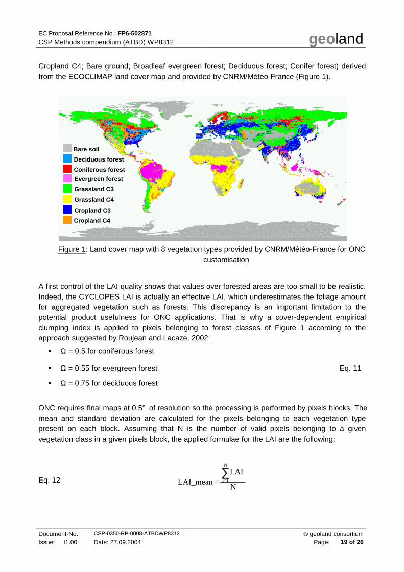
Cropland C4; Bare ground; Broadleaf evergreen forest; Deciduous forest; Conifer forest) derived from the ECOCLIMAP land cover map and provided by CNRM/Météo-France (Figure 1).

Figure 1: Land cover map with 8 vegetation types provided by CNRM/Météo-France for ONC customisation

A first control of the LAI quality shows that values over forested areas are too small to be realistic. Indeed, the CYCLOPES LAI is actually an effective LAI, which underestimates the foliage amount for aggregated vegetation such as forests. This discrepancy is an important limitation to the potential product usefulness for ONC applications. That is why a cover-dependent empirical clumping index is applied to pixels belonging to forest classes of Figure 1 according to the approach suggested by Roujean and Lacaze, 2002:

Ω = 0.5 for coniferous forest

Ω = 0.55 for evergreen forest Eq. 11

Ω = 0.75 for deciduous forest

ONC requires final maps at 0.5° of resolution so the processing is performed by pixels blocks. The mean and standard deviation are calculated for the pixels belonging to each vegetation type present on each block. Assuming that N is the number of valid pixels belonging to a given vegetation class in a given pixels block, the applied formulae for the LAI are the following:

Eq. 12

N

LAI LAI_mean

N

1i

i∑==

Bare soil

Deciduous forest

Coniferous forest

Evergreen forest

Grassland C3

Grassland C4

Cropland C3

Cropland C4




Eq. 13

Figure 2: Example of mean LAI maps of the different vegetation types.

Outputs are maps of average value, standard deviation, and number of valid pixel for each vegetation type. Figure 2 shows examples of mean LAI maps of the 8 vegetation classes for the synthesis period of 15th June 2002. They display a realistic north-south gradient of vegetation in

( )∑=

−=N

1i

2i LAI_meanLAI*

1-N

1 LAI_std

0 1 2 3 4 5 6

Bare soil

Coniferous forest

Deciduous Forest

Evergreen forest

Grassland C3

Grassland C4

Cropland C3

Cropland C4




the northern hemisphere. LAI are maxima on forested areas: Amazonia, and European coniferous forest. These values are relevant because of accounting for the vegetation clumping.

4.2 CUSTOMISATION FOR OLF

As the CYCLOPES fcover is already projected in the same regular latitude/longitude grid that the input VEGETATION data, the customisation consists in extracting the areas of interest from the global maps (Figure 3). In version 1 products, the coverage of Africa area (18° W-52° E; 38° N-36° S) is smaller than requested.

0 0.1 0.2 0.3 0.4 0.5 0.6 0.7 0.8 0.9

Figure 3: Fcover over Boreal Eurasia, 15th July 2002.

Figure 4: Fcover time profiles for pixels located on bare soil (15° N: orange), sahelian wooded grassland (10° N: red), sahelian woodland (5° N: magenta) in northern hemisphere along the 25° East meridian across Africa.

Figure 5: Fcover time profiles for pixels located on equatorial forest (0° S: green), woodland (15° S: blue), and bushland (25° S: cyan) in southern hemisphere along the 25° East meridian across Africa.

To detect the changes in land use, OLF needs clean fcover time profiles. Figure 4 and Figure 5 show examples of seasonal variations for pixels located on various vegetation types across Africa.



Document-No. CSP-0350-RP-0008-ATBDWP8312 © geoland consortium Issue: D1.10 Date: 27.09.2004 Page: 22 of 26

They display information about length of vegetative cycle, inter-annual changes and spatial coverage at the full vegetation development.

4.3 CUSTOMISATION FOR OFM

The customisation of fAPAR for VITO consists in extracting the Europe from the global maps. In version 1 products, the coverage of Europe is smaller (11° W - 30° E; 34° N - 60° N) than requested. For IGIK, the customisation of LAI and fAPAR consists in extracting the Poland from the global maps for the time period from 1st May to 30th June of each year in order to monitor the crop growth (Figure 6). For the LAI, a cover-dependent empirical clumping index is applied to pixels belonging to forest classes determined using the GLC2000 land cover map. Values of clumping index are defined in Eq.11.

Figure 6: FAPAR over Poland from the beginning of May to the end of June, 2002, at 10-day frequency.

0 0.2 0.4 0.6 0.8 1

5 May 15 May

25 May 5 June

15 June 25 June




5 REFERENCES

Brown, L.J. et al., Short wave infrared correction to the simple ratio: an image and model analysis, Remote Sensing of Environment, 71:16-25, 2000.

Chen, T.H. and co-authors, Cabauw experimental results from the project for inter-comparison of land-surface parameterization schemes, Journal of Climate, 10 (7), 1194-1215, 1997.

Chen, J.M., Canopy architecture and remote sensing of the fraction of photosynthetically active radiation absorbed by boreal conifer forest, IEEE Transactions on Geoscience and Remote Sensing, 34: 1353-1368, 1996.

Chen, J.M. and J. Cihlar, A hotspot function in a simple bi-directional reflectance model for satellite applications, Journal of Geophysical Research, 102, 25,907-25,913, 1997.

Chen, J.M. and S.G. Leblanc, A four-scale bi-directional reflectance model based on canopy architecture, IEEE Transactions on Geoscience and Remote Sensing, 35, 1316-1337, 1997.

Chen, J.M. and S.G. Leblanc, Multiple-scattering scheme useful for hyperspectral geometrical optical modelling, IEEE Transactions on Geoscience and Remote Sensing, 39, 1061-1071, 2001.

Chen, J.M., G. Pavlic, L. Brown, J. Cihlar, S.G. Leblanc, H.P. White, R.J. Hall, D. Peddle, D.J. King, J.A. Trofymov, E. Swift, J. Van der Sandem, and P. Pellikka, Validation of Canada-wide leaf area index maps using ground measurements and high and moderate resolution satellite imagery, Remote Sensing of Environment, 80, 165-184, 2002.

Chen, J.M. and F. Deng, Algorithms for global LAI/fAPAR estimation using VGT and ATSR satellite imagery, Technical note, ESRIN, Issue 2, Revision 0, 11 February 2004.

Ershov, D.V. and V.P. Novik, Features of burnt area mapping in forest of Siberia using SPOT S1-VGT data. Proceedings of the GOFC Fire Satellite Product Validation Workshop, Lisbon, July 9-11, 2001.

Hagolle, O., A. Lobo, P. Maisongrande, F. Cabot, B. Duchemin, A. De Peyreira, Quality assessment and improvement of temporally composited products of remotely sensed imagery by combination of VEGETATION 1&2 images, accepted in Remote Sensing of Environment, 2004.




Kempeneers, P, G. Lissens, F. Fierens, and J. Van Rensbergen, Development of a cloud, snow and shadow mask for VEGETATION imagery. Proceedings of VEGETATION 2000, 2 years of operation to prepare the future, International Users Committee, Vegetation Program, Toulouse, France, pp 302-306, 2000.

Knyazikhin, Y., J.V. Martonchik, R. B. Myneni, D.J. Diner and S.W. Running, Synergetic algorithm for estimating vegetation canopy leaf area index and fraction of absorbed photosynthetically active radiation from MODIS and MISR data, Journal of Geophysical Research, 103, 32,257-32,275, 1998.

Lacaze, R, P. Richaume, O. Hautecoeur, T. Lalanne, A. Quesney, F. Maignan, P. Bicheron, M. Leroy, et F. M. Bréon, Advanced algorithms of the ADEOS2/POLDER2 land surface processing line: application to the ADEOS1/POLDER1 data, Proceedings of the XXIIIth IGARSS Symposium, Toulouse, France, July 2003.

Leroy, M., J.L. Deuzé, F.M. Bréon, O. Hautecoeur, M. Herman, J.C. Buriez, D. Tanré, S. Boufiès, P. Chazette et J.L. Roujean, Retrieval of atmospheric properties and surface bi-directional reflectances over the land from POLDER/ADEOS, Journal of Geophysical Research, 102, 17,023-17,037, 1997.

Masson, V., J.L. Champeaux, F. Chauvin, C. Mériguet et R. Lacaze, A global database of land surface parameters at 1-km resolution in meteorological and climate models, Journal of Climate, 16, 1261-1282, 2003.

Myneni, R. B., R. R. Nemani, and S. W. Running, Estimation of global leaf area index and absorbed PAR using radiative transfer model, IEEE Transaction on Geoscience and Remote Sensing, 35, 1380-1393, 1997.

Plummer, S, J.M. Chen, G. Dedieu, and M. Simon, GLOBCARBON Detailed Processing Model, Issue 1, Revision 3, 07/03/03, ESRIN – ESA, 2003.

Rahman, H. and G. Dedieu, SMAC : a Simplified Method for the Atmospheric Correction of satellite measurements in the solar spectrum, International Journal of Remote Sensing, 15(1), 123-143, 1994.

Ross, J.K., The radiation regime and architecture of plant stands, Dr W. Junk Publishers, Boston, 1981.




Roujean, J.L., M. Leroy et P.Y. Deschamps, A bi-directional reflectance model of the Earth’s surface for the correction of remote sensing data, Journal of Geophysical Research, 97, 20,455-20,468, 1992.

Roujean, J.L. and F.M. Bréon, Estimating PAR absorbed by vegetation from bi-directional reflectance measurements, Remote Sensing of Environment, 51, 375-384, 1995.

Roujean, J.L., A tractable physical model of short-wave radiation interception by vegetative canopies, Journal of Geophysical Research, 101, 9523-9532, 1996.

Roujean, J.L. and R. Lacaze, Global mapping of vegetation parameters from POLDER multi-angular measurements for studies of surface-atmosphere interactions : a pragmatic method and its validation, Journal of Geophysical Research, 107, D12, 2002.

Sellers, P.J., F.G. Hall, G. Asrar, D.E. Strebel et R.E. Murphy, An overview of the First ISLSCP Field Experiment (FIFE), Journal of Geo-physical Research, 97, 18,354-18,372, 1992.

6 PSEUDO-CODE

As the customisation for OLF and OFM consists mainly in extraction of areas of interest, only the process applied to answer the ONC requirements is reported here. As the ATBD provider and recipient are the same partner (MEDIAS-France), the pseudo-code just gives the basic step of the customisation procedure.

-------------------------------------------------

Given p the index of biophysical parameters (p=1 to 4)

Given b the index of pixels blocks (b=1 to 720*360=259200)

Given v the index of vegetation classes (v=1 to 8)

Given X the value of the p biophysical parameter

Given Ωv the value of clumping index for the v vegetation class

For the p parameter

Open the p parameter file

Open the land cover file

Open the 8 mean_value files

Open the 8 standard_deviation value files

Open the 8 number_of_valid_pixel value files




For the b block

Read the b block in the parameter file

Read the b block in the land cover file

For the v vegetation class

Compute the number N of valid pixels of the v class in the b block

If N=0 then MEAN(Xp) = undefined and STD(Xp) = undefined

If N=1 then Begin

If p=LAI then Xp = Xp / Ωv

MEAN(Xp) = Xp and STD(Xp) = undefined

Endif

If N > 1 then Begin

If p=LAI then Xp = Xp / Ωv

MEAN(Xp) = ( ) / N and STD(Xp) =

Endif

Write MEAN(Xp) in the b pixel of the mean value file of the v class

Write STD(Xp) in the b pixel of the standard deviation value file of the v class

Write N in the b pixel of the number_of_valid_pixel value file of the v class

Endfor the v vegetation class

Endfor the b block

Close the p parameter file

Close the land cover file

Close the 8 mean_value files

Close the 8 standard_deviation value files

Close the 8 number_of_valid_pixel value files

Endfor the p parameter

-------------------------------------------------

∑=

N

i

pi

1

X( )

1N

)MEAN(X1

p

−

−∑=

N

ipiX

IP land, FP6-2002-SPACE-1 geoland · Integrated Project geoland ... 2.3 OFM requirements ... OLF...

Documents

Transcript of IP land, FP6-2002-SPACE-1 geoland · Integrated Project geoland ... 2.3 OFM requirements ... OLF...