Ionospheric delay gradient monitoring for aeronautical application in Thailand

Sarawoot Rungraengwajiake1, Assoc. Dr. Pornchai Supnithi1

Dr. Susumu Saito2, Nattapong Siansawasdi3, Dr. Apithep Saekow4

1Faculty of Engineering, King Mongkut’s Institute of Technology Ladkrabang (KMITL), Thailand 2Electronic Navigation Research Institute (ENRI), Japan 3Aeronautical Radio of Thailand (AEROTHAI), Thailand

4Stamford International University, Thailand

The International Reference Ionosphere (IRI) Workshop 2013

24-28 June 2013, Olstyzn, Poland

1

Outline

• Ionospheric delay gradient effects on Ground-Based Augmentation System (GBAS)

• Experimental Setup

• Results and Discussions

• Conclusions

2

Ionospheric effects to GBAS

Reference Station

GNSS Satellites

Ionosphere

Airplane

Differential correction

• The reference stations provide the differential corrections and integrity information to the receiver that are equipped in the aircraft in the nearby area. • However, the ionospheric irregularities can cause the error of the differential correction information that is broadcast to the aircraft. • For the GAST-D (GBAS Approach Service Type D), the error of differential corrections shall be less than 1.5 m within 5 km of the runway threshold (300 mm/km).

Ground-Based Augmentation System (GBAS)

3

Ionospheric effects to GBAS

S. Datta-Barua, et al., 2010.

20 November 2003

413 mm/km

This extreme event stimulate the ionospheric delay gradient research in various regions.

4

Ionospheric effects to GBAS

Reference Station

GNSS Satellites

Ionosphere

Airplane

Vairplane

Viono_front

h

d

Front Speed

Front Slope

Front Width

• Here, we investigate on the Front Slope or

“Ionospheric delay gradient”. • Causes of Ionospheric delay gradient, 1. Due to the physical ionospheric separation between aircraft and reference station. 2. Due to the ionospheric irregularities (plasma bubbles, SED).

• Q : How large of the ionospheric delay gradient in the low latitude regions can be?

In this study, we investigate on the ionospheric delay gradient associated with plasma bubbles in Thailand, which is located in low- latitude region.

Simplified ionosphere wave front model

Differential correction

5

Ionospheric effects to GBAS

S. Saito 2011.

Reference Station

GNSS Satellites

Ionosphere

Airplane Differential correction???

Plasma bubble

• Plasma bubble frequently occurs in low-latitude region after sunset , and more occurrence during high solar activity period.. • This phenomena can cause ionospheric delay gradient and also scintillation, which degrades the GBAS performance.

The ICAO has recently realize the impact of plasma bubble and recommended each country to investigate ionospheric delay gradient. 6

Objectives

• Investigate the ionospheric delay gradient during plasma bubble occurrence around Suvarnbhumi international airport, Thailand.

• Propose the processing-step for ionospheric delay gradient monitoring at low-latitude stations.

7

Short baseline experiments

• Short baseline experiment needs to be carried out to monitor the ionospheric delay gradients near Suvarnabhumi international airport. • Three dual-frequency GPS receivers have been installed as part of a cooperation project of 1. King Mongkut’s Institute of Technology Ladkrabang (KMITL) 2. Electronic Navigation Research Institute (ENRI), Japan 3. Aeronautical Radio of Thailand Ltd. (AEROTHAI) 4. Stamford International University • This project started July 2011.

8

ROTI (Rate of TEC change index)

( ) ( 1) ( ) ROT i STEC i STEC i

2

1

1( ( ) )

N

i

ROTI ROT i ROTN

• In order to detect the ionospheric irregularities, we use the rate of TEC change index or ROTI.

• The ROTI is defined by Standard deviation of rate of TEC change with 5-minute window.

SUNSET MIDNIGHT

Example ROTI

Quiet Condition

Irregularities

9

Results and Discussions

ROTI (5 minute window) of 18 days of September 2011

10

Results and Discussions

15 days have high ROTI values 11

1 September

Ionospheric delay gradient calculation

_1 _ 2

1 2 1 2( ) ( )

k k k

adj adj

k k

R R

dSTEC STEC STEC

STEC STEC B B

10 10.5 11 11.5 12 12.5 13 13.5 14 14.5 15-20

-10

0

10

20

30

40

ST

EC

(T

EC

U)

STEC

KMITL

STFD

10 10.5 11 11.5 12 12.5 13 13.5 14 14.5 152

4

6

8

10

Time (UTC)

dS

TE

C (

TE

CU

)

dSTEC

BrSTFD-BrKMITL

(STECSTFD-STECKMITL) + (BrKMITL-BrSTFD)

Quiet time Ionospheric disturbance

_1 1 _1

k k K

adj S RSTEC STEC B B

_ 2 2 _ 2

k k K

adj S RSTEC STEC B B

1 September 2011 Single difference method

12

PRN2

Ionospheric delay gradient calculation

1 2 1 2( ) ( )k k k

R RdSTEC STEC STEC B B 1 2

2

( ) ( )40.3( )

k kSTEC t STEC tI t

df

Ionospheric delay gradient (mm/km) 13

Results and Discussions 1st September 2011

8 10 12 14 16 18 20 22 24-5

0

5

10

15

dS

TE

C (

TE

CU

)

STFD-KMIT

8 10 12 14 16 18 20 22 24-5

0

5

10

15

Time (UTC)

dS

TE

C (

TE

CU

)

AERO-KMIT

dSTEC

PRN2, 9, 14, 21, 29

• The constant level can be considered as the differential receiver biases.

14

Results and Discussions 1st September 2011

8 10 12 14 16 18 20 22 24-5

0

5

10

15

dS

TE

C (

TE

CU

)

STFD-KMIT

8 10 12 14 16 18 20 22 24-5

0

5

10

15

Time (UTC)

dS

TE

C (

TE

CU

)

AERO-KMIT

dSTEC

4.28 –5.12 TECU

5.18 –6.78 TECU

uncertainty offset

BrSTFD-BrKMIT

BrAERO-BrKMIT

• However, we found a slight offset exist in AERO-KMIT direction due to the uncertainty offset in the adjustment step (L. Ciraolo, et al., 2007). • Therefore, we consider the differential receiver biases for each satellite.

15

PRN2, 9, 14, 21, 29

Results and Discussions 1st September 2011

8 10 12 14 16 18 20 22 24-5

0

5

10

15

dS

TE

C (

TE

CU

)

STFD-KMIT

8 10 12 14 16 18 20 22 24-5

0

5

10

15

Time (UTC)

dS

TE

C (

TE

CU

)

AERO-KMIT

8 10 12 14 16 18 20 22 24

-100

0

100

I (m

m/k

m)

STFD-KMIT

8 10 12 14 16 18 20 22 24

-100

0

100

Time (UTC)

I (m

m/k

m)

AERO-KMIT

( )I tdSTEC

4.28 –5.12 TECU

5.18 –6.78 TECU

-95.23 mm/km

107.7 mm/km

PRN2, 9, 14, 21, 29

uncertainty offset in the adjustment step

BrSTFD-BrKMIT

BrAERO-BrKMIT

16

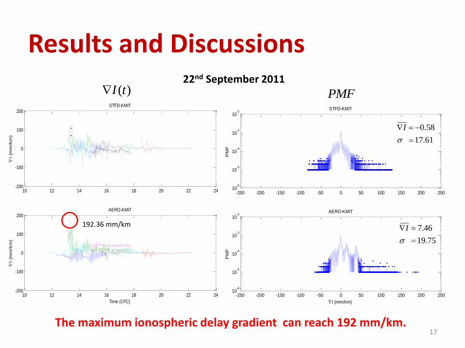
Results and Discussions

10 12 14 16 18 20 22 24-200

-100

0

100

200

I

(mm

/km

)

STFD-KMIT

10 12 14 16 18 20 22 24-200

-100

0

100

200

Time (UTC)

I

(mm

/km

)

AERO-KMIT

-250 -200 -150 -100 -50 0 50 100 150 200 25010

-6

10-5

10-4

10-3

10-2

PM

F

STFD-KMIT

-250 -200 -150 -100 -50 0 50 100 150 200 25010

-6

10-5

10-4

10-3

10-2

I (mm/km)

PM

F

AERO-KMIT

22nd September 2011

192.36 mm/km

0.58

17.61

I

7.46

19.75

I

( )I t PMF

17 The maximum ionospheric delay gradient can reach 192 mm/km.

Previous processing-step proposed

• In order to process a lot of GPS data for ionospheric delay gradient monitoring, the previous studies proposed the data processing-step, focus on the SED event on 20 November 2003.

• However, they did not consider the plasma bubble occurrence in equatorial and low-latitude regions.

S. Datta-Barua, et al., 2010.

J. Lee, et al., 2011. 18

Ionospheric delay gradient for equatorial an d low-latitude regions

Raw RINEX data

Pre-processing

Compute Slant TEC (STEC)

Find Maximum Ionospheric gradient

(Station Pair)

Manual Validation

Update Ionospheric Threat Model

Find Plasma Bubble Occurrence (using ROTI)

Processed by GPStk - Cycle slip detection - Short-arc removal

Using carrier (L1 , L2) and code measurement (C1 , P2)

ROTI > threshold

* Biases are not calibrated * Receiver biases are calibrated using station pair method

Validate the true ionospheric phenomena

Update a new bound Pseudorange and carrier phase measurements of dual-frequencies GPS receiver

19

Conclusions

• From this study, we show the ionospheric delay gradients near Suvarnabhumi international airport, Thailand, during September equinox 2011.

• Based on 15-day of high ROTI observations, we found that the maximum ionospheric delay gradient can reach 192.36 mm/km on 22nd September 2011.

• In order to process a lot of GPS data for monitoring stations at equatorial and low-latitude regions, we should include the ROTI for plasma bubble detection.

20

Thank you for your attention! Question?

21

Backup Slides

22