IOANNIS Z. GITAS AND CÉSAR CARMONA-MORENO...

I

IOANNIS Z. GITAS AND CÉSAR CARMONA-MORENO (EDITORS)

PROCEEDINGS OF THE 6TH INTERNATIONAL WORKSHOP OF THE EARSeL SPECIAL INTEREST GROUP ON FOREST FIRES

ADVANCES IN REMOTE SENSING AND GIS APPLICATIONS IN FOREST FIRE MANAGEMENT

TOWARDS AN OPERATIONAL USE

OF REMOTE SENSING IN FOREST FIRE MANAGEMENT

27-29 September 2007, THESSALONIKI - GREECE

II

The mission of the Institute for Environment and Sustainability is to provide scientific-technical support to the European Union’s Policies for the protection and sustainable development of the European and global environment. European Commission Joint Research Centre Institute for Environment and Sustainability Contact information Address: 1, via Fermi – 21020 Ispra (ITALY) E-mail: [email protected] – [email protected] Tel.: +39.0332.789654 +30.2310.992699 Fax: +39.0332.789073 +30.2310.998897 http://ies.jrc.ec.europa.eu http://www.jrc.ec.europa.eu Legal Notice Neither the European Commission nor any person acting on behalf of the Commission is responsible for the use which might be made of this publication. A great deal of additional information on the European Union is available on the Internet. It can be accessed through the Europa server http://europa.eu/ JRC 8072 EUR 22892 EN ISBN 978-92-79-06620-7 ISSN 1018-5593 Luxembourg: Office for Official Publications of the European Communities © European Communities, 2007 Reproduction is authorised provided the source is acknowledged Printed in Italy

III

Ioannis Z. Gitas and César Carmona-Moreno (Editors) (2007): Proceedings of the 6th International Workshop of The EARSeL Special Interest Group On Forest Fires - Advances in Remote Sensing and GIS Applications in Forest Fire Management: Towards An Operational Use of Remote Sensing in Forest Fire Management, European Association of Remote Sensing Laboratories (EARSeL), Special Interest Group on Forest Fires (FF-SIG) - Aristotle University of Thessaloniki, Faculty of Forestry and Natural Environment, Laboratory of Forest Management and Remote Sensing (AUTh) - European Commission - Joint Research Centre (JRC), Institute for Environment and Sustainability (IES) - Universidad de Alcalá Departamento de Geografía (UAH), 310 pages.

IV

EARSeL-FFSIG Organising Committees International Chairman: Ioannis Gitas, Aristotle University of Thessaloniki Members:

Michael Karteris, Aristotle University of Thessaloniki

Emilio Chuvieco, Universidad de Alcalá

Javier Salas Rey, Universidad de Alcalá

Paulo Barbosa, Joint Research Centre

César Carmona-Moreno, Joint Research Centre

Local:

Ioannis Gitas, Aristotle University of Thessaloniki

Michael Karteris, Aristotle University of Thessaloniki

Nikolaos Silleos, Aristotle University of Thessaloniki

Theodoros Astaras, Aristotle University of Thessaloniki

Maria Tsakiri, Aristotle University of Thessaloniki

Georgios Zalidis, Aristotle University of Thessaloniki

Ioannis Meliadis, National Agricultural Research Foundation / Forest Research Institute

Georgios Mallinis, Aristotle University of Thessaloniki

Georgios Mouflis Aristotle University of Thessaloniki

George Mitri, Aristotle University of Thessaloniki

Chara Minakou, Aristotle University of Thessaloniki

Konstantinos Ntouros, Aristotle University of Thessaloniki

Ioannis Stergiopoulos, Aristotle University of Thessaloniki

Anastasia PolychronakI, Aristotle University of Thessaloniki

Thomas Katagis, Aristotle University of Thessaloniki

Maria Tsakyrelli, Aristotle University of Thessaloniki

V

EARSeL-FFSIG Scientific Committee

Allgöwer Britta, University of Zurich

Barbosa Paulo, DG Joint Research Centre

Boschetti Luigi, University of Maryland

Brivio Pietro Alessandro, Consiglio Nazionale delle Ricerche

Camia Andrea, DG Joint Research Centre

Carmona-Moreno César, DG Joint Research Centre

Chuvieco Emilio, University of Alcalá

Csiszar Ivan, University of Maryland

de la Riva Juan, University of Zaragoza

Deshayes Michel, CEMAGREF

Gitas Ioannis, Aristotle University of Thessaloniki

Justice Chris, University of Maryland

Karteris Michael, Aristotle University of Thessaloniki

Kasischke Eric, University of Maryland

Koutsias Nikolaos, University of Ioannina

Martin Pilar, Consejo Superior de Investigaciones Científicas

Oertel Dieter, DLR German Aerospace

Pereira José Miguel, Instituto Superior de Agronomia

Pons Xavier, Centre de Recerca Ecològica i Aplicacions Forestals,

CREAF and Dep. of Geography. Autonomous University of Barcelona

Riano David, CSTARS, University of California

Roberts Dar, University of California

van Wagtendok Jan, United States Geological Survey

Wooster Martin, University of London

Yool Stephen R., University of Arizona

VI

CONTENTS Forward Fire Risk Estimation GRAND CHALLENGES IN WILDLAND FIRE TECHNOLOGY AND MANAGEMENT

STEPHEN R. YOOL ........................................................................................................................................................ 1 OPERATIONAL REMOTE SENSING IN FIRE PREVENTION: AN OVERVIEW

A. SEBASTIÁN-LÓPEZ, M.J. YAGÜE BALLESTER, M. SÁNCHEZ-GUISÁNDEZ ........................................................... 15 FIRE DETECTION AND MONITORING, (QUANTITATIVE USES OF ACTIVE FIRE THERMAL EMISSIONS)

M.J. WOOSTER & G. ROBERTS................................................................................................................................... 20 OPERATIONAL FIRE MONITORING, (A PROSPECTIVE VIEW ON SATELLITE BASED WILDFIRE MONITORING)

D. OERTEL .................................................................................................................................................................. 29 POST-FIRE EVALUATION OF THE EFFECTS OF FIRE ON THE ENVIRONMENT USING REMOTELY-SENSED DATA

E.S. KASISCHKE, E.E. HOY & M.R. TURETSKY......................................................................................................... 38 EUROPEAN FOREST FIRE INFORMATION SYSTEM (EFFIS) - RAPID DAMAGE ASSESSMENT: APPRAISAL OF BURNT AREA MAPS WITH MODIS DATA

P. BARBOSA, J. KUCERA, P. STROBL.......................................................................................................................... 57 FOREST FIRE RISK MANAGEMENT INFORMATION SYSTEM - FFRMIS

N. KANELLOPOULOS, G. TSIRONIS, G. VASILEIOU, TH. MANTES, A. GRYLLAKIS, M. KOUTLIS, D. VENIZELOS &V. N. CHRISTOFILAKIS ............................................................................................................................................ 63

AN INTERCOMPARISON STUDY OF MODELLED FOREST FIRE RISK IN THE MEDITERRANEAN FOR PRESENT DAY CONDITIONS

C. GIANNAKOPOULOS, P.LESAGER, E. KOSTOPOULOU, A. VAJDA & A. VENÄLÄINEN ........................................... 67 ASSESSING THE CAPABILITY OF MODIS DERIVED SPECTRAL INDICES FOR THE IDENTIFICATION OF FIRE PRONE AREAS

M. J. RODRIGUES........................................................................................................................................................ 74 A CONTROLLED LOOK-UP TABLE GENERATION FOR FUEL MOISTURE CONTENT ESTIMATION.

M. YEBRA, A. DE SANTIS & E. CHUVIECO ................................................................................................................ 74 AUTOMATED FEATURE EXTRACTION ON QUICKBIRD IMAGE REQUIRED TO MAP WILDLAND URBAN INTERFACES (WUI) IN THE FRENCH MEDITERRANEAN REGION

M. LONG, C. LAMPIN, M. JAPPIOT, D. MORGE, & C. BOUILLON.. ............................................................................. 79 ESTIMATION OF CROWN BIOMASS IN THE CONTEXT OF FOREST-FIRE MANAGEMENT IN MEDITERRANEAN AREAS

A. GARCÍA-MARTÍN, F. PÉREZ-CABELLO, J. DE LA RIVA FERNÁNDEZ & R. MONTORIO LLOVERÍA ........................ 84 ESTIMATION OF LIVE FUEL MOISTURE CONTENT ANOMALIES IN CENTRAL SPAIN DERIVED FROM AVHRR TIME SERIES IMAGERY

M. GARCÍA, I. AGUADO & E. CHUVIECO ................................................................................................................... 89 EVALUATION OF DRY FOLIAGE MATTER THROUGH NORMALISED INDEXES AND INVERSION OF REFLECTIVITY MODELS

A. ROMERO, I. AGUADO, E. CHUVIECO & M. YEBRA................................................................................................ 93

VII

USE OF REMOTE SENSING AND GIS IN FOREST FIRE SUPPRESSION PLANNING S. G. TSAKALIDIS & I.Z.GITAS .................................................................................................................................. 97

FOREST FIRE PREVENTION: A GIS TOOL FOR FIRE-FIGHTING PLANNING AND MANAGEMENT E. MARCHI, E. TESI, N. BRACHETTI MONTORSELLI, C. CONESE, L. BONORA & M. ROMANI................................ 102

FUEL TYPE MAPPING USING MEDIUM RESOLUTION IMAGERY AND GIS, CONSIDERING RADIOMETRIC, SPATIAL AND SPECTRAL ENHANCEMENTS OF THE ORIGINAL DATASET

I. STERGIOPOULOS, G. MALLINIS & I.Z. GITAS ....................................................................................................... 107 INTEGRATION OF LOCAL SCALE FUEL TYPE MAPPING AND FIRE BEHAVIOR PREDICTION USING HIGH SPATIAL RESOLUTION IMAGERY

G. MALLINIS, I.D. MITSOPOULOS, A.P. DIMITRAKOPOULOS,I.Z. GITAS & M. KARTERIS ...................................... 111 ON THE SPECTRAL SEPARABILITY OF PROMETHEUS FUEL TYPES IN THE MEDITERRANEAN ECOSYSTEMS OF THE ITALIAN PENINSULA

R. LASAPONARA & A. LANORTE.............................................................................................................................. 115 PREDICTING THE OCCURRENCE OF LIGHTING/HUMAN-CAUSED WILDFIRES USING ADVANCED TECHNIQUES OF DATA MINING

G. AMATULLI, F. PERÉZ-CABELLO,A. CAMIA, J. DE LA RIVA ................................................................................. 119 SYNERGY OF GIS AND REMOTE SENSING DATA IN FOREST FIRE DANGER MODELLING

P. A. HERNANDEZ-LEAL, A. GONZALEZ-CALVO, M. ARBELO, A. BARRETO & L. ARVELO-VALENCIA ................ 123 DETAILED CARTOGRAPHY SYSTEM OF FUEL TYPES FOR PREVENTING FOREST FIRES

A. STERGIADOU, E.VALESE & D. LUBELLO............................................................................................................. 127 THE EFFECTS OF SPATIAL RESOLUTION AND THE IMAGE ANALYSES TECHNIQUES ON PRE-FIRE WILD LAND MAPPING

M. A. TANASE, &I. GITAS ........................................................................................................................................ 132 THE VEGETATION CONDITIONS WHICH INFLUENCE OCCURRENCE, PROPAGATION AND DURATION OF FIRES IN ARGENTINA

M. FISCHER, C. M. DI BELLA & E. G. JOBBÁGY...................................................................................................... 137 TIME SERIES ANALYSIS OF REMOTE SENSING TO CALCULATE AND MAP OPERATIONAL INDICATORS OF WILDFIRE RISK

V. CHERET, J.P. DENUX. W. SAMPARA & M. GAY.................................................................................................. 143

Fire Detection A COMPARATIVE STUDY OF THE PERFORMANCE OF THE NDVI, THE TVI AND THE SAVI VEGETATION INDICES OVER BURNT AREAS, USING PROBABILITY THEORY AND SPATIAL ANALYSIS TECHNIQUES

G. SKIANIS, D. VAIOPOULOS & K. NIKOLAKOPOULOS............................................................................................ 152 A GLOBAL, MULTI-YEAR (2000-2007), VALIDATED BURNT AREA PRODUCT (L3JRC) DERIVED FROM DAILY SPOT VEGETATION DATA

K. TANSEY, J. M. GRÉGOIRE, J. M.C. PEREIRA, P. DEFOURNY, R. LEIGH, A. BARROS, J. F. PEKEL, J. M. SILVA E. VAN BOGAERT, E. BARTHOLOMÉ & S. BONTEMPS.............................................................................................. 154

ASSESSING THE INFORMATION CONTENT OF LANDSAT-5 THEMATIC MAPPER DATA FOR MAPPING AND CHARACTERIZING FIRE SCARS

N. KOUTSIAS, G. MALLINIS & M. TSAKIRI-STRATI................................................................................................. 159

VIII

FIRE OBSERVATIONS FROM ETM+ AND ASTER IMAGERY AND IMPLICATIONS FOR ACTIVE FIRE PRODUCT VALIDATION FROM COARSE RESOLUTION SENSORS

I. CSISZAR & W. SCHROEDER .................................................................................................................................. 163 FUZZY BASED APPROACH FOR MAPPING BURNT AREAS IN MEDITERRANEAN ENVIRONMENT USING ASTER IMAGES

P. A. BRIVIO, P. ZAFFARONI, M. BOSCHETTI & D. STROPPIANA............................................................................. 168 IMPROVING THE PERFORMANCE OF THE BAIM INDEX FOR BURNT AREA MAPPING USING MODIS DATA

I. G. NIETO & P. MARTÍN ......................................................................................................................................... 172 MAPPING BURNED AREA BY USING SPECTRAL ANGLE MAPPER IN MERIS IMAGES

P. OLIVA & P. MARTÍN............................................................................................................................................. 177 SPATIAL ANALYSIS OF ACTIVE FIRE COUNTS IN SOUTHEAST ASIA

MASTURA MAHMUD ................................................................................................................................................ 199 THE DEVELOPMENT OF A TRANSFERABLE OBJECT-BASED MODEL FOR BURNED AREA MAPPING USING ASTER IMAGERY

A. I. POLYCHRONAKI, I. Z. GITAS & A.M. KARTERIS............................................................................................. 187 THE GLOBAL MODIS BURNED AREA PRODUCT

D.P. ROY, L.BOSCHETTI & C.O.JUSTICE ................................................................................................................. 191 AUTOMATIC DISCRIMINATION OF CORE BURN SCARS USING LOGISTIC REGRESSION MODELS

A. BASTARRIKA, E. CHUVIECO & M.P. MARTÍN ..................................................................................................... 195 USING NASA’S WORLD WIND VIRTUAL GLOBE FOR INTERACTIVE INTERNET VISUALISATION AND QUALITY ASSESSMENT OF THE GLOBAL MODIS BURNED AREA PRODUCT

L.BOSCHETTI, D.P. ROY & C.O.JUSTICE ................................................................................................................. 200

Fire Effects Assessment

A DECISION SUPPORT SYSTEM FOR WILDFIRE MANAGEMENT AND IMPACT ASSESSMENT IN AFFECTED ZONES

C. KONTOES, P. ELIAS, I. KOTSIS, D. PARONIS, & I. KERAMITSOGLOU .................................................................. 204 A PRELIMINARY PROPOSAL FOR PHYSICALLY BASED TECHNIQUE FOR THE ESTIMATION OF BOREAL FOREST FIRE SEVERITY USING THE MODIS SENSOR, DEMONSTRATED USING SELECTED EVENTS FROM 2002 FIRE SEASON IN RUSSIA

G. N. MOTTRAM, M. WOOSTER , G. ROBERTS, H. BALZTER, J. KADUK, C. GEORGE & J. BEISLEY ....................... 208 AN OPERATIONAL PROTOCOL FOR POST-FIRE EVALUATION AT LANDSCAPE SCALE IN AN OBJECT-ORIENTED ENVIRONMENT

M.F. ÁLVAREZ, J.R. RODRÍGUEZ, D. VEGA-NIEVA & F. CASTEDO-DORADO......................................................... 212 ANALYSIS OF THE CAUSALITY OF FIRES (1985-1997) IN MACEDONIA, GREECE

G. D. MOUFLIS & I. Z. GITAS................................................................................................................................... 218 ASSESSMENT OF THE RESPONSE OF A MEDITERRANEAN-TYPE FOREST ECOSYSTEM TO RECURRENT WILDFIRES AND TO DIFFERENT RESTORATION PRACTICES USING REMOTE SENSING AND GIS TECHNIQUES

P. CHRISTAKOPOULOS, I.HATZOPOULOS, K. KALABOKIDIS & A. FILINTAS........................................................... 223

IX

ASSESSMENT OF THE SHORT-TERM IMPACT OF FOREST FIRES BY EMPLOYING OBJECT-BASED CLASSIFICATION AND GIS ANALYSIS

A.I. POLYCHRONAKI, T.G. KATAGIS, I.Z. GITAS & M.A. KARTERIS ..................................................................... 227 COMBINED METHODOLOGY OF FIELD SPECTROMETRY AND DIGITAL PHOTOGRAPHY IN ESTIMATING FIRE SEVERITY

R. MONTORIO LLOVERÍA, F. PÉREZ-CABELLO, A. GARCÍA-MARTÍN & J. DE LA RIVA FERNÁNDEZ ...................... 231 MAPPING ANNUAL BURNED AREAS IN MALAGASY SAVANNA ENVIRONMENTS AT LANDSCAPE SCALE USING MODIS TIME SERIES ANALYSIS

JACQUIN ANNE, DUMONT MELANIE, DENUX JEAN-PHILIPPE & GAY MICHEL ....................................................... 236 EVOLUTION OF DNBREXTENDED IN TERMS OF DIFFERENT FIRE-SEVERITY LEVELS AND PLANT COMMUNITIES IN WILDFIRES AREAS OF THE PRE-PYRENEES (SPAIN)

F. PÉREZ-CABELLO, R. MONTORIO LLOVERÍA, A. GARCÍA-MARTÍN & J. DE LA RIVA FERNÁNDEZ ...................... 242 INVERSION OF THE GEOSAIL RADIATIVE TRANSFER MODEL TO ESTIMATE BURN SEVERITY

A. DE SANTIS, M.YEBRA & E. CHUVIECO ............................................................................................................... 247 MAPPING POST-FIRE VEGETATION REGENERATION USING EO-1 HYPERION

G. H. MITRI & I. Z.GITAS......................................................................................................................................... 252 POST-FIRE EVALUATION OF DELAYED TREE MORTALITY IN A FOREST OF THE CENTRAL ALPS USING TIME SERIES OF COLOUR INFRARED IMAGES

L. LARANJEIRO & C. GINZLER ................................................................................................................................. 256 SPATIAL PATTERNS AND VARIATIONS OF FOREST FIRES IN SPAIN, 1991-2005

F. VERDÚ, J. SALAS & I. AGUADO ........................................................................................................................... 261 TEXTURE ANALYSIS OF A POST-FIRE LANDSCAPE USING AN OBJECT-BASED MULTI-SCALE IMAGE SEGMENTATION ALGORITHM

R. HERNÁNDEZ-CLEMENTE, R. M. NAVARRO-CERRILLO, I. Z. GITAS, J.E. HERNÁNDEZ-BERMEJO & M. GONZÁLEZ-AUDICANA ................................................................................................................................... 265

VEGETATION REGROWTH DETECTION AFTER A FOREST FIRE IN CENTRE CYPRUS USING LANDSAT TM AND ETM+ DATA

J. P. SOLANS VILA & P. BARBOSA ........................................................................................................................... 269

X

Foreword

During the last two decades, interest in forest fire research has grown steadily, as more and more

local and global impacts of burning are being identified. The definition of fire regimes as well as

the identification of factors explaining spatial and temporal variations in these fire characteristics

are recently hot fields of research. Changes in these fire regimes have important social and

ecological implications. Whether these changes are mainly caused by land use or climate

warming, greater efforts are demanded to manage forest fires at different temporal and spatial

scales.

The European Association of Remote Sensing Laboratories (EARSeL)’s Special Interest Group

(SIG) on Forest Fires was created in 1995, following the initiative of several researchers

studying Mediterranean fires in Europe. It has promoted five technical meetings and several

specialised publications since then, and represents one of the most active groups within the

EARSeL. The SIG has tried to foster interaction among scientists and managers who are

interested in using remote sensing data and techniques to improve the traditional methods of fire

risk estimation and the assessment of fire effect.

The aim of the 6th international workshop is to analyze the operational use of remote sensing in

forest fire management, bringing together scientists and fire managers to promote the

development of methods that may better serve the operational community. This idea clearly links

with international programmes of a similar scope, such as the Global Monitoring for

Environment and Security (GMES) and the Global Observation of Forest Cover/Land Dynamics

(GOFC-GOLD) who, together with the Joint Research Center of the European Union sponsor

this event.

Finally, I would like to thank the local organisers for the considerable lengths they have gone to

in order to put this material together, and take care of all the details that the organization of this

event requires.

Emilio Chuvieco Forest Fire SIG Chairman Alcalá de Henares (Spain), July, 2007

1

Grand Challenges in Wildland Fire Technology and Management

Stephen R. Yool, Ph.D., Associate Professor The University of Arizona Tucson, AZ 85721, [email protected]

Keywords: Wildland Fire, Remote Sensing, GIS, Decision Support System ABSTRACT: Will the global community promote actively the alliances between the natural and social sciences required to manage wildland fire effectively? We must to achieve this alliance integrate fire, climate and society variables. Meeting grand challenges in remote sensing and geographic information science (GIS) define first steps toward wildland fire management. The grandest challenge of all is, however, integrated decision support that empowers people and fire to co-exist, thus stabilize atmospheric processes and benefit from the renewal fire brings to natural systems. A Fire-Climate-Society (FCS) prototype uses the Analytical Hierarchy Process (AHP) to bring together suites of fire probability variables (e.g., fuel moistures; lightning and human ignition probabilities) and societal values at risk (e.g., property; recreation; endangered species). Resulting maps create consensus on high priority fuel treatment areas.

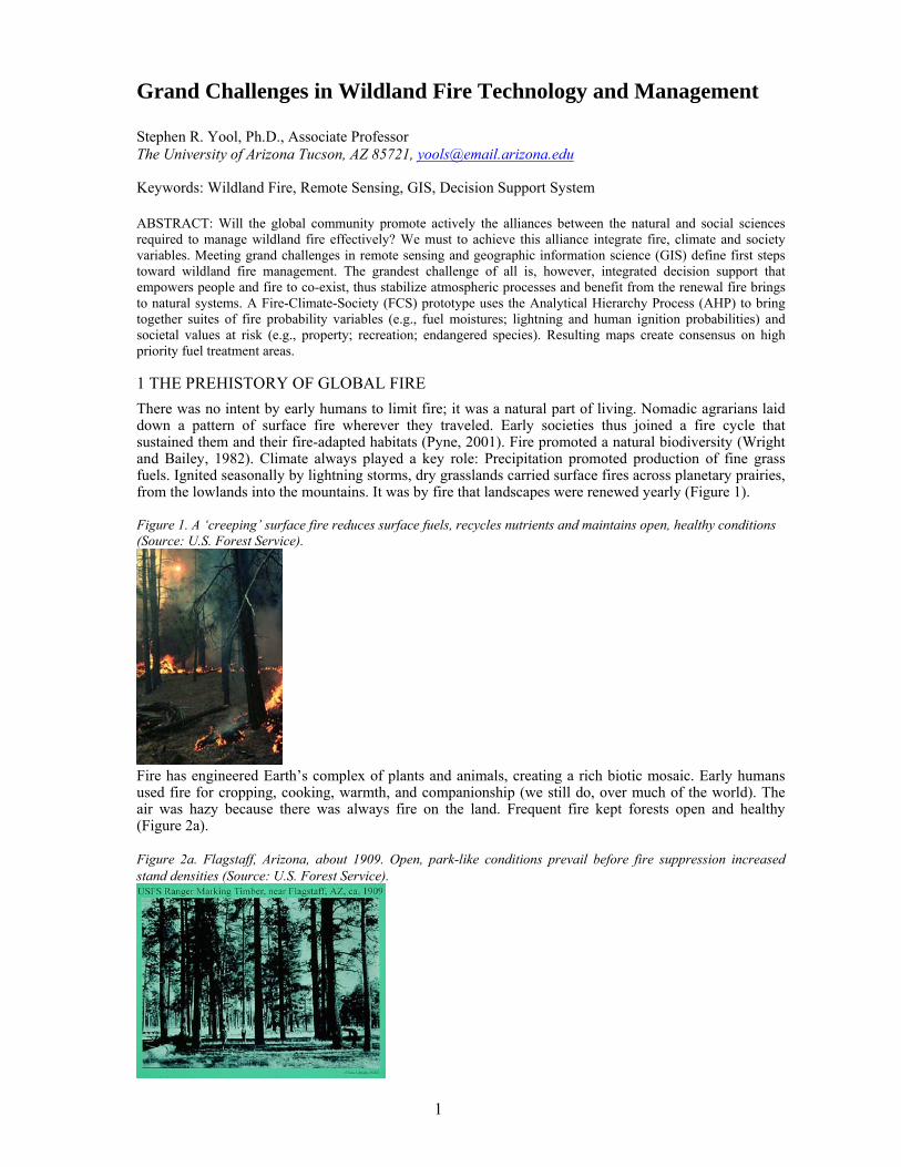
1 THE PREHISTORY OF GLOBAL FIRE There was no intent by early humans to limit fire; it was a natural part of living. Nomadic agrarians laid down a pattern of surface fire wherever they traveled. Early societies thus joined a fire cycle that sustained them and their fire-adapted habitats (Pyne, 2001). Fire promoted a natural biodiversity (Wright and Bailey, 1982). Climate always played a key role: Precipitation promoted production of fine grass fuels. Ignited seasonally by lightning storms, dry grasslands carried surface fires across planetary prairies, from the lowlands into the mountains. It was by fire that landscapes were renewed yearly (Figure 1).

Figure 1. A ‘creeping’ surface fire reduces surface fuels, recycles nutrients and maintains open, healthy conditions (Source: U.S. Forest Service).

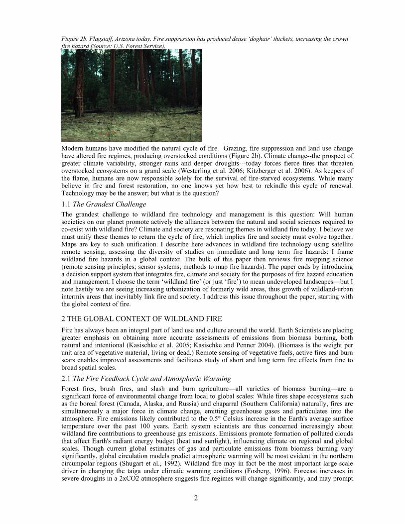
Fire has engineered Earth’s complex of plants and animals, creating a rich biotic mosaic. Early humans used fire for cropping, cooking, warmth, and companionship (we still do, over much of the world). The air was hazy because there was always fire on the land. Frequent fire kept forests open and healthy (Figure 2a).

Figure 2a. Flagstaff, Arizona, about 1909. Open, park-like conditions prevail before fire suppression increased stand densities (Source: U.S. Forest Service).

2

Figure 2b. Flagstaff, Arizona today. Fire suppression has produced dense ‘doghair’ thickets, increasing the crown fire hazard (Source: U.S. Forest Service).

Modern humans have modified the natural cycle of fire. Grazing, fire suppression and land use change have altered fire regimes, producing overstocked conditions (Figure 2b). Climate change--the prospect of greater climate variability, stronger rains and deeper droughts---today forces fierce fires that threaten overstocked ecosystems on a grand scale (Westerling et al. 2006; Kitzberger et al. 2006). As keepers of the flame, humans are now responsible solely for the survival of fire-starved ecosystems. While many believe in fire and forest restoration, no one knows yet how best to rekindle this cycle of renewal. Technology may be the answer; but what is the question?

1.1 The Grandest Challenge The grandest challenge to wildland fire technology and management is this question: Will human societies on our planet promote actively the alliances between the natural and social sciences required to co-exist with wildland fire? Climate and society are resonating themes in wildland fire today. I believe we must unify these themes to return the cycle of fire, which implies fire and society must evolve together. Maps are key to such unification. I describe here advances in wildland fire technology using satellite remote sensing, assessing the diversity of studies on immediate and long term fire hazards: I frame wildland fire hazards in a global context. The bulk of this paper then reviews fire mapping science (remote sensing principles; sensor systems; methods to map fire hazards). The paper ends by introducing a decision support system that integrates fire, climate and society for the purposes of fire hazard education and management. I choose the term ‘wildland fire’ (or just ‘fire’) to mean undeveloped landscapes—but I note hastily we are seeing increasing urbanization of formerly wild areas, thus growth of wildland-urban intermix areas that inevitably link fire and society. I address this issue throughout the paper, starting with the global context of fire.

2 THE GLOBAL CONTEXT OF WILDLAND FIRE Fire has always been an integral part of land use and culture around the world. Earth Scientists are placing greater emphasis on obtaining more accurate assessments of emissions from biomass burning, both natural and intentional (Kasischke et al. 2005; Kasischke and Penner 2004). (Biomass is the weight per unit area of vegetative material, living or dead.) Remote sensing of vegetative fuels, active fires and burn scars enables improved assessments and facilitates study of short and long term fire effects from fine to broad spatial scales.

2.1 The Fire Feedback Cycle and Atmospheric Warming Forest fires, brush fires, and slash and burn agriculture—all varieties of biomass burning—are a significant force of environmental change from local to global scales: While fires shape ecosystems such as the boreal forest (Canada, Alaska, and Russia) and chaparral (Southern California) naturally, fires are simultaneously a major force in climate change, emitting greenhouse gases and particulates into the atmosphere. Fire emissions likely contributed to the 0.5° Celsius increase in the Earth's average surface temperature over the past 100 years. Earth system scientists are thus concerned increasingly about wildland fire contributions to greenhouse gas emissions. Emissions promote formation of polluted clouds that affect Earth's radiant energy budget (heat and sunlight), influencing climate on regional and global scales. Though current global estimates of gas and particulate emissions from biomass burning vary significantly, global circulation models predict atmospheric warming will be most evident in the northern circumpolar regions (Shugart et al., 1992). Wildland fire may in fact be the most important large-scale driver in changing the taiga under climatic warming conditions (Fosberg, 1996). Forecast increases in severe droughts in a 2xCO2 atmosphere suggests fire regimes will change significantly, and may prompt

3

an escalating fire feedback cycle (Kurz et al., 1994): Increasingly longer fire seasons will spur increasingly large, high-intensity fires until a new climate-vegetation-fire equilibrium is reached (Westerling et al 2006). 2.2 Fire Hazards without Boundaries Wildland fires know no boundaries; fire is a lousy botanist: The capacity of fire to range unchecked over geopolitical lines, threaten rare species, delimit different cultures and management priorities draws global attention, and concern. In addition to catastrophic economic consequences, global fire can be devastating personally, claiming lives and property, fouling airsheds, precipitating floods and landslides. We have witnessed over the last decades major firestorms around the world: Recent global ‘hot spots’ include Indonesia, Brazil, Russia, Canada, and the United States. Satellite technology is being deployed increasingly to monitor active fires globally: The experimental Wildfire Automated Biomass Burning Algorithm (WFABBA) generates from the National Oceanic and Atmospheric Administration (NOAA) Geostationary Orbiting Environmental Satellite (GOES) half-hourly active fire images for the Western Hemisphere. WFABBA images are typically available within 90 minutes of satellite overpass. WFABBA products combine GOES data with a landcover map produced from ~1km resolution NOAA Advanced Very High Resolution Radiometer (AVHRR); fires the WFABBA detects in GOES data are superimposed on the AVHRR product (http://cimss.ssec.wisc.edu/goes/burn/wfabba.html).

2.3 Forest Fire Suppression: A Global Culture Consider Earth’s vast boreal forests: Boreal forests and other wooded land within the boreal zone span about 1.2 billion hectares. Approximately 920 million boreal hectares are closed forest--about 29% of the worlds total forest area and 73% of coniferous forest on the planet (Economy Commission for Europe/Food and Agricultural Organization of the United Nations, ECE/FAO 1985). The value of forest products exported from boreal forests is roughly 47% of the world total (Kuusela 1990, 1992), hence an economic incentive to suppress fires. Forest fire suppression is a global culture. Humans have for example mostly eliminated fire in Western Eurasia. Average annual area burned in Norway, Sweden and Finland is less than 4,000 hectares. Despite suppression--and indeed because of it--increasingly larger fires scorch the Earth—until stopped by weather. Major Eurasian wildland fires burn freely in the territory of the Russian Federation and other countries of the Commonwealth of Independent States. Burn scar maps derived from satellite data show that during the 1987 fire season, for example, approximately 14.5 million hectares were burned (Cahoon et al., 1994). In the same fire season about 1.3 million hectares of forests burned in the montane-boreal forests of Northeast China (Goldammer and Di 1990; Cahoon et al. 1991). Fires in boreal North America in the past decade burned an average 1-5 million hectares per year. An exceptional year was 1987: 7.4 million hectares of forests were burned in Canada (Fire Research Campaign Asia-North, FIRESCAN Science Team 1994).

3 ASSESSING GLOBAL FIRE HAZARDS WITH FIRE MAPPING SCIENCE The Food and Agricultural Organization of the United Nations (FAO) concluded the following in their 2001 world congress: ‘…the continued high annual rate of loss of tropical forest cover and outbreak of major wildfires over the past decade, in contrast to increased plantation development, successes in sustainable forest management and increases in protected areas show a complex picture of the past and possible future of the world's forests and mankind's interaction with them. Future global assessments should strive to improve both the accuracy and depth of the information provided by increasing country capacity, developing worldwide assessment standards and encouraging the development of a global forest survey system. Decision-makers must be fully involved in defining future information needs that will address their questions and concerns about the state and rate of change of the world's forests.’ (FAO, 2001, supp. 1) Patterns and dynamics of wildland fire across space and time are key information targets for the geography of fire. Geographers studying fire hazards use maps as their principal media of communication. Given the integrative nature of geography as a discipline, the geography of fire should, as we shall read, act to unify human and physical factors underlying the hazard map. Geospatial information technologies such as remote sensing and geographic information systems (GIS) are key tools for mapping fire hazards from local to global scales (Ahern et al. 2001). From ecologists interested in fire regimes, to earth systems scientists monitoring fire-related carbon fluxes to the atmosphere, to geographers investigating the spatial patterns of fire, there is always demand for geospatial methods that, when powered by human intellect, can coax refined information from raw data. This practice promotes exchange, replication and extension of scientific findings.

4

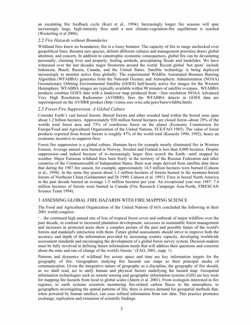
3.1 Remote Sensing: A Key Technology in Fire Mapping Science Remote sensing has over the past quarter century facilitated mapping and analysis of planetary resources (Townshend et al. 1991). Space-based images are now considered essential to global studies of land surface processes (Pinker 1990). Use of remote sensing for fire hazard assessments is based on the reflectance behaviors of vegetative fuels (Figure 3).

Figure 3. The spectrum of vegetative fuels: The visible, near-infrared and shortwave infrared portion of electromagnetic spectrum define the spectral response pattern of green vegetation: Absorption by leaf pigments (chiefly chlorophyll) controls reflectance in the ‘visible’ portion of the spectrum (0.4μm-0.7μm). Internal leaf structure mediates reflectance in the near-infrared portion of the spectrum. Leaf water content controls reflectance in the shortwave infrared, producing peaks in this graph at about 1.7μm and 2.2μm. The ‘valleys’ in the shortwave infrared represent absorption of energy in these wavelengths, chiefly by water vapor in the atmosphere (Source: Jensen, 2000).

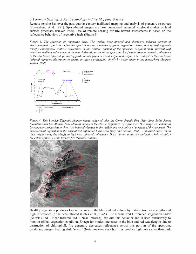
Figure 4. This Landsat Thematic Mapper image collected after the Cerro Grande Fire (May-June, 2000, Jemez Mountains and Los Alamos, New Mexico) enhances the classic ‘signature’ of a fire scar. This image was enhanced by computer processing to show fire-induced changes in the visible and near-infrared portions of the spectrum. The enhancement algorithm is the normalized difference burn ratio (Key and Benson, 2005). Unburned areas retain their bright tones, due chiefly to high near-infrared reflectance. Dark, burned areas are outlined to help visualize the extent of this ~19,000 hectare fire (Source: Author).

Healthy vegetation produces low reflectance in the blue and red chlorophyll absorption wavelengths and high reflectance in the near-infrared (Gates et al., 1965). The Normalized Difference Vegetation Index (NDVI: (Red – Near Infrared/Red + Near Infrared)) exploits this behavior and is used extensively to monitor global vegetation condition. Except for modest increases in the blue and red wavelengths due to destruction of chlorophyll, fire generally decreases reflectance across this portion of the spectrum, producing images bearing dark ‘scars.’ (Note however very hot fires produce light ash rather than dark

5

ash.) Computer enhancement of remotely sensed data can reveal spatial patterns of scarring following a fire (Figure 4).

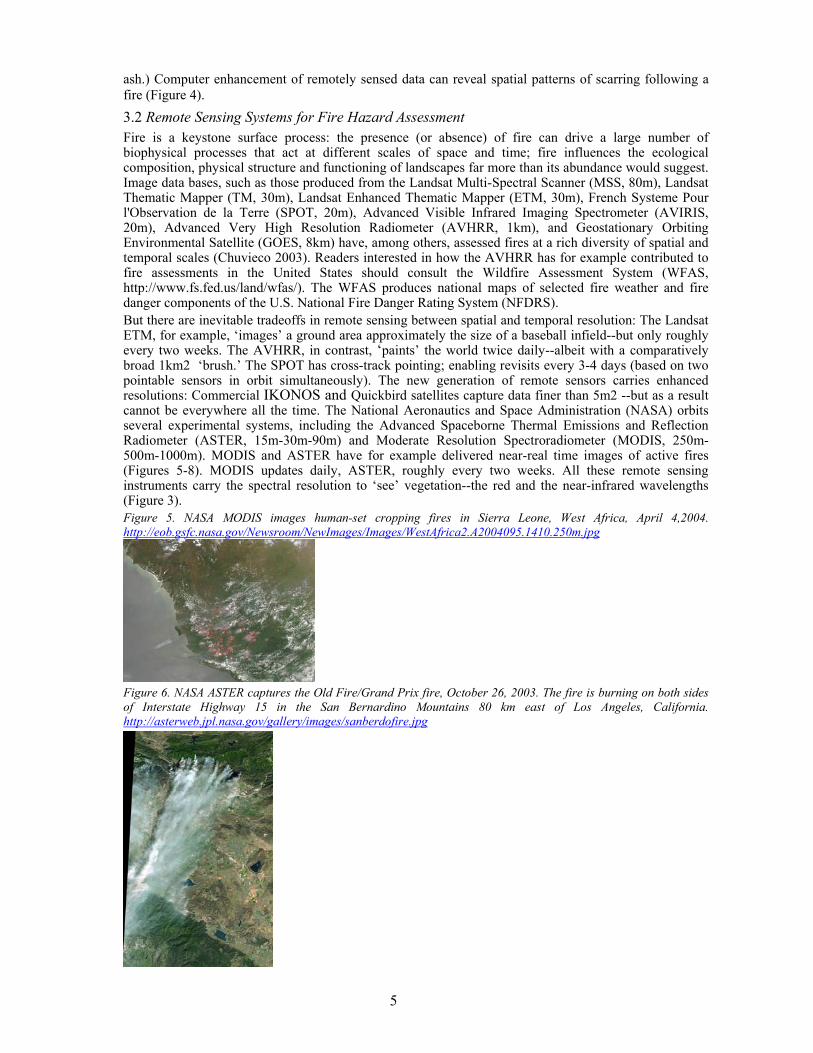
3.2 Remote Sensing Systems for Fire Hazard Assessment Fire is a keystone surface process: the presence (or absence) of fire can drive a large number of biophysical processes that act at different scales of space and time; fire influences the ecological composition, physical structure and functioning of landscapes far more than its abundance would suggest. Image data bases, such as those produced from the Landsat Multi-Spectral Scanner (MSS, 80m), Landsat Thematic Mapper (TM, 30m), Landsat Enhanced Thematic Mapper (ETM, 30m), French Systeme Pour l'Observation de la Terre (SPOT, 20m), Advanced Visible Infrared Imaging Spectrometer (AVIRIS, 20m), Advanced Very High Resolution Radiometer (AVHRR, 1km), and Geostationary Orbiting Environmental Satellite (GOES, 8km) have, among others, assessed fires at a rich diversity of spatial and temporal scales (Chuvieco 2003). Readers interested in how the AVHRR has for example contributed to fire assessments in the United States should consult the Wildfire Assessment System (WFAS, http://www.fs.fed.us/land/wfas/). The WFAS produces national maps of selected fire weather and fire danger components of the U.S. National Fire Danger Rating System (NFDRS). But there are inevitable tradeoffs in remote sensing between spatial and temporal resolution: The Landsat ETM, for example, ‘images’ a ground area approximately the size of a baseball infield--but only roughly every two weeks. The AVHRR, in contrast, ‘paints’ the world twice daily--albeit with a comparatively broad 1km2 ‘brush.’ The SPOT has cross-track pointing; enabling revisits every 3-4 days (based on two pointable sensors in orbit simultaneously). The new generation of remote sensors carries enhanced resolutions: Commercial IKONOS and Quickbird satellites capture data finer than 5m2 --but as a result cannot be everywhere all the time. The National Aeronautics and Space Administration (NASA) orbits several experimental systems, including the Advanced Spaceborne Thermal Emissions and Reflection Radiometer (ASTER, 15m-30m-90m) and Moderate Resolution Spectroradiometer (MODIS, 250m-500m-1000m). MODIS and ASTER have for example delivered near-real time images of active fires (Figures 5-8). MODIS updates daily, ASTER, roughly every two weeks. All these remote sensing instruments carry the spectral resolution to ‘see’ vegetation--the red and the near-infrared wavelengths (Figure 3). Figure 5. NASA MODIS images human-set cropping fires in Sierra Leone, West Africa, April 4,2004. http://eob.gsfc.nasa.gov/Newsroom/NewImages/Images/WestAfrica2.A2004095.1410.250m.jpg

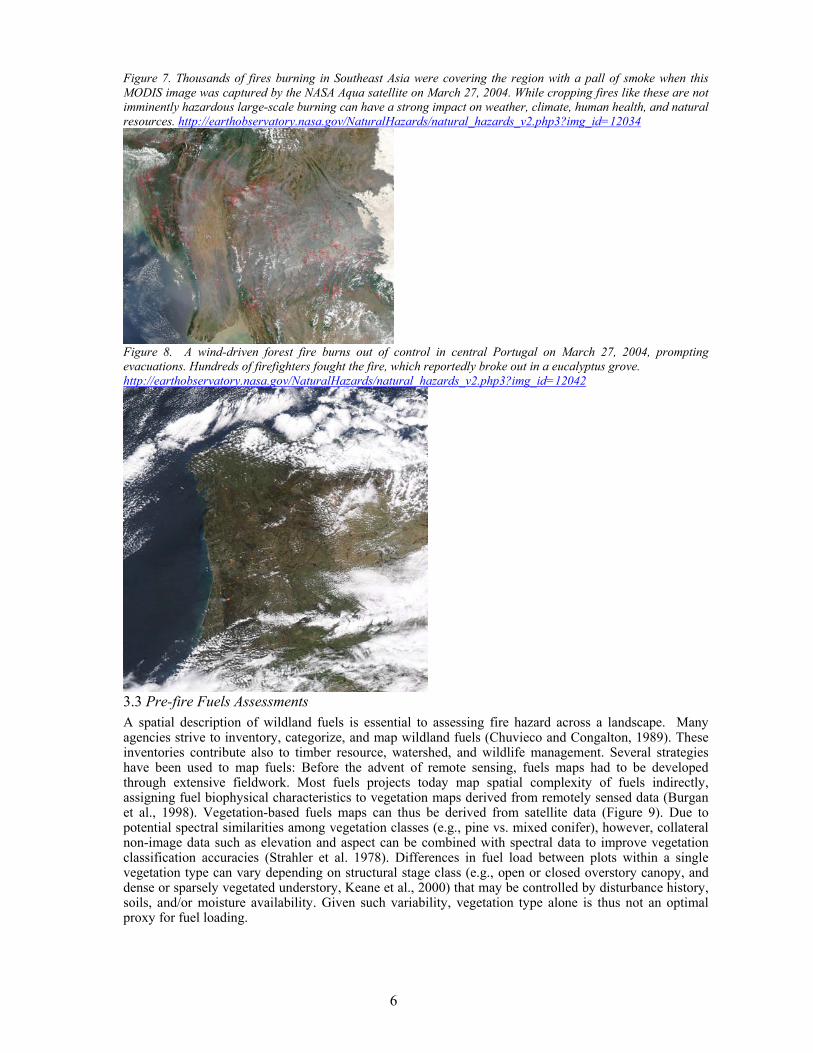
Figure 6. NASA ASTER captures the Old Fire/Grand Prix fire, October 26, 2003. The fire is burning on both sides of Interstate Highway 15 in the San Bernardino Mountains 80 km east of Los Angeles, California. http://asterweb.jpl.nasa.gov/gallery/images/sanberdofire.jpg

6

Figure 7. Thousands of fires burning in Southeast Asia were covering the region with a pall of smoke when this MODIS image was captured by the NASA Aqua satellite on March 27, 2004. While cropping fires like these are not imminently hazardous large-scale burning can have a strong impact on weather, climate, human health, and natural resources. http://earthobservatory.nasa.gov/NaturalHazards/natural_hazards_v2.php3?img_id=12034

Figure 8. A wind-driven forest fire burns out of control in central Portugal on March 27, 2004, prompting evacuations. Hundreds of firefighters fought the fire, which reportedly broke out in a eucalyptus grove. http://earthobservatory.nasa.gov/NaturalHazards/natural_hazards_v2.php3?img_id=12042

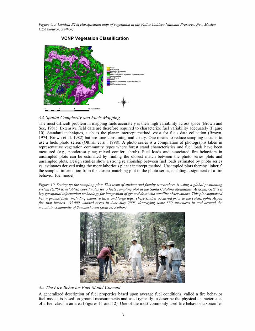
3.3 Pre-fire Fuels Assessments A spatial description of wildland fuels is essential to assessing fire hazard across a landscape. Many agencies strive to inventory, categorize, and map wildland fuels (Chuvieco and Congalton, 1989). These inventories contribute also to timber resource, watershed, and wildlife management. Several strategies have been used to map fuels: Before the advent of remote sensing, fuels maps had to be developed through extensive fieldwork. Most fuels projects today map spatial complexity of fuels indirectly, assigning fuel biophysical characteristics to vegetation maps derived from remotely sensed data (Burgan et al., 1998). Vegetation-based fuels maps can thus be derived from satellite data (Figure 9). Due to potential spectral similarities among vegetation classes (e.g., pine vs. mixed conifer), however, collateral non-image data such as elevation and aspect can be combined with spectral data to improve vegetation classification accuracies (Strahler et al. 1978). Differences in fuel load between plots within a single vegetation type can vary depending on structural stage class (e.g., open or closed overstory canopy, and dense or sparsely vegetated understory, Keane et al., 2000) that may be controlled by disturbance history, soils, and/or moisture availability. Given such variability, vegetation type alone is thus not an optimal proxy for fuel loading.

7

Figure 9. A Landsat ETM classification map of vegetation in the Valles Caldera National Preserve, New Mexico USA (Source: Author).

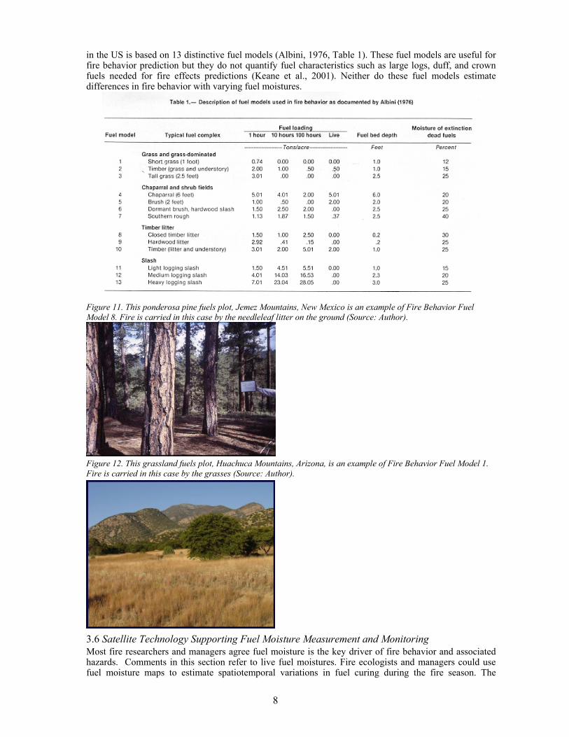
3.4 Spatial Complexity and Fuels Mapping The most difficult problem in mapping fuels accurately is their high variability across space (Brown and See, 1981). Extensive field data are therefore required to characterize fuel variability adequately (Figure 10). Standard techniques, such as the planar intercept method, exist for fuels data collection (Brown, 1974; Brown et al. 1982) but are time consuming and costly. One means to reduce sampling costs is to use a fuels photo series (Ottmar et al., 1998): A photo series is a compilation of photographs taken in representative vegetation community types where forest stand characteristics and fuel loads have been measured (e.g., ponderosa pine; mixed conifer; shrub). Fuel loads and associated fire behaviors in unsampled plots can be estimated by finding the closest match between the photo series plots and unsampled plots. Design studies show a strong relationship between fuel loads estimated by photo series vs. estimates derived using the more laborious planar intercept method. Unsampled plots thereby ‘inherit’ the sampled information from the closest-matching plot in the photo series, enabling assignment of a fire behavior fuel model.

Figure 10. Setting up the sampling plot: This team of student and faculty researchers is using a global positioning system (GPS) to establish coordinates for a fuels sampling plot in the Santa Catalina Mountains, Arizona. GPS is a key geospatial information technology for integration of ground data with satellite observations. This plot supported heavy ground fuels, including extensive litter and large logs. These studies occurred prior to the catastrophic Aspen fire that burned ~85,000 wooded acres in June-July 2003, destroying some 350 structures in and around the mountain community of Summerhaven (Source: Author). 3.5 The Fire Behavior Fuel Model Concept A generalized description of fuel properties based upon average fuel conditions, called a fire behavior fuel model, is based on ground measurements and used typically to describe the physical characteristics of a fuel class in an area (Figures 11 and 12). One of the most commonly used fire behavior taxonomies

8

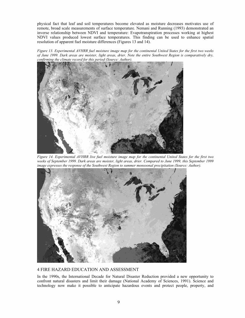
in the US is based on 13 distinctive fuel models (Albini, 1976, Table 1). These fuel models are useful for fire behavior prediction but they do not quantify fuel characteristics such as large logs, duff, and crown fuels needed for fire effects predictions (Keane et al., 2001). Neither do these fuel models estimate differences in fire behavior with varying fuel moistures.

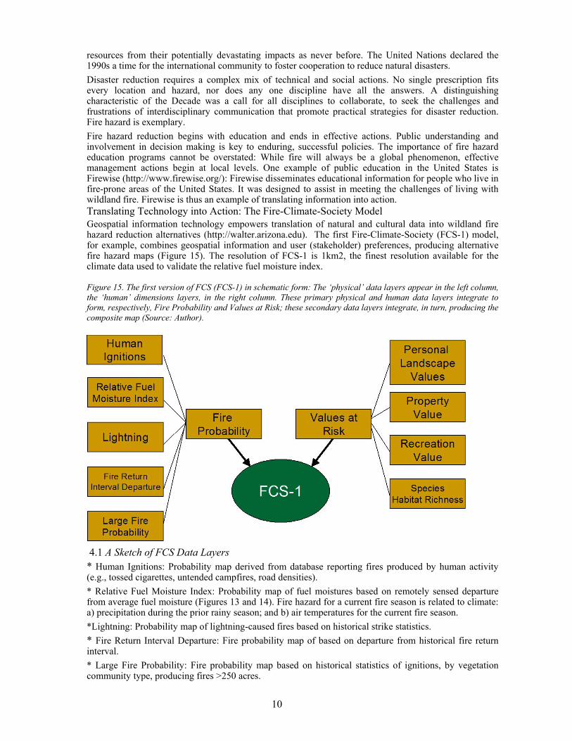
Figure 11. This ponderosa pine fuels plot, Jemez Mountains, New Mexico is an example of Fire Behavior Fuel Model 8. Fire is carried in this case by the needleleaf litter on the ground (Source: Author).

Figure 12. This grassland fuels plot, Huachuca Mountains, Arizona, is an example of Fire Behavior Fuel Model 1. Fire is carried in this case by the grasses (Source: Author).

3.6 Satellite Technology Supporting Fuel Moisture Measurement and Monitoring Most fire researchers and managers agree fuel moisture is the key driver of fire behavior and associated hazards. Comments in this section refer to live fuel moistures. Fire ecologists and managers could use fuel moisture maps to estimate spatiotemporal variations in fuel curing during the fire season. The

9

physical fact that leaf and soil temperatures become elevated as moisture decreases motivates use of remote, broad scale measurements of surface temperature. Nemani and Running (1993) demonstrated an inverse relationship between NDVI and temperature: Evapotranspiration processes working at highest NDVI values produced lowest surface temperatures. This finding can be used to enhance spatial resolution of apparent fuel moisture differences (Figures 13 and 14).

Figure 13. Experimental AVHRR fuel moisture image map for the continental United States for the first two weeks of June 1999. Dark areas are moister, light areas, drier. Note the entire Southwest Region is comparatively dry, confirming the climate record for this period (Source: Author).

Figure 14. Experimental AVHRR live fuel moisture image map for the continental United States for the first two weeks of September 1999. Dark areas are moister, light areas, drier. Compared to June 1999, this September 1999 image expresses the response of the Southwest Region to summer monsoonal precipitation (Source: Author).

4 FIRE HAZARD EDUCATION AND ASSESSMENT In the 1990s, the International Decade for Natural Disaster Reduction provided a new opportunity to confront natural disasters and limit their damage (National Academy of Sciences, 1991). Science and technology now make it possible to anticipate hazardous events and protect people, property, and

10

resources from their potentially devastating impacts as never before. The United Nations declared the 1990s a time for the international community to foster cooperation to reduce natural disasters. Disaster reduction requires a complex mix of technical and social actions. No single prescription fits every location and hazard, nor does any one discipline have all the answers. A distinguishing characteristic of the Decade was a call for all disciplines to collaborate, to seek the challenges and frustrations of interdisciplinary communication that promote practical strategies for disaster reduction. Fire hazard is exemplary. Fire hazard reduction begins with education and ends in effective actions. Public understanding and involvement in decision making is key to enduring, successful policies. The importance of fire hazard education programs cannot be overstated: While fire will always be a global phenomenon, effective management actions begin at local levels. One example of public education in the United States is Firewise (http://www.firewise.org/): Firewise disseminates educational information for people who live in fire-prone areas of the United States. It was designed to assist in meeting the challenges of living with wildland fire. Firewise is thus an example of translating information into action. Translating Technology into Action: The Fire-Climate-Society Model Geospatial information technology empowers translation of natural and cultural data into wildland fire hazard reduction alternatives (http://walter.arizona.edu). The first Fire-Climate-Society (FCS-1) model, for example, combines geospatial information and user (stakeholder) preferences, producing alternative fire hazard maps (Figure 15). The resolution of FCS-1 is 1km2, the finest resolution available for the climate data used to validate the relative fuel moisture index.

Figure 15. The first version of FCS (FCS-1) in schematic form: The ‘physical’ data layers appear in the left column, the ‘human’ dimensions layers, in the right column. These primary physical and human data layers integrate to form, respectively, Fire Probability and Values at Risk; these secondary data layers integrate, in turn, producing the composite map (Source: Author).

4.1 A Sketch of FCS Data Layers * Human Ignitions: Probability map derived from database reporting fires produced by human activity (e.g., tossed cigarettes, untended campfires, road densities). * Relative Fuel Moisture Index: Probability map of fuel moistures based on remotely sensed departure from average fuel moisture (Figures 13 and 14). Fire hazard for a current fire season is related to climate: a) precipitation during the prior rainy season; and b) air temperatures for the current fire season. *Lightning: Probability map of lightning-caused fires based on historical strike statistics. * Fire Return Interval Departure: Fire probability map of based on departure from historical fire return interval. * Large Fire Probability: Fire probability map based on historical statistics of ignitions, by vegetation community type, producing fires >250 acres.

11

* Personal Landscape Value: Derived from field interviews. Interviewees identified areas on maps having high personal values. These areas were digitized. * Property Value: Represented by cost of replacement. Given the requirement to place values on undeveloped property, this layer is particularly complex. * Recreation Value: Digitized hiking and biking trails. * Species Habitat Richness: Map of landscape characteristics favoring biodiversity.

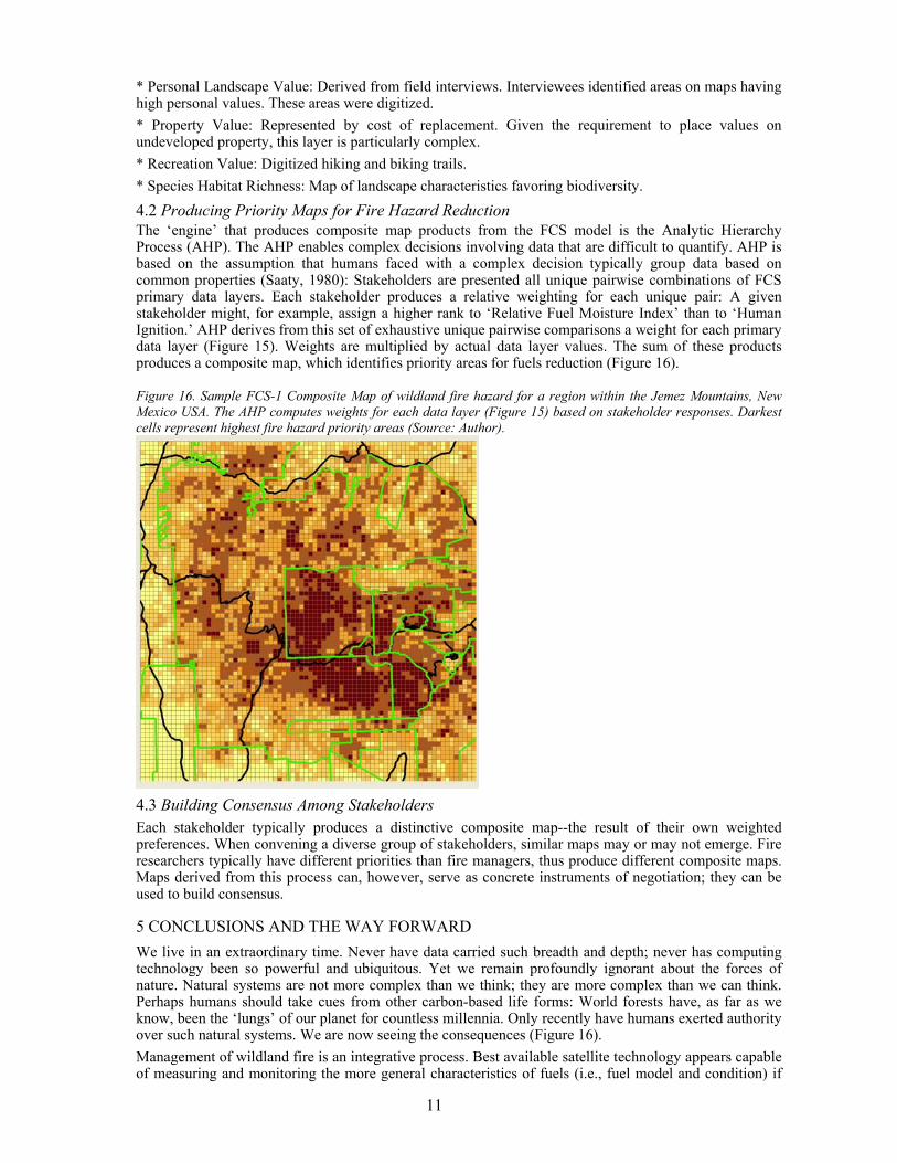
4.2 Producing Priority Maps for Fire Hazard Reduction The ‘engine’ that produces composite map products from the FCS model is the Analytic Hierarchy Process (AHP). The AHP enables complex decisions involving data that are difficult to quantify. AHP is based on the assumption that humans faced with a complex decision typically group data based on common properties (Saaty, 1980): Stakeholders are presented all unique pairwise combinations of FCS primary data layers. Each stakeholder produces a relative weighting for each unique pair: A given stakeholder might, for example, assign a higher rank to ‘Relative Fuel Moisture Index’ than to ‘Human Ignition.’ AHP derives from this set of exhaustive unique pairwise comparisons a weight for each primary data layer (Figure 15). Weights are multiplied by actual data layer values. The sum of these products produces a composite map, which identifies priority areas for fuels reduction (Figure 16).

Figure 16. Sample FCS-1 Composite Map of wildland fire hazard for a region within the Jemez Mountains, New Mexico USA. The AHP computes weights for each data layer (Figure 15) based on stakeholder responses. Darkest cells represent highest fire hazard priority areas (Source: Author).

4.3 Building Consensus Among Stakeholders Each stakeholder typically produces a distinctive composite map--the result of their own weighted preferences. When convening a diverse group of stakeholders, similar maps may or may not emerge. Fire researchers typically have different priorities than fire managers, thus produce different composite maps. Maps derived from this process can, however, serve as concrete instruments of negotiation; they can be used to build consensus.

5 CONCLUSIONS AND THE WAY FORWARD We live in an extraordinary time. Never have data carried such breadth and depth; never has computing technology been so powerful and ubiquitous. Yet we remain profoundly ignorant about the forces of nature. Natural systems are not more complex than we think; they are more complex than we can think. Perhaps humans should take cues from other carbon-based life forms: World forests have, as far as we know, been the ‘lungs’ of our planet for countless millennia. Only recently have humans exerted authority over such natural systems. We are now seeing the consequences (Figure 16). Management of wildland fire is an integrative process. Best available satellite technology appears capable of measuring and monitoring the more general characteristics of fuels (i.e., fuel model and condition) if

12

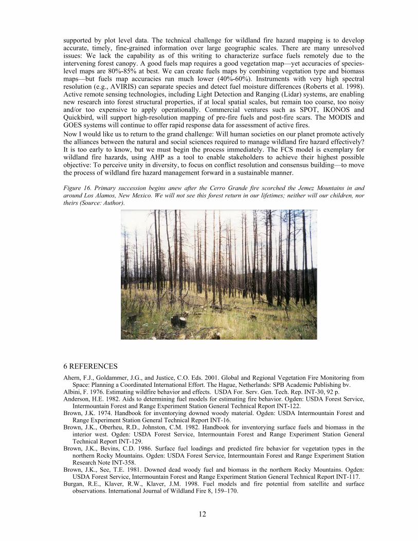
supported by plot level data. The technical challenge for wildland fire hazard mapping is to develop accurate, timely, fine-grained information over large geographic scales. There are many unresolved issues: We lack the capability as of this writing to characterize surface fuels remotely due to the intervening forest canopy. A good fuels map requires a good vegetation map—yet accuracies of species-level maps are 80%-85% at best. We can create fuels maps by combining vegetation type and biomass maps—but fuels map accuracies run much lower (40%-60%). Instruments with very high spectral resolution (e.g., AVIRIS) can separate species and detect fuel moisture differences (Roberts et al. 1998). Active remote sensing technologies, including Light Detection and Ranging (Lidar) systems, are enabling new research into forest structural properties, if at local spatial scales, but remain too coarse, too noisy and/or too expensive to apply operationally. Commercial ventures such as SPOT, IKONOS and Quickbird, will support high-resolution mapping of pre-fire fuels and post-fire scars. The MODIS and GOES systems will continue to offer rapid response data for assessment of active fires. Now I would like us to return to the grand challenge: Will human societies on our planet promote actively the alliances between the natural and social sciences required to manage wildland fire hazard effectively? It is too early to know, but we must begin the process immediately. The FCS model is exemplary for wildland fire hazards, using AHP as a tool to enable stakeholders to achieve their highest possible objective: To perceive unity in diversity, to focus on conflict resolution and consensus building—to move the process of wildland fire hazard management forward in a sustainable manner.

Figure 16. Primary succession begins anew after the Cerro Grande fire scorched the Jemez Mountains in and around Los Alamos, New Mexico. We will not see this forest return in our lifetimes; neither will our children, nor theirs (Source: Author).

6 REFERENCES Ahern, F.J., Goldammer, J.G., and Justice, C.O. Eds. 2001. Global and Regional Vegetation Fire Monitoring from

Space: Planning a Coordinated International Effort. The Hague, Netherlands: SPB Academic Publishing bv. Albini, F. 1976. Estimating wildfire behavior and effects. USDA For. Serv. Gen. Tech. Rep. INT-30, 92 p. Anderson, H.E. 1982. Aids to determining fuel models for estimating fire behavior. Ogden: USDA Forest Service,

Intermountain Forest and Range Experiment Station General Technical Report INT-122. Brown, J.K. 1974. Handbook for inventorying downed woody material. Ogden: USDA Intermountain Forest and

Range Experiment Station General Technical Report INT-16. Brown, J.K., Oberheu, R.D., Johnston, C.M. 1982. Handbook for inventorying surface fuels and biomass in the

interior west. Ogden: USDA Forest Service, Intermountain Forest and Range Experiment Station General Technical Report INT-129.

Brown, J.K., Bevins, C.D. 1986. Surface fuel loadings and predicted fire behavior for vegetation types in the northern Rocky Mountains. Ogden: USDA Forest Service, Intermountain Forest and Range Experiment Station Research Note INT-358.

Brown, J.K., See, T.E. 1981. Downed dead woody fuel and biomass in the northern Rocky Mountains. Ogden: USDA Forest Service, Intermountain Forest and Range Experiment Station General Technical Report INT-117.

Burgan, R.E., Klaver, R.W., Klaver, J.M. 1998. Fuel models and fire potential from satellite and surface observations. International Journal of Wildland Fire 8, 159–170.

13

Cahoon, D. R., Levine, J.S., Cofer, W.R., Miller, J.E., Minnis, P., Tennille, G.M., Yip, T.W., Stocks, B.J., Heck, P.W. 1991. The Great Chinese Fire of 1987: A view from space, in J. S. Levine, editor, Global biomass burning, 61-66, The MIT Press, Cambridge, MA.

Cahoon, D.R., Stocks, B.J., Levine, J.S., Cofer, W.R., J.M. Pierson, J.M. 1994. Satellite analysis of the severe 1987 forest fires in northern China and southeastern Siberia. J. Geophys. Res. 99(D9), 18627.

Chuvieco, E., Congalton, R.G. 1989. Application of remote sensing and geographical information systems to forest fire hazard mapping. Remote Sensing of Environment 29, 147–159.

Chuvieco, E. Ed. 2003 Wildland Fire Danger Estimation and Mapping: The Role of Remote Sensing Data. World Scientific, 280 pp.

Cohen, W.B. 1991. Response of vegetation indices to changes in three measure of leaf water stress. Photogrammetric Engineering & Remote Sensing 57(2): 195-202

ECE/FAO (Economy Commission for Europe/Food and Agricultural Organization of the United Nations), The Forest Resources of the ECE Region (Europe, the USSR, North America). ECE/FAO/27, Geneva, 1985.

FIRESCAN Science Team, Fire in Boreal Ecosystems of Eurasia: First results of the Bor Forest Island Fire Experiment, Fire Research Campaign Asia-North (FIRESCAN). World Resource Review 6, 499-523, 1994.

Food and Agricultural Organization of the United Nations, Committee On Forestry, Agenda Item 8(b) of the Provisional Agenda, Fifteenth Session, Results Of The Global Forest Resources

Assessment 2000, Rome, Italy, 12-16 March 2001, COFO-2001/6 Supp.1 Fosberg, M.A., Stocks, B.J., Lynham, T.J. 1996. Risk analysis in strategic planning: fire and climate change in the

boreal forest, in J.G. Goldammer and V.V. Furyaev, editors, Fire in Ecosystems of Boreal Eurasia, Kluwer Acad. Publ., Dordrecht, 495-504.

Gates, D.M., Keegan, H.J., Schleter, J.C., Weidner, V.R. 1965. Spectral properties of plants. Applied Optics 4: 11-20.

Goldammer, J.G., Xueying D. 1990. The role of fire in the montane-boreal coniferous forest of Daxinganling, Northeast China: A preliminary model, in J.G. Goldammer and M. J. Jenkins, editors, Fire in ecosystem dynamics. Mediterranean and northern perspectives, 175-184. SPB Academic Publishing, The Hague, 199 pp.

Hardy, C.C., Burgan, R.E. 1999. Evaluation of NDVI for monitoring live moisture in three vegetation types of the western U.S. Photogrammetric Engineering & Remote Sensing 65(5): 603-610.

Jensen, J. 2000. Remote Sensing of the Environment. New Jersey: Prentice Hall. 544pp. Kasischke, E.S., Hyre, E.P., Novelli, P.C., Bruhwiler, L.P., French, N.H.F. Sukhinin, A., Hewson, J., Stocks, B.J.

2005 Influences of boreal fire emissions on Northern Hemisphere atmospheric carbon and carbon monoxide, Global Biogeochemical Cycles, 19,GB1012, doi:10.1029/2004GB002300.

Kasischke, E.S., Penner J.E. 2004 Improving global estimates of atmospheric emissions from biomass burning, Journal of Geophysical Research, 109, D14S01, doi:10.1029/2004JD004972.

Keane, R.E., Mincemoyer, S.A., Schmidt, K.M., Long, D.G., Garner, J.L. 2000. Mapping vegetation and fuels for fire management on the Gila National Forest Complex, New Mexico. Missoula: USDA Forest Service, Rocky Mountain Research Station General Technical Report RMRS-46-CD.

Keane, R.E., Burgan, R., van Wagtendonk, J. 2001. Mapping wildland fuels for fire management across multiple scales: integrating remote sensing, GIS, and biophysical modeling. International Journal of Wildland Fire 10, 301–319.

Key, C.H., Benson, N. 2005. Landscape assessment: Ground measure of severity, the Composite Burn Index; and remote sensing of severity, the Normalized Burn Ratio. In D.C. Lutes, R.E. Keane, J.F. Caratti, C.H. Key, N.C. Benson & L.J. Gangi (Eds.), FIREMON: Fire Effects Monitoring and Inventory System (pp. CD:LA1-LA51). Ogden, UT: USDA Forest Service, Rocky Mountain Research Station, Gen. Tech. Rep. RMRS-GTR-164.

Kitzberger, T., Brown, P.M., Heyerdahl, E.K., Swetnam, T.W., Veblen, T.T. 2006. Contingent Pacific-Atlantic Ocean Influence on Multicentury Fire Synchrony over Western North America. Proceedings of the National Academy of Sciences 104(2): 543-548.

Kurz, W.A., Apps, M.J., Stocks, B.J., Volney, W.J.A. 1994. Global climate change: disturbance regimes and biospheric feedbacks of temperate and boreal forests. In: Woodwell, G.M.; F. Maackenzie, Eds. Biotic feedbacks in the global climate system: will the warming speed the warming? Oxford, UK:Oxford University Press; 119-133.

Kuusela, K. 1990 The Dynamics of Boreal Coniferous Forests. The Finnish National Fund for Research and Development (SITRA), Helsinki, Finland.

Kuusela, K. 1992. Boreal forestry in Finland: a fire ecology without fire. Unasylva 43 (170), 22. National Academy of Sciences 1991. A Safer Future: Reducing the Impacts of Natural Disasters, Washington, D.C.

National Academy Press. Nemani, R., L. Pierce, Running, S. 1993. Developing satellite-derived estimates of terrestrial moisture status.

Journal of Applied Meteorology 32: 548-557. Nemani, R., Running, S. 1989. Estimation of regional terrestrial resistance to evapotranspiration from NDVI and

thermal-IR AVHRR data. Journal of Applied Meteorology 28: 276-284. Ottmar, R.D., Vihnanek, R.E., Wright, C.S., 1998. Stereo Photo Series for Quantifying Natural Fuels Volume I:

Mixed-Conifer with Mortality, Western Juniper, Sagebrush, and Grassland Types in the Interior Pacific Northwest, National Wildfire Coordinating Group, Boise, National Interagency Fire Center PMS 830.

Pyne, S.J. 2001. Fire: A Brief History, London: The British Museum Press. Roberts, DA, Gardner, M, Church, R, Ustin, S, Scheer, G., Green, R.O. 1998. Mapping Chaparral in the Santa

Monica Mountains using Multiple Endmember Spectral Mixture Models, Rem. Sens. Environ. 65: 267-279.

14

Saaty T.L. 1980. The Analytic Hierarchy Process, New York: McGraw Hill. Shugart, H. H., Leemans, R., Bonan, G.B. Eds. 1992. Boreal Forest Modeling. A Systems Analysis of the Global

Boreal Forest, Cambridge University Press, Cambridge, UK. Strahler, A.H., Logan, T.L., Bryant, N.A. 1978. Improving forest cover classification accuracy from Landsat by

incorporating topographic information, 12th International Symposium on Remote Sensing of Environment, Environmental Research Institute of Michigan, Ann Arbor, pp. 927–942.

Westerling, A.L., Hidalgo, H.G., Cayan, D.R., Swetnam, T.W. 2006. Warming and Earlier Spring Increase Western U.S. Forest Wildfire Activity Science 18 August 2006: Vol. 313. no. 5789, pp. 940 – 943.

Wildfire and Biomass Burning Algorithm, http://cimss.ssec.wisc.edu/goes/burn/wfabba.html Wright, H.A., Bailey, A.W. 1982. Fire Ecology, New York: John Wiley & Sons.

15

1 INTRODUCTION In a broad sense wildfire prevention covers the all activities that are performed before a wildfire begins. Within the scope of wildfire management, wildfire prevention comprises all the activities that can be performed in order to reduce or prevent wildfire occurrence as well as to minimise wildfire potential impacts and damage (Vélez, 2002). Based on this, early warning related activities can be considered as wildfire prevention, since they aim to reduce wildfire impacts. Wildfire prevention is a simple concept involving a complex implementation. Prevention comprises fields as public awareness raising and environmental education, personnel training, preparedness and coordination (among the different institutions involved in wildfire management and suppression) and also, legislation enforcement. Regarding wildfire prevention, the legal framework normally includes restrictions to control fire ignition in high risk areas and periods. Hardly ever legislation regulates the inclusion of wildfire prevention activities as part of forest management plans. However, new pragmatic approaches, as “FireSmart Forest Management” include wildfire prevention activities as part of the regular forest management, adapting the traditional forest management practices to reduce the probability of fire ignitions, to decrease the fire behaviour potential of landscape and to enhance the capability of fire suppression resources (Hirsch et al. 2001). Related to this approach, agro-forestry policies that promote sustainable rural development (focusing on silvopastoral practices) are key issues for fire-smart forest management plans in the Mediterranean environment. In addition, a holistic approach to prevention should also include Research and Development programs aimed to gain a better understanding of the wildfire, as well as to optimise the implementation of the prevention strategies. Because of the broad spectrum of activities included, prevention can be designed and performed at different scales, involving a great variety of institutions ranging from communities and local agencies to regional and nationwide organisations. To effectively implement wildfire prevention strategies these institutions need to get accurate and comprehensive information about the landscape they plan to manage. Spatial databases containing fire occurrence records, fire causes, and the track of the suppression activities performed are vital for the success of prevention strategies (Mérida et al. 2007). Remote sensing (RS) techniques reveal as an excellent tool to obtain geo-information such as land cover and land use, vegetation condition, fuel type and load and meteorological data. The combination of geo-data with fire statistics, socioeconomic statistics, property maps and values at risk is useful to support long-term wildfire prevention planning, particularly important at the wildland-urban interface areas.

2 OPERATIVE CONTRIBUTIONS OF REMOTE SENSING TO FIRE PREVENTION The review of operative contributions of RS to forest fire prevention has turned up to be a complex task. The present analysis of the state of the art has searched beyond bibliography on potential applications of satellite products and has looked realistically into operational end users, i.e.: institutions with mandatory competencies in fire prevention, such as forest managers, civil protection departments, meteorological

Operational Remote Sensing in fire prevention: an Overview

A. Sebastián-López, ADCIF, Spanish Ministry of Environment, Gran Vía de S Francisco 4, Madrid 28005, [email protected]

M.J. Yagüe Ballester, GMV-Aerospace and Defense, Isaac Newton, 11. 28760 Madrid. Spain. [email protected]

M. Sánchez-Guisández, ADCIF, Spanish Ministry of Environment, Gran Vía de S Francisco 4, Madrid 28005. [email protected]

Keywords: Wildfire prevention, environmental satellites, forest management

ABSTRACT: Prevention is broadly considered as a key issue in wildfire management. Wildfire prevention embraces a wide range of activities and strategies. Many of them can benefit from remote sensing. In this paper we look at the mode that satellites products and remote observation techniques are operative for pre-fire planning. Our aim is to determine to what extent remote sensing products and techniques are being used by wildfire agencies and organizations and not to perform a complete revision of the remote sensing products and techniques available for wildfire prevention. We outline the reasons for the observed underutilization of remote sensing operational products and finally draw some recommendations for the implementation of their full potential.

16

institutes, army departments, owners and local associations. The analysis gets even more difficult considering the supra-national, national and regional levels of administrative competencies in forest fire prevention that meet in the same horizon. These difficulties advised against reviewing experiences exhaustively but rather presenting successful operative cases at global, continental and local scales. At global level wildfire prevention activities aim to get a better understanding of the interactions between large-scale phenomena and fire regimes. The analysis of wildfire role in climate change and the hydrological and biogeochemical cycles (among others subjects) requires information on fire timing, seasonality and inter-annual variability of fire locations. Several operational global monitoring systems supply for these needs providing georeferenced products of fire-affected areas and early fire-warnings1. In this context the GOFC/GOLD-Fire Mapping and Monitoring Theme2 aims at refining the international observation requirements and optimise the possible uses of fire products from the existing and future satellite observing systems, for fire management, policy decision-making and global change research. Similarly, the GFMC3 of the UN/ISDR gives access to various early-warning systems providing a workspace for wildlfire related documentation and monitoring that is accessible to the public through the Web. Pathfinding initiatives and operational prototyping by individual research groups working with GOES, AVHRR, TRMM, ATSR and DMSP have provided examples of how future operational products can be generated. NASA’s Moderate Resolution Imaging Spectroradiometer (MODIS) is currently the only system generating unique global systematic daily fire products, thus providing a prototype for future operational fire monitoring from the envisaged NPOESS VIIRS system (Justice et al. 2002, Roy et al. 2005). The MODIS Rapid Response System is also providing important advances in the web-based distribution of global data within near real time of satellite acquisition. The European Forest Fire Information System (EFFIS), developed by the Joint Research Centre (JRC) of the EC, provides large-scale cartography of burned areas larger than 50ha derived with MODIS imagery (Barbosa et al. 2006). Since 2003 the JRC is also responsible for the maintenance of the European database on wild fires. Analyses derived from this database significantly contribute to prevention through a better understanding of wildfires from the European perspective. In order to promote the operational use of RS products, the user-driven approach is a common feature of the ongoing EO European projects dealing with wildfire prevention. Among the several existing projects RISK-EOS and the PREVIEW projects are worth mentioning. Both intend to be fully operational in the mid-term horizon addressing organisation schemes to prepare the deployment and future operation of the services. Recent disaster events have highlighted the urgent need to consolidate information from disparate systems supporting citizen protection and disaster management operations. In this context, the ORCHESTRA project aims to design the specifications needed for a service oriented spatial data infrastructure to improve operability among risk management authorities in Europe. Finally it is also worth to underline the GSE Forest Monitoring, an element of the Global Monitoring for Environment and Security (GMES) Joint Initiative which supplies information on the state of forest in order to support sustainable management and related activities, including wildfire prevention. At national level, the number of responsibilities related to wildfire prevention increases. To illustrate the operational use of RS at this level Spain is an interesting case of study. The seventeen Spanish regional governments are responsible for wildfire prevention within their own boundaries. However the national wildfire management agency, ADCIF - belonging to the Ministry of Environment- supports the regions with additional resources. These comprise mainly prevention crews and aerial surveillance aircrafts. The ADCIF has made an important effort in order to take advantage of RS potential, specifically aimed at improving preparedness for one of its main duties: the dispatch of its suppression resources. For this the ADCIF relies on early-warnings obtained from MODIS and MSG-SEVIRI imagery (algorithm by Abel et al. 2006). In addition the ADCIF receives perimeters of fire-affected areas obtained from different sources (MODIS, Landsat, SPOT) and contractors. As it commonly happens in wildfire management agencies, in the ADCIF the fire risk forecast basically relies on the weather forecast, which is provided by the National Meteorological Institute. Weather data is supplied via Internet within a GIS that allows managers to create forecast maps. Among the data supplied, there is also cloud structure derived from MSG-SEVIRI and NDVI data from NOAA-AVHRR. Besides, the service includes specific fire variables such as daily maps of BEHAVE’s Probability of Ignition. The computation of fire risk indices that parameterise live fuel status with satellite data is currently under development.

1 MODIS website: http://modisfire.umd.edu/MCD45A1, GEM Unit at JRC (EC): http://www- gem.jrc.it//Disturbance_by_fire/index.htm 2 GOFC/GOLD (Global Observation f Forests and Land Cover Dynamics http://gofc-fire.umd.edu/bkgrd/index.asp) 3 GFMC (Global Fire Monitoring Center http://www.fire.uni-freiburg.de/ ), UNISDR (UN-International Strategy for Disaster Reduction http://www.unisdr.org/ )

17

Even though the use of satellite products at the regional level has not become widespread, hot-spots and burned area data are fairly common products used by the Spanish regional fire agencies. These products are usually provided by private companies, Universities or cartographic institutes. As and example, the cartographic institutes of Catalonia and Valencia provide the regional managers with yearly data of burned areas bigger than 5 ha, which are obtained using Landsat, SPOT and, sometimes, DMC and CASI data. The region of Asturias considers long-term fire recurrence derived from Landsat, along with other variables, to officially declare risk areas in its territory. In very few cases RS is used operatively to obtain dynamic risk indices, however, the regions have recently started to receive fuel moisture content estimations. Some regions, like Castilla y León, receive through a Web service daily estimations of this variable derived from MODIS according to the algorithm proposed by Chuvieco et al. (2004). Portugal and Greece are other interesting examples to illustrate the use of satellite products at national level. In Portugal, forestry managers use satellite data to obtain an annual fire risk map that combines the short- and long-term perspective. In the model the long-term approach uses the proportion of area burned - obtained from Landsat- as the independent variable, whereas the NDVI is used to account for the short-term risk (Pereira and Carreiras, 2007). In addition, the Portuguese fire managers are receiving annually (weekly during the summer fire season) burned area maps derived from MODIS. In Greece, the Civil Protection Department uses daily estimation of fire risk produced by the Aristotle University of Thessaloniki from MODIS data. This fire risk index is based on the computation of a series of vegetation indices and the computation of “change maps” for 10-days periods. We have observed that although the methods to create satellite-based risk indices are already available, in most countries the operative use of these products is still pending further validation. For instance, Italian Civil protection is testing the use of vegetation indices for fire danger forecasting (RISICO system). In Spain fire managers at different levels will test this summer the satellite products (FMC and fire risk, among other variables) from FIREMAP project4.

3 POTENTIAL vs REAL OPERABILITY Regarding the operational use of RS in fire prevention it is necessary to point out three main issues. First, it is essential to distinguish between what is technically feasible and what is actually operative. Second, it is necessary to understand that the use of RS data for wildfire prevention begins much earlier in time than the actual moment of fire detection. Finally, it is important to remind that the operative requirements of end users still remain undefined and research interests of the RS scientific community do not completely meet the operational needs of forest managers or wildfire agencies. Although RS has proved to be a useful tool for the integrate approach to wildfire prevention, gaps still remain in the operational use of satellite products. There are technological gaps clearly identified (CEOS-DMSG 2002), gaps in the definition of policies that affect forest management, and gaps in the coherence and operability of fire prevention practices and the way environmental data are effectively integrated into them. Deficiencies are found in the current architecture of satellites and sensors, as required for forest fire prevention: the gap between high spatial and high temporal resolution is there to be solved. Fires can break out at any moment and anywhere, so monitoring tools must be active on a permanent basis. Within the scope of remote sensors design, wildfires are a particularly sensitive application that poses the technical challenge of bringing together the benefits of geostationary satellites and sun-synchronous satellites. Furthermore, the characteristics and calibration of the thermal channels are critical, given the fact that wildfires have a large range of burning temperatures, ranging from lower than 500ºK to higher than 1000ºK, either in a whole pixel or as a variable fraction of burning area within a pixel. Operational remote fire observation needs to integrate high temporal resolution (geostationary) and, at least, medium spatial resolution. Specifically, this means less than 15 minutes of image provision lapse time, thermal range for night/dense smoke fire detection, ability to detect small (<1ha), low intensity and brief ignitions and the capacity to avoid false hot-spots detection (adjusted algorithms). The current most relevant geostationary satellite equipped for forest fire detection is MSG SEVIRI (Spinning Enhanced Visible and InfraRed Imager). SEVIRI was a remarkable advance in the temporal resolution required for early fire detection and warning; however, its spatial resolution (1 km at nadir) is far too coarse to satisfy the requirements. All sun-synchronous satellites have properties to match forest fire applications. MODIS is the most widely used on account of its temporal-spatial-radiometric characteristics. MODIS’s spatial resolution is ideal for hot spots detection, but the overpass schedule makes the system miss out the detection of the inter-passes short lasting fires (happening within 12 hours). Gaps are also found in the RS data supply chain of different agencies. European agencies have a highly controlled accessibility while American suppliers

4 http://www.geogra.uah.es:8080/firemap/

18

make data and products more easily available. This suggests that the larger the number of RS data users the greater the number of scientific results the end- user community may get. At European political and administrative level, although forest fires are of great concern for all land planning policies (i.e.: agriculture, urban, risk management, civil protection, land use), guidelines encouraging the use of RS for wildfire prevention have not been stated beyond simple recommendations. Just as the Common Agricultural Policy has framed the use of RS to control subsidies or to predict yields, forestry policies should include the use of RS in mandatory terms The validation of methodologies against detailed ground data and for different bioclimatic areas is one of the gaps found between the research results and the operational use of RS in fire management. Detailed and local verification procedures may put at risk some methods since the parameters considered for vegetation monitoring usually have a high temporal and spatial variability. Nonetheless, ground verification activities should be a major objective to develop in the near future. The lack of standards and validation protocols prevent the use of RS in the design of forest fire prevention strategies. Related to this local wildfire prevention agencies will have to closely work with researchers to design the contents of those protocols.

4 CONCLUSIONS AND RECOMMENDATIONS FOR THE FUTURE A large number of applications and RS products for wildfire prevention are available for final users. However the number of applications and RS products that are fully operational is quite small. Despite the potential of RS for wildfire prevention practices, today pre-fire planning does not rely on RS as much as fire detection, active fires monitoring and post-fire evaluation do. Important initiatives have been successfully implemented at global scale for years. However these products and results from RS have not yet had repercussions on regular wildfire prevention practices and procedures. The responsibility for the implementation of wildfire prevention strategies belong to lower levels, i.e. regional governments or local agencies. More often than not these wildfire management agencies lack resources, either technical skills or economic, to be able to benefit from RS in their regular prevention activities. In the particular case of Spain 17 different wildfire agencies are responsible for prevention within their own territories having different needs, requirements and management challenges. In this context, it is more difficult for the very first links of the RS chain to reach the final users and to develop products that fully meet their needs, especially in terms of spatial and temporal resolution. New satellites and observation instruments aim to improve the quality of the information needed to incorporate RS products and techniques into regular wildfire prevention planning. To improve the operational use of RS, greater attention has to be paid to data availability, product accuracy, data continuity, data access and the way data is used to obtain effective results. Validation of methodologies by means of ground data collection must be enhanced. Besides, there are no international standards regarding in situ measurements or common reporting procedures that should be developed by the international wildlfire community.

5 REFERENCES Calle, A., Casanova, J.L. and Romo, A. 2006. Fire detection and monitoring using MSG Spinning Enhanced Visible

and Infrared Imager (SEVIRI). Journal of Geophysical Research, 111. CEOS-DMSG. 2002. Fire Hazard Team Report (http://www.ceos.org/pages/DMSG/2001Ceos/overview.html) Chuvieco, E., Cocero, D., Riaño, D., Martín, M.P., Martínez-Vega, J., Riva, J. and Pérez, F. 2004. Combining

NDVI and Surface Temperature for the estimation of live fuel moisture content in forest fire danger rating. Remote Sensing of the Environment, 92: 322-331.

Barbosa, P., Kucera, J., Strobl,P., Vogt, P., Camia, A., San-Miguel-Ayanz, J., 2006.European forest fire information system (EFFIS) - rapid damage assessment: appraisal of burnt area maps in southern europe using modis data (2003 to 2005) , Proceedings of the 5th International Conference on Forest Fire Research, 27-30 Figueira da Foz, Portugal, Elsevier Pub. ISSN 0378-1127.

Hirsch, K., V. Kafka, C., Tymstra, R., McAlpine, B., Hawkes, H., Stegehuis, S., Quintilio, S. Gauthier and K. Peck. 2001. Fire-smart forest management: a pragmatic approach to sustainable forest management in fire-dominated ecosystems. The Forestry Chronicle 77(2):357-363.

Justice, C.O., Townshend, J., Vermote, E., Masuoka, E., Wolfe, R., Saleous, N., Roy, D.P. and Morisette, J. 2002. An overview of MODIS Land data processing and product status. Remote Sensing of the Environment, 83: 3-15.

Mérida J.C., Primo, E., Eleazar-Cubo, J. and Parra P.J. 2007. Las Bases de Datos de Incendios Forestales como herramienta de planificación: utilización en España por el Ministerio de Medio Ambiente. Proceedings of the 4th International Conference on Wildland Fire. Seville (Spain), May 13-17 2007. MMA Pub. 978-84-8014-690-6.

Pereira JMC., Carreiras J.M.B. 2007. How wildfire risk is mapped in Portugal: a naïf, flawed, and very effective approach. In proceedings of Statistical Extremes and Environmental Risk.Lisbon (Portugal), February 15-17, 2007.

19

Roy, D.P, Jin, Y., Lewis, P.E. and Justice, C.O. 2005. Prototyping a global algorithm for systematic fire-affected area mapping using MODIS time series data. Remote Sensing of Environment, 97: 137-162.

Vélez Muñoz, R. 2000. La defensa contra incendios forestales. Fundamentos y experiencias. Madrid, McGraw-Hill/Interamericana de España S.A.U.

20

1 INTRODUCTION Biomass burning is a key process in the Earth system, and in particular the terrestrial carbon cycle, and a globally significant source of atmospheric trace gases and aerosols which impact air quality, atmospheric chemical composition and the Earths radiation budget (Le Canut et al., 1996). Globally, on average, vegetation fires are believed to generate carbon emissions equivalent to between one third and one half of those from fossil fuel combustion, with those from savanna fires responsible for perhaps 50% of this total (Williams et al., 2007). Burning is prevalent on every significantly vegetated continent, and Africa is on average, the single largest biomass burning emissions source at the continental scale, responsible for between 30 and 50% of the total annual fuel consumption (van der Werf et al., 2006). Burning is typically characterized by strong interannual, seasonal, and diurnal cycles, and this strong variability means that, wherever possible, measurements of fires and their emissions are required for many science applications and the use of ‘climatological means’ is insufficient. These measurements generally come from data collected by Earth observation satellites, either responding to the active fire thermal emissions, the release of a particular trace gas species or aerosols, or the change in surface reflectance caused by the passage of fire over the landscape. This paper concentrates on reviewing the use of active fire thermal emissions for fire detection, which is something that has been undertaken since the 1980’s, and the more recent use of these emissions measurements in the quantification of fire magnitude (in terms of rate of energy output) and fuel consumption.

Fire Detection and Monitoring

(Quantitative uses of active fire thermal emissions)

M.J. Wooster & G. Roberts Environmental Monitoring & Modelling Research Group, Department of Geography,King's College London,Strand, London, WC2R 2LS, UK. [email protected]

Keywords: Active fire detection, space-borne infrared, fire radiative power, fire radiative energy

ABSTRACT: Fires emit large amounts of heat, and their peak wavelength of thermal energy emission is fortunately in the middle infrared atmospheric window region of the electromagnetic section. In this region, the spectral radiance emitted by a fire is thousands of times more intense that that from the ambient background, meaning that a fire need only fill between 10-3 and 10-4 of a pixel in order to be detected by either simple thresholding methods, or by more advanced spectral and spatial contextual processing techniques if a more wide-ranging and confident detection capability is required. The long-term records of active fire detections provided by such instruments as AVHRR, (A)ATSR, TRMM, and more recently MODIS have proved invaluable for depicting the areas most affected by fires, for quantifying interrannual variations in fire activity, and for scaling the emissions estimates made by other mechanisms. More recent developments have seen data from such instruments also used to estimate the rate of fire energy emission, and this has been related in turn to the rate of fuel consumption. This potentially provides a new route for emissions monitoring purposes and for those wishing to obtain quantitative estimates of fuel consumption to compare with those derived from alternative approaches. Geostationary systems are in theory optimum for his application due to their ability to sample the full fire diurnal cycle regularly and over large areas concurrently. This provides an ability to integrate fire radiative power measures to directly estimate total fuel consumption, but the coarse spatial resolution MIR and TIR measures provided by the current generation of geostationary systems limit their fire detection capability to those fire events at the larger/more intense end of the spectrum. Comparisons to MODIS for example indicate that regionally, the geostationary SEVIRI sensor on Meteosat-8 and –9 detects fires that are responsible, on average, for around 40-60% of the MODIS registered FRP (albeit almost continuously throughout the day, whereas MODIS is limited to ~ 4 observations per 24 hours). Statistical extrapolations can provide a first order method of adjusting the geostationary-derived estimates for the effects of these non-detections, but the availably of higher spatial resolution sensors providing occasional, but very detailed FRP observations over sub-samples of the area of interest seems likely to provide the best solution for overall quantification of the complete fire regime via blending of repetitive geostationary derived data with the more precise but less frequent polar-orbiting derived data products. Future launches of even higher spatial resolution systems with pixel sizes of the order of 250 m or better would allow the as yet largely unquantified low-FRP portion of the fire regime to be assessed.

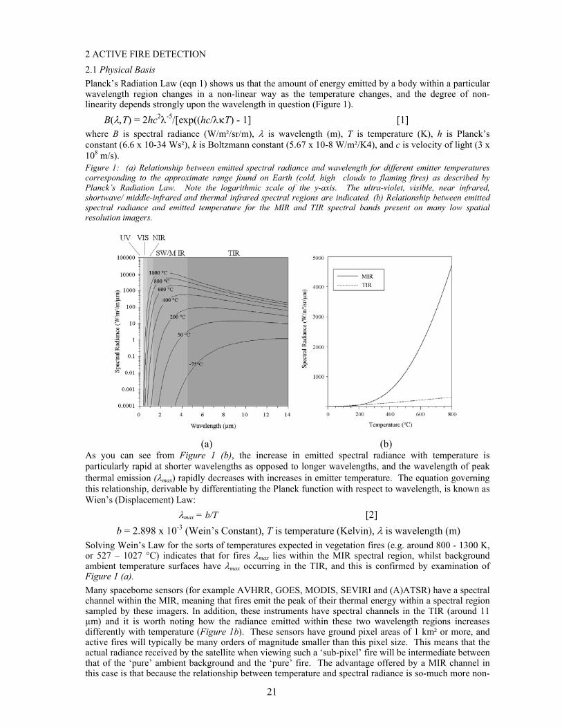
21

2 ACTIVE FIRE DETECTION 2.1 Physical Basis Planck’s Radiation Law (eqn 1) shows us that the amount of energy emitted by a body within a particular wavelength region changes in a non-linear way as the temperature changes, and the degree of non-linearity depends strongly upon the wavelength in question (Figure 1).

B(λ,T) = 2hc2λ-5/[exp((hc/λκT) - 1] [1] where B is spectral radiance (W/m²/sr/m), λ is wavelength (m), T is temperature (K), h is Planck’s constant (6.6 x 10-34 Ws²), k is Boltzmann constant (5.67 x 10-8 W/m²/K4), and c is velocity of light (3 x 108 m/s). Figure 1: (a) Relationship between emitted spectral radiance and wavelength for different emitter temperatures corresponding to the approximate range found on Earth (cold, high clouds to flaming fires) as described by Planck’s Radiation Law. Note the logarithmic scale of the y-axis. The ultra-violet, visible, near infrared, shortwave/ middle-infrared and thermal infrared spectral regions are indicated. (b) Relationship between emitted spectral radiance and emitted temperature for the MIR and TIR spectral bands present on many low spatial resolution imagers.

(a) (b)

As you can see from Figure 1 (b), the increase in emitted spectral radiance with temperature is particularly rapid at shorter wavelengths as opposed to longer wavelengths, and the wavelength of peak thermal emission (λmax) rapidly decreases with increases in emitter temperature. The equation governing this relationship, derivable by differentiating the Planck function with respect to wavelength, is known as Wien’s (Displacement) Law:

λmax = b/T [2] b = 2.898 x 10-3 (Wein’s Constant), T is temperature (Kelvin), λ is wavelength (m)

Solving Wein’s Law for the sorts of temperatures expected in vegetation fires (e.g. around 800 - 1300 K, or 527 – 1027 °C) indicates that for fires λmax lies within the MIR spectral region, whilst background ambient temperature surfaces have λmax occurring in the TIR, and this is confirmed by examination of Figure 1 (a). Many spaceborne sensors (for example AVHRR, GOES, MODIS, SEVIRI and (A)ATSR) have a spectral channel within the MIR, meaning that fires emit the peak of their thermal energy within a spectral region sampled by these imagers. In addition, these instruments have spectral channels in the TIR (around 11 µm) and it is worth noting how the radiance emitted within these two wavelength regions increases differently with temperature (Figure 1b). These sensors have ground pixel areas of 1 km² or more, and active fires will typically be many orders of magnitude smaller than this pixel size. This means that the actual radiance received by the satellite when viewing such a ‘sub-pixel’ fire will be intermediate between that of the ‘pure’ ambient background and the ‘pure’ fire. The advantage offered by a MIR channel in this case is that because the relationship between temperature and spectral radiance is so-much more non-

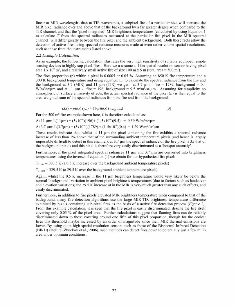
22

linear at MIR wavelengths than at TIR wavebands, a subpixel fire of a particular size will increase the MIR pixel radiance over and above that of the background by a far greater degree when compared to the TIR channel, and that the ‘pixel integrated’ MIR brightness temperatures (calculated by using Equation 1 to calculate T from the spectral radiances measured at the particular fire pixel in the MIR spectral channel) will differ greatly between the fire pixel and the ambient background. Both these facts allow the detection of active fires using spectral radiance measures made at even rather course spatial resolutions, such as those from the instruments listed above 2.2 Example Calculation As an example, the following calculation illustrates the very high sensitivity of suitably equipped remote sensing devices to highly sup-pixel fires. Here we a assume a 1km spatial resolution sensor having pixel area 1 x 106 m², and a relatively small active fire of size 100 m x 5 m (total area = 500 m²). The fires proportion (p) within a pixel is 0.0005 or 0.05 %. Assuming an 850 K fire temperature and a 300 K background temperature and using equation [1] to calculate the spectral radiance from the fire and the background at 3.7 (MIR) and 11 µm (TIR) we get: at 3.7 µm - fire = 1789, background = 0.4 W/m²/sr/µm and at 11 µm - fire = 196, background = 9.5 w/m²/sr/µm. Assuming for simplicity no atmospheric or surface emissivity effects, the actual spectral radiance of the pixel (L) is then equal to the area-weighted sum of the spectral radiances from the fire and from the background:

L(λ) = pB(λ,Tfire) + (1-p)B(λ,Tbackground) [3] For the 500 m² fire example shown here, L is therefore calculated as: At 11 µm: L(11µm) = (5x10-4)(196)+ (1-5x10-4)(9.5) = 9.59 W/m²/sr/µm At 3.7 µm: L(3.7µm) = (5x10-4 )(1789) + (1-5x10-4)(0.4) = 1.29 W/m²/sr/µm These results indicate that, whilst at 11 µm the pixel containing the fire exhibits a spectral radiance increase of less than 1% above that of the surrounding ambient temperature pixels (and hence is largely impossible difficult to detect in this channel), at 3.7 µm the spectral radiance of the fire pixel is 3x that of the background pixels and this pixel is therefore very easily discriminated as a ‘hotspot anomaly’. Furthermore, if the pixel integrated spectral radiances 11 µm and 3.7 µm are converted into brightness temperatures using the inverse of equation (1) we obtain for our hypothetical fire pixel: T11µm = 300.5 K (a 0.5 K increase over the background ambient temperature pixels) T3.7µm = 329.5 K (a 29.5 K over the background ambient temperature pixels) Again, whilst the 0.5 K increase in the 11 µm brightness temperature would very likely be below the normal ‘background’ variation in ambient pixel brightness temperatures (due to factors such as landcover and elevation variations) the 29.5 K increase at in the MIR is very much greater than any such effects, and easily discriminated. Furthermore, in addition to fire pixels elevated MIR brightness temperature when compared to that of the background, many fire detection algorithms use the large MIR-TIR brightness temperature difference exhibited by pixels containing sub-pixel fires as the basis of a active fire detection process (Figure 2). From this example calculation, it is seen that the fire pixel is easily discriminated, despite the fire itself covering only 0.05 % of the pixel area. Further calculations suggest that flaming fires can de reliably discriminated down to those covering around one fifth of this pixel proportion, though for the coolest fires this threshold maybe increased by an order of magnitude since their MIR thermal emissions are lower. By using quite high spatial resolution sensors such as those of the Bispectral Infrared Detection (BIRD) satellite (Zhuckov et al., 2006), such methods can detect fires down to potentially just a few m² in area under optimum conditions.

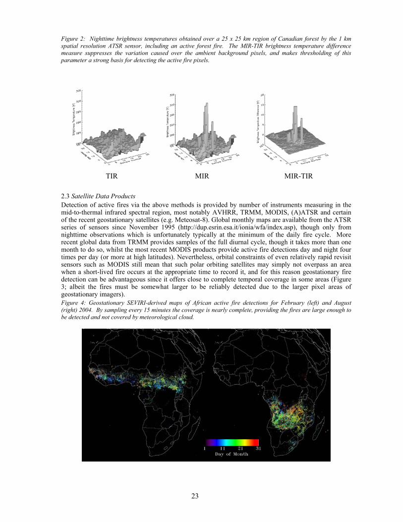
23

Figure 2: Nighttime brightness temperatures obtained over a 25 x 25 km region of Canadian forest by the 1 km spatial resolution ATSR sensor, including an active forest fire. The MIR-TIR brightness temperature difference measure suppresses the variation caused over the ambient background pixels, and makes thresholding of this parameter a strong basis for detecting the active fire pixels.

TIR MIR MIR-TIR

2.3 Satellite Data Products Detection of active fires via the above methods is provided by number of instruments measuring in the mid-to-thermal infrared spectral region, most notably AVHRR, TRMM, MODIS, (A)ATSR and certain of the recent geostationary satellites (e.g. Meteosat-8). Global monthly maps are available from the ATSR series of sensors since November 1995 (http://dup.esrin.esa.it/ionia/wfa/index.asp), though only from nighttime observations which is unfortunately typically at the minimum of the daily fire cycle. More recent global data from TRMM provides samples of the full diurnal cycle, though it takes more than one month to do so, whilst the most recent MODIS products provide active fire detections day and night four times per day (or more at high latitudes). Nevertheless, orbital constraints of even relatively rapid revisit sensors such as MODIS still mean that such polar orbiting satellites may simply not overpass an area when a short-lived fire occurs at the appropriate time to record it, and for this reason geostationary fire detection can be advantageous since it offers close to complete temporal coverage in some areas (Figure 3; albeit the fires must be somewhat larger to be reliably detected due to the larger pixel areas of geostationary imagers). Figure 4: Geostationary SEVIRI-derived maps of African active fire detections for February (left) and August (right) 2004. By sampling every 15 minutes the coverage is nearly complete, providing the fires are large enough to be detected and not covered by meteorological cloud.

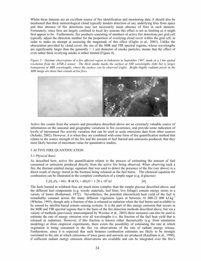
24

Whilst these datasets are an excellent source of fire identification and monitoring data, it should also be mentioned that thick meteorological cloud typically hinders detection of any underlying fires from space and thus absence of fire detections may not necessarily mean absence of fires in such datasets. Fortunately, since fires are largely confined to local dry seasons this effect is not as limiting as it might first appear to be. Furthermore, fire products consisting of numbers of active fire detections per grid cell typically adjust the detection number for the proportion of overlying cloud cover within the grid cell, in order to make an attempt at assessing the magnitude of this effect (Giglio et al., 2003). Unlike the obscuration provided by cloud cover, the use of the MIR and TIR spectral regions, whose wavelengths are significantly larger than the generally < 1 µm diameter of smoke particles, means that the effect of even rather thick overlying smoke is rather limited (Figure 4).

Figure 5: Daytime observations of a fire affected region in Indonesia in September 1997, made at a 1 km spatial resolution from the ATSR-2 sensor. The thick smoke masks the surface at NIR wavelengths (left) but is largey transparent at MIR wavelengths, where the surface can be observed (right). Bright (highly radiant) pixels in the MIR image are those that contain active fires.

Active fire counts from the sensors and procedures described above are an extremely valuable source of information on the seasonal and geographic variations in fire occurrence, and provide some indication of levels of interannual fire activity variation that can be used to scale emissions data from other sources (Schultz, 2002). However, it is when they are combined with some form of fire quantification method that relates to the source strength of the fire and the amount of fuel burned and emissions produced, that they most likely become of maximum value for quantitative studies.

3 ACTIVE FIRE QUANTIFICATION 3.1 Physical Basis As described here, active fire quantification relates to the process of estimating the amount of fuel consumed or emissions produced directly from the active fire being observed. When observing such a fire, the thermal emitted energy signature that was used to detect the presence of the fire (see above) is a direct result of energy stored in the biomass being released as the fuel burns. The chemical equation for combustion can be illustrated in the complete combustion of a simple sugar (e.g. d-glucose):

C6H12O6 + 6O2 6CO2 + 6H2O + 1.28 x 106 kJ [4] The fuels burned in wildland fires are much more complex than the simple glucose described above, and the different fuel components (e.g. woody materials, leaf litter, live foliage) contain energy stores in a variety of forms (Rothermel, 1972). Nevertheless, the potential (theoretical) heat yield of the fuel is remarkably constant across the many different vegetation types at between 16 000-22 000 kJ.kg-1 (Whelan, 1995), though only a fraction of this is released as radiation when the fuel burns and available to be sensed by satellite-based remote sensing systems. It is the part of this energy emission that occurs in the MIR and TIR spectral regions that is the basis of the fire detection methods described above, but via a variety of methods (previously intercompared by Wooster et al., 2003) these measures can also be used to estimate the rate of energy emission over all wavelengths (i.e. the fraction of the fuel heat yield that is released as radiation). However, if this fraction is known either theoretically (e.g. from simulation modeling) or from empirical experiments, there exists the possibility of estimating the rate at which vegetation is being consumed in the fire via observations of the rate of radiant energy release. Furthermore, since it is expected that such biomass combustion estimates are likely to be strongly correlated to the rate at which emissions of trace gases and aerosols are produced (Kaufman et al., 1996), if sufficient radiant energy emission observations are available and can be integrated over the fire’s

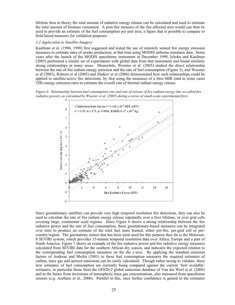
25

lifetime then in theory the total amount of radiative energy release can be calculated and used to estimate the total amount of biomass consumed. A post-fire measure of the fire-affected area would can then be used to provide an estimate of the fuel consumption per unit area, a figure that is possible to compare to field-based measures for validation purposes. 3.2 Application to Satellite Imagery Kaufman et al. (1996, 1998) first suggested and tested the use of remotely sensed fire energy emission measures to estimate rates of smoke production, at that time using MODIS airborne simulator data. Some years after the launch of the MODIS spaceborne instrument in December 1999, Ichoku and Kaufman (2005) performed a similar set of experiments with global data from that instrument and found similarly strong relationships in many areas. Meanwhile, Wooster et al. (2005) studied the direct relationship between the rate of fire radiant energy emission and the rate of fuel consumption (Figure 3), and Wooster et al (2003), Roberts et al (2005) and Zhukov et al (2006) demonstrated how such relationships could be applied to satellite-active fire detections, by first using the measures of a fires MIR (and in some cases TIR) energy emission rates to estimate the overall rate of thermal radiant energy release.

Figure 6: Relationship between fuel consumption rate and rate of release of fire radiant energy (the so-called fire radiative power), as calculated by Wooster et al. (2005) during a series of small-scale experimental fires.

Since geostationary satellites can provide very high temporal resolution fire detections, they can also be used to calculate the rate of fire radiant energy release repeatedly over a fires lifetime, or over grid cells covering large, continental scale regions. Since Figure 6 shows a strong relationship between the fire radiative power and the rate of fuel consumption, these geostationary-based measures can be integrated over time to produce an estimate of the total fuel mass burned, either per-fire, per-grid cell or per-country/region. The geostationy sensor that has been most used for this purpose thus far is the Meteosat-8 SEVIRI system, which provides 15-minute temporal resolution data over Africa, Europe and a part of South America. Figure 7 shows an example of the fire radiative power and fire radiative energy measures calculated from SEVIRI data for the southern African dry season, and indicates the expected relation to the corresponding fuel consumption measures on the rhs y-axis. By applying the standard emission factors of Andreae and Merlet (2001) to these fuel consumption measures the required estimates of carbon, trace gas and aerosol emissions can be easily calculated. Though rather taxing to validate, these new estimates of fuel consumption are currently being compared against the current ‘best available’ estimates, in particular those from the GFEDv2 global emissions database of Van der Werf et al. (2006) and in the future from inversions of atmospheric trace gas concentrations, also measured from spaceborne sensors (e.g. Arellano et al., 2006). Parallel to this, once further confidence is gained in the estimates

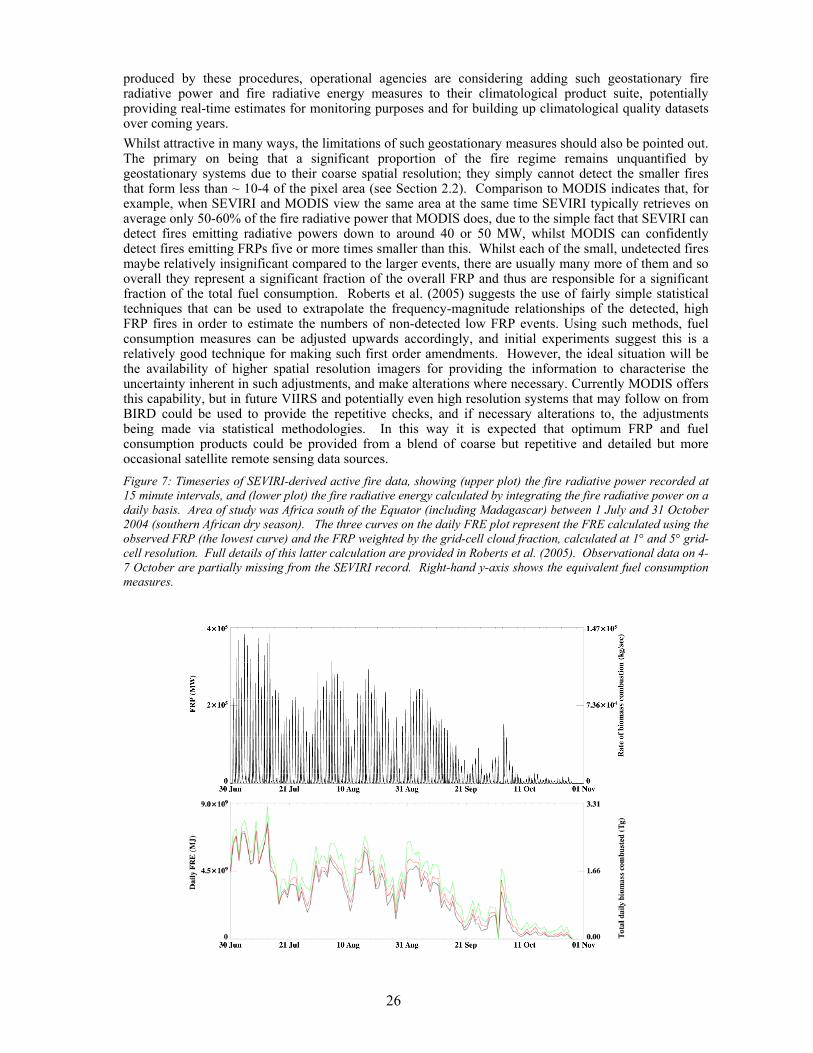
26

produced by these procedures, operational agencies are considering adding such geostationary fire radiative power and fire radiative energy measures to their climatological product suite, potentially providing real-time estimates for monitoring purposes and for building up climatological quality datasets over coming years. Whilst attractive in many ways, the limitations of such geostationary measures should also be pointed out. The primary on being that a significant proportion of the fire regime remains unquantified by geostationary systems due to their coarse spatial resolution; they simply cannot detect the smaller fires that form less than ~ 10-4 of the pixel area (see Section 2.2). Comparison to MODIS indicates that, for example, when SEVIRI and MODIS view the same area at the same time SEVIRI typically retrieves on average only 50-60% of the fire radiative power that MODIS does, due to the simple fact that SEVIRI can detect fires emitting radiative powers down to around 40 or 50 MW, whilst MODIS can confidently detect fires emitting FRPs five or more times smaller than this. Whilst each of the small, undetected fires maybe relatively insignificant compared to the larger events, there are usually many more of them and so overall they represent a significant fraction of the overall FRP and thus are responsible for a significant fraction of the total fuel consumption. Roberts et al. (2005) suggests the use of fairly simple statistical techniques that can be used to extrapolate the frequency-magnitude relationships of the detected, high FRP fires in order to estimate the numbers of non-detected low FRP events. Using such methods, fuel consumption measures can be adjusted upwards accordingly, and initial experiments suggest this is a relatively good technique for making such first order amendments. However, the ideal situation will be the availability of higher spatial resolution imagers for providing the information to characterise the uncertainty inherent in such adjustments, and make alterations where necessary. Currently MODIS offers this capability, but in future VIIRS and potentially even high resolution systems that may follow on from BIRD could be used to provide the repetitive checks, and if necessary alterations to, the adjustments being made via statistical methodologies. In this way it is expected that optimum FRP and fuel consumption products could be provided from a blend of coarse but repetitive and detailed but more occasional satellite remote sensing data sources. Figure 7: Timeseries of SEVIRI-derived active fire data, showing (upper plot) the fire radiative power recorded at 15 minute intervals, and (lower plot) the fire radiative energy calculated by integrating the fire radiative power on a daily basis. Area of study was Africa south of the Equator (including Madagascar) between 1 July and 31 October 2004 (southern African dry season). The three curves on the daily FRE plot represent the FRE calculated using the observed FRP (the lowest curve) and the FRP weighted by the grid-cell cloud fraction, calculated at 1° and 5° grid-cell resolution. Full details of this latter calculation are provided in Roberts et al. (2005). Observational data on 4-7 October are partially missing from the SEVIRI record. Right-hand y-axis shows the equivalent fuel consumption measures.

27

4 CONCLUSION Fire detections provided by polar orbiting and geostationary systems have long been providing useful data on fire incidence, timing and relative magnitude for use in many regional and earth system science applications, as well as certain operational monitoring initiatives, most particularly in the fields of carbon, trace gas and aerosol emissions estimation. The MIR and TIR spectral channels provided on many earth observation imaging systems mean that a wide variety of sensors have be used for providing such measures since the early 1980’s. More recent developments have seen data from such instruments also used to estimate the rate of fire energy emission, and this has been related in turn to the rate of fuel consumption. Provided the sensors used have sufficient dynamic range in the MIR spectral channel to avoid senor saturation over fires, whilst providing a signal-to-noise ratio that is useful in estimating the necessary ambient background signals, this potentially provides a new route for emissions monitoring purposes and for those wishing to obtain quantitative estimates of fuel consumption to compare with those derived from alternative approaches. Geostationary systems are particularly attractive for this application due to the highly repetitive nature of their observations, and thus the ability to integrate their fire radiative power measures to estimate total fuel consumption. However, the coarse resolution provided by such systems limits their fire detection capability to those fires at the larger/more intense end of the fire regime spectrum, and so statistical methods must be used to assess the fraction of the overall fire radiative power that maybe being missed. Such extrapolations can provide a first order method of adjusting the geostationary-derived estimates for this effect, but the availably of higher spatial resolution sensors providing occasional, but very detailed FRP observations over sub-samples of the area of interest is likely to provide the best solution for overall quantification of the complete fire regime.

5 REFERENCES Andreae, M. O., and P. Merlet., 2001. Emission of trace gases and aerosols from biomass burning, Global

Biogeochemical Cycles, 15, 995-966. Arellano, A. F., Jr., P. S. Kasibhatla, L. Giglio, G. R. van der Werf, J. T. Randerson, and G. J. Collatz., 2006. Time-

dependent inversion estimates of global biomass-burning CO emissions using Measurement of Pollution in the Troposphere (MOPITT) measurements, J. Geophys. Res., 111, D09303, doi:10.1029/2005JD006613.

Burgan, R.E. and Rothermel, R.C. 1984. BEHAVE – Fire Behaviour Prediction and Fuel Modeling System: Fuel Subsystem. USDA Forest Service General Technical Report, INT-238.

Giglio, L., Kendall, J. D., and Mack, R., 2003. A multi-year active fire dataset for the tropics derived from TRMM VIRS. International Journal of Remote Sensing. 24. 22. 4505-4525.

Ichoku, C. and Kaufman, Y. J., 2005. A method to derive smoke emission rtates from MODIS Fire Radiative Energy measurements. IEEE Transactions on Geoscience and Remote Sensing. 43. 1. 2636-2649.

Kaufman Y., L. Remer, R. Ottmar, D. Ward, L. Rong-R, R. Kleidman, R. Fraser, L. Flynn, D.McDougal, and G. Shelton., 1996. Relationship between remotely sensed fire intensity and rate of emission of smoke: SCAR-C experiment, in Global Biomass Burning, Levine, J. (ed), 685-696, MIT Press, Mass.

Kaufman, Y.J, R.G. Kleidman, and M.D. King,, 1998. SCAR-B fires in the tropics: properties and remote sensing from EOS-MODIS, J. Geophys. Res., 103, 31955-31968, 1998a.

La Canut, P., Andreae, M. O., Harris, G. W., Wienhold, F. G. and Zenker, T., 1996. Airborne studies of emissions from savanna fires in southern Africa. 1. Aerosol emissions measured with a laser optical particle counter. J. Geophys. Res., 101. 19. 23615-23630.

Pyne, S.J. 1984. Introduction to Wildland Fire: Fire Management in the United States. John Wiley and Sons, NY. Roberts G., Wooster, M. J., Perry, G. L. W. , Drake, N., Rebelo, L.-M., Dipotso, F., 2005. Retrieval of biomass

combustion rates and totals from fire radiative power observations: Application to southern Africa using geostationary SEVIRI imagery, J. Geophys. Res., 110. D21111. doi:10.1029/2005JD006018.

Rothermel, R. C. 1972. A Mathematical Model for Predicting Fire Spread in Wildland Fuels. USDA Forest Service, General Technical Report, GTR-INT 115.

Schultz, M., 2002. On the use of ATSR fire count data to estimate the seasonal and interannual variability of vegetation fire emissions, Atmos. Chem. Phys., 2, 387–395.

van der Werf, G. R., Randerson, J. T., Giglio, L., Collatz, G. J., Kasibhatla, P.S., and Avelino, A. F., 2006. Interannual variability in biomass burning emissions from 1997 to 2004. Atmos. Chem. Phys.Discussion. 6, 3175-3226.

van der Werf, G. R., Randerson, J. T., Giglio, L., Collatz, G. J., Kasibhatla, P.S., and Avelino, A. F., 2006. Interannual variability in biomass burning emissions from 1997 to 2004. Atmos. Chem. Phys.Discussion. 6, 3175-3226.

Whelan, R. J. 1995. The Ecology of Fire. Cambridge University Press. Cambridge. Williams, C. A., Hanan, N. P., Neff, J. C., Scholes, R. J., Berry, J. A., Denning, A. S., and Baker, D. E., 2007.

Africa and the global carbon cycle. Carbon Balance and Management. 2:3. doi:10.1186/1750-0680-2-3. Wooster M. J., Roberts, G., Perry, G. L. W., Kaufman, Y. J., 2005. Retrieval of biomass combustion rates and totals

from fire radiative power observations: FRP derivation and calibration relationships between biomass consumption and fire radiative energy release. J. Geophys. Res. 110, D24311. doi:10.1029/2005JD006318.

28

Wooster, M. J., 2002. Small-scale experimental testing of the fire radiative energy for quantifying mass combusted in natural vegetation. Geophys. Res. Let. 29. 21. 2027. doi:10.1029/2002GL015487.

Wooster, M. J., Zhukov, B., and Oertel, D., 2003. Fire radiative energy for quantitative study of biomass burning: derivation from the BIRD experimental satellite and comparison to MODIS fire products. Remote Sens. Environ. 86. 83-107.

Zhukov, B., Lorenz, E., Oertel, D., Wooster, M.J. and Roberts, G., 2006. Spaceborne detection and characterization of fires during the Bi-spectral Infrared Detection (BIRD) experimental small satellite mission (2001-2004). Remote Sens. Environ, 100, 29-51.

29

1 INTRODUCTION Wildland fire management decisions rely on timely information on fire location, intensity, direction and rate-of-spread, and burn severity (for post-fire rehabilitation needs). Operational fire monitoring is the repeated observation and quantitative evaluation of wildland fires during its active phase on a regular technical and logistic base. Currently, mostly in developed countries, aerial reconnaissance provides fire managers with this critical information, and space-borne sensors provide usually guidance information for the fire monitoring aircraft. Quantitative and geo-referenced satellite data based fire monitoring information is of great value for fire ecologists, health organisations and national administrations, too. 1.1 Sensitivity of IR spectral bands to signals from fires, background, and possible false alarms The radiance signatures of vegetative background, fire, sun-glints (both occupying only 1% of a pixel), and warm soil are shown in Figure 1 in the 0.4 – 15 µm wavelength region together with the relevant spectral bands for reliable detection and monitoring of wildfires [Zhukov, et al, 2006].

Operational Fire Monitoring

(A prospective view on satellite based wildfire monitoring)

D. Oertel Deutsches Zentrum für Luft- und Raumfahrt (DLR), Rutherford Strasse 2, Berlin, D-12489, Germany, [email protected] Keywords: Active fire monitoring, Space-borne infrared observation, Fire information systems

ABSTRACT: Satellite Earth observation is the only method able to provide repetitive data at the spatial and temporal scales necessary for detection and monitoring of wildfires. Most of the space borne sensors currently used for detection and monitoring of wildfires are multi-spectral scanners which have (a) broader application objectives and (b) channels in the mid and thermal infrared (MIR and TIR). For reliable HTE detection and monitoring imaging multi-spectral observations in the spectral range from the visible to the thermal infrared are needed but, the MIR channel is considered as the leading band for space-borne active fire observation. Existing meteorological and environmental satellite sensor systems, such as NOAA-AVHRR, MODIS, and some geo-stationary ameteorological satellite sensors, provided data which are useful for fire monitoring and post-assessment purposes on coarser scales, but often with limited value for on-the-ground fire managers mostly because of inherent data inaccuracies. All existing satellite-data based fire information systems provide occurrence data only for major fires and the spatial resolution (pixel size) of about 1 km is insufficient to accurately locate a fire and identify individual fire fronts. Data products do not offer information on fire attributes such as fire intensity, front line length or front line strength. Real-time-data processing procedures on-board of satellites are a means to improve the efficiency of satellite based detection and monitoring systems. Real-time detection and monitoring would enable global fire detection and monitoring services that can be rapidly delivered to on-the-ground wildland fire managers. The paper presents experiences with high definition fire detection and monitoring using the German Bi-spectral IR Detection (BIRD) satellite, also in comparison with active fire data obtained by the MODerate resolution Imaging Spectro-radiometer (MODIS), nearly simultaneously with BIRD records. Deficiencies of existing coarser spatial resolution InfraRed (IR) sensors are identified. Requirements to prospective fire detection and monitoring sensors operated in a Low Earth Orbit (LEO) are grouped. Alternatives for operational fire monitoring are discussed: (i) by combined use of existing coarse resolution IR sensors and the prospective Infrared Element, and (ii) use of dedicated fire monitoring constellations.

30

Figure 1: Radiance signatures of vegetative background, fire, sun-glints, & warm soil together with relevant spectral bands for space-borne fire detection and monitoring

Most of the space borne sensors currently used for detection and monitoring of wildfires are multi-spectral scanners, which have channels in the mid and thermal infrared (MIR and TIR). Because of the high sensitivity of the MIR spectral region (at ~ 4 µm) to the presence of high temperature sources that are even very significantly smaller than the pixel size (i.e. << 1%), hotspots are normally detected via their increased spectral signature in this wavelength region. For reliable fire detection and monitoring imaging multi-spectral observations in the spectral range from the visible to the thermal infrared are needed. Whilst sensor systems with IR bands in the short wave infrared (SWIR) and/or TIR (but without a MIR band), like Enhanced Thematic Mapper (ETM) or Advanced Space-borne Thermal Emission and Reflection Radiometer (ASTER), can in some circumstances be used for fire detection (albeit at a very poor temporal resolution totally unsuited for a ‘monitoring’ role) they offer very limited capability for quantitative characterization of wildfires since they saturate over even very modest fires [Oertel, 2005]. 1.2 Available satellite sensors for fire observations Moderate resolution polar orbiting satellites currently provide data used in the detection of active fires (and burn scars). The system having the clearest operational status is the National Oceanic and Atmospheric Administration (NOAA) Polar Orbiting Environmental Satellite (POES) Advanced Very High Resolution Radiometer (AVHRR). Many of the existing national or regional operational systems for detecting active fires rely on AVHRR data downloaded from direct readout stations. The National Aeronautics and Space Administration (NASA) Moderate-resolution Imaging Spectro-radiometer (MODIS), a research instrument, has demonstrated the value that improved spatial resolution (in the optical bands), radiometric calibration, geo-location accuracy, and, in particular, an extended suite of spectral bands with characteristics optimised for observation can add to fire remote sensing. MODIS sensors are currently flying on NASA’s Terra and Aqua satellites. Data from the European Space Agency (ESA) (Advanced) Along Track Scanning Radiometer ((A)ATSR) have been processed to produce multi-year global compilations of night-time active fires and daytime burn scars. Currently Imagers on the US Geostationary Operational Environmental Satellites (GOES) allow for diurnal fire detection and monitoring throughout the Western and Asian/Pacific hemispheres. The European “Meteosat-8” Spinning Enhanced Visible and Infrared Imager (SEVIRI) provides diurnal fire monitoring capabilities in Western Europe and Africa. Whilst these systems provide excellent possibilities for temporal sampling, their spatial resolution limits their use to the larger/more intense fires only.

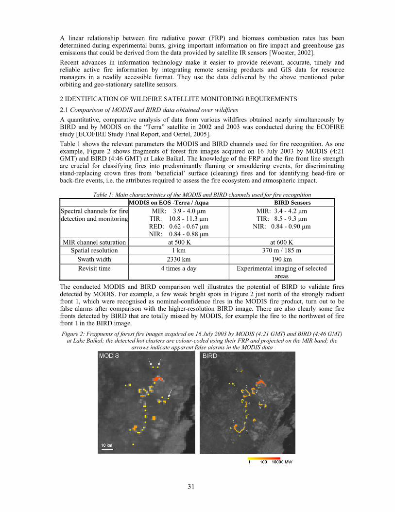
31

A linear relationship between fire radiative power (FRP) and biomass combustion rates has been determined during experimental burns, giving important information on fire impact and greenhouse gas emissions that could be derived from the data provided by satellite IR sensors [Wooster, 2002]. Recent advances in information technology make it easier to provide relevant, accurate, timely and reliable active fire information by integrating remote sensing products and GIS data for resource managers in a readily accessible format. They use the data delivered by the above mentioned polar orbiting and geo-stationary satellite sensors.

2 IDENTIFICATION OF WILDFIRE SATELLITE MONITORING REQUIREMENTS 2.1 Comparison of MODIS and BIRD data obtained over wildfires A quantitative, comparative analysis of data from various wildfires obtained nearly simultaneously by BIRD and by MODIS on the “Terra” satellite in 2002 and 2003 was conducted during the ECOFIRE study [ECOFIRE Study Final Report, and Oertel, 2005]. Table 1 shows the relevant parameters the MODIS and BIRD channels used for fire recognition. As one example, Figure 2 shows fragments of forest fire images acquired on 16 July 2003 by MODIS (4:21 GMT) and BIRD (4:46 GMT) at Lake Baikal. The knowledge of the FRP and the fire front line strength are crucial for classifying fires into predominantly flaming or smouldering events, for discriminating stand-replacing crown fires from ‘beneficial’ surface (cleaning) fires and for identifying head-fire or back-fire events, i.e. the attributes required to assess the fire ecosystem and atmospheric impact.

Table 1: Main characteristics of the MODIS and BIRD channels used for fire recognition MODIS on EOS -Terra / Aqua BIRD Sensors

Spectral channels for fire detection and monitoring

MIR: 3.9 - 4.0 μm TIR: 10.8 - 11.3 μm RED: 0.62 - 0.67 μm NIR: 0.84 - 0.88 μm

MIR: 3.4 - 4.2 μm TIR: 8.5 - 9.3 μm

NIR: 0.84 - 0.90 μm

MIR channel saturation at 500 K at 600 K Spatial resolution 1 km 370 m / 185 m

Swath width 2330 km 190 km Revisit time 4 times a day Experimental imaging of selected

areas The conducted MODIS and BIRD comparison well illustrates the potential of BIRD to validate fires detected by MODIS. For example, a few weak bright spots in Figure 2 just north of the strongly radiant front 1, which were recognised as nominal-confidence fires in the MODIS fire product, turn out to be false alarms after comparison with the higher-resolution BIRD image. There are also clearly some fire fronts detected by BIRD that are totally missed by MODIS, for example the fire to the northwest of fire front 1 in the BIRD image. Figure 2: Fragments of forest fire images acquired on 16 July 2003 by MODIS (4:21 GMT) and BIRD (4:46 GMT)

at Lake Baikal; the detected hot clusters are colour-coded using their FRP and projected on the MIR band; the arrows indicate apparent false alarms in the MODIS data

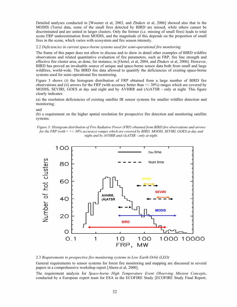
32

Detailed analyses conducted in [Wooster et al, 2003, and Zhukov et al, 2006] showed also that in the MODIS (Terra) data, some of the small fires detected by BIRD are missed, while others cannot be discriminated and are united in larger clusters. Only the former (i.e. missing of small fires) leads to total scene FRP underestimation from MODIS, and the magnitude of this depends on the proportion of small fires in the scene, which varies with ecosystem and fire season intensity.

2.2 Deficiencies in current space-borne systems used for semi-operational fire monitoring The frame of this paper does not allow to discuss and to show in detail other examples of BIRD wildfire observations and related quantitative evaluation of fire parameters, such as FRP, fire line strength and effective fire cluster area, as done, for instance, in [Oertel, et al, 2004, and Zhukov et al, 2006]. However, BIRD has proved an invaluable source of unique and space-borne sensor data both from small and large wildfires, world-wide. The BIRD fire data allowed to quantify the deficiencies of existing space-borne systems used for semi-operational fire monitoring. Figure 3 shows (i) the histogram distribution of FRP obtained from a large number of BIRD fire observations and (ii) arrows for the FRP (with accuracy better than +/- 30%) ranges which are covered by MODIS, SEVIRI, GOES at day and night and by AVHRR and (A)ATSR - only at night. This figure clearly indicates: (a) the resolution deficiencies of existing satellite IR sensor systems for smaller wildfire detection and monitoring; and (b) a requirement on the higher spatial resolution for prospective fire detection and monitoring satellite systems.

Figure 3: Histogram distribution of Fire Radiative Power (FRP) obtained from BIRD fire observations and arrows for the FRP (with < +/- 30% accuracy) ranges which are covered by BIRD, MODIS, SEVIRI, GOES at day and

night and by AVHRR and (A)ATSR - only at night.

2.3 Requirements to prospective fire monitoring systems in Low Earth Orbit (LEO) General requirements to sensor systems for forest fire monitoring and mapping are discussed in several papers in a comprehensive workshop report [Ahern et al, 2000]. The requirement analysis for Space-borne High Temperature Event Observing Mission Concepts, conducted by a European expert team for ESA in the ECOFIRE Study [ECOFIRE Study Final Report,

AVHRR, (A)ATSR

BIRD

MODIS

SEVIRI

GOES

Night time

Day time

33

Oertel, 2005] led to a mission refinement and to the review of the mission requirements for the InfraRed Element. The InfraRed Element was initially considered by ESA as: (1) a dedicated fire detecting and monitoring sensor, and (2) a payload passenger for the planned Sentinel -1,-2, and/or -3 satellites of the upcoming European initiative on Global Monitoring for Environment and Security (GMES) as outlined, for instance, in [ESA/PB-EO(2005)93]. During the ECOFIRE study and the Infrared Element mission requirement review three different application groups with diverging objectives and requirements have been identified [ECOFIRE Study Final Report, EO-PSM/1163 MR-dr] in 2005: Global group which covers the requirements on observations of Global Change related observation of forest-, savannah- and peat-fires for all relevant vegetation zones from the tropics to the boreal as well as fire observations relevant for global climate monitoring and European air quality forecasting, Eco-Regio group which covers the requirements on ecozonal fire monitoring and on three regional targeted applications: Mediterranean forest fires, boreal forest / steppe fires, and radioactively contaminated vegetation fires,and Special target group which covers the requirements on observations of volcanic activity, tropical peat land fires, and coal seam fires. The High Temperature Event (HTE) observation and data product requirements of these application groups are summarized in Table 2. A major disadvantage of existing sensors used currently, such as MODIS, GOES and SEVIRI, is their coarse spatial resolution. The finest currently available spatial resolution of 1000 m is a factor of 2-3 coarser than the 300 -500 m spatial resolution requirement of the Global group and a factor of ten coarser than the 100 m spatial requirement of the Eco-Regio group. Most of the currently available fire information systems are delivering GIS compatible vector/raster map information on fire ‘hot spots’, containing essentially the location of the larger fires only. Therefore, to close this significant gap for operational space-borne fire monitoring, higher spatial resolution satellite sensors with high radiometric dynamic in their MIR and TIR bands are required.

3 ALTERNATIVES FOR PROSPECTIVE SPACE-BORNE OPERATIONAL FIRE MONITORING The currently existing geo-stationary satellite sensor systems GOES and Meteosat 8 SEVIRI fulfill the requirements on temporal resolution and small data delivery very well, exhibit a good spatial coverage for latitudes and longitudes < +/- 50° from the nadir point, but provide a very coarse spatial resolution of > 3 km which allows the reliable detection of fires with a FRP > 50 MW only. The last is the most crucial deficiency of these systems. An assessment of the wildfires diurnal FRP cycle with geostationary satellites is also limited by their rather weak detection sensitivity due to larger pixel size. MODIS data are successfully used to validate the “Meteosat-8” SEVIRI data based FRP measurements, obtained over Africa [ECOFIRE Study Final Report]. Furthermore, the MODIS BIRD comparison showed that there is a high complementary potential of two types of Low Earth Orbiting (LEO) IR sensor systems for innovative active fire detection, monitoring and characterisation: MODIS type: Wide-swath low-to-moderate-resolution spectro-radiometers on polar-orbiting environmental satellites providing daily global coverage of fire detection, and BIRD type: Medium spatial resolution imagers to be flown: # on micro-satellite constellations, or # as payload passengers on medium-scale satellites allowing detailed monitoring and validation of the HTE information of hotspots which occurrence was detected before by: (a) MODIS type wide-swath sensors on other LEO satellites, (b) a wide-swath Fore Field Sensor on the same platform, and/or (c) geostationary satellite sensors. The term “BIRD-type IR sensor” means a push-broom sensor equipped in its MIR and TIR bands with photodiode line array detectors and integrated machine coolers. This detector technology allows to provide a Noise Equivalent Difference Temperature (NEDT) of the sensor below 0.4 K at a background temperature of 300 K in both the MIR and TIR bands.

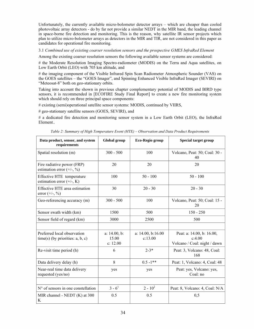
34

Unfortunately, the currently available micro-bolometer detector arrays – which are cheaper than cooled photovoltaic array detectors - do by far not provide a similar NEDT in the MIR band, the leading channel in space-borne fire detection and monitoring. This is the reason, why satellite IR sensor projects which plan to utilize micro-bolometer arrays as detectors in the MIR and TIR, are not considered in this paper as candidates for operational fire monitoring.

3.1 Combined use of existing coarser resolution sensors and the prospective GMES InfraRed Element Among the existing coarser resolution sensors the following available sensor systems are considered: # the Moderate Resolution Imaging Spectro-radiometer (MODIS) on the Terra and Aqua satellites, on Low Earth Orbit (LEO) with 705 km altitude, and # the imaging component of the Visible Infrared Spin Scan Radiometer Atmospheric Sounder (VAS) on the GOES satellites – the “GOES Imager”, and Spinning Enhanced Visible InfraRed Imager (SEVIRI) on “Meteosat-8” both on geo-stationary orbits. Taking into account the shown in previous chapter complementary potential of MODIS and BIRD type sensors, it is recommended in [ECOFIRE Study Final Report] to create a new fire monitoring system which should rely on three principal space components: # existing (semi)operational satellite sensor systems: MODIS, continued by VIIRS, # geo-stationary satellite sensors (GOES, SEVIRI), and # a dedicated fire detection and monitoring sensor system in a Low Earth Orbit (LEO), the InfraRed Element..

Table 2: Summary of High Temperature Event (HTE) – Observation and Data Product Requirements

Data product, sensor, and system requirements

Global group Eco-Regio group Special target group

Spatial resolution (m) 300 - 500 100 Volcano, Peat: 50; Coal: 30 - 40

Fire radiative power (FRP) estimation error (+/-, %)

20 20 20

Effective HTE temperature estimation error (+/-, K)

100 50 - 100 50 - 100

Effective HTE area estimation error (+/-, %)

30 20 - 30 20 - 30

Geo-referencing accuracy (m) 300 - 500 100 Volcano, Peat: 50; Coal: 15 - 20

Sensor swath width (km) 1500 500 150 - 250 Sensor field of regard (km) 3000 2500 500 Preferred local observation time(s) (by priorities: a, b, c)

a: 14.00, b: 15.00

c: 12.00

a: 14.00, b:16.00 c:13.00

Peat: a: 14.00, b: 16.00, c:4.00

Volcano / Coal: night / dawn Re-visit time period (h) 6 2-3* Peat: 3, Volcano: 48, Coal:

168 Data delivery delay (h) 8 0.5 -1** Peat: 1, Volcano: 4, Coal: 48 Near-real time data delivery requested (yes/no)

yes yes Peat: yes, Volcano: yes, Coal: no

N° of sensors in one constellation 3 - 61 2 - 102 Peat: 8, Volcano: 4, Coal: N/AMIR channel - NEDT (K) at 300 K

0.5 0.5 0,5

35

TIR channel - NEDT (K) at 300 K

0.2 - 03 0.2 - 03 0.2 - 03

MIR channel saturation level (K) 650 750 Volcano, Peat: 840; Coal: 920TIR channel saturation level (K) 580 630 Volcano, Peat: 730; Coal: 850Visible (RED) channel radiometric dynamic range [W/(m2·μm·srad)]

5 - 500 5 - 500 5 - 500

* Two (consecutive) measurements are requested within preferred local observation time (at afternoon), and a third observation at about 8 -10 h local time is desirable ** 0.5 - 1 h data delivery delay is required for the fire management related monitoring, and 8 h data delivery delay is required for ecological monitoring x NEDT – Noise equivalent difference temperature 13 with across track tilt and up to 6 without across track tilt of the sensors Field of View (FOV) 22 with across track tilt and up to 10 without across track tilt of the sensors FOV As a design baseline for the Infrared Element minimum of three spectral bands (MIR at 4 µm, TIR at 10 µm and Red at 0.55 µm) are needed at a spatial resolution between 100 and 250 m to capture the range from high-energy fires down to low temperature smouldering fires and in order to separate thermal background information from the temperature events to be detected [ECOFIRE Study Final Report, and EO-PSM/1163 MR-dr]. In November 2006, however, the requirements to the GMES Infrared Element was discussed in a broader application horizon at a workshop where it was recommended “to decide with priority if the IR Element should be optimised for one particular application or to a compromise which would fulfil the requirements of as many applications as possible“ [EOP-SM/1564/MB-mb 2006]. This decision is still pending. If the Infrared Element will be flown as a payload passenger of the GMES land-application satellite Sentinel-2 and / or the GMES ocean application satellite Sentinel-3, the local equator crossing times will be 10:30 / 22:30 h and / or 10:00 / 22:00 h, respectively – see [EOP-SM/1564/MB-mb 2006]. This is acceptable but far from optimum for fire monitoring. Therefore, it was also mentioned in [EO-PSM/1163 MR-dr] that the InfraRed Element does not necessarily have to be implemented on Sentinel-2 or -3, but could be flown on separate platforms to secure the afternoon local equator crossing. A critical aspect of the described combined use of data from (i) geo-stationary satellites, (ii) MODIS type systems and the (iii) GMES Infrared Element as one operational fire monitoring service maybe, that that the Fire Monitoring Information System(s) on ground must be able to receive and to process the data distributed by at least three different space segments (i) – (iii). 3.2 Dedicated fire monitoring satellite constellations To analyse the needs of a commercially a world-wide user community interested in operational fire detection and monitoring services to be provided by a constellation of dedicated micro-satellites, a market study for a Fire Recognition Satellite system (FIRES) was proposed [Oertel, D., Ruecker, G. 2004]. The space segment of the Fire Recognition Satellite system (FIRES) shall consist of four BIRD-like micro-satellites and it shall feature innovative on board processing capacities that perform detection, classification and geo-referencing of fire information, such as the FRP, fire line strength and other. This design feature FIRES shall enable the “on-board generation” of a very compact high-end product with a sufficiently small data size for a direct broadcast to mobile, hand-held reception units which could be integrated, for instance, with commercially available GPS receivers – building a “Fire-GPS” system. A qualitative phase of the FIRES market study was conducted by the German small enterprise ZEBRIS GbR, and the Integrated Fire Management Group (IFMG) on behalf of the German Aerospace Center - Technology Marketing division (DLR-TM) in 2005. The FIRES market study activities included an international workshop on “FIRES Concept and Product Test” with experienced fire managers and fire information experts from five continents [Ruecker, 2005]. Considering the workshop recommendations on observation characteristics, the FIRES satellite sensor base line design comprises four spectral bands (MIR at 4 µm, TIR at 9 µm NIR at 0.85 µm and Red at 0.55 µm) with a spatial resolution of 300 m. All four bands will have a swath width of ~ 1150 km on Earth surface.

36

The four FIRES satellites shall fly at about 600 km altitude in two angular spaced polar sun-synchronous orbit planes with two satellites phased by 180° in each orbit. These observation characteristics of the FIRES satellites will provide four observations in 24 hours (two at day time and two night time) of each point on the Earth land surface (except the polar regions, where no wildfires occur). The two orbit planes of the FIRES space segment shall be chosen in a way that the local equator crossing times of the two pairs of satellites will be at 14:00/02:00 h and 16:30/04:30 h, respectively, i.e. the local equator crossing times will be at the optimum for fire detection and monitoring (see Table 2). Fire attributes, to be transmitted in real time by the FIRES satellites, such as FRP and fire line strength, can support decisions by fire managers in fire suppression planning, crew mobilization & movement and post fire assessment. Direct broadcast of GIS ready fire information from the FIRES satellites would enable fast delivery to fire managers even operating at remote sites without internet or telephone connection. Establishment and maintenance of costly ground receiving stations would not be necessary. A specific aspect of a dedicated operational fire monitoring system with such an extreme high level of on-board autonomy is that its ground segment will be cheap, compact, mobile and simple in operation. This might be seen as an advantage, compared with a system described in the previous chapter. However, the workshop on “FIRES Concept and Product Test” revealed that there will be also relevant users interested to receive preferably the radiometrically and geometrically corrected imaging data (Level 1B data of all channels) from the FIRES satellites directly, because they plan to use their own receiving and processing stations and their own fire detection and monitoring algorithms. To fulfil this supplementary requirement will be technically possible, but it will generate additional operation cost. A crucial precondition for the implementation of a mostly commercially funded space mission is to get the financial support by an organisation or a consortium of organisations, which are ready to carry the financial risk of the mission. The AUSBIRD fire monitoring constellation proposal won the backing of insurers, state governments and fire fighting authorities in Australia, accordingly to [The Australian News, January 03, 2007]. The AUSBIRD project is a joint venture between German Aerospace Center (DLR), German technology companies BERATA and Kayser Threde, and the Australian partner Euro Pacific Strategies (EPS). The Victorian and South Australian governments had expressed their interest in the AUSBIRD project. South Australian Infrastructure Minister signed a memorandum on AUSBIRD with the joint venture consortium in Cologne, Germany, in December 2006. AUSBIRD shall provide a ground revisit time of 6,5 h for operational fire detection and monitoring over Australia, New Zealand, the several fire prone regions in North America (USA, Canada), and the Mediterranean region. The AUSBIRD sensors shall be able to detect flaming fires with an area > 10 m2 and shall not suffer from saturation in the MIR/TIR channel during the observation of large fires. AUSBIRD will be a constellation of at least four micro-satellites with identical sensors of the BIRD- type, with observation and product characteristics close to that explained for the FIRES constellation. On-board data processing is foreseen in AUSBIRD to generate compact “hot spot” information on the location and the extent of the fire fronts/clusters. Geo-referenced image products of all channels will be processed in the AUSBIRD ground segment.

4 CONCLUSION

Recent developments in small satellites for Earth observation, for instance, the German demonstrator mission on Bi-spectral InfraRed Detection (BIRD) show the potential to provide the information required for wildland fire management decisions and for fire ecology by: • combined utilisation of existing coarser resolution IR sensor systems together with new dedicated

spatially higher resolution IR sensor systems flown as payload passengers or free flyers, and / or • prospective constellations of dedicated micro-satellites equipped with compact and intelligent IR

sensor systems.

5 REFERENCES Ahern, F., Gregoire, J.-M., Justice, C. (Ed) 2000. Forest Fire Monitoring and Mapping: A Component of Global

Observation of Forest Cover, Report of a Workshop, held at Ispra, Italy, November 3-5, 1999

37

ECF-INSA-0400-TN-01, 2005, ECOFIRE Regional monitoring requirements, Madrid, Spain ECOFIRE Study Final Report (ESA Contract No 17690) 2005. Scientific Assessment of Space-borne High

Temperature Event Observing Mission Concepts ESA/PB-EO(2005)93, 16 September 2005: “GMES Space Component, Traceability of User Requirements Based on

European Policy Priorities” EOP-SM/1564/MB-mb 2006. Summary Report of the ESA Workshop on Consolidation the Requirements of the

Sentinel Infrared Payload, ESA/ EO Document EO-PSM/1163 MR-dr 2005, Infrared Element Mission Requirement Document (chapter 5 of the ESA/ EO

Document) Oertel, D., Ruecker, G. 2004. The FIRES / Fire-GPS – System, DLR and ZEBRIS, Berlin, Munich Oertel, D. (Ed) 2005. ECOFIRE Study on Scientific Assessment of Space-borne High Temperature Event Observing

Mission Concepts, Executive Summary, DLR Rücker, G. 2005. FIRES Concept and Product Test, Workshop report, ZEBRIS, Munich The Australian News, January 03, 2007. http://theaustralian.news.com/story/0,20867,21004485-2702,00.html Wooster, M.J. (2002) Small-scale experimental testing of fire radiative energy for quantifying mass combusted in

natural vegetation fires, Geophys. Res. Let., 29, 21, 10.1029/2002GL015487. Wooster, M., Zhukov, B., Oertel, D. 2003. Fire radiative energy release for quantitative study of biomass burning:

derivation from the BIRD experimental satellite and comparison to MODIS fire products. Remote Sens. Environm., 86, 83-107.

Zhukov, B. Lorenz, E., Oertel, D., Wooster, M., Roberts, G. 2006. Spaceborne Detection and Characterization of Fires during the Bi-spectral Infrared Detection (BIRD) Experimental Small Satellite Mission (2001-2004, Remote Sens. Environm. 100, 29-51.

38

1 INTRODUCTION While remote sensing scientists have a long history of using airborne and spaceborne remote sensing systems for the direct monitoring of active fires, mapping burned area, and assessing the impacts of biomass burning, it has only been over the past decade that fire scientists and land managers have recognized the importance of this technology for meeting their information needs. The advancement in computer technology (hardware, software, data storage, and data delivery) along with the advanced training of students in the use information generated from the analysis of remote sensing data within geographic information systems have produced the means for land managers and scientists to routinely use satellite-derived information for fire monitoring, management, and research. In turn, this infrastructure (human and technological) has produced an ever-increasing demand for the additional fire information products that are currently being developed. In this paper, I will review different approaches that are currently the topics for research on the utilization of satellite remote sensing data to assess and monitor landscape and regional-scale effects of fire on the environment. I begin this paper by discussing the requirements for information on the impacts of fire. This is followed by a review of research on using satellite remote-sensing data to monitor the immediate post-fire effects of fire. I then present results from ongoing studies in Alaska that use satellite data not only to monitor fire severity, but another important post-fire environmental characteristic, soil moisture. Results are presented that demonstrate how satellite data can be used to monitor and detect variations in post-disturbance vegetation regeneration that are a result of variations in fire severity. Finally, I outline what I feel are some key research areas which require the attention of the remote sensing community.

Post-Fire Evaluation of the Effects of Fire on the Environment using Remotely-Sensed Data

E.S. Kasischke & E.E. Hoy Department of Geography, University of Maryland, 2181LeFrak Hall, College Park, MD 20742 United States, [email protected], [email protected] N.H.F. French Michigan Tech Research Institute, 3600 Green Court, Suite 100, Ann Arbor, MI 48105, United States, [email protected] M.R. Turetsky Departments of Plant Biology, and Fisheries and Wildlife, Michigan State University, East Lansing, MI 48824, United States, [email protected] Keywords: Fire severity, burn severity, remote sensing, boreal forests, Alaska, Landsat, MODIS, SAR

ABSTRACT: Researchers working in different regions and ecosystem types have developed a variety of applications for satellite and airborne remote sensing data to monitor the post-fire environment. These studies have focused on assessing characteristics of the site immediately after the occurrence of a fire (measures of fire severity) as well as monitoring how a site recovers from the effects of a fire (burn severity). While most of this research has focused on using data from the visible and reflected infrared regions of the electromagnetic spectrum, studies have also been carried out using microwave data. Approaches have focused on quantifying patterns of fire and burn severity, monitoring specific post-fire surface characterististics such as soil moisture, and assessing vegetation regrowth after a fire,. Most research to date has focused on developing approaches to use satellite data to assess the immediate impacts of fire on the environment, and the results from these studies are reviewed here. In this paper, I also present examples from my own research in Alaska to illustrate recent research on using satellite remote sensing data to monitor the impacts of fire. While these test cases are for a specific biome, they illustrate the challenges and opportunities for using remote sensing data to monitor the post-fire environment in any region. Specifically, I present test cases that: (a) demonstrate the difficulties associated with using the Normalized Burn Ratio (NBR) to generate maps of fire severity in boreal forests; (b) show how imaging radar data can be used to assess patterns of soil moisture in burned black spruce forests; and (c) how MODIS data can be used to detect shifts in post-fire forest successional patterns that result from variations in fire severity.

39

2 INFORMATION REQUIREMENTS One of the challenges for researchers developing new applications for remote sensing data is understanding the specific information requirements of the end users. Since fire impacts a large number of environmental and ecosystem characteristics, the study of fire effects is truly inter-disciplinary in nature, involving scientists and managers spanning a wide-range of disciplines. This range of users and their broad range of information requirements, in turn, offer the opportunity to exploit data from a variety of land-surface remote sensing systems, a point that is obvious to the attendees of this conference. As with any endeavor involving managers and scientists from different disciplines, an understanding of the nomenclature being used to study or describe a process or phenomenon is essential, and this is especially true in the fire science community. Jain (2004) provides a conceptual framework for describing and discussing fire through what she refers to as the “Fire Disturbance Continuum”. We find this framework provides a rationale basis for remote sensing scientists to readily separate the different classes of users who are interested in using data products for the study of fire: 1 The Pre-Fire Environment – the environmental characteristics of a site prior to the fire; 2 The Fire Environment – the environmental characteristics of a site during the fire (the processes

involved with combustion of biomass, including fire intensity and fire behavior); 3 The Post-Fire Environment – the environmental characteristics of a site immediately after the fire;

and 4 Response – the longer-term biological, physical, and chemical responses of the environment

(including ecosystems) at a site to variations in the effects of the fire. The fire science community uses a variety of terms to describe the characteristics of fire and its effects. This paper addresses research associated with two of these terms: fire severity and burn severity. As noted by Lentile et al. (2006) and others, these terms are often used interchangeably in describing the post-fire environment (something we admit to being guilty of in the past), when in fact each refers to a specific time period in the Fire Disturbance Continuum. Here, we follow Lentile et al. (2006), who define fire severity as a measure of the immediate impacts fire has on the environment (e.g., The Post-Fire Environment), whereas burn severity refers to how an ecosystem and environment recover from the impacts of fire (Response). The two terms are related in that Burn Severity = f (Pre-Fire Environment + Fire Severity) One of the challenges in temporally separating these two terms is that different processes related to each can occur at different time scales, even within the same ecosystem. For example, tree mortality is a common characteristics that is related to fire severity. However, in many systems the damage inflicted by fire takes several years to cause mortality in overstory trees. Thus, measuring this characteristic of fire severity takes place over several years. The degree of vegetative reproduction that occurs at a site depends on the number of propogules that are not removed or damaged by burning (a measure of fire severity). The rate of regrowth through vegetative reproduction from propogules represents a measure of burn severity can take place over the same time period that tree mortality is occurring. Thus, those attempting to monitor the effects of fire can have situations where they are analyzing land surfaces that are simultaneously exhibiting the effects of fire severity (impacts of fire) and burn severity (the response of the system to the impacts from fire). In such situations, the correct interpretation of the signatures observed on satellite remote sensing data will depend on an understanding of the vegetative processes that are occurring. While the understanding the difference in nomenclature used in describing the fire environment is important, it is only the first step in determining the information requirements for a specific user group, as different disciplines focus on specific environmental features or characteristics that are impacted by fire. Thus, while a generic approach to defining a surface measure that characterizes burn or fire severity (such as the composite burn index of Key and Benson 2006) may be attractive in that it provides a simple, consistent approach to quantify the effects of fire, such indices are only useful if they can predict the characteristics of fire/burn severity that are of interest to the end user. In most cases, end users of fire/burn severity information focus on specific characteristics of an ecosystem or an environment, such as tree mortality (Keyser et al. 2006), changes in soil repellency/surface run-off (Doerr et al. 2006; Lewis et al. 2006), changes to the permafrost regime and soil moisture and temperature characteristics (Yoshikawa et al. 2002; Kasischke and Johnstone 2005), variations in tree mortality, levels of biomass consumption during a fire (Kasischke et al. 2005), post-fire soil respiration (O’Neill et al. 2002, 2003; Bergner et al. 2004), and patterns of post-fire seedling recruitment and succession (Johnstone and Kasischke 2005; Jayen et al. 2006; Kemball et al. 2006), amongst many others.

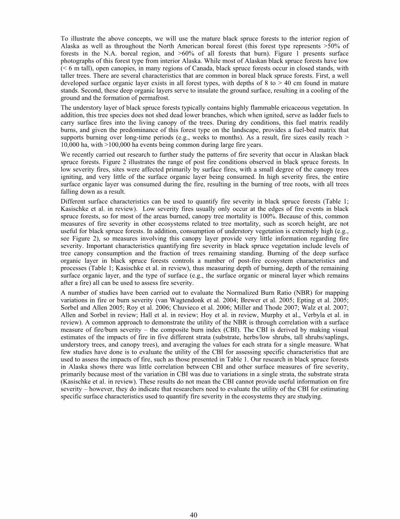
40

To illustrate the above concepts, we will use the mature black spruce forests to the interior region of Alaska as well as throughout the North American boreal forest (this forest type represents >50% of forests in the N.A. boreal region, and >60% of all forests that burn). Figure 1 presents surface photographs of this forest type from interior Alaska. While most of Alaskan black spruce forests have low (< 6 m tall), open canopies, in many regions of Canada, black spruce forests occur in closed stands, with taller trees. There are several characteristics that are common in boreal black spruce forests. First, a well developed surface organic layer exists in all forest types, with depths of 8 to > 40 cm found in mature stands. Second, these deep organic layers serve to insulate the ground surface, resulting in a cooling of the ground and the formation of permafrost. The understory layer of black spruce forests typically contains highly flammable ericaceous vegetation. In addition, this tree species does not shed dead lower branches, which when ignited, serve as ladder fuels to carry surface fires into the living canopy of the trees. During dry conditions, this fuel matrix readily burns, and given the predominance of this forest type on the landscape, provides a fuel-bed matrix that supports burning over long-time periods (e.g., weeks to months). As a result, fire sizes easily reach > 10,000 ha, with >100,000 ha events being common during large fire years. We recently carried out research to further study the patterns of fire severity that occur in Alaskan black spruce forests. Figure 2 illustrates the range of post fire conditions observed in black spruce forests. In low severity fires, sites were affected primarily by surface fires, with a small degree of the canopy trees igniting, and very little of the surface organic layer being consumed. In high severity fires, the entire surface organic layer was consumed during the fire, resulting in the burning of tree roots, with all trees falling down as a result. Different surface characteristics can be used to quantify fire severity in black spruce forests (Table 1; Kasischke et al. in review). Low severity fires usually only occur at the edges of fire events in black spruce forests, so for most of the areas burned, canopy tree mortality is 100%. Because of this, common measures of fire severity in other ecosystems related to tree mortality, such as scorch height, are not useful for black spruce forests. In addition, consumption of understory vegetation is extremely high (e.g., see Figure 2), so measures involving this canopy layer provide very little information regarding fire severity. Important characteristics quantifying fire severity in black spruce vegetation include levels of tree canopy consumption and the fraction of trees remaining standing. Burning of the deep surface organic layer in black spruce forests controls a number of post-fire ecosystem characteristics and processes (Table 1; Kasischke et al. in review), thus measuring depth of burning, depth of the remaining surface organic layer, and the type of surface (e.g., the surface organic or mineral layer which remains after a fire) all can be used to assess fire severity. A number of studies have been carried out to evaluate the Normalized Burn Ratio (NBR) for mapping variations in fire or burn severity (van Wagtendonk et al. 2004; Brewer et al. 2005; Epting et al. 2005; Sorbel and Allen 2005; Roy et al. 2006; Chuvieco et al. 2006; Miller and Thode 2007; Walz et al. 2007; Allen and Sorbel in review; Hall et al. in review; Hoy et al. in review, Murphy et al., Verbyla et al. in review). A common approach to demonstrate the utility of the NBR is through correlation with a surface measure of fire/burn severity – the composite burn index (CBI). The CBI is derived by making visual estimates of the impacts of fire in five different strata (substrate, herbs/low shrubs, tall shrubs/saplings, understory trees, and canopy trees), and averaging the values for each strata for a single measure. What few studies have done is to evaluate the utility of the CBI for assessing specific characteristics that are used to assess the impacts of fire, such as those presented in Table 1. Our research in black spruce forests in Alaska shows there was little correlation between CBI and other surface measures of fire severity, primarily because most of the variation in CBI was due to variations in a single strata, the substrate strata (Kasischke et al. in review). These results do not mean the CBI cannot provide useful information on fire severity – however, they do indicate that researchers need to evaluate the utility of the CBI for estimating specific surface characteristics used to quantify fire severity in the ecosystems they are studying.

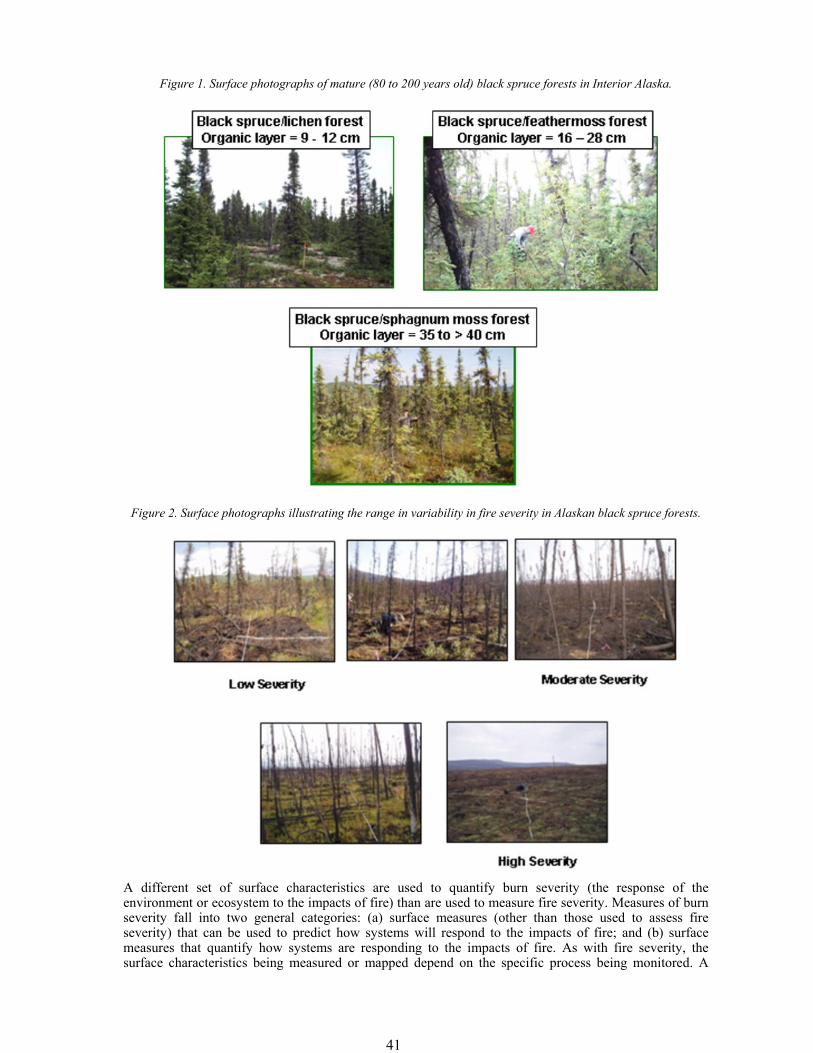
41

Figure 1. Surface photographs of mature (80 to 200 years old) black spruce forests in Interior Alaska.

Figure 2. Surface photographs illustrating the range in variability in fire severity in Alaskan black spruce forests.

A different set of surface characteristics are used to quantify burn severity (the response of the environment or ecosystem to the impacts of fire) than are used to measure fire severity. Measures of burn severity fall into two general categories: (a) surface measures (other than those used to assess fire severity) that can be used to predict how systems will respond to the impacts of fire; and (b) surface measures that quantify how systems are responding to the impacts of fire. As with fire severity, the surface characteristics being measured or mapped depend on the specific process being monitored. A

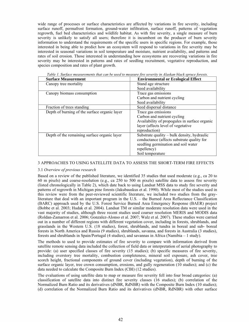
42

wide range of processes or surface characteristics are affected by variations in fire severity, including surface runoff, permafrost formation, ground-water infiltration, surface runoff, patterns of vegetation regrowth, fuel bed characteristics and wildlife habitat. As with fire severity, a single measure of burn severity is unlikely to satisfy all users; therefore it is incumbent on the producer of burn severity information to understand the requirements of the specific users in specific regions. For example, those interested in being able to predict how an ecosystem will respond to variations in fire severity may be interested in seasonal variations in soil temperature and moisture, nutrient availability, and patterns and rates of soil erosion. Those interested in understanding how ecosystems are recovering variations in fire severity may be interested in patterns and rates of seedling recruitment, vegetative reproduction, and species composition and rates of plant growth.

Table 1. Surface measurements that can be used to measure fire severity in Alaskan black spruce forests. Surface Measurement Environmental or Ecological Effect Canopy tree mortality Stand age structure

Seed availability Canopy biomass consumption Trace gas emissions

Carbon and nutrient cycling Seed availability

Fraction of trees standing Seed dispersal distance Depth of burning of the surface organic layer Trace gas emissions

Carbon and nutrient cycling Availability of propogules in surface organic layer (affects level of vegetative reproduction)

Depth of the remaining surface organic layer Substrate quality – bulk density, hydraulic conductance (affects substrate quality for seedling germination and soil water repellency) Soil temperature

3 APPROACHES TO USING SATELLITE DATA TO ASSESS THE SHORT-TERM FIRE EFFECTS 3.1 Overview of previous research Based on a review of the published literature, we identified 35 studies that used moderate (e.g., ca 20 to 60 m pixels) and coarse-resolution (e.g., ca 250 to 500 m pixels) satellite data to assess fire severity (listed chronologically in Table 2), which date back to using Landsat MSS data to study fire severity and patterns of regrowth in Michigan pine forests (Jakubauskus et al. 1990). While most of the studies used in this review were from the peer-reviewed scientific literature, we included two studies from the gray-literature that deal with an important program in the U.S. – the Burned Area Reflectance Classification (BARC) approach used by the U.S. Forest Service Burned Area Emergency Response (BAER) project (Bobbe et al. 2003; Hudak et al. 2004). Landsat TM or similar moderate resolution data were used in the vast majority of studies, although three recent studies used coarser resolution MERIS and MODIS data (Roldan-Zamarron et al. 2006; Gonzalez-Alonso et al. 2007; Walz et al. 2007). These studies were carried out in a number of different regions with different vegetation cover, including in forests, shrublands, and grasslands in the Western U.S. (18 studies), forest, shrublands, and tundra in boreal and sub- boreal forests in North America and Russia (9 studies), shrublands, savanna, and forests in Australia (3 studies), forests and shrublands in Spain/Portugal (4 studies), and savannas in Africa (Namibia – 1 study). The methods to used to provide estimates of fire severity to compare with information derived from satellite remote sensing data included the collection of field data or interpretation of aerial photography to provide: (a) user specified classes of fire severity (15 studies); (b) specific measures of fire severity, including overstory tree mortality, combustion completeness, mineral soil exposure, ash cover, tree scorch height, fractional components of ground cover (including vegetation), depth of burning of the surface organic layer, tree crown consumption, erosions, and gully regeneration (10 studies); and (c) the data needed to calculate the Composite Burn Index (CBI) (12 studies). The evaluations of using satellite data to map or measure fire severity fell into four broad categories: (a) classification of satellite data into distinct fire severity classes (16 studies); (b) correlation of the Normalized Burn Ratio and its derivatives (dNBR, RdNBR) with the Composite Burn Index (10 studies); (d) correlation of the Normalized Burn Ratio and its derivatives (dNBR, RdNBR) with other surface

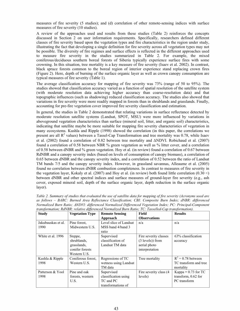
43

measures of fire severity (5 studies); and (d) correlation of other remote-sensing indices with surface measures of fire severity (10 studies). A review of the approaches used and results from these studies (Table 2) reinforces the concepts discussed in Section 2 on user information requirements. Specifically, researchers defined different classes of fire severity based upon the vegetation types and fire characteristics in the region under study, illustrating the fact that developing a single definition for fire severity across all vegetation types may not be possible. The diversity of fire regimes and surface effects is reflected in the different approaches used to measure fire severity in the studies summarized in Table 2. For example, the mixed coniferous/deciduous southern boreal forests of Siberia typically experience surface fires with some crowning. In this situation, tree mortality is a key measure of fire severity (Isaev et al. 2002). In contrast, black spruce forests common to the boreal region of interior experience stand replacing crown fires (Figure 2). Here, depth of burning of the surface organic layer as well as crown canopy consumption are typical measures of fire severity (Table 1). The average classification accuracy for mapping of fire severity was 73% (range of 50 to 95%). The studies showed that classification accuracy varied as a function of spatial resolution of the satellite system (with moderate resolution data achieving higher accuracy than coarse-resolution data) and that topographic influences (such as shadowing) reduced classification accuracy. The studies also showed that variations in fire severity were more readily mapped in forests than in shrublands and grasslands. Finally, accounting for pre-fire vegetation cover improved fire severity classification and estimation. In general, the studies in Table 2 demonstrated that relating variations in surface reflectance detected by moderate resolution satellite systems (Landsat, SPOT, MSU) were more influenced by variations in aboveground vegetation characteristics than surface (mineral soil, litter, and organic soil) characteristics, indicating that satellite maybe be more suitable for mapping fire severity characteristics of vegetation in many ecosystems. Kushla and Ripple (1998) showed the correlation (in this paper, the correlations we present are all R2 values) between a Tassel-Cap Transformation and tree mortality was 0.78, while Isaev et al. (2002) found a correlation of 0.82 between tree mortality and ΔNDVI. Robichaud et al. (2007) found a correlation of 0.58 between NBR % green vegetation as well as % litter cover, and a correlation of 0.58 between dNBR and % green vegetation. Hoy et al. (in review) found a correlation of 0.67 between RdNBR and a canopy severity index (based on levels of consumption of canopy biomass), a correlation of 0.65 between dNBR and the canopy severity index, and a correlation of 0.52 between the ratio of Landsat TM bands 7/5 and the canopy severity index. However, in grassland savannas, Alleaume et al. (2005) found no correlation between dNBR combustion completeness. In contrast to measures of fire severity in the vegetation layer, Kokaly et al. (2007) and Hoy et al. (in review) both found little correlation (0.30 <) between dNBR and other spectral indices and surface measures of ground-layer fire severity (e.g., ash cover, exposed mineral soil, depth of the surface organic layer, depth reduction in the surface organic layer).

Table 2. Summary of studies that evaluated the use of satellite data for mapping of fire severity (Acronyms used are as follows – BARC: Burned Area Reflectance Classification; CBI: Composite Burn Index; dNBR: differenced Normalized Burn Ratio; ΔNDVI: differenced Normalized Differenced Vegetation Index; PC: Principal-Component transformation; RdNBR: relative differenced Normalized Burn Ratio; TC: Tasselled-Cap transformation). Study Vegetation Type Remote Sensing

Approach Field Observations

Results

Jakubauskas et al. 1990

Pine forest, Midwestern U.S.

Level slice of Landsat MSS band 4/band 3 ratio

n/a n/a

White et al. 1996 Steppe, shrublands, grasslands, conifer forests Western U.S.

Supervised classification of Landsat TM data

Fire severity classes (3 levels)) from aerial photo interpretation

63% classification accuracy

Kushla & Ripple 1998

Coniferous forest, Western U.S.

Regressions of TC

wetness using Landsat TM data

Tree mortality R2 = 0.78 between TC transform and tree mortality

Patterson & Yool 1998

Pine and oak forests, western U.S.

Supervised classification using TC and PC transformations of

Fire severity class (4 levels)

Kappa = 0.73 for TC transform, 0.62 for PC transform

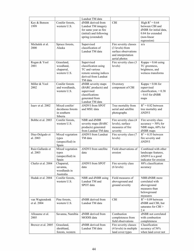
44

Landsat TM data Key & Benson 1999

Conifer forests, western U.S.

dNBR derived from Landsat TM imagery for same year as fire (initial) and following spring (extended)

CBI High R2 = 0.64 between CBI and dNBR for initial data, 0.84 for extended (non-linear regression)

Michalek et al. 2000

Spruce forests, Alaska

Supervised classification of Landsat TM data

Fire severity classes (3 levels) from surface observations and interpretation aerial photos

n/a

Rogan & Yool 2001

Grassland, woodland, chaparral, western U.S.

Supervised classification using TC and various remote sensing indices derived from Landsat TM data


Kappa = 0.66 using TC greenness, brightness, and wetness transforms

Miller & Yool 2002

Conifer forests and woodlands, western U.S.

dNBR severity maps (BARC products) and supervised classifications generated from Landsat TM data

Overstory component of CBI

Kappa = 0.86 for supervised classification, = 0.38 – 0.63 for dNBR maps

Isaev et al. 2002 Mixed conifer/ deciduous forests in southern Siberia

ΔNDVI from SPOT and MSU data

Tree mortality from aerial and satellite photographs

R2 = 0.82 between tree mortality and ΔNDVI

Bobbe et al. 2003 Conifer forests, western U.S.

NBR and dNBR severity maps (BARC products) generated from Landsat TM data

Fire severity class (4 levels), surface measures of fire severity

Fire severity class accuracy = 50% for NBR maps, 60% for dNBR maps

Diaz-Delgado et al. 2003

Mixed vegetation types (unspecified) in Spain

ΔNDVI from Landsat TM data


R2 = 0.55 between fire severity and ΔNDVI

Ruiz-Gallardo et al. 2003

Mixed vegetation types (unspecified) in Spain

ΔNDVI from satellite data

Field observations of erosion

Combined with other landscape features, ΔNDVI is a good indicator for erosion

Chafer et al. 2004 Chaparral, savanna, woodlands in Australia

ΔNDVI from SPOT data


88% classification accuracy

Hudak et al. 2004 Conifer forests, western U.S.

NBR and dNBR using Landsat TM and SPOT data

Field measures of aboveground and ground severity

NBR/dNBR more correlated with aboveground measures than belowground measures

van Wagtendonk et al. 2004

Pine forests, western U.S.

dNBR derived from Landsat TM data

CBI R2 = 0.89 between dNBR and CBI, but saturates for CBI > 2.4

Alleaume et al. 2005

Savanna, Namibia dNBR derived from MODIS data

Combustion completeness from field observations

dNBR not correlated with combustion completeness

Brewer et al. 2005 Grassland, shrubland, forests, western


Fire severity classes (4 levels) in multiple land cover types

Classification accuracy of 56% when land cover not

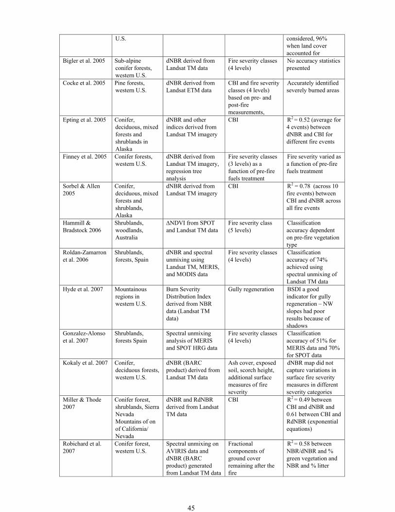
45

U.S. considered, 96% when land cover accounted for

Bigler et al. 2005 Sub-alpine conifer forests, western U.S.


Fire severity classes (4 levels)

No accuracy statistics presented

Cocke et al. 2005 Pine forests, western U.S.

dNBR derived from Landsat ETM data

CBI and fire severity classes (4 levels) based on pre- and post-fire measurements,

Accurately identified severely burned areas

Epting et al. 2005 Conifer, deciduous, mixed forests and shrublands in Alaska

dNBR and other indices derived from Landsat TM imagery

CBI R2 = 0.52 (average for 4 events) between dNBR and CBI for different fire events

Finney et al. 2005 Conifer forests, western U.S.

dNBR derived from Landsat TM imagery, regression tree analysis

Fire severity classes (3 levels) as a function of pre-fire fuels treatment

Fire severity varied as a function of pre-fire fuels treatment

Sorbel & Allen 2005

Conifer, deciduous, mixed forests and shrublands, Alaska

dNBR derived from Landsat TM imagery

CBI R2 = 0.78 (across 10 fire events) between CBI and dNBR across all fire events

Hammill & Bradstock 2006

Shrublands, woodlands, Australia

ΔNDVI from SPOT and Landsat TM data


Classification accuracy dependent on pre-fire vegetation type

Roldan-Zamarron et al. 2006

Shrublands, forests, Spain

dNBR and spectral unmixing using Landsat TM, MERIS, and MODIS data


Classification accuracy of 74% achieved using spectral unmixing of Landsat TM data

Hyde et al. 2007 Mountainous regions in western U.S.

Burn Severity Distribution Index derived from NBR data (Landsat TM data)

Gully regeneration BSDI a good indicator for gully regeneration – NW slopes had poor results because of shadows

Gonzalez-Alonso et al. 2007

Shrublands, forests Spain

Spectral unmixing analysis of MERIS and SPOT HRG data


Classification accuracy of 51% for MERIS data and 70% for SPOT data

Kokaly et al. 2007 Conifer, deciduous forests, western U.S.

dNBR (BARC product) derived from Landsat TM data

Ash cover, exposed soil, scorch height, additional surface measures of fire severity

dNBR map did not capture variations in surface fire severity measures in different severity categories

Miller & Thode 2007

Conifer forest, shrublands, Sierra Nevada Mountains of on of California/ Nevada

dNBR and RdNBR derived from Landsat TM data

CBI R2 = 0.49 between CBI and dNBR and 0.61 between CBI and RdNBR (exponential equations)

Robichard et al. 2007

Conifer forest, western U.S.

Spectral unmixing on AVIRIS data and dNBR (BARC product) generated from Landsat TM data

Fractional components of ground cover remaining after the fire

R2 = 0.58 between NBR/dNBR and % green vegetation and NBR and % litter

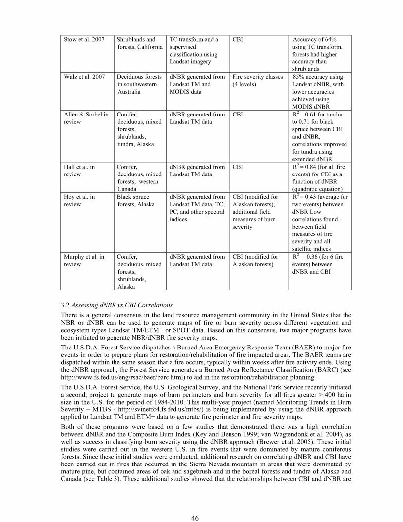
46

Stow et al. 2007 Shrublands and forests, California

TC transform and a supervised classification using Landsat imagery

CBI Accuracy of 64% using TC transform, forests had higher accuracy than shrublands

Walz et al. 2007 Deciduous forests in southwestern Australia

dNBR generated from Landsat TM and MODIS data


85% accuracy using Landsat dNBR, with lower accuracies achieved using MODIS dNBR

Allen & Sorbel in review

Conifer, deciduous, mixed forests, shrublands, tundra, Alaska

dNBR generated from Landsat TM data

CBI R2 = 0.61 for tundra to 0.71 for black spruce between CBI and dNBR, correlations improved for tundra using extended dNBR

Hall et al. in review

Conifer, deciduous, mixed forests, western Canada


CBI R2 = 0.84 (for all fire events) for CBI as a function of dNBR (quadratic equation)

Hoy et al. in review

Black spruce forests, Alaska

dNBR generated from Landsat TM data, TC, PC, and other spectral indices

CBI (modified for Alaskan forests), additional field measures of burn severity

R2 = 0.43 (average for two events) between dNBR Low correlations found between field measures of fire severity and all satellite indices

Murphy et al. in review

Conifer, deciduous, mixed forests, shrublands, Alaska


CBI (modified for Alaskan forests)

R2 = 0.36 (for 6 fire events) between dNBR and CBI

3.2 Assessing dNBR vs.CBI Correlations There is a general consensus in the land resource management community in the United States that the NBR or dNBR can be used to generate maps of fire or burn severity across different vegetation and ecosystem types Landsat TM/ETM+ or SPOT data. Based on this consensus, two major programs have been initiated to generate NBR/dNBR fire severity maps. The U.S.D.A. Forest Service dispatches a Burned Area Emergency Response Team (BAER) to major fire events in order to prepare plans for restoration/rehabilitation of fire impacted areas. The BAER teams are dispatched within the same season that a fire occurs, typically within weeks after fire activity ends. Using the dNBR approach, the Forest Service generates a Burned Area Reflectance Classification (BARC) (see http://www.fs.fed.us/eng/rsac/baer/barc.html) to aid in the restoration/rehabilitation planning. The U.S.D.A. Forest Service, the U.S. Geological Survey, and the National Park Service recently initiated a second, project to generate maps of burn perimeters and burn severity for all fires greater > 400 ha in size in the U.S. for the period of 1984-2010. This multi-year project (named Monitoring Trends in Burn Severity – MTBS - http://svinetfc4.fs.fed.us/mtbs/) is being implemented by using the dNBR approach applied to Landsat TM and ETM+ data to generate fire perimeter and fire severity maps. Both of these programs were based on a few studies that demonstrated there was a high correlation between dNBR and the Composite Burn Index (Key and Benson 1999; van Wagtendonk et al. 2004), as well as success in classifying burn severity using the dNBR approach (Brewer et al. 2005). These initial studies were carried out in the western U.S. in fire events that were dominated by mature coniferous forests. Since these initial studies were conducted, additional research on correlating dNBR and CBI have been carried out in fires that occurred in the Sierra Nevada mountain in areas that were dominated by mature pine, but contained areas of oak and sagebrush and in the boreal forests and tundra of Alaska and Canada (see Table 3). These additional studies showed that the relationships between CBI and dNBR are

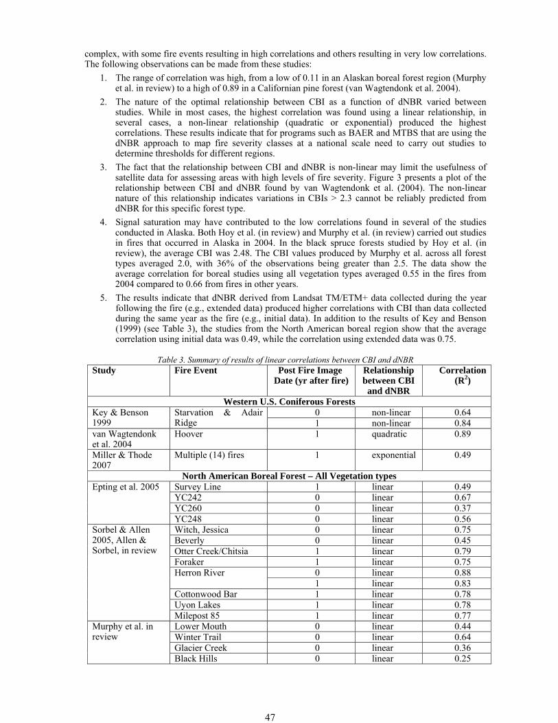
47

complex, with some fire events resulting in high correlations and others resulting in very low correlations. The following observations can be made from these studies:

1. The range of correlation was high, from a low of 0.11 in an Alaskan boreal forest region (Murphy et al. in review) to a high of 0.89 in a Californian pine forest (van Wagtendonk et al. 2004).

2. The nature of the optimal relationship between CBI as a function of dNBR varied between studies. While in most cases, the highest correlation was found using a linear relationship, in several cases, a non-linear relationship (quadratic or exponential) produced the highest correlations. These results indicate that for programs such as BAER and MTBS that are using the dNBR approach to map fire severity classes at a national scale need to carry out studies to determine thresholds for different regions.

3. The fact that the relationship between CBI and dNBR is non-linear may limit the usefulness of satellite data for assessing areas with high levels of fire severity. Figure 3 presents a plot of the relationship between CBI and dNBR found by van Wagtendonk et al. (2004). The non-linear nature of this relationship indicates variations in CBIs > 2.3 cannot be reliably predicted from dNBR for this specific forest type.

4. Signal saturation may have contributed to the low correlations found in several of the studies conducted in Alaska. Both Hoy et al. (in review) and Murphy et al. (in review) carried out studies in fires that occurred in Alaska in 2004. In the black spruce forests studied by Hoy et al. (in review), the average CBI was 2.48. The CBI values produced by Murphy et al. across all forest types averaged 2.0, with 36% of the observations being greater than 2.5. The data show the average correlation for boreal studies using all vegetation types averaged 0.55 in the fires from 2004 compared to 0.66 from fires in other years.

5. The results indicate that dNBR derived from Landsat TM/ETM+ data collected during the year following the fire (e.g., extended data) produced higher correlations with CBI than data collected during the same year as the fire (e.g., initial data). In addition to the results of Key and Benson (1999) (see Table 3), the studies from the North American boreal region show that the average correlation using initial data was 0.49, while the correlation using extended data was 0.75.

Table 3. Summary of results of linear correlations between CBI and dNBR Study Fire Event Post Fire Image

Date (yr after fire) Relationship between CBI

and dNBR

Correlation(R2)

Western U.S. Coniferous Forests 0 non-linear 0.64 Key & Benson

1999 Starvation & Adair Ridge 1 non-linear 0.84

van Wagtendonk et al. 2004

Hoover 1 quadratic 0.89

Miller & Thode 2007

Multiple (14) fires 1 exponential 0.49

North American Boreal Forest – All Vegetation types Survey Line 1 linear 0.49 YC242 0 linear 0.67 YC260 0 linear 0.37

Epting et al. 2005

YC248 0 linear 0.56 Witch, Jessica 0 linear 0.75 Beverly 0 linear 0.45 Otter Creek/Chitsia 1 linear 0.79 Foraker 1 linear 0.75

0 linear 0.88 Herron River 1 linear 0.83

Cottonwood Bar 1 linear 0.78 Uyon Lakes 1 linear 0.78

Sorbel & Allen 2005, Allen & Sorbel, in review

Milepost 85 1 linear 0.77 Lower Mouth 0 linear 0.44 Winter Trail 0 linear 0.64 Glacier Creek 0 linear 0.36

Murphy et al. in review

Black Hills 0 linear 0.25

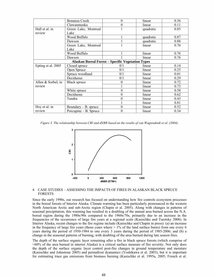
48

Bonanza Creek 0 linear 0.36 Clawanmenka 0 linear 0.11 Green Lake, Montreal Lake

1 quadratic 0.85

Wood Buffalo 1 quadratic 0.87 Dawson 1 quadratic 0.88 Green Lake, Montreal Lake

1 linear 0.76

Wood Buffalo 1 linear 0.76

Hall et al. in review

Dawson 1 linear 0.76 Alaskan Boreal Forest – Specific Vegetation Types

Closed spruce 0/1 linear 0.14 Open Spruce 0/1 linear 0.25 Spruce woodland 0/1 linear 0.01

Epting et al. 2005

Deciduous 0/1 linear 0.29 0 linear 0.72 Black spruce 1 linear 0.73

White spruce 0 linear 0.58 Deciduous 0 linear 0.62

0 linear 0.43

Allen & Sorbel, in review

Tundra 1 linear 0.81

Boundary – B. spruce 0 linear 0.52 Hoy et al. in review Porcupine – B. Spruce 0 linear 0.34

Figure 3. The relationship between CBI and dNBR based on the results of van Wagtendonk et al. (2004).

4 CASE STUDIES – ASSESSING THE IMPACTS OF FIRES IN ALASKAN BLACK SPRUCE FORESTS

Since the early 1990s, our research has focused on understanding how fire controls ecosystem processes in the boreal forests of Interior Alaska. Climate warming has been particularly pronounced in the western North American Arctic and sub-Arctic region (Chapin et al. 2005). Along with changes in patterns of seasonal precipitation, this warming has resulted in a doubling of the annual area burned across the N.A. boreal region during the 1980s/90s compared to the 1960s/70s, primarily due to an increase in the frequencies of the occurrence of large fire years at a regional scale (Kasischke and Turetsky 2006). In Interior Alaska, recent changes to the fire regime include (Kasischke and Chapin in press): (a) an increase in the frequency of large fire years (those years where > 1% of the land surface burns) from one every 6 years during the period of 1950-1984 to one every 3 years during the period of 1985-2006; and (b) a change in the seasonal patterns of burning, with doubling of the area burned during late season fires. The depth of the surface organic layer remaining after a fire in black spruce forests (which comprise of >60% of the area burned in interior Alaska) is a critical surface measure of fire severity. Not only does the depth of the surface organic layer control post-fire changes in ground temperature and moisture (Kasischke and Johnstone 2005) and permafrost dyanamics (Yoshikawa et al. 2003), but it is important for estimating trace gas emissions from biomass burning (Kasischke et al. 1995a, 2005; French et al.

0

1

2

3

-300 0 300 600 900 1200dNBR (ETM+)

CB

I

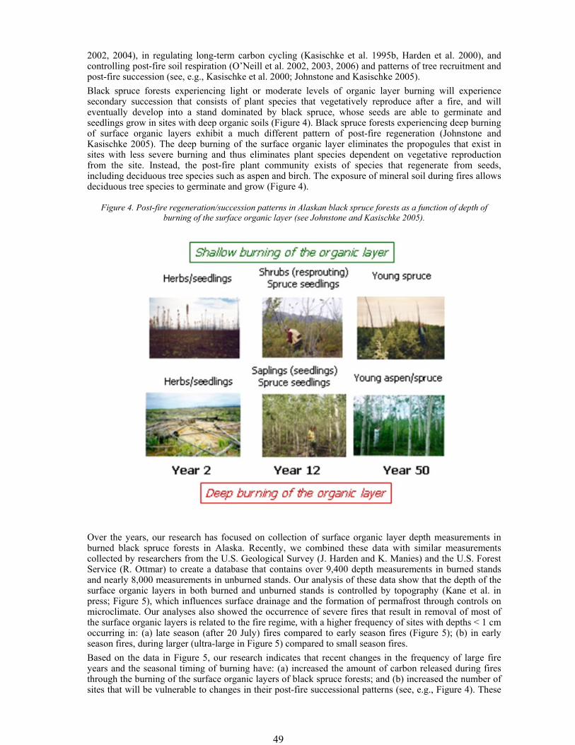
49

2002, 2004), in regulating long-term carbon cycling (Kasischke et al. 1995b, Harden et al. 2000), and controlling post-fire soil respiration (O’Neill et al. 2002, 2003, 2006) and patterns of tree recruitment and post-fire succession (see, e.g., Kasischke et al. 2000; Johnstone and Kasischke 2005). Black spruce forests experiencing light or moderate levels of organic layer burning will experience secondary succession that consists of plant species that vegetatively reproduce after a fire, and will eventually develop into a stand dominated by black spruce, whose seeds are able to germinate and seedlings grow in sites with deep organic soils (Figure 4). Black spruce forests experiencing deep burning of surface organic layers exhibit a much different pattern of post-fire regeneration (Johnstone and Kasischke 2005). The deep burning of the surface organic layer eliminates the propogules that exist in sites with less severe burning and thus eliminates plant species dependent on vegetative reproduction from the site. Instead, the post-fire plant community exists of species that regenerate from seeds, including deciduous tree species such as aspen and birch. The exposure of mineral soil during fires allows deciduous tree species to germinate and grow (Figure 4).

Figure 4. Post-fire regeneration/succession patterns in Alaskan black spruce forests as a function of depth of burning of the surface organic layer (see Johnstone and Kasischke 2005).

Over the years, our research has focused on collection of surface organic layer depth measurements in burned black spruce forests in Alaska. Recently, we combined these data with similar measurements collected by researchers from the U.S. Geological Survey (J. Harden and K. Manies) and the U.S. Forest Service (R. Ottmar) to create a database that contains over 9,400 depth measurements in burned stands and nearly 8,000 measurements in unburned stands. Our analysis of these data show that the depth of the surface organic layers in both burned and unburned stands is controlled by topography (Kane et al. in press; Figure 5), which influences surface drainage and the formation of permafrost through controls on microclimate. Our analyses also showed the occurrence of severe fires that result in removal of most of the surface organic layers is related to the fire regime, with a higher frequency of sites with depths < 1 cm occurring in: (a) late season (after 20 July) fires compared to early season fires (Figure 5); (b) in early season fires, during larger (ultra-large in Figure 5) compared to small season fires. Based on the data in Figure 5, our research indicates that recent changes in the frequency of large fire years and the seasonal timing of burning have: (a) increased the amount of carbon released during fires through the burning of the surface organic layers of black spruce forests; and (b) increased the number of sites that will be vulnerable to changes in their post-fire successional patterns (see, e.g., Figure 4). These

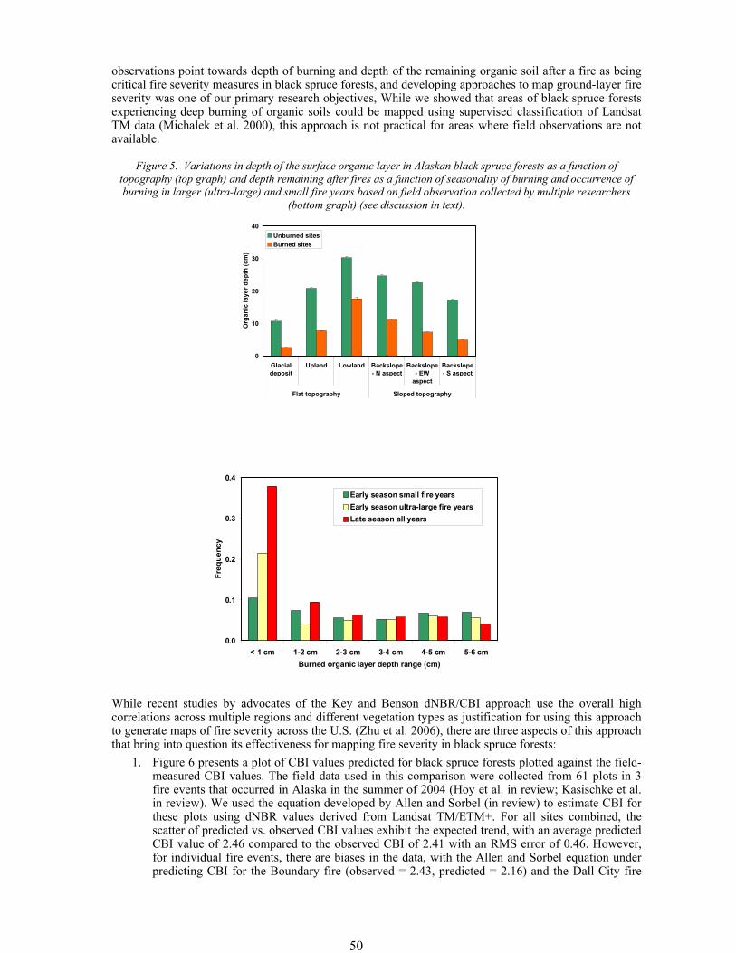
50

observations point towards depth of burning and depth of the remaining organic soil after a fire as being critical fire severity measures in black spruce forests, and developing approaches to map ground-layer fire severity was one of our primary research objectives, While we showed that areas of black spruce forests experiencing deep burning of organic soils could be mapped using supervised classification of Landsat TM data (Michalek et al. 2000), this approach is not practical for areas where field observations are not available.

Figure 5. Variations in depth of the surface organic layer in Alaskan black spruce forests as a function of topography (top graph) and depth remaining after fires as a function of seasonality of burning and occurrence of burning in larger (ultra-large) and small fire years based on field observation collected by multiple researchers

(bottom graph) (see discussion in text).

While recent studies by advocates of the Key and Benson dNBR/CBI approach use the overall high correlations across multiple regions and different vegetation types as justification for using this approach to generate maps of fire severity across the U.S. (Zhu et al. 2006), there are three aspects of this approach that bring into question its effectiveness for mapping fire severity in black spruce forests:

1. Figure 6 presents a plot of CBI values predicted for black spruce forests plotted against the field-measured CBI values. The field data used in this comparison were collected from 61 plots in 3 fire events that occurred in Alaska in the summer of 2004 (Hoy et al. in review; Kasischke et al. in review). We used the equation developed by Allen and Sorbel (in review) to estimate CBI for these plots using dNBR values derived from Landsat TM/ETM+. For all sites combined, the scatter of predicted vs. observed CBI values exhibit the expected trend, with an average predicted CBI value of 2.46 compared to the observed CBI of 2.41 with an RMS error of 0.46. However, for individual fire events, there are biases in the data, with the Allen and Sorbel equation under predicting CBI for the Boundary fire (observed = 2.43, predicted = 2.16) and the Dall City fire

0

10

20

30

40

Glacialdeposit

Upland Lowland Backslope- N aspect

Backslope- EW

aspect

Backslope- S aspect

Flat topography Sloped topography

Org

anic

laye

r dep

th (c

m)

Unburned sitesBurned sites

0.0

0.1

0.2

0.3

0.4

< 1 cm 1-2 cm 2-3 cm 3-4 cm 4-5 cm 5-6 cmBurned organic layer depth range (cm)

Freq

uenc

y

Early season small fire yearsEarly season ultra-large fire yearsLate season all years

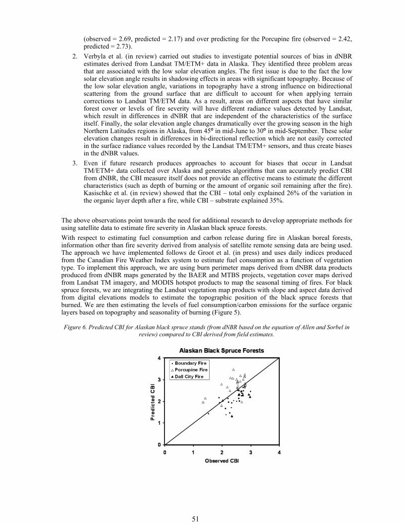
51

(observed = 2.69, predicted = 2.17) and over predicting for the Porcupine fire (observed = 2.42, predicted = 2.73).

2. Verbyla et al. (in review) carried out studies to investigate potential sources of bias in dNBR estimates derived from Landsat TM/ETM+ data in Alaska. They identified three problem areas that are associated with the low solar elevation angles. The first issue is due to the fact the low solar elevation angle results in shadowing effects in areas with significant topography. Because of the low solar elevation angle, variations in topography have a strong influence on bidirectional scattering from the ground surface that are difficult to account for when applying terrain corrections to Landsat TM/ETM data. As a result, areas on different aspects that have similar forest cover or levels of fire severity will have different radiance values detected by Landsat, which result in differences in dNBR that are independent of the characteristics of the surface itself. Finally, the solar elevation angle changes dramatically over the growing season in the high Northern Latitudes regions in Alaska, from 45º in mid-June to 30º in mid-September. These solar elevation changes result in differences in bi-directional reflection which are not easily corrected in the surface radiance values recorded by the Landsat TM/ETM+ sensors, and thus create biases in the dNBR values.

3. Even if future research produces approaches to account for biases that occur in Landsat TM/ETM+ data collected over Alaska and generates algorithms that can accurately predict CBI from dNBR, the CBI measure itself does not provide an effective means to estimate the different characteristics (such as depth of burning or the amount of organic soil remaining after the fire). Kasischke et al. (in review) showed that the CBI – total only explained 26% of the variation in the organic layer depth after a fire, while CBI – substrate explained 35%.

The above observations point towards the need for additional research to develop appropriate methods for using satellite data to estimate fire severity in Alaskan black spruce forests. With respect to estimating fuel consumption and carbon release during fire in Alaskan boreal forests, information other than fire severity derived from analysis of satellite remote sensing data are being used. The approach we have implemented follows de Groot et al. (in press) and uses daily indices produced from the Canadian Fire Weather Index system to estimate fuel consumption as a function of vegetation type. To implement this approach, we are using burn perimeter maps derived from dNBR data products produced from dNBR maps generated by the BAER and MTBS projects, vegetation cover maps derived from Landsat TM imagery, and MODIS hotspot products to map the seasonal timing of fires. For black spruce forests, we are integrating the Landsat vegetation map products with slope and aspect data derived from digital elevations models to estimate the topographic position of the black spruce forests that burned. We are then estimating the levels of fuel consumption/carbon emissions for the surface organic layers based on topography and seasonality of burning (Figure 5).

Figure 6. Predicted CBI for Alaskan black spruce stands (from dNBR based on the equation of Allen and Sorbel in review) compared to CBI derived from field estimates.

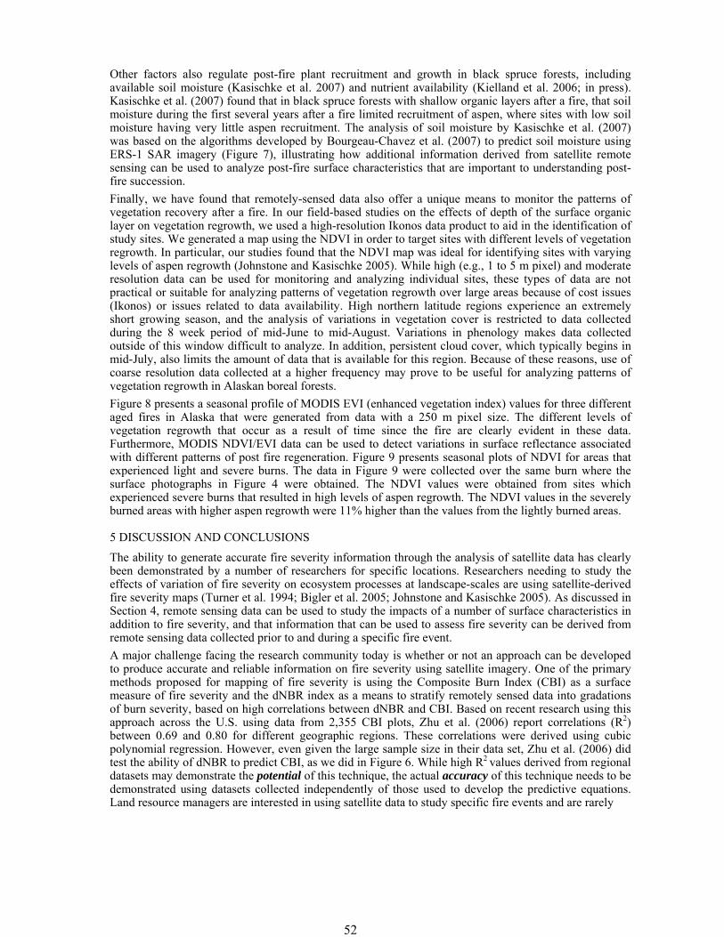
52

Other factors also regulate post-fire plant recruitment and growth in black spruce forests, including available soil moisture (Kasischke et al. 2007) and nutrient availability (Kielland et al. 2006; in press). Kasischke et al. (2007) found that in black spruce forests with shallow organic layers after a fire, that soil moisture during the first several years after a fire limited recruitment of aspen, where sites with low soil moisture having very little aspen recruitment. The analysis of soil moisture by Kasischke et al. (2007) was based on the algorithms developed by Bourgeau-Chavez et al. (2007) to predict soil moisture using ERS-1 SAR imagery (Figure 7), illustrating how additional information derived from satellite remote sensing can be used to analyze post-fire surface characteristics that are important to understanding post-fire succession. Finally, we have found that remotely-sensed data also offer a unique means to monitor the patterns of vegetation recovery after a fire. In our field-based studies on the effects of depth of the surface organic layer on vegetation regrowth, we used a high-resolution Ikonos data product to aid in the identification of study sites. We generated a map using the NDVI in order to target sites with different levels of vegetation regrowth. In particular, our studies found that the NDVI map was ideal for identifying sites with varying levels of aspen regrowth (Johnstone and Kasischke 2005). While high (e.g., 1 to 5 m pixel) and moderate resolution data can be used for monitoring and analyzing individual sites, these types of data are not practical or suitable for analyzing patterns of vegetation regrowth over large areas because of cost issues (Ikonos) or issues related to data availability. High northern latitude regions experience an extremely short growing season, and the analysis of variations in vegetation cover is restricted to data collected during the 8 week period of mid-June to mid-August. Variations in phenology makes data collected outside of this window difficult to analyze. In addition, persistent cloud cover, which typically begins in mid-July, also limits the amount of data that is available for this region. Because of these reasons, use of coarse resolution data collected at a higher frequency may prove to be useful for analyzing patterns of vegetation regrowth in Alaskan boreal forests. Figure 8 presents a seasonal profile of MODIS EVI (enhanced vegetation index) values for three different aged fires in Alaska that were generated from data with a 250 m pixel size. The different levels of vegetation regrowth that occur as a result of time since the fire are clearly evident in these data. Furthermore, MODIS NDVI/EVI data can be used to detect variations in surface reflectance associated with different patterns of post fire regeneration. Figure 9 presents seasonal plots of NDVI for areas that experienced light and severe burns. The data in Figure 9 were collected over the same burn where the surface photographs in Figure 4 were obtained. The NDVI values were obtained from sites which experienced severe burns that resulted in high levels of aspen regrowth. The NDVI values in the severely burned areas with higher aspen regrowth were 11% higher than the values from the lightly burned areas.

5 DISCUSSION AND CONCLUSIONS

The ability to generate accurate fire severity information through the analysis of satellite data has clearly been demonstrated by a number of researchers for specific locations. Researchers needing to study the effects of variation of fire severity on ecosystem processes at landscape-scales are using satellite-derived fire severity maps (Turner et al. 1994; Bigler et al. 2005; Johnstone and Kasischke 2005). As discussed in Section 4, remote sensing data can be used to study the impacts of a number of surface characteristics in addition to fire severity, and that information that can be used to assess fire severity can be derived from remote sensing data collected prior to and during a specific fire event. A major challenge facing the research community today is whether or not an approach can be developed to produce accurate and reliable information on fire severity using satellite imagery. One of the primary methods proposed for mapping of fire severity is using the Composite Burn Index (CBI) as a surface measure of fire severity and the dNBR index as a means to stratify remotely sensed data into gradations of burn severity, based on high correlations between dNBR and CBI. Based on recent research using this approach across the U.S. using data from 2,355 CBI plots, Zhu et al. (2006) report correlations (R2) between 0.69 and 0.80 for different geographic regions. These correlations were derived using cubic polynomial regression. However, even given the large sample size in their data set, Zhu et al. (2006) did test the ability of dNBR to predict CBI, as we did in Figure 6. While high R2 values derived from regional datasets may demonstrate the potential of this technique, the actual accuracy of this technique needs to be demonstrated using datasets collected independently of those used to develop the predictive equations. Land resource managers are interested in using satellite data to study specific fire events and are rarely

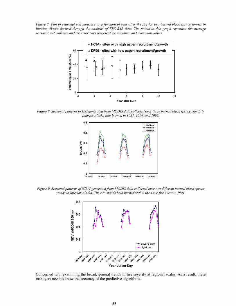
53

Figure 7. Plot of seasonal soil moisture as a function of year after the fire for two burned black spruce forests in Interior Alaska derived through the analysis of ERS SAR data. The points in this graph represent the average seasonal soil moisture and the error bars represent the minimum and maximum values.

Figure 8. Seasonal patterns of EVI generated from MODIS data collected over three burned black spruce stands in

Interior Alaska that burned in 1987, 1994, and 1999.

Figure 9. Seasonal patterns of NDVI generated from MODIS data collected over two different burned black spruce stands in Interior Alaska. The two stands both burned within the same fire event in 1994.

Concerned with examining the broad, general trends in fire severity at regional scales. As a result, these managers need to know the accuracy of the predictive algorithms.

0

0.2

0.4

0.6

0.8

2001

-001

2001

-081

2001

-161

2001

-241

2001

-321

2002

-033

2002

-113

2002

-193

2002

-273

2002

-353

2003

-065

2003

-145

2003

-225

Year-Julian Day

ND

VI (M

OD

IS 2

50 m

)

Severe burnLight burn

0

0.1

0.2

0.3

0.4

0.5

01-Jan-01 20-Jul-01 05-Feb-02 24-Aug-02 12-Mar-03 28-Sep-03

MO

DIS

EVI

1987 burn1994 burn1999 burn

0

20

40

60

0 2 4 6 8 10 12Year after burn

Volu

met

ric s

oil m

oist

ure

(%)

HC94 - sites with high aspen recruitment/growth

DF99 - sites with low aspen recruitment/growth

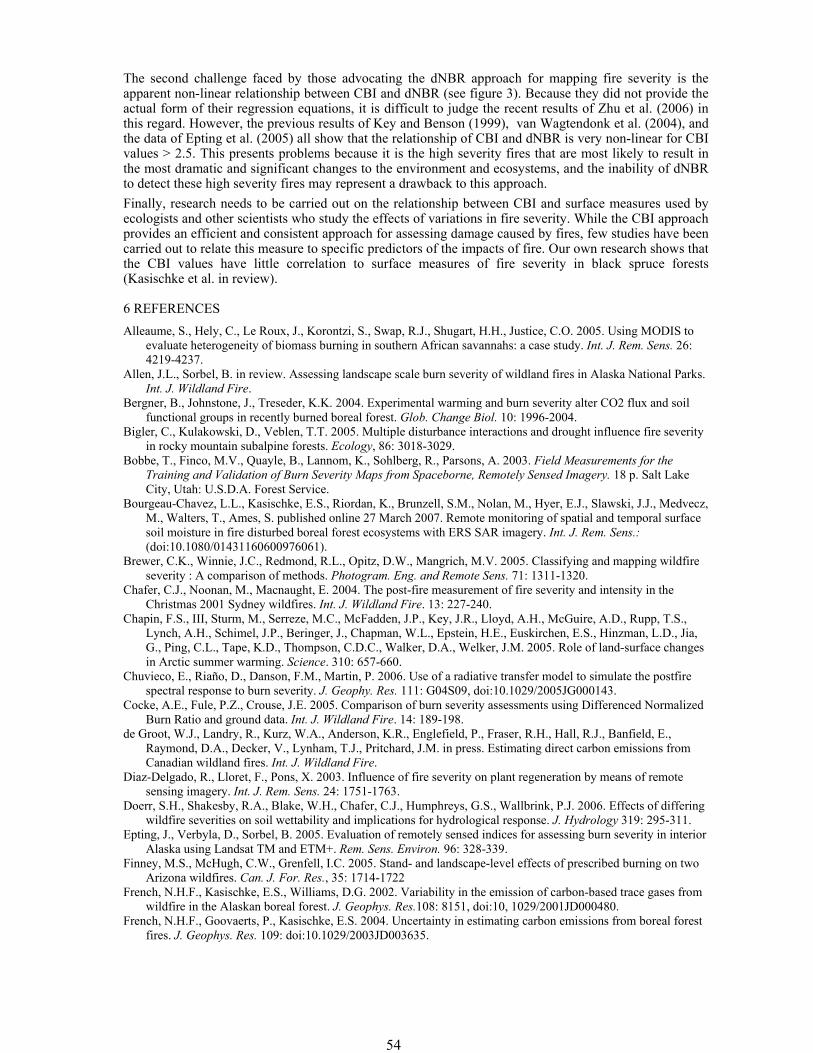
54

The second challenge faced by those advocating the dNBR approach for mapping fire severity is the apparent non-linear relationship between CBI and dNBR (see figure 3). Because they did not provide the actual form of their regression equations, it is difficult to judge the recent results of Zhu et al. (2006) in this regard. However, the previous results of Key and Benson (1999), van Wagtendonk et al. (2004), and the data of Epting et al. (2005) all show that the relationship of CBI and dNBR is very non-linear for CBI values > 2.5. This presents problems because it is the high severity fires that are most likely to result in the most dramatic and significant changes to the environment and ecosystems, and the inability of dNBR to detect these high severity fires may represent a drawback to this approach. Finally, research needs to be carried out on the relationship between CBI and surface measures used by ecologists and other scientists who study the effects of variations in fire severity. While the CBI approach provides an efficient and consistent approach for assessing damage caused by fires, few studies have been carried out to relate this measure to specific predictors of the impacts of fire. Our own research shows that the CBI values have little correlation to surface measures of fire severity in black spruce forests (Kasischke et al. in review).

6 REFERENCES Alleaume, S., Hely, C., Le Roux, J., Korontzi, S., Swap, R.J., Shugart, H.H., Justice, C.O. 2005. Using MODIS to

evaluate heterogeneity of biomass burning in southern African savannahs: a case study. Int. J. Rem. Sens. 26: 4219-4237.

Allen, J.L., Sorbel, B. in review. Assessing landscape scale burn severity of wildland fires in Alaska National Parks. Int. J. Wildland Fire.

Bergner, B., Johnstone, J., Treseder, K.K. 2004. Experimental warming and burn severity alter CO2 flux and soil functional groups in recently burned boreal forest. Glob. Change Biol. 10: 1996-2004.

Bigler, C., Kulakowski, D., Veblen, T.T. 2005. Multiple disturbance interactions and drought influence fire severity in rocky mountain subalpine forests. Ecology, 86: 3018-3029.

Bobbe, T., Finco, M.V., Quayle, B., Lannom, K., Sohlberg, R., Parsons, A. 2003. Field Measurements for the Training and Validation of Burn Severity Maps from Spaceborne, Remotely Sensed Imagery. 18 p. Salt Lake City, Utah: U.S.D.A. Forest Service.

Bourgeau-Chavez, L.L., Kasischke, E.S., Riordan, K., Brunzell, S.M., Nolan, M., Hyer, E.J., Slawski, J.J., Medvecz, M., Walters, T., Ames, S. published online 27 March 2007. Remote monitoring of spatial and temporal surface soil moisture in fire disturbed boreal forest ecosystems with ERS SAR imagery. Int. J. Rem. Sens.: (doi:10.1080/01431160600976061).

Brewer, C.K., Winnie, J.C., Redmond, R.L., Opitz, D.W., Mangrich, M.V. 2005. Classifying and mapping wildfire severity : A comparison of methods. Photogram. Eng. and Remote Sens. 71: 1311-1320.

Chafer, C.J., Noonan, M., Macnaught, E. 2004. The post-fire measurement of fire severity and intensity in the Christmas 2001 Sydney wildfires. Int. J. Wildland Fire. 13: 227-240.

Chapin, F.S., III, Sturm, M., Serreze, M.C., McFadden, J.P., Key, J.R., Lloyd, A.H., McGuire, A.D., Rupp, T.S., Lynch, A.H., Schimel, J.P., Beringer, J., Chapman, W.L., Epstein, H.E., Euskirchen, E.S., Hinzman, L.D., Jia, G., Ping, C.L., Tape, K.D., Thompson, C.D.C., Walker, D.A., Welker, J.M. 2005. Role of land-surface changes in Arctic summer warming. Science. 310: 657-660.

Chuvieco, E., Riaño, D., Danson, F.M., Martin, P. 2006. Use of a radiative transfer model to simulate the postfire spectral response to burn severity. J. Geophy. Res. 111: G04S09, doi:10.1029/2005JG000143.

Cocke, A.E., Fule, P.Z., Crouse, J.E. 2005. Comparison of burn severity assessments using Differenced Normalized Burn Ratio and ground data. Int. J. Wildland Fire. 14: 189-198.

de Groot, W.J., Landry, R., Kurz, W.A., Anderson, K.R., Englefield, P., Fraser, R.H., Hall, R.J., Banfield, E., Raymond, D.A., Decker, V., Lynham, T.J., Pritchard, J.M. in press. Estimating direct carbon emissions from Canadian wildland fires. Int. J. Wildland Fire.

Diaz-Delgado, R., Lloret, F., Pons, X. 2003. Influence of fire severity on plant regeneration by means of remote sensing imagery. Int. J. Rem. Sens. 24: 1751-1763.

Doerr, S.H., Shakesby, R.A., Blake, W.H., Chafer, C.J., Humphreys, G.S., Wallbrink, P.J. 2006. Effects of differing wildfire severities on soil wettability and implications for hydrological response. J. Hydrology 319: 295-311.

Epting, J., Verbyla, D., Sorbel, B. 2005. Evaluation of remotely sensed indices for assessing burn severity in interior Alaska using Landsat TM and ETM+. Rem. Sens. Environ. 96: 328-339.

Finney, M.S., McHugh, C.W., Grenfell, I.C. 2005. Stand- and landscape-level effects of prescribed burning on two Arizona wildfires. Can. J. For. Res., 35: 1714-1722

French, N.H.F., Kasischke, E.S., Williams, D.G. 2002. Variability in the emission of carbon-based trace gases from wildfire in the Alaskan boreal forest. J. Geophys. Res.108: 8151, doi:10, 1029/2001JD000480.

French, N.H.F., Goovaerts, P., Kasischke, E.S. 2004. Uncertainty in estimating carbon emissions from boreal forest fires. J. Geophys. Res. 109: doi:10.1029/2003JD003635.

55

Gonzalez-Alonso, F., Merino-De-Miguel, S., Roldan-Zamarron, A., Garcia-Gigorro, S., Cuevas, J.M. 2007. MERIS Full Resolution data for mapping level-of-damage caused by forest fires: the Valencia de Alcantara event in August 2003. Int. J. Rem. Sens. 28: 797-809.

Hall, R.J., Freeburn, J.T., de Groot, W.J., Pritchard, J.M., Lynham, T.J., Landry, R. in review. Remote sensing of burn severity: experience from Western Canada boreal fires. Int. J. Wildland Fire.

Hammill, K.A., and Bradstock, R.A. 2006. Remote sensing of fire severity in the Blue Mountains: influence of vegetation type and inferring fire intensity. Int. J. Wildland Fire. 15: 213-226.

Harden, J.W., Trumbore, S.E., Stocks, B.J., Hirsch, A., Gower, S.T., O'Neill, K.P., Kasischke, E.S. 2000. The role of fire in the boreal carbon budget. Global Change Biology 6: 174-184.

Hoy, E.E., French, N.H.F., Turetsky, M.R., Trigg, S.N., Kasischke, E.S. in review. Evaluating the potential of the normalized burn ratio and other spectral indices for assessment of fire severity in Alaskan black spruce forests. Int. J. Wildland Fire.

Hudak, A.T., Robichaud, P.R., Evans, J.B., Clark, J., Lannom, K., Morgan, P., Stone, C. 2004. Field validation of Burned Area Reflectance Classification (BARC) products for post fire assessment In:Paper presented at Remote sensing for field users - Tenth Forest Service Remote Sensing Applications Conference in Salt Lake City, Utah. April 5-9, 2004.

Hyde, K., Woods, W.W., Donahue, J. 2007. Predicting gully rejuvenation after wildfire using remotely sensed burn severity data. Geomorphology. 86: 496-511.

Isaev, A.S., Korovin, G.N., Bartalev, S.A., Ershov, D.V., Janetos, A., Kasischke, E.S., Shugart, H.H., French, N.H., Orlick, B.E., Murphy, T.L. 2002. Using remote sensing for assessment of forest wildfire carbon emissions. Clim. Change. 55(1-2): 231-255.

Jakubauskas, M.E., Lulla, K.P., Mausel, P.W. 1990. Assessment of vegetation change in a fire altered forest landscape. Photogrammetric Engineering and Remote Sensing. 56: 371-377.

Jain, T. B., 2004, Tongue-tied, Wildfire June/July:22-26. Jayen, K., Leduc, A., Bergeron, Y. 2006. Effect of fire severity on regeneration success in the boreal forest of

northwest Quebec, Canada. Ecoscience 13: 143-151. Johnstone, J.F., Kasischke, E.S. 2005. Stand-level effects of burn severity on post-fire regeneration in a recently-

burned black spruce forest. Can J. For. Res. 35: 2151-2163. Kasischke, E.S., Chapin III, F.S. in press. Increasing Vulnerability of Alaska's Boreal Forest as a Result of Climate

Warming and the Changing Fire Regime. In M.C. MacCracken, F. Moore, and J.C.J. Topping (Eds.), Sudden and DisruptiveClimate Change:Its Likelihood, Character and Significance. London: Earthscan Publications.

Kasischke, E.S., French, N.H.F., Bourgeau-Chavez, L.L., Christensen Jr, N., L. 1995. Estimating release of carbon from 1990 and 1991 forest fires in Alaska. J. Geophy. Res. 100: 2941-2951.

Kasischke, E.S., Turetsky, M.R. 2006. Recent changes in the fire regime across the North American boreal region- spatial and temporal patterns of burning across Canada and Alaska. Geophys. Res. Lett. 33: L09703, doi:10.1029/2006GL025677.

Kasischke, E.S., Johnstone, J.F. 2005. Variation in post-fire organic layer thickness in a black spruce forest complex in Interior Alaska and its effects on soil temperature and moisture. Can J. For. Res. 35: 2164-2177.

Kasischke, E.S., O'Neill, K.P., French, N.H.F., Bourgeau-Chavez, L.L., Richter, D. 2000. Influence of fire on long-term patterns of forest succession in Alaskan boreal forests. In E.S. Kasischke & B.J. Stocks (Eds.), Fire, Climate Change, and Carbon Cycling in the North American Boreal Forest. 214-238. New York: Springer-Verlag.

Kasischke, E.S., Christensen, N.L., Jr., Stocks, B.J. 1995b. Fire, global warming, and the carbon balance of boreal forests. Ecological Applications 5: 437-451.

Kasischke, E.S., Hyer, E., Novelli, P., Bruhwiler, L., French, N.H.F., Sukhinin, A.I., Hewson, J.H.,Stocks, B.J. 2005. Influences of boreal fire emissions on Northern Hemisphere atmospheric carbon and carbon monoxide. Glob. Biogeochem. Cycles 19: GB1012, d0i:10.1029/GB002300.

Kasischke, E.S., Bourgeau-Chavez, L.L., Johnstone, J.F. 2007. Assessing spatial and temporal variations in surface soil moisture in fire-disturbed black spruce forests using spaceborne synthetic aperture radar imagery - implications for post-fire tree recruitment. Rem. Sens. Environ. 108: 42-58, doi:10.1016/j.rse.2006.10.020.

Kasischke, E.S., Turetsky, M.R., Ottmar, R.D., French, N.H.F., Hoy, E.E., Kane, E.S. in review. Evaluation of the composite burn index for assessing fire severity in Alaskan black spruce forests. Int. J. Wildland Fire.

Kemball, K.J., Wang, G.G., Westwood, A.R. 2006. Are mineral soils exposed by severe wildfire better seedbeds for conifer regeneration? Can J. For. Res. 36: 1943-1950.

Key, C.H., Benson, N.C. 2006. Landscape Analysis (LA) Sampling and Analysis Methods,. U.S.D.A. Forest Service Gen. Tech. Report RMRS-GTR-164-CD, 55 p.

Key, C.H., Benson, N.C. 1999. unpublished data presented at http://www.nrmsc.usgs.gov/research/ndbr.htm. Keyser, T.L., Smith, K.W., Lentile, L.B., Sheppard, W.D. 2006. Modeling postfire mortality of ponderosa pine

following a mixed-severity wildfire in the Black Hills: The role of tree morphology and direct fire effects. Forest Science 52: 530-539.

Kielland, K., McFarland, J.W., Olson, K. 2006. mino acid uptake in deciduous and coniferous taiga ecosystems. Plant and Soil. 288: 297-307.

56

Kielland, K., McFarland, J.W., Ruess, R.W., Olson, K. in press. Rapid organic nitrogen cycling in taiga forest ecosystems. Ecosystems.

Kokaly, R.F., Rockwell, B.W., Haire, S.L., King, T.V.V. 2007. Characterization of post-fire surface cover, soils, and bum severity at the Cerro Grande Fire, New Mexico, using hyperspectral and multispectral remote sensing. Rem. Sens. Environ. 106: 305-325.

Kushla, J.D., Ripple, W.J. 1998. Assessing wildfire effects with Landsat thematic mapper data. Int. J. Rem. Sens. 19: 2493-2507.

Lentile, L.B., Holden, Z.A., Smith, A.M.S., Falkowski, M.J., Hudakl, A.T., Morgan, P., Lewis, S.A., Gessler, P.E., Benson, N.C. 2006. Remote sensing techniques to assess active fire characteristics and post-fire effects. Int. J. Wildland Fire. 15: 319-345.

Lewis, S.A., Wu, J.Q., Robichaud, P.R. Assessing burn severity and comparing soil water repellency, Hayman Fire, Colorado. Hydrol. Proc. 20: 1-16.

Michalek, J.L., French, N.H.F., Kasischke, E.S., Johnson, R.D., Colwell, J.E. 2000. Using Landsat TM data to estimate carbon release from burned biomass in an Alaskan spruce complex. Int. J. Rem. Sens. 21(2): 323-338.

Miller, A.B., Yool, S.R. 2002. Mapping forest post-fire canopy consumption in several overstory types using multi-temporal Landsat. Rem. Sens. Environ. 82: 481-496.

Miller, J.D., Thode, A.E. 2007. Quantifying burn severity in a heterogeneous landscape with a relative version of the delta Normalized Burn Ratio (dNBR). Rem. Sens. Environ. 109: 66-80.

Murphy, K.A., Reynolds, J.H., Koltun, J.M. in review. Does dNBR detect ecologically significant burn severity in boreal forests? Int. J. Wildland Fire.

O'Neill, K.P., Kasischke, E.S., Richter, D.D. 2002. Environmental controls on soil CO2 flux following fire in black spruce, white spruce, and aspen stands of interior Alaska. Can. J. For. Res. 32: 1525-1541.

O'Neill, K.P., Kasischke, E.S., Richter, D.D. 2003. Seasonal and decadal patterns of soil carbon uptake and emission along an age sequence of burned black spruce stands in interior Alaska. J. Geophys. Res.108: 8155, doi:10.1029/2001JD000443.

O'Neill, K.P., Richter, D.D., Kasischke, E.S. 2006. Succession-driven changes in soil respiration following fire in black spruce stands of Interior Alaska. Biogeochem. 80: 1-20.

Patterson, M.W., Yool, S.R. 1998. Mapping Fire-Induced Vegetation Mortality Using Landsat Thematic Mapper Data - Rincon Mountain Wilderness, Arizona, U.S.A. Rem. Sens. Environ. 65: 132-142.

Robichaud, P.R., Lewis, S.A., Laes, D.Y.M., Hudad, A.T., Kokaly, R.F., Zamudio, J.A. 2007. Postfire soil burn severity mapping with hyperspectral image unmixing. Rem. Sens. Environ. 108: 467-580.

Rogan, J., Yool, S.R. 2001. Mapping fire-induced vegetation depletion in the Peloncillo Mountains, Arizona and New Mexico. Int. J. Rem. Sens. 16: 3101-3121.

Roldan-Zamarron, A., Merino-De-Miguel, S., Gonzalez-Alonso, F., Garcia-Gigorro, S., Cuevas, J.M. 2006. Minas de Riotinto (south Spain) forest fire: Burned area assessment and fire severity mapping using Landsat 5-TM, Envisat-MERIS, and Terra-MODIS postfire images. J. Geophy. Res. 111: Art. No. G04S11.

Roy, D.R., Boschetti, L., Trigg, S.N. 2006. Remote sensing of fire severity: Assesing the performance of the normalized Burn ratio. IEEE Trans. Geosci. Rem. Sens. Lttrs. 3: 112-116.

Ruiz-Gallardo, J.R., Castaño, S., Alfonso, C. 2003. Application of remote sensing and GIS to locate priority intervention areas after wildland fires in Mediterranean systems: a case study from south-eastern Spain. Int. J. Wildland Fire. 13: 241-252.

Sorbel, B., Allen, J. 2005. Space-based burn severity mapping in Alaska's Nat. Parks. Alaska Park Science: 4-11. Stow, D., Peterson, A., Rogan, J., Franklin, J. 2007. Mapping Burn Severity of Mediterranean-Type Vegetation

Using Satellite Multispectral Data. GIScience Rem. Sensing. 44: 1-23. Turner, M.G., Hargrove, W.W., Gardner, R.H., Romme, W.H. 1994. Effects of fire on landscape heterogeneity in

Yellowstone National Park, Wyoming. J. Veg. Sci. 5: 731-742. van Wagtendonk, J.W., Root, R.R., Key, C.H. 2004. Comparison of AVIRIS and Landsat ETM+ detection

capabilities for burn severity. Rem. Sens. Environ. 92: 397-408. Verbyla, D., Kasischke, E.S., Hoy, E.E. in review. Seasonal and topographic effects on estimating fire severity from

remote sensing data. Int. J. Wildland Fire. Walz, Y., Maier, S.W., Dech, S.W., Conrad, C., Colditz, R.R. 2007. Classification of burn severity using Moderate

Resolution Imaging Spectroradiometer (MODIS): A case study in the jarrah-marri forest of southwest Western Australia. J. Geophy. Res. 112: Art. No. G02002.

White, J.D., Ryan, K.C., Key, C.C., Running, S.W. 1996. Remote sensing of forest fire severity and vegetation recovery. International Journal of Wildland Fire. 6: 125-136.

Yoshikawa, K., Bolton, W.R., Romanovsky, V., Fukuda, M., Hinzman, L.D. 2002. Impacts of wildfire on the permafrost in the boreal forests of Interior Alaska. J. Geophy. Res. 107: 8148, doi:10.1029/2001JD000438.

Zhu, Z., Key, C., Ohlen, D., Benson, N. 2006. Evaluate Sensitivities of Burn-Severity Mapping Algorithms for Different Ecosystems and Fire Histories in the United States. 36 pp. Sioux Falls, SD: U.S. Depart.of Interior.

57

European Forest Fire Information System (EFFIS) - Rapid Damage Assessment: Appraisal of burnt area maps with MODIS data

Paulo Barbosa European Commission, Joint Research Centre, Institute for Environment and Sustainability, T.P. 261, Via E. Fermi, 1 - 21020 Ispra (VA) Italy, [email protected]

Jan Kucera [email protected]

Peter Strobl [email protected]

ABSTRACT: The European Commission, Joint Research Centre (JRC) has established within its Institute for Environment and Sustainability (IES) the European Forest Fires Information System (EFFIS). A number of exceptionally large uncontrolled fires that occurred during 2003 and destroyed important parts of the land resources led to the development of the Rapid Damage Assessment (RDA) module within EFFIS. In this paper we present the different steps of the implementation of the RDA module that was built in order to map the extent of burned areas during the summer fire season. Burned areas of at least 50 ha were mapped from 2003 to 2006. The data used for the burned area mapping are both TERRA and AQUA MODIS images at 250 meters resolution, although the use of the 500 meters short-infrared bands is also foreseen. During 2003 only a selected number of images were used and the burned areas were visually classified. In 2004 the system was improved using an automatic method for scene identification and Quick Look retrieval followed by a visual inspection of these Quick Looks before downloading the full data sets. In 2005 the image selection was further improved by automating the Quick Look analyses considering the percentage of cloud free land in each scene. Selected images were then automatically downloaded, geo-coded and used to compile time series in 8 different tiles covering most of Europe. In 2006 the system was set to receive the MODIS imagery through direct broadcast allowing for a better time response and to have an European tailored service. The results of the burned area mapping of 2006 in a number of European countries are presented and compared with official statistics from each analysed country. An alternative to visual classification that relies on imagery time series analysis is also presented; this method is based on abrupt post-fire vegetation change detected from MODIS daily time series that will allow for a better and less user-dependent classification of the burned areas

1 INTRODUCTION The European Commission, Directorate General Joint Research Centre (DG-JRC) has established within its Institute for Environment and Sustainability (IES) the European Forest Fires Information System (EFFIS) supporting the Forest Focus regulation (EC-2152/2003) concerning monitoring of forests and environment interactions in the Community (European Commission, 2005). The initial aims of EFFIS were to develop and implement advanced methods for the evaluation of forest fire danger forecast and for the estimation of burnt areas in the European Union. Hence, the first two modules of EFFIS that were developed were the EFFIS Fir Danger, providing daily 1 to 3 days forecast of fire risk, and the EFFIS Damage Assessment, performing the mapping and evaluation of damages caused by fires of at least 50 ha that was done through the classification of images of the Wide Field Sensor (WiFS), on board the Indian Remote Sensing (IRS) satellites, from 2000 to 2004 at the end of each summer fire season. EFFIS also includes forest fire information collected by the Member States and provided to the EC through Regulation EC-2158/92 expired in December 2002 (now replaced by the broader mentioned “Forest Focus” regulation), and stored in a EU Fire Database. Other modules, under development within EFFIS, are now looking into other aspects of forest fires such as vegetation regeneration after fires, estimation of forest fire emissions, and the identification of post-fire risk areas that may be subject to further damages such as soil loss and/or landslides. The 2003 European summer fire campaign was characterized by extreme weather conditions that resulted in one of the most severe fire seasons experienced during the last decades in Southern Europe. This campaign was not only exceptional in terms of damage in some countries, but also on the number of casualties resulting from these fires. Over 40 people amongst civilians and fire fighters died due the 2003 summer fires. The critical level of fire risk reached during the summer in many areas, estimated with EFFIS Fire Danger, and a number of exceptionally large uncontrolled fires that destroyed important parts of the land resources, lead the European Commission to activate the EFFIS Damage Assessment module

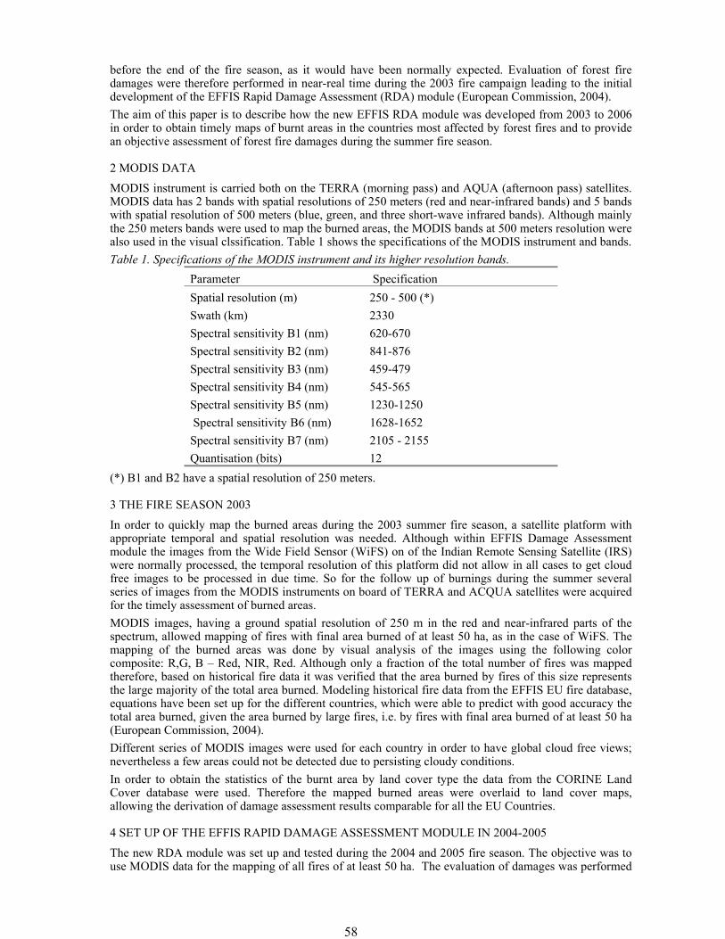
58

before the end of the fire season, as it would have been normally expected. Evaluation of forest fire damages were therefore performed in near-real time during the 2003 fire campaign leading to the initial development of the EFFIS Rapid Damage Assessment (RDA) module (European Commission, 2004). The aim of this paper is to describe how the new EFFIS RDA module was developed from 2003 to 2006 in order to obtain timely maps of burnt areas in the countries most affected by forest fires and to provide an objective assessment of forest fire damages during the summer fire season.

2 MODIS DATA MODIS instrument is carried both on the TERRA (morning pass) and AQUA (afternoon pass) satellites. MODIS data has 2 bands with spatial resolutions of 250 meters (red and near-infrared bands) and 5 bands with spatial resolution of 500 meters (blue, green, and three short-wave infrared bands). Although mainly the 250 meters bands were used to map the burned areas, the MODIS bands at 500 meters resolution were also used in the visual clssification. Table 1 shows the specifications of the MODIS instrument and bands. Table 1. Specifications of the MODIS instrument and its higher resolution bands.

Parameter Specification Spatial resolution (m) 250 - 500 (*) Swath (km) 2330 Spectral sensitivity B1 (nm) 620-670 Spectral sensitivity B2 (nm) 841-876 Spectral sensitivity B3 (nm) 459-479 Spectral sensitivity B4 (nm) 545-565 Spectral sensitivity B5 (nm) 1230-1250 Spectral sensitivity B6 (nm) 1628-1652 Spectral sensitivity B7 (nm) 2105 - 2155 Quantisation (bits) 12

(*) B1 and B2 have a spatial resolution of 250 meters.

3 THE FIRE SEASON 2003

In order to quickly map the burned areas during the 2003 summer fire season, a satellite platform with appropriate temporal and spatial resolution was needed. Although within EFFIS Damage Assessment module the images from the Wide Field Sensor (WiFS) on of the Indian Remote Sensing Satellite (IRS) were normally processed, the temporal resolution of this platform did not allow in all cases to get cloud free images to be processed in due time. So for the follow up of burnings during the summer several series of images from the MODIS instruments on board of TERRA and ACQUA satellites were acquired for the timely assessment of burned areas. MODIS images, having a ground spatial resolution of 250 m in the red and near-infrared parts of the spectrum, allowed mapping of fires with final area burned of at least 50 ha, as in the case of WiFS. The mapping of the burned areas was done by visual analysis of the images using the following color composite: R,G, B – Red, NIR, Red. Although only a fraction of the total number of fires was mapped therefore, based on historical fire data it was verified that the area burned by fires of this size represents the large majority of the total area burned. Modeling historical fire data from the EFFIS EU fire database, equations have been set up for the different countries, which were able to predict with good accuracy the total area burned, given the area burned by large fires, i.e. by fires with final area burned of at least 50 ha (European Commission, 2004). Different series of MODIS images were used for each country in order to have global cloud free views; nevertheless a few areas could not be detected due to persisting cloudy conditions. In order to obtain the statistics of the burnt area by land cover type the data from the CORINE Land Cover database were used. Therefore the mapped burned areas were overlaid to land cover maps, allowing the derivation of damage assessment results comparable for all the EU Countries.

4 SET UP OF THE EFFIS RAPID DAMAGE ASSESSMENT MODULE IN 2004-2005

The new RDA module was set up and tested during the 2004 and 2005 fire season. The objective was to use MODIS data for the mapping of all fires of at least 50 ha. The evaluation of damages was performed

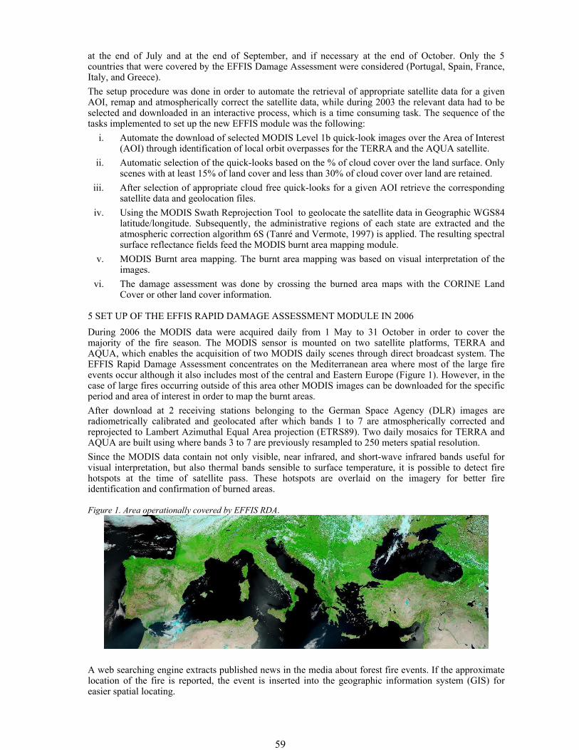
59

at the end of July and at the end of September, and if necessary at the end of October. Only the 5 countries that were covered by the EFFIS Damage Assessment were considered (Portugal, Spain, France, Italy, and Greece). The setup procedure was done in order to automate the retrieval of appropriate satellite data for a given AOI, remap and atmospherically correct the satellite data, while during 2003 the relevant data had to be selected and downloaded in an interactive process, which is a time consuming task. The sequence of the tasks implemented to set up the new EFFIS module was the following:

i. Automate the download of selected MODIS Level 1b quick-look images over the Area of Interest (AOI) through identification of local orbit overpasses for the TERRA and the AQUA satellite.

ii. Automatic selection of the quick-looks based on the % of cloud cover over the land surface. Only scenes with at least 15% of land cover and less than 30% of cloud cover over land are retained.

iii. After selection of appropriate cloud free quick-looks for a given AOI retrieve the corresponding satellite data and geolocation files.

iv. Using the MODIS Swath Reprojection Tool to geolocate the satellite data in Geographic WGS84 latitude/longitude. Subsequently, the administrative regions of each state are extracted and the atmospheric correction algorithm 6S (Tanré and Vermote, 1997) is applied. The resulting spectral surface reflectance fields feed the MODIS burnt area mapping module.

v. MODIS Burnt area mapping. The burnt area mapping was based on visual interpretation of the images.

vi. The damage assessment was done by crossing the burned area maps with the CORINE Land Cover or other land cover information.

5 SET UP OF THE EFFIS RAPID DAMAGE ASSESSMENT MODULE IN 2006 During 2006 the MODIS data were acquired daily from 1 May to 31 October in order to cover the majority of the fire season. The MODIS sensor is mounted on two satellite platforms, TERRA and AQUA, which enables the acquisition of two MODIS daily scenes through direct broadcast system. The EFFIS Rapid Damage Assessment concentrates on the Mediterranean area where most of the large fire events occur although it also includes most of the central and Eastern Europe (Figure 1). However, in the case of large fires occurring outside of this area other MODIS images can be downloaded for the specific period and area of interest in order to map the burnt areas. After download at 2 receiving stations belonging to the German Space Agency (DLR) images are radiometrically calibrated and geolocated after which bands 1 to 7 are atmospherically corrected and reprojected to Lambert Azimuthal Equal Area projection (ETRS89). Two daily mosaics for TERRA and AQUA are built using where bands 3 to 7 are previously resampled to 250 meters spatial resolution. Since the MODIS data contain not only visible, near infrared, and short-wave infrared bands useful for visual interpretation, but also thermal bands sensible to surface temperature, it is possible to detect fire hotspots at the time of satellite pass. These hotspots are overlaid on the imagery for better fire identification and confirmation of burned areas.

Figure 1. Area operationally covered by EFFIS RDA.

A web searching engine extracts published news in the media about forest fire events. If the approximate location of the fire is reported, the event is inserted into the geographic information system (GIS) for easier spatial locating.

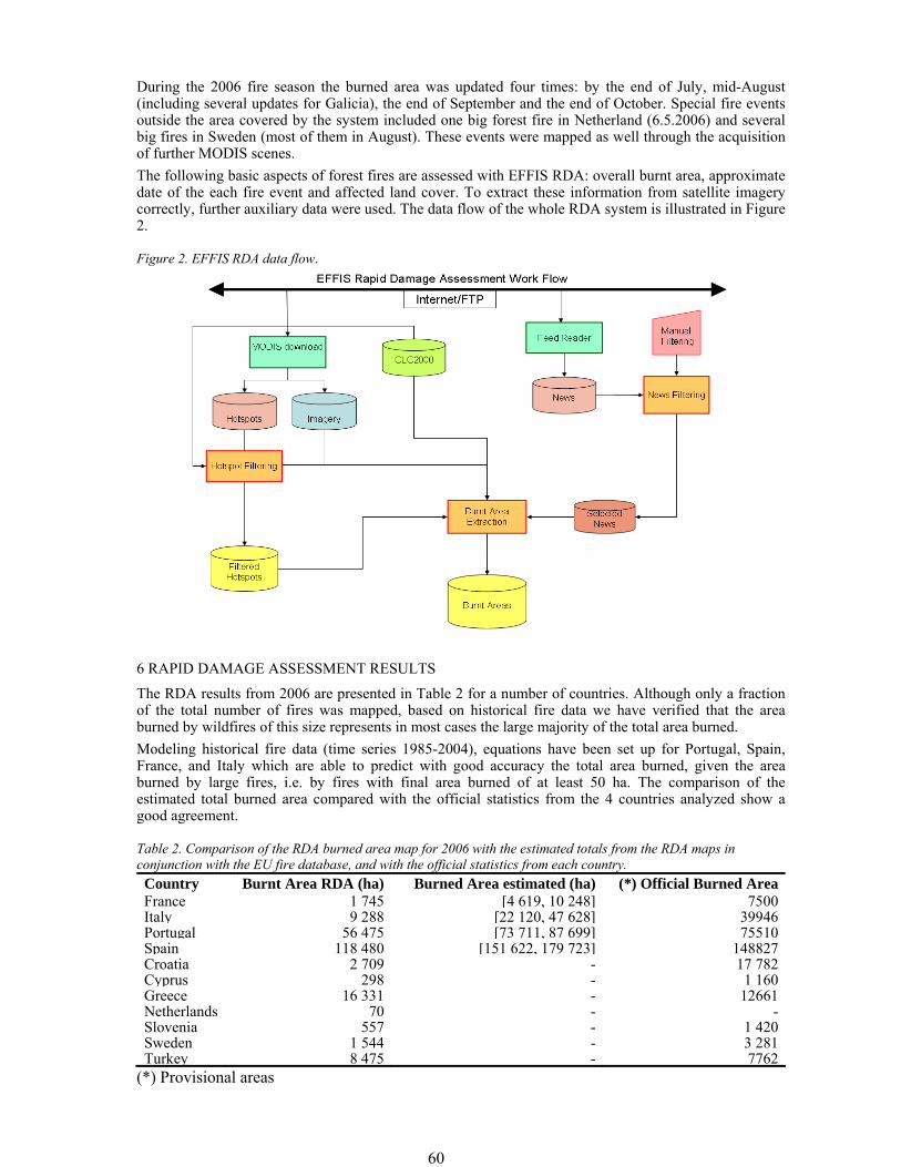
60

During the 2006 fire season the burned area was updated four times: by the end of July, mid-August (including several updates for Galicia), the end of September and the end of October. Special fire events outside the area covered by the system included one big forest fire in Netherland (6.5.2006) and several big fires in Sweden (most of them in August). These events were mapped as well through the acquisition of further MODIS scenes. The following basic aspects of forest fires are assessed with EFFIS RDA: overall burnt area, approximate date of the each fire event and affected land cover. To extract these information from satellite imagery correctly, further auxiliary data were used. The data flow of the whole RDA system is illustrated in Figure 2.

Figure 2. EFFIS RDA data flow.

6 RAPID DAMAGE ASSESSMENT RESULTS The RDA results from 2006 are presented in Table 2 for a number of countries. Although only a fraction of the total number of fires was mapped, based on historical fire data we have verified that the area burned by wildfires of this size represents in most cases the large majority of the total area burned. Modeling historical fire data (time series 1985-2004), equations have been set up for Portugal, Spain, France, and Italy which are able to predict with good accuracy the total area burned, given the area burned by large fires, i.e. by fires with final area burned of at least 50 ha. The comparison of the estimated total burned area compared with the official statistics from the 4 countries analyzed show a good agreement.

Table 2. Comparison of the RDA burned area map for 2006 with the estimated totals from the RDA maps in conjunction with the EU fire database, and with the official statistics from each country. Country Burnt Area RDA (ha) Burned Area estimated (ha) (*) Official Burned Area France 1 745 [4 619, 10 248] 7500Italy 9 288 [22 120, 47 628] 39946Portugal 56 475 [73 711, 87 699] 75510Spain 118 480 [151 622, 179 723] 148827Croatia 2 709 - 17 782Cyprus 298 - 1 160Greece 16 331 - 12661 Netherlands 70 - -Slovenia 557 - 1 420Sweden 1 544 - 3 281Turkey 8 475 - 7762

(*) Provisional areas

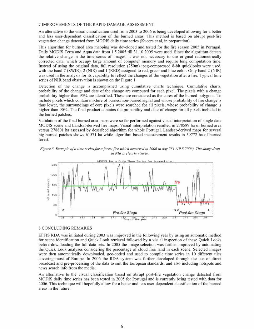
61

7 IMPROVEMENTS OF THE RAPID DAMAGE ASSESSMENT An alternative to the visual classification used from 2003 to 2006 is being developed allowing for a better and less user-dependent classification of the burned areas. This method is based on abrupt post-fire vegetation change detected from MODIS daily time series (Kucera et al, in preparation). This algorithm for burned area mapping was developed and tested for the fire season 2005 in Portugal. Daily MODIS Terra and Aqua data from 1.5.2005 till 31.10.2005 were used. Since the algorithm detects the relative change in the time series of images, it was not necessary to use original radiometrically corrected data, which occupy large amount of computer memory and require long computation time. Instead of using the original data, full resolution (250m) jpeg-compressed 8-bit quicklooks were used, with the band 7 (SWIR), 2 (NIR) and 1 (RED) assigned to red, green and blue color. Only band 2 (NIR) was used in the analysis for its capability to reflect the changes of the vegetation after a fire. Typical time series of NIR band observation is shown on the Figure 1. Detection of the change is accomplished using cumulative charts technique. Cumulative charts, probability of the change and date of the change are computed for each pixel. The pixels with a change probability higher than 95% are identified. These are considered as the cores of the burned polygons. To include pixels which contain mixture of burned/non-burned signal and whose probability of fire change is thus lower, the surroundings of core pixels were searched for all pixels, whose probability of change is higher than 90%. The final product contains the probability and date of change for all pixels included in the burned patches. Validation of the final burned area maps were so far performed against visual interpretation of single date MODIS scene and Landsat-derived fire maps. Visual interpretation resulted in 278589 ha of burned area versus 278801 ha assessed by described algorithm for whole Portugal. Landsat-derived maps for several big burned patches shows 61571 ha while algorithm based measurement results in 59772 ha of burned forest.

Figure 3. Example of a time series for a forest fire which occurred in 2006 in day 231 (19.8.2006). The sharp drop in NIR is clearly visible.

8 CONCLUDING REMARKS EFFIS RDA was initiated during 2003 was improved in the following year by using an automatic method for scene identification and Quick Look retrieval followed by a visual inspection of these Quick Looks before downloading the full data sets. In 2005 the image selection was further improved by automating the Quick Look analyses considering the percentage of cloud free land in each scene. Selected images were then automatically downloaded, geo-coded and used to compile time series in 10 different tiles covering most of Europe. In 2006 the RDA system was further developed through the use of direct broadcast and pre-processing of the data to suit the European standards, and also including hotspots and news search info from the media. An alternative to the visual classification based on abrupt post-fire vegetation change detected from MODIS daily time series has been tested in 2005 for Portugal and is currently being tested with data for 2006. This technique will hopefully allow for a better and less user-dependent classification of the burned areas in the future.

62

9 REFERENCES European Commission, 2004. Special Report: Assessment of fire damages in the EU Mediterranean Countries

during the 2003 Forest Fire Campaign. Official Publication of the European Communities, SPI.04.64 EN. European Commission, 2005. Forest Fires in Europe 2004, Report No5. Official Publication of the European

Communities, SPI.05.147 EN. Tanre D. and Vermote E., 1997. Second simulation of the satellite signal in the solar spectrum. IEEE Transactions

on Geoscience and Remote Sensing, 35, pp.675-686.

63

1 INTRODUCTION The geo-informational system is based mainly on Geographic Information System (GIS) technologies, makes use of spatial data combined with intelligent techniques and algorithms, and provides its users with a set of information that can be used to estimate the risk of forest fires and better coordination of fire trucks, both before and after the outbreak of a forest fire. In particular, the system provides the ability to: • Monitor the fleet of fire trucks in real time, transmitting GPS information using wireless networks. • Receive temperature, relative humidity, wind speed and direction measurements, in real time, from

stationary (Automatic Weather Station – AWS) and mobile weather stations (attached to folding mast on top of fire trucks).

• Support the work of the forest fire fighting coordinator with tools that allow: o Approximate knowledge of the weather conditions at any point in the island where a fire breaks

out, so that he can estimate how dangerous it is and mobilize the appropriate number of vehicles. o Deployment of forces in an optimal manner, according to various factors, such as the progress of

the fire, the accessibility of the area, its geophysical configuration, its combustible materials, the availability of sources for drawing water in the area, volunteers, and other private or public fire fighting means that are available near the area of the fire.

o Precise estimation of the expansion of a fire in time, using data received in real time from the participating fire trucks, as well as other information regarding the terrain of the area and the combustible materials.

o Laying of the fire trucks plan on the map, and its broadcast in real time to all participating forces, as well as other authorities or services.

o Transmission of information about the state of the fire, from the area in the front to the coordinator (while he is present in the area).

• Support the work of the fire trucks that, through the system, are in a position to know information about the precise location and bounds of the fire or fires, relief map of the terrain, roads in the area and the optimal accessibility, locations of the other vehicles, nearest water resupply points

• Estimate the risk of a new fire breaking out, anywhere on the island, in real time, using

Forest Fire Risk Management Information System - FFRMIS

N. Kanellopoulos (Assistant professor) Ionian University, [email protected]

G. Tsironis, G. Vasileiou, Th. Mantes, A. Gryllakis & M. Koutlis Talent Information Systems S.A., Athens GR-10561, Greece, [email protected], [email protected], [email protected], [email protected], [email protected]

D. Venizelos &V. N. Christofilakis Emphasis Telematics, Athens, GR-115 26, Greece, [email protected], [email protected] Keywords: forest fire, risk man/ment, gprs, gis, telematic, behaveplus

ABSTRACT: The Forest Fire Risk Management Information System (FFRMIS) presented, constitutes an integrated innovation system consisting of telematics, meteorological, computing equipment and software, which aims to provide information to the appropriate parties of the Region of the Ionian Islands (RII) for the management and handling of the forest fires hazard. The innovation system has been installed and is an essential information and management tool (Control -Command - Coordinate - Communicate) for the Regional Fire Service Administration (RFSA) of the Ionian Islands, which is responsible for facing the problem of forest fires. The FFRMIS is based on state of the art technologies that utilize geographical-spatial data entered by the user, real-time meteorological and vehicle position data and in conjunction with intelligent techniques and algorithms it processes, manipulates and provides a series of useful information to its users for the best co-ordination of the fire tenders before and after the outburst of a forest fire. The FFRMIS consists of aGeographic Information System (GIS), which visualizes and manipulates spatial data of the area in concern, a Forecast Fire Spread Model, which forecasts the fire expansion on time using the BehavePlus simulation model and a Vehicle Track System, which allows the users of the system to know the exact real-time geographical position of every fire tender using satellite tracking technology (Global Positioning System - GPS).

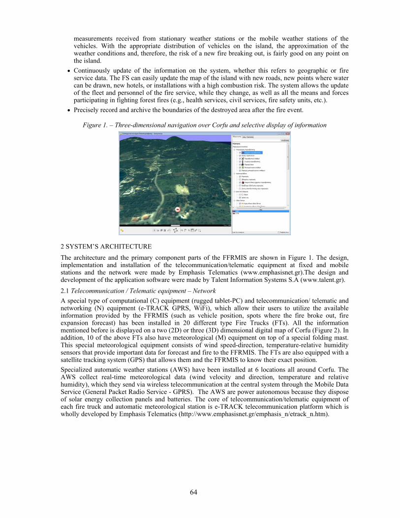
64

measurements received from stationary weather stations or the mobile weather stations of the vehicles. With the appropriate distribution of vehicles on the island, the approximation of the weather conditions and, therefore, the risk of a new fire breaking out, is fairly good on any point on the island.

• Continuously update of the information on the system, whether this refers to geographic or fire service data. The FS can easily update the map of the island with new roads, new points where water can be drawn, new hotels, or installations with a high combustion risk. The system allows the update of the fleet and personnel of the fire service, while they change, as well as all the means and forces participating in fighting forest fires (e.g., health services, civil services, fire safety units, etc.).

• Precisely record and archive the boundaries of the destroyed area after the fire event.

Figure 1. – Three-dimensional navigation over Corfu and selective display of information

2 SYSTEM’S ARCHITECTURE

The architecture and the primary component parts of the FFRMIS are shown in Figure 1. The design, implementation and installation of the telecommunication/telematic equipment at fixed and mobile stations and the network were made by Emphasis Telematics (www.emphasisnet.gr).The design and development of the application software were made by Talent Information Systems S.A (www.talent.gr). 2.1 Telecommunication / Telematic equipment – Network A special type of computational (C) equipment (rugged tablet-PC) and telecommunication/ telematic and networking (N) equipment (e-TRACK GPRS, WiFi), which allow their users to utilize the available information provided by the FFRMIS (such as vehicle position, spots where the fire broke out, fire expansion forecast) has been installed in 20 different type Fire Trucks (FTs). All the information mentioned before is displayed on a two (2D) or three (3D) dimensional digital map of Corfu (Figure 2). In addition, 10 of the above FTs also have meteorological (M) equipment on top of a special folding mast. This special meteorological equipment consists of wind speed-direction, temperature-relative humidity sensors that provide important data for forecast and fire to the FFRMIS. The FTs are also equipped with a satellite tracking system (GPS) that allows them and the FFRMIS to know their exact position. Specialized automatic weather stations (AWS) have been installed at 6 locations all around Corfu. The AWS collect real-time meteorological data (wind velocity and direction, temperature and relative humidity), which they send via wireless telecommunication at the central system through the Mobile Data Service (General Packet Radio Service - GPRS). The AWS are power autonomous because they dispose of solar energy collection panels and batteries. The core of telecommunication/telematic equipment of each fire truck and automatic meteorological station is e-TRACK telecommunication platform which is wholly developed by Emphasis Telematics (http://www.emphasisnet.gr/emphasis_n/etrack_n.htm).

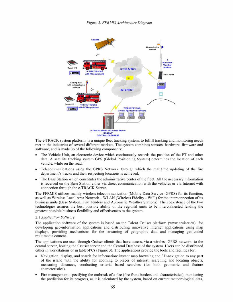
65

Figure 2. FFRMIS Architecture Diagram

The e-TRACK system platform, is a unique fleet tracking system, to fulfill tracking and monitoring needs met in the industries of several different markets. The system combines sensors, hardware, firmware and software, and is made up of the following components: • The Vehicle Unit, an electronic device which continuously records the position of the FT and other

data. A satellite tracking system GPS (Global Positioning System) determines the location of each vehicle, while on the road.

• Telecommunications using the GPRS Network, through which the real time updating of the fire department’s trucks and their respecting locations is achieved.

• The Base Station which constitutes the administrative center of the fleet. All the necessary information is received on the Base Station either via direct communication with the vehicles or via Internet with connection through the e-TRACK Server.

The FFRMIS utilizes mainly wireless telecommunication (Mobile Data Service -GPRS) for its function, as well as Wireless Local Area Network – WLAN (Wireless Fidelity - WiFi) for the interconnection of its business units (Base Station, Fire Tenders and Automatic Weather Stations). The coexistence of the two technologies assures the best possible ability of the regional units to be interconnected lending the greatest possible business flexibility and effectiveness to the system. 2.1 Application Software The application software of the system is based on the Talent Cruiser platform (www.cruiser.eu) for developing geo-information applications and distributing innovative internet applications using map displays, providing mechanisms for the streaming of geographic data and managing geo-coded multimedia content. The applications are used through Cruiser clients that have access, via a wireless GPRS network, to the central server, hosting the Cruiser server and the Central Database of the system. Users can be distributed either in workstations or in tablet-PCs (Figure 3). The applications provide the tools and facilities for: • Navigation, display, and search for information: instant map browsing and 3D-navigation to any part

of the island with the ability for zooming to places of interest, searching and locating objects, measuring distances, conducting criteria based searches (for both geometric and feature characteristics).

• Fire management: specifying the outbreak of a fire (fire-front borders and characteristics), monitoring the prediction for its progress, as it is calculated by the system, based on current meteorological data,

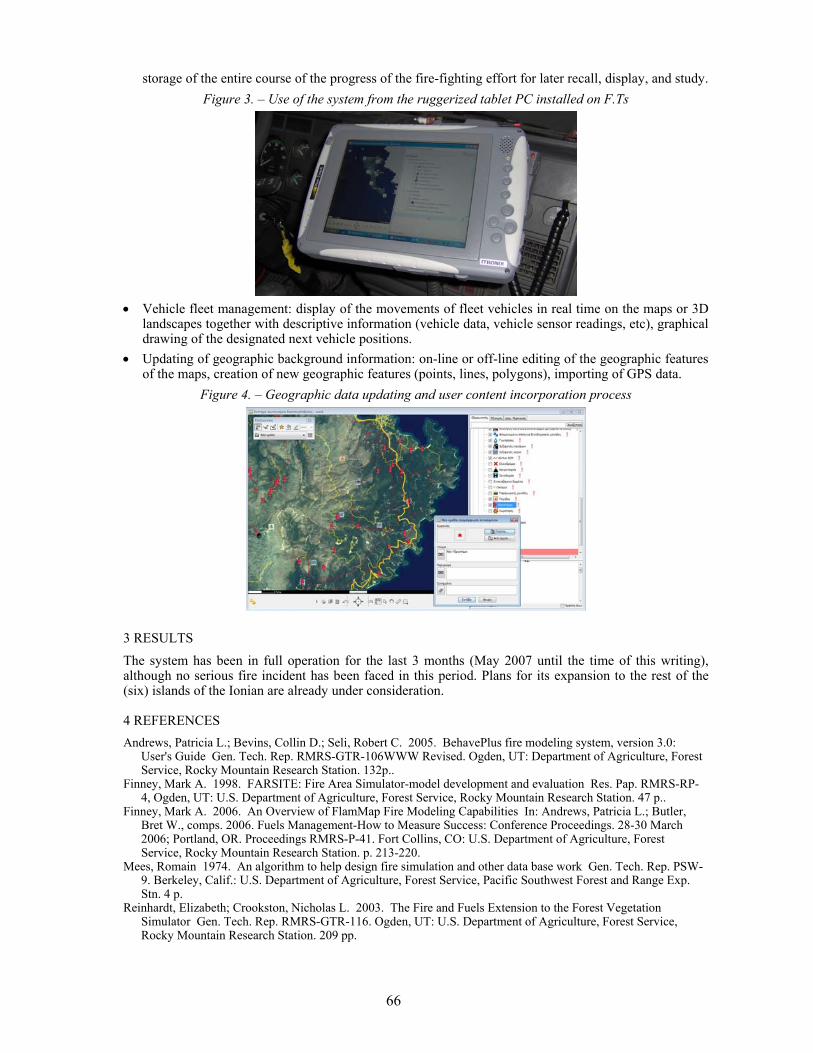
66

storage of the entire course of the progress of the fire-fighting effort for later recall, display, and study. Figure 3. – Use of the system from the ruggerized tablet PC installed on F.Ts

• Vehicle fleet management: display of the movements of fleet vehicles in real time on the maps or 3D

landscapes together with descriptive information (vehicle data, vehicle sensor readings, etc), graphical drawing of the designated next vehicle positions.

• Updating of geographic background information: on-line or off-line editing of the geographic features of the maps, creation of new geographic features (points, lines, polygons), importing of GPS data.

Figure 4. – Geographic data updating and user content incorporation process

3 RESULTS The system has been in full operation for the last 3 months (May 2007 until the time of this writing), although no serious fire incident has been faced in this period. Plans for its expansion to the rest of the (six) islands of the Ionian are already under consideration.

4 REFERENCES Andrews, Patricia L.; Bevins, Collin D.; Seli, Robert C. 2005. BehavePlus fire modeling system, version 3.0:

User's Guide Gen. Tech. Rep. RMRS-GTR-106WWW Revised. Ogden, UT: Department of Agriculture, Forest Service, Rocky Mountain Research Station. 132p..

Finney, Mark A. 1998. FARSITE: Fire Area Simulator-model development and evaluation Res. Pap. RMRS-RP-4, Ogden, UT: U.S. Department of Agriculture, Forest Service, Rocky Mountain Research Station. 47 p..

Finney, Mark A. 2006. An Overview of FlamMap Fire Modeling Capabilities In: Andrews, Patricia L.; Butler, Bret W., comps. 2006. Fuels Management-How to Measure Success: Conference Proceedings. 28-30 March 2006; Portland, OR. Proceedings RMRS-P-41. Fort Collins, CO: U.S. Department of Agriculture, Forest Service, Rocky Mountain Research Station. p. 213-220.

Mees, Romain 1974. An algorithm to help design fire simulation and other data base work Gen. Tech. Rep. PSW-9. Berkeley, Calif.: U.S. Department of Agriculture, Forest Service, Pacific Southwest Forest and Range Exp. Stn. 4 p.

Reinhardt, Elizabeth; Crookston, Nicholas L. 2003. The Fire and Fuels Extension to the Forest Vegetation Simulator Gen. Tech. Rep. RMRS-GTR-116. Ogden, UT: U.S. Department of Agriculture, Forest Service, Rocky Mountain Research Station. 209 pp.

67

1 INTRODUCTION Several fire indices have been used to estimate forest fire risk. However, their construction varies widely from one index to another, reflecting different approaches. In addition, the reliability of an index may depend on the region where it is applied, since indices or their readings are usually fine tuned for specific regions of interest. According to Good et al. (2007) and Moriondo et al. (2006), defining fire seasons with FWI is more robust than with temperature and allows avoiding false alarm. In the present study, two indices are considered: the Canadian Fire Weather Index (FWI) and the Finish Forest Fire Index (FFI). The Canadian FWI depends on temperature, precipitation, relative humidity and wind measurements, while the Finnish FFI relies on potential evaporation, precipitation and snow coverage. The two indices are compared through inter-correlation in the Mediterranean region. The Canadian Fire Weather Index (FWI) is based on weather readings taken at noon standard time and rates fire danger at the mid afternoon peak from 2:00 – 4:00 pm. Meteorological variables required are:

• Air temperature (in the shade) • Relative Humidity (in the shade) • Wind speed (at 10 m above ground, averaged over at least 10 minutes) • Rainfall (for the previous 24 hours)

The FWI System consists of six components: three fuel moisture codes (Fine Fuel Moisture Code, Duff Moisture Code, Drought Code) and three fire behaviour indices (Initial Spread index, Build Up Index, Fire Weather Index). Calculation of the index requires previous day records of the fuel moisture codes. FWI is divided into four fire danger classes: Low 0 – 7, Medium 8 – 16, High 17 – 31, Extreme > 32 The calculation of the Finnish Forest Fire Index (FFI) is based on surface moisture estimation and requires the following input:

• Potential evaporation from 24-hours centred on time of calculation • Accumulated precipitation for 24 hours • Flag specifying the presence or absence of snow cover

Previous day records of the above are required to compute the index. FFI is divided into three fire danger classes: Low 1 – 4, Medium 4 – 5, High > 5. It is noteworthy that both indices reflect similar weather conditions, since relative humidity, temperature and wind can be combined to determine evaporation (Singh and Xu, 1997). Both indices depend on previous day conditions regarding one or more of their components and they both define fire danger classes.

An intercomparison study of modelled forest fire risk in the Mediterranean for present day conditions

C. Giannakopoulos*, P.LeSager & E. Kostopoulou, National Observatory of Athens, Greece. *email: [email protected]

A. Vajda, A. Venäläinen Finnish Meteorological Institute, Finland Keywords: forest fire risk, Europe, Mediterranean, comparison, Canadian Fire Weather Index, Finnish Fire Index

ABSTRACT: In the present study, two indices are considered: the Canadian Fire Weather Index (FWI) and the Finish Forest Fire Index (FFI). The Canadian FWI depends on temperature, precipitation, relative humidity and wind measurements, while the Finnish FFI relies on potential evaporation, precipitation and snow coverage. The two indices are compared through inter-correlation in the Mediterranean region. In general, FWI and FFI determine a fairly similar fire risk for a set of weather readings. Higher correlations are found especially for locations under significant fire risk. The results improve for the lower values of fire risk if a spinning period is used in the computation of FFI. Both indices show similar features especially during summer, but some deviations are typical during early spring and autumn, as FWI probably overestimates the fire risk.

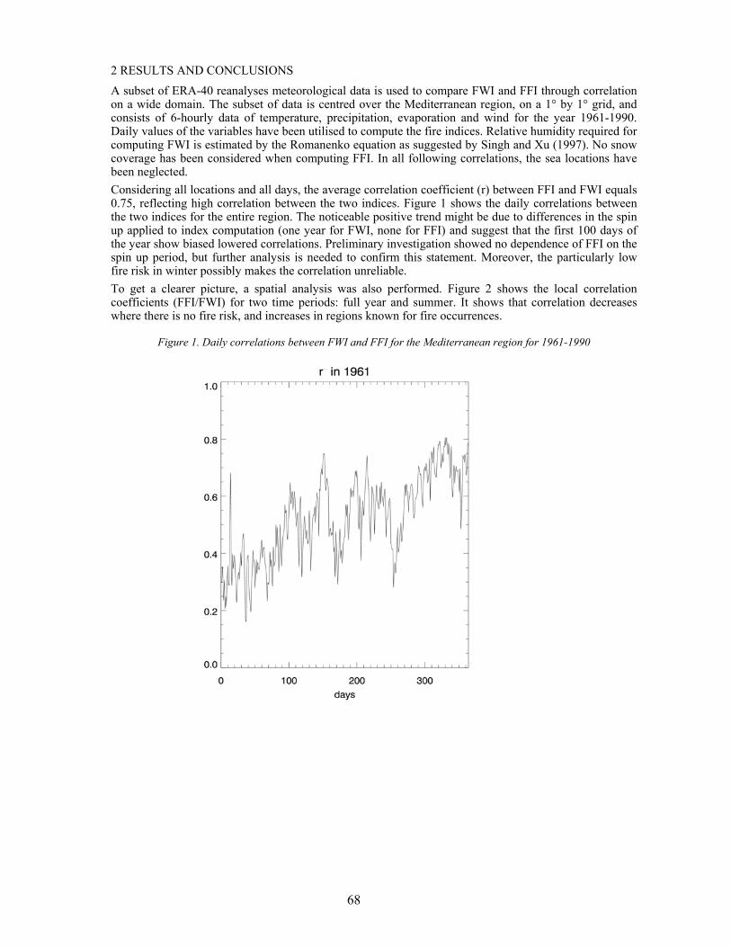
68

2 RESULTS AND CONCLUSIONS A subset of ERA-40 reanalyses meteorological data is used to compare FWI and FFI through correlation on a wide domain. The subset of data is centred over the Mediterranean region, on a 1° by 1° grid, and consists of 6-hourly data of temperature, precipitation, evaporation and wind for the year 1961-1990. Daily values of the variables have been utilised to compute the fire indices. Relative humidity required for computing FWI is estimated by the Romanenko equation as suggested by Singh and Xu (1997). No snow coverage has been considered when computing FFI. In all following correlations, the sea locations have been neglected. Considering all locations and all days, the average correlation coefficient (r) between FFI and FWI equals 0.75, reflecting high correlation between the two indices. Figure 1 shows the daily correlations between the two indices for the entire region. The noticeable positive trend might be due to differences in the spin up applied to index computation (one year for FWI, none for FFI) and suggest that the first 100 days of the year show biased lowered correlations. Preliminary investigation showed no dependence of FFI on the spin up period, but further analysis is needed to confirm this statement. Moreover, the particularly low fire risk in winter possibly makes the correlation unreliable. To get a clearer picture, a spatial analysis was also performed. Figure 2 shows the local correlation coefficients (FFI/FWI) for two time periods: full year and summer. It shows that correlation decreases where there is no fire risk, and increases in regions known for fire occurrences.

Figure 1. Daily correlations between FWI and FFI for the Mediterranean region for 1961-1990

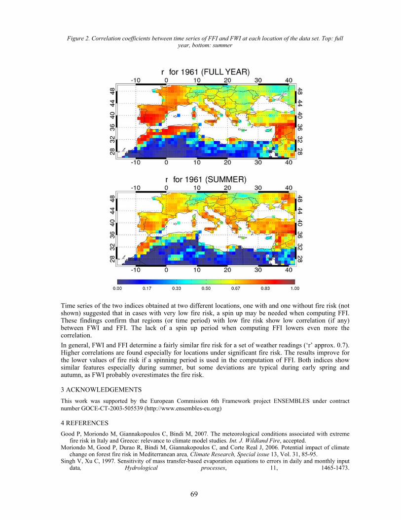
69

Figure 2. Correlation coefficients between time series of FFI and FWI at each location of the data set. Top: full year, bottom: summer

Time series of the two indices obtained at two different locations, one with and one without fire risk (not shown) suggested that in cases with very low fire risk, a spin up may be needed when computing FFI. These findings confirm that regions (or time period) with low fire risk show low correlation (if any) between FWI and FFI. The lack of a spin up period when computing FFI lowers even more the correlation. In general, FWI and FFI determine a fairly similar fire risk for a set of weather readings (‘r’ approx. 0.7). Higher correlations are found especially for locations under significant fire risk. The results improve for the lower values of fire risk if a spinning period is used in the computation of FFI. Both indices show similar features especially during summer, but some deviations are typical during early spring and autumn, as FWI probably overestimates the fire risk.

3 ACKNOWLEDGEMENTS This work was supported by the European Commission 6th Framework project ENSEMBLES under contract number GOCE-CT-2003-505539 (http://www.ensembles-eu.org)

4 REFERENCES Good P, Moriondo M, Giannakopoulos C, Bindi M, 2007. The meteorological conditions associated with extreme

fire risk in Italy and Greece: relevance to climate model studies. Int. J. Wildland Fire, accepted. Moriondo M, Good P, Durao R, Bindi M, Giannakopoulos C, and Corte Real J, 2006. Potential impact of climate

change on forest fire risk in Mediterranean area, Climate Research, Special issue 13, Vol. 31, 85-95. Singh V, Xu C, 1997. Sensitivity of mass transfer-based evaporation equations to errors in daily and monthly input

data, Hydrological processes, 11, 1465-1473.

70

1 INTRODUCTION Fuel moisture content is a critical factor affecting both fire ignition and propagation. The moisture content of dead fuels is highly dependent on meteorological conditions (Viegas et al. 1992) and is relevant for fire ignition (Dimitrakopoulos & Papaioannou, 2001). Instead, live fuel moisture content plays a significant role on fire propagation (Viegas, 1998; Carlson & Burgan, 2003). Nonetheless, vegetation susceptibility to wildfires is only partly affected by fuel moisture content since there are other factors, like human practices, that also contribute to fire ignition probability (Chuvieco et al. 2003). When estimating fuel moisture content it is usually assumed that variations of vegetation chlorophyll content and leaves degree of curing mirror vegetation moisture content variations (Illera et al. 1996; Paltridge & Barber, 1998; Burgan, 1988; Chuvieco, et al. 1999), even if this assumption is not true for all vegetation types and is dependent on the ecosystems (Ceccato et al. 2001). Besides, the above mentioned variations are better related to vegetation status which is influenced by several factors, one of which can be the lack of water (Ceccato et al. 2001). Moreover, these limitations prevails the problem of up-scaling the fuel moisture content results from leaf to canopy level due to the fact that at this scale other effects must be considered (Peñuelas et al. 1993; Ceccato et al. 2002). Even so, satellite data constitutes a widely accepted practical means to be used when monitor vegetation conditions at global scale; furthermore, they constitute an effective tool able to give insights about fire prone areas, which are a key factor in the framework of fire danger and short-term fire risk assessment. For these reasons a time series of Moderate Resolution Imaging Spectroradiometer (MODIS) data was used to derive several spectral indices for the continental territory of Portugal during the 2003 fire season. The indices were computed both for burnt and unburnt areas before the event occurred and then analyzed by means of a multivariate statistical approach. The aim of the present study is to infer the existence of differences in areas that were affected by fire from those that were not by means of several vegetation and water indices. To achieve this objective, a Canonical Discriminant Analysis was conduced both: (1) to verify the possibility of separating going-to-burn areas from those that will not be interested by fire; (2) to assess the relative importance of each independent variable as separation indicator.

2 DATASET AND METHODOLOGY The study focused on the 2003 fire season (March-August), in the continental territory of Portugal, a country severely affected every year by the phenomenon. On the basis of the European CORINE Land Cover 2000 map, the following main land cover (LC) classes were considered: grassland, scrubland and mixed forest. Agricultural areas and bare soils were discharged. For each LC class 40 test sites (consisting of 10 pixels each) were identified, half of them located in areas interested by fire and the remaining ones in areas that did not burn in that year. Pixels were sampled throughout all the season until the date of the

Assessing the capability of MODIS derived spectral indices for the identification of fire prone areas

M. J. Rodrigues International Doctoral School “Crop Systems, Forestry and Environmental Sciences”, Department of Crop Systems, Forestry and Environmental Sciences, University of Basilicata, Potenza, 85100, Italy, [email protected] Keywords: short-term fire risk, spectral indices, MODIS, Canonical Discriminant Analysis

ABSTRACT: The estimation of vegetation conditions by means of remotely sensed data represents an useful tool for the identification of possible fire prone areas in the framework of short-term fire risk assessment. The aim of the present study is to monitor the presence of different conditions of the vegetation both in going-to-burn areas and in unburnt areas, and to select the variables that most account for their separability. A Canonical Discriminant Analysis (CDA) was applied to several spectral indices (independent variables) derived using Moderate Resolution Imaging Spectroradiometer (MODIS) data, relative to the 2003 fire season in Portugal. The CDA was performed for three main land cover (LC) classes: grassland, scrubland and mixed forests. The results showed the existence of significant differences between fire prone and unburnt areas (p<0.0001) that permitted their spectral separation. In the case of grass and scrub LC classes, the indices that most contributed for the spectral separability were the water based indices. On the other side, the vegetation indices showed to have a more meaningful behavior in the mixed forest LC class.

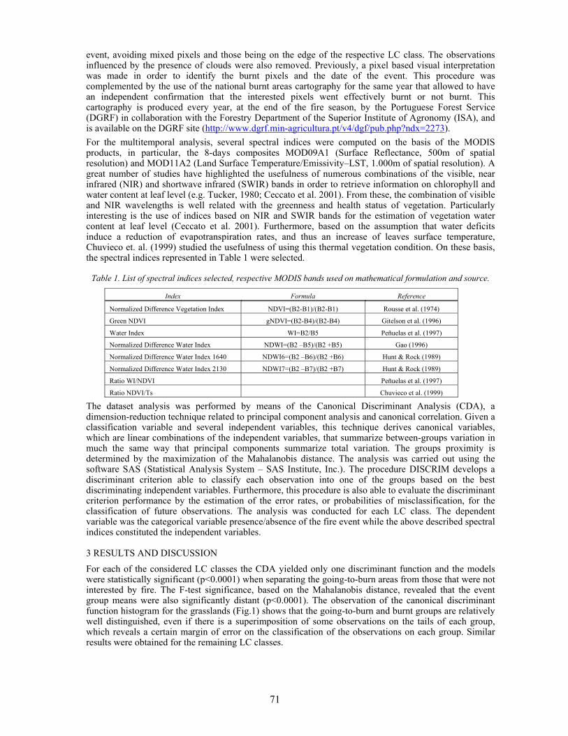
71

event, avoiding mixed pixels and those being on the edge of the respective LC class. The observations influenced by the presence of clouds were also removed. Previously, a pixel based visual interpretation was made in order to identify the burnt pixels and the date of the event. This procedure was complemented by the use of the national burnt areas cartography for the same year that allowed to have an independent confirmation that the interested pixels went effectively burnt or not burnt. This cartography is produced every year, at the end of the fire season, by the Portuguese Forest Service (DGRF) in collaboration with the Forestry Department of the Superior Institute of Agronomy (ISA), and is available on the DGRF site (http://www.dgrf.min-agricultura.pt/v4/dgf/pub.php?ndx=2273). For the multitemporal analysis, several spectral indices were computed on the basis of the MODIS products, in particular, the 8-days composites MOD09A1 (Surface Reflectance, 500m of spatial resolution) and MOD11A2 (Land Surface Temperature/Emissivity–LST, 1.000m of spatial resolution). A great number of studies have highlighted the usefulness of numerous combinations of the visible, near infrared (NIR) and shortwave infrared (SWIR) bands in order to retrieve information on chlorophyll and water content at leaf level (e.g. Tucker, 1980; Ceccato et al. 2001). From these, the combination of visible and NIR wavelengths is well related with the greenness and health status of vegetation. Particularly interesting is the use of indices based on NIR and SWIR bands for the estimation of vegetation water content at leaf level (Ceccato et al. 2001). Furthermore, based on the assumption that water deficits induce a reduction of evapotranspiration rates, and thus an increase of leaves surface temperature, Chuvieco et. al. (1999) studied the usefulness of using this thermal vegetation condition. On these basis, the spectral indices represented in Table 1 were selected.

Table 1. List of spectral indices selected, respective MODIS bands used on mathematical formulation and source.

Index Formula Reference

Normalized Difference Vegetation Index NDVI=(B2-B1)/(B2-B1) Rousse et al. (1974)

Green NDVI gNDVI=(B2-B4)/(B2-B4) Gitelson et al. (1996)

Water Index WI=B2/B5 Peñuelas et al. (1997)

Normalized Difference Water Index NDWI=(B2 –B5)/(B2 +B5) Gao (1996)

Normalized Difference Water Index 1640 NDWI6=(B2 –B6)/(B2 +B6) Hunt & Rock (1989)

Normalized Difference Water Index 2130 NDWI7=(B2 –B7)/(B2 +B7) Hunt & Rock (1989)

Ratio WI/NDVI Peñuelas et al. (1997)

Ratio NDVI/Ts Chuvieco et al. (1999)

The dataset analysis was performed by means of the Canonical Discriminant Analysis (CDA), a dimension-reduction technique related to principal component analysis and canonical correlation. Given a classification variable and several independent variables, this technique derives canonical variables, which are linear combinations of the independent variables, that summarize between-groups variation in much the same way that principal components summarize total variation. The groups proximity is determined by the maximization of the Mahalanobis distance. The analysis was carried out using the software SAS (Statistical Analysis System – SAS Institute, Inc.). The procedure DISCRIM develops a discriminant criterion able to classify each observation into one of the groups based on the best discriminating independent variables. Furthermore, this procedure is also able to evaluate the discriminant criterion performance by the estimation of the error rates, or probabilities of misclassification, for the classification of future observations. The analysis was conducted for each LC class. The dependent variable was the categorical variable presence/absence of the fire event while the above described spectral indices constituted the independent variables.

3 RESULTS AND DISCUSSION For each of the considered LC classes the CDA yielded only one discriminant function and the models were statistically significant (p<0.0001) when separating the going-to-burn areas from those that were not interested by fire. The F-test significance, based on the Mahalanobis distance, revealed that the event group means were also significantly distant (p<0.0001). The observation of the canonical discriminant function histogram for the grasslands (Fig.1) shows that the going-to-burn and burnt groups are relatively well distinguished, even if there is a superimposition of some observations on the tails of each group, which reveals a certain margin of error on the classification of the observations on each group. Similar results were obtained for the remaining LC classes.

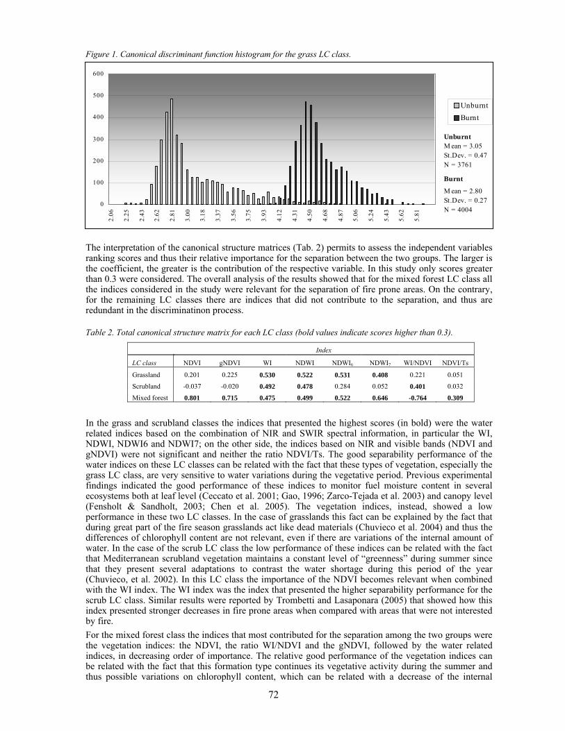
72

Figure 1. Canonical discriminant function histogram for the grass LC class. The interpretation of the canonical structure matrices (Tab. 2) permits to assess the independent variables ranking scores and thus their relative importance for the separation between the two groups. The larger is the coefficient, the greater is the contribution of the respective variable. In this study only scores greater than 0.3 were considered. The overall analysis of the results showed that for the mixed forest LC class all the indices considered in the study were relevant for the separation of fire prone areas. On the contrary, for the remaining LC classes there are indices that did not contribute to the separation, and thus are redundant in the discriminatinon process. Table 2. Total canonical structure matrix for each LC class (bold values indicate scores higher than 0.3).

Index

LC class NDVI gNDVI WI NDWI NDWI6 NDWI7 WI/NDVI NDVI/Ts

Grassland 0.201 0.225 0.530 0.522 0.531 0.408 0.221 0.051

Scrubland -0.037 -0.020 0.492 0.478 0.284 0.052 0.401 0.032

Mixed forest 0.801 0.715 0.475 0.499 0.522 0.646 -0.764 0.309

In the grass and scrubland classes the indices that presented the highest scores (in bold) were the water related indices based on the combination of NIR and SWIR spectral information, in particular the WI, NDWI, NDWI6 and NDWI7; on the other side, the indices based on NIR and visible bands (NDVI and gNDVI) were not significant and neither the ratio NDVI/Ts. The good separability performance of the water indices on these LC classes can be related with the fact that these types of vegetation, especially the grass LC class, are very sensitive to water variations during the vegetative period. Previous experimental findings indicated the good performance of these indices to monitor fuel moisture content in several ecosystems both at leaf level (Ceccato et al. 2001; Gao, 1996; Zarco-Tejada et al. 2003) and canopy level (Fensholt & Sandholt, 2003; Chen et al. 2005). The vegetation indices, instead, showed a low performance in these two LC classes. In the case of grasslands this fact can be explained by the fact that during great part of the fire season grasslands act like dead materials (Chuvieco et al. 2004) and thus the differences of chlorophyll content are not relevant, even if there are variations of the internal amount of water. In the case of the scrub LC class the low performance of these indices can be related with the fact that Mediterranean scrubland vegetation maintains a constant level of “greenness” during summer since that they present several adaptations to contrast the water shortage during this period of the year (Chuvieco, et al. 2002). In this LC class the importance of the NDVI becomes relevant when combined with the WI index. The WI index was the index that presented the higher separability performance for the scrub LC class. Similar results were reported by Trombetti and Lasaponara (2005) that showed how this index presented stronger decreases in fire prone areas when compared with areas that were not interested by fire. For the mixed forest class the indices that most contributed for the separation among the two groups were the vegetation indices: the NDVI, the ratio WI/NDVI and the gNDVI, followed by the water related indices, in decreasing order of importance. The relative good performance of the vegetation indices can be related with the fact that this formation type continues its vegetative activity during the summer and thus possible variations on chlorophyll content, which can be related with a decrease of the internal

0

100

200

300

400

500

600

2.06

2.25

2.43

2.62

2.81

3.00

3.18

3.37

3.56

3.75

3.93

4.12

4.31

4.50

4.68

4.87

5.06

5.24

5.43

5.62

5.81

UnburntBurnt

M ean = 3.05St.Dev. = 0.47N = 3761

Unburnt

Burnt

M ean = 2.80St.Dev. = 0.27N = 4004

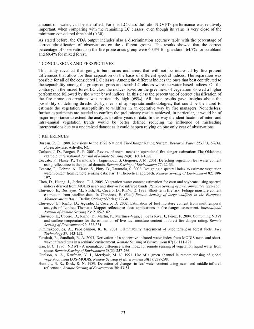
73

amount of water, can be identified. For this LC class the ratio NDVI/Ts performance was relatively important, when comparing with the remaining LC classes, even though its value is very close of the minimum considered threshold (0.30). As stated before, the CDA output includes also a discrimination accuracy table with the percentage of correct classification of observations on the different groups. The results showed that the correct percentage of observations on the fire prone areas group were 60.3% for grassland, 64.7% for scrubland and 69.4% for mixed forest.

4 CONCLUSIONS AND PERSPECTIVES This study revealed that going-to-burn areas and areas that will not be interested by fire present differences that allow for their separation on the basis of different spectral indices. The separation was possible for all of the considered LC classes. Among the different indices the ones that best contributed to the separability among the groups on grass and scrub LC classes were the water based indices. On the contrary, in the mixed forest LC class the indices based on the greenness of vegetation showed a higher performance followed by the water based indices. In this class the percentage of correct classification of the fire prone observations was particularly high (69%). All these results gave insights about the possibility of defining thresholds, by means of appropriate methodologies, that could be then used to estimate the vegetation susceptibility to wildfires in an operative way by fire managers. Nonetheless, further experiments are needed to confirm the preliminary results achieved, in particular, it would be of major importance to extend the analysis to other years of data. In this way the identification of inter- and intra-annual vegetation trends would be better defined reducing the influence of misleading interpretations due to a undersized dataset as it could happen relying on one only year of observations.

5 REFERENCES Burgan, R. E. 1988. Revisions to the 1978 National Fire-Danger Rating System. Research Paper SE-273, USDA,

Forest Service. Ashville, NC. Carlson, J. D., Burgan, R. E. 2003. Review of users’ needs in operational fire danger estimation: The Oklahoma

example. International Journal of Remote Sensing 24(8): 1601-1620. Ceccato, P., Flasse, P., Tarantola, S., Jaquemoud, S, Grégoire, J. M. 2001. Detecting vegetation leaf water content

using reflectance in the optical domain. Remote Sensing of Environment 77: 22-33. Ceccato, P., Gobron, N., Flasse, S., Pinty, B., Tarantola, S. 2002. Designing a spectral index to estimate vegetation

water content from remote sensing data: Part 1. Theoretical approach. Remote Sensing of Environment 82: 188-197.

Chen, D., Huang, J., Jackson, T. J. 2005. Vegetation water content estimation for corn and soybeans using spectral indices derived from MODIS near- and short-wave infrared bands. Remote Sensing of Environment 98: 225-236.

Chuvieco, E., Deshayes, M., Stach, N., Cocero, D., Riaño, D. 1999. Short-term fire risk: Foliage moisture content estimation from satellite data. In Chuvieco, E. (Eds.) Remote Sensing of large wildfires in the European Mediterranean Basin. Berlin: Springer-Verlag: 17-38.

Chuvieco, E., Riaño, D., Aguado, I., Cocero, D. 2002. Estimation of fuel moisture content from multitemporal analysis of Landsat Thematic Mapper reflectance data: applications in fire danger assessment. International Journal of Remote Sensing 23: 2145-2162.

Chuvieco, E., Cocero, D., Riaño, D., Martin, P., Martìnez-Vega, J., de la Riva, J., Pérez, F. 2004. Combining NDVI and surface temperature for the estimation of live fuel moisture content in forest fire danger rating. Remote Sensing of Environment 92: 322-331.

Dimitrakopoulos, A., Papaioannou, K. K. 2001. Flammability assessment of Mediterranean forest fuels. Fire Technology 37: 143-152.

Fensholt, R., Sandholt, R. A. 2003. Derivation of a shortwave infrared water index from MODIS near- and short-wave infrared data in a semiarid environment. Remote Sensing of Environment 87(1): 111-121.

Gao, B. C. 1996. NDWI - A normalized difference water index for remote sensing of vegetation liquid water from space. Remote Sensing of Environment 58(3): 257-266.

Gitelson, A. A., Kaufman, Y. J., Merzlyak, M. N. 1991. Use of a green channel in remote sensing of global vegetation from EOS-MODIS. Remote Sensing of Environment 58(3): 289-298.

Hunt Jr., E. R., Rock, R. N. 1989. Detection of changes in leaf water content using near- and middle-infrared reflectance. Remote Sensing of Environment 30: 43-54.

74

1 INTRODUCTION

Remote sensing data have been proven to be very useful for FMC estimation at local, regional and global level (Chen 2005; Chuvieco et al. 2004; Roberts et al. 2006). Both laboratory spectroradiometry measurements and satellite imagery data have been used to estimate FMC though different approaches. The most widespread approach has been the use of empirical methods based on statistical fittings between field measured FMC and reflectance or temperature satellite-derived data. However, simulation methods, based on RTM, both in directed and inverse mode, are increasingly used. They provide a deeper understanding of the physical processes that control canopy reflectance for any observational configuration conditions, and therefore they can be used in very diverse areas and periods. In general terms, the object of the inversion approach is to identify the set of input parameters that produces the most similar reflectance to the observed spectrum of a particular pixel. Basically, this can be achieved by using iterative optimization techniques (Zarco-Tejada et al. 2003) or simulated LUT (Knyazikhin et al. 1999). Whatever the approach is, FMC could only be retrieved from RTM when either is one of the input parameters, or is related to them. FMC can be defined as the quotient of two biophysical parameters included in most RTM: Dry matter content (DM, equation 2) and Equivalent Water Thickness (EWT, equation 3), defined as:

(1); (2); (3)

The common problem of all the RTM inversion approaches is that several combinations of biophysical variables can lead to similar spectral signals. In other words, similar reflectance can be simulated from different FMC values if other parameters widely vary. This is known as the “ill-posed” problem (Weiss 2000), and has greatest importance in practical inversion cases. The underlying problem is related to the lack of ecophysiological background of most RTM. They are physical models, but do not take into account that some combination of input parameters may never occur in reality, since they are associated to plant physiological characteristics. For example, several studies have shown a clear covariance between DM and EWT variations since high levels of sclerophyl (DM) are induced by low water availability and high light intensity (Castro-Díez et al. 1997) so DM normally increases during the summer months, when EWT values are minimum. Therefore, it would be unrealistic to obtain high EWT values with low DM, creating potential problems for an accurate FMC estimation. As a result of previous comments, auxiliary information must be used to constrain the input parameters of

A controlled Look-Up Table generation for Fuel Moisture Content estimation.

Marta Yebra, Angela De Santis & Emilio Chuvieco Department of Geography, University of Alcalá, Calle Colegios 2, Alcalá de Henares, Madrid 28801, Spain.

Keywords: MODIS, Radiative Transfer Models, Quercus ilex, Fuel Moisture Content

ABSTRACT: This study involved the generation of a controlled Look-Up Table (LUT) for the retrieval of Fuel Moisture Content (FMC) in areas dominated by Quercus ilex (holm-oak). To avoid unrealistic simulated spectrums in the LUT, parameter combinations observed in drying holm-olk were used as input to the PROSPECT and SAILH radiative transfer models (RTM). MODIS/Terra reflectance data, extracted from 4 oak dominated areas, was used to carry out the LUT inversion based on the search of the minimum relative root mean square error (RMSE*) between these observed reflectance and the simulated reflectance found in the LUT. Five inversion options, which included different MODIS wavebands and vegetation indices in the RMSE* computation, were tested in order to search for the optimal spectral sampling necessary for accurately estimating FMC. Their retrieval performance was evaluated with FMC values measured at the four study sites. In parallel, a non Holm oak specific LUT was used in the same way to evaluate whether or not the specific LUT retrieved FMC was more accurate. The results showed that the LUT generated with holm-oak observed data provided better FMC estimations in most of the inversion options. The most accurate FMC estimations were obtained from vegetation indices computed with Near infrared (NIR) and short wave infrared (SWIR) using both, the specific LUT (RMSE of 26.65% and 29.84 with GMVI6 and NDII6, respectively) an the non specific LUT (RMSE of 32.73% and 29.89 with GMVI6 and NDII6, respectively). Further work will be focus on generating a LUT adapted to a wider range of species based on data extracted from field measures and bibliography search.

100(%) ×=DMEWTFMC

AWscmgrDM =− ).( 2

AWdWfcmgrEWT −=− ).( 2

75

the RTM to model conditions as closely as possible to the actual canopy (Combal et al. 2002). Some authors have chosen to include as input parameters data derived from satellite images (Zarco-Tejada et al. 2003). Others have relied upon experimental data in controlled conditions (Riaño et al. 2005). Finally, there are also studies who define the prior information based on field measurements (Ustin et al. 1998; Yebra et al. 2007). The aim of this paper is to build a LUT adapted to a wide range of observed biophysical conditions and relationships, at both leaf and canopy level, in order to obtain more accurate FMC estimation from the inversion of RTM in Mediterranean areas. As the first attempt the LUT has been adapted to Quercus ilex a dominant type of Mediterranean vegetation.

2 METHODS

2.1 Radiative transfer models The PROSPECT (Jacquemoud et al. 1990) and SAILH (Verhoef 1984) models were chosen to simulate spectral reflectances between 400 and 2500 nm. The first one simulates reflectance and transmittance at leaf level by considering it as a set of N stacked layers with several absorption components: chlorophyll content (Ca+b), the EWT, and DM. The SAILH is a 1D turbid medium RTM which uses three variables to describe the canopy structure space (Leaf Area Index or LAI; Leaf Angle Distribution Function or LADF and the hotspot parameter or h), as well as the soil substrate reflectance and the viewing and illumination conditions (Sun zenith angle or Ts, view zenith angle Tv, relative azimuth sensor-sun or Psr and atmospheric transmissivity) to characterize observation conditions. 2.2 Input parameters definition The space of canopy realization (leaf and canopy biophysical parameters) was build using the values measured by De Santis, et al. (2006) for Quercus Ilex subesp. ilex under laboratory experimentation. These values consist of six temporal measures of spectral reflectances and their associated leaf and canopy parameters while plant is drying (table 1). Since this study was carried out with young oaks, LAI measures were considered lower than those encountered in natural conditions, so they were no used. Instead, a range of LAI values with a minimum of 0.6 (minimum of the experimentation) and a maximum of 4.9 (Bussotti et al. 2002) was used. In order to better sample domains where the reflectance is more sensible to LAI variations, a transformed variable was used to generated the LAI distribution, as is explained in Weiss (2000). Finally, the parameter N was obtained by the inversion of the Prospect model using the observed spectrum measured by De Santis, et al. (2006) with GER2700 spectroradiometer (GER Corp., Millbrook, NY). The hotspot parameter was fixed on 0.001 and the LADF on plagiofile. The scenario of simulation was targeted to resemble MODIS acquisition conditions. For doing that a four-year dataset of MODIS data (2001-2005) from our study site was used to extract the maximum and minimum values of Ts, Tv and Psr angles. The reflectance spectra of three different types of soil, obtained by multiplying a ground reference spectrum by a wet and dry soil brightness parameter (0.6 and 1.4, respectively), were also used for the instrument space definition. The reference soil spectral signature was measured in Cabañeros National Park with the GER2700 spectroradiometer. A total of 36288 simulations were generated by running the PROSPECT and SAILH programs extracted from the CSTARS RTM Repository Project (http://rtm.casil.ucdavis.edu/?RTM) within the inputs parameter values showed in table 1. 2.3 Field observations A field measured FMC dataset was used to evaluate the LUT inversion performance. Field FMC values were measured under the framework of two projects, Firerisk and Firemap, following a standard protocol (a detailed description can be found in Chuvieco et al, 2003). Four oak dominated areas located in Central Spain were selected from the full dataset (table 2). The measures in plots P1 and P2 were taken every 16 days, while the P3 and P4 consist of isolated measures that were taken during a field sampling campaign developed in Spring and Summer 2006. The total number of sampled measurements chosen were 29. 2.4 Reflectance data The MOD09A1 product (500m) was chosen as the source of observed reflectance data needed for the inversion, due to its proven capacity for estimating FMC (Zarco-Tejada et al. 2003). The original products were downloaded from the Land Processes Distributed Active Archive Center (LP DAAC) of the United States Geological Survey (USGS) (http://edcimswww.cr.usgs.gov/pub/imswelcome/) and reprojected from sinusoidal to UTM 30 T Datum European 1950 (ED50), using nearest neighbor interpolation resampling. The reflectance values of a given plot were extracted from each composited image using the median value of a 3x3 pixels kernel located at the center of the field plot.

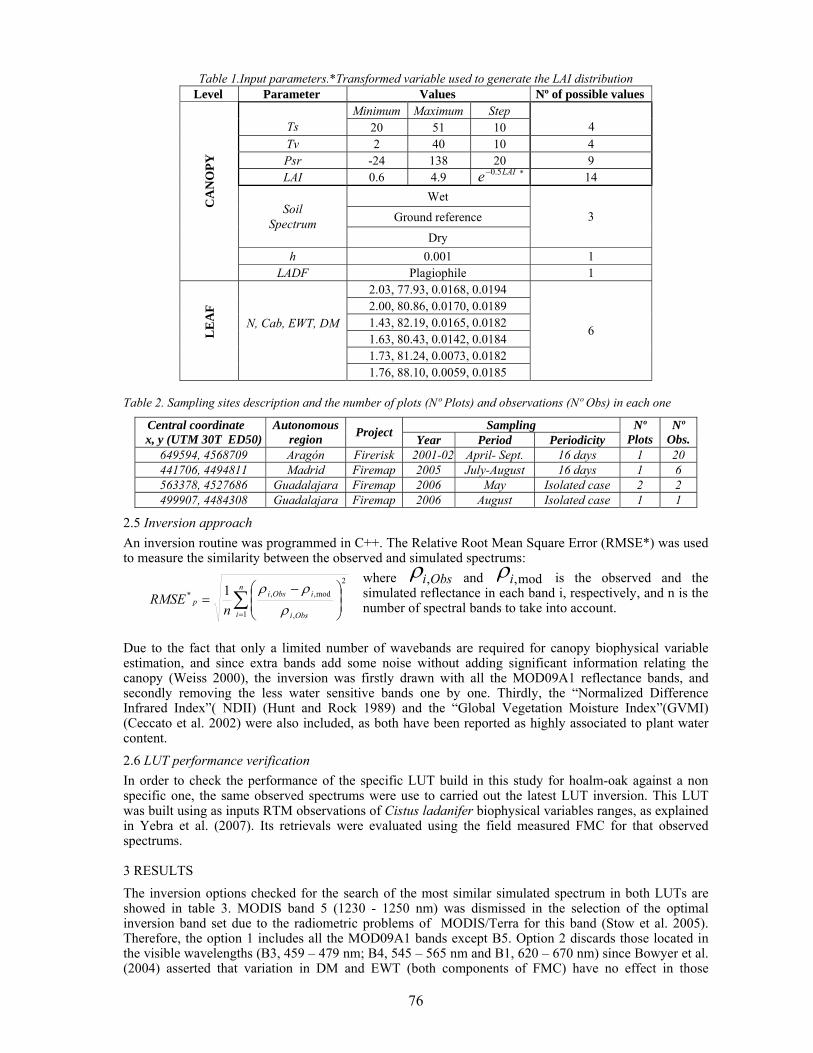
76

Table 1.Input parameters.*Transformed variable used to generate the LAI distribution Level Parameter Values Nº of possible values

Minimum Maximum Step Ts 20 51 10 4 Tv 2 40 10 4 Psr -24 138 20 9 LAI 0.6 4.9 LAIe 5.0− * 14

Wet Ground reference Soil

Spectrum Dry

3

h 0.001 1

CA

NO

PY

LADF Plagiophile 1 2.03, 77.93, 0.0168, 0.0194 2.00, 80.86, 0.0170, 0.0189 1.43, 82.19, 0.0165, 0.0182 1.63, 80.43, 0.0142, 0.0184 1.73, 81.24, 0.0073, 0.0182

LE

AF

N, Cab, EWT, DM

1.76, 88.10, 0.0059, 0.0185

6

Table 2. Sampling sites description and the number of plots (Nº Plots) and observations (Nº Obs) in each one

Sampling Central coordinate x, y (UTM 30T ED50)

Autonomous region Project Year Period Periodicity

Nº Plots

Nº Obs.

649594, 4568709 Aragón Firerisk 2001-02 April- Sept. 16 days 1 20 441706, 4494811 Madrid Firemap 2005 July-August 16 days 1 6 563378, 4527686 Guadalajara Firemap 2006 May Isolated case 2 2 499907, 4484308 Guadalajara Firemap 2006 August Isolated case 1 1

2.5 Inversion approach An inversion routine was programmed in C++. The Relative Root Mean Square Error (RMSE*) was used to measure the similarity between the observed and simulated spectrums:

where Obsi,ρ and mod,iρ is the observed and the simulated reflectance in each band i, respectively, and n is the number of spectral bands to take into account.

Due to the fact that only a limited number of wavebands are required for canopy biophysical variable estimation, and since extra bands add some noise without adding significant information relating the canopy (Weiss 2000), the inversion was firstly drawn with all the MOD09A1 reflectance bands, and secondly removing the less water sensitive bands one by one. Thirdly, the “Normalized Difference Infrared Index”( NDII) (Hunt and Rock 1989) and the “Global Vegetation Moisture Index”(GVMI) (Ceccato et al. 2002) were also included, as both have been reported as highly associated to plant water content. 2.6 LUT performance verification In order to check the performance of the specific LUT build in this study for hoalm-oak against a non specific one, the same observed spectrums were use to carried out the latest LUT inversion. This LUT was built using as inputs RTM observations of Cistus ladanifer biophysical variables ranges, as explained in Yebra et al. (2007). Its retrievals were evaluated using the field measured FMC for that observed spectrums.

3 RESULTS The inversion options checked for the search of the most similar simulated spectrum in both LUTs are showed in table 3. MODIS band 5 (1230 - 1250 nm) was dismissed in the selection of the optimal inversion band set due to the radiometric problems of MODIS/Terra for this band (Stow et al. 2005). Therefore, the option 1 includes all the MOD09A1 bands except B5. Option 2 discards those located in the visible wavelengths (B3, 459 – 479 nm; B4, 545 – 565 nm and B1, 620 – 670 nm) since Bowyer et al. (2004) asserted that variation in DM and EWT (both components of FMC) have no effect in those

2

1 ,

mod,,* 1 ∑=

⎟⎟⎠

⎞⎜⎜⎝

⎛ −=

n

i Obsi

iObsip

nRMSE

ρρρ

77

wavelengths, and also, at near infrared (NIR) (B2, 841 – 876 nm) and short wave infrared (SWIR) (B6, 1628 - 1652 nm and B7, 2105 - 2155 nm) wavelengths, the confounding influence of variation in LAI is small while the sensitivity to variation in FMC is consistently strong. Option 3 considers only B2 and B6 since the use of the shorter wavelengths of the SWIR would appear to be more useful for an accurate estimation of FMC (Bowyer and Danson 2004). Options 4 and 5 contemplate the inversion using vegetation indices computed with B2 and B6. The decision of calculating the indices with the B6 rather than the B7 was based on the above mentioned assertion.

The Prospect-Sailh RTM inversion performs better when using the LUT specifically built for areas dominated by oaks in all the inversion options except number 3 (table 3). This option has the highest RMSE for both LUTs, which suggests that FMC cannot be accurately estimated when using only the MODIS bands located in the NIR and the shortest band of the SWIR region. This is in disagreement with Bowyer (2004) who stated that those two bands were enough for an accurate estimation of FMC, although Bowyer required further experimental work to confirm that assertion. The reason for this can be found in a study carried out by Weiss

(2000). In that study, the highest RMSE values between actual and estimated biophysical variables were found when less than two bands were use for the similarity function calculation. Focusing on the inversion result with the specific LUT, option 2 performs better than option 1 having a lower RMSE (29.35), which agrees with previously comments. The use of vegetation indices produces good estimations. GVMI6 performs better (RMSE=26.65%) than NDII6 (RMSE=29.84) since it was specifically designed to maximize sensitivity to vegetation water content and minimize sensitivity to other factors such as atmospheric perturbations and angular effects (Ceccato et al. 2002).

4 CONCLUSIONS In this study, a LUT inversion approach was used for FMC retrievals. It has been shown that including observed biophysical parameter combinations when drawing the Prospect-Sailh models can lead to more accurate estimations. As preliminary conclusion, the most efficient inversion option for Holm oak was based on the GVMI6 since it had the lowest RMSE between actual and estimated FMC, and reduced the computational time, as less radiometric information was required for the inversion. Further work will be focus on generating a LUT adapted to a wider range of species based on data extracted from field measures and bibliography search.

5 ACKNOWLEDGEMENTS This research has been funded by the Spanish Ministry of Education and Science by means of the FPU grant program, and the CICYT Firemap project (CGL2004-060490C04-01/CLI). We would like to give special thanks to Cesar Lobo for their computer programming help.

6 REFERENCES

Bowyer, P., & Danson, F.M. (2004). Sensitivity of spectral reflectance to variation in live fuel moisture content at leaf and canopy level. Remote Sensing of Environment, 92, 297-308

Bussotti, F., Bettini, D., Grossoni, P., Mansuino, S., Nibbi, R., Soda, C., & Tani, C. (2002). Structural and functional traits of Quercus ilex in response to water availability. Environmental and Experimental Botany, 47, 11-23

Castro-Díez, P., Villar-Salvador, P., Pérez-Rontomé, C., Maestro-Martínez, M., & Montserrat-Martí, G. (1997). Leaf morphology and leaf chemical composition in three Quercus (Fagaceae) species along a rainfall gradient in NE Spain. Trees - Structure and Function, 11, 127-134

Ceccato, P., Flasse, S., & Gregoire, J.M. (2002). Designing a spectral index to estimate vegetation water content from remote sensing data: Part 2. Validation and applications. Remote Sensing of Environment, 82, 198–207

Chen, D. (2005). Vegetation water content estimation for corn and soybeans using spectral indices derived from MODIS near- and short-wave infrared bands. Remote Sensing of Environment, 98, 225-236

Table 3 .RMSE values between actual and estimated FMC with both, the specific and non specific LUT for each of

the five inversion options checked. RMSE (%)

Option Radiometric information

Non specific

LUT

Specific LUT

1 B1, B2, B3, B4, B6, B7 35.90 30.72

2 B2, B6, B7 32.78 29.35 3 B2, B6 34.37 39.54 4 NDII6 29.89 29.84 5 GVMI6 32.73 26.65

78

Chuvieco, E., Aguado, I., Cocero, D., & Riaño, D. (2003). Design of an Empirical Index to Estimate Fuel Moisture Content from NOAA-AVHRR Analysis In Forest Fire Danger Studies. International Journal of Remote Sensing, 24, 1621-1637

Chuvieco, E., Cocero, D., Riaño, D., Martín, M.P., Martínez-Vega, J., de la Riva, J., & Pérez, F. (2004). Combining NDVI and Surface Temperature for the estimation of live fuel moisture content in forest fire danger rating. Remote Sensing of Environment, 92, 322–331

Combal, B., Baret, F., Weiss, M., Trubuil, A., Mace, D., Pragne`re, A., Myneni, R., Knyazikhin, Y., & Wang, L. (2002). Retrieval of canopy biophysical variables from bidirectional reflectance using prior information to solve the ill-posed inverse problem. Remote Sensing of Environment, 84, 1-15

De Santis, A., Vaughan, P., & Chuvieco, E. (2006). Foliage moisture content estimation from 1-D and 2-D spectroradiometry for fire danger assessment. Journal of Geophysical Research - Biosciences, 111, doi:10.1029/2005JG000149

Hunt, E.R., & Rock, B.N. (1989). Detection of changes in leaf water content using near and middle-infrared reflectances. Remote Sensing of Environment, 30, 43-54

Jacquemoud, S., & Baret, F. (1990). PROSPECT: A Model of Leaf Optical Properties Spectra. Remote Sensing of Environment, 34, 75-91

Knyazikhin, Y., Glassy, J., Privette, J.L., Tian, Y., Lotsch, A., Zhang, Y., Wang, Y., Morisette, J.T., Votava, P., Myneni, R.B., Nemani, R.R., & Running, S.W. (1999). MODIS Leaf Area Index (LAI) And Fraction Of Photosynthetically Active Radiation Absorbed By Vegetation (FPAR) Product (MOD15). Algorithm Theoretical Basis Document. http://eospso.gsfc.nasa.gov/atbd/modistables.html

Riaño, D., Ustin, S.L., Usero, L., & Patricio, M.A. (2005). Estimation of fuel moisture content using neural networks. Artificial Intelligence and Knowledge Engineering Applications: A Bioinspired Approach, Pt 2, Proceedings, 3562, 489-498

Roberts, D.A., Peterson, S., Dennison, P.E., Sweeney, S., & Rechel, J. (2006). Evaluation of Airborne Visible/Infrared Imaging Spectrometer (AVIRIS) and Moderate Resolution Imaging Spectrometer (MODIS) measures of live fuel moisture and fuel condition in a shrubland ecosystem in southern California. Journal of Geophysical Research, 111, G04S02, doi:10.1029/2005JG000113

Stow, D., Niphadkar, M., & Kaiser, J. (2005). MODIS-derived visible atmospherically resistant index for monitoring chaparral moisture content. International Journal of Remote Sensing, 26, 3867-3873

Ustin, S.L., Roberts, D.S., Pinzón, J., Jacquemoud, S., Gardner, M., Scheer, B., Castañeda, C.M., & Palacios-Orueta, A. (1998). Estimating canopy water content of chaparral shrubs using optical methods. Remote Sensing of Environment, 65, 280-291

Verhoef, W. (1984). Light scattering by leaf layers with application to canopy reflectance modeling: the SAIL model. Remote Sensing of Environment, 16, 125-141

Vermote, E.F., & Vermeulen, A. (1999). Atmospheric correction algorithm: Spectral Reflectances (MOD09). In (p. 109 pp): NASA

Weiss, M., Baret, F., Myneni, R.B., Pragnère, A., Knyazikhin, Y. (2000). Investigation of a model inversion technique to estimate canopy biophysical variables from spectral and directional reflectance data. Agronomie, 20, 3-22

Yebra, M., Chuvieco, E., & Riaño, D. (2007). Estimation of live Fuel Moisture Content from MODIS images for fire risk assessment. Agricultural and Forest Meteorology, Accepted

Zarco-Tejada, P.J., Rueda, C.A., & Ustin, S.L. (2003). Water content estimation in vegetation with MODIS reflectance data and model inversion methods. Remote Sensing of Environment, 85, 109-124

79

1 INTRODUCTION

1.1 Context of the study Every year about 2,800 forest fires affect more than 25,000 hectares of vegetation in the French Mediterranean area (Promethée database 1973-2006). Some years have heavy consequences with human dead life, burned houses and many hectares of burned vegetation on different areas in the South of France, recently 61,424 hectares in 2003. Deep land transformations have been observed during the last decades in the Mediterranean region and these dynamics of land cover increase forest fire risk. Agricultural fallows and orchards are slowly colonized by vegetation and forest is not exploited enough anymore, both conducting to fuel load accumulations. Besides, especially in the South of France, urbanization joined to the forest extension phenomenon generates new spatial configurations called wildland urban interfaces (WUI). Then, assessing forest fire risk in the WUI is a need for wildfire prevention and land management.

1.2 Definition Wildland Urban Interface (WUI) is the area where houses meet or intermingle with undeveloped wildland vegetation (Radeloff et al. 2005). WUI concerns integrate "natural" vegetation connected to urban systems both interfering on the risk elements: hazard (breaking out probability, distribution) and vulnerability of urban area which can be characterized through the spatial arrangement between houses and vegetation.

Automated feature extraction on Quickbird image required to map wildland urban interfaces (WUI) in the French Mediterranean region

Long Marlène, Lampin Corinne, Jappiot Marielle, Morge Denis & Bouillon Christophe. Mediterranean ecosystems and fire risk Research Unit, Cemagref, 3275 Route de Cézanne – CS 40061, 13182 Aix-en-Provence Cedex 5, France. [email protected], [email protected], [email protected], [email protected], [email protected] Keywords: very high resolution satellite imagery, feature extraction, classification, land cover, wildland urban interfaces

ABSTRACT: In the French Mediterranean region, forest fire risk increases because of dynamics of land cover: fuel load accumulation due to agricultural fallows and non exploited forest, urbanisation expansion. Urbanization joined to the forest extension phenomenon, generates new spatial configurations called Wildland Urban Interfaces (WUI) (Jappiot et al., 2002; Lampin et al., 2006). WUI concerns integrate "natural" vegetation connected to urban systems which bring out both components of forest fire risk: hazard (breaking out probability, distribution) and vulnerability (Blanchi et al., 2002). As these interfaces should extend in the next years, assessing forest fire risk in the WUI is a need for wildfire prevention and land management. To characterize wildland urban interfaces, satellite images allow us to work on large and spectral homogeneous areas that was not possible on aerial photos. Traditional classifications per-pixel were adapted to high resolution images (10 m) but do not let working on textural information appearing on very high resolution satellite images. Characterizing and mapping WUI need to extract involved shapes like houses or roads for urban features, but also involved textures like scrublands or forest with different densities of trees for “natural features”. A lot of papers uses feature extraction or segmentation programs on homogeneous areas to detect specific objects: man-made (Sithole and Vosselman, 2006), burnt area (Mitri and Gitas, 2004) or fuel mapping (Gitas, 2006). In our case, we need to extract these objects in heterogeneous contexts where natural, agricultural and artificial features are interconnected. This paper presents a methodology, using remote sensing in pre-fire planning: automated feature extraction to map an accurate and reliable land cover required to characterize WUI at a large scale. The study area is located in the Meyreuil district near Aix en Provence (South of France). A Quickbird image taken in June 2006 was acquired. A principal component merge between 0.6 panchromatic and 2.4 multispectral Quickbird images was done to retain the spectral information of the four Quickbird MS bands. A feature extraction program, Feature Analyst 4.1® for Erdas Imagine®, was tested in the framework of the FireParadox European research program. Using multiple spatial attributes (size, shape, texture, pattern, spatial association) with spectral information, this software improves considerably automated detection of involved land cover structures. Vegetation classes integrate the texture of the objects: arrangement of pixels with different radiometry, shadows, etc. Mineral objects can be easily identified only if they have a specific shape (that is not the case of roads here), otherwise it is difficult as algorithms used by Feature Analyst® are unknown.

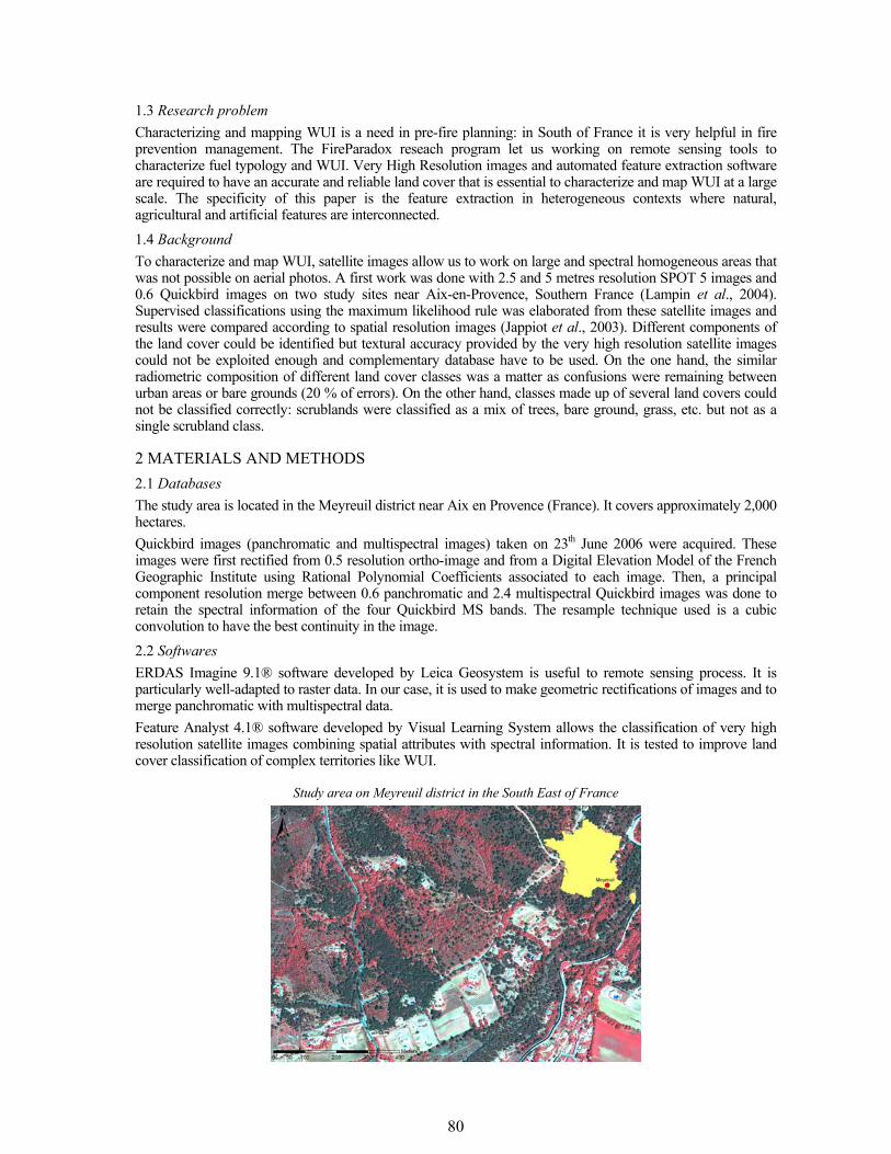
80

1.3 Research problem Characterizing and mapping WUI is a need in pre-fire planning: in South of France it is very helpful in fire prevention management. The FireParadox reseach program let us working on remote sensing tools to characterize fuel typology and WUI. Very High Resolution images and automated feature extraction software are required to have an accurate and reliable land cover that is essential to characterize and map WUI at a large scale. The specificity of this paper is the feature extraction in heterogeneous contexts where natural, agricultural and artificial features are interconnected. 1.4 Background To characterize and map WUI, satellite images allow us to work on large and spectral homogeneous areas that was not possible on aerial photos. A first work was done with 2.5 and 5 metres resolution SPOT 5 images and 0.6 Quickbird images on two study sites near Aix-en-Provence, Southern France (Lampin et al., 2004). Supervised classifications using the maximum likelihood rule was elaborated from these satellite images and results were compared according to spatial resolution images (Jappiot et al., 2003). Different components of the land cover could be identified but textural accuracy provided by the very high resolution satellite images could not be exploited enough and complementary database have to be used. On the one hand, the similar radiometric composition of different land cover classes was a matter as confusions were remaining between urban areas or bare grounds (20 % of errors). On the other hand, classes made up of several land covers could not be classified correctly: scrublands were classified as a mix of trees, bare ground, grass, etc. but not as a single scrubland class.

2 MATERIALS AND METHODS 2.1 Databases The study area is located in the Meyreuil district near Aix en Provence (France). It covers approximately 2,000 hectares. Quickbird images (panchromatic and multispectral images) taken on 23th June 2006 were acquired. These images were first rectified from 0.5 resolution ortho-image and from a Digital Elevation Model of the French Geographic Institute using Rational Polynomial Coefficients associated to each image. Then, a principal component resolution merge between 0.6 panchromatic and 2.4 multispectral Quickbird images was done to retain the spectral information of the four Quickbird MS bands. The resample technique used is a cubic convolution to have the best continuity in the image. 2.2 Softwares ERDAS Imagine 9.1® software developed by Leica Geosystem is useful to remote sensing process. It is particularly well-adapted to raster data. In our case, it is used to make geometric rectifications of images and to merge panchromatic with multispectral data. Feature Analyst 4.1® software developed by Visual Learning System allows the classification of very high resolution satellite images combining spatial attributes with spectral information. It is tested to improve land cover classification of complex territories like WUI.

Study area on Meyreuil district in the South East of France

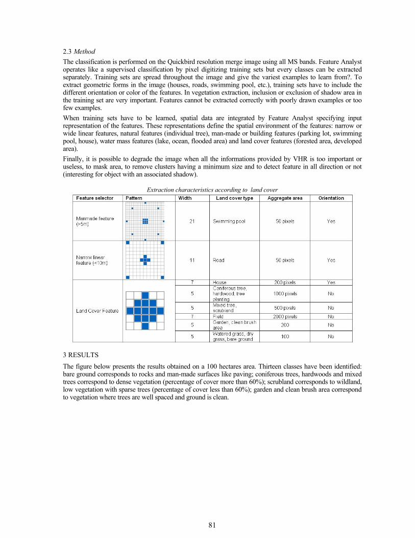
81

2.3 Method The classification is performed on the Quickbird resolution merge image using all MS bands. Feature Analyst operates like a supervised classification by pixel digitizing training sets but every classes can be extracted separately. Training sets are spread throughout the image and give the variest examples to learn from?. To extract geometric forms in the image (houses, roads, swimming pool, etc.), training sets have to include the different orientation or color of the features. In vegetation extraction, inclusion or exclusion of shadow area in the training set are very important. Features cannot be extracted correctly with poorly drawn examples or too few examples. When training sets have to be learned, spatial data are integrated by Feature Analyst specifying input representation of the features. These representations define the spatial environment of the features: narrow or wide linear features, natural features (individual tree), man-made or building features (parking lot, swimming pool, house), water mass features (lake, ocean, flooded area) and land cover features (forested area, developed area). Finally, it is possible to degrade the image when all the informations provided by VHR is too important or useless, to mask area, to remove clusters having a minimum size and to detect feature in all direction or not (interesting for object with an associated shadow).

Extraction characteristics according to land cover

3 RESULTS The figure below presents the results obtained on a 100 hectares area. Thirteen classes have been identified: bare ground corresponds to rocks and man-made surfaces like paving; coniferous trees, hardwoods and mixed trees correspond to dense vegetation (percentage of cover more than 60%); scrubland corresponds to wildland, low vegetation with sparse trees (percentage of cover less than 60%); garden and clean brush area correspond to vegetation where trees are well spaced and ground is clean.

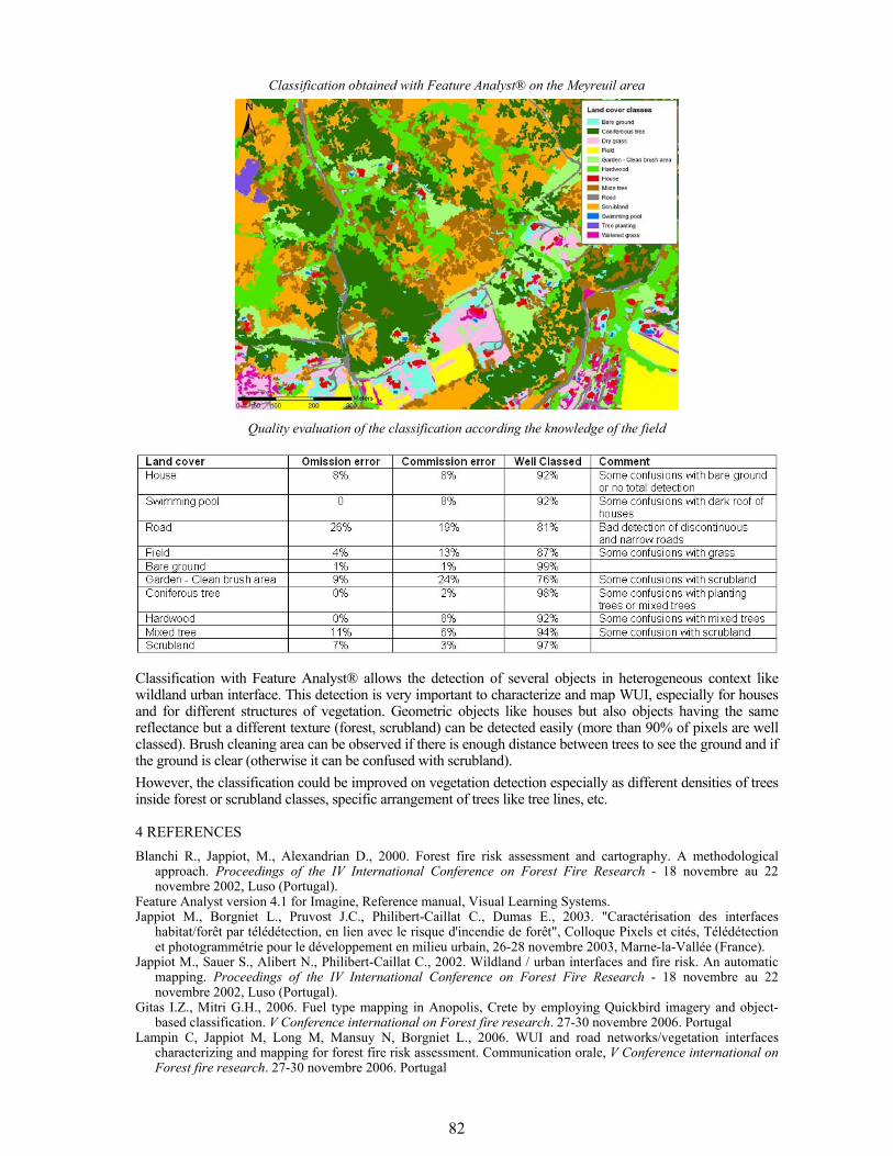
82

Classification obtained with Feature Analyst® on the Meyreuil area

Quality evaluation of the classification according the knowledge of the field

Classification with Feature Analyst® allows the detection of several objects in heterogeneous context like wildland urban interface. This detection is very important to characterize and map WUI, especially for houses and for different structures of vegetation. Geometric objects like houses but also objects having the same reflectance but a different texture (forest, scrubland) can be detected easily (more than 90% of pixels are well classed). Brush cleaning area can be observed if there is enough distance between trees to see the ground and if the ground is clear (otherwise it can be confused with scrubland). However, the classification could be improved on vegetation detection especially as different densities of trees inside forest or scrubland classes, specific arrangement of trees like tree lines, etc.

4 REFERENCES Blanchi R., Jappiot, M., Alexandrian D., 2000. Forest fire risk assessment and cartography. A methodological

approach. Proceedings of the IV International Conference on Forest Fire Research - 18 novembre au 22 novembre 2002, Luso (Portugal).

Feature Analyst version 4.1 for Imagine, Reference manual, Visual Learning Systems. Jappiot M., Borgniet L., Pruvost J.C., Philibert-Caillat C., Dumas E., 2003. "Caractérisation des interfaces

habitat/forêt par télédétection, en lien avec le risque d'incendie de forêt", Colloque Pixels et cités, Télédétection et photogrammétrie pour le développement en milieu urbain, 26-28 novembre 2003, Marne-la-Vallée (France).

Jappiot M., Sauer S., Alibert N., Philibert-Caillat C., 2002. Wildland / urban interfaces and fire risk. An automatic mapping. Proceedings of the IV International Conference on Forest Fire Research - 18 novembre au 22 novembre 2002, Luso (Portugal).

Gitas I.Z., Mitri G.H., 2006. Fuel type mapping in Anopolis, Crete by employing Quickbird imagery and object-based classification. V Conference international on Forest fire research. 27-30 novembre 2006. Portugal

Lampin C, Jappiot M, Long M, Mansuy N, Borgniet L., 2006. WUI and road networks/vegetation interfaces characterizing and mapping for forest fire risk assessment. Communication orale, V Conference international on Forest fire research. 27-30 novembre 2006. Portugal

83

Lampin C., Chandioux O., Paulet V., Jappiot M., 2004. Typologie de la végétation combustible dans les interfaces agriculture - forêt - urbain. Rapport final, Conseil Régional, 116 p.

Mitri G. and Gitas I., 2004. A semi-automated object-oriented model for burned area mapping in the Mediterranean region using Landsat-TM imagery. International Journal of Wildland Fire, 13, 267 – 276.

Rational Polynomial Orthorectification of IKONOS/QuickBird Images, www.microimages.com/documentation/cplates/69rpc.pdf

Sithole G. and Vosselman G., 2006. Bridge detetection in airborne laser scanner data. Journal of photogrammetry and remote sensing, 61, 33 – 46.

Volpe F., Orthorectification of QuickBird basic and standard orthoready data, 2005, Eurimage, http://www.ipi.uni-hannover.de/html/publikationen/2005/workshop/150-volpe.pdf

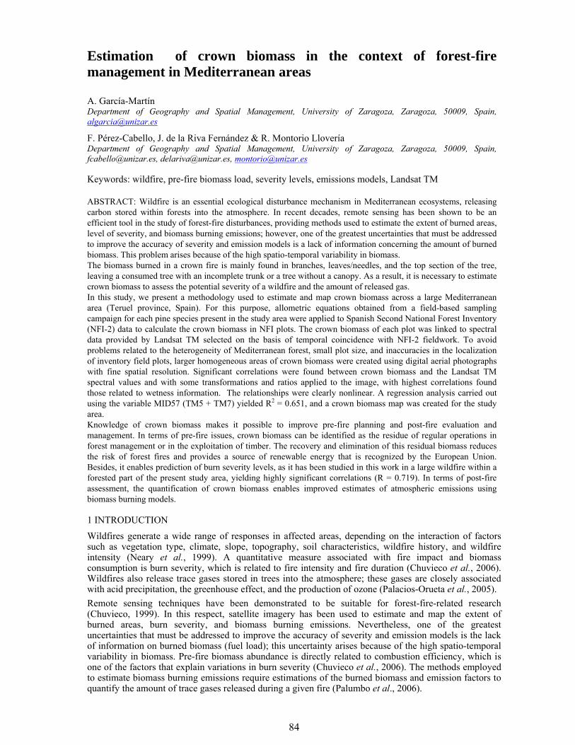
84

1 INTRODUCTION Wildfires generate a wide range of responses in affected areas, depending on the interaction of factors such as vegetation type, climate, slope, topography, soil characteristics, wildfire history, and wildfire intensity (Neary et al., 1999). A quantitative measure associated with fire impact and biomass consumption is burn severity, which is related to fire intensity and fire duration (Chuvieco et al., 2006). Wildfires also release trace gases stored in trees into the atmosphere; these gases are closely associated with acid precipitation, the greenhouse effect, and the production of ozone (Palacios-Orueta et al., 2005). Remote sensing techniques have been demonstrated to be suitable for forest-fire-related research (Chuvieco, 1999). In this respect, satellite imagery has been used to estimate and map the extent of burned areas, burn severity, and biomass burning emissions. Nevertheless, one of the greatest uncertainties that must be addressed to improve the accuracy of severity and emission models is the lack of information on burned biomass (fuel load); this uncertainty arises because of the high spatio-temporal variability in biomass. Pre-fire biomass abundance is directly related to combustion efficiency, which is one of the factors that explain variations in burn severity (Chuvieco et al., 2006). The methods employed to estimate biomass burning emissions require estimations of the burned biomass and emission factors to quantify the amount of trace gases released during a given fire (Palumbo et al., 2006).

Estimation of crown biomass in the context of forest-fire management in Mediterranean areas

A. García-Martín Department of Geography and Spatial Management, University of Zaragoza, Zaragoza, 50009, Spain, [email protected]

F. Pérez-Cabello, J. de la Riva Fernández & R. Montorio Llovería Department of Geography and Spatial Management, University of Zaragoza, Zaragoza, 50009, Spain, [email protected], [email protected], [email protected] Keywords: wildfire, pre-fire biomass load, severity levels, emissions models, Landsat TM

ABSTRACT: Wildfire is an essential ecological disturbance mechanism in Mediterranean ecosystems, releasing carbon stored within forests into the atmosphere. In recent decades, remote sensing has been shown to be an efficient tool in the study of forest-fire disturbances, providing methods used to estimate the extent of burned areas, level of severity, and biomass burning emissions; however, one of the greatest uncertainties that must be addressed to improve the accuracy of severity and emission models is a lack of information concerning the amount of burned biomass. This problem arises because of the high spatio-temporal variability in biomass. The biomass burned in a crown fire is mainly found in branches, leaves/needles, and the top section of the tree, leaving a consumed tree with an incomplete trunk or a tree without a canopy. As a result, it is necessary to estimate crown biomass to assess the potential severity of a wildfire and the amount of released gas. In this study, we present a methodology used to estimate and map crown biomass across a large Mediterranean area (Teruel province, Spain). For this purpose, allometric equations obtained from a field-based sampling campaign for each pine species present in the study area were applied to Spanish Second National Forest Inventory (NFI-2) data to calculate the crown biomass in NFI plots. The crown biomass of each plot was linked to spectral data provided by Landsat TM selected on the basis of temporal coincidence with NFI-2 fieldwork. To avoid problems related to the heterogeneity of Mediterranean forest, small plot size, and inaccuracies in the localization of inventory field plots, larger homogeneous areas of crown biomass were created using digital aerial photographs with fine spatial resolution. Significant correlations were found between crown biomass and the Landsat TM spectral values and with some transformations and ratios applied to the image, with highest correlations found those related to wetness information. The relationships were clearly nonlinear. A regression analysis carried out using the variable MID57 (TM5 + TM7) yielded R2 = 0.651, and a crown biomass map was created for the study area. Knowledge of crown biomass makes it possible to improve pre-fire planning and post-fire evaluation and management. In terms of pre-fire issues, crown biomass can be identified as the residue of regular operations in forest management or in the exploitation of timber. The recovery and elimination of this residual biomass reduces the risk of forest fires and provides a source of renewable energy that is recognized by the European Union. Besides, it enables prediction of burn severity levels, as it has been studied in this work in a large wildfire within a forested part of the present study area, yielding highly significant correlations (R = 0.719). In terms of post-fire assessment, the quantification of crown biomass enables improved estimates of atmospheric emissions using biomass burning models.

85

In employing the complete-tree concept introduced by Young et al. (1964) to define the biomass components of trees, the tree biomass consumed in a crown fire is mainly found in foliage, branches, and the unmerchantable stem top, leaving a consumed tree with an incomplete trunk or a tree without a canopy (Palumbo et al., 2006). As a result, it is necessary to estimate crown biomass to assess the potential burn severity and the amount of trace gases released during a crown wildfire. The estimation of biophysical variables is one of the most successful lines of research in forestry-related applications of remote sensing. Several previous works in this field of research focus on aboveground biomass estimation (AGB) using Landsat images (Lu, 2006), although few reports concentrate on Mediterranean areas. AGB cannot be directly measured from satellite images, even though the reflectance provided by such images can be related to AGB estimated from fieldwork (Dong et al., 2003). The same principle can be applied to the crown biomass. In the context of the above framework, the current paper presents a methodology used to estimate and map crown biomass in the pine forests of a large Mediterranean area (Teruel province, Spain). To achieve this objective, specific crown-biomass regressions for each pine species in the study area were applied to Spanish Second National Forest Inventory (NFI-2) data to determine the crown biomass in NFI-2 plots. To avoid problems related to the heterogeneity of Mediterranean forest and spatial inaccuracies in plots, larger homogeneous areas of crown biomass based on NFI-2 plots were created using digital aerial photographs with fine spatial resolution. Finally, to test the capacity to predict burn severity, crown biomass estimations were correlated with burn severity values calculated for a wildfire that took place in the study area 1 month after the time that the estimations were made.

2 STUDY AREA

The study area is the province of Teruel (14,804 km2), northeast Spain (Figure 1). From a biogeographical viewpoint, all of the territory lies in the Mediterranean Region, and 27% is forested land. The distribution of these forests is non-uniform: most of the forested areas are concentrated in the Iberian ranges, being mainly pine forests (total of 235,431 ha of pine forest in 1994) (MMA, 1996). The four pine species present in the study area are Pinus sylvestris, Pinus halepensis, Pinus nigra, and Pinus pinaster. The analyzed wildfire occurred in the Maestrazgo region (northeast of the study area) from the 2nd to the 8th of July 1994. The fire affected a forested area of 16,000 ha, mainly covered by Pinus halepensis and to a much lesser degree Quercus ilex rotundifolia.

Figure 1. Study area

3 MATERIALS AND METHODS 3.1 Crown biomass data In calculating the crown biomass in each plot for 1994, specific crown-biomass regressions for each pine species in the study area were applied to NFI-2 data for the same year. These regressions were developed in the context of the LIGNOSTRUM project, based on destructive field-based sampling. The total number of sampled trees was 186 (30 of P. sylvestris, 59 of P. halepensis, 57 of P. nigra, and 40 of P. pinaster). The wet weight of the crown biomass was obtained using a balance with an accuracy of 250 grams. Two size measurements were taken for each sampled tree: Diameter at Breast Height (DBH) and height. It was necessary to collect samples of leaves and branches to calculate the dry weight. Finally, a regression equation was obtained for each species with a coefficient of regression above 0.90. Further details are provided in Alonso et al. (2005). The 1994 NFI-2 involved the systematic field sampling of permanent plots located in the corners of the UTM grid present in the 1:50,000 National Topographic Cartography. The placement of plots in the field was performed using georeferenced 1:30,000 aerial photographs and topographic cartography. Plots have

Provinceof Teruel

Maestrazgo wildfire

Provinceof Teruel

Maestrazgo wildfire

86

a circular shape, with radii ranging from 5 to 25 m depending on the DBH of the trees. The NFI-2 fieldwork in Teruel was undertaken from March to August 1994. DBH and total height were measured for all trees. A detailed description of NFI-2 is provided in the summary report of the inventory (MMA, 1996). In applying the crown biomass equations, we only chose those plots in which pines fell within the range utilized in the specific equations. The equations were applied to every tree in every plot, and the calculated crown biomass of each plot was expressed in tons/ha. To avoid complexity in the spectral data, only mono-species plots were selected (482). 3.2 Selection of images and pre-processing This study made use of Landsat 5 TM images recorded on 10 June 1994 and 16 August 1994 (Path 131/Row 32). The earlier image was selected on the basis of its temporal coincidence with NFI-2 fieldwork, while the later image was selected because of its timing just several weeks after the large wildfire that took place in the northeast part of the study area at the beginning of July 1994. The first image was used to estimate crown biomass across all of the study area; both images were used to estimate the burn severity of the wildfire. Pre-processing techniques were applied to both images. The images were geometrically rectified into a local UTM projection using a second-order polynomial model, yielding a Root Mean Square Error (RMSE) of less than 1 pixel. The Minnaert Correction method was applied to both images to negate atmospheric and topographic effects. Finally, several transformations and ratios were applied to the transformed June image to increase the amount of spectral information. 3.3 Relating crown biomass ground data to June Landsat data Previous studies have documented the difficulties involved in estimating forest parameters for Mediterranean areas using a Landsat TM image (e.g., Salvador and Pons, 1998). These problems are related to the heterogeneity of Mediterranean forest, small plot size, inaccuracies in the localization of inventory field plots, and the small number of plots used in the analysis. Correlations have been demonstrated despite these limitations; however, they are insufficient in terms of establishing prediction models. To overcome these problems, we applied a methodology based on the use of high-resolution aerial photographs. This approach has been shown to be useful in forest-inventory applications (Lu, 2006). A composite digital aerial photograph of Teruel province (1 m spatial resolution) was used to extend the plot areas to larger sizes of visually similar composition and forest structure. This was performed using an on-screen digitizing technique within a GIS application. The selected NFI-2 plots were displayed over the composite digital aerial photograph. Where possible, we then identified larger homogeneous areas containing the in situ plots. Each newly delineated homogeneous area was assigned a quality value. These values indicate the quality of the defined areas in terms of the degree of similarity between observations made from the aerial photograph of the NFI-2 plot and the newly delimited area (0 = impossible to define; 1= low quality; 2 = medium quality; 3 = high quality). Finally, these areas were linked to spectral data. 3.4 Mapping burn severity To determine the burn severity of the wildfire, Normalized Burn Ratio (NBR) was calculated for both pre-fire (June) and post-fire (August) periods. The post-fire NBR was subtracted from pre-fire NBR to obtain the change image (dNBR) (Key and Benson, 2006). 3.5 Statistical approach to estimating crown biomass and a test of its capacity to predict burn severity To explore the nature of the relationships among crown biomass and the June TM bands and derived spectral variables, we analyzed an individual scatter plot for each pair. The type of relationship controls the subsequent regression model. The performance of the model was evaluated based on the coefficient of determination, the Mean Absolute Error (MAE), and RMSE. To test the capacity of the adopted approach in predicting burn severity, we studied the correlation between crown biomass estimated before the wildfire and burn severity values.

4 RESULTS 4.1 Estimation of crown biomass The scatter plots that compare crown biomass and spectral variables show nonlinear relationships; consequently, Spearman’s correlation coefficient was used to evaluate these relationships. Correlation values were higher for areas defined as being of higher quality. For all three categories of quality, the spectral variables related to wetness recorded the highest coefficients of correlation, with the most

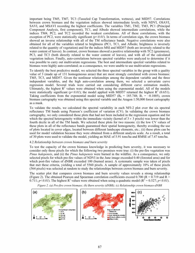
87

important being TM5, TM7, TC3 (Tasseled Cap Transformation, wetness), and MID57. Correlations between crown biomass and the vegetation indices showed intermediate levels, with NDVI, OSAVI, SAVI, and MSAVI recording the highest coefficients. The variables TM1, TM2, TM3, PC1 (Principal Component Analysis, first component), TC1, and Albedo showed intermediate correlations, while the indices TM4, PC2, and TC2 recorded the weakest correlations. All of these correlations, with the exception of PC2, were statistically significant (p<0.01). In terms of correlation sign, the crown biomass showed an inverse relationship with all of the TM reflectance bands. Negative correlations were also obtained for all of the variables related to brightness (PC1, TC1, and Albedo; brightness is inversely related to the quantity of vegetation) and for the indices MSI and MID57 (both are inversely related to the water content of leaves). In contrast, crown biomass showed a positive relationship with TC2 (greenness), PC3, and TC3 (both directly related to the water content of leaves), and with all of the calculated vegetation indices. Finally, auto-correlations between spectral variables were analyzed to determine if it was possible to carry out multivariate regressions. The best and intermediate spectral variables related to biomass were highly auto-correlated; as a consequence, we were unable to use multivariate regressions. To identify the best predictive model, we selected the three spectral variables in the group with a quality value of 3 (made up of 131 homogeneous areas) that are most strongly correlated with crown biomass: TM5, TC3, and MID57. Given the nonlinear relationships among the dependent variable and the three independent variables, and the high auto-correlation among them, we selected a univariate curve regression model. Several trials were carried out considering different curve estimation models. Ultimately, the highest R2 values were obtained when using the exponential model. All of the models were statistically significant (p<0.01); the model applied with MID57 returned the highest R2 (0.651). Taking coefficients from the exponential model using MID57 (B0 = 185.748; B1 = –0.1005), crown biomass cartography was obtained using this spectral variable and the Aragon 1:50,000 forest cartography as a mask. To validate the results, we calculated the spectral variability in each NFI-2 plot over the six spectral reflectance TM bands using Pearson’s coefficient of variation (CV). In validating the crown biomass cartography, we only considered those plots that had not been included in the regression equation and for which the spectral heterogeneity within the immediate vicinity (kernel of 3 × 3 pixels) was lower than the fourth decile in all of the TM bands. We selected these plots for two reasons: (i) the low CV values of these plots in all of the reflectance bands guaranteed their spatial homogeneity, thereby avoiding the use of plots located in cover edges, located between different landscape elements, etc.; (ii) these plots can be used for model validation because they were obtained from a different analysis scale. As a result, a total of 30 plots were used to validate the model, yielding an MAE of 5.91 tons/ha and RMSE of 7.47 tons/ha. 4.2 Relationship between crown biomass and burn severity To test the capacity of the crown biomass knowledge in predicting burn severity, it was necessary to consider only those pixels for which the following two premises were true: (i) the pre-fire vegetation was Pinus halepensis, and (ii) the Pinus halepensis were burned in the wildfire. As a consequence, we only selected pixels for which pre-fire values of NDVI in the June image exceeded 0.40 (forested area) and for which post-fire values of dNBR exceeded 100 (burned areas). A systematic sample was taken of pixels that met these criteria, yielding a total of 5560 pixels. A sample of approximately 10% of these pixels (564 pixels) was selected at random to study the relationships between crown biomass and burn severity. The scatter plot that compares crown biomass and burn severity values reveals a strong relationship (Figure 2). The obtained Pearson and Spearman correlation coefficients exceed 0.700 (R = 0.719 and R = 0.711; p<0.01). The highest R2 values were obtained when using a quadratic model (R2 = 0.527; p<0.01).

Figure 2. (a) Pre-fire crown biomass; (b) Burn severity (dNBR); (c) Relationship crown biomass-dNBR

(a) (b) (c)(a) (b) (c)

88

5 DISCUSSION AND CONCLUSIONS This work demonstrates the utility of Landsat TM images and NFI data in estimating crown biomass in Mediterranean areas. Such information can be useful in terms of both pre-fire and post-fire issues. Regarding pre-fire issues, knowledge of crown biomass can help to overcome the lack of information on forest residual biomass, for which its use as an energy source helps to reduce the risk of wildfires (García-Martín et al., 2006). Besides, it has been shown that knowledge of crown biomass enables the prediction of burn severity levels. In post-fire issues, although it has not been considered in this work, the quantification of crown biomass enables improved estimates of atmospheric emissions via biomass burning models. The remaining errors in estimates of crown biomass can be attributed to the following factors: (i) inaccuracies in the fieldwork undertaken to establish the allometric equations; (ii) limitations related to the spectral, radiometric, and spatial resolution of the TM sensor; (iii) problems involved in relating NFI plots to satellite data; (iv) inaccuracies related to heterogeneity, despite the efforts made to combat this problem.

6 ACKNOWLEDGEMENTS

This research has been supported by a grant provided by the Ministry of Science and Technology (AP2003-3097) and the projects AGL2002-03917-CGL2005-04863/CLI and PIR_FIRE (PIP098/2005).

7 REFERENCES Alonso, E., Asín, J., Pascual, J. 2005. Biomasa residual forestal: regresiones para las especies del género Pinus

existentes en la provincia de Teruel. In Sociedad Española de Ciencias Forestales (Ed.) La ciencia forestal: respuestas para la sostenibilidad. 4º Congreso Forestal Español. Zaragoza, Sociedad Española de Ciencias Forestales.

Chuvieco, E. (Ed.). 1999. Remote sensing of large wildfires in the European Mediterranean Basin. Heidelberg, Spinger.

Chuvieco, E., Riaño, D., Danson, F.M., Martín, P. 2006. Use of a radiative transfer model to simulate the postfire spectral response to burn severity. Journal of Geophysical Research 111, G04S09, doi:10.1029/2005JG000143.

Dong, J., Kaufmann, R.K., Myneni, R.B., Tucker, C.J., Kauppi, P., Liski, J., Buermann, W., Alexeyev, V., Hughes, M.K. 2003. Remote sensing estimates of boreal and temperate forest woody biomass: Carbon pools, sources, and sinks. Remote Sensing of Environment 84: 393-410.

García-Martín, A., Pérez-Cabello, F., de la Riva Fernández, J. 2006. Evaluación de los recursos de biomasa residual forestal mediante imágenes del satélite Landsat y SIG. GeoFocus 6: 205-230.

Key, C.H., Benson, N. 2006. Landscape assessment. Sampling and analysis methods. USDA Forest Service. General Technical Report. RMRS-GTR-164-CD.

Lu, D. 2006. The potential and challenge of remote sensing-based biomass estimation. International Journal of Remote Sensing 27: 1297-1328.

MMA. 1996. Segundo Inventario Forestal Nacional (1986-1995): Aragón, Teruel. Madrid, MMA. Neary, D.G., Klopatek, C.C, DeBano, F.F., Folliott, P.F. 1999. Fire effects on belowground sustainability: a review

and synthesis. Forest Ecology and Management 122: 51-71. Palacios-Orueta, A., Chuvieco, E., Parra, A., Carmona-Moreno, C. 2005. Biomass burning emissions: a review of

models using Remote-Sensing data. Environmental Monitoring and Assessment 104: 189-209. Palumbo, I., Kucera, J., Barbosa, P., O’Brien, V.W. and Valentín, R. 2006. Using SEVIRI geostationary imagery for

active fires análisis and burned biomass estimation: a case study in a Mediterranean ecosystem. In Viegas, D.X. (Ed.) Proceedings of V Internacional Conference on Forest Fire Research. University of Coimbra [CD-Rom].

Salvador, R., Pons, X. 1998. On the applicability of Landsat TM images to Mediterranean forest inventories. Forest Ecology and Management 104: 193-208.

Young, H.E., Strand, L., Altenberger, R. 1964. Preliminary fresh and dry weigh tables for seven tree species in Maine. In Richardson, J., Björheden, R., Hakkila, P., Lowe, A.T., Smith C.T. (Eds.) 2002. Bioenergy from Sustainable Forestry: Guiding Principles and Practice. Forestry Sciences Vol. 71. Dordrecht, Kluwer Academic Publishers.

89

1 INTRODUCTION Live Fuel Moisture Content (LFMC) is a key variable to estimate forest fire danger since it is highly related to fire propagation and fire intensity. Thus, vegetation will act as a heat sink or as a heat source depending on its water content (Ceccato et al., 2003). Among the methods used to estimate LFMC, field sampling constitutes the most direct method however it is difficult to assure a representative sample both temporally and spatially. Meteorological indices are widely used in fire danger rating systems (Viegas et al., 1994; Camia et al., 1999), nevertheless they are spatially limited. In this sense, methods relying on remote sensing data can provide information at a spatial and temporal scale to be used operatively. NDVI derived from NOAA/AVHRR imagery has been successfully used to estimate LFMC for herbaceous species (Chladil y Nunez, 1995; Paltridge and Barber, 1988), however worse results have been found when applied to shrubs and trees (Chuvieco et al., 1999; Hardy and Burgan, 1999) since the LFMC-NDVI relationship for grasslands is related to the chlorophyll activity whilst for shrubs this relation is affected by other variables such as variation in the Leaf Area Index (LAI), viewing and illumination geometry, or background reflectance. Some authors have proposed indices based on the water absorption characteristics, using the short wave infrared region, which was proven to be the most sensitive to water content variations (Danson and Bowyer, 2004; Gao, 1996; Ceccato et al., 2002). Other authors combined spectral indices with thermal data to estimate LFMC (Alonso et al., 1996; Chuvieco et al., 2004). This paper revises the equations proposed by Chuvieco et al. (2004), considering dry/wet years in order to avoid the overestimation found when applying them to dry years, and it presents LFMC_anomalies for AVHRR time series imagery.

2 METHODS Images were acquired by the NOAA/AVHRR receiving station installed at the Department of Geography of the University of Alcalá. Raw data were converted into reflectance using NOAA coefficients (including degradation rates) and surface temperature (ST) was calculated applying the method proposed by Coll and Caselles (1997). Subsequently, images were navigated using orbital models, and

Estimation of Live Fuel Moisture Content Anomalies in central Spain derived from AVHRR time series imagery

M. García Department of Geography, University of Alcalá, Alcalá de Henares, Madrid, Spain. [email protected]

I. Aguado & E. Chuvieco Department of Geography, University of Alcalá, Alcalá de Henares, Madrid, Spain. [email protected], [email protected] Keywords: Life Fuel Moisture Content (LFMC), NOAA/AVHRR, MVC-TB(AVHRR/Ch4), LFMC_ Anomalies

ABSTRACT: Estimation of Live Fuel Moisture Content (LFMC) is an important variable within a fire danger rating system and in fire risk analysis. LFMC is critical both, in fire ignition and fire propagation since vegetation will act as a heat sink or as a heat source depending on its water content. The NOAA/AVHRR sensor provides data at required spatial and temporal scales to estimate LFMC. 8-day Maximum Brightness Temperature Value Composites (MVC-TB/Ch4) were created to solve cloud contamination and to reduce residual atmospheric effects. Two types of years were considered (dry/wet) based on a simple drought index, and a temporal variable was fitted to the LFMC field measurements to take into account its seasonal trends. LFMC was estimated from 1996 to 2005, using an empirical model fitted for grassland and shrubland using NDVI, TS and a function of the day of the year. Determination coefficients of 0.85 and 0.81 were obtained for Grassland and C. Ladanifer. The Corine Land Cover 2000 was used to mask these covers from forested and non vegetated areas. LFMC-anomalies were computed considering the deviation of FMC values for each year from a mean value for the whole period considered. This anomaly-value may help to improve the fire danger estimation provided by the LFMC value for a given date since it will reflects the interannual variation of the vegetation status, pointing out areas and periods of higher fire danger related to a mean LFMC value.

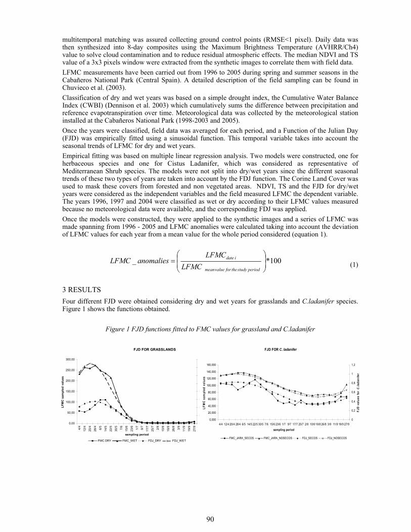
90

multitemporal matching was assured collecting ground control points (RMSE<1 pixel). Daily data was then synthesized into 8-day composites using the Maximum Brightness Temperature (AVHRR/Ch4) value to solve cloud contamination and to reduce residual atmospheric effects. The median NDVI and TS value of a 3x3 pixels window were extracted from the synthetic images to correlate them with field data. LFMC measurements have been carried out from 1996 to 2005 during spring and summer seasons in the Cabañeros National Park (Central Spain). A detailed description of the field sampling can be found in Chuvieco et al. (2003). Classification of dry and wet years was based on a simple drought index, the Cumulative Water Balance Index (CWBI) (Dennison et al. 2003) which cumulatively sums the difference between precipitation and reference evapotranspiration over time. Meteorological data was collected by the meteorological station installed at the Cabañeros National Park (1998-2003 and 2005). Once the years were classified, field data was averaged for each period, and a Function of the Julian Day (FJD) was empirically fitted using a sinusoidal function. This temporal variable takes into account the seasonal trends of LFMC for dry and wet years. Empirical fitting was based on multiple linear regression analysis. Two models were constructed, one for herbaceous species and one for Cistus Ladanifer, which was considered as representative of Mediterranean Shrub species. The models were not split into dry/wet years since the different seasonal trends of these two types of years are taken into account by the FDJ function. The Corine Land Cover was used to mask these covers from forested and non vegetated areas. NDVI, TS and the FJD for dry/wet years were considered as the independent variables and the field measured LFMC the dependent variable. The years 1996, 1997 and 2004 were classified as wet or dry according to their LFMC values measured because no meteorological data were available, and the corresponding FDJ was applied. Once the models were constructed, they were applied to the synthetic images and a series of LFMC was made spanning from 1996 - 2005 and LFMC anomalies were calculated taking into account the deviation of LFMC values for each year from a mean value for the whole period considered (equation 1).

(1)

3 RESULTS Four different FJD were obtained considering dry and wet years for grasslands and C.ladanifer species. Figure 1 shows the functions obtained.

Figure 1 FJD functions fitted to FMC values for grassland and C.ladanifer

100*_ ⎟⎟⎠

⎞⎜⎜⎝

⎛=

periodstudytheforvaluemean

idate

LFMCLFMC

anomaliesLFMC

FJD FOR GRASSLANDS

0,00

50,00

100,00

150,00

200,00

250,00

300,00

4/4

12/4

20/4

28/4 6/5

14/5

22/5

30/5 7/6

15/6

23/6 1/7

9/7

17/7

25/7 2/8

10/8

18/8

26/8 3/9

11/9

19/9

27/9

sampling period

LFM

C sa

mpl

ed v

alue

s

0

0,2

0,4

0,6

0,8

1

1,2

1,4

1,6

FJD

valu

es fo

r gra

ssla

nds

FMC DRY FMC_WET FDJ_DRY FDJ_WET

FJD FOR C. ladanifer

0,000

20,000

40,000

60,000

80,000

100,000

120,000

140,000

160,000

4/4 12/4 20/4 28/4 6/5 14/5 22/5 30/5 7/6 15/6 23/6 1/7 9/7 17/7 25/7 2/8 10/8 18/8 26/8 3/9 11/9 19/9 27/9

sampling period

LFM

C sa

mpl

ed v

alue

s

0

0,2

0,4

0,6

0,8

1

1,2

FJD

valu

es fo

r C.

lada

nife

r

FMC_JARA_SECOS FMC_JARA_NOSECOS FDJ_SECOS FDJ_NOSECOS

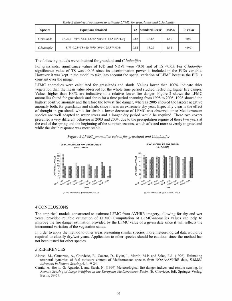
91

Table 2 Empirical equations to estimate LFMC for grasslands and C.ladanifer

Species Equations obtained r2 Standard Error RMSE P-Valor

Grasslands 27.95-1.194*TS+331.865*NDVI+115.514*FDJg 0.85 36.88 42.01 <0.01

C.ladanifer 8.73-0.23*TS+40.79*NDVI+125.87*FDJs 0.81 13.27 15.11 <0.01

The following models were obtained for grassland and C.ladanifer: For grasslands, significance values of FJD and NDVI were <0.01 and of TS <0.05. For C.ladanifer significance value of TS was >0.05 since its discrimination power is included in the FJDs variable. However it was kept in the model to take into account the spatial variation of LFMC because the FJD is constant over the image. LFMC anomalies were calculated for grasslands and shrub. Values lower than 100% indicate drier vegetation than the mean value observed for the whole time period studied, reflecting higher fire danger. Values higher than 100% are indicative of a relative lower fire danger. Figure 2 shows the LFMC anomalies found for grasslands and shrub for a time period spanning from 1998 to 2005. 1998 showed the highest positive anomaly and therefore the lowest fire danger, whereas 2005 showed the largest negative anomaly both, for grasslands and shrub, since it was an extremely dry year. Especially clear is the effect of drought in grasslands while for shrub a lower decrease of LFMC was observed since Mediterranean species are well adapted to water stress and a longer dry period would be required. These two covers presented a very different behavior in 2003 and 2004, due to the precipitation regime of these two years at the end of the spring and the beginning of the summer seasons, which affected more severely to grassland while the shrub response was more stable.

Figure 2 LFMC_anomalies values for grassland and C.ladanifer

4 CONCLUSIONS The empirical models constructed to estimate LFMC from AVHRR imagery, allowing for dry and wet years, provided reliable estimation of LFMC. Computation of LFMC-anomalies values can help to improve the fire danger estimation provided by the LFMC value of a given date since it will reflects the interannual variation of the vegetation status. In order to apply the method to other areas presenting similar species, more meteorological data would be required to classify dry/wet years. Application to other species should be cautious since the method has not been tested for other species.

5 REFERENCES Alonso, M., Camarasa, A., Chuvieco, E., Cocero, D., Kyun, I., Martín, M.P. and Salas, F.J., (1996). Estimating

temporal dynamics of fuel moisture content of Mediterranean species from NOAA/AVHRR data, EARSEL Advances in Remote Sensing.4, 4, 9-24.

Camia, A; Bovio, G; Aguado, I. and Stach, N. (1999) Meteorological fire danger índices and remote sensing. In Remote Sensing of Large Wildfires in the European Mediterranean Basin. (E. Chuvieco, Ed), Springer-Verlag, Berlin, 39-59.

020406080

100120140160180200

LFM

C AN

OM

ALY

VALU

E

ALFMC_1998

ALFMC_1999

ALFMC_2000

ALFMC_2001

ALFMC_2002

ALFMC_2003

ALFMC_2004

ALFMC_2005

YEAR

LFMC ANOMALIES FOR GRASSLANDS (10-17 JUNE)

LFMC ANOMALIES MEAN LFMC VALUE

0

20

40

60

80

100

120

LFM

C AN

OM

ALY

VAL

UE

ALFMC_1998

ALFMC_1999

ALFMC_2000

ALFMC_2001

ALFMC_2002

ALFMC_2003

ALFMC_2004

ALFMC_2005

YEAR

LFMC ANOMALIES FOR SHRUB(10-17 JUNE)

LFMC ANOMALIES MEAN LFMC VALUE

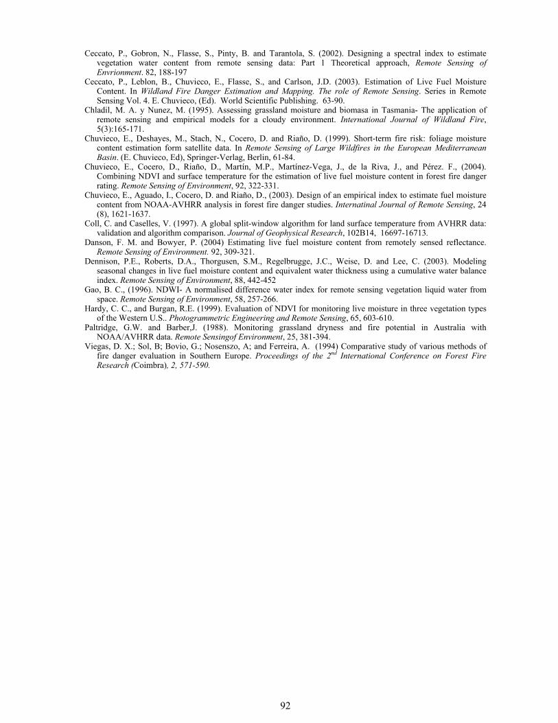
92

Ceccato, P., Gobron, N., Flasse, S., Pinty, B. and Tarantola, S. (2002). Designing a spectral index to estimate vegetation water content from remote sensing data: Part 1 Theoretical approach, Remote Sensing of Envrionment. 82, 188-197

Ceccato, P., Leblon, B., Chuvieco, E., Flasse, S., and Carlson, J.D. (2003). Estimation of Live Fuel Moisture Content. In Wildland Fire Danger Estimation and Mapping. The role of Remote Sensing. Series in Remote Sensing Vol. 4. E. Chuvieco, (Ed). World Scientific Publishing. 63-90.

Chladil, M. A. y Nunez, M. (1995). Assessing grassland moisture and biomasa in Tasmania- The application of remote sensing and empirical models for a cloudy environment. International Journal of Wildland Fire, 5(3):165-171.

Chuvieco, E., Deshayes, M., Stach, N., Cocero, D. and Riaño, D. (1999). Short-term fire risk: foliage moisture content estimation form satellite data. In Remote Sensing of Large Wildfires in the European Mediterranean Basin. (E. Chuvieco, Ed), Springer-Verlag, Berlin, 61-84.

Chuvieco, E., Cocero, D., Riaño, D., Martín, M.P., Martínez-Vega, J., de la Riva, J., and Pérez. F., (2004). Combining NDVI and surface temperature for the estimation of live fuel moisture content in forest fire danger rating. Remote Sensing of Environment, 92, 322-331.

Chuvieco, E., Aguado, I., Cocero, D. and Riaño, D., (2003). Design of an empirical index to estimate fuel moisture content from NOAA-AVHRR analysis in forest fire danger studies. Internatinal Journal of Remote Sensing, 24 (8), 1621-1637.

Coll, C. and Caselles, V. (1997). A global split-window algorithm for land surface temperature from AVHRR data: validation and algorithm comparison. Journal of Geophysical Research, 102B14, 16697-16713.

Danson, F. M. and Bowyer, P. (2004) Estimating live fuel moisture content from remotely sensed reflectance. Remote Sensing of Environment. 92, 309-321.

Dennison, P.E., Roberts, D.A., Thorgusen, S.M., Regelbrugge, J.C., Weise, D. and Lee, C. (2003). Modeling seasonal changes in live fuel moisture content and equivalent water thickness using a cumulative water balance index. Remote Sensing of Environment, 88, 442-452

Gao, B. C., (1996). NDWI- A normalised difference water index for remote sensing vegetation liquid water from space. Remote Sensing of Environment, 58, 257-266.

Hardy, C. C., and Burgan, R.E. (1999). Evaluation of NDVI for monitoring live moisture in three vegetation types of the Western U.S.. Photogrammetric Engineering and Remote Sensing, 65, 603-610.

Paltridge, G.W. and Barber,J. (1988). Monitoring grassland dryness and fire potential in Australia with NOAA/AVHRR data. Remote Sensingof Environment, 25, 381-394.

Viegas, D. X.; Sol, B; Bovio, G.; Nosenszo, A; and Ferreira, A. (1994) Comparative study of various methods of fire danger evaluation in Southern Europe. Proceedings of the 2nd International Conference on Forest Fire Research (Coimbra), 2, 571-590.

93

1 INTRODUCTION The estimation of the total biomass of a forest is an element of great importance to determine the existing amount of carbon available and other chemical elements in each of its components. (Schlegel et al., 2000). On the other hand, the aerial biomass is a very important component due to its interest when it comes to learning about the distribution of nutrients in the ground, as well as to determine the fuel accumulation (Lu, 2005). It is also important in the field of forest fires, because it is a key factor in elaborating risk models, as well as for the obtaining fuel models used in the modelling of fire propagation of the fire (French et al., 2000). At leaf level the estimation of the contents of dry foliage matter (Cm) is the first step to determine the foliar biomass of the arboreal canopy (product of LAI and the leaf’s Cm). On the other hand, the content of dry foliage matter is a crucial parameter in the estimation of the humidity content of the vegetation (Riaño, et al., 2005), and serves as an indicator of the stress and growth of the plants (Jacquemoud et al., 1996). Among the methods used to estimate foliar biomass one can find the models of reflectivity, which allow estimating the reflectivity of a vegetal cover from a series of entrance variables. In addition, only the models based on the theory of the radiative transference can be inverted by means of iterative methods with the purpose of providing relevant information on the biochemical or anatomical components of the vegetation (Gemmel et al., 2002).

Evaluation of dry foliage matter through normalised indexes and inversion of reflectivity models

A. Romero Departamento de Geografía, Universidad Alcalá de Henares, Alcalá de Henares,, CP 28007, España, [email protected]

I. Aguado, E. Chuvieco & M. Yebra Departamento de Geografía, Universidad Alcalá de Henares, Alcalá de Henares,, CP 28007, España ,[email protected], [email protected], [email protected]. Keywords: dry matter, biomass, normalised indexes, reflectivity models.

ABSTRACT: This research evaluates the contents of dry foliage matter of forest species through teledetection methods, aimed at the use of this parameter in fire risk models and/or evaluation of woodland biomass. The data used comes from the Leaf Optical Properties Experiment 93 (LOPEX 93) database, provided by the Joint Research Centre, Institute for Remote Sensing Applications of Ispra, Italy. This research essay is developed in two parts. The first one gives a Normalised Index in order to evaluate the contents of dry foliage matter, taking into account the biophysical and biochemical factors that intervene in the process. By means of an exploratory analysis, we selected the wave longitudes that were most sensible to the dry matter’s contents and that minimized the effect of other biophysical and biochemical parameters. In the second part of this research, the contents of dry foliage matter is evaluated by inverting the PROSPECT reflectivity model, using all biophysical and biochemical parameters and selecting the inverted parameter that is most related to the contents of the dry matter. Of a total of 11 species, 5 samples of fresh leaves were taken to determine its biochemical components. The dry samples were taken by drying the fresh samples, to re-evaluate the previously mentioned parameters, except for the “leaf internal structure” parameter, which was calculated through an inversion of the PROSPECT model. The relationship between the data of the created index (R2305-R1495)/(R2305+R1495) and the contents of the dry matter from LOPEX93 database offers an overall r2= 0.67 for fresh and dry samples. On the other hand, the adjustment degree between the LOPEX93 values and those estimated using this equation report a Pearson coefficient of 0.79 for both types of samples; 0.83 for fresh samples and 0.87 for dry ones. With respect to the use of inversion of the PROSPECT model, this relationship reduces to a Pearson coefficient of 0.71 (fresh and dry samples) using all biophysical and biochemical parameters. As a result of this research, it is considered that both methods are valid to evaluate dry foliage matter. However, the evaluation of the contents of dry matter using the (R2305-R1495)/(R2305+R1495) index requires the existence of reflectivity in both wave longitudes. This condition limits it to be valid only for studies in which one has a laboratory spectrometry and/or hyperspectral sensors. However, the inversion of the PROSPECT model can be used when one does not has laboratory measurements or hyperspectral sensors. On the other hand, we recommend a validation of the proposed index for other forest species, and even for agricultural species

94

The PROSPECT model proposed by Jacquemoud and Baret (1990) is one of the most used at the leaf level, based on Allen’s lamina model, which represents the optical properties of the leaves between 400 - 2500 nm, obtaining the reflectivity and transmissivity from the following parameters: internal structure of the leaf (N), chlorophyll a+b (Cab, gμ /cm2), the equivalent water thickness (EWT) expressed in (g/cm2) and the content of dry matter (Cm, g/cm2). The studies that have used the PROSPECT model applied to the estimation of the Cm in forest species indicate a high variation of the contents of dry matter among species (Riaño et al. 2005). This research is aimed at estimating the contents of dry foliar matter in different forest species or of forest interest, from normalised indexes and inversion of the radiative transfer PROSPECT model. The used data come from the Leaf Optical Properties Experiment 93 (LOPEX 93) database, available for public use at the following website: http://www-gvm.jrc.it/stars/lopex.htm, facilitated by the Joint Research Centre, Intitute for Remote Sensing Applications, Ispra. (Italy).

2 MATERIAL AND METHODS In the estimation of dry foliar matter, the following forest species have been selected from the LOPEX93 database (Hosgood et al.1994): Robinia pseudoacacia L., Acer pseudoplatanus L., Castanea sativa, Fraxinus excelsior L., Quercus pubescens, Populus canadensis, Fagus sylvatica L., Juglans regia L., Morus nigra, Corylus avellana L.y Tilia platyphyllos. 2.1 Estimation of the content of dry matter from Normalised Indexes. Direct method. In first place, the value of the observed Cm (obtained in the LOPEX93 database) with the parameters N and Cw were correlated, with the purpose of estimating the Cm through the use of the linear regression equation obtained from the best relation. Nevertheless, it was not possible to correlate them with the Cab since only a single measurement per species exists and it accounts for a low number of observations from the statistical point of view. Due to the low relation found when analyzing the correlation with fresh and dry samples, these data were separated according to the sample type, to then repeat the previous process and estimate the Cm of the leaf, which was used for the later elaboration of the LUT table (Look Up Tables)(Weiss, 2000). After that, the observed and estimated Cm values were reduced to obtain the residual values; from the residual maximum and minimum, the combinations of possible biophysic and biochemical parameters in the nature found in the LUT table were selected. The estimation of the leaves’ Cm using the LUT technique was divided into the following stages: 1. Stage of parameterization and construction of the LUT: It consists in creating scenarios using the PROSPECT model, varying the entrance parameters within a known rank. By doing so, the variables related to the dry matter—both for fresh samples as for dry samples—are oscillated between the maximum and minimum obtained values from the LOPEX93 database, with more frequent variation jumps in those variables where the relation with Cm is greater. Once the values of the biophysic and biochemical parameters are found, the Matlab version 7 software was used, to make all the possible combinations. 2. Stage of elimination of unreal combinations: Because not all combinations of the variables that take part in the modelling are possible in nature, it is necessary to apply some restrictions, based on the relation of the contents of dry matter with other biophysic parameters. To do so, the Cm was related to parameters N and EWT, and with it, empirical equations were obtained that allowed to apply a rule to eliminate unreal situations (equation 1): Rmin < Cm LUT – Cm est < Rmax (1), where Cm LUT is the simulated Cm in the LUT and Cm est is the estimate from the empirical equation. On the other hand, Rmin and Rmax are the residual minimum and maximum that were previously calculated with the values of the LOPEX93 database. 3. Obtaining indexes related to the Cm: Then, the reflectivity and transmissivity were simulated with the use of the PROSPECT model. Next, the reflectivity of the different wavelengths were correlated with each one of the biophysic and biochemical parameters of the LUT, to later be graphically represented in order to better select the two wavelengths that were most adequate to create the normalised index of the Cm. The choice of the two wavelengths to calculate the normalised index was based on the fact that the correlations between each one of the N, Cab and Cw (LUT) parameters and the reflectivity were similar in both selected lengths, in such a way that when removing them they are annulled. Next, this index was applied to the observed reflectivity (LOPEX93), to then be correlated with the Cm. This relation allowed estimating the Cm through the obtained regression equation

95

2.2 Estimation of the contents of dry matter from the inversion of the PROSPECT model. The inverse method consists of estimating the contents of dry matter by means of the Inv-Prospect program (Rueda, 2001), using the reflectivity measured by the radiometer in the laboratory. On the other hand, this method allows estimating the content of dry matter by means of an adjustment of the parameters of the model until the directly modelled spectrums adjust to the observed ones, thus allowing the extraction of the entrance parameters that best simulate the observed conditions (Zarco- Tejada et al., 2001). In this study, besides estimating the Cm using the N, Cab and Cw entrance parameters, the Cm in absence of ab chlorophyll and water contents in the leaf were also estimated, with the purpose of finding out the error estimated in each one of the cases. Nevertheless, the Cm in the absence of the N parameter could not be estimated, since the PROSPECT model did not allow it.

3 RESULTS

3.1 Estimating the content of dry matter from Normalised Indices. Direct method. The estimation of the leaf structure parameter (N) varied between the values of 1.183 and 3,168. The root mean square error (RMSE) between the observed and estimated spectrum for fresh samples was of 0.235, and for dry samples was of 1.221, using the entire spectral rank. The results show that the contents of dry matter in fresh and dry samples altogether maintains a narrow relation with the internal structure of the leaf parameter (r = 0.53). On the other hand, the correlation was increased considerably in the analysis of dry samples (r = 0.81). With respect to the analysis of the fresh samples a narrower relation with the water content is established (r=0.75), although the correlation with the N parameter continues to be elevated (r=0.70). The reason for this can be derived from the increase of the leaf weight in fresh samples—the greater water content, the more weight—and this increase will be proportional to the Cm (Barceló et al., 2003). Therefore, since the contents of dry matter displayed better correlations with the biophysic parameters in separated form, the use of one or the other parameter was decided, depending on the type of sample (dry or fresh). The Cm using Cw was estimated as the independent variable for fresh samples and the N parameter was estimated for dry samples. Residuals (observed Cm – estimated Cm) were calculated for both types of samples. A residual minimum of a -0.0021 and residual maximum of 0.0023 resulted for the fresh samples; in turn, dry samples rendered -0.0015 and 0.0025 as residual minimum and maximum, respectively. In the parameterization process 10 values for N and Cw were selected for the fresh samples, with jumps of 0.0683 and 0.0011 (gr/cm2) respectively, since both variables displayed similar correlations with the Cm (r=0.70 and 0.75 respectively). However, for the dry samples those jumps were more frequent for the N parameter (0.1850) due to their greater relation with the Cm (r=0.81). With the use of the Matlab version 7 software, a total of 10,000 spectrums were generated for fresh samples and 4,000 for dry samples. The elimination of the combinations of unrealistic biophysic and biochemical parameters offered a LUT of 6,001 combinations for fresh samples and 1,838 for dry samples. The normalised index that fulfilled the requirements that the correlations between each one of the N, Cab and Cw (LUT) parameters and the reflectivity had to be similar in both selected lengths and that when removing them they were annulled was (R2305-R1495)/ (R2305+R1495), obtaining a Pearson coefficient of -0.805 when correlating reflectivity with the Cm of the LOPEX93, resulting in the exponential equation y = 0.0011*e-7.5234*X to consider the value of Cm (x being the reflectivity values of the index). 3.2 Estimation of the content of dry matter from the inversion of the PROSPECT model. Inverse method. The estimation of the contents of leaf dry matter was conducted by means of the inversion of the observed spectrums and leaving the entrance parameters fixed (N, Cab and Cw), obtained from the LOPEX93 database. Additionally, the Cm in the absence of ab chlorophyll and the contents of water in the leaf were estimated, with the purpose of finding out the error in the estimation that is produced by the lack of a parameter. Table 1 offers a summary of the Pearson coefficients, obtained between the observed and estimated contents of dry matter, using the different methods explained up to this moment.

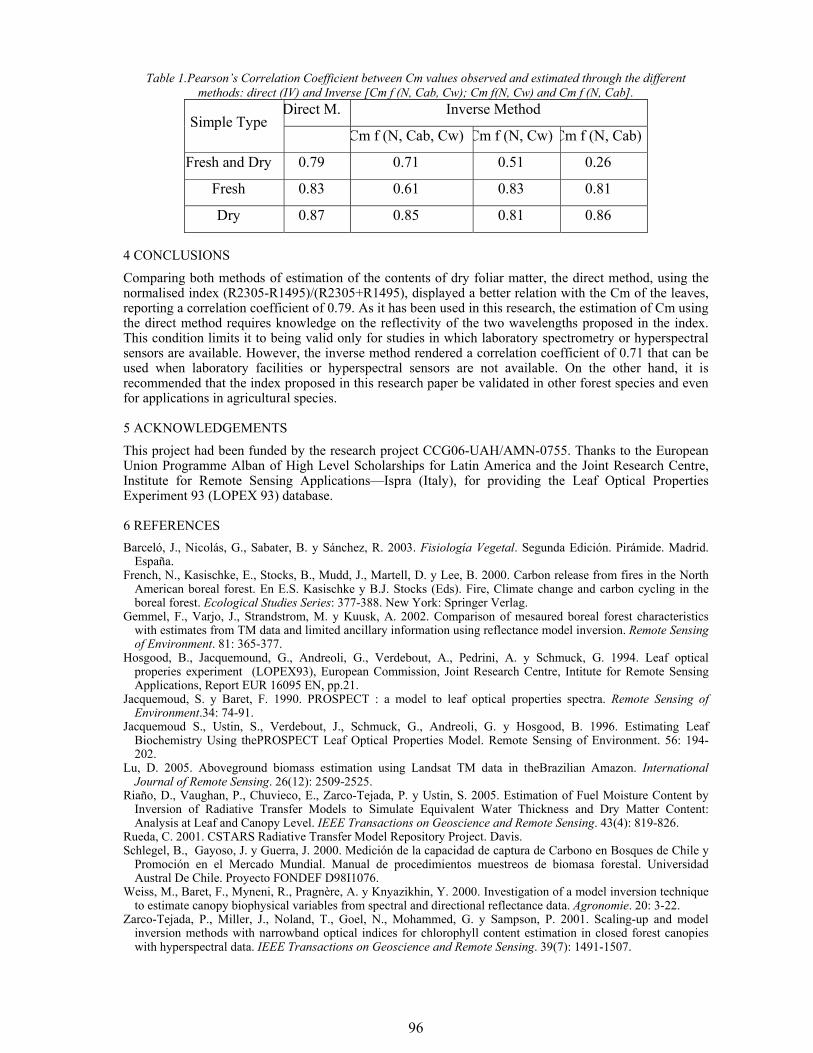
96

Table 1.Pearson’s Correlation Coefficient between Cm values observed and estimated through the different methods: direct (IV) and Inverse [Cm f (N, Cab, Cw); Cm f(N, Cw) and Cm f (N, Cab].

Direct M. Inverse Method Simple Type

Cm f (N, Cab, Cw) Cm f (N, Cw) Cm f (N, Cab)

Fresh and Dry 0.79 0.71 0.51 0.26

Fresh 0.83 0.61 0.83 0.81

Dry 0.87 0.85 0.81 0.86

4 CONCLUSIONS Comparing both methods of estimation of the contents of dry foliar matter, the direct method, using the normalised index (R2305-R1495)/(R2305+R1495), displayed a better relation with the Cm of the leaves, reporting a correlation coefficient of 0.79. As it has been used in this research, the estimation of Cm using the direct method requires knowledge on the reflectivity of the two wavelengths proposed in the index. This condition limits it to being valid only for studies in which laboratory spectrometry or hyperspectral sensors are available. However, the inverse method rendered a correlation coefficient of 0.71 that can be used when laboratory facilities or hyperspectral sensors are not available. On the other hand, it is recommended that the index proposed in this research paper be validated in other forest species and even for applications in agricultural species.

5 ACKNOWLEDGEMENTS This project had been funded by the research project CCG06-UAH/AMN-0755. Thanks to the European Union Programme Alban of High Level Scholarships for Latin America and the Joint Research Centre, Institute for Remote Sensing Applications—Ispra (Italy), for providing the Leaf Optical Properties Experiment 93 (LOPEX 93) database.

6 REFERENCES Barceló, J., Nicolás, G., Sabater, B. y Sánchez, R. 2003. Fisiología Vegetal. Segunda Edición. Pirámide. Madrid.

España. French, N., Kasischke, E., Stocks, B., Mudd, J., Martell, D. y Lee, B. 2000. Carbon release from fires in the North

American boreal forest. En E.S. Kasischke y B.J. Stocks (Eds). Fire, Climate change and carbon cycling in the boreal forest. Ecological Studies Series: 377-388. New York: Springer Verlag.

Gemmel, F., Varjo, J., Strandstrom, M. y Kuusk, A. 2002. Comparison of mesaured boreal forest characteristics with estimates from TM data and limited ancillary information using reflectance model inversion. Remote Sensing of Environment. 81: 365-377.

Hosgood, B., Jacquemound, G., Andreoli, G., Verdebout, A., Pedrini, A. y Schmuck, G. 1994. Leaf optical properies experiment (LOPEX93), European Commission, Joint Research Centre, Intitute for Remote Sensing Applications, Report EUR 16095 EN, pp.21.

Jacquemoud, S. y Baret, F. 1990. PROSPECT : a model to leaf optical properties spectra. Remote Sensing of Environment.34: 74-91.

Jacquemoud S., Ustin, S., Verdebout, J., Schmuck, G., Andreoli, G. y Hosgood, B. 1996. Estimating Leaf Biochemistry Using thePROSPECT Leaf Optical Properties Model. Remote Sensing of Environment. 56: 194-202.

Lu, D. 2005. Aboveground biomass estimation using Landsat TM data in theBrazilian Amazon. International Journal of Remote Sensing. 26(12): 2509-2525.

Riaño, D., Vaughan, P., Chuvieco, E., Zarco-Tejada, P. y Ustin, S. 2005. Estimation of Fuel Moisture Content by Inversion of Radiative Transfer Models to Simulate Equivalent Water Thickness and Dry Matter Content: Analysis at Leaf and Canopy Level. IEEE Transactions on Geoscience and Remote Sensing. 43(4): 819-826.

Rueda, C. 2001. CSTARS Radiative Transfer Model Repository Project. Davis. Schlegel, B., Gayoso, J. y Guerra, J. 2000. Medición de la capacidad de captura de Carbono en Bosques de Chile y

Promoción en el Mercado Mundial. Manual de procedimientos muestreos de biomasa forestal. Universidad Austral De Chile. Proyecto FONDEF D98I1076.

Weiss, M., Baret, F., Myneni, R., Pragnère, A. y Knyazikhin, Y. 2000. Investigation of a model inversion technique to estimate canopy biophysical variables from spectral and directional reflectance data. Agronomie. 20: 3-22.

Zarco-Tejada, P., Miller, J., Noland, T., Goel, N., Mohammed, G. y Sampson, P. 2001. Scaling-up and model inversion methods with narrowband optical indices for chlorophyll content estimation in closed forest canopies with hyperspectral data. IEEE Transactions on Geoscience and Remote Sensing. 39(7): 1491-1507.

97

Use of Remote Sensing and GIS in forest fire suppression planning

S. G. Tsakalidis & I.Z.Gitas Laboratory of Forest Management and Remote Sensing, School of Forestry and Natural Environment, Aristotle University of Thessaloniki, P.O.Box 248, Thessaloniki, Greece. Email: [email protected], [email protected]. Keywords: vegetation indices, vegetation cover density, defensible space, object-based classification, GIS.

ABSTRACT: In order to minimise the consequences of forest fires, an efficient forest fire suppression mechanism is needed. Spatial information such as, the vegetation cover density and the location and defensible space of buildings, can contribute to the improvement of forest fire suppression planning. Geographic Information Systems and Remote Sensing are tools that can be implemented to extract, store and process relevant information, while new image processing techniques such as the object-based classification can be used in order to classify very high resolution (VHR) satellite data. The aim of this study was to create an operational GIS database to be used in forest fire suppression planning. The main objectives were: a) to compare a number of vegetation indices in order to determine the one that correlates best with vegetation cover density, b) to identify the location of buildings as well as to use the selected vegetation index and VHR satellite data in the development of an object-based classification model in order to define different vegetation cover density classes and, finally, c) to estimate the “Defensible Space” of buildings. The methodology was developed by taking into consideration the forest fire suppression methods, in order to create useful, from the operational perspective, information. It comprised three steps. The first step was to create reference data, by means of photo-interpretation techniques, relative to vegetation cover density and to correlate them with a number of selected vegetation indices in order to select the optimal one. The second step was to employ Principal Components Analysis, in order to classify buildings into two classes (tile vs concrete roofing), and then to re-segmented the unclassified area and classify it, by using the best performing Vegetation Index (Simple Ratio), into six vegetation cover density classes. The third but equally important step was to take advantage of GIS and classification results in order to estimate the relative area of desirable classes inside two zones peripherally adjacent to buildings (0-10 and 10-30 meters). This expresses the endangerment of buildings by forest fires. The Simple Ratio (SR) vegetation index was found to correlate best with vegetation cover density (Pearson index, 0,89) whereas the overall classification accuracy of the vegetation cover density classes was 96 %. The overall classification accuracy of buildings was found to be 82,69 %. It is concluded from the results that object-based classification and GIS can be used in order to create an operational GIS database of high accuracy. The information extracted would be expected to improve forest fire suppression planning as well as the effectiveness of decision-making during fire suppression.

1 INTRODUCTION During the last decades there has been an exponential increase in the number of fires across the Mediterranean (Pausas και Vallejo 1999). Most of the fires are caused by human activity (Velez 1990) whereas many natural factors, such as fuels, weather and topography (Countryman 1972), influence the spread of fires and govern their devastating effects. Fuels constitute the only readily alterable factor that can be affected by human action in order to minimise the forest fire ignition and propagation danger, and at the same time to increase the efficiency of fire suppression. There are two main forest fire suppression methods (Βορίσης 2001, Γκόφας 2001), the “direct” and the “indirect” method. In the direct method the fire-fighting forces attack the front of advance of the fire directly and separate the burnt from the unburnt fuels. Conversely in the indirect method the fire fighting forces create a line of defence at a suitable distance from the fire front, while the intermediate fuel between this line and the fire is burnt, in order to widen the zone devoid of fuel; this burning receives the name “Burning of Widening”. When the fireline intensity and spread rate are high it is not possible for ground forces to apply direct assault. However, if the vegetation distribution and density are known, ground fire suppression forces can determine the spots where the spread rate and intensity are expected to decrease. In the indirect fire suppression method, clearances and patches of land with low vegetation cover density can determine the path and location that will have the line of defence in order to reduce the clearing task to a minimum, saving time and energy. Additionally the distribution of these areas can determine the spots where lumberjack teams can work in order to unite neighbouring patches of land with low vegetation and as a result to increase the fire fighting space. The location of buildings constitutes also valuable information in order to undertake appropriate protection measures as well as to estimate the “Defensible Space”.

98

Geographic Information Systems and Remote Sensing are tools that can be implemented to extract, store and process relevant information, while new image processing techniques such as the object-based classification can be used in order to: a) classify VHR satellite data alleviating negative effects of pixel based methods such as the “salt-and-pepper effect” (eCognition 4.0 User Guide 2004) and b) to create and classify homogeneous areas or objects of interest (e.g. patches of land with low vegetation cover density or buildings). Moreover Jensen (2007) cites that Vegetation Indices can indicate relative abundance and activity of green vegetation, including leaf-area-index (LAI), percentage of green cover, chlorophyll content, green biomass, and absorbed photosynthetically active radiation (APAR). The aim of this study was to create an operational GIS database to be used in forest fire suppression planning. The main objectives were: a) to compare a number of vegetation indices in order to determine the one that correlates best with vegetation cover density, b) to identify the location of buildings as well as to use the selected vegetation index and VHR satellite data in the development of an object-based classification model in order to define different vegetation cover density classes and, finally, c) to estimate the “Defensible Space” of buildings.

2 STUDY AREA AND DATASETS The study area consists of a small area in the North-eastern part of the island of Thasos which is located in the northern Aegean Sea. Its surface area is 399 km2, and its perimeter is approximately 102 km. Elevation ranges from sea level to 1217 m. Pinus brutia is the dominant vegetation at the lower elevations (0-800m), whereas Pinus nigra is found at higher altitudes (Gitas 1999). Other types of Mediterranean vegetation are also present such as maquis and garigue. Thasos constitutes a fire-prone ecosystem which has suffered from repetitive devastating forest fires during the last decades. Four large fires in 1984, 1985, 1989 and 2000 have consumed nearly 20.600 hectares of forest land. The image on the right side of figure 1 was initially intended to be used for this work. Nevertheless, due to the high demand on computer memory and processing speed, a subset of the image (depicted inside the yellow frame) was used as the study area. Figure 1. Left: General view of Northern Greece and Thasos location. Middle: The island of Thasos, Right: The initial and final study area

Two very high spatial resolution Quickbird images were used in this study (a multispectral image and the corresponding panchromatic). These images were captured on the 20th of October 2004. The classification and processing of spatial information was performed by means of the following software: ERDAS IMAGINE 8.7, DEFINIENS 5.0, ArcGIS 9.2, ArcView 3.3, whereas the statistical analysis with SPSS 13.0.

3 METHODOLOGY

According to the aim and the objectives set, the study comprised three steps. The first step was to create reference data, by means of photo-interpretation techniques, in relation to vegetation cover density, and to correlate them with a number of selected vegetation indices in order to select the one that correlated more closely. Six vegetation indices (VI), namely, the Wide Dynamic Range Vegetation Index (WDRVI), the Modified Soil Adjusted Vegetation Index (MSAVI), the Simple Ratio (SR), the Tasselled Cap Greeness, the Triangular Vegetation Index (TVI), and the Normalized Difference Vegetation Index (NDVI) were selected from the literature and tested. Since there were not any reliable reference data, photointerpetation techniques were employed to create them. A 20 by 20 meter chessboard segmentation was applied on the image and the mean values of the VIs were extracted for each square. Then each pixel of the multispectral image was transformed into point in order to create a regular network of dots. The panchromatic and multispectral (improved after resolution merge with the panchromatic image) images were used as background over which the regular network of dots and squares were set.

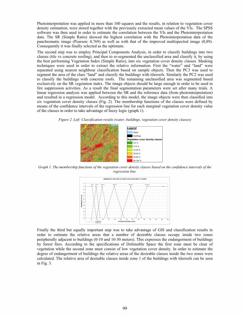
99

Photointerpretation was applied in more than 100 squares and the results, in relation to vegetation cover density estimation, were stored together with the previously extracted mean values of the VIs. The SPSS software was then used in order to estimate the correlation between the VIs and the Photointerpretation data. The SR (Simple Ratio) showed the highest correlation with the Photointerpretation data of the panchromatic image (Pearson: 0,769) as well as with that of the improved multispectral image (0,89). Consequently it was finally selected as the optimum. The second step was to employ Principal Components Analysis, in order to classify buildings into two classes (tile vs concrete roofing), and then to re-segmented the unclassified area and classify it, by using the best performing Vegetation Index (Simple Ratio), into six vegetation cover density classes. Masking techniques were used in order to extract the relative information. First the “water” and “land” were separated using nearest neighbour classification based on sample objects. Then the PC3 was used to segment the area of the class “land” and classify the buildings with tileroofs. Similarly the PC2 was used to classify the buildings with concrete roofs. The remaining unclassified area was segmented based exclusively on the SR vegetation index. The image objects should be large enough in order to be used in fire suppression activities. As a result the final segmentation parameters were set after many trials. A linear regression analysis was applied between the SR and the reference data (from photointerpretation) and resulted in a regression model. According to this model, the image objects were then classified into six vegetation cover density classes (Fig. 2). The membership functions of the classes were defined by means of the confidence intervals of the regression line for each marginal vegetation cover density value of the classes in order to take advantage of fuzzy logic (graph 1).

Figure 2. Left: Classification results (water, buildings, vegetation cover density classes)

LegendWater

Buildings

Vegetation cover density classes0-5 %

5-10 %

10-20 %

20-40 %

40-60 %

60-100 % Graph 1. The membership functions of the vegetation cover density classes based on the confidence intervals of the

regression line.

MEMBERSHIP FUNCTIONS OF VEGETATION COVER DENSITY CLASSES

0.0

0.1

0.2

0.3

0.4

0.5

0.6

0.7

0.8

0.9

1.0

1.1

0 20 40 60 80 100 120 140 160 180 200 220 240 260 280

SR VEGETATION INDEX VALUES

MEM

BER

SHIP

VA

LUES

0-5 % 5-10 % 10-20 % 20-40 % 40-60 % 60-100 %

CONFIDENCE INTERVALS

Finally the third but equally important step was to take advantage of GIS and classification results in order to estimate the relative areas that a number of desirable classes occupy inside two zones peripherally adjacent to buildings (0-10 and 10-30 meters). This expresses the endangerment of buildings by forest fires. According to the specifications of Defensible Space the first zone must be clear of vegetation while the second zone must consist of low vegetation cover density. In order to estimate the degree of endangerment of buildings the relative areas of the desirable classes inside the two zones were calculated. The relative area of desirable classes inside zone 1 of the buildings with tileroofs can be seen in Fig. 3.

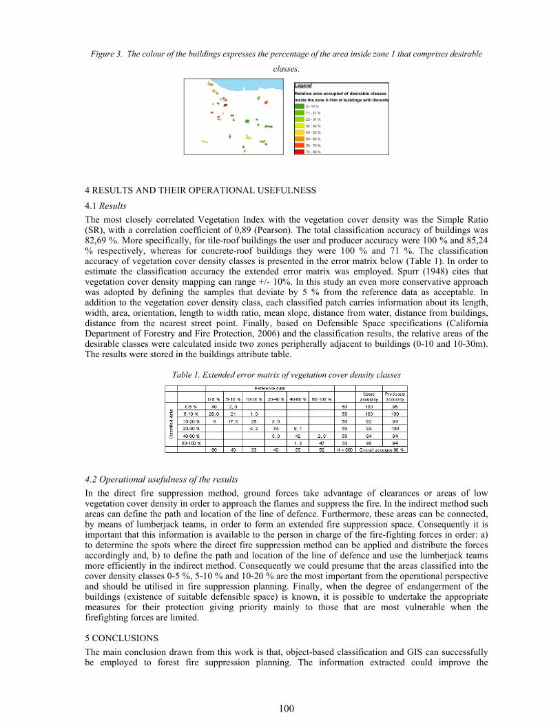
100

Figure 3. The colour of the buildings expresses the percentage of the area inside zone 1 that comprises desirable

classes.

LegendRelative area occupied of desirable classesinside the zone 0-10m of buildings with tileroofs

0 - 10 %

11 - 21 %

22 - 31 %

32 - 42 %

43 - 52 %

53 - 62 %

63 - 73 %

74 - 83 %

4 RESULTS AND THEIR OPERATIONAL USEFULNESS 4.1 Results The most closely correlated Vegetation Index with the vegetation cover density was the Simple Ratio (SR), with a correlation coefficient of 0,89 (Pearson). The total classification accuracy of buildings was 82,69 %. More specifically, for tile-roof buildings the user and producer accuracy were 100 % and 85,24 % respectively, whereas for concrete-roof buildings they were 100 % and 71 %. The classification accuracy of vegetation cover density classes is presented in the error matrix below (Table 1). In order to estimate the classification accuracy the extended error matrix was employed. Spurr (1948) cites that vegetation cover density mapping can range +/- 10%. In this study an even more conservative approach was adopted by defining the samples that deviate by 5 % from the reference data as acceptable. In addition to the vegetation cover density class, each classified patch carries information about its length, width, area, orientation, length to width ratio, mean slope, distance from water, distance from buildings, distance from the nearest street point. Finally, based on Defensible Space specifications (California Department of Forestry and Fire Protection, 2006) and the classification results, the relative areas of the desirable classes were calculated inside two zones peripherally adjacent to buildings (0-10 and 10-30m). The results were stored in the buildings attribute table.

Table 1. Extended error matrix of vegetation cover density classes

4.2 Operational usefulness of the results In the direct fire suppression method, ground forces take advantage of clearances or areas of low vegetation cover density in order to approach the flames and suppress the fire. In the indirect method such areas can define the path and location of the line of defence. Furthermore, these areas can be connected, by means of lumberjack teams, in order to form an extended fire suppression space. Consequently it is important that this information is available to the person in charge of the fire-fighting forces in order: a) to determine the spots where the direct fire suppression method can be applied and distribute the forces accordingly and, b) to define the path and location of the line of defence and use the lumberjack teams more efficiently in the indirect method. Consequently we could presume that the areas classified into the cover density classes 0-5 %, 5-10 % and 10-20 % are the most important from the operational perspective and should be utilised in fire suppression planning. Finally, when the degree of endangerment of the buildings (existence of suitable defensible space) is known, it is possible to undertake the appropriate measures for their protection giving priority mainly to those that are most vulnerable when the firefighting forces are limited. 5 CONCLUSIONS The main conclusion drawn from this work is that, object-based classification and GIS can successfully be employed to forest fire suppression planning. The information extracted could improve the

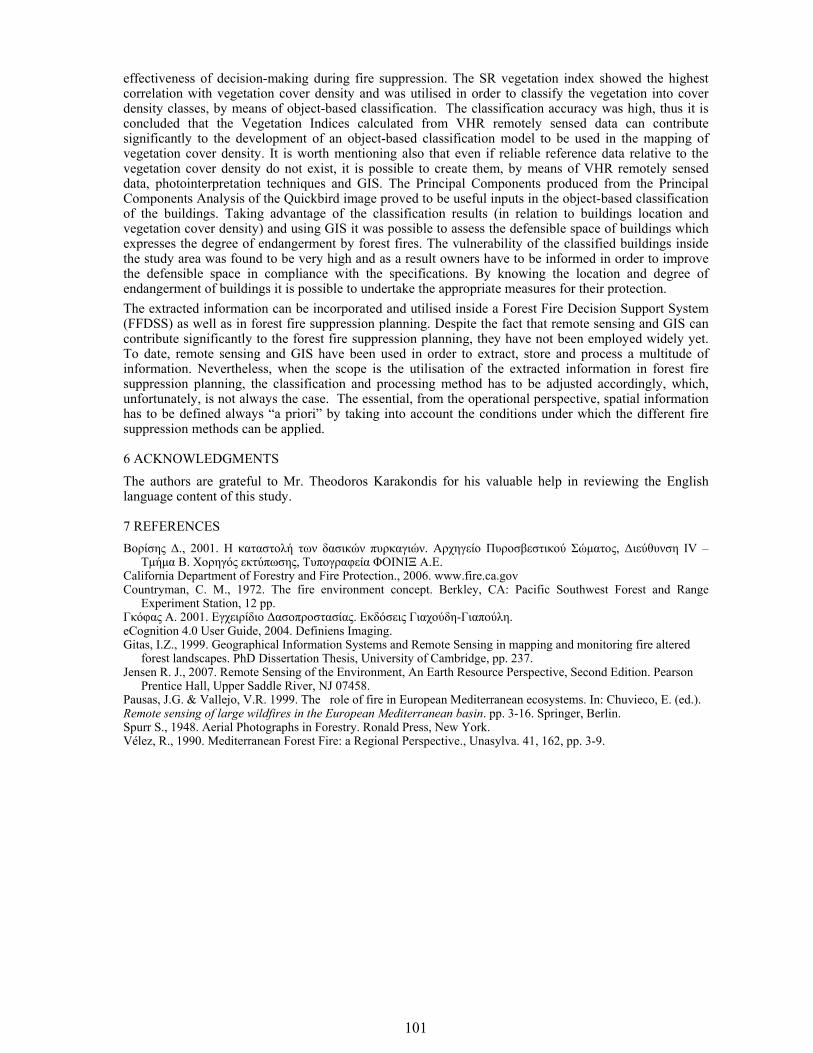
101

effectiveness of decision-making during fire suppression. The SR vegetation index showed the highest correlation with vegetation cover density and was utilised in order to classify the vegetation into cover density classes, by means of object-based classification. The classification accuracy was high, thus it is concluded that the Vegetation Indices calculated from VHR remotely sensed data can contribute significantly to the development of an object-based classification model to be used in the mapping of vegetation cover density. It is worth mentioning also that even if reliable reference data relative to the vegetation cover density do not exist, it is possible to create them, by means of VHR remotely sensed data, photointerpretation techniques and GIS. The Principal Components produced from the Principal Components Analysis of the Quickbird image proved to be useful inputs in the object-based classification of the buildings. Taking advantage of the classification results (in relation to buildings location and vegetation cover density) and using GIS it was possible to assess the defensible space of buildings which expresses the degree of endangerment by forest fires. The vulnerability of the classified buildings inside the study area was found to be very high and as a result owners have to be informed in order to improve the defensible space in compliance with the specifications. By knowing the location and degree of endangerment of buildings it is possible to undertake the appropriate measures for their protection. The extracted information can be incorporated and utilised inside a Forest Fire Decision Support System (FFDSS) as well as in forest fire suppression planning. Despite the fact that remote sensing and GIS can contribute significantly to the forest fire suppression planning, they have not been employed widely yet. To date, remote sensing and GIS have been used in order to extract, store and process a multitude of information. Nevertheless, when the scope is the utilisation of the extracted information in forest fire suppression planning, the classification and processing method has to be adjusted accordingly, which, unfortunately, is not always the case. The essential, from the operational perspective, spatial information has to be defined always “a priori” by taking into account the conditions under which the different fire suppression methods can be applied.

6 ACKNOWLEDGMENTS The authors are grateful to Mr. Theodoros Karakondis for his valuable help in reviewing the English language content of this study.

7 REFERENCES Βορίσης Δ., 2001. Η καταστολή των δασικών πυρκαγιών. Αρχηγείο Πυροσβεστικού Σώματος, Διεύθυνση IV –

Τμήμα Β. Χορηγός εκτύπωσης, Τυπογραφεία ΦΟΙΝΙΞ Α.Ε. California Department of Forestry and Fire Protection., 2006. www.fire.ca.gov Countryman, C. M., 1972. The fire environment concept. Berkley, CA: Pacific Southwest Forest and Range

Experiment Station, 12 pp. Γκόφας Α. 2001. Εγχειρίδιο Δασοπροστασίας. Εκδόσεις Γιαχούδη-Γιαπούλη. eCognition 4.0 User Guide, 2004. Definiens Imaging. Gitas, I.Z., 1999. Geographical Information Systems and Remote Sensing in mapping and monitoring fire altered forest landscapes. PhD Dissertation Thesis, University of Cambridge, pp. 237. Jensen R. J., 2007. Remote Sensing of the Environment, An Earth Resource Perspective, Second Edition. Pearson Prentice Hall, Upper Saddle River, NJ 07458. Pausas, J.G. & Vallejo, V.R. 1999. The role of fire in European Mediterranean ecosystems. In: Chuvieco, E. (ed.). Remote sensing of large wildfires in the European Mediterranean basin. pp. 3-16. Springer, Berlin. Spurr S., 1948. Aerial Photographs in Forestry. Ronald Press, New York. Vélez, R., 1990. Mediterranean Forest Fire: a Regional Perspective., Unasylva. 41, 162, pp. 3-9.

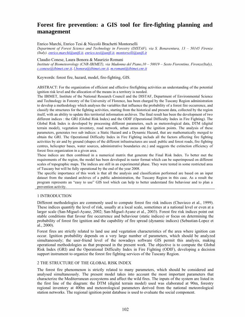
102

Forest fire prevention: a GIS tool for fire-fighting planning and management

Enrico Marchi, Enrico Tesi & Niccolò Brachetti Montorselli Department of Forest Science and Technology in Forestry (DISTAF), via S. Bonaventura, 13 – 50145 Firenze (Italy). [email protected], [email protected], [email protected]

Claudio Conese, Laura Bonora & Maurizio Romani Institute of Biometeorology (CNR-IBIMET), via Madonna del Piano,10 – 50019 – Sesto Fiorentino, Firenze(Italy), [email protected], [email protected], [email protected] Keywords: forest fire, hazard, model, fire-fighting, GIS. ABSTRACT: For the organization of efficient and effective firefighting activities an understanding of the potential ignition risk level and the allocation of the means in a territory is needed. The IBIMET, Institute of the National Research Council and the DISTAF, Department of Environmental Science and Technology in Forestry of the University of Florence, has been charged by the Tuscany Region administration to develop a methodology which analyses the variables that influence the probability of a forest fire occurrence, and classify the structures for the fighting activities, starting from the historical and present data, collected by the region itself, with an ability to update this territorial information archives. The final result has been the development of two different indices : the GRI (Global Risk Index) and the ODIF (Operational Difficulty Index in Fire Fighting). The Global Risk Index is developed by processing different parameters, such as meteorological data, DTM (digital terrain model), vegetation inventory, road network, urban areas and the ignition points. The analysis of these parameters, generates two sub indices: a Static Hazard and a Dynamic Hazard, that are mathematically merged to obtain the GRI. The Operational Difficulty Index in Fire Fighting includs all the factors affecting fire fighting activities by air and by ground (shapes of the different infrastructures are used: public and forest roads, fire fighting centres, helicopter bases, water sources, administrative boundaries etc.) and suggests the extinction efficiency of forest fires organization in a given area. These indices are then combined in a numerical matrix that generate the Final Risk Index. To better met the requirements of the region, the model has been developed in raster format which can be superimposed on different scales of topographic maps. The indices are still in an experimental phase. They were tested in some restricted area of Tuscany but will be fully operational by the end of the year 2008. The specific importance of this work is that all the analysis and classification performed are based on an input dataset from the standard archives of a public administration, the Tuscany Region in this case. As a result the program represents an “easy to use” GIS tool which can help to better understand fire behaviour and to plan a prevention activity. 1 INTRODUCTION Different methodologies are commonly used to compute forest fire risk indices (Chuvieco et al., 1999). These indices quantify the level of risk, usually at a local scale, sometimes at a national level or even at a larger scale (San-Miguel-Ayanz, 2002; San-Miguel-Ayanz et al., 2003). Forest fire risk indices point out stable conditions that favour fire occurrence and behaviour (static indices) or focus on determining the probability of forest fire ignition and the capability of fire spread (dynamic indices) (Sebastian-Lopez et al., 2000). Forest fires are strictly related to land use and vegetation characteristics of the area where ignition can occur. Ignition probability depends on a very large number of parameters, which should be analyzed simultaneously; the user-friend level of the nowadays software GIS permit this analysis, making operational methodologies as that proposed in the present work. The objective is to compute the Global Risk Index (GRI) and the Operational Difficulty Index in Fire Fighting (ODIF), developing a decision support instrument to organize the forest fire fighting services of the Tuscany Region.

2 THE STRUCTURE OF THE GLOBAL RISK INDEX The forest fire phenomenon is strictly related to many parameters, which should be considered and analysed simultaneously. The present model takes into account the most important parameters that characterize the Mediterranean ecosystems and affect the wild fires. The inputs of the system are listed in the first line of the diagram: the DTM (digital terrain model) used was elaborated at 90m, forestry regional inventory at 400m and meteorological parameters derived from the national meteorological station networks. The regional ignition point database is used to evaluate the social component.

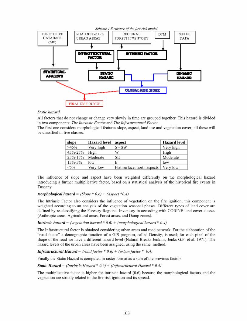
103

Scheme 1 Structure of the fire risk model

Static hazard All factors that do not change or change very slowly in time are grouped together. This hazard is divided in two components: The Intrinsic Factor and The Infrastructural Factor. The first one considers morphological features slope, aspect, land use and vegetation cover; all these will be classified in five classes.

slope Hazard level aspect Hazard level >45% Very high S - SW Very high 45%-25% High W High 25%-15% Moderate SE Moderate 15%-5% low E low <5% Very low Flat surface, north aspects Very low

The influence of slope and aspect have been weighted differently on the morphological hazard introducing a further multiplicative factor, based on a statistical analysis of the historical fire events in Tuscany

Morphological hazard = (Slope * 0.6) + (Aspect *0.4)

The Intrinsic Factor also considers the influence of vegetation on the fire ignition; this component is weighted according to an analysis of the vegetation seasonal phases. Different types of land cover are defined by re-classifying the Forestry Regional Inventory in according with CORINE land cover classes (Anthropic areas, Agricultural areas, Forest areas, and Damp zones).

Intrinsic hazard = (vegetation hazard * 0.6) + (morphological hazard * 0.4)

The Infrastructural factor is obtained considering urban areas and road network; For the elaboration of the “road factor” a demographic function of a GIS program, called Density, is used; for each pixel of the shape of the road we have a different hazard level (Natural Breaks Jenkins, Jenks G.F. et al. 1971). The hazard levels of the urban areas have been assigned, using the same method.

Infrastructural Hazard = (road factor * 0.6) + (urban factor * 0.4)

Finally the Static Hazard is computed in raster format as a sum of the previous factors:

Static Hazard = (Intrinsic Hazard * 0.6) + (Infrastructural Hazard * 0.4)

The multiplicative factor is higher for intrinsic hazard (0.6) because the morphological factors and the vegetation are strictly related to the fire risk ignition and its spread.

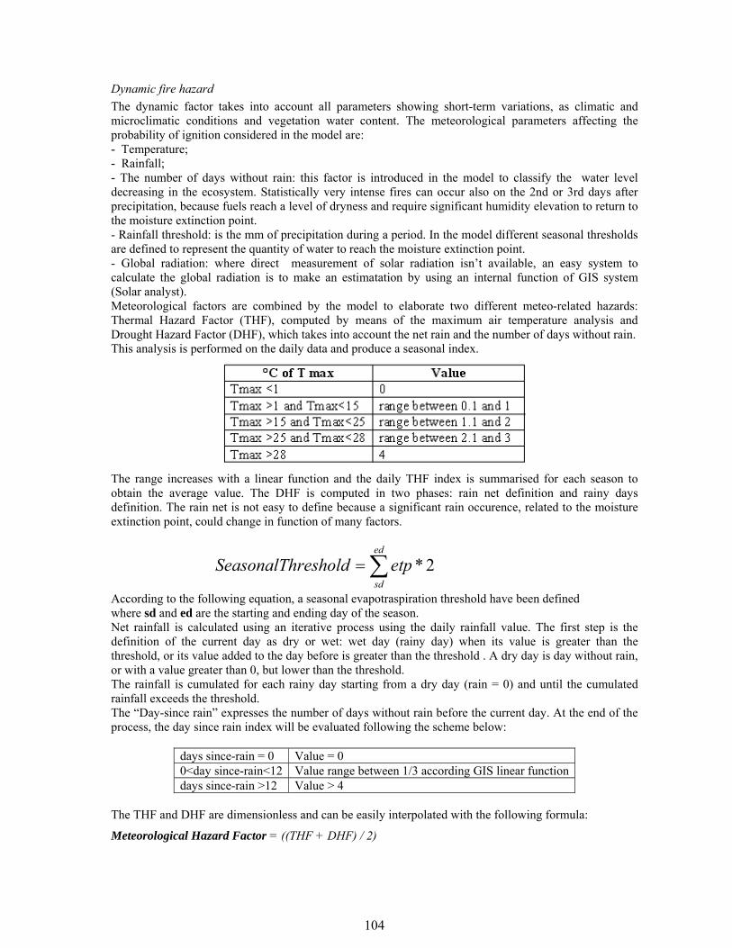
104

Dynamic fire hazard The dynamic factor takes into account all parameters showing short-term variations, as climatic and microclimatic conditions and vegetation water content. The meteorological parameters affecting the probability of ignition considered in the model are: - Temperature; - Rainfall; - The number of days without rain: this factor is introduced in the model to classify the water level decreasing in the ecosystem. Statistically very intense fires can occur also on the 2nd or 3rd days after precipitation, because fuels reach a level of dryness and require significant humidity elevation to return to the moisture extinction point. - Rainfall threshold: is the mm of precipitation during a period. In the model different seasonal thresholds are defined to represent the quantity of water to reach the moisture extinction point. - Global radiation: where direct measurement of solar radiation isn’t available, an easy system to calculate the global radiation is to make an estimatation by using an internal function of GIS system (Solar analyst). Meteorological factors are combined by the model to elaborate two different meteo-related hazards: Thermal Hazard Factor (THF), computed by means of the maximum air temperature analysis and Drought Hazard Factor (DHF), which takes into account the net rain and the number of days without rain. This analysis is performed on the daily data and produce a seasonal index.

The range increases with a linear function and the daily THF index is summarised for each season to obtain the average value. The DHF is computed in two phases: rain net definition and rainy days definition. The rain net is not easy to define because a significant rain occurence, related to the moisture extinction point, could change in function of many factors.

According to the following equation, a seasonal evapotraspiration threshold have been defined where sd and ed are the starting and ending day of the season. Net rainfall is calculated using an iterative process using the daily rainfall value. The first step is the definition of the current day as dry or wet: wet day (rainy day) when its value is greater than the threshold, or its value added to the day before is greater than the threshold . A dry day is day without rain, or with a value greater than 0, but lower than the threshold. The rainfall is cumulated for each rainy day starting from a dry day (rain = 0) and until the cumulated rainfall exceeds the threshold. The “Day-since rain” expresses the number of days without rain before the current day. At the end of the process, the day since rain index will be evaluated following the scheme below:

days since-rain = 0 Value = 0 0<day since-rain<12 Value range between 1/3 according GIS linear function days since-rain >12 Value > 4

The THF and DHF are dimensionless and can be easily interpolated with the following formula:

Meteorological Hazard Factor = ((THF + DHF) / 2)

∑=ed

sd

etpresholdSeasonalTh 2*

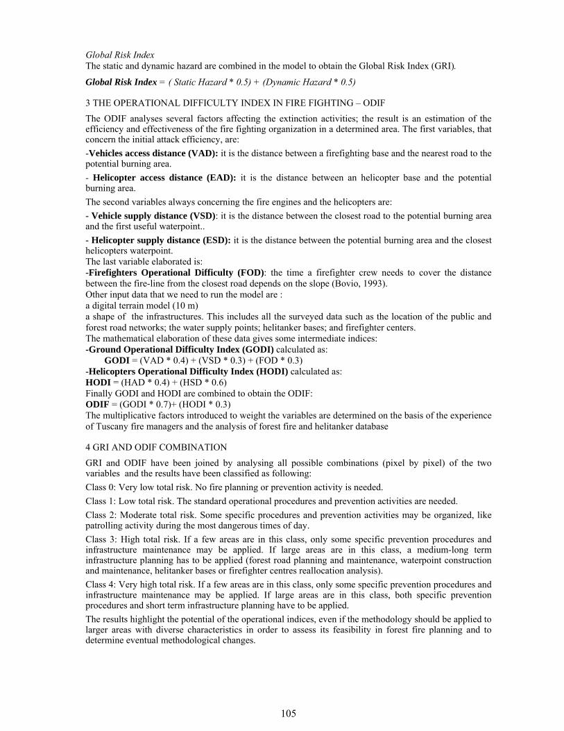
105

Global Risk Index The static and dynamic hazard are combined in the model to obtain the Global Risk Index (GRI).

Global Risk Index = ( Static Hazard * 0.5) + (Dynamic Hazard * 0.5)

3 THE OPERATIONAL DIFFICULTY INDEX IN FIRE FIGHTING – ODIF The ODIF analyses several factors affecting the extinction activities; the result is an estimation of the efficiency and effectiveness of the fire fighting organization in a determined area. The first variables, that concern the initial attack efficiency, are: -Vehicles access distance (VAD): it is the distance between a firefighting base and the nearest road to the potential burning area. - Helicopter access distance (EAD): it is the distance between an helicopter base and the potential burning area. The second variables always concerning the fire engines and the helicopters are: - Vehicle supply distance (VSD): it is the distance between the closest road to the potential burning area and the first useful waterpoint.. - Helicopter supply distance (ESD): it is the distance between the potential burning area and the closest helicopters waterpoint. The last variable elaborated is: -Firefighters Operational Difficulty (FOD): the time a firefighter crew needs to cover the distance between the fire-line from the closest road depends on the slope (Bovio, 1993). Other input data that we need to run the model are : a digital terrain model (10 m) a shape of the infrastructures. This includes all the surveyed data such as the location of the public and forest road networks; the water supply points; helitanker bases; and firefighter centers. The mathematical elaboration of these data gives some intermediate indices: -Ground Operational Difficulty Index (GODI) calculated as:

GODI = (VAD * 0.4) + (VSD * 0.3) + (FOD * 0.3) -Helicopters Operational Difficulty Index (HODI) calculated as: HODI = (HAD * 0.4) + (HSD * 0.6) Finally GODI and HODI are combined to obtain the ODIF: ODIF = (GODI * 0.7)+ (HODI * 0.3) The multiplicative factors introduced to weight the variables are determined on the basis of the experience of Tuscany fire managers and the analysis of forest fire and helitanker database

4 GRI AND ODIF COMBINATION GRI and ODIF have been joined by analysing all possible combinations (pixel by pixel) of the two variables and the results have been classified as following: Class 0: Very low total risk. No fire planning or prevention activity is needed. Class 1: Low total risk. The standard operational procedures and prevention activities are needed. Class 2: Moderate total risk. Some specific procedures and prevention activities may be organized, like patrolling activity during the most dangerous times of day. Class 3: High total risk. If a few areas are in this class, only some specific prevention procedures and infrastructure maintenance may be applied. If large areas are in this class, a medium-long term infrastructure planning has to be applied (forest road planning and maintenance, waterpoint construction and maintenance, helitanker bases or firefighter centres reallocation analysis). Class 4: Very high total risk. If a few areas are in this class, only some specific prevention procedures and infrastructure maintenance may be applied. If large areas are in this class, both specific prevention procedures and short term infrastructure planning have to be applied. The results highlight the potential of the operational indices, even if the methodology should be applied to larger areas with diverse characteristics in order to assess its feasibility in forest fire planning and to determine eventual methodological changes.

106

5 REFERENCES Bovio G., 1993. – “Comportamento degli incendi boschivi estinguibili con attacco diretto”. Monti e Boschi 44, 4,

19-24. Chuvieco, E., Salas, F.J.,Carvacho, L., Rodriguez-Silva, F., 1999. Integrated fire risk mapping, in E. Chuvieco (ed.),

Remote Sensing of Large Wildfires. New York: Springerverlag. Claudio Conese, Laura Bonora, Maurizio Romani and Elisabetta Checcacci, 2004 Forest fire hazard model

definition for local land user (Tuscany Region) Hippoliti G., 2003 – “Note pratiche per la realizzazione della viabilità forestale”, Compagnia delle Foreste, Arezzo Jenks G.F.,Caspall F.C., 1971. Error on Choropletic maps: definition, measurement, reduction. Annals of the

Association of American Geographers, 61, 217-244. San-Miguel-Ayanz, J., Barbosa, P. M., Schmuck, G. , Libertà, G., 2003, The European Forest Fire Information

System (EFFIS), 2003, Joint International Workshop of EARSeL SIG on Forest Fires and the GOFC/GOLD-Fire Program: Innovative Concepts and Methods in Fire Danger Estimation, held in Ghent (Belgium) on 5-7 June 2003.

San-Miguel-Ayanz, J., 2002, Methodologies for the evaluation of forest fire risk: from long-term (static) to dynamic indices, in Forest Fires: Ecology and Control, Anfodillo T. and Carraro, V. (Eds), Forest Fires: Ecology and Control, Univesity degli Studi di Padova, pp. 117-132.

Viegas X, Bovio G, Ferreira A, Nosenzo A, Sol B 2000 Comparative study of various methods of fire danger evaluation in southern Europe. International Journal of Wildland Fire 9, 235-246.

107

1 INTRODUCTION

The classification of various vegetation types into fuel models is an important component of wildland fire management (Pyne, 1984). Especially fine scale or landscape-level fuel mapping is essential for local fire management because it describes fuel hazard and fire behavior potential in regional fire management planning (Chuvieco, 1989; Maselli, 1996; Keane, 2001). Therefore, a lot of studies have tried to accurately delineating fuel maps in local to regional scales. Van Wagtendonk (2003) following a multitemporal approach discriminated six different fuel classes Yosemite National Park, USA. Koutsias and Karteris (2003) classified a Landsat-5 TM image, in a typical Mediterranean test site, evaluating fuel complexes mapping considering the main forest species present in the area, while Riano et al. (2002) for the same task adopted a Mediterranean-specific fuel description. However, the complex Mediterranean anaglyph poses often several problems to fuel type mapping due to errors induced in the radiometric values of the images from terrain shadowing. In order to cover the needs for fuel complexes mapping in Europe and more specifically in the Mediterranean basin, the Prometheus fuel model system (Table 1) has been developed relatively recent (Prometheus, 1999). It includes 7 fuel types and considers both floristic and structural parameters of the vegetation:

Fuel type mapping using medium resolution imagery and GIS, considering radiometric, spatial and spectral enhancements of the original dataset.

I. Stergiopoulos, G. Mallinis & I.Z. Gitas Laboratory of Forest Management and Remote Sensing, School of Forestry and Natural Environment, Aristotle University of Thessaloniki ,P.O. Box 248, Greece, e-mail: [email protected] Keywords: fuel mapping, topographic correction, enhancement, Prometheus fuel type system

ABSTRACT: In recent years, a lot of emphasis has been given in the prevention of forest fires as well as in pre-fire planning. Crucial to fire management is forest fuel loads mapping, since fuel is the only factor related to forest fire behaviour that humans can control, manage and modify. Remote sensing in combination with GIS, constitute a powerful tool in the process and analysis of satellite imagery and other data which provide spatial and temporal information about forests. However, limitations in its use result from the spatial detail resolvable from the sensors, especially in the case of heterogeneous, fragmented landscapes. The main purpose of this study was to evaluate the use of satellite remote sensing data for fuel type mapping, following the European fuel type classification system Prometheus. An additional aim of our work was the evaluation of a topographic normalization procedure in terms of improving the accuracy of the final type map as well as the use of synthetic channels. A 40.000 hectares study area was selected in Northern Greece due to its spatial heterogeneity in vegetation structure and composition. A Landsat TM image was the primary source of information for the study. Prior to the development of the classification, the cosine and the C-correction methods of minimizing errors in the radiometric values of the image due to the anaglyph were evaluated. Following that, a series of multi-spectral transformations were estimated and integrated in the original data for improving the accuracy of the classification process. Development of the classification scheme was supported through extensive field survey. In total, 205 homogeneous patches were located in the field using GPS measurements and categorized to different fuel types according to the Prometheus system. For the classification of the image, the maximum likelihood algorithm was employed. Problems were noticed in the final fuel type maps resulting from poor discrimination of the understory vegetation. The overall accuracy of the classification approach using the original data was around 71%. Following the topographic correction and the addition of the synthetic bands the classification accuracy was increased, reaching around 78%. Overall, despite the preprocessing and the enhancements applied to the original imagery, the operational use of medium spatial resolution data, for mapping fuel complexes in the Mediterranean region, seems questionable.

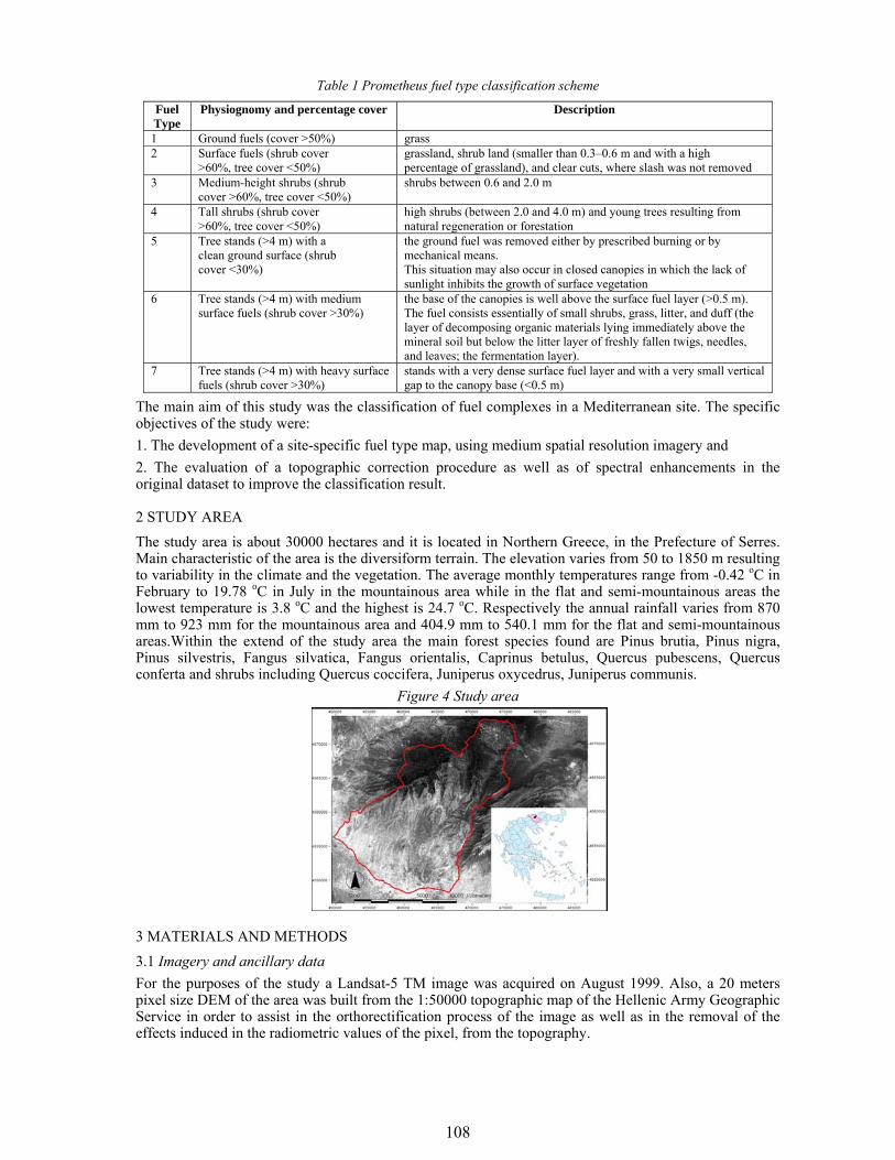
108

Table 1 Prometheus fuel type classification scheme

Fuel Type

Physiognomy and percentage cover Description

1 Ground fuels (cover >50%) grass 2 Surface fuels (shrub cover

>60%, tree cover <50%) grassland, shrub land (smaller than 0.3–0.6 m and with a high percentage of grassland), and clear cuts, where slash was not removed

3 Medium-height shrubs (shrub cover >60%, tree cover <50%)

shrubs between 0.6 and 2.0 m

4 Tall shrubs (shrub cover >60%, tree cover <50%)

high shrubs (between 2.0 and 4.0 m) and young trees resulting from natural regeneration or forestation

5 Tree stands (>4 m) with a clean ground surface (shrub cover <30%)

the ground fuel was removed either by prescribed burning or by mechanical means. This situation may also occur in closed canopies in which the lack of sunlight inhibits the growth of surface vegetation

6 Tree stands (>4 m) with medium surface fuels (shrub cover >30%)

the base of the canopies is well above the surface fuel layer (>0.5 m). The fuel consists essentially of small shrubs, grass, litter, and duff (the layer of decomposing organic materials lying immediately above the mineral soil but below the litter layer of freshly fallen twigs, needles, and leaves; the fermentation layer).

7 Tree stands (>4 m) with heavy surface fuels (shrub cover >30%)

stands with a very dense surface fuel layer and with a very small vertical gap to the canopy base (<0.5 m)

The main aim of this study was the classification of fuel complexes in a Mediterranean site. The specific objectives of the study were: 1. The development of a site-specific fuel type map, using medium spatial resolution imagery and 2. The evaluation of a topographic correction procedure as well as of spectral enhancements in the original dataset to improve the classification result.

2 STUDY AREA The study area is about 30000 hectares and it is located in Northern Greece, in the Prefecture of Serres. Main characteristic of the area is the diversiform terrain. The elevation varies from 50 to 1850 m resulting to variability in the climate and the vegetation. The average monthly temperatures range from -0.42 oC in February to 19.78 oC in July in the mountainous area while in the flat and semi-mountainous areas the lowest temperature is 3.8 oC and the highest is 24.7 oC. Respectively the annual rainfall varies from 870 mm to 923 mm for the mountainous area and 404.9 mm to 540.1 mm for the flat and semi-mountainous areas.Within the extend of the study area the main forest species found are Pinus brutia, Pinus nigra, Pinus silvestris, Fangus silvatica, Fangus orientalis, Caprinus betulus, Quercus pubescens, Quercus conferta and shrubs including Quercus coccifera, Juniperus oxycedrus, Juniperus communis.

Figure 4 Study area

3 MATERIALS AND METHODS

3.1 Imagery and ancillary data For the purposes of the study a Landsat-5 TM image was acquired on August 1999. Also, a 20 meters pixel size DEM of the area was built from the 1:50000 topographic map of the Hellenic Army Geographic Service in order to assist in the orthorectification process of the image as well as in the removal of the effects induced in the radiometric values of the pixel, from the topography.

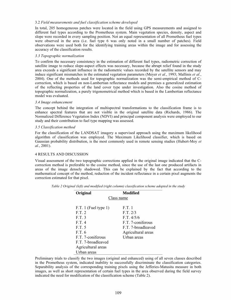
109

3.2 Field measurements and fuel classification scheme developed In total, 205 homogeneous patches were located in the field using GPS measurements and assigned to different fuel types according to the Prometheus system. Main vegetation species, density, aspect and slope were recorded in every sampling position. Not an equal representation of all Prometheus fuel types were observed in the area (i.e. fuel type 6 was only noted in a small number of patches). Field observations were used both for the identifying training areas within the image and for assessing the accuracy of the classification results. 3.3 Topographic normalization To confirm the necessary consistency in the estimation of different fuel types, radiometric correction of satellite image to reduce slope-aspect effects was necessary, because the abrupt relief found in the study area exceeds a significant influence in the radiometric values recorded by the satellite sensors and may induce significant mismatches in the estimated vegetation parameters (Meyer et al., 1993; Mallinis et al., 2004). One of the methods used for topographic normalization was the semi-empirical method of C-correction, which is based on non-Lambertian reflectance models and premises a generalized estimation of the reflecting properties of the land cover type under investigation. Also the cosine method of topographic normalization, a purely trigonometrical method which is based in the Lambertian reflectance model was evaluated. 3.4 Image enhancement The concept behind the integration of multispectral transformations to the classification frame is to enhance spectral features that are not visible in the original satellite data (Richards, 1986). The Normalized Difference Vegetation Index (NDVI) and principal component analysis were employed to our study and their contribution to fuel type mapping was assessed.

3.5 Classification method For the classification of the LANDSAT imagery a supervised approach using the maximum likelihood algorithm of classification was employed. The Maximum Likelihood classifier, which is based on Gaussian probability distribution, is the most commonly used in remote sensing studies (Hubert-Moy et al., 2001).

4 RESULTS AND DISCUSSION Visual assessment of the two topographic corrections applied in the original image indicated that the C-correction method is preferable to the cosine method, since the use of the last one produced artifacts in areas of the image densely shadowed. This can be explained by the fact that according to the mathematical concept of the method, reduction of the incident reflectance in a certain pixel augments the correction estimated for that pixel.

Table 2 Original (left) and modified (right column) classification scheme adopted in the study

Original Modified Class name

F.T. 1 (Fuel type 1) F.T. 1 F.T. 2 F.T. 2/3 F.T. 3 F.T. 4/5/6 F.T. 4 F.T. 7-coniferous F.T. 5 F.T. 7-broadleaved F.T. 6 Agricultural areas F.T. 7-coniferous Urban areas F.T. 7-broadleaved Agricultural areas Urban areas

Preliminary trials to classify the two images (original and enhanced) using of all seven classes described in the Prometheus system, indicated inability to successfully discriminate the classification categories. Separability analysis of the corresponding training pixels using the Jefferies-Matusita measure in both images, as well as short representation of certain fuel types in the area observed during the field survey indicated the need for modification of the classification scheme (Table 2).

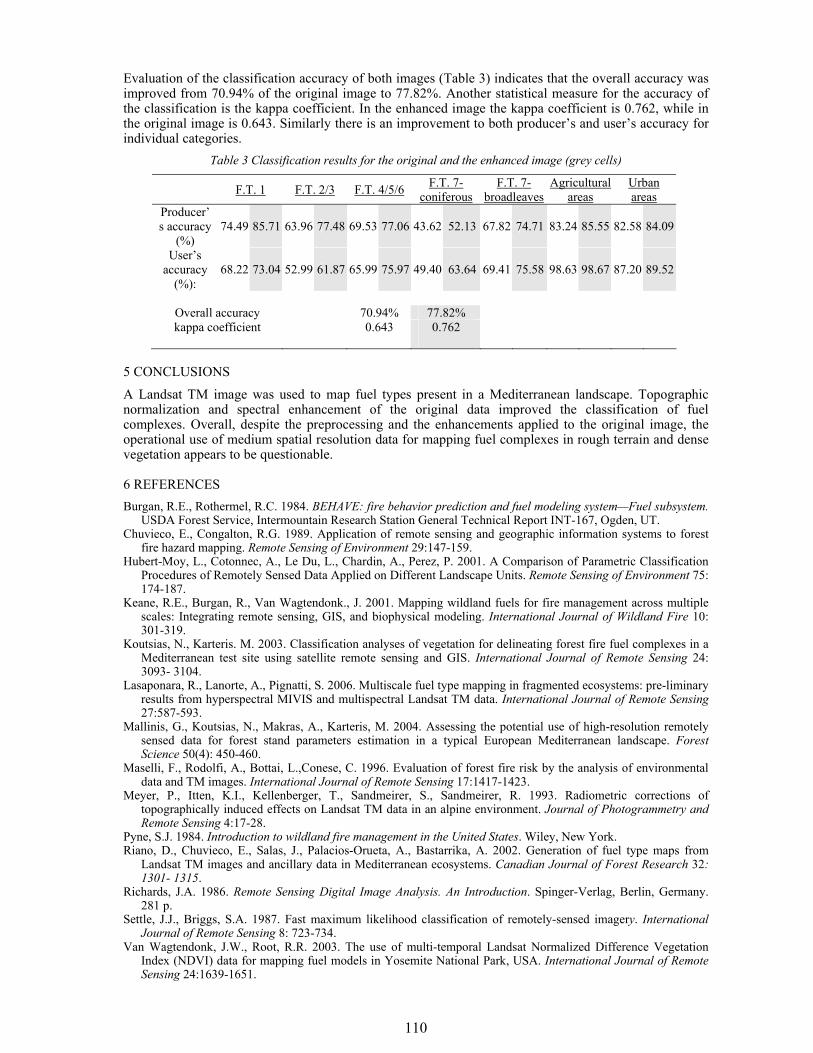
110

Evaluation of the classification accuracy of both images (Table 3) indicates that the overall accuracy was improved from 70.94% of the original image to 77.82%. Another statistical measure for the accuracy of the classification is the kappa coefficient. In the enhanced image the kappa coefficient is 0.762, while in the original image is 0.643. Similarly there is an improvement to both producer’s and user’s accuracy for individual categories.

Table 3 Classification results for the original and the enhanced image (grey cells)

F.T. 1 F.T. 2/3 F.T. 4/5/6 F.T. 7-coniferous

F.T. 7-broadleaves

Agricultural areas

Urban areas

Producer’s accuracy

(%) 74.49 85.71 63.96 77.48 69.53 77.06 43.62 52.13 67.82 74.71 83.24 85.55 82.58 84.09

User’s accuracy

(%): 68.22 73.04 52.99 61.87 65.99 75.97 49.40 63.64 69.41 75.58 98.63 98.67 87.20 89.52

Overall accuracy 70.94% 77.82% kappa coefficient 0.643 0.762

5 CONCLUSIONS

A Landsat TM image was used to map fuel types present in a Mediterranean landscape. Topographic normalization and spectral enhancement of the original data improved the classification of fuel complexes. Overall, despite the preprocessing and the enhancements applied to the original image, the operational use of medium spatial resolution data for mapping fuel complexes in rough terrain and dense vegetation appears to be questionable.

6 REFERENCES Burgan, R.E., Rothermel, R.C. 1984. BEHAVE: fire behavior prediction and fuel modeling system—Fuel subsystem.

USDA Forest Service, Intermountain Research Station General Technical Report INT-167, Ogden, UT. Chuvieco, E., Congalton, R.G. 1989. Application of remote sensing and geographic information systems to forest

fire hazard mapping. Remote Sensing of Environment 29:147-159. Hubert-Moy, L., Cotonnec, A., Le Du, L., Chardin, A., Perez, P. 2001. A Comparison of Parametric Classification

Procedures of Remotely Sensed Data Applied on Different Landscape Units. Remote Sensing of Environment 75: 174-187.

Keane, R.E., Burgan, R., Van Wagtendonk., J. 2001. Mapping wildland fuels for fire management across multiple scales: Integrating remote sensing, GIS, and biophysical modeling. International Journal of Wildland Fire 10: 301-319.

Koutsias, N., Karteris. M. 2003. Classification analyses of vegetation for delineating forest fire fuel complexes in a Mediterranean test site using satellite remote sensing and GIS. International Journal of Remote Sensing 24: 3093- 3104.

Lasaponara, R., Lanorte, A., Pignatti, S. 2006. Multiscale fuel type mapping in fragmented ecosystems: pre-liminary results from hyperspectral MIVIS and multispectral Landsat TM data. International Journal of Remote Sensing 27:587-593.

Mallinis, G., Koutsias, N., Makras, A., Karteris, Μ. 2004. Assessing the potential use of high-resolution remotely sensed data for forest stand parameters estimation in a typical European Mediterranean landscape. Forest Science 50(4): 450-460.

Maselli, F., Rodolfi, A., Bottai, L.,Conese, C. 1996. Evaluation of forest fire risk by the analysis of environmental data and TM images. International Journal of Remote Sensing 17:1417-1423.

Meyer, P., Itten, K.I., Kellenberger, T., Sandmeirer, S., Sandmeirer, R. 1993. Radiometric corrections of topographically induced effects on Landsat TM data in an alpine environment. Journal of Photogrammetry and Remote Sensing 4:17-28.

Pyne, S.J. 1984. Introduction to wildland fire management in the United States. Wiley, New York. Riano, D., Chuvieco, E., Salas, J., Palacios-Orueta, A., Bastarrika, A. 2002. Generation of fuel type maps from

Landsat TM images and ancillary data in Mediterranean ecosystems. Canadian Journal of Forest Research 32: 1301- 1315.

Richards, J.A. 1986. Remote Sensing Digital Image Analysis. An Introduction. Spinger-Verlag, Berlin, Germany. 281 p.

Settle, J.J., Briggs, S.A. 1987. Fast maximum likelihood classification of remotely-sensed imagery. International Journal of Remote Sensing 8: 723-734.

Van Wagtendonk, J.W., Root, R.R. 2003. The use of multi-temporal Landsat Normalized Difference Vegetation Index (NDVI) data for mapping fuel models in Yosemite National Park, USA. International Journal of Remote Sensing 24:1639-1651.

111

1 INTRODUCTION Based on knowledge about the spatial extent of the fuels, fire managers can design strategies related to the use and distribution of available firefighting resources, which can prevent or at least minimize fire effects (Lasaponara, 2006). Also, accurate knowledge of the spatial distribution of the different fuel load complexes can provide valuable guidance in fuel treatments strategies. The wide range of the fuel physical characteristics (i.e. load, size, bulk density etc) found within an area and the need for standardization in fuel description across different areas since the resulting fuel type maps are used as input to fire behavior models such as FARSITE and BEHAVE, have resulted to development of predefined classification schemes. There a lot of fuel models worldwide, among which the most widely-spread are the models developed for the U.S. Forest Service which includes 13 fuel types, which are used as input in the BEHAVE and FARSITE fire behavior simulators, the National Fire Danger Rating System–NFDRS (Deeming et al., 1978; Burgan, 1988), which includes 20 different fuel types and finally the Canadian Forest Fire Behaviour Prediction System–FBP (Lawson et al., 1985) which is based on a 16 fuel types discrimination. In Greece, 7 fuel models representative of Mediterranean vegetation have been created by Dimitrakopoulos (2002). Fuel models mapping was strengthen among others from the availability of satellite data with very fine spatial resolution. This type of imagery brought about a reconsideration of the methods used so far for the extraction of the information. For purposes of fuel complexes mapping Gitas et al. (2006) evaluated the use of a multiscale object based approach using subsets of high spatial resolution imagery, in order to explore forest fuels delineation in Crete, Greece. Arroyo et al., (2005) classified a Quickbird image following the PROMETHEUS fuel type model based originally on a pixel based classification approach which was later refined using contextual information within a hierarchical network of objects. Classification And Regression Trees analysis (Breiman et al., 1984) has been employed in the past in fuel model mapping studies only in the classification of medium resolution imagery using a pixel-based approach (Amatulli et al., 2005). Aim of this study was the generation of accurate fire behavior maps in a

Integration of local scale fuel type mapping and fire behavior prediction using high spatial resolution imagery

G. Mallinis Laboratory of Forest Management and Remote Sensing, School of Forestry and Natural Environment, Aristotle University of Thessaloniki, P.O.Box, 54124, Thessaloniki, Greece, e-mail: [email protected]

I.D. Mitsopoulos & A.P. Dimitrakopoulos Laboratory of Forest Protection, School of Forestry and Natural Environment, Aristotle University of Thessaloniki, P.O.Box228 , 54124, Thessaloniki, Greece.

I.Z. Gitas & M. Karteris Laboratory of Forest Management and Remote Sensing, School of Forestry and Natural Environment, Aristotle University of Thessaloniki, P.O.Box, 54124, Thessaloniki, Greece,

Keywords: remote sensing, fuel mapping, fire behavior, remote sensing, FARSITE, landscape.

ABSTRACT: Judicial wildland fire prevention and management requires precise information on fuel characteristics and spatial distribution of the various vegetation types present in an area. This study is an integrated approach to fire management since it combines local scale fuel type mapping with fire behavior simulation. The spatial extent of the different fuel types of a forested landscape in Northern Greece characterized by heterogeneous vegetation and topography was determined using a Quickbird high spatial resolution image. Following necessary pre-processing of the image to compensate geometric errors, multi-scale components of the scene were delineated through a segmentation algorithm. The resulting image objects were assigned to respective fuel types using a CART statistical model. Site specific fuel models were created by measuring fuel parameters in representative natural fuel complexes. FARSITE fire simulation model was used to simulate potential wildland fire growth and behavior. Utilizing the spatial database capabilities of GIS, FARSITE allows the user to simulate the spatial and temporal spread and behavior of a fire burning in heterogeneous terrain, fuels, and weather. The proposed methodology presents an innovative integration of fuel mapping with remote sensing techniques and fire behavior simulation for fire management planning across the landscape. The final fire behaviour maps are an end product which can be fully exploited operationally from local fire management authorities without further processing.

112

fragmented landscape, considering detailed local scale fuel maps derived through object based image analysis of high spatial resolution imagery.

2 STUDY AREA Aristotle’s University Forest is located in Northern Greece and has a total of around 60 km2 area. The altitude in the University Forest ranges from 320 to 1200 meters. The overall landscape pattern is considered fragmented with pure and mixed stands of various species intermingling with patches of bare land.

3 METHODOLOGY

3.1 Fuel sampling All the areas in the study site were stratified on vegetation maps according to the dominant vegetation types. All the stratified areas were surveyed on site and 10 representative locations with typical ('average') fuel conditions for each area were selected. A similar approach to Dimitrakopoulos (2002) was followed in order to inventory fuel characteristics. In every representative location, fuel structural parameters were measured in 10 m2 sampling plots (Brown et al., 1982). The clip-and-weigh method was used for the determination of all fuel loads by size category. The line-intercept method was used in order to estimate the area cover by each vegetation type (Bonham, 1989). All fuel loads (fuel weight per unit surface area) are expressed on a dry- weight basis.

3.2 Imagery and ancillary data A Quickbird image was acquired on June 2004. For the process of the geometric rectification, a DTM was used with 10 meter cell size and ground control points identified over existing orthophotographs. The original image was subject to the IHS transformation along with the calculation of two vegetation indices (NDVI-RVI). Finally a ground survey was conducted in the study site and 82 plots were accurately located using a GPS handheld device and print outs of the panchromatic image with a scale 1:2000. Structural and floristic vegetation parameters within each plot were recorded in detail. 3.3 Image segmentation and classification The original image along with the derivative bands was subject to a multi-resolution segmentation following the Fractal Net Evolution Approach (FNEA) concept. Four different levels of objects were created considering the intensity and saturation bands with less weight given to the last one due to the greater variability observed in its DN values. The upper level of the hierarchy included the larger objects, corresponding to homogeneous patches presenting the same vegetation physiognomy. Various spectral features for the original nine bands as well as features related to the shape, the texture and the context of the fourth’s level objects were evaluated as potential predictors in the CART analysis.

3.4 Fire behavior maps Fire behavior prediction (fireline intensity and flame length) for every fuel model was calculated by FARSITE fire growth model (Finey, 1998) using as input data the DEM of the area, the spatial extent of the fuel models and the fuel values of each model. Summer burning conditions were simulated by setting 1-hr fuel moisture content at 8% for 10 km/hr midflame windspeed. The live foliage moisture content was set at 100%. Heat content and surface area-to-volume ratio values were obtained by Dimitrakopoulos and Panov (2001).

4 RESULTS AND DISCUSSION The fuel models that resulted from the field sampling represent all the major vegetation types of the study area (Table 1). The shrublands (maquis) fuel model 1 incorporates maquis with height up to 2.0 m featuring high proportion of foliage load (22.8%) and a substantial part of the fuel load distributed to the large size class (100-hr fuels 10.7%). The grasslands, the litter of pine forests, oak forests, beech forests and the litter of the mixed forests demonstrated limited spatial heterogeneity and are represented by fuel model 2 for pine forests (total fuel load 3.1 t/ha), fuel model 3 for oak forest litter (total fuel load 5 t/ha), fuel model 4 for beech forest litter (total fuel load 4.7 t/ha), fuel model 5 for the mixed forests (total fuel load 3.2 t/ha) and fuel model 6 for grasslands (total fuel load 4.7 t/ha). The tree biomass (stems, branches and crowns) of the pine, oak and beech forests were not measured. The variation of total fuel load was low in all fuel models, as suggested by the magnitude of the standard deviation (S.D.). The total loads of all fuel models were found to be statistically different at p = 0.05

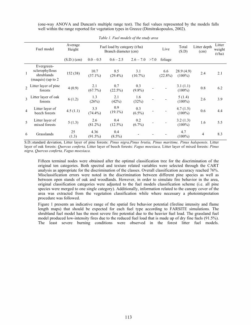
113

(one-way ANOVA and Duncan's multiple range test). The fuel values represented by the models falls well within the range reported for vegetation types in Greece (Dimitrakopoulos, 2002).

Table 1. Fuel models of the study area

Fuel model Average Height

Fuel load by category (t/ha) Branch diameter (cm) Live Total

(S.D) Litter depth

(cm)

Litter weight (t/ha)

(S.D.) (cm) 0.0 – 0.5 0.6 – 2.5 2.6 – 7.0 >7.0 foliage

1

Evergreen-sclerophyllous

shrublands (maquis) (up to 2

)

152 (38) 10.7 (37.1%)

8.5 (29.4%)

3.1 (10.7%) 6.6

(22.8%)28.9 (4.9) (100%) 2.4 2.1

2 Litter layer of pine forests 4 (0.9) 2.1

(67.7%) 0.7

(22.5%) 0.3

(9.8%) - - 3.1 (1.1) (100%) 0.8 6.2

3 Litter layer of oak forests 6 (1.2) 1.3

(26%) 2.1

(42%) 1.6

(32%) - - 5 (1.4) (100%) 2.6 3.9

4 Litter layer of beech forests 4.5 (1.1) 3.5

(74.4%) 0.9

(19.1%) 0.3

(6.5%) - - 4.7 (1.5) (100%) 0.6 4.4

5 Litter layer of mixed forests 5 (1.3) 2.6

(81.2%) 0.4

(12.5%) 0.2

(6.7%) - - 3.2 (1.3) (100%) 1.6 5.5

6 Grasslands 25 (1.3)

4.36 (91.5%)

0.4 (8.5%) - - - 4.7

(100%) 4 8.3

S.D.:standard deviation, Litter layer of pine forests: Pinus nigra,Pinus brutia, Pinus maritime, Pinus halepensis. Litter layer of oak forests: Quercus conferta, Litter layer of beech forests: Fagus moesiaca, Litter layer of mixed forests: Pinus nigra, Quercus conferta, Fagus moesiaca.

Fifteen terminal nodes were obtained after the optimal classification tree for the discrimination of the original ten categories. Both spectral and texture related variables were selected through the CART analysis as appropriate for the discrimination of the classes. Overall classification accuracy reached 76%. Misclassification errors were noted in the discrimination between different pine species as well as between open stands of oak and woodlands. However, in order to simulate fire behavior in the area, original classification categories were adjusted to the fuel models classification scheme (i.e. all pine species were merged to one single category). Additionally, information related to the canopy cover of the area was extracted from the vegetation classification while where necessary a photointepretation procedure was followed. Figure 1 presents an indicative range of the spatial fire behavior potential (fireline intensity and flame length maps) that should be expected for each fuel type according to FARSITE simulations. The shrubland fuel model has the most severe fire potential due to the heavier fuel load. The grassland fuel model produced low-intensity fires due to the reduced fuel load that is made up of dry fine fuels (91.5%). The least severe burning conditions were observed in the forest litter fuel models.

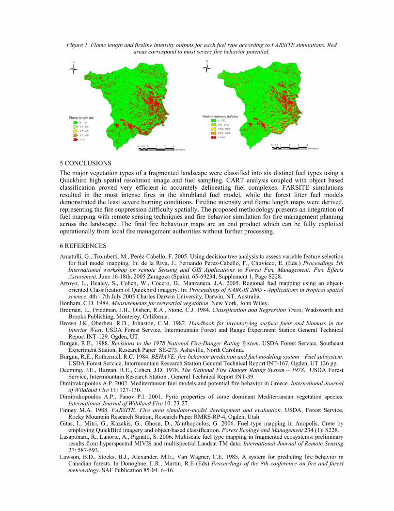
Figure 1. Flame length and fireline intensity outputs for each fuel type according to FARSITE simulations. Red areas correspond to most severe fire behavior potential.

5 CONCLUSIONS The major vegetation types of a fragmented landscape were classified into six distinct fuel types using a Quickbird high spatial resolution image and fuel sampling. CART analysis coupled with object based classification proved very efficient in accurately delineating fuel complexes. FARSITE simulations resulted in the most intense fires in the shrubland fuel model, while the forest litter fuel models demonstrated the least severe burning conditions. Fireline intensity and flame length maps were derived, representing the fire suppression difficulty spatially. The proposed methodology presents an integration of fuel mapping with remote sensing techniques and fire behavior simulation for fire management planning across the landscape. The final fire behaviour maps are an end product which can be fully exploited operationally from local fire management authorities without further processing.

6 REFERENCES Amatulli, G., Trombetti, M., Peréz-Cabello, F. 2005. Using decision tree analysis to assess variable feature selection

for fuel model mapping, In: de la Riva, J., Fernando Perez-Cabello, F., Chuvieco, E. (Eds.) Proceedings 5th International workshop on remote Sensing and GIS Applications to Forest Fire Management: Fire Effects Assessment. June 16-18th, 2005 Zaragoza (Spain). 65-69234, Supplement 1, Page S228.

Arroyo, L., Healey, S., Cohen, W., Cocero, D., Manzanera, J.A. 2005. Regional fuel mapping using an object-oriented Classification of Quickbird imagery. In: Proceedings of NARGIS 2005 - Applications in tropical spatial science. 4th - 7th July 2005 Charles Darwin University, Darwin, NT, Australia.

Bonham, C.D. 1989. Measurements for terrestrial vegetation. New York, John Wiley. Breiman, L., Friedman, J.H., Olshen, R.A., Stone, C.J. 1984. Classification and Regression Trees, Wadsworth and

Brooks Publishing, Monterey, California. Brown J.K, Oberheu, R.D., Johnston, C.M. 1982. Handbook for inventorying surface fuels and biomass in the

Interior West. USDA Forest Service, Intermountain Forest and Range Experiment Station General Technical Report INT-129. Ogden, UT.

Burgan, R.E., 1988. Revisions to the 1978 National Fire-Danger Rating System. USDA Forest Service, Southeast Experiment Station, Research Paper SE-273. Asheville, North Carolina.

Burgan, R.E., Rothermel, R.C. 1984. BEHAVE: fire behavior prediction and fuel modeling system—Fuel subsystem. USDA Forest Service, Intermountain Research Station General Technical Report INT-167, Ogden, UT 126 pp.

Deeming, J.E., Burgan, R.E., Cohen, J.D. 1978. The National Fire Danger Rating System – 1978. USDA Forest Service, Intermountain Research Station , General Technical Report INT-39

Dimitrakopoulos A.P. 2002. Mediterranean fuel models and potential fire behavior in Greece. International Journal of Wildland Fire 11: 127-130.

Dimitrakopoulos A.P., Panov P.I. 2001. Pyric properties of some dominant Mediterranean vegetation species. International Journal of Wildland Fire 10: 23-27.

Finney M.A. 1988. FARSITE: Fire area simulator-model development and evaluation. USDA, Forest Service, Rocky Mountain Research Station, Research Paper RMRS-RP-4, Ogden, Utah

Gitas, I., Mitri, G., Kazakis, G., Ghosn, D., Xanthopoulos, G. 2006. Fuel type mapping in Anopolis, Crete by employing QuickBird imagery and object-based classification. Forest Ecology and Management 234 (1): S228.

Lasaponara, R., Lanorte, A., Pignatti, S. 2006. Multiscale fuel type mapping in fragmented ecosystems: preliminary results from hyperspectral MIVIS and multispectral Landsat TM data. International Journal of Remote Sensing 27: 587-593.

Lawson, B.D., Stocks, B.J., Alexander, M.E., Van Wagner, C.E. 1985. A system for predicting fire behavior in Canadian forests. In Donoghue, L.R., Martin, R.E (Eds) Proceedings of the 8th conference on fire and forest meteorology. SAF Publication 85-04. 6–16.

115

1 INTRODUCTION

Space-borne satellite imagery is increasingly used for the characterization and mapping of vegetation types and properties. In the context of fire management, satellite imagery can provide valuable information for fuel mapping at different temporal and spatial scales including the global, regional and landscape levels.The spatial distribution of fuel type is highly requested for the management of fire hazard and risk and for understanding the ecological relationships between wildland fire and landscape structure. The availability of satellite sensors with increased spatial and spectral resolution, compared to those provided by the early space-borne sensors, may improve the accuracy and reduce the cost for mapping fuel types. In order to fully exploit the capability of these sensors, the adquate selection of fuel type features and their spectral classes is mandatory. Over the years, in the context of pattern recognition issues, a number of feature selection techniques have been proposed to optimize the spectral characterization of data classes. Among the most widely applied procedures there are the “statistically separability indices” which enable the selection of adequate subset of features by evaluating the degree of interclass separability. Such an evaluation is highly recomanded, expecially in a complex landscape, where the high within-class spectral variance of fuel distribution classes can strongly affect the classification accuracy. In this paper, the selection of fuel features and the comparison of their signatures was performed by using the Jeffries– Matusita (JM) distance that is a saturating transform of the Bhattacharya distance. The remotely sensed characterization of fuel types was performed by adopting as reference the fuel types classification developed for Mediterranean ecosystems in the framework of the Prometheus project (Prometheus Project 1999). The investiation was performed using Advanced Space-borne Thermal Emission and Reflection Radiometer (ASTER) and MODIS data. Fieldwork fuel types recognitions, carried out at the same time as remote sensing data acquisitions, were used as ground-truth dataset to assess the results obtained for the considered test areas.

2 JEFFRIES– MATUSITA (JM) DISTANCE The spectral separability index based on the Jm distance (see Richards, 1986) is regarded to be an appropiate measure for feature selectio before apraching a classification process. The Jeffries– Matusita (JM) distance has been defined as follows

21

2

⎪⎭

⎪⎬⎫

⎪⎩

⎪⎨⎧

⎥⎥⎦

⎤

⎢⎢⎣

⎡⎟⎠

⎞⎜⎝

⎛−⎟⎠⎞⎜

⎝⎛= ∫

xji

ij dxxpxpJ ωω [1]

On the spectral separability of Prometheus fuel types in the Mediterranean ecosystems of the Italian Peninsula

R. Lasaponara & A. Lanorte National Research Council, Institute of Methodologies of Environmental Analysis, C. da S. Loja, Tito Scalo, Potenza 85050, Italy Keywords: fuel type, ASTER, MODIS, Jeffries– Matusita (JM) distance

ABSTRACT: The spatial and spectral characterization of fuel types is a very important issue for mapping fire danger/risk and simulating fire growth and intensity across a landscape. Nevertheless, due to the complex nature of fuel characteristics, a fuel map is considered one of the most difficult thematic layers to build. The advent of satellite sensors with increased spatial and spectral resolution may improve the accuracy and reduce the cost for mapping fuel types. In this study, Advanced Spaceborne Thermal Emission and Reflection Radiometer (ASTER) and MODIS data were analysed for the Mediterranean ecosystems of the Italian Peninsula in order to evaluate the spectral separability of Prometheus fuel types. The comparison of fuel signatures was performed by using the Jeffries– Matusita (JM) distance that is a saturating transform of the Bhattacharya distance. Results from our investigations showed that satellite remote sensing data classification provide valuable information for the characterization and mapping of fuel types and vegetation properties at different spatial scales.

116

where ⎟⎠⎞⎜

⎝⎛

ixp ω and

⎟⎠

⎞⎜⎝

⎛j

xp ω are the conditional probability density functions for the feature vector x,

given the data classes iω and jω , respectively. Equation 1 can be rewritten as

( )ijbij eJ −−= 12 [2]

where bij is the Bhattacharya distance defined as equation 3.

⎪⎭

⎪⎬⎫

⎪⎩

⎪⎨⎧

⎟⎠

⎞⎜⎝

⎛⎟⎠⎞⎜

⎝⎛−= ∫

xji

ij dxxpxpb ωωln [3]

Equation 3 can be rewritten as

[ ]( ) ⎥⎦

⎤⎢⎣⎡ ΣΣ

⎥⎥⎦

⎤

⎢⎢⎣

⎡

+−−=

Σ+Σ

−Σ+Σ

21

2

1

2 ln21)()(

81

bf

bfT

bf

bf

bfBD μμμμ

where μf and μ b are the mean of and ∑f and ∑ b are the covariance matrix of archaeological the two considered classes (1) archaeological feature and (2) their background. From eqaution 4, the Bhattacharya distance can be seen as two components. The first component of equation (4) represents the mean, whereas the second part is the covariance difference. For the BD a greater value indicates a greater average distance. A drawback of the BD is that such an index does not provide any indication of threshold values for separability. In the Jeffries Matusita (JM) distance, shown in equation 2, the presence of the exponential factor gives an exponentially decreasing weight to increasing separations between spectral classes. The JM distance has an upper boundary of 1.41 ( 2 ), and a lower boundary of 0. The JM distance is asymptotic to the value 2 for increasing class separability. A value of 2 for JM distance would imply that the classification will be performed with 100% accuracy. When the calculated distance is zero, the signatures can be said to be totally inseparable. Lee and Choi (2000) suggested that: (i) a JM distance of 1.09 corresponds to a classification error probability of 10%, and this means that the signatures can be separable; (ii) a JM distance of 1.24 corresponds to a classification error probability of 5%, and this means that the signatures can be highly separable; As been pointed out the J-M index has been designed for measuring a statistical separability of two classes. In order to extend the J-M to multiclass cases, over the years, different strategies have been proposed. The most common is based on the use of J-M computed over the all pairs of classes . A second approach was based on the selection of feature subset which enables the best separation between the least separable pair of classes. In the current paper we adopted the first approach.

3 SATELLITE DATA ANALYSIS

The considered data set refers to typical fuel types of Mediterranean ecosystems (Prometheus Project 1999). Table 1 shows the fuel type developed for Mediterranean ecosystems in the framework of the Prometheus project (Prometheus Project 1999). For each pixel, the feature vectors was formed by the spectral bands provided by the given satellite sensors. Advanced Spaceborne Thermal Emission and Reflection Radiometer (ASTER) and MODIS.

[4]

117

Table 1. Fuel type classification developed for Mediterranean ecosystems in the framework of Prometheus project (Prometheus Project 1999)

Fuel Type class

Fuel Type description in terms of percentage of cover

Fuel Type description in terms of vegetation typology

1 Ground fuels (cover >50%) grass 2 Surface fuels (shrub cover >60%, tree

cover <50%) grassland, shrub land (smaller than 0.3–0.6 m and with a high percentage of grassland), and clear cuts, where slash was not removed

3 Medium-height shrubs (shrub cover >60%, tree cover <50%)

shrubs between 0.6 and 2.0 m

4 Tall shrubs (shrub cover >60%, tree cover <50%)

high shrubs (between 2.0 and 4.0 m) and young trees resulting from natural regeneration or forestation

5 Tree stands (>4 m) with a clean ground surface (shrub cover <30%)

the ground fuel was removed either by prescribed burning or by mechanical means. This situation may also occur in closed canopies in which the lack of sunlight inhibits the growth of surface vegetation

6 Tree stands (>4 m) with medium surface fuels (shrub cover >30%)

the base of the canopies is well above the surface fuel layer (>0.5 m). The fuel consists essentially of small shrubs, grass, litter, and duff (the layer of decomposing organic materials lying immediately above the mineral soil but below the litter layer of freshly fallen twigs, needles, and leaves; the fermentation layer).

7 Tree stands (>4 m) with heavy surface fuels (shrub cover >30%)

stands with a very dense surface fuel layer and with a very small vertical gap to the canopy base (<0.5 m)

Table 2. JM index values obtained from ASTER data for a test area selected within Sila National Park in the Calabria Region

SAN GIOVANNI

no fuel

fuel type1

fuel type2

fuel type3

fuel type4

fuel type5

fuel type6

fuel type7 unclassified

no fuel \ 1,980 1,983 1,976 1,984 1,998 1,998 1,917 1,984 fuel type1 1,980 \ 1,415 1,286 1,984 2,000 2,000 1,977 2,000 fuel type2 1,983 1,415 \ 1,499 1,830 2,000 1,979 1,898 2,000 fuel type3 1,976 1,286 1,499 \ 1,623 2,000 1,965 1,816 2,000 fuel type4 1,984 1,984 1,830 1,623 \ 2,000 1,883 1,581 2,000 fuel type5 1,998 2,000 2,000 2,000 2,000 \ 2,000 2,000 1,999 fuel type6 1,998 2,000 1,979 1,965 1,883 2,000 \ 1,955 2,000 fuel type7 1,917 1,977 1,898 1,816 1,581 2,000 1,955 \ 2,000 unclassified 1,984 2,000 2,000 2,000 2,000 1,999 2,000 2,000 \

Table 3. JM index values obtained from ASTER data for a test area selected within Pollino National Park in the Basilicata Region

POLLINO

no fuel

fuel type1

fuel type2

fuel type3

fuel type4

fuel type5

fuel type6

fuel type7 unclassified

no fuel \ 1,9343 1,9841 1,9956 2,0000 2,0000 2,0000 2,0000 2,0000 fuel type1 1,9343 \ 1,6628 1,7576 1,9998 2,0000 2,0000 1,9999 2,0000 fuel type2 1,9841 1,9841 \ 0,8785 1,6491 1,9691 1,7706 1,6335 2,0000 fuel type3 1,9956 1,7576 0,8785 \ 1,4437 1,9904 1,8721 1,6443 2,0000 fuel type4 2,0000 1,9998 1,6491 1,4437 \ 1,9249 1,4917 0,8838 2,0000 fuel type5 2,0000 2,0000 1,9691 1,9904 1,9249 \ 1,7199 1,9305 2,0000 fuel type6 2,0000 2,0000 1,7706 1,8721 1,4917 1,7199 \ 1,5100 1,9998 fuel type7 2,0000 1,9999 1,6335 1,6443 0,8838 1,9305 1,5100 \ 1,9957 unclassified 2,0000 2,0000 2,0000 2,0000 2,0000 2,0000 1,9998 1,9957 \

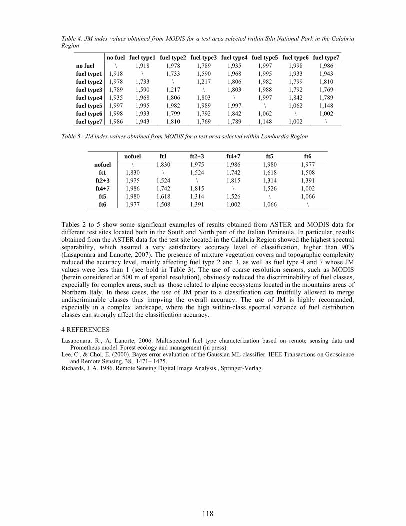
118

Table 4. JM index values obtained from MODIS for a test area selected within Sila National Park in the Calabria Region

no fuel fuel type1 fuel type2 fuel type3 fuel type4 fuel type5 fuel type6 fuel type7no fuel \ 1,918 1,978 1,789 1,935 1,997 1,998 1,986 fuel type1 1,918 \ 1,733 1,590 1,968 1,995 1,933 1,943 fuel type2 1,978 1,733 \ 1,217 1,806 1,982 1,799 1,810 fuel type3 1,789 1,590 1,217 \ 1,803 1,988 1,792 1,769 fuel type4 1,935 1,968 1,806 1,803 \ 1,997 1,842 1,789 fuel type5 1,997 1,995 1,982 1,989 1,997 \ 1,062 1,148 fuel type6 1,998 1,933 1,799 1,792 1,842 1,062 \ 1,002 fuel type7 1,986 1,943 1,810 1,769 1,789 1,148 1,002 \

Table 5. JM index values obtained from MODIS for a test area selected within Lombardia Region

nofuel ft1 ft2+3 ft4+7 ft5 ft6

nofuel \ 1,830 1,975 1,986 1,980 1,977 ft1 1,830 \ 1,524 1,742 1,618 1,508

ft2+3 1,975 1,524 \ 1,815 1,314 1,391 ft4+7 1,986 1,742 1,815 \ 1,526 1,002

ft5 1,980 1,618 1,314 1,526 \ 1,066 ft6 1,977 1,508 1,391 1,002 1,066 \

Tables 2 to 5 show some significant examples of results obtained from ASTER and MODIS data for different test sites located both in the South and North part of the Italian Peninsula. In particular, results obtained from the ASTER data for the test site located in the Calabria Region showed the highest spectral separability, which assured a very satisfactory accuracy level of classification, higher than 90% (Lasaponara and Lanorte, 2007). The presence of mixture vegetation covers and topographic complexity reduced the accuracy level, mainly affecting fuel type 2 and 3, as well as fuel type 4 and 7 whose JM values were less than 1 (see bold in Table 3). The use of coarse resolution sensors, such as MODIS (herein considered at 500 m of spatial resolution), obviuosly reduced the discriminability of fuel classes, expecially for complex areas, such as those related to alpine ecosystems located in the mountains areas of Northern Italy. In these cases, the use of JM prior to a classification can fruitfully allowed to merge undiscriminable classes thus imrpving the overall accuracy. The use of JM is highly recomanded, expecially in a complex landscape, where the high within-class spectral variance of fuel distribution classes can strongly affect the classification accuracy.

4 REFERENCES Lasaponara, R., A. Lanorte, 2006. Multispectral fuel type characterization based on remote sensing data and

Prometheus model Forest ecology and management (in press). Lee, C., & Choi, E. (2000). Bayes error evaluation of the Gaussian ML classifier. IEEE Transactions on Geoscience

and Remote Sensing, 38, 1471– 1475. Richards, J. A. 1986. Remote Sensing Digital Image Analysis., Springer-Verlag.

119

1 INTRODUCTION

The Description and study of the fire events distribution in terms of probability/density of the fire ignitions and their causes have always been challenging tasks in fire pattern modelling and risk assessment, and nowadays is becoming essential for landscape modelling, fire management and prevention actions. In particular, the prediction of wildfire and the interrelationships of the fire predictor variables open a wide field of research in the framework of fire risk long-term assessment. Besides, the increasing availability of sophisticated and flexible data analysis techniques such as spatially explicit regression models and non-parametric statistical methods, , together with the potential offered by faster computational power reached in the last decade, allow highlighting complex variable relations and provide a practical help to perform complex data analysis. The empirically based assessment of long-term fire risk is often approached using multiple regressions analysis techniques where the fire occurrence response variable is predicted against a set of environmental and human predictor variables. The final aim is to understand the weight and role of the most important predictor variables capable to explain the variance of the fire phenomena. When the response variable is the probability of fire occurrence, the most appropriate parametric method is usually, a logistic regression, but this requires a number of assumptions to be verified, including careful consideration of predictor variables interactions and autocorrelation analysis. 1.1 Objectives Built on the results of a previous work (Amatulli et al., 2007), this paper attempts to go one step further in exploratory data analysis and presents a statistical approach to enhance the understanding of complex

Predicting the occurrence of lighting/human-caused wildfires using advanced techniques of data mining

Giuseppe Amatulli Joint Research Centre of the European Commission, Institute for Environment and Sustainability, Via E. Fermi, 21020 Ispra (VA), Italy – [email protected]

Fernando Peréz-Cabello University of Zaragoza, Department of Geography and Spatial Management, Calle Pedro Cerbuna 12, 50009 Zaragoza, Spain

Andrea Camia Joint Research Centre of the European Commission, Institute for Environment and Sustainability, Via E. Fermi, 21020 Ispra (VA), Italy

Juan de la Riva University of Zaragoza, Department of Geography and Spatial Management, Calle Pedro Cerbuna 12, 50009 Zaragoza, Spain Keywords: fire occurrence, long-term fire risk, fire ignition patterns, fire prediction models.

ABSTRACT: The fire scientific community and even more the fire managers are trying to assess and describe the fire occurrence parameters that are involved in the fire phenomena. The heterogeneous nature of the variables involved in the process lead to the use of complex predictive models which have to deal with their non-normal distribution in the spatial and temporal domains. Besides, human and natural causes of fire ignition need to be investigated by means of predictor variables that can be spatially related under non-linear and non-additive relationships. Due to these actual limitations, the fire modelling community is seeking innovative and flexible models able to deal with these complex data relationships. This paper aims to overcome the limitations of the common regression techniques by testing alternative methodologies (Regression Tree) based on powerful models part of the family of the data mining or/and non-parametric techniques. In the framework of long-term wildfire risk assessment, lightning/human-caused occurrence has been used in this study as response variable against several predictors. The wildfire occurrence variable has been calculated by kernel density estimation technique using ignition points collected in the Aragón’s autonomy (Spain) in a 19 years period (1983-2001). The predictor variables included physical and human layers considered as relevant in the fire distribution processes (road and population density, climate condition, topographic aspects, etc.). Model performance was then evaluated looking the explained variance and the RMSE. The results enlightened the potential of the new considered model that resulted to be able to properly identify the relationships between the considered variables and explain the fire phenomena in the study area.

120

relationships among wildfire occurrence variables. The scope is achieved applying a powerful non-parametric regression technique, the Regression Tree analysis (RT) (Breiman, et al. 1984) and a non-parametric statistical test, the Spearman's coefficient (ρ) of two scenarios of lighting/human-caused wildfire occurrence. Advantages and disadvantages of the proposed techniques will be highlighted, in view of the future implementation of regression algorithms such as MARS and SGB, GAM.


2.1 Study area and dataset Wildfire lighting/human-caused wildfire occurrences of the Aragón’s autonomy (Spain) have been used as response variables to identify differences in the fire causes pattern. The lighting/human-caused wildfire occurrence data layers were spatially interpolated by the adaptive kernel technique using fire events collected over 19 years. The detailed methodology is largely described on Amatulli et al. (2007). The results of this work produced two wildfire occurrence datasets (DL_RC_K16 and DH_ RA_K8 respectively for the lighting- and human- caused wildfire events) in the form of a continue grid surface (250 m cell size) representing the probability of a fire event expressed in terms of # ignition points/km2. The two fire occurrence grids exhibit a clear difference in fire pattern distribution also revealed by a low r = 0.348 and low ρ = 0.462. Several variables were used as predictors and they included physical and human layers considered relevant for understanding the spatial pattern of fire occurrence. All the variables were considered as points, lines o polygons depending on their nature and on the available data source. Nonetheless all of them were spatialized into a continue surface that matched the cell size and spatial context of the fire occurrence grid layers. All the variables were masked using wildland surface (Mapa Forestal de Aragón 1:50.000) to concentrate the attention on the relationships of the variables inside the areas prone to wildfires. As a result, 392210 grid cells of 250 m size were retained in the analyzed dataset. 2.2 Methodology – Predictor variables selection A set of predictor variables was pre-selected on the basis of previous works and on their expected ability to predict fire occurrence. They were treated separately in accordance to their nature, herein a summary is reported for the two main groups: human and physical variables. Among the former, primary and forestry roads, train and power lines, village/hamlet location, dump areas, recreational areas, wildland-urban/wildland-agriculture/wildland-pasture interfaces. These variables were used to extrapolate point/line distance and kernel density surfaces using several bandwidths (from 1 up to 20 km). Afterwards, the optimal bandwidth size was selected based on the calculation of the ρ coefficient between each predictor versus the two fire occurrence maps (DL_RC_K16 and DH_ RA_K8). In this way each single variable was expressed in the most suitable form (the one more correlated with the response variables). Altitude, slope, aspect were obtained from a DEM. Several variables related to vegetation and ecological characteristics were extracted from the Mapa Forestal de Aragón. They were: vegetation types and height, climax classes/levels and fragmentation classes (following the procedure described in Vogt et al., 2006). These variables summarize the ecological attitude of the vegetation cover to be prone to wildfire. Other variables more related to wildland uses and land management were protected areas, ownership, hunting permission, land use change. The most common climatic parameters such as: annual mean precipitation/temperature and precipitation/temperature of the coldest/warmest quarter were included to give information of the different climate conditions. The human behaviour was tried to be considered by means of variables such as total population variation, variation of the population dedicated to agriculture activity, incoming money, unemployment grade, amount of old people dedicate to agriculture, agriculture machines, presence of fire towers as a discourage element of arson actions. The presence of tourists and leisure areas were indicated by the presence of hotels, campings, free campings, tourist flats, tourist rural houses, and expressed in terms of total number and total room/site/bed number. 2.3 Methodology – Correlation and Regression Tree analysis The correlation analysis expressed by the Spearman's coefficient was computed for each predictor variable against the two fire occurrence layers. This procedure helps to understand the predictors behaviour against the fire occurrence variables, in the sense of positive or negative correlation. In order to predict the fire occurrence and keep in mind the constraints described in the introduction, the packages rpart, rgdal and sp of the free Open Source R statistical software were used. The software allows the implementation of complex iteration and data analysis for modelling applications also in GIS applications. Among the wide alternative of non-parametric regression models the RT model was selected due to the its several advantages such as being less restrictive in terms of assumptions, being non-parametric and allowing the retrieval of the data distribution from the training dataset. Furthermore, the RT model can handle discrete and continuous variables and the resulting regression functions are easy to

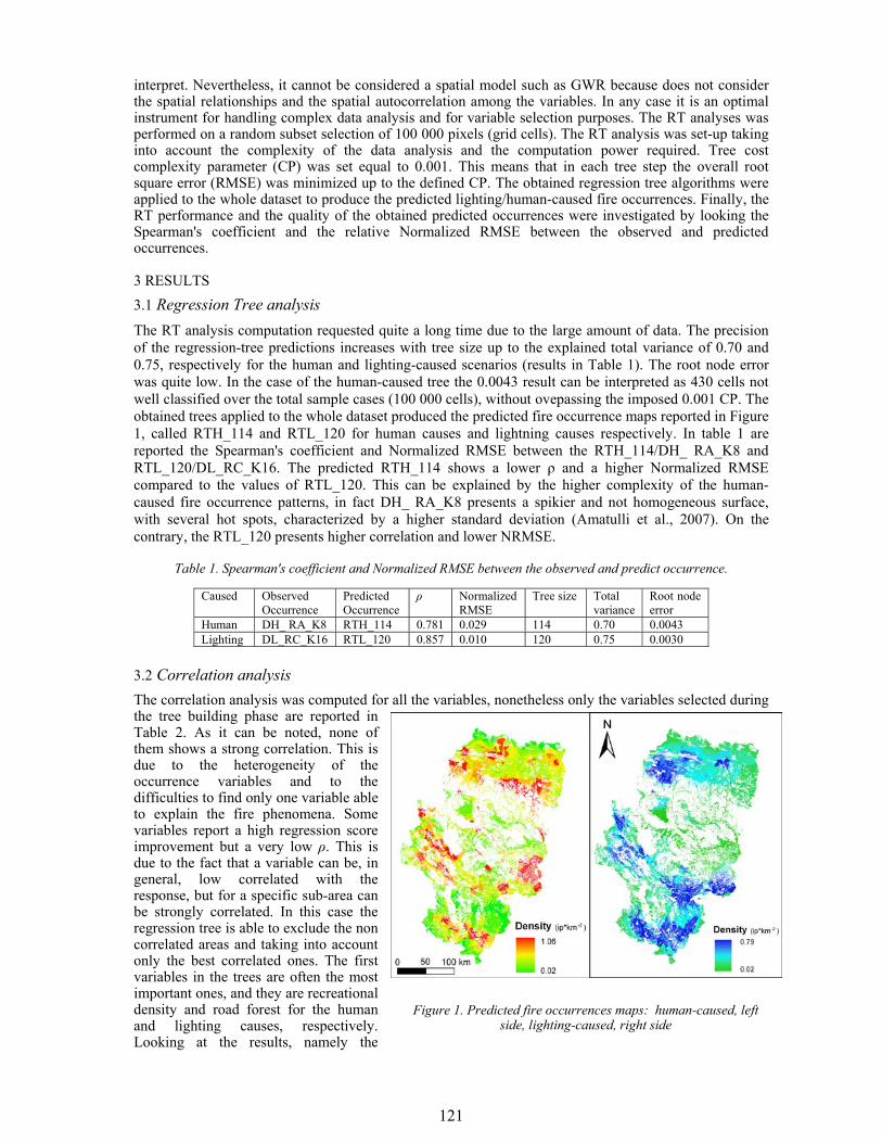
121

interpret. Nevertheless, it cannot be considered a spatial model such as GWR because does not consider the spatial relationships and the spatial autocorrelation among the variables. In any case it is an optimal instrument for handling complex data analysis and for variable selection purposes. The RT analyses was performed on a random subset selection of 100 000 pixels (grid cells). The RT analysis was set-up taking into account the complexity of the data analysis and the computation power required. Tree cost complexity parameter (CP) was set equal to 0.001. This means that in each tree step the overall root square error (RMSE) was minimized up to the defined CP. The obtained regression tree algorithms were applied to the whole dataset to produce the predicted lighting/human-caused fire occurrences. Finally, the RT performance and the quality of the obtained predicted occurrences were investigated by looking the Spearman's coefficient and the relative Normalized RMSE between the observed and predicted occurrences.

3 RESULTS 3.1 Regression Tree analysis The RT analysis computation requested quite a long time due to the large amount of data. The precision of the regression-tree predictions increases with tree size up to the explained total variance of 0.70 and 0.75, respectively for the human and lighting-caused scenarios (results in Table 1). The root node error was quite low. In the case of the human-caused tree the 0.0043 result can be interpreted as 430 cells not well classified over the total sample cases (100 000 cells), without ovepassing the imposed 0.001 CP. The obtained trees applied to the whole dataset produced the predicted fire occurrence maps reported in Figure 1, called RTH_114 and RTL_120 for human causes and lightning causes respectively. In table 1 are reported the Spearman's coefficient and Normalized RMSE between the RTH_114/DH_ RA_K8 and RTL_120/DL_RC_K16. The predicted RTH_114 shows a lower ρ and a higher Normalized RMSE compared to the values of RTL_120. This can be explained by the higher complexity of the human-caused fire occurrence patterns, in fact DH_ RA_K8 presents a spikier and not homogeneous surface, with several hot spots, characterized by a higher standard deviation (Amatulli et al., 2007). On the contrary, the RTL_120 presents higher correlation and lower NRMSE.

Table 1. Spearman's coefficient and Normalized RMSE between the observed and predict occurrence.

3.2 Correlation analysis The correlation analysis was computed for all the variables, nonetheless only the variables selected during the tree building phase are reported in Table 2. As it can be noted, none of them shows a strong correlation. This is due to the heterogeneity of the occurrence variables and to the difficulties to find only one variable able to explain the fire phenomena. Some variables report a high regression score improvement but a very low ρ. This is due to the fact that a variable can be, in general, low correlated with the response, but for a specific sub-area can be strongly correlated. In this case the regression tree is able to exclude the non correlated areas and taking into account only the best correlated ones. The first variables in the trees are often the most important ones, and they are recreational density and road forest for the human and lighting causes, respectively. Looking at the results, namely the

Caused Observed Occurrence

Predicted Occurrence

ρ Normalized RMSE

Tree size Total variance

Root node error

Human DH_ RA_K8 RTH_114 0.781 0.029 114 0.70 0.0043 Lighting DL_RC_K16 RTL_120 0.857 0.010 120 0.75 0.0030

Figure 1. Predicted fire occurrences maps: human-caused, left side, lighting-caused, right side

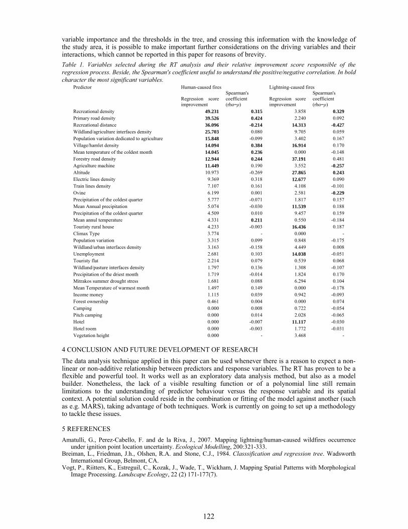
122

variable importance and the thresholds in the tree, and crossing this information with the knowledge of the study area, it is possible to make important further considerations on the driving variables and their interactions, which cannot be reported in this paper for reasons of brevity. Table 1. Variables selected during the RT analysis and their relative improvement score responsible of the regression process. Beside, the Spearman's coefficient useful to understand the positive/negative correlation. In bold character the most significant variables.

Predictor Human-caused fires Lightning-caused fires

Regression score improvement

Spearman's coefficient (rho=ρ)

Regression score improvement

Spearman's coefficient (rho=ρ)

Recreational density 49.231 0.315 3.858 0.329 Primary road density 39.526 0.424 2.240 0.092 Recreational distance 36.096 -0.214 14.313 -0.427 Wildland/agriculture interfaces density 25.703 0.080 9.705 0.059 Population variation dedicated to agriculture 15.848 -0.099 3.402 0.167 Village/hamlet density 14.094 0.384 16.914 0.170 Mean temperature of the coldest month 14.045 0.236 0.000 -0.148 Forestry road density 12.944 0.244 37.191 0.481 Agriculture machine 11.449 0.190 3.552 -0.257 Altitude 10.973 -0.269 27.865 0.243 Electric lines density 9.369 0.318 12.677 0.090 Train lines density 7.107 0.161 4.108 -0.101 Ovine 6.199 0.001 2.581 -0.229 Precipitation of the coldest quarter 5.777 -0.071 1.817 0.157 Mean Annual precipitation 5.074 -0.030 11.539 0.188 Precipitation of the coldest quarter 4.509 0.010 9.457 0.159 Mean annul temperature 4.331 0.211 0.550 -0.184 Touristy rural house 4.233 -0.003 16.436 0.187 Climax Type 3.774 - 0.000 - Population variation 3.315 0.099 0.848 -0.175 Wildland/urban interfaces density 3.163 -0.158 4.449 0.008 Unemployment 2.681 0.103 14.038 -0.051 Touristy flat 2.214 0.079 0.539 0.068 Wildland/pasture interfaces density 1.797 0.136 1.308 -0.107 Precipitation of the driest month 1.719 -0.014 1.824 0.170 Mitrakos summer drought stress 1.681 0.088 6.294 0.104 Mean Temperature of warmest month 1.497 0.149 0.000 -0.178 Income money 1.115 0.039 0.942 -0.093 Forest ownership 0.461 0.004 0.000 0.074 Camping 0.000 0.008 0.722 -0.054 Pitch camping 0.000 0.014 2.028 -0.065 Hotel 0.000 -0.007 11.117 -0.030 Hotel room 0.000 -0.003 1.772 -0.031 Vegetation height 0.000 - 3.468 -

4 CONCLUSION AND FUTURE DEVELOPMENT OF RESEARCH The data analysis technique applied in this paper can be used whenever there is a reason to expect a non-linear or non-additive relationship between predictors and response variables. The RT has proven to be a flexible and powerful tool. It works well as an exploratory data analysis method, but also as a model builder. Nonetheless, the lack of a visible resulting function or of a polynomial line still remain limitations to the understanding of predictor behaviour versus the response variable and its spatial context. A potential solution could reside in the combination or fitting of the model against another (such as e.g. MARS), taking advantage of both techniques. Work is currently on going to set up a methodology to tackle these issues.

5 REFERENCES Amatulli, G., Perez-Cabello, F. and de la Riva, J., 2007. Mapping lightning/human-caused wildfires occurrence

under ignition point location uncertainty. Ecological Modelling, 200:321-333. Breiman, L., Friedman, J.h., Olshen, R.A. and Stone, C.J., 1984. Classsification and regression tree. Wadsworth

International Group, Belmont, CA. Vogt, P., Riitters, K., Estreguil, C., Kozak, J., Wade, T., Wickham, J. Mapping Spatial Patterns with Morphological

Image Processing. Landscape Ecology, 22 (2) 171-177(7).

123

1 INTRODUCTION Forest Fires around the earth constitute an extremely important problem for the global ecosystem degradation. Only considering the European Union, more than 50.000 fires are active every year with a mean total extension of 500.000 ha. where Spain and Portugal are usually the most affected countries (Gabban, et al., 2006). Recent and ongoing satellite programs for the earth observing (TERRA, AQUA, ENVISAT…), with improvements in their spatial, spectral, radiometric and temporal resolution provide an important tool to give fire early alerts moreover an evaluation of areas under risk and a post fire estimation of damage to the landscape. A combination of environmental factors, meteorological conditions and anthropogenic causes account for the majority of wild land fires. High terrain steepness along with high summer temperature supplemented with high wind velocity and the availability of flammable material in the forest floor accounts for the major damage and wide wild spread of forest fire. However human activities remains as one of the most important causes and this makes especially difficult the generation of risk maps that alert in an effective and proper way about the areas that can finally be burnt. Anyway, satellite information can provide really useful information because of its wide temporal and spatial resolution about areas with high levels of risk. On that sense the estimation of water content of plants is one of the key parameters on the models developed not only for agricultural applications but for forest research and is usually expressed as the Fuel Moisture Content (FMC), defined as the percentage of water weight over the dry sample weight (Chuvieco et al., 2004). Long term series of NOAA-AVHRR data and recently TERRA-MODIS products have been used with good correlations between FMC and the Normalized Difference Vegetation Index obtained by means of visible and near infrared bands (Chladil and Nuñez, 1995). In addition to Vegetation Indexes, data from ground stations (air temperature, wind velocity, humidity, etc.) and static risk factors like proximity to main roads, insolation hours, etc, would let us defined in a better way, risk indexes that takes into account the great variety of factors involved (Chuvieco et al., 2003, Leblon, B., 2001). In this paper we show a study centred in La Palma Island situated in Canary Islands (Spain). Data from two different sensors (AVHRR, MODIS) are used to evaluate pre-fire conditions for a fire that took place in that island during the first weeks of September 2005. A dynamic index has been developed and introduced as the Fire Risk Dynamic Index (FRDI) in which the temporal trends in vegetation water stress, by mean of NDVI graphics (for both AVHRR and MODIS data), are modulated by a static probability function of fire risk. This index mean values are analyzed in four different regions during the months previous to that event.

2 DATA AND METHODOLOGY Two time series and sources of satellite data have been used in this work for the dynamic fire risk modelling: 8 months data of NOAA-AVHRR NDVI images (1 km) (March-September 2005) and 3 months of MODIS NDVI data (250 m.) (June-September 2005).

Synergy of GIS and Remote Sensing data in forest fire danger modelling

P. A. Hernandez-Leal, A. Gonzalez-Calvo, M. Arbelo, A. Barreto & L. Arvelo-Valencia Grupo de Observación de la Tierra y la Atmósfera (GOTA), Departamento de Física, Universidad de La Laguna, La Laguna 38200, Canary Islands (SPAIN) España, email: [email protected] Keywords: GIS, Fire risk, Vegetation indexes, AVHRR, MODIS.

ABSTRACT: During the last decades, the use of remote sensing data have provided a useful tool to make a detailed analysis of forests status and great improvements in pre- and post- fire management. Satellite data have widely proved its value to generate fire risk maps, as well as giving fire early alerts, or even making easier the estimation of areas affected by them. In this paper we propose a dynamic fire risk index that takes into account different static and dynamic factors of risk for fire occurrence. This methodology has been previously tested for some fires in the Canary Islands (Spain), and in this case we prove its usefulness using both NOAA-AVHRR and TERRA-MODIS sensors data. As a test site, a fire that took place in September 2005 in La Palma Island (Canary Islands) has been considered in order to validate the suitability of these tools for a regional scale application, in an area were multiple microclimates are present mainly due to its steep orography and the trade winds.

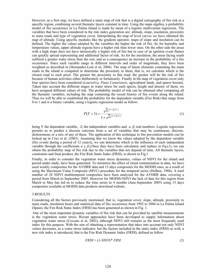
124

However, as a first step, we have defined a static map of risk that is a digital cartography of fire risk in a specific region, combining several thematic layers constant in time. Using the maps algebra, a probability model of fire occurrence in La Palma Island is made by mean of a logistic multivariate regression. The variables that have been considered in the risk index generation are: altitude, slope, insolation, proximity to main roads and type of vegetation cover. Interpolating the map of level curves we have obtained the map of altitude. Using specific modules like the gradient operator, maps of slope and insolation can be defined. The higher the values adopted by the variables the higher the risk of fire. So for humidity and temperature values, upper altitude regions have a higher risk than lower ones. On the other side the areas with a high slope does not have intrinsically a higher risk of fire but in case of an ignition event flames can quickly spread representing and additional factor of risk. As for the insolation, the areas facing south suffered a greater water stress than the rest, and as a consequence an increase in the probability of a fire occurrence. Since each variable range in different intervals and order of magnitude, they have been weighted as described in (Hernandez-Leal et al, 2006). The map of linear elements containing the main roads in the island is computed to determine the proximity to them, that is, we calculate which is the closest road to each pixel. The greater the proximity to this road, the greater will be the risk of fire because of human activities either deliberately or fortuitously. Finally in the map of vegetation cover only four species have been considered (Laurisilva, Pinus Canariensis, agricultural lands, and sparse broom). Taken into account the different stages in water stress for each specie, height and density of them, we have assigned different values of risk. The probability model of risk can be obtained after computing all the thematic variables, including the map containing the recent history of fire events along the island. Thus we will be able to established the probability for the dependent variable (Fire Risk) that range from 0 to 1 and is a binary variable, using a logistic regression model as follow:

∑+

∑==

+

+

)(

)(

1)1(

ii

ii

X

X

eeYP

βα

βα

(1)

being Y the dependent variable, Xi the independent variables and α, βi real numbers. Logistic regression permits us to predict a discrete outcome from a set of variables that may be continuous, discrete, dichotomous or a mix of any of these. The application of this technique in fire prevention models can be looked up in Cruz et al. (2003). Assuming that we know the values adopted by the dependent variable (fire events during a period of 12 years)), we can determine which is the influence of each independent variable through the coefficients α y βi).Once they have been calculated, and replace in Eq.(1), we can obtain the probability map of fire risk due to the variables that not depend of time. All thematic layers, constraints and final product, the Fire Risk Static Index (FRSI), is shown in Fig.1 Finally, in order to consider the vegetation water stress dynamics, values of NDVI for the island and period under study, have been generated. To minimize the effect of cloud contamination in data, we have used weekly composites for the AVHRR data and 15 days composites for the MODIS ones, as a result of using the Maximum Value Composite (MVC) procedure for the temporal series (Holben, 1986). A total number of 28 NDVI multitemporal composites have been analyzed for the AVHRR data, covering a period from March to September 2005. However for MODIS-NDVI the lack of data for this region from March to May has led us to reduce the time series to 4 months (June-September 2005) using 15 days composites available at MODIS data products download website.

3 RESULTS Considering all the factors previously mentioned, that is, vegetation cover, slope, altitude, proximity to main roads, insolation hours and statistical data of fire occurrence from 1992 to 2004 in La Palma Island (Spain), the Fire Risk Static Index (FRSI) has been generated as shown in Fig. 1. One of the most important dynamic variables of fire risk that can be provided by satellite measurements is the vegetation water stress. Recent approaches have been developed to supply information about vegetation water stress (Ceccato et al, 2002), although NDVI still remains as the most frequently used index for this purpose. With the aim of obtaining a representation that takes into account not only NDVI values decreases, as a water stress indicator, but the factors included in the static index (FRSI) as well, a new risk index is introduced, that is the Fire Risk Dynamic Index (FRDI), defined as follow

FRDI = (1-NDVI)* FRSI (2)

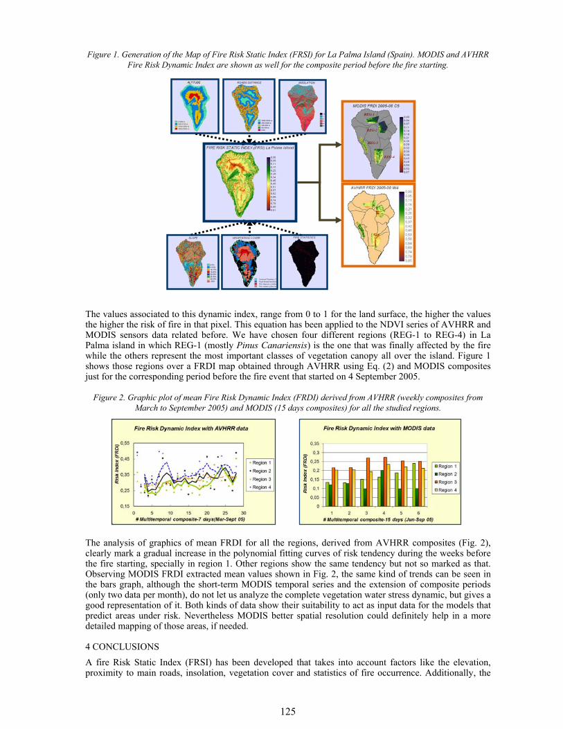
125

Figure 1. Generation of the Map of Fire Risk Static Index (FRSI) for La Palma Island (Spain). MODIS and AVHRR Fire Risk Dynamic Index are shown as well for the composite period before the fire starting.

The values associated to this dynamic index, range from 0 to 1 for the land surface, the higher the values the higher the risk of fire in that pixel. This equation has been applied to the NDVI series of AVHRR and MODIS sensors data related before. We have chosen four different regions (REG-1 to REG-4) in La Palma island in which REG-1 (mostly Pinus Canariensis) is the one that was finally affected by the fire while the others represent the most important classes of vegetation canopy all over the island. Figure 1 shows those regions over a FRDI map obtained through AVHRR using Eq. (2) and MODIS composites just for the corresponding period before the fire event that started on 4 September 2005.

Figure 2. Graphic plot of mean Fire Risk Dynamic Index (FRDI) derived from AVHRR (weekly composites from

March to September 2005) and MODIS (15 days composites) for all the studied regions.

The analysis of graphics of mean FRDI for all the regions, derived from AVHRR composites (Fig. 2), clearly mark a gradual increase in the polynomial fitting curves of risk tendency during the weeks before the fire starting, specially in region 1. Other regions show the same tendency but not so marked as that. Observing MODIS FRDI extracted mean values shown in Fig. 2, the same kind of trends can be seen in the bars graph, although the short-term MODIS temporal series and the extension of composite periods (only two data per month), do not let us analyze the complete vegetation water stress dynamic, but gives a good representation of it. Both kinds of data show their suitability to act as input data for the models that predict areas under risk. Nevertheless MODIS better spatial resolution could definitely help in a more detailed mapping of those areas, if needed.

4 CONCLUSIONS A fire Risk Static Index (FRSI) has been developed that takes into account factors like the elevation, proximity to main roads, insolation, vegetation cover and statistics of fire occurrence. Additionally, the

126

use of different satellite sensors has contributed to demonstrate the usefulness of them in providing early fire risk alerts, given extra information about vegetation water stress. The analysis of the Fire Risk Dynamic Index (FRDI) derived from AVHRR and MODIS data over the static FRSI layer, clearly remark the increase in this risk indicator for the week and fifteen days prior to the dramatic fire event that took place in La Palma Island (Canary Islands-Spain) during the first week of September 2005 (2150 ha. burnt). Although the AVHRR Fire Risk shows a great variability in the four different selected regions, mainly due to its steep orography and possible persistence of partial cloud contamination, the polynomial fitting curves mark the tendency in fire risk as expected, due to the drought effects on vegetation during that summer. As for the FRDI (MODIS) this effect is specially important in the burnt area (Region 1) It is important to remark that this research is a part of a project to develop a complete map of fire risk for the Canary Islands. The suitability of this technique has also been tested in previous works for fires that took place in Tenerife Island, but still have to be validated in different conditions and geographic areas. Our next objective is the addition of data from ground stations (air temperature, wind velocity, humidity, etc.), that surely will improve the modelling of risk considering the great variety of factors involved.

5 ACKNOWLEDGEMENTS We would like to express our gratitude to the “Area de Medioambiente y Politica Territorial del Excmo. Cabildo Insular de la Palma (Spain)” for given us access to the statistics of fires that took place in La Palma island, that have been used in the static risk index (FRSI) generation. This work has been supported by the “Gobierno Autónomo Canario” under Project PI042005/108 and the “Ministerio de Educación y Ciencia (Spain), under Project CGL2004-06099-C03-02/CLI.

6 REFERENCES Ceccato, P. Gobron, N. Flasse, S., et al. Designing a spectral index to estimate vegetation water content from remote

sensing data. 1. Theoretical approach. Remote Sensing of Environment, 82, 188-197, 2002. Chladil, M. A., Nuñez, M., Assessing grassland moisture and biomass in Tasmania. The application of remote

sensing and empirical models for a cloudy environment. International Journal of Wildland Fire, 5, 165-171, 1995.

Chuvieco, E., Aguado, I., Cocero, D. et al. Design of and empirical index to estimate fuel moisture content from NOAA-AVHRR images in forest fire danger studies. International Journal of Remote Sensing, 24, 1621-1637, 2003.

Chuvieco, E. Cocero D. Riaño, D., et al. Combining NDVI and surface temperature for the estimation of live fuel moisture content in forest fire danger rating, 92, 322-331, 2004.

Cruz, M. G., Alexander, M. E., Wakimoto, R. H. Assessing the probability of crown fire initiation based on fire danger indices. Forestry Chronicle, 79, 976-983, 2003.

Gabban, A., San-Miguel-Ayanz, J. Barbosa, et al. Analysis of NOAA-AVHRR NDVI inter-annual variability for forest fire risk estimation. International Journal of Remote Sensing, (27) 8, 1725-1732, 2006.

Holben, B. N. Characteristics of maximum-value composite images from temporal AVHRR data. International Journal of Remote Sensing, 11, 1511-1519, 1986.

Hernandez-Leal P. A., Arbelo, M., Gonzalez-Calvo, A. Fire Risk assessment using satellite data, Advances in Space research, (37(4), 741-746, 2006.

Leblon, B. Forest wildfire hazard monitoring using remote sensing. A review. Remote Sensing Reviews, 20(1), 1-57, 2001.

127

1 INTRODUCTION 1.1 Study area The public Forest of Pertouli is nearly 3300 ha, the see level of the forest is between 1.100 – 1.700 meters (m) and from 1951 is used from the Aristotle University of Thessaloniki for academicals reasons. Geographical belongs to Prefecture of Trikala Thessaly - Greece. Although the study area is near by the semi-alpaca boundaries, seven fires have been taken place the last ten years. The mean reasons were: forest sub products, thunders and alpinists activities. The fired damaged areas were only 10 ha, because of the climatic conditions, similar to Eastern-Italian alpine regions. 1.2 Pre-fire and risk fire maps Fire prevention aims to reduce the incidence and extent of fires by preventing them from occurring in crital areas. Federal, state, and local agencies have implemented a variety of fire prevention programs, including such activities as education, patrol, code enforcement, and signs. In general, these programs have been shown to be highly effective at reducing incidence of fire (Sapsis 2003). Pre-fire activities such as clearing a defensible space, putting in and maintaining fire safe landscaping, utilizing prescribed fire, creating fuel breaks, and forest management practices are proven methods of reducing wildfire destruction (www.fire.ca.gov 2006). A forest fire risk map usually prepared as an early warning system (Saito 2002). A fire risk map, updated on an annual basis, is of great importance in terms of forest and civil protection.

2 METHODOLOGY: VERIFYING PRE-FIRE RESOURCES AND CRITICAL AREAS 2.1 Preparing Data Starting from contour lines we derived Digital Elevation Model (DEM) with a 20 m cell size. Slope and Aspect grid files were obtained through the 3D Analyst tool (ArcGis 9.1 ®, 2007). Corine Land Cover has only three forest classification (softwood, hardwood and mixed forest) and polygons quality is raw, so we used a more detailed map of forest types. Each type had its number code, dividing study area in productive forests, protective/other function forests and meadows. Productive forests (Pinus nigra, Abies cephalonica and Abies alba) were divided in five classes according to the quality and quantity of wood, from best to bad quality (Figure 1).

Detailed Cartography System of fuel types for preventing forest fires

A. Stergiadou Lecturer, Dept. Forestry & Naturel Environment /Lab. Mechanical Science & Topography, Aristotle University of Thessaloniki, Greece, [email protected]

E.Valese & D. Lubello PhD, Scuola di Dottorato di ricerca T.A.R.S., Dipartimento Te.S.A.F. - Università di Padova, Legnaro, Italy, email: [email protected] [email protected] Keywords: Forest fires, Fuel model, forest road network, GIS, fire risk maps

ABSTRACT: Forest fires the last decades are a common phenomenon especially at Mediterranean countries. Forest fires have a significant economic, social, and environmental impact in Greece and that is the purpose of our interest in preventing forest fires. The System we used here allows the creation of detailed cartography of fuel types from DEM and satellite images. As research area has been chosen Pertouli – Trikala – Greece, because it is a University Forest and is used mainly for academicals research. The purpose of this paper is to use a model for making a GIS Fire Risk map, which will describe the fire potential of an area. This model will be tested and implemented by making a fire risk map for Pertouli area. A known methodology FOMFIS (Forest Fire Management and Fire Protection System) has been defined and used. Unlikely most forest maps that categorize the forest in terms of species and age are not so accurate. Here the forest has been categorized according to their fire behavior properties. The resulting fuel map combined with slope, integrated into ArcGIS 9.1 program and a computer based fire system that allows forest managers to plan fire prevention and fire fighting strategies based on real distribution of burnable material and realistic assumptions about fire behavior. The forest road network plays the role of a hand out help for the fire fighters.

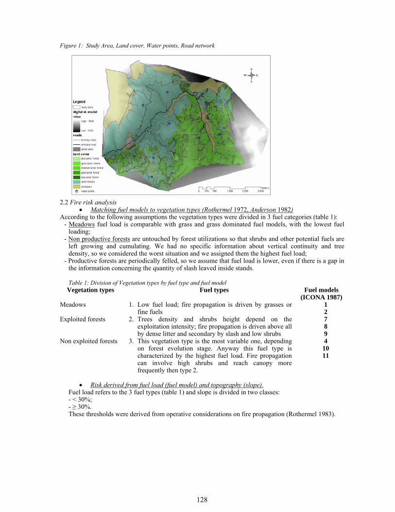
128

Figure 1: Study Area, Land cover, Water points, Road network

2.2 Fire risk analysis • Matching fuel models to vegetation types (Rothermel 1972, Anderson 1982)

According to the following assumptions the vegetation types were divided in 3 fuel categories (table 1): - Meadows fuel load is comparable with grass and grass dominated fuel models, with the lowest fuel

loading; - Non productive forests are untouched by forest utilizations so that shrubs and other potential fuels are

left growing and cumulating. We had no specific information about vertical continuity and tree density, so we considered the worst situation and we assigned them the highest fuel load;

- Productive forests are periodically felled, so we assume that fuel load is lower, even if there is a gap in the information concerning the quantity of slash leaved inside stands. Table 1: Division of Vegetation types by fuel type and fuel model Vegetation types Fuel types Fuel models

(ICONA 1987) Meadows 1. Low fuel load; fire propagation is driven by grasses or

fine fuels 1 2

Exploited forests 2. Trees density and shrubs height depend on the exploitation intensity; fire propagation is driven above all by dense litter and secondary by slash and low shrubs

7 8 9

Non exploited forests 3. This vegetation type is the most variable one, depending on forest evolution stage. Anyway this fuel type is characterized by the highest fuel load. Fire propagation can involve high shrubs and reach canopy more frequently then type 2.

4 10 11

• Risk derived from fuel load (fuel model) and topography (slope).

Fuel load refers to the 3 fuel types (table 1) and slope is divided in two classes: - < 30%; - ≥ 30%. These thresholds were derived from operative considerations on fire propagation (Rothermel 1983).

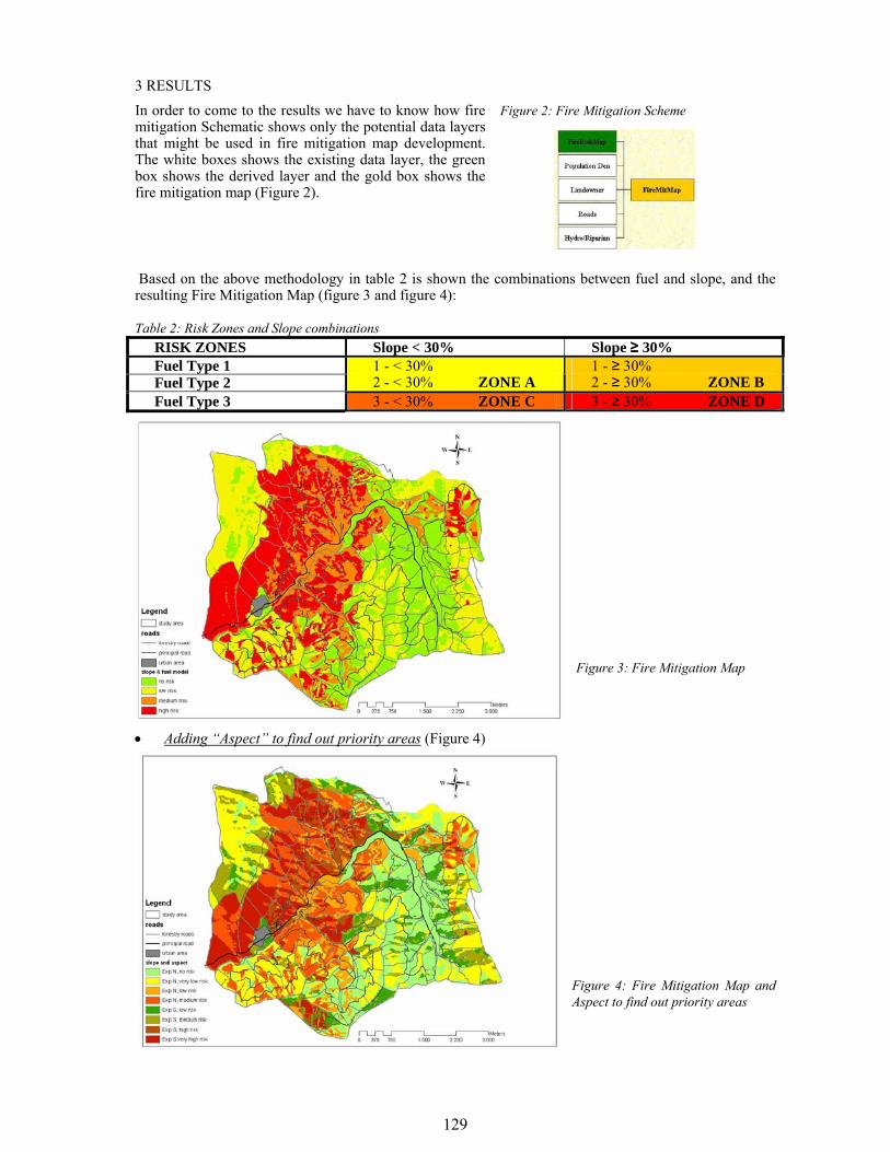
129

3 RESULTS In order to come to the results we have to know how fire mitigation Schematic shows only the potential data layers that might be used in fire mitigation map development. The white boxes shows the existing data layer, the green box shows the derived layer and the gold box shows the fire mitigation map (Figure 2).

Figure 2: Fire Mitigation Scheme

Based on the above methodology in table 2 is shown the combinations between fuel and slope, and the resulting Fire Mitigation Map (figure 3 and figure 4):

Table 2: Risk Zones and Slope combinations

RISK ZONES Slope < 30% Slope ≥ 30% Fuel Type 1 Fuel Type 2

1 - < 30% 2 - < 30% ZONE A

1 - ≥ 30% 2 - ≥ 30% ZONE B

Fuel Type 3 3 - < 30% ZONE C 3 - ≥ 30% ZONE D

Figure 3: Fire Mitigation Map

• Adding “Aspect” to find out priority areas (Figure 4)

Figure 4: Fire Mitigation Map and Aspect to find out priority areas

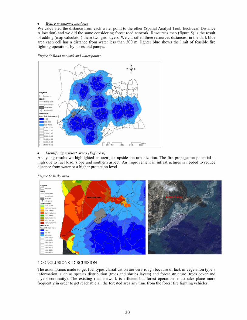
130

• Water resources analysis We calculated the distance from each water point to the other (Spatial Analyst Tool, Euclidean Distance Allocation) and we did the same considering forest road network Resources map (figure 5) is the result of adding (map calculator) these two grid layers. We classified three resources distances: in the dark blue area each cell has a distance from water less than 300 m; lighter blue shows the limit of feasible fire fighting operations by hoses and pumps.

Figure 5: Road network and water points

• Identifying riskiest areas (Figure 6) Analysing results we highlighted an area just upside the urbanization. The fire propagation potential is high due to fuel load, slope and southern aspect. An improvement in infrastructures is needed to reduce distance from water or a higher protection level. Figure 6: Risky area

4 CONCLUSIONS- DISCUSSION

The assumptions made to get fuel types classification are very rough because of lack in vegetation type’s information, such as species distribution (trees and shrubs layers) and forest structure (trees cover and layers continuity). The existing road network is efficient but forest operations must take place more frequently in order to get reachable all the forested area any time from the forest fire fighting vehicles.

131

A pre-fire safety plan program must been held with the following steps: 1. Emergency Response Personnel: An organization or a group of people trained in fire

behaviour. The emergency response personnel include the local Fire Department and Safety and Environmental Affairs personnel.

2. Fire Department Information Centre: A locked container used to store Pre-Fire Safety Plans and related data. Keys to open these containers are assigned to only select organizations which are the local Fire Department and Safety and Environmental Affairs.

3. A back up Pre-Fire Safety Plan: A document containing general information/data about a building to be used by public emergency response agencies or the University for coordinating an emergency response.

4. Residential Properties: A property owned by the University and used for students and working families.

Cartography system of fuel types as that we used; it seems to be necessary for preventing forest fires and surely can be a useful decision tool for Fire Department and Offices of Forestry.

5 REFERENCES Anderson H.E., 1982. Aids to determining fuel models for estimating fire behaviour, USDA Forest Service, General

Technical Report INT-122: 22 p. ICONA 1987. Clave fotografica para la identificaciòn de modelos de combustible M.A.P.A. I.C.O.N.A. Area de

defensa contra incendios forestales, Madrid. Rothermel R.C.,1972. A mathematical model for predicting fire spread in wildlands fuels, USDA Forest Service,

Research Paper INT-I 15, Ogden, UT USA, 40 p. Rothermel RC., 1983. How to predict the spread and intensity of forest and range fires, USDA Forest Service,

General Technical Report INT-143, Ogden, UT USA. http://www.fire.ca.gov , 2006. What is pre fire management. (last entry: 6-7-2007). Saito H., Sawada Y. & Sawada H. 2002. The Development of the Forest Fire Risk Map. Indones For Fire Environ

Impacts 15th Glob Environ Tsukuba, 2002:130-136 Sapsis D., 2003. Pre-fire Effectiveness in Fire Management -- A Summary of State-of-Knowledge.

http://frap.cdf.ca.gov/projects/prefire_mgmt/prefire.html (last entry: 6-7-2007).

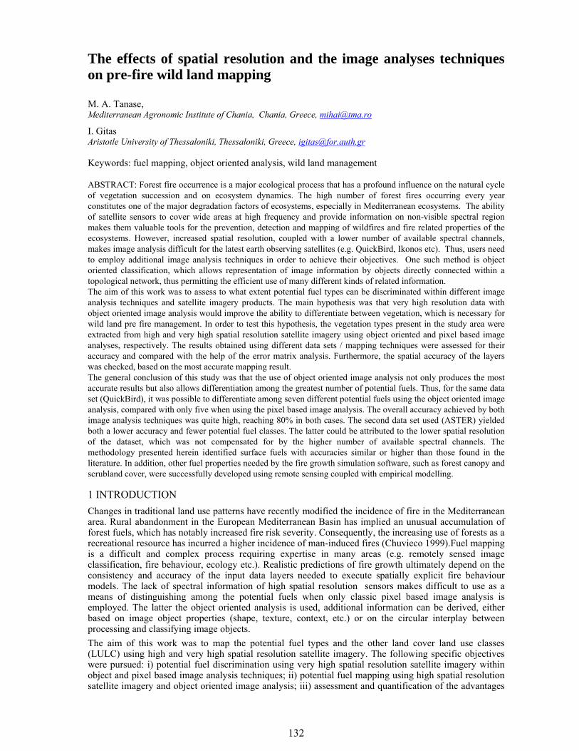
132

The effects of spatial resolution and the image analyses techniques on pre-fire wild land mapping

M. A. Tanase, Mediterranean Agronomic Institute of Chania, Chania, Greece, [email protected]

I. Gitas Aristotle University of Thessaloniki, Thessaloniki, Greece, [email protected] Keywords: fuel mapping, object oriented analysis, wild land management ABSTRACT: Forest fire occurrence is a major ecological process that has a profound influence on the natural cycle of vegetation succession and on ecosystem dynamics. The high number of forest fires occurring every year constitutes one of the major degradation factors of ecosystems, especially in Mediterranean ecosystems. The ability of satellite sensors to cover wide areas at high frequency and provide information on non-visible spectral region makes them valuable tools for the prevention, detection and mapping of wildfires and fire related properties of the ecosystems. However, increased spatial resolution, coupled with a lower number of available spectral channels, makes image analysis difficult for the latest earth observing satellites (e.g. QuickBird, Ikonos etc). Thus, users need to employ additional image analysis techniques in order to achieve their objectives. One such method is object oriented classification, which allows representation of image information by objects directly connected within a topological network, thus permitting the efficient use of many different kinds of related information. The aim of this work was to assess to what extent potential fuel types can be discriminated within different image analysis techniques and satellite imagery products. The main hypothesis was that very high resolution data with object oriented image analysis would improve the ability to differentiate between vegetation, which is necessary for wild land pre fire management. In order to test this hypothesis, the vegetation types present in the study area were extracted from high and very high spatial resolution satellite imagery using object oriented and pixel based image analyses, respectively. The results obtained using different data sets / mapping techniques were assessed for their accuracy and compared with the help of the error matrix analysis. Furthermore, the spatial accuracy of the layers was checked, based on the most accurate mapping result. The general conclusion of this study was that the use of object oriented image analysis not only produces the most accurate results but also allows differentiation among the greatest number of potential fuels. Thus, for the same data set (QuickBird), it was possible to differentiate among seven different potential fuels using the object oriented image analysis, compared with only five when using the pixel based image analysis. The overall accuracy achieved by both image analysis techniques was quite high, reaching 80% in both cases. The second data set used (ASTER) yielded both a lower accuracy and fewer potential fuel classes. The latter could be attributed to the lower spatial resolution of the dataset, which was not compensated for by the higher number of available spectral channels. The methodology presented herein identified surface fuels with accuracies similar or higher than those found in the literature. In addition, other fuel properties needed by the fire growth simulation software, such as forest canopy and scrubland cover, were successfully developed using remote sensing coupled with empirical modelling.

1 INTRODUCTION Changes in traditional land use patterns have recently modified the incidence of fire in the Mediterranean area. Rural abandonment in the European Mediterranean Basin has implied an unusual accumulation of forest fuels, which has notably increased fire risk severity. Consequently, the increasing use of forests as a recreational resource has incurred a higher incidence of man-induced fires (Chuvieco 1999).Fuel mapping is a difficult and complex process requiring expertise in many areas (e.g. remotely sensed image classification, fire behaviour, ecology etc.). Realistic predictions of fire growth ultimately depend on the consistency and accuracy of the input data layers needed to execute spatially explicit fire behaviour models. The lack of spectral information of high spatial resolution sensors makes difficult to use as a means of distinguishing among the potential fuels when only classic pixel based image analysis is employed. The latter the object oriented analysis is used, additional information can be derived, either based on image object properties (shape, texture, context, etc.) or on the circular interplay between processing and classifying image objects. The aim of this work was to map the potential fuel types and the other land cover land use classes (LULC) using high and very high spatial resolution satellite imagery. The following specific objectives were pursued: i) potential fuel discrimination using very high spatial resolution satellite imagery within object and pixel based image analysis techniques; ii) potential fuel mapping using high spatial resolution satellite imagery and object oriented image analysis; iii) assessment and quantification of the advantages

133

Figure 1 Lower level segmentation

of each imagery type and classification method used. The indirect mapping method of fuels (Keane et al., 2001) was adopted in this study.

2 STUDY AREA AND DATASETS The study area cover an 8 by 8 km rectangle located near Anopoli village in the southern west part of Crete Island. The area extends from sea level up to an elevation of more than 1500 m, and is characterized by rough terrain and steep slopes. The aspect is mainly south and the climate is characterized as xero-thermo Mediterranean. The most important remnant coniferous forests of Crete are found in this area and the tree species forms mixed stands. The phrygana formations cover large areas on the lower altitudes. Two satellite images were used to derive the land cover/land use classes present in the study area. The first image was a very high spatial resolution (VHR) QuickBird image acquired on 10th June 2003, while the second was a high spatial resolution (HR) Advanced Spaceborne Thermal Emission and Reflection Radiometer (ASTER) image acquired on 7th August 2002.

3 METHODOLOGY To assess the effectiveness of the image analysis method while differentiating LULC classes, the VHR image was used with two different image analyses techniques (object oriented and pixel based), and the results were qualitatively and quantitatively evaluated. Secondly, in order to compare the spatial resolution influence on the discrimination power of the LULC classes the same image analysis technique (object oriented) was employed for both available datasets (VHR and HR imagery). The object oriented analysis was carried out using eCognition software, based on the Fractal Net Evolution Approach (FNEA).

3.1 Very high resolution imagery – object oriented approach The analysis of the VHR imagery was performed in two steps. In the first step, two segmentation levels were produced using only the multispectral imagery. The first (lower) level was used to extract and classify the image-object ‘primitives’ (e.g. individual/grouped trees, road and building sections) that were subsequently used as building blocks to classify the second (higher) level. The objects in the low segmentation level (Figure 1) were classified mainly on spectral information while the objects from the higher segmentation level were classified based on both spectral and contextual information. The second level objects` classification was based on class-related features, object`s features or on a combination of feature values and class-related features. In the second step, further separation of the existing coniferous species was achieved using two different texture features (“area of sub-objects: mean” and

“avrg. mean diff to neighbors of sub-objects”) based on panchromatic band segmentation. With the use of this two-step approach seven different potential fuels (‘pine forests’, ‘cypress forests’, ‘mixed cypress/kermes oak forests’, ‘kermes oak forests’, ‘phryganic ecosystems’, ‘sparse vegetation’ and ‘alpine vegetation’), together with seven land cover/ land use classes (‘bare ground’, ‘olive orchards’, ‘crops’, ‘vineyards/grasslands’, ‘roads’, ‘artificial surfaces’ and ‘sea’), were classified in the study area. 3.2 High resolution imagery – object oriented approach The pixel size of the HR imagery (15 x 15 meters – VNIR bands) does not allow for an efficient sub-object based analysis, since multiple entities are mixed in a single image unit. Therefore, it was not possible to adopt the approach used for VHR image analysis. Instead, fuzzy membership functions, based on combinations of feature thresholds and class-related features, were used to differentiate among different LULC classes. Only one segmentation level was used to extract and classify the image-objects. At the end of the classification process, five land cover/land use classes (‘bare ground’, ‘sea’, ‘olive orchards’, ‘crops’ and ‘vineyards/grasslands’) and four potential fuels (‘coniferous forests’, broadleaved/mixed forests’, ‘prhyganic ecosystems’ and ‘alpine vegetation’) were identified using ASTER imagery and object oriented analysis.

3.3 Very high resolution imagery – pixel based approach In order to classify the Anopoli study area using the pixel based approach, a combination of unsupervised and supervised classifiers was used on both panchromatic and multispectral imageries. Firstly, an unsupervised, exploratory analysis was carried out on the panchromatic imagery using the ISODATA algorithm to group the pixels according to the data’s inherent properties. The resulting spectral classes were grouped into four categories of interest: ‘bare soil elements’, ‘shadows&sea elements’, ‘tree

134

elements’ and ‘vegetation elements’. A rule-based classifier was developed using the unsupervised clustered panchromatic image, the multispectral image and other computed datasets (e.g. NDVI, DEM, NIR-RED, etc.) as variables. The classifier was created based on spectral/class values, class relations and inverted class similarities. The implementation of pixel based image analysis yielded ten different land cover/land use classes. Among these, five were potential fuel types (‘coniferous forests’, ‘broadleaved forests’, ‘phryganic ecosystems’, ‘alpine vegetation’ and ‘sparse vegetation’), two were other land cover classes (‘sea’ and bare ‘ground’), while the remaining three were land use classes (‘olive orchards’, ‘vineyards/grasslands’ and ‘artificial surfaces’). 3.4 Accuracy assessment A key concern regarding remotely sensed data is that they are often judged to be of insufficient quality for operational applications (Foody 2002). Therefore, it is essential that users of remotely sensed data have knowledge of data accuracy and the methods used to evaluate it in order to effectively use products derived by digital image classification (Congalton 1999). 3.4.1. Absolute accuracy assessment A random, stratified by area, sampling scheme, followed by an error matrix analysis, was employed for the accuracy assessments carried out in this study. The accuracy assessment grid was comprised of 815 points, of which 60 were assessed during the field work. For all other points the reference data was collected via visual interpretation of the QuickBird imagery (panchromatic and multispectral channels).

Table 1 Classification schemes of the image analyses used VHR - object based analysis

Code

VHR - pixel based analysis Code

HR - object based analysis Code

Vineyards/Grasslands 19 Vineyards/Grasslands 19 Vineyards/Grasslands 19 Pine forests 21 Cypress forests 22 Coniferous forests 21/22 Coniferous forests 21/22

Broadleaved forests 36 Broadleaved forests 36 Mixed forests 37

Broadleaves/Mixed forests 36/37

Alpine vegetation 25 Alpine vegetation 25 Alpine vegetation 25 Crops 24 Crops 24 Artificial surfaces 26 Artificial surfaces 26 Bare ground 27 Bare ground 27/33 Bare ground 26/27/33 Olive orchards 31 Olive orchards 31 Olive orchards 31 Phrygana 32 Phrygana 32 Phrygana 32 Roads 33 Sea 34 Sea 34 Sea 34 Sparse vegetation 35 Sparse vegetation 35

Given the high spatial resolution of Quick Bird imagery, evaluation of the ground truth was feasible, taking into account the extensive knowledge of the study area. The ground truth of the sample points assessed for the pixel based analysis’s accuracy assessment was obtained by analyzing the pixels in which the points were located. For the object-oriented analysis’s accuracy assessment, a buffer zone of 10 m radius was generated and analyzed for each sampling point with respect to the land cover/land use category (Guerrero et al. 2007). The classification scheme implemented for each analysis is presented in Table 1.

3.4.2 Relative accuracy assessment Relative accuracy was implemented to assess the extent of spatial agreement among all three image analyses. This type of analysis needs both a base (ground truth) map and a common classification scheme. As a result of the absolute accuracy assessment, the classification obtained through QuickBird`s object oriented image analysis was chosen as a base map, since it provided the best class discrimination, together with the highest accuracy. The common classification scheme was obtained by grouping or reassigning narrower classes to common broader classes. The result was a classification scheme with seven classes (‘forests’, ‘alpine vegetation’, ‘phryganic ecosystems and crops’, ‘bare ground and artificial surfaces’, ‘vineyards and grasslands’, ‘olive orchards’ and ‘sea’). Since the confusion matrix is calculated by comparing the location and class of each ground truth pixel with the corresponding location and class in the classified images, the relative accuracy analysis results express the degree of spatial agreement between the evaluated classifications and the base image. Thus, an accuracy assessment of spatial agreement between ASTER`s object oriented image analysis and QuickBird`s pixel based image analysis to the VHR object oriented analysis was performed.

135

4 RESULTS AND DISCUSSION 4.1 QuickBird object oriented image analysis The overall accuracy of the VHR imagery classification using the object-oriented approach was 80%, with individual classes’ accuracy ranging from 56% to 96%. The lowest class accuracy was achieved for the ‘cypress forests’ due to the frequent confusion between cypress and pine trees. The confusions occurred because of the nature of the textural information (mean area of sub-objects) used during the classification process. If cypress and pine forests classes were collapsed to form a common coniferous forest class, the overall accuracy increased to 83%. With a KHAT value of 0.74, the classification had a moderate to strong agreement according to Landis and Koch (1977). The fuel complexes identified indicate that forest tree types may be properly classified using object oriented analysis, despite the low spectral resolution of Quick Bird’s imagery. On the other hand, automatic mapping of the phrygana species was impossible, even after an extensive field reconnaissance had been conducted. No consistent pattern of species distribution/mixing was found for the shrub species, which could have been used to automatically differentiate one species from another. The use of the multi-spectral bands with their spatial resolution was sufficient to separate most of the land use/land cover classes. However, the panchromatic band had to be employed in order to differentiate among coniferous species present in the area. 4.2 ASTER object oriented image analysis The overall accuracy obtained after classifying the HR imagery using object-oriented analysis was relatively low (70%), and fewer classes were differentiated. The individual class accuracies ranged from 42% to 86%. The most frequent error was the confusion between ‘phrygana’, ‘coniferous’ and ‘broadleaved forests’, followed by confusion among different types of forests. The main obstacle in achieving a better accuracy appeared to be the much higher pixel size. Small, interspersed patches of various categories were misclassified, since they were included, due to the segmentation process, into objects belonging to other land cover/land use classes. The lower spatial resolution of ASTER imagery was not compensated for by the presence of six additional SWIR channels. 4.3 QuickBird pixel based image analysis The pixel based classification of the VHR imagery yielded a similar overall accuracy (80%) with that of the object oriented image analysis, but with fewer LULC classes differentiated. This approach failed to separate the coniferous forests into the two main constituent species (cypress and pine) and to identify the mixed forests present in the area. Since the same image was used in both approaches (object oriented and pixel oriented), the failure can only be explained by the lack of the contextual information available while using the pixel oriented approach. The individual class accuracy ranged between 41% and 94%, which was similar to that obtained by the object oriented analysis. The common errors were confusion of ‘coniferous forests’, ‘bare ground’ and ‘broadleaved forest’ with ‘phryganic ecosystems’ and the confusion between ‘broadleaf forests’ and ‘coniferous forests’. When comparing pixel vs. object analysis for the same data set, it is obvious that not only higher accuracies but, more important, better class discrimination can be achieved using object related information. The classification takes advantage of high spatial resolution, thus improving the results in both accuracy and class discrimination. 4.4 Relative accuracy assessment All classifications had a high overall spatial agreement (78.6% and 79.4%, respectively) with a moderate chance agreement KHAT coefficient (66.7 and 67.3 respectively). Although the overall accuracies were quite similar, the omission and commission errors for each class were different in the pixel-based analysis of the QuickBird image compared with the Aster image analysis. Two classes (‘olive orchards’ and ‘grasslands/vineyards’) presented the highest omissions/commissions errors in both classifications (from 40 to 87%), which was most probably due to the pixel size (ASTER analysis) and the analysis approach, respectively. The high omission errors registered for forests and olive orchard classes in the Quick Bird pixel image analysis appeared due to the inherent properties of the analysis process: only tree pixels (olives, coniferous or broadleaves trees) were classified in the pixel based approach; in contrast, the object oriented analysis included, whitin the classified objects, pixels located in the gaps between the trees. All the other classes registered variation in the spatial agreement, but within much lower limits (7% to 25%).

136

5 CONCLUSIONS Object oriented image analysis allowed the integration of contextual information into the classification process, therefore facilitating a better class discrimination, especially when dealing with potential fuel complexes. Seven different potential fuels were classified using the object oriented approach, compared with only five fuel complexes separated using the pixel based image analysis. More important, differentiation among coniferous species was possible using texture information in a sub-object analysis. The spatial resolution of Quick Bird`s multispectral channels was sufficient to classify all fuel complexes present in the area, except for the main coniferous species. The characterization of fuel complexes was more accurate using very high spatial resolution imagery compared with high resolution imagery. The ASTER data set yielded both lower accuracy and fewer land cover/land use classes, which could only be attributed to the lower spatial resolution of the dataset that was not compensated for by the higher number of available spectral channels. Overall, very VHR imagery, coupled with object oriented image analysis, proved to be an effective tool for the mapping and characterization of wild land potential fuels across the study area. The methodology presented herein identified surface fuels with accuracies similar or higher than those found in the literature. In addition, other fuel properties (not presented here) needed by fire growth simulation software, such as forest canopy and scrubland percentage cover and biomass loadings were successfully developed.

6 REFERENCES Chuvieco, E. 1999. Remote sensing of large wildfires. Springer: 1-2; Congalton, R.G., Green, K. 1999. Assessing the accuracy of remotely sensed data: principles and practices. Boca

Raton: Lewis Publishers. Foody, G.M. 2002. Status of land cover classification accuracy assessment. Remote Sensing of Environment 80:

185-201 Guerrero, I., Tanase, M.A., Manakos, I., Gitas, I., 2007 A semi-operational approach for land cover mapping in the

Mediterranean. In Bochenek, O.Z., (Ed.) New Developments and Challenges in Remote Sensing, Millpress, Rotterdam: 299-310.

Keane, R., Burgan, R., Wagtendonk, J., 2001. Mapping wildland fuels for fire management across multiple scales: Integrating remote sensing and GIS, and biophysical modeling. International Journal of Wildland Fire 10: 301-319.

Landis, J.R., Koch, G.G., 1977. The measurement of observer agreement for categorical data. Biometrics 33: 159-174.

137

1 INTRODUCTION Fire is one of the most important factors influencing terrestrial ecosystems (Mueller-Dombois and Goldamer 1990). The frequency, magnitude and behavior of fires affect the ecosystems in different ways. For instance, high fire frequency affects the complete ecosystem recovery, changing the structure and composition of vegetation cover (Diaz Delgado et al. 2003, Peláez et al. 1997). The propagation and duration of fires hinders the fire suppression (Cruzten & Andrade 1990), this way, the environmental damage is increased and the ecosystems recovery is delayed. These three fire magnitude variables (occurrence, propagation and duration) are influenced by some environmental factors such as: vegetation

The vegetation conditions which influence occurrence, propagation and duration of fires in Argentina

Fischer, María de los Ángeles Instituto de Clima y Agua, Instituto Nacional de Tecnología Agropecuaria (INTA) Los reseros y Las Cabañas s/n, Hurlingham, Pcia. de Buenos Aires, Argentina, [email protected]

Di Bella, Carlos Marcelo Instituto de Clima y Agua, Instituto Nacional de Tecnología Agropecuaria (INTA), Consejo Nacional de Investigaciones Científicas y Técnicas (CONICET). Los reseros y Las Cabañas s/n, Hurlingham, Pcia. de Buenos Aires, Argentina, [email protected]

Jobbágy, Esteban Gabriel Grupo de Estudios Ambientales de la Universidad Nacional de San Luis (GEA), Consejo Nacional de Investigaciones Científicas y Técnicas (CONICET). Av. Ejército de los Andes 950, San Luis, Pcia. de San Luis, Argentina, [email protected] Keywords: Fire, Propagation, Duration, Remote Sensing, NDVI, Argentina

ABSTRACT: Fire is a key factor influencing terrestrial ecosystems and its occurrence, propagation and duration responds to environmental characteristics such as vegetation (type, structure, quantity, water content, photosynthetic activity), climate (humidity, precipitation, temperature, wind speed and direction, global radiation), topography (elevation, slope, illumination) human conditions (roads accessibility and camping zones), among others. In Argentina three million hectares burn every year. Our objective was to understand how vegetation conditions affect occurrence, propagation and duration of fires using satellite and complementary data in the semiarid belt of Argentina from September 2003 to May 2006. This area was selected because it concentrates 70% of the fires of the whole country. Pre-fire vegetation condition was assessed with spectral data from MODIS satellite images. Comparing burned vs. non-burned areas across all vegetation types, the first presented greater NDVII (annual integer, n=6852, p<0.001), suggesting that higher biomass accumulation may have favored burning. Across vegetation types pre-fire NDVI in burned compared to non-burned areas was higher in shrublands (n=5417, p>0.001), similar in steppes (n=516, p=0.17), and lower in forests (n=292, p<0.001), the others vegetation types belongs to general results that involving every vegetation type (n=624, p<0,001). The comparison between vegetation conditions of sites affected by different fire sizes the results showed that the areas affected by small fires presented higher NDVII values than areas affected by bigger disturbs (n=6852, p<0.001). The smaller fires are usually caused by the fieldsmen to reduce accumulated biomass and to favor the vegetation re-growth, which have greater forage quality. It’s probably the cause of the NDVII values obtained in those areas. Nevertheless, the biggest fires presented smaller NDVII values before fire occurrence. This result could indicate lower green coverage associated to greater amount of dry biomass, which could increase the fire propagation risk. The fire propagation risk could increase beyond the amount of accumulated biomass. The comparison between the vegetation indices from areas affected by different fire duration showed that NDVII values were higher in areas burned by longer fires (n=6852, p<0.001), proposing that the amount of accumulated fuel is an important variable which influences the fire duration capability. This response was opposite for closed shrublands vegetation types. The fires with most durability occurred in areas with lower NDVII values, this could be associated to the fuel status required before fire beginning. The high density covers (forests and dense shrublands) presented lower NDVII values before the most intense fires occurred. These results would be associated to the necessity of dry fuel presence for the fire ignition. However, in areas occupied by low density cover types (steppes and grasslands), the amount of fuel accumulate is a more important variable which influences the fire intensity. Have knowledge about the vegetation conditions, fuel state and quantity; from satellite data is an important tool to estimate the fire magnitude risk. This product is usefully to fire managers and the total population with the purpose of take anticipated decisions and then, to reduce the fires environmental impacts.

138

(type, structure, cover level, moisture content, photosynthetic activity) (Viegas 1998; Viegas et al. 1998), climate (relative humidity, precipitation, temperature, speed and wind direction, global radiation), topography (elevation, slope aspect) and human conditions (accessibility to roads and camping zones) (Chuvieco et al. 1999). In this context, the remote sensing results a useful tool to study fires at different spatial and temporal scales (Cahoon et al. 1992; Chuvieco & Kasischke 2007; Justice & Dowty 1994; Dwyer et al. 2000). Its different applications are based on the capture of spectral information at different wavelengths. This tool allows obtaining information of the surface status and its composition. For example, the information at visible and near infrared bands is commonly associated to the productivity and quantity of accumulated biomass, vegetation structure and volume (Ceccato et al. 2001; Chuvieco et al. 1990), the middle infrared to the vegetation water status (Bowman 1989; Carter 1991; Chuvieco et al. 1990; Hunt and Rock, 1989) and the thermal data is mainly related to the vegetation stress level and the surface temperature (Chuvieco et al. 1990; Pierce et al. 1990). The fire studies could be grouped in three applications: Pre-Fire, During-Fire and Post fire. The pre-fire investigations are normally based on the fire risk analysis (Chuvieco et al. 1999, Calle Montes & Casanova 2002, Alonso-Betanzos et al. 2003), and the fuels analysis (Chuvieco et al. 2003, Justice et al. 1993), generating important data to prevent the damage caused by ignition (Andreae et al. 1998). Most of during fire works are centered on fire detection (Prins & Schmetz 1999, Arino et al. 1998) and the estimation of burned area (Chuvieco et al. 2007, Jaiswal et al. 2002). Based on those data it is possible to analyze the characteristics of ecosystems which influence the fire patterns (Di Bella et al. 2006). On the other hand, most of post-fires analyses are mainly focused on the ecosystem recovery, the vegetation types that prevail, the post-fire land cover composition (Chuvieco et al. 2003, Diaz Delgado et al. 2003), and the atmospheric changes (Crutzen & Andrade1990, Andreae et al. 1998), among others. In Argentina, the Semiarid Region is one of the areas most affected by fires, and it is characterized by a long history of fires. Initially, fires have been a natural phenomenon that modified the succession of the ecosystems (Levine et al. 1996). Nevertheless, with the man's arrival, the humans altered the fire regimen (Mbow et al. 2004) to obtain coal, to manage grasslands, and to promote the regeneration of palatable grasses, among others (Levine et al. 1996). The prevalence of fire in these ecosystems is an important concern for scientists because of its amplitude and implication in the overall natural resource management. However, in the Semiarid Region of Argentina, there are few published investigations in order to study this phenomenon. The little fire suppression efforts in addition to the appropriate conditions of this environment, allows the fire recurrence in each dry season and the increases of fire magnitude (propagation, duration, advance speed). The principal aim was to understand the mechanisms of fire occurrence, propagation and duration in semiarid ecosystems using satellite and complementary information.

2 MATERIALS AND METHODS 2.1 Study Area In the world, 23 million rural hectares are annually burned. In Argentina, the fire destroyed around 3 million hectares every year affecting: 46% shrublands, 35% native forests and 19% grasslands. The Semiarid Region is one of the most affected areas. It contains 70% of fires, most part of them with big size and long duration (Amaya et al. 2002). The study area, which is part of Semiarid Region, extends over 536.336 km2. From an administrative viewpoint, it is divided into 4 provinces: Cordoba, La Pampa, Mendoza and San Luis (Fig. 1). The region is characterized by climatic and topographic variability. The mean annual precipitation ranged between 200 mm and 1000 mm, the mean annual temperatures from 15 to 18 ºC and topography varies from plains to hilly and mountainous zones (reaching the maximum altitude by Aconcagua: 6959 m above sea level). This area is dominated by xerophytes vegetation types, located in savannas, grasslands, steppes and forest (Cabrera & Willink 1973; Burkart et al. 1999; Paruelo et al. 2001). 2.2 Satellite Information

2.2.1 Fires The CONAE generates daily cartographies of the hot spots detected by MODIS sensor (http://www.conae.gov.ar/WEB_Emergencias, visited 2004-2006), with 1000 m of spatial resolution. The hot spot detection is possible as a result of the application of certain algorithms differenced for day and night, containing surface emission data at 4 µm (T4) and 11 µm (T11) (Giglio et al. 2003; Dozier 1981; Matson & Dozier 1981). The detected hot spots from January 2003 to May 2006 were analyzed and only

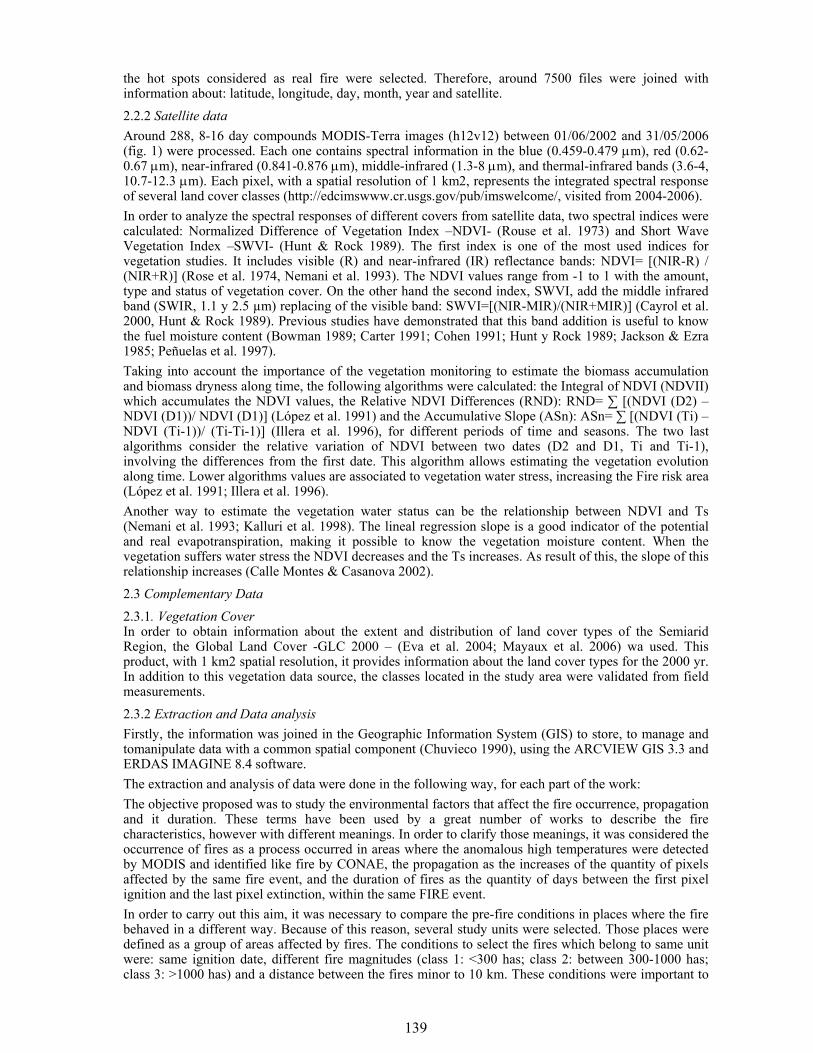
139

the hot spots considered as real fire were selected. Therefore, around 7500 files were joined with information about: latitude, longitude, day, month, year and satellite. 2.2.2 Satellite data Around 288, 8-16 day compounds MODIS-Terra images (h12v12) between 01/06/2002 and 31/05/2006 (fig. 1) were processed. Each one contains spectral information in the blue (0.459-0.479 μm), red (0.62-0.67 μm), near-infrared (0.841-0.876 μm), middle-infrared (1.3-8 μm), and thermal-infrared bands (3.6-4, 10.7-12.3 μm). Each pixel, with a spatial resolution of 1 km2, represents the integrated spectral response of several land cover classes (http://edcimswww.cr.usgs.gov/pub/imswelcome/, visited from 2004-2006). In order to analyze the spectral responses of different covers from satellite data, two spectral indices were calculated: Normalized Difference of Vegetation Index –NDVI- (Rouse et al. 1973) and Short Wave Vegetation Index –SWVI- (Hunt & Rock 1989). The first index is one of the most used indices for vegetation studies. It includes visible (R) and near-infrared (IR) reflectance bands: NDVI= [(NIR-R) / (NIR+R)] (Rose et al. 1974, Nemani et al. 1993). The NDVI values range from -1 to 1 with the amount, type and status of vegetation cover. On the other hand the second index, SWVI, add the middle infrared band (SWIR, 1.1 y 2.5 µm) replacing of the visible band: SWVI=[(NIR-MIR)/(NIR+MIR)] (Cayrol et al. 2000, Hunt & Rock 1989). Previous studies have demonstrated that this band addition is useful to know the fuel moisture content (Bowman 1989; Carter 1991; Cohen 1991; Hunt y Rock 1989; Jackson & Ezra 1985; Peñuelas et al. 1997). Taking into account the importance of the vegetation monitoring to estimate the biomass accumulation and biomass dryness along time, the following algorithms were calculated: the Integral of NDVI (NDVII) which accumulates the NDVI values, the Relative NDVI Differences (RND): RND= ∑ [(NDVI (D2) – NDVI (D1))/ NDVI (D1)] (López et al. 1991) and the Accumulative Slope (ASn): ASn= ∑ [(NDVI (Ti) – NDVI (Ti-1))/ (Ti-Ti-1)] (Illera et al. 1996), for different periods of time and seasons. The two last algorithms consider the relative variation of NDVI between two dates (D2 and D1, Ti and Ti-1), involving the differences from the first date. This algorithm allows estimating the vegetation evolution along time. Lower algorithms values are associated to vegetation water stress, increasing the Fire risk area (López et al. 1991; Illera et al. 1996). Another way to estimate the vegetation water status can be the relationship between NDVI and Ts (Nemani et al. 1993; Kalluri et al. 1998). The lineal regression slope is a good indicator of the potential and real evapotranspiration, making it possible to know the vegetation moisture content. When the vegetation suffers water stress the NDVI decreases and the Ts increases. As result of this, the slope of this relationship increases (Calle Montes & Casanova 2002). 2.3 Complementary Data

2.3.1. Vegetation Cover In order to obtain information about the extent and distribution of land cover types of the Semiarid Region, the Global Land Cover -GLC 2000 – (Eva et al. 2004; Mayaux et al. 2006) wa used. This product, with 1 km2 spatial resolution, it provides information about the land cover types for the 2000 yr. In addition to this vegetation data source, the classes located in the study area were validated from field measurements.

2.3.2 Extraction and Data analysis Firstly, the information was joined in the Geographic Information System (GIS) to store, to manage and tomanipulate data with a common spatial component (Chuvieco 1990), using the ARCVIEW GIS 3.3 and ERDAS IMAGINE 8.4 software. The extraction and analysis of data were done in the following way, for each part of the work: The objective proposed was to study the environmental factors that affect the fire occurrence, propagation and it duration. These terms have been used by a great number of works to describe the fire characteristics, however with different meanings. In order to clarify those meanings, it was considered the occurrence of fires as a process occurred in areas where the anomalous high temperatures were detected by MODIS and identified like fire by CONAE, the propagation as the increases of the quantity of pixels affected by the same fire event, and the duration of fires as the quantity of days between the first pixel ignition and the last pixel extinction, within the same FIRE event. In order to carry out this aim, it was necessary to compare the pre-fire conditions in places where the fire behaved in a different way. Because of this reason, several study units were selected. Those places were defined as a group of areas affected by fires. The conditions to select the fires which belong to same unit were: same ignition date, different fire magnitudes (class 1: <300 has; class 2: between 300-1000 has; class 3: >1000 has) and a distance between the fires minor to 10 km. These conditions were important to

140

reduce climate, topography and vegetation variability. Within the unit, it was also selected a non-burned area (control area) of 3x3 pixels dimension (9 km2) (fig 2). As a result of this selection, 24 study units were considered. For each area, satellite data and complementary information were extracted using AOIs. The information was compiled in some databases with the following data for each analyzed pixel: geographic location (province, department, latitude, longitude); condition (Non-Burned and Burned); study unit (number); vegetation type (GLC classes), occurrence date, fire size (hectares; class1, 2 or 3) and duration (days), spectral data (reflectance on visible, near, middle and thermal infrared); vegetation indices values (NDVI, SWVI); values of vegetation monitoring algorithms (RND, ASn, relation NDVI-TS). 2.4 Statistical analysis ANOVA tests and Linear Regressions analysis were applied to study and to characterize the differences between the pre-fire conditions of places where the fire spread and it lasted in different way. In order to reduce the noise caused by the study areas, it was considered a nested effect of the factors to this variable, which is a Nested Statistical Design Model.

3 RESULTS AND DISCUSSION

3.1 Fire Occurrence When the fire occurrences were studied, the first proposed question was related to the factors that influence this process. In order to answer this question, previous works detected two different factors classes. The first group involves the ignition factors and the other group contains the fire proneness factors (Jaiswal et al. 2002). The first is associated to the causes of fire, for example human (accidental or intentional) or natural causes (lightning). Their random behavior hinders their study. This part of work was focused in the second factors (e.g. vegetation, climate and topography) because it is possible to study them using the satellite information and the complementary data. In order to analyze the vegetation conditions which influence the fire occurrence, it was compared the burned and the non-burned areas. The affected areas presented greater pre-fire NDVII (n=6853, p<0.001), suggesting a higher biomass accumulation (fig. 10). A bigger quantity of accumulated biomass represents bigger quantity of fuel for the ignition, and therefore, a high risk of fire occurrence. The NDVI/TS ratio was also analyzed by presents a good association with the fuel moisture content -FMC- (Chuvieco et al. 1999). It was compared the NDVI/TS trends for fire and no-fire conditions. The obtained results did not show significant differences between them. This result would support the fact that is more important for the promotion of the fire occurrence, the quantity of accumulated biomass previous to the ignition than the status of them. In our study area, probably this is a foreseen result because the most of fires are caused by humans with the purpose to reduce the accumulated biomass and to favor the vegetation re-growth. As a result of this, a bigger accumulated fuel is a common characteristic in places where this phenomenon occurred. Another explanation could be associated to the fact that in this region, by its characteristic semiarid climate, the vegetation cover naturally possesses a low content of moisture. Then, the restrictive of the ignition would be the quantity of fuel and in smaller measure the status of them. When this analysis was differenced by vegetation types, the shrublands response agreed with the general trend (n=5418, p>0.001). Nevertheless, it was opposite for forest (n=293, p<0.001). And there wasn't differences between burned and non-burned areas in steppes (n=517, p=0.17). As it was mentioned previously, the shrubs answer could be explained by the fact that these lands were affected by man-made fires with the purpose to reduce biomass, promoting the vegetation re-growth. However, the forests responses could be associated to the fact that these vegetation types are not usually burnt by man. In general, these types of vegetation are located in hillsides of mountains, which many times are unproductive for the fieldsmen. In those places, the quantity of biomass isn’t a limiting factor; therefore, the status of fuel could be the principal reason of occurrence of fires. If a forest is drier, the fire risk increases. 3.2 Fire Propagation At this time, the objective was to study the density of fires with different propagation levels (1, 2, and 3) according to the vegetation type. As a result of this, it was observed a big number of the large-scale fires which were concentrated in shrublands and forests (fig. 11). This trend may be due to the common large extensions of shrublands in the establishments without obstacles (for example: cut-fire street), and to fact that the forest is located in hills where the accessibility for the fire control is limited.

141

On the other hand, the conditions of the vegetation which influence the fire propagation were studied using spectral data. As a result of this, it was observed that the places affected by small fires presented significantly high values of NDVII during the pre-fire period that those places where the fire reached bigger surfaces (n=4669, p<0.001) (fig. 12). In order to explain this result we take account two indicators: a) High values of NDVII are associated to a bigger quantity of accumulated green biomass, b) The lower NDVII values could not only indicate smaller quantity of green cover but rather they could also be associated to the dry biomass presence. As we have seen before, in this area, the use of the fire is a common agricultural practice. Therefore, it is possible to consider that the fires mainly happen in areas where the accumulation of biomass previous to fire occurrence was high (fig.10). However, the characteristics of the whole area burned by a single fire, not always are the same ones (fig. 12).. According to the obtained results in this section, it is possible to infer that the fires that overcome the 100 hectares affect places where is most important the fuel dryness than the biomass accumulated previous to fire. In order to confirm this supposition it was carried out this analysis using the SWVI (n=4669, p<0.001) and the RND (n=4669, p<0.001). The observed tendencies were similar to the previous result obtained using the NDVI. This information allowed confirming the fact that the greater fires affect places where the fuel is drier. As conclusion, a greater quantity of dry biomass could increase the fire propagation risk and, the fire propagation risk could increase beyond the amount of accumulated green biomass. 3.3 Fire Duration Studying the characteristics previous to the ignition in places where the fire behaved in a different way, it was observed that in the places where the fire finished early, the NDVII was significantly bigger compared to places where the fire extended later from two or three days (n=4669, p<0.001). A possible cause of this result could be the amount of green biomass and its low inflammability. It could be possible that a bigger quantity of green biomass reduces the probability of duration of fires. On the other hand, the lowest values of the index are due to a bigger proportion of dry and senescence biomass accumulated in the surface. This hypothesis is support by the RND analysis. As a consequence, we could demonstrate that the fuel status is an important variable that influences the durability of fires. The behavior for each vegetation type was also analyzed. In forests, the biggest duration of fires was observed in places where the previous NDVII was bigger (n= 181, p<0.001). In these types of vegetation, the cover density is an important factor that influences the duration of fires. Nevertheless, the areas occupied by shrublands showed the lower values of NDVII where the duration of fires was bigger. An explanation of this result could be associated to the fuel status, and the increases of fire durability risk with the amount of dry biomass presence.

4 CONCLUSIONS This paper describes several conditions of the vegetation which influence their behavior. Based on the obtained results, we can conclude that in the Semiarid Region of Argentina the spatial and temporal distribution, and the behavior of the fires is not only the answer to the human's action but also of other natural factors. We could observe that the spatial-temporal distribution is strongly associated to the vegetation type that prevail, the climate, and the land use. And the knowledge about the conditions of vegetation, fuel state and quantity, using satellite data is an important tool to estimate the fire magnitude risk. This product is useful for the fire managers and the people with the purpose of to take decisions and to reduce the environmental impacts of fires.

5 ACKNOWLEDGEMENTS

This work was carried out with the aid of a grant from the Inter-American Institute for Global Change Research (IAI) CRN-2031 which is supported by the US National Science Foundation (Grant GEO-0452325). I am grateful for financial support from INTA and to the members of the Area of Remote Sensing and GIS, of the Instituto de Clima y Agua from INTA Castelar for their constant support and bias to contribute knowledge.

6 REFERENCES Alonso-Betanzos A., Fontela-Romero O., Guijarro-Berdiñas B., Hernández-Pereira E., Andrade M., Jiménez E.,

Soto J.L. & Carballas T. 2003. “An intelligent system for forest FIRE risk prediction and FIRE fighting management in Galicia”. Expert Systems with Applications. 25: 545-554.

Amaya J., Merenson C., Esper J., Chiavassa S., Calisalla J. & Rubieti C. 2002. “Estadística de Incendios Forestales”. Edit. Sec.de Ambiente y Desarrollo Sustentable, Ministerio de Desarrollo Social. - www.medioambiente.gov.ar

142

Andreae M.O., Andreae T.W., Anne-garn H., Beer J., Cachier H., LeCanut P., Elbert W., Maenhaut W., Salma I., Wienhold F.G. & Zenker T. 1998. “Airborn estudies of aerosol emissions from savanna fires in southern Africa: 2. Aerosol chemical composition”. Journal of Geophysical Research. 103: 32119-32128.

Arino, O. & Melinotte, J. M. 1998. “The 1993 Africa fire map”. International Journal of Remote Sensing, 19: 2019–2013.

Bowman, W. D. 1989. "The relationship between leaf water status, gas exchange, and spectralreflectance in cotton leaves", Remote Sensing of Environment. 30: 249-255.

Burkart R 1999. “Conservación de la biodiversidad en bosques naturales productivos del subtrópico argentino”. Ed: Mateucci, Solbrig, Morillo & Halffter. Biodiversidad y uso de la tierra. Conceptos y ejemplos de Latinoamérica. Eudeba, Buenos Aires. pp 131-174

Cabrera, A.L. & A. Willink. 1973. “Biogeografía de América Latina”. Monografía Nº 13, Serie Biología, Organización de Estados Americanos, Washington, US.

Calle Montes, A. & Casanova, J.L. 2002. “Cartografía del Riesgo de Incendios Forestales”. LATUV (Laboratorio de Teledetección de la Universidad de Valladolid). España.

Carter, G. A. 1991. "Primary and secondary effects of water content on the spectral reflectance of leaves", American Journal of Botany. 78: 916-924.

Cayrol, P., Chehbouni, A., Kergoat, L. Dedieu, G. Mordelet, P. and Nouvellon, Y. 2000. “Grassland modeling and monitoring with SPOT-4 VEGETATION instrument during 1997-1999 SALSA experiment”. Agricultural and Forest Meteorology, 105, 91-115.

Ceccato, P., Flasse, S., Tarantola, S., Jacquemoud, S., Grégoire, J. M. 2001. “Detecting vegetation leaf water content using reflectance in the optical domain”. Remote Sensing of Environment, 77, 22–23.

Chuvieco, E. 1990. “Chuvieco, Fundamentos de teledetección espacial”. RIALP, Madrid, pp 453. Chuvieco E., Salas F.J., Carvacho L., & Rodriguez-Silva F. 1999. “Integrated fire risk mappingg”. Ed: Chuvieco.

Remote Sensing of Large Wildfires. New York: Springerverlag. Chuvieco, E. D. Riaño, J.Van Wagtendok, and F. Morsdof. 2003. “Fuel loads and fuel type mapping, In Wildland

Fire Danger Estimation and Mapping: The Role of Sensing Data, Edited by Chuvieco, pp. 119-142, Word Sci. Publ., Singapore.

Chuvieco, E., and E. S. Kasischke (2007), Remote sensing information for fire management and fire effects assessment, J. Geophys. Res., 112, G01S90, doi:10.1029/2006JG000230.

Cohen, W. B. 1991. "Temporal versus spatial variation in leaf reflectance under changing water stress conditions", International Journal of Remote Sensing. 12: 1865-1876

Crutzen, P.J. & Andrade, M.O.1990. "Biomasa burning in the tropics: Impact on atmospheric chemistry and biogeochemical cycles”. Science. vol. 250: 1669-1678.

Díaz Delgado, R.; Lloret, F. & Pons, X. 2003. "Influence of fire severity on plant regeneration by means of remote sensing imagery". International Journal of Remote Sensing. Vol.24 No.8, 1751-1763.

Di Bella C.M., Jobbágy E.G.; Paruelo J.M. & Pinnock S. 2006. “Fire density controls in South America”. Global Ecology and Biogeography.

Dozier, J. 1981. “A method for satellite identification of surface temperature fields of subpixel resolution”. Remote Sensing of Environment, 11:221-229.

Dwyer, E., Pinnock, S., Grégoire, J-M. & Pereira, J.M.C. 2000. “Global spatial and temporal distribution of vegetation fire as determined from satellite information”. International Journal of Remote Sensing, 21, 1289-1302.

Eva H.D., Belward A.S., De Miranda E.E., Di Bella C.M., Gond V., Huber O., Jones S., Sgrenzaroli M. & Fritz S., 2004. “A land cover map of South America”. Global Change Biology.10, 1-14, Blackwell Publishing Ltd.

Giglio L., Descloitres J., Justice C. O. & Kaufman, Y. 2003. “An enhanced contextual fire detection algorithm for MODIS”. Remote Sensing of Environment, 87:273-282.

Hunt, E. R. & Rock, B. N. 1989. "Detection of changes in leaf water content using near and middle-infrared reflectances", Remote Sensing of Environment, 30, pp. 43-54.

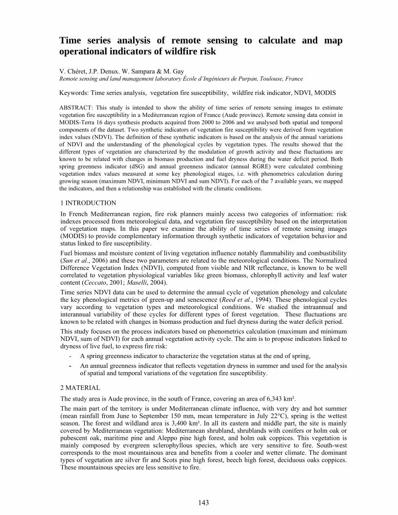
143

1 INTRODUCTION

In French Mediterranean region, fire risk planners mainly access two categories of information: risk indexes processed from meteorological data, and vegetation fire susceptibility based on the interpretation of vegetation maps. In this paper we examine the ability of time series of remote sensing images (MODIS) to provide complementary information through synthetic indicators of vegetation behavior and status linked to fire susceptibility. Fuel biomass and moisture content of living vegetation influence notably flammability and combustibility (Sun et al., 2006) and these two parameters are related to the meteorological conditions. The Normalized Difference Vegetation Index (NDVI), computed from visible and NIR reflectance, is known to be well correlated to vegetation physiological variables like green biomass, chlorophyll activity and leaf water content (Ceccato, 2001; Maselli, 2004). Time series NDVI data can be used to determine the annual cycle of vegetation phenology and calculate the key phenological metrics of green-up and senescence (Reed et al., 1994). These phenological cycles vary according to vegetation types and meteorological conditions. We studied the intraannual and interannual variability of these cycles for different types of forest vegetation. These fluctuations are known to be related with changes in biomass production and fuel dryness during the water deficit period. This study focuses on the process indicators based on phenometrics calculation (maximum and minimum NDVI, sum of NDVI) for each annual vegetation activity cycle. The aim is to propose indicators linked to dryness of live fuel, to express fire risk:

- A spring greenness indicator to characterize the vegetation status at the end of spring, - An annual greenness indicator that reflects vegetation dryness in summer and used for the analysis

of spatial and temporal variations of the vegetation fire susceptibility.

2 MATERIAL The study area is Aude province, in the south of France, covering an area of 6,343 km². The main part of the territory is under Mediterranean climate influence, with very dry and hot summer (mean rainfall from June to September 150 mm, mean temperature in July 22°C), spring is the wettest season. The forest and wildland area is 3,400 km². In all its eastern and middle part, the site is mainly covered by Mediterranean vegetation: Mediterranean shrubland, shrublands with conifers or holm oak or pubescent oak, maritime pine and Aleppo pine high forest, and holm oak coppices. This vegetation is mainly composed by evergreen sclerophyllous species, which are very sensitive to fire. South-west corresponds to the most mountainous area and benefits from a cooler and wetter climate. The dominant types of vegetation are silver fir and Scots pine high forest, beech high forest, deciduous oaks coppices. These mountainous species are less sensitive to fire.

Time series analysis of remote sensing to calculate and map operational indicators of wildfire risk

V. Chéret, J.P. Denux. W. Sampara & M. Gay Remote sensing and land management laboratory École d’Ingénieurs de Purpan, Toulouse, France Keywords: Time series analysis, vegetation fire susceptibility, wildfire risk indicator, NDVI, MODIS

ABSTRACT: This study is intended to show the ability of time series of remote sensing images to estimate vegetation fire susceptibility in a Mediterranean region of France (Aude province). Remote sensing data consist in MODIS-Terra 16 days synthesis products acquired from 2000 to 2006 and we analysed both spatial and temporal components of the dataset. Two synthetic indicators of vegetation fire susceptibility were derived from vegetation index values (NDVI). The definition of these synthetic indicators is based on the analysis of the annual variations of NDVI and the understanding of the phenological cycles by vegetation types. The results showed that the different types of vegetation are characterized by the modulation of growth activity and these fluctuations are known to be related with changes in biomass production and fuel dryness during the water deficit period. Both spring greenness indicator (dSG) and annual greenness indicator (annual RGRE) were calculated combining vegetation index values measured at some key phenological stages, i.e. with phenometrics calculation during growing season (maximum NDVI, minimum NDVI and sum NDVI). For each of the 7 available years, we mapped the indicators, and then a relationship was established with the climatic conditions.

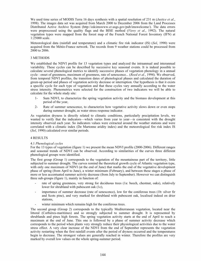
144

We used time series of MODIS Terra 16 days synthesis with a spatial resolution of 231 m (Justice et al., 1998). The images data set was acquired from March 2000 to December 2006 from the Land Processes Distributed Active Archive System (http://edcimswww.cr.usgs.gov/pub/imswelcome/). The data errors were preprocessed using the quality flags and the BISE method (Viovy et al., 1992). The natural vegetation types were mapped from the forest map of the French National Forest Inventory (IFN) at 1:25000 scale. Meteorological data (rainfall and temperature) and a climatic fire risk indicator (IS) (Sol, 1990) were acquired from the Météo-France network. The records from 9 weather stations could be processed from 2000 to 2006.

3 METHODS

We established the NDVI profile for 13 vegetation types and analyzed the intraannual and interannual variability. These cycles can be described by successive key seasonal events. It is indeed possible to calculate several phenological metrics to identify successive phases of vegetation phenology in a annual cycle : onset of greenness, maximum of greenness, rate of senescence... (Reed et al., 1994). We observed, from temporal NDVI profiles, the transition dates of phenological phases and calculated the duration of green-up period and phases of vegetation activity decrease or interruption. Our hypothesis is that it exists a specific cycle for each type of vegetation and that these cycles vary annually according to the water stress intensity. Phenometrics were selected for the construction of two indicators we will be able to calculate for the whole study site:

1- Sum NDVI, to characterize the spring vegetation activity and the biomass development at this period of the year,

2- Rate of summer senescence, to characterize how vegetative activity slows down or even stops during summer drought, as water stress response indicator.

As vegetation dryness is directly related to climatic conditions, particularly precipitation levels, we wanted to verify that the indicators—which varies from year to year—is consistent with the drought intensity observed each year. So indicators values were extracted around the weather stations and were correlated with a climatic index (De Martonne aridity index) and the meteorological fire risk index IS (Sol, 1990) calculated over similar periods.

4 RESULTS 4.1 Phenological cycles For the 13 types of vegetation (figure 1) we present the mean NDVI profile (2000-2006). Different ranges and seasonal trends of NDVI can be observed. According to similarities of the curves three different phenological groups were identified. The first group (Group 1) corresponds to the vegetation of the mountainous part of the territory, little subjected to summer drought. The curves remind the theoretical growth cycle of Atlantic vegetation type, with only one maximum of NDVI (at the end of June) that marks the end of the vegetative development phase of spring (from April to June), a winter minimum (February), and between these stages a phase of more or less accentuated summer activity decrease (from July to September). However we can distinguish three sub-groups (figure 1), mainly in function of:

- rate of spring greenness, very strong for deciduous trees (1a: beech, chestnut, oaks), relatively lower for shrubland with pubescent oak (1c),

- importance of summer decrease (rate of senescence), low for the coniferous trees (1b: silver fir and Scots pine), and very marked for shrubland with pubescent oak, localised indeed on drier stations,

- winter minimum which remains high for the coniferous trees. The second group (Group 2) corresponds to the typically Mediterranean vegetation, located near the littoral (Corbières-maritimes) and so strongly subjected to summer drought. It is represented by shrublands and pines high forests. The spring vegetation activity starts at the end of April to reach a maximum at the end of June. This one is followed by a phase of summer activity decrease which corresponds to the period when plants very strongly reduce their physiological activities due to the water stress effect. A very clear increase of the NDVI from the end of September represents the vegetation activity restarting when the first rainfall events after the period of dryness occurred and the temperatures begin to decrease. The strongest values are generally reached in winter. Therefore the profiles are very marked by overall low values on the whole spring-summer period.

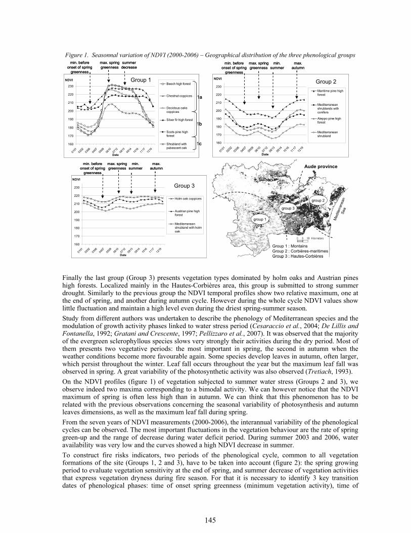
145

Figure 1. Seasonnal variation of NDVI (2000-2006) – Geographical distribution of the three phenological groups

Finally the last group (Group 3) presents vegetation types dominated by holm oaks and Austrian pines high forests. Localized mainly in the Hautes-Corbières area, this group is submitted to strong summer drought. Similarly to the previous group the NDVI temporal profiles show two relative maximum, one at the end of spring, and another during autumn cycle. However during the whole cycle NDVI values show little fluctuation and maintain a high level even during the driest spring-summer season. Study from different authors was undertaken to describe the phenology of Mediterranean species and the modulation of growth activity phases linked to water stress period (Cesaraccio et al., 2004; De Lillis and Fontanella, 1992; Gratani and Crescente, 1997; Pellizzaro et al., 2007). It was observed that the majority of the evergreen sclerophyllous species slows very strongly their activities during the dry period. Most of them presents two vegetative periods: the most important in spring, the second in autumn when the weather conditions become more favourable again. Some species develop leaves in autumn, often larger, which persist throughout the winter. Leaf fall occurs throughout the year but the maximum leaf fall was observed in spring. A great variability of the photosynthetic activity was also observed (Tretiach, 1993). On the NDVI profiles (figure 1) of vegetation subjected to summer water stress (Groups 2 and 3), we observe indeed two maxima corresponding to a bimodal activity. We can however notice that the NDVI maximum of spring is often less high than in autumn. We can think that this phenomenon has to be related with the previous observations concerning the seasonal variability of photosynthesis and autumn leaves dimensions, as well as the maximum leaf fall during spring. From the seven years of NDVI measurements (2000-2006), the interannual variability of the phenological cycles can be observed. The most important fluctuations in the vegetation behaviour are the rate of spring green-up and the range of decrease during water deficit period. During summer 2003 and 2006, water availability was very low and the curves showed a high NDVI decrease in summer. To construct fire risks indicators, two periods of the phenological cycle, common to all vegetation formations of the site (Groups 1, 2 and 3), have to be taken into account (figure 2): the spring growing period to evaluate vegetation sensitivity at the end of spring, and summer decrease of vegetation activities that express vegetation dryness during fire season. For that it is necessary to identify 3 key transition dates of phenological phases: time of onset spring greenness (minimum vegetation activity), time of

group 1

Aude province

Group 1 : MontainsGroup 2 : Corbières-maritimesGroup 3 : Hautes-Corbières

group 3

group 2

Med

iterra

nean

Sea

group 1

Aude province

Group 1 : MontainsGroup 2 : Corbières-maritimesGroup 3 : Hautes-Corbières

group 3

group 2

Med

iterra

nean

Sea

160

170

180

190

200

210

220

230

0101

0202

0306

0407

0509

0610

0712

0813

0914

1016

1117

1219

Date

NDVI

Holm oak coppices

Austrian pine highforest

Mediterraneanshrubland with holmoak

min. before onset of spring

greenness

max. spring greenness

min. summer

Group 3

max. autumn

160

170

180

190

200

210

220

230

0101

0202

0306

0407

0509

0610

0712

0813

0914

1016

1117

1219

Date

NDVI

Holm oak coppices

Austrian pine highforest

Mediterraneanshrubland with holmoak


greenness


min. summer

Group 3

max. autumn

160

170

180

190

200

210

220

230

0101

0202

0306

0407

0509

0610

0712

0813

0914

1016

1117

1219

Date

NDVI

Maritime pine highforest

Mediterraneanshrublands withconifers

Aleppo pine highforest

Mediterraneanshrubland


greenness


min. summer

Group 2

max. autumn

160

170

180

190

200

210

220

230

0101

0202

0306

0407

0509

0610

0712

0813

0914

1016

1117

1219

Date

NDVI

Maritime pine highforest

Mediterraneanshrublands withconifers

Aleppo pine highforest

Mediterraneanshrubland


greenness


min. summer

Group 2

max. autumn

160

170

180

190

200

210

220

230

0101

0202

0306

0407

0509

0610

0712

0813

0914

1016

1117

1219

Date

NDVIBeech high forest

Chestnut coppices

Decidous oakscoppices

Silver fir high forest

Scots pine highforest

Shrubland withpubescent oak

1a

1b

1c


greenness


summer decrease

Group 1

160

170

180

190

200

210

220

230

0101

0202

0306

0407

0509

0610

0712

0813

0914

1016

1117

1219

Date

NDVIBeech high forest

Chestnut coppices

Decidous oakscoppices

Silver fir high forest

Scots pine highforest

Shrubland withpubescent oak

1a

1b

1c


greenness


summer decrease

Group 1

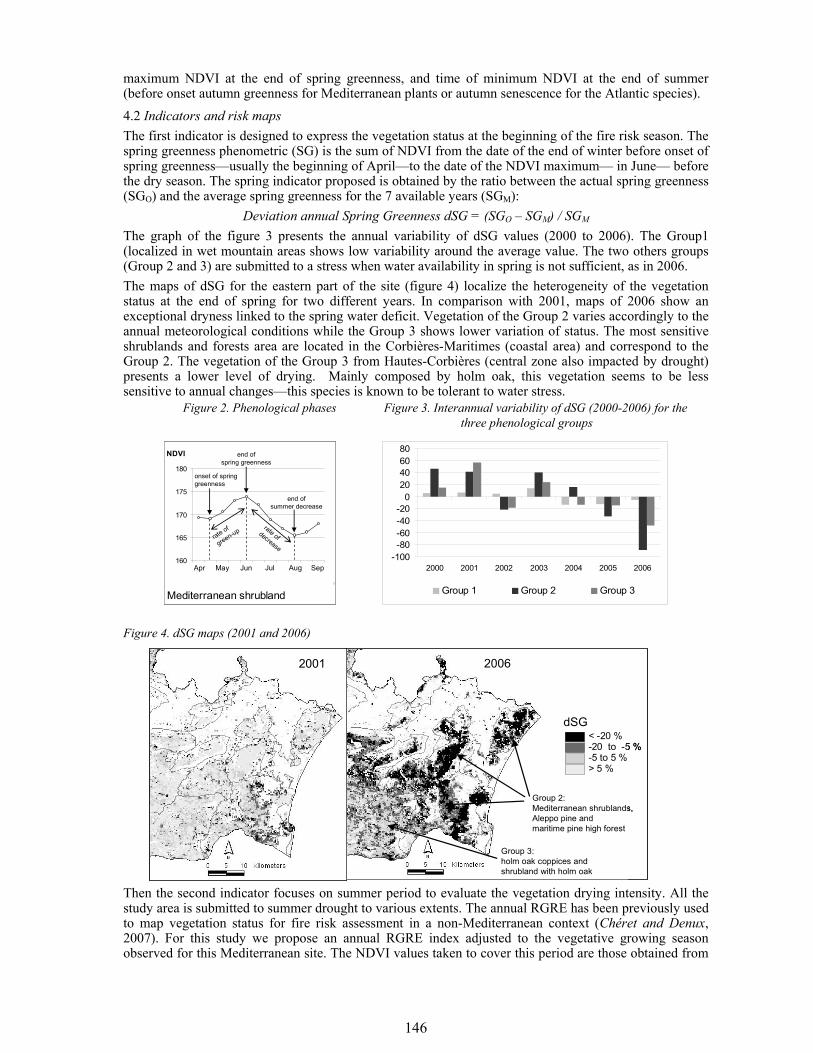
146

maximum NDVI at the end of spring greenness, and time of minimum NDVI at the end of summer (before onset autumn greenness for Mediterranean plants or autumn senescence for the Atlantic species). 4.2 Indicators and risk maps The first indicator is designed to express the vegetation status at the beginning of the fire risk season. The spring greenness phenometric (SG) is the sum of NDVI from the date of the end of winter before onset of spring greenness—usually the beginning of April—to the date of the NDVI maximum— in June— before the dry season. The spring indicator proposed is obtained by the ratio between the actual spring greenness (SGO) and the average spring greenness for the 7 available years (SGM):

Deviation annual Spring Greenness dSG = (SGO – SGM) / SGM

The graph of the figure 3 presents the annual variability of dSG values (2000 to 2006). The Group1 (localized in wet mountain areas shows low variability around the average value. The two others groups (Group 2 and 3) are submitted to a stress when water availability in spring is not sufficient, as in 2006. The maps of dSG for the eastern part of the site (figure 4) localize the heterogeneity of the vegetation status at the end of spring for two different years. In comparison with 2001, maps of 2006 show an exceptional dryness linked to the spring water deficit. Vegetation of the Group 2 varies accordingly to the annual meteorological conditions while the Group 3 shows lower variation of status. The most sensitive shrublands and forests area are located in the Corbières-Maritimes (coastal area) and correspond to the Group 2. The vegetation of the Group 3 from Hautes-Corbières (central zone also impacted by drought) presents a lower level of drying. Mainly composed by holm oak, this vegetation seems to be less sensitive to annual changes—this species is known to be tolerant to water stress.

Figure 4. dSG maps (2001 and 2006)

Then the second indicator focuses on summer period to evaluate the vegetation drying intensity. All the study area is submitted to summer drought to various extents. The annual RGRE has been previously used to map vegetation status for fire risk assessment in a non-Mediterranean context (Chéret and Denux, 2007). For this study we propose an annual RGRE index adjusted to the vegetative growing season observed for this Mediterranean site. The NDVI values taken to cover this period are those obtained from

Figure 2. Phenological phases Figure 3. Interannual variability of dSG (2000-2006) for the three phenological groups

Mediterranean shrubland

160

165

170

175

180

0322

0423

0525

0626

0728

0829

Date

NDVI end ofspring greenness

onset of spring greenness

end ofsummer decrease

rate of

green-uprate of

decrease


160

165

170

175

180

0322

0423

0525

0626

0728

0829

Date




rate of

green-uprate of

decrease


160

165

170

175

180

0322

0423

0525

0626

0728

0829

Date




rate of

green-uprate of

decrease

JunMay JulApr SepAug-100-80-60-40-20

020406080

2000 2001 2002 2003 2004 2005 2006

Group 1 Group 2 Group 3

2001 2006

dSG

Group 2:Mediterranean shrublands,Aleppo pine andmaritime pine high forest

Group 3:holm oak coppices andshrubland with holm oak

< -20 %-20 to -5 %-5 to 5 %> 5 %

2001 2006

dSG

Group 2:Mediterranean shrublands,Aleppo pine andmaritime pine high forest

Group 3:holm oak coppices andshrubland with holm oak

< -20 %-20 to -5 %-5 to 5 %> 5 %

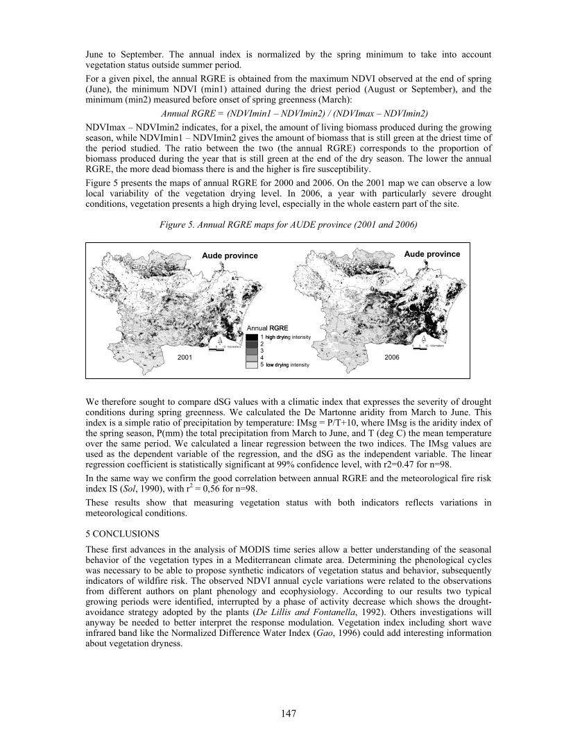
147

June to September. The annual index is normalized by the spring minimum to take into account vegetation status outside summer period. For a given pixel, the annual RGRE is obtained from the maximum NDVI observed at the end of spring (June), the minimum NDVI (min1) attained during the driest period (August or September), and the minimum (min2) measured before onset of spring greenness (March):

Annual RGRE = (NDVImin1 – NDVImin2) / (NDVImax – NDVImin2) NDVImax – NDVImin2 indicates, for a pixel, the amount of living biomass produced during the growing season, while NDVImin1 – NDVImin2 gives the amount of biomass that is still green at the driest time of the period studied. The ratio between the two (the annual RGRE) corresponds to the proportion of biomass produced during the year that is still green at the end of the dry season. The lower the annual RGRE, the more dead biomass there is and the higher is fire susceptibility. Figure 5 presents the maps of annual RGRE for 2000 and 2006. On the 2001 map we can observe a low local variability of the vegetation drying level. In 2006, a year with particularly severe drought conditions, vegetation presents a high drying level, especially in the whole eastern part of the site.

Figure 5. Annual RGRE maps for AUDE province (2001 and 2006)

We therefore sought to compare dSG values with a climatic index that expresses the severity of drought conditions during spring greenness. We calculated the De Martonne aridity from March to June. This index is a simple ratio of precipitation by temperature: IMsg = P/T+10, where IMsg is the aridity index of the spring season, P(mm) the total precipitation from March to June, and T (deg C) the mean temperature over the same period. We calculated a linear regression between the two indices. The IMsg values are used as the dependent variable of the regression, and the dSG as the independent variable. The linear regression coefficient is statistically significant at 99% confidence level, with r2=0.47 for n=98. In the same way we confirm the good correlation between annual RGRE and the meteorological fire risk index IS (Sol, 1990), with r2 = 0,56 for n=98. These results show that measuring vegetation status with both indicators reflects variations in meteorological conditions.

5 CONCLUSIONS

These first advances in the analysis of MODIS time series allow a better understanding of the seasonal behavior of the vegetation types in a Mediterranean climate area. Determining the phenological cycles was necessary to be able to propose synthetic indicators of vegetation status and behavior, subsequently indicators of wildfire risk. The observed NDVI annual cycle variations were related to the observations from different authors on plant phenology and ecophysiology. According to our results two typical growing periods were identified, interrupted by a phase of activity decrease which shows the drought-avoidance strategy adopted by the plants (De Lillis and Fontanella, 1992). Others investigations will anyway be needed to better interpret the response modulation. Vegetation index including short wave infrared band like the Normalized Difference Water Index (Gao, 1996) could add interesting information about vegetation dryness.

12345

2001 2006

Aude province Aude province

Annual RGREhigh drying intensity

low drying intensity

12345

2001 2006

Aude province Aude province

Annual RGREhigh drying intensity

low drying intensity

148

We could also verify if the use of 8 days synthesis allow to refine the results and above all to make the products more operational through earlier data availability: the aim is to be able to transmit information for fire protection plans the fastest as possible. The two indicators, dSG and Annual RGRE, are proposed in a dynamic approach because this information had to be available each year:

- the dSG, to product early warning maps of fire susceptibility at the beginning of the risk season, - the Annual RGRE—indicator of vegetation drying intensity at the end of summer for post-risk

season assessment—to verify the appropriateness of fire prevention actions and fire fighting means.

The use of phenometrics presents also a complementary interest in providing of semipermanent data. For example, the vegetation biomass is an important parameter for a long-term fire danger index model (Castro and Chuvieco, 1998) and this variable could be considered stable-in-time, since they change slowly. In this case this is more the spatial information variability on combustible than temporal that is interesting. Following this aim, a purpose could also be to work on the conversion in combustibility level the assessment of live biomass, using phenometrics as spring sum NDVI (SG). In the same way, dSG average, calculated on a reference period, is a data we can linked to the vegetation flammability level.

6 ACKNOWLEDGEMENTS This study has been supported by Direction Départementale de l’Agriculture et de la Forêt de l’AUDE and Conservatoire de la Forêt Méditerranéenne, with the participation of Office National des Forêts de l’AUDE (Service de la Défense des Forêts contre les Incendies). We thank Julien Zambelli for his contribution.

7 REFERENCES Castro, R., and E. Chuvieco (1998), Modeling forest fire danger from geographic information, Geocarto

International, 13 (1), 15-23. Ceccato, P. (2001), Estimation of vegetation water content using remote sensing for the assessment of fire risk

occurrence and burning efficiency, 155 pp., University of Greenwich, Ispra, Italy. Cesaraccio, C., G. Pellizaro, P. Duce, and D. Spano (2004), Analysis of phenological behaviour of some

Mediterranean shrub species in responses to warming and drought conditions, 16th Biometeorology and Aerobiology Conference, Vancouver, BC.

Chéret, V., and J.P. Denux (2007), Mapping wildfire danger at regional scale with an index model integrating coarse spatial resolution remote sensing data, J. Geophys. Res., 112. G02006, doi:10.1029/2005JG000125.

De Lillis, M., and A. Fontanella (1992), Comparative phenology and growth in different species of the Mediterranean maquis of central Italy, Plant ecology, 1, 83-96.

Gao, B. (1996), NDWI A Normalized Difference Water Index for Remote Sensing of Vegetation Liquid Water From Space, Remote Sensing of Environment (58), 257-266.

Gratani, L., and M.F. Crescente (1997), Phenology and leaf adaptive strategies of Mediterranean maquis plants, Ecologia mediterranea, 23 (3/4), 11-18.

Justice, C.O., E. Vermote, J.R.G. Townshend, R. Defries, D.P. Roy, D.K. Hall, V.V. Salomonson, J.L. Privette, G. Riggs, A.H. Strahler, W. Lucht, R.B. Myneni, Y. Knyazikhin, S.W. Running, R.R. Nemani, Z. Wan, A. Huete, W. van Leeuwen, R.E. Wolfe, L. Giglio, J.-P. Muller, P. Lewis, and M. Barnsley, J. (1998), The Moderate Resolution Imaging Spectroradiometer (MODIS): land remote sensing for global change research, IEEE Transactions on Geoscience and Remote Sensing, 36 (4), 1228-1249.

Maselli, F. (2004), Monitoring forest conditions in a protected Mediterranean coastal area by the analysis of multiyear NDVI data, Remote Sensing of Environment, 89, 423-433.

Pellizzaro, G., C. Cesaraccio, P. Duce, A. Ventura, and Z. Pierpaolo. (2007), Effects of seasonal weather variations and phenology on live fuel moisture content and ignitability of mediterranean species, pp. 11, 4th international wildland fire conference, Seville, Spain, 13 to 17 May 2007.

Reed, B.C., J.F. Brown, D. VanderZee, T.R. Loveland, J.W. Merchant, and D.O. Ohlen (1994), Measuring phenological variability from satellite imagery, Journal of Vegetation Science, 5, 703-714.

Sol, B. (1990), Estimation du risque météorologique d'incendies de forêts dans le sud-est de la France, Revue Forestière Française, Numéro spécial Espaces forestiers et incendies, 263-271.

Sun, L., X. Zhou, S. Mahalingam, and D.R. Weise (2006), Comparison of burning characteristics of live and dead chaparrals fuel, Combustion and Flame, 144, 349-359.

Tretiach, M. (1993), Photosynthesis and transpiration of evergreen Mediterranean and deciduous trees in an ecotone during season, Acta OEcologia 14 (3), 341-360.

Viovy, N., O. Arino, and A.S. Belward (1992), The Best Index Slope Extraction (BISE): A method for reducting noise in NDVI time-series, International Journal of Remote Sensing, 13 (8), 1585-1590.

149

A Comparative Study of the Performance of the NDVI, the TVI and the SAVI Vegetation Indices over burnt areas, using probability theory and spatial analysis techniques

G. Skianis Remote Sensing Laboratory, Faculty of Geology and Geoenvironment, University of Athens, Panepistimiopolis, Athens 157 84, Greece, [email protected]

D. Vaiopoulos University of Athens, Athens, Greece, [email protected]

K. Nikolakopoulos Institute of Geological and Mineral Exploration (IGME), Athens, Greece, [email protected] Keywords: NDVI, TVI, SAVI, standard deviation, signal to noise ratio, correlogram

ABSTRACT: In the present paper we study the behaviour of the NDVI, SAVI and TVI vegetation indices, focusing on their performance over burnt areas. The quantitative criteria which we use in our study, are the standard deviation of the image of each vegetation index, the signal to noise ratio, the correlogram function and the spatial standard deviation of each pixel. Using proper distributions and taking into account probabilistic theorems, we found that the TVI vegetation index has the highest standard deviation and SAVI has the lowest one. We also found that the signal to noise ratio increases with the ratio of the near infrared to red reflectance. The study of the spatial variation of the vegetation indices of a multispectral image over a burnt region, showed that there is a stronger autocorrelation in the TVI image than in the SAVI and NDVI images. Finally, we propose a modified version of the TVI vegetation index, which is called MTVI, in order to broaden the spectrum of possible images of vegetation indices. We observed that the standard deviation of the MTVI image depends on a characteristic parameter, by which the infrared reflectivity is multiplied, in the mathematical expression for the MTVI vegetation index. The results and conclusions of this paper may be useful in environmental research, and specifically in mapping burnt regions using satellite imagery.

1 INTRODUCTION

Vegetation indices may be used in mapping burnt areas and assessing the consequences of a natural disaster. The problem of evaluating the performance and the efficiency of various vegetation indices over different land cover types is still under question. Empirical approaches have been carried out to study the functionality of various proposed vegetation indices and modify them, in order to achieve optimum results. In the present paper we study the behaviour of the NDVI, SAVI and TVI vegetation indices, which, although they have a similar algebraic structure, they may not produce similar results, in qualitative and in quantitative terms. The quantitative criteria which we use in order to assess the performance of these three vegetation indices are the standard deviation of the image of each vegetation index, the signal to noise ratio, the autocorrelation function and the coefficient of variation of each pixel. The standard deviation (stdev) of the image histogram is a measure of the contrast of the image. A high standard deviation means a good contrast. The signal to noise ratio (SNR) is a measure of how clearly a target of interest (for example a burnt area) is expressed and in what extent the noise is suppressed. The autocorrelation function and the coefficient of variation of each pixel may provide information about the spatial variation and the texture of the vegetation index image. The study of the stdev and the SNR of the vegetation index images is based on a probabilistic methodology developed by Vaiopoulos et.al. 2004. The study of the spatial variation of the values of the vegetation indices is carried out empirically, making spatial analysis of a Landsat image over Zakynthos Island, with burnt areas. Finally, we introduce the modified TVI (MTVI) vegetation index and study its performance over the same satellite image. The results and conclusions of this paper may be useful in mapping burnt areas using satellite imagery.

2 THE STANDARD DEVIATION AND THE SIGNAL TO NOISE RATIO The NDVI vegetation index is defined by (Rouse et.al. 1973):

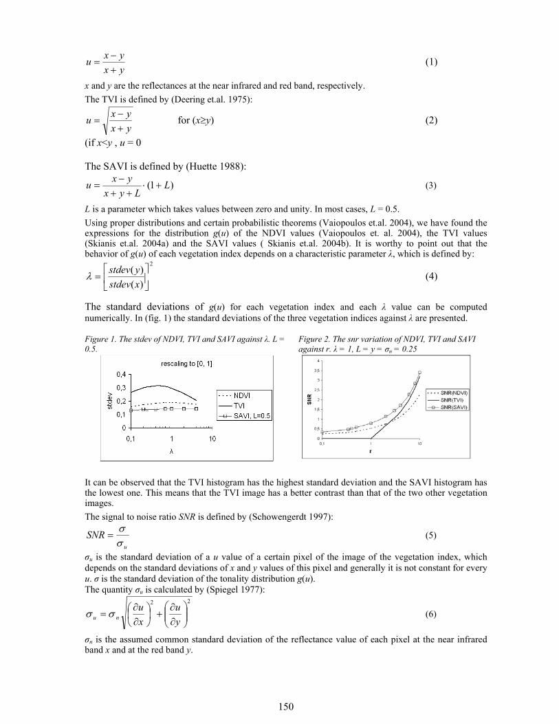
150

yxyxu

+−

= (1)

x and y are the reflectances at the near infrared and red band, respectively. The TVI is defined by (Deering et.al. 1975):

yxyxu

+−

= for (x≥y) (2)

(if x<y , u = 0 The SAVI is defined by (Huette 1988):

)1( LLyx

yxu +⋅++

−= (3)

L is a parameter which takes values between zero and unity. In most cases, L = 0.5. Using proper distributions and certain probabilistic theorems (Vaiopoulos et.al. 2004), we have found the expressions for the distribution g(u) of the NDVI values (Vaiopoulos et. al. 2004), the TVI values (Skianis et.al. 2004a) and the SAVI values ( Skianis et.al. 2004b). It is worthy to point out that the behavior of g(u) of each vegetation index depends on a characteristic parameter λ, which is defined by:

2

)()(⎥⎦

⎤⎢⎣

⎡=

xstdevystdevλ (4)

The standard deviations of g(u) for each vegetation index and each λ value can be computed numerically. In (fig. 1) the standard deviations of the three vegetation indices against λ are presented. Figure 1. The stdev of NDVI, TVI and SAVI against λ. L = 0.5.

Figure 2. The snr variation of NDVI, TVI and SAVI against r. λ = 1, L = y = σn = 0.25

It can be observed that the TVI histogram has the highest standard deviation and the SAVI histogram has the lowest one. This means that the TVI image has a better contrast than that of the two other vegetation images. The signal to noise ratio SNR is defined by (Schowengerdt 1997):

u

SNRσσ

= (5)

σu is the standard deviation of a u value of a certain pixel of the image of the vegetation index, which depends on the standard deviations of x and y values of this pixel and generally it is not constant for every u. σ is the standard deviation of the tonality distribution g(u). The quantity σu is calculated by (Spiegel 1977):

22

⎟⎟⎠

⎞⎜⎜⎝

⎛∂∂

+⎟⎠⎞

⎜⎝⎛

∂∂

=yu

xu

nu σσ (6)

σn is the assumed common standard deviation of the reflectance value of each pixel at the near infrared band x and at the red band y.

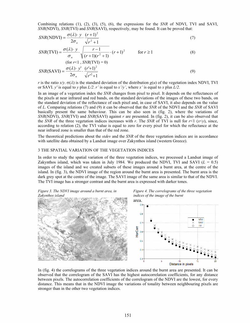
151

Combining relations (1), (2), (3), (5), (6), the expressions for the SNR of NDVI, TVI and SAVI, SNR(NDVI), SNR(TVI) and SNR(SAVI), respectively, may be found. It can be proved that:

1)1(

2)()NDVI(

2

2

+

+⋅

⋅=

rrySNR

nσλσ

(7)

1for )1()1)(1(

1)()TVI( 22 ≥+⋅

++−

⋅⋅

= rrrr

rySNRnσ

λσ (8)

(for r<1 , SNR(TVI) = 0)

1')1'(

2')()SAVI(

2

2

+

+⋅

⋅=

r

rySNRnσ

λσ (9)

r is the ratio x/y. σ(λ) is the standard deviation of the distribution g(u) of the vegetation index NDVI, TVI or SAVI. y' is equal to y plus L/2. r’ is equal to x’/y’, where x’ is equal to x plus L/2. In an image of a vegetation index the SNR changes from pixel to pixel. It depends on the reflectances of the pixels at near infrared and red bands, on the standard deviations of the images of these two bands, on the standard deviation of the reflectance of each pixel and, in case of SAVI, it also depends on the value of L. Comparing relations (7) and (9) it can be observed that the SNR of the NDVI and the SNR of SAVI basically present the same behaviour. This can be also seen in (fig. 2), where the variations of SNR(NDVI), SNR(TVI) and SNR(SAVI) against r are presented. In (fig. 2), it can be also observed that the SNR of the three vegetation indices increases with r. The SNR of TVI is null for r<1 (x<y), since, according to relation (2), the TVI value is equal to zero for every pixel for which the reflectance at the near infrared zone is smaller than that of the red zone. The theoretical predictions about the stdev and the SNR of the three vegetation indices are in accordance with satellite data obtained by a Landsat image over Zakynthos island (western Greece).

3 THE SPATIAL VARIATION OF THE VEGETATION INDICES In order to study the spatial variation of the three vegetation indices, we processed a Landsat image of Zakynthos island, which was taken in July 1984. We produced the NDVI, TVI and SAVI (L = 0.5) images of the island and we created subsets of these images around a burnt area, at the centre of the island. In (fig. 3), the NDVI image of the region around the burnt area is presented. The burnt area is the dark grey spot at the centre of the image. The SAVI image of the same area is similar to that of the NDVI. The TVI image has a stronger contrast and the burnt area is expressed with darker tones. Figure 3. The NDVI image around a burnt area, in Zakynthos island

Figure 4. The correlograms of the three vegetation indices of the image of the burnt area.

In (fig. 4) the correlograms of the three vegetation indices around the burnt area are presented. It can be observed that the correlogram of the SAVI has the highest autocorrelation coefficients, for any distance between pixels. The autocorrelation coefficients of the correlogram of the NDVI are the lowest, for every distance. This means that in the NDVI image the variations of tonality between neighbouring pixels are stronger than in the other two vegetation indices.

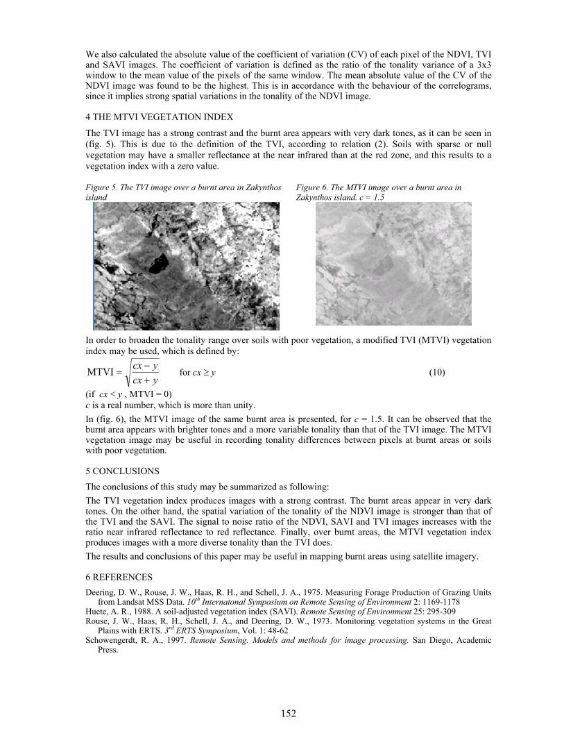
152

We also calculated the absolute value of the coefficient of variation (CV) of each pixel of the NDVI, TVI and SAVI images. The coefficient of variation is defined as the ratio of the tonality variance of a 3x3 window to the mean value of the pixels of the same window. The mean absolute value of the CV of the NDVI image was found to be the highest. This is in accordance with the behaviour of the correlograms, since it implies strong spatial variations in the tonality of the NDVI image.

4 THE MTVI VEGETATION INDEX

The TVI image has a strong contrast and the burnt area appears with very dark tones, as it can be seen in (fig. 5). This is due to the definition of the TVI, according to relation (2). Soils with sparse or null vegetation may have a smaller reflectance at the near infrared than at the red zone, and this results to a vegetation index with a zero value. Figure 5. The TVI image over a burnt area in Zakynthos island

Figure 6. The MTVI image over a burnt area in Zakynthos island. c = 1.5

In order to broaden the tonality range over soils with poor vegetation, a modified TVI (MTVI) vegetation index may be used, which is defined by:

ycxycx

+−

=MTVI for cx ≥ y (10)

(if cx < y , MTVI = 0) c is a real number, which is more than unity. In (fig. 6), the MTVI image of the same burnt area is presented, for c = 1.5. It can be observed that the burnt area appears with brighter tones and a more variable tonality than that of the TVI image. The MTVI vegetation image may be useful in recording tonality differences between pixels at burnt areas or soils with poor vegetation.

5 CONCLUSIONS

The conclusions of this study may be summarized as following: The TVI vegetation index produces images with a strong contrast. The burnt areas appear in very dark tones. On the other hand, the spatial variation of the tonality of the NDVI image is stronger than that of the TVI and the SAVI. The signal to noise ratio of the NDVI, SAVI and TVI images increases with the ratio near infrared reflectance to red reflectance. Finally, over burnt areas, the MTVI vegetation index produces images with a more diverse tonality than the TVI does. The results and conclusions of this paper may be useful in mapping burnt areas using satellite imagery.

6 REFERENCES Deering, D. W., Rouse, J. W., Haas, R. H., and Schell, J. A., 1975. Measuring Forage Production of Grazing Units

from Landsat MSS Data. 10th Internatonal Symposium on Remote Sensing of Environment 2: 1169-1178 Huete, A. R., 1988. A soil-adjusted vegetation index (SAVI). Remote Sensing of Environment 25: 295-309 Rouse, J. W., Haas, R. H., Schell, J. A., and Deering, D. W., 1973. Monitoring vegetation systems in the Great

Plains with ERTS. 3rd ERTS Symposium, Vol. 1: 48-62 Schowengerdt, R. A., 1997. Remote Sensing. Models and methods for image processing. San Diego, Academic

Press.

153

Skianis, G. Aim., Vaiopoulos, D., and Nikolakopoulos, K., (2004). A study of the behavior of vegetation index SAVI, based on probability theory. Proceedings of the 7th Panhellenic Congress of the Hellenic Geographical Society. Mytilini, Greece, October 2004. Vol. 1: 41-48

Skianis, G. Aim., Vaiopoulos, D., and Nikolakopoulos, K., 2004. Assesment of the TVI vegetation index with the aid of probability theory. Proceedingsof the 10th International Congress of the Geological Society of Greece. Thessaloniki, 15-17 April 2004. Vol. 3: 1337-1346

Spiegel, M. R., 1977. Probability and Statistics. New York, McGraw-Hill. Athens, ESPI. Vaiopoulos, D., Skianis, G. Aim., and Nikolakopoulos, K., 2004. The contribution of probability theory in assessing

the efficiency of two frequently used vegetation indices. International Journal of Remote Sensing 25: 4219-4236

154

A global, multi-year (2000-2007), validated burnt area product (L3JRC) derived from daily SPOT VEGETATION data

K. Tansey Department of Geography, University of Leicester, University Road, Leicester, UK, [email protected]

Jean-Marie Grégoire Joint Research Centre of the European Commission, Ispra, Italy, [email protected]

José M.C. Pereira Instituto Superior de Agronomia, Technical University of Lisbon, Portugal

Pierre Defourny Université Catholique de Louvain, Louvain-la-Neuve, Belgium

Roland Leigh Department of Geography, University of Leicester, University Road, Leicester, UK, [email protected]

Ana Barros Instituto de Investigação Cientifica Tropical, Lisbon, Portugal

Jean-François Pekel Université Catholique de Louvain, Louvain-la-Neuve, Belgium

Joao M. Silva Instituto de Investigação Cientifica Tropical, Lisbon, Portugal

Eric van Bogaert Université Catholique de Louvain, Louvain-la-Neuve, Belgium

Etienne Bartholomé Joint Research Centre of the European Commission, Ispra, Italy, [email protected]

Sophie Bontemps Université Catholique de Louvain, Louvain-la-Neuve, Belgium Keywords: burnt area, global, fire, emissions, SPOT VEGETATION, biomass burning

ABSTRACT: Global burned area products are in high demand from research groups and communities interested in modeling the carbon cycle, understanding the relationships between fire regime and climate, atmospheric emissions and pollution resulting from fires and the impact of vegetation burning on land cover change. Currently, global burned area products at medium resolution, such as GBA2000 and GlobScar, are limited to the year 2000. Whilst these global products provided the user community with strong evidence of the scale of global vegetation burning, multi-annual products are needed to strengthen the arguments of relationships between vegetation, climate and fire. Recent initiatives are underway by both the European Space Agency (ESA) and a team working on MODIS data to implement regional algorithms over a multi-year time period. At this time, we still await the release of the full data sets. It is in this context that the L3JRC (pronounced L-three-J-R-C) product has been developed. Its name refers to the consortium of academies involved in the development: the University of Leicester (UK), the Catholic University of Louvain-la-Neuve (BE), the Tropical Research Institute, Lisbon (PT) and the Joint Research Centre of the European Commission (EU). A single algorithm was used to classify the SPOT-VEGETATION data to burned areas. It makes use of a temporal index in the near infrared channel. Global, daily, atmospheric corrected SPOT VGT S1 data were used as input. Results show that the total amount of area burnt varies between 3.5 million km2 and 4.5 million km2. The amount burnt each year by vegetation cover type indicated by the GLC2000 is shown as well as a visual indication of the spatial distribution of burnt area. The L3JRC product has been evaluated against a 72 Landsat TM and ETM+ image pairs and quicklooks. We evaluate the product in its ability to correctly quantify the amount of burnt area by computing comparative values over a global hexagonal grid with a cell spacing of 60 km. This is done over a number of different vegetation and biome types. The results of this validation by geographical region and vegetation type are shown in this paper. The L3JRC product is available from the web page: http://www-tem.jrc.it/Disturbance_by_fire/products/burnt_areas/index.htm

155

1 INTRODUCTION Global burned area products are in high demand from research groups and communities interested in modelling the carbon cycle, understanding the relationships between fire regime and climate, atmospheric emissions and pollution resulting from fires and the impact of vegetation burning on land cover change (Patra et al., 2005; Jupp et al., 2006). Burned area is a crucial component in the computation of gas emissions (Seiler and Crutzen, 1980). Currently, global burned area products have been limited in time. As its name suggests, the GBA2000 product (see Tansey et al., 2004) was limited to the year 2000. Recent initiatives by ESA to implement a number of regional algorithms from the GBA2000 project combined with GlobScar results over the period 1998-2007 has resulted in some problems caused by scaling up of the algorithms. We still await a multi-year MODIS global burned area product (Roy et al., 2005). Whilst these global products provided the user community with strong evidence of the scale of global vegetation burning, multi-annual products are needed to strengthen the arguments of relationships between vegetation, climate and fire. A number of papers have reported on burned area estimates using active fire data as a proxy. Schultz (2002) used ATSR fire count data; Sukhinin et al. (2004) used AVHRR data between 1995 and 2003; Giglio et al. (2006) used MODIS data. These authors highlight the lack of accurate, consistent long-term information on global burned area as the reason for their decision to use active fire data. The uncertainties associated with using active fires as a proxy for burned area are described in van der Werf et al. (2006). The product described in this paper serves to address this data gap. We announce to the scientific community the availability of a long-term (covering seven global fire seasons be 2000 and 2007), moderate spatial resolution (1km2), high temporal resolution (daily intervals) global burned area product derived from direct observations from the SPOT VEGETATION system. Furthermore, the product has been evaluated against a large number of Landsat TM and ETM+ image pairs and quicklooks. We evaluate the product in its ability to correctly quantify the amount of burnt area by computing comparative values over a global hexagonal grid with a cell spacing of 60km. This is done over a number of different vegetation types.

2 METHODOLOGY A single algorithm, initially described in Tansey et al. (2004) and subsequently modified by the authors was applied to SPOT VEGETATION S1 data. Global, daily, atmospheric corrected S1 data were used as input. In the pre-processing module, cloud and snow masks are generated based on thresholds at blue and middle infrared wavelengths. A viewing zenith mask is applied that restricts observations of the ground to angles less than 50.5 degrees. A fire smoke mask is then generated using thresholds at blue wavelengths. A cloud shadow mask is then derived using solar and view azimuth and zenith angles and assuming a constant cloud height of 10km. A mask is then derived of all pixels that have saturated in the shortwave infrared (SWIR) channel. A sun shadow mask is produced from the GTOPO 30 global DEM. We compute aspect and slope and use a threshold that assumes a pixel will be in shadow if the cosine of the sun incidence angle is less than 0.256 radians. These masks are combined. The main processing algorithm makes use of a temporal index in the near infrared (NIR) channel of SPOT VEGETATION. This index I is computed using the following method:

(1)

where S1NIR = S1 daily product pixel DN and ICNIR = intermediate composite pixel DN. Mean and standard deviation values are computed for the index I over a window of 200 by 200 pixels ignoring all pixels with a value of zero or identified as being contaminated. A pixel is flagged as being burnt if the value in the array I is lower than the mean value minus two standard deviations. Two further checks are made on reflectance values in the NIR and SWIR channels to confirm the burnt area. To compute the updated intermediate composite in the near infrared channel (ICNIR), we first calculate a phase value that uses sun and viewing angles (both zenith and azimuth) to evaluate the suitability of a pixel to be used in future composites. If this test is passed, then the new value of the composite is the average between the existing composite value and the pixel value of the S1 product being analysed. Post-processing of the data serves to utilise the latest land cover information to remove some over detections believed mainly to be due to some shadowing not excluded with the relief/sun shadow mask, the multi-annual detection of leaf off conditions in temperate regions and lake melt conditions at high northern latitudes. The GLC2000 land cover product was used (Global Land Cover 2000 database, European Commission, Joint Research Centre, 2003, http://www-gem.jrc.it/glc2000) to provide updated information on water bodies, snow and ice, bare surfaces and urban areas. We used the ‘sparse herbaceous or sparse shrub cover’ class of

NIRNIR

NIRNIR

ICSICSI

+−

=11

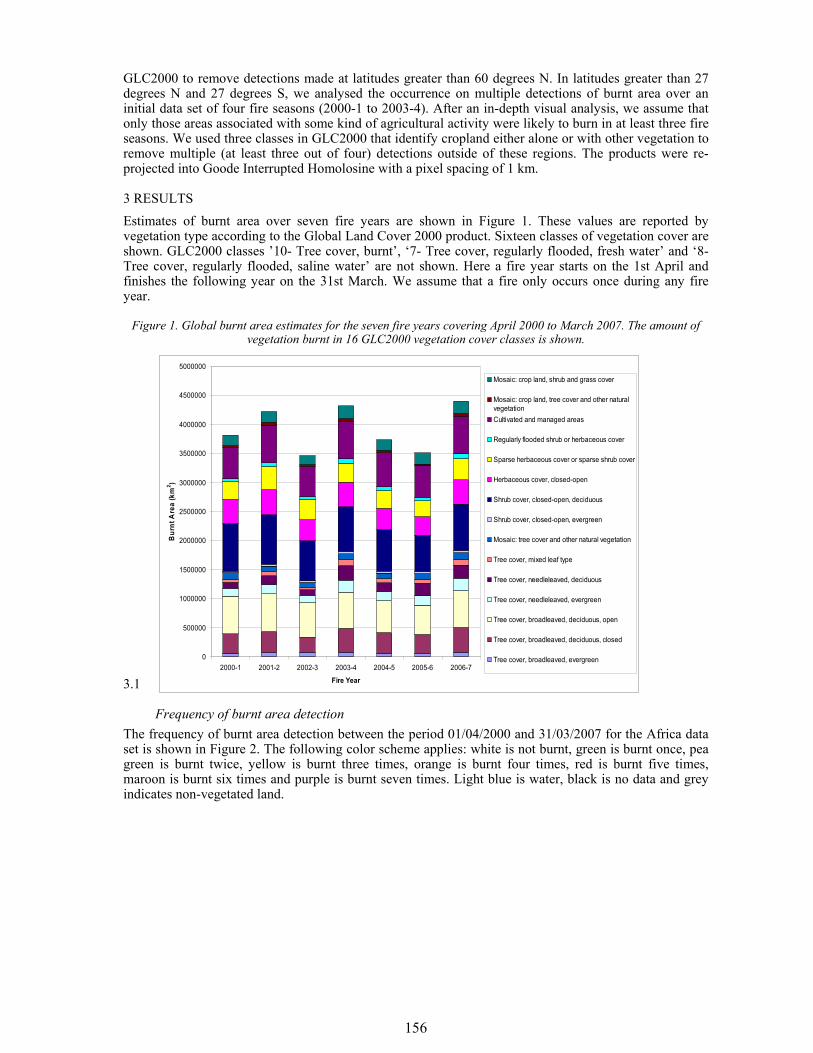
156

GLC2000 to remove detections made at latitudes greater than 60 degrees N. In latitudes greater than 27 degrees N and 27 degrees S, we analysed the occurrence on multiple detections of burnt area over an initial data set of four fire seasons (2000-1 to 2003-4). After an in-depth visual analysis, we assume that only those areas associated with some kind of agricultural activity were likely to burn in at least three fire seasons. We used three classes in GLC2000 that identify cropland either alone or with other vegetation to remove multiple (at least three out of four) detections outside of these regions. The products were re-projected into Goode Interrupted Homolosine with a pixel spacing of 1 km.

3 RESULTS Estimates of burnt area over seven fire years are shown in Figure 1. These values are reported by vegetation type according to the Global Land Cover 2000 product. Sixteen classes of vegetation cover are shown. GLC2000 classes ’10- Tree cover, burnt’, ‘7- Tree cover, regularly flooded, fresh water’ and ‘8- Tree cover, regularly flooded, saline water’ are not shown. Here a fire year starts on the 1st April and finishes the following year on the 31st March. We assume that a fire only occurs once during any fire year.

Figure 1. Global burnt area estimates for the seven fire years covering April 2000 to March 2007. The amount of vegetation burnt in 16 GLC2000 vegetation cover classes is shown.

3.1

Frequency of burnt area detection The frequency of burnt area detection between the period 01/04/2000 and 31/03/2007 for the Africa data set is shown in Figure 2. The following color scheme applies: white is not burnt, green is burnt once, pea green is burnt twice, yellow is burnt three times, orange is burnt four times, red is burnt five times, maroon is burnt six times and purple is burnt seven times. Light blue is water, black is no data and grey indicates non-vegetated land.

0

500000

1000000

1500000

2000000

2500000

3000000

3500000

4000000

4500000

5000000

2000-1 2001-2 2002-3 2003-4 2004-5 2005-6 2006-7

Fire Year

Bur

nt A

rea

(km

2 )

Mosaic: crop land, shrub and grass cover

Mosaic: crop land, tree cover and other naturalvegetationCultivated and managed areas

Regularly flooded shrub or herbaceous cover

Sparse herbaceous cover or sparse shrub cover

Herbaceous cover, closed-open

Shrub cover, closed-open, deciduous

Shrub cover, closed-open, evergreen

Mosaic: tree cover and other natural vegetation

Tree cover, mixed leaf type

Tree cover, needleleaved, deciduous

Tree cover, needleleaved, evergreen

Tree cover, broadleaved, deciduous, open

Tree cover, broadleaved, deciduous, closed

Tree cover, broadleaved, evergreen

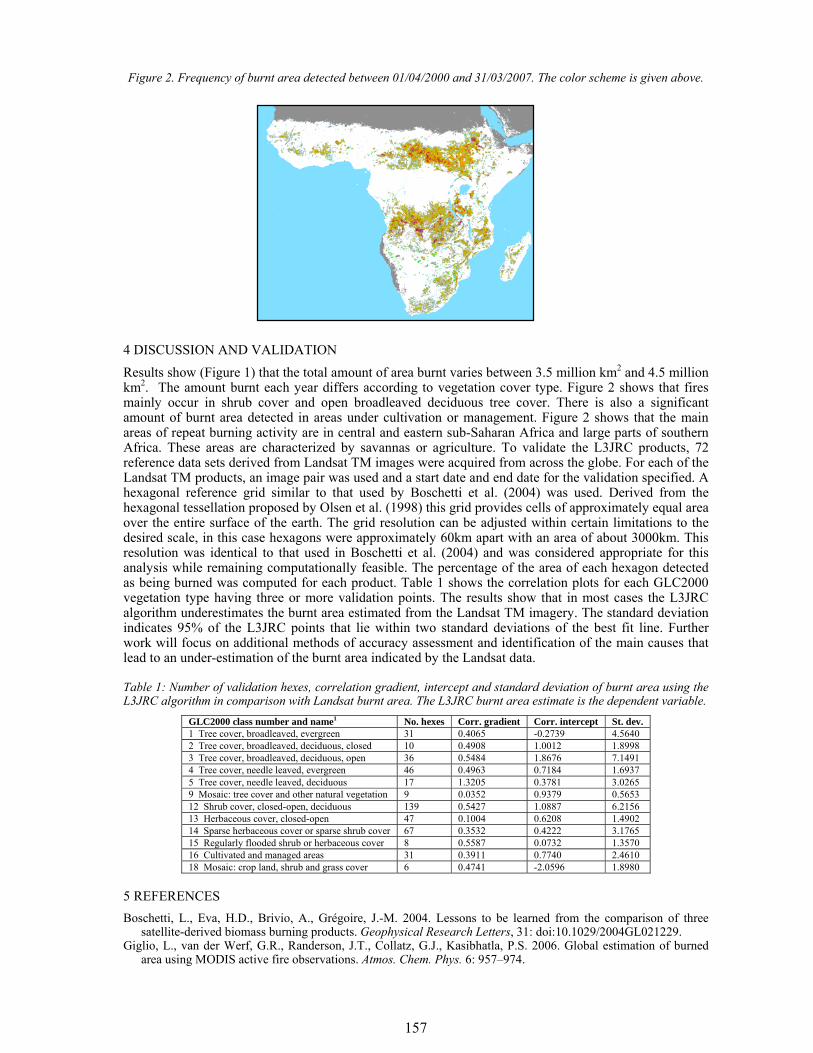
157

Figure 2. Frequency of burnt area detected between 01/04/2000 and 31/03/2007. The color scheme is given above.

4 DISCUSSION AND VALIDATION Results show (Figure 1) that the total amount of area burnt varies between 3.5 million km2 and 4.5 million km2. The amount burnt each year differs according to vegetation cover type. Figure 2 shows that fires mainly occur in shrub cover and open broadleaved deciduous tree cover. There is also a significant amount of burnt area detected in areas under cultivation or management. Figure 2 shows that the main areas of repeat burning activity are in central and eastern sub-Saharan Africa and large parts of southern Africa. These areas are characterized by savannas or agriculture. To validate the L3JRC products, 72 reference data sets derived from Landsat TM images were acquired from across the globe. For each of the Landsat TM products, an image pair was used and a start date and end date for the validation specified. A hexagonal reference grid similar to that used by Boschetti et al. (2004) was used. Derived from the hexagonal tessellation proposed by Olsen et al. (1998) this grid provides cells of approximately equal area over the entire surface of the earth. The grid resolution can be adjusted within certain limitations to the desired scale, in this case hexagons were approximately 60km apart with an area of about 3000km. This resolution was identical to that used in Boschetti et al. (2004) and was considered appropriate for this analysis while remaining computationally feasible. The percentage of the area of each hexagon detected as being burned was computed for each product. Table 1 shows the correlation plots for each GLC2000 vegetation type having three or more validation points. The results show that in most cases the L3JRC algorithm underestimates the burnt area estimated from the Landsat TM imagery. The standard deviation indicates 95% of the L3JRC points that lie within two standard deviations of the best fit line. Further work will focus on additional methods of accuracy assessment and identification of the main causes that lead to an under-estimation of the burnt area indicated by the Landsat data.

Table 1: Number of validation hexes, correlation gradient, intercept and standard deviation of burnt area using the L3JRC algorithm in comparison with Landsat burnt area. The L3JRC burnt area estimate is the dependent variable.

GLC2000 class number and name1 No. hexes Corr. gradient Corr. intercept St. dev. 1 Tree cover, broadleaved, evergreen 31 0.4065 -0.2739 4.5640 2 Tree cover, broadleaved, deciduous, closed 10 0.4908 1.0012 1.8998 3 Tree cover, broadleaved, deciduous, open 36 0.5484 1.8676 7.1491 4 Tree cover, needle leaved, evergreen 46 0.4963 0.7184 1.6937 5 Tree cover, needle leaved, deciduous 17 1.3205 0.3781 3.0265 9 Mosaic: tree cover and other natural vegetation 9 0.0352 0.9379 0.5653 12 Shrub cover, closed-open, deciduous 139 0.5427 1.0887 6.2156 13 Herbaceous cover, closed-open 47 0.1004 0.6208 1.4902 14 Sparse herbaceous cover or sparse shrub cover 67 0.3532 0.4222 3.1765 15 Regularly flooded shrub or herbaceous cover 8 0.5587 0.0732 1.3570 16 Cultivated and managed areas 31 0.3911 0.7740 2.4610 18 Mosaic: crop land, shrub and grass cover 6 0.4741 -2.0596 1.8980

5 REFERENCES Boschetti, L., Eva, H.D., Brivio, A., Grégoire, J.-M. 2004. Lessons to be learned from the comparison of three

satellite-derived biomass burning products. Geophysical Research Letters, 31: doi:10.1029/2004GL021229. Giglio, L., van der Werf, G.R., Randerson, J.T., Collatz, G.J., Kasibhatla, P.S. 2006. Global estimation of burned

area using MODIS active fire observations. Atmos. Chem. Phys. 6: 957–974.

158

Jupp, T.E., Taylor, C.M., Balzter, H., George, C.T., 2006. A statistical model linking Siberian forest fire scars with early summer rainfall anomalies. Geophysical Research Letters 33: L14701, doi:10.1029/2006GL026679.

Olsen, A.R., Stevens, D.L., and White, D., 1998. Application of global grids in environmental sampling. Computing Science and Statistics, ed. S. Weisberg. Farfax Station, VA: Interface Foundation of North America, Inc. .

Patra, P. K., Ishizawa, M., Maksyutov, S., Nakazawa, T., Inoue, G. 2005. Role of biomass burning and climate anomalies for land-atmosphere carbon fluxes based on inverse modeling of atmospheric CO2. Global Biogeochem. Cycles 19: GB3005, doi:10.1029/2004GB002258.

Roy, D.P, Jin, Y., Lewis, P.E., Justice, C.O. 2005. Prototyping a global algorithm for systematic fire affected area mapping using MODIS time series data. Rem. Sens. Env. 97: 137-162.

Schultz, M.G. 2002. On the use of ATSR fire count data to estimate the seasonal and interannual variability of vegetation fire emissions. Atmos. Chem. Phys. 2: 387-395.

Stohl, A., Berg, T., Burkhart, J.F., Fjæraa, A.M., Forster, C., Herber, A., Hov, Ø., Lunder, C., McMillan, W.W., Oltmans, S., Shiobara, M., Simpson, D., Solberg, S., Stebel, K., Ström, J., Tørseth, K., Treffeisen, R., Virkkunen, K., Yttri, K.E. 2006. Arctic smoke record high air pollution levels in the European Arctic due to agricultural fires in Eastern Europe. Atmos. Chem. Phys. Discussions 6: 9655-9722.

Sukhinin, A.I., French, N.H.F., Kasischke, E.S., Hewson, J.H., Soja, A.J., Csiszar, I.A., Hyer, E.J., Loboda, T., Conrad, S.G., Romasko, V.I., Pavlichenko, E.A., Miskiv, S.I., Slinkina, O.A. 2004. AVHRR-based mapping of fires in Russia: New products for fire management and carbon cycle studies. Rem. Sens. Env. 93: 546-564.

Tansey, K., Grégoire, J.-M., Stroppiana, D., Sousa, A., Silva, J., Pereira, J. M. C., Boschetti, L., Maggi, M., Brivio, P. A., Fraser, R., Flasse, S., Ershov, D., Binaghi, E., Graetz, D., Peduzzi, P. 2004. Vegetation burning in the year 2000: Global burned area estimates from SPOT VEGETATION data. J. Geophys. Res. 109: D14S03, doi:10.1029/2003JD003598.

van der Werf, G. R., Randerson, J. T., Giglio, L., Collatz, G. J., Kasibhatla, P.S., Arellano, A.F. Jr. 2006. Global estimation of burned area using MODIS active fire observations. Atmos. Chem. Phys. 6: 3423–3441.

159

1 INTRODUCTION - BACKGROUND A classical problem in multispectral satellite sensor data is the choice of the most effective three-channel color composites for enhancing certain characteristics of the scene, as for instance fire scars. Giving a paradigm, there are 210 unique ways to present in a three dimensional color space (i.e. RGB) the seven available spectral channels of Landsat-5 Thematic Mapper data (Sheffield 1985). In literature, they have been proposed and used different methods to account for spectral information content assessment among and within satellite sensors (Chavez et al. 1982, Price 1984, Benson and DeGloria 1985, Sheffield 1985, Chavez and Bowell 1988, Mausel et al. 1990, Dwivedi and Rao 1992). Occasionally, visual comparison of various RGB color composites can be used, however, deciding the best possible combination visually is relatively difficult, subjective and time-consuming (Dwivedi and Rao 1992). One of the methods is to choose those channels with the largest sum of squared principal axes, which account for the largest total variance. However, the consideration of the total variance, as a measure for the information content of three-channel composites, is problematic. Instead, Sheffield (1985) proposed the use of the ellipsoid of maximum volume. This approach discourages selecting spectral channels with high correlation. He concluded that the TM4, TM5 and TM1 RGB color composite consistently ranked high regardless of image location. Since eye is most sensitive to green followed by red and blue part of electromagnetic spectrum, he associated the spectral channel with the maximum variance to the green, the channel with the second largest variance to the red and the channel with the smallest variance to the blue color plane (Sheffield 1985).

Assessing the information content of Landsat-5 Thematic Mapper data for mapping and characterizing fire scars

Nikos Koutsias Department of Environmental and Natural Resources Management, University of Ioannina, Seferi 2, GR-30100, Agrinio, Greece. [email protected], [email protected]

Georgios Mallinis School of Forestry and Natural Environment, Aristotle University of Thessaloniki, Box 248, GR-54124, Thessaloniki, Greece. [email protected]

Maria Tsakiri-Strati Department of Cadastre, Photogrammetry and Cartography, Faculty of Rural and Surveying, Engineering, Aristotle University of Thessaloniki, GR-54124, Thessaloniki, Greece [email protected]

Keywords: information content, spectral properties, fire scars, Landsat-5 Thematic Mapper

ABSTRACT: A classical problem in multispectral satellite sensor data is the choice of the most effective three-channel color composites for enhancing certain characteristics of the scene, as for instance fire scars. Giving a paradigm, there are 210 unique ways to present in a three dimensional color space (i.e. RGB) the seven available spectral channels of Landsat-5 Thematic Mapper data (Sheffield, 1985). In literature, they have been proposed and used different methods to account for spectral information content assessment among and within satellite sensors, including visual comparison of various RGB color composites, consideration of the total variance within each band, principal component analysis, separability measurements, as for instance Transformed Divergence (TD) and Jefferies-Matusita distance (JM). However, there is no any systematic work concerning the spectral in-formation content of Landsat-5 TM data in respect to burned land discrimination and characterization. Following the literature review in the general topic of information content assessment, as well as the associated literature on spectral properties of burned areas, we try to systematically characterize and quantify the information content carrying on the Landsat-5 TM data. For the discrimination of the burned areas, emphasis is given on the maximization of their spectral discrimination against other land cover types, while minimizing at the same time their within spectral variability. For the characterization of the burned areas, emphasis is given on the maximization of the spectral variability found within the burned areas. Under this perspective we discuss the information contained in each spectral band and we present the best three-channel color composites. Using all land cover types the grouping of the spectral channels is a follows. There are two distinct groups consisting of TM1 and the rest. The second division is between TM5 and the rest, while the third one is between TM4 and the rest followed by TM7. These channels contain the most useful information for general land cover discrimination. It is interesting to mention that Koutsias and Karteris (2000) found that the best three channel color composite consists of TM7, TM4 and TM1.

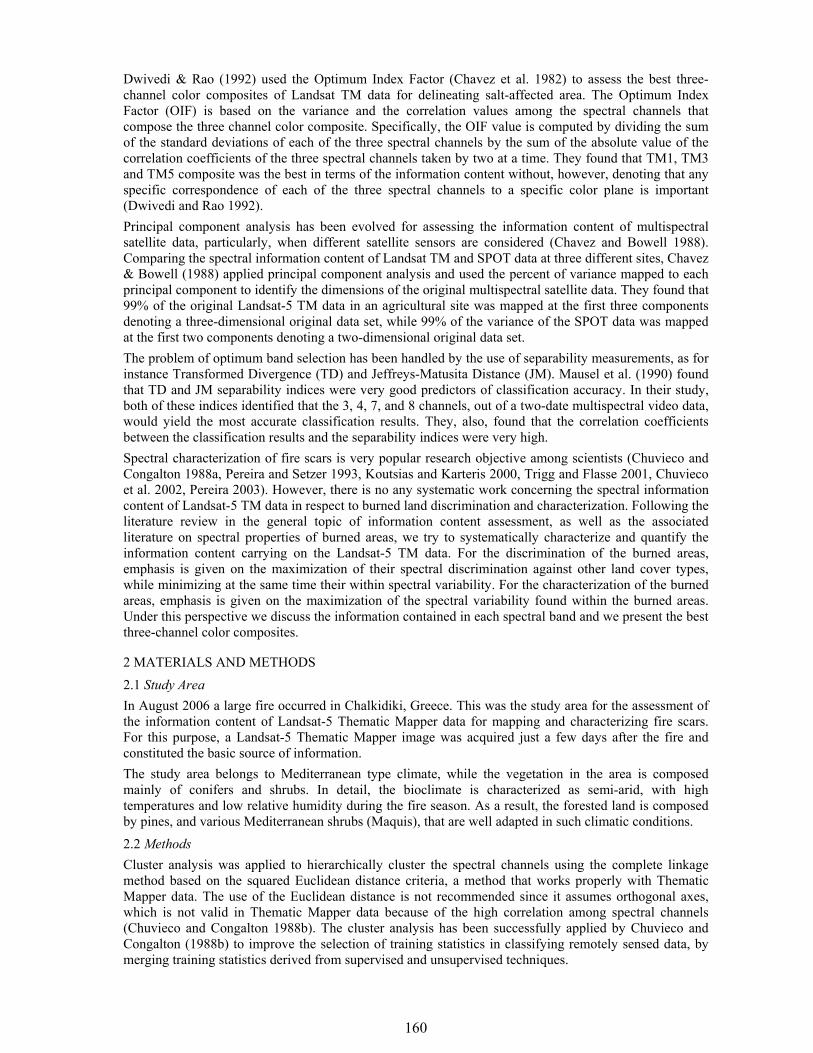
160

Dwivedi & Rao (1992) used the Optimum Index Factor (Chavez et al. 1982) to assess the best three-channel color composites of Landsat TM data for delineating salt-affected area. The Optimum Index Factor (OIF) is based on the variance and the correlation values among the spectral channels that compose the three channel color composite. Specifically, the OIF value is computed by dividing the sum of the standard deviations of each of the three spectral channels by the sum of the absolute value of the correlation coefficients of the three spectral channels taken by two at a time. They found that TM1, TM3 and TM5 composite was the best in terms of the information content without, however, denoting that any specific correspondence of each of the three spectral channels to a specific color plane is important (Dwivedi and Rao 1992). Principal component analysis has been evolved for assessing the information content of multispectral satellite data, particularly, when different satellite sensors are considered (Chavez and Bowell 1988). Comparing the spectral information content of Landsat TM and SPOT data at three different sites, Chavez & Bowell (1988) applied principal component analysis and used the percent of variance mapped to each principal component to identify the dimensions of the original multispectral satellite data. They found that 99% of the original Landsat-5 TM data in an agricultural site was mapped at the first three components denoting a three-dimensional original data set, while 99% of the variance of the SPOT data was mapped at the first two components denoting a two-dimensional original data set. The problem of optimum band selection has been handled by the use of separability measurements, as for instance Transformed Divergence (TD) and Jeffreys-Matusita Distance (JM). Mausel et al. (1990) found that TD and JM separability indices were very good predictors of classification accuracy. In their study, both of these indices identified that the 3, 4, 7, and 8 channels, out of a two-date multispectral video data, would yield the most accurate classification results. They, also, found that the correlation coefficients between the classification results and the separability indices were very high. Spectral characterization of fire scars is very popular research objective among scientists (Chuvieco and Congalton 1988a, Pereira and Setzer 1993, Koutsias and Karteris 2000, Trigg and Flasse 2001, Chuvieco et al. 2002, Pereira 2003). However, there is no any systematic work concerning the spectral information content of Landsat-5 TM data in respect to burned land discrimination and characterization. Following the literature review in the general topic of information content assessment, as well as the associated literature on spectral properties of burned areas, we try to systematically characterize and quantify the information content carrying on the Landsat-5 TM data. For the discrimination of the burned areas, emphasis is given on the maximization of their spectral discrimination against other land cover types, while minimizing at the same time their within spectral variability. For the characterization of the burned areas, emphasis is given on the maximization of the spectral variability found within the burned areas. Under this perspective we discuss the information contained in each spectral band and we present the best three-channel color composites.


2.1 Study Area In August 2006 a large fire occurred in Chalkidiki, Greece. This was the study area for the assessment of the information content of Landsat-5 Thematic Mapper data for mapping and characterizing fire scars. For this purpose, a Landsat-5 Thematic Mapper image was acquired just a few days after the fire and constituted the basic source of information. The study area belongs to Mediterranean type climate, while the vegetation in the area is composed mainly of conifers and shrubs. In detail, the bioclimate is characterized as semi-arid, with high temperatures and low relative humidity during the fire season. As a result, the forested land is composed by pines, and various Mediterranean shrubs (Maquis), that are well adapted in such climatic conditions. 2.2 Methods Cluster analysis was applied to hierarchically cluster the spectral channels using the complete linkage method based on the squared Euclidean distance criteria, a method that works properly with Thematic Mapper data. The use of the Euclidean distance is not recommended since it assumes orthogonal axes, which is not valid in Thematic Mapper data because of the high correlation among spectral channels (Chuvieco and Congalton 1988b). The cluster analysis has been successfully applied by Chuvieco and Congalton (1988b) to improve the selection of training statistics in classifying remotely sensed data, by merging training statistics derived from supervised and unsupervised techniques.

161

The cluster analysis has been applied using a sample of some of the most important and representative land cover types that of the area.


Figure 1 shows the dendrograms resulting from the cluster analysis taking into account basic land cover types found in the satellite imagery. Each graph shows the similarity of the spectral channels for each land cover. For example, the spectral information of the Landsat-5 Thematic Mapper channels creates two distinct groups; the first composed of TM1, TM7 and TM5 and the second composed of TM2, TM3 and TM4. The first group also is consisted of two distinct sub-groups TM5 alone and TM1 and TM7. Each land cover presents a unique pattern concerning the similarity of the spectral channels. Using all land cover types the grouping of the spectral channels is a follows. There are two distinct groups consisting of TM1 and the rest. The second division is between TM5 and the rest, while the third one is between TM4 and the rest followed by TM7. These channels contain the most useful information for general land cover discrimination. It is interesting to mention that Koutsias and Karteris (2000) found that the best three channel color composite consists of TM7, TM4 and TM1.

Figure 1 Cluster analysis of spectral channels of Landsat-5 Thematic Mapper data.

Complete LinkageSquared Euclidean distances

Linkage Distance

TM4 TM3 TM2 TM5 TM7 TM1

0 5e5 1e6 1.5e6 2e6 2.5e6


Linkage Distance


0 2e6 4e6 6e6 8e6 1e7

burned areas wheat cultivations (dry)


Linkage Distance


0 2e6 4e6 6e6 8e6 1e7


Linkage Distance


0 1e6 2e6 3e6 4e6 5e6 6e6 7e6 8e6

sea(shallow, near coast) sea(deep, far from coast)


Linkage Distance


0 5e5 1e6 1.5e6 2e6 2.5e6 3e6


Linkage Distance


0 5e5 1e6 1.5e6 2e6 2.5e6 3e6 3.5e6 4e6

urban areas vegetation (pines)

162


Linkage Distance


0 1e6 2e6 3e6 4e6 5e6 6e6


Linkage Distance


0 5e6 1e7 1.5e7 2e7 2.5e7

vegetation (cultivations) all categories

4 REFERENCES Benson, A. S., and S. D. DeGloria. 1985. Interpretation of Landsat-4 Thematic Mapper and Multispectral

Scanner data for forest surveys. Photogrammetric Engineering & Remote Sensing 51:1281-1289. Chavez, P. S. J., G. L. Berlin, and L. B. Sowers. 1982. Statistical methods for selecting Landsat-MSS

ratios. Journal of Applied Photogrammetric Engineering 8:23-30. Chavez, P. S. J., and J. A. Bowell. 1988. Comparison of the spectral information content of Landsat

Thematic Mapper and SPOT for three different sites in the Phoenix, Arizona region. Photogrammetric Engineering & Remote Sensing 54:1699-1708.

Chuvieco, E., and R. G. Congalton. 1988a. Mapping and inventory of forest fires from digital processing of TM data. Geocarto International 4:41-53.

Chuvieco, E., and R. G. Congalton. 1988b. Using cluster analysis to improve the selection of training statistics in classifying remotely sensed data. Photogrammetric Engineering & Remote Sensing 54:1275-1281.

Chuvieco, E., M. P. Martín, and A. Palacios. 2002. Assessment of different spectral indices in the red-near-infrared spectral domain for burned land discrimination. International Journal of Remote Sensing 23:5103-5110.

Dwivedi, R. S., and B. R. M. Rao. 1992. The selection of the best possible Landsat TM band combination for delineating salt-affected soils. International Journal of Remote Sensing 13:2051-2058.

Koutsias, N., and M. Karteris. 2000. Burned area mapping using logistic regression modeling of a single post-fire Landsat-5 Thematic Mapper image. International Journal of Remote Sensing 21:673-687.

Mausel, P. W., W. J. Kramber, and J. K. Lee. 1990. Optimum band selection for supervised classification of multispectral data. Photogrammetric Engineering & Remote Sensing 56:55-60.

Pereira, J. M. C. 2003. Remote sensing of burned areas in tropical savannas. International Journal of Wildland Fire 12:259-270.

Pereira, J. M. C., and A. W. Setzer. 1993. Spectral characteristics of fire scars in Landsat-5 TM images of Amazonia. International Journal of Remote Sensing 14:2061-2078.

Price, J. C. 1984. Comparison of the information content of data from the Landsat-4 Thematic Mapper and the Multispectral Scanner. IEEE Transactions on Geoscience and Remote Sensing GE-22:272-281.

Sheffield, C. 1985. Selecting band combinations from multispectral data. Photogrammetric Engineering & Remote Sensing 51:681-687.

Trigg, S., and S. Flasse. 2001. An evaluation of different bi-spectral spaces for discriminating burned shrub-savannah. International Journal of Remote Sensing 22:2641-2647.

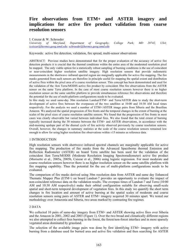
163

1 INTRODUCTION

High resolution sensors with shortwave–infrared spectral channels are marginally applicable for active fire mapping. The production of fire masks from the Advanced Spaceborne thermal Emission and Reflection Radiometer (ASTER) on board Terra satellite has been used for the validation of the coincident 1km Terra/MODIS (Moderate Resolution Imaging Spectroradiometer) active fire product (Morisette et al., 2005a, 2005b, Csiszar et al., 2006) using logistic regression. For most moderate and coarse resolution sensors however there is no higher resolution sensor on the same satellite platform with fire mapping capability. Thus the potential for the use of multi-platform configurations needs to be evaluated. The comparison of fire masks derived using 30m resolution data from ASTER and same day Enhanced Thematic Mapper Plus (ETM+) on board Landsat-7 provides an opportunity to evaluate the impact of non-coincident reference data on the validation results. The overpass times of Landsat-7 and Terra (10:00 AM and 10:30 AM respectively) make their orbital configuration suitable for observing small-scale spatial and short-term temporal development of vegetation fires. In this study we quantify the short term changes in fire location and amount of active burning at the spatial scales of moderate and coarse resolution sensors using pairs of ASTER and ETM+ imagery acquired 30 minutes apart. We tested our methodology over Amazonia and Siberia, two areas marked by contrasting fire regimes.

2 DATA

We collected 10 pairs of same-day imagery from ETM+ and ASTER showing active fires over Siberia and the Amazon in 2001, 2002 and 2003 (Figure 1). Over the two broad and climatically different regions we also attempted to collect fires burning in the forest, the forest/non-forest interface and in more sparsely vegetated areas dominated by grassland. The selection of the available image pairs was done by first identifying ETM+ imagery with active burning from a database used for burned area and active fire validation and then searching for ASTER

Fire observations from ETM+ and ASTER imagery and implications for active fire product validation from coarse resolution sensors

I. Csiszar & W. Schroeder University of Maryland, Department of Geography, College Park, MD 20742, USA; [email protected]; [email protected] Keywords: active fire detection, validation, fire spread, multi-sensor observations

ABSTRACT: Previous studies have demonstrated that for the proper evaluation of the accuracy of active fire detection products it is crucial that the thermal conditions within the entire area of the moderated resolution pixel be mapped. The only viable option for a statistically robust sampling of burning conditions is the use of coincident or near-coincident higher resolution satellite imagery. High resolution sensors that provide radiometric measurements in the shortwave–infrared spectral region are marginally applicable for active fire mapping. The fire masks generated from such sensors are therefore in principle useful for mapping the spatial extent and distribution of active fires within the pixel area of a coarse resolution sensor. This concept has been demonstrated and used for the validation of the 1km Terra/MODIS active fire product by coincident 30m fire observations from the ASTER sensor on the same Terra platform. In the case of most coarse resolution sensors however there is no higher resolution sensor on the same satellite platform to provide simultaneous reference fire observations and therefore the potential for the use of multi-platform configurations needs to be evaluated. In this study we used same-day 30m resolution Landsat/ETM+ and Terra/ASTER data to study the short-term development of active fires between the overpasses of the two satellites at 10:00 and 10:30 AM local times respectively. For the analysis we used a number of ETM+/ASTER image pairs from Siberia and the Brazilian Amazon. We analyzed the spatial progression of fire fronts and the temporal changes in the extent of burning at the scales of the pixel sizes of coarse resolution satellite sensors. We found that the progression of fire fronts in most cases was clearly observable but varied between individual fires. We also found that the total extent of burning typically increased during the 30 minutes between the ETM+ and ASTER observations, in accordance with the mid-morning upslope part of the diurnal cycle of fire activity observed previously by coarse resolution sensors. Overall, however, the changes in summary statistics at the scale of the coarse resolution sensors remained low enough to allow for using higher resolution fire observations within ±15 minutes as reference data.

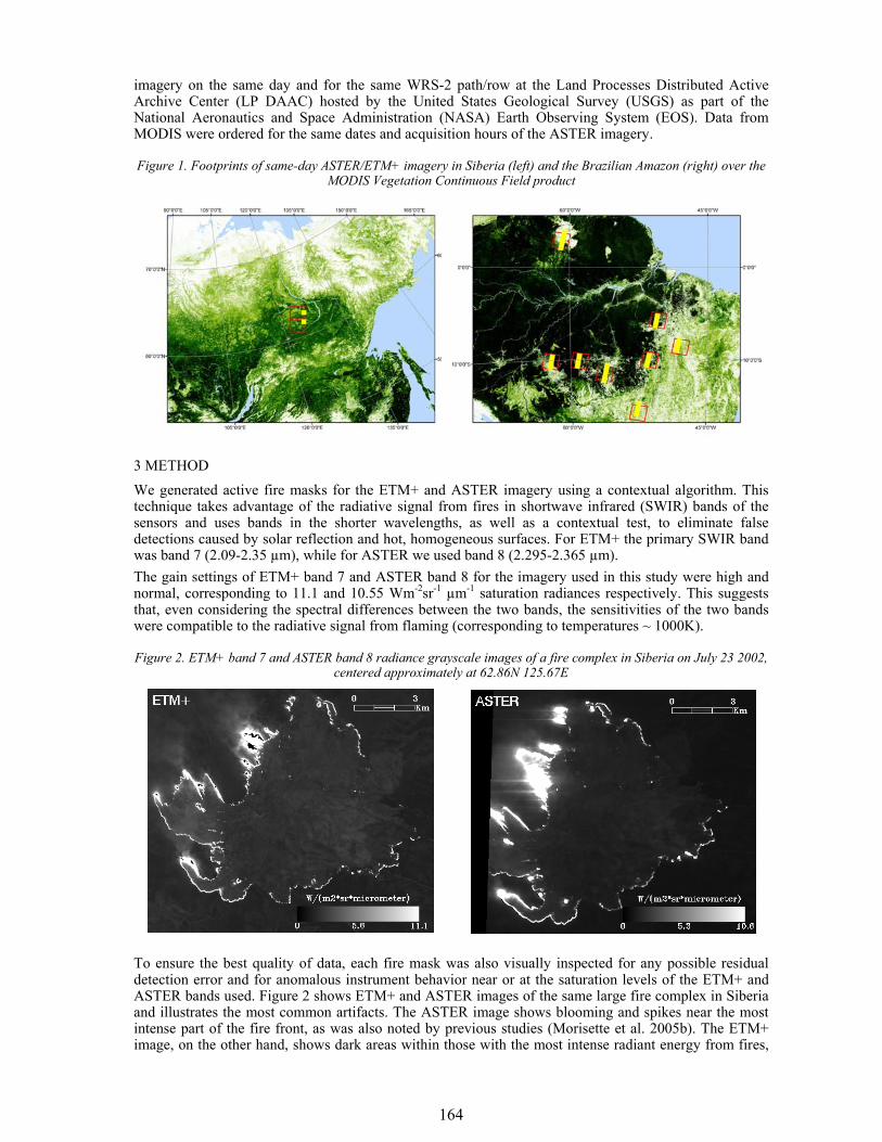
164

imagery on the same day and for the same WRS-2 path/row at the Land Processes Distributed Active Archive Center (LP DAAC) hosted by the United States Geological Survey (USGS) as part of the National Aeronautics and Space Administration (NASA) Earth Observing System (EOS). Data from MODIS were ordered for the same dates and acquisition hours of the ASTER imagery.

Figure 1. Footprints of same-day ASTER/ETM+ imagery in Siberia (left) and the Brazilian Amazon (right) over the MODIS Vegetation Continuous Field product

3 METHOD We generated active fire masks for the ETM+ and ASTER imagery using a contextual algorithm. This technique takes advantage of the radiative signal from fires in shortwave infrared (SWIR) bands of the sensors and uses bands in the shorter wavelengths, as well as a contextual test, to eliminate false detections caused by solar reflection and hot, homogeneous surfaces. For ETM+ the primary SWIR band was band 7 (2.09-2.35 µm), while for ASTER we used band 8 (2.295-2.365 µm). The gain settings of ETM+ band 7 and ASTER band 8 for the imagery used in this study were high and normal, corresponding to 11.1 and 10.55 Wm-2sr-1 µm-1 saturation radiances respectively. This suggests that, even considering the spectral differences between the two bands, the sensitivities of the two bands were compatible to the radiative signal from flaming (corresponding to temperatures ~ 1000K).

Figure 2. ETM+ band 7 and ASTER band 8 radiance grayscale images of a fire complex in Siberia on July 23 2002, centered approximately at 62.86N 125.67E

To ensure the best quality of data, each fire mask was also visually inspected for any possible residual detection error and for anomalous instrument behavior near or at the saturation levels of the ETM+ and ASTER bands used. Figure 2 shows ETM+ and ASTER images of the same large fire complex in Siberia and illustrates the most common artifacts. The ASTER image shows blooming and spikes near the most intense part of the fire front, as was also noted by previous studies (Morisette et al. 2005b). The ETM+ image, on the other hand, shows dark areas within those with the most intense radiant energy from fires,

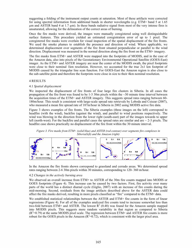
165

suggesting a folding of the instrument output counts at saturation. Most of these artifacts were corrected for using spectral information from additional bands in shorter wavelengths (e.g. ETM+ band 5 at 1.65 µm and ASTER band 4 at 1.7 µm). In these bands radiative signal from most of the very intense fires is unsaturated, allowing for the delineation of the correct areas of burning. Once the fire masks were derived, the images were manually coregistered using well distinguishable surface features. This procedure yielded an estimated coregistration error of up to 1 pixel. The coregistered fire masks were overlain for visual inspection of the spatial displacement of the fire fronts. We used the smoke plumes to establish the presence and direction of wind. Where applicable, we determined displacement over segments of the fire front situated perpendicular or parallel to the wind direction. Displacement was measured in the normal direction along the fire front on the ETM+ imagery. The fire masks from ETM+ and ASTER were mapped into the footprints of MODIS, and in the case of the Amazon data, also into pixels of the Geostationary Environmental Operational Satellite (GOES-East) imager. As the ETM+ and ASTER imagery are near the center of the MODIS swath, the pixel footprints were close to their nominal 1km resolution. However, we accounted for the true 2x1 km footprint of MODIS caused by the triangular line scan function. For GOES-East the Amazon region is also close to the sub-satellite point and therefore the footprints were close in size to their 4km nominal resolution.

4 RESULTS 4.1 Spatial displacement We inspected the displacement of fire fronts of four large fire clusters in Siberia. In all cases the propagation of the fire front was found to be 1-3 30m pixels within the ~30 minute time interval between the acquisition times of the ETM+ and ASTER imagery. This suggests spread rates ranging between 60-180m/hour. This result is consistent with large-scale spread rate retrievals by Loboda and Csiszar (2007), who measured a mean fire spread rate of 187m/hour in Siberia in 2002 using MODIS active fire data. Figure 3 shows examples of fire fronts. The Siberia examples (three images on the left) correspond to headfire (with the wind), backfire (against the wind), and parallel to wind positions respectively. The wind was blowing in the direction from the lower right (south-east) part of the images towards to upper left (north-west). For the backfire and parallel cases the spread rates are similar and are ~ 2-3 pixels. The headfire case shows practically no displacement of the fire front within the 30 minute interval.

Figure 3. Fire masks from ETM+ (solid blue) and ASTER (red contour) over segments fire complexes in Siberia(left) and the Amazon (right)

In the Amazon the fire fronts shown correspond to grassland and cerrado areas. We determined spread rates ranging between 2-6 30m pixels within 30 minutes, corresponding to 120- 360 m/hour. 4.2 Changes in the actively burning area We observed an overall increase from ETM+ to ASTER of the 30m fire counts mapped into MODIS or GOES footprints (Figure 4). This increase can be caused by two factors. First, fire activity over many parts of the world has a distinct diurnal cycle (Giglio, 2007) with an increase of fire counts during the mid-morning. Second, residuals from the image artifacts described above for the ASTER data could affect the fire masks derived, resulting in more pixels classified as “fire” compared to the ETM+ data. We established statistical relationships between the ASTER and ETM+ fire counts in the form of linear regressions (Figure 4). For all of the examples analyzed fire counts tend to increase somewhat less than two-fold between ETM+ and ASTER. The lowest R2 (0.48) was found for the Amazon sample mapped into MODIS pixels. This suggests more random variability in that region as compared to Siberia (R2=0.79) at the same MODIS pixel scale. The regression between ETM+ and ASTER fire counts is more robust for the GOES pixels in the Amazon (R2=0.72), which is consistent with the larger pixel area.

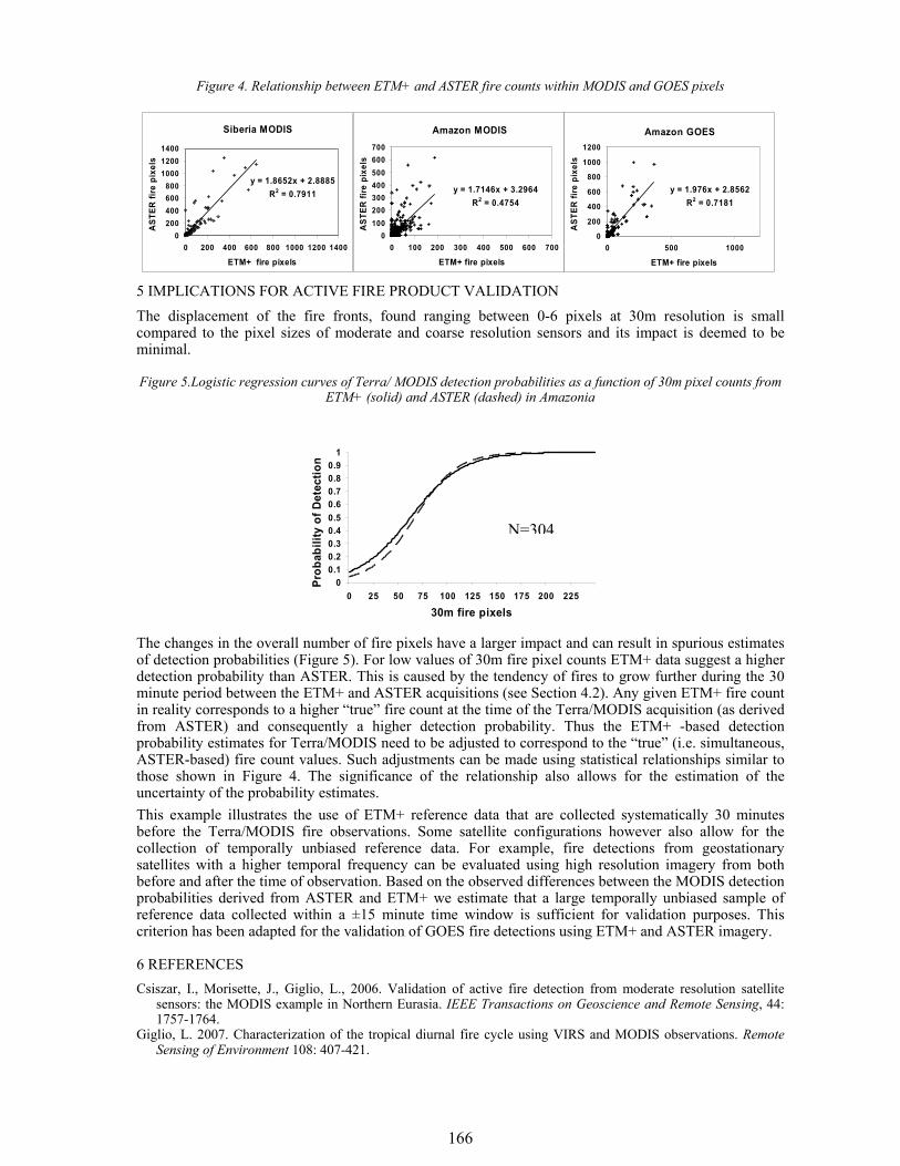
166

Figure 4. Relationship between ETM+ and ASTER fire counts within MODIS and GOES pixels

5 IMPLICATIONS FOR ACTIVE FIRE PRODUCT VALIDATION The displacement of the fire fronts, found ranging between 0-6 pixels at 30m resolution is small compared to the pixel sizes of moderate and coarse resolution sensors and its impact is deemed to be minimal.

Figure 5.Logistic regression curves of Terra/ MODIS detection probabilities as a function of 30m pixel counts from ETM+ (solid) and ASTER (dashed) in Amazonia

The changes in the overall number of fire pixels have a larger impact and can result in spurious estimates of detection probabilities (Figure 5). For low values of 30m fire pixel counts ETM+ data suggest a higher detection probability than ASTER. This is caused by the tendency of fires to grow further during the 30 minute period between the ETM+ and ASTER acquisitions (see Section 4.2). Any given ETM+ fire count in reality corresponds to a higher “true” fire count at the time of the Terra/MODIS acquisition (as derived from ASTER) and consequently a higher detection probability. Thus the ETM+ -based detection probability estimates for Terra/MODIS need to be adjusted to correspond to the “true” (i.e. simultaneous, ASTER-based) fire count values. Such adjustments can be made using statistical relationships similar to those shown in Figure 4. The significance of the relationship also allows for the estimation of the uncertainty of the probability estimates. This example illustrates the use of ETM+ reference data that are collected systematically 30 minutes before the Terra/MODIS fire observations. Some satellite configurations however also allow for the collection of temporally unbiased reference data. For example, fire detections from geostationary satellites with a higher temporal frequency can be evaluated using high resolution imagery from both before and after the time of observation. Based on the observed differences between the MODIS detection probabilities derived from ASTER and ETM+ we estimate that a large temporally unbiased sample of reference data collected within a ±15 minute time window is sufficient for validation purposes. This criterion has been adapted for the validation of GOES fire detections using ETM+ and ASTER imagery.

6 REFERENCES Csiszar, I., Morisette, J., Giglio, L., 2006. Validation of active fire detection from moderate resolution satellite

sensors: the MODIS example in Northern Eurasia. IEEE Transactions on Geoscience and Remote Sensing, 44: 1757-1764.

Giglio, L. 2007. Characterization of the tropical diurnal fire cycle using VIRS and MODIS observations. Remote Sensing of Environment 108: 407-421.

Amazon MODIS

y = 1.7146x + 3.2964R2 = 0.4754

0100200300400500600700

0 100 200 300 400 500 600 700

ETM+ fire pixels

AST

ER fi

re p

ixel

s

Siberia MODIS

y = 1.8652x + 2.8885R2 = 0.7911

0200400600800

100012001400

0 200 400 600 800 1000 1200 1400

ETM+ fire pixels

AST

ER fi

re p

ixel

s

Amazon GOES

y = 1.976x + 2.8562R2 = 0.7181

0

200

400

600

800

1000

1200

0 500 1000

ETM+ fire pixels

AST

ER fi

re p

ixel

s0

0.10.20.30.40.50.60.70.80.9

1

0 25 50 75 100 125 150 175 200 225

30m fire pixels

Prob

abili

ty o

f Det

ectio

n

N=304

167

Giglio, L., Csiszar, I. and Justice, C.O., 2006. Global Distribution and Seasonality of Active Fires as Observed with the Terra and Aqua MODIS Sensors. Journal of Geophysical Research – Biogeosciences 111: G02016, doi:10.1029/2005JG000142.

Loboda, T., Csiszar, I. 2007. Reconstruction of Fire Spread within Wildland Fire Events in Northern Eurasia from the MODIS Active Fire Product. Global and Planetary Change 56: 258-273.

Morisette, J.T., Giglio, L., Csiszar, I., Setzer, A., Schroeder, W., Morton, D., Justice, C.O., 2005a. Validation of MODIS active fire detection products derived from two algorithms. Earth Interactions 9, paper no. 9.

Morisette, J.T., Giglio, L., Csiszar, I., Justice, C.O., 2005b. Validation of the MODIS Active fire product over Southern Africa with ASTER data. International Journal of Remote Sensing 26: 4239-4264.

168

1 INTRODUCTION Vegetation fires are a disturbance factor in almost all the ecosystems around the world (Thonicke et al. 2001). Globally, most of the fire events are human-initiated and only a small proportion of the fire activity is due to natural causes (Levine 2000). Mediterranean countries of southern Europe are greatly affected by fires especially in the summer season when the dry and hot weather set the ideal conditions for the spread of fire. In Italy, fires seriously damage the forest ecosystems with numerous events every year that can get particularly intense during the dry summer season in the southern regions of the country. Since remote sensing satellites are able to cover wide areas and to provide information in several spectral regions, they represent a valuable tool for the detection, mapping and the prevention of wildland fires. Much work has been done in the recent years to investigate how satellite images can be used to detect and map burned areas both at continental and regional scale using medium and high resolution imagery. Very few works focused on the use of images acquired by the Advanced Spaceborne Thermal Emission and Reflection Radiometer (ASTER) sensor for fire monitoring, although the sensor offers spectral and spatial resolutions potentially suitable for this purpose. The non operational character of the ASTER mission could be the major reason that prevented the use of these data in monitoring activities. Classification approaches used in the literature for burnt area mapping with high resolution data range from single date supervised classification, such as Maximum Likelihood (Brivio et al., 2003) or more recently introduced object-oriented (Mitri & Gitas, 2004), to threshold based techniques of specifically developed spectral indices, such as the Burned Area Index (BAI) (Chuvieco et al., 2002) and the Normalized Burnt Ratio (NBR) (Key and Benson, 2002). This study, developed in the framework of a project promoted by Direzione Protezione Natura of the Italian Ministry of Environment, presents a new method that exploits Ordered Weight Averaging (OWA) operators for mapping burnt areas and compares the results obtained using ASTER images over six parks in Southern Italy for the period 2001-2005 with results derived with supervised multi-threshold approach.

2 MATERIALS AND METHODS 2.1 Data and study areas The ASTER sensor, on board the NASA Terra platform, acquires data in the visible to thermal infrared regions of the spectrum along a 60 km wide track with a spatial resolution between 15 m and 90 m. The AST07 product, used in this work, is composed of images acquired in the visible, near-infrared and shortwave infrared regions of the spectrum. The dataset was processed by the NASA EOS Data Gateway (http://edcimswww.cr.usgs.gov/pub/imswelcom) for the period 2001 to 2005. Study areas covered in this experiment concern with national parks of Southern Italy, that are typical of the Mediterranean ecosystem (fig. 1). For developing the methodology a data set of four ASTER images were used; algorithm performance was evaluated on two images of the previous data set and map accuracy was evaluated on two images not seen before (Table 1).

Fuzzy based approach for mapping burnt areas in Mediterranean environment using ASTER images

Pietro Alessandro Brivio, Paolo Zaffaroni, Mirco Boschetti & Daniela Stroppiana CNR-IREA, Institute for Electromagnetic Sensing of the Environment,Via Bassini 15 – 20133 Milan, Italy, [email protected]. [email protected], [email protected], [email protected]

Keywords: Fire Affected Areas, ASTER, Burned Area Index, Normalized Burnt Ratio, Fuzzy Set

ABSTRACT: A new approach for mapping burnt areas with high spatial resolution satellite data is proposed here. The approach that exploits the advantages offered by the approximate reasoning and fuzzy set theory is based on the concept of the reinforcement of evidence brought by a set of features, each contributing to the likelihood of burning. The contribution of each index is quantified by a fuzzy membership function, defined using a partially data driven approach. The likelihood of burnt is computed by a fuzzy aggregation operator defined in the class of the Ordered Weighted Averaging (OWA) operators, that allow to flexibly reflect the more or less conservative attitude of the analyst. The approach has been experimented on some National Parks of Southern Italy using ASTER images acquired in the period 2001-2005. Results obtained with the application of a more traditional method based on image to image tuning and this innovative approach are compared and discussed.

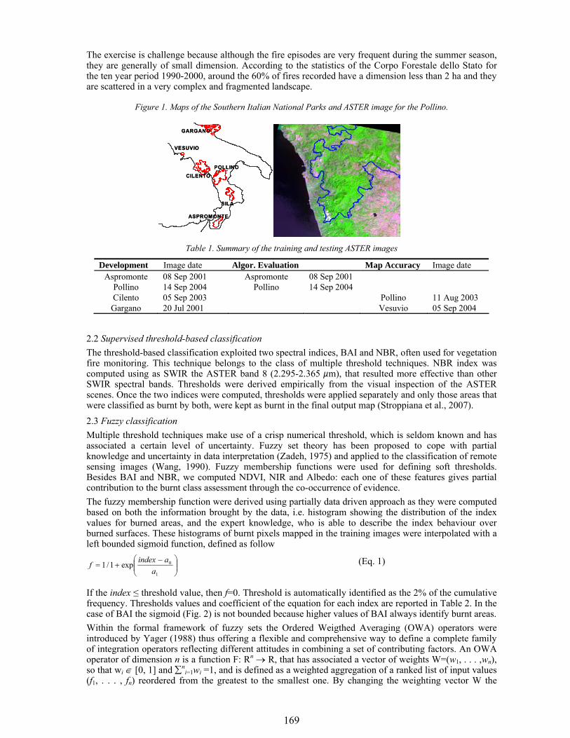
169

The exercise is challenge because although the fire episodes are very frequent during the summer season, they are generally of small dimension. According to the statistics of the Corpo Forestale dello Stato for the ten year period 1990-2000, around the 60% of fires recorded have a dimension less than 2 ha and they are scattered in a very complex and fragmented landscape.

Figure 1. Maps of the Southern Italian National Parks and ASTER image for the Pollino.

Table 1. Summary of the training and testing ASTER images

Development Image date Algor. Evaluation Map Accuracy Image date Aspromonte 08 Sep 2001 Aspromonte 08 Sep 2001

Pollino 14 Sep 2004 Pollino 14 Sep 2004 Cilento 05 Sep 2003 Pollino 11 Aug 2003 Gargano 20 Jul 2001 Vesuvio 05 Sep 2004

2.2 Supervised threshold-based classification The threshold-based classification exploited two spectral indices, BAI and NBR, often used for vegetation fire monitoring. This technique belongs to the class of multiple threshold techniques. NBR index was computed using as SWIR the ASTER band 8 (2.295-2.365 μm), that resulted more effective than other SWIR spectral bands. Thresholds were derived empirically from the visual inspection of the ASTER scenes. Once the two indices were computed, thresholds were applied separately and only those areas that were classified as burnt by both, were kept as burnt in the final output map (Stroppiana et al., 2007). 2.3 Fuzzy classification Multiple threshold techniques make use of a crisp numerical threshold, which is seldom known and has associated a certain level of uncertainty. Fuzzy set theory has been proposed to cope with partial knowledge and uncertainty in data interpretation (Zadeh, 1975) and applied to the classification of remote sensing images (Wang, 1990). Fuzzy membership functions were used for defining soft thresholds. Besides BAI and NBR, we computed NDVI, NIR and Albedo: each one of these features gives partial contribution to the burnt class assessment through the co-occurrence of evidence. The fuzzy membership function were derived using partially data driven approach as they were computed based on both the information brought by the data, i.e. histogram showing the distribution of the index values for burned areas, and the expert knowledge, who is able to describe the index behaviour over burned surfaces. These histograms of burnt pixels mapped in the training images were interpolated with a left bounded sigmoid function, defined as follow

⎟⎟⎠

⎞⎜⎜⎝

⎛ −+=

1

0exp1/1a

aindexf (Eq. 1)

If the index ≤ threshold value, then f=0. Threshold is automatically identified as the 2% of the cumulative frequency. Thresholds values and coefficient of the equation for each index are reported in Table 2. In the case of BAI the sigmoid (Fig. 2) is not bounded because higher values of BAI always identify burnt areas. Within the formal framework of fuzzy sets the Ordered Weigthed Averaging (OWA) operators were introduced by Yager (1988) thus offering a flexible and comprehensive way to define a complete family of integration operators reflecting different attitudes in combining a set of contributing factors. An OWA operator of dimension n is a function F: Rn → R, that has associated a vector of weights W=(w1, . . . ,wn), so that wi ∈ [0, 1] and ∑n

i=1wi =1, and is defined as a weighted aggregation of a ranked list of input values (f1, . . . , fn) reordered from the greatest to the smallest one. By changing the weighting vector W the

POLLINO

GARGANO

SILA

CILENTO

ASPROMONTE

VESUVIO

POLLINO

GARGANO

SILA

CILENTO

ASPROMONTE

VESUVIO

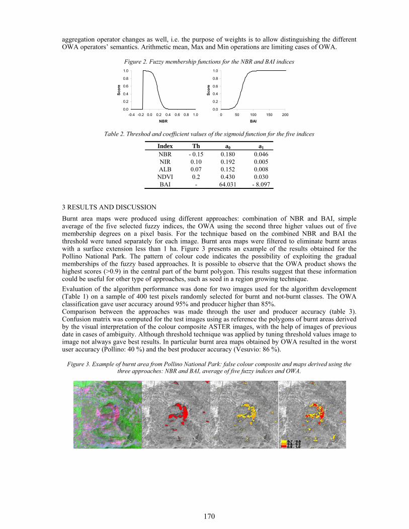
170

aggregation operator changes as well, i.e. the purpose of weights is to allow distinguishing the different OWA operators’ semantics. Arithmetic mean, Max and Min operations are limiting cases of OWA.

Figure 2. Fuzzy membership functions for the NBR and BAI indices

Table 2. Threshod and coefficient values of the sigmoid function for the five indices


Burnt area maps were produced using different approaches: combination of NBR and BAI, simple average of the five selected fuzzy indices, the OWA using the second three higher values out of five membership degrees on a pixel basis. For the technique based on the combined NBR and BAI the threshold were tuned separately for each image. Burnt area maps were filtered to eliminate burnt areas with a surface extension less than 1 ha. Figure 3 presents an example of the results obtained for the Pollino National Park. The pattern of colour code indicates the possibility of exploiting the gradual memberships of the fuzzy based approaches. It is possible to observe that the OWA product shows the highest scores (>0.9) in the central part of the burnt polygon. This results suggest that these information could be useful for other type of approaches, such as seed in a region growing technique. Evaluation of the algorithm performance was done for two images used for the algorithm development (Table 1) on a sample of 400 test pixels randomly selected for burnt and not-burnt classes. The OWA classification gave user accuracy around 95% and producer higher than 85%. Comparison between the approaches was made through the user and producer accuracy (table 3). Confusion matrix was computed for the test images using as reference the polygons of burnt areas derived by the visual interpretation of the colour composite ASTER images, with the help of images of previous date in cases of ambiguity. Although threshold technique was applied by tuning threshold values image to image not always gave best results. In particular burnt area maps obtained by OWA resulted in the worst user accuracy (Pollino: 40 %) and the best producer accuracy (Vesuvio: 86 %).

Figure 3. Example of burnt area from Pollino National Park: false colour composite and maps derived using the three approaches: NBR and BAI, average of five fuzzy indices and OWA.

Index Th a0 a1 NBR - 0.15 0.180 0.046 NIR 0.10 0.192 0.005 ALB 0.07 0.152 0.008 NDVI 0.2 0.430 0.030 BAI - 64.031 - 8.097

0.0

0.2

0.4

0.6

0.8

1.0

0 50 100 150 200

BAI

Scor

e

0.0

0.2

0.4

0.6

0.8

1.0

-0.4 -0.2 0.0 0.2 0.4 0.6 0.8 1.0

NBRSc

ore

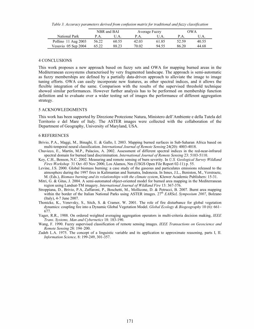
171

Table 3. Accuracy parameters derived from confusion matrix for traditional and fuzzy classification

NBR and BAI Average Fuzzy OWA National Park P.A. U.A. P.A. U.A. P.A. U.A.

Pollino 11 Aug 2003 56.22 60.55 42.03 61.85 52.59 40.55 Vesuvio 05 Sep 2004 65.22 88.23 70.02 94.55 86.20 44.68

4 CONCLUSIONS This work proposes a new approach based on fuzzy sets and OWA for mapping burned areas in the Mediterranean ecosystems characterised by very fragmented landscape. The approach is semi-automatic as fuzzy memberships are defined by a partially data-driven approach to alleviate the image to image tuning efforts. OWA can easily incorporate new features, as other spectral indices, and it allows the flexible integration of the same. Comparison with the results of the supervised threshold technique showed similar performances. However further analysis has to be performed on membership function definition and to evaluate over a wider testing set of images the performance of different aggregation strategy.

5 ACKNOWLEDGMENTS This work has been supported by Direzione Protezione Natura, Ministero dell’Ambiente e della Tutela del Territorio e del Mare of Italy. The ASTER images were collected with the collaboration of the Department of Geography, University of Maryland, USA.

6 REFERENCES Brivio, P.A., Maggi, M., Binaghi, E. & Gallo, I. 2003. Mapping burned surfaces in Sub-Saharan Africa based on

multi-temporal neural classification. International Journal of Remote Sensing 24(20): 4003-4018. Chuvieco, E., Martín, M.P., Palacios, A. 2002. Assessment of different spectral indices in the red-near-infrared

spectral domain for burned land discrimination. International Journal of Remote Sensing 23: 5103-5110. Key, C.H., Benson, N.C. 2002. Measuring and remote sensing of burn severity. In U.S. Geological Survey Wildland

Fires Workshop 31 Oct -03 Nov 2000, Los Alamos, Nm (USGS Open File Report 02-11) p. 55. Levine, J.S. 2000. Global biomass burning: a case study of the gaseous and particulates emissions released to the

atmosphere during the 1997 fires in Kalimantan and Sumatra, Indonesia. In Innes, J.L., Beniston, M., Verstraete, M. (Eds.), Biomass burning and its relationships with the climate system, Kluwer Academic Publishers: 15-31.

Mitri, G. & Gitas, J. 2004. A semi-automated object-oriented model for burned area mapping in the Mediterranean region using Landsat-TM imagery. International Journal of Wildland Fire 13: 367-376.

Stroppiana, D., Brivio, P.A, Zaffaroni, P., Boschetti, M., Mollicone, D. & Petrucci, B. 2007. Burnt area mapping within the border of the Italian National Parks using ASTER images. 27th EARSeL Symposium 2007, Bolzano (Italy), 4-7 June 2007.

Thonicke, K., Venevsky, S., Sitch, S. & Cramer, W. 2001. The role of fire disturbance for global vegetation dynamics: coupling fire into a Dynamic Global Vegetation Model. Global Ecology & Biogeography 10 (6): 661–677.

Yager, R.R., 1988. On ordered weighted averaging aggregation operators in multi-criteria decision making, IEEE Trans. Systems, Man and Cybernetics 18: 183-190.

Wang, F. 1990. Fuzzy supervised classification of remote sensing images. IEEE Transactions on Geoscience and Remote Sensing 28: 194–200.

Zadeh L.A. 1975. The concept of a linguistic variable and its application to approximate reasoning, parts I, II. Information Science, 8: 199-249, 301-357.

172

1 INTRODUCTION On a global and regional scale, satellite imagery has become a normal tool among researchers and public administration managers involved in forest fire contingency and damage assessment. Spectral indices are among the most widely used and tested techniques (Kasischke and French, 1995; Barbosa et al., 1998; Martín and Chuvieco, 1998; Trigg and Flasse, 2001; Chuvieco et al., 2005). Within this line of research are indices specifically designed for burned area mapping and discrimination (Martín and Chuvieco, 1998; Trigg and Flasse, 2001; Chuvieco et al., 2005). In compliance with the spectral index design proposals from Verstraete and Pinty (1996), the BAI was designed by Martín (1998) to map burned areas on a regional scale using NOAA-AVHRR imagery. The author assumes that the ideal burned area index could be defined as a function of its spectral distance to reference values which are considered as standard in burned areas (convergence points). BAI was later applied to data from the Moderate-Resolution Imaging Spectroradiometer (MODIS) (Martín et al., 2005), after adjusting its parameters as follows:

where pcNIR and pcSWIR are the convergence values for the near infrared (NIR) and the shortwave infrared (SWIR) at 0.04 and 0.2, respectively. Although BAIM was successfully applied for Martín et al. (2005), it continues to show confusion problems among certain landcovers (especially waterbodies).

Improving the performance of the BAIM index for burnt area mapping using MODIS data.

Israel Gómez Nieto Institute of Economics and Geography, Spanish Council for Scientific Research, Pinar 25, Madrid, 00 34 91 411 10 98, [email protected]

Pilar Martín Institute of Economics and Geography, Spanish Council for Scientific Research, Pinar 25, Madrid, 00 34 91 411 10 98,[email protected]. Associated Research Unit GEOLAB: Univ. Alcala-IEG-CSIC Keywords: BAIM, Burnt area mapping, MODIS

ABSTRACT: The analysis of fire effects and its influence on the structure, composition and functioning of terrestrial ecosystems (Michalek et al., 2000) at regional and global scales relies on the feasibility of obtaining accurate estimations on burnt areas. Remote sensing has proven to be an adequate tool for this objective and many different methodologies have been proposed in order to obtain maps of burnt area on different scales. Most methodologies are based on the use of spectral indices, some of which have been traditionally applied to estimate vegetation conditions, such as the NDVI, whereas others have been specifically designed for burnt area mapping (Kasischke and French, 1996; Barbosa et al., 1996; Martín and Chuvieco, 1998; Trigg and Flasse, 2001; Chuvieco et al., 2005). Among the latter is the Burnt Area Index (BAI) which was originally designed for burnt area mapping using NOAA-AVHRR data (Martín, 1998). BAI was recently adapted to MODIS data (BAIM) increasing its discrimination ability by including information from the MODIS SWIR bands (Martín et al., 2005). In spite of the good performance showed by the BAIM in discriminating recently burned areas in different environments (Martin et al., 2005; http://www.geogra.uah.es/aql/), some confusions have been reported regarding specific land covers. This paper proposes an improvement of BAIM by implementing two new factors in order to increase the discrimination capability and to reduce reported confusions between burnt and unburnt covers (especially those containing water bodies). The design of the Improved BAIM index (IBAIM) is based on the statistical analysis of sample pixels obtained from MODIS images. The samples where selected using images from two different years (2001 and 2003) and include the most representative landcovers in the Iberian Peninsula as well as burned areas. The accuracy of the new index was tested using official fire perimeters obtained with GPS and also by visual interpretation of high resolution images.

22 )()(1

SWIRSWIRNIRNIR pcpcBAIM

ρρ −+−=

173

RED

NIR

NIR

SWIR

SWIRSWIRIRCICR pcpcIBAIM

ρρ

ρρ

ρρ**

)()(1

22 −+−=

2 AIMS AND METHODS This paper attempts to improve the BAIM using two factors to increase the discrimination capacity and to decrease the level of confusion in certain covers. The improved index (IBAIM) has taken into account, an analysis of several sets of pixel samples from burned and unburned areas in two MODIS images acquired over the Iberian Peninsula (multitemporal composites based on maximum temperature criteria from two MODIS products: MODIS/Terra Surface Reflectance Daily L2G Global 500m SIN Grid V004 and MODIS/Terra Land Surface Temperature and Emissivity Daily L3 Global 1Km SIN Grid V004). The images were acquired in August 2001 and 2003. The samples (over 5.000 pixels) were randomly selected, based on the CORINE Landcover 2000 and fire perimeters supplied by fire managers in Spain and Portugal. This data, together with the literature available, was used to carry out a statistical study aimed at defining the factors which could be applied on the BAIM, bearing in mind the spectral behaviour of the burned and unburned landcovers in different spectral bands and the main confusions reported from the use of BAIM in previous works. The efficiency of the new IBAIM versus the BAIM was tested using two validation processes: a sensitivity analysis and a comparison of burned area estimation validated with official perimeters. Thus, the two sample datasets (2001 and 2003) were used in the first validation process (sensitivity analysis). The aim of this test was to determine the degree of confusion between burned and unburned areas on condition that the indices detected 100 % of the sample pixels belonging to the burned class. In the second validation test, the performance of the new index was tested on the images, on which four windows were selected within areas of the Iberian Peninsula where official fire perimeter data was available. The areas were: (1) sectors in the Arribes del Duero and Catalonia, using the August 2001 image, (2) Portugal, using the August 2003 image and (3) Galicia, using the August 2006 image. The reference perimeters were obtained either using GPS (Catalonia 2001 and Portugal 2003), or via visual analysis using higher spatial resolution imagery namely Landsat and AWIFS (Arribes de Duero 2001 and Galicia 2006).

3 RESULTS

The improvement of the index was obtained using two weighting factors, both of which consisted in band ratios. The final formulation of the index would be the following: Added factors to the original BAIM index are based on the use of the rSWIR, (MODIS band 7), and rNIR and rRED, (MODIS bands 2 and 1, respectively). The first factor is the b7/b2 ratio, which is a vegetation index in itself and has also been applied to burned area mapping (Bastarrika and Chuvieco, 2006). One of the immediate effects that this ratio produces is a reduction in the terrain effects, that is, radiometric variations in the same type of land cover due to changes in slope and illumination (Kushla and Ripple, 1998). When applying this ratio to the sample data (Table 1) it can be observe a tendency towards values above 1 for the burned class and below 1 for the rest of the classes, except for bare rock (which does not increase its confusion with burned areas since their BAIM values are sufficiently distant). Therefore, by multiplying the BAIM times the b7/b2 ratio, burned class values (and to smaller extent bare rock) increased, while in the remaining classes the values decreased.

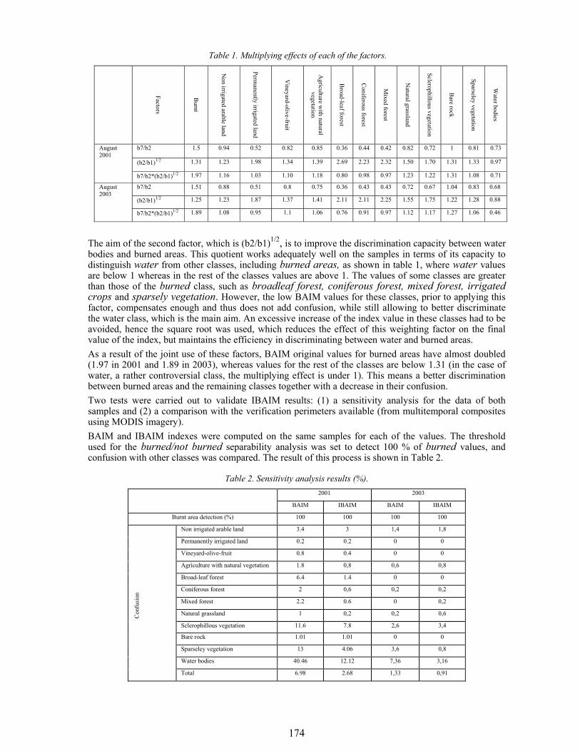
174

Table 1. Multiplying effects of each of the factors.

Factors

Burnt

Non irrigated arable land

Permanently irrigated land

Vineyard-olive-fruit

Agriculture w

ith natural vegetation

Broad-leaf forest

Coniferous forest

Mixed forest

Natural grassland

Sclerophillous vegetation

Bare rock

Sparseley vegetation

Water bodies

b7/b2 1.5 0.94 0.52 0.82 0.85 0.36 0.44 0.42 0.82 0.72 1 0.81 0.73

(b2/b1)1/2 1.31 1.23 1.98 1.34 1.39 2.69 2.23 2.32 1.50 1.70 1.31 1.33 0.97

August 2001

b7/b2*(b2/b1)1/2 1.97 1.16 1.03 1.10 1.18 0.80 0.98 0.97 1.23 1.22 1.31 1.08 0.71

b7/b2 1.51 0.88 0.51 0.8 0.75 0.36 0.43 0.43 0.72 0.67 1.04 0.83 0.68

(b2/b1)1/2 1.25 1.23 1.87 1.37 1.41 2.11 2.11 2.25 1.55 1.75 1.22 1.28 0.88

August 2003

b7/b2*(b2/b1)1/2 1.89 1.08 0.95 1.1 1.06 0.76 0.91 0.97 1.12 1.17 1.27 1.06 0.46

The aim of the second factor, which is (b2/b1)1/2, is to improve the discrimination capacity between water bodies and burned areas. This quotient works adequately well on the samples in terms of its capacity to distinguish water from other classes, including burned areas, as shown in table 1, where water values are below 1 whereas in the rest of the classes values are above 1. The values of some classes are greater than those of the burned class, such as broadleaf forest, coniferous forest, mixed forest, irrigated crops and sparsely vegetation. However, the low BAIM values for these classes, prior to applying this factor, compensates enough and thus does not add confusion, while still allowing to better discriminate the water class, which is the main aim. An excessive increase of the index value in these classes had to be avoided, hence the square root was used, which reduces the effect of this weighting factor on the final value of the index, but maintains the efficiency in discriminating between water and burned areas. As a result of the joint use of these factors, BAIM original values for burned areas have almost doubled (1.97 in 2001 and 1.89 in 2003), whereas values for the rest of the classes are below 1.31 (in the case of water, a rather controversial class, the multiplying effect is under 1). This means a better discrimination between burned areas and the remaining classes together with a decrease in their confusion. Two tests were carried out to validate IBAIM results: (1) a sensitivity analysis for the data of both samples and (2) a comparison with the verification perimeters available (from multitemporal composites using MODIS imagery). BAIM and IBAIM indexes were computed on the same samples for each of the values. The threshold used for the burned/not burned separability analysis was set to detect 100 % of burned values, and confusion with other classes was compared. The result of this process is shown in Table 2.

Table 2. Sensitivity analysis results (%). 2001 2003

BAIM IBAIM BAIM IBAIM

Burnt area detection (%) 100 100 100 100

Non irrigated arable land 3.4 3 1,4 1,8

Permanently irrigated land 0.2 0.2 0 0

Vineyard-olive-fruit 0.8 0.4 0 0

Agriculture with natural vegetation 1.8 0,8 0,6 0,8

Broad-leaf forest 6.4 1.4 0 0

Coniferous forest 2 0,6 0,2 0,2

Mixed forest 2.2 0.6 0 0,2

Natural grassland 1 0,2 0,2 0,6

Sclerophillous vegetation 11.6 7.8 2,6 3,4

Bare rock 1.01 1.01 0 0

Sparseley vegetation 13 4.06 3,6 0,8

Water bodies 40.46 12.12 7,36 3,16

Con

fusi

on

Total 6.98 2.68 1,33 0,91

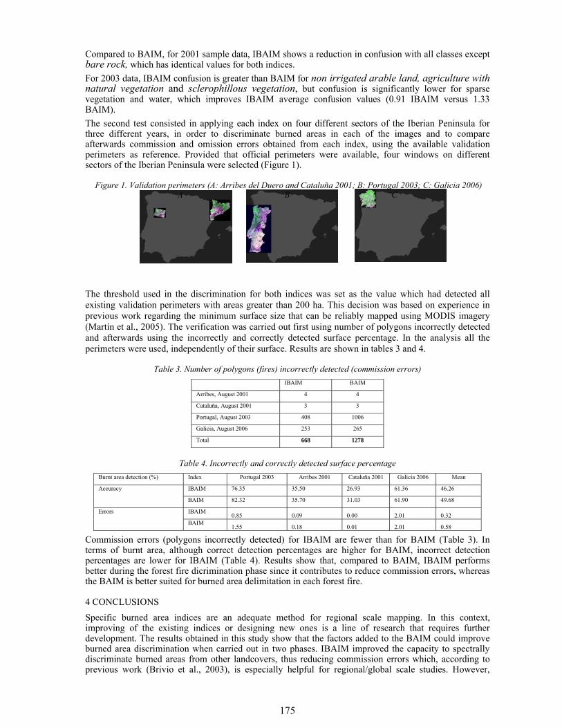
175

Compared to BAIM, for 2001 sample data, IBAIM shows a reduction in confusion with all classes except bare rock, which has identical values for both indices. For 2003 data, IBAIM confusion is greater than BAIM for non irrigated arable land, agriculture with natural vegetation and sclerophillous vegetation, but confusion is significantly lower for sparse vegetation and water, which improves IBAIM average confusion values (0.91 IBAIM versus 1.33 BAIM). The second test consisted in applying each index on four different sectors of the Iberian Peninsula for three different years, in order to discriminate burned areas in each of the images and to compare afterwards commission and omission errors obtained from each index, using the available validation perimeters as reference. Provided that official perimeters were available, four windows on different sectors of the Iberian Peninsula were selected (Figure 1).

Figure 1. Validation perimeters (A: Arribes del Duero and Cataluña 2001; B: Portugal 2003; C: Galicia 2006) A B C

The threshold used in the discrimination for both indices was set as the value which had detected all existing validation perimeters with areas greater than 200 ha. This decision was based on experience in previous work regarding the minimum surface size that can be reliably mapped using MODIS imagery (Martín et al., 2005). The verification was carried out first using number of polygons incorrectly detected and afterwards using the incorrectly and correctly detected surface percentage. In the analysis all the perimeters were used, independently of their surface. Results are shown in tables 3 and 4.

Table 3. Number of polygons (fires) incorrectly detected (commission errors) IBAIM BAIM

Arribes, August 2001 4 4

Cataluña, August 2001 3 3

Portugal, August 2003 408 1006

Galicia, August 2006 253 265

Total 668 1278

Table 4. Incorrectly and correctly detected surface percentage Burnt area detection (%) Index Portugal 2003 Arribes 2001 Cataluña 2001 Galicia 2006 Mean

IBAIM 76.35 35.50 26.93 61.36 46.26 Accuracy

BAIM 82.32 35.70 31.03 61.90 49.68

IBAIM 0.85 0.09 0.00 2.01 0.32

Errors

BAIM 1.55 0.18 0.01 2.01 0.58

Commission errors (polygons incorrectly detected) for IBAIM are fewer than for BAIM (Table 3). In terms of burnt area, although correct detection percentages are higher for BAIM, incorrect detection percentages are lower for IBAIM (Table 4). Results show that, compared to BAIM, IBAIM performs better during the forest fire dicrimination phase since it contributes to reduce commission errors, whereas the BAIM is better suited for burned area delimitation in each forest fire.

4 CONCLUSIONS Specific burned area indices are an adequate method for regional scale mapping. In this context, improving of the existing indices or designing new ones is a line of research that requires further development. The results obtained in this study show that the factors added to the BAIM could improve burned area discrimination when carried out in two phases. IBAIM improved the capacity to spectrally discriminate burned areas from other landcovers, thus reducing commission errors which, according to previous work (Brivio et al., 2003), is especially helpful for regional/global scale studies. However,

176

further analysis is required to asses the full capacity of the index proposed and its potential for discriminating burned area from other land covers in other geographic environments using sensors with spectral bands in the visible, NIR and SWIR, such as MODIS.

5 REFERENCES Barbosa, P. M., J. M. C. Pereira, et al. 1998. Compositing criteria for burnt area assessment using multitemporal

low resolution satellite data Remote Sensing of Environment 65: 38-49. Bastarrika, A. and E. Chuvieco 2006. Cartografía del area quemada mediante crecimiento de regiones: aplicación

en entornos mediterráneos con imágenes TM y ETM+. GeoFocus 6:182-204. Brivio, P. A., Maggi, E. Binahi, I. Gallo 2003. Mapping burned surfaces in Sub-Saharan Africa based on multi-

temporal neural classification. Int, J. Remote Sensing 24(20): 4003-4018. Chuvieco, E., G. Ventura, P. Martín, I. Gómez 2005. Assessment of multitemporal compositing techniques of

MODIS and AVHRR images for burned land mapping. Remote Sensing of Environment 94: 450-462. Kasischke, E. and N. H. French 1995. Locating and estimating the areal extent of wildfires in Alaskan boreal forest

using multiple-season AVHRR NDVI composite data. Remote Sensing of Environment 51: 263-275. Kushla, J. D. and W. J. Ripple 1998. Assessing wildfire effects with Landsat thematic mapper data. International

Journal of Remote Sensing 19(13): 2493-2507. Martín, M. P. 1998. Cartografía e inventario de incendios forestales en la Península Ibérica a partir de imágenes

NOAA-AVHRR. Departamento de Geografía. Alcalá de Henares, Universidad de Alcalá. Martín, M. P. and E. Chuvieco (1998). Cartografía de grandes incendios forestales en la Península Ibérica a partir

de imágenes NOAA-AVHRR. Serie Geográfica 7: 109-128. Martín, P., I. Gómez, E. Chuvieco 2005. Performance of a burned-area index (BAIM) for mapping Mediterranean

burned scars from MODIS data. Proceedings of the 5th International Workshop on Remote Sensing and GIS Applications to Forest Fire Management: Fire Effects Assessment, Zaragoza, Universidad de Zaragoza

Trigg, S. and S. Flasse 2001. An evaluation of different bi-spectral spaces for discriminating burned shrub-savannah. International Journal of Remote Sensing 22(13): 2641–2647.

Verstraete, M. M. and B. Pinty 1996. Designing optimal spectral indexes for remote sensing applications. IEEE Transactions on Geoscience and Remote Sensing 34(5): 1254-1265.

177

1 INTRODUCTION Several studies have shown that biomass burning plays an important role in global warming (Levine, 1991), because of the trace gases and aerosols that are released during a fire event (Houghton, 1991). Nevertheless, the uncertainties about the estimate of emission volume are large, since they depend on several parameters that don’t have the necessary accuracy to provide reliable results (Dignon and Penner, 1991). One of these uncertainties is the extent of fire-affected areas over the world, which is one of the parameters used to calculate the amount of biomass burned and the total gas emissions (Levine, 1991). Therefore, accurate inventory of the location and extent of burned areas is required, not only to assess the damage caused on ecosystem and human resources by fires, but also to quantify the emissions effects on atmospheric chemistry (Arino et al., 2001); (Levine et al., 1991), and to enable researches, managers, and policy makers to monitor the impacts in ecosystems and also to follow ecosystem dynamics after a fire event. The spatial resolution of the sensor determine the minimum area burned that can be discriminate and establishes the optimal omission and commission errors (Boschetti et al., 2004). In this study it is proposed the use of ENVISAT-MERIS (Medium Resolution Imaging Spectrometer) images in order to improve the spatial resolution utilized at regional scale to map fire-affected areas. Application of MERIS images to forest fires is not frequent, in fact, from the bibliographic search, only one study was found, in which MERIS images were used to detect smoke plumes and map fire scars in combination with other Envisat sensors (Huang and Siegert, 2004). They combined Reduced Resolution MERIS imagery with 1200 meters pixel size, AATSR (Advanced Along Track Scanning Radiometer) hotspots, and ASAR (Advanced Synthetic aperture Radar) images which avoid clouds cover. Authors concluded that MERIS images were useful to map large fire-affected areas and to identify the haze produced by fires, however their low-spatial resolution involve an underestimate of the burned area, thus they expect that the use of Full Resolution MERIS data will enhance the fire scar mapping. The main objective of this study is to explore the potential of MERIS imagery to map fire-affected areas at a regional scale by using spectral angle mapping techniques. Since there are not previous studies that accomplished the burned land mapping using just MERIS images, it is still to be explored their usefulness to this application. We assessed the performance of SAM to obtain burned area maps testing different reference spectrums obtained from MERIS image, and from field spectroradiometer measures.

Mapping burned area by using Spectral angle Mapper in MERIS images

P. Oliva Department of Geography, University of Alcalá, Madrid, 28801, Spain, [email protected]

P. Martín Institute of Economics and Geography, Spanish Council for Scientific Research, Madrid, Spain, [email protected] Keywords: burned area, MERIS, spectral indices, Spectral Angle Mapper, Pareto Boundary.

ABSTRACT: A conjunction of meteorological and human factors caused that thousand hectares were burned in the northwestern part of the Iberian Peninsula on summer 2006. We have used MERIS images to map fire-affected areas, since this sensor provides a good balance between spectral, temporal and spatial resolution. MERIS sensor acquires images in 15 narrow spectral bands (between 409 and 900 nm) with a temporal resolution of 3 days, and a spatial resolution of 300 m. Spectral Angle Mapping (SAM) technique has been applied to map fire-affected areas. SAM is a hyperspectral classification method that measures the similarity between a known spectrum and a reference spectrum. The reference spectrum may be obtained from the image or from laboratory or field spectroradiometric measurements. Both methods were tested in order to assess the potential of this technique. Validation was accomplished by comparing the results with fire perimeters visually digitized from AWIFS image (60m pixel size). We use the Pareto Boundary method to evaluate the errors taking into account the spatial resolution of the sensor. This allows us to discriminate the errors caused by the spatial resolution and the errors caused by the weakness of the technique. Finally, the distance between the errors and the Pareto Boundary function was calculated in order to be able to decide the best result in an objective way.

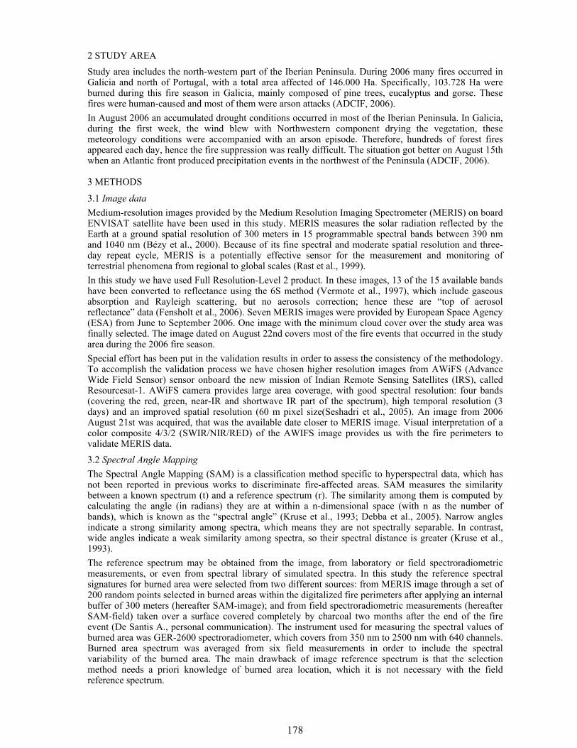
178

2 STUDY AREA Study area includes the north-western part of the Iberian Peninsula. During 2006 many fires occurred in Galicia and north of Portugal, with a total area affected of 146.000 Ha. Specifically, 103.728 Ha were burned during this fire season in Galicia, mainly composed of pine trees, eucalyptus and gorse. These fires were human-caused and most of them were arson attacks (ADCIF, 2006). In August 2006 an accumulated drought conditions occurred in most of the Iberian Peninsula. In Galicia, during the first week, the wind blew with Northwestern component drying the vegetation, these meteorology conditions were accompanied with an arson episode. Therefore, hundreds of forest fires appeared each day, hence the fire suppression was really difficult. The situation got better on August 15th when an Atlantic front produced precipitation events in the northwest of the Peninsula (ADCIF, 2006).

3 METHODS

3.1 Image data Medium-resolution images provided by the Medium Resolution Imaging Spectrometer (MERIS) on board ENVISAT satellite have been used in this study. MERIS measures the solar radiation reflected by the Earth at a ground spatial resolution of 300 meters in 15 programmable spectral bands between 390 nm and 1040 nm (Bézy et al., 2000). Because of its fine spectral and moderate spatial resolution and three-day repeat cycle, MERIS is a potentially effective sensor for the measurement and monitoring of terrestrial phenomena from regional to global scales (Rast et al., 1999). In this study we have used Full Resolution-Level 2 product. In these images, 13 of the 15 available bands have been converted to reflectance using the 6S method (Vermote et al., 1997), which include gaseous absorption and Rayleigh scattering, but no aerosols correction; hence these are “top of aerosol reflectance” data (Fensholt et al., 2006). Seven MERIS images were provided by European Space Agency (ESA) from June to September 2006. One image with the minimum cloud cover over the study area was finally selected. The image dated on August 22nd covers most of the fire events that occurred in the study area during the 2006 fire season. Special effort has been put in the validation results in order to assess the consistency of the methodology. To accomplish the validation process we have chosen higher resolution images from AWiFS (Advance Wide Field Sensor) sensor onboard the new mission of Indian Remote Sensing Satellites (IRS), called Resourcesat-1. AWiFS camera provides large area coverage, with good spectral resolution: four bands (covering the red, green, near-IR and shortwave IR part of the spectrum), high temporal resolution (3 days) and an improved spatial resolution (60 m pixel size(Seshadri et al., 2005). An image from 2006 August 21st was acquired, that was the available date closer to MERIS image. Visual interpretation of a color composite 4/3/2 (SWIR/NIR/RED) of the AWIFS image provides us with the fire perimeters to validate MERIS data. 3.2 Spectral Angle Mapping The Spectral Angle Mapping (SAM) is a classification method specific to hyperspectral data, which has not been reported in previous works to discriminate fire-affected areas. SAM measures the similarity between a known spectrum (t) and a reference spectrum (r). The similarity among them is computed by calculating the angle (in radians) they are at within a n-dimensional space (with n as the number of bands), which is known as the “spectral angle” (Kruse et al., 1993; Debba et al., 2005). Narrow angles indicate a strong similarity among spectra, which means they are not spectrally separable. In contrast, wide angles indicate a weak similarity among spectra, so their spectral distance is greater (Kruse et al., 1993). The reference spectrum may be obtained from the image, from laboratory or field spectroradiometric measurements, or even from spectral library of simulated spectra. In this study the reference spectral signatures for burned area were selected from two different sources: from MERIS image through a set of 200 random points selected in burned areas within the digitalized fire perimeters after applying an internal buffer of 300 meters (hereafter SAM-image); and from field spectroradiometric measurements (hereafter SAM-field) taken over a surface covered completely by charcoal two months after the end of the fire event (De Santis A., personal communication). The instrument used for measuring the spectral values of burned area was GER-2600 spectroradiometer, which covers from 350 nm to 2500 nm with 640 channels. Burned area spectrum was averaged from six field measurements in order to include the spectral variability of the burned area. The main drawback of image reference spectrum is that the selection method needs a priori knowledge of burned area location, which it is not necessary with the field reference spectrum.

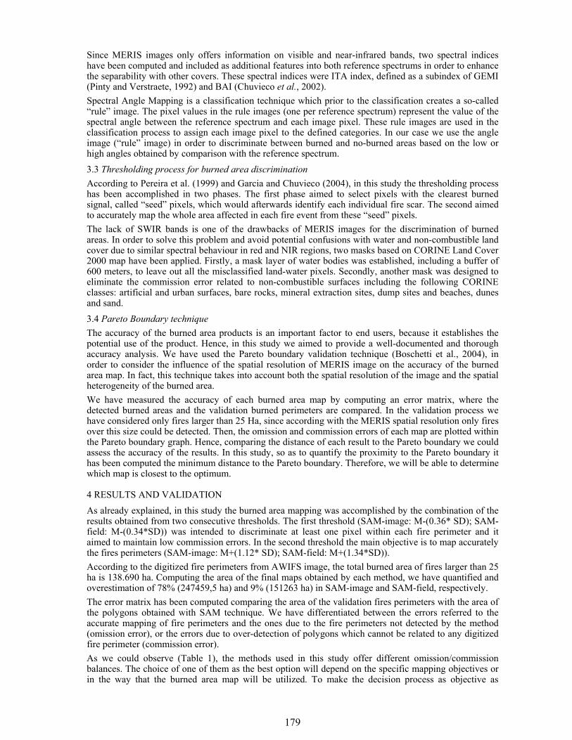
179

Since MERIS images only offers information on visible and near-infrared bands, two spectral indices have been computed and included as additional features into both reference spectrums in order to enhance the separability with other covers. These spectral indices were ITA index, defined as a subindex of GEMI (Pinty and Verstraete, 1992) and BAI (Chuvieco et al., 2002). Spectral Angle Mapping is a classification technique which prior to the classification creates a so-called “rule” image. The pixel values in the rule images (one per reference spectrum) represent the value of the spectral angle between the reference spectrum and each image pixel. These rule images are used in the classification process to assign each image pixel to the defined categories. In our case we use the angle image (“rule” image) in order to discriminate between burned and no-burned areas based on the low or high angles obtained by comparison with the reference spectrum. 3.3 Thresholding process for burned area discrimination According to Pereira et al. (1999) and Garcia and Chuvieco (2004), in this study the thresholding process has been accomplished in two phases. The first phase aimed to select pixels with the clearest burned signal, called “seed” pixels, which would afterwards identify each individual fire scar. The second aimed to accurately map the whole area affected in each fire event from these “seed” pixels. The lack of SWIR bands is one of the drawbacks of MERIS images for the discrimination of burned areas. In order to solve this problem and avoid potential confusions with water and non-combustible land cover due to similar spectral behaviour in red and NIR regions, two masks based on CORINE Land Cover 2000 map have been applied. Firstly, a mask layer of water bodies was established, including a buffer of 600 meters, to leave out all the misclassified land-water pixels. Secondly, another mask was designed to eliminate the commission error related to non-combustible surfaces including the following CORINE classes: artificial and urban surfaces, bare rocks, mineral extraction sites, dump sites and beaches, dunes and sand. 3.4 Pareto Boundary technique The accuracy of the burned area products is an important factor to end users, because it establishes the potential use of the product. Hence, in this study we aimed to provide a well-documented and thorough accuracy analysis. We have used the Pareto boundary validation technique (Boschetti et al., 2004), in order to consider the influence of the spatial resolution of MERIS image on the accuracy of the burned area map. In fact, this technique takes into account both the spatial resolution of the image and the spatial heterogeneity of the burned area. We have measured the accuracy of each burned area map by computing an error matrix, where the detected burned areas and the validation burned perimeters are compared. In the validation process we have considered only fires larger than 25 Ha, since according with the MERIS spatial resolution only fires over this size could be detected. Then, the omission and commission errors of each map are plotted within the Pareto boundary graph. Hence, comparing the distance of each result to the Pareto boundary we could assess the accuracy of the results. In this study, so as to quantify the proximity to the Pareto boundary it has been computed the minimum distance to the Pareto boundary. Therefore, we will be able to determine which map is closest to the optimum.

4 RESULTS AND VALIDATION As already explained, in this study the burned area mapping was accomplished by the combination of the results obtained from two consecutive thresholds. The first threshold (SAM-image: M-(0.36* SD); SAM-field: M-(0.34*SD)) was intended to discriminate at least one pixel within each fire perimeter and it aimed to maintain low commission errors. In the second threshold the main objective is to map accurately the fires perimeters (SAM-image: M+(1.12* SD); SAM-field: M+(1.34*SD)). According to the digitized fire perimeters from AWIFS image, the total burned area of fires larger than 25 ha is 138.690 ha. Computing the area of the final maps obtained by each method, we have quantified and overestimation of 78% (247459,5 ha) and 9% (151263 ha) in SAM-image and SAM-field, respectively. The error matrix has been computed comparing the area of the validation fires perimeters with the area of the polygons obtained with SAM technique. We have differentiated between the errors referred to the accurate mapping of fire perimeters and the ones due to the fire perimeters not detected by the method (omission error), or the errors due to over-detection of polygons which cannot be related to any digitized fire perimeter (commission error). As we could observe (Table 1), the methods used in this study offer different omission/commission balances. The choice of one of them as the best option will depend on the specific mapping objectives or in the way that the burned area map will be utilized. To make the decision process as objective as

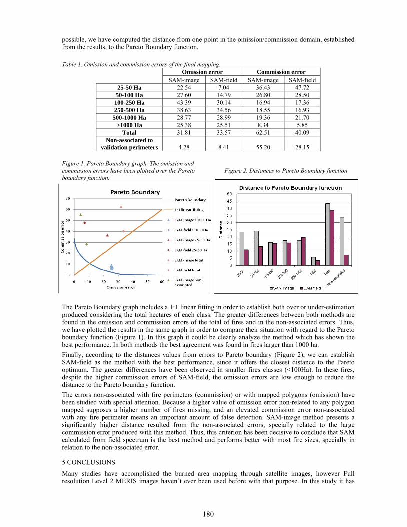
180

possible, we have computed the distance from one point in the omission/commission domain, established from the results, to the Pareto Boundary function. Table 1. Omission and commission errors of the final mapping.

Omission error Commission error SAM-image SAM-field SAM-image SAM-field

25-50 Ha 22.54 7.04 36.43 47.72 50-100 Ha 27.60 14.79 26.80 28.50 100-250 Ha 43.39 30.14 16.94 17.36 250-500 Ha 38.63 34.56 18.55 16.93

500-1000 Ha 28.77 28.99 19.36 21.70 >1000 Ha 25.38 25.51 8.34 5.85

Total 31.81 33.57 62.51 40.09 Non-associated to

validation perimeters 4.28 8.41 55.20 28.15 Figure 1. Pareto Boundary graph. The omission and commission errors have been plotted over the Pareto Figure 2. Distances to Pareto Boundary function boundary function.

The Pareto Boundary graph includes a 1:1 linear fitting in order to establish both over or under-estimation produced considering the total hectares of each class. The greater differences between both methods are found in the omission and commission errors of the total of fires and in the non-associated errors. Thus, we have plotted the results in the same graph in order to compare their situation with regard to the Pareto boundary function (Figure 1). In this graph it could be clearly analyze the method which has shown the best performance. In both methods the best agreement was found in fires larger than 1000 ha. Finally, according to the distances values from errors to Pareto boundary (Figure 2), we can establish SAM-field as the method with the best performance, since it offers the closest distance to the Pareto optimum. The greater differences have been observed in smaller fires classes (<100Ha). In these fires, despite the higher commission errors of SAM-field, the omission errors are low enough to reduce the distance to the Pareto boundary function. The errors non-associated with fire perimeters (commission) or with mapped polygons (omission) have been studied with special attention. Because a higher value of omission error non-related to any polygon mapped supposes a higher number of fires missing; and an elevated commission error non-associated with any fire perimeter means an important amount of false detection. SAM-image method presents a significantly higher distance resulted from the non-associated errors, specially related to the large commission error produced with this method. Thus, this criterion has been decisive to conclude that SAM calculated from field spectrum is the best method and performs better with most fire sizes, specially in relation to the non-associated error.

5 CONCLUSIONS Many studies have accomplished the burned area mapping through satellite images, however Full resolution Level 2 MERIS images haven’t ever been used before with that purpose. In this study it has

181

been revealed the potential of those images to map fire-affected areas. Besides, we have applied spectral angle mapping technique to map burned areas, which has not been used before in this area. We have explored two ways of obtaining the reference spectrum to compute SAM: from the image (“SAM-image”) and from a field spectrum measurement (“SAM-field”). The results obtained in this study have shown that, in general terms, SAM-field method performs better than SAM-image. The key factor that has determined what the best method is has been the relation of the errors non-associated with fire perimeters (commission error) or with mapped polygons (omission error). Since, the distance to the Pareto optimum function in SAM-image method according to the non-associated errors is far higher than the distance in SAM-field, because of the elevated commission error values that move the point away from the Pareto function. Therefore we have demonstrated the possibility of using field spectra as reference to compute spectral angle mapping technique. That facilitates SAM computation since it is not necessary to have previous knowledge of fire locations to obtain the reference spectrum. The use of field spectroradiometric measurements to apply SAM technique also allows to take into account different burned spectra, which means that this method could be apply over larger areas including different ecosystems and burned conditions (in terms of combustion efficiency). Since, it have been demonstrated that the burned spectral signature varies according to several factors (Trigg and Flasse, 2000; Stroppiana et al., 2002; Roy and Landmann, 2005b); using a spectral library with different burned signatures would eventually allow to map the variability of the burned area. Another possibility for SAM computation is using a spectral library of simulated spectrum as reference spectrum. This will allow to explore a wide range of different burning conditions related to the combustion efficiency or the type of vegetation affected by the fire, when field spectra are not available.

6 ACKNOWLEDGEMENTS

The Spanish Ministry of Science and Technology supports Patricia Oliva within the FPU Programme framework. This study has been funding through the Preview European Project (www.preview-risk.com).

7 REFERENCES Adcif 2006. Incendios Forestales en España. Año 2006: Avance informativo, Direccion General para la

Biodiversidad, Ministerio de Medio Ambiente. 9. Arino, O., Piccolini, I., Kasischke, E., et al. 2001. Methods of mapping burned surfaces in vegetation fires. Global

and Regional Vegetation Fire Monitoring from Space: Planning a coordinated international effort. F. J. Ahern, J. G. Goldammer and C. O. Justice. The Haghe, The Netherlands, SPB Academic Publishing: 227-255.

Bézy, J. L., Delwart, S. and Rast, M. 2000. MERIS - A new generation of Ocean-Color sensor onboard Envisat. ESA Bulletin 103: 48-56.

Boschetti, L., Flasse, S. P. and Brivio, P. A. 2004. Analysis of the conflict between omission and commission in low spatial resolution dichotomic thematic products: The Pareto Boundary. Remote Sensing of Environment 91(280-292).

Chuvieco, E., Martín, M. P. and Palacios, A. 2002. Assessment of different spectral indices in the red-near-infrared spectral domain for burned land discrimination. International Journal of Remote Sensing 23(23): 5103-5110.

Debba, P., Van Ruitenbeek, F. J. A., Van Der Meer, F. D., Carranza, J. M. and Stein, A. 2005. Optimal field sampling for targeting minerals using hyperspectral data. Remote Sensing of Environment 99: 373-386.

Dignon, J. and Penner, J. E. 1991. Biomass burning: A source of nitrogen oxides in the atmosphere. Global biomass burning: atmospheric, climatic, and biospheric implications. J. S. Levine, Massachusetts Institute of Technology.

Fensholt, R., Sandholt, I. and Stisen, S. 2006. Evaluating MODIS, MERIS and VEGETATION vegetation indices using In situ measurements in a semiarid environment. IEEE Transactions on Geoscience and Remote Sensing 44(7): 1774-1786.

Garcia, M. and Chuvieco, E. 2004. Assessment of the potential of SAC-C/MMRS imagery for mapping burned areas in Spain. Remote Sensing of Environment 92: 414–423.

Houghton, R. A. 1991. Biomass burning from the perspective of the Global Carbon cycle. Global biomass burning: atmospheric, climatic, and biospheric implications. J. S. Levine, Massachusetts Institute of Technology: 321-325.

Huang, S. and Siegert, F. 2004. ENVISAT multisensor data for fire monitoring and imapact assessment. International Journal of Remote Sensing 25(20): 4411-4416.

Kruse, F. A., Lefkoff, A. B., Boardman, J. W., Heidebrecht, K. B., Shapiro, A. T., Barloon, P. J. and GOETZ, A. F. H. 1993. The Spectral Image Processing System (SIPS) - Interactive Visualization and Analysis of Imaging Spectrometer Data. Remote Sensing of Environment 44: 145-163.

Levine, J. S. 1991. Global Biomass Burning: atmospheric, Climatic, and Biospheric implications, Massachusetts Institute of Technology

182

Levine, J. S., Cofer III, W. R., Winstead, E. L., et al. 1991. Biomass burning: combustion emissions, satellite imagery, and biogenic emission. Global biomass burning: atmospheric, climatic, and biospheric implications. J. S. Levine, Massachusetts Institute of Technology: 264-271.

Pereira, J. M. C. 1999. A Comparative Evaluation of NOAA/AVHRR Vegetation Indexes for Burned Surface Detection and Mapping. IEEE Transactions on Geoscience and Remote Sensing 37(1): 217-226.

Pinty, B. and Verstraete, M. M. 1992. GEMI:a non-linear index to monitor global vegetation from satellites. Vegetatio 101: 15-20.

Rast, M., Bézy, J. L. and BruzzI, S. 1999. The ESA Medium Resolution Imaging Spectrometer MERIS - a review of the instrument and its mission. International Journal of Remote Sensing 20(9): 1681-1702.

Roy, D. P. and Landmann, T. 2005b. Characterizing the surface heterogeneity of fire effects using multi-temporal reflective wavelength data. International Journal of Remote Sensing 26(19): 4197-4218.

SeshadrI, K. S. V., Rao, M., Jayaraman, V., Thyagarajan, K. and Murthi, K. R. S. 2005. Resourcesat-1: A global multi-observation mission for resources monitoring. Acta Astronautica 57: 534-539.

Stroppiana, D., Pinnick, S., Pereira, J. M. C. and Grégoire, J. M. 2002. Radiometric analysis of SPOT-VEGETATION images for burnt area detection in Nothern Australia. Remote Sensing of Environment 82: 21-37.

Trigg, S. and Flasse, S. 2000. Characterizing the spectral-temporal response of burned savannah using in situ spectroradiometry and infrared thermometry. International Journal of Remote Sensing 21(16): 3161-3168.

Vermote, E. F., Tanré, D., Deuzé, J. L., Herman, M. and Morcrette, J. J. 1997. Second Simulation of the Satellite Signal in the Solar Spectrum, 6S: An Overview. IEEE Transactions on Geoscience and Remote Sensing 35(3): 675-686.

183

Spatial analysis of active fire counts in Southeast Asia

Mastura Mahmud Universiti Kebangsaan Malaysia, 43600, Bangi, Selangor, Malaysia, email: [email protected] Keywords : active fire counts, Southeast Asia, spatial analysis, air pollution ABSTRACT: An emergency state was declared on 11 August 2005 at two districts in Selangor, Peninsular Malaysia when the air pollutant index reached hazardous levels that was harmful to the health of the public. The main contributor of the haze was attributed to the intense vegetation fires in Sumatra, Indonesia. Spatial analysis on the active fires detected by the MODIS and NOAA satellites revealed that during the first 10 days of August 2005, fires were concentrated in the provinces of Riau and Sumatera Utara. Centrographic statistics such as the mean centres and centres of minimum distance were often similar, particularly on days when burning was intense and concentrated over a relatively small area. Average standard distance values of approximately 100 km displayed by the NOAA, Terra, and Aqua satellites revealed that clustering of burning were sustained from mid-morning to late evening. The intense burning activities during this short period aggravated the transboundary haze conditions, causing the air quality to deteriorate in the neighbouring western coast of Peninsular Malaysia, particularly located less than 200 km away from Riau. Significant clustering exists spatially and temporally for all the fires detected by the three satellites. Approximately 80% of the incidences of fires during the four weeks in August were both close in distance and close in time on a weekly and monthly basis.

1 INTRODUCTION Since the past ten years, transboundary haze from biomass burning instigated by Indonesia has been one of the problematic issues in Southeast Asia. This paper investigates the spatial patterns of the active fire counts to understand the characteristics of the burning patterns in Sumatera that caused the downstream impacts of very poor air quality in Peninsular Malaysia. Hotspot information was derived from three satellites; the National Oceanic Atmospheric Administration (NOAA), Aqua and Terra Moderate Resolution Imaging Spectroradiometer (MODIS), with spatial resolutions of approximately 1 km. The study is concentrated in Sumatera as the smoke is advected by the prevailing wind regime during the southwest monsoon towards Peninsular Malaysia, which is only 200 km from the coast of Riau in Sumatera.

2 METHODOLOGY: SPATIAL STATISTICS The general spatial distribution of the hotspots in Sumatera such as the centre of distribution of burning and spread of fires were investigated. Clustering was shown by statistics such as the nearest neighbour statistics, Moran’s I and Geary C (Geary, 1954), which are autocorrelation indicators. The Knox and Mantel indices can provide a simple comparison of relationships between the occurrences of hotspots in terms of distances and times (Mantel, 1967; Mantel and Bailar, 1970).

3 RESULTS

3.1 Centrographic Analysis More than 3500 active fire counts were detected by the MODIS satellite during August 2005 in Sumatera. The daily mean central (MC) locations of the hotspots from the three satellites were slightly different from one another (Figure 1). Terra and Aqua detect hotspots at approximately 10 am and 2 pm local time, respectively, while the NOAA overpass time is at 5 pm local time. The MC locations were influenced by the total number of hotspots detected and their extreme locations. In August, 67% of the burning activities were centred in the province of Riau. Other MCs of burning were also located in Sumatera Selatan (18%), Sumatera Utara (11%), Jambi (7%), and Lampung (3%).

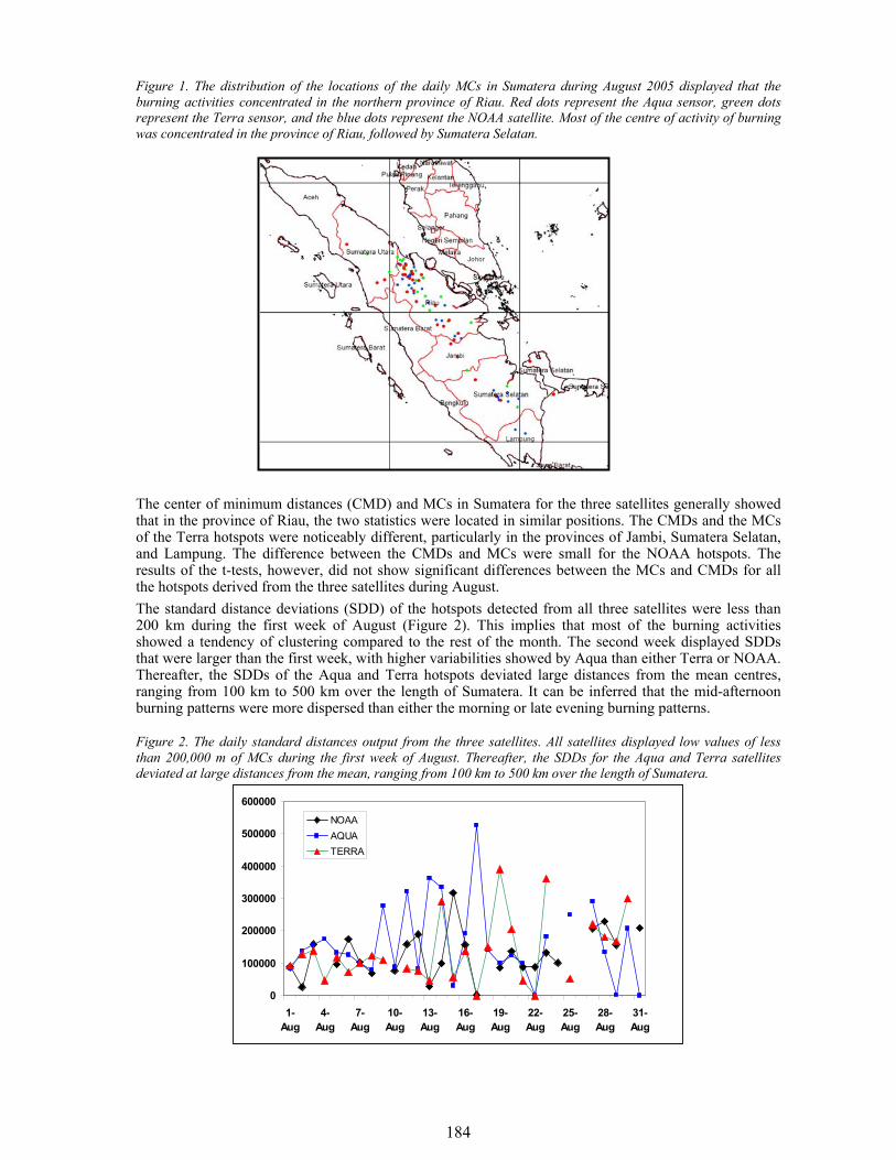
184

Figure 1. The distribution of the locations of the daily MCs in Sumatera during August 2005 displayed that the burning activities concentrated in the northern province of Riau. Red dots represent the Aqua sensor, green dots represent the Terra sensor, and the blue dots represent the NOAA satellite. Most of the centre of activity of burning was concentrated in the province of Riau, followed by Sumatera Selatan. The center of minimum distances (CMD) and MCs in Sumatera for the three satellites generally showed that in the province of Riau, the two statistics were located in similar positions. The CMDs and the MCs of the Terra hotspots were noticeably different, particularly in the provinces of Jambi, Sumatera Selatan, and Lampung. The difference between the CMDs and MCs were small for the NOAA hotspots. The results of the t-tests, however, did not show significant differences between the MCs and CMDs for all the hotspots derived from the three satellites during August. The standard distance deviations (SDD) of the hotspots detected from all three satellites were less than 200 km during the first week of August (Figure 2). This implies that most of the burning activities showed a tendency of clustering compared to the rest of the month. The second week displayed SDDs that were larger than the first week, with higher variabilities showed by Aqua than either Terra or NOAA. Thereafter, the SDDs of the Aqua and Terra hotspots deviated large distances from the mean centres, ranging from 100 km to 500 km over the length of Sumatera. It can be inferred that the mid-afternoon burning patterns were more dispersed than either the morning or late evening burning patterns. Figure 2. The daily standard distances output from the three satellites. All satellites displayed low values of less than 200,000 m of MCs during the first week of August. Thereafter, the SDDs for the Aqua and Terra satellites deviated at large distances from the mean, ranging from 100 km to 500 km over the length of Sumatera.

0

100000

200000

300000

400000

500000

600000

1-Aug

4-Aug

7-Aug

10-Aug

13-Aug

16-Aug

19-Aug

22-Aug

25-Aug

28-Aug

31-Aug

NOAAAQUATERRA

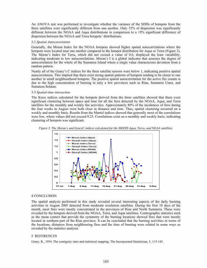
185

An ANOVA test was performed to investigate whether the variance of the SDDs of hotspots from the three satellites were significantly different from one another. Only 32% of dispersion was significantly different between the NOAA and Aqua distributions in comparison to a 19% significant difference of dispersion between the NOAA and Terra hotspots’ distributions.

3.2 Spatial Autocorrelation Generally, the Moran Index for the NOAA hotspots showed higher spatial autocorrelations where the hotspots were located near one another compared to the hotspot distribution for Aqua or Terra (Figure 3). The Moran’s Index for Terra, which did not exceed a value of 0.6, displayed the least variability, indicating moderate to low autocorrelations. Moran’s I is a global indicator that assesses the degree of autocorrelation for the whole of the Sumatera Island where a single value characterizes deviation from a random pattern. Nearly all of the Geary’s C indices for the three satellite sensors were below 1, indicating positive spatial autocorrelation. This implied that there exist strong spatial patterns of hotspots tending to be closer to one another in small neighbourhood hotspots. The positive spatial autocorrelation for the active fire counts is due to the high concentration of burning in only a few provinces such as Riau, Sumatera Utara, and Sumatera Selatan.

3.3 Spatial-time interaction The Knox indices calculated for the hotspots derived from the three satellites showed that there exist significant clustering between space and time for all the fires detected by the NOAA, Aqua, and Terra satellites for the monthly and weekly fire activities. Approximately 80% of the incidences of fires during the four weeks in August were both close in distance and time. Thus, spatial clustering occurred on a weekly and monthly basis. Results from the Mantel indices showed that generally most of the correlations were low, where values did not exceed 0.25. Correlations exist on a monthly and weekly basis, indicating clustering of hotspots was significant.

Figure 3. The Moran’s and GearyC indices calculated for the MODIS Aqua, Terra, and NOAA satellites.

0

0.2

0.4

0.6

0.8

1

1.2

1.4

1.6

27-Jul 1-Aug 6-Aug 11-Aug 16-Aug 21-Aug 26-Aug 31-Aug 5-Sep

Moran Index (Aqua)GearyC Index (Aqua)Moran Index (Terra)GearyC Index (Terra)Moran Index (NOAA)GearyC Index (NOAA)

4 CONCLUSION The spatial analysis performed in this study revealed several interesting aspects of the daily burning activities in August 2005 detected from moderate resolution satellites. During the first 10 days of the month, most fires were mostly concentrated in the provinces of Riau and North Sumatera. These were revealed by the hotspots derived from the NOAA, Terra, and Aqua satellites. Centrographic statistics such as the mean centers that provide the symmetry of the burning locations showed fires that were mostly located in northern part of the Riau province. It can be concluded that the burning activities in terms of the locations, distances from neighbouring fires and the time of burning were related in some ways as revealed by the statistics analysis.

5 REFERENCES Geary, R., 1954. The contiguity ratio and statistical mapping. The Incorporated Statistician, 5, 115-145.

186

Mantel, N. and J. C. Bailar, 1970. A class of permutational and multinomial test arising in epidemiological research, Biometrics, 26, 687-700.

Mantel, N., 1967. The detection of disease clustering and a generalized regression approach. Cancer Research, 27, 209-220.

187

1 INTRODUCTION Today, the development of a standard classification procedure to be used in operational basis for burned area mapping seems feasible, since higher spatial and spectral resolution satellite data are available. The next generation in remote sensing imaging capabilities includes the ASTER instrument which covers a wide spectral region with 14 bands from the visible to the thermal infrared with high spatial, spectral and radiometric resolution. Even ASTER data has been used in a wide array of global change-related application areas (FalkowskiI et al. 2005; Muukkonen and Heiskanen 2005; Rowan et al. 2005; San and Süzen 2005), the use of ASTER imagery has as yet had rather limited applications in the mapping of burned areas. Moreover, given the fact that LANDSAT imagery the traditional used for burned area mapping is no longer available, there is an accentuated need for the use of ASTER data to be investigated in this area of application. A further motive for this investigation is the similar technical characteristics of the two aforementioned satellite data. Furthermore, new and advanced image classification techniques, such as object-oriented image analysis, which can contribute to powerful automatic and semi-automatic analysis for most remote sensing applications (Benz et al. 2004), have recently been introduced and have showed promising results in the field of burned area mapping (Gitas et al. 2004; Mitri and Gitas 2004). The basic processing units of object-oriented image analysis are segments, so-called image objects, and not single pixels, while the advantages of this approach are meaningful statistic and texture calculation, an increased feature space using shape and topological features, and close relation between real-world and image objects. This relation improves the value of the final classification and cannot be fulfilled by common, pixel-based approaches (Benz et al. 2004). The aim of this work was to investigate whether a transferable object-based classification model for burned area mapping using ASTER imagery can be developed. The specific objectives were:

• to investigate the development of an object-based classification for mapping a burned area in Portugal using an ASTER image;

• to test the transferability of the model developed when mapping another burned area on the same ASTER image; and

• to further test the transferability of the model when mapping a burned area in Spain using a different ASTER image.

2 STUDY AREA AND DATASETS

The study area is located in Central Portugal, between the districts of Santarem and Castelo Branco,

The development of a transferable object-based model for burned area mapping using ASTER imagery

A. I. Polychronaki*, I. Z. Gitas and A.M. Karteris Laboratory of Forest Management and Remote Sensing, Aristotle University of Thessaloniki, P.O. Box 248, University Campus, Greece. E-mail*: [email protected]

Keywords: ASTER imagery, burned area mapping, object-based image analysis

ABSTRACT: Nowadays, the availability of enhanced satellite data, such as ASTER imagery, in combination with the introduction of new and advanced image analysis techniques, such as object-based approach, render the development of an automated methodology for burned area mapping possible. In this context, this work aimed at investigating whether a transferable object-based classification model for burned area mapping using ASTER imagery can be developed. More specifically, the initial step of the investigation involved the development of a classification model for accurately mapping burned areas in central Portugal using an ASTER image, and subsequently, the examination of the model to assess its transferability when mapping different burned areas. In particular, the model was applied to map fire affected areas located on the same ASTER image frame used when developing the model, and burned areas located on a different ASTER image that showed fire burns in central Spain. The classification results showed that the object-based classification model developed was able to map burned areas in Portugal with high accuracy (98.88%). Moreover, an examination of the transferability of the model when mapping different fire affected areas (98.5% overall accuracy when using the same ASTER image frame and 97.75% overall accuracy when using a different ASTER image) indicated that the model could effectively be used as an operational tool for identifying and mapping burned areas.

188

which are separated by the Zézere River, a tributary of the Tagus River. The study area is mainly covered by woodland and agricultural land. The woodland mainly consists of Pinus pinaster atlantica, Pinus pinea, Quercus suber and Quercus fraginea. The agricultural areas in the southern parts comprise vineyards, olive groves and fruit trees. A second study area, the Special Protected Area (SPA) num. 56 Encinares de los rios Alberche y Cofio, is located 40 km south west of Madrid (Central Spain) and was also used in this work. Grassland, shrubs, and various tree species (such as Pinus pinea, Pinus pinaster, Quercus ilex and Castanea sativa) dominate the ‘natural’ vegetation in this area (Romero-Calcerrada and Perry 2002). An ASTER L1A data product showing burns that occurred during the summer of 2003 in the first study area and an ASTER L1B image data showing fire burns from a forest fire that occurred in the second study area in August 2003 were obtained for this study. In addition, the maps of the official fire perimeters were provided by the Portuguese Forest Service and the Spanish Forest Service in order to evaluate the classification results.

3 METHODOLOGY The strategy in the development of the model for burned area mapping was based on a subset of the ASTER image (the thermal bands were excluded) showing fire burns in Portugal. Moreover, the Normalized Difference Vegetation Index (NDVI) was generated and utilized as an additional input in the methodology. Three levels of classifications were finally created for the development of the model (the software Definiens Professional 5 was used). Several parameters, such as the scale, the layer weights and the heterogeneity criterion, had to be set for the segmentation, while for the classification of the image objects, the appropriate object features had to be found in order to best separate the burned and unburned areas. The parameters used are described in the paragraphs that follow: Level 2: The scale parameter for the segmentation algorithm used at this level was 10, while weight was given only to layer three and the NDVI layer. For the heterogeneity criterion, full importance was given to colour. In order to achieve the best separation in the classification of the burned area from the other landcover types, an arithmetic feature was created. Arithmetic features are composed of existing features, variables and constants, which are combined via arithmetic operations. In this case, features ‘mean of layer 3’ and ‘mean of NDVI’ were arithmetically added producing a new feature, namely ‘mean&ndvi’. In addition to the new feature, features ‘mean of layer 3’, ‘mean of layer 1’ and ‘ratio of layer 1’ were evaluated to be the most appropriate for the discrimination of the burned areas. Classification was implemented for all image objects using the aforementioned features, and two classes were finally created at this level: ‘Burned area at level 2’ and ‘water’. Level 3: At this level, the region of interest where the algorithms were implemented was all objects of the class ‘Burned at level 2’ which was created at level 2. Thus, the segmentation procedure was implemented only on objects that were classified as ‘Burned at level 2’ and the scale parameter that was used was 300. Weight was given only to layer three and the NDVI layer and for the heterogeneity criterion full importance was given to colour. For the classification, features such as ‘mean of layer 3’ and ‘mean&ndvi’ were used, while the classification algorithm, as mentioned above was executed on all objects that comprised sub-objects that were classified as ‘Burned at level 2’. Some objects, however, were misclassified and, in order to enhance the classification result, appropriate algorithms were implemented on all objects classified as ‘Burned at level 3’. The execution of these algorithms resulted in modification of the objects’ sizes. Thus, the suitable features such as mean of layer were found and the final classification at this level resulted in the generation of two classes: ‘Burned at level 3(b)’ and ‘water 2’. Level 1: Level 1 was the final level to be created and was the lowest in the level’s hierarchy. The domain for the execution of the segmentation algorithm was all objects that were classified as ‘Burned at level 2’. The scale parameter used was 1, weight was given to layer three and the NDVI layer and, for the heterogeneity criterion, weight of 0.9 was given to colour. The image object domain for the execution of the classification algorithm was all objects classified as ‘Burned at level 3(b)’. Features such as, ‘mean of layer 3’ and ‘ratio of layer 1’ were used and classes ‘Burned at level 1’, ‘slightly burned’, ‘burned 20’, ‘water 3’, ‘vegetated’, and ‘bare land’ were finally created. The next step in the methodology was to examine the transferability of the model for burned area mapping. In particular, the model was applied to map two different burned areas: the first one was located on the same ASTER image used when developing the model, while the second was located on a different ASTER image that showed fire burns in central Spain. The resulting burned area maps were compared

189

with the official fire perimeter provided by the Forest Services, and the transferability of the model was evaluated.


4.1 Object-based classification model In order to assess the classification accuracy of the object-based classification model that was developed based on the ASTER image, the appropriate descriptive statistics were generated. An error matrix was computed using the official fire perimeter produced by the Portuguese Forest Service as reference data. Results showed that the overall accuracy for the burned areas was 98.88%. Producers’ Accuracy was 97.99%, Users’ Accuracy was 97.50%, while the overall Kappa coefficient was found to be 0.9699 for the classification of the burned areas. In addition, it was found that the degree of spatial agreement between the burned area resulting from the object-based classification model and the official fire perimeter was very high (97.27%) (Figure 1). 4.2 Examination of the transferability of the model when mapping different burned areas As previously mentioned, the examination of the transferability of the model developed for burned area mapping that it be implemented on different fire affected areas that were located on the same ASTER image frame (i.e. the same image that was used for the development of the model) and also on a burned area located on a different ASTER image. The transferability of the model proved to be successful in both cases, according to the error matrices that were computed: in the first case, overall classification for the burned areas was estimated to be 98.50%, while Users’ accuracy and Producers’ accuracy were estimated at 98.86% and 97.74%, respectively. The Kappa coefficient was found to be 0.9696. In addition, it was found the degree of spatial agreement between the burned areas mapped by the model and the official fire perimeter was high (84.65%). For the second case (i.e. using a different ASTER image), it was found that the overall classification accuracy for the burned areas was 97.75%. Users’ accuracy and Producers’ accuracy were estimated at 97.99% and 94.94%, respectively, while the Kappa coefficient was found to be 0.9480. Moreover, the degree of spatial agreement between the burned area resulting from the model and the official fire perimeter was 89.3% (Figure 2). However, it is important to mention that the model should be calibrated before being implemented on the different burned areas. In particular, the model had to be adjusted with regard to the thresholds of the membership functions of the feature values used in the object-based classification model developed. The main reasons for doing so are the different spectral behaviours of the different burned areas due to:

• the different degrees of fire severity of the burned areas; • the time period which intervened between the fire incident and the acquisition of the satellite

images; • the existence of old fire scars and recently burned areas in the same image frame; • the different climatic conditions; • the different ASTER product even if the embedded radiometric and geometric coefficients of the

image were applied.

Figure 1 Burned area mapping resulting from the object-based classification model developed (in grey) and the official fire perimeter (in red)

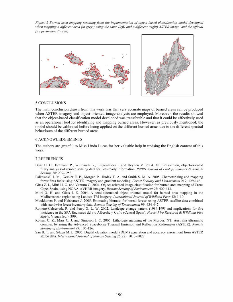
190

Figure 2 Burned area mapping resulting from the implementation of object-based classification model developed when mapping a different area (in grey ) using the same (left) and a different (right) ASTER image and the official fire perimeters (in red)

5 CONCLUSIONS The main conclusion drawn from this work was that very accurate maps of burned areas can be produced when ASTER imagery and object-oriented image analysis are employed. Moreover, the results showed that the object-based classification model developed was transferable and that it could be effectively used as an operational tool for identifying and mapping burned areas. However, as previously mentioned, the model should be calibrated before being applied on the different burned areas due to the different spectral behaviours of the different burned areas.

6 ACKNOWLEDGEMENTS The authors are grateful to Miss Linda Lucas for her valuable help in revising the English content of this work.

7 REFERENCES Benz U. C., Hofmann P., Willhauck G., Lingenfelder I. and Heynen M. 2004. Multi-resolution, object-oriented

fuzzy analysis of remote sensing data for GIS-ready information. ISPRS Journal of Photogrammetry & Remote Sensing 58: 239– 258.

FalkowskiI J. M., Gessler E. P., Morgan P., Hudak T. A. and Smith S. M. A. 2005. Characterizing and mapping forest fires fuels using ASTER imagery and gradient modeling. Forest Ecology and Management 217: 129-146.

Gitas Z. I., Mitri H. G. and Ventura G. 2004. Object-oriented image classification for burned area mapping of Creus Cape, Spain, using NOAA-AVHRR imagery. Remote Sensing of Environment 92: 409-413.

Mitri G. H. and Gitas I. Z. 2004. A semi-automated object-oriented model for burned area mapping in the Mediterranean region using Landsat-TM imagery. International Journal of Wildland Fires 12: 1-10.

Muukkonen P. and Heiskanen J. 2005. Estimating biomass for boreal forests using ASTER satellite data combined with standwise forest inventory data. Remote Sensing of Environment 99: 434-447.

Romero-Calcerrada R. and Perry G. L. W. 2002. Landcape change pattern (1984-199) and implications for fire incidence in the SPA Encinares del rio Alberche y Cofio (Central Spain). Forest Fire Research & Wildland Fire Safety, Viegas (ed.): 399.

Rowan C. Z., Mars C. J. and Simpson J. C. 2005. Lithologic mapping of the Mordor, NT, Australia ultramafic complex by using the Advanced Spaceborne Thermal Emission and Reflection Radiometer (ASTER). Remote Sensing of Environment 99: 105-126.

San B. T. and Süzen M. L. 2005. Digital elevation model (DEM) generation and accuracy assessment from ASTER stereo data. International Journal of Remote Sensing 26(22): 5013–5027.

191

1 INTRODUCTION As part of NASA’s Earth Observing System, the Moderate Resolution Imaging Spectroradiometer (MODIS) is onboard the Terra (launched 1999) and Aqua (launched 2001) polar orbiting satellites and their data are being used to generate global coverage data products on a systematic basis (Justice et al. 2002a). The algorithm used to define the global 1km MODIS active fire product has been refined several times (Kaufman et al. 1998, Justice et al. 2002b, Giglio et al. 2003). A complementary MODIS algorithm defined to map burned area has been developed for global application (Roy et al. 2005a); this algorithm has been implemented in the MODIS processing chain to map burned areas globally. The present paper overviews the main characteristics of the MODIS global burned area product (MCD45A1). Burned areas are characterized by deposits of charcoal and ash, removal of vegetation, and alteration of the vegetation structure (Roy et al. 1999). The MODIS algorithm to map burned areas takes advantage of these spectral, temporal, and structural changes. The algorithm detects the approximate date of burning by locating the occurrence of rapid changes in daily 500m surface reflectance time series data. It is an improvement on previous methods, through the use of a bidirectional reflectance model to deal with angular variations found in satellite data and the use of a statistical measure to detect change probability from a previously observed state. MODIS reflectance sensed within a temporal window of a fixed number of days is used to predict the reflectance on a subsequent day. A statistical measure is used to determine if the difference between the predicted and observed reflectance is a significant change of interest. Rather than attempting to minimize the directional information present in wide field-of-view satellite data by compositing, or by the use of spectral indices, this information is used to model the directional dependence of reflectance. This provides a semi-physically based method to predict change in reflectance from the previous state. A temporal constraint is used to identify and remove temporary changes, such as shadows, that are spectrally similar to more persistent fire induced changes. Further details are provided in Roy et al. (2005a).

The global MODIS burned area product

D.P. Roy Geographic Information Science Center of Excellence, South Dakota State University (USA); email: [email protected]

L.Boschetti and C.O.Justice, Department of Geography, University of Maryland (USA);email: [email protected] [email protected] Keywords: MODIS, Burned Areas, Global Product, Multitemporal, BRDF

ABSTRACT: The global MODIS burned area product, part of the recent NASA Collection 5 MODIS land product suite, is presented. The algorithm uses the recently published Bi-Directional Reflectance Model-Based Expectation change detection approach and maps at 500m the location and approximate day of burning. The algorithm does not use training data but rather applies a wavelength independent threshold and spectral constraints defined by the noise characteristics of the reflectance data and knowledge of the spectral behavior of burned vegetation and spectrally confusing changes that are not associated with burning. Temporal constraints are applied capitalizing on the spectral persistence of fire-affected areas. The algorithm is applied to MODIS-Terra and MODIS-Aqua land surface reflectance time series. It has been implemented in the MODIS land production system as part of the standard MODIS land product suite to systematically map burned areas globally for the 6+ year MODIS observation record.

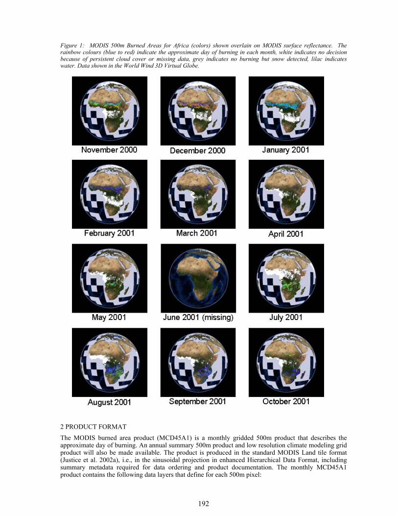
192

Figure 1: MODIS 500m Burned Areas for Africa (colors) shown overlain on MODIS surface reflectance. The rainbow colours (blue to red) indicate the approximate day of burning in each month, white indicates no decision because of persistent cloud cover or missing data, grey indicates no burning but snow detected, lilac indicates water. Data shown in the World Wind 3D Virtual Globe.

2 PRODUCT FORMAT The MODIS burned area product (MCD45A1) is a monthly gridded 500m product that describes the approximate day of burning. An annual summary 500m product and low resolution climate modeling grid product will also be made available. The product is produced in the standard MODIS Land tile format (Justice et al. 2002a), i.e., in the sinusoidal projection in enhanced Hierarchical Data Format, including summary metadata required for data ordering and product documentation. The monthly MCD45A1 product contains the following data layers that define for each 500m pixel:

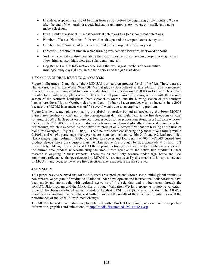
193

• Burndate: Approximate day of burning from 8 days before the beginning of the month to 8 days after the end of the month, or a code indicating unburned, snow, water, or insufficient data to make a decision.

• Burn quality assessment: 1 (most confident detection) to 4 (least confident detection). • Number of Passes: Number of observations that passed the temporal consistency test. • Number Used: Number of observations used in the temporal consistency test. • Direction: Direction in time in which burning was detected (forward, backward or both). • Surface Type: Information describing the land, atmospheric, and sensing properties (e.g. water,

snow, high aerosol, high view and solar zenith angles). • Gap Range 1 and 2: Information describing the two largest numbers of consecutive

missing/cloudy days (if any) in the time series and the gap start days.

3 EXAMPLE GLOBAL RESULTS & ANALYSIS Figure 1 illustrates 12 months of the MCD45A1 burned area product for all of Africa. These data are shown visualized in the World Wind 3D Virtual globe (Boschetti et al. this edition). The non–burned pixels are shown as transparent to allow visualization of the background MODIS surface reflectance data in order to provide geographic context. The continental progression of burning is seen, with the burning season of the Northern hemisphere, from October to March, and the burning season of the Southern hemisphere, from May to October, clearly evident. No burned area product was produced in June 2001 because the MODIS instrument was off for several weeks due to an engineering problem. Figure 2 shows scatter plots comparing the global proportion burned as labeled by the 500m MODIS burned area product (y axis) and by the corresponding day and night 1km active fire detections (x axis) for August 2001. Each point on these plots corresponds to the proportions found in a 10x10km window. Evidently the MODIS burned area product detects more area burned globally at this scale than the active fire product, which is expected as the active fire product only detects fires that are burning at the time of cloud-free overpass (Roy et al. 2005a). The data are shown considering only those pixels falling within 0-100% and 0-10% percentage tree cover ranges (left column) and within 0-10 and 0-2 leaf area index (LAI) ranges (right column). Globally, at low tree cover and low LAI, the 500m MODIS burned area product detects more area burned than the 1km active fire product by approximately 44% and 43% respectively. At high tree cover and LAI the opposite is true (not shown due to insufficient space) with the burned area product underestimating the area burned relative to the active fire product. Further research is ongoing in these respects. These results are likely because under high %tree and LAI conditions, reflectance changes detected by MDC45A1 are not as easily discernable as hot spots detected by MOD14, and because the active fire detections may exaggerate the area burned.

4 SUMMARY

This paper has overviewed the MODIS burned area product and shown some initial global results. A comprehensive program of product validation is under development and international collaborations have been made and are sought with regional networks of fire scientists and product users through the GOFC/GOLD program and the CEOS Land Product Validation Working group. A prototype validation protocol has been developed using multi-date Landsat ETM+ data (Roy et al 2005b). The MODIS burned area algorithm may be enhanced further based on the results of these validation initiatives or if the performance of the MODIS instrument changes. The MODIS burned area product may be obtained, with a Product User Guide, news and other supporting information, graphics and animations, at http://modis-fire.umd.edu/MCD45A1.asp.

194

Figure 2: Global results: August 2001; Scatterplots of the proportion of area burned (y axes) and active fire pixels (x axis) with a linear regression line forced to pass through the origin shown in red. Percentage tree cover and leaf area index (LAI) ranges are defined by consideration of the annual 500m percent tree cover and monthly composited 8-day 1km LAI MODIS products respectively. Each point corresponds to the proportions found in a 10x10km window (cell); only cells with no missing data in the three products are used. Due to the large number of points (~1million, top left) many points are over plotted.

5 REFERENCES Boschetti, L., Roy, D.P., Justice, C.O., Using NASA’s World Wind Virtual Globe for Interactive Internet

Visualisation of the Global MODIS Burned Area Product, this edition & submitted to Int. Journal of Remote Sensing.

Giglio, L., Descloitres, J., Justice, C.O., Kaufman, Y.J., 2003, An Enhanced Contextual Fire Detection Algorithm for MODIS, Remote Sensing of Environment, 87:273-382.

Justice, C., Townshend, J., Vermote, E., Masuoka, E., Wolfe, R., Saleous, N., Roy, D.P., Morisette, J. 2002a, An overview of MODIS Land data processing and product status, Remote Sensing of Environment, 83:3-15.

Justice, C.O., Giglio, L., Korontzi, S., Owens, J., Morisette, J., Roy, D.P, Descloitres, J., Alleaume, S., Petitcolin, F., Kaufman, Y., 2002b, The MODIS fire products, Remote Sensing of Environment, 83: 244-262.

Kaufman, Y.J., Justice, C.O., Flynn, L.P., Kendall, J.D., Prins, E.M., Giglio, L., Ward, D.E., Menzel, W.P., Setzer, A.W., 1998, Potential global fire monitoring from EOS-MODIS, Journal Of Geophysical Research-Atmospheres, 103:32215-32238.

Roy, D.P., Giglio, L., Kendall, J.D., Justice, C.O., 1999, A multitemporal active-fire based burn scar detection algorithm. International Journal of Remote Sensing, 20:1031-1038.

Roy, D.P., Jin, Y., Lewis, P.E., Justice, C.O., 2005a, Prototyping a global algorithm for systematic fire affected area mapping using MODIS time series data, Remote Sensing of Environment, 97:137-162.

Roy, D.P., Frost, P., Justice, C.O., Landmann, T., Le Roux, J., Gumbo, K., Makungwa, S., Dunham, K., Du Toit, R., Mhwandagara, K., Zacarias, A., Tacheba, B., Dube, O., Pereira, J., Mushove, P., Morisette, J., Vannan, S., Davies, D. 2005b. The Southern Africa Fire Network (SAFNet) regional burned area product validation protocol. International Journal of Remote Sensing, 26:4265-4292.

Acknowledgement This research funded by NASA Earth System Science Program grant NNG04HZ18C.

195

1 INTRODUCTION The spectral characterization of burnt areas is widely affected by fire intensity, residence-time and pre-fire biomass loads, all of which affect the amount of green versus scorched leaves, the proportion of ash and char, and the amount of remnant leaves. The time elapsed between fire occurrence and the acquisition of the image can also significantly alter the spectral behaviour of the burned area. Additional variations are expected for various illumination types and observation angles, especially in low resolution imagery. Consequently, spectral features of burned scars may be very diverse, and hence the automatic discrimination, especially at regional and global scales becomes very difficult. Previous studies have tried to tackle these problems by modifying global algorithms to local and regional conditions, but yet either omission or commission errors were made, depending on whether the local thresholds match the field conditions. Moreover, these modifications limit the operational application of the proposed algorithms. An alternative to this approach is the discrimination of burned scars in two phases: the first one aims detecting the most likely burned areas (core pixels), whereas the second one should improve the burned area mapping by analysing the neighbours of the previously detected pixels. Based on this method (Benvenuti et al., 2000) proposed a valid approach for mapping small/medium size burned areas (larger than 1 ha) in Italy. The algorithm was tested in three test-sites in three different years (1998, 1999 and 2000) and it was based on the processing of three pairs of Landsat TM and ETM+ images, acquired before and after each fire-season. Later this methodology was applied in a semi-operative way in the ITALSCAR project (Paganini et al., 2003) to map burned areas during four consecutive years (1997-2000). Recently, Bastarrika and Chuvieco (2006) have used on this bi-phase approach in four Mediterranean sites supported by unitemporal TM and ETM+ data. This methodology was also applied to low resolution imagery. Martín (1998) proposed a similar approach to analyse

Automatic discrimination of core burn scars using logistic regression models

A. Bastarrika Surveying Engineering Department, University of Basque Country, Nieves Cano 12, 01006 Vitoria-Gasteiz , Spain, [email protected]

E. Chuvieco Department of Geography, University of Alcalá , Calle Colegios 2, 28801 Alcalá de Henares, Spain, [email protected]

M.P. Martín Institute of Economics and Geography, Spanish Council for Scientific Research (CSIC), Pinar 25-28006 Madrid, Spain, [email protected] Keywords: Burnt area mapping, logistic regression, spectral indices

ABSTRACT: Recent works have demonstrated the benefits of using a two phase methodology to improve burned area mapping from remotely sensing data. In this approach, the first phase aims at detecting the most likely burned areas (core pixels), whereas the second one improves the burned area mapping by analyzing the neighbors of previously detected pixels. This work tries to tackle the first phase by means of several logistic regression models, using original bands and spectral indices and exploring unitemporal and multi temporal approaches. To adjust the models we used 5 pairs of Landsat TM/ETM+ data including a representative sample of burned areas in Mediterranean ecosystems. The validation of the models has been done using a Landsat scene located between Portugal and Spain with a large number of fires of different size. Visual interpretation of a color composite has been used to discriminate the fire perimeters used for validation. Logistic regression models have shown to be an effective technique to identify burned core pixels due to their ability to identify the most appropriate variables for burned area discrimination. All proposed models achieved a correct identification of the areas affected by fires larger than 25 ha where the burned patches detection probability increased up to 95%. The models that include the Red, -NIR – and two SWIR regions have shown the most adequate, particularly the model postMIRBI-postTM54-preMIRBI-preNDVI that offered confusion rates of 0.1%, almost 100% detection probability of burned patches larger than 25 ha, and 88% for those less than 25 ha, as well as 46.7% of total burnt area detected.

196

NOAA-AVHRR images, which was more recently used by (Martín et al., 2002) with MODIS data for the discrimination of large fires in the Iberian Peninsula. Fraser et al. (2002) applied this method in Canada during the 1998-2000 fire-season using VEGETATION ten day composite data. Garcia and Chuvieco (2004) analysed SAC-C/MMRS images for burned area mapping in three large fires in Spain during the summer of 2002. This paper focuses on the first phase of this approach. The objective of this phase is to minimize commission errors, avoiding confusion with other covers presenting similar spectral behaviour such as cloud shadows, water and topographical shade. We made use of reflectance bands and spectral indices for a set of multitemporal Landsat TM images on five sites that include a representative range of burnt areas in Mediterranean ecosystems. Several logistic regression models were developed to discriminate core burn scars.

2 METHODS 2.1 Test areas and data The development of various logistic regression models have been accomplished using TM and ETM+ imagery of five Mediterranean areas affected by forest fires: four of them are located in Spain (Buñol in Valencia, Atazar , Méntrida and Guadalajara in the Center of the country) and another one in Greece (Kassandra in the Northeast of the country). These areas have been selected to take into account different land cover types that are burned in Mediterranean ecosystems. Atazar fire mainly burned sclerophyllous vegetation (90%), being the rest marginal agricultural areas. In Buñol, almost half of the burned area was also sclerophyllous (47%), and the rest transitional woodland-scrub (25%), coniferous forest (22%) and agricultural land (6%). In Guadalajara mainly forest mass got burned, coniferous (66%) and mixed forest (15%), together with sclerophyllous vegetation (11%) and transitional woodland-scrub (6%). Finally, fires in Kassandra and Méntrida burned mainly agricultural land (66% and 49% respectively), being transitional woodland-scrub (14% and 22%), sclerophyllous vegetation (18% and 6%) and grassland (2% and 14%) the rest. Atazar, Kassandra and Méntrida were medium size fires, with burned areas of 1089 ha, 1675 ha and 1900 ha, respectively, while Guadalajara and Buñol were big fires, with more than 13 000 and 23 000 ha burned, respectively. For each of the test areas we chose a pair of Landsat TM/ETM+ images acquired before and after the fire. In all cases, the post-fire images were acquired soon after the fire, with a maximum interval of 20 days after fire extinction, whereas the pre-fire images were about the same year time. The validation of the models was carried out in a dataset of areas located between Portugal and Spain covered by the 202-032 Landsat scene: a post ETM+ image acquired on the 5th of September of 2000 and a pre-fire image of the 30th of July of 1995; here, 417 patches smaller than 25 ha, 102 patches between 25-100 ha and 104 patches bigger than 100 ha were visually identified, with an approximately 66,910 ha total burned area. The biggest proportion is scrub and herbaceous vegetation (65%), agricultural land (20%) and forest (15%) the rest. 2.2 Geometric and atmospheric correction and reflectance The post-fire images were geometrically corrected to UTM projection (Datum ED50 for Spain, EGSA87 for Greece and WGS84 for the validation scene between Spain and Portugal), within one pixel (RMS<1pixel) using control points and reference cartography. The pre-fire images were adjusted to the former by an image to image geometric correction to minimize misregistration errors. For the 202-032 complete scene the itpfind (Kennedy and Cohen, 2003) tool was used with a relative error below 0.5 pixels. The images were then converted to radiance values using sensor calibration values, and to reflectance using an atmospheric correction procedure based on the Dark Object Subtraction method (Chavez, 1996). 2.3 Development of logistic regression models Discrimination models based on logistic regression analysis were based on both the original bands and on spectral indices that improved the discrimination of burnt areas, such as Normalized Difference Vegetation Index (NDVI), Global Environmental Monitoring Index (GEMI), Burnt Area Index (BAI), Modified Burned Area Index (BAIM), and the ratios TM7/TM4 and TM5/TM4. Once visually delimited the burned areas (by means of TM7-TM4-TM3 colour composition), we have followed the criteria proposed by Koutsias and Karteris (1998) to extract the burned sample pixels. To get the non-burned samples we select representative samples of different land covers in each test area using as a reference the Corine Land Cover map. Burned samples were taken from random extractions within

197

the burned perimeters. 60,000 samples were obtained: 30,000 burned and 30,000 non-burned. Models have been calibrated using 50% of the samples, while the other 50% were kept for initial consistency tests. The models were developed considering the different spectral spaces of the most common sensors used for the burned area mapping; Red-NIR spectral domain (NOAA-AVHRR/2, IRS-WiFS, ENVISAT-MERIS, SPOT-HRV), Red-NIR-SWIR domain (NOAA-AVHRR/3, SPOT-VEGETATION, IRS-AWiFS, SPOT-HRVIR) and Red-NIR-2SWIR domain -with two bands in the SWIR region- (Landsat TM y ETM+, TERRA/AQUA-MODIS, TERRA-ASTER). In this way, we have developed 10 different models using the Stepwise logistic regression method and adding the bands and indices that belong to each spectral domain considered. Some of the models have been constructed using only post-fire images and others with multiemporal data (before and after the fire) to allow for both situations in which data before the fire is or not available. The logistic regression models provided a probabilistic result between 0 (non-burned) and 1 (burned). Generally the threshold of 0.5 is used to classify the output variable because it represents an ideal balance between omission and commission errors. The goal of this phase was to minimize commission errors; however, it is also necessary to detect the maximum number of burned patches and this is the reason why thresholds applied are rather strict. Not all the models presented the same ability for burned patches identification; for this reason the thresholds were set up statistically at median of the burned samples used for the adjustment of models. These thresholds proved to be appropriate among all the validation data set and allowed an objective comparison between the models. 2.4 Validation For the 203-032 scene validation perimeters were generated by visual interpretation of TM7-TM4-TM3 colour composites in the post-fire image, supported by the Portugal official perimeters. They do not provide the registration date of the fire and we have not been able to identify the fires that still do not appear in our image. This is the reason they have not been used as reference validation data.


In general, all the models provided a correct identification of the largest fires (table 1), specially those bigger than 25 ha where the detection of the burned patches reach 95%. It is important to note that there was not cloud problems in this scene, therefore, the models based on the Red-NIR spectral regions don’t have problems with the clouds shadows, one of the common problems of this spectral domain (Chuvieco et al., 2002). On this domain, the models which include BAI, specially the post-fire approach (postBAI), show large confusion with water areas. This confusion mainly arises due to the difficulty of discerning limits betteen water bodiesand land, and also due to the construction of new water reservoirs between pre and post fire images. The postNIR-preNIR-preNDVI-postRED-postGEMI model shows similar confusion rates than de postBAI-preBAI model, but with a less significant confusion with water areas, and also between soil and scrub, although it increases the confusion with agricultural areas. In Models that incorporate a SWIR band to the Red-NIR domain, such as the unitemporal and multitemporal BAIM models showed more confusion rate than the previous domain models, with less confusion with water areas but increased the confusion with all other land cover types, especially soil, scrub and old burned areas. Within the models that include 2 SWIR bands, the model composed by MIRBI (postMIRBI-postTM54-preMIRBI-preNDVI) showed high confusion rates with water cover due to MIRBI index, but showed less confusion in the rest of covers than the other models, although, they detected significant less burned area than the other two models (40% vs. 70%); however, they were able to detect almost all the burn patches bigger than 25 ha, and 88% of those smaller than 25 ha. The other two models, the unitemporal postNIR-postSWIR(TM7)- postGEMI- postSWIR(TM5) and multitemporal postNIR-postSWIR(TM7)- postSWIR(TM5)- postGEMI-preNDVI-preNIR showed an effective detection of the burned areas (almost 100%), and showed less confusion with water areas (specially the unitemporal); however, they increased confusion with soil and area burned in previous years (specially the unitemporal).

4 CONCLUSIONS The logistic regression models have demonstrated to be an effective technique to identify burn core pixels due to their sensitivity to identify the most sensible input variables for discrimination. This work incorporates different unitemporal and multitemporal models taking into account different spectral domains and thus they can be used with different type of sensors. In our validation data, the models that

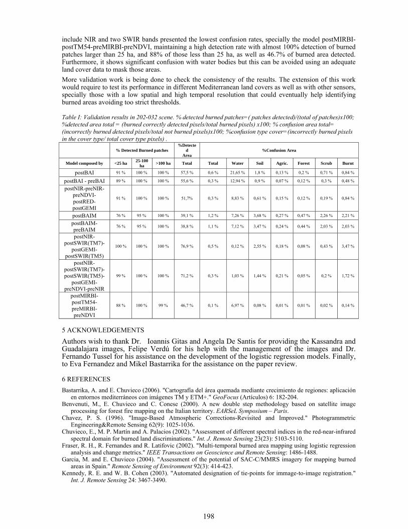
198

include NIR and two SWIR bands presented the lowest confusion rates, specially the model postMIRBI-postTM54-preMIRBI-preNDVI, maintaining a high detection rate with almost 100% detection of burned patches larger than 25 ha, and 88% of those less than 25 ha, as well as 46.7% of burned area detected. Furthermore, it shows significant confusion with water bodies but this can be avoided using an adequate land cover data to mask those areas. More validation work is being done to check the consistency of the results. The extension of this work would require to test its performance in different Mediterranean land covers as well as with other sensors, specially those with a low spatial and high temporal resolution that could eventually help identifying burned areas avoiding too strict thresholds.

Table I: Validation results in 202-032 scene. % detected burned patches=( patches detected)/(total of patches)x100; %detected area total = (burned correctly detected pixels/total burned pixels) x100; % confusion area total= (incorrectly burned detected pixels/total not burned pixels)x100; %confusion type cover=(incorrectly burned pixels in the cover type/ total cover type pixels) .

% Detected Burned patches %Detecte

d Area

%Confusion Area

Model composed by <25 ha 25-100 ha >100 ha Total Total Water Soil Agric. Forest Scrub Burnt

postBAI 91 % 100 % 100 % 57,5 % 0,6 % 21,65 % 1,8 % 0,13 % 0,2 % 0,71 % 0,84 %

postBAI - preBAI 89 % 100 % 100 % 55,6 % 0,3 % 12,94 % 0,9 % 0,07 % 0,12 % 0,3 % 0,48 %

postNIR-preNIR-preNDVI-postRED-postGEMI

91 % 100 % 100 % 51,7% 0,3 % 8,83 % 0,61 % 0,15 % 0,12 % 0,19 % 0,84 %

postBAIM 76 % 95 % 100 % 39,1 % 1,2 % 7,26 % 3,68 % 0,27 % 0,47 % 2,26 % 2,21 %

postBAIM-preBAIM

76 % 95 % 100 % 38,8 % 1,1 % 7,12 % 3,47 % 0,24 % 0,44 % 2,03 % 2,03 %

postNIR-postSWIR(TM7)-

postGEMI- postSWIR(TM5)

100 % 100 % 100 % 76,9 % 0,5 % 0,12 % 2,55 % 0,18 % 0,08 % 0,43 % 3,47 %

postNIR-postSWIR(TM7)- postSWIR(TM5)-

postGEMI-preNDVI-preNIR

99 % 100 % 100 % 71,2 % 0,3 % 1,03 % 1,44 % 0,21 % 0,05 % 0,2 % 1,72 %

postMIRBI-postTM54-preMIRBI-preNDVI

88 % 100 % 99 % 46,7 % 0,1 % 6,97 % 0,08 % 0,01 % 0,01 % 0,02 % 0,14 %

5 ACKNOWLEDGEMENTS

Authors wish to thank Dr. Ioannis Gitas and Angela De Santis for providing the Kassandra and Guadalajara images, Felipe Verdú for his help with the management of the images and Dr. Fernando Tussel for his assistance on the development of the logistic regression models. Finally, to Eva Fernandez and Mikel Bastarrika for the assistance on the paper review.

6 REFERENCES Bastarrika, A. and E. Chuvieco (2006). "Cartografía del área quemada mediante crecimiento de regiones: aplicación

en entornos mediterráneos con imágenes TM y ETM+." GeoFocus (Artículos) 6: 182-204. Benvenuti, M., E. Chuvieco and C. Conese (2000). A new double step methodology based on satellite image

processing for forest fire mapping on the Italian territory. EARSeL Symposium – Paris. Chavez, P. S. (1996). "Image-Based Atmospheric Corrections-Revisited and Improved." Photogrammetric

Engineering&Remote Sensing 62(9): 1025-1036. Chuvieco, E., M. P. Martín and A. Palacios (2002). "Assessment of different spectral indices in the red-near-infrared

spectral domain for burned land discriminations." Int. J. Remote Sensing 23(23): 5103-5110. Fraser, R. H., R. Fernandes and R. Latifovic (2002). "Multi-temporal burned area mapping using logistic regression

analysis and change metrics." IEEE Transactions on Geoscience and Remote Sensing: 1486-1488. Garcia, M. and E. Chuvieco (2004). "Assessment of the potential of SAC-C/MMRS imagery for mapping burned

areas in Spain." Remote Sensing of Environment 92(3): 414-423. Kennedy, R. E. and W. B. Cohen (2003). "Automated designation of tie-points for immage-to-image registration."

Int. J. Remote Sensing 24: 3467-3490.

199

Koutsias, N. and M. Karteris (1998). "Logistic regression modelling of multitmporal Thematic Mapper data for burned area mapping." Int. J. Remote Sensing 19(18): 3499-3514.

Martín, M. P. (1998). "Cartografía e inventario de incendios forestales en la Península Ibérica a partir de imágenes NOAA-AVHRR." Doctoral thesis, Universidad de Alcalá, Alcalá de Henares.

Martín, M. P., R. Diaz-Delgado, E. Chuvieco and G. Ventura (2002). Burned land mapping using NOAA-AVHRR and TERRA-MODIS. IV International Conference on Forest Fire Research, , Luso, November, 2002. (CDRom).

Paganini, M., O. Arino, M. Benvenuti, M. Cristaldi, M. Bordin, C. Coretti and A. Musone (2003). "ITALSCAR, a Regional Burned Forest Mapping demonstration project in Italy." IEEE Transactions on Geoscience and Remote Sensing: 1290-1292.

200

1 INTRODUCTION In the last decade there has been an information revolution in remote sensing, both in the capacity to generate products and to disseminate products to users. Today, digital satellite data products can be obtained from dedicated centres that may physically and institutionally be separated from the place of product generation. Users can submit requests via the internet using personal computers, and can request that products be sent on media or over the internet using file transfer protocols. At the same time, commercial internet search engines and services have raised expectations and awareness for the delivery of geographic information and services over the internet. This paper shows how, using the open source World Wind visualization technology developed at NASA AMES, it is possible to make such information readily available to a wide range of users. This capability will expand access to the MODIS Burned Area Product, which is a standard product developed by the MODIS Fire Group and is being generated globally as part of the Collection 5 production (WWW1, Roy et al. this edition). The MODIS burned area product was developed to meet the needs of both the science and fire management communities, providing spatially explicit monthly products of global burned area at 500m that describe the approximate day of burning (Roy et al. 2005). The product was designed for use by a range of users, from global change modelers as an input to fire emissions and air quality models, to national fire management agencies concerned with identifying and quantifying the area and location of burning during the fire season (Justice et al. 2002a, Roy et al. 2005). Although scientists are capable of managing complex data formats and image analysis tools, most decision makers do not have the necessary time or training (Trigg and Roy, 2007).Virtual globes provide an unprecedented opportunity to give all types of users easy access to large datasets of geographic data (Butler, 2006).

2 THE MODIS BURNED AREA PRODUCT The MODIS Burned Area Product (MCD45) has been recently implemented in the MODIS land production system at NASA’s Goddard Space Flight Centre (Justice et al. 2002b), to systematically map burned areas globally for the entire MODIS observation record (6+ years to date). The algorithm uses a Bi-Directional Reflectance Model-Based Expectation change detection approach to globally map at 500m the location and approximate day of burning (Roy et al. 2005). The MODIS burned area product user guide and

Using NASA’s World Wind Virtual Globe for Interactive Internet Visualisation and Quality Assessment of the Global MODIS Burned Area Product

L.Boschetti Department of Geography, University of Maryland (USA); email: [email protected]

D.P. Roy Geographic Information Science Center of Excellence, South Dakota State University (USA);email: [email protected]

C.O.Justice Department of Geography, University of Maryland (USA); email: [email protected] Keywords: MODIS, Burned Areas, Global Products, World Wind, Interactive 3D visualisation, Virtual globes.

ABSTRACT: Virtual globes provide visualization of spatially explicit data from different views projected onto the Earth’s surface in three dimensions. Users may interactively pan, zoom and rotate the data, usually superimposed on a selected background that provides geographic context. Virtual globes are changing the way in which geographic information is distributed and how the public perceive such information. This paper describes how World Wind, an open source virtual globe developed by the National Aeronautics and Space Administration (NASA), is currently being used for visualisation of the MODIS Burned Area product. The procedures adopted for converting the product into a format compatible with World Wind, as well the spatial generalisation of these data at different scales, are overviewed. The potential benefits of integrating the visualisation capability of Virtual Globes into the next generation of remotely sensed product internet analysis and distribution systems are emphasised. This is in keeping with NASA’s goal to move towards a more distributed, heterogeneous data and information environment, with an interoperable architecture and increased data access and usability for the science research, application and modeling communities.

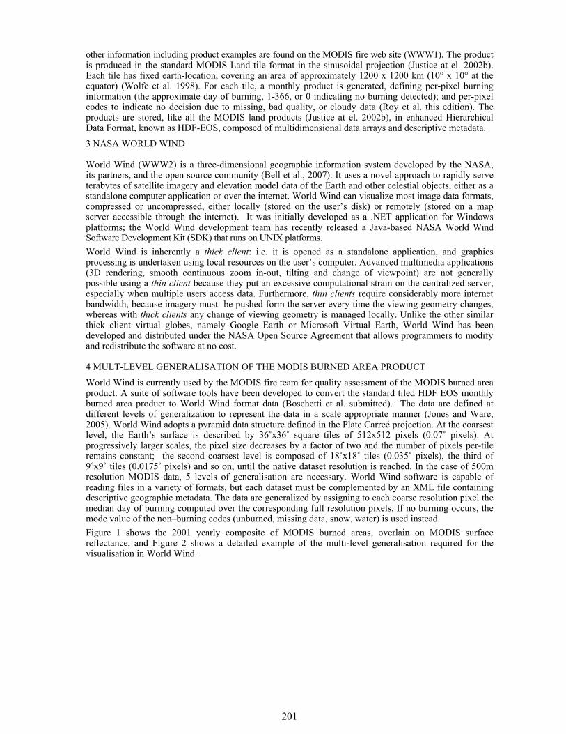
201

other information including product examples are found on the MODIS fire web site (WWW1). The product is produced in the standard MODIS Land tile format in the sinusoidal projection (Justice at el. 2002b). Each tile has fixed earth-location, covering an area of approximately 1200 x 1200 km (10° x 10° at the equator) (Wolfe et al. 1998). For each tile, a monthly product is generated, defining per-pixel burning information (the approximate day of burning, 1-366, or 0 indicating no burning detected); and per-pixel codes to indicate no decision due to missing, bad quality, or cloudy data (Roy et al. this edition). The products are stored, like all the MODIS land products (Justice at el. 2002b), in enhanced Hierarchical Data Format, known as HDF-EOS, composed of multidimensional data arrays and descriptive metadata. 3 NASA WORLD WIND

World Wind (WWW2) is a three-dimensional geographic information system developed by the NASA, its partners, and the open source community (Bell et al., 2007). It uses a novel approach to rapidly serve terabytes of satellite imagery and elevation model data of the Earth and other celestial objects, either as a standalone computer application or over the internet. World Wind can visualize most image data formats, compressed or uncompressed, either locally (stored on the user’s disk) or remotely (stored on a map server accessible through the internet). It was initially developed as a .NET application for Windows platforms; the World Wind development team has recently released a Java-based NASA World Wind Software Development Kit (SDK) that runs on UNIX platforms. World Wind is inherently a thick client: i.e. it is opened as a standalone application, and graphics processing is undertaken using local resources on the user’s computer. Advanced multimedia applications (3D rendering, smooth continuous zoom in-out, tilting and change of viewpoint) are not generally possible using a thin client because they put an excessive computational strain on the centralized server, especially when multiple users access data. Furthermore, thin clients require considerably more internet bandwidth, because imagery must be pushed form the server every time the viewing geometry changes, whereas with thick clients any change of viewing geometry is managed locally. Unlike the other similar thick client virtual globes, namely Google Earth or Microsoft Virtual Earth, World Wind has been developed and distributed under the NASA Open Source Agreement that allows programmers to modify and redistribute the software at no cost.

4 MULT-LEVEL GENERALISATION OF THE MODIS BURNED AREA PRODUCT World Wind is currently used by the MODIS fire team for quality assessment of the MODIS burned area product. A suite of software tools have been developed to convert the standard tiled HDF EOS monthly burned area product to World Wind format data (Boschetti et al. submitted). The data are defined at different levels of generalization to represent the data in a scale appropriate manner (Jones and Ware, 2005). World Wind adopts a pyramid data structure defined in the Plate Carreé projection. At the coarsest level, the Earth’s surface is described by 36˚x36˚ square tiles of 512x512 pixels (0.07˚ pixels). At progressively larger scales, the pixel size decreases by a factor of two and the number of pixels per-tile remains constant; the second coarsest level is composed of 18˚x18˚ tiles (0.035˚ pixels), the third of 9˚x9˚ tiles (0.0175˚ pixels) and so on, until the native dataset resolution is reached. In the case of 500m resolution MODIS data, 5 levels of generalisation are necessary. World Wind software is capable of reading files in a variety of formats, but each dataset must be complemented by an XML file containing descriptive geographic metadata. The data are generalized by assigning to each coarse resolution pixel the median day of burning computed over the corresponding full resolution pixels. If no burning occurs, the mode value of the non–burning codes (unburned, missing data, snow, water) is used instead. Figure 1 shows the 2001 yearly composite of MODIS burned areas, overlain on MODIS surface reflectance, and Figure 2 shows a detailed example of the multi-level generalisation required for the visualisation in World Wind.

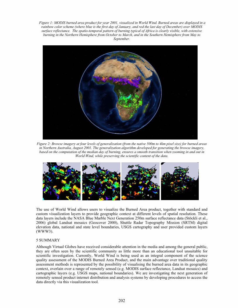
202

Figure 1: MODIS burned area product for year 2001, visualized in World Wind. Burned areas are displayed in a rainbow color scheme (where blue is the first day of January, and red the last day of December) over MODIS surface reflectance. The spatio-temporal pattern of burning typical of Africa is clearly visible, with extensive burning in the Northern Hemisphere from October to March, and in the Southern Hemisphere from May to

September.

Figure 2: Browse imagery at four levels of generalization (from the native 500m to 4km pixel size) for burned areas in Northern Australia, August 2001. The generalization algorithm developed for generating the browse imagery, based on the computation of the median day of burning, ensures a smooth transition when zooming in and out in

World Wind, while preserving the scientific content of the data.

The use of World Wind allows users to visualize the Burned Area product, together with standard and custom visualization layers to provide geographic context at different levels of spatial resolution. These data layers include the NASA Blue Marble Next Generation 250m surface reflectance data (Stöckli et al., 2006) global Landsat mosaics (Geocover 2000), Shuttle Radar Topography Mission (SRTM) digital elevation data, national and state level boundaries, USGS cartography and user provided custom layers (WWW3).

5 SUMMARY

Although Virtual Globes have received considerable attention in the media and among the general public, they are often seen by the scientific community as little more than an educational tool unsuitable for scientific investigation. Currently, World Wind is being used as an integral component of the science quality assessment of the MODIS Burned Area Product, and the main advantage over traditional quality assessment methods is represented by the possibility of visualising the burned area data in its geographic context, overlain over a range of remotely sensed (e.g. MODIS surface reflectance, Landsat mosaics) and cartographic layers (e.g. USGS maps, national boundaries). We are investigating the next generation of remotely sensed product internet distribution and analysis systems by developing procedures to access the data directly via this visualization tool.

203

Sample MODIS burned area World Wind compatible datasets, animations, and installation instructions, are available to the public from the MODIS fire web site (WWW1).

6 ACKNOWLEDGEMENT This research funded by NASA Earth System Science Program grant NNG04HZ18C.

7 REFERENCES Bell, D. G., Kuehnel, F., Maxwell, C., Kim, R., Kasraie, K., Gaskins, T., Hogan, P. and Coughlan, J. NASA World

Wind: Opensource GIS for Mission Operations, Proceedings of the 2007 IEEE Aerospace Conference, 3-10 March 2007 Page(s):1 – 9.

Boschetti, L ., Roy, D. and Justice, C., Using NASA's World Wind Virtual Globe for Interactive Visualization of the Global MODIS Burned Area Product, International Journal of Remote Sensing , submitted.

Butler, D., 2006, The web-wide world, Nature, Vol. 439, no. 7078, 776-778. Jones, C.B. and Ware, J.M. (2005) Map generalization in the Web age, International Journal of Geographical

Information Science, DOI: 10.1080/13658810500161104, Volume 19, pages 859 – 870. Justice, C., Giglio, L., Korontzi, S., Owens, J., Morisette, J., Roy, D., Descloitres, J., Alleaume, S., Petitcolin, F.,

Kaufman, Y., 2002a, The MODIS fire products, Remote Sensing of Environment, 83: 244-262. Justice, C., Townshend, J., Vermote, E., Masuoka, E., Wolfe, R., Saleous, N., Roy, D., Morisette, J. (2002b), An

overview of MODIS Land data processing and product status, Remote Sensing of Environment, 83:3-15. Roy, D.P., Jin, Y., Lewis, P.E., Justice, C.O., (2005), Prototyping a global algorithm for systematic fire-affected area

mapping using MODIS time series data, Remote Sensing of Environment, 97: 137-162. Stöckli R., Vermote E., Saleous N., Simmon R., Herring D. (2006). True Color Earth Data Set Includes Seasonal

Dynamics. EOS Transactions, American Geophyisical Union, 87, 5, 49-55. Roy, D.P., Boschetti, L, Justice, C., this edition, The global MODIS burned area product Trigg, S.N and Roy D.P., 2007, A focus group study of factors that promote and constrain the use of satellite derived

fire products by resource managers in southern Africa, Journal of Environmental Management, 82:95-110. Wolfe, R., Roy, D., Vermote, E., (1998), The MODIS land data storage, gridding and compositing methodology: L2

Grid, IEEE Transactions on Geoscience and Remote Sensing, 36:1324-1338. WWW1: http://modis-fire.umd.edu/MCD45A1.asp WWW2: http://worldwind.arc.nasa.gov/ WWW3: http://www.worldwindcentral.com/add-ons/list

204

1 INTRODUCTION The SITHON Project was successfully competed and funded in 2003 under the Operational Program of Competitiveness of the Ministry of Development-GSRT-Action 4.5.1: Natural Environment and Sustainable Development. The project was originally entitled “Application and evaluation of terrestrial and airborne telemetric methods for rapid detection- early awareness and real time monitoring of wildfires”. The project was a three-year funded effort which initiated in July 2003. Between the objectives of the project was a) to foster collaboration between the private service sector, technological partners and research community and b) demonstrate the synergy of evolving technologies (terrestrial, airborne and EO) for increasing the information content of the collected data and enhance the timeliness in data collection, processing and transmission in respect to an efficient management of wildfire suppression actions. There were five main focused elements of collaborative effort: 1) A research and development element which specifically focused on advancing the development of a remote sensing airborne imaging infrared system for real time monitoring of fire fronts and in time detection of hot spots. 2) A technological element which focused on the installation and synergetic use of a number of terrestrial optical cameras. 3) A technological element which focused on the establishment of reference data bases providing support to wildfire fighting and suppression activities. 4) An application, demonstration and validation element which focused on test bedding and demonstrating the benefit from the synergetic use of the R&D and technological developments of the project.

A decision support system for wildfire management and impact assessment in affected zones

C. Kontoes, P. Elias, I. Kotsis, D. Paronis, & I. Keramitsoglou Institute for Space Applications and Remote Sensing, National Observatory of Athens, Metaxa & Vas. Pavlou, GR-15236, Palea Penteli, Athens, Greece. Email: [email protected] Keywords: Wildfire detection and monitoring, Airborne infrared imaging platform, GPS/INS, GIS, Change Vector Analysis

ABSTRACT: An integrated decision support system for wildfire management has been developed and operated by the Institute for Space Applications and Remote Sensing of the National Observatory of Athens (ISARS/NOA). It integrates EO, airborne imaging and satellite navigation technologies in order to meet fire modelling, fire detection and fire mapping requirements during and after the occurrence of the fire event. The system supports real-time monitoring of wildfires, dynamic detection and mapping of hot spots and fire fronts, real-time transmission of relevant information to the fire managers, accurate mapping of burnt areas as well as assessment of the fires’ consequences at the end of the fire season. To fulfil the need for real-time monitoring the system operates an airborne remote sensing infrared platform lying on state-of-the-art technologies such as: (a) thermal infrared image processing and thresholding for real-time assessment of the recorded temperatures (b) satellite kinematic positioning in conjunction with inertial navigation systems for real time geo-referencing of the thermal infrared acquisitions and (c) dynamic integration and representation of the collected images in the GIS system operated by the wildfire managers. Moreover to meet the requirement for post-fire management, the system integrates and process EO data together with the airborne collected thermal data to derive accurate detection and delineation of burnt areas as well as maps and statistics indicating the land cover classes and areas affected by fire. Innovative image processing methods are implemented to precisely map the land cover changes at post-fire stage. To this end a specific change detection algorithm has been developed, tested and modified accordingly to meet the standardisation requirements of operational projects. The technique behind this algorithm is based on the principles of the so-called change vector analysis (CVA) method, using a 3n+2 dimensional feature space, with n denoting the number of spectral bands of the input satellite scenes. The paper presents the two basic components of the system comprising of the airborne part or subsystem and the “ground” (post-fire) subsystem. The characteristics, the performance and the functional elements of the two components are described in detail. The results of the airborne subsystem deployment over the Sithonia Peninsula in Chalkidiki are also presented. The airborne infrared subsystem was assessed for its temperature sensitivity (~6ºC /0-500ºC) and detection capability (fires of few square meters on the ground are easily detected). In addition the functional and performance characteristics of the “ground” post-fire subsystem for precise mapping of the devastated areas after the fire season are also commented.

205

5) In parallel to SITHON developments, a fifth R&D element focusing on automatic change detection in the devastated areas, delineation of burn scars and assessment of fire impact was developed, tested and evaluated. In the following a presentation of elements (1) and (5) above is given.

2 BACKGROUND

In the last decade, there have been advancements in technologies that support wild land fire management and emergency response (Ambrosia V. G. et al., 2003, Light D., 2001, Hutton J. and Melihen A, 2006, Sifakis N. et al, 2001). These advancements include: a) improved capability for remote sensing towers, aircrafts and satellites; b) Geographic Information Systems; c) image processing and image geo-referencing; d) Global Positioning System (GPS) in combination with Inertial Navigation Systems (INS); and e) fire behavior models. Fast fire detection and real time monitoring of a fire (fire spread, location of hot spots) are crucial for the success of the initial attack on and containment of a fire. Infrared sensors have been viewed, as detection and monitoring systems, but are better viewed as equipment of a detection/monitoring system. Uncooled forward looking infrared cameras provide an opportunity for lower cost fire detection and monitoring. On this basis it was decided in the frame of SITHON project: a) to conduct further R&D in the area of using new smaller and less expensive IR uncooled cameras for fire detection and monitoring; b) to conduct further R&D in the area of image processing coupled with GIS, GPS and INS technologies to assist in the dynamic translation of the raw image data to usable products (coordinates/maps of hot spots and fire fronts, isothermal contour lines, geo-referenced/projected videos and thermal images).

3 FIRE DETECTION AND MONITORING - SITHON AIRBORNE SUBSYSTEM 3.1 Major elements of imaging payload The imaging payload in its current version is for a low-cost system. The infrared camera Thermovision R 570 was flown on a CESNA 3100 two-engine aircraft own and operated by AEROPHOTO Ltd. The

integration of the camera was facilitated by the design elements of the plane, equipped with a gyro-stabilized camera mount on which the infrared camera body was mounted and fixed. The Thermovision R 570 is a light weigh, high performance IR camera. It uses advanced uncooled Focal Plane Array (FPA) micro-bolometer technology and stores images and data to memory cards. Significant software developments were made to allow remote control and operation of the camera system by the payload engineer on board. The infrared camera Thermovision R 570 characteristics are summarized in table 1. The camera has been laboratory calibrated to resolve fire intensities up to 500 oC. For this range of temperatures discrimination was approximately 1.0 oC per digital count with a systematic shift (bias) of 6 oC. This was adequate because in the frame of the SITHON

project the interest is more focused on mapping relative temperature differences between points than estimating absolute temperatures. To recover the camera’s interior orientation that is the principal point (xp, yp) and the principal distance (c), an analytical 3-D camera calibration (bundle adjustment with self calibration) using a 3-D calibration test field was performed. The resulted interior camera orientation expressed in pixels is reported also in table 1. Direct image geo-referencing was based on the combination of GPS for position and inertial

measurements for the camera’s orientation angles. This GPS/INS combination allowed the real time determination of both attitude (pitch, roll, yaw) and position (X, Y, Z) of the camera at the time of exposure. The MIDG II GPS/INS system of Microbotics was used. It is a low-cost, light weight, small size and low power package which integrates an internal GPS receiver that collects GPS positions and

Table 1: AGGA Thermovision R570 Infrared camera

FOV 24ox18o/0.5m built in IFOV 1.3 mrad

Detector type Focal Plane Array / uncooled

Spectral range 7.5-13 μm

Video output CCIR/PAL Composite and S-video

Image resolution

12 bit images stored on PC-Card hard disc

Interior orientation

xo=16.0452, yo=31.6923, c=0.5329

Figure 1. The SITHON airborne system configuration

Grabber

Thermo Cam

GPS Antenna

Client

Server

INT INS

Switch

Switch

SMBFireWire 6pin

FireWire 4pinRCA

RJ45

RJ45

MIDG Special Pin - Out

Db9

Db25 SMA

Rs2

32

Rs422 Coaxial 50Ω

FireWire IEEE1394a UTP

Air

UTP

Coaxial 75Ω

Airborne Station

Ground Station

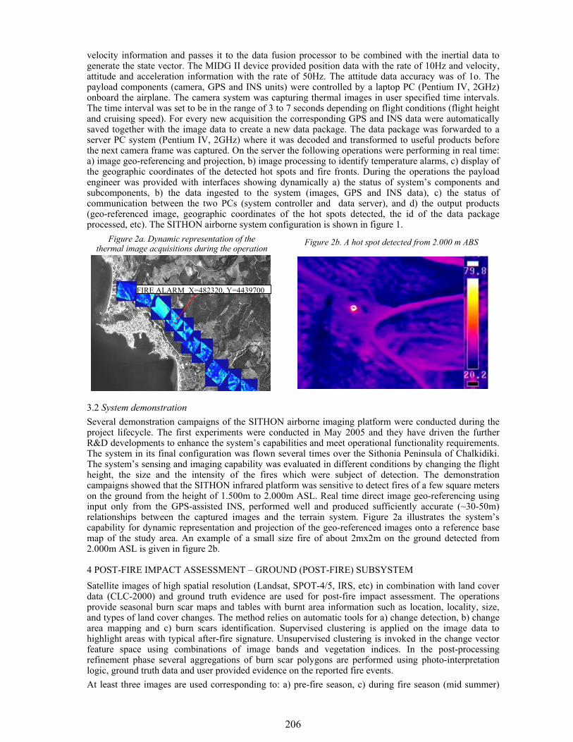
206

velocity information and passes it to the data fusion processor to be combined with the inertial data to generate the state vector. The MIDG II device provided position data with the rate of 10Hz and velocity, attitude and acceleration information with the rate of 50Hz. The attitude data accuracy was of 1o. The payload components (camera, GPS and INS units) were controlled by a laptop PC (Pentium IV, 2GHz) onboard the airplane. The camera system was capturing thermal images in user specified time intervals. The time interval was set to be in the range of 3 to 7 seconds depending on flight conditions (flight height and cruising speed). For every new acquisition the corresponding GPS and INS data were automatically saved together with the image data to create a new data package. The data package was forwarded to a server PC system (Pentium IV, 2GHz) where it was decoded and transformed to useful products before the next camera frame was captured. On the server the following operations were performing in real time: a) image geo-referencing and projection, b) image processing to identify temperature alarms, c) display of the geographic coordinates of the detected hot spots and fire fronts. During the operations the payload engineer was provided with interfaces showing dynamically a) the status of system’s components and subcomponents, b) the data ingested to the system (images, GPS and INS data), c) the status of communication between the two PCs (system controller and data server), and d) the output products (geo-referenced image, geographic coordinates of the hot spots detected, the id of the data package processed, etc). The SITHON airborne system configuration is shown in figure 1.

3.2 System demonstration Several demonstration campaigns of the SITHON airborne imaging platform were conducted during the project lifecycle. The first experiments were conducted in May 2005 and they have driven the further R&D developments to enhance the system’s capabilities and meet operational functionality requirements. The system in its final configuration was flown several times over the Sithonia Peninsula of Chalkidiki. The system’s sensing and imaging capability was evaluated in different conditions by changing the flight height, the size and the intensity of the fires which were subject of detection. The demonstration campaigns showed that the SITHON infrared platform was sensitive to detect fires of a few square meters on the ground from the height of 1.500m to 2.000m ASL. Real time direct image geo-referencing using input only from the GPS-assisted INS, performed well and produced sufficiently accurate (~30-50m) relationships between the captured images and the terrain system. Figure 2a illustrates the system’s capability for dynamic representation and projection of the geo-referenced images onto a reference base map of the study area. An example of a small size fire of about 2mx2m on the ground detected from 2.000m ASL is given in figure 2b.

4 POST-FIRE IMPACT ASSESSMENT – GROUND (POST-FIRE) SUBSYSTEM Satellite images of high spatial resolution (Landsat, SPOT-4/5, IRS, etc) in combination with land cover data (CLC-2000) and ground truth evidence are used for post-fire impact assessment. The operations provide seasonal burn scar maps and tables with burnt area information such as location, locality, size, and types of land cover changes. The method relies on automatic tools for a) change detection, b) change area mapping and c) burn scars identification. Supervised clustering is applied on the image data to highlight areas with typical after-fire signature. Unsupervised clustering is invoked in the change vector feature space using combinations of image bands and vegetation indices. In the post-processing refinement phase several aggregations of burn scar polygons are performed using photo-interpretation logic, ground truth data and user provided evidence on the reported fire events. At least three images are used corresponding to: a) pre-fire season, c) during fire season (mid summer)

Figure 2a. Dynamic representation of the thermal image acquisitions during the operation

FIRE ALARM X=482320, Y=4439700

Figure 2b. A hot spot detected from 2.000 m ABS

207

and c) post-fire season. The change detection technique is based on the principles of the change vector analysis (CVA) Chen et al. 2003. A synthetic image is created by coupling image bands with vegetation indices. Using as reference the synthetic image corresponding to the pre-fire season and combining it with the other two images corresponding to mid-summer and after-summer seasons, the algorithm a) defines the change vector between any two dates, b) calculates the change vector magnitude together with the change vector elements (direction and sign of direction) and c) performs unsupervised clustering of the change vector data to obtain change clusters including those corresponding to burnt sites. Once the clustering operations are successfully terminated the operator examines the clustering output and sets the appropriate label to the burnt area clusters. The method proved to be an effective solution in the frame of operational projects. It limits considerably the time of data processing and classifies with high accuracy (88%-96% overall accuracy) the burnt areas and the types of change categories in the devastated areas (Kontoes C., 2007).

5 CONCLUSIONS The R&D developments in the frame of SITHON project resulted in the delivery of an efficient and cost-effective airborne imaging system capable to detect and monitor wildfires in real time. The demonstrations showed that this system can lead to a significant improvement in tactical fire imaging from the air and can reduce the fire information ingestion process to few minutes, thereby minimizing the potential loss of resources, personnel, and property during fire event. On the other side the ground subsystem allows precise burnt area mapping and supports the effective management of the affected zones after fire. It assists the rapid mapping of the devastated areas and provides the solution to the problem of large time delays between the end of the fire season and the time to deploy the available cartographic capacities on site (aerial campaigns, field surveys).

6 ACKNOWLEDGEMENTS The authors acknowledge the contribution of Prof. M. Santamouris (Institute of Accelerating Systems and

Applications-University of Athens) in providing the Infrared camera Thermovision 570. We acknowledge the participation of Mr P. Doukas in the preparation and realization of the airborne campaigns over

the Sithonia Peninsula. We are grateful to Dr. P. Konstantinides and Dr. G. Tsiourlis (Forest Research Institute-NAGREF) for their valuable

efforts in managing the SITHON project and ensure its proper and undisturbed continuation in the three-years project lifecycle.

We thank the pilot Mr P. Boutsoukis, and the owners Grigoris and Giannis Noitsis of AEROPHOTO ltd for providing us their valuable help and technical support to fly the airborne infrared imaging system over the Sithonia Peninsula in Chalkidiki.

7 REFERENCES Ambrosia, V.G., Wegener, S.S., Sullivan, D.V., Buechel, S.W., Dunagan, S.E., Brass, J.A., Stoneburner J.,

Schoenung S.M. 2003. Demonstrating UAV-acquired real-time thermal data over fires. Photogrammetric Engineering and Remote Sensing: 69:391-402.

Chen, J., Gong, P., He, C., Pu, R., Shi, P., 2003. Land-use/Land-cover change detection using improved change-vector analysis. Photogrammetric Engineering and Remote Sensing: 69:369-379.

Hutton, J., Melihen, A. 2006. Emergency response remote sensing evolves in the wake of experience. Photogrammetric Engineering and Remote Sensing: 72:977-981.

Kontoes, C. 2007. Operational land cover change detection using change vector analysis. International Journal of Remote Sensing. Under final review.

Light, D. 2001. An airborne direct digital imaging system. Photogrammetric Engineering and Remote Sensing: 67:1299-1305.

Sifakis, N., Paronis, D., Kontoes, C. 2001. Operational application of satellite observations in monitoring of forest fires in quasi real time and guidance of firemen to impassable mountain areas. Proceedings of the Conference on “Integrated development in mountain areas: Theory and Action”. Metsovo Greece (in Greek).

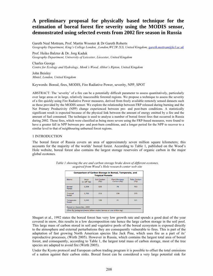
208

1 INTRODUCTION The boreal forest of Russia covers an area of approximately seven million square kilometers; this accounts for the majority of the worlds’ boreal forest. According to Table 1, published on the Wood’s Hole website, boreal forest also contains the largest storage reservoirs of organic carbon in the major global ecotones.

Shugart et al., 1992 states the boreal forest has very low growth rate and spends a good deal of the year covered in snow, this results in a low decomposition rate hence the large carbon storage in the soil pool. This large mass of carbon stored in soil and vegetative pools of the boreal ecosystem is exposed directly to the atmosphere and external perturbations they are consequently vulnerable to fires. This is part of the adaptation of fast growing North American species like Jack Pine, which uses fire as a part of its’ reproductive processes, (Wirth 2005). However in Russia, which contains the largest total area of boreal forest, and consequently, according to Table 1, the largest total mass of carbon storage, most of the tree species are adapted to avoid fire (Wirth 2005). Under the Kyoto protocol and European carbon trading program it is possible to offset the total emissions of a nation against their carbon sinks. Boreal forest can be considered a very large potential sink for

A preliminary proposal for physically based technique for the estimation of boreal forest fire severity using the MODIS sensor, demonstrated using selected events from 2002 fire season in Russia

Gareth Neal Mottram, Prof. Martin Wooster & Dr Gareth Roberts Geography Department, King’s College London, ,London,WC2R 2LS, United Kingdom, [email protected]

Prof. Heiko Balzter & Dr. Jorg Kaduk Geography Department, University of Leicester, Liecester, United Kingdom

Charles George Centre for Ecology and Hydrology, Monk’s Wood, Abbot’s Ripton, United Kingdom

John Beisley Mintel, London, United Kingdom Keywords: Boreal, fires, MODIS, Fire Radiative Power, severity, NPP, SPOT

ABSTRACT: The ‘severity’ of a fire can be a potentially difficult parameter to assess quantitatively, particularly over large areas or in large, relatively inaccessible forested regions. We propose a technique to assess the severity of a fire quickly using Fire Radiative Power measures, derived from freely available remotely sensed datasets such as those provided by the MODIS sensor. We explore the relationship between FRP released during burning and the Net Primary Productivity (NPP) change experienced between pre- and post-burn conditions. A statistically significant result is expected because of the physical link between the amount of energy emitted by a fire and the amount of fuel consumed. The technique is used to analyse a number of boreal forest fires that occurred in Russia during 2002. Those fires, which were classified as being more severe using the FRP-based measures, were found to have a greater fall in NPP between pre- and post-burn conditions, and a longer period for the NPP to recover to a similar level to that of neighbouring unburned forest regions.

Table 1 showing the are and carbon storage brake down of different ecotones, acquired from Wood’s Hole research center web site

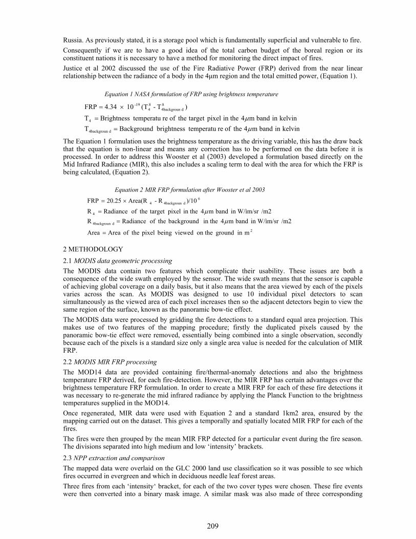
209

Russia. As previously stated, it is a storage pool which is fundamentally superficial and vulnerable to fire. Consequently if we are to have a good idea of the total carbon budget of the boreal region or its constituent nations it is necessary to have a method for monitoring the direct impact of fires. Justice et al 2002 discussed the use of the Fire Radiative Power (FRP) derived from the near linear relationship between the radiance of a body in the 4μm region and the total emitted power, (Equation 1).

The Equation 1 formulation uses the brightness temperature as the driving variable, this has the draw back that the equation is non-linear and means any correction has to be performed on the data before it is processed. In order to address this Wooster et al (2003) developed a formulation based directly on the Mid Infrared Radiance (MIR), this also includes a scaling term to deal with the area for which the FRP is being calculated, (Equation 2).

2 METHODOLOGY 2.1 MODIS data geometric processing The MODIS data contain two features which complicate their usability. These issues are both a consequence of the wide swath employed by the sensor. The wide swath means that the sensor is capable of achieving global coverage on a daily basis, but it also means that the area viewed by each of the pixels varies across the scan. As MODIS was designed to use 10 individual pixel detectors to scan simultaneously as the viewed area of each pixel increases then so the adjacent detectors begin to view the same region of the surface, known as the panoramic bow-tie effect. The MODIS data were processed by gridding the fire detections to a standard equal area projection. This makes use of two features of the mapping procedure; firstly the duplicated pixels caused by the panoramic bow-tie effect were removed, essentially being combined into a single observation, secondly because each of the pixels is a standard size only a single area value is needed for the calculation of MIR FRP. 2.2 MODIS MIR FRP processing The MOD14 data are provided containing fire/thermal-anomaly detections and also the brightness temperature FRP derived, for each fire-detection. However, the MIR FRP has certain advantages over the brightness temperature FRP formulation. In order to create a MIR FRP for each of these fire detections it was necessary to re-generate the mid infrared radiance by applying the Planck Function to the brightness temperatures supplied in the MOD14. Once regenerated, MIR data were used with Equation 2 and a standard 1km2 area, ensured by the mapping carried out on the dataset. This gives a temporally and spatially located MIR FRP for each of the fires. The fires were then grouped by the mean MIR FRP detected for a particular event during the fire season. The divisions separated into high medium and low ‘intensity’ brackets. 2.3 NPP extraction and comparison The mapped data were overlaid on the GLC 2000 land use classification so it was possible to see which fires occurred in evergreen and which in deciduous needle leaf forest areas. Three fires from each ‘intensity‘ bracket, for each of the two cover types were chosen. These fire events were then converted into a binary mask image. A similar mask was also made of three corresponding

kelvinin band m4 theof re temperatubrightness Background Tkelvinin band m4 in the pixel target theof re temperatuBrightness T

)T - (T10 4.34 FRP

d4backgroun

4

8d4backgroun

84

-19

μμ

==

×=

Equation 1 NASA formulation of FRP using brightness temperature

2

d4backgroun

4

6d4backgroun 4

min ground on the viewedbeing pixel theof Area Area

/m2in W/ìm/sr band m4 in the background theof Radiance R/m2in W/ìm/sr band m4 in the pixel target theof Radiance R

)/10R -Area(R20.25 FRP

=

==

×=

μμ

Equation 2 MIR FRP formulation after Wooster et al 2003

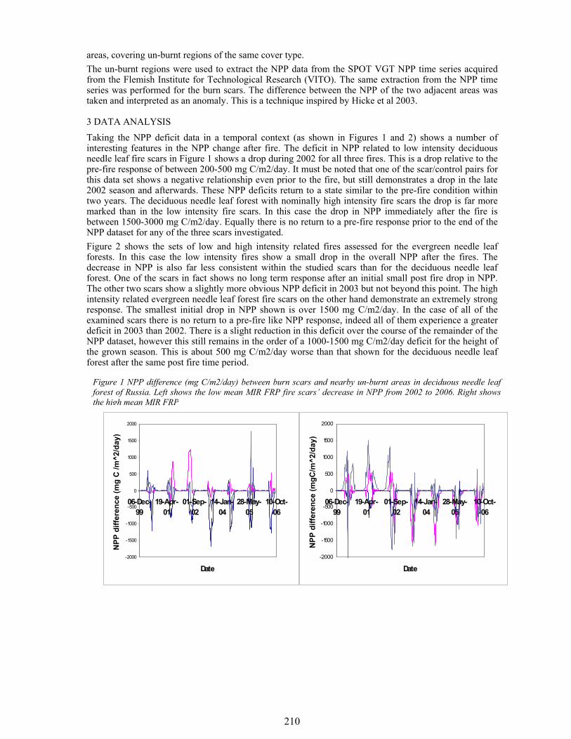
210

areas, covering un-burnt regions of the same cover type. The un-burnt regions were used to extract the NPP data from the SPOT VGT NPP time series acquired from the Flemish Institute for Technological Research (VITO). The same extraction from the NPP time series was performed for the burn scars. The difference between the NPP of the two adjacent areas was taken and interpreted as an anomaly. This is a technique inspired by Hicke et al 2003.

3 DATA ANALYSIS Taking the NPP deficit data in a temporal context (as shown in Figures 1 and 2) shows a number of interesting features in the NPP change after fire. The deficit in NPP related to low intensity deciduous needle leaf fire scars in Figure 1 shows a drop during 2002 for all three fires. This is a drop relative to the pre-fire response of between 200-500 mg C/m2/day. It must be noted that one of the scar/control pairs for this data set shows a negative relationship even prior to the fire, but still demonstrates a drop in the late 2002 season and afterwards. These NPP deficits return to a state similar to the pre-fire condition within two years. The deciduous needle leaf forest with nominally high intensity fire scars the drop is far more marked than in the low intensity fire scars. In this case the drop in NPP immediately after the fire is between 1500-3000 mg C/m2/day. Equally there is no return to a pre-fire response prior to the end of the NPP dataset for any of the three scars investigated. Figure 2 shows the sets of low and high intensity related fires assessed for the evergreen needle leaf forests. In this case the low intensity fires show a small drop in the overall NPP after the fires. The decrease in NPP is also far less consistent within the studied scars than for the deciduous needle leaf forest. One of the scars in fact shows no long term response after an initial small post fire drop in NPP. The other two scars show a slightly more obvious NPP deficit in 2003 but not beyond this point. The high intensity related evergreen needle leaf forest fire scars on the other hand demonstrate an extremely strong response. The smallest initial drop in NPP shown is over 1500 mg C/m2/day. In the case of all of the examined scars there is no return to a pre-fire like NPP response, indeed all of them experience a greater deficit in 2003 than 2002. There is a slight reduction in this deficit over the course of the remainder of the NPP dataset, however this still remains in the order of a 1000-1500 mg C/m2/day deficit for the height of the grown season. This is about 500 mg C/m2/day worse than that shown for the deciduous needle leaf forest after the same post fire time period.

-2000

-1500

-1000

-500

0

500

1000

1500

2000

06-Dec-99

19-Apr-01

01-Sep-02

14-Jan-04

28-May-05

10-Oct-06

Date

NPP

diff

eren

ce (m

gC/m

^2/d

ay)

-2000

-1500

-1000

-500

0

500

1000

1500

2000

06-Dec-99

19-Apr-01

01-Sep-02

14-Jan-04

28-May-05

10-Oct-06

Date

NPP

diff

eren

ce (m

g C

/m^2

/day

)

Figure 1 NPP difference (mg C/m2/day) between burn scars and nearby un-burnt areas in deciduous needle leaf forest of Russia. Left shows the low mean MIR FRP fire scars’ decrease in NPP from 2002 to 2006. Right shows the high mean MIR FRP

211

4 CONCLUSION This preliminary investigation suggests that there is a good chance that a variable derived from MIR FRP, in this case Mean MIR FRP, can be used as an indication of fire severity. Though this sample is too small to warrant any quantitative extrapolations at the present time it merits further investigation. It may be necessary to tailor any interpretations derived from MIR FRP intensity measures to the particular cover type as the evergreen needle leaf forest seemed to be more susceptible to high intensity fires than the deciduous needle leaf forest, at least within the limited scope of this investigation.

5 REFERENCES J.A Hicke, G.P Asner, E.S. Kasischke, N.H.F. French, J.T. Randerson, J.G. Collatz, B.J. Stocks, C.J. Tucker, S.O. Los, and C.B. Field. Postfire response of north american boreal forest net primary produictivity

analyzed with satellite observations. Global Change Biology, 9:1145–1157, 2003. C.O. Justice, L. Giglio, S. Korontzi, J. Owens, J.T. Morrisette, D Roy, J. Descloitres, S. Al-leaume, F. Petitcolin,

and Y. Kaufman. The MODIS fire products. Remote Sensing of Environment, 83:244–262, 2002. Herman H. Shugart, Rik Leemans, and Gordon B. Bonan, editors. A Systems analysis of the Global Boreal Forest.

Cambridge University Press, 1992. C. Wirth. Forest Diversity and Function: Ecological Studies 176, Temperate and Boreal Ecosystems, chapter 15,

Fire Regime and Tree Diversity in Boreal Forests : Implications for the Carbon Cycle. Springer, 2005. M.J Wooster, B Zhukov, and D Oertel. Fire radiative energy for quantitative study of biomass burning: derivation

from the bird experimantal sattelite and comparison to MODIS fire products. Remote Sensing of Environment, 86:83–107, 2003.

Woods Hole Research Center Web Site : http://www.whrc.org/borealnamerica/index.htm

-3000

-2500

-2000

-1500

-1000

-500

0

500

1000

1500

2000

06-Dec-99

19-Apr-01

01-Sep-02

14-Jan-04

28-May-05

10-Oct-06

Date

NPP

diff

eren

ce (m

g C

/m^2

/day

)

-2000

-1500

-1000

-500

0

500

1000

1500

2000

06-Dec-99

19-Apr-01

01-Sep-02

14-Jan-04

28-May-05

10-Oct-06

Date

NPP

(

mg

C/m

^2/D

ay)

Figure 2 NPP difference (mg C/m2/day) between burn scars and nearby un-burnt areas in evergreen needle leaf forest of Russia. Left shows the low mean MIR FRP fire scars’ decrease in NPP from 2002 to 2006. Right shows the high mean MIR FRP

212

1 INTRODUCTION Post-fire effect assessment and mapping is a useful tool from two points of view: (i) for post-fire planning, because it minimizes field work in restoration plans (Diaz Delgado, 2000; Chafer et al., 2004), and (ii) as information source for probabilistic models for fire simulation by using the existing relationships between post-fire effects and environmental parameters (Kushla and Ripple, 1997). Post-fire planning is crucial in areas with frequent precipitations, which require identifying and characterizing the scenario derived of precipitations rapidly, due to the possibility of suffering runoff phenomena. Although it is known that erosion is a consequence of post-fire precipitations, there are not many studies about how areas with different burn severity react to precipitations or how soils react regarding water repellence when different severities are considered (Shakesby et al. 2003; Chafer et al., 2004; Lewis et al., 2004). Zoning regarding post-fire intervention priority in Spain has been tackled in several studies (Díaz-Delgado, 2000; Navarro et al., 2001; Ruiz-Gallardo et al., 2004) by using post-fire effect mapping based on medium spatial resolution remote sensing imagery and achieving classification accuracies higher that 75%. Nevertheless the inconsistent use of fire descriptors (fire intensity, fire severity, burn severity) confuses measurement and interpretation of field and remote sensed fire effects. Lentile et al. (2006) recommend that processes associated with fire intensity and severity be evaluated in terms of either active fire characteristics or post fire effects. Therefore, post-fire effects would involve all measurements

An operational protocol for post-fire evaluation at landscape scale in an object-oriented environment

M.F. Álvarez University of León, Avda. Astorga sn 24400, Ponferrada (León), Spain, [email protected]

J.R. Rodríguez University of León, Avda. Astorga sn 24400, Ponferrada (León), Spain, [email protected]

D. Vega-Nieva University of Vigo, Campus As Lagoas, Pontevedra, Spain, [email protected]

F. Castedo-Dorado University of León, Avda. Astorga sn 24400, Ponferrada (León), Spain, [email protected] Keywords: object-oriented classification, post-fire evaluation, mapping, Landsat 5 TM, change detection, image processing protocol

ABSTRACT: Post-fire effect assessment and mapping in a very fragmented and diverse landscape is crucial to prioritize management actions, mainly when fires are very numerous and disperse. The processing protocol should be affordable and operational, in order to be applied when management decisions were required by the administration. The consistency and quality of the results is linked to the image processing stages to address image radiometry, normalization, and computation of the spectral indices. Computation errors, disk storage needs, and processing time required diminished when image processing steps were algebraically combined, so that the sequential integrated data processing protocol operates in memory and produces only the desired final outputs, and it can be easily repeated. The individual elements of the algorithm (raw Landsat 5 TM imagery, calibrated data, top-of-atmosphere reflectance, spectral indices) are described, as well as the protocol resulting of its combination. In this communication the processing protocol is utilized to map burns and post-fire effects in NW Spain. The resulting spectral indices were used as inputs in a new process, consisting on applying a non-parametric thresholding method to spectrally homogeneous objects. Thresholds were calibrated and validated using field data, gathered according to a protocol developed in coordination with the main fire research station in NW Spain. Validation of burn area classification using a random sample of 200 burn perimeters identified on the imagery showed 100% agreement with the results of the automatic classification, by using the dNDVI and NIRpostfire. If NIRpostfire was not used commission error increased significantly (at p > 0.001). The validation of the post-fire effect classification showed 100% agreement for moderate and high burn severity (post-fire effects), and 66% accuracy for the low class. Omission errors in the latter class are not very important in this environment, because those areas are not a priority for managers. Advantages of using an object-oriented approach instead of a pixel-based classification were demonstrated. Computing times for preprocessing decreased 50% using the IDL protocol, compared to the traditional approach. The adapted version of this protocol is therefore available to be used for detecting, mapping and classifying burn areas, so that 17 days are required to achieved the classifications and maps if one person is doing it. As a result, burns were mapped according to three post-fire effect levels, in agreement to the Ministry of Forestry request for a functional tool for decision making

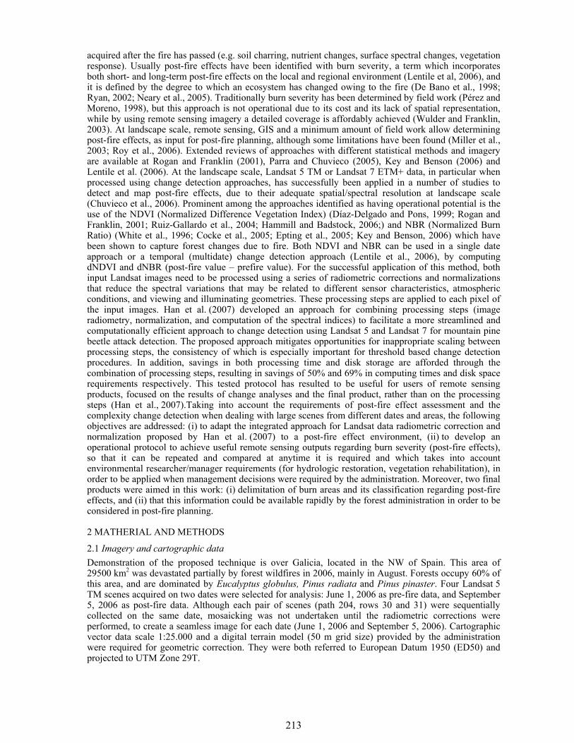
213

acquired after the fire has passed (e.g. soil charring, nutrient changes, surface spectral changes, vegetation response). Usually post-fire effects have been identified with burn severity, a term which incorporates both short- and long-term post-fire effects on the local and regional environment (Lentile et al, 2006), and it is defined by the degree to which an ecosystem has changed owing to the fire (De Bano et al., 1998; Ryan, 2002; Neary et al., 2005). Traditionally burn severity has been determined by field work (Pérez and Moreno, 1998), but this approach is not operational due to its cost and its lack of spatial representation, while by using remote sensing imagery a detailed coverage is affordably achieved (Wulder and Franklin, 2003). At landscape scale, remote sensing, GIS and a minimum amount of field work allow determining post-fire effects, as input for post-fire planning, although some limitations have been found (Miller et al., 2003; Roy et al., 2006). Extended reviews of approaches with different statistical methods and imagery are available at Rogan and Franklin (2001), Parra and Chuvieco (2005), Key and Benson (2006) and Lentile et al. (2006). At the landscape scale, Landsat 5 TM or Landsat 7 ETM+ data, in particular when processed using change detection approaches, has successfully been applied in a number of studies to detect and map post-fire effects, due to their adequate spatial/spectral resolution at landscape scale (Chuvieco et al., 2006). Prominent among the approaches identified as having operational potential is the use of the NDVI (Normalized Difference Vegetation Index) (Díaz-Delgado and Pons, 1999; Rogan and Franklin, 2001; Ruiz-Gallardo et al., 2004; Hammill and Badstock, 2006;) and NBR (Normalized Burn Ratio) (White et al., 1996; Cocke et al., 2005; Epting et al., 2005; Key and Benson, 2006) which have been shown to capture forest changes due to fire. Both NDVI and NBR can be used in a single date approach or a temporal (multidate) change detection approach (Lentile et al., 2006), by computing dNDVI and dNBR (post-fire value – prefire value). For the successful application of this method, both input Landsat images need to be processed using a series of radiometric corrections and normalizations that reduce the spectral variations that may be related to different sensor characteristics, atmospheric conditions, and viewing and illuminating geometries. These processing steps are applied to each pixel of the input images. Han et al. (2007) developed an approach for combining processing steps (image radiometry, normalization, and computation of the spectral indices) to facilitate a more streamlined and computationally efficient approach to change detection using Landsat 5 and Landsat 7 for mountain pine beetle attack detection. The proposed approach mitigates opportunities for inappropriate scaling between processing steps, the consistency of which is especially important for threshold based change detection procedures. In addition, savings in both processing time and disk storage are afforded through the combination of processing steps, resulting in savings of 50% and 69% in computing times and disk space requirements respectively. This tested protocol has resulted to be useful for users of remote sensing products, focused on the results of change analyses and the final product, rather than on the processing steps (Han et al., 2007).Taking into account the requirements of post-fire effect assessment and the complexity change detection when dealing with large scenes from different dates and areas, the following objectives are addressed: (i) to adapt the integrated approach for Landsat data radiometric correction and normalization proposed by Han et al. (2007) to a post-fire effect environment, (ii) to develop an operational protocol to achieve useful remote sensing outputs regarding burn severity (post-fire effects), so that it can be repeated and compared at anytime it is required and which takes into account environmental researcher/manager requirements (for hydrologic restoration, vegetation rehabilitation), in order to be applied when management decisions were required by the administration. Moreover, two final products were aimed in this work: (i) delimitation of burn areas and its classification regarding post-fire effects, and (ii) that this information could be available rapidly by the forest administration in order to be considered in post-fire planning.

2 MATHERIAL AND METHODS

2.1 Imagery and cartographic data Demonstration of the proposed technique is over Galicia, located in the NW of Spain. This area of 29500 km2 was devastated partially by forest wildfires in 2006, mainly in August. Forests occupy 60% of this area, and are dominated by Eucalyptus globulus, Pinus radiata and Pinus pinaster. Four Landsat 5 TM scenes acquired on two dates were selected for analysis: June 1, 2006 as pre-fire data, and September 5, 2006 as post-fire data. Although each pair of scenes (path 204, rows 30 and 31) were sequentially collected on the same date, mosaicking was not undertaken until the radiometric corrections were performed, to create a seamless image for each date (June 1, 2006 and September 5, 2006). Cartographic vector data scale 1:25.000 and a digital terrain model (50 m grid size) provided by the administration were required for geometric correction. They were both referred to European Datum 1950 (ED50) and projected to UTM Zone 29T.

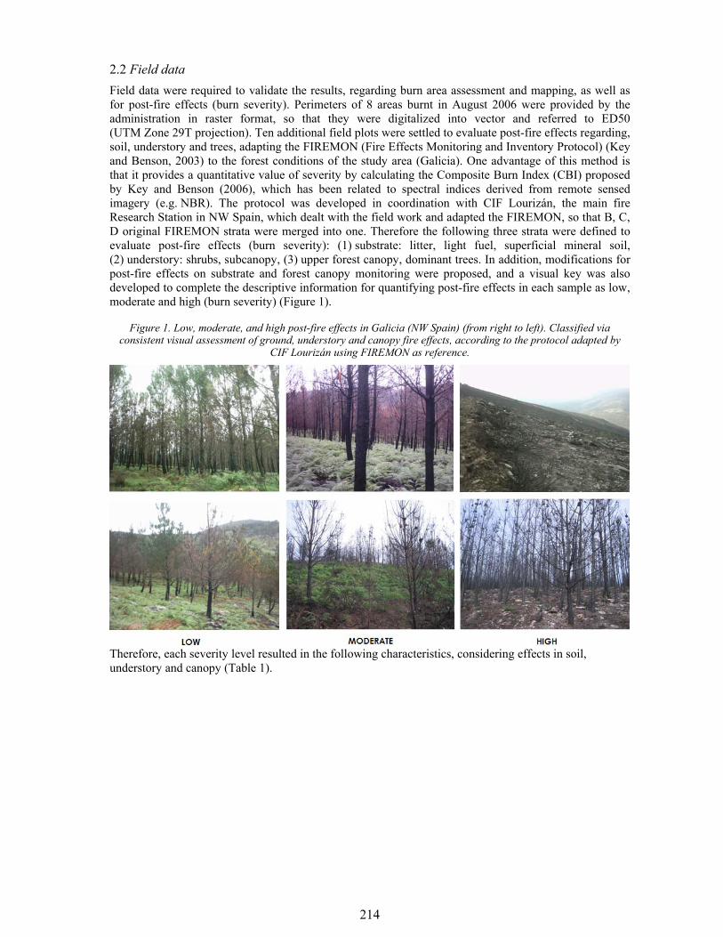
214

2.2 Field data Field data were required to validate the results, regarding burn area assessment and mapping, as well as for post-fire effects (burn severity). Perimeters of 8 areas burnt in August 2006 were provided by the administration in raster format, so that they were digitalized into vector and referred to ED50 (UTM Zone 29T projection). Ten additional field plots were settled to evaluate post-fire effects regarding, soil, understory and trees, adapting the FIREMON (Fire Effects Monitoring and Inventory Protocol) (Key and Benson, 2003) to the forest conditions of the study area (Galicia). One advantage of this method is that it provides a quantitative value of severity by calculating the Composite Burn Index (CBI) proposed by Key and Benson (2006), which has been related to spectral indices derived from remote sensed imagery (e.g. NBR). The protocol was developed in coordination with CIF Lourizán, the main fire Research Station in NW Spain, which dealt with the field work and adapted the FIREMON, so that B, C, D original FIREMON strata were merged into one. Therefore the following three strata were defined to evaluate post-fire effects (burn severity): (1) substrate: litter, light fuel, superficial mineral soil, (2) understory: shrubs, subcanopy, (3) upper forest canopy, dominant trees. In addition, modifications for post-fire effects on substrate and forest canopy monitoring were proposed, and a visual key was also developed to complete the descriptive information for quantifying post-fire effects in each sample as low, moderate and high (burn severity) (Figure 1).

Figure 1. Low, moderate, and high post-fire effects in Galicia (NW Spain) (from right to left). Classified via consistent visual assessment of ground, understory and canopy fire effects, according to the protocol adapted by

CIF Lourizán using FIREMON as reference.

Therefore, each severity level resulted in the following characteristics, considering effects in soil, understory and canopy (Table 1).

215

Table 1. Low, moderate, and high post-fire effects in Galicia (NW Spain): characteristics of each level according to the protocol adapted by CIF Lourizán using FIREMON as reference.

Effect on the strata Post-fire effect class Soil Understory Canopy cover

Low

Duff and litter affected by scorch. Mot exposed mineral soil

Shrub affected by scorch. Incomplete consumption of ferns.

Green crowns or occasionally scorched. Scorch height less than 2 m.

Moderate

Presence of duff affected by scorch. Less than 50% of the surface area showing exposed mineral soil.

Shrub retains the outer fine branching. Ferns have only the central stalk

Crowns that retain scorched leaves. Scorched height between than 4 and 7 m.

High

Exposed mineral soil, which can loose soil structure because of the consumption of the organic matter. Frequent presence of heating points.

Shrub only maintains the stump or the outer thick branching. Complete consumption of ferns.

Total consumption of the crown. Scorched height greater than 7 m or the whole tree.

2.3 Remote sensing approach: indices selection, preprocessing, classification and validation Burn area and post-fire effect detection and mapping were performed by using the dNDVI and dNBR indices. As the dNDVI and the dNBR are calculated based on the spectral indices derived from two input images, any variations between the inputs that are not indicative of actual changes in land cover should be minimized prior to their computation. Sources of such variations include different sensor characteristics, atmospheric conditions, and view and illumination geometries. A series of processing steps is proposed to reduce these possible sources of variation. The processing steps comprise top-of-atmosphere (TOA) radiance correction, TOA-reflectance correction, and normalization. The TOA-radiance and reflectance corrections are employed for atmospheric correction when in-situ measurements of atmospheric and climate conditions at the time of image acquisition are unknown and the imagery was acquired under clear-sky conditions. Using the gain and offset derived from dark and bright targets, the normalization is conducted to reduce image discrepancies possibly remaining from differing illumination geometries of the input imagery that were not fully addressed by the TOA-corrections. All this steps were semi-automatized in two IDL (ENVI scripts). Co-registration between images was performed, but not a geometric correction, in order to preserve original reflectance values as much as possible, so that orthorectification was performed on the final classification, not on the raw imagery. After imagery preprocessing and indices computation (as well as image differencing), imagery was segmented using a scale parameter of 10 (Alvarez, 2006) and bands TM 3, 4, 7 (post-fire image) and dNDVI (software eCognition 5.0). Burn area detection and mapping were performed using the dNDVI (NDVIpost-fire- NDVIpre-fire) and NIRpostfire (Band TM 4 in the post-fire image) values. Segments were classified in an object oriented approach, so that thresholding values were settled considering several burn areas identified visually on the image by using adequate band combinations. NIRpostfire was necessary to avoid misclassifications due to phenological differences in agricultural areas. Burn areas were later classified according to the three post-fire effects defined in Table 1 and Figure 1, by using the dNBR (NBRpost-fire- NBRpre-fire) and NBRpostfire values. Burn perimeters were validated using field data and visual tests on the images. Post-fire effect classification was validated with the field sample of 10 plots described above. Prior to calculating perimeters, areas and mapping, results were orthorectified using ERDAS Imagine and cartographic and MDT data described above. Afterwards a calendar identifying the critical steps of the process was developed, in order to help managers to decide whether the method is useful and operational for their rehabilitation interests.

3 RESULTS AND DISCUSSION Validation of burn area classification using a random sample of 200 burn perimeters identified on the imagery showed 100% agreement with the results of the automatic classification, by using the dNDVI and NIRpostfire. If NIRpostfire was not used commission error increased significantly (at p>0.001). If imagery from August or late July were available as pre-fire data source, phonological differences would be not so important and the NIR might be not so crucial, as reported in studies which only considered dNDVI (Ruiz-Gallardo et al., 2004; Hammill and Badstock, 2006; Díaz-Delgado and Pons, 1999; Rogan and Franklin, 2001).

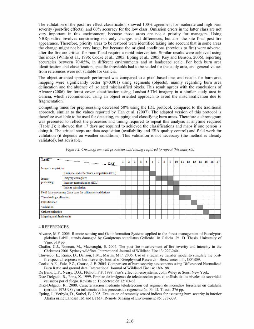
216

The validation of the post-fire effect classification showed 100% agreement for moderate and high burn severity (post-fire effects), and 66% accuracy for the low class. Omission errors in the latter class are not very important in this environment, because those areas are not a priority for managers. Using NBRpostfire involves considering not only changes and differences, but also the site final post-fire appearance. Therefore, priority areas to be restored were identified taking into account that in some areas the change might not be very large, but because the original conditions (previous to fire) were adverse, after the fire are critical for runoff and require a rapid intervention. Similar results were achieved using this index (White et al., 1996; Cocke et al., 2005; Epting et al., 2005; Key and Benson, 2006), reporting accuracies between 70-85%, in different environments and at landscape scale. For both burn area identification and classification, specific thresholds had to be settled for the study area, and general values from references were not suitable for Galicia. The object-oriented approach performed was compared to a pixel-based one, and results for burn area mapping were significantly better (p>0.001) using segments (objects), mainly regarding burn area delineation and the absence of isolated misclassified pixels. This result agrees with the conclusions of Alvarez (2006) for forest cover classification using Landsat 5 TM imagery in a similar study area in Galicia, which recommended using an object oriented approach to avoid the misclassification due to fragmentation. Computing times for preprocessing decreased 50% using the IDL protocol, compared to the traditional approach, similar to the values reported by Han et al. (2007). The adapted version of this protocol is therefore available to be used for detecting, mapping and classifying burn areas. Therefore a chronogram was presented to reflect the processes and timing required to repeat this analysis at anytime required (Table 2); it showed that 17 days are required to achieved the classifications and maps if one person is doing it. The critical steps are data acquisition (availability and ESA quality control) and field work for validation (it depends on weather conditions). This validation is not necessary (the method is already validated), but advisable.

Figure 2. Chronogram with processes and timing required to repeat this analysis.

4 REFERENCES Alvarez, M.F. 2006. Remote sensing and Geoinformation Systems applied to the forest management of Eucalyptus

globulus Labill. stands damaged by Gonipterus scutellatus Gyllenhal in Galicia. Ph. D. Thesis. University of Vigo. 319 pp.

Chafter, C.J., Noonan, M., Macnaught, E. 2004. The post-fire measurement of fire severity and intensity in the Christmas 2001 Sydney wildfires. International Journal of Wildland Fire 13: 227-240.

Chuvieco, E., Riaño, D., Danson, F.M., Martín, M.P. 2006. Use of a radiative transfer model to simulate the post-fire spectral response to burn severity. Journal of Geophysical Research - Biosciences 111, G04S09.

Cocke, A.E., Fule, P.Z., Crouse, J. E. 2005. Comparison of burn severity assessments using Differenced Normalized Burn Ratio and ground data. International Journal of Wildland Fire 14: 189-198.

De Bano, L.F., Neary, D.G., Ffoliott, P.F. 1998. Fire’s effect on ecosystems. John Wiley & Sons. New York. Díaz-Delgado, R., Pons, X. 1999. Empleo de imágenes de teledetección para el análisis de los niveles de severidad

causados por el fuego. Revista de Teledetección 12: 63-68. Díaz-Delgado, R., 2000. Caracterización mediante teledetección del régimen de incendios forestales en Cataluña

(periodo 1975-98) y su influencia en los procesos de regeneración. Ph. D. Thesis. 276 pp. Epting, J., Verbyla, D., Sorbel, B. 2005. Evaluation of remotely sensed indices for assessing burn severity in interior

Alaska using Landsat TM and ETM+. Remote Sensing of Environment 96: 328-339.

217

Hammill, K.A., Badstock, R.A. 2006. Remote sensing of fire severity in the Blue Mountains: influence of vegetation type and inferring fire intensity. International Journal of Wildland Fire 15: 213-226.

Han, T., Wulder, M.A., White J.C., Coops N.C., Álvarez M.F., Butson, C. 2007. An efficient protocol to process Landsat images for change detection with Tasselled Cap Transformation, IEEE Geoscience and Remote Sensing Letters. 4 (1): 147-151.

Key, C.H., Benson, N.C. 2003. Final Draft- Landscape Assessment (LA) Sampling & Analysis Methods. Available at

Key, C.H., Benson, N.C. 2006. Landscape Assessment: Ground measure of severity, the Composite Burn Index; and Remote sensing of severity, the Normalized Burn Ratio. In: Lutes, D.C., Keane, R.E., Caratti, J.F. et al., (Eds.) FIREMON: Fire Effects Monitoring and Inventory System. Ogden, UT, USDA Forest Service, Rocky Mountain Research Station, Gen. Tech. Rep. RMRS-GTR-164: CD:LA1-LA51.

Kushla, J.D., Ripple, W.J. 1998. Assessing wildfire effects with Landsat Thematic Mapper data. International Journal of Remote Sensing 19(13): 2493–2507.

Lewis, S.A., Robichaud, P.R., Elliot, W.J., Frazier, B.E., Wu, J.Q. 2004. Hyperspectral Remote Sensing of Postfire Soil Properties. In: Remote Sensing for Field Users, Proceedings of the Tenth Forest Service Remote Sensing Applications Conference, Salt Lake City, Utah, April 5-9, 2004. CD-ROM. 9 pp.

Lentile, L.B., Holden, Z.A., Smith, A.M.S., Falkowski, M.J., Hudak, A.T., Morgan, P., Lewis, S.A., Gessler, P.E., Benson, N.C. 2006. Remote sensing techniques to assess active fire characteristics and post-fire effects. International Journal of Wildland Fire 15: 319-345.

Miller, D., Luce, C., Benda, L. 2003. Time, space and episodicity of physical disturbance in streams. Forest Ecology and Management 178: 121-140.

Navarro, R.M., Fernández. F., Escuin, S. 2001. Evaluación de daños producidos por incendios forestales mediante imágenes de satélite. Propuesta de restauración. In: III Congreso forestal Español, 25–28 September 2001: 482–487.

Neary, D.G., Ffolliott, P.F., Landsberg, J.D. 2005. Fire and streamflow regimes. In: Neary, D.G., Ryan K.C., DeBano, L.F. (Eds.) Wildland Fire in Ecosystems: Effects of Fire on Soil and Water. General Technical Report RMRS-GTR-42, vol. 4, Rocky Mountain Research Station, Forest Service, U.S. Department of Agriculture, Fort Collins, Colorado:. 107-118.

Parra, A., Chuvieco E. 2005. Assessing burn severity using Hyperion data. In: Riva, J., Pérez-Cabello, F., Chuvieco, F. (Eds.) Proceedings of the 5th International Workshop on Remote Sensing and GIS applications to Forest Fire Management: Fire Effects Assessment (editado por). Paris, Universidad de Zaragoza, GOFC-GOLD, EARSeL: 239-244.

Pérez, B., Moreno, J.M. 1998. Fire-type and forestry management effects on the early postfire vegetation dynamics of a Pinus pinaster woodland. Plant Ecology 134: 27-41.

Rogan, J., Franklin, J. 2001. Mapping wildfire burn severity in southern California forests and shrublands using Enhanced Thematic Mapper imagery, GeoCarto International 16: 89-99.

Roy, D.P., Boschetti, L., Trigg, S. 2006. Remote Sensing of Fire Severity: Assessing the performance of the Normalized Burn Ratio. IEEE Geoscience and Remote Sensing Letters 3: 112- 116.

Ruiz-Gallardo, J.R., Castaño, S., Calera, A. 2004. Application of remote sensing and GIS to locate priority intervention areas after wildland fires in Mediterranean systems: a case study from south-eastern Spain. International Journal of Wildland Fire 13: 241-252.

Ryan, K.C. 2002. Dynamic interactions between forest structure and fire behavior in boreal ecosystems. Silva Fennica 36(1): 13-39.

Shakesby, R.A., Chafer, C.J., Doerr, S.H., Blake, W.H., Wallbrink, P.J., Humphreys, G.S., Harrington, B.A. 2003. Fire severity, water repellency characteristics and hydrogeomorphological changes following the Christmas 2001 Sydney forest fires. Australian Geographer 34: 147-175.

White, J.D., Ryan, K.C., Key, C.K., Running, S.W. 1996. Remote sensing of forest fire severity and vegetation recovery. International Journal of Wildland Fire 6: 125-136.

Wulder, M., Franklin, S. 2003. Remote sensing of forest environments, Introduction: The transition from theory to information, In: Wulder M., Franklin, S. (Eds.) Remote Sensing of Forest Environments: Concepts and Case Studies, Kluwer Academic Publishers, Dordrecht / Boston / London, 519 pp.

218

Analysis of the causality of fires (1985-1997) in Macedonia, Greece

George D. Mouflis & Ioannis Z. Gitas Laboratory of Forest Management and Remote Sensing, School of Forestry and Natural Environment, Aristotle University of Thessaloniki P.O. Box 248, GR 541 24, Thessaloniki, Greece, e-mails:[email protected], [email protected]

Keywords: fire cause, elevation, proximity, distance, towns, roads, rivers.

ABSTRACT: Fire is an integral part of many ecosystems, particularly in Mediterranean areas. In the preceding decades there has been an exponential increase in the number of fires in European Mediterranean areas. Wildfires however are mainly due to human-related causes. As a result, an analysis of possible associations of particular fire causes with the underlying topographic and anthropogenic template would be useful in the understanding of the fire causality. The aim of this paper was to determine if different fire causes exhibit a statistically significant preferential occurrence under particular physiographic or human-related conditions, specifically proximity to urban centres, roads and rivers. The data analysed were the geographical distribution of fires that occurred during the period 1985-1997 in Macedonia, Greece. The methodology was multiple comparison of means of fire causes in single factor ANOVAs and polynomial regression. The results showed that there were significant differences in the distribution of fire causes relative to the underlying topography and distance to towns and roads and these results are discussed. Arson, stubble burning and pasture burning were the most serious known causes accounting for 48% of the total area burnt.

1 INTRODUCTION Wildland fires constitute serious natural hazards in countries with warm and dry summers as in the Mediterranean basin; they inflict grave cost to the environment, the economy and the social welfare in rural or even urban areas. A key driver of the increase of fire numbers and sizes over the last decades (Moreno et al., 1998), is rural depopulation and abandonment of agricultural land which shifts to scrubland and forest and the associated fuel build-up (Le Houérou, 1987; Moreira et al., 2001; Romero-Calcerrada & Perry, 2002).

2 STUDY AREA AND DATASETS DESCRIPTION The study area is the geographic department of Macedonia (north Greece) having an area of 34,231 km² (3,423,100 ha) and a population of 2,625,681. Wildfire ignition locations georeferenced data were obtained for this area covering a time-span of 13 years. The aim was to analyse the causes of fire occurrences of the period 1985-1997, in Macedonia, Greece, in relation to topographic relief, distance from towns, roads and rivers. Specific objectives were to examine if individual causes of fires occur in different ranges of the variables examined. The data on fires that occurred throughout Macedonia between 1985-1997 (study period), were obtained from the Mininistry of Rural Development and Food, General Secretariat of Forests and Natural Environment and imported into a GIS. The 3347 ignition locations of wildfires that occurred during the study period were combined with the 30m resolution raster layers of DEM, aspect, slope, distance to towns, roads and rivers to extract a comprehensive dataset of conditions present at these locations. For each fire event there was a description of the cause of fire ignition. Apart from unknown/unspecified category, there were 18 specified causes that are presented in Table.

3 METHODS

The relationship of each independent variable with fire occurrence frequency was examined by regression and each of the eighteen causes was examined for differences of means with single factor analysis of variance, using Bonferroni-corrected confidence intervals for the number of fire causes compared.

4 RESULTS

During the 13 years of the study period 3347 fires occurred, which burnt 110,947.4 ha or 3.24% of the study area. The estimated fire rotation period (fr) is therefore fr=13/(110947.4/3423100)= 401 years (Díaz-Delgado et al., 2004). This theoretical rotation period means that every 400 years a cumulative area equal to the total study area of Macedonia gets burnt, although actual fire recurrence is considerably

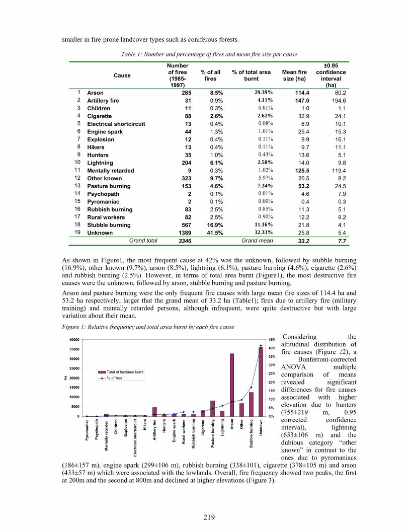
219

smaller in fire-prone landcover types such as coniferous forests.

Table 1: Number and percentage of fires and mean fire size per cause

Cause Number of fires (1985-1997)

% of all fires

% of total area burnt

Mean fire size (ha)

±0.95 confidence

interval (ha)

1 Arson 285 8.5% 29.39% 114.4 80.2 2 Artillery fire 31 0.9% 4.11% 147.0 194.6 3 Children 11 0.3% 0.01% 1.0 1.1 4 Cigarette 88 2.6% 2.61% 32.9 24.1 5 Electrical shortcircuit 13 0.4% 0.08% 6.9 10.1 6 Engine spark 44 1.3% 1.01% 25.4 15.3 7 Explosion 12 0.4% 0.11% 9.9 16.1 8 Hikers 13 0.4% 0.11% 9.7 11.1 9 Hunters 35 1.0% 0.43% 13.6 5.1

10 Lightning 204 6.1% 2.58% 14.0 9.8 11 Mentally retarded 9 0.3% 1.02% 125.5 119.4 12 Other known 323 9.7% 5.97% 20.5 8.2 13 Pasture burning 153 4.6% 7.34% 53.2 24.5 14 Psychopath 2 0.1% 0.01% 4.6 7.9 15 Pyromaniac 2 0.1% 0.00% 0.4 0.3 16 Rubbish burning 83 2.5% 0.85% 11.3 5.1 17 Rural workers 82 2.5% 0.90% 12.2 9.2 18 Stubble burning 567 16.9% 11.16% 21.8 4.1 19 Unknown 1389 41.5% 32.33% 25.8 5.4

Grand total 3346 Grand mean 33.2 7.7 As shown in Figure1, the most frequent cause at 42% was the unknown, followed by stubble burning (16.9%), other known (9.7%), arson (8.5%), lightning (6.1%), pasture burning (4.6%), cigarette (2.6%) and rubbish burning (2.5%). However, in terms of total area burnt (Figure1), the most destructive fire causes were the unknown, followed by arson, stubble burning and pasture burning. Arson and pasture burning were the only frequent fire causes with large mean fire sizes of 114.4 ha and 53.2 ha respectively, larger that the grand mean of 33.2 ha (Table1); fires due to artillery fire (military training) and mentally retarded persons, although infrequent, were quite destructive but with large variation about their mean. Figure 1: Relative frequency and total area burnt by each fire cause

Considering the altitudinal distribution of fire causes (Figure 22), a

Bonferroni-corrected ANOVA multiple comparison of means revealed significant differences for fire causes associated with higher elevation due to hunters (755±219 m, 0.95 corrected confidence interval), lightning (653±106 m) and the dubious category “other known” in contrast to the ones due to pyromaniacs

(186±157 m), engine spark (299±106 m), rubbish burning (338±101), cigarette (378±105 m) and arson (433±57 m) which were associated with the lowlands. Overall, fire frequency showed two peaks, the first at 200m and the second at 800m and declined at higher elevations (Figure 3).

0

5000

10000

15000

20000

25000

30000

35000

40000

Pyro

man

iac

Psyc

hopa

th

Men

tally

ret

arde

d

Child

ren

Exp

losi

on

Elec

trica

l sho

rtcir

cuit

Hike

rs

Artil

lery

fire

Hunt

ers

Engi

ne s

park

Rur

al w

orke

rs

Rubb

ish

burn

ing

Cig

aret

te

Past

ure

burn

ing

Ligh

tnin

g

Ars

on

Oth

er

Stub

ble

burn

ing

Unk

now

n

ha

0%

5%

10%

15%

20%

25%

30%

35%

40%

45%

Total of hectares burnt% of fires

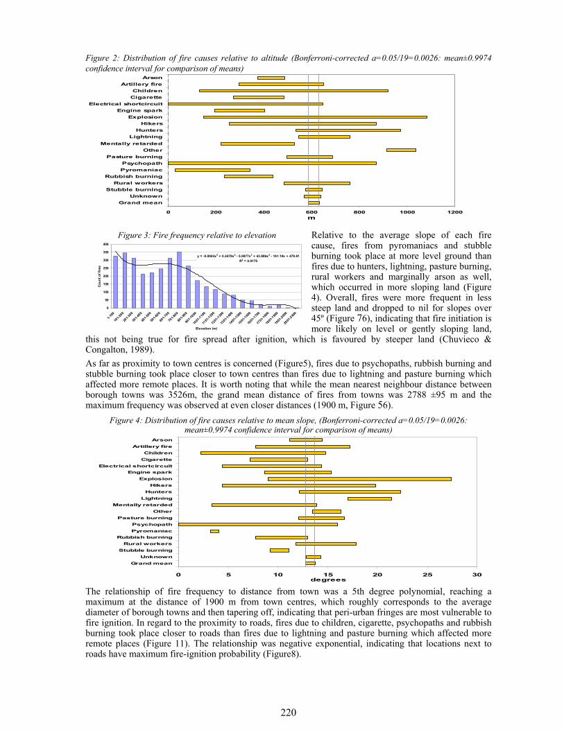
220

Figure 2: Distribution of fire causes relative to altitude (Bonferroni-corrected a=0.05/19=0.0026: mean±0.9974 confidence interval for comparison of means)

0 200 400 600 800 1000 1200

ArsonArtillery fire

ChildrenCigarette

Electrical shortcircuitEngine spark

ExplosionHikers

HuntersLightning

Mentally retardedOther

Pasture burningPsychopathPyromaniac

Rubbish burningRural workers

Stubble burningUnknown

Grand mean

m

Relative to the average slope of each fire cause, fires from pyromaniacs and stubble burning took place at more level ground than fires due to hunters, lightning, pasture burning, rural workers and marginally arson as well, which occurred in more sloping land (Figure 4). Overall, fires were more frequent in less steep land and dropped to nil for slopes over 45º (Figure 76), indicating that fire initiation is more likely on level or gently sloping land,

this not being true for fire spread after ignition, which is favoured by steeper land (Chuvieco & Congalton, 1989). As far as proximity to town centres is concerned (Figure5), fires due to psychopaths, rubbish burning and stubble burning took place closer to town centres than fires due to lightning and pasture burning which affected more remote places. It is worth noting that while the mean nearest neighbour distance between borough towns was 3526m, the grand mean distance of fires from towns was 2788 ±95 m and the maximum frequency was observed at even closer distances (1900 m, Figure 56).

Figure 4: Distribution of fire causes relative to mean slope, (Bonferroni-corrected a=0.05/19=0.0026: mean±0.9974 confidence interval for comparison of means)

The relationship of fire frequency to distance from town was a 5th degree polynomial, reaching a maximum at the distance of 1900 m from town centres, which roughly corresponds to the average diameter of borough towns and then tapering off, indicating that peri-urban fringes are most vulnerable to fire ignition. In regard to the proximity to roads, fires due to children, cigarette, psychopaths and rubbish burning took place closer to roads than fires due to lightning and pasture burning which affected more remote places (Figure 11). The relationship was negative exponential, indicating that locations next to roads have maximum fire-ignition probability (Figure8).

Figure 3: Fire frequency relative to elevation

y = -0.0043x5 + 0.2479x4 - 5.0877x3 + 43.806x2 - 161.19x + 479.81R2 = 0.9179

0

50

100

150

200

250

300

350

400

1-100

101-2

00

201-3

00

301-4

00

401-5

00

501-6

00

601-7

00

701-8

00

801-9

00

901-1

000

1001

-1100

1101

-1200

1201

-1300

1301

-1400

1401

-1500

1501

-1600

1601

-1700

1701

-1800

1801

-1900

1901

-2000

2001

-2400

Elevation (m)

Cou

nt o

f fire

s

0 5 10 15 20 25 30

ArsonArtillery fire

ChildrenCigarette


ExplosionHikers

HuntersLightning





Grand mean

degrees

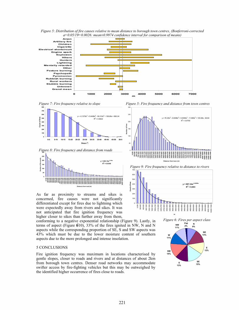
221

Figure 5: Distribution of fire causes relative to mean distance to borough town centres, (Bonferroni-corrected

a=0.05/19=0.0026: mean±0.9974 confidence interval for comparison of means)

0 1000 2000 3000 4000 5000 6000 7000

ArsonArtillery fire

ChildrenCigarette


ExplosionHikers

HuntersLightning





Grand mean

m

As far as proximity to streams and sikes is concerned, fire causes were not significantly differentiated except for fires due to lightning which were expectedly away from rivers and sikes. It was not anticipated that fire ignition frequency was higher closer to sikes than further away from them, conforming to a negative exponential relationship (Figure 9). Lastly, in terms of aspect (Figure 610), 33% of the fires ignited in NW, N and N aspects while the corresponding proportion of SE, S and SW aspects was 43% which must be due to the lower moisture content of southern aspects due to the more prolonged and intense insolation.

5 CONCLUSIONS Fire ignition frequency was maximum in locations characterised by gentle slopes, closer to roads and rivers and at distances of about 2km from borough town centres. Denser road networks may accommodate swifter access by fire-fighting vehicles but this may be outweighed by the identified higher occurrence of fires close to roads.

Figure 7: Fire frequency relative to slope

y = -0.1576x4 + 5.6498x3 - 58.316x2 + 106.66x + 682.24R2 = 0.9922

0

100

200

300

400

500

600

700

800

0-5 5-10 10-15 15-20 20-25 25-30 30-35 35-40 40-45 45-50 50-55

Slope (o)

Cou

nt o

f fire

s

Figure 9: Fire frequency relative to distance to rivers

y = 887,34e-0,2929x

R2 = 0,903

0

100

200

300

400

500

600

700

0-30

0

300-

600

600-

900

900-

1200

1200

-150

0

1500

-180

0

1800

-210

0

2100

-240

0

2400

-270

0

2700

-300

0

3000

-330

0

3300

-360

0

3600

-390

0

3900

-420

0

4200

-450

0

4500

-480

0

4800

-550

0

5500

-600

0

4800

-550

0

5500

-600

0

6000

-650

0

6500

-700

0

7000

-800

0

8000

-900

0

9000

-100

00

1000

0-11

000

m

Cou

nt o

f fir

es

Figure 8: Fire frequency and distance from roads

y = 285.18e-0.084x

R2 = 0.9348

0

50

100

150

200

250

300

0-10

010

0-20

020

0-30

030

0-40

040

0-50

050

0-60

060

0-70

070

0-80

080

0-90

090

0-10

0010

00-1

100

1100

-120

012

00-1

300

1300

-140

014

00-1

500

1500

-160

016

00-1

700

1700

-180

018

00-1

900

1900

-200

020

00-2

100

2100

-220

022

00-2

300

2300

-240

024

00-2

500

2500

-260

026

00-2

700

2700

-280

028

00-2

900

2900

-300

030

00-3

100

3100

-320

032

00-3

300

3300

-340

034

00-3

500

3500

-360

036

00-3

700

3700

-380

038

00-3

900

3900

-400

040

00-4

150

4150

-430

043

00-4

500

4500

-480

048

00-5

100

5100

-550

055

00-6

000

6000

-650

065

00-7

500

7500

-900

090

00-1

2000

Distance from road (m)

Num

ber o

f fire

eve

nts

Figure 6: Fires per aspect class N

9%

NE13%

E12%

SE15%

S13%

SW14%

W11%

NW11%

Flat2%

Figure 5: Fire frequency and distance from town centres

y = 7E-05x5 - 0.0098x4 + 0.5056x3 - 11.669x2 + 105.98x - 90.64R2 = 0.9759

0

50

100

150

200

250

300

0-25

025

0-50

050

0-75

075

0-10

0010

00-1

250

1250

-150

015

00-1

750

1750

-200

020

00-2

250

2250

-250

025

00-2

750

2750

-300

030

00-3

250

3250

-350

035

00-3

750

3750

-400

040

00-4

250

4250

-450

045

00-4

750

4750

-500

050

00-5

250

5250

-550

055

00-5

750

5750

-600

060

00-6

250

6250

-650

065

00-6

750

6750

-700

070

00-7

250

7250

-750

075

00-7

750

7750

-800

080

00-8

250

8250

-850

085

00-8

750

8750

-900

090

00-1

0000

1000

0-11

000

1100

0-12

000

1200

0-14

000

1400

0-21

000

Distance from town (m)

Num

ber o

f fire

s

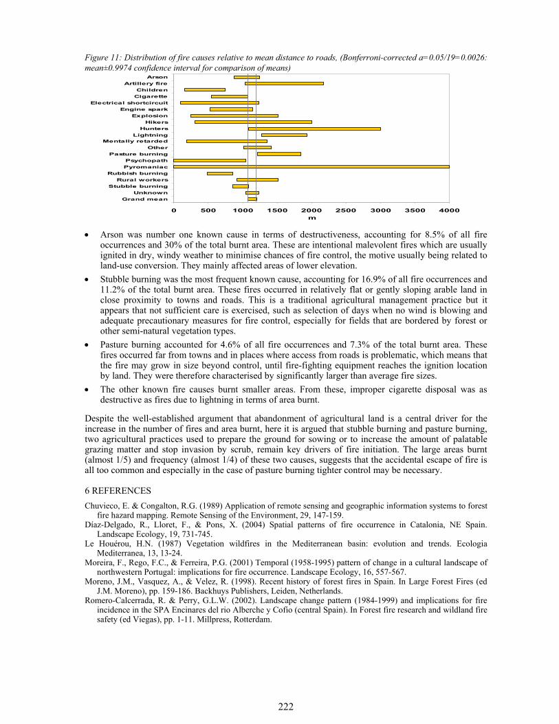
222

Figure 11: Distribution of fire causes relative to mean distance to roads, (Bonferroni-corrected a=0.05/19=0.0026: mean±0.9974 confidence interval for comparison of means)

0 500 1000 1500 2000 2500 3000 3500 4000

ArsonArtillery fire

ChildrenCigarette


ExplosionHikers

HuntersLightning





Grand mean

m

• Arson was number one known cause in terms of destructiveness, accounting for 8.5% of all fire occurrences and 30% of the total burnt area. These are intentional malevolent fires which are usually ignited in dry, windy weather to minimise chances of fire control, the motive usually being related to land-use conversion. They mainly affected areas of lower elevation.

• Stubble burning was the most frequent known cause, accounting for 16.9% of all fire occurrences and 11.2% of the total burnt area. These fires occurred in relatively flat or gently sloping arable land in close proximity to towns and roads. This is a traditional agricultural management practice but it appears that not sufficient care is exercised, such as selection of days when no wind is blowing and adequate precautionary measures for fire control, especially for fields that are bordered by forest or other semi-natural vegetation types.

• Pasture burning accounted for 4.6% of all fire occurrences and 7.3% of the total burnt area. These fires occurred far from towns and in places where access from roads is problematic, which means that the fire may grow in size beyond control, until fire-fighting equipment reaches the ignition location by land. They were therefore characterised by significantly larger than average fire sizes.

• The other known fire causes burnt smaller areas. From these, improper cigarette disposal was as destructive as fires due to lightning in terms of area burnt.

Despite the well-established argument that abandonment of agricultural land is a central driver for the increase in the number of fires and area burnt, here it is argued that stubble burning and pasture burning, two agricultural practices used to prepare the ground for sowing or to increase the amount of palatable grazing matter and stop invasion by scrub, remain key drivers of fire initiation. The large areas burnt (almost 1/5) and frequency (almost 1/4) of these two causes, suggests that the accidental escape of fire is all too common and especially in the case of pasture burning tighter control may be necessary.

6 REFERENCES Chuvieco, E. & Congalton, R.G. (1989) Application of remote sensing and geographic information systems to forest

fire hazard mapping. Remote Sensing of the Environment, 29, 147-159. Díaz-Delgado, R., Lloret, F., & Pons, X. (2004) Spatial patterns of fire occurrence in Catalonia, NE Spain.

Landscape Ecology, 19, 731-745. Le Houérou, H.N. (1987) Vegetation wildfires in the Mediterranean basin: evolution and trends. Ecologia

Mediterranea, 13, 13-24. Moreira, F., Rego, F.C., & Ferreira, P.G. (2001) Temporal (1958-1995) pattern of change in a cultural landscape of

northwestern Portugal: implications for fire occurrence. Landscape Ecology, 16, 557-567. Moreno, J.M., Vasquez, A., & Velez, R. (1998). Recent history of forest fires in Spain. In Large Forest Fires (ed

J.M. Moreno), pp. 159-186. Backhuys Publishers, Leiden, Netherlands. Romero-Calcerrada, R. & Perry, G.L.W. (2002). Landscape change pattern (1984-1999) and implications for fire

incidence in the SPA Encinares del rio Alberche y Cofio (central Spain). In Forest fire research and wildland fire safety (ed Viegas), pp. 1-11. Millpress, Rotterdam.

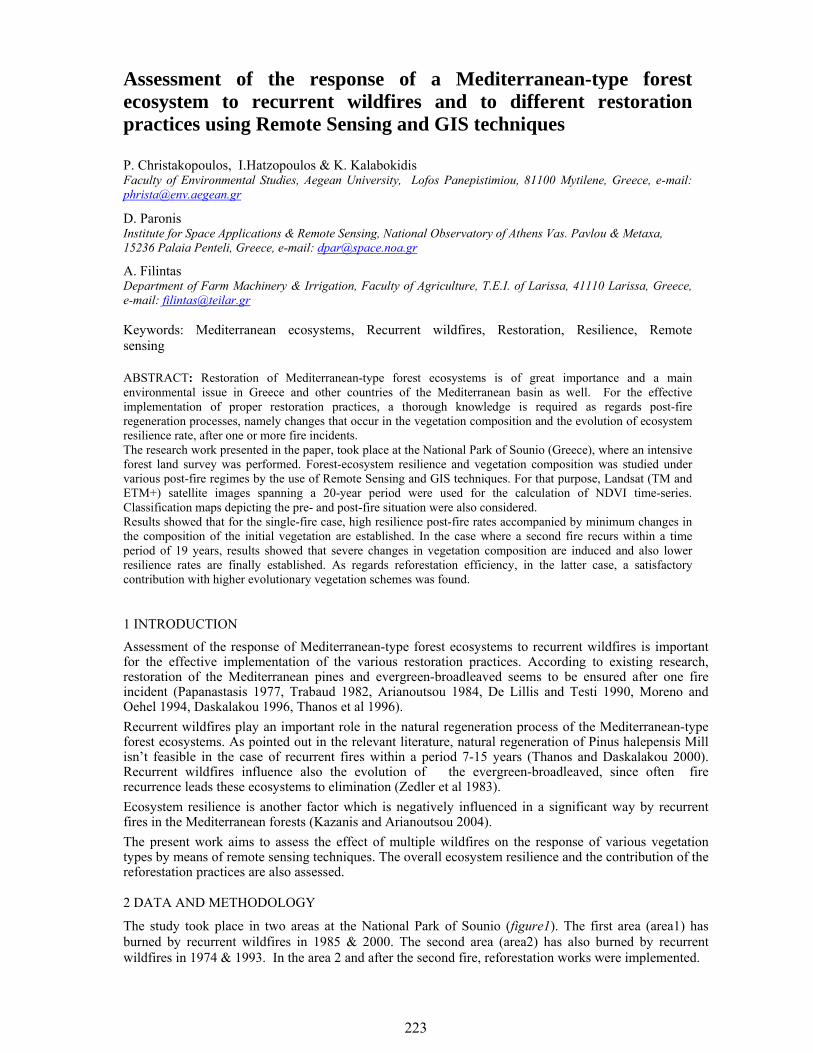
223

1 INTRODUCTION

Assessment of the response of Mediterranean-type forest ecosystems to recurrent wildfires is important for the effective implementation of the various restoration practices. According to existing research, restoration of the Mediterranean pines and evergreen-broadleaved seems to be ensured after one fire incident (Papanastasis 1977, Trabaud 1982, Arianoutsou 1984, De Lillis and Testi 1990, Moreno and Oehel 1994, Daskalakou 1996, Thanos et al 1996). Recurrent wildfires play an important role in the natural regeneration process of the Mediterranean-type forest ecosystems. As pointed out in the relevant literature, natural regeneration of Pinus halepensis Mill isn’t feasible in the case of recurrent fires within a period 7-15 years (Thanos and Daskalakou 2000). Recurrent wildfires influence also the evolution of the evergreen-broadleaved, since often fire recurrence leads these ecosystems to elimination (Zedler et al 1983). Ecosystem resilience is another factor which is negatively influenced in a significant way by recurrent fires in the Mediterranean forests (Kazanis and Arianoutsou 2004). The present work aims to assess the effect of multiple wildfires on the response of various vegetation types by means of remote sensing techniques. The overall ecosystem resilience and the contribution of the reforestation practices are also assessed.

2 DATA AND METHODOLOGY

The study took place in two areas at the National Park of Sounio (figure1). The first area (area1) has burned by recurrent wildfires in 1985 & 2000. The second area (area2) has also burned by recurrent wildfires in 1974 & 1993. In the area 2 and after the second fire, reforestation works were implemented.

Assessment of the response of a Mediterranean-type forest ecosystem to recurrent wildfires and to different restoration practices using Remote Sensing and GIS techniques

P. Christakopoulos, I.Hatzopoulos & K. Kalabokidis Faculty of Environmental Studies, Aegean University, Lofos Panepistimiou, 81100 Mytilene, Greece, e-mail: [email protected]

D. Paronis Institute for Space Applications & Remote Sensing, National Observatory of Athens Vas. Pavlou & Metaxa, 15236 Palaia Penteli, Greece, e-mail: [email protected]

A. Filintas Department of Farm Machinery & Irrigation, Faculty of Agriculture, T.E.I. of Larissa, 41110 Larissa, Greece, e-mail: [email protected] Keywords: Mediterranean ecosystems, Recurrent wildfires, Restoration, Resilience, Remote sensing ABSTRACT: Restoration of Mediterranean-type forest ecosystems is of great importance and a main environmental issue in Greece and other countries of the Mediterranean basin as well. For the effective implementation of proper restoration practices, a thorough knowledge is required as regards post-fire regeneration processes, namely changes that occur in the vegetation composition and the evolution of ecosystem resilience rate, after one or more fire incidents. The research work presented in the paper, took place at the National Park of Sounio (Greece), where an intensive forest land survey was performed. Forest-ecosystem resilience and vegetation composition was studied under various post-fire regimes by the use of Remote Sensing and GIS techniques. For that purpose, Landsat (TM and ETM+) satellite images spanning a 20-year period were used for the calculation of NDVI time-series. Classification maps depicting the pre- and post-fire situation were also considered. Results showed that for the single-fire case, high resilience post-fire rates accompanied by minimum changes in the composition of the initial vegetation are established. In the case where a second fire recurs within a time period of 19 years, results showed that severe changes in vegetation composition are induced and also lower resilience rates are finally established. As regards reforestation efficiency, in the latter case, a satisfactory contribution with higher evolutionary vegetation schemes was found.

224

Six Landsat (TM and ETM+) satellite images (1984, 1987, 1990, 1999, 2002 and 2005) and one IKONOS image (2004) were used. All images were calibrated and corrected geometrically and atmospherically. In order to study the vegetation evolution after the recurrent wildfires, classification maps were produced from two Landsat satellite images for years 1984, 1999 and the IKONOS image for year 2004 (figure3). Supervised classification techniques aided by photo-interpretation of aerial photos and ortho-maps produced by the forest service, were applied. For the 2004 image, suitable training areas were carefully selected during a field campaign. For the estimation of the ecosystem resilience, a parameter which is related to the total vegetation biomass, average NDVI values were calculated for the study areas for the six years under consideration. For each year, a resilience indicator R was computed as the ratio of the average NDVI value of an area that has been burned, to the value of a neighbouring unburned stud. The resilience indicator R has proven to be insensitive to factors such as moisture, visibility, and temperature variations (Diaz-Delgado et al 2002).


The evolution of vegetation coverage in the area which was burned twice by recurrent fires in 1985 and 2000 is presented in figure 2:

Figure 1: Areas of study in National Park of Sounio

Figure2: The evolution of vegetation coverage after two recurrent wildfires in 1985 & 2000 (area 1)

050

100150200250300350400450500

1984 1985 1999 2000 2004YEAR

Ha

Pinus halepensis ShrubberyPhrygana Rocky-uncover

As we observe in the graph of figure 1, after the first fire (in 1985), a failure of Pinus halepensis Mill natural regeneration occurs, resulting in 1999 to a 28 % decrease of the coverage compared to the value calculated for the 1984 image. This fact could be attributed mainly to the rocky character of study area. After the second fire, that occurs 15 years later (in 2000), we observe that even in 2004 (4 years after the second fire), Pinus halepensis Mill is almost eliminated from the area. This could be explained from the fact that the 15-years young Pinus halepensis Mill, did not present satisfactory bearing to support natural regeneration for a second time (Thanos and Daskalakou 2000). As regards shrubbery, we can remark that they present a stable appearance in the ecosystem, even after the two intense fires that took place in the area. On the other hand, phrygana’s cover is increased significantly after the first fire and even more after the second. As a consequence, the extent of rocky-uncovered areas was increased lightly after the first fire but the increase is more intense after second fire. Considering Pinus halepensis Mill stands as a higher evolutionary level, shrubbery as a transitional stage and phrygana as inferior stages of the natural evolution, we could conclude that as regards vegetation coverage, after the first wildfire, the higher vegetation schemes were shifted to inferior schemes while the middle class schemes (shrubbery) weren’t significantly affected. This trend became more evident after the second fire, where an almost complete “inversion” between vegetation schemes of higher evolutionary stages and those of the lower stages, is observed. The only fact that prevents the complete “inversion” after the second fire, is the enhanced presence of phrygana, which could be considered as the last feedback mechanism of the Mediterranean forest ecosystem to total desertification. Figure 4 depicts the evolution of the vegetation coverage in the area which was burned twice by recurrent fires (1974 and 1993) and has been reforested after the second fire:

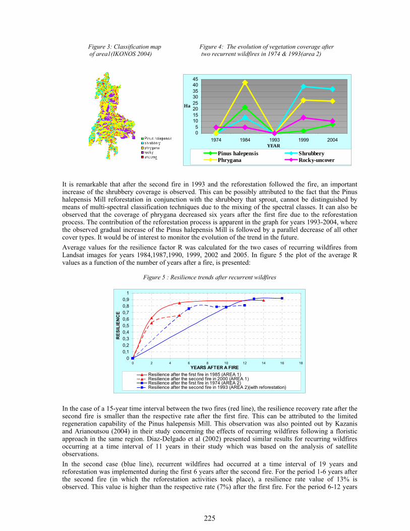
225

Figure 3: Classification map

of area1(IKONOS 2004)

Figure 4: The evolution of vegetation coverage after

two recurrent wildfires in 1974 & 1993(area 2)

05

1015202530354045

1974 1984 1993 1999 2004YEAR

Ha

Pinus halepensis ShrubberyPhrygana Rocky-uncover

It is remarkable that after the second fire in 1993 and the reforestation followed the fire, an important increase of the shrubbery coverage is observed. This can be possibly attributed to the fact that the Pinus halepensis Mill reforestation in conjunction with the shrubbery that sprout, cannot be distinguished by means of multi-spectral classification techniques due to the mixing of the spectral classes. It can also be observed that the coverage of phrygana decreased six years after the first fire due to the reforestation process. The contribution of the reforestation process is apparent in the graph for years 1993-2004, where the observed gradual increase of the Pinus halepensis Mill is followed by a parallel decrease of all other cover types. It would be of interest to monitor the evolution of the trend in the future. Average values for the resilience factor R was calculated for the two cases of recurring wildfires from Landsat images for years 1984,1987,1990, 1999, 2002 and 2005. In figure 5 the plot of the average R values as a function of the number of years after a fire, is presented:

Figure 5 : Resilience trends after recurrent wildfires

00,10,20,30,40,50,60,70,80,9

1

0 2 4 6 8 10 12 14 16 18YEARS AFTER A FIRE

RES

ILIE

NC

E

Resilience after the first fire in 1985 (AREA 1)Resilience after the second fire in 2000 (AREA 1) Resilience after the first fire in 1974 (AREA 2)Resilience after the second fire in 1993 (AREA 2)(with reforestation)

In the case of a 15-year time interval between the two fires (red line), the resilience recovery rate after the second fire is smaller than the respective rate after the first fire. This can be attributed to the limited regeneration capability of the Pinus halepensis Mill. This observation was also pointed out by Kazanis and Arianoutsou (2004) in their study concerning the effects of recurring wildfires following a floristic approach in the same region. Diaz-Delgado et al (2002) presented similar results for recurring wildfires occurring at a time interval of 11 years in their study which was based on the analysis of satellite observations. In the second case (blue line), recurrent wildfires had occurred at a time interval of 19 years and reforestation was implemented during the first 6 years after the second fire. For the period 1-6 years after the second fire (in which the reforestation activities took place), a resilience rate value of 13% is observed. This value is higher than the respective rate (7%) after the first fire. For the period 6-12 years

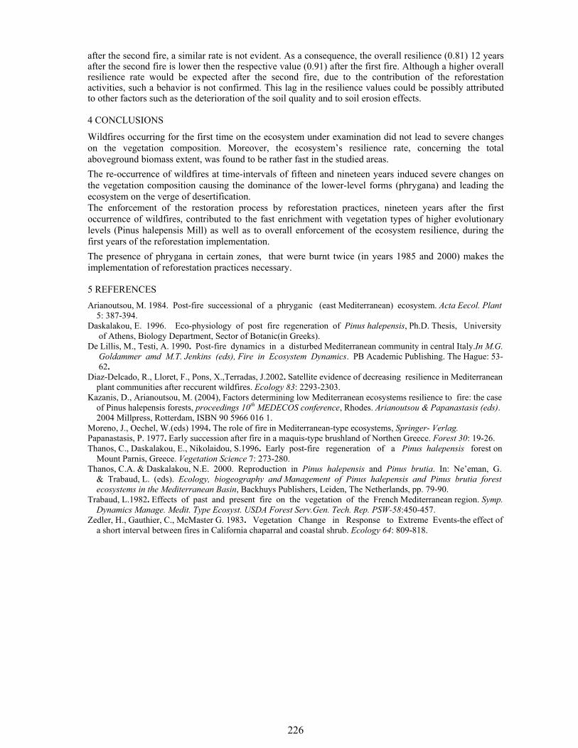
226

after the second fire, a similar rate is not evident. As a consequence, the overall resilience (0.81) 12 years after the second fire is lower then the respective value (0.91) after the first fire. Although a higher overall resilience rate would be expected after the second fire, due to the contribution of the reforestation activities, such a behavior is not confirmed. This lag in the resilience values could be possibly attributed to other factors such as the deterioration of the soil quality and to soil erosion effects.

4 CONCLUSIONS

Wildfires occurring for the first time on the ecosystem under examination did not lead to severe changes on the vegetation composition. Moreover, the ecosystem’s resilience rate, concerning the total aboveground biomass extent, was found to be rather fast in the studied areas. The re-occurrence of wildfires at time-intervals of fifteen and nineteen years induced severe changes on the vegetation composition causing the dominance of the lower-level forms (phrygana) and leading the ecosystem on the verge of desertification. The enforcement of the restoration process by reforestation practices, nineteen years after the first occurrence of wildfires, contributed to the fast enrichment with vegetation types of higher evolutionary levels (Pinus halepensis Mill) as well as to overall enforcement of the ecosystem resilience, during the first years of the reforestation implementation. The presence of phrygana in certain zones, that were burnt twice (in years 1985 and 2000) makes the implementation of reforestation practices necessary.

5 REFERENCES Arianoutsou, M. 1984. Post-fire successional of a phryganic (east Mediterranean) ecosystem. Acta Eecol. Plant 5: 387-394. Daskalakou, E. 1996. Eco-physiology of post fire regeneration of Pinus halepensis, Ph.D. Thesis, University of Athens, Biology Department, Sector of Botanic(in Greeks). De Lillis, M., Testi, A. 1990. Post-fire dynamics in a disturbed Mediterranean community in central Italy.In M.G. Goldammer amd M.T. Jenkins (eds), Fire in Ecosystem Dynamics. PB Academic Publishing. The Hague: 53- 62. Diaz-Delcado, R., Lloret, F., Pons, X.,Terradas, J.2002. Satellite evidence of decreasing resilience in Mediterranean plant communities after reccurent wildfires. Ecology 83: 2293-2303. Kazanis, D., Arianoutsou, M. (2004), Factors determining low Mediterranean ecosystems resilience to fire: the case of Pinus halepensis forests, proceedings 10th MEDECOS conference, Rhodes. Arianoutsou & Papanastasis (eds). 2004 Millpress, Rotterdam, ISBN 90 5966 016 1. Moreno, J., Oechel, W.(eds) 1994. The role of fire in Mediterranean-type ecosystems, Springer- Verlag. Papanastasis, P. 1977. Early succession after fire in a maquis-type brushland of Northen Greece. Forest 30: 19-26. Thanos, C., Daskalakou, E., Nikolaidou, S.1996. Early post-fire regeneration of a Pinus halepensis forest on Mount Parnis, Greece. Vegetation Science 7: 273-280. Thanos, C.A. & Daskalakou, N.E. 2000. Reproduction in Pinus halepensis and Pinus brutia. In: Ne’eman, G. & Trabaud, L. (eds). Ecology, biogeography and Management of Pinus halepensis and Pinus brutia forest ecosystems in the Mediterranean Basin, Backhuys Publishers, Leiden, The Netherlands, pp. 79-90. Trabaud, L.1982. Effects of past and present fire on the vegetation of the French Mediterranean region. Symp. Dynamics Manage. Medit. Type Ecosyst. USDA Forest Serv.Gen. Tech. Rep. PSW-58:450-457. Zedler, H., Gauthier, C., McMaster G. 1983. Vegetation Change in Response to Extreme Events-the effect of a short interval between fires in California chaparral and coastal shrub. Ecology 64: 809-818.

227

1 INTRODUCTION Natural fires in the Mediterranean European Basin, which have probably influenced vegetation since the appearance of the first terrestrial plants, represent one of the most important evolutionary factors (Di Pasquale et al. 2004). However, the general trend in the number of fires and surface burns has increased spectacularly in recent decades in the countries of Mediterranean Europe (Pausas & Vallejo, 1999) rendering forest fires a real threat to natural environment. In general, the impact of fires on forest ecosystems can be divided into short term and long term. According to Karteris (1996), short term impact assessment involves quantification of the severity of burn, derivation of the affected land cover types and the approximation of the wood volume lost, while estimation of the long term impacts include evaluation of the vegetation recovery, forest natural regrowth, land degradation, hydrological response, atmospheric pollution and the ecological impact in terms of modifying or affecting plant and animal species. Detailed and current information concerning the location and extent of the burned areas and the level of fire damage is important in order to assess economic and ecological effects and to monitor land use and land cover changes (Gitas, 1999). Remote sensing has been widely applied to overcome the problem of accurately mapping fire boundaries. Indeed, satellite data have been effectively used in mapping burned areas, since they provide synoptic information over wide areas with high acquisition frequency (Richards, 1993; Myneni et al., 1997) and complement field work measurements. Moreover, the use of Geographical Information Systems (GIS) has made it possible to combine several spatial variables, update or retrieve spatial information, and derive cartographic models by combining, in different ways, the layers of information included in a data base (Chuvieco & Congalton, 1989). One main advantage of a GIS is its ability to produce realistic calculations of the true surface (3D) area by incorporating ancillary data such as a Digital Elevation Model (DEM), thus taking into account the effects of terrain relief (Gitas, 1999). Actual surface is preferred in forest and land use management and can lead to more accurate estimations when mapping burn scars than horizontal reference plane (planimetric or 2D) area calculations. The aim of this work was to accurately map the spatial extent of a recently burned area in Portugal and also to estimate the short-term fire effects. The specific objectives were:

i. to investigate whether object-based analysis can be employed for burned area mapping using Disaster Monitoring Constellation (DMC) imagery;

ii. to employ an in-house developed GIS (BAS 2) in order to estimate the planimetric (2D) and true surface (3D) burned area as a total, as well as the size of the main land cover classes existing in the area .

Assessment of the short-term impact of forest fires by employing object-based classification and GIS analysis

A.I. Polychronaki, T.G. Katagis*, I.Z. Gitas & M.A. Karteris Laboratory of Forest Management and Remote Sensing, Aristotle University of Thessaloniki, P.O. Box 248, University Campus, Greece. E-mail*:[email protected]

Keywords: DMC imagery, object-based classification, post-fire assessment

ABSTRACT: It has been reported that the combined use of Remote Sensing and GIS is able to contribute to an efficient and rapid assessment of forest fire damage by mapping the extent of the area burned and quantifying the fire effects. The aim of this work was to accurately map the spatial extent of recently burned areas and also to estimate the short-term fire effects. More specifically, an object-based classification model was developed to map burned areas in Portugal by employing a Disaster Monitoring Constellation (DMC) satellite image. Accuracy assessment was conducted by comparing the resulting burned area with the fire perimeter map provided by the Forest Service, and the overall classification accuracy was found to be 90%. Subsequently, fire statistics for the main land cover classes affected by the fire were estimated both in planimetric (2D) and actual surface area (3D), using the GIS software BAS 2 (Burned Area Statistics). In general, it was found that 88% percent (in 2D and 3D) of the fire affected area was characterized as forest and semi-natural areas, while 11% of the area damaged by the fire was classified as agricultural land.

228

2 STUDY AREA AND DATASET The study area is located in Central Portugal, about 140 km northeast of Lisbon and is separated by the districts of Leiria, Castelo Branco and Santarem, while River Zézere, which rises in the Serra da Estrala mountains range and joins the Tagus River, crosses the area. The woodland that covers the study area mainly consists of pines, while the the agricultural areas are covered by vineyards, olive groves and fruit trees. Large fires occurred in the area during the summer of 2006 along the banks of the Zézere River. A DMC satellite image captured after the fire, with a spatial resolution of 32m, was acquired for classification of the burned areas. The standard DMC Imager is a 6 channel, Surrey Linear Imager (SLIM6) which was built by Surrey Satellite Technology Ltd (SSTL), UK. The SLIM6 is designed to collect and detect radiation from the Earth in a swath 600 km wide as it passes overhead, by using the spacecraft orbital motion to provide an along-track scan. The other data sets used in this work were a georeferenced LANDSAT image and the forest fire perimeter provided by the Forest Service of Portugal. The burned areas were mapped by the Forest Service using MODIS imagery.

3 METHODOLOGY

The methodology followed in this work involved mainly two steps: 1. development of the object-based classification model for burned area mapping, and 2. assessment of the fire damage using GIS.

Prior to mapping of burned areas, the DMC image was geometrically corrected. A GCP-based transformation approach was used by identifying numerous control points and determining their location in the image and their geographic coordinates from the reference source (the LANDSAT image). 3.1 Development of the object-based classification model In an object-oriented approach, a prerequisite to classification is image segmentation, which is the subdivision of an image into separated regions. Image objects resulting from segmentation represent image object primitives, serving as information carriers and building blocks for further classification or other segmentation processes (eCognition User Guide, 2004). Throughout the segmentation procedure (software used Definiens Professional 5), the image was segmented and image objects were generated based upon several adjustable criteria of scale, band weights and homogeneity in colour and shape. Four levels of segmentation were finally created with the scale parameter set to 150, 100, 20 and 2 for levels 4, 3, 2 and 1, respectively, in order to extract the desired image objects which would provide optimal information for further processing. Therefore, a hierarchical network of the image objects was constructed, that represented image information in different spatial resolutions simultaneously In the classification process, which is based on fuzzy logic, certain feature objects, such as layer ratio, layer mean value and class-related features, namely the relation to super-objects, were selected, while the membership functions for each feature for each class were appropriately set in order to perform the classification at each level. Thus, at level 4, two classes were created, that represented the unburned area and one class, that represented the burned area. Nevertheless, a classification based fusion took place. The principle of the classification based fusion is that all adjacent image objects, which represent identical structures or are parts of identical structures, are merged into one new image object. Thus, two classes were finally created at level 4: “burned area 4” and “unburned area 4”. Subsequently, classification at level 3 resulted in two classes, namely “burned area 3” and “water 3”, while at level 2 one class was finally created, namely “water 2”. At level 1, the final classification took place and five classes were created: “burned area 1”, “slightly burned”, “bare land”, “other land cover types” and “vegetated areas”. Classes representing unburned areas and classes representing burned areas were finally merged into two different classes, namely “burned area” and “unburned area”, using the appropriate algorithm (Figure 1).

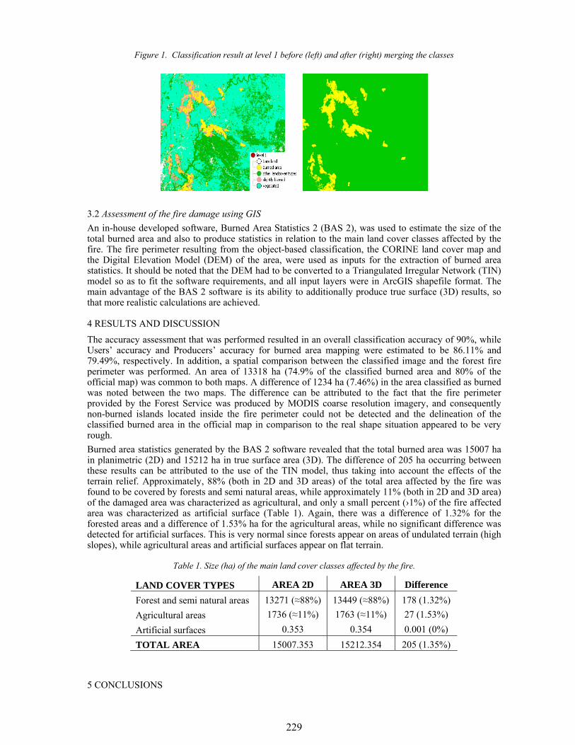
229

Figure 1. Classification result at level 1 before (left) and after (right) merging the classes

3.2 Assessment of the fire damage using GIS An in-house developed software, Burned Area Statistics 2 (BAS 2), was used to estimate the size of the total burned area and also to produce statistics in relation to the main land cover classes affected by the fire. The fire perimeter resulting from the object-based classification, the CORINE land cover map and the Digital Elevation Model (DEM) of the area, were used as inputs for the extraction of burned area statistics. It should be noted that the DEM had to be converted to a Triangulated Irregular Network (TIN) model so as to fit the software requirements, and all input layers were in ArcGIS shapefile format. The main advantage of the BAS 2 software is its ability to additionally produce true surface (3D) results, so that more realistic calculations are achieved.

4 RESULTS AND DISCUSSION The accuracy assessment that was performed resulted in an overall classification accuracy of 90%, while Users’ accuracy and Producers’ accuracy for burned area mapping were estimated to be 86.11% and 79.49%, respectively. In addition, a spatial comparison between the classified image and the forest fire perimeter was performed. An area of 13318 ha (74.9% of the classified burned area and 80% of the official map) was common to both maps. A difference of 1234 ha (7.46%) in the area classified as burned was noted between the two maps. The difference can be attributed to the fact that the fire perimeter provided by the Forest Service was produced by MODIS coarse resolution imagery, and consequently non-burned islands located inside the fire perimeter could not be detected and the delineation of the classified burned area in the official map in comparison to the real shape situation appeared to be very rough. Burned area statistics generated by the BAS 2 software revealed that the total burned area was 15007 ha in planimetric (2D) and 15212 ha in true surface area (3D). The difference of 205 ha occurring between these results can be attributed to the use of the TIN model, thus taking into account the effects of the terrain relief. Approximately, 88% (both in 2D and 3D areas) of the total area affected by the fire was found to be covered by forests and semi natural areas, while approximately 11% (both in 2D and 3D area) of the damaged area was characterized as agricultural, and only a small percent (›1%) of the fire affected area was characterized as artificial surface (Table 1). Again, there was a difference of 1.32% for the forested areas and a difference of 1.53% ha for the agricultural areas, while no significant difference was detected for artificial surfaces. This is very normal since forests appear on areas of undulated terrain (high slopes), while agricultural areas and artificial surfaces appear on flat terrain.

Table 1. Size (ha) of the main land cover classes affected by the fire.

LAND COVER TYPES AREA 2D AREA 3D Difference Forest and semi natural areas 13271 (≈88%) 13449 (≈88%) 178 (1.32%) Agricultural areas 1736 (≈11%) 1763 (≈11%) 27 (1.53%) Artificial surfaces 0.353 0.354 0.001 (0%) TOTAL AREA 15007.353 15212.354 205 (1.35%)

5 CONCLUSIONS

230

The combination of medium-high resolution remote sensing data, such as DMC imagery, object-based image analysis, and an in-house developed software (BAS 2) for burned area statistics was successful in estimating the impact of fire on the natural environment. In particular, the object-based classification model that was developed using DMC imagery resulted in the accurate mapping of the burned areas (90% overall accuracy) in central Portugal. Although spectral confusion between burned and unburned areas was observed, which can be attributed to the limited number of spectral bands of the DMC data, the use of not only spectral information but also contextual information (class-related features) in the classification process resulted in successful mapping of the burned areas. Moreover, the BAS 2 software, which was used to generate the burned area statistics, was found to be easy to handle and led to a relatively rapid calculation of the fire statistics. The difference that was observed between the total burned area in planimetric (15007 ha, 2D) and in true surface area (15212 ha, 3D) was attributed to the use of the TIN model, thus taking into account the effects of the terrain relief. Furthermore, it was found that approximately 88% of the total area (both in 2D and 3D) affected by the fire was covered by forest and semi natural areas, while 11% (both in 2D and 3D) was agricultural area.

6 ACKNOWLEDGEMENTS

The authors are grateful to Miss Linda Lucas for her valuable help in revising the English content of this work.

7 REFERENCES Chuvieco, E., Congalton, R. G. 1989. Application of Remote Sensing and Geographic Information Systems to

Forest Fire Hazard Mapping. Remote Sensing of Environment, 29:147-159. eCognition 2004, User Guide. (Definiens Imaging GmbH: München). Di Pasquale G., Di Martino P. and Mazzoleni S. 2004. Forest History in the Mediterranean Region. Recent

Dynamics of the Mediterranean Vegetation and Landscape. G. In: di Pasquale, Mulligan, M., Di Martino, P., Rego, F., (eds), John Wiley & Sons, Ltd.

Gitas, I.Z. 1999. Geographical information systems and remote sensing in mapping and monitoring fire-altered forest landscapes. PhD thesis, University of Cambridge, Cambridge, UK.

Karteris, M.A. 1995. Burned land mapping and post-fire effects, Remote Sensing and GIS applications to Forest Fire Management, (Ed, Chuvieco, E.), University of Alcala de Henares, Spain, pp. 35-44.

Lloret, F., Calvo, E., Pons, X., Diaz-Delgado, R. 2002. Wildfires and landscape patterns in the Eastern Iberian Peninsula. Landscape Ecology, 17: 745-759.

Myneni, R. B., Keeling, C. D., Tucker, C. J., Asrar, G., Nemani, R. R. 1997. Increased plant growth in the northern high latitudes from 1981– 1991. Nature, 386: 698–702.

Pausas J.G., Vallejo R.V. 1999. The role of fire in European Mediterranean ecosystems. In E. Chuvieco (Ed.), Remote Sensing of large wildfires (pp.3-16). Berlin: Springer-Verlang.

Richards, J.A. 1993. Remote sensing digital image analysis: An introduction (2nd ed.).Heilderberg: Springer-Verlag, pp 340.

San-Miguel-Ayanz, J., Barbosa, P., Schmuck, G., Liberta, G., Schulte, E. 2002. Towards a coherent forest fire information system in Europe: The European Forest Fire Information System (EFFIS). Forest Fire Research & Wildland Fire Safety, Viegas (ed.). Millpress, Rotterdam, ISBN 90-77017-72-0.

231

1 INTRODUCTION Given that forest dynamics are strongly influenced by fire, it is important to analyze those variables that control postfire forest dynamics (Pérez and Moreno, 1998). Among these variables, the marked influence of severity on vegetation response and erosion processes means that it is commonly considered to be critical in assessing postfire effects (Miller and Yool, 2002; Chuvieco et al., 2006). In the complex terminology related to severity, the term ‘fire severity’ refers to the direct effects of the combustion process, while the term ‘burn severity’ refers to the subsequent effects of fire from a short- or long-term perspective (Jain, 2004; Key and Benson, 2005). The present research focuses on the immediate effects of the combustion process in terms of the postfire surface materials present in recently burned areas. This situation is referred to as fire severity, as it does not take into account the prefire environmental characteristics or the postfire environmental response. The estimation of severity is the ultimate goal of many remote sensing studies. Satellite images are cost-efficient, provide continuous information, and represent a superior spatial approach to investigating fire-related processes; however, ground-level studies are a necessary first step in establishing the validity of

Combined methodology of field spectrometry and digital photography in estimating fire severity

R. Montorio Llovería Department of Geography and Spatial Management, University of Zaragoza, Zaragoza 50009, Spain, [email protected]

F. Pérez-Cabello, A. García-Martín & J. de la Riva Fernández Department of Geography and Spatial Management, University of Zaragoza, Zaragoza 50009, Spain, [email protected], [email protected], [email protected] Keywords: fire severity, field spectrometry, high spatial resolution photography, post-fire surface materials/combustion products

ABSTRACT: Fire severity can be considered as one of the most influential factors in the postfire development of burned areas. Remote sensing data are suitable for detecting and mapping fire severity because disturbances in vegetation and soil produce detectable changes in their spectral responses. The mid-infrared region of the spectrum, with its sensitivity to water content, is one of the most important regions in estimating fire severity. Nevertheless, the visible and near-infrared regions also provide useful information for this purpose because of their marked responses to changes in vegetation. Few studies have considered changes in reflectance values at ground level, despite the usefulness of such an approach in improving the discrimination of spatial severity across large areas and in establishing the validity of empirical relationships prior to analyzing remote sensing data. The objective of this study is to detect those spectral regions most sensitive to severity levels by investigating the relationship between postfire combustion-related surface materials (black carbon, ash, and the remains of vegetation) and reflectance values. A total of 34 field plots, each covering 380 cm2, were analyzed immediately following natural fires that occurred in the summer of 2006 in Ibieca (Huesca, Spain) and Zuera (Zaragoza, Spain). In obtaining postfire data (photographs and reflectance values), we used a portable metallic structure with a fixed system to hold the digital camera and the field spectroradiometer, thereby ensuring that both registered the same surface at any given time. Following this methodology, we obtained high spatial resolution photographs and reflectance values, both in the VIS–NIR range. The reflectance of the captured surface was extracted from the total surface area covered by the photographs, and the proportions of the different postfire surface materials were obtained via a supervised classification process (maximum likelihood method). Reflectance values and convolved Landsat-TM bands were statistically correlated with the individual postfire surface materials and with a fire severity index derived from its combination: the Combustion Products Index (CPI). The most sensitive wavelengths to individual postfire materials were 450.6, 758.2, and 797 nm for ash, black carbon, and vegetation remains, respectively, although these bands can be included in ranges of comparable behavior. Finally, two stepwise regression models were applied to estimate CPI: one using the original reflectance bands and the other using the convolved Landsat-TM bands. Two individual wavelengths were selected in the first model: 450.6 nm (placed in the blue region of the spectrum, with a positive sign) and 767.9 nm (placed in the infrared region, with a negative sign), thereby yielding a significant model (r2 = 0.856). The corresponding Landsat-TM bands, bands 1 and 4, were selected by the second model (r2 = 0.838), raising the possibility of applying this index to large-scale areas with medium spatial-resolution data.

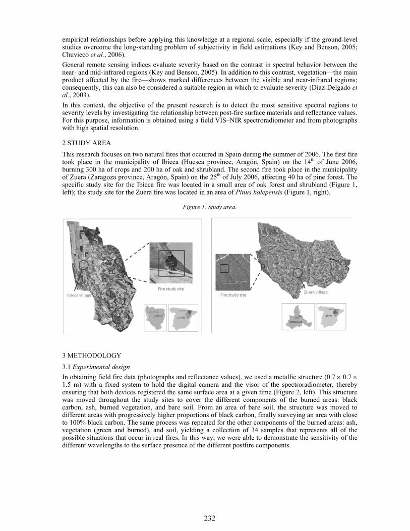
232

empirical relationships before applying this knowledge at a regional scale, especially if the ground-level studies overcome the long-standing problem of subjectivity in field estimations (Key and Benson, 2005; Chuvieco et al., 2006). General remote sensing indices evaluate severity based on the contrast in spectral behavior between the near- and mid-infrared regions (Key and Benson, 2005). In addition to this contrast, vegetation—the main product affected by the fire—shows marked differences between the visible and near-infrared regions; consequently, this can also be considered a suitable region in which to evaluate severity (Díaz-Delgado et al., 2003). In this context, the objective of the present research is to detect the most sensitive spectral regions to severity levels by investigating the relationship between post-fire surface materials and reflectance values. For this purpose, information is obtained using a field VIS–NIR spectroradiometer and from photographs with high spatial resolution.

2 STUDY AREA This research focuses on two natural fires that occurred in Spain during the summer of 2006. The first fire took place in the municipality of Ibieca (Huesca province, Aragón, Spain) on the 14th of June 2006, burning 300 ha of crops and 200 ha of oak and shrubland. The second fire took place in the municipality of Zuera (Zaragoza province, Aragón, Spain) on the 25th of July 2006, affecting 40 ha of pine forest. The specific study site for the Ibieca fire was located in a small area of oak forest and shrubland (Figure 1, left); the study site for the Zuera fire was located in an area of Pinus halepensis (Figure 1, right).

Figure 1. Study area.

3 METHODOLOGY 3.1 Experimental design In obtaining field fire data (photographs and reflectance values), we used a metallic structure (0.7 × 0.7 × 1.5 m) with a fixed system to hold the digital camera and the visor of the spectroradiometer, thereby ensuring that both devices registered the same surface area at a given time (Figure 2, left). This structure was moved throughout the study sites to cover the different components of the burned areas: black carbon, ash, burned vegetation, and bare soil. From an area of bare soil, the structure was moved to different areas with progressively higher proportions of black carbon, finally surveying an area with close to 100% black carbon. The same process was repeated for the other components of the burned areas: ash, vegetation (green and burned), and soil, yielding a collection of 34 samples that represents all of the possible situations that occur in real fires. In this way, we were able to demonstrate the sensitivity of the different wavelengths to the surface presence of the different postfire components.

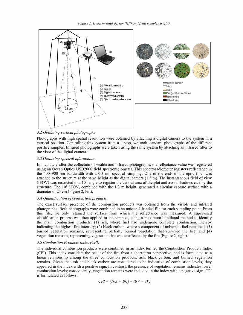
233

Figure 2. Experimental design (left) and field samples (right).

3.2 Obtaining vertical photographs Photographs with high spatial resolution were obtained by attaching a digital camera to the system in a vertical position. Controlling this system from a laptop, we took standard photographs of the different postfire samples. Infrared photographs were taken using the same system by attaching an infrared filter to the visor of the digital camera.

3.3 Obtaining spectral information Immediately after the collection of visible and infrared photographs, the reflectance value was registered using an Ocean Optics USB2000 field spectroradiometer. This spectroradiometer registers reflectance in the 400–900 nm bandwidth with a 0.3 nm spectral sampling. One of the ends of the optic fiber was attached to the structure at the same height as the digital camera (1.3 m). The instantaneous field of view (IFOV) was restricted to a 10° angle to register the central area of the plot and avoid shadows cast by the structure. The 10° IFOV, combined with the 1.3 m height, generated a circular capture surface with a diameter of 23 cm (Figure 2, left). 3.4 Quantification of combustion products The exact surface presence of the combustion products was obtained from the visible and infrared photographs. Both photographs were combined in an unique 4-banded file for each sampling point. From this file, we only retained the surface from which the reflectance was measured. A supervised classification process was then applied to the samples, using a maximum-likelihood method to identify the main combustion products: (1) ash, where fuel had undergone complete combustion, thereby indicating the highest fire intensity; (2) black carbon, where a component of unburned fuel remained; (3) burned vegetation remains, representing partially burned vegetation that survived the fire; and (4) vegetation remains, representing vegetation that was unaffected by the fire (Figure 2, right). 3.5 Combustion Products Index (CPI) The individual combustion products were combined in an index termed the Combustion Products Index (CPI). This index considers the result of the fire from a short-term perspective, and is formulated as a linear relationship among the three combustion products: ash, black carbon, and burned vegetation remains. Given that ash and black carbon are considered to be indicative of combustion levels, they appeared in the index with a positive sign. In contrast, the presence of vegetation remains indicates lower combustion levels; consequently, vegetation remains were included in the index with a negative sign. CPI is formulated as follows:

CPI = (10A + BC) – (BV + 4V)

Black carbon Ash Soil Vegetation remains Branches Shadows

23 cm

10˚

1.3 m

(2)

(1) Metallic structure(2) Laptop(3) Digital camera(4) Spectroradiometer(5) Spectroradiometer ’s visor

(4)

(3)

(1)

(5)

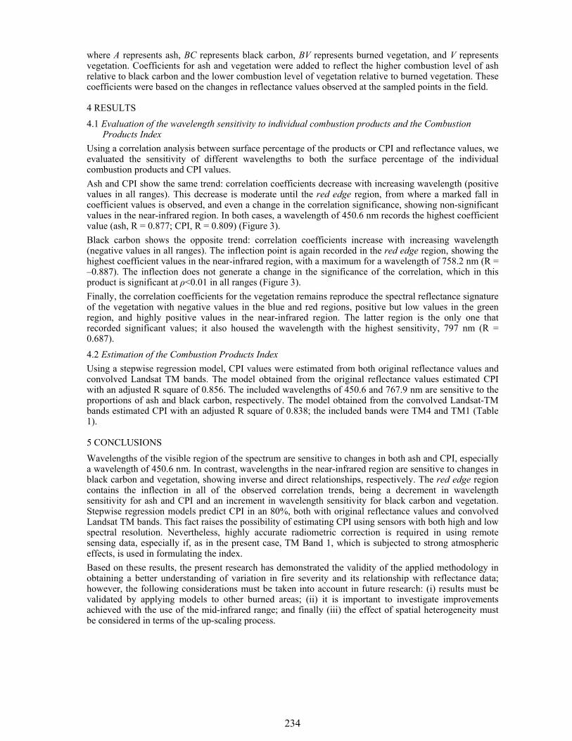
234

where A represents ash, BC represents black carbon, BV represents burned vegetation, and V represents vegetation. Coefficients for ash and vegetation were added to reflect the higher combustion level of ash relative to black carbon and the lower combustion level of vegetation relative to burned vegetation. These coefficients were based on the changes in reflectance values observed at the sampled points in the field.

4 RESULTS

4.1 Evaluation of the wavelength sensitivity to individual combustion products and the Combustion Products Index

Using a correlation analysis between surface percentage of the products or CPI and reflectance values, we evaluated the sensitivity of different wavelengths to both the surface percentage of the individual combustion products and CPI values. Ash and CPI show the same trend: correlation coefficients decrease with increasing wavelength (positive values in all ranges). This decrease is moderate until the red edge region, from where a marked fall in coefficient values is observed, and even a change in the correlation significance, showing non-significant values in the near-infrared region. In both cases, a wavelength of 450.6 nm records the highest coefficient value (ash, R = 0.877; CPI, R = 0.809) (Figure 3). Black carbon shows the opposite trend: correlation coefficients increase with increasing wavelength (negative values in all ranges). The inflection point is again recorded in the red edge region, showing the highest coefficient values in the near-infrared region, with a maximum for a wavelength of 758.2 nm (R = –0.887). The inflection does not generate a change in the significance of the correlation, which in this product is significant at ρ<0.01 in all ranges (Figure 3). Finally, the correlation coefficients for the vegetation remains reproduce the spectral reflectance signature of the vegetation with negative values in the blue and red regions, positive but low values in the green region, and highly positive values in the near-infrared region. The latter region is the only one that recorded significant values; it also housed the wavelength with the highest sensitivity, 797 nm (R = 0.687). 4.2 Estimation of the Combustion Products Index Using a stepwise regression model, CPI values were estimated from both original reflectance values and convolved Landsat TM bands. The model obtained from the original reflectance values estimated CPI with an adjusted R square of 0.856. The included wavelengths of 450.6 and 767.9 nm are sensitive to the proportions of ash and black carbon, respectively. The model obtained from the convolved Landsat-TM bands estimated CPI with an adjusted R square of 0.838; the included bands were TM4 and TM1 (Table 1).

5 CONCLUSIONS Wavelengths of the visible region of the spectrum are sensitive to changes in both ash and CPI, especially a wavelength of 450.6 nm. In contrast, wavelengths in the near-infrared region are sensitive to changes in black carbon and vegetation, showing inverse and direct relationships, respectively. The red edge region contains the inflection in all of the observed correlation trends, being a decrement in wavelength sensitivity for ash and CPI and an increment in wavelength sensitivity for black carbon and vegetation. Stepwise regression models predict CPI in an 80%, both with original reflectance values and convolved Landsat TM bands. This fact raises the possibility of estimating CPI using sensors with both high and low spectral resolution. Nevertheless, highly accurate radiometric correction is required in using remote sensing data, especially if, as in the present case, TM Band 1, which is subjected to strong atmospheric effects, is used in formulating the index. Based on these results, the present research has demonstrated the validity of the applied methodology in obtaining a better understanding of variation in fire severity and its relationship with reflectance data; however, the following considerations must be taken into account in future research: (i) results must be validated by applying models to other burned areas; (ii) it is important to investigate improvements achieved with the use of the mid-infrared range; and finally (iii) the effect of spatial heterogeneity must be considered in terms of the up-scaling process.

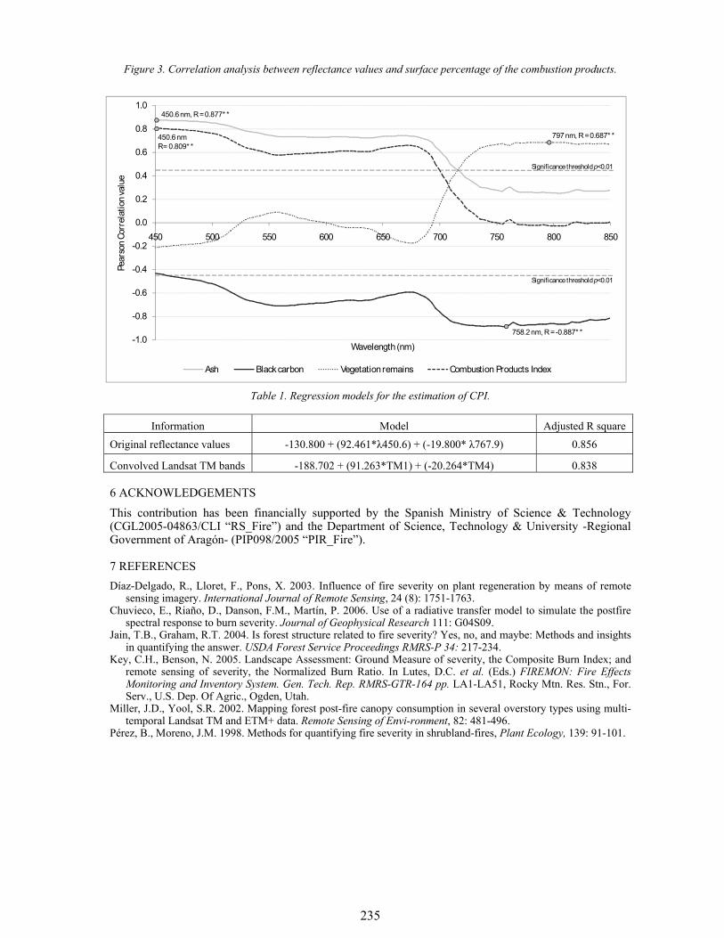
235

Figure 3. Correlation analysis between reflectance values and surface percentage of the combustion products.

Table 1. Regression models for the estimation of CPI.

6 ACKNOWLEDGEMENTS

This contribution has been financially supported by the Spanish Ministry of Science & Technology (CGL2005-04863/CLI “RS_Fire”) and the Department of Science, Technology & University -Regional Government of Aragón- (PIP098/2005 “PIR_Fire”).

7 REFERENCES Díaz-Delgado, R., Lloret, F., Pons, X. 2003. Influence of fire severity on plant regeneration by means of remote

sensing imagery. International Journal of Remote Sensing, 24 (8): 1751-1763. Chuvieco, E., Riaño, D., Danson, F.M., Martín, P. 2006. Use of a radiative transfer model to simulate the postfire

spectral response to burn severity. Journal of Geophysical Research 111: G04S09. Jain, T.B., Graham, R.T. 2004. Is forest structure related to fire severity? Yes, no, and maybe: Methods and insights

in quantifying the answer. USDA Forest Service Proceedings RMRS-P 34: 217-234. Key, C.H., Benson, N. 2005. Landscape Assessment: Ground Measure of severity, the Composite Burn Index; and

remote sensing of severity, the Normalized Burn Ratio. In Lutes, D.C. et al. (Eds.) FIREMON: Fire Effects Monitoring and Inventory System. Gen. Tech. Rep. RMRS-GTR-164 pp. LA1-LA51, Rocky Mtn. Res. Stn., For. Serv., U.S. Dep. Of Agric., Ogden, Utah.

Miller, J.D., Yool, S.R. 2002. Mapping forest post-fire canopy consumption in several overstory types using multi-temporal Landsat TM and ETM+ data. Remote Sensing of Envi-ronment, 82: 481-496.

Pérez, B., Moreno, J.M. 1998. Methods for quantifying fire severity in shrubland-fires, Plant Ecology, 139: 91-101.

Information Model Adjusted R square

Original reflectance values -130.800 + (92.461*λ450.6) + (-19.800* λ767.9) 0.856

Convolved Landsat TM bands -188.702 + (91.263*TM1) + (-20.264*TM4) 0.838

-1.0

-0.8

-0.6

-0.4

-0.2

0.0

0.2

0.4

0.6

0.8

1.0

450 500 550 600 650 700 750 800 850

Pear

son

Corr

elat

ion

valu

e

Wavelength (nm)

Ash Black carbon Vegetation remains Combustion Products Index

450.6 nm, R= 0.877* *

797 nm, R= 0.687* *

758.2 nm, R= -0.887* *

450.6 nmR= 0.809* *

Significance threshold p<0.01

Significance threshold p<0.01

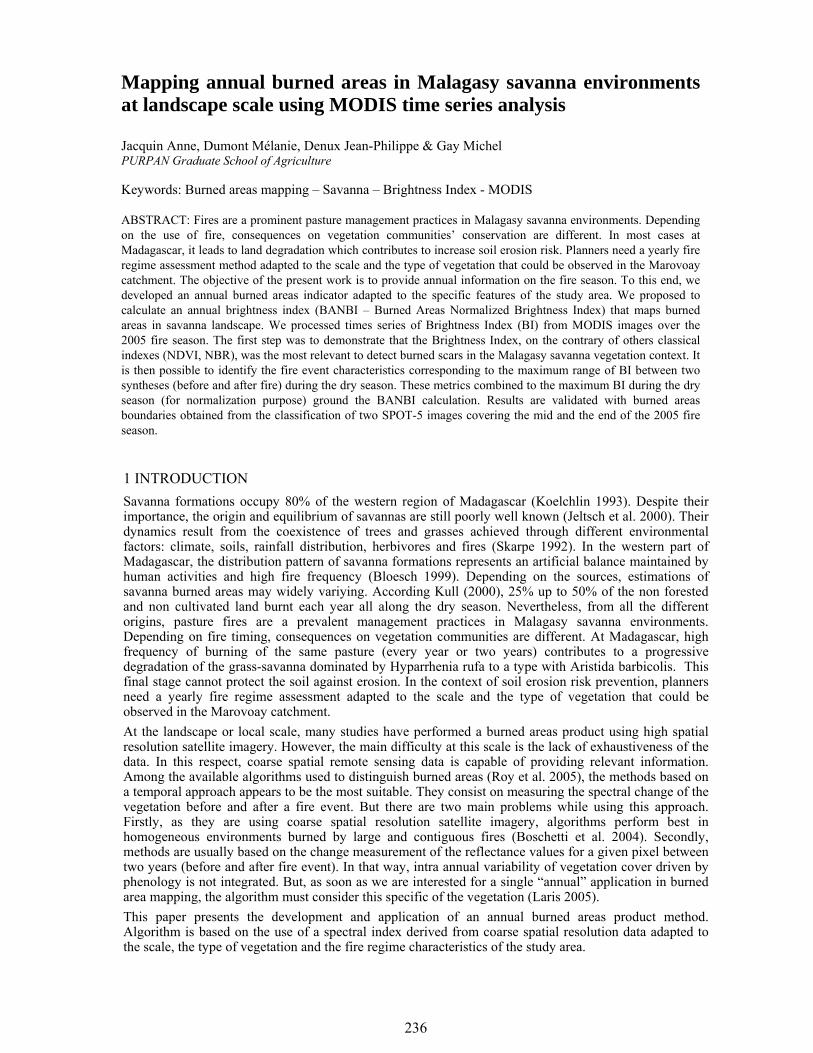
236

Mapping annual burned areas in Malagasy savanna environments at landscape scale using MODIS time series analysis

Jacquin Anne, Dumont Mélanie, Denux Jean-Philippe & Gay Michel PURPAN Graduate School of Agriculture Keywords: Burned areas mapping – Savanna – Brightness Index - MODIS

ABSTRACT: Fires are a prominent pasture management practices in Malagasy savanna environments. Depending on the use of fire, consequences on vegetation communities’ conservation are different. In most cases at Madagascar, it leads to land degradation which contributes to increase soil erosion risk. Planners need a yearly fire regime assessment method adapted to the scale and the type of vegetation that could be observed in the Marovoay catchment. The objective of the present work is to provide annual information on the fire season. To this end, we developed an annual burned areas indicator adapted to the specific features of the study area. We proposed to calculate an annual brightness index (BANBI – Burned Areas Normalized Brightness Index) that maps burned areas in savanna landscape. We processed times series of Brightness Index (BI) from MODIS images over the 2005 fire season. The first step was to demonstrate that the Brightness Index, on the contrary of others classical indexes (NDVI, NBR), was the most relevant to detect burned scars in the Malagasy savanna vegetation context. It is then possible to identify the fire event characteristics corresponding to the maximum range of BI between two syntheses (before and after fire) during the dry season. These metrics combined to the maximum BI during the dry season (for normalization purpose) ground the BANBI calculation. Results are validated with burned areas boundaries obtained from the classification of two SPOT-5 images covering the mid and the end of the 2005 fire season.

1 INTRODUCTION Savanna formations occupy 80% of the western region of Madagascar (Koelchlin 1993). Despite their importance, the origin and equilibrium of savannas are still poorly well known (Jeltsch et al. 2000). Their dynamics result from the coexistence of trees and grasses achieved through different environmental factors: climate, soils, rainfall distribution, herbivores and fires (Skarpe 1992). In the western part of Madagascar, the distribution pattern of savanna formations represents an artificial balance maintained by human activities and high fire frequency (Bloesch 1999). Depending on the sources, estimations of savanna burned areas may widely variying. According Kull (2000), 25% up to 50% of the non forested and non cultivated land burnt each year all along the dry season. Nevertheless, from all the different origins, pasture fires are a prevalent management practices in Malagasy savanna environments. Depending on fire timing, consequences on vegetation communities are different. At Madagascar, high frequency of burning of the same pasture (every year or two years) contributes to a progressive degradation of the grass-savanna dominated by Hyparrhenia rufa to a type with Aristida barbicolis. This final stage cannot protect the soil against erosion. In the context of soil erosion risk prevention, planners need a yearly fire regime assessment adapted to the scale and the type of vegetation that could be observed in the Marovoay catchment. At the landscape or local scale, many studies have performed a burned areas product using high spatial resolution satellite imagery. However, the main difficulty at this scale is the lack of exhaustiveness of the data. In this respect, coarse spatial remote sensing data is capable of providing relevant information. Among the available algorithms used to distinguish burned areas (Roy et al. 2005), the methods based on a temporal approach appears to be the most suitable. They consist on measuring the spectral change of the vegetation before and after a fire event. But there are two main problems while using this approach. Firstly, as they are using coarse spatial resolution satellite imagery, algorithms perform best in homogeneous environments burned by large and contiguous fires (Boschetti et al. 2004). Secondly, methods are usually based on the change measurement of the reflectance values for a given pixel between two years (before and after fire event). In that way, intra annual variability of vegetation cover driven by phenology is not integrated. But, as soon as we are interested for a single “annual” application in burned area mapping, the algorithm must consider this specific of the vegetation (Laris 2005). This paper presents the development and application of an annual burned areas product method. Algorithm is based on the use of a spectral index derived from coarse spatial resolution data adapted to the scale, the type of vegetation and the fire regime characteristics of the study area.

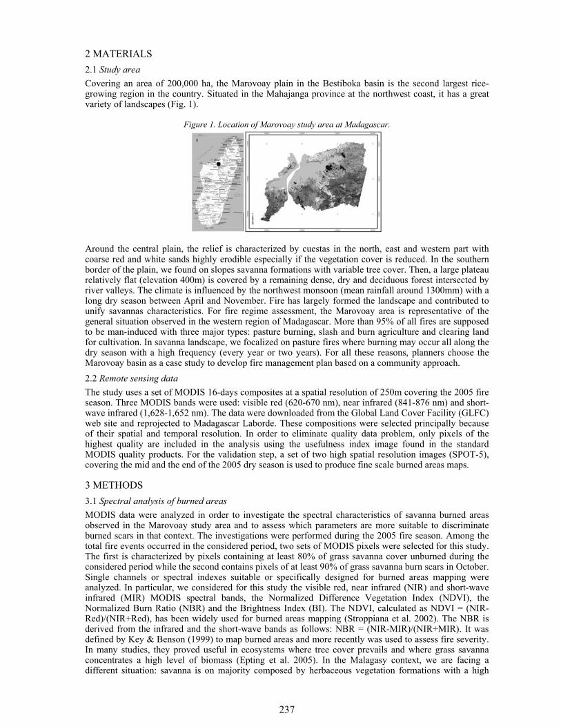
237

2 MATERIALS 2.1 Study area Covering an area of 200,000 ha, the Marovoay plain in the Bestiboka basin is the second largest rice-growing region in the country. Situated in the Mahajanga province at the northwest coast, it has a great variety of landscapes (Fig. 1).

Figure 1. Location of Marovoay study area at Madagascar.

Around the central plain, the relief is characterized by cuestas in the north, east and western part with coarse red and white sands highly erodible especially if the vegetation cover is reduced. In the southern border of the plain, we found on slopes savanna formations with variable tree cover. Then, a large plateau relatively flat (elevation 400m) is covered by a remaining dense, dry and deciduous forest intersected by river valleys. The climate is influenced by the northwest monsoon (mean rainfall around 1300mm) with a long dry season between April and November. Fire has largely formed the landscape and contributed to unify savannas characteristics. For fire regime assessment, the Marovoay area is representative of the general situation observed in the western region of Madagascar. More than 95% of all fires are supposed to be man-induced with three major types: pasture burning, slash and burn agriculture and clearing land for cultivation. In savanna landscape, we focalized on pasture fires where burning may occur all along the dry season with a high frequency (every year or two years). For all these reasons, planners choose the Marovoay basin as a case study to develop fire management plan based on a community approach. 2.2 Remote sensing data The study uses a set of MODIS 16-days composites at a spatial resolution of 250m covering the 2005 fire season. Three MODIS bands were used: visible red (620-670 nm), near infrared (841-876 nm) and short-wave infrared (1,628-1,652 nm). The data were downloaded from the Global Land Cover Facility (GLFC) web site and reprojected to Madagascar Laborde. These compositions were selected principally because of their spatial and temporal resolution. In order to eliminate quality data problem, only pixels of the highest quality are included in the analysis using the usefulness index image found in the standard MODIS quality products. For the validation step, a set of two high spatial resolution images (SPOT-5), covering the mid and the end of the 2005 dry season is used to produce fine scale burned areas maps.

3 METHODS 3.1 Spectral analysis of burned areas MODIS data were analyzed in order to investigate the spectral characteristics of savanna burned areas observed in the Marovoay study area and to assess which parameters are more suitable to discriminate burned scars in that context. The investigations were performed during the 2005 fire season. Among the total fire events occurred in the considered period, two sets of MODIS pixels were selected for this study. The first is characterized by pixels containing at least 80% of grass savanna cover unburned during the considered period while the second contains pixels of at least 90% of grass savanna burn scars in October. Single channels or spectral indexes suitable or specifically designed for burned areas mapping were analyzed. In particular, we considered for this study the visible red, near infrared (NIR) and short-wave infrared (MIR) MODIS spectral bands, the Normalized Difference Vegetation Index (NDVI), the Normalized Burn Ratio (NBR) and the Brightness Index (BI). The NDVI, calculated as NDVI = (NIR-Red)/(NIR+Red), has been widely used for burned areas mapping (Stroppiana et al. 2002). The NBR is derived from the infrared and the short-wave bands as follows: NBR = (NIR-MIR)/(NIR+MIR). It was defined by Key & Benson (1999) to map burned areas and more recently was used to assess fire severity. In many studies, they proved useful in ecosystems where tree cover prevails and where grass savanna concentrates a high level of biomass (Epting et al. 2005). In the Malagasy context, we are facing a different situation: savanna is on majority composed by herbaceous vegetation formations with a high

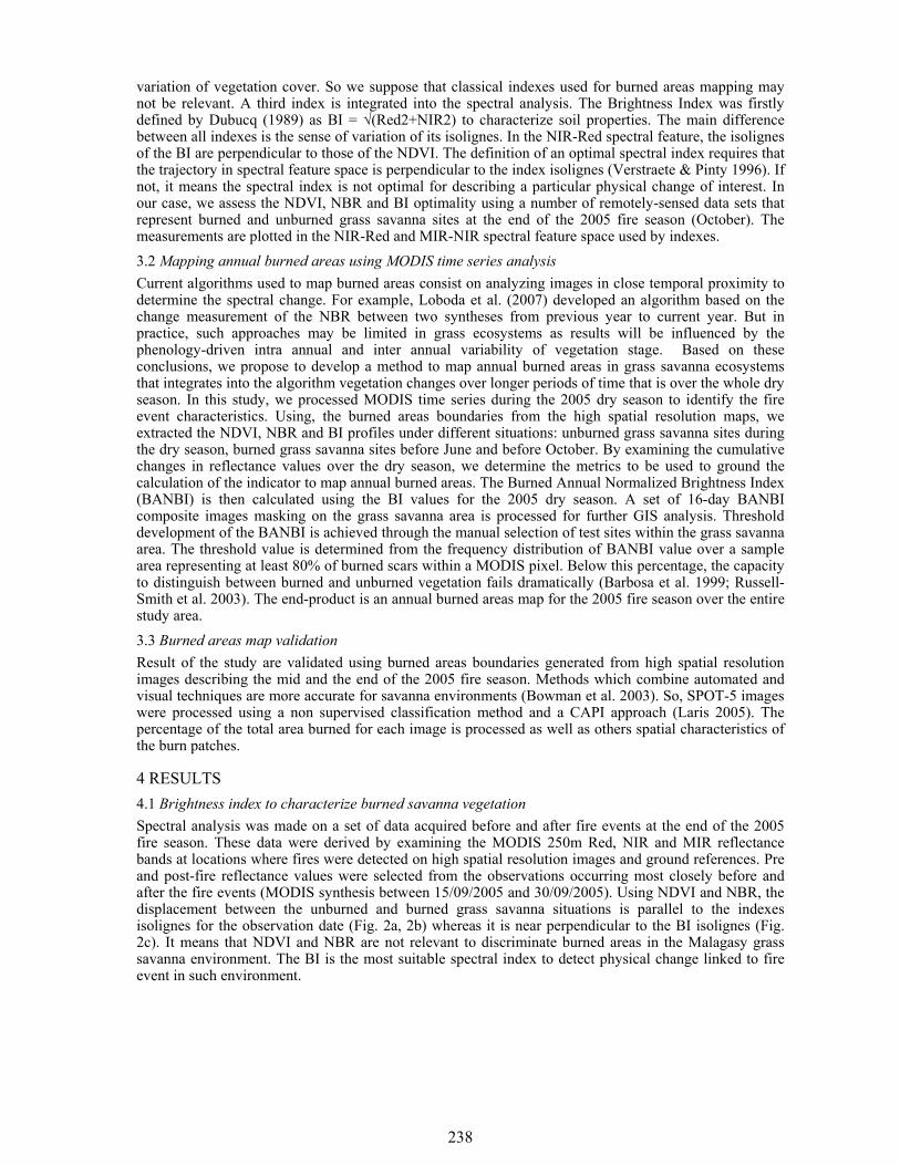
238

variation of vegetation cover. So we suppose that classical indexes used for burned areas mapping may not be relevant. A third index is integrated into the spectral analysis. The Brightness Index was firstly defined by Dubucq (1989) as BI = √(Red2+NIR2) to characterize soil properties. The main difference between all indexes is the sense of variation of its isolignes. In the NIR-Red spectral feature, the isolignes of the BI are perpendicular to those of the NDVI. The definition of an optimal spectral index requires that the trajectory in spectral feature space is perpendicular to the index isolignes (Verstraete & Pinty 1996). If not, it means the spectral index is not optimal for describing a particular physical change of interest. In our case, we assess the NDVI, NBR and BI optimality using a number of remotely-sensed data sets that represent burned and unburned grass savanna sites at the end of the 2005 fire season (October). The measurements are plotted in the NIR-Red and MIR-NIR spectral feature space used by indexes. 3.2 Mapping annual burned areas using MODIS time series analysis Current algorithms used to map burned areas consist on analyzing images in close temporal proximity to determine the spectral change. For example, Loboda et al. (2007) developed an algorithm based on the change measurement of the NBR between two syntheses from previous year to current year. But in practice, such approaches may be limited in grass ecosystems as results will be influenced by the phenology-driven intra annual and inter annual variability of vegetation stage. Based on these conclusions, we propose to develop a method to map annual burned areas in grass savanna ecosystems that integrates into the algorithm vegetation changes over longer periods of time that is over the whole dry season. In this study, we processed MODIS time series during the 2005 dry season to identify the fire event characteristics. Using, the burned areas boundaries from the high spatial resolution maps, we extracted the NDVI, NBR and BI profiles under different situations: unburned grass savanna sites during the dry season, burned grass savanna sites before June and before October. By examining the cumulative changes in reflectance values over the dry season, we determine the metrics to be used to ground the calculation of the indicator to map annual burned areas. The Burned Annual Normalized Brightness Index (BANBI) is then calculated using the BI values for the 2005 dry season. A set of 16-day BANBI composite images masking on the grass savanna area is processed for further GIS analysis. Threshold development of the BANBI is achieved through the manual selection of test sites within the grass savanna area. The threshold value is determined from the frequency distribution of BANBI value over a sample area representing at least 80% of burned scars within a MODIS pixel. Below this percentage, the capacity to distinguish between burned and unburned vegetation fails dramatically (Barbosa et al. 1999; Russell-Smith et al. 2003). The end-product is an annual burned areas map for the 2005 fire season over the entire study area. 3.3 Burned areas map validation Result of the study are validated using burned areas boundaries generated from high spatial resolution images describing the mid and the end of the 2005 fire season. Methods which combine automated and visual techniques are more accurate for savanna environments (Bowman et al. 2003). So, SPOT-5 images were processed using a non supervised classification method and a CAPI approach (Laris 2005). The percentage of the total area burned for each image is processed as well as others spatial characteristics of the burn patches.

4 RESULTS 4.1 Brightness index to characterize burned savanna vegetation Spectral analysis was made on a set of data acquired before and after fire events at the end of the 2005 fire season. These data were derived by examining the MODIS 250m Red, NIR and MIR reflectance bands at locations where fires were detected on high spatial resolution images and ground references. Pre and post-fire reflectance values were selected from the observations occurring most closely before and after the fire events (MODIS synthesis between 15/09/2005 and 30/09/2005). Using NDVI and NBR, the displacement between the unburned and burned grass savanna situations is parallel to the indexes isolignes for the observation date (Fig. 2a, 2b) whereas it is near perpendicular to the BI isolignes (Fig. 2c). It means that NDVI and NBR are not relevant to discriminate burned areas in the Malagasy grass savanna environment. The BI is the most suitable spectral index to detect physical change linked to fire event in such environment.

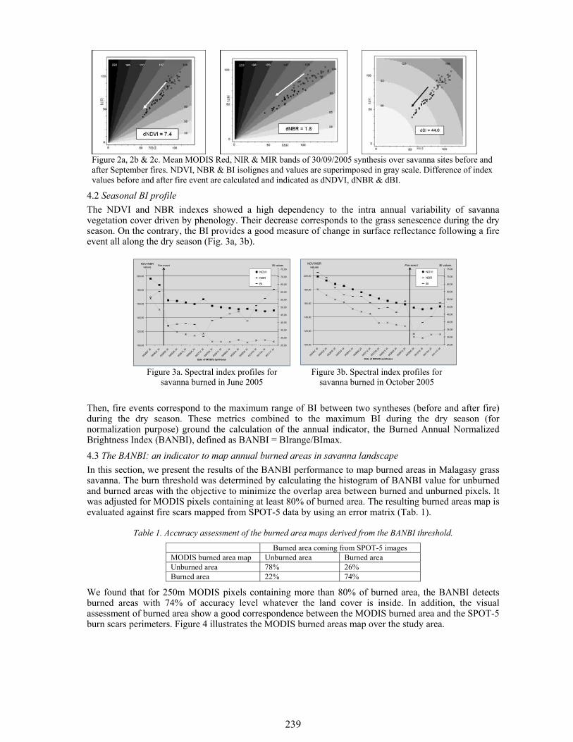
239

Figure 2a, 2b & 2c. Mean MODIS Red, NIR & MIR bands of 30/09/2005 synthesis over savanna sites before and after September fires. NDVI, NBR & BI isolignes and values are superimposed in gray scale. Difference of index values before and after fire event are calculated and indicated as dNDVI, dNBR & dBI.

4.2 Seasonal BI profile The NDVI and NBR indexes showed a high dependency to the intra annual variability of savanna vegetation cover driven by phenology. Their decrease corresponds to the grass senescence during the dry season. On the contrary, the BI provides a good measure of change in surface reflectance following a fire event all along the dry season (Fig. 3a, 3b).

NDVI/NBR values BI valuesFire event

25,00

30,00

35,00

40,00

45,00

50,00

55,00

60,00

65,00

70,00

75,00

100,00

120,00

140,00

160,00

180,00

200,00

Date of MODIS syntheses

NDVI

NBR

BI

NDVI/NBR values BI valuesFire event

25,00

30,00

35,00

40,00

45,00

50,00

55,00

60,00

65,00

70,00

75,00

100,00

120,00

140,00

160,00

180,00

200,00

Date of MODIS syntheses

NDVI

NBR

BI

Figure 3a. Spectral index profiles for

savanna burned in June 2005 Figure 3b. Spectral index profiles for

savanna burned in October 2005 Then, fire events correspond to the maximum range of BI between two syntheses (before and after fire) during the dry season. These metrics combined to the maximum BI during the dry season (for normalization purpose) ground the calculation of the annual indicator, the Burned Annual Normalized Brightness Index (BANBI), defined as BANBI = BIrange/BImax. 4.3 The BANBI: an indicator to map annual burned areas in savanna landscape In this section, we present the results of the BANBI performance to map burned areas in Malagasy grass savanna. The burn threshold was determined by calculating the histogram of BANBI value for unburned and burned areas with the objective to minimize the overlap area between burned and unburned pixels. It was adjusted for MODIS pixels containing at least 80% of burned area. The resulting burned areas map is evaluated against fire scars mapped from SPOT-5 data by using an error matrix (Tab. 1).

Table 1. Accuracy assessment of the burned area maps derived from the BANBI threshold.

Burned area coming from SPOT-5 images MODIS burned area map Unburned area Burned area Unburned area 78% 26% Burned area 22% 74%

We found that for 250m MODIS pixels containing more than 80% of burned area, the BANBI detects burned areas with 74% of accuracy level whatever the land cover is inside. In addition, the visual assessment of burned area show a good correspondence between the MODIS burned area and the SPOT-5 burn scars perimeters. Figure 4 illustrates the MODIS burned areas map over the study area.

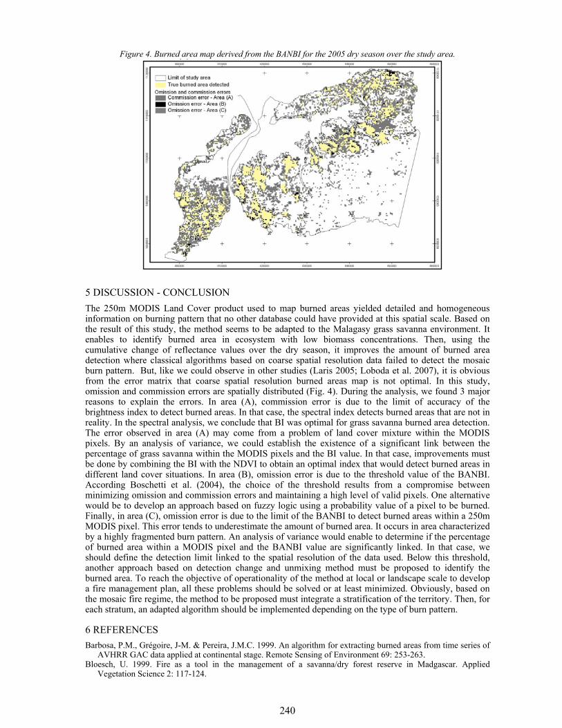
240

Figure 4. Burned area map derived from the BANBI for the 2005 dry season over the study area.

5 DISCUSSION - CONCLUSION The 250m MODIS Land Cover product used to map burned areas yielded detailed and homogeneous information on burning pattern that no other database could have provided at this spatial scale. Based on the result of this study, the method seems to be adapted to the Malagasy grass savanna environment. It enables to identify burned area in ecosystem with low biomass concentrations. Then, using the cumulative change of reflectance values over the dry season, it improves the amount of burned area detection where classical algorithms based on coarse spatial resolution data failed to detect the mosaic burn pattern. But, like we could observe in other studies (Laris 2005; Loboda et al. 2007), it is obvious from the error matrix that coarse spatial resolution burned areas map is not optimal. In this study, omission and commission errors are spatially distributed (Fig. 4). During the analysis, we found 3 major reasons to explain the errors. In area (A), commission error is due to the limit of accuracy of the brightness index to detect burned areas. In that case, the spectral index detects burned areas that are not in reality. In the spectral analysis, we conclude that BI was optimal for grass savanna burned area detection. The error observed in area (A) may come from a problem of land cover mixture within the MODIS pixels. By an analysis of variance, we could establish the existence of a significant link between the percentage of grass savanna within the MODIS pixels and the BI value. In that case, improvements must be done by combining the BI with the NDVI to obtain an optimal index that would detect burned areas in different land cover situations. In area (B), omission error is due to the threshold value of the BANBI. According Boschetti et al. (2004), the choice of the threshold results from a compromise between minimizing omission and commission errors and maintaining a high level of valid pixels. One alternative would be to develop an approach based on fuzzy logic using a probability value of a pixel to be burned. Finally, in area (C), omission error is due to the limit of the BANBI to detect burned areas within a 250m MODIS pixel. This error tends to underestimate the amount of burned area. It occurs in area characterized by a highly fragmented burn pattern. An analysis of variance would enable to determine if the percentage of burned area within a MODIS pixel and the BANBI value are significantly linked. In that case, we should define the detection limit linked to the spatial resolution of the data used. Below this threshold, another approach based on detection change and unmixing method must be proposed to identify the burned area. To reach the objective of operationality of the method at local or landscape scale to develop a fire management plan, all these problems should be solved or at least minimized. Obviously, based on the mosaic fire regime, the method to be proposed must integrate a stratification of the territory. Then, for each stratum, an adapted algorithm should be implemented depending on the type of burn pattern.

6 REFERENCES Barbosa, P.M., Grégoire, J-M. & Pereira, J.M.C. 1999. An algorithm for extracting burned areas from time series of

AVHRR GAC data applied at continental stage. Remote Sensing of Environment 69: 253-263. Bloesch, U. 1999. Fire as a tool in the management of a savanna/dry forest reserve in Madgascar. Applied

Vegetation Science 2: 117-124.

241

Boschetti, L., Flasse, S.P. & Brivio, P.A. 2004. Analysis of the conflict between omission and commission in low spatial dichotomic thematic products: The Pareto Boundary. Remote Sensing of Environment 91: 280-292.

Bowman, D.M.J.S., Zang, Y., Walsh, A. & Williams, R.J. 2003. Experimental comparison of four remote sensing techniques to map tropical savanna fire-scar using Landsat-TM imagery. International Journal of Wildland Fire 12: 341-348.

Dubucq, M. 1989. Identification et cartographie par télédétection des sols érodés : application au Lauragais Toulousain. Université Paul Sabatier, Toulouse.

Epting, J., Verbyla, D. & Sorbel, B. 2005. Evaluation of remotely sensed indices for assessing burn severity in interior Alaska using Landsat TM and ETM+. Remote Sensing of Environment 96: 328-339.

Jeltsch, F., Weber, G.E. & Grimm, V. 2000. Ecological buffering mechanisms in savannas: a unifying theory of long-term tree-grass coexistence. Plant Ecology 161: 161-171.

Key, C.H. & Benson, N.C. 1999. Measuring and remote sensing of burn severity. In: Neuenschwander, L.F., Ryan, K.C. & Goldberg, G.E. (Eds.) Proceedings of the Joint Fire Science Conference, Boise, Idaho 15-17 June, 1999. University of Idaho and the International Association of Wildland fire, vol. II, 284p.

Koelchlin, J. 1993. Grasslands of Madagascar. In: Coupland, R.T. (Ed.) Natural grasslands. Ecosytems of the World 8 (B): 291-301. Elsevier, Amsterdam.

Kull, A.C. 2000. Isle of Fire: The Political Ecology of Landscape Burning in Madagascar. The University of Chicago Press, 256p.

Laris, P.S. 2005. Spatiotemporal problems with detecting and mapping mosaic fire regimes with coarse-resolution satellite data in savanna environments. Remote Sensing of Environment 99: 412-424.

Loboda, T., O’Neal, K.J. & Csiszar, I. 2007. Regionally adaptable dNBR-based algorithm for burned area mapping from MODIS data. Remote Sensing of Environment X: .

Roy, D.P., Yin, Y, Lewis, P.E. & Justice, C.O. 2005. Prototyping a global algorithm for systematic fire-affected area mapping using MODIS time series data. Remote Sensing of Environment 97: 137-162.

Russell-Smith, J., Whitehead, P.J., Williams, R.J. & Flannigan, M. 2003. Fire and savanna landscapes in northern Australia. Regional lessons and global challenges. International Journal of Wildland Fire 12, v-ix.

Skarpe, C. 1992. Dynamics of savanna ecosystems. Journal of Vegetation Science 3: 293-300. Stroppiana, D., Pinnock, S., Pereira, J.M.C. & Grégoire, J-M. 2002. Radiometric analysis of SPOT VEGETATION

images for burnt area detection in Northern Australia. Remote Sensing of Environment 82, 21-37. Verstraete, M.M. & Pinty, B. 1996. Designing optimal spectral indexes for remote sensing applications. IEEE Trans.

Geosci. Remote Sens. 34 (5): 1254-1265.

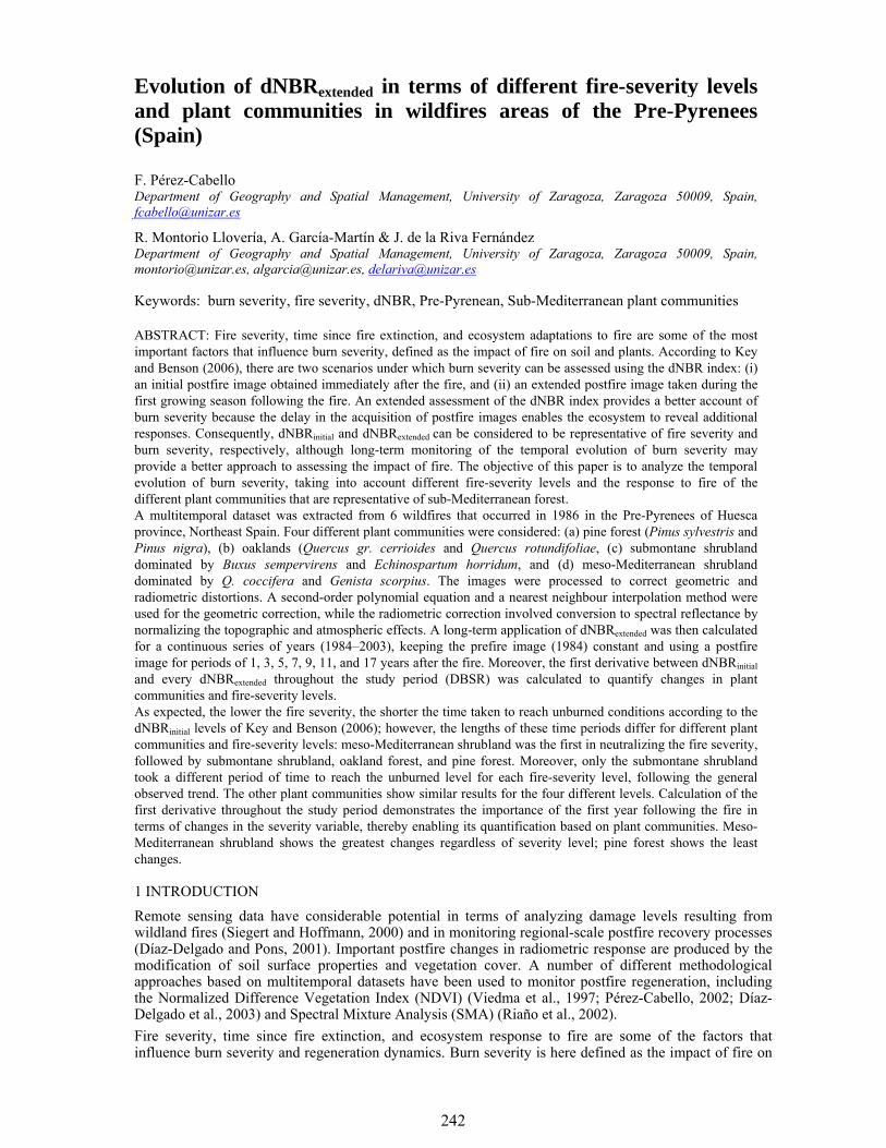
242

1 INTRODUCTION Remote sensing data have considerable potential in terms of analyzing damage levels resulting from wildland fires (Siegert and Hoffmann, 2000) and in monitoring regional-scale postfire recovery processes (Díaz-Delgado and Pons, 2001). Important postfire changes in radiometric response are produced by the modification of soil surface properties and vegetation cover. A number of different methodological approaches based on multitemporal datasets have been used to monitor postfire regeneration, including the Normalized Difference Vegetation Index (NDVI) (Viedma et al., 1997; Pérez-Cabello, 2002; Díaz-Delgado et al., 2003) and Spectral Mixture Analysis (SMA) (Riaño et al., 2002). Fire severity, time since fire extinction, and ecosystem response to fire are some of the factors that influence burn severity and regeneration dynamics. Burn severity is here defined as the impact of fire on

Evolution of dNBRextended in terms of different fire-severity levels and plant communities in wildfires areas of the Pre-Pyrenees (Spain)

F. Pérez-Cabello Department of Geography and Spatial Management, University of Zaragoza, Zaragoza 50009, Spain, [email protected]

R. Montorio Llovería, A. García-Martín & J. de la Riva Fernández Department of Geography and Spatial Management, University of Zaragoza, Zaragoza 50009, Spain, [email protected], [email protected], [email protected] Keywords: burn severity, fire severity, dNBR, Pre-Pyrenean, Sub-Mediterranean plant communities

ABSTRACT: Fire severity, time since fire extinction, and ecosystem adaptations to fire are some of the most important factors that influence burn severity, defined as the impact of fire on soil and plants. According to Key and Benson (2006), there are two scenarios under which burn severity can be assessed using the dNBR index: (i) an initial postfire image obtained immediately after the fire, and (ii) an extended postfire image taken during the first growing season following the fire. An extended assessment of the dNBR index provides a better account of burn severity because the delay in the acquisition of postfire images enables the ecosystem to reveal additional responses. Consequently, dNBRinitial and dNBRextended can be considered to be representative of fire severity and burn severity, respectively, although long-term monitoring of the temporal evolution of burn severity may provide a better approach to assessing the impact of fire. The objective of this paper is to analyze the temporal evolution of burn severity, taking into account different fire-severity levels and the response to fire of the different plant communities that are representative of sub-Mediterranean forest. A multitemporal dataset was extracted from 6 wildfires that occurred in 1986 in the Pre-Pyrenees of Huesca province, Northeast Spain. Four different plant communities were considered: (a) pine forest (Pinus sylvestris and Pinus nigra), (b) oaklands (Quercus gr. cerrioides and Quercus rotundifoliae, (c) submontane shrubland dominated by Buxus sempervirens and Echinospartum horridum, and (d) meso-Mediterranean shrubland dominated by Q. coccifera and Genista scorpius. The images were processed to correct geometric and radiometric distortions. A second-order polynomial equation and a nearest neighbour interpolation method were used for the geometric correction, while the radiometric correction involved conversion to spectral reflectance by normalizing the topographic and atmospheric effects. A long-term application of dNBRextended was then calculated for a continuous series of years (1984–2003), keeping the prefire image (1984) constant and using a postfire image for periods of 1, 3, 5, 7, 9, 11, and 17 years after the fire. Moreover, the first derivative between dNBRinitial and every dNBRextended throughout the study period (DBSR) was calculated to quantify changes in plant communities and fire-severity levels. As expected, the lower the fire severity, the shorter the time taken to reach unburned conditions according to the dNBRinitial levels of Key and Benson (2006); however, the lengths of these time periods differ for different plant communities and fire-severity levels: meso-Mediterranean shrubland was the first in neutralizing the fire severity, followed by submontane shrubland, oakland forest, and pine forest. Moreover, only the submontane shrubland took a different period of time to reach the unburned level for each fire-severity level, following the general observed trend. The other plant communities show similar results for the four different levels. Calculation of the first derivative throughout the study period demonstrates the importance of the first year following the fire in terms of changes in the severity variable, thereby enabling its quantification based on plant communities. Meso-Mediterranean shrubland shows the greatest changes regardless of severity level; pine forest shows the least changes.

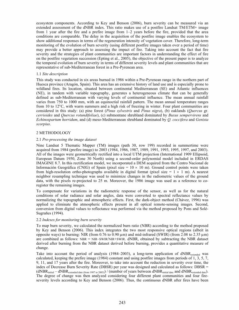
243

ecosystem components. According to Key and Benson (2006), burn severity can be measured via an extended assessment of the dNBR index. This ratio makes use of a postfire Landsat TM/ETM+ image from 1 year after the fire and a prefire image from 1–2 years before the fire, provided that the area conditions are comparable. The delay in the acquisition of the postfire image enables the ecosystem to show additional responses in terms of the regeneration intensity of vegetation cover. Therefore, long-term monitoring of the evolution of burn severity (using different postfire images taken over a period of time) may provide a better approach to assessing the impact of fire. Taking into account the fact that fire severity and the strategies of plant communities are important factors in understanding the effect of fire on the postfire vegetation succession (Epting et al., 2005), the objective of the present paper is to analyze the temporal evolution of burn severity in terms of different severity levels and plant communities that are representative of sub-Mediterranean forest in a Pre-Pyrenean area.

1.1 Site description This study was conducted in six areas burned in 1986 within a Pre-Pyrenean range in the northern part of Huesca province (Aragón, Spain). This area has an extensive history of land use and is especially prone to wildland fires. Its location, situated between continental Mediterranean (SE) and Atlantic influences (NE), in tandem with variable topography, generates a heterogeneous climate that can be generally defined as sub-Mediterranean with varying levels of continental influence. The mean annual rainfall varies from 750 to 1000 mm, with an equinoctial rainfall pattern. The mean annual temperature ranges from 10 to 12°C, with warm summers and a high risk of freezing in winter. Four plant communities are considered in this study: (a) pine forest (Pinus sylvestris and Pinus nigra), (b) oaklands (Quercus gr. cerrioides and Quercus rotundifoliae), (c) submontane shrubland dominated by Buxus sempervirens and Echinospartum horridum, and (d) meso-Mediterranean shrubland dominated by Q. coccifera and Genista scorpius.

2 METHODOLOGY 2.1 Pre-processing the image dataset Nine Landsat 5 Thematic Mapper (TM) images (path 30, row 199) recorded in summertime were acquired from 1984 (prefire image) to 2003 (1984, 1986, 1987, 1989, 1991, 1993, 1995, 1997, and 2003). All of the images were geometrically rectified into a local UTM projection (International 1909 Ellipsoid, European Datum 1950, Zone 30 North) using a second-order polynomial model included in ERDAS IMAGINE 8.7. In this rectification model, we incorporated a DEM acquired from the Centro Nacional de Información Geográfica (CNIG) of Spain (pixel size = 10 × 10 m). Ground control points were taken from high-resolution ortho-photographs available in digital format (pixel size = 1 × 1 m). A nearest neighbor resampling technique was used to minimize changes in the radiometric values of the ground data, with the pixels re-projected to 25 m. Moreover, the 1986 image was used as a reference to co-register the remaining images. To compensate for variations in the radiometric response of the sensor, as well as for the natural conditions of solar radiance and solar angles, data were converted to spectral reflectance values by normalizing the topographic and atmospheric effects. First, the dark-object method (Chávez, 1996) was applied to eliminate the atmospheric effects present in all optical remote-sensing images. Second, conversion from digital values to reflectance was performed via the method proposed by Pons and Solé-Sugrañes (1994). 2.2 Indexes for monitoring burn severity To map burn severity, we calculated the normalized burn ratio (NBR) according to the method proposed by Key and Benson (2006). This index integrates the two most responsive optical regions (albeit in opposite ways) to burning: NIR (from 0.76 to 0.90 μm) and mid-infrared (SWIR) (from 2.08 to 2.35 μm) are combined as follows: NBR = NIR–SWIR/NIR+SWIR. dNBR, obtained by subtracting the NBR dataset derived after burning from the NBR dataset derived before burning, provides a quantitative measure of change. Take into account the period of analysis (1984–2003), a long-term application of dNBRextended was calculated, keeping the prefire image (1984) constant and using postfire images from periods of 1, 3, 5, 7, 9, 11, and 17 years after the fire. Moreover, to take into account the reduction in severity over time, the index of Decrease Burn Severity Rate (DBSR) per year was designed and calculated as follows: DBSR = (dNBRinitial – dNBRextended date (from 1987 to 2003)) / (number of years between dNBRinitial date and dNBRextended date). The degree of change was then analyzed considering four different plant communities and four fire-severity levels according to Key and Benson (2006). Thus, the continuous dNBR after fires have been

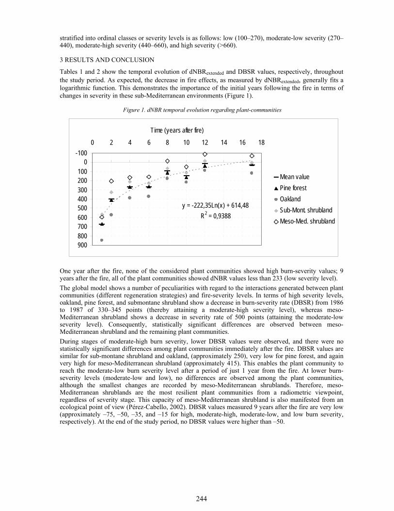
244

stratified into ordinal classes or severity levels is as follows: low (100–270), moderate-low severity (270–440), moderate-high severity (440–660), and high severity (>660).

3 RESULTS AND CONCLUSION

Tables 1 and 2 show the temporal evolution of dNBRextended and DBSR values, respectively, throughout the study period. As expected, the decrease in fire effects, as measured by dNBRextended, generally fits a logarithmic function. This demonstrates the importance of the initial years following the fire in terms of changes in severity in these sub-Mediterranean environments (Figure 1).

Figure 1. dNBR temporal evolution regarding plant-communities

One year after the fire, none of the considered plant communities showed high burn-severity values; 9 years after the fire, all of the plant communities showed dNBR values less than 233 (low severity level). The global model shows a number of peculiarities with regard to the interactions generated between plant communities (different regeneration strategies) and fire-severity levels. In terms of high severity levels, oakland, pine forest, and submontane shrubland show a decrease in burn-severity rate (DBSR) from 1986 to 1987 of 330–345 points (thereby attaining a moderate-high severity level), whereas meso-Mediterranean shrubland shows a decrease in severity rate of 500 points (attaining the moderate-low severity level). Consequently, statistically significant differences are observed between meso-Mediterranean shrubland and the remaining plant communities. During stages of moderate-high burn severity, lower DBSR values were observed, and there were no statistically significant differences among plant communities immediately after the fire. DBSR values are similar for sub-montane shrubland and oakland, (approximately 250), very low for pine forest, and again very high for meso-Mediterranean shrubland (approximately 415). This enables the plant community to reach the moderate-low burn severity level after a period of just 1 year from the fire. At lower burn-severity levels (moderate-low and low), no differences are observed among the plant communities, although the smallest changes are recorded by meso-Mediterranean shrublands. Therefore, meso-Mediterranean shrublands are the most resilient plant communities from a radiometric viewpoint, regardless of severity stage. This capacity of meso-Mediterranean shrubland is also manifested from an ecological point of view (Pérez-Cabello, 2002). DBSR values measured 9 years after the fire are very low (approximately –75, –50, –35, and –15 for high, moderate-high, moderate-low, and low burn severity, respectively). At the end of the study period, no DBSR values were higher than –50.

y = -222,35Ln(x) + 614,48R2 = 0,9388

-1000

100200300400500600700800900

0 2 4 6 8 10 12 14 16 18

Time (years after fire)

Mean valuePine forestOaklandSub-Mont. shrublandMeso-Med. shrubland

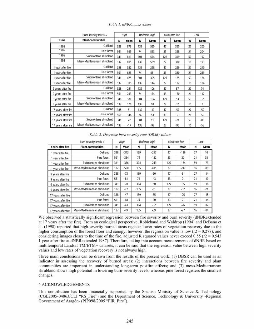
245

Table 1. dNBRextended values

Burn severity levels » High Moderate-high Moderate-low Low Time Plant-communities N Mean N Mean N Mean N Mean

1986 Oakland 338 876 139 555 47 365 27 200 1986 Pine forest 561 959 74 563 33 358 21 204 1986 Submontane shrubland 341 811 304 554 127 369 59 197 1986 Meso-Mediterranean shrubland 137 815 135 559 27 370 16 193

1 year after fire Oakland 338 532 139 298 47 229 27 210 1 year after fire Pine forest 561 625 74 431 33 380 21 239 1 year after fire Submontane shrubland 341 475 304 305 127 185 59 124 1 year after fire Meso-Mediterranean shrubland 137 315 135 144 27 122 16 104

9 years after fire Oakland 338 221 139 106 47 87 27 74 9 years after fire Pine forest 561 233 74 174 33 170 21 112 9 years after fire Submontane shrubland 341 180 304 104 127 53 59 32 9 years after fire Meso-Mediterranean shrubland 137 120 135 10 27 32 16 3

17 years after fire Oakland 338 81 139 -40 47 -57 27 -59 17 years after fire Pine forest 561 148 74 53 33 5 21 -50 17 years after fire Submontane shrubland 341 72 304 11 127 -74 59 -86 17 years after fire Meso-Mediterranean shrubland 137 -17 135 -98 27 -96 16 -53

Table 2. Decrease burn severity rate (DBSR) values

Burn severity levels » High Moderate-high Moderate-low Low Years after fire Plant-communities N Mean N Mean N Mean N Mean

1 year after fire Oakland 338 -343 139 -257 47 -136 27 10

1 year after fire Pine forest 561 -334 74 -132 33 22 21 35

1 year after fire Submontane shrubland 341 -336 304 -249 127 -184 59 -73

1 year after fire Meso-Mediterranean shrubland 137 -500 135 -415 27 -247 16 -89

9 years after fire Oakland 338 -73 139 -50 47 -31 27 -14

9 years after fire Pine forest 561 -81 74 -43 33 -21 21 -10

9 years after fire Submontane shrubland 341 -70 304 -50 127 -35 59 -18

9 years after fire Meso-Mediterranean shrubland 137 -77 135 -61 27 -37 16 -21

17 years after fire Oakland 338 -47 139 -35 47 -25 27 -15

17 years after fire Pine forest 561 -48 74 -30 33 -21 21 -15

17 years after fire Submontane shrubland 341 -43 304 -32 127 -26 59 -17

17 years after fire Meso-Mediterranean shrubland 137 -49 135 -39 27 -27 16 -14

We observed a statistically significant regression between fire severity and burn severity (dNBRextended at 17 years after the fire). From an ecological perspective, Robichaud and Waldrop (1994) and DeBano et al. (1998) reported that high-severity burned areas register lower rates of vegetation recovery due to the higher consumption of the forest floor and canopy; however, the regression value is low (r2 = 0.278), and considering images closer to the time of the fire, adjusted R squared values never exceed 0.55 (r2 = 0.543 1 year after fire at dNBRextended 1987). Therefore, taking into account measurements of dNBR based on multitemporal Landsat TM/ETM+ datasets, it can be said that the regression value between high severity values and low rates of vegetation recovery is not always high. Three main conclusions can be drawn from the results of the present work: (1) DBSR can be used as an indicator in assessing the recovery of burned areas; (2) interactions between fire severity and plant communities are important in understanding long-term postfire effects; and (3) meso-Mediterranean shrubland shows high potential in lowering burn-severity levels, whereas pine forest registers the smallest changes.

4 ACKNOWLEDGEMENTS This contribution has been financially supported by the Spanish Ministry of Science & Technology (CGL2005-04863/CLI “RS_Fire”) and the Department of Science, Technology & University -Regional Government of Aragón- (PIP098/2005 “PIR_Fire”).

246

5 REFERENCES Chavez, P.S. 1996. Image-based atmospheric corrections. Revisited and improved. Photogrammetric Engineering

and Remote Sensing 62 (9): 1025-1036. DeBano, L.F., Neary, D.G., Ffolliott, P.F. 1998. Fire’s Effects on Ecosystems. New York: John Wiley & Sons. 333

p. Díaz-Delgado, R., Lloret, F. and Pons, X. 2003. Influence of fire severity on plant regeneration through remote

sensing imagery. International Journal of Remote Sensing 24(8): 1751-1763. Díaz-Delgado, R., Pons, X. 2001. Spatial patterns of forest fires in Catalonia (NE Spain) along the period 1975-

1995. Analysis of vegetation recovery after fire. Forest Ecology and Management 147(1): 67-74. Epting, J., Verbyla, D. L., Sorbel, B. 2005. Evaluation of remotely senses indices for assessing burn severity in

interior Alaska using Landsat TM and ETM+. Remote Sensing of Environment 96: 328-339. Key, C.H., Benson, N. 2006. Landscape assessment. Sampling and analysis methods. USDA Forest Service.

General Technical Report. RMRS-GTR-164-CD. Pérez Cabello, F. 2002. Paisajes forestales y fuego en el prepirineo occidental oscense: un modelo regional de

reconstrucción ambiental. Zaragoza, 2002. 358 p. Serie Investigación, 33. ISBN 84-89862-27-3. Pons, X. y Solé-Sugrañes, L. 1994. A simple radiometric correction model to improve automatic mapping of

vegetation from multispectral satellite data. Remote Sensing of Environment 48: 191-204. Riaño, D., Chuvieco, E., Ustin, S., Zomer, R., Dennison, P., Roberts, D., Salas, J., 2002. Assessment of vegetation

regeneration after fire through multitemporal analysis of AVIRIS images in the Santa Monica Mountains. Remote Sensing of Environment 79:60-71.

Robichaud, P.R., Waldrop, T.A. 1994. A comparison of surface runoff and sediment yields from a low- and high-severity site preparation burns. Water Resources Bulletin 30 (1): 27- 34.

Siegert F., Hoffmann A. 2000. The 1998 Forest Fires in East-Kalimantan (Indonesia): A quantitative evaluation using high resolution, multitemporal ERS-2 SAR Images and NOAA-AVHRR hotspot data. Remote Sensing of Environment 72: 64-77.

Viedma, O., Meliá, J., Segarra, D. y García-Haro, J. 1997. Modeling rates of ecosystem recovery after fires by using Landsat TM data. Remote Sensing of Environment 61: 383-398.

247

1 INTRODUCTION In the post-fire management, the knowledge of the damage level distribution in the burnt area is a key factor to prioritize treatments for protecting resources at risk and to help the selection of the more appropriate treatments to apply on site (Bobbe, 2001). Both short- and long-term post-fire effects on vegetation and soil and related processes can be estimated in terms of “burn severity” (Chuvieco et al., 2006b; De Santis and Chuvieco, 2007; Key and Benson, 2005; Lentile, 2006; van Wagtendonk et al., 2004; White et al., 1996). Different methods of burn severity estimation have been proposed using post-fire field measurements (Moreno and Oechel, 1989; Pérez and Moreno, 1998). Since field surveys are costly and time-consuming and do not provide a good spatial coverage, remotely sensed images are proposed as a sound alternative, since they provide relatively cheap, fast and spatially representative coverage of the area affected by the fire. Recent studies (Chuvieco et al., 2006a; Chuvieco et al., 2006b; De Santis and Chuvieco, 2007) have proposed the use of the Radiative Transfer Models (RTMs) to simulate the continuum of burn severity levels in terms of Composite Burn Index (CBI) (Key and Benson, 2005). The performance of RTMs greatly depends on the type of model selected, its ability to simulate real conditions, and the quality of input data to estimate the required parameters. Most commonly, models at different scales are linked (leaf-canopy-landscape-atmosphere), to provide a more comprehensive and realistic simulation. At leaf level the main input parameters of simulation models are clorophyll a+b content (Cab), leaf optical thickness (defined as an structural parameter N), brown pigments content (Cb), water content (Cw) and dry matter content (Cm). They have been measured or estimated individually in several studies. However, there are no example of a systematic study of the fire induced variation of biophysical leaf parameters and reflectance/transmittance leaf measurements. Therefore, the objectives of this paper are:

- The experimental estimation of the leaf biophysical parameter variation related to the dry and scorch process caused by fire.

- To link leaf parameters to simulate burn severity values at landscape level using the GEOSAIL model.

Inversion of the GeoSAIL radiative transfer model to estimate burn severity

Angela De Santis, Marta Yebra, Emilio Chuvieco Department of Geography, University of Alcalá, Calle Colegios 2, 28801 Alcalá de Henares (Madrid-Spain), [email protected], [email protected], [email protected]

Keywords: Burn Severity, CBI, simulation model, model inversion, GeoSAIL.

ABSTRACT: Burn severity is a key factor to estimate fire effects on vegetation and soil, to assist forest managers in allocating resources for restoration efforts and to estimate the potential regeneration of the vegetation. In previous studies we inverted the Kuusk model to estimate burn severity, as defined by the Composite Burn Index (CBI). This approach provided better results than empirical models. However, the accuracy of the estimation of intermediate CBI values was no acceptable. In this paper we explore the use of a geometric simulation model to improve the previous results obtained with the Kuusk model. Laboratory radiometry experimentation at leaf level was performed with Cork oak (Quercus suber) (a Mediterranean species). Using the GER 2600 spectroradiometer with an integration sphere Licor, both reflectance and transmittance of green and scorched leaves were measured. The results were used as input to run the GeoSAIL model in direct mode. The C language version of the GeoSAIL model was selected because it made it possible the simulation of two vegetation layers plus a substrate, hence resembling more closely the five-layer strata of the CBI method. The result of this forward simulation was turned in to a spectral library and used as reference spectra for the inversion of the model, using the Spectral Angle Mapper algorithm. The validation was performed comparing the results to the field estimated CBI (99 plots). The study area, located in central Spain, was affected by a large forest fire in 2005. The results show an improvement in the burn severity estimation in all range of CBI respect to the Kuusk simulation. The Root Mean Square Error (RMSE) between field and simulated CBI was equal to 0.18 for 92 of 99 plots. The remaining 7 plots presented sub-estimation of the damage (RMSE=1.75), because they have a very high fraction of cover of the tree stratum (FCOV>60%) and green canopies which masked out the signal of the burnt area underneath.

248

- Compare the results of GEOSAIL inversion with previous results using the Kuusk model (De Santis and Chuvieco, 2007).

2 MATERIALS AND METHODS 2.1 Species selection and description The species selected for this study was Cork oak (Quercus suber), which is economically important and commonly present in Mediterranean Forest. A total of 30 leaves of different cork oaks were collected in the campus of the UC DAVIS (USA) in December 2005. After the collection, the leaves were placed in zip-bags and transported to the lab. 2.2 Sampling timing determination The first step was to determinate the sampling timing necessary to cover all the drying/scorching process. To achieve it, 5 leaves were weighed in fresh and placed into the oven at 60º C (QL Model 10 Lab Oven ™). Their weights were taken again every 10 sec until resulting constant. Then the temperature of the oven was increased to 100º C (max T) and the weight was taken again (at the same interval) until the leaf was scorched. After the time in the oven, the complete scorching was obtained using the direct flame of a lighter. To avoid the leaf curling due to the drying process what could make difficult both radiometric and biophysical measurements, the leaves were placed on a paper tray and were pinned up with clips.

2.3 Spectroradiometric measurements Reflectance and transmittance measurements of the same leaves were taken after weighing and measuring the biophysical parameter above mention. A GER 2600 (GER Corp., Millbrook, NY) spectroradiometer coupled to a LI-COR 1800 integrating sphere (LI-COR, inc.,4421 Superior Street, P.O. Box 4425, Lincoln, Nebraska 68504-0425 USA) by a standard optical fibre was used. Four reflectance and four transmittance measurements per leaf (two for each side of the central leaf nerve) and time were done. Targets were calibrated against a Labshere Spectralon™ white reference panel (Labsphere, Inc. North Sutton, New Hampshire). The laboratory geometry was kept fixed throughout the experiment. 2.4 Biophysical measurements For each sampling time and leaf, the following parameters were measured: -Leaf Area: was measured by the classification of a digital photo. Each leaf was placed on a millimetre paper, for the pixel calibration, and a perpendicular picture was taken. -Leaf weight: was obtained using a precision balance (DENVER Instrument, 4 digits accuracy) managed by the software Labtronics Balance Talk XL TM. -Water content: was computed as both Equivalent Water Thickness (EWT) and Fuel Moisture Content (FMC) as follow:

Where Wf and Wd are fresh and dry weight, respectively, and A is leaf area.

-Dry matter: was measured as Specific Leaf Weight (SLW)(3); -Chlorophyll a+b content (Ca+b), brown pigments content (Cs) and structure parameter N were estimated by the inversion of PROSPECT model (http://rtm.casil.ucdavis.edu/?Models: PROSPECT) using the observed reflectance and transmittance and keeping fix the inputs corresponding to the measured leaf parameters.

2.5 Simulation models Two simulation models were used in this study. The PROSPECT model was used in forward mode to simulate four reference spectra at leaf level, corresponding to four damage levels: from null (green leaf) to high (scorched leaf). For this simulation, the inputs the parameters derived from the experiment (see table 1). Finally, these simulated spectra were used as inputs, joined to different substratum spectra and vegetation structure parameters (derived from field measurement in the Guadalajara fire), to perform the simulation of the burn severity at canopy level with the GeoSAIL model (Huemmrich, 1995; http://rtm.casil.ucdavis.edu/?Models:GEOSAIL), in terms of CBI (table 1). The result of this last simulation was a look up table, which was turned into a spectral library (RSI, ENVI 4.3). The spectral

AWW

cmgEWT df −=)/()1( 2 100(%))2( ×

−=

d

df

WWW

FMC AW

cmgSLW d=)/()3( 2

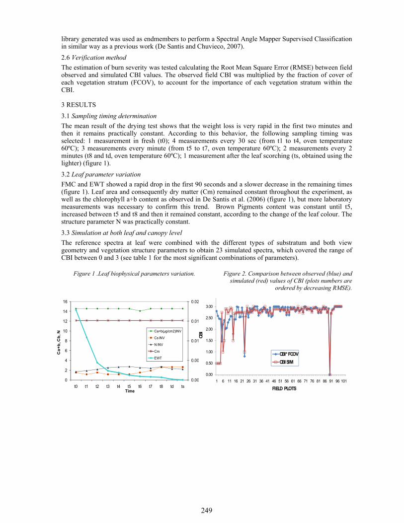
249

library generated was used as endmembers to perform a Spectral Angle Mapper Supervised Classification in similar way as a previous work (De Santis and Chuvieco, 2007). 2.6 Verification method The estimation of burn severity was tested calculating the Root Mean Square Error (RMSE) between field observed and simulated CBI values. The observed field CBI was multiplied by the fraction of cover of each vegetation stratum (FCOV), to account for the importance of each vegetation stratum within the CBI.

3 RESULTS 3.1 Sampling timing determination The mean result of the drying test shows that the weight loss is very rapid in the first two minutes and then it remains practically constant. According to this behavior, the following sampling timing was selected: 1 measurement in fresh (t0); 4 measurements every 30 sec (from t1 to t4, oven temperature 60ºC); 3 measurements every minute (from t5 to t7, oven temperature 60ºC); 2 measurements every 2 minutes (t8 and td, oven temperature 60ºC); 1 measurement after the leaf scorching (ts, obtained using the lighter) (figure 1).

3.2 Leaf parameter variation FMC and EWT showed a rapid drop in the first 90 seconds and a slower decrease in the remaining times (figure 1). Leaf area and consequently dry matter (Cm) remained constant throughout the experiment, as well as the chlorophyll a+b content as observed in De Santis et al. (2006) (figure 1), but more laboratory measurements was necessary to confirm this trend. Brown Pigments content was constant until t5, increased between t5 and t8 and then it remained constant, according to the change of the leaf colour. The structure parameter N was practically constant. 3.3 Simulation at both leaf and canopy level The reference spectra at leaf were combined with the different types of substratum and both view geometry and vegetation structure parameters to obtain 23 simulated spectra, which covered the range of CBI between 0 and 3 (see table 1 for the most significant combinations of parameters).

Figure 1 .Leaf biophysical parameters variation. Figure 2. Comparison between observed (blue) and simulated (red) values of CBI (plots numbers are

ordered by decreasing RMSE).

0.000

0.005

0.010

0.015

0.020

0

2

4

6

8

10

12

14

16

t0 t1 t2 t3 t4 t5 t6 t7 t8 td ts

EW

T, Cm

Ca+

b, C

b, N

Time

Ca+b(µg/cm2)INV

Cs INV

N INV

Cm

EWT

0.00

0.50

1.00

1.50

2.00

2.50

3.00

1 6 11 16 21 26 31 36 41 46 51 56 61 66 71 76 81 86 91 96 101

CBI

FIELD PLOTS

CBI*FCOVCBI SIM

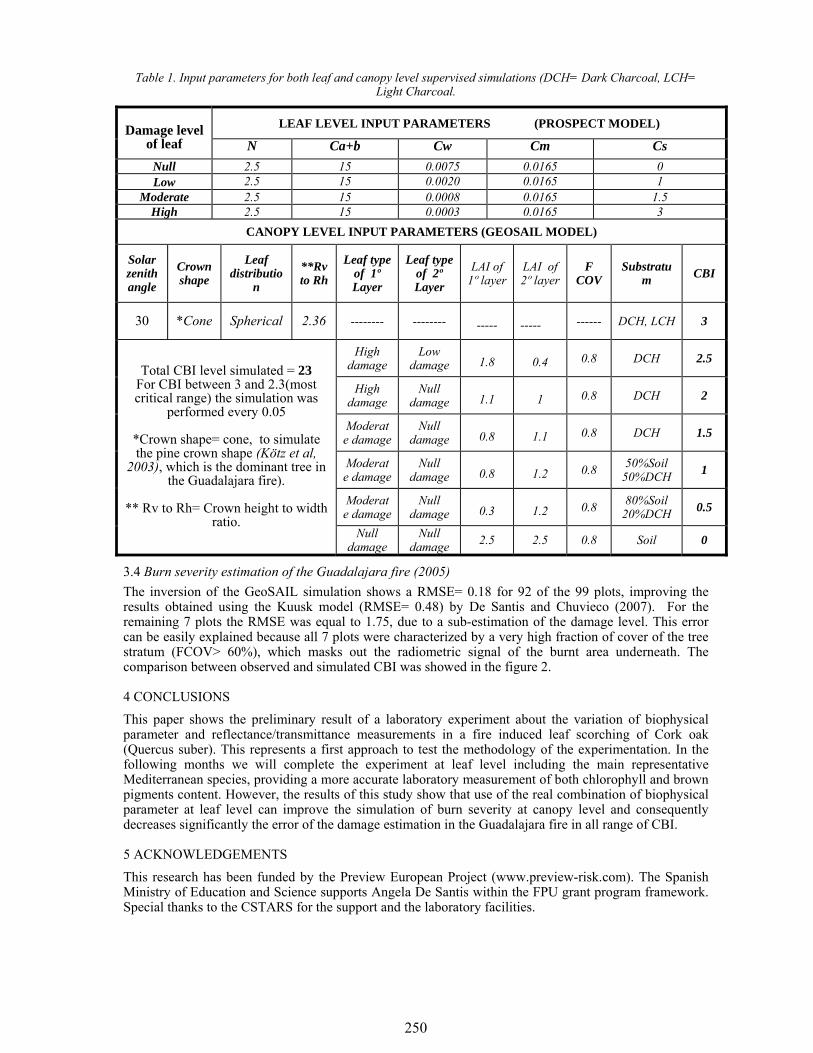
250

Table 1. Input parameters for both leaf and canopy level supervised simulations (DCH= Dark Charcoal, LCH= Light Charcoal.

LEAF LEVEL INPUT PARAMETERS (PROSPECT MODEL) Damage level of leaf N Ca+b Cw Cm Cs

Null 2.5 15 0.0075 0.0165 0 Low 2.5 15 0.0020 0.0165 1

Moderate 2.5 15 0.0008 0.0165 1.5 High 2.5 15 0.0003 0.0165 3

CANOPY LEVEL INPUT PARAMETERS (GEOSAIL MODEL)

Solar zenith angle

Crown shape

Leaf distributio

n

**Rv to Rh

Leaf type of 1º Layer

Leaf type of 2º Layer

LAI of

1º layer

LAI of 2º layer

F COV

Substratum CBI

30 *Cone Spherical 2.36 -------- -------- ----- ----- ------ DCH, LCH 3

High damage

Low damage 1.8 0.4 0.8 DCH 2.5

High damage

Null damage 1.1 1 0.8 DCH 2

Moderate damage

Null damage 0.8 1.1 0.8 DCH 1.5

Moderate damage

Null damage 0.8 1.2 0.8 50%Soil

50%DCH 1

Moderate damage

Null damage 0.3 1.2 0.8 80%Soil

20%DCH 0.5

Total CBI level simulated = 23 For CBI between 3 and 2.3(most critical range) the simulation was

performed every 0.05

*Crown shape= cone, to simulate the pine crown shape (Kötz et al,

2003), which is the dominant tree in the Guadalajara fire).

** Rv to Rh= Crown height to width

ratio. Null

damage Null

damage 2.5 2.5 0.8 Soil 0

3.4 Burn severity estimation of the Guadalajara fire (2005) The inversion of the GeoSAIL simulation shows a RMSE= 0.18 for 92 of the 99 plots, improving the results obtained using the Kuusk model (RMSE= 0.48) by De Santis and Chuvieco (2007). For the remaining 7 plots the RMSE was equal to 1.75, due to a sub-estimation of the damage level. This error can be easily explained because all 7 plots were characterized by a very high fraction of cover of the tree stratum (FCOV> 60%), which masks out the radiometric signal of the burnt area underneath. The comparison between observed and simulated CBI was showed in the figure 2.

4 CONCLUSIONS This paper shows the preliminary result of a laboratory experiment about the variation of biophysical parameter and reflectance/transmittance measurements in a fire induced leaf scorching of Cork oak (Quercus suber). This represents a first approach to test the methodology of the experimentation. In the following months we will complete the experiment at leaf level including the main representative Mediterranean species, providing a more accurate laboratory measurement of both chlorophyll and brown pigments content. However, the results of this study show that use of the real combination of biophysical parameter at leaf level can improve the simulation of burn severity at canopy level and consequently decreases significantly the error of the damage estimation in the Guadalajara fire in all range of CBI.

5 ACKNOWLEDGEMENTS This research has been funded by the Preview European Project (www.preview-risk.com). The Spanish Ministry of Education and Science supports Angela De Santis within the FPU grant program framework. Special thanks to the CSTARS for the support and the laboratory facilities.

251

6 REFERENCES Bobbe, T., Finco, M.V., Quayle, B., Lannom, K., Sohlberg, R., Parsons, A. (2001). Field measurements for the

training and validation of burn severity maps from spaceborne, remotely sensed imagery, USDA Forest Service, Remote Sensing Applications Center, Salt Lake City, Utah.

Chuvieco, E., De Santis, A., Riaño, D., Halligan, K., (2006a). Simulation tools for burn severity estimation using remotely sensed images, Proceeding of 3dr International Fire Ecology And Management Congress, San Diego (Usa), 13-17 November 2006.

Chuvieco, E., Riaño, D., Danson, F.M., Martín, P. (2006b), Use of a radiative transfer model to simulate the postfire spectral response to burn severity, Journal Of Geophysical Research. 111(g04s09): doi: 10.1029/2005jg000143.

De Santis, A., Chuvieco, E. (2007), Burn severity estimation from remotely sensed data: performance of simulation versus empirical models, Remote Sensing Of Environment. 108(4): 422-435.

De Santis, A., Vaughan, P. Chuvieco, E. (2006), Foliage moisture content estimation from 1-d and 2-d spectroradiometry for fire danger assessment, Journal Of Geophysical Research - Biosciences. 111(g04s03).

Key, C.H., Benson, N. (2005), Landscape assessment: ground measure of severity, the composite burn index; and remote sensing of severity, the normalized burn ratio. In: firemon: fire effects monitoring and inventory system (d.c. Lutes, r.e. Keane, j.f. Caratti, c.h. Key, n.c. Benson and l.j. Gangi, eds.), Usda Forest Service, Rocky Mountain Research Station, gen. Tech. Rep. Rmrs-gtr-164, ogden, ut, pp. Cd:la1-la51.

Kötz, B., Schepman, M., Morsdorf, F., Itten, K, Allogöwer, B., Bowyer, P., (2003) Multi-resolution Imaging Spectroscopy Resolving the structure of Heterogeneous Canopies for Forest Fire Fuel Properties Mapping. IEEE 0-7803-7929-2/03.

Huemmrich, K. F., (1995) An analysis of remote sensing of the fraction of absorbed photosynthetically active radiation in forest canopies. University of Maryland, Ph. D.

Lentile, L.B., Holden, Z. A., Smith, A.M.S., Falkowski, M. J., Hudak, A.T., Morgan, P., Lewis, S.A., Gessler, P.E., Benson, N. C. (2006), Remote sensing techniques to assess active fire characteristics and post-fire effects, International Journal Of Wildland Fire. 15: 319-345.

Moreno, J.M., Oechel, W.C. (1989), A simple method for estimating fire intensity after a burn in california chaparral, Acta Ecologica (Ecologia Plantarum). 10(1): 57-68.

Pérez, B. , Moreno, J.M. (1998), Methods for quantifying fire severity in shrubland-fires, Plant Ecology. 139: 91-101.

Van Wagtendonk, J.W., Root, R.R., Key, C.H. (2004), Comparison of Aviris and Landsat ETM+ detection capabilities for burn severity, Remote Sensing Of Environment. 92(3): 397-408.

White, J.D., Ryan, K.C., Key, C., Running, S.W. (1996), Remote sensing of forest fire severity and vegetation recovery, International Journal Of Wildland Fire. 6(3): 125-136.

252

1 INTRODUCTION

Detailed, current information concerning the location and extent of the burned areas, the state and success of forest regeneration, and ecosystem recovery is important for assessing economic losses and ecological effects, monitoring land use and land cover changes, and modelling atmospheric and climatic impacts of biomass burning (Gitas 1999). Accurate assessments aid in evaluating the effectiveness of measures taken to rehabilitate the fire damaged area, and allow forest managers to identify and target areas for intensive or special restoration (Jakubauskas et al. 1990), thus avoiding long-term site degradation. In order to estimate the ecological impact of fires on the Mediterranean ecosystems, effective analysis techniques need to be implemented. To date, the predominant problems preventing measurement of the impact of forest fires have been the major expense involved in conducting large scale forest investigations and the complex sampling problems associated with collecting relevant descriptive data (Gitas 1999). Given the extremely broad spatial expanse and often limited accessibility of the areas affected by fire, satellite remote sensing is an essential technology for gathering the required information (Mitri and Gitas 2004). The development of new remote sensing instruments, both airborne and spaceborne, has provided an opportunity to study vegetation recovery after wildfire (Riano et al. 2002). Hyperspectral data with the typical high number of bands could be used to enable the differentiation of material due to their typical spectra. A number of recent studies have indicated the advantages of using discrete narrowband data from specific portions of the spectrum, as opposed to broadband data, to obtain the most sensitive quantitative or qualitative information on vegetation characteristics (Carter 1998, Elvidge and Chen 1995, Thenkabail et al. 2000). The evolution of spaceborne remote sensing has led to the introduction of hyperspectral instruments. Hyperion, which has the same spatial resolution as the Landsat Thematic Mapper, is the first spaceborne hyperspectral instrument to acquire both visible near-infrared [(VNIR) 400–1000 nm] and shortwave infrared [(SWIR) 900–2500 nm] spectra (Ungar et al. 2003). With the introduction of advanced remotely sensed data, it is imperative that new methods and techniques

Mapping post-fire vegetation regeneration using EO-1 Hyperion

G. H. Mitri Department of Biology, University of Trieste, via Weiss 2, 34127 Trieste, Italy. Email: [email protected]

I. Z.Gitas Laboratory of Forest Management and Remote Sensing, School of Forestry and Natural Environment, Aristotle University of Thessaloniki, P.O.Box 248, Thessaloniki, Greece. Email: [email protected] Keywords: vegetation regeneration, hyperspectral remote sensing, object-based classification

ABSTRACT: The estimation of post-fire forest regeneration and vegetation recovery is very important in order to identify and target areas for intensive or special restoration, thus avoiding long-term site degradation. New types of satellite data, such as hyperspectral EO-1 Hyperion imagery, are opening up a new frontier in remote sensing. In addition, new classification techniques, such as object-based classification, have recently been developed. The aim of this study was to map post-fire forest regeneration and vegetation recovery on the Mediterranean island of Thasos using EO-1 Hyperion imagery and by employing object-based classification. Specific objectives were to investigate whether it is possible to:

1. distinguish between areas of forest regeneration and areas of other vegetation recovery after fire; 2. distinguish between the regeneration of the two main forest species, namely, Pinus brutia and Pinus nigra; 3. discriminate between young and mature forest.

The methodology comprised three consecutive steps. The first step was to select a number of training sites by taking information collected during a field survey into account. Once the training sites had been selected on the image, the next step was to develop an object-oriented model. This involved two steps, namely, image segmentation and classification. The process resulted in the separation of five classes (‘brutia mature’, ‘nigra mature’, ‘brutia regeneration’, ‘nigra regeneration’, and ‘other vegetation’). The accuracy of the results was assessed by comparing the final map derived from the classification with data collected in the field. The accuracy assessment revealed very promising results (approximately 75.81% overall accuracy, with a Kappa Index of Agreement of 0.689). Some confusion between the classes of pine regeneration and ‘other vegetation’ were recorded. This confusion could be attributed to the absence of large homogenous areas of regenerated pine trees. The main conclusion drawn in the present study was that object-based classification of hyperspectral data can be used to accurately map regenerated areas of forest and other vegetation and to successively differentiate between forest - non forest, brutia - nigra regeneration and old - young forest.

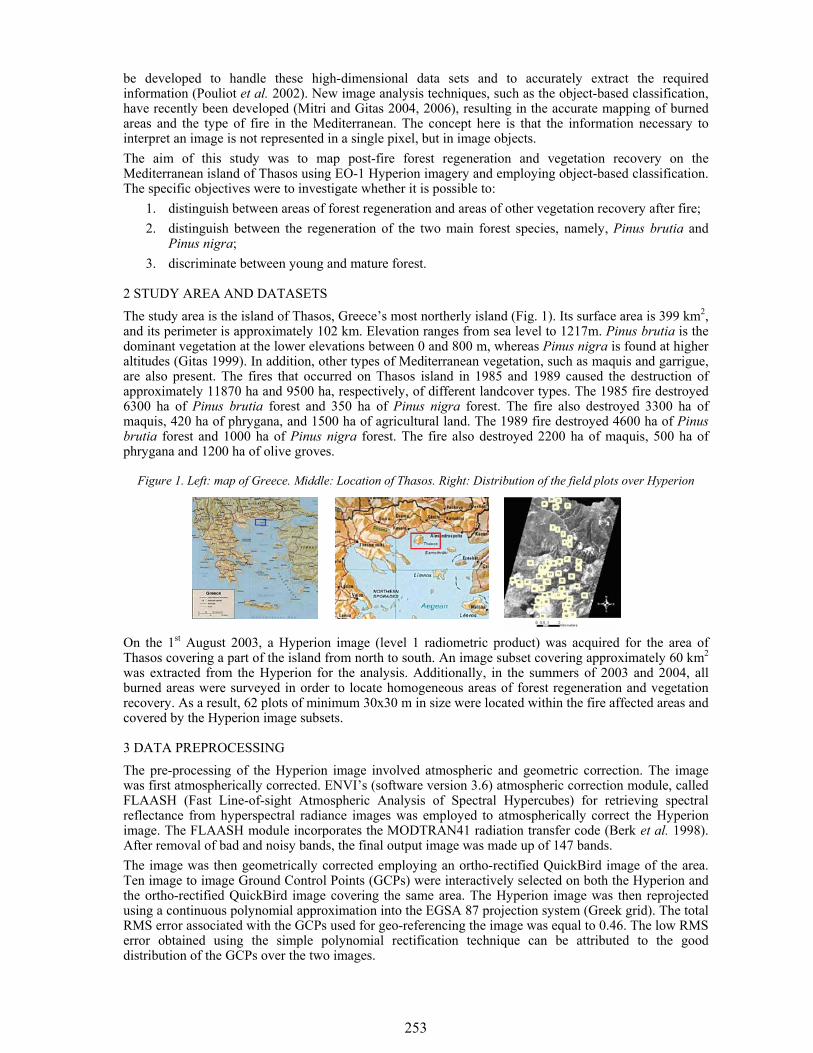
253

be developed to handle these high-dimensional data sets and to accurately extract the required information (Pouliot et al. 2002). New image analysis techniques, such as the object-based classification, have recently been developed (Mitri and Gitas 2004, 2006), resulting in the accurate mapping of burned areas and the type of fire in the Mediterranean. The concept here is that the information necessary to interpret an image is not represented in a single pixel, but in image objects. The aim of this study was to map post-fire forest regeneration and vegetation recovery on the Mediterranean island of Thasos using EO-1 Hyperion imagery and employing object-based classification. The specific objectives were to investigate whether it is possible to:

1. distinguish between areas of forest regeneration and areas of other vegetation recovery after fire; 2. distinguish between the regeneration of the two main forest species, namely, Pinus brutia and

Pinus nigra; 3. discriminate between young and mature forest.

2 STUDY AREA AND DATASETS The study area is the island of Thasos, Greece’s most northerly island (Fig. 1). Its surface area is 399 km2, and its perimeter is approximately 102 km. Elevation ranges from sea level to 1217m. Pinus brutia is the dominant vegetation at the lower elevations between 0 and 800 m, whereas Pinus nigra is found at higher altitudes (Gitas 1999). In addition, other types of Mediterranean vegetation, such as maquis and garrigue, are also present. The fires that occurred on Thasos island in 1985 and 1989 caused the destruction of approximately 11870 ha and 9500 ha, respectively, of different landcover types. The 1985 fire destroyed 6300 ha of Pinus brutia forest and 350 ha of Pinus nigra forest. The fire also destroyed 3300 ha of maquis, 420 ha of phrygana, and 1500 ha of agricultural land. The 1989 fire destroyed 4600 ha of Pinus brutia forest and 1000 ha of Pinus nigra forest. The fire also destroyed 2200 ha of maquis, 500 ha of phrygana and 1200 ha of olive groves.

Figure 1. Left: map of Greece. Middle: Location of Thasos. Right: Distribution of the field plots over Hyperion

On the 1st August 2003, a Hyperion image (level 1 radiometric product) was acquired for the area of Thasos covering a part of the island from north to south. An image subset covering approximately 60 km2 was extracted from the Hyperion for the analysis. Additionally, in the summers of 2003 and 2004, all burned areas were surveyed in order to locate homogeneous areas of forest regeneration and vegetation recovery. As a result, 62 plots of minimum 30x30 m in size were located within the fire affected areas and covered by the Hyperion image subsets.

3 DATA PREPROCESSING The pre-processing of the Hyperion image involved atmospheric and geometric correction. The image was first atmospherically corrected. ENVI’s (software version 3.6) atmospheric correction module, called FLAASH (Fast Line-of-sight Atmospheric Analysis of Spectral Hypercubes) for retrieving spectral reflectance from hyperspectral radiance images was employed to atmospherically correct the Hyperion image. The FLAASH module incorporates the MODTRAN41 radiation transfer code (Berk et al. 1998). After removal of bad and noisy bands, the final output image was made up of 147 bands. The image was then geometrically corrected employing an ortho-rectified QuickBird image of the area. Ten image to image Ground Control Points (GCPs) were interactively selected on both the Hyperion and the ortho-rectified QuickBird image covering the same area. The Hyperion image was then reprojected using a continuous polynomial approximation into the EGSA 87 projection system (Greek grid). The total RMS error associated with the GCPs used for geo-referencing the image was equal to 0.46. The low RMS error obtained using the simple polynomial rectification technique can be attributed to the good distribution of the GCPs over the two images.

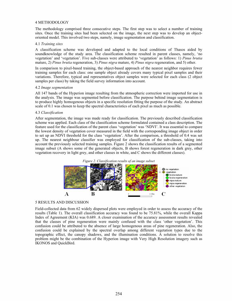
254

4 METHODOLOGY The methodology comprised three consecutive steps. The first step was to select a number of training sites. Once the training sites had been selected on the image, the next step was to develop an object-oriented model. This involved two steps, namely, image segmentation and classification. 4.1 Training sites A classification scheme was developed and adapted to the local conditions of Thasos aided by soundknowledge of the study area. The classification scheme resulted in parent classes, namely, ‘no vegetation’ and ‘vegetation’. Five sub-classes were attributed to ‘vegetation’ as follows: 1) Pinus brutia mature, 2) Pinus brutia regeneration, 3) Pinus nigra mature, 4) Pinus nigra regeneration, and 5) other. In comparison to pixel-based training, the object-based approach of the nearest neighbor requires fewer training samples for each class: one sample object already covers many typical pixel samples and their variations. Therefore, typical and representatives object samples were selected for each class (2 object samples per class) by taking the field survey information into account. 4.2 Image segmentation All 147 bands of the Hyperion image resulting from the atmospheric correction were imported for use in the analysis. The image was segmented before classification. The purpose behind image segmentation is to produce highly homogenous objects in a specific resolution fitting the purpose of the study. An abstract scale of 0.1 was chosen to keep the spectral characteristics of each pixel as much as possible. 4.3 Classification After segmentation, the image was made ready for classification. The previously described classification scheme was applied. Each class of the classification scheme formulated contained a class description. The feature used for the classification of the parent class ‘vegetation’ was ‘NDVI’. It was essential to compare the lowest density of vegetation cover measured in the field with the corresponding image object in order to set up an NDVI threshold for the class ‘vegetation’. After the comparison, a threshold of 0.4 was set up. The nearest neighbour classifier was employed for classification of the sub-classes, taking into account the previously selected training samples. Figure 2 shows the classification results of a segmented image subset (A shows some of the generated objects, B shows forest regeneration in dark grey, other vegetation recovery in light grey, and other classes in white, and C shows the different classes).

Figure 2. Classification results of an image subset

5 RESULTS AND DISCUSSION Field-collected data from 62 widely dispersed plots were employed in order to assess the accuracy of the results (Table 1). The overall classification accuracy was found to be 75.81%, while the overall Kappa Index of Agreement (KIA) was 0.689. A closer examination of the accuracy assessment results revealed that the classes of pine regeneration were mainly confused with the class ‘other vegetation’. This confusion could be attributed to the absence of large homogenous areas of pine regeneration. Also, the confusion could be explained by the spectral overlap among different vegetation types due to the topographic effect, the canopy shadows, and the illumination conditions. A solution to resolve this problem might be the combination of the Hyperion image with Very High Resolution imagery such as IKONOS and QuickBird.

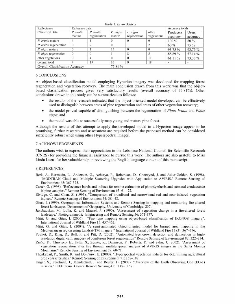
255

Table 1. Error Matrix Reflectance Reference data Accuracy totals Classified Data P. brutia

mature P. brutia regeneration

P. nigra mature

P. nigra regeneration

other vegetations

Producers accuracy

Users accuracy

P. brutia mature 4 1 0 0 0 100 % 80 % P. brutia regeneration 0 9 0 1 2 60 % 75 % P. nigra mature 0 1 15 0 0 93.75 % 93.75 % P. nigra regeneration 0 0 1 8 5 88.89 % 57.14 % other vegetations 0 4 0 0 11 61.11 % 73.33 % column total 4 15 16 9 18 - - Overall Classification Accuracy 75.81 %

6 CONCLUSIONS An object-based classification model employing Hyperion imagery was developed for mapping forest regeneration and vegetation recovery. The main conclusion drawn from this work was that the object-based classification process gives very satisfactory results (overall accuracy of 75.81%). Other conclusions drawn in this study can be summarized as follows:

• the results of the research indicated that the object-oriented model developed can be effectively used to distinguish between areas of pine regeneration and areas of other vegetation recovery;

• the model proved capable of distinguishing between the regeneration of Pinus brutia and Pinus nigra; and

• the model was able to successfully map young and mature pine forest. Although the results of this attempt to apply the developed model to a Hyperion image appear to be promising, further research and assessment are required before the proposed method can be considered sufficiently robust when using other Hyperspectral images.

7 ACKNOWLEDGEMENTS

The authors wish to express their appreciation to the Lebanese National Council for Scientific Research (CNRS) for providing the financial assistance to pursue this work. The authors are also grateful to Miss Linda Lucas for her valuable help in reviewing the English language content of this manuscript.

8 REFERENCES Berk, A., Bernstein, L., Anderson, G., Acharya, P., Robertson, D., Chetwynd, J. and Adler-Golden, S. (1998).

"MODTRAN Cloud and Multiple Scattering Upgrades with Application to AVIRIS." Remote Sensing of Environment 65: 367-375.

Carter, G. (1998). "Reflectance bands and indices for remote estimation of photosynthesis and stomatal conductance in pine canopies." Remote Sensing of Environment 63: 61– 72.

Elvidge, C. and Chen, Z. (1995). "Comparison of broadband and narrowband red and near-infrared vegetation indices." Remote Sensing of Environment 54: 38– 48.

Gitas, I. (1999). Geographical Information Systems and Remote Sensing in mapping and monitoring fire-altered forest landscapes. Department of Geography, University of Cambridge: 237.

Jakubauskas, M., Lulla, K. and Mausel, P. (1990). "Assessment of vegetation change in a fire-altered forest landscape." Photogrammetric Engineering and Remote Sensing 56: 371-377.

Mitri, G. and Gitas, I. (2006). "Fire type mapping using object-based classification of IKONOS imagery". International Journal of Wildland Fire 15: 457-462.

Mitri, G. and Gitas, I. (2004). "A semi-automated object-oriented model for burned area mapping in the Mediterranean region using Landsat-TM imagery." International Journal of Wildland Fire 13 (3): 367–376.

Pouliot, D., King, D., Bell, F. and Pitt, D. (2002). "Automated tree crown detection and delineation in high-resolution digital cam. imagery of coniferous forest regeneration” Remote Sensing of Environment 82: 322–334.

Riaño, D., Chuvieco, E., Ustin, S., Zomer, R., Dennison, P., Roberts, D. and Salas, J. (2002). "Assessment of vegetation regeneration after fire through multitemporal analysis of AVIRIS images in the Santa Monica Mountains." Remote Sensing of Environment 79: 60-71.

Thenkabail, P., Smith, R. and De-Pauw, E. (2000). "Hyperspectral vegetation indices for determining agricultural crop characteristics." Remote Sensing of Environment 71: 158–182.

Ungar, S., Pearlman, J., Mendenhall, J. and Reuter, D. (2003). "Overview of the Earth Observing One (EO-1) mission." IEEE Trans. Geosci. Remote Sensing 41: 1149–1159.

256

1 INTRODUCTION

The 2003 Leuk fire was considered to be a mixed fire with an intensity range from moderate to severe, 300 ha were burned in a altitudinal gradient of 800 m a.s.l to 2100 m a.s.l.. This range of altitude is reflected on a stratified forest regarding forest composition. Oak (Quercus pubescens Willd.), pine (Pinus sylvestris L.), spruce (Picea abies L.) and larch (Larix decidua Mill.) are the main species present along the altitudinal gradient with mixed forests (e.g. Oak-pine) in between. Forests play an important role in all Switzerland and the canton Valais is no exception to that. In the 20th century the temperature in Switzerland has increased to twice the global average (Rebetez 1999; Rebetez 2001; Frei et al. 2001). With the canton Valais being extraordinarily affected by a climate change that is leading to an increase in the number of fires in the region (Tinner et al. 2006), becoming this occurrences a major disturbance factor in parts of the Swiss Alps where before they were not (Schumacher 2004), it is important to know how the forest and its different species respond to these type of events. Although the burned area in question was savage during the following years after fire due to the treat of bark beetles, the number of trees and the variation in crown damage of the remaining trees was so considerable that we decide that we had enough data to proceed with this study.

2 MATERIAL AND METHODS The studied area is located in Leuk at 46°20′N, 7°39′E. The canton Valais is an inner-alpine valley in the southeast of Switzerland with low annual precipitation and a continental climate (Bendel et al. 2006). Mean annual temperature decreases from 8.6 °C at 640 m a.s.l. to 5.2 °C at 1500 m a.s.l., while annual precipitation increases from 600 mm at 640 m a.s.l. to 1000 mm at 1500 m a.s.l. (Aschwanden et al. 1996). In this study special attention was paid to tree height, tree location and altitude in relation to the tree species mentioned above.

Post-fire evaluation of delayed tree mortality in a forest of the Central Alps using time series of colour infrared images

L. Laranjeiro & C. Ginzler Swiss Federal Research Institute WSL, 8903 Birmensdorf, Switzerland, [email protected], [email protected]

Keywords: post-fire delayed mortality, altitudinal gradient, aerial photo interpretation, false colour infrared images, digital photogrammetry

ABSTRACT: In August 2003 after a very dry summer, the region of Leuk (Kt. Valais) was the center of the largest forest fire in Switzerland for the last 30 years. 310 ha, 20% of which on protected forest, were burned along an altitudinal gradient of 800 to 2100 m a.s.l.. This range of altitude is reflected on a stratified forest regarding forest composition. Forest changes gradually along the altitudinal gradient from an oak forest at the lowest altitude to pine, spruce and larch forest at the highest altitude. The objective of this study is to evaluate the fire-effect on the forest fire border. The focus lies on post-fire tree delayed mortality on residuals and on trees outside the burned area, in order to estimate the real perimeter of the damaged area on subsequent years and its relations to other external factors. Several variables contribute to different responses from trees towards fire and its secondary effects. In this study, special attention is paid to tree species, tree height, tree location and altitude in relation to the increase of area affected by fire. Colour infrared images (CIR) at a scale of 1:15’000 and 1:5’000 are used for digital stereo interpretation. The time series consists of pre-fire images from 1999, shortly after the fire 2003, 2005 and 2006. The results indicate that P .abies was the species that reacted less well to post fire. P. sylvestris is the species with the most stable vitality. L. decidua and Q. pubescens are the species with higher values of regeneration. The same tendency was found for younger trees (exception of P. sylvestris), green island and for low and high altitudes. Q. pubescens revealed an ability to completely resprout from a totally scorched crown in two years. The differences in the survival of species along the altitudinal gradient are delineating a different forest mosaic for the area affected by fire and may lead to a different forest composition in future decades. This study reveals particular importance to the forest fire impact assessment as well as for forest management studies and post-fire management activities.

257

The best indicator of crown injury appears to be the proportion of the crown scorched or killed (Ryan 1982; Peterson 1985; Ryan et al. 1988). Crown damage, which includes crown scorch and crown consumption (Rigolot 2004), was analyzed according to the following classes (from 0 to 4): 0%, 1-35%, 36-65%, 66-99% and 100% of living crown. All trees presenting a change in tree crown between 2003, 2005 or 2006 were recorded. Crown trees affected by the fire but still alive and presenting no change along the following years were also recorded. True colour aerial photos from 2003 (shortly after the fire) and colour infrared photos from 2005 and 2006 with an average scale of 1:5000 were used for this study. The images where digitized with a resolution of 14μm. The absolute orientation was done using LPS software from Leica. The RMS after triangulation was lower than 0.5 m. Tree species, crown damage, tree height and tree location where gathered stereoscopically using ArcMap and SocetSet for ArcGIS.

3 RESULTS A total of 2104 trees, showed a change in crown damage along the years or were crown damage living trees and were therefore measured. Norway spruce (P. abies) was the species that reacted less well to post fire with 80.69% of the trees death or dying three years after fire (Table 1).

Table 1. Percentage of tree species mortality

2005

Death (%) 2006

Death (%) 2006

Dying (%) 2006

Death or Dying

Larix decidua 15.83 6.60 7.83 30.26 Picea abies 65.09 11.60 4.00 80.69 Pinus sylvestris 9.43 4.90 7.55 21.88 Quercus pubescens 6.12 0.50 1.61 8.23

Q. pubescens (Pubescent Oak) and L. decidua (European Larch) were the species with higher percentage of resprouting with 91.53% and 59.83% respectively (Table 2). From all the trees still resprouting in 2006, Q. pubescens was the only species presenting higher values of resprouting for trees < 10 m in comparison with taller trees (Table 2). 50.56% of all pine trees maintained the same vitality, 21.88% (Table 1) died or are dying and 28.68% are resprouting (Table 2).

Table 2. Percentage of tree species resprouting in 2006

2006 (%)

2006 Trees ≥ 10 m (%)

2006 Trees < 10 m (%)

Larix decidua 59.83 37.22 22.61 Picea abies 10.56 8.57 1.99 Pinus sylvestris 28.68 20.38 8.3 Quercus pubescens 91.53 30.35 61.18

After separating all 2104 trees in two classes of heights, young P. abies revealed a higher percentage of recovery in comparison with taller P. abies trees (Table 3). Young larch trees presented 73.86% of ability to resprout in contrast to the 53.63% of taller larch trees (Table 3). 95.59% of oak young trees resprouted against an 84.31% of taller oak trees (Table 3).

Table 3. Tree vitality state in 2006 according to tree height

Trees ≥ 10m (%) Trees < 10m (%)

Regenerating Death or Dying Regenerating Death or Dying

Larix decidua 53.63 28.32 73.86 15.91 Picea abies 9.36 61.06 23.53 57.35 Pinus sylvestris 29.83 22.65 26.19 13.10 Quercus pubescens 84.31 11.76 95.59 3.31

Note: Death or dying does not include trees with 100% vitality in 2003.

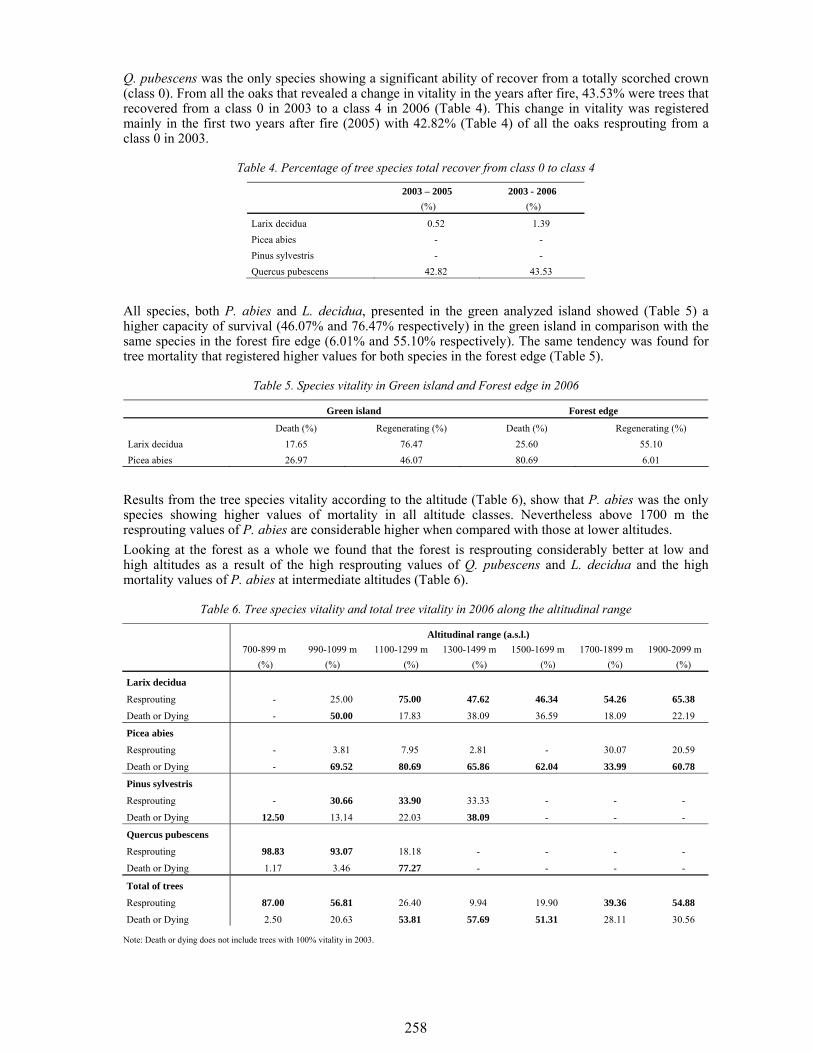
258

Q. pubescens was the only species showing a significant ability of recover from a totally scorched crown (class 0). From all the oaks that revealed a change in vitality in the years after fire, 43.53% were trees that recovered from a class 0 in 2003 to a class 4 in 2006 (Table 4). This change in vitality was registered mainly in the first two years after fire (2005) with 42.82% (Table 4) of all the oaks resprouting from a class 0 in 2003.

Table 4. Percentage of tree species total recover from class 0 to class 4

2003 – 2005

(%) 2003 - 2006

(%)

Larix decidua 0.52 1.39 Picea abies - - Pinus sylvestris - - Quercus pubescens 42.82 43.53

All species, both P. abies and L. decidua, presented in the green analyzed island showed (Table 5) a higher capacity of survival (46.07% and 76.47% respectively) in the green island in comparison with the same species in the forest fire edge (6.01% and 55.10% respectively). The same tendency was found for tree mortality that registered higher values for both species in the forest edge (Table 5).

Table 5. Species vitality in Green island and Forest edge in 2006

Green island Forest edge

Death (%) Regenerating (%) Death (%) Regenerating (%) Larix decidua 17.65 76.47 25.60 55.10 Picea abies 26.97 46.07 80.69 6.01

Results from the tree species vitality according to the altitude (Table 6), show that P. abies was the only species showing higher values of mortality in all altitude classes. Nevertheless above 1700 m the resprouting values of P. abies are considerable higher when compared with those at lower altitudes. Looking at the forest as a whole we found that the forest is resprouting considerably better at low and high altitudes as a result of the high resprouting values of Q. pubescens and L. decidua and the high mortality values of P. abies at intermediate altitudes (Table 6).

Table 6. Tree species vitality and total tree vitality in 2006 along the altitudinal range

Altitudinal range (a.s.l.)

700-899 m

(%) 990-1099 m

(%) 1100-1299 m

(%) 1300-1499 m

(%) 1500-1699 m

(%) 1700-1899 m

(%) 1900-2099 m

(%)

Larix decidua

Resprouting - 25.00 75.00 47.62 46.34 54.26 65.38

Death or Dying - 50.00 17.83 38.09 36.59 18.09 22.19

Picea abies

Resprouting - 3.81 7.95 2.81 - 30.07 20.59

Death or Dying - 69.52 80.69 65.86 62.04 33.99 60.78

Pinus sylvestris

Resprouting - 30.66 33.90 33.33 - - -

Death or Dying 12.50 13.14 22.03 38.09 - - -

Quercus pubescens

Resprouting 98.83 93.07 18.18 - - - -

Death or Dying 1.17 3.46 77.27 - - - -

Total of trees

Resprouting 87.00 56.81 26.40 9.94 19.90 39.36 54.88

Death or Dying 2.50 20.63 53.81 57.69 51.31 28.11 30.56

Note: Death or dying does not include trees with 100% vitality in 2003.

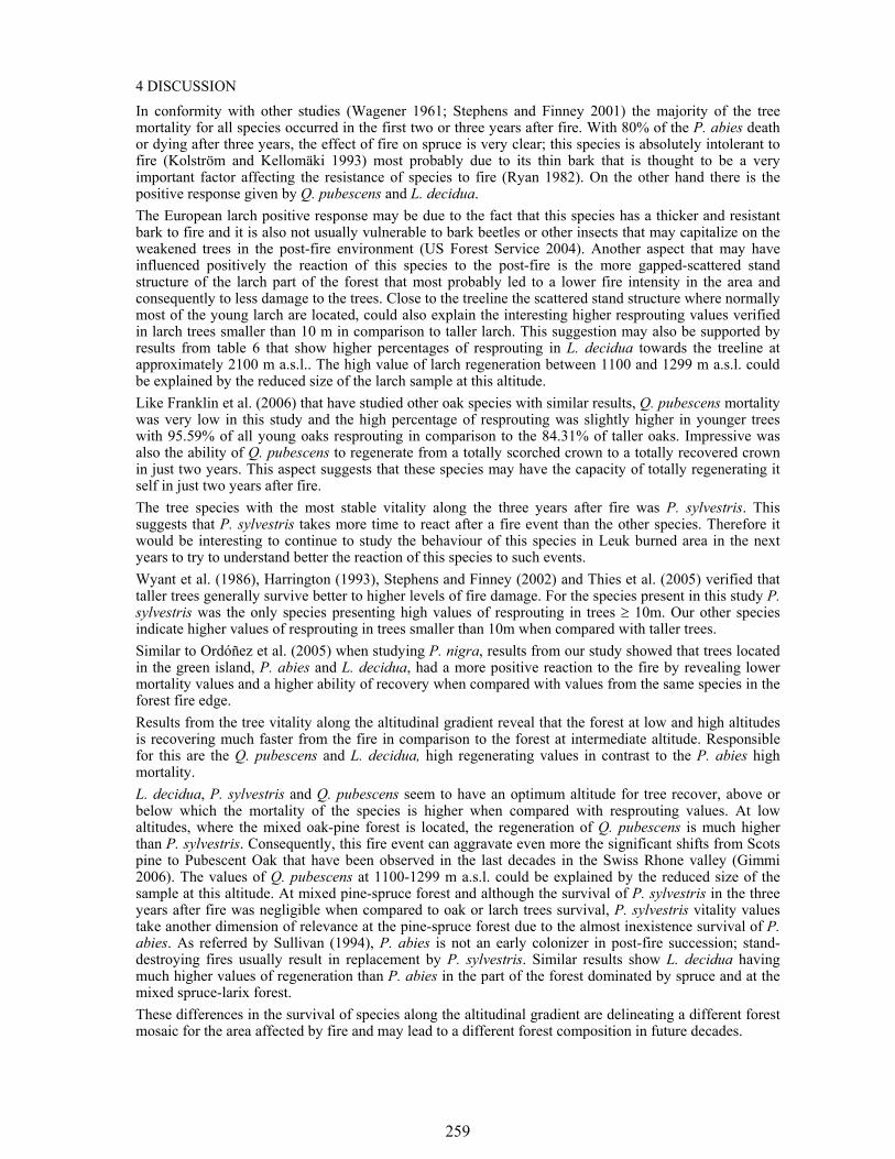
259

4 DISCUSSION In conformity with other studies (Wagener 1961; Stephens and Finney 2001) the majority of the tree mortality for all species occurred in the first two or three years after fire. With 80% of the P. abies death or dying after three years, the effect of fire on spruce is very clear; this species is absolutely intolerant to fire (Kolström and Kellomäki 1993) most probably due to its thin bark that is thought to be a very important factor affecting the resistance of species to fire (Ryan 1982). On the other hand there is the positive response given by Q. pubescens and L. decidua. The European larch positive response may be due to the fact that this species has a thicker and resistant bark to fire and it is also not usually vulnerable to bark beetles or other insects that may capitalize on the weakened trees in the post-fire environment (US Forest Service 2004). Another aspect that may have influenced positively the reaction of this species to the post-fire is the more gapped-scattered stand structure of the larch part of the forest that most probably led to a lower fire intensity in the area and consequently to less damage to the trees. Close to the treeline the scattered stand structure where normally most of the young larch are located, could also explain the interesting higher resprouting values verified in larch trees smaller than 10 m in comparison to taller larch. This suggestion may also be supported by results from table 6 that show higher percentages of resprouting in L. decidua towards the treeline at approximately 2100 m a.s.l.. The high value of larch regeneration between 1100 and 1299 m a.s.l. could be explained by the reduced size of the larch sample at this altitude. Like Franklin et al. (2006) that have studied other oak species with similar results, Q. pubescens mortality was very low in this study and the high percentage of resprouting was slightly higher in younger trees with 95.59% of all young oaks resprouting in comparison to the 84.31% of taller oaks. Impressive was also the ability of Q. pubescens to regenerate from a totally scorched crown to a totally recovered crown in just two years. This aspect suggests that these species may have the capacity of totally regenerating it self in just two years after fire. The tree species with the most stable vitality along the three years after fire was P. sylvestris. This suggests that P. sylvestris takes more time to react after a fire event than the other species. Therefore it would be interesting to continue to study the behaviour of this species in Leuk burned area in the next years to try to understand better the reaction of this species to such events. Wyant et al. (1986), Harrington (1993), Stephens and Finney (2002) and Thies et al. (2005) verified that taller trees generally survive better to higher levels of fire damage. For the species present in this study P. sylvestris was the only species presenting high values of resprouting in trees ≥ 10m. Our other species indicate higher values of resprouting in trees smaller than 10m when compared with taller trees. Similar to Ordóñez et al. (2005) when studying P. nigra, results from our study showed that trees located in the green island, P. abies and L. decidua, had a more positive reaction to the fire by revealing lower mortality values and a higher ability of recovery when compared with values from the same species in the forest fire edge. Results from the tree vitality along the altitudinal gradient reveal that the forest at low and high altitudes is recovering much faster from the fire in comparison to the forest at intermediate altitude. Responsible for this are the Q. pubescens and L. decidua, high regenerating values in contrast to the P. abies high mortality. L. decidua, P. sylvestris and Q. pubescens seem to have an optimum altitude for tree recover, above or below which the mortality of the species is higher when compared with resprouting values. At low altitudes, where the mixed oak-pine forest is located, the regeneration of Q. pubescens is much higher than P. sylvestris. Consequently, this fire event can aggravate even more the significant shifts from Scots pine to Pubescent Oak that have been observed in the last decades in the Swiss Rhone valley (Gimmi 2006). The values of Q. pubescens at 1100-1299 m a.s.l. could be explained by the reduced size of the sample at this altitude. At mixed pine-spruce forest and although the survival of P. sylvestris in the three years after fire was negligible when compared to oak or larch trees survival, P. sylvestris vitality values take another dimension of relevance at the pine-spruce forest due to the almost inexistence survival of P. abies. As referred by Sullivan (1994), P. abies is not an early colonizer in post-fire succession; stand-destroying fires usually result in replacement by P. sylvestris. Similar results show L. decidua having much higher values of regeneration than P. abies in the part of the forest dominated by spruce and at the mixed spruce-larix forest. These differences in the survival of species along the altitudinal gradient are delineating a different forest mosaic for the area affected by fire and may lead to a different forest composition in future decades.

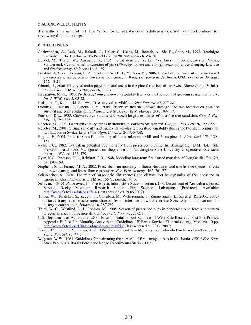
260

5 ACKNOWLEDGMENTS The authors are grateful to Eliane Weber for her assistance with data analysis, and to Fabio Lombardi for reviewing this manuscript.

6 REFERENCES Aschwanden, A., Beck, M., Häberli, C., Haller, G., Keine, M., Roesch, A., Sie, R., Stutz, M., 1996. Bereinigte

Zeitreihen – Die Ergebnisse des Projekts Klima 90. SMA-Zürich, Zürich. Bendel, M., Tinner, W., Ammann, B., 2006. Forest dynamics in the Pfyn forest in recent centuries (Valais,

Switzerland, Central Alps): interaction of pine (Pinus sylvestris) and oak (Quercus sp.) under changing land use and fire frequency. Holocene 16, 81-89.

Franklin, J., Spears-Lebrun, L. A., Deutschman, D. H., Marsden, K., 2006. Impact of high-intensity fire on mixed evergreen and mixed conifer forests in the Peninsular Ranges of southern California. USA. For. Ecol. Manage. 235, 18-29.

Gimmi, U., 2006. History of anthropogenic disturbances in the pine forest belt of the Swiss Rhone valley (Valais). PhD-thesis ETHZ no. 16764, Zurich, 112 pp

Harrington, M. G., 1993. Predicting Pinus ponderosa mortality from dormant season and growing season fire injury. Int. J. Wildl. Fire 3, 65-72.

Kolström. T., Kellomäki. S., 1993. Tree survival in wildfires. Silva Fennica. 27, 277-281. Ordóñez. J., Retana. J., Espelta. J. M., 2005. Effects of tree size. crown damage. and tree location on post-fire

survival and cone production of Pinus nigra trees. For. Ecol. Manage. 206, 109-117. Peterson, D.L., 1985. Crown scorch volume and scorch height: estimates of post-fire tree condition. Can. J. For.

Res. 15, 596–598. Rebetez, M., 1999. Twentieth century trends in droughts in southern Switzerland. Geophys. Res. Lett. 26, 755-758. Rebetez, M., 2001. Changes in daily and nightly day-to-day temperature variability during the twentieth century for

two stations in Switzerland. Theor. Appl. Climatol. 26, 755-758. Rigolot, E., 2004. Predicting postfire mortality of Pinus halepensis Mill. and Pinus pinea L. Plant Ecol. 171, 139–

151. Ryan, K.C., 1982. Evaluating potential tree mortality from prescribed burning. In: Baumgartner. D.M. (Ed.). Site

Preparation and Fuels Management on Steppe Terrain. Washington State University Cooperative Extension. Pullman, WA, pp. 167–179.

Ryan, K.C., Peterson. D.L., Reinhart, E.D., 1988. Modeling long-term fire caused mortality of Douglas-fir. For. Sci. 34, 190–199.

Stephens, S. L., Finney, M. A., 2002. Prescribed fire mortality of Sierra Nevada mixed conifer tree species: effects of crown damage and forest floor combustion. For. Ecol. Manage. 162, 261-271.

Schumacher, S., 2004. The role of large-scale disturbances and climate fort he dynamics of the landscape in European Alps. PhD-thesis ETHZ no. 15573, Zurich, 141 pp.

Sullivan, J. 2004. Picea abies. In: Fire Effects Information System, (online). U.S. Department of Agriculture, Forest Service, Rocky Mountain Research Station, Fire Sciences Laboratory (Producer). Available: http://www.fs.fed.us/database/feis/ (last accessed on 29.06.2007)

Tinner, W., Hofstetter. S., Zeugin. F., Conedera. M., Wohlgemuth. T., Zimmermann. L., Zweifel. R., 2006. Long-distance transport of macroscopic charcoal by an intensive crown fire in the Swiss Alps – implications for history reconstruction. Holocene 16, 287-292.

Thies, W. G., Westlind, D. J., Loewen, M., 2005. Season of prescribed burn in ponderosa pine forests in eastern Oregon: impact on pine mortality. Int. J. Wildl. Fire 14, 223-231.

U.S. Department of Agriculture, 2004. Environmental Impact Statment of West Side Reservoir Post-Fire Project. Appendix E: Post-Fire Mortality Analysis and Guidelines. US Forest Service. Flathead County, Montana. 10 pp. http://www.fs.fed.us/r1/flathead/nepa/west_res/feis/ ( last accessed on 29.06.2007).

Wyant, J.G., Omi, P. N., Laven, R. D., 1986. Fire Induced Tree Mortality in a Colorado Ponderosa Pine/Douglas-fir Stand. For. Sci. 32, 49-59.

Wagener, W.W., 1961. Guidelines for estimating the survival of fire damaged trees in California. USDA For. Serv. Miss. Pap.60, California Forest and Range Experimental Station, 11 p.

261

1 INTRODUCTION

Wildfires play a critical role in ecosystems dynamics in many different parts of the world. The Mediterranean area has been very influenced under millennia by different civilizations that had made a really strong impression on both vegetation and landscape. It is important to understand the fire from a forest fire management point of view in order to prevent and defend vegetation and landscape (Houerou, 1973; Velez, 2000). The devastating effects of the forest fires have catastrophic effects to ecological level, among others it is possible to emphasize that it produces a loss of biodiversity with the loss of nutrients (Neary et al. 1996) and it affects the composition of species (Prasad et al. 2007). The fires come to alter the composition of species of successive stages and, therefore, at local level in the later occurrence of forest fires (Turner y Romme, 1994; Diaz-Delgado et al. 2004). In addition, forest fires contribute exceedingly with the gas emission to the greenhouse effect (van der Werf et al. 2004). This paper aims to obtain the spatial patterns of wildfires in Spain (excepting Canary Islands) corresponding to the period 1991-2005. We hypothesize in terms that wildfire occurrence in Spain show a spatial pattern that depends on numerous factors and that are related to the ignition and spread of wildfires. The mixed composition of those factors would generate different spatial patterns among ecozones that could explain wildfire occurrence and extent.

2 METHODS In order to characterize the effect of wildfires on vegetation a spatial analysis was needed. This was carried out in two different levels in order to see the spatial variation that wildfires have: at a global scale and on an ecozones basis. It was utilized a database of mapped fires ≥ 25 ha from 1991 – 2005 (n=1968 fires). The study area comprises Spain (excepting Canary Islands). We divided the different factors in 4 big groups: climate (mean temperature, mean summer temperature, solar radiation, annual precipitation, spring precipitation and summer precipitation); topographic (elevation, slope and aspect); Land cover (land cover use, national forest inventory, fuel models and ecozones (Rivas-Martinez, 1987)) and anthropogenic (distance to the closest road, distance to the closest urban area and population density). Since we needed to analyze the spatial patterns between the area burned and the variables two methods were used: 1) a cross-tabulate method to see the range of every single variable related to area burned and

Spatial patterns and variations of forest fires in Spain, 1991-2005

F. Verdú Department of Geography, University of Alcalá, Alcalá de Henares, Madrid, Spain, [email protected]

J. Salas & I. Aguado Department of Geography, University of Alcalá, Alcalá de Henares, Madrid, Spain, [email protected], [email protected] Keywords: Spatial analysis; area burned; logistic regression; tabulate area; ecozones

ABSTRACT: Wildland fires have a tremendous impact on vegetation and the landscape. Due to its effects not just ecological but economical it is extremely important from a forest fire management point of view to determine the spatial patterns of forest fires (area burned). In order to characterized the spatial patterns of forest fires, the present study aims to explain the relationships between the fire occurrence (area burned) and different factors such as climatic topographic, vegetation and anthropogenic. We broke down the analysis in two separate levels to establish the extent to which the variance in area burned is explained by those factors: at a global scale and on an ecozones basis. It was utilized a database of mapped fires ≥ 25 ha from 1991 – 2005 (n=1968 fires). The study area comprises Spain (excepting Canary Islands). Two types of spatial analysis were applied: On the one hand, a tabulate area method to establish the usual ranges of the explanatory variables that area burned had. On the other hand, a logistic regression model was used to estimate the presence of fires as a function of explanatory variables (factors). From the first method it was possible to suggest that there is a spatial variation within ecozones. Results from the logistic model imply that a variable such as mean spring and summer precipitation, average temperature of summer highest temperatures, and different vegetation covers such as coniferous, shrublands and grasslands are very decisive in fire occurrence. Our results provide valuable information to forest managers for forest plan and forest fire risk management.

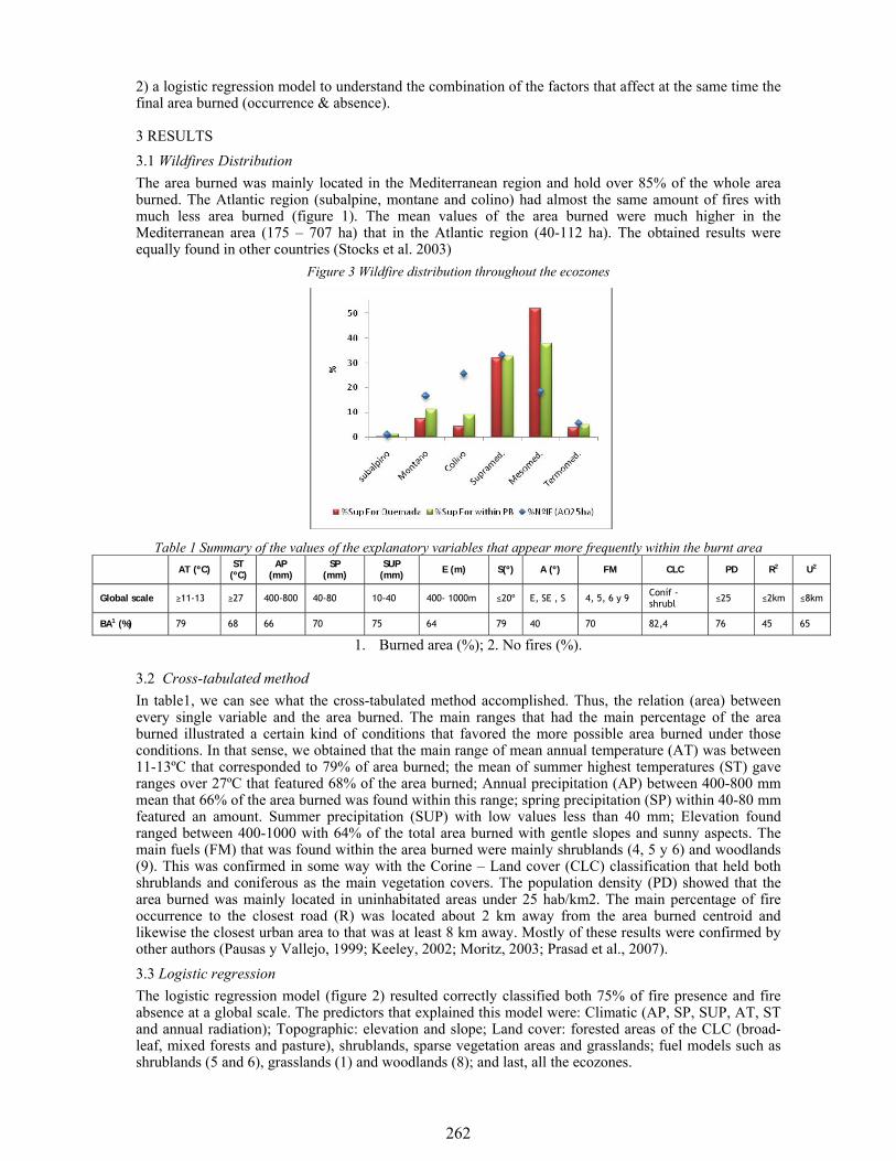
262

2) a logistic regression model to understand the combination of the factors that affect at the same time the final area burned (occurrence & absence).

3 RESULTS 3.1 Wildfires Distribution The area burned was mainly located in the Mediterranean region and hold over 85% of the whole area burned. The Atlantic region (subalpine, montane and colino) had almost the same amount of fires with much less area burned (figure 1). The mean values of the area burned were much higher in the Mediterranean area (175 – 707 ha) that in the Atlantic region (40-112 ha). The obtained results were equally found in other countries (Stocks et al. 2003)

Figure 3 Wildfire distribution throughout the ecozones

Table 1 Summary of the values of the explanatory variables that appear more frequently within the burnt area

AT (ºC) ST (ºC)

AP (mm)

SP (mm)

SUP (mm) E (m) S(º) A (º) FM CLC PD R2 U2

Global scale ≥11-13 ≥27 400-800 40-80 10-40 400- 1000m ≤20º E, SE , S 4, 5, 6 y 9 Coníf - shrubl ≤25 ≤2km ≤8km

BA1 (%) 79 68 66 70 75 64 79 40 70 82,4 76 45 65

1. Burned area (%); 2. No fires (%).

3.2 Cross-tabulated method In table1, we can see what the cross-tabulated method accomplished. Thus, the relation (area) between every single variable and the area burned. The main ranges that had the main percentage of the area burned illustrated a certain kind of conditions that favored the more possible area burned under those conditions. In that sense, we obtained that the main range of mean annual temperature (AT) was between 11-13ºC that corresponded to 79% of area burned; the mean of summer highest temperatures (ST) gave ranges over 27ºC that featured 68% of the area burned; Annual precipitation (AP) between 400-800 mm mean that 66% of the area burned was found within this range; spring precipitation (SP) within 40-80 mm featured an amount. Summer precipitation (SUP) with low values less than 40 mm; Elevation found ranged between 400-1000 with 64% of the total area burned with gentle slopes and sunny aspects. The main fuels (FM) that was found within the area burned were mainly shrublands (4, 5 y 6) and woodlands (9). This was confirmed in some way with the Corine – Land cover (CLC) classification that held both shrublands and coniferous as the main vegetation covers. The population density (PD) showed that the area burned was mainly located in uninhabitated areas under 25 hab/km2. The main percentage of fire occurrence to the closest road (R) was located about 2 km away from the area burned centroid and likewise the closest urban area to that was at least 8 km away. Mostly of these results were confirmed by other authors (Pausas y Vallejo, 1999; Keeley, 2002; Moritz, 2003; Prasad et al., 2007). 3.3 Logistic regression The logistic regression model (figure 2) resulted correctly classified both 75% of fire presence and fire absence at a global scale. The predictors that explained this model were: Climatic (AP, SP, SUP, AT, ST and annual radiation); Topographic: elevation and slope; Land cover: forested areas of the CLC (broad-leaf, mixed forests and pasture), shrublands, sparse vegetation areas and grasslands; fuel models such as shrublands (5 and 6), grasslands (1) and woodlands (8); and last, all the ecozones.

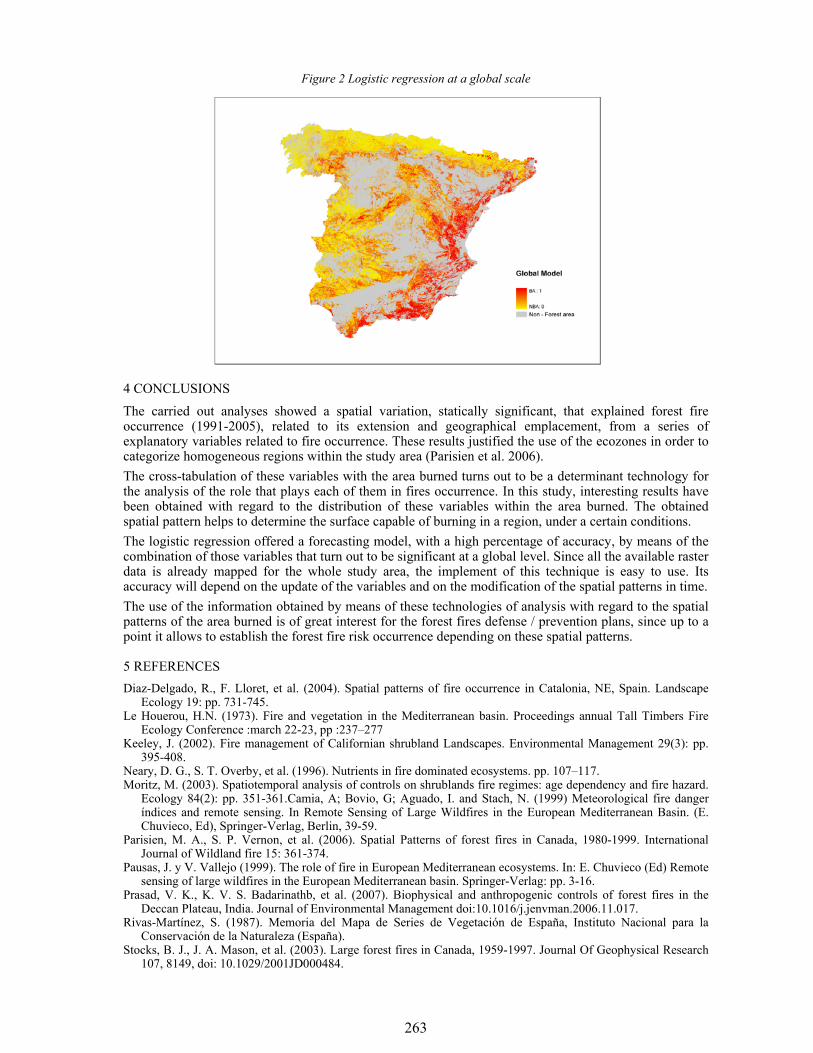
263

Figure 2 Logistic regression at a global scale

4 CONCLUSIONS The carried out analyses showed a spatial variation, statically significant, that explained forest fire occurrence (1991-2005), related to its extension and geographical emplacement, from a series of explanatory variables related to fire occurrence. These results justified the use of the ecozones in order to categorize homogeneous regions within the study area (Parisien et al. 2006). The cross-tabulation of these variables with the area burned turns out to be a determinant technology for the analysis of the role that plays each of them in fires occurrence. In this study, interesting results have been obtained with regard to the distribution of these variables within the area burned. The obtained spatial pattern helps to determine the surface capable of burning in a region, under a certain conditions. The logistic regression offered a forecasting model, with a high percentage of accuracy, by means of the combination of those variables that turn out to be significant at a global level. Since all the available raster data is already mapped for the whole study area, the implement of this technique is easy to use. Its accuracy will depend on the update of the variables and on the modification of the spatial patterns in time. The use of the information obtained by means of these technologies of analysis with regard to the spatial patterns of the area burned is of great interest for the forest fires defense / prevention plans, since up to a point it allows to establish the forest fire risk occurrence depending on these spatial patterns.

5 REFERENCES Diaz-Delgado, R., F. Lloret, et al. (2004). Spatial patterns of fire occurrence in Catalonia, NE, Spain. Landscape

Ecology 19: pp. 731-745. Le Houerou, H.N. (1973). Fire and vegetation in the Mediterranean basin. Proceedings annual Tall Timbers Fire

Ecology Conference :march 22-23, pp :237–277 Keeley, J. (2002). Fire management of Californian shrubland Landscapes. Environmental Management 29(3): pp.

395-408. Neary, D. G., S. T. Overby, et al. (1996). Nutrients in fire dominated ecosystems. pp. 107–117. Moritz, M. (2003). Spatiotemporal analysis of controls on shrublands fire regimes: age dependency and fire hazard.

Ecology 84(2): pp. 351-361.Camia, A; Bovio, G; Aguado, I. and Stach, N. (1999) Meteorological fire danger índices and remote sensing. In Remote Sensing of Large Wildfires in the European Mediterranean Basin. (E. Chuvieco, Ed), Springer-Verlag, Berlin, 39-59.

Parisien, M. A., S. P. Vernon, et al. (2006). Spatial Patterns of forest fires in Canada, 1980-1999. International Journal of Wildland fire 15: 361-374.

Pausas, J. y V. Vallejo (1999). The role of fire in European Mediterranean ecosystems. In: E. Chuvieco (Ed) Remote sensing of large wildfires in the European Mediterranean basin. Springer-Verlag: pp. 3-16.

Prasad, V. K., K. V. S. Badarinathb, et al. (2007). Biophysical and anthropogenic controls of forest fires in the Deccan Plateau, India. Journal of Environmental Management doi:10.1016/j.jenvman.2006.11.017.

Rivas-Martínez, S. (1987). Memoria del Mapa de Series de Vegetación de España, Instituto Nacional para la Conservación de la Naturaleza (España).

Stocks, B. J., J. A. Mason, et al. (2003). Large forest fires in Canada, 1959-1997. Journal Of Geophysical Research 107, 8149, doi: 10.1029/2001JD000484.

264

Turner, M. G. y W. H. Romme (1994). Landscape dynamics in crown fire ecosystems. Landscape Ecology 9(1): pp 59-77.

van der Werf, G. R., J. Randerson, et al. (2004). Continental Scale-partitioning of fire emissions during the 1997 to 2001 El Niño/La Niña period. Science 303: 73-76.

Vélez, R. (2000). La defensa contra incendios forestales. Fundamentos y experiencias. Madrid, McGraw-Hill.

265

1 INTRODUCTION Post-fire Mediterranean landscapes are complex systems composed of a large number of heterogeneous components and unexpected behaviour and self-organization, all of which produce characteristic patterns that change depending on their observation scale (Allen and Starr, 1982). In this context, the description of plant communities after fire is even more difficult. A useful starting point for deriving processes from patterns has been to explore the landscape as groups of plant communities or ecosystems forming ecological units (patches) which have been distinguishable structure, function, geo-morphology, and disturbance regimes (Forman and Godron, 1986). Central to this epistemology is the problem of properly distinguishing analysis units. The application of ordination techniques can be a useful tool in the process of description, recognition, analysis and prediction of such units (Jongman et al., 1987). Once post-fire communities have been described, a second challenge is to identify these complex structures through remote sensing data. The difficulty of this task lies in distinguishing the boundaries of the different communities in the space. Multiresolution segmentation (Spann and Wilson, 1985) is a promising strategy for boundary refining. In this context, scale is a crucial aspect of image understanding. Although scale is constrained by the image pixel resolution, the desired objects are formed by their own inherent scale, compared to a user-defined threshold called scale parameter. The criteria for selecting an adequate scale parameter in forest classification are still under research. In order to improve the discriminant power of very high resolution imagery, the texture feature (Haralick et al., 1973) has often been used in texture classification or texture segmentation (Franklin et al., 2000, Hay et al., 2001). Although texture analysis is not a new task, the integration of advanced texture analyses on a multi-scale approach is actually being developed. The objective of this research was therefore to determine which textural variables contributed most to

Texture analysis of a post-fire landscape using an object-based multi-scale image segmentation algorithm.

R. Hernández-Clemente Departamento f Forestry Engineer, University of Cordoba, Córdoba, Spain, [email protected].

R. M. Navarro-Cerrillo University of Cordoba, Córdoba, Spain, [email protected]

I. Z. Gitas Aristotle University of Thessaloniki, Thessaloniki, Greece; [email protected].

J.E. Hernández-Bermejo University of Cordoba , Córdoba, Spain, [email protected]

M. González-Audicana University of Navarra, Navarra, [email protected] Keywords: multiscale object-based analysis, texture, scale parameter, post-fire landscape.

ABSTRACT: Post-fire landscapes are complex systems to analyse through remote sensing data. An important challenge of this paradigm is to understand how textural features change with scale in a real variety of landscapes. The complexity of these systems can best be explored through their partition into objects or patches. The challenge and flexibility of the multi-scale segmentation/object algorithm lies in defining the parameters that relate to different organization levels. Quantitative changes in measurements across space scales differ depending on how the scale is defined. The purpose of this study was to evaluate how different textural features contribute most to discriminating vegetation types. The textural indices analyzed were: homogeneity, entropy and contrast. The study was carried out on a forest fire that occurred in Sierra de Tejeda and Almijara (South Spain) in 1999. An Ikonos satellite image provided coverage for 2005. Training areas were selected recording the following variables: altitude, soil type, slope, aspect, and vegetation type. The methodology involves: i) multiscale dataset generation using an object-based image analysis and an upscaling technique ii) multi-scale analysis of textural features of the objects iii) a scale effect evaluation using discriminant analysis. Results showed that the entropy derived from the infra-red band and defined with a scale factor of 90 had the highest discriminant capacity. These results provides the support for the highlighting of the textural indices that can be readily and accurately extrapolated or interpolated across space scales based on an image object segmentation of different post-fire scenarios.

266

discriminating post-fire vegetation communities, and which factor scale had the highest discrimination capacity. The study area is located in Otivar (Granada), southern Spain. A fire occurring between 16th

and 18th August, 1999, affected around 2,326 ha. Eight years after the fire, Mediterranean gorse forms the predominant type of ground cover composed by Dwarf gorse (Ulex spp., Genista spp.), Rock rose (Rosmarinus officinalis) or (Cistus albidus) and, to a lesser extent, Holm oak (Quercus ilex subsp. rotundifolia), and Aleppo pine (Pinus halepensis).

2 METHODOLOGY 2.1 Image processing The satellite image used in this study is a multi-spectral Ikonos imagery taken on 6 May 2005. The image was orthorectified using a rigorous model method. A total of 129 GCPs were identified on the panchromatic band and georreferenced on the ground. RMS errors obtained for multispectral and panchromatic band were less than 1 pixel. In order to acquire a higher space resolution, the image was fused by means of a wavelet transformation (González-Audícana et al., 2005, Nuñez et al., 1999). 2.2 Field data The field trial, took place in May, 2007. Samples were randomly located within the burnt area and located on the ground with a GPS (error< 1m). The total area sampled was 16 plots, each with a 10-m radius. Two 10 m long perpendicular lineal transects (one in the direction of the maximum slope) were defined for each plot and measured following the linear interception method (Bonham, 1989). Along each transect, the morphologic variable measurements were tree and brush canopy interception longitude (lBBk

BB). Ground data were used to calculate fractional cover (CBiB) reckoned from the sum of intercepted fraction per species: CBB 1iB=B Σ lBkPB

PP/50 and CBB 2i B=B BBΣ lBBkBB/50 for each transect and obtaining CBB iBbB as CBB iBbB=B (CBB 1iB+ CBB 2iB)/2. Other biophysical variables like altitude, slope or soil type were also collected. 2.3 Texture analysis on a post-fire landscape using object-based multi-scale image segmentation

algorithm The analysis consisted of: i) Definition of plant communities within the burnt area through two different ordination methods: cluster analysis and detrending correspondence analysis (DCA). ii) Advanced texture heuristic analysis of the Ikonos images. From the second order texture features (Haralick et al, 1973) implemented in eCognition software were extracted the homogeneity, the contrast and the entropy at different scales: 30, 90, 120, 150, 180 and 210. iii) Determination of the variables that contribute most to discriminant functions, and, therefore, to group separation through a discriminant analysis. Detrended Discriminant Analysis (DFA) generates a linear combination of variables, which maximizes the probability of correctly assigning observations to pre-determined classes with two or more variables recorded for each observation.

3 RESULTS

Plant communities were identified by cluster analysis and DCA. Results of the cluster analysis are presented in Fig. 1. Both analyses present similar results, grouping the samples inventoried in five different groups of vegetation: 1. Draft gorse (Ulex parviflorus) on basic soils as main species, accompanied by others to a lesser extent. Plots: 1, 3, 2, 11, 7, 12. 2. Draft gorse (Ulex parviflorus) on basic soils in a very moderate proportion and accompanied by a large number of species such as Rosmarinus officinalis, Cistus clusii, Cistus albidus and others. Plots: 4, 8. 3. Rock rose (Rosmarinus officinalis) on basic soils as main species accompanied by others to a lesser extent. Plots: 5, 16. 4. Bolinas (Genista umbelata) on acid soils accompanied by others to a a lesser extent. Plots: 10, 6, 13. 5. Selective bush clearing. Regeneration of: Phlomis purpurea, Juniperus oxycedrus, Quercus ilex and Pinus halepensis. Plots: 9, 15, 14. Based on this ordination and through a visual interpretation of the communities, it could be observed that the space patterns of the communities within each group had similar textures (Fig. 2).

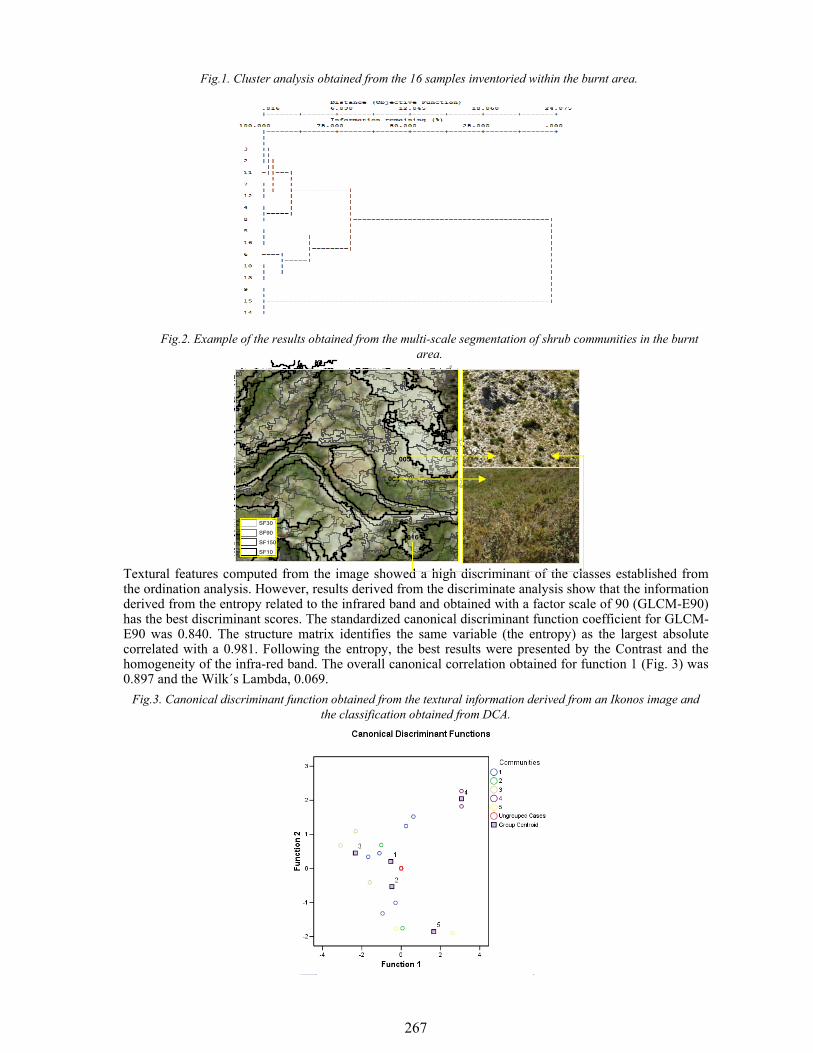
267

Fig.1. Cluster analysis obtained from the 16 samples inventoried within the burnt area.

Fig.2. Example of the results obtained from the multi-scale segmentation of shrub communities in the burnt area.

Textural features computed from the image showed a high discriminant of the classes established from the ordination analysis. However, results derived from the discriminate analysis show that the information derived from the entropy related to the infrared band and obtained with a factor scale of 90 (GLCM-E90) has the best discriminant scores. The standardized canonical discriminant function coefficient for GLCM-E90 was 0.840. The structure matrix identifies the same variable (the entropy) as the largest absolute correlated with a 0.981. Following the entropy, the best results were presented by the Contrast and the homogeneity of the infra-red band. The overall canonical correlation obtained for function 1 (Fig. 3) was 0.897 and the Wilk´s Lambda, 0.069.

Fig.3. Canonical discriminant function obtained from the textural information derived from an Ikonos image and the classification obtained from DCA.

016

004

005

SF30

SF90

SF150

SF10

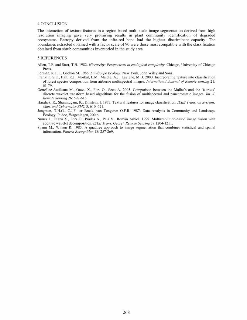
268

4 CONCLUSION The interaction of texture features in a region-based multi-scale image segmentation derived from high resolution imaging gave very promising results in plant community identification of degraded ecosystems. Entropy derived from the infra-red band had the highest discriminant capacity. The boundaries extracted obtained with a factor scale of 90 were those most compatible with the classification obtained from shrub communities inventoried in the study area.

5 REFERENCES Allen, T.F. and Starr, T.B. 1982. Hierarchy: Perspectives in ecological complexity. Chicago, University of Chicago

Press. Forman, R.T.T., Godron M. 1986. Landscape Ecology. New York, John Wiley and Sons. Franklin, S.E., Hall, R.J., Moskal, L.M., Maidie, A.J., Lavigne, M.B. 2000. Incorporating texture into classification

of forest species composition from airborne multispectral images. International Journal of Remote sensing 21: 61-79.

González-Audícana M., Otazu X., Fors O., Seco A. 2005. Comparison between the Mallat’s and the ‘à trous’ discrete wavelet transform based algorithms for the fusion of multispectral and panchromatic images. Int. J. Remote Sensing 26: 597-616.

Haralick, R., Shanmugam, K., Dinstein, I. 1973. Textural features for image classification. IEEE Trans. on Systems, Man, and Cybernetics SMC 3: 610–621.

Jongman, T.H.G., C.J.F. ter Braak, van Tongeren O.F.R. 1987. Data Analysis in Community and Landscape Ecology. Pudoc, Wageningen, 200 p.

Nuñez J., Otazu X., Fors O., Prades A., Palà V., Román Arbiol. 1999. Multiresolution-based image fusion with additive wavelet decomposition. IEEE Trans. Geosci. Remote Sensing 37:1204-1211.

Spann M., Wilson R. 1985. A quadtree approach to image segmentation that combines statistical and spatial information. Pattern Recognition 18: 257-269.

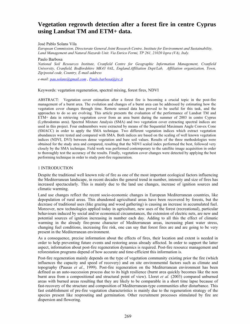
269

1 INTRODUCTION Despite the traditional well known role of fire as one of the most important ecological factors influencing the Mediterranean landscape, in recent decades the general trend in number, intensity and size of fires has increased spectacularly. This is mainly due to the land use changes, increase of ignition sources and climatic warming. Land use changes reflect the recent socio-economic changes in European Mediterranean countries, like depopulation of rural areas. This abandoned agricultural areas have been recovered by forests, but the decrease of traditional uses (like grazing and wood gathering) is causing an increase in accumulated fuel. Moreover, new technologies applied today in agriculture, new uses of the forest (recreational), particular behaviours induced by social and/or economical circumstances, the extension of electric nets, are new and potential sources of ignition increasing in number each day. Adding to all this the effect of climatic warming in the already fire-prone character of Mediterranean areas, increasing plant water stress, changing fuel conditions, increasing fire risk, one can say that forest fires are and are going to be very present in the Mediterranean environment. As a consequence, precise information about the effects of fires, their location and extent is needed in order to help preventing future events and restoring areas already affected. In order to support the latter aspect, information about post-fire regeneration dynamics is required. Post-fire resource management and reforestation programs depend of how accurate and time-efficient this information is. Post-fire regeneration mainly depends on the type of vegetation community existing prior the fire (which influences the capacity and speed of recovery) and on site environmental factors such as climate and topography (Pausas et al., 1999). Post-fire regeneration on the Mediterranean environment has been defined as an auto-succession process due to its high resilience (burnt area quickly becomes like the non burnt area from a compositional and structural point of view). Lloret et al. (2003) compared unburned areas with burned areas resulting that they are likely to be comparable in a short time lapse because of fast-recovery of the structure and composition of Mediterranean-type communities after disturbance. This fast establishment of pre-fire vegetation characteristics is mainly due to the regeneration strategy of the species present like resprouting and germination. Other recruitment processes stimulated by fire are dispersion and flowering.

Vegetation regrowth detection after a forest fire in centre Cyprus using Landsat TM and ETM+ data.

José Pablo Solans Vila European Commission, Directorate General Joint Research Centre, Institute for Environment and Sustainability, Land Management and Natural Hazards Unit. Via Enrico Fermi, TP 261, 21020 Ispra (VA), Italy.

Paulo Barbosa National Soil Resources Institute, Cranfield Centre for Geographic Information Management, Cranfield University, Cranfield, Bedfordshire MK43 0AL, England.Affiliation Dept/Lab, Affiliation organization, Town, Zip/postal code, Country, E-mail address

e-mail: [email protected] , [email protected]

Keywords: vegetation regeneration, spectral mixing, forest fires, NDVI

ABSTRACT: Vegetation cover estimation after a forest fire is becoming a crucial topic in the post-fire management of a burnt area. The evolution and changes of a burnt area can be addressed by estimating how the vegetation cover changes through time. Remote sensed data has proved to be useful for this task, and the approaches to do so are evolving. This article presents the evaluation of the performance of Landsat TM and ETM+ data in retrieving vegetation cover from an area burnt during the summer of 2003 in centre Cyprus (Lythrodontas area). Spectral Mixture Analysis (SMA) and two vegetation cover extracting spectral indices are used in this project. Four endmembers were extracted by means of the Sequential Maximum Angle Convex Cone (SMACC) in order to apply the SMA technique. Two different vegetation indices which extract vegetation abundances were tested and compared with SMA. Both indices are based on the scaling of well known vegetation indices (NDVI, DVI) between dense vegetation and bare soil values. Results of the three methodologies were obtained for the study area and compared, resulting that the NDVI scaled index performed the best, followed very closely by the SMA technique. Field work was performed contemporary to the satellite image acquisition in order to thoroughly test the accuracy of the results. Finally, vegetation cover changes were detected by applying the best performing technique in order to study post-fire regeneration.

270

The aims of this study are first, to test a straight forward and robust radiometric normalization method for multi-temporal studies, and second to detect vegetation regrowth after a forest fire using Landsat data by applying the most accurate technique among Spectral Mixture Analysis (SMA) and the two different vegetation indices (VeCoSN and VeCoSD).

2 STUDY AREA AND SATELLITE DATA

2.1 Study area and field campaigns The study area is located in Centre Cyprus (30km south-west from Nicosia), in the Lytrhodontas district. The burnt area was private and state land for a total of 602 ha. The main species was Pinus brutia with understory of shrubs (Quercus alnifolia, Pistacia terebinthus, Calycotome villosa, Cistus spp. etc). Part of the area was burnt in 1959 and reforested afterwards by constructing small terraces and sowing. After the fire of 2001 some reforestation works were carried out by sowing Pinus brutia on the old terraces. The average rainfall of the area is 37 mm/year, with an average minimum temperature of 18.35°C and an average maximum temperature of 32.4°C during the highest fire risk period (May-September). A field work campaign was carried out during summer 2005. In each of the 18 plots, percent vegetation cover was extracted from the measurements made along 4 transects (N, E, S, W) of 30 meters long, by using the Line Intercept Method. Plots were located and found by means of a differential GPS Trimble Pro-XRS. 2.2 Satellite data and geometric correction In this project 8 near anniversary Landsat images were used: 5 Landsat ETM+ images (1999, 2000a, 2000b, 2001, 2002) and 3 Landsat TM images (2003, 2004, 2005). An empirical geometric correction technique was applied in order to relocate as accurately as possible the image in its correct geographic position. An ortho-corrected 15m spatial resolution Landsat image and a DEM of the area were used for this purpose. Around 40 Ground Control Points per image were selected an used for a first degree polynomial transformation, applying after a Nearest Neighbour resampling technique. The RMSE values achieved ranged from 0.15 to 0.21.

3 PRE-PROCESSING In a temporal sequence of images the atmospheric conditions, illumination angles and sensor calibration of each image may not be comparable. In order to extract comparable reflectance values, a radiometric, topographic and atmospheric correction were applied. Atmospheric corrections could be divided in two groups: absolute atmospheric correction methods and relative atmospheric correction methods. The former uses radiative transfer models in conjunction with in situ atmospheric measurements. These techniques are more precise, but also complex as they require collection of atmospheric measurements. Relative atmospheric correction methods usually do not require these atmospheric measurements, using instead information within the images. A combination of absolute and relative atmospheric corrections was the technique applied in this project. When using both Landsat TM and ETM+ data in studies where the radiometric consistency between images is required, a cross-calibration is needed before performing the absolute radiometric correction in order to reduce the differences due to sensors response. Therefore, the cross-calibration procedure proposed by Vogelmann et al. (2001) was followed. Landsat TM images were first converted to Landsat ETM+ images. Secondly, a reference image was selected form the image series by checking the lower path radiance term. Image from 2003 was selected as reference image. The absolute reflectance from this image was obtained by applying the DOS (Dark Object Saturation) and COST methods (Chavez, 1996). The COST method has proven to be as accurate as the methods that use atmospheric measurements at the time of data acquisition. All images were then converted from DN to spectral radiance units and a haze correction (DOS method) was implemented. By applying the haze correction before the topographic correction, the atmospheric scattering component was eliminated in advance as suggested by some authors (Ekstrand, 1996). Once the haze corrected radiance images were obtained, and due to the mountainous nature of the study area, the Minnaert topographic correction was applied. This topographic correction was performed prior to the atmospheric correction. By doing this, the possible reduction of radiance values in areas with low illumination that could appear if atmospheric correction was done first is avoided.

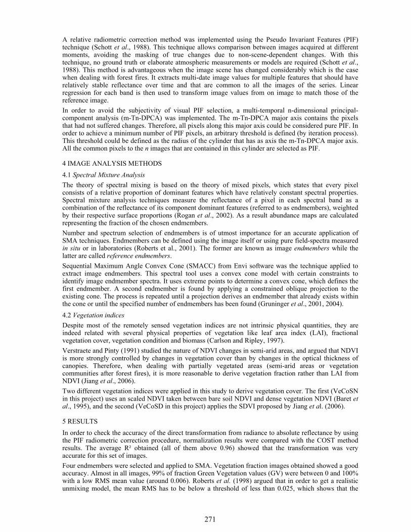
271

A relative radiometric correction method was implemented using the Pseudo Invariant Features (PIF) technique (Schott et al., 1988). This technique allows comparison between images acquired at different moments, avoiding the masking of true changes due to non-scene-dependent changes. With this technique, no ground truth or elaborate atmospheric measurements or models are required (Schott et al., 1988). This method is advantageous when the image scene has changed considerably which is the case when dealing with forest fires. It extracts multi-date image values for multiple features that should have relatively stable reflectance over time and that are common to all the images of the series. Linear regression for each band is then used to transform image values from on image to match those of the reference image. In order to avoid the subjectivity of visual PIF selection, a multi-temporal n-dimensional principal-component analysis (m-Tn-DPCA) was implemented. The m-Tn-DPCA major axis contains the pixels that had not suffered changes. Therefore, all pixels along this major axis could be considered pure PIF. In order to achieve a minimum number of PIF pixels, an arbitrary threshold is defined (by iteration process). This threshold could be defined as the radius of the cylinder that has as axis the m-Tn-DPCA major axis. All the common pixels to the n images that are contained in this cylinder are selected as PIF.

4 IMAGE ANALYSIS METHODS

4.1 Spectral Mixture Analysis The theory of spectral mixing is based on the theory of mixed pixels, which states that every pixel consists of a relative proportion of dominant features which have relatively constant spectral properties. Spectral mixture analysis techniques measure the reflectance of a pixel in each spectral band as a combination of the reflectance of its component dominant features (referred to as endmembers), weighted by their respective surface proportions (Rogan et al., 2002). As a result abundance maps are calculated representing the fraction of the chosen endmembers. Number and spectrum selection of endmembers is of utmost importance for an accurate application of SMA techniques. Endmembers can be defined using the image itself or using pure field-spectra measured in situ or in laboratories (Roberts et al., 2001). The former are known as image endmembers while the latter are called reference endmembers. Sequential Maximum Angle Convex Cone (SMACC) from Envi software was the technique applied to extract image endmembers. This spectral tool uses a convex cone model with certain constraints to identify image endmember spectra. It uses extreme points to determine a convex cone, which defines the first endmember. A second endmember is found by applying a constrained oblique projection to the existing cone. The process is repeated until a projection derives an endmember that already exists within the cone or until the specified number of endmembers has been found (Gruninger et al., 2001, 2004).

4.2 Vegetation indices Despite most of the remotely sensed vegetation indices are not intrinsic physical quantities, they are indeed related with several physical properties of vegetation like leaf area index (LAI), fractional vegetation cover, vegetation condition and biomass (Carlson and Ripley, 1997). Verstraete and Pinty (1991) studied the nature of NDVI changes in semi-arid areas, and argued that NDVI is more strongly controlled by changes in vegetation cover than by changes in the optical thickness of canopies. Therefore, when dealing with partially vegetated areas (semi-arid areas or vegetation communities after forest fires), it is more reasonable to derive vegetation fraction rather than LAI from NDVI (Jiang et al., 2006). Two different vegetation indices were applied in this study to derive vegetation cover. The first (VeCoSN in this project) uses an scaled NDVI taken between bare soil NDVI and dense vegetation NDVI (Baret et al., 1995), and the second (VeCoSD in this project) applies the SDVI proposed by Jiang et al. (2006).

5 RESULTS In order to check the accuracy of the direct transformation from radiance to absolute reflectance by using the PIF radiometric correction procedure, normalization results were compared with the COST method results. The average R² obtained (all of them above 0.96) showed that the transformation was very accurate for this set of images. Four endmembers were selected and applied to SMA. Vegetation fraction images obtained showed a good accuracy. Almost in all images, 99% of fraction Green Vegetation values (GV) were between 0 and 100% with a low RMS mean value (around 0.006). Roberts et al. (1998) argued that in order to get a realistic unmixing model, the mean RMS has to be below a threshold of less than 0.025, which shows that the

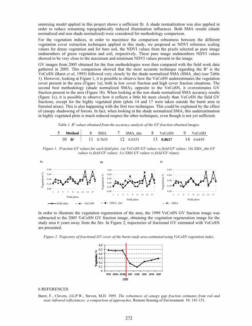
272

unmixing model applied in this project shows a sufficient fit. A shade normalization was also applied in order to reduce remaining topographically induced illumination influences. Both SMA results (shade normalized and non shade normalized) were considered for methodology comparison. For the vegetation indices, in order to maximize the comparison robustness between the different vegetation cover extraction techniques applied in this study, we proposed as NDVI reference scaling values for dense vegetation and for bare soil, the NDVI values from the pixels selected as pure image endmembers of green vegetation and soil, respectively. These pure image endmembers NDVI values showed to be very close to the maximum and minimum NDVI values present in the image. GV images from 2005 obtained for the four methodologies were then compared with the field work data gathered in 2005. This comparison showed that the most accurate technique regarding the R² is the VeCoSN (Baret et al, 1995) followed very closely by the shade normalized SMA (SMA_shn) (see Table 1). However, looking at Figure 1, it is possible to observe how the VeCoSN underestimates the vegetation cover present in the area (Figure 1a), both in low cover fraction and high cover fraction situations. The second best methodology (shade normalized SMA), opposite to the VeCoSN, it overestimates GV fraction present in the area (Figure 1b). When looking at the non shade normalized SMA accuracy results (figure 1c), it is possible to observe how it reflects a little bit more closely than VeCoSN the field GV fractions, except for the highly vegetated plots (plots 14 and 17 were taken outside the burnt area in forested areas). This is also happening with the first two techniques. This could be explained by the effect of canopy shadowing of forests. In fact, when looking at the shade normalized SMA, this underestimation in highly vegetated plots is much reduced respect the other techniques, even though is not yet sufficient.

Table 1. R² values obtained from the accuracy analysis of the GV fraction obtained images.

5 Method 6 SMA 7 SMA_shn 8 VeCoSN 9 VeCoSD 10 R² 11 0.7635 12 0.8353 13 0.8617 14 0.6439

Figure 1. Fraction GV values for each field plot. 1a) VeCoSN GV values vs field GV values; 1b) SMA_shn GV values vs field GV values; 1c) SMA GV values vs field GV vlaues.

In order to illustrate the vegetation regeneration of the area, the 1999 VeCoSN GV fraction image was subtracted to the 2005 VeCoSN GV fraction image, obtaining the vegetation regeneration image for the study area 6 years away from the fire. In Figure 2, trajectories of fractional GV estimated with VeCoSN are presented.

Figure 2. Trajectory of fractional GV cover of the burnt study area estimated using VeCoSN vegetation index.

6 REFERENCES Baret, F., Clevers, J.G.P.W., Steven, M.D. 1995. The robustness of canopy gap fraction estimates from red and

near-infrared reflectances: a comparison of approaches. Remote Sensing of Environment 54: 141-151.

1b

0,00

0,20

0,40

0,60

0,80

1,00

1 3 5 7 9 11 13 15 17

Field plots

Veg

etat

ion

%

SMA_shn

1a

0,00

0,20

0,40

0,60

0,80

1 3 5 7 9 11 13 15 17

Field plots

Veg

etat

ion

%

Field data VeCoSN

1c

0,00

0,20

0,40

0,60

0,80

1 3 5 7 9 11 13 15 17

Field plots

Veg

etat

ion

%

SMA

273

Carlson, T.N., Ripley, D.A. 1997. On the relation between NDVI, fractional vegetation cover, and leaf area index. Remote Sensing of Environment 62: 241-252.

Chavez, P.S., Jr. 1996. Image-based atmospheric corrections – Revisited and improved. Photogrammetric Engineering & Remote Sensing 62(9): 1025-1036.

Ekstrand, S. 1996. Landsat TM-based forest damage assessment: correction for topographic effects. Photogrammetric Engineering & Remote Sensing 62(2): 151-161.

Gruninger, J., Sundberg, R.L., Fox, M.J., Levine, R., Mundkowsky, W.F., Salisbury, M.S., Ratcliff, A.H. 2001. Automated optimal channel selection for spectral imaging sensors. Proceedings SPIE: Algorithms for mutlispectral and hyperspectral imagery VII, 54381-07

Gruninger, J., Ratkowski, A.J., Hoke, M.L. 2004. The Sequential Maximum Angle Convex Cone (SMACC) endmember Model. Proceedings SPIE: Algorithms for mutlispectral and hyperspectral and ultraspectral imagery, Orlando, April 2004, 5425-1.

Jiang, Z., Huete, A.R., Chen, J., Chen, Y., Li, J., Yan, G., Zhang, X. 2006. Analysis of NDVI and scaled difference vegetation index retrievals of vegetation fraction. Remote Sensing of Environment 101: 366-378.

Lloret, F., Pausas, J.G., Vilà, M. 2003. Responses of Mediterranean plant species to different fire frequencies in Garraf Natural Park (Catalonia, Spain): field observations and modeling predictions. Plant Ecology 167: 223-235

Paolini, L., Grings, F., Sobrino, J.A., Jimenez Muñoz, J.G., Karszenbaum, H. 2006. Radiometric correction effects in Landsat multi-date/multi-sensor change detection studies. International Journal of Remote Sensing 27(4): 685-704.

Pausas, J.G., Vallejo, V.R. 1999. The role of fire in European Mediterranean ecosystems. In: Chuvieco, E. (Ed.), Remote sensing of large wildfires in the European Mediterranean basin, pp. 3-16. Berlin: Springer-Verlag.

Roberts, D.A., Gardner, M., Church, R., Ustin, S., Scheer, G., Green, R.O. 1998. Mapping chaparral in the Santa Monica Mountains using multiple endmember spectral mixture models. Remote Sensing of Environment 65(3): 267-279.

Rogan, J., Franklin, J., Roberts, D.A. 2002. A comparison of methods for monitoring multitemporal vegetation change using Thematic Mapper imagery. Remote Sensing of Environment 80: 143-156.

Schott, J.R., Salvaggio, C., Volchok, W.J. 1988. Radiometric scene normalization using Pseudoinvariant Features. Remote Sensing of Environment 26: 1-16.

Vogelmann, J.E., Helder, D., Morfitt, R., Choate, M.J., Merchant, J., Bulley, H. 2001. Effects of Landsat 5 Thematic Mapper and Landsat 7 Enhanced Thematic Mapper Plus radiometric and geometric calibrations and corrections on landscape characterization. Remote Sensing of Environment 78: 55-70.

274

European Commission EUR 22892 EN Joint Research Centre – Institute for Environment and Sustainability Title: Proceedings of the 6th International Workshop of the EARSeL Special Interest Group on Forest Fire. Towards an Operational Use of Remote Sensing in Forest Fire Management Editors: IOANNIS Z. GITAS and CÉSAR CARMONA-MORENO Luxembourg: Office for Official Publications of the European Communities 2007 – 275 pp. – 16,2 x 22,9 cm EUR – Scientific and Technical Research series – ISSN 1018-5593 ISBN 978-92-79-06620-7

IOANNIS Z. GITAS AND CÉSAR CARMONA-MORENO...

Documents

Transcript of IOANNIS Z. GITAS AND CÉSAR CARMONA-MORENO...