
Ioannis Ntzoufras greek stochastics delta 2012jbn/papers/files/24... · As you can understand this...
44
Blackboard 1
Transcript of Ioannis Ntzoufras greek stochastics delta 2012jbn/papers/files/24... · As you can understand this...

Blackboard 1

Blackboard 2
Presentation by
Ioannis Ntzoufras
Department of StatisticsAthens University of Economics and [email protected]://stat-athens.aueb.gr/~jbn/

Blackboard 3
AgendaAn Obsession: Model selection and the Paradox
An Idea: Avoiding (?) the paradox
Conclusion
Break: At last time for coffee
1
2
5
1:00pm
4
Illustrations and comparisons
1
2
1:00pm
1
2
1:00pm
1
2
3
1
2

Blackboard 4
1. An ObsessionModel selection and the Paradox
A Bayesian approach to inference under model uncertainty proceeds as follows.
Suppose
• data y generated by a model m M
• Each model specifies the distribution of y,
• βm is the parameter vector for model m. • f(m) is the prior probability of model mThen posterior inference is based on posterior model probabilities
Blackboard 5
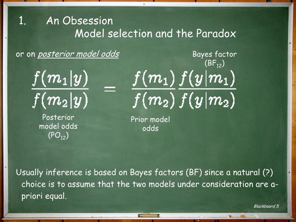
1. An ObsessionModel selection and the Paradox
or on posterior model odds
Usually inference is based on Bayes factors (BF) since a natural (?) choice is to assume that the two models under consideration are a-priori equal.
Prior model odds
Bayes factor (BF12)
Posterior model odds
(PO12)

Blackboard 6
1. An ObsessionModel selection and the Paradox
The Lindley-Bartlett-Jeffreys Paradox (1)
For a single model inference,
a highly diffuse prior on the model parameters is often used (torepresent ignorance).
Then the posterior density takes the shape of the likelihood and is insensitive to the exact value of the prior density function, provided that the prior is relatively flat over the range of parameter values with non-negligible likelihood.

Blackboard 7
1. An ObsessionModel selection and the Paradox
The Lindley-Bartlett-Jeffreys Paradox (2)
For multiple models inference:The use of such a prior creates an apparent difficulty. For illustration, let us consider the simple case where model m1 is
completely specified (no unknown parameters) and model m2 has parameter
• Then, for any observed data y, BF12 can be made arbitrarily large by choosing a sufficiently diffuse prior distribution for
• Hence, under model uncertainty, two different diffuse prior distributions for model parameters might lead to essentially thesame posterior distributions for those parameters, but very different BFs.

Blackboard 8
1. An ObsessionModel selection and the Paradox
The Lindley-Bartlett-Jeffreys Paradox (3)
ThereforeBF12
when the Prior variance of whatever data y we have…Fully supporting the simpler model and making the procedure informative (?)

Blackboard 9
1. An ObsessionModel selection and the Paradox
The Lindley-Bartlett-Jeffreys Paradox (4)
Discussed by • Lindley (1957, Bka) ; referred to as `Lindley's paradox'
he actually noted the sensitivity of BF on the sample size and not on the prior
• it is also variously attributed to Bartlett (1957, Bka) and he also added the sensitivity on the prior variance in a note complementary to the publication of Lindley (1957); published in the next issue of Bka.
• Also discussed by Jeffreys in his book
As you can understand this became my obsession (and of many others). The aim was to overcome this paradoxical behavior…

Blackboard 10
1. An ObsessionModel selection and the Paradox
The Lindley-Bartlett-Jeffreys Paradox (5)
Dawid (2011) ==> the Bayes factor is only one of the two elements on the posterior
model odds. ==> The prior model probabilities are of equal significance.
By focusing on the impact of the prior distributions for model parameters on the Bayes factor, there is an implicit understanding that the prior model probabilities are specified independently of these prior distributions.
This is often the case in practice, where a uniform prior distribution over models is commonly adopted, as a reference position.

Blackboard 11
1. An ObsessionModel selection and the Paradox
Priors on model spaceNon-uniform priors have been suggested (but not widely used)• Chipman (1996, Canad.J.Stat.), based on interaction structure and
associations between covariates• Laud and Ibrahim (1996, Bka) & Chen, Ibrahim & Yiannoutsons (1999,
RSSB): based on prior information and elicitation• Brown, Vannuci & Fearn (1998, J.Chemometrics): Beta-Binomial for
variable inclusion probabilities• Chipman , George & McCulloch (2001): Beta-Binomial prior (and
generalization) and dilution probabilities • George and Forster (2001, Bka): Empirical Bayes• Yuan & Lin (2005, JASA); model probs adjusted by XTX• Beta-Binomial becomes more and more dominant => Clyde and George
(2004, Stat.Sci.), Nott and Kohn (2005,Bka), Cui and George (2008, JSPI), Ley and Steel (2009, J.App.Econ.), Wilson etal (2010, Ann.appl.Stat).
• Scott & Berger (2010, Annals); Empirical Bayes and Beta-Binomial

Blackboard 12
2. An Idea: Avoiding (?) the paradox
Joint Prior on parameters and model space
We propose a different approach
The two elements of the prior distribution (on model space and within each model) might be jointly specified so that perceived problems with Bayesian model comparison can be avoided.
This leads to a non-uniform specification for the prior distribution over models, depending directly on the prior distributions for model parameters.

Blackboard 13
2. An Idea: Avoiding (?) the paradox
We focus on models in which • the parameters can be a-priori expressed by a multivariate normal
prior density with mean and variance-covariance matrix Vm
• the likelihood is sufficiently regular for standard asymptotic results to apply.
Linear regression models and GLMs are such models.

Blackboard 14
2. An Idea: Avoiding (?) the paradox
We rewrite the prior variance matrix as where • cm is the scale of the prior dispersion• Σm is a semi-positive matrix with a fixed volume |Σm| Τhen, the posterior is given by
[dm stands for the dimension of βm]

Blackboard 15
2. An Idea: Avoiding (?) the paradox
[dm stands for the dimension of βm]
Hence, as cm gets larger, f(m|y) gets smaller, assuming everything else remains fixed.
Therefore, for two models of different dimension and equal cm=c, the posterior odds in favor of the more complex model tends to zero as cm gets larger.
This is essentially the Lindley-Bartlett-Jeffreys paradox.
and for suitably large cm

Blackboard 16
2. An Idea: Avoiding (?) the paradox
Using Laplace approximation, we can write
where
• C is a normalizing constant;
• is the maximum likelihood estimate and
• is the second derivative matrix of the log-posterior density

Blackboard 17
2. An Idea: Avoiding (?) the paradox
Using Laplace approximation, we can write
where
• C is a normalizing constant; n is the sample size
• is the maximum likelihood estimate •
is the Fisher information matrix for a unit observation • is the second derivative matrix of the log-posterior
density

Blackboard 18
2. An Idea: Avoiding (?) the paradox
The idea –Step 1 [rewrite the prior variance]Any prior variance matrix Vm can be rewritten as
resulting in
where cm defined as

Blackboard 19
2. An Idea: Avoiding (?) the paradox
The idea – Step 2 [express posterior probs as BIC and additional penalties]
BICAdditional dimension penalty (1)
Additional penalty 2 (Shrinkage/Ridge type penalty)
Additional penalty 3
(from prior model probs)
.

Blackboard 20
2. An Idea: Avoiding (?) the paradox
The idea –Step 2 [express posterior probs as BIC and additional penalties]
BIC can be obtained if• cm=1• Prior mean of βm is set equal to its MLEs• Prior model probabilities are assummed equal for all models. Similar to Kass and Wasserman (1995)

Blackboard 21
2. An Idea: Avoiding (?) the paradox
The idea – Step 2 [express posterior probs as BIC and additional penalties]
This is eliminated for large prior variances
This still remains
unspecifiedAnd it can be used to effectively
eliminate the prior penalty 1 which causes the paradoxical behavior
This term causes the Lindleys paradox since it explodes for large prior variances

Blackboard 22
2. An Idea: Avoiding (?) the paradox
The idea –Step 3 [eliminating additional penalty 1]
We suggest choosing the cm freely to express the desired amountof shrinkage (to the prior mean), and choose prior model probabilities to adjust for the resulting effect this will have on the posterior model probabilities.
where p(m) are some baseline model probabilities.

Blackboard 23
2. An Idea: Avoiding (?) the paradox
The idea – Step 3 [eliminating additional penalty 1]
Under this prior set-up
Log p(m) can be also interpreted as an additional dimension penalty

Blackboard 24
2. An Idea: Avoiding (?) the paradox
For normal models Using Normal-inverse-gamma prior set-up results become exact.Here we present results using a multivariate normal prior for βm with mean
. and variance Vm σ2 and f(σ2) 11/σ2
Using the prior model probabilities of type
Results in posterior model probabilitiesResidual sum of squares
Shrinkage penalty
Dimension penalty

Blackboard 25
2. An Idea: Avoiding (?) the paradox
What do we achieve
• Separate the prior effect within each model from the posterior inference on model space
• The prior of the parameters contributes on the model evaluation through a shrinkage term measuring the difference between data and the prior
• The posterior (dimension) penalty on model space is solely controlled by p(m)
• Setting all p(m) equal leads to a model determination based on a modified BIC involving penalized maximum likelihood.

Blackboard 26
2. An Idea: Avoiding (?) the paradox
What is p(m)? p(m) can be based on a model complexity penalty which is a-priori
seems to be appropriate. Default option => Setting all p(m) equal leading to a modified BIC
procedureHence, the impact of the prior distribution of the model
parameters is through the shrinkage factor (additional penalty 2) and it is straightforward to assess, and any undesirable side effects of large prior variances are eliminated.

Blackboard 27
2. An Idea: Avoiding (?) the paradox
What is p(m)? To chose p(m) such that it corresponds to a particular complexity penalty, we
need to evaluate cm-2 (i.e. the number of units of information introduced by
the prior of βm).Except in certain cases, e.g. normal linear models, this quantity depends on
the unknown model parameters βm . This is not appropriate as a specification for the marginal prior distribution
over model space.One possibility is to use a sample-based estimate in the Fisher information
matrix to determine the `prior' model probability (not fully Bayesian).Alternatively we may substitute βm by its prior mean into the Fisher
information matrix. This has a unit information interpretation but the model comparison is not asymptotically based the procedure described above (a correction term is required)

Blackboard 28
2. An Idea: Avoiding (?) the paradox
Some arguments in favor of this approachARGUMENT 1: Constant probability in a neighborhood of the prior
meanLet us consider the prior probability of the event
Then, for any ε>0,

Blackboard 29
2. An Idea: Avoiding (?) the paradox
Some arguments in favor of this approachARGUMENT 1: Constant probability in a neighborhood of the prior
mean
Therefore, if the joint prior probability of model m in conjunction with βm being in some specified neighborhood of its prior mean is to be uniform across models then we require
Blackboard 30
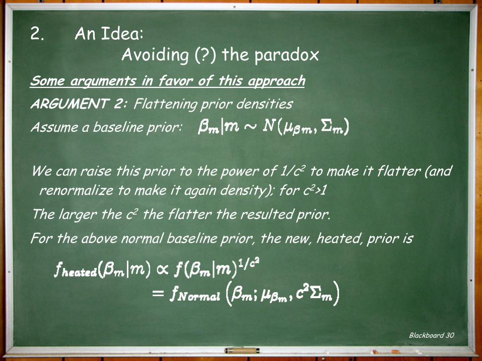
2. An Idea: Avoiding (?) the paradox
Some arguments in favor of this approachARGUMENT 2: Flattening prior densities Assume a baseline prior:
We can raise this prior to the power of 1/c2 to make it flatter (and renormalize to make it again density); for c2>1
The larger the c2 the flatter the resulted prior. For the above normal baseline prior, the new, heated, prior is

Blackboard 31
2. An Idea: Avoiding (?) the paradox
Some arguments in favor of this approachARGUMENT 2: Flattening prior densities Doing the same procedure for the joint prior on parameter and model
space we end up to
Where C0 = (2π)-1/2 |Σm|-1/2 is the normalizing constant of the baseline prior
for large cm

Blackboard 32
2. An Idea: Avoiding (?) the paradox
Some arguments in favor of this approachARGUMENT 2: Flattening prior densities Hence the heated prior model probabilities are equivalent to our
proposal with
Implementing a procedure similar to Fisher Information Criterion(FIC, Wei, 1992, Annals of Statistics)
The above choice of p(m) does not requires to evaluate the Fisher information matrix

Blackboard 33
Even the BMA estimates are affected by the Lindley’s paradox and the proposed adjustment avoids the incoherent behavior
Comparison of two simple models differing by one coefficient βwith MLE value equal to one
Some arguments in favor of this approachARGUMENT 3: Bayesian model averaging and shrinkage
2. An Idea: Avoiding (?) the paradox
Uniform prior on model space
BMA estimate shrinks towards zero for non-informative priors
Adjusted prior
BMA estimate shrinks towards the MLE value for non-informative priors

Blackboard 34
3. Illustrations and comparisons:
Example 1: A simple linear regression example
Data from Montgomery, Peck
and Vining (2001) with n=25
MLE for β1=1.417ρ= 0.98g-prior with
g=0.04n (RIC)
g-prior with g=0.256n (AIC)
Intrinsic with n*=20
g-prior with c2=1 (g=n, BIC)

Blackboard 35
3. Illustrations and comparisons:
Example 1: A simple linear regression example

Blackboard 36
Example 2: Simulated regressions
3. Illustrations and comparisons:
g-prior with c2=1 (g=n, BIC or unit information prior)
Posterior model probabilities Posterior variable inclusion probabilities
Black Solid line: constant model; Red short dashed line: X4+X5 model; Blue long dashed line: X4+X5+X12 model.

Blackboard 37
Example 2: Simulated regressions
3. Illustrations and comparisons:
Posterior variable inclusion probabilities
Obtained by equating the shrinkage g/(g+1) with the prior expected value under the hyper-g prior
Posterior model probabilities

Blackboard 38
Example 2: Simulated regressions
3. Illustrations and comparisons:
1) Extremely robust for a wide range of values
2) Low posterior model probabilities=> Increased posterior model uncertainty
3) Nonsense covariates have (inflated?) posterior inclusion probabilities in 0.2-0.4

Blackboard 39
Example 2: Simulated regressions
3. Illustrations and comparisons:
4) The Lindley-Bartlett paradox is still here But for values a -> 2

Blackboard 40
Example 2: Simulated regressions
3. Illustrations and comparisons:
5) There is also a shrinkage paradox (more evident in shrinkage methods such as
lasso); Lykou and Ntzoufras (2012) for similar illustrations

Blackboard 41
Example 2: Simulated regressions
3. Illustrations and comparisons:
Posterior variable inclusion probabilities
Posterior model probabilities1) They are robust
2) They do give reasonably high posterior model probabilities to best models
3) Inclusion probabilities of non-sense covariates are low < 0.2
4) They do not suffer from Lindleys paradox
5) No shrinkage paradox

Blackboard 42
3. Illustrations and comparisons:
Example 3: A 3x2x4 contingency table example with available prior information
DF=Dellaportas & Forster prior (non-informative for model comparison); KS=Knuiman and Speeed prior (informative within each model)IND=Independence prior

Blackboard 43
4. ConclusionWhat we do argue is:
1) there is nothing sacred about a uniform prior distribution over models.
2) It is reasonable to consider specifying jointly f(βm, m) and hence f(m) in a way which takes account of the prior distributions for the modelparameters for individual models.
We propose priors of type as a possible choice which
a) Separates (in a reasonable way) inference within and across models
β) Avoids Lindley-Bartlett paradox
γ) Implements a desired complexity/dimensionality penalty and a shrinkage penalty (on the same time)
δ) Can be used even when the prior is informative for some parameters

Blackboard 44
5. Coffee time
At last …