INVISIBLE CONTROL OF SELF-ORGANIZING AGENTS … · INVISIBLE CONTROL OF SELF-ORGANIZING AGENTS...

SIAM J. APPL. MATH. c© 2016 Society for Industrial and Applied MathematicsVol. 76, No. 4, pp. 1683–1710

INVISIBLE CONTROL OF SELF-ORGANIZING AGENTSLEAVING UNKNOWN ENVIRONMENTS∗

GIACOMO ALBI† , MATTIA BONGINI† , EMILIANO CRISTIANI‡ , AND DANTE KALISE§

Abstract. In this paper we are concerned with multiscale modeling, control, and simulationof self-organizing agents leaving an unknown area under limited visibility, with special emphasis oncrowds. We first introduce a new microscopic model characterized by an exploration phase and anevacuation phase. The main ingredients of the model are an alignment term, accounting for theherding effect typical of uncertain behavior, and a random walk, accounting for the need to explorethe environment under limited visibility. We consider both metrical and topological interactions.Moreover, a few special agents, the leaders, not recognized as such by the crowd, are “hidden” inthe crowd with a special controlled dynamic. Next, relying on a Boltzmann approach, we derive amesoscopic model for a continuum density of followers, coupled with a microscopic description forthe leaders’ dynamics. Finally, optimal control of the crowd is studied. It is assumed that leadersaim at steering the crowd towards the exits so to ease the evacuation and limit clogging effects, andlocally optimal behavior of leaders is computed. Numerical simulations show the efficiency of thecontrol techniques in both microscopic and mesoscopic settings. We also perform a real experimentwith people to study the feasibility of such a bottom-up control technique.

Key words. pedestrian models, agent-based models, kinetic models, evacuation, herding effect,soft control

AMS subject classifications. 91B10, 35Q93, 49K15, 34H05, 65C05

DOI. 10.1137/15M1017016

1. Introduction. Self-organizing systems are not as mysterious as they werewhen researchers began to deal with them. A number of local interaction rules wereidentified, such as repulsion, attraction, alignment, self-propulsion, etc., and the large-scale outcome triggered by the combination of them is so far sufficiently understood[54]. Researchers have also achieved a certain knowledge regarding the control of self-organizing systems, namely the methods to dictate a target behavior to the agentsstill keeping the local rules active all the time.

In this paper we are concerned with multiscale modeling, control, and simulationsof self-organizing agents which leave an unknown area. Agents are not informed aboutthe positions of the exits, so they need to explore the environment first. Agents areassumed not to communicate with each other and they cannot share informationdirectly. Moreover, they are selfish and do not intend to help the other agents.

The guiding application is that of a human crowd leaving an unknown environ-ment under limited visibility. In that case, we claim that people exhibit two oppositetendencies: on the one hand, they tend to spread out in order to explore the environ-ment efficiently, and on the other hand, they follow the group mates in the hope that

∗Received by the editors April 16, 2015; accepted for publication (in revised form) May 16, 2016;published electronically August 30, 2016.

http://www.siam.org/journals/siap/76-4/M101701.htmlFunding: This research has received funding from the European Union under grant ERC-STG

306274 (HDSPCONTR) and ERC-ADG 668998 (OCLOC).†TUM, M15 - Chair of Numerical Mathematics, Boltzmann straße. 3, D-85748 Garching, Munich,

Germany ([email protected], [email protected]).‡Istituto per le Applicazioni del Calcolo “M. Picone”, Consiglio Nazionale delle Ricerche, Via dei

Taurini 19, I-00185, Rome, Italy ([email protected]).§Johann Radon Institute for Computational and Applied Mathematics, Altenberger Straße 69,

A-4040 Linz, Austria ([email protected]).

1683

http://www.siam.org/journals/siap/76-4/M101701.html

mailto:[email protected]




1684 G. ALBI, M. BONGINI, E. CRISTIANI, AND D. KALISE

they have already found a way out (herding effect). Controlling these natural behav-iors is not easy, especially in emergency or panic situations. Typically, the emergencymanagement actors (e.g., police, stewards) adopt a top-down approach: they receiveinformation about the current situation, update the evacuation strategies, and finallyinform people communicating directives. It is useful to stress here that this approachcan be very inefficient in large environments (where communications to people are dif-ficult) and in panic situations (since “instinctive” behavior prevails over the rationalone). Let us also mention that in some cases people are simply not prone to followauthority’s directives because they are opposing it (e.g., in public demonstrations).

In this paper we explore the possibility of controlling crowds adopting a bottom-upapproach. Control is obtained by means of special agents (leaders) who are hiddenin the crowd, and they are not recognized by the mass as special. From the modelingpoint of view, this is translated by the fact that the individuals of the crowd (followers)interact in the same way with both the other crowd mates and the leaders.

Goals. We first introduce a new microscopic (agent-based) model characterizedby an exploration phase and an evacuation phase. This is achieved by a combinationof repulsion, alignment, self-propulsion, and random (social) force, together with theintroduction of an exit’s visibility area. We also consider both metrical and topologicalinteractions so to avoid unnatural all-to-all interactions. A few leaders, not recognizedas such by the crowd, are added to the model with a special, controlled dynamics.

Second, relying on a Boltzmann approach, we derive a mesoscopic model for acontinuum density of followers, coupled with a microscopic description for the leaders’dynamics. This procedure, based on a binary interaction approximation, shows that,in a grazing collision regime, the microscopic-kinetic limit system is the mesoscopicdescription of the original microscopic dynamics.

Finally, dynamic optimization procedures with short- and long-time horizon areconsidered. It is assumed that leaders aim at steering the crowd toward the exits soto ease the evacuation and limit clogging effects. The goal is achieved by exploitingthe herding effect. Locally optimal behavior of leaders is computed by means oftwo methods: the model predictive control and a modified compass search. Severalnumerical simulations show the efficiency of the optimization methods in both themicroscopic and mesoscopic settings.

Beside numerical simulations, we performed a real experiment with people tostudy the feasibility of the proposed bottom-up crowd control technique.

Relevant literature. This paper falls in several crossing, and often independent,lines of research. Concerning pedestrian modeling, virtually any kind of model hasbeen investigated so far and several reviews and books are available. For a quickintroduction, we refer the reader to the reviews [9, 42] and the books [29, 44]. Somepapers deal specifically with evacuation problems: a very good source of referencesis the paper [1], where evacuation models both with and without optimal planningsearch are discussed. The paper [1] itself proposes a cellular automata model coupledwith a genetic algorithm to find a top-down optimal evacuation plan. Evacuationproblems were studied by means of lattice models [23, 37], social force models [49],cellular automata models [1, 56], mesoscopic models [2], and macroscopic models [21].Limited visibility issues were considered in [21, 23, 37]. A real experiment involvingpeople can be found in [37].

The control of self-organizing agents can be achieved in several ways. For example,the dynamics of all agents can be controlled by means of a single control variable,which remains active at all times [3]. This kind of control is suitable, e.g., to modelthe influence of television on people. Alternatively, every agent can be controlled by an

INVISIBLE CONTROL OF SELF-ORGANIZING AGENTS 1685

independent control variable. This is the most effective but also the most “expensive”control technique because of the large number of interactions with the agents that isrequired [13]. A more parsimonious control technique, called sparse control, can beobtained by penalizing the number of these interventions by means of an L1 controlcost, so that the control is active only on few agents at every instant [11, 12, 18].If the existing behavioral rules of the agents cannot be redesigned, the control ofthe system can be obtained by means of external agents. Here the literature splitsinto two branches: the case of recognizable leaders, characterized by the fact that theexternal agents have an influence on normal agents stronger than the influence exertedby group mates (like, e.g., a celebrity) [6, 15, 32, 47]; and the case of invisible leaders,which are instead characterized by the fact that the external agents are completelyanonymous and are perceived as normal group mates [26, 31, 40, 41]. Alternativeapproaches, based on the control of the surrounding environment rather than of theagents themselves, are proposed in [27, 30, 43].

Let us focus on the invisible control, also known as soft control. In the seminalpaper [26] a repulsion-alignment-attraction model is considered, for which the authorsshow that a little percentage of informed agents pointing towards a target is sufficientto steer the whole system to it. The papers [40, 41] deal with a Vicsek-like (purealignment) model with a single leader. A feedback control for the leader is proposed,which is able to align the whole group along a desired direction from any initialcondition. Invisible control was successfully implemented in real experiments involvinganimals, where leaders come in the form of disguised robots; see, e.g., [39], which dealswith cockroaches and [16], which deals with zebrafishes.

The complexity reduction of microscopic models when the number of interactingagents is large has received deep interest in the last few years. The main techniqueto address the curse of dimensionality is to recast the original microscopic dynamicsin the form of a PDE, by substituting the influence that the entire population hason a single agent with an averaged one. Several approaches have been used to deriverigorously this procedure, like the BBGKY hierarchy [38], the mean-field limit [10, 17],or the binary interaction approximation [4, 48]. Furthermore, only recently has thisproblem been investigated for optimal control of multiagent systems [36].

In the case of the control by means of external agents, if the number of leadersis relatively small in comparison to the crowd of followers, it might be convenientto apply the above dimension reduction techniques to the followers’ population only[14, 35]. The resulting modeling setting is described by a coupled ODE-PDE sys-tem, where we control the microscopic dynamics in order to steer the macroscopicquantities. Nonetheless, from the computational point of view, one has to face thenumerical tractability of the optimal control problem, whose solution requires the iter-ated evaluation of the macroscopic system. Since the underling dynamics are typicallynonlinear and imply the resolution of high-dimensional integro-differential terms, adhoc approaches have to be developed in order to avoid time-consuming strategies.One possibility is to use a fixed dynamics for the system of ODEs, assigned by themodelers or as feedback control derived by a properly designed functional; see, e.g.,[5, 24].

Paper organization. This paper is organized as follows. In section 2 we introducethe main features of the model, valid at any scale of observation. In section 3 wepresent in detail the model at the microscopic scale. In section 4 we derive theassociated Boltzmann-type equation and the coupled ODE (micro)—PDE (kinetic)model by means of the grazing collision limit, following the path laid out in [50].In section 5 we introduce the control and optimization problem and in section 6


we show the results of the numerical tests. In section 7 we report the results ofa real experiment with pedestrians aimed at validating the proposed crowd controltechnique. We conclude the paper sketching some research perspectives.

2. Model guidelines. In this section we describe the model at a general level.Hereafter, we divide the population between leaders, which are the controllers andbehave in some optimal way (to be defined), and followers, which represent the massof agents to be controlled. Followers cannot distinguish between followers and leaders.

First- versus second-order model. One can notice that walking people, animals,and robots are in general able to adjust their velocity almost instantaneously, reduc-ing to a negligible duration the acceleration/deceleration phase. For this reason, asecond-order (inertia-based) framework does not appear to be the most natural set-ting. However, if we include in the model the tendency of the agents to move togetherand to align with group mates we implicitly assume that agents can perceive the ve-locity of the others. This makes unavoidable the use of a second-order model, whereboth positions and velocities are state variables. See [29, sect. 4.2] for a general dis-cussion on this point. In our model we adopt a mixed approach, describing leaders bya first-order model (since they do not need to align) and followers by a second-orderone. In the latter case, the small inertia is obtained by means of a fast relaxationtowards the target velocity.

Metrical versus topological interactions. Interaction of one agent with group matesis said to be metrical if it involves only mates within a predefined sensory region, re-gardless of the number of individuals which actually fall in it. Interaction is insteadsaid to be topological if it involves a predefined number of group mates regardlessof their distance from the considered agent. Again, in our model we adopt a mixedapproach, assuming short-range interactions to be metrical and long-range ones to betopological.

Isotropic versus anisotropic interactions. Living agents (people, animals) are gen-erally asymmetric, in the sense that they better perceive stimuli coming from their“front”, rather than their “back”. In pedestrian models, e.g., interactions are usu-ally restricted to the half-space in front of the person, since the human visual fieldis approximately 180. Nevertheless, humans can easily see all around them by sim-ply turning their head. In the case we are interested in, people have no idea of thelocation of their target; hence we expect that they often look around to explore theenvironment and see the behavior of the others. This is why we prefer to adhere toisotropic interactions.

Let us describe the social forces acting on the agents.Leaders.• Leaders are subject to an isotropic metrical short-range repulsion force di-

rected against all the others, translating the fact that they want to avoidcollisions and that a maximal density exists.

• Leaders are assumed to know the environment and the self-organizing featuresof the crowd. They respond to an optimal force which is the result of an offlineoptimization procedure, defined as to minimizing some cost functional (seesection 5).

Followers.• Similarly to leaders, followers respond to an isotropic metrical short-range

repulsion force directed against all the others.• Followers tend to a desired velocity which corresponds to the velocity the

would follow if they were alone in the domain. This term takes into account


the fact that the environment is unknown. Followers describe a random walkif the exit is not visible (exploration phase) or a sharp motion toward theexit if the exit is visible (evacuation phase). In addition, we include a self-propulsion term which translates the tendency to reach a given characteristicspeed (modulus of the velocity).

• If the exit is not visible, followers are subject to an isotropic topologicalalignment force with all the others, i.e., they tend to have the same velocityof the group mates. Assuming that the agents’ positions are close enough,this corresponds to the tendency to go where group mates go (herding effect).

3. The microscopic model. In this section we introduce the microscopic modelfor followers and leaders. We denote by d the dimension of the space in which themotion takes place (typically d = 2), by Nf the number of followers, and by N l Nf

the number of leaders. We also denote by Ω ≡ Rd the walking area and by xτ ∈ Ωthe target point. To define the target’s visibility area, we consider the set Σ, withxτ ∈ Σ ⊂ Ω, and we assume that the target is completely visible from any pointbelonging to Σ and completely invisible from any point belonging to Ω\Σ.

For every i = 1, . . . , Nf, let (xi(t), vi(t)) ∈ R2d denote position and velocity ofthe agents belonging to the population of followers at time t ≥ 0 and, for everyk = 1, . . . , N l, let (yk(t), wk(t)) ∈ R2d denote position and velocity of the agentsamong the population of leaders at time t ≥ 0. Let us also define x := (x1, . . . , xNf)and y := (y1, . . . , yNl).

Finally, let us denote by Br(x) the ball of radius r > 0 centered at x ∈ Ω, byBN (x; x,y) the minimal ball centered at x encompassing at least N agents, and byN ∗ the actual number of agents in BN (x; x,y). Note that N ∗ ≥ N .

Remark 3.1. The computation of BN (x; x,y) requires the knowledge of the po-sitions of all the agents, since all the distances |xi − x|, i = 1, . . . , Nf, and |yk − x|,k = 1, . . . , N l, must be evaluated in order to find the N closest agents to x.

The microscopic dynamics described by the two populations is given by the fol-lowing set of ODEs: for i = 1, . . . , Nf and k = 1, . . . , N l,(3.1)

xi = vi,

vi = A(xi, vi) +∑Nf

j=1Hf(xi, vi, xj , vj ; x,y) +

∑Nl

`=1Hl(xi, vi, y`, w`; x,y),

yk = wk =∑Nf

j=1Kf(yk, xj) +

∑Nl

`=1Kl(yk, y`) + uk.

We assume the following:• A is a self-propulsion term, given by the relaxation toward a random direction

or the relaxation toward a unit vector pointing to the target (the choicedepends on the position), plus a term which translates the tendency to reacha given characteristic speed s ≥ 0 (modulus of the velocity), i.e.,

A(x, v) := θ(x)Cz(z − v) + (1− θ(x))Cτ

(xτ − x|xτ − x|

− v)

+ Cs(s2 − |v|2)v,

(3.2)

where θ : Rd → [0, 1] is the characteristic function of Ω\Σ, θ(x) = χΩ\Σ(x), zis a d-dimensional random vector with normal distribution N (0, σ2), and Cz,Cτ , Cs are positive constants.


• The interactions follower-follower and follower-leader coincide and are equalto(3.3)

Hf(x, v, x′, v′; x,y) := −CfrRγ,r(x, x

′) + θ(x)CaN ∗

(v′ − v)χBN (x;x,y)(x′),

Hl(x, v, y, w; x,y) := Hf(x, v, y, w; x,y)

for given positive constants Cfr , Ca, r, and γ, and

Rγ,r(x, x′) =

e−|x

′−x|γ x′−x|x′−x| if x′ ∈ Br(x)\x,

0 otherwise,

models a (metrical) repulsive force, while the second term accounts for the(topological) alignment force, which vanishes inside Σ. Note that, once thesummations over the agents

∑j H

f and∑`H

l are done, the alignment termmodels the tendency of the followers to relax toward the average velocity of theN closer agents. With the choice Hf ≡ Hl the leaders are not recognized bythe followers as special. This feature opens a wide range of new applications,including the control of crowds not prone to follow authority’s directives.

• The interactions leader-follower and leader-leader reduce to a mere (metrical)repulsion, i.e., Kf = Kl = −Cl

rRζ,r, where Clr > 0 and ζ > 0 are in general

different from Cfr and γ, respectively. Note that here the repulsion force is

interpreted as a velocity field, while for followers it is an acceleration field.• uk : R+ → RdNl

is the control variable, to be chosen in a set of admissiblecontrol functions.

Remark 3.2. The behavior of the leaders is entirely encapsulated in the controlterm u but for a short-range repulsion force. The latter should be indeed interpretedas a force due to the presence of the others, thereby noncontrollable.

4. Formal derivation of a Boltzmann-type equation. As already men-tioned, our main interest in (3.1) lies in the case N l Nf; that is, the populationof followers exceeds by far the one of leaders. When Nf is very large, a microscopicdescription of both populations is no longer a viable option. We thus consider theevolution of the distribution of followers at time t ≥ 0, denoted by f(t, x, v), togetherwith the microscopic equations for the leaders (whose number is still small). To thisend, we denote with mf the total mass of followers, i.e.,

mf(t) =

∫R2d

f(t, x, v) dx dv,

which we shall eventually require to be equal to Nf. We introduce, for symmetryreasons, the distribution of leaders g and their total mass

(4.1) g(t, x, v) =

Nl∑k=1

δ(yk(t),wk(t))(x, v), ml(t) =

∫R2d

g(t, x, v) dx dv = N l.

The evolution of f can be then described by a Boltzmann-type dynamic, derivedfrom the above instantaneous control formulation, which is obtained by analyzing thebinary interactions between a follower and another follower and the same followerwith a leader. The application of standard methods of binary interactions (see [22])


shall yield a mesoscopic model for the distribution of followers, to be coupled withthe previously presented ODE dynamics for leaders.

To derive the Boltzmann-type dynamics, we assume that, before interacting, eachagent has at his disposal the values x and y that he needs in order to perform itsmovement: hence, in a binary interaction between two followers with state parameters(x, v) and (x, v), the value of Hf(x, v, x, v; x,y) does not depend on x and y. In thecase of Hf of the form (3.3), this means that the ball BN (x; x,y) and the value ofN ∗ have been already computed before interacting.

Moreover, since we are considering the distributions f and g of followers andleaders, respectively, the vectors x and y are derived from f and g by means of thefirst marginals of f and g, π1f and π1g, respectively, which give the spatial variables ofthose distributions. Hence, since no confusion arises, we write Hf(x, v, x, v;π1f, π1g)in place of Hf(x, v, x, v; x,y) to stress the dependence of this term on f and g.

We thus consider two followers with state parameters (x, v) and (x, v), respec-tively, and we describe the evolution of their velocities after the interaction accordingto

v∗ = v + ηf [θ(x)Czξ + S(x, v) +mfHf(x, v, x, v;π1f, π1g)] ,

v∗ = v + ηf[θ(x)Cz ξ + S(x, v) +mfHf(x, v, x, v;π1f, π1g)

],

(4.2)

where ηf is the strength of interaction among followers, ξ, ξ are random variableswhose entries are independently and identically distributed following a normal dis-tribution with mean 0, variance ς2 (which shall be related to the variance σ2 of therandom vector z in (3.2) in such a way that we recover from (4.2) a Fokker–Planck-type dynamic for f), taking values in a set B, and S is defined as the deterministicpart of the self-propulsion term (3.2),

S(x, v) = −θ(x)Czv + (1− θ(x))Cτ

(xτ − x|xτ − x|

− v)

+ Cs(s2 − |v|2)v.(4.3)

We then consider the same follower as before with state parameters (x, v) and a leaderagent (x, v); in this case the modified velocities satisfy

v∗∗ = v + ηlmlHl(x, v, x, v;π1f, π1g),v∗ = v,

(4.4)

where ηl is the strength of the interaction between followers and leaders. Note that(4.4) accounts for only the change of the followers’ velocities, since leaders are notevolving via binary interactions.

Since we are interested in studying the problem in the widest possible framework,and avoid sticking only to the previous choice of the functions S, Hf, and Hl, in whatfollows we assume that

(Inv) the systems (4.2) and (4.4) constitute invertible changes of variables from(v, v) to (v∗, v∗) and from (v, v) to (v∗∗, v∗), respectively.

The time evolution of f is then given by a balance between bilinear gain and lossof space and velocity terms according to the two binary interactions (4.2) and (4.4),quantitatively described by the following Boltzmann-type equation:

∂tf + v · ∇xf = λfQ(f, f) + λlQ(f, g),(4.5)

where λf and λl stand for the interaction frequencies among followers and betweenfollowers and leaders, respectively. The interaction integrals Q(f, f) and Q(f, g) are


defined as

Q(f, f)(t) = E(∫

R4d

(1

Jff(t, x∗, v∗)f(t, x∗, v∗)− f(t, x, v)f(t, x, v)

)dx dv

),

Q(f, g)(t) = E(∫

R4d

(1

Jlf(t, x∗∗, v∗∗)g(t, x∗, v∗)− f(t, x, v)g(t, x, v)

)dx dv

),

where the couples (x∗, v∗) and (x∗, v∗) are the preinteraction states that generate(x, v) and (x, v) via (4.2), and Jf is the Jacobian of the change of variables given by(4.2) (well-defined by (Inv)). Similarly, (x∗∗, v∗∗) and (x∗, v∗) are the preinteractionstates that generate (x, v) and (x, v) via (4.4), and Jl is the Jacobian of the changeof variables given by (4.4). Moreover, the expected value E is computed with respectto (w.r.t.) ξ ∈ B.

In what follows, for the sake of compactness, we shall omit the time dependencyof f and g, and hence of Q(f, f) and Q(f, g), too.

Remark 4.1. If we would have opted for a description of agents as hard-sphereparticles, the arising Boltzmann equation (4.5) would be of Enskog type; see [51].The relationship between the hard- and soft-sphere descriptions (i.e., where repulsiveforces are considered, instead) has been deeply discussed, for instance, in [7]. In ourmodel, the repulsive force Rγ,r is not singular at the origin for computational reasons;therefore, the parameters γ and r have to be chosen properly to avoid arbitrary highdensity concentrations.

4.1. Notation and basic definitions. We shall start the analysis of (4.5) by

fixing some notation and terminology. First of all, for any β ∈ Nd we set |β| =∑di=1 βi,

and for any function h ∈ Cp(Rd×Rd,R), with p ≥ 0 and any β ∈ Nd such that |β| ≤ p,we define for every (x, v) ∈ Rd × Rd,

∂βv h(x, v) :=∂|β|h

∂β1v1 · · · ∂βdvd(x, v),

with the convention that if β = (0, . . . , 0), then ∂βv h(x, v) := h(x, v).

Definition 4.2 (test functions). We denote by Tδ the set of compactly supportedfunctions ϕ from R2d to R such that for any multi-index β ∈ Nd we have the following:

1. if |β| < 2, then ∂βvϕ(x, ·) is continuous for every x ∈ Rd;2. if |β| = 2, then there exists M > 0 such that

(a) ∂βvϕ(x, ·) is uniformly Holder continuous of order δ for every x ∈ Rdwith Holder bound M ; that is, for every x ∈ Rd and for every v, w ∈ Rd,it holds that ∥∥∂βvϕ(x, v)− ∂βvϕ(x,w)

∥∥ ≤M ‖v − w‖δ ;

(b) ‖∂βvϕ(x, v)‖ ≤M for every (x, v) ∈ R2d.

Notice that C∞c (Rd × Rd;R) ⊆ Tδ for every 0 < δ ≤ 1.Let M0(R2d) denote the set of measures taking values in R2d. For any two

functions f and ϕ from R2d to R for which the integral below is well-defined (inparticular, when f ∈M0(R2d) and ϕ ∈ Tδ), we set

〈f, ϕ〉 :=

∫R2d

ϕ(x, v)f(x, v) dx dv.

Finally, we say that (f, y1, w1, . . . , yNl , wNl) ∈ M0(R2d)× R2dNl

is admissible ifthe following quantities exist and are finite:


(i)∫R2d S(x, v)f(x, v) dx dv,

(ii)∫R4d H

f(x, v, x, v;π1f,y)f(x, v)f(x, v) dx dv dx dv,

(iii)∑Nl

`=1

∫R2d H

l(x, v, y`, w`;π1f,y)f(x, v) dx dv,

(iv)∫R2d K

f(yk, x)f(x, v) dx dv for every k = 1, . . . , N l,

(v)∑Nl

`=1Kl(yk, y`) for every k = 1, . . . , N l.

Consequently, we introduce our definition of solution for the combined ODE-PDEsystem for the dynamics of microscopic leaders and mesoscopic followers.

Definition 4.3. Fix T > 0, δ > 0, and u : [0, T ]→ RdNl

. By a δ-weak solutionof the initial value problem for the equation

∂tf + v · ∇xf = λfQ(f, f) + λlQ(f, g),

yk = wk =

∫R2d

Kf(yk, x)f(x, v) dx dv +

Nl∑`=1

Kl(yk, y`) + uk,(4.6)

corresponding to the control u and the initial datum (f0, y01 , . . . , y

0Nl) ∈ M0(R2d) ×

RdNl

in the interval [0, T ], we mean any (f, y1, . . . , yNl) ∈ L2([0, T ],M0(R2d)) ×C1([0, T ],RdNl

) such that1. f(0, x, v) = f0(x, v) for every (x, v) ∈ R2d;2. the vector (f(t), y1(t), y1(t), . . . , yNl(t), yNl(t)) is admissible for every t ∈

[0, T ];3. there exists RT > 0 such that supp(f(t)) ⊂ BRT (0) for every t ∈ [0, T ];4. mf(t) = Nf for every t ∈ [0, T ];5. f satisfies the weak form of (4.5), i.e.,

∂

∂t〈f, ϕ〉+ 〈f, v · ∇xϕ〉 = λf 〈Q(f, f), ϕ〉+ λl 〈Q(f, g), ϕ〉

for all t ∈ (0, T ] and all ϕ ∈ Tδ, where

〈Q(f, f), ϕ〉 = E(∫

R4d

(ϕ(x, v∗)− ϕ(x, v)) f(x, v)f(x, v) dx dv dx dv

),

(4.7)

〈Q(f, g), ϕ〉 = E(∫

R4d

(ϕ(x, v∗∗)− ϕ(x, v)) f(x, v)g(x, v) dx dv dx dv

),

(4.8)

and where v∗ and v∗∗ are given by (4.2) and (4.4), respectively;6. for every k = 1, . . . , N l, yk satisfies in the Caratheodory sense

yk = wk =

∫R2d


Nl∑`=1

Kl(yk, y`) + uk.

4.2. The grazing interaction limit. In order to obtain a more regular operatorthan the Boltzmann operator in (4.5), we introduce the so-called grazing interactionlimit. This technique, analogous to the so-called grazing collision limit in plasmaphysics, has been thoroughly studied in [55] and allows one, as pointed out in [48],to pass the binary Boltzmann description introduced in the previous section to themean-field limit. This process, while somehow losing the microscopic interaction rules


(4.2)–(4.4), allows a better understanding of the solution behavior for large times; see[6, 50]. Moreover, the regularized operator of Fokker–Planck type will directly showthe connection with the microscopic model.

In what follows, we shall assume that our agents densely populate a small re-gion but weakly interact with each other. Formally, we assume that the interactionstrengths ηf and ηl scale according to a parameter ε, the interaction frequencies λf

and λl scale as 1/ε, and we let ε → 0. In order to avoid losing the diffusion term inthe limit, we also scale the variance of the noise term ς2 as 1/ε. More precisely, weset

(4.9) ηf = ε, ηl = ε, λf =1

εmf, λl =

1

εml, ς2 =

σ2

ε.

We now study the Boltzmann equation (4.5) to see whether simplifications may occurunder the above scaling assumptions.

Let us fix T > 0, δ > 0, ε > 0, a control u : [0, T ] → RdNl

, and an initial datum(f0, y0

1 , . . . , y0Nl) ∈M0(R2d)×RdNl

. We consider a δ-weak solution (f, y1, . . . , yNl) ofsystem (4.6) with control u, initial datum (f0, y0

1 , . . . , y0Nl), and define g as in (4.1).

Let the scaling (4.9) hold for the chosen ε. Following the ideas in [20, 25], we canexpand ϕ(x, v∗) inside (4.7) in Taylor’ series of v∗ − v up to the second order, to get

〈Q(f, f), ϕ〉 = E

(∫R4d

∇vϕ(x, v) · (v∗ − v) f(x, v)f(x, v) dx dv dx dv

+1

2

∫R4d

d∑i,j=1

∂(i,j)v ϕ(x, v) (v∗ − v)i (v∗ − v)j

f(x, v)f(x, v) dx dv dx dv

)+Rf

ϕ,

where the remainder Rfϕ of the Taylor expansion has the form

Rfϕ = E

(1

2

∫R4d

d∑i,j=1

(∂(i,j)v ϕ(x, v)− ∂(i,j)

v ϕ(x, vf))

(v∗ − v)i (v∗ − v)j


),

with vf = ϑfv∗ + (1 − ϑf)v, for some ϑf ∈ [0, 1]. By using the substitution given bythe interaction rule (4.2), i.e.,

v∗ − v = ηf [θ(x)Czξ + S(x, v) +mfHf(x, v, x, v;π1f, π1g)] ,

we obtain∫R4d

∇vϕ(x, v) · (v∗ − v) f(x, v)f(x, v) dx dv dx dv

= ηf

∫R4d

∇vϕ(x, v) · [θ(x)Czξ + S(x, v) +mfHf(x, v, x, v;π1f, π1g)]


= ηfmf 〈f,∇vϕ · θCzξ〉+ ηfmf 〈f,∇vϕ · (S +Hf[f ])〉 ,(4.10)

having denoted

Hf[f ](x, v) =

∫R2d

Hf(x, v, x, v;π1f, π1g)f(x, v) dx dv.


By taking the expected value w.r.t. ξ ∈ B of (4.10), the term ηfmf 〈f,∇vϕ · θCzξ〉 iscanceled out, since E (ξ) = 0.

Writing (whenever possible) Hf, Hl, θ, and S in place of Hf(x, v, x, v;π1f, π1g),Hl(x, v, x, v;π1f, π1g), θ(x), and S(x, v), respectively, the same substitution yieldsfor the second-order term

1

2

∫R4d

d∑i,j=1

∂(i,j)v ϕ(x, v) (v∗ − v)i (v∗ − v)j


=1

2(ηf)2

∫R4d

[d∑

i,j=1

∂(i,j)v ϕ(x, v) (θCzξ + S +mfHf)i

(θCzξ + S +mfHf)j

]f(x, v)f(x, v) dx dv dx dv.

Notice that if we compute the expected value of the expression above, all the crossterms ξiξj vanish, since they are drawn independently from each other. Hence weobtain

λf 〈Q(f, f), ϕ〉 = λfηfmf 〈f,∇vϕ · (S +Hf[f ])〉+1

2λf (ηf)

2mfς2

⟨f, (θCz)

2∆vϕ⟩

+1

2λf (ηf)

2Ξfϕ[f, f ] + λfRf

ϕ,

where the notation Ξfϕ[f, f ] stands for

Ξfϕ[f, f ] =

∫R4d

[d∑

i,j=1

∂(i,j)v ϕ (S +mfHf)i (S +mfHf)j

]f(x, v)f(x, v) dx dv dx dv.

By means of the same computations, we can derive a similar expression for 〈Q(f, g), ϕ〉.Indeed, from (4.8) we have

λl 〈Q(f, g), ϕ〉 = λlηlml 〈f,∇vϕ · Hl[g]〉+1

2λl (ηl)

2Ξlϕ[f, g] + λlRl

ϕ,

having denoted

Hl[g](x, v) =

∫R2d

Hl(x, v, x, v;π1f, π1g)g(x, v) dx dv,

Ξlϕ[f, g] = (ml)

2∫R4d

[d∑

i,j=1

∂(i,j)v ϕ(x, v)Hl

iHlj

]f(x, v)g(x, v) dx dv dx dv,

Rlϕ = E

(1

2

∫R4d

d∑i,j=1

(∂(i,j)v ϕ(x, v)− ∂(i,j)

v ϕ(x, vl))

(v∗∗ − v)i (v∗∗ − v)j

f(x, v)g(x, v) dx dv dx dv

),


with vl = ϑlv∗∗ + (1− ϑl)v for some ϑl ∈ [0, 1].If we now apply the rescaling rules (4.9), the following simplifications occur:

λfηfmf = 1, λlηlml = 1, λf (ηf)2ς2mf = σ2, λl (ηl)

2= ε, λl (ηl)

2= ε.

Hence, if we let ε→ 0 and we assume that, for every ϕ ∈ Tδ,

limε→0

(ε

2

∥∥Ξfϕ[f, f ]

∥∥+ε

2

∥∥Ξlϕ[f, g]

∥∥+1

ε

∥∥Rfϕ

∥∥+1

ε

∥∥Rlϕ

∥∥) = 0(4.11)

holds true, we obtain the weak formulation of a Fokker–Planck-type equation for thefollowers’ dynamics

∂

∂t〈f, ϕ〉+ 〈f, v · ∇xϕ〉 =

⟨f,∇vϕ · G [f, g] +

1

2σ2(θCz)

2∆vϕ

⟩,(4.12)

where

G [f, g] = S +Hf[f ] +Hl[g].

We leave the details of the proof of the limit (4.11) to the following section, section4.3.

Since ϕ has compact support, (4.12) can be recast in strong form by means ofintegration by parts. Coupling the resulting PDE with the microscopic ODEs for theleaders k = 1, . . . , N l, we eventually obtain the system

(4.13)

∂tf + v · ∇xf = −∇v · (G [f, g] f) + 1

2σ2(θCz)

2∆vf,

yk = wk =

∫R2d


Nl∑`=1

Kl(yk, y`) + uk.

Remark 4.4. Observe that, assuming f in (4.13) to be the empirical measure

f =∑Nf

i=1 δ(xi(t),vi(t)) concentrated on the trajectories (xi(t), vi(t)) of the microscopicdynamics (3.1), we recover the original microscopic model itself.

Remark 4.5. In terms of model hierarchy one could image computing the mo-ments of (4.13) in order to further reduce the complexity. Let us stress that deriving aconsistent macroscopic system from the kinetic equation is, in general, a difficult task,since equilibrium states are difficult to obtain; therefore, no closure of the momentsequations is possible. For self-organizing models similar to (4.13), in the noiseless case(i.e., σ ≡ 0), a standard way to obtain a closed hydrodynamic system is to assumethe velocity distribution to be monokinetic, i.e., f(t, x, v) = ρ(t, x)δ(v − V (t, x)), andthe fluctuations to be negligible; thus computing the moments of (4.13) leads to thefollowing macroscopic system for the density ρ and the bulk velocity V :

(4.14)

∂tρ+∇x · (ρV ) = 0,

∂t(ρV ) +∇x · (ρV ⊗ V ) = Gm [ρ, ρl, V, V l] ρ,

yk = wk =

∫RdKf(yk, x)ρ(t, x) dx+

Nl∑`=1

Kl(yk, y`) + uk,

where ρl(x, t), V l(x, t) represent the leaders’ macroscopic density and bulk velocity,respectively, and Gm the macroscopic interaction operator; see [5, 20] for further


details. For σ > 0, the derivation of a macroscopic system depends highly on thescaling regime between the noise and the interaction terms; see, for example, [19, 20,45]. Furthermore, the presence of diffusion operator in model (4.13) depends on thespatial domain; therefore, the derivation of a reasonable macroscopic model is nottrivial and it is left for further studies.

4.3. Estimates for the remainder terms. Motivated by the results in [50],we shall estimate the quantity

∥∥Rfϕ

∥∥ as follows: since vf = ϑfv∗ + (1 − ϑf)v implies‖v − vf‖ ≤ ϑf ‖v − v∗‖, then for every ϕ ∈ Tδ it follows that∥∥∥∂(i,j)

v ϕ(x, v)− ∂(i,j)v ϕ(x, vf)

∥∥∥ ≤M ‖v − vf‖δ ≤M (ϑf)δ ‖v − v∗‖δ .

Hence, we get

1

ε

∥∥Rfϕ

∥∥ ≤ 1

2εM (ϑf)

δ E(∫

R4d

‖v∗ − v‖2+δf(x, v)f(x, v) dx dv dx dv

)=

1

2εM (ϑf)

δ |ηf|2+δE(∫

R4d

‖θξ + S +mfHf‖2+δf(x, v)f(x, v) dx dv dx dv

)=

1

2M (ϑf)

δ |ε|1+δE(∫

R4d

‖θξ + S +mfHf‖2+δf(x, v)f(x, v) dx dv dx dv

).

From the inequality

‖θξ + S +mfHf‖2+δ ≤ 22+2δ(‖θξ‖2+δ

+ ‖S‖2+δ+ ‖mfHf‖2+δ

),

and since θ ∈ [0, 1], we obtain

∥∥Rfϕ

∥∥ ≤ 21+2δM (ϑf)δ |ε|1+δ

((mf)

2 E(‖ξ‖2+δ

)+mf

∫R2d

‖S‖2+δf(x, v) dx dv

+ (mf)2+δ

∫R4d

‖Hf‖2+δf(x, v)f(x, v) dx dv dx dv

).

Analogously for∥∥Rl

ϕ

∥∥ we get

∥∥Rlϕ

∥∥ ≤ 1

2M (ϑl)

δ |ε|1+δ (ml)2+δ

∫R4d

‖Hl‖2+δf(x, v)g(x, v) dx dv dx dv.

Similar computations performed on the terms Ξfϕ[f, f ] and Ξl

ϕ[f, g] yield the inequal-ities

ε

2

∥∥Ξfϕ[f, f ]

∥∥ ≤ ε

2Mϑf

(mf

∫R2d

‖S‖2 f(x, v) dx dv

+ (mf)2∫R4d

‖Hf‖2 f(x, v)f(x, v) dx dv dx dv

),

ε

2

∥∥Ξlϕ[f, g]

∥∥ ≤ ε

2Mϑl (ml)

2∫R4d

‖Hl‖2 f(x, v)g(x, v) dx dv dx dv.

Remembering that solutions of (4.6) have support uniformly bounded in time andfinite constant mass (i.e., mf(t) = mf(0) < +∞), we have proven the following result.


Theorem 4.6. Fix T > 0, δ > 0, u : [0, T ] → RdNl

, and let, for every ε > 0,(fε, yε1, . . . , y

εNl) be a δ-weak solution of (4.6) corresponding to the control u and the

initial condition (f0, y01 , . . . , y

0Nl), and where the quantities ηf, ηl, λf, λl, and ς2 are

rescaled w.r.t. ε according to (4.9). Suppose that

1. E(‖ξ‖2+δ

)is finite,

2. the functions S,Hf and Hl are in Lploc for p = 2, 2 + δ.Then, as ε → 0, the solutions (fε, yε1, . . . , y

εNl) converge pointwise, up to a subse-

quence, to (f, y1, . . . , yNl), where f satisfies the Fokker–Planck-type equation (4.12)with initial datum (f0, y0

1 , . . . , y0Nl), and for every k = 1, . . . , N l, yk satisfies yk = wk =

∫R2d


Nl∑`=1

Kl(yk, y`) + uk,

yk(0) = y0k.

Remark 4.7. The hypothesis of admissibility in Definition 4.3 makes sure that allthe integrals considered in the proof of Theorem 4.6 exist and are finite.

Remark 4.8. The choice of the functions S,Hf, and Hl made in (4.3) and (3.3)clearly satisfy the hypotheses of Theorem 4.6 for any δ > 0. Hence, we expect thesimulation of system (4.6) with the scaling (4.9) to be a good approximation of theones of the original microscopic model (3.1) for sufficiently small values of ε.

5. Optimal control of the crowd. In this section we discuss how one can(optimally) control the crowd of followers by means of “invisible” leaders, whosedynamics are obtained by the minimization of certain cost functionals. It is wellknown that in case of alignment-dominated models the invisibility of leaders is not alimitation per se, but nothing is known about more complex models. In particular,the coupling between random walk and alignment gives rise to interesting phenomena;cf. [53]. Note that, in order to fit real behavior (see also section 7), the ratio betweenrandom walk force and alignment force should be large enough to assure a completeexploration of the domain, and small enough to catch the herding behavior. By theway, this also narrows the choice of parameters.

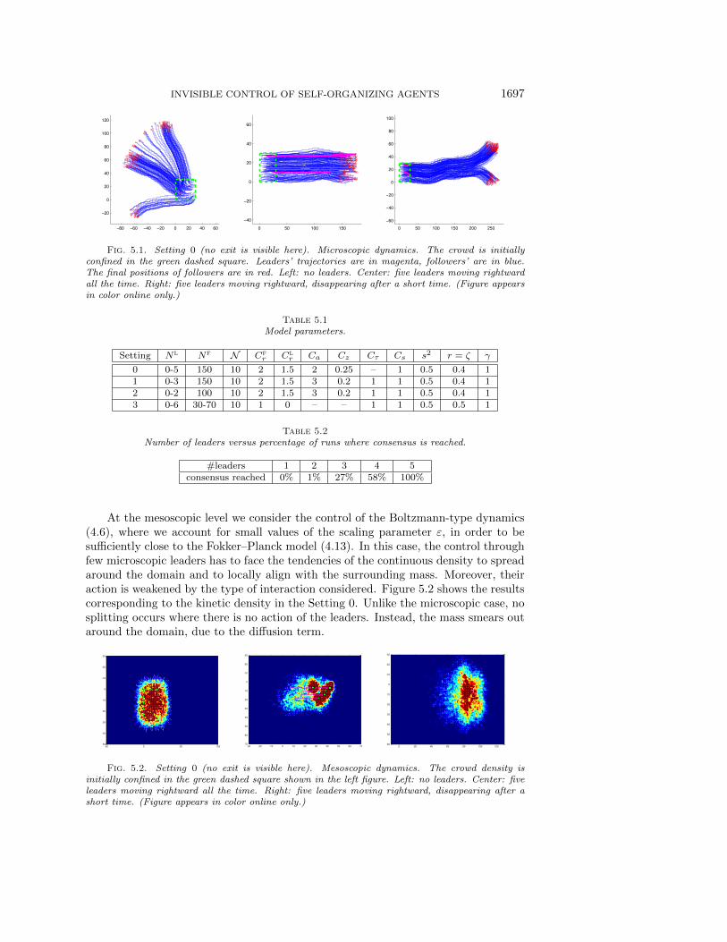
5.1. A preliminary test. To fix the ideas, we plot a typical outcome of themicrosimulator when the crowd is far away from the exit. At the initial time, agentsare uniformly distributed in a square; see Figure 5.1. We refer to this situation asSetting 0 (model parameters for this and the following simulations are reported inTable 5.1). With no leaders, the group splits into several subgroups, each of themhaving a common direction of motion (local consensus is reached in a very shorttime); see Figure 5.1 (left). With five leaders moving rightward, the crowd reachesimmediately a consensus and aligns with leaders; see Figure 5.1 (center). If, for somereason, leaders cease to be influential, the crowd tend to split again; see Figure 5.1(right).

This makes it clear how difficult it is to control the crowd in this scenario, sinceleaders have to fight continuously against the natural tendency of the crowd to splitinto subgroups and move randomly, even after that a consensus is reached; cf. [41].

A natural question is about the minimum number of leaders needed to lead thewhole crowd to consensus, i.e., to align all the agents along a desired direction. Numer-ical simulations suggest that this number strongly depends on the initial conditions.Table 5.2 gives a rough idea in the case of multiple runs with random initial conditions.


−80 −60 −40 −20 0 20 40 60

−20

0

20

40

60

80

100

120

0 50 100 150

−40

−20

0

20

40

60

0 50 100 150 200 250

−60

−40

−20

0

20

40

60

80

100

Fig. 5.1. Setting 0 (no exit is visible here). Microscopic dynamics. The crowd is initiallyconfined in the green dashed square. Leaders’ trajectories are in magenta, followers’ are in blue.The final positions of followers are in red. Left: no leaders. Center: five leaders moving rightwardall the time. Right: five leaders moving rightward, disappearing after a short time. (Figure appearsin color online only.)

Table 5.1Model parameters.

Setting Nl Nf N Cfr Cl

r Ca Cz Cτ Cs s2 r = ζ γ

0 0-5 150 10 2 1.5 2 0.25 – 1 0.5 0.4 11 0-3 150 10 2 1.5 3 0.2 1 1 0.5 0.4 12 0-2 100 10 2 1.5 3 0.2 1 1 0.5 0.4 13 0-6 30-70 10 1 0 – – 1 1 0.5 0.5 1

Table 5.2Number of leaders versus percentage of runs where consensus is reached.

#leaders 1 2 3 4 5consensus reached 0% 1% 27% 58% 100%

At the mesoscopic level we consider the control of the Boltzmann-type dynamics(4.6), where we account for small values of the scaling parameter ε, in order to besufficiently close to the Fokker–Planck model (4.13). In this case, the control throughfew microscopic leaders has to face the tendencies of the continuous density to spreadaround the domain and to locally align with the surrounding mass. Moreover, theiraction is weakened by the type of interaction considered. Figure 5.2 shows the resultscorresponding to the kinetic density in the Setting 0. Unlike the microscopic case, nosplitting occurs where there is no action of the leaders. Instead, the mass smears outaround the domain, due to the diffusion term.

-50 0 50 100

-30

-20

-10

0

10

20

30

40

50-30 -20 -10 0 10 20 30 40 50 60 70

-30

-20

-10

0

10

20

30

40

50

60

70

0 20 40 60 80 100 120

-30

-20

-10

0

10

20

30

40

50

60

Fig. 5.2. Setting 0 (no exit is visible here). Mesoscopic dynamics. The crowd density isinitially confined in the green dashed square shown in the left figure. Left: no leaders. Center: fiveleaders moving rightward all the time. Right: five leaders moving rightward, disappearing after ashort time. (Figure appears in color online only.)


5.2. Setting the optimization problem. The functional to be minimized canbe chosen in several ways. The effectiveness mostly depends on the optimizationmethod which is used afterwards. The most natural functional is the evacuationtime,

(5.1) mint > 0 | xi(t) /∈ Ω ∀i = 1, . . . , Nf,

subject to (3.1) or (4.6) and with u(·) ∈ Uadm, where Uadm is the set of admissiblecontrols (including, for instance, box constraints to avoid excessive velocities).

Another cost functional, more affordable by standard methods [3, 15], is

(5.2) l(x,y, u) = µfNf∑i=1

‖xi − xτ‖2 + µlNf∑i=1

Nl∑k=1

‖xi − yk‖2 + ν

Nl∑k=1

‖uk‖2

for some positive constants µf, µl, and ν. The first term promotes the fact thatfollowers have to reach the exit while the second forces leaders to keep contact with thecrowd. The last term penalizes excessive velocities. This minimization is performedat every instant (instantaneous control), or along a fixed time frame [ti, tf ]

(5.3) minu(·)∈Uadm

∫ tf

ti

l(x(t),y(t), u(t)) dt subject to (3.1) or (4.6).

With regards to the mesoscopic scale, both functionals (5.1) and (5.2) can beconsidered. However, at the continuous level the presence of few invisible leaders doesnot ensure that the whole mass of followers is evacuated. The major difficulty to reacha complete evacuation of the continuous density is mainly due to the presence of thediffusion term and to the invisible interaction w.r.t. the leaders. Therefore, a moreappropriate functional is given by the mass evacuated at the final time T ,


mf(T ) =

∫Rd

∫Ω

f(T, x, v) dx dv

subject to (4.6).

Remark 5.1. We will not require that leaders themselves reach the exit, but onlythe followers.

5.2.1. Model predictive control. A computationally efficient way to addressthe optimal control problem (5.3) is by means of a relaxed approach known as modelpredictive control (MPC) [46]. We consider a sampling of the dynamics (3.1) atevery time interval ∆t, and the following minimization problem over Nmpc time steps,starting from the current time step n:


n+Nmpc−1∑n=n

l(x(n∆t),y(n∆t), u(n∆t))

generating an optimal sequence of controls u(n∆t), . . . , u((n+Nmpc − 1)∆t), fromwhich only the first term is taken to evolve the dynamics for a time ∆t, to recast theminimization problem over an updated time frame n← n+1. Note that for Nmpc = 2,the MPC approach recovers an instantaneous controller, whereas for Nmpc = (tf −ti)/∆t it solves the full time frame problem (5.3). Such flexibility is complementedwith a robust behavior, as the optimization is reinitialized every time step, allowingone to address perturbations along the optimal trajectory.


5.2.2. Modified compass search. When the cost functional is highly irregularand the search of local minima is particularly difficult, it could be convenient to movetowards random methods as compass search (see [8] and references therein), geneticalgorithms, or particle swarm optimization. In the following we describe a compasssearch method that works surprisingly well for our problem.

First of all, we consider only piecewise constant trajectories, introducing suitableswitching times for the leaders’ controls. More precisely, we assume that leaders moveat constant velocity for a given fixed time interval and when the switching time isreached, a new velocity vector is chosen. Therefore, the control variables are thevelocities at the switching times for each leader. Note that controlling directly thevelocities rather than the acceleration makes the optimization problem much simplerbecause minimal control variations have an immediate impact on the dynamics.

Starting from an initial guess, at each iteration the optimization algorithm modi-fies the current best control strategy found so far by means of small random variationsof the current values. Then, the cost functional is evaluated. If the variation is ad-vantageous (the cost decreases), the variation is kept; otherwise it is discarded. Themethod stops when the strategy cannot be improved further. As an initial guess forthe strategy, leaders move at constant speed along the direction joining the targetwith their initial position.

6. Numerical tests. In what follows we present some numerical tests to validateour modeling framework at the microscopic and mesoscopic levels.

The microscopic model (3.1) is discretized by means of the explicit Euler methodwith a time step ∆t = 0.1. The evolution of the kinetic density in (4.13) is approxi-mated by means of binary interaction algorithms, which approximates the Boltzmanndynamics (4.5) with a meshless Monte Carlo method for small values of the parameterε, as presented in [4]. We choose ε = 0.02, ∆t = 0.01, and a sample of Ns = 10000particles to reconstruct the kinetic density. This type of approach is inspired by nu-merical methods for plasma physics and it allows one to solve the interaction dynamicswith a reduced computational cost compared with mesh-based methods, and an accu-

racy of O(N−1/2s ). For further details on this class of binary interaction algorithms,

see [4, 48].Concerning optimization, in the microscopic case we adopt either the compass

search with functional (5.1) or MPC with functional (5.3). In the mesoscopic case weadopt the compass search with functional (5.4).

We consider three settings for pedestrians, without and with obstacles, hereafterreferred to Settings 1, 2, and 3, respectively. In Setting 1 we set the compass searchswitching times every 20 time steps, and in Setting 2 every 50, having fixed themaximal random variation to 1 for each component of the velocity. In Setting 1, theinner optimization block of the MPC procedure is performed via a direct formulation,by means of the fmincon routine in MATLAB, which solves the optimization problemvia an SQP method.

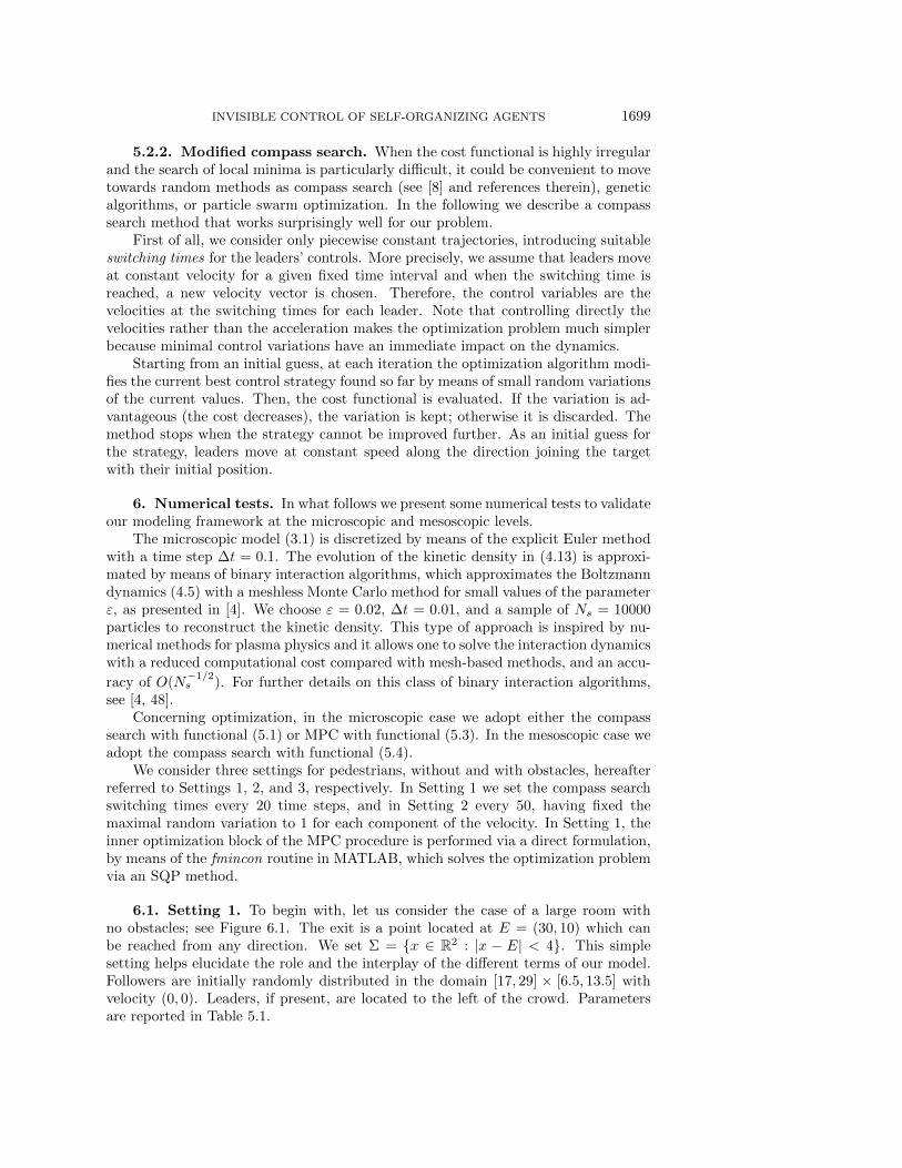
6.1. Setting 1. To begin with, let us consider the case of a large room withno obstacles; see Figure 6.1. The exit is a point located at E = (30, 10) which canbe reached from any direction. We set Σ = x ∈ R2 : |x − E| < 4. This simplesetting helps elucidate the role and the interplay of the different terms of our model.Followers are initially randomly distributed in the domain [17, 29] × [6.5, 13.5] withvelocity (0, 0). Leaders, if present, are located to the left of the crowd. Parametersare reported in Table 5.1.


15 20 25 30 355

10

15

15 20 25 30 35

4

6

8

10

12

14

16

Fig. 6.1. Setting 1. Left: initial positions of followers (circles) and leaders (squares). Right:uniform density of followers and the microscopic leaders (squares).

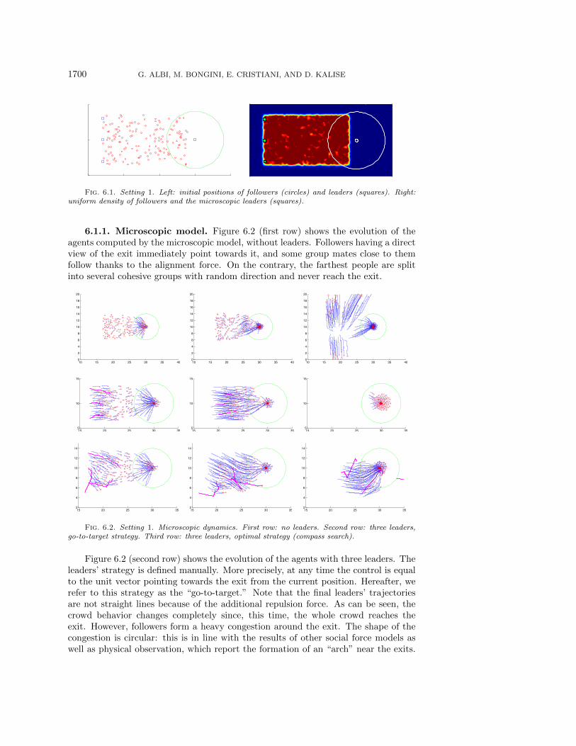
6.1.1. Microscopic model. Figure 6.2 (first row) shows the evolution of theagents computed by the microscopic model, without leaders. Followers having a directview of the exit immediately point towards it, and some group mates close to themfollow thanks to the alignment force. On the contrary, the farthest people are splitinto several cohesive groups with random direction and never reach the exit.

10 15 20 25 30 35 400

2

4

6

8

10

12

14

16

18

20

10 15 20 25 30 35 400

2

4

6

8

10

12

14

16

18

20

10 15 20 25 30 35 400

2

4

6

8

10

12

14

16

18

20

15 20 25 30 355

10

15

15 20 25 30 355

10

15

15 20 25 30 355

10

15

15 20 25 30 352

4

6

8

10

12

14

15 20 25 30 352

4

6

8

10

12

14

15 20 25 30 352

4

6

8

10

12

14

Fig. 6.2. Setting 1. Microscopic dynamics. First row: no leaders. Second row: three leaders,go-to-target strategy. Third row: three leaders, optimal strategy (compass search).

Figure 6.2 (second row) shows the evolution of the agents with three leaders. Theleaders’ strategy is defined manually. More precisely, at any time the control is equalto the unit vector pointing towards the exit from the current position. Hereafter, werefer to this strategy as the “go-to-target.” Note that the final leaders’ trajectoriesare not straight lines because of the additional repulsion force. As can be seen, thecrowd behavior changes completely since, this time, the whole crowd reaches theexit. However, followers form a heavy congestion around the exit. The shape of thecongestion is circular: this is in line with the results of other social force models aswell as physical observation, which report the formation of an “arch” near the exits.


The arch is correctly substituted here by a full circle due to the absence of walls. Notethat the congestion notably delays the evacuation. This suggests that the strategy ofthe leaders is not optimal and can be improved by an optimization method.

Figure 6.2 (third row) shows the evolution of the agents with three leaders and theoptimal strategy obtained by the compass search algorithm. Surprisingly enough, theoptimizator prescribes that leaders divert some pedestrians from the right direction,so as not to steer the whole crowd to the exit at the same time. In this way congestionis avoided and pedestrian flow through the exit is increased.

In this test we have also run the MPC optimization, including a box constraintuk(t) ∈ [−1, 1]. We choose µf = 1, µl = 10−5, and ν = 10−5. MPC results areconsistent in the sense that for Nmpc = 2, the algorithm recovers a controlled behaviorsimilar to the application of the instantaneous controller (or go-to-target strategy).Increasing the time frame up to Nmpc = 6 improves both congestion and evacuationtimes, but results still remain noncompetitive if compared to the whole time frameoptimization performed with a compass search.

In Figure 6.3 we compare the occupancy of the exit’s visibility zone as a functionof time for go-to-target strategy and optimal strategies (compass search, 2-step, and 6-step MPC). We also show the decrease of the value function as a function of attempts(compass search) and time (MPC). Evacuation times are compared in Table 6.1. Itcan be seen that only the long-term optimization strategies are efficient, being ableto moderate congestion and clogging around the exit.

100 200 300 400 500 6000

20

40

60

80

100

Time steps

# Agents inside Σ

Compass searchGo−to−target

0 10 20 30 40 50 60 70 80 90 100400

450

500

550

600Compass search - Value function

# attempts

0 10 20 30 40 50 60 70 80 90 100240

260

280

300

320150 followers50 followers

0 100 200 300 400 500 600 700

Time steps

0

20

40

60

80

100

2-step MPC, 150 agents

CPU time optimization MPC

Value function MPC

# Agents inside Σ

0 100 200 300 400 500 600 700

Time steps

0

20

40

60

80

100

6-step MPC, 150 agents

CPU time optimization MPC

Value function MPC

# Agents inside Σ

Fig. 6.3. Setting 1. Optimization of the microscopic dynamics. Top-left: occupancy of theexit’s visibility zone Σ as a function of time for optimal strategy (compass search) and go-to-targetstrategy. Top-right: decrease of the value function (5.1) as a function of the iterations of the compasssearch (for 50 and 150 followers). Bottom: MPC optimization. Occupancy of the exit’s visibilityzone Σ as a function of time, CPU time of the optimization call embedded in the MPC solver, andthe evolution of the corresponding value ( 2-step and 6-step).


Table 6.1Setting 1. Evacuation times (time steps). CS = compass search, IG = initial guess.

No leaders Go-to-target 2-MPC 6-MPC CS (IG)Nf = 50 335 297 342 278 248 (318)Nf = 150 ∞ 629 619 491 459 (554)

This suggests a quite unethical but effective evacuation procedure, namely mis-leading some people to a false target and then leading them back to the right one,when exit conditions are safer. Note that in real-life situations, most of the injuriesare actually caused by overcompression and suffocation rather than urgency.

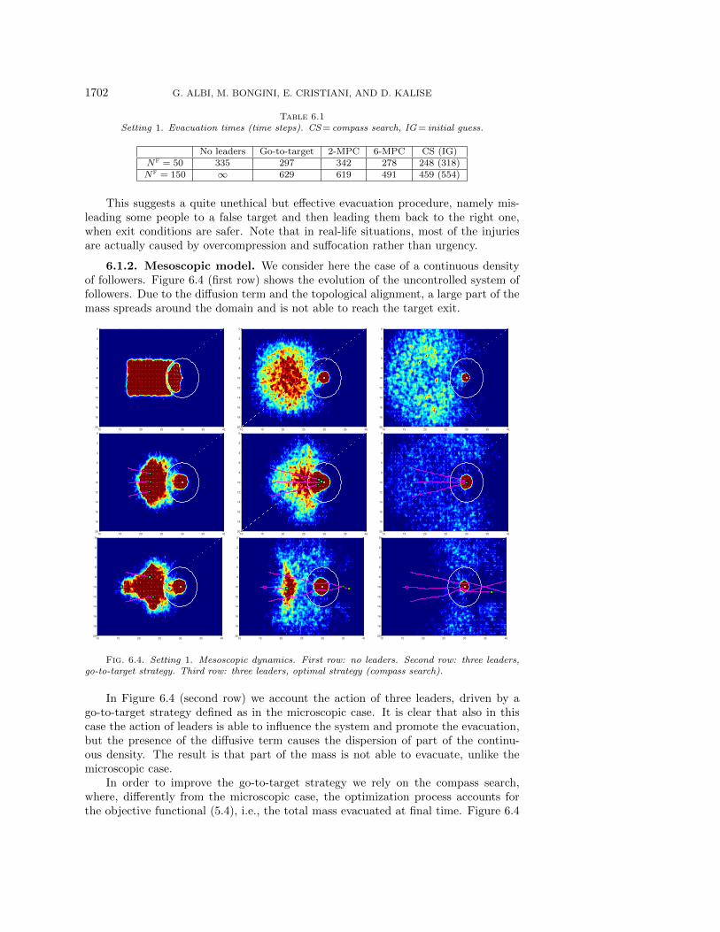
6.1.2. Mesoscopic model. We consider here the case of a continuous densityof followers. Figure 6.4 (first row) shows the evolution of the uncontrolled system offollowers. Due to the diffusion term and the topological alignment, a large part of themass spreads around the domain and is not able to reach the target exit.

10 15 20 25 30 35 40

0

2

4

6

8

10

12

14

16

18

2010 15 20 25 30 35 40

0

2

4

6

8

10

12

14

16

18

2010 15 20 25 30 35 40

0

2

4

6

8

10

12

14

16

18

20

10 15 20 25 30 35 40

0

2

4

6

8

10

12

14

16

18

2010 15 20 25 30 35 40

0

2

4

6

8

10

12

14

16

18

2010 15 20 25 30 35 40

0

2

4

6

8

10

12

14

16

18

20

10 15 20 25 30 35 40

0

2

4

6

8

10

12

14

16

18

2010 15 20 25 30 35 40

0

2

4

6

8

10

12

14

16

18

2010 15 20 25 30 35 40

0

2

4

6

8

10

12

14

16

18

20

Fig. 6.4. Setting 1. Mesoscopic dynamics. First row: no leaders. Second row: three leaders,go-to-target strategy. Third row: three leaders, optimal strategy (compass search).

In Figure 6.4 (second row) we account the action of three leaders, driven by ago-to-target strategy defined as in the microscopic case. It is clear that also in thiscase the action of leaders is able to influence the system and promote the evacuation,but the presence of the diffusive term causes the dispersion of part of the continu-ous density. The result is that part of the mass is not able to evacuate, unlike themicroscopic case.

In order to improve the go-to-target strategy we rely on the compass search,where, differently from the microscopic case, the optimization process accounts forthe objective functional (5.4), i.e., the total mass evacuated at final time. Figure 6.4


(third row) sketches the optimal strategy found in this way: on one hand, the twoexternal leaders go directly towards the exit, evacuating part of the density; on theother hand, the central leader moves slowly backward, misleading part of the densityand only later does it move forward towards the exit. The efficiency of the leaders’strategy is due, in particular, to the latter movement of the last leader, which is ableto gather the followers’ density left behind by the others, and to reduce the occupancyof the exit’s visibility area by delaying the arrival of part of the mass.

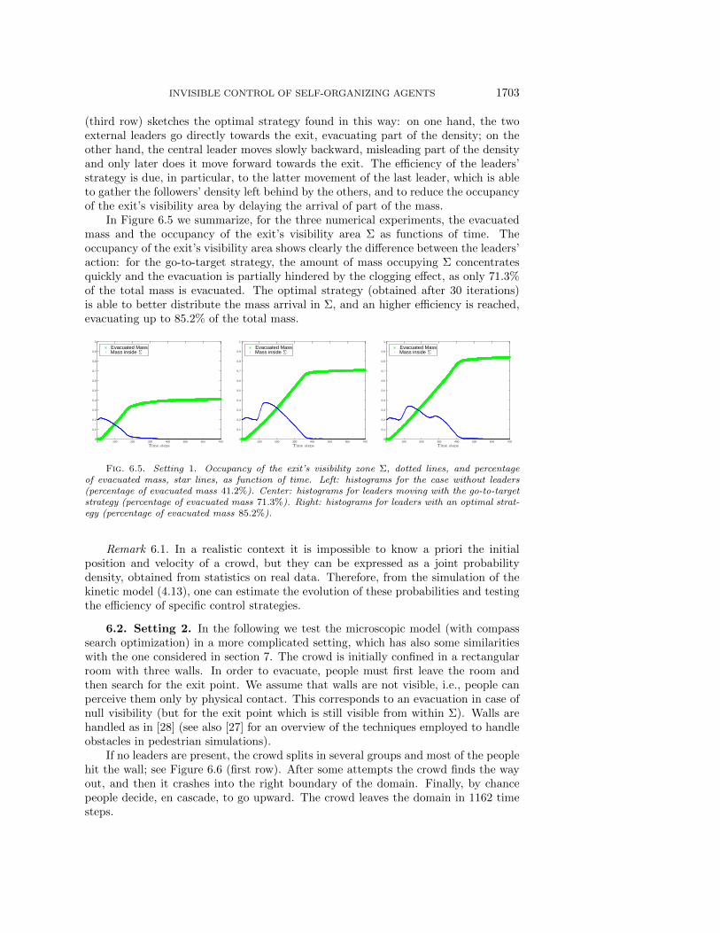
In Figure 6.5 we summarize, for the three numerical experiments, the evacuatedmass and the occupancy of the exit’s visibility area Σ as functions of time. Theoccupancy of the exit’s visibility area shows clearly the difference between the leaders’action: for the go-to-target strategy, the amount of mass occupying Σ concentratesquickly and the evacuation is partially hindered by the clogging effect, as only 71.3%of the total mass is evacuated. The optimal strategy (obtained after 30 iterations)is able to better distribute the mass arrival in Σ, and an higher efficiency is reached,evacuating up to 85.2% of the total mass.

Time steps0 100 200 300 400 500 600 700

0

0.1

0.2

0.3

0.4

0.5

0.6

0.7

0.8

0.9

1

Evacuated MassMass inside Σ

Time steps0 100 200 300 400 500 600 700

0

0.1

0.2

0.3

0.4

0.5

0.6

0.7

0.8

0.9

1


Time steps0 100 200 300 400 500 600 700

0

0.1

0.2

0.3

0.4

0.5

0.6

0.7

0.8

0.9

1


Fig. 6.5. Setting 1. Occupancy of the exit’s visibility zone Σ, dotted lines, and percentageof evacuated mass, star lines, as function of time. Left: histograms for the case without leaders(percentage of evacuated mass 41.2%). Center: histograms for leaders moving with the go-to-targetstrategy (percentage of evacuated mass 71.3%). Right: histograms for leaders with an optimal strat-egy (percentage of evacuated mass 85.2%).

Remark 6.1. In a realistic context it is impossible to know a priori the initialposition and velocity of a crowd, but they can be expressed as a joint probabilitydensity, obtained from statistics on real data. Therefore, from the simulation of thekinetic model (4.13), one can estimate the evolution of these probabilities and testingthe efficiency of specific control strategies.

6.2. Setting 2. In the following we test the microscopic model (with compasssearch optimization) in a more complicated setting, which has also some similaritieswith the one considered in section 7. The crowd is initially confined in a rectangularroom with three walls. In order to evacuate, people must first leave the room andthen search for the exit point. We assume that walls are not visible, i.e., people canperceive them only by physical contact. This corresponds to an evacuation in case ofnull visibility (but for the exit point which is still visible from within Σ). Walls arehandled as in [28] (see also [27] for an overview of the techniques employed to handleobstacles in pedestrian simulations).

If no leaders are present, the crowd splits in several groups and most of the peoplehit the wall; see Figure 6.6 (first row). After some attempts the crowd finds the wayout, and then it crashes into the right boundary of the domain. Finally, by chancepeople decide, en cascade, to go upward. The crowd leaves the domain in 1162 timesteps.


If instead we hide in the crowd two leaders who point fast towards the exit (Figure6.6 (second row)), the evacuation from the room is completed in very short time, butafter that, the influence of the leaders vanishes. Unfortunately, this time people decideto go downward after hitting the right boundary, and nobody leaves the domain.Slowing down the two leaders helps keeping the leaders’ influence for a longer time,although it is quite difficult to find a good choice.

Compass search optimization finds (after 30 iterations) a nice strategy for the twoleaders which remarkably improves the evacuation time; see Figure 6.6 (third row).One leader behaves similarly to the previous case, while the other diverts the crowdpointing southeast (SE), then comes back to wait for the crowd, and finally pointsnortheast (NE) towards the exit. This strategy allows one to bring everyone to theexit in 549 time steps, without bumping anyone against the boundary, and avoidingcongestion near the exit.

0 5 10 15 20 254

6

8

10

12

14

16

18

20

22

0 5 10 15 20 254

6

8

10

12

14

16

18

20

22

0 5 10 15 20 254

6

8

10

12

14

16

18

20

22

0 5 10 15 20 254

6

8

10

12

14

16

18

20

22

0 5 10 15 20 254

6

8

10

12

14

16

18

20

22

0 5 10 15 20 254

6

8

10

12

14

16

18

20

22

0 5 10 15 20 254

6

8

10

12

14

16

18

20

22

0 5 10 15 20 254

6

8

10

12

14

16

18

20

22

0 5 10 15 20 254

6

8

10

12

14

16

18

20

22

Fig. 6.6. Setting 2. Microscopic simulation. First row: no leaders (see M101701 01.mp4[local/web 12.9MB]). Second row: two leaders and go-to-target strategy (see M101701 02.mp4 [lo-cal/web 9.71MB]) and with slower leader (see M101701 03.mp4 [local/web 6.87MB]). Third row: twoleaders and best strategy computed by the compass search (see M101701 04.mp4 [local/web 7.19MB]).

6.3. Setting 3. In the following test we propose a different use of the leaders.Rather than steering the mass towards the exit, they can be employed to fluidifythe evacuation near a door. In fact, it is observed that when several pedestriansreach a bottleneck at the same time they slow each other down, possibly coming to adeadlock. As a consequence, none of them can pass through the bottleneck. We wantto investigate the possibility of using leaders as small smart obstacles, which alleviatethe high friction among the bodies just moving randomly near the exit.

We consider a large room with a single exit door located on the right wall, visiblefrom any point (Σ = R2). We nullify the repulsion force perceived by the leaders; seeTable 5.1. Most important, in this test we assume that followers have nonzero sizeand hard collisions are not possible. This is achieved assuming that they are circular-

M101701_01.mp4

http://epubs.siam.org/doi/suppl/10.1137/15M1017016/suppl_file/M101701_01.mp4

M101701_02.mp4

M101701_02.mp4


M101701_03.mp4


M101701_04.mp4



25 26 27 28 29 307.5

8

8.5

9

9.5

10

10.5

11

11.5

12

12.5

25 26 27 28 29 307.5

8

8.5

9

9.5

10

10.5

11

11.5

12

12.5

n=307

0 1 2 3 4 5 60

10

20

30

40

50

60

70

80

90

100

# leaders

% fa

ilure

30 followers50 followers70 followers

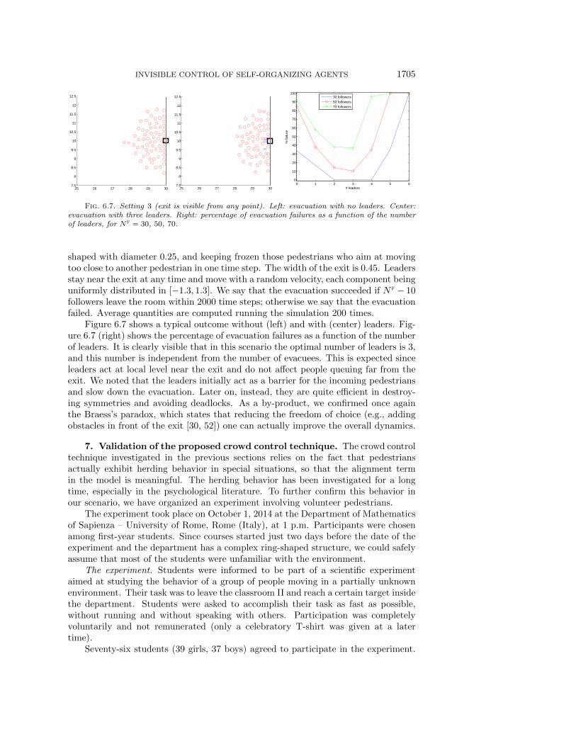
Fig. 6.7. Setting 3 (exit is visible from any point). Left: evacuation with no leaders. Center:evacuation with three leaders. Right: percentage of evacuation failures as a function of the numberof leaders, for Nf = 30, 50, 70.

shaped with diameter 0.25, and keeping frozen those pedestrians who aim at movingtoo close to another pedestrian in one time step. The width of the exit is 0.45. Leadersstay near the exit at any time and move with a random velocity, each component beinguniformly distributed in [−1.3, 1.3]. We say that the evacuation succeeded if Nf − 10followers leave the room within 2000 time steps; otherwise we say that the evacuationfailed. Average quantities are computed running the simulation 200 times.

Figure 6.7 shows a typical outcome without (left) and with (center) leaders. Fig-ure 6.7 (right) shows the percentage of evacuation failures as a function of the numberof leaders. It is clearly visible that in this scenario the optimal number of leaders is 3,and this number is independent from the number of evacuees. This is expected sinceleaders act at local level near the exit and do not affect people queuing far from theexit. We noted that the leaders initially act as a barrier for the incoming pedestriansand slow down the evacuation. Later on, instead, they are quite efficient in destroy-ing symmetries and avoiding deadlocks. As a by-product, we confirmed once againthe Braess’s paradox, which states that reducing the freedom of choice (e.g., addingobstacles in front of the exit [30, 52]) one can actually improve the overall dynamics.

7. Validation of the proposed crowd control technique. The crowd controltechnique investigated in the previous sections relies on the fact that pedestriansactually exhibit herding behavior in special situations, so that the alignment termin the model is meaningful. The herding behavior has been investigated for a longtime, especially in the psychological literature. To further confirm this behavior inour scenario, we have organized an experiment involving volunteer pedestrians.

The experiment took place on October 1, 2014 at the Department of Mathematicsof Sapienza – University of Rome, Rome (Italy), at 1 p.m. Participants were chosenamong first-year students. Since courses started just two days before the date of theexperiment and the department has a complex ring-shaped structure, we could safelyassume that most of the students were unfamiliar with the environment.

The experiment. Students were informed to be part of a scientific experimentaimed at studying the behavior of a group of people moving in a partially unknownenvironment. Their task was to leave the classroom II and reach a certain target insidethe department. Students were asked to accomplish their task as fast as possible,without running and without speaking with others. Participation was completelyvoluntarily and not remunerated (only a celebratory T-shirt was given at a latertime).

Seventy-six students (39 girls, 37 boys) agreed to participate in the experiment.


The students were then divided randomly in two groups: group A (42 people) andgroup B (34 people). The two groups performed the experiment independently oneafter the other. The target was communicated to the students just before the begin-ning of the experiment. It was the Istituto Nazionale di Alta Matematica (INdAM),which is located just upstairs w.r.t. the classroom II. Due to the complex shape of theenvironment, there are many paths joining classroom II and INdAM. The shortestpath requires people to leave the classroom, go leftward in a rarely frequented andunfamiliar area (even for experienced students), and climb the stairs. The target canbe also reached by going rightward and climb other, more frequented, stairs.

In group B there were five incognito students, hereafter referred to as leaders, ofthe same age of the others. Leaders were previously informed about the goal of theexperiment and the location of the target. They were also trained in order to steerthe crowd toward the target in minimal time. Nobody recognized them as “special”before or during the experiment. Unexpectedly, also in group A there was a girl whoknew the target. Therefore, she acted as an unaware leader.

It is important to stress that all of the other students continued their usual activ-ities and participants were not officially recorded by the organizers. This choice wascrucial to get natural behavior and meaningful results; cf. [29, sect. 3.4.3]. The priceto pay is that we had to extract participants’ trajectories by low-resolution videostaken by two observers. Moreover, the area just outside classroom II was rathercrowded, introducing a high level of noise into the experiment. Finally, let us mentionthat some participants broke the rules of the experiment speaking with others andrunning (confirming the natural behavior...). Our experiment can be compared withthose in [33], although in those experiments group cohesion was imposed as a rule tothe participants.

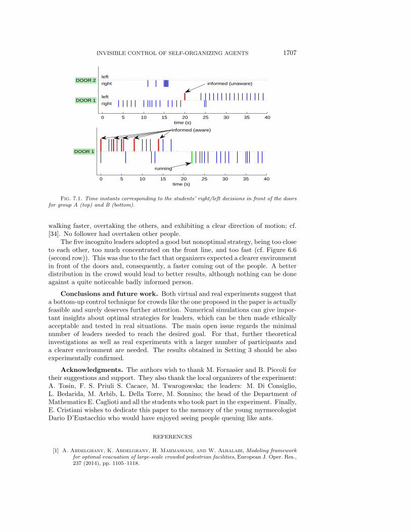
Results. In Figure 7.1 we show the history of left/right decisions taken by thestudents just outside the two doors of the classroom. Group A used both exits of theclassroom. The 8-people group which used door 2 was uncertain about the directionfor awhile. Then, once the first two students decided to go rightward, the othersdecided simultaneously to follow them. Similarly, the first student leaving from door1 was uncertain for a few second; then he moved rightward and triggered a cleardomino effect. At t = 20 s the unaware leader moved to the left, inducing hesitationand mixed behavior in the followers. After that, another domino effect arose.

Group B used only door 1. Invisible leaders were able to trigger a domino effectbut this time four people decided unilaterally not to follow them, although they werenot informed about the destination. At t = 20 s, after the passage of the last leader,a girl passed through the door and went leftward. Then, at t = 22 s, she suddenlybegan to run toward the right. She first induced hesitation and then triggered a newrightward domino effect.

Discussion. Students have shown a tendency to go rightward, since that part ofthe department is more familiar, but this tendency was greatly overcome by the wishto follow the group mates in front, regardless of their right/left preferences. Also,after the experiment, the students admitted that they had been influenced by theleaders because of their clear direction of motion. Interestingly, no more than fivepeople had been influenced by a single leader. This is compatible with the topologicalalignment term used in our model. The small value of N here is due to the fact thatthe space in front of the doors was rather crowded and the visibility was reduced.

It is also interesting to note that only four students reached the target alone. Thisconfirms the tendency not to remain isolated and to form clusters. Video recordingsalso show that (bad or well) informed people behaved in a rather recognizable manner,


0 5 10 15 20 25 30 35 40time (s)

DOOR 1

DOOR 2

right

left

right

left

informed (unaware)

0 5 10 15 20 25 30 35 40time (s)

DOOR 1

running

informed (aware)

Fig. 7.1. Time instants corresponding to the students’ right/left decisions in front of the doorsfor group A (top) and B (bottom).

walking faster, overtaking the others, and exhibiting a clear direction of motion; cf.[34]. No follower had overtaken other people.

The five incognito leaders adopted a good but nonoptimal strategy, being too closeto each other, too much concentrated on the front line, and too fast (cf. Figure 6.6(second row)). This was due to the fact that organizers expected a clearer environmentin front of the doors and, consequently, a faster coming out of the people. A betterdistribution in the crowd would lead to better results, although nothing can be doneagainst a quite noticeable badly informed person.

Conclusions and future work. Both virtual and real experiments suggest thata bottom-up control technique for crowds like the one proposed in the paper is actuallyfeasible and surely deserves further attention. Numerical simulations can give impor-tant insights about optimal strategies for leaders, which can be then made ethicallyacceptable and tested in real situations. The main open issue regards the minimalnumber of leaders needed to reach the desired goal. For that, further theoreticalinvestigations as well as real experiments with a larger number of participants anda clearer environment are needed. The results obtained in Setting 3 should be alsoexperimentally confirmed.

Acknowledgments. The authors wish to thank M. Fornasier and B. Piccoli fortheir suggestions and support. They also thank the local organizers of the experiment:A. Tosin, F. S. Priuli S. Cacace, M. Twarogowska; the leaders: M. Di Consiglio,L. Bedarida, M. Arbib, L. Della Torre, M. Sonnino; the head of the Department ofMathematics E. Caglioti and all the students who took part in the experiment. Finally,E. Cristiani wishes to dedicate this paper to the memory of the young myrmecologistDario D’Eustacchio who would have enjoyed seeing people queuing like ants.

REFERENCES

[1] A. Abdelghany, K. Abdelghany, H. Mahmassani, and W. Alhalabi, Modeling frameworkfor optimal evacuation of large-scale crowded pedestrian facilities, European J. Oper. Res.,237 (2014), pp. 1105–1118.


[2] J. P. Agnelli, F. Colasuonno, and D. Knopoff, A kinetic theory approach to the dynamicsof crowd evacuation from bounded domains, Math. Models Methods Appl. Sci., 25 (2015),pp. 109–129.

[3] G. Albi, M. Herty, and L. Pareschi, Kinetic description of optimal control problems andapplications to opinion consensus, Commun. Math. Sci., 13 (2015), pp. 1407–1429.

[4] G. Albi and L. Pareschi, Binary interaction algorithms for the simulation of flocking andswarming dynamics, Multiscale Model. Simul., 11 (2013), pp. 1–29, doi:10.1137/120868748.

[5] G. Albi and L. Pareschi, Modeling of self-organized systems interacting with a few individuals:From microscopic to macroscopic dynamics, Appl. Math. Lett., 26 (2013), pp. 397–401.

[6] G. Albi, L. Pareschi, and M. Zanella, Boltzmann-type control of opinion consensus throughleaders, Philos. Trans. R. Soc. Lond. Ser. A Math. Phys. Eng. Sci., 372 (2014), 20140138.

[7] H. C. Andersen, J. D. Weeks, and D. Chandler, Relationship between the hard-spherefluid and fluids with realistic repulsion force, Phys. Rev. A, 4 (1971), pp. 1597–1607,doi:10.1103/PhysRevA.4.1597.

[8] C. Audet, K.-C. Dang, and D. Orban, Optimization of algorithms with OPAL, Math. Pro-gram. Comput., 6 (2014), pp. 233–254.

[9] N. Bellomo and C. Dogbe, On the modeling of traffic and crowds: A survey of models,speculations, and perspectives, SIAM Rev., 53 (2011), pp. 409–463, doi:10.1137/090746677.

[10] F. Bolley, J. A. Canizo, and J. A. Carrillo, Stochastic mean-field limit: Non-Lipschitzforces and swarming, Math. Models Methods Appl. Sci., 21 (2011), pp. 2179–2210.

[11] M. Bongini and M. Fornasier, Sparse stabilization of dynamical systems driven by attractionand avoidance forces, Netw. Heterog. Media, 9 (2014), pp. 1–31.

[12] M. Bongini, M. Fornasier, O. Junge, and B. Scharf, Sparse control of alignment modelsin high dimension, Netw. Heterog. Media, 10 (2015), pp. 647–697.

[13] M. Bongini, M. Fornasier, and D. Kalise, (Un)conditional consensus emergence underperturbed and decentralized feedback controls, Discrete Contin. Dyn. Syst. Ser. A, 35 (2015),pp. 4071–4094.

[14] M. Bongini, M. Fornasier, F. Rossi, and F. Solombrino, Mean-Field Pontryagin MaximumPrinciple, preprint, http://arxiv.org/abs/1504.02236, 2015.

[15] A. Borzı and S. Wongkaew, Modeling and control through leadership of a refined flockingsystem, Math. Models Methods Appl. Sci., 25 (2015), pp. 255–282.

[16] S. Butail, T. Bartolini, and M. Porfiri, Collective response of zebrafish shoals to a free-swimming robotic fish, PLoS ONE, 8 (2013), e76123, doi:10.1371/journal.pone.0076123.

[17] J. A. Canizo, J. A. Carrillo, and J. Rosado, A well-posedness theory in measures forsome kinetic models of collective motion, Math. Models Methods Appl. Sci., 21 (2011),pp. 515–539.

[18] M. Caponigro, M. Fornasier, B. Piccoli, and E. Trelat, Sparse stabilization and optimalcontrol of the Cucker-Smale model, Math. Control Relat. Fields, 3 (2013), pp. 447–466.

[19] J. A. Carrillo, M. R. D’Orsogna, and V. Panferov, Double milling in self-propelled swarmsfrom kinetic theory, Kinet. Relat. Models, 2 (2009), pp. 363–378.

[20] J. A. Carrillo, M. Fornasier, G. Toscani, and F. Vecil, Particle, kinetic, and hydro-dynamic models of swarming, in Mathematical Modeling of Collective Behavior in Socio-economic and Life Sciences, Birkhauser Boston, Boston, 2010, pp. 297–336.

[21] J. A. Carrillo, S. Martin, and M.-T. Wolfram, An improved version of the Hughes modelfor pedestrian flow, Math. Models Methods Appl. Sci., 26 (2016), pp. 671–697.

[22] C. Cercignani, R. Illner, and M. Pulvirenti, The Mathematical Theory of Dilute Gases,Springer-Verlag, New York, 1994.

[23] E. N. M. Cirillo and A. Muntean, Dynamics of pedestrians in regions with no visibility - alattice model without exclusion, Phys. A, 392 (2013), pp. 3578–3588.

[24] R. Colombo and M. Lecureux-Mercier, An analytical framework to describe the interactionsbetween individuals and a continuum, J. Nonlinear Sci., 22 (2012), pp. 39–61.

[25] S. Cordier, L. Pareschi, and G. Toscani, On a kinetic model for a simple market economy,J. Stat. Phys., 120 (2005), pp. 253–277.

[26] I. D. Couzin, J. Krause, N. R. Franks, and S. A. Levin, Effective leadership and decision-making in animal groups on the move, Nature, 433 (2005), pp. 513–516.

[27] E. Cristiani and D. Peri, Handling obstacles in pedestrian simulations: Models and opti-mization, preprint, http://arxiv.org/abs/1512.08528, 2016, Appl. Math. Model., in press.

doi:10.1137/120868748

doi:10.1103/PhysRevA.4.1597

doi:10.1137/090746677

http://arxiv.org/abs/1504.02236

doi:10.1371/journal.pone.0076123

http://arxiv.org/abs/1512.08528


[28] E. Cristiani, B. Piccoli, and A. Tosin, Multiscale modeling of granular flows with ap-plication to crowd dynamics, Multiscale Model. Simul., 9 (2011), pp. 155–182, doi:10.1137/100797515.

[29] E. Cristiani, B. Piccoli, and A. Tosin, Multiscale Modeling of Pedestrian Dynamics, Mod-eling, Simulation & Applications, Springer, Cham, 2014.

[30] E. Cristiani, F. S. Priuli, and A. Tosin, Modeling rationality to control self-organizationof crowds: An environmental approach, SIAM J. Appl. Math., 75 (2015), pp. 605–629,doi:10.1137/140962413.

[31] H. Duan and C. Sun, Swarm intelligence inspired shills and the evolution of cooperation, Sci.Rep., 4 (2014), 5210.

[32] B. During, P. Markowich, J.-F. Pietschmann, and M.-T. Wolfram, Boltzmann andFokker-Planck equations modelling opinion formation in the presence of strong leaders,Proc. R. Soc. Lond. Ser. A Math. Phys. Eng. Sci., 465 (2009), pp. 3687–3708.

[33] J. R. G. Dyer, A. Johansson, D. Helbing, I. D. Couzin, and J. Krause, Leadership,consensus decision making and collective behaviour in humans, Phil. Trans. R. Soc. B, 364(2009), pp. 781–789, doi:10.1098/rstb.2008.0233.

[34] J. J. Faria, J. R. G. Dyer, C. R. Tosh, and J. Krause, Leadership and social informationuse in human crowds, Animal Behaviour, 79 (2010), pp. 895–901.

[35] M. Fornasier, B. Piccoli, and F. Rossi, Mean-field sparse optimal control, Philos. Trans. R.Soc. Lond. Ser. A Math. Phys. Eng. Sci., 372 (2014), 20130400.

[36] M. Fornasier and F. Solombrino, Mean-field optimal control, ESAIM Control Optim. Calc.Var., 20 (2014), pp. 1123–1152.

[37] R.-Y. Guo, H.-J Huang, and S. C. Wong, Route choice in pedestrian evacuation underconditions of good and zero visibility: Experimental and simulation results, TransportationRes. B, 46 (2012), pp. 669–686, doi:10.1016/j.trb.2012.01.002.

[38] S.-Y. Ha and E. Tadmor, From particle to kinetic and hydrodynamic descriptions of flocking,Kinet. Relat. Models, 1 (2008), pp. 415–435.

[39] J. Halloy, G. Sempo, G. Caprari, C. Rivault, M. Asadpour, F. Tache, I. Saıd, V. Durier,S. Canonge, J. M. Ame, C. Detrain, N. Correll, A. Martinoli, F. Mondada, R. Sieg-wart, and J. L. Deneubourg, Social integration of robots into groups of cockroaches tocontrol self-organized choices, Science, 318 (2007), pp. 1155–1158.

[40] J. Han, M. Li, and L. Guo, Soft control on collective behavior of a group of autonomousagents by a shill agent, J. Syst. Sci. Complex., 19 (2006), pp. 54–62.

[41] J. Han and L. Wang, Nondestructive intervention to multi-agent systems through an intelli-gent agent, PLoS ONE, 8 (2013), e61542.

[42] D. Helbing, Traffic and related self-driven many-particle systems, Rev. Mod. Phys., 73 (2001),pp. 1067–1141, doi:10.1103/RevModPhys.73.1067.

[43] A. Johansson and D. Helbing, Pedestrian flow optimization with a genetic algorithm basedon Boolean grids, in Pedestrian and Evacuation Dynamics 2005, N. Waldau, P. Gatter-mann, H. Knoflacher, and M. Schreckenberg, eds., Springer-Verlag, Berlin, Heidelberg,2007, pp. 267–272.

[44] P. Kachroo, S. J. Al-nasur, S. A. Wadoo, and A. Shende, Pedestrian Dynamics: FeedbackControl of Crowd Evacuation, Understanding Complex Systems, Springer-Verlag, Berlin,Heidelberg, 2008.

[45] T. K. Karper, A. Mellet, and K. Trivisa, Hydrodynamic limit of the kinetic Cucker–Smaleflocking model, Math. Models Methods Appl. Sci., 25 (2015), pp. 131–163.

[46] D. Q. Mayne, J. B. Rawlings, C. V. Rao, and P. O. M. Scokaert, Constrained modelpredictive control: Stability and optimality, Automatica J. IFAC, 36 (2000), pp. 789–814.

[47] S. Motsch and E. Tadmor, A new model for self-organized dynamics and its flocking behavior,J. Stat. Phys., 144 (2011), pp. 923–947.

[48] L. Pareschi and G. Toscani, Interacting Multi-agent Systems: Kinetic Equations & MonteCarlo Methods, Oxford University Press, New York, 2013.

[49] D. R. Parisi and C. O. Dorso, Microscopic dynamics of pedestrian evacuation, Phys. A, 354(2005), pp. 606–618.

[50] G. Toscani, Kinetic models of opinion formation, Commun. Math. Sci., 4 (2006), pp. 481–496.[51] G. Toscani and N. Bellomo, The Enskog-Boltzmann equation in the whole space R3: Some

global existence, uniqueness and stability results, Comput. Math. Appl., 13 (1987), pp. 851–859.

[52] M. Twarogowska, P. Goatin, and R. Duvigneau, Macroscopic modeling and simulationsof room evacuation, Appl. Math. Model., 38 (2014), pp. 5781–5795.

[53] T. Vicsek, A. Czirok, E. Ben-Jacob, I. Cohen, and O. Shochet, Novel type of phasetransition in a system of self-driven particles, Phys. Rev. Lett., 75 (1995), pp. 1226–1229.

doi:10.1137/100797515

doi:10.1137/100797515

doi:10.1137/140962413

doi:10.1098/rstb.2008.0233

doi: 10.1016/j.trb.2012.01.002

doi:10.1103/RevModPhys.73.1067


[54] T. Vicsek and A. Zafeiris, Collective motion, Phys. Rep., 517 (2012), pp. 71–140.[55] C. Villani, A review of mathematical topics in collisional kinetic theory, in Handbook of

Mathematical Fluid Dynamics, Vol. 1, North–Holland, Amsterdam, 2002, pp. 71–305.[56] J. Wang, L. Zhang, Q. Shi, P. Yang, and X. Hu, Modeling and simulating for congestion

pedestrian evacuation with panic, Phys. A, 428 (2015), pp. 396–409, doi:10.1016/j.physa.2015.01.057.

doi:10.1016/j.physa.2015.01.057

doi:10.1016/j.physa.2015.01.057

INVISIBLE CONTROL OF SELF-ORGANIZING AGENTS … · INVISIBLE CONTROL OF SELF-ORGANIZING AGENTS...

Documents

Transcript of INVISIBLE CONTROL OF SELF-ORGANIZING AGENTS … · INVISIBLE CONTROL OF SELF-ORGANIZING AGENTS...