Investors’ Beliefs and Cryptocurrency Prices*

Matteo Benetton¶ Giovanni Compiani�

June 1, 2021

Abstract

We explore the impact of investors’ beliefs on cryptocurrency demand and prices

using three new individual-level surveys. We find that younger individuals with lower

income and education are more optimistic about the future value of cryptocurrencies,

as are late investors. We then estimate the cryptocurrency demand functions using a

structural model with rich heterogeneity in investors’ beliefs and preferences. To iden-

tify the model, we combine observable beliefs with an instrumental variable strategy

that exploits variation in the production of different cryptocurrencies. Counterfactual

analyses show that: i) entry of late optimistic investors increased the price of cryp-

tocurrencies on average by about 38% during the boom in January 2018; ii) growing

concerns among investors about the sustainability of energy-intensive Proof-of-Work

cryptocurrencies lead to portfolio reallocations toward non Proof-of-Work cryptocur-

rencies and alternative investment opportunities, with Bitcoin and Ethereum experi-

encing the largest losses.

JEL codes: D84, G11, G41.

Keywords: Beliefs, Demand system, Cryptocurrencies, Surveys, Sentiment, Retail

investors.

*We thank Nick Barberis, Nicolae Garleanu, Amir Kermani, Jiasun Li, Ye Li (discussant), Yukun Liu,Matteo Maggiori, Christine Parlour, Johannes Stroebel, Annette Vissing-Jørgensen, and seminar participantsat numerous conferences for helpful comments. Tianyu Han, Haoliang Jiang, Aiting Kuang, Jiarui Su andZheng Zhang provided excellent research assistance. All remaining errors are our own.

¶Haas School of Business, University of California, Berkeley. Email: benetton@berkeley.edu.�Booth School of Business, University of Chicago. Email: Giovanni.Compiani@chicagobooth.edu.

1 Introduction

Beliefs play an important role in explaining economic outcomes, such as firms’ real in-

vestments (Gennaioli et al., 2016; Coibion et al., 2018, 2019), consumers’ housing choices

(Piazzesi and Schneider, 2009; Kaplan et al., 2017; Bailey et al., 2019), and investors’ portfo-

lio allocations (Vissing-Jørgensen, 2003; Greenwood and Shleifer, 2014; Giglio et al., 2019).

Understanding to what extent beliefs affect allocations and prices is particularly relevant in

the case of new financial assets, for which substantial variability in beliefs over time and

across investors could lead to large price movements including bubbles.1

In this paper, we explore the role of investors’ beliefs for portfolio allocations and asset

prices using the cryptocurrency industry as a laboratory. As new financial assets, cryp-

tocurrencies have exhibited extreme volatility in recent times (Liu and Tsyvinski, 2018; Liu

et al., 2019).2 We focus on the period between the end of 2017 and the beginning of 2018,

when the entry of late and perhaps overly optimistic investors, “fear of missing out,” and

contagious social dynamics may have contributed to a rampant increase in cryptocurrency

prices. For example, the investing platform Robinhood started allowing retail investors to

trade cryptocurrencies on their apps during our sample period.3,4 The same forces, together

with a larger involvement of institutional investors, are likely behind the recent rapid growth

of the cryptocurrency market, which reached a market capitalization of approximately $750

1A number of papers have explored the links between heterogeneous investors’ beliefs and bubbles the-oretically (Barberis et al., 1998; Scheinkman and Xiong, 2003; Barberis et al., 2015; Adam et al., 2017;Barberis et al., 2018). On the empirical side, previous works have looked at beliefs and asset prices duringthe South Sea bubble (Temin and Voth, 2004), the DotCom mania (Ofek and Richardson, 2003; Brunner-meier and Nagel, 2004), and the U.S. housing boom (Fostel and Geanakoplos, 2012; Hong and Sraer, 2013;Cheng et al., 2014). Gennaioli and Shleifer (2020) provide a recent review of the related literature.

2Figure A1 in Appendix A shows the price of Bitcoin, which increased from about $2,000 to almost$20,000 in the space of six months between July and December 2017, only to drop below $5,000 in thefollowing six months. Similarly, the volume of Bitcoin transactions spiked and then plummeted. Thecorrelation between price and volume is 0.89. The correlation in the changes between price and volume isalmost 0.7.

3See https://www.cnbc.com/2018/01/25/stock-trading-app-robinhood-to-roll-out-bitcoin-ethereum-trading.html.

4Similarly, (overly) optimistic beliefs about house prices played an important role in the housing boomof the early 2000s in the U.S. (Cheng et al., 2014; Burnside et al., 2016; Kaplan et al., 2017).

2

billion at the end of 2020. While the debate about the benefits and costs of cryptocurrencies

is still open, is it undeniable that this asset class has become an integral part of both retail

and institutional investors consideration set, and an important area for regulatory scrutiny

and possible intervention.5

The key contribution of this paper is the estimation of a demand system for cryptocurren-

cies that allows for a quantification of the role of heterogeneous investors’ entry and beliefs

for equilibrium prices. To this end, we use three surveys that capture beliefs and choices

for both consumers and investors. The first one is the Survey of Consumer Payment Choice

(SCPC), collected by the Federal Reserve Banks of Atlanta and Boston, which provides data

on beliefs about future prices and holdings of cryptocurrencies for a representative sample of

U.S. consumers. The second dataset, the 2018 ING International Survey on Mobile Banking,

complements the first one by covering Europe and Australia, in addition to the U.S. The

third and main dataset is a survey run by a U.S. trading platform, which focuses on investors

worldwide. Relative to the first two, this survey targets individuals with an interest in new

investment opportunities. As such, they are more likely to be representative of the popula-

tion of investors who play a role in determining the market equilibrium and we simply call

them “investors” throughout the paper.6

We begin our analysis with a series of reduced-form regressions to study the drivers

of beliefs about future cryptocurrency prices, and the role of beliefs for cryptocurrency

investment choices. We obtain three main stylized facts. First, we find that consumers that

5As an example of the prominent role that the cryptocurrency market has reached for the society atlarge, the IRS has added a cryptocurrency question to Form 1040 for 2020 (See: https://fortune.com/

2020/09/28/the-irs-is-adding-a-cryptocurrency-question-to-form-1040-for-2020/).6The main advantage of our survey data is that we have information on both investors’ holdings

of and beliefs about cryptocurrencies. The main limitation is that our coverage relative to the uni-verse of cryptocurrencies investors is very limited. However, anecdotal evidence during the period weanalyze point to an important role of new retail investors which are well represented in our survey(See for example https://www.nytimes.com/2017/11/27/technology/bitcoin-price-10000.html andhttps://qz.com/1949850/why-investors-say-bitcoins-2020-surge-is-not-like-2017s/). An im-portant role for investor sentiment in explaining price fluctuations and returns is also supported by boththeoretical work (Sockin and Xiong, 2018; Cong et al., 2020), and empirical work based on aggregate data(Liu and Tsyvinski, 2018; Liu et al., 2019). Hence our results could be informative about the behavior ofsome of the marginal retail investors who were behind the large price movements during the sample period.Our survey asks investors when they bought their first cryptocurrency allowing us to identify early adopterand late entrants. We discuss in details our data in Section 2.

3

are younger and have lower income and assets are more likely to be more optimistic about

future cryptocurrency prices. Lower levels of education and having a part-time job are also

associated with more optimistic beliefs. In addition, we find that those who bought later

among the trading company respondents tend to be substantially more optimistic. This is

consistent with the fact that cryptocurrency prices—and the buzz associated with it—spiked

in the months leading up to the survey.

Second, we document large dispersion in beliefs across both consumers and investors that

is not explained by observable demographics, consistent with previous evidence from more

traditional assets (Malmendier and Nagel, 2011; Kuchler and Zafar, 2019; Giglio et al., 2019).

The (pseudo) R2 using different measures of beliefs as dependent variable is never above 0.05

for consumers and 0.25 for investors. Third, we find that, for both consumers and investors,

positive beliefs have a positive effect on the probability of holding cryptocurrencies, control-

ling for demographics and other determinants of demand (e.g., usage as a payment tool).

Most notably, short-term investors’ optimism about the future value of cryptocurrencies is

associated with: i) a higher probability of holding crytocurrencies, and ii) investors holding

more distinct crytocurrencies in larger amounts, conditional on holding.

Motivated by the reduced-form evidence about the drivers of beliefs and the effects of

beliefs on portfolio choices, we build a flexible, yet tractable, model of demand for cryp-

tocurrencies. We follow Koijen and Yogo (2019) to derive a characteristics-based demand

system from the cryptocurrency portfolio choice problem. In the model, investors have a fixed

amount of wealth and choose to allocate it among different cryptocurrencies or invest it in an

outside option, which captures all other investment opportunities. Investors’ choices depend

on observable cryptocurrency characteristics (e.g., the protocol used to validate transac-

tions and the currency’s market capitalization), observable investor beliefs as elicited by the

survey, and unobservable shocks.7 A standard market clearing condition closes the model.

Under the assumption of downward-sloping demand—which we fail to reject empirically—

7Foley et al. (2019) find that a large fraction of Bitcoin users are involved in illegal activities. Whilewe think this is unlikely to be the case for respondents in our survey, our demand system is well-suited toflexibly capturing investor preferences for characteristics such as anonymity.

4

the equilibrium price of each cryptocurrency is unique and can be computed as the solution

to a fixed point problem.

We estimate the model on our trading platform dataset. A key challenge in estimating

demand functions is that any unobservables affecting demand will also be correlated with

prices due to the simultaneity of supply and demand. Thus, prices are likely to be econo-

metrically endogenous (Berry et al., 1995). We leverage on our beliefs data to address this

endogeneity concern. Our data captures beliefs on: (i) the evolution of the entire asset class

of cryptocurrencies, both in the short term and in the long term; and (ii) the potential of

each individual cryptocurrency. By including these observed beliefs in the demand system,

we are able to control for a substantial part of the time-varying, currency-specific factors

that affect a given investor’s demand. This is in contrast to the more common setting in

which data on beliefs are not available and thus investor beliefs are subsumed by the error

term in the demand equation, thus exacerbating endogeneity concerns.8

Additionally, we use an instrumental variable strategy to address the potential corre-

lation between prices and unobservable demand shocks not captured by the beliefs data.

Specifically, we construct supply-side instruments for prices by leveraging a unique feature

of the asset class under consideration, the predetermined and exogenous production process

of proof-of-work cryptocurrencies (sometimes referred to as “mining”).9 Proof-of-work cryp-

tocurrencies (including Bitcoin, Ethereum and many others) follow a protocol whereby a

new coin is minted (or “mined”) whenever a new block of transactions is added to the cur-

rency blockchain. This process is predetermined—thus satisfying the exogeneity condition

required of instruments; further, the supply varies both across different cryptocurrencies and

8Beliefs themselves can be endogenous and correlated with unobservable shocks affecting demand. Ouridentification strategy controls for several household demographics and cryptocurrency characteristics, how-ever residual variation in unobservable demand that is correlated with variation in beliefs may still affectour estimates. Giglio et al. (2019) document large and persistent heterogeneity in beliefs, which supportsour choice to abstract away from endogeneity of non-price characteristics which tend to vary at a frequencylower than prices. Incorporating a more structural model of beliefs formation in an asset demand system oraccounting for beliefs endogeneity with a richer set of instruments could be interesting avenues for futureresearch, as also emphasized by Brunnermeier et al. (2021).

9In the context of demand for financial assets, Koijen and Yogo (2019) propose an instrument thatexploits variation in the investment universe across investors and the size of potential investors across assets.

5

over time, yielding strong first-stage regressions. This instrument is based on the standard

economic intuition that variables shifting supply—and notably the availability of different

products (Conlon and Mortimer, 2013)—should help identify the demand curve.10

Our estimates of the characteristics-based demand system illustrate two important advan-

tages of including data on beliefs in structural demand models. First, we find that including

beliefs in the demand system is important for correcting the upward bias in the estimates

of the price coefficient. In this sense, data on beliefs are complementary to standard in-

strumental variable strategies in addressing endogeneity concerns when estimating demand.

Second, data on beliefs capture important factors such as sentiment and disagreement across

investors, which would otherwise be subsumed by the error terms. In this sense, including

data on beliefs in the demand system has the potential to improve the fit of the model.11

With the estimated model in hand, we perform several counterfactual analyses to study

how changes in investors’ beliefs impact equilibrium prices and allocations. First, we perform

two counterfactual simulations that limit the widespread adoption of cryptocurrencies by

banning the entry of late—and, in our sample, more optimistic—investors in the market.12

In one exercise, we remove all investors who bought their first cryptocurrency in 2018 (the

last year in our data), and replace them by sampling at random from the population of

investors who did not invest in cryptocurrencies. This allows us to study how the composition

of the investor pool affects equilibrium cryptocurrency prices while leaving the number of

investors unchanged. In the second scenario, we simply ban entry of late investors, by

10Our identification strategy shares with some recent papers the advantage of looking at many cryptocur-rencies jointly, rather than focusing only on the most popular one (i.e., Bitcoin) (Liu et al., 2019; Irresbergeret al., 2020; Shams, 2020). While Bitcoin have maintained the lion share of the market, during the last sevenyears the cryptocurrency market has witnessed a rapid introduction of new assets. Specifically, the numberof cryptocurrencies listed on the Coinmarketcap website has increased from 7 in April 2013 to more than2,300 in January 2020 (see https://coinmarketcap.com/all/views/all/).

11Koijen and Yogo (2019) find that unobservable shocks (“latent demand”) explain a large fraction of thevariance of stock returns and interpret it as reflecting sentiment and disagreement among investors.

12Regulators around the world have discussed the introduction of “regulatory sandboxes” to promotethe introduction of new financial products, while at the same time managing risks, preserving stability andprotecting consumers. Jenik and Lauer (2017) define a regulatory sandbox as “a framework set up by afinancial sector regulator to allow small scale, live testing of innovations by private firms in a controlledenvironment.” For a recent debate on the application of regulatory sandbox in the cryptocurrency industrysee: https://blog.liquid.com/what-is-a-regulatory-sandbox-and-how-does-it-apply-to-crypto.

6

removing without replacement all investors who bought their first cryptocurrency in 2018.

This captures the full effect of restricting entry. Comparing the two counterfactuals allows

us to separately quantify the effect of investors’ beliefs and the effect of reducing market

size.

We estimate an elasticity of cryptocurrency prices to late investors’ short-term beliefs

of about 0.3, with significant heterogeneity across cryptocurrencies. Our counterfactual

shows that the entry of late optimistic investors played an important role in the increase of

cryptocurrency prices at the end of 2017 and beginning of 2018. Banning late investors leads

to an average decline in the value of cryptocurrencies by about 38%, of which 15% is due to

changes in investors’ beliefs.

Finally, we perform a counterfactual simulation to quantify the impact of investors be-

coming more pessimistic about the long-term potential of Proof-of-Work (PoW) cryptocur-

rencies. The PoW protocol assigns the right to validate a new block of transactions to

whoever solves a complex mathematical problem first. Several recent papers emphasize how

this leads to a huge computational burden and thus substantial energy costs, which suggests

that the PoW protocol might not be sustainable in the long run (De Vries, 2018; Budish,

2018; Benetton et al., 2019; Chiu and Koeppl, 2019; Saleh, 2019). Therefore, our counterfac-

tual simulation can be viewed as a way to assess how prices and allocations would respond

if investors became more aware of the inherent limitations of PoW currencies.13 We find

that, on average, equilibrium cryptocurrency prices decrease by around 12%, with Bitcoin

and Ethereum experiencing the largest absolute and relative decline. On the other hand,

the price of Ripple—a non-PoW currency—increases by around 6%.

Related literature. Our work is related to the growing literature studying various

aspects of the cryptocurrency industry. A series of recent theoretical papers have studied

speculative dynamics, multiple equilibria, and optimal design (Athey et al., 2016; Sockin

13Elon Musk’s popular tweets about the environmental impact of Bitcoin mining and transactions pro-vide a recent real-world example of our counterfactual exercise (See https://www.vox.com/recode/2021/5/18/22441831/elon-musk-bitcoin-dogecoin-crypto-prices-tesla and https://www.coindesk.com/

elon-musk-says-tesla-is-suspending-bitcoin-payments-over-environmental-concerns).

7

and Xiong, 2018; Biais et al., 2018; Schilling and Uhlig, 2019; Fernandez-Villaverde and

Sanches, 2019). On the empirical side, recent works have explored the characteristics of

cryptocurrency investors (Hasso et al., 2019; Lammer et al., 2019) and the dynamics of

cryptocurrency prices (Cheah and Fry, 2015; Corbet et al., 2018; Gandal et al., 2018; Liu

and Tsyvinski, 2018; Liu et al., 2019; Griffin and Shams, 2019; Hu et al., 2019; Makarov and

Schoar, 2019).

We contribute to this growing literature in two main ways. First, we analyze new detailed

investor-level data on cryptocurrency holdings and beliefs for representative samples of US

and worldwide consumers as well as for a large selected sample of cryptocurrency investors.

Second, we estimate a tractable structural model of cryptocurrency demand, which we then

use to shed light on the importance of including beliefs in the demand system and to per-

form counterfactual analyses. Thus, our work is related to the growing literature applying

structural tools from empirical industrial organization to study financial markets, like de-

posits (Egan et al., 2017; Xiao, 2019), corporate loans (Crawford et al., 2018), mortgages

(Allen et al., 2019; Benetton, 2018; Buchak et al., 2018; Robles-Garcia, 2019), credit cards

(Nelson, 2018), and insurance (Koijen and Yogo, 2016). Within this literature, our work

is closely related to Koijen and Yogo (2019), Koijen et al. (2020) and Egan et al. (2020).

Koijen and Yogo (2019) develop an equilibrium asset pricing model where investors’ portfolio

allocations are a function of their heterogeneous preferences for asset characteristics; Egan

et al. (2020) also adopt a characteristics-based demand estimation framework and apply it

to exchange-traded funds to recover investors’ expectations.

We apply the Koijen and Yogo (2019) framework to the cryptocurrency market and make

two main contributions. We include the survey measures of investors’ beliefs in the demand

system and show that: 1) the resulting price elasticities are consistent with beliefs partially

addressing the issue of price endogeneity; and 2) the role of unobservables in explaining the

cross-sectional variance of (log) returns is significantly reduced.

Finally, given our focus on the sharp increase in cryptocurrency prices in 2017 and the

subsequent steep decline in 2018, our paper is also related to the literature studying empir-

8

ically the role of investors’ sentiment and beliefs for bubbles (see, e.g., Brunnermeier and

Nagel (2004), Xiong and Yu (2011), Hong and Sraer (2013) and Cheng et al. (2014)). We

provide new evidence on heterogeneity in beliefs and holdings across both consumers and

investors for an asset class—cryptocurrencies—that could be prone to bubbles. Moreover,

we use rich micro-data to estimate a flexible, yet tractable, model of demand for cryptocur-

rencies to quantify the role of heterogeneous expectations and disagreement for equilibrium

price dynamics. To do so, we follow a growing literature that leverages survey data to investi-

gate the role of expectations in financial markets. While survey data—including ours—have

well-known limitations, they are typically the only source of information on expectations

and thus play an increasingly important role in the study of financial markets (Giglio et al.,

2019).

Overview. The remainder of the paper is organized as follows. Section 2 describes the

data sources and Section 3 provides reduced-form evidence on expectations and cryptocur-

rency demand. Section 4 describes the structural model. Section 5 details the estimation

approach and presents the results. Section 6 shows the counterfactual simulations and Sec-

tion 7 concludes.

2 Data

2.1 Sources

Our analysis combines several data sources. First, we collect publicly available data on

cryptocurrencies from https://coinmarketcap.com and https://www.blockchain.com. These

websites report daily information on prices, volumes, market capitalization and circulating

supply for several cryptocurrencies. The data have been employed in recent empirical work

on cryptocurrencies, such as Liu and Tsyvinski (2018), Griffin and Shams (2019) and Hu

et al. (2019), among others.

9

Next, we leverage three surveys about consumers’ and investors’ beliefs and holdings.14

First, we use the Survey of Consumer Payment Choice (SCPC), which is a collaborative

project of the Federal Reserve Banks of Boston and Atlanta. The surveys have been con-

ducted annually since 2009 with the aim to “gain a comprehensive understanding of the

payment behavior of U.S. consumers” and have a longitudinal panel component. In par-

ticular, they include questions about adoption and usage of nine payment instruments and

about respondents’ preferences for characteristics like security, cost, and convenience. Im-

portantly for our purposes, from 2015 onward the survey added a series of questions about

cryptocurrencies to understand their usage as a payment and investment tool.15 Thus, in

this paper we focus on the waves from 2015 to 2018. The total number of respondents in

each wave is around 3,000 of which about a third is present in all waves since 2015.

Second, we obtained access to the 2018 ING International Survey on Mobile Banking.

The purpose of the survey is to “gain a better understanding of how people around the

globe spend, save, invest and feel about money”. The survey we analyze in this paper was

conducted by Ipsos—a multinational market research and consulting firm—between March

26th and April 6th 2018. The total sample comprises almost 15,000 respondents across

Europe, the U.S. and Australia. About 1,000 individuals were surveyed in each country and

the sampling procedure reflects the gender and age distributions within each country.

Third, we obtained proprietary data from a trading platform about investors’ holdings

of cryptocurrencies as well as their expectations about these assets. The data comes from

the Cryptocurrency and Blockchain Consumer and Investor Surveys that the platform runs

twice times a year to understand the change in investors’ views about cryptocurrencies and

Blockchain and digital currencies. The trading platform invited investors to participate in an

online poll, maintaining anonymity of all survey responses and disabling online IP tracking.

In this paper we analyze two waves of these surveys conducted in January-February 2018

and July-August 2018, respectively.16 The first survey contains about 2,500 responses, while

14In Appendix B, we report the exact questions from the surveys that we use in our analysis.15Before 2015, the SCPC was conducted using the Rand Corporation’s American Life Panel (ALP), while

since 2015 the SCPC has been conducted using the Understanding America Study (UAS).16The trading platform has since the survey we employ in this analysis being acquired and unfortunately

10

the second survey contains about 3,000 responses. While the platform’s clientele is spread

across the world, the majority comes from North America (65%), followed by Asia (24%),

and South America and Europe (5%). The data does not link the identity of respondents

across the survey waves, so we treat the two datasets as repeated cross-sections.

2.2 Summary statistics

Table 1 shows the main variables from the two surveys on consumers. Panel A of Table

1 shows the main variables we use from the SCPC in the years 2015 to 2018. The average

age is 50 years old, but some respondents are as young as 18 years old. The average annual

gross income is approximately $75,000, ranging from $2,500 to $750,000. About 43% of

respondents are male and 47% have an education level below the Bachelor. About 50%

of respondents say that they have heard of cryptocurrencies, but only about 1% of the

respondent that are aware of cryptocurrencies report owning them. The survey also asks

how familiar people are with cryptocurrencies on a scale from one (not at all familiar) to five

(extremely familiar). There is quite a lot of variation in the data, with an average of about

1.6 (close to “slightly familiar”). Of the approximately 100 respondents who ever owned

cryptocurrencies only about 10% report to have used them as a means of payment. Finally,

the majority of respondents think the price will not vary much. On average, respondents seem

to expect a decrease in prices rather than an increase, but there is substantial heterogeneity

across households.

Panel B of Table 1 shows the summary statistics from the ING survey. The average age

is 45 years old and the average net monthly income is e2,400. About half of the respondents

are male, approximately 65% have an education level below a bachelor’s degree, and 23%

are unemployed, self-employed or in a part-time job. On average about 65% of respondents

are aware of cryptocurrencies. Almost 9% owned them in 2018 and about 20% expect to

own them in the future. With respect to beliefs, about one third of respondents expect

cryptocurrencies to increase in value over the next year, while 27% expect them to decrease

it has discontinued the survey.

11

Table 1: Summary statistics: Consumers’ Surveys

Panel A: U.S. consumers (SCPC)

Observations Mean Std. Dev. Minimum Median Maximum

Demographics:Age 11,084 50.57 15.12 18.00 51.00 100.00Income (dollars) 10,970 72,878.87 70,776.87 2,500.00 55,000.00 750,000.00Male 11,085 0.43 0.50 0.00 0.00 1.00Education (Below Bachelor) 11,085 0.47 0.50 0.00 0.00 1.00Asset ≤20K 10,844 0.51 0.50 0.00 1.00 1.00

Cryptocurrency questions (general):Awareness 11,030 0.53 0.50 0.00 1.00 1.00Holding 5,841 0.01 0.11 0.00 0.00 1.00Familiarity 5,843 1.59 0.86 1.00 1.00 5.00Usage for transaction 113 0.12 0.33 0.00 0.00 1.00

Cryptocurrency questions (beliefs):Increase 5,797 0.25 0.43 0.00 0.00 1.00Decrease 5,797 0.26 0.44 0.00 0.00 1.00

Panel B: Worldwide consumers (ING)

Observations Mean Std. Dev. Minimum Median Maximum

Demographics:Age 14,828 45.08 15.59 18.00 45.00 99.00Income (euros) 13,245 2,368.99 1,905.37 0.00 1,750.00 9,000.00Male 14,828 0.49 0.50 0.00 0.00 1.00Education (Below Bachelor) 14,828 0.64 0.48 0.00 1.00 1.00Non-standard employment 14,828 0.23 0.42 0.00 0.00 1.00

Cryptocurrency questions (general):Awareness 14,828 0.65 0.48 0.00 1.00 1.00Holding 14,828 0.09 0.28 0.00 0.00 1.00Holding (expected) 14,828 0.22 0.42 0.00 0.00 1.00

Cryptocurrency questions (beliefs):Increase 9,949 0.31 0.46 0.00 0.00 1.00Decrease 9,949 0.27 0.44 0.00 0.00 1.00

Note: Summary statistics for the main variables used in the analysis. Panel A shows the main variables from theSurvey of Consumer Payment Choice (SCPC) in the years 2015 to 2018. “Aware of cryptocurrencies” is the fractionof respondents who say they have heard of cryptocurrencies relative to the full sample. “Own cryptocurrencies” isthe fraction owning cryptocurrencies among the respondents who say they have heard of them. “How familiar” is anindex going from 1 (not at all familiar) to 5 (extremely familiar). “Used cryptocurrencies in transaction” is a dummyequal to one if the respondent used cryptocurrencies in a transaction. Week, month and year increase (decrease) aredummies equal to one if the individual expects the price of Bitcoin to increase (decrease) in the next week, monthand year. Panel B shows the main variables from the ING International Survey. “Employment” is a dummy equalto one if the individual is self-employed, part-time or unemployed. “Aware of cryptocurrencies” is the fraction ofrespondents who say they have heard of cryptocurrencies relative to the full sample. “Own cryptocurrencies” is thefraction owning cryptocurrencies relative to the full sample.

12

in value.

Table 2 shows the main variables we use from the surveys of the anonymous trading

company. Approximately half of the respondents are 30 years old or younger, and about

68% of them have an income lower or equal to $100 thousands. About 65% of respondents

are based in the North America and about 10% are individual accredited investors. Almost

all respondents have heard of cryptocurrencies and about 55% hold at least one. Interestingly,

the surveys do not focus only on Bitcoin, but ask about holdings of other cryptocurrencies

as well.

Conditional on having invested in at least one cryptocurrency, the average respondent

invests in almost three cryptocurrencies, and some investors hold a diversified portfolio with

all the main cryptocurrencies that we consider.17 The average investor in cryptocurrency has

on average about $40 thousands in cryptocurrencies, and there is a wide range going from

$500 to more than $1 million.18 About 40% of investors in cryptocurrencies bought their

first in 2018, during - after the large price increase in December 2017 and January 2018.

Turning to the questions on expectations, more than 60% of respondents believe the price

of cryptocurrencies is going to increase over the course of the year, while about 25% think

the price is going to decrease, and only about 8% believe that cryptocurrencies are never

going to be mainstream. In around 25% of all investor-cryptocurrency pairs, the investor

thinks that specific cryptocurrency has long-term potential.

Finally, in Table A1 of Appendix A we compare our different surveys on a few variables

that are common across them. For comparability, we focus on respondents from North

America in 2018. Overall, the sample surveyed by the trading company is tilted toward

younger respondents that are much more likely to invest in cryptocurrencies and tend to be

17Following the question in the survey we consider separately: Bitcoin, Ethereum, Litecoin, Ripple, Zcash,Dash, Monero and Bitcoin Cash. We group Swiftcoin and Bytecoin with other minor cryptocurrencies thatinvestors seldom mention in the open field of the question: “Other (please specify)”.

18We compute the amount invested taking the middle point of the following categories for the amountinvested in cryptocurrencies: < $1, 000, $1, 000 − $10, 000, $10, 000 − $100, 000, $100, 000 − $1, 000, 000,> $1, 000, 000. For the last category we take the lower bound. Unfortunately the survey does not ask toinvestors how much they invest in each specific cryptocurrency they invest to. When taking the model tothe data we combine the answer on the number of cryptocurrencies in the portfolio and the total amountinvested to compute the portfolio weights.

13

Table 2: Summary statistics: Investors’ Survey

Observations Mean Std. Dev. Minimum Median Maximum

Demographics:Age ≤ 30 4,647 0.50 0.50 0.00 0.00 1.00Income ≤ $100K 4,647 0.68 0.47 0.00 1.00 1.00Outside US 4,647 0.36 0.48 0.00 0.00 1.00Accredited investor 4,647 0.09 0.29 0.00 0.00 1.00

Cryptocurrency questions (general):Awareness 4,647 0.97 0.16 0.00 1.00 1.00Holding (at least one crypto) 4,647 0.56 0.50 0.00 1.00 1.00Holding (number of cryptos) 2,580 2.68 2.11 1.00 2.00 9.00Holding ($.000) 2,580 39.51 134.21 0.50 5.50 1,000.00Late buyers (2018) 2,580 0.39 0.49 0.00 0.00 1.00

Cryptocurrency questions (beliefs):Increase 4,647 0.62 0.49 0.00 1.00 1.00Decrease 4,647 0.24 0.43 0.00 0.00 1.00Never mainstream 4,647 0.08 0.28 0.00 0.00 1.00High potential 41,823 0.24 0.42 0.00 0.00 1.00

Note: Summary statistics for the main variables we use from the trading company survey. Demographicsare age and income, “outside US” is a dummy for investors outside the U.S., “investor” is a dummy foraccredited investors of the trading company. We observe a categorical variables for both age (< 18, 18− 30,30− 45, 45− 60,> 60) and income (< $100K, $100K − $150K,$150K − $200K, $200K − $300K,> $300K).We define the continuous version taking the midpoint in each category, and 70 years and $300K for thehighest category of age and income, respectively. “Aware of crypto” is a dummy equal to one if the investoris aware of cryptocurrencies; “invest in at least one crypto” is a dummy equal to one if the investor holdsat least one cryptocurrency; “number of cryptocurrencies” is the sum of cryptocurrencies an investor hold;“early (late) buyer” is a dummy equal to one is the investor purchased her first cryptocurrency before (after)2017. “Price increase (decrease)” is a dummy equal to one is the investor says the price is going to increase(decrease) by the end of the current year; “never mainstream” is a dummy equal to one if the investor thinkscryptocurrencies are never going to be widely adopted; “currency potential” is a dummy equal to one if theinvestor thinks a specific cryptocurrency has the potential to be successful.

somewhat more optimistic about the future of the asset class.

3 Reduced-form Evidence on Beliefs and Demand

3.1 Consumers Survey

In this section we describe our beliefs data in more detail and present some evidence on

both the drivers of beliefs and the impact of beliefs on demand for cryptocurrencies. We

begin by describing two aggregate patterns in the cryptocurrency industry in the last five

years using our survey of US consumers. First, Panel (a) of Figure 1 shows that the fraction

of US consumers who are aware of Bitcoin has increased over time, going from 45% in 2015

14

050

0010

000

1500

020

000

Bitc

oin

pric

e ($

)

0.1

.2.3

.4.5

.6.7

Frac

tion

hear

d of

Bitc

oin

(%)

01jul2015 01jul2016 01jul2017 01jul2018

Awareness Price

(a) Awareness and price

050

0010

000

1500

020

000

Bitc

oin

pric

e ($

)

0.1

.2.3

Frac

tion

expe

ct in

crea

se (%

)

01jul2015 01jul2016 01jul2017 01jul2018

Expectations Price

(b) Beliefs and price

Figure 1: Crypto Mania: Awareness and beliefsNote: The figure shows the daily price Bitcoin in 2015-2018. Data on the price of Bitcoin comes fromCoinmarketcap. Panel (a) shows the fraction of people that say they have heard of Bitcoin (“awareness”).Panel (b) shows the fraction of people, among those saying they have heard of Bitcoin, that think the priceof Bitcoin is going to increase in the next year (“beliefs”). The awareness and beliefs measures come fromthe Survey of Consumer Payment Choice (SCPC). We use the waves 2015 to 2018. The awareness measureis computed using all individuals responding to the survey. The beliefs measure is computed using theindividuals that say they have heard of Bitcoin and appear in all waves.

to almost 70% by the end of 2018. The increase has mainly taken place between 2017 and

2018, when the price of Bitcoin spiked and the industry received widespread press coverage.

Second, Panel (b) of Figure 1 shows the dynamics over time of consumers’ beliefs about

the future price of Bitcoin. We plot the fraction of consumers expecting the price of Bitcoin

to increase in the next year. This fraction increases from around 17% in Fall 2015 to ap-

proximately 27% in Fall 2017 to then decline slightly in 2018 following the rapid drop in the

price of Bitcoin.

We now explore what factors drive differences in beliefs across individuals in our data.

We estimate the following ordered logit model:

Bict = OrdLogit (βDi + γt + γc + εict) , (1)

where Bict are the beliefs of individual i living in country c in period t; Di are demographics

15

characteristics of individual i; γt and γc are time and country fixed effects; and εict captures

unobservable determinants of beliefs.

Table 3 shows the results for our two consumer surveys. Columns (1) show the results

from the survey of US consumer payments. The dependent variables is the consumers’

response to a question about the future price of Bitcoin.19 We find that consumers with

lower income and assets tend to be more optimistic about the future value of Bitcoin, as

do younger consumers. The result are significant and large in magnitude. All else equal,

younger and lower income consumers are 18% and 34% more likely to expect an increase in

the price of Bitcoin than the combined alternatives of no change or price decrease. Lower

education levels are also associated with more optimistic beliefs, but the results are noisy.

Finally, and perhaps surprisingly, we find that men tend to be less optimistic than women.

Column (4) of Table 3 shows the results from the 2018 ING worldwide survey. The de-

pendent variable is the consumers’ response to a question about the value of cryptocurrencies

in the next 12 months.20 As with the survey of US consumer payments, we find that the

most important predictor of beliefs is age. Younger people are significantly more optimistic

about the future value of cryptocurrencies. In addition, consumers without a bachelor’s de-

gree are significantly more optimistic about the future value of cryptocurrencies, and we find

again that men tend to be less optimistic. Interestingly, respondents who are unemployed,

self-employed or in a part-time job tend to have more positive beliefs.

We now present descriptive evidence on the role of beliefs in driving cryptocurrency

demand.

yict = αBict + βDi + γt + γc + εict, (2)

where yict denotes investor i’s demand outcome in country c at time t; Bict represents her

beliefs; Di are individual demographics; and γt and γc are time and country fixed effects,

19The variable can take five values: 1 (decrease a lot), 2 (decrease some), 3 (stay about the same), 4(increase some), and 5 (increase a lot).

20The variable can take five values: 1 (decrease a lot), 2 (decrease some), 3 (stay about the same), 4(increase some), and 5 (increase a lot).

16

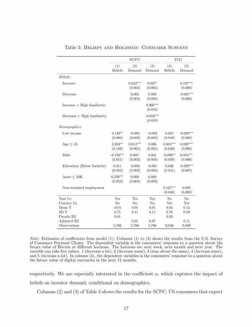
Table 3: Beliefs and Holdings: Consumer Surveys

SCPC ING

(1) (2) (3) (4) (5)Beliefs Demand Demand Beliefs Demand

Beliefs:

Increase 0.022∗∗∗ 0.007∗ 0.197∗∗∗

(0.004) (0.004) (0.008)

Decrease 0.002 0.003 -0.031∗∗∗

(0.004) (0.004) (0.008)

Increase × High familiarity 0.060∗∗∗

(0.018)

Decrease × High familiarity -0.058∗∗∗

(0.019)

Demographics:

Low income 0.139∗∗ -0.005 -0.002 0.021 -0.030∗∗∗

(0.060) (0.003) (0.003) (0.048) (0.008)

Age ≤ 45 0.263∗∗ 0.014∗∗∗ 0.006 0.604∗∗∗ 0.020∗∗∗

(0.109) (0.005) (0.005) (0.049) (0.008)

Male -0.156∗∗∗ 0.005∗ 0.001 -0.096∗∗ 0.054∗∗∗

(0.051) (0.003) (0.003) (0.038) (0.006)

Education (Below bachelor) 0.011 -0.002 -0.001 0.026 -0.028∗∗∗

(0.053) (0.003) (0.003) (0.041) (0.007)

Asset ≤ 20K 0.239∗∗∗ 0.000 0.000(0.053) (0.003) (0.003)

Non-standard employment 0.125∗∗∗ 0.005(0.046) (0.008)

Year f.e. Yes Yes Yes No NoCountry f.e. No No No Yes YesMean Y -0.01 0.01 0.01 0.04 0.13SD Y 0.71 0.11 0.11 0.76 0.33Pseudo R2 0.01 0.03Adjusted R2 0.01 0.07 0.11Observations 5,706 5,706 5,706 9,949 9,949

Note: Estimates of coefficients from model (1). Columns (1) to (3) shows the results from the U.S. Surveyof Consumer Payment Choice. The dependent variable is the consumers’ response to a question about thefuture value of Bitcoin at different horizons. The horizons are next week, next month and next year. Thevariable can take five values: 1 (decrease a lot), 2 (decrease some), 3 (stay about the same), 4 (increase some),and 5 (increase a lot). In column (4), the dependent variables is the consumers’ response to a question aboutthe future value of digital currencies in the next 12 months.

respectively. We are especially interested in the coefficient α, which captures the impact of

beliefs on investor demand, conditional on demographics.

Columns (2) and (3) of Table 3 shows the results for the SCPC. US consumers that expect

17

an increase in the price of Bitcoin are more likely to own Bitcoin. The effects are statistically

significant and large in magnitude. Positive expectations on future prices are associated with

a 2 percentage point higher probability to own Bitcoin. Given a low unconditional probability

of holding Bitcoin (≈ 1%), optimistic beliefs lead to a twofold increase in holdings. However,

the effects are smaller relative to the standard deviation. We find that moving from neutral to

optimist increases the holdings by about 0.19 standard deviations. Additionally, in column

(3) we study the heterogeneity in the effect of beliefs on holdings based on the level of

familiarity with cryptocurrencies. We find that the consumers with a higher familiarity

are significantly more likely to act based on their beliefs, consistent with previous work

suggesting that individuals who are more confident in their own beliefs are more likely to

trade on them (Odean, 1999; Barber and Odean, 2001; Giglio et al., 2019).

Finally, columns (5) of Table 3 reports the estimates of equation (2) for the ING survey.

Consumers expecting a price increase are 19 percentage point more likely to own Bitcoin,

while consumers expecting a decrease are about 3 percent points less likely to own Bit-

coin. Given an unconditional probability of 13%, the effect of positive (negative) beliefs is

approximately an increase (decrease) by 150% (-25%) in the probability of owning Bitcoin.

While our interest is in the effect of expectations on Bitcoin demand, the coefficients on

a few covariates are also interesting. Younger male consumers are significantly more likely

to own cryptocurrencies in both surveys. Despite having more optimistic beliefs on average,

lower income and education consumer are less likely to own cryptocurrencies once we control

for beliefs.

3.2 Investors Survey

In this section we study both the drivers of beliefs and the impact of beliefs on demand

for cryptocurrencies on our main survey of investors from the trading platform. We begin by

looking at the time series of investors’ first investment in cryptocurrencies. Figure 2 shows the

breakdown of investors who bought a cryptocurrency by years of first purchase. While Bitcoin

has been available since 2009, only about 30% of investors who bought a cryptocurrency

18

050

0010

000

1500

020

000

Bitc

oin

pric

e ($

)

0.1

.2.3

.4Fi

rst p

urch

ase

in y

ear (

%)

Dec-2009 Dec-2011 Dec-2013 Dec-2015 Dec-2017 Dec-2019

First purchase Price

Figure 2: First PurchaseNote: The figure shows the daily price of Bitcoin in 2010-2018. Data on the price of Bitcoin comes fromCoinmarketcap. Each vertical bar shows the fraction of investors who purchased their first cryptocurrencyin the two years before the vertical bar.

did so before 2017. The majority of investors bought their first cryptocurrency from 2016

onward, with almost 40% them investing in the crypto market for the first time only in

2018. Taken together, Figures 1 and 2 show that the months leading up to the end of 2017

were characterized by a rise in cryptocurrency prices,21 widespread awareness and optimism

about this asset class across the general public, and an increase in investors’ demand.

Table 4 shows the results on the determinants of investors’ beliefs. Column (1) shows

the estimates of equation (1) with the consumers’ response to a question about the trend

in value of cryptocurrencies in 2018, which we view as a measure of short-term beliefs, as

dependent variable. We confirm our previous result that younger consumers have more

optimistic beliefs, but we do not find significant differences in terms of income. Further,

investors who invested in cryptocurrencies tend to be more optimistic than those who did

not. In addition to that, investors who first invested in cryptocurrencies after 2017 are

relatively more optimistic than investors who entered the market earlier.

21While we focus on Bitcoin prices in the plots, all other major cryptocurrencies followed a very similartrend in prices (see Figure A2 in Appendix A).

19

Table 4: Drivers of Beliefs: Investor survey

Short-termBeliefs

Long-termBeliefs High Potential

(1) (2) (3) (4)

Demographics:

Income ≤ $100K 0.007 -0.206∗∗∗ 0.036∗ 0.035∗

(0.043) (0.074) (0.020) (0.020)

Age ≤ 30 0.144∗∗∗ 0.017 0.017 0.017(0.038) (0.058) (0.018) (0.019)

Outside US 0.209∗∗∗ 0.533∗∗∗ -0.031 -0.031(0.041) (0.072) (0.019) (0.019)

Accredited investor 0.073 0.145 0.144∗∗∗ 0.144∗∗∗

(0.068) (0.115) (0.035) (0.035)

Other variables:

Early Buyer 0.374∗∗∗ 0.555∗∗∗ 0.285∗∗∗ 0.341∗∗∗

(0.044) (0.073) (0.022) (0.026)

Early Buyer × Top3 -0.131∗∗∗

(0.036)

Late Buyer 0.556∗∗∗ 0.477∗∗∗ 0.334∗∗∗ 0.274∗∗∗

(0.050) (0.078) (0.023) (0.029)

Late Buyer × Top3 0.144∗∗∗

(0.041)

Wave f.e. Yes Yes Yes YesCryptocurrency f.e. No No Yes YesMean Y 0.38 0.92 0.24 0.24SD Y 0.85 0.28 0.42 0.42Pseudo R2 0.03 0.08 0.25 0.25Observations 4,647 4,647 41,823 41,823

Note: Estimates of coefficients from model (1) in columns (1) to (2), and model (3) in columns (3) and(4).“Short-term beliefs” is the investors’ response to a question about the value of cryptocurrencies overthe course of 2018. “Long-term beliefs” is a dummy equal to one if investors think that cryptocurrencieswill become mainstream. “Currency potential” is a dummy equal to one if the investor thinks a specificcryptocurrency has the potential to be successful.

In column (2), we estimate a logit specification using now as dependent variable a dummy

equal to one if the investor thinks that cryptocurrencies will become mainstream, which we

view as a measure of long-term beliefs. Interesting, lower income investors tend to be less

optimistic about the long-term prospect of cryptocurrencies. Similarly to the result in column

(1) for short-term beliefs, investors who invested in cryptocurrencies tend be more optimistic.

However, in contrast to short-term beliefs, we find that early and late buyers have similar

long-term beliefs.

20

Finally, in columns (3) and (4), we consider a question in the survey asking investors to

list the cryptocurrencies, if any, that they think have long-term potential. We estimate the

following probit model:

Bijct = Probit (βDi + αDi ×Xj + γt + γc + γj + εijct) , (3)

where Bijct is a dummy equal to one for each currency j that is mentioned by investor i in

survey wave t in country c; Di are demographics characteristics of individual i; Xj are charac-

teristics of cryptocurrency j; γt, γc and γj are time, country and cryptocurrency fixed effects,

respectively. First, we confirm that being young and having invested in cryptocurrencies is

associated with more optimistic beliefs.

Second, we exploit the fact that Bijct now varies not just in the cross-section of investors

but also across cryptocurrencies to consider the effect of currency characteristics Xj on

beliefs. In particular, in column (4), we find that late buyers tend to be especially optimistic

about the top three cryptocurrencies (Bitcoin, Ethereum and Ripple), whereas early buyers

exhibit the opposite pattern. This is consistent with the possibility that late buyers might

be more influenced by the buzz surrounding the top cryptocurrencies (perhaps the only ones

they are aware of) relative to earlier investors who may have a deeper understanding of the

market.

As a final remark, we note that there is a lot of variation in beliefs that our limited

demographics is not able to capture. The pseudo-R2 in Table 3 is always below 0.05. In Table

4, the pseudo-R2 does not increase above 0.25 even with the inclusion of the cryptocurrency

fixed effects. This result is in line with recent work by Giglio et al. (2019), and suggests that

including demographic variables in the cryptocurrency demand system is not sufficient to

control for differences in beliefs across investors.22 Motivated by this observation, we include

both beliefs and demographics as explanatory variables in the structural model of Section 4.

22Using detailed data on investors from a survey administered by Vanguard, Giglio et al. (2019) showthat beliefs are characterized by large and persistent individual heterogeneity, and that demographic char-acteristics explain only a small part of why some individuals are optimistic and some are pessimistic (Fact3 in their paper).

21

Next, we perform a series of reduced-form regressions to motivate the structural ap-

proach in the next section. Similarly to the analysis of consumers, we estimate equation

(2). However, given the richness of the investor survey we now present the results for several

outcome variables: (i) a dummy variable for whether an investor holds Bitcoin—the first

and most popular cryptocurrency; (ii) the number of cryptocurrencies that investors hold

in their portfolio; (iii) the total amount in dollars invested in cryptocurrencies; and (iv) the

share of investors wealth invested in cryptocurrencies.23 Table 5 shows the results.

First, we look at the “extensive” margin in columns (1) to (2). Column (1) shows the

effect of expecting the price of cryptocurrencies to increase or decrease over the rest of the

year, controlling for demographics and additional covariates. We find that investors that

expect an increase (decrease) during the course of the year are more (less) likely to own

Bitcoin. The effects are strongly significant and large in magnitude. Individuals that expect

prices to increase in the following year have a 10 percentage-points higher probability to own

Bitcoin, while individuals that expect prices to decrease have about a 4 percentage-points

lower probability of owning Bitcoin. Given an unconditional probability of about 45%, these

effects translate into an approximately 24% and 9% increase and decrease, respectively.

These results echo our analysis of the drivers of beliefs in Table 4. While investors’ demo-

graphics and beliefs are correlated, the latter have an independent impact on investment

choices. Long-term beliefs about the success of cryptocurrencies and the potential of Bitcoin

also have a significant effect on the probability of holding Bitcoin. A negative opinion about

the long-term success of cryptocurrencies is associated with a lower probability of holding

Bitcoin. Individuals thinking that cryptocurrencies will never become mainstream are about

8 percentage points less likely to hold Bitcoin. We find that the belief that Bitcoin will be

successful is associated with an almost 20 percentage-points increase in the probability of

holding Bitcoin, which correspond to more than a 40% increase relative to the mean.

Are the effect of beliefs on cryptocurrency holdings reasonable? To answer this ques-

tion, in column (2) of 5 we compute the fraction of investors’ wealth that is invested in

23In our data we do not observe investor’s wealth, but only their income bracket. Therefore we use theestimate in Emmons and Ricketts (2017) to impute wealth by multiplying income by 6.6.

22

Table 5: Beliefs and Demand: Investor Survey

Full Sample Investors with Positive Holdings

(1) (2) (3) (4) (5)Invest inBitcoin

Cryptoshare (%)

Number ofCrypto

Amount($.000)

Cryptoshare (%)

Beliefs (short-term):

Price Increase 0.106∗∗∗ 0.815∗∗ 0.340∗∗∗ 18.278∗∗ 1.425∗∗

(0.021) (0.330) (0.114) (7.661) (0.595)

Price Decrease -0.042∗ 0.059 -0.081 7.820 0.972(0.023) (0.374) (0.139) (9.292) (0.721)

Beliefs (long-term):

Never mainstream -0.081∗∗∗ -0.573 -0.107 -3.331 -0.710(0.026) (0.416) (0.191) (12.801) (0.993)

High Potential (Dummy) 0.202∗∗∗

(0.016)

High Potential (Number) 0.301∗∗∗ 0.637∗∗∗ -0.435 0.122(0.090) (0.031) (2.072) (0.161)

Demographics:

Income ≤ $100K -0.081∗∗∗ -3.489∗∗∗ -0.553∗∗∗ -69.318∗∗∗ -4.555∗∗∗

(0.016) (0.255) (0.081) (5.409) (0.420)

Age ≤ 30 0.117∗∗∗ 0.525∗∗ 0.295∗∗∗ 0.782 0.194(0.014) (0.231) (0.081) (5.410) (0.420)

Outside US 0.101∗∗∗ 0.149 0.374∗∗∗ -7.275 -0.494(0.015) (0.246) (0.081) (5.441) (0.422)

Accredited investor 0.175∗∗∗ 3.534∗∗∗ 0.845∗∗∗ 78.450∗∗∗ 4.617∗∗∗

(0.026) (0.414) (0.130) (8.712) (0.676)

Wave f.e. Yes Yes Yes Yes YesMean Y 0.45 2.13 2.68 39.51 3.83SD Y 0.50 7.83 2.11 134.21 10.20Adjusted R2 0.12 0.09 0.21 0.12 0.09Observations 4,647 4,647 2,580 2,580 2,580

Note: Estimates of coefficients from model (2). Columns (1) to (4) report the results from the full sample.Macroeconomic controls are the logarithm of the S&P 500 and the 3-Month London Interbank Offered Rate(LIBOR).

cryptocurrencies. We find that moving from neutral to optimist about the future value of

cryptocurrencies increase the crypto share by about 0.8, which corresponds to about 35%

relative to the mean equity share and 0.10 standard deviations. While our results is not

directly comparable to Giglio et al. (2019) as we do not have a continuous measure of ex-

pectations the magnitude of the effect relative to the standard deviation has a similar order

23

of magnitude.24 Additionally, a large effect of short-term optimistic beliefs on holding in

a volatile market such as the cryptocurrencies is consistent with gambling preferences as a

potential motive behind (excessive) trading, as documented by Liu et al. (2021) for Chinese

retail investors.

Second, we explore the “intensive margin” in columns columns (3) to (5) of Table 5.

The dependent variable in columns (3) is the number of cryptocurrencies in an investor’s

portfolio. Conditional on having at least one cryptocurrency, investors hold on average 2.7

cryptocurrencies, with a standard deviation slightly higher than two. Investors who expect

price to increase in the following year have a 13% higher number of cryptocurrencies relative

to the mean, while investors that expect price to decrease are not statistically different from

investors who expect the price to stay the same. Column (3) also shows that a larger num-

ber of cryptocurrencies with high potential is associated with an increase in the number of

cryptocurrencies held by about 24% relative to the mean, while thinking that cryptocurren-

cies will never become mainstream has no effect on the number of cryptocurrencies in the

portfolio.

In column (4) we shows the results using the total amount invested in cryptocurrencies

as dependent variable. Conditional on having at least one cryptocurrency, investors hold

on average $40 thousands in cryptocurrencies, with a lot of variation across investors as

we already documented in Table 2. Optimistic investors who expect price to increase in

the following year have about $18 thousands more invested in cryptocurrencies, which is

approximately 45% more than investors with less optimistic beliefs relative to mean amount

invested. Negative short-term beliefs, and long-term beliefs do not seem to play an important

role for the amount invested in cryptocurrencies, conditional on investing.

Finally in column (5) we use again the share invested in crypto as dependent variable,

but now focusing on investors with positive holdings. We find that moving from neutral to

optimist about the future value of cryptocurrencies increase the crypto share by about 1.4

among investors who hold cryptocurrencies, which corresponds to an increase by about 35%

24Giglio et al. (2019) find that a one-standard-deviation increase in expected 1-year stock returns isassociated with a 0.16 standard deviation increase in equity shares.

24

relative to the mean. The effect of moving from neutral to optimist account for about 0.14

of the standard deviation in the crypto share.

While our interest is in the effect of beliefs on Bitcoin demand, the coefficients on in-

vestor demographics are also interesting. We find that investors with lower income have

a significantly lower demand for cryptocurrencies, while younger investors have a signifi-

cantly higher demand. Because cryptocurrencies are a relatively new investment products,

the result that higher-income, younger investors are among the early adopters of these new

products is consistent with previous literature on technology adoption (see for example Fos-

ter and Rosenzweig (2010) for a review). In addition, relatively older people may have more

direct experience of losses (e.g., from the global financial crisis of 2008) relative to younger

investors, thus making them more risk averse and skeptical of investing in cryptocurrencies

(Malmendier and Nagel, 2011).25 Further, investors outside the U.S. have a significantly

higher demand for cryptocurrencies. The countries with the largest demand relative to the

number of investors from that country are in Asia and South America. This is consistent

with Asia, and especially China, being a hub for cryptocurrency mining and with investors

from Latin American countries having high appetite for cryptocurrencies given the relative

instability of their national currencies due to political turmoil.26

Overall, our analysis of consumers’ and investors’ beliefs and demand yields three main

stylized facts: 1) unsophisticated consumers and late investors are more likely to have more

optimistic beliefs about the future of cryptocurrencies; 2) there is a lot of dispersion in

beliefs across consumers and investors that is not explained by observable demographics;

and 3) short-term optimism about the future value of cryptocurrencies is associated with: i)

25Our result that younger individual are more likely to old Bitcoin is consistent with previous evidence.For example, a 2015 survey from Coindesk finds that about 60% of Bitcoin users are below 34 years old(https://www.coindesk.com/new-coindesk-report-reveals-who-really-uses-bitcoin).

26Regarding China, see Rauchs et al. (2018) and Benetton et al. (2019), among others. Brazil andArgentina are among the early adopters of cryptocurrencies. The founder of Solidus Capital, a hedgefund, was reported to say “Latin America is very volatile. Cryptos are turning into a new haven forthese families.” (see https://hackernoon.com/love-in-the-time-of-bitcoin-latin-america-and-cryptocurrency-42d60cc4c177). Finally, the recent ING survey on European, US and Australian customers that we use inthis paper finds that about 9, 8 and 7 percent of them currently own cryptocurrencies, respectively (seehttps://think.ing.com/reports/cracking-the-code-on-cryptocurrency/).

25

a higher probability of holding cryptocurrencies, and ii) a larger number of cryptocurrencies

and amount invested, conditional on holding. These facts motivate our structural model and

counterfactual exercises in which we assess how changes in beliefs affect investor holdings

and thus equilibrium prices.

4 A Structural Model of Cryptocurrencies

The descriptive results from Section 3 suggest that beliefs about the future play an im-

portant role in driving cryptocurrency demand and that late investors entered the market

with more optimistic beliefs than incumbent investors. In this section, we develop a sim-

ple model of demand for cryptocurrencies with heterogeneous investors and differentiated

cryptocurrencies to quantify the role of beliefs and the impact of entry of new optimistic

investors on equilibrium prices. Our model is closely related to the general framework for

estimating asset demand proposed by Koijen and Yogo (2019).

4.1 Supply

There are Jt cryptocurrencies in circulation in period t indexed by j = 1, ..., Jt. We

define Sjt as the supply at time t of cryptocurrency j (for example the number of bitcoins in

circulation). We focus on an endowment economy with a fixed supply of cryptocurrencies.

Thus, we abstract from two real-world complexities of the cryptocurrency industry: first,

the endogenous production of existing cryptocurrency (e.g., mining of Bitcoin) and, second,

the introduction of new cryptocurrencies.27

Regarding the first point, most cryptocurrencies follow a predetermined production pro-

cess. For example, Figure A3 in Appendix A shows that while the price of Bitcoin dis-

plays high volatility, the number of Bitcoins in circulation grows based on a predetermined

generation algorithm. Thus, we argue that the endogenous increase in supply of existing

27Production of cryptocurrencies has been studied in previous work (see Cong et al. (2019) and Schillingand Uhlig (2019) among others).

26

cryptocurrencies is not first-order for the study of short-term price dynamics—which is the

object of our analysis—and treat the supply of cryptocurrencies as exogenous.28 The in-

troduction of new cryptocurrencies could be an interesting dimension to explore in a richer

model that featured entry and exit on the supply side, but our analysis is constrained by the

fact that the surveys we use only cover the top cryptocurrencies in terms of market shares

and investors beliefs.

The market capitalization of cryptocurrency j at time t is given by MCjt = PjtSjt, where

Pjt is the unit price of cryptocurrency j in U.S. dollars. Given that Sjt is exogenous, only

Pjt is endogenous in our model. The expected gain from holding cryptocurrency j is given

by Pjt+1/Pjt.

Additionally, cryptocurrencies differ along other dimensions that investors possibly value.

For example, cryptocurrencies can be used as means of payments with different ease of use,

diffusion and privacy properties (Bohme et al., 2015; Goldfeder et al., 2018). Another im-

portant characteristic is the consensus algorithm used to validate transactions. For example,

Bitcoin uses the Proof-of-Work protocol, while other currencies rely on different algorithms,

such as Proof-of-Stake (Bentov et al., 2016; Budish, 2018; Saleh, 2019). Finally, previous

work has identified additional factors, such as volatility and momentum, varying both across

cryptocurrencies and over time as important determinants of cross-sectional cryptocurrencies

expected returns (Liu et al., 2019). We collect the different characteristics of cryptocurrency

j at time t into a vector Xjt.29

4.2 Demand

The demand for cryptocurrencies in each period t comes from i = 1, ..., It investors. Each

investor i in period t is endowed with an amount of wealth Ait. Investors choose how to

allocate their wealth across the J cryptocurrencies and an outside asset, denoted by 0. The

28In Section 5.1 we discuss how we exploit the predeterminted production process of proof-of-work cryt-pocurrencies as a supply-side shifter to identify our demand system.

29To fully capture unobservable characteristics that differ across cryptocurrencies, but are common acrossinvestors and time-invariant, we also include cryptocurrency fixed effects in a robustness analysis in AppendixA.

27

outside asset represents all of the alternative investment opportunities not captured by the

model (such as cash, equity or bonds). The gross return from investing in the outside option

is defined as R0t+1.

Investors choose the fraction of wealth to invest in each cryptocurrency (wijt) to maximize

expected log utility over terminal wealth at date T :

maxwijt

Eit [log(AiT )] . (4)

Investor wealth evolves according to the following intertemporal budget constraint:

Ait+1 = Ait

[(1−

J∑j=1

wijt)R0t+1 +J∑

j=1

wijtRjt+1

]. (5)

Investors also face short-sale constraints:

wijt ≥ 0;wijt < 1. (6)

Following Koijen and Yogo (2019), we assume that returns have a structure and that

expected returns are a function of the cryptocurrencies’ own characteristics. Under this

assumption, the optimal portfolio depends on cryptocurrencies’ characteristics (e.g., market

capitalization, consensus protocol, beta) and latent demand (e.g., unobserved characteristics

and investors demand shifters).

4.3 Equilibrium

To close the model, we write the market clearing condition for each cryptocurrency. The

equilibrium market capitalization for cryptocurrency j is obtained by summing demand for

cryptocurrency j across all investors, as follows:

MCjt =I∑

i=1

Aitwijt, (7)

28

where demand by investor i for cryptocurrency j is obtained by multiplying investor i’s

portfolio weight wijt by his wealth Ait. Under the assumption of downward sloping demand,

Koijen and Yogo (2019) show that the equilibrium is unique. In the counterfactual analysis

of Section 6, we solve for the equilibrium market capitalization using (7). The price of

cryptocurrency is then computed as Pjt =MCjt

Sjt.

5 Estimation and Results

5.1 Identification and Estimation

When taking the model to the data, we set J = 9, corresponding to the largest cryp-

tocurrencies in terms of market capitalization (among those in the data) and a composite

option capturing all remaining cryptocurrencies.30

We assume the following functional form for portfolio weights when taking the model

outlined in Section 4 to the data:

wijt

wi0t

= exp {αmcjt + βXjt + γBij + λDi} εijt, (8)

where mcjt is the logarithm of market capitalization of cryptocurrency j at time t; Xjt

captures other observable characteristics of cryptocurrency j (a dummy for proof-of-work

cryptocurrencies, beta, and momentum); Bij denotes investor i’s belief about cryptocur-

rency j; Di are investor i’s demographics; and εijt captures any unobserved factors affecting

demand—e.g. how convenient the cryptocurrency is as a means of payment for a given

investor (the “convenience yield” in the model of Sockin and Xiong (2018)). Thus, the ex-

pression in (8) is consistent with the idea that investors’ decisions might be driven by the

expected capital gain from the different cryptocurrencies as well as the possibility of using

them for payment purposes.

30Specifically, we focus on the eight largest cryptocurrencies in our sample (Bitcoin, Ethereum, Ripple,Litecoin, Bitcoin Cash, Zcash, Dash, and Monero), and group Swftcoin and Bytecoin together with otherless popular cryptocurrencies in the composite cryptocurrency.

29

Equation (8) and the budget constraint imply that the weight on cryptocurrency j is

given by:

wijt =exp {αmcjt + βXjt + γBij + λDi} εijt

1 +∑9

k=1 exp {αmckt + βXkt + γBik + λDi} εikt, (9)

and the portfolio weight on the outside asset (e.g., cash) is:

wi0t =1

1 +∑9

k=1 exp {αmckt + βXkt + γBik + λDi} εikt. (10)

We estimate the demand parameters from (8) using the generalized method-of-moments.

The parameters are estimated by matching the ratio of weightswijt

wi0tgiven by equation (8) to

the corresponding quantity in the data across investors and currencies. In the baseline model,

we pool all investors together, but we also re-estimate the model separately for different

groups based on demographics in Appendix A.31 The inclusion of investors’ demographics

Di and beliefs Bij in the demand function allows for flexible substitution patterns across

assets. For example, two investors with the same demographic characteristics and demand

shocks εit will typically have different portfolio weights (and different demand elasticities) if

their beliefs are different.

As discussed in Section 3.2, we observe: i) the number and identity of cryptocurrencies

that investors hold in their portfolio; ii) the total dollar amount invested in cryptocurrencies.

However, we do not know how that amount is allocated across all the cryptocurrencies in the

investor portfolio. In our baseline model, we compute the currency-specific weights wijt by

assuming that each investor allocates her cryptocurrency budget across the various currencies

she hold based on the market shares in our sample. Given that this assumption affects

the variation in our dependent variable, we test the robustness of our results to different

allocation rules. In particular, we also consider an allocation where all cryptocurrencies in

the portfolio receive equal weights and one where the weights are proportional to the market

31Koijen and Yogo (2019) estimate the their model for each investor in each period when investors havemore than 1,000 strictly positive holdings. In contrast, we have a cross section of nine cryptocurrencies formost of which holdings are equal to zero, which requires us to pool investors together.

30

shares in the investor’s demographics group.

Following the industrial organization literature on demand for differentiated products

(Berry et al., 1995; Nevo, 2001), we assume that characteristics other than prices, Xjt, are

exogenous. For example, Xjt includes a dummy for whether the currency follows the PoW

algorithm or not. Given that the consensus protocol for a currency is rarely changed,32 it

seems reasonable to treat this as a fixed, exogenous characteristic. Other characteristics in-

clude performance indicators such as market beta and momentum; for these, the assumption

is that they are mean-independent of the factors affecting demand that are not captured by

the other observable currency characteristics, demographics and beliefs.

Cryptocurrency prices could arguably be treated as exogenous from the point of view

of an individual (small) investor, as is the case in our data. However, even with atomistic

investors, unobservable factors affecting choices for all investors (e.g., the inherent quality

or media buzz surrounding a given currency) could shift aggregate demand and thus lead to

bias in the estimated coefficient on market capitalization. This is the standard challenge in

estimating a demand system from quantities and prices that are simultaneously determined

in the market equilibrium. More formally, the simultaneity between prices and quantities

could lead to violations of the restriction

E [εijt|mcjt, Xjt, Di] = E (εijt) = 1. (11)

The first equality is the substantive part of this restriction and it could be violated if price—

and thus market capitalization—is correlated with the unobservable determinants of de-

mand.33

To account for the endogeneity of prices we take two main steps. First, we leverage the

fact that in our data we observe measures of investor beliefs on both the short term price

evolution and the long-term potential of cryptocurrencies. We argue that these beliefs cap-

32For instance, Ethereum has been rumored to switch from PoW to Proof-of-Stake for years, but that hasnot happened to date.

33Setting the mean of εijt to 1 is a normalization without loss of generality.

31

ture an important portion of the time-varying aggregate shocks that affect investor choices.

Absent data on beliefs, these shocks would enter the unobservable error term εijt, but in our

setting we are able to control for them. Our exogeneity restriction then becomes:

E [εijt|mcjt, Xjt, Di, Bij] = 1. (12)

Including beliefs has the dual advantage of allowing flexibility in substitution patterns

across investors, as well as controlling for some of the otherwise unobservable determinants

of demand that could be correlated with prices. Beliefs themselves could be endogenous and

correlated with unobservable shocks affecting demand. With extrapolative expectations, one

possibility could be to use past cryptocurrency prices as instruments for current investor be-

liefs. However, such instruments would likely have limited power in explaining variation in

the cross-section of investors, given the substantial and persistent heterogeneity documented

in the literature (Giglio et al., 2019). For these reasons we decided to abstract from endo-

geneity in beliefs in our analysis. This is in line with the evolution of the demand estimation

literature in industrial organization, which first focused on price endogeneity alone and only

more recently has started dealing with endogeneity of non-price variables.

Second, we propose a supply-side instrumental variable strategy to tackle any remaining

endogeneity concerns for prices. Our instrument is based on differences across cryptocur-

rencies and over time in the production of new coins. Most of the cryptocurrencies in our

data follow the PoW protocol (Ripple is the only notable exception), whereby new coins are

generated (or “mined”) whenever a new block of transactions is validated. The frequency

with which a new coin is mined is a predetermined feature of each cryptocurrency’s protocol,

thus satisfying the exogeneity restriction. Further, changes in supply affect the currencies’

market capitalization, which ensures relevance of the instrument.

Figure 3 displays the two key sources of variation in our instrumental variable. Panel (a)

shows the average supply in January 2018 for the seven PoW cryptocurrencies in our sample.

For each currency, the measure is constructed by taking the average of the daily supply in

32

020

4060

8010

0Av

erag

e su

pply

in J

an 2

018

Bitcoin Bitcoin-cash Dash EthereumLitecoin Monero Zcash

(a) Cross-section

Wave 1 Wave 2

100

120

140

160

180

100

102

104

106

108

110

Supp

ly (n

orm

aliz

ed J

an 1

st 2

018

= 10

0)

01jan2018 01apr2018 01jul2018 01oct2018 01jan2019

Bitcoin Bitcoin-cash Litecoin DashEthereum Monero Zcash (right axis)

(b) Time-series

Figure 3: Supply-side instrumentsNote: Panel (a) shows the average supply in January 2018 for the seven PoW cryptocurrencies in our sample.For each currency, the measure is constructed by taking the average of the daily supply in January, whichis available from https://coinmetrics.io. The supply is given by the sum of all native units ever created andvisible on the ledger (i.e., issued) at the end of the day. Panel (b) of Figure 3 shows the time-series variationin supply in 2018. To account for the differences in scale across currencies we normalize the supply to 100on January 1st 2018.

January, which is available from https://coinmetrics.io.34 We can see there is substantial

heterogeneity in the levels of supply across currencies. Panel (b) of Figure 3 shows the

time-series variation in 2018. To account for the differences in scale across currencies, we

normalize the supply to 100 on January 1st 2018. The supply of all PoW currencies follows

a predetermined trajectory, but the slopes differ across currencies, which provides additional

identifying variation.

Our first-stage regression is given by:

mcjt = ψ log(Supplyjt) + τXjt + εjt, (13)

where Supplyj is the number of coins in circulation; and Xjt are the same controls used in the

demand estimation equation (8). With this instrumental variable in hand, the exogeneity

34The supply is given by the sum of all native units ever created and visible on the ledger (i.e., issued) atthe end of the day.

33

restriction needed to identify the model becomes:

E [εijt|Zjt, Xjt, Di, Bij] = 1. (14)

where Zjt is our supply-side instrument and all other variables are as in equation (12).

5.2 Results

Table 6 shows the estimates of the structural demand parameters. All columns report

the estimates based on the exclusion restriction given by (14). Column (1) shows the model

without controlling for investors’ belief. We find a coefficient on log market capitalization

of about 0.65. The fact that the coefficient on log market capitalization is smaller than

1 guarantees that demand is downward-sloping and the equilibrium is unique (Koijen and

Yogo, 2019). The coefficient is precisely estimated and the associated average own-price

elasticity is -0.36.

In addition, we find that investors have a strong and significant preference for PoW cryp-

tocurrencies, which is consistent with the fact that many of the oldest and most popular

currencies are based on PoW protocols. We also find a positive, statistically significant and

large coefficient on the cryptocurrency beta, while the effect of momentum is not significant

and small in magnitude. A positive beta suggests that investors tend to prefer cryptocurren-

cies that have a higher volatility in comparison to the overall volatility in the cryptocurrency

market.35

In column (2) of Table 6, we include our measures of short-term investor beliefs in the

demand system.36 The coefficient on market capitalization remains significant and consistent

with downward-sloping demand. Interestingly, the point estimate decreases, pushing the

35Following Liu et al. (2019), we estimate beta by regressing the cryptocurrency-specific excess return onthe cryptocurrency excess market return. The latter is constructed as the difference between the cryptocur-rency market index return and the risk-free rate measured by the one-month Treasury bill rate.

36The reduced-form results in Table 5 show that short-term optimism (i.e., expecting a price increase)has a positive and statistically significant effect on demand, while short-term pessimism (i.e., expecting aprice decrease) turns out not to be significant. Accordingly, we omit the price decrease dummy from ourbaseline specification. Table A2 in the Appendix shows the results that include the price decrease dummy.

34

price elasticity of demand up to -0.41. This is consistent with the fact that optimistic beliefs

are positively correlated with both price and demand and therefore omitting them from the

model leads to upwards bias on the price elasticities (in absolute value). Thus, including

beliefs in the demand system appears to help address the issue of price endogeneity.

We also find that expectations play a significant role for investor demand. Specifically,

investors who believe that the value of cryptocurrencies will increase in the next year are

more likely to demand cryptocurrencies, and the effect is precisely estimated.

Next, column (3) of Table 6 adds long-term expectations. We find that investors who

think cryptocurrencies are never going to be mainstream have a significantly lower demand

for cryptocurrencies. The magnitude of the effect is large.

Finally column (4) of Table 6 includes the cryptocurrency-specific dummy about long-

run potential. Investors believing that a given cryptocurrency has potential in the long run

tend to hold more of that currency in their portfolios. Again, the effect of this measure

of long-term optimism is significant and about five times larger than that for short-term

optimistic beliefs. The inclusion of cryptocurrency-specific dummy about long-run potential

further reduces the point estimate of the coefficient on market capitalization. As a result,

the average price elasticity of demand becomes -0.57. This is consistent with the idea that

controlling for currency-specific beliefs further helps to address the issue of price endogeneity.

In Appendix A, we report additional robustness checks, heterogeneity analyses and mea-

sures of the fit of the model, which we only briefly discuss here. First, we estimate the model

shown in column (4) of Table 6 using a different allocation rule for the amount invested across

cryptocurrencies, which affects our dependent variable. Column (1) of Table A2 shows the

results using weights based on market shares in different demographics groups, while column

(2) shows the results using equal weights. We also estimate a version of the model including

a dummy for negative short-term beliefs. The results are qualitatively similar to our baseline

specification. Second, in order to allow for additional heterogeneity across investors, we also

estimate the model in column (4) of Table 6 separately for different age and income groups.

Table A3 shows the results. The point estimates exhibit some variation across demographics,

35

Table 6: Structural Demand Parameters

(1) (2) (3) (4)

Characteristics:

Market capitalization 0.655∗∗∗ 0.599∗∗∗ 0.599∗∗∗ 0.439∗∗∗

(0.082) (0.087) (0.086) (0.098)

Proof-of-Work 0.824∗∗∗ 0.739∗∗∗ 0.697∗∗∗ 0.521∗∗∗

(0.153) (0.159) (0.161) (0.176)

Beta 2.214∗∗∗ 2.371∗∗∗ 2.493∗∗∗ 1.992∗∗∗

(0.230) (0.258) (0.263) (0.278)

Four-week momentum 0.169 0.244 0.246 0.046(0.227) (0.244) (0.236) (0.290)

Beliefs:

Price Increase 0.617∗∗∗ 0.444∗∗∗ 0.300∗

(0.165) (0.166) (0.171)

Never Mainstream -1.664∗∗∗ -1.497∗∗∗

(0.321) (0.363)

High Potential 1.516∗∗∗

(0.143)

Average own-price elasticity -0.36 -0.41 -0.41 -0.57

Macro controls Yes Yes Yes YesDemographics controls Yes Yes Yes YesMean Y 41,823 41,823 41,823 41,823

Note: Estimates of the structural demand parameters from the model of Section 4. “Price increase” is adummy equal to one if the respondent expects the price of Bitcoin to increase over the course of the year.“Never mainstream” is a dummy equal to one if the investor thinks cryptocurrencies are never going to bewidely adopted. “High potential” is a dummy equal to one if the investor thinks a given currency has thepotential to be successful in the long term. Demographics controls are dummies for age, income, and countryof residence. Additional individual-level controls include investor self-reported type, a dummy for whetherthe investor is a trading company customer, and year of first purchase. Macroeconomic controls are thelogarithm of the S&P 500 and the 3-Month London Interbank Offered Rate (LIBOR).

but are not statistically different. Finally, Figure A4 compares the portfolio weights in our

data to those predicted by the model in column (4). Our model slightly underestimates the

demand for Bitcoin and Ripple and tends to overestimate the demand for the remaining

cryptocurrencies, but overall it captures the patterns observed in the data well.

36

6 Counterfactual Analyses

With the estimated model in hand, we study the role of investors’ entry and beliefs for

equilibrium prices and allocations. In our first counterfactual simulation, we investigate

the effect of beliefs in the cryptocurrency market by preventing late optimistic buyers from

investing in cryptocurrencies. In a second counterfactual simulation, we make the currency-

specific expectations about PoW currencies more pessimistic and quantify the substitution

patterns toward other cryptocurrencies and alternative investment opportunities.

6.1 Late buyers, optimistic beliefs and cryptocurrency prices

As we have shown in Section 3, investors who bought their first cryptocurrency late (i.e.,

in 2018) tend to be more optimistic about the future value of cryptocurrencies. This may

have been driven partly by “fear of missing out” and contagious social dynamics.37 In this

section, we explore the quantitative importance of late investors’ beliefs by considering two

counterfactual scenarios in which we limit the widespread adoption of cryptocurrencies by

banning the entry of late optimistic investors in the market.38

Using the estimates in column (3) of Table 6 we construct two main counterfactuals. In

the first counterfactual, we remove all investors who bought their first cryptocurrency in

2018 and replace their beliefs by sampling at random from the population of non-buyers.

This allows us to isolate the effect of late investors’ beliefs on equilibrium cryptocurrency

prices. In the second counterfactual, we altogether ban entry of late investors, by removing

all investors who bought their first cryptocurrency in 2018 without replacing them. This

captures the full effect of restricting entry. Comparing the two counterfactuals allows us to

separately quantify the effect of investors’ beliefs and the effect of reducing market size.

37Similarly, (overly) optimistic beliefs about house prices played an important role in the housing boomof the early 2000s in the U.S. (Cheng et al., 2014; Burnside et al., 2016; Kaplan et al., 2017).

38Figure 1 in the Appendix shows that the rise and fall in prices corresponded to an increase in thenumber of unique addresses used on the Bitcoin blockchain. Unfortunately, it is not possible to distinguishwhether an address belongs to an existing investors opening a new account or to a new investor opening herfirst account. However, our survey data allows us to identify when individual investors bought their firstcryptocurrency.

37

Figure 4 shows the average percentage changes relative to the baseline for the first wave

of our survey in January 2018 (the “boom” period). In the first counterfactual, the number

of investors is unchanged, because we replace late investors with non-buyers, whereas in

the second counterfactual we prevent late buyers from purchasing cryptocurrencies, which

leads to a decline in the market size by about 22%. In both counterfactuals, the share

of investors with short-term positive beliefs declines by about 5-7%. As a result of less

optimistic beliefs, investors decrease their cryptocurrency holdings on average by about 4%

and cryptocurrency prices decline by more than 5% in equilibrium, keeping the market size

constant. The combined change in beliefs and reduction in market size leads to a decline

in the average investment in cryptocurrencies by more than 25% and a drop in equilibrium

cryptocurrency prices by approximately 38%.

Figure 4 shows the average effects across cryptocurrencies, whereas in Table 7, we report a

detailed breakdown across cryptocurrencies and the results of two additional counterfactuals.

First, we simulate a counterfactual in which we replace only the short-term beliefs of late

investors with short-term beliefs of non-buyers. Second, we expand our definition of late

investors by including all investors who bought their first cryptocurrency from 2016 onward

(as opposed to 2018 in our baseline specification).

Panel A reports summary statistics for number of investors and beliefs in the baseline

and counterfactual scenarios. Investors’ demographics and views of cryptocurrency-specific

potential are by construction unchanged in the counterfactual that only changes beliefs,

while they are also affected in the counterfactual in which we ban late investors. Panel B

reports the prices for the eight individual cryptocurrencies in our sample and the average

percentage changes across cryptocurrencies.

In columns (2) and (3) of Table 7, we report the results from the counterfactual in which

we replace only the short-term beliefs of late investors with short-term beliefs of non-buyers.

This change leads to a decrease in the fraction of short-term optimists by four percentage

points or 7.2% relative to a baseline of 63%. Lower optimism about the future value of

cryptocurrencies leads to a decrease in equilibrium prices by 2.2% on average. Hence, we

38

Counterfactual: Beliefs only Counterfactual: No entry0-5

-10

-15

-20

-25

-30

-35

-40

Cha

nge

rela

tive

to b

asel

ine

(%)

Number of investors Short-term positive beliefsPortfolio allocations Cryptocurrencies Prices

Figure 4: Late buyers, optimistic beliefs and cryptocurrency pricesNote: The figure shows the average percentage changes relative to the baseline for the first wave of oursurvey in January 2018 (the “boom” period) for two counterfactuals. In the first counterfactual (“Beliefsonly”) remove all investors who bought their first cryptocurrency in 2018 or later, and replace their beliefsby sampling at random from the population of non-buyers. In the second counterfactual (“No entry”) wesimply ban entry of late investors, by removing all investors who bought their first cryptocurrency in 2018or later without replacing them. Number of investors is change in the total number of potential investors inthe cryptocurrency market. Short-term positive beliefs in the change in the fraction of investors reportingan expected increase in the value of cryptocurrencies in the following year. Portfolio allocation is the averagechange in the amount in $ invested in the cryptocurrencies in our sample. Cryptocurrency prices is theaverage change in the price in $ in the cryptocurrencies in our sample. All bars are changes as a percentageof the relative value in the baseline.

estimate an elasticity of cryptocurrency prices to late investors short-term beliefs of about

0.3. This average elasticity masks heterogeneous effects across different cryptocurrencies.

The same decline in investors’ short-term optimism leads to a decrease in the price of Dash

by 1.5%, while Ripple’s price decline by more than twice as much.

In columns (4) and (5), we report the results for our baseline beliefs counterfactual in

which investors not only become more pessimistic in the short term, but also in the long

term (i.e., more likely to think that cryptocurrencies will not become mainstream). As a

result, the price of Bitcoin decrease by about $700 (5.4%), from $10,900 to $10,200. On

average, cryptocurrency prices decline by about twice as much relative to the counterfactual

in which we only change short-term positive beliefs. This result is consistent with the fact

39

that, as mentioned above, non-buyers tend to be more overall more pessimistic, paired with

the large effects of long-term beliefs on demand we documented in Section 5.2.

In columns (6) and (7), we expand our definition of late buyers to include all investors

who bought their first cryptocurrency from 2016 onward. Specifically, we replace the beliefs

of all investors who bought their first cryptocurrency after 2016 with the beliefs of non-

buyers, again keeping the number of investors unchanged. Panel A shows a larger decrease

(increase) in the share of short-term optimists (long-term pessimists), which translates into

larger declines in equilibrium cryptocurrency prices (Panel B). For example, the price of

Bitcoin now decreases by about $1,400, from $10,900 to $9,500. On average, cryptocurrency

prices decline by more than 12% as a result of the less optimistic beliefs of late investors

relative to early investors and non-buyers.

Finally, the last four columns of Table 7 show the results for the counterfactuals with no

entry of late investors. Specifically, banning late buyers decreases the number of potential

investors from about 4,600 to about 3,600, a 22% decline. As expected, fully banning entry

has a stronger effect for all cryptocurrencies, with prices declining by about 38% on average.

We find stronger effects for popular cryptocurrencies such as Ripple and Ethereum, which

decline by more than 40%, while Bitcoin is less affected. Columns (10) and (11) implement

a ban that also removes investors who bought their first cryptocurrency in 2016-2017. In

this case the market size declines by about 42%. On average, the combination of a smaller

investor pool and more pessimistic beliefs reduces cryptocurrency prices by 75% in January

2018.

To summarize, we find that the entry of late optimistic investors played an important

role in the increase of cryptocurrency prices at the end of 2017 and beginning of 2018. We

estimate an elasticity of cryptocurrency prices to late investors short-term beliefs of about

0.3. We also find that banning investors who bought their first cryptocurrency from 2018

(2016) onward leads to an average decline in the value of cryptocurrencies by about 38%

(75%). This effect is driven by a decline in the number of potential buyers, but also by the

fact that late buyers tend to be more optimistic relative to other investors.

40

Table 7: Late buyers, optimistic beliefs and cryptocurrency prices

Baseline Counterfactual: Beliefs Only Counterfactual: No Entry

Only short Baseline Late buyer Baseline Late buyerterm beliefs from 2016 from 2016

Level Level ∆ % Level ∆ % Level ∆ % Level ∆ % Level ∆ %(1) (2) (3) (4) (5) (6) (7) (8) (9) (10) (11)

Panel A: Market size and beliefsNumber of investors 4,647 4,647 0.0% 4,647 0.0% 4,647 0.0% 3,636 -21.8% 2,687 -42.2%Short-term price increase 63% 59% -7.2% 59% -7.2% 56% -11.2% 60% -5.6% 57% -10.7%Never mainstream 9% 9% 0.0% 11% 19.4% 12% 34.5% 10% 13.0% 12% 27.6%

Panel B: Cryptocurrency Pricesbitcoin 10869 10611 -2.4% 10277 -5.4% 9516 -12.4% 7004 -35.6% 2857 -73.7%bitcoin-cash 1662 1633 -1.8% 1577 -5.1% 1483 -10.7% 1040 -37.4% 468 -71.8%dash 727 716 -1.5% 692 -4.8% 640 -11.9% 461 -36.5% 184 -74.7%ethereum 1089 1066 -2.1% 1025 -5.9% 958 -12.1% 638 -41.4% 264 -75.7%litecoin 178 174 -2.6% 168 -5.7% 155 -13.0% 114 -35.9% 40 -77.7%monero 298 290 -2.5% 280 -5.9% 258 -13.3% 181 -39.4% 70 -76.5%ripple 1.16 1.13 -3.2% 1.08 -7.2% 1.00 -14.0% 0.65 -44.0% 0.27 -76.8%zcash 451 443 -1.9% 428 -5.1% 400 -11.3% 295 -34.7% 123 -72.7%

Average -2.2% -5.6% -12.3% -38.1% -75.0%

Note: The Table shows the results from the baseline and five counterfactual analyses for the first wave of our survey in January 2018 (the“boom” period). Panel A shows the number of investors, the fraction of investors that believe the price of cryptocurrencies is going toincrease, and the fraction of investors that believe cryptocurrencies will never become mainstream. Panel B shows the equilibrium pricesfor all cryptocurrency in our sample and the average across them. Column (1) is the baseline; columns (2) and (3) show the scenario inwhich we replace only the short-term beliefs of late investors with short-term beliefs of non-buyers; columns (4) and (5) show the baselinebeliefs counterfactual in which we replace all beliefs of late investors with short-term beliefs of non-buyers; columns (6) and (7) show thebeliefs counterfactual in which we replace all investors who bought their first cryptocurrency from 2016 onward; columns (8) and (9) showthe baseline no-entry counterfactual in which we ban entry of late investors, by removing all investors who bought their first cryptocurrencyin 2018 or later without replacing them; and columns (10) and (11) show the no-entry counterfactual in which we ban entry of all investorswho bought their first cryptocurrency from 2016 onward.

41

6.2 Energy sustainability and cryptocurrency allocations

In a second set of counterfactuals, we study the role of long-term beliefs about specific

cryptocurrencies for investors’ portfolio allocations and equilibrium prices. Specifically, using

the estimates in column (4) of Table 6, we simulate the market equilibrium when investor

long-term beliefs about PoW currencies become more negative. As mentioned above, PoW is

increasingly criticized due to its huge energy consumption and so our counterfactual exercise

speaks to how the market would react if investors became more aware of its limitations.39

Figure 5 shows the changes in equilibrium allocations and prices for the three largest

cryptocurrencies in the market: Bitcoin and Ethereum, which are based on the PoW protocol,

and Ripple, which has a different, less energy-intensive consensus protocol. Panel (a) of

Figure 5 shows the changes in investor portfolio allocations when we make 25% of investors

more pessimistic about PoW.40 The median investor reduces her holdings of Bitcoin and

Ethereum by about 33% and 17%, respectively, whereas holdings of Ripple increase by almost

5%. Panel (b) shows percentage changes in equilibrium prices relative to the baseline. The

prices of both Bitcoin and Ethereum decline by more than 20%, while Ripple’s price increases

by approximately 6%.

Table 8 shows portfolio allocations and equilibrium prices for all main cryptocurrencies in

our sample in the boom period. Columns (1) to (3) report portfolio allocations for the median

investor. In the baseline, the median investor has about $3,200 invested in cryptocurrencies,

which is about 1% of their total wealth. Approximately $1,600 are invested in Bitcoin, which

accounts for the lion’s share at more than 70% of the total amount invested. The other

cryptocurrencies with the highest shares in investors portfolio are Ethereum and Litecoin,

corresponding to 13% and 6%, respectively.

39Irresberger et al. (2020) offer an exhaustive discussions of advantages and limitations of different con-sensus protocols. Recent swings in cryptocurrency prices have been associated to Elon Musk’s populartweets about the environmental impact of Bitcoin mining (see https://www.vox.com/recode/2021/5/

18/22441831/elon-musk-bitcoin-dogecoin-crypto-prices-tesla and https://www.coindesk.com/

elon-musk-says-tesla-is-suspending-bitcoin-payments-over-environmental-concerns).40More precisely, we take 25% of the investors that list at least one PoW currency among those with

long-term potential and consider the counterfactual scenario in which they do not list any PoW currencyamong those with potential.

42

-35

-30

-25

-20

-15

-10

-50

510

Portf

olio

sha

re c

hang

e (%

)

Bitcoin Ethereum Ripple

(a) Portfolio Allocations

-35

-30

-25

-20

-15

-10

-50

510

Pric

e ch

ange

(%)

Bitcoin Ethereum Ripple

(b) Prices

Figure 5: Energy Sustainability and Cryptocurrency Allocations - PricesNote: The figure shows the percentage change in the equilibrium prices and median portfolio allocationsfor Bitcoin, Ethereum and Ripple in a counterfactual scenario in which we make 25% of investors morepessimistic about PoW. We take 25% of the investors that list at least one PoW currency among those withlong-term potential and consider the counterfactual scenario in which they do not list any PoW currencyamong those with potential. The values in the figure are changes as a percentage of the initial prices andportfolio allocations predicted by our model using January 2018 as the baseline.

In the counterfactual, a decline in the expected sustainability of PoW cryptocurrencies

leads the median investor to reduce her holdings of those currencies, while Ripple experiences

a modest increase. The median investor shifts almost $800 dollar away from Bitcoin, which

corresponds to a decline by about a third. Litecoin experiences the largest outflows declining

by more than 35%, while holdings of Dash, Zcash and Monero decline by a smaller amount

in both absolute and percentage terms. Overall, cryptocurrency holdings decline by 15% on

average, as the median investor shifts about $950 previously invested in cryptocurrencies to

the outside option (i.e., other investment opportunities).

Columns (4) to (6) of Table 8 show results for equilibrium prices. The average decrease in

equilibrium cryptocurrency prices is around 12%, with Bitcoin and Ethereum experiencing

the largest absolute and percentage declines. For example, the price of Bitcoin decreases

by about $2,700 (25%), from $10,900 to $8,200. Among other cryptocurrencies based on

the PoW consensus protocol, Litecoin also experiences a large decline, whereas Zcash and

Monero are the least affected PoW cryptocurrencies.

43

Table 8: Counterfactual Equilibrium Prices and Portfolio Allocations

Portfolio allocation Prices

Baseline Counterfactual Baseline Counterfactual

$ $ ∆ % $ $ ∆ %(1) (2) (3) (4) (5) (6)

bitcoin 2387 1590 -33.4% 10869 8202 -24.5%bitcoin-cash 64 49 -23.6% 1662 1477 -11.1%dash 43 40 -5.2% 727 655 -9.8%ethereum 410 339 -17.3% 1089 850 -21.9%litecoin 184 116 -37.2% 178 146 -18.1%monero 49 46 -5.2% 298 275 -7.7%ripple 78 82 4.6% 1.16 1.23 5.8%zcash 24 23 -3.4% 451 411 -8.9%

Average -15.1% -12.0%

Outside option 328,285 329,056 0.23%

Note: Equilibrium prices and median portfolio allocations for all main cryptocurrencies in our sample andthe outside option in the baseline and a counterfactual scenario in which we make 25% of investors morepessimistic about PoW. Baseline is the January 2018 wave (the “boom” period). In the counterfactuals wetake 25% of the investors that list at least one PoW currency among those with long-term potential andconsider the counterfactual scenario in which they do not list any PoW currency among those with potential.Prices and allocations are in US dollars. Changes are in US dollars and percent of the initial price.

7 Conclusion

In this paper, we shed light on the role of beliefs for asset demand using the cryptocur-

rency industry as a laboratory. Reduced-form evidence and a structural model of asset

demand point to an important impact of beliefs on individuals’ holdings of cryptocurren-

cies and their equilibrium prices. Notably, including observed beliefs in the demand system

alleviates the issue of price endogeneity and substantially reduces the importance of the

unobservables in explaining the cross-sectional variance of returns. We use the estimated

model to simulate how the market prices would react to (i) a counterfactual change in the

number and composition of investors, and (ii) investors becoming more pessimistic about a

large class of highly energy-intensive cryptocurrencies.

Our work could be extended with regards to both the data and the model. First, we

only relied on information from surveys. While our surveys ask about both expectations and

44

holdings, observing actual trading behavior for a panel of consumers and investors at a high

frequency—along the lines of Giglio et al. (2019)—could allow one to identify an even richer

model of cryptocurrency demand. For example, it might be possible to account for persistent

heterogeneity in beliefs and preferences across individuals, as well as explore short-selling

by pessimistic investors. Second, our model takes the number of cryptocurrencies in an

investor’s choice set as fixed. Endogenizing the set of available cryptocurrencies through a

model of entry could be a promising avenue for future research.

45

References

Adam, K., A. Marcet, and J. Beutel (2017): “Stock price booms and expected capital

gains,” American Economic Review, 107, 2352–2408.

Allen, J., R. Clark, and J.-F. Houde (2019): “Search frictions and market power in

negotiated-price markets,” Journal of Political Economy, 127, 1550–1598.

Athey, S., I. Parashkevov, V. Sarukkai, and J. Xia (2016): “Bitcoin pricing, adop-

tion, and usage: Theory and evidence,” .

Bailey, M., E. Davila, T. Kuchler, and J. Stroebel (2019): “House price beliefs

and mortgage leverage choice,” The Review of Economic Studies, 86, 2403–2452.

Barber, B. M. and T. Odean (2001): “Boys will be boys: Gender, overconfidence, and

common stock investment,” The quarterly journal of economics, 116, 261–292.

Barberis, N., R. Greenwood, L. Jin, and A. Shleifer (2015): “X-CAPM: An ex-

trapolative capital asset pricing model,” Journal of financial economics, 115, 1–24.

——— (2018): “Extrapolation and bubbles,” Journal of Financial Economics, 129, 203–227.

Barberis, N., A. Shleifer, and R. Vishny (1998): “A model of investor sentiment,”

Journal of financial economics, 49, 307–343.

Benetton, M. (2018): “Leverage regulation and market structure: An empirical model of

the uk mortgage market,” Available at SSRN 3247956.

Benetton, M., G. Compiani, and A. Morse (2019): “Cryptomining: Local evidence

from china and the U.S.” Tech. rep., Working paper.

Bentov, I., A. Gabizon, and A. Mizrahi (2016): “Cryptocurrencies without proof

of work,” in International Conference on Financial Cryptography and Data Security,

Springer, 142–157.

46

Berry, S., J. Levinsohn, and A. Pakes (1995): “Automobile prices in market equilib-

rium,” Econometrica: Journal of the Econometric Society, 841–890.

Biais, B., C. Bisiere, M. Bouvard, C. Casamatta, and A. J. Menkveld (2018):

“Equilibrium bitcoin pricing,” Available at SSRN 3261063.

Bohme, R., N. Christin, B. Edelman, and T. Moore (2015): “Bitcoin: Economics,

technology, and governance,” Journal of Economic Perspectives, 29, 213–38.

Brunnermeier, M., E. Farhi, R. S. Koijen, A. Krishnamurthy, S. C. Ludvigson,

H. Lustig, S. Nagel, and M. Piazzesi (2021): “Perspectives on the Future of Asset

Pricing,” The review of financial studies.

Brunnermeier, M. and S. Nagel (2004): “Hedge Funds and the Technology Bubble,”

Journal of Finance, 59, 2013–2040.

Buchak, G., G. Matvos, T. Piskorski, and A. Seru (2018): “The limits of shadow

banks,” Tech. rep., National Bureau of Economic Research.

Budish, E. (2018): “The economic limits of bitcoin and the blockchain,” Tech. rep., National

Bureau of Economic Research.

Burnside, C., M. Eichenbaum, and S. Rebelo (2016): “Understanding booms and

busts in housing markets,” Journal of Political Economy, 124, 1088–1147.

Cheah, E.-T. and J. Fry (2015): “Speculative bubbles in Bitcoin markets? An empirical

investigation into the fundamental value of Bitcoin,” Economics Letters, 130, 32–36.

Cheng, I.-H., S. Raina, and W. Xiong (2014): “Wall Street and the housing bubble,”

American Economic Review, 104, 2797–2829.

Chiu, J. and T. V. Koeppl (2019): “Blockchain-based settlement for asset trading,” The

Review of Financial Studies, 32, 1716–1753.

47

Coibion, O., Y. Gorodnichenko, and S. Kumar (2018): “How do firms form their

expectations? new survey evidence,” American Economic Review, 108, 2671–2713.

Coibion, O., Y. Gorodnichenko, and T. Ropele (2019): “Inflation expectations and

firm decisions: New causal evidence,” The Quarterly Journal of Economics, 135, 165–219.

Cong, L. W., Z. He, and J. Li (2019): “Decentralized mining in centralized pools,” Tech.

rep., National Bureau of Economic Research.

Cong, L. W., Y. Li, and N. Wang (2020): “Tokenomics: Dynamic adoption and valua-

tion,” Tech. rep., National Bureau of Economic Research.

Conlon, C. T. and J. H. Mortimer (2013): “Demand estimation under incomplete

product availability,” American Economic Journal: Microeconomics, 5, 1–30.

Corbet, S., B. Lucey, and L. Yarovaya (2018): “Datestamping the Bitcoin and

Ethereum bubbles,” Finance Research Letters, 26, 81–88.

Crawford, G. S., N. Pavanini, and F. Schivardi (2018): “Asymmetric information

and imperfect competition in lending markets,” American Economic Review, 108, 1659–

1701.

De Vries, A. (2018): “Bitcoin’s growing energy problem,” Joule, 2, 801–805.

Egan, M., A. Hortacsu, and G. Matvos (2017): “Deposit competition and financial

fragility: Evidence from the U.S. banking sector,” American Economic Review, 107, 169–

216.

Egan, M. L., A. MacKay, and H. Yang (2020): “Recovering Investor Expectations

from Demand for Index Funds,” Tech. rep., National Bureau of Economic Research.

Emmons, W. R. and L. R. Ricketts (2017): “Household Wealth is at a Post-WW II

High: Should We Celebrate or Worry?” Tech. rep., Federal Reserve Bank of St. Louis.

48

Fernandez-Villaverde, J. and D. Sanches (2019): “Can currency competition work?”

Journal of Monetary Economics, 106, 1–15.

Foley, S., J. R. Karlsen, and T. J. Putnins (2019): “Sex, drugs, and bitcoin: How

much illegal activity is financed through cryptocurrencies?” The Review of Financial

Studies, 32, 1798–1853.

Fostel, A. and J. Geanakoplos (2012): “Tranching, CDS, and asset prices: How finan-

cial innovation can cause bubbles and crashes,” American Economic Journal: Macroeco-

nomics, 4, 190–225.

Foster, A. D. and M. R. Rosenzweig (2010): “Microeconomics of technology adop-

tion,” Annu. Rev. Econ., 2, 395–424.

Gandal, N., J. Hamrick, T. Moore, and T. Oberman (2018): “Price manipulation

in the Bitcoin ecosystem,” Journal of Monetary Economics, 95, 86–96.

Gennaioli, N., Y. Ma, and A. Shleifer (2016): “Expectations and investment,” NBER

Macroeconomics Annual, 30, 379–431.

Gennaioli, N. and A. Shleifer (2020): A Crisis of Beliefs, Princeton University Press.

Giglio, S., M. Maggiori, J. Stroebel, and S. Utkus (2019): “Five facts about beliefs

and portfolios,” Tech. rep., National Bureau of Economic Research.

Goldfeder, S., H. Kalodner, D. Reisman, and A. Narayanan (2018): “When

the cookie meets the blockchain: Privacy risks of web payments via cryptocurrencies,”

Proceedings on Privacy Enhancing Technologies, 2018, 179–199.

Greenwood, R. and A. Shleifer (2014): “Expectations of returns and expected re-

turns,” The Review of Financial Studies, 27, 714–746.

Griffin, J. M. and A. Shams (2019): “Is bitcoin really un-tethered?” Available at SSRN

3195066.

49

Hasso, T., M. Pelster, and B. Breitmayer (2019): “Who trades cryptocurrencies,

how do they trade it, and how do they perform? Evidence from brokerage accounts,”

Journal of Behavioral and Experimental Finance, 23, 64–74.

Hong, H. and D. Sraer (2013): “Quiet bubbles,” Journal of Financial Economics, 110,

596–606.

Hu, A. S., C. A. Parlour, and U. Rajan (2019): “Cryptocurrencies: Stylized facts on

a new investible instrument,” Financial Management, 48, 1049–1068.

Irresberger, F., K. John, and F. Saleh (2020): “The Public Blockchain Ecosystem:

An Empirical Analysis,” Available at SSRN.

Jenik, I. and K. Lauer (2017): “Regulatory sandboxes and financial inclusion,” Wash-

ington, DC: CGAP.

Kaplan, G., K. Mitman, and G. L. Violante (2017): “The housing boom and bust:

Model meets evidence,” Tech. rep., National Bureau of Economic Research.

Koijen, R. S., R. J. Richmond, and M. Yogo (2020): “Which Investors Matter for

Equity Valuations and Expected Returns?” Tech. rep., National Bureau of Economic

Research.

Koijen, R. S. and M. Yogo (2016): “Shadow insurance,” Econometrica, 84, 1265–1287.

——— (2019): “A demand system approach to asset pricing,” Journal of Political Economy,

127, 1475–1515.

Kuchler, T. and B. Zafar (2019): “Personal experiences and expectations about aggre-

gate outcomes,” The Journal of Finance, 74, 2491–2542.

Lammer, D., T. Hanspal, and A. Hackethal (2019): “Who Are the Bitcoin Investors?

Evidence from Indirect Cryptocurrency Investments,” Evidence from Indirect Cryptocur-

rency Investments (December 10, 2019).

50

Liu, H., C. Peng, W. A. Xiong, and W. Xiong (2021): “Taming the bias zoo,” Journal

of Financial Economics, forthcoming.

Liu, Y. and A. Tsyvinski (2018): “Risks and returns of cryptocurrency,” Tech. rep.,

National Bureau of Economic Research.

Liu, Y., A. Tsyvinski, and X. Wu (2019): “Common risk factors in cryptocurrency,”

Tech. rep., National Bureau of Economic Research.

Makarov, I. and A. Schoar (2019): “Trading and arbitrage in cryptocurrency markets,”

Journal of Financial Economics.

Malmendier, U. and S. Nagel (2011): “Depression babies: do macroeconomic experi-

ences affect risk taking?” The Quarterly Journal of Economics, 126, 373–416.

Nelson, S. (2018): “Private information and price regulation in the U.S. credit card mar-

ket,” Unpublished Working Paper.

Nevo, A. (2001): “Measuring market power in the ready-to-eat cereal industry,” Econo-

metrica, 69, 307–342.

Odean, T. (1999): “Do investors trade too much?” American economic review, 89, 1279–

1298.

Ofek, E. and M. Richardson (2003): “Dotcom mania: The rise and fall of internet

stock prices,” The Journal of Finance, 58, 1113–1137.

Piazzesi, M. and M. Schneider (2009): “Momentum traders in the housing market:

survey evidence and a search model,” American Economic Review, 99, 406–11.

Rauchs, M., A. Blandin, K. Klein, G. Pieters, M. Recanatini, and B. Zhang

(2018): “2nd Global Cryptoasset Benchmarking Study,” .

Robles-Garcia, C. (2019): “Competition and incentives in mortgage markets: The role

of brokers,” Tech. rep., Working paper.

51

Saleh, F. (2019): “Blockchain without waste: Proof-of-stake,” Available at SSRN 3183935.

Scheinkman, J. A. and W. Xiong (2003): “Overconfidence and speculative bubbles,”

Journal of political Economy, 111, 1183–1220.

Schilling, L. and H. Uhlig (2019): “Some simple bitcoin economics,” Journal of Mon-

etary Economics, 106, 16–26.

Shams, A. (2020): “The Structure of Cryptocurrency Returns,” Charles A. Dice Center

Working Paper.

Sockin, M. and W. Xiong (2018): “A model of cryptocurrencies,” Unpublished

manuscript, Princeton University.

Temin, P. and H.-J. Voth (2004): “Riding the south sea bubble,” American Economic

Review, 94, 1654–1668.

Vissing-Jørgensen, A. (2003): “Perspectives on behavioral finance: Does” irrationality”

disappear with wealth? Evidence from expectations and actions,” NBER macroeconomics

annual, 18, 139–194.

Xiao, K. (2019): “Monetary transmission through shadow banks,” Available at SSRN

3348424.

Xiong, W. and J. Yu (2011): “The Chinese warrants bubble,” American Economic Re-

view, 101, 2723–53.

52

APPENDICES

Appendix A provides supplementary figures and tables, including robustness checks and a

model fit exercise. Appendix B reports the detailed questions about cryptocurrency holdings

and beliefs from the three surveys that we use in our main analysis.

53

A Additional Figures and Tables

Table A1: Comparison: Investors and Consumers

SCPC ING Trading company

Count Mean Count Mean Count Mean

Demographics:Age ≤ 30 3,153 0.08 1,008 0.22 2,956 0.42

Cryptocurrency questions (general):Awareness 3,149 0.69 1,008 0.57 2,956 0.97Holding 2,163 0.02 1,008 0.08 2,956 0.46

Cryptocurrency questions (beliefs):Increase 2,143 0.28 606 0.33 2,956 0.58Decrease 2,143 0.30 606 0.24 2,956 0.27

Note: Summary statistics for the three surveys used in the reduced-form analysis. For comparability, wefocus on 2018 and the North America. Specifically, for the Survey of Consumer Payment Choice (SCPC),we only use the 2018 wave. For the ING International Survey on Mobile Banking, we only focus on the U.S.For the trading company survey, we only focus on North America. The variables are as defined in Tables 1and 2.

54

Table A2: Structural Demand Parameters: Robustness

Portfolio share Additional controls

(1) (2) (3)Weighted by group Equally weighted

Characteristics:

Market capitalization 0.497∗∗∗ 0.274∗∗∗ 0.428∗∗∗

(0.108) (0.085) (0.097)

Proof-of-Work 0.552∗∗∗ 0.322∗∗ 0.517∗∗∗

(0.179) (0.158) (0.175)

Beta 2.194∗∗∗ 1.165∗∗∗ 2.015∗∗∗

(0.282) (0.292) (0.269)

Four-week momentum -0.042 0.063 0.052(0.287) (0.283) (0.289)

Beliefs:

Price Increase 0.321∗ 0.433∗∗∗ 0.338(0.178) (0.156) (0.238)

Price Decrease 0.067(0.293)

Never Mainstream -1.443∗∗∗ -1.593∗∗∗ -1.494∗∗∗

(0.381) (0.308) (0.354)

High Potential 1.448∗∗∗ 1.600∗∗∗ 1.528∗∗∗

(0.156) (0.128) (0.142)

Macro controls Yes Yes YesDemographics controls Yes Yes YesMean Y 41,823 41,823 41,823

Note: Estimates of the structural demand parameters from the model of Section 4. Column (1) includesweek fixed effects. Column (2) includes currency fixed effects. “Price increase (decrease)” is a dummy equalto one if the respondent expects the price of Bitcoin to increase (decrease) in the following year. “Nevermainstream” is a dummy equal to one if the investor thinks cryptocurrencies are never going to be adopted.“Currency potential” is a dummy equal to one if the investor thinks a given currency has the potential to besuccessful in the long term. Demographics controls are dummies for age, income, and country of residence.Additional individual-level controls include investor self-reported type, a dummy for whether the investor is acustomer of the trading company, and year of first purchase. The macroeconomic controls are the logarithmof the S&P 500 and the 3-Month London Interbank Offered Rate (LIBOR).

55

Table A3: Structural Demand Parameters: By Demographics

By income By age

(1) (2) (3) (4)≤ $100K > $100K ≤ 30 > 30

Characteristics:

Market capitalization 0.575∗∗∗ 0.164 0.266∗∗ 0.720∗∗∗

(0.136) (0.127) (0.105) (0.123)

Proof-of-Work 0.567∗∗ 0.482∗∗∗ 0.618∗∗∗ 0.462∗

(0.235) (0.155) (0.179) (0.264)

Beta 2.215∗∗∗ 1.897∗∗∗ 1.718∗∗∗ 4.414∗∗∗

(0.333) (0.527) (0.378) (0.648)

Four-week momentum -0.594∗∗ 1.115∗∗ 0.773∗∗ -1.031∗∗∗

(0.233) (0.489) (0.392) (0.280)

Beliefs:

Price Increase 0.489∗∗ 0.296 0.214 0.499∗∗

(0.234) (0.225) (0.220) (0.246)

Never Mainstream -1.263∗∗∗ -1.741∗∗∗ -1.388∗∗∗ -2.185∗∗∗

(0.451) (0.490) (0.420) (0.464)

High Potential 1.483∗∗∗ 1.577∗∗∗ 1.550∗∗∗ 1.484∗∗∗

(0.167) (0.176) (0.146) (0.197)

Macro controls Yes Yes Yes YesDemographics controls Yes Yes Yes YesMean Y 28,422 13,401 20,907 20,916

Note: Estimates of the structural demand parameters from the model of Section 4. Columns (1) and (2)show the estimates splitting the full sample by age, while columns (3) and (4) show the estimates splittingthe full sample by income. “Price increase (decrease)” is a dummy equal to one if the respondent expectsthe price of Bitcoin to increase (decrease) in the following year. “Never mainstream” is a dummy equal toone if the investor thinks cryptocurrencies are never going to be adopted. “Currency potential” is a dummyequal to one if the investor thinks a given cryptocurrency has the potential to be successful in the long term.Demographics controls are dummies for age, income, and country of residence. Additional individual-levelcontrols include investor self-reported type, a dummy for whether the investor is a customer of the tradingcompany, and year of first purchase. The macroeconomic controls are the logarithm of the S&P 500 and the3-Month London Interbank Offered Rate (LIBOR).

56

Correlationprice-volume: 0.89

050

0010

000

1500

020

000

2500

0Bi

tcoi

n vo

lum

e (M

$)

050

0010

000

1500

020

000

Bitc

oin

pric

e ($

)

01jan2017 01jul2017 01jan2018 01jul2018 01jan2019

Price Volume

(a) Levels

CorrelationΔprice-Δvolume: 0.68

-100

-50

050

100

Bitc

oin

pric

e ($

)

2017m1 2017m7 2018m1 2018m7 2019m1

Price Volume

(b) ∆

Figure A1: Crypto Mania: Prices and VolumesNote: The left figure shows the daily price and transaction volume of Bitcoin in 2017-2018. The right figureshows the monthly price changes and monthly transaction volume changes of Bitcoin in 2017-2018. Data onthe price of Bitcoin and transaction volumes comes from https://coinmarketcap.com.

Wave 1 Wave 2

050

010

0015

00N

orm

aliz

ed o

pen

pric

e (S

ep 2

017

= 10

0)

01oct2017 01jan2018 01apr2018 01jul2018 01oct2018

bitcoin bitcoin-cash dash ethereumlitecoin monero ripple zcash

Figure A2: Cryptocurrency Price VariationNote: The figure shows the daily prices for eight cryptocurrencies in 2017-2018. The cryptocurren-cies are: bitcoin, bitcoin-cash, dash, ethereum, litecoin, monero, ripple, zcash. Data comes fromhttps://coinmarketcap.com.

57

1012

1416

18Bi

tcoi

n in

circ

ulat

ion

(M)

050

0010

000

1500

020

000

Bitc

oin

pric

e ($

)

01jan2013 01jul2014 01jan2016 01jul2017 01jan2019

Price Supply

Figure A3: Bitcoin Price and SupplyNote: The figure shows the price of Bitcoin in US dollars and the number of Bitcoins in circulation. Data onthe price of Bitcoin comes from https://coinmarketcap.com. Data on the number of Bitcoin in circulationcomes from https://www.blockchain.com/charts.

0 .005 .01 .015 .02

ALT

monero

dash

zcash

bitcoin_cash

ripple

litecoin

ethereum

bitcoin

Data Model

Figure A4: Model FitNote: The figure shows the average portfolio weights for the main cryptocurrencies in our sample and thecomposite cryptocurrency. For each cryptocurrency, we report the average in the data and that predictedby the model using the estimates in column (4) of Table 6.

58

200

400

600

800

1000

Num

ber o

f Uni

que

Addr

esse

s (.0

00)

050

0010

000

1500

020

000

Bitc

oin

pric

e ($

)

01jan2017 01jul2017 01jan2018 01jul2018 01jan2019

Price Number of Unique Addresses

Figure A5: Investors’ EntryNote: The figure shows the daily price for Bitcoin and number of unique addresses used on the Bit-coin blockchain in 2017-2018. Data on the price of Bitcoin and transaction volumes comes fromhttps://coinmarketcap.com. Data on addresses comes from https://www.blockchain.com/charts.

59

B Questions from Surveys

In this Appendix, we report the main questions from the the different surveys that we

use in our analysis.

Survey of consumer payment system (SCPC).

� Question on beliefs: How do you expect the value of one Bitcoin (BTC) to change over

the following time periods?

Options: Decrease a lot, Decrease some, Stay about the same, Increase some, Increase

a lot. The different horizons are next week, next month, next year.

� Question on holdings: Do you have or own any of these virtual currencies?

Options: yes, no. The following currencies are available in the 2018 survey: Bitcoin,

Bitcoin Cash, Ethereum, Ripple, Litecoin, Stellar, EOS.

ING - International Survey.

� Question on beliefs: Please indicate how much you agree or disagree with the following

statements: “I think the value of digital currencies - such as Bitcoins - will increase in

the next 12 months?”

Options: Strongly agree, Agree, Neither agree or disagree, Disagree, Strongly disagree,

I don’t have an opinion.

� Question on holdings: I own some cryptocurrency.

Options: yes, no.

Trading Company Investors Survey.

60

� Question on short-term beliefs: How do you expect the values of cryptocurrencies to

trend in 2018?

Options: Decrease, Stay the same, Increase, I don’t know.

� Question on long-term beliefs: How long do you think it would take for cryptocurrency

to be accepted as mainstream?

Options: By end of 2020, By end of 2025, By end of 2030, It will never become

mainstream, I don’t know.

� Question on cryptocurrency potential: Which currencies do you think have the potential

to be successful in the long term? (SELECT TOP THREE)?

Options: Bitcoin, Ethereum, Litecoin, Ripple, Zcash, Dash, Monero, Swiftcoin, Bitcoin

Cash, Bytecoin, None of the above, I don’t know, Other (please specify).

� Question on holdings: Which of the following cryptocurrencies do you own? (SELECT

ALL THAT APPLY)

The following currencies are available in the survey: Bitcoin, Ethereum, Litecoin,

Ripple, Zcash, Dash, Monero, Swiftcoin, Bitcoin Cash, Bytecoin, None of the above,

Other (please specify).

� Question on holdings: How much do you own in cryptocurrencies (approximate USD

value today)?

Options: < 1, 000, 1, 000−10, 000, 10, 000−100, 000, 100, 000−1, 000, 0000, > 1, 000, 0000.

61