Investment Opportunities and Financing …ifrogs.org › PDF › CONF_2017 ›...

Investment Opportunities and Financing Externalities :

Evidence from the Golden Quadrilateral in India∗

S. Lakshmi Naaraayanan Daniel Wolfenzon

Hong Kong University of Science and Technology Columbia University and NBER

December 8, 2017

PRELIMINARY DRAFT

ABSTRACT

Do business groups impose financing externalities on standalone firms in the local economy?

We examine this question in the context of Indian business groups, specifically, using a recent

large-scale highway development project as a shock to local investment opportunity. We find

that business group affiliated firms invest more than standalone firms in response to upgraded

highway connectivity. We show that the investment behavior of standalone firms is affected by

the density of business groups in the local area. On the financing side, we find that the presence

of business groups makes it harder for other standalone firms in the local economy to raise exter-

nal finance. This business group externality works through the banking sector, when the banks

associated with standalone firms share lending relationships with, and have large exposure to,

firms affiliated with business groups. Overall, our study sheds light on a negative externality

in the economy and documents the costs of conglomeration wherein business groups inhibit the

growth of standalone firms due to lack of finance.

Keywords: Business Groups, investment, family firms, externalities, financial constraints

JEL classification : G32, G34

∗Contact Information: Naaraayanan ([email protected]) and Wolfenzon ([email protected]). We grate-fully acknowledge support from the Chazen Institute for Global Business at Columbia Business School. Naaraayananthanks Columbia Business School for hosting him during which this research was conducted. All errors are our own.

I. Introduction

A vast literature on conglomerates and business groups compares resource allocation in these

organizations relative to standalone firms.1 The objective of this comparison is to understand the

role played by internal labor or capital markets within conglomerates/business groups.2 While ex-

tant research has focused on understanding the functioning and efficiency of internal markets, there

is limited empirical evidence on the effects of conglomeration on other firms in the local economy.

For example, conglomerates might make it harder for small independent firms to raise external

financing. This can have implications for the allocative efficiency of external capital markets. To

this end, we study whether and how business groups impose externalities on other standalone firms

in the economy.

Multi-segment firms (or Conglomerates) as an organizational form are common in the United

States.3 However, there is a considerable decline in importance of internal reallocation within

conglomerates in the United States as a result of financial development. In contrast, many emerging

markets are characterized by weak legal environments and ineffectual investor protection. This, in

turn, makes it difficult for firms to raise external financing (La Porta, Lopez-de Silanes, Shleifer,

and Vishny (1997)). In such environments, firms are often organized as business groups - ”a

group of legally independent firms under common ownership” which share significant operational

and financial inter-linkages (Gopalan, Nanda, and Seru (2007)). Given the prevalence of this

organizational form, measuring the welfare consequences of business groups in a convincing way is

important in emerging markets.

Theoretically, models have identified a cost of conglomeration and have shown adverse effects

that presence of conglomerates might have on standalone firms in the economy. For example,

Almeida and Wolfenzon (2006) argue that financial market imperfections such as low investor

protection generate equilibrium costs of conglomeration. Specifically, too much capital is ”trapped”

1See, Khanna and Palepu (2000), and Almeida, Kim, and Kim (2015). For a review of the literature on conglom-erates, see, Stein (2003) and cites therein.

2Most papers examine the role of internal labor/capital markets in times of distress (Cestone, Fumagalli, Kramarz,and Pica (2016); Kuppuswamy and Villalonga (2015); Gopalan and Xie (2011)) and market turmoil (Matvos andSeru (2014)).

3We use the terms ”conglomerate” and ”business group” interchangeably. These organizational forms are differentin many aspects but have active internal capital markets which function in a similar manner. For example, businessgroup allocate capital among member firms while conglomerates allocate capital among divisions.

1

inside the business groups, and while the allocation of this capital might be efficient for the business

group itself, standalone firms deserving of capital are left starving.

To test the predictions of their model, we use a recent large-scale highway development project

(called Golden Quadrilateral, henceforth GQ) in India as a shock to local investment opportunity

of the firms located in those areas. Particularly, we exploit the upgrade of GQ road network as a

shock to local investment opportunity for firms located along the network as it increases those firms’

access to other regional markets. The GQ program offers an opportunity to study the changes in

investment opportunities of firms, which contemporaneously do not affect their financing capacity

thereby allowing us to study business group externality. These effects may be different compared

to situations when financial constraints are binding and can be informative of broader implications

of capital allocation by business groups.

We hypothesize that the presence of business groups makes it harder for other standalone firms

in the economy to raise capital. This effect would be particularly strong when standalone firms

are in locations surrounded by a large number of group-affiliated firms, and when banks associated

with standalone firms share lending relationships with and have large exposure to, firms affiliated

with business groups.

We employ a difference-in-differences specification that exploits the staggered commencement of

construction of highway stretches connecting various cities across Indian states. It involved upgra-

dation of the 5,800-kilometer highway system that connects the four major cities of Delhi, Mumbai,

Chennai, and Kolkata, making it the fifth-longest highway in the world.4 This program involved

significant investments by the government and represented a major infrastructure improvement for

India.5

As the first step, we start by establishing direct evidence that investment increases for firms

located in areas in which the roads are upgraded. We find a significant increase in the total

investments in the two years following the commencement of road upgrades. The magnitude of this

increase is substantial. For example, an average firm which benefits from this road network upgrade

increased its investments by 3% of total assets. This represents an increase of two-thirds relative

4In particular, it sought to upgrade highways to international standards of four or six-laned, dual-carriagewayhighways with grade separators and access roads.The road network connected as part of the GQ program represented4% of India’s highways in 2002, and the upgradation work raised this share to 12% by the end of 2006.

5See section II for background details.

2

to the mean level of investment. Relatedly, we also show that the firms’ total factor productivity

increased after the road upgrade, as they benefited from enhanced access to the road network.

Thus, the evidence suggests that we have a plausible investment opportunity shock.

Next, we analyze whether firms respond differentially to the road upgrades owing to differences

in their organizational structure. Prior work argues that group affiliated firms benefit from the

transfer of resources within the group, enabling them to capitalize on profitable new investment

opportunities. Such internal transfers can economize costs of external finance thus allowing firms to

allocate capital to the right project (Stein (2003)). However, standalone firms by definition do not

have access to such internal resource transfers. Thus, we expect differences in investment behavior

between group-affiliated firms and standalone firms.

Our results confirm that business group affiliated firms invest more than standalone firms. We

show that group-affiliated firms increase their total investment rather than merely reallocating

capital within the group. Our empirical strategy allows us to control for substantial heterogeneity

by way of high dimensional fixed effects and hence rule out concerns about location and industry

specific supply/demand effects that may differentially affect group-affiliated firms following the

GQ upgrades. Additionally, we do not find differences in investment behavior of group-affiliated

firms before the upgrade, ruling out concerns about reverse causality. In sum, group-affiliated

firms significantly increased their investments while standalone firms were unable to increase their

investments after the GQ road upgrade.

Furthermore, we examine whether standalone firms face financing externalities in the presence

of conglomerates, which renders them unable to capitalize on the investment opportunity afforded

by GQ upgrades. Our methodology compares standalone firms around the investment opportunity

shock as a function of the degree of conglomeration in the local market. We hypothesize that

the presence of business groups makes it harder for other standalone firms in the economy to

raise capital. Consistent with this hypothesis, our results suggest that the investment behavior

of standalone firms around an investment opportunity shock is affected by the density of business

groups in the local area. This effect is particularly stronger when standalone firms are in locations

surrounded by a large number of group-affiliated firms. We document that standalone firms are

unable to invest when the density of business groups in the local area is very high.

We also consider an alternative interpretation for our results. The investment opportunity

3

afforded by GQ upgrades might be mutually exclusionary. To put it differently, if group-affiliated

firms utilize all investment opportunities available locally by investing heavily, then standalone

firms will be unable to invest because of lack of locally available investment opportunity. Contrary

to this explanation, we find that in heavily export oriented industries, standalone firms in locations

surrounded by a large number of group-affiliated firms are severely financially constrained which

renders them unable to invest. This is consistent with the financing channel i.e. business group

externality is driving our results.

Next, we examine the factors driving such financial externalities. We present evidence that the

channel through which the business group externality works is the banking sector. We show that

the financial constraints for standalone firms are severe when banks associated with them have large

exposure to group-affiliated firms. Additionally, we find that standalone firms are unable to borrow

if they are associated with a critical lender who shares lending relationship with group-affiliated

firms.

Overall, our study sheds light on a negative externality in the economy and documents the

presence of costs of conglomeration wherein business groups inhibit the growth of standalone firms

due to lack of finance. Our paper is relevant to the large literature on business groups and conglom-

erates on several fronts. First, prior literature has often focused on examining conglomerates in

isolation and ignored their impact on other firms in the economy (Hoshi, Kashyap, and Scharfstein

(1991); Gopalan, Nanda, and Seru (2007); Almeida, Kim, and Kim (2015)).6 These studies provide

convincing evidence on the functioning and efficiency of internal capital markets. However, there

is limited empirical evidence on the effects of conglomeration on other firms in the economy. Our

paper provides such evidence.

Second, we provide empirical support for predictions from Almeida and Wolfenzon (2006). In

their model, they show that financial market imperfections such as low investor protection generate

equilibrium costs of conglomeration. Differences in pledgability of projects between conglomerates

and standalone firms make it optimal for standalone firms to supply the project’s capital to external

capital market. Therefore, high degree of conglomeration is associated with smaller supply of capital

6Recent work by Boutin, Cestone, Fumagalli, Pica, and Serrano-Velarde (2013) is the closest study which in-vestigates whether and how business groups exert influence on other sectors of the economy. They examine theeffect of business groups’ financial strength on product market competition and show that groups with deep-pocketssignificantly affect the entry and exit decisions of firms in industries. However, they do not have much to say onwhether groups impose externalities on other firms.

4

in the external market for standalone firms thereby affecting the efficiency of aggregate investment.

Lastly, our paper is also related to literature examining the impact of highway infrastructure

on local economic activity. Chandra and Thompson (2000) study the impact of U.S interstate

highways and show that they have differential impact on non-metropolitan areas, across industries

and affect the spatial allocation of economic activity. In the context of GQ, Datta (2012) finds

that firms in cities that lay along the routes of the four upgraded highways benefited significantly

from the improved highways. They find that firms had increased inventory efficiency due to lower

transportation obstacles to production and access to efficient suppliers. Ghani, Goswami, and Kerr

(2014) show that the upgraded GQ network had a strong impact on the growth of manufacturing

activity. While our findings are highly complementary in nature, we document significant differences

in response across firms which imposes externality on standalone firms.

The rest of the paper is organized as follows. The next section describes background about

the golden quadrilateral and discusses the main features of the network. Section III describes the

data with a special focus empirical methodology employed. Section IV contains the main empirical

results and section V concludes.

II. Background about the Golden Quadrilateral

India has second largest road network in the world.7 National highways are critical to this road

network and play a significant role in interstate trade while carrying nearly half of the total road

traffic volume. At the end of 1990s, India’s highway network was in a state of disarray marked by

poor connectivity, sub-par road conditions and congestion with limited lane capacity. Poor road

surface conditions, frequent stops at state borders for tax collection and increased demand from

growing traffic all contributed to congestion with 25% of roads categorized as congested (World-

Bank (2002)).

To tackle these issues, Government of India (GoI) launched the National Highways Development

Project (NHDP) in 1998 with the aim to improve the performance of the highway network. We

study the upgrade of the 5,800 kilometer highway system called the Golden Quadrilateral (GQ)

which connects the four major cities of Delhi, Mumbai, Chennai, and Kolkata, making it the fifth-

7It consists of expressways, national highways, state highways, major district and rural roads. Taken together,these roads carry close to 65 percent of freight in terms of weight.

5

longest highway in the world.8 The project was initially approved in 1998, but many stretches of

the project started only as late as 2001. These delays in the start of construction led to differences

in completion.9 Construction was complete for a significant portion of the stretches by the end of

2006, but minor work on additional phases of the project continued even as late as 2009.

To complete the GQ upgrades, 128 separate contracts were awarded.10 The cost of the project

was envisaged at 600 billion rupees (around US$ 9 billion) while actual cost incurred totaled to

250 billion rupees (around US$ 3.75 billion).11 Most of the construction involved public-private

partnerships and cost was to be recovered by levying a cess of INR 1 on petrol and diesel. Signifi-

cant portion of the funding came from federal government while the remainder from multi-lateral

financing agencies such as Asian Development Bank (ADB), and World Bank (WB).12 Therefore,

the road construction by itself didn’t impose constraints on the banking system.

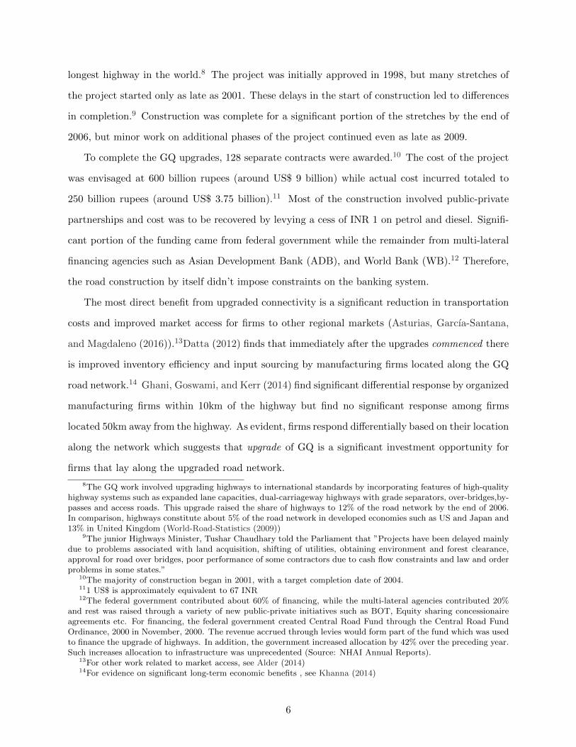
The most direct benefit from upgraded connectivity is a significant reduction in transportation

costs and improved market access for firms to other regional markets (Asturias, Garcıa-Santana,

and Magdaleno (2016)).13Datta (2012) finds that immediately after the upgrades commenced there

is improved inventory efficiency and input sourcing by manufacturing firms located along the GQ

road network.14 Ghani, Goswami, and Kerr (2014) find significant differential response by organized

manufacturing firms within 10km of the highway but find no significant response among firms

located 50km away from the highway. As evident, firms respond differentially based on their location

along the network which suggests that upgrade of GQ is a significant investment opportunity for

firms that lay along the upgraded road network.

8The GQ work involved upgrading highways to international standards by incorporating features of high-qualityhighway systems such as expanded lane capacities, dual-carriageway highways with grade separators, over-bridges,by-passes and access roads. This upgrade raised the share of highways to 12% of the road network by the end of 2006.In comparison, highways constitute about 5% of the road network in developed economies such as US and Japan and13% in United Kingdom (World-Road-Statistics (2009))

9The junior Highways Minister, Tushar Chaudhary told the Parliament that ”Projects have been delayed mainlydue to problems associated with land acquisition, shifting of utilities, obtaining environment and forest clearance,approval for road over bridges, poor performance of some contractors due to cash flow constraints and law and orderproblems in some states.”

10The majority of construction began in 2001, with a target completion date of 2004.111 US$ is approximately equivalent to 67 INR12The federal government contributed about 60% of financing, while the multi-lateral agencies contributed 20%

and rest was raised through a variety of new public-private initiatives such as BOT, Equity sharing concessionaireagreements etc. For financing, the federal government created Central Road Fund through the Central Road FundOrdinance, 2000 in November, 2000. The revenue accrued through levies would form part of the fund which was usedto finance the upgrade of highways. In addition, the government increased allocation by 42% over the preceding year.Such increases allocation to infrastructure was unprecedented (Source: NHAI Annual Reports).

13For other work related to market access, see Alder (2014)14For evidence on significant long-term economic benefits , see Khanna (2014)

6

Or identification strategy exploits variation in the commencement of road construction for cities

located on the GQ road network to study the spillover effects of group-affiliated firms on standalone

firms in the local economy. We compare outcomes for firms located along GQ to firms located away

from GQ. This methodology has been used in a number of papers to study the economic impacts of

US inter-state highways (see Chandra and Thompson (2000) and Michaels (2008)). It is, however,

crucial to remember that a highway network already existed between these four cities, and the

project merely upgraded the system thereby reducing congestion and travel times.

III. Data and Empirical Methodology

A. Data

Financial data are from Prowess, a database maintained by CMIE, Center for Monitoring

the Indian Economy. This data set has been used by a number of prior studies on Indian firms,

including Bertrand, Mehta, and Mullainathan (2002), Gopalan, Nanda, and Seru (2007), Lilienfeld-

Toal, Mookherjee, and Visaria (2012) and Gopalan, Mukherjee, and Singh (2016). Prowess contains

annual financial data sourced from balance sheets and income statements for about 34,000 publicly

listed and private Indian firms. The data is of panel nature covering about 2000 to 6000 firms every

year with assets plus sales of over INR 40 million. It contains additional descriptive information

on the location of the registered office, industry classification, year of incorporation and group

affiliation. We adopt Prowess’ group classification to identify whether a firm is affiliated to a

business group or not.15 This group affiliation has been most notably used in Khanna and Palepu

(2000) and Bertrand, Mehta, and Mullainathan (2002). We assign firms to treatment group which is

defined as receiving an upgraded road based on the location of the registered office (see Appendix A

for details).16 We extract data from the latest vintage of Prowess which is free from survivorship

bias as highlighted by Siegel and Choudhury (2012).

15According to Gopalan, Nanda, and Seru (2007), Prowess’ broad-based classification is more representative ofgroup affiliation than a narrow equity based classification. However, we note that the very few firms change theirgroup affiliation in the data.

16We do not observe changes in registered office location. We believe many firms are unlikely to change theirlocation in response to upgrade. Ghani, Goswami, and Kerr (2014) find that incumbent firms along the GQ networkfacilitated output growth and increase in allocative efficiency. Also, there are significant costs involved in relocationespecially for larger and national firms (e.g. group affiliated firms). We address this concern by focusing on relativelylarger firms. However, we cannot completely rule out that firms respond by changing their location.

7

In our analyses ”year” refers to financial year as opposed to calendar year because the financial

year in India runs from April 1 to March 31. Thus, we refer to the financial year starting on Apri1

l, 2014 and ending on March 31, 2015 as year 2014-15. All dates are adjusted to reflect financial

year rather than the calendar year. From the overall Prowess sample of 1989 to 2016, we exclude

all financial firms (NIC code: 641-663), firms owned by central and state governments, firms with

less than three years of data with positive values of total assets and sales, firms with leverage

outside the [0,1] range, and observations with ratio of investment to lagged total assets greater

than 1.17 We exclude all firms in other manufacturing industries (NIC code: 321-329), coke and

refined petroleum products (NIC code: 191-199), and construction firms (NIC code: 420-439).

To better capture the subsample of firms capable of investing, we restrict the sample to firms

with a book value of total assets greater than INR 10 million (around US$ 0.15 million). We

exclude firms with sales growth exceeding 100% to avoid potential business discontinuities caused

by mergers and acquisitions. To mitigate outliers, we require that the firm’s capital, book assets,

and sales be at least INR 2.5 million (around US$ 0.03 million) in the previous year. Finally, we

also require firms to have a minimum of three observations within panel.

B. Descriptive Firm Statistics

Table I reports statistics for our sample of firms. Panel A reports descriptive statistics for all

firms in our sample while Panel B reports information on group affiliated firms’ characteristics. In

Panel A, Columns (1) and (2) present summary statistics for group affiliated firms and Columns

(3) and (4) report information for standalone firms in our sample. Columns (5) and (6) presents

descriptive statistics for all the firms in our sample. In Panel B, Columns (1) and (2) presents

statistics for Indian business groups.

Panel A of the table shows that, on average, group firms are larger, and more profitable.

Investments to total assets ratio is similar to an average firm in the sample. In addition, debt to

total assets ratio is slightly lower than an average sample firm while they have higher cash flow

relative to standalone firms. Our sample has 51,575 firm-year observations with 40,850 standalone

firm-year observations and 10,725 group firm-year observations. Panel B suggests that an average

17Firms with leverage greater than 1 are considered to be bankrupt in India and hence we exclude such firms fromour analyses.

8

Indian business group has about 6 subsidiaries, operates across 4 industries and 2 states.18 The

number of observations for the different tests vary because of missing data and dropping of singleton

observations in high-dimensional fixed effects estimation.

C. Empirical Methodology

Upgraded connectivity reduces transportation costs significantly and increases access to regional

markets for firms located along the road network. This benefits firms along the road network due

to access to an enhanced highway system. To examine the effect of this treatment, we estimate a

difference-in-differences specification. We assign firms to treatment group based on the location of

their registered office. To identify the firms that are affected by the commencement of GQ upgrades,

we define treatment as the start year of construction of a particular highway stretch connecting two

cities. We assign firms located at either end of a particular stretch to be treated as they both benefit

from this connection.This definition of treatment assumes that firms’ operation is concentrated in

the city of registered office. We follow Datta (2012) in defining nodal cities and districts which

include Delhi, Mumbai, Kolkata, Chennai, and Bangalore and their contiguous suburbs (Gurgaon,

Faridabad, Ghaziabad, and NOIDA for Delhi; Thane for Mumbai). Hence, we also assign firms

located in these nodal areas to treatment group.

To perform the analyses, we estimate a difference-in-differences (DID) model of the following

form for firm i in year t:

yi,t = αi +5∑

k=1

β−kStart−kit +

6∑k=1

βkStart+kit + κXit−1 + ωjt + θst + δrt + εit (1)

subscripts i refers to firm ,j to industry, r to treated,s to state, and t to time. We include all firms

even those that do not help to identify βk i.e. firms not affected by the construction of GQ network

because they help to identify the secular trends in firms’ financial and investment policies. We

choose a window size of twelve years (five years in pre-period and six years in post-period) and

define Start−5 (Start+6) equals one if it is five (six) or more years before(after) the commencement

of the GQ upgrade work. The model is fully saturated with the immediate start year of construction

18States here refer to the state of registered office. For a sample of firms for which we can observe both headquartersand registered office location, we find that 83% of the firms report same address for both locations.

9

as the excluded category. Therefore, the coefficients on Start−k (Start+k) compare the level of the

dependent variable ‘k’ years before (after) the start of construction of GQ network. The inclusion of

firm fixed effects, αi, ensures that each dummy variable is estimated using only within firm variation

in the dependent variable, and time dummies, αt, control for national-level trends. We recognize

that treated firms along the GQ network may have secular time trends that differ from Non-GQ

firms. To control for this, we include interaction between the time and treatment dummies (δrt)

for all firms. The identification at firm-level aids in absorbing time-varying industry and state-level

heterogeneity. We also include control variables (Xit−1) such as Size, Sales Growth, Age, Cash flow

and Profitability in our regressions. Inclusion of control variables improves the efficiency of the

estimates.

Our main dependent variables are firm-level investment and borrowings. Investment is capital

expenditures divided by lagged total assets. Borrowings is total outstanding debt from banks and

financial institutions divided by lagged total assets. All the nominal values are deflated using

Wholesale Price Index (WPI) values at 2010 constant prices. To mitigate the effect of outliers, we

winsorise all the ratios at 1% tails of their empirical distributions. Standard errors are corrected for

heteroscedasticity and auto-correlation, and they are clustered at registered city level to account

for correlations within cities (Bertrand, Duflo, and Mullainathan (2004)).

While we focus on investment and borrowing, we also estimate the effect on firm productivity.

We use a measure of total factor productivity (TFP). TFP is the difference in actual output and

predicted output. To compute this, we follow the literature and use a log-linear Cobb-Douglas

production function (Syverson (2004) and Foster, Haltiwanger, and Syverson (2008)). We estimate

the residual at firm-level from the following regression model:

yi,t = β0 + βkkit + βllit + βmmit + εit (2)

where y is the logarithm of output and k,l, and m are logarithms of capital,labor and material

inputs, respectively(see Appendix B for further details).19 To allow varying intensities for factors

of production across industries, we run this estimation for each 2-digit NIC industry separately.

Thus, we measure TFP for each firm relative to other firms within the same industry.

19We estimate this using structural method developed by Levinsohn and Petrin (2003). We find qualitativelysimilar results when computing TFP using either OLS or Olley and Pakes (1996).

10

Our main focus is on understanding differential response of firms based on their organizational

structure. We use the specification in Equation 1 but interact Start+k with Group (Standalone)

which is a dummy variable that identifies whether the firm is affiliated to a business group(or not).

We also test whether the coefficients estimated are significantly different for group affiliated firms

relative to standalone firms. To allow for differences in organizational forms, we interact Group

(Standalone) with the fixed effects and controls. Thus, we are able to control for substantial hetero-

geneity owing to differences in organization structures which helps strengthen our interpretation.

While we present results using just the location of upgrade, the magnitude and interpretation of

these results is understated as other nearby cities indirectly benefit from upgraded connectivity to

GQ.

IV. Main Results

A. Investment and Total Factor Productivity

We begin our empirical analysis by documenting that upgraded connectivity was indeed a shock

to investment opportunity for treated firms. Table II shows the effect of GQ upgrade on investment

and total factor productivity around the commencement of construction for treated firms. As shown

in column (1), investment at treated firms increases by 0.029 percentage points which corresponds

to an increase of 59% (0.029 versus sample average of 0.049). Economic magnitude of the estimates

are quantitatively similar when we use controls in our regressions. These estimates are reported in

column (2). We find that this significant effect occurs in the second year after the commencement

of upgrade work. The median completion time for a particular stretch is around 2.3 years and firms

significantly increase their investments around the completion time. Given the large economic

magnitude of investments, we also note that the coefficient on dummies decrease for other years

which bolsters our conjecture that firms invested heavily in response to the investment opportunity

afforded by construction of road network.

A key identifying assumption of our DID strategy is the parallel-trends assumption i.e. in the

absence of treatment the behaviour of treated and control firms are similar. We document absence

of any pre-trends in investment decision of firms. The coefficients on Start−k are economically

and statistically insignificant suggesting no pre-existing differential trends. This validates a key

11

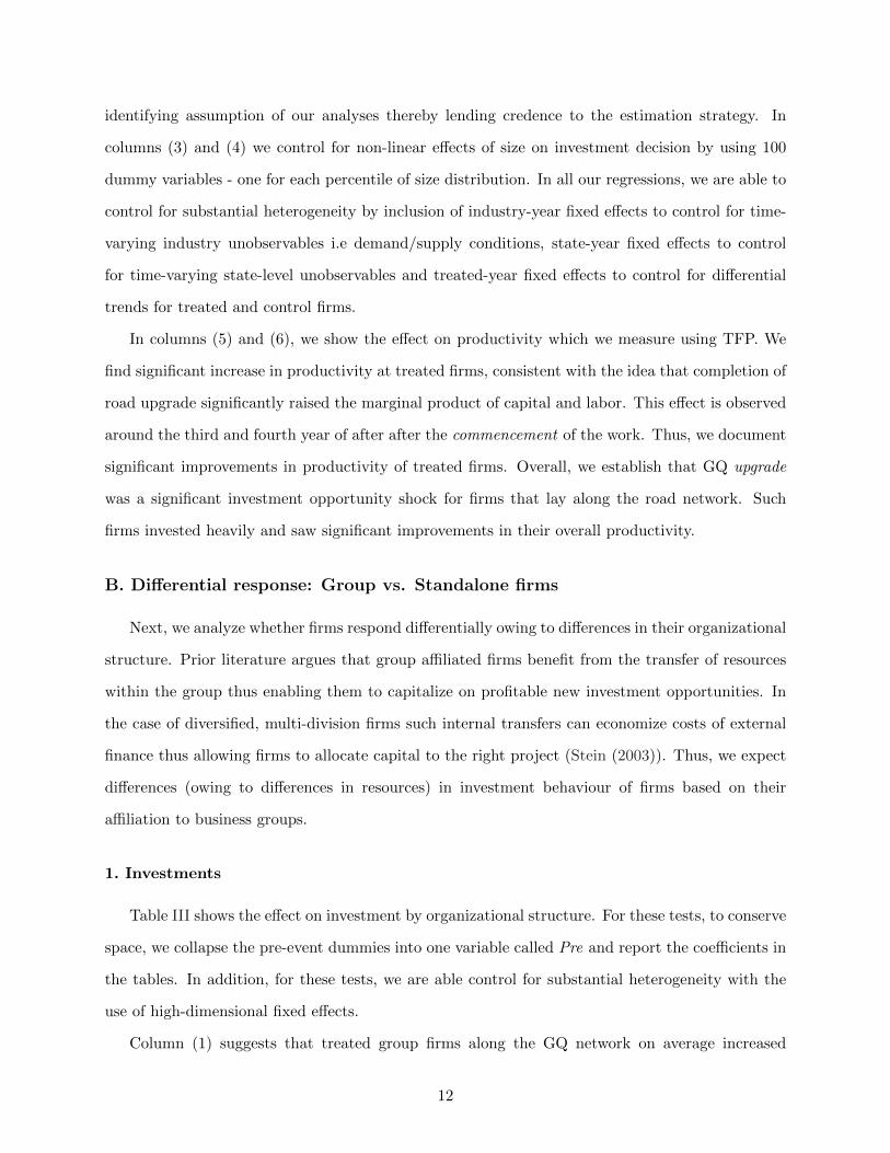
identifying assumption of our analyses thereby lending credence to the estimation strategy. In

columns (3) and (4) we control for non-linear effects of size on investment decision by using 100

dummy variables - one for each percentile of size distribution. In all our regressions, we are able to

control for substantial heterogeneity by inclusion of industry-year fixed effects to control for time-

varying industry unobservables i.e demand/supply conditions, state-year fixed effects to control

for time-varying state-level unobservables and treated-year fixed effects to control for differential

trends for treated and control firms.

In columns (5) and (6), we show the effect on productivity which we measure using TFP. We

find significant increase in productivity at treated firms, consistent with the idea that completion of

road upgrade significantly raised the marginal product of capital and labor. This effect is observed

around the third and fourth year of after after the commencement of the work. Thus, we document

significant improvements in productivity of treated firms. Overall, we establish that GQ upgrade

was a significant investment opportunity shock for firms that lay along the road network. Such

firms invested heavily and saw significant improvements in their overall productivity.

B. Differential response: Group vs. Standalone firms

Next, we analyze whether firms respond differentially owing to differences in their organizational

structure. Prior literature argues that group affiliated firms benefit from the transfer of resources

within the group thus enabling them to capitalize on profitable new investment opportunities. In

the case of diversified, multi-division firms such internal transfers can economize costs of external

finance thus allowing firms to allocate capital to the right project (Stein (2003)). Thus, we expect

differences (owing to differences in resources) in investment behaviour of firms based on their

affiliation to business groups.

1. Investments

Table III shows the effect on investment by organizational structure. For these tests, to conserve

space, we collapse the pre-event dummies into one variable called Pre and report the coefficients in

the tables. In addition, for these tests, we are able control for substantial heterogeneity with the

use of high-dimensional fixed effects.

Column (1) suggests that treated group firms along the GQ network on average increased

12

their investments. There is a 7.1 percentage point increase in investment which translates to a

substantial increase of 147% (7.1 versus average for group firms of 4.8). Column (2) suggests that

standalone treated firms in the same areas as group firms on average have no statistically discernible

change in their investments. The timing of these investments corresponds to the overall investment

documented in Table II suggesting that the increase in investments is entirely driven by group

firms.

Results in columns (3) and (4) includes controls variables and estimates are similar to when

we exclude controls. We test whether the coefficients estimated are significantly different for group

firms relative to standalone firms. In column titled Diff, we report the estimate difference with

standard errors in parentheses. There is a differential investment of 6 percentage points between

group and standalone firms which is statistically significant at the conventional levels of significance

in either of the specifications. The coefficients on Pre are economically and statistically insignificant

suggesting no pre-existing differential trends between group and standalone firms. Thus, evidence

from Table III suggests that group firms invests differentially relative to standalone firms in response

to the investment opportunity shock.

2. Shifts in Investment?

In the preceding subsection, we document significant investments by treated group firms in

response to the investment opportunity shock afforded by GQ upgrade. A plausible concern with

this evidence relates to reallocation of investment within groups. Group headquarters may choose

to shift their investments from one location to another in response to new investment opportunities

(Giroud (2013) and Giroud and Mueller (2015)). Thus, treated groups merely reallocate capital

in response to the investment opportunity without any overall increase in investment. To rule out

concerns that reallocation maybe driving our results, we present evidence on investments at the

group-level. Table IV presents results to address these concerns.

For these tests we focus only on group affiliated firms and estimate the specification as in

Equation 1. We begin with a firm-fixed effects specification and report results in column (1). We

note that there is a significant increase in investment among treated group firms. The increase in

investment is 0.059 percentage points which is slighly lower than what we document in our tests

in Table III. Next, we use owner-group fixed effect rather than firm fixed effects specification. The

13

inclusion of these fixed effects, ensures that each dummy variable is estimated using only within

group variation in the dependent variable. Thus, if reallocation is driving our results, we should

not expect changes in investment within groups. However, results in column (2) seem to suggest

otherwise. We find that estimates remain unchanged in magnitude and significance.

In columns (3) and (4), we control for non-linear effects of size on investment decision by using

a set of 10 dummy variables that identify firm size deciles based on Sizet−1. Controlling for such

size effects, sharpens our estimates and leaves our interpretation unchanged. Two points are worth

mentioning based on the evidence from this table. First, lower magnitudes than baseline results

suggest some reallocation but on average there is an increase in group-level investments. Second,

there are no pre-existing trends in investment decision by firms either at the firm-level or at the

group-level. Thus, evidence from this table bolsters our conjecture that group firms responded by

increasing overall investment rather than shifting investment across locations.

3. External Financing

Evidence from preceding subsections, establish a significant increase in investment by treated

group firms which is not driven just mere reallocation within group firms. Here, we attempt to

understand financing behaviour of treated firms. Our focus is on external financing behaviour as we

intend to characterize financing externalities on standalone firms.20 We focus on total outstanding

debt from banks and financial institutions. Table V reports the results on external borrowings for

group and standalone firms.

We document that treated group firms predominantly borrow from banks and financial insti-

tutions in response to access to upgraded GQ network. These effects are significant and persistent.

The difference in borrowings between group and standalone firms is statistically significant and

entirely driven by group affiliated firms. The coefficient estimates suggest that group affiliated

firms on average borrow 7.5% of total assets from external sources which is almost twice as large

when compared to the magnitude of the average investment. The increase in external borrowings

is persistent and continues until five years after the commencement of the upgrade work.

20Group firms can rely on intra-group equity and loans, external borrowing, external equity, or internal cash theygenerate. It is important to note that in India corporate debt market is underdeveloped and bank lending is oneof the major sources of corporate borrowing. Therefore, we focus on external borrowing from banks and financialinstitutions. In unreported results, we find significant intra-group equity and loan transfer to treated firms and nochange in cash holdings for treated firms.

14

The large magnitude and opposite sign on the coefficients is suggestive of crowding-out effect at

play. The large magnitude of external borrowing more than what was invested coupled with opposite

signs on borrowing raises suspicion whether group affiliated firms impose financing constraints on

standalone firms which are unable to raise external capital. This explanation seems plausible and is

consistent with predictions in Almeida and Wolfenzon (2006). They show that efficient reallocation

of capital inside groups may increase financial constraints on independent firms and be harmful to

economy-wide capital allocation.21 Overall, we document significant increase in external borrowings

from group affiliated firms.

C. Effect on Standalone firms

In this subsection, we attempt to establish whether standalone firms face financing externali-

ties in the presence of conglomerates which renders them unable to capitalize on the investment

opportunity afforded by GQ upgrade. Our methodology compares standalone firms around the

investment opportunity shock as a function of the degree of conglomeration in the local market.

We hypothesize that presence of business groups make it harder for other standalone firms in the

economy to raise capital.

1. Group concentration

We begin by exploring the effect of group affiliated firms’ concentration on investment behaviour

of standalone firms. Given our identification strategy relies on location of upgrade, we create a

location based measure to capture this effect. We create a new measure of group concentration

at the city level which is the basis of our treatment. For each city, we create a concentration

measure based on median sales in the period before GQ upgrade was announced i.e. 1989 to 1997.

We then define High Conc(Low Conc) as a dummy variable equal to 1 if sales concentration in

the city is above(below) the 75th percentile of the median group sales across the years before the

announcement. Thus, this measure captures concentration of groups firms around standalone firms

21Alternatively, the crowding out might be exacerbated as a result of financing being used up for GQ upgradeitself in the form of project financing. Thus, the effects we present here have downward bias and are understated.However, this is likely not the case as a substantial amount of financing was borne by international agencies (such asWorld Bank, Asian Development Bank etc) and federal government.

15

at each location.22 Thus, our measure indicates that if High Conc(Low Conc) equals 1, then the

group concentration in that location is Dense(Sparse).

Table VI reports results of the effects of group concentration at each location on standalone

firms in the same location. We restrict our sample to standalone firms for these tests and estimate

a similar specification as in Equation 1 where we interact Start+k with High Conc (Low Conc). The

model is fully saturated with the start year of construction as the excluded category. All regressions

include firm fixed effects, state-year, industry-year and treated-year fixed effects. Control variables

include Size, Age, Cash flow and Profitability. All control variables are interacted with High Conc

(Low Conc) to allow for differential trends.

Results in column (1) presents investment behaviour of standalone firms within high concen-

tration locations along GQ network. We find that in high concentration areas there is significant

reduction in investment by standalone firms. The decline in investment is significant in magnitude

and much larger than the increase in investment by group affiliated firms. In contrast, we do not

find any statistically discernible change in investments for standalone firms in sparsely concentrated

areas. These estimates remain stable in sign and magnitude even after inclusion of controls. No-

ticeably, in the pre-event period there are no pre-existing differential trends between investment by

these firms across these locations. If anything, we find that standalones invested more in highly

concentrated areas but the effect is statistcally insignificant.

Results in panel B for external financing mirror those in panel A. column (1) presents borrowings

for standalone firms within high concentration locations along GQ network. We find that in high

concentration areas there is significant reduction in borrowings by standalone firms. The decline

in borrowings is significant in magnitude and similar to increase in borrowings by group affiliated

firms in our baseline tests. In contrast, we find that there is a substantial increase in borrowings

for standalone firms in sparsely concentrated areas. These estimates remain stable in sign and

magnitude even after inclusion of controls but become statistically insignificant. Similar to earlier

results, we find no evidence of pre-existing differential trends by these firms across these locations.

Hence, the evidence presented here suggests that standalone firms seem to face financing exter-

nality as a function of degree of conglomeration in the local area.

22For the purpose of our analyses, we restrict the our sales measure to GQ network. The idea behind this is thatgroup firms with greater ex-ante exposure will respond significantly to these upgrades than firms with low exposure.The results remain qualitatively similar if we use a sales measure across all locations.

16

2. Mutually exclusive investment opportunities?

An alternative interpretation for the evidence in preceding section might be that the investment

opportunity afforded by GQ upgrade is mutually exclusive. To put it differently, if group affiliated

firms utilize all investment opportunities available locally by investing heavily then standalone

firms will be unable to invest because of lack of locally available investment opportunity. This

could explain what we find above.

To rule out this concern, we repeat the tests in Table VI for high exporting industries. Our un-

derlying assumption is that GQ upgrade afforded a local investment opportunity shock by improving

access to regional and local markets. By focusing on exporting industries (i.e. both group affiliated

and standalone firms operating in heavily export oriented industries), we alleviate concerns that

mutually exclusive local investment opportunities may be driving our results.

We measure High exporting industry in the following manner. For each firm, we observe export

earnings to sales each year and we measure the median ratio for each industry in the period before

GQ upgrade was announced i.e. 1989 to 1997. We keep industries if export earnings to sales in

each industry is above(below) the 75th percentile of the median export earnings to sales across the

years before the announcement of the GQ road network upgrade. Our group concentration measure

remains the as in Table VI.

Table VII presents results on the effects of group concentration in high exporting industries.

Results in column (1) presents investment behaviour of standalone firms within high concentration

locations along GQ network. We find there is significant reduction in investment by standalone

firms. The decline in investment is significant in magnitude and much larger than the increase in

investment by group affiliated firms. This effect is larger and persistent in comparison to Table VI.

In contrast, we find weakly statistically discernible change in investments for standalone firms

in sparsely concentrated areas. These estimates remain stable in sign and magnitude even after

inclusion of controls.

Results in panel B for external financing mirror those in panel A. column (1) presents borrowings

for standalone firms within high concentration locations along GQ network. We find that in high

concentration areas there is significant reduction in external borrowings by standalone firms. The

decline in borrowings is significant in magnitude and similar to increase in borrowings by group

17

affiliated firms in our baseline tests. In contrast, we find that there is a substantial increase in

borrowings for standalone firms in sparsely concentrated areas. These estimates remain stable in

sign and magnitude even after inclusion of controls but become statistically insignificant.

In sum, we find suggestive evidence that standalone firms face externalities when surrounded by

group firms and are able to rule out concerns of mutually exclusive local investment opportunity.

D. Financing Externalities

While the results so far are informative about the quantitative importance of organizational

structure in driving financial externalities, they are silent about the precise mechanisms that en-

gender such externalities. In this subsection, we explore the role of banking sector in driving

business group externalities.

1. Shared Lenders

If the supply of capital is limited, standalone firms may face significant financing externalities

when they borrow from lenders with lending relationships to group affiliated firms. This effect is

likely exacerbated when the standalone firms borrow from only one external source. To explore

such effects, we exploit lending relationships of standalone firms.

We create a measure of whether standalone firms borrowed from the same lender as a group

affiliated firm.23 For each standalone firm, we match the lender’s name to lending relationships of

group affiliated firms. We then create a dummy variable One Shared (Others) which equals 1 if

standalone firm shares atleast one lender with the group firm in the five years preceding GQ up-

grade.24 To better capture externalities and quantify the importance of a specific lender to the firm,

we restrict this classification to standalone firms borrowing from only one external bank/financial

institution. Thus, our measure indicates that when One Shared equals 1, the standalone firm

borrows from only one external source and this lender has exposure to group affiliated firms. We

present the effect on external borrowings of standalone firms with shared lenders in Table VIII.

23We observe lending relationships between banks, financial institutions and firms in our sample. These lendingrelationships are used in Gopalan, Mukherjee, and Singh (2016)

24In Others, we have three types of lending relationships with standalone firms, (1) borrow from multiple ex-ternal source(s) and share lending relationships, (2) borrow from multiple external sources but don’t share lendingrelationships, and (3) no external source(s).

18

In column (1), we examine borrowings by standalone firms with shared lenders. We document

a significant reduction in borrowings around the commencement of GQ upgrade. The decline in

borrowings is significant in magnitude and similar to increase in borrowings by group affiliated

firms in our baseline tests. In contrast, we find that there is a substantial increase in borrowings for

standalone firms when they are associated with multiple shared lenders. The difference between the

two groups is statistically significant indicating the differential borrowing behaviour of standalone

firms in relation to their exposure to shared lenders. We obtain similar estimates after inclusion of

controls.

These results are consistent with the negative externality argument, according to which business

group firms impose external financing constraints on standalone firms through the shared lending

relationships and rationing by banks.

2. Lenders’ Group Exposure

In the previous subsections, we show that group firms impose externality on standalone firms

which renders them unable to capitalize on investment opportunity. Furthermore, these effects are

stronger for high exporting industries, where we are able to rule out concerns of mutually exclusive

investment opportunities. In addition, standalone firms are unable to borrow if they are associated

with a critical lender who also shares lending relationships with group-affiliated firms. In this

subsection, we study the effect from supply side i.e banks’ lending exposure.

While we do not observe lending amounts by banks, we do observe lending relationships between

banks, financial institutions and firms. Using these lending relationships we are able to create a

exposure measure for each bank and financial institution. We create a new measure of lending

exposure to group firms in the following manner. In the period before GQ upgrade was announced,

for each firm, we divide the total outstanding debt by banks and financial institutions equally

among all lenders. For each lender, we then define High(Low) as a dummy variable equal to 1 if

their lending amount is above(below) the median across the years before the announcement. We

then assign each lender to standalone firms in our sample. Thus, the measure captures standalones’

association with lenders having varying degree of exposure to group firms.25 Thus, our measure

25For the purpose of our analyses, we restrict our measure to GQ network. Lenders with greater ex-ante exposureto group firms will respond significantly to these upgrades than lenders with low exposure. The results remainqualitatively similar if we use a measure across all locations.

19

indicates that if High Exp(Low Exp) equals 1, then the lender associated with the standalone has

High(Low) lending exposure to group firms.

Table IX presents results on the effects of lenders’ group exposure on standalone firms. Results

in column (1) presents borrowing behaviour of standalone firms within different exposure measure

along GQ network. We find that there is no change in borrowings by standalone firms when they

are associated with lenders with high group exposure. Next, we examine the effect in low exposure

groups. From column (2), it is evident that there is significant increase in borrowing. The decline

in borrowings is significant in magnitude and similar to increase in borrowings by standalone firms

when they are associated with banks having low exposure to groups. We interpret this as evidence

of banks supplying available capital to group affiliated firms than to standalone firms thereby

possibly exacerbating the differential wedge in investment. These estimates remain stable in sign

and magnitude even after inclusion of controls.

Overall, we find evidence that standalone firms indeed face financing externality when sur-

rounded by group firms and are unable to borrow funds if they are associated with lenders having

greater lending exposure to group affiliated firms.

20

V. Conclusion

In this paper, we study whether and how business groups influence standalone firms in the

local economy. We use a recent large-scale highway development project in India as a shock to

local investment opportunity for firms located in those areas. We show that investment behavior

of standalone firms around an investment opportunity shock is affected by the density of business

groups in the local area. Our evidence shows that the channel through which the business group

externality works is through the banking sector. Taken together, the evidence is consistent with the

predication that business group affiliated firms impose financial externalities on standalone firms,

leaving them worse-off. Our results suggest that capital rationing by banks propagates and amplifies

the negative externality to other firms. This has important implications as financial intermediaries

could adversely affect capital allocation when external capital markets are less developed especially

in the case of emerging markets.

21

REFERENCES

Alder, Simon, 2014, Chinese roads in india: The effect of transport infrastructure on economic development,Work. Pap., Univ. North Carolina, Chapel Hill .

Almeida, Heitor, Chang-Soo Kim, and Hwanki Brian Kim, 2015, Internal capital markets in business groups:Evidence from the asian financial crisis, The Journal of Finance 70, 2539–2586.

Almeida, Heitor, and Daniel Wolfenzon, 2006, Should business groups be dismantled? the equilibrium costsof efficient internal capital markets, Journal of Financial Economics 79, 99–144.

Asturias, Jose, Manuel Garcıa-Santana, and Roberto Ramos Magdaleno, 2016, Competition and the welfaregains from transportation infrastructure: Evidence from the golden quadrilateral of india, Working paper.

Bertrand, Marianne, Esther Duflo, and Sendhil Mullainathan, 2004, How much should we trust differences-in-differences estimates?, The Quarterly Journal of Economics 119, 249–275.

Bertrand, Marianne, Paras Mehta, and Sendhil Mullainathan, 2002, Ferreting out tunneling: An applicationto indian business groups, The Quarterly Journal of Economics 117, 121–148.

Boutin, Xavier, Giacinta Cestone, Chiara Fumagalli, Giovanni Pica, and Nicolas Serrano-Velarde, 2013, Thedeep-pocket effect of internal capital markets, Journal of Financial Economics 109, 122–145.

Cestone, Giacinta, Chiara Fumagalli, Francis Kramarz, and Giovanni Pica, 2016, Insurance between firms:The role of internal labor markets .

Chandra, Amitabh, and Eric Thompson, 2000, Does public infrastructure affect economic activity?: Evidencefrom the rural interstate highway system, Regional Science and Urban Economics 30, 457–490.

Datta, Saugato, 2012, The impact of improved highways on indian firms, Journal of Development Economics99, 46–57.

Foster, Lucia, John Haltiwanger, and Chad Syverson, 2008, Reallocation, firm turnover, and efficiency:Selection on productivity or profitability?, The American economic review 98, 394–425.

Ghani, Ejaz, Arti Grover Goswami, and William R Kerr, 2014, Highway to success: The impact of the goldenquadrilateral project for the location and performance of indian manufacturing, The Economic Journal126, 317–357.

Giroud, Xavier, 2013, Proximity and investment: Evidence from plant-level data, The Quarterly Journal ofEconomics 128, 861–915.

Giroud, Xavier, and Holger M Mueller, 2015, Capital and labor reallocation within firms, The Journal ofFinance 70, 1767–1804.

Gopalan, Radhakrishnan, Abhiroop Mukherjee, and Manpreet Singh, 2016, Do debt contract enforcementcosts affect financing and asset structure?, Review of Financial Studies 29, 2774–2813.

Gopalan, Radhakrishnan, Vikram Nanda, and Amit Seru, 2007, Affiliated firms and financial support: Evi-dence from indian business groups, Journal of Financial Economics 86, 759–795.

Gopalan, Radhakrishnan, and Kangzhen Xie, 2011, Conglomerates and industry distress, The Review ofFinancial Studies 24, 3642–3687.

Hoshi, Takeo, Anil Kashyap, and David Scharfstein, 1991, Corporate structure, liquidity, and investment:Evidence from japanese industrial groups, The Quarterly Journal of Economics 33–60.

Khanna, Gaurav, 2014, The road oft taken: The route to spatial development, Working Paper .

22

Khanna, Tarun, and Krishna Palepu, 2000, Is group affiliation profitable in emerging markets? an analysisof diversified indian business groups, The Journal of Finance 55, 867–891.

Kuppuswamy, Venkat, and Belen Villalonga, 2015, Does diversification create value in the presence of externalfinancing constraints? evidence from the 2007–2009 financial crisis, Management Science 62, 905–923.

La Porta, Rafael, Florencio Lopez-de Silanes, Andrei Shleifer, and Robert W Vishny, 1997, Legal determi-nants of external finance, The Journal of Finance 52, 1131–1150.

Levinsohn, James, and Amil Petrin, 2003, Estimating production functions using inputs to control forunobservables, The Review of Economic Studies 70, 317–341.

Lilienfeld-Toal, Ulf von, Dilip Mookherjee, and Sujata Visaria, 2012, The distributive impact of reforms incredit enforcement: Evidence from indian debt recovery tribunals, Econometrica 80, 497–558.

Matvos, Gregor, and Amit Seru, 2014, Resource allocation within firms and financial market dislocation:Evidence from diversified conglomerates, Review of Financial Studies 27, 1143–1189.

Michaels, Guy, 2008, The effect of trade on the demand for skill: Evidence from the interstate highwaysystem, The Review of Economics and Statistics 90, 683–701.

Olley, G. Steven, and Ariel Pakes, 1996, The dynamics of productivity in the telecommunications equipmentindustry, Econometrica 64, 1263–1297.

Siegel, Jordan, and Prithwiraj Choudhury, 2012, A reexamination of tunneling and business groups: Newdata and new methods, Review of Financial Studies hhs008.

Stein, Jeremy C, 2003, Agency, information and corporate investment, Handbook of the Economics of Finance1, 111–165.

Syverson, Chad, 2004, Market structure and productivity: A concrete example, Journal of Political Economy112, 1181–1222.

World-Bank, 2002, India’s transport sector: The challenges ahead, World Bank Reports 1–65.

World-Road-Statistics, 2009, World road statistics 2009: Data 2002-2007 .

23

Figure 1. Construction start year distribution along GQ network

This figure shows the distribution of start year of construction of the four important stretches forming part of the golden quadrilateral which connects the fournodal cities of Delhi, Mumbai, Chennai and Kolkata.

24

(a) 2000 (b) 2001

(c) 2002 (d) 2004

Figure 2. Spatial distribution of stretches along GQ network

This figure shows the spatial distribution of various stretches over start year of construction that form part of the5,846 km stretch of golden quadrilateral connecting four nodal cities of Delhi, Mumbai, Chennai and Kolkata. Mapsource: National Highway Authority of India.

25

Table I. Summary Statistics

This table reports mean, median values for our sample. Panel A reports descriptive statistics for all firms in oursample while Panel B reports information on group affiliated firms’ characteristics. All variables are defined inAppendix Table 1. From the overall Prowess sample of 1989 to 2016, we exclude all financial firms (NIC code:641-663), firms owned by central and state governments, firms with less than three years of data with positive valuesof total assets and sales, firms with leverage outside the [0,1] range, and drop observations with ratio of investmentto lagged total assets greater than 1.For group affiliation, we rely on CMIE Prowess’ classification. We use 2-digitNational Industrial Classification (NIC) to classify industries. All the financial variables are adjusted for inflationusing Wholesale Price Index (WPI) at 2010 constant prices. We also correct for changes in financial reportingyear by adjusting values for number of months. To mitigate the effect of outliers, we winsorise all the ratios at 1% tails.

Panel A: Firm Characteristics

Group firms Standalone All firms

Mean Median Mean Median Mean Median

(1) (2) (3) (4) (5) (6)

Total Assets (INR millions) 13586 2180 1629 390 4115 514

EBITDA (INR millions) 1646 214 180 38 485 50

Age (in years) 36 29 24 20 27 21

Investment/Total assets 0.048 0.019 0.050 0.016 0.049 0.017

Debt/Total assets 0.243 0.215 0.261 0.241 0.257 0.236

Profitability/Total assets 0.117 0.114 0.109 0.107 0.110 0.108

Cash flow/Total assets 0.073 0.069 0.055 0.054 0.059 0.058

Number of firm years 10,725 40,850 51,575

Panel B: Business Group Characteristics

Mean Median

(1) (2)

Number of Subsidiaries 5.8 4

Number of Industries 3.6 3

Number of States 2.2 2

26

Table II. Effect of Golden Quadrilateral on Investment and Total Factor Productivity

This table presents the estimates from difference-in-differences regression for firms located along the golden quadrilat-eral at the start of construction of a stretch. The dependent variable in columns (1) through (4) is Investment whilein columns (5) and (6) is Total factor productivity. Appendix B outlines the estimation procedure for total factorproductivity using Levinsohn and Petrin (2003). All the financial variables are adjusted for inflation using WholesalePrice Index (WPI) at 2010 constant prices. We also correct for changes in financial reporting year by adjusting valuesfor number of months. To mitigate the effect of outliers, we winsorise all the ratios at 1% tails and drop observationswith ratio of investment to lagged total assets greater than 1. Data period spans from beginning of the financial year1989 to end of financial year 2016. The model is fully saturated with the start year of construction as the excludedcategory. All regressions include firm fixed effects and state-year fixed effects. We use 2-digit National IndustrialClassification (NIC) in our fixed effects. Other control variables include Size, Age, Cash flow and Profitability. Wealso include a set of 100 dummy variables that identify firm size percentiles based on Sizet−1. Standard errorsare corrected for heteroscedasticity and auto correlation, and clustered at the registered city level. Standarderrors are reported in parentheses.∗,∗∗, and ∗∗∗ indicate significance at 10%,5% and 1% respectively.The sample in-cludes all non-missing observations for non-government, non-foreign, non-financial and non-utility firms from Prowess.

Dependent variable: IATt−1

Total Factor Productivity

(1) (2) (3) (4) (5) (6)

Start−5 0.036 0.016 0.027 -0.013 -2.670 -2.653(0.048) (0.045) (0.053) (0.037) (1.861) (1.860)

Start−4 0.020 0.012 0.010 -0.017 -0.774 -0.793(0.024) (0.025) (0.021) (0.024) (0.531) (0.541)

Start−3 -0.005 -0.012 -0.017 -0.035 -0.077 -0.070(0.025) (0.025) (0.027) (0.027) (0.448) (0.456)

Start−2 0.011 0.011 -0.002 -0.003 -0.249 -0.226(0.010) (0.011) (0.011) (0.013) (0.327) (0.315)

Start−1 0.017 0.017 0.016 0.007 -0.188 -0.205(0.018) (0.018) (0.020) (0.017) (0.218) (0.213)

Start+1 0.009 0.009 0.011 0.010 -0.135 -0.131(0.018) (0.017) (0.019) (0.015) (0.160) (0.159)

Start+2 0.029 0.027 0.034 0.030 0.070 0.083(0.012)∗∗ (0.011)∗∗ (0.012)∗∗∗ (0.010)∗∗∗ (0.168) (0.164)

Start+3 -0.002 -0.004 0.007 0.009 0.304 0.308(0.016) (0.015) (0.018) (0.015) (0.188) (0.186)∗

Start+4 0.008 0.007 0.019 0.029 0.305 0.310(0.015) (0.014) (0.016) (0.013)∗∗ (0.185)∗ (0.182)∗

Start+5 -0.003 -0.004 0.008 0.019 0.256 0.244(0.015) (0.016) (0.015) (0.014) (0.251) (0.249)

Start+6 -0.010 -0.010 0.001 0.019 0.434 0.414(0.016) (0.017) (0.016) (0.016) (0.267) (0.264)

Controls No Yes No Yes No YesFirm Yes Yes Yes Yes Yes YesIndustry*Year Yes Yes Yes Yes No NoState*Year Yes Yes Yes Yes Yes YesTreated*Year Yes Yes Yes Yes No NoSize dummies No No Yes Yes No NoAdj.-R2 0.097 0.114 0.110 0.283 0.774 0.775Observations 37240 37240 35039 35039 25389 25389

27

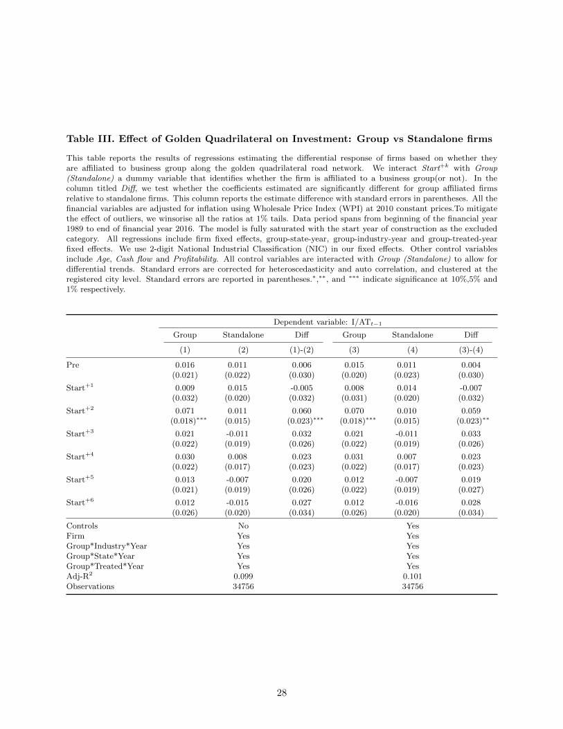
Table III. Effect of Golden Quadrilateral on Investment: Group vs Standalone firms

This table reports the results of regressions estimating the differential response of firms based on whether theyare affiliated to business group along the golden quadrilateral road network. We interact Start+k with Group(Standalone) a dummy variable that identifies whether the firm is affiliated to a business group(or not). In thecolumn titled Diff, we test whether the coefficients estimated are significantly different for group affiliated firmsrelative to standalone firms. This column reports the estimate difference with standard errors in parentheses. All thefinancial variables are adjusted for inflation using Wholesale Price Index (WPI) at 2010 constant prices.To mitigatethe effect of outliers, we winsorise all the ratios at 1% tails. Data period spans from beginning of the financial year1989 to end of financial year 2016. The model is fully saturated with the start year of construction as the excludedcategory. All regressions include firm fixed effects, group-state-year, group-industry-year and group-treated-yearfixed effects. We use 2-digit National Industrial Classification (NIC) in our fixed effects. Other control variablesinclude Age, Cash flow and Profitability. All control variables are interacted with Group (Standalone) to allow fordifferential trends. Standard errors are corrected for heteroscedasticity and auto correlation, and clustered at theregistered city level. Standard errors are reported in parentheses.∗,∗∗, and ∗∗∗ indicate significance at 10%,5% and1% respectively.

Dependent variable: I/ATt−1

Group Standalone Diff Group Standalone Diff

(1) (2) (1)-(2) (3) (4) (3)-(4)

Pre 0.016 0.011 0.006 0.015 0.011 0.004(0.021) (0.022) (0.030) (0.020) (0.023) (0.030)

Start+1 0.009 0.015 -0.005 0.008 0.014 -0.007(0.032) (0.020) (0.032) (0.031) (0.020) (0.032)

Start+2 0.071 0.011 0.060 0.070 0.010 0.059(0.018)∗∗∗ (0.015) (0.023)∗∗∗ (0.018)∗∗∗ (0.015) (0.023)∗∗

Start+3 0.021 -0.011 0.032 0.021 -0.011 0.033(0.022) (0.019) (0.026) (0.022) (0.019) (0.026)

Start+4 0.030 0.008 0.023 0.031 0.007 0.023(0.022) (0.017) (0.023) (0.022) (0.017) (0.023)

Start+5 0.013 -0.007 0.020 0.012 -0.007 0.019(0.021) (0.019) (0.026) (0.022) (0.019) (0.027)

Start+6 0.012 -0.015 0.027 0.012 -0.016 0.028(0.026) (0.020) (0.034) (0.026) (0.020) (0.034)

Controls No YesFirm Yes YesGroup*Industry*Year Yes YesGroup*State*Year Yes YesGroup*Treated*Year Yes YesAdj-R2 0.099 0.101Observations 34756 34756

28

Table IV. Effect of Golden Quadrilateral on Investments at group level

This table presents the estimates from difference-in-differences regression for group-affiliated firms located along thegolden quadrilateral. The dependent variable in columns (1) through (4) is Investment. All the financial variablesare adjusted for inflation using Wholesale Price Index (WPI) at 2010 constant prices.To mitigate the effect ofoutliers, we winsorise all the ratios at 1% tails. Data period spans from beginning of the financial year 1989 to endof financial year 2016. The model is fully saturated with the start year of construction as the excluded category. Allregressions include firm fixed effects, state-year, industry-year and treated-year fixed effects. We use 2-digit NationalIndustrial Classification (NIC) in our fixed effects. Other control variables include Age, Cash flow and Profitability.We also include a set of 10 dummy variables that identify firm size deciles based on Sizet−1. Standard errors arecorrected for heteroscedasticity and auto correlation, and clustered at the registered city level. Standard errors arereported in parentheses.∗,∗∗, and ∗∗∗ indicate significance at 10%,5% and 1% respectively.


(1) (2) (3) (4)

Start−5 -0.080 -0.030 -0.093 -0.021(0.025)∗∗∗ (0.029) (0.029)∗∗∗ (0.026)

Start−4 0.027 -0.000 0.031 0.015(0.035) (0.039) (0.038) (0.040)

Start−3 -0.063 -0.074 -0.056 -0.069(0.066) (0.072) (0.078) (0.074)

Start−2 0.020 0.027 0.014 0.024(0.025) (0.021) (0.028) (0.023)

Start−1 0.023 0.022 0.005 0.002(0.024) (0.026) (0.023) (0.025)

Start+1 -0.004 0.004 0.003 -0.000(0.030) (0.030) (0.028) (0.029)

Start+2 0.059 0.059 0.067 0.057(0.018)∗∗∗ (0.017)∗∗∗ (0.020)∗∗∗ (0.018)∗∗∗

Start+3 0.006 0.009 0.018 0.009(0.024) (0.023) (0.025) (0.023)

Start+4 0.014 0.013 0.023 0.011(0.024) (0.025) (0.022) (0.024)

Start+5 -0.009 -0.013 0.011 -0.008(0.023) (0.023) (0.022) (0.023)

Start+6 -0.003 -0.004 0.004 -0.010(0.027) (0.026) (0.027) (0.027)

Controls No Yes No YesFirm Yes No Yes NoOwner-Group No Yes No YesIndustry*Year Yes Yes Yes YesState*Year Yes Yes Yes YesTreated*Year Yes Yes Yes YesSize dummies No No Yes YesAdj.-R2 0.086 0.108 0.088 0.115Observations 8840 8899 8059 8126

29

Table V. Effect of Golden Quadrilateral on External Financing: Group vs Standalonefirms

This table reports the results on external financing response for firms along the golden quadrilateral road network.We interact Start+k with Group (Standalone) a dummy variable that identifies whether the firm is affiliated to abusiness group(or not). In the column titled Diff, we test whether the coefficients estimated are significantly differentfor group affiliated firms relative to standalone firms. This column reports the estimate difference with standarderrors in parentheses. All the financial variables are adjusted for inflation using Wholesale Price Index (WPI) at2010 constant prices.To mitigate the effect of outliers, we winsorise all the ratios at 1% tails. Data period spans frombeginning of the financial year 1989 to end of financial year 2016. The model is fully saturated with the start year ofconstruction as the excluded category. All regressions include firm fixed effects, group-state-year, group-industry-yearand group-treated-year fixed effects. We use 2-digit National Industrial Classification (NIC) in our fixed effects.Other control variables include Size, Sales Growth and Profitability. All control variables are interacted withGroup (Standalone) to allow for differential trends. Standard errors are corrected for heteroscedasticity and autocorrelation, and clustered at the registered city level. Standard errors are reported in parentheses.∗,∗∗, and ∗∗∗

indicate significance at 10%,5% and 1% respectively.

Dependent variable: Debt/ATt−1

Group Standalone Diff Group Standalone Diff

(1) (2) (1)-(2) (3) (4) (3)-(4)

Pre 0.025 -0.017 0.041 0.015 -0.011 0.026(0.020) (0.029) (0.029) (0.018) (0.029) (0.029)

Start+1 0.042 -0.002 0.044 0.032 -0.002 0.033(0.021)∗∗ (0.017) (0.029) (0.020) (0.016) (0.027)

Start+2 0.086 0.011 0.075 0.080 -0.000 0.080(0.020)∗∗∗ (0.021) (0.026)∗∗∗ (0.020)∗∗∗ (0.020) (0.025)∗∗∗

Start+3 0.110 0.011 0.098 0.105 -0.000 0.105(0.026)∗∗∗ (0.024) (0.035)∗∗∗ (0.025)∗∗∗ (0.025) (0.033)∗∗∗

Start+4 0.123 -0.003 0.125 0.122 -0.018 0.140(0.030)∗∗∗ (0.029) (0.047)∗∗∗ (0.027)∗∗∗ (0.027) (0.041)∗∗∗

Start+5 0.111 0.001 0.109 0.107 -0.013 0.120(0.034)∗∗∗ (0.033) (0.052)∗∗ (0.031)∗∗∗ (0.031) (0.046)∗∗∗

Start+6 0.142 -0.022 0.163 0.149 -0.038 0.187(0.041)∗∗∗ (0.038) (0.062)∗∗∗ (0.037)∗∗∗ (0.035) (0.055)∗∗∗

Controls No YesFirm Yes YesGroup*Industry*Year Yes YesGroup*State*Year Yes YesGroup*Treated*Year Yes YesAdj-R2 0.610 0.640Observations 34756 34756

30

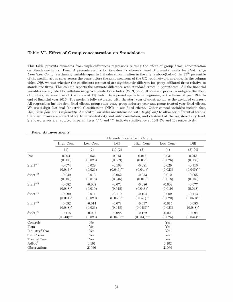
Table VI. Effect of Group concentration on Standalones

This table presents estimates from triple-differences regressions relating the effect of group firms’ concentrationon Standalone firms. Panel A presents results for Investments whereas panel B presents results for Debt. HighConc(Low Conc) is a dummy variable equal to 1 if sales concentration in the city is above(below) the 75th percentileof the median group sales across the years before the announcement of the GQ road network upgrade. In the columntitled Diff, we test whether the coefficients estimated are significantly different for group affiliated firms relative tostandalone firms. This column reports the estimate difference with standard errors in parentheses. All the financialvariables are adjusted for inflation using Wholesale Price Index (WPI) at 2010 constant prices.To mitigate the effectof outliers, we winsorise all the ratios at 1% tails. Data period spans from beginning of the financial year 1989 toend of financial year 2016. The model is fully saturated with the start year of construction as the excluded category.All regressions include firm fixed effects, group-state-year, group-industry-year and group-treated-year fixed effects.We use 2-digit National Industrial Classification (NIC) in our fixed effects. Other control variables include Size,Age, Cash flow and Profitability. All control variables are interacted with High(Low) to allow for differential trends.Standard errors are corrected for heteroscedasticity and auto correlation, and clustered at the registered city level.Standard errors are reported in parentheses.∗,∗∗, and ∗∗∗ indicate significance at 10%,5% and 1% respectively.

Panel A: Investments


High Conc Low Conc Diff High Conc Low Conc Diff

(1) (2) (1)-(2) (3) (4) (3)-(4)

Pre 0.044 0.031 0.013 0.045 0.031 0.015(0.056) (0.026) (0.059) (0.055) (0.026) (0.058)

Start+1 -0.074 0.029 -0.103 -0.081 0.029 -0.110(0.043)∗ (0.023) (0.046)∗∗ (0.044)∗ (0.023) (0.046)∗∗

Start+2 -0.049 0.013 -0.062 -0.053 0.012 -0.065(0.046) (0.018) (0.046) (0.046) (0.018) (0.046)

Start+3 -0.082 -0.008 -0.074 -0.086 -0.009 -0.077(0.048)∗ (0.019) (0.048) (0.048)∗ (0.019) (0.048)

Start+4 -0.099 0.011 -0.110 -0.104 0.009 -0.113(0.051)∗ (0.020) (0.050)∗∗ (0.051)∗∗ (0.020) (0.050)∗∗

Start+5 -0.092 -0.014 -0.078 -0.097 -0.015 -0.083(0.048)∗ (0.023) (0.048) (0.048)∗∗ (0.023) (0.048)∗

Start+6 -0.115 -0.027 -0.088 -0.122 -0.029 -0.094(0.043)∗∗∗ (0.025) (0.043)∗∗ (0.044)∗∗∗ (0.025) (0.044)∗∗

Controls No YesFirm Yes YesIndustry*Year Yes YesState*Year Yes YesTreated*Year Yes YesAdj-R2 0.101 0.102Observations 21066 21066

31

Panel B: External Financing



(1) (2) (1)-(2) (3) (4) (3)-(4)

Pre 0.036 -0.009 0.045 0.095 -0.001 0.096(0.119) (0.028) (0.122) (0.112) (0.030) (0.116)

Start+1 -0.105 0.010 -0.116 -0.072 0.006 -0.078(0.051)∗∗ (0.014) (0.051)∗∗ (0.047) (0.014) (0.048)

Start+2 0.018 0.042 -0.024 0.028 0.023 0.006(0.080) (0.021)∗∗ (0.080) (0.080) (0.022) (0.081)

Start+3 0.024 0.062 -0.038 0.028 0.042 -0.013(0.085) (0.024)∗∗∗ (0.087) (0.089) (0.026) (0.088)

Start+4 0.042 0.034 0.009 0.038 0.010 0.029(0.092) (0.030) (0.091) (0.095) (0.034) (0.093)

Start+5 0.033 0.053 -0.020 0.034 0.023 0.010(0.092) (0.035) (0.091) (0.095) (0.037) (0.091)

Start+6 0.041 0.037 0.004 0.043 0.003 0.041(0.094) (0.036) (0.090) (0.098) (0.041) (0.093)


32

Table VII. Effect of Group Concentration on Standalones: High Exporting Industries

This table presents estimates from triple-differences regressions relating the effect of group firms’ concentration onStandalone firms in high exporting industries. Panel A presents results for Investments whereas panel B presentsresults for Debt. We keep industries if export earnings to sales in each industry is above(below) the 75th percentile ofthe median export earnings to sales across the years before the announcement of the GQ road network upgrade. HighConc(Low Conc) is a dummy variable equal to 1 if sales concentration in the city is above(below) the 75th percentileof the median group sales across the years before the announcement of the GQ road network upgrade. In the columntitled Diff, we test whether the coefficients estimated are significantly different for group affiliated firms relative tostandalone firms. This column reports the estimate difference with standard errors in parentheses. All the financialvariables are adjusted for inflation using Wholesale Price Index (WPI) at 2010 constant prices.To mitigate the effectof outliers, we winsorise all the ratios at 1% tails. Data period spans from beginning of the financial year 1989 toend of financial year 2016. The model is fully saturated with the start year of construction as the excluded category.All regressions include firm fixed effects, group-state-year, group-industry-year and group-treated-year fixed effects.We use 2-digit National Industrial Classification (NIC) in our fixed effects. Other control variables include Size,Age, Cash flow and Profitability. All control variables are interacted with High(Low) to allow for differential trends.Standard errors are corrected for heteroscedasticity and auto correlation, and clustered at the registered city level.Standard errors are reported in parentheses.∗,∗∗, and ∗∗∗ indicate significance at 10%,5% and 1% respectively.

Panel A: Investments



(1) (2) (1)-(2) (3) (4) (3)-(4)

Pre 0.103 0.051 0.051 0.087 0.053 0.034(0.103) (0.020)∗∗ (0.105) (0.099) (0.020)∗∗∗ (0.101)

Start+1 -0.093 0.012 -0.106 -0.100 0.012 -0.112(0.041)∗∗ (0.016) (0.044)∗∗ (0.042)∗∗ (0.017) (0.045)∗∗

Start+2 -0.086 0.033 -0.119 -0.098 0.031 -0.129(0.059) (0.015)∗∗ (0.061)∗ (0.059)∗ (0.015)∗∗ (0.060)∗∗

Start+3 -0.112 0.004 -0.116 -0.125 0.002 -0.127(0.057)∗ (0.020) (0.063)∗ (0.057)∗∗ (0.020) (0.062)∗∗

Start+4 -0.133 0.027 -0.159 -0.148 0.024 -0.172(0.061)∗∗ (0.021) (0.058)∗∗∗ (0.061)∗∗ (0.021) (0.057)∗∗∗

Start+5 -0.117 -0.004 -0.113 -0.133 -0.007 -0.127(0.069)∗ (0.022) (0.066)∗ (0.068)∗ (0.022) (0.064)∗∗

Start+6 -0.134 0.005 -0.139 -0.156 0.004 -0.160(0.059)∗∗ (0.025) (0.058)∗∗ (0.059)∗∗∗ (0.025) (0.058)∗∗∗


33

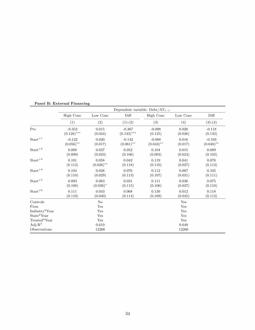
Panel B: External Financing



(1) (2) (1)-(2) (3) (4) (3)-(4)

Pre -0.352 0.015 -0.367 -0.098 0.020 -0.118(0.128)∗∗∗ (0.024) (0.133)∗∗∗ (0.125) (0.026) (0.132)

Start+1 -0.122 0.020 -0.142 -0.088 0.016 -0.103(0.056)∗∗ (0.017) (0.061)∗∗ (0.043)∗∗ (0.017) (0.048)∗∗

Start+2 0.088 0.037 0.052 0.104 0.015 0.089(0.099) (0.023) (0.106) (0.093) (0.024) (0.102)

Start+3 0.101 0.058 0.042 0.119 0.041 0.078(0.112) (0.026)∗∗ (0.118) (0.110) (0.027) (0.113)

Start+4 0.104 0.028 0.076 0.112 0.007 0.105(0.110) (0.029) (0.113) (0.107) (0.031) (0.111)

Start+5 0.093 0.063 0.031 0.111 0.036 0.075(0.108) (0.036)∗ (0.115) (0.106) (0.037) (0.110)

Start+6 0.111 0.043 0.068 0.130 0.012 0.118(0.110) (0.040) (0.114) (0.109) (0.045) (0.112)


34

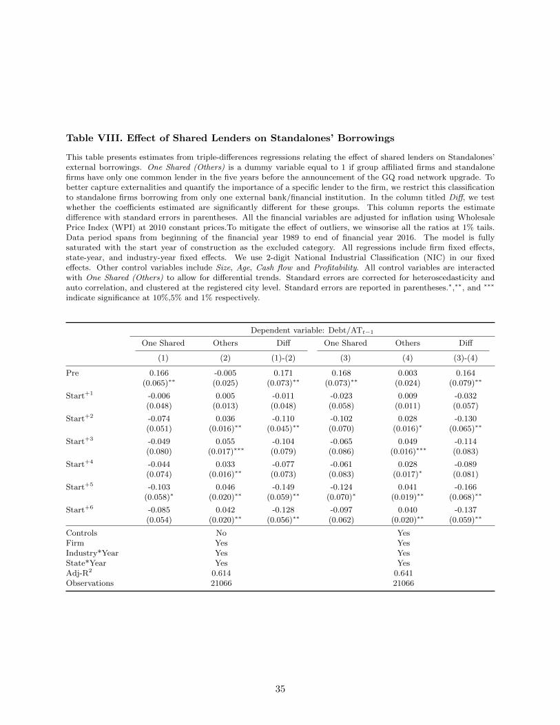
Table VIII. Effect of Shared Lenders on Standalones’ Borrowings

This table presents estimates from triple-differences regressions relating the effect of shared lenders on Standalones’external borrowings. One Shared (Others) is a dummy variable equal to 1 if group affiliated firms and standalonefirms have only one common lender in the five years before the announcement of the GQ road network upgrade. Tobetter capture externalities and quantify the importance of a specific lender to the firm, we restrict this classificationto standalone firms borrowing from only one external bank/financial institution. In the column titled Diff, we testwhether the coefficients estimated are significantly different for these groups. This column reports the estimatedifference with standard errors in parentheses. All the financial variables are adjusted for inflation using WholesalePrice Index (WPI) at 2010 constant prices.To mitigate the effect of outliers, we winsorise all the ratios at 1% tails.Data period spans from beginning of the financial year 1989 to end of financial year 2016. The model is fullysaturated with the start year of construction as the excluded category. All regressions include firm fixed effects,state-year, and industry-year fixed effects. We use 2-digit National Industrial Classification (NIC) in our fixedeffects. Other control variables include Size, Age, Cash flow and Profitability. All control variables are interactedwith One Shared (Others) to allow for differential trends. Standard errors are corrected for heteroscedasticity andauto correlation, and clustered at the registered city level. Standard errors are reported in parentheses.∗,∗∗, and ∗∗∗

indicate significance at 10%,5% and 1% respectively.


One Shared Others Diff One Shared Others Diff

(1) (2) (1)-(2) (3) (4) (3)-(4)

Pre 0.166 -0.005 0.171 0.168 0.003 0.164(0.065)∗∗ (0.025) (0.073)∗∗ (0.073)∗∗ (0.024) (0.079)∗∗

Start+1 -0.006 0.005 -0.011 -0.023 0.009 -0.032(0.048) (0.013) (0.048) (0.058) (0.011) (0.057)

Start+2 -0.074 0.036 -0.110 -0.102 0.028 -0.130(0.051) (0.016)∗∗ (0.045)∗∗ (0.070) (0.016)∗ (0.065)∗∗

Start+3 -0.049 0.055 -0.104 -0.065 0.049 -0.114(0.080) (0.017)∗∗∗ (0.079) (0.086) (0.016)∗∗∗ (0.083)

Start+4 -0.044 0.033 -0.077 -0.061 0.028 -0.089(0.074) (0.016)∗∗ (0.073) (0.083) (0.017)∗ (0.081)

Start+5 -0.103 0.046 -0.149 -0.124 0.041 -0.166(0.058)∗ (0.020)∗∗ (0.059)∗∗ (0.070)∗ (0.019)∗∗ (0.068)∗∗

Start+6 -0.085 0.042 -0.128 -0.097 0.040 -0.137(0.054) (0.020)∗∗ (0.056)∗∗ (0.062) (0.020)∗∗ (0.059)∗∗

Controls No YesFirm Yes YesIndustry*Year Yes YesState*Year Yes YesAdj-R2 0.614 0.641Observations 21066 21066

35

Table IX. Effect of Lenders’ Group Exposure on Standalones’ Borrowings

This table presents estimates from triple-differences regressions relating the effect of lenders’ group exposure onStandalone firms. High Exp(Low Exp) is a dummy variable equal to 1 if banks’ group exposure is above(below) the75th percentile of the median group debt across the years before the announcement of the GQ road network upgrade.In the column titled Diff, we test whether the coefficients estimated are significantly different for group affiliatedfirms relative to standalone firms. This column reports the estimate difference with standard errors in parentheses.All the financial variables are adjusted for inflation using Wholesale Price Index (WPI) at 2010 constant prices.Tomitigate the effect of outliers, we winsorise all the ratios at 1% tails. Data period spans from beginning of thefinancial year 1989 to end of financial year 2016. The model is fully saturated with the start year of constructionas the excluded category. All regressions include firm fixed effects, group-state-year, group-industry-year andgroup-treated-year fixed effects. We use 2-digit National Industrial Classification (NIC) in our fixed effects. Othercontrol variables include Size, Age, Cash flow and Profitability. All control variables are interacted with High(Low)to allow for differential trends. Standard errors are corrected for heteroscedasticity and auto correlation, andclustered at the registered city level. Standard errors are reported in parentheses.∗,∗∗, and ∗∗∗ indicate significanceat 10%,5% and 1% respectively.


High Exp Low Exp Diff High Exp Low Exp Diff

(1) (2) (1)-(2) (3) (4) (3)-(4)

Pre -0.012 -0.022 0.010 -0.014 -0.009 -0.004(0.031) (0.033) (0.038) (0.032) (0.031) (0.037)

Start+1 0.005 0.015 -0.010 0.001 0.016 -0.014(0.020) (0.018) (0.024) (0.022) (0.018) (0.025)

Start+2 0.001 0.034 -0.033 -0.013 0.022 -0.035(0.026) (0.025) (0.022) (0.027) (0.026) (0.024)

Start+3 0.030 0.074 -0.045 0.010 0.058 -0.048(0.029) (0.027)∗∗∗ (0.020)∗∗ (0.031) (0.029)∗∗ (0.020)∗∗

Start+4 0.018 0.042 -0.024 -0.001 0.025 -0.026(0.037) (0.032) (0.018) (0.039) (0.036) (0.020)

Start+5 0.033 0.063 -0.030 0.010 0.043 -0.033(0.041) (0.039) (0.009)∗∗∗ (0.044) (0.041) (0.014)∗∗

Start+6 0.029 0.038 -0.009 0.009 0.018 -0.009(0.041) (0.040) (0.008) (0.043) (0.043) (0.012)


36

Appendix Table I. Variable Definitions

Variable Definition

Agei,t Firm i’s age since incorporation in year t.

Cash flowi,t Ratio of cash flow from operations relative to book value of assets in year t.

Debti,t Total outstanding debt from bank and institutions of firm i in year t relative to book valueof assets in year t.

EBITDAi,t Earnings before interest, depreciation, taxes, and amortization of firm i in year t.

Groupg A dummy variable which takes a value of one if firm i is a group firm and zero otherwise.

Investmentsi,t/TAi,t Ratio of gross plant of firm i in year t relative to book value of assets in year t.

Profitabilityi,t Earnings before interest, depreciation, taxes, and amortization relative to book value ofassets in year t.

Return on Assetsi,t Profit after tax of firm i in year t relative to book value of assets in year t.

Sales Growthi,t Measured as the annual growth rate of sales of firm i in year t.

Sizei,t Measured as the log of book value of assets in year t.

Total Assetsi,t Total book value assets of firm i in year t.

37

Appendix A.

Empirical Appendix

Data Source on GQ Details: According to National Highway Authority of India (NHAI), the GQ highwaywas a collection of 128 contracts which was implemented all over the country starting in 1998. By Feb 2015, all ofthese contracts had been executed and the project completed. We compile information on each of these 128 projectsfrom the annual reports of NHAI from 1998-99 to 2013-2014 as well as from the Ministry of Roads, Transport andHighways (MORTH). These annual reports identified the project name for the highway stretch, the length of thehighway stretch, the national highway number, the start date for the project, cost of the stretch, financiers of thestretch and target and actual completion dates.

Mapping GQ Projects to cities: In most cases, the name of the project indicated the start and end towns ona highway stretch along with highway number. This information was used to identify city names in CMIE Prowessto identify location along these cities. In some cases, the project name was not clear or the town name could not belocated. In such cases, we used information on the NHAI website for the highway project chainage and mapped tothe preceding or succeeding highway stretch.

Implementation Date: We assign the start year of construction of a stretch and adjust for differences infinancial year. We then match city names to individual highway project stretches and their start dates. In doing so,we allow firms atleast six months to respond to any such treatment. Several cities touch two or more stretches ofhighway. For such cities, we allocated them to the latest start date as they had access to some connectivity beforeother cities did. However, we did not allocate the start year as an earlier year if the earlier GQ project was River OverBridge (ROB), a bridge section, or a short bypass, as most of these constructions were small in terms of kilometersof length.

38

Appendix B.

Total Factor Productivity: Estimation Procedure

Output is measured by the value of total sales that includes income earned by the company from the sale of industrialgoods as well as their raw materials, byproducts, stores and waste.

Capital is measured by gross fixed assets of a firm that includes both tangible assets, such as land, building, plant,and machinery, and intangible assets, such as goodwill assets, software, etc.

Labor, which is a freely moving variable in the estimation of the production function, is measured by compensationto employees that includes all cash and payments in kind made by a company to its employees.

Intermediate inputs, is the combined value of raw materials, power and fuel consumptions. Raw materials are thesum of expenses on raw materials, stores, spares and tools used up by firms in the production process. Power andfuel include expenses made by the firms on power, fuel and water. The sum of these three variables is used as theproxy in the estimation of the production function.

In estimating firm-level TFP, we include firm size as a control variable.

39

Investment Opportunities and Financing …ifrogs.org › PDF › CONF_2017 ›...

Documents

Transcript of Investment Opportunities and Financing …ifrogs.org › PDF › CONF_2017 ›...