Investment Climate and Firm Performance in Developing Economies

By David Dollar, Mary Hallward-Driemeier, and Taye Mengistae*

Development Research Group, World Bank

November 2003

Abstract: Drawing on recently completed firm-level surveys in Bangladesh, China, India, and Pakistan, this paper investigates the relationship between investment climate and firm performance. These standardized surveys of large, random samples of firms in common sectors reveal that objective measures of the investment climate vary significantly across countries and across locations within these countries. The authors focus primarily on measures of the time or monetary cost of different bottlenecks (e.g., days to clear goods through customs, days to get a telephone line, sales lost to power outages). For many of these costs, the obstacles are lower in China than in Bangladesh or India, which in turn are superior to Pakistan. There is also systematic variation across cities within countries. The authors estimate a production function for garment firms and show that total factor productivity is systematically related to the investment climate indicators. Factor returns (wages for a given quality of human capital and rate of profit) are also higher where investment climate is better. These higher returns then have dynamic effects: accumulation and growth at the firm level is higher where investment climate is good.

* We would like to thank Aart Kraay, Norman Loayza, and John Sutton for helpful comments on an initial draft of this paper and Sergio Kurlat and Victoria Levin for excellent research assistance. We are grateful for the financial support from the United Kingdom’s Department for International Development and the Research Support Budget. Views expressed are those of the authors and do not necessarily reflect official views of the World Bank.

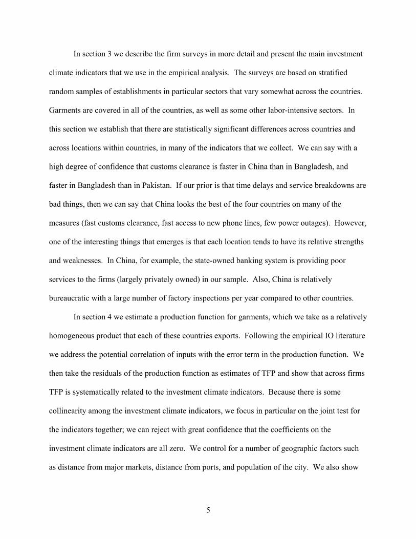
1. Introduction The developing world contains both the fastest-growing and slowest-growing locations

on earth. If one ranks countries by 1990 per capita GDP and looks at subsequent growth rates,

one finds that virtually all rich-country growth rates are in a tight band between 1 and 3, whereas

poor-country growth rates vary from highly negative up to China’s spectacular 7 percent per

annum (figure 1). Within countries as well there are often large differences in growth rates of

different regions or cities. This is the general puzzle with which we are concerned: why some

locations in the developing world grow so rapidly, while others stagnate. There is not likely to

be a single explanation of this phenomenon. We are going to explore the hypothesis that

variations in “investment climate” across locations can explain much of this variation in growth

rates.

What we mean by investment climate is the institutional, policy, and regulatory

environment in which firms operate – factors that influence the link from sowing to reaping. If

the local government is highly bureaucratic and corrupt; if government’s own provision or

regulation of infrastructure and financial services is inefficient so that firms cannot get reliable

services – then returns on potential investments will be low and uncertain, and one would not

expect much accumulation and growth in these environments. On the other hand, in developing

locations that create a good governance environment, returns and accumulation should be high.

This concept of investment climate is closely related to what some authors in the macro

literature have called high-quality institutions (Knack and Keefer 1995, Acemoglu, Johnson, and

Robinson 2001) or “social infrastructure” (Hall and Jones, 1999). The latter authors, for

example, write:

Our hypothesis is that differences in capital accumulation, productivity, and therefore output per worker are fundamentally related to differences in social infrastructure across

2

countries. By social infrastructure we mean the institutions and government policies that determine the economic environment within which individuals accumulate skills, and firms accumulate capital and produce output. A social infrastructure favorable to high levels of output per worker provides an environment that supports productive activities and encourages capital accumulation, skill acquisition, invention, and technology transfer….Social institutions to protect the output of individual productive units from diversion are an essential component of a social infrastructure favorable to high levels of output per worker... Regulations and laws may protect against diversion, but they all too often constitute the chief vehicle of diversion in an economy.

This idea has been investigated in the cross-country studies noted above using proxies for

strength of property rights and government efficiency. This literature is suggestive, but suffers

from three problems: (1) there are not that many countries in the world so that the statistical

results are not that robust;1 (2) the proxies used as explanatory variables do not provide much

specific guidance about what countries need to do to improve their investment climates; and (3)

using national-level data assumes that the investment climate is the same across locations within

a country, when in fact there may be interesting variation based on local governance.

Our contribution is to go down to the firm level to collect data on how institutional and

policy weaknesses actually affect firms. We have collaborated with in-country partners on large,

random surveys of establishments in Bangladesh (924), China (1500), India (1900), and Pakistan

(965). These surveys include data on inputs and outputs, as well as on objective aspects of the

investment climate. We describe these in more detail below, but in general we are interested in

aspects of the environment such as how long it takes to get goods through customs, how long it

takes to get a phone line, or how frequent and disruptive are power outages. We developed the

questionnaire through pilot testing and with input from firms about the key bottlenecks that they

face. Note that the four countries reflect the puzzle that we start with: China, Bangladesh, India,

and Pakistan had similar per capita GDP in 1990, but in the subsequent decade their growth rates

1 See Levine and Renelt (1992); Rodriguez and Rodrik (2000); Dollar and Kraay (2003).

3

were 7.2 percent, 2.7 percent, 4.1 percent, and 1.3 percent, respectively. They are also all major

exporters of garments and other labor-intensive manufactures. So, it is natural to inquire why

their performances have been so diverse.

In the next section we present the analytical framework for this study. We draw on

models from empirical IO (industrial organization), trade theory, and growth theory. The story

we want to explore is the following: if there are systematic differences in investment climate

across locations, then for the plants that exist in these locations, total factor productivity should

be related to investment climate. Bureaucratic harassment, power outages, etc. result in less

value added being produced from the same capital and labor in different locations. We then turn

to trade theory and argue that since these countries are exporting similar products (have the same

comparative advantage), poor investment climate locations would have to have lower wages and

return to capital in order to compete. To foreshadow our results, if Bangladesh has a worse

investment climate than China, it can still export garments, but it will need lower wages and

lower return to capital in order to do so at the same prices as Chinese exporters. Turning to

growth theory, it is these potential differences in rates of return to accumulation that lead to the

prediction that locations with poor institutions and policies will have lower rates of accumulation

and slower growth. These models provide a framework for investigating whether objective

measures of the investment climate are related to six outcome variables that we obtain from the

firm surveys: estimates of total factor productivity, average wages (controlling for human

capital), rate of return on fixed assets, and growth rates of output, fixed assets, and employment.

We note that there are other, not mutually exclusive hypotheses, that could account for why

locations perform so differently – in particular that natural geography and/or agglomeration

economies could be important.

4

In section 3 we describe the firm surveys in more detail and present the main investment

climate indicators that we use in the empirical analysis. The surveys are based on stratified

random samples of establishments in particular sectors that vary somewhat across the countries.

Garments are covered in all of the countries, as well as some other labor-intensive sectors. In

this section we establish that there are statistically significant differences across countries and

across locations within countries, in many of the indicators that we collect. We can say with a

high degree of confidence that customs clearance is faster in China than in Bangladesh, and

faster in Bangladesh than in Pakistan. If our prior is that time delays and service breakdowns are

bad things, then we can say that China looks the best of the four countries on many of the

measures (fast customs clearance, fast access to new phone lines, few power outages). However,

one of the interesting things that emerges is that each location tends to have its relative strengths

and weaknesses. In China, for example, the state-owned banking system is providing poor

services to the firms (largely privately owned) in our sample. Also, China is relatively

bureaucratic with a large number of factory inspections per year compared to other countries.

In section 4 we estimate a production function for garments, which we take as a relatively

homogeneous product that each of these countries exports. Following the empirical IO literature

we address the potential correlation of inputs with the error term in the production function. We

then take the residuals of the production function as estimates of TFP and show that across firms

TFP is systematically related to the investment climate indicators. Because there is some

collinearity among the investment climate indicators, we focus in particular on the joint test for

the indicators together; we can reject with great confidence that the coefficients on the

investment climate indicators are all zero. We control for a number of geographic factors such

as distance from major markets, distance from ports, and population of the city. We also show

5

that the results are robust to including country dummies, so that identification comes only from

the variation across locations within a country. The coefficients are economically meaningful.

For example, they suggest that the good investment climate indicators in Shanghai give its

garment factories a productivity advantage over South Asian cities (advantages of 18 percent

versus Bangalore, 43 percent versus Dhaka, 78 percent versus Calcutta, and 81 percent versus

Karachi). In this section we also estimate equations for average wages and profits relative to

fixed assets, for garment firms. After controlling for firm-specific characteristics of the labor

force (schooling, experience), investment climate indicators are related to wages in the intuitive

direction. Similarly, investment climate differences are related to the rate of profit at the

establishment level.

In section 5 we estimate equations for the other outcome variables of interest. Here we

pool the data across industries in order to get the maximum number of observations, and include

industry dummies to account for differences in industry price and output cycles. The growth

rates of output, capital stock, and employment are calculated for the two years prior to the survey

date. In each case we can estimate an equation and find that the investment climate measures are

significant determinants of input and output growth, with plausible magnitudes for the

coefficients. In some of these equations the geography variables work fairly well also. It seems

very likely that there is some truth to the stories that emphasize natural geography and

agglomeration economies. We do not find manufacturing plants randomly distributed around

rural locations. That said, most of the locations we cover are large cities, and many of them are

ports, with potential access to the international market. Nevertheless, locations such as Karachi

(Pakistan), Chittagong (Bangladesh), Calcutta (India), and Tianjin (China) are not performing as

well as Guangzhou and Shanghai in China. So, while being a big port city is an advantage, the

6

advantage can easily be undone by poor local governance. The fact that the investment climate

indicators are highly significant even after controlling for geography, population, and even

country dummies, is consistent with the view that local governance is important.

Thus, we conclude in the final section that a number of major cities in China have created

quite good investment climates, compared to other locations at similar levels of development ten

years ago and with similar good potential for access to the international market. The result of

this better investment climate is that there is a strong connection between sowing and reaping.

The plants that exist in these good environments produce more value from given capital and

labor and thus can pay higher wages and have higher profits. These superior returns then spur

greater accumulation, so that the typical plant is rapidly expanding capital stock, employment,

and output. Given the large differences in investment climate that we find in our surveys, it is

not surprising that growth rates vary so much across these locations.

2. Analytical Framework

The analytical framework that we have in mind for our investigation of the relationship

between investment climate and firm productivity and growth combines elements of theory from

industrial organization, trade, and growth.

The empirical IO literature often starts with a simple production function written in logs

as:

(1) jjim

jiK

jiLo

ji mkly i εαααα ++++=

where y is gross output, k is capital input, l is labor input, m is material input,ε is an unobserved

productivity shock, and i and j index firms and locations. We are working with firms in different

countries, but we assume that in a common export sector, such as garments, firms face the same

international price for their output. There is a world market price for men’s shirts of a certain

7

quality, and all firms are price-takers. We further assume that the countries allow firms in these

export sectors to purchase capital equipment and raw materials at world market prices. So, the

dollar value of capital and materials and the dollar value of output can be compared across

countries. Wages are going to diverge, as we will see below, so the labor input in the production

function needs to be in physical rather than value units (e.g., number of workers, adjusted for

years of schooling and experience).

In general the coefficients of this production function cannot be estimated consistently

with OLS, because there are good reasons to think that the productivity shock is correlated with

at least some of the inputs. Olley and Pakes (1996) divide the productivity shock into two

components, ω , which is a state variable that affects the firm’s decisions, while ε is a pure

shock that does not.

(2) jji

jim

jiK

jiLo

ji mkly i εωαααα +++++=

Suppose that labor is adjusted relatively easily, and capital not. In this context, a good

productivity state leads the firm to use more labor – that is, labor input is correlated with part of

the unobserved error. An OLS estimate that does not adjust for this will have biased estimates

for the coefficients of both labor and capital. We are going to use the technique introduced by

Levinsohn and Petrin (2000) to address this endogeneity problem and arrive at consistent

estimates of the coefficients of (2).

Where firms are producing in the same location, it makes sense to think of them facing

the same basic investment climate: quality of public infrastructure, efficiency of regulation,

degree of corruption, access to financial services. However, we want to explore the idea that

these factors vary to a large extent across countries and even to some considerable extent across

cities within developing countries. So, we introduce into the production function a term, A, that

8

captures the influence of the investment climate on production of the firm. A, in turn, we will

model as a function of observable indicators of the investment climate, X:

(3) jji

jjim

jiK

jiLo

ji Amkly i εωαααα ++++++=

(4) j η+∂= jj XA

If we have consistent estimates of the parameters of the production function, then we can

estimate the effect of investment climate indicators as:

(5) [ ] ji

ji

jjim

jiK

jiLo

ji mkly εωαααα - - - - ++Χ∂=

The left-hand-side here is what is conventionally called total factor productivity. We are in

effect decomposing TFP into a part that depends on the local investment climate, plus a firm-

specific productivity shock.

Equation (5) is the first one that we are going to estimate across a sample of garment

firms from different countries. Now, foreshadowing our results, suppose that we find that the

investment climate is better in China than in Bangladesh, so that China’s typical firm is

producing more value added than the typical Bangladeshi firm, with the same capital and labor

inputs. How then does Bangladesh compete with China? Why would any Bangladeshi firms

survive? Here we turn to international trade theory.

Schott (2000) finds that the basic Heckscher-Ohlin model of trade explains global

production patterns fairly well, provided that we recognize that countries are in different “cones

of diversification.” In particular, he estimates a labor-abundant cone that includes countries with

overall capital-labor ratios up to $5,000. It happens that all of the countries in our sample are in

this cone. Thus, they have comparative advantage in the same labor-intensive agricultural and

manufacturing products, and tend to import more capital- and skill-intensive items. In this

model, these countries in the same cone would have the same factor prices, provided that they all

9

have the same As in their production functions. In the trade literature, differences in the “As” are

usually interpreted as differences in technology. But the algebra is the same if we interpret these

as differences in investment climate. It is straightforward to introduce into the trade model

neutral differences in As across countries. In other words, if investment climate varies across

countries and affects different industries to the same extent, then the basic predictions of the

trade model go through, with one important change: if China is 20% better than Bangladesh at

everything, then prices for capital and labor have to be 20% higher in China than in Bangladesh.

Firms in China and Bangladesh will choose the same techniques, since they face the same

relative factor prices. With 20% lower factor prices, Bangladeshi firms will be able to export at

the same prices as Chinese firms. So, from trade theory we derive a second equation to estimate:

(6) ji

jji

ji vw +Χ+Ζ= φγ

The average wage will vary across firms based on firm characteristics, Z (eg., average schooling

of the firm’s workers, average experience) and the local investment climate indicators. This

model only makes sense if there is restricted labor mobility across countries, which is clearly the

case for the developing countries we consider. It is also necessary that there be restrictions on

outflows of capital (otherwise all of the capital would leave Pakistan) – and in fact all of the

countries we consider do limit capital outflows.

Finally, we turn to the issue of growth. Ventura (2000) embeds a Heckscher-Ohlin trade

model of the kind above, into a Ramses growth model. In the one-sector Ramses growth model,

a difference in investment climate in two countries that are otherwise the same would result in a

higher return to capital in the good environment and a higher investment and growth rate

initially. As capital is accumulated, however, diminishing returns reduce profitability and the

growth rate slows down. In the steady state the two countries would have the same growth rate.

10

Ventura shows that the multi-sector trade model suggests that the transition could be prolonged

for the following reason: Imagine that the agricultural sector is the most labor-intensive, and that

the “cone” that China, Bangladesh, et al. are in also includes labor-intensive manufactures. The

latter are more capital intensive than agriculture, but less capital intensive than other

manufactured products.

In this model, if all countries had the same “As” for their production functions, then in

general poor countries would grow more rapidly than rich ones. They would have a higher

return to capital and would accumulate rapidly. As they did, labor would shift from agriculture

to labor-intensive manufactures. As long as the country remains within the “cone,” the return to

capital would be stable and one would not have the offset to the high growth rate of diminishing

returns. Eventually the capital accumulation leads the country to a more capital-abundant cone

with lower return to capital. So, in the long run the model performs like the traditional model –

but the model provides a plausible explanation for why the transition is long.

Again, it is straightforward to introduce systematic differences across countries in the As

of the production functions. If the investment climate is very poor in Pakistan, then it will not

have a high return to capital and no strong incentive to accumulate. (Some capital mobility from

rich to poor countries would reinforce this process. If the return to capital is very high in China

and very low in Pakistan, then some capital will flow from rich countries to China and accelerate

the growth process of labor shifting out of agriculture into labor-intensive manufactures.) This

kind of model in which A varies systematically across countries is behind the empirical growth

literature, which is trying to explain these differences in terms of institutional, policy, and other

variables.

11

A range of empirical studies [Knack and Keefer (1995); Hall and Jones (1999);

Acemoglu, Johnson, and Robinson (2001)] find a relationship between long-run growth, on the

one hand, and measures of institutional quality, on the other. We are going to do something

analogous with firm-level data. In particular, we are going to explore whether at the firm level

growth rates of output, capital stock, and employment are systematically related to measures of

the investment climate. Note, however, that at the firm level one would not expect firms of all

sectors to be expanding rapidly in a good investment climate – because of comparative

advantage. If rapid accumulation is shifting comparative advantage, then firms in emerging

sectors would be growing rapidly, while firms in sectors of declining comparative advantage

would not be. If two countries are in different cones of specialization, then a good investment

climate could result in different sectors expanding in these countries. So, in pooling data on firm

growth in our four countries, we are making use of the fact that they are in the same cone of

diversification and that we think that a sector such as garments would be expanding as these

countries accumulate capital and as their labor force shifts out of agriculture.

To summarize: there are theoretical reasons to expect that a poor investment climate

would lead to lower TFP at the firm level, lower factor prices (both lower wages for a given

quality of labor and a lower return to capital), and slower growth of capital, employment, and

output for the typical firm in sectors which should be expanding as the country accumulates

capital. The faster growth is a transitional phenomenon, but the transition could be quite long.

In any empirical investigation it is useful to think about what kind of evidence would refute the

main hypotheses and what kind of competing models might explain the observation that firms

are growing much more rapidly in some locations of the developing world than in others. In the

next section we are going to explore whether a number of investment climate indicators that we

12

have collected from firms vary systematically across locations. If the indicators do not vary

across locations, then they will not be able to explain differences in performance. We then relate

the investment climate indicators to six different left-hand-side variables, following the

discussion above. The dependent variables are firm-level TFP, average wage, average return to

capital, capital stock growth, employment growth, and output growth. To accept the notion that

investment climate is important, one would need to find a consistent pattern of relationships

between investment climate, on the one hand, and firm productivity, factor prices, and growth

rates, on the other. Finally, we will control for other variables that we associate with competing

(but not mutually exclusive) hypotheses, especially the idea that agglomeration economies and

natural geography are important for explaining the location of production around the world.2

3. Measuring Investment Climate with Firm-Level Data

The empirical growth literature has used a number of proxy variables that get at different

aspects of the investment climate: subjective measures of the strength of the rule of law,

expropriation risk, and government effectiveness in providing public services. This approach has

the advantage that it can cover a lot of countries and establish a general link from investment

climate to growth. The disadvantage of these indicators is that they are subjective and do not

provide much specific guidance about how the investment climate affects firms and about which

aspects of the investment climate are especially important. It is for these reasons that we turned

to firm-level data to get better measures of the investment climate and a clearer understanding of

2 Krugman and Venables (1999) argue that in many lines of production there are advantages to producers locating close together and that these agglomeration economies could explain the concentration of production in certain locations. Limao and Venables (2000) provide cross-country empirical support for this notion. Gallup and Sachs (1999) focus on a different aspect of geography: the debilitating effect of malaria and other diseases and their impact on productivity. In our work we will introduce variables that attempt to capture the importance of being close to markets and major concentrations of population, as highlighted by the Krugman-Venables work. We are not well placed at the moment to look at the geographic factors emphasized in Sachs’s recent work, because the locations that we cover in this study do not have major malaria or disease problems. As the investment climate surveys are extended to more locations (surveys for example are underway in Tanzania and Uganda in Africa and in India, including states such as Uttar Pradesh), it will be possible to examine this idea as well.

13

how it relates to firm performance and growth. At the end of the day, all growth occurs at the

firm level (defining firms broadly to include farms and productive households).

The investment climate measures that we are going to present are based on large, random

samples of firms in specific sectors in four countries: Bangladesh, China, India, and Pakistan.

This investment climate survey project has evolved over time and has a number of precursors

within the World Bank: the Regional Program on Enterprise Development has been collecting

firm-level data in Sub-Saharan Africa countries for a decade; the World Business Environment

Survey covered small numbers of firms in a large number of countries; and the research

department sponsored firm surveys in India, Bolivia, and Morocco in 1999-2000. Each of these

surveys used somewhat different questions and survey methodologies. Based on this experience,

we have developed a common set of objective questions that will be included in all future

surveys sponsored by the Bank. Bangladesh, China, India, and Pakistan are among the first

countries to be covered by this common survey instrument. Each survey also uses a similar

methodology: a stratified random sample of establishments is drawn in each country. It is

stratified first on sub-sector: we want to collect production and investment data from firms

producing broadly the same product. The garment sector was covered in each of these countries

and is the best example of a relatively homogeneous industry in which we have observations

from all four countries and for which we can estimate a production function (in the next section).

The other sectors covered are textiles, leather products, and food products in Bangladesh;

business services, IT, electronic equipment and components, consumer appliances, and auto parts

in China; textiles, leather goods, food products, drugs and pharmaceuticals, electronic consumer

goods, metal products, plastics and machine tools in India; and textiles, leather goods, food

processing, sporting goods, electronics, chemicals, and IT in Pakistan.

14

The samples are also stratified based on location. The locations covered are Dhaka and

Chittagong in Bangladesh; Beijing, Chengdu, Guangzhou, Shanghai, and Tianjin in China; 38

cities in India; and 12 in Pakistan including Karachi, Lahore, Islamabad, Faislabad and

Peshawar. The sample sizes are 1001 in Bangladesh, 1900 in India, 879 in Pakistan, and 1500 in

China. In each country we worked with a local partner to draw these samples and to train

enumerators to visit the establishments. The typical observation is based on a three-hour visit to

the factory. Because of the interest and support from the business community in each country,

we have been able to attain high levels of cooperation from firms.

Table 1 presents a broad list of quantitative measures of the investment climate collected

by the survey. Within this list there are sometimes multiple indicators that cover a similar theme.

For example, as a measure of access to finance, there is information on use of overdraft facilities

as well as the share of firms that have a bank loan. Within the same theme, the correlation of the

indicators is high. Thus, while we will discuss the longer list, in the empirical analysis in the

next two sections we decided to focus on five indicators (highlighted in bold in Table 1). The

five were selected based on being available for all four countries and capturing different key

dimensions of the investment climate. We should say at the outset that one potential issue to be

aware of is the problem of omitted variables. The list of indicators that we have arrived at has

evolved based on interviews with firms, including open-ended questions about the main

problems that they face. Nevertheless, it is always possible that something important is

overlooked.

The survey includes a number of questions that get at the efficiency of the government in

providing services that are essential for firms. For example, a question that relates both to

bureaucracy in general and to bureaucratic control of access to international markets in

15

particular, is how long it took importing firms to get their last shipment of goods through

customs. China comes out best in this category (7.9 days), followed by India (9.1), Bangladesh

(11.7), and Pakistan (17.2). Note that response to this question is limited to firms that actually

import materials, so that the number responding is considerably smaller than the overall sample

size (434 firms in China, for example). Nevertheless, standard errors are small, and we can say

that China is significantly better than Bangladesh, which in turn is significantly better than

Pakistan, in terms of moving goods through customs. We also ask exporting firms how long it

took to clear their last shipment of exports through customs. Export clearance times tend to be

shorter than import clearance times, but there is still quite a bit of variation across countries, with

again China being the best (5.4 days) and Pakistan the worst (9.7 days) on this dimension.

Our experience with this survey work over several years has taught us that reliability of

the public power grid is a big concern for firms. We ask firms to estimate the loss in sales owing

to power outages. In this group, China is the best (2.0%), significantly better than Bangladesh

(3.3%), which in turn is much better than either Pakistan (5.4%) or India (5.5%). For all of these

measures there is also a lot of variation within countries. In India, for example, Bangalore is

similar to China (2% of sales lost) while Calcutta is very poor for a large city (6% of sales).

Keep in mind also that the samples are not designed to be representative of the country as a

whole. The India survey covers a lot of small cities in which the power problem is especially

acute.

Given the losses stemming from power failures, many firms respond by running their

own generator. While it not uncommon for large firms in any location to have their own power

generators, for small and medium enterprises (SMEs) the cost of maintaining a power generator

is quite high and burdensome. Thus, another gauge of the reliability of the power supply is the

16

proportion of firms that have their own generators. The results are similar; the share of firms

with their own generator is 61% in the Pakistan sample and only 27% in the China sample. The

numbers for firms with their own wells are comparable in countries in which we asked the

question.

Another question that relates to both infrastructure and government bureaucracy, is how

many days it took to secure a phone line, for firms that have secured one in the past two years.

Again, China looks relatively good (16 days), followed by India (36 days), Pakistan (42 days),

and Bangladesh (130 days). These are all countries in which the public sector plays a role in

allocating fixed phone lines.

Overall, the questions addressing the efficiency of the public sector in providing a good

infrastructure environment (including the soft infrastructure of customs administration) provide a

consistent picture in which China looks better than the other three countries and in which

Bangladesh and India generally look better than Pakistan. Within China, the cities of Guangzhou

and Shanghai look especially good, and there is quite a bit of variation within India as well.

The questionnaire also includes questions that address governance more generally. As a

measure of the intrusiveness of the public bureaucracy, we ask firms how many times per year

they are visited by government inspectors. Obviously some amount of public regulation of

safety, health, and environmental conditions is positive for social welfare. The issue we explore

is the extent to which this varies across countries and across locations within countries. In the

case of our four countries, the reported number of inspections is higher in Pakistan (33 per year)

and China (28) than in Bangladesh (19) or India (8). A related question is how much time

management spends dealing with government regulations. Here, the responses paint rather a

different picture: India has the highest reported time (15% of management time, compared to

17

10% in Pakistan, 8% in China, and only 4% in Bangladesh). We have also experimented with

asking questions about corruption, which is admittedly difficult since we are basically asking

firms to report on illegal activity. For what it is worth, the reported responses in Bangladesh,

China, and Pakistan were quite similar: 2.2% to 2.5% of sales paid in total unofficial payments to

officials. Thus, for these more general governance questions, there is no clear differentiation

across the four countries.

It is interesting to relate these measures to the cross-country indicators of governance and

corruption. For example, the index of graft that Kaufmann, Kraay, and Zoido-Lobaton construct

from all the different indices of corruption ranks our four countries, from least to most corrupt,

India (-.25), China (-.41), Pakistan (-.73), and Bangladesh (-1.12), where the cross-country index

is normalized to have a mean of zero and standard deviation of 1.0. The fact that we do not find

a consistent ranking along these lines may mean that we are measuring something different or

that the level of corruption is inherently hard to measure accurately. It also turns out in our

statistical analysis that the general governance and corruption variables from our survey do not

have much explanatory power. It is possible that the intrusiveness of the government

bureaucracy and the level of corruption do not vary much across these countries and/or that we

have not done a good job measuring them. But it is also possible that the general quality of

governance is less important than the ability of the government to provide a framework for

relatively efficient delivery of very specific services that firms need, such as customs

administration or reliable power. According to the KKZ measure, all of our countries have poor

governance; nevertheless, there seem to be significant differences across the countries and across

cities within the countries in the quality of the support services that firms need.

18

The survey also includes questions about the financial services to which firms have

access. Again, in all of these countries the government has a dominant role in the financial

sector. On the question of whether firms have overdraft facilities, the responses range from a

low of 18% in China, to 23% in Pakistan, 57% in India, and a high of 66% in Bangladesh. The

share of firms with a loan from a bank or financial institution also varies quite a bit across these

countries. Average clearance times for checks ranges from 2 days in Pakistan to 3 days in

Bangladesh, 4 days in China, and 11 days in India.

In summary, across these countries and within these countries there is very significant

variation in many of the investment climate measures, so that the potential is there to explain

differences in firm performance based on variation in the investment climate across locations. In

subsequent sections in which we relate investment climate indicators to firm performance, the

five measures highlighted in bold in Table 13 emerge consistently as important determinants of

performance, so we focus the discussion on them. But some of these measures are quite highly

correlated, so in the empirical analysis we are aware that individual indicators may be proxying

for broader problems. As a group, however, the five indicators cover a range of problems that

firms typically find burdensome. Also, while in general the indicators are correlated, there are

interesting patterns across the countries. China, for example, looks very good in infrastructure

related areas such as power reliability, access to phone lines, and speedy customs clearance; at

the same time its private firms are not well served by the government-owned financial system

and are exposed to a burdensome regulatory and inspections regime.

In our empirical analysis, we are going to treat the investment climate as exogenous to

firms. We have tried to develop questions that objectively measure the investment climate.

3 The five measures are: days to clear import customs; days to clear export customs; the share of sales lost due to power outages; the days to get a new phone connection; and the share of firms with an overdraft facility.

19

Nevertheless, there may be endogeneity problems resulting from firm performance affecting

these measures. For example, it is possible that an especially efficient firm can work within the

exogenously given environment to reduce inspections, or power losses, or days for customs

clearance or phone lines. To address this potential, we average the indicators across firms of a

common sector in a particular location. So, for example, we take an average of these indicators

for garment firms in Dhaka, and that sector-location mean enters the empirical analysis. (The

reason we do this for each sector is that there are plausible reasons why customs clearance times

might vary between garment firms and pharmaceutical firms, where the latter may be importing

dangerous chemicals that require more inspection. The samples inevitably have different

sectoral composition in each location and we do not want to ascribe what in reality are sector

differences, to locations.) This approach has a further important advantage for us: only 277

firms in Bangladesh report getting a phone line in the past two years and hence answer how long

it took. If we took each investment climate indicator at the firm level, we would end up with a

relatively small sample of observations in which all the investment climate indicators are

available. By creating the sector-location averages, we are taking the view that the average

experience of Dhaka garment firms in getting phones in the past two years, tells us something

about the investment climate that is relevant to all garment firms in Dhaka.

4. Investment Climate and Firm Performance: the Case of Garments

To isolate and test for the importance of the investment climate on firm performance, we

begin by comparing firms producing similar goods with similar technologies in different

locations. Firms in the garment industry are good candidates: garments are clearly tradable

goods, firms face common prices and the technology is fairly standard. Garment firms are well

represented across the four countries, providing 775 firms for the analysis. As a first step,

20

production functions are estimated to retrieve measures of total factor productivity (TFP). TFP

is then related to differences in the investment climate across the firm locations. The indicators

are collectively highly significant and indicate that firms in the best investment climate can be

nearly twice as productive as those in weaker environments. The next step is to examine if

workers in areas with better investment climates share in the benefit from this higher

productivity in the form of higher wages. On this second measure of firm performance, we again

find that stronger investment climate indicators translate into higher wages. Finally, we confirm

that profits or the return to capital is also higher in better investment climate locations.

Table 2 reports the estimates of the production function for the garment firms. With three

years of data for each firm, a random effects specification is used to capture possible unobserved

heterogeneity across firms. Column 1 simply controls for the labor and capital inputs. While the

capital used is tradable, there could be differences in the quality of workers that would not be

captured in the simple quantity of workers. In column 2 the average schooling of workers within

a plant is included to control for the quality of labor. The coefficient on education is significant

and results in raising labor’s coefficient. It should be noted that there is no evidence of

unexploited economies of scale. In fact, there is some evidence of small diseconomies of scale.

In these regressions, the firms are pooled across countries. The validity of the assumption of a

common technology is demonstrated in columns (3) and (4) where the coefficients are allowed to

vary by country. It should be noted that there is no statistical difference in the coefficients across

countries. Using the labor quality adjusted parameters (column (2)), the residuals are used to

generate a measure of total factor productivity.

It has long been recognized, however, that there could be correlation between the levels

of inputs and the unobserved firm-specific shocks in the estimation of production functions.

21

Firms that receive a positive productivity shock could respond by using higher levels of inputs.

If this is not controlled for, the parameter estimates – and thus the TFP measures – are biased.

This issue has been addressed by different methods. Some have proposed using fixed effects,

but this requires a component of the productivity shock to be invariant over time. Instrumental

variables is another option, but valid instruments are hard to find. An alternative approach was

first proposed by Olley and Pakes (1996) and adapted by Levinsohn and Petrin (2000). The idea

is instead to condition out a serially correlated unobserved productivity shock. The productivity

shock is divided into two parts, one part is a state variable that affects firms’ input decisions and

the other is an i.i.d. component. Labor and intermediate inputs are considered to be freely

variable while capital is a state variable that is assumed to adjust slowly to productivity shocks.

Thus, using the production function in logs (see equation (1)), the demand for

intermediate inputs is assumed to take the following form:

),m( ttt km ω=

Assuming a monotonocity condition, this can be inverted

),(m ttt kωω =

Substituting this into the production function and using a polynomial in m and k,

consistent estimates of labor can be obtained. Assuming the productivity component ω follows

a first-order Markov process, last period’s intermediate input use is orthogonal to the unexpected

part of this period’s productivity shock. Combined with the assumption that capital does not

respond to the innovation in productivity, the coefficients on capital and the intermediate inputs

can also be estimated with a series estimator.

While the bias on the OLS coefficients is indeterminant, if labor is more likely to be

correlated with the productivity shock, then the OLS coefficient on labor is likely to be

22

overestimated and the OLS coefficient on capital is likely underestimated. The last column in

Table 2, column 5, shows the results of estimating the production function using the Levinsohn-

Petrin technique. Labor’s coefficient is now lower while that of capital is higher. The direction

of the changes in these parameters is as expected and of a magnitude consistent with other

studies (see Levinsohn-Petrin for additional references). Using these parameters, a second total

factor productivity series is calculated. Both TFP series are then used when examining the role

of the investment climate on firm performance. The higher coefficient on capital will have the

effect of lowering the estimated productivity of capital-intensive firms. Thus, in comparing

results between the two TFP series, Chinese firms, which tend to be more capital intensive, will

likely have lower productivity in the second set of results. Using two different TFP series

provides a robustness check on the results.

We start in Tables 3 with the GLS productivity estimates and a simple specification with

only the investment climate indicators and year dummies. Losses from an inconsistent power

supply have a strong negative correlation with productivity, and delays in import customs are

negatively related with a t-statistic of 1.42.

The basic specification is augmented in column 2 to include several geographic variables

that have been hypothesized in the literature as important determinants of productivity and

growth. The findings on the investment climate are robust to the inclusion of the distance from

each city to ports and to major markets as well as population as an agglomeration measure

(column 2).4 These variables either do not enter significantly or have counter-intuitive signs

(being far from markets is positively related to productivity). As a further robustness check,

4 The distance to major markets variable is the smallest of, distance from the location to Brussels, Washington, or Tokyo – the capitals of the three largest markets. The distance to port variables captures the fact that some locations in our sample are interior locations (Chengdu, Lahore, Lucknow) while other are themselves port cities (Chittagong, Karachi, Guangzhou, Shanghai, Tianjin). The third geography variable that we use is population of the city, which indicates whether there is a large market in the immediate vicinity of the firm.

23

country dummies are included. There are a whole host of reasons, other than these investment

climate factors, why productivity might vary among countries and the country dummies will pick

up factors such as macro or political stability, trade policy, or national-level institutions. In

column 3, identification comes only from differences within a country. Interestingly, the joint

significance of the investment climate indicators is strongest in this specification (the Chi-

squared test on the five indicators has a p-value below .01). While the significance of the

investment climate variables declines somewhat, the joint significance is still strong. Power

losses come through as the most important of the indicators. But we prefer not to put emphasis

on the individual coefficients but rather to focus on the joint significance and the fact that the

coefficients together predict economically significant and plausible differences in productivity

across the locations. For example, as a thought experiment we can ask what would be the impact

on productivity of garment firms if cities achieved the vector of investment climate

characteristics that we find in our Shanghai sample. The productivity improvements would be

18 percent for firms in Bangalore, 43 percent for Dhaka, 78 percent for Calcutta, and 81 percent

for Karachi.

Table 4 repeats the productivity equations using the coefficients from the Levinsohn-

Petrin estimation to calculate TFP. The results are broadly the same. Power losses remain the

most important single indicator. Now export customs is significant as well. None of the

geography or country dummy variables is significant, except that the India indicator has a

positive coefficient (30% productivity premium) that is borderline significant.

We turn next to the impact of investment climate on factor prices, starting with wages.

Bangladesh, despite its relatively poor investment climate compared to China, is nevertheless a

moderately successful exporter of garments. One plausible explanation for this is that the same

24

investment climate factors that influence productivity, also lead to differences in wages and other

factor prices.

Table 5 reports the results of regressing average wages for each firm on the investment

climate variables and firm characteristics. We are assuming that labor markets are locally

competitive, but that labor is immobile across these countries and has fairly limited mobility

within these countries as well. Our prior is that the investment climate indicators should affect

wages in the same direction as productivity. Years of schooling and the average experience of

workers are controlled for, as are the size and age of the firm. These worker and firm

characteristics are all highly significant determinants of wages and have the predictable

relationships (Table 5, column 1). The investment climate indicators collectively have a strong

relationship with wages, with again power losses being the most important single variable. As

with TFP, we then control for distance from major markets, distance from the nearest port and

the city’s population in column 2. None of the geography variables is significant. However, the

collective significance of the investment climate variables remains very strong and the

coefficients barely change with these controls added. The joint significance of the investment

climate variables remains at 2% even with the inclusion of country dummies. Using the

coefficients from this last specification, improving the investment climate to that enjoyed by

Shanghai would lead to wage increases of 11% in Dhaka, 23% in Karachi, and 38% in Calcutta.

The large differences in productivity across locations and the relatively smaller wage

premiums paid there, point to substantial profitability of firms in good investment climate

locations. Table 6 reports on the link between the investment climate and the gross return to

capital (specifically, gross profits relative to fixed assets). This is our least satisfactory equation,

perhaps reflecting difficulties in accurately measuring the rate of profit. The rate of profit is

25

positively related to firm age (which is plausible), but has a very strong negative relationship

with the initial size of the capital stock. It is hard to think of an economic explanation for this;

on the other hand, random measurement error would produce this correlation since the stock of

assets is the denominator of the dependent variable. In Table 7 we replace the initial stock of

capital with the size of the labor force, a different scale variable. Now, there is no relationship

between scale and profitability. Whether we use initial capital stock or initial employment, the

relationship between profits and the other variables in our analysis is qualitatively similar.

The only investment climate indicator that is consistently significant in the profit

equation is customs clearance time for exports, which has a negative coefficient. Among the

geography variables, distance from major markets is significantly negative. None of the country

dummies is significant. The investment climate indicators are jointly significant in all of the

specifications, at the 1% level. However, the coefficients do not align perfectly with the

productivity and wage analysis. The productivity analysis suggests that Shanghai has the best

investment climate among the cities that we have highlighted. The profits equation suggests that

the rate of return should be 36% higher in Shanghai than in Karachi. However, the equation

predicts no difference between Shanghai and Calcutta and an advantage of 28% for Bangalore.

5. Investment Climate and Growth

We saw in the previous section that the investment climate indicators that we have

collected are systematically related to TFP, wages, and profit rates in the garment industry. The

indicators collectively are highly significant, and the magnitudes of the coefficients are plausible.

The better investment climate leads to both higher wages and higher returns to capital. As

discussed in section 2, the higher return to capital, other things equal, should lead to faster

accumulation and growth for the typical firm in sectors that should be expanding as the country

26

accumulates capital. In this section we introduce other outcome variables (growth rate of output,

growth rate of employment, and growth rate of fixed assets) to see if there is in fact a consistent

relationship with the investment climate indicators.

Estimating production functions for the other industries is something that we leave for

future work. Some of the other industries are quite heterogeneous, creating problems for

estimation; and garments is the sector for which we had the largest number of firms. As more

surveys are completed, it will be possible to investigate whether the link between investment

climate and TFP is similar across sectors. For the moment, we have shown that poor

infrastructure and inefficient regulation reduce productivity in garments, and we take it as

plausible that these factors are important for other sectors as well. We make this assumption so

that we can bring in the data from all of the other industries in what follows. Most of these

industries are at the labor-intensive end of manufacturing, industries such as leather goods,

sporting goods, electronics. By pooling them we are assuming that they are all sectors that

would expand as these countries accumulate capital.

In Table 8 we estimate an equation for the growth rate of firm output, across 5052 firms

in different sectors. We include but do not report year dummies to take account of business

cycles and industry dummies to take account of different output and price cycles in different

lines of business. New firms tend to grow significantly faster; and there is always a strong

negative relationship between lagged level of output and rate of growth of output (Column 1).

Any random error in the level of output would tend to produce this pattern in the data; beyond

that, it may reflect a steep learning curve as firms move from small levels of output to higher

levels. After controlling for these firm characteristics, the investment climate indicators have a

large effect on output growth: export customs delays and power losses have significant negative

27

coefficients and availability of overdraft facilities has a large positive one. The results are robust

to inclusion of the geography variables and country dummies. The country dummies ensure that

we are not simply picking up a spurious correlation between the fact that China has a good

investment climate and also has dynamic firms. Even with country dummies the results are quite

strong: we can reject at the 1% level the hypothesis that the coefficients on all of the investment

climate indicators are zero. The one anomaly is that delays in getting phone lines has a positive

coefficient, but it is not robust across all of the specifications.

We also estimate an equation for the growth rate of fixed assets (table 9). As with the growth of

output, there is a significant negative coefficient on power losses and a positive one on

availability of overdraft facilities. Here, country dummies are highly significant. After

controlling for other factors, including the investment climate indicators, the growth rate of fixed

assets is much higher in China than in the other countries, and significantly higher in Bangladesh

and India than in Pakistan. The decision to expand fixed assets has long-term consequences so it

is plausible that political stability or other national level characteristics (size of market) are

especially important in this calculation. Collectively the investment climate indicators are

significant at the 1% level, after controlling for geography and the country dummies. If we apply

the coefficients from Column 1 to the actual difference between the investment climate

indicators of Shanghai and those of other cities, Shanghai’s advantages translate into differentials

in the growth rates of fixed assets of 1.7 percentage points per year versus Tianjin, 2.7

percentage points versus Calcutta, and 3.9 percentage points versus Karachi.

We get similar results explaining employment growth (table 10). Employment growth is

negatively related to age of the firm and initial employment level. Beyond that, investment

climate matters. There are negative coefficients on power losses and export customs delays,

28

though neither is significant at conventional levels. The availability of overdraft facilities has a

highly significant positive coefficient. The one anomaly here is the significant positive

relationship between phone delays and employment growth. We showed in the previous section

that incumbent workers receive some of the benefits of a good investment climate in the form of

higher wages. In addition, there is some evidence that better investment climate spurs faster

growth of employment. We take it that there is in each of these countries a fairly large pool of

nearby rural labor that would move to the big cities covered in our surveys provided that there is

employment at a urban wage that is above rural returns to labor.

6. Conclusions

Investment climate matters for the level of productivity, wages, and profit rates, and for

the growth rates of output, employment, and capital stock at the firm level – in garments and

similar sectors. We see these results as consistent with the larger literature on the importance of

institutions and policies for economic growth. Our contribution is to collect data from a large

number of firms in order to see how weak institutions actually affect the environment in which

firms operate and to investigate the importance of local governance. Most of the existing work

on the relationship between institutions and growth assumes that the important institutions are

constant within a country. The empirical link that we establish between investment climate

indicators and firm performance is robust to the inclusion of country dummies, which reveals

that there is significant variation in the investment climate across locations within countries. So,

local governance is important.

In our presentation we have stressed the joint significance of the investment climate

indicators and the fact that together they predict performance differences across locations whose

magnitudes are both plausible and important. As more surveys are completed and the sample

29

size grows, it will be possible to gain more confidence about the importance of specific aspects

of the investment climate. Where we stand on this at the moment is that, for productivity and

profitability, power outages and customs delays are the most serious bottlenecks. These

problems are important in some of the growth equations as well. In addition, we get the

plausible result that our indicator for availability of financial services has a strong positive effect

on growth rates of assets, employment, and output. These findings suggest that the

government’s role in providing a good regulatory framework for infrastructure, access to the

international market, and financial services is particularly important. We do not find that general

measures of governance and corruption explain differences in outcomes across these countries or

across locations within the countries. It may be that we have not measured these effectively.

But for the moment we conclude that the government’s role in providing a framework for very

specific services that firms need – infrastructure, access to the international market, and finance –

seems more important than general issues of governance and corruption.

Looking to the future, there are a number of directions for further work, all of which will

be easier as more of these investment climate surveys are completed. First, it will be useful to

estimate production functions for sectors other than garments, to confirm whether or not

investment climate affects productivity similarly in different industries. Second, as more data

are collected it will be possible to get a better fix on exactly which aspects of the investment

climate are important. Finally, we plan to sponsor repeat surveys (rolling panels) on about a

three-year cycle. Many of the institutional features that we are capturing are likely to be quite

persistent. On the other hand, there are communities around the world that are deliberately

trying to create a better environment for entrepreneurship and productivity, so gradually we

should be able to find time-series variation in the investment climate and to investigate the

30

question of whether, within a location, improvements in the investment climate lead to higher

productivity, factor returns, and growth. We hope that these surveys will be a useful tool for

communities that are trying to improve their investment climates, helping them to benchmark

themselves against other locations and to measure their progress over time.

31

References

Acemoglu, Daron, Simon Johnson, and James A. Robinson (2001). “The Colonial Origins of Comparative Development: An Empirical Investigation.” American Economic Review 91:5 (December) 1369-1401.

Ackerberg, Daniel (2002). “Notes on the Structural Estimation of Production Functions,”

unpublished working paper.Dollar, David, Giuseppe Iarossi, and Taye Mengistae (2002). “Investment Climate and Economic Performance: Some Firm Level Evidence from India,” working paper, Stanford U.

Dollar, David and Aart Kraay (2003). “Institutions, Trade, and Growth,” Journal of Monetary

Economics 50(1) January, pp. 133-162. Gallup, John Luke, and Jeffrey D. Sachs, with Andrew Mellinger, (1999). “Geography and

Economic Development.” CID Working Paper No. 1, March. Hall, Robert E., and Charles Jones (1999). “Why Do Some Countries Produce So Much More

Output per Worker than Others?” Quarterly Journal of Economics, volume 114 n 1 February, pp. 83-116.

Hallward-Driemeier, Scott Wallsten, and L. Colin Xu (2003), “The Investment Climate and the

Firm: Firm-Level Evidence from China,” Policy Research Working Paper, World Bank.

Knack, Steven and Philip Keefer (1995). “Institutions and Economic Performance: Cross-Country Tests Using Alternative Measures.” Economics and Politics, 7, 207-227.

Krugman, Paul and Anthony Venables (1999). “Globalization and the Inequality of Nations.”

The Economics of Regional Policy (1999): 129-52. Cheltenham, U.K. and Northampton, Mass.

Levine, Ross, and David Renelt (1992). “A Sensitivity Analysis of Cross-Country Growth Regressions.” American Economic Review, September, 82(4): pp. 942-963.

Limao, Nuno and Anthony Venables (2001). “Infrastructure, Geographical Disadvantage,

Transport Costs, and Trade.” World Bank Economic Review, v15, n3 (2001): 451-79.

Levinsohn, James and Amil Petrin (2000). “Estimating Production Functions Using Inputs to Control for Unobservables.” National Bureau of Economic Research Working Paper, No. 7819 (Cambridge MA).

Olley, Steven and Ariel Pakes (1996). “The Dynamics of Productivity in the Telecommunications Equipment Industry.” Econometrica, 64 (6): 1263-1297.

32

Rodriguez, Francisco and Dani Rodrik (2000). “Trade Policy and Economic Growth: A Skeptic’s Guide to the Cross-National Evidence.” Macroeconomics Annual 2000, Ben Bernanke and Kenneth Rogoff, eds., MIT Press for NBER.

Schott, Peter K. (2001). “One Size Fits All? Heckscher-Ohlin Specialization in Global

Production.” National Bureau of Economic Research Working Paper, No. 8244, Cambridge, MA.

Tybout, James (2000). “Manufacturing Firms in Developing Countries: How Well do they do

and Why?” Journal of Economic Literature, 38 (1):11-45. Ventura, Jaume (1997). “Growth and Interdependence.” Quarterly Journal of Economics vol.

112 no. 1, February, pp. 57-84.

33

Grow

th ra

te, 19

90-9

9

GDP per capita, 1990 (log)6.20193 10.1996

-.088288

.071987

ARG

ATGAUS

AUT

BDI

BELBENBFA

BGD

BLR

BLZBOL BRABRB

BWA

CAN

CHE

CHL

CHN

CIVCMR

COG

COL

COM

CPVCRI

CZE

DNK

DOM

DZAECU

EGYESP

ETH

FINFJIFRA

GAB

GBRGER

GHA

GIN

GMB

GNB

GNQ

GRCGRD

GTM

GUY

HKG

HND

HUN

IDN

IND

IRL

IRN

ISLISR

ITA

JAM

JORJPN

KEN

KNA

KOR

LBN

LCA

LKA

LSO

LUX

LVA

MACMAR

MDG

MEX

MLI

MOZMRT

MUS

MWI

MYS

NAM

NER

NGA

NIC

NLDNORNPL

NZLPAKPAN

PER

PHL

PNG

POLPRT

PRY

ROM

RWA

SEN

SLV

SVK

SVNSWESYC

SYR

TCD

TGO

THA

TTO

TUN

TUR

TZA

UGA

UKR

URY

USAVCT

VEN

YEM

ZAF

ZMBZWE

Figure 1. Per capita GDP growth rate 1990-99 and per capita GDP in 1990

34

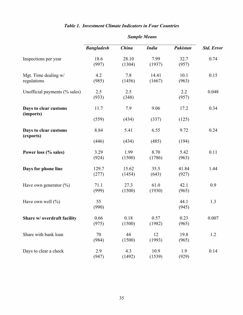
Table 1. Investment Climate Indicators in Four Countries Sample Means

Bangladesh China India Pakistan Std. Error Inspections per year 18.6 28.10 7.99 32.7 0.74 (997) (1304) (1937) (957) Mgt. Time dealing w/ regulations

4.2 (985)

7.8 (1456)

14.41 (1667)

10.1 (963)

0.15

Unofficial payments (% sales) 2.5 2.5 2.2 0.048 (933) (348) (957) Days to clear customs (imports)

11.7 7.9 9.06 17.2 0.34

(559) (434) (337) (125) Days to clear customs (exports)

8.84 5.41 6.55 9.72 0.24

(446) (434) (485) (194) Power loss (% sales) 3.29 1.99 8.70 5.42 0.11 (924) (1500) (1786) (963) Days for phone line 129.7 15.62 35.5 41.84 1.44 (277) (1454) (643) (927) Have own generator (%) 71.1 27.3 61.0 42.1 0.9 (999) (1500) (1930) (965) Have own well (%) 55 44.1 1.3 (990) (945) Share w/ overdraft facility 0.66

(975) 0.18

(1500) 0.57

(1982) 0.23 (965)

0.007

Share with bank loan 70 44 12 19.8 1.2 (984) (1500) (1993) (965) Days to clear a check 2.9 4.3 10.9 1.9 0.14 (947) (1492) (1539) (929)

35

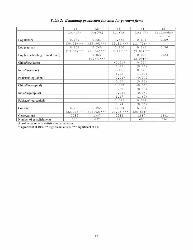
Table 2: Estimating production function for garment firms (1) (2) (3) (4) (5) Log(VA) Log(VA) Log(VA) Log(VA) Levinsohn-

Petrin Log (labor) 0.647 0.653 0.636 0.621 0.59 (30.29)*** (29.96)*** (11.81)*** (11.73)*** Log (capital) 0.258 0.240 0.250 0.246 0.36 (13.96)*** (12.56)*** (9.11)*** (9.01)*** Log (av. schooling of workforce) 0.022 0.026 .023 (2.77)*** (3.09)*** China*log(labor) -0.019 0.134 (0.19) (0.86) India*log(labor) 0.106 0.128 (1.42) (1.62) Pakistan*log(labor) -0.047 -0.072 (0.55) (0.83) China*log(capital) 0.017 -0.060 (0.38) (0.90) India*log(capital) -0.036 -0.049 (1.17) (1.60) Pakistan*log(capital) 0.025 0.029 (0.74) (0.86) Constant 6.238 6.265 6.354 6.334 (32.36)*** (28.62)*** (29.05)*** (25.86)*** Observations 2082 1887 2082 1887 1882 Number of establishments 775 697 775 697 694 Absolute value of z statistics in parentheses * significant at 10%; ** significant at 5%; *** significant at 1%

36

Table 3: Explaining Productivity I

Dependent Variable: TFP from GLS estimates of garment firms (1) (2) (3) tfp tfp tfp Log (customs days-export) 0.049 -0.042 0.034 (0.73) (0.61) (0.41) Log (customs days-import) -0.175 -0.218 -0.062 (1.42) (1.43) (0.38) Log (power loss) -0.131 -0.371 -0.566 (2.37)** (2.86)*** (3.77)*** Log (phone days) -0.040 -0.161 0.010 (0.84) (2.01)** (0.08) Log (overdraft facility) 0.012 0.103 0.055 (0.17) (1.19) (0.58) Log (distance from market) 0.542 0.239 (2.34)** (0.54) Log (distance from port) 0.016 0.006 (1.62) (0.55) Log (population) 0.005 0.030 (0.12) (0.75) Bangladesh -0.328 (1.50) China -0.287 (0.70) India 0.232 (2.03)** Constant 0.866 3.207 4.557 (2.71)*** (1.78)* (1.17) Year dummies Yes Yes Yes Observations 2205 1961 1961 Number of establishments 808 714 714 Chi2 9.03 10.78 17.01 Prob>Chi2 0.1078 0.0559 0.0045 Absolute value of z statistics in parentheses * significant at 10%; ** significant at 5%; *** significant at 1%

37

Table 4: Explaining Productivity II

Dependent variable: TFP from Levinsohn-Petrin estimates of garment firms

(1) (2) (3) tfp tfp tfp Log (customs days-export) -0.191 -0.163 -0.184 (2.70)*** (2.16)** (2.01)** Log (customs days-import) 0.423 0.254 0.326 (2.79)*** (1.53) (1.82)* Log (power loss) -0.018 -0.367 -0.488 (0.27) (2.60)*** (2.97)*** Log (phone days) 0.198 0.077 0.046 (3.56)*** (0.89) (0.38) Log (overdraft facility) 0.054 0.083 -0.006 (0.67) (0.89) (0.06) Log (distance from market) 0.786 0.351 (3.12)*** (0.73) Log (distance from port) 0.009 0.004 (0.85) (0.34) Log (population) 0.026 0.019 (0.61) (0.43) Bangladesh 0.130 (0.55) China -0.499 (1.10) India 0.295 (1.71)* Constant 2.181 -3.548 0.293 (5.32)*** (1.80)* (0.07) Year dummies Yes Yes Yes Observations 1980 1980 1980 Number of establishments 721 721 721 Chi2 58.01 54.8 24.60 Prob>Chi2 0.00 0.00 0.00 Absolute value of z statistics in parentheses * significant at 10%; ** significant at 5%; *** significant at 1%

38

Table 5: Explaining Average Wages Rates in Garment Firms (1) (2) (3) lnwage lnwage lnwage Log (age of establishment) -0.041 -0.039 -0.044 (1.18) (1.13) (1.24) Log (labor in initial period) 0.899 0.908 0.897 (34.52)*** (32.22)*** (29.36)*** Log (average schooling) 0.029 0.030 0.030 (3.06)*** (3.15)*** (3.11)*** Log (av. age of workers) 0.076 0.074 0.075 (4.68)*** (4.52)*** (4.52)*** Log (Av.age sq.) -0.001 -0.001 -0.001 (4.17)*** (4.07)*** (4.08)*** Log (customs days-export) 0.125 0.138 0.232 (2.23)** (2.34)** (3.27)*** Log (customs days-import) -0.206 -0.225 -0.175 (1.77)* (1.76)* (1.27) Log (power loss) -0.257 -0.299 -0.323 (3.76)*** (2.72)*** (2.57)** Log (phone days) -0.084 -0.083 0.042 (1.75)* (1.13) (0.44) Log (overdraft facility) -0.057 -0.075 -0.039 (0.91) (1.04) (0.49) Log (distance from market) 0.142 0.790 (0.68) (2.14)** Log (distance from port) -0.002 -0.006 (0.26) (0.64) Log (population) -0.018 0.006 (0.57) (0.17) Bangladesh -0.136 (0.70) China 0.780 (2.17)** India 0.006 (0.04) Constant 6.444 5.576 -1.022 (14.64)*** (3.38)*** (0.32) Year dummies Yes Yes Yes Observations 1378 1378 1378 Number of establishments 709 709 709 Chi2 32.95 17.42 14.60 Prob>Chi2 0.000 0.0038 .0122 Absolute value of z-statistics in parentheses

* significant at 10%; ** significant at 5%; *** significant at 1%

39

Table 6: Explaining gross return on capital in garment firms I

(1) (2) (3) Log (capital, initial period) -0.247 -0.261 -0.260 (8.94)*** (9.27)*** (8.78)*** Log (age) 0.111 0.126 0.126 (2.35)** (2.65)*** (2.62)*** Log (customs days-export) -0.205 -0.261 -0.371 (2.28)** (2.80)*** (3.34)*** Log (customs days-import) 0.049 0.225 0.092 (0.29) (1.18) (0.45) Log (power loss) -0.344 -0.058 0.109 (4.08)*** (0.34) (0.55) Log (phone days) 0.347 0.475 0.300 (5.32)*** (4.61)*** (2.11)** Log (overdraft facility) -0.021 -0.100 -0.069 (0.22) (0.94) (0.57) Log (distance from market) -0.394 -0.578 (1.37) (1.19) Log (distance from port) -0.024 -0.016 (1.83)* (1.11) Log (population) 0.034 0.001 (0.67) (0.03) Bangladesh 0.257 (0.93) China -0.243 (0.52) India -0.280 (1.37) Constant 3.560 5.324 8.354 (5.79)*** (2.34)** (1.94)* Year dummies Yes Yes Yes Observations 1356 1356 1356 Number of establishments 715 715 715 Chi2 111.89 99.86 32.29 Prob>Chi2 0.000 0.000 0.000 Absolute value of z-statistics in parentheses * significant at 10%; ** significant at 5%; *** significant at 1%

40

Table 7: Explaining return to capital II (1) (2) (3) Log (labor in initial period) -0.032 -0.040 -0.013 (0.77) (0.89) (0.27) Log (age) 0.044 0.053 0.066 (0.83) (0.97) (1.21) Log (customs days-export) -0.436 -0.455 -0.603 (4.55)*** (4.54)*** (5.12)*** Log (customs days-import) 0.340 0.409 0.329 (1.92)* (2.00)** (1.51) Log (power loss) 0.006 0.089 0.124 (0.06) (0.48) (0.57) Log (phone days) 0.366 0.428 0.197 (5.02)*** (3.62)*** (1.26) Log (overdraft facility) 0.034 -0.012 -0.110 (0.33) (0.10) (0.83) Log (distance from market) -0.082 -0.987 (0.26) (1.89)* Log (distance from port) -0.013 -0.009 (0.88) (0.61) Log (population) 0.003 -0.051 (0.05) (0.89) Bangladesh 0.377 (1.23) China -0.121 (1.45) India 0.052 (0.23) Constant 0.077 0.264 0.186 (0.14) (0.11) (2.13)** Observations 1302 1302 1302 Number of establishments 701 701 701 Chi2 86.24 64.64 42.39 Prob>Chi2 0.000 0.000 0.000 Absolute value of z-statistics in parentheses * significant at 10%; ** significant at 5%; *** significant at 1%

41

Table 8. Explaining Output Growth Dependent variable: annual growth rate of output

(1) (2) (3) (4) (5)

Log(lagged output level) -0.068 -0.067 -0.064 -0.061 -0.059(17.62)** (17.41)** (16.69)** (16.22)** (15.97)**

Log (lagged age of firm) -0.050 -0.050 -0.049 -0.051 -0.051(8.30)** (8.20)** (8.04)** (8.35)** (8.41)**

Log(customs days - export) -0.019 -0.018 -0.017 -0.014 -0.013(1.87) (1.77) (1.67) (1.41) (1.31)

Log(customs days - import) 0.002 0.006 0.012 0.009 0.011(0.22) (0.63) (1.26) (0.97) (1.21)

Log (power loss) -0.033 -0.018 -0.037 -0.093 -0.087(1.67) (0.99) (1.95) (7.43)** (7.46)**

Log (phone days) 0.059 0.055 0.013 -0.001 -0.008(3.68)** (3.58)** (1.11) (0.06) (0.83)

Log (overdraft facility) 0.102 0.110 0.031 0.035 0.043(5.11)** (5.93)** (2.16)* (2.56)* (3.22)**

Log (population) 0.025 0.009(2.73)** (1.04)

Log (distance from markets) 0.137 -0.115(2.18)* (2.99)**

Log (distance from port) -0.000 -0.002(0.19) (1.15)

China 0.281 0.190(4.83)** (5.35)**

India -0.105 -0.115(3.39)** (3.83)**

Bangladesh -0.167 -0.164(4.06)** (4.20)**

Constant -0.462 1.059 1.916 1.160 1.214(0.79) (11.91)** (5.18)** (14.88)** (16.97)**

NoIndustry dummy Yes Yes Yes Yes YesYear dummy Yes Yes Yes Yes

Observations 7971 7971 7971 7971 7971Number of firms 5052 5052 5052 5052 5052

Chi2(5) 52.49 54.62 18.89 60.94 61.62Prob> Chi2 0 0 0.002 0 0Absolute value of z statistics in parentheses* significant at 5%; ** significant at 1%

42

Table 9: Explaining Fixed Assets Growth Dependent variable: Annual growth rate of fixed assets

(1) (2) (3) (4) (5)

Log (lagged fixed asset level) -0.004 -0.004 -0.003 -0.001 -0.001(3.37)** (3.41)** (2.64)** (0.75) (0.43)

Log (lagged age of firm) -0.011 -0.011 -0.012 -0.013 -0.014(4.69)** (4.58)** (4.72)** (5.19)** (5.71)**

Log (customs days - export) -0.002 -0.003 -0.009 -0.010 -0.011(0.59) (0.70) (2.21)* (2.69)** (2.71)**

Log (customs days - import) -0.001 0.000 -0.002 -0.004 -0.004(0.24) (0.03) (0.45) (1.13) (1.20)

Log (power loss) -0.024 -0.021 -0.010 -0.051 -0.058(3.29)** (3.16)** (1.38) (10.65)** (13.00)**

Log (phone days) 0.003 0.006 -0.015 -0.020 -0.029(0.52) (1.02) (3.29)** (4.90)** (7.77)**

Log (overdraft facility) 0.015 0.010 0.057 0.043 0.045(2.01)* (1.41) (10.49)** (8.32)** (8.90)**

Log (population) 0.002 -0.008(0.62) (2.57)*

Log (distance from markets) 0.002 -0.141(0.08) (9.52)**

Log (distance from port) 0.001 0.002(2.19)* (4.12)**

China 0.193 0.191(8.78)** (13.95)**

India 0.120 0.125(10.63)** (11.34)**

Bangladesh 0.073 0.077(4.83)** (5.41)**

Constant -0.040 -0.013 1.497 0.230 0.271(0.18) (0.41) (10.60)** (8.29)** (10.73)**

Industry dummy? Yes Yes Yes Yes NoYear dummy? Yes Yes Yes Yes Yes

Observations 7729 7729 7729 7729 7729Number of firms 4936 4936 4936 4936 4936

Chi2(5) 17.14 14.98 132.05 177.84 260.61Prob> Chi2 0.004 0.0105 0 0 0Absolute value of z statistics in parentheses* significant at 5%; ** significant at 1%

43

Table 10: Explaining Employment Growth

44

Dependent variable: Annual growth rate of employment

(1) (2) (3) (4) (5)

Log(lagged employment level) -0.050 -0.049 -0.045 -0.043 -0.040(18.46)** (18.38)** (17.13)** (16.99)** (16.31)**

Log (lagged age of firm) -0.003 -0.003 -0.003 -0.004 -0.005(1.36) (1.30) (1.59) (1.79) (2.36)*

Log (customs days - export) -0.006 -0.006 -0.004 -0.004 -0.002(1.23) (1.22) (0.92) (0.80) (0.51)

Log (customs days - import) 0.005 0.006 0.005 0.004 0.005(1.01) (1.32) (1.19) (0.93) (1.22)

Log (power loss) -0.008 0.004 -0.018 -0.038 -0.035(0.87) (0.48) (1.97)* (6.26)** (6.23)**

Log (phone days) 0.018 0.021 0.029 0.024 0.020(2.41)* (2.92)** (5.22)** (4.66)** (4.17)**

Log (overdraft facility) 0.035 0.035 0.024 0.024 0.026(3.70)** (3.96)** (3.50)** (3.66)** (4.04)**

Log (population) 0.002 0.001(0.44) (0.18)

Log (distance from markets) 0.113 -0.048(3.78)** (2.62)**

Log (distance from port) -0.000 -0.001(0.32) (0.70)

China 0.185 0.100(6.57)** (5.80)**

India -0.025 -0.023(1.71) (1.57)

Bangladesh 0.060 0.042(3.05)** (2.25)*

Textiles 0.059 0.058 0.050 0.048(3.76)** (3.72)** (3.21)** (3.13)**

Constant -0.817 0.156 0.556 0.199 0.234(2.93)** (4.33)** (3.18)** (6.85)** (9.46)**

Industry dummy Yes Yes Yes Yes NoYear dummy Yes Yes Yes Yes Yes

Observations 8697 8697 8697 8697 8697Number of firms 5138 5138 5138 5138 5138Prob> Chi2 0.0001 0 0 0 0Absolute value of z statistics in parentheses* significant at 5%; ** significant at 1%