Investigations of eddy current vibration damping - · PDF fileInvestigations of eddy current...

Inter-noise 2014 of 14

Investigations of eddy current vibration damping

Karel RUBER1; Sangarapillai KANAPATHIPILLAI

2; Robert RANDALL

3

1,2,3 School of Mechanical and Manufacturing Engineering, The University of NSW (UNSW), Sydney, Australia

ABSTRACT

Eddy currents are generated in electrically conductive materials such as copper in response to a moving

magnetic field and they generate forces in the opposite direction of the relative movement of the magnetic

field to the conductive material. Those forces have been used for braking applications and are proportional to

the relative velocity between the conductive material and the magnetic field, similar to viscous damping

forces in vibration attenuation applications.

This paper investigates various geometrical configurations of magnet and copper assemblies with the

purpose of quantifying and maximising the eddy current forces. The effects of air gaps, magnetic field

strength, orientation and surface area are investigated with Finite Element Analysis (FEA) and validated with

measurements.

Keywords: Vibration Damping, Eddy Currents

I-INCE Classification of Subjects Number(s): 46 and 47

1. INTRODUCTION

The phenomena of eddy currents was discovered in the 19th

century and it has been applied to

braking of machinery and vehicle braking for decades.

The principle of the eddy current forces phenomena is that a change in the magnetic field

surrounding an electrical conductor induces an electrical potential in the conductor which creates

electrical currents. The induced currents create a magnetic field which opposes the changes in the

magnetic field that created the currents.

Faraday’s law states that an electromagnetic force (emf) is generated in a conductor whenever there

is a change in the magnetic field and the emf ε [V] is equal to the rate of change of the magnetic field

expressed by the magnetic flux density ØB [Tesla], experienced by the conductor (1).

In the case of a wire conductor, the emf creates a current I[A] which is proportional to the resistance

R[Ohms] of the wire. In the case where the conductor is a solid body (or when the skin effect is

considerable such as in the case of high frequency excitations) – the induced current density J [A/m2]

is proportional to the conductor’s material resistivity ρ [Ohms∙m] and to the electric field E [V/m].

Lentz’s law states that the induced currents will create a magnetic field in a direction that will

oppose the changes in the magnetic field that induces the currents which is shown by the minus sign in

equation 1.

Eddy currents flowing in an electrical conductor create Lorentz forces FL [N] that oppose the

relative movement between the conductor and the magnetic field. In absence of an electrical field

1 [email protected]

2 [email protected]

3 [email protected]

𝜀 = −𝑑𝜙𝐵

𝑑𝑡 (1)

𝐼 =𝜀

𝑅 𝑎𝑛𝑑 𝐽 =

�⃗⃗�

𝜌 (2)

mailto:[email protected]



of 14 Inter-noise 2014

Page 2 of 14 Inter-noise 2014

Lorentz forces are equal to the cross product of the current and the magnetic flux density. If the current

density is not uniform then the Lorentz forces density FLt [N/m3] is calculated from the induced current

density J instead of the current. The Lorentz forces can be calculated by integrating the Lorentz forces

density.

Bae at al (2) investigated analytically and experimentally the characteristics of eddy current

damping when a permanent magnet was moving inside a copper tube. The steady-state damping force

was measured and calculated from the terminal velocity of the magnet during a free fall in the tube. A

dynamic-state damping was measured by exciting the magnet with a low frequency (<8 Hz) sinusoidal

motion and both measurement results were compared against theoretical results. One of the main

finding was that above approximately 4 Hz the measured dynamic-state damping results diverge from

the predicted and measured steady state results.

The research presented in this paper investigates the effects of geometrical and physical parameters

of the conductive pipe and magnet on the eddy current damping magnitude. The validation of the FEA

model is done by comparison of the Impedance of the mass and eddy damper system measured with a

broad band excitation between 7 Hz and 200 Hz.

2. Model Configurations and Investigated Effects

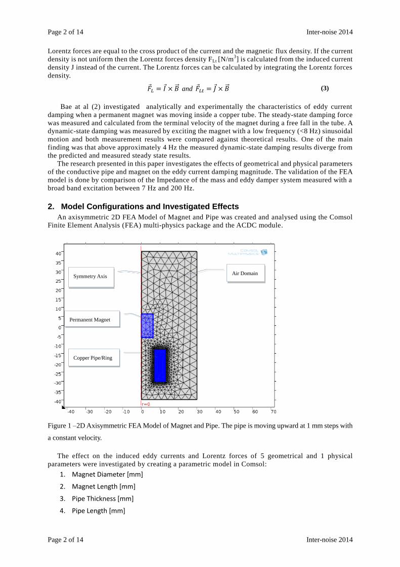
An axisymmetric 2D FEA Model of Magnet and Pipe was created and analysed using the Comsol

Finite Element Analysis (FEA) multi-physics package and the ACDC module.

Figure 1 –2D Axisymmetric FEA Model of Magnet and Pipe. The pipe is moving upward at 1 mm steps with

a constant velocity.

The effect on the induced eddy currents and Lorentz forces of 5 geometrical and 1 physical

parameters were investigated by creating a parametric model in Comsol:

1. Magnet Diameter [mm]

2. Magnet Length [mm]

3. Pipe Thickness [mm]

4. Pipe Length [mm]

�⃗�𝐿 = 𝐼 × �⃗⃗� and �⃗�𝐿𝑡 = 𝐽 × �⃗⃗� (3)

Symmetry Axis

Permanent Magnet

Copper Pipe/Ring

Air Domain


Inter-noise 2014 Page 3 of 14

5. Air Gap [mm]

6. Velocity [mm/sec]

Each parameter was defined at three levels and only one variable changed in each run, no cross

interaction effects were studied at this time.

2.1 FEA validation against Test Results

In order to validate the FEA model and analysis results, test were conducted on two samples of

magnets and short copper pipes (rings) using an electro dynamic shaker to generate a random vibration

excitation in the range of 7Hz-200Hz. The moving part was the magnet which was attached to a small

permanent magnet shaker LDS V201, through an impedance head B&K 8001 which measured

simultaneously the forces and acceleration of the magnet while the copper part was held steady.

Figure 2–Shaker, magnet and copper pipe (ring)

The acceleration signal was integrated to give velocity and the driving point transfer function (or

more correctly called Frequency Response Function) H1 between the Force and Velocity of the magnet

was calculated by the B&K Pulse FFT analyser and displayed as an Impedance Magnitude spectrum

[N∙s/m]. A typical screen capture of Pulse s/w is shown below in Figure 3.

All magnet samples were permanent cylindrical magnets axially magnetised and made of

Neodymium (NdFeB) with a rating of N42. The magnetic remanence was between 0.56 T and 1.1 T. In

the first test configuration a magnet with diameter and length of 12.7 mm was tested with a short

copper pipe (ring): inner diameter (ID) 13 mm, outer diameter (OD) 44 mm and length 15.5 mm. This

configuration of magnet and copper ring is referred to as Config 1.

Copper Pipe/Ring

Electrodynamic

Shaker

Magnet



Figure 3 – B&K Pulse FFT analyser screen showing FRF H1- Impedance Magnitude on the top right,

Coherence between the Force and Acceleration below and the autopower spectra of the individual signals on

bottom left of the screen. Third channel connected to a small accelerometer B&K type 4394 was not used in

this case.

Looking at the FRF spectrum, it can be seen that the Impedance curve is relatively flat in the low

frequency region where the damping effect of the eddy current is dominant and has a rising slope at

frequencies where the mass effect is dominant. The measured impedance matches the theoretical

model of a mass and damper system, when the excitation force is applied to the mass and the damper

is fixed at one end, while the other end is attached to the moving mass:

Where c is the damping [N∙s/m] and m [kg] is the total mass of the magnet and the shaker support

including the internal armature (the mass of all the moving parts). The stiffness effect is ignored as the

resonance of the system is below the frequency range of the measurement as can be seen from the

Impedance spectrum and from source (3).

The copper ring was positioned such as that the magnet’s top face was in the middle of the copper

ring in the axial direction, i.e. equal distance from both ends of the copper ring. This location was

found by the FEA analysis to maximise the damping forces (see below).

The measured damping (c) due to eddy current effect was approximately 6.8 N∙s/m.

The FEA model was configured with the same parameters as in the test configuration and analysed.

The results shown below in Figure 4 indicate that maximum damping is achieved at a location when

one of the magnet faces is at an equal distance from the copper pipe ends. The maximum damping

force value is 0.061 N for a velocity of 10 mm/s which corresponds to a damping value of 6.1 N∙s/m.

𝑍 = 𝑐 + 𝑗𝜔𝑚 (4)



Figure 4 – Lorentz Forces (FL) vs. the Copper Ring relative axial distances (x axis of the figure) relative to

the magnet - for a 10 mm/sec relative velocity. Test Configuration 1

Notice that the curve is symmetrical about the position of maximum force as expected from the

physical symmetry of the configuration.

A second test configuration (Config 2) consisted of a magnet with a diameter of 19 mm, 28.2 mm

length and the copper ring dimensions were 20mm (ID), 37.7 mm (OD) and 15 mm length. The value

of the maximum damping force calculated by the FEA (Figure 5) is 0.12 N for a velocity of 10 mm/s

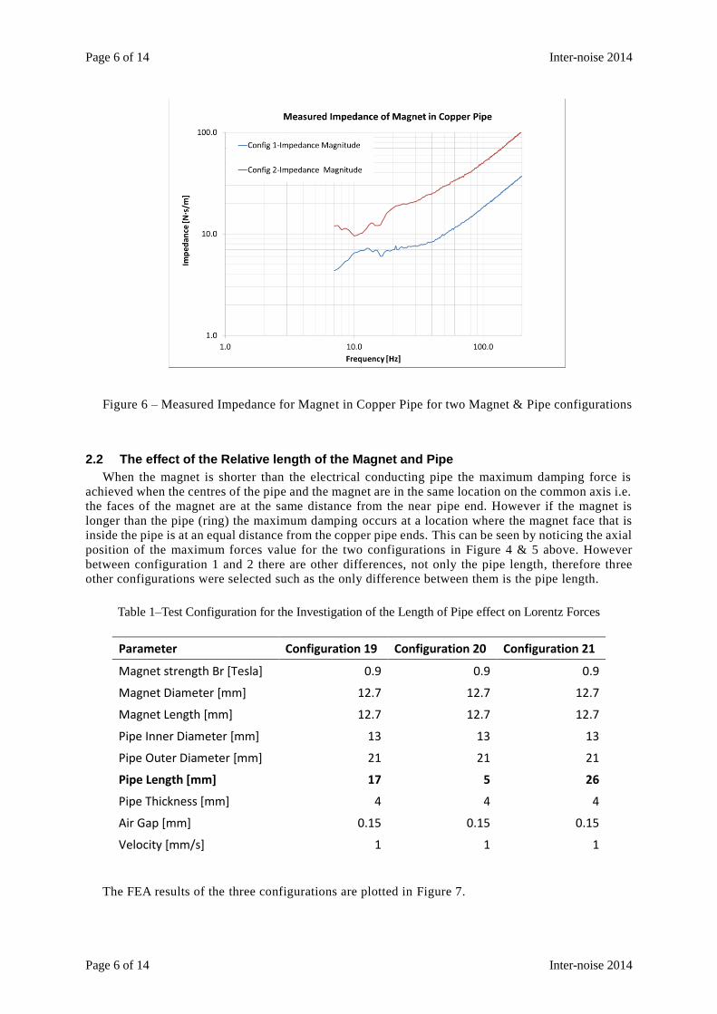
which corresponds to a damping value of 12 N∙s/m. This value is within the range of the measured

Impedance for Config 2 at low frequencies (7 Hz-15 Hz), which is below the frequency range where

the effect of the mass is dominant – see Config 2 curve in Figure 6.

Figure 5 – Lorentz Forces (FL) vs. the Copper Ring relative axial distances (x axis of the figure) relative to

the magnet for a 10 mm/sec relative velocity. Test Configuration 2



Figure 6 – Measured Impedance for Magnet in Copper Pipe for two Magnet & Pipe configurations

2.2 The effect of the Relative length of the Magnet and Pipe

When the magnet is shorter than the electrical conducting pipe the maximum damping force is

achieved when the centres of the pipe and the magnet are in the same location on the common axis i.e.

the faces of the magnet are at the same distance from the near pipe end. However if the magnet is

longer than the pipe (ring) the maximum damping occurs at a location where the magnet face that is

inside the pipe is at an equal distance from the copper pipe ends. This can be seen by noticing the axial

position of the maximum forces value for the two configurations in Figure 4 & 5 above. However

between configuration 1 and 2 there are other differences, not only the pipe length, therefore three

other configurations were selected such as the only difference between them is the pipe length.

Table 1–Test Configuration for the Investigation of the Length of Pipe effect on Lorentz Forces

Parameter Configuration 19 Configuration 20 Configuration 21

Magnet strength Br [Tesla] 0.9 0.9 0.9

Magnet Diameter [mm] 12.7 12.7 12.7

Magnet Length [mm] 12.7 12.7 12.7

Pipe Inner Diameter [mm] 13 13 13

Pipe Outer Diameter [mm] 21 21 21

Pipe Length [mm] 17 5 26

Pipe Thickness [mm] 4 4 4

Air Gap [mm] 0.15 0.15 0.15

Velocity [mm/s] 1 1 1

The FEA results of the three configurations are plotted in Figure 7.



Figure 7 – FEA calculated Lorentz Forces (FL) vs. the Copper Pipe relative axial distances (graph

x axis) relative to the magnet - for 3 pipe lengths.

Figure 8 – FEA simulation of the Magnetic Flux Density and the Induced Eddy Currents Density for

Configuration 19

Figure 9 – FEA simulation of the Magnetic Flux Density and the Induced Eddy Currents Density for

Configuration 20



Figure 10 – FEA simulation of the Magnetic Flux Density and the Induced Eddy Currents Density

for Configuration 21

Figure 11 – FEA simulation of the Magnetic Flux Density Vector and the Lorentz Forces Density


Figure 12 – FEA simulation of the Magnetic Flux Density Vector and the Lorentz Forces Density




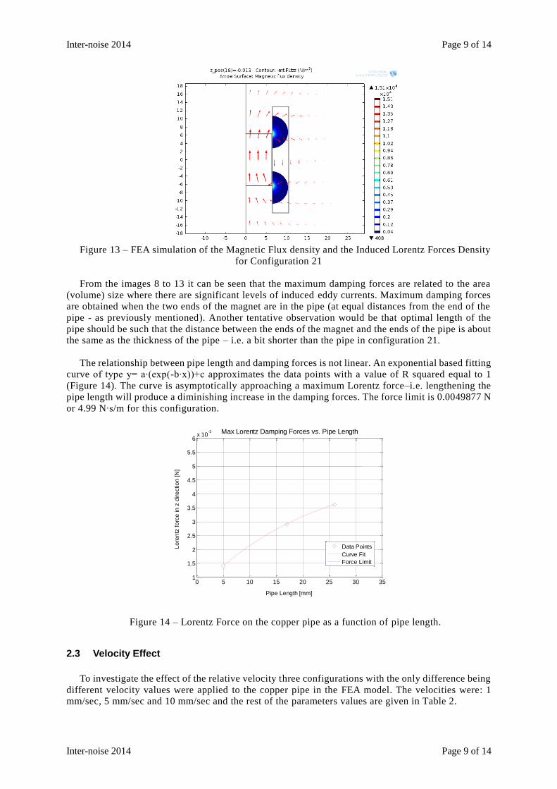
Figure 13 – FEA simulation of the Magnetic Flux density and the Induced Lorentz Forces Density


From the images 8 to 13 it can be seen that the maximum damping forces are related to the area

(volume) size where there are significant levels of induced eddy currents. Maximum damping forces

are obtained when the two ends of the magnet are in the pipe (at equal distances from the end of the

pipe - as previously mentioned). Another tentative observation would be that optimal length of the

pipe should be such that the distance between the ends of the magnet and the ends of the pipe is about

the same as the thickness of the pipe – i.e. a bit shorter than the pipe in configuration 21.

The relationship between pipe length and damping forces is not linear. An exponential based fitting

curve of type y= a∙(exp(-b∙x))+c approximates the data points with a value of R squared equal to 1

(Figure 14). The curve is asymptotically approaching a maximum Lorentz force–i.e. lengthening the

pipe length will produce a diminishing increase in the damping forces. The force limit is 0.0049877 N

or 4.99 N∙s/m for this configuration.

Figure 14 – Lorentz Force on the copper pipe as a function of pipe length.

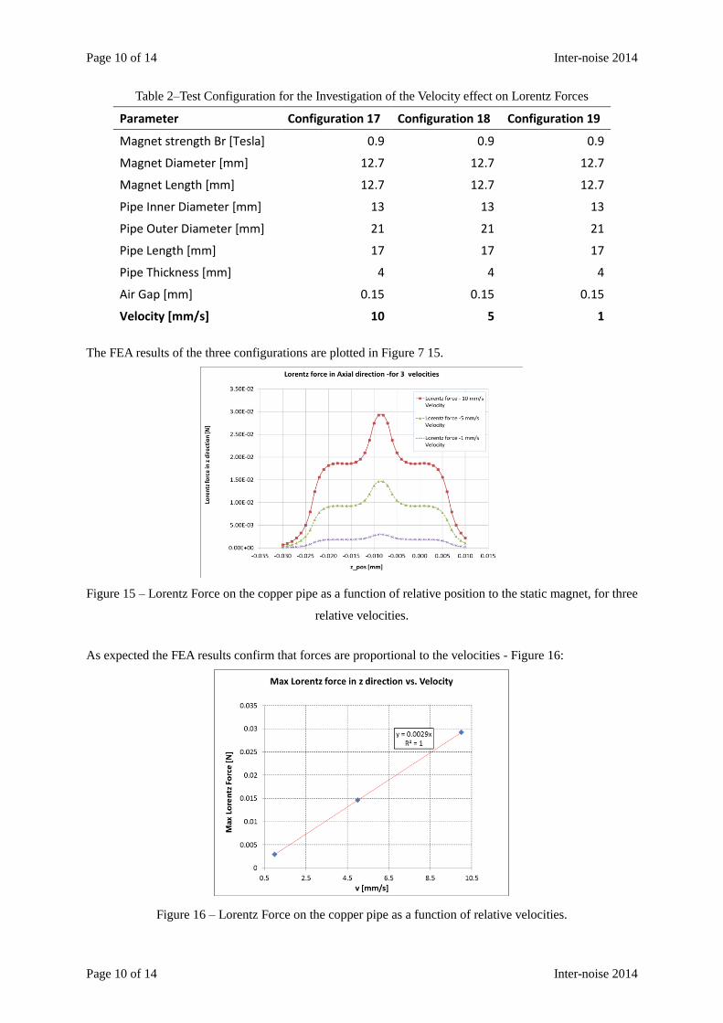
2.3 Velocity Effect

To investigate the effect of the relative velocity three configurations with the only difference being

different velocity values were applied to the copper pipe in the FEA model. The velocities were: 1 mm/sec, 5 mm/sec and 10 mm/sec and the rest of the parameters values are given in Table 2.

0 5 10 15 20 25 30 351

1.5

2

2.5

3

3.5

4

4.5

5

5.5

6x 10

-3

Pipe Length [mm]

Lo

ren

tz fo

rce

in

z d

ire

ctio

n [N

]

Max Lorentz Damping Forces vs. Pipe Length

Data Points

Curve Fit

Force Limit



Table 2–Test Configuration for the Investigation of the Velocity effect on Lorentz Forces









Air Gap [mm] 0.15 0.15 0.15


The FEA results of the three configurations are plotted in Figure 7 15.

Figure 15 – Lorentz Force on the copper pipe as a function of relative position to the static magnet, for three

relative velocities.

As expected the FEA results confirm that forces are proportional to the velocities - Figure 16:

Figure 16 – Lorentz Force on the copper pipe as a function of relative velocities.



When dividing the forces by the respective velocities a constant damping force of 2.92 N∙s/m is

obtained regardless of the excitation velocity. This behaviour of eddy current damping is the same as

viscous damping more commonly employed in commercial dampers and shock absorbers.

2.4 Electrical Conductor Thickness Effect

The effect of the pipe thickness was evaluated by changing the outer diameter of the pipe while the

other parameters were the same for the three configurations:

Table 3–Test Configuration for the Investigation of the Thickness Effect on the Lorentz Forces






Pipe Outer Diameter [mm] 18.85 12.5 10.5


Pipe Thickness [mm] 12.35 6 4

Air Gap [mm] 0.15 0.15 0.15


The FEA results of the three configurations are plotted in Figure 7 17.


pipe thickness values.

The relationship between the pipe thickness and damping forces is of an exponential type y=

a∙(exp(-b∙x))+c as shown in Figure 18.



Figure 18 – Lorentz Force on the copper pipe as a function of pipe thickness.

The effect of increasing the thickness of the copper pipe has diminishing benefits on the damping

forces, as we have seen before with the pipe length effect. The maximum damping force that can be

achieved for this configuration is 0.05241 N or 5.24 N∙s/m

2.5 Air Gap Effect

The effect of an air gap is to reduce the strength of the magnetic flux density penetrating the

conductor. To achieve various air gaps without changing the pipe thickness both the inner and outer

diameter were changed by the same amount. The parameters used in the three configurations are given

below.

Table 4–Test Configuration for the Investigation of the Air Gap Effect on the Lorentz Forces

0 5 10 150.042

0.044

0.046

0.048

0.05

0.052

0.054

Pipe Thickness [mm]

Lo

ren

tz fo

rce

in

z d

ire

ctio

n [N

]

Max Lorentz Damping Forces vs. Pipe Thickness

Data Points

Curve Fit

Force Limit









Air Gap [mm] 0.15 0.65 1.15





air gap values.

As the air gap increases the damping forces are decreasing –fitting the data with an exponential

curve gives an R squared value of 0.9995. The curve asymptotically approaches a zero force value as

the air gap increases and the maximum force for this configuration when the gap is zero, is predicted to

be 0.0521 N or 5.21 N s/m

Figure 20 – Lorentz Force on the copper pipe as a function Air Gap values.

3. CONCLUSIONS

This investigation examined the effects of a number of geometrical and physical parameters on the

damping forces experienced by a magnet moving inside an electrical conductive pipe, which are caused by

induced eddy currents and their associated magnetic fields. The simple model used in this paper is the basis

of eddy currents dampers that may be utilized for attenuating vibrations in vehicles, machinery and

structures in general.

Only one parameter was changed each time in order to evaluate the effect of that parameter in isolation.

The FEA results matched the test results and the effect of varying each parameter matched the expected



behaviour. Some of the effects of increasing the value of parameters such as the pipe length and pipe

thickness on the damping forces is characterised by a “diminishing benefits” behaviour which indicates the

potential to optimise the values of the parameters for weight and cost reduction.

In particular there is no benefit to have a magnet longer than the pipe because only one pole is creating the

current damping effect.

Further work is required to establish if there are any significant interactions between the parameters, by

conducting a factorial or partial factorial experiment design.

REFERENCES

1. Schwartz M. Principles of Electrodynamics: Dover Publications.

2. Bae J-S, Hwang J-H, Park J-S, Kwag D-G. Modeling and experiments on eddy current damping caused

by a permanent magnet in a conductive tube. J Mech Sci Technol. 2009;23(11):3024-35.

3. Fox LG. Electrodynamic shaker fundamentals. Sound & Vibration. 1997;31(4):14-23.

Investigations of eddy current vibration damping - · PDF fileInvestigations of eddy current...

Documents

Transcript of Investigations of eddy current vibration damping - · PDF fileInvestigations of eddy current...