Investigation of Target Tracking Errors in Monopulse Radars
123
.4 INVESTIGATION OF TARGET TRACKING ERRORS IN MONOPULSE RADARS FINAL TECHNICAL REPORT by G.W. Ewell, N.T. Alexander, and E. L. Tomberlin July 1972 Prepared for Advanced Sensors Directorate Research, Development, Engineering " f) and Missile Systems Laboratory N-' CJ•_ 1IP.. U.S. Army Missile Command s~ - Redstone Arsenal, Alabama 35809 by Engineering Experiment Station , Georgia Institute of Technology ... Atlanta, Georgia 30332 o. DISTRIBUTION OF THIS DOCUMENT IS UNLIMITED NATPONAL TECHNICAL INFORMATION SERVICE "44 , A 2,2~ ........... .w1'4
Transcript of Investigation of Target Tracking Errors in Monopulse Radars

.4
INVESTIGATION OF TARGET TRACKING ERRORS
IN MONOPULSE RADARS
FINAL TECHNICAL REPORT
by G. W. Ewell, N. T. Alexander, and E. L. Tomberlin
July 1972
Prepared for
Advanced Sensors Directorate
Research, Development, Engineering " f)and Missile Systems Laboratory N-' CJ•_ 1IP..U. S. Army Missile Command s~ -
Redstone Arsenal, Alabama 35809
byEngineering Experiment Station ,
Georgia Institute of Technology ...
Atlanta, Georgia 30332 o.
DISTRIBUTION OF THIS DOCUMENT IS UNLIMITED
NATPONAL TECHNICALINFORMATION SERVICE
"44 , A 2,2~
........... .w1'4

Information and data contained inthisstdarbseonheiptvillettetime of preparation. Because the results m~ay be subject to change and concern only limitedaspects of this subject, this document should not be construed to represent the official positionof the U. S. Army Material Command.
The findings in this report are not to be construed as an official Department of the Armyposition unless so designated by other authorized documents.
Destroy this report when no longer needed. Do not return it to the originator.
I I

UNCLASSIFIEDSecurity Classification
DOCUMENT CONTROL DATA. .R & D(S.ecw.t. cfa.ajtfitil ,of flit.. .bott. of obetr, and Wettingd.i notatio, must be entered when the o.....l r.po. t is d. lf..d
OI,•INATING ACTIVITY (Cotpott* . 1U1t) Za. REPORT SECURITY CLASSIFICATION
Engineering Experiment Station UnclassifiedGeorgia Institute of Technology 2b. GROUP
N. A.3 REPORT TITLE
Investigation of Target Tracking Errors in Monopulse Radars.
4 DESCRIPTIVE NOTES (Type of report and Inclusive date*)
Final Technical Report May 1971-July 1972I AU THORIS( (Firet name. middle Initial. last name)
George W. Ewell, Neal T. Alexander, and Edwin L. Tomberlin
6 REPORT DATE 74. TOTArL NO OF PAGES 7b. NO. OF REFS
July 1972 119 55$0. CONTRACT OR GRANT NO N. ORIGINATOR'S REPORT WUML48RIS)
DAAHO0-71-C-1192 GIT-A-1336-Fb. PROJEC T NO
C Oh. OTHER REPORT NOMS) (Any oteht nVLMb0,. that "ay be *eel*nedtitle roport)
d. Georgia Tech Project A-133610 01TRIIOUTION SIATEMENT
Distribution of this document is unlimited
Iit SUPPLEMENTARY NOTES 12. SPONSORING MILITARY ACTIVITY
U.S. Army Missile CommandRedstone Arsenal, Alabama 35809
13 AOSTRAC TThis Final Technical Report on Contract DAAIIOI-71-C-1192 discusses investigation
of tracking errors associated with a particular monopulse phased-array radar system,called the Experimantal Array Radar (EAR). The free-space performance of the EARis first analyzed and degradations of performance due to particular target Dopplershifts and multipath returns are noted. A computer analysis of the trackingperformance of the EAR is then presented, and it is noted that there are significanttracking errors due to multipath returns for targets at altitudes less Chan 1200feet. An analysis of the effectiveness of frequency-agile operation in reduc ngthe effects of these multipath returns is presented, and shows that the avail blefrequency-agility bandwidth of a modified EAR would significantly reduce mult path-induced tracking errors, particularly for higher antenna and target locationsImproved MTI filters which provide more nearly uniform responses for a wide rangeof Doppler frequencies are then discussed and a number of representative imprcvedfilter responses presented.
D FORM 1w 4DDI NOV 661473 UNCLASS IFIED
Security Classification

UNCLASSIFIEDS•curtty ClausIfIcation________
II IC Lit. A LINK 8 LINK C
111101-17 WT POLK WNT POLK WT
Angle Tracking
Frequency Agility
Multipath
MTI
Digital Ml
Digital Filters
4,''
UNCLASSIFIEDSecurlty Classlflcation

INVESTIGATION OF TARGET TRACKING ERRORS IN
MONOPULSE RADARS
Final Technical Report
by
G. W Ewell, N. T. Alexander, and E. L. Tomberlin
July 1972
Contract DAAH01-71-C-1192
Project A-1336
Prepared forAdvanced Sensors Directorate
Research, Development, Engineering andMissile Systems Laboratory
U. S. Army Missile CommandRedstone Arsenal, Alabama 35809
by
\Engineering Experiment Station
Georgia Institute of TechnologyAtlanta, Georgia 30332 -- '1
\Dt tmu
• Distribution of this document is unlimited

ABSTRACT
This Final Technical Report on Contract DAAH0O-7* -C-1192 discussesinvestigations of tracking errors associated with a particular monopulsephased-array radar system, called the Experimental Array Radar (EAR). Thefree-space performance of the EAR is first analyzed and degradations ofperformance due to particular target Doppler shifts and multipath returnsare noted. A computer analysis of the tracking performance of the EAR is thenpresented, and it is noted that there are significant tracking errors due tomultipath returns for targets at altitudes less than 1200 feet. An analysisof the effectiveness of frequency-agile operation in reducing the effectsof these multipath returns is presented, which shows that the availablefrequency-agility bandwidth of a modified EAR would significantly reducemultipath-induced tracking errors, particularly for higher antenna and targetlocations. Improved M.T filters which provide more nearly uniform responsesfor a wide range of Doppler frequencies are then discussed and a number ofrepresentative improved filter responses' presented.
.4i

FOREWORD
The efforts of numerous people at MICOM and at Georgia Tech havecontributed substantially to the performance of the work described i.:this report. At MICOM the cooperation of a number of people involved withthe EAR program has substantially aided the investigation described herein.The assistance and guidance provided by Mr. J. Hatcher and Mr. R. Fletcherwere particularly valuable. Without the continuing interest and supportof Mr. W. Lindberg and Mr. W. Low, this program would not have been possible.
At Georgia Tech, in addition to the authors, Mr. T. Brewer and Dr.R. Larson made substantial contributions to the technical effort.
i I
Preceoing page bhankV

TABLE OF CONTENTS
Page
I. INTRODUCTION ...... ....... ........................... I
II. PRELIMINARY INVESTIGATION OF EAR PERFORMANCE ..... ......... 3
A. Free-Space Signal-to-Noise Ratio ...... ... ........... 3
B. Tracking Errors Due to Glint and Thermal Noise .... ..... 5
j C. Radar Angle Tracking Errors Due to Mulripath Returns . . 8
D. Clutter Effects on the EAR ......... ................ 8
III. MULTIPATH EFFECTS ON EAR ANGLE TRACKING ACCURACY ......... ... 13
A. Introduction ......... ..................... ..... 13
B. Geometry of the Target Trajectory ....... ............. 13
C. Calculation of Received Signals and Indicated Errors . . . 15
D. Antenna Pattern Generation ...... ................ .... 17
E. Program Organization ....... ................... ... 20
F. Results of Computer Analysis ...... .............. ... 20
IV. APPLICABILITY OF FREQUENCY AGILITY TO THE EAR ........... .... 27
A. Required Overall Frequency Agility Bandwidth ..... ...... 33
B. Effect of Frequency Agility on Angle Tracking Performance. 36
C. Adaptive Processing for the EAR System ............. ... 36
V. IMPROVED MTI PROCESSORS ....... .................... ... 43
A. Use of Statistical Detection Theory in DevelopingOptimum MTI Receivers ....... ... ................... 43
B. Optimization of MTI Processors Using Weighted Sums ofSampled Signals ......... ...................... ... 46
C. MTI Processor Design as a Filter Optimization Problem. . 47
D. Conventional Digital-Filter Design Procedures ........... 49
E. Optimum Transversal Digital-Filter Design Procedures forUnstaggered prf Systems .......... .................. 50
I. "Cost" Minimization MTI Filters .... ............ ... 50
2. Filter Design by Linear Programming ........... ..... 52
3. MTI Clutter Rejection Filters Using an rms Error
Specification ....... ..................... .... 57
a. Improvement for an Arbitrary N-Pulse Canceller 59
b. Error Statement ................ ......... ... 60
Preceding page blankvii

TABLE OF CONTENTS (cont.)
4 Page
c. Optimization .......... ................... ... 61
d. Results ......... ...................... ... 62
4. Maximally Flat Non-Recursive Digital MTI Filters . . . 67
F. MTI Processors Using Staggered prf ..... ............ ... 70
VI. CONCLUSIONS AND RECOMMENDATIONS ...... ................ ... 79
A. Primary Conclusions ......... .................... ... 79
B. Principal Recommendations ........ ............... ... 79
VII. REFERENCES .............. .......................... ... 81
VIII. APPENDICES ................... .......................... 87
v.i
viii
-- 2

w
LIST OF FIGURES
Figure Page
1. Average signal-to-noise ratio for the EAR system as a functionSof range . . . . . . . . . . . . . . . . . . . . . . . . . . . . . 4ofan e...e........eo e...........................
2. Response of a conventional three-pulse canceller having filtertap weights of 1, -2, and 1 ...... ..... ................... 6
3. Average tracking errors due to thermal noise and glint asfunctions of range for the EAR system ................... . 7
4. RMS tracking errors due to multipath as a function of the ratioof direct to indirect signals at the receiver...... ......... 9
5. Signal-to-clutter ratio after MTI filtering (56 dB MTIimprovement) as a function of range for the EAR system usinga one-microsecond pulse ...... ... ..................... .. 11
6. Antenna/target geometry ...... ... ..................... .. 14
7. Indicated angular error versus actual angular error forSK = 0.86 . . . . . . . . . . . . . . . . . . . . . . . . . . . . . 16K 0.86.......... ..................., ....... ,...l
8, Indicated angular error versus actual angular error forK = 0.845 + 0.335 (e scan/30) ........ ... .................. 18
9. Typical sum (solid lines) and difference (dashed lines)patterns used in the computer analysis..... .............. .. 19
10. Tracking error as a function of time. H = 100 ft, Ht = 300 ft,f = 5.5 GHz, p = 0.3, tilt angle = 0 a t 21
11. Tracking error as a function of time. H = 100 ft, Ht = 300 ft,f = 5.5 GHz, p = 0.5, tilt angle = 300 a . 22
12. Tracking error as a function of rime, H = 100 ft, Hi= 500 ft,f = :.5 GHz, p = 0.5, tilt angle = 3 0 0a . 24
13. Tracking error as a function of time. a = 15 ft, Ht = 300 ft,f = 5.5 GHz, p = 0.5, tilt angie = 30°. . . . . . . . . . . . . . 25
14. Peak-to-peak elevation tracking errors as functions cf targetheight for 15 and 100 feet antenna heights. p = 0.5 andfrequency is 5.5 GHz ....... ......... ......... ... ........ 26
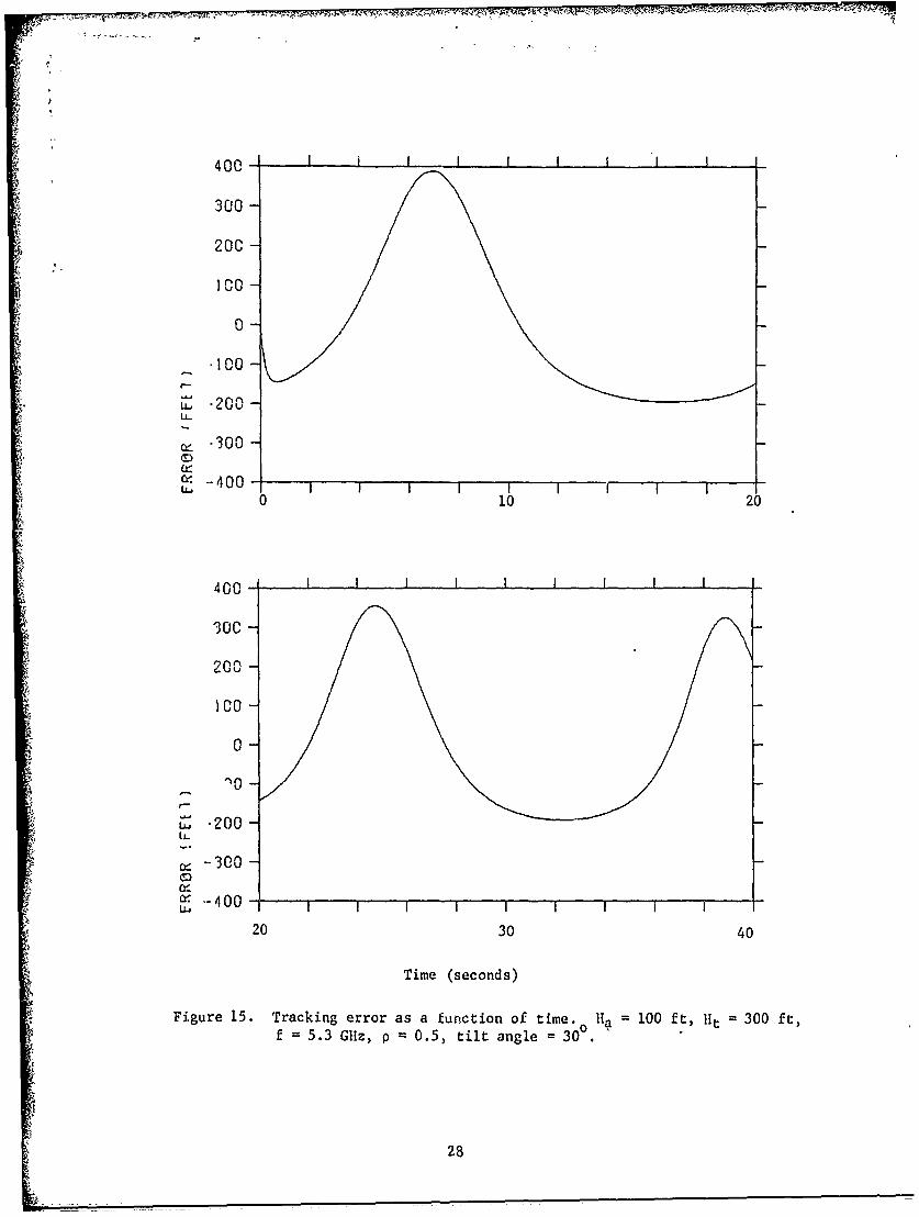
15. Tracking error as a function 6f time. 0 h = 100 fr, Ht = 300 ft,f 5.3 GHz, p = 0.5, tilt angle = 30 a . 28
16. Tracking error as a function of time, i " 100 ft, Ht = 300 ft,f = 5.4 Grijz. p = 0.5, tilt angle =30.. . . . . . . . . . . . . .a 29
17. Tracking error as a function of time. H a= 00 ft, Ht 300 ftI f = 5.5 GHz, p = 0.5, tilt angle = 300.. . ... . ......... ..... 30
j. . . . . . . . 3

LIST OF FIGURES (cont.)
Figure Page
18. Tracking error as a functioa of time. H = 100 ft, Ht = 300 ft,f = 5.6 GHz, p = 0.5, tilt angle = 300°. ........... . .. . . 31
19. Tracking error as a function of time. H = 100 ft, Ht = 300 ft,f = 5.7 GHz, p = 0.5, tilt angle = 30°. a......... t . . . 32
20. Frequency change required to change the relative phase of thedirect and reflected signals by rr. Antenna height = 15 ft. . . . 34
21. Frequency change required to change the relative phase of thedirect and reflected signals by rr. Antenna height = 100 ft .. . 35
22. Tracking error as a function of target height using frequencyagility. H = 100 ft ...... ......... ..................... 37
23. 'Ti-Udking error as a function of target height using frequencyt, :!itN'. H = 15 ft .......... ...................... . 38
a
2'ý. Tracking error as a function of target height using frequencyagiiity, Ha = 100 ft .......... ..................... ... 39
25. Complex indicated angle (CIA) as a function of time for thesame carget-radar parameters described in Figure 17 .... ...... 41
26. Sum signal variations as a function of time for the same target-radar parameters described in Figure 17 .... ............. .. 42
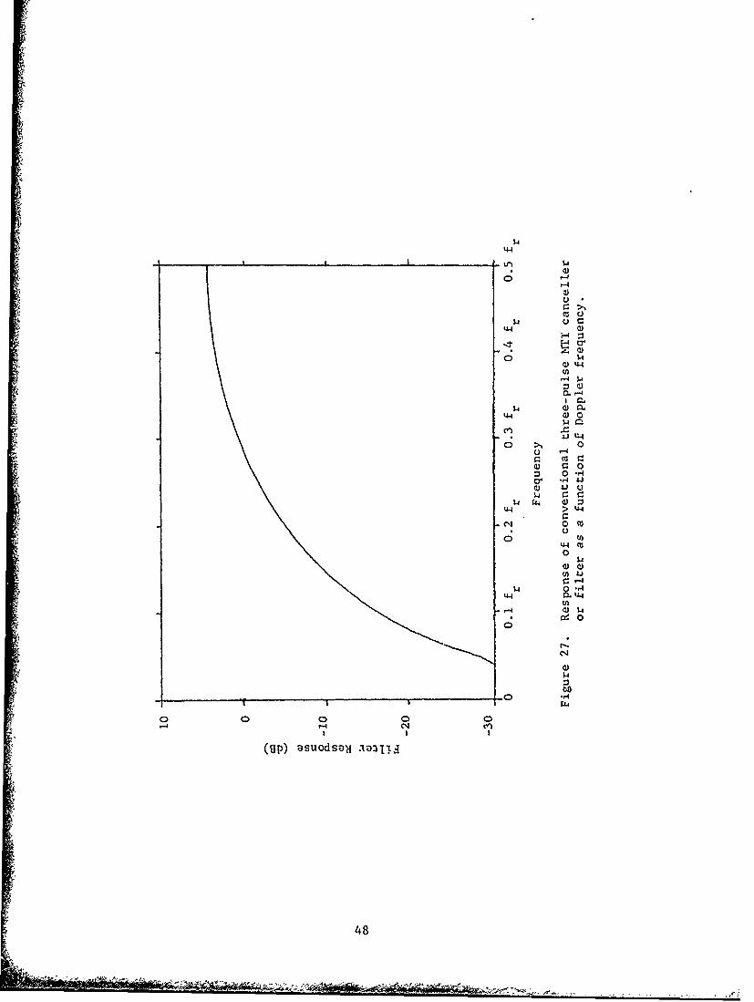
27. Response of conventional throe-pulse MTI canceller or filteras a function of Doppler frequency ...... ................ .. 48
28. Filter response for a four-pole Butterworth high-pass filter(labelled steady-state response) and the output of the samerecursive filter terminated after N = 3, 5, and 7 pulses were
processed. The stead5-state response has been offset forclarity ...... ......... ............................. .. 51
29. MTI filter responses developed using linear programming
techniques. 0.8-, 1.8-, and 3-dB ripple specification. See
text for details ....... ....... ....................... .. 54
30. Effects on MTI filter response of too stringent a ripple
specification. See text for details ..... ............... .. 55
31. Ripple vs. clutter attenuation for 5-pulse filters with 500 Hz
and 750 Hz lower cutoff frequencies ..... ............... .. 56
32. Bandstop filters showing effects of increasing allowable ripple
Son stop band characteristics. F = 250 Hz ................ .. 58
x

LIST OF FIGURES (cont.)
Figure Page
33. Comparison of the response of a conventional three-pulse MTIfilter and a miniwrum-rms-error filter designed for I = 60 dB,prf = 5000 pps, cc = 8.0, and 'n = 0.1 ....... .............. 63
34. Comparison of responses of minimum-rms-error filters designed for
1=10, 30, and 60 dB. I = 0.1, prf = 50 0 0 pps, and=8.0 .............. ....... ........................ 64
35. Comparison of minimuri-rms-error filter responses for 3, 5, and7 pulses processed. I = 60 dB, prf 5000 pps, c = 8.0,=0.1 ....... ....... ............................. ... 65
36. Comparison of responses of five-pulse minimum-rms-error f±itersfor 1 = 0 and 1 = 0.1. I = 60 dB, ac = 8.0, prf = 5000 ppe. • • 66
37. Maximally flat three-pulse MTI filter response. I = 60 dB . . . 68
38. Comparison of responses for three-puise maximally flat threepulse MTI filter (I = 60 dB) and minimum-rms-error MTI filter(I = 60 dB, 11 = 0.1, a c = 8.0, prf = 5000) .... ........... ... 69
39. Maximally flat MTI filter responses for three- and four-pulsesprocessed ....... ......... ......... ......... ..... ...... 71
40. Maximally flat filter responses for a four-pulse MTI filterfor i = 0, and i = I ...... ... ...................... ... 72
41. Maximally flat filter responses for a five-pulse MTI filterfor i = 0, 1, and 2 ............ ....................... 73
42. Filter response for a conventional three-pulse MTI filter whenvarious values of stagger, e, are used ..... ............. ... 74 "I
43. System improvement versus clutter spectral widtlh for radar systemwith f = 5 kHz and X = 5.5 cm, K = stagger ratio for
stgee pf....................................77staggered prf . . . . . . . . . . . . . . . . . . . . . . . . . . 7
44. Response of an optimum unstaggered MI filter when used with4 various amount of prf stagger, e ...... ................ ... 78
A-I. Three-pulse MTI filter ........ ..................... .... 90
A-2. System improvement versus clutter spectral width for radar systemwith f 5 kHz and ) 5.5 cm ...... ................. ... 94r
C-I. Representative received pulse shape showing the samples used inthe range-tracking algorithms ........ .................. 98
xi
LIST OF FIGURES (cont.)
Figure Page
C-2. e k as a function of t /T for f T = I andA 1T o 13dB 100
C-3. e /k as a function of t /T forf T=2
and A/T = 1 .o... . .3dB 101
E-1. Main computer program. . . ................. 104
E-2. Subroutine GAIN ........... ......................... .. 106
E-3. Subroutine DIST ........... ......................... .. 107
E-4. Subroutine STNDEV ......... ..... ........................ 108
E-5. Subroutine ERRO ......... ... ........................ .. 109
E-6. L ýroutine RCS ............ ......................... . I..1
D-1. Velocity response for frequency-agile radar using three-pulseMTI filter. F = 5.3 GHz, Ff f = 5.6 GHz,Step = 0.05 GHz......... ..... ......................... 114
D-2. Velocity response for frequency-agile radar using three-pulseMTI filter. F = 5.3 GHz, Ffinal = 5.8 GHz,Step = 0.03125s ýf...z ............................... .. 1
F-I. General form of non-recursive digital filters ............. .. 118
xii

I. INTRODUCTION
This Final Technical Rep•ort describes w;ork performed for the U. S. ArmyMissile Command under Contract DAAH01-71-C-1192 from May 1971 through May 1972.The investigations carried out during this period involved analyzing theExperimental Array Radar (EAR) being constructed by the Missile SystemsLaboratory, and developing methods for improving its performance.
These investigations were initially based on w~rk performed for theMissile Command under Contract DAAHOI-70-C-0535 [1] , under which GeorgiaTech examined the effects of polarization agility on monopulse radar angletracking. The techniques and target models developed under this earlierMissile Command contract formed the basis for a substantial portion of thework performed under the current contract.
The initial phase of the program was concerned with preliminary analysesof the performance of the EAR system and identification of areas of marginalperformance. A modified C-Band radar at Georgia Tech was used to estimateanticipated radar cross-section of targets for incorporation into thispreliminary performance analysis. Results of this preliminary analysis arepresented in Section II, and indicate deterioration in the performance of theEAR when the target has a relatively low Doppler frequency and/or when strongmultipath returns are being received by the system.
The effect of strong multipath returns on the tracking performance ofthe EAR when tracking low-flying targets is analyzed in some detail in SectionIII. The applicability of frequency agility to the EAR system for the purposeof minimizing these multipath-induced errors is discussed in Section IV. "'1heanalyses in both of these chapters leans heavily on a computer prediction ofthe EAR performance which included realistic representation of antennabeamshapes, null positions, and sidelobe levels.
The design of optimum MTI processors for use in the EAR system is treatedin some detail in Section V. Previous work in digital processing is reviewedand improved procedures for design of processors having optimum responsesfor a range of Doppler shifts are prescnted.
Conclusions and recommendationb :csulting from this study are presentedin Section VI.
Numbers in brackets refer to References in Section VII.

II. PRELIMINARY INVESTIGATION OF EAR PERFORMANCE
The initial step in the research program was a preliminary systemanalysis to define the performance of the EAR and to focus attention to thoseareas where performance is marginal. First, the free-space signal-to-noiseratio was calculated for the EAR system, and the effect of thermal noise onangle-tracking accuracy was analyzed. Next, the effect of multipath returnsentering the antenna sidelobes (the high angle tracking case) was considered,and finally signal-to-clutter ratios were calculated 'or the EAR system
A. Free-Space Signal-to-Noise RatioThe system parameters assumed in the preliminary analysis of the free-
space signal-to-noise ratio for the EAR system were:
P = peak transmitted power = 75 kW;t
G = antenna gain (assumed to be same for both transmit andreceive modes) = 25 dB;
X = wavelength = 5.45 x 10⁻² meters (5.5 GHz); and
N = noise power = -93 dBm (10-dB noise figure, lO-104z bandwidth).
The free-space, single-pulse, signal-to-noise ratio (S/N), is given by
SIN t G 2.245 x 10160
N (4T) 3R4 R4
where
R = range in meters, and
a = target radar cross-section in square meters.
The average signal-to-noise ratio (averaged over all Doppler frequenciesand relative phases) is unaffected by MTI processing. This can be seenreadily by considering that the average power gain of a two-channel MTlprocessor is six, and that six noise samples are added during processing, sothat the output signal-to-noise is unaffected. In a single-channel processor,the average gain is reduced to three (due to the necessity of averaging overall relative phases) but now only three noise pulses are added, so the outputsignal-to-noise ratio remains unchanged.
When processing in triplets, as in the EAR system [21, the 48 pulses ona target produce 16 independent qamples. Approximately 10 dB should be addedto the signal-to-noise ratio calculated earlier to account for effects ofintegration of these 16 samples. Figure I shows the average free-space signal-to-noise ratio as a function of range for several values of targeL -idarcross-section.
Preceding page blank3

35 ~~ ~
30
a=O.Olrmr30 250 n
220 252
Li,9
o 20z0
to
*N 15
10
5
0
1 2 3 4 5 6 7 8 9 10 15 20
Range (km)
Figure 1. Average signal-to-noise ratio for the EAR system as afunction of range. These values should be mouified bythe response at the specific target Doppler frequencyobtained from Figure 2.
4

The average signal-to-noise ratio is given by the above expression;however, the response at a particular Doppler frequency may be considerablydifferent from this average value. The frequency response for the conventional
three-pulse MTI filter is derived in Appendix A and plotted in Figure 2.Figure 2 has been normalized so that the signal-to-noise ratio for a giventarget may be determined by adding the response at the desired Doppler frequencyfrom Figure 2 to the values read from Figure 1. For very slow targets and for
targets near the blind speed, substantial reductions in performance arepossible. The design of improved MTI filters having more nearly uniformresponse is discussed in Section V.
B. Tracking Errors Due to Glint and Thermal NoiseThe rms tracking error due to thermal noise has been derived by a
number of authors to be [3]
ek 2BT (S/N)
m
where
Ot rms angle-tracking error,
e = 3 dB antenna beamwidth,
k = difference-channel error slope,m
B = i-f bandwidth,
T = pulse length, and
S/N = signal-to-noise power rati ,
0If one assumes BT 2, k = 1.57, and e = 2 which might be reasonable choices,
then m
a !0.9
where at is expressed in degrees.
This rms tracking error in degrees is plotted as a function of range
in Figure 3 for a number of target radar cross-sections. The 10 dB of inte-
gration gain included in Figure I is also incorporated into the results shown
in Figure 3. The signal-to-noise ratio used was the average over all
Doppler frequencie.; at some particular frequencies, the performance may be
appreciably worse due to the frequency response of the MTI processor.
The treatment of rms error du2 to target glint may be considerably
simplified by characterizing the target by an ",ains effective length," Leff.
5

Cd 0
p V) -4
to 0
UobV00
Ca. 0
00
u 0 r4 (I
oo r44 0 a-Z 0
MW0
0~ 04 a
UI) r4
0 0 0:
t1 Orq 0)
01 -A 0 1
C4J
o U))
C)0 0 C)
Cfl4 0n
(9p)~ asodo4 0 S-a
1.00.9 - Th~ermal Noise Limited0.8 - Glint Limited-•-0.7 ,-
0.6
! 0.5 .Leff = 10 meters - O.Im2
0.4
0.3
4 0.2 Leff 5m = Vm
I-I
S0.1
0.09 lom"0.08
0.07H 0.06
0.05
0.04 Leff lmeter = loom2
0.03
0.02
0.01. . I I . I I i I I1 2 3 4 5 6 7 8 9 10 15 20
Range (km)
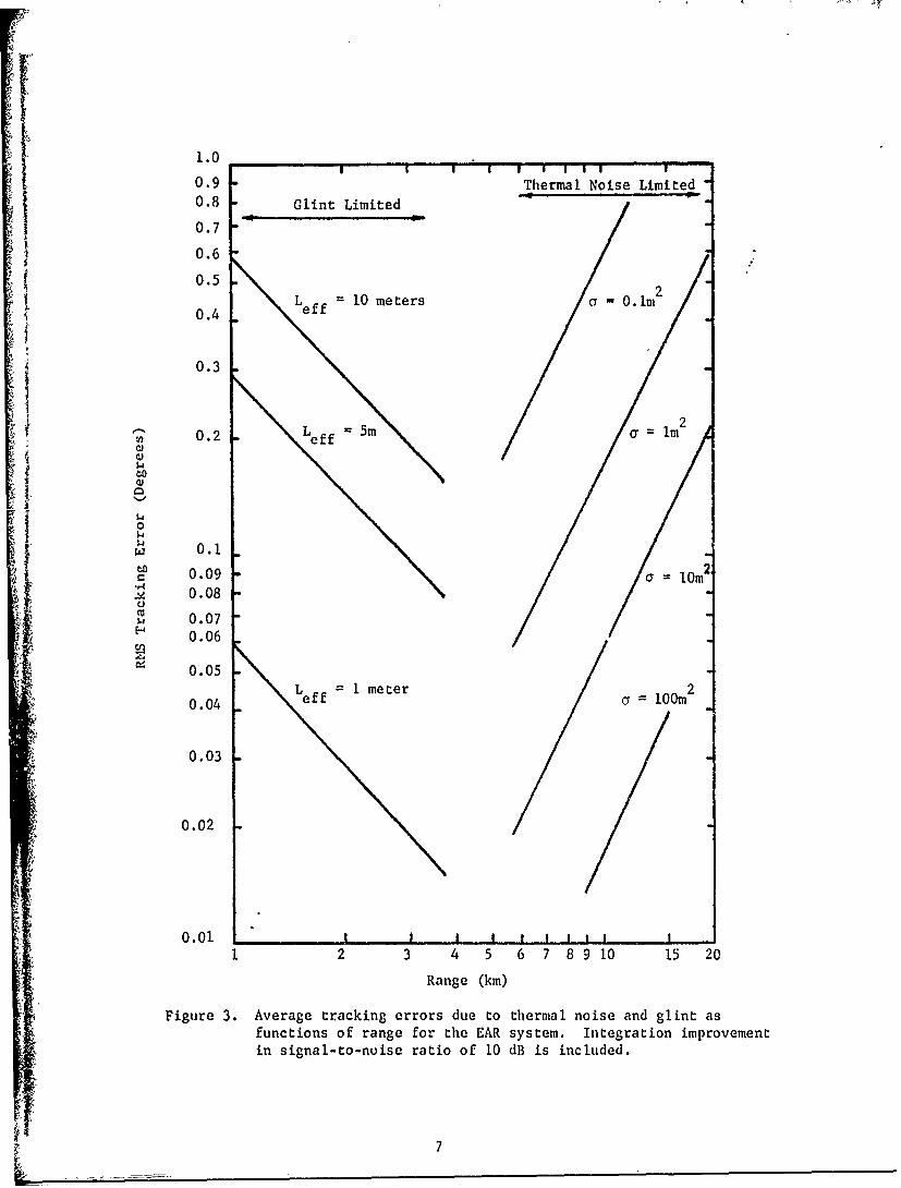
Figure 3. Average tracking errors due to thermal noise and glint asfunctions of range for the EAR system. Integration improvementin signal-to-noise ratio of 10 dB is included.
7
The rms angular error in degrees as a function of range is also plotted inFigure 3 for targets having several values of L . Results of analysesperformed during earlier contracts at Georgia Tecn and surveys of theavailable literature indicate that an effective length of from 5 to 10 metersin azimuth is representative of values to be expected from many targets ofinterest. The effective length in elevation will probably be somewhat less;reasonable values probably lie between l and 3 meters.
Figure 3 indicates that the region of maximum average angle trackingaccuracy lies roughly between 3 and 7 km, depending upon the specific choicesof target radar cross-section and effective target length assumed.
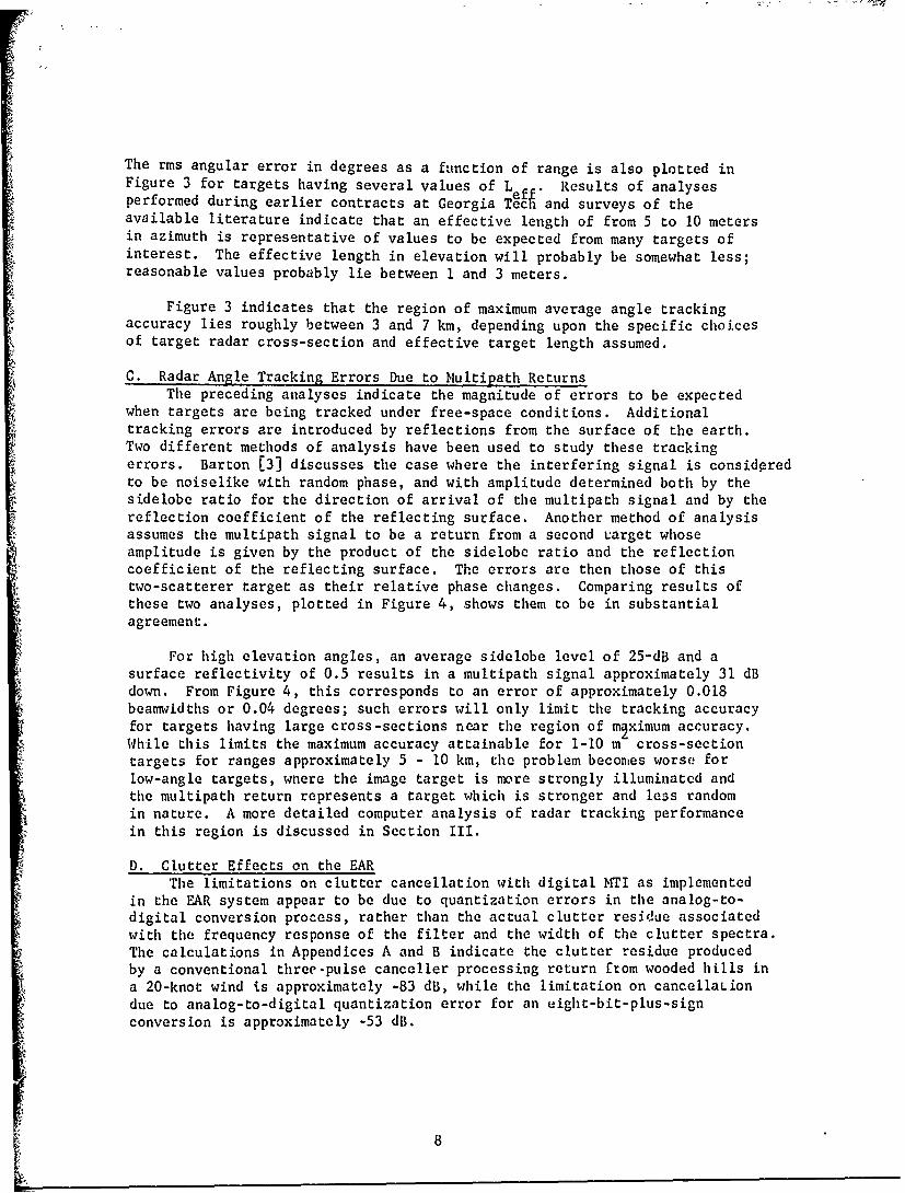
C. Radar Angle Tracking Errors Due to Multipath ReturnsThe preceding analyses indicate the magnitude of errors to be expected
when targets are being tracked under free-space conditions. Additionaltracking errors are introduced by reflections from the surface of the earth.Two different methods of analysis have been used to study these trackingerrors. Barton [3] discusses the case where the interfering signal is consideredto be noiselike with random phase, and with amplitude determined both by thesidelobe ratio for the direction of arrival of the multipath signal and by thereflection coefficient of the reflecting surface. Another method of analysisassumes the multipath signal to be a return from a second Larget whoseamplitude is given by the product of the sidelobe ratio and the reflectioncoefficient of the reflecting surface. The errors are then those of thistwo-scatterer target as their relative phase changes. Comparing results ofthese two analyses, plotted in Figure 4, shows them to be in substantialagreement.
For high elevation angles, an average sidelobe level of 25-dB and asurface reflectivity of 0.5 results in a multipath signal approximately 31 dBdown. From Figure 4, this corresponds to an error of approximately 0.018beamwidths or 0.04 degrees; such errors will only limit the tracking accuracyfor targets having large cross-sections near the region of m~ximum accuracy.While this limits the maximum accuracy attainable for 1-10 m cross-sectiontargets for ranges approximately 5 - 10 km, the problem becomes worse forlow-angle targets, wnere the image target is more strongly illuminated andthe multipath return represents a target which is stronger and less randomin nature. A more detailed computer analysis of radar tracking performancein this region is discussed in Section III.
D. Clutter Effects on the EARThe limitations on clutter cancellation with digital MTI as implemented
in the EAR system appear to be due to quantization errors in the analog-to-digital conversion process, rather than the actual clutter residue associatedwith the frequency response of the filter and the width of the clutter spectra.The calculations in Appendices A and B indicate the clutter residue producedby a conventional three-pulse canceller processing return from wooded hills ina 20-knot wind is approximately -83 dB, while the limitation on cancellaLiondue to analog-to-digital quantization error for an eight-bit-plus-signconversion is approximately -53 dB.
8

0.1 - -o0.2
0.09 0.18
0.08- -0.16
0.07 -0.14
-0.06 - 0.12
0.05 -- 0.1
0.04 - 0.08
Two-Scatterer0.03 Model
0.03e -0.06
Barton1K=1.6
m0.02 0.04
0 0
o.o0 0.02 o 4o 4W 0.009- 0.018 .
S 0.008 -0.016
f0.007- 0.014
0.006 0.012
0.005 - 0.01
"0.004 0.008
0.0O03 __(_______________ 1006
-40 -30 -20 -10
Ratio of Direct to Indirect Signals at Receiver
Figure 4. RMS tracking errors due to multirxth as a functionof the ratio of direct to indiL'ect signals at thereceiver.
9

The received signal-to-clutter power ratio (S/C) before MTI processingmay be approximated by
aSrtS 1 2
/C = rtrg x 20 R6A Tc
where
a = target radar cross-section,
Srt = gain in the sum channel on reception for target,
S rt = gain in the sum channel on reception for reflected energy,rg
0a = radar cross-section per unit area of clutter,
R = range,
A = azimuth 3-dB beamwidth,A
T = pulse length, and
c = velocity of light.
For the vertical array, where the broae azimuth beamwidth (approximately 300)results in large clutter power and the broad transmitting pattern is assumed
to illuminate the clutter and the target with approximatley equal intensity,the S/C ratio is a function of elevation angle. However, if elevationgreater than approximately 20, the gain for the clutter signal will beapproximately the average gain in the sidelobes of the vertical array. Forsimplicity, assume that this gain is approximately -25 dB. Values of S/Cratio may now be calculated and then modified by the clutter cancellation ofthe system.
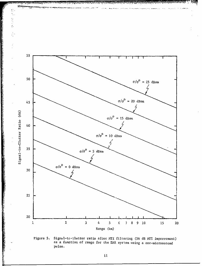
A plot of the average signal-to-clutter ratio after cancellation for aone-microsecond pulse and various rations of a/a 0 valid for elevation anglesgreater than approximately 20 is presented in Figure 5. These values mustbe modified by the response of the MTI processor for the particular targetvelocity.
2 o
To illuitrate the use of Figure 5, consider a = I m and C = -20 dB ora/ao = 100 m = 20 dBsm. The average signal-to-clutter ratio is approximately43 dB at a range of 10 km. However, the frequency response of the MTIprocessor must be added to this value; since the processor response may besubstantially smaller than -20 dB, the value obtained from Figure 5 may bemodified substantially. This reduction of signal-to-clutter ratio is anothermanifestation of nonuniform Doppler responses produced by conventional WI
processors, and illustrates the need for improved MTI filter responses asdiscussed in Section V.
10
55 ii'" "
50 -/ G o = '25 dBsm"
45 - ' 0"Ia° 20 dBsm
Vo • l/o =15 dBsm
O 40
41cra =1 dBsm
504 5
2~~a 5 d •89 015 2
Figre5. igal-a-o lte 0ai afe d fl.rng(6d sT mroeet
2 0
1 ~ ~ ~ ~ / 2= 10 15 20
as a function of range for the EAR sys,.em tising a one-microsecondpulse.

III. MULTIPATH EFFECTS ON EAR ANGLE TRACKING ACCURACY
A. IntroductionIn the previous section, it was noted that multipath reflections returned
to the antenna through the low-amplitude sidelobes of the EAR antenna do notlimit system performance except for the case of large targets near the regionof maximum accuracy. However, when target elevation is reduced, multipathreturns become stronger, errors are less random in nature, and trackingaccuracy lessens; consequently, multipath signals in this situation canseriously limit EAR system performance.
Characteristics of the target, reflecting surface, tracking antenna, andradar data processor all influence the nature and severity of multipath-induced tracking errors. A computer program was written to assist indetermining the effects of these factors on tracking performance of the EARin multipath situations. The program permits calculation of elevation-angletracking error, and signal amplitude and phase variations, and allows imple-mentation of various processing techniques.
The geometry of the target trajectory, calculation of received signalsand indicated errors, antenna pattern generation, program organization, andresults of this computer analysis are discussed in the following paragraphs.
B. Geometry of the Target TrajectoryThe analysis assumes a target flying at constant altitude on a radial
path toward the antenna as shown in Figure 6. Target altitude is denoted byH and the antenna is located at height H . The surface is assumed to beflat, so that simple specular reflection occurs, and to hav( a reflectioncoefficient p (in most of the analyses p was assumed to be real). The anglesnecessary to define the geometry are indicated in Figure I as follows:
THT Angle between antenna and target measured from horizontal
THIM Angle between antenna and target image measured fromhorizontal
THANT Pointing angle of antenna normal measured from horizontal
THSCAN Angle at which antenna beam is scanned from antenna normal
THBEAM Pointing angle of antenna beam measured from horizontal
THI Angle between antenna beam and target measured from antennabase
TH2 Angle between antenna beam and target image measured fromantenna beam
Preceding page blank
13

AntennaNormal
BeamDirection
THSCAN
THANT THI 1 Target
S __Direct t-
Antenna •/
THBEA THT- I
!Reflected
TH2
\ ~/
/
Z Ground Surface
Note: All angles are measured,positive in the CCWdirection. Dotted arcsdenote angles which arenegative for the con-figuration shown.
'rarget Image
14
Figre6. ntnn/tage gemer4
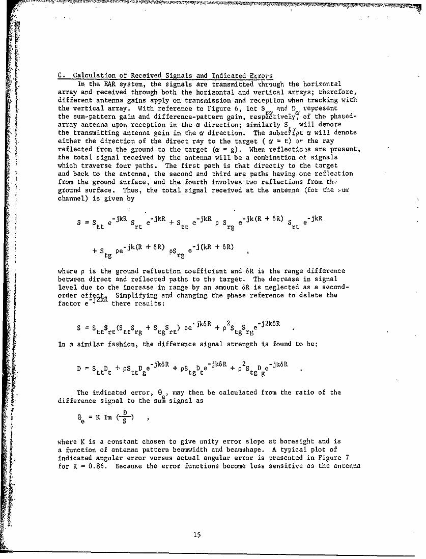
C. Calculation of Received Signals and Indicated Errors"In the EAR system, the signals are transmitted throcigh the horizontal
array and received through both the horizontal and vertical arrays; therefore,different antenna gains apply on transmission and reception when tracking withthe vertical array. With reference to Figure 6, let S and D representthe sum-pattern gain and difference-pattern gain, respectively, of the phased-array antenna upon reception in the a direction; similarly S will denotethe transmitting antenna gain in the o direction. The subscrit a wi.l denoteeither the direction of the direct ray to the target ( a = t) or the rayreflected from the ground to the target (a = g). When reflectJios are present,the total signal received by the antenna will be a combination of signalswhich traverse four paths. The first path is that directiy to the targetand back to the antenna, the second and third are paths having one refle.:tionfrom the ground surface, and the fourth involves two reflections from th,'ground surface. Thus, the total signal received at the antenna (for the 'ýumchannel) is given by
S e-jkR -e RjkR + ekR e-jk(R + 6R) e-jkR. St r Stt p rg Srt
+Sg pe S-jk(R + 6R) -j(kR + 8R)tg rg
where p is the ground reflection coefficient and 6R is the range differencebetween direct and reflected paths to the target. The decrease in signallevel due to the increase in range by an amount 6R is neglected as a second-order effe•^ Simplifying and changing the phase reference to delete thefactor e 3 ha there results:
S = S ttrt (SttSrg + S tgSrt) pe" k6R + p2Stg Srge-j2k6R
In a similar fashion, the difference signal strength is found to be:
-jk6R + Pgt-Jk8R +2S D ejk6RD = SttDt + pSttDge + pS tgDt ek +R P + tg gD 9
The indicated error, e . may then be calculated from the ratio of the
difference signal to the sum signal as
6e =K Im (+)
'i where K is a constant chosen to give unity error slope at boresight and isa function of antenna pattern beamwidth and beamshape. A typical plot ofindicated angular error versus actual angular error is presented in Figure 7for K = 0.86. Because the error functions become less sensitive as the antenna
15

0n00H 0
u cn
u~00
C4
,;
0 U) 1
40 0 n
0130
@0 u-
to
0 CD
4.4
I ~ \0 144 0
r.4
@0~~ 03' -
0 0
0 oto-,4
a~~ln~u0 o<3opu
16-

is scanned (due to increasing antenna beamwidth) it may be advantageous tormake K a function of scan angle so the curves for all scan angles haveapproximately unity slope at the origin. Curves for this case are shown inFigure 8 where K = 0.845 + 0.335 (8 scan/30).
D. Antenna Pattern GenerationFor the system simulation, it was decided to use a simple scheme that
would give an adequate representation of the antenna patterns to be approxi-mated. The characteristics of the antenna pattern used for the computeranalysis of vertical array are shown in Table I, and compared with measuredvalues given in parentheses:
Table I - Antenna Pattern Characteristics
Parameter Boresight 50° ScanSum 3 dB BW 2 (2) 3 (3)
Gain Reduction 0 dB (0) 4 dB (3.5)
Sidelobe Level. -27 dB (-28) -30 dB (-28)
Peak Difference -2 dB (-2.7) -2.5 dB (-2.7)Pattern Level(referred to peak ofsum patterns)
The patterns were generated using assumed aperture illuminations ofthe form
f(x) = A cos -IXa
which result in far-field patterns having the form
g(u) = klF 2Cos U
T 22 -u
where
u k 2 F sin 1
To generate the sum and difference patterns, . is assigned values0 and 6 + 6 , where Q is the offset angle of the bh.am. The two patternsthus createg are adde2 and subtracted to produce sum and difference far-fieldpatterns ksee Figure 9). In order to cause the patterns to vary with scanangle, both eo and F are made to be functions of scan angle, the specificfunction being determined empirically to produce the desired pattern variation.
The transmitted signal is radiated through the horizontal array whichhas very nearly constant gain over a wide range of elevation angles. Theelevation pattern for this antenna was simulated as being that of an isotropicradiator.
17

0l00
V)l
a)
00
I00 00 .
00
CD c*
s~0 .Cl)
p u
w. 0 0
0 w C0
06~0 C11~,-4 Cl
'& .4 :1 COO
U100L
W Nt
41Co
1 44 0
(saaaIap) a~oaa3z~ avlrn~uV pativopul

Gain(dB)
0
SI iI ~lI/ '
/ II I
0 50 00
p I .I
I ' I
,% I II II i II IpI IlI
10
15
11 II
200
I 25
,o 300
Si35
-4 -2 0 4
Far-Field Angle (degrees)
Figure 9. Typical sum (solid lines) and difference (dashed lines) patternsused in the computer analysis.
19

E. Program OrganizationThe computer program used for analysis (Appendix E) consists of a large
main program which performs input and output tasks with several subroutinesto do specialized computations. All parameters are initialized in the mainprogram; this program controls the execution of the various subroutines.The subroutine ERRO, for example, provides for calculation of the indicatedangular error between antenna and target and returns this information to themain program for antenna beam-pointing calculations. Trajectory prediction';are computed in the main program, while frequency-agility calculations andsignal processing are performed in subroutine ERRO. The subroutine GAINcalculates antenna pattern data (see Section E) and feeds this informationto ERRO. The remaining subroutines are used to perform statistical analyseson the calculated data and produce output plots.
Various versions of the program include provision for different beam-pointing calculations (including linear and parabolic predictions andpredictor-corrector filters) and the implementation of frequency agility.The trajectory prediction programs fit linear and parabolic curves, respec-tively, to a set of three data points to predict where the antenna beam shouldbe pointed for the next look. The frequency-agility program permits selectionof start and stop frequencies and thie frequency step size. Each frequency istransmitted for three pulses and then stepped; when the stop frequency isreached a new cycle is begun. Since a total of 48 pulses are transmittedfor each look at the target, the frequency parameters are normally chosen suchthat 16 frequencies are transmitted before a new cycle is begun in order tomaximize the information obtained. Data from all frequencies may be averagedto calculate the indicated angular position of the target or adaptive-processingtechniques may be used to select data samples from the available set.
F. Results of Computer AnalysisFrom the computer analysis are obtained plots of the elevation tracking
error in feet as a function of time. These results are affected by antennaheight and tilt angle, target height and backscattering characteristics, radarfrequency, and the properties of the reflecting surface. A representativeplot of tracking error is shown in Figure 10; this particular run was calculatedfor an isotropic-scatterer target having a radial velocity of 250 mph, andwas initiated at a distance of ten miles. The frequency of operation waschosen to be 5.5 GHz, and the physical face of the antenna was vertical(antenna normal horizontal). The reflection at the earth surface was charac-terized by a (voltage) reflection coefficient of 0.5.
The beamshape produced by the antenna varies with scan angle, beamwidthbeing minimum when the beam is normal tc, the face of the array, and broaderfor non-zero scan angles. Therefore, the physical orientation of the antennamay be chosen so as to minimize antenna beamwidth and maximize tracking accuracyfor the region of most interest. Figure 11 shows the effect of tilting theantenna back, which enhances accuracy at high angles at the expense of low-angle accuracy (compare with Figure 10). The most desirable tilt angle forthe antenna depends upon a number of factors and may differ with mission
20

400 I
'300 -
200 -
100 -
0-
- -100 -
wU.. -200 -
C.) -300 -"400
0 10 20
400- I
'300 4
200 -
100 -
0
.100
,, -200 -
• *300 -
"LU .400 '
20 30 40
Time (seconds)
Figure 10. Tracking error as a function of time. |i = 100 ft, lt= 300 ft.f = 5.5 GIiz, o = 0.5, tilt angle = 0 .
21

400 ! .... I
300 -
200
100 -
0
-100
LL -200 -
--300 -
" -400 1 1 1 I I
0 10 20
400 I
300 -
200 -
100
0
-100 -
U . 200 -
, -300 -:Zk
"w - 400
20 30 40
Time (seconds)
Figure 11. Tracking error as a function of time. la= 100 ft, IIt = 300 ft,f = 5.5 GIlz, p = 0.5, tilt angle = 300.
22

requirements. An angle of 30 was chosen arbitrarily for use in most of theremaining computer analyses.
Figures 11 and 12 present a comparisonof results for lit = 300 ft andH =500 ft for an antenna tilt angle of 30 . These two figures illustratethe influence of target height on che multipath-induced tracking errors. Thetarget hiight is seen to influence both the amplitude and frequency of thesemultipath-induced errors. These errors are also affected by changes in antennaheight: Figure 13 shows the same situation as Figure 11 (on a different timescale), but with antenna height reduced to 15 feet. The peak amplitude of thetracking error is somewhat less at the lower antenna height, and the frequencyof the excursions is significantly lower.
Numerous runs of the type shown in Figures 9 - 13 were performed in order
to define more clearly the effect of multipath returns on the tracking accuracyof the EAR system. An antenna tilt angle of 300 was selected for most ofthese analyses, and an isotropic-scatterer target having a radial velocity of250 mph was used. A surface reflection coefficient of 0.5 was chosen for all
of these analyses. Figure 14 summarizes the results as plots of peak-to-peak tracking error as a function of target height for two values of antenna
height chosen to approximate the heights of the initial EAR Test Bed site
and a similar antenna mounted en a tracked vehicle. Figure 14 indicatesthat multipath error is significant for targets below 1200 feet, and ismaximum at altitudes of about 400 to 800 feet.
Figure 14 shows that tracking error due to multipath can be of such amagnitude as to severely limit radar system performance. Various methods
for alleviating the effect of multipath returns have been proposed, and are
discussed at length in an earlier Georgia Tech report [4]. The most practical
method for implementation with the EAR is frequency agility, and the appli-cability of this approach to the EAR system is discussed in detail in thenext section.
23

400 \
300 -
U- 0
" 100 -
0 -
1-00
•-200
-300 -
-400- i -'-0 10 20
400
300 -
,- 200 -
LL• O0 -
0-
LU-100
--200 -
-300
-40020 30 40
Time (seconds)
Figure 12. Tracking error as a function of time. 11, 100 ft, it = 500 ft,f = 5.5 GHz, p 0.5, tilt angle 30°.
24

C*00
'.0 -
N
tA 44
c0
-4-
00II
1 4-4
* 4 4
C4 pO04J0
0 0
'0 0 414
E--4
C.,., C
-4J
00
0 0 0 O0 0It M C14 4 -4 N CN
25 .

• •800
p =0.5
5.5 Gllz
700
600
• • H =100 f t
500
S,• Ha=15 f t
A •" 400
V ~0I-to
C 300"-,4
U
200
100
0
0 400 800 1200 1600 2000
Target Height (feet)
Figure 14. Peak-to-peak elevation tracking errors as functions of targetheight for 15 and 100 feet antenna heights. P = 0.5 andfrequency is 5.5 Gllz.
26

IV. APPLICABILITY OF FREQUENCY AGILITY TO THE EAR
Frequency agility is often proposed as a method for reducing effectsof both glint and multipath on radar tracking accuracy. The effectivenessof frequency agility on glint-induced tracking errors has been investigatedin an earlier Georgia Tech report [4]. While the EAR presents a somewhatdifferent situation (C-band vs X-Band), the results set forth in thatreport are generally indicative of what could be achieved if frequencyagility were used with the EAR system in tracking a free-space target.
The analysis presented in Section III shows that the effect ofmultipath returns on the EAR system performance is significant for targetsat altitudes less than 1200 ft. Numerous methods for reducing the tracking
error have been proposed; these include multiple-height antennas, spacediversity (in the azimuth plane), high-resolutio,. antennas, polarizationagility, shaped antenna beams, and frequency agility. The discussionsin an earlier Georgia Tech Report [5], coupled with the physical constraintsof the EAR system, make frequency agility seem to be a promising candidatetechnique for reducing multipath-induced tracking drrors. Therefore, aninvestigation of the effectiveness of frequency agility in reducing thesemultipath-induced tracking errors was begun.
When frequency agility is used, a set of pulses is radiated in sequencewith frequency changed from pulse to pulse; the received pulses are eitheraveraged to obtain a more accurdte, stable, and repeatable indication oftarget position, or a selection rule is used to select optimum data from theavailable set. In the remainder of this section, the term "frequency agility"will be used to describe the averaging process, and the term "adaptive pro-cessing" used to denote the selection process.
Changing the transmitted frequency permits the acquisition of a numberof independent samples of target location by changing the relative phasebetween direct and indirect rays (altering their electrical path lengths).by changing the amplitude and phase of the reflection coefficient of thereflecting surface, or by affecting the scattering characteristics of thetarget. Within the normally achievable bandwidths of most frequency-agileradars, the reflection coefficient of many reflecting surfaces remainsessentially unchanged. The effect of small frequency changes on targetcharacteristics has not been exhaustively investigated, but should be smallfor most low-altitude targets, particularly in the vertical plane [51. Thus,the principal mechanism by which frequency changes affect tracking error isthe change in relative phase of direct and indirect signals received at theantenna. These changes in electrical path length produce what are oftensubstantial shifts in the location in range of the extremes of the trackingerrors. Figures 1f through 19 show the tracking errors for the EAR systemwith operating frequencies of 5.3, 5.4, 5.5, 5.6, and 5.7 Gliz. The changes inthe pattern of the tracking error with changes in frequency are clearly seen,and these changes indicate that practical frequency changes may indeed beeffective in obtaining a number of independent samples for further processing.
27
400 I I I
300 -
200 -
0-
.100-
* 200 -LL.
• -300 -
cI. --400
0 10 20
400-
30C -
200I OO -100
0
")0
u, .200
w --3000:
- -400
20 30 40
Time (seconds)
Figure 15. Tracking error as a function of time. Ha = 100 ft, lit = 300 ft,f = 5.3 GHz, p = 0.5, tilt angle = 300.
28

400 I I
300 -
200
100
--100.2 0 u
,,., "200-IL
-300 -
ci .400-
0 10 20
4,-00-
300
200
100
, 200 -'Li..
,,, oo II I tS20 30 40
Time (seconds)
Figure 16. Tracking error as a function of time. o H = 100 ft, Ht = 300 ft,f = 5.4 GHz, p = 0.5, tilt angle = 30
29
I<

400 - I
300
r- 200
2 00
I ,0
400
0 10 20
400 - I I
JOo -4
Cr/
200 304
3030

400 I I I I I
300 -
200 -
100 -
0 •
1• , 0 0 -
S-200 -LL-
S.300 -0r,C.r 4C0C
0 10 20
400 1 I I
300
200
I00
0
-100
u __ -2 0 0
c. 300
or -403
20 30 40
Time (seconds)
Figure 18. Tracking error as a function of time. 0 1100 ft, i= 300 ft,f = 5.6 GIIz, O = 0.5, tilt angle = 30t
•j. 31

c0- I00 I I I I I I
300 -
200 -
)OC-CC
4Cu., . 2t1
,, 300
C" 4CC-
0 10 20
4,
U4, 3 --
I I I I II-Z))
20 30 40
Time (seconds)
Figure 19. Tracking error as a function of time.o Ila 1 00 ft, fit 300 ft,f =5.7 Gliz, p =0.5, tilt angle =30.at
32

While coherent systems such as the EAR may usually be modified forfrequency agility with a minimum of transmitter and antenna changes, caremust be taken not to degrade the system MTI performance. In the EAR degrada-tion is circumvented by use of a "triplet" canceller as opposed to the normal"sliding window" canceller [6]. A central consideration in implementing sucha system is the amount of frequency agility bandwidth required; this topicis discussed in the next section.
A. Required Overall Frequency Agility BandwidthAn approximate estimate of the amount of overall frequency change
required may be arrived at by considering the relative phase of indirect anddirect rays. The relative phase. ý, between signals which traverse two pathswhose physical lengths differ by AR is given by
S=2rr AR = 2r rARX c
When frequency agilty is used, in order to sample all possible indicatedtarget positions, it is necessary to change ý by Tr; the corresponding requiredfrequency change, Af, may be arrived at as follows:
S+ TT = 2.r(f + 6f) AR
c
or
Af c2AR "
Taking c = 3 x 10⁸ m/sec, then
3 x 10⁸A - 2AR
and if Af is Miz and AR in meters,
Af = 150/AR
Since for mulipath situation [71,
2H (11 + 11)AR aa t
R
the required frequency change becomes
Af ~ 75fSIHa (a T t
The required changes for 11 = 15 feet and 100 feet have been calculatedand are plotted in Figures 20 and 21. These data indicate that the 400 to
33

y
400
H H=,Oi
H =500f t
1000ftHHt1000f0
H =15ft6a
w
C.)01
$4 10
I I t
500 1,000 5,000 10,000 20,000
Range (meters)
Figure 20. Frequency change required to change the relative phase ofthe direct and reflected signals by ,. Antenna height = l5ft.
34

400
H = 100 fta
[t 100 ft
100
Ht =500 ft
lit 1000 ft
10
500 1000 5,000 10,000 20,000
Range (meters)
Figure 21. Frequency change required to change the relative phase ofthe direct and reflected signals by ~.Antenna height 1O0ft.
35
-CU

500 MHz potential frequency agility bandwidth of the EAR system is sufficientto be at least partially effective in reducing multipath effects on the EAR,particularly for higher altitude targets, higher antenna site, and shorterranges.
B. Effect of Frequency Agility on Angle Tracking PerformanceThe computer analysis of EAR tracking performance described earlier was
used as tool to examine the effectiveness of frequency agility in reducingmultipath-induced angle tracking errors. The format selected was to radiate16 frequencies and wait 0.1 seconds between looks at the target. The indicatedangular errors for each of the 16 frequencies were then averaged togetherto provide an estimate of true target position.
The degree of improvement that may be realized with frequency agilityis a function of target and antenna heights, and of the frequency-agilitybandwidth (overall frequency excursion). Data from a number of runs havebeen summarized by presenting peak-to-peak tracking error as a function oftarget height for various frequency-agility bandwidths and antenna heights.
Figure 22 shows one such set of data, indicating the effectiveness ofvarious frequency-agility bandwidths in reducing multipath-induced trackingerror. The three curves plotted in Figure 22 represent the performanceachievable with fixed-frequency operation, 200-fiz bandwidth frequency-agileoperation, and 400 MHz bandwidth frequency-agile operation for a 100-footantenna height. The 400-MHz bandwidth is particularly effective in reducingthese errors, especially for higher targets.
As discussed earlier and shown in Figures 20 and 21, the antenna heightinfluences the amount of frequency excursion necessary. Figure 23 shows theresults obtained when frequency agility was used with a 15-foot antennaheight. While tracking performance was improved with frequency agility, theimprovement is not as dramatic as seen in Figure 22 for 100-foot antennaheight.
The reflection coefficient also influences the tracking performance ofthe EAR in a multipath situation. A reflection coefficient of P = 0.5 wasused for most of these analyses, however, both higher and lower values ofP were also used during the course of the analysis. Figure 24 shows theresults obtained when a value of p = 0.7 was used, indicating the while themagnitude of the errors increases with increasing p, the relative effectivenessof frequency agility remains essentially the same.
These data indicate that substantial reduction in angle tracking erroris possible when frequency agility is used in the EAR system, provided thefull frequency agility bandwidth of the EAR system is utilized.
C. Adaptive Processingý for the EAR SystemUse of the relative phase difference between sum and difference signals
as an indication of the acceptability (or quality) of the tracking informationis based on the fact that when tracking a single target in free space, the
36
S•. J•,••.•.-• • i' -- il" •~ •_.• • . .- . ...... . ' -Z' •-? °i-, _ "-- -

800
H 100 fta
700 p = 0.5
600
500 •Fixed Frequency5.5 GHz
0
400
-A-
U Frequency Agile5.4 - 5.6 Gllz
300
200
Frequency Agile5.3 -5.7 Gllz
100
O0
0*I I I I400 800 1200 1600 2000
Target Height (feet)
Figure 22. Tracking error as a function of target height usingfrequency agility. 11a = 100 ft.
37

800
S700 a = 15 ft
p = 0.5
600
500
Fixed Frequency 5.5 GHz
¢ 400
0 Frequency Agile5.4 - 5.6 GHz
'• 300-' 300--Frequency Agile
5.3 - 5.7 GHz
200
1.00
O0
4. 0 I I I,'. .. .. I
0 400 800 1200 1600 2000
Target Height (feet)
Figure 23. Tracking error as a function of target height usingfrequency agility. Ha =15 ft.
38

1000
H = 100 ftap = 0.7
800
600 Fixed Frequency - 5.5 GHz
"* 400
r 5.3 - 5.7 GHz
.4)
U 200
0400 800 1200 1600 2000
Target Hleight (feet)
Figure 24. Tracking error as a function of target height usingfrequency agility. He a lOOft.
39
r "IlT i...• °I I m , ' " --

difference signal has relative phase of 0 or 180 (depending on which side ofthe axis the target lies) when compared with the sum signal. When severalunresolved targets (or a single target and its image) are illuminated by theradar, this phase relationship no longer holds. The basis of one adaptiveprocessing scheme is to use this relative phase between sum and differencesignals, the so-called Complex Indicated Angle (CIA) [8] as a measure of thequality of the position data. A plot of the CIA as a function of time for thesame run shown in Figure 17 is given in Figure 25. A correlation is seenbetween the phase deviations of the CIA from 0 and 180 0and the peaks of thetracking error. However, these phase variations are rather small and thepresence of thermal noise, random target characteristics, and equipmentinaccuracies would probably make it difficult to appreciably improve the qualityof the track data by using the CIA.
Use of the amplitude of the received sum signal as a means of identifyingacceptable track data has also been proposed [9]. Figure 26 shows the amplitudeof the sum signal for the same situation shown earlier in Figure 17. Comparingthese two figures indicates a high degree of correlation between the minimumof the received signals and the peaks of large tracking error. This isprobably the most significant correlation which may be used to assess thequality of tracking information, and on which has been proposed to reduceglint-induced tracking errors. In the multipath situation, when tracking acomplex target, variations in target cross-section with frequency may be as
( large or larger than the variations in received power due to multipath sienals.Thus, there is no guarantee that optimum processing is bbtained by selectingthe signal of minimum amplitude. However, weighting of the track informationbased on the amplitude of the received sum signal appears to be a reasonableapproach, since it has a high likelihood of improving the overall quality oftrack data, if for no other reason than that low-amplitude signals likely tobe corrupted by thermal noise will be deemphasized. Computer analysis of morecomplex target models in a multipath situation using adaptive processing hasshown no clearly identifiable improvement in the quality of track data overconventional frequency agility. While there were cases where track dataimprovea appreciably, there were also cases where it did not, dependingupon details of the lobing of the target and the lobing due to multipath.
40

20J0 - I I I I I I I
150 " -
200
50-
10,
24
-0 -
•100 -
50
100
• 2 0 I I
0 10 20
Time (Seconds)
I I I I I I II
1504-
-So
•; 50-$4
104
20 30 40
Time (Seconds)
Figure 25. Complex indicated angle (CIA) as a function of time for
the same target-radar parameters described in Figure 17.
41.

1~ 40
~30.-4
EC
10
0 10 20
Time (Seconds)
40-
r-4 0
.r4
120 -
10
20 30 40
Time (Seconds)
Figure 26. Sum signal variations as a function of time for thesame target-radar parameters described in Figure 17.
42
V. IMPROVED MTI PROCESSORS
A number of factors enter into che design and specification of the dataprocessor for an MTI radar system. Among the constraints are requirementsthat the system have sufficient clutter attenuation for operation in a heavyclutter environment, that the target detectability remain relatively constantfor the range of expected Doppler frequencies, and that processing be performedusing some specified number of received pulses. The motivation for the firsttwo requirements are rather obvious, and the last requirement is dictated bythe desire to minimize the number of pulses required on a given target (andconsequently to maximize the number of targets which can be invostigated)in a beam-agile radar such as a phased-array radar, or by the desire tooptimize performance when frequency agility is used (by minimizing the numberof pulses transmitted at one frequency).
The basic points to be developed in this section are these: (1) Theoptimum MTl processor (optimum from a point of view of statistical detectiontheory) which operates on more than two received pulses has not yet beendeveloped. (2) If such a processor had been developed, its performancewould be limited by practical equipment considerati.ons. (3) Several improvedfilter designs for unstaggered prf systems have been developed which offersubstantial clutter attenuation while maintaining more nearly uniform responseto various Doppler frequencies. (4) Similar improved filter designs areneeded for the staggered prf case.
In this section, several design procedures are presented for the realiza-tion of improved MITI processors (cancellers, or clutter filters), and charac-teristics of processors designed using these procedures are discussed. SectionA reviews receivers that are optimum from the point of view of statisticaldetection theory. Previous work directed toward development of optimumdigital MTI processors is presented in Section B, where difficulties inobtaining acceptable M14 processor performance are discussed, and realisticconstraints set by equipment limitations and by system performance specificationsare outlined. MT1 processors that are optimum from a filter-design point ofview are developed in Section C, and conventional filter design procedures arereviewed in Section D. In Section E, several design procedures for use inunstaggered MTI radar systems are outlined. Some representative results offilter responses developed using these design procedures will be presented,and the limitations of each approach discussed.
M1I filtets for use in systems employing staggered prf are brieflydiscussed in Section F. The effect of using several different pulse staggerratios ir. a staggered prf system is analyzed, and available design proceduresfor staggered systems are summarized.
A. Use of Statistical Detection Theory in Developing Optimum MTI Receivers
Development of optimum receivers has been of substantial interest since
radar was first developed. The earliest optimum receiver was for detection
of a single pulse in white noi-a. This concept led to the development of the
43
43

so-called "matched filter" [10,11,121, namely, one which maximizes peak signal-to-noise ratio, and has a frequency response given by the complex conjugateof the voltage spectrum of the received pulse.
If the power spectrum of the noise plus received clutter varies withfrequency (so-called colored noise), then the optimum filter response becomes(except for a constant time delay) the complex conjugate of the voltagespectrum of the received pulse divided by the power spectrum of the receivernoise plus received clutter [13,14]. This fact was used by Urkowitz [15] toderive optimum receivers for detection of targets in clutter.
Rihaczek [16] has pointed out that the class of filters developed byUrkowitz is optimum only when thermal noise may be neglected, and that thepresance of both fluctuating clutter and thermal noise requries more complexfilters than those developed by Urkowitz.
If desired targets and unwanted clutter returns are separated in time(range) and/or in frequency, substantial improvement in performance is possibleusing combined signal and filter optimization. Delong and Hoffsteader [17,18]consider the problem of detection of a point target in random clutter usingcombined signal-receiver optimization. The detection of a target of knownDoppler shift has been treated by Stuart and Westerfield [19] and by Van Trees[20]. Spafford [21,22], Stutt and Spafford [23], and Rummler [24] have treatedthe optimum reciever when clutter and target signals have different areas ofoccupancy ou the range-frequency plane.
In many cases the expected Doppler shift of the received signal is notknown, a priori, and the expected range of signals overlaps the clutter inboth range and in frequency. The optimum estimation receiver for this casebecomes essentially a bank of matched filters, one for each expected Dopplerfrequency [25]; this configuration is very similar to the pulsed Doppler radarwhich employs a comb filter or a filter bank followed by a threshold for bothvelocity estimation and target detection.
The optimum detection receiver corresponding to the conventional MTIradar system appears to have been first discussed in the radar context byWainstein and Zubakov [26]. Because of the importance of this work, theirbasic approach to this problem will be briefly reviewed.
The formulation of the optimum MTI receiver is one of testing generalGaussian hypotheses for the case of a nonfluctuating target and interferingsignals which are Gaussian random variables. Two hypothese H and HI aredefined in terms of the received signal as follows:
H 0: r(t) = n(t)
SI : r(t) = n(t) +re(t) ,
where m(t) is a received signal reflected from a point target; in generalm(t) will have experienced some Doppler shift. The interfering signal n(t) isdue to both thermal. noise and reflections from clutter.
44

Define several matrices:
the observation matrix,
r =
rnj
the mean of the matrix r,
m = E(r)
the covariance matrix
A Cov(r) = E [(r - m).(rT- ,T)]
and the inverse covariance matrix
2 = A-'
The optimum Bayes and Neyman-Pearson tests are both likelihoodratios. The likelihood ratio (which is a function *'f both the Doppler shiftPd due to target radial velocity and the initial phase of the received signal e)is given by Van Trees [27),"
Ljr(8,) Wd) = exp [{ T-m)Qr m)-TQr]
under the assumption that the mean value of n(t) = 0.
Since Q is symmetric about its diagonal, that is, QT = Q, then mTQm = rTQm.Using this fact, the likelihood ratio may be written
L IE (ce, wd ) = exp [-½ (M TQr)] exp (M T Q E-)Since both the anticipated Doppler shift, w , and the initial phase
are unknown, the average likelihood ratio test teen becomes, assuming all uWdand 9 are equally probable,
L()= .2n exp [-½ T exp (m1 Q r) dwddO.
0 4
45

The evaluation of this likelihood ratio in a closed form is a formidabletask. The first integration introduces Bessel functions of the second kindof order zero, making the second integration difficult. Wainstein and Zubakov[26] have applied the addition formula for Bessel functions and evaluated thisintegral exactly for the case where the observation consists of two pulses.
The optimum HrI receiver derived by Wainstein and Zubakov for processingtwo received signals consists of optimum processing of both the in-phase andquadrature components of tho received signal, pairwise subtraction of thesetwo in-phase and quadrature samples, formation of the square of each of thesedifferences, and comparison oV the sum of these squares with the threshold [261.This processing corresponds to -he conventional two-pulse MTI canceller.
Selin [28] expanded the Bessel function of the second kind of order zeroin a power series valid for small ratios of signal to interfering signal inorder to simplify integration of the Bessel functions. Selin then furtherconfines his discussion to the case of white noise interference (which isuncorrelated from pulse to pulse). The results of this analysis have limitedapplicability due to their complexity and because in many cases of interest,the interfering signal is highly correlated from pulse to pulse due to thepresence of strong clutter returns.
Brennon, Reed, and Sollfrey [29] approximate the integral of the Besse!function by a finite sum. This approximation is used to compare the perfor-mance of optimum receivers under various conditions, but it does not giveinformation concerning how to construct an optimum M-I receiver; only how toapproximate its performance by means of a Doppler filter bank.
From this review, it becomes evident that the specification of theoptimum Uri processor from the point of view of statistical detection theoryis a tormidable task, and one which has been solved exactly only for the caseof the two-pulse processor. Because of the difficulty in specifying theperformance of the optimum 1f1l receiver, considerable attention has beenfocused on the design of optimum weighted sums for processing sampledsequences of the return from moving targets in a clutter environment. Thiswork is summarized in the following section.
B. Optimization of MTI Processors Using Weighted Sums of Sampled SignalsIt was brought out in the previous section that the optimum 11rl receiver,
from the point of view of statistical detection theory, is known only for thetwo-pulse case. The receiver for'larger-numbers of received pulses has oftenbeen approximated as a linear combination of a number of sample values ofeither the in.-phase or the quadrature component of the received signal. Maximi-zation of the ratio of average output signal (averaged over all expected valuesof Doppler frequency shifts, w ) to interfe:.ing signal has been treated byCapon [30]. Capon shows that Ehe optimum weight functions, defined as thosewhich optimize the average-output-signal-to-interfering-signal ratio (calledthe reference gain, Gn , or more commonly the MrI improvement I) depend only
upon the covariance matrix of the interfering signal. For highly correlatedpulse-to-pulse interference, such as that due to slowly moving clutter, these
46
ON IN'

optimum weight functions reduce to the conventional three-pulse canceller forthe case of processing three received pulses. Capon also shows that thereference gain for the three-pulse canceller closely approximates that fora large number of received pulses when processing signals in a background ofstrongly correlated clutter.
There are two main objections to Capon's approach. First, there is noreason to believe that the optimum processor may be realized in the generalconfiguration assumed by Capon; and second, the concept of the average systemgain, G , produces poor signal detectability at some Doppler frequencies ofinteres2. It is perhaps appropriate to note that if the linear processingformat discussed by Capon were the configuration of the optimum processor,then the optimum Neyman-Pearson test would be the one which maximizes G(see, for example, Spafford [22]). n
The average gain Gn is maximized by increasing gain at frequencies whereclutter return is small and decreasing it at frequencies whereclutter issignificantly present. Thus, processors designed to maximize G may haveunacceptably low responses to targets with Doppler frequencies in the sameregion as the clutter. The problem of optimizing che response of url systemsfor a wide range of target Doppler frequencies may be approached by consideringthe processor as a filter. This approach is developed in the next section.
C. MTI Processor Design as a Filter Optimization ProblemAs discussed in the preceding section, maximization of the average
system gain, I, is often not a very satisfactory method for optimizing theprocessing scheme for an HTI radar, since this leads to poor detectabilityof targets having some particular range of Doppler frequency shifts. Thisleads one to consider uniformity of response of the processor as a functionof wd as an important consideration in system design. This approach leadsnaturally to considering the processor to be a filter having as inputs a signalat the Doppler frequency and a signal from clutter plus thermal noise withknown power spectral density. Then the filter output can be plotted as afunction of input Doppler frequency; one such representation is shown inFigure 27 for the conventional three-pulse canceller. As one can see, theresponse is very non-uniform, and considerable improvement may be made in theshape of the curve while still maintaining a substantial value of I.
The second reason why maximizing I is not always entirely suitable foroptimizing system response is that there are often substantial practicallimitations which are not included in the theory. Most modern high-performanceMTl proccssors utilize digital processing, mainly to obtain storage withoutrecirculating analog delay lines. While round-off error in the quantizationor digitizing process does not usually appreciably limit performance, analog-to-digital quantization errors usually constrain I to be substantially lessthan its theoretically achievable maximum value. A comprehensive treatment ofthe limitations in improvement due to quantization errors is given in Appendix F.Therefore, it is often possible for I to be reduced somewhaL, providing moreuniform detectability of targets of differenL Doppler shifts, without substan-tially affecting overall system performance.
47
.44
4-4
-4
>1uC:
s...
u- c
oo r.
,li
U4O > -4
0- co~
4.4 (o
o >1 0
(1) "-
44 t*&-4~
4 C14
48-

Another factor which limits the performance of some real radar systemsis the presence of slowly moving discrete targets such as birds, insects, andautomobilas [31,321. The presence of these extraneous targets sometimesrequires that a "stop-band" be established, usually centered about zerofrequency, in order to reject these unwanted returns which would otherwisecompletely overload the system.
Therefore, one might conclude from these remarks that a practical design
procedure for digital MTI filters would be: (1) establish a desired andachievable value of I, based both on desired system performance and on practicale-uipment limitations, (2) within this constraint, produce an optimally uniformreeponse for all Doppler frequencies of interest, while (3) rejecting unwantedreturns. The filter responses are a function of the shape of the clutterspectrum, the optimization criteria applied to the response (such as minimumrms error, equal ripple in the pass band, etc.) and the expected range ofvelocities of the desired and undesired targets.
The following discussions will be largely confined to consideration oftransversal filters [33,34] (nonrecursive filters or those with no internalfeedback loops), because in a real application only limited number of pulsesmay be processed from each target. Several constraints determine the numberof pulses that may be processed from a given target. In a beam-agile radarsuchas a phased-array system, minimizing the number of pulses on a giventarget maximizes the number of targets the radar can accomodate. If frequencyagility is used, the radar must remain at a given frequency for a sufficientnumber of pulses to extract the desired information concerning a target;minimizing the number of pulses on target thus maximizes the number ofavailable frequencies the radar may radiate in a specified time. The perfor-mance of several conventional transversal digital HTrl filters is discussedas Appendix A. While a recursive filter (one containing feedback loops) couldbe used and its transient response truncated after the desired number of pulses,the response of such a truncated recursive filter may always be realized asa transversal filter. The difference between the two lies in the practicalimplementation of the filter.
D. Conventional Digital-Filter Design ProceduresVarious methods have been developed for designing digital filters [35,361.
Their design is often approached by defining an analog filter prototype andappropriately transforming the response to obtain the z-transform of the desiredfilter. In general, this approach yields a recursive filter; while thisfilter's output may be truncated after the desired number of pulses, there isgenerally little control over the number of pulses required to closely appro-ximate the desired steady-state response.
To illustrate the errors in filter response that may occur due totruncation of a recursive filter designed for a certain steady-state response,a four-pole Butterworth filter response was considered. Its z-transform wasexpanded to powers of z - by long division and the series truncated aftera selected number ol terms. The impulse response of the filter represented by
49

this series was then calculated to determine the truncated frequencyresponse. Figure 28 compares the steady-state response and responsesobtained by truncating the filter response after 3, 5, and 7 pulses. Ascan be seen, the response of the truncated series is a poor extreme case,due to the rapid low-frequency roll-off of the filter, but it serves toillustrate the need for specialized design procedures where the number ofavailable samples is limited.
Three procedures are commonly used in designing transversal digitalfilters [35-43]. The first involves specifying the sampled finiteimpulse response of a filter (obtained as an input specification or as atransform of a frequency-sampled response) and utilizing an impulse-invarianttransformation to specify the digital filter. Various weighing windows maybe used to smooth the ripples in the resulting frequency response. The secondmethod uses a Fourier-series approximation (with appropriate windows oftenincorporated) to a desired response, while the third method is a direct-searchmethod using linear programming techniques to optimize the desired response.These techniques are not particularly applicable to the design of MTI processingfilters, since they do not incorporate clutter characteristics into the filterdesign procedure as a design specification. In many cases they accept aspecific filter shape as the design goal, rather than developing optimumprocessing for a predetermined number of received pulses, a constraint whichis determined by the energy budget of the overall radar system. Four techniquesthat have been developed for design of optimum MTI processing filters forradars using unstaggered prf's will be outlined in the next section. Thestaggered prf case is considerably more complex; however, some related workhas been done in this area and will be reviewed in Section F.-
E. Optimum Transversal Digital-Filter Design Procedures for Unstaggered prfSystemsThe design of optimum MTI filters should take into account a number of
factors, including maintaining desired values of I, providing uniformity ofresponse for some range of Doppler frequencies, and in some cases providinga stop-band (usually centered about zero frequency) for rejection of unwantedtargets. In this section four different design procedures are described whichtake some of these factors into account.
1. "Cost" Minimization MTI Filter3Jacomini L44] has developed a design procedure that takes into account
the clutter attenuation in the pass band, the response in a stop-band, anidripple in the pass band. A "cost" is assigned to each of these factors anddesigns developed which minimize the overall "cost" of the filter. Thisapproach has the disadvantage that there is usually no straightforward meansfor selecting the various costs. In practice, when the filter is beingdesigned, the improvement, I, is constrained to be some constant, the costis apportioned between the pass and stop bands, and the relative costsadjusted until an intuitively satisfying filter response is obtained.
E 50

W U
r4
4L
4-4 4J 1. 4.4:)~ 0
LA~
10 V)
to W tit,
44 sJ1I z .
P~ 0 Zi)
(n' 0w
oo c14Si PL 0)
0.)0 0 04-1"0 0U) 0. .)
(v a) C) w 42'r
EnC' o *)
Li4 U 41$4 4 010.) -4E-
0. 1-s 0 L 44 '
r4 > a)i.04 C)' 0U-A U
WC 4o.4a 4
0a) Z~ UlCLO 0)U)>
44 ) WC1 0)L-4 -4 E WA- -A'. M(. 01
14 U4 44 U 4
co
C14 14
(up) osuodswd~1T~

More straightforward means for obtaining the same types of results are describedin following sections.
2. Filter Design by Linear ProgrammingThe frequency response of transversal filters can be completely specified
by an equation which is a linear function of the C's (see Appendix F). Thisfact simplifies the design of this class of filters, permitting use of well-established linear programming techniques. Optimization by linear programmingmakes use of the fact that, given a set of linear constraint equations, alongwith an "objective function" which is also a linear equation, the extremevalue of the linear objective function lies on the boundary of the "feasibleregion" which is defined by this set of constraint equations. This importantfact gives rise to the "simplex" method of linear programming; an optimizationscheme which methodically searches the boundary of the feasible region forthe extremum of the linear objective function.
When a desired filter response is to be approximated, several techniquesmay be used to determine the appropriate filter coefficients: two of theseare the "least-mean-square-error" (LMSE) method and the "minimax" method.The LMSE minimizes the least-mean-square error between the specified responseand the approximation for all frequencies of interest.
In the LSME method, if Q(w) is the specified response function and G(w)is the response of the filter, the goal is to minimize
S2
ýR [G()- Q(to)]1 dw
where R is the frequency range of interest [451. For many applications thismethod of filter design is desirable and is treated in Section 3. However,simplex methods are not applicable for LSME specification since the resultingequations are not linear.
The "minimax" method is used to reduce the maximum deviation from thefilter specification at a number of selected frequencies. The minimax formulareduces
I 0(() - (W) max
for a number of discrete values of w contained in R, the frequency range ofinterest. For example, a typical application might be to design MTI filterswith bounded ripple over some specified frequency range while maximizingattenuation for undesired targets and clutter.
Such a minimax program was implemented on the Univac 1108 using a well-known linear programming scheme .461 The procedure used was to identifya number of frequencies at which the frequency response would be controlled.At each of these frequencies, minimum and maximum values of frequency responsewere specified. In addition, a linear objective function (LOF) was defined.
52

For this work, the clutter attentuation divided by C was chosen as the LOF;since C I 1 for most practical filters, minimizing ?lie LOF corresponded tomaximizing the clutter cancellation. The linear programming technique which wasused minimized the LOF, subject to the constraint that the frequency responseremain within the bounds established earlier. One substantial problemencountered using this technique was that roundoff error seriously influencedthe clutter attenuation that could be calculated. Nevertheless, practicalfilter responses could be developed using these techniques. A seconddifficulty involved the large number of equations that had to be entered intothe program. Successful results were obtained for three- and five-pulsefilters, but greater than five pulses was beyond the scope of this program.
This linear programming scheme has been used to design a number of filterresponses. Most of the results discussed here will be for five-pulse filters.The filter response for these five-pulse filters were specified in 250-Hzintervals from zero to 2500 Hz, and the constraint at zero frequency was thatthe response be non-negative.
Figure 29 shows three of the MTI filter responses were developed usingthe program. The tradeoff between ripple and low-frequency clutter attentuationcan be seen clearly. The 3-dB filter has sharper low-frequency cutoff thanthe 0.8- and 1.8-dB filters, thus increasing the attenuation for clutter andslowly moving targets. With more available pulses, the cutoff slope couldbe further increased (thus increasing clutter attenuation) while retainingconstant ripple.
The ripple constraint in the pass band can be made so restrictive thatthe filter provides essentially no clutter attenuation, as is seen in Figure30. When the ripple constraint for this particular filter was changed from3 dB to 0.8 dB, it failed to provide appreciable attenuation for low frequencies.The minimum specified frequency was 250 lHz.
This relationship between ripple and clutter attenuation was investigatedfor five-pulse radar filters, resulting in the graph shown in Figure 31. Thecurves show the ripple vs clutter attenuation relationship for 500 Hz and750 Hz filters calculated using a 36-bit computer. Extensions to these curvesand slightly increased accuracy could have resulted if more computing accuracyhad been available. It is possible to project the clutter attentuation for awide variety of filters by using curves of this type.
All the filters previously discussed have been developed to suppressclutter having a spectral width that is n.•rrow in comparison with the systembandpass; the clutter has been treated essentially as ar impulse at zerofrequency. However, situations often arise in which targets or clutter lyingsomewhat higher in frequency need to be suppressed. This may be caused byunusual clutter Londitions or by the presence of undesired slowly moving targets.A stop band which will suppress these freqitencies can be synthesized easilyby simply rewriting the system constraint equations to define these newrequirements. This will usually require that the ripple constraint be relaxed
53

ba or. 4.
0oa)
4.41
0oa)> ia,
4-4
C14
00
A4 .r44Cf*-4 r
00I0
Lo oa
a,4 C-4t-4
U44
(sp asoda I~j
54.
ogaff.

$4
$4
tw
4-4 044 00
u 0CI)~
000
$4$4 ..41
W 0. 1 a
A 0 4
00 00C; 4.1
P ~0 0-4~U 0 ~ '
44 J $44
$414 W4$
00
0 to0
o" ciuI-4
(Up)~~4. asosw aj
'55
W0

LfLi
0
1444
0004 0 a
-Lii 0 O Q
C') -Li
CU 0)
C') ti
flN
04 40
(2p)~0 u)dd['
56'0

somewhat. In Figure 32 some low-frequency stopband filters with ripples of1, 2, and 3 dB which were developed using linear programming techniques are
plotted. Not shown, however, are the low-frequency attenuation characteristics
below 30-dB attenuation. The 3-dB ripple filter achieved approximately 10 dB
more attenuation in the stop band than the 2-dB ripple filter. Similardifferences were noted between the I- and 2-dB cases.
These cases show the relationship which exists between ripple and clutterattentuation for some practical filters, give guidelines for filter performance,and demonstrate the use of filters with stop bands. In all of these filters,
performance was ultimately limited by the number of pulses available, and
processing larger numbers of pulses would have resulted in filters havingmore desirable performance.
3. MTI Clutter Rejection Filters Using an rms Error Specification
The specific problem investigated was to maximize detectability of
moving targets over some range of Doppler frequencies while maintaining some
minimum clutter attenuation. The procedure used was to constrain the target-
to-clutter ratio improvement factor, I, to be some selected value while
minimizing the function
f r/2 -2S r (G(f) - F(f)) df
r
where
f = the pulse reprtition frequency,r
11 = a fraction 0q<0.5,
G(f) = the power response of the filter, and
G(f) = average response of the filter.
The choice of • amounts to establishing a pass band of interest; for the EAR
parameters, 1 = 0.1 corresponds to minimizing the error for targets above
approximately 30 mph. The value of G(f) was chosen equal to one.
The problem now posed is one which may be solved readily by Lagrange
multiplier techniques. The steps involved in solution of the problem are
(I) write an expression for the improvement, I, (2) write an expression for
the error, (3) apply Lagrange multiplier techniques, and (4) solve for the
coefficients. These steps are outlined in the following sections It is
worth noLing a related analysis has been performed by Martin [331, for cases
considered here, his analysis is a special case of the work which follows with
11=0.
57

04
44 4
03-4
4-4
r. 0
o 4-4 4
Cf1 -4 0
4J e
4-4 CO.
* 0
04.
$4 0
4-4 0
r-4 r-4 C1440Y
(up) asodwdio4~
o58 L
a. Improvement for an Arbitrary N-Pulse Canceller
As shown in Appendix F, the power response is
N
G() = + 2 i q cos qtut
q=l
a..d a Gaussian clutter power spectral density input is assumed,
C _ 2 /2a 2-• uf2rr
c
The clutter output is given by Cout' where
f /2 N 2 2r ( C -f /2a
Co = (C +2 C cos qwT) P e dfou -f /2 0 q=l q c
2Sf r/2 N f2/02
=( + 2 C cos qwT) e df0 0 q=l q c
Since a <<fr ,
CON / -f2 /12G2
C fut o (C0 + 2 L C cos qwT) (-c.- e c df
0 ~ q=\c.Lr
or
rrO f22 N co2/22Co At 2C C e 2 df + 2 z (Cq cos qwT) (e /c)df
Nc" ""2 q21 2--
C out CC +2 L C q
which is the desired result.The average target output power, T , is0
T. fT --L r G(f) dfTo
r o
T. f. N~f r + 2 L C cos 2nfqT df
r o L o q=l q -J
C T.0 1
59

ThenC
0
N= 2222C 0+ 2 > C 2q T oc
q=l q
This expression checks with earlier results if the exponentials areexpanded in a Taylor series and the first non-zero terms retained. Considerthe three-pulse canceller where C0 = 6, C0 = -4, C2 =1. Then
- -2TT2T2a 2 -8T2T2 o2-,c6 - 8 + 2e 8T2T2 0 c61_
2
substituting ex 1 +X + x2
r
If
! ~fr = 5 x10³
r = 0.22
X = 5.5 cm
are used to calculate i for the three-pulse canceller (C = 6, C 1 -4,and C2 = 1), a value I = 83.01 dB is obtained, which agrees closely withearlier results.
b. Error StatementThe error we have chosen to minimize over the reg'cn Ilf to f /2
is the function
f /2 2E=Sr (G(f) - 1) df
Sfr
Now,
[G(w) - 112 [C I + 2 C cos qwT] 2
0 q 6
60
2 N N(C - 1) + 4C° C cos qwT - 4 •-cos q +ut0 0 ql q1q=1 q=1
N N4 E Z CqCk cos qwr cos kwT
q=1 k=1
Therefore,
E = f f [G(f) - 1]2 df'if
r
2 N N= (CO - 1) (fr/ 2 )(l - 211) -2C°0 Z E cqCk frqk +
q=1 k=l
N N N2 5 qr sin 271lq +4 Z 2_ q CqCkfrqk
q=1 Tq q=1 k=l
where
r sin 2Tr(q - k) _ sin 2 (gq + k)k- 47(q-k) 4n(q + k) q 7-
1 iqk sin 4.e1"I4, 2- q=k
c. OptimizationUsing stand. d Lagrange multiplier techniques, we wish to minimize
F E'= - v) frr o
subject to the constraint that
Sconstant =y
This is done by solving the system of equations
6F _
0
-06CN
61

Noting that a = ,k , these expressions are somewhat simplified; for afhree-pulse filter, 2his becomes
C (I - - 2C sin 2c 2 sin 4j + X(1 - y) = I -2q
_ 2 2 2 sin 2jjq-2Co0in +C18aI + C2812 +( 2 - 2 Tc) = -2 I
-20.sin 8r 2 T 2 2 sin 4nTq-2Coo 2 rr + C18c21 + C28c22 + X(2e" GO -2 2Tr
2e.2 2T22 2T2 2
(1- y) C + C1 2 + C2 2e i" oc = 0
The system of equations readily expands for larger numbers of receivedpulses. A computer program was written to solve for the C's for up to 100pulses. Results obtained using this program are discussed in the next section.
d. ResultsThe filter responses for the conventional three-.pulse MTI filter
and one of the minimum-error filters designed for I = 60 dB is shown inFigure 33. The improvement in detectability for targets having low-frequencyDoppler returns is evident.
The shape of the filter response is a function of the exact value of Ispecified; Figure 34 shows results for optimur r.esponses for I = 10 dB,30 dB, and 60 dB, indicating the increased ripple associated with largervalues of I. This illustrates the desirability of choosing I no greaterthan necessary because of the consequent compromises in filter responses.
The flatness of the filter increases as the number of pulses processedincreases, but the number of ripples also increases. This is illustrated inFigure 35 which shows responses for I = 60 dB for 3, 3, and 7 pulses processed.
Differences in responses for q = 0 and ] = 0.1 are not particularlygreat, but the case ] = 0.1 does show a slight improvement in flatness ofresponse. Figure 36 compares results for 5-pulse response with I = 60 dBfor qI= 0 and ]] 0.1.
62
01)$
03
44
rd ) I-i
0 $4 4 4
4 JC 4. > 14 0r
C: -4 0 u 0 P r
C:)
00
$4 .1.4 0
W) 4-4~.-
0C) 44-44 Q
0
ý4 0 00
4o fi ) co
*H a)i r=-4 44(.)J- 44
Cl)
0 0 0 00 c
63

4.ý
0
9; 0
tJ 0
'4-44 *d ,-
0 0En
04
O o~=.0 0.
00
'44 0c'0
000
V-4
HCl 40 i
I 0
-4 (4 C11III r4
(qp) asuodsed ia:IITq
- - ~64 -

* ~$444)
00
V)
U-4 r. 4
0 $4
0 02
r.4
420
$4 4
44-
r-4a
0 4
tfC)
0,42
z) V) .CL4 .,.4 M)
00
00 It) 11.0
0.0
U)0-4 C14 142
1- 1- CO
(u)auosl
650

V)
0
44-
- It-
CU)
oo
U)
4-44
0 >..
40 00) 4-4
5.1C4 4)
00 .,q
0e)
r44 II
0S4-4.4) zU)dsH az3
664(4

4. Maximally Flat Non-Recursive Digital MTI FiltersThe digital MTI filters designed up to this point have had ripples
in the pass band, with consequent variation in target detectability. Thisvariation is objectionable in some cases; therefore, maximally flat non-recursive digital filter responses having a specified improvement factor havebeen developed for consideration for implementation in the EAR radar system.
By a "maximally flat" filter is meant one having a number of its deriva-tives with respect to frequency set equal to.zero at some specified frequencyor frequencies [41]. For the iFrI case, it is also required that these filtershave a certain specified amount of improvement in target-to-clutter ratio.In addition, the filter must have a non-zero amplitude specified at a givenfrequency, in order to prevent a solution which is identically equal to zero.
The procedure which was used to derive the maximally flat nonrecursivedigital MTI filters is described below. As before, the power response of thefilter is given by
NG(w) = C + 2 Z C cos qWT
0 q1 qand the target-to-clutter improvement, I, is given by
C
N1 0 2222C0 + N Z: exp (2
q=l q1
Following the above discussion, choose a value for I -, and choose G('rf ) r .Then there are N-2 derivatives which may be set equal tý zero. The pointrat which to set these derivatives equal to zero were chosen to be w = 0 andw = irf r. The way that these derivatives are apportioned between these twofrequencies determines the shape of the filter characteristic.
A three-pulse canceller has only one derivative to set equal to zero; inorder to obtain a high-pass filter characteristic this derivative must be zerofor w = nfr" For the three-pulse canceller, the equations for the C's become
G(TTf) = i
2 r
Y
The filter response for I = 60 dB, a = 8, and T = 1/f = 1/5000 is shownc r
in Figure 37. Figure 38 compares this maximally flat three-pulse filterresponse with that of a minimum-rms-error three-pulse canceller, indicatingthe improved flatness of response obtained using a maximally flat filter response.
67

10
0tWI$4
.54s-I 0
'44 W)
0
r-4
00
C)~ 0 C-,4
(gp)~~ asosN0j~
68)

I1F-00
l44
WI~
r4 -A
0i cl0
41-
o ca 0ý0 0 ~
(n cn 'r'
01 0 H 4
0~4 --40
0r 0. .,
44 0- H "w 0ý
r-4 -A 0
I :11-0 '
t-4 -4 0 Co i-A
(sip) asuodsoI~j~
69

If N pulses are processed, there are N-2 derivatives which may be setequal to zero, and these derivatives are specified at a = 0 and (1 = Tif
rDefine the order, i, of the filter as being the number of derivatives setequal to zero at w = 0. Responses for filters with i = 0, and N = 3 and N 4are compared in Figure 39, where it may be seen that increasing N has littleeffect on the filter response. However, higher-order filters for N > 3,permit establishment of a stop band to reject slowly moving targets. Responsesfor N = 4 and N = 5 for variou,, values of i are shown in Figures 40 and 41 toillustrate the shape of the pass and stop bands produced by various choicesof N and i.
F. MTI Processors Using Staggered prfOne of the serious limitations of the systems discussed up to this point
is that the filter responses exhibit so-called "blind speeds" -- targetradial velocities for which the filter output is zero. These speeds are thosefor which the Doppler frequency is an integral multiple of the system prf.
If it is appropriately implemented, frequency agility may be used toreduce effects of blind speeds on system performance. An analysis of theeffects of frequency agility on blind speeds is presented as Appendix D, whereit is shown that this technique is effective only against targets having largeradial velocities.
The other method for reducing the effects of blind speeds is the use ofprf stagger, that is, varying the interpulse spacing from interval to interval.Use of stagger effects both the shape of the frequency response and the MTIimprovement, I of the system. An analysis of effects of prf stagger onconventional IITI processors will now be briefly discussed.
Changing the interpulse period by a fraction, e, will greatly reduce thedepth of the nulls of the filter response and provide, in some cases, adesirable response without blind speeds.
For a three-pulse filter having a stagger, e, about the center pulsethe impulse response, h(t), is given by
h(t) = 6(t + T(I-e)) - 2 6(t) + 6(t = T(l+C))and the frequency response, G(w), of this filter is given by the Fourier
Transform of h(t),
G0w) 6 -8 cos wT cos wTe + 2 cos 2wT
Figure 42 shows the response of such a filter with values of e rangingfrom 0 to 0.1, showing how the lower blind speeds are eliminated.
The reduction in I due to staggered prf may be determined as shown byNathanson [48].
70
-4 54

1<h
U))
44
4.4
4-4
$4
440
C)04
U-4
$4 U
4-4
$4 $
ý 4
oco-
0)0
U) 0)
0)(~
11 -44
(Up) auodsad3D4li
71 0
4<14
4 41
'4
1 4 4 .14J
1-4
4 4
,0
0~P 0
(U
$4
4.41
-r-
$44
cu 0
J 1w
C.)
I ~I(up) asuodsma aaiII
720
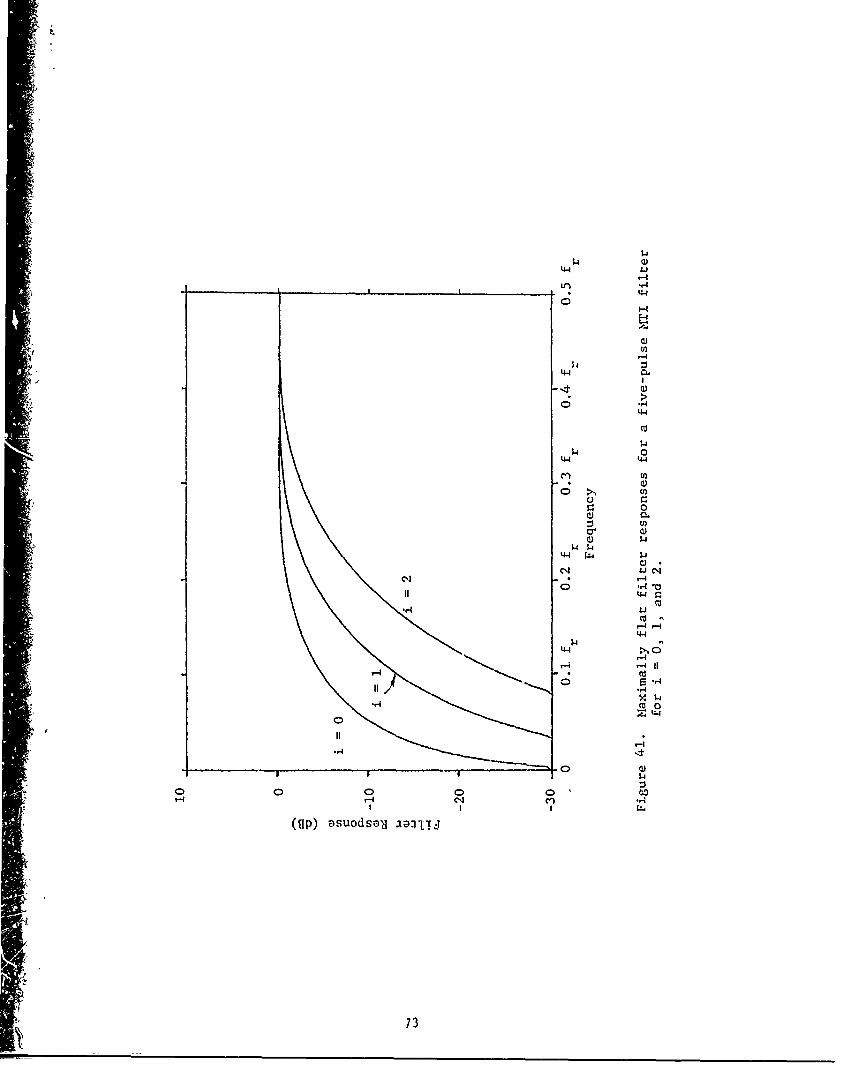
44 4
$4
4-4
*~4-4
co)
$-4$4 03
-4 0)
0 ".0
cci
W $4
14 0
4- 4-4C
co)
04 -4(44
$41.
-,4
0 r404.4
$4
* cc
(Up) suodva jilT0
73-
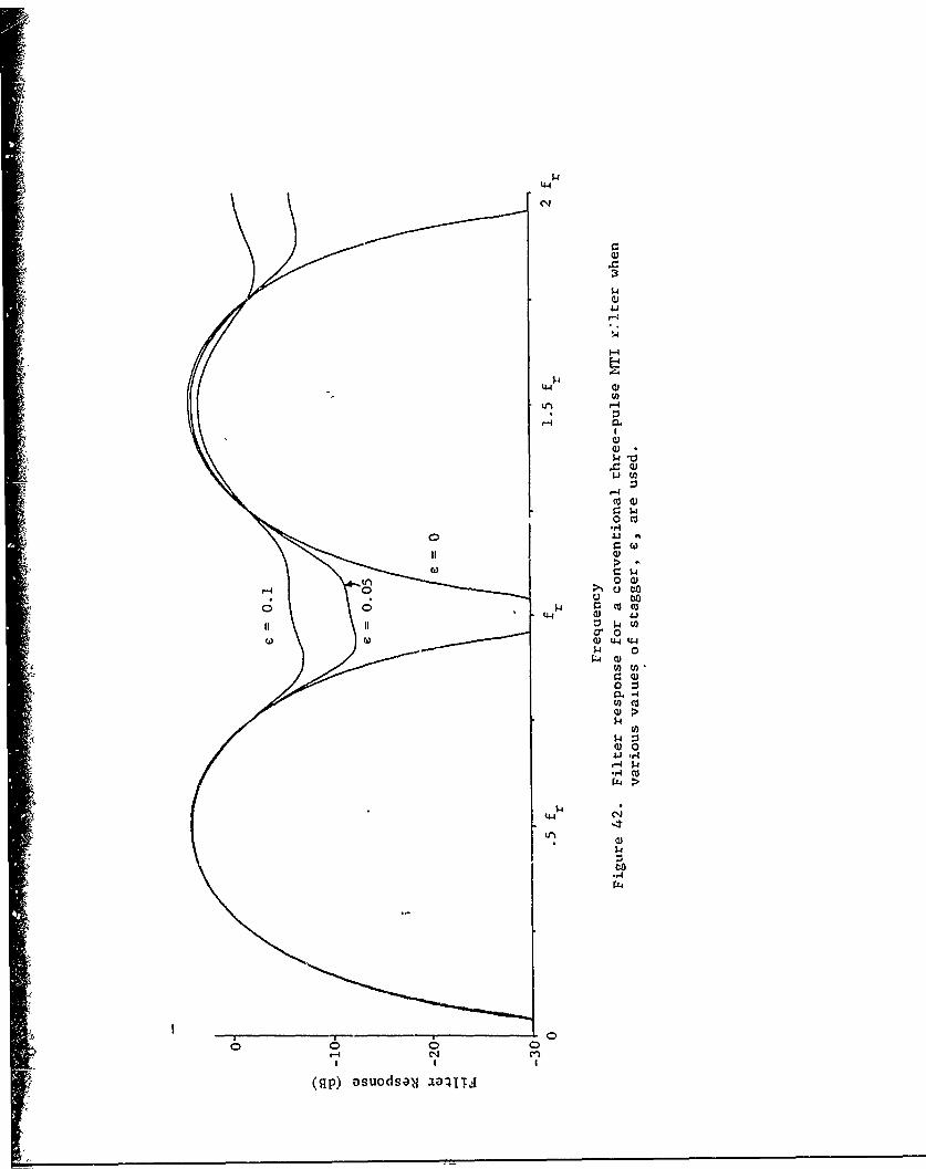
44
$4
'-4
.r4ci,
0 u0w
4441cw
oc 0
w 0
P4 0)
ra. Q)
m 4
4J r.4
"-4 MU
44$4 C
44)
0$4
(qp) oDsuodsa\j aate1l
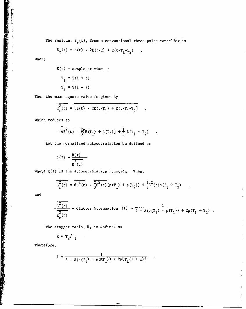
The residue, E (t), from a conventional three.-pulse canceller isr
E r(t) E(t) - 2E(t-T) + E(t-TI-T2 )
where
E(t) = sample at time, t
T =T(I + e)
T2 T(I - :)
Then the mean square value is given by
Er (t) = [E(t) - 2E(t-TI) + E(t-TI-T2 ]
which reduces to
= 6E 2 (t) - ý[R(TI) + R(T 2 )] + - R(TI + T2 )
Let the normalized autocorrelation be defined as
p(T) = R(r)
E 2(t)
where R(T) is the autocorrelatzn function. Then,
2 2 2 2 +pT)+ E(pT1 2 'Er (t) = 6E (t) - 3E (t)(P(Tl) + P(T2)) + -2(t)p(TI + T2)
and
E2(t) -Clutter Attenuation (I) 6 T2 6 - 8(p(TI1 + P(T 2) + 2p(TI1 + T 2)E (t)+ 2T)
r
The staggar ratio, K, is defined as
K T2 /TI
Therefore,
6. 8(P(Tl) + p(KT1 )) + 2pLTT(1 + K)]

The improvement, I , with staggered prf is I multiplied by the averagegain (six)
I = 1S -4(p(TI + p(KTI)) + V[TI(1 + K)]
The loss due to staggering is [40]
4a _T (2 K) 2 + 16 2 (- K) 4
s 3T2 (1 + K)2 (1 + K)4
iX
'T 4 --ov
where
X = wavelength (meters)
a = rms clutter velocity (m/sec)
So, Ls, the loss due to staggering is given by
L= X2 (1 - K) 2 + 16 4 K2 (1 - K') 4
s 2 22 2 412KL12TT'2av (I + K) ( + K) 12
In Figure 43 1 for a three-pulse canceller has been plotted for variousstagger ratios.
Since both the frequency response curve and the tI improvement, I,are affected by varying the interpulse period, the designs dev!loped for theunstaggered case are not necessarily optimum for the staggered case as isillustrated in Figure 44. The results shown in Figure 44 illustrate theeffects of prf stagger on the response of one of the minimum-rms error filtersdeveloped earlier; in fact its response might L'- considered less desirablethan the conventional, response shown in Figure 42.
76

'0-4
S4
00
UZ4 0
Jco
a)-4' CO
cu~
:4
"a)
* 0 -4
uf LI)
-4.J
ci >
w. NQ)
li >N
41 0
0 Vl
Lni
(UP) ~atUD~adt)
771~

'-i
4-4
0i
v.4-
00LI(I
4 .4
0
44-40
0 0
0-
So 14
00.,4i:7
1-i C1 cnu
(Up)- asosSail
78U-

VI. CONCLUSIONS AND RECOLMENDATIONS
A. Primary ConclusionsThe free-space performance of the EAR system may be seriously affected
by changes in Doppler frequency of the target. The region of optimum angle-tracking accuracy of the EAR system is approximately four to seven kilometers,depending upon the cross-section and physical size of the target. Cluttercancellation of the EAR system will primarily be limited by analog-to-digitalconversion quantization noise.
The effect on system performance of changes in Doppler frequency of thetarget may be minimized by using samples with non-integral sample weights.The design procedures set forth in Section V produced significantly improvedMTI processors for'the unstaggered prf case, but vary little his been uonein the case of staggered prf.
System perfor.i nce may be seriously limited by multipath returns whentracking low-flying targets. These tracking errors are significant fortargets flying at altitudes less than approximately 1500 feet.
Frequency agility may be of appreciable help in reducing the efiect ofmultipath returns on system performance. The effectiveness of frequencyagility in reducing multipath-induced errors is a strong functiorn of thefrequency-agility bandwidth used, the target heights, and the antenna height.The 400-filz bandwidth which may be possible with a modified EAR wouldsignificantly reduce these low-angle tracking errors, particularly forhigher antenna heights.
B. Principal RecommendationsBased on the information studied during this program, the following
recommendations are presented for the EAR development program.
(1) A flexible digital MTI filter or processor should be incorporatedinto the system. The performance obtainable by the selection of sample weightsappears necessary if acceptable system operation over a wide range of targetDoppler frequencies is to be achieved.
(2) Stagger of the prf should be incorporated into the EAR system conceptin order to eliminate "blind speeds" of the system, and investigation ofimproved MI. filters for staggered systems should be initiated.
(3) Frequency agility should be incorporated into the EAR system, bothto ieduce free-space tracking errors due to target glint, and to reduce low-angle tracking errors due to multipath sigi.als. Weighing of the receivedsignals on the basis of the sum signal amplitude appears desirable.
Exzerimental evaluation of the EAR shouJ be paralleled by carefultheoretical studies as an aid in planning significant experiments and toassist in interpreting results of these e).periments.
79

VII. REFERENCES
1. G. W. Ewell, N. T. Alexander, and E. L. Tomberlin, "Investigation ofthe EffecLs of Polarization Agility on Monopulse Radar Angle Tracking,"Final Technical Report on Contract DAAHOI-70-C-0535, Georgia Instituteof Technology, June 1971.
2. J. L. Hatcher, H. G. Woods, and H. B. Buie, "Preliminary Action IIRadar Hardware System Requirements," Report No. RE-TR-69-23, U.S. ArmyMissile Command, Redstone Arsenal, Alabama, November 1969.
3. D. K. Barton and H. R. Ward, Handbook of Radar Measurement, p. 24,
Prentice-Hall, Inc., Englewood Cliffs, N.J., 1969.
4. Reference I, Chapter IV.
5. Reference 1, Chapter V.
6. Reference 2, p. 10.
7. M. I. Skolnik, Introduction to Radar Systems, p. 502, McGraw-Hill, Inc.,New York, New York, L962.
8. S. M. Sherman, "Complex Indicated Angles Applied to Unresolved RadarTargets and Multipath," IEEE Transactions on Aerospace and ElectronicSystems, Vol. AES-7, No. 1, pp. 160-170, January 1971.
9. Reference i, p. 79.
10. D. 0. Noith, An Analysis of the Factors Which Determine the Signal/NoiseDiscrimination in Radar, Technical Report PtR-6C, RCA Laboratories,Princeton, U. J., June 25, 1943.
11. J. Van Vleck and D. Middleton, "A Theoretical Comparison of the Visual,Aural, and Meter Reception of Pulsed Signals in the Presence of Noise,"Journal of Applied Physics, Vol. 17, pp. 940-971, November 1946.
12. H1. L. Van Trees, Detection, Estimation a-d Modulation Theory, Part I,
p. 249, John Wiley and Sons, Inc., New York, New York, 1968.
13. T. S. George, Report No. 159, Philco Corp. Research Division.
14. B. M. Dwork, "Detection of a Pulse Superimposed on Fluctuation Noise,"Proceedings of the IRE, Vol. 38, pp. 771-774, July 1950.
Preceding page blank81

15. H. Urkowitz, "Filters for Detection of Small Radar Signals in Clutter,"Journal of Applied Physics, Vol. 24, No. 8, pp. 1024-1031, August 1953.
16. A. W. Rihaczek, "Optimum Filters for Signal Detection in Clutter,"
IEEE Transactions on Aerospace and Electronics Systems, Vol. AES-I,
No. 3, pp. 297-299, December 1965.
17. D. F. DeLong, Jr., and E. M. Hofstetter, "The Design of Clutter-
Resistant Radar Waveforms with Limited Dynamic Range," IEEE Transactionson Information Theory, Vol. IT-15, No. 3, pp. 376-385, May 1969.
18. D. F. DeLong, Jr., and E. M. Hofstetter, "On the Design of Optimum Radar
Waveforms for Clutter Rejection," IEEE Transactions on InformationTheory, Vol. IT-13, No. 3, July 1967.
19. E. C. Westerfield, R. H. Prager, and J. L. Stewart, "Processing Gains
Against Reverberation (Clutter) Using Matched Filters," IEEE Trans-actions on Information Theory, Vol. IT-6, pp. 342-348, June 1960.
20. H. L. Van Trees, "Optimum Signal Design and Processing for Reverberation
Limited Environments," IEEE Transactions on Military Electronics, Vol.
MIL-9, pp. 212-229, July 1965.
21. L. J. Spafford, "Optimum Radar Signal Processing in Clutter," IEEE
Transactions on Information Theory, Vol. IT-14, No. 5, pp. 734-743,September 1968.
22. L. J. Spafford, Optimum Radar Signal Processing in Clutter, Ph.D.dissertation, Pcilytechnic Institute of Brooklyn, Brooklyn, N.Y.,
June 1967.
23. C. A. Stutt and L. J. Spafford, "A 'Best' Mismatched Filter Responsefor Radar Clutter Discrimination," IEEE Transactions on Information
Theory, Vol. IT-14, No. 2, pp. 280-287, March 1968.
24. W. D. Rummier, "Clutter Supression by Complex Weighing of Coherent
Pulse Trains," IEEE Transactions on Aerospace and Electronic Systems,Vol. AES-2, No. 6, pp. 689-699, November 1966.
25. H. L. Van Trees, Detection, Estimation and Modulation Theory, Vol. 3,
p. 278, John Wiley and Sons, Inc., New York, New York, 1971.
26. L. A Wainstein and V. D. Zubakov, Extraction of Signals from Noise,
Chapter 6, Prentice-Hall International, London, 1962.
82

27. Reference 12, Section 2.6.
28. I. Selin, "Detection of Coherent Radar Returns of Unknown DopplerShift," IEEE Transactions on Information Theory, Vol. IT-Il, pp.396-400, July 1965.
29. L. E. Brennan, I. S. Reed, and W. Sollfrey, "A Comparison of AverageLikelihood and Maximum Likelihood Ratio Tests for Detecting RadarTargets of Unknown Doppler Frequency," IEEE Transactions on Informa-tion Theory, Vol. IT-14, No. 1, pp. 104-110, January 1968.
30. J. Capon, "Optimum Weighing Functions for the Detection of SampledSignals in Noise," IEEE Transactions on Information Theory, Vol. IT-IO,pp. 152-159, April 1964.
31. H R. Ward, " A Model Environment for Search Radar Evaluation,"EASCON '71 Record, Electronics and Aerospace Systems Convention,pp. 164-171, October 1971
32. W. W. Shrader, "An MTI Surveillance Radar Philosophy," EASCON '71Record, Electronics and Aerospace Systems Convention, pp. 171-174,October 1971.
33. H. E Kallman, "Transversal Filters," Proceedings of the IRE, pp. 302-310, July 1940.
34. L. R. Rabiner and R. W Schafer, "Recursive and Nonrecursive Realiza-tions of Digital Filters Designed by Frequency Sampling Techniques,"IEEE Transactions on Audio and Electroacoustics, Vol. Au-19, No. 3,September 1971.
35. B. Gold and C. M. Rader, Digital Processing of Signals, Chapter 3,McGraw Hill Book Company, New York, New York, 1969.
36. R. M. Golden, Parametric Design of Digital Filters, Course Notes,Technology Service Corp., January 1970.
37. L. R. Rabiner, B. Gold, and C. A. McGonegal, "An Approach to theApproximation Problem for Nonrecursive Digital Filters," IEEE
Transactions on Audio and Electroacoustics, Vol. AU-18, No. 2, pp.83-106, June 1970.
38. D. W. Tufts, D. W. Rorabacher, and W. E. Moser, "Designing Simple,Effective Digital Filters," IEEE Transactions on Audio and Electro-acoustics, Vol. AU-18, No. 2, pp. 142-158, June 1970.
83

39. H. D. Helms, "Digital Filters with Equiripple or Minimax Responses,"IEEE Transactions onz Audio and Electroacoustics, Vol. AU-19, No. 1,pp. 87-93, March 1971.
40. A. A. G. Requicha and H. B. Voelcker, "Design of Nonrecursive Filtersby Specification of Frequency Domain Zeros," IEEE Transactions onAudio and Electroacoustics, Vol. AU-18, No. 4, pp. 464-470, December1970.
41. B. Gold and K. L. Jordan, Jr., "A Direct Search Procedure for DesigningFinite Duration Impulse Response Filters," IEEE Transactions on Audioand Electroacoustics, Vol. AU-17, No. 1, pp. 33-36, March 1969.
42. G. C. O'Leary, "Nonrecursive Digital Filtering Using Cascade FastFourier Transformers," IEEE Transactions on Audio and Electroacoustics,Vol. AU-18, No. 2, pp. 177-183, June 1970.
43. L. R. Rabiner, "Linear Program Design of Digital Filters," 1972 IEEEConvention Record, paper 611.2, pp. 336-337, March 1972.
44. 0. J. Jacomini, "Optimum Symmetrical Weighing Factors for a Video MTIRadar," IEEE Transactions on Aerospace and Electronic Systems, Vol.AES-7, No. 1, pp. 244-209, January 1971.
45. R. G Martin, Optimum Synthesis of Transversal Filter Radar Moving-Target indicator, Ph.D. Dissertation, 'he Johns Hopkins University,Baltimore, Maryland, 1970.
46. It. G. Daellenbach, and E. J. Bell, User's Guide to Linear Programming,Prentice Hall, Inc., Englewood Cliffs, N. J., 1970.
47. L. Weinberg, Network Analysis and Synthesis, p. 491, McGraw Hill BookCo., New York, New York, 1962.
48. F. E. Nathanson, Radar Design Principles, Chapter 9, McGraw HillBook Company, New York, New York, 1969.
49. L. E. Brennan and I. S. Reed, "Optimum Processing of Unequally SpacedRadar Pulse Trains for Clutter Rejection," IEEE Transactions onAerospace and Electronic Systems, Vol. AES-4, No. 3, pp. 474-477.
50. R. Roy and 0. Lowenschuss, "Design of MTI Detection Filters withNonuniform Interpulse Periods," IEEE Transactions on Circuit Theory,Vol. CT-17, No. 4, pp. 604-612, November 1970.

51. M. I. Skolnik (editor), Radar Handbook, Chapter 17 by N. W. Shrader,
pp. 38-45, McGraw-Hill Book Co., New York, New York, 1970.
52. Reference 51, pp. 9-17.
53. Reference 51, pp. 12-35.
54. Mischa Schwartz, Information Transmission Modulation and Noise, p. 240,McGraw-Hill Book Co., New York, New York, 1959.
S3. Athanasios Papoulis, The Fourier Integral and Its Applications, p. 104,McGraw-Hill Book Co., New York, New York, 1962.
'II
ii
85

ii; APPENDICES
Preceding page blank

Appendix A
CONVENTIONAL THREE-PLSE MTI FILTERS
Consider the two-delay filter shown in Figure A-i. The impulse responseof this configuration is
h(t) = 6(t) - 2 6(t - T) + 6(t - 2T)
In the frequency domain
H(w) = 1 - 2 ejWt + e2jit
and
G(w) = H(m) • H1(w) = 16 sin4 wT
It is interesting to examine the improqement in target-to-clutter ratiowhen this canceller is used as an MTI radar processor. This calculation willbe made assuming a Gaussian frequency distribution of clutter power. Thetotal received clutter power will be denoted by C.
Let target power be distributed uniformly in frequency, with a powerof T. The input target-to-clutter ratio, ri, is then
T.ri C
The output signal and clutter powers, T and C, must be computed, andthe output target-to-clutter ratio, r, will 0 then be
T0*OC
0
The improvement, I, if any, is then
r T /C0 2 0 0
r. TT.C_
Now,
f /2r
C0 (Clutter power spectral density) G(tp) df
-f /2Ir
Preceding page blank
89

•, 0
•! II
3 -4
a J J
.3.

f /2cr-f /2 aVC exp(-f2/2c) "16 sin (nfT) df
_f/2 •c C-
r
where f r= pulse repetition frequency
ac = clutter power standard deviation
T = interpulse period 1/fr.
For small values of x
sin x ; x and sinx x 4
Then16i 4 T4 C ( l f
Co l 4T4C •CO f 4 exp(_f 2 /2a2) df0 c
• 48n4 T4 a 4 C~C
The signal power out of the filter is now computed,
•'T . r4T 16 sin (,wT/2) dw
r 0
fT.r2 C 32n sin4 nfT df
r o
= 6T.
The output signal-to-clutter ratio, r, is
T 6T.r 0 4 So CO 48#4c4
0 48-aTaC
91

and
4r If
r 8' cl~i 8c
If is often customary to dei.ite a = a X/2, where X wavelength (meters).V c
Representative values of o are given in Table I, and Figure A-2 showsI plotted as a function of a fv : values of f = 5 kHz and F = 5.5 GHz, whereF = radar frequency.
Some sample calculations ,.t the improvement obtainable can be made withthe use of Table II.
If one assumes
a = 0.22 (wooded hills, 20 kts)v
X 5.5 cm
f 5 x 10³ Hz.then, r
I = 82.9 dB.
:• 92
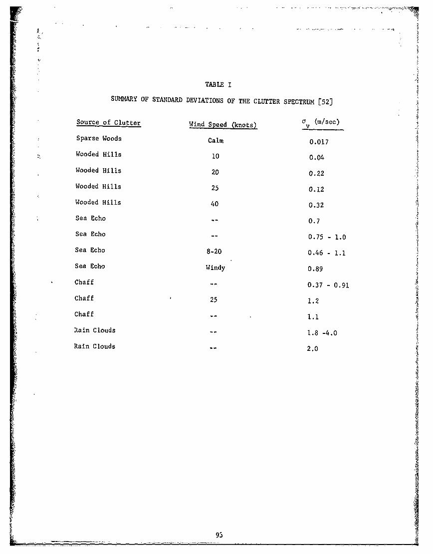
TABLE I
SUMMARY OF STANDARD DEVIATIONS OF THE CLUTTER SPECTRUM [52]
Source of Clutter Wind Speed (knots) a (m/sec)
Sparse Woods Calm 0.017
Wooded Hills 10 0.04
Wooded Hills 20 0.22
Wooded Hills 25 0.12
Wooded Hills 40 0.32
Sea Echo -- 0.7
Sea Echo -= 0.75 - 1.0
Sea Echo 8-20 0.46 - 1.1
Sea Echo Windy 0.89
Chaff -- 0.37 0.91
Chaff 25 1.2
Chaff -- 1.1
lain Clouds -- 1.8 -4.0
Rain Clouds -- 2.0
_ 93

r-I
co
$4
p4-)
U.
It~ 4-1l
0)
4-4
(qp) :uatuaoxdcu
94H -
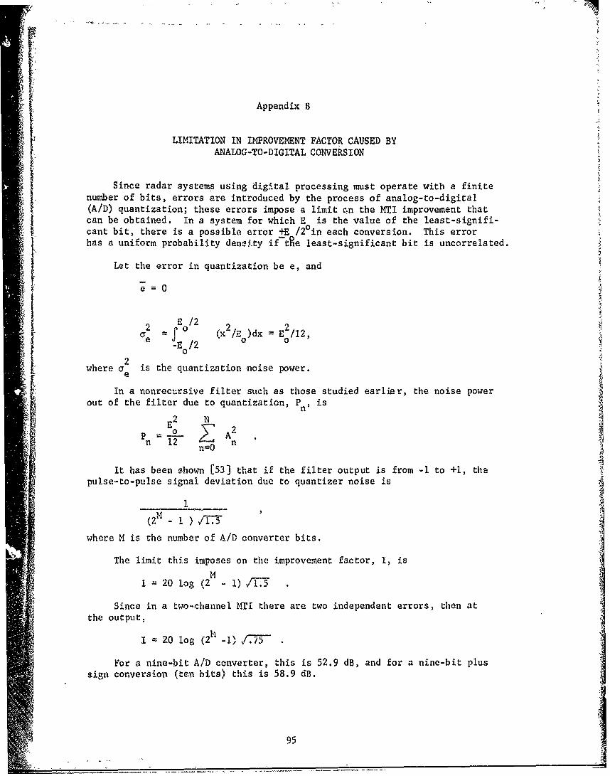
Appendix B
LIMITATION IN IMPROVEMENT FACTOR CAUSED BY
ANALOG-TO-DIGITAL CONVERSION
Since radar systems using digital processing must operate with a finitenumber of bits, errors are introduced by the process of analog-to-digital(A/D) quantization; these errors impose a limit c.n the MTI improvement thatcan be obtained. In a system for which E is the value of the least-signifi-cant bit, there is a possible error +E /2 0 in each conversion. This errorhas a uniform probability density if-t~e least-significant bit is uncorrelated.
Let the error in quantization be e, and
e=0
E /22 2 2 2Cae (x2/Eo)dx E2/12,
E /20
2where a is the quantization noise power.
e
In a nonrecursive filter such as those studied earlier, the noise powerout of the filter due to quantization, Pn' is
12 N
0 > 2_ AnPn 12 nn=O
It has been shown [533 that if the filter output is from -1 to +1, thepulse-to-pulse signal deviation due to quantizer noise is
1
(2m - ) iT3
where M is the number of A/D converter bits.
The limit this imposes on the improvement factor, I, isM
I = 20 log (2 - 1) /1 .5
Since in a two-channel MTi there are two independent errors, then atthe output,
I = 20 log (2 -)/75-
For a nine-bit A/D converter, this is 52.9 dB, and for a nine-bit plussign conversion (ten bits) this is 58.9 dB.
"95

-~~~ - ~ ~ ~ ~ -~ -iv ---~2.'r""r" , ý T- 7 I .
Appendix C
RANGE TRACKING
In conventional radar systems using analog signal processing, theso-called split-gate range tracker is often used to track a desired targetin range. In a radar using digital signal processing, however, the conventionalsplit-gate range tracker cannot be used, since received signals are sampledat discrete points. Nevertheless, the information obtained from these discretesamples may be used to perform a range-tracking function.
Consider a representative received pulse (figure C-l) which is sampledat points spaced A units of time ap8ý't. The c".crent estimate of pulseposition we designate by t and the pulse amplitude at t by Z . Associatedwith Z are two other samples, z and 0, which occur at0times0t^-A and to+Arespectively. These three samples may now be used to calculate 2he erroroinrange, e , between t and some point on the received pulse. A number ofcomputational algorithms are possible; one which appears very similar to theanalog split-gate range-tracking scheme is
=K er 0
where K is a porportionality constant. Another algorithm which has beenproposed by the General Electric Company is
.~ L 0r E+E 0
A brief analysis of the performance of these two range tracking algorithmshas been undertaken. There are a number of variables in such an analysisthat affect system performance, for example: the particular algorithm, thetransmitted pulse shape, the receiver bandpass, and the sample spacing. Inorder to simplify the analysis, a rectangular transmitted pulse and a Gaussianfilter response were assumed.
The first step in the analysis was to calculate the received pulse shapefor a rectangular transmitted pulse and the appropriate receiver bandpass.A Gaussian filter was assumed since this closely approximates the responsewhich will probably be implemented in the EAR system.
The frequency response of a Gaussian filter is given by [54]
H( ( ) A e 0 '35( /wc) 2
0
Preceding page blank97

• -. ,.,I•t• o. , ••• .• 2
Amplitude
zo
'5e
t 0 -A t t0+ATime
Figure C-l. Reresentative received pulse shape showing thesamples used in the range-tracking algorithms.
98

where,
H(w) - voltage output of the filter,
A = a scale factor,
w = angular frequency ( 2jTf)
Wc = 3-dB video bandwidth of the filter (in radians),
and the filter delay has arbitrarily been set equal to zero. In the aboveexpression, w , the 3-dB video bandwidth, is equivalent to half the 3-dBbandwidth at •he IF frequency.
The response of such a Gaussian filter, a(t), to a unit step functionis [55]
ýA C11t
a(t) =2. (1 + erf A/.5
where
2 X 2erf x L j' ey dy.
Therefore, the filter response, f(t), to a rectangular pulse of width, T, Nis given by
A A wt (t -tT)\
f(t) 0 1 + erf - 0 1 + erf 0
or Af(t) = A erf (0.845 wci t) - erf [0.845(t - T) Wc]l
This information was used to calculate sample values Z , Z, and ZThe range error was then calculated using each algorithm. esu~ts are plottedas functions of Cr/K versus normalized time error t /T. The conditiont 1= 0 corresponds to the on-target sample coinciding with the leadingedge of the rectangular pulse input to the filter, while t 0 /T = 1 correspondsto the trailing edge. Figure C-2 shows e /K as a function of t /T for the casef 1=l (f3dB is the IF 3-dB bandwidth End sample spacing A/To= 1. FigureC- is the same type of presentation for f dB = 2. The actual performanceof the EAR system probably lies somewhere 6etwe,•n these two cases.
The performance of the two tbackinS Algorithms in the presence of receivernoise is an important system design con-ideration While an exact analysisis beyond the scope of this projecc, an approximate analysis gives useful.
99

/k
1.0
4 _ - - • .•+ . ..% - • 4
C 1.0 0 L
0¢
Conventional
G.E.4
4 4i
P7
II
Fc0 forvenTSFgr 2 r 0 f3d3BI
and A/T =I.
z10

|3
ImI
E lk
1.0
A'0
4t 0 T-C1.00
Conventional
G.E.
Figure C-3. er/k as a function of t /T for f T 2ro 3dB.
and A/T = 1.
101

insight into the performance of the two algorithms.
Assume n , n , and nj are the noise voltages associated with Ze, Zo,and 7., respectively. Then for the conventional tracking algorithm
.- (Z•+n) n (X• + ) n
e = L L"e eSr =0 + n0
Assume the signal-to-noise ratio is greater than one, such that
0 0 0
Then
Sr e eE_ r KL
0
If n• and n are uncorrelated, and their noise powers are both equal to n,and the range tracker is on target (Z - e = 0), then the rms range error
due to noise, a rnisgvnb
0 rn
If SIN is the signal-to-noise power ratio, then
r = K-• •rn
While strictly true only for large S/N, the general prediction, thatrange errors are directly related to K and inversely related to the signal-Sto-no,'se ratio, appears to be indicative of the performance for other casesas well.
Figures C-2 and C-3 show that e/K is a much more nonlinear function ofrange error for the conventional algorithm than for the General Electricalgorithm. They- also show that the conventional algorithm is relativelyinsensitive to small variations in position about the true pulse location,particularly for the case f T = 2, as evidenced by the small slope ofe /K at t /T = 0.5. Because of the nonlinearity of the conventional algorithm,iE would appear that any assumed value of K for tlis system would be onlyapproximately correct over the region 0 5 t IT S 1; it appears that thisaverage K would closely approxir;:.c ;.he value of K for the General Electricalgorithm. so the noise performancc would be approximately the same for thetwo cases. These results indicate substantial advantages in using the algorithm"proposed by General Electric. Realistic values of K for the two algorithmsare comparable, indicating comparable noise performance. The greater linearityof the General Electric algorithm and the fact that it remains bounded for largeerrors offer substantial advantages. Partially offsetting this advantage isthe fact that the conventional algorithm tracks with a sample on the center ofthe pulse, thus providing the maximum signal-to-noise ratio.
102

Appendix D
EFFECTS OF FREQUENCY AGILITY ON BLIND SPEEDS
Changing the carrier frequency of MTI radar has no effect on thefrequency response of the filters, but the target blind speeds, V areshifted slightly, since
V N 0.29 prf (knots) N = I, 2.....
prf = pulse repetition frequency (Hz)
F = radar frequency (GHz).
In a frequency-agile radar the blind speeds vary from pulse to pulse,yielding a velocity response that is the sum of the output at each frequency.
Figures D-1 and D-2 show the response for a frequency-agile radaroperating with two frequency step sizes. Figure D-1 is for 50-MHz step sizeand Figure D-2 is for 31.25-Mlz step size. The starting frequency is 5.3 GHz,and the stopping frequency is 5.6 GHz for Figure D-1 and 5.8 GHz for Figure D-2.
It may be noted that a marked change is made in the velocity responsewithout benefit of pulse staggering, but approximately 20 dB null- are presentat the lower blind speeds.
103

()3
4JO
7 $• w C)
-4
C.))
, u3
0 cr "
00
-I ~ r tAJ.
i ticCII
0(or,) pn -4•

C)r
-Li
L 00
co.
4-3
a)
D c
441
0 I
a1)
~C4
14
:3j:to
14)
0 0) C0 0) 0C 0 0 0
(qp) apn:vTu2LN
105

Appendix E
COMPUTER PROGRAM
In this appendix is presented the FORTRAN V computer program used in thecomputation of multipath errors in the EAR system. The subroutines listedare representative of those employed in the generating data for this report;however, various slightly modified versions were used as necessary to producespecial outputs.
A Preceding page blank107

CALL PLOTS(Il3UF(1)v5ooop2)
900 FOR'.i"TC'ONO PREDICTION FILTER. FREQUENCY AGILE#)DIMrN IONJ NARRAY(5p000.X(lp00).ERRFTC1nOO)DIMENSION SLOGG(1000)
_RSA T A j0~,)RD=1870./PI
10o FOR'IAT()i-L.El-qR'.iATA!90ENT1~'x A RO)________102 FORMiAT(t BYE;)
PI.02=-IL2.-IDSTRT=-200JDSJOP=200ILAsT=dbOO
800 FbR44AT(9OENTER TRHANTpDLtVEL')REA0(5tIQ0) THANT#DLEMRrlO=0.
____AI(S:8593'4 _________________________
10 WRiTE(6p,101TREA)(5eioOENl=999pERR=999) H-A,HTtRSTARTtVpPR 'FFREQpRHQ
940 FR-AAT(OOENR PSTARTPFSTOP#FSTEPI)REA 00o) FSTART#FSTOPFSTEPRANGE:RSTýIRT*60009, ________________________
THTSASIN4( (H~T-HA)/RAN3E)
DELTAT=450/PRFT=Q.IFREQGINT( CFSTOP-FSTART)/FSTEP)+I
FMO)V.o3)(4 50. IFRr0)F RE fl) FREQ +FklO'7*STE PTHS-AN:T.1SCAN.ANE-RR-
CALLERRO (HA #THANT# rTt RAIE' tALA%~.A.ICERRpt VRHOTHTTUSCAN, TfFREOPC P~~STARTFSTOPtFSTE:PP,PRF;VE.LGC
T=T+DELTATX X=Tv~t"ANJWANT
____XCI )XX+AIGEqR____________ ___ ___
ERR:XX-T-4T - ______
____ERRFT CI) :RA4GE.E-RR/RD
F i,-ire le- I N air, Computer program~.
108

=RAI!$E*COSCTHT/RD) V.6.V*7b*ELTf5- ________
RAN3E=SQRTIY**2+ (-1T-.A) **2)
LC.NT=200 ______ ________________
LCtiLCtJT-ý __________
DO_40 1=1vL'T ______________________
TH-St" A N: -ICA NIAN3rRRCALL ERRO (HA, THANJT t HTPRAjGEt ALAM ANGERR V t RHO# THT tL;ASCAltJTtREQ tC FSTARTFSTOP,FSTEýPIPRFOLEVSLO'GG(I+3))
T=T+DELTAT__________________ ____
XX: tr4A NIT + THSC4ANXCI+ 3 )=XX+ANIGERRERR: XX -TH-TERRFT (1+3) :RANIG7*ERR/RQ_ _____________
- Y=RANGES*-OS( THT/R6))-V*-6.*DOLTArT/3.6
IF(FREoj.GE_,FSTOP) PR-4o=FSTART-FSTEP
CALL DIST(ARRAYpERRFTpIOST'RTtID TOP# LCNTt ICNTv IOVERP IUNDER)
928 FOR.IAT(IOENTER 1 TO PLOT DATA')REA)(t100 NPLOT___-_____
NCNT:NICNT+l____ I.tl;PLOTcJE.I) GO TO 9Pa3-___ ____ ____
IFeJCNIT.GT.1) GO TO 929
VTITLErI)zt777 CONJTI'IUE
VTITLrE(1,=ltRROR
VL3ND:)-40O.
926 FORMiAT(12A6)WRITE CG,927)
927 FORmtAT(#0O-NTER TITLE FOR HOR AXIS,)
- READ (5t 926) _TI TLE929 HLB9'O:TO
CALL SI NIPL(E-RRFT.LCNIT VL~3N)eVU3NIDH-L8NIDHu)RMD.VTI TLEeNTITLE)923 -CONTINIJE
_WRITE-(6,920) RA4E,"'i S
920 FORMAT(IORNIGE =40:7,1,1 FEETtel,5p, ITERATIONJS')
919 FORAAT('0ENlTE' 1 TO CONJTINUE t)__. _READ)(c3,00) SJCO'IT
IFc'-ONT.EO.n GO TO 918 -
999 -- C0tTINO~ECALL PLOT(j0.vO,.9n9)
0 0

COMPLE-X FUNC^TIONGAIN(TH,ýSCAN4THeN)THSCA\=AJS cSCANTqH)-COMPLEX TPARG______ ___
PI=2*P102 ___
R):ý=18O,/ iPI4 THZýRo=.73 + *27*(THSCANI/40,)
-0-5-- '.5;*(TFSA/;THM= (TH4-TH7--R0 I /R0Tl1P=CT.H+TrZERO)/RJ --.'lJM1:*33o9*PTrSINI(THM)___
T4=:'*P102*72.8*CVOS(UM1)/(PlO 2**P-UM**2)TP: ' *PI02*72.8*COS(UP)/(PIO?**2-UP**2)ARG=C'.'PL.X(O.,,P102) ____
I~CJ.E.2) T=TMA-TP )C P!R ,
RETUR?4 _________________ ___
EN D
Figure E-2. Subroutine GAIN
110
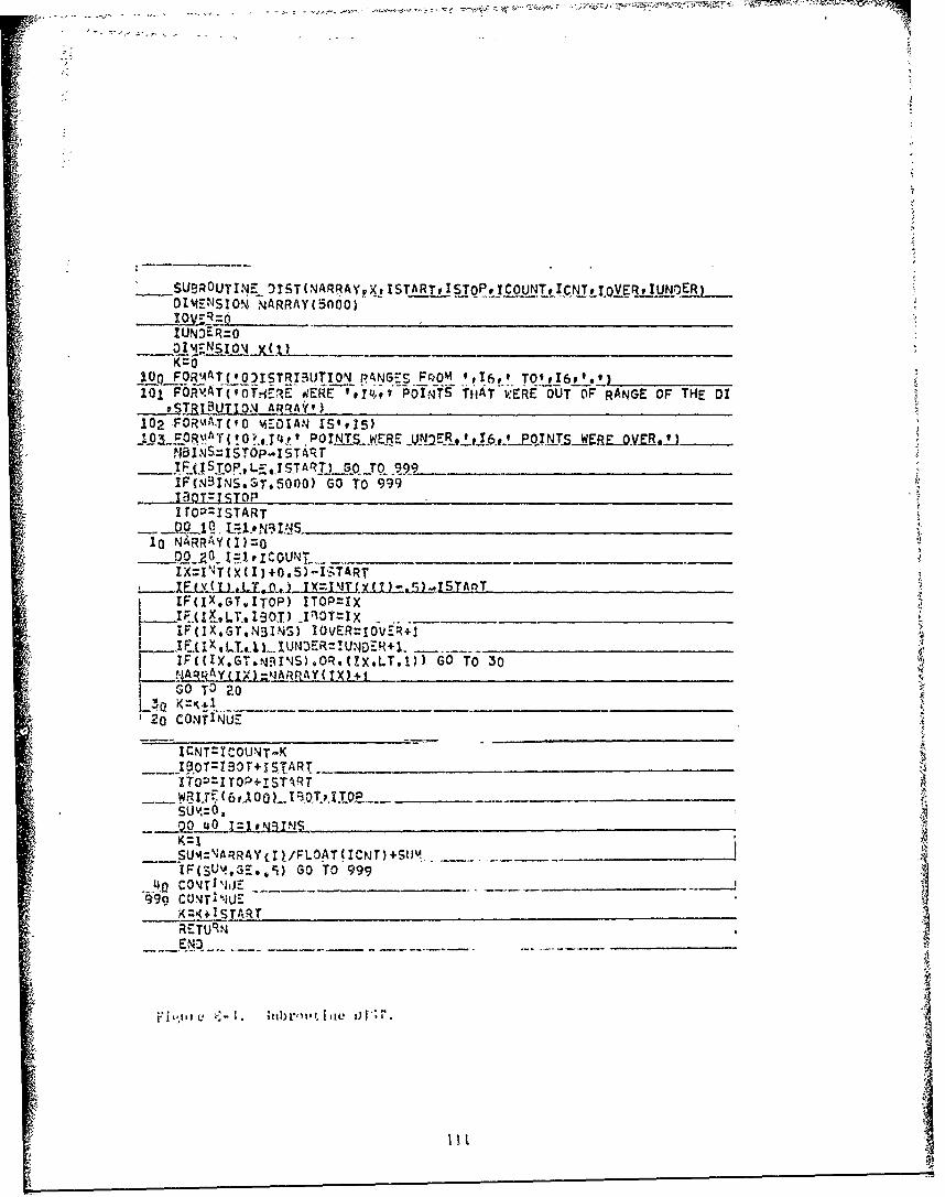
SUBOUTINý DIST NARRAY pX pISTARTP ISTOPP ICOUNTt ICNT# IOVER tIUNOER4 DI4ENSION NARRAY(50l00)
1O00J..OR4ATpOO2ISTRI3UTIONPJfANGrS FrOM ltI6t* TO',I610e.)___101 OR"A f0V.-IERE W'ERE *eI'k.t POINTS THAT WERE OUT OF RANGE OF THE DI..~$RLUTIý_APA
.102 -FORMAT(,O -MEDIANJ ISI#15)~~5RMT !0 ?.,,1 Iq Po rýLrs~~wEF- _!.ER j~t TR V R f _ _ _P13NS=ISTOP-ISTART
XiF(NBINS.GT.5000) GO TO 999
I TOP=ISTART
10 NARRAYUI)Z
I ELY1LIf.L ± 'JT (XILL- r,) - ST An TIF(IX*GToITOP) ITOP=IX
-VlOT=IX -__________
IFcIXGT,.N3I.N6) IOVER!iovzE+j
~~Ay r~RR AY T X)+ tV GO TO 20
20 CONTINJUE
ICNTIlCOtJNT-I_____IBoT:7o+jSART
ITODZITOP'4IS'rIRT
SUYI=01C- 4 0 2LE1L!NflT N SN
__SU,44ARRAY (1),/FLOAT (ICNr) +StJMi)GO 'TO 999 N
999 CU-1TIklUE,
RETU4 RN

___ SUBROUJT INE SThJDEV YvICU'.JT)31IEj-NSION XCI)
S=S+iXCI)XS'J:X(J)**p _______ .
XAVW^IS/ICOuNT
__ WRITE(6!100) XAVG .4
100 FOR\¶jAT(9O AVE;RAGF rs'.F6.1)
200 FOR'4ATCtO STANDOARD DEVIATION IS'.P6.1)
Figure E,-4. Subroutine STNDEV.
112
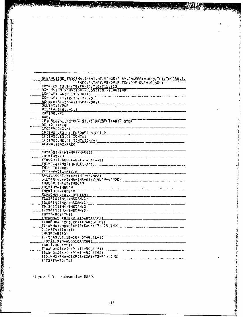
C FR.osTARTvCSTOPpFcSTEpvPRF#0LEVtSLOGlTCOMI-EXT3pT~pT5tT~pT9pTl0#T~ll?_12________________
C0.%iL~x_$AINEXPtRATIO __________________
AKS=. 845+ -335* 1TH.SCAV-.4.________________
PI :ATAN2(O 0, ,___________-1,____________
RO~luo,/PI
IF (1ý40DJE.STPFSTEQPRE%) FR0PTR~STEP
I F(I 140)..N4E. n) _1CNTt~lCNT+1_________
__ AL:A'iz99843/FREQ_
TrtT=ASIN((HT-HIA) /RANGE)- THT=THT*R:) _________
THIM=-ATANk2( U!l~tHT~ t ~ _____ ____-v---)
RANJ4iL=SQRT(Y**2+(HT-A b'i,**2)..-DELTAR=4.*pI*HA. (HA+!t) /_(ALAU* N G E)_
THB-EAM=iTHtANT+THSCAH
S. TH2=TH1Il-THBEA%
T6=GAIN(TdI#,A~SCAN#2)
7; 3 AIN (T i2 fT HSC A NIT8=T6 *.RCS(THl)
TlO=R4o~t.C-XP(r-xp) T7#*RCS(T042)T11i =4O*Ro*CxP (2*EX0l;T70CS (JH2)__-D:TB4T9+TlO+TlI
T3=Tl*RCS(T~l4)-,T4i:R'I*CEXP(EXP)*T1*RCS(H1~i) - .--. -,-,--
T5:iR4'3'C-XP(EXP) *T2.R^cS(Tdi2)T12=R.40RIC=-Xp(2*E-Xp)*T2*41' ,tTH2)S:T3+T4+T5+T12
P &" -iiEbrouiine E'IRRO.
113

I ) =2RA T I"D/ sXAm3 ( I) =AK S*A IMAG (R AT.1 0)________
IDEL5LzSLO9(-)-LS(--- 72SL _qT_#D.EV)_XANaI I=XANJG 1-1)
X=X+XAN*G(I)E_ OR,.A T-()____ ____
FREr01=FREO+. 000001IF( (FRro1,.ST*FsToP tAN.Jaj C-'ITt.EQOý F 3))FS.TABT~mSTEp..____
-SLOSIL.SLO3, I)
ATT4.01RREX -4
R ET URIN
Figure E-5. (contd)
1.14

FUNCTION RCS(TH)OATA R{J/57,29578/THR Ts-Ti/RD
T=COS( THR)**2
ENO
Figure E-6. Subroutine RCS.
115
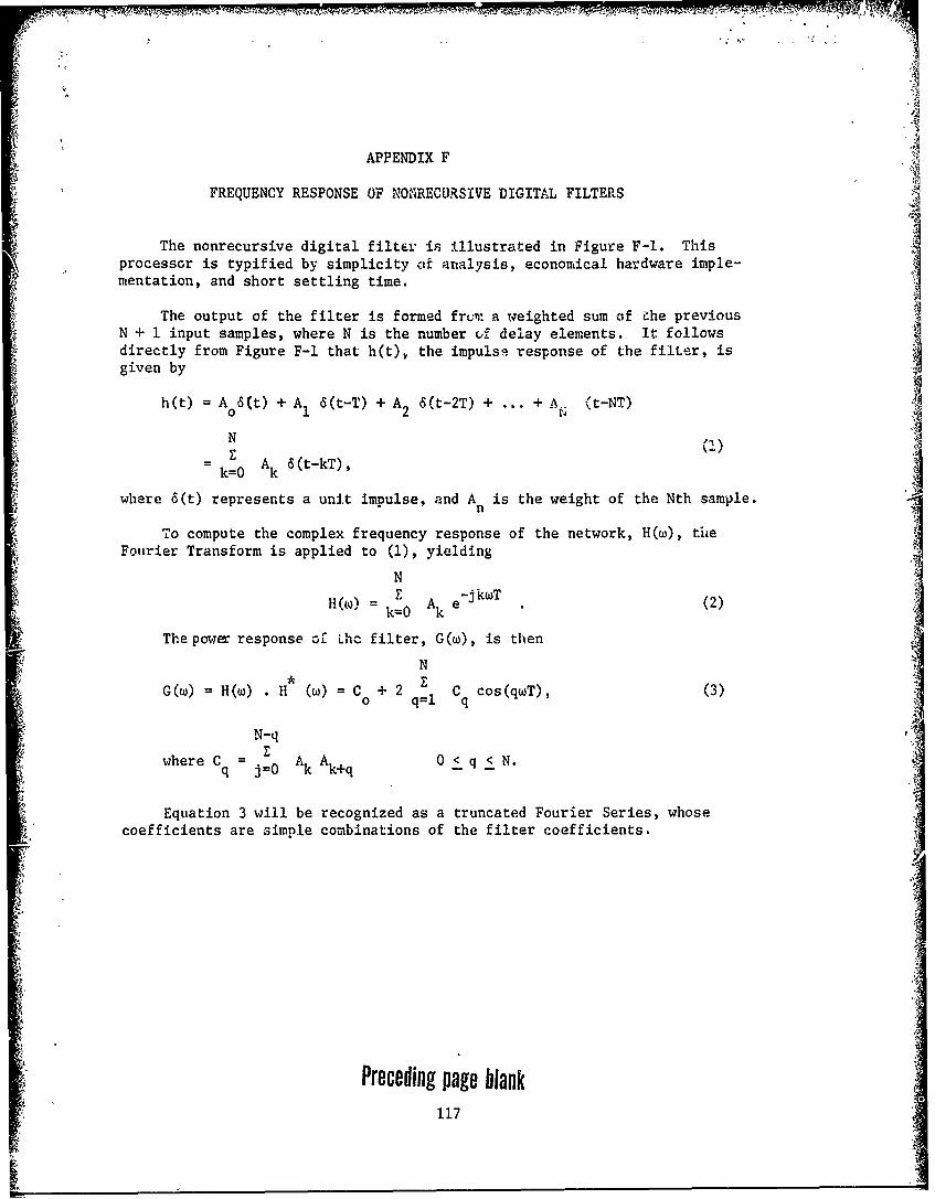
APPENDIX F
FREQUENCY RESPONSE OF NONRECURSIVE DIGITAL FILTERS
The nonrecursive digital filter is illustrated in Figure F-I. Thisprocessor is typified by simplicity vi analysis, economical hardware imple-mentation, and short settling time.
The output of the filter is formed frun: a weighted sum of ihe previousN + 1 input samples, where N is the number of delay elements. It followsdirectly from Figure F-I that h(t), the impulse response of the filter, isgiven by
h(t) = A0 6(t) + A1 6(t-T) + A2 6 (t-2T) + ... + A:. (t-NT)
N
k=O A 6(t-kT),
where 6(t) represents a unit impulse, and An is the weight of the Nth sample.
To compute the complex frequency response of the network, H(w), tile
Fourier Transform is applied to (1), yielding
NZ(• = -jkwT
H(o*) k=O Ak e (2)
The power response of Lhc filter, G(w), is then
N
G(w) = H(w) . H* (w) = C + 2 Z C cos(qwT), (3)
N-q
where C = Ak A 0 <_ q S N.q j0 k+q OqN
Equation 3 will be recognized as a truncated Fourier Series, whosecoefficients are simple combinations of the filter coefficients.
Preceding page blank117

-4400
E-4I
E-44
118O
![UWB Radars [EDocFind.com]](https://static.fdocuments.in/doc/165x107/577d2b9c1a28ab4e1eaae39f/uwb-radars-edocfindcom.jpg)