
Investigation of Spacecraft Cluster Autonomy Through...
188
Investigation of Spacecraft Cluster Autonomy Through An Acoustic Imaging Interferometric Testbed John P. Enright, David W. Miller September 1999 SERC #8-99
-
Upload
doannguyet -
Category
Documents
-
view
214 -
download
0
Transcript of Investigation of Spacecraft Cluster Autonomy Through...

Investigation of Spacecraft Cluster Autonomy Through An Acoustic Imaging Interferometric Testbed
John P. Enright, David W. Miller
September 1999 SERC #8-99

2

Investigation of Spacecraft Cluster Autonomy Through An Acoustic Imaging Interferometric Testbed
John P. Enright, David W. Miller
September 1999 SERC #8-99
This work is based on the unaltered thesis of John P. Enright submitted to the Departmentof Aeronautics and Astronautics in partial fulfillment of the requirements for the degree ofMaster of Science at the Massachusetts Institute of Technology.

2

ion isnes.is func-l envi-ate toent asvali-
Investigation of Spacecraft Cluster Autonomy Through An Acoustic Imaging Interferometric Testbed
by
JOHN ENRIGHT
Submitted to the Department of Aeronautics and Astronauticson September 3, 1999 in Partial Fulfillment of the
Requirements for the Master of Scienceat the Massachusetts Institute of Technology
ABSTRACT
The development and use of a novel testbed architecture is presented. Separated spacecraftinterferometers have been proposed for applications in sparse aperture radar or astronomi-cal observations. Modeled after these systems, an integrated hardware and software inter-ferometry testbed is developed. Utilizing acoustic sources and sensors as a simplifiedanalog to radio or optical systems, the Acoustic Imaging Testbed’s simplest functthat of a Michelson interferometer. Robot arms control the motion of microphoThrough successive measurements an acoustic image can be formed. On top of thtionality, a layered software architecture is developed. This software creates a virtuaronment that mimics the command, control and communications functions appropria space interferometer. Autonomous spacecraft agents interact within this environmthe logical equivalent of distributed satellites. Optimal imaging configurations are dated. A scalable approach to cluster autonomy is discussed.
Thesis Supervisor:Prof. David. W. MillerDept. of Aeronautics and Astronautics

4 ABSTRACT

ACKNOWLEDGMENTS
The author would like to thank the sponsor of this work. The Air Force Research Lab for
Grand Challenges in Space Technology: Distributed Satellite Systems - Contract
#F29601-97-K-0010 under the technical supervision of Lt. George Schneiderman, Dr. Jim
Skinner, and Mr. Richard Burns.
5

6 ACKNOWLEDGMENTS

7
Abstract . . . . . . . . . . . . . . . . . . . . . . . . . . . . . . . . . . . . . . . . . 3
Acknowledgments . . . . . . . . . . . . . . . . . . . . . . . . . . . . . . . . . . . 5
Chapter 1. Introduction . . . . . . . . . . . . . . . . . . . . . . . . . . . . . . 17
1.1 Distributed Satellite Systems (DSS) . . . . . . . . . . . . . . . . . . . . . 19
1.2 Why Sparse Apertures? . . . . . . . . . . . . . . . . . . . . . . . . . . . . 211.2.1 Military Space Missions . . . . . . . . . . . . . . . . . . . . . . . . 211.2.2 Civilian Space Missions . . . . . . . . . . . . . . . . . . . . . . . . 22
1.3 Objectives . . . . . . . . . . . . . . . . . . . . . . . . . . . . . . . . . . . 24
1.4 Outline . . . . . . . . . . . . . . . . . . . . . . . . . . . . . . . . . . . . . 26
Chapter 2. Background . . . . . . . . . . . . . . . . . . . . . . . . . . . . . . 27
2.1 Interferometry . . . . . . . . . . . . . . . . . . . . . . . . . . . . . . . . . 272.1.1 Historical Background . . . . . . . . . . . . . . . . . . . . . . . . . 282.1.2 Signal Processing Basics . . . . . . . . . . . . . . . . . . . . . . . . 322.1.3 Measuring Visibility . . . . . . . . . . . . . . . . . . . . . . . . . . 422.1.4 The Point Spread Function . . . . . . . . . . . . . . . . . . . . . . . 51
2.2 Distributed Processing . . . . . . . . . . . . . . . . . . . . . . . . . . . . 532.2.1 Parallel vs. Distributed Processing . . . . . . . . . . . . . . . . . . . 532.2.2 Algorithm Concepts . . . . . . . . . . . . . . . . . . . . . . . . . . 542.2.3 Connectivity . . . . . . . . . . . . . . . . . . . . . . . . . . . . . . 56
2.3 Background Summary . . . . . . . . . . . . . . . . . . . . . . . . . . . . . 58
Chapter 3. Architecture development . . . . . . . . . . . . . . . . . . . . . . 61
3.1 Overview . . . . . . . . . . . . . . . . . . . . . . . . . . . . . . . . . . . 61
3.2 Hardware . . . . . . . . . . . . . . . . . . . . . . . . . . . . . . . . . . . 633.2.1 Overview . . . . . . . . . . . . . . . . . . . . . . . . . . . . . . . . 633.2.2 Anechoic Chamber . . . . . . . . . . . . . . . . . . . . . . . . . . . 643.2.3 Sound Generation . . . . . . . . . . . . . . . . . . . . . . . . . . . 673.2.4 Signal Detection and Capture . . . . . . . . . . . . . . . . . . . . . 703.2.5 Arms . . . . . . . . . . . . . . . . . . . . . . . . . . . . . . . . . . 733.2.6 Computers and Network . . . . . . . . . . . . . . . . . . . . . . . . 82
3.3 Software . . . . . . . . . . . . . . . . . . . . . . . . . . . . . . . . . . . . 833.3.1 Overview . . . . . . . . . . . . . . . . . . . . . . . . . . . . . . . . 833.3.2 Software Layering . . . . . . . . . . . . . . . . . . . . . . . . . . . 843.3.3 Operating System . . . . . . . . . . . . . . . . . . . . . . . . . . . 873.3.4 The Parallel Virtual Machine . . . . . . . . . . . . . . . . . . . . . 87

8
3.3.5 The Distributed Information Protocol for Space Interferometry . . . 893.3.6 Motion Interface Software . . . . . . . . . . . . . . . . . . . . . . . 903.3.7 Data Acquisition Interface Software . . . . . . . . . . . . . . . . . . 923.3.8 AIT Virtual Ground Station . . . . . . . . . . . . . . . . . . . . . . 933.3.9 Virtual Spacecraft . . . . . . . . . . . . . . . . . . . . . . . . . . . 963.3.10 Matlab Client Interface . . . . . . . . . . . . . . . . . . . . . . . . 107
3.4 Summary . . . . . . . . . . . . . . . . . . . . . . . . . . . . . . . . . . . 108
Chapter 4. Performance Evaluation . . . . . . . . . . . . . . . . . . . . . . . 109
4.1 Optimal Imaging Configurations . . . . . . . . . . . . . . . . . . . . . . . 1094.1.1 Optimization Methods . . . . . . . . . . . . . . . . . . . . . . . . . 1104.1.2 AIT Performance: Single Source . . . . . . . . . . . . . . . . . . . 1134.1.3 AIT Performance: Multiple Sources . . . . . . . . . . . . . . . . . . 120
4.2 Deconvolution . . . . . . . . . . . . . . . . . . . . . . . . . . . . . . . . . 121
4.3 Uncertainty and Errors . . . . . . . . . . . . . . . . . . . . . . . . . . . . 1274.3.1 Random Errors . . . . . . . . . . . . . . . . . . . . . . . . . . . . . 1284.3.2 Secular Variation: Extended Operations . . . . . . . . . . . . . . . . 1294.3.3 Mechanically Induced Wavefront Errors . . . . . . . . . . . . . . . 132
4.4 Performance Conclusions . . . . . . . . . . . . . . . . . . . . . . . . . . . 136
Chapter 5. Artificial Intelligence and Autonomy . . . . . . . . . . . . . . . . 137
5.1 Artificial Intelligence . . . . . . . . . . . . . . . . . . . . . . . . . . . . . 1375.1.1 AI Approaches: Outlining the Field. . . . . . . . . . . . . . . . . . . 1385.1.2 Approaches to Reasoning Systems . . . . . . . . . . . . . . . . . . 140
5.2 Autonomy . . . . . . . . . . . . . . . . . . . . . . . . . . . . . . . . . . . 1425.2.1 Classifications of Autonomy . . . . . . . . . . . . . . . . . . . . . . 1425.2.2 Roles of Autonomous Systems in Space . . . . . . . . . . . . . . . . 144
5.3 Autonomy and the AIT . . . . . . . . . . . . . . . . . . . . . . . . . . . . 1465.3.1 Ground Autonomy . . . . . . . . . . . . . . . . . . . . . . . . . . . 1465.3.2 On-Board Autonomy . . . . . . . . . . . . . . . . . . . . . . . . . . 151
5.4 Algorithms in Development . . . . . . . . . . . . . . . . . . . . . . . . . . 1525.4.1 Bipartite Graph Matching . . . . . . . . . . . . . . . . . . . . . . . 1555.4.2 Centroid Updating . . . . . . . . . . . . . . . . . . . . . . . . . . . 155
5.5 Autonomy Conclusions . . . . . . . . . . . . . . . . . . . . . . . . . . . . 156
Chapter 6. Conclusions . . . . . . . . . . . . . . . . . . . . . . . . . . . . . . 159
6.1 Summary . . . . . . . . . . . . . . . . . . . . . . . . . . . . . . . . . . . 159

9
6.1.1 Background . . . . . . . . . . . . . . . . . . . . . . . . . . . . . . 1596.1.2 Architecture Development . . . . . . . . . . . . . . . . . . . . . . . 1606.1.3 Imaging Performance . . . . . . . . . . . . . . . . . . . . . . . . . 1616.1.4 Artificial Intelligence and Autonomy . . . . . . . . . . . . . . . . . 162
6.2 Further Work . . . . . . . . . . . . . . . . . . . . . . . . . . . . . . . . . 1636.2.1 AIT Refinements . . . . . . . . . . . . . . . . . . . . . . . . . . . . 1636.2.2 The Generalized Flight Operations Processing System (GFLOPS) . . 165
6.3 Concluding Remarks . . . . . . . . . . . . . . . . . . . . . . . . . . . . . 167
References . . . . . . . . . . . . . . . . . . . . . . . . . . . . . . . . . . . . . . . 169
Appendix A. The DIPSI Specification . . . . . . . . . . . . . . . . . . . . . . . 175
A.1 Client/Server Interactions . . . . . . . . . . . . . . . . . . . . . . . . . . . 175
A.2 DIPSI Messages . . . . . . . . . . . . . . . . . . . . . . . . . . . . . . . . 176
A.3 Message Interchanges . . . . . . . . . . . . . . . . . . . . . . . . . . . . . 179
Appendix B. Signal Processing Sequencing . . . . . . . . . . . . . . . . . . . . 183
B.1 Data Exchange Sequences . . . . . . . . . . . . . . . . . . . . . . . . . . . 183

10
11
29
33
. 34
. 37
dant 38
. 40
the 40
ints 41
. 43
of . 44
rity.
mpo-. 53
. 53
e d) . 57
. 63
ws.
. 65
. 65
66
le of . 68
ross-. 69
. 70
Figure 2.1 Michelson’s Optical Interferometer . . . . . . . . . . . . . . . . . . .
Figure 2.2 The Brightness function B(ξ) . . . . . . . . . . . . . . . . . . . . . .
Figure 2.3 Discrete sampling of a continuous function . . . . . . . . . . . . . .
Figure 2.4 The 20-point DFT of |X[k]| indexed from zero. 20 points of the original sequence were used in the transform . . . . . . . . . . . . . . . . .
Figure 2.5 Alternate indexing of |X[k]|, arrows indicate the extent of the non-reduninformation. . . . . . . . . . . . . . . . . . . . . . . . . . . . . . . .
Figure 2.6 A simple sequence, x[n] made up of two discrete delta functions. . .
Figure 2.7 Another simple sequence, h[n]. Three delta functions symmetric aboutorigin. . . . . . . . . . . . . . . . . . . . . . . . . . . . . . . . . . .
Figure 2.8 Convolution of h[n] and x[n]. Notice the replication of h near nonzero poof x. . . . . . . . . . . . . . . . . . . . . . . . . . . . . . . . . . . .
Figure 2.9 Schematic of a interferometer geometry in two dimensions. . . . . .
Figure 2.10 Sensing Geometry in one dimension. The source is offset from the linesight . . . . . . . . . . . . . . . . . . . . . . . . . . . . . . . . . .
Figure 2.11 True brightness function, a simple impulse. Plot shown obliquely for cla 52
Figure 2.12 UV coverage (Spectral Sensitivity Function). Dots indicate non-zero conents . . . . . . . . . . . . . . . . . . . . . . . . . . . . . . . . . .
Figure 2.13 Resulting Point Spread Function . . . . . . . . . . . . . . . . . . .
Figure 2.14 Common Network Schemes. a) Fully connected b) Linear c) HypercubBus/Broadcast . . . . . . . . . . . . . . . . . . . . . . . . . . . . .
Figure 3.1 Schematic overview of the Acoustic Imaging Testbed. . . . . . . . .
Figure 3.2 Overview of testbed hardware. Information flow is indicated by the arro64
Figure 3.3 Physical layout of the AIT anechoic chamber . . . . . . . . . . . .
Figure 3.4 AIT anechoic chamber . . . . . . . . . . . . . . . . . . . . . . . .
Figure 3.5 Effect of Multi-path interference. b shows a clear image with few multi-pathartifacts. Image a displays reduction in image quality when reflections arepermitted from robot linkages. . . . . . . . . . . . . . . . . . . . . .
Figure 3.6 Picture of nine speaker array. The middle speaker is aligned with middtestbed. Centre-to-Centre spacing is about 145mm. . . . . . . . . .
Figure 3.7 Source signal frequency content. Frequency separation ensures zero cchannel correlation . . . . . . . . . . . . . . . . . . . . . . . . . .
Figure 3.8 Block diagram of data acquisition system. . . . . . . . . . . . . . .
12
.
h 116
le . 118
h sig-
four.
. 123
123
ling 125
126
Figure 3.9 DAQ Schematic . . . . . . . . . . . . . . . . . . . . . . . . . . . . . 71
Figure 3.10 The AIT four-bar linkage robot arms . . . . . . . . . . . . . . . . . . 75
Figure 3.11 Motion plane spacing in the AIT . . . . . . . . . . . . . . . . . . . . 76
Figure 3.12 Testbed Coordinate System . . . . . . . . . . . . . . . . . . . . . . . 78
Figure 3.13 Arm Construction . . . . . . . . . . . . . . . . . . . . . . . . . . . . 79
Figure 3.14 The OSI 7-layer model. . . . . . . . . . . . . . . . . . . . . . . . . . 85
Figure 3.15 The AIT layering concept . . . . . . . . . . . . . . . . . . . . . . . . 86
Figure 3.16 State transitions for data acquisition . . . . . . . . . . . . . . . . . . 97
Figure 3.17 Testbed Geometric Effects. . . . . . . . . . . . . . . . . . . . . . . . 101
Figure 3.18 A simple digital system. The transfer function is that of a Digital Delay . . 103
Figure 3.19 Rational Delay . . . . . . . . . . . . . . . . . . . . . . . . . . . . . . 103
Figure 3.20 Frequency Response: linear interpolation vs. band-limited interpolation. Fil-ter length:1024 pts, 100 point granularity . . . . . . . . . . . . . . . . 105
Figure 3.21 The Matlab Client setup. Maneuver selection and post-processing is handled by matlab tools. . . . . . . . . . . . . . . . . . . . . . . . . . . . . . 107
Figure 4.1 Golay array configurations and PSF. From [Kong, et al 1998] . . . . . 111
Figure 4.2 Cornwell array configurations and UV Coverage. From [Kong, et al 1998 111
Figure 4.3 Speaker numbering. Perspective is from above, ‘outside’ of the testbed.113
Figure 4.4 Rectangular visibility sampling profiles (Single Source). Notice very higsidelobes create confusing field of view. . . . . . . . . . . . . . . . .
Figure 4.5 UV Coverage, Point Spread Functions and Measured Response. Singsource located in position 5. . . . . . . . . . . . . . . . . . . . . . .
Figure 4.6 Average Cross-correlation of source signals. At around 2 seconds, botnal generation methods lie close to 10-3 . . . . . . . . . . . . . . . . . . . . . 120
Figure 4.7 Two source images. Active speakers are located in positions three and122
Figure 4.8 Array Response as an LTI system. . . . . . . . . . . . . . . . . . .
Figure 4.9 The CLEAN Algorithm . . . . . . . . . . . . . . . . . . . . . . . . .
Figure 4.10 CLEANed images (One Source) Un-rectified. Notice negative intensitypeaks to the top right of main lobe. Colour variations are due to auto-scato maximize contrast. . . . . . . . . . . . . . . . . . . . . . . . . . .
Figure 4.11 CLEANed images (Two Sources) Rectified. Peaks are clearly defined

13
. 130
. 132
. 134
. 135
. 147
ura-. 150
e-. 153
. 153
154
155
. 180
n the 181
ts and . 184
ation.
corre-. 185
. 186
. . .
Figure 4.12 Visibility measurement of two sources as a function of integration time. a) multi-tone signal b) band limited noise . . . . . . . . . . . . . . . . . 128
Figure 4.13 Normalized standard deviation (magnitude) as a function of integration time. 129
Figure 4.14 Misalignment of testbed drums in ‘homed’ position following extended operations. . . . . . . . . . . . . . . . . . . . . . . . . . . . . . . .
Figure 4.15 RMS Fractional Variation (80 baselines) . . . . . . . . . . . . . . .
Figure 4.16 Phase Error Distribution for Arm 2. . . . . . . . . . . . . . . . . . .
Figure 4.17 Phase Error due to end-effector uncertainty and vertical deflection. .
Figure 5.1 Workspace accommodation . . . . . . . . . . . . . . . . . . . . . .
Figure 5.2 Partial fit of optimal baselines. Two free baselines and four array configtions are possible . . . . . . . . . . . . . . . . . . . . . . . . . . .
Figure 5.3 The configuration placement problem. Dotted lines indicate implicit baslines. . . . . . . . . . . . . . . . . . . . . . . . . . . . . . . . . . .
Figure 5.4 A bipartite graph. Heavy lines are represent a matching . . . . . . .
Figure 5.5 Algorithm for vertex placement . . . . . . . . . . . . . . . . . . . . .
Figure 5.6 Simple network for solving the maximum matching problem. . . . . .
Figure A.1 Message exchanges for position query and movement. . . . . . . . .
Figure A.2 Data collection sequence. The sequence operations are enumerated oright. . . . . . . . . . . . . . . . . . . . . . . . . . . . . . . . . . . .
Figure B.1 Start condition after sampling process. Coloured bars represent data seshading indicates segmentation of each data vector. . . . . . . . . .
Figure B.2 The first data exchange. This system implements sequential communic 184
Figure B.3 System state after first exchange. Calculation queue depicts the partiallation operations pending. . . . . . . . . . . . . . . . . . . . . . . .
Figure B.4 Second data exchange. Notice the ‘piggybacking’ of data within the exchange. . . . . . . . . . . . . . . . . . . . . . . . . . . . . . . .
Figure B.5 Final State. Each Spacecraft has equal computational tasks to perform186

14

15
TABLE 1.1 Evolution of Distributed Satellite Application . . . . . . . . . . . . . 18
TABLE 1.2 Some Examples of Autonomy Implementations . . . . . . . . . . . . 20
TABLE 1.3 Comparison of Technical Approaches in Sparse Aperture Systems . . 25
TABLE 3.1 AIT Functional Mappings . . . . . . . . . . . . . . . . . . . . . . . 62
TABLE 3.2 Acoustic Foam Performance . . . . . . . . . . . . . . . . . . . . . . 66
TABLE 3.3 Arm Calibration Parameters . . . . . . . . . . . . . . . . . . . . . . 82
TABLE 3.4 AIT hosts . . . . . . . . . . . . . . . . . . . . . . . . . . . . . . . . 83
TABLE 5.1 Common Approaches to Artificial Intelligence . . . . . . . . . . . . 138
TABLE 5.2 Jet Propulsion Lab Autonomy Levels . . . . . . . . . . . . . . . . . 143
TABLE A.1 DIPSI Messaging . . . . . . . . . . . . . . . . . . . . . . . . . . . . 177

16

Chapter 1
INTRODUCTION
ication
m at a
al or
ilarly
ities
stem:
ce mis-
Decentralization works. Not in every instance or application, but sometimes it just works.
Recently, distributed approaches are seeing application to problems that have traditionally
thwarted monolithic undertakings. In fields ranging from control theory to information
management, decentralized architectures are being viewed as an attractive design alterna-
tive. The resulting systems may not always be optimal for a specific task, but in general
distributed systems can offer advantages of robustness and flexibility that the traditional
designs lack. In fact it has been said of neural networks, the ultimate in decentralized com-
putation, that “…[they] are the second best way of doing just about anythinga.” Distrib-
uted design has recently been applied to space.
Of course, distributed approaches have their problems: coordination and commun
must be managed on a whole new level. Knowledge of the global state of a syste
given instant in time is no longer possible. Usually one must be content with only loc
partial information. Providing metrics and proving bounds on performance are sim
difficult. Most of all, to achieve a single function from a collection of self directed ent
requires extensive foresight into the architecture that governs their interactions.
Space missions are still a long way from that ubiquitous example of a distributed sy
The Internet. There is, however, increasing interest in distributed approaches to spa
a. Attributed to John Denker, AI theoretician [Russell and Norvig 1995]
17

18 INTRODUCTION
stel-
stems
inter-
level of
re with a
h the
ons to
gular
acing
hat of a
t.
meth-
t affect
erfor-
r inter-
sion design. Several constellations of satellites are currently in orbit about the Earth.
NavStar, commonly known as the Global Positioning System (GPS), relies on signals
from multiple satellites to fix one’s position on the Earth. The Iridium system is a con
lation of Low Earth Orbit satellites designed to provide global telephony. As these sy
increase in sophistication, there is a trend towards greater reliance on inter-satellite
actions (Table 1.1). One particular class of space missions is poised to advance the
collaboration even further. This field is known as sparse aperture synthesis.
Sparse aperture systems in general seek to replace a single large antenna or apertu
number of a carefully controlled smaller ones. This allows the system to function wit
angular ‘effectiveness’ of a much larger structure. This can be used in communicati
create a high directional gain, in an astronomical interferometer to provide fine an
resolution, or in a radar system to maintain high probability of target detection. By pl
each aperture on a separately orbiting spacecraft, the system response can mimic t
single antenna the size of the entire satellite cluster. This is a significant achievemen
This distributed approach to space mission design fundamentally alters traditional
ods of systems analysis. Multiple component missions possess many features tha
the way the system is controlled and maintained. Moreover, evaluation of their p
mance and cost is as intimately tied to the interactions between satellites as to thei
TABLE 1.1 Evolution of Distributed Satellite Application
Application Satellite InteractionsCoordination Requirements
Navigation (GPS)
Signals from multiple S/C compared in ground terminal
Low
Communication (Iridium)
Cross-linking of calls, caller hand-off
Med
Sparse Aperture Synthesis
(TechSat 21, TPF)
Formation Flying, High bandwidth dis-tributed signal pro-
cessing
High

Distributed Satellite Systems (DSS) 19
nal workings. To properly understand the issues involved, some re-evaluation of
traditional analysis tools is necessary
1.1 Distributed Satellite Systems (DSS)
The field of distributed satellite systems is expanding. People are coming up with applica-
tions faster than design theory can keep up. To fully realize the potential for this type of
architecture, innovations must first be made at the analysis and design phases of a pro-
gram. Implementation of such a design also requires the development of advanced tools to
manage and exploit the unique features of these missions. The Distributed Satellite Sys-
tems program at the MIT-Space Systems Lab is a study aimed at exploring some of these
issues.
The coordinated operation of several satellites for a single goal is the hallmark of a distrib-
uted satellite system [Shaw 1998]. Direct application of traditional systems-analysis meth-
odologies to distributed satellite systems usually deals unfairly with the distributed
system. A methodology based upon the theory of information networks has been devel-
oped by Shaw to enable more equitable comparisons.
The benefits of distributed approaches to military, science and commercial ventures are
numerous. Distributed systems often enjoy graceful degradation in performance rather
than hard failures. Manufacturing multiple, identical satellites allows learning curve sav-
ings to be realized [Wertz 1992]. In some situations, and in particular sparse aperture sys-
tems, synergistic effects can enhance the functional effectiveness (i.e. orbital dynamics
can be exploited to reduce maneuvering fuel) [Kong, et al 1999].
On the other hand, there is a price to be paid as well. Since each spacecraft must duplicate
some subsystems (i.e. attitude control, propulsion, etc.), DSS approaches are expected to
pay a penalty in terms of mass. Multiple spacecraft also create more complexity and inter-
dependancies. This can be especially crippling if each satellite shares a design flaw. Even
leaving aside inefficiencies and flaws, these systems still require additional design effort.

20 INTRODUCTION
prox-
It is necessary to develop hardware and software for asset management; a system that tra-
ditionally has little impact on monolithic designs. Without sophisticated techniques to
coordinate and control the space and ground resources, distributed satellite systems are
doomed to be high in cost (particularly operations) or grossly ineffective.
Investing space systems with autonomy has the potential to streamline operations and
enable advanced capabilities. Unfortunately, the best approach is it is often unclear.
Autonomy suffers from an extraordinarily broad definition. Implementations can be sim-
ple or complex, as well as narrow or broad in scope. Finding the correct balance between
risk, technological capabilities and required effectiveness is a very hard thing to do. It is
perhaps helpful to enumerate some simple examples of autonomy (Table 1.2).
Behaviour that is both simple and narrow of scope, usually aims to automate the opera-
tions of a single subsystem. The logic behind such systems is usually very straightforward
and the systems operate in a reactive (memoryless) fashion. A broad scope implementa-
tion of simple autonomy might apply simple control laws to the multivariate state of the
spacecraft. Other simple applications might apply simple heuristics to routing the flow of
information between linked satellites. Advanced autonomy typically involves reasoning
and planning of the type usually associated with artificial intelligence. Again, the imple-
mentation can be confined to a particular subsystem or can even span the aggregate
actions of a satellite constellation.
This thesis addresses some of the issues involved in the development of broad scope
autonomy for distributed clusters of satellites. Clusters (several spacecraft in ‘close’
TABLE 1.2 Some Examples of Autonomy Implementations
Narrow Scope Broad Scope
Simple Behaviour Autonomous Orbit Maintenance
Reactive sub-system management
Advanced Behaviour Fault Identification and Reconfiguration
Cluster-wide plan-ning and execution

Why Sparse Apertures? 21
imity) offer challenges not encountered in the management of constellations. This arises
from tightly coupled operation and the potential for disastrous outcomes, i.e. collisions.
Since clusters have been proposed for systems employing sparse aperture synthesis, this
class of mission seems to be an appropriate focus for the study.
1.2 Why Sparse Apertures?
Systems that rely on beam-forming or mapping can often benefit from the applications of
interferometry techniques. Many applications of sparse aperture systems are being consid-
ered both for military and civilian space missions.
1.2.1 Military Space Missions
The military, and particularly the Air Force, sees a particular interest in space based,
sparse aperture systems. Providing support functions from space offers these systems a
degree of immunity from the perils of the battlefield. Spacecraft clusters can supplement
traditional communications capabilities offering flexible access to both hand-held termi-
nals and fixed ground stations. Space surveillance also shows tremendous flexibility. By
employing principles of interferometry, images can be synthesized with exceptional angu-
lar resolution. Finally, particular applications to radar systems benefit from a sparse aper-
ture, cluster approach.
Small, low-mass communications satellites when arranged in a cluster can offer dual
mode operations. By themselves, each can serve as a relay between fixed stations either
through a transponder operation or utilizing inter-satellite links to reach distant sites. If the
cluster acts in concert, the resulting highly directional beam could reach mobile and even
hand-held terminals [Das & Cobb 1998].
Space surveillance is limited by the ability to launch large optical systems. Constraints of
fairing diameter place one bound on their maximum size (and hence resolution). Even
before reaching this limit, large aperture instruments are both expensive and fragile. Inter-

22 INTRODUCTION
ch has
s some
ferometry techniques offer a means of providing fine angular resolution using separated
apertures. The Ultralite program is a proposed imaging system composed of six apertures
connected by a deployable truss [Powers et al 1997]. While not a distributed satellite sys-
tem, this does make use of sparse aperture techniques.
Perhaps one of the more ambitious and innovative techniques proposed is the radar system
known as the Technology Satellite for the 21st Century (TechSat 21). TechSat 21 seeks to
validate the feasibility of a number of technologies aimed at making space systems
smaller, cheaper and more reliable. Even the chosen mission is a demonstration of tech-
nology. Using a cluster of four to twenty satellites, TechSat 21 will used advanced tech-
niques for Ground Moving Target Indication (GMTI). While traditional approaches to a
space-based GMTI system have required huge antennas, TechSat 21 seeks to exploit the
science of sparse aperture arrays, using antennas of only a couple of metres across. The
coherent processing and the use of transmitter and receiver diversity allows signal gains of
100-1000 or even more [Das & Cobb 1998]. While this figure is encouraging, it levies
stringent requirements on propagation modelling and on-board processing.
Many of these military applications have counterparts in civilian applications where the
emphasis is on looking out and not in. Astronomical observations have benefited for quite
some time from the advantages of ground-based interferometer systems. To address prob-
lems of sensitivity and atmospheric disturbances, there is now a push to launch interfero-
metric devices into space.
1.2.2 Civilian Space Missions
There is great interest on behalf of the National Aeronautics and Space Administration
(NASA) in the fundamental questions surrounding the origin of life on Earth. So clearly
does this tie into the organization’s goals, that a road-map for twenty years of resear
been developed [Naderi 1998]. This program, the Origins program, seeks to addres
fundamental, multi-disciplinary issues:
• The formation of galaxies, stars and planetary systems.

Why Sparse Apertures? 23
• The search for planets in ‘habitable zones’ around nearby stars.
• If such planets exist, do they show compositional signs of supporting life?
• Clues to the origins of life in our own solar system.
One of the keystone missions in the Origins program is called Terrestrial Planet Finder
(TPF). This mission is slated to employ an instrument known as an interferometer to allow
high resolution imaging of the possible planetary systems around distant stars. The funda-
mental limitation with astronomical observations is often that of angular resolution. The
larger the diameter of the telescope, the finer the details that can be resolved. Problems
come in the manufacture of such large telescopes. Ground systems are troubled by the
atmosphere, which distorts and blurs images. This leads to the desire to launch telescopes
into space.
Space offers many benefits in an observing system. There is no atmosphere to distort the
image, and instruments are more sensitive to faint sources [Quirrenbach & Eckart 1996].
Again, as in the case of military surveillance, large aperture telescopes are difficult and
expensive to launch into space. Some instruments such as the Next Generation Space
Telescope seek a way around this problem through the use of a deployable mirror. The pri-
mary mirror, the largest reflecting surface, is actually formed from multiple retractable
segments. These can be folded against the structure for launch, and then opened on orbit.
Interferometers offer even greater potential for fine angular resolution measurements.
The European Space Agency is also planning a large space interferometry mission. The
Darwin mission, like TPF, will aid in the search for Earth-like planets [Penny et al 1998].
As with TPF, DARWIN designers are considering both structurally connected and sepa-
rated spacecraft architectures.
Whatever the application, distributed satellite approaches pose their own unique set of
design challenges and constraints. While not ideal in all situations, certain applications
show significant improvements over traditional approaches.

24 INTRODUCTION
’t soft-
es of a
ach of
umber of
con-
rowing
ieved.
echnol-
ystem
lifying
grey
1.3 Objectives
The goal of this thesis is to develop an integrated architecture to allow exploration of
broad-scope autonomy as it relates to sparse aperture systems. This system will involve
the use of hardware and software to create a functioning synthesis system. Borrowing fea-
tures from the types of applications (i.e. radar, surveillance, astronomy) described earlier,
this testbed will provide a platform to examine common issues while avoiding technology
related hang-ups. The result is the Acoustic Imaging Testbed (AIT).
One might question the use of hardware in a testbed designed to be generic. Wouldn
ware simulation do just as good a job? After careful consideration, certain advantag
hardware based system became clear:
• Robustness: One of the common problems with the implementation ofautonomy is the brittleness of systems to phenomena not accounted forahead of time [Lindley 1995]. The use of hardware introduces a gap betweenmodeled operation and reality. Response of the autonomous system tounforeseen circumstances can be examined.
• Validity: In order to get a hardware based system to work satisfactorily,understanding of the theoretical operation is vital. Additionally, when a sys-tem architecture is designed to be analogous to real systems, it becomes eas-ier to ensure that the system doesn’t ‘cheat’ That is, all information flowused by the virtual spacecraft comes from a traceable source.
Before any design work can progress the form of the testbed must be established. E
the systems being considered for space-based sparse aperture synthesis has a n
specific technical challenges that drive the design. Although hardware integration is
sidered necessary, hardware challenges should not be a focus of this study. By bor
certain operational features from the envisioned missions, two goals can be ach
First, easy technical solutions from each system can be chosen. This ensures that t
ogy enables rather than constrains. Second, results obtained from this hybrid s
should be general enough to apply to any of the applications.
By comparing some of the technical requirements for the proposed systems, simp
features can be found (Table 1.3). The simplest technical solution is marked by the
Objectives 25
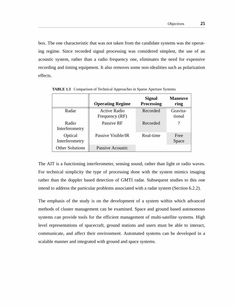
box. The one characteristic that was not taken from the candidate systems was the operat-
ing regime. Since recorded signal processing was considered simplest, the use of an
acoustic system, rather than a radio frequency one, eliminates the need for expensive
recording and timing equipment. It also removes some non-idealities such as polarization
effects.
The AIT is a functioning interferometer, sensing sound, rather than light or radio waves.
For technical simplicity the type of processing done with the system mimics imaging
rather than the doppler based detection of GMTI radar. Subsequent studies to this one
intend to address the particular problems associated with a radar system (Section 6.2.2).
The emphasis of the study is on the development of a system within which advanced
methods of cluster management can be examined. Space and ground based autonomous
systems can provide tools for the efficient management of multi-satellite systems. High
level representations of spacecraft, ground stations and users must be able to interact,
communicate, and affect their environment. Automated systems can be developed in a
scalable manner and integrated with ground and space systems.
TABLE 1.3 Comparison of Technical Approaches in Sparse Aperture Systems
Operating RegimeSignal
ProcessingManeuve
ring
Radar Active Radio Frequency (RF)
Recorded Gravita-tional
Radio Interferometry
Passive RF Recorded ?
Optical Interferometry
Passive Visible/IR Real-time Free Space
Other Solutions Passive Acoustic
26 INTRODUCTION
1.4 Outline
The theoretical basis for interferometry is developed in Chapter 2. Specific discussion is
made of the techniques involved in the AIT. The architecture development is presented in
Chapter 3. This includes examination of the interactions between hardware and software
along with their functional analogues in a real system. Chapter 4 evaluates the perfor-
mance of the AIT as an imaging interferometer. Optimal profiles are implemented and
sources of error in the system are identified. Advanced concepts of artificial intelligence
and autonomy are presented in Chapter 5. Finally, Chapter 6 offers conclusions and les-
sons learned in this study along with suggested directions for future research.

Chapter 2
BACKGROUND
The development of the Acoustic Imaging Testbed architecture borrows much from the
fields of Radio Astronomy, Optics, High Performance Computing, and Networking. This
section provides the theoretical background and justification for the testbed operation.
Advanced autonomy and artificial intelligence are considered in Chapter 5.
2.1 Interferometry
Two principal requirements determine the effectiveness of an astronomical instrument. As
most work in astronomy can be reduced to studying light emitted from distant sources, one
must first be able to collect photons. This is referred to as sensitivity. This requirement can
be met with large collecting areas and long dwell times. Maximizing the collected radia-
tion allows the sensing of very faint objects. The other principal requirement is that of
angular resolution. The better the angular resolution capability the more effective the
instrument is at discerning two objects in close proximity to one another. This attribute is
determined by the ratio of operating wavelength to aperture diameter. The smaller the
value, the smaller the separation that can be resolved. In a traditional, filled-aperture tele-
scope, the two requirements are satisfied simultaneously [Danner & Unwin 1999].
The theoretical angular resolution of a circular aperture, as given by the Rayleigh criterion
[Halliday, et al 1992, pp 976], is:
27

28 BACKGROUND
(2.1)
A telescope or other instrument able to resolve such a separation is said to be diffraction
limited. Obtaining such performance, levies increasingly heavy requirements on the man-
ufacturing process. Achieving diffraction limited optics requires the shape of the collect-
ing surfaces be controlled to within a fraction of a wavelength. Optimistically, the
tolerance can be as fine as λ/10 and is often more stringent [Born & Wolf 1980]. For large
telescopes this becomes prohibitively difficult, both technically and financially. Since the
push towards very large apertures is more often driven by the need for better angular reso-
lution rather than sensitivity, there is a way around the problem. Interferometry is a tech-
nique employing the coherent combination of observations from small, separated
apertures to produce enhanced angular resolution. In fact, such an array can have angular
resolution comparable to a filled aperture instrument of size equal to the linear dimension
of the array. This technique decouples sensitivity and angular resolution. Angular resolu-
tion is addressed by the size of the array. The desired sensitivity can be met by selecting an
appropriate balance between the amount of collecting area and the length of the dwell
time. These techniques have been employed in optical, infrared, and radio frequency
applications.
2.1.1 Historical Background
In this section, an abridged history of astronomical interferometry is presented. Both radio
and optical techniques are discussed. Significant technical breakthroughs are highlighted.
Some of the earliest astronomical uses of interferometers were made by Michelson around
1920-1921 [Thomson, et al, 1994 pp.11]. Using an optical instrument, he and his col-
leagues were able to make diameter measurements of some of the larger nearby stars
(Figure 2.1). By measuring the interference fringes or visibility produced in the combined
light, information about the brightness distribution can be surmised. Unfortunately, the
θ 1.22λd
-------------- sin 1–=

Interferometry 29
ignals
nts
c-
t
al to
. This
instrument was very sensitive to mechanical vibrations and atmospheric turbulence. This
limited the application of the technique.
The emergence of radio astronomy after World War II [Southworth 1945, Appleton 1945]
provided another opportunity to explore the capabilities of interferometry. Working with
dipole, VHF (175 MHz) antennas, Ryle and Vonburg [Ryle & Vonberg, 1946] were able to
create an equivalent system to Michelson’s work, only now in the radio regime.
These interferometers were all additive in their beam combination. Consider two s
from the separated apertures, E1 and E2. An interferometer seeks to measure compone
of the Fourier decomposition of an image. This is termed the fringe visibility V and is
obtained from the power signal E1E2 (Section 2.1.3). Due to the limitations of early ele
tronics, instruments were sensitive to the quantity (E1 + E2)2. To be useful, the scientis
had to account for the E12 and E2
2 components. This was less than ideal since the sign
noise in the system was sometimes very poor. The development of the phase switching
system in 1952 [Ryle 1952] allowed periodic reversal of phase on one of the signals
Figure 2.1 Michelson’s Optical Interferometer
θ∆
Telescope
Mirrors

30 BACKGROUND
y radio
al tar-
uired
ping
Cam-
rlands
n, et
rences
etry
aying
base-
fter
ied.
and
were
t capa-
produced outputs of (E1 + E2)2 and (E1 - E2)2. Subtracting the two allowed direct mea-
surement of E1E2.
The next decade saw radio interferometers used to conduct several sky surveys, detecting
and characterizing many stars and other radio sources. Most notable among these are the
famous Cambridge catalogs [Thomson, et al, 1994 pp. 22] which became definitive works
in radio astronomy. Whereas the emphasis in the 1950’s was on cataloging as man
sources as possible, the 60’s and 70’s saw a concentration of attention on individu
gets. High resolution imaging in two dimensions and detailed spectroscopy req
advances in technology along with reconfigurations in the interferometer design.
Multi-element arrays were built or modified during this period to speed up the map
process. Examples of prominent systems included the 5 km-Radio Telescope at
bridge (1972)[Ryle 1972], the Westerbork synthesis radio telescope in the Nethe
(1973)[Baars, et al 1973], and the Very Large Array in New Mexico (1980) [Thompso
al 1980].
The development of advanced recording devices and very accurate time refe
allowed huge arrays to be employed. Known as Very Long Baseline Interferom
(VLBI), this technique works by recording the data at disparate locations and then pl
the recordings back once they are brought together. This allows measurements with
lines thousands of kilometers long.
Meanwhile, in the field of optical/IR interferometry, progress was much slower. A
Michelson’s work, astronomical applications of visible/IR interferometry were stym
Little was done in the field until 1963 when Australian researchers Hanbury, Brown
Twiss, built and operated what is referred to as an intensity interferometer [Shao & Colav-
ita 1992]. Using incoherent light collected from several apertures, the researchers
able to make measurements of stellar diameters. This form of interferometry was no
ble of true imaging and had limited applications.

Interferometry 31
It was not until 1972, when Labeyerie [Shao & Colavita 1992] built his two telescope
interferometer (I2T), that optical interferometry really came into its own. Precise control
of the differential pathlength in the beams between the two apertures was maintained
using a beam combiner table. The data collected from this instrument was of high quality
and the apparatus has been upgraded several times.
Many of these studies utilized visible and near-infrared regions of the spectrum. Sensitiv-
ity becomes a little troublesome at the longer wavelengths due to system noise tempera-
ture. It is possible, however, to perform heterodyning of mid-infrared light. This leads to a
(simpler) signal processing problem analogous to radio interferometry [Townes 1984].
This allows multiplicative fringe measurements that most optical systems cannot provide.
Several of these instruments were employed to study dust clouds and atmospheric propa-
gation [Shao & Colavita 1992].
Today there are around nine, large, ground-based, optical interferometer facilities [Paresce
1996]. Several more are under construction and are anticipated to be operational in the
next several years. Facilities such as the Keck interferometer being constructed in Hawaii
offer exciting possibilities for astronomical study due to their very fine angular resolution.
Ground based observations using optical/IR interferometry suffer from a number of limi-
tations. Atmospheric turbulence, reduced sensitivity and small fields of view limit the
achievable performance of these systems [Bely 1996, Quirrenbach & Eckart 1996]. To
combat these problems, Bracewell [Bracewell & MacPhie 1979] suggested that a space
based interferometer might provide numerous improvements over a ground based system.
There are currently several large space interferometry missions in development. The
Space Interferometry Mission (SIM) is a structurally connected, multiple baseline, Mich-
elson interferometer designed to perform astrometry measurements. Its mission is also to
establish the technical heritage that would enable the subsequent Terrestrial Planet Finder
(TPF) mission. TPF, along with the European counterpart DARWIN, aim to directly detect
extra-solar planets.

32 BACKGROUND
To attain the long baselines necessary for these tasks, the concept of a separated spacecraft
interferometer becomes attractive [Jilla 1998]. Each collecting aperture resides on an indi-
vidual spacecraft. One or more of the spacecraft combine the incoming beams to measure
the visibility parameters. This technique has been considered for applications close to the
Earth and in free space. An Earth orbiting interferometer can exploit orbital dynamics to
vary the measurement baseline [Kong, et al 1999], while free flying systems have greater
flexibility in maneuvering and system design [Kong & Miller 1998].
To validate the techniques and hardware required for these demanding undertakings, sev-
eral pre-cursor experiments have been proposed including the Space Technology-3 Exper-
iment (Formally: Deep Space-3) [Linfield & Gorham 1998], and the FLITE/ASTRO-
SPAS concept [Johann, et al 1996]. These experiments seek to validate the structural mod-
eling and control, inter-spacecraft metrology, inter-spacecraft communication and other
critical techniques.
Most of the precursor studies to the large interferometer missions focus on very specific
technical challenges: optical pathlength management, structural control, metrology, etc.
This study seeks to address some larger issues associated with sparse array systems. The
Acoustic Imaging Testbed seeks not to examine the specific hardware technologies but
rather the technology involved in coordinating multiple spacecraft. It is important to note
that the AIT is still a functioning interferometer. Before discussing the issues involved in
distributed operation, one needs an understanding of the mathematics behind the science
of interferometry. The next section reviews some basics of signal processing while inter-
ferometer operation is explained in Section 2.1.3.
2.1.2 Signal Processing Basics
Fourier Transforms
Before delving into the theory of operation of interferometers, it is worthwhile to review
the basics of the Fourier transform theorems. These transforms lie at the heart of the inter-
ferometry technique employed in the AIT. Many applications for Fourier transform pairs
Interferometry 33
tions
ns. In a
angle
y,
are employed in science and engineering: time/frequency (signal analysis), position/
momentum (quantum mechanics), etc. The pair of note in the image synthesis problem is
that of brightness, B, and visibility, V.
Brightness is an intensity (power) map over a certain field of view. It is a standard
‘image.’ Visibility represents the spatial frequency content of the image. Rela
between these quantities can be developed for both discrete and continuous domai
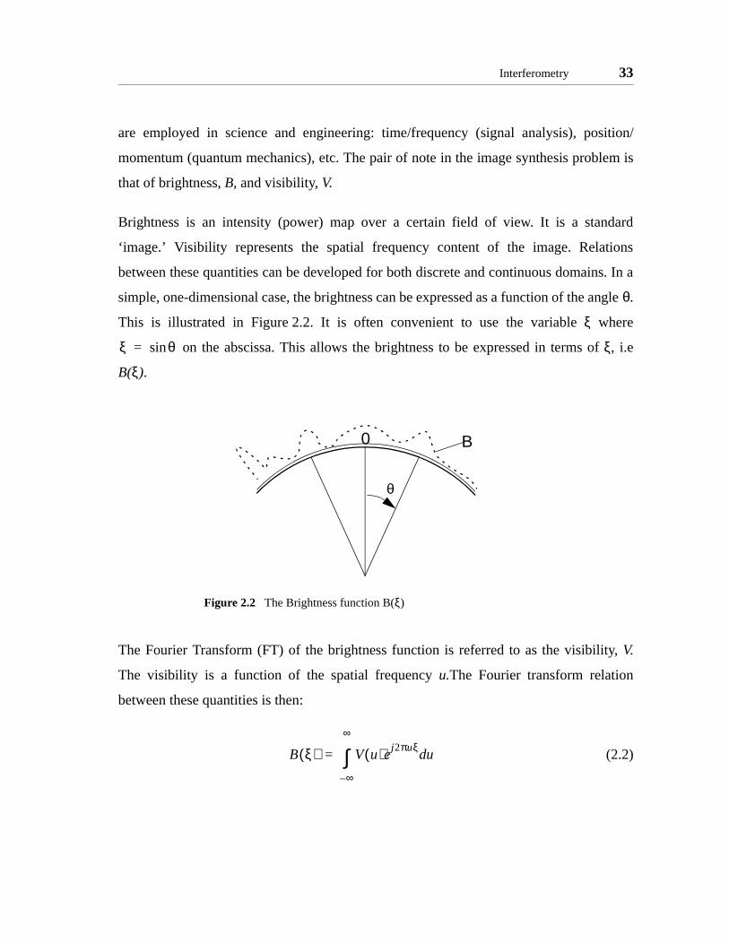
simple, one-dimensional case, the brightness can be expressed as a function of the θ.
This is illustrated in Figure 2.2. It is often convenient to use the variable ξ where
on the abscissa. This allows the brightness to be expressed in terms ofξ, i.e
B(ξ).
The Fourier Transform (FT) of the brightness function is referred to as the visibilitV.
The visibility is a function of the spatial frequency u.The Fourier transform relation
between these quantities is then:
(2.2)
Figure 2.2 The Brightness function B(ξ)
ξ θsin=
θ
0 Β
B ξ( ) V u( )ej2πuξ
ud
∞–
∞
∫=

34 BACKGROUND
to the
he spa-
(2.3)
This transform relation can be denoted:
(2.4)
For many systems, continuous variables are an idealization. In most cases, both the spatial
(B) and frequency (V) domain representations must be discretized. First, consider sam-
pling the brightness B at N equally spaced intervals of ξ, i.e. B(ξ0), B(ξ0 + ∆ξ)…
(Figure 2.3)
The Discrete Fourier Transform (DFT) can then be computed in a manner analogous
continuous case. Converting to a discrete expression represents sampling in both t
tial and frequency domains.
Figure 2.3 Discrete sampling of a continuous function
V u( ) B ξ( )e j2πuξ– ξd
∞–
∞
∫=
V u( ) B ξ( )↔
0 2 4 6 8 10 12 14 16 18 200
0.2
0.4
0.6
0.8
1
1.2
1.4
1.6
1.8
2
ξ
B

Interferometry 35
(2.5)
(2.6)
The change of variables from (ξ,u) to (m,n) is accomplished by noting that:
(2.7)
(2.8)
A simple expression relates the increments of brightness and visibility:
(2.9)
This rather innocuous expression has rather far reaching consequences. First, the choice of
the frequency increment determines the full field of view represented in the spatial
domain, i.e. the smaller the value of ∆u, the larger the extent of the space domain. Sec-
ondly, it can be seen that the maximum spatial frequency sampled (N·∆u) defines the reso-
lution (∆ξ) of the spatial domain. This is particularly important in the field of
interferometry. All other things being equal, the ability to sample higher spatial frequen-
cies yields better angular resolution.
Two dimensional transforms can also be defined. The continuous relations can be
expressed as:
(2.10)
B n[ ] 1N---- V k[ ]e
j2πkn
N-------------
k 0=
N 1–
∑=
V k[ ] B n[ ]ej2πkn
N-------------–
n 0=
N 1–
∑=
ξ n ∆ξ⋅=
u m ∆u⋅=
∆ξ 1N ∆u⋅---------------=
B ξ η,( ) V u v,( )ej2π ξu ηv+( ) ud vd
∞–
∞
∫∞–
∞
∫=

36 BACKGROUND
tions’.
s:
:
e
scret-
and
visi-
(2.11)
The two axes of the frequency domain form what is commonly called the UV plane. the
combination of u and v specify a two-dimensional spatial frequency. This can be thought
of as a particular wavelength and an orientation for a series of brightness ‘corruga
After a minor change of indices, the discrete transform relations can be expressed a
(2.12)
(2.13)
Where the brightness and visibility functions have been sampled in such a way that
(2.14)
(2.15)
The inclusion of the reference location (ξ0,η0) allows one to adjust the placement of th
origin in the discrete representation. An important point to realize is the effects of di
ization on the continuous functions. Eqs 2.14 and 2.15 hold only for
(or k and l, respectively). For values outside this range, the brightness and
bility are periodically replicated every M (or N) points. Hence,
(2.16)
and,
(2.17)
V u v,( ) B ξ η,( )e j2π ξu ηv+( )– ξd ηd
∞–
∞
∫∞–
∞
∫=
B m n,[ ] V k l,[ ]ej2π km
M------- nl
N-----+
l 0=
N 1–
∑k 0=
M 1–
∑=
V k l,[ ] B m n,[ ]ej2π km
M------- nl
N-----+
–
n 0=
N 1–
∑m 0=
M 1–
∑=
B m n,[ ] B ξ0 m∆ξ+ η0 n∆η+,( )=
V k l,[ ] V k∆u l∆v,( )=
m M 1–<
n N 1–<
B m rM+ n sN+,[ ] B m n,[ ]=
V k rM+ l sN+,[ ] V k l,[ ]=
Interferometry 37
The question of indexing and replication can be rather confusing. It may be helpful to con-
sider the following simple example.
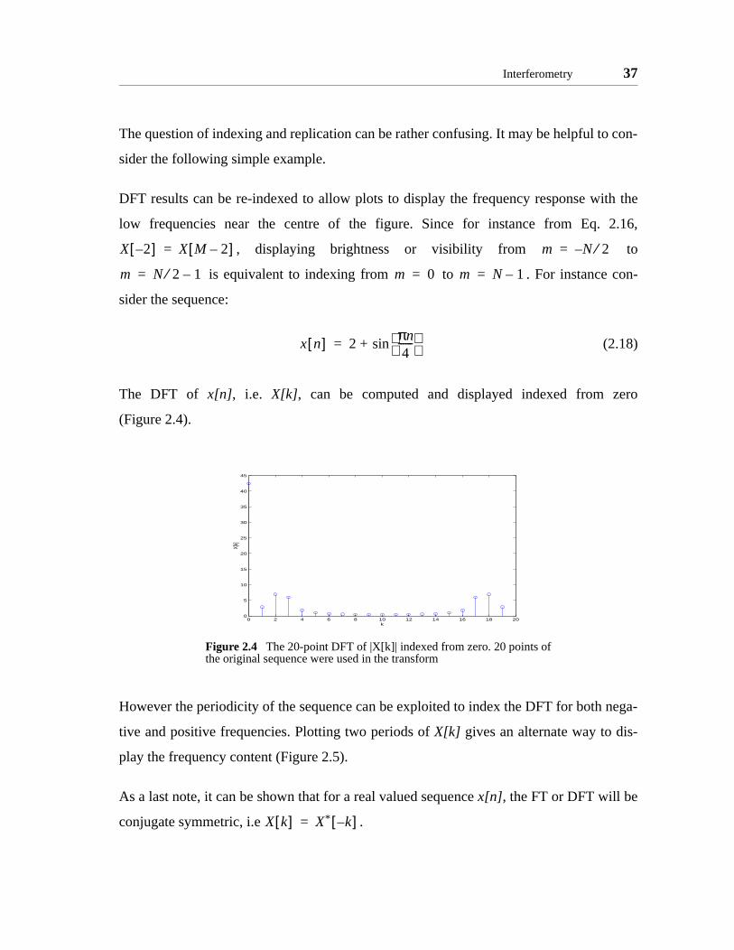
DFT results can be re-indexed to allow plots to display the frequency response with the
low frequencies near the centre of the figure. Since for instance from Eq. 2.16,
, displaying brightness or visibility from to
is equivalent to indexing from to . For instance con-
sider the sequence:
(2.18)
The DFT of x[n], i.e. X[k], can be computed and displayed indexed from zero
(Figure 2.4).
However the periodicity of the sequence can be exploited to index the DFT for both nega-
tive and positive frequencies. Plotting two periods of X[k] gives an alternate way to dis-
play the frequency content (Figure 2.5).
As a last note, it can be shown that for a real valued sequence x[n], the FT or DFT will be
conjugate symmetric, i.e .
Figure 2.4 The 20-point DFT of |X[k]| indexed from zero. 20 points ofthe original sequence were used in the transform
X 2–[ ] X M 2–[ ]= m N 2⁄–=
m N 2⁄ 1–= m 0= m N 1–=
x n[ ] 2πn4
------ sin+=
0 2 4 6 8 10 12 14 16 18 200
5
10
15
20
25
30
35
40
45
k
X[k]
X k[ ] X* k–[ ]=

38 BACKGROUND
The above material represents the basic nomenclature and operations encountered in sig-
nal processing. Both continuous and discrete functions can be expressed in terms of Fou-
rier transform pairs. Furthermore, discrete representations of continuous systems are
equivalent at the sample points, within the region of interest. Before examining the opera-
tion of an interferometer, a few more tools are necessary.
Convolution and Translations
Certain operations on a variable have predictable effects on its transform pair. Convolu-
tion and translations are two important examples of such operations.
Given a DFT pair, , it is possible to show that a translation (a shift in
position) of the brightness will have the following effect on the visibility:
(2.19)
Here it has been assumed for compactness of notation that M=N. This would correspond
to equal discretization in both dimensions. A translation of the brightness function is
equivalent to a multiplication of the visibility by a complex exponential. Although this
expression applies to a discrete case, a similar relation holds in continuous systems.
Two fundamental relations between different functions are that of convolution and corre-
lation. The convolution of two continuous functions f(x) and g(x) is defined by:
Figure 2.5 Alternate indexing of |X[k]|, arrows indicate the extent ofthe non-redundant information.
−20 −15 −10 −5 0 5 10 15 200
5
10
15
20
25
30
35
40
45
k
X[k]
B m n,[ ] V l m,[ ]↔
B m m0– n, n0–[ ] V k l,[ ]e j2π km0 ln0+( ) N⁄–↔

Interferometry 39
(2.20)
The discrete convolution can likewise be defined where f and g are of lengths M and N
respectively:
(2.21)
Before performing this operation, the sequences f and g must be zero-padded to length
so that the periodicity of the sequence will not produce aliasing. To understand
the role of convolution, consider the following definition of the discrete delta function.
(2.22)
The discrete delta function is analogous to the continuous delta function δ(x) defined by:
(2.23)
A simple sequence formed by:
(2.24)
is depicted graphically in Figure 2.6
A second sequence is then defined:
(2.25)
and this sequence is depicted graphically in Figure 2.7.
f x( )*g x( ) f α( ) g x α–( )⋅ αd
∞–
∞
∫=
f n[ ]*g n[ ] f m[ ] g n m–[ ]⋅m 0=
M N 1–+
∑=
M N 1–+
δ n[ ]1 n, 0=
0 otherwise,
=
δ x( ) xd
ε–
ε
∫ 1= δ x( ) 0 x 0≠,=
x n[ ] δ n 4+[ ] δ n 4–[ ]+=
h n[ ] 0.5 δ n 1–[ ] δ n 1+[ ]+( ) δ n[ ]+=

40 BACKGROUND
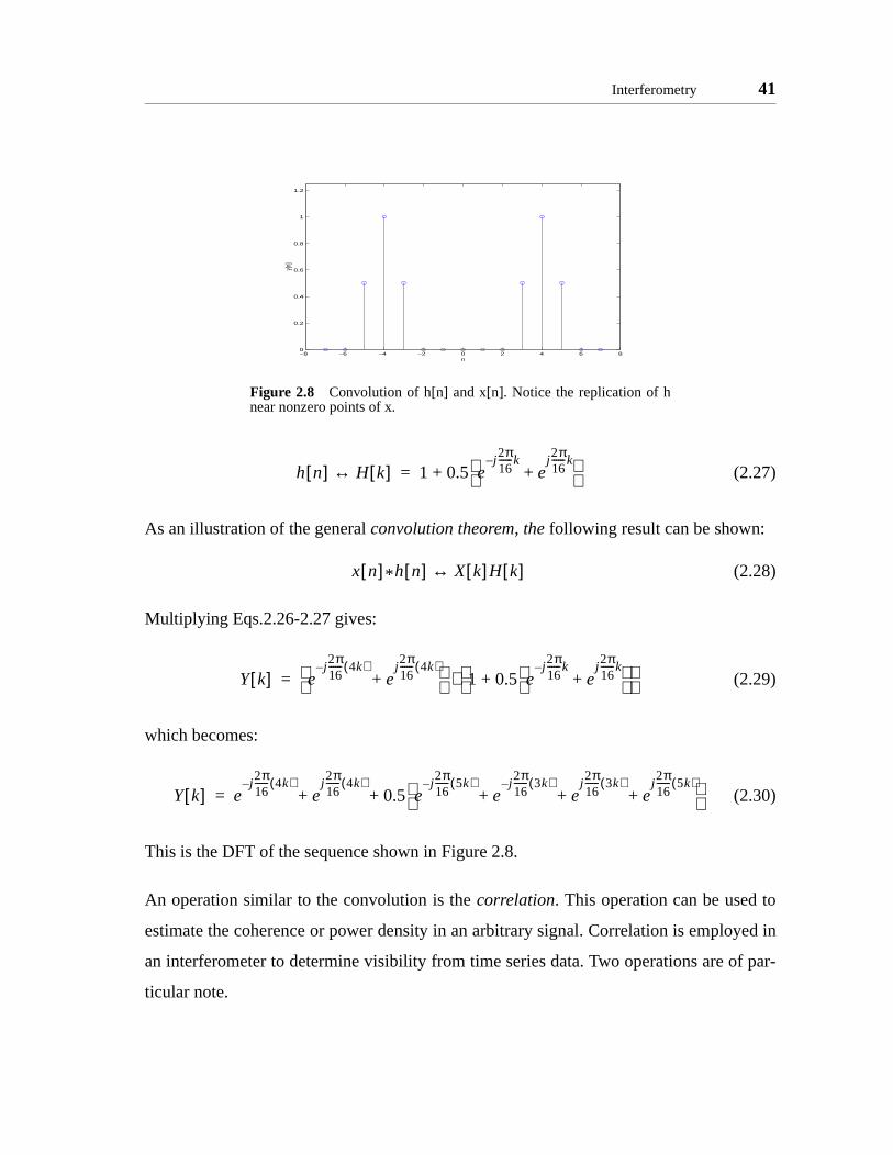
The convolution of the two sequences is shown in Figure 2.8. An intuitive explanation of
this operation is that the sequence h[n] has been replicated at each impulse of x[n]. The
two dimensional counterpart is very important in the discussion of telescope performance.
In a frequency domain representation the convolution is replaced by a multiplication. The
frequency domain representations of these sequences can be expressed as:
(2.26)
and:
Figure 2.6 A simple sequence, x[n] made up of two discrete deltafunctions.
Figure 2.7 Another simple sequence, h[n]. Three delta functions sym-metric about the origin.
−6 −4 −2 0 2 4 60
0.2
0.4
0.6
0.8
1
1.2
n
x[n]
−2 −1.5 −1 −0.5 0 0.5 1 1.5 20
0.2
0.4
0.6
0.8
1
1.2
n
h[n]
x n[ ] X k[ ]↔ ej2π16------ 4k( )–
ej2π16------ 4k( )
+=
Interferometry 41
(2.27)
As an illustration of the general convolution theorem, the following result can be shown:
(2.28)
Multiplying Eqs.2.26-2.27 gives:
(2.29)
which becomes:
(2.30)
This is the DFT of the sequence shown in Figure 2.8.
An operation similar to the convolution is the correlation. This operation can be used to
estimate the coherence or power density in an arbitrary signal. Correlation is employed in
an interferometer to determine visibility from time series data. Two operations are of par-
ticular note.
Figure 2.8 Convolution of h[n] and x[n]. Notice the replication of hnear nonzero points of x.
−8 −6 −4 −2 0 2 4 6 80
0.2
0.4
0.6
0.8
1
1.2
n
y[n]
h n[ ] H k[ ]↔ 1 0.5 ej2π16------k–
ej2π16------k
+ +=
x n[ ]*h n[ ] X k[ ]H k[ ]↔
Y k[ ] ej2π16------ 4k( )–
ej2π16------ 4k( )
+ 1 0.5 e
j2π16------k–
ej2π16------k
+ +
⋅=
Y k[ ] ej2π16------ 4k( )–
ej2π16------ 4k( )
0.5 ej2π16------ 5k( )–
ej–2π16------ 3k( )
ej2π16------ 3k( )
ej2π16------ 5k( )
+ + + + +=
42 BACKGROUND
e verti-
The auto-correlation is defined by:
(2.31)
(2.32)
The cross-correlation is similar:
(2.33)
(2.34)
The tools developed in the above sections allow subsequent analysis of interferometer sys-
tems. Most of the steps of interferometer operation are more intuitive in one domain or
another. The understanding of complimentary operations and relationships between these
operations and Fourier transform pairs helps to explain certain stages of computation.
2.1.3 Measuring Visibility
An astronomical interferometer achieves its excellent angular resolution through the mea-
surement of the visibility function. An interferometer, such as the one shown in
Figure 2.9, consists of two sensing apertures separated by a vector displacement. This rel-
ative displacement vector is referred to as the baselinea. A measurement taken at a particu-
lar baseline is equivalent to sampling a certain spatial frequency.
a. This displacement is depicted to lie in a plane normal to the ‘bore-sight.’ The apertures can also bcally displaced. This would simply require some geometric corrections and use of the projected baseline.
Φxx ξ( ) x* α( )x ξ α+( ) αd
∞–
∞
∫=
Φxx n[ ] 1M----- x*[m] x n m+[ ]⋅
m 0=
M 1–
∑=
Φxy ξ( ) x* α( )y ξ α+( ) αd
∞–
∞
∫=
Φxy n[ ] 1M----- x*[m] y n m+[ ]⋅
m 0=
M 1–
∑=

Interferometry 43
The following is a simplified development of the measurement process. Sources are
treated in isolation as mono-chromatic delta functions. For a more detailed treatment, the
reader is encouraged to refer to the Van Crittert-Zernike theorem presented in [Thomson,
et al, 1994]. The signal processing used in the AIT is closer to that of radio interferometry
than visible/IR. The principle of visibility measurement is slightly different for these opti-
cal systems but the overall result is the same.
Consider the simplified, one-dimensional system shown in Figure 2.10. A single, unity
strength point-source located in the far field emits monochromatic radiation. Two aper-
tures (telescopes, antennas, or microphones) located at a distance capture the incoming
signal.
The antennas are separated by a distance D measured normal to the line of sight of the
array. In this discussion, the directional gains of the individual antennas are assumed to be
uniform. For realistic systems the array sensitivity over the field of view is shaped by the
directionality of the individual apertures. The source is assumed far enough away that the
incoming rays are nearly parallel. As seen in Section 3.3.9 this requirement can be relaxed
provided certain corrections are made.
Figure 2.9 Schematic of a interferometer geometry in two dimensions.
x0
y0
Apertures
Source (lξ0,lη0)
x
θ0
y
ψ0
ab
l
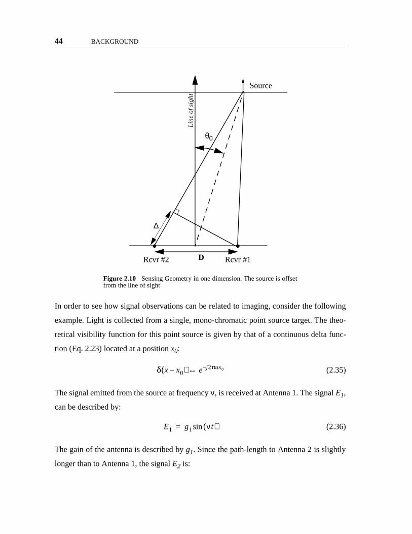
44 BACKGROUND
In order to see how signal observations can be related to imaging, consider the following
example. Light is collected from a single, mono-chromatic point source target. The theo-
retical visibility function for this point source is given by that of a continuous delta func-
tion (Eq. 2.23) located at a position x0:
(2.35)
The signal emitted from the source at frequency ν, is received at Antenna 1. The signal E1,
can be described by:
(2.36)
The gain of the antenna is described by g1. Since the path-length to Antenna 2 is slightly
longer than to Antenna 1, the signal E2 is:
Figure 2.10 Sensing Geometry in one dimension. The source is offsetfrom the line of sight
D
∆
Source
Rcvr #1Rcvr #2
θ0
Lin
e of
sig
ht
δ x x0–( ) e j2πux0–↔
E1 g1 νt( )sin=

Interferometry 45
(2.37)
where Φ is the phase delay caused by the differential path-length (DPL). Since the incom-
ing rays are assumed parallel, the DPL can be expressed as:
(2.38)
Introducing the coordinate ξ, where :
(2.39)
or in terms of phase angle:
(2.40)
Now, the processing of the incoming signals starts by calculating the cross-correlation of
the two signals. The interferometer response as a function of baseline D can be denoted as
rr(D).
(2.41)
Expanding the second sine term and combining the gain terms:
(2.42)
Multiplying out terms:
(2.43)
Using double angle formulas:
E2 g2 νt Φ–( )sin=
∆ D θ0sin=
ξ θsin=
∆ Dξ0=
Φ 2∆πλ
----------2πDξ0
λ-----------------= =
rr D( ) 12T------ g1g2 νt( ) νt Φ–( )sinsin td
T–
T
∫=
rr D( ) G2T------ νt( ) νt Φcossin Φ νtcossin–( )sin td
T–
T
∫=
rr D( ) G2T------ νtsin2 Φcos Φ νt νtsincossin–( ) td
T–
T
∫=
46 BACKGROUND
(2.44)
In the limit as ,the terms involving the cosine and sine of νt will be insignificant
compared to the linear (first) term. Therefore:
(2.45)
There is still an ambiguity in determining the sign of Φ and hence from Eq. 2.40, the sign
of ξ. Since the cosine function is positive in both the first and fourth quadrants, it impossi-
ble to discriminate between a source at +ξ and a source at -ξ. This can be resolved by
introducing an artificial phase shift of +π/2 in one of the signal branches and repeating the
correlation. Note that .
(2.46)
Expanding and simplifying:
(2.47)
Applying the double angle formulas and integrating will eliminate all but one of the terms.
(2.48)
These two terms (ri and rr) suggest a convenient notation in terms of the complex correla-
tor response r(D).
(2.49)
rr D( ) G2T------ 1
2--- Φ 1 2νtcos–( )cos
12--- Φ 2νtsinsin–
td
T–
T
∫=
T ∞→
rr D( ) G2---- Φcos=
xπ2---+
sin xcos=
ri D( ) G2T------ νt( ) νt Φ–( )sincos( ) td
T–
T
∫=
ri D( ) G2T------ νt νt Φcossincos νt Φsincos2–( ) td
T–
T
∫=
ri D( ) G2----– Φsin=
r D( ) G2---- Φcos j Φsin–( ) G
2----e jΦ–= =
Interferometry 47
Substituting for Φ from Eq. 2.40 gives:
(2.50)
Replacing with u, in Eq. 2.50, gives:
(2.51)
This equation, particularly the complex exponential, is in the same form as the calculated
source visibility (Eq. 2.35). This is particularly important for two reasons. First, it is clear
that calculating the correlator response at a particular value of is equivalent to
measuring a particular component of the visibility. Second, it gives a physical relation
between the baseline and the spatial frequency. The baseline, as measured in wavelengths,
corresponds to the spatial frequency currently being sampled. It is also worth noting that
exactly matching the receiver gains is not necessary; so long as the gain is time-invariant,
the visibility measurement will be accurate.
The corresponding result can be seen in the case of a digital system. If the incoming
sequences are digitized above the Nyquist frequency of the source, the recorded sequences
are given by:
(2.52)
(2.53)
The discrete frequency variable ω represents the operating frequency scaled by the sam-
pling frequency, i.e.
(2.54)
where Ts is the sampling period. The correlation over P samples is given by (see Eqs. 2.32,
2.41):
r D( ) G2----e
j2πDξ0
λ----------------–
=
D λ⁄
r u( ) G2----e j2πuξ0–=
u u0=
E1 n[ ] ωn( )sin=
E2 n[ ] ωn Φ+( )sin=
ω νTs=
48 BACKGROUND
(2.55)
So after expanding the right hand sine term, the result is identical to that of Eq. 2.45. The
sampling of the time sequence is unimportant provided the sampling rate is adequate and
enough sample points are taken so as to make the neglected terms vanish.
The second correlation proceeds in much the same manner. The phase shift is a little trick-
ier in discretely sampled sequences. One resolution to this problem is to consider the case
where the sampling frequency, , is much greater than the operating frequency νa. It is
reasonable to suppose in this case that there is some integer number of samples, α, that
corresponds to a quarter period. This allows the complex correlation to be calculated:
(2.56)
Section 3.3.9 presents an alternate way of dealing with this phase shift.
The above derivation assumes a one-dimensional problem with a single mono-chromatic
point-source. To address the problem of extended or multiple sources, it can be shown that
the method above is linear. Superposed sources will lead to superposed measurements pro-
vided that sources are mutually incoherent [Thomson, et al, 1994 pp. 60]. In this case,
radiation from different sources (or different parts of the same source) will give zero
cross-correlation. The van Crittert-Zernike theorem presented in [Thomson, et al, 1994]
treats the subject of finite bandwidth, wide-sense stationary sources.
Extending the one-dimensional problem to two dimensions is quite straightforward. First,
define the two coordinates and . A source located at (ξ0,η0), as
shown in Figure 2.9, will have a visibility function given by:
a. It is common to specify the sampling frequency in terms of the inverse period.
rr u( ) GP---- ωn( ) ωn Φ+( )sinsin
n 0=
P 1–
∑=
1 Ts⁄
ri u( ) GP---- E1 n[ ] E2 n α+[ ]⋅
n 0=
P 1–
∑=
ξ θsin= η ψsin=
Interferometry 49
(2.57)
or in discrete space (assuming a square map where M=N):
(2.58)
The complex correlator response is:
(2.59)
Where the real and imaginary parts are by definition:
(2.60)
(2.61)
It is important to remember that Eqs. 2.60-2.61 hold in both discrete and continuous space
domains. The derivation proceeds as before, leading to the same expression as Eq. 2.49.
The only difference is the value of the differential pathlength, ∆, in the phase shift Φ
(Eq.2.40). The differential pathlength is obtained by considering the two position vectors:
(2.62)
(2.63)
The differential path length can then be found. Assuming that the distance, l, to the source
plane is very great, i.e. .
V u v,( ) e j2π uξ0 vη0+( )–=
V k l,( ) ej2πN------ m0k n0l+( )–
=
r u v,( ) rr u v,( ) jri u v,( )+=
rr E1 p[ ] E2 p[ ]⋅p 0=
P 1–
∑=
ri E1 p[ ] E2 p α–[ ]⋅p 0=
P 1–
∑=
a lξ0
x0
2-----–
lη0
y0
2-----–
l=
b lξ0
x0
2-----+
lη0
y0
2-----+
l=
l x0 y0,»

50 BACKGROUND
aging
(2.64)
(2.65)
So ∆ is given by:
(2.66)
Finally, from Eqs. 2.40, 2.48, 2.66:
(2.67)
The corresponding discrete response is:
(2.68)
Since the DFT or FT of a real valued function (the brightness) must be conjugate symmet-
ric, the complementary visibility point is also known, i.e.:
(2.69)
(2.70)
The ability to measure visibility through the cross-correlation of spatially distributed sig-
nals is the defining principle of interferometry. Interferometric imaging requires a number
of visibility samples. The set of visibility measurements can be referred to as the spectral
sensitivity function. More complete sampling of the visibility will produce a better quality
image. Each additional measurement taken provides more information about the bright-
ness distribution. Provided the character of the source doesn’t change during the im
process, several techniques can be applied.
a l 112--- ξ0
2 η02 1
l--- x0ξ0 y0η0+( )–
14l2------- x0
2 y02+( )+ ++
≈
b l 112--- ξ0
2 η02 1
l--- x0ξ0 y0η0+( ) 1
4l2------- x0
2 y02+( )+ + ++
≈
∆ b a– x0ξ0 y0η+( )= =
r u v,( ) e j2π uξ0 vη0+( )–=
r k l,[ ] ej2πN------ mk nl+( )–
=
r u– v–,( ) ej2π uξ0 vη0+( )=
r M k– N l–,[ ] ej2πN------ mk nl+( )
=

Interferometry 51
projec-
along
rusting
the
charac-
pro-
visibil-
atial
e true
, con-
There are several strategies for interferometric imaging. The visibility measurements can
be made concurrently or consecutively, depending on the design of the interferometry sys-
tem. In systems with several apertures, signals are combined pair-wise for each baseline.
As the number of antennas/telescopes grows, the number of simultaneous visibility mea-
surements increases dramatically. For n apertures, the number of baselines Nb is:
(2.71)
Provided that the brightness distribution is time invariant, the u-v coverage of the array
can also be augmented by reconfiguring the geometry of the interferometer. In terrestrial
interferometry, this is often accomplished by exploiting the rotation of the Earth and by
mounting the antennas on tracks. The Earth’s rotation changes the orientation and
tion of the baselines while the lengths are further adjusted by moving the telescopes
tracks [Thomson, et al, 1994]. In a space-based system, a combination of active th
[Kong & Miller 1998] and orbital dynamics [Mallory et al 1998] can be used to adjust
u-v orientation of the array.
2.1.4 The Point Spread Function
An interferometer operating as an imaging system possesses certain performance
teristics. One of the most common measures used is what is know as the point spread
function (PSF). Reconfiguring an interferometer during imaging is a time consuming
cess. For reasons of geometry and efficiency, it is often not possible to sample the
ity at every location. This partial UV coverage will have zeros at certain sp
frequencies and the synthesized image will not be a perfect representation of th
brightness. In fact the measured brightness, , is equal to the true brightness,
volved with the array PSF:
(2.72)
Nbn n 1–( )
2--------------------=
B' B
B' k l,[ ] B k l,[ ]*PSF k l,[ ]=

52 BACKGROUND
he
mage
multi-
t must
brought
f com-
io fre-
The PSF is defined to be the Fourier transform of the spectral sensitivity function [Thom-
son, et al, 1994]. The spectral sensitivity function simply indicates which spatial frequen-
cies have been sampled (with possible allowance for the aperture gain pattern).
As an illustration, consider a brightness map with a point source at the origin
(Figure 2.11). The DFT of this source will give a visibility response of unity at each loca-
tion. However if some of the visibility coefficients are set to zero, representing partial
sampling of the UV plane (Figure 2.12), the new brightness map (Figure 2.13) will appear
different than a simple impulse. The point spread function adds artifacts to the image. This
distortion works in two ways. First, energy originating in the central lobe will appear as a
response in the sidelobes. The energy originating from the side-lobes, will ‘smear’ into t
central location. Methods to deconvolve the PSF function from an interferometer i
exist and are discussed in [Section 4.2].
To apply the interferometric processing developed above requires some thought. If
ple spacecraft are being used as sensors, there is a ‘collection’ type of problem tha
be addressed. Before any correlation can occur, the sensor streams must be
together. This is equally true in an optical system and radio systems. The method o
bination, be it a beam combiner or a correlator is the only thing that changes. In rad
Figure 2.11 True brightness function, a simple impulse. Plot shownobliquely for clarity.
020
4060
80100
120140
0
50
100
1500
0.2
0.4
0.6
0.8
1
kl
Re
spo
nse

Distributed Processing 53
ssor
quency systems, where the incoming signal is digitized before being combined, the
connection architecture for this information flow can be very important.
2.2 Distributed Processing
2.2.1 Parallel vs. Distributed Processing
Distributed processing represents a type of high performance computing. Concurrent cal-
culations are performed by several processors. The approach to distributed computation
differs from the canonical ‘parallel’ processing in the implementation of inter-proce
Figure 2.12 UV coverage (Spectral Sensitivity Function). Dots indi-cate non-zero components
Figure 2.13 Resulting Point Spread Function
0 20 40 60 80 100 1200
20
40
60
80
100
120
k
l
0 20 40 60 80 100 120 1400
20
40
60
80
100
120
140
k
l
Central Lobe

54 BACKGROUND
text.
may
ekas
mote
ns that
ciently
stbed
.60 and
a, how-
start.
s to a
al pro-
, most
ust then
rwise,
cess-
tializa-
uta-
for the
communication. In a parallel environment, each processor may typically share a back-
plane, memory or both. Hardware performance is reliable in terms of process integrity and
communications latency is generally low.
Distributed processing, in contrast, introduces uncertainty into algorithm development.
Processors are usually physically separate and communications must often be handled by
a potentially unreliable network. ‘Unreliable’ is interpreted here in a networking con
Depending on the underlying network implementation, transmitted data packets
arrive at their destination out of order, with errors, or may not even arrive at all [Bertz
& Gallager 1992]. Effective algorithms must be designed to be tolerant of faults in re
nodes and in the links joining them. Moreover, the separation of the processors mea
each node may only have partial knowledge of network topology and state.
That being said, the goals of distributed and parallel processing are the same: to effi
perform a certain set of computations. Data processing in the Acoustic Imaging Te
essentially resembles that of a space-based radio interferometer. As seen in Eqs. 2
2.61, the correlation process represents an enormous reduction in the volume of dat
ever, it is essential that the nodes hold this information before the computation can
Performing this operation within the cluster, rather than on the ground, translate
much less demanding requirement on the communications system. While a centr
cessing spacecraft for the entire cluster represents a possible implementation
schemes considered to date have involved identical spacecraft. Each spacecraft m
operate as an individual processing unit. With no immediate reason to suggest othe
each spacecraft will likely be identical to the others in terms of communications, pro
ing power and storage.
2.2.2 Algorithm Concepts
Distributed processing, when described in the abstract, consists of three steps: Ini
tion, Computation, and ‘Clean-up’. While the bulk of time is usually spent in the comp
tion phase, it is important to understand how the other steps establish the context

Distributed Processing 55
data
ust be
s in a
t the
mathe-
s
bution
able to
xceed
ensure
data
over
te the
each
pro-
IT is
computation. Other activities such as inter-node communication may occur during any or
all of these phases.
When a network of computational nodes is initialized, the initial distribution of data is of
interest. In particular, the following questions need to be addressed.
• Where are the data located?
• Which nodes need access to data that originates from another node?
In many situations the answers to these questions reflect the physical system of which they
are a part. In the AIT, every satellite starts a computational ‘cycle’ with a recorded
stream from its microphone. To perform the correlation, at least part of this data m
exchanged.
Stating that the computational load is balanced is equivalent to saying that all node
cluster will remain busy for the duration of the computation and that they will finish a
same time. If the processing speeds of the nodes are identical, and if the number of
matical operations in the problem can be predicted a priori, perfect load balancing reduce
to parceling out equal numbers of operations to each node. To make load distri
work, the data exchange must be organized in such a way that each spacecraft is
start computation at the same time. Assuming that the time spent calculating will e
that needed for inter-node communication and data exchange, care must be taken to
that the nodes remain busy at all times. Idle time spent while waiting for incoming
should be eliminated when possible.
Finally, when the computation phase is finished, the ‘answer’ is usually distributed
the nodes in the network. In most situations a collection stage is required to colla
final data in one location. The strategy taken in the operation of the AIT is to allow
virtual spacecraft to send its partial information to the ground for the final stage of
cessing. A more detailed discussion of the specific algorithm implemented on the A
given in Section 3.3.9

56 BACKGROUND
desti-
2.2.3 Connectivity
To effectively approach the problems of fairness and efficiency, the information network
formed by the satellites must be examined. Helpful analogs to canonical distributed archi-
tectures can be discussed with reference to the actual means of implementation. The first
step is to describe the interconnections between the nodes (or satellites). A number of
questions must be posed:
• From a given origin, which nodes are accessible with a direct communica-tion path?
• Must a message be relayed through a secondary node?
• Is multiple access to a shared medium a concern?
• Can several links be used simultaneously?
The answers to these questions suggest specific implementations of the inter-satellite com-
munication. Maintaining several simultaneous links requires duplication of receivers and
transmitters. Each signal path must also be isolated in some domain; i.e. frequency or code
for radio, space for laser. Whatever the implementation, the choice of a communications
architecture defines the network connectivity. Four common network schemes have clear
analogs in satellite systems (Figure 2.14).
The simplest example of network structure is full connectivity (Figure 2.14a); each node
can communicate directly with any other node in the cluster. The signal paths are separate
and as such, can operate simultaneously. Very fast performance can be achieved as all
communications go directly from source to destination. Thus, the maximum number of
links (maximum distance) a message must pass through is O(1).The disadvantage of this
system is the expense and complexity of maintaining the O(n2) links (n is the number of
satellites).
Another simple architecture class is that of linear connections (Figure 2.14b). These
include line, mesh and torroidal structures. Both the number of links, and the maximum
distance are O(n) in this case. As such, linear structures offer the advantage of simplicity
at the expense of message delay. When multiple ‘hops’ are required from source to
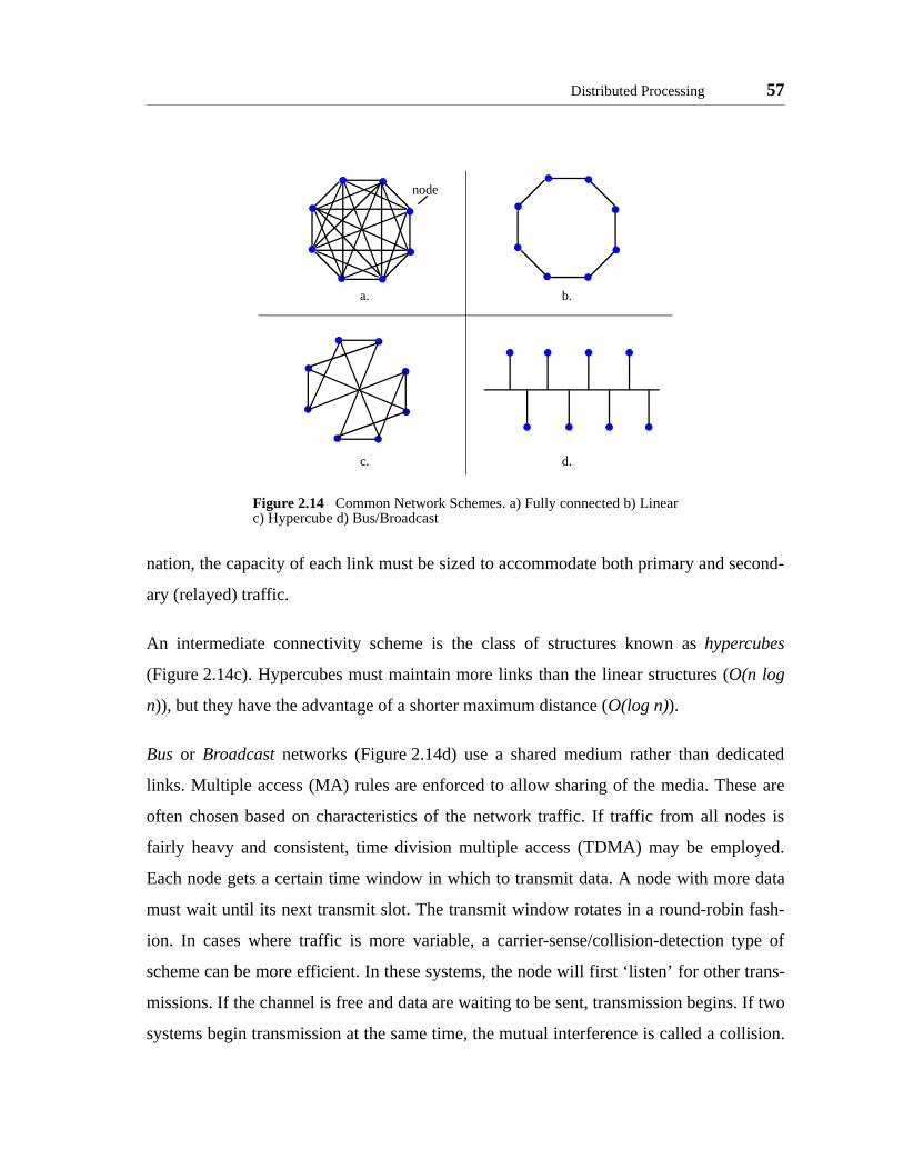
Distributed Processing 57
trans-
. If two
llision.
nation, the capacity of each link must be sized to accommodate both primary and second-
ary (relayed) traffic.
An intermediate connectivity scheme is the class of structures known as hypercubes
(Figure 2.14c). Hypercubes must maintain more links than the linear structures (O(n log
n)), but they have the advantage of a shorter maximum distance (O(log n)).
Bus or Broadcast networks (Figure 2.14d) use a shared medium rather than dedicated
links. Multiple access (MA) rules are enforced to allow sharing of the media. These are
often chosen based on characteristics of the network traffic. If traffic from all nodes is
fairly heavy and consistent, time division multiple access (TDMA) may be employed.
Each node gets a certain time window in which to transmit data. A node with more data
must wait until its next transmit slot. The transmit window rotates in a round-robin fash-
ion. In cases where traffic is more variable, a carrier-sense/collision-detection type of
scheme can be more efficient. In these systems, the node will first ‘listen’ for other
missions. If the channel is free and data are waiting to be sent, transmission begins
systems begin transmission at the same time, the mutual interference is called a co
Figure 2.14 Common Network Schemes. a) Fully connected b) Linearc) Hypercube d) Bus/Broadcast
node
a. b.
d.c.

58 BACKGROUND
ould
ble a
ctions
le in a
distri-
essing
plat-
ometer.
grees.
Some systems can detect collisions and stop transmission right away, while others wait for
a failed acknowledgment from the receiver to indicate a problem.
Efficiently allocating resources to communications and distributed computation is a com-
plicated issue. Optimal load balancing will often be heavily dependant on the tasks
involved. Hardware architecture must also be considered, weighing the relative costs of
computation and communication. Adding provision for dynamic adjustment of system
loading will often require settling for sub-optimal solutions either in terms of communica-
tions overhead or redundant calculation. Careful examination and algorithm design is nec-
essary to get the most productivity out of a science instrument and absolutely vital in a
continuous system such as radar.
2.3 Background Summary
The operation if the Acoustic Imaging Testbed captures elements of both visible/IR and
radio frequency interferometry. The spacecraft cluster concept is indicative of optical
imaging interferometry, or cluster radar systems. The digital signal processing is most
directly analogous to astronomical radio systems. An astronomical radio-frequency cluster
is a difficult concept to envision since the spacings between elements would have to be
huge. Very Long Baseline Interferometry uses a combination of ground and space obser-
vations [Thomson, et al, 1994]. A ‘cluster’ solely devoted to radio interferometry w
have to be of similar size to add greater functionality. At such sizes, it would resem
large constellation rather than a closely knit cluster. The capacity for coordinated a
would be greatly reduced. On the other hand, localized clusters would be acceptab
ground looking radar system. The specific processing methods are different but the
bution and autonomy issues are similar. With some adjustment in the signal proc
algorithms, such a system would be very well represented by AIT operation.
Rather than capture specifics of optical interferometry, the AIT provides an capable
form to study the operational issues associated with a separated spacecraft interfer
User control, automation and autonomy can all be applied in greater or lesser de

Background Summary 59
Chapter 3 examines the development and the capabilities of the AIT environment as a
starting point for investigation into operations.

60 BACKGROUND

Chapter 3
ARCHITECTURE DEVELOPMENT
f the
eration
ertures
order
red in
is
loca-
spatial
The underlying architecture of the Acoustic Imaging Testbed (AIT) is a complex system
of integrated hardware and software. The effectiveness of the AIT as an experimental tool
depends as much upon the architecture of the system as on the intelligence of the space-
craft cluster itself.
3.1 Overview
As discussed in Section 1.3 the AIT architecture seeks to map the operational concept of a
separated spacecraft interferometer (SSI) onto a simplified apparatus in the lab. Hardware
provides the physical interaction and the medium for performing interferometry. The soft-
ware establishes a consistent and simplified environment in which cluster automation can
be developed. Finally, the ‘intelligent’ logic of the virtual spacecraft captures many o
high level decision-making problems faced by an operational system.
To more easily understand the scope of the architecture, a simple top-down consid
of the operational concept is helpful. The SSI consists of a number of displaced ap
that must collect and coherently interfere radiation emitted from the target source. In
to successfully form an image of the target, sampling apertures must be maneuve
such a way so as to fill in the UV plane (Section 2.1.2). The emissions collected in th
fashion must be coherently combined to extract image information. Each sampling
tion or baseline yields an amplitude and phase value corresponding to a particular
61

62 ARCHITECTURE DEVELOPMENT
AIT.
he sec-
astly,
ed in
SI’s,
cho-
micro-
issue is
oment
ated in
ogical
t be inte-
There
frequency of the brightness map. When collected and subjected to an inverse Fourier
transform, these complex values yield an image of the target. Table 3.1 illustrates the func-
tional mapping between primary features of a ‘real’ interferometry system and the
The first column represents the feature of an operational system to be captured. T
ond column provides an abstraction of the real function as it relates to this study. L
the third column provides an indication of how the functional concept is implement
the AIT.
This study is primarily concerned with the high-level control issues encountered by S
not with the techniques if interferometry itself. Accordingly, an acoustic system was
sen as a technically simpler alternative to an electromagnetic one. As a result,
phones and speakers take the place of antennas and sources, respectively. This
discussed at some length in Section 3.2.
Although the hardware and software are discussed separately, it is useful to take a m
to consider the system as a whole (Figure 3.1). Many functions must be accommod
the architecture design: External users require a means of interacting with the AIT, l
spacecraft must be represented, and access to sensor and actuator hardware mus
grated. The division of hardware and software is merely an organizational device.
TABLE 3.1 AIT Functional Mappings
SSI Function Function Abstraction AIT RepresentationDistant Stars/Targets Source Objects Speaker Array
Space Propagation Space Anechoic Chamber
Spacecraft Bus and Collector Mobile Collection Apparatus Robotic Arm and microphone
Fast Optics Raw Data Combiner/Correlator ADC, Inter-satellite Communi-cation, Correlation processing
Downlink, post-processing Processed Data Synthesis Data-synthesis, simulated down-link
Spacecraft Processors, Ground Station
Controlling Logic Virtual Spacecraft Programs.

Hardware 63
are significant functional couplings between many software and hardware components.
The following sections provide detailed explanations of both the current incarnation of the
testbed as well as important milestones of the development process.
3.2 Hardware
3.2.1 Overview
The hardware systems of the AIT encompass support computers, data acquisition, motion
control, robotics, and other miscellaneous hardware (Figure 3.2). A distinction can be
made between primary hardware and support hardware. Primary components are those
subsystems that are most directly traceable to an SSI function (see Table 3.1). Support
hardware, in contrast, are those pieces of equipment designed to facilitate the operation of
the representative systems. The largest component in the AIT system is the anechoic
chamber. Mounted within is the array of speakers that act as the imaging targets. Four
robotic arms, each equipped with a tip-mounted microphone, complete the set of primary
hardware. Data acquisition and motion control electronics constitute the secondary sys-
tems.
Figure 3.1 Schematic overview of the Acoustic Imaging Testbed.
SpacecraftInteractions
GroundInteractions
(Some connections omitted for clarity)
Mic’s
Arms
Logical S/CComputer
1
Logical S/CComputer
3
Logical S/CComputer
4
Logical S/CComputer
2 Sen
sors
Mot
ionUp/
Dow
n-li
nk
Use
r M
anag
emen
t

64 ARCHITECTURE DEVELOPMENT
ones
round
reduce
aching
even
f the
walls.
.
ities in
3.2.2 Anechoic Chamber
The anechoic chamber is the largest and most striking component of the AIT. It also acts
as the central piece of primary hardware. A sketch of the testbed is shown in Figure 3.3.
Figure 3.4 is a photo of the interior of the completed structure. This chamber serves sev-
eral purposes. Most importantly, it must present a ‘black’ background to the microph
during imaging. In doing this, it also acts to isolate the testbed from transient backg
noise. Since the system resides in shared laboratory space, it is also necessary to
acoustic emissions as much as possible.
In order to maintain acceptable image quality, it is necessary to ensure that sound re
the microphones comes directly from the speakers. Any reflections from the walls or
the arms themselves will cause a degradation in the resulting image. This is calledmulti-
path interference (MPI). The use of sound absorbing material and careful shaping o
testbed geometry can reduce these effects.
Sound absorbing material minimizes reflected and external noise generation at the
An open-cell foam tiling manufactured by PartsExpress was chosen for this application
This helps to ensure an environment free from spurious noise. MPI creates ambigu
Figure 3.2 Overview of testbed hardware. Information flow is indicated by thearrows.
Band-limited Noise
(15.05kHz)
Band-limited Noise
(14.95 kHz)
Amplifier
Amplifier Speaker
SpeakerMicrophones
(4)Arms
(4)
Arm Control Computer
DAQ Computer
TestbedServer
Anechoic Chamber
WebCam
Web Server
Ethernet
Computer Audio(Line Out)
Left
Right
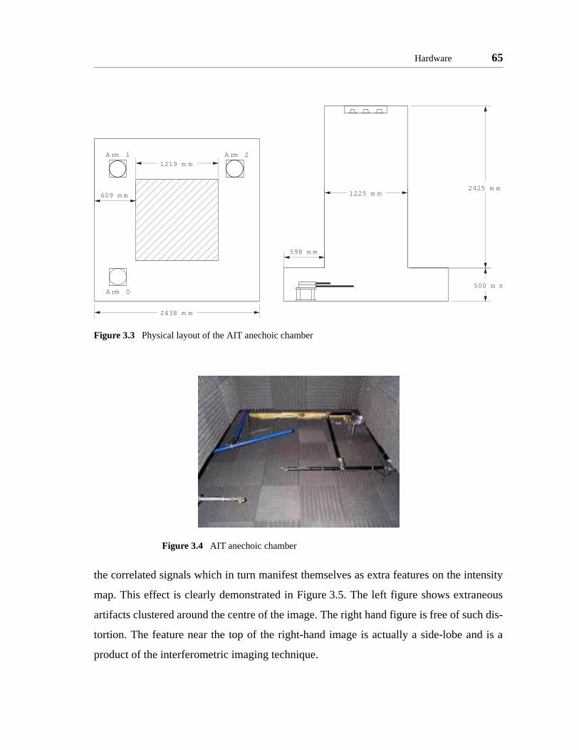
Hardware 65
the correlated signals which in turn manifest themselves as extra features on the intensity
map. This effect is clearly demonstrated in Figure 3.5. The left figure shows extraneous
artifacts clustered around the centre of the image. The right hand figure is free of such dis-
tortion. The feature near the top of the right-hand image is actually a side-lobe and is a
product of the interferometric imaging technique.
Figure 3.3 Physical layout of the AIT anechoic chamber
Figure 3.4 AIT anechoic chamber
1219 m m
2438 m m
609 m m
Arm 0
Arm 1 Arm 2
2425 m m
500 m m
598 m m
1225 m m

66 ARCHITECTURE DEVELOPMENT
The foam panels used for sound absorption are contoured to provide low reflections at any
incident angle. The physical dimensions of the foam panels are related to the corner-fre-
quency at which the reflection intensity is markedly reduced. A high operating frequency
improves image quality in a number of ways. Passive dampening material is more effec-
tive as frequency increases. High frequencies also improve the hypothetical performance
of the imaging system by increasing the ratio of baseline to wavelength. The panels
selected for use in the AIT are rated at a corner frequency of 1000 Hz. The resulting atten-
uation of the acoustic panels at various operational frequencies is shown in Table 3.2.
In addition to the acoustic foam, the shape of the testbed was designed to minimize delete-
rious reflections. The recessed mounting areas for the robotic arms prevent direct sound
impingement. These arm mountings have many hard, moving, metal surfaces. Directly
attaching the absorbent foam to these surfaces would be difficult. By placing the robots
out of the direct sound path, reflections are reduced. In addition, due to the use of larger
Figure 3.5 Effect of Multi-path interference. b shows a clear imagewith few multi-path artifacts. Image a displays reduction in image qual-ity when reflections are permitted from robot linkages.
TABLE 3.2 Acoustic Foam Performance
Frequency (Hz) Absorption%
500 83
1000 97
15000 99
a. b.XX
YY

Hardware 67
arm linkages than initially envisioned, the testbed must operate with the side access panels
removed. This has not caused any observable reduction in image quality.
Initially, only the interior surfaces of the AIT were lined with the absorbent foam. Persis-
tent image quality problems prompted further investigation of additional sources of MPI.
After careful examination, it was found that reflections from the linkages in the robot arms
created regions of constructive and destructive interference as the arms traversed their
workspace. Two actions were undertaken to correct this problem. Absorbent foam was
added to the arms themselves. By affixing this material to the primary linkages, the joints,
and around the microphone, some improvement was seen. Application of the foam was
constrained by the requirement for clearance between the motion planes. As a result, it
was decided that a higher operating frequency for the testbed would make the thin foam
layers on the arms more effective. Moving from 9.25 kHz to 15 kHz showed a dramatic
reduction in the image artifacts due to MPI.
3.2.3 Sound Generation
In order for the AIT to operate as an imaging device, it must have suitable targets. Where
a space interferometer would image stars, the AIT images speakers. The choice of an
acoustic system eliminates potentially confusing effects encountered in a real system and
suggests a straightforward implementation.
There is an important issue relating to the source radiation that separates this acoustic
approximation from a full fledged system. Stars emit wide band radiation; everything
from radio to gamma rays. An instrument observing the star would be sensitive to a select
band of frequencies by virtue of its construction. Furthermore, in an interferometer (either
optical or radio), narrow filters typically block all but a very narrow band of incident radi-
ation. The remaining light is used for the science in question. Lastly, electromagnetic radi-
ation propagates as a transverse wave. Sound on the other hand is longitudinal. This
means that polarization effects in an optical or RF system are absent when dealing with
acoustics.

68 ARCHITECTURE DEVELOPMENT
were
l audio
ssible
mpli-
utputs
uncorre-
a
ource
noise
of 100
r from
While wide-band noise emitted from the speakers would provide a good representation of
the source environment, it needlessly complicates the system. The scheme employed by
the testbed essentially moves the filters from the detector to the source. Using a narrow-
band source signal eliminates the need for the computation required for digital filtering or
the fickleness of sharp bandpass, analog filters. It is felt that this modification to technique
does not adversely affect the properties captured by the AIT.
To provide the capability to reconfigure the source ‘stars’, a set of nine speakers
mounted in a square array (Figure 3.6). These speakers are driven by a two channe
amplifier. Both one and two source images can be created allowing a total of 45 po
reconfigurations. Further investigations can be performed by adjusting the relative a
tude of the sources. A patch panel allows the operator to connect one or both of the o
from the audio amplifier, to the desired speaker(s).
One of the testbed computers generates the source signals. These signals must be
lated to avoid generating false or ghost images. This can be accomplished either with
wide-sense stationary, white-noise process or through the use of slightly offset s
tones. Experimentally, both methods yielded comparable results. The band-limited
sources were gaussian intensity signals centred about 15 kHz, with a bandwidth
Hz. The multi-tone method is preferred since it is easier to balance the output powe
Figure 3.6 Picture of nine speaker array. The middle speaker is alignedwith middle of testbed. Centre-to-Centre spacing is about 145mm.
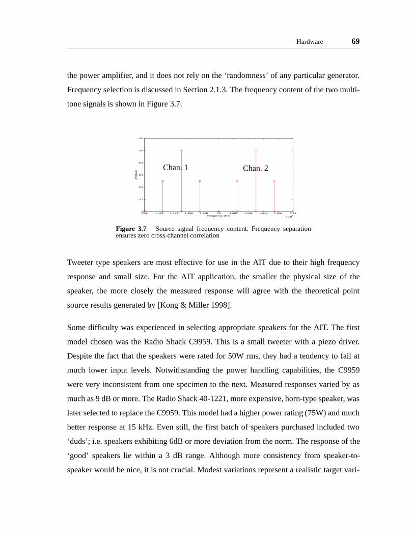
Hardware 69
rator.
multi-
uency
of the
l point
first
driver.
fail at
9959
d by as
er, was
much
ed two
of the
er-to-
t vari-
the power amplifier, and it does not rely on the ‘randomness’ of any particular gene
Frequency selection is discussed in Section 2.1.3. The frequency content of the two
tone signals is shown in Figure 3.7.
Tweeter type speakers are most effective for use in the AIT due to their high freq
response and small size. For the AIT application, the smaller the physical size
speaker, the more closely the measured response will agree with the theoretica
source results generated by [Kong & Miller 1998].
Some difficulty was experienced in selecting appropriate speakers for the AIT. The
model chosen was the Radio Shack C9959. This is a small tweeter with a piezo
Despite the fact that the speakers were rated for 50W rms, they had a tendency to
much lower input levels. Notwithstanding the power handling capabilities, the C
were very inconsistent from one specimen to the next. Measured responses varie
much as 9 dB or more. The Radio Shack 40-1221, more expensive, horn-type speak
later selected to replace the C9959. This model had a higher power rating (75W) and
better response at 15 kHz. Even still, the first batch of speakers purchased includ
‘duds’; i.e. speakers exhibiting 6dB or more deviation from the norm. The response
‘good’ speakers lie within a 3 dB range. Although more consistency from speak
speaker would be nice, it is not crucial. Modest variations represent a realistic targe
Figure 3.7 Source signal frequency content. Frequency separationensures zero cross-channel correlation
1.49 1.492 1.494 1.496 1.498 1.5 1.502 1.504 1.506 1.508 1.51
x 104
0
0.1
0.2
0.3
0.4
0.5
0.6
Frequency (Hz)
Ampli
tude Chan. 2Chan. 1

70 ARCHITECTURE DEVELOPMENT
ability. In situations where the outputs must be matched exactly, the speaker response can
be adjusted by increasing the amplifier gain.
The signals, once emitted from the speakers must be captured by a complementary aper-
ture. Small omni-directional microphones provide a convenient way of implementing this
part of the instrument
3.2.4 Signal Detection and Capture
Before any interferometry can occur, the sound reaching the microphones must be con-
verted into an appropriate form. A block diagram showing the key elements of this process
is shown in Figure 3.8. Sound from the speakers, first arrives at the microphones. An
amplifier built into the microphone housing provides initial signal gain. The remote condi-
tioner/pre-amp supplies the microphones with electrical power and further amplifies the
signal. Finally a set of sample and hold amplifiers (SHA) and an analog to digital con-
verter (ADC) convert the amplified analog signal into a binary representation that is made
available to the computer logic. Four identical copies of the microphone and pre-amp cir-
cuit drive the sensory microphones. The ADC is shared between the four channels.
Figure 3.8 Block diagram of data acquisition system.
MUX
Pre-amp SHA
ADC
Mics

Hardware 71
A schematic diagram of the data acquisition system (DAQ) is shown in Figure 3.9. For
the sake of simplicity only one of the four channels is shown in the diagram. The micro-
phone assemblies consist of the microphone, shielded audio cable and a 3.15 mm audio
plug. The microphones chosen for this application are made by DigiKey. Their part num-
ber is WM-62A. They exhibit good frequency response and more importantly, their
response is almost omni-directional. As a result, the vertical orientation of the micro-
phones is not crucial.
Power is supplied to the microphones from the audio pre-amplifier sub-assembly. The
capacitively coupled output signal from the microphones has a peak amplitude of 20 mV.
This signal is fed to a 3011 operational amplifier operating in non-inverting mode. The
gain of this amplifier circuit is set by the variable resistor and has a nominal value of about
100. This value can be trimmed to adjust the gain to account for variations between micro-
phone response. The output resistor (10kΩ) provides a finite DC load resistance when the
output is connected to the AC coupled input of the SHA.
Figure 3.9 DAQ Schematic
+
-
+5V
+5V
-5V
100K
2K
100K
.9K
10K
2K
m ic
220pF
10µF SH A
D A Q
DA Q - EnclosurePre-A m p Enclosure
Rem ote Cabl e

72 ARCHITECTURE DEVELOPMENT
of one
ted
ntrol
o sim-
e of
sam-
han-
DC is
tems
hat the
etween
known
to the
etter
d, they
As are
occurs
e AIT
012)
Effective interferometry requires measurement of the interference between two identical
wavefronts. In an optical system this translates into very tight requirements on the stability
of the differential optical pathlength travelled by the science light. In this acoustic system,
and indeed in radio interferometry, the problem becomes one of accurate timing. These
systems typically convert the incoming analog waveform into a train of digitized samples.
Aligning wavefronts between two pulse trains requires precise knowledge of the times and
intervals at which the samples have been taken. Radio systems often mandate timing
requirements of about 1º in phase. At the operating frequency of 15 kHz, the period
cycle is 66.6 µs. Thus the maximum allowable timing error is 185 ns. While distribu
time synchronization is essential in an operational SSI, maintaining precise co
between separated hardware is not a solution that the AIT wishes to demonstrate. T
plify this technical point, all four microphone signals are sampled by a single piec
hardware.
It is the sample and hold amplifier that maintains precise time-synchronization of the
ples while allowing the use of inexpensive hardware. Most modestly priced, multi-c
nel, analog to digital converters operate in a multiplexed mode; that is, a single A
scanned rapidly from one input channel to the next. Currently, ‘mid-range’ DAQ sys
are capable of about two million samples per second (2 Msamples/s). This means t
time offset between the sampling of one channel and the next is 500 ns. The time b
subsequent samples is too great to be considered simultaneous. If this delay is
accurately, digital signal processing can be used to shift the four signal channels
same ‘zero’. This strategy is very expensive however in terms of computation. A b
solution involves the use of the sample and hold amplifier.
One of these devices is connected to each of the input channels. When triggere
‘freeze’ the input signals. The ADC is then able to read each sample in turn. The SH
then released and the next sampling cycle begins. The sample-and-hold process
very rapidly, ensuring that the timing error is less than 10 ns between channels. Th
uses a combination of SHA and ADC made by National Instruments. The SHA (SH-1

Hardware 73
is an eight channel sample and hold device. The ADC (PCI-MIO-16-E-4) is a 12 bit, six-
teen channel device capable of 250 Ksamples/s. The effective sampling rate using four
input channels is 37 kHz. Some additional discussion about the sampling rate and its
effects is given in Section 3.3.7. From the ADC unit, the incoming data is transferred into
computer memory where it is made available to the appropriate software.
At this point in the processing the software environment takes over and determines the use
of the data. The data acquisition system provides signal conditioning and analog process-
ing of the microphone inputs. This represents the primary sensor operation in the virtual
spacecraft cluster. To complement this discussion it is insightful to consider the primary
effectors of the system: the arms.
3.2.5 Arms
The testbed arms represent the motive system for the virtual spacecraft. These serve as the
primary means of affecting their environment. The requirements for an effective, yet sim-
ple motion system is presented. From these requirements a concept and design for the
arms is developed. The positioning of the arms in the testbed is examined and the kinemat-
ics of the system is derived. Finally a brief discussion of motion control and calibration is
presented.
Requirements
In order to develop a mechanically simple motion system that captures all the relevant
effects encountered in interferometry experiments, the necessary motion dexterity must be
considered. This can be reduced to determining the minimum number of degrees-of-free-
dom (DOF) in the arms. While additional DOFs can offer more dexterity and range of
motion, they add complexity and weight. To begin with, consider the range of motion that
a spacecraft is capable of traversing.
Each element of an optical interferometer in free space has six degrees of freedom; three
rotational, three translational. An initial simplification reduces the problem substantially.

74 ARCHITECTURE DEVELOPMENT
ojected
in a
at the
. This
. This
ve two
ity to
nage-
in a
ation
ysical
Satellites making an observation will all be pointed in the same direction. It can reason-
ably be assumed that these three rotational motions are dealt with by the attitude control
systems onboard the satellites. This leaves the three possible translational motions. The
spacecraft must expend fuel to maneuver in cartesian space. To avoid wasting limited pro-
pellant, this motion which must be carefully planned. It is useful to examine the geometry
of this motion.
The target of the observation will define the line-of-sight (LOS) or bore-sight vector. From
the discussion of visibility measurements in Section 2.1.3, it has been shown that the pro-
jected spacing of the apertures, determines the spatial frequency sampled. This projection
is made to a plane normal to the LOS vector. This is the imaging plane. Out-of-plane
motion along the bore-sight of the array is unimportant in most imaging applicationsa.
Since the array performance is determined by the spacecraft’s maneuvering as pr
into the imaging plane, it appears that only two axes of motion need be considered.
A two-DOF arm appears to be the simplest solution to providing flexible maneuvering
plane. The AIT’s mobile sensors are represented in the testbed by four microphones
ends of robotic arms. Recall that it is the projection of their spacing that is important
suggests the possibility of making the individual motion in separate parallel planes
would have several advantages.
The arms are modeled after the mechanical construct of the four bar linkage and ha
degrees of freedom (Figure 3.10). When four such devices are placed in close proxim
one another the possibility of collision is very great. Since advanced workspace-ma
ment routines would be tricky to implement and not indicative of the problems faced
space mission, offsetting the arms in different planes resolves this complic
(Figure 3.11). This spacing provides sufficient clearance for the devices to avoid ph
a. The third dimension is often considered when the interferometer is within a gravity well. Gravitational effects can be exploited to save on fuel. [Kong, et al 1999] Out of plane motion is also important in an optical system where the length of the optical delay lines may set limits on the maximum absolute dis-placement

Hardware 75
contact with one another. There is a lesser problem that must be considered. Shadowing
can occur if a higher arm directly occludes an arm in a lower plane. This results in signifi-
cant signal attenuation, as observed by the lower channel. Also, some amount of multi-
path interference (Section 3.2.2) can occur when two microphones are in close proximity
to one another.
Construction
The testbed arms were fabricated by Prof. David Brocka. They are constructed predomi-
nantly out of machined aluminum parts. This section gives a brief overview of their oper-
ation and terminology.
Figure 3.10 The AIT four-bar linkage robot arms
a. Principal Research Scientist, MIT Artificial Intelligence Laboratory

76 ARCHITECTURE DEVELOPMENT
, is
The underlying mechanism in the arm assembly is the four bar linkage. Two pairs of paral-
lel rods are jointed to move in a plane. This device provides two degrees of freedom and
an annular end-effector workspace. Workspace bounds are limited by link size (outer
bound) and joint geometry (inner bound).
The motors are made by Pittman and are brush-type DC devices. The controllers can com-
mand torque (acceleration) and feedback is provided by an integral position encoder
mounted on each motor. The encoders have 500 counts per revolution and the two encoder
channels are quadrature phaseda. Counting each signal transition gives an encoder accu-
racy of 2000 pulses per revolution (3.142 mrad/count). The motor index pulse is not used
by the motion control system since the desired range of motion exceeds a single revolution
of the motor shaft.
The motor shafts are connected to threaded axles. Supple steel cables transfer the motion
to the arm assembly. These cables are secured to the drums with a stop-block and tension-
Figure 3.11 Motion plane spacing in the AIT
a. There are two square wave encoder channels offset by 90º in phase. Each transition, lo-hi or hi-lodetected
not to scale
2590
mm
45 m
m
Hardware 77
sition
rs are
ntain
nd in
icro-
asure-
local
es two
osition
atics
metry
in the
glo-
2), i.e.
coordi-
ing screw. This mechanism acts as a simple gearing system. The nominal ratio between
the shaft motion and drum motion is about 20:1. Thus the AIT has position knowledge of
the arms to within ± 0.157 mrad. The translational accuracy depends the current po
of the arms. Around the ‘home’ position (i.e. a 90º angle), position of the end effecto
known to within about 0.2 mm. The controllers that manage the arm motion mai
position to within about 1 mm. More detailed analysis of positioning error can be fou
(Section 4.3.3).
Kinematics and Coordinate Systems
Cartesian coordinates are most intuitive when considering the planar motion of the m
phones. The motor commands, however, must be specified in terms of angular me
ments relative to the base of the arm. The orientation of each arm defines a
coordinate system. Derivation of the kinematics of the arm mechanism addresse
problems. The reverse kinematics is the process where a desired end effector p
must be converted into a series of joint angles. This contrasts with the forward kinem
which describes the position of the end effector as determined by mechanism geo
and the joint angles.
Consider the global coordinate system, anchored to the testbed. Global positions
testbed can be described by a vector r, where:
(3.1)
The variables x and y are the standard Cartesian coordinates. The origin of the testbed
bal coordinate system is located in the lower left as seen from the door (Figure 3.1
the entire area of interest lies in the first quadrant. Each testbed arm defines a local
nate frame. Consequently:
(3.2)
r x
y=
r di pi+=

78 ARCHITECTURE DEVELOPMENT
The vector di is the position of the local origin for arm i. Likewise, pi represents the posi-
tion of the spacecraft with respect to the local origin, as expressed in the global frame.
Now, the local frame is actually rotated with respect to the global frame to account for the
orientation of the arms. Hence:
(3.3)
The matrix Ci represents the rotation from the local frame to the global. The vector ρi rep-
resents the spacecraft position in the local, rotated frame. In general, the rotation matrix
can be expressed as:
(3.4)
This expression considers that the rotation angle φ is taken in the clockwise sense. The
arms are numbered starting from zero, and progressing in a clockwise direction around the
testbed. Admittedly this is opposite to the standard angle sign convention, but it allows a
more natural understanding of the arm motion.
Figure 3.12 Testbed Coordinate System
r di Ciρi+=
Ciφicos φisin–
φisin φicos=
Imaging Area
X
Y
(0,0)
(0.34,0.2)
(1.42,1.32)
Door Dimensions in m.

Hardware 79
The next task is to derive the inverse kinematics for the arms. The arm construction is a
four-bar linkage. The two motor position parameters that determine the position of the end
effector are θ1 and θ2. These variables respectively correspond to: the angle of the primary
link, as measured from the local Y-axis, and the angle of the secondary link, measured
from the local X-axis. Both angles are measured in the clockwise direction. Alternately,
the four-bar linkage is seen to be equivalent to a simple two link robot with slight adjust-
ment in parameters. The links of this conceptual mechanism are shown in black in
Figure 3.13. The shape of this device can be specified in terms of the successive joint
angles α and β and the link lengths l1 and l2. Clearly:
(3.5)
(3.6)
The inverse kinematics for this simple robot system are well known [Craig 1989]. Starting
from a desired ρ which can be expressed as:
Figure 3.13 Arm Construction
l1
θ2
l2
β
α
θ1
x
y
xl
yl
ρ
θ1 α=
θ2 α β π2---–+=
80 ARCHITECTURE DEVELOPMENT
(3.7)
The quantities c and s are defined:
(3.8)
(3.9)
These are simply the cosine and sine of the angle β. It is important to preserve the correct
angle relations, so the four-quadrant arctangent function (denoted atan2) must be used.
(3.10)
In order to determine the value of angle α, the constants k1 and k2 are introduced.
(3.11)
(3.12)
This leaves an expression for α of the form:
(3.13)
Eqs. 3.5, 3.6, 3.10, and 3.13 provide a means for solving for the drum angles θ1 and θ2,
given the entries in ; i.e. the position of the end effector in cartesian coordinates. The
motor positions delivered to the controllers γj are obtained from the drum positions using
the gear ratios gj. The axes in the testbed are numbered from zero. Axis 0 corresponds to
θ1 for arm 0, axis 5 corresponds to θ2 for arm 2. In general, the drum angles for the entire
testbed can be denoted as θi (i=0 to 7). It should be clear from the context of the discussion
whether local or global indexing is being used.
ρxl
yl
=
cxl
2yl
2l12
l22
+( )–+
2 l1 l2⋅ ⋅---------------------------------------------=
s 1 c2
–=
β 2 s c,( )atan=
k1 l1 c l2⋅+=
k2 s l2⋅=
α atan2 η ζ,( ) atan2 k2 k1,( )–=
ρ
Hardware 81
tics are
ut the
counts
x and
blem.
essary
engths
try
degree
sts of
. The
stab-
made.
ms of
red to
otor
A slight adjustment of this procedure must be used for correct operation of arms 1 and 3.
Since these arms have been assembled in a ‘right-handed’ sense, the kinema
slightly different. The absolute sign convention of the motors remains the same, b
kinematic effect of rotations are reversed. Using gear ratios with negative signs, ac
for this difference. Furthermore, because the orientation of the arms is reversed, the
y coordinates in the local frame must be exchanged.
The forward kinematics for the arm system are simpler to derive than the inverse pro
Hence the local coordinates can be expressed as:
(3.14)
where:
(3.15)
Calibration
Due to minor manufacturing and assembly differences in the arms, calibration is nec
before high precision motion is possible. This process seeks to determine the link l
(l1, l2) and the gear ratios (g1, g2) for a given arm. Due to the somewhat complex geome
of the arms, direct measurement of these parameters cannot be performed to a high
of precision.
To correct this problem, a calibration grid was installed in the testbed. This consi
mylar sheeting, ruled at regular intervals. It is mounted underneath the acoustic foam
foam is removed during the calibration process. An origin position for each arm is e
lished with reference to this grid. Initial estimates of the calibration parameters are
Following this step, the arm is commanded to a number of positions, specified in ter
motor angles. The end effector position is measured with a plumb-bob and compa
the theoretical position obtained by applying the forward kinematics to the known m
ρ x
y
l2 β αsincos β αcossin+( ) l+ 1 αsin
l2 β αcossin β αsincos–( ) l+ 1 αcos= =
α θ1 β, θ2 θ1–π2---+= =
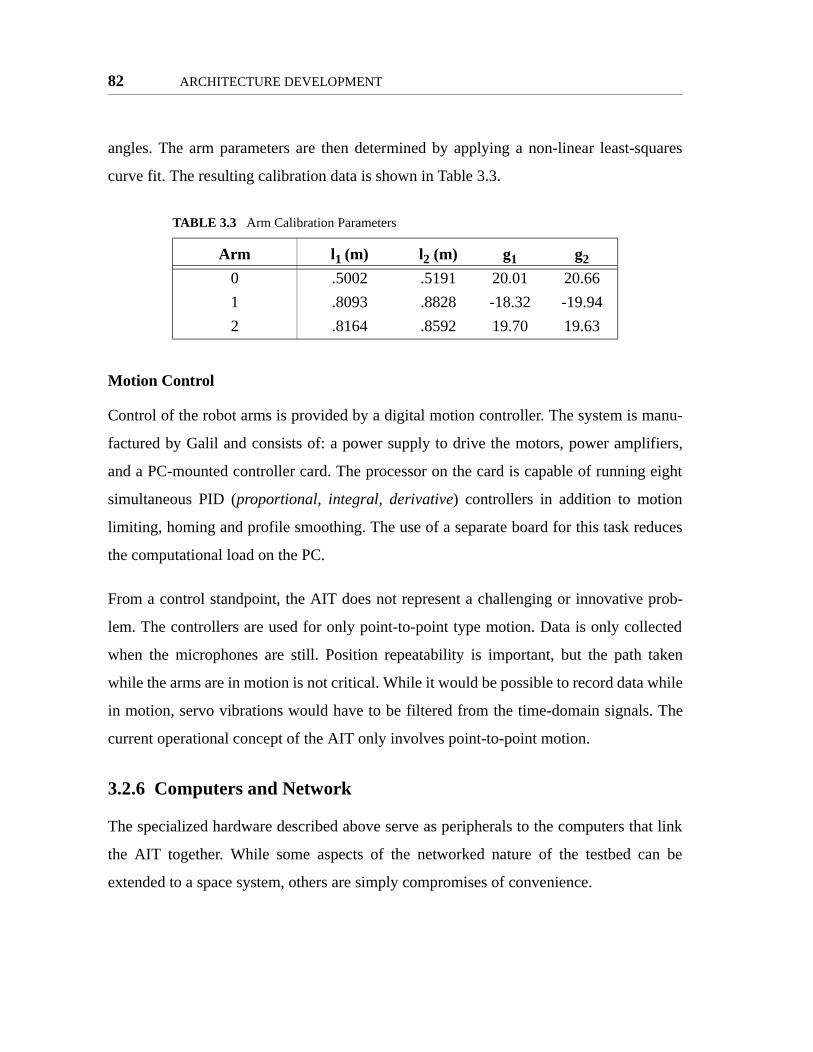
82 ARCHITECTURE DEVELOPMENT
angles. The arm parameters are then determined by applying a non-linear least-squares
curve fit. The resulting calibration data is shown in Table 3.3.
Motion Control
Control of the robot arms is provided by a digital motion controller. The system is manu-
factured by Galil and consists of: a power supply to drive the motors, power amplifiers,
and a PC-mounted controller card. The processor on the card is capable of running eight
simultaneous PID (proportional, integral, derivative) controllers in addition to motion
limiting, homing and profile smoothing. The use of a separate board for this task reduces
the computational load on the PC.
From a control standpoint, the AIT does not represent a challenging or innovative prob-
lem. The controllers are used for only point-to-point type motion. Data is only collected
when the microphones are still. Position repeatability is important, but the path taken
while the arms are in motion is not critical. While it would be possible to record data while
in motion, servo vibrations would have to be filtered from the time-domain signals. The
current operational concept of the AIT only involves point-to-point motion.
3.2.6 Computers and Network
The specialized hardware described above serve as peripherals to the computers that link
the AIT together. While some aspects of the networked nature of the testbed can be
extended to a space system, others are simply compromises of convenience.
TABLE 3.3 Arm Calibration Parameters
Arm l1 (m) l2 (m) g1 g2
0 .5002 .5191 20.01 20.66
1 .8093 .8828 -18.32 -19.94
2 .8164 .8592 19.70 19.63

Software 83
the
e test-
e of this
Three computers compose the backbone of the AIT network. Each of these contributes
both specific and general computational capability to the system as a whole. A fourth
computer was used as a web server when experiments in remote monitoring were per-
formed. A summary of the hosts used is shown in Table 3.4. All of these computers were
networked through the MITnet ethernet system. This network architecture supports 10
MBps transfer rates.
The AIT architecture demonstrates mechanisms for distributed satellite control. A remote
user can direct the testbed using only a standard internet connection. For a real system,
additional steps would have to be taken to ensure authorization and authentication require-
ments were met. Implementing secure network access was judged to be neither cost effec-
tive nor illuminating for the AIT investigations. System security is discussed at greater
length in Section 3.3.8.
3.3 Software
3.3.1 Overview
If the AIT hardware is to provide the physical representation of the interferometry process,
the software must provide a mapping between the actual hardware and the environment
that the testbed is trying to capture. There are two primary tasks that must be accom-
plished; develop ‘intelligent’ spacecraft logic, and more fundamentally, to provide
environment that allows these agents to interact. For cost and simplicity reasons, th
bed does not possess four separate sets of sensing and actuation hardware. Som
TABLE 3.4 AIT hosts
Host Name IP address CPU Primary Function Memory (MB)
darling-downs 18.33.0.52 PII-400 Server 128
ayers-rock 18.33.0.117 PII-266 DAQ 128
gold-coast 18.33.0.118 PII-266 DMC 128
woomera 18.34.0.127 PII-266 Web Server 128

84 ARCHITECTURE DEVELOPMENT
areful
ive that
ile the
they
ction
of the
ation
g with
niques
orking
ereby
els of
tions.
uit for
s a
.
f layers
lation.
capability is shared by a single piece of electronics. Although this creates a slight compro-
mise in the AIT’s accuracy of representation, corrections can be made through c
engineering of the software environment. Thus, each of the spacecraft agents perce
they have their own dedicated sensing apparatus.
Most software has been written in the C language. Some elements use C++. Wh
applications run under the Windows NT operating system, with very few exceptions
are intended to be portable. The message passing application programming interface
(API) is a multi-platform application and the socket programming uses standard Berkeley
Systems Division (BSD) implementations.
This section details the operation of the various software components that fun
together to create the AIT environment. The description begins with a description
approach to software engineering taken with the AIT. This is followed by an examin
of the hardware interface software. Lastly, the virtual spacecraft are described alon
the protocols guiding their behaviour.
3.3.2 Software Layering
Modern software design promotes the use of layering and encapsulation. These tech
help to promote robust, scalable, and portable code. A popular example from netw
is the Open Standards Interface (OSI) so-called seven-layer model (Figure 3.14). Layering
refers to the technique used both in networking and within a single computer, wh
system functionality is extended through well documented layers. The lowest lev
software deal directly with the hardware involved. This is the physical layer in the OSI
model. Increasing levels provide additional capabilities and more abstracted opera
This can be seen with the OSI model. The physical layer is simply a bit-pipe, a cond
bits. The data-link control layer provides error correction and framing; i.e. it transform
stream of bits into distinct data. The network layer handles complex information routing
Each layer is designed to provide services to the layer above and request them o
below. These interfaces should be well defined and embody the concept of encapsu

Software 85
The functioning elements within a layer should be replacable without affecting the opera-
tion of the adjoining levels.
In networking there is the notion of peer processes. Protocols describe the interactions
between the corresponding layers in each node. Such layers are considered to be peers.
This interaction establishes a conceptual or logical information pathway. The data flow
between peers must traverse several layers and the physical connection medium. Due to
the concept of encapsulation, peer interactions can be described and developed with refer-
ence only to the logical pathway.
These ideas can also be applied to the software running on a single computer. The physical
devices (i.e. computer, peripherals) are accessed through the operating system and device
driver. User applications in turn, execute in the environment that the operating system cre-
ates. Task management, interrupt handling and the like can be treated as high level con-
cepts. The operating system takes care of the details.
The software architecture of the AIT incorporates elements of both inter- and intra-com-
puter operation. A conceptual diagram is presented in Figure 3.15. The operating systems
Figure 3.14 The OSI 7-layer model.
Application
Presentation
Session
Transport
Network
DLC
Physical
Application
Presentation
Session
Transport
Network
DLC
Physical
Logical Information Flow
Actual Flow

86 ARCHITECTURE DEVELOPMENT
and low-level device drivers provide the fundamental link between hardware and soft-
ware. This software has been written by the respective manufacturers and provides an
application programming interface (API) for the user. This API defines methods for data
acquisition, motion control and networking at a higher conceptual level than juggling
memory addresses. These routines are used by software entities that in turn interact with
the virtual spacecraft. A message passing layer allows seamless communication between
and within machines.
At the highest conceptual level, there are two sets of software components. These pro-
grams represent the virtual spacecraft (VSC) and the virtual ground station (VGS). Multi-
threaded applications handle the sub-functions of the spacecraft, but most of the inter-
entity communication is handled by a central process. For this communication to be effec-
tive, each agent must employ a predefined protocol for formatting and passing messages.
To maintain a logical progression from the hardware issues discussed above, the software
shall be examined in increasing complexity from the hardware interface to the design of
the agents themselves.
Figure 3.15 The AIT layering concept
Computer Computer Computer Special Hardware
Operating System(Process Management, Networking)
Hardware Drivers
PVM(Inter-process Communication)
Hardware Drivers
VSC VSC
VGS(Server)
User(Client)
(Optional ‘Security’ layer)

Software 87
3.3.3 Operating System
The computational capability of the AIT is embodied in three computers as described in
Section 3.2.6. The operating system provides services to the user applications in terms of
network services, task management and hardware access. The AIT system employs the
Microsoft Windows NT 4.0 operating system. This choice was made based on the avail-
ability of driver software. The data acquisition, motion control and camera hardware all
require software support for proper operation. While other operating systems such as Unix
offer a more robust suite of task-management tools, hardware support was limited. Given
additional resources (people and time) separate drivers could be developed for the addi-
tional operating systems, but it was judged most expedient to use the available operating
system and software.
3.3.4 The Parallel Virtual Machine
One difficulty with writing portable distributed code is the mechanism that handles inter-
process communication. While pipes are useful within a given computer and socket con-
nections can be employed between network nodes, management of these features can
become confusing. This heterogeneous collection of information streams is unnecessarily
complicated. When designing applications for the AIT (VSCs, VGS, etc.) an automated
management scheme for these connections would be very useful.
The Parallel Virtual Machine (PVM) package, developed by Oak Ridge National Labora-
tories, provides these capabilities. PVM is an API that provides the user with a set of com-
munications routines that handle intra- and inter-computer message passing in a
transparent fashion. This allows flexible computing topologies and simple application
design.
Central to the operation of PVM is the concept of the virtual machine. The system is ini-
tialized on a primary host computer by running a daemona program. Through a console-
type interface, the user can then alter the virtual machine. Additional hosts can then be

88 ARCHITECTURE DEVELOPMENT
ginat-
. This
PVM
rocess
lock-
ce can
t ser-
ived in
g to a
y will
algo-
ccept-
’t been
a full
added to increase the general computing pool that composes the virtual machine. Adding
these hosts involves spawning slave copies of the PVM daemon on each member com-
puter. Any network-accessible system with PVM installed can be added to the virtual
machine. These daemons act as intermediaries between all the PVM-aware applications
running on the virtual machine, acting as a kind of postal system.
Every user process that begins on one of the active hosts is assigned a process identifier
(TID). Primitive routines allow a process to obtain the TIDs of its parent (the invoking
process) or children (spawned processes). Communication then takes the form of message
passing. A message buffer is initialized and ‘packed’ with the desired data. The ori
ing process then sends the message to a particular TID, often with an identifying tag
tag is a user defined, numeric identifier designed to specify the type of message. The
daemons (PVMD) then direct the message to the destination host. The recipient p
can receive messages by ‘checking’ with the local PVMD. Reception can occur in a b
ing (execution suspended until receipt) or non-blocking manner. Reception preferen
be given to messages with specific TIDs or message tags.
While easy to implement and flexible, PVM can only make weak guarantees abou
vice. For a given origin/destination a string of messages is assured of being rece
order. This does not necessarily extend to several communicating nodes transmittin
single receiver. Time of delivery is not assured, nor is the queue order in which the
be received. As a result it may be necessary to incorporate extra flexibility into PVM
rithms. While this sounds dire, observed performance has been very good and is a
able for the AIT investigation.
There are many process control and message context features of PVM that haven
utilized in the AIT. The interested reader is advised to consult [Geist et al 1996] for
discussion of PVM capabilities.
a. Daemons are applications that run in the background on a computer. They often extend the capabilities of the operating system.

Software 89
Within the context of the testbed, all interprocess communication is accomplished using
PVM messages. This links the VGS, the VSCs, various spacecraft sub-functions, and the
specialized interface applications. While this has specified the medium for passing mes-
sages between processes, the format and content of the communication has yet to be deter-
mined.
3.3.5 The Distributed Information Protocol for Space Interferometry
Before describing any of the advanced software applications that comprise the AIT, it is
important to examine how the testbed is directed. As described above, the PVM environ-
ment provides a means of passing messages from one process to the next. Without a stan-
dardized definition of content and meaning, the messaging is useless. Message labels,
content and exchange sequences must be defined. The Distributed Information Protocol
for Space Interferometry (DIPSI) provides a medium through which a base set of opera-
tions can be defined. It is an attempt to build up a set of message/command primitives
from which more complex behaviour can be derived.
Messages in the AIT system are classified according to content. DIPSI begins by defining
a message type: i.e. motion requests, position reports, etc. Each message type is assigned
an identifier. These identifiers exist as numeric values, and corresponding macro defini-
tions (in the C language). An attempt has been made to ensure that the macro name
reflects the purpose of the message. These message identifiers, or tags, are used as labels
by PVM. Programs can selectively receive a certain type of message by looking for a par-
ticular tag. While PVM defines procedures for packing and unpacking various data types
from message buffers, the content of the messages is left up to the user. The DIPSI specifi-
cation then specifies the content of each message type in terms of data types (integer, dou-
bles, strings, etc.) and the packing order. Some parameters are optional depending on the
source/destination pair. These variable parameters are clearly marked. Also included in
the DIPSI definitions are the text formatting rules for message conversion. The use of
these additional definitions is described in Section 3.3.8.
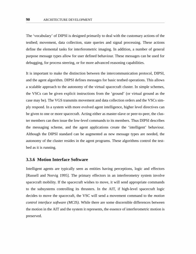
90 ARCHITECTURE DEVELOPMENT
f the
actions
neral
used for
IPSI,
allows
emes,
the
s sim-
s can
e clus-
scribes
viour.
ded, the
e test-
ectors
olve
ands
logic
en
tion is
The ‘vocabulary’ of DIPSI is designed primarily to deal with the customary actions o
testbed; movement, data collection, state queries and signal processing. These
define the elemental tasks for interferometric imaging. In addition, a number of ge
purpose message types allow for user defined behaviour. These messages can be
debugging, for process steering, or for more advanced reasoning capabilities.
It is important to make the distinction between the intercommunication protocol, D
and the agent algorithm. DIPSI defines messages for basic testbed operations. This
a scalable approach to the autonomy of the virtual spacecraft cluster. In simple sch
the VSCs can be given explicit instructions from the ‘ground’ (or virtual ground as
case may be). The VGS transmits movement and data collection orders and the VSC
ply respond. In a system with more evolved agent intelligence, higher level directive
be given to one or more spacecraft. Acting either as master-slave or peer-to-peer, th
ter members can then issue the low-level commands to its members. Thus DIPSI de
the messaging scheme, and the agent applications create the ‘intelligent’ beha
Although the DIPSI standard can be augmented as new message types are nee
autonomy of the cluster resides in the agent programs. These algorithms control th
bed as it is running.
3.3.6 Motion Interface Software
Intelligent agents are typically seen as entities having perceptions, logic and eff
[Russell and Norvig 1995]. The primary effectors in an interferometry system inv
spacecraft mobility. If the spacecraft wishes to move, it will send appropriate comm
to the subsystems controlling its thrusters. In the AIT, if high-level spacecraft
decides to move the spacecraft, the VSC will send a movement command to the motion
control interface software (MCIS). While there are some discernible differences betwe
the motion in the AIT and the system it represents, the essence of interferometric mo
preserved.

Software 91
f the
space
space-
will
en the
ing of
coast
ffects.
imply
sition
pre-
as the
The software entities that interact between the logical spacecraft and the physical portions
of the AIT are generally fairly simple applications. The sharing of a single process
between a number of virtual spacecraft detracts somewhat from the analogy between the
testbed and a real system. It was felt however that such an approach would not compro-
mise the AIT investigations. As a result, the motion control for all four arms as well as the
data collection are handled directly through a single application.
The motion interface software receives motion requests from each of the virtual spacecraft
and issues corresponding commands to the digital motion controller (see Section 3.2.4).
The spacecraft reckon their motions relative to the global coordinate system. Conse-
quently the interface software first makes the conversion to local arm coordinates. Inverse
kinematics (Eq. 3.5 through Eq. 3.13) then translates the rectilinear coordinates into angu-
lar commands that can be issued to the motors. Requests for motion from each arm are
processed separately. There is no ‘out-of-context’ flow of information, and none o
VSCs have access to information about the other spacecraft.
Two differences are readily observed between spacecraft and AIT motion. First, in a
system, the motion control would be handled by a physical sub-component of the
craft. In the AIT, the motion control ‘object’ is actually shared by all the VSCs. Each
send the ‘move’ command to the same TID. The second obvious difference betwe
two systems is the quality of motion. Thrusters command an acceleration. The tim
firings translate to reorienting the spacecraft array through a cycle of acceleration,
and deceleration. The AIT in contrast does not (at present) capture such dynamic e
Motion is considered in a point-to-point sense. A spacecraft at a given position s
moves to a specified end position. The intermediate path is of no interest.
A secondary function of the motion interface software is to provide an absolute po
reference. VSCs can query the MCIS to find out their own position in the AIT. This re
sents the operation of a cluster metrology system or an external mechanism such

92 ARCHITECTURE DEVELOPMENT
Global Positioning System (GPS). This position reference is used in planning array
Reconfiguration and to calculate correction factors during signal processing operations.
3.3.7 Data Acquisition Interface Software
The data acquisition interface software (DAIS) serves a purpose similar to the MIS
described above (Section 3.3.6). The DAIS is in fact a very simple application. When a
number of virtual spacecraft wish to participate in an observation, they will each send an
observation request to the DAIS. The DAIS records the desired amount of data from the
input channels and then distributes the information to the participating VSCs.
There is a slight loss of representational validity in this procedure. Each participant VSC
knows which of its fellows are included in a particular measurement. So too does the
DAIS. The first observation request contains a description of the participating set of
VSCs. The DAIS does not in fact record any data until notification has been received from
all of the participating VSC. This, in effect, sidesteps the need for precise synchronization
between participants. While timing issues are important for a radio interferometer, differ-
ent issues arise in optical systems where this requirement manifests itself as optical path
control. In either case, these problems are considered matters of hardware implementation
and are not relevant to the high-level logic represented by the testbed.
Each measurement request specifies the requested sampling rate and the number of sam-
ples to collect. Due to limitations imposed by the sample-and-hold assembly the maxi-
mum sampling rate for four input channels is 37 kHz. This is the default sampling rate
used in all of the testbed activities to date. Considering that the operational frequency is 15
kHz, the sampling rate is 2.46 times the highest frequency of interest. This satisfies the
Nyquist criterion, and the signal of interest should be represented accurately. While 2.4
samples per cycle does not provide a good view of any particular cycle, discrete time the-
ory indicates that this is sufficient to reconstruct the original band-limited signal and hence
determine its magnitude and phase.

Software 93
mes-
‘out-of-
well as
sed is
e
te cli-
No attempt has been made to add an anti-aliasing stage to the signal path. Since the sam-
pling frequency is 37 kHz, a source frequency of 22 kHz would be needed to create alias-
ing at 15 kHz. Both the tweeters and the microphones exhibit significant attenuation in
this frequency regime. Since there are no significant sources of input energy at these fre-
quencies, an anti-aliasing, low-pass filter was considered unnecessary.
The DAIS represents the source of sensor data for the system. From there it must be dis-
tributed to the spacecraft. The virtual spacecraft exchange relevant information and then
calculate the visibility coefficients. Finally, the processed data must reach the user.
3.3.8 AIT Virtual Ground Station
In a real space system, a user cannot usually communicate directly with a satellite. In the
AIT, user input is routed through what is know as the virtual ground station (VGS). This
serves as an up and down-link between the PVM-based systems of the virtual cluster and
any remote client applications. The VGS provides two main streams of data and command
access. The one most often used is the ‘in-context’ communication. This refers to
sages and commands that are analogous to real world commands. In contrast, the
context’ commands provide the user with diagnostics from the testbed elements, as
an omniscient view into the ongoing activities of the testbed.
The VGS is a type of application know as a server. That is, it will accept connections
using standard network protocols from a remote client on the internet. The protocol u
called the Transport Control Protocol/Internet Protocol (TCP/IP). The manner of opera-
tion is straightforwarda. First the server application creates a variable called a socket
descriptor. The descriptor is then associated or bound to a port on the host machine. Th
host machine name and the port number conceptually defines a point to which remo
a. This description of socket programming refers to the Berkeley Systems Division (BSD) implementation. BSD sockets are the most popular implementation and are supported by most operating systems. The use of some APIs such as Microsoft Foundation Classes (MFC) will sometimes encapsulate the BSD func-tionality.

94 ARCHITECTURE DEVELOPMENT
Elm
rt on
mands
ning of
he tak-
mand
nual
system
tion
d from
ocket
ents can connect. Consider the machine name as a street address and the port as an office
number. Different services are made available on different ports. A de facto standard
exists, defining which ports are which; telnet connections use port 23, the smtp mail proto-
col uses port 25, and web connections using http typically use port 80. Once the socket
descriptor has been created and bound to a port, the server listens for incoming connec-
tions.
Once a connection has been established, a socket stream exists between the client and
server. In a manner similar to file access, the two linked programs can read and write to
the stream. Data written by the client can be read from the server and vice versa. While
binary data can be sent through the socket stream, it is a common practice to make use of
plain text in many circumstances. This allows a server to support many different client
implementations. As an example of this distinction, consider the case of electronic mail.
There are many email clients available: Qualcomm’s Eudora, Microsoft Outlook, and
to name a few. All essentially provide a user interface to the underlying standard mail
transport protocol (SMTP). One can even use a telnet client, connect to the SMTP po
a computer, and send an email message using the simple, text-based, protocol com
(see Appendix A for an example).
The VGS is a net based server that by default resides on port 2346. While the mea
lower numbered ports are well established, higher numbers are essentially free for t
ing. Port 2346 was chosen arbitrarily. A different value can be specified on the com
line when invoking the AIT-VGS. The text DIPSI standard defines the format for ma
entry of messages. The typical format for the commands to be relayed through the
is:
> commandID destination param1 param2 ...
CommandID is a numeric identifier, defined in the DIPSI specification. The destina
refers to the recipient of the message. In nominal operations, the VSCs are numbere
0 to 3, the MIS is 4 and the DAIS has an ID of 5. The VGS reads input from the s

Software 95
ingle
itional
accord-
even-
dware
-VGS
t pro-
n out
ight
many
ilitating
DIPSI
es it:
stream and automatically generates a PVM message. The converse is also true. PVM mes-
sages addressed to the VGS are converted into text and delivered to the socket. Some mes-
sages, i.e. SC_SHUTDOWN, actually spawn broadcast messages from the VGS. To
instruct spacecraft 1 to move to position x=1.2 m., y=1.3 m. in absolute coordinates, the
following would be sent to the server:
> 16 1 1 1.2 1.3
The AIT-VGS acts as a gateway between the PVM-driven AIT environment and an exter-
nal user. Users are able to operate and observe the testbed with a minimal amount of setup
on the client side.
Many internet based servers support multiple connections up to a predefined limit. As
each incoming connection is made, the server will typically spawn a program thread to
deal with the particular stream. For simplicity’s sake, the AIT-VGS supports only s
connections at a time. Multiple users accessing the testbed would require an add
level of contention management. Commands would have to be scheduled, perhaps
ing a user priority level. It has been envisioned that an additional server layer could
tually be added to the AIT environment. The supplementary server could handle har
contention, user authentication and authorization, task scheduling, etc. The AIT
would then simply be slaved to this multi-user server. At present this work has no
gressed.
Some command structures initially added to the DIPSI specification have since falle
of use. They remain in the specification for the moment, but future revisions m
remove them for the sake of compactness. The DIPSI protocol does not make
assumptions about the spacecraft behaviour. It serves instead as a means of fac
unambiguous communication. In order to gain a good understanding of the role that
plays in AIT operations it is useful to examine the primary piece of software that us
the virtual spacecraft.

96 ARCHITECTURE DEVELOPMENT
3.3.9 Virtual Spacecraft
The main purpose of the AIT is to study the behaviour of automated and autonomous clus-
ters of spacecraft in the conduct of synthetic imaging. The central element in this study
must then be the Virtual Spacecraft (VSC) applications. These programs are written in C/
C++. The basic application is coded in normal C while some of the intelligent aspects are
written using C++. The intelligent aspects depend on the particular role or experiment of
interest. This section examines the implementation of the basic suite of functions con-
tained in the DIPSI specification. The general organization of the VSC coding is examined
first. This is followed by a detailed study of some of the particular behaviours and algo-
rithms that are built into the code.
The operation of the basic VSC is rather simple. At the heart of the VSC code is a simple
loop that looks for incoming PVM messages. A large switch statement sorts the message
by its tag and specialized code processes the contents. While this is admittedly a some-
what primitive approach, it avoids the platform dependence that an event-driven code
would produce. Except in rare instances, all PVM messages are received in the main loop.
This helps to prevent deadlock, a condition in which VSC operation is suspended while
waiting for a response that may not come. In this manner, the VSCs are able to receive
abort or shutdown commands at any time. One inconvenience of this method is the
requirement to keep careful knowledge of the current state.
Each operation that the spacecraft must perform has a number of steps or states. Transi-
tions from one state to the next typically requires an external trigger. Consider
Figure 3.16. This figure illustrates the sequence of operations that go into a particular
data-acquisition sequence. From the idle state, the spacecraft receives a sample request.
Sample requests are sent initially to a lead VSC. The leader then relays the sample request
to the other participating agents. Each submits a sample request to the DAIS. The VSCs
must then receive the gathered data. Before signal processing can occur, each spacecraft
must exchange a segment of its data with the other members of the cluster. When the data
are processed, the result is forwarded to the VGS and the VSC returns to its idle state.

Software 97
ng a
. The
, at the
e been
of the
hange
ns in
tasks of
uence
is that
buted
ting
The only trouble with this scheme is that the current ‘state’ (or logical position) duri
data acquisition cycle must be maintained, independent of the program execution
VSC must always be able to accept and properly interpret additional messages but
same time, recognize the next trigger event. At present, the state variables hav
established separately for each of the event cycles. In the future, a generalization
spacecraft state handling might provide a more robust solution. Several exc
sequences are further examined in Appendix B.
Most of the tasks handled by the VSC are straightforward. The DIPSI specificatio
Appendix A detail the data formats and the expected responses. There are several
particular interest: Data Collection and Exchange, Signal Processing and Seq
Queueing.
Data Collection and Exchange
One of the essential tasks for the successful implementation of parallel algorithms
of computational load and communication balancing. One wishes to design distri
algorithms that will distribute the required computation fairly amongst the participa
Figure 3.16 State transitions for data acquisition
1. Idle
2. DAQ request
3. Data Exchange
4. Data Processing
5. Data Return

98 ARCHITECTURE DEVELOPMENT
ecall-
ts
time-
erates a
onsid-
ivided
ent of
nodes. In the case of homogeneous nodes, fairness usually implies an equal amount of
computation. From the standpoint of distributed algorithms, the interferometric processing
isn’t very interesting. The underlying operation is essentially that of a dot-product. R
ing from Eqs. 2.60-2.61 that the Fourier visibility coefficien
are found by:
(3.16)
(3.17)
Where the delay α corresponds to a phase shift of π/2. Assuming for the moment that α is
an integer, the above operation is similar to a dot-product operation. The two
sequences are multiplied element-wise and summed. Since each pair of VSCs gen
set of Fourier coefficients, this procedure is repeated for each baseline computed. C
ering the participant spacecraft in a pair-wise manner, the above calculation can be d
neatly in two:
(3.18)
(3.19)
The number of calculations required to produce a result is known a priori. Each VSC is
guaranteed of receiving the same amount of calculations to perform. The establishm
a few simple exchange rules will partition the tasks effectively.
V k l,( ) rr k l,( ) jri k l,( )+=
rr k l,( ) E1 n[ ] E2 n[ ]⋅n 0=
N 1–
∑=
ri k l,( ) E1 n[ ] E2 n α–[ ]⋅n 0=
N 1–
∑=
rr k l,( ) t1 n[ ] t2 n[ ]⋅n 0=
N2---- 1–
∑ t1 n[ ] t2 n[ ]⋅n N=
N 1–
∑+=
ri k l,( ) i t1 n[ ] t2 n α–[ ]⋅n 0=
N2---- 1–
∑ t1 n[ ] t2 n α–[ ]⋅n N=
N 1–
∑+
=

Software 99
1. Each spacecraft a will share half of its data with partner b.
2. If a>b, then a will send the later half of its data to b. Otherwise it will sendthe first half.
These rules are reflexive. They work equally well for both spacecraft involved. After cal-
culation, the partial results are sent to the VGS for synthesis. A detailed walk-through of
an exchange sequence is given in Appendix B.
As discussed in Section 2.2.3 the creation of a distributed algorithm depends to some
extent on the connection architecture between nodes. PVM offers all-to-all connectivity at
least at a conceptual level. Any message can be sent directly to any other node. Unfortu-
nately, underlying the PVM system is the bus architecture of ethernet. Propagation delays
observed with PVM are not necessarily reconcilable with the connection scheme one is
trying to represent. Of course applications are free to adopt any virtual connection archi-
tecture that they want. That is one of the benefits of the virtual machine concept.
Regardless of the scheme chosen, the fact remains that the four VSCs of the AIT represent
a degenerate connection architecture. The only distinction that can be made is between a
totally connected system and a ring. Barring the use of a rather contrived, linear connec-
tivity for the AIT, there is only a difference of two links between the possible schemes.
Another issue associated with connectivity is simultaneity and channel isolation. A cluster
of spacecraft communicating by radio link might employ a broadcast exchange; i.e. all
spacecraft can receive a given transmission. Unless the cluster has access to a lot of band-
width, only a few spacecraft can transmit at a given time. This is similar to a bus type of
system. Another systems engineering choice might employ an electronically steered col-
lection of phased array antennas. The beams are tight and can be rapidly retargeted to a
different spacecraft. Frequency reuse is possible, but each satellite has an immediate con-
nection to only a subset of the cluster. For an optical communications system, total con-
nectivity may be prohibitive in terms of cost and hardware complexity. In such a system
the topology of the intersatellite links (ISLs) would be fixeda, but would support much

100 ARCHITECTURE DEVELOPMENT
igura-
higher transmission capacities. Generally, when designing the architecture for inter-space-
craft communication, one should bear in mind:
• Hardware Complexity: This relates to multiple transmitters and receivers.Greater numbers give more links, but more mass and cost.
• Spectrum Resources: How much aggregate bandwidth is required for thesystem to function? Can frequencies be reused?
• Simultaneity: Is performance limited by computation or communication?How much data is required to do useful work. For computationaly heavytasks, pacing communications to match processing speeds may reduce tech-nical requirements.
• Robustness: How tolerant are cluster operations to failures of individuallinks or entire spacecraft?
An exchange procedure must be developed to allow for sharing the interferometry data in
the AIT. Since the integrity of the AIT analogy is a little thin when discussing the timing
and delay behaviour of the communications systems, the ordering of data exchanges does
not directly reflect realistic implementations. For each baseline, a given spacecraft will
pack the appropriate half of its own data into a message buffer and transmit it to its part-
ner. For a full, four spacecraft cluster, some exchanges are a compound message of its own
data, and data relayed from another VSC. A walkthrough of this exchange procedure is
presented in Appendix B. There is a slight overlap in the amount of data transmitted due to
the fact that corrections must be made to the data streams to account for non-idealities of
the testbed.
Non-Ideal Signal Processing
The straightforward calculation of the visibility parameters as given in Eqs. 3.16 and 3.17
must be modified to account for physical non-idealities of the AIT. Recall from
Section 2.1.3 that the basic formulation of the cross-correlation assumes a source at infin-
ity. This would produce a planar wavefront. The finite length of the testbed translates into
a spherical wavefront at the imaging plane. Making corrections for the wavefront shape
a. By ‘fixed’ it is meant that the topology is static on the time scale of a communication cycle. Reconftion would be possible but not a rapid operation.

Software 101
and the vertical offset of the microphones is a preprocessing task that must be performed
before correlation is feasible.
It is not the shape of the wavefront that is crucial to testbed operations. Rather it is neces-
sary that the wavefronts be aligned. Two factors work against this. First, the spherical
wavefront creates one phase error. There is a 6 cm vertical deviation from the middle of
the testbed to the corners. Second, the imaging plane is not really a plane at all. The verti-
cal offset between microphones must be accounted for. These ideas are depicted in
Figure 3.17.
Both of these factors create the same deleterious effect. The spherical shape of the wave-
front and the vertical microphone offset create a path-length difference between the two
microphones. This translates into a phase shift between the two incoming signals. Unless
this is removed, the resulting image will be garbleda. In order to do this, the VSCs need
knowledge of the testbed geometry. Consider a single, two-microphone measurement. The
Figure 3.17 Testbed Geometric Effects.
L1
L2
d2d1

102 ARCHITECTURE DEVELOPMENT
f
plane
lay is
phase
ource)
s:
d in the
m of
end effector positions are given as (x1, y1) and (x2, y2). In order to correct for the path
length difference a ‘target’ point must be identified (xc, yc). This is the point on the top o
the testbed that coincides with the bore-sight axis. The two paths d1 and d2 can be com-
puted:
(3.20)
The variable h represents the vertical distance from the speaker array to the motion
of the microphone in question. The differential pathlength is then:
(3.21)
The signal from the microphone with the short path length must be delayed. This de
chosen such that sound originating from a source at the centre of the array will be in
with the sound arriving at the other microphone. The phase angle (for a pure tone s
is:
(3.22)
If the time spacing between samples is given by T, then the required sample delay i
(3.23)
where the radian frequency of the source signal is denoted by Ω. This would be fine if τ
was an integer, but what about fractional values of τ? Does x[n-0.35] have a meaning in a
discrete sequence? This notation is awkward. The process is more easily understoo
context of applying a digital delay filter to the input signal. Consider the simple syste
Figure 3.18.
a. Each visibility measurement would have a different phase error. The additive contribution of these errors will degrade the image quality
di xi xc–( )2yi yc–( )2
h( )2+ +=
∆ d1 d2–=
Φ 2π∆λ---=
τ ΦΩT--------=
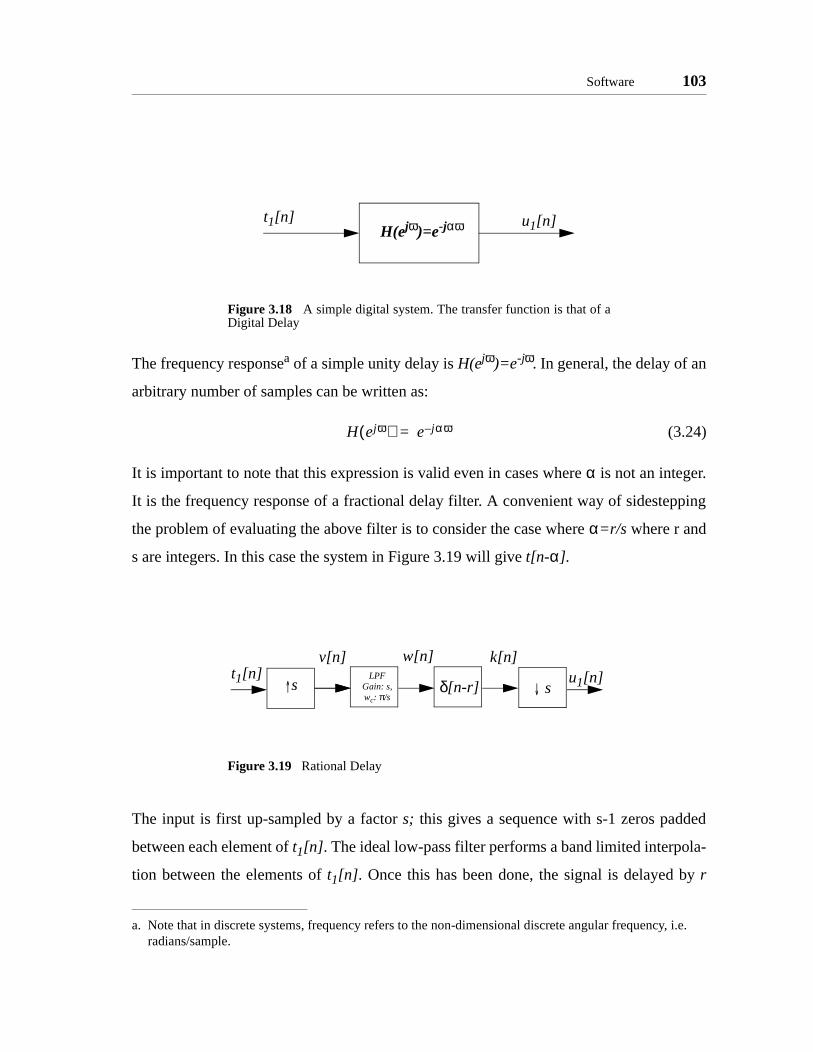
Software 103
The frequency responsea of a simple unity delay is H(ejω)=e-jω. In general, the delay of an
arbitrary number of samples can be written as:
(3.24)
It is important to note that this expression is valid even in cases where α is not an integer.
It is the frequency response of a fractional delay filter. A convenient way of sidestepping
the problem of evaluating the above filter is to consider the case where α=r/s where r and
s are integers. In this case the system in Figure 3.19 will give t[n-α].
The input is first up-sampled by a factor s; this gives a sequence with s-1 zeros padded
between each element of t1[n]. The ideal low-pass filter performs a band limited interpola-
tion between the elements of t1[n]. Once this has been done, the signal is delayed by r
Figure 3.18 A simple digital system. The transfer function is that of aDigital Delay
a. Note that in discrete systems, frequency refers to the non-dimensional discrete angular frequency, i.e. radians/sample.
Figure 3.19 Rational Delay
t1[n] u1[n]H(ejω)=e-jαω
H ejω( ) e jαω–=
LPFGain: s, wc: π/s
t1[n] u1[n]s δ[n-r] s
v[n] w[n] k[n]
104 ARCHITECTURE DEVELOPMENT
’t dis-
nly an
ilter
n-zero
samples and then down-sampled by a factor of s. The result is the fractional shift of the
input sequence. Conceptually, this method would work as presented. It is however ineffi-
cient in terms of computation. Only the terms of the intermediate sequence that aren
carded need to be calculated. One must also realize that an ideal low-pass filter is o
abstraction. This filter will be approximated by a finite impulse response (FIR) f
(h[n]) of length N+1.
Consider the zero-padded sequence v[n]:
(3.25)
The filtered sequence w[n] is the result of linear convolution of the input v[n] with h[n].
(3.26)
(3.27)
Since v[n] has been zero padded, many of its entries are zero. The sum over the no
terms can then be rewritten as:
(3.28)
where,
(3.29)
Now delaying the output by r, yields:
v n[ ]t1 p[ ] n, mp=
0 otherwise,
=
w n[ ] v n[ ]*h n[ ]=
w n[ ] v m[ ] h n m–[ ]⋅m N 2⁄–=
N 2⁄
∑=
w n[ ] v ms[ ] h n ms–[ ]⋅m b–=
b
∑=
b Ns----=
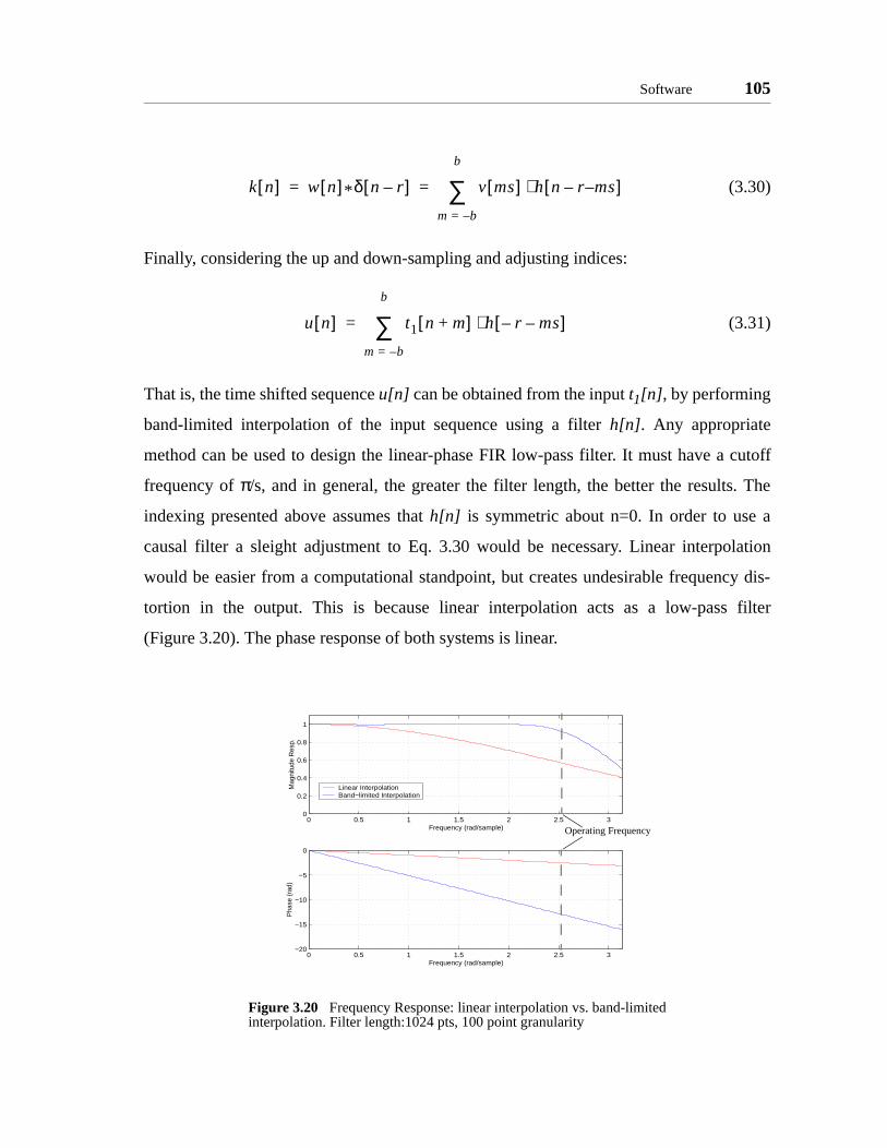
Software 105
(3.30)
Finally, considering the up and down-sampling and adjusting indices:
(3.31)
That is, the time shifted sequence u[n] can be obtained from the input t1[n], by performing
band-limited interpolation of the input sequence using a filter h[n]. Any appropriate
method can be used to design the linear-phase FIR low-pass filter. It must have a cutoff
frequency of π/s, and in general, the greater the filter length, the better the results. The
indexing presented above assumes that h[n] is symmetric about n=0. In order to use a
causal filter a sleight adjustment to Eq. 3.30 would be necessary. Linear interpolation
would be easier from a computational standpoint, but creates undesirable frequency dis-
tortion in the output. This is because linear interpolation acts as a low-pass filter
(Figure 3.20). The phase response of both systems is linear.
Figure 3.20 Frequency Response: linear interpolation vs. band-limitedinterpolation. Filter length:1024 pts, 100 point granularity
k n[ ] w n[ ]*δ n r–[ ] v ms[ ] h n r ms––[ ]⋅m b–=
b
∑= =
u n[ ] t1 n m+[ ] h r– ms–[ ]⋅m b–=
b
∑=
0 0.5 1 1.5 2 2.5 30
0.2
0.4
0.6
0.8
1
Frequency (rad/sample)
Mag
nitu
de R
esp.
Linear Interpolation Band−limited Interpolation
0 0.5 1 1.5 2 2.5 3−20
−15
−10
−5
0
Frequency (rad/sample)
Pha
se (r
ad)
Operating Frequency

106 ARCHITECTURE DEVELOPMENT
metry
e visi-
easily
o any
nt cor-
mated
load a
uvering
tion of
ber of
he x-y
VSCs.
ement
his mes-
pling
pant, it
error
‘idle’ it
olved.
The particular implementation chosen for the AIT uses a 1024 pt. low-pass filter. The
VSCs are designed to interpolate to within 0.01 of a sample. This allows phase correction
to within 1º. This is considered acceptable [Thomson, et al, 1994] for most interfero
applications.
This same interpolation technique is used to compute the complex component of th
bility function. That procedure requires introducing a phase shift of π/2 into one of the sig-
nals. For a very narrow-band signal, such as those used in the AIT, this is most
accomplished by adding a delay to the signal in question. This delay is in addition t
wavefront correction that may be necessary. Since each baseline requires a differe
rection, the shifted sequences must be computed separately from one another.
Image Automation
One of the more recent additions to the VSC logic has been the addition of auto
sequencing of testbed operations. This message format allows the VGS to up
sequence of sampling positions at once. The VSCs then proceed through the mane
profile without further input from the ground.
This type of DIPSI message contains several parts. The first component is a descrip
the sampling parameters. All sample points in a sequence must take the same num
samples. The next section consists of several lists of coordinates. These detail t
position and ordering of the VSC movement.
The queue command is sent from the VGS (though it need not do so) to one of the
This VSC is the designated leader of the motion sequence. After receiving the mov
data, the leader sends a message to each of the VSCs flagged as a participant. T
sage is to verify that the VSCs involved have not been committed to another sam
sequence. If the leader is successful in obtaining message locks from each partici
will commence the sampling procedure. Otherwise it will reset itself and send an
message to the VGS. Once the queue has been activated, if the leader finds itself
will send out a round of motion and data acquisition commands to the spacecraft inv

Software 107
ore
.
st be
d, the
h exist-
emat-
as a
ipts
anism
s
C and
tlab
trou-
d to
After the data exchange and signal processing is completed, the participants send an
acknowledgment to the leader. This marks the end of a cycle, allowing the next to com-
mence. This process repeats until all the imaging locations have been visited. The lead
spacecraft will then clear the ‘lock’ on the other participants.
Image automation is the most complex activity explicitly defined by DIPSI. M
advanced behaviour will employ combinations of these elementary cluster functions
3.3.10 Matlab Client Interface
The virtual ground station is a network server. In order to perform useful tasks it mu
directed by a client application. While specialized client interfaces are easy to buil
need for post-processing the data suggests a scheme that would integrate well wit
ing tools. The Matlab application, made by MathWorks, is an industry standard math
ics tool. A specialized application was developed that would allow Matlab to act
client application for the AIT, and direct its operation from user provided scr
(Figure 3.21).
Matlab is not equipped with socket functionality. It does however possess a mech
that allows creation of external functions called MEX files. These Matlab EXecutable file
are compiled libraries that the user creates. They can be written and compiled in
then used from within Matlab. A MEX library was created for the AIT that allows Ma
basic socket functions: connect/disconnect and read/write.
Giving Matlab access to the AIT testbed is not sufficient. To save the human user the
ble of individually directing AIT operations, various Matlab scripts were develope
Figure 3.21 The Matlab Client setup. Maneuver selection and post-processing is handled by matlab tools.

108 ARCHITECTURE DEVELOPMENT
automate many tasks. Generally, these scripts will initiate and display the progress of an
imaging sequence.
In [Kong & Miller 1998], the author performs a point-spread function optimization. These
optimal profiles can be fed into Matlab, and then sent to the AIT. These automation scripts
are somewhat intelligent in their own right. Profiles are typically specified in terms of ori-
gin centred positions of the spacecraft. The spacecraft maneuvers are symmetric about the
origin. Unfortunately due to the geometric limitations of the AIT arms, such symmetric
profiles are often not possible. However, it is not the absolute positions of the sensors that
matter for array synthesis. It is only their relative spacing. The Matlab automation scripts
search for sensor positions that satisfy both the required spacing and the constraints of
geometry. After delivering the profile in terms of a queue directive, Matlab collects and
displays the returning data.
3.4 Summary
The architecture if the AIT is very complex. Interactions between hardware and software
must be tracked carefully. Attempts have been made to ensure that all sub-components
have been developed with well defined interfaces.
The role of this extensive architecture development is designed to lay the groundwork for
investigations into agent based autonomy in the context of interferometry. The next few
chapters evaluate the performance of the testbed system in automated tasks and then
attempt to apply advanced strategies to their control.

Chapter 4
PERFORMANCE EVALUATION
In this chapter the performance of the Acoustic Imaging Testbed is evaluated. Optimal UV
point configurations are converted to maneuvers in the testbed environment. Maneuver
sequences of various lengths are evaluated for both single and multiple target configura-
tions. End effector positioning accuracy is calculated along with a general discussion of
other error sources. Measurement variability is observed with regards to source wave-
forms and integration time. Deconvolution procedures are introduced as a means of image
post-processing and enhancement.
4.1 Optimal Imaging Configurations
Interferometry is a synthesis process (Section 2.1.3). As such, several factors must be
traded when considering array configurations. As a rule, more visibility samples will cor-
respond to a higher quality image. This image quality does not come without a price. Extra
apertures cost money to build, reconfiguration of a spaceborne interferometer may spend
fuel, and even if array reconfiguration is possible, time becomes a factor. Balancing multi-
ple scientific goals will limit the availability of any modern instrument. This motivates the
researcher to make intelligent choices regarding the extent of UV coverage.
109

110 PERFORMANCE EVALUATION
4.1.1 Optimization Methods
Many problems can be reduced to setting a limit on the number of baselines available for a
given image. Recall that each visibility measurement represents the coherent correlation
of collected radiation from a pair of apertures. The vector displacement between apertures
determines the Fourier component sampled. In a given array, the baselines may be taken
through pair-wise combination of all the apertures. All available pairs can be measured at
once, provided sufficient hardware exists for the correlation. However, there is still the
question of which ones should be sampled. Several methods exist for optimizing the cov-
erage, but the particular application may influence the selection.
It can be shown [Thomson, et al, 1994] that to minimize the energy in the side-lobes, one
must ensure that there are no redundant baselines in the array configuration. This work
was pioneered by Bracewell in reference to linear array systems. It can also be extended to
two dimensional arrays. Golay [Golay 1971] proposed optimization methods emphasizing
the compactness of the UV coverage. The principal of this technique was to provide a suf-
ficient number of baselines to fill all the grid points in the UV plane of a given extent and
granularity. An example of a Golay configuration for an hexagonal grid is shown in
Figure 4.1. It should be noted though that the Golay arrays assume simultaneous rather
then sequential sampling.
The non-redundancy criterion for interferometer arrays is a rather simple one. It is possi-
ble to add further criteria to the UV selection. Using a simulated annealing optimization,
Cornwell [Cornwell 1988] derived aperture placements that maximized the spacing
between the UV points. Using a cost function calculated from the logarithm of the UV
point spacings. the simulated annealing technique determined the placement of apertures.
The use of the logarithm emphasizes low spatial frequencies. The aperture placements
were confined to a circular area. As it turns out, the optimization process placed the aper-
ture positions on the outer rim of the domain. Like Golay, Cornwell envisioned an instan-
taneous imaging operation, rather than periodic reorientation. Examples of Cornwell point
placement (commonly known as Cornwell points) are shown with their UV coverage in

Optimal Imaging Configurations 111
Figure 4.2. The point spread function of the Cornwell arrays are much more compact than
the Golay [Kong, et al 1998]. This is perhaps a poor comparison as they employed differ-
ent optimization goals, i.e.higher angular resolution comes at the cost of sparse spatial fre-
quency coverage.
Recent work on the Distributed Satellite Systems program, at the MIT Space Systems Lab
by Kong approached the problem in a different manner. Recall that due to discretization
Figure 4.1 Golay array configurations and PSF. From [Kong, et al1998]
Figure 4.2 Cornwell array configurations and UV Coverage. From[Kong, et al 1998

112 PERFORMANCE EVALUATION
d the
a sub-
side-
valua-
esire
and under-sampling of the UV plane, the impulse response of the array will have finite
width. A single delta-function source will yield the extended response that has been
termed the point spread function. The flexible optimization method used seeks to mini-
mize the mean-squared error between the point-spread function and the ideal (filled aper-
ture) response. The methodology considered the placement of apertures on a hexagonal
grid. As with the Cornwell optimization, simulated annealing was used to determine aper-
ture placement. The cost function was computed as:
(4.1)
The normalized (equal energy) response of a candidate point spread function correspond-
ing to a particular array configuration is denoted by IN, while the nominal response of the
ideal filled aperture was denoted Io. The ideal aperture was still considered to have dis-
crete UV coverage; i.e. The same grid was used, but every point within the boundary was
considered to have been sampled.
In comparison to the Cornwell distributions, these array configurations had wider main
lobes, but generally lower side-lobes. The choice of distributions becomes one of priori-
ties. The researcher must evaluate the relative importance of resolution versus side lobe
spreading/sensitivity. One advantage worth mentioning is that Kong’s method allowe
tailoring of response. If desired, the MSE evaluation could be considered only over
region of the image. This might be useful in a ground-looking application where high
lobe levels beyond the Earth disk can be tolerated.
This optimization method is well adapted to sequential imaging. The performance e
tion of the AIT employed the profiles generated by Kong. This was motivated by a d
to add some experimental validation to the theoretical work.
MSEIN ξi ηj,( ) Io ξi ηj,( )–( )2
j 0=
M 1–
∑i 0=
M 1–
∑M2
--------------------------------------------------------------------------------=

Optimal Imaging Configurations 113
f the
4.1.2 AIT Performance: Single Source
The optimal array configurations proposed by Kong form the basis for the testbed perfor-
mance evaluation. By way of comparison, several images are first made with visibility
measurements located on a square grid. This allows a basic understanding of how optimi-
zation of the visibility measurements can affect the image quality. Through the testbed
development, the predicted performance was a useful diagnostic tool in the identification
of faults and problems.
The speaker array (Section 3.2.3) allowed the use of reconfigureable sources. Tests were
run on both double and single source systems. This section evaluates the performance of
the AIT in the imaging of single sources. It would be useful at this point to introduce a
numbering scheme for the speakers in the array. The nominal numbering scheme is shown
in Figure 4.3.
The first batch of tests consisted of a repetitive series of images of speaker 5. These tests
allow a good comparison with the point spread function. Since the centre speaker lies in
the middle of the nominal field of view, it provides the best preliminary target. Situated
farthest from the walls of the testbed, the prospects of any multipath manifesting itself in
the meaningful parts of the image is slight. The ‘meaningful’ region is the area o
image that corresponds to the top of the testbed, extending to the walls.
Figure 4.3 Speaker numbering. Perspective is from above, ‘outside’ ofthe testbed.
1 2 3
4 5 6
7 8 9
Door Position
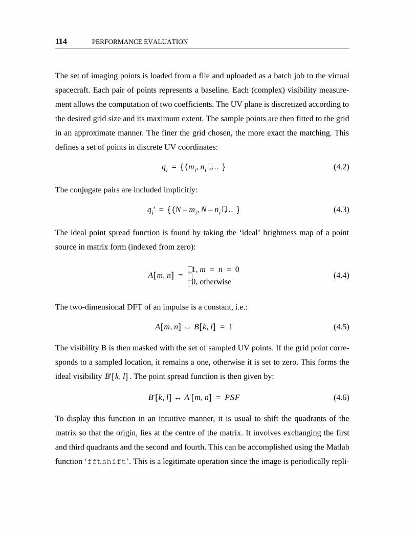
114 PERFORMANCE EVALUATION
point
rre-
ms the
f the
first
Matlab
pli-
The set of imaging points is loaded from a file and uploaded as a batch job to the virtual
spacecraft. Each pair of points represents a baseline. Each (complex) visibility measure-
ment allows the computation of two coefficients. The UV plane is discretized according to
the desired grid size and its maximum extent. The sample points are then fitted to the grid
in an approximate manner. The finer the grid chosen, the more exact the matching. This
defines a set of points in discrete UV coordinates:
(4.2)
The conjugate pairs are included implicitly:
(4.3)
The ideal point spread function is found by taking the ‘ideal’ brightness map of a
source in matrix form (indexed from zero):
(4.4)
The two-dimensional DFT of an impulse is a constant, i.e.:
(4.5)
The visibility B is then masked with the set of sampled UV points. If the grid point co
sponds to a sampled location, it remains a one, otherwise it is set to zero. This for
ideal visibility . The point spread function is then given by:
(4.6)
To display this function in an intuitive manner, it is usual to shift the quadrants o
matrix so that the origin, lies at the centre of the matrix. It involves exchanging the
and third quadrants and the second and fourth. This can be accomplished using the
function ‘fftshift’. This is a legitimate operation since the image is periodically re
qi mi ni,( ) …, =
qi' N mi N ni–,–( ) …, =
A m n,[ ]1 m, n 0= =
0 otherwise,
=
A m n,[ ] B k l,[ ]↔ 1=
B' k l,[ ]
B' k l,[ ] A' m n,[ ]↔ PSF=

Optimal Imaging Configurations 115
d mea-
eakers
rces. A
r error
the
ld start
lved
g this
acking
wable
sed in
od of
luded
that the
elobes,
cated in both axes. As a final note, it is often desirable to normalize the energy in the PSF.
Using Parseval’s theorem:
(4.7)
Qualitatively, the sharpness and shape of the main and side-lobes in the ideal an
sured responses can be examined. Quantitative analysis is more difficult. The sp
used in the AIT have finite dimension and as such, cannot be considered point sou
mean-squared error comparison with a delta function source would indicate a highe
than is justified. It is therefore very difficult to perform quantitative comparison of
ideal and measured point spread function. One strategy that was considered wou
with an estimate of the ‘true’ extended profile of the speaker. This would be convo
with the PSF and compared to the experimental image. The results obtained usin
method would depend very much on assumptions made about the speaker pattern. L
any external ‘truth’ measure, the concept was discarded.
Square-Grid Visibility Coverage
Generating visibility samples on a square grid is a very simple operation. The allo
imaging area determines the maximum baseline. A regular grid is then superimpo
the image plane yielding a number of non-redundant measurements. This meth
selecting visibility measurements, while easy, does not yield good results. It is inc
here to show the effect of careful selection of imaging locations.
The baselines selected for the imaging sequences are non-redundant. This means
sidelobe energy is the same as in the optimal cases. The placement of these sid
however, has significant effect on image quality.
AN' m n,[ ] A'
A' r s,[ ] 2
s∑
r∑-------------------------------------=

116 PERFORMANCE EVALUATION
ctive-
sh the
Images were made using 40, 60, 84, and 98 baselines. The images were of a single operat-
ing source located at the centre of the array (location 5). The exact number of baselines is
dependant on the number of grid points. These images are shown in Figure 4.4.
The sidelobes in these figures are very prominent. Although the definition of the central
peak is very good, the proximity of the sidelobes would make it very difficult to identify
the ‘real’ content of a complex image without resorting to post-processing. The effe
ness of the MSE method of selecting visibility coverage is due to the tendency to pu
sidelobes outwards from the centre, creating a ‘clean’ central field of view.
Figure 4.4 Rectangular visibility sampling profiles (Single Source). Notice very high sidelobes create con-fusing field of view.
−0.4 −0.3 −0.2 −0.1 0 0.1 0.2 0.3 0.4−0.4
−0.3
−0.2
−0.1
0
0.1
0.2
0.3
0.4
40 B
asel
ine
−0.4 −0.3 −0.2 −0.1 0 0.1 0.2 0.3 0.4−0.4
−0.3
−0.2
−0.1
0
0.1
0.2
0.3
0.4
X
Y60
Bas
elin
e
−0.4 −0.3 −0.2 −0.1 0 0.1 0.2 0.3 0.4−0.4
−0.3
−0.2
−0.1
0
0.1
0.2
0.3
0.4
X
Y84
Bas
elin
e
−0.4
−0.3
−0.2
−0.1
0
0.1
0.2
0.3
0.4−0.4 −0.3 −0.2 −0.1 0 0.1 0.2 0.3 0.4
Y
X98
Bas
elin
e

Optimal Imaging Configurations 117
Optimal Visibility Coverage
This section examines the performance of more advanced methods of selecting visibility
samples. The issue at stake is whether the quality of the image can be improved by tailor-
ing the (spatial) frequency sensitivity of the array, while keeping the overall number of
measurements constant. The optimized profiles developed by Kong seek to do just that.
The optimization considered the placement of each baseline individually, a perfect appli-
cation for a two microphone interferometer. Although interferometric operation was dem-
onstrated with three arms, the optimization technique employed by Kong was better suited
to the two spacecraft case.
The seven optimal profiles used in this test are shown in Figure 4.5. Images were taken
with 20, 40, 60, 80, 100, 120, and 140 baselines. A five second integration time was taken
for the first two cases. The remaining images utilized a two second integration. As
expected, the width of the central lobe remains approximately constant throughout. This is
consistent with the observation that all array configurations are scaled to the same maxi-
mum baseline. The prominence of the side-lobes drops sharply as the number of baselines
increases.
It should be noted that these images are much better qualitatively than those depicted
above. Careful selection of UV samples allows control over sidelobe placement. The fur-
ther out the sidelobes, the better the quality of the central field of view.
Comparing the measured result to the point spread function shows a number of key fea-
tures. Visibly, the quality of the pictures gets better with additional sampling. The shape
and positioning of the principle side-lobes seems to be captured accurately. The possible
exception being the 60 baseline profile. It is not entirely clear what caused the feature near
the top edge, a little left of centre. The spike does not appear to correspond directly with
one of the sidelobes. Since the feature is repeatable, it is thought that it might be a result of
some particular interaction between the maneuver profile and the walls of the testbed.

118 PERFORMANCE EVALUATION
Figure 4.5 UV Coverage, Point Spread Functions and Measured Response. Single source located in posi-tion 5.
−25 −20 −15 −10 −5 0 5 10 15 20 25−25
−20
−15
−10
−5
0
5
10
15
20
25
U
V
20 B
asel
ines
UV Coverage
U
V
−0.4 −0.3 −0.2 −0.1 0 0.1 0.2 0.3 0.4−0.4
−0.3
−0.2
−0.1
0
0.1
0.2
0.3
0.4
X
Point Spread Function
Y
Theoretical
X
Y
−0.4 −0.3 −0.2 −0.1 0 0.1 0.2 0.3 0.4−0.4
−0.3
−0.2
−0.1
0
0.1
0.2
0.3
0.4
X
Y
Measured
X
Y
−25 −20 −15 −10 −5 0 5 10 15 20 25−25
−20
−15
−10
−5
0
5
10
15
20
25
U
V
40 B
asel
ines
U
V
−0.4 −0.3 −0.2 −0.1 0 0.1 0.2 0.3 0.4−0.4
−0.3
−0.2
−0.1
0
0.1
0.2
0.3
0.4Point Spread Function
X
Y
X
Y
−0.4 −0.3 −0.2 −0.1 0 0.1 0.2 0.3 0.4−0.4
−0.3
−0.2
−0.1
0
0.1
0.2
0.3
0.4
X
Y
X
Y
−25 −20 −15 −10 −5 0 5 10 15 20 25−25
−20
−15
−10
−5
0
5
10
15
20
25
U
V
60 B
asel
ines
U
V
−0.4 −0.3 −0.2 −0.1 0 0.1 0.2 0.3 0.4−0.4
−0.3
−0.2
−0.1
0
0.1
0.2
0.3
0.4Point Spread Function
X
Y
X
Y
−0.4 −0.3 −0.2 −0.1 0 0.1 0.2 0.3 0.4−0.4
−0.3
−0.2
−0.1
0
0.1
0.2
0.3
0.4
X
Y
X
Y
−25 −20 −15 −10 −5 0 5 10 15 20 25−25
−20
−15
−10
−5
0
5
10
15
20
25
U
V
80 B
asel
ines
U
V
−0.4 −0.3 −0.2 −0.1 0 0.1 0.2 0.3 0.4−0.4
−0.3
−0.2
−0.1
0
0.1
0.2
0.3
0.4Point Spread Function
X
Y
X
Y
−0.4 −0.3 −0.2 −0.1 0 0.1 0.2 0.3 0.4−0.4
−0.3
−0.2
−0.1
0
0.1
0.2
0.3
0.4
X
Y
X
Y
−25 −20 −15 −10 −5 0 5 10 15 20 25−25
−20
−15
−10
−5
0
5
10
15
20
25
U
V
100
Bas
elin
es
U
V
−0.4 −0.3 −0.2 −0.1 0 0.1 0.2 0.3 0.4−0.4
−0.3
−0.2
−0.1
0
0.1
0.2
0.3
0.4Point Spread Function
X
Y
X
Y
−0.4 −0.3 −0.2 −0.1 0 0.1 0.2 0.3 0.4−0.4
−0.3
−0.2
−0.1
0
0.1
0.2
0.3
0.4
X
Y
X
Y

Optimal Imaging Configurations 119
ffects.
pe can
. Con-
aring’
rrors
posed
lts from
ferom-
coarse
spatial
The extended feature immediately to the right of the central lobe is also of interest.
Appearing as it does in most of the images, it likely represents an artifact of the imaging
apparatus. It is suspected that vertical ‘droop’ of arm 2 was responsible for these e
For a further discussion of error sources, see Section 4.3.
The low level side-lobes appear distorted in most images. Although the general sha
be identified, the fine structure is lost. This could be caused by a number of factors
volution of an extended source with the point-spread function can lead to a ‘sme
effect. This might obscure the faintly resolvable lines. Visibility measurement e
caused by testbed non-idealities would also contribute to a distortion of the super
response.
Additional single source images of each of the array speakers were made. The resu
these tests showed similar features and verified the accurate localization of the inter
eter. Pin-point accuracy of these features could not be achieved due to the rather
(~3 cm) pixel size. Resolution is determined by the maximum baseline and hence,
Figure 4.5 UV Coverage, Point Spread Functions and Measured Response. Single source located in posi-tion 5.
−25 −20 −15 −10 −5 0 5 10 15 20 25−25
−20
−15
−10
−5
0
5
10
15
20
25
U
V
120
Bas
elin
esUV Coverage
U
V
−0.4 −0.3 −0.2 −0.1 0 0.1 0.2 0.3 0.4−0.4
−0.3
−0.2
−0.1
0
0.1
0.2
0.3
0.4Point Spread Function
X
Y
Theoretical
X
Y
−0.4 −0.3 −0.2 −0.1 0 0.1 0.2 0.3 0.4−0.4
−0.3
−0.2
−0.1
0
0.1
0.2
0.3
0.4
X
Y
Measured
X
Y
−25 −20 −15 −10 −5 0 5 10 15 20 25−25
−20
−15
−10
−5
0
5
10
15
20
25
U
V
140
Bas
elin
es
U
V
−0.4 −0.3 −0.2 −0.1 0 0.1 0.2 0.3 0.4−0.4
−0.3
−0.2
−0.1
0
0.1
0.2
0.3
0.4Point Spread Function
X
Y
X
Y
−0.4 −0.3 −0.2 −0.1 0 0.1 0.2 0.3 0.4−0.4
−0.3
−0.2
−0.1
0
0.1
0.2
0.3
0.4
X
Y
X
Y

120 PERFORMANCE EVALUATION
cur-
erposed
e com-
from
urces
lation
g the
tegra-
t
frequency (see Eq. 2.9). This limit is a result of the maximum baseline of the interferome-
ter. These images are not included for the sake of brevity.
4.1.3 AIT Performance: Multiple Sources
An image of a single source provides good calibration and an indication that the system is
functioning. Realistic imaging of astronomical objects would likely involve many sources.
Even a relatively narrow field of view will likely contain several stars. The multiple
source images taken on the testbed were of two sources. Although the speaker array can
theoretically handle nine ‘stars,’ limitations of sound generation and amplification
rently limit the AIT to two sources.
The response of the array is expected to be linear. Superposed sources lead to sup
visibility measurements as long as the sources are not correlated. The only possibl
plication would be a need for longer integration time to ensure minimal contribution
incoherent cross-correlations. This would ensure that contributions from different so
make no contribution to the measured visibility. The ensemble average cross-corre
of the signal generation methods is shown in Figure 4.6. As it turned out, increasin
integration time was not necessary to ensure good image quality. Two seconds of in
tion time yields cross-correlations of about 10-3. This would indicate that the somewha
arbitrary times chosen for the single source images were reasonable.
Figure 4.6 Average Cross-correlation of source signals. At around 2seconds, both signal generation methods lie close to 10-3
0 0.2 0.4 0.6 0.8 1 1.2 1.4 1.6 1.8 210
−8
10−7
10−6
10−5
10−4
10−3
10−2
10−1
100
Integration time (s)
Ave
rage
Cro
ss−
Cor
rela
tion
Band Limited NoiseMulti−Tone Signals

Deconvolution 121
en-
ls, one
e fre-
The seven profiles from Section 4.1.2 were run with two source speakers activated
(Figure 4.7). Integration time was the same as the previous case (5 seconds for 20 and 40
baselines, 2 seconds otherwise). The speakers activated in these tests were numbers 3 and
4. To examine the intensity sensitivity, the signal to speaker 3 was greater in magnitude
than speaker 4. Localization of the sources was very good. The speakers appeared where
expected in the images. Greater fluctuations of the background intensity were observed in
the multiple speaker case than in the single source. This comes as a result of additional
side-lobe energy. The feature appearing in the lower left corner of several images is actu-
ally a side-lobe of the response to speaker 3. In the previous section the PSF shown was
cropped to the interesting region around the bore-sight. The offset nature of speaker 3
brings the side-lobe into the field of view.
While there is a clear improvement in performance through the 80 baseline case, further
improvement is limited. Subsequent tests indicated that the image artifacts in the later
sequences were insensitive to integration time. This suggested further effects of arm
deflections (Section 4.3.3).
4.2 Deconvolution
As discussed in previous sections, the interferometer array measures visibility at only a
subset of the spatial frequencies. This selective sampling causes the image to be a convo-
lution of the true brightness map with the PSF of the array. Since the geometry and hence
the point response of the array is known, is it possible to remove image features caused by
the point-spread function in post-processing? The image distortions were added through a
process of convolution; is there a complementary operation to deconvolve the response?
The solution is not quite as simple as it may appear.
The point-spread function can actually be treated as the impulse response of a linear sys-
tem, described by the array. The visibility ‘mask’ is then equivalent to a (two-dim
sional) frequency response (Figure 4.8). For such problems in systems or contro
could, at least theoretically, fashion a compensator by taking the reciprocal of th
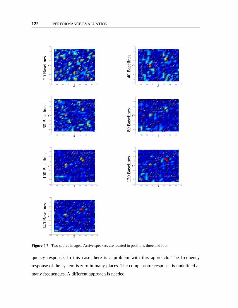
122 PERFORMANCE EVALUATION
quency response. In this case there is a problem with this approach. The frequency
response of the system is zero in many places. The compensator response is undefined at
many frequencies. A different approach is needed.
Figure 4.7 Two source images. Active speakers are located in positions three and four.
−0.4 −0.3 −0.2 −0.1 0 0.1 0.2 0.3 0.4−0.4
−0.3
−0.2
−0.1
0
0.1
0.2
0.3
0.4
X
Y
20 B
asel
ines
X
Y
−0.4 −0.3 −0.2 −0.1 0 0.1 0.2 0.3 0.4−0.4
−0.3
−0.2
−0.1
0
0.1
0.2
0.3
0.4
X
Y
40 B
asel
ines
X
Y
−0.4 −0.3 −0.2 −0.1 0 0.1 0.2 0.3 0.4−0.4
−0.3
−0.2
−0.1
0
0.1
0.2
0.3
0.4
X
Y
60 B
asel
ines
X
Y
−0.4 −0.3 −0.2 −0.1 0 0.1 0.2 0.3 0.4−0.4
−0.3
−0.2
−0.1
0
0.1
0.2
0.3
0.4
X
Y
80 B
asel
ines
X
Y
−0.4 −0.3 −0.2 −0.1 0 0.1 0.2 0.3 0.4−0.4
−0.3
−0.2
−0.1
0
0.1
0.2
0.3
0.4
X
Y
100
Bas
elin
es
Y
X−0.4 −0.3 −0.2 −0.1 0 0.1 0.2 0.3 0.4
−0.4
−0.3
−0.2
−0.1
0
0.1
0.2
0.3
0.4
X
Y
120
Bas
elin
es
X
Y
−0.4 −0.3 −0.2 −0.1 0 0.1 0.2 0.3 0.4−0.4
−0.3
−0.2
−0.1
0
0.1
0.2
0.3
0.4
X
Y
140
Bas
elin
es
X
Y

Deconvolution 123
While several techniques exist for deconvolution [Thomson, et al, 1994], only one will be
described here in detail. The AIT makes use of what is known as the CLEAN algorithm.
The deconvolution procedure represents a post processing step in the preparation of an
image. The technique was originally developed in 1974 by Hogbom [Cornwell, 1996].
The algorithm conceptualizes the sky as a bunch of point sources against a dark back-
ground. This assumption provides an implicit means of interpolating the missing visibility
functions. The main steps of the algorithm are shown in Figure 4.9.
Starting with the raw or dirty image, the algorithm selects the largest magnitude peak, P.
The nominal point-spread function is scaled by both P and γ. The quantity γ is a damping
Figure 4.8 Array Response as an LTI system.
Figure 4.9 The CLEAN Algorithm
H(ej(u+v))B(ξ,η) B’(ξ,η)
Start(Dirty Image)
Find Max. Peak
Sub. P*γ*PSF
Clean Image
|P| < ε ?
Add Residual(Dirty)from Dirty
Add P to Clean
|P|
Image

124 PERFORMANCE EVALUATION
which
ed from
ted by
(The
g the
peak
dirty
mmon
be of
10 and
clearly
en dis-
. The
e nega-
ixels
is sug-
Barring
ctua-
istake
that a
ertain
ally in
factor and must be chosen based on the complexity of the image and the ‘depth’ to
the cleaning process is to go. This scaled PSF is translated to the peak and subtract
the dirty image. At the same time that this occurs, a clean, model image is construc
adding a translated delta function of amplitude to the current model of the image
model starts empty). Essentially, the algorithm builds the clean image by interpretin
dirty image as a collection of delta functions. The procedure terminates when the
value of the dirty image falls below a certain threshold. The residual contents of the
array are added to the clean model at this stage. As a final step (not shown) it is co
practice to convolve the resulting image with a Gaussian beam, fit to the central lo
the PSF. This reduces apparent ‘super-resolution’ effects that sometimes occura.
The cleaned images of the one-source and two-source trials are shown in Figure 4.
Figure 4.11. The improvement over the raw images is remarkable. The sources are
defined and stand out against the background. The single source images have be
played showing both positive and negative intensity. These are unrectified images
two source images, as well as raw images shown earlier, have been rectified. Sinc
tive intensity has little physical meaning, the rectification sets all negative intensity p
equal to zero. The cleaned, single source images show a strong negative peak. Th
gests a uncorrected phase error appearing in some of the signals (Section 4.3.3).
the issue of rectification, few artifacts remain in the image and the background flu
tions are very low.
One notices indecipherable images in the 20 baseline configurations. This is not a m
in processing. It simply agrees with the warning given by Schwarz [Schwarz 1979],
minimum number of UV samples are required to ensure good results. Without a c
minimum amount of UV coverage, the PSF does not have enough definition, especi
the presence of noise.
a. Consider the deconvolution of simple, one-source image with an array that possesses a broad central beam (short baseline). The CLEAN method might identify the source as a point to precision greater than could be expected from an ideal filled aperture.
γP
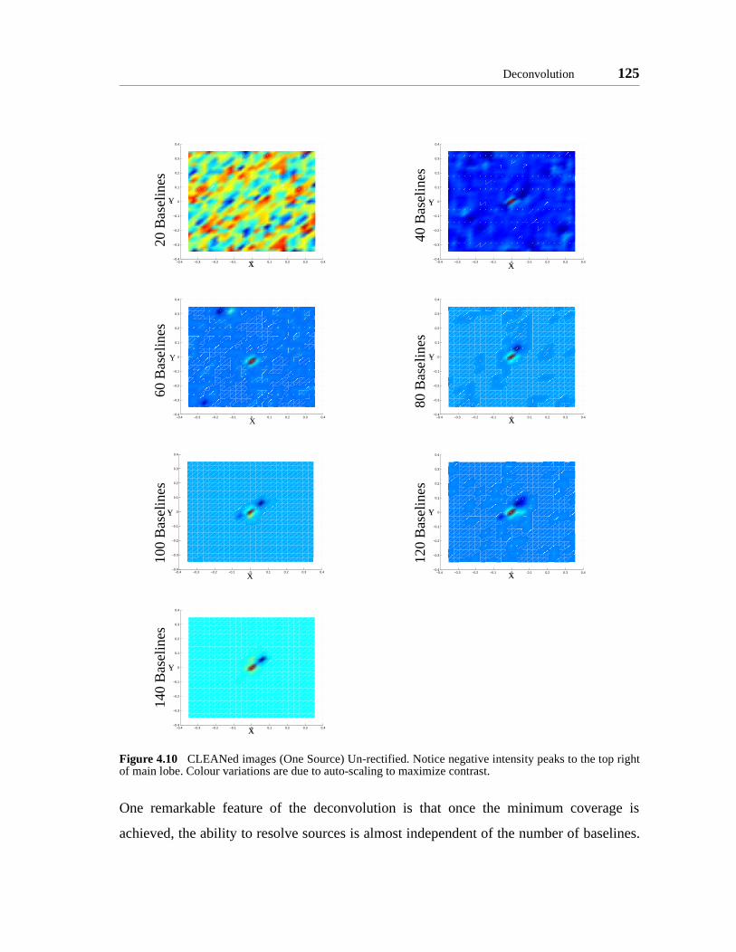
Deconvolution 125
One remarkable feature of the deconvolution is that once the minimum coverage is
achieved, the ability to resolve sources is almost independent of the number of baselines.
Figure 4.10 CLEANed images (One Source) Un-rectified. Notice negative intensity peaks to the top rightof main lobe. Colour variations are due to auto-scaling to maximize contrast.
−0.4 −0.3 −0.2 −0.1 0 0.1 0.2 0.3 0.4−0.4
−0.3
−0.2
−0.1
0
0.1
0.2
0.3
0.4
X
Y
20 B
asel
ines
Y
X −0.4 −0.3 −0.2 −0.1 0 0.1 0.2 0.3 0.4−0.4
−0.3
−0.2
−0.1
0
0.1
0.2
0.3
0.4
X
Y
40 B
asel
ines
Y
X
−0.4 −0.3 −0.2 −0.1 0 0.1 0.2 0.3 0.4−0.4
−0.3
−0.2
−0.1
0
0.1
0.2
0.3
0.4
60 B
asel
ines
Y
X−0.4 −0.3 −0.2 −0.1 0 0.1 0.2 0.3 0.4
−0.4
−0.3
−0.2
−0.1
0
0.1
0.2
0.3
0.4
X
Y
80 B
asel
ines
Y
X
−0.4 −0.3 −0.2 −0.1 0 0.1 0.2 0.3 0.4−0.4
−0.3
−0.2
−0.1
0
0.1
0.2
0.3
0.4
X
Y
100
Bas
elin
es
Y
X−0.4 −0.3 −0.2 −0.1 0 0.1 0.2 0.3 0.4
−0.4
−0.3
−0.2
−0.1
0
0.1
0.2
0.3
0.4
X
Y
120
Bas
elin
es
Y
X
−0.4 −0.3 −0.2 −0.1 0 0.1 0.2 0.3 0.4−0.4
−0.3
−0.2
−0.1
0
0.1
0.2
0.3
0.4
X
Y
140
Bas
elin
es
Y
X

126 PERFORMANCE EVALUATION
Granted, the AIT is observing very strong source emissions, but it still indicates the suc-
cess of even this primitive deconvolution.
Figure 4.11 CLEANed images (Two Sources) Rectified. Peaks are clearly defined
−0.4 −0.3 −0.2 −0.1 0 0.1 0.2 0.3 0.4−0.4
−0.3
−0.2
−0.1
0
0.1
0.2
0.3
0.4
X
Y
20 B
asel
ines
Y
X−0.4 −0.3 −0.2 −0.1 0 0.1 0.2 0.3 0.4
−0.4
−0.3
−0.2
−0.1
0
0.1
0.2
0.3
0.4
X
Y
40 B
asel
ines
Y
X
−0.4 −0.3 −0.2 −0.1 0 0.1 0.2 0.3 0.4−0.4
−0.3
−0.2
−0.1
0
0.1
0.2
0.3
0.4
X
Y
60 B
asel
ines
Y
X−0.4 −0.3 −0.2 −0.1 0 0.1 0.2 0.3 0.4
−0.4
−0.3
−0.2
−0.1
0
0.1
0.2
0.3
0.4
X
Y
80 B
asel
ines
Y
X
−0.4 −0.3 −0.2 −0.1 0 0.1 0.2 0.3 0.4−0.4
−0.3
−0.2
−0.1
0
0.1
0.2
0.3
0.4
X
Y
100
Bas
elin
es
Y
X−0.4 −0.3 −0.2 −0.1 0 0.1 0.2 0.3 0.4
−0.4
−0.3
−0.2
−0.1
0
0.1
0.2
0.3
0.4
X
Y
120
Bas
elin
es
Y
X
−0.4 −0.3 −0.2 −0.1 0 0.1 0.2 0.3 0.4−0.4
−0.3
−0.2
−0.1
0
0.1
0.2
0.3
0.4
X
Y
140
Bas
elin
es
Y
X

Uncertainty and Errors 127
ere a
terna-
CLEAN represents a simple method of image deconvolution. As described above it does
suffer from some drawbacks. First, it does require some intelligent iteration in application.
The threshold and damping values must be set manually, and the solution can in fact
diverge if poor choices are made of these initial parameters. As mentioned above, the
algorithm works by implicitly approximating visibility coefficients. These approximations
can be very good at moderate spatial frequencies. Unfortunately, the algorithm poorly cap-
tures both very short and very long spacings. Several improvements in the basic algorithm
are cited in [Thomson, et al, 1994] and [Cornwell, 1996] to address these issues. They also
discuss alternate means of deconvolution such as Maximum Entropy Methods. It was felt
that the scene complexity offered by the AIT speaker system did not warrant the imple-
mentation of these more advanced systems.
4.3 Uncertainty and Errors
A number of observed behaviours of the AIT fall short of expectations. As seen in
Figure 4.5 and Figure 4.7 noticeable distortion of the background response obscures the
nominal PSF pattern. Large peaks of negative intensity are found in close proximity to the
actual sources. This is especially noticeable in the un-rectified, CLEANed images. The
image artifacts such as the high background noise and spurious peaks, are repeatable.
Many factors could account for the observed under-performance. Certain evidence would
indicate that mechanical problems play the largest role in the image distortions. Random
noise was considered and discarded. Any random signals on the input channels would
simply give zero correlation. Besides which, the signals from the signal pre-amps appear
very clean. Common mode noise or cross talk could present a problem if it gave a finite
correlation. During development, some signal crosstalk was observed. A redesign of the
physical layout of the preamp circuitry eliminated the problem. Multipath effects were
also discounted. The signal from a single speaker, driven by a pure sine wave, appears
‘clean’ and constant in magnitude when captured by a microphone. If multipath w
factor, one would expect to see a beating effect with a stationary microphone. Al

128 PERFORMANCE EVALUATION
on
ation is
tively, moving the microphone would show varying amplitude. Neither of these phenom-
ena were observed.
Before presenting the analysis of the mechanical difficulties, the results of several consis-
tency tests will be presented. These were designed to establish the role of random and sys-
temic errors in the testbed operation.
4.3.1 Random Errors
In this section the effect of integration time is examined. Multiple visibility measurements
were made from the same location. Measurements were made both with multi-tone and
band-limited noise source signals. A discussion of the composition of these signals is
given in Section 3.2.3. The variability of the measurements with respect to the real com-
ponent, imaginary component, and magnitude were calculated. The results were averaged
and plotted with error bars as a function of integration time (Figure 4.12).
The error bars mark one standard deviation from the mean. The fluctuations in the mean as
integration time increases is very small, and the mean visibility at eight seconds (assumed
to be the ‘true’ visibility) lies within the one-sigma bound for all but a couple of points
the complex measurement of the noise-driven case. The normalized standard devi
Figure 4.12 Visibility measurement of two sources as a function of integration time. a) multi-tone signal b)band limited noise
0 1 2 3 4 5 6 7 8 90
0.5
1
1.5
2
2.5
3
3.5
Integration time (s)
Mea
sure
d V
isib
ility
a.
RealImaginaryMagnitude
0 1 2 3 4 5 6 7 8 90
0.5
1
1.5
2
2.5
3
3.5
Integration time (s)
Mea
sure
d V
isib
ility
b.
RealImaginaryMagnitude

Uncertainty and Errors 129
shown for both signal inputs is shown in Figure 4.13. The reduction in this value as a func-
tion of integration time appears to be linear. This is to be expected when one considers that
that averaging visibility measurements is equivalent to taking longer integration time.
The 5.5% deviation exhibited by the multi-tone source was considered acceptable. Thus,
most measurements were made using a two second integration time. The low-baseline
count array profiles used a higher value of five seconds. This variation seems to have min-
imal effect on testbed performance due to the presence of other errors. If the accompany-
ing error sources were reduced, longer integration times would be profitable.
4.3.2 Secular Variation: Extended Operations
Since the AIT is supposed be representative of a remotely operated spacecraft cluster,
extended operation without user intervention is a desirable trait. In this section, the results
of some extended operations tests are examined. Suggestions for improvement of the
extended operations mode are provided.
Figure 4.13 Normalized standard deviation (magnitude) as a functionof integration time.
1 2 3 4 5 6 7 80.01
0.02
0.03
0.04
0.05
0.06
0.07
0.08Multi−tone SourcesBL Noise Sources

130 PERFORMANCE EVALUATION
Limitations on continued testbed operations are imposed by the loss of position reference.
Since the motor encoders only operate in a differential mode, there is no absolute refer-
ence available to the system. Reliable operations can continue only as long as the corre-
spondence between the integrated position and the actual position is maintained. The
encoder hardware and motion controller are responsible for maintaining the pulse count
which specifies the arm motor position. There is no reason to believe that either piece of
hardware is prone to errors. However, observed behaviour would indicate that position
knowledge degrades over time.
The mechanism for the introduction of this error stems from the coupling between the
motor drive-shafts and the arms themselves. A tensioned cable drive transfers the torque
from the motors to the drum. The differential sizing of the threaded drive-shaft and the
larger drum provides gearing effects. While the cable is affixed directly to the drum, cable
is coupled to the drive shaft by friction alone. Slipping at this interface can cause a loss of
correspondence between the drum angle and shaft angle. Misalignment was observed after
an extended time operating (Figure 4.14). This usually manifested itself after about 150-
200 maneuvers.
This position error translates into a secular variation in measured visibility. To show this, it
is necessary to demonstrate a trend in the image data. This is difficult to quantify due to
the multi-dimensional nature of the problem. Since the information content of the image is
Figure 4.14 Misalignment of testbed drums in ‘homed’ position fol-lowing extended operations.
Alignment marks

Uncertainty and Errors 131
contained in the visibility measurements, an aggregate metric was defined to try to iden-
tify secular variations.
Consider repeating a imaging sequence several times without adjusting the apparatus.
Each image provides a set of visibility measurements Vi[k,l]. After normalizing the power,
(4.8)
An averaged visibility over k images can be defined:
(4.9)
Now, define the RMS Fractional Variation, ei of the real part of .
(4.10)
A similar equation can be defined for the imaginary component and magnitude. These
expressions were evaluated from the results of multiple imaging profiles. Tests were per-
formed on the seven different profile sizes described earlier. The results were very similar
and only one plot is shown here (Figure 4.15).
The shape of this curve suggests a secular variation over time. Since this analysis com-
pares each image to an average image, the trend in the data shows a movement towards
and then away from an average value. This is consistent with a gradual drift in the align-
ment over time. While the drift in magnitude appears to span a 30% range, little qualita-
tive change is apparent in the image, at least in the central field.
Vi’ k l,[ ]Vi k l,[ ]
1N2------ Vi r s,[ ] 2
s∑
r∑
------------------------------------------------=
V k l,[ ] 1k--- V'i k l,[ ]
i 1=
k
∑=
Vi’
ei1
N2------
ℜ V k l,[ ] V'i k l,[ ]–( )
ℜ V k l,[ ]( )--------------------------------------------------
2
l 0=
N 1–
∑k 0=
N 1–
∑=
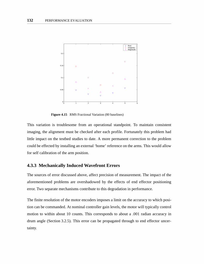
132 PERFORMANCE EVALUATION
allow
t of the
ioning
posi-
trol
acy in
uncer-
This variation is troublesome from an operational standpoint. To maintain consistent
imaging, the alignment must be checked after each profile. Fortunately this problem had
little impact on the testbed studies to date. A more permanent correction to the problem
could be effected by installing an external ‘home’ reference on the arms. This would
for self calibration of the arm position.
4.3.3 Mechanically Induced Wavefront Errors
The sources of error discussed above, affect precision of measurement. The impac
aforementioned problems are overshadowed by the effects of end effector posit
error. Two separate mechanisms contribute to this degradation in performance.
The finite resolution of the motor encoders imposes a limit on the accuracy to which
tion can be commanded. At nominal controller gain levels, the motor will typically con
motion to within about 10 counts. This corresponds to about a .001 radian accur
drum angle (Section 3.2.5). This error can be propagated through to end effector
tainty.
Figure 4.15 RMS Fractional Variation (80 baselines)
0 1 2 3 4 5 60
0.05
0.1
0.15
0.2
Real ImaginaryMagnitude

Uncertainty and Errors 133
For an arbitrary function error propagation dictates:
(4.11)
Applying this to the forward kinematics equations (3.14, 3.15) and combining the two dis-
placement components:
(4.12)
(4.13)
(4.14)
The phase error in the received signal is caused by the differential pathlength between the
calculated and actual location. Since the wavefront correction is based on the estimated
location of the end effector, if the position knowledge is in error, the correction process
may fail to completely correct for wavefront effects. The worst-case DPL is encountered
when the error displacement is radially away from the centre of the imaging plane. Con-
sider that the displacement will put the microphone at the modified position . The
DPL is then:
(4.15)
This DPL can then be transformed into a phase error. This phase error is shown for arm 2
in Figure 4.16. Please note that the axes represent the workspace extent in local coordi-
nates.
This error is modest over the lower half of the figure. While accuracy to one degree is
desirable, the maximum excursion is not too great. In the upper half of the workspace, the
degradation is more severe due to the sensitivity between drum and position error in these
F F x1 x2 x3 …, , ,( )≡
∆Fx1∂
∂F ∆xi 2
x2∂∂F ∆x2
2…+ +=
∆x l1 θ1cos( )2 ∆θ1( )2⋅ l2 θ2 θ1–π2---+
θ1 θ2 θ1–π2---+
θ1sinsin–coscos ⋅
2∆θ2( )2⋅+=
∆y
2–( )l2 θ2 θ1–π2---+
θ1coscos θ2 θ1–π2---+
θ1sinsin+ l1 θ1( )sin–⋅
2∆θ1( )2 +⋅
l2 θ2 θ1–π2---+
θ1coscos θ2 θ1–π2---+
θ1sinsin+ ⋅
2∆θ2( )2⋅
=
∆r ∆x( )2 ∆y( )2+=
x’ y’,( )
DPL x’2 y’2 h2+ + x2 y2 h2+ +–=

134 PERFORMANCE EVALUATION
regions. If this were the only difficulty, adjustment of controller gain might remove some
of the variation.
Unfortunately, another factor exacerbates the phase problem. The arm is essentially canti-
levered off the central shaft. At large extension, gravity exerts considerable torque on the
bearings and other mechanisms. Even with no tip-loading, vertical deflection of the end
effector has been observed. A visible observation suggest that this arises from play in the
bearings and flexure of the drum webs. A 1 cm vertical deflection has been observed when
the arm is at full deflection. Re-evaluating the DPL (Eq. 4.15) calculation gives:
(4.16)
For purposes of illustration, a parabolic vertical deflection was hypothesized. Vertical
deflection can be parameterized in terms of the distance of the end effector from the hub:
(4.17)
Figure 4.16 Phase Error Distribution for Arm 2.
Pha
se E
rror
(de
g)
−20
−15
−10
−5
0
5
0.3 0.4 0.5 0.6 0.7 0.8 0.9 1 1.1 1.20.3
0.4
0.5
0.6
0.7
0.8
0.9
1
1.1
1.2
X(m)
Y(m
)
DPL x’2 y’2 h δh+( )2+ + x2 y2 h2+ +–=
δh m r rmin–( )2 m,δhmax
rmax rmin–( )2---------------------------------= =

Uncertainty and Errors 135
This deflection expression is somewhat arbitrary, but the results are very similar when a
linear deflection is used. The phase error can then be reevaluated. This is shown in
Figure 4.17.
These errors are enormous. An uncorrected phase shift of a third of a wavelength can
wreak havoc with the measurement of visibility. The strong negative peaks seen in the
cleaned images in Figure 4.10 are thought to be the result of this effect. This uncorrected
phase perturbation distorts many of the visibility measurements. This distortion can then
cause the main lobe power to appear in different locations. Instead of adding construc-
tively, this distorted visibility creates ghost peaks.
This deflection problem resisted mechanical fixes. Adjustment of the bearing loading
yielded some improvement. Stiffening the drum webs also provided some benefits. Unfor-
tunately, the 1 cm deflection quoted above was actually measured after these modifica-
tions. In the short term, careful characterization of this deflection would allow software
correction to remove this phase error at the signal processing stage (Section 3.3.9). These
corrections would still be open loop; their performance would depend on modelling accu-
Figure 4.17 Phase Error due to end-effector uncertainty and verticaldeflection.
Pha
se E
rror
(de
g)
10
20
30
40
50
60
70
80
90
100
110
0.3 0.4 0.5 0.6 0.7 0.8 0.9 1 1.1 1.20.3
0.4
0.5
0.6
0.7
0.8
0.9
1
1.1
1.2
X (m)
Y(m
)

136 PERFORMANCE EVALUATION
racy. Longer term improvements might necessitate re-engineering the arm design or add-
ing a height sensor.
4.4 Performance Conclusions
The AIT has demonstrated the ability to act as an automated imager for the validation of
interferometer profiles. After receiving the profile description from the virtual ground sta-
tion, the appointed cluster leader is able to coordinate action. Visibility is calculated using
a computationaly efficient, parallel correlation algorithm. These measurements are col-
lected and forwarded to the VGS, where they are synthesized into an image. The strategy
is flexible and can accommodate an arbitrary number of satellites.
Imaging using the AIT is rapid and requires little intervention from the user during nomi-
nal operations. The DIPSI communications protocol is an enabling technology that allows
discourse between the satellites. Representing an effective vocabulary for interferometry,
it serves as a medium through which higher-level functionality can be added.
Chapter 5 examines issues of artificial intelligence as it relates to cluster applications. It
discusses autonomous features implemented and proposed for the AIT and provides sug-
gestions for future examinations of cluster autonomy.
Sadly, the degradation of image quality caused by mechanical difficulty prevented
advanced validation of the optimized array configurations. While validated at the qualita-
tive level, quantitative performance assessment was not possible. Permanent improvement
would likely require redesign of the robotic hardware.
Very encouraging results were observed using the CLEAN algorithm as a tool for decon-
volution. The resulting images suggest that in some situations where detection is more
important than high resolution imaging, good results can be obtained with only a small
number of visibility samples.

Chapter 5
ARTIFICIAL INTELLIGENCE AND AUTONOMY
lli-
dmit-
and
The intertwined topics of artificial intelligence (AI), and autonomy have many applica-
tions to space missions. Developing a clear understanding of the issues involved can be
difficult. There is first the question of vocabulary: AI and autonomy mean different things
to different people. They exist not so much as well defined classifications, but rather as
overlapping, nebulous concepts. In order to foster a better understanding of these con-
cepts, it is insightful to start with high-level definitions and examine some of the common
approaches to these topics. Specific application to space systems will also be discussed.
Following this background information, the particular implementations seen on the AIT
will be examined. Autonomy and AI algorithms currently implemented or planned for the
AIT are outlined.
5.1 Artificial Intelligence
The field of artificial intelligence is a very broad one. Research in the latter half of this
century on what is commonly referred to as AI has borrowed inspiration from many fields:
logic, philosophy, mathematics and biology to name a few. The breadth of approaches and
applications is so great that one of the only unifying definitions is that “…artificial inte
gence attempts to understand intelligent entities [Russell and Norvig 1995, pp 3].” A
tedly, this definition is too broad to be useful. However, venturing a little deeper
examining the common approaches to AI is more illuminating.
137

138 ARTIFICIAL INTELLIGENCE AND AUTONOMY
wing
espon-
movies
5.1.1 AI Approaches: Outlining the Field.
In their book on Artificial intelligence, Russell and Norvig [Russell and Norvig 1995] sug-
gest classification of AI research in terms of the approach taken. An adaptation of their
scheme is shown in Table 5.1.
Expanded examination of the details of these schemes is informative.
Thinking Like Humans
Concerned with the modeling and description of the way humans think, this area if inquiry
is often labeled with the term cognitive science. By definition, the task is impossible with-
out an understanding of how humans in fact think. Hence this area of research is often
paired with clinical studies designed to assess the mechanisms of human thought.
Acting Like Humans
This branch of research probably represents the colloquial definition of AI. Can the
breadth of human activities be replicated in a machine? Can machines be made to think?
The classical thought experiment of the Turing Test arose from this line of inquiry. Alan
Turing posited that a machine could be considered ‘intelligent’ if a human intervie
the machine (via a terminal or some such device) could not establish whether the r
dent was human or not. This concept has entered into popular culture through such
as Blade Runner.
TABLE 5.1 Common Approaches to Artificial Intelligencea
a. Adapted from Russell and Norvig 1995
Humanist Rationalist
Cognitive Thinking like Humans Thinking Rationally
Behavioural Acting like Humans Acting Rationally

Artificial Intelligence 139
tems
r con-
in spe-
tems.
ulty
om
poor
d, the
rongly
indley
oals,
ssion
n
d
ed a
pan-
d exe-
sub-
tions,
ly
t exist
Thinking Rationally
This approach to artificial intelligence is sometimes referred to as the ‘Laws of Thought’
or logicist method. It is deeply linked to the study of modern logic theory. These sys
are often concerned with the process of representing knowledge, and drawing furthe
clusions through an inference process [Kirsch 1991]. These have been successful
cialized applications such as automated theorem provers or ‘expert’ sys
Unfortunately, implementations based purely on rational thought often run into diffic
in transition from ‘toy’ problems to the real world [Lindley 1995]. This often stems fr
two problems. First, the inferencing procedures commonly adopted demonstrate
computational efficiency when applied in real-time applications [Maes 1993]. Secon
knowledge representation schemes are often ‘brittle’; performance depends very st
on the degree to which the features of the world can be modeled and described [L
1995].
Acting Rationally
Acting rationally is concerned with the process of “…acting so as to achieve one’s g
given one’s beliefs[Russell and Norvig 1995].” A construct that arises from the discu
of rational behaviour is that of the intelligent agent. Russell and Norvig use rational actio
as a defining principle of the agent-based approach to AIa. These entities are concerne
with the intelligent mapping of perception to action. Intelligent Agency is consider
fundamental principle of modernist AI. Implementation can be simple or complex; s
ning the range from simple, reflexive responses to evolved utility based planning an
cution.
One particularly interesting feature of the ‘acting rationally’ approach is the ability to
sume other techniques. While logical inference may be very useful in some situa
many times an agent must do something even without knowing that the action is provab
correct. When designing systems with the focus of rational action, mechanisms mus
a. In contrast [Lindley 1995] extends the intelligent agent approach to include some work in logicist AI.
140 ARTIFICIAL INTELLIGENCE AND AUTONOMY
ion of
stems
uta-
ieldy.
eived
situa-
s. Rea-
ystems
995].
input,
rtual
the
works
to allow the agent to make decisions when constraints of time or perception preclude opti-
mum decisions. Thus, such entities can use layered decision making systems combining
logical inferencing, neural networks, fuzzy logic and other techniques [Powell, et al
1998]. These techniques each have their own domain of efficacy when dealing with prob-
lems with different amounts of uncertainty and complexity.
5.1.2 Approaches to Reasoning Systems
In this section, several of the more common approaches to AI are introduced. These
descriptions are not meant to be exhaustive or even very deep. They serve as a quick out-
line of the rationale behind some of the more popular techniques.
Rule-Based Systems
Also known as ‘expert’ systems, rule-based reasoning schema utilize a combinat
expert knowledge and an inferencing engine to deal with problems. Usually these sy
are limited in application to very narrow domains [Sary & Werking 1997]. The comp
tion required to search through complex systems often makes broad application unw
Model-Based Reasoning
This technique is a type of logical inferencing based on causal rules. A preconc
model of the world describes the effects produced by hidden causes. Hypothetical
tions are modeled and the predicted observations compared to the true observation
soning is less concentrated on ‘first-principles’ than rule based systems. Causal s
typically allow strong conclusions to be drawn about the world [Russell and Norvig 1
Neural Networks
The study of neural networks uses small computational units to represent multi-
multi-output functions. Patterned after simple models of the brain, networks of vi
neurons (or perceptrons) can be trained to respond to certain input/output pairs. Once
training period is over, they are left to respond to new data on their own. Neural net

Artificial Intelligence 141
rocess
dom’
s-over
earch
ruth to
the
n suc-
ell, et
sing a
ttempts
These
intelli-
nomous
intel-
can be adapted to a variety of applications but in some situations, especially where
‘explainable’ decisions are required, their applications are limited.
Genetic Algorithms
Genetic Algorithms represent a learning, optimization system patterned after the p
of natural selection. Provided with a means of evaluating the usefulness of a ‘ran
solution, useful candidates are retained, while poor performers are eliminated. Cros
between different individuals and random mutation provide for expansion of the s
space.
Fuzzy Logic
Fuzzy Logic allows reasoning about vagueness. Propositions have a degree of t
them. “Fred is sort of tall.” is a fuzzy statement. Fred’s height may be known but
degree to which he is tall is what is being discussed. While fuzzy systems have bee
cessful in simple applications, they do not handle complex systems very well [Pow
al 1998].
Case Based Reasoning
This technique attempts in part to mimic the problem solving process of humans. U
database compiled from previous problems and solutions, case-based reasoning a
to solve new problems based upon their similarity to those previously encountered.
systems are typically easy to set up and maintain.
The techniques described above are just a smattering of the approaches to artificial
gence. They can all be employed to greater or lesser degrees in the design of auto
agents. But what is autonomy? An attempt to understand the application of artificial
ligence to space systems is presented in the next section.
142 ARTIFICIAL INTELLIGENCE AND AUTONOMY
5.2 Autonomy
Autonomy, like artificial intelligence, is a broad and nebulous subject. It has had applica-
tions to space systems in various capacities for many years. Recently efforts to reduce the
cost of mission operations has altered the perception of spacecraft autonomy. Once seen as
a last resort, it is now an attractive tool [Powell, et al 1998]. It has been estimated that
employing autonomy can translate into savings of up to 60% in the operations cost of a
typical earth orbiting mission [Doyle 1997].
System autonomy as the ability to function without human intervention is not a new idea.
Deep space missions, such as those typically under the provenance of the Jet Propulsion
Laboratory, have required spacecraft to function without ground support. Remoteness and
its side effects (bandwidth, occultation, time-of-flight) drove the development of at least a
minimal level of autonomous function.
Not all autonomous systems are equal. At any given level of technical heritage, it is possi-
ble to find the right balance between autonomous and user directed function.
5.2.1 Classifications of Autonomy
Implementation of autonomy can be described on many axes. The balanced role in deci-
sion-making between space assets, ground computers, and human operators is one axis.
The choice of which systems and activities to include represents another. Faced with a
desire to codify some of these possibilities, the Air Force commissioned a study from JPL.
Out of this program came the level of autonomy scale presented in Table 5.2 [Marshall
1981]. The representative level of autonomy can vary between missions, and even
between subsystems. Implementation of autonomy can even be varied temporally. Staged
deployment of higher autonomy levels over the mission lifetime has been considered for
certain applications[Powell, et al 1998].
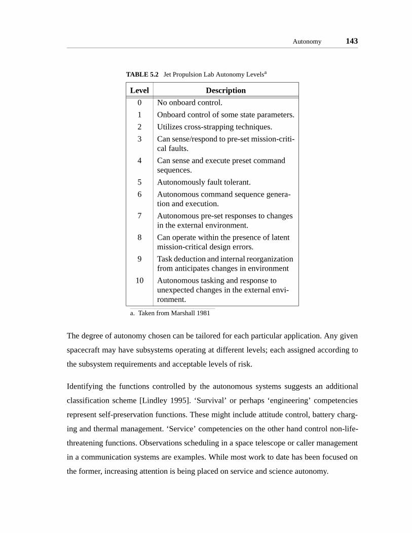
Autonomy 143
cies
harg-
n-life-
gement
sed on
The degree of autonomy chosen can be tailored for each particular application. Any given
spacecraft may have subsystems operating at different levels; each assigned according to
the subsystem requirements and acceptable levels of risk.
Identifying the functions controlled by the autonomous systems suggests an additional
classification scheme [Lindley 1995]. ‘Survival’ or perhaps ‘engineering’ competen
represent self-preservation functions. These might include attitude control, battery c
ing and thermal management. ‘Service’ competencies on the other hand control no
threatening functions. Observations scheduling in a space telescope or caller mana
in a communication systems are examples. While most work to date has been focu
the former, increasing attention is being placed on service and science autonomy.
TABLE 5.2 Jet Propulsion Lab Autonomy Levelsa
Level Description
0 No onboard control.
1 Onboard control of some state parameters.
2 Utilizes cross-strapping techniques.
3 Can sense/respond to pre-set mission-criti-cal faults.
4 Can sense and execute preset command sequences.
5 Autonomously fault tolerant.
6 Autonomous command sequence genera-tion and execution.
7 Autonomous pre-set responses to changes in the external environment.
8 Can operate within the presence of latent mission-critical design errors.
9 Task deduction and internal reorganization from anticipates changes in environment
10 Autonomous tasking and response to unexpected changes in the external envi-ronment.
a. Taken from Marshall 1981

144 ARTIFICIAL INTELLIGENCE AND AUTONOMY
some
Automatic data reduction in scientific missions maximizes science payoff for a fixed cost
[Sterling 1998]. Although scientists have traditionally been leery of anything but
untouched data, economic practicalities are starting to sway general opinion. Similar eco-
nomic realities are responsible for the development of autonomous resource management
systems for space constellations. Direct ground-based administration of communications
systems like Teledesic or Iridium would be grossly inefficient. Facilities for automated
call management is a central part of their systems design. [Vasudevan et al 1996]
5.2.2 Roles of Autonomous Systems in Space
Many uses of intelligent systems have been implemented or envisioned for space systems.
Some represent advanced tools facilitating ground interaction with the spacecraft. Other
implementations grant greater self-direction to the onboard systems. In this section, some
of the common applications of autonomous systems are examined.
Automatic Code Generation (ACG)
Much of the research in command, control and communications centre around the devel-
opment of a high-level, standardized language with which to control space systems [Pow-
ell, et al 1998]. One particular example of such a system was the Spacecraft Command
Language (SCL) employed on the Clementine lunar mission [Buckley & Van Gaasbeck
1994]. High level operational scripts to manage resources and tasks are automatically con-
verted into the lower level machine code to effect those actions. The automated generation
of low level machine code from high-level directives facilitates human-in-the-loop inter-
actions. This effect is particularly noticeable when the code generation also involves tem-
poral planning and scheduling.
Fault Detection, Identification and Mitigation
One might consider a spacecraft safing operation to be a primitive implementation of
autonomy. Upon detecting unexpected or dangerous conditions, the spacecraft shuts-down
non-essential functions and ‘calls for help.’ This response is unsatisfactory during

Autonomy 145
to be
ediate
acecraft
ft activ-
s, or
et al
over-
tasks.
space
d with
limited
y fail-
mission critical activities however. For instance, the Saturn Orbital Insertion of the Cassini
probe must be done autonomously, hidden from a direct view of the earth. If the spacecraft
experiences failures during the thruster firing, it must be capable of (limited) self-recovery
[Pell et al 1998]. Even when a safe mode is a possibility, continued operation, albeit in a
degraded state is often preferable to completely paralyzing the spacecraft.
The fault detection systems often combine fuzzy logic or neural-networks together with
rule or model based expert systems. One example of such a system is the Mode Identifica-
tion and Reconfiguration (MIR) module in the Remote Agent architecture [Bernard et al
1998]. Developed by NASA Ames and employed in an experiment on the Deep Space I
probe, MIR attempts to detect component failures. The module maintains a finite state
machine representation of the spacecraft which it compares to observed state parameters.
Failed systems can then be circumvented as hardware permits.
Procedure Planning and Execution
This field is related in some respects to that of the automated code generation. While ACG
is predominantly viewed as a ground based tool, ‘planners’ are often considered
spacecraft based applications. Planning concerns itself with the generation of interm
steps between a start condition and a specified goal. Care must be taken that the sp
is not put into a dangerous state in the process of plan execution. Certain spacecra
ities may involve time criticality, simultaneous coordination of several subsystem
complex prerequisites. Correct ordering can be vital to mission success [Bernard
1998]. In general, this problem is NP complete [Powell, et al 1998]. Without human
sight or good heuristics for search, space implementation may be limited to modest
The scalable nature of autonomy implementation allows a mixture of ground and
based planning. Major sequencing operations could be completed on the groun
allowance made for some space-based adjustments. Allowing the spacecraft a
scope for replanning can have many benefits. This replanning could be motivated b
ures [Pell et al 1998] or specific targets of opportunity [Bernard et al 1998].

146 ARTIFICIAL INTELLIGENCE AND AUTONOMY
thout
men-
onigs-
small
tion is
it can
blem
s heu-
f sub-
alable
und-
trans-
pro-
mous
cessing
guage
Behavioural Agents
This class of agents can probably be considered closer to control theory than conventional
AI. Modeling the agent as a dynamic system allows the derivation of control formulae.
This principle can be applied to satellite navigation [Deutschmann et al 1998], orbit main-
tenance [Konigsmann et al 1996], and even simple constellation management [Radice at al
1998]. Typically the agents do not ‘understand’ what they are doing; they react wi
memory of past actions or any long term strategy in mind. Consequently, their imple
tation must be engineered to provide some protections to prevent mission loss. K
maan proposes a system in which the agent uses a simple control law to fire a very
thruster for orbit maintenance. Each orbit, the agent checks to see if micro-correc
necessary. In the worst case, the agent thrusts in the wrong direction. The authority
exert is very small, and operators on the ground will undoubtedly notice the pro
before it becomes dangerous.
Another approach to this type of agent is to use such simplified control strategies a
ristics to limit the search space in more informed techniques or for the generation o
goals in planning.
5.3 Autonomy and the AIT
The autonomy development on the Acoustic Imaging Testbed has followed a sc
approach. Improved capabilities are first implemented in Matlab, an analogy for gro
based planning systems. As the algorithms are verified, they are parallelized and
ferred to the satellite platform. Several competencies installed in the VSC and VGS
grams are examined. Suggested algorithms for further implementation of autono
behaviour are suggested along with implementation strategies
5.3.1 Ground Autonomy
The usual maxim that applies to space computation applies here as well. Space pro
always lags behind ground processing. The virtual spacecraft are written in the C lan

Autonomy and the AIT 147
and have access to all the appropriate language features. The user interface is a Matlab
script. While C is very flexible, Matlab scripting is an undeniably faster way of rapidly
prototyping computational algorithms. Over the course of AIT development, operations
were first verified from the Matlab client before transferring the intelligence to the satel-
lites. Some tasks are still performed on the ground.
Motion Planning
The array configuration for an imaging sequence is stored in a text file as a list of UV dis-
placements. Before the spacecraft can be commanded to follow the profile, these baselines
must be converted into testbed coordinates. In an ideal space-based interferometer, these
profiles would remain centred around a common point. Spacecraft positions would then be
directly scaled from the UV points. The AIT represents a heterogeneous system. Arm 0 is
shorter than arm 2 and consequently both VSCs do not have equal mobility. Each baseline
must be fit into the imaging plane of the testbed such that both endpoints can be reached
by the arms (Figure 5.1).
Figure 5.1 Workspace accommodation
Workspace 2
Workspace 0
Centred B
aseline
Fit Baseline

148 ARTIFICIAL INTELLIGENCE AND AUTONOMY
in a
e fuel
uence
tilizes
ould
nts are
tions.
when
. This
since
ly, it is
ts of a
n be
‘stop’
The baseline placement can be formulated as a constrained optimization. Starting with the
baseline description (a cartesian vector) the endpoints must be chosen. These endpoints
are chosen so that the centre of the baseline is as close to the centre of the testbed as possi-
ble, subject to the workspace constraints of the arms. The constraints represent the maxi-
mum and minimum radii and the edges of the imaging plane. The cost function can be
expressed as:
(5.1)
Other possible cost functions might be to minimize the differential path length (reducing
wavefront correction) or to minimize the movement from the last imaging location. The
choice of cost function has a minimal effect on testbed operations. This isn’t true
space-based interferometer. Greater effort would have to be expended to minimiz
usage and time spent.
Once selected, the spacecraft positions are collected into a formal imaging seq
which can be sent to the VSCs through the ground station. This communication u
DIPSI (Section 3.3.5) for its formatting.
While the AIT doesn’t represent a dynamic system, a ‘real’ space interferometer w
require cluster-level autonomy to oversee spacecraft maneuvering. These requireme
much more central to survival than those encountered with widely spaced constella
Two examples come immediately to mind. First, safeguards should be incorporated
coordinating operations to prevent the firing of thrusters directly at one’s neighbours
problem has some similarities to arm collision avoidance. The connection is weak
the design of the testbed reduces the necessity of collision considerations. Second
also desirable to reduce the chance of collision. Since free-space motion consis
‘start’ thruster pulse, followed by a ‘stop,’ a system failure in the intervening time ca
hazardous. Timing again comes into play to sequence the firings so that a missed
cannot lead to collision.
C x y,( ) x xc–( )2 y yc–( )2+=

Autonomy and the AIT 149
ated at
p vis-
elines.
aseline
st be
ers of
rofile
ration
ven
eneral
ember
n the
estion
itive
ener-
, given
al ori-
of the
ering
es
limit-
ntelli-
ear.
Multiple Arm Profile Generation
The optimizations of array configurations presented by Kong [Kong, et al 1998] are of two
types. The first type are known as ‘snapshot’ images where all baselines are gener
once. The second type represents ‘incremental’ profiles where two spacecraft build u
ibility samples, one baseline at a time. Difficulty arises in the consideration of n-satellite,
reconfigurable arrays. Snapshot arrays give poor images at low numbers of bas
Given that the array is being reconfigured, there is no guarantee that the higher b
cases are still efficient. The following is discussion of some of the issue that mu
addressed when considering the application of incremental profiles to greater numb
spacecraft.
Intelligent imaging strategies must consider two problems. The first deals with p
optimizations under nominal conditions. In these circumstances, the array reconfigu
problem is concerned with optimizing visibility coverage (or image quality) for a gi
number of spacecraft and reconfigurations. The second problem deals with a more g
case. This problem examines the behaviour of the array when the number of m
spacecraft is not fixed. The desire to continue operations, without intervention, i
event of spacecraft failures (or additions) is the key requirement. While some sugg
for approaching the problem are offered, further work is required before defin
answers can be given.
The optimization of visibility coverage for a two spacecraft array is a somewhat deg
ate case. Only one baseline need be considered per reorientation. Furthermore
equally maneuverable spacecraft, motion is always simply mirrored through a centr
gin. The optimization procedure described by Kong considers the placement of one
spacecraft in half of the imaging plane. The other is implicitly mirrored and maneuv
domains do not overlap. In contrast, for n-spacecraft each reconfiguration creat
baselines, of which can be chosen independently. It is not clear that
ing the motion of each spacecraft to a non-overlapping wedge of radians is an i
gent decision. The most effective method of performing these optimizations is not cl
n n 1–( )2
-------------------- n 1–2πn
------

150 ARTIFICIAL INTELLIGENCE AND AUTONOMY
of
them
ura-
er of
the
raft. If
the tri-
A slightly different problem addresses the adaptation of a given set of visibility samples
(baselines) to an arbitrary number of spacecraft. This approach takes the view that a given
coverage optimization has a certain worth and that re-calculating the optimization when
the number of spacecraft changes is undesirable. Take for instance the problem of fitting
an incremental profile to a three spacecraft cluster. The fundamental element of a profile
are the baselines. In a three spacecraft case, three visibility measurements are made simul-
taneously. The constraint however is that the baselines must form a triangle. In general,
the individual baselines from the simple incremental case cannot be arranged into sets of
triangles. This leads to two alternatives. The first would select two optimized baselines per
configuration. The third would be left to ‘float’. This still leaves four possible ways
constructing each configuration. It is not clear how to intelligently decide between
(Figure 5.2). An alternate approach would involve approximating the optimal config
tions by ‘fitting’ the ideal baselines into triangles. This would maintain the total numb
visibility samples. It may however destroy the ‘optimal’ nature of the array profile if
baselines cannot be easily fit into triangles.
What is needed are profiles designed for reconfigurable arrays of multiple spacec
the UV points can be generated in triples the problem is then reduced to translating
Figure 5.2 Partial fit of optimal baselines. Two free baselines and fourarray configurations are possible

Autonomy and the AIT 151
ofile.
olved.
rec-
rk for
ities
city as
tion
a lan-
iety of
s for
abili-
meta-
e very
ples into testbed coordinates. Some initial work was implemented on the position selection
for multiple spacecraft. Discussion of the method is given in Section 5.4.
5.3.2 On-Board Autonomy
The earliest VSCs did none of the processing onboard. Their entire data-set was routed
through the VGS to the Matlab client. This was a very inefficient methodology as the
socket stream was not optimized for high volume traffic. The VSCs are now responsible
for autonomously processing their own data. Signal processing consists of data exchange,
interpolation (for wavefront correction) and correlation. These activities are explained in
more detail in Section 3.3.9.
Likewise, motion selection has partially migrated from ground to space. Sequencing,
while once commanded position by position, is now handled automatically. The operator,
through the VGS, designates a ‘lead’ spacecraft and provides it with a position pr
This VSC is then responsible for requesting services of the other spacecraft inv
While the inter-spacecraft negotiation is rather primitive, it does have the capability to
ognize some problems and request help from the user.
Much of the time investment to date has been concerned with laying the groundwo
more evolved intelligence. The DIPSI protocol allows description of most of the activ
representative of space interferometry. Further development could improve its capa
a formal language.
One of the difficulties with multi-agent systems is that of inter-agent communica
[Lindley 1995]. The process of sharing knowledge and coordinating actions requires
guage that balances expressiveness with determinism. The ability to articulate a var
sentences without ambiguity is the crux of the problem. DIPSI contains mechanism
simple inter-agent communication. Further work would aim at expanding these cap
ties. An important new addition to the VSC competency would be some degree of
reasoning. The ability to judge the degree of truth of another agent’s statement can b

152 ARTIFICIAL INTELLIGENCE AND AUTONOMY
ent,
e other
of the
ts, and
exam-
lgo-
ion for
anner
e clus-
motion
, four
s in the
must
figura-
oblem
useful. These facilities are particularly important if one VSC is behaving erratically,
potentially in a failed state. Being able to build consensus among cluster members as to
the state of their fellows, is crucial to the diagnoses of cluster-based faults.
Charting the proposed development of the AIT autonomy would show two main branches
of study. One would be the implementation of ‘small’ intelligences; motion placem
workspace management, etc. These are task-specific, self-contained strategies. Th
branch would be the enrichment of the agent environment. Generalizing the format
knowledge base (what a VSC ‘knows’), enabling discourse about the state of agen
the advanced handling of resource negotiation are a few examples. Even the former
ples are not trivial. The later will require significant work to achieve. The distributed a
rithm for a proposed simple intelligences are presented in the next section.
5.4 Algorithms in Development
This section examines a proposed algorithm for the generalized maneuver allocat
an n-spacecraft cluster. This task is intended to be implemented in a distributed m
across an arbitrary number of satellites. Given a predetermined array orientation, th
ter must maneuver to create the required baselines. An additional constraint on this
is added by imposing a limited range of motion, or workspace, for each spacecraft. An
abstraction of this task is represented in Figure 5.3.
The problem begins by specifying an array configuration. In a four spacecraft case
vertices (or three vectors) describe the shape of the array. The other three baseline
figure are represented implicitly. The centroid (or any other fixed point) of the array
then be adjusted so that each of the vertices Vi lie within the workspace Wj. Each work-
space (possibly overlapping) is associated with a satellite. In order to accept a con
tion, it must be possible to associate each vertex with a different workspace. This pr
is related to the matching problem in bipartite graphs.

Algorithms in Development 153
A bipartite graph(Figure 5.4) is a graph B, comprised of two sets of nodes (U, V), and a set
of edges (or arcs) E. This is denoted:
(5.2)
The edges are subject to the constraint that each must connect a node of V to a node of U.
Figure 5.3 The configuration placement problem. Dotted lines indicateimplicit baselines.
Figure 5.4 A bipartite graph. Heavy lines are represent a matching
W0 W1
W2W3
V3
V4
V0
V2
C
B V U E, ,( )=
V UE

154 ARTIFICIAL INTELLIGENCE AND AUTONOMY
A matching M, is the set of edges from E, subject to the constraint that no two edges of M
share a common node. The maximum matching of a graph B, is a matching with the great-
est possible number of edges. Furthermore, if , that is if the number
of edges in M is equal to the number of nodes in U or V, the matching is said to be com-
plete.
Consider the following algorithm for the cluster problem (Figure 5.5). One spacecraft, Sj
proposes a centroid location . Each constituent spacecraft (or node) evaluates
their judgement of the suitability of the plan. Each will generate an array describing which
vertices lie within their workspace and possibly any preferences they may have. This
information forms an matrix describing edges in the bipartite graph
formed by the workspace and vertices. If the configuration is suitable, i.e. a complete
matching is found, the plan can be accepted (and perhaps refined). If a complete matching
cannot be found a new centroid location must be proposed.
The following is a description of the validation algorithm and a proposed scheme for
updating the centroid location. The maximum matching algorithm is a classic graph-the-
ory optimization. The algorithm presented is taken from [Papadimitriou & Steiglitz 1982].
The updating concept is a crude heuristic. While it appears to work, it can certainly be
refined. This scheme has been implemented in the specialized case of three spacecraft.
The refinement of an acceptable plan will not be discussed here.
Figure 5.5 Algorithm for vertex placement
M min V U,( )=
Ci xi yi,( )=
n 1–( ) n 1–( )×
ProposeCentroid
CollectResponses
CompleteMatching?
Formulatenew plan
Accept/Refine Plan
YesNo

Algorithms in Development 155
5.4.1 Bipartite Graph Matching
The maximum matching problem in un-weighted, bipartite graphs can be reduced to the
common problem referred to as the Max-Flow Problem. From the bipartite graph B
defined above, the simple network N(B), is created (Figure 5.6).
Note that B is now considered a directed graph (i.e. the edges have a direction associated
with them). This does not change the problem. The network is considered simple because
each node in V has unity inflow and each node in U has unity outflow. The maximum flow
problem can be solved with any max-flow algorithma. The complexity of the algorithm is
. One such max-flow algorithm is given in [Papadimitriou & Steiglitz 1982
pp. 205].
For reasonably sized arrays, this operation will probably be performed on the lead space-
craft, without any attempt to further parallelize the verification stage.
5.4.2 Centroid Updating
If the matching generated by the validation stage is not complete, a new centroid must be
proposed and the process started again. Using a most-constrained variable type of heuris-
tic, the spacecraft proposing the rejected plan, delegates the most constrained respondent
Figure 5.6 Simple network for solving the maximum matching prob-lem.
a. The maximum flow problem is a canonical class of problems in graph theory. For examples of algorithms the reader is advised to refer to [Papadimitriou & Steiglitz 1982] or any other text on graph theory
V UE
O E V 2⋅( )

156 ARTIFICIAL INTELLIGENCE AND AUTONOMY
pace-
begin.
n. The
ovably
erma-
entroid
new
gh to
l
her, the
ssible
with
ecraft
ttempt
lates
ry array
yment
to propose an alternative plan. The ‘most-constrained’ spacecraft is nominally the s
craft with the fewest number of edge connections to vertices.
Once a spacecraft is delegated the task of proposing a new plan, the difficulties
Efficient choice of a new proposal is essential for ensuring convergence to a solutio
method selected here is very preliminary and no attempt is made to present it as pr
correct. Additional research is certainly necessary before adopting this method in a p
nent fashion.
The job of the new leader is to propose an alternate to the previously considered c
Ci.The new centroid Ci+1, is found by displacing the old in such a way as to move a
vertex within the node’s workspace. The displacement considered is actually enou
move the vertex within the workspace by at least a distance δ (The displacement is norma
to the boundary). If several such displacements have magnitudes close to one anot
algorithm will prefer the one that effects the greatest positive change in vertices acce
to the spacecraft (It is possible to move other vertices into or out of the workspace
this displacement).
A crude implementation of this scheme was adopted for the purpose of fitting 3 spac
profiles within the reach of arms (0,1,2). The method seemed to work although no a
at rigorous performance analysis was made.
5.5 Autonomy Conclusions
This chapter has provided an overview of autonomy and artificial intelligence as it re
to space systems. Further discussion about the autonomy needs of an interferomet
was also provided. The concept of increasing levels of autonomy and staged deplo
were also considered as techniques that help to minimize risk.

Autonomy Conclusions 157
Further autonomy development of the AIT was described as proceeding along two tracks.
A lesser track implementing the automation of specific tasks was contrasted with the
broad scope topic of enriching the discourse between satellites.

158 ARTIFICIAL INTELLIGENCE AND AUTONOMY

Chapter 6
CONCLUSIONS
ated
rome-
e con-
ual,
tech-
tbed is
. When
e their
ove-
The goals outlined for this thesis in Chapter 1, revolved around a central concept: The
development of an architecture for investigations into cluster autonomy and operations.
The desire to investigate broad-scope autonomy in a highly coupled system of multiple
spacecraft suggested a certain class of target missions. Interferometric imaging, the chosen
‘mission’ for the Acoustic Imaging Testbed (AIT), has a particular affinity to separ
satellite implementations. The development of a functioning sparse aperture interfe
ter provided a truth measure from which to evaluate the performance of the softwar
trol. Effective integration of hardware and software yielded an effective, virt
experimental environment. This scalable environment was a product of advanced
niques such as software layering and functional encapsulation. The resulting tes
capable of implementing a wide range of operational concepts.
6.1 Summary
This section recounts the key features and results of each of the previous chapters
appropriate, the interaction between various findings is discussed.
6.1.1 Background
Ground based interferometers have made excellent contributions to astronomy sinc
conception earlier this century. Unfortunately, atmospheric effects limit further impr
159

160 CONCLUSIONS
tocol
ed inter-
ments. Efforts to improve angular resolution by moving to space are gaining momentum.
Interferometers have taken the first tentative steps outside of the atmosphere with coordi-
nated radio observations between the Very Long Baseline Interferometer and several satel-
lites. Scientific interest in both the USA and Europe is growing for instruments capable of
direct detection of extra-solar planets. Visible and Infrared interferometry is seen as the
most likely means of achieving this end.
Looking inward and not out, is of interest to the military. The Air Force envisions that
interferometer platforms can provide enabling technology for advanced reconnaissance
and radar missions.
To achieve any of these goals the effective management of interferometric arrays must be
explored. While resorting to simulation was considered, the implementation of a function-
ing interferometer was judged to allow for better assessment of system robustness with
respect to real-time implementation complexity and sensitivity to noise and calibration.
6.1.2 Architecture Development
The Acoustic Imaging Testbed is a functional representation of a distributed system. A
careful layering of hardware and software components provides a rich virtual environ-
ment.
In its simplest interpretation, the AIT represents an automated interferometric imager. The
reality is much more than that. At a high conceptual level, the testbed captures the salient
features of a separated spacecraft system. Virtual spacecraft interact with their environ-
ment. These entities can both receive input from their environment and subsequently
effect changes. Their perceptions are manifested in microphones and in communications
links. Communication is also an active function which, when paired with self-mobility,
comprised the spacecraft’s actuators.
Rational discourse and cluster level organization is enabled by a high level pro
designed specifically for the actions and events foreseen as relevant to a space bas

Summary 161
ferometer. Software agents communicate with each other and with the ground using the
Distributed Information Protocol for Space Interferometry. All communications are han-
dled by a message passing facility that provides the programmer with a transparent means
of communication between programs running on the same or different computer systems.
Progress in software agent development has successfully implemented many autonomous
functions including signal processing and movement sequencing. These tasks are coordi-
nated by onboard processes. The automated, simple tasks represent a toolset available to
more evolved intelligence.
Signal processing was performed onboard the satellites. Computational load sharing
allowed equal partitioning of tasks. Unfortunately, the small population (2-4 spacecraft)
reflects a somewhat degenerate system in terms of network connectivity. This hampered
the investigation of connection schema.
6.1.3 Imaging Performance
The evaluation of the imaging capabilities of the AIT yielded mixed results. Previously
developed optimal array configurations provided direction for the imaging process. While
the major image features were captured accurately, hardware problems limited the identi-
fication of fine scale structures. Post-processing methods were also examined. Efforts to
remove artifacts of sparse array imaging through deconvolution yielded good results.
Building on previous work by Kong in the field of optimal interferometer array configura-
tions, the AIT sought to provide experimental validation of his work. The results were
only partially realized. The large scale features of point-spread functions were adequately
reproduced in the AIT images. These results were verified for both simple (one source)
and compound (two source) images. Qualitative comparisons were very encouraging but
quantitative comparison of the theoretical and experimental imaging results was difficult.
Hardware difficulties prevented high quality measurements.
162 CONCLUSIONS
Uncertainty in the position of the microphone arms introduced phase errors in the interfer-
ometric measurements. These errors were especially pronounced when the effects of tip
deflection due to gravity were considered. The uncorrected phase errors caused severe dis-
tortion of the correlation function and a resulting degradation in image quality. Despite the
negative effect that this had on image quality, it provides justification for the selection of a
hardware-based testbed. A testbed relying solely on simulation could easily overlook
these effect.
Deconvolution of the image artifacts introduced by sparse aperture techniques was very
effective. In fact, once a minimum threshold of UV coverage was reached, the image
results were relatively insensitive to variations in the number of baselines. Applications of
these techniques to detection rather than imaging problems are potentially useful.
6.1.4 Artificial Intelligence and Autonomy
While space systems can benefit from operations cost savings through the adoption of
autonomous systems, these advantages do not come without risk. Strategic formulation of
design policy can help to mitigate this problem. The commitment to autonomy in each
spacecraft sub-system can reflect the current state of technology, operational requirements
and acceptable levels of risk. This scalable deployment strategy helps to reconcile new
techniques with a risk-adverse industry.
The agent based architecture of the AIT serves as an ideal platform for further develop-
ments in cluster autonomy. Implementation of autonomy on the AIT over the course of
this study has been limited to simple functions. A significant part of the effort to date has
emphasized the architecture development. From an architectural standpoint, the AIT can
support sophisticated behaviour. Limitations of time prevented the adoption of sophisti-
cated autonomous capabilities, but this progress can, and will, be supplemented by further
work.

Further Work 163
6.2 Further Work
This section is divided into two parts. The first examines near-term suggestions for
enhancement of the AIT environment. This includes modifications to hardware, software
and methodologies aimed at improving the system. Also discussed are suggestions for
additional investigations, expanding the functionality of the AIT system. The section
involves the extension of techniques and strategies implemented on the AIT to aid in other
studies.
6.2.1 AIT Refinements
Hardware Improvements
The limiting feature in the imaging performance of the AIT is the uncorrected phase error
introduced by the microphone tip deflection. Several possible solutions to this problem
exist. They are presented here, roughly in increasing order of difficulty
1. Confine Workspace: The phase errors introduced by tip deflection increaserapidly with arm extension (Figure 4.17). The presence of four operatingarms in the testbed would allow each arm to nominally remain within itsown quadrant.
2. Characterize Displacement: Careful measurement and possibly modeling ofthe structure could allow for functional prediction of the tip displacement.Phase corrections could then be added in software.
3. Closed Loop Metrology: The addition of some manner of height sensor to theAIT to directly measure tip deflection during operation would allow greateraccuracy correction than the open loop example above.
4. Hardware Redesign: This would involve the extensive reassessment of themobility systems. Mechanical assemblies will be redesigned as needed toensure better position knowledge and greater stiffness. The arms themselvescould even be replaced.
Other minor hardware modifications can also be made to correct the lesser problems. A
zero reference would allow longer term operations, and controller tuning would eliminate
some of position uncertainty.

164 CONCLUSIONS
Software Improvements
The most likely modifications to testbed software lie in the enhancement of the autonomy
represented by the AIT. Both simple and complex enhancements can be made.
In the near term there are a number of simple functions that can be automated and trans-
ferred to onboard control. Motion selection, particularly the algorithm presented in
Section 5.4, would ideally be handled by the virtual spacecraft (VSCs). Autonomous han-
dling of simple failures should be developed. This would include features such as: data
integrity checks (clipping and silence detection) as well as the detection and recovery in
the event of a failed cluster member in n-spacecraft configurations. Repetition of the same
baseline using different spacecraft pairings could be used as a form of concurrent calibra-
tion.
Larger software issues would add capabilities to the software agents. Enhancing the DIPSI
language to provide for expressiveness regarding confidence in knowledge and greater
negotiation powers would allow for sophisticated inter-satellite discourse. Generalization
of spacecraft state and global information would allow the creation of an arbitrary knowl-
edge base. This structure would enable the VSCs to easily incorporate new functionality
and operating modes.
Additional Investigations
Additional investigations with the AIT can proceed along several tracks. Greater integra-
tion of the n-spacecraft imaging will not only lead to faster imaging sequences, but would
allow the study of more complicated clusters. This investigation could include theoretical
research into techniques for n-element arrays combined with augmentation of the AIT
with additional mobile and possible fixed microphones. Deconvolution can also be studied
to determine the limits of its application. Finally a greater characterization of the testbed
response to more sophisticated source configurations can be examined.
Further Work 165
tion of
ved in
algo-
ters.
better
his
e tar-
in the
ource
mage.
search
logy is
erture
stem.
en on
ill do
een in
nvi-
To fully examine the issues involved in a large population cluster, experiments must be
performed with a non-degenerate system. Without an optimization method to determine
intelligent array configurations, multiple aperture interferometers are crippled. This tech-
nique could generate imaging locations from scratch or represent a ‘smart’ adapta
two aperture profiles. Multiple spacecraft systems can also examine issues invol
replanning an imaging sequence after a spacecraft failure.
The deconvolution methods employed in the image post-processing is a very simple
rithm. Application of the algorithm required a certain amount of ‘tweaking’ of parame
More sophisticated approaches may be more computationaly efficient and respond
to ‘hands-off’ operation. Exploration of the limits of convolution would be helpful. T
might be concerned both with the required extent of UV coverage and nature of th
gets. Initial tests with sources of unequal strength tend to lose the weaker signal
CLEANing process.
Finally, additional investigations into source configurations can be made. Varying s
amplitude and driving more than two speakers can increase the complexity of the i
The impact of these changes on AIT performance is not clear.
6.2.2 The Generalized Flight Operations Processing System (GFLOPS)
The interferometric cluster research begun on the AIT can be applied to other re
programs. The Space Systems Laboratory at the Massachusetts Institute of Techno
developing a software testbed to provide real-time simulation of a distributed ap
radar system. This facility will be designed to support the design of the TechSat21 sy
GFLOPS will capture a greater range of environmental and dynamic effects than se
the AIT.
While the AIT was designed to represent high-level cluster interaction, GFLOPS w
much more. Building on the maneuvering, signal processing and communication s
the AIT, GFLOPS will provide an additional level of realism. Orbital dynamics and e

166 CONCLUSIONS
ronmental effects will be included. Subsystem performance of the spacecraft will be mod-
eled along with their possible failure. Simulated radar returns must be processed at high
speed. Real time execution will require efficient and realistic code development. The
greater number of spacecraft will require effective and comprehensive communications
methodologies.
The GFLOPS will explore the following areas of research:
1. Computational Load Leveling: The array processing for TechSat21 isextremely calculation intensive. To ensure maximum performance from thesystem it is imperative that the system never reaches a state in which ongo-ing calculations on a single machine delay the actions of the whole cluster.Careful division of the computational load will ensure that each satellite willfinish each stage of processing at the same time.
2. Asynchronous Communication and Control: The TechSat21 system mustpossess a large degree of autonomy on both spacecraft and cluster levels.Tasks that must be managed in an autonomous fashion include, data process-ing, cluster management, metrology recording, and ground contact. Provi-sion must be made to accommodate targets of opportunity withoutcompromising the ability to return to nominal operation without humanintervention.
3. Fault Detection and Recovery: Intelligent routines controlling the spacecraftlogic must monitor the integrity of communication it shares with other satel-lites. Immediate, obvious failures such as dropping an intersatellite link orother hardware difficulties must be automatically corrected. More subtleproblems such as Byzantine behavior require more sophisticated detectionmechanisms. Redundant information pathways in the intersatellite commu-nications architecture will help to identify these problems.
4. Dynamic Consensus Building: Voting schemes between satellites allow adegree of soft decision making to occur. These can be employed for bothradar processing and cluster management. While the array and pulse-dopplerprocessing are solitary operations identifying targets must be a collaborativeeffort. Formation flying and failure diagnosis can also be effected with con-sensus building interaction.
5. Dynamic Resource Allocation: The flexibility afforded by electronic beamsteering and array synthesis allows advanced operational modes. Updatetime over certain sections of the field of regard can be tailored to match thepreviously observed traffic in those regions. Certain operational modes may

Concluding Remarks 167
require the system to simultaneously track certain identified targets whileproceeding with a low rate scan in other areas.
This is not a comprehensive list, but it does provide a flavour of the direction of research
in autonomy and distributed processing that will be undertaken. GFLOPS development
will be made easier through the valuable experience gained in the AIT development.
6.3 Concluding Remarks
While overall performance of the AIT as an interferometer system is marred somewhat by
hardware problems, the central goals were satisfactorily achieved. The successful layering
of hardware and software provided a multi-agent simulation environment capable of rep-
resenting essential cluster behaviours such as communication and coordination. Subse-
quent addition of a dynamic simulation environment and a more complex function enable
more complete understanding of the factors affecting autonomous implementations of
sparse aperture using spacecraft clusters.

168 CONCLUSIONS

REFERENCES
[Appleton 1945] Appleton, E. V. Departure of Long Wave Solar Radiation from BlackBody Intensity Nature 156, 534-535, 1945
[Baars, et al 1973] Baars, J. W. M.; van der Brugge, J. F.; Hamaker, J. P. ; Sondaar L. H.Visser, J. J.; Wellington, K. J.; The Synthesis Radio Telsecope at Westerbork,Proc. IEEE, 61, 1258-1266, 1973
[Bely 1996] Bely P.Y; Kilometric Baseline Space Inteferometry Infrared Space Intefer-ometry:Astrophysics and the Study of Earthlike Planets, Proc. Wrksp. Mar.11-141996 Toledo Spain. Pub. Kulwer Academic Press 1997
[Bernard et al 1998] Bernard, D. E.; Dorais, G.; Fry, C;Gamble Jr., E. B.; Kanefsky, B.;Kurien, J.;Millar, W.; Muscettola, N.; Nayak, P. P. ; Pell, B.; Rajan, K.; Rou-quette, N.; Smith, B.; Williams, B. C.; Design of the Remote Agent Experimentfor Spacecraft Autonomy. IEEE Aerospace Conf. 0-7803-4311-5/98, 1998
[Bertzekas & Gallager 1992] Berzekas, D.; Gallager, R.; Data Networks 2nd Edition,Prentice-Hall 1992
[Born & Wolf 1980] Born, M.; Wolf, E.; Principles of Optics, 6th Edition, CambridgeUniversity Press, 1980
[Bracewell & MacPhie 1979] Bracewell, R.N.; MacPhie R. H. 1979, Icarus, 28, 13 6
[Buckley & Van Gaasbeck 1994] Buckley, B; Van Gaasbeck, J.; SCL: An Off-The-ShelfSystem for Spacecraft Control; 3rd Intl Symp. On Space Mission Operations andData Systems NASA CP3281, 1994
[Cornwell 1988] Cornwell, T. J.; A novel Principle for Optimization of the InstantaneousFourier Plane Coverage of Correlation Arrays.
[Cornwell, 1996] Cornwell, Tim and Bridle, Alan Deconvolution Tutorial National RadioAstronomy Observatory, Web reference http://www.cv.nrao.edu/~abridle/decon-vol/deconvol.html, 1996
[Craig 1989] Craig, J. Introduction to Robotics Addison-Wesley 1989
[Danner & Unwin 1999] Danner, R.; Unwin, S. (Eds.) Space Interferometry MissionNASA Jet Propulsion Lab, March 1999
[Das & Cobb 1998] Das, A.; Cobb, R.; TechSat 21: Space Missions Using CollaboratingConstellations of Satellites.SSC98-VI-1, Proc. of the 12th An. AIAA/USU Conf.
169

170 REFERENCES
on Small Sat. Logan, Utah, Sept 1998
[Deutschmann et al 1998] Deutschmann, J.; Harman, R.;Bar-Itzhack Itzhack; An Innova-tive Method for Low Cost, Autonomous Navigation for Low Earth Orbit SatellitesAIAA-98-4183, AIAA/AAS Astrodynamics Spec. Conf. Aug 10-12, Boston,MA 1998
[Doyle 1997] Doyle, R. The Emergence of Spacecraft Autonomy 14th Natl. Conf. on AI,Providence, RI Jul 1997
[Geist et al 1996] Geist, A.; Beguelin, A.; Dongarra, J.; Jiang, W.; Manchek, R.; Sun-deram, V. PVM Parallel Virtual Machine MIT Press, 1996
[Golay 1971] Golay, M. J. E. Point Arrays Having Compact Nonredundant Autocorrela-tions J. of the Optical Soc. America V61 pp. 272, 1971
[Halliday, et al 1992] Halliday, David; Resnick, Robert; Krane, Kenneth Physics 4th Edi-tion John Wiley & Sons, New York 1992
[Jilla 1998] Jilla, Cyrus Separated Spacecraft Interferometry-System Architecture Designand Optimization, SERC Report #15-98 MIT-Space Systems Laboratory, 1998
[Johann, et al 1996] Johann, U.; Danzmann, K.; Schalinski, C.J.; Sesselman R.; FLITE:Free Flyer Laser Interferometer Test Experiment Infrared Space Inteferome-try:Astrophysics and the Study of Earthlike Planets, Proc. Wrksp. Mar.11-141996 Toledo Spain. Pub. Kulwer Academic Press 1997
[Kirsch 1991] Kirsch, D. Foundations of AI: The Big Issues Artificial Intelligence, 47,79-106, 1991
[Konigsmann et al 1996] Konigsmann, H. J.; Collins, J. T.; Dawson, S.; Wertz, J. R.;Autonomous Orbit Maintenance System Acta Astronautica V39, No. 9-12 pp977-985, 1996
[Kong, et al 1999] Kong, E.; Miller, D; Sedwick R.. Exploiting Orbital Dynamics forStellar Separated Spacecraft Interferometry American Control Conference 1999
[Kong & Miller 1998] Kong, E.; Miller, D. Optimization of Separated Spacecraft Inter-ferometer Trajectories in the Absence of a Gravity Well Proc. from Astro. Tele-scopes. Mar98 Kona Hawaii, SPIE 3350-13, 1998
[Kong, et al 1998] Kong, E. Sedwick, R, Miller D. Optimal Trajectories and OrbitDesign for Separated Spacecraft Interferometry SERC Report #13-98 MIT-Space Systems Laboratory, 1998
[Lindley 1995] Lindley, Craig; An Architecture and Protocol for Communications Satel-lite Constellations Regarded as Multi-Agent Systems 1995 Goddard Conference

REFERENCES 171
on Space Applications of Artificial Intelligence and Emerging Information Tech-nologies. 1995
[Linfield & Gorham 1998] SLinfield, R. P.; Gorham, P. W.; Science Capabilities of theDS3 Mission, Proc. from Astro. Telescopes. Mar98 Kona Hawaii, SPIE 3350-10,1998
[Maes 1993] Maes, P.; Behaviour Based Artificial Intelligence Proc. of 2nd Intl. Conf.on Simulation of Adaptive Behaviour. MIT Press, 1993
[Mallory et al 1998] Mallory, G. Jilla, C. Miller, D.; Optimization of GeosynchronousSatellite Constellations for Interferometric Earth Imaging AIAA/AAS Astrody-namics Specialist Conference, August 1998.
[Marshall 1981] Marshall, M. Goals for the Air Force Autonomous Spacecraft USAFReport-SD-TR-81-72, JPL Report 7030-1
[Naderi 1998] Naderi, F. M.; NASA Origins and Fundamental Physics Program. Proc.from Astro. Telescopes. Mar98 Kona Hawaii, SPIE 3350-125, 1998
[Papadimitriou & Steiglitz 1982] Papadimitriou, C. H.; Steiglitz, K.; CombinatorialOptimization: Algorithms and Complexity Prentice-Hall, 1982
[Paresce 1996] Paresce, F. Ground-Based Optical/IR Long Baseline Interferometry Infra-red Space Inteferometry:Astrophysics and the Study of Earthlike Planets, Proc.Wrksp. Mar.11-14 1996 Toledo Spain. Pub. Kulwer Academic Press 1997
[Pell et al 1998] Pell, B.; Sawyer, S.; Muscettola, N.; Smith, B.; Bernard, D. MissionOperations with an Autonomous Agent IEEE Aerospace Conf. 0-7803-4311-5/98, 1998
[Penny et al 1998] Penny, A. J.; Leger, A.; Mariotti, J.-M.; Schalinski, C.; Eiroa, C.; Lau-rance, R.; Fridlund, M.; The Darwin Interferometer Proc. from Astro. Tele-scopes. Mar98 Kona Hawaii, SPIE 3350-16, 1998
[Powell, et al 1998] Powell Jr., G. E. ;Lane, M. T.; Indseth, R.; A Layered Architecturefor Autonomous Satellite Command and Control , AIAA-98-4384, AIAA/AASAstrodynamics Spec. Conf. Aug 10-12, Boston, MA 1998
[Powers et al 1997] Powers, M.; Leitner, J.; Hackne, E.; Bell, K. D.; Boucher, R.; Rob-ertson, L.; Schrader, K.; Assessment of a Large Aperture Teslescope Trade Spaceand Opto-Mechanical Control Architecture. IEEE Aerospace Applications Con-ference. p197-229 Feb 1-2, 1997
[Quirrenbach & Eckart 1996] Quirrenbach A.; Eckart A.; Imaging with a Space-BasedInfrared Interferometer. Infrared Space Inteferometry:Astrophysics and the

172 REFERENCES
gy
lanet
Study of Earthlike Planets, Proc. Wrksp. Mar.11-14 1996 Toledo Spain. Pub.Kulwer Academic Press 1997
[Radice at al 1998] Radice, G.; Gilles, E. A.; Johnston, A. G. Y.; McInnes, C. R.; Auton-omous Action Selection for Micro-Satellite Constellations IAF 49th Intl. Astro-nautical Cong. Sept 28-Oct 2, Melbourne, Australia, 1998
[Ryle & Vonberg, 1946] Ryle, M, Vonberg, D. D, Solar Radiation at 175 Mc/s Nature158, 339-340, 1946
[Ryle 1952] Ryle, M, A New Radio Interferometer and its Application to the Observa-tion of Weak Radio Stasrs, Proc. R. Soc. A., 211, 351-375, 1952
[Ryle 1972] Ryle, M. The 5 km Radio Telescope at Cambridge, Nature, 239, 435-438,1972
[Russell and Norvig 1995] Russell, S. J.; Norvig, P.; Artificial Intelligence: A ModernApproach Prentice-Hall, 1995
[Sary & Werking 1997] Sary, C.; Werking, C.; Intelligent Systems Applied to the Aero-space Industry Proc. of the 11th An. AIAA/USU Conf. on Small Sat. Logan,Utah, Sept 1997
[Schwarz 1979] Schwartz, U. J. The method ’CLEAN’- use, misuse and variationsinImage Formation from Coherence Functions in Astronomy. C van Schooneveld,Ed. D Reidel 1979.
[Shao & Colavita 1992] Shao, M.; Colvita, M. M. Long Baseline Optical and InfraredStellar Interferometry, Annu. Rev. Astron. Astrophys. 357-398, 1992
[Shaw 1998] Shaw, G. B. The Generalized Information Network Analysis Methedolofor Distributed Satellite Systems. PhD Thesis, MIT Dept. of Aeronautics andAstronautics. 1998
[Southworth 1945] Southworth, G. C. Microwave Radiation from the Sun, J. FranklinInst., 239, 285-297, 1945
[Stephenson & Miller 1998] Stephensom, R. L.; Miller, D. W. A Comparison of Structur-ally Connected and Separated Spacecraft Architectures for the Terrestrial PFinder Proc. from Astro. Telescopes. Mar98 Kona Hawaii, SPIE 3350-17, 1998
[Sterling 1998] sterling, T. New Approaches to Spaceborne Computing IEEE AerospaceConf. 0-7803-4311-5/98, 1998
[Thompson, et al 1980] Thompson, A. R.; Clarke, B. G.; Wade, C. M.; Napier, P. J., TheVery Large Array, Astrophys. J. Suppl., 44, 151-167, 1980.

REFERENCES 173
[Thomson, et al, 1994] Thomson, A. Richard; Moran, James M. and Swenson, George W.Jr. Interferometry and Synthesis Techniques in Radio Astronomy Krieger Publish-ing Company, Malabar Florida, 1994.
[Townes 1984] Townes, C. H. J. Astrophys. Astron. 5:111-130;
[Vasudevan et al 1996] Vasudevan, V.; Rastogi, R; Wolfenbarger, D.; Moss, G.; Modelingof Low Earth Orbiting Satellite Networks: A Case Study in Intelligent NetworkManagement White Paper, Object Services and Consulting Inc./Motorola. 1996
[Wertz 1992] Wertz, J & Larson, W (eds.); Space Mission Analysis and Design; Micro-cosm Press, 1992

174 REFERENCES
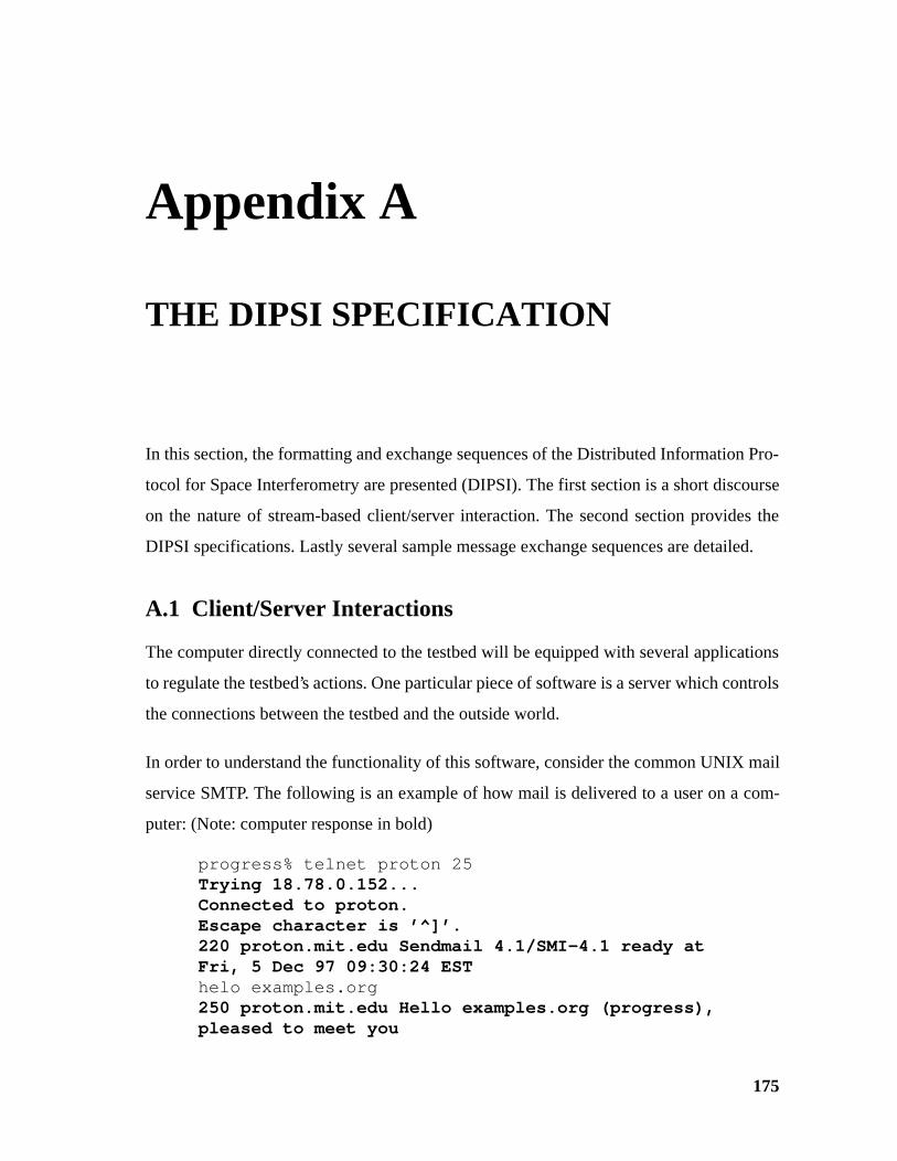
Appendix A
THE DIPSI SPECIFICATION
In this section, the formatting and exchange sequences of the Distributed Information Pro-
tocol for Space Interferometry are presented (DIPSI). The first section is a short discourse
on the nature of stream-based client/server interaction. The second section provides the
DIPSI specifications. Lastly several sample message exchange sequences are detailed.
A.1 Client/Server Interactions
The computer directly connected to the testbed will be equipped with several applications
to regulate the testbed’s actions. One particular piece of software is a server which controls
the connections between the testbed and the outside world.
In order to understand the functionality of this software, consider the common UNIX mail
service SMTP. The following is an example of how mail is delivered to a user on a com-
puter: (Note: computer response in bold)
progress% telnet proton 25Trying 18.78.0.152...Connected to proton.Escape character is ’^]’.220 proton.mit.edu Sendmail 4.1/SMI-4.1 ready at Fri, 5 Dec 97 09:30:24 ESThelo examples.org250 proton.mit.edu Hello examples.org (progress), pleased to meet you
175

176 APPENDIX A
mail from: [email protected] [email protected]... Sender okrcpt to: enright250 enright... Recipient okdata354 Enter mail, end with "." on a line by itselfI’ve got a great at price on Florida swampland. Call me and I’ll see what I can do for you.
P.T. Barnum.250 Mail acceptedquit221 proton.mit.edu delivering mailConnection closed by foreign host.progress%
In most instances the input to SMTP would be automated by the client-side mail routing
software, but the information exchange would be of the same form. This is the same thing
that we want to do with the AIT. The following defines the initial set of instructions which
the sever must be able to parse, and the responses it must provide.
A.2 DIPSI Messages
The message formats for DIPSI are given in Table A.1. Formatting information refers to
either the variable packing order (internal messages) or the command line ordering.

APPENDIX A 177
TABLE A.1 DIPSI Messaging
Message
ID Parametersa Sn
dr.b
Rcv
r.
Response CommentsSC_ALIVE 11 Id(I) VSC ANY Spacecraft Startup suc-
cessful. Internal mes-sage. Id is the spacecraft
IDc
SC_SHUTDOWN 12 VGS ANY SC_SHUTDOWN_ACK Commands AIT pro-cesses to terminate exe-
cution.
SC_SHUTDOWN_ACK 13 Id(i) Any VGS Acknowledgement of shutdown order. Pro-
cess terminating
SC_CLIENTALIVE 14 Id(i) DAIS, MIS
ANY Startup successful
SC_IDS 15 IdList([I]) VGS ANY Initialization command. VGS distribution of pro-
cess identifiers.
SC_MOVESC 16 Dest(I), Id(I) X(D), Y(D)
ANY VSC, MIS
SC_POSITION Commands motion to specified position. If
dest is a VSC, treated as suggestion. If dest is MIS, arm is moved.
SC_POSITION 17 Id(I), X(D), Y(D) ANY ANY Reflects senders knowl-edge of the position of
‘id’
SC_SAMPLE 18 Obsolete
SC_DATAHEADER 19 Obsolete
SC_DATA 20 Obsolete
SC_DATAEND 21 Obsolete
SC_GOAHEAD 22 dest(I) Any Any Generic Acknowledge-ment or Start Signal
SC_TBACTIVE 23 Any MIS SC_TBSTATUS Activates arm servos on testbed.
SC_TBINACTIVE 24 Any MIS SC_TBSTATUS Disables testbed servos
SC_TBSTATUS 25 Err(I), State(I), ActiveAxes(I)
MIS ANY Err is an error state , State describes whether movement is enabled, ActiveAxes describes which arms are opera-tional (bit packing in
4LSB)
SC_TBOKAY 26 More of a status flag than a command.
SC_TBCANTLOADSETTINGS
27 Error flag. Error read-ing initialization file.
SC_TBCANTGETHANDLE
28 Error Flag. Unable to access hardware (DAIS/
MIS)
SC_SETPOSITION 29 Obsolete
SC_POSITIONREQ 30 dest(I), Id(I) Any Any SC_POSITION Request sent to dest. Response is the destina-tion’s knowledge of the
position of ID.
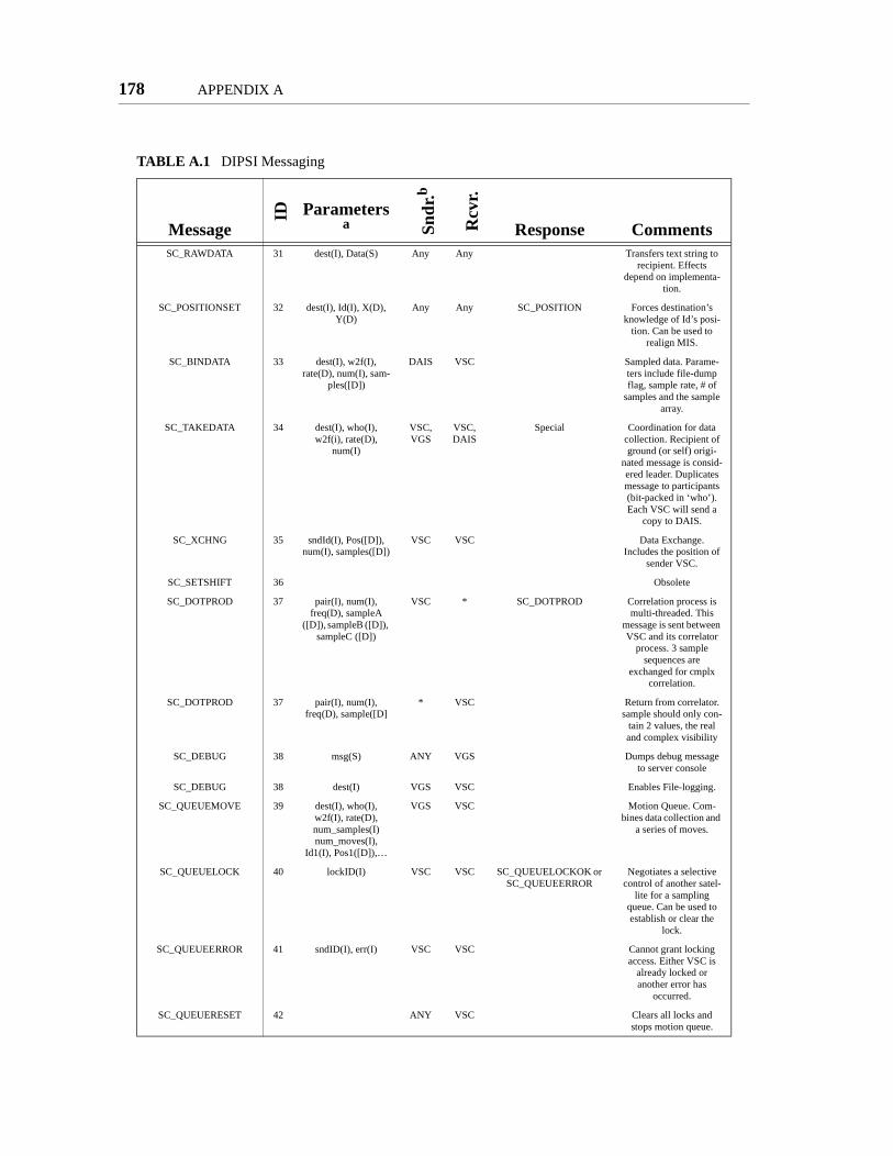
178 APPENDIX A
SC_RAWDATA 31 dest(I), Data(S) Any Any Transfers text string to recipient. Effects
depend on implementa-tion.
SC_POSITIONSET 32 dest(I), Id(I), X(D), Y(D)
Any Any SC_POSITION Forces destination’s knowledge of Id’s posi-
tion. Can be used to realign MIS.
SC_BINDATA 33 dest(I), w2f(I), rate(D), num(I), sam-
ples([D])
DAIS VSC Sampled data. Parame-ters include file-dump flag, sample rate, # of
samples and the sample array.
SC_TAKEDATA 34 dest(I), who(I), w2f(i), rate(D),
num(I)
VSC, VGS
VSC, DAIS
Special Coordination for data collection. Recipient of ground (or self) origi-
nated message is consid-ered leader. Duplicates message to participants (bit-packed in ‘who’). Each VSC will send a
copy to DAIS.
SC_XCHNG 35 sndId(I), Pos([D]), num(I), samples([D])
VSC VSC Data Exchange. Includes the position of
sender VSC.
SC_SETSHIFT 36 Obsolete
SC_DOTPROD 37 pair(I), num(I), freq(D), sampleA
([D]), sampleB ([D]), sampleC ([D])
VSC * SC_DOTPROD Correlation process is multi-threaded. This
message is sent between VSC and its correlator
process. 3 sample sequences are
exchanged for cmplx correlation.
SC_DOTPROD 37 pair(I), num(I), freq(D), sample([D]
* VSC Return from correlator. sample should only con-
tain 2 values, the real and complex visibility
SC_DEBUG 38 msg(S) ANY VGS Dumps debug message to server console
SC_DEBUG 38 dest(I) VGS VSC Enables File-logging.
SC_QUEUEMOVE 39 dest(I), who(I), w2f(I), rate(D), num_samples(I) num_moves(I),
Id1(I), Pos1([D]),…
VGS VSC Motion Queue. Com-bines data collection and
a series of moves.
SC_QUEUELOCK 40 lockID(I) VSC VSC SC_QUEUELOCKOK or SC_QUEUEERROR
Negotiates a selective control of another satel-
lite for a sampling queue. Can be used to establish or clear the
lock.
SC_QUEUEERROR 41 sndID(I), err(I) VSC VSC Cannot grant locking access. Either VSC is
already locked or another error has
occurred.
SC_QUEUERESET 42 ANY VSC Clears all locks and stops motion queue.
TABLE A.1 DIPSI Messaging
Message
ID Parametersa Sn
dr.b
Rcv
r.
Response Comments

APPENDIX A 179
A.3 Message Interchanges
The DIPSI specification defined in Section A.2 describes the formatting and types of mes-
sages that can be exchange between the software components of the AIT. This section
offers some graphical depiction of some of these interchanges. A message interchange
refers to the originating message and the associated responses and actions that it engen-
ders.
Some actions are very simple. Both the movement and query messages have very straight-
forward operations. These are shown in Figure A.1. The originator sends a single message
and receives a single reply. Communication can be between two spacecraft or a spacecraft
and the virtual ground station (VGS). Not shown in these figures are some of the underly-
ing messages that are utilized in the current implementation of spacecraft intelligence.
When a virtual spacecraft (VSC) receives a motion request, it in turn sends a movement
message to the motion interface software (MIS) to carry out the requested maneuver. The
same principle holds for position requests; the VSC will request a position update from the
MIS. Thus, the mechanism for position determination can be altered without affecting the
top level message exchange.
SC_QUEUECHECK 43 sndId(I) VSC VSC Sent to the queue man-ger spacecraft after sig-nal processing complete.
SC_QUEUELOCKOK 44 sndId(I) VSC VSC Locking access accepted for Id.
a. Abbreviations: S: String, D: Double precision floating point, I: Integer, []: Array of relevant type. Command line instructions start with the message ID.
b. VSC: Virtual Spacecraft, VGS: Virtual Ground Station, DAIS: Data Acquisition Interface Software, MIS: Motion Interface Software.
c. Id’s 0-3 refer to VSCs, 4 is the MIS, and 5 is the DAIS
TABLE A.1 DIPSI Messaging
Message
ID Parametersa Sn
dr.b
Rcv
r.
Response Comments

180 APPENDIX A
It should be noted that the VSCs can actually send messages to themselves. This allows
the low level reactions (motion) to be decoupled from the higher level cluster automation
activities such as automatic profile execution.
A more elaborate communication sequence can be seen in the case of the data collection
(Figure A.2). The first recipient VSC is considered the leader for a given collection
sequence. Its special task is to arrange for the participation of the other spacecraft involved
in the measurement. Next, these VSCs will request the data acquisition interface software
(DAIS) to make a recording. Separate streams of data are distributed to each VSC. Before
the correlation can take place, the VSCs must exchange their data. Upon completion of the
exchange and subsequent arithmetic, the partial correlation products are sent to the VGS
where they are collected.
The activities presented above serve as some of the basic operations for the distributed
operations of the AIT cluster. Higher level functionality is layered on top of these simple
activities.
Figure A.1 Message exchanges for position query and movement.
Position Query
1. pos_qry(GND,#1)
4. pos (#1,GND)
2. pos_qry(GND,#1)
3. pos (#1,GND)
1. pos_qry(#2,#1)
2. pos (#1,#2)
Move Spacecraft
1.moveto(GND,#1)
4. pos (#1,GND)
2. moveto(GND,#1)
3. pos (#1,GND)
1. moveto(#2,#1)
2. pos (#1,#2)

APPENDIX A 181
Figure A.2 Data collection sequence. The sequence operations are enumerated on theright.
1. 2. 3.
Dat
a A
cqui
sitio
n
3.
1. record (GND,#1, (123))2. record (GND,#1, (123))3. record (#1, #2, (123)) record (#1, #3, (123))4. record(#1, DAQ, (123))(etc…)5. raw_data(DAQ,#1)(etc...)6. xchng(#1, #2, (123))(etc….)7. proc_data(#1, GND, (1-2)) proc_data(#1, GND, (1-3))(etc)8. proc_data(#1, GND, (1-2))(etc…)
4.
4.
5.
5.
5.
6.
6.
7.
7.
7.8.

182 APPENDIX A

Appendix B
SIGNAL PROCESSING SEQUENCING
This appendix provides a detailed examination of the data exchange process between vir-
tual spacecraft (VSC). This process allows the coherent combination of separate data
streams and represents an essential part of the interferometry technique.
B.1 Data Exchange Sequences
The virtual spacecraft in the Acoustic Imaging Testbed (AIT) follow a rigorous sequence
in exchanging the data during data processing. The following example illustrates this data
exchange and the balanced loading experienced in a four spacecraft observation.
After data collection, each spacecraft has only its own data (Figure B.1). The four units in
the figure represent areas of spacecraft memory. The left (white) side is simply storage; i.e
what the spacecraft knows. The right (grey) is the current list of pending calculations to be
performed. Before any correlation can take place, data sequences from neighbouring
spacecraft must be shared between cluster members. The correlation process is a straight-
forward procedure and is very tolerant of partitioning. That is, the operations involved in
the correlation can easily be performed in isolated segments without necessitating redun-
dant computation or communication1. The first data exchange (Figure B.2) is made
according to the rules presented in Section 3.3.9.
183
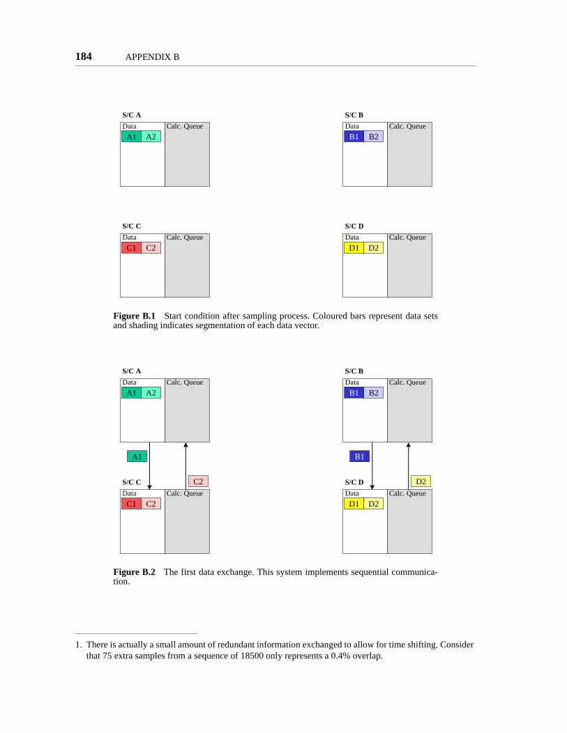
184 APPENDIX B
1. There is actually a small amount of redundant information exchanged to allow for time shifting. Consider that 75 extra samples from a sequence of 18500 only represents a 0.4% overlap.
Figure B.1 Start condition after sampling process. Coloured bars represent data setsand shading indicates segmentation of each data vector.
Figure B.2 The first data exchange. This system implements sequential communica-tion.
Data Calc. Queue
S/C A
A1 A2Data Calc. Queue
S/C B
Data Calc. Queue
S/C D
Data Calc. Queue
S/C C
B1 B2
C1 C2 D1 D2
Data Calc. Queue
S/C A
A1 A2Data Calc. Queue
S/C B
Data Calc. Queue
S/C D
Data Calc. Queue
S/C C
B1 B2
C1 C2 D1 D2
A1
C2
B1
D2

APPENDIX B 185
In general, the system represented by the AIT might allow simultaneous communication
to several other spacecraft. A simpler architecture was chosen for the AIT. In this system,
connectivity is limited and only one link can be employed at a time. Provided that calcula-
tions are more time consuming than communication, this distinction is not very important.
As soon as some incoming data arrives, calculations are added to the computation
(Figure B.3). Each sequential communication cycle will add more contents to the calcula-
tion queue. Based on the assumption about the relative time costs of multiplication and
communication, the queue should only empty after all the sequential exchanges have been
performed.
If the exchanges are sequential, some efficiency gains may be realized by combining the
second and third exchanges (Figure B.4). This assumes that communicating n units of data
will take a time T, where . The constant τ0 represents a fixed cost for send-
ing a message, while τi is the incremental cost for each unit of data. The ability to piggy-
back this data depends upon careful selection of exchange order and spacecraft number-
ing. The reader can verify that the data transferred satisfies the appropriate exchange rules.
Figure B.3 System state after first exchange. Calculation queue depicts the partial cor-relation operations pending.
Data Calc. Queue
S/C B
Data Calc. Queue
S/C A
A1 A2
Data Calc. Queue
S/C D
Data Calc. Queue
S/C C
B1 B2
C1 C2 D1 D2
C2
A1
A1C1
C2A2 D2B2
D1 B1
D2
B1
T τ0 n τi⋅+=

186 APPENDIX B
The final system state shows each VSC with three partial correlations to perform. A total
of six visibility measurements are made during this calculation. A final exchange may be
necessary in order to collect the partial correlations together in the memory of a single sat-
ellite.
Figure B.4 Second data exchange. Notice the ‘piggybacking’ of data within theexchange.
Figure B.5 Final State. Each Spacecraft has equal computational tasks to perform.
Data Calc. Queue
S/C A
A1 A2Data Calc. Queue
S/C B
Data Calc. Queue
S/C D
Data Calc. Queue
S/C C
B1 B2
C1 C2 D1 D2
C2
A1
A1C1
C2A2 D2B2
D1 B1
D2
B1
A1
B1
D2
D2
C1
C2 A1
B2D2
Data Calc. Queue
S/C A
A1 A2Data Calc. Queue
S/C B
Data Calc. Queue
S/C D
Data Calc. Queue
S/C C
B1 B2
C1 C2 D1 D2
C2
A1
A1C1
C2A2 D2B2
D1 B1
D2
B1
D2
C1D1
D1 A1
D2C2
B1C1
D2
D2A2
B2A2
A1B1
C2B2B2
D2B1
A1C2
C1
A1