Investigation of OFDM as a Modulation Technique for ... · PDF fileInvestigation of OFDM as a...
249
Investigation of OFDM as a Modulation Technique for Broadband Fixed Wireless Access Systems A dissertation submitted for the degree of Doctor of Philosophy V. S. Abhayawardhana, Churchill College May 2003 Laboratory for Communications Engineering Department of Engineering University of Cambridge
Transcript of Investigation of OFDM as a Modulation Technique for ... · PDF fileInvestigation of OFDM as a...
Investigation of OFDM as a Modulation Technique for Broadband
Fixed Wireless Access Systems
A dissertation submitted for the degree
of Doctor of Philosophy
V. S. Abhayawardhana, Churchill College May 2003
Laboratory for Communications Engineering
Department of Engineering
University of Cambridge

ii

iii
To my parents .....
... for being the pillars of strength in my life.

iv

Abstract
Broadband Fixed Wireless Access (BFWA) systems offer an effective way to over-
come the ‘last mile problem’ associated with offering pervasive broadband Inter-
net coverage to households and business users. Orthogonal Frequency Division
Multiplexing (OFDM) meanwhile is being widely promoted for adoption as the
physical layer standard for BFWA systems owing to its unprecedented success
in other systems, particularly in digital broadcasting and Wireless LANs. BFWA
systems are characterised by burst transmission from the Access Points (APs)
to one or more Subscriber Units (SUs) and vice-versa. Owing to latency and
throughput considerations, it is desirable that the OFDM system can operate ef-
fectively with a relatively low number of subchannels (typically in the order of
64-256). In order to maximise throughput it is important to optimise the use of
these subchannels. An additional difficulty is that the system is required to func-
tion effectively with the use of inexpensive and low quality oscillators at the SUs.
These issues pose fresh challenges that need to be addressed if successful opera-
tion of BFWA networks is to be achieved from both a technical and a commercial
perspective. This dissertation presents research conducted with the specific aim
of applying OFDM effectively and efficiently to the BFWA scenario.
Although OFDM is robust in the presence of multipath channels, its suscepti-
bility to Phase Noise (PN) is widely known. An investigation conducted as part
of this work has demonstrated that the effect of PN is two-fold. The first effect
is that of phase rotation which is evident on the demodulated constellations of all
the subchannels and is known as Common Phase Error (CPE). The second effect
is owing to the loss of orthogonality between the subchannels and gives rise to
Inter Carrier Interference (ICI) between the subchannels. A simple yet effective
algorithm to counter the effects of CPE is presented in this thesis. Simulation re-
v

vi
sults show that algorithm provides gains of up to 6 dB in terms of Signal to Phase
Noise Ratio (SPNR) when applied to a 64 subchannel OFDM system with a PN
Power Spectral Density (PSD) bandwidth of 100 kHz in the presence of a typical
BFWA channel.
Accurate symbol (frame) and frequency offset synchronisation are also critical
in an OFDM system. This is often accomplished by sending one or more training
symbols at the start of each frame. The Schmidl and Cox Algorithm (SCA), al-
though very robust in OFDM systems which use a large number of subchannels,
fails badly in the BFWA scenario. This dissertation proposes the Iterative Symbol
Offset Correction Algorithm (ISOCA) that complements the SCA and achieves
perfect symbol synchronisation in the presence of BFWA channels at reasonable
SNR levels. The SCA alone by contrast has a probability of only 0.48 of achiev-
ing perfect symbol synchronisation for a 64 subchannel OFDM system in a BFWA
channel. In addition the SCA has a finite probability of yielding very damaging
positive symbol offset estimations. A novel algorithm which complements the
frequency offset correction function of the SCA is also proposed. This algorithm,
known as the Residual Frequency Offset Correction Algorithm (RFOCA), miti-
gates the residual frequency offset errors remaining after the application of the
SCA. The simulations show that the RFOCA is capable of reducing the residual
frequency offset error variance by several orders of magnitude compared with that
achieved by the SCA alone.
The use of a Time Domain Equaliser (TEQ) for OFDM systems in wireless
channels is also addressed in this work. The TEQ reduces the apparent length of
the multipath channel, thus reducing the length of the Cyclic Prefix (CP) that is re-
quired and so improving the transmission efficiency. An existing algorithm, which
is termed the Dual Optimising Time Domain Equaliser (DOTEQ) is introduced
and its limitations are identified. To overcome these problems a novel TEQ train-
ing algorithm, namely the Frequency Scaled Time Domain Equaliser (FSTEQ) is
proposed. The FSTEQ is designed specifically for use in BFWA channels and
it optimises its function in both the time and the frequency domains. It shows a
10-100 fold BER improvement as compared to the DOTEQ while maintaining a
superior rate of convergence.
Time Domain Windowing (TDW) can be used to shape the spectra of the

vii
OFDM subchannels, thus reducing side lobe levels. The dissertation investigates
the use of an adaptive TDW scheme, which is applied separately to both the trans-
mitter and the receiver in a BFWA system. The results show that TDW should be
used if and only if there are uncorrupted samples that can be utilised as part of
the windowing function within the CP. Otherwise, performance improvements are
negligible. The dissertation also presents some preliminary results based on the
concept of using a Maximum Likelihood Sequence Estimator (MLSE) instead of
a Decision Feedback Equaliser (DFE), for the purpose of per-subchannel equali-
sation. The initial results appear to hold some promise though at the cost of very
high complexity.
In summary, this dissertation presents novel algorithms that address several
problems that arise when OFDM is used as the physical layer in a BFWA system.
The solutions in general are not computationally demanding and offer cost effec-
tive and substantial improvements in system performance for the BFWA scenario.

viii

Declaration
Except where noted in the text, this dissertation is the result of my own work and
includes nothing which is done by someone else or in collaboration.
I hereby declare that this dissertation is not substantially the same as any that
I have submitted for a degree or diploma or other qualification at any other Uni-
versity. I further state that no part of my dissertation has already been or is being
concurrently submitted for any such degree, diploma or qualification.
This dissertation comprises approximately 42,000 words, 112 figures and 3
tables.
V. S. Abhayawardhana
May 28, 2003
ix

x

Acknowledgements
First and foremost I would like to thank my supervisor, Dr. I. J. Wassell for his
guidance, encouragement and support both in academic work and otherwise. I
especially enjoyed the discussions we had over coffee, first thing in the morning
while accommodating the bizarre times I used to work at.
My most sincere appreciation is extended to the Cambridge Commonwealth
Trust (CCT) and the Overseas Research Students Award Scheme (ORS) for spon-
soring my research and thus giving me an opportunity to study at probably the
best place in the world. I also thank the Adaptive Broadband Limited (ABL) for
providing me with industrial support during the second year of my research.
I would like to thank my adviser, Dr. N. G. Kingsbury, Dr. M. D. Macleod
and Dr. M. Sellars for providing me with valuable feedback from time to time.
I am grateful for the efforts of my College tutor Dr. N. Morrison in helping
me to secure funding during my final year. I would also like to thank Mrs. Les
Dixon of Churchill College and Mrs. M. Cossnett at the Cambridge University
Engineering Department (CUED) library for being so patient with my numerous
requests.
Special thanks to all the members at the Laboratory for Communications En-
gineering (LCE) for making it such an enjoyable yet stimulating place to work.
Last, but certainly not least, to Prof. A. Hopper for providing me with such an
excellent environment for research.
xi

xii

Publications
Some of the work discussed in this dissertation has been presented in the following
publications;
1. V. S. Abhayawardhana, I. J. Wassell, “Common phase error correction with
feedback for OFDM in wireless communication”, IEEE Global Telecommu-
nications Conference (IEEE GLOBECOM), Volume: 1, Page(s): 651-655,
November 2002.
2. V. S. Abhayawardhana, I. J. Wassell, “Iterative symbol offset correction
algorithm for coherently modulated OFDM systems in wireless commu-
nication”, IEEE International Symposium on Personal, Indoor and Mo-
bile Radio Communications (IEEE PIMRC), Volume: 2, Page(s): 545-549,
September 2002.
3. V. S. Abhayawardhana, I. J. Wassell, “Common phase error correction for
OFDM in wireless communication”, International Conference on Commu-
nication Systems, Networking and Digital Signal Processing (CSNDSP),
Volume: 1, Page(s): 224-227, July 2002.
4. V. S. Abhayawardhana, I. J. Wassell, “Residual frequency offset correc-
tion for coherently modulated OFDM systems in wireless communication”,
IEEE Vehicular Technology Conference (IEEE VTC), Spring, Volume: 2,
Page(s): 777-781, May 2002.
5. V. S. Abhayawardhana, I. J. Wassell, “Frequency scaled time domain equal-
isation for OFDM in broadband fixed wireless access channels”, IEEE Wire-
less Communications and Networking Conference (IEEE WCNC), Volume:
1, Page(s): 17-21, March 2002.
xiii

xiv
6. V. S. Abhayawardhana, I. J. Wassell, “Frequency Scaled Time Domain
Equalisation for OFDM in Wireless Communication”, European Wireless
Conference, Volume: 2, Page(s): 776-780, February 2002.

Contents
Glossary xxv
1 Introduction 1
1.1 Use of OFDM for BFWA systems . . . . . . . . . . . . . . . . . 4
1.2 Overview of the Thesis . . . . . . . . . . . . . . . . . . . . . . . 5
2 Theory of OFDM 13
2.1 Introduction to Digital Communication . . . . . . . . . . . . . . . 13
2.2 Motivation to Use Multitone Modulation . . . . . . . . . . . . . . 16
2.3 Orthogonal Frequency Division Multiplexing . . . . . . . . . . . 17
2.3.1 Mathematical Description of OFDM . . . . . . . . . . . . 19
2.3.2 Orthogonality of Subchannel Carriers . . . . . . . . . . . 20
2.4 Simulated Conventional OFDM System . . . . . . . . . . . . . . 21
2.4.1 The effect of the Cyclic Prefix . . . . . . . . . . . . . . . 24
2.4.2 Frequency Domain Equaliser . . . . . . . . . . . . . . . . 26
3 Common Phase Error Correction 29
3.1 Phase Noise Mask . . . . . . . . . . . . . . . . . . . . . . . . . . 31
3.2 Analysis of the Effect of Phase Noise on OFDM . . . . . . . . . . 35
3.2.1 Common Phase Error . . . . . . . . . . . . . . . . . . . . 37
3.2.2 Inter Carrier Interference . . . . . . . . . . . . . . . . . . 38
3.2.3 Probability of Error Analysis . . . . . . . . . . . . . . . . 39
3.3 Related Work . . . . . . . . . . . . . . . . . . . . . . . . . . . . 42
3.4 Common Phase Error Correction Algorithm . . . . . . . . . . . . 43
3.5 Simulation Parameters and Results . . . . . . . . . . . . . . . . . 52
xv

xvi CONTENTS
3.6 Conclusion . . . . . . . . . . . . . . . . . . . . . . . . . . . . . 60
4 Symbol Offset Correction 63
4.1 Related Work . . . . . . . . . . . . . . . . . . . . . . . . . . . . 65
4.2 Effect of Symbol Offset in OFDM . . . . . . . . . . . . . . . . . 66
4.2.1 Symbol Offset −v ≤ ξ < 0 . . . . . . . . . . . . . . . . . 67
4.2.2 Symbol Offset ξ > 0 . . . . . . . . . . . . . . . . . . . . 67
4.3 Schmidl and Cox Algorithm . . . . . . . . . . . . . . . . . . . . 69
4.4 Iterative Symbol Offset Correction Algorithm . . . . . . . . . . . 75
4.4.1 1st Part - Iterative Symbol Offset Estimation . . . . . . . 75
4.4.2 2nd Part - Error Comparison . . . . . . . . . . . . . . . . 79
4.5 Simulation Parameters and Results . . . . . . . . . . . . . . . . . 80
4.6 Conclusions . . . . . . . . . . . . . . . . . . . . . . . . . . . . . 92
5 Residual Frequency Offset Correction 93
5.1 Related Work . . . . . . . . . . . . . . . . . . . . . . . . . . . . 94
5.2 Effect of Frequency Offset in OFDM . . . . . . . . . . . . . . . . 96
5.3 Schmidl and Cox Algorithm . . . . . . . . . . . . . . . . . . . . 98
5.4 Residual Frequency Offset Correction Algorithm . . . . . . . . . 100
5.5 Simulation Parameters and Results . . . . . . . . . . . . . . . . . 104
5.6 Conclusion . . . . . . . . . . . . . . . . . . . . . . . . . . . . . 117
6 Time Domain Equalisation 119
6.1 Related Work . . . . . . . . . . . . . . . . . . . . . . . . . . . . 120
6.2 Basics of Time Domain Equalisation . . . . . . . . . . . . . . . . 122
6.3 Dual Optimising Time Domain Equaliser . . . . . . . . . . . . . 124
6.4 Frequency Scaled Time Domain Equaliser . . . . . . . . . . . . . 125
6.5 Z-Plane Analysis of FSTEQ . . . . . . . . . . . . . . . . . . . . 132
6.6 Comparison of Computational Complexity . . . . . . . . . . . . . 135
6.7 Simulation Parameters and Results . . . . . . . . . . . . . . . . . 137
6.8 Conclusions . . . . . . . . . . . . . . . . . . . . . . . . . . . . . 143
7 Adaptive Time Domain Windowing 145
7.1 Related Work . . . . . . . . . . . . . . . . . . . . . . . . . . . . 146

CONTENTS xvii
7.2 Time Domain Windowing at the Receiver . . . . . . . . . . . . . 147
7.2.1 Simulation Parameters and Results . . . . . . . . . . . . . 151
7.3 Time Domain Windowing at the Transmitter . . . . . . . . . . . . 156
7.3.1 Simulation Parameters and Results . . . . . . . . . . . . . 157
7.4 Conclusion . . . . . . . . . . . . . . . . . . . . . . . . . . . . . 159
8 Conclusions and Future Work 163
8.1 Future Work . . . . . . . . . . . . . . . . . . . . . . . . . . . . . 166
A Complex Baseband Representation 169
A.1 Spectra of Signals . . . . . . . . . . . . . . . . . . . . . . . . . . 170
A.2 Power Spectral Density . . . . . . . . . . . . . . . . . . . . . . . 172
B Channel Models 175
B.1 Large-Scale Variations of the Signal Envelope . . . . . . . . . . . 175
B.1.1 Free Space Propagation . . . . . . . . . . . . . . . . . . . 175
B.1.2 Two Ray Model . . . . . . . . . . . . . . . . . . . . . . . 176
B.1.3 Log-Normal Shadowing . . . . . . . . . . . . . . . . . . 178
B.2 Small-scale Variations of the Signal Envelope . . . . . . . . . . . 178
B.2.1 AWGN Channel . . . . . . . . . . . . . . . . . . . . . . 178
B.2.2 Multipath Channel . . . . . . . . . . . . . . . . . . . . . 178
B.2.3 Distribution of Signal Envelope . . . . . . . . . . . . . . 181
B.2.4 Local Movements and Doppler Shifts . . . . . . . . . . . 181
B.3 Stanford University Interim Channel Models . . . . . . . . . . . . 183
C Equalisation in FMT Modulation 187
C.1 A Brief Introduction to Subband Systems . . . . . . . . . . . . . 188
C.1.1 Polyphase Decomposition . . . . . . . . . . . . . . . . . 190
C.1.2 Transmultiplexers . . . . . . . . . . . . . . . . . . . . . . 190
C.1.3 Overlapped Basis Functions . . . . . . . . . . . . . . . . 191
C.1.4 Filter Bank based modulation for Communication . . . . . 191
C.2 Introduction to Filtered Multitone . . . . . . . . . . . . . . . . . 192
C.2.1 ISI Caused by FMT . . . . . . . . . . . . . . . . . . . . . 195
C.2.2 Achievable Bit Rate . . . . . . . . . . . . . . . . . . . . 196

xviii CONTENTS
C.3 Simulation Results . . . . . . . . . . . . . . . . . . . . . . . . . 198
C.4 Conclusions . . . . . . . . . . . . . . . . . . . . . . . . . . . . . 201
References 203

List of Figures
2.1 Basic elements of a digital communication system . . . . . . . . . 13
2.2 Block diagram of a conventional OFDM system . . . . . . . . . . 22
3.1 Magnitude response of the DFT without frequency deviation . . . 30
3.2 Magnitude response of the DFT with frequency deviation . . . . . 31
3.3 Block diagram of a PLL frequency synthesiser . . . . . . . . . . . 32
3.4 Components of the PN density . . . . . . . . . . . . . . . . . . . 33
3.5 Phase Noise PSD of a typical oscillator . . . . . . . . . . . . . . 35
3.6 Simulated one-sided PN mask . . . . . . . . . . . . . . . . . . . 36
3.7 Constellation of post-FFT data symbols with an AWGN and PN . 39
3.8 QPSK constellation subject to a phase rotation owing to ψCPE . . 40
3.9 Theoretical and simulated results of OFDM systems without CPE
correction subject to AWGN and PN . . . . . . . . . . . . . . . . 42
3.10 The variation of CPESE for N = 64 . . . . . . . . . . . . . . . . 45
3.11 Phase of the CTF being offset owing to a low value of ψCPE,Nt. . 47
3.12 Symbol with most errors and a low value of ψCPE,Nt. . . . . . . 48
3.13 Phase of the CTF being offset owing to a high value of ψCPE,Nt. 49
3.14 Symbol with most errors and a high value of ψCPE,Nt. . . . . . . 50
3.15 Individual subchannel error analysis with AWGN and high SPNR 51
3.16 Individual subchannel error analysis with AWGN and low SPNR . 51
3.17 CPE Correction (CPEC) algorithm . . . . . . . . . . . . . . . . . 53
3.18 Demodulated constellations with and without CPEC for N = 64 . 54
3.19 Demodulated constellations with and without CPEC for N = 256 54
3.20 Performance of the CPEC algorithm for fh = 100 kHz . . . . . . 55
3.21 Performance of the CPEC algorithm for fh = 200 kHz . . . . . . 56
xix

xx LIST OF FIGURES
3.22 Performance of different components of the CPEC algorithm for
N = 64 . . . . . . . . . . . . . . . . . . . . . . . . . . . . . . . 58
3.23 Performance of different components of the CPEC algorithm for
N = 256 . . . . . . . . . . . . . . . . . . . . . . . . . . . . . . . 59
3.24 The variation of CPESE for N = 256 . . . . . . . . . . . . . . . 59
3.25 Comparison with the Onizawa CPEC algorithm . . . . . . . . . . 61
3.26 The effect of AWGN on the CPEC algorithm . . . . . . . . . . . 61
3.27 The effect of channel estimation on the CPEC algorithm . . . . . 62
4.1 Training symbols in SCA . . . . . . . . . . . . . . . . . . . . . . 70
4.2 Output of the timing metric for N = 64 . . . . . . . . . . . . . . 71
4.3 Variation of θi for N = 64, ε = 0.5, with AWGN only at 15 dB
SNR . . . . . . . . . . . . . . . . . . . . . . . . . . . . . . . . . 76
4.4 Variation of θi for N = 64, ε = 0.5 with AWGN at 15 dB SNR
and CIR . . . . . . . . . . . . . . . . . . . . . . . . . . . . . . . 76
4.5 Phase unwrapping algorithm . . . . . . . . . . . . . . . . . . . . 77
4.6 Performance of the unwrapping algorithm for N = 64, with CIR . 78
4.7 Two cases of ISOCA correction . . . . . . . . . . . . . . . . . . 81
4.8 ISOCA flow graphs . . . . . . . . . . . . . . . . . . . . . . . . . 82
4.9 Performance of original SCA with AWGN alone for N = 64 . . . 83
4.10 Performance of modified SCA with AWGN alone for N = 64 . . 84
4.11 Performance after 1st part of ISOCA with AWGN for N = 64 . . 85
4.12 Performance after 2nd part of ISOCA with AWGN for N = 64 . . 85
4.13 Probability of convergence failure with AWGN alone for N = 64 . 86
4.14 Symbol offset error variance with AWGN for N = 64 . . . . . . . 87
4.15 Symbol offset error variance with AWGN for N = 128, 256 . . . 87
4.16 Performance of modified SCA with SUI-II CIR for N = 64 . . . . 88
4.17 Performance after 1st part of ISOCA with SUI-II CIR for N = 64 89
4.18 Performance after 2nd part of ISOCA with SUI-II CIR for N = 64 89
4.19 Probability of convergence failure with SUI-II CIR for N = 64 . . 90
4.20 Symbol offset error variance with SUI-II CIR for N = 64 . . . . . 91
4.21 Symbol offset error variance with SUI-II CIR for N = 128, 256 . 91
5.1 Analysis of CTIR vs relative frequency offset, ε . . . . . . . . . . 98
LIST OF FIGURES xxi
5.2 Block diagram of the RFOCA . . . . . . . . . . . . . . . . . . . 101
5.3 Frequency offset error variance in AWGN for ε = 0.5 . . . . . . . 105
5.4 BER performance of RFOCA in AWGN for ε = 0.5 . . . . . . . . 106
5.5 Frequency offset error variance in AWGN for ε = 1.5 . . . . . . . 106
5.6 BER performance of RFOCA in AWGN for ε = 1.5 . . . . . . . . 107
5.7 The effect of symbol offset on RFOCA for N = 256 and ε = 0.5 . 108
5.8 Frequency offset error variance in SUI-II CIR for ε = 0.5 . . . . . 109
5.9 BER performance of RFOCA in SUI-II CIR for ε = 0.5 . . . . . . 110
5.10 Frequency offset error variance in SUI-II CIR for ε = 1.5 . . . . . 110
5.11 BER performance of RFOCA in SUI-II CIR for ε = 1.5 . . . . . . 111
5.12 Performance of the phase unwrapping algorithm and DROT at 20
dB SNR . . . . . . . . . . . . . . . . . . . . . . . . . . . . . . . 113
5.13 Performance of the phase unwrapping algorithm and DROT at 14
dB SNR . . . . . . . . . . . . . . . . . . . . . . . . . . . . . . . 113
5.14 Effect of unwrapping algorithm for different numbers of iterations 114
5.15 The effect of Nw on the performance of the RFOCA . . . . . . . . 114
5.16 Effect of channel estimation on RFOCA . . . . . . . . . . . . . . 115
5.17 Estimation of the phase of the CTF for different symbol offsets . . 116
5.18 The DROT analysis for different symbol offsets . . . . . . . . . . 116
6.1 Block diagram of the TEQ . . . . . . . . . . . . . . . . . . . . . 123
6.2 DOTEQ performance: Impulse responses . . . . . . . . . . . . . 126
6.3 DOTEQ performance: Transfer functions . . . . . . . . . . . . . 126
6.4 FSTEQ algorithm: Initial TTF . . . . . . . . . . . . . . . . . . . 127
6.5 FSTEQ algorithm: Block diagram . . . . . . . . . . . . . . . . . 131
6.6 FSTEQ performance: Impulse responses . . . . . . . . . . . . . . 133
6.7 FSTEQ performance: Transfer functions . . . . . . . . . . . . . . 133
6.8 Z-plane analysis: DOTEQ response . . . . . . . . . . . . . . . . 135
6.9 Z-plane analysis: FSTEQ response . . . . . . . . . . . . . . . . . 136
6.10 BER performance for different TEQs of length 60 . . . . . . . . . 139
6.11 MSE for various TEQ schemes with length of 60 . . . . . . . . . 140
6.12 BER performance for TEQs using shorter training iterations . . . 140
6.13 The effect of SNR on different TEQ schemes with length of 60 . . 141

xxii LIST OF FIGURES
6.14 BER performance for different TEQs of length 50 . . . . . . . . . 142
6.15 BER performance for different TEQs of length 40 . . . . . . . . . 142
6.16 BER performance for different TEQs at a lower sample rate . . . . 143
7.1 Decomposition of a Nyquist window . . . . . . . . . . . . . . . . 149
7.2 Comparison of different Nyquist windows in the time domain . . . 150
7.3 Comparison of different Nyquist windows in the frequency domain 150
7.4 Processing required when windowing is performed at the receiver 152
7.5 Effect of RC windowing at the the receiver for AWGN channels . 153
7.6 Performance of various Nyquist windows for AWGN channels . . 154
7.7 Performance of TPW subject to SUI-II channels . . . . . . . . . . 155
7.8 Performance of TPW subject to PN and SUI-II channels . . . . . 156
7.9 Processing required when windowing is performed at the transmitter158
7.10 Effect of TPW at the transmitter for SUI-II channels for α = 0.25 160
7.11 Effect of TPW at the transmitter for SUI-II channels for α = 0.5 . 160
A.1 Comparison of P (ω) and S(ω) . . . . . . . . . . . . . . . . . . . 171
B.1 Two-ray model . . . . . . . . . . . . . . . . . . . . . . . . . . . 177
B.2 Tapped delay line channel model . . . . . . . . . . . . . . . . . . 180
B.3 Typical Doppler spectra for Rayleigh and Rician distributions . . . 183
C.1 Block diagram of a subband system . . . . . . . . . . . . . . . . 189
C.2 Communication System using Filter Bank modulation . . . . . . . 193
C.3 Subchannel frequency responses in a FMT system . . . . . . . . . 194
C.4 Efficient implementation of a critically sampled FMT system . . . 195
C.5 Overall Subchannel Impulse Response (OSIR) of an FMT system 196
C.6 Performance OFDM and FMT equalised by a DFE and an MLSE . 200
C.7 The effect of MLSE length on equalisation performance . . . . . . 200

List of Tables
3.1 Performance gains obtained by different components of the CPEC 60
6.1 Comparison of computational complexity per iteration . . . . . . 137
B.1 SUI-II channel profile . . . . . . . . . . . . . . . . . . . . . . . . 185
xxiii

xxiv LIST OF TABLES

Glossary
ABR Achievable Bit rate
ADSL Asymmetric Digital Subscriber Line
AWGN Additive White Gaussian Noise
BER Bit Error Rate
BFWA Broadband Fixed Wireless Access
CIR Channel Impulse Response
CP Cyclic Prefix
CPE Common Phase Error
CPEC Common Phase Error Correction
CPESE Common Phase Error Symbol Estimate
CTF Channel Transfer Function
DFE Decision Feedback Equaliser
DMT Digital Multitone
DOTEQ Dual Optimising Time Domain Equaliser
DROT Dynamic Residual Offset Tracking
EIR Effective Impulse Response
xxv

xxvi GLOSSARY
ETF Effective Transfer Function
FBCF Feedback Correction Factor
FEQ Frequency Domain Equaliser
FFT Fast Fourier Transform
FIR Finite Impulse Response
FMT Filtered Multitone
FSTEQ Frequency Scaled Time Domain Equaliser
IBI Inter Block Interference
ICI Inter Carrier Interference
IEE Institute of Electrical Engineers
IEEE Institute of Electrical and Electronic Engineers
IFFT Inverse Fast Frequency Transform
ISI Inter Symbol Interference
ISOCA Iterative Symbol Offset Correction Algorithm
LMS Least Mean Square
LOS Line of Sight
MAF Moving Average Filter
MLSE Maximum Likelihood Sequence Estimator
MMDS Multichannel Multipoint Distribution Service
MMSE Minimum Mean Squared Error
OFDM Orthogonal Frequency Division Multiplexing
OSIR Overall Subchannel Impulse Response

xxvii
PDF Probability Density Function
PN Phase Noise
PSD Power Spectral Density
QPSK Quaternary Phase Shift Keying
RC Raised Cosine
RFO Residual Frequency Offset
RFOCA Residual Frequency Offset Correction Algorithm
RLS Recursive Least Square
SC Single Carrier
SCA Schmidl and Cox Algorithm
SNR Signal to Noise Ratio
SOF Start of Frame
SPNR Signal to Phase Noise Ratio
SUI Stanford University Interim
TEQ Time Domain Equaliser
TIR Target Impulse Response
TPW Trapezoidal Windowing
TTF Target Transfer Function
VC Virtual Carrier

xxviii GLOSSARY

Chapter 1
Introduction
The tremendous success and exponential growth of the Internet encouraged by the
development of novel applications has resulted in requirements for significantly
higher network access data rates. The novel broadband applications that are fore-
seen range from e-commerce, telemedicine, teleteaching and large file transfer to
multimedia. These applications are about to revolutionise both the economies of
the world and our lifestyles. Any country that ignores broadband communication
is going to suffer a severe economic impact. The UK government has identified
the provision of broadband as a major objective and has developed strategies to
deliver the most extensive and competitive broadband market in the G7 by 2005.
As a consequence, the Broadband Stakeholder Group (BSG) has been appointed
as the UK government’s key advisory group with the aim of achieving this tar-
get [1].
The demand for broadband places huge requirements on both the access and
the backbone networks of communication systems. The problems of the backbone
networks have been addressed by sustained development of switching and trans-
mission technology. However the major bottleneck lies in the access network,
known in the industry as the ‘last (or first) mile problem’.
There are two possible approaches for delivering broadband. The first ap-
proach is by the use of wired technology, represented by optical fibres, Digital
Subscriber Lines (xDSL) and cable modems. The second approach is by the use
of wireless technology, represented by satellite systems, stratospheric platforms
1

2 CHAPTER 1. INTRODUCTION
and Broadband Fixed Wireless Access (BFWA) systems. Among the many xDSL
standards, the most commonly used is known as Asymmetric Digital Subscriber
Line (ADSL). Currently only cable modems, ADSL systems and BFWA systems
have been practically implemented owing to issues of cost and effectiveness. As
at November 2002, terrestrial broadband (ADSL, cable modems and BFWA but
not satellite) only has the potential to provide service to 67% of UK’s households
and coverage remains concentrated around areas of high population density. On
the other hand, the number of broadband subscribers has grown by 300% in 2002
to reach approximately 4% of all households in UK. This surge in demand is pre-
dicted to continue in the near future. In terms of geographical coverage by each
technology, ADSL, cable modems and BFWA systems had reached 61%, 40%
and 12%, respectively by November 2002 [2]. It is proposed by the BSG that
BFWA systems be extensively implemented, particularly in suburban and rural
areas to obtain full broadband coverage in the UK and to avoid a ‘broadband di-
vide’ among the population. One of the key recommendations is to encourage
more operators to use BFWA by allocating more spectrum to such systems [3].
BFWA systems can be broadly categorised into Point to Point (PTP) and Point
to Multipoint (PMP) terminal radio systems. The PTP and PMP systems usually
operate in different frequency bands. For example the Local Multipoint Distribu-
tion Systems (LMDS) are in the 28 GHz band, the Multichannel Multipoint Dis-
tribution Service (MMDS) is in the 2.5 GHz band and the Unlicensed National
Information Infrastructure (UNII) is in the 5 GHz band. Spectrum at 3.5 GHz has
also been allocated for PMP systems in Europe. These systems are implemented
by placing one or more Subscriber Units (SUs) at the customer premises which
has access to a base station, also known as the Access Point (AP). Usually, the
downlink from the AP is shared among the several SUs. The uplinks from the
SUs usually have a random access element since more than one SU may wish to
transmit to an AP at any one time [4].
ADSL modems are designed to use the voice-grade copper telephone channel.
The main advantage of this approach is the availability of an extensive existing
infrastructure and relatively low installation costs. However the main challenges
are the interference due to Near End Crosstalk (NEXT), the restricted bandwidth
and the moderate Signal to Noise Ratio (SNR) on the channels. The available

3
bit rate and hence the applications are limited by the quality of the copper loops
already in place. ADSL offers a maximum bandwidth of 6-8 Mb/s downstream
and up to 768 kb/s upstream [5].
Cable modems offer downstream data rates of up to 10Mb/s and upstream rates
of up to 200 kb/s [6]. Even though there is a large subscriber base, the technology
suffers from security issues since the cable link is shared by many users. Cable
modems also offer a limited bandwidth for upstream traffic and consequently the
implementation of high bandwidth interactive applications will be difficult.
Satellite access offers extremely high rates, offering data rates of up to the
order of 10 Mb/s [7]. Satellite access has the advantage of total coverage indepen-
dent of local population density. However it will be mainly used by the Internet
Service Providers (ISP) who lack access to a wide bandwidth backbone rather
than individual subscribers owing to the high cost of terminals.
Another area generating interest is the support for relatively broadband appli-
cations targeted to mobile devices. These standards are broadly known as Interna-
tional Telecommunication Union’s (ITU) IMT-2000, popularly known as ‘third-
generation’ (3G) mobile communication systems. Standards such as the Universal
Mobile Telecommunication Systems (UMTS) in Europe will offer data rates up
to 384 kb/s for high-mobility users and 2 Mb/s for low mobility users with local
coverage, which will enable high value broadband information, commerce and
entertainment to be made available to mobile users [8]. While 3G systems are
designed to provide ‘full mobility’, another dimension that is gaining popularity
are Wireless Local Area Networks (WLANs) that provide limited mobility with
superior data rates [9]. They are commonly known by their standardisation group
names or identifiers, for example, the 802.11 suite proposed by the U.S. based
Institute of Electrical and Electronics Engineers (IEEE) [10], HIPERLAN1 and
2 proposed by the Broadband Wireless Access Networks (BRAN) project of the
European Telecommunication Standard Institute (ETSI) [11] and HiSWAN pro-
posed by the Japanese based Association of Radio Industries and Broadcasting
(ARIB). These standards were initially designed to extend the coverage of wired
LANs and offer a similar level of functionality. However issues concerning se-
curity, mobility, network management, ease of use and scalability remain to be
addressed [12, 13].

4 CHAPTER 1. INTRODUCTION
With the deregulation of the telecommunication industry, massive growth in
mobile communication, the emergence of multimedia applications and advanced
information services has led to an increase in demand for the telecommunication
services resulting in the roll-out of radio based broadband access. The advan-
tages of wireless technology are that it is flexible, supports any traffic mix, has an
open-ended uplink-downlink ratio and is suitable for incremental installation and
rapid deployment. In developed economies it offers an economic entry into the
market enabling effective competition with incumbent operators. In developing
economies it permits them to jump a complete technological generation in terms
of access technologies. However broadband terrestrial radio transmission has its
own problems which need to be addressed, e.g. Inter Symbol Interference (ISI)
owing to dispersive channels and Inter Carrier Interference (ICI) and Co channel
Interference (CCI) owing to other users. In this dissertation the use of Orthogo-
nal Frequency Division Multiplexing (OFDM) is investigated as a solution to the
problems encountered when implementing BFWA systems.
1.1 Use of OFDM for BFWA systems
A modulation technique known as OFDM is gaining popularity among wireless
network operators and is actively used in many standards owing to its efficiency
and robustness in channels exhibiting multipath delay spread. OFDM involves
splitting the original high bit rate data stream into a large number of parallel
lower rate data streams which are transmitted in closely spaced subchannels in
the frequency domain. The characteristics of OFDM will be discussed in more
detail in the chapters that follow. One of the first examples of the widespread use
of OFDM is within the Digital Audio Broadcasting (DAB) [14] and the Digital
Video Broadcasting - Terrestrial (DVB-T) standards [15]. Here, its use allows
terrestrial transmitters placed at different geographical locations to transmit at the
same time using the same frequency bands. Hence they are known as Single Fre-
quency Networks (SFNs). Later OFDM was adopted as the physical layer for
WLAN standards such as IEEE 802.11a and HIPERLAN2 [16].
It has been apparent for some time that OFDM was going to be a major con-
tender when it came to standardising BFWA systems following its widespread
1.2. OVERVIEW OF THE THESIS 5
use in WLANs. The IEEE set up the 802.16 working group to define standard
specifications for the Metropolitan Area Networks (MANs) based on broadband
wireless access. The air interface is known as WirelessMAN. This group’s initial
interest lay in the 10-66 GHz band where a Line of Sight (LOS) path between
the terminals is deemed an absolute necessity and consequently the propagation
distances remain relatively short. A Single Carrier (SC) based air interface has
been selected. Later the work was extended in the guise of the 802.16a project
to cover the 2-11 GHz range that includes both licenced and unlicensed bands.
In this case the physical layer specification has been driven by the requirement
for Non-Line-of-Sight (NLOS) operation and hence significant multipath propa-
gation is expected. Hence two out of the three air interfaces proposed are based
on OFDM [17, 18]. The work carried out in parallel by the ETSI-BRAN project
has resulted in the standard known as HIPERACCESS, which specifies an out-
door, fixed wireless network providing access to a wired infrastructure [19]. It
is a SC system which operates in the frequency range from 26 to 28 GHz and
also at 40 GHz and provides bit rates of up to 25 Mb/s. It has been extended to
cover lower frequency bands from 2 to 11 GHz in the guise of the HIPERMAN
standard. HIPERMAN enables both PMP and Mesh network configurations. An-
other standard that is proposed by the ETSI-BRAN project is HIPERLINK that
allows very hight speed (up to 155 Mb/s) indoor, static interconnections between
the HIPERACCESS and the HIPERLAN systems. However, HIPERMAN and
HIPERLINK are yet to be finalised but are expected to be OFDM based when
ratified. Hence it is evident that OFDM will have widespread use in the future,
particularly in BFWA systems.
1.2 Overview of the Thesis
This thesis presents research which investigates various problems that arise when
using OFDM as the physical layer in a BFWA system. Consequently the per-
formance of OFDM systems in the BFWA scenario has been investigated via
extensive and representative computer simulations. The investigation concen-
trates primarily on coherent, Grey coded Quaternary Phase Shift Keying (QPSK)
modulated OFDM systems although some initial work concerning Filtered Multi-

6 CHAPTER 1. INTRODUCTION
tone (FMT) modulation is also presented in appendix C. The measure of perfor-
mance, unless stated otherwise, is the Bit Error Rate (BER) as a function of the
received SNR.
In typical OFDM based wireless LAN systems, the number of subchannels,
N is kept relatively low, typically less than 512. This is done for a number of
reasons. The transmitted OFDM signal is generated by adding together randomly
varying complex sinusoids, which gives rise to a transmitted signal with a very
high dynamic range. An accepted measure of this is the Peak-to-Average Power
Ratio (PAPR). A high value of N leads to a high PAPR, demanding the use of
highly linear and consequently inefficient power amplifiers [20]. Also note that
for typical wireless data transmission systems, for example HIPERLAN-2, short
data bursts employing a low number of subchannels (e.g. 64) are used owing to
latency and protocol efficiency considerations [21]. Also a high value of N will
reduce the inter-carrier spacing of the OFDM signal which renders the system
more susceptible to frequency offset and oscillator phase noise. These issues will
be discussed in detail in later chapters. For these reasons the OFDM systems that
are considered in this thesis have between 64 and 256 subchannels.
In practical OFDM systems, the subchannels at the edges of the multiplex
cannot be used to transmit data since their use gives rise to high sidelobe levels
yielding unacceptable levels of adjacent channel interference. Besides, the IF
filters at the receiver requires a finite roll off bandwidth. The unused subchannels
at either end of the OFDM multiplex are known as Virtual Carriers (VCs). The
number of VCs required is determined by the standard that is applicable for the
particular system and will clearly affect the throughput of the system. However in
this work, the number of VCs is assumed to be zero since throughput will not be
used as a measure of performance.
In OFDM based systems that are subject to channels with severe frequency
selective attenuation, for example in xDSL systems, different subchannels are
mapped using different modulation constellations depending upon the subchan-
nel SNR. This is known as ‘bit loading’. Although the channels that are relevant
to BFWA systems show a certain degree of frequency selectivity, they are not as
hostile as those experienced in xDSL, consequently this operation will not yield a
significant gain. A bit loading algorithm will require feedback from the receiver
1.2. OVERVIEW OF THE THESIS 7
and also owing to the variation of the channel between transmission bursts, it is
not usually employed in fixed wireless systems [22]. Consequently, the OFDM
systems investigated in this thesis will be mapped using QPSK for all subchannels
and as mentioned previously, all of them will be used for data transmission.
It is assumed that the transmission is performed in relatively short bursts at
a sampling frequency of 20 MHz unless stated otherwise. Channel models for
BFWA systems were being developed while the research was being carried out.
The Stanford University Interim (SUI) models [23] were selected for use owing to
their widespread acceptance and have been used throughout the thesis. The trans-
mission burst length selected for use is less than or equal to 2500 symbols with
two or more training symbols at the beginning of each burst. At the chosen sam-
ple rate of 20 MHz the transmission of a burst takes less than 10 ms. Appendix B
introduces the SUI channel models that are extensively used in the following sim-
ulations, giving their associated parameter values. The temporal characteristics of
the channel model are significantly static during a time period of 10 ms. Hence it
has been assumed that the channel remains stationary throughout the transmission
burst for all the simulations.
Conventional OFDM systems, such as WLANs, require high quality Radio
Frequency (RF) oscillators to generate stable frequencies and thus avoid the ef-
fects of frequency offset and phase noise. The RF oscillators form a significant
component of the cost of the Subscriber Units (SUs). A lower quality oscillator
will reduce the overall cost of the SU and consequently will make BFWA systems
more competitive with other broadband systems available in the market. One of
the key aims of this research is to mitigate the performance degradation caused
by the use of low quality oscillators via the use of novel Digital Signal Processing
(DSP) algorithms. Another aim is to improve the performance of both timing and
frequency synchronisation.
The performance of OFDM systems employing the DSP algorithms proposed
in this work are compared against those of conventional OFDM systems, either
employing existing algorithms or in the absence of correction algorithms.
The structure and contents of the thesis will now be briefly introduced. Chap-
ter 2 presents the various components of a digital communication system and also
outlines the advantages of using multitone modulation schemes such as OFDM.
8 CHAPTER 1. INTRODUCTION
It is shown that the subchannel spectra of an OFDM signal overlap and orthogo-
nality is maintained only if timing and frequency synchronisation are preserved.
The sidelobe levels of the subchannel spectra are quite high, which also leads to
susceptibility to oscillator phase noise [24].
The effects of phase noise on the system performance is investigated in detail
in chapter 3. It is found that phase noise introduces two distinct effects. The first
effect rotates the subchannel phase and is known as Common Phase Error (CPE)
while the second effect gives rise to ICI. The chapter also proposes a novel and ef-
fective Common Phase Error Correction (CPEC) algorithm to counter the effects
of CPE in a coherently modulated OFDM system. The algorithm shows signif-
icant performance gains as compared to conventional OFDM systems in BFWA
channels, at only a moderate cost in terms of computational complexity.
Coherently modulated OFDM systems, such as in WLANs, generally employ
training symbols usually placed at the beginning of the transmitted burst to achieve
frame (symbol) and frequency synchronisation. One of the more robust schemes is
the Schmidl and Cox Algorithm (SCA) [25]. Although the SCA performs well for
OFDM systems with a large number of subchannels (i.e. N of the order of 1000 or
more), its performance degrades for systems with lower values of N . In chapter 4
the symbol synchronisation function of the SCA is examined in more detail. It
also proposes the novel Iterative Symbol Offset Correction Algorithm (ISOCA)
which complements the SCA and is shown to achieve virtually perfect symbol
synchronisation.
Chapter 5 analyses the effects of frequency offset on the performance of an
OFDM system. It also investigates the frequency offset correction function of
the SCA. It is found that when the SCA is applied to OFDM systems with lower
values ofN , a residual frequency offset remains that rotates the demodulated con-
stellations at a reduced rate (compared with not using the SCA), but one that is
significant enough to induce bit errors. One method that could be employed to
mitigate this effect is to embed pilot symbols into the OFDM symbols by plac-
ing them in predefined OFDM subchannels. However, this method reduces the
transmission efficiency, particularly when the number of subchannels, N is kept
low. Since the policy of this work is to use all the subchannels to transmit data,
this method will not be adopted. Instead this chapter proposes the data driven
1.2. OVERVIEW OF THE THESIS 9
Residual Frequency Offset Correction Algorithm (RFOCA) that complements the
frequency offset correction function of the SCA and is shown to provide signifi-
cant performance gains.
An elegant method of equalising the effects of a channel exhibiting multipath
delay spread is to prepend each transmitted OFDM symbol with samples taken
from the end of the OFDM symbol sufficient to cover the duration of the channel
delay spread. These samples are known as the Cyclic Prefix (CP) and are dis-
cussed in detail in chapter 2. However, the use of the CP reduces the transmission
efficiency. A method that is adopted widely in ADSL systems is to include a filter
ahead of the demodulator (i.e. the Fast Fourier Transform (FFT)) known as the
Time Domain Equaliser (TEQ). The purpose of the TEQ is to reduce the effect
of the channel delay spread. Hence the Effective Impulse Response (EIR) after
the TEQ is arranged to be shorter than that of the original channel, consequently
the overall OFDM system is capable of working with a shorter CP. However, the
current TEQ algorithms optimise the EIR only in the time domain, often result-
ing in deep nulls in the frequency response. Any subchannels that fall in to these
frequency nulls will be severely degraded. Chapter 6 proposes a new algorithm,
namely the Frequency Scaled Time Domain Equaliser (FSTEQ) that optimises
both in the time and frequency domains so that the overall response avoids spec-
tral nulls as well as reducing residuals in the time domain. Thus the overall per-
formance is improved compared with that achieved when optimising in the time
domain alone.
Conventional OFDM systems use rectangular windows to shape the transmit-
ted OFDM symbols in the time domain and this leads to the high sidelobe levels as
mentioned previously. One way of reducing the sidelobe levels is to employ non-
rectangular window functions. Note that if these window types do not conform to
the Nyquist criterion, they will give rise to a loss of orthogonality. In chapter 7
the use of Nyquist time domain windowing is investigated. However the use of
non-rectangular Nyquist windows requires more uncorrupted samples within the
CP if the OFDM symbols are to be processed without introducing ICI than does
the use of a rectangular window. In the approach presented in chapter 7 it is pro-
posed that uncorrupted samples in the CP are used to maintain orthogonality when
non-rectangular windows are employed. However, if no uncorrupted samples are

10 CHAPTER 1. INTRODUCTION
available in the CP, the length of the CP will have to be extended specifically
to accommodate the windowing function, leading to an increase in the transmis-
sion bandwidth and thus decreasing the SNR. It has been found that in such a
scenario, non-rectangular windowing does not give any performance gains. It is
recommended that windowing be employed only if there are uncorrupted samples
available in the CP and if the system specification does not allow the length of the
CP to be reduced.
Chapter 8 summarises the findings and proposes areas in which the presented
work can be extended in the future.
Another area that is receiving attention is that of filterbank based modulation.
FMT is one such scheme that was originally proposed for VDSL systems [26].
The filter banks that are employed provide very high sidelobe attenuation but with
the penalty of introducing Inter Symbol Interference (ISI). The low sidelobe lev-
els reduce the ICI but now per-subchannel equalisation is required to mitigate the
effects of ISI. Decision Feedback Equalisers (DFEs) are often used for this pur-
pose, however the per-subchannel error performance remains low using such an
approach. Appendix C investigates the use of a Maximum Likelihood Sequence
Estimator (MLSE) rather than a DFE for performing the per-subchannel equali-
sation in an FMT system. Some preliminary results are presented concerning the
proposed approach and a comparison with a DFE based scheme is given. Minimis-
ing the computational burden is not the intension of the presented work, rather the
aim being to understand the performance limits of per-subchannel equalisation in
an FMT system.
In summary, the novel algorithms proposed and results presented in this work
are as follows;
• The Common Phase Error Correction (CPEC) algorithm that corrects the
CPE component owing to the phase noise in a coherently modulated OFDM
system. The performance the algorithm in various systems is analysed and
its performance is compared against other algorithms.
• The two-part Iterative Symbol Offset Correction Algorithm (ISOCA) that
complements the symbol (frame) synchronisation function of the SCA and
is shown to yield virtually perfect symbol synchronisation.
1.2. OVERVIEW OF THE THESIS 11
• The Residual Frequency Offset Correction Algorithm (RFOCA) that com-
plements the frequency offset correction function of the SCA. The RFOCA
is shown to reduce the variance of the residual frequency offset by several
orders of magnitude.
• The Frequency Scaled Time Domain Equaliser (FSTEQ) that performs opti-
misation in both the time and the frequency domains and is shown to provide
significant gains over existing proposals.
• An analysis of the effect of adaptive Time Domain Windowing (TDW)
when applied to an OFDM system in a BFWA application. Simulations
are performed when the windowing is applied at either the receiver or the
transmitter.
• A preliminary analysis concerning the performance gains that can be ob-
tained by replacing the usual DFEs by MLSEs for per-subchannel equalisa-
tion of an FMT system.

12 CHAPTER 1. INTRODUCTION
Chapter 2
Theory of OFDM
2.1 Introduction to Digital Communication
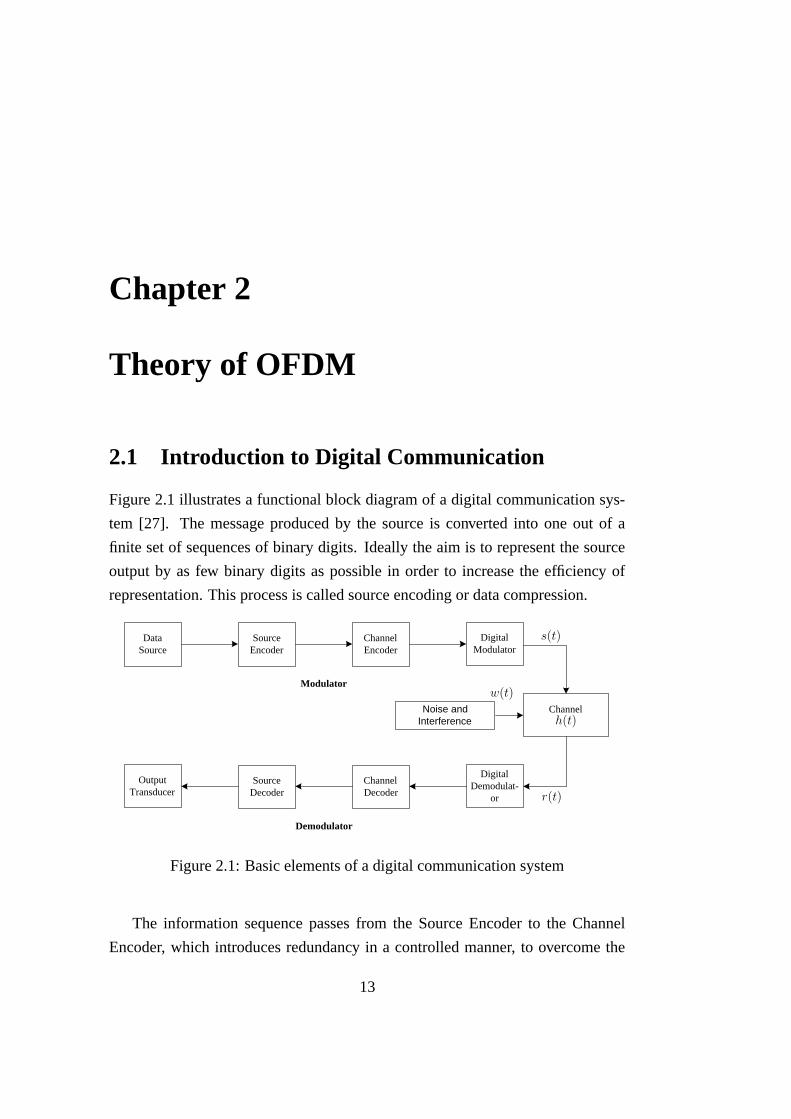
Figure 2.1 illustrates a functional block diagram of a digital communication sys-
tem [27]. The message produced by the source is converted into one out of a
finite set of sequences of binary digits. Ideally the aim is to represent the source
output by as few binary digits as possible in order to increase the efficiency of
representation. This process is called source encoding or data compression.
Data Source
Digital Modulator
Source Encoder
Channel
Channel Encoder
Digital Demodulat-
or
Channel Decoder
Source Decoder
Output Transducer
Modulator
Demodulator
Noise and Interference
PSfrag replacements
s(t)
h(t)
r(t)
w(t)
Figure 2.1: Basic elements of a digital communication system
The information sequence passes from the Source Encoder to the Channel
Encoder, which introduces redundancy in a controlled manner, to overcome the
13

14 CHAPTER 2. THEORY OF OFDM
effects of noise and interference in the channel. The errors that are caused by the
impairments are detected at the receiver and sometimes corrected. There are two
encoding approaches, namely, block or convolutional encoding, such schemes are
known as Error Control Coding (ECC). Although the use of an ECC greatly im-
proves the overall error rate performance of the system the objective of the author
of this thesis is to find the raw performance gains that could be obtained from using
the proposed algorithms over the conventional OFDM system. Hence, the work
presented in this thesis will not address Channel Encoding and hence this func-
tion is not included in the simulations. Besides, the use of an ECC would greatly
increase the complexity of the system, thus the simulation time and resources will
also be increased. The Digital Modulator maps the binary information sequence
to a waveform capable of being transmitted over the channel and being retrieved
at the receiver. The communication channel is the physical medium that is used to
carry the signal from the transmitter to the receiver. Possibilities include wireless,
local loop (telephone wires), optical fibre or coaxial cable etc. Whatever the chan-
nel, the transmitted data is corrupted in a random manner by a variety of possible
mechanisms, the most common being additive thermal noise.
The Digital Demodulator takes the received analogue waveform and produces
an estimate of the data stream originally applied to the Digital Modulator. The
Channel Decoder removes the redundancy introduced by the Channel Encoder
permitting errors at the Demodulator output to be identified and possibly cor-
rected. Schemes that are capable of correcting errors at the receiver are known as
Forward Error Correction (FEC) methods. Finally, the Source Decoder regener-
ates the original information. The challenge of the communication engineer is to
design a system that ensures the retrieval of data at an acceptable level of fidelity
for given channel conditions and available resources, e.g. transmitter power.
The received signal r(t) after it has travelled through the channel is,
r(t) = (s(t) ∗ h(t)) + w(t) (2.1)
where h(t) represents the channel response and w(t) represents the additive
noise and interference terms and ∗ represents the convolution operation. Note that
all simulations and analysis in this thesis, unless stated otherwise, are performed
2.1. INTRODUCTION TO DIGITAL COMMUNICATION 15
in the complex baseband domain. Please refer Appendix A for an introduction
to the concepts of complex baseband. We may express the frequency response,
H(f), of the channel as
H(f) = |H(f)| ejθ(f) (2.2)
where |H(f)| and θ(f) are known as the amplitude response and the phase
response, respectively. H(f) is also known as the Channel Transfer Function
(CTF). A channel is said to be non distorting or ideal if the amplitude response is
constant for all significant frequencies and the phase response is a linear function
of the frequency. Practical channels do not conform to these criteria perfectly.
In a practical channel, as a result of the convolution operation, the successive
transmitted signals will be smeared into one another. This phenomenon is called
Inter Symbol Interference (ISI).
From this point onward the emphasis will be on wireless channels only. There
are many modes of propagation for electromagnetic waves through a wireless
medium. For frequencies above 2 GHz, the dominant mode of transmission is via
Line-of-Sight (LOS) propagation. This means for terrestrial systems, the transmit-
ter and the receiver antennas must be in direct LOS with relatively little obstruc-
tion in between. The dominant noise limiting the performance of such a system
is thermal noise generated at the receiver and Co-channel Interference (CCI) from
other users. Even if the antennas at both ends do have a LOS path, the transmitted
signal may arrive at the receiver via multiple propagation paths. Delayed signals
could be the result of reflections from terrain features such as trees, mountains or
objects such as vehicles or buildings. This is very common and limits the perfor-
mance of such a system in urban or mountainous areas. The multipath propagation
gives rise to the reception of several copies of the same signal at the receiver an-
tenna each with a random phase. This generally causes ISI and moreover, the
received signals can add destructively, resulting in signal fading. See appendix B
for details of the effects of multipath channels. Multitone Modulation (MTM) is
a technique that is used to overcome the effects of multipath propagation.

16 CHAPTER 2. THEORY OF OFDM
2.2 Motivation to Use Multitone Modulation
The concept of MTM has been known since the middle of the 1960’s [28, 29]. The
approach is to transmit the data using a large number of subchannels, thereby re-
ducing the symbol rate carried by each subchannel. The theoretically ideal MTM
system has an infinite number of subchannels, and consequently a transmitted
symbol with an infinite length. Hence, if the Channel Impulse response (CIR) is
finite, the MTM system remains immune to distortion. However MTM was not
practical to implement until the discovery that it could be achieved via the use
of the Discrete Fourier Transform (DFT) [30]. Today it looks even more attrac-
tive owing to implementation of the DFT using the computationally efficient Fast
Fourier Transforms (FFT). MTM has attracted much interest owing to the devel-
opment of powerful Digital Signal Processing (DSP) circuits [31, 32]. There are
various MTM techniques and they have been referred to by many names. Among
them are Orthogonal Frequency Division Multiplexing (OFDM), Discrete Multi-
tone (DMT) and Filtered Multitone (FMT).
In order to understand the reasoning behind the use of Multitone transmission,
one must have a background of information theory. Claude Shannon in his revo-
lutionary work [33] showed that given a transmission source with power P , and
any linear time-invariant (LTI) channel with transfer function H(f) and additive
Gaussian noise with a two-sided Power Spectral Density (PSD) of N0/2 W/Hz,
it is possible to send a finite number of bits per second, Rb bps, over the channel
with a probability of making an error approaching zero as long asRb is lower than
a value called the capacity, C. Readers are referred to Appendix A for an intro-
duction to the PSD. For a perfectly bandlimited signal with bandwidth W Hz and
noise PSD N0/2 W/Hz, the capacity is given by,
C = W log2
[
1 +P
N0W
]
bps (2.3)
here P/N0W is the Signal to Noise Ratio (SNR). The signal power is related

2.3. ORTHOGONAL FREQUENCY DIVISION MULTIPLEXING 17
to the signal PSD Ps(f) by,
P = 2
∞∫
0
Ps(f)df . (2.4)
For a general LTI channel H(f), Shannon showed that the capacity is given
by,
C =
∞∫
0
log2
[
1 +|H(f)|2 Ps(f)
N0/2
]
bps . (2.5)
It is possible to maximise the capacity C, for a given value of P by optimising
Ps(f). It is given by,
Ps(f)opt =
[
λ− N0/2
|H(f)|2]
(2.6)
where λ is the Lagrange multiplier. This is the popular ‘water pouring’ solu-
tion. The essence of the solution requires utilising the entire channel bandwidth,
however the PSD of the transmitted signal is shaped such that Ps(f) is higher
where H(f) is not attenuated and lower where H(f) is attenuated.
Kalet has compared the use of multitone Quadrature Amplitude Modulation
(QAM) to single carrier QAM in [34]. The performance improvement for the mul-
titone system was not significant in Gaussian channels, however large improve-
ments were shown for channels with spectral nulls and for dynamic channels.
One particular form of MTM, namely OFDM will be discussed in detail in the
next section.
2.3 Orthogonal Frequency Division Multiplexing
Multipath propagation is the main cause for signal fading in radio reception. The
problem is exaggerated, if the receiver and/or the transmitter is/are mobile as the
added dimension of mobility will introduce more sever temporal characteristics
of the channel. In frequency selective fading, part of the frequency band will
experience severe attenuation while in others the response may be enhanced. If
the signal is narrowband and falls within a band where attenuation is high, it will
result in a significant reduction of the received SNR.

18 CHAPTER 2. THEORY OF OFDM
If the bandwidth of the signal is less than the coherence bandwidth of the chan-
nel, the distortion is minimised and this is called a frequency flat or a ‘flat’ fading
channel. However there is a significant chance that the signal will be subject to
severe attenuation on some occasions, i.e. temporal fading. A wideband signal
will experience more distortion, but will suffer reduced variations in terms of the
total received power. OFDM overcomes multipath propagation by transmitting a
large number of narrow band digitally modulated signals over a large bandwidth.
Consequently, each channel experiences ‘flat’ fading.
Consider a typical channel with a deep null in the frequency response. A sin-
gle carrier system, such as QAM, will need some form of time domain equalisa-
tion. Linear equalisation will increase noise, while a Decision Feedback equaliser
(DFE) will be more complex and its ultimate performance is limited by error
propagation. A Maximum Likelihood Sequence Estimator (MLSE) will be even
more complex. Since multicarrier systems, such as OFDM, approximate a con-
stant transfer function for each subchannel, equalisation becomes very simple.
Recently there have been proposals to use frequency domain equalisation for SC
systems (SC/FDE), for example [22, 35, 36]. The complexity of the SC/FDE sys-
tem is similar to the OFDM system, but the method requires training symbols
(also known as unique words) to be sent periodically to train the equalisers. Other
advantages of MTM methods are the reduced effects of impulsive noise as a re-
sult of the extended symbol duration, the flexibility to not transmit in corrupted
subchannels in the case of narrowband interference and the ability to transmit im-
portant data in subchannels with a high SNR. If the frequency separation between
the subchannel carriers, ∆f is chosen to be 1/T , where T is the symbol duration
of the subchannel carriers, then the complexity can be minimised by using FFT
techniques for implementation.
The receiver may be viewed as a bank of demodulators translating each sub-
channel carrier to baseband and integrating over the bit period. The subchannel
carrier frequencies are selected such that the subchannel spacing is an integral
multiple of symbol periods (i.e. the carriers are orthogonal over the symbol pe-
riod). Thus when integrated over the bit period, the other carriers yield a zero
contribution.
The ‘Frequency Division Multiplex’ part in the terminology is due to the data

2.3. ORTHOGONAL FREQUENCY DIVISION MULTIPLEXING 19
being divided among a large number of closely spaced subchannels. Often, prac-
tical OFDM systems, such as DAB and DVB-T, include a Forward Error Correc-
tion (FEC) stage for example using convolutional coding [14, 15]. Hence practical
systems are known as Coded OFDM (COFDM). The sidebands of individual sub-
channels do overlap in the frequency domain but the signals are received without
Inter Carrier Interference (ICI) owing to the orthogonal relationship between the
subchannels.
Members of an orthogonal set are linearly independent. Mathematically, an el-
ement ψp in a set of signals ψ will have the following relationship in an orthogonal
system;
b∫
a
ψp(t)ψ∗q (t)dt = K for p = q
= 0 for p 6= q . (2.7)
2.3.1 Mathematical Description of OFDM
Mathematically, each subchannel carrier within the frequency multiplex may be
represented by the complex signal given by,
sc(t) = Ac(t)ej[2πfct+φc(t)] (2.8)
where Ac(t) and φc(t) are the amplitude and the phase of the carrier, which
vary on a symbol-by-symbol basis. For QPSK, the amplitude is constant and the
phase takes on one of four possible values per symbol. Note that the transmitted
bandpass signal is the real part of sc(t). In OFDM we have many subchannels, thus
for N subchannel carriers the normalised transmitted complex baseband signal is
given by,
s(t) =
√
1
N
N−1∑
k=0
Ak(t)ej[2πfkt+φk(t)] . (2.9)

20 CHAPTER 2. THEORY OF OFDM
The subchannel carrier frequencies may be written in the following form;
fk = f0 + k∆f for k = 0, 1, . . . ., N − 1 (2.10)
where ∆f = 1/Ts. Here Ts is the duration of the QPSK symbols. Without
loss of generality we can let f0 = 0. If we assume that the phase and the amplitude
of the transmitted signal do not change over a symbol period, we can neglect the
amplitude and the phase dependence on time and express (2.9) as,
s(t) =
√
1
N
N−1∑
k=0
Akej[2π( k
Ts)t+φk] . (2.11)
This is a continuous time signal, which we wish to represent as a discrete time
signal with sampling frequency of 1/T , consequently Ts = NT , where T is the
sample period and N is the number of samples per OFDM symbol. In discrete
time format, (2.11) can be written as,
s(nT ) =
√
1
N
N−1∑
k=0
Akejφkej
2πknN . (2.12)
Comparing this with the normalised form of Inverse Discrete Fourier Trans-
form (IDFT),
g(nT ) =
√
1
N
N−1∑
k=0
G
(
k
NT
)
ej2πkn
N (2.13)
we note the similarity between (2.12) and (2.13). It is evident that the required
time domain signal s(nT ) can be obtained through an IDFT of the QPSK symbol
Akejφk . Hence it is shown that the OFDM carriers could be generated by IDFT,
or its efficient counterpart, the Inverse Fast Fourier Transform (IFFT). In general,
Akejφk can be taken from any QAM constellation.
2.3.2 Orthogonality of Subchannel Carriers
The subchannel carriers of the OFDM signal are given by,
ψk(t) = ej2πkt
Ts . (2.14)

2.4. SIMULATED CONVENTIONAL OFDM SYSTEM 21
Using (2.7) it follows that
b∫
a
ψp(t)ψ∗q (t)dt =
b∫
a
ej[2π(p−q)t/Tsdt
= (b− a) for p = q (2.15)
=ej[2π(p−q)b/Ts] − ej[2π(p−q)a/Ts]
j2π(p− q)/Ts
=ej[2π(p−q)b/Ts]
[
1 − ej[2π(p−q)(a−b)/Ts]]
j2π(p− q)/Ts
=ej[2π(p−q)(b+Ts
2 )/Ts][
ej[π(p−q)] − e−j[π(p−q)]]
j2π(p− q)/Ts
= ej[2π(p−q)(b+Ts2 )/Ts]sinc(p− q)
= 0 for p 6= q . (2.16)
The integration period for a symbol is (b − a) = Ts, which is used in the
5th line of the derivation. Note that p and q are integers. Hence the carriers are
orthogonal over time intervals equal to the symbol duration, or integer multiples
of the symbol duration.
2.4 Simulated Conventional OFDM System
Figure 2.2 shows the block diagram of a conventional OFDM system. The perfor-
mance of this baseline system will be used as a benchmark for comparison with
similar OFDM systems employing the novel algorithms to be presented through-
out this thesis. The input binary data stream is first distributed among the sub-
channels and mapped into a complex sequence using the chosen modulation con-
stellation. In this thesis the mapping scheme employed is always QPSK and it is
assumed that all the OFDM subchannels are used for data transmission.

22 CHAPTER 2. THEORY OF OFDM
Data Mapper
IFFT Mod.
Append Cyclic Prefix
Channel Response
P/S Conver-
sion
+
S/P Conver-
sion
Remov- al of
Cyclic Prefix
FFT Demod.
One-tap FEQ
Data Demap-
per
AWGN
Data In
Data Out
Shift Correlator
Calculation of FEQ taps
Training symbol
generator
Synch.
Synch.
Slicer
PSfrag replacements
A0,m
AN−1,m
s0,m
sN−1−v,m
sN−1,m
s(m)
h
wn
r0,m
rN−1,m
Y0,m
YN−1,m
A0,NtAN−1,Nt
C0,mCN−1,m
Y0,m
YN−1,m
A0,m
AN−1,m
Figure 2.2: Block diagram of a conventional OFDM system

2.4. SIMULATED CONVENTIONAL OFDM SYSTEM 23
The nth sample of the mth OFDM symbol generated by the Inverse FFT
(IFFT) at the transmitter is
sm,n =
√
1
N
N−1∑
k=0
Am,kej2π kn
N , 0 ≤ n ≤ N − 1 (2.17)
where Am,k is the QPSK symbol modulated on to the kth subchannel of the
mth OFDM symbol. Note that sm,n is the complex baseband equivalent of the
transmitted OFDM signal. The data is converted into a serial sequence, then a
Cyclic Prefix (CP) of length v is prepended. Thus the mth transmitted OFDM
symbol is
s(m) = [sm,N−v, .., sm,N−1, sm,0, .., sm,N−1]T . (2.18)
A finite length CIR is assumed havingNh samples, h = [h0, .., hNh−1]T , where
v ≥ Nh − 1. The received sequence can be expressed as,
rn = (sn ∗ hn) + wn (2.19)
where sn represents the serially concatenated transmitted symbols s(m) and
wn is the component due to Additive White Gaussian Noise (AWGN). The AWGN
samples that are used in the simulations were drawn from a Gaussian process hav-
ing a flat PSD over the entire signal bandwidth. The noise power for each transmit-
ted burst was estimated by averaging over a sequence as long as the burst length.
Finally, the noise power is averaged over all transmitted bursts before presenta-
tion of results. At the receiver, samples corresponding to the CP are discarded and
the remaining samples of the active OFDM symbol are used for decoding. The
symbol after FFT demodulation is
Ym,l =
√
1
N
N−1∑
n=0
rm,ne−j2π ln
N , 0 ≤ l ≤ N − 1 (2.20)
where rm,n, 0 ≤ n ≤ N − 1 are the received samples of the FFT window
for the mth OFDM block taken from rn, as determined by the synchronisation
algorithm. Chapter 4 will discuss the synchronisation method in more detail.

24 CHAPTER 2. THEORY OF OFDM
2.4.1 The effect of the Cyclic Prefix
Peled and Ruiz [37] first showed that digital parallel data transmission can be
achieved through an FFT and that ISI and ICI can be combated by the use of
a CP. If A(m) = [Am,0, .., Am,N−1]T denotes the vector of N data symbols and
F is the N × N DFT matrix, where the element Fk,n is given by e−j2πknN , the
modulated OFDM symbol, as shown in (2.17) is given by 1√NF
∗A(m). Here (.)∗
represents the complex conjugation operation and 1√N
is used for the normali-
sation of power. The transmitted OFDM symbol including the CP is given by
s(m) = 1√NTF
∗A(m), where T is a (N + v) ×N matrix given by,
T =
O I1
I2
(2.21)
where O is a matrix of size v × (N − v) containing zeros, I1 is a identity
matrix of size v and I2 is an identity matrix of size N . The effect of the CP is that
it converts the linear convolution of the CIR into a circular convolution. If r(m) =
[rm,0, .., rm,N−1]T is the vector of received OFDM symbols after discarding the CP
and assuming perfect synchronisation and v ≥ Nh − 1, it can be shown that,
r(m) =1√N
HF∗A(m) + w(m) (2.22)
where w(m) is the noise vector and H is the N ×N circulant matrix given by,
H =
h0 0 . . . hNh−1 . . . . . . h1
h1 h0 0 hNh−1 . . . h2
.... . . . . . . . .
.... . . . . . hNh−1
hNh−1. . . . . .
.... . . . . . . . .
0 . . . hNh−1 . . . h1 h0
(2.23)
2.4. SIMULATED CONVENTIONAL OFDM SYSTEM 25
Demodulation by the normalised DFT at the receiver yields,
1√N
Fr(m) =1
NF (HF
∗A(m) + w(m)) (2.24)
which can be simplified into,
1√N
Fr(m) = ∆A(m) +W (m) (2.25)
where ∆ is the size N diagonal matrix containing the DFT of the CIR h and
W (m) is the DFT of the noise vector. The DFT output consists of a summation
of random complex exponentials. Hence, for a system with a sufficiently large
value of N , from the Central Limit Theorem the output of the DFT will converge
to a Gaussian distribution. Since the DFT is a linear operation, for an input signal
w(m) drawn from a Gaussian process, the output statistics of W (m) will also
be Gaussian. It is assumed in the rest of this thesis that N is large enough so
that W (m) has the same statistical characteristics as w(m). In other words, the
demodulated output of the lth subchannel in the mth block is given by,
Ym,l = Am,lHl +Wl (2.26)
where Hl is the coefficient of the frequency domain CTF approximated at
subchannel l. Under the same assumptions (2.26) can also be written as,
Ym,l =1
N
N−1∑
n=0
N−1∑
k=0
Am,kHkej2π kn
N
e−j2πlnN +Wl (2.27)
In practical OFDM systems, the filter elements will often not have a linear
phase response and hence a constant group delay. Consequently, carriers of some
subchannels will arrive at the receiver at different time delays to others. The CP
of these systems are extended beyond the CIR length to absorb the variation in the
group delay. In all systems presented in this thesis, it is assumed that the filters
have linear phase response, yielding a constant absolute group delay hence, the
CP is set to be equal to the CIR length.

26 CHAPTER 2. THEORY OF OFDM
2.4.2 Frequency Domain Equaliser
It is evident from (2.26) that the symbols on each subchannel can only be de-
tected properly if the CTF is also estimated. The required correction amounts to
only one complex division per subchannel, which is performed by the Frequency
Domain Equaliser (FEQ) of the OFDM system. This is one major advantage
of OFDM over Single Carrier (SC) systems that use time domain equalisation,
which need complex and perhaps lengthy equalisers to nullify the effect of the
channel. The method adopted for the conventional system employed in the sim-
ulations is to transmit a known training symbol occupying OFDM symbol num-
ber Nt of each burst. In the simulations it is set to Nt = 0, i.e. the training
symbol is sent at the beginning of the burst. The training symbol is denoted as,
A = [ANt,0, .., ANt,N−1]T . Using the corresponding demodulated symbols YNt,l,
0 ≤ l ≤ N − 1, the FEQ coefficients are calculated as,
CNt,l =YNt,l
ANt,l
, 0 ≤ l ≤ N − 1 (2.28)
where CNt,l approximates CTFHl on subchannel l. If the CIR is time varying,
the FEQ coefficients will have to be updated accordingly using pilot symbols that
are transmitted throughout the burst. Since it is assumed throughout this work
that only short bursts are transmitted, it has been assumed that the CIR remains
approximately constant throughout the burst (see appendix B for further details)
and consequently the FEQ coefficients are not updated within the burst. This
assumption is made throughout the thesis. The symbols after the FEQ for all
other OFDM blocks m are given as,
Ym,l =Ym,lCNt,l
, 0 ≤ l ≤ N − 1 . (2.29)
The decoded symbols, Am,l are obtained by sending Ym,l through a slicer.
The CTF estimation by (2.28) is obviously affected by AWGN. The error can be
reduced by sending more than one training symbol and taking an average of all
the estimations. For the simulations presented in all chapters except for chapter 4
and chapter 5, an average of three such symbols is considered. Since the Schmidl

2.4. SIMULATED CONVENTIONAL OFDM SYSTEM 27
and Cox Algorithm (SCA) is used in the work presented in chapters 4 and 5,
the second training symbol of the SCA is used for channel estimation. Since
channel estimation is not the focus of the research presented in this work, it will
not be dealt with in isolation in the following chapters, however any degradation
that is introduced specifically by the channel estimation process is analysed via
simulations where appropriate.
Having introduced the basic concepts underlying OFDM systems, in the next
chapter the problem of Common Phase Error (CPE) arising as a result of oscillator
phase noise will now be addressed by the use of a novel Common Phase Error
Correction (CPEC) algorithm.

28 CHAPTER 2. THEORY OF OFDM

Chapter 3
Common Phase Error Correction
OFDM has proven to be more sensitive than SC systems to the Phase Noise (PN)
of the oscillators used in the up and down conversion process employed at the
transmitter and the receiver, respectively [38]. However in a BFWA scenario the
Base Station (BS) will have an oscillator with a relatively high accuracy and sta-
bility. Consequently, the main contribution to the PN of the system will arise from
the local oscillators in the Subscriber Units (SU). This is primarily due to the ne-
cessity for cheaper subscriber equipment which results in the use of inexpensive
oscillators with lower accuracy and stability. In this chapter it will be assumed
that PN will be introduced into the system only at the SU.
It is important to explain the DFT operation in order to understand the suscep-
tibility of OFDM to PN. The DFT of a sampled signal x(k) is defined as,
X(n) =
√
1
N
N−1∑
k=0
x(k)e−j2πknN (3.1)
where X(n) is equal to the spectrum of x(k) at the sampled frequency points
n. The DFT of the complex exponential x(k) = ej2πfhkT with frequency fh and
sample spacing T is given as,
X(n) = ejπfhTN−nN−1N
sin[π(fhTN − n)]
sin[π(fhTN − n)/N ]. (3.2)
29

30 CHAPTER 3. COMMON PHASE ERROR CORRECTION
Now let,
fhTN = m+ ε (3.3)
where m is the discrete frequency and ε is the relative frequency deviation.
The magnitude response of (3.2) with the substitution of (3.3) is given as;
|X(n)| =
∣
∣
∣
∣
∣
sin[π(m− n+ ε)]
sin[π(m− n+ ε)/N ]
∣
∣
∣
∣
∣
. (3.4)
The response of |X(n)| in (3.4) with frequency deviation, ε = 0 is shown in
figure 3.1 for N = 16 at two discrete frequencies, m − n = 0 and m − n = −1.
It shows that an unwindowed (i.e. rectangular window) DFT response has high
sidelobes with the first sidelobe just 13 dB below the mainlobe. However, as long
as ε is zero (or an integer value) the responses remain orthogonal to each other.
0 2 4 6 8 10 12 14 16−40
−35
−30
−25
−20
−15
−10
−5
0
5
|X(n
)| d
B
n
m−n=0m−n=−1
Figure 3.1: Magnitude response of the DFT due to a complex exponents of twodifferent frequencies with N = 16
Figure 3.2 shows the effect of leakage caused by non zero values of frequency
deviation, ε. It shows that even with a small value of deviation, e.g. ε = 0.4,
there is significant interference from the given subchannel to the others. Also the
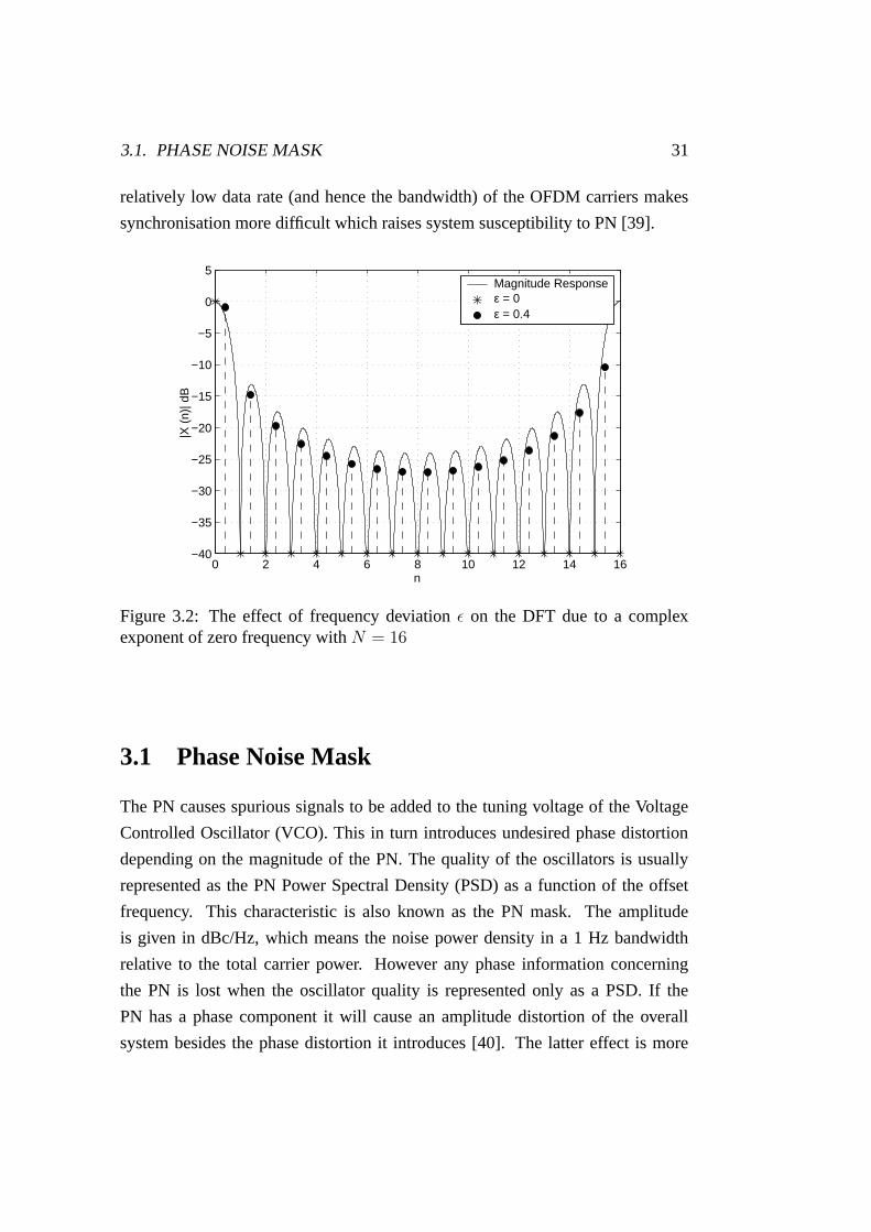
3.1. PHASE NOISE MASK 31
relatively low data rate (and hence the bandwidth) of the OFDM carriers makes
synchronisation more difficult which raises system susceptibility to PN [39].
0 2 4 6 8 10 12 14 16−40
−35
−30
−25
−20
−15
−10
−5
0
5
n
|X (
n)| d
B
Magnitude Responseε = 0ε = 0.4
Figure 3.2: The effect of frequency deviation ε on the DFT due to a complexexponent of zero frequency with N = 16
3.1 Phase Noise Mask
The PN causes spurious signals to be added to the tuning voltage of the Voltage
Controlled Oscillator (VCO). This in turn introduces undesired phase distortion
depending on the magnitude of the PN. The quality of the oscillators is usually
represented as the PN Power Spectral Density (PSD) as a function of the offset
frequency. This characteristic is also known as the PN mask. The amplitude
is given in dBc/Hz, which means the noise power density in a 1 Hz bandwidth
relative to the total carrier power. However any phase information concerning
the PN is lost when the oscillator quality is represented only as a PSD. If the
PN has a phase component it will cause an amplitude distortion of the overall
system besides the phase distortion it introduces [40]. The latter effect is more

32 CHAPTER 3. COMMON PHASE ERROR CORRECTION
significant [40] and hence in this work it will be assumed that the PN introduces
only a phase distortion.
It is important to describe the components of a practical OFDM receiver to un-
derstand the effect of PN. The front end of the OFDM receiver contains a Tuner,
an Intermediate Frequency (IF) amplifier, an I/Q demodulator and an A/D con-
verter. The conversion to baseband may be either direct or more usually via single
or double down conversions through one or two IF stages. The Radio Frequency
(RF) modulated signal from the antenna is amplified by a Low Noise Amplifier
(LNA) before frequency down conversion in a Mixer driven by a Local Oscillator
(LO). The IF amplifier filters out the adjacent channels and amplifies the wanted
signal. The I/Q demodulator delivers the complex baseband signal in the form of
an in-phase component, I and a quadrature component Q. After lowpass filtering,
A/D conversion yields sampled values of the received complex baseband signals.
To permit receiver tuning, the LO is usually implemented as a tunable VCO.
The stability of the VCO is maintained by the use of a Phase Lock Loop (PLL).
Figure 3.3 shows the main components of a PLL based frequency synthesiser [40].
Phase Detector
VCO
Low Pass Filter
Frequency Divider
Reference Oscillator
Figure 3.3: Block diagram of a PLL frequency synthesiser
The reference oscillator provides a stable frequency that is usually maintained
by the use of a crystal tuning element. The phase detector compares the phase
of the VCO signal (following frequency division) and generates an output pro-
portional to the difference of the phase between this and the reference source. In

3.1. PHASE NOISE MASK 33
general the higher the carrier frequency, the greater is the oscillator PN. The VCO
is the main cause of PN since it operates at the carrier frequencies. All distur-
bances of the VCO are imposed upon the signal. If the VCO has a wide frequency
range the tuning sensitivity is very high. Consequently even the smallest spurious
signals added to the tuning voltage will give rise to an undesired angle modula-
tion when the VCO runs free [41]. The signal from the phase detector is passed
through a low pass loop filter, to generate the VCO tuning voltage. The overall
transfer function of the PLL determines the damping ratio and the loop bandwidth.
The action of the PLL is to reduce the PN within the loop bandwidth, as given by
its transfer function [40]. The total PN density of a PLL synthesiser system is
given by,
Sψ(f) = SV CO(f)HPLL(f) + SREFn2 + Sδ (3.5)
where SV CO is the PN density of the VCO, HPLL is the is the overall transfer
function of the PLL, SREF is the PN density of the reference oscillator, n is the
divide ratio of the frequency divider and Sδ is the additional PN density of all other
sources [40]. SREF usually decreases with frequency and SV CO is controlled by
HPLL. A typical one-sided spectrum for Sψ(f) is shown in figure 3.4.
Legend
f
Noise Density (dB)
PSfrag replacements
SREFn2
SV CO(f)
HPLL(f)
Sψ(f)
Figure 3.4: Components of the PN density

34 CHAPTER 3. COMMON PHASE ERROR CORRECTION
It can be concluded that a typical PN density will have a flat region close to the
the carrier frequency and will then roll off to a PN floor. The published literature
shows that there are two main approaches used to model the PN. The authors
in [38, 42] model PN as a non stationary, infinite power Weiner process. More
often as in [43] and [44], PN is considered as a stationary, band limited, finite
power process. In such models, the PN is approximated by a piece-wise linear
function in the log-linear domain. The latter model is adopted in this contribution.
The PN is modelled as a phasor ejψ(n), where the sampled PN process ψ(n) is
zero-mean and wide-sense stationary with a narrow band Power Spectral Density
(PSD) mask, Sψ(f) given by (3.6) having a finite power σ2ψ [43]. So,
Sψ(f) = 10−c +
10−a |f | < fl,
10−(f−fl)(b/fh−fl)−a f > fl,
10(f+fl)(b/fh−fl)−a f < −fl(3.6)
where parameter c determines the noise floor of the oscillator and a determines
the noise PSD from the center frequency out to a frequency of ±fl. Parameter b
gives the noise fall off rate and at fh the noise PSD is 10b dB lower than the value
at fl (See figure 3.5). Typical parameter values for a 5.2 GHz synthesised source
are a = 8, b = 2, c = 12, fl = 10 kHz and fh = 100 kHz [44]. Figure 3.6 shows
the one-sided PN mask of the simulated PN mask for the same parameters. The
frequency axis is normalised to half-sampling frequency. We have assumed that
the sampling frequency is 20 MHz.
The oscillators practically used by operators for BFWA systems, for exam-
ple [45, 46] have PSD of PN of a similar order as given in [44]. Typically, the
values for fh are of the order of 100 kHz and for a it is of the order of 7-12. Hence
the models used in the following section are quite close representations of PN of
oscillators used practically in the industry.
The two most important parameters in determining the quality of an oscillator
are the PN bandwidth, which is mainly determined by fl and the PN power, which
is determined primarily by a and c. Signal to Phase Noise Ratio (SPNR) will
be widely used as the performance criteria for the comparison of results in latter
sections. It is defined as the ratio between the signal power and PN power. In

3.2. ANALYSIS OF THE EFFECT OF PHASE NOISE ON OFDM 35
-10a
-10c
10b
PSfrag replacements
Sψ(f)(dBc/Hz)
f (Hz)fhfl−fl−fh
Figure 3.5: Phase Noise PSD of a typical oscillator
most cases, as is done in this work, the signal power and the carrier power are
normalised to unity. In which case, the SPNR is equal to the inverse of the PN
power. For a given PN bandwidth, SPNR will show how robust the system is
against PN. It has been proven in [47, 48] that the degradation experienced in
an OFDM system without any correction depends on PN variance but not the
shape of the PN spectrum. Hence SPNR is a representative criteria to compare
performance.
3.2 Analysis of the Effect of Phase Noise on OFDM
A good analysis on the subject is given in [48], but a different approach is adopted
here. The results, however are similar. The PN is modelled as a multiplicative
error term ejψ(n) and the ideal received sequence given in (2.19) is changed to,
rn = [(sn ∗ hn) + wn] ejψ(n) . (3.7)
Assuming perfect synchronisation and the length of the Cyclic Prefix (CP) is

36 CHAPTER 3. COMMON PHASE ERROR CORRECTION
0 0.002 0.004 0.006 0.008 0.01 0.012 0.014 0.016 0.018 0.02−180
−160
−140
−120
−100
−80
−60
Normalised Frequency (2*f/fs)
Sψ (
dB)
Figure 3.6: Simulated one-sided PN mask for a = 8, b = 4, c = 12, fl = 10kHz,fh = 100kHz at fs = 20MHz
greater than the length of the Channel Impulse response (CIR), v ≥ Nh − 1, the
demodulated signal at the lth subchannel in the mth block is now given by [44],
Ym,l =1
N
N−1∑
n=0
N−1∑
k=0
Am,kHkej2π kn
N
ejψ(n)
e−j2πlnN +Wl (3.8)
compared with that presented previously in (2.27). HereWl is the contribution
due to AWGN. Note that the rotation caused by PN does not change the statistical
characteristics of AWGN [48]. If ψ(n) takes small values, then for analytical
purposes a simplifying assumption using the first two terms of the Taylor series
expansion is,
ejψ(n) ≈ 1 + jψ(n), ψ 1 . (3.9)

3.2. ANALYSIS OF THE EFFECT OF PHASE NOISE ON OFDM 37
Using this assumption in (3.8) gives,
Ym,l =1
N
N−1∑
n=0
N−1∑
k=0
Am,kHkej2π kn
N
(1 + jψ(n))
e−j2πlnN +Wl (3.10)
which can be further simplified to,
Ym,l ≈ Am,lHl + Am,lHl1
N
N−1∑
n=0
jψ(n) +
1
N
N−1∑
k=0k 6=l
Am,kHk
N−1∑
n=o
(1 + jψ(n))e−j2π(l−k)n
N +Wl (3.11)
The first term on the r.h.s. of (3.11) is the useful component. The channel
coefficient for subchannel l can easily be equalised by the FEQ coefficient CNt,l,
as calculated in (2.28). The second component introduces an equal phase rotation
on to each subchannel and is independent of the particular subchannel concerned,
l. This is commonly known as the Common Phase Error (CPE). The third term is
the Inter-Carrier Interference (ICI) caused by contributions from all subchannels
k 6= l on l owing to the loss of orthogonality. Let us denote these components as
ψCPE and ψICI respectively. Unlike the CPE, the ICI is not easy to estimate.
3.2.1 Common Phase Error
The CPE is given as,
ψCPE =1
N
N−1∑
n=0
jψ(n) (3.12)
which results in a rotation of the entire signal constellation within an OFDM
symbol. The CPE is linearly related to the sampled PN process ψ(n) and as a
result is Gaussian with mean and variance given by [39],
E[ψCPE] =1
N
N−1∑
n=0
jE[ψ(n)] = 0 (3.13)
σ2CPE = E[|ψCPE|2] =
∫ fs/2
−fs/2
Sψ(f)
N2
∣
∣
∣
∣
∣
sin((πNf)/fs)
sin((πf)/fs
∣
∣
∣
∣
∣
2
df (3.14)

38 CHAPTER 3. COMMON PHASE ERROR CORRECTION
where fs is the sampling frequency. It can be noted that the variance σ2CPE
is monotonically decreasing with N . It implies that OFDM systems using fewer
subchannels within a given bandwidth will experience a larger rotation of the con-
stellation owing to CPE [39].
3.2.2 Inter Carrier Interference
The ICI component depends upon the data symbols in the current OFDM symbol.
Assuming that the number of subchannels, N is large and since the data symbols
are statistically independent, we can then assume that the ICI component is also a
zero mean Gaussian process. Consequently, the effect of ICI is similar to that of
AWGN. Since both CPE and ICI are Gaussian, the variance of both the CPE and
the ICI should be equal to the variance of the sum of both components. Hence the
variance of the ICI component can be calculated as [39],
σ2ICI = E[|ψICI |2] =
∫ fs/2
−fs/2Sψ(f) df −
∫ fs/2
−fs/2
Sψ(f)
N2
∣
∣
∣
∣
∣
sin((πNf)/fs)
sin((πf)/fs
∣
∣
∣
∣
∣
2
df
(3.15)
It can be noted that σ2ICI is monotonically increasing as a function ofN [39]. A
similar conclusion is drawn in [43]. Intuitively, the effect ofN on the CPE and the
ICI components can be explained as follows. For a given transmission bandwidth
the inter carrier spacing of the OFDM subchannels is reduced if a higher value
of N is used. For a given non-ideal oscillator with a certain PN bandwidth, each
subchannel will be corrupted by signals that fall within the PN bandwidth. Hence,
the ICI will be higher for a higher N since there is a higher probability of more
subchannels falling within the same PN bandwidth. Since the sum of the variances
of CPE and ICI should remain the same, the CPE component will reduce with an
increase in N . The figures in 3.7 show the demodulated constellation (i.e. after
the FFT) at the receiver of all OFDM symbols of the whole burst for two systems,
one with N = 64 and the other with N = 256. Both are subjected to a SUI-II [23]
CIR and AWGN yielding an SNR of 20 dB and a SPNR of 15 dB. The plots are
the result of demodulating 2500 OFDM symbols for the N = 64 system and 625
OFDM symbols for the N = 256 system. Both systems used QPSK for mapping
and hence the total QPSK symbols demodulated for both systems was 160,000.

3.2. ANALYSIS OF THE EFFECT OF PHASE NOISE ON OFDM 39
The plot forN = 64 shows a greater phase rotation owing to CPE, whereas for the
system with N = 256 more dispersion is evident owing to the increased level of
ICI. Alternatively, for a given OFDM system with a certain inter-carrier spacing
(that is determined by N ), the ICI will come to dominate CPE with an increasing
PN bandwidth [49, 50].
(a) N = 64 (b) N = 256
Figure 3.7: Constellation of post-FFT data symbols with an AWGN SNR of 20dB and a SPNR at 15 dB with a SUI-II CIR
3.2.3 Probability of Error Analysis
The effect of CPE on OFDM will be modelled as a rotational component given by
a multiplicative error ejψCPE . Hence if the received sample vector is denoted as r,
then the result after CPE is,
r = rejψCPE (3.16)
The ICI component is modelled as an additive Gaussian noise component with
variance σ2ICI . Hence the total additive noise component is a zero mean Gaussian
process with total variance being σ2T = σ2
ICI + σ2w, where σ2
w is the variance due
to thermal noise. Hence the input to the slicer is [39],
y = r + wT = (x+ nTr) + j(y + nT i) (3.17)

40 CHAPTER 3. COMMON PHASE ERROR CORRECTION
where x and y are the real and imaginary parts of r respectively and nTr and
nT i are the real and imaginary components of the total additive Gaussian noise
component, respectively. The effect of both components of PN can be represented
as shown in figure 3.8. This is a snapshot of one demodulated OFDM symbol.
The concentric circles represent the contours of the Gaussian dispersion of the
data points of each constellation point of the QPSK mapping. Here Es is the
transmitted symbol power.
Transmitted Reference
Received Reference
Legend
PSfrag replacements
ψCPE
√Es
ar(ψCPE)
ai(ψCPE)
Figure 3.8: QPSK constellation subject to a phase rotation owing to ψCPE

3.2. ANALYSIS OF THE EFFECT OF PHASE NOISE ON OFDM 41
The real and imaginary components of y are statistically independent Gaussian
processes with equal variances. Hence their joint probability distribution is given
by [39],
Px, y =1
2πσ2T
exp(
−(x− x)
2σ2T
)
exp(
−(y − y)
2σ2T
)
. (3.18)
The probability for a correct decision for a symbol in the presence of AWGN
and PN can be expressed as [51],
Pc|ψCPE= Q
(
− 1
σTar(ψCPE)
)
.Q(
− 1
σTai(ψCPE)
)
(3.19)
where,
ar(ψCPE) =√
Es sin(
π
4− ψCPE
)
(3.20)
ai(ψCPE) =√
Es cos(
π
4− ψCPE
)
. (3.21)
The function Q(.) is the area under the tail of the Gaussian PDF and is defined
as [27, pg 40],
Q(x) =1√2π
∫ ∞
xet
2/2 dt, x ≥ 0 . (3.22)
Hence the Symbol Error Rate (SER) of an OFDM system with no CPE cor-
rection for a given rotational angle of ψCPE can be calculated as [51],
Pe|ψCPE= Q
(
1
σTar(ψCPE)
)
+Q(
1
σTai(ψCPE)
)
−
Q(
1
σTar(ψCPE)
)
.Q(
1
σTai(ψCPE)
)
(3.23)
Since Grey coding is used for the QPSK mapping, the overall BER can be
assumed to be half of this value. Figure 3.9 shows the theoretical predictions
based on (3.23) for OFDM systems with N equal to 64 and 256 subject to AWGN
yielding a SNR of 20 dB and PN with b = 4, fl = 10 kHz and fh = 100 kHz.
Equation (3.14) gives the SER for a particular value of the CPE phase, ψCPE .
The SPNR and the variance of ψCPE (using equation (3.14)) is determined by the
area under the PN mask. The variance of the ICI is determined using (3.15). It is
assumed that the ICI has a similar effect to AWGN and that the total additive noise
variance σ2T in (3.23) is calculated as the sum of the variance of AWGN and ICI.

42 CHAPTER 3. COMMON PHASE ERROR CORRECTION
The theoretical curves for OFDM systems without CPE correction in figure 3.9
are evaluated by drawing values for ψCPE from a source having a Gaussian PDF
with the variance given in (3.14) and, using expectation theory, integrating over
all values of ψCPE . The simulated values are also shown as points for comparison.
The figure shows that the theoretical predictions show very close agreement with
the simulated points. It also proves that the performance of the OFDM system
under consideration when subject to only AWGN and PN with fh = 100 kHz
does not depend upon the number of subchannels, N . It also shows an error floor
at a BER of approximately 10−12. This can be attributed to the fact that AWGN
and ICI become more dominant over CPE at high values of SPNR.
5 10 15 20 25 30 35 4010
−12
10−10
10−8
10−6
10−4
10−2
100
SPNR (dB)
BE
R
N = 64, TheoreticalN = 64, SimulatedN = 256, TheoreticalN = 256, Simulated
Figure 3.9: The theoretical and simulated results for OFDM systems without CPEcorrection with N = 64 and 256 subject to AWGN yielding an SNR of 20 dB andPN with fh = 100 kHz
3.3 Related Work
In this section related work not cited previously in the chapter will be summarised.
Pollet in [38] was the first to show that OFDM is orders of magnitude more sen-
3.4. COMMON PHASE ERROR CORRECTION ALGORITHM 43
sitive to PN and frequency offsets than Single Carrier (SC) systems. Many other
authors have also analysed the effect of PN in terms of CPE and ICI, for exam-
ple [43, 52, 44]. The author in [43] further proposes a feedback CPE correction
method for an OFDM system with a total of 2048 subchannels by transmitting pi-
lot symbols in some of the subchannels in every OFDM symbol. The pilot symbol
positions are dynamically rotated after every OFDM symbol to avoid them falling
into a frequency null. The known pilot symbols are used to estimate the CPE
by determining the phase change of each received pilot. A reliability estimate is
given to each pilot before the CPE is estimated, but the author does not specify
how these reliability estimates are generated. The author in [53] assumes a PN
mask model similar to that in [38]. Analytical solutions of the error rate perfor-
mance are given for BPSK, QPSK, differential BPSK and differential QPSK. It
is proposed to implement the differential modulation scheme within the OFDM
symbol (in the frequency domain) rather than between adjacent OFDM symbols
in order to minimise the effect of phase noise. The conclusions show that for
QPSK, the performance strongly degrades if the 3dB bandwidth of the PN mask
is greater than 0.04 of the intercarrier spacing. Armada in [52] concludes that
the effects of PN can be corrected when the PN bandwidth is smaller than the
intercarrier spacing. Hanzo in [41] compares the effect of PN on an OFDM mo-
dem and a serial modem. The comparisons use coloured (using a PN mask) and
white PN models and it is found that the performance is similar for all PN mod-
els based on PN power. This confirms that irrespective of the mask, PN power
determines the performance. The author in [47] analyses the effect of PN on Or-
thogonal Frequency Division Multiple Access (OFDMA) and Frequency Division
Multiple Access (FDMA) systems in a multi user scenario and compares it with
conventional OFDM. The authors concluded that when all subchannels have the
same power and are subjected to the same PN mask, the degradation is equal to
that in OFDM and also that FDMA is slightly more robust than OFDMA.
3.4 Common Phase Error Correction Algorithm
An algorithm is proposed in this section to estimate and correct for the CPE com-
ponent in each OFDM symbol. Since the effect of ICI is similar to AWGN, and as-
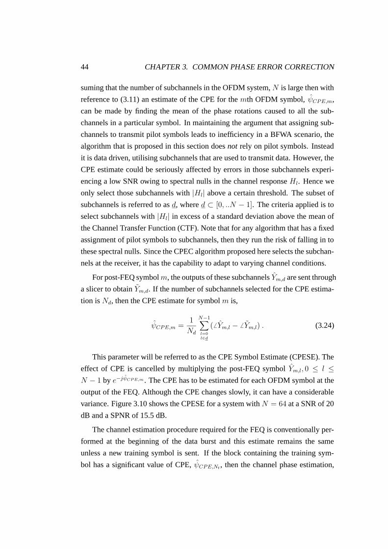
44 CHAPTER 3. COMMON PHASE ERROR CORRECTION
suming that the number of subchannels in the OFDM system, N is large then with
reference to (3.11) an estimate of the CPE for the mth OFDM symbol, ψCPE,m,
can be made by finding the mean of the phase rotations caused to all the sub-
channels in a particular symbol. In maintaining the argument that assigning sub-
channels to transmit pilot symbols leads to inefficiency in a BFWA scenario, the
algorithm that is proposed in this section does not rely on pilot symbols. Instead
it is data driven, utilising subchannels that are used to transmit data. However, the
CPE estimate could be seriously affected by errors in those subchannels experi-
encing a low SNR owing to spectral nulls in the channel response Hl. Hence we
only select those subchannels with |Hl| above a certain threshold. The subset of
subchannels is referred to as d, where d ⊂ [0, ..N − 1]. The criteria applied is to
select subchannels with |Hl| in excess of a standard deviation above the mean of
the Channel Transfer Function (CTF). Note that for any algorithm that has a fixed
assignment of pilot symbols to subchannels, then they run the risk of falling in to
these spectral nulls. Since the CPEC algorithm proposed here selects the subchan-
nels at the receiver, it has the capability to adapt to varying channel conditions.
For post-FEQ symbolm, the outputs of these subchannels Ym,d are sent through
a slicer to obtain Ym,d. If the number of subchannels selected for the CPE estima-
tion is Nd, then the CPE estimate for symbol m is,
ψCPE,m =1
Nd
N−1∑
l=0l∈d
( 6 Ym,l − 6 Ym,l) . (3.24)
This parameter will be referred to as the CPE Symbol Estimate (CPESE). The
effect of CPE is cancelled by multiplying the post-FEQ symbol Ym,l, 0 ≤ l ≤N − 1 by e−jψCPE,m . The CPE has to be estimated for each OFDM symbol at the
output of the FEQ. Although the CPE changes slowly, it can have a considerable
variance. Figure 3.10 shows the CPESE for a system with N = 64 at a SNR of 20
dB and a SPNR of 15.5 dB.
The channel estimation procedure required for the FEQ is conventionally per-
formed at the beginning of the data burst and this estimate remains the same
unless a new training symbol is sent. If the block containing the training sym-
bol has a significant value of CPE, ψCPE,Nt, then the channel phase estimation,
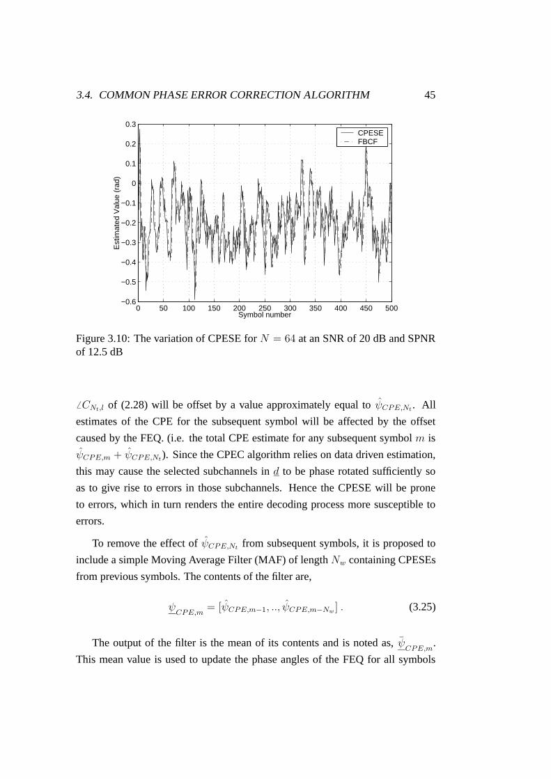
3.4. COMMON PHASE ERROR CORRECTION ALGORITHM 45
0 50 100 150 200 250 300 350 400 450 500−0.6
−0.5
−0.4
−0.3
−0.2
−0.1
0
0.1
0.2
0.3
Symbol number
Est
imat
ed V
alue
(ra
d)
CPESEFBCF
Figure 3.10: The variation of CPESE for N = 64 at an SNR of 20 dB and SPNRof 12.5 dB
6 CNt,l of (2.28) will be offset by a value approximately equal to ψCPE,Nt. All
estimates of the CPE for the subsequent symbol will be affected by the offset
caused by the FEQ. (i.e. the total CPE estimate for any subsequent symbol m is
ψCPE,m + ψCPE,Nt). Since the CPEC algorithm relies on data driven estimation,
this may cause the selected subchannels in d to be phase rotated sufficiently so
as to give rise to errors in those subchannels. Hence the CPESE will be prone
to errors, which in turn renders the entire decoding process more susceptible to
errors.
To remove the effect of ψCPE,Ntfrom subsequent symbols, it is proposed to
include a simple Moving Average Filter (MAF) of length Nw containing CPESEs
from previous symbols. The contents of the filter are,
ψCPE,m
= [ψCPE,m−1, .., ψCPE,m−Nw] . (3.25)
The output of the filter is the mean of its contents and is noted as, ψCPE,m
.
This mean value is used to update the phase angles of the FEQ for all symbols
46 CHAPTER 3. COMMON PHASE ERROR CORRECTION
m > Nt,6 Cm,l = 6 Cm−1,l + ψ
CPE,m, 0 ≤ l ≤ N − 1 . (3.26)
The parameter ψCPE,m
is referred to as the Feedback Correction Factor (FBCF).
Figure 3.10 shows that the FBCF closely tracks the CPESE. The argument can be
further explained in the following diagrams. Figure 3.11 shows the actual phase
of the CTF and the estimated phase of the CTF ( 6 CNt,l) when a low value of
ψCPE,Ntis present. The OFDM system for this example has N = 64 with a SNR
of 20 dB and a SPNR of 15 dB subjected to a SUI-II CIR. Figure 3.12(a) shows a
polar plot of the demodulated data following the FEQ (Ym,l) corresponding to the
OFDM symbol that yields the greatest number of errors within the burst. It shows
that the data points are rotated clockwise owing to a combination of the CPE of
symbol m and Nt. The data points that are selected to calculate the CPESE are
based on these points. It shows that most of the data points lie within the decision
boundaries, i.e. the vertical and horizontal axes. A CPEC algorithm that relies
only on a CPESE would perform adequately in this case. Figure 3.12(b) shows
data points that result if the FEQ is used in conjunction with a FBCF. It shows
that the FBCF maintains the data points further within the decision boundaries.
Figure 3.12(c) shows the result after the proposed CPEC which employs both the
FBCF and the CPESE. Following correction by both factors it can be seen that the
data points lie very close to the original constellation points.
A second case is presented in figure 3.13 which shows the estimated phase
of the CTF ( 6 CNt,l) for a different transmission burst with the same CIR but this
time for a larger value of ψCPE,Nt. Since the state of the oscillator is random, this
value is unpredictable. Figure 3.14(a) shows the demodulated data symbols of
the OFDM symbol which generates the greatest number of errors. This time the
constellation is rotated counter-clockwise. However it clearly shows that many of
the data points after the FEQ (Ym,l) have crossed the decision boundaries. Hence,
a conventional OFDM system would be subjected to a large number of errors. In
addition a CPEC algorithm that relies only on a CPESE will generate an erroneous
estimate that will further rotate the data points counter-clockwise. Ultimately the
data points will lie in a different quadrant compared to the transmitted ones. The
constellation of data points following the FBCF for the same scenario is shown
3.4. COMMON PHASE ERROR CORRECTION ALGORITHM 47
0 10 20 30 40 50 60−1.2
−1
−0.8
−0.6ar
g(H
l ) (
rad)
Subchannel index, l
ActualEstimated
Figure 3.11: Estimation of the phase of the CTF which is offset owing to a lowvalue of ψCPE,Nt
in figure 3.14(b). It clearly shows that when the FBCF is used, it is able to track
the rotation caused by the FEQ and the CPE and contain the data points to be
within the correct quadrant. As shown in figure 3.14(c), a further correction by
the CPESE that is based on the data points shown in figure 3.14(b) results in the
corrected data points being very close to the original constellation points. Hence
it is clear that the data driven CPEC algorithm proposed for a coherent OFDM
system requires both the FBCF and the CPESE to be used.
Figure 3.15(a) shows a subchannel-wise error analysis of the whole burst con-
ducted for the same OFDM system at a SPNR of 15.5 dB. It shows the subchannels
selected for CPEC, and the number of errors in the I channel (in black) and the
Q channel (in white) as a stacked bar graph. The magnitude plot of the estimated
CTF, |Hl| is also superimposed for clarity. At the chosen SPNR, the majority of
the subchannels selected for the CPEC algorithm have a very low number of errors
in the whole burst, justifying the selection criteria adopted for the algorithm. Fig-
ure 3.15(b) shows that all the subchannels are free from errors after the proposed
CPEC is used. However, as shown in figure 3.16(a), when the PN power increases

48 CHAPTER 3. COMMON PHASE ERROR CORRECTION
0.5
1
1.5
30
210
60
240
90
270
120
300
150
330
180 0
Tx const.After FEQ
(a) after FEQ
0.5
1
1.5
30
210
60
240
90
270
120
300
150
330
180 0
Tx const.After FBCF
(b) after FBCF
0.5
1
1.5
30
210
60
240
90
270
120
300
150
330
180 0
Tx const.After CPEC
(c) after CPEC
Figure 3.12: Performance of the symbol with most errors and a low value ofψCPE,Nt
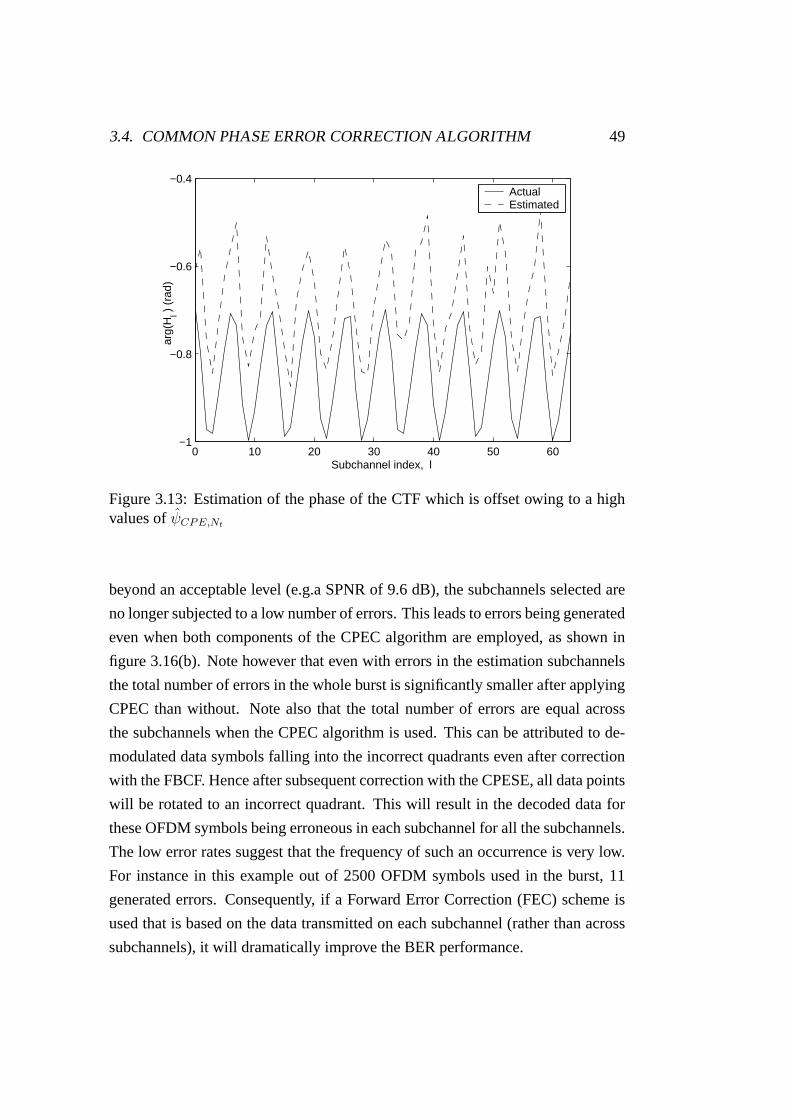
3.4. COMMON PHASE ERROR CORRECTION ALGORITHM 49
0 10 20 30 40 50 60−1
−0.8
−0.6
−0.4ar
g(H
l ) (
rad)
Subchannel index, l
ActualEstimated
Figure 3.13: Estimation of the phase of the CTF which is offset owing to a highvalues of ψCPE,Nt
beyond an acceptable level (e.g.a SPNR of 9.6 dB), the subchannels selected are
no longer subjected to a low number of errors. This leads to errors being generated
even when both components of the CPEC algorithm are employed, as shown in
figure 3.16(b). Note however that even with errors in the estimation subchannels
the total number of errors in the whole burst is significantly smaller after applying
CPEC than without. Note also that the total number of errors are equal across
the subchannels when the CPEC algorithm is used. This can be attributed to de-
modulated data symbols falling into the incorrect quadrants even after correction
with the FBCF. Hence after subsequent correction with the CPESE, all data points
will be rotated to an incorrect quadrant. This will result in the decoded data for
these OFDM symbols being erroneous in each subchannel for all the subchannels.
The low error rates suggest that the frequency of such an occurrence is very low.
For instance in this example out of 2500 OFDM symbols used in the burst, 11
generated errors. Consequently, if a Forward Error Correction (FEC) scheme is
used that is based on the data transmitted on each subchannel (rather than across
subchannels), it will dramatically improve the BER performance.

50 CHAPTER 3. COMMON PHASE ERROR CORRECTION
0.5
1
1.5
30
210
60
240
90
270
120
300
150
330
180 0
Tx constAfter FEQ
(a) after FEQ
0.5
1
1.5
30
210
60
240
90
270
120
300
150
330
180 0
Tx constAfter FBCF
(b) after FBCF
0.5
1
1.5
30
210
60
240
90
270
120
300
150
330
180 0
Tx constAfter CPEC
(c) after CPEC
Figure 3.14: Performance of the symbol with most errors and a high ψCPE,Nt
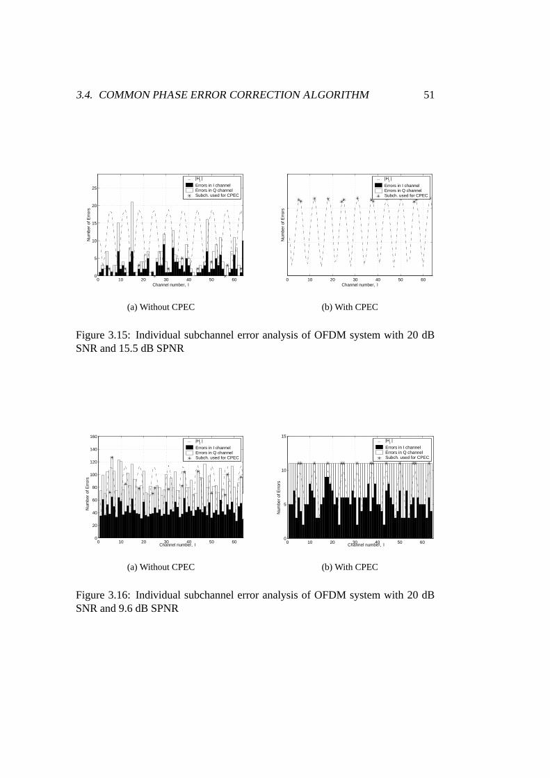
3.4. COMMON PHASE ERROR CORRECTION ALGORITHM 51
0 10 20 30 40 50 600
5
10
15
20
25
Num
ber
of E
rror
s
Channel number, l
|Hl |
Errors in I channelErrors in Q channelSubch. used for CPEC
(a) Without CPEC
0 10 20 30 40 50 60N
umbe
r of
Err
ors
Channel number, l
|Hl |
Errors in I channelErrors in Q channelSubch. used for CPEC
(b) With CPEC
Figure 3.15: Individual subchannel error analysis of OFDM system with 20 dBSNR and 15.5 dB SPNR
0 10 20 30 40 50 600
20
40
60
80
100
120
140
160
Num
ber
of E
rror
s
Channel number, l
|Hl |
Errors in I channelErrors in Q channelSubch. used for CPEC
(a) Without CPEC
0 10 20 30 40 50 600
5
10
15
Num
ber
of E
rror
s
Channel number, l
|Hl |
Errors in I channelErrors in Q channelSubch. used for CPEC
(b) With CPEC
Figure 3.16: Individual subchannel error analysis of OFDM system with 20 dBSNR and 9.6 dB SPNR

52 CHAPTER 3. COMMON PHASE ERROR CORRECTION
The CPEC algorithm can be summarised as follows.
1. Select the subset of subchannels with peaks in the channel transfer function,
d, at the start of the burst based on the calculated FEQ values.
2. Evaluate ψCPE,m
by finding the mean of the previous Nw CPE estimates in
the MAF.
3. Use ψCPE,m
for each symbolm to update the phase of the FEQ coefficients,6 Cm,l. This effectively makes the FEQ track the CPE as closely as possible.
4. Obtain Ym,d from the FEQ output and then Ym,d by the use of a slicer. Use
the difference in angles of them to get an estimate of the CPE, ψCPE,m. Use
it to correct the CPE.
5. Update the MAF with ψCPE,m to estimate ψCPE,m+1
.
Figure 3.17 illustrates the CPEC algorithm. The main advantage of the CPEC
algorithm is its simplicity and low computational demand. Assuming that the de-
termination of the phase of a complex number is performed via a look up table, the
processing of each OFDM symbol requires an additional Nd subtractions, Nd − 1
additions and one division for the calculation of the CPESE as required in (3.24)
and Nw − 1 additions and one division in the calculation of FBCF and finally N
additions to update the FEQ angles, as shown in (3.26). Unlike the scheme pro-
posed in [39], which only performs compensation using the CPESE ψCPE,m, the
FBCF in this scheme is able to continuously track and correct for the error caused
by the PN in the FEQ.
Figure 3.18 shows the improvement the CPEC makes to the demodulated con-
stellation for a system with N = 64 while figure 3.19 shows the results for a
system with N = 256.
3.5 Simulation Parameters and Results
To maintain consistency, the SUI-II channel model has been assumed for the sim-
ulations [23]. OFDM systems with N = 64, 128, 256 have been simulated at a

3.5. SIMULATION PARAMETERS AND RESULTS 53
FFT Demod
FEQ Select
Channel
arg(.) arg(.)
mean(.) X
-
Moving Average Filter
exp(-j*[.])
To QPSK Slicer
PSfrag replacements
Ym,l
ψCPE,m
Ym,l
Ym,l Ym,d Ym,d
ψCPE,m
Figure 3.17: CPE Correction (CPEC) algorithm

54 CHAPTER 3. COMMON PHASE ERROR CORRECTION
(a) Without CPEC (b) With CPEC
Figure 3.18: Demodulated constellations with (a) and without (b) CPEC for N =64 and at 20 dB SNR and 15 dB SPNR with a SUI-II CIR
(a) Without CPEC (b) With CPEC
Figure 3.19: Demodulated constellations with (a) and without (b) CPEC for N =256 and at 20 dB SNR and 15 dB SPNR with a SUI-II CIR

3.5. SIMULATION PARAMETERS AND RESULTS 55
sampling rate of 20 MHz with a CP equal to 20 samples, thus the subchannel
spacings are approximately 312 kHz, 156 kHz and 78 kHz respectively. QPSK
mapping for all subchannels has been employed and all the subchannels are used
to transmit data. A burst equivalent to 2500 OFDM symbols is transmitted and
the channel is assumed to remain static within the burst. Each data point in the
simulation results is obtained by averaging over 750 such bursts, each experi-
encing a random channel realisation in accordance with the SUI-II profile. The
received Signal to Noise Ratio (SNR) due to AWGN is set at 20 dB for all of the
simulations. The value selected for the FB buffer length, Nw is 2.
8 10 12 14 16 18 20 22 24 26 2810
−7
10−6
10−5
10−4
10−3
10−2
10−1
SPNR (dB)
BE
R
N=64, noCPECN=128, noCPECN=256, noCPECN=64, CPECN=128, CPECN=256, CPEC
Figure 3.20: Performance of the CPEC algorithm for b = 4 and fh = 100 kHz
Figure 3.20 shows the simulation results for the CPEC algorithm with N =
64, 128, 256 for PN mask parameters fh = 100 kHz and b = 4. The received
signal power and the LO power are normalised to unity. The curves are plotted
against SPNR (1/σ2ψ). The PN variance is set using the parameters a and c. It can
be seen that without the CPEC algorithm an OFDM system withN = 64 performs
worse than the system with N = 256. This is because for the PN mask selected
the conventional OFDM system with N = 64 suffers from greater CPE than does
the N = 256 system. This can be confirmed by observing the greater rotation of

56 CHAPTER 3. COMMON PHASE ERROR CORRECTION
the constellations evident in figure 3.18 (a) compared with that in figure 3.19 (a).
The rotation caused by the higher CPE power for N = 64 causes more bit errors
than the lower CPE power present when N = 256.
It can also be seen in figure 3.20 that forN = 64, the CPEC algorithm achieves
a performance gain of 6 dB at BER of 10−5 over a system without CPEC. The
performance gain can be seen to decrease with increasing N , for example with
N = 256 the gain is reduced to 3 dB. This can be attributed to the fact that the
CPE variance decreases with increasing N , which is confirmed by the theoretical
analysis presented previously in the section 3.2. The improvements are very small
once SPNR is above 20 dB owing to AWGN becoming dominant over PN. It
should be noted that for the SUI-II channel model at the selected SNR of 20 dB
(AWGN only), a BER floor of the order of 10−7 is achieved. Obviously, if the SNR
had been set higher, the improvements due to CPEC would be correspondingly
greater.
6 8 10 12 14 16 18 20 22 24 2610
−7
10−6
10−5
10−4
10−3
10−2
10−1
SPNR (dB)
BE
R
N=64, noCPECN=128, noCPECN=256, noCPECN=64, CPECN=128, CPECN=256, CPEC
Figure 3.21: Performance of the CPEC algorithm for b = 4 and fh = 200 kHz
Figure 3.21 shows the results of the simulations carried out using the PN mask
with fh = 200 kHz. All other parameters are similar to the previous case. Hence
the PN will induce more spectral spillage and will have a higher variance for

3.5. SIMULATION PARAMETERS AND RESULTS 57
the same values of the parameters a and c. The performance gain is 4 dB for
N = 64 but is reduced to 2.3 dB for N = 256 at a BER of 10−5. The number
of subchannels selected in the CPE estimation, Nd averaged 12 for N = 64 over
all bursts. Hence the total number of additional computations on average was 12
additions, 12 subtractions and 2 divisions per OFDM symbol. The gain due to
CPEC algorithm is significant considering the low additional computation effort.
Other CPEC algorithms have been proposed by other authors. They are al-
most exclusively feedforward methods (i.e. the correction for CPE is made after
the FEQ). The algorithms fall into two categories. In [43] a symbol-by-symbol
estimation is performed in a manner similar to that if only the CPESE part of the
algorithm proposed in this work is used. In [54], rather than relying on a single
estimate, Onizawa proposed to correct for CPE after processing the CPESE values
in a moving average filter in order to control their variance. Both of these schemes
are different from the CPEC algorithm proposed in this work since the FBCF is
implemented at the level of the FEQ, which modifies the data points prior to the
calculation of CPESE. Another important point is that all these schemes rely on
pilot symbols being transmitted, which reduces the throughput of the system. In
addition, the algorithm proposed here can select the subchannels with the highest
SNR for the estimation process. In [55] a similar scheme to the one proposed
is presented. Here the FBCF is taken as the average of all the CPESEs up to
that time. However since E[ψCPE] = 0 having a shorter window to calculate the
FBCF appears to be more sensible. Also it does not propose a method to compen-
sate for spectral nulls. Note that the CPEC presented in this work and the scheme
presented in [55] have been developed simultaneously but independently.
Figure 3.22 shows the performance of the individual components of the pro-
posed CPEC algorithm for an OFDM system with N = 64 subject to PN with
mask parameters b = 4 and fh = 100kHz. It shows that the performance gain
obtained using the CPESE alone is only 2 dB at a BER of 10−5. The use of both
the CPESE and the FBCF is seen to give a 6 dB advantage. However, the use of
FBCF alone also shows a performance improvement of 5.8 dB. Figure 3.23 shows
the performance of a system with N = 256 in the same conditions. At a BER
of 10−5 the use of the CPESE alone shows a gain of 1.8 dB while the use of the
FBCF alone shows a gain of 0.5 dB. The combination of both CPESE and FBCF

58 CHAPTER 3. COMMON PHASE ERROR CORRECTION
gives a gain of 3 dB. This can be explained as follows. Compare the variation
of CPESE for N = 64, as seen in figure 3.10 to that when N = 256, as seen
in figure 3.24. Both plots were generated under similar conditions. They show
that the CPESE varies at a slower rate when N is smaller. Hence for N = 64 the
FBCF can track the CPESE and would expect a significant portion of the CPE to
be corrected by the FBCF alone. However, for N = 256 the CPESE varies more
rapidly and it is much more difficult for the FBCF to track the CPESE. Hence, the
portion of CPE corrected by the FBCF alone will be correspondingly less.
8 10 12 14 16 18 20 22 24 26 2810
−6
10−5
10−4
10−3
10−2
10−1
SPNR (dB)
BE
R
noCPECCPEC with only CPESECPEC with only FBCFCPEC with FBCF and CPESE
Figure 3.22: Performance of different components of the CPEC algorithm forN = 64, b = 4 and fh = 100 kHz
Figure 3.25 shows a comparison with the algorithm proposed by Onizawa [54].
In this approach a MA filter processes the CPESEs and the result is used to correct
for CPE at the feedforward stage after the FEQ. The results show that the Onizawa
method shows very little gain compared to that achieved using only the CPESE.
This is in marked contrast to the proposed CPEC algorithm where including the
FBCF gives a significant improvement in performance compared with that using
the CPESE alone.
Figure 3.26 shows the effect of AWGN on the CPEC proposed. It is clear that
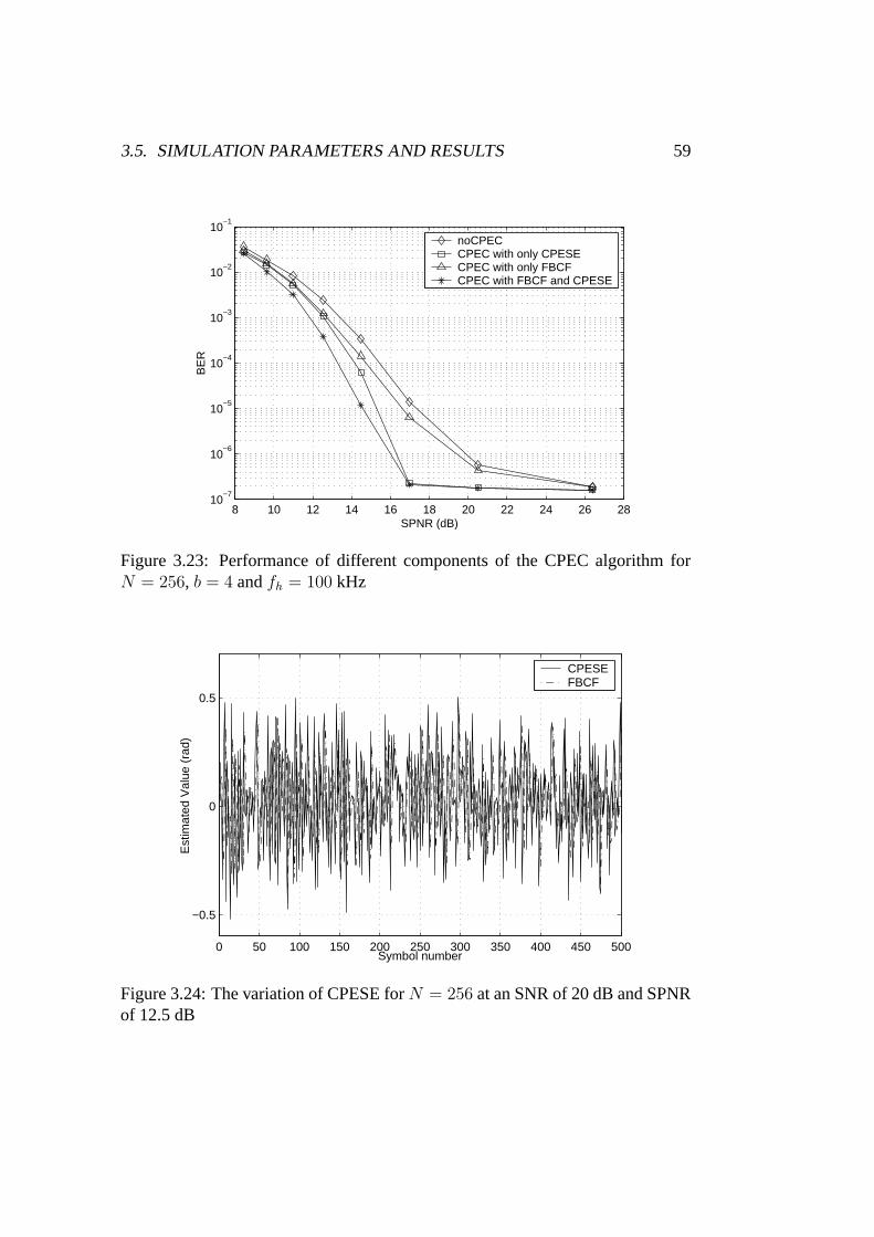
3.5. SIMULATION PARAMETERS AND RESULTS 59
8 10 12 14 16 18 20 22 24 26 2810
−7
10−6
10−5
10−4
10−3
10−2
10−1
SPNR (dB)
BE
R
noCPECCPEC with only CPESECPEC with only FBCFCPEC with FBCF and CPESE
Figure 3.23: Performance of different components of the CPEC algorithm forN = 256, b = 4 and fh = 100 kHz
0 50 100 150 200 250 300 350 400 450 500
−0.5
0
0.5
Symbol number
Est
imat
ed V
alue
(ra
d)
CPESEFBCF
Figure 3.24: The variation of CPESE for N = 256 at an SNR of 20 dB and SPNRof 12.5 dB

60 CHAPTER 3. COMMON PHASE ERROR CORRECTION
Performance gain in SPNR at an BER of 10−5 (dB)
Using only CPESE Using only FBCF Using both
N = 64 2 5.8 6
N = 256 1.8 0.5 3
Table 3.1: Performance gains obtained by different components of the CPEC withb = 4 and fh = 100 kHz
the error floor observed at an BER of about 10−6 is mainly due to the presence of
AWGN.
Figure 3.27 shows the effect that non-ideal channel estimation has on the per-
formance of the proposed CPEC algorithm for the previous system. It is important
to analyse the channel estimation since the selection of subchannels for the CPEC
is based on the estimated CTF. If a perfect channel estimation can be made, a 3 dB
gain in performance can be achieved even without the use of CPEC at a BER of
10−5. With the assumption of perfect channel estimation the use of the proposed
CPEC gives a performance gain of 5 dB compared to the case when CPEC is not
used with the same assumptions. This is comparable with the 6 dB improvement
shown previously in figure 3.20. Hence it is evident that channel estimation in
itself does not significantly degrade the performance of the proposed CPEC algo-
rithm.
3.6 Conclusion
The effect of PN in OFDM has been shown to have a dual effect. Specifically
one component is found that affects all subchannels equally, which is termed CPE
and another which affects the orthogonality of the subchannel carriers, is known
as ICI. The theoretical and simulated BER performance as a function of SPNR of
OFDM systems subject to AWGN and PN are shown to be in very close agree-
ment. A simple, yet effective algorithm that has two correction factors has been
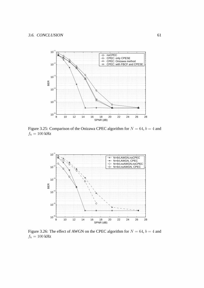
3.6. CONCLUSION 61
8 10 12 14 16 18 20 22 24 26 2810
−6
10−5
10−4
10−3
10−2
10−1
SPNR (dB)
BE
R
noCPECCPEC: only CPESECPEC: Onizawa methodCPEC: with FBCF and CPESE
Figure 3.25: Comparison of the Onizawa CPEC algorithm for N = 64, b = 4 andfh = 100 kHz
8 10 12 14 16 18 20 22 24 26 2810
−6
10−5
10−4
10−3
10−2
10−1
SPNR (dB)
BE
R
N=64,AWGN,noCPECN=64,AWGN, CPECN=64,noAWGN,noCPECN=64,noAWGN, CPEC
Figure 3.26: The effect of AWGN on the CPEC algorithm for N = 64, b = 4 andfh = 100 kHz

62 CHAPTER 3. COMMON PHASE ERROR CORRECTION
8 10 12 14 16 18 20 22 24 26 2810
−6
10−5
10−4
10−3
10−2
10−1
SPNR (dB)
BE
R
noCPEC: Noisy Ch. Est.noCPEC: Perf. Ch. EstCPEC: Noisy Ch. Est.CPEC: Perf. Ch. Est.
Figure 3.27: The effect of channel estimation on the CPEC algorithm for N = 64,b = 4 and fh = 100 kHz
presented to remove the CPE. The performance gains obtained by each correction
factor, acting alone and in combination, are investigated via simulations and are
also compared with algorithms proposed by others. It has been shown that when
the algorithm is applied to a BFWA system operating in the MMDS SUI-II chan-
nel at an SNR of 20 dB, performance gains of up to 6 dB are achieved. The use of
the proposed CPEC algorithm might allow MMDS equipment manufacturers to
use lower quality RF oscillators without performance degradation, thus allowing
significant cost savings.
Chapter 4
Symbol Offset Correction
It has been shown in chapter 2 that OFDM is more robust in the presence of mul-
tipath propagation owing to the use of the Cyclic Prefix (CP) than SC systems.
However, as was demonstrated in chapter 3, OFDM is very sensitive to oscilla-
tor Phase Noise (PN). Unfortunately OFDM is also sensitive to frequency offsets
caused by oscillator tuning inaccuracies. In spite of these limitations, OFDM is
quite robust in the presence of timing offsets [24]. Timing offsets can be fur-
ther divided into symbol (frame) offsets and sampling clock offsets. The former
refers to errors in determining the correct position of the FFT window required
for demodulation at the receiver and the latter refers to timing errors in the re-
ceiver A/D converter sample clock. Throughout the work, ideal sampling clock
synchronisation is assumed and in this chapter only symbol (frame) synchronisa-
tion will be addressed. Interested readers can find out more about the effects of
sampling clock offsets in for example [56, 57]. Previous work has often addressed
the issues of frequency offset synchronisation and symbol offset synchronisation
in tandem since they can be mitigated using similar algorithms. One such algo-
rithm is presented by T. M. Schmidl and D. Cox in [25, 58]. Henceforth it will be
referred to as the Schmidl and Cox Algorithm (SCA). The SCA performs well for
OFDM systems with large symbol lengths (N ). However, the importance of us-
ing OFDM systems with smaller values of N for BFWA applications has already
been mentioned in chapter 1. This chapter will concentrate on the symbol offset
synchronisation function of the SCA and will then introduce a novel algorithm
63

64 CHAPTER 4. SYMBOL OFFSET CORRECTION
that complements the SCA so that virtually perfect symbol synchronisation can
be achieved even with lower values of N . The next chapter will deal with the
issue of frequency offset synchronisation.
An OFDM system will be more robust if the length of the CP, v is selected to
be slightly longer than the length of the CIR, Nh. Hereafter this difference will be
denoted as the Excess Length, p (i.e. p = v − Nh). As long as the symbol syn-
chronisation offset, ξ causes the start of each FFT window to be within the Excess
Length (i.e. −p ≤ ξ ≤ 0), the decoded OFDM symbols will not be subject to
Inter Block Interference (IBI) which is introduced when adjacent OFDM symbols
cause interference to the OFDM symbol currently being detected [59]. Note for
AWGN channels the start of the FFT window can be placed anywhere within the
CP (i.e. −v ≤ ξ ≤ 0) without suffering any degradation in performance, provided
that no other degradations are present, e.g. frequency offset. Although increasing
p in general will make the system more robust against symbol synchronisation er-
rors it also decreases throughput due to the use of an extended CP. This becomes
even more significant when operating at higher sample rates since the length of
the same CIR will now span a greater number of received samples.
This chapter is organised as follows. In section 4.1 a synopsis of the research
carried out by other authors is presented. There have been numerous approaches
to achieving symbol synchronisation in OFDM and they will be critically anal-
ysed in this section. Section 4.2 will introduce the theoretical derivations of the
degradation caused by symbol offsets in OFDM and will highlight the motivation
underlying the work. Section 4.3 introduces the SCA and identifies the limita-
tions of the algorithm. The proposed Iterative Symbol Offset Correction Algo-
rithm (ISOCA) is introduced in section 4.4. This is a two part iterative algorithm
that complements SCA enabling it to be successfully used in BFWA applications.
Section 4.5 presents results for OFDM systems when used in AWGN alone and
for OFDM systems including a CIR appropriate for the BFWA scenario. The re-
sults will clearly show a significant increase in performance is brought about by
the use of ISOCA. Finally, section 4.6 draws some conclusions.

4.1. RELATED WORK 65
4.1 Related Work
A good tutorial on the subject of symbol offset in OFDM is given in [60]. The
algorithms that are already available for symbol synchronisation can be broadly
categorised into Pilot Symbol Aided (PSA) and Non Pilot Symbol Aided (NPSA)
schemes. PSA schemes are based on correlating the received signal with a known
signal. These can be further divided into schemes that use a preamble or a known
OFDM training symbol [25] or schemes that periodically insert pilot symbols on
particular subchannels [61]. NPSA schemes are generally based on correlating
received samples taken one OFDM symbol length apart, in order to make use of
the periodicity created by the insertion of the CP [62]. Some schemes however
employ a hybrid of PSA and NPSA methods [63, 64]. Another approach is the
use of null symbols [65, 66]. The drop in receiver power is used to detect the
start of a burst. This method would not perform well in BFWA systems which
employ burst mode transmission since there would be no difference between the
null symbol and the idle period between bursts. In [67], the authors propose a
blind synchronisation method based on the second order statistics of the received
signal, but it has a very high computational demand.
The authors in [64, 68, 69] extend the work of [62] that make use of the repeti-
tion introduced by the addition of the CP. In [64], a second estimation using pilot
symbols is performed and in [69] the authors add a second correlator to the orig-
inal output determined in [62] to be used in situations where the CIR is likely to
have two equal paths. The original estimation in [62] can be biased heavily by the
position of the main tap of the CIR [68]. Consequently the authors further propose
a fine symbol synchronisation method that estimates the CIR using pilot symbols
that are sent at intermediate positions of the OFDM symbol. However, in general
it should be noted that the performance of schemes using Maximum Likelihood
(ML) estimators that rely upon the repetition introduced by the CP decreases in
the presence of frequency offsets.
The authors in [70] propose a ML based timing estimation algorithm for the
WLAN specifications developed by the IEEE 802.11 standardisation group. This
standard uses a preamble with short and long OFDM symbols. However the per-
formance of the algorithm depends heavily on the fact that the initial timing esti-

66 CHAPTER 4. SYMBOL OFFSET CORRECTION
mate falls within the Excess Length, p.
In some of the related work, the Inter-Block Interference (IBI) caused by a
CIR that is longer than the CP is analysed [71, 72, 73]. In [71] the PSD of the IBI
is characterised in terms of the length of the CP and it concludes that the samples
corresponding with the tails of the CIR do not uniformly contribute to the PSD
of the IBI, but rather the contribution grows linearly as the samples get closer to
the edges of the CIR. The authors in [74, 75] address the issue of synchronisation
in Digital Multitone (DMT) systems used in Asymmetric Digital Subscriber Line
(ADSL) systems. The work of other authors will be presented in the next sections
where they are directly relevant to the subject being addressed.
4.2 Effect of Symbol Offset in OFDM
Section 2.4 introduced the analysis of a conventional OFDM system assuming
perfect synchronisation. The demodulated OFDM symbol under those assump-
tions is given in (2.20). The effect of a carrier frequency offset (relative to the
intercarrier spacing), ε can be introduced to the system by redefining the demod-
ulated symbol as,
Ym,l =
√
1
N
N−1∑
n=0
rm,ne−j2π ln+(ε−ε)
N , 0 ≤ l ≤ N − 1 (4.1)
where rm,n, 0 ≤ n ≤ N−1 are the received samples of the FFT window for the
mth OFDM block taken from the received sequence, that includes the component
due to AWGN, wn (see (2.19) and (2.20)). Here ε represents the estimated carrier
frequency offset at the receiver. For the purpose of analysing the effect of symbol
offset it will be assumed that the Residual Frequency Offset (RFO) is zero (i.e.
ε − ε = 0) for the remainder of this section. If perfect symbol synchronisation is
achieved the samples selected for decoding symbol m are,
rm = [rm,0, rm,1.., rm,N−1] (4.2)
and hence,
Ym,l = Am,lHl +Wl (4.3)

4.2. EFFECT OF SYMBOL OFFSET IN OFDM 67
where Wl is the component due to AWGN and Hl is the coefficient of the
Channel Transfer Function (CTF) approximated at subchannel l. It will be as-
sumed that Wl has the same statistics as wn. In order to understand the effect
of symbol offset on performance, initially the demodulation of OFDM is inves-
tigated for the situations where AWGN is the only channel impairment. Two
different values of symbol offset, ξ are considered.
4.2.1 Symbol Offset −v ≤ ξ < 0
In this case, the FFT window selected for decoding is,
rm = [rm,N−ξ, .., rm,N−1, rm,0, .., rm,N−1−ξ] . (4.4)
Then,
Ym,l =1
N
N−1∑
k=0
Am,k
ξ−1∑
n=0
ej2πk(n+N−ξ)−nl
N +
1
N
N−1∑
k=0
Am,kN−1∑
n=ξ
ej2πk(n−ξ)−nl
N +Wl (4.5)
and hence,
Ym,l = Am,lej2π ξl
N +Wl . (4.6)
Equation (4.6) shows that so long as the symbol offset results in the beginning
of each FFT window to lie within the CP, the orthogonality of the carriers is main-
tained. The desired term experiences a phase shift, which can be estimated and
corrected.
4.2.2 Symbol Offset ξ > 0
In this situation, the FFT window selected for decoding is,
rm = [rm,ξ, .., rm,N−1, rm+1,N−v, .., rm+1,N−v−1+ξ] (4.7)
68 CHAPTER 4. SYMBOL OFFSET CORRECTION
here, it is assumed ξ ≤ v. Then,
Ym,l =1
N
N−1∑
k=0
Am,k
N−ξ−1∑
n=0
ej2πk(n+ξ)−nl
N +
1
N
N−1∑
k=0
Am+1,k
N−1∑
n=N−ξej2π
k(n+ξ−v)−nl
N +Wl (4.8)
Ym,l =N − ξ
NAm,le
j2π ξl
N +
1
N
N−1∑
k=0k 6=l
Am,k
N−ξ−1∑
n=0
ej2πk(n+ξ)−nl
N +
1
N
N−1∑
k=0
Am+1,k
N−1∑
n=N−ξej2π
k(n+ξ−v)−nl
N +Wl . (4.9)
The first term on the r.h.s. of the equation (4.9) shows that the desired term
experiences an attenuation and a phase shift. The second and the third terms are
the ICI and ISI respectively. A similar result can be obtained if ξ > v. The
analysis can be extended to the case when a CIR is included. In this case unless
the symbol offset lies within −p ≤ ξ ≤ 0, the demodulated symbols are given
by [76],
Ym,l =N − ξ
NAm,lHle
j2π ξl
N +Wξ,l +Wl (4.10)
where Wξ,l is the interference term caused by ISI and ICI. It also proves to
be the dominant interference term, the power of which can be approximated by
zero-mean Gaussian noise with power [76],
σ2ξ =
∑
i
|hi|2(2∆i
N− (
∆i
N)2) (4.11)
where
∆i =
ξ − i ξ > i,
i− v − ξ 0 < ξ < −(v − i),
0 else.
(4.12)
Symbol offset in a coherent OFDM system has an even more severe effect

4.3. SCHMIDL AND COX ALGORITHM 69
on performance. Symbol synchronisation not only determines the position of the
FFT window for the subsequent OFDM symbols, it also implicitly determines the
channel estimation by the FEQ coefficients. If ξ > 0 or ξ < −p the interference
term Wξ,l will affect the channel estimation and consequently the decoding of all
the symbols in the data burst. OFDM systems that are used in rapidly changing
channels require the FEQ coefficients to be updated frequently. To do so, pi-
lot symbols are embedded in to each OFDM symbol at periodic intervals, which
are then used to estimate the FEQ coefficients by using interpolation to generate
coefficients for every subchannel over which data is sent. Consequently a sym-
bol offset in such a system would cause even more severe degradation owing to
the poor estimation of the FEQ coefficients. In the absence of noise, the Mean
Squared Error (MSE) of the channel estimate is given as [61],
MSE =N−1∑
l=0
∣
∣
∣Hl − Hl(ξ)∣
∣
∣
2(4.13)
where Hl(ξ) is the estimated CTF as a function of ξ. The important point
that should be noted from equations (4.5)-(4.10) is that the demodulated OFDM
symbols will always contain a phase rotation proportional to the symbol offset, ξ
and the subchannel index, l as evidenced by the term ej2πξl
N in equation (4.10). In
the next two sections, an algorithm that uses this phase rotation to determine and
correct the symbol offset is presented.
4.3 Schmidl and Cox Algorithm
A robust scheme to estimate both symbol synchronisation and frequency offset
estimation is the SCA [25, 58]. It uses two training symbols with the first one
having identical first and second halves (neglecting the CP). This is achieved by
utilising only the even subchannels and setting the odd subchannels to zero at the
input to the IFFT modulator. Figure 4.1 shows the organisation of the two training
symbols in the SCA.
Symbol (frame) synchronisation is achieved by searching for a training symbol
with two identical halves. If L = N/2, the sum of L consecutive correlations

70 CHAPTER 4. SYMBOL OFFSET CORRECTION
Training Symbol 1
CP
Training Symbol 2
CP
v L
N
Figure 4.1: Training symbols in SCA
between pairs of samples spaced L samples apart is found as,
P (d) =L−1∑
n=0
(r∗d+nrd+n+L) (4.14)
which can be recursively implemented as,
P (d+ 1) = P (d) + (r∗d+Lrd+2L) − (r∗drd+L) . (4.15)
The received energy for the second half-symbol which is given by
R(d) =L−1∑
n=0
|rd+n+L|2 (4.16)
can also be recursively implemented as,
R(d+ 1) = R(d) + |rd+N |2 − |rd+L|2 (4.17)
and is used to normalise the correlator output. This yields a timing metric given
by,
M(d) =|P (d)|2(R(d))2
. (4.18)
The timing metric, given by (4.18) will reach a peak at the end of the CP of
the first training symbol. The peak is actually maintained for a length equal to
the Excess Length, (p + 1) just prior to the end of the CP of the first training
symbol (i.e. the beginning of the useful part of the first training symbol). Thus
the correlator output will take the form of a plateau. This is because the last p

4.3. SCHMIDL AND COX ALGORITHM 71
90 100 110 120 130 140 150 160 170 180 1900
0.2
0.4
0.6
0.8
1
1.2M
(d
)
d
Figure 4.2: Output of the timing metric for N = 64 and p = 10 at an SNR of20dB
samples of the CP are not corrupted by the CIR. Figure 4.2 shows a typical output
for M(d) for N = 64 and p = 10 at an SNR of 20 dB. If it is not possible to find
such a plateau region it is assumed that the SCA has resulted in a condition of non
acquisition. The method adopted to locate this region is explained in detail in the
following paragraphs.
Symbol synchronisation is achieved by locating the end of this plateau, de-
noted as dopt. The authors in [25] propose a different method to identify the opti-
mal synchronisation point. Firstly, the sample corresponding to the maximum of
the timing metric, given by (4.18) is found. Then the sample positions to the left
and the right of the identified point which have an amplitude equal to 90% of the
maximum are found. The optimum point, d′opt is selected as the mean position be-
tween these two points. The objective of this procedure was to find the mid point
of the CP. Preliminary simulation results showed that although d′opt fell within the
CP for higher values of SNR, the method failed badly at lower SNR values. To
overcome this problem, the following approach has been developed. First of all,
the variance for p consecutive samples of the timing metric is calculated. The

72 CHAPTER 4. SYMBOL OFFSET CORRECTION
position of dopt is taken to be the point when the minimum variance occurs. The
rationale for doing this is that the p samples corresponding to the plateau will be
very similar and hence will generate the minimum variance. Note that for AWGN
channels, the number of consecutive samples selected will be v. The superiority
of this method will be demonstrated in the simulation results to be presented later
in this chapter. Hence,
dopt4=
min
d1
p− 1
p−1∑
i=0
[M(d− i) −M(d)p]2 (4.19)
where M(d)p is the mean of the samples from d to d − p + 1. The Start of
Frame (SOF) is determined as the start of first training symbol, given by dopt − v.
The estimated SOF given by the SCA is denoted as ˆSOFSCA. Since the CP ensures
that there is no Inter Block Interference (IBI) between OFDM symbols, the effect
of the CIR on the first training symbol is cancelled if the conjugate of a sample
from the first half is multiplied by the corresponding sample from the second half.
Hence the phase difference between the two halves of the first training symbol is
caused by the frequency offset, i.e. φ = πε. The phase difference can be estimated
as,
φ = 1/(p+ 1)p∑
n=0
6 P (dopt − n) . (4.20)
If ε < 1 there is no phase ambiguity in φ and the fractional part of the fre-
quency offset can be estimated as,
εSCA = φ/π (4.21)
The second training symbol is used in order to avoid potential ambiguity and
determine the integer part of the frequency offset. This technique will be consid-
ered fully in the next chapter when relative frequency offsets in excess of unity are
addressed. Note that the algorithms about to be presented perform equally well
for relative frequency offsets in excess of unity, i.e. having an integer part. For
purposes of brevity it will be assumed that ε < 1 for the remainder of this section.
If ˆSOFSCA is different from the actual Start of Frame namely, SOFideal it gives

4.3. SCHMIDL AND COX ALGORITHM 73
rise to a symbol offset, ξSCA. i.e.
ξSCA = ˆSOFSCA − SOFideal . (4.22)
The effect of AWGN on the correct estimation of dopt and hence ˆSOFSCA is re-
duced with higher values ofL, and hence the number of FFT pointsN , particularly
when operating at low values of SNR. It has been shown that the SCA performs
well for OFDM systems with N in excess of 1000 [25]. However, for BFWA
systems, data is transmitted in short bursts, particularly in the uplink. In this sit-
uation, it would be wasteful to use an OFDM system with a large value of N .
When the SCA is used for systems with lower values of N , the estimate εSCA is
no longer sufficiently accurate. This error results in a residual frequency offset
that rotates the received constellation at a reduced rate, but one that is still signifi-
cant enough to cause bit errors in coherently demodulated OFDM systems. Hence
OFDM systems with low values of N will require a residual frequency offset cor-
rection algorithm to continuously track the carrier frequency offset. Some of the
proposed algorithms [77] (which will be presented in the next chapter) rely on
the phase gradient of the decoded OFDM symbols to estimate the residual carrier
frequency offset. Even though −p ≤ ξSCA ≤ 0 will not result in any Inter Block
Interference (IBI), the additional phase gradient caused by a non zero value of
ξSCA will seriously affect residual carrier frequency offset correction algorithms
based on the measurement of the phase gradient. This will be demonstrated in
section 5.5 in the next chapter. Hence it is imperative that perfect symbol syn-
chronisation is achieved (i.e. the final symbol offset, ξF = 0). In the next section
an Iterative Symbol Offset Correction Algorithm (ISOCA) is proposed that em-
ploys a two step process that virtually guarantees perfect symbol synchronisation
even under conditions of very low SNR.
An approach to increase the performance of the timing synchronisation of
the SCA is presented in [78, 79]. The authors propose two methods, one using
a sliding window method to smooth out the plateau at the correlator output and
another based on dividing the training symbol into four parts, with the last two
parts being the sign negative of the first two. Even though the correlator output
gives a sharper peak, the FFT size, N needs to be quite large for the algorithm

74 CHAPTER 4. SYMBOL OFFSET CORRECTION
to perform well. Indeed the authors only consider FFT sizes in excess of 1024.
In [80, 81] the author proposes to follow the symbol estimate determined using
the sliding window correlator of the SCA with a matched filter based correlator.
This method generates a more significant peak at the matched filter output, hence
detection of the SOF is more accurate than using the plateau of the timing metric
as utilised by the SCA.
Another algorithm that makes use of the phase gradient that is a result of sym-
bol offset is presented in [82]. In their scheme, the estimated time offset per pair
of adjacent tones is,
ξ =N
2π
[
6(
Ym,l
Am,l
)
− 6(
Ym,l+1
Am,l+1
)]
(4.23)
where Ym,l and Am,l are the demodulated symbol and the decoded symbol at lth
subchannel in OFDM symbol m. Each tone pair provides a separate noisy esti-
mate of ξ. The data is modulated with differential QPSK across the subchannels.
Hence the above estimate will create a QPSK constellation that is slightly rotated
depending on ξ. For a QPSK constellation each pair of tones will differ in phase
from each other by a multiple of π/4. This effect on the rotated constellation can
be eliminated and all the points brought in to the same quadrant by raising the
complex points to the 4th power. Finally, ξ is estimated by locating the centroid
of the noisy constellation points. This estimate is quite robust in frequency selec-
tive fading since even if a pair of tones fall in to a frequency null in the CTF, the
pair will only have a low amplitude when used in (4.23). Consequently, it will
contribute less when locating the centroid. This scheme appears to be quite ro-
bust, but it assumes that initial symbol offset is less than half of the FFT size (i.e.
ξ ≤ N/2). Although this is a safe assumption for higher values of N , it might
not be the case for lower ones. In [83] the authors also make use of the phase
gradient caused by symbol offset. It relies on sending pilot tones continuously
within OFDM symbols. An estimate of the symbol offset is generated after ev-
ery OFDM symbol and the final estimate is updated by finding the average of the
symbol-by-symbol estimates found up to that point. The authors in [84] also look
at the same principle, but to avoid the symbol offset from causing the SOF to fall
into adjacent OFDM symbols, it proposed to use long cyclic prefix and a cyclic
4.4. ITERATIVE SYMBOL OFFSET CORRECTION ALGORITHM 75
postfix. The novel iterative algorithm proposed in the next chapter performs well
even when only a prefix is used.
4.4 Iterative Symbol Offset Correction Algorithm
A novel algorithm that is developed by the author, which is based on the phase
gradient caused by the symbol offset is presented in this section. It is divided
into two parts. The first is the Iterative Symbol Offset Estimation, in which the
symbol offset is iteratively estimated until the value is zero. The second part is
the Error Comparison, where a second estimate is used that is based on the errors
generated within the second training symbol of the SCA. If the ISOCA fails in the
Error Comparison stage, the Iterative Symbol Offset Estimation is repeated after
a reinitialisation. Both parts of the algorithm must should yield a positive result
for the ISOCA to return a final estimated SOF. There are numerous check points
in the algorithm to prevent it from iterating in an infinite loop. The two parts of
the ISOCA algorithm are discussed in detail in the next two subsections.
4.4.1 1st Part - Iterative Symbol Offset Estimation
Using the SCA an initial estimate of both the SOF and the frequency offset namelyˆSOFSCA and εSCA, are made. It is proposed to estimate the symbol offset at the
end of the SCA, ξSCA based on the phase gradient it gives rise to, as indicated in
(4.10). To do this, the demodulated output of the second SCA training symbol
YNt2 is utilised. Here, it is assumed that the two training symbols of the SCA
occupy the symbol positions at the start of the frame, specifically Nt1 and Nt2.
The phase difference between the received and the transmitted second training
symbol of the SCA is calculated as follows,
θi = 6 (YNt2,i/ANt2,i), 0 ≤ i ≤ N − 1 (4.24)
where ANt2,i and YNt2,i represent the Nt2th transmitted and demodulated sym-
bols of the ith subchannel, respectively based on the use of ˆSOFSCA.
Figure 4.3 shows a typical plot of θi against the subchannel index for N = 64

76 CHAPTER 4. SYMBOL OFFSET CORRECTION
0 10 20 30 40 50 60−4
−3
−2
−1
0
1
2
3
4
θ i (ra
d)
Subchannel Index, i
Figure 4.3: Variation of θi for N = 64, ε = 0.5, with AWGN only at 15 dB SNR
0 10 20 30 40 50 60−4
−3
−2
−1
0
1
2
3
4
θ i (ra
d)
Subchannel Index, i
Figure 4.4: Variation of θi for N = 64, ε = 0.5 with AWGN at 15 dB SNR andCIR

4.4. ITERATIVE SYMBOL OFFSET CORRECTION ALGORITHM 77
+ +
Z -1
- PSfrag replacements
θi
θi−1
θiαSAWπ(.)
Figure 4.5: Phase unwrapping algorithm
ε = 0.5 and ξSCA = 1 including AWGN at an SNR of 15 dB. The frequency offset
is corrected using the estimate εSCA made using the SCA. The phase gradient
caused by the residual frequency offset is very small compared to that caused by
the symbol offset. This will be demonstrated in section 5.5 of the next chapter.
Thus it can be assumed that ε − εSCA ≈ 0 during the estimation of the symbol
offset. Figure 4.4 shows a similar plot, this time with the inclusion of a 3-tap
SUI-II CIR appropriate for the BFWA scenario with v = 20 and p = 10. As
seen from the figures 4.3 and 4.4, θi maintains a distinct gradient even when a
representative CIR is included. However due to the phase wrapping effect, θimust be first unwrapped by a suitable unwrapping algorithm. Although accurate
phase unwrapping algorithms are available, they are very complex. Since the
algorithm only makes use of the phase gradient and not the absolute phase values,
a relatively simple scheme was selected for the unwrapping of the phase [85]. For
purposes of clarity, the ith sample of the wrapped phase and the unwrapped phase
are denoted as θi and θi, respectively. The phase unwrapping algorithm can be
expressed as,
θi = θi−1 + αSAWπ(θi − θi−1) (4.25)
where SAWπ(.) is a sawtooth function that limits the output to ±π and α is
a parameter that controls the variance of the unwrapped phase. The algorithm is
illustrated in figure 4.5. Figure 4.6 shows the action of the unwrapping algorithm
for the same scenario that produced the results presented in figure 4.4 with α = 1.
The estimate of the symbol offset is calculated as the gradient of the un-

78 CHAPTER 4. SYMBOL OFFSET CORRECTION
0 10 20 30 40 50 60−4
−3
−2
−1
0
1
2
3
4
5
6
θ i (ra
d)
Subchannel Index, i
Unwrapped PhaseWrapped Phase
Figure 4.6: Performance of the unwrapping algorithm for N = 64, ε = 0.5, withAWGN at 15 dB SNR and CIR at α = 1
wrapped phase sample vector θ = [θ0, .., θN−1],
ξ = ROUND(GRAD(θ).N/2π) (4.26)
where the GRAD(.) function finds the Maximum Likelihood (ML) gradient
of the parameter in a least-squares sense and the ROUND(.) function rounds the
parameter to the nearest integer. Now ξ is used to update the initial SOF, namely
the ˆSOFSCA. However, a single estimate may not be accurate in the presence of
channel impairments. Hence it is proposed to repeat the above process until ξ = 0,
updating the estimated SOF at the end of each iteration. (i.e. at the end of mth
iteration ˆSOF(m) = ˆSOF(m− 1)+ ξ(m)). Note that ε is estimated at each step to
increase the accuracy. The number of iterations taken to achieve the condition ξ =
0 is denoted as u. The iterative process is initialised by letting ˆSOF(0) = ˆSOFSCA.
It is found that in most cases the algorithm achieves the correct SOF within a
few iterations even when a CIR is included. However at very low SNR values,
there is a small probability of non-convergence. To prevent continual iteration,
4.4. ITERATIVE SYMBOL OFFSET CORRECTION ALGORITHM 79
the algorithm is allowed to iterate only a predetermined number of times, Nit (i.e.
u ≤ Nit). In practice, this does not pose a significant problem, since the receiver
can always request a retransmission if convergence is not achieved. This is a far
better option than estimating the SOF incorrectly and as a consequence obtaining
samples comprising two OFDM received symbols in the FFT window. In this case
the error rate will be very high.
4.4.2 2nd Part - Error Comparison
Figure 4.7 shows how the ISOCA works for two possible scenarios. The first is
when ξSCA < N/2 as shown in figure 4.7(a). The symbol offset is estimated and
corrected at the end of the iterative part of the ISOCA after u iterations. In the
unlikely event that ξSCA > N/2, the gradient of θi actually changes sign. This
will result in the unwrapping algorithm calculating a gradient with the opposite
sign to that required, which will subsequently cause the estimated symbol offset,
ξ during the iterative process to move away from SOFideal. In this case when the
iterative process terminates, the estimated SOF will be more than N/2 samples
away from the desired position as shown in figure 4.7(b).
To address this situation, a second correction is made at the end of the iterative
process. Here the decoded output due to the second training symbol, ANt2 deter-
mined using the estimated SOF at end of iterative process, ˆSOF(u) is compared
with the transmitted symbol, ANt2 . However, the resulting comparison will be
seriously affected by subchannels experiencing a low SNR resulting from spec-
tral nulls in the channel response Hl. To overcome this problem, an estimate of
the channel response Hl is made by comparing the transmitted and demodulated
output of the second training symbol, specifically,
Hl = YNt2/ANt2 (4.27)
Only those subchannels with |Hl| above a certain threshold are selected. This
subset of subchannels is denoted as d ⊂ [0, ..N − 1]. The chosen criteria se-
lects only those subchannels with |Hl| in excess of a standard deviation above
the mean. The outputs of these subchannels YNt2,d are sent through a slicer to
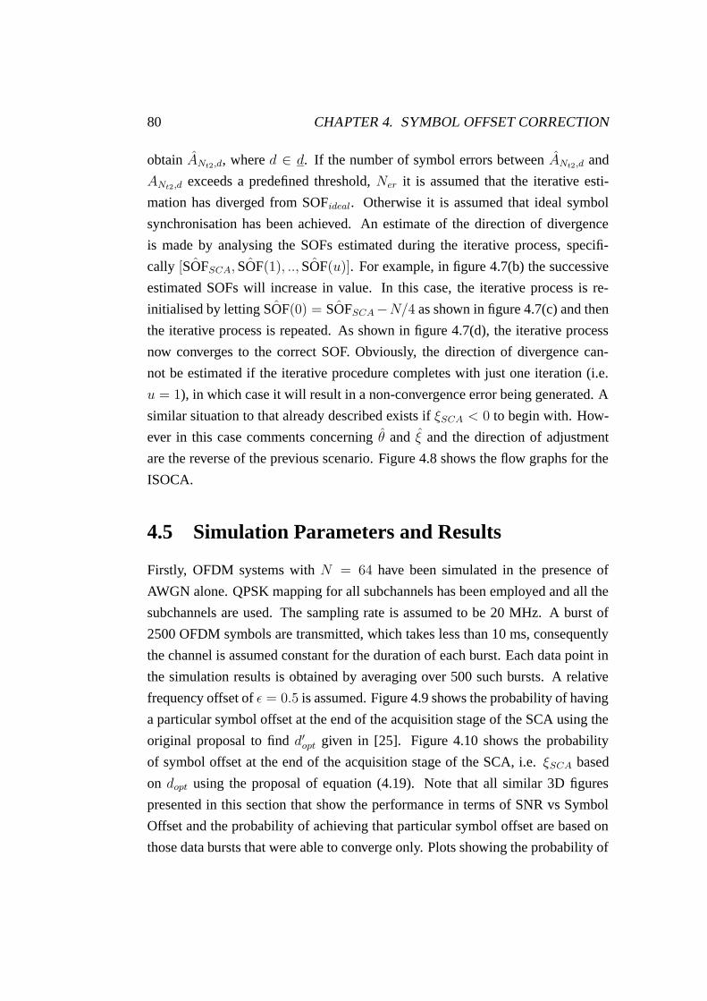
80 CHAPTER 4. SYMBOL OFFSET CORRECTION
obtain ANt2,d, where d ∈ d. If the number of symbol errors between ANt2,d and
ANt2,d exceeds a predefined threshold, Ner it is assumed that the iterative esti-
mation has diverged from SOFideal. Otherwise it is assumed that ideal symbol
synchronisation has been achieved. An estimate of the direction of divergence
is made by analysing the SOFs estimated during the iterative process, specifi-
cally [ ˆSOFSCA, ˆSOF(1), .., ˆSOF(u)]. For example, in figure 4.7(b) the successive
estimated SOFs will increase in value. In this case, the iterative process is re-
initialised by letting ˆSOF(0) = ˆSOFSCA−N/4 as shown in figure 4.7(c) and then
the iterative process is repeated. As shown in figure 4.7(d), the iterative process
now converges to the correct SOF. Obviously, the direction of divergence can-
not be estimated if the iterative procedure completes with just one iteration (i.e.
u = 1), in which case it will result in a non-convergence error being generated. A
similar situation to that already described exists if ξSCA < 0 to begin with. How-
ever in this case comments concerning θ and ξ and the direction of adjustment
are the reverse of the previous scenario. Figure 4.8 shows the flow graphs for the
ISOCA.
4.5 Simulation Parameters and Results
Firstly, OFDM systems with N = 64 have been simulated in the presence of
AWGN alone. QPSK mapping for all subchannels has been employed and all the
subchannels are used. The sampling rate is assumed to be 20 MHz. A burst of
2500 OFDM symbols are transmitted, which takes less than 10 ms, consequently
the channel is assumed constant for the duration of each burst. Each data point in
the simulation results is obtained by averaging over 500 such bursts. A relative
frequency offset of ε = 0.5 is assumed. Figure 4.9 shows the probability of having
a particular symbol offset at the end of the acquisition stage of the SCA using the
original proposal to find d′opt given in [25]. Figure 4.10 shows the probability
of symbol offset at the end of the acquisition stage of the SCA, i.e. ξSCA based
on dopt using the proposal of equation (4.19). Note that all similar 3D figures
presented in this section that show the performance in terms of SNR vs Symbol
Offset and the probability of achieving that particular symbol offset are based on
those data bursts that were able to converge only. Plots showing the probability of
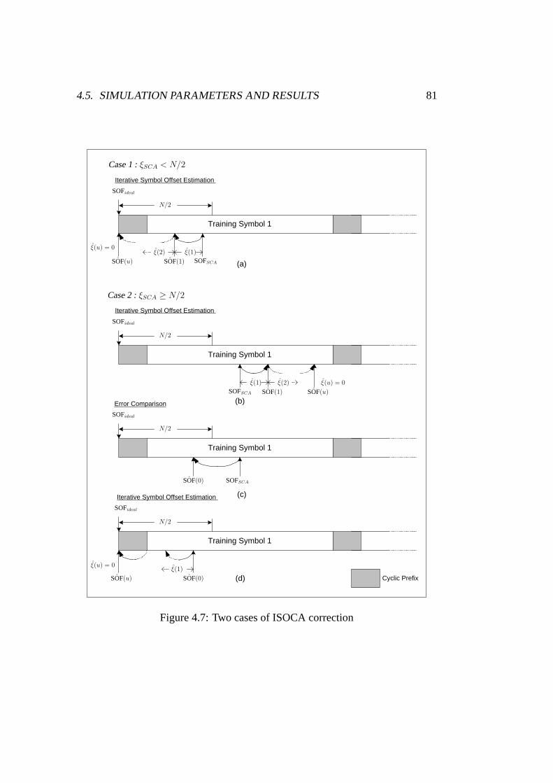
4.5. SIMULATION PARAMETERS AND RESULTS 81
Training Symbol 1
Training Symbol 1
Training Symbol 1
Training Symbol 1
Iterative Symbol Offset Estimation
Error Comparison
Cyclic Prefix
Iterative Symbol Offset Estimation
Iterative Symbol Offset Estimation
(a)
(b)
(c)
(d)
PSfrag replacements
N/2
N/2
N/2
N/2
SOFSCA
SOFSCA
SOFSCA
ξ(1)
ξ(1)
ξ(1)
ˆSOF(1)
ˆSOF(1)
ξ(2)
ξ(2)
ˆSOF(u)
ˆSOF(u)
ˆSOF(u)
ξ(u) = 0
ξ(u) = 0
ξ(u) = 0
SOFideal
SOFideal
SOFideal
SOFideal
Case 1 : ξSCA < N/2
Case 2 : ξSCA ≥ N/2
ˆSOF(0)
ˆSOF(0)
Figure 4.7: Two cases of ISOCA correction

82 CHAPTER 4. SYMBOL OFFSET CORRECTION
Find Good Subchannels
No of iterations >
1
Find Errors
No. of Errors >
Find Direction of
Convergence
Increasing ?
2
2
1
1 1
No. Iterations >
Yes
No
Yes
No
No
Yes
Yes
No
Yes No
1
Estimate
Calculate
Update SOF
Estimate
Calculate
Phase Unwrap
Estimate
Non- Convergence
Error
Non- Convergence
Error
Successful Convergence
PSfrag replacements
M(d)
ε
Correct YNt2
with ε
θi
ξ
ξ = 0
Nit
Ner
ˆSOF(0) = ˆSOFSCA− ˆSOF(0) = ˆSOFSCA+
using ξ
ξI = ROUND(ξ)
HlˆSOF(0) =ˆSOFSCA
N/4N/4
Figure 4.8: ISOCA flow graphs: First correction (left), second correction (right)

4.5. SIMULATION PARAMETERS AND RESULTS 83
010
2030
40
−50
0
500
0.2
0.4
0.6
0.8
SNR (dB)Symbol Offset
Pro
babi
lity
Figure 4.9: Performance after SCA using the original algorithm with AWGNalone for N = 64, ε = 0.5
non-convergence are shown separately later on. The original proposal is devised
to locate d′opt at the mid point of the timing metric plateau. In the case of AWGN
channels the length of the timing metric plateau is equal to the length of the CP, i.e.
v. Hence the SOF is estimated as ˆSOFSCA = d′opt−v/2. From figure 4.9 it can be
seen that the estimation process performs badly at SNRs less than 15 dB. At these
SNR levels there is a high probability of even getting a positive symbol offset.
The maximum probability of getting perfect symbol synchronisation is 0.75 even
at high SNR levels. The new proposal as expressed in (4.19) is in contrast devised
to find the edge of the plateau. From figure 4.10 it can be seen that in most
instances ξSCA lies within the CP following application of the modified SCA. (i.e.
the condition −v ≤ ξSCA ≤ 0 is satisfied). The probability of achieving perfect
symbol synchronisation has now increased to 0.9 at high SNR levels. However the
range of symbol offsets present are quite significant still. Hereafter unless stated
otherwise, it will be assumed that the new proposal using equation (4.19) will be
used for the estimation of the SOF for the SCA, namely ˆSOFSCA.
The results after performing the first correction process of the ISOCA are
shown in figure 4.11 (i.e. ξ(u) reached at the end of the first correction process).
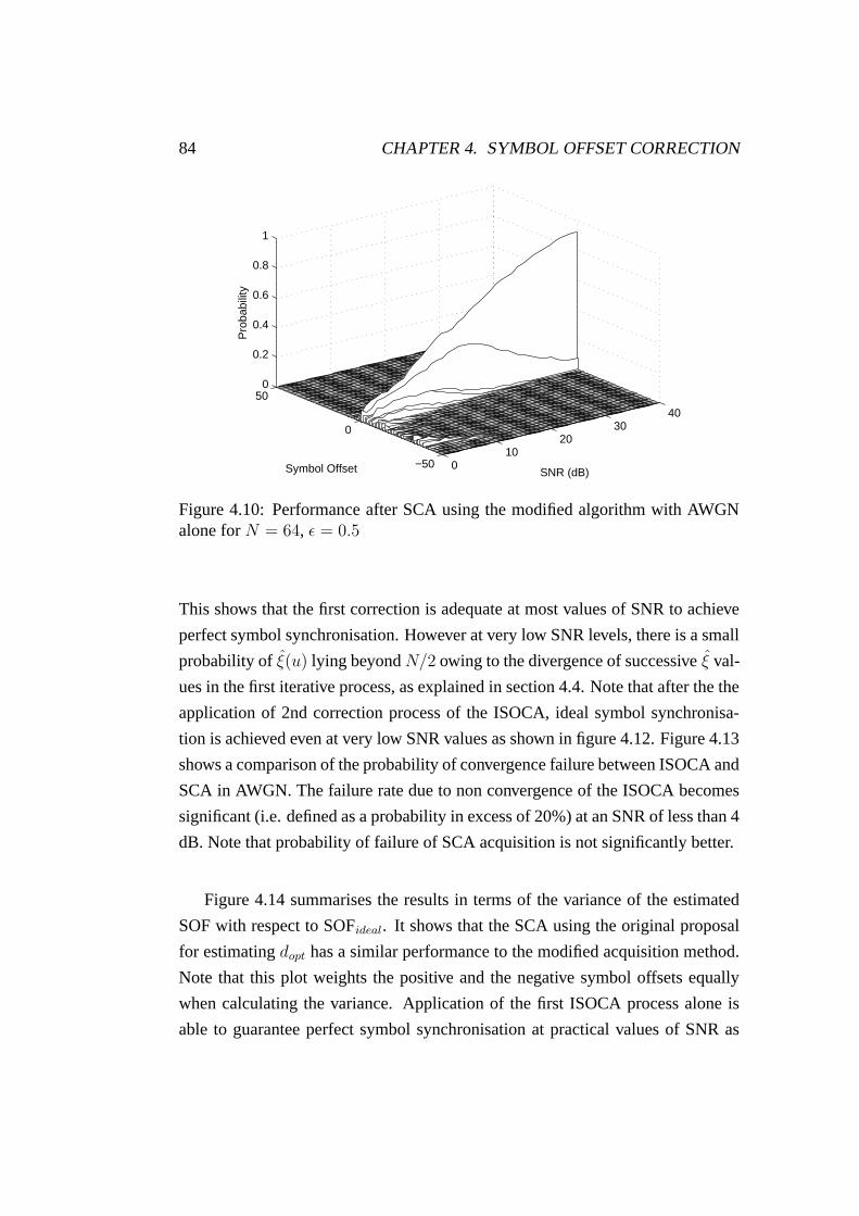
84 CHAPTER 4. SYMBOL OFFSET CORRECTION
010
2030
40
−50
0
500
0.2
0.4
0.6
0.8
1
SNR (dB)Symbol Offset
Pro
babi
lity
Figure 4.10: Performance after SCA using the modified algorithm with AWGNalone for N = 64, ε = 0.5
This shows that the first correction is adequate at most values of SNR to achieve
perfect symbol synchronisation. However at very low SNR levels, there is a small
probability of ξ(u) lying beyond N/2 owing to the divergence of successive ξ val-
ues in the first iterative process, as explained in section 4.4. Note that after the the
application of 2nd correction process of the ISOCA, ideal symbol synchronisa-
tion is achieved even at very low SNR values as shown in figure 4.12. Figure 4.13
shows a comparison of the probability of convergence failure between ISOCA and
SCA in AWGN. The failure rate due to non convergence of the ISOCA becomes
significant (i.e. defined as a probability in excess of 20%) at an SNR of less than 4
dB. Note that probability of failure of SCA acquisition is not significantly better.
Figure 4.14 summarises the results in terms of the variance of the estimated
SOF with respect to SOFideal. It shows that the SCA using the original proposal
for estimating dopt has a similar performance to the modified acquisition method.
Note that this plot weights the positive and the negative symbol offsets equally
when calculating the variance. Application of the first ISOCA process alone is
able to guarantee perfect symbol synchronisation at practical values of SNR as
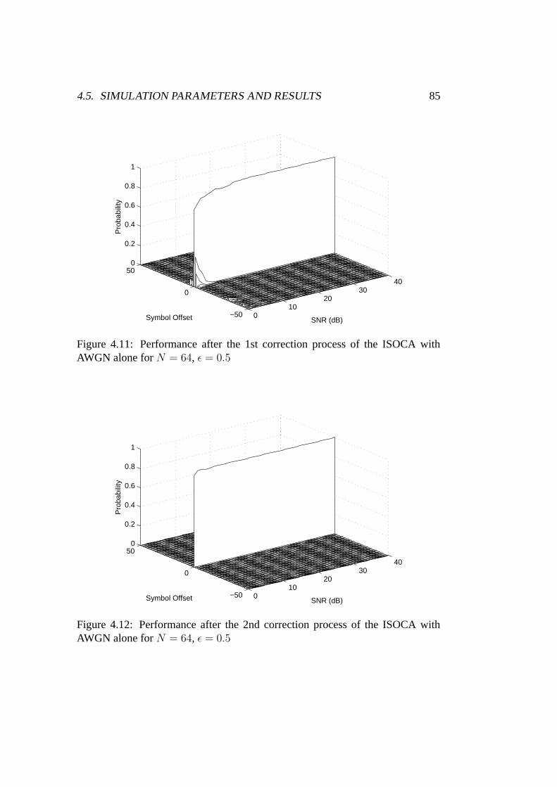
4.5. SIMULATION PARAMETERS AND RESULTS 85
010
2030
40
−50
0
500
0.2
0.4
0.6
0.8
1
SNR (dB)Symbol Offset
Pro
babi
lity
Figure 4.11: Performance after the 1st correction process of the ISOCA withAWGN alone for N = 64, ε = 0.5
010
2030
40
−50
0
500
0.2
0.4
0.6
0.8
1
SNR (dB)Symbol Offset
Pro
babi
lity
Figure 4.12: Performance after the 2nd correction process of the ISOCA withAWGN alone for N = 64, ε = 0.5

86 CHAPTER 4. SYMBOL OFFSET CORRECTION
0 5 10 15 20 25 30 35 400
0.1
0.2
0.3
0.4
0.5
0.6
0.7
SNR (dB)
Pro
babi
lity
SCAISOCA
Figure 4.13: Probability of convergence failure with AWGN alone for N = 64,ε = 0.5
shown in figure 4.11, although the variance increases significantly at low SNR
values. However, even at very low SNR values (< 10 dB), the application of both
parts of the ISOCA significantly reduces the variance. Figure 4.15 shows similar
results, this time for N = 128 and N = 256. It shows that there is a finite proba-
bility of symbol offset at very low SNR values after employing only the first part
of ISOCA . The results given by the second ISOCA process cannot be presented in
the same figure since the simulated offset results are zero. Consequently, perfect
synchronisation is achieved when both parts of the ISOCA are employed.
Next the performance of ISOCA is analysed in the presence of SUI-II chan-
nels [23]. OFDM systems with N = 64 have been simulated at a sampling rate
of 20 MHz with a guard interval, v equal to 20 samples for all symbols except
the first training symbol. To improve the acquisition performance of the SCA, the
length of the CP of the first training symbol is increased to give an Excess Length,
p = 10.
Figure 4.16 shows that the performance of the modified SCA deteriorates sig-
nificantly from that achieved in AWGN alone when the SUI-II CIR is incorpo-

4.5. SIMULATION PARAMETERS AND RESULTS 87
0 5 10 15 20 25 30 35 4010
−3
10−2
10−1
100
101
102
103
SNR (dB)
Err
or V
aria
nce
SCA originalSCA modifiedISOCA Part1ISOCA Part2
Figure 4.14: Variance of the estimated SOF with respect to SOFideal for AWGNchannels with N = 64 and ε = 0.5
0 5 10 15 20 25 30 35 4010
−3
10−2
10−1
100
101
102
103
SNR (dB)
Err
or V
aria
nce
SCA−N128SCA−N256ISOCA Part1−N128ISOCA Part1−N256
Figure 4.15: Variance of the estimated SOF with respect to SOFideal for AWGNchannels with N = 128, 256 and ε = 0.5
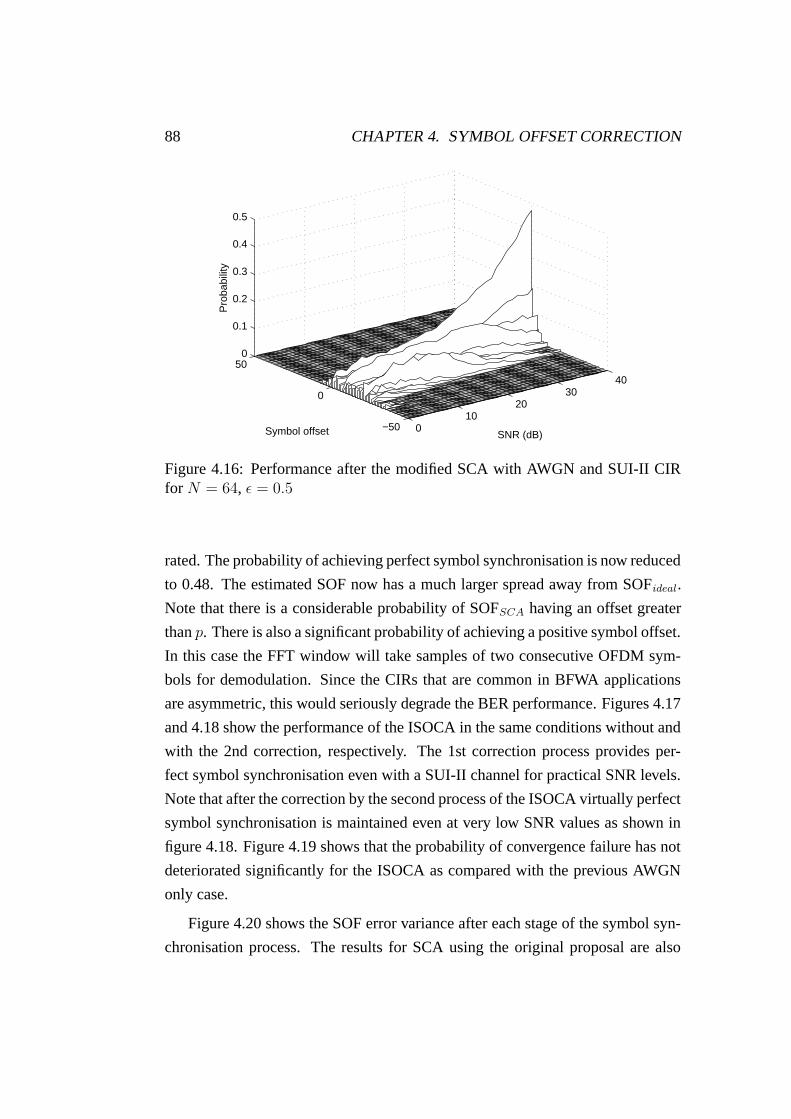
88 CHAPTER 4. SYMBOL OFFSET CORRECTION
010
2030
40
−50
0
500
0.1
0.2
0.3
0.4
0.5
SNR (dB)Symbol offset
Pro
babi
lity
Figure 4.16: Performance after the modified SCA with AWGN and SUI-II CIRfor N = 64, ε = 0.5
rated. The probability of achieving perfect symbol synchronisation is now reduced
to 0.48. The estimated SOF now has a much larger spread away from SOFideal.
Note that there is a considerable probability of SOFSCA having an offset greater
than p. There is also a significant probability of achieving a positive symbol offset.
In this case the FFT window will take samples of two consecutive OFDM sym-
bols for demodulation. Since the CIRs that are common in BFWA applications
are asymmetric, this would seriously degrade the BER performance. Figures 4.17
and 4.18 show the performance of the ISOCA in the same conditions without and
with the 2nd correction, respectively. The 1st correction process provides per-
fect symbol synchronisation even with a SUI-II channel for practical SNR levels.
Note that after the correction by the second process of the ISOCA virtually perfect
symbol synchronisation is maintained even at very low SNR values as shown in
figure 4.18. Figure 4.19 shows that the probability of convergence failure has not
deteriorated significantly for the ISOCA as compared with the previous AWGN
only case.
Figure 4.20 shows the SOF error variance after each stage of the symbol syn-
chronisation process. The results for SCA using the original proposal are also

4.5. SIMULATION PARAMETERS AND RESULTS 89
010
2030
40
−50
0
500
0.2
0.4
0.6
0.8
1
SNR (dB)Symbol Offset
Pro
babi
lity
Figure 4.17: Performance after the 1st correction of ISOCA with AWGN and theSUI-II CIR for N = 64, ε = 0.5
010
2030
40
−50
0
500
0.2
0.4
0.6
0.8
1
SNR (dB)Symbol Offset
Pro
babi
lity
Figure 4.18: Performance after the 2nd correction of ISOCA with AWGN and theSUI-II CIR for N = 64, ε = 0.5

90 CHAPTER 4. SYMBOL OFFSET CORRECTION
0 5 10 15 20 25 30 35 400
0.1
0.2
0.3
0.4
0.5
0.6
0.7
SNR (dB)
Pro
babi
lity
SCAISOCA
Figure 4.19: Probability of convergence failure with AWGN and the SUI-II CIRfor N = 64, ε = 0.5
included. The length of the timing metric plateau is now assumed to be p, hence
the SOF is estimated as ˆSOFSCA = d′opt−p/2 for the original proposal. Compared
to the AWGN only results presented in figure 4.14, it shows that even when the
modified method for acquisition of dopt is employed, SCA suffers considerable
symbol offset. As in figure 4.14 the positive and negative offsets are weighted the
same in this figure. As previous results have shown, whereas the SCA alone has a
significant probability of giving positive symbol offsets at lower SNR values, the
ISOCA has a higher probability of yielding only the less damaging negative sym-
bol offsets. Employing only the first part of the ISOCA is shown to improve the
performance giving perfect symbol synchronisation at practical values of SNR.
Figure 4.21 shows results for similar conditions for N = 128 and 256. It shows
similar results on completion of the first ISOCA process. The simulation results
also showed that employing both parts of the ISOCA achieved perfect synchro-
nisation even at very low values of SNR for N = 128, 256. Again, these results
cannot be presented since the variance was zero at all values of SNR tested.
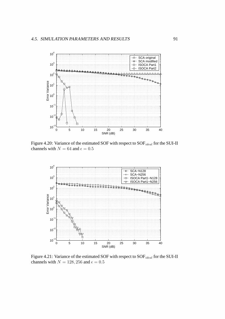
4.5. SIMULATION PARAMETERS AND RESULTS 91
0 5 10 15 20 25 30 35 4010
−3
10−2
10−1
100
101
102
103
104
SNR (dB)
Err
or V
aria
nce
SCA originalSCA modifiedISOCA Part1ISOCA Part2
Figure 4.20: Variance of the estimated SOF with respect to SOFideal for the SUI-IIchannels with N = 64 and ε = 0.5
0 5 10 15 20 25 30 35 4010
−3
10−2
10−1
100
101
102
103
104
SNR (dB)
Err
or V
aria
nce
SCA−N128SCA−N256ISOCA Part1−N128ISOCA Part1−N256
Figure 4.21: Variance of the estimated SOF with respect to SOFideal for the SUI-IIchannels with N = 128, 256 and ε = 0.5
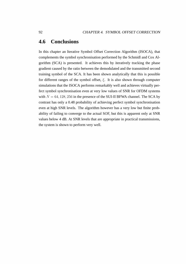
92 CHAPTER 4. SYMBOL OFFSET CORRECTION
4.6 Conclusions
In this chapter an Iterative Symbol Offset Correction Algorithm (ISOCA), that
complements the symbol synchronisation performed by the Schmidl and Cox Al-
gorithm (SCA) is presented. It achieves this by iteratively tracking the phase
gradient caused by the ratio between the demodulated and the transmitted second
training symbol of the SCA. It has been shown analytically that this is possible
for different ranges of the symbol offset, ξ. It is also shown through computer
simulations that the ISOCA performs remarkably well and achieves virtually per-
fect symbol synchronisation even at very low values of SNR for OFDM systems
with N = 64, 128, 256 in the presence of the SUI-II BFWA channel. The SCA by
contrast has only a 0.48 probability of achieving perfect symbol synchronisation
even at high SNR levels. The algorithm however has a very low but finite prob-
ability of failing to converge to the actual SOF, but this is apparent only at SNR
values below 4 dB. At SNR levels that are appropriate in practical transmissions,
the system is shown to perform very well.
Chapter 5
Residual Frequency Offset
Correction
Chapter 4 showed the effect that symbol offset has on the performance of OFDM
systems and presented the Schmidl and Cox Algorithm (SCA) [25, 58] which may
be used to achieve both symbol synchronisation and frequency offset synchronisa-
tion. The same chapter identified performance limitations of the symbol synchro-
nisation function of the SCA when applied to OFDM systems in BFWA channels.
To overcome these limitations the Iterative Symbol Offset Correction Algorithm
(ISOCA) is proposed which complements the SCA. It has been shown via exten-
sive simulations that the ISOCA greatly improves the acquisition of symbol timing
in this application. In this chapter attention is directed toward the frequency offset
synchronisation function of the SCA. Throughout this chapter it will be assumed
that the system achieves perfect symbol synchronisation. This assumption is valid
since we have shown in chapter 4 that the ISOCA achieves virtually perfect sym-
bol synchronisation for the BFWA channels under consideration. The frequency
offset in this chapter is defined relative to the intercarrier spacing and is denoted
as ε.
This chapter is organised as follows. Section 5.1 presents the work carried out
by others in the same area. Section 5.2 will show the effects of frequency offset
and highlight its severe impact on performance. The SCA will be presented in sec-
tion 5.3 with particular emphasis directed towards its ability to correct frequency
93

94 CHAPTER 5. RESIDUAL FREQUENCY OFFSET CORRECTION
offset. As noted earlier, the SCA does not perform well with OFDM systems hav-
ing a low number of subchannels, N . The Residual Frequency Offset Correction
Algorithm (RFOCA) to be presented in section 5.4 complements the frequency
offset correction functions of the SCA to reduce any Residual Frequency Off-
set (RFO) remaining after application of the SCA. Section 5.5 presents results
obtained through computer simulations which investigate the performance of the
RFOCA in both AWGN and BFWA channels. Section 5.6 will draw conclusions.
5.1 Related Work
Moose was one of the first authors to present a frequency offset correction method
for OFDM that utilises repetitive sections of the transmit data [86]. He proposed
to have two repetitive OFDM symbols. Hence the relative frequency offset, ε that
can be estimated without phase ambiguity is equal to half the intercarrier spacing
(i.e. |ε| < 0.5). The SCA uses a training symbol that is repetitive with a period
equal to half the symbol period. Hence using only the first training symbol, the es-
timation limit was increased to the intercarrier spacing (i.e. |ε| < 1). The authors
in [87] propose to use only the first training symbol of the SCA but to form it from
more than two identical parts. The fractional part of the frequency offset estimate
is modified compared with that of the SCA and is computationally much more
intensive. Usually, the frequency offset and symbol synchronisation is done using
the same training symbols. Adding more repetitions to the first training symbol
of the SCA also compromises the symbol synchronisation part of the SCA. In
general, having a training symbol with M identical parts increases the frequency
offset estimation range to ±M/2 intercarrier spacings. Even though increasing the
training symbol repetition further increases the resolution, it will compromise the
accuracy of the frequency offset estimate owing to the smaller number of samples
used by the correlation filter [88]. The WLAN standards such as HIPERLAN/2
and IEEE 802.11a use two OFDM symbols as a preamble, one symbol being di-
vided into short subsequences and the other into two identical subsequences. One
of the uses of the preambles is to estimate the frequency offset. Two estimates
are performed, the first is a coarse frequency offset estimation made using a de-
lay and correlate method between the shorter sequences. A fine frequency offset

5.1. RELATED WORK 95
estimation is then made by calculating the angular rotation between the post-FFT
samples of the two training symbols [24].
Other suggestions utilise the correlation between the cyclic prefix and the last
few samples of the OFDM symbol [62]. In [89] the authors extend the work
of [62] by proposing a new likelihood function for joint estimation of symbol
and frequency offset based on direct matrix inversion. Once again though, its
performance for dispersive channels is not acceptable for small values of N .
The authors in [90, 91] propose to periodically scatter the pilot symbols in
some subchannels in the time-frequency grid. This avoids the use of OFDM sym-
bols for training. The estimate has to be averaged over a number of OFDM sym-
bols to get a reasonable estimate even with the assumption of perfect channel
knowledge. As noted in chapter 1, in general for short burst data transmission, the
use of some subchannels for pilot symbols is not practical.
Other approaches are the self-cancellation schemes presented in [92] and [93,
94], where the data to be transmitted is mapped repeatedly on to adjacent pairs of
subchannels rather than on to a single subchannel. If the data is negated in one of
the adjoining subchannels the overall effects of ICI due to frequency offset can be
eliminated. Again, when N is low this approach is not practical and the number
of available subchannels is also reduced by at least one half.
In [95, 96, 97, 98] blind frequency offset estimation techniques are proposed.
These techniques avoid the use of training symbols and rely on the second order
statistics of the received signal and generally have a high computational burden.
The authors in [99, 100] propose algorithms to estimate only the integer part of
the frequency offset. It is assumed that the fractional part can be estimated and
corrected perfectly by some other technique such as the SCA. This assumption is
not correct as will be shown in later sections. The authors in [101] show analyti-
cally that the use of non-rectangular windowing reduces the effect of ICI caused
as a result of frequency offset. The use of such windows will be investigated in
more detail in chapter 7.
In section 5.4 a novel algorithm will be presented that does not utilise any
continuous pilots nor null symbols yet tracks the residual offset quite effectively.
It also performs very well for BFWA applications.

96 CHAPTER 5. RESIDUAL FREQUENCY OFFSET CORRECTION
5.2 Effect of Frequency Offset in OFDM
Assuming that the length of the Cyclic Prefix (CP) is longer than the length of
the CIR (i.e. v ≥ Nh − 1), and that N is large enough such that the frequency
selective channel is divided into contiguous flat fading subchannels the expression
of (2.27) for the demodulated symbol of lth subchannel in mth OFDM block is
modified to,
Ym,l =1
N
N−1∑
n=0
N−1∑
k=0
Am,kHkej2π
n(k+ε)N
e−j2πlnN +Wl (5.1)
for 0 ≤ n ≤ N − 1. Here Hk is the Channel Transfer Function (CTF) at the
subchannel index k, Wl is the component due to AWGN and ε is the frequency
offset relative to the intercarrier spacing. The expression in (5.1) allows the output
of the lth subchannel to be expressed as the sum of three components,
Ym,l = Rl + Il +Wl (5.2)
where Rl and Il are the desired and the Inter Carrier Interference (ICI) terms,
respectively. By substituting the condition k = l in the inner sum of (5.1), we can
obtain Rl. Thus,
Rl =1
N
N−1∑
n=0
(Am,lHl)ej2π
n(l+ε)N e−j2π
nlN
=Am,lHl
N
1 − ej2πε
1 − ej2πε/N
= (Am,lHl)sin(πε)
N sin(πε/N)ejπε
N−1N . (5.3)
Equation (5.3) shows that the desired term Am,lHl experiences amplitude re-
duction and phase rotation. Since N πε, sin(πε/N) can be approximated by
(πε)/N . Hence,
Rl ≈ Am,lHlsin(πε)
N(πε/N)ejπε
N−1N = Am,lHlsinc(ε)ejπε
N−1N . (5.4)
As ε → 0, Rl → Am,lHl, hence the degradation of the required term vanishes

5.2. EFFECT OF FREQUENCY OFFSET IN OFDM 97
when the received data does not experience any frequency offset. In practice, the
effect of the channel transfer function Hl is removed by the FEQ following the
FFT, as shown in section 2.4.
The effect due to ICI in (5.2) can be calculated as,
Il =1
N
N−1∑
k=0k 6=l
N−1∑
n=0
(Am,kHk)ej2π
n(k+ε)N e−j2π
nlN
=N−1∑
k=0k 6=l
Am,kHk
N
1 − ej2π(k+ε−l)
1 − ej2π(k+ε−l)/N
=N−1∑
k=0k 6=l
(Am,kHk)sin π(k + ε− l)
N sinπ(k + ε− l)/Nejπ(k+ε−l) N−1
N . (5.5)
If we assume that the transmitted data is zero mean and uncorrelated (i.e.
E[Am,k] = 0 and E[Am,lA∗m,k] = σAδl,k, then E[Il] = 0. Hence the ICI power is,
E[|Il|2] = σA[sinπε]2N−1∑
k=0k 6=l
E[|Hk|2][N sin π(k + ε− l)/N ]2
. (5.6)
A measure of the impact of frequency offset is given by defining the Carrier
to Interference Ratio (CTIR) in an OFDM system as, CTIR = E[|Rl|2]/E[|Il|2].Assuming the average channel gain, E[|Hk|2 is unity and with zero AWGN, (i.e.
Wl = 0) then,
CTIR =
∑N−1k=0k 6=l
1/[N sinπ(k + ε− l)/N ]2
[N sin(πε/N)]2. (5.7)
A similar analysis on the effect of frequency offset on OFDM can be found
in [86] and [94]. Also see [102] for an analysis of the ICI power when the OFDM
system is subject to channels giving rise to Doppler spreading. Figure 5.1 shows
the CTIR in decibels as a function of ε. Simulated CTIR values for N = 64 and
256 using QPSK data mapping are also shown. It shows that the CTIR drops
significantly when the relative frequency offset, ε increases beyond 0.1. An im-
portant observation is that the CTIR is insensitive to the values of N between 64

98 CHAPTER 5. RESIDUAL FREQUENCY OFFSET CORRECTION
0.05 0.1 0.15 0.2 0.25 0.3 0.35 0.4 0.45 0.5−5
0
5
10
15
20
25
Relative frequency offset (ε)
CT
IR (
dB)
TheoreticalSimulated (N = 256)Simulated (N = 64)
Figure 5.1: Analysis of CTIR vs relative frequency offset, ε
and 256. The authors in [57] derive a similar parameter and are able to show
that the interference due to frequency offsets across the subchannels also remains
virtually the same except for the ones at the edges of the OFDM multiplex.The
authors in [103] derive the probability of bit error for a QPSK mapped OFDM
system as a function of the frequency offset.
5.3 Schmidl and Cox Algorithm
As stated previously, the SCA is utilised to estimate both symbol timing and fre-
quency offset. In section 4.3 the symbol synchronisation function of SCA was
introduced. In this section the frequency offset correction function will be in-
vestigated. Perfect symbol synchronisation is assumed to be achieved using the
ISOCA presented previously.
For perfect symbol synchronisation the Start of Frame (SOF) will be deter-
mined as the start of first training symbol, given by dopt − v as explained previ-
ously in section 4.3. The phase difference between received samples L = N/2

5.3. SCHMIDL AND COX ALGORITHM 99
samples apart is estimated as,
φ = 1/(p+ 1)p∑
n=0
6 P (dopt − n) (5.8)
where P (d) is the correlator output given in (4.14). The fractional part of ε is
estimated as,
εSCA = φ/π . (5.9)
In order to resolve potential ambiguity due to the integer part of ε, use is
made of the second SCA training symbol. By estimating the phase shift between
the two training symbols, the integer part of the ε can be estimated. First, the
training symbols are corrected using φ/π and then any additional phase shift due
to the integer part of the frequency offset is found as the value of g, namely g that
maximises the function
B(g) =|∑k∈X x∗1,k+2g v
∗k x2,k+2g|2
2(∑
k∈X |x2,k|2)2 (5.10)
where x1,k and x2,k are the FFT demodulated outputs corresponding with the
two training symbols, that have already undergone partial frequency offset com-
pensation using φ/π and vk is the ratio of the two symbols being transmitted in
the even subchannels of the two SCA training symbols [25]. Note g is the index
spanning the even subchannels i.e. X = 0, 2, . . . , N − 4, N − 2, hence the total
frequency offset is estimated as [25],
εSCA = φ/π + 2g . (5.11)
Note that if ε has only a fractional part, g would yield zero when calculated
using (5.10). In theory, this method can estimate frequency offsets in the range
−(L+1) < ε < (L−1). In [88] and [104] the authors propose to use only the first
training symbol of the SCA to estimate the frequency offset. They estimate the
fractional part of the frequency offset in a similar manner to that proposed in the
SCA. The integer part of the SCA will introduce a shift in the positions of the de-
modulated data across the subchannels. They propose to estimate the integer part
by modulating the first training symbol differentially across the subchannels [88]

100 CHAPTER 5. RESIDUAL FREQUENCY OFFSET CORRECTION
or to simply find the position shift using the even frequencies of the first training
symbol of the SCA [104]. The residual frequency offset following application
of the fractional correction part must be very small to achieve acceptable system
performance.
As stated previously, it should be noted that the effect of AWGN on the cor-
rect estimation of ε depends on the number of FFT points, N . The SCA performs
well for OFDM systems with frequency offsets when N is in excess of 1000 [25].
When the SCA is used for systems with lower values of N , the estimate εSCAresults in a Residual Frequency Offset (RFO), ε that rotates the received constel-
lation at a reduced rate, but one that is still significant enough to cause bit errors in
coherently demodulated OFDM systems. Hence OFDM systems with low values
of N will require a RFO correction algorithm to continuously track the carrier
frequency offset. In the next section the proposed Residual Frequency Offset Cor-
rection Algorithm (RFOCA) is presented. This algorithm complements the SCA
by cascading it with a tracking function that continuously compensates for the
RFO.
5.4 Residual Frequency Offset Correction Algorithm
In the approach proposed here, an initial frequency offset estimation is made using
the SCA. The resulting RFO, ε is estimated by tracking the rate of change of
phase of the demodulated data at the FEQ outputs, Ym,l as shown in figure 5.2.
However, the estimate of ε could be seriously affected by subchannels with a
low SNR owing to spectral nulls in the channel response Hl. An estimate of
Hl is made by taking the ratio between the transmitted and decoded output of
the second training symbol of the SCA. Hence only those subchannels with |Hl|above a certain threshold are selected. This subset of subchannels is denoted
as d ⊂ [0, ..N − 1]. The criteria applied is to select subchannels with |Hl| in
excess of a standard deviation above the mean. For symbol m, the outputs of
these subchannels Ym,d are sent through a slicer to obtain Ym,d, where d ∈ d.
For symbol m the phase errors between the demodulated data, Ym,d and the

5.4. RESIDUAL FREQUENCY OFFSET CORRECTION ALGORITHM 101
Parellel to serial
and
FFT Demod
FEQ Select
Channel
arg[.]
To QPSK Slicer
X
Blocks Unwrap Phase
Find Gradient
Block Count
Received Data
arg[.]
- Update
Initialise with
PSfrag replacements
Ym,l Ym,l Ym,d Ym,d
θiθiεm
εm
εm
θm,d
ej[(m−1)N+n](.)
N
Nw
Nw
εSCA
Figure 5.2: Block diagram of the Residual Frequency Offset Correction Algorithm(RFOCA)

102 CHAPTER 5. RESIDUAL FREQUENCY OFFSET CORRECTION
detected data, Ym,d of the selected subchannels, namely θm,d are found as,
θm,d = 6 Ym,d − 6 Ym,d . (5.12)
The phase errors are stored in a buffer, b for a block of Nw OFDM symbols.
Note that only the selected subchannels will be stored. Hence if the number of
subchannels selected in d is Nd then the length required for the buffer is only
NdNw. Note, in this thesis QPSK data mapping is assumed although the tech-
nique could be extended to other constellations. Initially, ε can be quite high and
if the values of the phase errors, θm,d > π/4, then it results in decoding errors
being produced by the slicer which subsequently results in phase wrapping of
θm,d at ±π/4. Hence it is imperative that θm,d is first unwrapped before the cal-
culation of ε begins. As before the simple phase unwrapping algorithm that is
presented in [85] is employed. Note that phase unwrapping is also required in fre-
quency offset estimation algorithms proposed for the Single Carrier (SC) systems
in [105, 106]. For reasons of clarity, the ith sample of the wrapped phase and the
unwrapped phase are denoted as θi and θi, respectively. The phase unwrapping
algorithm in this instance can be expressed as
θi = θi−1 + αSAWπ/4(θi − θi−1) (5.13)
where SAWπ/4(.) is a sawtooth function that limits the output to ±π/4 and
α is a parameter that controls the variance of the unwrapped phase. Note that
the unwrapping algorithm will be used only once every Nw OFDM symbols are
demodulated (i.e. when the buffer is full). The Maximum Likelihood (ML) esti-
mate of the RFO is calculated as the gradient of the unwrapped values stored in
the buffer. If q denotes a positive integer and θ denotes the vector of unwrapped
phase values at a particular iteration, then the estimated RFO after qNw blocks is
given as,
εqNw= GRAD(θ) (5.14)
where GRAD(.) function finds the ML gradient. The error due to frequency
offset is compensated for by multiplying the pre-FFT received symbols, rm,n with
ejεm[(m−1)N+n]/N , where εm is the frequency offset correction factor for symbol

5.4. RESIDUAL FREQUENCY OFFSET CORRECTION ALGORITHM 103
m. Note that εm is initialised to εSCA following the initial estimation made using
the SCA. The correction factor is updated after every Nw OFDM symbols using
εqNw. Hence at symbol number qNw, εqNw
is updated according to
εqNw= εqNw−1 + εqNw
(5.15)
For OFDM symbols (q − 1)Nw to qNw − 1, ε(q−1)Nwis used as the frequency
offset correction factor.
The choice of Nw is critical since a large value will cause the updating of
εm with too high a latency and will require more memory. However after a few
updates the values of εqNwbecome quite small. Hence to get a better estimate in
the presence of AWGN, a larger value of Nw is more appropriate since this will
reduce the variance. The RFOCA can be summarised as follows.
1. Perform an initial frequency offset estimation εSCA using the SCA.
2. Select the subset of subchannels with magnitudes exceeding the defined
threshold in the channel transfer function, d, at the start of the burst.
3. Obtain Ym,d from the FEQ output and then Ym,d by use of a slicer for each
symbol m, where d ∈ d. Calculate and store θm,d for a block of Nw OFDM
symbols.
4. Find the unwrapped phase θ from the wrapped phase θ. Find the gradient
of θ, namely εqNw. This process is done once every Nw symbols.
5. Once every Nw OFDM symbol blocks, calculate the new frequency offset
correction factor εqNwusing εqNw.
Another RFO correction algorithm has been presented by Kobayashi in [107].
He proposes having two training symbols and estimates the frequency offset in
two steps. The first estimation is made by multiplying the received training sym-
bols with the conjugate of the transmitted training symbols. By taking an FFT
over both symbols a coarse estimate of frequency offset is given by detecting the
peak of the FFT output. A fine estimate is then taken based on the phase shift
between the two training symbols. In this proposal both estimates are based on
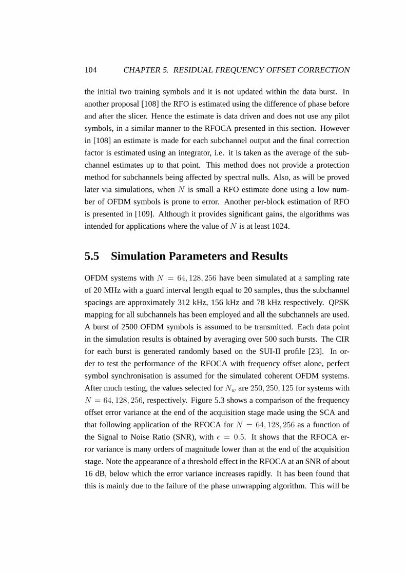
104 CHAPTER 5. RESIDUAL FREQUENCY OFFSET CORRECTION
the initial two training symbols and it is not updated within the data burst. In
another proposal [108] the RFO is estimated using the difference of phase before
and after the slicer. Hence the estimate is data driven and does not use any pilot
symbols, in a similar manner to the RFOCA presented in this section. However
in [108] an estimate is made for each subchannel output and the final correction
factor is estimated using an integrator, i.e. it is taken as the average of the sub-
channel estimates up to that point. This method does not provide a protection
method for subchannels being affected by spectral nulls. Also, as will be proved
later via simulations, when N is small a RFO estimate done using a low num-
ber of OFDM symbols is prone to error. Another per-block estimation of RFO
is presented in [109]. Although it provides significant gains, the algorithms was
intended for applications where the value of N is at least 1024.
5.5 Simulation Parameters and Results
OFDM systems with N = 64, 128, 256 have been simulated at a sampling rate
of 20 MHz with a guard interval length equal to 20 samples, thus the subchannel
spacings are approximately 312 kHz, 156 kHz and 78 kHz respectively. QPSK
mapping for all subchannels has been employed and all the subchannels are used.
A burst of 2500 OFDM symbols is assumed to be transmitted. Each data point
in the simulation results is obtained by averaging over 500 such bursts. The CIR
for each burst is generated randomly based on the SUI-II profile [23]. In or-
der to test the performance of the RFOCA with frequency offset alone, perfect
symbol synchronisation is assumed for the simulated coherent OFDM systems.
After much testing, the values selected for Nw are 250, 250, 125 for systems with
N = 64, 128, 256, respectively. Figure 5.3 shows a comparison of the frequency
offset error variance at the end of the acquisition stage made using the SCA and
that following application of the RFOCA for N = 64, 128, 256 as a function of
the Signal to Noise Ratio (SNR), with ε = 0.5. It shows that the RFOCA er-
ror variance is many orders of magnitude lower than at the end of the acquisition
stage. Note the appearance of a threshold effect in the RFOCA at an SNR of about
16 dB, below which the error variance increases rapidly. It has been found that
this is mainly due to the failure of the phase unwrapping algorithm. This will be

5.5. SIMULATION PARAMETERS AND RESULTS 105
10 12 14 16 18 20 22 24 26
10−12
10−10
10−8
10−6
10−4
SNR (dB)
Err
or V
aria
nce
SCA−N 64SCA−N 128SCA−N 256RFOCA−N 64RFOCA−N 128RFOCA−N 256
Figure 5.3: Comparison of the frequency offset error variance for SCA andRFOCA in AWGN for N = 64, 128, 256 and ε = 0.5
discussed in more detail later in the section. Figure 5.4 shows the performance of
the RFOCA in terms of Bit Error Rate (BER) vs SNR again in AWGN. The BER
is virtually zero at values of SNR above 16 dB but increases markedly below this
value. This result is a direct consequence of the threshold effect observed with
the previous error variance results presented in figure 5.3. It is observed in the
simulations that at an SNR of 16 dB only a few out of the total of 500 received
bursts give rise to errors. However, these errors are significant giving rise to a high
overall BER. Such occurrences became more common when the SNR is reduced
below 15 dB, thus increasing the BER very rapidly.
Figures 5.5 and 5.6 show the simulation results for identical systems to those
simulated previously, but this time with a larger relative frequency offset, i.e.
ε = 1.5. Since ε now has both a fractional and an integer part, the latter will
be determined as shown in (5.10) and (5.11). Comparison with the previous re-
sults presented in figure 5.3 and 5.4 show that the performance of RFOCA does
not degrade with increasing values of ε.
Figure 5.7(a) shows the effect that symbol timing offsets have on the perfor-

106 CHAPTER 5. RESIDUAL FREQUENCY OFFSET CORRECTION
12 13 14 15 16 17 1810
−5
10−4
10−3
10−2
10−1
100
SNR (dB)
BE
RN 64N 128N 256
Figure 5.4: Performance of RFOCA in AWGN for N = 64, 128, 256 and ε = 0.5
10 12 14 16 18 20 22 24 26
10−12
10−10
10−8
10−6
10−4
SNR (dB)
Err
or V
aria
nce
SCA−N 64SCA−N 128SCA−N 256RFOCA−N 64RFOCA−N 128RFOCA−N 256
Figure 5.5: Comparison of the frequency offset error variance for SCA andRFOCA in AWGN for N = 64, 128, 256 and ε = 1.5

5.5. SIMULATION PARAMETERS AND RESULTS 107
12 13 14 15 16 17 1810
−5
10−4
10−3
10−2
10−1
100
SNR (dB)
BE
R
N 64N 128N 256
Figure 5.6: Performance of RFOCA in AWGN for N = 64, 128, 256 and ε = 1.5
mance of the RFOCA. It plots the error variance for a system with N = 256
and ε = 0.5 using two approaches to determine the SOF. The first approach as-
sumes ideal symbol synchronisation (shown as SOFideal) and the other uses the
SOF as determined using the SCA alone (shown as ˆSOFSCA). It shows that the
performance of the RFOCA degrades severely when subjected to the symbol off-
set introduced by the SCA. This is primarily due to the fact that the presence of
symbol offset introduces an additional phase gradient when calculating θ in (5.12)
in addition to that owing to the RFO alone. The gradient introduced by the symbol
offset is much higher than that owing to the RFO. Even though the phase gradient
induced by symbol offset is absorbed by the FEQ, the estimation of the εSCA using
(5.9) and (5.8) is degraded by the symbol offset. Figure 5.7(b) shows the results
for the same scenario in terms of BER vs SNR.
In order to maintain consistency with other results presented in this thesis the
second model of the Stanford University Interim channels (SUI-II) [23] has been
selected as the BFWA channel model. The transmitted burst takes less than 10
ms to send at the selected sampling frequency and consequently the channel is
assumed constant for the duration of each burst.

108 CHAPTER 5. RESIDUAL FREQUENCY OFFSET CORRECTION
10 12 14 16 18 20 22 24 2610
−12
10−10
10−8
10−6
10−4
10−2
100
SNR (dB)
Err
or V
aria
nce
RFOCA: SOF ideal
RFOCA: SOF SCA
(a) Frequency offset error variance
12 14 16 18 20 22 24 26 2810
−5
10−4
10−3
10−2
10−1
100
SNR (dB)
BE
R
RFOCA: SOF ideal
RFOCA: SOF SCA
(b) BER
Figure 5.7: Comparison of the effect of symbol offset on RFOCA in AWGN forN = 256 and ε = 0.5
Figure 5.8 allows a comparison of the frequency offset error variance due to
the SCA and that following the RFOCA for an OFDM system with ε = 0.5 in the
SUI-II channel. A new channel in accordance with the SUI-II profile is randomly
generated for the transmission of each burst. The RFOCA error variance is seen
to be many orders of magnitude lower than that due to the SCA alone despite the
presence of the SUI-II channel.
Figure 5.9 shows the performance of the RFOCA in terms of BER vs SNR
for the SUI-II channel and again ε = 0.5. The threshold effect now occurs at an
SNR in the region of 20 dB owing to the effect of the SUI-II channel. It shows
that the performance of the RFOCA degrades with the increase of N . Clearly, the
subchannels are placed more closely together with a larger value of N . Conse-
quently, a given residual offset not corrected by the algorithm yields more ICI that
will degrade the estimation process according to (5.12) to (5.14). Since RFOCA
is a feedback correction method, this in turn affects the correction factor in (5.15).
Also, the RFOCA selects the subchannels used for the estimation process based
on the estimated CIR. A higher ICI will also affect the estimation of the CIR.
Figures 5.10 and 5.11 show the results for identical systems to those simulated
previously, this time with a relative frequency offset of ε = 1.5 (i.e. it has an in-
teger part). The results are similar to that shown previously in figures 5.8 and 5.9.

5.5. SIMULATION PARAMETERS AND RESULTS 109
16 17 18 19 20 21 22 23 24 25 26
10−12
10−10
10−8
10−6
10−4
SNR (dB)
Err
or V
aria
nce
SCA−N 64SCA−N 128SCA−N 256RFOCA−N 64RFOCA−N 128RFOCA−N 256
Figure 5.8: Comparison of the frequency offset error variance for SCA andRFOCA with AWGN and SUI-II CIR for N = 64, 128, 256 and ε = 0.5
Hence it shows that the performance of the RFOCA does not depend on the initial
relative frequency offset ε.
An investigation into the threshold effect that is apparent in the RFOCA will
now be presented. Figure 5.12(a) shows the typical performance of the phase un-
wrapping algorithm in RFOCA during the first iteration for an OFDM system with
N = 64, ε = 0.5 and at an SNR of 20 dB. Note that the superimposed estimated
gradient follows the unwrapped phase closely. Figure 5.12(b) shows the how the
residual frequency offset is tracked by the RFOCA at an SNR of 20 dB. This type
of illustration is referred to as the Dynamic Residual Offset Tracking (DROT).
It shows the absolute error at end of each iteration. The iteration process is ini-
tialised to the estimate of frequency offset given by the SCA, namely εSCA. The
error between εSCA and the actual value is shown as the DROT value at iteration
0. In this case, following the SCA the error is of the order 10−5. Immediately after
the first iteration, the error has been reduced to the order of 10−7 and remains at
this order of magnitude for subsequent iterations. The result of this is that the RFO
is so small that a large number of samples are required to estimate it accurately.
That is the reason why Nw has to be selected in the order of hundreds. The other

110 CHAPTER 5. RESIDUAL FREQUENCY OFFSET CORRECTION
17 18 19 20 21 22 23 2410
−8
10−6
10−4
10−2
100
SNR (dB)
BE
R
N 64N 128N 256
Figure 5.9: Performance of RFOCA with AWGN and SUI-II CIR for N =64, 128, 256 and ε = 0.5
16 17 18 19 20 21 22 23 24 25 26
10−12
10−10
10−8
10−6
10−4
SNR (dB)
Err
or V
aria
nce
SCA−N 64SCA−N 128SCA−N 256RFOCA−N 64RFOCA−N 128RFOCA−N 256
Figure 5.10: Comparison of the frequency offset error variance for SCA andRFOCA with AWGN and SUI-II CIR for N = 64, 128, 256 and ε = 1.5
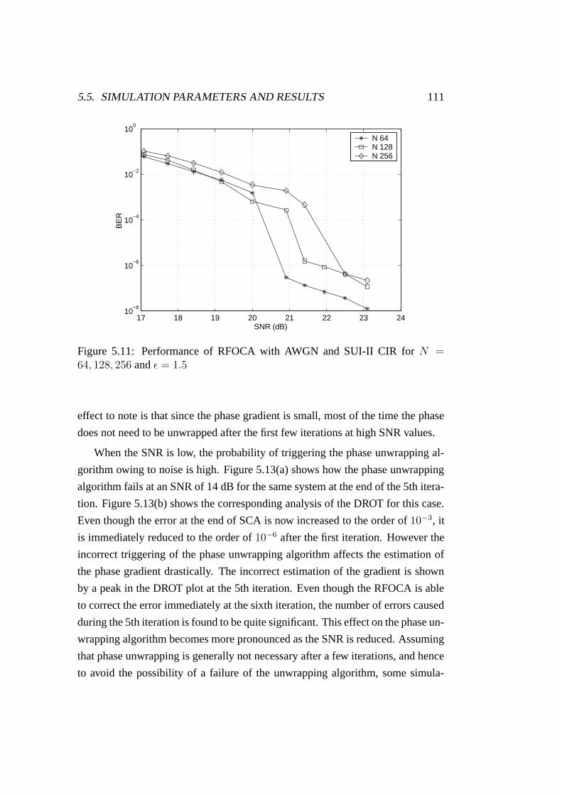
5.5. SIMULATION PARAMETERS AND RESULTS 111
17 18 19 20 21 22 23 2410
−8
10−6
10−4
10−2
100
SNR (dB)
BE
R
N 64N 128N 256
Figure 5.11: Performance of RFOCA with AWGN and SUI-II CIR for N =64, 128, 256 and ε = 1.5
effect to note is that since the phase gradient is small, most of the time the phase
does not need to be unwrapped after the first few iterations at high SNR values.
When the SNR is low, the probability of triggering the phase unwrapping al-
gorithm owing to noise is high. Figure 5.13(a) shows how the phase unwrapping
algorithm fails at an SNR of 14 dB for the same system at the end of the 5th itera-
tion. Figure 5.13(b) shows the corresponding analysis of the DROT for this case.
Even though the error at the end of SCA is now increased to the order of 10−3, it
is immediately reduced to the order of 10−6 after the first iteration. However the
incorrect triggering of the phase unwrapping algorithm affects the estimation of
the phase gradient drastically. The incorrect estimation of the gradient is shown
by a peak in the DROT plot at the 5th iteration. Even though the RFOCA is able
to correct the error immediately at the sixth iteration, the number of errors caused
during the 5th iteration is found to be quite significant. This effect on the phase un-
wrapping algorithm becomes more pronounced as the SNR is reduced. Assuming
that phase unwrapping is generally not necessary after a few iterations, and hence
to avoid the possibility of a failure of the unwrapping algorithm, some simula-

112 CHAPTER 5. RESIDUAL FREQUENCY OFFSET CORRECTION
tions have been performed where the unwrapping algorithm is only active during
the first three iterations and disabled thereafter. Figure 5.14 shows the results for
the cases where the unwrapping algorithm is used for all iterations and for only
three iterations for comparison. The results show that disabling the unwrapping
algorithms gives only a modest gain in performance. Changing the variance con-
trol parameter of the unwrapping algorithm, α in (5.13) did not show a significant
change in performance, however a more complex adaptive method to change α
proportional to the variance of the final estimate in (5.15) could have shown some
improvement.
Figure 5.15 shows the effect of varying the the number of OFDM symbols
stored in the buffer, Nw. (in other words the frequency with which updates of
the RFO correction factor, εm occur). It shows the RFO error variance for an
OFDM system with N = 64 for three different values of Nw. Updating the RFO
correction factor after every symbol gives a worse performance than the SCA.
This is because the number of noisy samples is not enough to make a reasonable
estimate. It further shows that to obtain a good estimate, Nw should be of the
order of 100.
Figure 5.16(a) and 5.16(b) shows the effect of channel estimation on the per-
formance of RFOCA in terms of error variance and BER vs SNR, respectively.
The curve ’RFOCA: ideal ch. est’ refers to the case when the perfect knowledge
of the channel is assumed at the receiver and the curve ’RFOCA: non-ideal ch.
est’ refers to the case when the channel is estimated using the second training
symbol of the SCA. From figure 5.16(b), it can be seen that ideal channel es-
timation gives an improvement in the performance of RFOCA of about 3.5 dB
for an OFDM system with N = 64 at a BER of 10−4. Channel estimation in
this scheme is performed using only one training symbol. Obviously, if a more
elaborate scheme were adopted, the performance of the RFOCA would improve
towards that achieved with ideal channel estimation. In any case, channel estima-
tion is not the focus of the work in this thesis.
A further analysis has been carried out to show the effect of symbol timing
offset on the performance of the RFOCA. Figure 5.17(a) shows the actual and
the estimated phase of the CTF when perfect symbol synchronisation is achieved.
Note that the FEQ is updated with the inverse of the estimated CTF. The difference
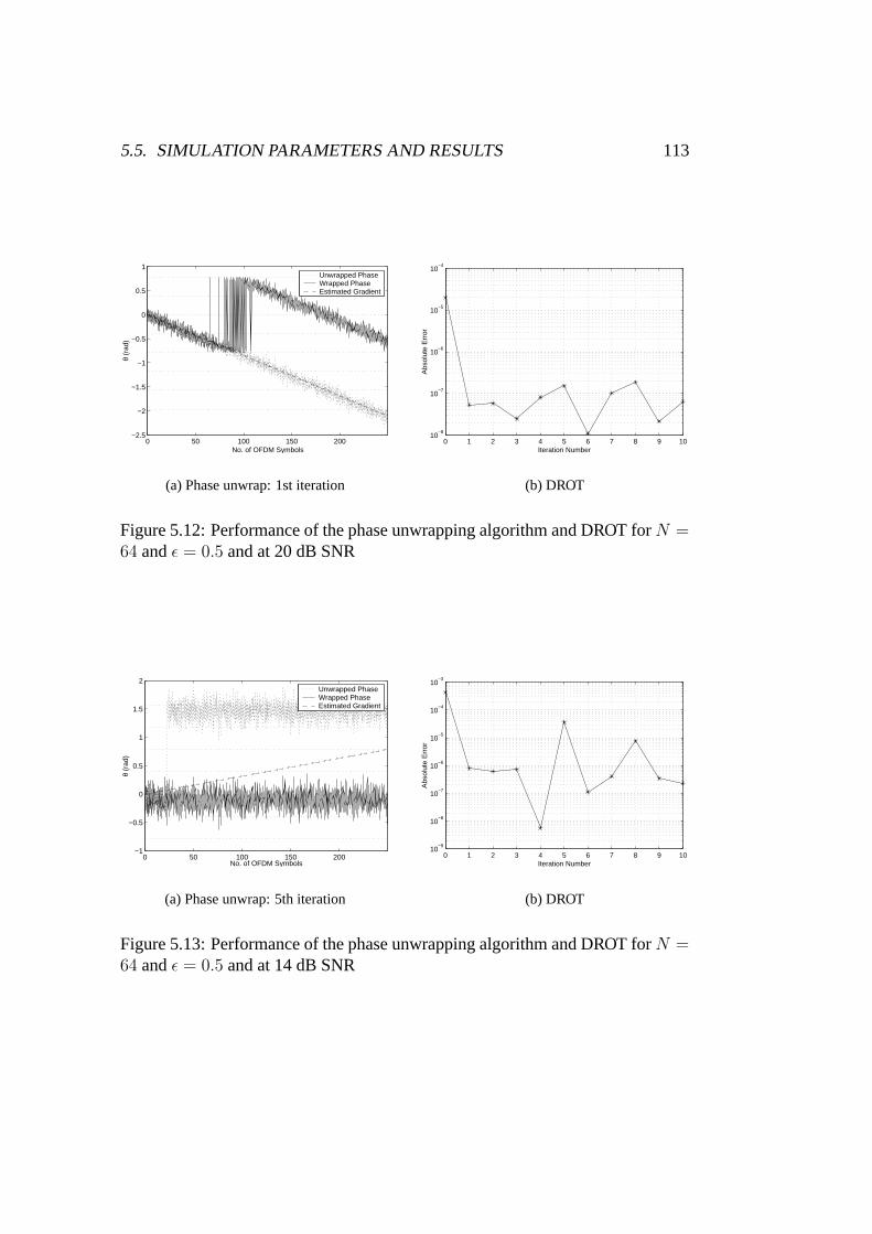
5.5. SIMULATION PARAMETERS AND RESULTS 113
0 50 100 150 200−2.5
−2
−1.5
−1
−0.5
0
0.5
1
θ (r
ad)
No. of OFDM Symbols
Unwrapped PhaseWrapped PhaseEstimated Gradient
(a) Phase unwrap: 1st iteration
0 1 2 3 4 5 6 7 8 9 1010
−8
10−7
10−6
10−5
10−4
Iteration Number
Abs
olut
e E
rror
(b) DROT
Figure 5.12: Performance of the phase unwrapping algorithm and DROT for N =64 and ε = 0.5 and at 20 dB SNR
0 50 100 150 200−1
−0.5
0
0.5
1
1.5
2
θ (r
ad)
No. of OFDM Symbols
Unwrapped PhaseWrapped PhaseEstimated Gradient
(a) Phase unwrap: 5th iteration
0 1 2 3 4 5 6 7 8 9 1010
−9
10−8
10−7
10−6
10−5
10−4
10−3
Iteration Number
Abs
olut
e E
rror
(b) DROT
Figure 5.13: Performance of the phase unwrapping algorithm and DROT for N =64 and ε = 0.5 and at 14 dB SNR

114 CHAPTER 5. RESIDUAL FREQUENCY OFFSET CORRECTION
11 12 13 14 15 16 17 1810
−5
10−4
10−3
10−2
10−1
100
SNR (dB)
BE
R
Unwrap all BlocksUnwrap 3 BlocksN =64N =256
Figure 5.14: The effect of using the unwrapping algorithm for different numbersof iterations, for N = 64, 256, ε = 0.5
16 17 18 19 20 21 22 23 24 25 26
10−10
10−5
100
SNR (dB)
Err
or V
aria
nce
SCARFOCA: N
w = 250
RFOCA: N w
= 10RFOCA: N
w = 1
Figure 5.15: Comparison of the effect of Nw on the performance of the RFOCAfor N = 64 and ε = 0.5
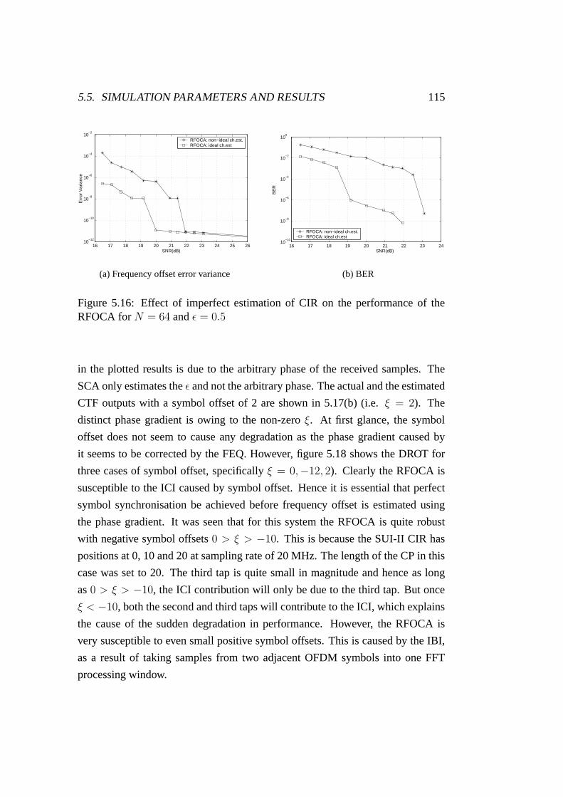
5.5. SIMULATION PARAMETERS AND RESULTS 115
16 17 18 19 20 21 22 23 24 25 2610
−12
10−10
10−8
10−6
10−4
10−2
SNR(dB)
Err
or V
aria
nce
RFOCA: non−ideal ch.est.RFOCA: ideal ch.est
(a) Frequency offset error variance
16 17 18 19 20 21 22 23 2410
−10
10−8
10−6
10−4
10−2
100
SNR(dB)
BE
R
RFOCA: non−ideal ch.est.RFOCA: ideal ch.est
(b) BER
Figure 5.16: Effect of imperfect estimation of CIR on the performance of theRFOCA for N = 64 and ε = 0.5
in the plotted results is due to the arbitrary phase of the received samples. The
SCA only estimates the ε and not the arbitrary phase. The actual and the estimated
CTF outputs with a symbol offset of 2 are shown in 5.17(b) (i.e. ξ = 2). The
distinct phase gradient is owing to the non-zero ξ. At first glance, the symbol
offset does not seem to cause any degradation as the phase gradient caused by
it seems to be corrected by the FEQ. However, figure 5.18 shows the DROT for
three cases of symbol offset, specifically ξ = 0,−12, 2). Clearly the RFOCA is
susceptible to the ICI caused by symbol offset. Hence it is essential that perfect
symbol synchronisation be achieved before frequency offset is estimated using
the phase gradient. It was seen that for this system the RFOCA is quite robust
with negative symbol offsets 0 > ξ > −10. This is because the SUI-II CIR has
positions at 0, 10 and 20 at sampling rate of 20 MHz. The length of the CP in this
case was set to 20. The third tap is quite small in magnitude and hence as long
as 0 > ξ > −10, the ICI contribution will only be due to the third tap. But once
ξ < −10, both the second and third taps will contribute to the ICI, which explains
the cause of the sudden degradation in performance. However, the RFOCA is
very susceptible to even small positive symbol offsets. This is caused by the IBI,
as a result of taking samples from two adjacent OFDM symbols into one FFT
processing window.

116 CHAPTER 5. RESIDUAL FREQUENCY OFFSET CORRECTION
0 10 20 30 40 50 60 70−4
−3
−2
−1
0
1
2
3
4
Subchannel Idndex
Ang
le (
rad)
Actual CTFEstimated CTF
(a) ξ = 0
0 10 20 30 40 50 60−4
−3
−2
−1
0
1
2
3
4
Subchannel Idndex
Ang
le (
rad)
Actual CTFEstimated CTF
(b) ξ = 2
Figure 5.17: Estimation of the phase of the CTF for different symbol timing off-sets, ξ for N = 64 and ε = 0.5
0 1 2 3 4 5 6 7 8 9 1010
−8
10−7
10−6
10−5
10−4
10−3
10−2
10−1
Iteration Number
Abs
olut
e E
rror
Sym. Off.= 0Sym. Off.= −12Sym. Off.= 2
Figure 5.18: The DROT with symbol offset = 0,2,-12 for N = 64 and ε = 0.5
5.6. CONCLUSION 117
5.6 Conclusion
In this chapter the Residual frequency Offset Correction Algorithm (RFOCA),
which complements the initial frequency acquisition process performed by the
Schmidl and Cox Algorithm (SCA) has been presented. The RFOCA continu-
ously tracks and compensates for the RFO that is present after the acquisition
stage. The RFOCA is applied for OFDM systems operating over both AWGN
and BFWA channels (SUI-II channel profile), and is shown to give a significant
reduction in the frequency error variance. Although the algorithm may appear to
suffer from a threshold effect it still gives a significant performance advantage at
realistic signal to noise ratios. The performance of RFOCA is analysed through
extensive simulations. It is concluded that the threshold effect of the RFOCA is
primarily due to the failure of the phase unwrapping algorithm. The RFOCA is
also susceptible to non-ideal symbol synchronisation, however this does not pose
a serious problem as perfect symbol synchronisation can be achieved using the
ISOCA presented in chapter 4.

118 CHAPTER 5. RESIDUAL FREQUENCY OFFSET CORRECTION
Chapter 6
Time Domain Equalisation
As shown previously in section 2.4, the orthogonality of consecutive OFDM sym-
bols is maintained by prepending a length v Cyclic Prefix (CP) at the start of each
symbol [37]. One major disadvantage with the OFDM system is the reduction
in the transmission efficiency by a factor N/(N + v) caused by the CP. This is
of even greater concern when the transmitted symbol rate is higher, because this
makes a Channel Impulse Response (CIR) with the same rms delay spread span
a greater number of samples, hence necessitating the use of a longer CP. Future
broadband wireless applications are likely to require data rates in excess of 50
Mb/s. Although a typical wireless fixed access channel delay spread is short in
comparison to the symbol duration for transmission rates that are in use today,
it will not be the case for higher symbol rates. One way of increasing the effi-
ciency is to increase the FFT size, N . The consequences of increasing N were
highlighted in chapter 1.
An alternative to increasing the number of subchannels is to precede the FFT
demodulator at the receiver with a Time Domain Equaliser (TEQ) in order to
constrain the length of the overall response to be shorter than the original CIR.
The cascade of the channel and the TEQ response is hereafter referred to as the
Effective Channel Impulse Response (EIR). This permits the use of a much shorter
CP than could otherwise be employed and so raises the transmission efficiency.
A TEQ is almost essential in DMT systems when used in Digital Subscriber Line
(DSL) applications owing to their relatively long CIRs. As far as the author of this
119
120 CHAPTER 6. TIME DOMAIN EQUALISATION
thesis is aware, the application of a TEQ to compensate for the CIRs experienced
in broadband wireless applications has not been throughly investigated to date. In
this chapter a novel TEQ algorithm is presented, namely, the Frequency Scaled
Time Domain Equaliser (FSTEQ). The FSTEQ is designed specifically to be used
in BFWA channels.
This chapter is organised as follows. Section 6.1 briefly introduces relevant
previous work concerning TEQs while section 6.2 presents the theory of TEQ de-
sign. The next two sections introduce two TEQ algorithms. The first described in
section 6.3 is the Dual Optimising Time Domain Equaliser (DOTEQ), which is a
modified version of a design previously presented by another author [110]. The
limitations of using the DOTEQ in wireless channels are highlighted and in sec-
tion 6.4 the novel FSTEQ is introduced which overcomes most of the limitations
of the DOTEQ. A Z-plane analysis of the performance of the DOTEQ and the
FSTEQ is performed in section 6.5 and a comparison of the computational com-
plexity of the TEQ schemes presented is undertaken in section 6.6. Section 6.7
presents the results obtained via computer simulations and finally the conclusions
are drawn in section 6.8.
6.1 Related Work
Time Domain Equalisation is a very rich and deep area of research. There have
been contributions by many authors and the objective here is to highlight the
most important and relevant ones. CIR shortening has been proposed as long
ago as 1973 to permit the design of practical Maximum Likelihood Sequence
Estimation (MLSE) receivers based on the Viterbi Algorithm [110]. Later there
was a flurry of research aimed at reducing the length of the CP in DMT sys-
tems [111, 112, 113, 114]. The first two references are based on the Minimum
Mean Squared Error (MMSE) criterion to arrive at the solution for the TEQ.
The latter two references seek to minimise the so called Shortened SNR (SSNR),
where the ratio between the power in a set of consecutive v samples of the EIR
to the power in the rest of the residuals is considered. To avoid trivial all-zero
solutions, additional constraints such as the Unit Energy Constraint (UEC) [110]
or the Unit Tap Constraint (UTC) [111, 115] are set on the Target Impulse Re-
6.1. RELATED WORK 121
sponse (TIR) when the MMSE criterion is used. The TIR, as will be shown later,
is used to generate the error term in the adaptation process. However the emphasis
is to reduce the power of the residuals of the EIR in the time domain. The trans-
fer function of the resulting EIR in the frequency domain often has spectral nulls
causing some subchannels to have a low SNR and consequently rendering them
unusable. A different equalisation criterion is introduced in [112, 116], namely
the ‘geometric SNR’. The objective here is to maximise the overall bit rate of a
DMT system. The structure is the same as for the MMSE case, but the objective
function is based on optimising the SNR of individual subchannels, and hence the
bit rate. It was later extended by optimising the bandwidth in [117]. The authors
in [118, 119] include ISI in the objective function of the original geometric mean
criterion to improve the performance. The geometric SNR criterion is ideal for
DMT systems since the modulation of DMT presumes data is mapped into the
subchannels at various rates using different modulation constellations. In another
modification of the original geometric SNR criterion, the authors in [120] include
the effect of Inter-Block Interference in the optimisation process. However, the
algorithm is very complex and needs several FFT operations at each iteration.
To overcome the slow convergence of adaptive algorithms, some authors have
proposed channel estimate based methods [121, 111]. The former paper also pro-
poses how the delay between the TEQ and the TIR may be optimised. It involves
optimising the algorithm for each value of the delay and selecting the delay that
provides the minimum error. This method is much more efficient than that pro-
posed in [111]. The delay is indeed critical when the channel responses have
pre-cursors and post-cursors since it is used to locate the main tap of the CIR.
However the broadband wireless channels under consideration in this work gen-
erally do not have precursors and so optimising the delay is not such an important
issue in this case.
Attempts have also been made to optimise the TEQ in the frequency do-
main [122, 123]. An issue with [122] in particular is that the solution rarely
results in a global minimum error. The authors in [124] introduce the concept
of weighting the frequency domain coefficients, which appears to improve upon
the original frequency domain criterion. The authors in [123, 125] propose the
‘per-tone equaliser’ which operates in the frequency domain. The TEQ in the

122 CHAPTER 6. TIME DOMAIN EQUALISATION
time domain is converted into an equivalent FEQ with multiple taps at each sub-
channel output of the IFFT demodulator. Even though this method appears to
be more robust to delay differences between the equaliser and the TIR, the im-
plementation is more complex and needs a significant amount of memory. The
authors in [126, 127] propose a version of a TEQ that uses a feedback path from
the point after the FEQ rather than from the TIR. Due to the parallel processing of
the OFDM symbols, the feedback path is effectively only used once per OFDM
symbol. This necessitates a high SNR for the algorithm to perform effectively.
The MMSE TEQ does its best to emphasise the low noise part of the received
signal, while suppressing the channel noise over the rest of the frequency band.
This process however generates nulls in the effective transfer function [128]. For a
DMT system, the consequence is that quite a few subchannels are not assigned any
data. The same paper proposes guidelines for designing a better TEQ, specifically
it suggests optimising the TIR such that it does not contain nulls in the frequency
response and also keeps the Mean Squared Error (MSE) relatively low. It proves
that the geometric SNR criterion is a generalised form of avoiding spectral nulls.
Since the original proposal utilising the geometric SNR criterion is computation-
ally expensive, the authors propose a more simple eigen filter approach. A similar
approach is adopted in [129]. It can be noted that the FSTEQ that is proposed in
section 6.4 does conform to the guidelines proposed in [128].
6.2 Basics of Time Domain Equalisation
Channel shortening with the use of a TEQ in the MMSE sense can be explained
with reference to the block diagram shown in figure 6.1. For clarity the transmis-
sion variables are given in vector form in this chapter. Unless otherwise stated, an
underlined variable will denote a vector and a variable that is not underlined with
a numeric subscript will denote the individual elements in the vector. In general,
variables in the time domain will be denoted in the lower case and those in the
frequency domain in the upper case.
The objective is to shorten the sampled CIR of length Nh, h = [h0, .., hNh−1]T
to an EIR having significant samples for a lengthNb, whereNb < Nh, with the use
of a TEQ of length Nf , f = [f0, .., fNf−1]T . The error sequence, e(n) is generated

6.2. BASICS OF TIME DOMAIN EQUALISATION 123
CIR
TIR
TEQ + +
AWGN
_
PSfrag replacementsx
w(n)
h f
b
e(n)r
Figure 6.1: Block diagram of the TEQ
by comparing the output sequence of the TEQ to the result of convolving the
transmitted data stream, x = [x(n), .., x(n − Nb + 1)]T , with a desired TIR, b =
[b0, .., bNb−1]T of length Nb. Here, n represents the time index and x(n) = 0 for
n < 0. If the TEQ performs perfectly, the OFDM system can now operate with a
shorter CP of length Nb − 1 (i.e. v = Nb − 1).
If the received data is given by r(n), then,
r(n) = hTx′ + w(n) (6.1)
where w(n) is the zero mean Additive White Gaussian Noise (AWGN) term
and x′ = [x(n), .., x(n−Nh + 1)]T . Hence the error signal after the TEQ is given
as,
e(n) = fT r − bTx (6.2)
where r = [r(n), .., r(n − Nf + 1)]T . The time index n is defined as before
with r(n) = 0 for n < 0. The squared error is given by,
E|e(n)|2 = fTRrrf∗ + bTRxxb
∗ − fTRrxb∗ − bTRrxf
∗ (6.3)
where (.)∗ denotes complex conjugation and Rrr ,Rxx and Rrx are the corre-
sponding correlation matrices of r and x. The optimal equaliser tap coefficients
can be obtained by solving for the MMSE given by,
d(E|e(n)|2)/df = 0 (6.4)
124 CHAPTER 6. TIME DOMAIN EQUALISATION
which leads to,
<[fopt
] = R−1rr Rrx<[b]
=[fopt
] = R−1rr Rrx=[b] (6.5)
where < and = are the Real and the Imaginary part of a complex variable,
respectively. Note that the solution of (6.5) depends on b. Substituting the above
relation in equation 6.3 results in
E|e(n)|2 = bT (Rxx −RTrxR
−1rr Rrx)b
∗ = bTO b∗ . (6.6)
By minimising equation 6.6 the optimal coefficients for the TIR, namely boptcan be found as the eigenvector corresponding to the smallest eigenvalue of the
matrix O. Solutions for the case of real data can be found in [130].
6.3 Dual Optimising Time Domain Equaliser
An alternative iterative solution is presented in [110] for real data, a modified
form of which is presented here for the case of complex data. Assuming the
transmitted sequence is known during training, both the TIR coefficients b, and
the TEQ coefficients f , can be obtained iteratively via steepest descent gradient
methods such as Least Mean Square (LMS). Hence,
fn+1 = fn − ∆f e(n)r∗ (6.7)
and
bn+1 = bn + ∆b e(n)x∗ (6.8)
where fn and bn are the tap coefficients at the nth iteration and ∆f and ∆b are
the LMS convergence control parameters. To avoid the trivial all-zero solution,
the UEC constraint on the TIR is used. This is achieved using,
bn+1 =bn+1
|bn+1| . (6.9)

6.4. FREQUENCY SCALED TIME DOMAIN EQUALISER 125
This algorithm is referred to as the Dual Optimising TEQ (DOTEQ). Fig-
ure 6.2 shows the performance of the DOTEQ algorithm in the time domain using
the UEC for a TIR length of 14 at an SNR of 20 dB. The original CIR is assumed
to be 40 samples long, with only 3 significant taps. It can be observed that the
EIR is similar to the TIR within the length of the TIR. The length of the TEQ is
60 samples and hence the EIR has 100 samples. More importantly, the residuals
beyond the TIR length (and hence the CP) are low in magnitude compared with
the samples lying within the TIR length.
Hereafter, the transfer functions in the frequency domain of the CIR, TIR and
EIR are defined as the Channel Transfer Function (CTF), the Target Transfer
Function (TTF) and the Effective Transfer Function (ETF), respectively. How-
ever, as shown in figure 6.3, the ETF obtained using the DOTEQ algorithm for
the time domain EIR shown in figure 6.2 has deep spectral nulls. Consequently
subchannels that fall in to the nulls will be severely degraded giving rise to a low
subchannel SNR. This situation will not be improved by the FEQ since its coeffi-
cients are given by the inverse of the ETF. To address this problem, an algorithm
will now be presented that achieves both a flatter ETF (frequency domain) and
also a reduction of the residuals of the EIR (time domain).
6.4 Frequency Scaled Time Domain Equaliser
The objective of the FSTEQ in the time domain is to iteratively obtain an opti-
mal solution to the TEQ. Thus the CIR will be processed to yield an EIR with
a length (defined as that spanning the significant coefficients of the EIR) that is
much shorter than that of the CIR. The purpose of also optimising in the frequency
domain is to avoid the spectral nulls that are usually created by the DOTEQ algo-
rithm. Hence, the overall system can effectively operate with a much shorter CP
of length v.
As noted in appendix B, the antennas used for Point-to-Point (PTP) and Point-
to-Multipoint (PMP) communication in the BFWA scenario are of high gain and
directivity. Hence the CIRs that are encountered are not severe, usually having
a dominant direct path and a small number of weak delayed paths. The CIRs
experienced in good terrain conditions, which are those pertaining to the proposed

126 CHAPTER 6. TIME DOMAIN EQUALISATION
10 20 30 40 50 60 70 80 90 1000
0.1
0.2
0.3
0.4
0.5
0.6
0.7
0.8
0.9
n (x 25ns)
|h (
n )|
CIRTIREIR
Figure 6.2: DOTEQ performance: Impulse responses
0 10 20 30 40 50 600
0.2
0.4
0.6
0.8
1
1.2
1.4
1.6
1.8
2
|Hi |
Subchannel Index, i
CTFETF
Figure 6.3: DOTEQ performance: Transfer functions

6.4. FREQUENCY SCALED TIME DOMAIN EQUALISER 127
0 10 20 30 40 50 600.5
0.6
0.7
0.8
0.9
1
1.1
1.2|H
i |
Subchannel Index, i
CTFInitial TTFThresholds
Figure 6.4: FSTEQ algorithm: Initial TTF
SUI-II delay profile [23], also have a high Ricean factor in the direct path. The
consequence of this is that the delay profile is likely to have an exponentially
decaying envelope. The FSTEQ is designed with this kind of delay profile in
mind. The design criteria of the FSTEQ is to convert the exponentially decaying
CIR into an EIR which is also exponentially decaying but at a much faster rate.
Thus the ETF will have a smoother response than the CTF.
In order to initialise the FSTEQ an estimate of the CTF is required. A known
training symbol is sent by the transmitter so that the coefficients of the FEQ can
be calculated at the receiver. The ratio of the known transmitted training symbol
to the corresponding demodulated OFDM data symbols before applying the TEQ
is employed to estimate the CTF. This is so because the TEQ will modify the CTF.
All FFT and IFFT operations performed hereafter in the FSTEQ are of length
N unless otherwise stated. Using the average delay profile of the SUI-II channel
profile, namely g two thresholds are calculated in the frequency domain. The av-
erage delay profile can be calculated by averaging over a large number of channel
estimates made on different bursts or simply by using channel models such as the
128 CHAPTER 6. TIME DOMAIN EQUALISATION
SUI model. Note that this does not require knowledge of the CIR experienced by
a particular transmitted data burst. The transfer function of g, denoted by G, is
calculated by taking an FFT of g. The actual coefficients ofG are a system param-
eter and can be selected at implementation. Subsequent simulations have shown
that the performance is not sensitive to the values selected for G, provided that
they approximately follow the envelope of the CTF. The mean and the standard
deviation of the gain of CTF are calculated from the estimate made previously.
These values are denoted as µH and σH , respectively. An upper threshold, Gu and
a lower threshold, Gl are set as follows,
Gu = G+ µH + σH
Gl = G+ µH − σH . (6.10)
The values for µH and σH are estimated at the start of each received burst but
since G is a predefined system parameter it could be implemented as a look-up
table. The purpose of the two thresholds is to follow the envelope of the CTF
magnitude response, and as will be described later, to limit the magnitude varia-
tion of the TTF (frequency domain). If (6.10) is used to determine the thresholds,
they span a range which is twice the standard deviation of the estimated CTF.
Figure 6.4 shows the calculated thresholds for a typical SUI-II channels profile.
To ensure that the solution converges correctly, the length of the TIR is set
equal to the desired CP length, v. The next step of the algorithm is to decide on
an initial TIR, b0
where the superscript refers to the iteration number. Initial tests
showed that using an arbitrary or a null TIR to start with does not guarantee that
the algorithm will converge quickly. Hence, it is proposed to use an initial TIR
function which is exponentially decaying but at a much faster rate than that of the
CIR power profile. To determine the decay rate (i.e. the time constant), a desired
attenuation at the end of the TIR length, v is selected. Denoting this desired value
as κ, then the decay rate is found as λ = ln |κ|/(v − 1). The unscaled initial TIR,
b0 is defined as,
b0 = [1, eλ, .., eλ(v−1)] . (6.11)
The convergence rate of the ETF depends upon the initial TIR. Since the goal
6.4. FREQUENCY SCALED TIME DOMAIN EQUALISER 129
of the algorithm is to obtain a TEQ that yields an ETF that lies within the thresh-
olds, the gain of the unscaled initial TTF, |B0| must be scaled so that it lies within
the calculated frequency domain thresholds before iteration begins. To do this, the
minimum and the maximum gains of the TTF have to be found. They are denoted
as |B0|min and |B0|max respectively. The scaled gain of the initial TTF is given
as,
|B0| =(|B0| − |B0|min).2σH(|B0|max − |B0|min)
+Gl (6.12)
which is now guaranteed to lie within the two thresholds as shown in fig-
ure 6.4. Unless otherwise stated, the scaled variables are denoted by the symbol
‘ ’. The complete initial TTF is determined by setting the phase of the scaled
initial TTF to be equal to the phase of the unscaled initial TTF, 6 B0. i.e.,
B0
= |B0| ej 6 B0
. (6.13)
In other words, only the gain and not the phase of the TTF is scaled. This
holds true at each iteration. The scaled initial TIR, b0
is found by taking an IFFT
of length N of the initial scaled TTF, B0. Since N is longer than the TIR length
v, only the first v samples of the IFFT output are used to initialise the TIR. Once
the TIR is initialised, the final solution of the FSTEQ is achieved in the MMSE
sense using a steepest gradient optimisation method. If the LMS algorithm is
used, the TIR and the TEQ are updated in a similar manner to that employed in
the DOTEQ as given by equations (6.7) and (6.8). However LMS is known to
converge slowly and the rate of convergence can be improved dramatically by
using the Recursive Least Squares (RLS) algorithm at the expense of an increase
in the number of computations [27, pg. 654]. The RLS algorithm when used
for the FSTEQ requires 6 parameters to be evaluated for each iteration of the
algorithm to calculate the TEQ and TIR coefficients. For the TEQ a weighting
factor Ωf (where 0 > Ωf > 1), a Kalman gain vector Knf (of length Nfx1)
and a square inverse correlation matrix Pnf (of size NfxNf ) need to be evaluated.
Again the superscript refers to the iteration number and the subscript f is used to
identify them as TEQ parameters. Similarly, for the TIR, Ωb (0 > Ωb > 1), Knb
(of length Nbx1) and the square matrix Pnb (of size NbxNb) need to be evaluated.
130 CHAPTER 6. TIME DOMAIN EQUALISATION
The interested reader is referred to [27] for more details about the RLS algorithm.
The correlation matrices are initialised to identity matrices. Once the TEQ output,
the TIR output and the error is calculated as given in (6.2), the TEQ parameters
are updated using the RLS algorithm as follows,
Kn+1f =
Pnf r
∗
Ωf + rT Pnf r
∗
Pn+1f =
1
Ωf
[Pnf −Kn
f rT
Pnf ]
fn+1 = fn −Kn+1f e(n) . (6.14)
The first equation of (6.14) computes the Kalman gain vector, the second up-
dates the inverse of the correlation matrix and the third updates the TEQ coeffi-
cients. Note that all 3 steps have to be performed at each iteration. Similarly, the
corresponding equations for the TIR are,
Kn+1b =
Pnb x
∗
Ωb + xT Pnb x
∗
Pn+1b =
1
Ωb
[Pnb −Kn
b xT
Pnb ]
bn+1 = bn +Kn+1b e(n) . (6.15)
However the TIR coefficients obtained at a particular iteration may exceed the
previously calculated frequency domain thresholds. Hence, after the unscaled TIR
coefficients are obtained at the (n+1)th iteration using either the LMS algorithm,
as given in (6.8) or by using the RLS algorithm, as shown in (6.15), the unscaled
TTF, Bn+1 is obtained using an FFT of size N . If |Bn+1| exceeds the thresholds,
it is scaled to obtain |Bn+1| in a similar manner to that employed at initialisation
as given by (6.12). The complete TTF is obtained by multiplying with the phase
response in a similar way to that shown in (6.13). Figure 6.5 shows the block
diagram of the FSTEQ algorithm.
To prevent the FSTEQ converging to a null solution it has been discovered that
rather than using the UEC as employed in DOTEQ, the convergence is faster if
the UTC is adopted. Besides, the UEC criterion requires a significant number of
computations to implement. Consequently, the first tap of the TIR is not changed

6.4. FREQUENCY SCALED TIME DOMAIN EQUALISER 131
N-point FFT
Within thresholds
?
Scaling N-point
IFFT
No
Yes
LMS or RLS
PSfrag replacements
bn
Bn+1
bn+1
= bn+1
Bn+1
bn+1
bn+1
bn+10 = b00
bn+1
Figure 6.5: FSTEQ algorithm: Block diagram
during the iterations, i.e. bn+10 = b00, ∀ n ≥ 0.
Finally, after the iterations are complete the FEQ needs to be updated with
the inverse of the ETF (and not the CTF). The ETF is estimated by sending the
received training symbol through the converged TEQ and then taking the ratio
between the transmitted and the decoded symbols. The algorithm can be sum-
marised as follows,
1. Using the CTF, set both Upper and Lower frequency domain thresholds (Gu
and Gl, respectively). The thresholds are selected such that they follow the
envelope of the power delay profile of the channel as shown in figure 6.4.
These thresholds are used to constrain the TTF (frequency domain), thus
reducing the null depths in the ETF.
2. The TTF is initialised to be an exponentially decaying function so that the
initial TTF is within the two threshold values. The initial TIR is set to be
the IFFT of the initial TTF.
3. At each iteration, the TIR and TEQ are optimised concurrently in the time
domain using the LMS algorithm as in (6.7) and (6.8) or by use of the RLS

132 CHAPTER 6. TIME DOMAIN EQUALISATION
algorithm as in (6.14) and (6.15). In other words, the unscaled TIR bn+1 is
calculated from bn.
4. Next the TTF, namely Bn+1 of size N is calculated by taking the FFT of
bn+1. If |Bn+1| exceeds the two threshold values, it is scaled so that the
resulting |Bn+1| lies within the thresholds. The updated TIR coefficients,
bn+1
, are calculated by performing an IFFT on Bn+1
.
5. The TIR coefficients are updated by the scaled values bn+1
, except for bn+10
which is forced to be equal to b00 of the initial TIR. Thus the TTF is con-
strained to lie within the upper and lower thresholds.
6. The FEQ coefficients are calculated based on the converged ETF.
It has been observed that training the TEQ needs at least 1500 iterations when
the LMS algorithm is used. The overhead of transmitting such a long training se-
quence cannot be justified. This is avoided by sending a shorter training sequence
and passing the same training sequence through the equaliser several times until
an acceptable level of convergence is achieved. This method is known as acceler-
ated (or multiple) training [131, 132].
Figure 6.6 shows the performance of FSTEQ algorithm in the time domain for
the same CIR used to give the DOTEQ results presented in figure 6.2. Note that the
peak magnitude of the EIR occurs at the beginning and is well within the length
of the CP. The FSTEQ has effectively converted the CIR into an exponentially
decaying EIR, which has a much higher rate of roll-off in the time domain. The
residuals beyond the TIR length of 14 are also reduced to values with insignificant
power. Figure 6.7 shows the corresponding ETF (frequency domain). The final
ETF shows very close convergence to the Initial TTF (see figure 6.4) and more
significantly, an absence of deep nulls in the ETF as compared with that achieved
by the DOTEQ results presented in figure 6.3.
6.5 Z-Plane Analysis of FSTEQ
An FIR filter is inherently stable. However the zeros, or the roots of the filter
polynomial, determine its frequency response. If all the zeros fall within the unit

6.5. Z-PLANE ANALYSIS OF FSTEQ 133
10 20 30 40 50 60 70 80 90 1000
0.1
0.2
0.3
0.4
0.5
0.6
0.7
0.8
0.9
n (x 25ns)
|h (
n )|
CIRTIREIR
Figure 6.6: FSTEQ performance: Impulse responses
0 10 20 30 40 50 600.5
0.6
0.7
0.8
0.9
1
1.1
1.2
|Hi |
Subchannel Index, i
CTFETFThresholds
Figure 6.7: FSTEQ performance: Transfer functions

134 CHAPTER 6. TIME DOMAIN EQUALISATION
circle in the Z-plane, the filter response is deemed minimum phase. There are
several characteristics of a minimum phase response. One is that the group delay
is minimum and also the partial energy (defined as the sum of magnitude squared
impulse response from −∞ to n) is maximum among all filters of the same mag-
nitude response [133, pg. 250]. This is equivalent to the impulse response of the
minimum phase system being more concentrated near to the origin than any other
system. Hence, the peak of the impulse response would lie closer to the origin.
An exponentially decaying response is an example of a minimum phase response.
It is also shown in [134] that for an exponentially decaying response with a time
constant λ, most zeros are close to the circle r = eλ/2 in the Z-plane. Hence an
exponentially decaying response will have most of its zeros within the unit circle
with a very high probability.
Figure 6.8 shows an example, but nevertheless representative, Z-plane analysis
of the roots of the final converged EIR when a DOTEQ is used. The initial CIR
is also included for comparison. Since the CIR has the profile of an exponentially
decaying function, all of its zeros lie within the unit circle and thus it is minimum
phase. However once the DOTEQ is used, some of these zeros are pushed outside
the unit circle and some are even placed very close to the unit circle. The zeros
that are close to the unit circle are called critical zeros. The critical zeros pull
the transfer functions to a null at the corresponding frequency. Since some of
the zeros lie outside the unit circle it makes the overall EIR non-minimum phase
(mixed phase). A filter that provides the reciprocal of a particular response is
known as the inverse filter. Thus H(z) is an inverse filter to the response of H(z)
in the following system
H(z) = 1/H(z) . (6.16)
If H(z) is minimum phase, the inverse filter is causal and stable [135] as the
poles of the inverse filter lie in the unit circle. In an OFDM system, the FEQ
is used to generate the inverse response of the ETF. If the ETF contains nulls, it
will cause the FEQ to have coefficients with high gain. This can lead to non-ideal
characteristics such as AWGN and Phase Noise (PN) being boosted along with
the signal.
Figure 6.9 shows the zeros of the converged EIR when the FSTEQ is used for

6.6. COMPARISON OF COMPUTATIONAL COMPLEXITY 135
0.2
0.4
0.6
0.8
1
30
210
60
240
90
270
120
300
150
330
180 0
CIREIR
Figure 6.8: Z-plane analysis: DOTEQ response
the same CIR as used for the previous DOTEQ example. It clearly shows that the
minimum phase characteristic is still retained by the FSTEQ even at the end of the
convergence. Furthermore, there are no critical zeros. This is achieved because
the algorithm is designed to specifically avoid spectral nulls.
6.6 Comparison of Computational Complexity
The following analysis is performed per iteration and all the multiplications and
additions considered are complex. The calculation of the error term given in (6.2)
requires Nf + Nb multiplications, Nf + Nb − 2 additions and one subtraction.
This is common to all the algorithms discussed in this chapter. Updating the TEQ
coefficients using the DOTEQ algorithm, given in (6.7) requires Nf + 1 multipli-
cations and Nf subtractions. Similarly updating the TIR coefficients using (6.8)
requires Nb + 1 multiplications and Nb additions. Enforcing the UEC criterion,
given in (6.9), requires Nb multiplications to calculate the energy, a square root
operation and a further Nb divisions.
FSTEQ algorithms only require two FFT operations per iteration unlike the

136 CHAPTER 6. TIME DOMAIN EQUALISATION
0.2
0.4
0.6
0.8
1
30
210
60
240
90
270
120
300
150
330
180 0
CIREIR
Figure 6.9: Z-plane analysis: FSTEQ response
algorithm proposed in [120]. Ignoring the computations required for the initial-
isation of the TIR, the LMS version of the FSTEQ requires (6.7) and (6.8) to
be evaluated. It will be assumed that the FFT operation required to obtain the
unscaled TTF coefficients require N log2N additions and N/2 log2N multipli-
cations [136, Ch.6]. The comparison with the two thresholds requires 2N sub-
tractions. If the TTF has crossed the thresholds, calculating the minimum and the
maximum values require a further 2N subtractions. The scaling operation, given
in (6.12) needs N + 1 subtractions, N multiplications and N additions. To find
the complete TTF, given in (6.13) requiresN multiplications. Converting the TTF
to the scaled TIR coefficients requires the IFFT operation.
The RLS version of the FSTEQ requires the same number of operations for the
scaling function, but the RLS operation requires a much higher number of com-
putations. Updating the Kalman gain factor of the TEQ in (6.14) requires 3N 2f
multiplications, 3Nf (Nf − 1) + 1 additions and Nf divisions. Updating the cor-
relation matrix requires 2N 2f − 1 additions, 2N 2
f multiplications, N 2f subtractions
and a similar number of divisions. Finally updating the TEQ coefficients requires
Nf multiplications and Nf subtractions. Hence in total, updating the TEQ using

6.7. SIMULATION PARAMETERS AND RESULTS 137
the RLS algorithm requires 5N 2f − 3Nf + 1 additions, 5N 2
f +Nf multiplications
and Nf (Nf − 1) subtractions and divisions. Similarly updating the TIR requires
5N2b − 3Nb + 1 additions, 5N 2
b + Nb multiplications and Nb(Nb − 1) subtrac-
tions and divisions. Even though the number of computations appears to be high
at first glance, there are number of algorithms that perform the RLS more effi-
ciently [137]. Also note that the above calculation is per iteration, so since the
RLS requires fewer iterations, the overall number of computations is not exceed-
ingly high.
Algorithm Additions Subtractions Multiplications Divisions
DOTEQ Nf +Nb Nf +Nb 2Nf + 3Nb Nb
−2 +1 +2FSTEQ Nf +Nb Nf +Nb 2(Nf +Nb) 1(LMS) +2N log2N +5N +N log2N
+N − 2 +2(N + 1)FSTEQ 5(N 2
f +N2b ) Nf (Nf + 1) 5(N 2
f +N2b ) Nf (Nf + 1)
(RLS) −2(Nf +Nb) +Nb(Nb + 1) +2(Nf +Nb) +Nb(Nb + 1)+2N log2N +5N +2N log2N +1
+N +2N
Table 6.1: Comparison of computational complexity per iteration
Table 6.1 shows the total computational load required by each algorithm per
iteration. It can be stated that the computational complexities per iteration are
of the order of O(Nf + Nb), O(Nf + Nb + N log2N) and O(N 2f + N2
b ) for
DOTEQ, FSTEQ (LMS) and FSTEQ (RLS) respectively. For an OFDM system
with N = 64, Nf = 60 and Nb = 14, the complexity per iteration for DOTEQ,
FSTEQ (LMS) and FSTEQ (RLS) are of the order 74, 458 and 3796, respectively.
6.7 Simulation Parameters and Results
For the simulations, OFDM systems with N = 64 have been selected. Without
loss of generality, QPSK mapping for all subchannels has been employed and all
subchannels are used. The maximum burst length is set to 2500 symbols. As in
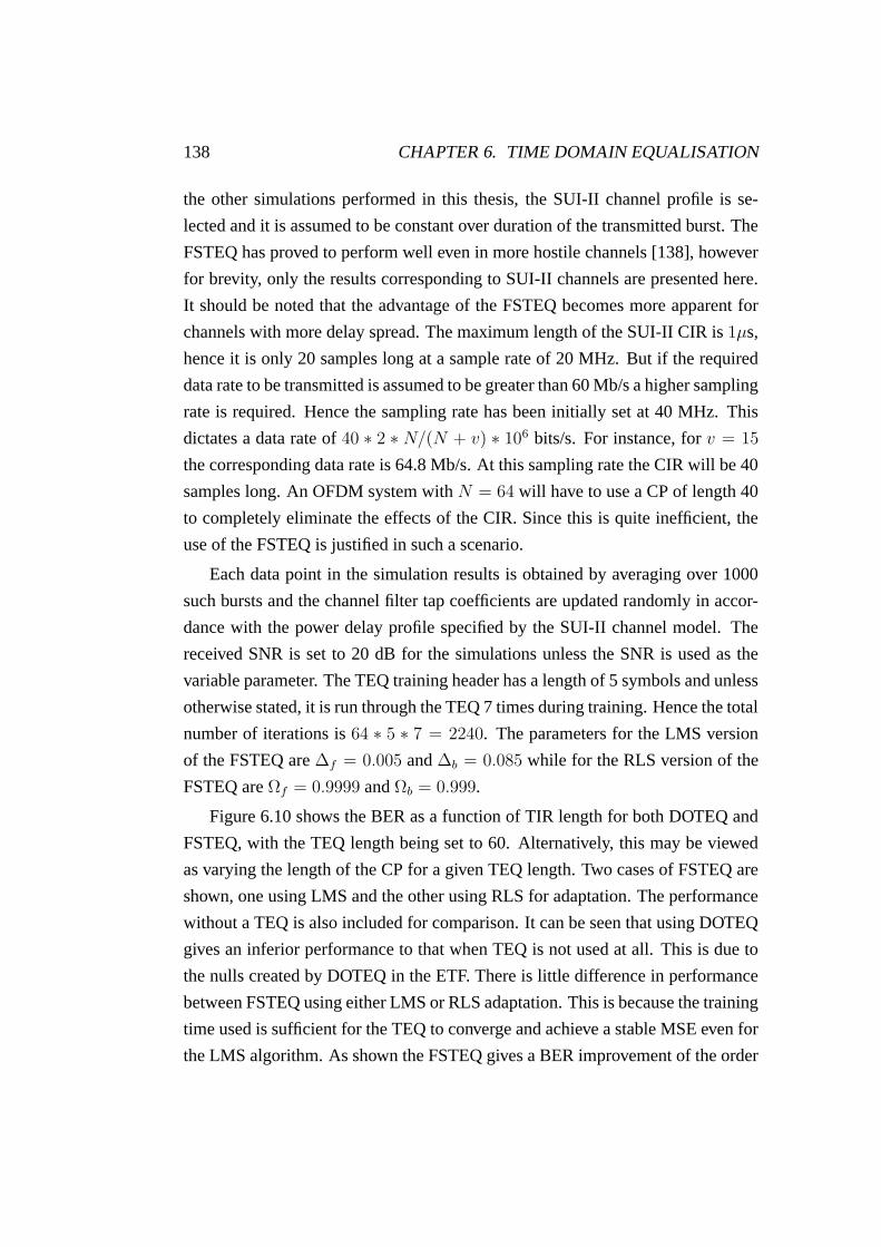
138 CHAPTER 6. TIME DOMAIN EQUALISATION
the other simulations performed in this thesis, the SUI-II channel profile is se-
lected and it is assumed to be constant over duration of the transmitted burst. The
FSTEQ has proved to perform well even in more hostile channels [138], however
for brevity, only the results corresponding to SUI-II channels are presented here.
It should be noted that the advantage of the FSTEQ becomes more apparent for
channels with more delay spread. The maximum length of the SUI-II CIR is 1µs,
hence it is only 20 samples long at a sample rate of 20 MHz. But if the required
data rate to be transmitted is assumed to be greater than 60 Mb/s a higher sampling
rate is required. Hence the sampling rate has been initially set at 40 MHz. This
dictates a data rate of 40 ∗ 2 ∗ N/(N + v) ∗ 106 bits/s. For instance, for v = 15
the corresponding data rate is 64.8 Mb/s. At this sampling rate the CIR will be 40
samples long. An OFDM system with N = 64 will have to use a CP of length 40
to completely eliminate the effects of the CIR. Since this is quite inefficient, the
use of the FSTEQ is justified in such a scenario.
Each data point in the simulation results is obtained by averaging over 1000
such bursts and the channel filter tap coefficients are updated randomly in accor-
dance with the power delay profile specified by the SUI-II channel model. The
received SNR is set to 20 dB for the simulations unless the SNR is used as the
variable parameter. The TEQ training header has a length of 5 symbols and unless
otherwise stated, it is run through the TEQ 7 times during training. Hence the total
number of iterations is 64 ∗ 5 ∗ 7 = 2240. The parameters for the LMS version
of the FSTEQ are ∆f = 0.005 and ∆b = 0.085 while for the RLS version of the
FSTEQ are Ωf = 0.9999 and Ωb = 0.999.
Figure 6.10 shows the BER as a function of TIR length for both DOTEQ and
FSTEQ, with the TEQ length being set to 60. Alternatively, this may be viewed
as varying the length of the CP for a given TEQ length. Two cases of FSTEQ are
shown, one using LMS and the other using RLS for adaptation. The performance
without a TEQ is also included for comparison. It can be seen that using DOTEQ
gives an inferior performance to that when TEQ is not used at all. This is due to
the nulls created by DOTEQ in the ETF. There is little difference in performance
between FSTEQ using either LMS or RLS adaptation. This is because the training
time used is sufficient for the TEQ to converge and achieve a stable MSE even for
the LMS algorithm. As shown the FSTEQ gives a BER improvement of the order

6.7. SIMULATION PARAMETERS AND RESULTS 139
11 12 13 14 15 16 17 1810
−8
10−7
10−6
10−5
10−4
10−3
10−2
10−1
TIR length
BE
R
no TEQDOTEQLMS FSTEQRLS FSTEQ
Figure 6.10: Comparison of the schemes for a TEQ length of 60, at a sample rateof 40 MHz and 2240 training iterations
of 10-100 over the case where no TEQ is used. Figure 6.11 shows the MSE as
a function of the number of iterations for various TEQ schemes. The plots were
obtained after averaging over 200 realisations. Note that the MSE of DOTEQ is
high even after 1200 iterations. The FSTEQ achieves a much lower MSE but note
that the LMS based training seems to be slightly more erratic at the beginning of
the training period.
Figure 6.12 shows the effect of using only 1280 iterations for training. It shows
a slight performance degradation of the LMS based FSTEQ owing to its slow
convergence, but the RLS based FSTEQ loses little in performance. Figure 6.13
shows the effect of SNR on the performance of various schemes with a TEQ length
of 60 and a TIR length (i.e. system CP length) of 14 when using the original
training length of 2240. It shows that significant gains cannot be achieved at an
SNR below 16 dB even with the use of FSTEQ. At an SNR in excess of 20 dB the
RLS based FSTEQ has a slight advantage over that of the LMS based one.
Figures 6.14 and 6.15 show the performance for TEQ lengths of 50 and 40

140 CHAPTER 6. TIME DOMAIN EQUALISATION
0 200 400 600 800 1000 1200−25
−20
−15
−10
−5
0
5
10
Iterations
MS
E(d
B)
DOTEQFSTEQ(LMS)FSTEQ(RLS)
Figure 6.11: Comparison of the MSE for various TEQ schemes with a length of60, at a sample rate of 40 MHz
11 12 13 14 15 16 17 1810
−8
10−6
10−4
10−2
100
TIR length
BE
R
no TEQDOTEQLMS FSTEQRLS FSTEQ
Figure 6.12: Comparison of the schemes for a TEQ length of 60, at a sample rateof 40 MHz but 1280 training iterations

6.7. SIMULATION PARAMETERS AND RESULTS 141
10 12 14 16 18 20 22 24 2610
−10
10−8
10−6
10−4
10−2
100
SNR (dB)
BE
R
no TEQDOTEQLMS FSTEQRLS FSTEQ
Figure 6.13: The effect of SNR on different TEQ schemes with a length of 60, aCP of length of 14 and a sample rate of 40 MHz
respectively with the other parameter values identical to those used in figure 6.10.
It appears that the ability of the TEQ to force the EIR towards the initial TIR
increases with the length of TEQ. If the TEQ length is too short, the time domain
residuals beyond the TIR length (and hence the CP) become significant and give
rise to both ISI and ICI. Since a CIR length of 40 samples is assumed it has
been observed that, the TEQ should be at least as long as the CIR for the TEQ
to give a significant performance gain. This is demonstrated in figures 6.10 and
6.15, where for example with a TIR length of 11 samples a FSTEQ length of 60
performs much better than one of length 40.
To investigate the performance of FSTEQ with shorter channels, a series of
simulations have been performed at sample rate of 20 MHz using the same sys-
tem as before. Hence the SUI-II channel is now only 20 samples long. Fig-
ure 6.16 shows the BER performance with TEQ of length 30 and TIR lengths (i.e
CP lengths) in the range from 4 to 11. It shows that the performance gains are
reduced compared with the previous scenario.
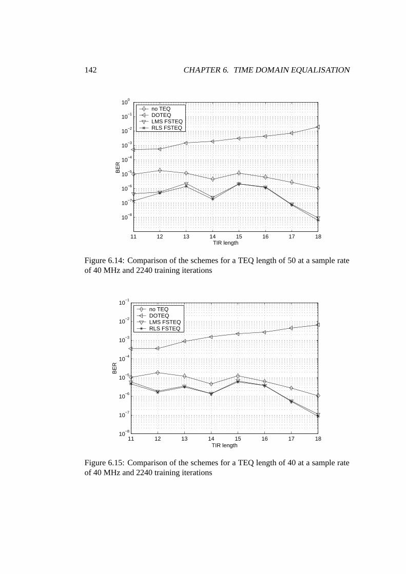
142 CHAPTER 6. TIME DOMAIN EQUALISATION
11 12 13 14 15 16 17 18
10−8
10−7
10−6
10−5
10−4
10−3
10−2
10−1
100
TIR length
BE
R
no TEQDOTEQLMS FSTEQRLS FSTEQ
Figure 6.14: Comparison of the schemes for a TEQ length of 50 at a sample rateof 40 MHz and 2240 training iterations
11 12 13 14 15 16 17 1810
−8
10−7
10−6
10−5
10−4
10−3
10−2
10−1
TIR length
BE
R
no TEQDOTEQLMS FSTEQRLS FSTEQ
Figure 6.15: Comparison of the schemes for a TEQ length of 40 at a sample rateof 40 MHz and 2240 training iterations
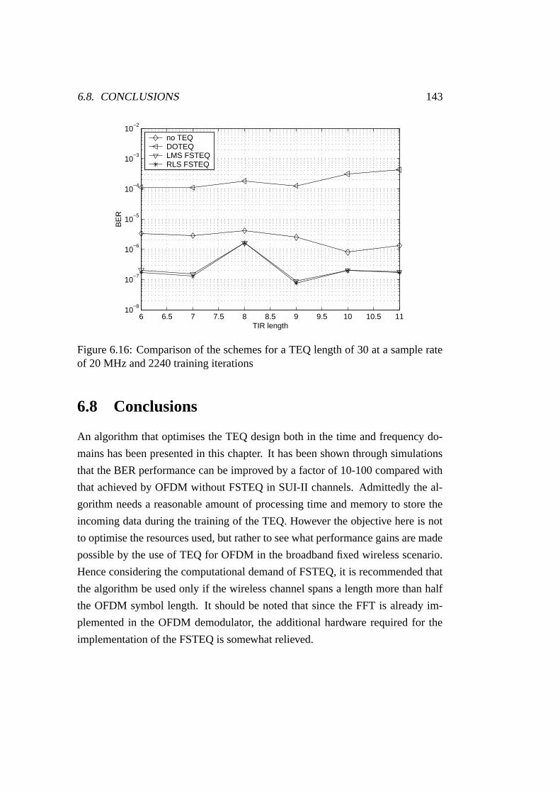
6.8. CONCLUSIONS 143
6 6.5 7 7.5 8 8.5 9 9.5 10 10.5 1110
−8
10−7
10−6
10−5
10−4
10−3
10−2
TIR length
BE
R
no TEQDOTEQLMS FSTEQRLS FSTEQ
Figure 6.16: Comparison of the schemes for a TEQ length of 30 at a sample rateof 20 MHz and 2240 training iterations
6.8 Conclusions
An algorithm that optimises the TEQ design both in the time and frequency do-
mains has been presented in this chapter. It has been shown through simulations
that the BER performance can be improved by a factor of 10-100 compared with
that achieved by OFDM without FSTEQ in SUI-II channels. Admittedly the al-
gorithm needs a reasonable amount of processing time and memory to store the
incoming data during the training of the TEQ. However the objective here is not
to optimise the resources used, but rather to see what performance gains are made
possible by the use of TEQ for OFDM in the broadband fixed wireless scenario.
Hence considering the computational demand of FSTEQ, it is recommended that
the algorithm be used only if the wireless channel spans a length more than half
the OFDM symbol length. It should be noted that since the FFT is already im-
plemented in the OFDM demodulator, the additional hardware required for the
implementation of the FSTEQ is somewhat relieved.

144 CHAPTER 6. TIME DOMAIN EQUALISATION

Chapter 7
Adaptive Time Domain Windowing
As noted previously in chapter 2 the use of rectangular pulse shapes in conven-
tional OFDM systems result in ‘sinc’ sidelobes being generated in the frequency
domain. The presence of these high sidelobe levels is found to render OFDM
systems sensitive to Phase Noise (PN) and frequency offsets. An intuitive ap-
proach to reduce these problems is to use Time Domain Windowing (TDW) to
lower the sidelobe levels. For example time domain windowing is introduced
in the IEEE 802.11a standard to smooth out the transitions between consecutive
OFDM symbols and to reduce the out-of-band spectral spillage [139]. However
unless a window is used which satisfies the Nyquist pulse shaping criterion, the
windowing process will cause the OFDM carriers to lose their orthogonality. Thus
a non-Nyquist window will introduce severe Inter Carrier Interference (ICI) even
though the sidelobe levels in the frequency domain may be low. In this chapter
an investigation is performed to quantify the performance gains that are available
with the use of Nyquist windowing in OFDM systems when applied to BFWA
networks.
A Nyquist window has a roll off region at either end. For an active OFDM
symbol with length N , the Nyquist window length, D will be N < D < 2N −1. Hence in order to incorporate windowing, uncorrupted contiguous samples
of a length greater than N are required for each OFDM symbol at the receiver.
This will in general require the transmission of extra samples, however if the CIR
length is less than the CP length, it is possible to use the last few samples of the
145

146 CHAPTER 7. ADAPTIVE TIME DOMAIN WINDOWING
CP to lie within the roll-off region of the window function. In the former case,
the extra samples would increase the bandwidth, which in turn would increase the
received noise power. In the second case, the SNR will remain the same as that
of a conventional OFDM system, since we are not using any additional samples.
The latter case will be assumed by default in this chapter, although performance
comparisons with the former case will be presented later in the chapter. In order
to use windowing the proposal is to make use of the all the samples in the CP
in the case of AWGN only channels or to use only those samples lying within
the Excess Length of the CP (i.e. the last p = v − Nh samples in the CP) for
channels with delay spread. If the OFDM system uses a cyclic prefix as well as a
cyclic postfix, these samples can lie within the roll off regions at either side of the
window function. However this approach is not possible in conventional OFDM
systems since only a cyclic prefix is used. In this situation the proposal is to use
the samples available in the Excess Length of the CP and the ones in the active
part of the transmitted symbol. The process is explained in detail in section 7.2.
Only a limited amount of research has previously been carried out in this area,
the most important of which will be described in section 7.1. In this chapter the
analysis of the effect of time domain windowing on OFDM systems is divided
into two parts. Section 7.2 introduces the effect of windowing at the receiver
and section 7.3 introduces the effect of windowing at the transmitter. Finally
section 7.4 draws some conclusions.
7.1 Related Work
Different types of windows have been proposed by various authors. The au-
thor in [140] uses Raised-Cosine (RC) windowing at the receiver, while in [141]
Root Raised Cosine (RRC) windowing is used at both the transmitter and the
receiver. The authors in [142] use modified window shapes that introduce sig-
nificant changes to the structure of the transmitter, which go beyond the scope
of this chapter. The authors in [143, 144] introduce an algorithm to optimise the
window coefficients in the MMSE sense when the OFDM system is subjected to
frequency offsets and they conclude that the RC window shapes are far from opti-
mal. Indeed their investigations show that the Trapezoidal Window (TPW) is very

7.2. TIME DOMAIN WINDOWING AT THE RECEIVER 147
close to the optimal window function. Several authors, for example [141, 101]
have investigated the effect that time domain windowing has on the tolerance of
OFDM systems to time and frequency synchronisation errors. They conclude that
the windowed OFDM system is more tolerant to such errors than is a conventional
system. The author in [92] provides a brief discussion of related work concerning
time domain windowing.
The authors in [141, 145, 146] investigate the use of time domain windowing
but do not apply the Nyquist criterion to the window function. Although such
window functions reduce OFDM subchannel sidelobe levels they introduce inter-
ference by sacrificing the orthogonality between the subchannels. To counter the
loss of orthogonality, per-subchannel Decision feedback Equalisers (DFEs) are
used after the FFT demodulator.
A considerable amount of work has also been performed concerning the effect
of frequency domain windowing during channel estimation. In systems subjected
to fast fading channels, in order to maintain the accuracy of the channel estimate
pilot symbols are sent continuously in some subchannels. After obtaining the
channel coefficients corresponding to the subchannels corresponding to the pilot
symbols, the coefficients of the other subchannels are obtained through interpola-
tion or a weighted IDFT/DFT operation. In the later case windowing may be used
to reduce errors due to aliasing [147]. However this is not the focus of the work
presented in this chapter.
7.2 Time Domain Windowing at the Receiver
The window function, gk has a maximum non-zero length of 2N − 1 samples.
Subchannel orthogonality is maintained if the time domain window complies with
the Nyquist criterion, which is given by [144],
∞∑
i=−∞gk+iN = const, 0 ≤ k ≤ N − 1 (7.1)
with gk = 0 for at least k < −N/2 and k > 3N/2. An example of a Nyquist

148 CHAPTER 7. ADAPTIVE TIME DOMAIN WINDOWING
window is the rectangular window, which can be written as,
ck =
1 0 ≤ k ≤ N − 1,
0 k < 0 or k ≥ N.(7.2)
Any sample within the region k < 0 and k ≥ N are called the roll-off samples.
Hence, the rectangular window does not have any non-zero roll-off samples. Fig-
ure 7.1 shows the decomposition of a typical Nyquist Window. The rectangular
window is also included for comparison. Any non-rectangular Nyquist window
will have up to vβ + 1 non-zero samples in the roll-off region. The window is
extended by vβ samples on its left hand side and vβ + 1 samples on its right hand
side. The roll-off factor, α = (2vβ + 1)/N determines vβ [144]. The longest
window length is reached if the roll off factor is equal to unity. As shown in fig-
ure 7.1, a Nyquist window can be generated from the rectangular window function
by using time limited roll-off modification samples βk, provided that the following
condition holds [144]
gk = ck + βk − βk−N . (7.3)
Figure 7.2 shows the time domain characteristics of the RC window and the
TPW with α = 0.5. The rectangular window is also shown for comparison. The
effect of the window functions is more obvious in the frequency domain plots
given in figure 7.3. The TPW and the RC window functions show very high
sidelobe decay rates whereas the first sidelobe of the rectangular window func-
tion shows the familiar 13 dB reduction in comparison to the main lobe. How-
ever the fast sidelobe decay rates of the non-rectangular windows are achieved
at the cost of longer time domain pulses. Muschallik in [140] showed that the
conventional OFDM system is equivalent to a filter bank system with rectangu-
lar windows. The noise power in each subchannel is equivalent to the integrated
power of the common area between the window transfer function placed at the
subchannel frequency and the noise PSD. He further showed that non-rectangular
Nyquist windows by having lower sidelobes will ensure lower subchannel noise
powers. Hence non-rectangular windowing improves the performance even in
AWGN channels [140].

7.2. TIME DOMAIN WINDOWING AT THE RECEIVER 149
PSfrag replacements
ck
βk
βkgk
−βk−N
k−vβ N (N + vβ)
Figure 7.1: Decomposition of a Nyquist window
The demodulated OFDM symbol Ym,l of the lth subchannel of the mth block
in a conventional OFDM system is shown in (2.20). To incorporate windowing, it
is modified to become
Ym,l =
√
1
N
N−1∑
n=0
ν=+1∑
ν=−1
gνN+nrm,(νN+n)MODN
e−j2πlnN , 0 ≤ l ≤ N−1 (7.4)
where rm,n are the samples of the active part of the OFDM symbol. The
inner summation in (7.4) describes the preprocessing required to fold the roll-
off samples of the window function. Hence, the outer sum, which describes the
N point FFT remains the same as in a conventional OFDM system. Figure 7.4
illustrates the processing required at the receiver. Figure 7.4(a) shows how the first
v−p samples in the CP are corrupted by the CIR because they are affected by Inter
Block Interference (IBI) from the previous OFDM symbol. Here p represents the
Excess Length and we set vβ = (p−1)/2. The receiver selects the lastN+2vβ+1
samples of the transmitted OFDM symbol to be multiplied by the window function
as shown in figure 7.4(b). The result is zero padded using N − vβ samples on the
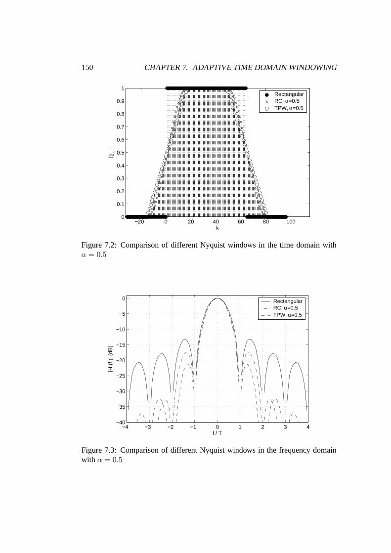
150 CHAPTER 7. ADAPTIVE TIME DOMAIN WINDOWING
−20 0 20 40 60 80 1000
0.1
0.2
0.3
0.4
0.5
0.6
0.7
0.8
0.9
1
k
|gk |
RectangularRC, α=0.5TPW, α=0.5
Figure 7.2: Comparison of different Nyquist windows in the time domain withα = 0.5
−4 −3 −2 −1 0 1 2 3 4−40
−35
−30
−25
−20
−15
−10
−5
0
f / T
|H (
f )| (
dB)
RectangularRC, α=0.5TPW, α=0.5
Figure 7.3: Comparison of different Nyquist windows in the frequency domainwith α = 0.5
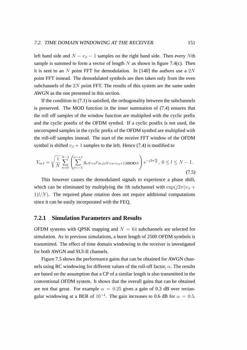
7.2. TIME DOMAIN WINDOWING AT THE RECEIVER 151
left hand side and N − vβ − 1 samples on the right hand side. Then every N th
sample is summed to form a vector of length N as shown in figure 7.4(c). Then
it is sent to an N point FFT for demodulation. In [140] the authors use a 2N
point FFT instead. The demodulated symbols are then taken only from the even
subchannels of the 2N point FFT. The results of this system are the same under
AWGN as the one presented in this section.
If the condition in (7.1) is satisfied, the orthogonality between the subchannels
is preserved. The MOD function in the inner summation of (7.4) ensures that
the roll off samples of the window function are multiplied with the cyclic prefix
and the cyclic postfix of the OFDM symbol. If a cyclic postfix is not used, the
uncorrupted samples in the cyclic prefix of the OFDM symbol are multiplied with
the roll-off samples instead. The start of the receive FFT window of the OFDM
symbol is shifted vβ + 1 samples to the left. Hence (7.4) is modified to
Ym,l =
√
1
N
N−1∑
n=0
ν=+1∑
ν=−1
gνN+nrm,(νN+n+vβ+1)MODN
e−j2πlnN , 0 ≤ l ≤ N − 1.
(7.5)
This however causes the demodulated signals to experience a phase shift,
which can be eliminated by multiplying the lth subchannel with exp(j2π(vβ +
1)l/N). The required phase rotation does not require additional computations
since it can be easily incorporated with the FEQ.
7.2.1 Simulation Parameters and Results
OFDM systems with QPSK mapping and N = 64 subchannels are selected for
simulation. As in previous simulations, a burst length of 2500 OFDM symbols is
transmitted. The effect of time domain windowing in the receiver is investigated
for both AWGN and SUI-II channels.
Figure 7.5 shows the performance gains that can be obtained for AWGN chan-
nels using RC windowing for different values of the roll-off factor, α. The results
are based on the assumption that a CP of a similar length is also transmitted in the
conventional OFDM system. It shows that the overall gains that can be obtained
are not that great. For example α = 0.25 gives a gain of 0.3 dB over rectan-
gular windowing at a BER of 10−4. The gain increases to 0.6 dB for α = 0.5.

152 CHAPTER 7. ADAPTIVE TIME DOMAIN WINDOWING
N N N
N p
v
a). Select samples for windowing
CP active OFDM symbol
n+1 n-1 n
b). Multiply with the window function and zero pad at ends
zero pad zero pad
N
c). Preprocess and fold the result before FFT demodulation
+
+
To the N - point FFT for demodulation
Samples in CP
corrupted by CIR
pre-processing window:
PSfrag replacements
vβ vβ + 1
ν = −1
ν = −1
ν = 0
ν = 0
ν = +1
ν = +1
Figure 7.4: Processing required at the receiver for the windowed OFDM system
These results confirm the results observed in [140]. If the conventional system is
assumed to have transmitted no CP and only the windowed system to have trans-
mitted a CP of length v = p in AWGN, then the additional bandwidth introduces
a SNR penalty equivalent to a factor of (N + p)/N to the windowed system. For
a windowed system with N = 64 and α = 0.25 and the Excess Length required,

7.2. TIME DOMAIN WINDOWING AT THE RECEIVER 153
5 6 7 8 9 10 11 12 1310
−7
10−6
10−5
10−4
10−3
10−2
10−1
SNR (dB)
BE
R
RectangularRC Win, α=0.25RC Win, α=0.5
Figure 7.5: Comparison of the effect of RC Nyquist windowing at the the receiverwith AWGN channels
p is equal to 16. Hence the SNR penalty is 0.9 dB. It increases to 1.7 dB for a
system with α = 0.5. If the SNR is normalised to reflect any additional band-
width required by the windowing system, the results for the windowed schemes
are actually worse.
Figure 7.6 shows the effect of using different types of windows, namely the
RC and the TPW function. It shows that the use of a TPW gives a slight advantage
over RC windowing. This coincides with the observation made by [144] that RC
pulses are suboptimal and TPW is very close to the optimal window function.
Hence from this point on, the simulations will be performed using only TPW.
Even so, it will be evident that the performance gains recorded are not that high.
Figure 7.7 shows the BER performance of the OFDM system using a TPW at
the receiver in the presence of SUI-II channels. The gains compared to rectangular
windowing again are small. At a BER of 10−4 the gains are 0.3 dB and 0.5 dB
for α = 0.25 and 0.5, respectively. Here too, the assumption is made that the CP
length is greater than the CIR length and that the samples in the Excess Length
are adequate for windowing to be incorporated. If we change the assumption so
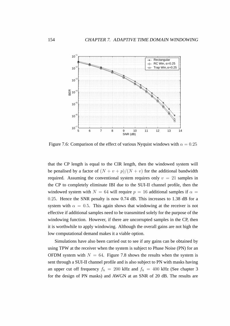
154 CHAPTER 7. ADAPTIVE TIME DOMAIN WINDOWING
5 6 7 8 9 10 11 12 13 1410
−7
10−6
10−5
10−4
10−3
10−2
10−1
SNR (dB)
BE
R
RectangularRC Win, α=0.25Trap Win, α=0.25
Figure 7.6: Comparison of the effect of various Nyquist windows with α = 0.25
that the CP length is equal to the CIR length, then the windowed system will
be penalised by a factor of (N + v + p)/(N + v) for the additional bandwidth
required. Assuming the conventional system requires only v = 21 samples in
the CP to completely eliminate IBI due to the SUI-II channel profile, then the
windowed system with N = 64 will require p = 16 additional samples if α =
0.25. Hence the SNR penalty is now 0.74 dB. This increases to 1.38 dB for a
system with α = 0.5. This again shows that windowing at the receiver is not
effective if additional samples need to be transmitted solely for the purpose of the
windowing function. However, if there are uncorrupted samples in the CP, then
it is worthwhile to apply windowing. Although the overall gains are not high the
low computational demand makes it a viable option.
Simulations have also been carried out to see if any gains can be obtained by
using TPW at the receiver when the system is subject to Phase Noise (PN) for an
OFDM system with N = 64. Figure 7.8 shows the results when the system is
sent through a SUI-II channel profile and is also subject to PN with masks having
an upper cut off frequency fh = 200 kHz and fh = 400 kHz (See chapter 3
for the design of PN masks) and AWGN at an SNR of 20 dB. The results are

7.2. TIME DOMAIN WINDOWING AT THE RECEIVER 155
10 11 12 13 14 15 16 17 18 1910
−7
10−6
10−5
10−4
10−3
10−2
SNR (dB)
BE
R
RectangularTPW α=0.25TPW, α=0.5
Figure 7.7: Comparison of the effect of TPW for SUI-II channels with α = 0.25and 0.5
presented in terms of Signal to Phase Noise Ratio (SPNR). The gain at a BER of
10−5 with the mask at fh = 200 kHz is 0.2 dB in terms of SPNR, but is increased
to 0.6 dB when the mask has fh = 400 kHz. This can be explained as follows;
as explained in chapter 3 the effect of PN on OFDM is two-fold. Specifically,
the presence of Common Phase Error (CPE) rotates the received constellation
and Inter-Carrier Interference (ICI) has a similar effect to AWGN. When fh is
increased the number of adjoining subchannels that fall into the PN mask of a
particular subchannel increases. Hence the ratio between the ICI power to the
CPE power increases. TPW is incapable of mitigating CPE but has a small effect
on ICI. Since the mask with fh = 400 kHz gives rise to more ICI then windowing
produces greater gains than with fh = 200 kHz and hence a better gains are seen
with it. Even so, the overall gains are not significant. To mitigate the effects of
CPE, the CPE Correction (CPEC) algorithm presented previously in section 3.4
will also have to be used.

156 CHAPTER 7. ADAPTIVE TIME DOMAIN WINDOWING
9 10 11 12 13 14 15 16 17 1810
−6
10−5
10−4
10−3
10−2
10−1
BE
R
SPNR (dB)
Rectangular, fh =200kHz
TPW, fh =200kHz,
Rectangular, fh =400kHz
TPW, fh =400kHz,
Figure 7.8: The effect of TPW with α = 0.5 for SUI-II channels with PN andAWGN at a SNR of 20 dB
7.3 Time Domain Windowing at the Transmitter
Figure 7.9 illustrates the processing that is required if the windowing is performed
at the transmitter rather than at the receiver. Firstly, the channel length has to be
estimated. The samples that are not going to be corrupted by the CIR during trans-
mission will be used for windowing as discussed in the previous section. However,
it is imperative to transmit zeros during the first few samples of the CP, the dura-
tion of which is equal to the channel length, Nh as shown in figure 7.9(a). Oth-
erwise orthogonality is lost at the receiver due to the lengthening of each symbol
owing to the CIR which gives rise to IBI. As shown in figure 7.9(b), the receiver
will have to consider these samples during the processing of each OFDM symbol.
Hence the number of samples selected at the receiver for each OFDM symbol will
be 2vβ +N +Nh + 1. Compare this to the number of samples selected when the
windowing is performed at the receiver, which is 2vβ + N + 1. (see figure 7.4).
Another difference is the number of zeros that are padded at either end before pre-
processing; if the windowing is performed at the receiver the numbers are equal
but this is not the case if the windowing is performed at the transmitter. As shown

7.3. TIME DOMAIN WINDOWING AT THE TRANSMITTER 157
in figure 7.9(c) every N th sample is summed to form a vector of length N , which
is sent to a N -point FFT for demodulation.
Even though selecting an additional Nh samples at the receiver will maintain
orthogonality, it will also introduce more noise to the system. If the additional Nh
samples at the tail of the symbol are not considered for processing at the receiver
(in a similar fashion to that described in the previously in section 7.2), it will
result in the introduction of ICI. However the interference power introduced will
not be significant if the CIR is not too hostile. This is certainly the case for SUI-II
channels and as will be as shown in the next subsection, the noise power that is
introduced to the system by considering the additional Nh samples is greater than
that of the interference power that it avoids. Multiplication performed by the TDW
at the transmitter is equivalent to a convolution of the subchannel sinc spectrum
with the spectrum of the window function in the frequency domain. In theory,
this means the windowing process can be corrected in the frequency domain as
part of the correction process at the FEQ. However, the method that is proposed
here guarantees orthogonality. Besides, the additional computation effort required
in the proposed method is not too high to warrant a frequency domain correction
method.
7.3.1 Simulation Parameters and Results
Figure 7.10 shows the performance of a TPW system in the SUI-II channel, with
α = 0.25 at the transmitter and for comparison, that of a conventional OFDM
system. Here too, it has been assumed that there are sufficient uncorrupted sam-
ples available in the CP to be included within the roll off samples of the window
function. Since zeros are transmitted within the first part of the CP for the win-
dowed system, the average power of the transmitted signal will be lower than that
of the conventional OFDM system. To get a meaningful comparison, the power
of the windowed system is normalised to a value similar to that of the simulated
conventional OFDM system, which in this case is unity. For TPW, the results are
presented for two cases. The curve labelled as ‘TPW: Full’ relates to the case
where all 2vβ + N + Nh + 1 samples are considered during the demodulation at
the receiver. This system will not introduce ICI since orthogonality is maintained,
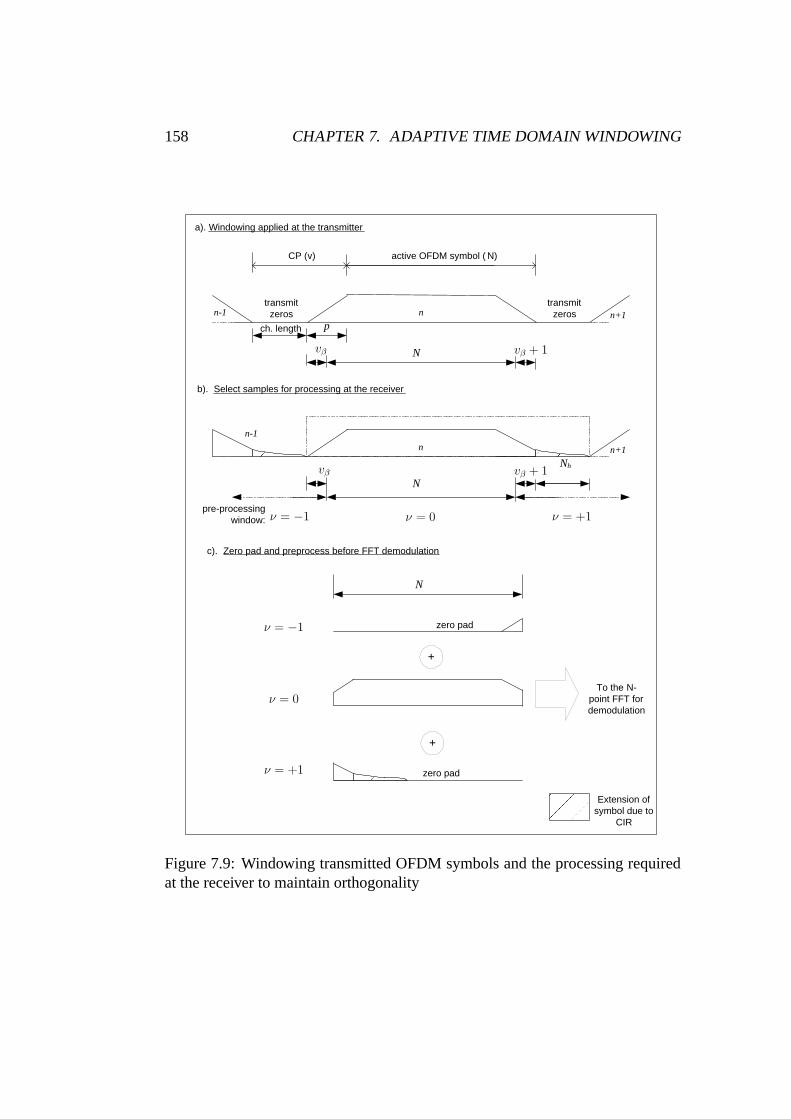
158 CHAPTER 7. ADAPTIVE TIME DOMAIN WINDOWING
N
p
a). Windowing applied at the transmitter
CP ( v ) active OFDM symbol ( N )
n+1 n-1 n
b). Select samples for processing at the receiver
zero pad
zero pad
N
c). Zero pad and preprocess before FFT demodulation
+
+
To the N - point FFT for demodulation
Extension of
symbol due to CIR
ch. length
N
n+1 n
transmit zeros
transmit zeros
n-1
N h
pre-processing window:
PSfrag replacements
vβ
vβ vβ + 1
vβ + 1
ν = −1
ν = −1
ν = 0
ν = 0
ν = +1
ν = +1
Figure 7.9: Windowing transmitted OFDM symbols and the processing requiredat the receiver to maintain orthogonality

7.4. CONCLUSION 159
but more noise will be introduced because more samples are considered during the
FFT demodulation. The case where the number of samples considered is reduced
to 2vβ +N + 1 is shown as ‘TPW: Reduced’. It clearly shows that including the
additional Nh samples gives a worse BER performance. To get another compari-
son, the first Nh samples of the conventional OFDM system have also been zero
padded, and again the average power is normalised to unity. This result is labelled
as the ‘Rect Win: with zeros’ in figure 7.10. At a BER of 10−4 the windowed
system that considers the decay samples shows a gain of 0.3 dB over the conven-
tional OFDM system that does not transmit zeros in the CP. The performance gain
increases to 0.9 dB if the decay samples are avoided. The Rectangular windowed
OFDM system with zeros transmitted in the CP performs similarly to the TPW
system with no delay samples. If the windowed system requires the transmission
of additional samples, as calculated in the previous section the SNR penalty of
0.74 dB has to be applied. This largely negates any performance gains achieved
owing to the use of windowing.
Figure 7.11 shows the performance of an OFDM system using a TPW at the
transmitter with α = 0.5, again in a SUI-II channel. The labelling of the plots fol-
lows the convention established in figure 7.10. The windowed system that uses the
decay samples shows a performance gain of 0.8 dB over the conventional OFDM
system. This increases to 1.4 dB if the decay samples are not included during
processing at the receiver. If additional samples requires transmission solely for
the purpose of windowing as shown in previous section, the penalty increases to
1.38 dB.
7.4 Conclusion
In this chapter the use of Time Domain Windowing (TDW) is investigated in
the context of OFDM systems operating in BFWA channels. The windowing
is applied separately in the receiver and the transmitter and their performance is
compared with a conventional OFDM system. Irrespective of whether windowing
is applied at the transmitter or the receiver, the performance gains that have been
achieved are not substantial and indeed if the transmission of additional samples
is required, the performance is actually worse. However the computational burden

160 CHAPTER 7. ADAPTIVE TIME DOMAIN WINDOWING
10 11 12 13 14 15 16 1710
−9
10−8
10−7
10−6
10−5
10−4
10−3
10−2
BE
R
SNR (dB)
Rect. WinRect.Win: with ZerosTPW: FullTPW: Reduced
Figure 7.10: Effect of TPW at the transmitter for SUI-II channels for α = 0.25
10 11 12 13 14 15 16 1710
−9
10−8
10−7
10−6
10−5
10−4
10−3
10−2
SNR (dB)
BE
R
Rect. WinRect.Win: with ZerosTPW: FullTPW: Reduced
Figure 7.11: Effect of TPW at the transmitter for SUI-II channels for α = 0.5

7.4. CONCLUSION 161
of the windowing process is relatively low and so it is proposed that windowing
should only be used if there are uncorrupted samples within the Excess Length
of the CP. If the terrain conditions are extremely good, which results in a very
short CIR, there may be suitable uncorrupted samples available within the CP of
the transmitted symbols. If the length of the CP is set according to a particular
standard and cannot be reduced, windowing could be viable in these conditions.

162 CHAPTER 7. ADAPTIVE TIME DOMAIN WINDOWING

Chapter 8
Conclusions and Future Work
In chapter 3 the effect of Phase Noise (PN) on the performance of coherent OFDM
systems is analysed and is found to have a dual effect. Specifically, one compo-
nent is found to rotate all the subchannels equally and gives rise to Common Phase
Error (CPE) and the other which affects the orthogonality of the subchannel car-
riers giving rise to Inter-Carrier Interference (ICI). The chapter also derives an
analytical result to estimate the Bit Error Rate (BER) when OFDM is subject to
a particular level of AWGN and PN. Subsequent simulations show a close match
with the analytical derivations. The PN mask, which describes the PSD of the
PN process is also introduced and the shape of the PN mask that is selected for
the simulation work is justified by comparison with the PSD of practical oscilla-
tors. The effect of PN on coherent OFDM systems subject to SUI-II channels is
also analysed. An algorithm to correct the CPE component found to be present
in coherent OFDM systems subject to PN is presented. The so called Common
Phase Error Correction (CPEC) algorithm is entirely data driven and contains two
correction factors, namely the CPE Symbol Estimate (CPESE) and the Feedback
Correction Factor (FBCF). The CPESE is calculated for each demodulated OFDM
symbol and previous CPESEs are used to generate the FBCF which tracks the
CPE variation at the Frequency Domain Equaliser (FEQ). It has been shown via
extensive simulation results that both components of the algorithm are necessary
for optimum performance when applied to coherent OFDM systems in the BFWA
scenario. The performance of the algorithm is tested via simulations and is also
163

164 CHAPTER 8. CONCLUSIONS AND FUTURE WORK
compared against other CPEC algorithms. It is shown that the use of the algorithm
will allow performance gains of up to 6 dB in terms of SPNR at a BER of 10−5
for a coherent OFDM systems with N = 64, a PN mask bandwidth of fh = 100
kHz and a SNR of 20 dB in the SUI-II channel.
Chapter 4 analyses the effect of symbol (frame) offsets in OFDM. It is shown
that symbol offset results in a distinct phase gradient that is seen across the de-
modulated subchannel outputs. It also introduces the symbol synchronisation
function of the Schmidl and Cox Algorithm (SCA), which is shown to perform
sub-optimally in a BFWA scenario. However the use of only two training sym-
bols and the avoidance of pilot symbols in the SCA make it a strong contender
for application to BFWA systems. The chapter also proposes an improved method
for determining the Start of Frame (SOF) compared to the method originally pro-
posed in [25]. The chapter also proposes a very robust symbol synchronisation
algorithm, namely the Iterative Symbol Offset Correction Algorithm (ISOCA)
that complements the symbol synchronisation function of the SCA. The ISOCA
makes use of the phase gradient that occurs as a result of the symbol offset and has
two functional parts. The ISOCA demonstrates an ability to obtain perfect symbol
synchronisation in a system subject to a BFWA channel at reasonable values of
SNR while maintaining a low probability of non-convergence at very low values
of SNRs. This is a remarkable improvement considering that using the SCA alone
yields a probability of only 0.48 of achieving perfect symbol synchronisation. The
results are presented in a comprehensive manner to show the performance on com-
pletion of each part of the two-part algorithm. Simulation results are presented for
both AWGN and SUI-II channels.
The effect of frequency offset on coherent OFDM systems is analysed in chap-
ter 5. It is shown that the Carrier-to-Interference Ratio (CTIR) drops significantly
even with a low relative frequency offset of 0.1. Again the SCA is selected be-
cause of its low level of computational complexity and its broad frequency offset
acquisition range. The frequency offset function of the SCA is analysed in de-
tail and it is found that the SCA, when used in a BFWA scenario, gives rise to
a significant Residual Frequency Offset (RFO). To address this problem an algo-
rithm to complement the frequency offset correction function of the SCA, namely
the Residual Frequency Offset Correction Algorithm (RFOCA) is proposed. It is
165
important to note that the RFOCA is entirely data driven and is based on track-
ing the rotating phase of the demodulated OFDM symbols. The simulated results
show that the RFO error variance can be reduced by several orders of magnitude
compared to the values that are observed at the end of the acquisition stage of the
SCA, for both AWGN and in the presence of SUI-II channels. Simulations have
also been carried out which show that the performance of the RFOCA does not
degrade even with a relative frequency offset that has an integer part. The pre-
sented simulation results show the performance of the RFOCA for various BFWA
scenarios.
Chapter 6 introduced the concept of using a Time Domain Equaliser (TEQ) for
OFDM systems in BFWA. The chapter first discusses different approaches to TEQ
design with the emphasis on the Minimum Mean Squared Error (MMSE) crite-
rion. An iterative method for training the TEQ which was first proposed for real
data in [110], is modified for the case of complex data. This approach is known
as the Dual Optimising Time Domain Equaliser (DOTEQ) since the adaptation
is applied to both the Target Impulse Response (TIR) and the TEQ coefficients.
However the algorithm only performs optimisation in the time domain, resulting
in severe nulls being generated in the frequency domain of the Effective Impulse
Response (EIR). A modified version of the DOTEQ is proposed, namely the Fre-
quency Scaled Time Domain equaliser (FSTEQ), which in contrast optimises both
in the time and the frequency domain. In this case the suitability of both the Least
Mean Square (LMS) and the Recursive Least Square (RLS) algorithms for the
adaptation of the FSTEQ is investigated. Comprehensive investigations are then
performed concerning the FSTEQ in terms of a Z-plane analysis and also its com-
putational complexity. Simulation results show that the FSTEQ improves the BER
performance of OFDM by up to two orders of magnitude while still maintaining
a superior rate of convergence compared to the original DOTEQ.
Chapter 7 investigated the use of window functions that adhere to the Nyquist
criterion to shape the OFDM symbols. The length of the window function is made
adaptive relative to the length of the CIR and it proposes to use the uncorrupted
samples lying within the Excess Length of the Cyclic Prefix (CP) as the roll off
samples. Consequently, the FFT window is shifted to include part of the CP. The
phase change of the demodulated symbols that is a direct consequence of this op-

166 CHAPTER 8. CONCLUSIONS AND FUTURE WORK
eration is corrected at the FEQ. It is seen that Trapezoidal Windowing (TPW) pro-
vides slightly better performance than Raised Cosine (RC) windowing in AWGN.
In the first instance, the windowing operation is performed at the receiver. It is
observed in this case that windowing provides very modest gains in the presence
of AWGN and PN. The analysis and the simulation is then extended to the case
where windowing is performed at the transmitter. To preserve orthogonality, ze-
ros are transmitted at the beginning of the CP. However, if orthogonality is to be
maintained at the receiver, the number of samples selected has to be greater than
is the case when the windowing is performed at the receiver. It is found that for
SUI-II channels, the noise enhancement caused by having to use a higher number
of samples is greater than the interference it avoids in terms of ICI and ISI. It is
recommended that windowing be applied to an OFDM system only if uncorrupted
samples are available in the CP and if the specifications do not allow the CP of the
OFDM system to be shortened.
8.1 Future Work
The investigations presented in this thesis are limited to coherent OFDM systems
based on QPSK mapping. However, the novel algorithms proposed in this thesis
could also be applied to other modulation schemes e.g. QAM. An investigation
into the performance of such systems could be undertaken in the future. The chan-
nel model selected for use throughout this work is the SUI-II channel profile since
this is representative of many typical environments where BFWA systems will be
deployed. The performance of the proposed algorithms could be investigated for
more hostile channels.
Chapter 3 proposes a CPEC algorithm that uses two functional elements, namely
the CPESE and the FBCF to successfully correct the CPE component of PN in a
coherent OFDM system. However, further investigation could be carried out to
determine, both analytically and via simulations, the exact contributions made by
each of these components. The channel selection criteria used prior to the calcu-
lation of the CPESE and the FBCF is currently to select those subchannels whose
gain is a standard deviation above the mean. The same channel selection criterion
is also adopted in chapters 4 and 5. However, since the SUI-II channel is not too

8.1. FUTURE WORK 167
hostile, the selection criteria does not significantly affect the overall performance.
However, for more difficult channels a different approach to subchannel selection
may have to be adopted. Also the performance of the CPEC algorithm proposed
in this work can be compared against a CPEC algorithm that is based on pilot
tone.
The ISOCA that is proposed in chapter 4 shows a very small probability of
non-convergence at very low SNR levels. Further investigations could be carried
out to try to reduce this already low probability.
The RFOCA that is proposed in chapter 5 is shown to suffer from a thresh-
old effect at low values of SNR owing to the triggering of the phase unwrapping
algorithm by spurious noise. Future work could be carried out to modify the un-
wrapping algorithm to avoid this phenomenon. It has also been observed that the
residual frequency offset values become very small particularly after a few itera-
tions of the RFOCA. Consequently, the number of OFDM symbols that need to be
buffered before each iteration is in the order of 100 to achieve good performance.
This increases the memory requirements and hence the latency of the overall sys-
tem. Further investigations could focus on reducing the number of symbols that
need to be buffered. A possibility is that the algorithm could be made adaptive in
terms of the buffer size and also determining when the phase unwrapping algo-
rithm should be triggered.
The FSTEQ presented in chapter 6 requires an FFT and an IFFT operation at
each iteration in order to scale the Target Transfer Function (TTF). This places
a high computational burden on the receiver. This is a limitation to the practical
application of the FSTEQ. The FFT/IFFT operations could be made adaptive so
that they are only performed after a certain number of iterations depending upon
the rate of convergence and the Channel Impulse Response (CIR). Even though
the two thresholds that need to be calculated do not dramatically affect the per-
formance of the FSTEQ, the proposed method requires knowledge of the power
delay profile of the CIR. Also it is seen that the actual initial Target Impulse Re-
sponse (TIR) selected determines the speed of convergence of the equaliser. In
this proposal a profile having a faster decay rate than the CIR is used as the ini-
tial TIR. It is possible that the selection of the initial TIR could be obtained in a
more optimum manner. Also the performance of FSTEQ can be compared against
168 CHAPTER 8. CONCLUSIONS AND FUTURE WORK
Multiple-Output-Multiple-Input (MIMO) OFDM systems.
Chapter 7 discussed the use of Time Domain Windowing (TDW), both at the
transmitter and at the receiver. If all samples of the CP are used for windowing,
rather than being limited to those samples within the excess length, it will certainly
introduce interference in terms of ICI and ISI. Investigations could be carried out
to determine the performance trade-off available between reducing input thermal
noise compared to the additional ISI and ICI introduced. Also the analysis in
chapter 7 is limited to windowing in the presence of AWGN and PN. This could
be extended to encompass frequency offsets.
Throughout the thesis, various impairments to OFDM systems are treated in
isolation and algorithms are presented to counter these effects. Investigations
could also be carried out to find the optimum parameters for the situation where
combinations of these algorithms are applied to a complete system.
All results presented in the thesis were obtained based on computer simula-
tions. In general, ideal conditions were assumed and possible implementation
impairments such as I-Q imbalance, DC offsets, Automatic Gain Control (AGC)
errors and quantisation effects were ignored. Prior to implementing the algorithms
proposed in this thesis it would be prudent to determine how these practical con-
siderations impact the performance.
Finally, the initial work undertaken concerning the use of MLSE for per-
subchannel equalisation presented in appendix C could be extended to address
areas such as complexity reduction and performance in BFWA channels.

Appendix A
Complex Baseband Representation
In this appendix the complex baseband representation of modulated signals is in-
troduced very briefly. A latter section will introduce the Power Spectral Density
(PSD) of stochastic processes. Any real modulated signal can be represented as,
s(t) = a(t) cos(ωct+ φ(t)) (A.1)
where, t is the representation of time, ωc is the carrier frequency and a(t) and
φ(t) are the time varying amplitude and phase of the signal. Now, the cos term in
(A.1) can be represented as a real part of a complex signal. Hence,
s(t) = <[a(t) ej(ωct+φ(t))]
= <[p(t) ej(ωct)] (A.2)
where,
p(t) = a(t) ejφ(t) . (A.3)
This is known as the complex baseband equivalent of the modulated signal.
It is also known as the ‘lowpass equivalent’ or the ‘phasor representation’. Note
that p(t) is devoid of the effects of carrier frequency [27, pg155]. Analysis of
the modulated signals in the complex baseband domain will require less compu-
tational power. Therefore all simulations presented in this thesis are performed in
the complex baseband domain. The signal in (A.3) is in general complex and can
169
170 APPENDIX A. COMPLEX BASEBAND REPRESENTATION
be written as
p(t) = si(t) + jsq(t) (A.4)
where,
si(t) = a(t) cos(φ(t))
sq(t) = a(t) sin(φ(t)) (A.5)
also, substituting (A.4) in (A.2) yields,
s(t) = si(t) cos(ωct) − sq(t) sin(ωct) . (A.6)
A.1 Spectra of Signals
Let us consider the real, unmodulated carrier signal, sc(t) = cos(ωct). Note that
it is preferred to have the frequency scale in Hz rather than rad/s when represent-
ing spectra, hence a one-sided spectrum of sc(t) would show a non-zero value of
power at frequency f = fc, where fc = ωc/2π. In such a spectrum, frequen-
cies are considered to be purely positive. However it is convenient to represent
signals in terms of complex exponentials or phasors. To represent a real cosi-
nusoidal signal using Fourier theory, two complex exponential (or phasor) terms
are required, that is one phasor rotates anti-clockwise (known as the positive fre-
quency) and the other clockwise (known as the negative frequency). Equivalently,
we can show that the Fourier Transform (FT) of sc(t) is,
Sc(ω) = Fsc(t) =1
2[δ(ω − ωc) + δ(ω + ωc)] (A.7)
Note the representation of (A.7) has two non zero components, at f = fc and
f = −fc. As mentioned previously, the latter component is known as the negative
frequency component. Since the spectrum of (A.7) has both positive and negative
frequencies, we call such a representation a two-sided spectrum of sc(t).
It is interesting to note the relationship between the spectra of the modulated
signal, s(t) and the complex baseband representation, p(t). Equation (A.2) can be

A.1. SPECTRA OF SIGNALS 171
represented as,
s(t) = <[p(t) ejωc(t)] =1
2[p(t) ejωc(t) + p∗(t) e−jωc(t)] . (A.8)
If the FT of p(t) is given by P (ω), then FT of p∗(t) is given by P ∗(−ω).
Consequently,
S(ω) = Fs(t) =1
2[P (ω − ωc) + P ∗(−(ω − ωc))] . (A.9)
Equation (A.9) reveals that if P (ω) is sufficiently narrowband relative to ωc,
then S(ω) comprises of P (ω) shifted to ωc and the conjugated, reversed version
of P (ω) shifted to −ωc [148]. Figure A.1 shows the relationship between P (ω)
and S(ω) with the two-sided bandwidth of P (ω) beingB. Note that the amplitude
A in the P (ω) is halved in S(ω).
PSfrag replacements
|P (ω)|
|S(ω)|
f
f−fc fc
BB
B
A
A/2
Figure A.1: Comparison of P (ω) and S(ω)

172 APPENDIX A. COMPLEX BASEBAND REPRESENTATION
A similar analysis can be performed on AWGN. Real, bandlimited AWGN
wc(t) can be represented in terms of complex baseband equivalent, w(t)
wc(t) = <[w(t)ejωct] (A.10)
where,
w(t) = [wi(t) + wq(t)]ejφw . (A.11)
Here, wi(t) and wq(t) are real uncorrelated, independent noise waveforms. φwis an arbitrary constant.
A.2 Power Spectral Density
A stationary stochastic process is an infinite energy signal and, hence, its FT does
not exist [27, pg67]. The spectral characteristics of a stochastic signal are obtained
by computing the FT of the Autocorrelation Function (ACF). This is known as
the Power Spectral Density (PSD). For a random process Xt, (here, t shows the
relationship with time), the ACF is defined as,
E(Xt1Xt2) =∫ ∞
∞
∫ ∞
∞xt1xt2p(xt1, xt2) dxt1dx2 (A.12)
where, E(.) is the expectation operator, xt1 and xt2 are samples drawn from
Xt at time t1 and t2, and p(.) is the joint probability between the two samples.
For a stationary process,
E(Xt1Xt2) = ψ(t1, t2) = ψ(t1 − t2) = ψ(τ) . (A.13)
In other words, for a stationary signal the ACF depends on the time difference,
τ and not the exact values of time. Hence, the PSD of a stationary stochastic signal
is given by [27, pg67],
Ψ(f) =∫ ∞
∞ψ(τ)e−j2πfτ dτ . (A.14)

A.2. POWER SPECTRAL DENSITY 173
The inverse Fourier relationship is given by,
ψ(f) =∫ ∞
∞Ψ(τ)ej2πfτ df . (A.15)
The PSD is the distribution of power of the stochastic process as a function
of frequency. Hence the units of the PSD are W/Hz. Also note that the area
under the PSD is equal to the average power of the signal [27, pg67]. The PSD is
very important in understanding the characteristics of the stochastic process. For
instance, AWGN will have equal power across all frequencies, hence the PSD of
AWGN is flat. This is in contrast to Phase Noise (PN) where the power density
closer to zero frequency is greater than at higher frequencies.

174 APPENDIX A. COMPLEX BASEBAND REPRESENTATION

Appendix B
Channel Models
Accurate channel modelling is essential for the realistic and successful simulation
of communication systems. A review of channel models will now be undertaken.
The statistics of the received power level can be divided into large-scale and small-
scale effects [149]. The local mean of the received signal power is affected by
effects such as Line of Sight (LOS) path loss and shadowing. The signal envelope
undergoes rapid fluctuations due to multipath propagation and movement of the
receiver or transmitter antenna, which in turn cause small-scale effects. The pro-
posed work is based on data transmission at high rates, so it is prudent to discuss
issues such as the delay spread and Doppler spread, which severely limit the data
rate.
B.1 Large-Scale Variations of the Signal Envelope
These issues will now be discussed below
B.1.1 Free Space Propagation
We begin with a description of radio propagation in a single-path free space chan-
nel. In free space, the relationship between the transmitted power Pt and the
175

176 APPENDIX B. CHANNEL MODELS
received power Pr is given by,
Pr = PtGtGr
(
λ
4πd
)2
=P0
d2(B.1)
where Gt and Gr are the transmitter and receiver antenna gains respectively,
and d is the distance between the transmit and the receive antennas, λ = c/f
is the wavelength of the transmitted signal and c is the velocity of radio wave
propagation in free space. Defining P0 = PtGtGr(λ/4π)2, it can be seen that over
a single path, the received signal power reduces with the square of the distance.
B.1.2 Two Ray Model
The most simple multipath propagation models is one with a single direct path
and a single strong reflected path, often from the ground. In general if we assume
a single sinusoid is transmitted, the received signal power with L received paths
is given by,
Pr = P0
∣
∣
∣
∣
∣
L∑
i=1
aidiejφi
∣
∣
∣
∣
∣
2
(B.2)
where, ai, di and φi are the reflection coefficient, the distance travelled by and
the received phase respectively of the ith path. Figure 5.1 depicts a possible two-
path scenario with the height of the transmitter and the receiver antennas being
h1 and h2, respectively. If we assume the distance between the two ends, d to be
much greater than the antenna heights, and that the ground reflection coefficient
is −1, then the received power can be approximated as
Pr ∼=P0
d2
∣
∣
∣1 − ej∆φ∣
∣
∣
2(B.3)
where ∆φ is the phase difference between the two paths. Using the same
assumption the difference between the two paths can be approximated as,
∆d =2h1h2
d(B.4)

B.1. LARGE-SCALE VARIATIONS OF THE SIGNAL ENVELOPE 177
and hence
∆φ =2π
λ× 2h1h2
d(B.5)
for small values of ∆φ, we have,
∣
∣
∣1 − ejφ∣
∣
∣
∼= |1 − (1 − j∆φ)| = |∆φ| . (B.6)
Hence
Pr =P0
d2
(
2π
λ
)2
× 4h21h
22
d2(B.7)
Note the exponent of the distance-power relationship is increased to four. In
general the received power as a function of the distance d from the transmitter is
proportional to d−n, where n is the path loss exponent. The value for n is 2 for
free space, 1.6 to 1.8 for indoor line of sight, 4 to 6 for obstructed indoor, 2.7 to
3.5 for urban cellular radio and 3 to 5 for shadowed urban cellular [149]. Many of
these values are found empirically from propagation measurements.
h 1
h 2
d
Tx
Rx
q q
Direct Path
Reflected Path
Figure B.1: Two-ray model

178 APPENDIX B. CHANNEL MODELS
B.1.3 Log-Normal Shadowing
The local mean in a particular area also experiences some additional variation
about its average caused by the presence of obstructions in the transmission path.
At a particular location at distance d from the transmitter, the local mean received
power, s can be modelled as a log-normal distribution around the mean of all
locations s, given by
p(s) =1
σ√
2πexp
[
− (s− s)2
2σ2
]
. (B.8)
B.2 Small-scale Variations of the Signal Envelope
The signal envelope can have extreme variations over a short distance of about half
a wavelength or over a short period of time owing to constructive or destructive
interference between signals arriving via paths with different/varying lengths.
B.2.1 AWGN Channel
The Additive White Gaussian Noise (AWGN) channel is the simplest model which
effectively only accounts for impairments owing to the thermal noise at the re-
ceiver. Usually performance in the AWGN channel is used as a benchmarker for
comparison of performance achieved in other channels. The received constel-
lation points are spread over the region with a pattern equivalent to a Gaussian
distribution function. It is evident that as the variance is increased, the probability
of a transmitted constellation point falling onto the ‘wrong side’ of the decision
threshold increases dramatically, thus increasing the Bit Error Rate (BER).
B.2.2 Multipath Channel
Multiple copies of the transmitted signal can arrive at the receiver antenna delayed
in time and with varying amplitudes due conditions such as reflections, refractions
and scattering. The receiver will experience a superposition of all such copies.
To model a specific case very accurate knowledge of the characteristics of each

B.2. SMALL-SCALE VARIATIONS OF THE SIGNAL ENVELOPE 179
reflector, its position and its mobility is required. Since this data is usually un-
available, an accepted approximation is the multipath delay line channel model.
A time varying Channel Impulse Response (CIR) can be modelled as,
h(τ, t) = A0
L∑
i=1
ai(t)
diejφi(t)δ(t− τi) . (B.9)
Assuming a stationary CIR,
h(τ) = A0
L∑
i=1
aidiejφiδ(t− τi) (B.10)
where the notations are as (B.2) with A0 =√P0. If we assume βi = A0ai/di,
we have,
h(τ) =L∑
i=1
βiejφiδ(t− τi) . (B.11)
The output of the channel neglecting noise is,
r(t) =L∑
i=1
βiejφis(t− τi) (B.12)
where, s(t) is the transmitted data sequence. The equation (B.12) is used
for statistical modelling of both indoor and outdoor radio propagation using the
tapped delay model shown in figure B.2. The tap gains depend on the rate of
fluctuation, the modelling of which will be discussed later. The phase is usually
taken as having a uniform distribution between [0, 2π] radians. Often the assump-
tion of wide-sense stationary uncorrelated scattering (WSSUS) is used. The first
and second order statistics are invariant in time and frequency in a WSSUS chan-
nel [150]. The physical meaning of the channels is that signal variations on paths
arriving at different delays are uncorrelated and the correlation properties of the
channel are stationary. Thus the amplitudes of the tap gains can be generated in-
dependently as long as they conform to the assumed probability density function.
In order to assess the performance of various wireless systems it is necessary
to have a convenient numerical measure of the multipath delay spread. The dif-

180 APPENDIX B. CHANNEL MODELS
X X X
Transmitted Signal
Received Signal
PSfrag replacements
τ1 τ2 − τ1 τL − τL−1
β1ejφ1 β2e
jφ2 βLejφL
Σ
Figure B.2: Tapped delay line channel model
ference between the earliest and the latest arrival is termed as excess delay spread.
Since the received signal is often a continuum, this measure is often defined as
the time taken for the delay spread to fall below a particular level (typically 20 or
30 dB) below the strongest path. However this is not a good indicator as different
channels with the same excess delay spreads can have different profiles. A better
indicator is the rms delay spread, which is the second central moment of the chan-
nel impulse response. For a carrier frequency of about 900 MHz, the rms delay
spread is of the order from 1.3 to 25 µs in an urban environment, 200 to 2110 ns
in a suburban environment and 10 to 1470 ns in a indoor environments [149]. It is
defined in [151] as,
τRMS =√
τ 2 − (τ)2 (B.13)
where,
τn =
∑Li τ
ni (βi)
2
∑Li (βi)2
, with n = 1, 2 . (B.14)
For reliable digital transmission, the symbol duration should be much longer
than the rms delay spread. Another parameter that is associated with the multi-
path delay spread is the coherence bandwidth, which is the inverse of a certain
percentage of the rms delay spread. It is the measure of the range of frequencies
over which the signal of a certain frequency shows a high degree (usually 90%)
of correlation with a signal of another frequency. It is obvious that the transmit-
ted signal bandwidth should be much less than the coherence bandwidth to avoid

B.2. SMALL-SCALE VARIATIONS OF THE SIGNAL ENVELOPE 181
distortion. If it is greater than the coherence bandwidth, the channel is termed as
frequency selective. Such systems have to rely on equalisation to avoid the effects
of significant variations in frequency response.
B.2.3 Distribution of Signal Envelope
When there are several paths of approximately equal power arriving at the re-
ceiver, the signal envelope can be modelled as a Rayleigh distribution with the
Probability Density Function (PDF),
p(r) =r
σ2exp
[
−r2
2σ2
]
, 0 ≤ r ≤ ∞ (B.15)
where σ is the rms value of the received signal voltage. The mean of the
distribution is σ√
π/2 and the variance is σ2(2 − π/2). If the signal has a strong
LOS path, the signal envelope is modelled using the Rician PDF given by,
p(r) =r
σ2exp
[
−(r2 + A2)
2σ2
]
I0
(
Ar
σ2
)
, A ≥ 0 and r ≥ 0 (B.16)
here I0(.) is the modified Bessel function of the first kind and A is the am-
plitude of the dominant component. When modelling assuming the WSSUS fre-
quency selective channel, the amplitudes of the tapped delay line are selected
independently using a Rayleigh distribution with the required parameters. For a
Rician distribution, an additional constant term is added to the delay line output.
Other distributions that are used in practise are, the Suzuki, the Weibull and the
Nakagami distributions. These are used mainly for the modelling of envelope
fading in indoor and urban radio channels. These distributions have the disad-
vantage of having complicated mathematical forms, which limit the use of them
practically.
B.2.4 Local Movements and Doppler Shifts
It is well known that whenever the transmitter and the receiver antennas are in
relative motion, the received carrier frequency is shifted relative to the transmitted

182 APPENDIX B. CHANNEL MODELS
one. This is known as the Doppler effect. If the transmitter and the receiver are
stationary and the distance between two terminals is do, the received signal is
represented by,
r(t) = <[Arej2πfc(t−τ0)] (B.17)
where τ0 = d0/c is the time required for the radio wave to travel between the
terminals at a velocity of c. Now, assuming one of the terminals travels toward the
other at a speed of vm, then the propagation time will change with time as,
τ(t) =d(t)
c=d0 − vmt
c= τ0 −
vmct . (B.18)
Then the received signal will be,
r(t) = <[Arej2πfc(t−τ(t))] = <[Are
j[2π(fc+fd)t−φ]] (B.19)
where φ = 2πfcτ0 is a constant and
fd =vmcfc =
vmλ
(B.20)
is known as the Doppler frequency shift. Note the maximum Doppler fre-
quency shift can occur when either the transmitter or the receiver is moving di-
rectly toward or away from the other. If the receiver is moving directly towards
the wave, then the apparent frequency would be fc + fd, and if it is moving away,
the apparent frequency is fc − fd. A vehicle travelling at the speed of 126 km/h
(35 m/s) will be subjected to a Doppler shift of 233 Hz at a carrier frequency of 2
GHz, whereas a pedestrian walking at a typical speed of 1.25m/s will be subjected
to a Doppler shift of only 8.3 Hz at the same carrier frequency.
Assuming that the arrival angles of each path are uniformly distributed in
[0, 2π], then the Doppler shift at a given azimuth angle θ is given by f(θ) =
fm cos(θ), where fm is the maximum Doppler shift given in (B.20). Then the
Doppler power spectrum is given by,
D(f) =1
2πfm
1 −(
f − fcfm
)2
−1/2
|f − fc| ≤ fm . (B.21)

B.3. STANFORD UNIVERSITY INTERIM CHANNEL MODELS 183
Such a spectrum rises to two high peaks at the edge frequencies of fc± fm [150]
and has been confirmed by practical signal measurements. Figure B.3 shows the
typical Doppler spread of Rayleigh and Rician distributed envelopes. Note the im-
pulse in the Rician channel due to the dominant path. From equation (B.21), it is
evident that if fm is very small, the received spectrum will undergo little spreading
and will have little effect on the received signal. The Doppler bandwidth is defined
as twice the maximum Doppler shift. If the signal has a bandwidth much larger
than the Doppler bandwidth, the signal will experience little effect from Doppler
shifts. Coherence time is defined as the time over which the signal remains rel-
atively constant. In other words, time duration over which the samples remain
fairly correlated. Hence to maintain correlation between samples and avoid dis-
tortion, the symbol duration of the signal should be less than the coherence time.
The coherence time is inversely proportional to the Doppler bandwidth.
1
2
3
1
2
3
PSfrag replacements
fc − fmfc − fm fcfc fc + fmfc + fm
|D(f)|2|D(f)|2
Figure B.3: Typical Doppler spectra for Rayleigh (left) and Rician (right) dis-tributed mobile channels
B.3 Stanford University Interim Channel Models
Accurate channel models for the Broadband Fixed Wireless Applications were
still being discussed while the research presented by this thesis was being un-
dertaken. At the time the Stanford University Interim (SUI) channel models pre-
sented for the IEEE 802.16 Broadband Wireless Access Working Group [23] were
achieving widespread acceptance. The Point to Point (PTP) and the Point to Mul-

184 APPENDIX B. CHANNEL MODELS
tipoint (PMP) systems considered for the BFWA systems in this research are as-
sociated with highly directional antennas at the Base Station (BTS), and near Line
of Sight (LOS) conditions. Trials have shown that microwave propagation in the
MMDS band with directional and omni-directional antennas will provide a chan-
nel with maximum delay spread that is well under 1 µs [152]. Consequently the
CIR is not hostile. Typical scenarios for the SUI channel models are very similar.
Some of the conditions are,
• Cell size radius: 6.4 km (4 miles)
• BTS antenna height: 17 m (50 ft)
• Receive antenna height: 3 m (10 ft)
• BTS antenna beamwidth: 120
• Receive antenna beamwidth: Omnidirectional (360) and 30
• Vertical Polarisation only
Six channel models are proposed in total with two for each of the three terrain
conditions. Category A has the maximum path loss associated with hilly terrains
with moderate to heavy tree densities. Category C has the minimum path loss
and is associated with mostly flat terrain with light tree densities. Category B
is defined for intermediate conditions. Out of the 6 models, the SUI -II channel
model with an Omnidirectional receiver antenna was selected as the standard CIR
model for all the simulations undertaken in this work. Owing to the time required
to perform each simulation, the algorithms presented have not been tested using
other channel models. The characteristics of the SUI-II channel model are given
in the table B.1
The sampling frequencies considered for the simulated systems in this work
are 20MHz or higher. The transmitted frames have a maximum of 2500 OFDM
symbols. Hence the time taken to transmit each frame is approximately 10 ms.
As noted in table B.1, the Doppler frequencies are significantly low and conse-
quently it is assumed that the channel remains static throughout each transmitted
data frame. Channel Estimation is performed at the beginning of each frame using

B.3. STANFORD UNIVERSITY INTERIM CHANNEL MODELS 185
Tap1 Tap2 Tap3 Units
Delay 0 0.5 1 µs
Power (Omni ant.) 0 -12 -15 dB
Power (30 ant.) 0 -18 -27 dB
K factor 10 0 0
Doppler∗ 0.4 0.4 0.4 Hz
Terrain Type: C, overall K = 5 (linear)RMS delay spread for Omnidirectional antennas: 0.2 µs.
∗ Rounded Doppler spectrum, maximum frequency
Table B.1: SUI-II channel profile
the training symbol, which is used to initialise the FEQ coefficients. The FEQ co-
efficients are held static throughout the frame. For each new transmitted frame, a
new realisation of a SUI-II channel is applied and the FEQ is updated accordingly.

186 APPENDIX B. CHANNEL MODELS

Appendix C
Equalisation in FMT Modulation
A different approach to limiting the interference between subchannels in a parallel
modulation scheme is to use per-subchannel filtering. One such system is known
as Filtered Multitone (FMT) [26]. By relaxing orthogonality between subchannels
their spectra can be designed to have much higher roll off levels in the frequency
domain. The non-orthogonality will introduce Inter Symbol Interference (ISI)
into the system, which has to be equalised using per-subchannel equalisation but
owing to its rapid roll-off in the frequency domain, the system is subjected to low
levels of Inter Channel Interference (ICI). Much of the previous work has pro-
posed the use of Decision Feedback Equalisers (DFE) for per-subchannel equal-
isation. Usually the application considered is for high-speed DSLs rather than
BFWA. The use of equalisation dramatically increases the complexity of the re-
ceiver. The author has investigated the use of Maximum Likelihood Sequence
Estimators (MLSE) for the per-subchannel equalisation of FMT systems to gauge
the performance limits for this approach. Undoubtedly, this further increases the
complexity, but the author’s goal is to find the practical performance limits of the
system and compare it with that of a conventional OFDM systems.
The appendix is organised as follows. Section C.1 gives a brief introduction to
subband systems. Since this area of research is quite diverse, this section is kept
relatively short and concentrates only on the issues that relate to FMT. Section C.2
introduces the FMT modulation technique including different implementations of
FMT and pointing out that the ISI caused by non-orthogonal filters is a major con-
187

188 APPENDIX C. EQUALISATION IN FMT MODULATION
cern. It then introduces various contributions concerning FMT, particularly ones
that address wireless systems. Section C.3 shows the simulation results which
concentrate upon the performance of MLSE based detection of FMT in com-
parison with that achieved by DFE based per-subchannel equalisation. Finally
section C.4 draws some conclusions.
C.1 A Brief Introduction to Subband Systems
FMT modulation has its roots in Multirate systems for example, digital filters
and Wavelet decomposition [153, 154]. This is a very rich and diverse area of
research and consequently the focus will be on those areas relevant to FMT. In
many applications such as audio and image coding, most of the energy in the
information sequence is concentrated at low frequencies. Hence when it comes
to source compression greater resolution can be given to high-energy bands if the
information sequence can be separated into subbands in the frequency domain
by the use of bandpass filters. Appropriate processing can then be performed
separately in each band.
In anN -band decomposition with equal bandwidth filters, the subband signals
will have a bandwidth approximately equal to π/N . Hence each subband signal
can be subsampled by a factor of N , i.e. only one out of every N samples is
retained. This process is known as decimation and it overcomes the problem of
information growth. Since the bandpass filters are not expected to be ideal brick
wall filters, the decimation process introduces aliasing. Aliasing is just one of the
issues that has to be dealt with in subband coding. At the reconstruction level, the
sampling rate of the processed signal has to be increased by a factor of N in order
to retrieve the original signal. This process is known as interpolation. The term
Multirate System is associated with such a system as it operates at a number of
sample rates.
Figure C.1 shows a block diagram of a subband processing system. H0(z)
to HN−1(z) represent the transfer functions of the so called decomposition or
analysis filters, while F0(z) to FN−1(z) represent the transfer functions of the
reconstruction or synthesis filters. The decimation and interpolation functions (by
a factor of N ) are represented by the symbols ↓N and the ↑N, respectively. The

C.1. A BRIEF INTRODUCTION TO SUBBAND SYSTEMS 189
subband signals X0(m) to XN−1(m) are obtained after decimating the outputs of
the analysis filters. The reconstructed signal x(n) is obtained by adding together
all outputs of all the synthesis filters.
H 0 (z) N
H N-1 (z ) N
H 1 (z) N
x(n) X 0 (m)
X N-1 (m)
X 1 (m)
PRO
CE
SSIN
G
F 0 (z) N ) ( ˆ
0 m X
F 1 (z) N ) ( ˆ
1 m X
F N-1 (z) N ) ( ˆ
1 m X N -
+
+ ) ( ˆ n x
Figure C.1: Block diagram of a subband system
Ideally the subband system should have good signal reconstruction. If the
subband signals are not modified during processing, the output of the synthesis
filter bank should be equal to the input signal. That is x(n) = x(n − D), where
D is an acceptable processing delay introduced by the filters. Hence the only
modifications to the signal should be due to any processing which takes place
in the subbands and not due to the filters. Such a system is known as a perfect
reconstruction (PR) filter bank. It can be shown that the PR condition is satisfied
if and only if [153]
N−1∑
k=0
∞∑
m=−∞fk(n−mN)hk(mN − l) = δ(n− l −D) (C.1)
where δ(.) is the Kronecker delta function and hi(n) and fk(n) are the impulse
responses of the analysis and synthesis filters, respectively. However designing
realisable filters which satisfy equation (C.1) is far from a trivial task. It can be
shown that if the analysis and synthesis filters are ideal bandpass filters, then the
condition of (C.1) will be satisfied. Therefore by designing good bandpass Finite
Impulse Response (FIR) filters, using the window approach for example, permits
a close approximate to the PR condition to be made. FIR filters can be designed
to have linear phase. If all channels are forced to have the same delay, then the

190 APPENDIX C. EQUALISATION IN FMT MODULATION
overall subband system will have no phase distortion, and so uncancelled aliasing
leads only to amplitude distortion. Hence FIR filters are used more frequently in
subband coding systems.
C.1.1 Polyphase Decomposition
Polyphase components appear very commonly in the analysis of the multirate
signal processing systems. The polyphase components are formed by selecting
all indices, which are identical modulo N . That is the kth polyphase component
hk(m) is formed by passing the impulse response h(n) though a delay z−k and a
N : 1 decimator. If Hk(z) is the z-transform of the kth polyphase hk(m), it can
be shown that,
H(z) =N−1∑
k=0
z−kHk(zN) . (C.2)
C.1.2 Transmultiplexers
Transmultiplexers were first designed in the 1970s for the conversion between
the older Frequency Division Multiplex (FDM) based telephony systems to new
Time Division Multiplex (TDM) based systems employing Pulse Code Modu-
lation (PCM) [155]. TDM-to-FDM transition was done by upsampling (which
created spectral images) followed by bandpass filters, which selected one of the
bands. The primary concerns in transmultiplexer design are distortion and crosstalk.
Distortion refers to any changes that are introduced by the filtering and crosstalk
refers to the leakage from one channel to another. FIR filters of orders exceed-
ing 2000 were required to reduce crosstalk to acceptable levels. However the
use of polyphase network based filter banks made the implementation practi-
cal. Vetterli [156] showed that the transmultiplexer is the dual of the maximally-
decimated filter bank and that crosstalk is the dual of the aliasing. This relation-
ship allows the results applying to filter banks to be used for transmultiplexers.
More specifically, the PR conditions can be used in the form of crosstalk cancel-
lation. However sampling must be synchronised at both ends and as a result, a
timing signal may have to be sent along with the transmitted signal.
C.1. A BRIEF INTRODUCTION TO SUBBAND SYSTEMS 191
C.1.3 Overlapped Basis Functions
All block transforms, such as the DFT and the Discrete Cosine Transform (DCT)
with a transform matrix of size N × N are characterised by an input vector of
length N . Thus if x is an input vector of length N , transformation is obtained by
the applying the transformation matrix AT as given by
X = ATx (C.3)
where T here denotes complex transposition. The original signal can be ob-
tained using
x = [AT ]−1X . (C.4)
If AT = A
−1 then A is an orthogonal transform. Each column of A is a
basis function and is of size N . The N -band filter bank with each filter having
a length N can also be looked at in this way. In this case, they are known as
critically sampled or uniform filter banks. However, such restrictions will limit
the frequency domain resolution and gives rise to blocking effects when applied
to image coding. The Lapped Transforms [157] were introduced to overcome this
problem by having the length of the basis function, L to be equal to an even integer
multiple of the number of subbands. i.e. L = 2KN , where, K is known as the
overlap factor.
C.1.4 Filter Bank based modulation for Communication
There has been a lot of work concerning the use of Filter Bank based Modulation
(FBM) for DSL systems. Discrete Multitone (DMT) [158] has already found
practical application in ADSL systems. DMT uses IFFT based modulators (as
in OFDM), but employs Hermetian symmetry within the data vector of the IFFT
modulator to convert the complex data symbols in to real transmitted signals. As
with OFDM, the performance of DMT is limited by the high subchannel sidelobe
levels.
Several schemes have adopted Cosine Modulated Filter Bank (CMFB) based
orthogonal transmultiplexers [159, 160] to overcome the problem of high sidelobe
levels. DMT in particular relies on Time Domain Equalisation (TEQ), to shorten

192 APPENDIX C. EQUALISATION IN FMT MODULATION
the effect of the channel impulse response (see chapter 6 for details of TEQ de-
sign). This requires channel estimation, which is based on the transmission of
pilot tones and training symbols. The authors of [160, 161] proposed a modula-
tion scheme, namely the Discrete Wavelet Multitone Modulation (DWMT), which
claims to be more robust under non-ideal tap settings of the equalisers owing to
the fact that the basis functions have very high spectral containment. The authors
in [162] compare DFT and CMFB based filter banks. The level of ICI is shown
to be lower in CMFB but at a cost of higher ISI in the unequalised received sym-
bols. The authors in [163] use Lapped Transforms (LT) to remove narrowband
interference in a DS-CDMA scheme. It is shown that LT domain interference
suppression is less sensitive to narrowband jamming as compared to DFT or DCT
based schemes.
C.2 Introduction to Filtered Multitone
A different approach to LT based designs has been adopted by Cherubini et al.
in their definition of the Filtered Multitone (FMT) system [26, 164]. Originally
the scheme was proposed for Very High-Speed Digital Subscriber Lines (VDSL),
which is the next step upward in bit rate from ADSL systems. VDSL is intended
to bridge the gap between the copper based technology available today and future
all-fibre backbone networks. The view is that the fibre will terminate close to
the subscriber and that VDSL modems will enable data rates of up to 60 Mb/s to
be achieved to users located within a few thousand feet of the termination point.
FMT uses a polyphase filter bank based scheme, but has relaxed the PR and crit-
ical sampling criteria to achieve a high stopband attenuation of the order of -60
dB. Consequently the ICI introduced in to the system is insignificant. As with
DWMT, the FMT schemes does not require the use of a CP. Even though CMFB
schemes such as LTs and DWMT have a greater subband attenuation than OFDM
or DMT, the adjacent subchannel sidelobes cross at a level 3 dB below that of
the mainlobe. To satisfy the PR condition usually entails substantial overlap of
the adjacent channels. FMT on the other hand does not have that limitation. The
biggest advantage of FMT is the that fewer Virtual Carriers (VC) need to be used
compared with other schemes. Owing to the distortion introduced by the bandpass
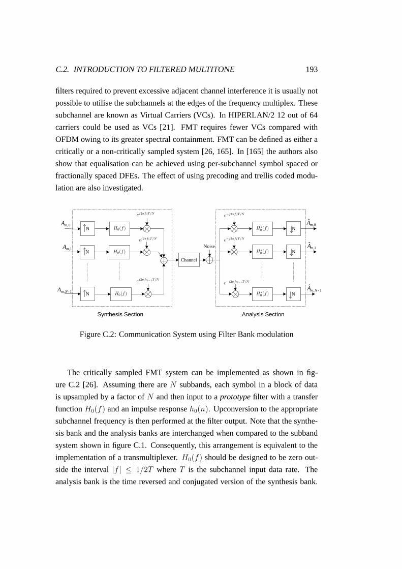
C.2. INTRODUCTION TO FILTERED MULTITONE 193
filters required to prevent excessive adjacent channel interference it is usually not
possible to utilise the subchannels at the edges of the frequency multiplex. These
subchannel are known as Virtual Carriers (VCs). In HIPERLAN/2 12 out of 64
carriers could be used as VCs [21]. FMT requires fewer VCs compared with
OFDM owing to its greater spectral containment. FMT can be defined as either a
critically or a non-critically sampled system [26, 165]. In [165] the authors also
show that equalisation can be achieved using per-subchannel symbol spaced or
fractionally spaced DFEs. The effect of using precoding and trellis coded modu-
lation are also investigated.
N
N
N
N
N
N
0 , m A
1 , m A
1 , - N m A
Channel
0 , ˆ
m A
1 , ˆ
m A
1 , ˆ
- N m A
Noise
Synthesis Section Analysis Section
PSfrag replacements
ej2πf0T/N
ej2πf1T/N
ej2πfN−1T/N
e−j2πf0T/N
e−j2πf1T/N
e−j2πfN−1T/N
H0(f)
H0(f)
H0(f)
H∗0 (f)
H∗0 (f)
H∗0 (f)
Figure C.2: Communication System using Filter Bank modulation
The critically sampled FMT system can be implemented as shown in fig-
ure C.2 [26]. Assuming there are N subbands, each symbol in a block of data
is upsampled by a factor of N and then input to a prototype filter with a transfer
function H0(f) and an impulse response h0(n). Upconversion to the appropriate
subchannel frequency is then performed at the filter output. Note that the synthe-
sis bank and the analysis banks are interchanged when compared to the subband
system shown in figure C.1. Consequently, this arrangement is equivalent to the
implementation of a transmultiplexer. H0(f) should be designed to be zero out-
side the interval |f | ≤ 1/2T where T is the subchannel input data rate. The
analysis bank is the time reversed and conjugated version of the synthesis bank.
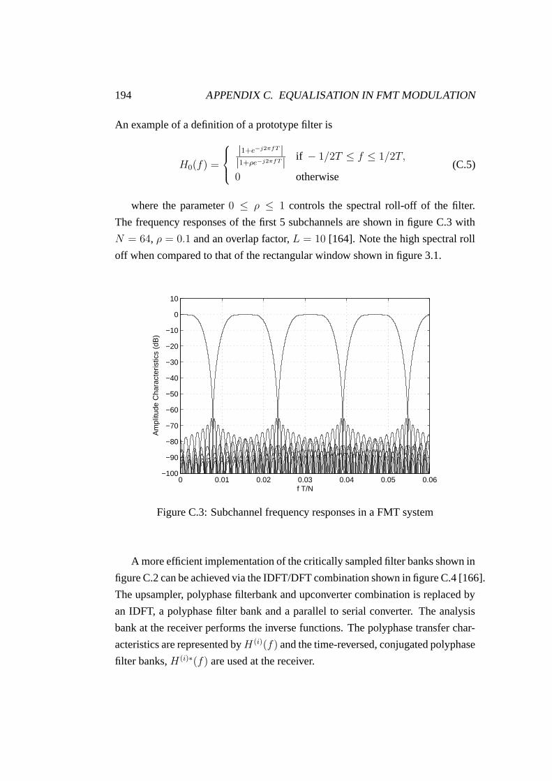
194 APPENDIX C. EQUALISATION IN FMT MODULATION
An example of a definition of a prototype filter is
H0(f) =
|1+e−j2πfT ||1+ρe−j2πfT | if − 1/2T ≤ f ≤ 1/2T,
0 otherwise(C.5)
where the parameter 0 ≤ ρ ≤ 1 controls the spectral roll-off of the filter.
The frequency responses of the first 5 subchannels are shown in figure C.3 with
N = 64, ρ = 0.1 and an overlap factor, L = 10 [164]. Note the high spectral roll
off when compared to that of the rectangular window shown in figure 3.1.
0 0.01 0.02 0.03 0.04 0.05 0.06−100
−90
−80
−70
−60
−50
−40
−30
−20
−10
0
10
Am
plitu
de C
hara
cter
istic
s (d
B)
f T/N
Figure C.3: Subchannel frequency responses in a FMT system
A more efficient implementation of the critically sampled filter banks shown in
figure C.2 can be achieved via the IDFT/DFT combination shown in figure C.4 [166].
The upsampler, polyphase filterbank and upconverter combination is replaced by
an IDFT, a polyphase filter bank and a parallel to serial converter. The analysis
bank at the receiver performs the inverse functions. The polyphase transfer char-
acteristics are represented byH (i)(f) and the time-reversed, conjugated polyphase
filter banks, H (i)∗(f) are used at the receiver.

C.2. INTRODUCTION TO FILTERED MULTITONE 195
0 , m A
1 , m A
1 , - N m A
Channel
0 , ˆ
m A
1 , ˆ
m A
1 , ˆ
- N m A
Noise
Synthesis Section Analysis Section
P/S IDFT S/P DFT PSfrag replacements
H(0)(f)
H(1)(f)
H(N−1)(f)
H(0)∗(f)
H(1)∗(f)
H(N−1)∗(f)
Figure C.4: Efficient implementation of a critically sampled FMT system usingIDFT, DFT and polyphase filter banks
C.2.1 ISI Caused by FMT
Although FMT has negligible ICI owing to its rapid subband roll off, it introduces
ISI into the system because of the loss of orthogonality. For a system with an
overlap factor, L = 10, each polyphase branch is 10 samples long. Hence, each
subchannel will have an Overall Subchannel Impulse Response (OSIR) length of
19 samples. Since the prototype is symmetric, all subchannels will be subject
to the same OSIR. The OSIR of an FMT system with N = 64 and L = 10
with the prototype as defined in (C.5) is shown in figure C.5. It is important to
note the high level of ISI. In all proposals regarding FMT modulation some form
of equalisation is necessary to counter this subchannel ISI. This often takes the
form of a Decision Feedback Equaliser (DFE). The DFE length should be of the
same order as the length of the pulse that is being equalised. So, to equalise the
OSIR shown in figure C.5, the symbol spaced Feedforward (FF) and Feedback
(FB) filters should have a length greater than 10 symbol periods. It is evident
that although increasing the overlap factor increases the subchannel decay rate, a
longer DFE will be required to equalise the ISI caused by the longer OSIR.
Another more powerful but significantly more complex method of equali-
sation can be achieved by the use of the Maximum Likelihood Sequence Es-
timator (MLSE). This algorithms searches for the minimum euclidean distance

196 APPENDIX C. EQUALISATION IN FMT MODULATION
0 2 4 6 8 10 12 14 16 18−0.2
0
0.2
0.4
0.6
0.8
1
1.2
n
Ove
rall
Sub
chan
nel I
mpu
lse
Res
pons
e (O
SIR
)
Figure C.5: Overall Subchannel Impulse Response (OSIR) of an FMT system
path through the trellis that characterises the memory of the overall impulse re-
sponse [27, p.250]. If the length of the OSIR is given byNo, then for a modulation
which has two states there are 2No−1 states in the trellis. Also if the sequence has
a length K, the total number of possible sequences is 2K . The MLSE finds the
sequence that has the highest posterior probability given the received sequence of
symbols. Directly implementing the MLSE requires a prohibitive amount of mem-
ory. The number of sequences may be reduced using the Viterbi Algorithm [167]
to eliminate unlikely sequences each time new data is received from the demodu-
lator.
C.2.2 Achievable Bit Rate
In chapter 2 it was shown that theoretical channel capacity can be achieved by dis-
tributing the energy according the the ‘waterpouring’ algorithm. In most proposals
regarding FMT, the authors have chosen a parameter known as the Achievable Bit
Rate (ABR) as the criteria to compare system performance. It is based on allocat-
ing different numbers of bits to different subchannel depending on the subchannel
C.2. INTRODUCTION TO FILTERED MULTITONE 197
SNR. As given in [164], the number of bits allocated to subchannel i is given as,
bi = log2
(
SNRi.ΓcΓg
+ 1
)
(C.6)
where SNRi is the SNR of subchannel i, Γc is the assumed coding gain and Γg
is the SNR gap between the channel capacity and the actual capacity usage of the
transmission scheme. The ABR is given by
ABR =N−1∑
i=0
bi . (C.7)
The use of FMT for wireless communication channels has been addressed by
Benvenuto et al. [168, 169, 170]. In [168], the authors compare the performance
of DMT and FMT in the presence of multipath delay spread and Phase Noise. The
authors use only critically sampled FMT systems and use the ABR as the criterion
of comparison. The authors in [169] propose a fixed DFE to equalise the OSIR
and a one-tap equaliser to compensate the effects of the channel. The latter is
equivalent to the FEQ in OFDM. However, for CIRs with long delay spreads, this
assumption is no longer valid. The author in [171] proposes a fixed DFE computed
offline in combination with a short adaptive linear equaliser with a few number
of taps to be used for channels with long multipath delay spreads. In [170] the
authors propose three different per-subchannel equalisation methods to counter
the combined effects of the CIR and the OSIR. The first type described is known
as the Decision Feedback Multichannel Equaliser (DFME), which calculates the
DFE coefficients on a per-subchannel basis. The second is a Post DFT Simplified
DFE (postDFME). If the assumption is made that the Channel Transfer Function
(CTF) is constant over the subchannel, the channel effects can be equalised by
an array of one tap equalisers following the DFT. The OSIRs are then equalised
separately by an array of per-subchannel DFEs. Hence the coefficients for the
DFE will be the same for all subchannels. The third type described is known as
a Pre DFT Simplified DFME (PreDFME). Here the polyphase analysis bank is
replaced by the FF filters. Since FMT and OFDM uses different number of VCs
and the CP is used only by an OFDM system, a normalised SNR is introduced
for both OFDM and FMT, so that the performance may be compared realistically.

198 APPENDIX C. EQUALISATION IN FMT MODULATION
For QPSK the normalised SNRs are [170],
SNRO =σ2A(N + v − VO)
σ2w(N − VO)
N
N − VO(C.8)
SNRF =σ2A
σ2w
N
N − VO(C.9)
where SNRO and SNRF are the normalised SNRs for OFDM and FMT, σ2A,
σ2w, v, VO and VF are the signal power, noise power, the CP length, the number of
VCs used in OFDM and the number of VCs used in FMT, respectively.
As discussed previously, the channel bit allocation will be optimal for the very
harsh channels that are associated with DSL systems. There is little gain to be
achieved using optimum bit allocation in the BFWA scenario using the relatively
benign SUI-II channel. Hence for the studies presented here BER will be used as
the performance indicator rather than the ABR.
C.3 Simulation Results
Since the objective of the analysis to be presented here is to determine the limits
imposed by equalisation of the OSIR, AWGN alone is introduced to the system.
Figure C.6 presents the simulation results. The performance of an OFDM sys-
tem has been also been included for comparison. For the DFE, a FF length of 15
and a FB length of 15 is used. Optimal DFE coefficients are obtained by sending
a very long training sequence. Since the DFE lengths and the OSIR are fixed,
these coefficients will be the same for each transmitted burst. Hence, these coef-
ficients (once obtained via training) are preloaded and 2000 QPSK symbols are
sent in each burst. The SNR is normalised as given in (C.8) and (C.9). Since only
AWGN channels are considered, the CP length, v is set to zero. The number of
VCs selected for OFDM and FMT are 10 and 2, respectively. For each value of
SNR, 500 bursts are transmitted and the BER is taken as the average. Only one
subchannel is equalised at a time owing to limitations in the computer memory.
To reduce the complexity of the MLSE simulations, the last few samples at either
end of the OSIR in figure C.5 are neglected since they are small in value. Conse-

C.3. SIMULATION RESULTS 199
quently, for the results presented in figure C.6, the last 3 samples and the first 3
samples are not considered and so length of the OSIR is taken to be 13 samples.
In this case, the number of states in the trellis is 4096. Note that the OSIR is
completely real. Although QPSK symbols are transmitted, the OSIR will affect
the real and the imaginary parts of the received signal in a similar way. Hence,
the received signal can be perceived as two BPSK channels. Equalisation by the
MLSE is performed using two parallel equalisers that process the real and the
imaginary parts of the received sequence separately in a particular subchannel.
Again, only one subchannel is considered at a time owing to limitations in the
simulation environment.
As can be observed in figure C.9, since there is very little ICI, the difference
in BER performance between the subchannel at the edge (with subchannel index
0) and one in the middle (with subchannel index 31) is insignificant. The OFDM
system shows a 2.5 dB advantage over MLSE equalisation of FMT and an advan-
tage of 3.5 dB over FMT equalised using DFEs. However the analysis is based on
AWGN channels and so the OFDM system did not have to use a CP. In a multi-
path channel a CP will be required and so the OFDM advantage will be reduced
according to (C.8).
Figure C.7 shows the effect of reducing the number of states on the perfor-
mance of the MLSE. It compares two cases of the MLSE, one when the number
of states is 4096 and another where 1024 states are used. The number of samples
neglected on either side of the OSIR shown previously in figure C.5 are 3 in the
former case and 4 in the later case. Consequently, the length of the OSIR is as-
sumed to be 13 samples and 11 samples, respectively. For both cases, equalisation
of the 0th and the 31st subchannel is considered separately. Equalisation using an
MLSE with 4096 states takes a long time and a lot of simulation resources. The re-
sults shows that the performance degradation caused when using a shorter MLSE
is insignificant below a SNR of 15 dB. As shown in figure C.5 the first 4 samples
on either side of the OSIR are quite small and neglecting these samples has little
effect on the subchannel BER.

200 APPENDIX C. EQUALISATION IN FMT MODULATION
5 10 15 2010
−6
10−5
10−4
10−3
10−2
10−1
100
BE
R
SNR
OFDMDFE: Subch. 0DFE: Subch. 31MLSE: Subch. 0MLSE: Subch. 31
Figure C.6: The comparison of OFDM and FMT equalised by a DFE and anMLSE
5 10 15 2010
−6
10−5
10−4
10−3
10−2
10−1
100
BE
R
SNR
OFDMMLSE 4096 states: Subch.0MLSE 4096 states: Subch.31MLSE 1024 states: Subch.0MLSE 1024 states: Subch.31
Figure C.7: The effect of MLSE length on equalisation performance

C.4. CONCLUSIONS 201
C.4 Conclusions
This appendix shows some preliminary simulation results concerning the equal-
isation of the OSIR in an FMT system using DFE and MLSE approaches. Sub-
channel error performance is worse than the conventional OFDM irrespective of
the equalisation method used. However, as expected, the MLSE outperforms the
DFE in all situations. Since the OSIR of the FMT system selected contains very
low pre-cursor and post-cursor values, reducing the number of states in the MLSE
has little effect on the subchannel BER. The real advantage of FMT lies in the use
of fewer VCs and eliminating the requirement for a CP. Even though the subchan-
nel BER is worse than OFDM in FMT, a comparison of the ABR and overall BER
(utilising all the subchannels) is required to ascertain the potential performance
gains.
Owing to lack of time and resources, the analysis is limited to a study of the
per-subchannel BER in this work. The work presented here could be extended
to accommodate systems subject to channels with multipath delay spread. In this
case, the equalisation will have to take into account the CIR as well as the OSIR.
The use of the CP increases the SNR penalty of OFDM systems but this effect is
not included in the presented results. Further analysis could be carried out to find
the total BER taking into account the VCs. However, this will require a very high
level of simulation resources.

202 APPENDIX C. EQUALISATION IN FMT MODULATION
References
[1] “Broadband Stakeholder Group (BSG) - homepage.”
http://www.broadbanduk.org/index.html.
[2] “Broadband Stakeholder Group (BSG) second annual re-
port and strategic recommendations, november 2002.”
http://www.broadbanduk.org/reports/BSG Second Annual Report.pdf.
[3] “Broadband Stakeholder Group (BSG) wireless report, november
2002.” http://www/broadbanduk.org/reports/BSG Second Annual Report-
Wireless Report.pdf.
[4] A. Norbotten, “LMDS systems and their applications,” IEEE Communica-
tions Magazine, pp. 150–154, June 2000.
[5] “ADSL tutorial, twisted pair access to the information highway.”
http://www.adsl.com/adsl tutorial.html.
[6] A. Dutta-Roy, “Bringing home the internet,” IEEE Spectrum, pp. 32–38,
March 1999.
[7] J. Farserotu and R. Prasad, “A survey of future broadband multimedia satel-
lite systems, issues and trends,” IEEE Communications Magazine, vol. 37,
no. 10, pp. 122–126, 2000.
[8] K. W. Richardson, “UMTS overview,” IEE Electronics and Communication
Engineering Journal, pp. 93–100, June 2000.
203

204 REFERENCES
[9] R. van Nee, G. Awater, M. M. H. Takanashi, M. Wester, and K. Halford,
“New high-rate wireless LAN standards,” IEEE Communications Maga-
zine, vol. 37, pp. 82–88, December 1999.
[10] “IEEE wireless local area networks - homepage.”
http://grouper.ieee.org/groups/802/11/.
[11] “ETSI collaborative portal.” http://portal.etsi.org/portal common/.
[12] P. S. Henry and H. Luo, “WiFi: What’s next?,” IEEE Communications
Magazine, vol. 40, pp. 66–72, December 2002.
[13] J. Khun-Jush, P. Schramm, G. Malmgren, and J. Torsner, “HiperLAN2:
Broadband wireless communication at 5 GHz,” IEEE Communications
Magazine, vol. 40, pp. 130–136, June 2002.
[14] P. Shelswell, “The COFDM modulation system: The heart of digital audio
broadcasting,” IEE Electronics and Communication Engineering Journal,
vol. 7, pp. 127–136, June 1995.
[15] U. Reimers, “Digital video broadcasting,” IEEE Communications Maga-
zine, vol. 36, pp. 104–110, June 1998.
[16] A. Doufexi, S. Armour, M. Butler, A. Nix, D. Bull, J. McGeehan, and
P. Karlsson, “A comparison of the HIPERLAN/2 and IEEE 802.11a wire-
less LAN standards,” IEEE Communications Magazine, vol. 40, pp. 172–
180, May 2002.
[17] I. Koffman and V. Roman, “Broadband wireless access solutions based on
OFDM access in IEEE 802.16,” IEEE Communications Magazine, vol. 40,
pp. 96–103, April 2002.
[18] C. Ekland, R. B. Marks, K. L. Stanwood, and S. Wang, “IEEE standard
802.16: A technical overview of the WirelessMAN air interface for broad-
band wireless access,” IEEE Communications Magazine, vol. 40, pp. 98–
107, June 2002.

REFERENCES 205
[19] K. Fazel, C. Decanis, J. Klein, G. Licitra, L. Lindh, and V. Y. Lebert, “An
overview of the ETSI-BRAN HIPERACCESS physical layer air interface,”
in Proceedings of the 13th IEEE International Symposium on Personal,
Indoor and Mobile Radio Communications (PIMRC), vol. 1, pp. 49–53,
2002.
[20] H. Ochiai and H. Imai, “Performance analysis of deliberately clipped
OFDM signals,” IEEE Transactions on Communications, vol. 50, pp. 89–
101, January 2002.
[21] ETSI, Broadband Radio Access Networks (BRAN); HIPERLAN2; Physical
Layer, December 2001.
[22] D. Falconer, S. L. Ariyavisitakul, A. Benyamin-Seeyar, and B. edison,
“Frequency domain equalization for single-carrier broadband wireless sys-
tems,” IEEE Communications Magazine, vol. 40, pp. 58–66, April 2002.
[23] V. Erceg, K. V. S. Hari, et al., “Channel models for fixed wireless ap-
plications,” tech. rep., IEEE 802.16 Broadband Wireless Access Working
Group, January 2001. Ref: IEEE 802.16.3c-01/29.
[24] M. K. A. Aziz, A. R. Nix, and P. N. Fletcher, “The impact and correction of
timing error, frequency offset and phase noise in IEEE 802.11a and ETSI
HiperLAN/2,” in Proceedings of the IEEE Vehicular Technology Confer-
ence, vol. 1, pp. 214–218, May Spring, 2002.
[25] T. M. Schmidl and D. Cox, “Robust frequency and timing synchronisation
for OFDM,” IEEE Transactions on Communications, vol. 45, pp. 1613–
1621, December 1997.
[26] G. Cherubini, E. Eleftheriou, S. Olcer, and J. Cioffi, “Filter bank modula-
tion techniques for Very high-speed Digital Subscriber Lines,” IEEE Com-
munications Magazine, vol. 38, pp. 98–104, May 2000.
[27] J. G. Proakis, Digital Communication, third edition. McGraw-Hill Book
Co., 1995.

206 REFERENCES
[28] R. W. Chang, “High-speed multichannel data transmission with bandlim-
ited orthogonal signals,” Bell System Journal, vol. 45, pp. 1775–1796, De-
cember 1966.
[29] B. R. Saltzberg, “Performance of an efficient parallel data transmission sys-
tems,” IEEE Transactions on Communication Technology, vol. 15, pp. 805–
811, December 1967.
[30] S. Weinstien and P. Ebert, “Data transmission by frequency division mul-
tiplexing using the discrete fourier transform,” IEEE Transactions in Com-
munication Technology, vol. COM-19, pp. 628–634, October 1971.
[31] B. Hirosaki, “An orthogonal multiplexed QAM system using the Discrete
Fourier Transform,” IEEE Transactions on Communications, vol. COM-
29, July 1981.
[32] J. A. C. Bingham, “Multicarrier modulation for data transmission: An idea
whose time has come,” IEEE Communications Magazine, pp. 5–14, May
1990.
[33] C. Shannon, “The zero capacity of a noisy channel,” IEEE Transactions on
Information Theory, vol. 2, pp. 8–19, September 1956.
[34] I. Kalet, “Multitone channel,” IEEE Transactions on Communications,
vol. 37, February 1989.
[35] A. Gusmao, R. Dinis, and N. Esteves, “On frequency-domain equalization
and diversity combining for broadband wireless communications,” IEEE
Transactions on Communications, vol. 51, pp. 1029–1033, July 2003.
[36] H. Witsching, T. Mayer, et al., “A different look on cyclic prefix for
SC/DFE,” in Proceedings of the IEEE International Symposium on Per-
sonal, Indoor and Mobile Radio Communications, vol. 2, pp. 824–828,
September 2002.
[37] A. Peled and A. Ruiz, “Frequency domain data transmission using reduced
computationally complexity algorithms,” in Proceedings of IEEE Interna-

REFERENCES 207
tional Conference of Acoustics, Speech and Signal Processing, pp. 964–
967, April 1980.
[38] T. Pollet, M. V. Bladel, and M. Moeneclaey, “BER sensitivity of OFDM
systems to carrier frequency offsets and wiener phase noise,” IEEE Trans-
actions on Communications, vol. 43, pp. 191–193, February/March/April
1995.
[39] M. S. El-Tanany, Y. Wu, and L. Hazy, “Analytical modelling and simula-
tion of phase noise interference in OFDM-based digital television terres-
trial broadcasting systems,” IEEE Transactions on Broadcasting, vol. 47,
pp. 20–31, March 2001.
[40] C. Muschallik, “Influence of RF oscillators on an OFDM signal,” IEEE
Transactions on Consumer Electronics, vol. 41, pp. 592–603, August 1995.
[41] L. Hanzo, W. Webb, and T. Keller, Single- and Multi-carrier Quadrature
Amplitude Modulation. John Wiley & Sons Ltd., 2000.
[42] E. Costa and S. Pupolin, “M-QAM-OFDM system performance in the pres-
ence of a nonlinear amplifier and phase noise,” IEEE Transactions in Com-
munications, vol. 50, pp. 462–472, March 2002.
[43] P. Robertson and S. Kaiser, “Analysis of the effects of phase-noise in Or-
thogonal Frequency Division Multiplex (OFDM) systems,” in Proceedings
of the IEEE International Conference on Communications, vol. 3, (Seattle,
USA), pp. 1652–1657, June 1995.
[44] B. Stantchev and G. Fettweis, “Time-variant distortions in OFDM,” IEEE
Communications Letters, vol. 4, pp. 312–314, September 2000.
[45] “Universal Microwave Corporation - specifications control drawings for
VCOs of the UMZ series.” http://www.vco1.com/UMZ.html.
[46] “SANYO corp. - VCO (voltage con-
trolled oscillator) module SM012567V.”
http://service.semic.sanyo.co.jp/semi/ds pdf e/SM012567V.pdf.

208 REFERENCES
[47] H. Steendam, M. Moeneclaey, and H. Sari, “The effect of carrier phase
jitter on the performance of orthogonal frequency-division multiple-access
systems,” IEEE Transactions on Communications, vol. 46, pp. 456–458,
April 1998.
[48] L. Piazzzo and P. Mandarini, “Analysis of phase noise effects in OFDM
modems,” IEEE Transactions in Communications, vol. 50, pp. 1696–1705,
October 2002.
[49] A. G. Armada, “Understanding the effects of phase noise in Orthogonal
Frequency Division Multiplexing (OFDM),” IEEE Transactions on Broad-
casting, vol. 47, pp. 153–159, June 2001.
[50] J. H. Stott, “The effects of phase noise in COFDM,”
EBU Technical Review (No. 276), pp. 12–25, 1998.
http://www.bbc.co.uk/rd/pubs/papers/pdffiles/jsebu276.pdf.
[51] R. Hasholzner, C. Drewes, and J. S. Hammerschmidt, “The effects of phase
noise on 26 mb/s OFDMA broadband radio in the local loop systems,” in
Proceedings of the International Zurich Seminar on Broadband Communi-
cations, pp. 105–112, February 1998.
[52] A. G. Armada and M. Calvo, “Phase noise and sub-carrier spacing effects
on the performance of an OFDM communication system,” IEEE Commu-
nications Letters, vol. 2, pp. 11–13, January 1998.
[53] L. Tomba, “On the effect of wiener phase noise in OFDM,” IEEE Transac-
tions on Communications, vol. 46, pp. 580–583, May 1998.
[54] T. Onizawa, M. Mizoguchi, T. Sakata, and M. Morikura, “A new sim-
ple adaptive phase tracking scheme employing phase noise estimation for
OFDM signals,” in Proceedings of the IEEE Vehicular Technology Confer-
ence, Spring 2002, May 2002.
[55] K. Nikitopoulos and A. Polydoros, “Compensation schemes for phase
noise and residual frequency offset in OFDM systems,” in Proceedings

REFERENCES 209
of the IEEE Global Telecommunications Conference, vol. 1, pp. 330–333,
November 2001.
[56] L. Tomba and W. A. Krzymien, “A model for the analysis of timing jitter
in OFDM system,” in Proceedings of IEEE International Conference on
Communications, vol. 3, pp. 1227–1231, June 1998.
[57] M. El-Tanany, Y. Wu, and L. Hazy, “OFDM uplink for interactive broadcast
wireless: Analysis and simulation in the presence of carrier, clock and tim-
ing errors,” IEEE Transactions on Broadcasting, vol. 47, pp. 3–19, March
2001.
[58] T. M. Schmidl, Synchronization Algorithms for Wireless Data Transmission
Using Orthogonal Frequency Division Multiplexing (OFDM). PhD thesis,
Stanford University, USA, June 1997.
[59] M. Speth, D. Daecke, and H. Meyr, “Minimum overhead burst synchroniza-
tion for OFDM based broadband transmission,” in Proceedings of the IEEE
Global Telecommunications Conference, vol. 5, pp. 2777–2782, November
1998.
[60] T. Pollet and M. Peeters, “Synchronization with DMT modulation,” IEEE
Communications Magazine, pp. 80–86, April 1999.
[61] M. Speth, F. Classen, and H. Meyr, “Frame synchronization of OFDM sys-
tems in frequency selective fading channels,” in Proceedings of the IEEE
Vehicular Technology Conference, vol. 3, pp. 1807–1811, May 1997.
[62] J.-J. van de Beek and M. Sandell, “ML estimation of time and fre-
quency offset in OFDM systems,” IEEE Transactions on Signal Processing,
vol. 45, pp. 1800–1805, July 1997.
[63] T. Keller, L. Piazzo, P. Mandarini, and L. Hanzo, “Orthogonal frequency di-
vision multiplex synchronization techniques for frequency-selectivity fad-
ing channels,” IEEE Journal on Selected Areas in Communications, vol. 19,
pp. 999–1007, June 2001.

210 REFERENCES
[64] D. Landstrom, S. K. Wilson, J.-J. van de Beek, and P. Odling, “Symbol
time offset estimation in coherent OFDM systems,” in Proceedings of the
IEEE International Conference on Communication, vol. 1, pp. 500–505,
June 1999.
[65] G. Santella, “A frequency and symbol synchronization system for OFDM
signals: Architecture and simulation results,” IEEE Transactions on vehic-
ular Technology, vol. 49, pp. 254–275, January 2000.
[66] H. Nogami and T. Nagashima, “A frequency and timing period acquisi-
tion technique for OFDM systems,” in Proceedings of the IEEE Interna-
tional Symposium on Personal, Indoor and Mobile Radio Communications,
pp. 1010–1015, September 1995.
[67] R. Negi and J. Cioffi, “Blind OFDM symbol synchronization in ISI chan-
nels,” in Proceedings of the IEEE Global Telecommunications Conference,
vol. 5, pp. 2812–2817, November 1998.
[68] B. Yang, K. B. Letaief, R. S. Cheng, and Z. Cao, “Timing recovery for
OFDM transmission,” IEEE Journal on Selected Areas in Communications,
vol. 18, pp. 2278–2290, November 2000.
[69] A. Palin and J. Rinne, “Enhanced symbol synchronization method for
OFDM systems in SFN channels,” in Proceedings of the IEEE Global
Telecommunications Conference, vol. 5, pp. 2788–2793, November 1998.
[70] E. G. Larsson and G. L. ad G. B. Giannakis, “Joint symbol timing and chan-
nel estimation for OFDM based WLANs,” IEEE Communications Letters,
vol. 5, pp. 325–327, August 2001.
[71] S. Celebi, “Interblock interference (IBI) and time of reference (TOR)
computation in OFDM systems,” IEEE Transactions on Communications,
vol. 49, pp. 1895–1900, November 2001.
[72] J. L. Seoane, S. K. Wilson, and S. Gelfand, “Analysis of intertone and
interblock interference in OFDM when the length of the cyclic prefix is

REFERENCES 211
shorter than the length of the impulse response of the channel,” in Proceed-
ings of the IEEE Global Telecommunications Conference, vol. 1, pp. 32–35,
1997.
[73] D. Kim and G. L. Stuber, “Residual ISI cancellation for OFDM with appli-
cations to HDTV broadcasting,” IEEE Journal on Selected Areas in Com-
munications, vol. 16, pp. 1590–1599, October 1998.
[74] T. N. Zogakis and J. M. Cioffi, “The effect of timing jitter on the perfor-
mance of a discrete multitone system,” IEEE Transactions on Communica-
tions, vol. 44, pp. 799–808, July 1996.
[75] E. Martos-Naya, J. Lopez-Ferdinandez, L. D. del Rio, M. C. Aguayo-
Torres, and J. T. E. Munoz, “Optimized interpolator filters for timing error
correction in DMT systems for xDSL applications,” IEEE Journal on Se-
lected Areas in Communications, vol. 19, pp. 2477–2485, December 2001.
[76] M. Speth, S. A. Fechtel, G. Fock, and H. Meyr, “Optimum receiver design
for wireless broad-band systems using OFDM - part I,” IEEE Transactions
on Communications, vol. 47, pp. 1668–1677, November 1999.
[77] V. S. Abhayawardhana and I. J. Wassell, “Residual frequency offset cor-
rection for coherently modulated OFDM systems in wireless communica-
tions,” in Proceedings of the 55th IEEE Vehicular Technology Conference,
Spring 2002, vol. 2, pp. 777–781, 2002.
[78] H. Minn and V. K. Bhargava, “A simple and efficient timing offset esti-
mation for OFDM systems,” in Proceedings of the 51st IEEE Vehicular
Technology Conference, vol. 1, pp. 51–55, May 2000.
[79] H. Minn, M. Zeng, and V. K. Bhargava, “On timing offset estimation for
OFDM systems,” IEEE Communications Letters, vol. 4, pp. 242–244, July
2000.
[80] A. J. Coulson, “Maximum likelihood synchronization for OFDM using a
pilot symbol: Algorithms,” IEEE Journal on Selected Areas in Communi-
cations, vol. 19, pp. 2486–2494, December 2001.

212 REFERENCES
[81] A. J. Coulson, “Maximum likelihood synchronization for OFDM using a
pilot symbol: Analysis,” IEEE Journal on Selected Areas in Communica-
tions, vol. 19, pp. 2495–2503, December 2001.
[82] B. McNair, L. J. Cimini, Jr., and N. Sollenberger, “A robust timing and
frequency offset estimation scheme for orthogonal frequency division mul-
tiplexing (OFDM) systems,” in Proceedings of the IEEE 49th Vehicular
technology Conference, vol. 1, pp. 690–694, May 1999.
[83] M. J. Garcia, S. Zazo, and J. M. Borrallo, “Tracking of time-frequency
misalignments in 2D-pilot-symbol-aided coherent OFDM systems,” in Pro-
ceedings of the IEEE Vehicular Technology Conference (Fall), vol. 4,
pp. 1704–1708, September 2000.
[84] K. Nikitopoulos and A. Polydoros, “Post-FFT fine frame synchronization
for OFDM systems,” in Proceedings of the IST Mobile Summit, June 2002.
[85] H. Meyr, M. Moeneclaey, and S. A. Fechtel, Digital Communication Re-
ceivers; Synchronization Channel Estimation and Signal Processing. John
Wiley & Sons Inc., 1998.
[86] P. H. Moose, “A technique for orthogonal frequency division multiplex-
ing frequency offset correction,” IEEE Transactions on Communications,
vol. 42, pp. 2908–2914, October 1994.
[87] M. Morelli and U. Mengali, “An improved frequency offset estimator for
OFDM applications,” IEEE Communications Letters, vol. 3, pp. 75–77,
March 1999.
[88] Y. H. Kim, I. Song, S. Yoon, and S. R. Park, “An efficient frequency offset
estimator for OFDM systems and its performance characteristics,” IEEE
Transactions on Vehicular Technology, vol. 50, pp. 1307–1312, September
2001.
[89] N. Lashkarian and S. Kiaei, “Class of cyclic-based estimators for
frequency-offset estimation of OFDM systems,” IEEE Transactions on
Communications, vol. 48, pp. 2139–2149, December 2000.

REFERENCES 213
[90] M. Garcia, O. Edfors, and J. Paez-Bprallo, “Frequency offset correction
for coherent OFDM in wireless systems,” IEEE Transactions on Consumer
Electronics, vol. 47, pp. 187–193, February 2001.
[91] S. Y. Park and C. G. Kang, “Performance of pilot-assisted channel esti-
mation for OFDM system under time-varying multi-path Rayleigh fading
with frequency offset compensation,” in Proceedings of the IEEE Vehicular
Technology Conference (Spring), vol. 2, pp. 1245–1249, 2000.
[92] J. Armstrong, “Analysis of new and existing methods of reducing intercar-
rier interference due to carrier frequency offset in OFDM,” IEEE Transac-
tions on Communications, vol. 47, pp. 365–369, March 1999.
[93] Y. Zhao and S.-G. Haggman, “Sensitivity to Doppler and carrier frequency
errors in OFDM systems - the consequences and solutions,” in Proceedings
of the IEEE Vehicular Technology Conference, vol. 3, pp. 1564–1568, 1996.
[94] Y. Zhao and S.-G. Haggman, “Intercarrier interference self-cancellation
scheme for OFDM mobile communication systems,” IEEE Transactions
on Communications, vol. 49, pp. 1185–1191, July 2001.
[95] U. Tureli, H. Liu, and M. D. Zoltowski, “OFDM blind carrier offset estima-
tion: ESPRIT,” IEEE Transactions on Communications, vol. 48, pp. 1459–
1461, September 2000.
[96] V. B. Manimohan and W. J. Fitzgerald, “Blind frequency synchronisation
for OFDM systems with pulse shaping,” in Proceedings of the IEEE Inter-
national Conference on Communications, pp. 178–181, June 1999.
[97] H. Bolcskei, “Blind estimation of symbol timing and carrier frequency off-
set in wireless OFDM systems,” IEEE Transactions in Communications,
vol. 49, pp. 988–999, June 2001.
[98] M. A. Visser, P. Zong, and Y. Bar-Ness, “A novel method for blind fre-
quency offset correction in an OFDM system,” in Proceedings of the 9th
IEEE International Symposium on Personal, Indoor and Mobile radio
Communications, vol. 2, pp. 816–820, 1998.

214 REFERENCES
[99] K. Bang, N. Cho, J. Cho, H. Jun, K. Kim, H. Park, and D. Hong, “A course
frequency offset estimation in an OFDM system using the concept of coher-
ence phase bandwidth,” IEEE Transactions on Communications, vol. 49,
pp. 1320–1324, August 2001.
[100] M. Morelli, A. N. D’Andrea, and U. Mengali, “Frequency ambiguity reso-
lution in OFDM systems,” IEEE Communications Letters, vol. 4, pp. 134–
136, April 2000.
[101] M. Gudmundson and P.-O. Anderson, “Adjacent channel interference in
an OFDM system,” in Proceedings of the IEEE 46th Vehicular Technology
Conference, vol. 2, pp. 918–922, April-May 1996.
[102] Y. Li and L. J. Cimini, “Bounds on the interchannel interference of OFDM
in time-varying impairments,” IEEE Transactions on Communications,
vol. 49, pp. 401–404, March 2001.
[103] K. Sathananthan and C. Tellambura, “Probability of error calculation for
OFDM systems with frequency offset,” IEEE Transactions on Communi-
cations, vol. 49, pp. 1884–1888, November 2001.
[104] Y. S. Lim and J. H. Lee, “An efficient carrier frequency offset estimation
scheme for an OFDM system,” in Proceedings of the IEEE Vehicular Tech-
nology Conference (Fall), vol. 5, pp. 2453–2458, September 2000.
[105] W.-Y. Kuo and M. P. Fitz, “Frequency offset compensation of pilot symbol
assisted modulation in frequency flat fading,” IEEE Transactions in Com-
munications, vol. 45, pp. 1412–1416, November 1997.
[106] O. Besson and P. Stoica, “On frequency offset estimation for flat-fading
channels,” IEEE Communications Letters, vol. 5, pp. 402–404, October
2001.
[107] H. Kobayashi, “A novel symbol frame and carrier frequency synchroniza-
tion for burst mode OFDM signal,” in Proceedings of the IEEE Vehicular
Technology Conference (Fall), vol. 3, pp. 1392–1396, September 2000.

REFERENCES 215
[108] H. Kobayashi, “A novel coherent demodulation for M-QAM OFDM signal
operating in the burst mode,” in Proceedings of the IEEE Vehicular Tech-
nology Conference (Fall), vol. 3, pp. 1387–1391, September 2000.
[109] M. Luise and R. Reggiannini, “Carrier frequency acquisition and track-
ing for OFDM systems,” IEEE Transactions on Communications, vol. 44,
pp. 1590–1598, November 1996.
[110] D. Falconer and F. Magee, “Adaptive channel memory truncation for max-
imum likelihood sequence estimation,” Bell System Technical Journal,
vol. 52, pp. 1541–1562, November 1973.
[111] J. S. Chow and J. M. Cioffi, “A cost-effective maximum likelihood receiver
for multicarrier systems,” in Proceedings of IEEE International Conference
on Communication, pp. 948–952, June 1992.
[112] N. Al-Dhahir and J. M. Cioffi, “Optimum finite-length equalization for
multicarrier transceivers,” IEEE Transactions on Communications, vol. 44,
pp. 56–64, January 1996.
[113] P. J. Melsa, R. C. Younce, and C. E. Rohrs, “Impulse response shorten-
ing for discrete multitone transceivers,” IEEE Transactions on Communi-
cations, vol. 44, pp. 1662–1672, December 1996.
[114] B. Lu, L. D. Clark, G. Arslan, and B. L. Evans, “Fast time-domain equal-
ization for discrete multitone modulation systems,” in Proceedings of the
IEEE Digital Signal Processing Workshop, 2000.
[115] I. Lee, J. S. Chow, and J. M. Cioffi, “Performance evaluation of a fast com-
putation algorithm for the DMT in high-speed subscriber loop,” IEEE Jour-
nal on Selected Areas of Communications, vol. 13, pp. 1564–1570, Decem-
ber 1995.
[116] N. Al-Dhahir and J. M. Cioffi, “Optimum finite-length equalization for
multicarrier transceivers,” Proceedings of the IEEE Global Telecommuni-
cations Conference, vol. 3, pp. 1884–1888, November 1994.

216 REFERENCES
[117] N. Al-Dhahir and J. M. Cioffi, “A bandwidth-optimized reduced-
complexity equalized multicarrier transceiver,” IEEE Transactions on
Communications, vol. 45, pp. 948–956, August 1997.
[118] G. Arslan, B. L. Evans, and S. Kiaei, “Optimum channel shortening for
discrete multitone transceivers,” in Proceedings of the IEEE International
Conference on Acoustics, Speech and Signal Processing, vol. 5, pp. 2965–
2968, 2000.
[119] G. Arslan, B. L. Evans, and S. Kiaei, “Equalization for discrete multitone
transceivers to maximise bit rate,” IEEE Transactions on Signal Processing,
vol. 49, pp. 3123–3135, December 2001.
[120] W. Henkel and T. Kessler, “Maximising the channel capacity of multi-
carrier transmission by suitable adaptation of the time-domain equalizer,”
IEEE Transactions on Communications, vol. 48, pp. 2000–2004, December
2000.
[121] N. Al-Dhahir and J. M. Cioffi, “A low-complexity pole-zero MMSE equal-
izer for ML receivers,” in Proceedings of the Allertron Conference on Com-
munications Control and Computing, pp. 623–632, September 1994.
[122] J. S. Chow, J. M. Cioffi, and J. A. Bingham, “Equalizer training algorithms
for multicarrier modulation systems,” in Proceedings of IEEE International
Conference on Communication, pp. 761–765, May 1993.
[123] T. Pollet, M. Peetersa, M. Moonen, and L. Vandendorpe, “Equalization
for DMT-based broadband modems,” in IEEE Communications Magazine,
pp. 106–113, May 2000.
[124] B. Wang and T. Adali, “Joint impulse response shortening for discrete mul-
titone systems,” in Proceedings of the IEEE Global Telecommunications
Conference, vol. 5, pp. 2508–2512, December 1999.
[125] K. V. Acker, G. Leus, M. Moonen, O. van de Weil, and T. Pollet, “Per tone
equalization for DMT receivers,” in Proceedings of IEEE Global Telecom-
munications Conference, vol. 5, pp. 2311–2315, 1999.

REFERENCES 217
[126] S. Armour, A. Nix, and D. Bull, “Performance analysis of a pre-FFT
equalizer design for DVB-T,” IEEE Transactions on Consumer Electronics,
vol. 45, pp. 544–552, August 1999.
[127] S. Armour, A. Nix, and D. Bull, “A pre-FFT equalizer design for applica-
tion to HIPERLAN/2,” in Proceedings of the IEEE Vehicular Technology
Conference, (Fall), vol. 4, pp. 1690–1697, 2000.
[128] B. Farhang-Boroujney and M. Ding, “Design methods for time-domain
equalizers in DMT transceivers,” IEEE Transactions on Communications,
vol. 49, pp. 554–562, March 2001.
[129] N. Lashkarian and S. Kiaei, “Optimum equalization of multicarrier sys-
tems: A unified geometric approach,” IEEE Transactions on Communica-
tions, vol. 49, pp. 1762–1769, October 2001.
[130] M. V. Bladel and M. Moeneclaey, “Time-domain equalization for multicar-
rier communication,” in Proceedings of IEEE Global Telecommunications
Conference, pp. 167–171, November 1995.
[131] S. U. H. Qureshi, “Adaptive equalization,” IEEE Proceedings, pp. 1349–
1387, September 1985.
[132] W.-R. Wu and Y.-M. Tsuie, “An LMS-based decision feedback equalizer
for IS-136 receivers,” IEEE Transactions on Vehicular Technology, vol. 51,
pp. 130–143, January 2002.
[133] C. W. Therrien, Discrete Random Signals and Statistical Signal Processing.
Prentice-Hall Inc., 1992.
[134] R. Schober and W. H. Gerstacker, “On the distribution of zeros of mobile
channels with application to GSM/EDGE,” IEEE Journal on Selected Areas
in Communications, vol. 19, pp. 1289–1299, July 2001.
[135] A. V. Oppenheim and R. W. Schafer, Digital Signal Processing. Prentice
Hall International Editions, 1975.

218 REFERENCES
[136] J. G. Proakis and D. G. Manolakis, Digital Signal Processing, Principles,
Algorithms and Applications: Third Edition. Prentice-Hall Inc., 1996.
[137] F. Ling and J. G. Proakis, “Adaptive lattice decision-feedback equalizers
- their performance and application to time-variant multipath channels,”
IEEE Transactions on Communications, vol. COM-33, pp. 348–356, April
1985.
[138] V. S. Abhayawardhana and I. J. Wassell, “Frequency scaled time domain
equalization for OFDM in wireless communication,” in Proceedings of the
European Wireless Conference, vol. 2, pp. 776–780, February 2002.
[139] IEEE 802.11 Website URL: http://ieee802.org/11.
[140] C. Muschallik, “Improving an OFDM reception using an adaptive Nyquist
windowing,” IEEE Transactions on Consumer Electronics, vol. 42,
pp. 259–269, August 1996.
[141] L. Wei and C. Schlegel, “Synchronization requirements for multi-user
OFDM on satellite and two-path Rayleigh fading channels,” IEEE Trans-
actions on Communications, vol. 43, pp. 887–895, February/March/April
1995.
[142] A. Vahlin and N. Holte, “Optimal finite duration pulses for OFDM,” IEEE
Transactions on Communications, vol. 44, pp. 10–14, 1996.
[143] S. H. Muller-Weinfurtner and J. Huber, “Optimum Nyquist windowing for
improved OFDM receivers,” in Proceedings of the IEEE Global Telecom-
munications Conference, vol. 2, pp. 711–715, November 2000.
[144] S. H. Muller-Weinfurtner, “Optimum Nyquist windowing in OFDM re-
ceivers,” IEEE Transactions on Communications, vol. 49, pp. 417–420,
March 2001.
[145] S. Kapoor and S. Nedic, “Interference suppression in DMT receivers us-
ing windowing,” in Proceedings of the IEEE International Conference on
Communications, pp. 778–782, June 2000.

REFERENCES 219
[146] Y. Lee and P. Huang, “Performance analysis of a decision feedback or-
thogonality restoration filter for IEEE802.11a,” in Proceedings of the IEEE
Wireless Communications and Networking Conference, March 2002.
[147] B. Yang, Z. Cao, and K. B. Letaief, “Analysis of low-complexity windowed
DFT-based MMSE channel estimator for OFDM systems,” IEEE Transac-
tions on Communications, vol. 49, pp. 1977–1987, November 2001.
[148] N. G. Kingsbury, “E5 analogue modulation and noise course.” Cambridge
University Engineering Department, 2000.
[149] K. Pahlavan and A. H. Levesque, Wireless Information Networks. New
York: J. Wiley & Sons, 1995.
[150] R. Steele, Mobile Radio Communications. Pentech Press, 1994.
[151] T. S. Rappaport, Wireless Communications. Prentice-Hall, 1996.
[152] J. W. Porter and J. A. Thweatt, “Microwave propagation characteristics
in the MMDS frequency band,” in Proceedings of the IEEE International
Conference on Communications (ICC), vol. 3, pp. 1578–1582, 2000.
[153] P. P. Vaidyanathan, Multirate Systems and Filter Banks. Prentice Hall,
1993.
[154] G. Strang and T. Nguyen, Wavelets and Filter Banks. Wellesley-Cambridge
Press, 1997.
[155] A. N. Akansu and M. J. Medley, eds., Wavelet, Subband and Block Trans-
forms in Communication and Multimedia. Kluwer Academic Publishers,
1999.
[156] M. Vitterli, “Perfect transmultiplexers,” in Proceedings of the IEEE In-
ternational Conference on Acoustics, Speech and Signal Processing,
pp. 2567–2570, April 1986.
[157] H. S. Malvar, Signal Processing with Lapped Transforms. Artech House,
1992.

220 REFERENCES
[158] J. M. Cioffi, “A multicarrier primer,” Tech. Rep. 91-157, ANSI T1E1.4
Committee Contribution, 1992.
[159] G. W. Worell, “Emerging applications of multirate signal processing and
wavelets in digital communication,” Proceedings of the IEEE - Special Is-
sue on Wavelets, vol. 84, pp. 586–603, April 1996.
[160] S. D. Sandberg and M. A. Tzannes, “Overlapped discrete multitone mod-
ulation for high speed copper wire communication,” IEEE Journal on Se-
lected Areas in Communications, vol. 13, pp. 1571–1585, December 1995.
[161] M. A. Tzannes, M. C. Tzannes, J. G. Proakis, and P. N. Heller, “DMT
systems, DWMT systems and digital filter banks,” in Proceedings of the
IEEE International Conference on Communications, vol. 1, pp. 311–315,
May 1994.
[162] A. D. Rizos, J. G. Proakis, and T. Q. Nguyen, “Comparison of DFT and
cosine modulated filter banks in multicarrier modulation,” in Proceedings
of the IEEE Global Telecommunications Conference, vol. 2, pp. 687–691,
November 1994.
[163] M. J. Medley, G. J. Saulnier, and P. K. Das, “Narrow-band interference ex-
cision in spread spectrum systems using lapped transforms,” IEEE Trans-
actions on Communications, vol. 45, November 1997.
[164] G. Cherubini, E. Eleftheriou, and S. Olcer, “Filtered multitone modulation
for VDSL,” in Proceedings of the IEEE Global Telecommunications Con-
ference, pp. 1139–1144, December 1999.
[165] G. Cherubini, E. Eleftheriou, and S. Olcer, “Filtered multitone modulation
for Very high-speed Digital Subscriber Lines,” IEEE Journal on Selected
Areas in Communication, vol. 20, pp. 1016–1028, June 2002.
[166] M. G. Bellenger, G. Bonnerot, and M. Coudreuse, “Digital filtering
by polyphase networks: Application to sample-rate alteration and filter
banks,” IEEE Transactions on Acoustics, Speech and Signal Processing,
vol. ASSP-24, pp. 109–114, April 1976.

REFERENCES 221
[167] G. D. F. Jr., “The Viterbi algorithm (invited paper),” Proceedings of the
IEEE, vol. 61, pp. 268–278, March 1973.
[168] N. Benvenuto, G. Chrubini, and L. Tomba, “Achievable bit rates of DMT
and FMT systems in the presence of phase noise and multipath,” in Pro-
ceeding of the IEEE Vehicular Technology Conference, vol. 3, pp. 2108–
2112, 2000.
[169] N. Benvenuto, S. Tomasin, and L. Tomba, “Receiver architectures for FMT
broadband wireless systems,” in Proceeding of the IEEE Vehicular Tech-
nology Conference, vol. 1, pp. 643–647, May 2001.
[170] N. Benvenuto, S. Tomasin, and L. Tomba, “Equalization methods in OFDM
and FMT systems for broadband wireless communication,” IEEE Transac-
tions on Communications, vol. 50, pp. 1413–1418, September 2002.
[171] I. Berenguer, “Filtered multitone (FMT) modulation for broadband fixed
wireless systems,” Master’s thesis, University of Cambridge, August 2002.