INVESTIGATION OF NONLINEAR CONTROL STRATEGIES USING … · INVESTIGATION OF NONLINEAR CONTROL...
238
INVESTIGATION OF NONLINEAR CONTROL STRATEGIES USING GPS SIMULATOR AND SPACECRAFT ATTITUDE CONTROL SIMULATOR by Scott A. Kowalchuk Dissertation submitted to the Faculty of the Virginia Polytechnic Institute and State University in partial fulfillment of the requirements for the degree of Doctor of Philosophy in Aerospace Engineering Committee Members Christopher D. Hall, Committee Chair Wayne Scales, Committee Member Craig A. Woolsey, Committee Member Scott L Hendricks, Committee Member Cornel Sultan, Committee Member September 7, 2007 Blacksburg, Virginia Keywords: Spacecraft Attitude Control, Orbit Control, Spacecraft Formation Flying Copyright 2007, Scott A. Kowalchuk
Transcript of INVESTIGATION OF NONLINEAR CONTROL STRATEGIES USING … · INVESTIGATION OF NONLINEAR CONTROL...

INVESTIGATION OF NONLINEAR CONTROL
STRATEGIES USING GPS SIMULATOR AND
SPACECRAFT ATTITUDE CONTROL SIMULATOR
by
Scott A. Kowalchuk
Dissertation submitted to the Faculty of the
Virginia Polytechnic Institute and State University
in partial fulfillment of the requirements for the degree of
Doctor of Philosophyin
Aerospace Engineering
Committee Members
Christopher D. Hall, Committee Chair
Wayne Scales, Committee Member
Craig A. Woolsey, Committee Member
Scott L Hendricks, Committee Member
Cornel Sultan, Committee Member
September 7, 2007
Blacksburg, Virginia
Keywords: Spacecraft Attitude Control, Orbit Control, Spacecraft Formation FlyingCopyright 2007, Scott A. Kowalchuk

INVESTIGATION OF NONLINEAR CONTROL STRATEGIES USING GPS
SIMULATOR AND SPACECRAFT ATTITUDE CONTROL SIMULATOR
Scott A. Kowalchuk
Abstract
In this dissertation, we discuss the Distributed Spacecraft Attitude Control System Simulator
(DSACSS) testbed developed at Virginia Polytechnic Institute and State University for the purpose
of investigating various control techniques for single and multiple spacecraft. DSACSS is comprised
of two independent hardware-in-the-loop simulators and one software spacecraft simulator. The two
hardware-in-the-loop spacecraft simulators have similar subsystems as flight-ready spacecraft (e.g.
command and data handling; communications; attitude determination and control; power; payload;
and guidance and navigation). The DSACSS framework is a flexible testbed for investigating a
variety of spacecraft control techniques, especially control scenarios involving coupled attitude and
orbital motion.
The attitude hardware simulators along with numerical simulations assist in the development
and evaluation of Lyapunov based asymptotically stable, nonlinear attitude controllers with three
reaction wheels as the control device. The angular rate controller successfully tracks a time varying
attitude trajectory. The Modified Rodrigues Parmater (MRP) attitude controller results in success-
fully tracking the angular rates and MRP attitude vector for a time-varying attitude trajectory. The
attitude controllers successfully track the reference attitude in real-time with hardware similar to
flight-ready spacecraft.
Numerical simulations and the attitude hardware simulators assist in the development and eval-
uation of a robust, asymptotically stable, nonlinear attitude controller with three reaction wheels
as the actuator for attitude control. The MRPs are chosen to represent the attitude in the develop-
ment of the controller. The robust spacecraft attitude controller successfully tracks a time-varying
reference attitude trajectory while bounding system uncertainties.
The results of a Global Positioning System (GPS) hardware-in-the-loop simulation of two

spacecraft flying in formation are presented. The simulations involve a chief spacecraft in a low
Earth orbit (LEO), while a deputy spacecraft maintains an orbit position relative to the chief space-
craft. In order to maintain the formation an orbit correction maneuver (OCM) for the deputy space-
craft is required. The control of the OCM is accomplished using a classical orbital element (COE)
feedback controller and simulating continual impulsive thrusting for the deputy spacecraft. The
COE controller requires the relative position of the six orbital elements: a, e, I , Ω, ω, M0. The
deputy communicates with the chief spacecraft to obtain the current orbit position of the chief space-
craft, which is determined by a numerical orbit propagator. The position of the deputy spacecraft
is determined from a GPS receiver that is connected to a GPS hardware-in-the-loop simulator. The
GPS simulator creates a radio frequency (RF) signal based on a simulated trajectory, which results
in the GPS receiver calculating the navigation solution for the simulated trajectory. From the relative
positions of the spacecraft the COE controller calculates the OCM for the deputy spacecraft. The
formation flying simulation successfully demonstrates the closed-loop hardware-in-the-loop GPS
simulator.
This dissertation focuses on the development of the DSACSS facility including the development
and implementation of a closed-loop GPS simulator and evaluation of nonlinear feedback attitude
and orbit control laws using real-time hardware-in-the-loop simulators.
iii

To my wife, parents
and
in memory of the 32 members of the Virginia Tech
community that lost their lives April 16, 2007
“We will continue to invent the future through our blood and tears
and through all our sadness... We will prevail...”
- Nikki Giovanni, University Distinguished Professor, poet, activist

Acknowledgments
I express my deep gratitude to Dr. Christopher Hall for his advice, support, and mentoring during
my Ph.D. studies at Virginia Tech. I also express my thanks to Dr. Wayne Scales, Dr. Craig
Woolsey, Dr. Scott Hendricks, and Dr. Cornel Sultan for their valuable input over the past three
years.
Thanks to all that participated in the Space Systems Simulation Laboratory for their time and
dedication as well as the support staff in the Aerospace and Ocean Engineering Department. I have
enjoyed interacting with all the staff and students.
A special thanks to my parents, John and Gerry Kowalchuk, for their sacrifice and support
throughout the years. Finally, I must express my greatest appreciation to my wife, Emily, who has
always provided me with encouragement and support. I have enjoyed my time in Blacksburg and
have made many good friends with many cherished memories.
“Destiny is not a matter of chance. It is a matter of choice.
It’s not a thing to be waited for - it is a thing to be achieved.”
- William Jennings Bryan
v

Contents
Acknowledgments v
List of Figures xi
List of Tables xix
List of Symbols xxi
1 Introduction 1
1.1 Distributed Space Systems . . . . . . . . . . . . . . . . . . . . . . . . . . . . . . 1
1.2 Dissertation Objective . . . . . . . . . . . . . . . . . . . . . . . . . . . . . . . . . 3
1.3 Dissertation Overview . . . . . . . . . . . . . . . . . . . . . . . . . . . . . . . . 4
2 Literature Review 6
2.1 Spacecraft Simulators . . . . . . . . . . . . . . . . . . . . . . . . . . . . . . . . . 6
2.2 Nonlinear Control . . . . . . . . . . . . . . . . . . . . . . . . . . . . . . . . . . . 7
2.3 Attitude Control . . . . . . . . . . . . . . . . . . . . . . . . . . . . . . . . . . . . 8
2.4 Orbit Control . . . . . . . . . . . . . . . . . . . . . . . . . . . . . . . . . . . . . 9
2.5 Summary . . . . . . . . . . . . . . . . . . . . . . . . . . . . . . . . . . . . . . . 12
3 Distributed Spacecraft Attitude Control System Simulator (DSACSS) 13
3.1 Attitude Hardware-in-the-loop Simulators . . . . . . . . . . . . . . . . . . . . . . 14
vi
Contents
3.1.1 Power Bus . . . . . . . . . . . . . . . . . . . . . . . . . . . . . . . . . . 16
3.1.2 Flight Computer and Communications . . . . . . . . . . . . . . . . . . . . 18
3.1.3 Attitude Determination . . . . . . . . . . . . . . . . . . . . . . . . . . . . 19
3.1.3.1 Attitude Sensors . . . . . . . . . . . . . . . . . . . . . . . . . . 19
3.1.3.2 Attitude Determination Algorithms . . . . . . . . . . . . . . . . 21
3.1.4 Attitude Control Devices . . . . . . . . . . . . . . . . . . . . . . . . . . . 22
3.2 Software Simulator . . . . . . . . . . . . . . . . . . . . . . . . . . . . . . . . . . 27
3.3 DSACSS Operational Code . . . . . . . . . . . . . . . . . . . . . . . . . . . . . . 27
3.4 GPS Hardware-in-the-loop Simulator for GN&C Simulations . . . . . . . . . . . . 30
3.4.1 Spirent GPS Simulator . . . . . . . . . . . . . . . . . . . . . . . . . . . . 31
3.4.2 Ashtech G12 HDMA GPS Receiver . . . . . . . . . . . . . . . . . . . . . 32
3.4.3 Closed-hardware-in-the-loop Spacecraft GPS Simulator . . . . . . . . . . 32
3.4.4 Coordinate Transformations for GPS Receiver . . . . . . . . . . . . . . . 35
3.4.4.1 WGS84 / ECEF Coordinate Transformation . . . . . . . . . . . 35
3.4.4.2 ECEF / ECI Coordinate Transformation . . . . . . . . . . . . . 38
3.4.5 Example of Navigation Determination using GPS Receiver . . . . . . . . 39
3.5 Summary . . . . . . . . . . . . . . . . . . . . . . . . . . . . . . . . . . . . . . . 44
4 Spacecraft Kinematics and Rigid Body Dynamics 46
4.1 Attitude Parameters . . . . . . . . . . . . . . . . . . . . . . . . . . . . . . . . . . 46
4.1.1 Quaternion . . . . . . . . . . . . . . . . . . . . . . . . . . . . . . . . . . 46
4.1.2 Modified Rodrigues Parameters (MRP) . . . . . . . . . . . . . . . . . . . 48
4.2 Rigid Body Dynamics . . . . . . . . . . . . . . . . . . . . . . . . . . . . . . . . . 50
4.2.1 Euler’s Rotational Equations of Motion . . . . . . . . . . . . . . . . . . . 50
4.2.2 Euler’s Rotational Equations of Motion with Momentum Exchange Devices 50
4.3 Summary . . . . . . . . . . . . . . . . . . . . . . . . . . . . . . . . . . . . . . . 52
5 Lyapunov Based Spacecraft Attitude Control Laws 53
vii
Contents
5.1 Nonlinear Stability and Control . . . . . . . . . . . . . . . . . . . . . . . . . . . . 53
5.2 Angular Rate Control . . . . . . . . . . . . . . . . . . . . . . . . . . . . . . . . . 54
5.2.1 Whorl−I Angular Rate Controller Simulation . . . . . . . . . . . . . . . . 57
5.2.1.1 Regulator . . . . . . . . . . . . . . . . . . . . . . . . . . . . . 58
5.2.1.2 Tracking . . . . . . . . . . . . . . . . . . . . . . . . . . . . . . 61
5.2.2 Whorl−II Angular Rate Controller Simulation . . . . . . . . . . . . . . . 70
5.3 Modified Rodrigues Parameter Control . . . . . . . . . . . . . . . . . . . . . . . . 73
5.3.1 Whorl−I MRP Controller Simulation . . . . . . . . . . . . . . . . . . . . 78
5.3.1.1 Regulator . . . . . . . . . . . . . . . . . . . . . . . . . . . . . 79
5.3.1.2 Tracking . . . . . . . . . . . . . . . . . . . . . . . . . . . . . . 84
5.3.2 Whorl−II MRP Controller Simulation . . . . . . . . . . . . . . . . . . . . 91
5.4 Summary . . . . . . . . . . . . . . . . . . . . . . . . . . . . . . . . . . . . . . . 96
6 Sliding Mode Spacecraft Attitude Control Law 97
6.1 Attitude Control Law Development . . . . . . . . . . . . . . . . . . . . . . . . . . 97
6.2 Gain Selection . . . . . . . . . . . . . . . . . . . . . . . . . . . . . . . . . . . . . 104
6.3 Parameter Bounds . . . . . . . . . . . . . . . . . . . . . . . . . . . . . . . . . . . 107
6.4 Sliding Mode Control Simulation . . . . . . . . . . . . . . . . . . . . . . . . . . . 110
6.4.1 Numerical Sliding Mode Control Simulations . . . . . . . . . . . . . . . . 110
6.4.1.1 Equivalent Control Term With No Uncertainties . . . . . . . . . 110
6.4.1.2 Equivalent Control Term With Uncertainties . . . . . . . . . . . 115
6.4.1.3 Robust Attitude Controller . . . . . . . . . . . . . . . . . . . . 119
6.4.2 Whorl−I Sliding Mode Control Simulation . . . . . . . . . . . . . . . . . 124
6.4.2.1 Regulator . . . . . . . . . . . . . . . . . . . . . . . . . . . . . 125
6.4.2.2 Tracking . . . . . . . . . . . . . . . . . . . . . . . . . . . . . . 129
6.4.3 Whorl−II Sliding Mode Control Simulation . . . . . . . . . . . . . . . . 138
6.4.3.1 Regulator . . . . . . . . . . . . . . . . . . . . . . . . . . . . . 138
6.4.3.2 Rest to Rest Maneuver . . . . . . . . . . . . . . . . . . . . . . . 144
viii

Contents
6.5 Summary . . . . . . . . . . . . . . . . . . . . . . . . . . . . . . . . . . . . . . . 149
7 Classical Orbital Element Controller 150
7.1 Controller . . . . . . . . . . . . . . . . . . . . . . . . . . . . . . . . . . . . . . . 150
7.2 GPS Formation Flying Simulation using COE Controller . . . . . . . . . . . . . . 154
7.2.1 Implementation of Classical Orbital Element Controller . . . . . . . . . . 155
7.2.2 LEO Formation Flying Simulation . . . . . . . . . . . . . . . . . . . . . . 156
7.3 Summary . . . . . . . . . . . . . . . . . . . . . . . . . . . . . . . . . . . . . . . 164
8 Sliding Mode Classical Orbital Element Controller 165
8.1 Modification to Gauss’ form of Lagrange’s Planetary Equations . . . . . . . . . . 165
8.2 Sliding Mode Orbit Control Law with Position Uncertainty . . . . . . . . . . . . . 168
8.2.1 Control Law . . . . . . . . . . . . . . . . . . . . . . . . . . . . . . . . . 168
8.2.2 Gains and Parameter Bound Selection . . . . . . . . . . . . . . . . . . . . 171
8.2.3 LEO Control Simulation using GPS Simulator . . . . . . . . . . . . . . . 174
8.3 Summary . . . . . . . . . . . . . . . . . . . . . . . . . . . . . . . . . . . . . . . 181
9 Conclusions and Recommendations 182
9.1 Conclusions . . . . . . . . . . . . . . . . . . . . . . . . . . . . . . . . . . . . . . 182
9.2 Recommendations . . . . . . . . . . . . . . . . . . . . . . . . . . . . . . . . . . . 183
Bibliography 185
A Appendix: Reaction Wheel Controller 192
A.1 Reaction Wheel Controller Development . . . . . . . . . . . . . . . . . . . . . . . 192
A.2 Summary . . . . . . . . . . . . . . . . . . . . . . . . . . . . . . . . . . . . . . . 198
B Appendix: Implementation of Attitude Control Laws into DSACSS 199
B.1 Implementation Process . . . . . . . . . . . . . . . . . . . . . . . . . . . . . . . . 199
B.2 Template Files . . . . . . . . . . . . . . . . . . . . . . . . . . . . . . . . . . . . . 200
ix
Contents
B.3 Summary . . . . . . . . . . . . . . . . . . . . . . . . . . . . . . . . . . . . . . . 207
C Appendix: Implementation of Orbit Control Laws into DSACSS Framework 208
C.1 Implementation Process . . . . . . . . . . . . . . . . . . . . . . . . . . . . . . . . 208
C.2 Template Files . . . . . . . . . . . . . . . . . . . . . . . . . . . . . . . . . . . . . 209
C.3 Summary . . . . . . . . . . . . . . . . . . . . . . . . . . . . . . . . . . . . . . . 214
x

List of Figures
1.1 Distributed Space Systems Concept . . . . . . . . . . . . . . . . . . . . . . . . . 3
2.1 Two Spacecraft in Formation . . . . . . . . . . . . . . . . . . . . . . . . . . . . . 10
3.1 “Tabletop” Style Air Bearing Spacecraft Simulator (Whorl−I) . . . . . . . . . . . 15
3.2 “Dumbbell” Style Air Bearing Spacecraft Simulator (Whorl−II) . . . . . . . . . . 16
3.3 Whorl−I System Block Diagram . . . . . . . . . . . . . . . . . . . . . . . . . . 17
3.4 Whorl−II System Block Diagram . . . . . . . . . . . . . . . . . . . . . . . . . . 18
3.5 DSACSS Communication Schematic . . . . . . . . . . . . . . . . . . . . . . . . . 20
3.6 Whorl−I Angular Rates from Extended Kalman Filter During Control Simulation . 23
3.7 Whorl−I Quaternion Vector from Extended Kalman Filter During Control Simulation 23
3.8 Whorl−II Angular Rates from Extended Kalman Filter During Simulation . . . . . 24
3.9 Whorl−II Quaternion Vector from Extended Kalman Filter During Simulation . . . 24
3.10 Reaction Wheel Axes . . . . . . . . . . . . . . . . . . . . . . . . . . . . . . . . . 26
3.11 Software Simulator (Whorl−III) . . . . . . . . . . . . . . . . . . . . . . . . . . . 27
3.12 DSACSS-Ops Code Functional Diagram . . . . . . . . . . . . . . . . . . . . . . . 28
3.13 GPS Open-loop Simulator . . . . . . . . . . . . . . . . . . . . . . . . . . . . . . 31
3.14 GPS Closed-hardware-in-the-loop Simulator . . . . . . . . . . . . . . . . . . . . . 34
3.15 High-level GN&C Block Diagram . . . . . . . . . . . . . . . . . . . . . . . . . . 35
3.16 Whorl-I Orbit Radius Determined from the GPS Receiver in the ECI Reference Frame 40
xi

List of Figures
3.17 Whorl−I Orbit Velocity Determined from the GPS Receiver in the ECI Reference
Frame . . . . . . . . . . . . . . . . . . . . . . . . . . . . . . . . . . . . . . . . . 40
3.18 Whorl−I Orbit Trajectory Determined from the GPS Receiver in the ECI Reference
Frame . . . . . . . . . . . . . . . . . . . . . . . . . . . . . . . . . . . . . . . . . 41
3.19 Semi-Major Axis Time History for Whorl−I . . . . . . . . . . . . . . . . . . . . . 41
3.20 Eccentricity Time History for Whorl−I . . . . . . . . . . . . . . . . . . . . . . . 42
3.21 Inclination Time History for Whorl−I . . . . . . . . . . . . . . . . . . . . . . . . 42
3.22 Longitude of the Ascending Node Time History for Whorl−I . . . . . . . . . . . . 43
3.23 Argument of Perigee Time History for Whorl−I . . . . . . . . . . . . . . . . . . . 43
3.24 True Anomaly Time History for Whorl−I . . . . . . . . . . . . . . . . . . . . . . 44
3.25 Whorl−I GPS Receiver Parameters (PDOP, HDOP, VDOP, and TDOP) . . . . . . 44
3.26 Number of GPS Satellites Used to Determine Navigation Solution . . . . . . . . . 45
4.1 Illustration of Whorl−I and Whorl−II Reaction Wheel . . . . . . . . . . . . . . . 51
5.1 Whorl−I Angular Rates for Angular Rate Controller . . . . . . . . . . . . . . . . 59
5.2 Numerical Simulation Angular Rates for Angular Rate Controller . . . . . . . . . 59
5.3 Whorl−I Control Torque for Angular Rate Controller . . . . . . . . . . . . . . . . 60
5.4 Numerical Simulation Control Torque for Angular Rate Controller . . . . . . . . . 60
5.5 Whorl−I Reaction Wheel Speed for Angular Rate Controller . . . . . . . . . . . . 61
5.6 Numerical Simulation Reaction Wheel Speed for Angular Rate Controller . . . . . 62
5.7 Whorl−I Angular Rates for Angular Rate Controller . . . . . . . . . . . . . . . . 63
5.8 Numerical Simulation Angular Rates for Angular Rate Controller . . . . . . . . . 63
5.9 Whorl−I Angular Rate Error for Angular Rate Controller . . . . . . . . . . . . . . 64
5.10 Numerical Simulation Angular Rate Error for Angular Rate Controller . . . . . . . 64
5.11 Whorl−I Control Torque for Angular Rate Controller . . . . . . . . . . . . . . . . 65
5.12 Numerical Simulation Control Torque for Angular Rate Controller . . . . . . . . . 65
5.13 Whorl−I Reaction Wheel Rates for Angular Rate Controller . . . . . . . . . . . . 66
xii

List of Figures
5.14 Numerical Simulation Reaction Wheel Speed for Angular Rate Controller . . . . . 66
5.15 Whorl−I Angular Rates for Angular Rate Controller . . . . . . . . . . . . . . . . 68
5.16 Whorl−I Angular Rate Error for Angular Rate Controller . . . . . . . . . . . . . . 68
5.17 Whorl−I Control Torque for Angular Rate Controller . . . . . . . . . . . . . . . . 69
5.18 Whorl−I Reaction Wheel Speed for Angular Rate Controller . . . . . . . . . . . . 69
5.19 Whorl−II Angular Rates for Angular Rate Controller . . . . . . . . . . . . . . . . 71
5.20 Numerical Simulation Angular Rates for Angular Rate Controller . . . . . . . . . 71
5.21 Whorl−II Control Torque for Angular Rate Controller . . . . . . . . . . . . . . . 72
5.22 Numerical Simulation Control Torque for Angular Rate Controller . . . . . . . . . 72
5.23 Whorl−II Reaction Wheel Speed for Angular Rate Controller . . . . . . . . . . . 73
5.24 Numerical Simulation Reaction Wheel Speed for Angular Rate Controller . . . . . 73
5.25 Whorl−I Angular Rates for MRP Controller . . . . . . . . . . . . . . . . . . . . . 80
5.26 Numerical Simulation Angular Rates for MRP Controller . . . . . . . . . . . . . . 80
5.27 Whorl−I MRP Vector for MRP Controller . . . . . . . . . . . . . . . . . . . . . . 81
5.28 Numerical Simulation MRP Vector for MRP Controller . . . . . . . . . . . . . . . 82
5.29 Whorl−I Control Torque for MRP Controller . . . . . . . . . . . . . . . . . . . . 82
5.30 Numerical Simulation Control Torque for MRP Controller . . . . . . . . . . . . . 83
5.31 Whorl−I Reaction Wheel Speed for MRP Controller . . . . . . . . . . . . . . . . 83
5.32 Numerical Simulation Reaction Wheel Speed for MRP Controller . . . . . . . . . 84
5.33 Whorl−I Angular Rates for MRP Controller . . . . . . . . . . . . . . . . . . . . . 85
5.34 Numerical Simulation Angular Rates for MRP Controller . . . . . . . . . . . . . . 86
5.35 Whorl−I Angular Rate Errors for MRP Controller . . . . . . . . . . . . . . . . . . 86
5.36 Numerical Simulation Angular Rate Errors for MRP Controller . . . . . . . . . . . 87
5.37 Whorl−I MRP Vector for MRP Controller . . . . . . . . . . . . . . . . . . . . . . 87
5.38 Numerical Simulation MRP Vector for MRP Controller . . . . . . . . . . . . . . . 88
5.39 Whorl−I MRP Error Vector for MRP Controller . . . . . . . . . . . . . . . . . . . 88
5.40 Numerical Simulation MRP Error Vector for MRP Controller . . . . . . . . . . . . 89
xiii

List of Figures
5.41 Whorl−I Control Torque for MRP Controller . . . . . . . . . . . . . . . . . . . . 89
5.42 Numerical Simulation Control Torque for MRP Controller . . . . . . . . . . . . . 90
5.43 Whorl−I Reaction Wheel Speed for MRP Controller . . . . . . . . . . . . . . . . 90
5.44 Numerical Simulation Reaction Wheel Speed for MRP Controller . . . . . . . . . 91
5.45 Whorl−II Angular Rates for MRP Controller . . . . . . . . . . . . . . . . . . . . 92
5.46 Numerical Simulation Angular Rates for MRP Controller . . . . . . . . . . . . . . 93
5.47 Whorl−II MRP Vector for MRP Controller . . . . . . . . . . . . . . . . . . . . . 93
5.48 Numerical Simulation MRP Vector for MRP Controller . . . . . . . . . . . . . . . 94
5.49 Whorl−II Control Torque for MRP Controller . . . . . . . . . . . . . . . . . . . . 94
5.50 Numerical Simulation Control Torque for MRP Controller . . . . . . . . . . . . . 95
5.51 Whorl−II Reaction Wheel Speed for MRP Controller . . . . . . . . . . . . . . . . 95
5.52 Numerical Simulation Reaction Wheel Speed for MRP Controller . . . . . . . . . 96
6.1 Sliding Mode Control Numerical Simulation Angular Rates with only Equivalent
Control . . . . . . . . . . . . . . . . . . . . . . . . . . . . . . . . . . . . . . . . 112
6.2 Sliding Mode Control Numerical Simulation Angular Rate Errors with only Equiv-
alent Control . . . . . . . . . . . . . . . . . . . . . . . . . . . . . . . . . . . . . 113
6.3 Sliding Mode Control Numerical Simulation MRPs with only Equivalent Control . 113
6.4 Sliding Mode Control Numerical Simulation MRP Errors with only Equivalent Con-
trol . . . . . . . . . . . . . . . . . . . . . . . . . . . . . . . . . . . . . . . . . . . 114
6.5 Sliding Mode Control Numerical Simulation Equivalent Control Time History . . . 114
6.6 Sliding Mode Control Numerical Simulation Angular Rates with only Equivalent
Control . . . . . . . . . . . . . . . . . . . . . . . . . . . . . . . . . . . . . . . . 117
6.7 Sliding Mode Control Numerical Simulation Angular Rate Errors with only Equiv-
alent Control . . . . . . . . . . . . . . . . . . . . . . . . . . . . . . . . . . . . . 117
6.8 Sliding Mode Control Numerical Simulation MRPs with only Equivalent Control . 118
6.9 Sliding Mode Control Numerical Simulation MRP Errors with only Equivalent Con-
trol . . . . . . . . . . . . . . . . . . . . . . . . . . . . . . . . . . . . . . . . . . . 118
xiv

List of Figures
6.10 Sliding Mode Control Numerical Simulation Equivalent Control Time History . . . 119
6.11 Sliding Mode Control Numerical Simulation Angular Rates . . . . . . . . . . . . . 121
6.12 Sliding Mode Control Numerical Simulation Angular Rate Errors . . . . . . . . . 121
6.13 Sliding Mode Control Numerical Simulation MRPs . . . . . . . . . . . . . . . . . 122
6.14 Sliding Mode Control Numerical Simulation MRP Errors . . . . . . . . . . . . . . 122
6.15 Sliding Mode Control Numerical Simulation Control Time History . . . . . . . . . 123
6.16 Sliding Mode Control Numerical Simulation Reaction Wheel Time History . . . . 123
6.17 Sliding Mode Control Numerical Simulation Reaction Sliding Variable Time History 124
6.18 Whorl−I Angular Rates for MRP Sliding Mode Controller . . . . . . . . . . . . . 126
6.19 Numerical Simulation Angular Rates for MRP Sliding Mode Controller . . . . . . 126
6.20 Whorl−I MRP Vector for MRP Sliding Mode Controller . . . . . . . . . . . . . . 127
6.21 Numerical Simulation MRP Vector for MRP Sliding Mode Controller . . . . . . . 127
6.22 Whorl−I Control Torque for MRP Sliding Mode Controller . . . . . . . . . . . . . 128
6.23 Numerical Simulation Control Torque for MRP Sliding Mode Controller . . . . . . 128
6.24 Whorl−I Sliding Variable for MRP Sliding Mode Controller . . . . . . . . . . . . 129
6.25 Whorl−I Reaction Wheel Speed for MRP Sliding Mode Controller . . . . . . . . . 130
6.26 Numerical Simulation Reaction Wheel Speed for MRP Sliding Mode Controller . . 130
6.27 Whorl−I Angular Rates for MRP Sliding Mode Controller . . . . . . . . . . . . . 131
6.28 Numerical Simulation Angular Rates for MRP Sliding Mode Controller . . . . . . 132
6.29 Whorl−I Angular Rate Errors for MRP Sliding Mode Controller . . . . . . . . . . 132
6.30 Numerical Simulation Angular Rate Errors for MRP Sliding Mode Controller . . . 133
6.31 Whorl−I MRP Vector for MRP Sliding Mode Controller . . . . . . . . . . . . . . 133
6.32 Numerical Simulation MRP Vector for MRP Sliding Mode Controller . . . . . . . 134
6.33 Whorl−I MRP Vector for MRP Sliding Mode Controller . . . . . . . . . . . . . . 134
6.34 Numerical Simulation MRP Vector for MRP Sliding Mode Controller . . . . . . . 135
6.35 Whorl−I Control Torque for MRP Sliding Mode Controller . . . . . . . . . . . . . 135
6.36 Numerical Simulation Control Torque for MRP Sliding Mode Controller . . . . . . 136
xv

List of Figures
6.37 Whorl−I Sliding Variable for MRP Sliding Mode Controller . . . . . . . . . . . . 136
6.38 Whorl−I Reaction Wheel Speed for MRP Sliding Mode Controller . . . . . . . . . 137
6.39 Numerical Simulation Reaction Wheel Speed for MRP Sliding Mode Controller . . 137
6.40 Whorl−II Angular Rates for MRP Sliding Mode Controller . . . . . . . . . . . . . 139
6.41 Numerical Simulation Angular Rates for MRP Sliding Mode Controller . . . . . . 140
6.42 Whorl−II MRP Vector for MRP Sliding Mode Controller . . . . . . . . . . . . . . 140
6.43 Numerical Simulation MRP Vector for MRP Sliding Mode Controller . . . . . . . 141
6.44 Whorl−II Control Torque for MRP Sliding Mode Controller . . . . . . . . . . . . 141
6.45 Numerical Simulation Control Torque for MRP Sliding Mode Controller . . . . . . 142
6.46 Whorl−II Sliding Variable for MRP Sliding Mode Controller . . . . . . . . . . . . 142
6.47 Whorl−II Reaction Wheel Speed for MRP Sliding Mode Controller . . . . . . . . 143
6.48 Numerical Simulation Reaction Wheel Speed for MRP Sliding Mode Controller . . 143
6.49 Whorl−II Angular Rates for MRP Sliding Mode Controller . . . . . . . . . . . . . 145
6.50 Numerical Simulation Angular Rates for MRP Sliding Mode Controller . . . . . . 145
6.51 Whorl−II MRP Vector for MRP Sliding Mode Controller . . . . . . . . . . . . . . 146
6.52 Numerical Simulation MRP Vector for MRP Sliding Mode Controller . . . . . . . 146
6.53 Whorl−II Control Torque for MRP Sliding Mode Controller . . . . . . . . . . . . 147
6.54 Numerical Simulation Control Torque for MRP Sliding Mode Controller . . . . . . 147
6.55 Whorl−II Sliding Variable for MRP Sliding Mode Controller . . . . . . . . . . . . 148
6.56 Whorl−II Reaction Wheel Speed for MRP Sliding Mode Controller . . . . . . . . 148
6.57 Numerical Simulation Reaction Wheel Speed for MRP Sliding Mode Controller . . 149
7.1 Orbit Plane Coordinate Frame Illustration . . . . . . . . . . . . . . . . . . . . . . 152
7.2 Spacecraft Formation Flying Simulation Scheme . . . . . . . . . . . . . . . . . . 156
7.3 Mean Semi-Major Axis Time History for Chief Spacecraft . . . . . . . . . . . . . 158
7.4 Mean Eccentricity Time History for Chief Spacecraft . . . . . . . . . . . . . . . . 158
7.5 Mean Inclination Time History for Chief Spacecraft . . . . . . . . . . . . . . . . 159
7.6 Deputy Spacecraft GPS Receiver Parameters (PDOP, HDOP, VDOP, and TDOP) . 159
xvi

List of Figures
7.7 Number of GPS Satellites Used to Determine Navigation Solution . . . . . . . . . 160
7.8 Mean Semi-Major Axis Time History for Deputy Spacecraft . . . . . . . . . . . . 160
7.9 Mean Eccentricity Time History for Deputy Spacecraft . . . . . . . . . . . . . . . 161
7.10 Mean Inclination Time History for Deputy Spacecraft . . . . . . . . . . . . . . . 161
7.11 Mean Semi-Major Axis Error Time History for Deputy Spacecraft . . . . . . . . . 162
7.12 Mean Eccentricity Error Time History for Deputy Spacecraft . . . . . . . . . . . . 162
7.13 Mean Inclination Error Time History for Deputy Spacecraft . . . . . . . . . . . . 163
7.14 Deputy Spacecraft Control Acceleration History . . . . . . . . . . . . . . . . . . . 163
8.1 Orbit Plane Coordinate Frame Illustration . . . . . . . . . . . . . . . . . . . . . . 166
8.2 Spacecraft Orbit Control Scheme . . . . . . . . . . . . . . . . . . . . . . . . . . . 175
8.3 Spacecraft GPS Receiver Parameters (PDOP, HDOP, VDOP, and TDOP) . . . . . 176
8.4 Number of GPS Satellites Used to Determine Navigation Solution . . . . . . . . . 176
8.5 Mean Semi-Major Axis Time History for Spacecraft . . . . . . . . . . . . . . . . 177
8.6 Mean Eccentricity Time History for Spacecraft . . . . . . . . . . . . . . . . . . . 178
8.7 Mean Inclination Time History for Spacecraft . . . . . . . . . . . . . . . . . . . . 178
8.8 Mean Semi-Major Axis Error Time History for Spacecraft . . . . . . . . . . . . . 179
8.9 Mean Eccentricity Error Time History for Spacecraft . . . . . . . . . . . . . . . . 179
8.10 Mean Inclination Error Time History for Spacecraft . . . . . . . . . . . . . . . . . 180
8.11 Spacecraft Control Acceleration History . . . . . . . . . . . . . . . . . . . . . . . 180
A.1 Whorl−I Reaction Wheel 3 Steady State Wheel Speed Time Behavior . . . . . . . 193
A.2 Whorl−I Reaction Wheel 3 Steady State Wheel Speed Time Behavior Curve Fit . . 194
A.3 Steady State Reaction Wheel Speed verses Power Commanded to Reaction Wheel
Motor for a Range from -1000 to 1000 motor units for Whorl−I Reaction Wheel 3 195
A.4 Steady State Reaction Wheel Speed verses Power Commanded to Reaction Wheel
Motor for a Range from -100 to 100 motor units for Whorl−I Reaction Wheel 3 . 195
xvii
List of Figures
A.5 Power Commanded to Reaction Wheel Motor verses Scaled Steady State Reaction
Wheel Speed Curve Fit for Whorl−I Reaction Wheel 3 . . . . . . . . . . . . . . . 196
A.6 Power Commanded to Reaction Wheel Motor verses Scaled Steady State Reaction
Wheel Speed Curve Fit for Whorl−I Reaction Wheel 3 . . . . . . . . . . . . . . . 196
xviii

List of Tables
5.1 Angular Rate Controller Parameters . . . . . . . . . . . . . . . . . . . . . . . . . 58
5.2 Angular Rate Controller Parameters . . . . . . . . . . . . . . . . . . . . . . . . . 62
5.3 Angular Rate Controller Parameters . . . . . . . . . . . . . . . . . . . . . . . . . 67
5.4 Angular Rate Controller Parameters . . . . . . . . . . . . . . . . . . . . . . . . . 70
5.5 MRP Controller Parameters . . . . . . . . . . . . . . . . . . . . . . . . . . . . . . 79
5.6 MRP Controller Parameters . . . . . . . . . . . . . . . . . . . . . . . . . . . . . . 85
5.7 MRP Controller Parameters . . . . . . . . . . . . . . . . . . . . . . . . . . . . . . 92
6.1 Sliding Mode Control Numerical Simulation Parameters with only Equivalent Con-
trol with no Parameter Uncertainties . . . . . . . . . . . . . . . . . . . . . . . . . 112
6.2 Sliding Mode Control Numerical Simulation Parameters with only Equivalent Con-
trol with Parameter Uncertainties . . . . . . . . . . . . . . . . . . . . . . . . . . . 116
6.3 Sliding Mode Control Numerical Simulation Parameters . . . . . . . . . . . . . . 120
6.4 Sliding Mode Control Simulation Parameters for Whorl−I . . . . . . . . . . . . . 125
6.5 Sliding Mode Control Simulation Parameters for Whorl−I . . . . . . . . . . . . . 131
6.6 Sliding Mode Control Simulation Parameters for Whorl−II . . . . . . . . . . . . . 139
6.7 Sliding Mode Control Simulation Parameters for Whorl−II . . . . . . . . . . . . . 144
7.1 Chief and Deputy Spacecraft Initial Conditions . . . . . . . . . . . . . . . . . . . 157
xix

List of Tables
8.1 Spacecraft Simulation Parameters . . . . . . . . . . . . . . . . . . . . . . . . . . 175
xx

List of Symbols
Lower Case Greek
η Positive Constant Vector rad/s2
λ Longitude rad or deg
ω Argument of Perigee rad or deg
ω Spacecraft Angular Rate rad/s
ωn Natural Frequency rad/s
φ Boundary Layer Thickness rad/s
φ Latitude rad or deg
σ Modified Rodrigues Parameters
ψ Heading rad or deg
θrw Maximum Reaction Wheel Fractional Angular Error of Torque
θGMST Greenwich Mean Standard Time Angle rad or deg
θ Argument of Ascending Node rad or deg
ζ Damping Ratio
xxi
List of Symbols
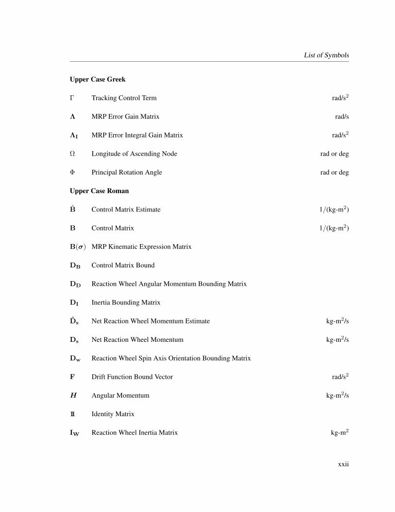
Upper Case Greek
Γ Tracking Control Term rad/s2
Λ MRP Error Gain Matrix rad/s
ΛI MRP Error Integral Gain Matrix rad/s2
Ω Longitude of Ascending Node rad or deg
Φ Principal Rotation Angle rad or deg
Upper Case Roman
B Control Matrix Estimate 1/(kg-m2)
B Control Matrix 1/(kg-m2)
B(σ) MRP Kinematic Expression Matrix
DB Control Matrix Bound
DD Reaction Wheel Angular Momentum Bounding Matrix
DI Inertia Bounding Matrix
Ds Net Reaction Wheel Momentum Estimate kg-m2/s
Ds Net Reaction Wheel Momentum kg-m2/s
Dw Reaction Wheel Spin Axis Orientation Bounding Matrix
F Drift Function Bound Vector rad/s2
H Angular Momentum kg-m2/s
11 Identity Matrix
IW Reaction Wheel Inertia Matrix kg-m2
xxii

List of Symbols
I Inertia Matrix kg-m2
K Gain Matrix rad/s2
L Torque N-m
Lmax Torque Bound N-m
M Mean Anomaly
Ω Reaction Wheel Speed rad/s
P Gain Matrix kg-m2/s
R Rotation Matrix
T Decay Time s
V Lyapunov Function
Ws Reaction Wheel Spin Axis Matrix
Lower Case Roman
a Orbit Semi-Major Axis km
b Semi-Minor Axis km
drw Maximum Reaction Wheel Fractional Error of Torque
e Principal Rotation Axis
e Orbit Eccentricity
f Drift Function Estimate rad/s2
f Drift Function rad/s2
f True Anomaly rad or deg
xxiii

List of Symbols
f Flattening Ratio of Elliptical Earth Model
h Altitude Above Earth Surface km
hs Reaction Wheel Spin Axis Angular Momentum kg-m2/s
i Orbit Inclination rad or deg
p Semi-Latus Rectum km
q Quaternion
rECEF Position Vector in ECEF Coordinates km
rD Chief Spacecraft Orbit Radius km
rD Deputy Spacecraft Orbit Radius km
s Sliding Variable Vector rad/s
t Time s
u Torque Control Vector N-m
ueq Equivalent Control Vector N-m
urob Robust Control Vector N-m
vg Ground Velocity m/s
vv Vertical Velocity m/s
x State Vector
z Integral Term rad/s
xxiv

1 Introduction
Spacecraft formation flying has potential for missions involving coordinated pointing, interferome-
try, stereographic imaging, and synthetic apertures. Many of these scientific missions require precise
relative position and attitude knowledge. A spacecraft formation is a distributed system comprised
of multiple spacecraft. Each spacecraft has an independent attitude and orbit control system that
controls the attitude and orbital position of each spacecraft and cooperates with the other spacecraft
to control the relative attitudes and positions of the spacecraft within the formation. The control
decisions for each spacecraft must be coordinated to ensure the stability and convergence of the
global system.
1.1 Distributed Space Systems
There are many strategies to control the attitude and orbital position of a single spacecraft. The
control effort required depends on the specific mission objectives. In the past few years much
research has been conducted with regards to controlling the relative position between spacecraft
using classical orbital elements (COE).1,2,3,4,5 Recently, spacecraft formation flying research is
directed toward the relative attitude and orbit control of spacecraft within the formation. Much of
the relative attitude and orbit control research includes development of estimation techniques.6,7,8,9
Spacecraft formation flying is an attractive alternative to the traditional single satellite mission
architecture. Multiple spacecraft provide a higher level of redundancy in the case of a failure as
compared with single spacecraft due to replacing a smaller, cheaper spacecraft or the ability to re-
1
1.1 Distributed Space Systems
configure the formation to achieve mission objectives. Typically the individual spacecraft within
the formation will be smaller in comparison with a single spacecraft which directly leads to cheaper
launch costs. The ability to re-configure the formation allows components to be upgraded within
the formation by replacing specific spacecraft with new spacecraft.
There is currently an initiative referred to as “Responsive Space”.∗ The initiative is in response
to the scenario where a critical military or scientific spacecraft unexpectedly cannot satisfy the
critical mission objectives. Spacecraft component failures from solar flares, meteoroids, or hostile
actions are some situations in which a spacecraft might become nonoperational. The Responsive
Space general concept is small, low-cost spacecraft can be stored on the ground and then can be
rapidly launched. The objective is to reduce cost per satellite and to rapidly add space assets for a
variety of mission objectives.
The Responsive Space initiative is an ideal concept to fulfill needs of formation flying, where
the desire for multiple smaller, cheaper, and rapidly deployed space vehicles satisfy the mission
objectives of large expensive single spacecraft mission. The Responsive Space initiative takes ad-
vantage of mass production techniques to reduce the overall cost per vehicle. The reduction in cost
for individual spacecraft will increase the interest in using a formation of spacecraft to achieve the
objectives typically achieved by a large, expensive, single spacecraft.
The use of spacecraft formation flying to achieve mission objectives is limited by the high visi-
bility of space missions, the high cost associated with space missions, and the higher risk associated
with the implementation of new concepts. Advancements in formation flying technology will re-
duce the higher-risk associated with formation flying as compared with single spacecraft missions.
Simulations provide valuable knowledge for validating concepts and missions. Many of these sim-
ulations are software-based architectures. At Virginia Polytechnic Institute and Sate University we
have developed a hardware-in-the-loop Distributed Spacecraft Attitude Control System Simulator
(DSACSS) to provide a more realistic demonstration of expected performance of distributed space
systems as compared with software-based architectures.
∗Information about Responsive Space may be obtained at www.responsivespace.com
2

1.2 Dissertation Objective
1.2 Dissertation Objective
The DSACSS is developed to experimentally demonstrate formation flying control strategies to
provide a more realistic demonstration of expected performance as compared with numerical simu-
lations.
The DSACSS can investigate linear and nonlinear control strategies in real-time for multiple
spacecraft in a coordinated activity such as shown in Figure 1.1. The two spacecraft in Figure 1.1
are an example of a distributed space concept. The two spacecraft are in low Earth orbit (LEO)
and determine the navigation solution using GPS receivers while independently determining their
respective attitude.
Figure 1.1: Distributed Space Systems Concept
3

1.3 Dissertation Overview
In the distributed space systems concept, Spacecraft 1 has a larger, but less refined sensor
footprint than Spacecraft 2. In this example, Spacecraft 1 is inspecting a large area on the surface of
the Earth and determines an area of interest where further investigation is warranted and additional
sensors are needed. Spacecraft 1 transmits the location of the area of interest to Spacecraft 2.
Mission requirements are such that the relative distance (r12) between Spacecraft 1 and 2 must
be maintained within a specific tolerance throughout the mission. Spacecraft 2 has a small sensor
footprint and must precisely control the pointing of the sensor unit to adequately investigate the area
of interest.
Precise relative orbit and attitude determination and control are required to successfully achieve
mission objectives. The DSACSS has been developed for the previously described scenario, which
can be used to investigate a variety of control schemes. GPS receivers are implemented into the
simulator for navigation control. Magnetometers, accelerometers, and rate gyros are implemented
for attitude determination and reaction wheels and thrusters are implemented for real-time control.
The capability to investigate distributed space system control strategies in a real-time hardware-in-
the-loop simulation is extremely unique and immensely valuable in evaluating the control strategies.
1.3 Dissertation Overview
Chapter 2 presents a literature review that includes a discussion on hardware-in-the-loop spacecraft
simulators, nonlinear control, spacecraft attitude control, and spacecraft orbit control. Chapter 3
presents the Distributed Spacecraft Attitude Control System Simulator (DSACSS) and the closed-
loop, hardware-in-the-loop GPS simulator that has been developed to investigate distributed space
system control strategies. Chapter 4 presents the spacecraft kinematic expressions for the quater-
nion and modified Rodrigues parameter attitude representations and derives the spacecraft rigid
body dynamics with momentum exchange devices. Chapter 5 presents the development of nonlin-
ear Lyapunov based spacecraft attitude control laws. The development and demonstration on the
hardware attitude simulators of an asymptotically stable angular rate controller and modified Ro-
drigues parameter attitude controller are shown. Chapter 6 presents the development of a nonlinear
4

1.3 Dissertation Overview
sliding mode spacecraft attitude controller that tracks a reference attitude using reaction wheels as
the actuator while bounding system uncertainties. Numerical and hardware-in-the-loop simulations
demonstrate the capabilities of the controller. Chapter 7 presents the results of a GPS hardware-
in-the-loop formation flying simulation using a nonlinear Lyapunov based classical orbital element
feedback controller. Chapter 8 develops a classical orbital element feedback control law based on
the sliding mode methodology while bounding system uncertainties and demonstrates the controller
using the GPS simulator. Chapter 9 summarizes this text and provides suggestions for future work.
5

2 Literature Review
In this chapter we summarize the relevant work associated with distributed space systems and non-
linear attitude and orbit control strategies. A review of air bearing platforms for space applications
is presented. Discussions on nonlinear control, attitude control, and orbit control are presented.
2.1 Spacecraft Simulators
Air bearing platforms have been used since the 1950’s to evaluate hardware components and soft-
ware for space applications. Air bearing platforms typically have a spherical ball floating on air,
which provides a nearly torque free environment between the interaction of the ball and pedestal.
Therefore spherical air bearing platforms are a common device for attitude dynamics research. Var-
ious configurations of the platforms exist depending on the desired application. The air bearing
platforms only provide rotational motion about a fixed point.
A three-axis air bearing platform was developed at NASA Marshall Space Flight Center, which
was used for the NIMBUS second generation weather satellite and the proposed Orbiting Astro-
nomical Observatory. NASA Goddard Space Flight Center developed a spherical air bearing to
investigate energy dissipation, which had plagued missions such as Explorer-1, Applications Tech-
nology Satellite-5, and TACSAT-1.10
In 1975 Stanford University was the first university to develop and use for research an air
bearing platform. Spacecraft contractors such as Lockheed Martin, Boeing, and TRW have small to
large scale air bearing platforms, but very little publicly available information. In 1995 the Naval
6

2.2 Nonlinear Control
Postgraduate School developed an air bearing three axis attitude dynamics and control simulator
to demonstrate the dynamics and control of a twin mirror bifocal relay spacecraft that uses laser
beams. Another air bearing platform is used for evaluating flight hardware-in-the-loop at the Naval
Postgraduate School.10
Utah State University developed an air bearing spacecraft simulator to test the attitude deter-
mination and control system for the Space Dynamics Laboratory’s Skipper spacecraft and was able
to identify a number of integration problems between various spacecraft subsystems. Georgia Tech
has several air bearing platforms for undergraduate and graduate education and nonlinear control
investigations.10
In the early 1990s the Air Force Research Laboratory and Naval Research Laboratory devel-
oped large spherical air bearing platforms to investigate the interaction between control input and
structure. The systems have been used for space based laser research and robust nonlinear control
and model reduction techniques for coupled attitude control and energy storage.10
NASA Goddard Space Flight Center has developed a Formation Flying Testbed (FFTB) to
demonstrate relative navigation technologies for spacecraft.11 The testbed is comprised of oper-
ational GPS receivers and Spirent Federal Systems GPS simulators. The closed-loop, hardware
simulation allows for testing of navigation and control software using real hardware.12 A real-time
autonomous formation flying software has been tested using the FFTB to estimate the absolute and
relative states of the spacecraft within the formation to a control precision in the meter range.5 A
sample low earth orbit demonstration of Precision Formation Flying (PFF) to demonstrate various
guidance navigation and control strategies has been investigated using the FFTB.1
2.2 Nonlinear Control
Nonlinear control deals with the analysis and design of control strategies for nonlinear systems
such as spacecraft attitude and orbit control. The objective of the nonlinear controller is to design a
controller that satisfies the desired response.
Linear control has been successfully implemented for a variety of applications such as missile,
7

2.3 Attitude Control
aircraft, and spacecraft GN&C (guidance, navigation, and control). A system, such as a “collection
of interacting elements which there are cause-and-effect relationships between the variables,”13 is
typically nonlinear in nature and is described through a mathematical model. The nonlinear model
is linearized to obtain the linear model from which the linear controller is derived. Nonlinear con-
trol is preferred over linear control for improvement of existing control systems, analysis of hard
nonlinearities, dealing with model uncertainty, and design simplicity.14
Nonlinear control may be an improvement to existing linear control systems, because linear
control is typically valid for a small operation range. As the range of operation increases the perfor-
mance, accuracy and precision of the linear controller decreases for a highly nonlinear system due
to the contribution of the nonlinear terms. A nonlinear controller can be designed to directly handle
a large range of operation.14
Hard nonlinearities is a term used to describe nonlinearities which are discontinuous in nature
with no linear approximation such as Coulomb friction, saturation, and dead-zones.14 The hard
nonlinearities must be evaluated to prevent adverse control behavior such as system instabilities.14
Linear control assumes the system parameters are well known, which for a real system the
parameters may not be well known. Parametric uncertainties and un-modeled dynamics can have
an adverse effect on controlling a nonlinear system. Nonlinear control provides two control technics
to account for system uncertainties. The two effects can be dealt with through robust or adaptive
control. Robust control is structured such that the controller has a nominal term and additional
terms are added to account for the model uncertainty. Adaptive control updates the model during
operation to account for model uncertainty.14
2.3 Attitude Control
Parametric uncertainties and un-modeled dynamics can have an adverse effect on controlling the
attitude of a nonlinear system. A common robust control technique is the sliding control method-
ology also referred to in the literature as variable structure control. Sliding control ensures stability
and consistent performance with system uncertainties.14 Sliding mode control is a popular closed
8
2.4 Orbit Control
loop technique for robust spacecraft attitude control.15,16,17,18,19,20,21,22,23,24
Reference 19 derives a Cayley-Rodrigues attitude sliding mode controller that is asymptotically
stable. A decoupled linearization of the attitude parameters was used in the control law. The con-
troller demonstrated rest to rest maneuver using jet thrusters for the attitude control. The controller
successfully drove the errors to zero.
Reference 15 derives a general attitude representation sliding mode controller that uses n re-
action wheels as the attitude actuator for a spacecraft. The controller accounts for parameter un-
certainties for the reaction wheels and un-modeled dynamics. The general attitude representation
is the relative rotation between the desired and actual attitude. An issue that arises by using the
attitude representation outlined in the paper is the approximation that θerror = ωerror. The approx-
imation breaks down at large attitude errors. The numerical simulation results show the controller
successfully satisfies the objective of the scenario, which was to track a specified ground station.
Reference 16 derives a Modified Rodrigues Parameter (MRP) sliding mode controller for the
regulation and tracking problem of a spacecraft. The controller is not designed for a specific atti-
tude actuator such as thrusters or reaction wheels. Therefore the uncertainties associated with the
actuators are not accounted for in the controller. The paper omits the discussion for determining
the robust control term gain. Only the numerical simulation results for the regulation problem is
presented, which demonstrates the MRP and angular rate errors converging to zero.
2.4 Orbit Control
Spacecraft formation flying involves controlling the relative position of multiple spacecraft. Current
interests in spacecraft formations include, but are not limited to clusters used for sparse aperture
radar dish in space,25 Earth-based remote sensing, and upper atmospheric sciences.2
Propulsion systems apply a force to the spacecraft, which controls the orbit. A primary concern
with spacecraft formation flying is fuel consumption. Controller design is crucial for the purpose
of conserving fuel. Obviously, a good spacecraft controller will use as little fuel as possible to
accomplish the maneuver. There are a variety of linear control strategies such as linear quadratic
9

2.4 Orbit Control
regulator (LQR), quantitative feedback control (QFC), and H∞ approaches to control the relative
positions of multiple spacecraft.
Figure 2.1 is a diagram of two spacecraft in formation where x, y, and z, are the distances
between the deputy spacecraft and chief spacecraft. The chief orbit radius is specified as rC and the
deputy orbit radius is rD. The true anomaly difference is specified as ∆f .
Figure 2.1: Two Spacecraft in Formation
The nonlinear equations of motion for controlling the relative position of the deputy spacecraft
10

2.4 Orbit Control
based on the chief spacecraft for no environmental perturbations acting on either spacecraft are25,26
x− 2f(y − y rcrc
)− xf2 − µ
r2c
= − µ
r3D
(rc + x) + uDx (2.1)
y + 2f(x− xrcrc
)− yf2 = − µ
r3D
y + uDy (2.2)
z = − µ
r3D
z + uDz (2.3)
where µ is the gravitational constant and uD is the control acceleration for the deputy spacecraft.
Equation (2.3) is simplified by assuming the relative distances between the spacecraft are small
compared to rC and higher order terms are neglected results in the following general form25
x− x(θ2 + 2
µ
r3C
)− yθ − 2yθ = uDx (2.4)
y + xθ + 2xθ − y(θ2 − µ
r3C
)= uDy (2.5)
z +µ
r3C
z = uDz (2.6)
where θ is ω + f .
The Clohessy-Wiltshire (CW) equations,27 which are often referred to as the Hill equations, are
obtained from Equation 2.6 by assuming the chief satellite is in a circular orbit which results in25,28
x− 2ny − 3n2x = uDx (2.7)
y + 2nx = uDy (2.8)
z + n2z = uDz (2.9)
where n is the mean motion of the chief spacecraft.
The CW equations are used to investigate rendezvous and docking and relative position be-
tween two spacecraft using linear control strategies.27,29,30 The CW equations do not take into
account orbital perturbations, large separation distances ( larger than 1 km), and noncircular orbits (
eccentricity greater than 0.00001).31 Reference 32 includes a modified version of the CW equations,
11
2.5 Summary
which allows large separation distances and an elliptical chief orbit. Again, linear control strategies
are implemented.
In the past few years much research has been conducted with regards to controlling the relative
position between spacecraft using nonlinear control strategies. A popular nonlinear orbit control
strategy is a Lyapunov based classical orbital element (COE) feedback controller.1,2,3,4,5,25 The
COE vector is comprised of semi-major axis (a), eccentricity (e), inclination (i), longitude of
ascending node (Ω), argument of perigee (ω), and mean anomaly (M). The controllers control the
relative orbital parameters between the space vehicles.
2.5 Summary
This chapter summarizes the relevant work associated with hardware spacecraft simulators and
nonlinear attitude and orbit control strategies. Many companies and government agencies such
as NASA and AFRL have used air bearing platforms to evaluate hardware and software compo-
nents for space applications. A common nonlinear robust control technique is the sliding control
methodology, which ensures stability and consistent performance with system uncertainties. Sliding
mode control is a popular closed loop technique for robust spacecraft attitude control. Orbit control
for multiple spacecraft involves linear control strategies based on the Clohessy-Wiltshire equations.
Nonlinear orbit control strategies for multiple spacecraft have recently concentrated on relative clas-
sical orbital element feedback control. The controllers control the relative position between multiple
spacecraft.
We have developed a high fidelity solution for Earth-based real-time hardware-in-the-loop sim-
ulations of space vehicles to evaluate nonlinear control strategies for distributed space systems.
Chapter 3 discusses the development and operation of the distributed spacecraft attitude and orbit
control simulators.
12

3 Distributed Spacecraft Attitude Control
System Simulator (DSACSS)
The Distributed Spacecraft Attitude Control System Simulator (DSACSS) facility housed in the
Space Systems Simulation Laboratory (SSSL)∗ provides a high fidelity solution for Earth-based
real-time hardware-in-the-loop simulations of space vehicles. DSACSS allows individual and com-
ponent level development and testing of hardware and software interfaces. DSACSS is comprised
of two hardware simulators and one software spacecraft simulator mounted on separate platforms
that allow the ability to demonstrate decentralized control algorithms. The two hardware simulators
are mounted on individual spherical air bearing platforms, which allow only for rotational motion.
The two hardware simulators have different configurations and consequently a different amounts of
rotational freedom. The third simulator is comprised of software running on a flight computer. The
operating system and DSACSS code for each simulator are maintained as open source.33,34,10,35
The Global Positioning System (GPS) Laboratory at Virginia Tech provides a real-time hardware-
in-the-loop navigation solution by simulating GPS RF signals. The GPS simulator has been inte-
grated into the DSACSS facility to simulate the trajectory of low Earth orbit (LEO) spacecraft.36,37
In the following sections, we discuss the DSACSS system control capabilities, which include
the hardware and software, the control capabilities of the system, and the visualization tools inte-
grated into the DSACSS system to assist with spacecraft related dynamics and control research.
∗Information about the SSSL may be obtained at www.sssl.aoe.vt.edu
13

3.1 Attitude Hardware-in-the-loop Simulators
3.1 Attitude Hardware-in-the-loop Simulators
As previously mentioned DSACSS is comprised of two attitude spacecraft hardware simulators
mounted on individual spherical balls floating on air, which allow only for rotational motion. The
air bearing platforms provide a nearly torque-free environment for simulating attitude control. The
simulators are referred to as Whorl−I and Whorl−II.†
Whorl−I is shown in Figure 3.1, which is a “tabletop” style configuration and provides one
complete axis of freedom. The yaw axis has rotational freedom of 360 while the roll and pitch
axes have± 6.5. The axes for Whorl−I are defined in Figure 3.1. Whorl−I has a 48 inch (122 cm)
by 48 inch footprint with a height of 88 inches (224 cm). The simulator has a maximum payload of
300 pounds (136 kg).33
Whorl−I and Whorl−II have detailed computer aided drawings (CAD), which provide an esti-
mate of the mass and inertia matrix for each simulator. The mass estimate is 88.5 kg and the inertia
matrix estimate is
I =
8.8 0.7 −0.2
0.7 7.7 −0.1
−0.2 −0.1 13.0
kg-m2 (3.1)
for Whorl−I where (·) indicates parameter estimate.
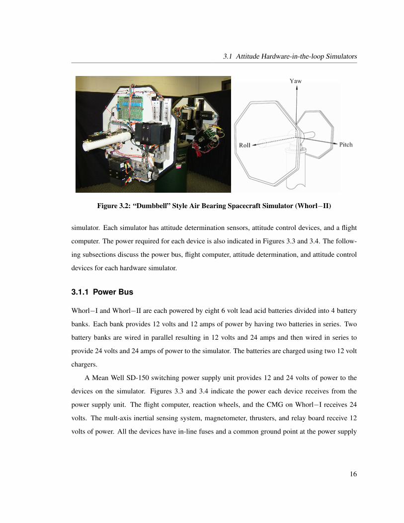
Whorl−II is shown in Figure 3.2, which is a “dumbbell” style configuration and provides two
complete axes of freedom. The yaw and roll axes have rotational freedom of 360 while the pitch
axis has ± 30. The axes for Whorl−II are defined in Figure 3.2. Whorl−II has a 70 inch (179 cm)
by 70 inch footprint with a height of 70 inches (179 cm). The simulator has a maximum payload of
300 lbs (136 kg).33
†The name Whorl comes from The Book of the Long Sun by Gene Wolfe. In the science fiction novel Whorl is the nameof a starship that has been traveling through space for hundreds of years.
14

3.1 Attitude Hardware-in-the-loop Simulators
Figure 3.1: “Tabletop” Style Air Bearing Spacecraft Simulator (Whorl−I)
The mass estimate is 249.6 lbs (113.2 kg) and the inertia matrix estimate is
I =
3.8 1.4 −1.2
1.4 26.1 0.2
−1.2 0.2 26.1
kg-m2 (3.2)
for Whorl−II.
Whorl−I and Whorl−II have similar subsystems as flight ready spacecraft (e.g. command and
data handling; communications; attitude determination and control; power; payload; and guidance
and navigation). The system block diagrams for Whorl−I and Whorl−II are shown in Figures 3.3
and 3.4.
The system block diagrams for Whorl−I and Whorl−II are identical except Whorl−I has a
control moment gyro (CMG). As seen can be seen in Figures 3.1 and 3.2 the various devices for
attitude determination and control are at different locations due to the configuration of each attitude
15
3.1 Attitude Hardware-in-the-loop Simulators
Figure 3.2: “Dumbbell” Style Air Bearing Spacecraft Simulator (Whorl−II)
simulator. Each simulator has attitude determination sensors, attitude control devices, and a flight
computer. The power required for each device is also indicated in Figures 3.3 and 3.4. The follow-
ing subsections discuss the power bus, flight computer, attitude determination, and attitude control
devices for each hardware simulator.
3.1.1 Power Bus
Whorl−I and Whorl−II are each powered by eight 6 volt lead acid batteries divided into 4 battery
banks. Each bank provides 12 volts and 12 amps of power by having two batteries in series. Two
battery banks are wired in parallel resulting in 12 volts and 24 amps and then wired in series to
provide 24 volts and 24 amps of power to the simulator. The batteries are charged using two 12 volt
chargers.
A Mean Well SD-150 switching power supply unit provides 12 and 24 volts of power to the
devices on the simulator. Figures 3.3 and 3.4 indicate the power each device receives from the
power supply unit. The flight computer, reaction wheels, and the CMG on Whorl−I receives 24
volts. The mult-axis inertial sensing system, magnetometer, thrusters, and relay board receive 12
volts of power. All the devices have in-line fuses and a common ground point at the power supply
16

3.1 Attitude Hardware-in-the-loop Simulators
Figure 3.3: Whorl−I System Block Diagram
unit.
A power control scheme has been implemented on Whorl−I to allow the flight computer to
control independently the power to each device. The flight computer turns on and off the devices
through a digital acquisition (DAQ) card by opening or closing a relay switch located on the relay
board. The power control scheme provides the user with the ability to turn off devices that are not
needed for the simulation. The power control scheme is also an added safety measure as it allows
the flight computer to turn off devices (including the flight computer) due to any unexpected event
during a simulation.
17

3.1 Attitude Hardware-in-the-loop Simulators
Figure 3.4: Whorl−II System Block Diagram
3.1.2 Flight Computer and Communications
Each simulator is controlled by its own flight computer as shown in Figures 3.3 and 3.4. Each flight
computer is a PC/104 stack comprised of a 733 MHz processor, 512 MB of RAM, and an 8 GB flash
drive. Each flight computer has an additional 30 GB of space through a private wireless network
connection to a shared drive for the purpose of developing and evaluating code. The operating
system on the PC/104 computers is Scientific Linux 4 (SL4).‡
Each PC104 stack has a HE104 vehicle power supply unit that receives 24 volts from the sim-
ulator batteries. Analog and digital devices interface with the PC/104 through a Diamond Systems
‡Scientific Linux is an open source operating system that is a recompiled version of Enterprise Linux. The primarycontributors are Fermilab and CERN with other labs and universities participating.
18
3.1 Attitude Hardware-in-the-loop Simulators
DMM-32 analog and digital (A/D) board with 32 analog inputs (16 bit resolution), 4 analog outputs
(12 bit resolution), and 32 digital I/O lines. An eight port XDB-9 RS-232 USB serial adapter data
control box manufactured by Vscom is interfaced with the flight computer through a USB port for
communicating with the reaction wheels, linear actuators, and magnetometers.
The flight computers communicate with each other and with other laboratory resources using
a wireless multi-client bridge/access point. The wireless bridge operates at 2.4 GHz and supports
802.11b wireless standard. The bridge uses 64/128-bit WEP data encryption and requires no drivers.
Configuration is accomplished through a web browser interface and the bridge connects to the com-
puter through a RJ45 port. USB wireless adapters were implemented in the past, but replaced with
the wireless bridges due to the lack of drivers available for Linux.
Figure 3.5 is a diagram showing the DSACSS communication scheme. The Whorls communi-
cate between each other through a wireless router. The spacecraft simulators also communicate with
lab computers such as Severian and Typhon. Severian provides orbit information for each simulator
and is discussed in following sections. Typhon is used for development and testing of the simulation
code. Severian and Typhon both use SL4 as the operating system.
3.1.3 Attitude Determination
Whorl−I and Whorl−II determine their respective attitudes using angular rate gyros, accelerome-
ters, and magnetometers, along with an user choice of attitude determination algorithms.
3.1.3.1 Attitude Sensors
The multi-axis inertial sensing system (BEI MotionPak II) has three-axis rate gyros and accelerome-
ters, which are used for attitude determination. The MotionPak senses up to±75 degrees per second
and maximum accelerations of ±1.5 g in their respective axes. The MotionPak is powered by 12
volts and communicates with the flight computer through the analog channels of the DAQ card.
The magnetometer (Honeywell HMR2300 Smart Digital Magnetometer) measures the mag-
netic field in the 3 sensor body axes. The flight computer communicates with the magnetometer
19

3.1 Attitude Hardware-in-the-loop Simulators
Figure 3.5: DSACSS Communication Schematic
through RS-232 serial data interface in binary mode. The magnetometer has a range of ±2 gauss
with less than 70 µgauss resolution and is powered by 12 volts.
The magnetometer on Whorl−I is mounted on a boom 49 inches (124 cm) above the rotation
point of the simulator to reduce the magnetic interference from the air-bearing platform and devices
on the simulator. The magnetometer on Whorl−II is mounted on a boom 10 inches (25 cm) from the
simulator. The boom length is constrained to 10 inches, because Whorl−II is inside an aluminum
and plexiglass cage for safety reasons. Due to the constraint, the magnetometer on Whorl−II expe-
riences more magnetic interference from the air-bearing platform and devices on the simulator than
20
3.1 Attitude Hardware-in-the-loop Simulators
the magnetometer on Whorl−I.
The magnetic interference on Whorl−II was resolved by calibrating the magnetometer mea-
surements to account for hard and soft iron distortion as outlined in Ref. 38. Hard iron distortions
are due to ferrous materials such as magnets and steel that are mounted on the same rigid platform
as the magnetometer. The magnetic distortion adds a constant component along each magnetically
sensed axis independent of the attitude of the magnetometer. For Whorl−II the hard iron distor-
tion arises from the components and structure of the simulator except for the air-bearing platform.
Soft iron distortions come from ferrous materials not mounted on the same rigid platform as the
magnetometer. The distortion component along each sensed axis is a function of attitude of the
magnetometer. The air-bearing platform for Whorl−II is the main contributor to soft iron distor-
tions.
The calibration technique is based on how hard and soft iron distortions affect the measure-
ments differently. Consider only 2-D motion of the magnetometer, such as would be the case for
determining heading of an aircraft. If the magnetometer is rotated 360, and there are no magnetic
distortions, the plot of the x and y sensor components results in a circle centered at the origin. In the
previous scenario, if only hard iron distortions are present, graphing x and y components results in a
circle with an offset from the origin. Subtracting the offset from every measurement eliminates the
hard iron disturbance. If only soft iron distortions are present, graphing x and y components results
in an ellipse rotated by θ. Reference 38 suggests removing the soft iron disturbance by rotating the
ellipse by −θ, scaling the semi-major axis to change the ellipse to a circle, and then rotating the
measurement by θ. The calibration technique works very well for Whorl−II. The magnetometer
calibration is also implemented on Whorl−I.
3.1.3.2 Attitude Determination Algorithms
Two three-axis attitude determination algorithms have been implemented on Whorl−I and Whorl−II.
One is a deterministic method and the other is an extended Kalman filter (EKF).
The TRIAD algorithm implemented on Whorl−I and Whorl−II is a popular three-axis attitude
21

3.1 Attitude Hardware-in-the-loop Simulators
determination algorithm for spacecraft, because the algorithm is simple. The algorithm uses only
two vector observations.39 For Whorl−I and Whorl−II the gravity and magnetic field vectors are
used.
The algorithm creates two “TRIAD” frames from the two body and inertial frame measure-
ments to determine the attitude matrix.40 Any number of attitude representations may be used once
the attitude matrix is known. The development and implementation of the TRIAD algorithm is
found in Refs. 39 and 40.
The Kalman filter represents an optimal method for attitude estimation when uncertainties are
present.41 The filter is a probability-based algorithm that minimizes the error in the estimate of
the state vector.41,42,43 There are numerous types of Kalman filters being used for spacecraft atti-
tude determination. For the attitude determination on Whorl−I and Whorl−II a discrete extended
Kalman filter presented in Ref. 42 is implemented.
The EKF uses a multiplicative error quaternion in the body frame to replace the four compo-
nents of the quaternion vector with three error components. The quaternion is discussed in Sec-
tion 4.1.1. The filter allows for n number of vector observations. The standard multiplicative
quaternion EKF algorithm is computationally expensive due to inverting a 3n× 3n matrix to solve
for the Kalman gains. A modification of the algorithm to decrease the computational load is im-
plemented based on processing one vector observation at a time, which results in inverting a 3 × 3
matrix n times and is typically referred to as Murrell’s Version.42,44
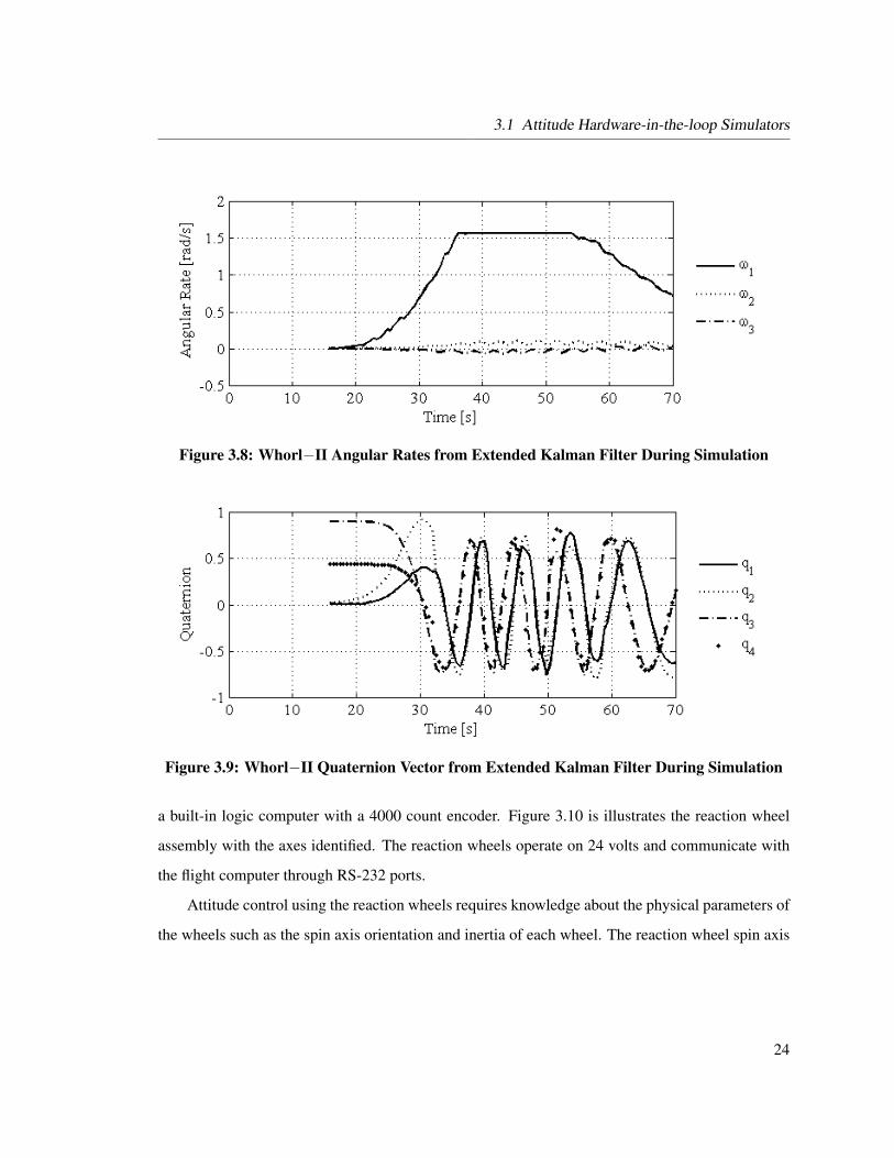
Figures 3.6 and 3.7 demonstrate the attitude determination system of Whorl−I and Whorl−II
by obtaining measurements from the MotionPak and magnetometer and using the EKF to estimate
the quaternion. Figures 3.6 and 3.8 show the angular rates and Figures 3.7 and 3.9 show the quater-
nion during an attitude control simulation, which is discussed in later chapters.
3.1.4 Attitude Control Devices
The attitudes of Whorl−I and Whorl−II can be controlled using reaction wheels, nitrogen gas (N2)
thrusters, and in the case of Whorl−I, a control moment gyro (CMG). There are three linear actua-
22

3.1 Attitude Hardware-in-the-loop Simulators
Figure 3.6: Whorl−I Angular Rates from Extended Kalman Filter During Control Simulation
Figure 3.7: Whorl−I Quaternion Vector from Extended Kalman Filter During Control Sim-ulation
tors, one along each of three mutually orthogonal axes. The linear actuators are used to change the
center-of-mass of each simulator to be co-located with the center-of-rotation.
Each simulator has a total of three custom reaction wheels. A reaction wheel is mounted on
each axis (x, y, & z also referred to as 1, 2, & 3). Each reaction wheel assembly is comprised of
an aluminum hub and steel rim (0.075 kg·m2) attached to a SM3430 Smart Motor. The motor has
23
3.1 Attitude Hardware-in-the-loop Simulators
Figure 3.8: Whorl−II Angular Rates from Extended Kalman Filter During Simulation
Figure 3.9: Whorl−II Quaternion Vector from Extended Kalman Filter During Simulation
a built-in logic computer with a 4000 count encoder. Figure 3.10 is illustrates the reaction wheel
assembly with the axes identified. The reaction wheels operate on 24 volts and communicate with
the flight computer through RS-232 ports.
Attitude control using the reaction wheels requires knowledge about the physical parameters of
the wheels such as the spin axis orientation and inertia of each wheel. The reaction wheel spin axis
24

3.1 Attitude Hardware-in-the-loop Simulators
orientation matrix estimate for Whorl−I is
Ws =
1 0 0
0 1 0
0 0 1
(3.3)
where (·) indicates a parameter estimate. The reaction wheel spin axis orientation matrix for
Whorl−II is
Ws =
−1 0 0
0 −1 0
0 0 1
(3.4)
The reaction wheel spin axis inertia estimate for each wheel is
IWsi= 0.075 kg-m2 i = 1, 2, 3 (3.5)
An attitude control law determines the necessary torque about each body axis to satisfy the
desired attitude objective. The reaction wheel controller receives the attitude control vector (u)
and determines the necessary wheel speed for each reaction wheel to produce the desired control
torque. A low-level reaction wheel controller has been developed and implemented on Whorl−I
and Whorl−II and is presented in Appendix A.
The CMG assembly consists of a SM3430 Smart Motor, wheel, and a linear actuator assembly
that allows a maximum gimbal angle of ±45. The CMG operates on 24 volts and communicates
with the flight computer through RS-232 ports.
The compressed-air thrusters provide another three-axis control capability. There are 6 thrusters
on Whorl−I and 8 on Whorl−II. The thrusters are supplied by 21 ft3 nitrogen tanks and are con-
trolled by a manual multistage regulator with a maximum delivery pressure of 50 psi. Each thruster
assembly consists of a 1/4 inch (6.35 mm) round nozzle with a 1/16 inch (1.58 mm) orifice diam-
25

3.1 Attitude Hardware-in-the-loop Simulators
Figure 3.10: Reaction Wheel Axes
eter and an Evolutionary Concepts 654-2207 solenoid. The solenoids are controlled by the flight
computer through the relay board.
As previously mentioned, an attitude control law specifies the necessary torque about each body
axis to satisfy the desired attitude objective. A thruster control module for Whorl−I and Whorl−II
is in development which will take the attitude control vector (u) and determines the firing duration
time for each thruster using a pulse width modulation (PWM) scheme.45,46,47
The primary purpose for the linear actuators is to position the center-of-mass of the simulator
at the center of rotation to eliminate the gravitational torque resulting from the offset. The linear
actuators are manufactured by Servo Systems and have a travel distance of 8 inches. The 5023-
122D stepper motor is controlled by a 1240i controller card running on 12 volts. Both devices are
manufactured by Applied Motion Products. Each actuator assembly can support 30 lbs (13.6 kg).
The flight computer communicates with the controller cards through RS-232 ports.
26

3.2 Software Simulator
3.2 Software Simulator
The software simulator is referred to as Whorl−III and is shown in Figure 3.11. Whorl−III is
identical to the flight computers on Whorl−I and Whorl−II, except hardware is not interfaced with
the computer. Whorl−III provides a third spacecraft attitude simulator. DSACSS has the capability
of simulating distributed attitude control between three spacecraft. Whorl−I and Whorl−II provide
realistic attitude motion while Whorl−III provides numerical attitude results.
Whorl−III also serves as a backup flight computer for Whorl−I and Whorl−II. In the event of
a flight computer failure on Whorl−I or Whorl−II the flight computers can be swapped seamlessly
with minimal down time.
Figure 3.11: Software Simulator (Whorl−III)
3.3 DSACSS Operational Code
The DSACSS Operational (DSACSS-Ops) code to operate the attitude simulators is specifically
designed for the hardware in the DSACSS facility. The architecture of DSACSS-Ops is based on
Object-Oriented-Programming (OOP) in C++. DSACSS-Ops is maintained as open-source soft-
ware.
27

3.3 DSACSS Operational Code
Figure 3.12 is a functional diagram of DSACSS-Ops. The dependences directory contains third
person open-source software. The documentation directory contains html documentation generated
using an open-source program (Doxygen§). The source directory contains the drivers for running
the simulators and conducting simulations. The work directory contains the configuration file and
allows users to develop simulation scenarios.
Figure 3.12: DSACSS-Ops Code Functional Diagram
Within the dependences directory there are 4 libraries. The matrix operations directory contains
a library for of matrix operations such as determination of eigenvalues and eigenvectors. The open§Information on Doxygen can be found at www.doxygen.org
28
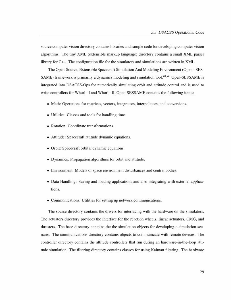
3.3 DSACSS Operational Code
source computer vision directory contains libraries and sample code for developing computer vision
algorithms. The tiny XML (extensible markup language) directory contains a small XML parser
library for C++. The configuration file for the simulators and simulations are written in XML.
The Open-Source, Extensible Spacecraft Simulation And Modeling Environment (Open - SES-
SAME) framework is primarily a dynamics modeling and simulation tool.48,49 Open-SESSAME is
integrated into DSACSS-Ops for numerically simulating orbit and attitude control and is used to
write controllers for Whorl−I and Whorl−II. Open-SESSAME contains the following items:
• Math: Operations for matrices, vectors, integrators, interpolators, and conversions.
• Utilities: Classes and tools for handling time.
• Rotation: Coordinate transformations.
• Attitude: Spacecraft attitude dynamic equations.
• Orbit: Spacecraft orbital dynamic equations.
• Dynamics: Propagation algorithms for orbit and attitude.
• Environment: Models of space environment disturbances and central bodies.
• Data Handling: Saving and loading applications and also integrating with external applica-
tions.
• Communications: Utilities for setting up network communications.
The source directory contains the drivers for interfacing with the hardware on the simulators.
The actuators directory provides the interface for the reaction wheels, linear actuators, CMG, and
thrusters. The base directory contains the the simulation objects for developing a simulation sce-
nario. The communications directory contains objects to communicate with remote devices. The
controller directory contains the attitude controllers that run during an hardware-in-the-loop atti-
tude simulation. The filtering directory contains classes for using Kalman filtering. The hardware
29

3.4 GPS Hardware-in-the-loop Simulator for GN&C Simulations
directory contains classes for communicating with the DAQ card. The data logging directory pro-
vides a class for recording data during a simulation. The observer directory contains the attitude
determination algorithms that have been developed. The orbit controller directory contains the or-
bit controllers used for the simulators. The orbit observer directory contains the classes to interface
with the GPS simulator, which is discussed in the next section. The power control directory provides
an interface for turning power on and off for devices on Whorl−I. The sensors directory provides
the interface for the MotionPak, magnetometer, and camera. The utilities directory provides classes
to interface with the programs in the dependences directory and simulation time classes. The STK
(Satellite Tool Kit) visualization directory provides classes for displaying attitude and orbit infor-
mation using STK developed by AGI.
3.4 GPS Hardware-in-the-loop Simulator for GN&C Simulations
The Global Positioning System (GPS) Laboratory at Virginia Tech provides a real-time hardware-
in-the-loop navigation solution capability for a variety of vehicles (e.g., automotive, ship, aircraft,
and spacecraft) by simulating real GPS RF signals. The GPS simulator can run in an open-loop
configuration for navigation simulations. Navigation, Guidance, and Control (GN&C) simulations
can be performed using the GPS simulator in a closed-loop configuration.
The manufacturer of the GPS simulator provides the open-loop configuration for simulating
vehicle trajectories. The closed-loop configuration is typically user specific; therefore the user must
develop the necessary tools for closed-loop GN&C simulations.
The closed-loop hardware-in-the-loop GPS simulator is integrated into the DSACSS facility to
simulate the GN&C of low Earth orbit (LEO) spacecraft. The closed-loop GPS system runs in real-
time and is comprised of a motion propagator, three RF signal generators, and four high dynamic
GPS receivers that provide the capability of simulating GN&C for spacecraft in low Earth orbit.
30
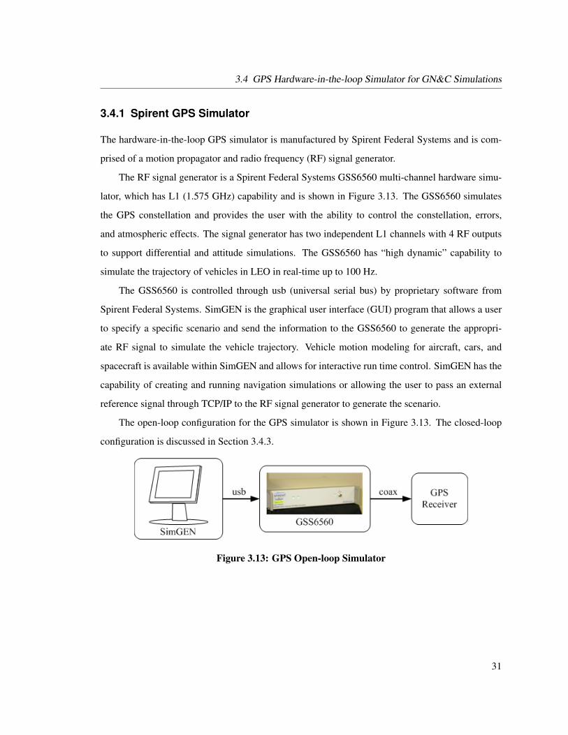
3.4 GPS Hardware-in-the-loop Simulator for GN&C Simulations
3.4.1 Spirent GPS Simulator
The hardware-in-the-loop GPS simulator is manufactured by Spirent Federal Systems and is com-
prised of a motion propagator and radio frequency (RF) signal generator.
The RF signal generator is a Spirent Federal Systems GSS6560 multi-channel hardware simu-
lator, which has L1 (1.575 GHz) capability and is shown in Figure 3.13. The GSS6560 simulates
the GPS constellation and provides the user with the ability to control the constellation, errors,
and atmospheric effects. The signal generator has two independent L1 channels with 4 RF outputs
to support differential and attitude simulations. The GSS6560 has “high dynamic” capability to
simulate the trajectory of vehicles in LEO in real-time up to 100 Hz.
The GSS6560 is controlled through usb (universal serial bus) by proprietary software from
Spirent Federal Systems. SimGEN is the graphical user interface (GUI) program that allows a user
to specify a specific scenario and send the information to the GSS6560 to generate the appropri-
ate RF signal to simulate the vehicle trajectory. Vehicle motion modeling for aircraft, cars, and
spacecraft is available within SimGEN and allows for interactive run time control. SimGEN has the
capability of creating and running navigation simulations or allowing the user to pass an external
reference signal through TCP/IP to the RF signal generator to generate the scenario.
The open-loop configuration for the GPS simulator is shown in Figure 3.13. The closed-loop
configuration is discussed in Section 3.4.3.
Figure 3.13: GPS Open-loop Simulator
31

3.4 GPS Hardware-in-the-loop Simulator for GN&C Simulations
3.4.2 Ashtech G12 HDMA GPS Receiver
An Ashtech G12 HDMA GPS receiver is interfaced with the GSS6560 RF signal generator through a
co-axial BNC socket as shown in Figures 3.13 and 3.14. The Ashtech G12 HDMA GPS receiver has
been integrated into systems such as the Super Sonic Naval Ordinance Research Track (SNORT),
NASA’s X-34 vehicle, and used for sounding rocket missions.50 The G12 provides real-time posi-
tion, velocity, and time measurements by processing signals from the simulated GPS constellation
produced by the GSS6560. The receiver has 12 channels for the L1 band and can be used in a
standalone or differential GPS (DGPS) mode.
The standard G12 receiver has limits placed on altitude and velocity up to equivalent dynamics
that an airliner would experience in standard operation. The HDMA version of the G12 turns off
the limits and provides a navigation solution for vehicles with equivalent dynamics as vehicles in
LEO.
The G12 is able to compute the navigation solution at 20 Hz. A position and velocity filter
provided as an option within the G12 software is used to reduce the noise effects. The smoothing
interval is set to 100 seconds. The velocity measurements are computed using doppler values and
all measurements are provided in the World Geodetic System 1984 (WGS-84) reference frame.
The position query command returns the number of satellites used to compute the position, the
current UTC time, latitude, longitude, altitude, heading, ground speed, vertical velocity, positional
dilution of precision (PDOP), horizontal dilution of precision (HDOP), vertical dilution of precision
(VDOP), and time dilution of precision (TDOP). Dilution of precision values between 1 and 3 are
very good, values between 4 and 5 are good, values around 6 are fair, and values greater than 6 are
poor.
3.4.3 Closed-hardware-in-the-loop Spacecraft GPS Simulator
The objective of integrating the GPS hardware-in-the-loop simulator into DSACSS is to provide
GN&C capability to Whorl−I, Whorl−II, and Whorl−III. The open-loop configuration previously
discussed provides navigation, but lacks the ability for real-time control. A real-time closed-loop
32
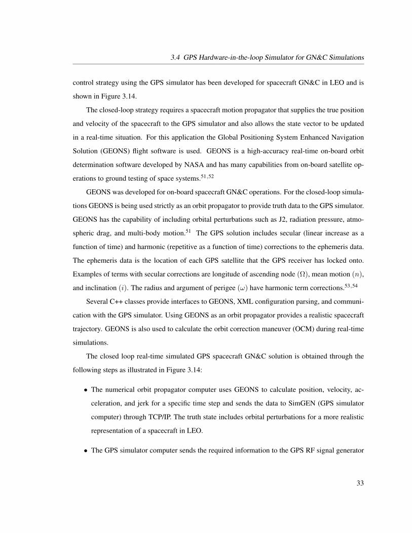
3.4 GPS Hardware-in-the-loop Simulator for GN&C Simulations
control strategy using the GPS simulator has been developed for spacecraft GN&C in LEO and is
shown in Figure 3.14.
The closed-loop strategy requires a spacecraft motion propagator that supplies the true position
and velocity of the spacecraft to the GPS simulator and also allows the state vector to be updated
in a real-time situation. For this application the Global Positioning System Enhanced Navigation
Solution (GEONS) flight software is used. GEONS is a high-accuracy real-time on-board orbit
determination software developed by NASA and has many capabilities from on-board satellite op-
erations to ground testing of space systems.51,52
GEONS was developed for on-board spacecraft GN&C operations. For the closed-loop simula-
tions GEONS is being used strictly as an orbit propagator to provide truth data to the GPS simulator.
GEONS has the capability of including orbital perturbations such as J2, radiation pressure, atmo-
spheric drag, and multi-body motion.51 The GPS solution includes secular (linear increase as a
function of time) and harmonic (repetitive as a function of time) corrections to the ephemeris data.
The ephemeris data is the location of each GPS satellite that the GPS receiver has locked onto.
Examples of terms with secular corrections are longitude of ascending node (Ω), mean motion (n),
and inclination (i). The radius and argument of perigee (ω) have harmonic term corrections.53,54
Several C++ classes provide interfaces to GEONS, XML configuration parsing, and communi-
cation with the GPS simulator. Using GEONS as an orbit propagator provides a realistic spacecraft
trajectory. GEONS is also used to calculate the orbit correction maneuver (OCM) during real-time
simulations.
The closed loop real-time simulated GPS spacecraft GN&C solution is obtained through the
following steps as illustrated in Figure 3.14:
• The numerical orbit propagator computer uses GEONS to calculate position, velocity, ac-
celeration, and jerk for a specific time step and sends the data to SimGEN (GPS simulator
computer) through TCP/IP. The truth state includes orbital perturbations for a more realistic
representation of a spacecraft in LEO.
• The GPS simulator computer sends the required information to the GPS RF signal generator
33

3.4 GPS Hardware-in-the-loop Simulator for GN&C Simulations
Figure 3.14: GPS Closed-hardware-in-the-loop Simulator
(GSS6560) based on the position, velocity, acceleration, jerk, and time through usb.
• The GPS receiver retrieves the RF signal and determines the navigation solution.
• The GPS interface computer is connected to the G12 receiver through a RS-232 port and
provides the interface for communicating with the G12 receiver over TCP/IP from a remote
source. The interface computer allows any flight computer with TCP/IP access to communi-
cate directly with the GPS receiver.
• The spacecraft flight computer retrieves the navigation solution and determines the OCM
based on the orbit control law being investigated. The OCM is sent to the numerical orbit
propagator computer over TCP/IP where GEONS simulates orbit thrusting of the spacecraft.
The high-level scheme for doing GN&C algorithm development using the GPS simulator is
outlined in Figure 3.15. The closed-loop nonlinear orbit control simulations using the scheme shown
in Figure 3.15 are presented in later chapters.
34

3.4 GPS Hardware-in-the-loop Simulator for GN&C Simulations
Figure 3.15: High-level GN&C Block Diagram
3.4.4 Coordinate Transformations for GPS Receiver
The Ashtech G12 GPS receiver returns WGS84 coordinates, but many of the controllers require the
coordinates to be Earth-center-inertial (ECI) coordinates or classical orbital elements (COE). The
latitude (φ), longitude (λ), altitude (h), heading(ψ), ground speed (vg), vertical velocity (vv) have to
be transformed into the desired coordinates. Mappings from WGS84 to Earth-centered-Earth-fixed
(ECEF) and ECEF to ECI are provided in the following subsections.
3.4.4.1 WGS84 / ECEF Coordinate Transformation
The mapping from latitude, longitude and altitude to ECEF position (rECEF) is54
rECEF =
(n+ h) cosφ cosλ
(n+ h) cosφ sinλ(n(1− 2f − f2
)+ h)
sinφ
(3.6)
35

3.4 GPS Hardware-in-the-loop Simulator for GN&C Simulations
where n is defined as
n =a√
1− (2f − f2) sin 2φ(3.7)
Note that a (6278.137 km) is the semi-major axis of the elliptical Earth and f (1/298.257) is the
flattening ratio of the elliptical Earth model. The relationship between flattening ratio and semi-
minor axis (b) is54
b = a(1− f) (3.8)
The mapping from north, east, down velocity (rNED) to ECEF velocity (rECEF) is
rECEF = R321(0,−φ− π/2, λ)T rNED (3.9)
where the rotation matrix (R321(0,−φ− π/2, λ)) is given by
R321(0,−φ− π/2, λ) = R2(−φ− π/2)R3(λ) (3.10)
The base rotation matrices about the 1, 2, and 3 axes are
R1(θ) =
1 0 0
0 cos θ sin θ
0 − sin θ cos θ
(3.11)
R2(θ) =
cos θ 0 − sin θ
0 1 0
sin θ 0 cos θ
(3.12)
36

3.4 GPS Hardware-in-the-loop Simulator for GN&C Simulations
R3(θ) =
cos θ sin θ 0
− sin θ cos θ 0
0 0 1
(3.13)
To compute WGS84 coordinates from ECEF coordinates requires using closed-form or iterative
solutions. The method implemented in DSACSS is by Bowring.55,56 Longitude is given by
λ = tan−1
(rECEFy
rECEFx
)(3.14)
Latitude is determined by an iterative method using
ρ =√r2
ECEFx+ r2
ECEFy(3.15)
βi = tan−1
((1− f) sinφi−1
cosφi−1
)for i = 1, 2, 3, . . . (3.16)
φi = tan−1
rECEFz + (1−f)(2f−f2)1−2f+f2 a sin3 βi
ρ− (2f − f2)a cos3 βi)
for i = 0, 1, 2, . . . (3.17)
where
β0 = tan−1
(rECEFz
(1− f)ρ
)(3.18)
is used on the initial step. For most applications two iterations should be sufficient.55,56 Once the
37

3.4 GPS Hardware-in-the-loop Simulator for GN&C Simulations
latitude is determined, the altitude is given by
h = ρ cosφ+ (rECEFz + (2f − f2)n sinφ) sinφ− n (3.19)
The mapping from rECEF to rNED is
rNED = R321(0,−φ− π/2, λ)rECEF (3.20)
The next section discusses the mapping between ECEF and ECI coordinates.
3.4.4.2 ECEF / ECI Coordinate Transformation
The mapping from ECEF position (rECEF) to ECI position (rECI) is
rECI = R3(θGMST)TrECEF (3.21)
where θGMST is defined as
θGMST = θGMST2000 + 86, 400ωEarth(Jday + 0.5) (3.22)
Note that GMST stands for Greenwich Mean Sidereal Time. The reference value for Jan 1, 2000
results in θGMST2000 (1.745 rad). The angular rate of the Earth is (ωEarth) 7.292 × 10⁻⁵ rad/s. The
Julian time is specified as Jday.
The mapping from ECEF velocity (rECEF) to ECI velocity (rECI) is
rECI =π
43, 200R3(θGMST)
TrECEF + R3(θGMST)T rECEF (3.23)
38

3.4 GPS Hardware-in-the-loop Simulator for GN&C Simulations
where the derivative of the rotation about the 3 axis is
R3(θ) =
− sin θ cos θ 0
− cos θ − sin θ 0
0 0 0
θ (3.24)
The mapping from rECI to rECEF is
rECEF = R3(θGMST)rECI (3.25)
The mapping from rECI to rECEF is
rECEF =π
43, 200R3(θGMST)rECI + R3(θGMST)rECI (3.26)
The coordinate transformations are used in the next section to determine the classical orbital
elements from the GPS receiver.
3.4.5 Example of Navigation Determination using GPS Receiver
This experiment is an open-loop simulation using the GPS simulator and Whorl−I. The initial
orbital conditions of Whorl-I are semi-major axis, a = 6978.15 km, eccentricity, e = 0.05, incli-
nation, i = 30, right ascension of ascending node, Ω = 0, argument of periapsis, ω = 45, and
Mean anomaly, M = 0.
The GPS receiver takes several minutes to lock onto at least 4 GPS satellites, which is the
minimum necessary to determine the navigation solution. Complete acquisition for a range of 6 to
10 GPS satellites varies from 5 to 30 minutes when simulating a spacecraft LEO trajectory.
The results of a 130 minute real-time open-loop simulation using Whorl−I are presented in
Figures 3.16 – 3.26. Figures 3.16 and 3.17 show the orbit radius and orbit velocity determined by
the GPS receiver in the ECI reference frame. Figure 3.18 shows the trajectory of the spacecraft
determined from the GPS receiver. The classical orbital elements time histories are shown in Fig-
39
3.4 GPS Hardware-in-the-loop Simulator for GN&C Simulations
ures 3.19 – 3.24. The GPS receiver parameters are shown in Figure 3.25. The PDOP increases to
approximately 5 in the interval of 75 to 80 minutes. The result of the increase in PDOP can be seen
as an increase in noise for the semi-major axis in Figure 3.19. The number of GPS satellites used to
determine the navigation solution is shown in Figure 3.26.
Figure 3.16: Whorl-I Orbit Radius Determined from the GPS Receiver in the ECI ReferenceFrame
Figure 3.17: Whorl−I Orbit Velocity Determined from the GPS Receiver in the ECI ReferenceFrame
40

3.4 GPS Hardware-in-the-loop Simulator for GN&C Simulations
Figure 3.18: Whorl−I Orbit Trajectory Determined from the GPS Receiver in the ECI Refer-ence Frame
Figure 3.19: Semi-Major Axis Time History for Whorl−I
41

3.4 GPS Hardware-in-the-loop Simulator for GN&C Simulations
Figure 3.20: Eccentricity Time History for Whorl−I
Figure 3.21: Inclination Time History for Whorl−I
42

3.4 GPS Hardware-in-the-loop Simulator for GN&C Simulations
Figure 3.22: Longitude of the Ascending Node Time History for Whorl−I
Figure 3.23: Argument of Perigee Time History for Whorl−I
43

3.5 Summary
Figure 3.24: True Anomaly Time History for Whorl−I
Figure 3.25: Whorl−I GPS Receiver Parameters (PDOP, HDOP, VDOP, and TDOP)
3.5 Summary
This chapter discusses the DSACSS control capabilities, which includes the hardware and software,
the control capabilities of the system, and the visualization tools integrated into the DSACSS system
to assist with spacecraft related dynamics and control research. The attitude hardware-in-the-loop
44

3.5 Summary
Figure 3.26: Number of GPS Satellites Used to Determine Navigation Solution
spacecraft simulators are described in detail along with estimates of their mass properties. The
attitude sensors are described in detail along with the attitude determination algorithms. The attitude
control devices for each simulator are described. The development of the reaction wheel controller
for the simulators is provided in Appendix A. The software, DSACSS-Ops, to run the simulators is
described in detail. The implementation of an attitude controller into DSACSS-Ops is described in
Appendix B. The GPS simulator and receiver are described in detail. A closed-loop hardware-in-
the-loop GPS simulation capability is developed and discussed.
The purpose of the attitude spacecraft hardware simulators is to mimic the expected response of
a spacecraft in orbit. The kinematic and rigid body equations that describe the motion of a spacecraft
in orbit are developed in Chapter 4.
45

4 Spacecraft Kinematics and Rigid Body
Dynamics
In this chapter we introduce the quaternion and modified Rodrigues parameters to describe the
attitude of a rigid body. Euler’s rotational equations of motion for a spacecraft with reaction wheels
are also presented.
4.1 Attitude Parameters
Attitude parameters are sets of coordinates that describe the orientation of an objective relative
to a frame of reference. The following sections discuss the quaternion and modified Rodrigues
parameter attitude representations, which are used in the following chapters.
4.1.1 Quaternion
The quaternion is a popular attitude coordinate that is nonsingular and can describe large rotations.
In the literature25,57 the quaternion is also referred to as Euler Parameters. The quaternion is com-
46
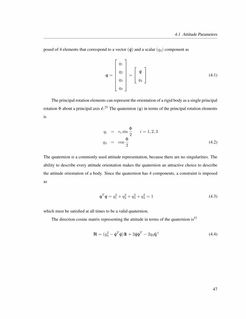
4.1 Attitude Parameters
posed of 4 elements that correspond to a vector (q) and a scalar (q4) component as
q =
q1
q2
q3
q4
=
q
q4
(4.1)
The principal rotation elements can represent the orientation of a rigid body as a single principal
rotation Φ about a principal axis e.25 The quaternion (q) in terms of the principal rotation elements
is
qi = ei sinΦ2
i = 1, 2, 3
q4 = cosΦ2
(4.2)
The quaternion is a commonly used attitude representation, because there are no singularities. The
ability to describe every attitude orientation makes the quaternion an attractive choice to describe
the attitude orientation of a body. Since the quaternion has 4 components, a constraint is imposed
as
qTq = q21 + q2
2 + q23 + q2
4 = 1 (4.3)
which must be satisfied at all times to be a valid quaternion.
The direction cosine matrix representing the attitude in terms of the quaternion is57
R = (q24 − qT q)11 + 2qqT − 2q4q× (4.4)
47
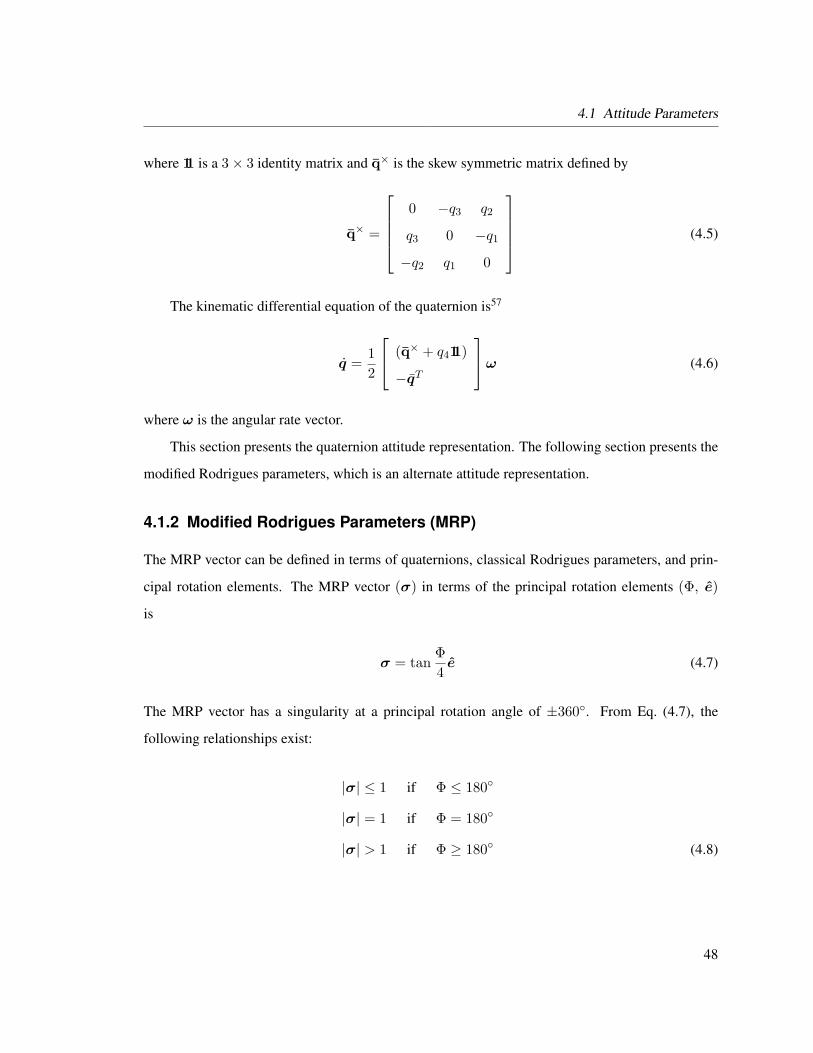
4.1 Attitude Parameters
where 11 is a 3× 3 identity matrix and q× is the skew symmetric matrix defined by
q× =
0 −q3 q2
q3 0 −q1
−q2 q1 0
(4.5)
The kinematic differential equation of the quaternion is57
q =12
(q× + q411)
−qT
ω (4.6)
where ω is the angular rate vector.
This section presents the quaternion attitude representation. The following section presents the
modified Rodrigues parameters, which is an alternate attitude representation.
4.1.2 Modified Rodrigues Parameters (MRP)
The MRP vector can be defined in terms of quaternions, classical Rodrigues parameters, and prin-
cipal rotation elements. The MRP vector (σ) in terms of the principal rotation elements (Φ, e)
is
σ = tanΦ4e (4.7)
The MRP vector has a singularity at a principal rotation angle of ±360. From Eq. (4.7), the
following relationships exist:
|σ| ≤ 1 if Φ ≤ 180
|σ| = 1 if Φ = 180
|σ| > 1 if Φ ≥ 180 (4.8)
48

4.1 Attitude Parameters
The relationships between the other attitude representations and the MRP vector can be found in
Ref. 25.
The MRP vector is a convenient attitude representation for attitude feedback control. Using the
relationship
σs1,2,3 =−σ1,2,3
σTσ(4.9)
the MRP vector can always represent a principal rotation angle less than or equal to 180.25 The
MRP mapping is exploited to develop the nonlinear attitude controllers presented in the following
chapters.
The direction cosine matrix in terms of the MRP vector is25
R = 11 +8σ×σ× − 4(1− σTσ)σ×
1 + σTσ(4.10)
where σ× is the skew symmetric matrix defined in Eq. (4.5)
The MRP error vector in terms of two MRP vectors is expressed as25
δσ =(1− |σ′|2)σ − (1− |σ|2)σ′ + 2σ × σ′
1 + |σ′|2|σ|2 + 2σ′ · σ(4.11)
The MRP kinematic differential equation is25
σ =(1− σ2)I + 2σ× + 2σσT
4ω (4.12)
σ =14B(σ)ω (4.13)
B(σ) = (1− σ2)I + 2σ× + 2σσT (4.14)
This section presents the MRP attitude representation. The next section presents the spacecraft
rigid body dynamics.
49

4.2 Rigid Body Dynamics
4.2 Rigid Body Dynamics
The rotational rigid body dynamics of a spacecraft with momentum devices is presented in the
following subsections, which will be used in later chapters to develop the attitude control laws.
Euler’s rotational equations of motion for a spacecraft are presented. The equations of motion
for a spacecraft with reaction wheels are presented.
4.2.1 Euler’s Rotational Equations of Motion
Euler’s rotational equations of motion for a rigid body spacecraft are25,28
Iω = −ω×Iω + u+Lext (4.15)
where I is the inertia matrix in the body frame (B), ω is the angular velocity of the spacecraft with
respect to the inertial frame (N ) expressed in the body frame (B),ω× is the skew symmetric matrix,
Lext is the external torque, and u is the control torque.
4.2.2 Euler’s Rotational Equations of Motion with Momentum Exchange
Devices
Each simulator has three orthogonal reaction wheels for attitude control as discussed in Section 3.1.4.
The spacecraft equations of motion with momentum exchange devices are required to develop the
attitude control laws in later chapters.
The equations of motion for a rigid spacecraft with N reaction wheels are25
Iω = −ω× (Iω + Wshs) + Wsu+L (4.16)
where Ws is a 3×N matrix defining the spin axis orientation of the reaction wheels,
Ws = [ws1 · · · wsN ] (4.17)
50

4.2 Rigid Body Dynamics
and hs is the reaction wheel angular momentum.
The spacecraft inertia matrix (I) for a rigid body with N reaction wheels is25
I = IB +N∑i=1
(IWti
wtiwTti + IWti
wgiwTgi
)(4.18)
where IB is the spacecraft inertia matrix in the body frame (B), IWt is the wheel inertia in the wgi
and wti directions, and IWs is the wheel inertia in the spin axis wsi . The reaction wheel axes are
illustrated in Figure 4.1.
Figure 4.1: Illustration of Whorl−I and Whorl−II Reaction Wheel
The reaction wheel angular momentum is25
hsi = IWsi
(wTsiω + Ωi
)(4.19)
where IWsiis the reaction wheel spin axis inertia and Ωi is the wheel speed.
The reaction wheel motor torque is25
ui = −IWsi
(wTsiω + Ωi
)(4.20)
51
4.3 Summary
where Ωi is the reaction wheel acceleration.
4.3 Summary
This chapter presents the kinematic and rigid body equations of motion of a spacecraft. The atti-
tude representations, quaternion and modified Rodrigues parameters (MRP), used throughout the
following chapters are presented. The development of the equations of motion for a spacecraft with
N reaction wheels as the control devices are presented.
The kinematic equations and rotational equations of motion developed in this chapter are used
in the development of the Lyapunov based attitude controllers in Chapter 5 and the sliding mode
controller in Chapter 6.
52

5 Lyapunov Based Spacecraft Attitude
Control Laws
In this chapter we develop and demonstrate Lyapunov based spacecraft attitude control laws using
numerical simulations, Whorl−I, and Whorl−II. The chapter starts by discussing nonlinear stability
and control, then presents the development of the angular rate controllers, and concludes with the
development of the modified Rodrigues parameter controllers.
5.1 Nonlinear Stability and Control
Lyapunov’s direct method is used to design the nonlinear spacecraft attitude controllers in this chap-
ter. Lyapunov’s direct method allows a control designer to make rigorous, analytical stability claims
for nonlinear systems.14,25,58 The nonlinear system stability and controller design are accomplished
by studying the behavior of an energy-like function referred to as a Lyapunov function (V (x)).25
Summarizing Refs. 14 and 25, a nonlinear system (x = f(x)) has a Lyapunov function if the
scalar function V (x) is continuous and has a continuous partial derivative while also satisfying the
following conditions:
V (x 6= 0) > 0 positive definite function (5.1)
V (x = 0) = 0 (5.2)
V (x) ≤ 0 negative semi-definite function (5.3)
53

5.2 Angular Rate Control
A nonlinear system is locally stable about the origin if a Lyapunov function exists. If the
Lyapunov function is
V (x 6= 0) < 0 negative definite function (5.4)
then the stability is asymptotic.14,25,58 Global stability claims require the Lyapunov function to be
radially unbounded (i.e. V (x)→∞ as ‖x‖ → ∞).14
If V (x) ≤ 0, asymptotic stability can still be determined by investigating higher order deriva-
tives of the Lyapunov function for autonomous systems (systems that do not explicitly depend on
time). In the case where V (x) ≤ 0 for an autonomous system, Theorem 8.5 in Ref. 25 states that
a sufficient condition for asymptotic stability is the first non-zero, odd higher order derivative of
V (x) must be negative definite (i.e. diV (x)/dxi < 0 where i is odd). Global stability claims can
be made if the Lyapunov function is radially unbounded. An alternate method to prove asymptotic
stability for an autonomous system where V (x) ≤ 0 uses LaSalle’s Invariance Principle.14,58
5.2 Angular Rate Control
In this section we develop a nonlinear spacecraft attitude control law that asymptotically drives the
angular velocity errors to zero. The angular velocity error is
δω = ω − ωr (5.5)
where ω is the angular velocity of the spacecraft and ωr is the reference angular velocity. The
spacecraft angular velocity (ω) has components in the body frame (B) and typically ωr has com-
ponents in the reference frame (R). The angular velocity error expressed in the body frame (B)
is
Bδω = Bω −RBR Rωr (5.6)
54

5.2 Angular Rate Control
where(RBR
)is the rotation matrix from the reference frame to the body frame.
The derivative of the rotation matrix is
RBR = −ωB/R×RBR
= −( Bω −RBR Rωr
)×RBR (5.7)
Differentiating Eq. (5.6) and using Eq. (5.7) results in
ddt
(δω) =ddt
(ω)−RBR ddt
( Rωr)−ddt(RBR
) Rωr=
ddt
(ω)−RBR ddt
( Rωr) +( Bω −RBR Rωr
)×(RBR Rωr
)= ω −RBR Rωr + ω×RBR Rωr (5.8)
where for simplicity the following notation is implemented ω = Bω.
Lyapunov’s direct method is used to design the angular rate controller. Assume the candidate
Lyapunov function provided is25
V (δω) =12δωT Iδω (5.9)
where I is the inertia matrix in the body frame. Taking the derivative of Eq. (5.9) and substituting
Eq. (4.16) results in
V (δω) = δωT Iδω
= δωT I(ω −RBR Rωr + ω×RBR Rωr
)= δωT
(Iω − I
(RBR Rωr + ω×RBR Rωr
))= δωT
(−ω× (Iω + Wshs) + Wsu+L
−I(RBR Rωr − ω×RBR Rωr
))(5.10)
If the objective of the angular rate controller is to drive the angular rates to zero, Eq. (5.10)
55

5.2 Angular Rate Control
simplifies to
V (ω) = ωT(−ω× (Iω + Wshs) + Wsu+L
)(5.11)
The reference angular velocity is zero for the desired situation where the angular rates go to zero
and Eq. (5.5) simplifies to δω = ω.
To guarantee asymptotic stability, we set Eq. (5.11) equal to the following negative definite
function:
V (δω) = −δωTPδω
= −ωTPω if Rωr = 0 (5.12)
where P is a positive definite gain matrix. The result is
−ωTPω = ωT (−ω× (Iω + Wshs) + Wsu+L) (5.13)
Rearranging Eq. (5.13) results in the following asymptotically stable angular rate control law
for driving the angular rates to zero:
u = Ws−1(−Pω + ω× (Iω + Wshs)−L
)(5.14)
For a real system the inertia matrix (I) may have a high uncertainty. Therefore a control law
that does not depend on the inertia matrix is desirable. Equation (5.13) is simplified by noting that
ωTω× = 0, which results in
−ωTPω = −ωTω×Iω + ωT (−ω×Wshs + Wsu+L)
= ωT (−ω×Wshs + Wsu+L)(5.15)
Rearranging Eq. (5.15) results in the following asymptotically stable angular rate control law for
56
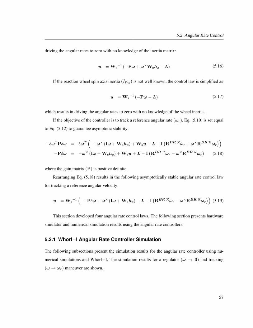
5.2 Angular Rate Control
driving the angular rates to zero with no knowledge of the inertia matrix:
u = Ws−1 (−Pω + ω×Wshs −L) (5.16)
If the reaction wheel spin axis inertia (IWS) is not well known, the control law is simplified as
u = Ws−1 (−Pω −L) (5.17)
which results in driving the angular rates to zero with no knowledge of the wheel inertia.
If the objective of the controller is to track a reference angular rate (ωr), Eq. (5.10) is set equal
to Eq. (5.12) to guarantee asymptotic stability:
−δωTPδω = δωT(− ω× (Iω + Wshs) + Wsu+L− I
(RBR Rωr + ω×RBR Rωr
))−Pδω = −ω× (Iω + Wshs) + Wsu+L− I
(RBR Rωr − ω×RBR Rωr
)(5.18)
where the gain matrix (P) is positive definite.
Rearranging Eq. (5.18) results in the following asymptotically stable angular rate control law
for tracking a reference angular velocity:
u = Ws−1(−Pδω + ω× (Iω + Wshs)−L+ I
(RBR Rωr − ω×RBR Rωr
))(5.19)
This section developed four angular rate control laws. The following section presents hardware
simulator and numerical simulation results using the angular rate controllers.
5.2.1 Whorl−I Angular Rate Controller Simulation
The following subsections present the simulation results for the angular rate controller using nu-
merical simulations and Whorl−I. The simulation results for a regulator (ω → 0) and tracking
(ω → ωr) maneuver are shown.
57

5.2 Angular Rate Control
5.2.1.1 Regulator
Assuming no external torque and substituting the reaction wheel spin axis orientation matrix (Ws)
for Whorl−I into the control law (Eq. (5.16)) simplifies to
u = −Pω + ω×hs
where the angular rates are driven to zero. The estimates for the simulator parameters are provided
in Section 3.1.
The angular rate controller parameters are provided in Table 5.1. The angular rate controller
results are shown in Figures 5.1 – 5.6. Whorl−I was given an initial angular rate about the 3
body axis and then the angular rate controller was turned on. The 16 second delay in the start of
the controller at the beginning of the simulation is due to the time necessary to initialize the three
reaction wheels.
Table 5.1: Angular Rate Controller ParametersParameter ValueControl Rate 2 HzObserve Rate 2 HzWheel Speed Query 10 Hzω(t0) (-0.002, -0.009, 0.088) rad/sP diag( 3.64, 3.40, 4.41 ) kg-m2/sΩ1 0 rad/sΩ2 0 rad/sΩ3 0 rad/s
The control results from Whorl−I are compared to numerical simulation control results. Fig-
ures 5.1 and 5.2 provide the angular rate time history for Whorl−I and the numerical simulation
respectively. Whorl−I has approximately zero angular rate in the 3 axis after 20 seconds into the
simulation. The numerical simulation has approximately zero angular rate after 15 seconds into
the simulation. The angular rates for Whorl−I have the same decreasing trend as predicted by the
numerical simulation. After 20 seconds the noise from the angular rate measurements can be clearly
58

5.2 Angular Rate Control
seen.
Figure 5.1: Whorl−I Angular Rates for Angular Rate Controller
Figure 5.2: Numerical Simulation Angular Rates for Angular Rate Controller
Figures 5.3 and 5.4 show the required control torque specified by the angular rate controller for
Whorl−I and the numerical simulation respectively. The control torques specified by the angular
rate controller for Whorl−I have the same control torque trend to zero as the numerical simulation.
Figures 5.5 and 5.6 show the reaction wheel speed time history for the controller running on
Whorl−I and the numerical simulation respectively. The reaction wheels have the same speed
trend as the numerical simulation. The reaction wheel aligned along the 3 axis for Whorl−I has a
59

5.2 Angular Rate Control
Figure 5.3: Whorl−I Control Torque for Angular Rate Controller
Figure 5.4: Numerical Simulation Control Torque for Angular Rate Controller
60

5.2 Angular Rate Control
similar trend as the numerical simulation. The numerical simulation ends with an angular velocity
of approximately 15 rad/s as compared with 17 rad/s for the reaction wheel aligned along the 3 axis
on Whorl−I. The discrepancies in the wheel speeds between Whorl−I and the numerical simulation
are due to the simplified reaction wheel motor torque model used in the numerical simulation and
shown in Eq. (4.20). Reference 59 provides a high fidelity dynamic model of a reaction wheel motor.
The model takes into account the electrical resistance of the motor armature, voltage limits, current
limits, viscosity damping, and static friction of the rotor, which are not considered in the simplified
reaction wheel model in Eq. (4.20). Even with the discrepancies, the numerical simulation and
Whorl−I results match.
Figure 5.5: Whorl−I Reaction Wheel Speed for Angular Rate Controller
5.2.1.2 Tracking
Assuming no external torque Eq. (5.16) simplifies to
u = Ws−1(−Pδω + ω× (Iω + Wshs) + I
(RBR Rωr − ω×RBR Rωr
))where the angular rate errors are driven to zero. The estimates for the simulator parameters are
provided in Section 3.1.
61
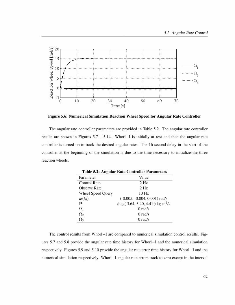
5.2 Angular Rate Control
Figure 5.6: Numerical Simulation Reaction Wheel Speed for Angular Rate Controller
The angular rate controller parameters are provided in Table 5.2. The angular rate controller
results are shown in Figures 5.7 – 5.14. Whorl−I is initially at rest and then the angular rate
controller is turned on to track the desired angular rates. The 16 second delay in the start of the
controller at the beginning of the simulation is due to the time necessary to initialize the three
reaction wheels.
Table 5.2: Angular Rate Controller ParametersParameter ValueControl Rate 2 HzObserve Rate 2 HzWheel Speed Query 10 Hzω(t0) (-0.005, -0.004, 0.001) rad/sP diag( 3.64, 3.40, 4.41 ) kg-m2/sΩ1 0 rad/sΩ2 0 rad/sΩ3 0 rad/s
The control results from Whorl−I are compared to numerical simulation control results. Fig-
ures 5.7 and 5.8 provide the angular rate time history for Whorl−I and the numerical simulation
respectively. Figures 5.9 and 5.10 provide the angular rate error time history for Whorl−I and the
numerical simulation respectively. Whorl−I angular rate errors track to zero except in the interval
62

5.2 Angular Rate Control
of 80 to 100 seconds. After 100 seconds the angular rate errors converge to zero. The numerical
simulation tracks the angular rates perfectly. The reaction wheels are the reason for the discrepan-
cies between Whorl−I and the numerical simulation. In the interval of 80 to 100 seconds Ω3 is close
to zero and is in the dead band zone for the electric motor, which results in the control authority
accuracy decreasing.
Figure 5.7: Whorl−I Angular Rates for Angular Rate Controller
Figure 5.8: Numerical Simulation Angular Rates for Angular Rate Controller
Figures 5.11 and 5.12 show the required control torque specified by the angular rate controller
for Whorl−I and the numerical simulation respectively. The control torques specified by the angular
63

5.2 Angular Rate Control
rate controller for Whorl−I have the same control torque trend as the numerical simulation, except
between 80 and 100 seconds into the simulation.
Figure 5.9: Whorl−I Angular Rate Error for Angular Rate Controller
Figure 5.10: Numerical Simulation Angular Rate Error for Angular Rate Controller
Figures 5.13 and 5.14 show the reaction wheel speed time history for the controller running on
Whorl−I and the numerical simulation respectively. The reaction wheels have the same speed trend
as the numerical simulation, except between 80 and 100 seconds. The numerical simulation and
Whorl−I results match, except between 80 and 100 seconds.
64
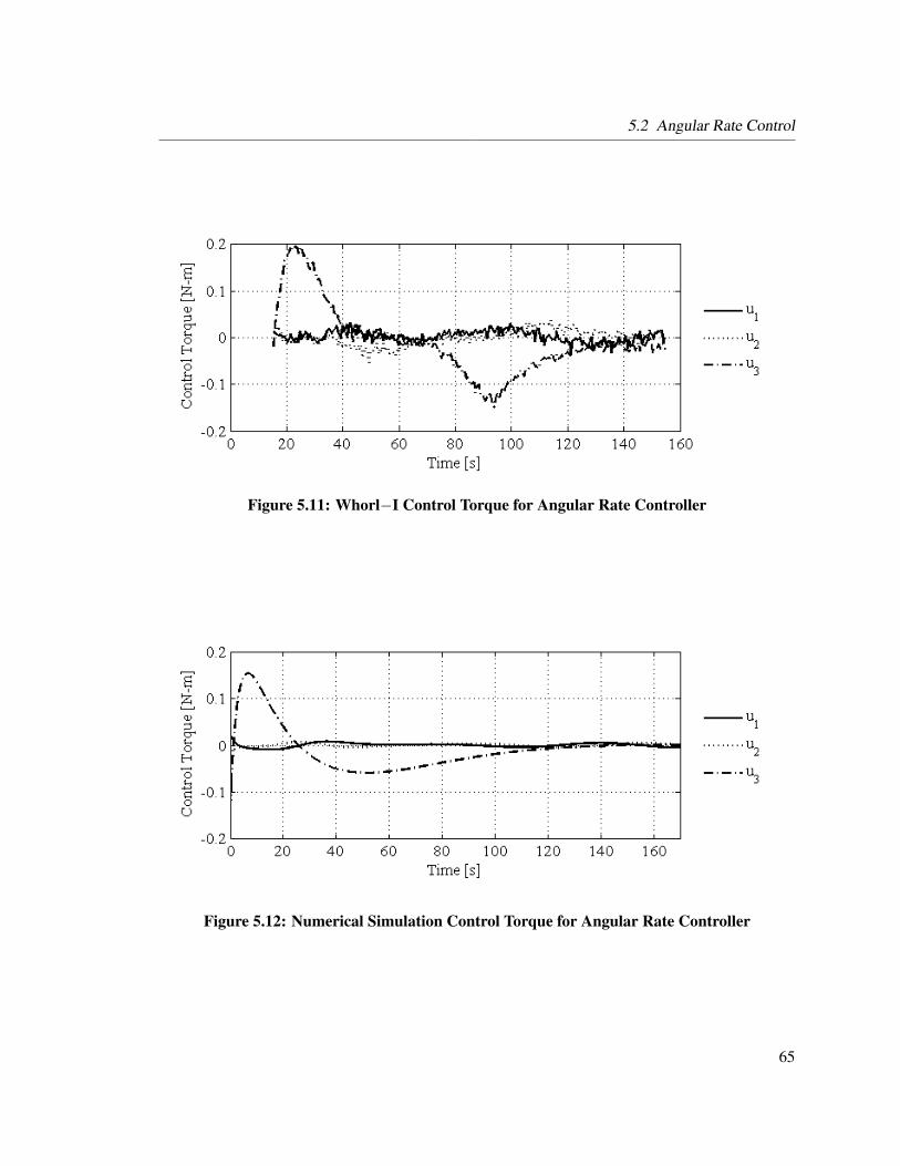
5.2 Angular Rate Control
Figure 5.11: Whorl−I Control Torque for Angular Rate Controller
Figure 5.12: Numerical Simulation Control Torque for Angular Rate Controller
65

5.2 Angular Rate Control
Figure 5.13: Whorl−I Reaction Wheel Rates for Angular Rate Controller
Figure 5.14: Numerical Simulation Reaction Wheel Speed for Angular Rate Controller
66

5.2 Angular Rate Control
The following Whorl−I angular rate tracking simulation avoids the dead band region for Ω3 by
setting the initial wheel speed to -40 rad/s. The angular rate controller parameters are provided in
Table 5.3. The angular rate controller results are shown in Figures 5.15 – 5.18. Whorl−I is initially
at rest then the angular rate controller is turned on to track the desired angular rates. The 25 second
delay in the start of the controller at the beginning of the simulation is due to the time necessary to
initialize the three reaction wheels.
Table 5.3: Angular Rate Controller ParametersParameter ValueControl Rate 2 HzObserve Rate 2 HzWheel Speed Query 10 Hzω(t0) (-0.003, -0.001, 0.007) rad/s[P ] diag( 3.64, 3.40, 4.41 ) kg-m2/sΩ1 0 rad/sΩ2 0 rad/sΩ3 -40 rad/s
Figure 5.15 provides the angular rate time history for Whorl−I. Figure 5.16 provides the an-
gular rate error time history for Whorl−I . The angular rate errors are tracking to zero throughout
the simulation, which is an improvement compared to the previous tracking simulation where Ω3 is
initially set to zero.
Figure 5.17 shows the required control torque specified by the angular rate controller for
Whorl−I . The control torques specified by the angular rate controller for Whorl−I have the same
control torque trend as the previous numerical simulation.
Figure 5.18 shows the reaction wheel speed time history for the controller running on Whorl−I.
Avoiding the electric motor deadband region results in the expected performance for the angular rate
controller.
67
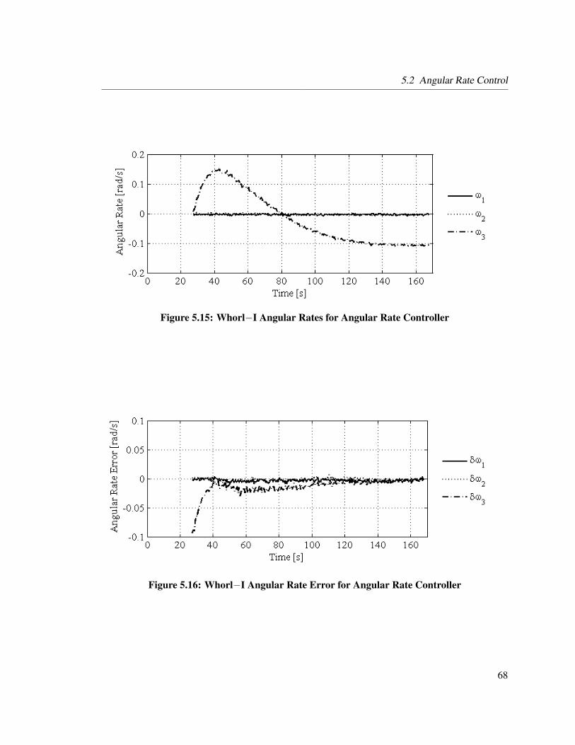
5.2 Angular Rate Control
Figure 5.15: Whorl−I Angular Rates for Angular Rate Controller
Figure 5.16: Whorl−I Angular Rate Error for Angular Rate Controller
68

5.2 Angular Rate Control
Figure 5.17: Whorl−I Control Torque for Angular Rate Controller
Figure 5.18: Whorl−I Reaction Wheel Speed for Angular Rate Controller
69

5.2 Angular Rate Control
5.2.2 Whorl−II Angular Rate Controller Simulation
The simulation results for the angular rate controller (Eq. (5.16)) using numerical simulations and
Whorl−II are presented for a regulator (ω → 0) problem.
Assuming no external torque the control law (Eq. (5.16)) simplifies to
u = Ws−1 (−Pω + ω×Wshs)
where the angular rates are driven to zero. The estimates for the simulator parameters are provided
in Section 3.1.
The angular rate controller parameters are provided in Table 5.4. The angular rate controller
results are shown in Figures 5.19 – 5.24. Whorl−II is given an initial angular rate about the 3
body axis and then the angular rate controller is turned on. The 16 second delay in the start of
the controller at the beginning of the simulation is due to the time necessary to initialize the three
reaction wheels.
Table 5.4: Angular Rate Controller ParametersParameter ValueControl Rate 2 HzObserve Rate 2 HzWheel Speed Query 10 Hzω(t0) (0.013, -0.007, 0.222) rad/sP diag( 3.64, 3.40, 4.41 ) kg-m2/sΩ1 0 rad/sΩ2 0 rad/sΩ3 0 rad/s
The control results from Whorl−II are compared to numerical simulation control results. Fig-
ure 5.19 and 5.20 provide the angular rate time history for Whorl−I and the numerical simulation
respectively. Whorl−II has approximately zero angular rate after 20 seconds into the simulation.
The numerical simulation has approximately zero angular rate after 20 seconds into the simula-
tion. The angular rates for Whorl−II have the same decreasing trend as predicted by the numerical
70
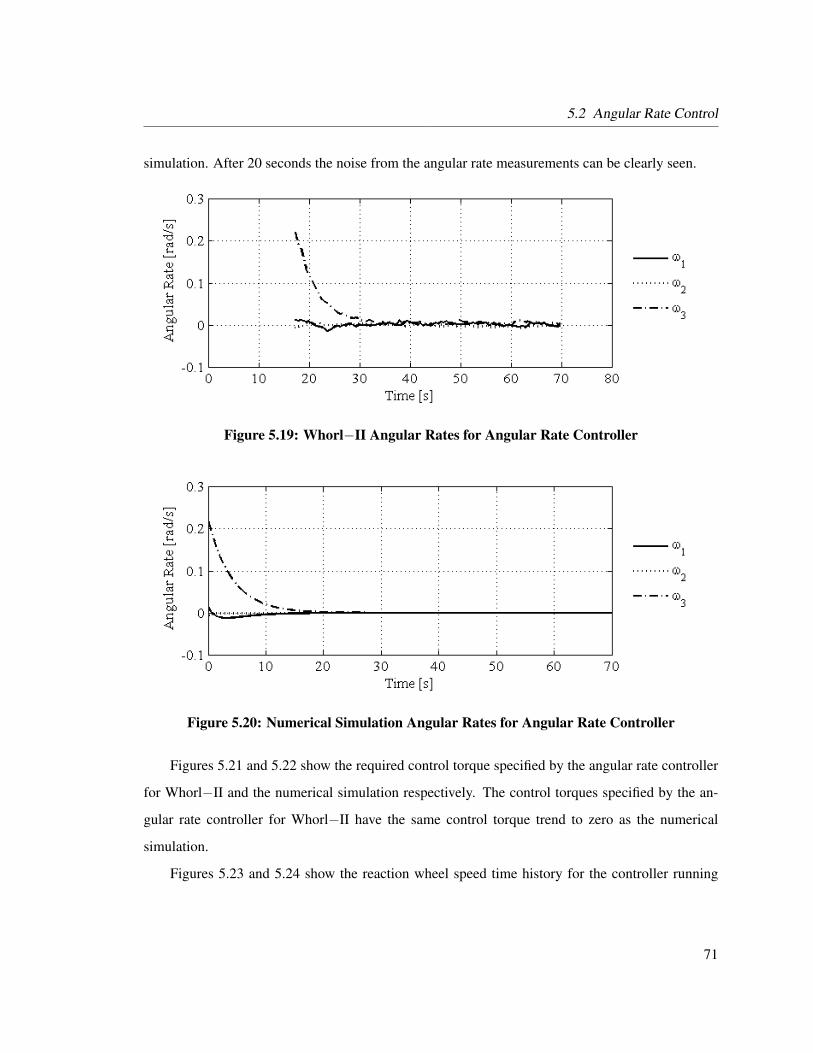
5.2 Angular Rate Control
simulation. After 20 seconds the noise from the angular rate measurements can be clearly seen.
Figure 5.19: Whorl−II Angular Rates for Angular Rate Controller
Figure 5.20: Numerical Simulation Angular Rates for Angular Rate Controller
Figures 5.21 and 5.22 show the required control torque specified by the angular rate controller
for Whorl−II and the numerical simulation respectively. The control torques specified by the an-
gular rate controller for Whorl−II have the same control torque trend to zero as the numerical
simulation.
Figures 5.23 and 5.24 show the reaction wheel speed time history for the controller running
71

5.2 Angular Rate Control
Figure 5.21: Whorl−II Control Torque for Angular Rate Controller
Figure 5.22: Numerical Simulation Control Torque for Angular Rate Controller
72

5.3 Modified Rodrigues Parameter Control
on Whorl−II and the numerical simulation respectively. The reaction wheels have the same speed
trends as the numerical simulation. Whorl−I and the numerical simulation results closely match.
Figure 5.23: Whorl−II Reaction Wheel Speed for Angular Rate Controller
Figure 5.24: Numerical Simulation Reaction Wheel Speed for Angular Rate Controller
5.3 Modified Rodrigues Parameter Control
In this section we develop a nonlinear spacecraft attitude control law that asymptotically drive the
angular velocity errors and MRP errors to zero. Lyapunov’s direct method is used to design the MRP
73

5.3 Modified Rodrigues Parameter Control
control law for controlling the attitude of a spacecraft. Assume the candidate Lyapunov function
is25
V (δω, δσ) =12δωT Iδω︸ ︷︷ ︸V (δω)
+ 2K ln(1 + δσT δσ
)︸ ︷︷ ︸V (δσ)
(5.20)
where K is a positive scalar gain quantity. Eq. (5.20) is represented in terms of V (δω) and V (δσ).
Taking the derivative of Eq. (5.20) results in
V (δω, δσ) = V (δω) + V (δσ) (5.21)
where V (δω) is previously derived in Section 5.2.
The MRP Lyapunov term in Eq. (5.20) is
V (δσ) = 2K ln (1 + δσT δσ) (5.22)
The derivative of Eq. (5.22) is
V (δσ) = 4K1
1 + δσT δσδσT δσ
= 4K1
1 + δσT δσδσT
(1− δσ2)I3×3 + 2δσ× + 2δσδσT
4δω
= K1
1 + δσT δσ
(1− δσ2)δσT + 2 δσT δσ×︸ ︷︷ ︸0
+2 (δσT δσ)︸ ︷︷ ︸δσ2
δσT
δω
= K1
1 + δσT δσ
(1− δσ2 + 2δσ2
)δσT δω
= K1
1 + δσTσ
(1 + δσT δσ
)δσT δω
= KδσT δω
= δωT (Kδσ) (5.23)
74

5.3 Modified Rodrigues Parameter Control
Substituting Eq. (5.10) and Eq. (5.23) into Eq. (5.21) results in
V (δω, δσ) = δωT(−ω× (Iω + Wshs) + Wsu+L
−I(RBR Rωr − ω×RBR Rωr
)+Kδσ
)(5.24)
If the objective of the MRP controller is to drive the MRP attitude vector to zero, Eq. (5.24)
simplifies to
V (δω, δσ) = ωT(−ω× (Iω + Wshs) + Wsu+L+Kσ
)(5.25)
where the reference MRP and reference angular velocity are zero and Eq. (5.5) simplifies to δω = ω
and δσ = σ.
To guarantee asymptotic stability, we set Eq. (5.25) equal to the following semi-negative defi-
nite function:
V (δω) = −δωTPδω
= −ωTPω if Rωr = 0 (5.26)
where P is a positive definite gain matrix. The result is
−ωTPω = ωT(−ω× (Iω + Wshs) + Wsu+L+Kσ
)(5.27)
Rearranging Eq. (5.27) results in the following stable angular MRP control law for driving σ
and ω to zero:
u = Ws−1 (−Kσ −Pω + ω× (Iω + Wshs)−L) (5.28)
Asymptotic stability is investigated for the control law in Eq. (5.28) by taking higher order
derivatives of V (ω,σ) and satisfying the sufficient conditions for asymptotic stability as discussed
at the beginning of this chapter.
75

5.3 Modified Rodrigues Parameter Control
The higher order derivatives for V (ω,σ) are
V (ω,σ) = −ωTPω
= 0
V (ω,σ) = −2ωTPω
= 0...V (ω,σ) = −2ωTPω − 2ωTPω
= −2ωTPω (5.29)
where ω is solved for by substituting the control law into the equations of motion resulting in
ω = I−1 (−Kσ −Pω) (5.30)
The third derivative of the Lyapunov function is
...V (ω,σ) = −2K2
(I−1σ
)T P(I−1σ
)< 0 (5.31)
where P and I−1 are positive definite. The sufficient conditions for asymptotic stability are satisfied
and the control law in Eq. (5.28) is globally asymptotically stable.
It may be desirable to have a control law that does not depend on the inertia matrix as mentioned
in Section 5.2. Equation (5.27) is simplified by noting that ωTω× = 0, which results in
−ωTPω = −ωTω×Iω + ωT(−ω×Wshs + Wsu+L+Kσ
)= ωT
(−ω×Wshs + Wsu+L+Kσ
)(5.32)
Rearranging Eq. (5.32) results in the following stable MRP control law for driving the MRPs and
76

5.3 Modified Rodrigues Parameter Control
angular rates to zero with no knowledge of the inertia matrix:
u = Ws−1(−Kσ −Pω + ω×Wshs −L
)(5.33)
By investigating the higher order derivatives of V (ω,σ) and satisfying the sufficient conditions for
asymptotic stability the control law in Eq. (5.33) is shown to be globally asymptotically stable.
If the reaction wheel spin axis inertia (IWs) is not well known, the control law is simplified as
u = Ws−1 (−Kσ −Pω −L) (5.34)
which drives the MRP vector and angular rates to zero with no knowledge of the wheel inertia.
Again, the control law in Eq. (5.34) is shown to be globally asymptotically stable by investigating the
higher order derivatives of V (ω,σ) and satisfying the sufficient conditions for asymptotic stability
as discussed for the control law in Eq. (5.28).
If the objective of the controller is to track a reference MRP vector (σr), Eq. (5.24) is set equal
to Eq. (5.12) to guarantee asymptotic stability:
−δωTPδω = δωT(−ω× (Iω + Wshs) + Wsu+L
−I(RBR Rωr − ω×RBR Rωr
)+Kσ
)−Pδω = −ω× (Iω + Wshs) + Wsu+L
−I(RBR Rωr − ω×RBR Rωr
)+Kσ (5.35)
where the gain matrix (P) is positive definite.
Rearranging Eq. (5.35) results in the following stable angular rate control law for tracking a
reference MRP and angular rate vector:
u = Ws−1(−Kσ −Pδω + ω× (Iω + Wshs)−L+ I
(RBR Rωr − ω×RBR Rωr
))(5.36)
77

5.3 Modified Rodrigues Parameter Control
Asymptotic stability is investigated for the control law in Eq. (5.36) by taking higher order
derivatives of V (δω, δσ) and satisfying the sufficient conditions for asymptotic stability as dis-
cussed at the beginning of this chapter.
The higher order derivatives for V (δω, δσ) are
V (δω, δσ) = −δωTPδω
= 0
V (δω, δσ) = −2δωTPδω
= 0...V (δω, δσ) = −2δωTPδω − 2δωTPδω
= −2δωTPδω (5.37)
where δω is solved for by substituting the control law into the error dynamics.
δω = I−1 (−Kδσ −Pδω) (5.38)
Therefore the third derivative of the Lyapunov function is
...V (δω = 0, δσ) = −2K2
(I−1δσ
)T P(I−1δσ
)< 0 (5.39)
where P and I−1 are positive definite. The sufficient conditions for asymptotic stability are satisfied
and the control law in Eq. (5.36) is globally asymptotically stable.
5.3.1 Whorl−I MRP Controller Simulation
The following subsections present the simulation results for the MRP controller using numerical
simulations and Whorl−I. The simulation results for a regulator (ω → 0,σ → 0) and tracking
(ω → ωr,σ → σr) problem are shown.
78

5.3 Modified Rodrigues Parameter Control
5.3.1.1 Regulator
Assuming no external torque Eq. (5.33) simplifies to
u = Ws−1(−Kσ −Pω + ω×Wshs
)where the angular rates and MRPs are driven to zero. The estimates for the simulator parameters
are provided in Section 3.1.
The results of running the controller on Whorl−I along with a numerical simulation comparing
the results are presented. The MRP controller parameters are provided in Table 5.5. The MRP
controller results are shown in Figures 5.25 – 5.32. Whorl−I is given an initial angular rate about
the 3 body axis and then the MRP controller is turned on. The 16 second delay in the start of
the controller at the beginning of the simulation is due to the time necessary to initialize the three
reaction wheels.
Table 5.5: MRP Controller ParametersParameter ValueControl Rate 2 HzObserve Rate 2 HzWheel Speed Query 10 Hzσ(t0) (-0.003, 0.015, 0.482 )ω(t0) (-0.007, -0.005, 0.118) rad/sK 1.5 kg-m2/s2
P diag( 3.64, 3.40, 4.41 ) kg-m2/sΩ1 0 rad/sΩ2 0 rad/sΩ3 0 rad/s
The control results from Whorl−I are compared to numerical simulation control results. Fig-
ures 5.25 and 5.26 provide the angular rate time history for Whorl−I and the numerical simulation
respectively. Whorl−I has approximately zero angular rate in the 3 axis after 45 seconds into the
control simulation. The numerical simulation has approximately zero angular rate after 42 seconds
into the simulation. The angular rates for Whorl−I have the same decreasing trend as predicted by
79

5.3 Modified Rodrigues Parameter Control
the numerical simulation.
Figure 5.25: Whorl−I Angular Rates for MRP Controller
Figure 5.26: Numerical Simulation Angular Rates for MRP Controller
Figures 5.27 and 5.28 provide the MRP vector time history for Whorl−I and the numerical
simulation respectively. Whorl−I has approximately a constant offset from zero for σ3 after 50
seconds into the simulation. The numerical simulation has approximately a zero MRP vector after
42 seconds into the simulation. The constant offset seen in Figure 5.27 is due to atmospheric drag
torque acting on Whorl−I. The steady state offset for σ3 is approximately 0.02. The external torque
80

5.3 Modified Rodrigues Parameter Control
vector expression is25
σsteady state =LextK
(5.40)
where Lext is the external torque. The external torque acting on Whorl−I is 0.03 N-m from
Eq. (5.40). The external torque is in agreement with the atmospheric drag lower bound analysis
presented in Ref. 34 for Whorl−I. The MRP vector for Whorl−I has the same decreasing trend as
predicted by the numerical simulation.
Figure 5.27: Whorl−I MRP Vector for MRP Controller
Figures 5.3 and 5.4 show the required control torque specified by the angular rate controller for
Whorl−I and the numerical simulation respectively. The control torques specified by the angular
rate controller for Whorl−I have the same control torque trend to zero as the numerical simulation.
Figures 5.5 and 5.6 show the reaction wheel speed time history for the controller running on
Whorl−I and the numerical simulation respectively. The reaction wheels have the same speed
trend as the numerical simulation. The reaction wheel aligned along the 3 axis for Whorl−I has a
similar trend as the numerical simulation. The numerical simulation ends with an angular velocity
of approximately 20 rad/s as compared with 23 rad/s for the reaction wheel aligned along the 3 axis
of Whorl−I. The discrepancies in the wheel speeds between Whorl−I and the numerical simulation
81
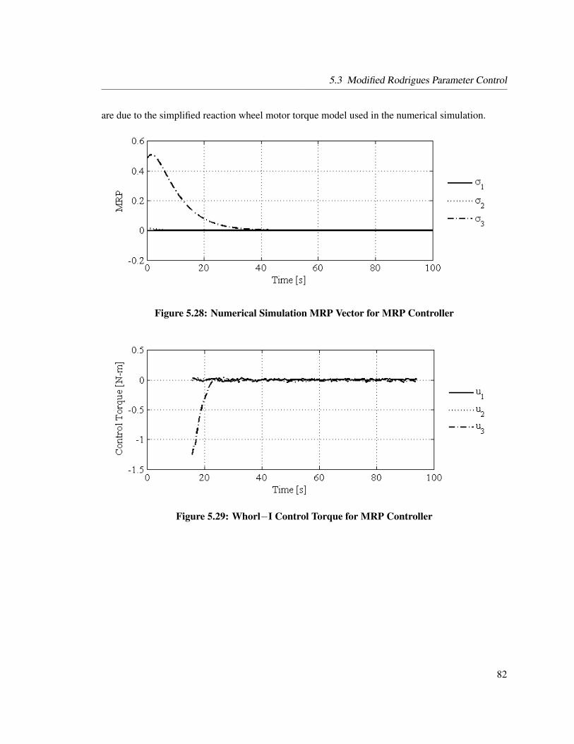
5.3 Modified Rodrigues Parameter Control
are due to the simplified reaction wheel motor torque model used in the numerical simulation.
Figure 5.28: Numerical Simulation MRP Vector for MRP Controller
Figure 5.29: Whorl−I Control Torque for MRP Controller
82

5.3 Modified Rodrigues Parameter Control
Figure 5.30: Numerical Simulation Control Torque for MRP Controller
Figure 5.31: Whorl−I Reaction Wheel Speed for MRP Controller
83

5.3 Modified Rodrigues Parameter Control
Figure 5.32: Numerical Simulation Reaction Wheel Speed for MRP Controller
5.3.1.2 Tracking
Assuming no external torque Eq. (5.36) simplifies to
u = Ws−1(−Kσ −Pδω + ω× (Iω + Wshs) + I
(RBR Rωr − ω×RBR Rωr
))where the MRP and angular rate errors are driven to zero. The estimates for the simulator parameters
are provided in Section 3.1.
The MRP controller parameters are provided in Table 5.6. The MRP controller results are
shown in Figures 5.33 – 5.44. Whorl−I is initially at rest and then the MRP controller is turned on
to track the desired attitude. The 40 second delay in the start of the controller at the beginning of
the simulation is due to the time necessary to initialize the three reaction wheels.
The control results from Whorl−I are compared to numerical simulation control results. Fig-
ures 5.33 and 5.34 provide the angular rate time history for Whorl−I and the numerical simulation
respectively. Figures 5.35 and 5.36 provide the angular rate error time history. Whorl−I has ap-
proximately zero angular rate error in the 3 axis after 65 seconds into the control simulation. The
numerical simulation has approximately zero angular rate after 55 seconds into the simulation. The
angular rates and angular rate errors for Whorl−I have the same decreasing trend as predicted by
84
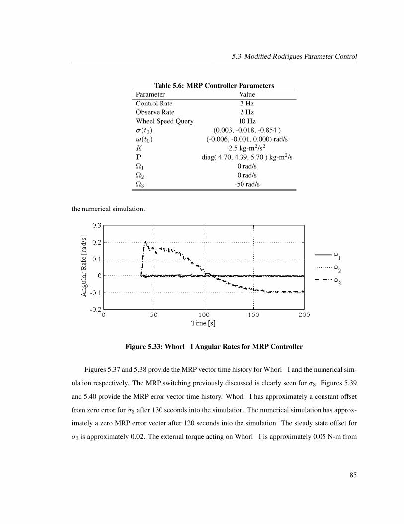
5.3 Modified Rodrigues Parameter Control
Table 5.6: MRP Controller ParametersParameter ValueControl Rate 2 HzObserve Rate 2 HzWheel Speed Query 10 Hzσ(t0) (0.003, -0.018, -0.854 )ω(t0) (-0.006, -0.001, 0.000) rad/sK 2.5 kg-m2/s2
P diag( 4.70, 4.39, 5.70 ) kg-m2/sΩ1 0 rad/sΩ2 0 rad/sΩ3 -50 rad/s
the numerical simulation.
Figure 5.33: Whorl−I Angular Rates for MRP Controller
Figures 5.37 and 5.38 provide the MRP vector time history for Whorl−I and the numerical sim-
ulation respectively. The MRP switching previously discussed is clearly seen for σ3. Figures 5.39
and 5.40 provide the MRP error vector time history. Whorl−I has approximately a constant offset
from zero error for σ3 after 130 seconds into the simulation. The numerical simulation has approx-
imately a zero MRP error vector after 120 seconds into the simulation. The steady state offset for
σ3 is approximately 0.02. The external torque acting on Whorl−I is approximately 0.05 N-m from
85

5.3 Modified Rodrigues Parameter Control
Figure 5.34: Numerical Simulation Angular Rates for MRP Controller
Figure 5.35: Whorl−I Angular Rate Errors for MRP Controller
86

5.3 Modified Rodrigues Parameter Control
Figure 5.36: Numerical Simulation Angular Rate Errors for MRP Controller
Eq. (5.40). The external torque is in agreement with the atmospheric drag lower bound analysis
presented in Ref. 34 for Whorl−I. The MRP error vector for Whorl−I has the same decreasing
trend as predicted by the numerical simulation.
Figure 5.37: Whorl−I MRP Vector for MRP Controller
Figures 5.41 and 5.42 show the required control torque specified by the angular rate controller
for Whorl−I and the numerical simulation respectively. The control torques specified by the MRP
controller for Whorl−I have the same control torque trend to zero as the numerical simulation.
87

5.3 Modified Rodrigues Parameter Control
Figure 5.38: Numerical Simulation MRP Vector for MRP Controller
Figure 5.39: Whorl−I MRP Error Vector for MRP Controller
88
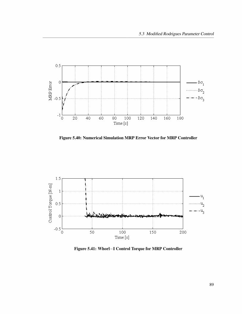
5.3 Modified Rodrigues Parameter Control
Figure 5.40: Numerical Simulation MRP Error Vector for MRP Controller
Figure 5.41: Whorl−I Control Torque for MRP Controller
89
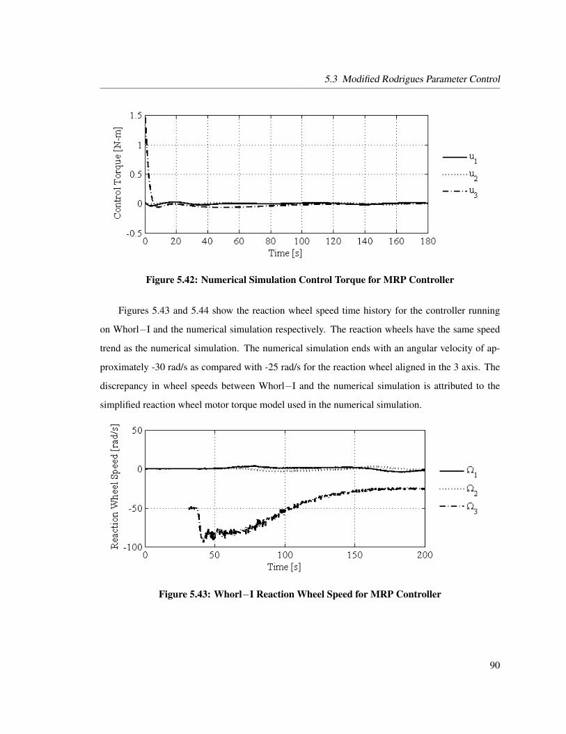
5.3 Modified Rodrigues Parameter Control
Figure 5.42: Numerical Simulation Control Torque for MRP Controller
Figures 5.43 and 5.44 show the reaction wheel speed time history for the controller running
on Whorl−I and the numerical simulation respectively. The reaction wheels have the same speed
trend as the numerical simulation. The numerical simulation ends with an angular velocity of ap-
proximately -30 rad/s as compared with -25 rad/s for the reaction wheel aligned in the 3 axis. The
discrepancy in wheel speeds between Whorl−I and the numerical simulation is attributed to the
simplified reaction wheel motor torque model used in the numerical simulation.
Figure 5.43: Whorl−I Reaction Wheel Speed for MRP Controller
90

5.3 Modified Rodrigues Parameter Control
Figure 5.44: Numerical Simulation Reaction Wheel Speed for MRP Controller
5.3.2 Whorl−II MRP Controller Simulation
In this section we present the simulation results of the MRP controller using numerical simulations
and Whorl−II. The simulation results for a regulator (ω → 0,σ → 0) problem are shown.
Assuming no external torque Eq. (5.33) simplifies to
u = Ws−1(−Kσ −Pω + ω×Wshs
)where the angular rates and MRPs are driven to zero. The estimates for the simulator parameters
are provided in Section 3.1.
The results of running the controller on Whorl−II along with a numerical simulation comparing
the results are presented. The MRP controller parameters are provided in Table 5.7. The MRP
controller results are shown in Figures 5.45 – 5.52. Whorl−II is given an initial angular rate about
the 3 body axis and then the MRP controller is activated. The 16 second delay in the start of
the controller at the beginning of the simulation is due to the time necessary to initialize the three
reaction wheels.
Figures 5.45 and 5.46 provide the angular rate time history for Whorl−II and the numerical
simulation respectively. Whorl−II has approximately zero angular rate in the 3 axis after 45 seconds
91
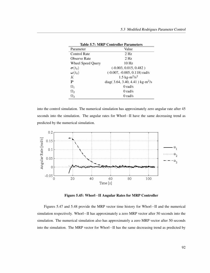
5.3 Modified Rodrigues Parameter Control
Table 5.7: MRP Controller ParametersParameter ValueControl Rate 2 HzObserve Rate 2 HzWheel Speed Query 10 Hzσ(t0) (-0.003, 0.015, 0.482 )ω(t0) (-0.007, -0.005, 0.118) rad/sK 1.5 kg-m2/s2
P diag( 3.64, 3.40, 4.41 ) kg-m2/sΩ1 0 rad/sΩ2 0 rad/sΩ3 0 rad/s
into the control simulation. The numerical simulation has approximately zero angular rate after 45
seconds into the simulation. The angular rates for Whorl−II have the same decreasing trend as
predicted by the numerical simulation.
Figure 5.45: Whorl−II Angular Rates for MRP Controller
Figures 5.47 and 5.48 provide the MRP vector time history for Whorl−II and the numerical
simulation respectively. Whorl−II has approximately a zero MRP vector after 50 seconds into the
simulation. The numerical simulation also has approximately a zero MRP vector after 50 seconds
into the simulation. The MRP vector for Whorl−II has the same decreasing trend as predicted by
92
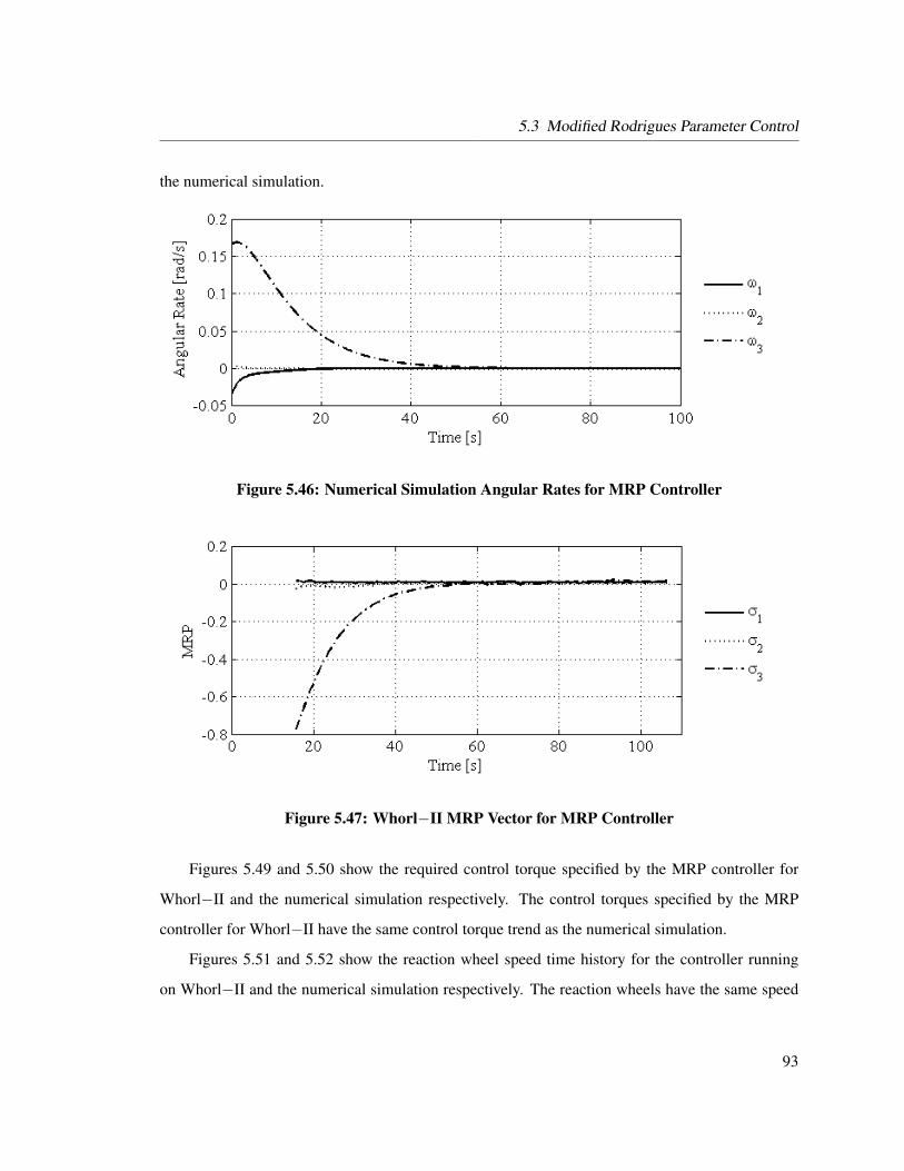
5.3 Modified Rodrigues Parameter Control
the numerical simulation.
Figure 5.46: Numerical Simulation Angular Rates for MRP Controller
Figure 5.47: Whorl−II MRP Vector for MRP Controller
Figures 5.49 and 5.50 show the required control torque specified by the MRP controller for
Whorl−II and the numerical simulation respectively. The control torques specified by the MRP
controller for Whorl−II have the same control torque trend as the numerical simulation.
Figures 5.51 and 5.52 show the reaction wheel speed time history for the controller running
on Whorl−II and the numerical simulation respectively. The reaction wheels have the same speed
93

5.3 Modified Rodrigues Parameter Control
Figure 5.48: Numerical Simulation MRP Vector for MRP Controller
Figure 5.49: Whorl−II Control Torque for MRP Controller
94
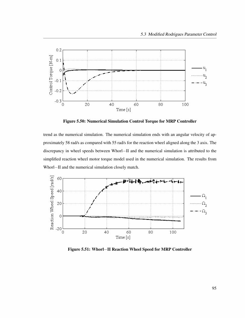
5.3 Modified Rodrigues Parameter Control
Figure 5.50: Numerical Simulation Control Torque for MRP Controller
trend as the numerical simulation. The numerical simulation ends with an angular velocity of ap-
proximately 58 rad/s as compared with 55 rad/s for the reaction wheel aligned along the 3 axis. The
discrepancy in wheel speeds between Whorl−II and the numerical simulation is attributed to the
simplified reaction wheel motor torque model used in the numerical simulation. The results from
Whorl−II and the numerical simulation closely match.
Figure 5.51: Whorl−II Reaction Wheel Speed for MRP Controller
95

5.4 Summary
Figure 5.52: Numerical Simulation Reaction Wheel Speed for MRP Controller
5.4 Summary
In this chapter we develop nonlinear asymptotically stable angular rate control laws. The attitude
hardware simulators successfully demonstrate the angular rate controllers. We also develop nonlin-
ear asymptotically stable MRP attitude control laws that drive the attitude to zero and track a time
varying reference attitude. The attitude hardware simulators successfully demonstrate the MRP
attitude controllers.
The attitude controllers developed in this chapter assume perfect knowledge of system param-
eters such as spacecraft mass properties, reaction wheel alignment, and perfect attitude knowledge.
Real systems only have estimates of these quantities. The next chapter develops a robust attitude
control law that tracks a reference attitude while bounding system uncertainties.
96
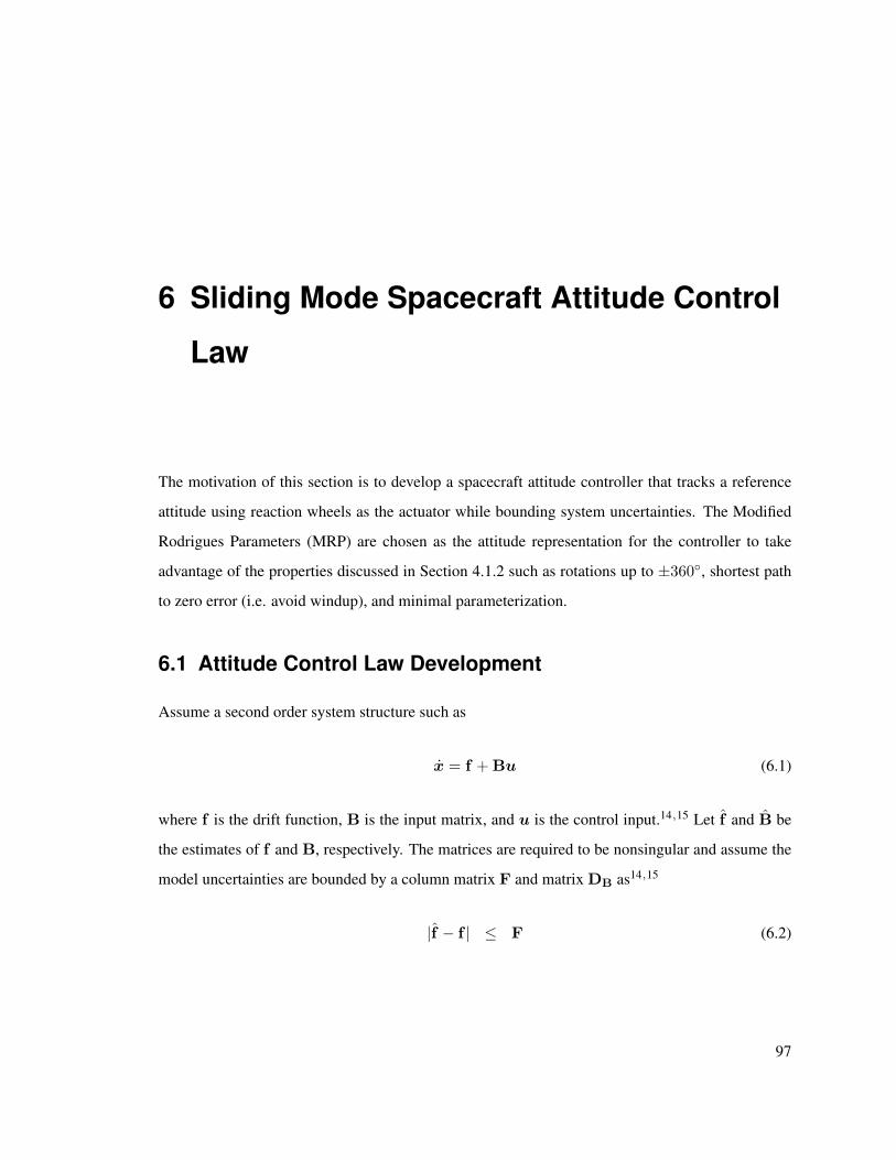
6 Sliding Mode Spacecraft Attitude Control
Law
The motivation of this section is to develop a spacecraft attitude controller that tracks a reference
attitude using reaction wheels as the actuator while bounding system uncertainties. The Modified
Rodrigues Parameters (MRP) are chosen as the attitude representation for the controller to take
advantage of the properties discussed in Section 4.1.2 such as rotations up to ±360, shortest path
to zero error (i.e. avoid windup), and minimal parameterization.
6.1 Attitude Control Law Development
Assume a second order system structure such as
x = f + Bu (6.1)
where f is the drift function, B is the input matrix, and u is the control input.14,15 Let f and B be
the estimates of f and B, respectively. The matrices are required to be nonsingular and assume the
model uncertainties are bounded by a column matrix F and matrix DB as14,15
|f − f | ≤ F (6.2)
97

6.1 Attitude Control Law Development
B = (11 +4B) B, for |4B| ≤ DB (6.3)
where 11 is a 3×3 identity matrix. Note that with no uncertainty F = 0, f = f , 4B = 0, and
B = B.
The spacecraft equations of motion with reaction wheels (Eq. (4.16)) are provided as
ω = −I−1ω× (Iω + Wshs) + I−1L︸ ︷︷ ︸f
+ I−1Ws︸ ︷︷ ︸B
u (6.4)
where f is 3× 1 matrix and B is 3× n matrix where n is the number of reaction wheels.
The design procedure for sliding mode control involves choosing the sliding manifold that
achieves the control objective and designing the sliding conditions that satisfy the sliding mani-
fold.21
The sliding variable (s) is defined as a class of linear sliding vectors as
s(δω, δσ) , δω + Λδσ (6.5)
where Λ is a 3 × 3 symmetric positive-definite constant matrix, δω is the difference in angular
velocity, and δσ is the difference in the MRP vector between the spacecraft and reference model.
The system will track the desired state if the system stays on the sliding manifold (s = 0).21
The attitude tracking errors (δσ) when on the sliding manifold are investigated by making use of
the nonlinear transformation in Eq. (4.14)(
14B(δσ)
)and Eq. (6.5):21
14B(δσ) (δω + Λδσ) = 1
4B(δσ)s
δσ + 14B(δσ)Λδσ = 1
4B(δσ)s
δσ + 14B(δσ)Λδσ = 0 (6.6)
98

6.1 Attitude Control Law Development
Consider the following candidate Lyapunov function for the system in Eq. (6.6).
V (δσ) = 2δσT δσ (6.7)
Differentiating Eq. (6.7) and substituting Eq. (6.6) results in
V (δσ) = 4δσT δσ
= −4δσT(1− δσ2)I3×3 + 2δσ× + 2δσδσT
4Λδσ
= −
(1− δσ2)δσT + 2 δσT δσ×︸ ︷︷ ︸0
+2 (δσT δσ)︸ ︷︷ ︸δσ2
δσT
Λδσ
= −(1− δσ2 + 2δσ2
)δσTΛδσ
= −(1 + δσ2
)δσTΛδσ (6.8)
Equation (6.7) is a Lyapunov function due to satisfying the necessary conditions by the function
being continuously differentiable, V (δσ = 0) = 0 and V (δσ 6= 0) > 0. The gain matrix Λ is
positive definite and V (δσ = 0) = 0, therefore V (δσ 6= 0) ≤ 0. The negative semi-definite
function indicates that the error between the true state and desired state will converge to zero as
t→∞.
The control is designed such that the sliding manifold is reached and sliding on the manifold
occurs. The best approximation of a continuous control law (ueq) that will result in s(δω, δσ) = 0
is developed by substituting the error dynamics (Eq. (5.8) and Eq. (4.14)) and system equations of
motion (Eq. (6.4)) into s(δω, δσ), which results in
s(δω, δσ) = δω + Λδσ
= ω −RBR Rωr + ω×RBR Rωr +14ΛB(δσ)δω
= f + Bu−RBR Rωr + ω×RBR Rωr +14ΛB(δσ)δω (6.9)
99

6.1 Attitude Control Law Development
Setting s(δω, δσ) = 0, the equivalent control expression (ueq) is
ueq = B+
(−f + RBR Rωr − ω×RBR Rωr −
14ΛB(δσ)δω
)(6.10)
where the estimates of B and f are used to determine the control and B+ indicates the pseudo
inverse. The equivalent control keeps the sliding variable on the sliding surface in the absence of
errors (i.e. s(δω, δσ) = 0 if the dynamics are precisely known such that B = B and f = f ).
The equivalent control (ueq) shown in Eq. (6.10) results in driving the angular rate error to
zero. The MRP error results in a constant offset from zero. Integral control is implemented into the
equivalent control law to drive the MRP error to zero. The sliding variable (s) is now defined as
s(δω, δσ, z) , δω + Λδσ + z (6.11)
z = ΛI
∫ t
0δσdt (6.12)
where Λ and ΛI are 3× 3 symmetric positive-definite constant matrices.
The system will track the desired state if the system stays on the sliding manifold (s = 0).21
The attitude tracking errors (δσ) when on the sliding manifold are investigated by making use of
the nonlinear transformation in Eq. (4.14)(
14B(δσ)
)and Eq. (6.11):
14B(δσ) (δω + Λδσ + z) = 1
4B(δσ)s
δσ + 14B(δσ) (Λδσ + z) = 1
4B(δσ)s
δσ + 14B(δσ) (Λδσ + z) = 0 (6.13)
Consider the following candidate Lyapunov function for the system in Eq. (6.13):
V (δσ, z) = 2 log (1 + δσT δσ) +12zTΛI
−1z (6.14)
100
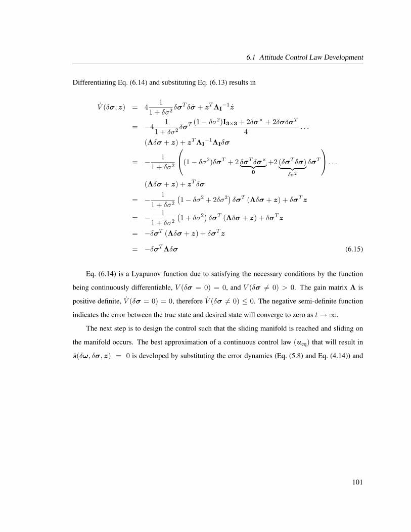
6.1 Attitude Control Law Development
Differentiating Eq. (6.14) and substituting Eq. (6.13) results in
V (δσ, z) = 41
1 + δσ2δσT δσ + zTΛI
−1z
= −41
1 + δσ2δσT
(1− δσ2)I3×3 + 2δσ× + 2δσδσT
4. . .
(Λδσ + z) + zTΛI−1ΛIδσ
= − 11 + δσ2
(1− δσ2)δσT + 2 δσT δσ×︸ ︷︷ ︸0
+2 (δσT δσ)︸ ︷︷ ︸δσ2
δσT
. . .
(Λδσ + z) + zT δσ
= − 11 + δσ2
(1− δσ2 + 2δσ2
)δσT (Λδσ + z) + δσTz
= − 11 + δσ2
(1 + δσ2
)δσT (Λδσ + z) + δσTz
= −δσT (Λδσ + z) + δσTz
= −δσTΛδσ (6.15)
Eq. (6.14) is a Lyapunov function due to satisfying the necessary conditions by the function
being continuously differentiable, V (δσ = 0) = 0, and V (δσ 6= 0) > 0. The gain matrix Λ is
positive definite, V (δσ = 0) = 0, therefore V (δσ 6= 0) ≤ 0. The negative semi-definite function
indicates the error between the true state and desired state will converge to zero as t→∞.
The next step is to design the control such that the sliding manifold is reached and sliding on
the manifold occurs. The best approximation of a continuous control law (ueq) that will result in
s(δω, δσ, z) = 0 is developed by substituting the error dynamics (Eq. (5.8) and Eq. (4.14)) and
101

6.1 Attitude Control Law Development
system equations of motion (Eq. (6.4)) into s(δω, δσ, z), which results in
s(δω, δσ, z) = δω + Λδσ + z
= ω −RBR Rωr + ω×RBR Rωr
+14ΛB(δσ)δω + ΛIδσ
= f + Bu−RBR Rωr + ω×RBR Rωr
+14ΛB(δσ)δω + ΛIδσ (6.16)
Setting s(δω, δσ, z) = 0, the equivalent control expression (ueq) is
ueq = B+(−f + RBR Rωr − ω×RBR Rωr
−14ΛB(δσ)δω −ΛIδσ
)(6.17)
where the estimates of B and f are used to determine the control. The equivalent control keeps the
sliding variable on the sliding surface in the absence of errors (i.e. s(δω, δσ, z) = 0 if the dynamics
are precisely known such that B = B and f = f ).
The condition where the sliding variable (s) is not on the sliding surface must be addressed.
Adding a robustness term (urob) to the control guarantees that s converges to the sliding surface.
Ensuring s converges to the sliding surface can be achieved if each element of the sliding variable
si satisfies the sliding condition (also known as the reachability condition60) specified as
12
ddts(δω, δσ, z)2
i ≤ −ηi|s(δω, δσ, z)i| (6.18)
where ηi is a strictly positive constant. The sliding surface condition ensures that the system trajec-
tory points to the surface and that once the system trajectory reaches the sliding surface it remains
on that surface.14
The robust control term (urob) ensures that the sliding condition given in Eq. (6.18) is met in
102

6.1 Attitude Control Law Development
the presence of model uncertainty. The robust control term is given as a sign or saturation function,
urob = B+K sign (s(δω, δσ, z)) (6.19)
urob = B+K sat(si(δω, δσ, z)
φi
)(6.20)
where K is a diagonal matrix whose values are not yet identified.
The sign function is defined as14
sign (si(δω, δσ, z)) =
−1 if si(δω, δσ, z) < 0
1 if si(δω, δσ, z) ≥ 0(6.21)
and the saturation function is defined as14
sat(si(δω, δσ, z)
φi
)=
si(δω, δσ, z)
φiif |si(δω, δσ, z)| ≤ φi
sign(si(δω, δσ, z)) if |si(δω, δσ, z)| > φi
(6.22)
where φi is a boundary layer thickness that will eliminate chatter if appropriately chosen so that the
un-modeled high-frequency dynamics are not excited.
The final control law includes the equivalent and robust control terms as
u = ueq − urob (6.23)
For the purpose of this analysis the continuous saturation function is desired over the discon-
tinuous sign function to prevent chattering of the controller. The final robust tracking control law
is
u = B+(− f + RBR Rωr − ω×RBR Rωr
−14ΛB(δσ)δω −ΛIδσ −K sat
(si(δω, δσ, z)
φi
))(6.24)
103

6.2 Gain Selection
where the control gains are presented in the next section.
6.2 Gain Selection
This section determines the appropriate gains for the sliding mode controller shown in Eq. (6.24).
The gains associated with the equivalent control are Λ and ΛI with the only stipulation being that
the matrices are symmetric and positive definite. The robust control gain K is required to be a
diagonal matrix.
The relationship between the two feedback gains for the equivalent control part of the controller
are determined by investigating the closed-loop dynamics of the system using the equivalent control
with no uncertainties and perfect dynamics.
Substituting the equivalent control (Eq. (6.17)) into Euler’s rotational equation of motion (Eq. (6.4))
and using the expression in Eq. (5.8) results in the closed-loop dynamics as
δω = −Λδσ −ΛIδσ (6.25)
Linearizing the MRP kinematic differential equation (Eq. (4.14)) about 0 results in
δσ ≈ 14δω (6.26)
which is valid for large rotations.25
The linear closed-loop dynamics are rewritten as
δσ
δω
=
0 1411
−ΛI −14Λ
δσ
δω
(6.27)
The linear closed-loop dynamics can be decoupled by requiring Λ and ΛI to be diagonal. Now
104

6.2 Gain Selection
the decoupled dynamics are expressed as
δσi
δωi
=
0 14
−ΛIi −14Λi
δσ(t)i
δω(t)i
i = 1, 2, 3 (6.28)
The linear closed-loop natural frequencies (ωni) for the system in Eq. (6.28) are determined from
the square root of the determinant of the matrix, which results in
ωni =12
√ΛIi i = 1, 2, 3 (6.29)
The roots for the system in Eq. (6.28) are
λi = −18
(Λi ±
√Λ2i − 16ΛIi
)i = 1, 2, 3 (6.30)
The damping ratio (ζi) is the parameter that determines whether the responses oscillate and
decay or purely decay. If ζi < 1 the responses will have decaying oscillations and the system is
underdamped, if ζi > 1 the responses will have exponential decay and the system is overdamped,
and if ζi = 1 the system is critically damped. The damping ratio is determined from the roots and
natural frequency based on the following general form:61
λ = −ζωn ±√ζ2 − 1 (6.31)
From the previous equation, the damping ratio is
ζi =Λi
4√
ΛIii = 1, 2, 3 (6.32)
The time it takes for the state errors to decay to 1/e based on the initial values is provided in
the following expression:61,25
Ti =8Λi
i = 1, 2, 3 (6.33)
105

6.2 Gain Selection
The gains Λ and ΛI can now be selected based on the desired system response by selecting ωni , ζi,
and Ti.
The gain expression (K) in the robustness term is developed by substituting the control signal
(u) given in Eq. (6.24) into Eq. (6.16) and solving for the sliding surface constraint in Eq. (6.18).
The result is shown as
12
ddt(sTs
)= s(δω, δσ, z)Ts(δω, δσ, z)
= (Γ + f + Bu)T s(δω, δσ, z)
=(f −BB+f
)Ts(δω, δσ, z)
+((
I−BB+)
Γ)Ts(δω, δσ, z)
−(
BB+K sat(si(δω, δσ, z)
φi
))Ts(δω, δσ, z) (6.34)
where
Γ = −RBR Rωr + ω×RBR Rωr +14ΛB(δσ)δω + ΛIδσ (6.35)
The diagonal matrix terms (diag(K)) are determined by satisfying the sliding condition in Eq. (6.18),
which results in
−η ≥ f −BB+f +(11−BB+
)Γ−BB+K sat
(si(δω, δσ, z)
φi
)(6.36)
K sat(si(δω, δσ, z)
φi
)≥ BB+f − f +
(BB+ − 11
)Γ + BB+η
diag(K) ≥∣∣∣BB+f − f +
(BB+ − 11
)Γ + BB+η
∣∣∣ (6.37)
106

6.3 Parameter Bounds
The gain expression is simplified as
diag(K) ≥ BB+F +∣∣∣(BB+ − 11
)(f + Γ
)+ BB+η
∣∣∣ (6.38)
by noting that f = f + (f − f) and |f − f | ≤ F.
Using Eq. (6.3) results in
BB−1 = (11 +4B)−1BB−1
= (11 +4B)−1
≤ (11−DB)−1 (6.39)
The expression for the diagonal matrix terms (diag(K)) are rewritten as
diag(K) ≥ (11−DB)−1 F +∣∣∣((11−DB)−1 − 11
)(f + Γ
)∣∣∣+ (11−DB)−1 η
= (11−DB)−1(F +
∣∣∣DB
(f + Γ
)∣∣∣+ η)
=(
11−DB
)−1 (F +
∣∣∣DB
(f −RBR Rωr + ω×RBR Rωr
+14ΛB(δσ)δω + ΛIδσ
)∣∣∣∣+ η)
(6.40)
In summary the sliding mode controller is specified in Eq. (6.24) and the gain expression is
provided in Eq. (6.40).
6.3 Parameter Bounds
The various parameter bounds that complete the control definition are determined in the following
analysis. Modifying Eq. (6.4) such that Ds = Wshs results in
f = −I−1ω× (Iω + Ds) + I−1L
B = I−1Ws (6.41)
107

6.3 Parameter Bounds
The estimates of f and B are
f = −I−1ω×(Iω + Ds
)B = I−1Ws (6.42)
assuming no knowledge of the external torque.
The estimate of the inertia matrix I is defined as
I = (11 +4I)I, with |4I | ≤ DI
I−1 ≈ I−1(11−4I), first order approximation (6.43)
where DI is the bounding matrix. The external torque is assumed to have a bounded magnitude
given by
||L|| ≤ Lmax (6.44)
The reaction wheel spin axis orientation matrix Ws is the size 3 × n, where n is the number
of reaction wheels. The hardware simulators each have three reaction wheels, which results in a
square matrix. For generality consider Ws as 3× n. A pseudo inverse for Ws is indicated as W+s .
The estimate of the wheel spin axis orientation matrix is
Ws = (11 +4w) Ws, with |4w| ≤ Dw (6.45)
where the reaction wheel spin axis orientation matrix is bounded by Dw. The matrix Dw is
Dw =
drw (1 + drw)θrw (1 + drw)θrw
(1 + drw)θrw drw (1 + drw)θrw
(1 + drw)θrw (1 + drw)θrw drw
(6.46)
where the matrix is defined by assuming the maximum fractional error of torque and maximum
angular error of torque to be drw and θrw.15
108

6.3 Parameter Bounds
The actual net reaction wheel momentumDs is assumed to be
Ds = (11 +4D)Ds, with |4D| ≤ DD (6.47)
where the matrix DD bounds the reaction wheel angular momentum and is assumed to have a
similar form as matrix Dw.15
The difference between the actual and estimated drift is
f − f ≈ I−1(4Iω
× − ω×4I +4Iω×4I
)Iω
+I−1(4Iω
× − ω×4D +4Iω×4D
)Ds
+I−1 (11−4I)L (6.48)
The bound F is determined as
|f − f | ≤ F = I−1∣∣∣(DIω
× − ω×DI + DIω×DI
)Iω
+(DIω
× − ω×DD + DIω×DD
)Ds
∣∣∣+I−1 (11 + DI)Lmax1 (6.49)
where 1 is a vector comprised of ones(1 = [1, 1, 1]T
).
The input matrix (B) is approximated from Eq. (6.41) and Eq. (6.43) as
B ≈ I−1(11−4I)(11 +4w)Ws
≈ I−1(11−4I)(11 +4w)I︸ ︷︷ ︸(11+4B)
B (6.50)
109

6.4 Sliding Mode Control Simulation
The uncertainty in the input matrix (4B) is
4B = I−1(11−4I)(11 +4w)I− 11
= I−1 (11 +4w −4I −4I4w) I− 11
= I−1 (4w −4I −4I4w) I (6.51)
The bound DB results in
DB =∣∣∣I−1 (4w −4I −4w4I) I
∣∣∣= I−1 (Dw + DI + DIDw) I (6.52)
All the parameter uncertainties are bounded for the spacecraft hardware-in-the-loop simulators.
6.4 Sliding Mode Control Simulation
This section demonstrates the robust nonlinear attitude controller using numerical simulation, Whorl−I,
and Whorl−II.
6.4.1 Numerical Sliding Mode Control Simulations
There are three numerical simulations presented in this section. The first and second simulation
demonstrates the performance of only the equivalent control part of the controller. The third simu-
lation demonstrates the performance of the complete sliding mode controller. The configuration and
parameters of the spacecraft closely match Whorl−I to get a better idea of expected performance of
the controller on the hardware simulator.
6.4.1.1 Equivalent Control Term With No Uncertainties
The first numerical simulation evaluates the equivalent control term (ueq) with no parameter uncer-
tainties and no un-modeled external torques. As previously mentioned Whorl−I has three reaction
110
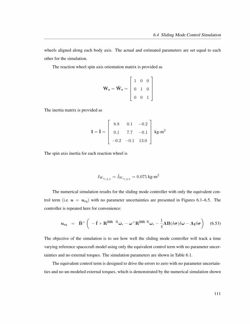
6.4 Sliding Mode Control Simulation
wheels aligned along each body axis. The actual and estimated parameters are set equal to each
other for the simulation.
The reaction wheel spin axis orientation matrix is provided as
Ws = Ws =
1 0 0
0 1 0
0 0 1
The inertia matrix is provided as
I = I =
8.8 0.1 −0.2
0.1 7.7 −0.1
−0.2 −0.1 13.0
kg-m2
The spin axis inertia for each reaction wheel is
IWs1,2,3= IWs1,2,3
= 0.075 kg-m2
The numerical simulation results for the sliding mode controller with only the equivalent con-
trol term (i.e. u = ueq) with no parameter uncertainties are presented in Figures 6.1–6.5. The
controller is repeated here for convenience:
ueq = B+
(− f + RBR Rωr − ω×RBR Rωr −
14ΛB(δσ)δω −ΛIδσ
)(6.53)
The objective of the simulation is to see how well the sliding mode controller will track a time
varying reference spacecraft model using only the equivalent control term with no parameter uncer-
tainties and no external torques. The simulation parameters are shown in Table 6.1.
The equivalent control term is designed to drive the errors to zero with no parameter uncertain-
ties and no un-modeled external torques, which is demonstrated by the numerical simulation shown
111

6.4 Sliding Mode Control Simulation
Table 6.1: Sliding Mode Control Numerical Simulation Parameters with only Equivalent Con-trol with no Parameter Uncertainties
Parameter Valueω(t0) (0.017, 0.017, 0.087) rad/sσ(t0) (0.05, 0.01, -0.01)Λ diag( 0.4, 0.4, 0.4 ) rad/sΛI diag( 0.01, 0.01, 0.01 ) rad/s2
Lunmodeled ( 0, 0, 0 ) N-m
in Figures 6.1 – 6.5. Figures 6.2 and 6.4 show the angular rate and MRP errors go to zero after
approximately 140 seconds. Figure 6.3 shows the MRP vector where the MRP switching condition
is activated at approximately 70 seconds. The required control torque to drive the angular rate and
MRP errors to zero has a maximum amplitude of 0.1 N-m as shown in Figure 6.5.
Figure 6.1: Sliding Mode Control Numerical Simulation Angular Rates with only EquivalentControl
112

6.4 Sliding Mode Control Simulation
Figure 6.2: Sliding Mode Control Numerical Simulation Angular Rate Errors with onlyEquivalent Control
Figure 6.3: Sliding Mode Control Numerical Simulation MRPs with only Equivalent Control
113

6.4 Sliding Mode Control Simulation
Figure 6.4: Sliding Mode Control Numerical Simulation MRP Errors with only EquivalentControl
Figure 6.5: Sliding Mode Control Numerical Simulation Equivalent Control Time History
114

6.4 Sliding Mode Control Simulation
6.4.1.2 Equivalent Control Term With Uncertainties
The second numerical simulation evaluates the equivalent control term (ueq) with parameter un-
certainties and un-modeled external torques. The actual and estimated reaction wheel spin axis
orientation matrices are provided as
Ws =
0.9951 0.0697 0.0697
0.0697 0.9951 0.0697
0.0697 0.0756 0.0697
Ws =
1 0 0
0 1 0
0 0 1
The inertia matrix estimate is
I =
8.8 0.1 −0.2
0.1 7.7 −0.1
−0.2 −0.1 13.0
kg-m2
The actual inertia matrix is specified as
I =
10.6 0.3 0.2
0.3 7.7 0.2
0.2 0.2 15.6
kg-m2
The spin axis inertia for each reaction wheel is
IWs1,2,3= 0.075 kg-m2
115

6.4 Sliding Mode Control Simulation
The actual spin axis inertia for each reaction wheel is
IWs1,2,3= 0.072 kg-m2
The numerical simulation results for the sliding mode controller with only the equivalent con-
trol term (i.e. u = ueq) are presented in Figures 6.6 – 6.10. The controller is repeated for conve-
nience in Eq. (6.53). The objective of the simulation is to see how well the sliding mode controller
will track a time varying reference spacecraft model without using the robust control term. The
estimates of the parameters are used to determine the equivalent control and the actual values are
used in determining the response of the simulated spacecraft. The simulation parameters are shown
in Table 6.2. An un-modeled external torque is included in the simulation.
Table 6.2: Sliding Mode Control Numerical Simulation Parameters with only Equivalent Con-trol with Parameter Uncertainties
Parameter Valueω(t0) (0.017, 0.017, 0.087) rad/sσ(t0) (0.05, 0.01, -0.01)Λ diag( 0.4, 0.4, 0.4 ) rad/sΛI diag( 0.01, 0.01, 0.01 ) rad/sLunmodeled ( 0.05, -0.03, 0.01 ) N-m
Figures 6.7 and 6.9 show the angular rate and MRP errors do not go to zero. The expectation
is that the equivalent control term would not drive the errors to zero with the inclusion of parameter
uncertainties and un-modeled external torques in the simulation. In the development of the sliding
mode controller, the robust control term is included to account for the parameter uncertainties and
un-modeled torques.
116
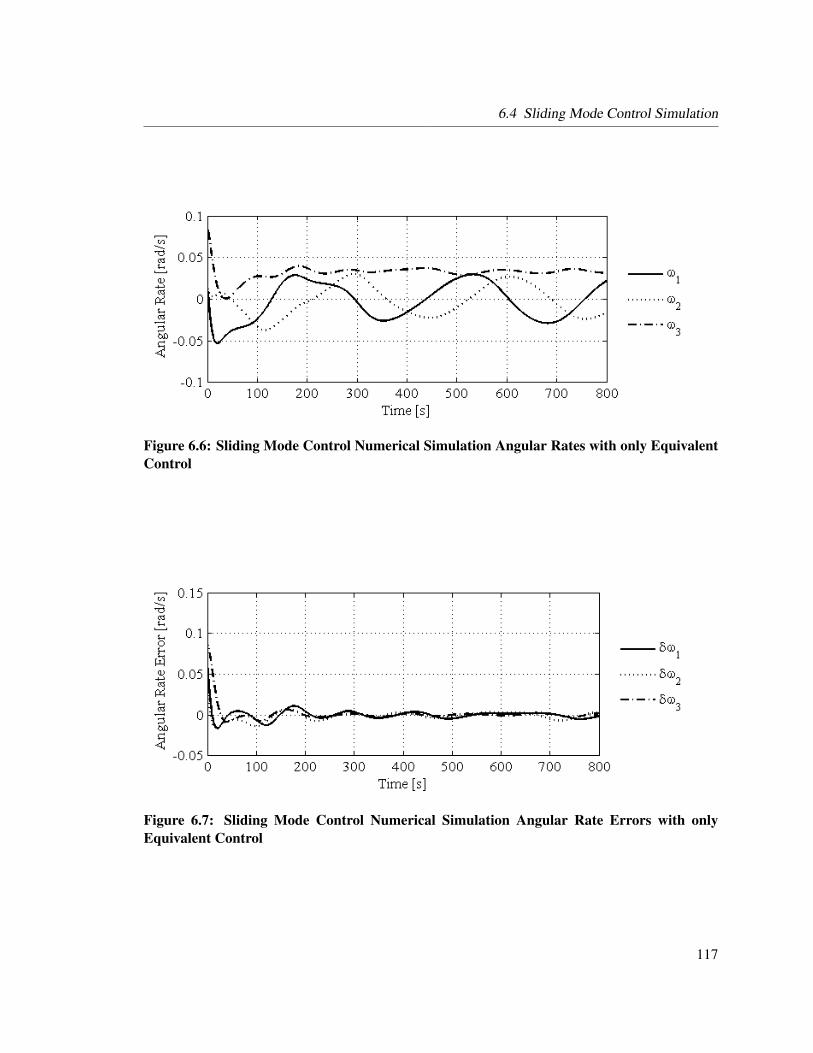
6.4 Sliding Mode Control Simulation
Figure 6.6: Sliding Mode Control Numerical Simulation Angular Rates with only EquivalentControl
Figure 6.7: Sliding Mode Control Numerical Simulation Angular Rate Errors with onlyEquivalent Control
117
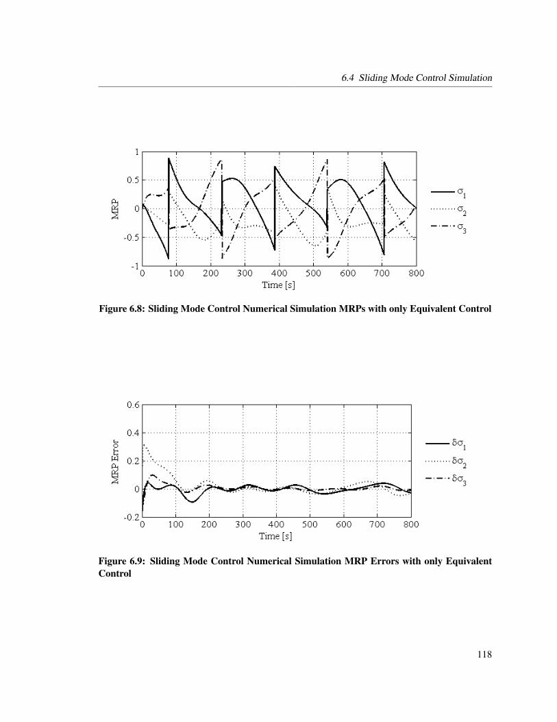
6.4 Sliding Mode Control Simulation
Figure 6.8: Sliding Mode Control Numerical Simulation MRPs with only Equivalent Control
Figure 6.9: Sliding Mode Control Numerical Simulation MRP Errors with only EquivalentControl
118
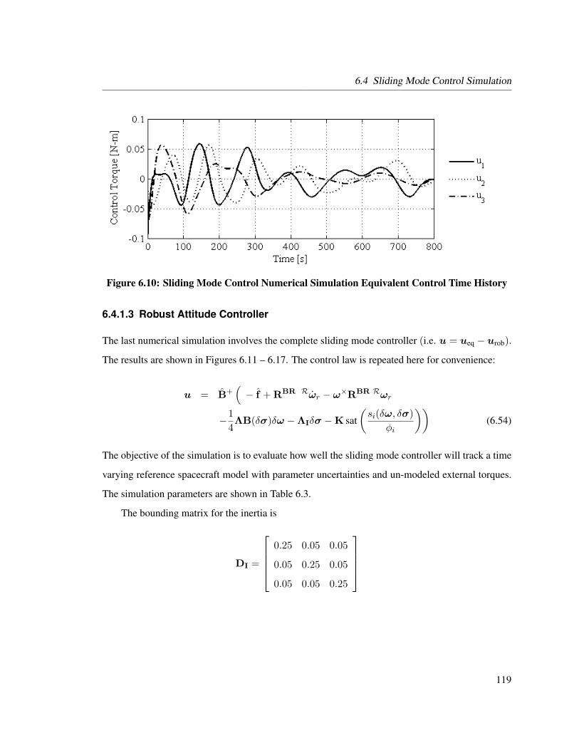
6.4 Sliding Mode Control Simulation
Figure 6.10: Sliding Mode Control Numerical Simulation Equivalent Control Time History
6.4.1.3 Robust Attitude Controller
The last numerical simulation involves the complete sliding mode controller (i.e. u = ueq − urob).
The results are shown in Figures 6.11 – 6.17. The control law is repeated here for convenience:
u = B+(− f + RBR Rωr − ω×RBR Rωr
−14ΛB(δσ)δω −ΛIδσ −K sat
(si(δω, δσ)
φi
))(6.54)
The objective of the simulation is to evaluate how well the sliding mode controller will track a time
varying reference spacecraft model with parameter uncertainties and un-modeled external torques.
The simulation parameters are shown in Table 6.3.
The bounding matrix for the inertia is
DI =
0.25 0.05 0.05
0.05 0.25 0.05
0.05 0.05 0.25
119

6.4 Sliding Mode Control Simulation
Table 6.3: Sliding Mode Control Numerical Simulation ParametersParameter Valueω(t0) (0.017, 0.017, 0.087) rad/sσ(t0) (0.05, 0.01, -0.01)Λ diag( 0.4, 0.4, 0.4 ) rad/sΛI diag( 0.01, 0.01, 0.01 ) rad/sφ 0.016 rad/sη ( 0.01, 0.01, 0.01 ) rad/s2
Lunmodeled ( 0.05, -0.03, 0.01 ) N-mΩ1 0 rad/sΩ2 0 rad/sΩ3 0 rad/s
The bounding matrix for the reaction wheels is
Dw =
0.10 0.09 0.09
0.09 0.10 0.09
0.09 0.09 0.10
The bounding matrix for the reaction wheel angular momentum (DD) is assumed to be the same as
the bounding matrix for the reaction wheels (Dw).
Figures 6.12 and 6.14 show the angular rate and MRP errors, which go to zero after approx-
imately 45 seconds. The robust control term does result in accounting for parameter uncertainties
and un-modeled external torques as clearly seen by comparing the previous simulations. Figure 6.17
shows the norm of the sliding variable (‖s‖2) time history, which goes to the sliding surface within
1 second. Figure 6.16 shows the maximum reaction wheel rate is 20 rad/s. The required control
torque shown in the numerical simulation indicates that the initial angular rates and gain selections
for the controller are appropriate for Whorl−I and Whorl−II, since the hardware simulators have a
maximum wheel rate of 100 rad/s.
The performance of the sliding mode controller using reaction wheels for attitude control will
vary due to the selection of Λ, ΛI, φ, and η. A critical consideration for determining the afore-
mentioned parameters is saturation of the reaction wheels. As Λ and ΛI increase the commanded
120

6.4 Sliding Mode Control Simulation
Figure 6.11: Sliding Mode Control Numerical Simulation Angular Rates
Figure 6.12: Sliding Mode Control Numerical Simulation Angular Rate Errors
121
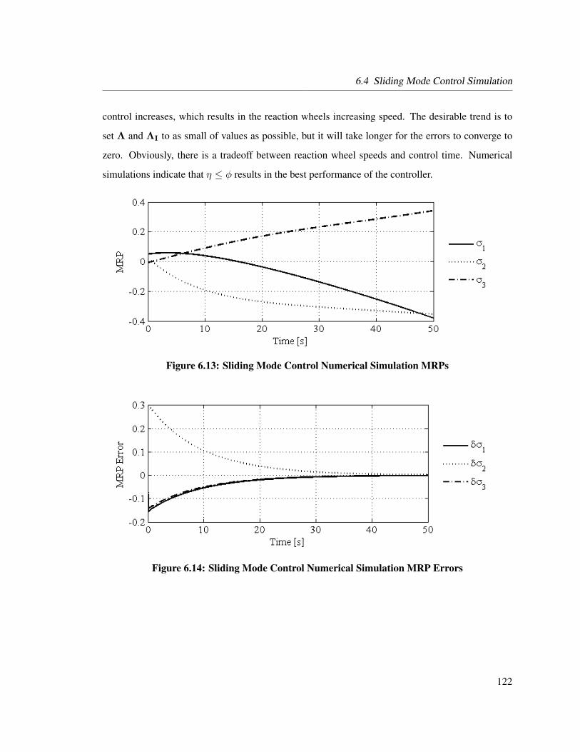
6.4 Sliding Mode Control Simulation
control increases, which results in the reaction wheels increasing speed. The desirable trend is to
set Λ and ΛI to as small of values as possible, but it will take longer for the errors to converge to
zero. Obviously, there is a tradeoff between reaction wheel speeds and control time. Numerical
simulations indicate that η ≤ φ results in the best performance of the controller.
Figure 6.13: Sliding Mode Control Numerical Simulation MRPs
Figure 6.14: Sliding Mode Control Numerical Simulation MRP Errors
122

6.4 Sliding Mode Control Simulation
Figure 6.15: Sliding Mode Control Numerical Simulation Control Time History
Figure 6.16: Sliding Mode Control Numerical Simulation Reaction Wheel Time History
123

6.4 Sliding Mode Control Simulation
Figure 6.17: Sliding Mode Control Numerical Simulation Reaction Sliding Variable TimeHistory
6.4.2 Whorl−I Sliding Mode Control Simulation
The following subsections present the simulation results for the MRP sliding mode controller using
numerical simulations and Whorl−I. The simulation results for a regulator (ω → 0,σ → 0) and
tracking (ω → ωr,σ → σr) problem are shown. The estimates for the simulator parameters are
provided in Section 3.1.
The bounding matrix for the inertia is
DI =
0.35 0.05 0.05
0.05 0.35 0.05
0.05 0.05 0.35
(6.55)
The bounding matrix for the reaction wheels is
Dw =
0.10 0.08 0.08
0.08 0.10 0.08
0.08 0.08 0.10
(6.56)
124

6.4 Sliding Mode Control Simulation
The bounding matrix for the reaction wheel angular momentum (DD) is assumed to be the
same as the bounding matrix for the reaction wheels (Dw).
The actual simulator parameters used in the numerical simulation are not necessarily the true
parameters for the simulator, but chosen so as to satisfy the bounding matrices. Therefore there will
be expected differences between Whorl−I and the numerical simulations.
6.4.2.1 Regulator
The results of running the controller on Whorl−I along with a numerical simulation comparing the
results are presented. The MRP sliding mode controller parameters are provided in Table 6.4. The
controller results are shown in Figures 6.18 – 6.26. Whorl−I is given an initial angular rate about
the 3 body axis and then the controller is activated. The 18 second delay in the start of the controller
at the beginning of the simulation is due to the time necessary to initialize the three reaction wheels.
Table 6.4: Sliding Mode Control Simulation Parameters for Whorl−IParameter ValueControl Rate 2 HzObserve Rate 2 HzWheel Speed Query 10 Hzω(t0) (-0.006, 0.003, 0.144) rad/sσ(t0) (-0.006, -0.004, -0.229)Λ diag( 0.89, 0.89, 1.26 ) rad/sΛI diag( 0.05, 0.05, 0.1 ) rad/s2
φ 0.5 rad/sη ( 0.04, 0.04, 0.04 ) rad/s2
Lmax 0.02 N-mΩ1 0 rad/sΩ2 0 rad/sΩ3 0 rad/s
Figures 6.18 and 6.19 provide the angular rate time history for Whorl−I and the numerical
simulation respectively. Whorl−I has approximately zero angular rate about the 3 axis after 12
seconds into the control simulation. The numerical simulation has approximately zero angular
rate after 12 seconds into the simulation. The angular rates for Whorl−I have the same trends as
125

6.4 Sliding Mode Control Simulation
predicted by the numerical simulation.
Figure 6.18: Whorl−I Angular Rates for MRP Sliding Mode Controller
Figure 6.19: Numerical Simulation Angular Rates for MRP Sliding Mode Controller
Figures 6.20 and 6.21 provide the MRP vector time history for Whorl−I and the numerical
simulation respectively. Whorl−I has approximately a zero MRP vector after 12 seconds into the
simulation. The numerical simulation has approximately a zero MRP error vector after 12 seconds
into the simulation. The MRP vector for Whorl−I has the same decreasing trend as predicted by
the numerical simulation.
126

6.4 Sliding Mode Control Simulation
Figure 6.20: Whorl−I MRP Vector for MRP Sliding Mode Controller
Figure 6.21: Numerical Simulation MRP Vector for MRP Sliding Mode Controller
127

6.4 Sliding Mode Control Simulation
Figures 6.22 and 6.23 show the required control torque specified by the MRP sliding mode con-
troller for Whorl−I and the numerical simulation respectively. The control torques specified by the
controller for Whorl−I have a similar control torque trend as the numerical simulation. Figure 6.20
indicates a larger over shoot as compared with the numerical simulation. More control torque is
commanded to compensate for the over shoot for σ3.
Figure 6.22: Whorl−I Control Torque for MRP Sliding Mode Controller
Figure 6.23: Numerical Simulation Control Torque for MRP Sliding Mode Controller
Figure 6.24 shows the sliding variable specified by the MRP sliding mode controller for Whorl−I.
128

6.4 Sliding Mode Control Simulation
The sliding variable for Whorl−I goes to approximately zero after 10 seconds.
Figure 6.24: Whorl−I Sliding Variable for MRP Sliding Mode Controller
Figures 6.25 and 6.26 show the reaction wheel speed time history for the controller running
on Whorl−I and the numerical simulation respectively. The reaction wheels have the same wheel
speed trend as the numerical simulation. The final wheel speeds for Whorl−I are 0 rad/s for Ω1, -3
rad/s for Ω2, and 30 rad/s for Ω3. The final wheel speeds for the numerical simulation are -0.5 rad/s
for Ω1, -2 rad/s for Ω2, and 32 rad/s for Ω3.
6.4.2.2 Tracking
The results of running the controller on Whorl−I along with a numerical simulation for tracking a
time varying attitude are presented. The MRP sliding mode controller parameters are provided in
Table 6.5.
The controller results are shown in Figures 6.27 – 6.26. Whorl−I is at rest and then the con-
troller is turned on. The 48 second delay in the start of the controller at the beginning of the
simulation is due to the time necessary to initialize the three reaction wheels and to spin up Ω3 to a
steady state condition of -50 rad/s.
Figures 6.27 and 6.28 provide the angular rate time history for Whorl−I and the numerical sim-
129

6.4 Sliding Mode Control Simulation
Figure 6.25: Whorl−I Reaction Wheel Speed for MRP Sliding Mode Controller
Figure 6.26: Numerical Simulation Reaction Wheel Speed for MRP Sliding Mode Controller
130
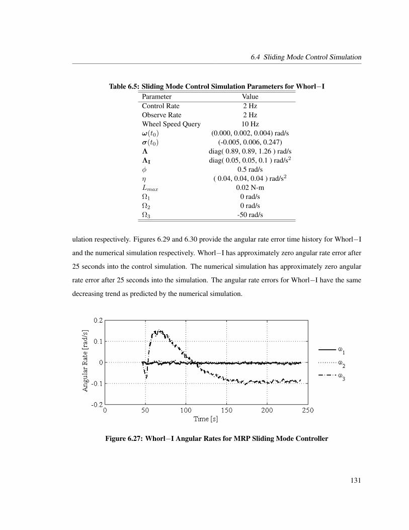
6.4 Sliding Mode Control Simulation
Table 6.5: Sliding Mode Control Simulation Parameters for Whorl−IParameter ValueControl Rate 2 HzObserve Rate 2 HzWheel Speed Query 10 Hzω(t0) (0.000, 0.002, 0.004) rad/sσ(t0) (-0.005, 0.006, 0.247)Λ diag( 0.89, 0.89, 1.26 ) rad/sΛI diag( 0.05, 0.05, 0.1 ) rad/s2
φ 0.5 rad/sη ( 0.04, 0.04, 0.04 ) rad/s2
Lmax 0.02 N-mΩ1 0 rad/sΩ2 0 rad/sΩ3 -50 rad/s
ulation respectively. Figures 6.29 and 6.30 provide the angular rate error time history for Whorl−I
and the numerical simulation respectively. Whorl−I has approximately zero angular rate error after
25 seconds into the control simulation. The numerical simulation has approximately zero angular
rate error after 25 seconds into the simulation. The angular rate errors for Whorl−I have the same
decreasing trend as predicted by the numerical simulation.
Figure 6.27: Whorl−I Angular Rates for MRP Sliding Mode Controller
131

6.4 Sliding Mode Control Simulation
Figure 6.28: Numerical Simulation Angular Rates for MRP Sliding Mode Controller
Figure 6.29: Whorl−I Angular Rate Errors for MRP Sliding Mode Controller
132

6.4 Sliding Mode Control Simulation
Figure 6.30: Numerical Simulation Angular Rate Errors for MRP Sliding Mode Controller
Figures 6.31 and 6.32 provide the MRP vector time history for Whorl−I and the numerical sim-
ulation respectively. Figures 6.33 and 6.34 provide the MRP error vector time history for Whorl−I
and the numerical simulation respectively. Whorl−I has approximately a zero MRP error vector
offset for σ3 of 0.02 after 80 seconds into the control simulation. The numerical simulation has
approximately a zero MRP error vector after 70 seconds into the simulation. The MRP vector for
Whorl−I has the same decreasing trend as predicted by the numerical simulation.
Figure 6.31: Whorl−I MRP Vector for MRP Sliding Mode Controller
133

6.4 Sliding Mode Control Simulation
Figure 6.32: Numerical Simulation MRP Vector for MRP Sliding Mode Controller
Figure 6.33: Whorl−I MRP Vector for MRP Sliding Mode Controller
134
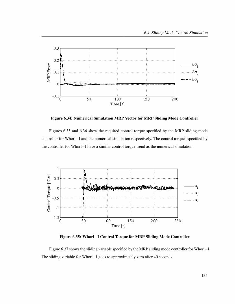
6.4 Sliding Mode Control Simulation
Figure 6.34: Numerical Simulation MRP Vector for MRP Sliding Mode Controller
Figures 6.35 and 6.36 show the required control torque specified by the MRP sliding mode
controller for Whorl−I and the numerical simulation respectively. The control torques specified by
the controller for Whorl−I have a similar control torque trend as the numerical simulation.
Figure 6.35: Whorl−I Control Torque for MRP Sliding Mode Controller
Figure 6.37 shows the sliding variable specified by the MRP sliding mode controller for Whorl−I.
The sliding variable for Whorl−I goes to approximately zero after 40 seconds.
135
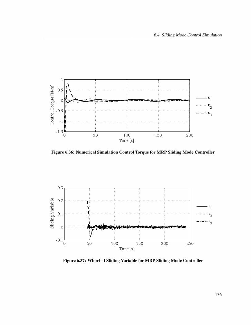
6.4 Sliding Mode Control Simulation
Figure 6.36: Numerical Simulation Control Torque for MRP Sliding Mode Controller
Figure 6.37: Whorl−I Sliding Variable for MRP Sliding Mode Controller
136

6.4 Sliding Mode Control Simulation
Figures 6.38 and 6.39 show the reaction wheel speed time history for the controller running on
Whorl−I and the numerical simulation respectively. The reaction wheels have a similar speed trend
as the numerical simulation. The final wheel speeds for Whorl−I are 0 rad/s for Ω1, 0 rad/s for Ω2,
and -25 rad/s for Ω3. The final wheel speeds for the numerical simulation are 0 rad/s for Ω1, 0 rad/s
for Ω2, and -27 rad/s for Ω3.
Figure 6.38: Whorl−I Reaction Wheel Speed for MRP Sliding Mode Controller
Figure 6.39: Numerical Simulation Reaction Wheel Speed for MRP Sliding Mode Controller
137

6.4 Sliding Mode Control Simulation
6.4.3 Whorl−II Sliding Mode Control Simulation
The following subsections present the simulation results for the MRP sliding mode controller using
numerical simulations and Whorl−II. The simulation results for a regulator (ω → 0,σ → 0) and
rest to rest (ω → 0,σ → 0) maneuver are shown. The estimates for the simulator parameters are
provided in Section 3.1.
The bounding matrix for the inertia is
DI =
0.35 0.05 0.05
0.05 0.35 0.05
0.05 0.05 0.35
(6.57)
The bounding matrix for the reaction wheels is
Dw =
0.10 0.08 0.08
0.08 0.10 0.08
0.08 0.08 0.10
(6.58)
The bounding matrix for the reaction wheel angular momentum (DD) is assumed to be the
same as the bounding matrix for the reaction wheels (Dw).
6.4.3.1 Regulator
The results of running the controller on Whorl−II along with a numerical simulation comparing the
results are presented. The MRP sliding mode controller parameters are provided in Table 6.6. The
controller results are shown in Figures 6.40 – 6.48. Whorl−II is given an initial angular rate about
the 3 body axis and then the controller is activated. The 45 second delay in the start of the controller
at the beginning of the simulation is due to the time necessary to initialize the three reaction wheels.
Figures 6.40 and 6.41 provide the angular rate time history for Whorl−II and the numerical
simulation respectively. Whorl−II has approximately zero angular rate in the 3 axis after 60 seconds
138

6.4 Sliding Mode Control Simulation
Table 6.6: Sliding Mode Control Simulation Parameters for Whorl−IIParameter Valueω(t0) (-0.040, -0.047, -0.183) rad/sσ(t0) (0.026, 0.033, 0.773)Λ diag( 0.90, 0.90, 0.28 ) rad/sΛI diag( 0.05, 0.05, 0.005 ) rad/sφ 0.5 rad/sη ( 0.04, 0.04, 0.04 ) rad/s2
Lmax 0.02 N-mΩ1 10 rad/sΩ2 -10 rad/sΩ3 10 rad/s
into the control simulation. The numerical simulation has approximately zero angular rate after 60
seconds into the simulation. The angular rates for Whorl−II have the same decreasing trend as
predicted by the numerical simulation.
Figure 6.40: Whorl−II Angular Rates for MRP Sliding Mode Controller
Figures 6.42 and 6.43 provide the MRP vector time history for Whorl−II and the numerical
simulation respectively. Whorl−II has approximately a constant offset from zero error for σ3 after
80 seconds into the simulation. The numerical simulation has approximately a zero MRP error
vector after 60 seconds into the simulation. The steady state offset for σ3 is approximately 0.02. The
139

6.4 Sliding Mode Control Simulation
Figure 6.41: Numerical Simulation Angular Rates for MRP Sliding Mode Controller
MRP vector for Whorl−II has the same decreasing trend as predicted by the numerical simulation.
Figure 6.42: Whorl−II MRP Vector for MRP Sliding Mode Controller
Figures 6.44 and 6.45 show the required control torque specified by the MRP sliding mode
controller for Whorl−II and the numerical simulation respectively. The control torques specified by
the controller for Whorl−II have a similar control torque trend as the numerical simulation.
Figure 6.46 shows the sliding variable specified by the MRP sliding mode controller for Whorl−II.
The sliding variable for Whorl−II goes to approximately 0 after 40 seconds.
140
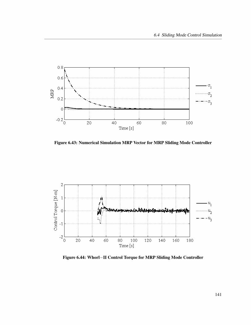
6.4 Sliding Mode Control Simulation
Figure 6.43: Numerical Simulation MRP Vector for MRP Sliding Mode Controller
Figure 6.44: Whorl−II Control Torque for MRP Sliding Mode Controller
141

6.4 Sliding Mode Control Simulation
Figure 6.45: Numerical Simulation Control Torque for MRP Sliding Mode Controller
Figure 6.46: Whorl−II Sliding Variable for MRP Sliding Mode Controller
142

6.4 Sliding Mode Control Simulation
Figures 6.47 and 6.48 show the reaction wheel speed time history for the controller running
on Whorl−II and the numerical simulation respectively. The reaction wheels have a similar speed
trend as the numerical simulation. The numerical simulation ends with an angular velocity of ap-
proximately -60 rad/s as compared with -55 rad/s for the reaction wheel aligned along the 3 axis.
The discrepancy in wheel speeds between Whorl−II and the numerical simulation is attributed to
the simplified reaction wheel motor torque model used in the numerical simulation.
Figure 6.47: Whorl−II Reaction Wheel Speed for MRP Sliding Mode Controller
Figure 6.48: Numerical Simulation Reaction Wheel Speed for MRP Sliding Mode Controller
143

6.4 Sliding Mode Control Simulation
6.4.3.2 Rest to Rest Maneuver
The results of running the controller on Whorl−II along with a numerical simulation comparing the
results are presented. The MRP sliding mode controller parameters are provided in Table 6.7. The
controller results are shown in Figures 6.49 – 6.57. Whorl−II is at rest and then the controller is
activated. The 22 second delay in the start of the controller at the beginning of the simulation is due
to the time necessary to initialize the three reaction wheels.
Table 6.7: Sliding Mode Control Simulation Parameters for Whorl−IIParameter Valueω(t0) (-0.003, 0.003, -0.007) rad/sσ(t0) (0.002, 0.002, 0.621)Λ diag( 0.90, 0.90, 0.28 ) rad/sΛI diag( 0.05, 0.05, 0.005 ) rad/sφ 0.5 rad/sη ( 0.04, 0.04, 0.04 ) rad/s2
Lmax 0.02 N-mΩ1 10 rad/sΩ2 -10 rad/sΩ3 10 rad/s
Figures 6.49 and 6.50 provide the angular rate time history for Whorl−II and the numerical
simulation respectively. Whorl−II has approximately zero angular rate in the 3 axis after 50 seconds
into the control simulation. The numerical simulation has approximately zero angular rate after 50
seconds into the simulation. The angular rates for Whorl−II have the same decreasing trend as
predicted by the numerical simulation.
Figures 6.51 and 6.52 provide the MRP vector time history for Whorl−II and the numerical
simulation respectively. Whorl−II has approximately a zero MRP vector after 70 seconds into the
simulation. The numerical simulation has approximately a zero MRP vector after 70 seconds into
the simulation. The MRP vector for Whorl−II has the same decreasing trend as predicted by the
numerical simulation.
Figures 6.53 and 6.54 show the required control torque specified by the MRP sliding mode
144

6.4 Sliding Mode Control Simulation
Figure 6.49: Whorl−II Angular Rates for MRP Sliding Mode Controller
Figure 6.50: Numerical Simulation Angular Rates for MRP Sliding Mode Controller
145

6.4 Sliding Mode Control Simulation
Figure 6.51: Whorl−II MRP Vector for MRP Sliding Mode Controller
Figure 6.52: Numerical Simulation MRP Vector for MRP Sliding Mode Controller
146

6.4 Sliding Mode Control Simulation
controller for Whorl−II and the numerical simulation respectively. The control torque specified by
the controller for Whorl−II has a similar control torque trend as the numerical simulation.
Figure 6.53: Whorl−II Control Torque for MRP Sliding Mode Controller
Figure 6.54: Numerical Simulation Control Torque for MRP Sliding Mode Controller
Figure 6.55 shows the sliding variable specified by the MRP sliding mode controller for Whorl−II.
The sliding variable for Whorl−II goes to approximately zero after 55 seconds.
Figures 6.56 and 6.57 show the reaction wheel speed time history for the controller running
on Whorl−II and the numerical simulation respectively. The reaction wheels have a similar speed
147

6.4 Sliding Mode Control Simulation
Figure 6.55: Whorl−II Sliding Variable for MRP Sliding Mode Controller
trend as the numerical simulation. The numerical simulation ends with an angular velocity of ap-
proximately 8 rad/s as compared with 12 rad/s for the reaction wheel aligned along the 3 axis. The
discrepancy in wheel speeds between Whorl−II and the numerical simulation is attributed to the
simplified reaction wheel motor torque model used in the numerical simulation.
Figure 6.56: Whorl−II Reaction Wheel Speed for MRP Sliding Mode Controller
148

6.5 Summary
Figure 6.57: Numerical Simulation Reaction Wheel Speed for MRP Sliding Mode Controller
6.5 Summary
In this chapter we develop a robust nonlinear attitude control law that tracks a reference attitude
while bounding system uncertainties. The development of the controller is described along with a
method to determine the equivalent control term gain matrices and robust control term gain matrix.
Bounding the spacecraft system uncertainties is discussed. Numerical simulations, Whorl−I, and
Whorl−II successfully demonstrate the spacecraft MRP attitude sliding mode controller.
The hardware-in-the-loop spacecraft attitude control simulators have demonstrated the perfor-
mance of several angular rate, MRP, and robust nonlinear attitude controllers. The following chap-
ter investigates the relative position control between spacecraft in low Earth orbit. A spacecraft
formation flying control simulation using a GPS simulator and the flight computers on the hardware
simulators is demonstrated using a classical orbital element feedback controller.
149

7 Classical Orbital Element Controller
A nonlinear Lyapunov based classical orbital element (COE) feedback controller based on the work
of Naasz, Karlgaard, and Hall in Refs. 2 and 62 is presented in the following sections along with a
Global Positioning System (GPS) hardware-in-the-loop simulation of multiple spacecraft flying in
formation using the COE controller.
Six pieces of information are necessary to identify the location of a spacecraft within an orbit
relative to an inertial reference frame (N ). The position (r) and velocity (r) vectors are one rep-
resentation. Another representation is the classical orbital elements. The classical orbital elements
have six elements. The semi-major axis (a) and eccentricity (e) define the spacecraft orbit and
shape. The inclination (i), longitude of ascending node (Ω), and argument of perigee (ω) define the
orbit plane orientation. The mean anomaly (M) provides the location of the spacecraft on the orbit
trajectory at time t.25,63,64
7.1 Controller
The COE feedback controller is a technique to control the six orbital element (a, e, I , Ω, ω, M0)
relative motion of a spacecraft in low Earth orbit (LEO). The development of the controller from
Ref. 62 is summarized in this section.
150

7.1 Controller
Gauss’s variational equations are25,63
dadt
=2a2
h
(e sin f ur +
p
ruθ
)(7.1)
dedt
=1h
(p sin f ur +
((p+ r) cos f + re
)uθ
)(7.2)
didt
=r cos θh
uh (7.3)
dΩdt
=r sin θh sin i
uh (7.4)
dωdt
=1he
(− p cos f ur + (p+ r) sin f uθ
)− r sin θ cos i
h sin iuh (7.5)
dMdt
= n+b
ahe
((p cos f − 2re) ur − (p+ r) sin f uθ
)(7.6)
where h is the angular momentum, f is the true anomaly, p is the semi-latus rectum, r is the scalar
orbit radius, θ is the argument of latitude (ω + f), b is the semi-minor orbit axis, and ur, uθ, uh are
the control acceleration components in the local vertical, local horizon (LVLH) frame. The LVLH
frame is a rotating coordinate frame where ur is the control in the orbit radial direction (er), uh
is the control in the orbit normal direction (eh), and uθ is the control in the direction (eθ) that is
perpendicular to the radial and orbit normal directions as shown in Figure 7.1.25,63
Gauss’ variational equations have the nonlinear structure as62
x = f (x) + Bu (7.7)
where x has the elements a, e, i, Ω, ω, and M . The mean anomaly is
M = M0 + nt (7.8)
where n is the mean motion and is equal toõ
a3where µ is the gravitational parameter of the Earth
with a value of 3.986× 10⁵ km3/s2.
151
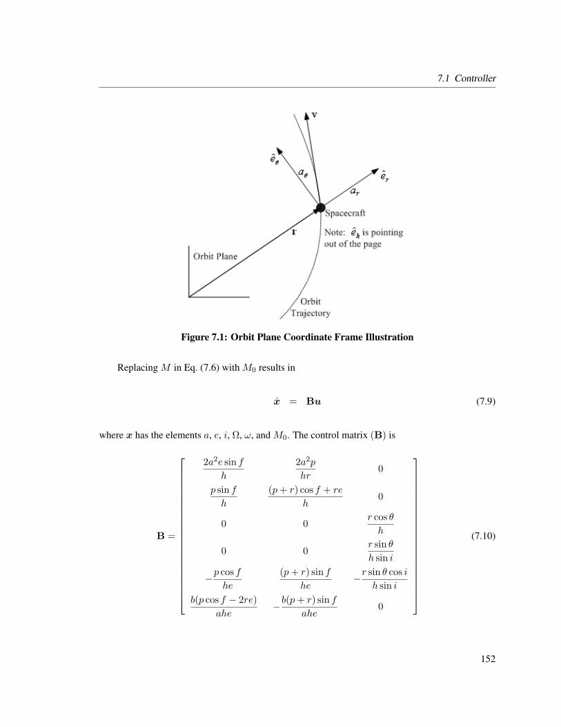
7.1 Controller
Figure 7.1: Orbit Plane Coordinate Frame Illustration
Replacing M in Eq. (7.6) with M0 results in
x = Bu (7.9)
where x has the elements a, e, i, Ω, ω, and M0. The control matrix (B) is
B =
2a2e sin fh
2a2p
hr0
p sin fh
(p+ r) cos f + re
h0
0 0r cos θh
0 0r sin θh sin i
−p cos fhe
(p+ r) sin fhe
−r sin θ cos ih sin i
b(p cos f − 2re)ahe
−b(p+ r) sin fahe
0
(7.10)
152

7.1 Controller
Reference 2 developed the following Lyapunov based COE feedback controller by expanding
Ilgen’s work in Ref. 65:
u = −
2a2e sin fh
2a2p
hr0
p sin fh
(p+ r) cos f + re
h0
0 0r cos θh
0 0r sin θh sin i
−p cos fhe
(p+ r) sin fhe
−r sin θ cos ih sin i
b(p cos f − 2re)ahe
−b(p+ r) sin fahe
0
T
Kaδa
Keδe
Kiδi
KΩδΩ
Kωδω
KMδMo
(7.11)
where Kδ(·) are the gains and δ(·) is defined as the relative orbital element values of the controlled
spacecraft with respect to the reference spacecraft as
δ(·) = (·)controlled − (·)reference (7.12)
The symbol (·) indicates the appropriate orbital element. Reference 2 proved the control law in
Eq. (7.11) is globally asymptotically stable.
153

7.2 GPS Formation Flying Simulation using COE Controller
Reference 2 developed the following expressions for the full state feedback gains:
Ka =h2
4a4(1 + e)2∆t(7.13)
Ke =h2
4p2∆t(7.14)
Ki =(h+ eh cos(ω + arcsin(e sinω))
p(−1 + e2 sin2 ω)
)2 1∆t
(7.15)
KΩ =(h sin(i) (−1 + e sin(ω + arcsin(e sinω)))
p(1− e2 cos2 ω)
)2 1∆t
(7.16)
Kω =e2h2
4p2
(1− e2
4
)1
∆t(7.17)
KM =a2e2h2
4b2p2
(1− e2
4
)∆t (7.18)
where ∆t is the the thruster duration and the gains are calculated at the beginning of the maneuver
as a function of the desired orbit and held constant.2
7.2 GPS Formation Flying Simulation using COE Controller
The results of a GPS hardware-in-the-loop simulation of two spacecraft flying in formation are
presented. The simulations involve a chief spacecraft in a low Earth orbit (LEO), while a deputy
spacecraft maintains an orbit position relative to the chief spacecraft. In order to maintain the for-
mation an orbit correction maneuver (OCM) for the deputy spacecraft is required. The control of
the OCM is accomplished using the COE controller presented in the previous section and simulat-
ing continual impulsive thrusting for only the deputy spacecraft. The COE controller requires the
relative position of the six orbital elements (a, e, I , Ω, ω, M0). The deputy communicates with the
chief spacecraft to obtain the current orbit position of the chief spacecraft, which is determined by
a numerical orbit propagator. The position of the deputy is determined from a GPS receiver that is
connected to a GPS hardware-in-the-loop simulator. The GPS simulator creates an RF signal based
on a simulated trajectory, which results in the GPS receiver calculating the navigation solution for
154
7.2 GPS Formation Flying Simulation using COE Controller
the simulated trajectory. From the relative positions of the spacecraft the COE controller calculates
the OCM for the deputy spacecraft.
The following sections discuss the implementation of the COE controller and the results of the
LEO formation flying simulation.
7.2.1 Implementation of Classical Orbital Element Controller
For this study the controller is used to control the relative orbit of the deputy spacecraft with re-
spect to the chief spacecraft. The deputy spacecraft retrieves the navigation solution from the GPS
receiver, which includes orbital perturbations. The mean orbital elements are determined by trans-
forming WGS-84 coordinates to Earth Centered Earth Fixed (ECEF) coordinates to Earth Centered
Inertial (ECI) coordinates to osculating orbit elements and then mapped to mean orbital elements.
The mapping between osculating and mean orbital elements is a first-order mapping algorithm out-
lined in Ref. 25. Mean elements are orbital elements with the short and long period motion removed.
The COE controller uses the mean orbital elements to determine the control acceleration.
The chief spacecraft determines its position by retrieving the ECI coordinates from the numeri-
cal orbit propagator through TCP/IP and converts the coordinates to osculating orbital elements and
maps the elements to mean orbital elements. The controller scheme is illustrated in Figure 7.2.
A desired relative orbit between the chief and deputy spacecraft is specified and the COE con-
troller determines the appropriate ∆V for the deputy spacecraft. Most spacecraft have fixed magni-
tude thrusters. For this study the thrust magnitude is constrained by the available thrust magnitude
(Tavailable) with instantaneous thrust direction. The deputy spacecraft will thrust if and only if the
requested thrust is greater than the available thrust(Trequested > Tavailable
). The ∆V in the instanta-
neous requested direction is determined from
∆V =Tavailable
m∆t (7.19)
where m is the mass and ∆t is the thrust duration of the deputy spacecraft.
The available thrust magnitude and thrust direction are assumed to be known perfectly. The
155

7.2 GPS Formation Flying Simulation using COE Controller
Figure 7.2: Spacecraft Formation Flying Simulation Scheme
∆V is sent to the numerical orbit propagator computer through TCP/IP as shown in Figure 3.14.
7.2.2 LEO Formation Flying Simulation
The real-time hardware-in-the-loop LEO formation flying simulation presented in this section demon-
strates the ability of the GPS simulator and the DSACSS facility to simulate controlling the semi-
major axis of the deputy spacecraft relative to the chief spacecraft.
The chief spacecraft has a mass of 100 kg and has no orbital control capability. The spacecraft
obtains its position and velocity by querying a numerical orbit propagator, which includes orbital
perturbations. The position and velocity are returned through TCP/IP in the ECI reference frame
and assumed to be known perfectly. The osculating orbital elements are determined from the po-
sition and velocity and mapped into mean orbital elements. The mean orbital elements are sent to
the deputy spacecraft. The initial mean orbital elements for the chief spacecraft are provided in
Table 7.1. The chief spacecraft position and velocity is queried at 0.5 Hz.
The deputy spacecraft has a mass of 100 kg with an orbital thrust magnitude capability of 1.0 N
with an impulse thrust duration of 2.0 seconds. As previously mentioned the deputy spacecraft
156

7.2 GPS Formation Flying Simulation using COE Controller
Table 7.1: Chief and Deputy Spacecraft Initial ConditionsParameter Chief Spacecraft Deputy Spacecrafta 7116.0 km 7113.2 kme 0.0486 0.0487i 5.0 5.0
Ω -0.004 39.329
ω 0.001 0.352
M0 0.006 0.321Mass 100 kg 100 kgThruster Magnitude NA 1.0 NThrust Duration NA 2.0 secNote: (·) indicates mean element.
obtains its position and velocity by querying the Ashtech G12 HDMA GPS receiver through TCP/IP.
The returned filtered position and velocity in the WGS-84 reference frame is converted to ECEF
coordinates and then to ECI coordinates as illustrated in Figure 7.2. The mean orbital elements are
mapped from the osculating orbital elements, which are determined from the position and velocity
in the ECI reference frame. The initial mean orbital elements for the deputy spacecraft are provided
in Table 7.1. The deputy spacecraft queries the GPS receiver at 0.5 Hz.
The desired semi-major axis difference between the deputy spacecraft and chief spacecraft is
15 km. The initial relative semi-major axis between the chief spacecraft and deputy spacecraft
is 2.7 km. The deputy spacecraft desired mean semi-major axis is approximately 7131 km. The
simulation results are shown in Figures 7.3 – 7.14.
The chief spacecraft mean semi-major axis, eccentricity, and inclination are shown in Fig-
ures 7.3 – 7.5. The mean semi-major axis is approximately 7116.0 km throughout the simulation.
The mean eccentricity is approximately 0.048 and the mean inclination is approximately 5.0 degrees
throughout the simulation.
The PDOP, HDOP, VDOP, and TDOP values for the deputy spacecraft GPS receiver are shown
in Figure 7.6. The DOP values range from 1 to 3 throughout the simulation. The number of GPS
satellites used to determine the navigation solution range from 7 to 10 throughout the simulation as
shown in Figure 7.7.
157
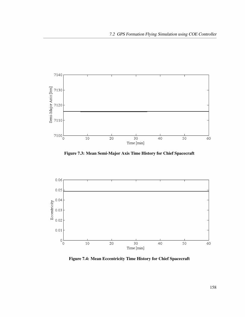
7.2 GPS Formation Flying Simulation using COE Controller
Figure 7.3: Mean Semi-Major Axis Time History for Chief Spacecraft
Figure 7.4: Mean Eccentricity Time History for Chief Spacecraft
158

7.2 GPS Formation Flying Simulation using COE Controller
Figure 7.5: Mean Inclination Time History for Chief Spacecraft
Figure 7.6: Deputy Spacecraft GPS Receiver Parameters (PDOP, HDOP, VDOP, and TDOP)
159
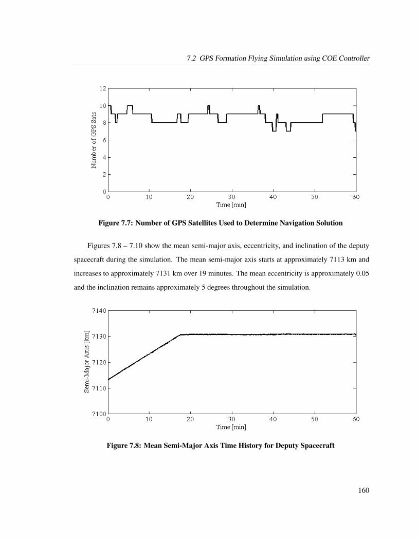
7.2 GPS Formation Flying Simulation using COE Controller
Figure 7.7: Number of GPS Satellites Used to Determine Navigation Solution
Figures 7.8 – 7.10 show the mean semi-major axis, eccentricity, and inclination of the deputy
spacecraft during the simulation. The mean semi-major axis starts at approximately 7113 km and
increases to approximately 7131 km over 19 minutes. The mean eccentricity is approximately 0.05
and the inclination remains approximately 5 degrees throughout the simulation.
Figure 7.8: Mean Semi-Major Axis Time History for Deputy Spacecraft
160

7.2 GPS Formation Flying Simulation using COE Controller
Figure 7.9: Mean Eccentricity Time History for Deputy Spacecraft
Figure 7.10: Mean Inclination Time History for Deputy Spacecraft
161
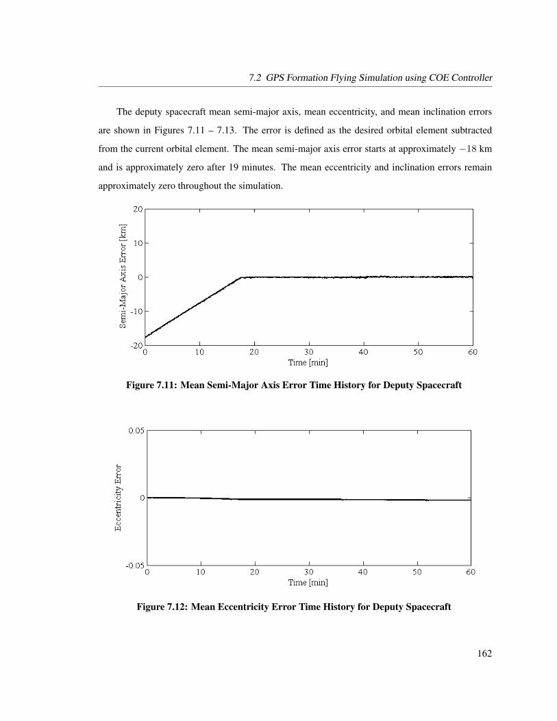
7.2 GPS Formation Flying Simulation using COE Controller
The deputy spacecraft mean semi-major axis, mean eccentricity, and mean inclination errors
are shown in Figures 7.11 – 7.13. The error is defined as the desired orbital element subtracted
from the current orbital element. The mean semi-major axis error starts at approximately −18 km
and is approximately zero after 19 minutes. The mean eccentricity and inclination errors remain
approximately zero throughout the simulation.
Figure 7.11: Mean Semi-Major Axis Error Time History for Deputy Spacecraft
Figure 7.12: Mean Eccentricity Error Time History for Deputy Spacecraft
162
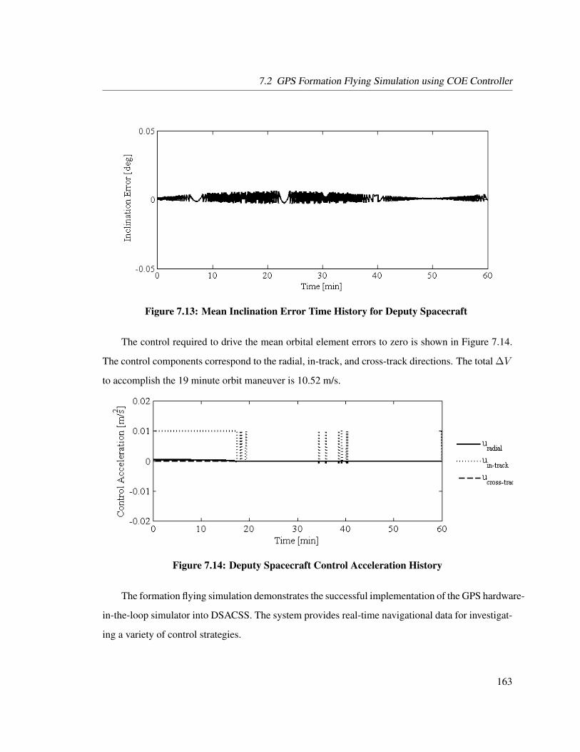
7.2 GPS Formation Flying Simulation using COE Controller
Figure 7.13: Mean Inclination Error Time History for Deputy Spacecraft
The control required to drive the mean orbital element errors to zero is shown in Figure 7.14.
The control components correspond to the radial, in-track, and cross-track directions. The total ∆V
to accomplish the 19 minute orbit maneuver is 10.52 m/s.
Figure 7.14: Deputy Spacecraft Control Acceleration History
The formation flying simulation demonstrates the successful implementation of the GPS hardware-
in-the-loop simulator into DSACSS. The system provides real-time navigational data for investigat-
ing a variety of control strategies.
163

7.3 Summary
7.3 Summary
In this chapter we summarize the classical orbital element feedback controller developed in Ref. 2.
We implement the orbit controller into DSACSS and successfully demonstrate the performance of
the controller using a space qualified GPS receiver and GPS simulator. A low Earth orbit formation
flying simulation is conducted using the flight computers from the attitude hardware simulators.
The COE controller successfully controls the relative orbital elements between the chief and deputy
spacecraft while increasing the semi-major axis of the deputy spacecraft to the desired relative value.
164

8 Sliding Mode Classical Orbital Element
Controller
In this chapter we develop a classical orbital element (COE) feedback control law based on the slid-
ing mode methodology while bounding system uncertainties. Gauss’ form of Lagrange’s Planetary
Equations are modified to provide the control vector in the orbit velocity direction, orbit normal di-
rection, and direction perpendicular to the previous two directions. A COE control law is developed
and a low Earth orbit (LEO) simulation is presented using the GPS hardware-in-the-loop simulator.
8.1 Modification to Gauss’ form of Lagrange’s Planetary
Equations
Gauss’ variational equations are shown in Eqs. 7.1 – 7.6 and are repeated here for convenience:
dadt
=2a2
h
(e sin fur +
p
ruθ
)dedt
=1h
(p sin fur + ((p+ r) cos f + re)uθ)
didt
=r cos θh
uh
165
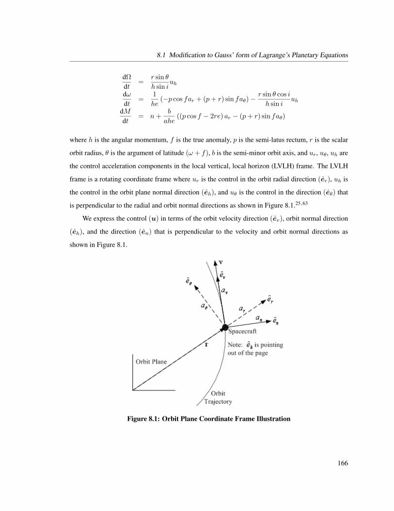
8.1 Modification to Gauss’ form of Lagrange’s Planetary Equations
dΩdt
=r sin θh sin i
uh
dωdt
=1he
(−p cos far + (p+ r) sin faθ)−r sin θ cos ih sin i
uh
dMdt
= n+b
ahe((p cos f − 2re) ar − (p+ r) sin faθ)
where h is the angular momentum, f is the true anomaly, p is the semi-latus rectum, r is the scalar
orbit radius, θ is the argument of latitude (ω + f), b is the semi-minor orbit axis, and ur, uθ, uh are
the control acceleration components in the local vertical, local horizon (LVLH) frame. The LVLH
frame is a rotating coordinate frame where ur is the control in the orbit radial direction (er), uh is
the control in the orbit plane normal direction (eh), and uθ is the control in the direction (eθ) that
is perpendicular to the radial and orbit normal directions as shown in Figure 8.1.25,63
We express the control (u) in terms of the orbit velocity direction (ev), orbit normal direction
(eh), and the direction (en) that is perpendicular to the velocity and orbit normal directions as
shown in Figure 8.1.
Figure 8.1: Orbit Plane Coordinate Frame Illustration
166

8.1 Modification to Gauss’ form of Lagrange’s Planetary Equations
As can be seen in Figure 8.1, going from er, eθ, eh to en, ev, eh involves a rotation about
the eh axis. The orbit plane control accelerations in the er and eθ directions are25
ur
uθ
=h
pv
p/r e sin f
−e sin f p/r
un
uv
(8.1)
Substituting Eq. (8.1) into Eqs. (7.1) – (7.6) results in the following form of Gauss’ variational
equations:25
dadt
=2a2v
µuv (8.2)
dedt
=1v
(ra
sin fun + 2 (e+ cos f)uv)
(8.3)
didt
=r cos θh
uh (8.4)
dΩdt
=r sin θh sin i
uh (8.5)
dωdt
=1ev
(−(
2e+r
a
)cos fan + 2 sin fav
)− r sin θ cos i
h sin iuh (8.6)
dMdt
= n+b
aev
(r
acos fan − 2
(1 + e2 r
p
)sin fav
)(8.7)
The modified form of Gauss’ variational equations has the nonlinear structure of
x = f (x) + Bu (8.8)
where x has the elements a, e, i, Ω, ω, and M . The mean anomaly is
M = M0 + nt (8.9)
where n is the mean motion and is equal toõ
a3where µ is the gravitational parameter for the
Earth with a value of 3.986× 10⁵ km3/s2.
167
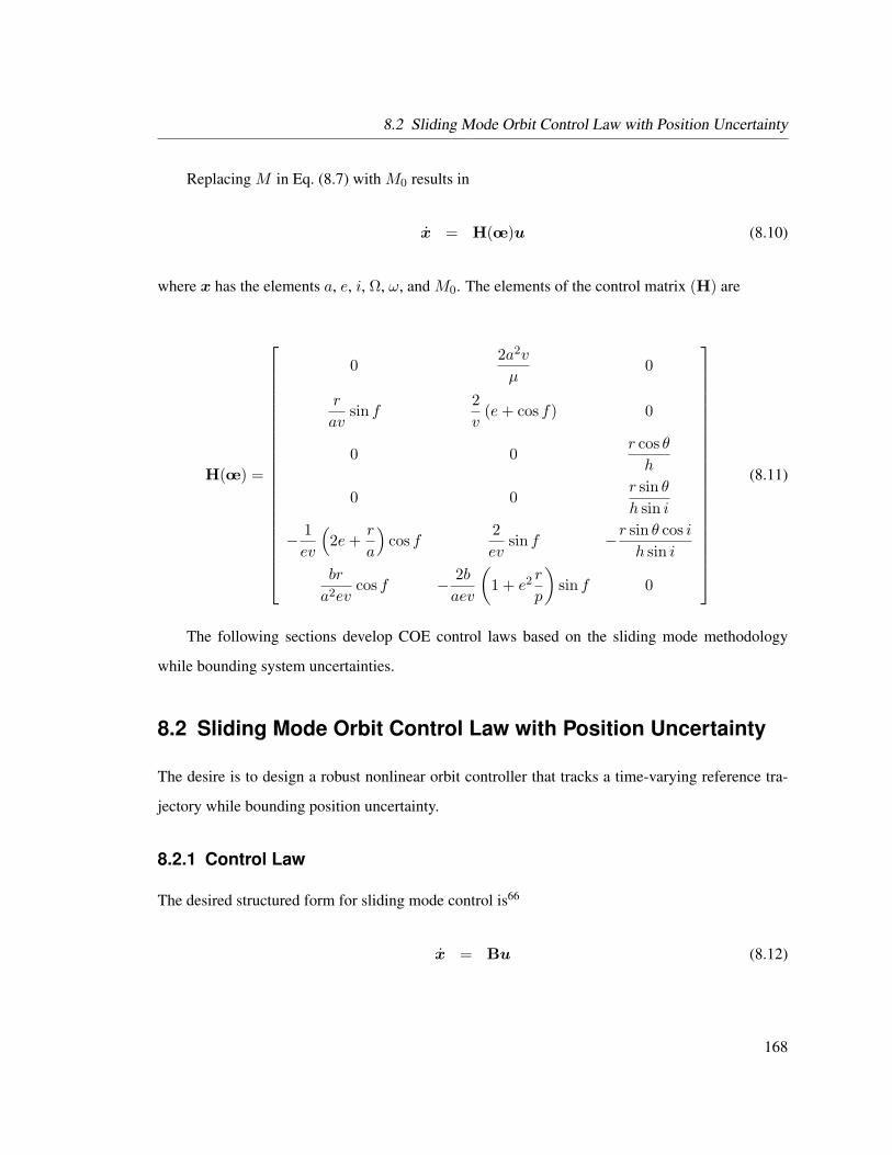
8.2 Sliding Mode Orbit Control Law with Position Uncertainty
Replacing M in Eq. (8.7) with M0 results in
x = H(oe)u (8.10)
where x has the elements a, e, i, Ω, ω, and M0. The elements of the control matrix (H) are
H(oe) =
02a2v
µ0
r
avsin f
2v
(e+ cos f) 0
0 0r cos θh
0 0r sin θh sin i
− 1ev
(2e+
r
a
)cos f
2ev
sin f −r sin θ cos ih sin i
br
a2evcos f − 2b
aev
(1 + e2 r
p
)sin f 0
(8.11)
The following sections develop COE control laws based on the sliding mode methodology
while bounding system uncertainties.
8.2 Sliding Mode Orbit Control Law with Position Uncertainty
The desire is to design a robust nonlinear orbit controller that tracks a time-varying reference tra-
jectory while bounding position uncertainty.
8.2.1 Control Law
The desired structured form for sliding mode control is66
x = Bu (8.12)
168

8.2 Sliding Mode Orbit Control Law with Position Uncertainty
From Eq. (8.10), the structured form is
x = H(oe)︸ ︷︷ ︸B
u (8.13)
The sliding variable (s) is defined as
s(δoe) , Λδoe (8.14)
where Λ is a 6× 6 positive-definite gain matrix, oe is the 6× 1 matrix of orbital elements, and δoe
is defined as the relative orbital elements with respect to the reference orbital elements:
δoe = oe− oer (8.15)
Ensuring s converges to the sliding surface can be achieved if each element of the sliding
variable si satisfies the sliding condition (also known as the reachability condition60) specified as
12
ddts(δoe)2
i ≤ −ηi|s(δoe)i| (8.16)
where ηi is a positive constant. The sliding surface condition ensures that the system trajectory
point to the surface and that once the system trajectory reaches the sliding surface it remains on that
surface.14
The control acceleration vector u ensures that the sliding condition given in Eq. (8.16) is met
in the presence of model uncertainty. The controller that satisfies the sliding condition is given as a
sign or saturation function:66
u = −B+K sign (s(δoe)) (8.17)
u = −B+K sat(si(δoe)φi
)(8.18)
where K is a 6×6 diagonal matrix whose values are not yet identified and B+ is the pseudo-inverse
169

8.2 Sliding Mode Orbit Control Law with Position Uncertainty
for the estimate of the control matrix.
The control matrix, B, is a 6 × 3 matrix and the inverse is determined by a pseudo-inverse or
weighted pseudo-inverse. The pseudo-inverse is25
B+ = BT(BBT
)−1(8.19)
The pseudo-inverse can also be found using singular value decomposition:
B = USVT (8.20)
where U and V are orthogonal m× n matrices and S is a positive diagonal n× n matrix. Then the
pseudo-inverse is67
B+ = V(STS
)−1STUT (8.21)
The weighted pseudo-inverse is25
B+ = WBT(BWBT
)−1(8.22)
where W is a diagonal matrix with user desired weighted values.
The sign function is defined as14
sign (si(δoe)) =
−1 if si(δoe) < 0
1 if si(δoe) ≥ 0(8.23)
The saturation function is defined as14
sat(si(δoe)φi
)=
si(δoe)φi
if |si(δoe)| ≤ φi
sign(si(δoe)) if |si(δoe)| > φi
(8.24)
170

8.2 Sliding Mode Orbit Control Law with Position Uncertainty
where φi is a boundary layer thickness that will eliminate chatter if appropriately chosen so that the
un-modeled high-frequency dynamics are not excited.
8.2.2 Gains and Parameter Bound Selection
This section develops the gain matrix K, the gain matrix Λ, and the control bound DB. The
derivative of the sliding variable is
s(δoe) = Λδoe
= Λoe
= ΛBu (8.25)
The gain (K) expression is solved for by substituting the control signal (u) given in Eq. (8.17)
into s(δoe) and solving for the sliding surface constraint in Eq. (8.16). The result is
12
ddt(sTs
)= s(δoe)Ts(δoe)
= (ΛBu)T s(δoe)
= −(ΛBB+Ksign (s(δoe))
)Ts(δoe) (8.26)
The diagonal matrix terms (diag(K)) are determined by satisfying the sliding condition in
Eq. (8.16), which results in
−η ≥ −ΛBB+Ksign (s(δoe)) (8.27)
171

8.2 Sliding Mode Orbit Control Law with Position Uncertainty
The matrix diag(K) expression is solved for by
ΛBB−1Ksign (s(δoe)) ≥ η
Ksign (s(δoe)) ≥(ΛBB+
)−1η
Ksign (s(δoe)) ≥ BB+Λ−1η
diag(K) ≥∣∣∣BB+Λ−1η
∣∣∣ (8.28)
The control matrix is bounded as
B = (11 +4B) B (8.29)
where |4B| ≤ DB. From Eq. (8.29), BB−1 results in
BB+ = (11 +4B)−1BB+
= (11 +4B)−1BBT(BBT
)−1
= (11 +4B)−1
≤ (11−DB)−1 (8.30)
The diagonal matrix terms, diag(K), are rewritten as
diag(K) =∣∣∣(11−DB)−1 Λ−1η
∣∣∣ (8.31)
The full state feedback gains (Λ) developed in Ref. 2 and shown in Eqs. (7.13)–(7.18) are
developed based on the response of each orbital element to thrust impulses. These gain expressions
172
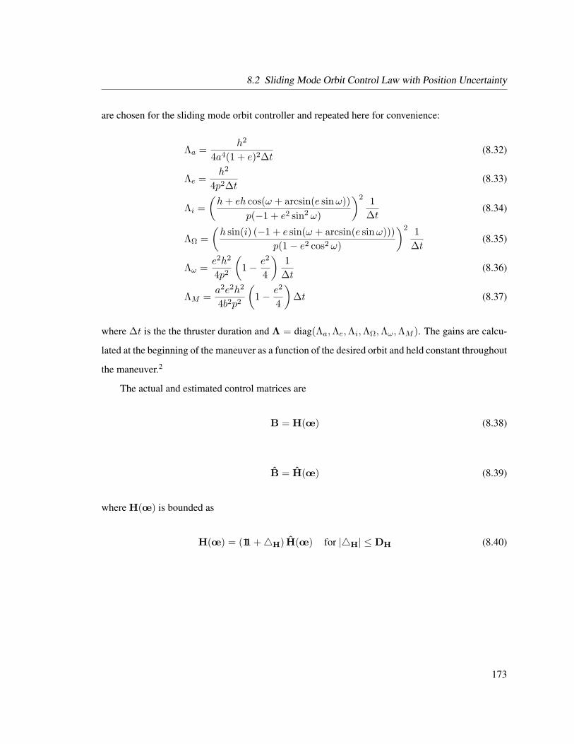
8.2 Sliding Mode Orbit Control Law with Position Uncertainty
are chosen for the sliding mode orbit controller and repeated here for convenience:
Λa =h2
4a4(1 + e)2∆t(8.32)
Λe =h2
4p2∆t(8.33)
Λi =(h+ eh cos(ω + arcsin(e sinω))
p(−1 + e2 sin2 ω)
)2 1∆t
(8.34)
ΛΩ =(h sin(i) (−1 + e sin(ω + arcsin(e sinω)))
p(1− e2 cos2 ω)
)2 1∆t
(8.35)
Λω =e2h2
4p2
(1− e2
4
)1
∆t(8.36)
ΛM =a2e2h2
4b2p2
(1− e2
4
)∆t (8.37)
where ∆t is the the thruster duration and Λ = diag(Λa,Λe,Λi,ΛΩ,Λω,ΛM ). The gains are calcu-
lated at the beginning of the maneuver as a function of the desired orbit and held constant throughout
the maneuver.2
The actual and estimated control matrices are
B = H(oe) (8.38)
B = H(oe) (8.39)
where H(oe) is bounded as
H(oe) = (11 +4H) H(oe) for |4H| ≤ DH (8.40)
173

8.2 Sliding Mode Orbit Control Law with Position Uncertainty
The control matrix bound DB is
B = H(oe)
= (11 +4H) H(oe)
= (11 +4H)︸ ︷︷ ︸11+4B
B
|4B| = |4H|
DB = DH (8.41)
In summary the robust orbit controller with the saturation function selected is
u = −B+K sat(si(δoe)φi
)(8.42)
s(δoe) = Λδoe (8.43)
diag(K) =∣∣∣(11−DB)−1 Λ−1η
∣∣∣ (8.44)
where B is provided in Eq. (8.11).
8.2.3 LEO Control Simulation using GPS Simulator
The real-time hardware-in-the-loop simulation presented in this section demonstrates the ability of
the sliding mode control law shown in Eq. (8.42) to increase the semi-major axis of a spacecraft
in LEO. The Ashtech G12 GPS receiver is used for the simulation along with the GPS simulator
described in Section 3.4.
The spacecraft obtains its position and velocity by querying the Ashtech G12 HDMA GPS
receiver through TCP/IP. The returned filtered position and velocity in the WGS-84 reference frame
are converted to ECEF coordinates and then to ECI coordinates as illustrated in Figure 8.2. The
mean orbital elements are mapped from the osculating orbital elements, which are determined from
the position and velocity in the ECI reference frame.
The initial mean orbital elements of the spacecraft, and other simulation parameters, are pro-
174
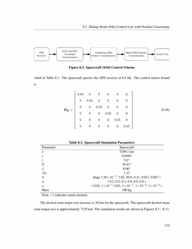
8.2 Sliding Mode Orbit Control Law with Position Uncertainty
Figure 8.2: Spacecraft Orbit Control Scheme
vided in Table 8.1. The spacecraft queries the GPS receiver at 0.5 Hz. The control matrix bound
is
DB =
0.05 0 0 0 0 0
0 0.05 0 0 0 0
0 0 0.05 0 0 0
0 0 0 0.05 0 0
0 0 0 0 0.05 0
0 0 0 0 0 0.05
(8.45)
Table 8.1: Spacecraft Simulation ParametersParameter Spacecrafta 7109.1 kme 0.0485i 5.0
Ω 39.41
ω 0.06
M0 1.23Λ diag( 1.26×10⁻⁷, 7.02, 30.9, 0.21, 0.017, 0.067 )φ ( 0.2, 0.2, 0.3, 0.9, 0.9, 0.9 )η ( 0.01, 1×10⁻⁵, 0.01, 1×10⁻⁷, 1×10⁻⁶, 1×10⁻⁶ )Mass 100 kgNote: (·) indicates mean element.
The desired semi-major axis increase is 20 km for the spacecraft. The spacecraft desired mean
semi-major axis is approximately 7129 km. The simulation results are shown in Figures 8.3 – 8.11.
175

8.2 Sliding Mode Orbit Control Law with Position Uncertainty
The PDOP, HDOP, VDOP, and TDOP values for the spacecraft GPS receiver are shown in
Figure 8.3. The DOP values range from 0.6 to 2.8 during the simulation. The number of GPS
satellites used to determine the navigation solution range from 8 to 10 during the simulation as
shown in Figure 8.4.
Figure 8.3: Spacecraft GPS Receiver Parameters (PDOP, HDOP, VDOP, and TDOP)
Figure 8.4: Number of GPS Satellites Used to Determine Navigation Solution
176

8.2 Sliding Mode Orbit Control Law with Position Uncertainty
Figures 8.5 – 8.7 show the mean semi-major axis, eccentricity, and inclination of the orbit
during the simulation. The mean semi-major axis starts at approximately 7109 km and increases
to approximately 7129 km over 19 minutes. The mean eccentricity is approximately 0.05 and the
inclination remains approximately 5 degrees throughout the simulation.
Figure 8.5: Mean Semi-Major Axis Time History for Spacecraft
The orbit mean semi-major axis, mean eccentricity, and mean inclination errors are shown in
Figures 8.8 – 8.10. The mean semi-major axis error starts at approximately −20 km and is approx-
imately zero after 19 minutes. The mean inclination error is approximately zero after 32 minutes
into the simulation.
The control required to drive the mean orbital element errors to zero is shown in Figure 8.11.
The control components correspond to the ev, eh, and en directions. The total ∆V to accomplish
the successful semi-major axis increase maneuver is 19.6 m/s in 19 minutes .
177

8.2 Sliding Mode Orbit Control Law with Position Uncertainty
Figure 8.6: Mean Eccentricity Time History for Spacecraft
Figure 8.7: Mean Inclination Time History for Spacecraft
178
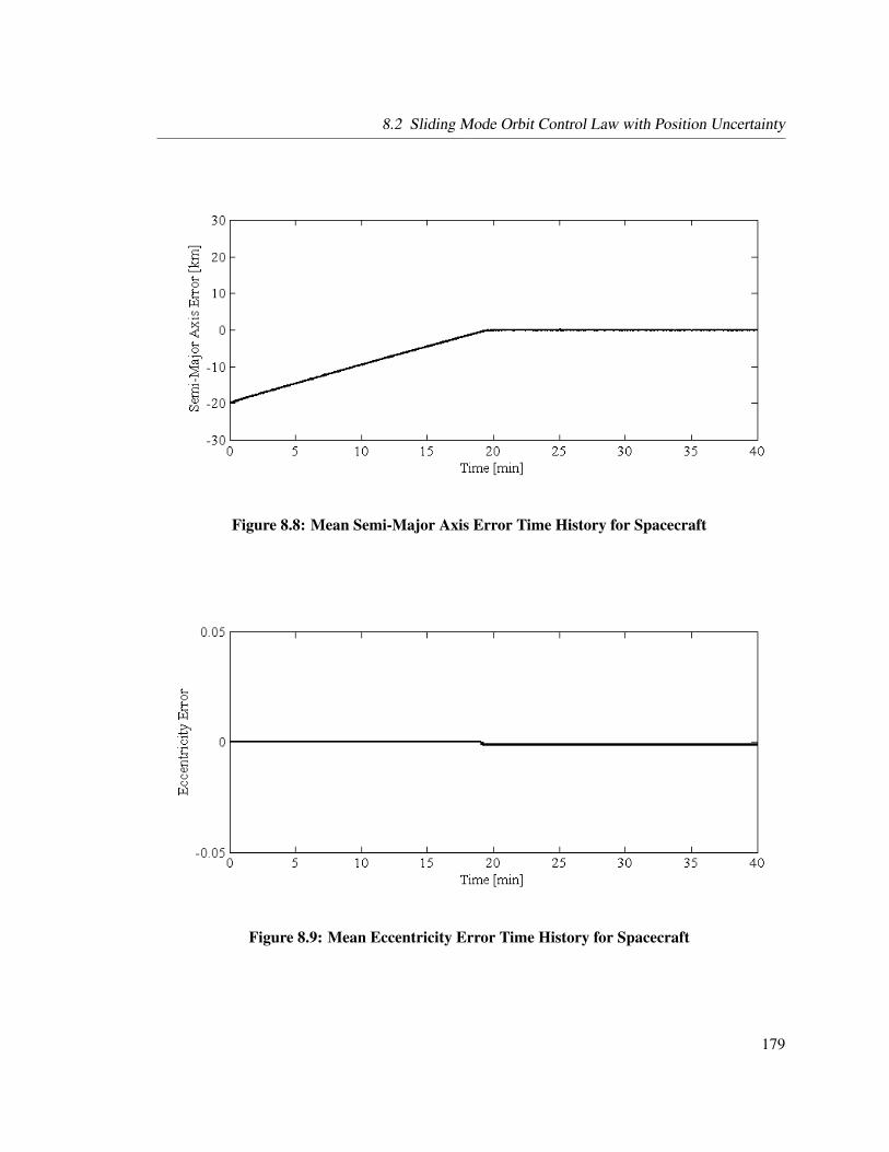
8.2 Sliding Mode Orbit Control Law with Position Uncertainty
Figure 8.8: Mean Semi-Major Axis Error Time History for Spacecraft
Figure 8.9: Mean Eccentricity Error Time History for Spacecraft
179

8.2 Sliding Mode Orbit Control Law with Position Uncertainty
Figure 8.10: Mean Inclination Error Time History for Spacecraft
Figure 8.11: Spacecraft Control Acceleration History
180

8.3 Summary
8.3 Summary
In this chapter we develop a classical orbital element feedback controller based on the sliding mode
methodology to account for uncertainties in the control matrix. The development of the controller is
described along with a method to determine the gain matrices. The orbit controller is implemented
into DSACSS. A low Earth orbit spacecraft control simulation is conducted using the flight com-
puters from the attitude hardware simulators and the GPS simulator. The controller successfully
increases the mean semi-major axis of the spacecraft.
181

9 Conclusions and Recommendations
This dissertation presents the development of the Distributed Spacecraft Attitude Control System
Simulator (DSACSS) for evaluating nonlinear attitude and orbit control strategies. The system is
comprised of two attitude hardware-in-the-loop simulators floating on individual spherical air bear-
ing platforms for a nearly torque free environment, a numerical attitude and orbit control simulator,
and a closed-loop hardware-in-the-loop GPS simulator.
9.1 Conclusions
The DSACSS is capable of real-time closed-loop orbit control using an operational space vehicle
GPS receiver. The closed-loop GPS simulator provides a realistic orbit trajectory by including
orbital perturbations, solar radiation pressure, and atmospheric drag. A classical orbital element
feedback controller is successfully evaluated using the closed-loop simulator.
The real-time hardware-in-the-loop attitude simulators determine attitude and have three-axis
attitude control capability through the use of reaction wheels. The development and implementation
on the simulators of angular rate and MRP nonlinear attitude controllers are shown. The attitude
controllers successfully drive the errors to zero and match the trends expected from numerical sim-
ulations.
A robust, asymptotically stable, nonlinear MRP attitude controller is developed and evaluated
using numerical simulations and both real-time hardware-in-the-loop attitude simulators. The robust
spacecraft attitude control law is based on the sliding mode methodology by bounding un-modeled
182

9.2 Recommendations
dynamics and system uncertainties. The robust spacecraft MRP attitude controller successfully
tracks a time varying reference attitude trajectory for both real-time hardware-in-the-loop attitude
simulators.
A classical orbital element feedback controller based on the sliding mode methodology is de-
veloped and evaluated using the closed-loop GPS simulator. The development of the controller is
described along with a method to determine the gain matrices. The controller successfully controls
the classical orbital elements of the spacecraft.
The DSACSS framework is a flexible testbed for investigating a variety of spacecraft control
techniques, especially control scenarios involving coupled attitude and orbital motion. DSACSS
allows individual or component level development and testing of hardware and software interfaces.
The DSACSS facility also allows for investigation into spacecraft formation flying such as con-
trolling the formation and pointing accuracy. The advantage of DSACSS over software simulator
architectures is that hardware-in-the-loop simulations for testing and validation of concepts provide
a more realistic demonstration of expected performance of space systems.
9.2 Recommendations
The DSACSS can be easily upgraded and modified to suit the needs of the specific research. The
hardware components are modular in nature, which allows for quick and easy replacement in the
case of failure or poor performance. The hardware-in-the-loop simulation software is also modular
in nature, which allows for easy continued development of DSACSS-Ops.
A document describing C++ coding conventions has been adopted for DSACSS-Ops.∗ The
style rules outlined in the document are for the purpose of making the process of reviewing and
scanning for errors of the source code more efficient. An important point is to ensure that the code
is thoroughly evaluated through testing and group reviews to ensure continued successful opera-
tion of DSACSS. Approximately 85% of DSACSS-Ops has been written or rewritten based on the
coding conventions. A strong recommendation is to rewrite the rest of DSACSS-Ops to the coding
∗http://www.sssl.aoe.vt.edu/documentation/software/codingdocument.txt
183

9.2 Recommendations
standards.
Each air bearing platform has a fixed rotation point (f.r.p.). If the center of gravity (c.g.) of the
simulator is not co-located with the f.r.p., a torque is introduced into the system. The desire is to
have the c.g. and f.r.p. co-located. The linear actuators can be used to move the c.g. to the f.r.p.
The recommendation is to develop an estimation technique similar to the one outlined in Ref. 34
to estimate the c.g. offset (rc.g.). Once an estimate of rc.g. is determined, a control scheme can be
devised to drive rc.g. to zero by using the linear actuators.
The reaction wheel interface for controlling the attitude of the hardware simulators is fully
developed. The recommendation is to develop a pulse width modulation (PWM) scheme for the
thrusters to control the attitude of the hardware simulators.
The attitude determination for Whorl−II needs improvement. The magnetic field in the North
East corner of the Whorl−II enclosure is not in a consistent direction. Therefore investigating
attitude control pointing within the North East direction is not recommended at this time. Possible
solutions to improve attitude determination for Whorl−II are: 1) improve estimation techniques, 2)
use a distributed magnetometer configuration, and 3) develop a visual attitude sensor.
The Ashtech G12 GPS receiver is implemented into the spacecraft low Earth orbit closed-
loop hardware-in-the-loop GPS simulator. Three Ashtech DG14 HDMA GPS receivers have been
procured for the purpose of investigating spacecraft formation flying using multiple GPS receivers.
The DG14 receivers have been successfully tested using the GPS simulator in an open-loop aircraft
scenario. The recommendation is to test and implement the DG14 receivers into the spacecraft low
Earth orbit closed-loop hardware-in-the-loop GPS simulation.
184

Bibliography
[1] B. J. Naasz, R. D. Burns, D. Gaylor, and J. Higinbotham, “Hardware-in-the-loop Testing of
Continuous Conrol Algorithms for a Precision Formation Flying Demonstration Mission,”
18th International Symposium on Space Flight Dynamics, Haus der Bayerischen Wirtschaft,
Munich, Germany, October 11–15, 2004.
[2] B. J. Naasz, C. D. Karlgaard, and C. D. Hall, “Application of Several Control Techniques for
the Ionospheric Observation Nanosatellite Formation,” 2002 AAS/AIAA Space Flight Mechan-
ics Conference, San Antonio, Texas, January 27–30, 2002.
[3] H. Schaub, S. R. Vadali, J. L. Junkins, and K. T. Alfriend, “Spacecraft Formation Flying
Control Using Mean Orbit Elements,” Journal of the Astronautical Sciences, Vol. 48, No. 1,
2000, pp. 69–89.
[4] P. Gurfil, “Control-Theorectic Analysis of Low-Thrust Orbital Transfer using Orbital Ele-
ments,” Journal of Guidance, Control, and Dynamics, Vol. 26, No. 6, 2003, pp. 979–1011.
[5] S. Leung, E. Gill, O. Montenbruck, and S. Montenegro, “A Navigation Processor for Flexible
Real-Time Formation Flying Applications,” International Symposium Formation Flying Mis-
sions and Technologies, Centre National d’Etudes Spatiales Toulouse Space Centre - France,
October 29–31, 2002.
[6] S. Kim, J. L. Crassidis, Y. Cheng, A. M. Fosbury, and J. L. Junkins, “Kalman Filtering for Rel-
ative Spacecraft Attitude and Position Estimation,” AIAA Guidance, Navigation, and Control
Conference and Exhibit, San Francisco, California, August 15–18, 2005.
185
Bibliography
[7] M. C. VanDyke and C. D. Hall, “Decentralized Coordinated Attitude Control of a Formation
of Spacecraft,” Journal of Guidance, Control, and Dynamics, Vol. 29, No. 5, 2006, pp. 1101–
1109.
[8] G. Q. Xing and S. A. Parvez, “Relative Attitude Kinematics and Dynamics Equations and
Its Applications to Spacecraft Attitude State Capture and Tracking in Large Angle Slewing
Maneuvers,” 1999 Space Control Conference, MIT Lincoln Laboratory, 1999. April 13-15.
[9] F. L. Markley, J. L. Crassidis, and Y. Cheng, “Nonlinear Attitude Filtering Methods,” AIAA
Guidance, Navigation, and Control Conference and Exhibit, San Francisco, California, August
15–18, 2005.
[10] J. L. Schwartz, M. A. Peck, and C. D. Hall, “Historical Survey of Air-Bearing Spacecraft
Simulators,” Journal of Guidance, Control, and Dynamics, Vol. 26, No. 4, 2003, pp. 513–522.
[11] J. Leitner, “A Hardware-in-the-loop Testbed for Spacecraft Formation Flying Applications,”
IEEE Aerospace Conference, Big Sky, Montana, 2001.
[12] R. D. Burns and B. J. Naasz, “An Environment for Hardware-in-the-Loop Formation Naviga-
tion and Control,” AIAA/AAS Astrodynamics Specialist Conference and Exhibit, Providence,
Rhode Island, 16–19 August 2004.
[13] C. M. Close and D. K. Frederick, Modeling and Analysis of Dynamic Systems. Boston, MA:
Houghton Mifflin, 2nd ed., 1993.
[14] J. E. Slotine and W. Li, Applied Nonlinear Control. Upper Saddle River, New Jersey: Prentice
Hall, 1991.
[15] B. B. Goeree and E. D. Faase, “Sliding Mode Attitude Control of a Small Satellite for Ground
Tracking Maneuvers,” American Control Conference, Chicago, Illinois, June 2000.
[16] J. L. Crassidis and F. L. Markley, “Sliding Mode Control Using Modified Rodrigues Parame-
ters,” Journal of Guidance, Control, and Dynamics Control, Vol. 19, No. 6, 1996, pp. 1381–
1383.
[17] Y.-J. Cheon, “Sliding Mode Control for Attitude Tracking of Thruster-Controlled Spacecraft,”
Transactions on Control, Automation, and Systems Engineering, Vol. 3, December 2001,
186

Bibliography
pp. 257–261.
[18] T. A. Dwyer and H. Sira-Ramirez, “Variable-Structure Control of Spacecraft Attitude Maneu-
vers,” Journal of Guidance, Control, and Dynamics, Vol. 11, May 1988, pp. 262–270.
[19] H. Sira-Ramirez and T. A. Dwyer, “Variable Structure Control of Spacecraft Reorientation Ma-
neuvers,” Guidance, Navigation and Control Conference, AIAA, August 18–20 1986, pp. 86–
96.
[20] Y. B. Shtessel, “Decentralized Sliding Mode Control in Three-Axis Inertial Platforms,” Jour-
nal of Guidance, Control, and Dynamics, Vol. 18, July 1995, pp. 773–781.
[21] S.-C. Lo and Y.-P. Chen, “Smooth Sliding-Mode Control for Spacecraft Attitude Tracking Ma-
neuvers,” Journal of Guidance, Control, and Dynamics, Vol. 18, December 1995, pp. 1345–
1349.
[22] H. Bang and Y. H. Lho, “Sliding Mode Control for Spacecraft Containing Rotating Wheels,”
AIAA Guidance, Navigation, and Control Conference and Exhibit, Montreal, Canada, AIAA,
August 6–9 2001.
[23] J. C. Chiou, M.-C. Hwang, and S.-D. Wu, “Robust Control of Nonlinear Dynamic Systems Us-
ing Sliding Mode Control and Productive Networks,” American Control Conference, Seattle,
Washington, June 1995.
[24] D. Shin and J. Kim, “Robust Spacecraft Attitude Control Using Sliding Mode Control,” AIAA
Guidance, Navigation, and Control Conference and Exhibit, AIAA, August 10–12 1998.
[25] H. Schaub and J. L. Junkins, Analytical Mechanics of Space Systems. Reston, VA: AIAA
Education Series, 2003.
[26] D. Irvin, “A Study of Linear vs. Nonlinear Control Techniques for the Reconfiguration of
Satellite Formations,” Master’s thesis, Air Force Institute of Technology, Wright-Patterson
AFB, OH, 2001.
[27] W. H. Clohessey and R. S. Wiltshire, “Terminal Guidance System for Satellite Rendezvous,”
Journal of the Aerospace Sciences, Vol. 27, 1960, pp. 653–658.
[28] B. Wie, Space Vehicle Dynamics and Control. Reston, VA: AIAA Education Series, 1998.
187

Bibliography
[29] S. E. Lennox, “Coupled Attitude and Orbital Control System using Spacecraft Simulators,”
Master’s thesis, Virginia Polytechnic Institute and State University, Blacksburg, Virginia,
Blacksburg, VA, 2004.
[30] S. R. Vadali, K. T. Alfriend, and S. Vaddi, “Hill’s Equations, Mean Orbit Elements, and Forma-
tion Flying of Satellites,” The Richard H. Battin Astrodynamics Conference, College Station,
TX, AAS, March 2000.
[31] S. Vaddi, Modeling and Control of Satellite Formations. PhD thesis, Texas A&M University,
College Station, TX, May 2003.
[32] K. T. Alfriend, H. Yan, and S. R. Vadali, “Nonlinear Considerations in Satellite Formation
Flying,” AIAA/AAS Astrodynamics Specialist Conference and Exhibit, Monterey, California,
5–8 August 2002.
[33] J. L. Schwartz and C. D. Hall, “The Distributed Spacecraft Attitude Control System Simulator:
Development, Progress, Plans,” 2003 Flight Mechanics Symposium, NASA Goddard Space
Flight Center, Greenbelt, Maryland, October 28–30, 2003.
[34] J. L. Schwartz, Distributed Spacecraft AttitudeControl System Simulator From Design to De-
centralized Control. PhD thesis, Virginia Polytechnic Institute and State University, Blacks-
burg, VA, 2004.
[35] S. A. Kowalchuk and C. D. Hall, “Distributed Spacecraft Attitude Control System Simulator:
Feedback Control Capabilities and Visualization Techniques,” 7th International Quantitative
Feedback Theory and Robust Frequency Domain Symposium, University of Kansas, Lawrence,
Kansas, August 5–7, 2005.
[36] S. A. Kowalchuk and C. D. Hall, “Hardware-in-the-Loop Simulation of Classical Element
Feedback Controller,” Goddard Flight Mechanics Symposium, Greenbelt, Maryland, October
18–20, 2005.
[37] S. A. Kowalchuk and C. D. Hall, “GPS Hardware-in-the-loop Spacecraft Formation Flying
Simulation,” AAS/AIAA Space Flight Mechanics Meeting, Sedona, Arizona, Jan. 28–Feb. 1,
2007.
188
Bibliography
[38] M. J. Caruso, “Applications of Magnetic Sensors for Low Cost Compass Systems,” tech. rep.,
Honeywell Solid State Electronics Center, Morristown, NJ, 2006.
[39] M. D. Shuster and S. D. Oh, “Three-Axis Attitude Determination From Vector Observations,”
Journal of Guidance and Control, Vol. 4, January 1981, pp. 70–77.
[40] C. D. Hall, “AOE 4140 Spacecraft Dynamics and Control Lecture Notes,” Available at www.
aoe.vt.edu/˜cdhall/courses/aoe4140/, Blacksburg, VA 2003.
[41] R. F. Stengel, Optimal Control and Estimation. New York: Dover Publications, 1994.
[42] J. L. Crassidis and J. L. Junkins, Optimal Estimation of Dynamic Systems. New York: CRC
Press Company, 2004.
[43] D. Simon, Optimal State Estimation. New Jersey: Wiley, 2006.
[44] J. W. Murrell, “Precision Attitude Determination for Multimission Spacecraft,” AIAA Guid-
ance, Navigation, and Control Conference and Exhibit, Palo Alto, California, AIAA, August
1978, pp. 70–87.
[45] H. Sira-Ramirez, “On the Design of Nonlinar Pulse-Width-Modulation Controllers,” Control
and Applications, IEEE, April 1989, pp. 397–402.
[46] K. H. Kienitz and J. Bals, “Pulse Modulation for Attitude Control with Thrusters Subject
to Switching Restrictions,” German Aerospace Congress, Vol. III, Friedrichshafen, Germany,
2005.
[47] D. J. Zimpfer, L. S. Shieh, and J. W. Sunkel, “Digitally Redesigned Pulse-Width Modulation
Spacecraft Control,” AIAA Guidance, Navigation and Control Conference, Balitmore, MD,
AIAA, August 7–10 1995.
[48] A. J. Turner and C. D. Hall, “An Open Source, Extensible Spacecraft Simulation and Model-
ing Environment Framework,” Proceedings of the AAS/AIAA Astrodynamics Specialist Con-
ference, Big Sky, Montana, August 3 -7 2003.
[49] A. J. Turner, “An Open Source, Extensible Spacecraft Simulation and Modeling Environment
Framework,” Master’s thesis, Virginia Polytechnic Institute and State University, Blacksburg,
VA, 2003.
189

Bibliography
[50] L. Haas, “The Ashtech G12-HDMA: A Low Cost, High Performance GPS Space Receiver,”
Institute of Navigation International Technical Meeting ION GPS-2000, Salt Lake City, 2000.
September 19-22.
[51] Goddard Space Flight Center, Guidance Navigation and Control, CSC-5570-16R0UD0, “Posi-
tioning System (GPS) Enhanced Onboard Navigation System, System Description and User’s
Guide, Version 2, Release 2.1.A,” tech. rep., Computer Sciences Corporation, December 2003.
[52] Goddard Space Flight Center, Guidance Navigation and Control, CSC-5570-14R0UD0,
“Global Positioning System (GPS) Enhanced Onboard Navigation System, Mathematical
Specifications, Version 2, Release 2.1, Update 1,” tech. rep., Computer Sciences Corporation,
December 2003.
[53] B. W. Parkinson and J. J. Spilker, Global Positionion System: Theory and Applications, Vol. 1.
Washington, D.C.: AIAA Education Series, 1996.
[54] E. D. Kaplan and C. J. Hegarty, Understanding GPS Principles and Applications. Boston,
MA: Artech House Inc, 2nd ed., 2005.
[55] B. R. Bowring, “The Accuracy of Geodetic Latitude and Height Equations,” Survey review -
Directorate of Overseas Surveys, Surrey, England, October 28 1985, pp. 202–206.
[56] R. Burtch, “A Comparison of Methods used in Rectangular to Geodetic Coordinate Trans-
formations,” ACSM Annual Conference and Technology Exhibition, Orlando, Florida, ACSM,
April 21–26 2006.
[57] P. C. Hughes, Spacecraft Attitude Dynamics. Mineola, New York: Dover Publications, 2004.
[58] H. K. Khalil, Nonlinear Systems. New Jersey: Prentice Hall, third ed., 2002.
[59] M. J. Sidi, Spacecraft Dynamics and Control. New York: Cambridge University Press, 1997.
[60] W. Perruquetti and J. P. Barbot, Sliding Mode Control in Engineering. Control Engineering
Series, New York: Marcel Dekker, Inc, 2002.
[61] B. H. Tongue, Principles of Vibration. New York: Oxford University Press, 1996.
[62] B. J. Naasz, “Classical Element Feedback Control for Spacecraft Orbital Maneuvers,” Master’s
thesis, Virginia Polytechnic Institute and State University, Blacksburg, Virginia, Blacksburg,
190

Bibliography
VA, 2002.
[63] R. H. Battin, An Introduction to the Mathematics and Methods of Astrodynamics, Revised
Edition. Reston, VA: AIAA Education Series, 1999.
[64] R. R. Bate, D. D. Mueller, and J. E. White, Fundamentals of Astrodynamics. New York: Dover
Publications, 1971.
[65] M. R. Ilgen, “Low Thrust OTV Guidance using Lyapunov Optimal Feedback Control Tech-
niques,” Advances in the Astronautical Sciences, Vol. 85, No. 2, 1993, pp. 1527–1545.
[66] F. Garofalo and L. Glielmo, Robust Control via Variable Structure and Lyapunov Techniques.
New York: Springer, 1996.
[67] A. J. Laub, Matrix Analysis for Scientists and Engineers. Philadelphia, PA: Society of Indus-
trial and Applied Mathematics, 2005.
191
A Appendix: Reaction Wheel Controller
An attitude control law determines the necessary torque about each body axis to satisfy the de-
sired attitude objective. The reaction wheel controller receives the attitude control vector (u)
and determines the necessary wheel speed for each reaction wheel to produce the desired control
torque. A low-level reaction wheel controller has been developed and implemented on Whorl−I
and Whorl−II. This appendix outlines the development of the reaction wheel controller.
A.1 Reaction Wheel Controller Development
The amount of control torque (ui) produced about the reaction wheel spin axis as a function of
wheel acceleration (Ωi) is
hi = ui
IWsΩi = ui (A.1)
where IWs is the reaction wheel spin axis inertia. The angular acceleration of the wheel is approxi-
mated as
Ωi ≈Ωfinali − Ωcurrenti
∆t(A.2)
and substituting into Eq. (A.1) results in an expression for the final wheel speed (Ωfinali) as
192
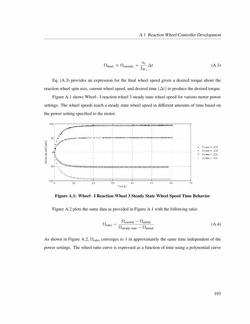
A.1 Reaction Wheel Controller Development
Ωfinali ≈ Ωcurrenti +uiIWs
∆t (A.3)
Eq. (A.3) provides an expression for the final wheel speed given a desired torque about the
reaction wheel spin axis, current wheel speed, and desired time (∆t) to produce the desired torque.
Figure A.1 shows Whorl−I reaction wheel 3 steady state wheel speed for various motor power
settings. The wheel speeds reach a steady state wheel speed in different amounts of time based on
the power setting specified to the motor.
Figure A.1: Whorl−I Reaction Wheel 3 Steady State Wheel Speed Time Behavior
Figure A.2 plots the same data as provided in Figure A.1 with the following ratio:
Ωratio =Ωcurrent − Ωinitial
Ωsteady state − Ωinitial(A.4)
As shown in Figure A.2, Ωratio converges to 1 in approximately the same time independent of the
power settings. The wheel ratio curve is expressed as a function of time using a polynomial curve
193
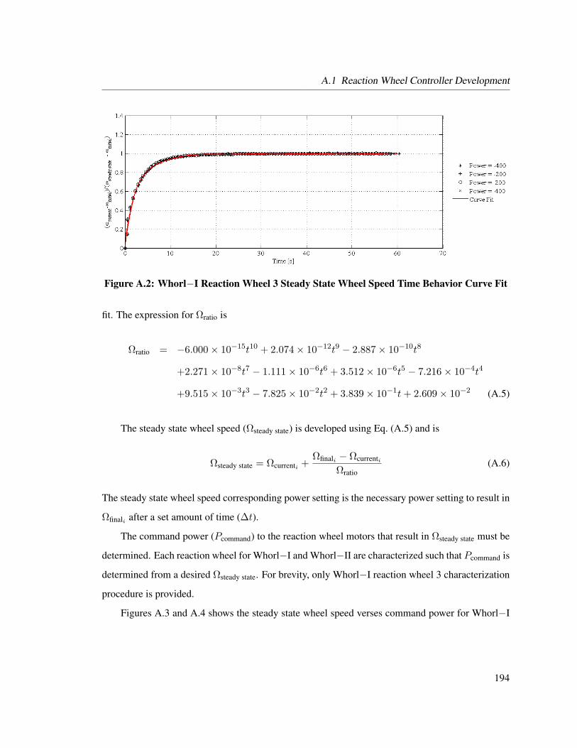
A.1 Reaction Wheel Controller Development
Figure A.2: Whorl−I Reaction Wheel 3 Steady State Wheel Speed Time Behavior Curve Fit
fit. The expression for Ωratio is
Ωratio = −6.000× 10⁻¹⁵t10 + 2.074× 10⁻¹²t9 − 2.887× 10⁻¹⁰t8
+2.271× 10⁻⁸t7 − 1.111× 10⁻⁶t6 + 3.512× 10⁻⁶t5 − 7.216× 10⁻⁴t4
+9.515× 10⁻³t3 − 7.825× 10⁻²t2 + 3.839× 10⁻¹t+ 2.609× 10⁻² (A.5)
The steady state wheel speed (Ωsteady state) is developed using Eq. (A.5) and is
Ωsteady state = Ωcurrenti +Ωfinali − Ωcurrenti
Ωratio(A.6)
The steady state wheel speed corresponding power setting is the necessary power setting to result in
Ωfinali after a set amount of time (∆t).
The command power (Pcommand) to the reaction wheel motors that result in Ωsteady state must be
determined. Each reaction wheel for Whorl−I and Whorl−II are characterized such that Pcommand is
determined from a desired Ωsteady state. For brevity, only Whorl−I reaction wheel 3 characterization
procedure is provided.
Figures A.3 and A.4 shows the steady state wheel speed verses command power for Whorl−I
194

A.1 Reaction Wheel Controller Development
reaction wheel 3. Figure A.3 shows a highly nonlinear behavior with an absolute command power
greater than 800 motor units. A dead-band for the reaction wheel from -22 to 22 motor units is
clearly seen in Figure A.4. The nonlinearity and dead-band regions have to be considered to design
an effective wheel controller.
Figure A.3: Steady State Reaction Wheel Speed verses Power Commanded to Reaction WheelMotor for a Range from -1000 to 1000 motor units for Whorl−I Reaction Wheel 3
Figure A.4: Steady State Reaction Wheel Speed verses Power Commanded to Reaction WheelMotor for a Range from -100 to 100 motor units for Whorl−I Reaction Wheel 3
Figures A.5 and A.6 show the axes switched and Ωsteady state divided by the motor voltage
195

A.1 Reaction Wheel Controller Development
(Ωscale = Ωsteady state/V ) recorded at each steady state sample as compared with Figures A.3 and
A.4. The command power curve as a function of Ωscale is developed using a polynomial curve fit
in four discrete regions. The four regions allow for a more accurate curve fit while excluding the
dead-band and nonlinearity zones.
Figure A.5: Power Commanded to Reaction Wheel Motor verses Scaled Steady State ReactionWheel Speed Curve Fit for Whorl−I Reaction Wheel 3
Figure A.6: Power Commanded to Reaction Wheel Motor verses Scaled Steady State ReactionWheel Speed Curve Fit for Whorl−I Reaction Wheel 3
196

A.1 Reaction Wheel Controller Development
The curve fit equations for Ω3 Whorl−I are
P =
0.3085Ω3scale + 4.3691Ω2
scale − 94.8364Ωscale − 15.6830 −7.6 ≤ Ωscale < −1.2
25.9997Ω2scale − 31.1477Ωscale + 25.9680 −1.2 ≤ Ωscale < 0
−26.1740Ω2scale − 31.1465Ωscale − 25.9364 0 ≤ Ωscale ≤ 1.2
0.1015Ω3scale − 1.9227Ω2
scale − 103.3392Ωscale + 24.3888 1.2 < Ωscale ≤ 7.6
(A.7)
and the curve fits are shown in Figures A.5 and A.6.
All the reaction wheels have the same trends, but with different coefficients in the power curve
fit expression. The coefficients in the power curve expression change as the reaction wheel electric
motors have more use. The change is gradual and is resolved by re-characterizing the reaction
wheels off-line to obtain new coefficients for the power curve expression at the users discretion.
The power curve fit equations for Ω1 Whorl−I are
P =
−0.0292Ω3scale + 0.4310Ω2
scale − 108.4810Ωscale − 33.3625 −7.6 ≤ Ωscale < −1.2
25.1189Ω2scale − 29.3981Ωscale + 25.4829 −1.2 ≤ Ωscale < 0
−24.8267Ω2scale − 29.6665Ωscale − 25.5515 0 ≤ Ωscale ≤ 1.2
0.3702Ω3scale − 5.0961Ω2
scale − 92.3245Ωscale + 18.2302 1.2 < Ωscale ≤ 7.6
(A.8)
The power curve fit equations for Ω2 Whorl−I are
P =
−0.1300Ω3scale − 0.3346Ω2
scale − 110.1343Ωscale − 31.3399 −7.6 ≤ Ωscale < −1.2
22.9303Ω2scale − 33.1892Ωscale + 26.6547 −1.2 ≤ Ωscale < 0
−23.5571Ω2scale − 33.2142Ωscale − 26.6669 0 ≤ Ωscale ≤ 1.2
0.0614Ω3scale − 1.9880Ω2
scale − 101.6096Ωscale + 22.7110 1.2 < Ωscale ≤ 7.6
(A.9)
197

A.2 Summary
The power curve fit equations for Ω1 Whorl−II are
P =
0.0073Ω3scale + 0.9891Ω2
scale − 106.5212Ωscale − 25.6702 −7.6 ≤ Ωscale < −1.2
23.9013Ω2scale − 34.0706Ωscale + 25.9916 −1.2 ≤ Ωscale < 0
−24.2972Ω2scale − 33.4746Ωscale − 26.1383 0 ≤ Ωscale ≤ 1.2
0.1442Ω3scale − 2.4665Ω2
scale − 102.3385Ωscale + 22.2794 1.2 < Ωscale ≤ 7.6
(A.10)
The power curve fit equations for Ω2 Whorl−II are
P =
0.0937Ω3scale + 2.0285Ω2
scale − 102.0626Ωscale − 27.1519 −7.6 ≤ Ωscale < −1.2
24.5453Ω2scale − 29.2204Ωscale + 25.0705 −1.2 ≤ Ωscale < 0
−25.3531Ω2scale − 28.4963Ωscale − 25.1400 0 ≤ Ωscale ≤ 1.2
0.1841Ω3scale − 2.8970Ω2
scale − 99.9913Ωscale + 26.7459 1.2 < ωscale ≤ 7.6
(A.11)
The power curve fit equations for Ω3 Whorl−II are
P =
0.1721Ω3scale + 2.4755Ω2
scale − 103.2449Ωscale − 20.4315 −7.6 ≤ Ωscale < −1.2
24.0252Ω2scale − 36.2669Ωscale + 26.3056 −1.2 ≤ Ωscale < 0
−24.7182Ω2scale − 35.9783Ωscale − 26.4078 0 ≤ Ωscale ≤ 1.2
0.2112Ω3scale − 3.3315Ω2
scale − 98.9996Ωscale + 15.0540 1.2 < Ωscale ≤ 7.6
(A.12)
A.2 Summary
This appendix discusses the development and implementation of a low-level reaction wheel con-
troller that determines the necessary wheel speed for each reaction wheel to produce the desired
torque. The power curve equations for each reaction wheel are provided, but will gradually change
as the reaction wheels are used. The power curve changes are resolved by re-characterizing the
reaction wheels off-line to obtain new coefficients for the power curve expression at the users dis-
cretion.
198
B Appendix: Implementation of Attitude
Control Laws into DSACSS
In this appendix we present the method for implementing attitude control laws into DSACSS-Ops
and running the controllers on Whorl−I and Whorl−II. The software structure is module, which
assists with quick and easy implementation of control laws. The following sections present the
method for implementing an attitude control law and template files to assist in the implementation.
B.1 Implementation Process
The process for implementing an attitude control law into DSACSS-Ops is as follows:
1. Copy and rename testController.h and testController.cpp. For convenience the new file name
is referred to as testController. Rename the testController class.
2. Implement the attitude control law in testController.cpp and modify testController.h
3. Modify the Makefile in the Controller directory to compile the new .cpp file.
4. Include testController.h in the WhorlSim.h file.
5. Add the object name for the controller to WhorlSim.h and WhorlSim.cpp.
6. Compile DSACSS-Ops and check for any warnings or errors during compilation.
199

B.2 Template Files
7. Modify the configuration file (DSACSSConfig.xml) in the work directory for the desired
simulation parameters.
8. Modify and rename templateController.cpp in the work directory for the desired simulation.
9. Modify the Makefile in the work directory to compile templateController.cpp.
10. Run the simulation executable file in the work directory.
B.2 Template Files
There are three template files to assist with implementing attitude control laws into DSACSS-Ops∗
to run on the hardware simulators. The testController.h and testController.cpp files are located in the
Controller directory in DSACSS-Ops. The testController.h file is where the functions and variables
are defined. The testController.cpp file on lines 99–101 is where the attitude control law is specified.
The templateController.cpp file is located in the work directory in DSACSS-Ops. Compiling
the templateController.cpp file produces the executable simulation file. The simulator name and
simulation duration are the parameters the user is required to modify.
1 //////////////////////////////////////////////////////////////////////////////////////////////////
2 /*! \file testController.h
3 * \brief Template file for implementation of an attitude controller using the hardware simulators.
4 * \author $Author: $
5 * \version $Revision: 1.1 $
6 * \date $Date: $
7 *//////////////////////////////////////////////////////////////////////////////////////////////////
8 /*!
9 */
10 //////////////////////////////////////////////////////////////////////////////////////////////////
1112 #ifndef __SSSL_TESTCONTROL_H__
13 #define __SSSL_TESTCONTROL_H__
1415 #include "Controller.h"
1617 using namespace std;
∗Complete documentation for DSACSS-Ops is provided on the web at www.sssl.aoe.vt.edu.
200

B.2 Template Files
18 using namespace O_SESSAME;
1920 class testController : public Controller
2122 public:
23 /** Constructors */
24 testController( );
25 testController( Whorl* ptr_whorl );
2627 /** Destructor */
28 virtual ˜testController( );
2930 /*! Runs the default controller */
31 int Run( );
3233 /*! Initializes the default controller */
34 int Initialize( );
3536 protected:
3738 Matrix m_gainMatrix;
39 Vector m_controlTorque;
40 ;
4142 #endif
4344 // Do not change the comments below - they will be added automatically by CVS
45 /*****************************************************************************
46 * $Log: testController.h,v $
47 *
48 ******************************************************************************/
1 //////////////////////////////////////////////////////////////////////////////////////////////////
2 /*! \file testController.cpp
3 * \brief Template file for implementation of an attitude controller using the hardware simulators.
4 * \author $Author: $
5 * \version $Revision: 1.1 $
6 * \date $Date: $
7 *//////////////////////////////////////////////////////////////////////////////////////////////////
8 /*!
9 */
10 //////////////////////////////////////////////////////////////////////////////////////////////////
1112 #include "testController.h"
13
201

B.2 Template Files
14 /*! /brief Constructor for testController */
15 testController::testController( )
16
17
1819 /*! /brief Constructor for testController
20 *
21 * @param ptr_whorl is a pointer to the Whorl object.
22 */
23 testController::testController( Whorl* ptr_whorl )
24
25 m_whorl = ptr_whorl;
2627 Initialize( );
2829
3031 /*! /brief De-Constructor for testController */
32 testController::˜testController( )
33
34
3536 /*! /brief Initialize testController */
37 int testController::Initialize( )
38
39 /* Initialize control vector */
40 m_controlTorque.initialize(3); // [N-m]
4142 /* Specify Max Wheel Torque */
43 m_uMax = 1.5; // [N-m]
4445 /* Initialize contorl gain matrix */
46 m_gainMatrix.initialize(3,3);
47 m_gainMatrix(1,1) = 0;
48 m_gainMatrix(2,2) = 0;
49 m_gainMatrix(3,3) = 2;
5051 /* Get orientation of Momentum Wheels. Defined in Controller Class. */
52 A = FindA( );
5354 /* Get Momentum Wheel spin axis MOI. Defined in Controller Class */
55 MOI_sw = FindMOI_sw( );
5657 /* Reference Model. Initialized in Controller.cpp */
202

B.2 Template Files
58 Quaternion qri( 0.0, 0.0, 0.0, 1.0 );
59 m_quaternionReference(1) = qri(1);
60 m_quaternionReference(2) = qri(2);
61 m_quaternionReference(3) = qri(3);
62 m_quaternionReference(4) = qri(4);
63 m_mrpReference = ModifiedRodriguezParameters( qri );
64 m_angularRateReference(1) = 0.0; // [rad/s]
65 m_angularRateReference(2) = 0.0; // [rad/s]
66 m_angularRateReference(3) = 0.0; // [rad/s]
6768 return( 0 );
69
7071 int testController::Run()
72
7374 cerr << "Start of testController algorithm" << endl;
7576 /* Attitude Reference Model */
7778 /* Error Vectors */
79 Vector angularRateError(3);
80 ModifiedRodriguezParameters mrpError;
8182 /* Set Whorl Error Values */
83 m_whorl->SetMRPError( mrpError );
84 m_whorl->SetAngularRateError( angularRateError );
8586 /* Set Whorl Reference Parameters */
87 m_whorl->SetReferenceOmegaBL( m_angularRateReference );
88 m_whorl->SetReferenceQuaternion( m_quaternionReference );
8990 /* Reaction Wheel Speed */
91 static Vector wheelSpeed(3);
92 double measurementTime;
93 m_whorl->GetMomentumWheel("REACTION_X")->GetWheelSpeed( wheelSpeed(1), measurementTime );
94 m_whorl->GetMomentumWheel("REACTION_Y")->GetWheelSpeed( wheelSpeed(2), measurementTime );
95 m_whorl->GetMomentumWheel("REACTION_Z")->GetWheelSpeed( wheelSpeed(3), measurementTime );
9697 /* Control law */
98 m_controlTorque(1) = 0; // [N-m]
99 m_controlTorque(2) = 0; // [N-m]
100 m_controlTorque(3) = 0; // [N-m]
101
203
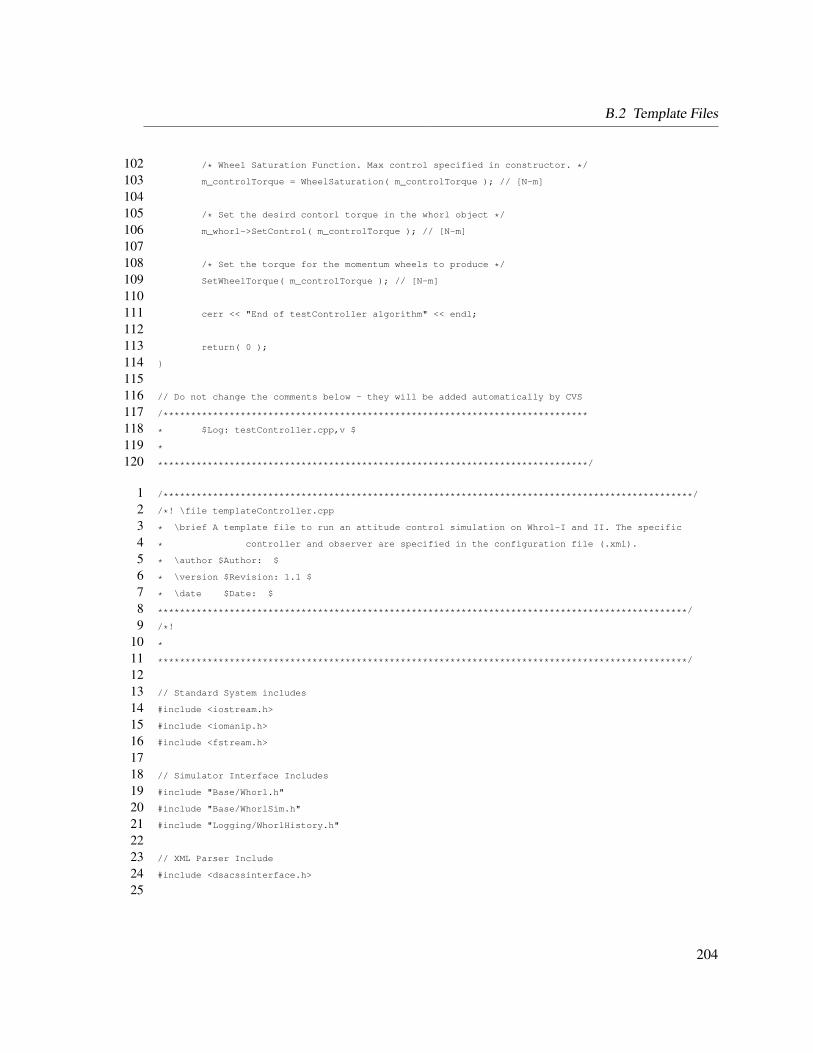
B.2 Template Files
102 /* Wheel Saturation Function. Max control specified in constructor. */
103 m_controlTorque = WheelSaturation( m_controlTorque ); // [N-m]
104105 /* Set the desird contorl torque in the whorl object */
106 m_whorl->SetControl( m_controlTorque ); // [N-m]
107108 /* Set the torque for the momentum wheels to produce */
109 SetWheelTorque( m_controlTorque ); // [N-m]
110111 cerr << "End of testController algorithm" << endl;
112113 return( 0 );
114
115116 // Do not change the comments below - they will be added automatically by CVS
117 /*****************************************************************************
118 * $Log: testController.cpp,v $
119 *
120 ******************************************************************************/
1 /************************************************************************************************/
2 /*! \file templateController.cpp
3 * \brief A template file to run an attitude control simulation on Whrol-I and II. The specific
4 * controller and observer are specified in the configuration file (.xml).
5 * \author $Author: $
6 * \version $Revision: 1.1 $
7 * \date $Date: $
8 ************************************************************************************************/
9 /*!
10 *
11 ************************************************************************************************/
1213 // Standard System includes
14 #include <iostream.h>
15 #include <iomanip.h>
16 #include <fstream.h>
1718 // Simulator Interface Includes
19 #include "Base/Whorl.h"
20 #include "Base/WhorlSim.h"
21 #include "Logging/WhorlHistory.h"
2223 // XML Parser Include
24 #include <dsacssinterface.h>
25
204

B.2 Template Files
26 using namespace O_SESSAME;
2728 // Specify Xml File to Parse
29 const char *fileName = "./DSACSSConfig.xml";
3031 int main()
32
33 /******************************************************************
34 * Load Configuration Parameters from xml file
35 *******************************************************************/
36 // Declare TiXmlDocument
37 TiXmlDocument config( fileName );
38 // Load Xml File
39 bool loadOkay = config.LoadFile();
40 checkLoadFile(loadOkay, fileName, config);
41 // Declare TiXmlHandle
42 TiXmlHandle docHandle( &config );
4344 /******************************************************************
45 * Setup Hardware-in-the-loop Attitude Simualation
46 *******************************************************************/
4748 /* Setup WhorlHistory to collect data. Note must be changed for
49 each simulator. */
50 WhorlHistory WhorlData( docHandle, "WHORL-I" );
5152 /* Create Whorl Object */
53 Whorl whorlOne;
54 /* Initialize Whorl Object */
55 whorlOne.Initialize( docHandle );
5657 /* Create WhorlSim Object */
58 WhorlSim whorlOneSim( &whorlOne );
59 /* Initialize WhorlSim Object */
60 whorlOneSim.Initialize( docHandle );
6162 /* Setup Time values */
63 ssfTime currentTime;
6465 /* Setup Vectors */
66 Vector attitudeState(7);
67 Vector attitudeControl(3);
68 Vector MRP(3);
69 Vector referenceAttitudeState(7);
205

B.2 Template Files
70 Vector referenceMRP(3);
71 Vector controlError(6);
7273 /******************************************************************
74 * Run Attitude Control Simulation
75 *******************************************************************/
76 cerr << "\n--------------------------------------------------------------" << endl;
77 cerr << "Start of Program " << endl;
78 cerr << "--------------------------------------------------------------" << endl;
7980 for ( int ii = 0; ii <= 200 ; ii++ )
81
82 /* Get Current attitude state */
83 whorlOneSim.Observe();
8485 /* Control based on attitude state */
86 whorlOneSim.Control();
8788 /* Get Current Time */
89 currentTime = Now( );
9091 /* Get attitude state vector (7x1) [ quaternion, angular rates [rad/s] ] */
92 attitudeState = whorlOne.GetState( );
9394 /* Get attitude Control vector (3x1) [N-m]*/
95 attitudeControl = whorlOne.GetControl( );
9697 /* Get MRP vector */
98 MRP = whorlOne.GetMRP( );
99100 /* Get reference attitude state (7x1) */
101 referenceAttitudeState( _(1,4) ) = whorlOne.GetReferenceQuaternion( );
102 referenceAttitudeState( _(5,7) ) = whorlOne.GetReferenceOmegaBL( );
103 referenceMRP = whorlOne.GetReferenceMRP( );
104105 /* Get control error */
106 controlError = whorlOne.GetControlError( );
107108 /* Save data to file specified in configuration file */
109 WhorlData.AppendHistory( currentTime, attitudeState, attitudeControl, MRP,
110 referenceAttitudeState, referenceMRP, controlError );
111112 /* Pause */
113 usleep( 500000 );
206

B.3 Summary
114 ;
115116 cout << "END of program " << endl;
117118 return( 0 );
119
120121 // Do not change the comments below - they will be added automatically by CVS
122 /*****************************************************************************
123 * $Log: templateController.cpp,v $
124 *
125 ******************************************************************************/
B.3 Summary
In this appendix we present the method for implementing attitude control laws into DSACSS-Ops
and running the controllers on Whorl−I and Whorl−II. The next appendix presents the method for
implementing orbit control laws into DSACSS-Ops.
207

C Appendix: Implementation of Orbit
Control Laws into DSACSS Framework
In this appendix we present the method for implementing orbit control laws into DSACSS-Ops and
running the controllers on Whorl−I and Whorl−II. The software structure allows for quick and easy
implementation of orbit control laws. The following sections present the method for implementing
orbit control laws and template files to assist in the implementation.
C.1 Implementation Process
The process for implementing an orbit control law into DSACSS-Ops is as follows:
1. Copy and rename testOrbitController.h and testOrbitController.cpp. For convenience the new
file name is referred to as testOrbitController. Rename the testOrbitController class.
2. Implement the orbit control law in testOrbitController.cpp and modify testOrbitController.h
3. Modify the Makefile in the Orbit Controller directory to compile the new .cpp file.
4. Include testOrbitController.h in the WhorlSim.h file.
5. Add the object name for the controller to WhorlSim.h and WhorlSim.cpp.
6. Compile DSACSS-Ops and check for any warnings or errors during compilation.
208

C.2 Template Files
7. Modify the configuration file (DSACSSConfig.xml) in the work directory for the desired
simulation parameters.
8. Modify and rename templateOrbitController.cpp in the work directory for the desired simu-
lation.
9. Modify the Makefile in the work directory to compile templateOrbitController.cpp.
10. Run the simulation executable file in the work directory.
C.2 Template Files
There are three template files to assist with implementing orbit control laws into DSACSS-Ops∗
to run on the hardware simulators. The testOrbitController.h and testOrbitController.cpp files are
located in the Orbit Controller directory in DSACSS-Ops. The testOrbitController.h file is where
the functions and variables are defined. The testOrbitController.cpp file on lines 61–63 is where the
orbit control law is specified.
The templateOrbitController.cpp file is located in the work directory in DSACSS-Ops. Com-
piling the templateOrbitController.cpp file produces the executable simulation file. The simulator
name and simulation duration are the parameters the user is required to modify.
1 //////////////////////////////////////////////////////////////////////////////////////////////////
2 /*! \file testOrbitController.h
3 * \brief Template file for implenting orbit control laws into DSACSS-Ops.
4 * \author $Author: $
5 * \version $Revision: 1.1 $
6 * \date $Date: $
7 *//////////////////////////////////////////////////////////////////////////////////////////////////
8 /*!
9 */
10 //////////////////////////////////////////////////////////////////////////////////////////////////
1112 #ifndef __SSSL_TESTORBITCONTROL_H__
13 #define __SSSL_TESTORBITCONTROL_H__
∗Complete documentation for DSACSS-Ops is provided on the web at www.sssl.aoe.vt.edu.
209

C.2 Template Files
1415 #include "OrbitController.h"
1617 using namespace std;
18 using namespace O_SESSAME;
1920 class testOrbitController : public OrbitController
2122 public:
23 /*! Constructors */
24 testOrbitController( );
25 testOrbitController( Whorl* ptr_whorl );
2627 /*! Destructor */
28 virtual ˜testOrbitController( );
2930 /*! Runs the default controller */
31 int Run( );
3233 /*! Initializes the default controller */
34 int Initialize( );
3536 protected:
3738 Vector m_Gains;
39 ;
4041 #endif
4243 // Do not change the comments below - they will be added automatically by CVS
44 /*****************************************************************************
45 * $Log: testOrbitController.h,v $
46 *
47 ******************************************************************************/
48
1 //////////////////////////////////////////////////////////////////////////////////////////////////
2 /*! \file testOrbitController.cpp
3 * \brief Template file for implenting orbit control laws into DSACSS-Ops.
4 * \author $Author: $
5 * \version $Revision: 1.1 $
6 * \date $Date: $
7 *//////////////////////////////////////////////////////////////////////////////////////////////////
8 /*!
9 */
210

C.2 Template Files
10 //////////////////////////////////////////////////////////////////////////////////////////////////
1112 #include "testOrbitController.h"
1314 /* Constructor */
15 testOrbitController::testOrbitController( Whorl* ptr_whorl )
16
17 m_whorl = ptr_whorl;
1819 Initialize( );
20
2122 /* Deconstructor */
23 testOrbitController::˜testOrbitController()
24
2526 int testOrbitController::Initialize( )
27
28 /* Control Acceleratin Gains */
29 m_Gains.initialize(6);
30 m_Gains(1) = 0;
31 m_Gains(2) = 0;
32 m_Gains(3) = 0;
33 m_Gains(4) = 0;
34 m_Gains(5) = 0;
35 m_Gains(6) = 0;
3637 /* Space Vehicle Id */
38 m_vehicleID = 1;
3940 /* Acceleration Duration [s] */
41 m_duration = 2;
4243 /* Space Vehicle Mass [kg] */
44 m_mass = 100;
4546 /* Current Time */
47 m_vehicleTime = Now( );
4849 /* Reset delta V time history from orbit propagator */
50 m_accelerationVector.ResetValues( );
5152 return( 0 );
53
211

C.2 Template Files
5455 int testOrbitController::Run( )
56
57 /* Get Classical Orbital Elements */
58 m_whorl->GetCOE( );
5960 /* Radial, In-Track, Cross-Track control acceleration [m/sˆ2] */
61 u(1) = 0;
62 u(2) = 0;
63 u(3) = 0;
6465 /* Current Time */
66 m_vehicleTime = Now( );
6768 /* Set Orbit Control Acceleration */
69 m_whorl->SetOrbitControl( u );
7071 /* Send control accleration to GPS simulator propagator (running on Severian) */
72 m_accelerationVector.SendAccelerationMessage( m_vehicleID, m_vehicleTime.GetSeconds( ),
73 m_duration, u, m_mass );
7475 return( 0 );
76
7778 // Do not change the comments below - they will be added automatically by CVS
79 /*****************************************************************************
80 * $Log: testOrbitController.cpp,v $
81 *
82 ******************************************************************************/
1 /************************************************************************************************/
2 /*! \file templateOrbitController.cpp
3 * \brief Orbit Control Simulation using GPS Receiver and Simulator
4 * \author $Author: $
5 * \version $Revision: 1.1 $
6 * \date $Date: $
7 ************************************************************************************************/
8 /*!
9 *
10 ************************************************************************************************/
1112 // Standard System includes
13 #include <iostream.h>
14 #include <iomanip.h>
15 #include <fstream.h>
212

C.2 Template Files
1617 // Simulator Interface Includes
18 #include "Base/Whorl.h"
19 #include "Base/WhorlSim.h"
2021 // XML Parser Include
22 #include <dsacssinterface.h>
2324 #include "Logging/WhorlHistory.h"
2526 #include "OrbitObserver/GPSObserver.h"
2728 using namespace O_SESSAME;
2930 // Specify Xml File to Parse
31 const char *fileName = "../DSACSSConfig.xml";
3233 int main( )
34
3536 /******************************************************************
37 * Load Configuration Parameters from xml file
38 *******************************************************************/
39 // Declare TiXmlDocument
40 TiXmlDocument config( fileName );
41 // Load Xml File
42 bool loadOkay = config.LoadFile();
43 checkLoadFile(loadOkay, fileName, config);
44 // Declare TiXmlHandle
45 TiXmlHandle docHandle( &config );
4647 /******************************************************************
48 *
49 *******************************************************************/
5051 WhorlHistory WhorlData( docHandle, "WHORL-III" );
5253 Whorl whorlOne;
5455 whorlOne.Initialize( docHandle );
5657 WhorlSim whorlOneSim(&whorlOne);
5859 whorlOneSim.Initialize( docHandle );
213
C.3 Summary
6061 ssfTime currentTime;
6263 Vector orbitState(6);
6465 Vector orbitControl(3);
6667 Vector orbitError(6);
6869 for ( int ii = 0; ii < 10; ii++ )
70
71 whorlOneSim.OrbitObserve( );
7273 whorlOneSim.OrbitControl( );
7475 currentTime = Now( );
7677 orbitState = whorlOne.GetOrbitState( );
7879 orbitControl = whorlOne.GetOrbitControl( );
8081 orbitError = whorlOne.GetOrbitError( );
8283 WhorlData.AppendOrbitHistory( currentTime, orbitState, orbitControl, orbitError );
8485 sleep(1);
86
8788 return(0);
89
9091 // Do not change the comments below - they will be added automatically by CVS
92 /*****************************************************************************
93 * $Log: templateOrbitController.cpp,v $
94 *
95 ******************************************************************************/
C.3 Summary
In this appendix we present the method for implementing orbit control laws into DSACSS-Ops and
running the controllers on Whorl−I and Whorl−II.
214