Investigation of gas presence in the aquifer of the ...
43
Investigation of gas presence in the aquifer of the Groningen field NAM Gulfiia Ishmukhametova Date September 2017 Editors Jan van Elk & Dirk Doornhof
Transcript of Investigation of gas presence in the aquifer of the ...
Investigation of gas presence in the aquifer of the Groningen field
NAM
Gulfiia Ishmukhametova
Date September 2017
Editors Jan van Elk & Dirk Doornhof

General Introduction
The subsurface model of the Groningen field was built and is used to model the first step in the causal
chain from gas production to induced earthquake risk. It models the pressure development in the gas
bearing formations in response to the extraction of gas and water.
The reservoir model of the Groningen field was built in 2011 and 2012 and has a very detailed model of
the fault zone in the field to support studies into induced earthquakes in the field. The model was used
to support Winningsplan 2013 (Ref. 1 to 3) and has since then been continuously improved (Ref. 4).
The pressure in the field is an important driver for compaction and therefore subsidence. Compaction in
turn affects stress and strain and is therefore of importance for the mechanism inducing earthquakes.
Away from the wells penetrating the reservoir, calibration of the model is difficult due to the paucity of
available data. The pressure in the aquifers adjacent to the reservoir therefore has larger uncertainty,
making it difficult to model water ingress into the reservoir and development of pressure in the aquifer
and reservoir.
Possible presence of gas at low saturations below the gas-water-contact can further impact water ingress
and complicate calibration of the model. This current report, provides a progress update of the
investigation into the presence of gas in the aquifers of the Groningen field. Insights into this can impact
the modelling of water ingress into the reservoir and the prediction of reservoir pressure in the gas field,
but especially in the aquifers adjacent to the reservoir.
For Winningsplan 2013 and Winningsplan 2016, the model was reviewed by an independent consultant
SGS Horizon. An extensive assurance review (Ref. 5) with opinion letter have been prepared by SGS
Horizon.
References
1. Winningsplan Groningen 2013, Nederlandse Aardolie Maatschappij BV, 29th November 2013.
2. Technical Addendum to the Winningsplan Groningen 2013; Subsidence, Induced Earthquakes and
Seismic Hazard Analysis in the Groningen Field, Nederlandse Aardolie Maatschappij BV (Jan van Elk
and Dirk Doornhof, eds), November 2013.
3. Supplementary Information to the Technical Addendum of the Winningsplan 2013, Nederlandse
Aardolie Maatschappij BV (Jan van Elk and Dirk Doornhof, eds), December 2013.
4. Groningen Field Review 2015 Subsurface Dynamic Modelling Report, Burkitov, Ulan, Van Oeveren,
Henk, Valvatne, Per, May 2016.
5. Independent Review of Groningen Subsurface Modelling Update for Winningsplan 2016, SGS
Horizon, July 2016.

Title Investigation of gas presence in the aquifer of the
Groningen field Date September
2017
Initiator NAM
Autor(s) Gulfiia Ishmukhametova Editors Jan van Elk and Dirk Doornhof
Organisation NAM Organisation NAM
Place in the Study and Data Acquisition Plan
Study Theme: Prediction Reservoir Pressure based on gas withdrawal Comment: The subsurface model of the Groningen field was built and is used to model the first step in the causal chain from gas production to induced earthquake risk. It models the pressure development in the gas bearing formations in response to the extraction of gas and water. The reservoir model of the Groningen field was built in 2011 and 2012 and has a very detailed model of the fault zone in the field to support studies into induced earthquakes in the field. The model was used to support Winningsplan 2013 and has since then been continuously improved. The pressure in the field is an important driver for compaction and therefore subsidence. Compaction in turn affects stress and strain and is therefore of importance for the mechanism inducing earthquakes. Away from the wells penetrating the reservoir, calibration of the model is difficult due to the paucity of available data. The pressure in the aquifers adjacent to the reservoir therefore has larger uncertainty, making it difficult to model water ingress into the reservoir and development of pressure in the aquifer and reservoir. Possible presence of gas at low saturations below the gas-water-contact can further impact water ingress and complicate calibration of the model. This current report, provides a progress update of the investigation into the presence of gas in the aquifers of the Groningen field. Insights into this can impact the modelling of water ingress into the reservoir and the prediction of reservoir pressure in the gas field, but especially in the aquifers adjacent to the reservoir. For Winningsplan 2013 and Winningsplan 2016, the model was reviewed by an independent consultant SGS Horizon. An extensive assurance review with opinion letter have been prepared by SGS Horizon.
Directliy linked research
(1) Model of the gas reservoir (2) Prediction of Compaction and Subsidence (3) Seismological Modelling

Used data Sub-surface data from the Groningen field; open-hole logs, core data, pressure data, production data etc.
Associated organisation
NAM
Assurance For Winningsplan 2013 and Winningsplan 2016, the model was reviewed by an independent consultant SGS Horizon.


EP201707201356 Investigation of gas presence in the aquifer of the Groningen field 1
Nederlandse Aardolie Maatschappij B.V.
Shell UPO
Investigation of gas presence in the aquifer of the
Groningen field
Date: 13-September-2017
Issued by: Gulfiia Ishmukhametova, Petrophysicist
EP number: EP201707201356
Name Role Date Signature
Approved by:
Emile Fokkema TA2, Discipline Lead Petrophysics
Reviewed by:
Leendert Geurtsen Team Lead Reservoir Engineering, Groningen Asset
Clemens Visser Discipline Lead Geology
Henk van Oeveren Reservoir Engineer, Groningen Asset
EP201707201356 Investigation of gas presence in the aquifer of the Groningen field 2
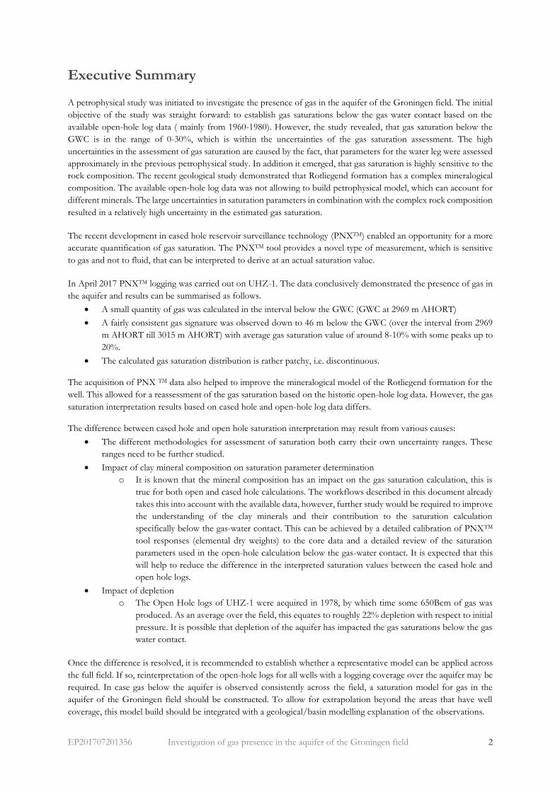
Executive Summary
A petrophysical study was initiated to investigate the presence of gas in the aquifer of the Groningen field. The initial
objective of the study was straight forward: to establish gas saturations below the gas water contact based on the
available open-hole log data ( mainly from 1960-1980). However, the study revealed, that gas saturation below the
GWC is in the range of 0-30%, which is within the uncertainties of the gas saturation assessment. The high
uncertainties in the assessment of gas saturation are caused by the fact, that parameters for the water leg were assessed
approximately in the previous petrophysical study. In addition it emerged, that gas saturation is highly sensitive to the
rock composition. The recent geological study demonstrated that Rotliegend formation has a complex mineralogical
composition. The available open-hole log data was not allowing to build petrophysical model, which can account for
different minerals. The large uncertainties in saturation parameters in combination with the complex rock composition
resulted in a relatively high uncertainty in the estimated gas saturation.
The recent development in cased hole reservoir surveillance technology (PNXTM) enabled an opportunity for a more
accurate quantification of gas saturation. The PNXTM tool provides a novel type of measurement, which is sensitive
to gas and not to fluid, that can be interpreted to derive at an actual saturation value.
In April 2017 PNXTM logging was carried out on UHZ-1. The data conclusively demonstrated the presence of gas in
the aquifer and results can be summarised as follows.
• A small quantity of gas was calculated in the interval below the GWC (GWC at 2969 m AHORT)
• A fairly consistent gas signature was observed down to 46 m below the GWC (over the interval from 2969
m AHORT till 3015 m AHORT) with average gas saturation value of around 8-10% with some peaks up to
20%.
• The calculated gas saturation distribution is rather patchy, i.e. discontinuous.
The acquisition of PNX TM data also helped to improve the mineralogical model of the Rotliegend formation for the
well. This allowed for a reassessment of the gas saturation based on the historic open-hole log data. However, the gas
saturation interpretation results based on cased hole and open-hole log data differs.
The difference between cased hole and open hole saturation interpretation may result from various causes:
• The different methodologies for assessment of saturation both carry their own uncertainty ranges. These
ranges need to be further studied.
• Impact of clay mineral composition on saturation parameter determination
o It is known that the mineral composition has an impact on the gas saturation calculation, this is
true for both open and cased hole calculations. The workflows described in this document already
takes this into account with the available data, however, further study would be required to improve
the understanding of the clay minerals and their contribution to the saturation calculation
specifically below the gas-water contact. This can be achieved by a detailed calibration of PNXTM
tool responses (elemental dry weights) to the core data and a detailed review of the saturation
parameters used in the open-hole calculation below the gas-water contact. It is expected that this
will help to reduce the difference in the interpreted saturation values between the cased hole and
open hole logs.
• Impact of depletion
o The Open Hole logs of UHZ-1 were acquired in 1978, by which time some 650Bcm of gas was
produced. As an average over the field, this equates to roughly 22% depletion with respect to initial
pressure. It is possible that depletion of the aquifer has impacted the gas saturations below the gas
water contact.
Once the difference is resolved, it is recommended to establish whether a representative model can be applied across
the full field. If so, reinterpretation of the open-hole logs for all wells with a logging coverage over the aquifer may be
required. In case gas below the aquifer is observed consistently across the field, a saturation model for gas in the
aquifer of the Groningen field should be constructed. To allow for extrapolation beyond the areas that have well
coverage, this model build should be integrated with a geological/basin modelling explanation of the observations.

EP201707201356 Investigation of gas presence in the aquifer of the Groningen field 3
Table of Contents Executive Summary ......................................................................................................................................................................... 2
1 Introduction ............................................................................................................................................................................ 5
2 Cased hole saturation evaluation ......................................................................................................................................... 7
2.1 Pulsed Neutron Logging .......................................................................................................... 7
2.2 New developments in logging – Pulsed Neutron Extreme ........................................................ 7
2.3 PNXTM data acquisition and processing workflow .................................................................... 8
3 Quantitative saturation assessment ................................................................................................................................... 10
3.1 General method ..................................................................................................................... 10
3.2 Multimineral petrophysical analysis for complex cases ............................................................ 10
4 Estimation of the mineralogy composition ..................................................................................................................... 11
4.1 Introduction ........................................................................................................................... 11
4.2 Sand components ................................................................................................................... 12
4.3 Clay components .................................................................................................................... 12
5 Uithuizen-1 FNXS analysis ................................................................................................................................................ 15
6 Multi-Mineral Petrophysical Analysis for cased hole evaluation ................................................................................. 17
6.1 Parameter initialization ........................................................................................................... 17
6.2 Main model setup ................................................................................................................... 17
6.3 Formation components .......................................................................................................... 19
6.4 Constraints and Constants ...................................................................................................... 20
6.5 MMPA main outputs.............................................................................................................. 21
6.6 MMPA cased hole results ....................................................................................................... 23
7 Multi-Mineral Petrophysical Analysis for open hole evaluation .................................................................................. 24
7.1 Parameter Initialization .......................................................................................................... 24
7.2 Main model inputs ................................................................................................................. 24
7.3 Formation components .......................................................................................................... 25
7.4 Wet Clay Model ..................................................................................................................... 25
7.5 Saturation Model .................................................................................................................... 26
7.5.1 Waxman-Smits saturation method ...................................................................................... 26
7.5.2 Waxman-Smits saturation parameters inputs ...................................................................... 27
7.6 Constraints and Constants ...................................................................................................... 28
7.7 MMPA main outputs.............................................................................................................. 28
7.8 MMPA open hole results ........................................................................................................ 30
8 Generalization and delimitations ....................................................................................................................................... 30
9 Conclusions and recommendations .................................................................................................................................. 31
10 References ............................................................................................................................................................................. 33

EP201707201356 Investigation of gas presence in the aquifer of the Groningen field 4
Appendix 1 – FNXS new measurement (courtesy of Schlumberger) .................................................................................. 34
Appendix 2 – Theoretical values for typical formation component (courtesy of Schlumberger) ................................... 35
Appendix 3 – List of main inputs and outputs of initialization method (TechlogTM helpfile) ..................................... 36
A3.1 Inputs .................................................................................................................................... 36
A3.2 Outputs .................................................................................................................................. 36
EP201707201356 Investigation of gas presence in the aquifer of the Groningen field 5
1 Introduction
Over the past years, NAM has executed an extensive study programme to increase the understanding of production
induced seismicity in the Groningen field (Van Elk, 2016). A specific study theme concerns with the presence of
residual gas below the gas water contact was conducted. The presence of gas in the aquifer might play an important
role in the dynamic behaviour of the Groningen field (Van Oeveren, 2015). There are various indications of gas below
the contact, including direct measurements:
• Calculated gas saturation from open-hole logs (although the measurement uncertainty is high within the
water leg).
There are also indirect measurements that suggest the presence of gas below the contact:
• Based on synthetic seismic created from the Groningen static model a sharp transition between a gas-
saturated and a gas-free zone is expected to show up as a clear direct hydrocarbon indicator. However, this
is not observed in the actual seismic, suggesting that the underlying aquifer does contain certain amounts of
residual gas.
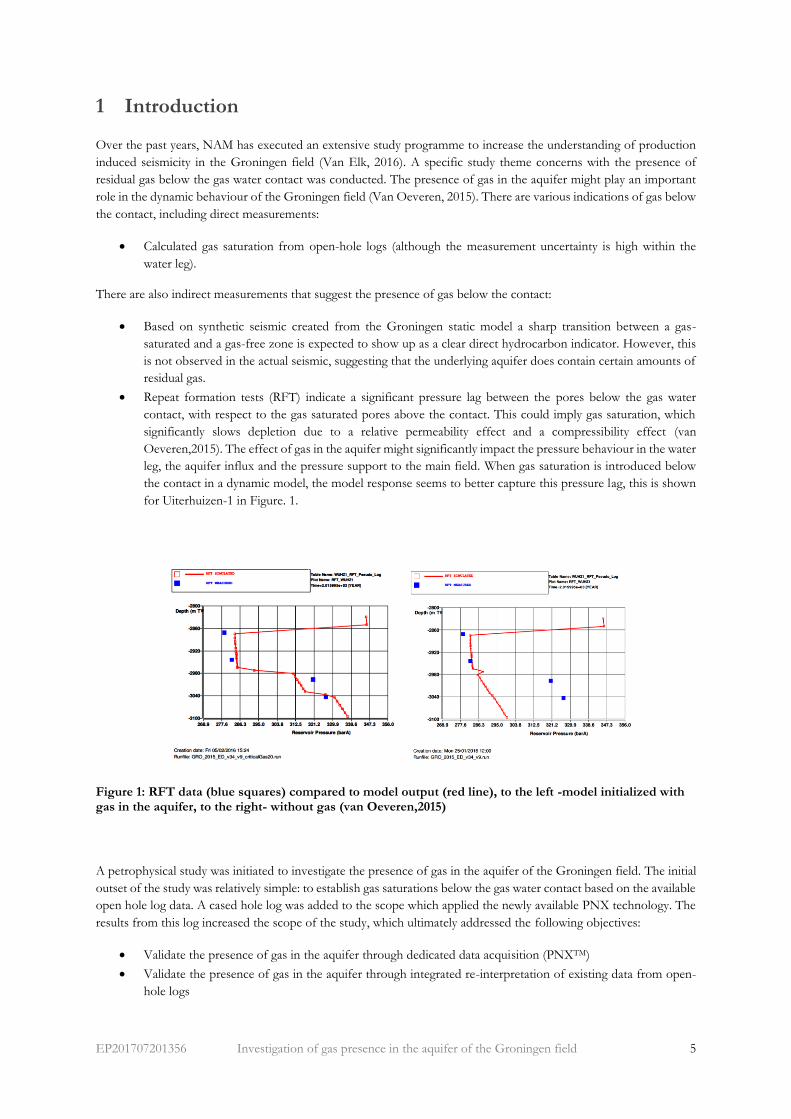
• Repeat formation tests (RFT) indicate a significant pressure lag between the pores below the gas water
contact, with respect to the gas saturated pores above the contact. This could imply gas saturation, which
significantly slows depletion due to a relative permeability effect and a compressibility effect (van
Oeveren,2015). The effect of gas in the aquifer might significantly impact the pressure behaviour in the water
leg, the aquifer influx and the pressure support to the main field. When gas saturation is introduced below
the contact in a dynamic model, the model response seems to better capture this pressure lag, this is shown
for Uiterhuizen-1 in Figure. 1.
Figure 1: RFT data (blue squares) compared to model output (red line), to the left -model initialized with gas in the aquifer, to the right- without gas (van Oeveren,2015)
A petrophysical study was initiated to investigate the presence of gas in the aquifer of the Groningen field. The initial
outset of the study was relatively simple: to establish gas saturations below the gas water contact based on the available
open hole log data. A cased hole log was added to the scope which applied the newly available PNX technology. The
results from this log increased the scope of the study, which ultimately addressed the following objectives:
• Validate the presence of gas in the aquifer through dedicated data acquisition (PNXTM)
• Validate the presence of gas in the aquifer through integrated re-interpretation of existing data from open-
hole logs

EP201707201356 Investigation of gas presence in the aquifer of the Groningen field 6
• Provide a quantitative assessment of gas saturation for the interval below the gas water contact (best
assessment for the given measurement uncertainties)
Water saturation determination (Sw) is one of the most challenging of petrophysical calculations and is used to quantify
the hydrocarbon (gas) saturation (1 – Sw ) (Petrowiki.org). Complexities arise because there are a number of
independent approaches that can be used to calculate gas saturation. This study will focus on the assessment of gas
saturation based on the cased hole data and calculation of saturation from resistivity logs, which were acquired in the
open-hole, when the well was drilled.
Schlumberger’s PNXTM tool is a recent development in cased hole reservoir surveillance technology. It provides a
novel type of measurement, which is sensitive to gas and not to fluid, that can be interpreted to derive at an actual
saturation value.
The Uithuizen-1 well was selected as a suitable candidate for PNXTM data acquisition, to complement the historical
open-hole logs that were acquired at the time of drilling. UHZ-1 was drilled in 1978 as an observation well located in
the North of the field, close to the earthquake-prone Loppersum area. By the time the well was drilled, around 650Bcm
of gas was produced. As an average over the field, this equates to roughly 22% depletion with respect to initial pressure.
It is possible that depletion of the aquifer has impacted the gas saturations below the gas water contact at the moment
when the open-hole data was acquired.
Historically, the well has been periodically used to measure reservoir pressure and potential water encroachment. The
presence of gas below the contact was already observed from the initial open-hole log evaluation, however, gas
saturation values were within the possible saturation measurement uncertainty.
EP201707201356 Investigation of gas presence in the aquifer of the Groningen field 7
2 Cased hole saturation evaluation
2.1 Pulsed Neutron Logging
The assessment of hydrocarbon saturation in cased holes has long been established by using pulsed neutron logs.
Pulse neutron logging (PNL) measures the thermal decay time of a neutron, bombarded into a formation (Morris, et
al. 2005). PNL uses a source (minitron), generating 14 MeV neutrons, which is turned on and off (pulsed). During the
time the minitron is off, the thermal-neutron or capture gamma-ray counts are measured. The thermal-neutron
population is created during the burst and dies away after the end of the burst, due primarily to the capture of these
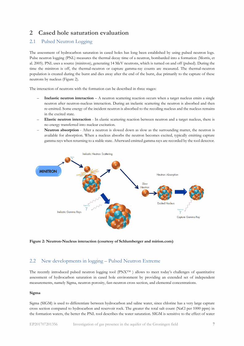
neutrons by nucleus (Figure 2).
The interaction of neutrons with the formation can be described in three stages:
– Inelastic neutron interaction – A neutron scattering reaction occurs when a target nucleus emits a single
neutron after neutron-nucleus interaction. During an inelastic scattering the neutron is absorbed and then
re-emitted. Some energy of the incident neutron is absorbed to the recoiling nucleus and the nucleus remains
in the excited state.
– Elastic neutron interaction - In elastic scattering reaction between neutron and a target nucleus, there is
no energy transferred into nuclear excitation.
– Neutron absorption - After a neutron is slowed down as slow as the surrounding matter, the neutron is
available for absorption. When a nucleus absorbs the neutron becomes excited, typically emitting capture
gamma rays when returning to a stable state. Afterward emitted gamma rays are recorded by the tool detector.
Figure 2: Neutron-Nucleus interaction (courtesy of Schlumberger and mirion.com)
2.2 New developments in logging – Pulsed Neutron Extreme
The recently introduced pulsed neutron logging tool (PNXTM ) allows to meet today’s challenges of quantitative
assessment of hydrocarbon saturation in cased hole environment by providing an extended set of independent
measurements, namely Sigma, neutron porosity, fast-neutron cross section, and elemental concentrations.
Sigma
Sigma (SIGM) is used to differentiate between hydrocarbon and saline water, since chlorine has a very large capture
cross section compared to hydrocarbon and reservoir rock. The greater the total salt count (NaCl per 1000 ppm) in
the formation waters, the better the PNL tool describes the water saturation. SIGM is sensitive to the effect of water
EP201707201356 Investigation of gas presence in the aquifer of the Groningen field 8
salinity, porosity, and shaliness of the rock and matrix composition (Morris et al.,2005). The main uncertainty in the
application of SIGM is the definition of the rock matrix values, which vary with lithology variations. Clay will typically
have a relatively high Sigma value, and thus can be a large source of inaccuracy if its volume, composition and endpoint
are not well defined or fluctuate (Zhou et al.,2016).
FNXS
The new generation of pulsed neutron logging tool are now able to register a new formation nuclear property, the fast
neutron cross section (FNXS), that was recently introduced in the logging industry (Rose et al.,2015). The novelty of
FNXS is to assess the formation’s ability to interact with the fast neutrons. It is very sensitive to gas-filled porosity,
while insensitive to liquid-filled porosity (Zhou et al.,2016). The measurement is derived from total gamma-ray counts
originating from inelastic interactions and is sensitive to the formation’s characteristic to attenuate high energy
neutrons (Rose et al.,2015). It is effective for distinguishing gas from rock matrix and fluids. Its response doesn’t
correlate to hydrogen index (Zhou et al., 2016).
TPHI
TPHI is a pulsed neutron version of a neutron porosity that is similar in response to the open hole dual detector
neutron tool. It responds primarily to hydrogen content. TPHI is the most susceptible to differentiate hydrogen liquids
such as water and oil from the non-clay rock matrix, which typically contains no hydrogen. Clay is a complicating
factor since it contains hydrogen and can lead to inaccuracy if its volume and response are not accurately compensated
for (Zhou et al.,2016).
Capture spectroscopy
Capture spectroscopy is used in cased hole to solve for complex lithology. Most of the key elements commonly present
in sedimentary rocks, such as Ca, Si, S, Fe, and Al can be measured with capture spectroscopy. Elements are typically
given as dry weight concentrations. These elements can be converted to dry weight mineralogy through various
methods, e.g. approach by Herron (Herron et al., 1996). If the lithology is unknown, this measurement is very useful
in establishing the elemental and mineral composition of the rock.
2.3 PNXTM data acquisition and processing workflow
Pulsed Neutron Xtreme (PNXTM) service was recorded for lithology and saturation across the target interval. To meet
the specific UHZ-1 job objectives the hybrid logging mode (so called GSH_Lith mode) was selected. This logging
mode enabled simultaneous acquisition of time (SIGM, TPHI and FNXS) and energy (spectroscopy) domain data.
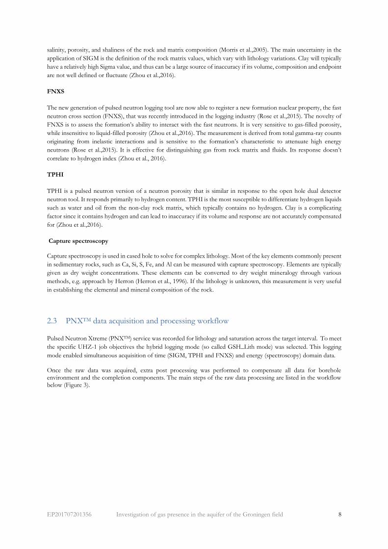
Once the raw data was acquired, extra post processing was performed to compensate all data for borehole environment and the completion components. The main steps of the raw data processing are listed in the workflow below (Figure 3).
EP201707201356 Investigation of gas presence in the aquifer of the Groningen field 9
Figure 3: PNXTM raw data processing workflow (courtesy of Schlumberger)
Time domain measurements were used to compute auto-compensated neutron porosity (TPHI), capture cross section
(SIGM) and the novel fast neutron cross section (FNXS). All cased hole measurements were self-compensated for
borehole environmental effects and completion components.
The first step in the energy domain processing was to get the inelastic and capture elemental yields. Afterwards, the
raw elemental yields from the near and far detectors were converted to dry weight elements (capture and inelastic)
using a closure model developed at SDR (Schlumberger Doll Research centre).
Energy domain
Time domain
Sigma & Thermal Neutron Porosity
FNXS analysis
Spectral Stripping
Lithology
Gas interpretation, matrix density
Time decay spectra analysis
Fast Neutron from deep count
analysis
Spectral to yields
From yield to elements (capture
and inelastic) to minerals, matrix
properties
EP201707201356 Investigation of gas presence in the aquifer of the Groningen field 10
3 Quantitative saturation assessment
3.1 General method
The general methodology for the determination of hydrocarbon saturation in cased hole is to use a single pulsed
neutron measurement, such as SIGM or TPHI in order to solve for two-phase hydrocarbon saturation. This
methodology is acceptable for straightforward cases, such as a gas column in a clean rock. As soon as more complex
questions arise, a more comprehensive approach should be adopted to provide quantitative results.
The general methodology is to develop a series of measurement response equations as well as to solve for unknown
formation volumes (Rose et al., 2017). Formation volumes can be distinguished into two main groups: rock matrix
and fluids. Further subdivision may be required based on the complexity of the rock and difference in the fluid system.
A generic volume in siliciclastic reservoirs are “sand” and “clays”. For simple interpretation cases the following
subdivision is sufficient. However, for a quantitative assessment of gas saturation in the aquifer a more comprehensive
multimineral petrophysical analysis is required.
3.2 Multimineral petrophysical analysis for complex cases
Multimineral petrophysical analysis (MMPA) is performed in a specially designed program for quantitative formation
evaluation (the Quanti Elan program within the Techlog software by Schlumberger) of cased and open-hole log
data. Evaluation is done by optimizing simultaneous equations described by one or more interpretation models. The
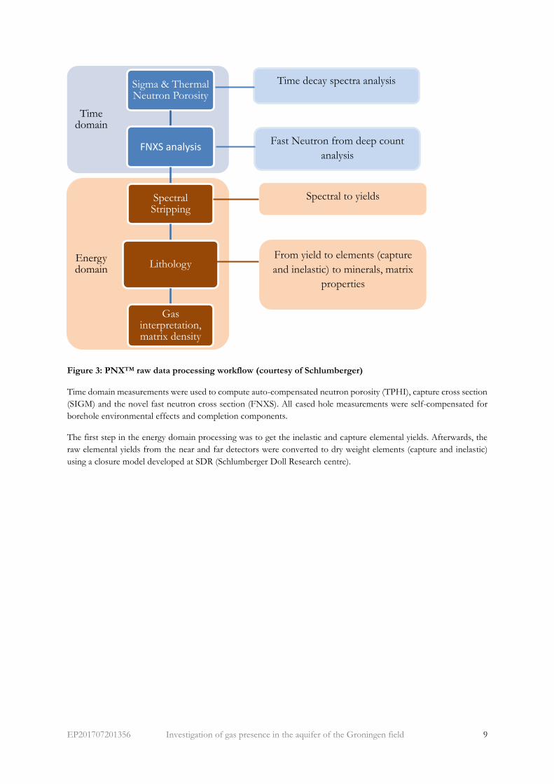
relationship is often presented in a triangular diagram (Figure 4), where t -input log data, v - formation component
volumes, R- responses of 100% formation component (rock, fluid, etc.).
Figure 4: Petrophysical model used by Quanti.Elan application (courtesy of Schlumberger)
MMPA uses both inverse and forward modelling. Inverse modelling is applied to compute only volumes of the
formation components. Forward modelling, also known as log reconstruction, computes synthetic curve, based on v
and R. By comparison of synthetic log responses to the actual log data the quality control assessment of a petrophysical
model is performed (TechlogTM help files).
The interpretation model consists of set of response equations, a set of formation components, a set of parameters
and constraints. Formation components define the minerals, rocks, and fluids, which volumetric outputs are required.
It is required that selected components are aligned with the geological description of the formation to which the model
is applied. Minerals are solids, which are characterized by a unique chemical formula, for example calcite -CaCO3.
Rock is a natural substance, a solid aggregate of one or more minerals (Wikipedia), such as sedimentary, metamorphic,
and igneous.
Response equations are the equations to be solved and their associated input data and uncertainties. The equations
describe the logging data. Parameters are the global and program control parameters, response parameters, binding
parameters, and salinity parameters. Constraints are the limits that the volumetric results must conform to. They used
to set the dependencies between one formation component and another. Constrains are a way to support MMPA
modelling with local geological knowledge (TechlogTM help files).

EP201707201356 Investigation of gas presence in the aquifer of the Groningen field 11
4 Estimation of the mineralogy composition
4.1 Introduction
The mineral composition of the Rotliegend reservoir of the Groningen has been reviewed by Visser (Visser, 2016).
This work includes an inventory of all the mineralogical and petrographical analyses carried out on Groningen core
material to date.
The bulk mineralogy of the rocks has been determined with whole-rock X-ray diffraction analysis (XRD). This data
has been acquired for multiple cored wells in the Groningen area (Figure 5). Quartz is the most abundant mineral,
followed by feldspars (plagioclase and K-feldspar), clay minerals (illite-smectite, kaolinite and chlorite) and carbonates
(mainly dolomite). The relative abundance of these minerals varies over the extent of the field:
– The ratio of total feldspar to quartz varies from South to North and from base to top of the Slochteren
Sandstone
– Authigenic clay mineralogy in the South is dominated by kaolinite and in the North by chlorite and kaolinite
– Trends in the abundance of clay minerals and carbonates are partly controlled by facies. Finer-grained and
clay-rich sediments tend to contain higher amounts of illite (plus illite-smectite) and dolomite.
These observations are relevant for the MMPA of logs from well UHZ-1. Analogue wells should preferentially be
located at limited distance to avoid bias from fieldwide trends. Figure 5 shows the location of UHZ-1 together with
all cored wells with at least 10 whole-rock XRD analyses available. The three wells closest to UHZ-1 are ZRP-3A,
ODP-1 and UHM-1A. Bulk mineralogy is available from these wells for both the Upper and the Lower Slochteren
Sandstone, and for both the gas leg and the aquifer.
The MMPA approach followed in this document requires as an input the relative composition of the rock matrix, but
split up in a sand component and a clay component. The sand component includes detrital grains and pore-filling
cements. The clay component includes both detrital and authigenic clay minerals.
Figure 5: Outline of the Groningen field with location of study well UHZ-1 and surrounding wells with
core coverage

EP201707201356 Investigation of gas presence in the aquifer of the Groningen field 12
4.2 Sand components
The composition of the sand component is shown in Figure 6. Data for wells ZRP-3A and ODP-1 are very
comparable. Samples from the aquifer contain circa 88% quartz, 10% feldspar and 2% dolomite, the composition of
the gas samples is circa 80% quartz, 17% feldspar and 3% dolomite.
Well UHM-1A has 45 out of 54 samples taken from the water leg. The average composition of these 45 samples is
72% quartz, 16% feldspar and 12% dolomite, which is different from the water leg samples in the other two wells. It
is not clear whether or not these differences are real or caused by, e.g., different analytical procedures. For example,
the petrography report on UHM-1A is dating from 1969 and reports an “approximate” mineral composition in
multiples of 5 percent points (Rahdon, 1969). The petrography work on ODP-1 was carried out in 2003 and on ZRP-
3A in 2016, both reporting with 1 percent point accuracy. This suggests that higher confidence should be assigned to
the ODP and ZRP data compared to the UHM-1A data.
Figure 6: Composition of the sand component of three offset wells for UHZ-1, split per well and per fluid
zone. Data obtained from whole-rock XRD analysis
Based on the above data for ZRP-3A and ODP-1 only, an average composition of the sand content in well UHZ-1
is estimated at (Figure 6):
– Quartz: 80%
– Feldspar: 17%
– Dolomite: 3%
4.3 Clay components
Total clay from whole-rock XRD analysis in well ZRP-3A is 8%, almost evenly split between chlorite, illite/smectite
and kaolinite. For well ODP-1 this is 16%, half of which is illite/smectite and the other half split between chlorite and
kaolinite. The composition of clay minerals based on clay-fraction XRD is shown in Figure 7. The two methods yield

EP201707201356 Investigation of gas presence in the aquifer of the Groningen field 13
fairly comparable results, taking into account the limited number of samples analyzed, the different sample preparation
techniques and the facies dependence of the clay minerals.
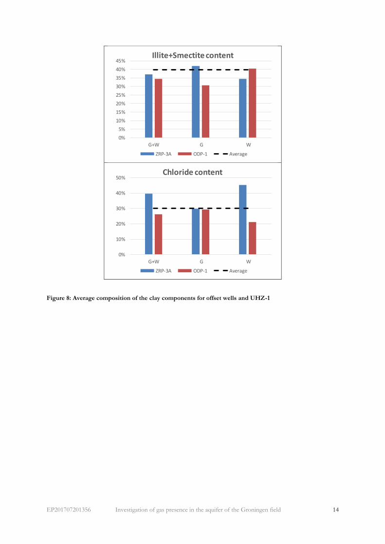
Based on this, the composition of the clay component in well UHZ-1 is estimated at (Figure 8):
– Illite/smectite:40%
– Chlorite: 30%
– Kaolinite: 30%
The whole-rock and clay-fraction XRD data for UHM-1A is of lower confidence but indicates a very comparable
composition.
Figure 7: Composition of the clay component of two offset wells for UHZ-1, split per well and per fluid
zone. Data obtained from clay-fraction XRD analysis.
0%
5%
10%
15%
20%
25%
30%
35%
40%
45%
G+W G W
Kaolinite content
ZRP-3A ODP-1 Average
EP201707201356 Investigation of gas presence in the aquifer of the Groningen field 14
Figure 8: Average composition of the clay components for offset wells and UHZ-1
0%
5%
10%
15%
20%
25%
30%
35%
40%
45%
G+W G W
Illite+Smectite content
ZRP-3A ODP-1 Average
0%
10%
20%
30%
40%
50%
G+W G W
Chloride content
ZRP-3A ODP-1 Average

EP201707201356 Investigation of gas presence in the aquifer of the Groningen field 15
5 Uithuizen-1 FNXS analysis
As discussed in section 2.2, the FNXS measurement is based on fast neutrons, which are indirectly measured through
the detection of induced inelastic gamma rays by the logging tool. This is done using a designed type of detector (deep
PNX YAP) coupled to an optimized source neutron pulsing scheme used by PNXTM. The response of the inelastic
gamma rays count rate is modelled in a wide range of cased hole environments. More details with regards to the subject
are given in Appendix 1.
FNXS -TPHI cross plot is used to differentiate intervals filled with gas and water. The main application of the plot is
similar to a neutron-density cross plot, that is widely used in open-hole formation evaluation.
Figure 9 illustrates the approach of identifying gas filled intervals based on FNXS-TPHI cross plot.
Figure 9: Example of interpretation envelope of FNXS measurement (courtesy of Schlumberger)
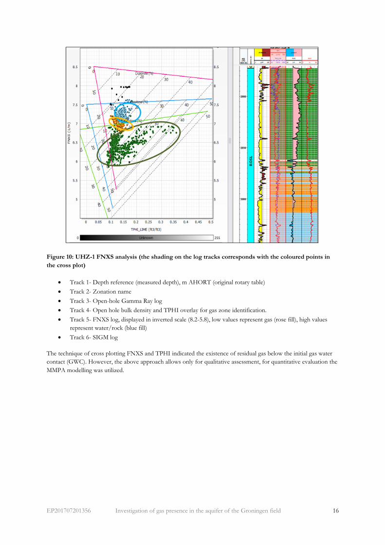
The same approach is used to analyse the UHZ-1 PNXTM logging data. As displayed below (Figure 10), the whole
logged interval can be subdivided into three zones based on TPHI-FNXS responses: gas filled (green), residual gas
(orange) and water zone (blue). The cloud of green points indicates the gas filled interval and is characterized with low
FNXS responses. The blue cloud represents the water zone and is characterized with high FNXS responses. The
orange zone between gas and water represents the residual gas.
EP201707201356 Investigation of gas presence in the aquifer of the Groningen field 16
Figure 10: UHZ-1 FNXS analysis (the shading on the log tracks corresponds with the coloured points in
the cross plot)
• Track 1- Depth reference (measured depth), m AHORT (original rotary table)
• Track 2- Zonation name
• Track 3- Open-hole Gamma Ray log
• Track 4- Open hole bulk density and TPHI overlay for gas zone identification.
• Track 5- FNXS log, displayed in inverted scale (8.2-5.8), low values represent gas (rose fill), high values
represent water/rock (blue fill)
• Track 6- SIGM log
The technique of cross plotting FNXS and TPHI indicated the existence of residual gas below the initial gas water
contact (GWC). However, the above approach allows only for qualitative assessment, for quantitative evaluation the
MMPA modelling was utilized.
EP201707201356 Investigation of gas presence in the aquifer of the Groningen field 17
6 Multi-Mineral Petrophysical Analysis for cased hole evaluation
MMPA involves the construction of a mineral model as a simplified representation of reality. All formation evaluation
problems are vastly underdetermined. It is unlikely that anyone will ever have enough measurements, with sufficient
accuracy and resolution in all dimensions, to fully describe the near-wellbore environment.
As was discussed in Chapter 4, the mineral composition of Rotliegend is complex. An accurate assessment of clay
volume is critical in determination of the reservoir properties from logs. The most important properties are porosity
and saturation. To address the complexity of clay and rock composition the multimineral petrophysical model is
required.
Acquisition of PNX data allows to build a complex model and assess volumes of clay minerals, rock components and
fluids. However, the understanding of clay minerals distribution across the Groningen field as wells as rock minerals
distribution and it vertical variability should be incorporated into the model as a way to introduce geological
knowledge.
MMPA analysis is designed to evaluate interval below the GWC and incorporates FNXS, SIGM, TPHI, spectroscopy
and open hole density data into one interpretation model. Each data input is used to quantify either matrix, shale or
fluid components. The parameter initialization step is required for MMPA run.
6.1 Parameter initialization
The parameter initialization step is required to arrive at parameters for water and gas, which depend on actual pressure
as well as temperature data varying with depth. Knowledge of water salinity and expected formation porosity are also
essential for calculating formation water density, conductivity and other parameters, which are required for MMPA.
The detailed list of main input and output curves can be found in the Appendix 3.
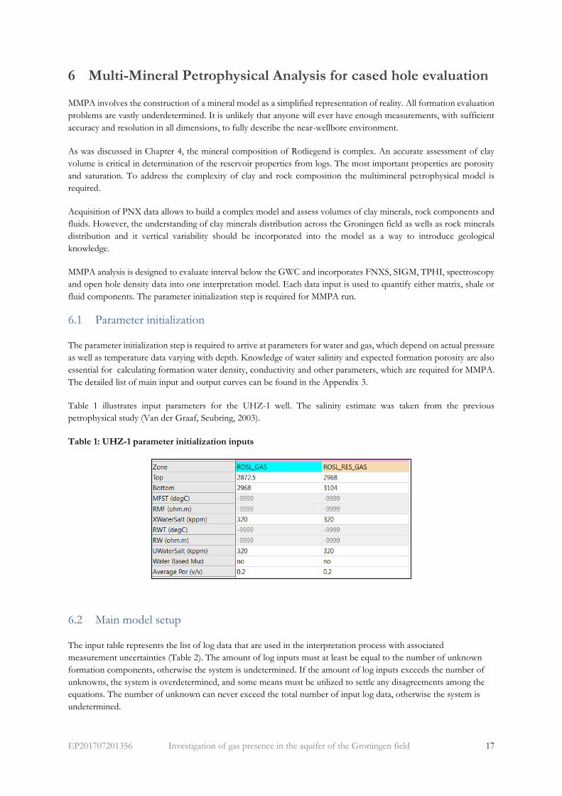
Table 1 illustrates input parameters for the UHZ-1 well. The salinity estimate was taken from the previous
petrophysical study (Van der Graaf, Seubring, 2003).
Table 1: UHZ-1 parameter initialization inputs
6.2 Main model setup
The input table represents the list of log data that are used in the interpretation process with associated
measurement uncertainties (Table 2). The amount of log inputs must at least be equal to the number of unknown
formation components, otherwise the system is undetermined. If the amount of log inputs exceeds the number of
unknowns, the system is overdetermined, and some means must be utilized to settle any disagreements among the
equations. The number of unknown can never exceed the total number of input log data, otherwise the system is
undetermined.
EP201707201356 Investigation of gas presence in the aquifer of the Groningen field 18
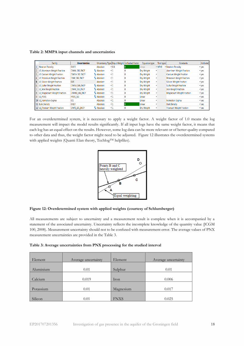
Table 2: MMPA input channels and uncertainties
For an overdetermined system, it is necessary to apply a weight factor. A weight factor of 1.0 means the log
measurement will impact the model results significantly. If all input logs have the same weight factor, it means that
each log has an equal effect on the results. However, some log data can be more relevant or of better quality compared
to other data and thus, the weight factor might need to be adjusted. Figure 12 illustrates the overdetermined systems
with applied weights (Quanti Elan theory, TechlogTM helpfiles).
Figure 12: Overdetermined system with applied weights (courtesy of Schlumberger)
All measurements are subject to uncertainty and a measurement result is complete when it is accompanied by a
statement of the associated uncertainty. Uncertainty reflects the incomplete knowledge of the quantity value (JCGM
100, 2008). Measurement uncertainty should not to be confused with measurement error. The average values of PNX
measurement uncertainties are provided in the Table 3.
Table 3: Average uncertainties from PNX processing for the studied interval
Element Average uncertainty Element Average uncertainty
Aluminium 0.01 Sulphur 0.01
Calcium 0.019 Iron 0.006
Potassium 0.01 Magnesium 0.017
Silicon 0.01 FNXS 0.025
EP201707201356 Investigation of gas presence in the aquifer of the Groningen field 19
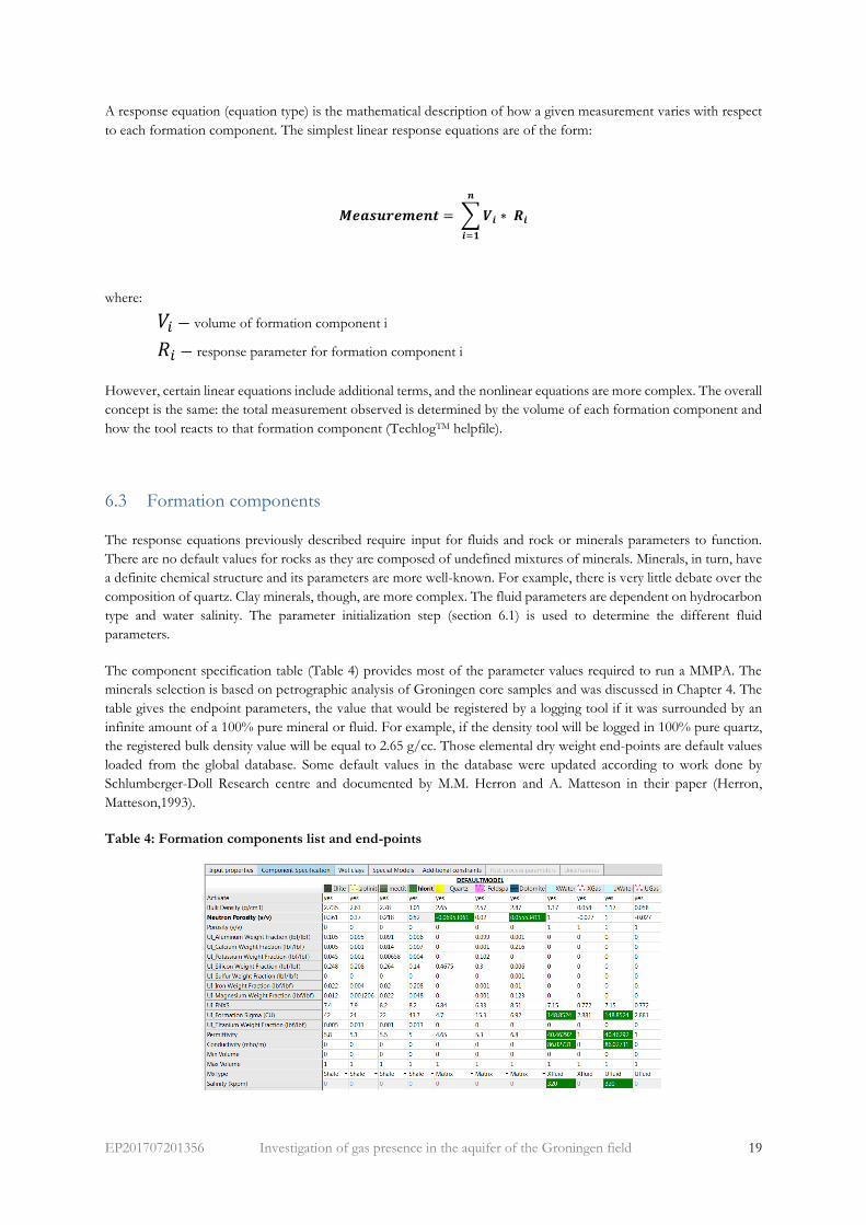
A response equation (equation type) is the mathematical description of how a given measurement varies with respect
to each formation component. The simplest linear response equations are of the form:
𝑴𝒆𝒂𝒔𝒖𝒓𝒆𝒎𝒆𝒏𝒕 = ∑ 𝑽𝒊 ∗ 𝑹𝒊
𝒏
𝒊=𝟏
where:
𝑉𝑖 – volume of formation component i
𝑅𝑖 – response parameter for formation component i
However, certain linear equations include additional terms, and the nonlinear equations are more complex. The overall
concept is the same: the total measurement observed is determined by the volume of each formation component and
how the tool reacts to that formation component (TechlogTM helpfile).
6.3 Formation components
The response equations previously described require input for fluids and rock or minerals parameters to function.
There are no default values for rocks as they are composed of undefined mixtures of minerals. Minerals, in turn, have
a definite chemical structure and its parameters are more well-known. For example, there is very little debate over the
composition of quartz. Clay minerals, though, are more complex. The fluid parameters are dependent on hydrocarbon
type and water salinity. The parameter initialization step (section 6.1) is used to determine the different fluid
parameters.
The component specification table (Table 4) provides most of the parameter values required to run a MMPA. The
minerals selection is based on petrographic analysis of Groningen core samples and was discussed in Chapter 4. The
table gives the endpoint parameters, the value that would be registered by a logging tool if it was surrounded by an
infinite amount of a 100% pure mineral or fluid. For example, if the density tool will be logged in 100% pure quartz,
the registered bulk density value will be equal to 2.65 g/cc. Those elemental dry weight end-points are default values
loaded from the global database. Some default values in the database were updated according to work done by
Schlumberger-Doll Research centre and documented by M.M. Herron and A. Matteson in their paper (Herron,
Matteson,1993).
Table 4: Formation components list and end-points

EP201707201356 Investigation of gas presence in the aquifer of the Groningen field 20
The end-points for SIGM, FNXS and TPHI are not default values, as they depend upon gas density, pressure, and
temperature. They should be calculated for each individual case. The end-point results for the mentioned log inputs
are listed in the Table 5.
Table 5: End points calculation of SIGM, FNXS, TPHI for the given gas properties (SG, P, T)
6.4 Constraints and Constants
It should be mentioned that within the Quanit-Elan model set-up there are two ways of imposing geological or
petrophysical information into the interpretation model: through constants and constraints. Constraints are absolute
minimum and/or maximum limits on formation component volumes. Unlike constant tools, which are weighted by
uncertainties, constraints are absolute limits. They do not represent a curve bound to data and are the means of adding
local knowledge to the model through equations. For example, when solving for complex clay system, it is beneficial
to incorporate knowledge of clay distribution from near-by wells for more precise model reconstruction.
For example, dolomite-to-quartz ration of the first well is around 5 %, and the geology is similar between two wells.
That knowledge can be included into the model as: quartz/dolomite=0.05 or 0=1*quartz-0.05*dolomite. UHZ-1 well
has a complex mineral composition and this is reflected through more complicated dependencies in constant tools
(Table 6).
It is valid to note that XRD inputs should be represented via constant tool and should not be used as absolute
controlling parameters for the model reconstruction due to uncertainties and possible errors associated with core
extraction and XRD analysis itself.
Table 6: Constraints and constant tool table
EP201707201356 Investigation of gas presence in the aquifer of the Groningen field 21
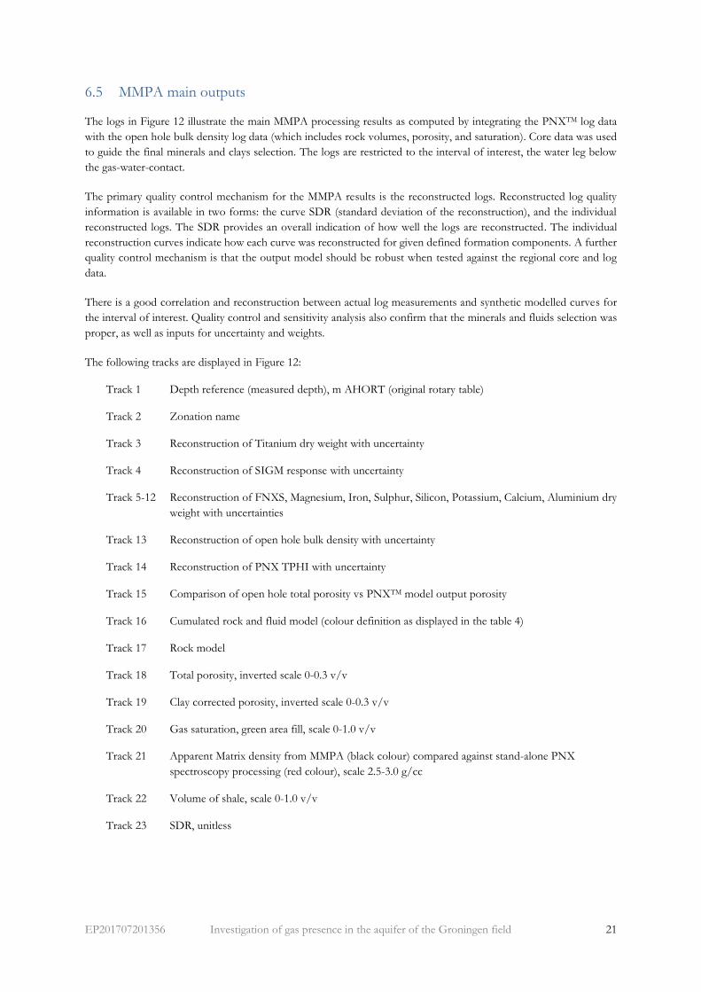
6.5 MMPA main outputs
The logs in Figure 12 illustrate the main MMPA processing results as computed by integrating the PNXTM log data
with the open hole bulk density log data (which includes rock volumes, porosity, and saturation). Core data was used
to guide the final minerals and clays selection. The logs are restricted to the interval of interest, the water leg below
the gas-water-contact.
The primary quality control mechanism for the MMPA results is the reconstructed logs. Reconstructed log quality
information is available in two forms: the curve SDR (standard deviation of the reconstruction), and the individual
reconstructed logs. The SDR provides an overall indication of how well the logs are reconstructed. The individual
reconstruction curves indicate how each curve was reconstructed for given defined formation components. A further
quality control mechanism is that the output model should be robust when tested against the regional core and log
data.
There is a good correlation and reconstruction between actual log measurements and synthetic modelled curves for
the interval of interest. Quality control and sensitivity analysis also confirm that the minerals and fluids selection was
proper, as well as inputs for uncertainty and weights.
The following tracks are displayed in Figure 12:
Track 1 Depth reference (measured depth), m AHORT (original rotary table)
Track 2 Zonation name
Track 3 Reconstruction of Titanium dry weight with uncertainty
Track 4 Reconstruction of SIGM response with uncertainty
Track 5-12 Reconstruction of FNXS, Magnesium, Iron, Sulphur, Silicon, Potassium, Calcium, Aluminium dry
weight with uncertainties
Track 13 Reconstruction of open hole bulk density with uncertainty
Track 14 Reconstruction of PNX TPHI with uncertainty
Track 15 Comparison of open hole total porosity vs PNXTM model output porosity
Track 16 Cumulated rock and fluid model (colour definition as displayed in the table 4)
Track 17 Rock model
Track 18 Total porosity, inverted scale 0-0.3 v/v
Track 19 Clay corrected porosity, inverted scale 0-0.3 v/v
Track 20 Gas saturation, green area fill, scale 0-1.0 v/v
Track 21 Apparent Matrix density from MMPA (black colour) compared against stand-alone PNX
spectroscopy processing (red colour), scale 2.5-3.0 g/cc
Track 22 Volume of shale, scale 0-1.0 v/v
Track 23 SDR, unitless

EP201707201356 Investigation of gas presence in the aquifer of the Groningen field 22
Figure 12: Cased hole MMPA main results (the box highlights difference in gas saturation with depth)
1 2 3 4 5 6 7 8 9 10 11 12 13 14 15 16 17 18 19 20 21 22 23
GWC

EP201707201356 Investigation of gas presence in the aquifer of the Groningen field 23
6.6 MMPA cased hole results
A Multimineral Petrophysical Analysis was performed for the cased hole environment across the depth interval below
the GWC. Such analysis enables a quantitative assessment of the gas saturation. However, it is important to note that
the resulting gas saturation is the best model estimate and does not incorporate an uncertainty assessment of gas
saturation to fully quantify the range. It became evident that a full uncertainties analysis around the gas saturation
measured through casing is complex. Additional data acquisition and statistical analysis is required to further study the
subject.
The main results can be summarized as follows:
• A small quantity of gas was calculated in the interval below the GWC (GWC at 2969 m AHORT)
• A fairly consistent gas signature was observed down to 46 m below the GWC (over the interval from 2969
m AHORT till 3015 m AHORT) with average gas saturation value of around 8-10% with some peaks up
to 20%.
• The calculated gas saturation distribution is rather patchy, than continuous.
EP201707201356 Investigation of gas presence in the aquifer of the Groningen field 24
7 Multi-Mineral Petrophysical Analysis for open hole evaluation
The acquisition of PNX TM spectroscopy data on UHZ-1 helped to improve the mineralogical model of the Rotliegend
formation for the well. This allowed for a reassessment of the gas saturation based on the historic open-hole log data.
The modelling of open-hole data is similar to the method described in Chapter 6, except that the gas saturation is
calculated using formation resistivity inputs and the Waxman-Smits model with saturation components for the water
leg, as described in the current Groningen field petrophysical model (Van der Graaf, Seubring, 2003).
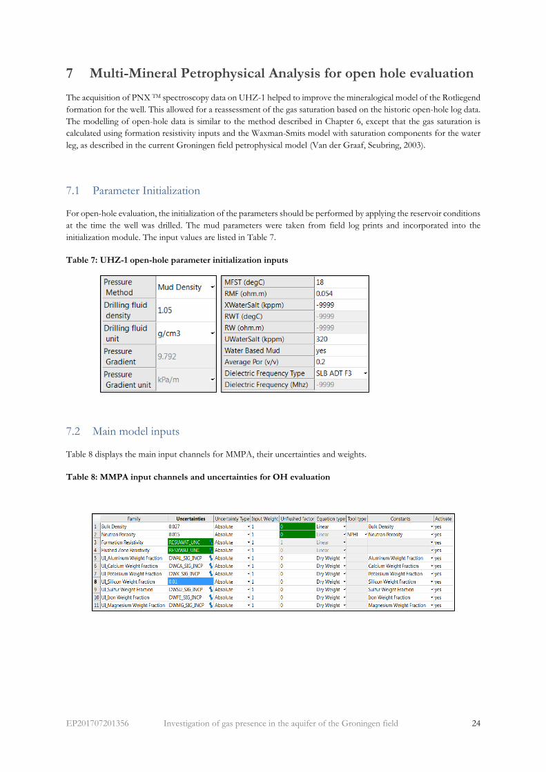
7.1 Parameter Initialization
For open-hole evaluation, the initialization of the parameters should be performed by applying the reservoir conditions
at the time the well was drilled. The mud parameters were taken from field log prints and incorporated into the
initialization module. The input values are listed in Table 7.
Table 7: UHZ-1 open-hole parameter initialization inputs
7.2 Main model inputs
Table 8 displays the main input channels for MMPA, their uncertainties and weights.
Table 8: MMPA input channels and uncertainties for OH evaluation

EP201707201356 Investigation of gas presence in the aquifer of the Groningen field 25
7.3 Formation components
The list of the minerals and fluids in the model and each component endpoint is shown in the Table 9 (no changes
with respect to the cased hole endpoints as described in section 6.3).
Table 9: Formation component end-points for OH evaluation
7.4 Wet Clay Model
To account for clay bound water in the Waxman-Smits saturation model, the wet clay inputs are required. The
parameters listed in Table 10 are extracted from the default database and calculated for the relevant temperature and
pressure at UHZ-1.
Table 10: Wet clay component end-points for OH evaluation

EP201707201356 Investigation of gas presence in the aquifer of the Groningen field 26
7.5 Saturation Model
7.5.1 Waxman-Smits saturation method
Water saturation determination is the most challenging of petrophysical calculations, especially if such assessment is
required for shaly sandstones, like the Rotliegend. The most common used shaly sand water saturation model is the
Waxman-Smits (W-S) model. The W-S model principles are available in the public domain and described in great
details by many authors (Waxman et al.,1968,1974)
The W-S water saturation formula is listed below:
where:
Rt formation resistivity, ohm-m
Qv cation exchange capacity per unit pore volume, eq/L
calculated total porosity, v/v
m* Waxman-Smits cementation exponent
n* Waxman-Smits saturation exponent
Rw formation water resistivity, ohm-m
B equivalent cationic conductance of a sodium ion
The W-S model addresses the clay effect while calculating the water saturation. There are two properties of clay
minerals that contribute to the problem of calculating water saturation in clay bearing sandstones: surface area and
cation exchange capacity (CEC) (Pittman,1989). Authigenic clay minerals, especially those with the fibrous
morphology (e.g. illite), possess a very high surface area. If the rock is water-wet, then the surface of the clay is covered
by a 1 or 2-molecule thick layer of water. The micropores among clay particles also hold water by capillary retention
forces. The water absorbed by the clay and held in the micropores is considered to be “bound water”.
The amount of bound water is dependent both on the morphology and CEC of the clay minerals. The table below
represents values of CEC and cation exchange capacity per unit total pore volume (Qv) for different clay minerals, as
used in the Waxman-Smits equation for the saturation evaluation.
Table 11: CEC and Qv values for different clays minerals
Clay Mineral CEC (meq/100g) Qv(meq.cm-3)
Kaolinite 2-15 0.015-0.12
Chlorite 0-40 0.052-0.24
Illite 10-40 0.051-0.22
Smectite 76-150 0.34-0.81
The ranges as outlined in Table 11 are a result of the variability of clay minerals within the reservoir, and various
abilities of the clays to “hold” water. It’s crucial to have an accurate assessment of individual clays in Slochteren
formation. The main clay morphotypes of the Rotliegend were identified in the study of the NE Netherlands (Kelly,
S., Greenwood, J., 1996) by SEM photomicrographs, and are presented in Figure 13.
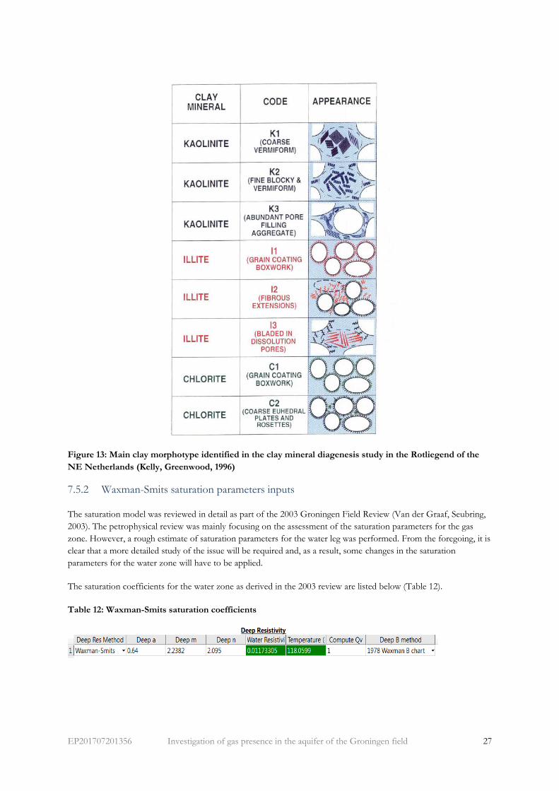
EP201707201356 Investigation of gas presence in the aquifer of the Groningen field 27
Figure 13: Main clay morphotype identified in the clay mineral diagenesis study in the Rotliegend of the
NE Netherlands (Kelly, Greenwood, 1996)
7.5.2 Waxman-Smits saturation parameters inputs
The saturation model was reviewed in detail as part of the 2003 Groningen Field Review (Van der Graaf, Seubring,
2003). The petrophysical review was mainly focusing on the assessment of the saturation parameters for the gas
zone. However, a rough estimate of saturation parameters for the water leg was performed. From the foregoing, it is
clear that a more detailed study of the issue will be required and, as a result, some changes in the saturation
parameters for the water zone will have to be applied.
The saturation coefficients for the water zone as derived in the 2003 review are listed below (Table 12).
Table 12: Waxman-Smits saturation coefficients

EP201707201356 Investigation of gas presence in the aquifer of the Groningen field 28
7.6 Constraints and Constants
Constraints and constants are identical to those described in section 6.4.
7.7 MMPA main outputs
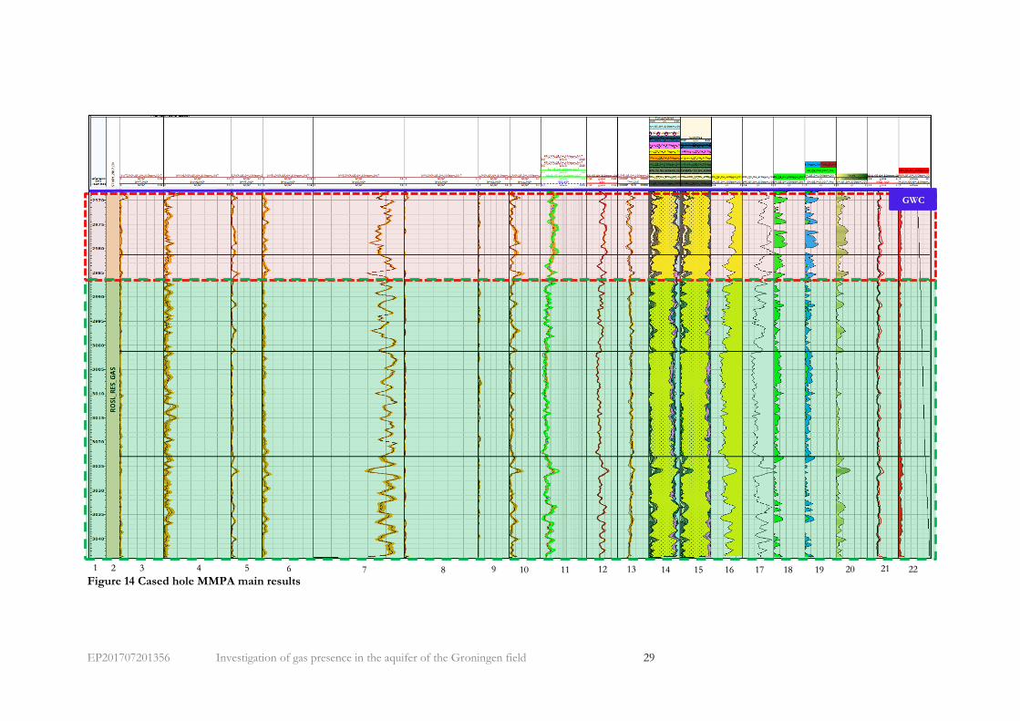
The log plots below (Figure 14) illustrate the main open-hole MMPA processing results, with rock volumes,
porosity, as well as saturation, computed by integrating PNX spectroscopy and open-hole log data.
Track 1 Depth reference (measured depth), m AHORT (original rotary table)
Track 2 Zonation name
Track 3-10 Reconstruction of Titanium, Magnesium, Iron, Sulphur, Silicon, Potassium, Calcium and
Aluminium dry weights with uncertainty
Track 11 Reconstruction of open hole formation resistivity (deep resistivity) with uncertainty
Track 12 Reconstruction of open hole bulk density with uncertainty
Track 13 Reconstruction of PNX TPHI with uncertainty (open hole neutron porosity was excluded from
evaluation due to a poor quality)
Track 14 Cumulated rock and fluid model (colour definition is displayed in the table 9)
Track 15 Rock model
Track 16 Total porosity, inverted scale 0-0.3 v/v
Track 17 Clay corrected porosity, inverted scale 0-0.3 v/v
Track 18 Open-hole gas saturation at September 1978, scale 0-1.0 v/v
Track 19 Overlay of open-hole gas saturation and cased hole gas saturation from the recent PNXTM
acquisition in April 2017, blue shading represents potential water influx in the zone below the
initial GWC, scale 0-1.0 v/v
Track 20 Volume of shale, v/v
Track 21 Apparent Matrix density from open-hole MMPA compared against stand-alone PNX
spectroscopy processing, g/cc
Track 22 SDR, unitless
EP201707201356 Investigation of gas presence in the aquifer of the Groningen field 29
Figure 14 Cased hole MMPA main results
1 2 3 4 5 6 7 8 9 10 11 12 13 14 15 16 17 18 19 20 21 22
GWC

EP201707201356 Investigation of gas presence in the aquifer of the Groningen field 30
7.8 MMPA open hole results
A multi-mineral petrophysical analysis was performed with the open-hole data across the depth interval below the
GWC. The model incorporates PNXTM spectroscopy data and available open-hole logs from 1978. It is important to
note, that the resulting gas saturation is the best model estimate and does not incorporate uncertainties related to
the possible ranges of gas saturation. It is revealed that the open hole saturation model for the water zone requires a
more detailed study and, as a result, some changes in the saturation parameters might be expected.
The main results can be summarized as follows:
• Continuous gas saturation distribution was calculated from the initial GWC (@ 2969 m AHORT) to the
well TD (@3043 m AHORT), resulting in 74 m AHORT column thickness.
• The highest gas saturation interval is observed from 2969 to 2988 m AHORT, overall 19 m of thickness.
The maximum calculated gas saturation values are up to 46 % and average is around 28%.
• The interval below 2988 m AHORT is characterized by a low gas saturation with a mean equal to 14%.
• Comparative analysis of open-hole (initial saturation) and cased hole (current day) gas saturation reveals
substantial difference in the interval from 2969 to 2988 m AHORT. This may indicate that the gas escaped
during the production of the Groningen field. However, the mechanism of gas migration from the zone
below the GWC during the depletion should be studied in more details and current observation, based on
limited data, should be considered with care.
8 Generalization and delimitations
• The rock and clay mineral inputs as applied in the UHZ-1 Multi-Mineral Petrophysical Analysis for open
hole and cased hole data were based on core measurements of nearby wells.
• Slight variations in MMPA mineral concentration outputs between the open-hole and cased hole models
should be expected due to different inputs logs and response equation used during modelling.
• It is assumed that the rock composition as well as the total porosity remains unchanged during the
production (depletion) history of the Groningen field.
• Mineral concentrations based on nearby well XRD data should be used as guidance for MMPA , since it is
known that the XRD measurement has possible sources of error (Herron et al.,2014), namely:
o Core samples may be misrepresentative of log formation response because of different depth of
investigation and differences in vertical resolution
o Cores could be contaminated with mud solids or filtrate
o Inaccurate in the analysis
• Saturation parameters in the water leg were used congruent to the ones quoted in the 2003 petrophysical
study (Van der Graaf, Seubring, 2003). That study was mainly focusing on assessment of saturation
parameters for the gas zone.

EP201707201356 Investigation of gas presence in the aquifer of the Groningen field 31
9 Conclusions and recommendations
A petrophysical study was done to investigate the presence of gas in the aquifer of the Groningen field. The study
conclusively demonstrates that there is gas below the original gas water contact at the UHZ-1 well location. The
results of this study will be used for analysis in the dynamic reservoir model.
PNXTM cased hole logging technology was used to assess the gas saturation below the gas water contact in UHZ-1.
Given the complexity of the topic, to assess residual gas saturation below the GWC, and sensitivity of gas saturation
results to clay mineralogy, the saturation evaluation was done using a Multi-Mineral Petrophysical Analysis (MMPA).
Analysis of the cased hole PNXTM measurements suggest patchy gas saturations distribution within the first 46m
below the gas water contact. The average values of around 8-10% , with peaks up to 20%. Some thin (1-2m) isolated
gas filled intervals are observed deeper down, however the gas saturation values are negligeable.
The 1978 open hole logs across the aquifer of UHZ-1 were also re-interpreted using MMPA Analysis (using the
PNXTM spectroscopy data), applying a Waxman-Smits saturation model. Continuous gas saturation values were
interpreted along the entire logging interval within the aquifer. The maximum calculated gas saturation values are up
to 46 % and average is around 28%. These saturation values are higher as compared to the cased hole analysis.
However, the saturation model was derived in 2003 with a focus on the gas leg. It is recommended to re-evaluate the
saturation parameters (a, m, n) with a focus specifically on the water leg. The available core data needs to be examined,
and if there is sufficient data available the saturation model may potentially be further refined to incorporate details
of the total clay composition within the rock.
The difference between cased hole and open hole saturation interpretation may result from various causes:
• The different methodologies for assessment of saturation both carry their own uncertainty ranges. These
ranges need to be further studied.
• Impact of clay mineral composition on saturation parameter determination
o It is known that the mineral composition has an impact on the gas saturation calculation, this is
true for both open and cased hole calculations. The workflows described in this document already
take this into account with the available data, however further study would be required to improve
the understanding of the clay minerals and their contribution to the saturation calculation
specifically below the gas-water contact. This can be achieved by a detailed calibration of PNXTM
tool responses (elemental dry weights) to the core data and a detailed review of the saturation
parameters used in the open-hole calculation below the gas-water contact. It is expected that this
will help to reduce the difference in the interpreted saturation values between the cased hole and
open hole logs.
• Impact of depletion.
o The Open Hole logs of UHZ-1 were acquired in 1978, by which time some 650Bcm of gas was
produced. As an average over the field, this equates to roughly 22% depletion with respect to initial
pressure. It is possible that depletion of the aquifer has impacted the gas saturations below the gas
water contact.
Once the difference is resolved, it is recommended to establish whether a representative model can be established
across the full field. If so, reinterpretation of the open-hole logs for all wells with a logging coverage over the aquifer
may be required. In case gas below the aquifer is observed consistently across the field, a saturation model for gas in
the aquifer of the Groningen field should be constructed. To allow for extrapolation beyond the areas that have well
coverage, this model build should be integrated with a geological/basin modelling explanation of the observations.
Additional points to be noted:
• Comparative analysis of open-hole (initial saturation) and cased hole (current day) gas saturation reveals
substantial difference in the interval from 2969 to 2988 m AHORT. This may indicate that the gas escaped
during the production of the Groningen field. However, the mechanism of gas migration from the zone

EP201707201356 Investigation of gas presence in the aquifer of the Groningen field 32
below the GWC during the depletion should be studied in more details and current observations, which are
based on limited data, should be considered with care.
• Rock with complex mineral and clay compositions benefit from implementing of Multi-Mineral
Petrophysical Analysis.
• The Groningen field is a very sizeable field that covers quite a large geographical area. The current
observations are based on PNXTM results in a single well. It is therefore advised to further investigate the
presence of gas below the GWC in other areas of the field.
• The current assessment of gas saturation below the GWC from the PNXTM and open-hole data only
incorporates measurement uncertainty. No further sensitivity analysis was done due to the limited amount
of available data.
• The PNX TM spectroscopy measurements were not calibrated to core spectroscopy data of the Groningen
field. It is recommended to acquire an additional PNX in a well that does have core data to allow for
calibration.

EP201707201356 Investigation of gas presence in the aquifer of the Groningen field 33
10 References 1. Van Elk, J., Study and Data Acquisition Plan Induced Seismicity in Groningen. Assen: NAM, 2016,
EP201604200072. 2. Van Oeveren, H.E.J., GFR2015: History matching and forecast uncertainty analysis. Assen: NAM,2015,
EP201602208918 3. Morris, C., Aswad, T., Morris, F. and Quinlan, T.,2005, Reservoir monitoring with pulsed neutron capture
logs: Paper, SPE, Madrid, Spain,13-16 June 4. Zhou, T., Rose, D., Quinlan, T., Thornton, Saldungaray, P., Gerges, N., Noordin, F. B. M., and Lukman,
A., 2016, Fast neutron cross-section measurement physics and applications: Paper EE, Transactions, SPWLA 57th Annual Logging Symposium, Reykjavik, Iceland, 25–29 June.
5. Rose, D., Zhou, T., Beekman, S., Quinlan, T., Delgadillo, M., Gonzalez, G., Fricke, S., Thornton, J., Clinton, D., Gicquel, F., Shestakova, I., Stephenson, K., Stoller, C., Philip, O., La Rotta Marin, J., Mainier, S., Perchonok, B., and Bailly, J.-P., 2015, An innovative slim pulsed neutron logging tool: Paper XXX, Transactions, SPWLA 56th Annual Logging Symposium, Long Beach, California, USA, 18–22 July.
6. Rose, D., Zhou, T., Saldungaray, P., 2017, Solving for Reservoir Saturations Using Multiple Formation Property Measurements from a Single Pulsed Neutron Logging Tool: SPWLA 58th Annual Logging Symposium, Oklahoma City, Oklahoma, USA,17-21 June
7. Visser, C., Petrographic aspects of the Rotliegend of the Groningen field. Assen: NAM, 2016,
EP201609201573
8. Rahdon, A.E., Diagenesis of the Rotliegend in Northwest Europe. Rijswijk, 1969, RKGR.0040.69 9. Van der Graaf, A., Seubring, J., Groningen Field Review –Groningen Field Static Modelling and Ultimate
Recovery Determination. Vol.4 – Reservoir Properties. Assen: NAM, 2003, NAM200308000869. 10. JCGM 100:2008. Evaluation of measurement data – Guide to the expression of uncertainty in
measurement 11. Herron M.M., Matteson A., “Elemental Composition and Nuclear Parameters of Some Common
Sedimentary Minerals,” Nuclear Geophysics, 1993, Vol. 7, No. 3, pp 383–406.
12. Waxman, M.H. and Smits, L.J.M. ,1968, Electrical Conductivities is Oil-Bearing Shaly Sands, Society of Petroleum Engineers Journal, June.
13. Waxman, Monroe H. and Thomas, E.C., Electrical Conductivities in Shaly Sands-I. The Relation Between Hydrocarbon Saturation and Resistivity Index; II. The Temperature Coefficient of Electrical Conductivity, 1974, Journal of Petroleum Technology, February
14. Pittman, E.D., Problem related to clay minerals in reservoir sandstones. In: J.F. Mason & P.A. Dickey (Eds.), Oil field development techniques. AAPG Studies in Geology, 1989, 28,237-244.
15. Kelly, S., Greenwood, J., Pattern of clay minerals diagenesis in the Rotliegend of the NE Netherlands. Assen: NAM, 1996, Rep. No. 28765.
16. Herron, S., Herron, M., Pirie, I., Saldungaray, P., Craddock, P., Charsky, A., Polyakov, M., Shray, F., Li, T.,2014, Application and quality control of core data for the development and validation of elemental spectroscopy log interpretation: SPWLA 55th Annual Logging Symposium, Abu Dhabi, United Arab Emirates,18-22 May.
EP201707201356 Investigation of gas presence in the aquifer of the Groningen field 34
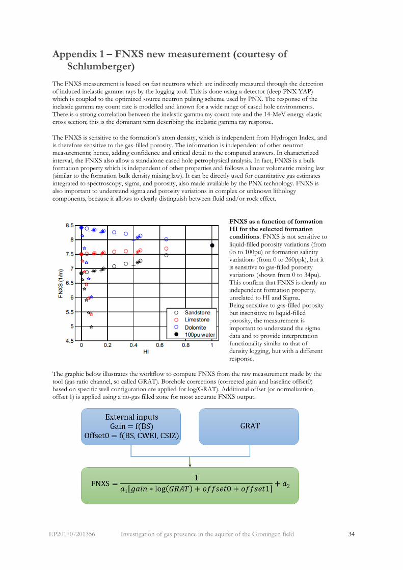
Appendix 1 – FNXS new measurement (courtesy of Schlumberger)
The FNXS measurement is based on fast neutrons which are indirectly measured through the detection of induced inelastic gamma rays by the logging tool. This is done using a detector (deep PNX YAP) which is coupled to the optimized source neutron pulsing scheme used by PNX. The response of the inelastic gamma ray count rate is modelled and known for a wide range of cased hole environments. There is a strong correlation between the inelastic gamma ray count rate and the 14-MeV energy elastic cross section; this is the dominant term describing the inelastic gamma ray response.
The FNXS is sensitive to the formation’s atom density, which is independent from Hydrogen Index, and is therefore sensitive to the gas-filled porosity. The information is independent of other neutron measurements; hence, adding confidence and critical detail to the computed answers. In characterized interval, the FNXS also allow a standalone cased hole petrophysical analysis. In fact, FNXS is a bulk formation property which is independent of other properties and follows a linear volumetric mixing law (similar to the formation bulk density mixing law). It can be directly used for quantitative gas estimates integrated to spectroscopy, sigma, and porosity, also made available by the PNX technology. FNXS is also important to understand sigma and porosity variations in complex or unknown lithology components, because it allows to clearly distinguish between fluid and/or rock effect.
FNXS as a function of formation HI for the selected formation conditions. FNXS is not sensitive to liquid-filled porosity variations (from 0o to 100pu) or formation salinity variations (from 0 to 260ppk), but it is sensitive to gas-filled porosity variations (shown from 0 to 34pu). This confirm that FNXS is clearly an independent formation property, unrelated to HI and Sigma. Being sensitive to gas-filled porosity but insensitive to liquid-filled porosity, the measurement is important to understand the sigma data and to provide interpretation functionality similar to that of density logging, but with a different response.
The graphic below illustrates the workflow to compute FNXS from the raw measurement made by the tool (gas ratio channel, so called GRAT). Borehole corrections (corrected gain and baseline offset0) based on specific well configuration are applied for log(GRAT). Additional offset (or normalization, offset 1) is applied using a no-gas filled zone for most accurate FNXS output.

EP201707201356 Investigation of gas presence in the aquifer of the Groningen field 35
Appendix 2 – Theoretical values for typical formation component (courtesy of Schlumberger)

EP201707201356 Investigation of gas presence in the aquifer of the Groningen field 36
Appendix 3 – List of main inputs and outputs of initialization
method (TechlogTM helpfile)
A3.1 Inputs
Name Unit Description
MFST degC Mud Filtrate Sample Temperature
RMF ohm.m Resistivity of Mud Filtrate
XWaterSalt kppm Flushed zone Water Salinity
RWT degC Formation Water Temperature
RW ohm.m Water Resistivity
UWaterSalt kppm Unflushed zone Water Salinity (formation salinity)
Mud Weight g/cm3 Drilling Fluid Density (Mud Weight for pressure estimation)
Water Based Mud
Mud type: Water or Oil
Average Por v/v Average Porosity (if Porosity is not defined as an input)
Temperature degC Temperature at the Depth value (if Temperature is not defined as an input)
Temperature Gradient
degC/m Geothermal gradient used to compute temperature curve (if Temperature is not defined as an input)
Depth m Reference depth used to compute the temperature gradient (if Temperature is not defined as an input)
A3.2 Outputs
Name Unit Description
SALT_XWATER
kppm Salinity of the water in the Flushed zone
SALT_UWATER
kppm Salinity of the water in the Unflushed zone
RHOB_IFAC unitless Bulk Density Invasion Factor
RHOB_XWAT g/cm3 Water Density in Flushed zone

EP201707201356 Investigation of gas presence in the aquifer of the Groningen field 37
RHOB_UWAT g/cm3 Water Density in Unflushed zone
RHOB_XGAS g/cm3 Gas Density in Flushed zone
RHOB_UGAS g/cm3 Gas Density in Unflushed zone
NPHI_IFAC unitless Neutron Porosity Invasion Factor
NPHI_XWAT v/v Neutron Porosity value for the Water in Flushed zone
NPHI_UWAT v/v Neutron Porosity value for the Water in Unflushed zone
NPHI_XGAS v/v Neutron Porosity value for the Gas in Flushed zone
NPHI_UGAS v/v Neutron Porosity value for the Gas in Unflushed zone
NPHI_DOL v/v Neutron Porosity value for the Dolomite
NPHI_QUARTZ
v/v Neutron Porosity value for the Quartz
SIGMA_XWAT v/v Sigma value for the Water in Flushed zone
SIGMA_UWAT v/v Sigma value for the Water in Unflushed zone
SIGMA_XGAS v/v Sigma value for the Gas in Flushed zone
SIGMA_UGAS v/v Sigma value for the Gas in Unflushed zone
U_XWATER b/cm3 Volumetric Photoelectric value for the Water in Flushed zone
U_UWATER b/cm3 Volumetric Photoelectric value for the Water in Unflushed zone
RES_XWAT ohm.m Water Resistivity for the Water resistivity in Flushed zone
RES_XWAT_UNC
ohm.m Uncertainties for the Water in Flushed zone
RES_UWAT ohm.m Water Resistivity for the Water in Unflushed zone
RES_UWAT_UNC
ohm.m Uncertainties for the Water Resistivity in Unflushed zone
M_DWA unitless Porosity exponent in Dual Water equation
CBWA mho/m Apparent bound water conductivity
ALPHAQV cm3/meq QV Effective
Ftemp degC Formation Temperature