Atmos. Chem. Phys., 13, 997–1009, 2013www.atmos-chem-phys.net/13/997/2013/doi:10.5194/acp-13-997-2013© Author(s) 2013. CC Attribution 3.0 License.

AtmosphericChemistry

and Physics

Investigation of effects of varying model inputs onmercury deposition estimates in the Southwest US

T. Myers1, R. D. Atkinson2, O. R. Bullock Jr.3, and J. O. Bash3

1ICF International, 101 Lucas Valley Rd., San Rafael, CA 94903, USA2Office of Water, US Environmental Protection Agency, Washington, DC, USA3National Exposure Research Laboratory, US Environmental Protection Agency, Research Triangle Park, NC, USA

Correspondence to:T. Myers (thomas.myers@icfi.com)

Received: 6 March 2012 – Published in Atmos. Chem. Phys. Discuss.: 20 April 2012Revised: 10 December 2012 – Accepted: 28 December 2012 – Published: 23 January 2013

Abstract. The Community Multiscale Air Quality (CMAQ)model version 4.7.1 was used to simulate mercury wetand dry deposition for a domain covering the continentalUnited States (US). The simulations used MM5-derived me-teorological input fields and the US Environmental Protec-tion Agency (EPA) Clear Air Mercury Rule (CAMR) emis-sions inventory. Using sensitivity simulations with differentboundary conditions and tracer simulations, this investiga-tion focuses on the contributions of boundary concentrationsto deposited mercury in the Southwest (SW) US. Concen-trations of oxidized mercury species along the boundaries ofthe domain, in particular the upper layers of the domain, canmake significant contributions to the simulated wet and drydeposition of mercury in the SW US. In order to better under-stand the contributions of boundary conditions to deposition,inert tracer simulations were conducted to quantify the rela-tive amount of an atmospheric constituent transported acrossthe boundaries of the domain at various altitudes and to quan-tify the amount that reaches and potentially deposits to theland surface in the SW US. Simulations using alternate setsof boundary concentrations, including estimates from globalmodels (Goddard Earth Observing System-Chem (GEOS-Chem) and the Global/Regional Atmospheric Heavy Metals(GRAHM) model), and alternate meteorological input fields(for different years) are analyzed in this paper. CMAQ drydeposition in the SW US is sensitive to differences in the at-mospheric dynamics and atmospheric mercury chemistry pa-rameterizations between the global models used for bound-ary conditions.

1 Introduction

Regional scale simulations of mercury deposition must relyon boundary concentrations to account for fluxes of species,in particular the various mercury species, into the modelingdomain from the remainder of the globe. In the North Ameri-can Mercury Model Intercomparison Study (NAMMIS) Bul-lock Jr. et al. (2008) found that the mercury deposition simu-lated by regional scale models depends strongly on the initialand boundary concentrations of mercury compounds usedfor the regional scale simulations. Pongprueksa et al. (2008)found that the influence of the initial conditions was muchweaker than the influence of boundary concentrations. There-fore, in order to interpret the results from regional scale sim-ulations of mercury deposition, it is important to understandthe influence that the boundary concentrations have on thesimulated mercury deposition.

In this study, the results obtained in the NAMMIS studyare expanded by considering, in addition to the effect of us-ing alternate boundary concentrations, the effect of severalother factors on simulated mercury deposition. Specifically,use of meteorological inputs for a different year; use of analternative global model as a source of boundary concentra-tions for the regional scale simulations; changes in the highaltitude boundary concentrations; and increased vertical res-olution in the regional scale modeling domain are examined.In addition, tracer simulations are used to clarify how thesimulated mercury species are transported from the bound-ary to areas in the domain that are impacted by the boundaryconcentrations. We use a 36 km resolution regional scale gridcovering most of North America, but some of the analyses

Published by Copernicus Publications on behalf of the European Geosciences Union.

998 T. Myers et al.: Investigation of effects of varying model inputs

are focused on locations in the Southwest (SW) US whereCMAQ model simulations showed high levels of total Hgdry deposition compared to other models considered in theNAMMIS (Bullock Jr. et al., 2008).

2 Background on simulations

The Community Multiscale Air Quality (CMAQ) model ver-sion 4.7.1 (Foley et al., 2010) was used to simulate mercurywet and dry deposition for a domain covering the contiguousUS and parts of Mexico and Canada. Mercury oxidation re-actions in CMAQ 4.7.1 include reaction of Hg0 with ozone,peroxide and the OH radical in gas phase. In aqueous phase,reaction of Hg0 with ozone, chlorine, and OH are included.Various reduction reactions are included in the aqueous phasechemistry, including Hg2+ reaction with sulfite and withHO2. More detailed documentation of the CMAQ mercurymechanism can be found in Bullock Jr. and Brehme (2002)and the technical support document for the Clean Air Mer-cury Rule (EPA, 2005a). The simulations in this study weremade with CMAQ 4.7.1 without the elemental Hg-NO3 re-action. Sommar et al. (1997) reported an oxidation rate con-stant for Hg0 with NO3 radicals and this was implemented inCMAQ 4.7. This oxidation mechanism can have an impacton atmospheric mercury (Subir et al., 2011). However, therate constant reported by Sommar et al. (1997) was not sta-tistically different from 0 and the assumed products are ther-modynamically unfavorable (Hynes et al., 2009). The inclu-sion of this reaction mechanism in CMAQ 4.7 was found tooverestimate the modeled wet deposition when compared toMDN observations (116 % normalized mean bias in Januaryand February 2002 simulations and 11 % normalized meanbias (NMB) in July and August 2002 simulations) and foundto result in ambient low, sub 1 ng m−3 Hg0 concentrations, inhemispheric CMAQ simulations. The removal of Hg0 oxida-tion by the NO3 radical reduced the January and Februarywet deposition bias (31 % NMB) and introduced a negativebias in the July and August 2002 simulations (−23 % NMBbut decreased the normalized mean error from 44 % to 39 %).CMAQ with v4.7.1 with this change to the chemical mecha-nism was found to simulate wet deposition well when com-pared to MDN observations and CAMx simulations (Bakerand Bash, 2012). This GEM oxidation pathway was removedin CMAQ 5.0. Total dry deposition of mercury presented hereincludes only deposition of divalent gas mercury and particu-late mercury. The deposition of elemental mercury simulatedby CMAQ is not included in the analyses. The bidirectionaldeposition algorithm for elemental mercury in CMAQ (Bash,2010) was not used in this study, and it is therefore assumedthat deposition of elemental mercury would be roughly off-set by subsequent evasion of elemental mercury. This studytherefore focusses on the deposition of divalent forms of mer-cury which would contribute to a net increase in the mercuryloadings of the affected land areas.

All simulations reported here used meteorological inputfiles derived from the Fifth Generation Mesoscale Model(MM5; Grell et al., 1994) simulations. The 2001 simulationsused meteorological files and emissions files from the NAM-MIS. The emissions files were developed from the US EPAClean Air Mercury Rule (CAMR) emissions inventory (EPA,2005b), and these emissions files were also used for the 2005simulations. In addition, the MM5 model outputs used to pre-pare the 2001 meteorological inputs were re-processed us-ing the Meteorology-Chemistry Interface Processor (MCIP)v3.4.1 (Otte et al., 2005) to prepare CMAQ input files withboth 14 vertical layers and 34 vertical layers. The 34-layerdata files were used only for the tracer simulations reportedin Sect. 7. CMAQ ready meteorological files for 2005 with 14vertical layers were also derived from MM5 outputs. These2005 files were acquired from EPA and had been used in pastEPA studies (EPA, 2009).

The 14-layer vertical grid configuration used for theCMAQ simulations reported here is the same as was usedfor the CMAQ simulations reported in NAMMIS: a sigma-pressure based vertical coordinate system with model top at10 kPa. The 34-layer grid configuration used in simulationsin Sect. 7 used the same model top with additional sigma lay-ers. The correspondence of layers for the 14 and 34 layer gridsystems is shown in Table 1.

The 2002 CMAQ simulation used 14-layer meteorologicalfiles derived from MM5 simulations and emissions from the2002 National Emissions Inventory (http://www.epa.gov/ttn/chief/net/critsummary.html).

Boundary and initial conditions for mercury speciesderived from GEOS-Chem (Bey et al., 2001) and theGlobal/Regional Atmospheric Heavy Metals (GRAHM)(Dastoor and Larocque, 2004; Ariya et al., 2004) are thosedeveloped by participants in NAMMIS: GEOS-Chem byHarvard University (Selin et al., 2007), and GRAHM by En-vironment Canada. Initial and boundary concentrations of allspecies other than mercury were derived from the NAMMISGEOS-Chem simulation and were the same for all simula-tions reported here.

Concentrations of oxidized mercury species along theboundaries of the domain, in particular the upper layers ofthe domain, can make significant contributions to the simu-lated wet and dry deposition of mercury in the SW US. Inorder to better understand the contributions of boundary con-ditions to deposition, inert tracer simulations were conductedto quantify the relative amount of atmospheric constituentstransported across the boundaries of the domain at various al-titudes and to quantify the amount of those traces that reachand potentially deposit to the land surface in the SW US.Using sensitivity simulations and tracer simulations, this in-vestigation focuses on the contributions of boundary concen-trations to deposited mercury in the SW US.

Simulations were initiated on 21 June and were runthrough 31 July of 2001 and 2005. Deposition totals are for1 July through 31 July. Additional simulations were run for

Atmos. Chem. Phys., 13, 997–1009, 2013 www.atmos-chem-phys.net/13/997/2013/

T. Myers et al.: Investigation of effects of varying model inputs 999

Table 1.Sigma-p layer definitions for 14-layer and 34-layer CMAQsimulations.

Layer No. in Layer No. in Sigma-p at Approximate height14-layer grid 34-layer grid layer top of layer top above

ground (m)∗

1 1 0.995 362 2 0.99 72

3 0.985 1073 4 0.98 144

5 0.97 2164 6 0.96 289

7 0.95 3635 8 0.94 437

9 0.93 51210 0.92 587

6 11 0.91 66312 0.9 74013 0.88 895

7 14 0.86 105215 0.84 121316 0.82 1375

8 17 0.8 154118 0.77 1795

9 19 0.74 205720 0.7 2417

10 21 0.65 288722 0.6 3383

11 23 0.55 390724 0.5 446425 0.45 5057

12 26 0.4 569427 0.35 638028 0.3 712629 0.25 7946

13 30 0.2 885531 0.15 988132 0.1 1106333 0.05 12464

14 34 0 14205

∗ Height is for cell 74, 56 located in the central United States which is at an elevationof approximately 444 m above sea level. Heights of cells will vary throughout thedomain depending on the height of the underlying terrain.

January–February and July–August 2002 that used boundaryconcentrations based on a CMAQ northern-hemispheric sim-ulation.

In the sections below, simulation results for the followingcases will be discussed: use of alternative sets of boundaryconcentrations for mercury species; effect of altering bound-ary concentrations of mercury at high altitudes; tracers show-ing the contribution of boundary regions to surface concen-trations; effect of alternate meteorology on estimated depo-sition (using 2001 vs. 2005 meteorological data); and effectof higher vertical resolution on tracer results.

Table 2. Definition of Statistical Performance Metrics for HgDeposition∗.

Performance Metric Equation

Mean Bias (ng m−2) MB =1N

N∑i=1

(Dm − Do)

Mean Error (ng m−2) ME =1N

N∑i=1

|Dm − Do|

Normalized Mean Bias(−1 to+∞)

Normalized Mean Error(0 to+∞)

NMB =

N∑i=1

(Dm−Do)

N∑i=1

Do

NME =

N∑i=1

|Dm−Do|

N∑i=1

Do

Mean Fractional Error(0 to+2)

MFE =1N

N∑i=1

|Dm−Do|(Do+Dm

2

)∗ Dm is model value andDo is observed value.

Statistical performance measures similar to those used inNAMMIS (Bullock Jr. et al., 2009) are presented for eachof the simulated periods presented in this paper. The sta-tistical comparison evaluates the simulated wet deposition,either monthly or bimonthly totals depending on the simula-tion period, against the Mercury Deposition Network (MDN)(Vermette et al., 1995) observed wet deposition totals for thesame period. In addition to mean value, standard deviation(σ), and the coefficient of determination (r2), the statisticalmeasures shown in Table 2 are presented. No evaluation ofdry deposition is included due to the lack of an adequatedatabase of observed dry deposition for the simulated peri-ods. Additional information on model performance for thefull annual simulations from which our monthly simulationsare derived can be found in other references. For instance,model performance for the 2001 meteorology was evaluatedin the NAMMIS paper (Bullock Jr. et al., 2009). Model per-formance summaries for mercury were also presented else-where for an annual 2005 simulation using the same modeloptions as the 2002 simulations presented here (Baker andBash, 2012).

3 Alternate sets of boundary concentrations

3.1 GEOS-Chem vs. GRAHM boundary conditions

The effect of global transport of mercury is embodied in theboundary concentrations used for a regional simulation. Thechoice of these boundary concentrations can have a signif-icant effect of the simulated estimates of deposition of at-mospheric pollutants (Schere et al., 2011). This comparison

www.atmos-chem-phys.net/13/997/2013/ Atmos. Chem. Phys., 13, 997–1009, 2013

1000 T. Myers et al.: Investigation of effects of varying model inputs

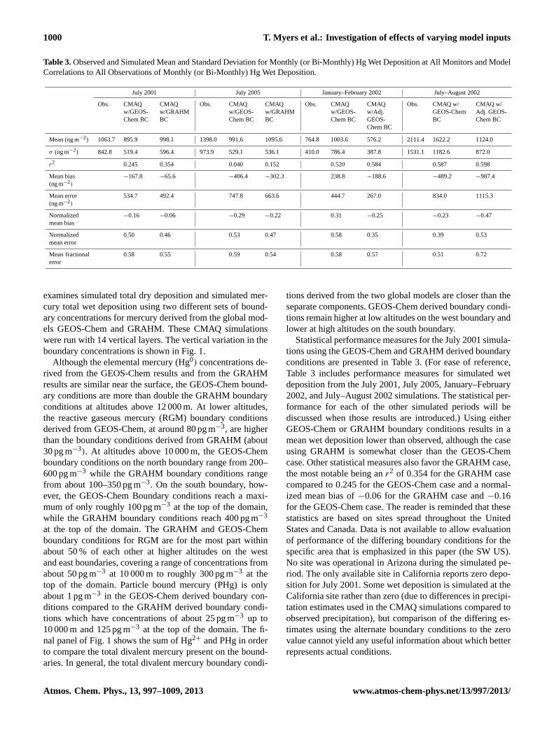
Table 3.Observed and Simulated Mean and Standard Deviation for Monthly (or Bi-Monthly) Hg Wet Deposition at All Monitors and ModelCorrelations to All Observations of Monthly (or Bi-Monthly) Hg Wet Deposition.

July 2001 July 2005 January–February 2002 July–August 2002

Obs. CMAQw/GEOS-Chem BC

CMAQw/GRAHMBC

Obs. CMAQw/GEOS-Chem BC

CMAQw/GRAHMBC

Obs. CMAQw/GEOS-Chem BC

CMAQw/Adj.GEOS-Chem BC

Obs. CMAQ w/GEOS-ChemBC

CMAQ w/Adj. GEOS-Chem BC

Mean (ng m−2) 1063.7 895.9 998.1 1398.0 991.6 1095.6 764.8 1003.6 576.2 2111.4 1622.2 1124.0

σ (ng m−2) 842.8 519.4 596.4 973.9 529.1 536.1 410.0 786.4 387.8 1531.1 1182.6 872.0

r2 0.245 0.354 0.040 0.152 0.520 0.584 0.587 0.598

Mean bias(ng m−2)

−167.8 −65.6 −406.4 −302.3 238.8 −188.6 −489.2 −987.4

Mean error(ng m−2)

534.7 492.4 747.8 663.6 444.7 267.0 834.0 1115.3

Normalizedmean bias

−0.16 −0.06 −0.29 −0.22 0.31 −0.25 −0.23 −0.47

Normalizedmean error

0.50 0.46 0.53 0.47 0.58 0.35 0.39 0.53

Mean fractionalerror

0.58 0.55 0.59 0.54 0.58 0.57 0.51 0.72

examines simulated total dry deposition and simulated mer-cury total wet deposition using two different sets of bound-ary concentrations for mercury derived from the global mod-els GEOS-Chem and GRAHM. These CMAQ simulationswere run with 14 vertical layers. The vertical variation in theboundary concentrations is shown in Fig. 1.

Although the elemental mercury (Hg0) concentrations de-rived from the GEOS-Chem results and from the GRAHMresults are similar near the surface, the GEOS-Chem bound-ary conditions are more than double the GRAHM boundaryconditions at altitudes above 12 000 m. At lower altitudes,the reactive gaseous mercury (RGM) boundary conditionsderived from GEOS-Chem, at around 80 pg m−3, are higherthan the boundary conditions derived from GRAHM (about30 pg m−3). At altitudes above 10 000 m, the GEOS-Chemboundary conditions on the north boundary range from 200–600 pg m−3 while the GRAHM boundary conditions rangefrom about 100–350 pg m−3. On the south boundary, how-ever, the GEOS-Chem Boundary conditions reach a maxi-mum of only roughly 100 pg m−3 at the top of the domain,while the GRAHM boundary conditions reach 400 pg m−3

at the top of the domain. The GRAHM and GEOS-Chemboundary conditions for RGM are for the most part withinabout 50 % of each other at higher altitudes on the westand east boundaries, covering a range of concentrations fromabout 50 pg m−3 at 10 000 m to roughly 300 pg m−3 at thetop of the domain. Particle bound mercury (PHg) is onlyabout 1 pg m−3 in the GEOS-Chem derived boundary con-ditions compared to the GRAHM derived boundary condi-tions which have concentrations of about 25 pg m−3 up to10 000 m and 125 pg m−3 at the top of the domain. The fi-nal panel of Fig. 1 shows the sum of Hg2+ and PHg in orderto compare the total divalent mercury present on the bound-aries. In general, the total divalent mercury boundary condi-

tions derived from the two global models are closer than theseparate components. GEOS-Chem derived boundary condi-tions remain higher at low altitudes on the west boundary andlower at high altitudes on the south boundary.

Statistical performance measures for the July 2001 simula-tions using the GEOS-Chem and GRAHM derived boundaryconditions are presented in Table 3. (For ease of reference,Table 3 includes performance measures for simulated wetdeposition from the July 2001, July 2005, January–February2002, and July–August 2002 simulations. The statistical per-formance for each of the other simulated periods will bediscussed when those results are introduced.) Using eitherGEOS-Chem or GRAHM boundary conditions results in amean wet deposition lower than observed, although the caseusing GRAHM is somewhat closer than the GEOS-Chemcase. Other statistical measures also favor the GRAHM case,the most notable being anr2 of 0.354 for the GRAHM casecompared to 0.245 for the GEOS-Chem case and a normal-ized mean bias of−0.06 for the GRAHM case and−0.16for the GEOS-Chem case. The reader is reminded that thesestatistics are based on sites spread throughout the UnitedStates and Canada. Data is not available to allow evaluationof performance of the differing boundary conditions for thespecific area that is emphasized in this paper (the SW US).No site was operational in Arizona during the simulated pe-riod. The only available site in California reports zero depo-sition for July 2001. Some wet deposition is simulated at theCalifornia site rather than zero (due to differences in precipi-tation estimates used in the CMAQ simulations compared toobserved precipitation), but comparison of the differing es-timates using the alternate boundary conditions to the zerovalue cannot yield any useful information about which betterrepresents actual conditions.

Atmos. Chem. Phys., 13, 997–1009, 2013 www.atmos-chem-phys.net/13/997/2013/

T. Myers et al.: Investigation of effects of varying model inputs 1001

 

 

 

0

2000

4000

6000

8000

10000

12000

14000

16000

18000

0.0 0.5 1.0 1.5 2.0 2.5

Hg0 conc. (ng/m3 @ STP)

Ht. (

m)

GRAHM West

Geos-Chem West

GRAHM East

Geos-Chem East

GRAHM South

Geos-Chem South

GRAHM North

Geos-Chem North

0

2000

4000

6000

8000

10000

12000

14000

16000

18000

0 100 200 300 400 500 600 700

RGM conc. (pg/m3 @ STP)

Ht.

(m)

GRAHM West

Geos-Chem West

GRAHM EastGeos-Chem East

GRAHM South

Geos-Chem SouthGRAHM North

Geos-Chem North

0.0 0.5 1.0 1.5 2.0

0

2000

4000

6000

8000

10000

12000

14000

16000

18000

0 25 50 75 100 125 150 175

GEOS-Chem PHg conc. (pg/m3 @ STP)

Ht.

(m)

GRAHM PHg conc. (pg/m3 @ STP)

GRAHM West

GRAHM East

GRAHM South

GRAHM North

Geos-Chem West

Geos-Chem East

Geos-Chem South

Geos-Chem North

 

 

 

0

2000

4000

6000

8000

10000

12000

14000

16000

18000

0.0 0.5 1.0 1.5 2.0 2.5

Hg0 conc. (ng/m3 @ STP)

Ht. (

m)

GRAHM West

Geos-Chem West

GRAHM East

Geos-Chem East

GRAHM South

Geos-Chem South

GRAHM North

Geos-Chem North

0

2000

4000

6000

8000

10000

12000

14000

16000

18000

0 100 200 300 400 500 600 700

RGM conc. (pg/m3 @ STP)

Ht.

(m)

GRAHM West

Geos-Chem West

GRAHM EastGeos-Chem East

GRAHM South

Geos-Chem SouthGRAHM North

Geos-Chem North

0.0 0.5 1.0 1.5 2.0

0

2000

4000

6000

8000

10000

12000

14000

16000

18000

0 25 50 75 100 125 150 175

GEOS-Chem PHg conc. (pg/m3 @ STP)

Ht.

(m)

GRAHM PHg conc. (pg/m3 @ STP)

GRAHM West

GRAHM East

GRAHM South

GRAHM North

Geos-Chem West

Geos-Chem East

Geos-Chem South

Geos-Chem North

 

 

 

0

2000

4000

6000

8000

10000

12000

14000

16000

18000

0.0 0.5 1.0 1.5 2.0 2.5

Hg0 conc. (ng/m3 @ STP)

Ht. (

m)

GRAHM West

Geos-Chem West

GRAHM East

Geos-Chem East

GRAHM South

Geos-Chem South

GRAHM North

Geos-Chem North

0

2000

4000

6000

8000

10000

12000

14000

16000

18000

0 100 200 300 400 500 600 700

RGM conc. (pg/m3 @ STP)

Ht.

(m)

GRAHM West

Geos-Chem West

GRAHM EastGeos-Chem East

GRAHM South

Geos-Chem SouthGRAHM North

Geos-Chem North

0.0 0.5 1.0 1.5 2.0

0

2000

4000

6000

8000

10000

12000

14000

16000

18000

0 25 50 75 100 125 150 175

GEOS-Chem PHg conc. (pg/m3 @ STP)

Ht.

(m)

GRAHM PHg conc. (pg/m3 @ STP)

GRAHM West

GRAHM East

GRAHM South

GRAHM North

Geos-Chem West

Geos-Chem East

Geos-Chem South

Geos-Chem North

 

0

2000

4000

6000

8000

10000

12000

14000

16000

18000

0 100 200 300 400 500 600 700

RGM+PHg conc. (pg/m3 @ STP)

Ht.

(m)

GRAHM West

Geos-Chem West

GRAHM East

Geos-Chem EastGRAHM South

Geos-Chem South

GRAHM North

Geos-Chem North

Fig. 1. Comparison of average vertical profiles of boundary conditions derived from the GEOS-Chem and GRAHM global models. (Notethat different scales are used for GEOS-Chem and GRAHM PHg concentrations.)

CMAQ with GEOS−Chem BCs , Max: 10.3 CMAQ with GRAHM BCs , Max: 12.3

CMAQ with GEOS−Chem BCs , Max: 8.8 CMAQ with GRAHM BCs , Max: 8.3

0 1.2 2.4 3.6 4.8 6

July Total Hg Wet Dep (µg m−2 month−1)

July Total Hg Dry Dep (µg m−2 month−1)

Fig. 2. CMAQ simulated mercury wet and dry deposition us-ing boundary conditions derived from GEOS-Chem and GRAHMglobal models, with 2001 meteorological inputs. Circles on wet de-position plots indicate locations of Mercury Deposition Networkwet deposition observations. Dry deposition includes only divalentforms of mercury.

Figure 2 demonstrates the substantially different esti-mates of mercury deposition that can result from thedifferent boundary conditions. In particular, dry deposi-tion in some parts of California and Nevada drops from4 µg m−2 month−1 using the GEOS-Chem boundary con-ditions to about 1.5 µg m−2 month−1 using the GRAHMboundary conditions. Simulated wet deposition of mercuryin some areas of Arizona is about 1.3 µg m−2 month−1 us-ing the GEOS-Chem boundary conditions but increases to1.5 µg m−2 month−1 using the GRAHM boundary condi-tions.

3.2 Adjusted GEOS-Chem boundary conditions

In this section, wet and dry mercury deposition simulated byCMAQ for January–February 2002 and July–August 2002are compared using boundary conditions based on (a) 2002GEOS-Chem global simulations and (b) the same GEOS-Chem simulations adjusted based on the results of a 2005CMAQ hemispheric simulation to keep the spatial and tem-poral dynamics and non-mercury species constant in theboundary conditions between the simulations. The frac-tion of divalent oxidized mercury, Hg2+, to total gaseousmercury, (Hg0 + Hg2+), was compared between the Aprilmonthly mean 2005 CMAQ hemispheric run, the GEOS-Chem boundary conditions, and measurements taken aloft

www.atmos-chem-phys.net/13/997/2013/ Atmos. Chem. Phys., 13, 997–1009, 2013

1002 T. Myers et al.: Investigation of effects of varying model inputsm

b

1000

800

600

400

200

West

1000

800

600

400

200

East

Hg2+ (Hg0 + Hg2+)

mb

0.0 0.1 0.2 0.3 0.4

1000

800

600

400

200

North

Hg2+ (Hg0 + Hg2+)0.0 0.1 0.2 0.3 0.4

1000

800

600

400

200

South

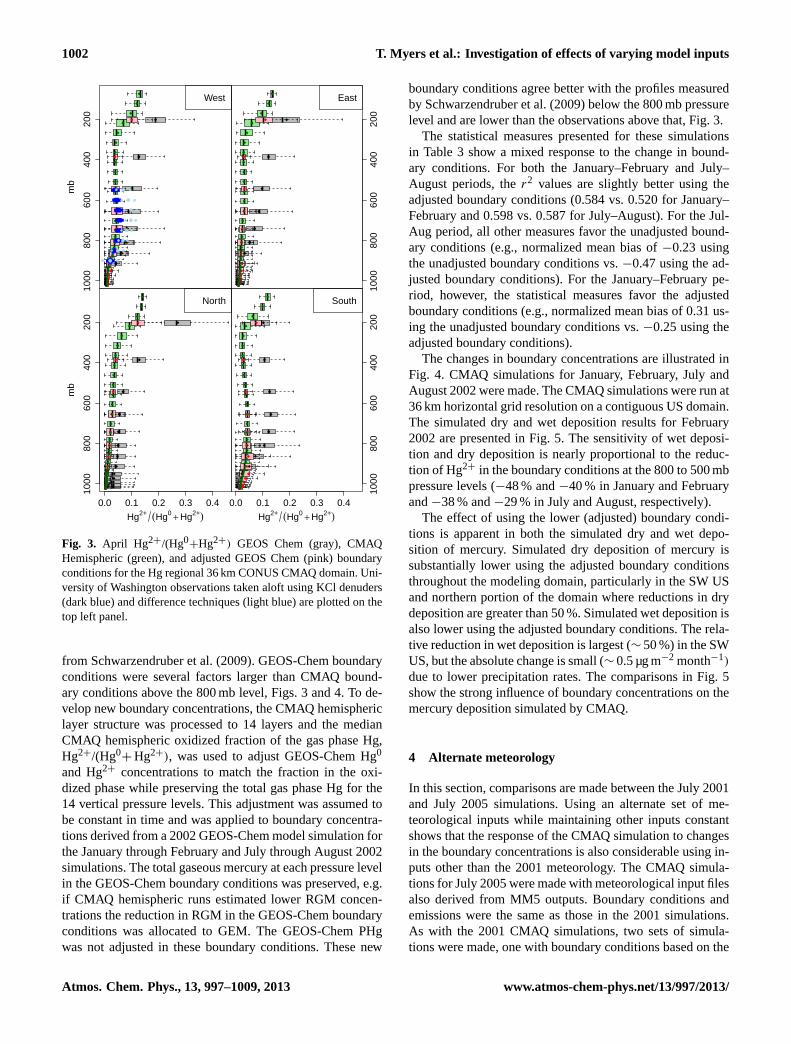
Fig. 3. April Hg2+/(Hg0+Hg2+) GEOS Chem (gray), CMAQ

Hemispheric (green), and adjusted GEOS Chem (pink) boundaryconditions for the Hg regional 36 km CONUS CMAQ domain. Uni-versity of Washington observations taken aloft using KCl denuders(dark blue) and difference techniques (light blue) are plotted on thetop left panel.

from Schwarzendruber et al. (2009). GEOS-Chem boundaryconditions were several factors larger than CMAQ bound-ary conditions above the 800 mb level, Figs. 3 and 4. To de-velop new boundary concentrations, the CMAQ hemisphericlayer structure was processed to 14 layers and the medianCMAQ hemispheric oxidized fraction of the gas phase Hg,Hg2+/(Hg0

+ Hg2+), was used to adjust GEOS-Chem Hg0

and Hg2+ concentrations to match the fraction in the oxi-dized phase while preserving the total gas phase Hg for the14 vertical pressure levels. This adjustment was assumed tobe constant in time and was applied to boundary concentra-tions derived from a 2002 GEOS-Chem model simulation forthe January through February and July through August 2002simulations. The total gaseous mercury at each pressure levelin the GEOS-Chem boundary conditions was preserved, e.g.if CMAQ hemispheric runs estimated lower RGM concen-trations the reduction in RGM in the GEOS-Chem boundaryconditions was allocated to GEM. The GEOS-Chem PHgwas not adjusted in these boundary conditions. These new

boundary conditions agree better with the profiles measuredby Schwarzendruber et al. (2009) below the 800 mb pressurelevel and are lower than the observations above that, Fig. 3.

The statistical measures presented for these simulationsin Table 3 show a mixed response to the change in bound-ary conditions. For both the January–February and July–August periods, ther2 values are slightly better using theadjusted boundary conditions (0.584 vs. 0.520 for January–February and 0.598 vs. 0.587 for July–August). For the Jul-Aug period, all other measures favor the unadjusted bound-ary conditions (e.g., normalized mean bias of−0.23 usingthe unadjusted boundary conditions vs.−0.47 using the ad-justed boundary conditions). For the January–February pe-riod, however, the statistical measures favor the adjustedboundary conditions (e.g., normalized mean bias of 0.31 us-ing the unadjusted boundary conditions vs.−0.25 using theadjusted boundary conditions).

The changes in boundary concentrations are illustrated inFig. 4. CMAQ simulations for January, February, July andAugust 2002 were made. The CMAQ simulations were run at36 km horizontal grid resolution on a contiguous US domain.The simulated dry and wet deposition results for February2002 are presented in Fig. 5. The sensitivity of wet deposi-tion and dry deposition is nearly proportional to the reduc-tion of Hg2+ in the boundary conditions at the 800 to 500 mbpressure levels (−48 % and−40 % in January and Februaryand−38 % and−29 % in July and August, respectively).

The effect of using the lower (adjusted) boundary condi-tions is apparent in both the simulated dry and wet depo-sition of mercury. Simulated dry deposition of mercury issubstantially lower using the adjusted boundary conditionsthroughout the modeling domain, particularly in the SW USand northern portion of the domain where reductions in drydeposition are greater than 50 %. Simulated wet deposition isalso lower using the adjusted boundary conditions. The rela-tive reduction in wet deposition is largest (∼ 50 %) in the SWUS, but the absolute change is small (∼ 0.5 µg m−2 month−1)

due to lower precipitation rates. The comparisons in Fig. 5show the strong influence of boundary concentrations on themercury deposition simulated by CMAQ.

4 Alternate meteorology

In this section, comparisons are made between the July 2001and July 2005 simulations. Using an alternate set of me-teorological inputs while maintaining other inputs constantshows that the response of the CMAQ simulation to changesin the boundary concentrations is also considerable using in-puts other than the 2001 meteorology. The CMAQ simula-tions for July 2005 were made with meteorological input filesalso derived from MM5 outputs. Boundary conditions andemissions were the same as those in the 2001 simulations.As with the 2001 CMAQ simulations, two sets of simula-tions were made, one with boundary conditions based on the

Atmos. Chem. Phys., 13, 997–1009, 2013 www.atmos-chem-phys.net/13/997/2013/

T. Myers et al.: Investigation of effects of varying model inputs 1003

Fig. 4.Hg2+ western boundary conditions from the GEOS-Chem and CMAQ hemispheric simulations for April 2005.

CMAQ with GEOS−Chem BCs , Max: 6.7 CMAQ with adjusted GEOS−Chem BCs , Max: 4.2

CMAQ with GEOS−Chem BCs , Max: 8.2 CMAQ with adjusted GEOS−Chem BCs , Max: 8.0

0 1.2 2.4 3.6 4.8 6

January February Total Hg Wet Dep (μg m−2 month−1)

January February Hg2+ & pHg Dry Dep (μg m−2 month−1)

Fig. 5a.Comparison of simulated dry and wet mercury depositionfor January–February 2002 from CMAQ runs using original GEOS-Chem based boundary conditions and adjusted boundary condi-tions. Circles on wet deposition plots indicate locations of MercuryDeposition Network wet deposition observations. Dry depositionincludes only divalent forms of mercury.

GEOS-Chem global model and the other with boundary con-ditions based on the GRAHM global model.

Statistical performance measures for the July 2005 simula-tions using the GEOS-Chem and GRAHM derived boundaryconditions are presented in Table 3. The simulated mean wetdeposition is lower than observed using either GEOS-Chemor GRAHM boundary conditions. The case using GRAHM issomewhat closer than the GEOS-Chem case, as was the casefor the July 2001 simulations. Other statistical measures areslightly in favor of the GRAHM case, the most notable beingan r2 of 0.152 for the GRAHM case compared to 0.040 forthe GEOS-Chem case. Data was again unavailable for a site

CMAQ with GEOS−Chem BCs , Max: 12.4 CMAQ with adjusted GEOS−Chem BCs , Max: 5.5

CMAQ with GEOS−Chem BCs , Max: 9.0 CMAQ with adjusted GEOS−Chem BCs , Max: 8.8

0 1.2 2.4 3.6 4.8 6

July − August Total Hg Wet Dep (μg m−2 month−1)

July − August Hg2+ & pHg Dry Dep (μg m−2 month−1)

Fig. 5b. Comparison of simulated dry and wet deposition for July–August 2002 from CMAQ runs using original GEOS-Chem basedboundary conditions and adjusted boundary conditions. Circles onwet deposition plots indicate locations of Mercury Deposition Net-work wet deposition observations. Dry deposition includes only di-valent forms of mercury.

in Arizona during this simulated period. Sites in Californiareported zero wet deposition for July 2005.

The wet and dry deposition of divalent mercury simulatedby CMAQ for the July 2005 time period using the GEOS-Chem and GRAHM derived boundary conditions are shownin Fig. 6. The simulated dry deposition of mercury using theJuly 2005 meteorological files was 50 to 100 % higher in theSW US than the simulated dry deposition of mercury us-ing the July 2001 meteorological files, with a greater differ-ence when the GEOS-Chem boundary conditions were used(compare to Fig. 2). Simulated wet deposition of mercuryshows large spatial variations between the two simulations

www.atmos-chem-phys.net/13/997/2013/ Atmos. Chem. Phys., 13, 997–1009, 2013

1004 T. Myers et al.: Investigation of effects of varying model inputs

CMAQ with GEOS−Chem BCs , Max: 6.8 CMAQ with GRAHM BCs , Max: 10.1

CMAQ with GEOS−Chem BCs , Max: 8.8 CMAQ with GRAHM BCs , Max: 8.1

0 1.2 2.4 3.6 4.8 6

July Total Hg Wet Dep (µg m−2 month−1)

July Total Hg Dry Dep (µg m−2 month−1)

Fig. 6. Simulated mercury deposition from CMAQ runs usingboundary conditions derived from GEOS-Chem and GRAHMglobal model simulations using 2005 meteorology.

using different meteorological inputs since wet deposition isdriven by the presence of rainfall. The response of the modelto the use of different boundary concentrations is similar us-ing the 2005 meteorology to the response using the 2001meteorology. Dry deposition of mercury in the SW US is50 % lower using the GRAHM based boundary conditionsregardless of whether 2001 or 2005 meteorology was used.The response in simulated dry deposition of mercury is morepronounced using the 2005 meteorology than the 2001 mete-orology. Although peak simulated wet deposition of mercurymay be higher or lower using either set of boundary condi-tions, in general the wet deposition of mercury is lower overthe contiguous US using the GRAHM boundary conditionscompared to GEOS-Chem boundary conditions. This is mostnoticeable in the Southeast (SE) US where simulated wet de-position is lower by about 50 % using the GRAHM bound-ary conditions compared to using the GEOS-Chem boundaryconditions, while in the SW US the difference is consistentlyless than 50 %.

5 Effect of high altitude mercury boundaryconcentrations

In order to assess the effects of the high altitude boundaryconcentrations on mercury deposition, boundary concentra-tions of all mercury species were zeroed out in the top twolayers (i.e. layers 13 and 14) which corresponds to a heightof approximately 5400 m and above. These simulations weremade with the GEOS-Chem boundary conditions using boththe 2001 and 2005 meteorology.

CMAQ w/ GEOS−Chem BCs 2001, Max: 7.7 CMAQ w/ GEOS−Chem BCs 2005, Max: 5.8

CMAQ w/ GEOS−Chem BCs 2001, Max: 8.6 CMAQ w/ GEOS−Chem BCs 2005, Max: 8.6

0 1.2 2.4 3.6 4.8 6

July Total Hg Wet Dep (µg m−2 month−1)

July Total Hg Dry Dep (µg m−2 month−1)

Fig. 7. Simulated mercury deposition from CMAQ runs usingboundary conditions derived from a GEOS-Chem simulation withthe upper layer mercury concentrations zeroed out using 2001 and2005 meteorology.

The simulated deposition in Fig. 7 can be compared di-rectly to Figs. 2 and 6. Note that both wet deposition and drydeposition are reduced in both meteorological years. In theSW US, the model estimates substantially lower depositionof mercury when the upper layers of the boundary concentra-tions are set to zero for all mercury species. To see the influ-ence of the upper layer mercury on deposition more clearly,the differences between the simulations with and withoutthe upper layer mercury boundary conditions were calcu-lated and expressed as a percent contribution from the upperlayer boundary conditions to deposition (Fig. 8).The stronginfluence of the higher altitude mercury boundary concentra-tions on the simulated deposition of mercury is clear fromthis figure. From 20 to 80 % of the simulated dry depositionof mercury in the SW US originated from the upper layersof the boundary conditions. The influence of the upper layerboundary conditions on simulated wet deposition of mercuryis even greater than for dry deposition. Over most of the SWUS, more than 80 % of the simulated wet deposition of mer-cury originates from the upper layer boundary conditions.Unlike other species that typically have low concentrationsat higher altitude, relatively high concentrations of mercuryat higher altitudes must be considered when setting boundaryconcentrations for CMAQ model simulations. Since these es-timates of influence of upper level boundary concentrationsare derived using exclusively the CMAQ model and its asso-ciated databases, studies using different models or observa-tional techniques could come to different conclusions.

Atmos. Chem. Phys., 13, 997–1009, 2013 www.atmos-chem-phys.net/13/997/2013/

T. Myers et al.: Investigation of effects of varying model inputs 1005.

Fig. 8. Simulated percent contribution of mercury originating from boundary concentrations above 5400 m for dry and wet mercury deposi-tion using both 2001 and 2005 meteorology.

6 Tracers showing upper tropospheric impact onsurface concentrations

In order to assess whether the contributions of high altitudeboundary concentrations to mercury deposition are primar-ily due to high mercury levels in the upper atmosphere ortransport from the upper layers to lower layers, simulationswere conducted with unit concentration tracers along each ofthe domain boundaries, broken down by model layer. Thesesimulations were conducted for the month of July using both2001 and 2005 meteorology.

Preparation of the tracer simulations involved a minormodification to the CMAQ 4.7.1 code and preparation ofinitial and boundary concentration files that included tracerconcentrations. The CMAQ “trac0” header files, such as“TR SPC.EXT”, are supplied in the release version of themodel with zero tracers. These files were modified to in-clude 26 tracers with names such as “TRAC1”, “TRAC2”,and so forth. These tracers were assigned to boundaries, ini-tial concentrations and layers as shown in Table 4. For exam-ple, therefore, “TRAC12” was assigned unit concentration in

layers 3 through 6 on the north boundary, and zero concen-tration elsewhere, including in the initial concentration file.

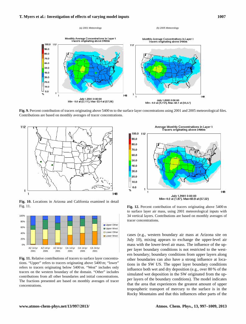
The spatial pattern of the contributions of the upper lay-ers to surface layer is similar for both sets of meteorologi-cal inputs (see Fig. 9), although the peak contribution fromthe upper layers is higher using the 2005 meteorology. Thegreater simulated dry deposition of mercury using the 2005meteorology appears to be at least in part a result of greaterinfluence of the upper layer boundaries on the surface layer.The spatial patterns suggest, and the conclusion is confirmedby examining animations of tracer concentrations, that thelargest contribution to the lower layers from the upper layersoccurs over the Rocky Mountains, which then spreads out toinfluence other parts of the domain.

At two locations in the domain, one in Arizona (grid cell(44, 45)) and one in California (grid cell (24, 51)), the in-fluence of the upper layer boundaries was examined in moredetail. These locations were chosen to represent areas in theSW US that are strongly impacted by upper layer boundaryconditions of mercury. The green symbols in Fig. 10 showthe locations subject to this more detailed examination. A

www.atmos-chem-phys.net/13/997/2013/ Atmos. Chem. Phys., 13, 997–1009, 2013

1006 T. Myers et al.: Investigation of effects of varying model inputs

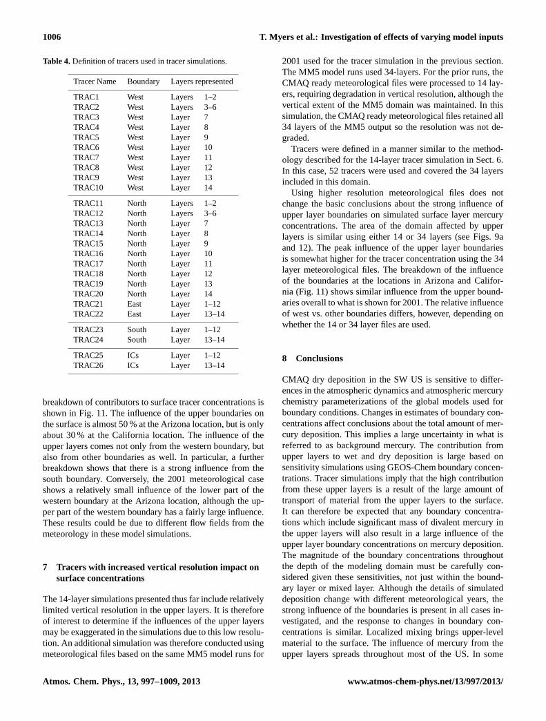
Table 4.Definition of tracers used in tracer simulations.

Tracer Name Boundary Layers represented

TRAC1 West Layers 1–2TRAC2 West Layers 3–6TRAC3 West Layer 7TRAC4 West Layer 8TRAC5 West Layer 9TRAC6 West Layer 10TRAC7 West Layer 11TRAC8 West Layer 12TRAC9 West Layer 13TRAC10 West Layer 14

TRAC11 North Layers 1–2TRAC12 North Layers 3–6TRAC13 North Layer 7TRAC14 North Layer 8TRAC15 North Layer 9TRAC16 North Layer 10TRAC17 North Layer 11TRAC18 North Layer 12TRAC19 North Layer 13TRAC20 North Layer 14TRAC21 East Layer 1–12TRAC22 East Layer 13–14

TRAC23 South Layer 1–12TRAC24 South Layer 13–14

TRAC25 ICs Layer 1–12TRAC26 ICs Layer 13–14

breakdown of contributors to surface tracer concentrations isshown in Fig. 11. The influence of the upper boundaries onthe surface is almost 50 % at the Arizona location, but is onlyabout 30 % at the California location. The influence of theupper layers comes not only from the western boundary, butalso from other boundaries as well. In particular, a furtherbreakdown shows that there is a strong influence from thesouth boundary. Conversely, the 2001 meteorological caseshows a relatively small influence of the lower part of thewestern boundary at the Arizona location, although the up-per part of the western boundary has a fairly large influence.These results could be due to different flow fields from themeteorology in these model simulations.

7 Tracers with increased vertical resolution impact onsurface concentrations

The 14-layer simulations presented thus far include relativelylimited vertical resolution in the upper layers. It is thereforeof interest to determine if the influences of the upper layersmay be exaggerated in the simulations due to this low resolu-tion. An additional simulation was therefore conducted usingmeteorological files based on the same MM5 model runs for

2001 used for the tracer simulation in the previous section.The MM5 model runs used 34-layers. For the prior runs, theCMAQ ready meteorological files were processed to 14 lay-ers, requiring degradation in vertical resolution, although thevertical extent of the MM5 domain was maintained. In thissimulation, the CMAQ ready meteorological files retained all34 layers of the MM5 output so the resolution was not de-graded.

Tracers were defined in a manner similar to the method-ology described for the 14-layer tracer simulation in Sect. 6.In this case, 52 tracers were used and covered the 34 layersincluded in this domain.

Using higher resolution meteorological files does notchange the basic conclusions about the strong influence ofupper layer boundaries on simulated surface layer mercuryconcentrations. The area of the domain affected by upperlayers is similar using either 14 or 34 layers (see Figs. 9aand 12). The peak influence of the upper layer boundariesis somewhat higher for the tracer concentration using the 34layer meteorological files. The breakdown of the influenceof the boundaries at the locations in Arizona and Califor-nia (Fig. 11) shows similar influence from the upper bound-aries overall to what is shown for 2001. The relative influenceof west vs. other boundaries differs, however, depending onwhether the 14 or 34 layer files are used.

8 Conclusions

CMAQ dry deposition in the SW US is sensitive to differ-ences in the atmospheric dynamics and atmospheric mercurychemistry parameterizations of the global models used forboundary conditions. Changes in estimates of boundary con-centrations affect conclusions about the total amount of mer-cury deposition. This implies a large uncertainty in what isreferred to as background mercury. The contribution fromupper layers to wet and dry deposition is large based onsensitivity simulations using GEOS-Chem boundary concen-trations. Tracer simulations imply that the high contributionfrom these upper layers is a result of the large amount oftransport of material from the upper layers to the surface.It can therefore be expected that any boundary concentra-tions which include significant mass of divalent mercury inthe upper layers will also result in a large influence of theupper layer boundary concentrations on mercury deposition.The magnitude of the boundary concentrations throughoutthe depth of the modeling domain must be carefully con-sidered given these sensitivities, not just within the bound-ary layer or mixed layer. Although the details of simulateddeposition change with different meteorological years, thestrong influence of the boundaries is present in all cases in-vestigated, and the response to changes in boundary con-centrations is similar. Localized mixing brings upper-levelmaterial to the surface. The influence of mercury from theupper layers spreads throughout most of the US. In some

Atmos. Chem. Phys., 13, 997–1009, 2013 www.atmos-chem-phys.net/13/997/2013/

T. Myers et al.: Investigation of effects of varying model inputs 1007

(a) 2001 Meteorology (b) 2005 Meteorology

 Fig. 9.Percent contribution of tracers originating above 5400 m to the surface layer concentrations using 2001 and 2005 meteorological files.Contributions are based on monthly averages of tracer concentrations.

Fig. 10. Locations in Arizona and California examined in detailFig. 11.

 

 

0%

20%

40%

60%

80%

100%

AZ 14-lyr2001

AZ 14-lyr2005

AZ 34-lyr2001

CA 14-lyr2001

CA 14-lyr2005

CA 34-lyr2001

Upper OtherUpper WestLower OtherLower West

Fig. 11.Relative contributions of tracers to surface layer concentra-tions. “Upper” refers to tracers originating above 5400 m; “lower”refers to tracers originating below 5400 m. “West” includes onlytracers on the western boundary of the domain. “Other” includescontributions from all other boundaries and initial concentrations.The fractions presented are based on monthly averages of tracerconcentrations.

Fig. 12. Percent contribution of tracers originating above 5400 mto surface layer air mass, using 2001 meteorological inputs with34 vertical layers. Contributions are based on monthly averages oftracer concentrations.

cases (e.g., western boundary air mass at Arizona site onJuly 10), mixing appears to exchange the upper-level airmass with the lower-level air mass. The influence of the up-per layer boundary conditions is not restricted to the west-ern boundary; boundary conditions from upper layers alongother boundaries can also have a strong influence at loca-tions in the SW US. The upper layer boundary conditionsinfluence both wet and dry deposition (e.g., over 80 % of thesimulated wet deposition in the SW originated from the up-per layers of the boundary conditions). The model indicatesthat the area that experiences the greatest amount of uppertropospheric transport of mercury to the surface is in theRocky Mountains and that this influences other parts of the

www.atmos-chem-phys.net/13/997/2013/ Atmos. Chem. Phys., 13, 997–1009, 2013

1008 T. Myers et al.: Investigation of effects of varying model inputs

domain. Elevated levels of Hg2+ have been observed at highaltitude monitoring sites and attributed to deep troposphericmixing (Faın et al., 2009) in agreement with these modeledresults. Increasing the vertical resolution of the input fieldsused for the CMAQ modeling does not reduce the influenceof the upper layer boundary concentrations on the surface airmass in the SW US, although the simulation of the tracersis altered somewhat by the use of higher vertical resolution.The influence of boundary concentrations of Hg on ambientsurface concentrations and subsequently dry deposition fromHg in the free troposphere in CMAQ is in agreement withthe measurements of Lyman and Gustin (2009) and Weiss-Penzias et al. (2009) and with the modeling results of Amoset al. (2012). If free tropospheric Hg(II) concentrations weretoo high in the boundary conditions, the entrainment of thisair in the model might partially explain the recently docu-mented discrepancies between modeled and observed speci-ated mercury concentrations at the surface (Baker and Bash,2012).

Supplementary material related to this article isavailable online at:http://www.atmos-chem-phys.net/13/997/2013/acp-13-997-2013-supplement.zip.

Acknowledgements.Financial support for the modeling conductedin this study was provided by the Office of Water, US Environ-mental Protection Agency and by the National Exposure ResearchLaboratory, US Environmental Protection Agency.

Disclaimer.Although this work was reviewed by EPA and approvedfor publication, it may not necessarily reflect official Agency policy.

Edited by: A. Dastoor

References

Amos, H. M., Jacob, D. J., Holmes, C. D., Fisher, J. A., Wang,Q., Yantosca, R. M., Corbitt, E. S., Galarneau, E., Rutter, A. P.,Gustin, M. S., Steffen, A., Schauer, J. J., Graydon, J. A., Louis,V. L. St., Talbot, R. W., Edgerton, E. S., Zhang, Y., and Sunder-land, E. M.: Gas-particle partitioning of atmospheric Hg(II) andits effect on global mercury deposition, Atmos. Chem. Phys., 12,591–603,doi:10.5194/acp-12-591-2012, 2012.

Ariya, P., Dastoor, A., Amyot, M., Schroeder, W., Barrie, L., An-lauf, K., Raofie, F., Ryzhkov, A., Davignon, D., Lalonde, J., andSteffen, A.: Arctic: A sink for mercury, Tellus, 56B, 397–403,2004.

Baker, K. and Bash, J.: Regional scale photochemical model evalu-ation of total mercury wet deposition and speciated ambient mer-cury, Atmos. Environ., 49, 151–162, 2012.

Bash, J. O.: Description and initial simulation of a dynamic bidi-rectional air-surface exchange model for mercury in CommunityMultiscale Air Quality (CMAQ) model, J. Geophys. Res., 115,D06305,doi:10.1029/2009JD012834, 2010.

Bey, I., Jacob, D., Yantosca, R., Logan, J., Field, D., Fiore, A., Li,Q., Liu, H., Mickley, L., and Schultz, M.: Global modeling oftropospheric chemistry with assimilated meteorology: Model de-scription and evaluation, J. Geophys. Res., 106, 23073–23095,2001.

Bullock Jr., O. and Brehme, K. A.: Atmospheric mercury simulationusing the CMAQ model: Formulation description and analysis ofwet deposition results, Atmos. Environ., 36, 2135–2146, 2002.

Bullock Jr., O., Atkinson, D., Braverman, T., Civerolo, K., Das-toor, A., Davignon, D., Ku, J., Lohman, K., Myers, T., Park, R.,Seigneur, C., Selin, N., Sistla, G., and Vijayaraghavan, K.: TheNorth American Mercury Model Intercomparison Study (NAM-MIS): Study description and model-to-model comparisons, J.Geophys. Res., 113, D17310,doi:10.1029/2008JD009803, 2008.

Bullock Jr., O., Atkinson, D., Braverman, T., Civerolo, K., Das-toor, A., Davignon, D., Ku, J.-Y., Lohman, K., Myers, T.,Park, R., Seigneur, C., Selin, N., Sistla, G., and Vijayaragha-van, K.: An Analysis of Simulated Wet Deposition of Mer-cury from the North American Mercury Model Intercom-parison Study (NAMMIS), J. Geophys. Res., 114, D08301,doi:10.1029/2008JD011224, 2009.

Dastoor, A. and Larocque, Y.: Global circulation of atmosphericmercury: A modeling study, Atmos. Environ., 38, 147–161,2004.

EPA: Technical support document for the final Clean Air Mer-cury Rule: Air quality modeling, EPA Office of Air Qual-ity Planning and Standards, Research Triangle Park, NorthCarolina, available at:http://www.epa.gov/ttn/atw/utility/aqmoar-2002-0056-6130.pdf, 2005a.

EPA: Emissions Inventory and Emissions Processing for the CleanAir Mercury Rule (CAMR), EPA OAQPS, available at:http://www.epa.gov/ttn/atw/utility/emissinv oar-2002-0056-6129.pdf, 2005b.

EPA: Meteorological Modeling Performance Evaluation for the An-nual 2005 Continental US 36-km Domain Simulation, EPA Of-fice of Air Quality Planning and Standards (OAQPS), 2009.

Faın, X., Obrist, D., Hallar, A. G., Mccubbin, I., and Rahn, T.:High levels of reactive gaseous mercury observed at a high eleva-tion research laboratory in the Rocky Mountains, Atmos. Chem.Phys., 9, 8049–8060,doi:10.5194/acp-9-8049-2009, 2009.

Foley, K. M., Roselle, S. J., Appel, K. W., Bhave, P. V., Pleim, J.E., Otte, T. L., Mathur, R., Sarwar, G., Young, J. O., Gilliam,R. C., Nolte, C. G., Kelly, J. T., Gilliland, A. B., and Bash, J.O.: Incremental testing of the Community Multiscale Air Quality(CMAQ) modeling system version 4.7, Geosci. Model Dev., 3,205–226,doi:10.5194/gmd-3-205-2010, 2010.

Grell, G., Dudhia, A., and Stauffer, D.: A description of the Fifth-Generation PennState/NCAR Mesoscale Model (MM5), NCARTechnical Note NCAR/TN-398+STR, available at:http://www.mmm.ucar.edu/mm5/doc1.html, 1994.

Hynes, A. J., Donohoue, D. L., Goodsite, M. E., and Hedgecock,I. M.: Our current understanding of major chemical and physicalprocesses affectinf mercury dynamics in the atmosphere and atthe air-water/terrestrial interfaces, in: Mercury Fate and Trans-port in the Global Atmosphere, editd by: Pirrone, N. and Mason,R., Springer, New York, 427–457, 2009.

Lyman, S. and Gustin, M. S.: Determinants of Atmospheric Mer-cury Concentrations in Reno, Nevada, USA, Sci. Total. Environ.,408, 431–438, 2009.

Atmos. Chem. Phys., 13, 997–1009, 2013 www.atmos-chem-phys.net/13/997/2013/

T. Myers et al.: Investigation of effects of varying model inputs 1009

Otte, T., Pouliot, G., Pleim, J., Young, J., Schere, K., Wong, D., Lee,P., Tsidulko, M., McQueen, J., Davidson, P., Mathur, R., Chuang,H., DiMego, G., and Seaman, N.: Linking the Eta model with theCommunity Multiscale Air Quality (CMAQ) modeling system tobuild a national air quality forecasting system, Weather Forecast.,20, 367–384, 2005.

Pongprueksa, P., Lin, C. J., Lindberg, S. E., Jang, C., Braverman,T., Bullock, O. R., Ho, T. C., and Chu, H. W.: Scientific uncer-tainties in atmospheric mercury models III: Boundary and initialconditions, model grid resolution, and Hg(II) reduction mecha-nism, Atmos. Environ., 42, 1828–1845, 2008.

Schere, K., Flemming, J., Vautard, R., Chemel, C., Colette, A.,Hogrefe, C., Bessagnet, B., Meleux, F., Mathur, R., Roselle, S.,Hu, R., Sokhi, R., Rao, S., and Galmarini, S.: Trace gas/aerosolboundary concentrations and their impacts on continental-scaleAQMEII modeling domains, Atmos. Environ., 53, 38–50, 2011.

Selin, N., Jacob, D., Park, R., Yantosca, R., Strode, S., Jaegle, L.,and Jaffe, D.: Chemical cycling and deposition of atmosphericmercury: Global constraints from observations, J. Geophys. Res.,112, D02308,doi:10.1029/2006JD007450, 2007.

Sommar, J., Hallquist, M., Ljungstrom, and Lindqvist, O.: On thegas phase reactions between volatile biogenic mercury speciesand the nitrate radical, J. Atmos. Chem., 27, 233–247, 1997.

Subir, M., Ariya, P. A., and Dastoor, A. P.: A review of uncertain-ties in atmospheric modeling of mercury chemistry I. Uncertain-ties in existing kinetic parameters – Fundamental limitations andthe importance of heterogeneous chemistry, Atmos. Environ., 45,5664–5676, 2011.

Swartzendruber, P., Jaffe, D., and Finley, B.: Development and firstresults of an aircraft-based, high time resolution technique forgaseous elemental and reactive (oxidized) gaseous mercury, En-viron. Sci. Technol., 43, 7484–7489, 2009.

Vermette, S., Lindberg, S., and Bloom, N.: Field Tests for a Re-gional Mercury Deposition Network – Sampling Design and pre-liminary Test Results, Atmos. Environ., 29, 1247–1251, 1995.

Weiss-Penzias, S., Gustin, M. S., and Lyman, S. N.: Observations ofspeciated atmospheric mercury at three sites in Nevada, USA: ev-idence for a free tropospheric source of reactive gaseous mercury,J. Geophys. Res., 114, D14302,doi:10.1029/2008JD011607,2009.

www.atmos-chem-phys.net/13/997/2013/ Atmos. Chem. Phys., 13, 997–1009, 2013