Investigation of an acoustooptic tunable filter

Laboratory exercise Author: Attila Barócsi

2017

Content 1. Introduction............................................................................................................ 2

2. Basic concepts of acousto-optics.......................................................................... 2

3. Acoustooptic tunable filter ................................................................................... 7

4. Measurement problems ........................................................................................ 9

4.1. Setup and qualitative investigation of the AOTF .............................. 9

4.2. AOTF measurements using lasers ..................................................... 12

4.3. Spectral measurements with the solid state spectrometer (demonstration only) ........................................................................... 13

5. References ............................................................................................................. 14

2

1. Introduction Acousto-optics in the scientific literature will definitely refer to the more than 50 years of technological progress initiated by the development of the laser in 1960. It became obvious that utilizing the acousto-optic (AO) effect provides an elegant way for influencing photons by altering the refractive index of the medium in which the light propagates.

The story begun in 1922 when L. Brillouin was investigating the properties of acoustic waves induced thermally in liquids and solids [1]. According to his model, the acoustic fluctuations yielded a periodic change of the density of the propagation medium resulting in an alteration of the dielectric permittivity. If so, this change could be determined from the scattering pattern of a light wave with appropriately short wavelength. Brilluein himself proposed the analogy between this scattering phenomenon and the diffraction of light from periodic structures (studied by W. H. Bragg and W. L. Bragg in the 1910s). Thus, the incidence angle of the light beam must be chosen so as to obtain constructive interference. A principal difference, he argued, was that an acoustic wave created a sinusoidal grating that allowed only two (±1) diffraction orders and the corresponding critical angles. Later, this phenomenon was termed Bragg diffraction. There is another distinction from an optical grating: the acoustic grating propagates with the speed of sound, hence the frequency of light is Doppler shifted by the acoustic frequency with opposite signs for the two orders.

There was 10 more years passed till the experiments were realized by P. Debye and F. W. Sears, as well as R. Lucas and P. Biquard demonstrating the AO effect by ultrasonic waves in liquids and solids [2, 3]. The results were, however, surprisingly different from Brilluein’s predictions: the critical angles could not be demonstrated and, for intense acoustic field, more than two orders appeared due to the small interaction volume as Debye and Sears realized. The finding is worth emphasizing that constructive interference can be maintained in a wide angular range: this fact allows for a finite interaction bandwidth being one of the most important parameters in terms of practical application of AO devices.

Although the AO effect was nicely formulated analytically later verified by a few experiments, not until the ‘laser era’ its practical application advanced. Then a boom in applied acousto-optics initiated from the various light controlling AO devices, such as traveling and standing wave modulators [4] and switches [5], single or multi-dimensional deflectors [6], tunable filters [7] and frequency shifters [8] to the sophisticated AO signal processing systems such as a real time power spectrum analyzer9, direction of arrival processor [10], or 3-dimensional (3D) AO light steering in multi-photon microscopy [11]. This progress seemed to cease by the spreading of laser diodes allowing a direct fast modulation of light. However, it has again been boosted by the utilization of the AO effect in the dispersion control and shaping of ultrafast laser beams [12].

The research and development of AO devices, systems and technology as well as the accompanying training of acousto-optics at different levels of the education have a long-term tradition at the Department of Atomic Physics dating back to the 1980s. The training starts at BSc level of higher education in physics and continues at MSc then PhD levels offering research activities in the topic [13, 14].

2. Basic concepts of acousto-optics The AO effect is induced in such materials possessing of large photoelastic effect, that is the change of refractive index is large due to the sound vibration (elastic displacement of atoms or molecules): Such materials are often artificial single crystals (e.g. TeO2, LiNbO3, PbMnO4, CaMoO4), or glasses (such as fused silica).

3

Due to the photoelastic effect, propagation of an acoustic wave in a medium induces a periodic change of its refractive index yielding a phase grating that travels at a speed of the acoustic wave in the medium. The gratings constant equals to the acoustic wavelength aλ , whereas the magnitude of the grating is proportional to the acoustic amplitude 0S and the magnitude p of the photoelastic effect. According to Figure 1a, consider an acoustic plane wave with wave vector xxk )/2( aaa k λπ== and angular frequency aω that propagates in the xx x= direction of the xz plane

)cos(),( 0 xktStxs aa −= ω , (1)

and an optical plane wave with 0k and 0ω propagating in the direction characterized by the internal angle 0θ from the x axis. Propagation of the optical beam in the medium is given by the wave equation

2

2

2

22 ),(),(),(

tt

ctxnt

∂∂

=∇rErE , (2)

where c is the speed of light in vacuum and ),( txn is the refractive index of the medium (Figure 1b), approximated as

2

),cos(),(21),( 0

33 Spnnxktnntxspnntxn aa =−−=−= δωδ (3)

with effective index n for small nδ magnitude of the index change. As the electromagnetic field is periodic, it can be decomposed into a Fourier-series [15]. Putting the Fourier decomposition into the wave equation and omitting higher order components, for scalar, slowly varying field, i.e.

|)(|/ zEkdzdE mm υ<< , yields

mBa

mmm EmkjEEnk

dzdE )sin(sin

cos)(

cos2 00

110

θθθθ

δυ −−=−+ −+ (4)

for the )(zEE mm = amplitude of order ,...}2,1,0{ ±±=m with wave number υυ λπ /2=k in vacuum and the Bragg angle

02

sink

kaB =θ (5)

ensuring constructive interference. Equation (5) can be generalized by applying the conservation of momentum for the interaction in terms of the wave vector matching (Figure 1c),

mam kkk =+0 , (6)

whereas the energy is conserved through the frequency condition of

mam ωωω =+0 . (7)

Although the derivation of the so called coupled wave equation (4) being fundamental in the quantitative description of the AO effect goes beyond the level of the laboratory exercise, its visual interpretation is well fit into the scalar diffraction theory using Fourier decomposition (Figure 1d). This aspect also explains the term Bragg diffraction occurring from thick volume grating as opposed to a thin grating producing many diffraction orders. In general, higher orders may exist if the term in Equation (5) is small as demonstrated experimentally in Figure 2c. We recall also on the basis of the scalar diffraction theory that the full width divergence aδθ and angular spectrum )( aS θ of a rectangular sound column with length L is approximated as

a

aa

aa SS

L δθπθθλδθ sinc)(, 0=≈ . (8)

4

From Equation (5) and the so called wave-vector diagram of Figure 1c, we know that the diffracted orders are separated by aB λλθ /sin2 0= , so the condition

aa

Ba nλλ

λλθθδθ υ==≈∆>> 0

0 2 (9)

ensures the appearance of higher orders, as depicted in Figures 2a–b.

Figure 1. Geometry of the AO interaction (a) with the refractive index change (b) and the wave vector matching for m = 1 at the Bragg condition (c). Association can also be made to the scalar diffraction model (d) that applies field decomposition into plane waves at an aperture with complex transmittance function τ (r).

Figure 2. The effect of the acoustic divergence (a) on the appearance of higher diffraction orders (b). Demonstration of many AO diffraction orders (c).

Upon changing the incidence angle of light, the relative intensities of orders change as in case of a regular phase grating. Using white illumination (lamp or white LED), the wavelengths (colors) will separate in the diffracted orders and will propagate in different directions: each order will be rainbow colored and spatially spread. In practice, Bragg diffraction is used with a thick sound column along the direction of light propagation that can be considered as a superposition of many gratings. The subsequent elementary gratings cancel each other along most of the angular directions, except for the vicinity of a given incidence referred to as the Bragg angle. This direction corresponds to the superposition of all elementary gratings yielding only the first (+1 or –1) order that can ideally contain ~100% of the zeroth order. If the frequency of the sound is changed so does the gratings constant resulting in the change of the direction and color of the diffracted orders. If only the first order is present, its output angle and color will change.

The theory of the AO effect can be introduced in a far simpler way by integrating the elementary dr complex amplitude reflectance coefficients upon planar layers separated by dx distance along the x direction (Figure 1a) to get the total amplitude reflectance [16]

dxdn

dndr

dxdrdx

dxdrr xk == ∫

−

,e2/

2/

sin2j 00

θ . (10)

5

The first derivative dndr / of the local change of amplitude reflectance dxdr / can be obtained from the Fresnel equations whereas the second term is calculated from Equation (3). This approach explains the term Bragg reflection.

As a basic experiment, the AO interaction geometry can be studied according to Figure 1a together with the visualization of the diffraction orders. Given the refractive index of the AO cell made of TeO2, the sound velocity aυ can be calculated from the external refraction geometry measured at the Bragg condition of Figure 1c. Also, as a practical application of the AO cell, the light deflector concept (Figure 3a) can be introduced by measuring the deflection angle Θ defined as the total external angle between the 1st and 0th order beam. Using Snells’s law

a

a

a

fnΘυ

λλλθ υυ

2arcsin2

2arcsin2)sinarcsin(2 0 === . (11)

For small angles, Equation (11) simplifies to a linear )( afΘ relationship versus acoustic frequency af .

Using a photodetector and a microvolt-meter or oscilloscope, the intensities of the diffracted orders can be determined. At the Bragg condition, the dη diffraction efficiency is defined as the ratio of the intensity of the 1st order beam to that of the 0th order one being equal to the peak reflectance that can be obtained upon evaluating Equation (10):

LHPSIr

II aa

aBd ===≡2

~|)(|20

32

0

1 rυθη . (12)

At low acoustic field intensities, the efficiency is proportional to the acoustic intensity aI with r being the density of the medium or, more conveniently, to the acoustic power LHIP aa = with L and H being the interaction length defined in Figure 1a and the width of the sound column, respectively. Idealizing that the acoustic power equals to the input electric power, ina PP ≈ , the linear )( ad Pη relationship can be measured.

Figure 3. The AO cell operated as a light deflector (a) and light modulator (b) with characteristic input and output signals. Insets of (a) show the ∆Θ scanning range and the τD transit time of the deflector. Inset of (b) shows τD for the modulator.

As the RF drive power of the AO cell increases, the linear )( ad Pη relationship will not hold. A more precise analysis (in which depletion of the incident beam is also considered) reveals the following expression:

)(sin)( 2aad PCP =η , (13)

where all material and geometric parameters are embedded in constant C . This diffraction efficiency function can also be measured versus RF driving power and will depict a curve similar to that of Figure 4. Equation (13) can be regarded as the modulation transfer function of the AO cell when

6

considered as a light intensity modulator. Amplitude modulation (AM) of an input electric signal is the simplest mode that can be realized by means of an AO modulator (Figure 3b).

The AM modulated input electric signal can be described as

)2cos()]2cos(1[)2cos()()( 0 tftfUtftutu aAMAMaAMin ππδπ +== (14)

with modulation amplitude )(tuAM , modulation frequency AMf and the parameter AMδ defined as the modulation depth. Figure 5 depicts a series of calculated electric )(tuAM to diffracted intensity

)(1 tI curves at different AMδ values with the corresponding measured oscillograms. The modulated

acoustic power, proportional to the squared modulated amplitude )(~)( 2 tutP AMAM , is also plotted. From these measurements, the low distortion region at 1<AMδ and the high distortion region at

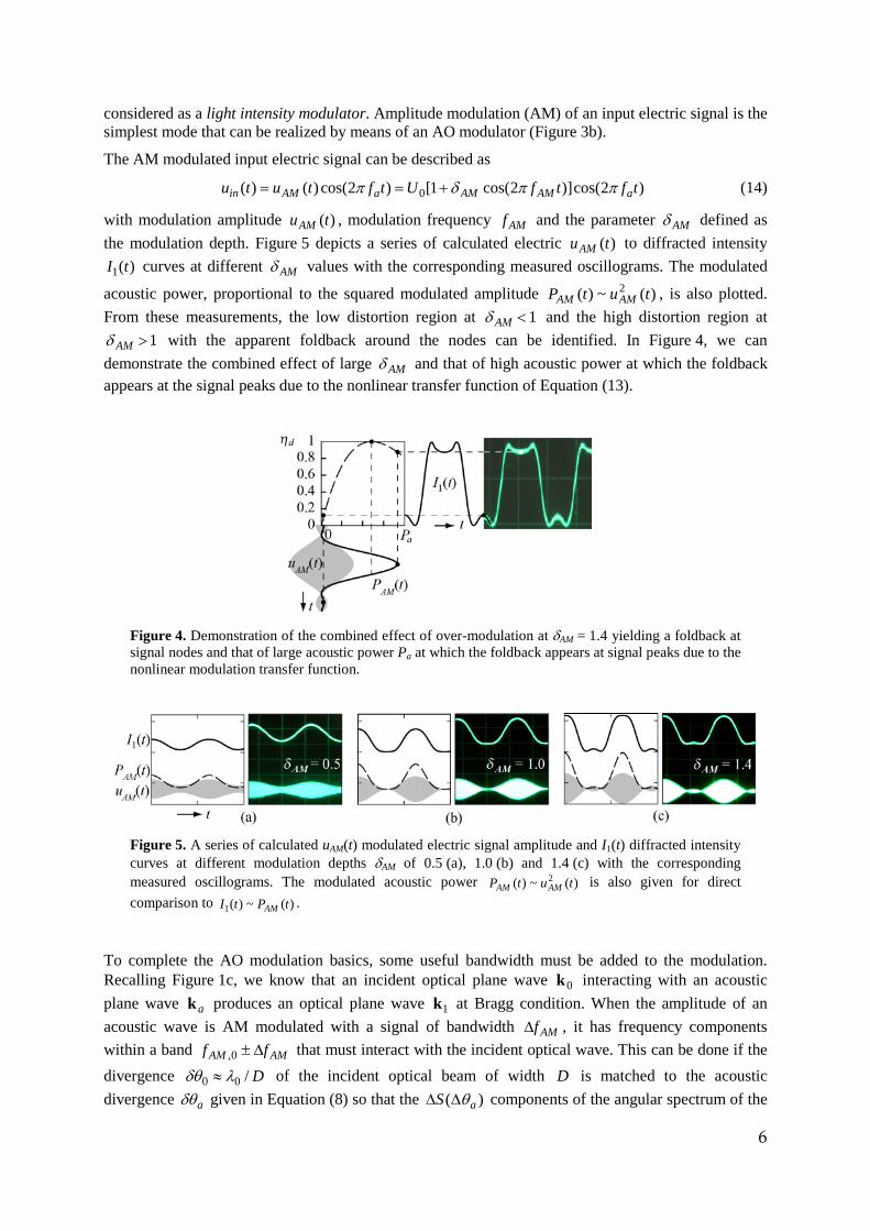
1>AMδ with the apparent foldback around the nodes can be identified. In Figure 4, we can demonstrate the combined effect of large AMδ and that of high acoustic power at which the foldback appears at the signal peaks due to the nonlinear transfer function of Equation (13).

Figure 4. Demonstration of the combined effect of over-modulation at δAM = 1.4 yielding a foldback at signal nodes and that of large acoustic power Pa at which the foldback appears at signal peaks due to the nonlinear modulation transfer function.

Figure 5. A series of calculated uAM(t) modulated electric signal amplitude and I1(t) diffracted intensity curves at different modulation depths δAM of 0.5 (a), 1.0 (b) and 1.4 (c) with the corresponding measured oscillograms. The modulated acoustic power )(~)( 2 tutP AMAM is also given for direct comparison to )(~)(1 tPtI AM .

To complete the AO modulation basics, some useful bandwidth must be added to the modulation. Recalling Figure 1c, we know that an incident optical plane wave 0k interacting with an acoustic plane wave ak produces an optical plane wave 1k at Bragg condition. When the amplitude of an acoustic wave is AM modulated with a signal of bandwidth AMf∆ , it has frequency components within a band AMAM ff ∆±0, that must interact with the incident optical wave. This can be done if the divergence D/00 λδθ ≈ of the incident optical beam of width D is matched to the acoustic divergence aδθ given in Equation (8) so that the )( aS θ∆∆ components of the angular spectrum of the

7

sound within aa δθθ =∆ will diffract the components of the light beam within 00 δθθ =∆ similarly to that in Figures 2a–b:

AMaa

aaa fD

∆=∆≈∆=∆≈==∆υλ

λλθθλδθδθθ 0

000

01, . (15)

From Equation (15), the AMf∆ bandwidth of the modulator can be expressed as

a

DD

AMDfυ

ττ

==∆ ,1 , (16)

where the transit time Dτ of sound across the light beam is introduced. Definition of Dτ holds for the collimated beam of the deflector in Figure 4a and the focused beam of the modulator in Figure 4b where the beam waist diameter is taken.

3. Acoustooptic tunable filter The laboratory experiment focuses on the investigation of an AO tunable filter (AOTF) with mono- and polychromatic light sources to learn about spectral analysis and synthesis.

High tuning speed, low driving power and small size with no moving parts allow plenty of applications, such as in spectrally tunable light source, spectrophotometry, or image analysis. The high diffraction efficiency allows the AOTF to be used for special tasks, such as external tuning of dye or diode lasers, or changing their coherence lengths. Recently, it is implemented as a pulse shaper of ultrafast laser pulses.

A major feature of an AOTF is that its narrow spectral transmission can be electronically tuned over a wide spectral range. It can be considered as a tunable monochromator. There are some considerations to successfully realize an AOTF of Figure 6b. Whereas the devices studied earlier typically operate at a single wavelength of a laser source, an AO filter must operate in a wide spectral tuning range

minmax λλλ −=∆ utilizing a light source with broad and, ideally, uniform emission in this range. The period of the AO gratings constant, equal to the acoustic wavelength, can be tuned by the acoustic frequency to change the optical wavelength at which the Bragg condition is satisfied in a preferably narrow spectral bandwidth δλ . As such, the AOTF is an inverse deflector: at each wavelength a narrow diffraction bandwidth, hence a high resolution δλλ /∆=ℜ , is realized even at large input beam divergence as well as the change of the position of the diffracted beam is avoided.

Figure 6. Anisotropic AO interaction (a) and typical geometry (b) for an AO tunable filter with characteristic input and output signals. Note the different propagation direction of acoustic energy Sa and wavefront ka.

The narrow diffraction bandwidth requires the reduction of the acoustic divergence (hence, realization of a thick sound column). The simultaneous broad tuning range requires the AOTF to be operated in a large spectral range that can be achieved with appropriate interaction geometry and large electrical bandwidth of the ultrasound transducer.

8

To satisfy all these conditions simultaneously, anisotropic AO interaction must be employed. In an anisotropic interaction, the polarization of the diffracted beam is changed. As a result, due to the birefringence of the medium, the refractive index for the diffracted beam also changes so the angles of incidence and diffraction will no longer be symmetric. Equation (6) for wave vector matching also hold for 1=m , but now the incident and diffracted wave vectors have different lengths, as illustrated in Figure 6a. A wavelength outside the Bragg condition will introduce a wave vector mismatch with magnitude k∆ so the normalized transmittance )( kT ∆λ will drop as

∆=∆

2sinc)( 2 LkkTλ . (17)

To compensate for the larger divergence of a broadband source, the Bragg condition must not change upon the infinitesimal change of the incident angles in the interaction plane 0/)( 0 =∆ δθδ k or the orthogonal plane 0/)( 0 =∆ δφδ k imposing the condition for parallel planes [17] of Figure 6a.

Expanding the constant C in Equation (13) at Bθθ =0 and using nδ from Equation (3) yields

=

=

HLPMnLk a

Bd 2cos

sincos2

sin 2

0

22

θλπδ

θη

υ

υ , (18)

that introduces the AO figure of merit )/( 3622 anpM rυ= , to be compared to Equations (3) and (12),

being high for the interaction geometry of the applied material TeO2. This is due to the extreme acoustic anisotropy of TeO2 that yields an acoustic velocity as low as m/s619=aυ along the [110] crystalline direction for shear (transversal) acoustic wave (Figure 7a). Moreover, this anisotropy causes a deviation between the acoustic wavefronts )( aa kθ and the direction of energy )( aa Sδ (Figure 7b). This effect is also illustrated in the AOTF geometry of Figure 6b.

Equation (18) also shows that the diffraction efficiency increases with the interaction length L having an additional advantage that the acoustic divergence is reduced according to Equation (8).

(a) (b) Figure 7. (a) Velocity of shear acoustic wave in TeO2 in two planes: (dashed) [xy0] plane containing the extreme direction of [110] and (solid) [110]–z plane. (b) Direction of acoustic energy propagation versus acoustic wave propagation angle measured from the extreme [110] direction towards z corresponding to the solid curve of (a).

In the interaction plane of Figure 6a, the refractive indices along the wave-vector surfaces can be described by a circle and an ellipse for the ordinary (o) and extraordinary (e) polarizations, respectively. A change in the optical wavelength results in the change of the axes and radius of these curves. At a given wavelength, the refractive indices yield onn =1 for the diffracted beam, and

21

20

2

20

2

0sincos

−

+=

eo nnn θθ , (19)

9

for the incident beam, where )( υλoo nn = and )( υλee nn = are the ordinary and extraordinary

refractive indices, respectively. Applying the appropriate acoustic wave-vector at direction aθ , the parallel tangent condition can be fulfilled.

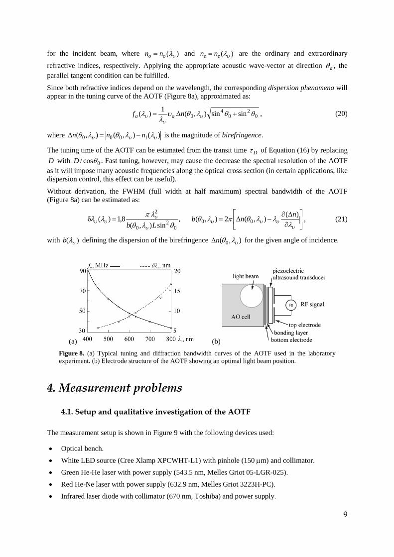
Since both refractive indices depend on the wavelength, the corresponding dispersion phenomena will appear in the tuning curve of the AOTF (Figure 8a), approximated as:

02

04

0 sinsin),(1)( θθλθυλ

λ υυ

υ +∆= nf aa , (20)

where )(),(),( 1000 υυυ λλθλθ nnn −=∆ is the magnitude of birefringence.

The tuning time of the AOTF can be estimated from the transit time Dτ of Equation (16) by replacing D with 0cos/ θD . Fast tuning, however, may cause the decrease the spectral resolution of the AOTF as it will impose many acoustic frequencies along the optical cross section (in certain applications, like dispersion control, this effect can be useful).

Without derivation, the FWHM (full width at half maximum) spectral bandwidth of the AOTF (Figure 8a) can be estimated as:

∂∆∂

−∆==υ

υυυυ

υυυ λ

λλθπλθθλθ

λπλλ )(),(2),(,sin),(

8,1)(δ 000

20

2 nnbLb

, (21)

with )( υλb defining the dispersion of the birefringence ),( 0 υλθn∆ for the given angle of incidence.

(a) (b) Figure 8. (a) Typical tuning and diffraction bandwidth curves of the AOTF used in the laboratory experiment. (b) Electrode structure of the AOTF showing an optimal light beam position.

4. Measurement problems

4.1. Setup and qualitative investigation of the AOTF

The measurement setup is shown in Figure 9 with the following devices used:

• Optical bench. • White LED source (Cree Xlamp XPCWHT-L1) with pinhole (150 µm) and collimator. • Green He-He laser with power supply (543.5 nm, Melles Griot 05-LGR-025). • Red He-Ne laser with power supply (632.9 nm, Melles Griot 3223H-PC). • Infrared laser diode with collimator (670 nm, Toshiba) and power supply.

10

• Dichroic mirrors (2 pieces) to combine the green/red/IR laser beams. • Programmable power supply to drive the LED (Fluke PM2813). • AOTF on a rotary/translation stage. • Programmable radiofrequency (RF) generator to drive the AOTF (Rohde & Schwarz SMY 01,

Figure 10). • Photodetector with power supply. • Solid state spectrometer (Ocean Optics Spark) with multimode fiber (Thorlabs MHP550L02). • Oscilloscope with built-in signal generator.

Figure 9. AOTF measurement setup.

Figure 10. Programmable RF generator.

11

To operate the AOTF, ultrasound is generated in the AO crystal by means of the RF generator. Turn the generator on. The output RF signal of the generator is connected to electrodes of the piezoelectric transducer bonded on the AO crystal via a matching LC circuitry. The mechanical oscillations of the transducer enter in the AO crystal made of TeO2. To ensure maximum interaction efficiency, the incident optical beam must overlap to either of the 2 top electrodes of the transducer as close to the electrode as possible according to Figure 8b.

Qualitative investigation of the AOTF is done by a collimated white LED source with typical spectral characteristics of Figure 11. Turn on its programmable supply with the rear switch. The display must show the “STADBY” and “ENABLE 1 2” messages. Check if channels “1” and “2” are enabled. To enable, select the channel by the (OUTPUT) “SELECT” button then press “ENABLE/DISABLE” button. Using the (SET) “V” and “I” buttons the channel voltage and current settings can be checked. Channel 2 drives the cooling fan (V=5 V; I=0.5 A). Channel 1 drives the LED (V=3.3 V; I=0.35 A). To avoid LED failure, channel 1 must be operated in constant current (CC) mode. New settings can be made directly using the numeric keys then pressing “ENTER”. The selected supply channels can be turned on using the “OPR/STBY” button. During on, the “– V +” and “– I +” buttons can also be used. Warning! The LED current must not reach >500 mA! To use the CC mode, the current protection must be turned off by the “OCP EN/OCP DIS” button. Otherwise, reaching the current limit will result in the automatic switch-off of the corresponding channel.

(a) (b)

Figure 11. (a) Typical spectral characteristics of the white LED source. (b) Optimum beam polarizations.

Place the screen behind the AOTF and turn on the LED. Pressing the “RF” button on the RF generator, adjust e.g. 45 MHz frequency with the rotary knob (this can also be done on the DATA numeric pad (e.g. with the combination of “4”, “5” and “MHz”). The “SHIFT” key will execute the blue commands. Select the dBm scale to be displayed using the “LEVEL” key (0 dBm = 1 mW, 10 dBm = 10 mW). Adjust the output to the maximum of +19 dBm by the rotary knob. Rotate the AOTF so that the LED beam is approximately perpendicular to the crystal window. What can be seen on the screen? Then change the generator frequency (by pressing the “RF” button) upward and downward while visible diffraction is seen on screen. Note the colors and the corresponding frequencies. The frequency-step can be adjusted by pressing the “STEP” button and entering a numeric value: adjust it to e.g. 0.1 MHz.

12

4.2. AOTF measurements using lasers

The measurements use 3 different lasers with the LED removed from the beam path. Check that the laser beams are properly aligned on a common axis to be combined along the AOTF interaction length. The 3 beams must coincide on the entrance face of the AOTF and on the screen. If so, the combined color appears in yellow. The laser diode must be turned on/off using the switch on its housing as transients of the mains supply may destroy the laser diode.

Turn on the red laser. On the screen, check and rotate the AOTF so that the beam enters the AOTF nearly perpendicularly. In this case the reflected beam from the entrance face will show up near to the output aperture of the laser. Please note that the reflected beam should never return back into the laser aperture. Place the detector into the beam path that leaves the AOTF. Measure the intensity on the detector counter, or using the oscilloscope. This will be referred to as the zeroth order intensity 0I (for each of the 3 laser wavelengths). Set the RF power level to +10 dBm and slowly change the frequency between 30 and 60 MHz (step is 0.1 MHz). The diffracted beam appears then disappears. Adjust the frequency where the diffracted intensity is maximal: this can be checked by the oscilloscope.

The detector can be operated by connecting its adaptor. After turning on, numbers appear on screen in 2 rows. The upper key on the detector housing sets the gain, the lower key sets the zero offset. The gain should be unchanged. If the detector aperture is closed, press the offset key multiple times until both numbers fall into the range of 1 … 10. Make note of these offset values. During measuring, either the upper or the lower number should be read and corrected by subtracting the noted offset. The upper and lower numbers differ so that they give digitized values of the measured signal at different sensitivity. The detector can be turned off by disconnected its adaptor. If the detector signal is read by using the oscilloscope connected to the detector analog output, adjusting the offset will have no significance.

TEST 1. Demonstrate a quick spectrometer. Turn on all 3 lasers. Tune the RF generator from ~20 MHz to ~50 MHz to identify, at which frequencies the 3 lasers are diffracted. Adjust the RF generator so that its frequency falls symmetrically between the green and IR diffractions: this will be the center frequency (~40MHz). Adjust the signal generator (of the oscilloscope) to produce low frequency (~8 Hz) sawtooth signal with 1 V amplitude. Connect this modulation signal to the “FM EXT” input of the RF generator and trigger the oscilloscope from this modulation signal (if necessary, use a T-connector) Press the “FM EXT DC” key: the diffracted orders should appear. Place the detector into the diffracted beam and connect its output to the oscilloscope. The appearing curve is the spectrum of the 3 beams that contain the transfer function of all optical elements and the detector. Change the frequency of the modulation signal. What is your experience?

TEST 2. Diffraction efficiency, tuning curve and diffraction bandwidth. Measure the maximum intensity 1I of each wavelength by tuning the RF frequency. Calculate the diffraction efficiency dη . Measure the RF frequency dependence of the diffraction efficiency )( ad fη . If necessary, decrease the frequency step by adjusting it using the “STEP” button. Extrapolate and plot the tuning curve )( υλaf based on the 3 frequencies corresponding to the 3 wavelengths. Measure and note also the frequencies corresponding to the half maxima at the 2 wavelengths and calculate their differences )( υλδ af . Using the extrapolated tuning curve, transform these data to the diffraction bandwidth )( υλδλ and plot it.

TEST 3. Diffraction efficiency versus Bragg-angle. Rotate the AOTF using the micrometer so as to make 2 turns from 0 to 0 (corresponding to 2*0.5 mm translation of the scale): this corresponds to ~2.5° rotation. Notice that the diffracted intensity is decreased, but can again be maximized by changing the frequency. Note the maximum diffraction efficiency and the corresponding frequency. Measure and note also the frequencies corresponding to the half maximum.

13

Hint: The maximum and half width frequencies can be read on the oscilloscope by programming the RF generator to “SWEEP” mode: Give the “START”, “STOP” and “STEP” frequencies so that the diffracted spectrum of a single wavelength appear. Adjust the “TIME/STEP” time to the minimum of 10 ms.

Repeat the readings for the rotations 2.5°, 5° and 7.5° in both directions from the optimum 0°. Measure the diffraction efficiency ),( 0θη ad f , acoustic frequency of the maximum diffraction

),( 0θλυaf and full width at half maximum ),( 0θλδ υaf curves versus angle of incidence. Obtain the converted ),( 0θλδλ υ diffraction bandwidth curves (at least for ±2.5°). Explain the curves using the AO theory and wave-vector triangle.

TEST 4. Diffraction geometry. Rotate the AOTF back into its optimum. Investigate, how accurately meet the diffracted beams (at frequencies corresponding to the maximum diffraction efficiencies) of each laser at a single point on screen. If necessary place the screen as far as possible on the setup. Qualitatively draw the wave-vector triangle for each wavelength (take of the approximate ratios). What is the possible cause of the deviations if any?

4.3. Spectral measurements with the solid state spectrometer (demonstration only)

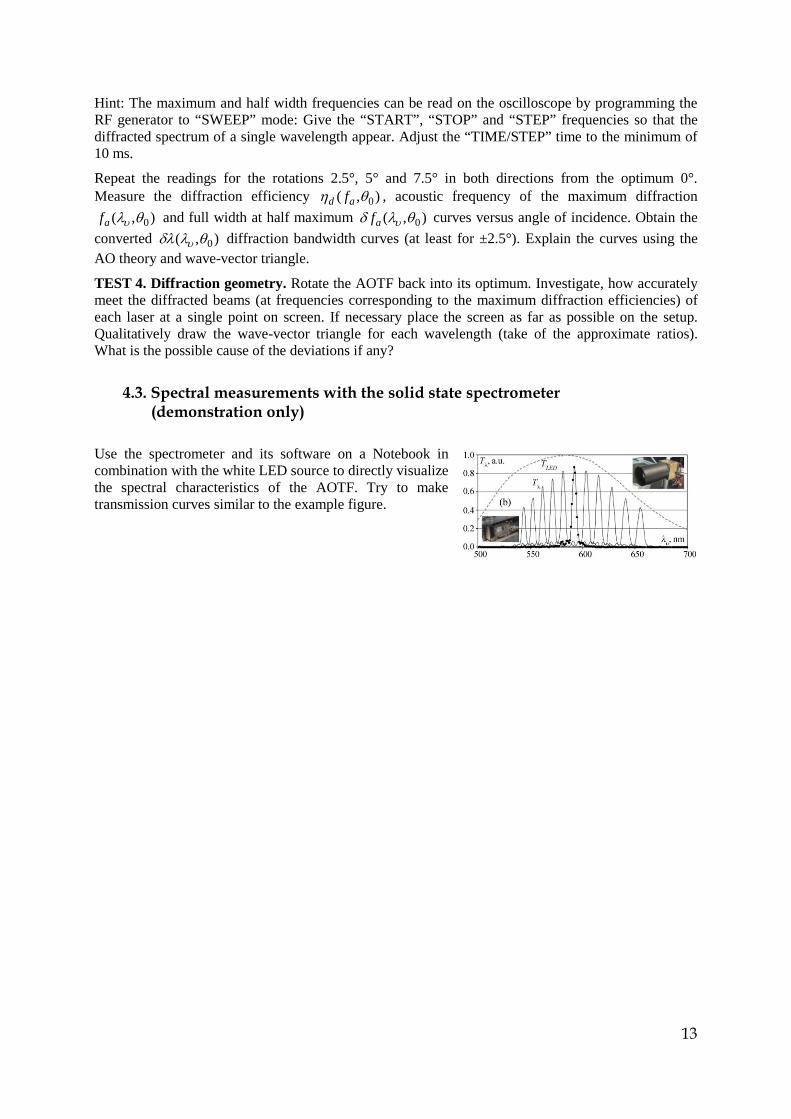
Use the spectrometer and its software on a Notebook in combination with the white LED source to directly visualize the spectral characteristics of the AOTF. Try to make transmission curves similar to the example figure.

14

5. References 1. Brillouin, L., "Diffusion of Light and X-rays by a Transparent Homogeneous Body: Influence of

thermal agitation," Annales de Physique 17, 88-122 (1922). 2. Debye, P. and Sears, F. W., "On the scattering of light by supersonic waves," PNAS 18(6), 409-

414 (1932). 3. Lucas, R. and Biquard, P., "Optical properties of solid and liquid medias subjected to high-

frequency elastic vibrations," Journal de Physique 71, 464–477 (1932). 4. Eichler, H. J., Barocsi, A., Jakab, L. and Liu, B., "Acousto-optic mode-locker for Nd:lasers using

paratellurite," Appl. Phys. B - Photo. 53(3), 194-197 (1991). 5. Maak, P., Jakab, L., Richter, P., Eichler, H. J., and Liu, B., "Efficient acousto-optic Q-switching of

Er:YSGG lasers at 2.79 µm wavelength," Appl. Optics 39(18), 3053-3059 (2000). 6. Maák, P., Jakab, L., Barócsi, A., and Richter, P., "Recent Developments and Results in 2D

Acousto-Optic Light Deflection," Proc. SPIE 3388, 48-53 (1998). 7. Maak, P., Lenk, S., Jakab, L., Barocsi, A. and Richter, P., "Optimization of transducer

configuration for bulk acousto-optic tunable filters," Opt. Commun. 241(1-3), 87-98 (2004). 8. Barocsi, A., Jakab, L. and Richter, P., "Efficient, extremely low frequency acousto-optic shifter

for optical heterodyning applications," Proc. SPIE 2240, 108-113 (1994). 9. Barocsi, A., Jakab, L., Szarvas, G., Richter, P. and Szonyi, I., "Recent developments and results in

acoustooptic signal processing," Proc. SPIE 2754, 21-30 (1996). 10. Jakab, L., Barocsi, A., Richter, P., Szonyi, I. and Rath, T., "Test measurement and calibration

problems of a direction finding system based on a five channel DOA processor," Proc. SPIE 2240, 43-49 (1994).

11. Katona, G., Szalay, G., Maak, P., Kaszas, A., Veress, M., Hillier, D., Chiovini, B., Vizi, E. S., Roska, B. and Rozsa, B., "Fast two-photon in vivo imaging with three-dimensional random-access scanning in large tissue volumes," Nature Methods 9(2), 201-208 (2012).

12. Maák, P., Kurdi, G., Barócsi, A., Osvay, K., Kovács, A. P., Jakab, L. and Richter, P., "Shaping of ultrashort laser pulses using bulk acousto-optic filter," Appl. Phys. B - Lasers O. 82(2), 283-287 (2006).

13. Barócsi, A., Lenk, S., Ujhelyi, F., Majoros, T., Maák, P., "Laboratory tools and e-learning elements in training of acousto-optics", Proc. SPIE 9793, Education and Training in Optics and Photonics: ETOP 2015, 97930U (8 October 2015).

14. Mihajlik, G., Barócsi, A. and Maák, P., “Measurement and general modeling of optical rotation in anisotropic crystal,” Opt. Commun. 310, 31-34 (2014).

15. Uchida, N. and Niizeki, N., "Acoustooptic deflection materials and techniques," Proc. IEEE 61(8), 1073-1092 (1973).

16. Saleh, B. E. A. and Teich, M. C., [Fundamentals of Photonics 2nd Edition], John Wiley & Sons, Inc., Hoboken, New Jersey, 804-833 (2007).

17. Chang, I. C., "Analysis of the noncollinear acousto-optic filter," Electron. Lett. 11(25/26), 617-618 (1975)

18. Cree XLamp XP-C LEDs, product family data sheet, CLD-DS19 Rev 9A, Cree, Inc. (2008-2013)