Investigation into the Use of OpenStack for Submarine ... into the Use of OpenStack for Submarine...

Investigation into the Use of OpenStack for Submarine Mission

Systems

Building a Private Cloud with OpenStack: Technological Capabilities and Limitations

(Volume 1)

August 2015

Project Team: Professor M. Ali Babar (Lead Researcher), Mr. David Silver (Researcher), Mr. Ben Ramsey (Researcher).

CREST - Centre of Research on Engineering Software Technologies,

University of Adelaide, Australia.

Contact Person: Professor M. Ali Babar, [email protected]

Phone number: 0432 460 451

-2-

Executive Summary Cloud Computing is an active area of experimentation and applications for a large number of organisations, public or private, because of the promising utility computing model supported by virtualization technologies. Cloud Computing has opened up new horizons for organisations to meet their increasing demands of computing, storage, and networking resources without huge upfront investment. Cloud Computing paradigm is broadly classified into service and deployment models. Infrastructure as a Service (IaaS), Platform as a Service (PaaS) and Software as a Service (SaaS) correspond to service models; whereas public, private, hybrid, community and virtual clouds are the categories of deployment models. Public and private Cloud infrastructures are two of the most common deployment models. Whilst public clouds led the adoption of Cloud Computing, there is an increasing trend to build and leverage private cloud infrastructures in different industrial domains for several reasons with security, privacy, and data location management being the predominant concerns. Defence Science and Technology (DST) recognises that Cloud Computing presents new opportunities for more flexible and efficient utilisation of computing resources. This report describes the objectives, scope, and outcomes of a research project aimed at gaining the required knowledge and competency for building and managing a private cloud infrastructure for mission systems in submarine domain. One of the key goals of this project was to explore the technical strengths and limitations of OpenStack cloud software and its related tools for designing and implementing a dynamically reconfigurable Cloud Computing infrastructure. This project has experimentally assessed the strengths and limitations of OpenStack cloud software (such as Rackspace, Mirantis, and DevStack), different virtualisation software (such as KVM and VMware’s ESXi), and baremetal provisioning tools (such as Razor and CloneZilla). This work has also developed a component architecture for dynamic assignment of compute loads to baremetal hardware or virtual machines. This work has also investigated the use of Graphics Processing Unit (GPU) within virtual machines and devised and applied a mechanism for comparing the suitability of different hypervisor implementations according to various performance metrics. We have identified several challenges of implementing a private cloud with OpenStack that supports a variety of architectures and capabilities that must be mapped to the functional and performance requirements of a private cloud infrastructure. OpenStack is usually hard to install, manage, and maintain for an administrator without an advanced knowledge of and practical skills in different aspects of state-of-the-art Information Technology (IT) infrastructure solutions. Private cloud implements a complex computer architecture utilising specialist, server grade processing and network hardware. Common consumer- or desktop-grade components may not fully support features such as virtualisation or remote power management and can be expected to offer sub-optimal performance. All components in a system must be selected bearing in mind the unique functional and performance requirements of a private cloud. Another significant challenge is that OpenStack has approximately 600 configuration options spread across 30 files. These settings must be configured in harmony with each other across multiple nodes to map the desired cloud architecture to servers and network hardware. It is also necessary to configure options of the firmware of servers, such as BIOS/UEFI settings. Complexity of debugging and maintenance is another challenge that we experienced. The search space for locating a point of failure may include the entire hardware-software stack. Systems administrators must be familiar with all layers of the cloud architecture in order to take appropriate remedial actions in the event of hardware failure. A comprehensive understanding of configuration dependencies is also required. This work has also identified some areas for further explorations to gain an in-depth knowledge about building and leveraging private cloud for submarine combat systems. Some of the key areas that DTS can consider for further research include but not limited to achieving security and scalability with containerised cloud infrastructure, what are the appropriate data capture and management technologies for the next generation of submarine combat systems, developing and evaluating domain specific tools for automating configuration and deployment of private clouds, and devising and deploying strategies for real-time scheduling of virtual machines based on heterogeneous hypervisors. The findings from this experimental work are expected to provide practitioners (DST and non-DST) with useful insights into different aspects of building and managing private cloud infrastructures using OpenStack technologies, different hypervisors, and baremetal provisioning tools. This report and a companion guide on installing and configuring private cloud with OpenStack technologies are expected to serve as a much needed source of information and guidance for building and managing a private cloud in mission critical industries in general and in Defence in particular.

-3-

Table of Contents 1. Introduction .................................................................................................................................................................. 5 2. OpenStack Private Cloud Software .............................................................................................................................. 7 3. OpenStack for Submarine Mission Systems ................................................................................................................ 9

3.1 OpenStack Setup .................................................................................................................................................... 9 3.2 Develop Software Component Model .................................................................................................................... 9 3.3 Develop Software Interaction Model ..................................................................................................................... 9 3.4 GPGPU With Virtualisation Technology ............................................................................................................... 9 3.5 Virtualisation Comparison ..................................................................................................................................... 9 3.6 Documentation ....................................................................................................................................................... 9

4. Private Cloud Laboratory Setup ................................................................................................................................. 11 5. Selection of the OpenStack Distribution .................................................................................................................... 15 6. Selection of the Baremetal Provisioning Mechanism ................................................................................................ 17 7. Cloud-Init ................................................................................................................................................................... 18 8. VMware and OpenStack ............................................................................................................................................ 19 9. OpenStack Private Cloud Dashboard (OPCD) ........................................................................................................... 20

9.1 The Main Window of OPCD ............................................................................................................................... 20 9.2 The Logical View of OPCD ................................................................................................................................. 23 9.3 Component Operations Flow Charts .................................................................................................................... 24 9.4 The Login Dialog ................................................................................................................................................. 24 9.5 The Baremetal Provisioning Configuration Dialog ............................................................................................. 25 9.6 The Server List ..................................................................................................................................................... 25 9.7 Booting a Virtual Machine Instance ..................................................................................................................... 26 9.8 Terminating a Virtual Machine Instance .............................................................................................................. 27 9.9 Bare Metal Provisioning of a Host ....................................................................................................................... 27 9.10 Server Details ..................................................................................................................................................... 27 9.11 The Components View ....................................................................................................................................... 27

9.11.1 Importing a Pre-Defined Component .......................................................................................................... 28 9.11.2 Removing a Component .............................................................................................................................. 28 9.11.3 Defining a Dummy Component Type ......................................................................................................... 28 9.11.4 Installing A Component on a Component Host .......................................................................................... 29 9.11.5 Component Context Menu .......................................................................................................................... 29 9.11.6 Refresh Button ............................................................................................................................................. 29

10. PCI Passthrough ....................................................................................................................................................... 30 10.1 Findings on PCI Passthrough ............................................................................................................................. 30 10.2 GPGPU Benchmarking ...................................................................................................................................... 31 10.3 Benchmark Results ............................................................................................................................................. 31

11. Hypervisor Suitability Comparison .......................................................................................................................... 32 11.1 Benchmark Methodology ................................................................................................................................... 32 11.2 Performance Tuning ........................................................................................................................................... 32 11.3 Other Benchmark Conditions ............................................................................................................................. 32 11.4 Running Phoronix Test Suite Benchmark .......................................................................................................... 33

-4-

11.5 CPU Performance Measurement ........................................................................................................................ 33 11.6 RAM Performance Measurement ....................................................................................................................... 33 11.7 Disk Performance Measurement ........................................................................................................................ 33 11.8 Interrupt Latency Measurement ......................................................................................................................... 33 11.9 Network Performance Measurement .................................................................................................................. 33

11.9.1 Pre-Benchmark Tuning ............................................................................................................................... 34 11.9.2 Benchmark Results ...................................................................................................................................... 35

11.10 Results Analysis ............................................................................................................................................... 36 11.11 Disk Performance ............................................................................................................................................. 37

11.11.1 CPU Performance ...................................................................................................................................... 37 11.11.2 RAM Performance .................................................................................................................................... 37 11.11.3 Interrupt Latency ....................................................................................................................................... 37 11.11.4 Network Performance ............................................................................................................................... 39

12. Summary .................................................................................................................................................................. 40 Figures: Figure 1: Most commonly known service and deployment models of cloud computing (reproduced diagram [4]) ....... 5 Figure 2: Conceptual Architecture of how the different services of OpenStack interact [15]. ....................................... 8 Figure 3: A high level overview of the hosts and network for the nova-network configuration. ................................. 11 Figure 4: A typical 2-node OpenStack deployment using Nova-network with FlatDHCPManager. ........................... 13 Figure 5: The main window of OPCD. ......................................................................................................................... 20 Figure 6: The conceptual layout of the OPCD main window. ...................................................................................... 21 Figure 7: A conceptual view of the different dialogs accessible from the main window. ............................................ 22 Figure 8: The logical view of the OPCD. ...................................................................................................................... 23 Figure 9: The baremetal provisioning workflow. .......................................................................................................... 23 Figure 10: The flowcharts of the component operations. .............................................................................................. 24 Figure 11: The login dialog for the OPCD .................................................................................................................... 24 Figure 12: the Launch Instance Dialog ......................................................................................................................... 26 Figure 13: The Install Component dialog. ..................................................................................................................... 29 Figure 14: The Component Context Menu. .................................................................................................................. 29 Figure 15: The logical view of the benchmark suite. .................................................................................................... 32 Figure 16: The histogram of interrupt latencies output by Cyclictest for the host system ("baremetal") ..................... 38 Figure 17: The histogram of interrupt latencies on a KVM virtual machine. ............................................................... 39 Figure 18: The histogram of interrupt latencies on a VMware virtual machine. .......................................................... 39 Tables: Table 1: Key Concepts for the Identification Model ....................................................................................................... 7 Table 2: Listing of Operating System vs Default User name vs SSH Login ................................................................ 18 Table 3: An example Component Log output. .............................................................................................................. 28 Table 4: Roy Longbottom CUDA MFLOPs benchmark results. .................................................................................. 31 Table 5: CUDA bandwidth test results ......................................................................................................................... 31 Table 6: Raw performance benchmark results. ............................................................................................................. 35 Table 7: Performance benchmark results compared. .................................................................................................... 36

-5-

1. Introduction Cloud Computing has gained widespread adoption in different sectors for providing Information Communication and Technology (ICT) infrastructure (i.e., computing, storage, and network). Cloud computing provides on demand scalability and flexibility as organisations can scale up or scale down their acquisition of ICT infrastructure based on their consumption patterns [1], [2]. An increasingly large number of small as well as large, private and public organisations have started using cloud-enabled services for business- and mission-critical systems in various domains. At the same time the number of companies offering cloud services is increasing dramatically with Google, Amazon, Rackspace, and Microsoft being some of the key players in Cloud Computing business. Different people define Cloud Computing differently, hence, it is important to have an operational definition of Cloud Computing for this report. We use the following definition of Cloud Computing provided by the US National Institute of Standards and Technology (NIST) [3]. “Cloud computing is a model for enabling convenient, on-demand network access to a shared pool of configurable computing resources (e.g., networks, servers, storage, applications, and services) that can be rapidly provisioned and released with minimal management effort or service provider interaction.” Cloud Computing solutions are broadly classified into three services and five deployment models. Three categories of service models are: Infrastructure as a Service (IaaS), Platform as a Service (PaaS) and Software as a Service (SaaS). Five deployment models include: public, private, hybrid, community and virtual private clouds.

Figure 1: Most commonly known service and deployment models of cloud computing (reproduced diagram [4])

IaaS cloud provides an abstraction to underlying computing, storage and network resources using virtualisation technologies. It provides basic software resources such as operating system to utilise the virtualized hardware resources. Amazon Elastic Cloud [5], Amazon Simple Storage Services [6], Eucalyptus [7] and OpenNebula [8] are some of the few examples of IaaS cloud platform. PaaS cloud provides Application Programmable Interfaces (APIs) to develop applications. Applications built using PaaS APIs do not need to handle resource provisioning of the underlying infrastructure. Google App Engine [9], Microsoft Azure platform [10] and SalesForce [11] are examples of the PaaS. Albeit PaaS provides support for seamless scalability and an easy way to develop cloud-based applications, it also has disadvantages of vendor lock-in, and limited support for programming languages and frameworks. SaaS represents applications that are built on top of either IaaS or PaaS clouds, and offers business solutions to End Users. One of the key features of these applications is multi-tenancy. It enables a single instance of an application to service a large number of organisations and End Users. SaaS provides limited support for customisation. Public clouds represent cloud infrastructure and software resources that are maintained by an organisation and are offered for use based on different pricing models; Amazon Elastic Compute Cloud (EC2) and Simple Storage Service (S3), Google App Engine and Microsoft Azure are the examples of public clouds. Private clouds represent infrastructure and software resources maintained by organisations for their internal use. In some cases, organisations adopt a hybrid cloud strategy and combine private infrastructure with public clouds. This is called a hybrid cloud. Virtual private cloud (VPC) and community cloud are built on top of public and private clouds. A VPC utilises resources of public cloud with additional features of virtual private network. It provides support for customisable

-6-

network topology and security settings. Organisations with shared business objectives decide to collaborate with each other and form a common cloud by combining their private clouds. This is referred to as a community cloud. There can be certain legal, political and/or socio-organisational reasons that may discourage (or even bar) an organisation from using public cloud infrastructure for certain kinds of activities, for example, processing and storing security sensitive or citizens’ private data. For these kinds of situations, private cloud infrastructure is considered an appropriate alternative. Hence, private cloud infrastructure is gaining much more popularity than the public cloud solutions. One of the key reasons for an increased interest in setting up and managing private clouds is that a significant amount of uncertainty exists about different legal and social implications with regards to privacy, security, location and ownership of data. On the economic side, the needs for and interest in processing and storing large amount of data are growing strongly in both industry and research. The need to conserve power by optimizing server utilisation is also booming. The market forces are on their way to on-demand ICT infrastructure for almost all sorts of business- and mission-critical systems. Based on the researchers’ previous experiences in setting up and managing private cloud and the work on this project, it is concluded that the private cloud solutions are expected to be more customizable for meeting an organisation’s quality requirements (such as flexibility, performance, security and scalability), but have greater installation and maintenance cost and steep learning curve at the start of building a private cloud infrastructure. The private cloud technologies have matured but documentation for Open Source solutions are usually lacking or obsolete. Private cloud is usually hard to install, manage and maintain for an administrator without an advanced knowledge of and practical skills in different aspects of modern Information and Communication Technologies (ICT). When an organisation decides to build and manage a private cloud, there is always a steep learning curve for the whole organisation, for both users and administrators. The key challenges for this project were caused by the complexities and lack of documentation of different OpenStack distributions. For example, RackSpace being too difficult to be installed without doing significant debugging of the source code, configuring complex networking arrangements in a large number of nodes, and hardware dependency for leveraging certain types of features of OpenStack technologies for setting up private cloud infrastructure. Moreover, a cloud administrator need to have a solid knowledge of various baremetal provisioning tools in order to evaluate their feasibility and apply them. Such tools require special types of hardware to be available to them, or some configuration options may need to be changed for the deployment layout that has been utilised.. It is becoming clear that there is an increasing demand and trend to build and manage private cloud infrastructures in different industrial domains for several reasons with security, privacy, and data location management being the predominant concerns. However, there is not much guidance on building, operating, trouble-shooting, and managing a private cloud infrastructure, especially for public and government agencies. It is asserted that there is an important need of experimentally gathered and systematically documented guidance on identifying and selecting appropriate technologies for building and operating private cloud infrastructure for business- and mission-critical systems. This report provides guidelines for evaluating cloud technologies for building a private cloud infrastructure using OpenStack cloud software. These guidelines have been derived based on our practical experiences from successfully completing a project on building and evaluating a private cloud infrastructure using OpenStack private cloud technologies.

-7-

2. OpenStack Private Cloud Software The OpenStack [12] Cloud software package is a collection of projects, which when combined create an Open Source IaaS Private Cloud system. An IaaS cloud allows users to be able to request computing resources as required. For example, a user is able to request a certain amount of CPU cores, RAM, and storage space, with a particular operating system image installed on top of the resources. However, a strict definition of IaaS means that a user can request either a physical host or a Virtual Machine (VM) from a cloud. Instead of version numbers, OpenStack releases are assigned code names in ascending order, alphabetically, of their first letter such as Austin, Bexar, Cactus, and Diablo. This project utilised the Juno series of releases. The current stable release at the time of writing is Kilo (April 30, 2015). With regards to a cloud deployment, the OpenStack cloud platform is a private cloud that usually runs on privately own hardware in a data center. It has been indicated that other deployment options are public cloud or a hybrid/federated cloud. A public cloud deployment means running a cloud platform on a service providers’ hardware. A hybrid, or federated cloud deployment is a combination of public and private cloud deployments. The use case of such a cloud is to be able to run confidential workloads on a privately own hardware, and the workloads where scalability is the major factor on the public cloud components. While some of the projects under the OpenStack header are optional and are used only if a use case requires it, there are some projects, which need to be included for building a functional cloud platform. These compulsory projects in the OpenStack header include Keystone (Identity Management), Nova (Computation Engine), Glance (Image Management), and either Nova-network or Neutron (Network Management). The choice of Nova-network and Neutron is one of requirements. Some of the OpenStack projects require new Neutron network management project; however, legacy projects usually require Nova-network that has a simpler use model and requires limited hardware compared with Neutron that requires more hardware for setting up a network for a private cloud. Other optional OpenStack projects include Ironic (Bare-metal Management), Heat (Orchestration Engine), Horizon (Web-based Dashboard), Magnum (Containers as a Service), Ceilometer (Cloud Telemetry), Trove (Database as a Service), Sahara (Big Data), Swift (Object Storage), and Cinder (Block Storage). It is a common practice to use Cinder to be able to attach storage capabilities to the computation resources, with Swift being used as a backup service, or image storage. The Keystone identity service provides an authentication model of the cloud as well as manages where the endpoints of each of the services are located, so that they can easily communicate with each other as required. Table 1 provides brief definitions of several key concepts related to Keystone : Table 1: Key Concepts for the Identification Model

Concept Definition

User A user of the cloud system. Tenant A project on the cloud, allows separation of allocated resources.

Role A mapping of a set of users to the operations that they can perform.

Domain Defines administration boundaries for identity management. i.e. allows the creation of users and projects within a particular domain.

Group A group of users that can have a role assigned to it to allow access management to be simplified.

The Nova Compute service allows users to launch virtual or physical instances dependent on users’ requirements as defined by an image and a flavor. The image is the operating system image that user requires. The flavor is the machine specifications that include such factors as CPU cores required, memory allocated, and storage requirements. Each node allocated as a compute node runs the nova-compute service, which acts as OpenStack's interface to a hypervisor running on that node. The nova-compute service abstracts away the differences between different types of hypervisor (e.g., QEMU/KVM or VMware ESXi). On each node, the service is configured with a driver that communicates with the specific type of hypervisor running on that node. A hypervisor provider can be a choice of several different options. Only one hypervisor driver can be placed on a single compute node. Some of the more common options for the hypervisor driver include Xen [13], QEMU/KVM [14], ESXi, Linux Containers (LXC), LXD, and Docker. Another option is to use the Ironic project baremetal hypervisor driver. The nova-compute service communicate with the Ironic Service through its API, which then uses the Ironic Conductor service to bring up a baremetal provisioned machine with the required specifications.

-8-

Figure 2: Conceptual Architecture of how the different services of OpenStack interact [15].

Both the Nova-network and Neutron provide basic network capabilities to Virtual Machines (VMs) for connecting to each other and the outside world. Neutron also provides some advanced networking features such as constructing multi-tiered networks, defining virtual networks, routers and subnet. Neutron has a series of plugins that can further enhance the network capabilities; for example, LBaaS (Load Balancer as a Service) is a plugin that can support automated scaling of resources within a cloud with a load balancer (such as HAproxy [16]) that is used to decide about the resources to be allocated from the available pool of services.

-9-

3. OpenStack for Submarine Mission Systems The Submarine Combat System Architecture Group at DST decided to investigate the suitability of the OpenStack private cloud package for building and experimenting with a private cloud infrastructure. The objective was to configure and manage a cluster of compute nodes using available tools, and to commence the configuration and/or development of the tools that may be required to build and manage a cloud for deployment and evaluation of relevant systems and/or components. This project was expected to help determine the benefits and limitations of leveraging cloud technology (including virtualisation) to support submarine mission system architectures. The work package of this project included:

3.1 OpenStack Setup The first task was to “develop a system which can demonstrate the creation and execution of a new compute node using a package based on OpenStack, for example Rackspace (preferred) or Mirantis, or alternatively building a new package directly from the OpenStack sources. Once setup, an OpenStack based private cloud system was expected:

• take a compute node from bare metal using a tool such as Razor or equivalent. • optionally assign a type-I hypervisor such as KVM, Xen1 or VMware ESXi. • load a kernel, either as a live image on a bare metal server or as a kernel on the hypervisor.

Furthermore, the built private cloud system must have included a tool with a suitable Graphical User Interface (GUI) to view the status of compute nodes, including those which are: unassigned, baremetal kernels, hypervisors (with each type distinguishable) and child virtual machines. That type of tool may be original, or developed by leveraging existing toolsets such as the Eclipse Modeling Framework (EMF) and DevOps tools such as Chef. These tools can be expanded to satisfy the objectives of the subtask two as described below.” The tool developed in this project is called, OpenStack Private Cloud Dashboard (OPCD).

3.2 Develop Software Component Model The second task was to “Further develop OPCD described in subtask one (above) such that it shows software components and their data inputs and outputs, and allows these components to be allocated to the kernels (baremetal or virtual) created in subtask one. The expansion of the tool must allow both software and ‘dummy’ components to be allocated using a GUI (i.e., via mouse clicks, drag and drop, or menu selection). To achieve these objectives component containers may be required; these can be implemented using Docker, Linux containers, or suitable alternatives.”

3.3 Develop Software Interaction Model The graphical tool was to be further extended to include publishing and subscribing to Data Distribution Service (DDS)-type topics from the ‘dummy’ components. The requirements stated that “DDS topics will be defined using the Object Management Group (OMG) standard for DDS topics, being based on relevant UML/IDL definitions. The EMF or an alternative tool that provides XMI-compliant data descriptions may be used. A ‘dummy’ component deployed to the available OpenStack environment will be able to be started and stopped from publishing / subscribing by accessing the component description in the developed graphical tool.”

3.4 GPGPU With Virtualisation Technology This task was aimed at investigating the options for incorporating General Purpose Graphics Processing Units (GPGPU) hardware into the OpenStack environment; including the accessibility of GPGPU hardware from nodes running a type-I hypervisor, issues influencing the suitability of hypervisor options, and any performance implications due to access through a hypervisor.

3.5 Virtualisation Comparison This task was to “Develop a mechanism to compare the suitability of different hypervisor implementations. In particular, the ability to compare the suitability of the KVM and VMware ESXi hypervisors for different roles in a combat system style environment.”

3.6 Documentation The final task was to document the process used and the results obtained for all the previous subtasks. In particular, the 1 Installation of Xen was not done under the project, by mutual agreement with DST. However, the developed tool can easily modified to install Xen

-10-

documentation was required to include descriptions of the following key research outcomes: • The processes developed for bringing up an OpenStack system from bare metal; • A guide to utilising the development tool; • The feasibility of accessing GPGPU technology via an OpenStack compute node, including: the technical or

other challenges, and the relative merits of the options surveyed; • The mechanism for comparing the suitability of different hypervisors for different roles;

-11-

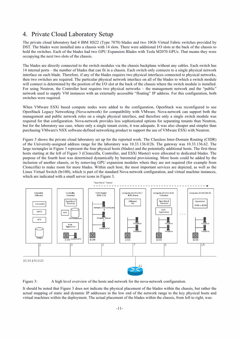
4. Private Cloud Laboratory Setup The private cloud laboratory had 4 IBM HS22 (Type 7870) blades and two 10Gb Virtual Fabric switches provided by DST. The blades were installed into a chassis with 14 slots. There were additional I/O slots at the back of the chassis to hold the switches. Each of the blades had two GPU Expansion Blades with Tesla M2070 GPUs. That means they were occupying the next two slots of the chassis. The blades are directly connected to the switch modules via the chassis backplane without any cables. Each switch has 14 internal ports – the number of blades that can fit in a chassis. Each switch only connects to a single physical network interface on each blade. Therefore, if any of the blades requires two physical interfaces connected to physical networks, then two switches are required. The particular physical network interface on all of the blades to which a switch module will connect is determined by the position of the I/O slot at the back of the chassis where the switch module is installed. For using Neutron, the Controller host requires two physical networks – the management network and the “public” network used to supply VM instances with an externally accessible “floating” IP address. For this configuration, both switches were required. When VMware ESXi based compute nodes were added to the configuration, OpenStack was reconfigured to use OpenStack Legacy Networking (Nova-network) for compatibility with VMware. Nova-network can support both the management and public network roles on a single physical interface, and therefore only a single switch module was required for that configuration. Nova-network provides less sophisticated options for separating tenants than Neutron, but for the laboratory use case, where only a single tenant exists, it was adequate. It was also cheaper and simpler than purchasing VMware's NSX software-defined networking product to support the use of VMware ESXi with Neutron. Figure 3 shows the private cloud laboratory set up for the reported work. The Classless Inter-Domain Routing (CIDR) of the University-assigned address range for the laboratory was 10.33.136.0/26. The gateway was 10.33.136.62. The large rectangles in Figure 3 represent the four physical hosts (blades) and the potentially additional hosts. The first three hosts starting at the left of Figure 3 (Clonezilla, Controller, and ESXi Master) were allocated to dedicated blades. The purpose of the fourth host was determined dynamically by baremetal provisioning. More hosts could be added by the inclusion of another chassis, or by removing GPU expansion modules where they are not required (for example from Clonezilla) to make room for more blades. Within each host, the most important services are depicted, as well as the Linux Virtual Switch (br100), which is part of the standard Nova-network configuration, and virtual machine instances, which are indicated with a small server icons in Figure 3.

Figure 3: A high level overview of the hosts and network for the nova-network configuration.

It should be noted that Figure 3 does not indicate the physical placement of the blades within the chassis, but rather the actual mapping of static and dynamic IP addresses in the low end of the network range to the key physical hosts and virtual machines within the deployment. The actual placement of the blades within the chassis, from left to right, was:

-12-

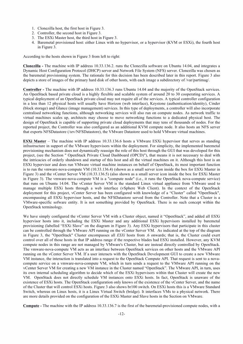
1. Clonezilla host, the first host in Figure 3. 2. Controller, the second host in Figure 3. 3. The ESXi Master host, the third host in Figure 3. 4. Baremetal provisioned host: either Linux with no hypervisor, or a hypervisor (KVM or ESXi), the fourth host

in Figure 3. According to the hosts shown in Figure 3 from left to right: Clonezilla - The machine with IP address 10.33.136.2. runs the Clonezilla software on Ubuntu 14.04, and integrates a Dynamic Host Configuration Protocol (DHCP) server and Network File System (NFS) server. Clonezilla was chosen as the baremetal provisioning system. The rationale for this decision has been described later in this report. Figure 3 also depicts a store of images of the primary hard disk of other hosts, with each image a subdirectory of /var/partimag/. Controller - The machine with IP address 10.33.136.3 runs Ubuntu 14.04 and the majority of the OpenStack services. An OpenStack based private cloud is a highly flexible and scalable system of around 20 to 30 cooperating services. A typical deployment of an OpenStack private cloud may not require all of the services. A typical controller configuration in a less than 12 physical hosts will usually have Horizon (web interface), Keystone (authentication/identity), Cinder (block storage) and Glance (image management) services. In this type of deployments, a controller will also incorporate centralised networking functions, although networking services will also run on compute nodes. As network traffic to virtual machines scales up, architects may choose to move networking functions to a dedicated physical host. The design of OpenStack is capable of supporting private cloud deployments that may tens of thousands of nodes. For the reported project, the Controller was also configured as an additional KVM compute node. It also hosts an NFS server that exports NFSDatastore (/srv/NFSDatastore), the VMware Datastore used to hold VMware virtual machines. ESXi Master – The machine with IP address 10.33.136.6 hosts a VMware ESXi hypervisor that serves as standing infrastructure in support of the VMware hypervisors within the deployment. For simplicity, the implemented baremetal provisioning mechanism does not dynamically reassign the role of this host through the GUI that was developed for this project, (see the Section " OpenStack Private Cloud Dashboard (OPCD)"), that means it is not necessary to deal with the intricacies of orderly shutdown and startup of this host and all the virtual machines on it. Although this host is an ESXi hypervisor and does run VMware virtual machine instances on behalf of OpenStack, its most important function is to run the vmware-nova-compute VM (10.33.136.4) (shown as a small server icon inside the box for ESXi Master in Figure 3) and the vCenter Server VM (10.33.136.5) (also shown as a small server icon inside the box for ESXi Master in Figure 3). The vmware-nova-compute VM is a "compute node" (i.e., it runs the OpenStack nova-compute service) that runs on Ubuntu 14.04. The vCenter Server VM is the standard Linux virtual appliance from VMware used to manage multiple ESXi hosts through a web interface (vSphere Web Client). In the context of the OpenStack deployment for this project, vCenter Server has been configured with knowledge of a “Cluster” called "OpenStack", encompassing all ESXi hypervisor hosts, and the NFSDatastore served from the Controller. Note that a Cluster is a VMware-specific sofware entity. It is not something provided by OpenStack. There is no such concept within the OpenStack terminology. We have simply configured the vCenter Server VM with a Cluster object, named it “OpenStack”, and added all ESXi hypervisor hosts into it, including the ESXi Master and any additional ESXi hypervisors installed by baremetal provisioning (labelled “ESXi Slave” on the diagram in Figure 3). Any ESXi hypervisors that participate in this cluster can be controlled through the VMware API running on the vCenter Server VM. As indicated at the top of the diagram in Figure 3, the "OpenStack" Cluster encompasses all ESXi hosts from .6 onwards; that is, the Cluster could exert control over all of those hosts in that IP address range if the respective blades had ESXi installed. However, any KVM compute nodes in this range are not managed by VMware's Cluster, but are instead directly controlled by OpenStack. The vmware-nova-compute VM acts as an interface between OpenStack services on other hosts and the VMware API running on the vCenter Server VM. If a user interacts with the OpenStack Development GUI to create a new VMware VM instance, the interaction is translated into a request to the OpenStack Compute API. That request is sent to a nova-compute service on a vmware-nova-compute VM, which in turn sends a request to the VMware API running on the vCenter Server VM for creating a new VM instance in the Cluster named “OpenStack”. The VMware API, in turn, uses its own internal scheduling algorithm to decide which of the ESXi hypervisors within that Cluster will create the new VM. OpenStack does not directly schedule VM instances onto ESXi hosts. In fact, OpenStack is unaware of the existence of ESXi hosts. The OpenStack configuration only knows of the existence of the vCenter Server, and the name of the Cluster that will control ESXi hosts. Figure 3 also shows br100 switch. On ESXi hosts this is a VMware Standard Switch, whereas on Linux hosts, it is a Linux Virtual Switch (bridge). It interfaces VMs to a physical network. There are more details provided on the configuration of the ESXi Master and Slave hosts in the Section on VMware. Compute - The machine with the IP address 10.33.136.7 is the first of the baremetal-provisioned compute nodes, with a

-13-

hostname and IP address allocated by the DHCP server on the Clonezilla host. In this example, it is an ESXi host, but it could equally be an OpenStack KVM compute node running on Ubuntu, or a Linux operating system, or indeed any kind of operating system whose file system is supported by Clonezilla, including Mac OS and Windows. In this instance the configuration of this host is fairly simple; it is just ESXi configured to join the Cluster named "OpenStack", using DHCP and a Standard Switch named br100. For baremetal provisioning, SSH root login is also enabled. Compute - The machine with the IP address 10.33.136.8 hosts a KVM compute node, comprising a subset of the OpenStack services (e.g., Nova-compute and Nova-network) and the KVM hypervisor, on Ubuntu.

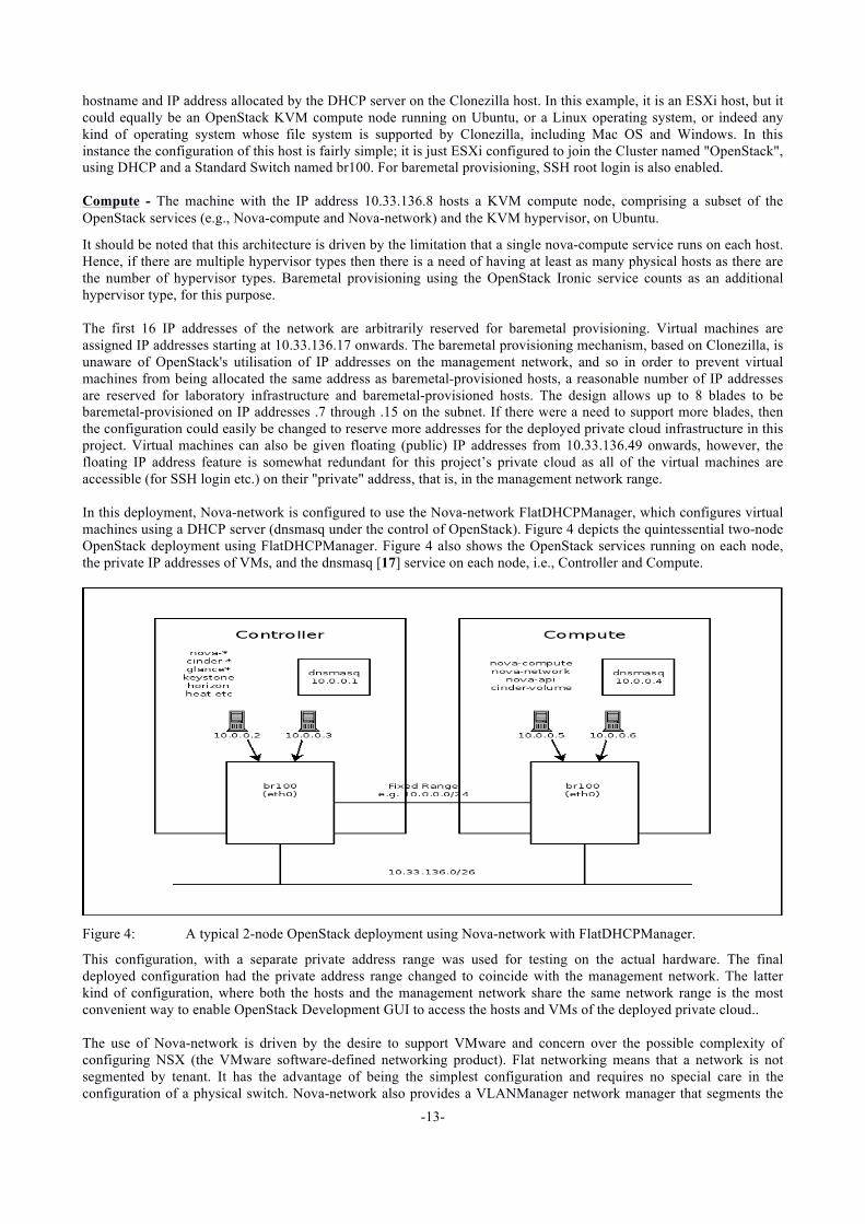
It should be noted that this architecture is driven by the limitation that a single nova-compute service runs on each host. Hence, if there are multiple hypervisor types then there is a need of having at least as many physical hosts as there are the number of hypervisor types. Baremetal provisioning using the OpenStack Ironic service counts as an additional hypervisor type, for this purpose. The first 16 IP addresses of the network are arbitrarily reserved for baremetal provisioning. Virtual machines are assigned IP addresses starting at 10.33.136.17 onwards. The baremetal provisioning mechanism, based on Clonezilla, is unaware of OpenStack's utilisation of IP addresses on the management network, and so in order to prevent virtual machines from being allocated the same address as baremetal-provisioned hosts, a reasonable number of IP addresses are reserved for laboratory infrastructure and baremetal-provisioned hosts. The design allows up to 8 blades to be baremetal-provisioned on IP addresses .7 through .15 on the subnet. If there were a need to support more blades, then the configuration could easily be changed to reserve more addresses for the deployed private cloud infrastructure in this project. Virtual machines can also be given floating (public) IP addresses from 10.33.136.49 onwards, however, the floating IP address feature is somewhat redundant for this project’s private cloud as all of the virtual machines are accessible (for SSH login etc.) on their "private" address, that is, in the management network range. In this deployment, Nova-network is configured to use the Nova-network FlatDHCPManager, which configures virtual machines using a DHCP server (dnsmasq under the control of OpenStack). Figure 4 depicts the quintessential two-node OpenStack deployment using FlatDHCPManager. Figure 4 also shows the OpenStack services running on each node, the private IP addresses of VMs, and the dnsmasq [17] service on each node, i.e., Controller and Compute.

Figure 4: A typical 2-node OpenStack deployment using Nova-network with FlatDHCPManager.

This configuration, with a separate private address range was used for testing on the actual hardware. The final deployed configuration had the private address range changed to coincide with the management network. The latter kind of configuration, where both the hosts and the management network share the same network range is the most convenient way to enable OpenStack Development GUI to access the hosts and VMs of the deployed private cloud.. The use of Nova-network is driven by the desire to support VMware and concern over the possible complexity of configuring NSX (the VMware software-defined networking product). Flat networking means that a network is not segmented by tenant. It has the advantage of being the simplest configuration and requires no special care in the configuration of a physical switch. Nova-network also provides a VLANManager network manager that segments the

-14-

network using VLANs. The default behaviour of Neutron is to isolate different tenants from one another. The VLANs, VXLANs or GRE tunnels can act as the underlying transport [18]. The networking configuration for this project was initially based on Neutron instead of Nova-network [19] as the plan was to use OpenStack's Ironic for baremetal provisioning. However, when it was decided to use Clonezilla instead of Ironic for baremetal provisioning, it was easier to configure Nova-network than Neutron due to a number of issues in connecting to virtual machines when using Neutron. (The details of those issues have been provided in a companion report “Installation and Configuration Guide’s section Neutron Network Configuration". Those problems were, for the most part, due to Neutron tunneling traffic over GRE or VXLANs, which Nova-network's FlatDHCPManager does not do. There can be problems with OpenStack routing to virtual machines when using Nova-network. In our case, the OpenStack API would show the virtual machines with an IP address that actually routed to the hypervisor host of the virtual machine. The virtual machine was inaccessible over the network and an SSH login to the host could be established on what was the virtual machine's address. The problem seemed more pronounced when starting more than one virtual machine at a time using Horizon. It also seemed to be exacerbated by having instances running on both KVM and VMware at the same time. Subsequent virtual machine instances did get allocated usable IP addresses after the problem had manifested. In order to diagnose the problem, the Nova-network configuration was changed so that the private address range of virtual machines did not coincide with the management network. That did not work. Further, in order to simplify the coding of the GUI, the option to allocate a virtual machine a floating (public) IP address on startup was enabled. Virtual machines did receive a floating IP, but it was not visible within the OpenStack API (for example to Horizon or the OpenStack Development GUI); only the floating IPs allocated manually after startup were visible to the API. Consequently, the configuration was reverted to drop automatic allocation of floating IPs and to place the private network on the same CIDR as the management network. There is apparently no mention of these issues on the OpenStack bug tracker. Sometimes instances got stuck during the boot process when their root file system was resized. Instances on VMware are not accessible via SSH until they have received an ICMP ping. Both of these problems appeared to be transient issues when using the master branch of the OpenStack Juno sources. These problems were not observed during the later stages of testing. When using Neutron for networking, the most common practice is to dedicate a physical interface on the network host (the host running the Neutron network service) for providing the public/external (floating) IP addresses of VMs. The OpenStack Configuration Reference [20] requires a minimum of two interfaces for Nova-network although it identifies a Linux virtual switch (br100) to be an interface for this purpose despite the fact that it is not a physical device. The Nova-network can also be configured to utilise a second physical interface to provide publically accessible addresses of VMs. Neutron networking can also be configured to provide a public network using only a single physical interface [21]. However, we were unable to get it working in that configuration, perhaps, because of the other technical problems documented in the Neutron Network Configuration Section of the Volume 2 of this report [22]. It is much easier and more conventional to use two physical interfaces, which for the IBM BladeCenter hardware means eth2 and eth3, and requires two switches, for reasons already discussed. In operation, the management address of the physical interface migrates to br100, which also has the IP address of the dnsmasq (DHCP) server and the address of all virtual machine instances. The physical interface and/or br100 are configured in promiscuous mode in order to be able to respond to traffic destined for the virtual machines. Figure 4 in this report shows the most typical physical interface as eth0. The actual HS22 blade hardware uses the 10Gb interface, eth2, to which the switch module is connected. The details of the configuration have been provided in the "Multi-Node DevStack on IBM HS22 (Type 7870) Blades" Section of the Volume 2 of this report21.

-15-

5. Selection of the OpenStack Distribution In the early stages of the project, various OpenStack distributions suggested in the contract were tried to evaluate their suitability for the project requirements, with particular consideration given to flexibility of baremetal deployment. The selected baremetal deployment mechanism must be sufficient to support a general operating system (Linux), as well as an Ubuntu-based KVM compute node and ESXi host. Rackspace Private Cloud was found to be extremely unreliable to install due to the underlying installation tool, Ansible. The first Ansible script to install OpenStack (there are several) failed repeatedly at various places in the script. Running it again usually moved the failure point forward a little. In addition to these problems, Rackspace technical support advised that a "bespoke" deployment of OpenStack would be the best choice given a broad description of the requirements, rather than being reliant on their distribution. Mirantis looked initially promising. Installation of a virtual test setup under Vagrant is very easy. The package allows definition of an OpenStack environment at a high level, including network settings, allocation of "roles" to hosts and selection of hypervisor type. Fuel defines "roles" to signify a bundle of capabilities, such as the Controller or Compute Nodes in the laboratory. Roles are then baremetal-deployed to discovered machines using a web interface. The deployment model of the Mirantis Fuel found to be too simple to fulfill this project’s requirements:

• A given environment can only support one hypervisor at a time. • According to Mirantis technical support, adapting Fuel to the requirements of the DST project would be very

difficult. • Modification of their underlying baremetal deployment mechanism (Cobbler) would be a significant

undertaking due to the reverse engineering effort involved. • Retrofitting Fuel to use Ironic as a baremetal deployment mechanism would be very difficult due to their use of

custom-built OpenStack packages.

Given these observations with the supposedly more productised OpenStack distributions, it was decided to use DevStack that installs OpenStack from the source code. It is possible to have a very basic DevStack installation of OpenStack in a virtual machine in a few hours, and most of that is the run-time of the installation script. However, non-trivial DevStack configurations will take more time depending on the complexity of the configuration and, by far, most importantly, how long it takes to debug. DevStack (and OpenStack) come with a variety of built-in problems. This report describes the solutions to the DevStack’ problems that were encountered during this project. The potential advantages of DevStack are:

• DevStack's mechanism is relatively simple to understand. It is a shell script. There is no need to learn a DevOps tools like Puppet or Chef (each with its own DSL).

• DevStack provides a simplified view of the OpenStack configuration settings. There are reportedly about 600 of these described in the OpenStack Configuration Reference [20]. Some of those are crucially important and must be configured the same or in harmony on multiple hosts. Others can be safely ignored. DevStack provides a filtered view of the most important of these settings as variables (with names in all capital letters), and this reduces cognitive load when someone tries to come to grips with what is, after all, a large suite of interoperating software programs.

• DevStack's stack.sh embodies expert knowledge about the interrelationship between settings, start order of services, and other interdependencies that determine the ordering of operations in an OpenStack installation. OpenStack beginners get the benefit of that knowledge without the time investment.

• DevStack provides a convenient mechanism for absorbing some of that expert knowledge by generating the underlying OpenStack configuration files, which can then be read.

• DevStack's configuration, local.conf, is small and dense. It delivers a high level understanding of the configuration of a host with little noise. This is compared to the underlying OpenStack configuration files that DevStack generates, where a large number of settings are visible.

• DevStack also acts as a common and well-debugged reference point. There is a large user and support base. All the OpenStack developers use it. Most people who try OpenStack start with DevStack and stay with it until their requirements outgrow it. Together, these points mean that a lot of common questions are already

-16-

answered on the support forums, and this can save debugging time. • DevStack is platform agnostic as it runs on a variety of operating system distributions.

The potential drawbacks of DevStack are:

• DevStack lacks polish. Some extra configuration steps must be taken in order to make OpenStack services restart correctly when a compute node is rebooted. The additional configuration steps have been described in the "Multi-Node DevStack on IBM HS22 (Type 7870) Blades" Section of the Volume 2 of this report [22]. DevStack is somewhat fragile. The OpenStack source trees on the Controller and compute nodes must be updated in lock step, or else it is possible for the DevStack installation script, stack.sh, to fail on compute nodes due to incompatible versions of various APIs.

• DevStack is poorly documented. For example, the relationship between variables in local.conf and the corresponding settings in the OpenStack Configuration Reference [20] is unexplained, except by reading the source code to DevStack. (However, that source code is very well commented.) Working out how to configure particular OpenStack configuration settings generally requires a search through the DevStack source code.

• DevStack provides best support for the most common configuration options. Less common configurations are supported in principle by inserting snippets of OpenStack configuration settings into local.conf. You will have to do this anyway, to resolve some of the more common configuration problems with OpenStack.

-17-

6. Selection of the Baremetal Provisioning Mechanism For baremetal provisioning, it was decided to use OpenStack Ironic that is a part of the OpenStack project (and now included in OpenStack’s new release called Kilo; this project used OpenStack Juno release). Ironic is covered by the OpenStack API abstractions and requires a simpler programming experience. Ironic also supports the Triple-O (OpenStack-On-OpenStack) deployment mechanism. It was discovered that out-of-band (i.e., lanplus protocol) IPMI 2.0 support was a hard requirement for using Ironic that would not have functioned unless it was fully configured with connection details for out-of-band IPMI 2.0. The documentation for the IBM HS22 blades indicates that out-of-band IPMI 2.0 is supported. For example, "Supports highly secure remote power management using IPMI 2.0. [23] " and in describing the IMM: "Intelligent Platform Management Interface (IPMI) 2.0 compliant; Remote power on/power off of a remote blade server" [24]. One IBM customer complained that that they purchased HS22 blades on the basis of these statements and assurances from the salesman, only to find that this was not the case. The true state of out-of-band IPMI support is: "IBM BladeCenter do not have IPMI remote access to the Baseboard Management Controller (BMC) on a Blade (the BMC IP address is not available outside of the BladeCenter). Remonte management can be performed through the BladeCenter Management Module interface [25], which means that the externally exposed interface is a proprietary mechanism that is incompatible with Ironic. Two baremetal deployment mechanisms were evaluated to replace Ironic: Razor and Clonezilla. Razor installs a base operating system from packages using Kickstart or Preseed. It supports Linux and VMware ESXi. Post-configuration of the OS is handled by Puppet. This approach requires additional time for installing the base OS before installing and configuring OpenStack using about the same amount of run-time and I/O as a DevStack installation. The requirement to use Puppet meant that, by the time that it was found necessary to drop Ironic, significant rework would need to be done to express the configuration that had been done by DevStack, and significant time would be spent on mastering Puppet. The Razor documentation states "You must provide an IPMI hostname if you provide either a username or password, since we only support remote, not local, communication with the IPMI target [26]". There is no mention of the use of SSH in any of the Razor documentation, which means Razor may have the same hard requirement on out-of-band IPMI that rules out Ironic. That makes it a high-risk choice. Learning Puppet, particularly for ESXi, can take a significant amount of time. Puppet can be used to provision ESXi. However, it can be a challenge to reproduce an exact ESXi configuration with Puppet as there is insufficient documentation of ESXi configuration files and ESXi command line utilities. Our experimentation with vCenter Server showed that the built-in command line tools were unable to change the IP address of a vCenter Server appliance without either raising an exception or leaving an inoperable system that had to be reinstalled. Clonezilla works with compressed images of hard disks [27], making it similar in principle to the image manipulation features built into Glance [28], an OpenStack project aimed at providing services such as discovering, registering, and retrieving virtual machine images. That means Clonezilla is more similar to Ironic than Razor. Clonezilla works at the disk level, hence, it can support most hardware. It was relatively easy to understand and simple to automate with shell scripts. It did have a few quirks and a flaw specific to the IBM HS22 blade hardware (the disk being too slow to initialise to be discovered by Clonezilla), but that flaw was corrected easily as the source code is included with Clonezilla that made it possible to correct the flaw. When working with ESXi, it was discovered that Clonezilla dropped support for the VMFS V3 and V5 filesystems in December 2014, due to a crash in the vmfs-tools package Clonezilla uses. Without vmfs-tools, raw image of an ESXi host with a 600GB local datastore (hard disk size on the blades) takes 90 minutes; it typically creates 180GB of compressed image data. An easy work around was to remove the local datastore from all ESXi hosts and use an NFS hosted shared datastore, which is recommended practice in any VMware installation. More details about these issues are given in the section "VMware and OpenStack" of this report. Clonezilla can run as a stand-alone CD (Clonezilla Live) or as a Linux system booted over the network using Preboot eXecution Environment (PXE) (Clonezilla SE (Server Edition)). Clonezilla is an extension of Diskless Remote Boot Linux (DRBL), which supports PXE booting of diskless Linux thin clients and booting installer CDs for various Linux distributions. An integrated approach combining both the formal, configuration controlled "configuration-as-program" approach of a DevOps tool like Puppet with an image manipulation tool like Clonezilla (or Ironic) can provide benefits to a production-quality OpenStack environment. That may be more pertinent to a large-scale Cloud infrastructure.

-18-

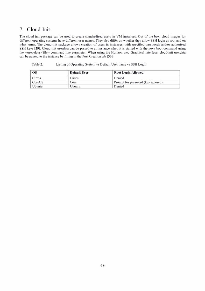
7. Cloud-Init The cloud-init package can be used to create standardised users in VM instances. Out of the box, cloud images for different operating systems have different user names. They also differ on whether they allow SSH login as root and on what terms. The cloud-init package allows creation of users in instances, with specified passwords and/or authorised SSH keys [29]. Cloud-init userdata can be passed to an instance when it is started with the nova boot command using the --user-data <file> command line parameter. When using the Horizon web Graphical interface, cloud-init userdata can be passed to the instance by filling in the Post Creation tab [30].

Table 2: Listing of Operating System vs Default User name vs SSH Login

OS Default User Root Login Allowed Cirros Cirros Denied CoreOS Core Prompt for password (key ignored) Ubuntu Ubuntu Denied

-19-

8. VMware and OpenStack The OpenStack VMware vCenter driver supports vSphere version 4.1 onwards. VMware vSphere versions 5.1 and later require fewer configuration steps than version 5.0 or earlier. At the time of this work, the latest version of vSphere was 6.0 and has been available for just over a month. The most recent OpenStack development will have been done against 5.5. Therefore, there is less risk of new defects (bugs and incompatibilities) being encountered by using ESXi 5.5. ESXi was much easier to install than OpenStack. The most difficult and time-consuming part of the installation was to setup an interface between OpenStack and VMware. The configuration challenges were mainly caused because some parts of the OpenStack documentation were outdated. For example, the OpenStack Configuration Reference document stipulates that ephemeral port binding should be used with the port group to which all VM NICs are attached (implying a vNetwork Distributed Switch (vDS) must be used, since it is apparently not a Standard Switch (SS) option), but is otherwise silent on whether a SS or vDS should be used. In practice, a Standard Switch works fine and is much simpler than trying to migrate the ESXi host's management network to a vDS. Such a process is complicated by the fact that the VM kernel port (vmk0) and the vCenter Server VM are using the Standard Switch. The latter point means that migration cannot trivially use the vSphere Web Client, since the vCenter Server loses connectivity during migration. The network recovery options in the ESXi host console do not help in this regard. It is possible to use Host Profiles from the vSphere Web Client. Changing the IP address of a vCenter Server appliance is non-trivial. The installer states that the IPv4 configuration of “nic0 cannot be edited post deployment”. There is a general requirement to be able to do that from time to time (e.g., changing datacenters) and, accordingly, there are several suggestions online for ways to do it. However, an attempt to run vami_set_network over SSH to vCenter Server rendered the appliance useless. The best option to change the IP address may be just to reinstall vCenter Server from scratch. The vSphere Web Client requires a later version of Adobe Flash than is supported on Linux, as well as the VMware Client Integration Plug-in, which necessitated the use of a Windows virtual machine, although Macs are also supported. At times, shutting down a virtual machine running under ESXi with a GPU attached by PCI pass-through would crash the ESXi host (eliciting the "Purple Screen of Death"). This may have been due to the VM in question having been originally cloned while shut down with an attached GPU. The original cloning operation crashed the host as well.

-20-

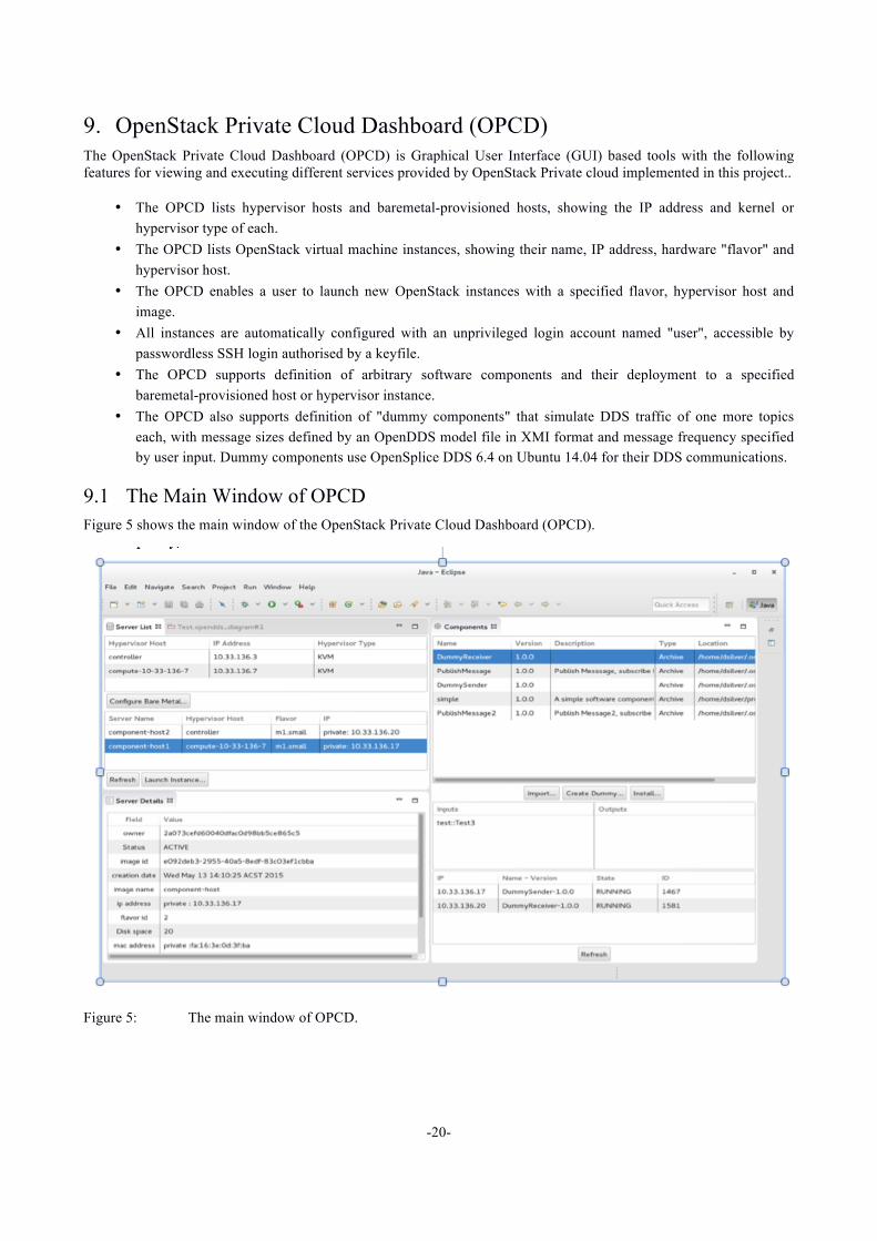
9. OpenStack Private Cloud Dashboard (OPCD) The OpenStack Private Cloud Dashboard (OPCD) is Graphical User Interface (GUI) based tools with the following features for viewing and executing different services provided by OpenStack Private cloud implemented in this project..

• The OPCD lists hypervisor hosts and baremetal-provisioned hosts, showing the IP address and kernel or hypervisor type of each.

• The OPCD lists OpenStack virtual machine instances, showing their name, IP address, hardware "flavor" and hypervisor host.

• The OPCD enables a user to launch new OpenStack instances with a specified flavor, hypervisor host and image.

• All instances are automatically configured with an unprivileged login account named "user", accessible by passwordless SSH login authorised by a keyfile.

• The OPCD supports definition of arbitrary software components and their deployment to a specified baremetal-provisioned host or hypervisor instance.

• The OPCD also supports definition of "dummy components" that simulate DDS traffic of one more topics each, with message sizes defined by an OpenDDS model file in XMI format and message frequency specified by user input. Dummy components use OpenSplice DDS 6.4 on Ubuntu 14.04 for their DDS communications.

9.1 The Main Window of OPCD Figure 5 shows the main window of the OpenStack Private Cloud Dashboard (OPCD).

Figure 5: The main window of OPCD.

-21-

Conceptually, the main window of the OPCD is laid out as depicted in Figure 6.

Figure 6: The conceptual layout of the OPCD main window.

As can be seen in the diagram, the various parts of the OPCD are viewed within the Eclipse main window.

-22-

A conceptual overview of other dialogs that are directly accessible from the main window by button clicks is shown in Figure 7.

Figure 7: A conceptual view of the different dialogs accessible from the main window.

-23-

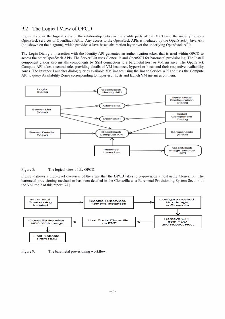
9.2 The Logical View of OPCD Figure 8 shows the logical view of the relationship between the visible parts of the OPCD and the underlying non-OpenStack services or OpenStack APIs. Any access to the OpenStack APIs is mediated by the OpenStack4j Java API (not shown on the diagram), which provides a Java-based abstraction layer over the underlying OpenStack APIs. The Login Dialog’s interaction with the Identity API generates an authentication token that is used within OPCD to access the other OpenStack APIs. The Server List uses Clonezilla and OpenSSH for baremetal provisioning. The Install component dialog also installs components by SSH connection to a baremetal host or VM instance. The OpenStack Compute API takes a central role, providing details of VM instances, hypervisor hosts and their respective availability zones. The Instance Launcher dialog queries available VM images using the Image Service API and uses the Compute API to query Availability Zones corresponding to hypervisor hosts and launch VM instances on them.

Figure 8: The logical view of the OPCD.

Figure 9 shows a high-level overview of the steps that the OPCD takes to re-provision a host using Clonezilla. The baremetal provisioning mechanism has been detailed in the Clonezilla as a Baremetal Provisioning System Section of the Volume 2 of this report [22]..

Figure 9: The baremetal provisioning workflow.

-24-

9.3 Component Operations Flow Charts Figure 10 shows how to install, uninstall, and check the status of the components in OPCD. The status information includes what components are installed and whether they are RUNNING, PAUSED or STOPPED, or if they are meant to be running but have crashed (status FAILED). The current status of all the installed components on a particular physical or virtual machine is stored as a set of PID files under /opt/components/archive/run/. In order for a component to run on a baremetal host or VM instance, the component infrastructure must be installed on that machine. For more information about the necessary infrastructure, see the Component Hosts Section of the Volume 2 of this report [22]. The OPCD uses SSH to run a Component status script on all physical and virtual machines currently active within the environment. If the script succeeds, it shows status information about all installed Components. If it fails, the OPCD deems that the host does not have the necessary infrastructure installed. The OPCD helps install and uninstall components over an SSH connection to the physical or virtual machine.

Figure 10: The flowcharts of the component operations.

9.4 The Login Dialog The login dialog appears once the Refresh button on the Server List view is pressed. A user needs to login to OpenStack Identity service in order to populate the different tables viewable from OPCD. The login dialog is shown in Figure 11.

Figure 11: The login dialog for the OPCD

The Endpoint URL includes the IP address of the Controller (10.33.136.3). The user should be "admin" in order for placement of virtual machine instances on specific hypervisors to work correctly and the Tenant (project name) should be that of an existing project, e.g. "demo". The login credentials are currently stored in clear text in configuration/.settings/osgui.prefs under the Eclipse

-25-

installation directory. The security of the credentials relies on this file being protected by the user's desktop login access restrictions. If separate users both want to access different OpenStack infrastructures, then they should use separate desktop login accounts rather than sharing a login.

9.5 The Baremetal Provisioning Configuration Dialog Before using the OPCD to provision baremetal, it is necessary to configure the OPCD with the same settings that are embodied in the Clonezilla installation. To show the Bare Metal Configuration dialog, press the Configure Bare Metal... button on the Server List view. The OPCD pre-configured with default settings that match the installation done during the project at the University of Adelaide. The settings are:

• Subnet CIDR: the CIDR of the combined management/private/public subnet. • Start Octet: the lowest final octet of any IP address allocated by the Clonezilla DHCP server. In the image

above, that address would be 10.33.136.7. This and subsequent addresses are allocated to baremetal kernels or hypervisor hosts as the hardware is reallocated by the baremetal provisioning mechanism.

• Hostname Prefix: this is the start of the hostname automatically assigned by the Clonezilla DHCP server. The blade at 10.33.136.7 is assigned hostname compute-10-33-136-7 by the DHCP server.

• Host MACs: this is a list of MAC addresses of network interfaces - one for each blade to be allocated by the DHCP server. As with all the other settings, this must match the corresponding setting in the Clonezilla installation.

• Clonezilla Server: this is the IP address of the host that runs the Clonezilla services. • OpenStack Controller: this is the IP address of the OpenStack Controller host. • Reserved Host: this is a list of IP addresses that should be protected from baremetal provisioning in the event

that the DHCP Start Octet is set such that they could be affected. It is an additional protection against accidental reprovisioning of key infrastructure hosts.

The Save button saves these settings and also forces a shutdown of Eclipse in order to guarantee that the OPCD runs with correct baremetal settings.

9.6 The Server List The Server List view consists of:

• A table of hypervisor hosts and baremetal-allocated hosts in the top half of the view, with their IP address and hypervisor type (unassigned, KVM, ESXi or Linux for a baremetal Linux installation with no hypervisor).

• A table of OpenStack instances (denoted "Servers") in the bottom half of the view, showing each instance's name, hypervisor host name, hardware flavor and IP address.

The tables of hypervisors and instances are separated by an adjustable splitter control, allowing the relative sizes of the tables to be adjusted. The Refresh button updates the list of instances to reflect what is currently running. It also brings up the Login dialog if a connection has not yet been made with the Identity Service.

-26-

9.7 Booting a Virtual Machine Instance The Launch Instance button on OPCD brings up the Instance Launcher dialog as shown in Figure 12. This dialog box accepts settings required to launch a new virtual machine instance.

Figure 12: the Launch Instance Dialog

In order to start a virtual machine instance, a user needs to specify an instance name, used within the instance as the hostname. The new instance's IP address will be automatically allocated. For the flavor (spelt according to the OpenStack documentation), you will generally want to specify at least m1.small in order to start a typical Linux guest operating system. The flavors are as defined in the OpenStack documentation. Some of the smaller flavors lack sufficient disk space to start a fully-fledged Linux system. Two custom flavors are also provided; m1.small.1-gpu and m1.small.2-gpu are identical to the m1.small flavor except that they also provide 1 or 2 (respectively) Tesla M2070 GPUs attached to the hypervisor host and passed to the instance by PCI passthrough. Note that the other requirements for PCI passthrough must also be met; in particular VT-d must be enabled in the UEFI configuration. During the performance benchmarking, the HS22 blades would lock up under high I/O load, typically during network performance benchmarks. Disabling VT-d was able to reliably fix this problem. The blades would also sometimes spontaneously hang if left running overnight with VT-d enabled – even under conditions of low system load. Recovering from these crashes was usually time-consuming. At the very least, the file system needed to be checked and repaired. If the Clonezilla host (which exports the NFSDatastore used by all VMware ESXi hosts) crashed in this way, all VMware-related infrastructure needed to be restarted and checked. Therefore, it therefore became customary to leave VT-d disabled unless required, and to check that it was enabled before any use. The Instance Zone option in the Instance Launcher allows the instance to be created in a specific Availability Zone. In OpenStack, Host Aggregates are groups of hosts (hypervisors) with associated metadata. A host can be in more than one aggregate. The host aggregates are only visible to administrators, but they can be exposed to OpenStack users in the form of an Availability Zone. The OPCD maintains a distinct Host Aggregate for each hypervisor host, named the same as the hypervisor host name. It also configures an Availability Zone for each Host Aggregate, with the same name. That is, for example, the KVM hypervisor compute-10-33-136-7 has a corresponding Host Aggregate called compute-10-33-136-7 and an Availability Zone with the same name. And a similar statement applies to the controller and vmware-compute-node, which controls the VMware cluster integrated in this OpenStack Deployment. Since each Availability Zone contains only a single hypervisor host, selecting the zone explicitly allocates the instance to a particular hypervisor. The OpenStack API contains no more direct way of achieving this end. The option "Any Availability Zone" allows the OpenStack scheduler to choose where to allocate the instance, based on the current load of each host. The Instance Image setting allows selection of the disk image used to boot the instance. In order to start instances in a VMware vCenter cluster, a user must select an image that has been specifically prepared with VMware in mind, in a VMware-supported format. OpenStack specifies a variety of requirements on guest operating system images, including that the root file system must be resizable and that cloud-init package is installed so that a user account and SSH key can be injected into the instance. The images listed in OPCD are those that were loaded into the OpenStack Image Service (Glance). The images include:

• "Ubuntu 14.04 - 64-bit" - A standard Ubuntu cloud image. As stated previously, most general Linux images require at least the m1.small flavor to boot.

• "Ubuntu 14.04 - 64-bit - VMware" - The same image, converted to VMware format and tagged for use on that

-27-

hypervisor. • "CirrOS 0.3.3 - 64-bit" - A minimal Linux variant that can be useful for testing. It will start even on the

m1.nano flavor. • "CirrOS 0.3.3 - 64-bit - VMware" - The VMware version of the CirrOS image. • "component-host" - A snapshot of an Ubuntu 14.04 m1.small instance running on KVM, with all of the

software needed to run components pre-installed. In order to install a component on an instance, the instance must be running an image with the supporting software installed. When booting this image, specify the m1.small flavor.

• "vmware-component-host" - This is the same as the "component-host" image, except that the instance will start on a VMware hypervisor.

• "ubuntu-kvm-2-gpu" - This is a snapshot of an Ubuntu 14.04 m1.small instance running on KVM. In addition, NVIDIA CUDA 7 has been installed to test PCI passthrough. Boot this instance with the m1.small.1-gpu or m1.small.2-gpu flavor. If you use the m1.small flavor, the instance will have no attached PCI passthrough device. Note, as previously mentioned, that other requirements for PCI passthrough may need to be verified, particularly enabling VT-d in the UEFI configuration. If all requirements are met, lspci run in the instance will show one or two Tesla M2070 GPUs, as configured by the flavor.

9.8 Terminating a Virtual Machine Instance To destroy a virtual machine instance, select it in the table, right click on it and select "Terminate Instance" from the context menu.

9.9 Bare Metal Provisioning of a Host To re-provision a hypervisor host right click on the host in the table of Hypervisor Hosts and select the bare metal image to install from the context menu displayed. Note that the Controller cannot be reprovisioned. The images are:

• "devstack-ubuntu-4-nics" - An installation of OpenStack using DevStack configured to run the KVM hypervisor, on Ubuntu 14.04. The host expects 4 network interfaces, with the management interface on the third of these, eth2.

• "ubuntu-component-host-4-nics" - Ubuntu 14.04 plus all of the supporting software necessary to run software components on a bare metal host instead of a virtual machine instance.

• "esxi-slave-4-nics" - A VMware ESXi hypervisor host, configured as a slave of the OpenStack cluster. Note that for VMware virtual machine instances to be started, the ESXi master host and the infrastructure virtual machines running under it (vCenter Server and vmware-nova-compute) must be powered on.

• "centos-7-4-nic" - A CentOS 7 installation on bare metal.

Installation of a baremetal image typically takes on the order of 10-12 minutes. The first 7 minutes of this are spent waiting for Unified Extensible Firmware Interface (UEFI) initialisation to complete and for PXE boot to start. The progress of baremetal provisioning by Clonezilla can be observed through the IBM Advanced Management Module (AMM) remote control web interface, used to view the console of the blade.

9.10 Server Details The Server Details view shows the attributes of the currently selected instance.

9.11 The Components View The Components view contains a list of known component types in the upper section, with lists of input and output message types (topics) for the currently selected component type. Each component type has a name, version number, optional description and type, signifying how it is installed on a host. The lower section of the view lists installed components, showing the IP address, the identifier of the component (in the form name-version), the state of the component (RUNNING, PAUSED, STOPPED or FAILED if it stops unexpectedly) and the ID of the running component, which is its process ID. A component consists of a JAR archive containing a manifest that describes the inputs and outputs, and commands to start, stop, pause, install and uninstall the component. The component archive also contains any other files that should be installed on the host to make the component run.

-28-

The OPCD will only install components on baremetal hosts and virtual machines that have the necessary runtime infrastructure, consisting of OpenSplice DDS 6.4, basic development tools and some supporting scripts installed under /opt/components/archive/. These machines are known as "Component Hosts"; for details see the Component Hosts Section of the Volume 2 of this report [22]. The OPCD installs components by unpacking the component's JAR file under /opt/components/ and running the install command specified in the component's manifest. Each component has an identifier based on its name and version number, e.g. PublishMessage-1.0.0, and the installation directory is named after this identifier, e.g. /opt/components/PublishMessage-1.0.0/. Uninstallation consists of stopping the component from running using the component's stop command, then running its uninstall command, and finally removing the subdirectory where all the component's files were installed. All commands to install, uninstall, start, stop, pause and monitor the state of components are run over an SSH connection to the Component Host as a standard user called "user". The Dummy Components have additional manifest fields that describe the names, sizes in bytes and frequency of publication of DDS messages. Their JAR archive contains a C++ binary that publishes and subscribes to DDS messages to simulate the traffic described in the manifest. Due to the overhead of header fields in these DDS messages, the minimum effective size of a DDS message is about 128 bytes, even if the message is defined as smaller than that number. Although originally started in Java, Dummy Components were eventually written in C++ because the OpenSplice DDS 6.4 Java API crashes due to an incompatible glibc version. OpenSplice DDS 6.4 CE was compiled for Ubuntu 12.04 (glibc 2.15) whereas Ubuntu 14.04 uses glibc 2.19. This causes a crash in Java JNI callbacks in the OpenSplice DDS Java API. PrismTech does offer a one-month trial of their full OpenSplice product which may provide a workaround for the problem. However, it was not evaluated since the license duration is not sufficient to cover the full duration of the project. OpenDDS was also evaluated for its Java API, but the OpenDDS installation process (make) fails to generate IDL for core DDS classes (Topic, DomainParticipant) and so the OpenDDS Java API could not be built. Given that the OpenSplice DDS C++ API was much simpler to install and smaller than OpenDDS, the former was the preferred option. The Dummy components log sent and received messages to /opt/component/<identifier>/log/log.txt. For received messages, the component identifier, process ID and IP address of the sending component are shown, as well as the message type, a sequence number and the size of the message in bytes. For sent messages, the log contains the identifier of the sending component, the component's process ID, the local IP address, the message type and a sequence number. An example of actual log contents follows: Table 3: An example Component Log output. 2015-05-13 10:35:43.682 Received Message from PublishMessage-1.0.0 (1877 at 10.33.136.17) seq 31 size 290 2015-05-13 10:35:43.979 PublishMessage2-1.0.0 3600 at 10.33.136.20 publishing Message2 seq 48 2015-05-13 10:35:44.479 PublishMessage2-1.0.0 3600 at 10.33.136.20 publishing Message2 seq 49 2015-05-13 10:35:44.682 Received Message from PublishMessage-1.0.0 (1877 at 10.33.136.17) seq 32 size 290 2015-05-13 10:35:44.979 PublishMessage2-1.0.0 3600 at 10.33.136.20 publishing Message2 seq 50 2015-05-13 10:35:45.479 PublishMessage2-1.0.0 3600 at 10.33.136.20 publishing Message2 seq 51

9.11.1 Importing a Pre-Defined Component The delivered software contains an example "simple" software component that does not do any DDS publication or subscription, but serves to illustrate the basic mechanisms. To register this component type in OPCD, click the "Import..." button on the Components view, browse to ~/.osd/components/ and select simple.jar.

9.11.2 Removing a Component The definition of a component type can be removed by right clicking on the component type in the upper part of the Components view and selecting Remove from the context menu popup.

9.11.3 Defining a Dummy Component Type To define a new dummy component type, click "Create Dummy..." on the Components view. The New Dummy Component dialog will appear as shown in Figure 13.

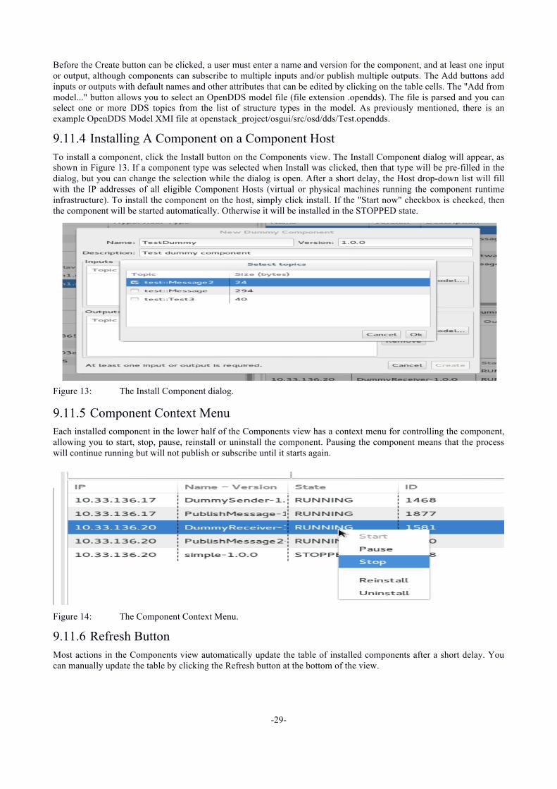
-29-

Before the Create button can be clicked, a user must enter a name and version for the component, and at least one input or output, although components can subscribe to multiple inputs and/or publish multiple outputs. The Add buttons add inputs or outputs with default names and other attributes that can be edited by clicking on the table cells. The "Add from model..." button allows you to select an OpenDDS model file (file extension .opendds). The file is parsed and you can select one or more DDS topics from the list of structure types in the model. As previously mentioned, there is an example OpenDDS Model XMI file at openstack_project/osgui/src/osd/dds/Test.opendds.

9.11.4 Installing A Component on a Component Host To install a component, click the Install button on the Components view. The Install Component dialog will appear, as shown in Figure 13. If a component type was selected when Install was clicked, then that type will be pre-filled in the dialog, but you can change the selection while the dialog is open. After a short delay, the Host drop-down list will fill with the IP addresses of all eligible Component Hosts (virtual or physical machines running the component runtime infrastructure). To install the component on the host, simply click install. If the "Start now" checkbox is checked, then the component will be started automatically. Otherwise it will be installed in the STOPPED state.

Figure 13: The Install Component dialog.

9.11.5 Component Context Menu Each installed component in the lower half of the Components view has a context menu for controlling the component, allowing you to start, stop, pause, reinstall or uninstall the component. Pausing the component means that the process will continue running but will not publish or subscribe until it starts again.

Figure 14: The Component Context Menu.

9.11.6 Refresh Button Most actions in the Components view automatically update the table of installed components after a short delay. You can manually update the table by clicking the Refresh button at the bottom of the view.

-30-

10. PCI Passthrough PCI passthrough provides the highest possible performance for accessing a GPU from within a virtual machine. DST showed an interest in PCI passthrough. It requires hardware support on the host and there are limitations on hypervisor type when used in an OpenStack environment (discussed below). For completeness, the other commonly used option to access a GPU from within a VM is known as API remoting, where the GPGPU API is split into front-end and back-end components. The front-end runs in the VM and emulates the GPGPU API. It communicates requests and results with the back-end, via shared memory or a network interface. Bandwidth between the front-end and back-end can be a significant determining factor in the efficacy of this technique. We also consulted the work by Walters and his colleagues from University of Southern California and Indiana University on GPU Passthrough Performance comparison of multiple hyperivsors [31].

10.1 Findings on PCI Passthrough PCI passthrough performance could not be tested. All the configuration requirements to make the Tesla M2070 GPUs visible to virtual machine instances were met. The PCI devices corresponding to the passed through GPUs were detected by the Linux kernel of VM instances and device nodes created by the operating system accordingly. But NVIDIA CUDA test programs were unable to function correctly with these devices. The same tests functioned correctly under Linux installed directly to the host, rather than a VM. More information on the procedures used to test and debug PCI passthrough and the relevant sources can be found in the Volume 2 of this report [22]. The general expectation with PCI passthrough devices in VMs is that:

• They perform at native speed. • They have access to the full native feature set. • No custom drivers are required (unlike API remoting).

The typically cited downsides of PCI passthrough of GPUs are that:

• You must install hardware specific drivers in VMs. • You lose the ability to snapshot and migrate VMs, since the GPUs can't be hotplugged. • The GPUs cannot be shared with other VMs or the host.

There are technologies that do allow sharing of PCI passthrough devices, such as Single Root I/O Virtualisation (SR-IOV) and Multi-Root I/O Virtualisation (MR-IOV). However, according to the Xen website, nobody has attempted SR-IOV of GPUs yet due to the complexity [32]. NVIDIA's GRID GPUs, designed for Virtual Desktop Infrastructure (VDI) supports PCI passthrough, but fine grained subdivision of the device for sharing between large numbers of VMs is handled using a proprietary technology called NVIDIA GRID vGPU (also known as VGX), which is available for several hypervisors, including Xen and VMware. Selection of PCI passthrough GPU hardware should take into account whether coarse-grained allocation of a whole GPU to a host will suffice or whether the workload should be more finely divided among a large number of VMs with modest GPU requirements, as is the case with GRID GPUs. Note that in the case of non-GRID GPUs, NVIDIA provides a Multi-Process Service [33] (MPS) implementation of the CUDA API to access Hyper-Q [34] capabilities on contemporary GPUs, thereby enabling up to 32 simultaneous connections to a single GPU from threads or processes, greatly increasing its potential utilisation. On the DST-provided HS22 blades, enabling VT-d made the hosts susceptible to complete lock-ups where the only possible recovery action was a reboot. This is apparently a known issue with VT-d on the HS22s. The problem seems to be exacerbated by high load, such as that experienced when running benchmarks.

-31-

10.2 GPGPU Benchmarking The Livermore Unstructured Lagrangian Explicit Shock Hydrodynamics (LULESH) [35] hydrodynamics simulation was considered as a potential GPGPU benchmark. However, that benchmark is coded using Open Accelerators [36] (ACC) and the supplied Makefile is for the proprietary PGI [37] pgcc compiler. A 15 day trial evaluation of the PGI compiler is available, but it is node-locked to a single hostid (MAC address), which makes it extremely unwieldy to use for baremetal and multiple virtual machines. GCC 5 supports OpenACC, but at the time of writing there was no release. The gcc-5-branch of the GCC sources was checked out of the GNU Subversion repository, but failed to build correctly. The Phoronix Test Suite [38] includes a number of Open Computing Language [39] (OpenCL) benchmarks, including ViennaCL, which looked promising. Installation was easy, but OpenCL only detected the Matrox display hardware for the blade consoles and there was apparently no documented way to configure OpenCL to use the Tesla M2070 GPUs instead. The only installed .icd file referenced the NVIDIA driver, but that was not sufficient to prevent OpenCL from using the wrong device. NVIDIA's CUDA 7 was the GPGPU framework that showed most promise. Roy Longbottom's reasonably well-known CUDA Mflops benchmark [40] was selected to exercise the API. The approach taken was to first establish baseline measurements of single and double precision Mflops using 64-bit binaries on a physical Ubuntu 14.04 host. And then to repeat those measurements on virtual machines under KVM and ESXi. The NVIDIA CUDA 7 sample program bandwidthTest was also used to measure transfer speed to between the host and GPU memories.

10.3 Benchmark Results The benchmark logs for the single precision, double precision, and the bandwidth test runs can be found in the Appendices according to the following sequence.

• Results for Roy Longbottom's CUDA Mflops benchmarks in single and double precision. • Results for the CUDA bandwidthTest example sample.

The key results are presented in Table 4 and 5 below. Table 4: Roy Longbottom CUDA MFLOPs benchmark results. Test Name Minimum GFLOPS Maximum GFLOPS Single Precision 10.665 354.17 Double Precision 8.155 139.483

Table 4 shows that while the minimum performance for single and double precision calculations are fairly similar. The maximum achieved performance is significantly different with single precision generating about 2.5x the performance of the double precision tests.

Table 5: CUDA bandwidth test results

Test Type Data Size (MB) Bandwidth (MB/s)

Host to device copy 33554432 5868.9

Device to host copy 33554432 6375.2

Device to device copy 33554432 105075.8

Table 5 shows that data copying from device to device achieves the best performance, and any data transfer between host and device causes a significant performance decrease. This implies that applications should attempt to minimize the amount of transfer between devices and hosts as much as they can.

-32-

11. Hypervisor Suitability Comparison The suitability of hypervisors under OpenStack for different roles in a combat system environment can be compared both qualitative and quantitatively. In qualitative terms, the limitations of the specific hypervisor implementations can rule out their use for some roles. For example, at the time of writing, only a patched version of Xen (RT-Xen) provides real-time scheduling guarantees on virtual machine instances, which rules out KVM and VMware for real-time use. We report more will be said about real-time scheduling of instances in a later section. Standard system benchmarks can quantify the performance of various subsytems (CPU, RAM, network, disk) within a virtual machine instance relative to the host. The relative merits of these metrics may warrant the use of a specific hypervisor for a particular task.

11.1 Benchmark Methodology We chose the Phoronix Test Suite for the majority of benchmarks to compare performance among hypervisors. The Phoronix Test Suite is a cross-platform, free and open source software suite for measuring system performance in a reproducible manner. It aggregates a large number of well-known benchmarks from multiple sources under one common user interface. To ensure the veracity of the tests, it also monitors the standard deviation of the results and automatically schedules additional runs if the standard deviation exceeds 3.5%. The selected benchmarks were:

• for CPU performance: scimark2 from Phoronix Test Suite, • for RAM performance: ramspeed from Phoronix Test Suite, • for disk performance: fio and compress-gzip from Phoronix Test Suite, • for network performance: iperf, run with a custom script, • and for interrupt latency: Cyclictest, also run with a custom script.

Figure 15: The logical view of the benchmark suite.

Each of these benchmarks is discussed in greater detail in subsequent sections.

11.2 Performance Tuning Performance tuning of the system is an essentially open-ended, iterative process where the system settings are adjusted to give an optimal metric of a selected real-world load or benchmark. As such, it could take an arbitrarily long time to obtain the best possible result for any given benchmark or load under a given hypervisor. For the purposes of this investigation, default system settings will be used in most cases, except where it is obvious that the baremetal performance is sub-par. For consistency all of the benchmarks were run on Ubuntu 14.04 Linux with an updated 3.13.0 kernel version installed.

11.3 Other Benchmark Conditions Hypervisor benchmarks were performed on a host that was otherwise quiescent, apart from the single virtual machine instance under test. Benchmarks were run for sufficient time to ensure that the startup time of the application was negligible. In the case of TCP benchmarks, the effect of TCP Slow Start was also considered negligible over the duration of the 60 second run. All benchmarks were run as the root user. Virtual machines were given the m1.small flavor: 1 Virtual CPU (vCPU), 2GB RAM, 20GB HDD. Raw result text files were checked into configuration management under

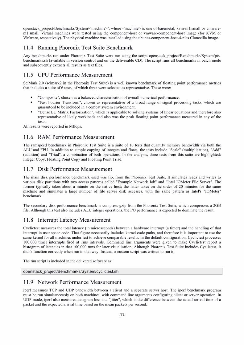
-33-

openstack_project/Benchmarks/System/<machine>/, where <machine> is one of baremetal, kvm-m1.small or vmware-m1.small. Virtual machines were tested using the component-host or vmware-component-host image (for KVM or VMware, respectively). The physical machine was installed using the ubuntu-component-host-4-nics Clonezilla image.

11.4 Running Phoronix Test Suite Benchmark Any benchmarks run under Phoronix Test Suite were run using the script openstack_project/Benchmarks/System/pts-benchmarks.sh (available in version control and on the deliverable CD). The script runs all benchmarks in batch mode and subsequently extracts all results as text files.

11.5 CPU Performance Measurement SciMark 2.0 (scimark2 in the Phoronix Test Suite) is a well known benchmark of floating point performance metrics that includes a suite of 6 tests, of which three were selected as representative. These were:

• "Composite", chosen as a balanced characterisation of overall numerical performance, • "Fast Fourier Transform", chosen as representative of a broad range of signal processing tasks, which are

guaranteed to be included in a combat system environment, • "Dense LU Matrix Factorization", which is applicable to solving systems of linear equations and therefore also

representative of likely workloads and also was the peak floating point performance measured in any of the tests.

All results were reported in Mflops.

11.6 RAM Performance Measurement The ramspeed benchmark in Phoronix Test Suite is a suite of 10 tests that quantify memory bandwidth via both the ALU and FPU. In addition to simple copying of integers and floats, the tests include "Scale" (multiplication), "Add" (addition) and "Triad", a combination of both operations. In the analysis, three tests from this suite are highlighted: Integer Copy, Floating Point Copy and Floating Point Triad.

11.7 Disk Performance Measurement The main disk performance benchmark used was fio, from the Phoronix Test Suite. It simulates reads and writes to various disk partitions with two access patterns called "Example Network Job" and "Intel IOMeter File Server". The former typically takes about a minute on the native host; the latter takes on the order of 20 minutes for the same machine and simulates a large number of file server disk accesses, with the same pattern as Intel's "IOMeter" benchmark. The secondary disk performance benchmark is compress-gzip from the Phoronix Test Suite, which compresses a 2GB file. Although this test also includes ALU integer operations, the I/O performance is expected to dominate the result.

11.8 Interrupt Latency Measurement Cyclictest measures the total latency (in microseconds) between a hardware interrupt (a timer) and the handling of that interrupt in user space code. That figure necessarily includes kernel code paths, and therefore it is important to use the same kernel for all machines under test to achieve comparable results. In the default configuration, Cyclictest processes 100,000 timer interrupts fired at 1ms intervals. Command line arguments were given to make Cyclictest report a histogram of latencies in that 100,000 runs for later visualisation. Although Phoronix Test Suite includes Cyclictest, it didn't function correctly when run in that way. Instead, a custom script was written to run it. The run script is included in the delivered software as: openstack_project/Benchmarks/System/cyclictest.sh

11.9 Network Performance Measurement iperf measures TCP and UDP bandwidth between a client and a separate server host. The iperf benchmark program must be run simultaneously on both machines, with command line arguments configuring client or server operation. In UDP mode, iperf also measures datagram loss and "jitter", which is the difference between the actual arrival time of a packet and the expected arrival time based on the mean packets per second.

-34-

The Clonezilla host was chosen to run the server side of iperf benchmarks, since it meets the requirements for hosts under test (Ubuntu 14.04, 3.13.0 kernel), is lightly loaded when not being used to do baremetal provisioning and delivers the full native networking performance without the overhead of a hypervisor. iperf command line arguments were set to show results at 10 second intervals as well as the final average after 60 seconds. The standard deviation of the intervals was checked to ensure that it was less than 3.5% of the mean. In order to enable TCP and UDP communication between the iperf server on the Clonezilla host and virtual machine instances, two additional access (firewall) rules were configured within OpenStack Horizon, for the demo tenant. These were added to the default security group. The rules were:

• Ingress, port 5001/TCP, address 0.0.0.0/0 (i.e. any). • Ingress, port 5001/UDP, address 0.0.0.0/0 (i.e. any).

11.9.1 Pre-Benchmark Tuning Initial benchmark results showed that with default settings on baremetal, the physical machine was unable to achieve even 10% of the capacity of the 10Gb/s interface in UDP. The UDP bandwidth was about 810Mb/s. Above 2Gb/s, the error rate gradually increased to tens of percentage points such that the overall bandwidth was even less. Virtual machine results reflected this limitation of the host by showing essentially identical performance. Based on the recommendation of a European project, DataTag, both the host and the VMs were tuned in the following ways to get more meaningful results [41].

• Receive and send buffer sizes were increased by about a factor of 10:

sysctl -w net.core.rmem_max=26214400 sysctl -w net.core.wmem_max=26214400

• The transmit queue size for the network interface was increased: ifconfig eth2 txqueuelen 2000

• The receive buffer size and UDP packet size were increased accordingly by adding the following arguments to the iperf command line:

--window 25M --len 32768 Of these two arguments, the more important by far is the --len setting which sends much larger UDP packets than the default (1470 bytes).

-35-

11.9.2 Benchmark Results The raw results from the various tests are shown in the Table below:

Table 6: Raw performance benchmark results.

Benchmark Test Units Baremetal KVM VMware compress-gzip 2GB File Compression sec 15.36 21.44 31.26 fio Example Network Job sec 56.66 87.72 55.28 fio Intel IOMeter Pattern sec 1100.86 1958.34 5071.22 SciMark2 Composite Mflops 983.15 920.58 939.66 SciMark2 FFT Mflops 195.31 187.11 184.84 SciMark2 Dense LU Matrix Fact. Mflops 1795.65 1619.49 1644 RAMspeed Integer Copy MB/s 18906.66 9224.36 9224.58 RAMspeed Floating Point Copy MB/s 17209.77 8423.5 8178.54 RAMspeed Floating Point Triad MB/s 19562.5 9355.87 9179.66 cyclictest Min Latency µs 4 17 3 cyclictest Avg Latency µs 6 76 13 cyclictest Max Latency µs 15 1714 6961 iperf TCP bandwidth Gb/s 9.41 9.39 9.36 iperf UDP bandwidth Gb/s 9.49 7.7 6.19 iperf UDP datagram loss % 0.0074 0 0.0029 iperf UDP jitter ms 0.022 0.034 0.041

Note that iperf uses G to denote 10243, not 109. Similarly, the RAMspeed benchmark uses MB to signify

10242 bytes.

-36-

11.10 Results Analysis Ratios between the raw results presented above are tabulated in the Table below:

Table 7: Performance benchmark results compared.

Benchmark Test Units Ratio KVM / VMware

Ratio KVM / Baremetal

Ratio VMware / Baremetal

compress-gzip 2GB File Compression sec 68.59% 139.58% 204% fio Example Network Job sec 158.68% 154.82% 98% fio Intel IOMeter Pattern sec 38.62% 177.89% 461% SciMark2 Composite Mflops 97.97% 93.64% 96% SciMark2 FFT Mflops 101.23% 95.80% 95% SciMark2 Dense LU Matrix Fact. Mflops 98.51% 90.19% 92% RAMspeed Integer Copy MB/s 100.00% 48.79% 49% RAMspeed Floating Point Copy MB/s 103.00% 48.95% 48% RAMspeed Floating Point Triad MB/s 101.92% 47.83% 47% cyclictest Min Latency µs 566.67% 425.00% 75% cyclictest Avg Latency µs 584.62% 1266.67% 217% cyclictest Max Latency µs 24.62% 11426.67% 46407% iperf TCP bandwidth Gb/s 100.32% 99.79% 99% iperf UDP bandwidth Gb/s 124.39% 81.14% 65% iperf UDP datagram loss % 0.00% 0.00% 39% iperf UDP jitter ms 82.93% 154.55% 186%

-37-

11.11 Disk Performance For the compress-gzip benchmark, KVM is about 40% slower than the host, whereas VMware takes slightly over twice as long. For the fio benchmarks, KVM takes 50 to 80% longer than the host, whereas VMware is on parity with the host for a small data set but many times slower than the host for a large data set. In the former case, the KVM instance's disk is a local backing file on the host, whereas VMware accesses a datastore shared by all ESXi hosts using NFS. That this is relatively fast for a small data set is indicative of good caching of data in ESXi. The NFS datastore was known to be relatively slow compared to the Cinder backing file used under KVM, based on the fact that it takes several times longer to install software packages to prepare a component host under VMware than it does under KVM. In the case of the larger data set, caching of disk accesses was not able to overcome the deficient performance of NFS. In hindsight, NFS performance would probably have benefited from the network tuning that was done for the iperf network benchmarks, which were performed last. In a production deployment of VMware, these benchmarks demonstrate the critical role of a performant NAS or SAN; sharing the datastore between multiple ESXi hosts is considered best practice for VMware, irrespective of whether it is integrated with OpenStack or not. Disk I/O performance could be a significant limiting factor in the choice of a hypervisor over a virtual machine if the role requires close to native disk access speed. Rigorous tuning and benchmarking with actual deployment hardware would need to be undertaken to evaluate this.

11.11.1 CPU Performance For the SciMark 2.0 benchmarks, KVM and VMware are within a couple of percentage points of one another and achieve about 90 to 95% of the host performance. The difference would probably not be considered a significant determining factor in the choice of a hypervisor, particularly given that much better performance from a given host could be achieved with GPGPU computing.

11.11.2 RAM Performance The RAMspeed results for baremetal are about double that of virtual machines, because both CPUs are utilised in the former case. Apart from that difference, on a per CPU basis, there is negligible difference in bandwidth between the two hypervisors. Focusing on the raw results, it can be seen that the FPU data paths are apparently optimised to make the Floating Point Triad about 10% faster than a simple Floating Point Copy through the FPU and about on par with the Integer Copy speed of the ALU. This is presumably an optimisation by the Intel designers with a view that data entering the FPU will always be processed in some way, rather than just loaded and stored. RAM bandwidth should be of negligible concern in the selection of a hypervisor.

11.11.3 Interrupt Latency The Cyclictest results show an average interrupt latency on the host of 6 microseconds, with a worst case of 15 microseconds. On KVM, the average latency is about 13 times the host latency, whereas on VMware, the average is only about double that of an Ubuntu host, indicating that ESXi has much leaner code paths when it comes to interrupt handling. Both hypervisors suffer from very large (on the order of several thousand microseconds) maximum latencies, and this is under the best possible conditions, of only a single virtual machine instance on the host. Neither KVM nor ESXi currently implements real-time scheduling of virtual machines, and consequently the interrupt latency of either of these hypervisors is arbitrarily large and dependent on what other virtual machines are scheduled on the same machine. A team of researchers from Washington University has led an effort to extend Xen for Real-Time Virtualisation, called RT-Xen [42] that does allow real-time scheduling constraints to be specified on virtual machines. It also allows real-time and non-real time virtual machines to be scheduled on the same host such that latency budgets are honoured while being able to fully utilise any spare capacity in the host. They also patched OpenStack to be aware of real-time scheduling requirements in RT-OpenStack [43]. The ability to provide hard real-time scheduling guarantees would be a significant determining factor in choosing a native machine over a hypervisor virtual machine instance, or in preferring the RT-Xen hypervisor over KVM or VMware ESXi.

-38-

Figure 16: The histogram of interrupt latencies output by Cyclictest for the host system ("baremetal")

Note that the horizontal axis of this plot is logarithmic (as well as the vertical axis), which makes the peak look deceptively broad. In fact, practically all 100,000 latency measurements depicted on the plot fall in just a handful of histogram bins, from 4 to 8 microseconds (each histogram bin is 1 microsecond wide). With a linear horizontal axis, this plot looks like a sheer cliff at the origin. The plot was generated with the following commands:

cd openstack_project/Benchmarks/System ./hct.sh baremetal/cyclictest-0.txt

You will need the octave package to run the script.

The spread of non-zero histogram bins is much broader; there is a long tail on the right side of the plot showing mostly single occurrences of latencies of several thousands of microseconds (i.e. on the order of milliseconds). The bulk of the measurements fall within a range of a few tens of microseconds (histogram bins with more than 1000 samples). The shape of the plot looks random, but is somewhat repeatable between Cyclictest runs. It reflects the natural periodicities of code paths within the hypervisor host and the virtual machine instance.

-39-

Figure 17: The histogram of interrupt latencies on a KVM virtual machine.

The peak is further to the left on the horizontal axis, because the average latency is much better. The curve is also much smoother, reflecting the relative simplicity and efficiency of the code paths of ESXi, being a true type I hypervisor. The heading shows that there were 3 overflows, meaning there were three latencies that exceeded the highest numbered bin allocated to Cyclictest in the command line arguments (corresponding to 4,500 microseconds).

Figure 18: The histogram of interrupt latencies on a VMware virtual machine.

11.11.4 Network Performance The iperf results show that both hypervisors can achieve practically the full TCP bandwidth of the host. The UDP bandwidth figures are more interesting. KVM achieves 80% of the UDP throughput of the host, whereas VMware only manages 65%. The guest operating system was tuned identically for KVM and VMware virtual machine instances. With the further tuning of the ESXi host would bring it up to parity with KVM. Both KVM and VMware suffer from more UDP jitter, reflective of longer code paths and more interrupt latency than the host, but the jitter is only on the order of 10 or 20 microseconds, respectively, for the two hypervisors. The network bandwidth, in particular UDP throughput, could be a significant determining factor in the selection of a hypervisor for some combat system roles. Each hypervisor under consideration would need to be tuned for the specific hardware in a combat system and the guest operating systems would also need to be tuned. To achieve close to the maximum throughput on the host or under a hypervisor, the use of jumbo frames is also a requirement. The default UDP packet size for iperf (1470 bytes) achieves only a small fraction of the optimal performance of the network.

-40-

12. Summary Cloud Computing has become a popular paradigm for designing and leveraging virtualised solutions for technical, economic, and political reasons. Cloud Computing technologies for compute virtualisation, virtual networks and network-accessible storage are expected to enable an organisation to benefit from efficient use of computing resources in terms of cost and energy dissipation, among other metrics. From different Cloud Computing deployment models (e.g., public, private, hybrid, and community), private cloud model is increasingly being adopted in different industrial domains for several reasons with security, privacy, and data location management being the predominant concerns. Defence Science and Technology (DST) has been engaged in different initiatives aimed at devising and evaluating virtualised mechanisms for meeting the demands imposed by the state-of-the-art and future submarine combat mission systems. Given the increasing popularity and adoption of Cloud Computing technologies for building and leveraging virtualised ICT infrastructure, DST decided to investigate the strengths and limitations of Cloud Computing for combat systems by building a private cloud. It was found that there was not much guidance on building, operating, trouble-shooting, and managing a private cloud infrastructure, especially for public and government agencies. It was decided to experimentally gather and systematically document a body of knowledge about identifying and selecting appropriate technologies for building and operating private cloud infrastructure for mission-critical systems. A collaborative research project was undertaken to experimentally understand and report different aspects of building and managing private cloud infrastructure using OpenStack private cloud technologies, different hypervisors, and baremeal provisioning tools on commodity server blades. This report provides guidelines for evaluating cloud technologies for building a private cloud infrastructure using OpenStack cloud software. These guidelines have been derived based on our practical experiences from building and evaluating a private cloud infrastructure using OpenStack private cloud technologies during the abovementioned collaborative research project. Based on the work carried out for this research project, we can state that building and evaluating a private cloud with OpenStack can best be seen as a large and complex integration problem involving a diverse range of open source and commercial software packages and protocols, and specialised server-grade computer hardware and networking equipment. Open source software, like OpenStack and its associated technologies and tools usually require significant amount of debugging and configuration as these systems can span so many layers; such as physical and virtual networks, physical and virtual CPUs, virtualisation hardware (e.g., VT-d) and software, and multiple layers of abstractions within the framework – multiple interconnecting services, protocols and APIs. Hence, setting up a private cloud can be a steep learning curve for an organisation. A custom-built design, installation, and management of a private cloud usually require significant amount of time and knowledge of organisational needs and cloud technologies and tools. It is strongly recommended that an organisation design and apply a suitable automation strategy for building and managing private cloud infrastructure in order to minimise the amount of manual and error-prone work. Construction of a large scale private cloud infrastructure for mission critical systems usually need a multi-disciplinary team of hardware, software and network specialists, who can give adequate attention to their respective areas of expertise. An appropriate amount of attention must be given to the selection of hardware that can meet the functional and performance requirements of the desired cloud. Through this project, we have also identified some areas for further investigation to gain in-depth knowledge about building and leveraging private cloud for submarine combat systems. We can conclude that future collaborative research projects can be devised to tackle the challenges such as achieving security and scalability with containerised cloud infrastructure, evaluating and selecting appropriate data capture and management technologies for the next generation of submarine combat systems, developing and evaluating domain specific tools for automating configuration and deployment of private clouds, and devising and deploying strategies for real-time scheduling of virtual machines based on heterogeneous hypervisors. The findings from this project will provide practitioners (DST and non-DST) with useful insights into different aspects of building and managing private cloud infrastructures using OpenStack technologies, different hypervisors, and baremetal provisioning tools. The practical knowledge created through this project are expected to serve as a much needed source of information and guidance for building and managing a private cloud for mission critical systems.

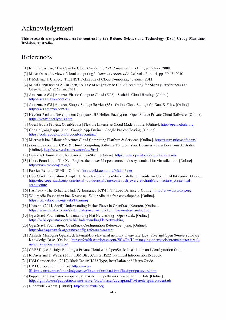
-41-

Acknowledgement This research was performed under contract to the Defence Science and Technology (DST) Group Maritime Division, Australia.

References

[1] R. L. Grossman, "The Case for Cloud Computing," IT Professional, vol. 11, pp. 23-27, 2009. [2] M Armbrust, "A view of cloud computing," Communications of ACM, vol. 53, no. 4, pp. 50-58, 2010. [3] P Mell and T Grance, "The NIST Definition of Cloud Computing," January 2011. [4] M Ali Babar and M A Chauhan, "A Tale of Migration to Cloud Computing for Sharing Experiences and

Observations," SECloud, 2011. [5] Amazon. AWS | Amazon Elastic Compute Cloud (EC2) - Scalable Cloud Hosting. [Online].

http://aws.amazon.com/ec2/ [6] Amazon. AWS | Amazon Simple Storage Service (S3) - Online Cloud Storage for Data & Files. [Online].

http://aws.amazon.com/s3/ [7] Hewlett-Packard Development Company. HP Helion Eucalyptus | Open Source Private Cloud Software. [Online].

https://www.eucalyptus.com [8] OpenNebula Project. OpenNebula | Flexible Enterprise Cloud Made Simple. [Online]. http://opennebula.org [9] Google. googleappengine - Google App Engine - Google Project Hosting. [Online].

https://code.google.com/p/googleappengine/ [10] Microsoft Inc. Microsoft Azure: Cloud Computing Platform & Services. [Online]. http://azure.microsoft.com/ [11] salesforce.com inc. CRM & Cloud Computing Software To Grow Your Business - Salesforce.com Australia.

[Online]. http://www.salesforce.com/au/?ir=1 [12] Openstack Foundation. Releases - OpenStack. [Online]. https://wiki.openstack.org/wiki/Releases [13] Linux Foundation. The Xen Project, the powerful open source industry standard for virtualization. [Online].

http://www.xenproject.org/ [14] Fabrice Bellard. QEMU. [Online]. http://wiki.qemu.org/Main_Page [15] OpenStack Foundation. Chapter 1. Architecture - OpenStack Installation Guide for Ubuntu 14.04 - juno. [Online].

http://docs.openstack.org/juno/install-guide/install/apt/content/ch_overview.html#architecture_conceptual-architecture

[16] HAProxy - The Reliable, High Performance TCP/HTTP Load Balancer. [Online]. http://www.haproxy.org [17] Wikimedia Foundation inc. Dnsmasq - Wikipedia, the free encyclopedia. [Online].

https://en.wikipedia.org/wiki/Dnsmasq [18] Hastexo. (2014, April) Understanding Packet Flows in OpenStack Neutron. [Online].

https://www.hastexo.com/system/files/neutron_packet_flows-notes-handout.pdf [19] OpenStack Foundation. Understanding Flat Networking - OpenStack. [Online].

https://wiki.openstack.org/wiki/UnderstandingFlatNetworking [20] OpenStack Foundation. OpenStack Configuration Reference - juno. [Online].

http://docs.openstack.org/juno/config-reference/content [21] Akilesh. Managing Openstack Internal/Data/External network in one interface | Free and Open Source Software

Knowledge Base. [Online]. https://fosskb.wordpress.com/2014/06/10/managing-openstack-internaldataexternal-network-in-one-interface/

[22] CREST. (2015, July) Building a Private Cloud with OpenStack: Installation and Configuration Guide. [23] R Davis and D Watts. (2011) IBM BladeCenter HS22 Technical Introduction Redbook. [24] IBM Corportation. (2012) BladeCenter HS22 Type, Installation and User's Guide. [25] IBM Corporation. [Online]. http://www-

01.ibm.com/support/knowledgecenter/linuxonibm/liaai.ipmi/liaaiipmipassword.htm [26] Puppet Labs. razor-server/api.md at master · puppetlabs/razor-server · GitHub. [Online].

https://github.com/puppetlabs/razor-server/blob/master/doc/api.md#set-node-ipmi-credentials [27] Clonezilla - About. [Online]. http://clonezilla.org

-42-

[28] OpenStack Foundation. Welcome to Glance’s documentation! [Online]. http://docs.openstack.org/developer/glance [29] Cloud-Init. Cloud Config Examples. [Online].

https://cloudinit.readthedocs.org/en/latest/topics/examples.html#including-users-and-groups [30] Sandro Mathys. (2013) Sandro Mathys: Blog: Setting a user password when launching cloud images. [Online].

http://blog.mathys.io/2013/07/setting-user-password-when-launching.html [31] John Paul Walters et al., "GPU Passthrough Performance: A Comparison of KVM, Xen, VMWare ESXi, and LXC

for CUDA and OpenCL Applications," in IEEE 7th International Conference on Cloud Computing (CLOUD), 2014, pp. 636-643.

[32] Kevian Tian. Graphics Virtualization (XenGT) | 01.org. [Online]. https://01.org/xen/blogs/srclarkx/2013/graphics-virtualization-xengt

[33] NVIDIA Corporation. Multi-Process Service. [Online]. https://docs.nvidia.com/deploy/pdf/CUDA_Multi_Process_Service_Overview.pdf

[34] Thomas Bradley. Hyper-Q Example. [Online]. http://docs.nvidia.com/cuda/samples/6_Advanced/simpleHyperQ/doc/HyperQ.pdf

[35] Lawrence Livermore National Security LLC. Codesign at Lawrence Livermore National Laboratory. [Online]. https://codesign.llnl.gov/lulesh.php

[36] Wikimedia Foundation Inc. OpenACC - Wikipedia, the free encyclopedia. [Online]. https://en.wikipedia.org/wiki/OpenACC

[37] NVIDIA Corporation. PGI Compilers & Tools. [Online]. http://www.pgroup.com [38] Phoronix Media. horonix Test Suite - Linux Testing & Benchmarking Platform, Automated Testing, Open-Source

Benchmarking. [Online]. http://www.phoronix-test-suite.com/ [39] Wikimedia Foundation Inc. OpenCL - Wikipedia, the free encyclopedia. [Online].

https://wikipedia.org/wiki/OpenCL [40] Roy Longbottom. CUDA nVidia Graphics Processor Parallel Computing Benchmarks Via Linux- Roy

Longbottom's PC benchmark Collection. [Online]. http://www.roylongbottom.org.uk/linux_cuda_mflops.htm [41] DataTag. How to achieve Gigabit speeds with Linux. [Online]. http://datatag.web.cern.ch/datatag/howto/tcp.html [42] real time xen. RT-Xen: Real-Time Virtualization based on Xen. [Online].

https://sites.google.com/site/realtimexen/home [43] Susu Xi et al., "RT-OpenStack: a Real-Time Cloud Management System," Washington University, Technical

2014.

A-1

Annex A Acronym and Definition List

Acronym Explanation AMM (IBM) Advanced Management Module API Application Programmable Interfaces AWS Amazon Web Service BMC Baseboard Management Controller CIDR Classless Inter-Domain Routing CORBA Common Object Request Broker Architecture COTS Commercial Off-The-Shelf CPU Central Processing Unit DDS Data Distribution Service DHCP Dynamic Host Configuration Protocol DRBL Diskless Remote Boot in Linux DSL Domain Specific Language EC2 Elastic Compute Cloud (Amazon) GPGPU General Purpose Graphics Processing Unit GPU Graphics Processing Unit GRE Generic Routing Encapsulation GUI Graphical User Interface IaaS Infrastructure as a Service ICT Information Communication and Technology IDL Interface Description Language IMM (IBM) Integrated Management Module IP Internet Protocol IPMI Intelligent Platform Management Interface KVM Kernel Virtual Machine – a hypervisor built into the Linux

kernel LBaaS Load Balancer as a Service MAC Media Access Control MR-IOV Multi-Root I/O Virtualisation NFS Network File System NIC Network Interface Controller NIST National Institute of Standards and Technology (US) OMG Object Management Group PaaS Platform as a Service POSIX Portable Operating System Interface PXE Preboot eXecution Environment QEMU Quick Emulator – an emulator, accelerated by KVM RAM Random Access Memory S3 Simple Storage Service SaaS Software as a Service SR-IOV Single Root I/O Virtualisation SS (VMware) Standard Switch SSH Secure Shell TCP Trasnmission Control Protocol UDP User Datagram Protocol UEFI Unified Extensible Firmware Interface UML Unified Modeling Language vCPU Virtual CPU vDS vNetwork Distributed Switch VLAN Virtual Local Area Network VPC Virtual Private Cloud VXLAN Virtual Extensible Local Area Network VM Virtual Machine

A-2

Acronym Explanation VPC Virtual Private Cloud XMI XML Metadata Interchange XML Extensible Markup Language

A-3

Annex B Benchmark Results

Roy Longbottoms CUDA MFLOPS single precision ##################################################### Assembler CPUID and RDTSC CPU GenuineIntel, Features Code BFEBFBFF, Model Code 000206C2 Intel(R) Xeon(R) CPU X5677 @ 3.47GHz Measured - Minimum 3466 MHz, Maximum 3467 MHz Linux Functions get_nprocs() - CPUs 16, Configured CPUs 16 get_phys_pages() and size - RAM Size 47.16 GB, Page Size 4096 Bytes uname() - Linux, compute-10-33-136-7, 3.13.0-24-generic #47-Ubuntu SMP Fri May 2 23:30:00 UTC 2014, x86_64 ##################################################### Linux CUDA 3.2 x64 32 Bits SP MFLOPS Benchmark 1.4 Tue Apr 14 17:30:16 2015 CUDA devices found Device 0: Tesla M2070 with 14 Processors 112 cores Global Memory 5249 MB, Shared Memory/Block 49152 B, Max Threads/Block 1024 Using 256 Threads Test 4 Byte Ops Repeat Seconds MFLOPS First All Words /Wd Passes Results Same Data in & out 100000 2 2500 0.842341 594 0.9295383095741 Yes Data out only 100000 2 2500 0.451488 1107 0.9295383095741 Yes Calculate only 100000 2 2500 0.046880 10665 0.9295383095741 Yes Data in & out 1000000 2 250 0.549819 909 0.9925497770309 Yes Data out only 1000000 2 250 0.279932 1786 0.9925497770309 Yes Calculate only 1000000 2 250 0.023131 21616 0.9925497770309 Yes Data in & out 10000000 2 25 0.455317 1098 0.9992496371269 Yes Data out only 10000000 2 25 0.239972 2084 0.9992496371269 Yes Calculate only 10000000 2 25 0.019734 25337 0.9992496371269 Yes Data in & out 100000 8 2500 0.853818 2342 0.9571172595024 Yes Data out only 100000 8 2500 0.460115 4347 0.9571172595024 Yes Calculate only 100000 8 2500 0.052759 37908 0.9571172595024 Yes Data in & out 1000000 8 250 0.557244 3589 0.9955183267593 Yes Data out only 1000000 8 250 0.281921 7094 0.9955183267593 Yes Calculate only 1000000 8 250 0.024181 82710 0.9955183267593 Yes Data in & out 10000000 8 25 0.453237 4413 0.9995489120483 Yes Data out only 10000000 8 25 0.239960 8335 0.9995489120483 Yes Calculate only 10000000 8 25 0.020322 98414 0.9995489120483 Yes Data in & out 100000 32 2500 0.867475 9222 0.8902152180672 Yes Data out only 100000 32 2500 0.486685 16438 0.8902152180672 Yes Calculate only 100000 32 2500 0.077913 102678 0.8902152180672 Yes Data in & out 1000000 32 250 0.561345 14251 0.9880878329277 Yes Data out only 1000000 32 250 0.286109 27961 0.9880878329277 Yes Calculate only 1000000 32 250 0.028279 282897 0.9880878329277 Yes Data in & out 10000000 32 25 0.458457 17450 0.9987964630127 Yes Data out only 10000000 32 25 0.242297 33017 0.9987964630127 Yes Calculate only 10000000 32 25 0.022588 354170 0.9987964630127 Yes Extra tests - loop in main CUDA Function Calculate 10000000 2 25 0.008120 61578 0.9992496371269 Yes Shared Memory 10000000 2 25 0.004462 112057 0.9992496371269 Yes Calculate 10000000 8 25 0.010004 199919 0.9995489120483 Yes Shared Memory 10000000 8 25 0.006758 295957 0.9995489120483 Yes

A-4

Calculate 10000000 32 25 0.017837 448511 0.9987964630127 Yes Shared Memory 10000000 32 25 0.014676 545113 0.9987964630127 Yes ##################################################### Assembler CPUID and RDTSC CPU GenuineIntel, Features Code BFEBFBFF, Model Code 000206C2 Intel(R) Xeon(R) CPU X5677 @ 3.47GHz Measured - Minimum 3467 MHz, Maximum 3467 MHz Linux Functions get_nprocs() - CPUs 16, Configured CPUs 16 get_phys_pages() and size - RAM Size 47.16 GB, Page Size 4096 Bytes uname() - Linux, compute-10-33-136-7, 3.13.0-24-generic #47-Ubuntu SMP Fri May 2 23:30:00 UTC 2014, x86_64 ##################################################### Linux CUDA 3.2 x64 32 Bits SP MFLOPS Benchmark 1.4 Tue Apr 14 17:33:15 2015 CUDA devices found Device 0: Tesla M2070 with 14 Processors 112 cores Global Memory 5249 MB, Shared Memory/Block 49152 B, Max Threads/Block 1024 Using 256 Threads Test 4 Byte Ops Repeat Seconds MFLOPS First All Words /Wd Passes Results Same Data in & out 100000 2 2500 0.845598 591 0.9295383095741 Yes Data out only 100000 2 2500 0.454587 1100 0.9295383095741 Yes Calculate only 100000 2 2500 0.046954 10649 0.9295383095741 Yes Data in & out 1000000 2 250 0.549901 909 0.9925497770309 Yes Data out only 1000000 2 250 0.279816 1787 0.9925497770309 Yes Calculate only 1000000 2 250 0.023149 21599 0.9925497770309 Yes Data in & out 10000000 2 25 0.453104 1104 0.9992496371269 Yes Data out only 10000000 2 25 0.239631 2087 0.9992496371269 Yes Calculate only 10000000 2 25 0.019721 25354 0.9992496371269 Yes Data in & out 100000 8 2500 0.855390 2338 0.9571172595024 Yes Data out only 100000 8 2500 0.461097 4337 0.9571172595024 Yes Calculate only 100000 8 2500 0.052919 37793 0.9571172595024 Yes Data in & out 1000000 8 250 0.558143 3583 0.9955183267593 Yes Data out only 1000000 8 250 0.281806 7097 0.9955183267593 Yes Calculate only 1000000 8 250 0.024198 82652 0.9955183267593 Yes Data in & out 10000000 8 25 0.453672 4408 0.9995489120483 Yes Data out only 10000000 8 25 0.239466 8352 0.9995489120483 Yes Calculate only 10000000 8 25 0.020295 98547 0.9995489120483 Yes Data in & out 100000 32 2500 0.867706 9220 0.8902152180672 Yes Data out only 100000 32 2500 0.487134 16423 0.8902152180672 Yes Calculate only 100000 32 2500 0.078520 101884 0.8902152180672 Yes Data in & out 1000000 32 250 0.561398 14250 0.9880878329277 Yes Data out only 1000000 32 250 0.286325 27940 0.9880878329277 Yes Calculate only 1000000 32 250 0.028276 282928 0.9880878329277 Yes Data in & out 10000000 32 25 0.455336 17569 0.9987964630127 Yes Data out only 10000000 32 25 0.241886 33073 0.9987964630127 Yes Calculate only 10000000 32 25 0.022587 354193 0.9987964630127 Yes Extra tests - loop in main CUDA Function Calculate 10000000 2 25 0.008121 61572 0.9992496371269 Yes Shared Memory 10000000 2 25 0.004464 112009 0.9992496371269 Yes Calculate 10000000 8 25 0.010005 199895 0.9995489120483 Yes Shared Memory 10000000 8 25 0.006757 296009 0.9995489120483 Yes Calculate 10000000 32 25 0.017848 448241 0.9987964630127 Yes Shared Memory 10000000 32 25 0.014675 545148 0.9987964630127 Yes

A-5

Roy Longbottom’s CUDA MFLOPS double precision: ##################################################### Assembler CPUID and RDTSC CPU GenuineIntel, Features Code BFEBFBFF, Model Code 000206C2 Intel(R) Xeon(R) CPU X5677 @ 3.47GHz Measured - Minimum 3467 MHz, Maximum 3467 MHz Linux Functions get_nprocs() - CPUs 16, Configured CPUs 16 get_phys_pages() and size - RAM Size 47.16 GB, Page Size 4096 Bytes uname() - Linux, compute-10-33-136-7, 3.13.0-24-generic #47-Ubuntu SMP Fri May 2 23:30:00 UTC 2014, x86_64 ##################################################### Linux CUDA 3.2 x64 64 Bits DP MFLOPS Benchmark 1.4 Tue Apr 14 17:44:39 2015 CUDA devices found Device 0: Tesla M2070 with 14 Processors 112 cores Global Memory 5249 MB, Shared Memory/Block 49152 B, Max Threads/Block 1024 Using 256 Threads Test 8 Byte Ops Repeat Seconds MFLOPS First All Words /Wd Passes Results Same Data in & out 100000 2 2500 1.613884 310 0.9294744580218 Yes Data out only 100000 2 2500 0.824916 606 0.9294744580218 Yes Calculate only 100000 2 2500 0.061312 8155 0.9294744580218 Yes Data in & out 1000000 2 250 1.021821 489 0.9925431921162 Yes Data out only 1000000 2 250 0.514558 972 0.9925431921162 Yes Calculate only 1000000 2 250 0.039237 12743 0.9925431921162 Yes Data in & out 10000000 2 25 0.883349 566 0.9992492055877 Yes Data out only 10000000 2 25 0.469843 1064 0.9992492055877 Yes Calculate only 10000000 2 25 0.037024 13505 0.9992492055877 Yes Data in & out 100000 8 2500 1.783158 1122 0.9571642109917 Yes Data out only 100000 8 2500 0.846180 2364 0.9571642109917 Yes Calculate only 100000 8 2500 0.068275 29293 0.9571642109917 Yes Data in & out 1000000 8 250 1.025476 1950 0.9955252302690 Yes Data out only 1000000 8 250 0.512468 3903 0.9955252302690 Yes Calculate only 1000000 8 250 0.039680 50403 0.9955252302690 Yes Data in & out 10000000 8 25 0.888617 2251 0.9995496465632 Yes Data out only 10000000 8 25 0.469567 4259 0.9995496465632 Yes Calculate only 10000000 8 25 0.036648 54574 0.9995496465632 Yes Data in & out 100000 32 2500 1.660054 4819 0.8903768345465 Yes Data out only 100000 32 2500 0.889716 8992 0.8903768345465 Yes Calculate only 100000 32 2500 0.123605 64722 0.8903768345465 Yes Data in & out 1000000 32 250 1.044909 7656 0.9881014965491 Yes Data out only 1000000 32 250 0.535691 14934 0.9881014965491 Yes Calculate only 1000000 32 250 0.063141 126701 0.9881014965491 Yes Data in & out 10000000 32 25 0.902941 8860 0.9987993043723 Yes Data out only 10000000 32 25 0.490324 16316 0.9987993043723 Yes Calculate only 10000000 32 25 0.057355 139483 0.9987993043723 Yes Extra tests - loop in main CUDA Function Calculate 10000000 2 25 0.011835 42249 0.9992492055877 Yes Shared Memory 10000000 2 25 0.007347 68056 0.9992492055877 Yes Calculate 10000000 8 25 0.020029 99856 0.9995496465632 Yes Shared Memory 10000000 8 25 0.016293 122752 0.9995496465632 Yes Calculate 10000000 32 25 0.055040 145349 0.9987993043723 Yes Shared Memory 10000000 32 25 0.052269 153053 0.9987993043723 Yes

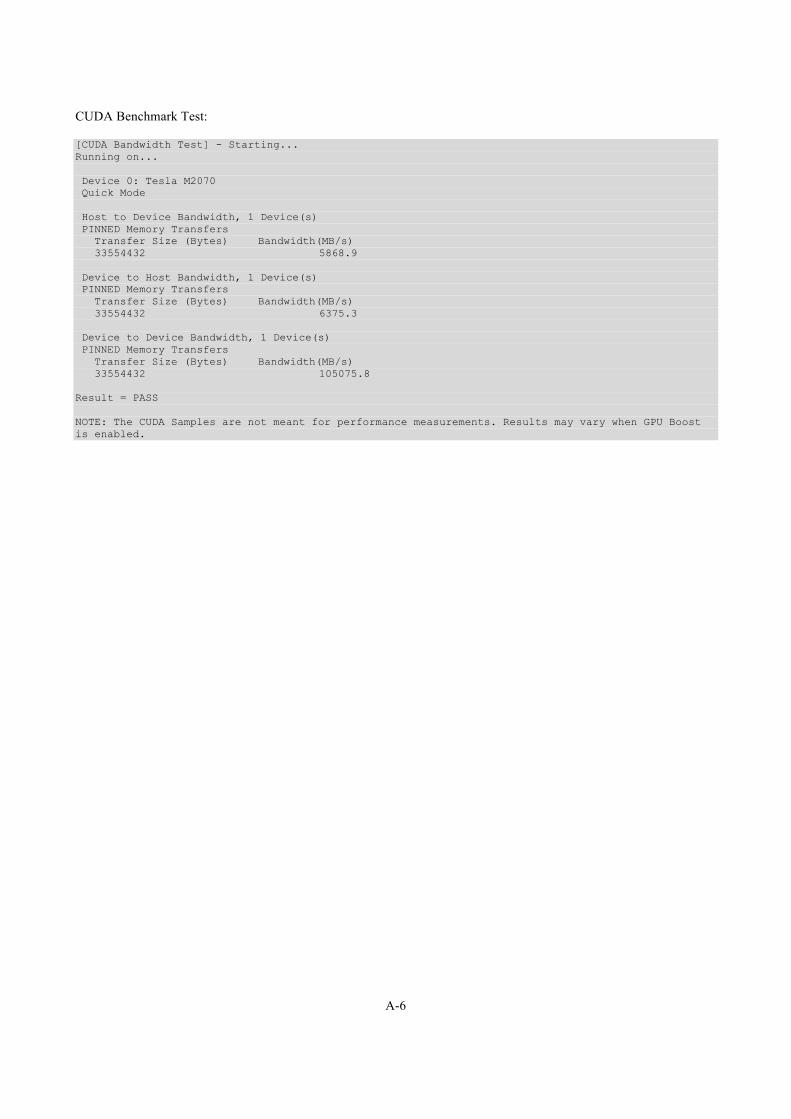
A-6

CUDA Benchmark Test: [CUDA Bandwidth Test] - Starting... Running on... Device 0: Tesla M2070 Quick Mode Host to Device Bandwidth, 1 Device(s) PINNED Memory Transfers Transfer Size (Bytes) Bandwidth(MB/s) 33554432 5868.9 Device to Host Bandwidth, 1 Device(s) PINNED Memory Transfers Transfer Size (Bytes) Bandwidth(MB/s) 33554432 6375.3 Device to Device Bandwidth, 1 Device(s) PINNED Memory Transfers Transfer Size (Bytes) Bandwidth(MB/s) 33554432 105075.8 Result = PASS NOTE: The CUDA Samples are not meant for performance measurements. Results may vary when GPU Boost is enabled.

Investigation into the Use of OpenStack for Submarine ... into the Use of OpenStack for Submarine...

Documents

Transcript of Investigation into the Use of OpenStack for Submarine ... into the Use of OpenStack for Submarine...