Investigating the Role of an Understudied North Atlantic ...
164
University of Massachuses Boston ScholarWorks at UMass Boston Graduate Masters eses Doctoral Dissertations and Masters eses 6-1-2012 Investigating the Role of an Understudied North Atlantic Right Whale Habitat: Right Whale Movement, Ecology, and Distribution in Jeffreys Ledge Kathryn Longley University of Massachuses Boston Follow this and additional works at: hp://scholarworks.umb.edu/masters_theses Part of the Behavior and Ethology Commons , and the Environmental Policy Commons is Open Access esis is brought to you for free and open access by the Doctoral Dissertations and Masters eses at ScholarWorks at UMass Boston. It has been accepted for inclusion in Graduate Masters eses by an authorized administrator of ScholarWorks at UMass Boston. For more information, please contact [email protected]. Recommended Citation Longley, Kathryn, "Investigating the Role of an Understudied North Atlantic Right Whale Habitat: Right Whale Movement, Ecology, and Distribution in Jeffreys Ledge" (2012). Graduate Masters eses. Paper 105.
Transcript of Investigating the Role of an Understudied North Atlantic ...

University of Massachusetts BostonScholarWorks at UMass Boston
Graduate Masters Theses Doctoral Dissertations and Masters Theses
6-1-2012
Investigating the Role of an Understudied NorthAtlantic Right Whale Habitat: Right WhaleMovement, Ecology, and Distribution in JeffreysLedgeKathryn LongleyUniversity of Massachusetts Boston
Follow this and additional works at: http://scholarworks.umb.edu/masters_theses
Part of the Behavior and Ethology Commons, and the Environmental Policy Commons
This Open Access Thesis is brought to you for free and open access by the Doctoral Dissertations and Masters Theses at ScholarWorks at UMassBoston. It has been accepted for inclusion in Graduate Masters Theses by an authorized administrator of ScholarWorks at UMass Boston. For moreinformation, please contact [email protected].
Recommended CitationLongley, Kathryn, "Investigating the Role of an Understudied North Atlantic Right Whale Habitat: Right Whale Movement, Ecology,and Distribution in Jeffreys Ledge" (2012). Graduate Masters Theses. Paper 105.

INVESTIGATING THE ROLE OF AN UNDERSTUDIED NORTH ATLANTIC
RIGHT WHALE HABITAT: RIGHT WHALE MOVEMENT, ECOLOGY, AND
DISTRIBUTION IN JEFFREYS LEDGE
A Thesis Presented
by
KATHRYN E. LONGLEY
Submitted to the Office of Graduate Studies,
University of Massachusetts Boston,
in partial fulfillment of the requirements for the degree of
MASTER OF SCIENCE
June 2012
Biology Program

© 2012 by Kathryn E. Longley
All rights reserved

INVESTIGATING THE ROLE OF AN UNDERSTUDIED NORTH ATLANTIC
RIGHT WHALE HABITAT: RIGHT WHALE MOVEMENT, ECOLOGY, AND
DISTRIBUTION IN JEFFREYS LEDGE
A Thesis Presented
by
KATHRYN E. LONGLEY
Approved as to style and content by:
________________________________________________
Solange Brault, Associate Professor
Chairperson of Committee
________________________________________________
Ruth H. Leeney, PhD, Muc Mhara Research & Conservation
Member
________________________________________________
Michael Rex, Professor
Member
_________________________________________
Alan Christian, Program Director
Biology Department
___________________________________
Rick Kesseli, Chairperson
Biology Department

iv
ABSTRACT
INVESTIGATING THE ROLE OF AN UNDERSTUDIED NORTH ATLANTIC RIGHT
WHALE HABITAT: RIGHT WHALE MOVEMENT, ECOLOGY, AND DISTRIBUTION IN
JEFFREYS LEDGE
June 2012
Kathryn Longley, B.A., Wesleyan University
M.S., University of Massachusetts Boston
Directed by Professor Solange Brault
The critically endangered North Atlantic right whale (Eubalaena glacialis)
consistently visits five major habitats throughout the year; however, they are known to
visit additional habitats. This project examines the role of Jeffreys Ledge as an additional
habitat of importance for this species by investigating three aspects of its distribution and
ecology. I first addressed the relationship of Jeffreys Ledge to a known significant right
whale feeding ground, Cape Cod Bay, by quantifying the movement of right whales
between the two habitats and comparing demographic characteristics of right whales seen
in these habitats. Secondly, I measured the quality of the zooplankton resource in
Jeffreys Ledge and the relationship between plankton characteristics and whale sightings
in this habitat. Thirdly, I examined the spatial distribution of right whales, and the
relationship between right whale sightings and bathymetric characteristics in Jeffreys
Ledge. While the populations of whales in these habitats do not appear to be

v
demographically distinct, the results suggest that there is more movement between
habitats by males than by females during the first few months of the year. Although there
was no observed relationship between sightings per unit effort (SPUE) and energetic
density of zooplankton prey resource in Jeffreys Ledge, low caloric density is a
significant predictor of whale absence in the region. The lack of a relationship between
SPUE and energetic density is likely the results of the zooplankton sampling
methodology. Spatial analysis identifies a hot spot of high SPUE which changes in size,
location and intensity throughout the study period, and both a binary logistic regression
and a generalized linear model support a relationship between whale sightings and depth
in the habitat. Results of this project highlight the need for more precise plankton
sampling in the region as well as the need for concurrent survey efforts in multiple
habitats. Assessing the importance the Jeffreys Ledge habitat to the right whale will help
conservation managers to better allocate resources and mitigate the effects of
anthropogenic threats to this highly endangered species in this region.

vi
ACKNOWLEDGEMENTS
This research was made possible by the Provincetown Center for Coastal Studies Ruth Hiebert
Memorial Fellowship, the Dr. Robert W. Spayne Research Grant from the Biology Department at
UMASS Boston, and a Healy Grant from UMASS Boston. A Lipke Grant from the Department
of Biology at UMASS Boston and a Professional Development Grant from the UMASS Boston
Graduate Student Assembly assisted with travel costs.
The Whale Center of New England, Provincetown Center for Coastal Studies, Northeast
Fisheries Science Center, and the New England Aquarium were all instrumental in the acquisition
of data. Karen Stamieszkin was responsible for my learning how to enumerate plankton, and
Jenn Tackaberry, Christin Khan, Allison Henry, Laura Ganley, Laura Howes, Kelly Slivka,
Christy Hudak, Heather Pettis, Philip Hamilton, and Sarah Fortune, were invaluable in providing
me with data sets, papers and answers to many technical questions throughout the project. Mason
Weinrich, Stormy Mayo, and Mark Baumgartner gave enormously helpful advice and guidance.
Bob Lynch, Mariam Monem and A.J. Devaux spent hours at the microscope assisting with
plankton counts. Thank you to my committee, Dr. Solange Brault, Dr. Ruth Leeney, and Dr.
Michael Rex, and to the Brault Lab, Stefanie Gazda, Ian Paynter, Christina Ciarfella, Caitlin
Soden and Miriam Mills for help and support!

vii
TABLE OF CONTENTS
ACKNOWLEDGEMENTS ........................................................................... vi
LIST OF TABLES ......................................................................................... x
LIST OF FIGURES ....................................................................................... xiii
CHAPTER Page
1. INTRODUCTION ............………………………………………. 1
2. EXAMINING THE RELATIONSHIP OF JEFFREYS LEDGE
TO OTHER KNOWN RIGHT WHALE CRITICAL
HABITATS ............................................................................ 7
Introduction ...................................................................... 7
Habitat overlap and transition probabilities ............... 7
Sexual segregation and sex ratio differences ............. 11
Methods............................................................................ 17
Jeffreys Ledge boat-based surveys ............................ 17
Jeffreys Ledge aircraft-based surveys ........................ 21
Cape Cod Bay aircraft-based surveys ........................ 24
Great South Channel confirmed sightings ................. 26
Individual identification ............................................. 26
Sightings per unit effort (SPUE calculations) ............ 28
Transition probabilities .............................................. 29
Definition of habitat categories .................................. 30
Statistical analysis ...................................................... 31
Results .............................................................................. 32
Habitat overlap ........................................................... 32
Transition probabilities .............................................. 34
Habitat reliability ....................................................... 34
Nutritional flexibility and site fidelity ....................... 35
Differences in habitat use by reproductive status ...... 36
Discussion ........................................................................ 37
Adjacent movement and transition probabilities ....... 37
Sex ratios .................................................................... 39
Data considerations .................................................... 41
Conclusions ...................................................................... 43
Tables ............................................................................... 44

viii
CHAPTER Page
3. INVESTIGATING THE RELATIONSHIP BETWEEN PREY
QUALITY AND RIGHT WHALE SIGHTINGS IN
JEFFREYS LEDGE ................................................................. 67
Introduction ...................................................................... 67
Methods............................................................................ 71
Jeffreys Ledge tows ................................................... 71
Enumeration ............................................................... 73
Calculation of density and energetic density ............. 75
Sightings per unit effort and plankton
characteristics ........................................................ 77
Statistical analysis ...................................................... 77
Results .............................................................................. 78
Sightings per unit effort and plankton
characteristics ........................................................ 78
Energetic density and whale presence/absence.......... 80
Energetic density and station types ............................ 81
Discussion ........................................................................ 81
Sightings per unit effort and plankton
characteristics ........................................................ 81
Conclusions ...................................................................... 85
Tables ............................................................................... 86
Figures.............................................................................. 90
4. RIGHT WHALE DISTRIBUTION IN JEFFREYS LEDGE:
IDENTIFYING HOT SPOTS AND ASSESSING THE
EFFECT OF BATHYMETRIC FEATURES ON RIGHT
WHALE SIGHTINGS ............................................................. 99
Introduction ...................................................................... 99
Methods............................................................................ 102
Base map .................................................................... 102
Hot spot analysis ........................................................ 103
Regression analysis .................................................... 105
Results .............................................................................. 107
Hot spot analysis ........................................................ 107
Regressions ................................................................ 108
Discussion ........................................................................ 108
Hot spot analysis ........................................................ 108
Bathymetry ................................................................. 110
Conclusions ...................................................................... 113
Tables ............................................................................... 114
Figures.............................................................................. 115
ix
APPENDIX
I. LIST OF ALL SURVEYS OF JEFFREYS LEDGE (JL)
AND CAPE COD BAY (CCB) DURING THE STUDY
PERIOD BY THE WHALE CENTER OF NEW ENGLAND
(WCNE), NORTHEAST FISHERIES SCIENCE CENTER
(NEFSC), AND PROVINCETOWN CENTER FOR
COASTAL STUDIES (PCCS) ................................................. 118
II. RELATIONSHIPS BETWEEN SIGHTINGS PER UNIT
EFFORT (SPUE) AND EFFORT ............................................ 128
III. LIST OF ALL PLANKTON SAMPLES WITH STATION,
STATION STYPE, TOW TYPE, PROPORTIONS OF
THREE MAJOR SPECIES, ORGANISMAL DENSITY,
AND ENERGETIC DENSITY ............................................... 130
REFERENCE LIST .................................................................................... 139

x
LIST OF TABLES
Table Page
2.1. Summary of survey effort in Jeffreys Ledge and Cape Cod Bay
from 2003 – 2010 ................................................................... 44
2.2. List of habitat categories and description of the individuals in
each category ......................................................................... 45
2.3. Number of individuals seen in each habitat by year ................... 46
2.4. Transition probabilities of individual right whale moving
between study areas in one month from October 2003 –
December 2009 ...................................................................... 46
2.5. Sex ratios of all individuals seen in Cape Cod Bay over the
study period (AllCCB) and all individuals seen in Jeffreys
Ledge during the study period (AllJL)................................... 47
2.6. Results of a Chi-square test comparing the sex ratios of all
individuals seen in Cape Cod Bay to the sex ratios of all
individuals seen in Jeffreys Ledge ......................................... 47
2.7. Sex ratios of all individuals seen only in Cape Cod Bay over
the study period (CCBOnly) and all individuals seen in only
Jeffreys Ledge during the study period (JLOnly) .................. 48
2.8. Results of a Chi-square test comparing the sex ratios of
individuals seen only in Cape Cod Bay to the sex ratios
of individuals seen only in Jeffreys Ledge ............................ 48
2.9. Number of individuals visiting Jeffreys Ledge and Cape Cod
Bay multiple times during the study period ........................... 49
2.10. Results of a Chi-square test comparing the frequency of
repeat individuals compared to total individuals in
Cape Cod Bay to that in Jeffreys Ledge ................................ 49

xi
Table Page
2.11. Sex ratios of all individuals thought to be alive in the
population during the study period (AllHab) compared
to the sex ratio of individuals seen in both Jeffreys Ledge
and Cape Cod Bay in a given sighting season (between
January and May) ................................................................... 50
2.12. Results of a Chi-square test comparing the sex ratios of all
individuals presumed to be alive during the study period to
the sex ratio of the individuals seen moving between
habitats ................................................................................... 50
2.13. Number of reproductive females compared to the total
number of individuals seen in each habitat during the study
period ..................................................................................... 51
2.14. Results of a Fisher’s Exact Test comparing the ratio of
reproductive females to the total number of individuals
between habitats ..................................................................... 51
2.15. Number of reproductive females in each habitat compared
to the total number of females in each habitat ....................... 52
2.16. Results of a Fisher’s Exact Test comparing the number
of reproductive females in each habitat compared to
the total number of females in each habitat ........................... 52
2.17. Number of females seen with calves in each habitat compared
to the total number of reproductive females seen in each
habitat over the study period .................................................. 52
2.18. Results of a Chi-square test comparing the ratio of females
seen with calves to the total number of reproductive
females seen in each habitat ................................................... 53
3.1. Estimate of species, stage, and stage-specific energy density
of copepods (From DeLorenzo Costa et al., 2006) ................ 86
3.2. Results of a univariate analysis of variance testing the effect
of tow type on energetic density at a sampling station .......... 86

xii
Table Page
3.3. Logistic model from a binary logistic regression measuring
predictive power of effect of energetic density of
surface samples on whale presence/absence .......................... 87
3.4. Results of a binary logistic regression testing the effect of
energetic density of surface samples on whale
presence/absence .................................................................... 87
3.5. Logistic model from a binary logistic regression measuring
the predictive power of energetic density of vertical
samples on whale presence/absence ...................................... 87
3.6. Results of a binary logistic regression testing the effect of
energetic density of vertical samples on whale
presence/absence .................................................................... 88
3.7. Results of a generalized linear model testing the effect of
station type on the energetic density of surface samples ....... 88
3.8. Results of a generalized linear model testing the effect of
station type on the energetic density of vertical samples ....... 89
4.1. Results of a binary logistic regression of the whale
presence/absence in relation to slope, depth, and an
interaction term in a 2 km2 grid cell....................................... 114
4.2. Results of a generalized linear model of SPUE value in
relation to slope, depth, and an interaction term in a 2 km2
grid cell .................................................................................. 114

xiii
LIST OF FIGURES
Figure Page
2.1. Whale Center of New England boat-based survey tracklines
and plankton sampling stations in Jeffreys Ledge ................. 54
2.2. Broadscale survey lines flown by Northeast Fisheries Science
Center ..................................................................................... 55
2.3. Sawtooth survey lines flown by Northeast Fisheries Science
Center ..................................................................................... 56
2.4. Example of an aerial survey flown by Northeast Fisheries
Science Center using the Sawtooth sampling scheme ........... 57
2.5. Jump Sawtooth survey lines flown by Northeast Fisheries
Science Center ....................................................................... 58
2.6. Example of an aerial survey flown by Northeast Fisheries
Science Center using the Jump Sawtooth sampling
scheme.................................................................................... 59
2.7. Example of a Dynamic Area Management Plan flight flown
by Northeast Fisheries Science Center .................................. 60
2.8. Provincetown Center for Coastal Studies aerial survey
tracklines in Cape Cod Bay .................................................... 61
2.9. Habitat boundaries of the Great South Channel, Jeffreys Ledge
and Cape Cod Bay, as used in analyses of habitat exchange
and transition probabilities ..................................................... 62
2.10. Aircraft-based sightings per unit effort (SPUE) compared to
boat-based sightings per unit effort in Jeffreys Ledge ........... 63
2.11. Breakdown of individuals by sex seen in Jeffreys Ledge,
Cape Cod Bay, and in adjacent seasons by year .................... 64
2.12. Number of individuals traveling between Jeffreys Ledge and
Cape Cod Bay by season, compared to effort from each
survey platform ...................................................................... 65

xiv
Figure Page
2.13. The total SPUE by month compared to the total trackline
effort by month in both habitats by season ............................ 66
3.1. Jeffreys Ledge survey area tracklines and regular sampling
stations with additional stations sampled by Provincetown
Center for Coastal Studies (PCCS) in 2005 –2006 ................ 90
3.2. Sightings per unit effort (SPUE) expressed in number of
individuals per kilometer of trackline and mean energetic
density of vertical plankton samples, expressed in
Kilojoules m-3
......................................................................... 91
3.3. Scatter plot of energetic density (expressed in kilojoules m-3
)
at a sampling station and SPUE (expressed in number of
individuals km-1
) for a survey date ........................................ 92
3.4. Sightings per unit effort (SPUE) expressed in the number of
individuals per kilometer of trackline and the proportion of
C. finmarchicus in vertical samples ....................................... 93
3.5. Scatter plot of the proportion of C. finmarchicus at a sampling
station and SPUE (expressed in number of individuals
km-1
) for a survey date ........................................................... 94
3.6. Sightings per unit effort (SPUE) expressed in the number of
individuals per kilometer of trackline and the proportion
of Centropages spp. in vertical samples ................................ 95
3.7. Scatter plot of the proportion of Centropages spp. at a
sampling station and SPUE (expressed in number of
individuals km-1
) for a survey date ........................................ 96
3.8. Sightings per unit effort (SPUE) expressed in the number of
individuals per kilometer of trackline and the proportion
of Pseudocalanus spp. in vertical samples ............................ 97
3.9. Scatter plot of the proportion of Pseudocalanus spp. at a
sampling station and SPUE (expressed in number of
individuals km-1
) for a survey date ........................................ 98

xv
Figure Page
4.1. Bathymetry of Jeffreys Ledge with boat-based whale sightings
September 2003 – December 2009 ........................................ 115
4.2. Results of Getis-Ord Gi* Hot Spot analysis of 2003 - 2009
SPUE ...................................................................................... 116
4.3. Results of Getis-Ord Gi* Hot Spot analysis of 2003 – 2005
SPUE ...................................................................................... 117
4.4. Results of Getis-Ord Gi* Hot Spot analysis of 2004 – 2006
SPUE ...................................................................................... 117
4.5. Results of Getis-Ord Gi* Hot Spot analysis of 2005 – 2007
SPUE ...................................................................................... 117
4.6. Results of Getis-Ord Gi* Hot Spot analysis of 2006 - 2008
SPUE ...................................................................................... 117
4.7. Results of Getis-Ord Gi* Hot Spot analysis of 2007 – 2009
SPUE ...................................................................................... 117

1
CHAPTER 1
INTRODUCTION
The North Atlantic right whale (Eubalaena glacialis) is a critically endangered
species. At present, the global population is estimated at 490 individuals (Right Whale
Consortium, 2011). Deemed the “right whale” to hunt, the population was severely
reduced by whaling. Right whale catches were recorded as early as the year 1039 and the
exploitation of this species continued until 1935 (Reeves et al., 2007). While the
population appears to be slowly increasing since then, ship strikes and entanglement in
fishing gear put the population at risk and remain the leading causes of death for these
animals. The current potential biological removal (PBR) for right whales is 0.7
individuals per year (NMFS, 2010), meaning that a loss of .07 individuals per year due to
anthropogenic sources will prevent the species from reaching its optimum sustainable
population (MMPA, 1972). In other words, a loss of even one animal per year to non-
natural causes threatens the survival of the species. The success of management
strategies to prevent accidental right whale deaths will determine whether the species will
persist and an understanding of how and why right whales use various habitats will
enhance the ability of conservation efforts to assess and address anthropogenic risk.

2
Throughout the year, right whales consistently frequent five major habitats along
the continental shelf from Eastern Canada to Florida: Cape Cod Bay from late winter to
early spring, the Great South Channel from late spring to early summer, the Bay of Fundy
and Roseway Basin during the summer months, and the coastal regions of the
southeastern United States during the winter (Kenney et al., 2001; Kraus & Rolland,
2007). However, there are other less-studied habitats where right whale sightings also
occur.
Jeffreys Ledge is one of these areas. This habitat is a relatively shallow glacial
deposit approximately 54 km in length and is located off the coast of New Hampshire. It
has recently been suggested that this area may qualify as an additional habitat of
importance. Using a combination of platform of opportunistic surveys, sightings data
from whale watching vessels, and dedicated survey efforts, Weinrich et al. (2000)
suggested that right whales sightings occur here frequently and consistently. More
importantly, feeding behavior is also regularly observed, particularly from October
through December (Whale Center of New England (WCNE), 2008)
An analysis of sightings data from surveys in Jeffreys Ledge was undertaken to
clarify whether Jeffreys Ledge might be considered an additional habitat of importance,
or whether it is a marginal habitat, where right whales might visit on their way to more
reliable feeding grounds or during periods of low productivity at other sites. Although
the distinction between a marginal and significant habitat may seem trivial, such
designations have the potential to dictate the extent to which management strategies are
directed at various regions. One such strategy attempts to reduce the risk of lethal vessel

3
strikes by designating Seasonal Management Areas (SMAs). SMAs are chosen to based
on areas where right whales are likely to aggregate at a specific time of year, and during
that time period, vessels over 65 feet must reduce their speed to 10 knots or less (Silber &
Bettridge, 2010).
Cape Cod Bay is one such SMA, with restrictions in effect from January 1st to
May 15th
. Cape Cod Bay is federally designated as a critical habitat and is the focus of
intense mitigation activities both at the State and Federal levels. During the right whale
sighting season, aerial surveys monitor and report the positions of right whales to the
Division of Marine Fisheries, the National Oceanographic and Atmospheric
Administration (NOAA) and the National Marine Fisheries Service (NMFS), as well as
mariners in the area. Acoustic buoys which detect specific right whale calls also serve as
a warning that right whales are in the bay. By monitoring the quantity and taxonomic
composition of plankton in Cape Cod Bay, researchers are able to forecast areas in which
right whales are likely to be located (Provincetown Center for Coastal Studies (PCCS),
2010). Assessing the significance of lesser-studied habitats will help conservation
managers better allocate resources and implement more intensive monitoring plans if
necessary.
One component of this study (Chapter 2) will assess the connectivity of Jeffreys
Ledge to a known significant habitat, Cape Cod Bay. Cape Cod Bay is the closest
significant feeding ground to Jeffreys Ledge. The sighting season in Jeffreys Ledge also
falls directly before the sighting season in Cape Cod Bay. This study examines two
subsets of animals; those that are seen in Jeffreys Ledge in the late fall/early winter and

4
subsequently in Cape Cod Bay in the late winter/early spring, and the animals that are
known to visit both Cape Cod Bay and Jeffreys Ledge between January and May, a
season in which a large segment of the population is expected to visit Cape Cod Bay.
Right whales show some degree of site fidelity. There are individual right whales
that are never documented in Cape Cod Bay, despite being documented elsewhere. For
example, there are individual right whales that are regularly seen in the Bay of Fundy
despite never being seen in Cape Cod Bay (Kraus & Rolland, 2007). An implication of
this finding is that alternative, possibly undocumented habitats exist for this species.
Because right whales are known to enter and exit the Cape Cod Bay region throughout
the sighting season (Baumgartner & Mate, 2005), a large amount of sighting overlap
between the two sites would suggest that right whales may visit the Jeffreys Ledge region
as an alternative destination during the typical Cape Cod Bay sighting season. Although
tracking individual movements between the two sites is beyond the scope of this study,
the calculation of transitional probabilities between the two sites will be indicative of the
extent to which these two sites are connected.
While the characteristics of the sightings subset will provide researchers and
conservation managers with valuable information, there are still unanswered questions
about what these whales are doing in Jeffreys Ledge in the first place. With the
exception of one subset of the population’s migration to the southeastern calving
grounds, right whale movement to these various habitats is thought to be motivated by
food. It follows that attributing significance to a habitat would likely depend on the
quality of the food resource in the region.

5
The right whale belongs to a group of baleen whales known as the “skim-
feeders.” This means that they feed by opening their mouths and swimming forward,
filtering organisms through the fine bristles of the baleen plates on either side of their
mouths. In doing so, their open mouths create an enormous amount of drag. It is
believed that in order for it to be energetically worthwhile to open their mouth to feed,
the density of plankton must reach a critical threshold of 3,750 organisms/m3 (PCCS,
2003). Therefore, it is likely that for a right whale habitat to be recognized as significant,
food availability and quality must be a primary concern. It is estimated that in order to
survive, a right whale must consume between 407,000 and 4,140,000 calories (1,702,888
– 17,321,760 kilojoules) per day (Baumgartner et al., 2007). Considering this massive
energetic requirement, it is not surprising that, with the exception of one subset of the
population’s migration to the southeastern calving grounds, right whale movement
between and within its habitats is thought to be motivated by food. Deep dives in
Jeffreys Ledge are often interpreted as foraging bouts, and skim-feeding is observed on
occasion, however there is limited information on the relationship between right whales
and their prey in this habitat. A second component of the study (Chapter 3) will address
the quality of the plankton resource in Jeffreys Ledge.
A third component of the project (Chapter 4) is a spatial analysis of right whale
sightings in Jeffreys Ledge. Spatial statistics methods in ArcGIS where used to
investigate whether areas of high right whale sightings per unit effort are clustered in the
habitat and whether right whale sightings are associated with bathymetric features.

6
While these analyses do little to make a case for habitat significance, they can be useful
to focus management activities within a region and to make future surveys more efficient.

7
CHAPTER 2
EXAMINING THE RELATIONSHIP OF JEFFREYS LEDGE TO OTHER KNOWN
RIGHT WHALE CRITICAL HABITATS
Introduction
Habitat overlap and transition probabilities
The North Atlantic right whale has been known to frequent five high-use habitats
throughout the year: Coastal waters off the Southeastern United States are used primarily
as a calving ground during the winter; Cape Cod Bay and Massachusetts Bay are
primary feeding grounds during the late winter and early spring, with feeding activities
taking place primarily in March and April; The Great South Channel is the primary
feeding ground for right whales in the spring and early summer; The Bay of Fundy and
the Scotian Shelf, specifically, Roseway Basin are two distinct summer and early fall
feeding grounds in Canadian waters (Kenney et al., 2001).
These areas are geographically distinct and have been the focus of regular,
seasonal survey effort since 1980, although survey efforts in Roseway Basin and Great
South Channel have become less frequent (Brown et al., 2001). However, this set of
regional habitats does not encompass the spatial and temporal complexity of right whale

8
movement. For example, from 2003 – 2009, right whales were regularly documented in
the Great South Channel in mid-winter, mainly February and March, before their
expected peak in the spring (Right Whale Consortium, 2012). Further, satellite data from
tagged right whales showed inconsistent site fidelity in a late summer feeding ground
characterized by right whales moving out of the Bay of Fundy and moving extensively
throughout the Western North Atlantic at an average speed of 79 km day-1
(Baumgartner
& Mate, 2005). Finally, this description of overall habitat use says little about where right
whales are found during the late fall and early winter. During this period, most of the
whales seen in the Southeastern habitat are females giving birth to calves, as well as some
juveniles (Kenney et al., 2001), while the location of the remainder of the population
during this time period is often uncertain.
It is during this time period that right whales are frequently observed in Jeffreys
Ledge. Weinrich et al. (2000) suggested that this area may a “habitat of unrecognized
importance”, with right whale sightings occurring during two different time periods: one
in the spring and summer consisting mainly of mother/calf pairs, and a second between
October and December. During this time all age classes were observed, with some
individuals resighted in the area over the course of several weeks.
A goal of this study is to gain a more thorough understanding about whether
Jeffreys Ledge is a more important habitat than previously thought by assessing the
relative use of and individual exchange between Jeffreys Ledge and a known critical
habitat, Cape Cod Bay. Critical habitats, as defined by the Endangered Species Act of
1973, refer to “(1) specific areas within the geographical area occupied by the species at

9
the time of listing, if they contain physical or biological features essential to
conservation, and those features may require special management considerations or
protection; and (2) specific areas outside the geographical area occupied by the species if
the agency determines that the area itself is essential for conservation.” Cape Cod Bay is
considered critical to the conservation of the North Atlantic right whale as it is a major
feeding habitat for this species (NMFS 1994). Cape Cod Bay is, geographically, the
closest critical habitat to Jeffreys Ledge, with the southern tip of Jeffreys Ledge located
approximately 65km from the mouth of Cape Cod Bay. The sighting season in Jeffreys
Ledge also falls directly before the sighting season in Cape Cod Bay. This study
examines the importance of the movement by subset of animals that are seen in Jeffreys
Ledge in the late fall/early winter, and then subsequently in Cape Cod Bay in the late
winter/early spring.
Cape Cod Bay is known to be a significant feeding ground, with as much as 50%
of the known population visiting the habitat within a given sighting season (PCCS, 2010).
In contrast, as of the year 2000, it was estimated that approximately 13.9% of the known
population frequents Jeffreys Ledge (Weinrich et al., 2001). Although this represents a
much smaller segment of the population, this area is of interest due to the feeding and
social behaviors, such as surface active groups (SAGs) that are regularly observed in the
region (Whale Center of New England (WCNE), 2008). The fact that right whales are
seen in these geographically adjacent habitats in temporally adjacent seasons leads to the
following questions about habitat connectivity. Are there many whales which frequent
both habitats, or do these seem to attract very different groups of individuals? Do

10
sightings in Jeffreys Ledge in the fall mirror sightings in Cape Cod Bay in the following
months? That these habitats are in close proximity spatially, but on opposite sides of a
shipping lane (Ward-Geiger et al., 2005) also suggests important conservation
implications for this type of investigation.
While it may be argued that study seasons and protected areas are, by nature,
human-defined and cannot completely capture the complexity of animal movement
within a continuous environment, these units of time and space are often the bases of
management decisions involving this species. Currently, high-use areas such as the Great
South Channel, Cape Cod Bay, and the Southeastern United States are considered critical
habitats for right whales, meaning that at the times of year when right whales are
expected to aggregate in these areas, a Seasonal Management Area management plan is
enacted, (i.e there are restrictions on vessel speeds and commercial fishing activities in
these habitat) (Merrick, 2005; NOAA, 1997). The conservation implication of the
complexity of right whale movement suggests that the current method of seasonal
management areas may be insufficient to protect animals that travel in and out of
protected habitats, and that additional models of inter-habitat movement should be
developed to predict when and where this species is at risk from anthropogenic threats.
In this study, I will measure the inter-habitat movement between Cape Cod Bay,
Jeffreys Ledge, and a third habitat, the Great South Channel. Transition probabilities are
estimates of the probability that an animal will move between habitats within a set time
period. A method of estimation of these probabilities was developed by Whitehead

11
(2001) based on resightings of known individuals; this method appears robust even when
survey efforts in different areas may be unequal or inconsistent.
The Great South Channel is examined as an additional habitat of interest in the
section on transitional probabilities because right whales are regularly seen in this area
before they are expected in Cape Cod Bay in large numbers (Right Whale Consortium,
2012). These areas are of interest particularly in the early part of the year as animals
might be seen in any of these habitats, but when residence time in any one habitat is
thought to be low. To date, there have not been simultaneous surveys of Jeffreys Ledge,
the Great South Channel and Cape Cod Bay. Although surveys in these three areas
employ similar methodology outlined by the Cetacean and Turtle Assessment Program
(CeTAP, 1982), particularly with respect to photo-identification methods, the frequency
of these surveys in all three areas has not been comparable. Therefore, the Whitehead
(2001) method may be the best way of constructing a model of inter-habitat movement in
this large-scale region which includes several known right whale habitats. Transitional
probabilities can also be estimated over a variety of time scales to examine both large and
fine-scale movements between habitats. Sightings data between 2003 and 2009 will be
used. The goal of this section is to clarify inter-habitat movement patterns over the entire
study period.
Sexual segregation and sex ratio differences
Another indication of how closely these habitats are connected is whether they are
used by the same groups of animals. This section will examine whether these two

12
habitats are used differently by animals of different sexes and reproductive status.
Differences in habitat use by various sub-groups may provide insight into the reasons that
whales visit Jeffreys Ledge and might also indicate disparate resources between the two
habitats.
There are a number of potential reasons for sex-specific habitat selection in
mammals. The forage-selection hypothesis suggests that females will choose a quality
food source while males will opt for food sources with more biomass, as is the case in
several species of ungulate (Ruckstahl & Neuhaus, 2002). In other species such as the
Northern bottlenose whale, reproductively receptive females, rather than food, are
thought to be the primary limiting resource for males. In these cases, males will
prioritize habitats based on the presence of estrous females, leading to differential habitat
choice between the sexes (Wimmer & Whitehead, 2004).
The presence of offspring may also lead to sexual segregation within a species.
The predator-risk hypothesis predicts that females will be more risk averse when
choosing habitats based on potential interaction with predators. For example, female
belugas with calves in the Beaufort Sea tend to favor open water habitats where the risk
of predation from polar bears and killer whales are lower (Loseto, L.L.L.L.L. et al.,
2006). In other species, such as the gray whale, females with calves are the last to leave
the winter calving grounds in Baja California, leading to skewed sex ratios in these
habitats at certain times of year (Rice et al., 1984). Females accompanying offspring
may also prioritize sheltered areas. For example, Southern right whales with calves off
the coast of South Africa show a preference for sandy-bottomed bays that are protected

13
from strong swells (Elwen & Best, 2004). The presence of sexual segregation in a habitat
may be indicative of differences in food quality, safety and reproductive resources, or
differences in time budgets between males and females of a species.
In a review of hypotheses on sexual segregation, Main et al. (1996) suggested
differential energy requirements resulting from differential costs of reproduction or
differences in metabolic requirements due to sexual dimorphisms may lead to differences
in foraging behavior or habitat choices. For example, female Rocky Mountain mule deer
select habitat cover types with higher species richness compared to the habitats favored
by males (Main et al., 1996), and male sperm whales are thought to target a broader range
of prey types than females (Teloni et al., 2008). However, because there is relatively
little data on sex-specific foraging behavior in non- sexually dimorphic mammals, it is
impossible to discern whether or not it is the cost of giving birth or merely the size
differences themselves which account for these differential nutritional needs (Ruckstuhl
& Neuhaus, 2000). Still, because a lack of adequate food availability has been implicated
as a possible explanation for the depressed birth rates of North Atlantic right whales
(Kraus et al. 2007), it is of interest to consider that the differential nutritional needs of
females, particularly reproductive females, may influence habitat selection.
While there are no data on the differing nutritional and energetic needs of male
and female right whales, the energetic costs of reproduction are thought to be high. The
long lactation period (up to eleven months) followed by a long calving interval (>3 years)
suggests that giving birth to a calf is energetically expensive for female right whales
(Kraus et al. 2007), and Stevick et al. (2002) suggested that differences in reproductive

14
statuses in marine mammals may lead to differences in habitat selections by sex. As
female right whales may be reluctant to visit habitats that have less reliable food
resources, it is expected that habitats with less reliable food resources be skewed towards
males in comparison to habitats with more consistent food sources. In this section, we
compare the sex ratio in Jeffreys Ledge to the sex ratio in a known reliable foraging
habitat, Cape Cod Bay to test the idea that more males in Jeffreys Ledge is indicative of a
less reliable food source there. The number of individuals returning to these two habitats
over the course of the study period will also be compared to test the idea of habitat
reliability.
An extension of this idea is that differing energetic requirements may prevent
females from engaging in far-ranging behavior to visit habitats which may or may not
have high-quality food. Indeed, an analysis on right whale sightings by Brown et al.
(2001) indicates that female right whales show slightly more site fidelity than males.
This is the case in other marine mammals such as the gray seal. Breed et al. (2009)
demonstrated that female gray seals showed a preference for foraging locations that were
smaller and closer to haul-out sites, and tended to spend less time traveling between
foraging sites than males. This suggests that, at least in some marine mammals, males
may have “nutritional flexibility”, meaning that they may be able to spend more time
traveling between habitats which may or may not yield an energetic payoff without a
critical loss of energy reserves. If indeed males have more “nutritional flexibility” that
would allow them to spend more time moving between potential foraging areas, we
would expect to see a male-biased sex ratio in the group of whales seen in both habitats

15
over the course of a single season. We will compare the sex ratio of this group to the sex
ratio of the entire population thought to be alive during this time period to detect whether
males exhibit greater inter-habitat movement.
Marine mammals select different habitats to meet different behavioral needs, such
as rest, reproduction, socialization, foraging, and predator evasion, (Allen et al., 2001),
which in turn may lead to demographic differences between habitats. For example, while
female sperm whales are mostly restricted to lower latitudes and warmer waters, males
disperse widely, and return to these warmer latitudes only to breed (Rice, 1989).
Demographic information may be used to provide evidence that an animal is using a
specific habitat to meet a specific requirement.
There is reason to believe that the Jeffreys Ledge may fall within a potential right
whale mating area, as right whale sightings are frequently documented during the time
period when conceptive mating is though to occur. Surface Active Groups (SAGs) are a
commonly observed behavior thought to be sexual in nature. While SAGs occur
throughout the year, and there is no indication that this behavior occurs more frequently
at one time of year or one particularly habitat, calving only occurs at a specific time of
year between December and March. Because most other large whales, including the
Southern Right Whale, to which the North Atlantic right whale is closely related, have
gestation periods lasting twelve to thirteen months, it is thought that mating occurs in the
late fall and early winter. Although this has not been confirmed (Kraus et al., 2007), the
timing suggests that mating activities could potentially be occurring in Jeffreys Ledge
and the surrounding regions.

16
Further, demographic analysis of Jordan’s Basin, located close to Jeffreys Ledge,
showed that many known fathers tended to congregate in this area, implicating this region
as a potential mating ground (T.V. Cole, personal communication, November 3, 2010).
Demographic analysis of surrounding areas may also give insight into the location and
extent of a right whale mating ground. From a conservation perspective, because the
loss of reproductive females can have a profound impact on the persistence of this species
(NMFS, 2010), it is important to understand how this group is using various habitats so
that conservation efforts can be directed there. If reproductive females are using one
habitat more than others, there is a case for directing increased management efforts to
those habitats. If Jeffreys Ledge is also an area where mating takes place, we might
expect a higher frequency of known reproductive females (that is, females who have
given birth to a calf during their lifetime), to visit that area than an area where mating is
not thought to occur. [The distinction of reproductive females is important because as of
2005, 12% of all adult females had never been sighted with a calf (Kraus et al., 2007).]
To test this idea that a higher frequency of reproductive females in a habitat might be
indicative of a mating ground, we compared the ratio of reproductive females to total
individuals in Jeffreys Ledge during the study period to that in Cape Cod Bay. We also
compared the ratio of reproductive females to total females in each habitat with the
expectation that a mating ground will have a higher frequency of reproductive females.
Differences in foraging behavior due to the differential energetic requirements of
reproduction may manifest themselves during the time when a female is pregnant or
lactating. Mate & Baumgartner (2003) showed that female right whales who are either

17
pregnant or with a calf spend longer time at the surface in between dives, while Nousek-
McGregor (2010) found that positive buoyancy in right whales changes diving behavior,
and that females had differences in duration of the ascent and descent phases of their
dives that could be attributed to differences in blubber thickness. Lactating females, on
average had thinner blubber layers, indicating that reproductive state has the potential to
play a role in diving behavior. With the possibility that lactation can influence small-
scale foraging behavior, it may also be expected to influence large-scale foraging
behavior such as habitat selection. To test this, we compared the ratio of females who
brought their calves to Jeffreys Ledge to the total number of reproductive females in the
habitat to that in Cape Cod Bay during the study period. Because we expect that
lactating females (i.e. those with calves) will have a need for a higher quality feeding
ground, we expect to see more females with calves in Cape Cod Bay than in Jeffreys
Ledge.
The subsequent chapter on the plankton resource in Jeffreys Ledge will provide
additional information about the factors which may influence movement between
habitats.
Methods
Jeffreys Ledge boat-based surveys
Between 2003 and 2009 the Whale Center of New England conducted boat-based
surveys for right whales between 15 September and 30 December on Jeffreys Ledge
using either a 21.3 or 30 m vessel following systematic track lines. In 2005, surveys

18
were conducted through the month of January; however, no right whales were observed
during that time. Both vessels were powered by twin diesel engines, and gave observers
a height of eye of 5.5 m above the waterline. Surveys were conducted twice weekly on
good weather days, with seas of Beaufort 4 or less. If seas became higher than that,
survey effort was aborted.
On each cruise, two out of three pre-determined transect lines (Figure 2.1) were
surveyed. Track # 1 was drawn over the shallow waters of the Ledge itself, while two
parallel survey lines covered the deeper water on the eastern (Track # 3) and western
(Track # 2) side of the Ledge. Two smaller V-shaped sections of trackline were included
to account for survey effort on the way to and from plankton sampling stations (points A
to D in Figure 2.1). Initially, protocol dictated that Track # 1 would be surveyed on every
cruise, while alternating which deep water track would be covered on the same day.
However, once it became apparent that the majority of sightings were taking place east of
the Ledge, Track # 3 was surveyed on each cruise, and alternating Track # 2 and Track #
1. The Jeffreys Ledge study area was defined using these tracks as a guideline. Using
ArcMap version 10, a 5km buffer was placed around these tracks, accounting for distance
over which a trained observer could spot and record the presence of a right whale from a
boat-based platform. The polygon encompassed by this buffer was used to define the
Jeffreys Ledge survey area (Figure 2.1). Only effort and sightings that occurred within
this polygon were included in analyses.
On several occasions, directed photo-identification surveys were conducted in
which the vessel deviated from survey tracklines to target previously identified

19
aggregations of right whales to maximize photo-identification opportunities. These
surveys are not included in later calculations of sightings per unit effort; however,
animals photographed during these surveys are included in demographic comparisons
between habitats and in the calculations of transition probabilities.
On each cruise, three observers scanned for marine mammals. One observer
faced towards the front of the vessel while the other scanned the areas to either side of the
vessel. All observers were either Whale Center of New England staff or other personnel
with extensive experience spotting and identifying whales to species. A principal
investigator of the project was almost always assigned as spotting team leader. This
person held the forward watch and was also responsible for recording human uses, such
as fishing gear and vessels observed in the study area. In addition to the three observers,
two additional staff, usually WCNE interns, acted as data collectors and, when necessary,
relief observers.
When a cetacean or group of cetaceans was sighted, data collectors recorded the
species, number of animals, time, location, distance, bearing from the vessel to the
animal, behavior of the animal, whether the vessel broke track for the sightings, photos
taken, and any additional notes for the sighting, such as the presence of calves. The
observer also determined how sure he/she was of the species determination based on the
sighting cues.
If uncertainty existed with the possibility that the animal was a right whale, the
vessel slowed and remained on track until the animal was resighted, or the animal was
approached for a closer sighting. If the animal was determined to be a right whale, the

20
vessel approached it for identification photographs and behavioral observations. The
time spent in the proximity of right whales was determined by the amount of time
necessary to obtain quality photographs of all animals in the vicinity. A Canon 10D
digital camera equipped with a 75-300 mm focal length lens was used to obtain
identification photographs of each animal, ideally capturing the callosity pattern unique
to each individual’s head. The interval spent in proximity to these animals was usually
between 20 and 30 minutes, but varied with surface behavior and dive time of the focal
animals.
Behavioral data collected during sightings included respiration rates, dive times,
and behavior sequences based on a modified version of an ethogram developed by The
Whale Center of New England in its previous work on humpback whales. If insufficient
time was spent observing the animal, or if behaviors were ambiguous, no behavior was
recorded.
Data on vessel position were recorded every 10 minutes using a GPS interfaced
with a laptop computer. Environmental parameters, such as visibility (as estimated by
observers), sea state, wind speed and direction were recorded with every position record.
All photos were sent to the New England Aquarium for individual identification,
confirmation, and archiving in their sightings database. Sightings were also reported in
near-real time to the National Marine Fisheries Service. All approaches to right whales
were done under permission of, and with the conditions noted in, marine mammal
research permit 65-1607 issued by NOAA Fisheries (WCNE, 2008).

21
Jeffreys Ledge aircraft-based surveys
The Northeast Fisheries Science Center supplied additional confirmed individual
sightings in Jeffreys Ledge between 2003 – 2009 during North Atlantic Right Whale
Sightings Surveys. Only sightings that occurred within the area defined in Figure 2.1
were used as part of the analysis. From 2003 until 2007, random stratified broad scale
surveys were flown along east-west tracklines bounded by the shoreline on the western
end of the line and the Hague Line on the eastern end of the line (Cole et al., 2007).
Lines are organized by blocks with 20 parallel lines spaced approximately 2.2 km apart
within each block. A line number between 1 and 20 is chosen at random and that
numbered line is flown in each survey block. On a survey day, the selected line number is
flown eastbound in one block, and then westbound in an adjacent block. 40 of these lines
from three different blocks (E, F, and G) pass through the Jeffreys Ledge study area
defined previously Figure 2.2, and between 2003 and 2007 31 flights surveyed this region
using this survey design .
In 2007, the survey scheme switched from broad scale to a random systematic
sawtooth design, in order to maximize coverage over regions where right whales had
been regularly seen during broad scale surveys. In this survey design, tracklines are
straight, parallel lines, which zig-zag across the study block, ending at points spaced
along the survey boundary. This survey scheme is often preferred because it eliminates
the need for transit time between survey lines which can be costly in terms of time and
money (Buckland et al., 2003). In this sampling scheme, a trackline number is chosen at
random, and this trackline zig zags across the length of the survey area. When the

22
boundary of the survey area is reached, a second line zig zags its way back across the
survey area in the opposite direction (Figure 2.3). From 2007 – 2009, 12 flights surveyed
the Jeffreys Ledge region using this survey design. In 2009, the sawtooth sampling
design was modified slightly to the jump sawtooth sampling scheme. Unlike in the
sawtooth scheme, there are transit legs between tracklines along the eastern and western
edges of the survey (Figure 2.5). The lengths of these transit legs (3 km) between
tracklines were not counted in the calculation of sightings per unit effort (SPUE). In
2009, 2 flights surveyed the Jeffreys Ledge region using this survey design.
On ten surveys during the study period, NEFSC conducted management flights to
verify or monitor right whale aggregations for Dynamic Area Management (DAM)
regulations. DAMs impose temporary commercial fishing restrictions when large
aggregations of right whales were reported in an area not covered by Seasonal Area
Management zones. During these surveys, parallel tracklines spaced 10 km apart were
surveyed according to standard protocol (Figure 2.7). The number and location of these
tracklines are dependent on the size and location of the aggregation that prompted the
issuance of the DAM. Fourteen management flights took place over the Jeffreys Ledge
region during the study period (2003 – 2010).
For all of these aforementioned survey schemes, a DeHavilland Twin Otter high-
wing aircraft was used. The aircraft was equipped with a bubble window on each side of
the plane to ensure that the observers had a full view both ahead and behind the aircraft.
The crew consisted of two pilots, one observer on either side of the plane, and a data
recorder. The surveys were conducted at a speed of 100 knots at an altitude of 230 m.

23
Sightings of all marine animals (except birds), including seals, turtles, sharks and large
fish, as well as vessels and fishing gear were recorded using a custom program (VOR,
designed by Lex Hiby & Phil Lovell and described in Hammond et al. 1995) which
simultaneously logged the time and location of each sighting, as well as a survey
waypoint every 5 seconds. Information on the species identification, the observer’s
confidence in his/her species identification, the number of animals, and the number of
calves were recorded for each cetacean sighting. In the event that a right whale or
potential right whale was sighted, the plane diverted from the trackline and circled the
animal to record a more exact location and for a more accurate determination of
behaviors and number of individuals. Photographs were also taken of the callosity
pattern on the animal’s head for individual identification. After enough photographs
were obtained to determine the individual identity of all of the right whales in the
aggregation, the plane returned to the trackline at the point where plane had originally
diverted.
Throughout the survey, observers also reported environmental variables such as
sea state, visibility, weather, cloud cover, and glare. Surveys were aborted if sea state
consistently exceeded a Beaufort level of 6 or if visibility was obscured by rain, snow or
fog. All photos were sent to the New England Aquarium for individual identification,
confirmation, and archiving in their sightings database. Sightings information was also
sent to Robert Kenney (University of Rhode Island) and to OBIS-SEAMAP (Duke
University; http://seamap.env.duke.edu/). Data were also stored in an in-house Oracle
database at the Northeast Fisheries Science Center. All aerial surveys were conducted
24
under the permission of, and with the conditions noted in marine mammal research
permit number 775-1875 issued by NOAA Fisheries .
Cape Cod Bay aircraft-based surveys
Sightings of individuals seen in Cape Cod Bay between 2004 and 2010 were
obtained from the Provincetown Center for Coastal Studies’ right whale aerial survey
program. Right whale surveys were conducted between January and May. Surveys were
flown along fourteen parallel east-west survey tracklines spaced 1.5 nm apart. Tracklines
3-15 covered the extent of Cape Cod Bay (Figure 2.8). The turn at the end of each survey
line was initiated approximately 1.5nm from shore in order to observe any animals close
to land. During these surveys, additional tracklines were routinely flown to the north of
Cape Cod Bay, as well as to the east of Cape Cod Bay; however, only individuals seen
within Cape Cod Bay are used in this analysis (PCCS, 2010).
For these surveys, a Cessna Skymaster high-wing twin engine aircraft was used.
The crew consisted of two pilots and two observers. During the flight, a laptop synced to
the plane’s GPS system recorded a survey waypoint every 5 seconds, including
information on altitude, speed, direction, geographic coordinates and time. The observer
on the right side of the plane was designated as the data recorder, and would record
sighting information into a voice recorder, along with the time of the sighting. The voice
recordings were later transcribed into the database created by Logger (IFAW, 2000) for
that survey so that each sighting is assigned to the nearest second. This protocol allowed

25
data to be recorded without the data recorder looking away from the aircraft window
(PCCS, 2007).
Data recorders logged sightings of all marine animals (except birds), including
seals, turtles, sharks and large fish, as well as vessels and fishing gear. When a cetacean
or group of cetaceans was sighted, information on the species identification, the
likelihood of correctly identifying the species, the number of animals, and the number of
calves were recorded. In the event that a right whale or potential right whale was sighted,
the plane diverted from the trackline and circled the animal in order for the data logger to
record a more exact position, and for a more accurate determination of behaviors and
number of individuals. The observer on the left side of the plane was responsible for
obtaining photographs were also taken of the callosity pattern on the animal’s head in
order for individual identification to occur. After enough photographs were obtained to
determine the individual identity of all of the right whales in the aggregation, the plane
returned to the trackline at the point where the trackline was originally broken (PCCS,
2007).
Throughout the survey, observers also reported environmental variables such as
sea state, visibility, weather, cloud cover, and glare. Surveys were aborted if sea state
consistently exceeded a Beaufort level of 4 or if visibility was consistently less than 2 nm
due to rain, snow or fog. All photos were sent to the New England Aquarium for
individual identification, confirmation, and archiving in their sightings database (PCCS,
2007).

26
All aerial surveys were conducted under the permission of, and with the
conditions noted in marine mammal research permit number 633-1763-00, issued by
NOAA Fisheries to Charles Mayo (Provincetown Center for Coastal Studies).
Surveys of all habitats by year are summarized in Table 2.1. A complete list of surveys
can be found in Appendix I.
Great South Channel confirmed sightings
Sightings from the Great South Channel were obtained via a data request to the
New England Aquarium and consist of all confirmed individuals seen in this area (Figure
2.9) from either an aerial or boat-based survey or an opportunistic platform. See
explanation of confirmed sightings in the following section. This approach for data
acquisition was determined to be preferable to acquiring data from individual institutions
due to the variety of platforms that have reported right whale sightings in this area during
the study period.
Individual identifications
North Atlantic right whales have raised patches of cornified skin along their
heads, near their blowholes, along their jawlines, on their chins, and next to their eyes.
These patches of skin are known as callosities, and the callosity pattern is unique to every
individual right whale. These callosities are inhabited by marine invertebrates known as
cyamids. Ranging in color from cream-colored to orange, their bright colors highlight
the individual callosity pattern enabling researchers to discern the identity of individual

27
right whales in photographs. Other distinct physical markings such as scars may also be
used in conjunction with the callosity pattern to determine the individual identity of a
right whale.
Right whale observers are trained to distinguish individual right whales from one
another, and matching right whales found in survey photographs to their identity using an
online catalog curated by the New England Aquarium is a standard part of the data
processing protocol. However, individual identifications are not said to be confirmed
unless the match has been examined and approved by one or two researchers at the New
England Aquarium. The sighting record then gets integrated into the North Atlantic
Right Whale Catalog, along with the date, time, geographic coordinates, an observer code
and any observed behaviors (Hamilton et al., 2007). At this point, the sighting is
considered confirmed. It is only these confirmed sightings that are included in the
following analyses.
Information on an individual’s sex is also part of the North Atlantic Right Whale
Catalog. Sex can be determined in the following ways. If a right whale is observed in
close association with a calf at least 3 times during a season or a year it assumed that that
animal is a female. Genetic analysis can also be performed in sloughed skin, biopsy or
fecal samples. Quality photographs of the genital area can also be used to determine the
sex of the individual (Hamilton et al., 2007).

28
Sightings per unit effort (SPUE) calculations
Because two different survey platforms were used in Jeffreys Ledge, the sightings
per unit effort (SPUE) were calculated separately for each platform by dividing the
number of individuals observed on a survey by the total km of tracklines covered on that
survey. A monthly SPUE derived from boat-based surveys did not correspond to a
monthly SPUE derived from aerial surveys (Figure 2.10), suggesting that it was
inappropriate to combine the SPUE between the two platforms.
Unless otherwise stated, SPUE reported for Jeffreys Ledge refers to SPUE
derived from the boat-based platform. The boat-based effort was chosen over the aerial
effort as the more appropriate way to calculate SPUE for two reasons. One was due to
the nature of right whale behavior in Jeffreys Ledge during the survey season. At this
time of year, right whales are frequently engaging in long dives, sometimes exceeding 30
minutes. Therefore, observers on a slower moving vessel are thought to be more likely to
observe a right whale than observers on a plane (WCNE, 2008). The second reason has
to do with the greater frequency of boat-based surveys.
For both platforms in all habitats, SPUE was calculated for the portions of
tracklines in which observers were said to be “on watch”. Therefore, transit to and from
the survey area, time spent off the trackline either searching for an animal, photographing
an animal, or collecting plankton samples were not included in the calculation of effort.
Additionally, time spent on the trackline when environmental conditions such as high sea
state, fog, or precipitation may have prevented an observer from spotting a whale were
not included in the calculation of effort. When SPUE for Jeffreys Ledge was calculated,

29
only the whales that were sighted and the portions of the tracklines that occurred within
the study area defined in Figure 2.1 were included in the calculation (See figures 2.2 –
2.7). When calculating SPUE, only individuals that were clearly photographed during
the survey, even if they could not ultimately be matched, were included in the
calculation; however, if the same individual was seen multiple times during a day, it was
not included in the calculation of SPUE.
Transition probabilities
The method of calculating transition probabilities in SocProg employs maximum
likelihood estimation to calculate the transition probabilities, and bootstrapping methods
to estimate their standard errors. This method uses the population size as a known
parameter and historical sighting data from the habitats of interest to calculate these
probabilities. These transition probability models are considered to be robust even when
survey efforts in different areas may be unequal or inconsistent (Whitehead, 2001).
Individual identifications from all three habitats from September 2003 – December 2009
were entered into SocProg (Whitehead, 2009), along with the date seen, and the habitat
associated with the sighting. Data from 2010 was omitted because at the time of writing,
the New England Aquarium had not completed matching for 2010 (H. Pettis, personal
communication, March 6, 2012). Only the sightings that occurred between October and
May were selected to encompass the primary survey seasons for the Jeffreys Ledge and
Cape Cod Bay habitats. The sampling period was set to one month, meaning that the
program calculates the probability of transition between areas over the course of a month.

30
To calculate transition probabilities, the ‘Movement Between Areas’ tool was
used. The population was set at 476 to reflect the number of identified individuals
thought to be alive during this time period (Right Whale Consortium, 2011). This
number differs slightly from the figure cited in the introduction, which was the most
recent population estimate from 2011, while the number used in this analysis reflects the
population estimate during the study period. The transition probability from Cape Cod
Bay and Great South Channel to Jeffreys Ledge was set to zero as our primary focus is
whales moving out of Jeffreys Ledge. Additionally, preliminary analysis using the
program indicated that movement into Jeffreys Ledge during this time period was close
to zero and had a large standard error. Extra areas were part of the estimation to account
for the fact that these three areas are not the only three habitats where right whales can be
sighted during this time period. The number of bootstrap replicates was set to 1000 so
that standards of error could be calculated for this measure. This number of bootstrap
replicates was recommended by Whitehead (2009) to obtain precise confidence intervals.
Definition of habitat categories
To compare the sex ratios between whales seen in Cape Cod Bay and Jeffreys
Ledge, all confirmed sightings in the previously defined habitats during the study period
were used. Individual whales were divided into eight habitat categories, described in
Table 2.2. Note that some individuals fall into multiple categories.

31
To compare the number of reproductive females that visit each habitat,
reproductive females were defined as any female right whale known to have given birth
in her lifetime.
Statistical analysis
Sex ratios of the different demographic groups were compared to one another
using Chi-square tests. A Fisher’s Exact Test was used by SPSS when there were a
relatively small number of observations, as determined by the program. We compared
(1) the sex ratios of all whales seen in Cape Cod Bay to all whales seen in Jeffreys Ledge;
(2) the sex ratios of the whales seen only in Cape Cod Bay to the whales seen only in
Jeffreys Ledge; (3) the sex ratio of these groups to the sex ratio of the population
assumed to be alive at this time; (4) the sex ratio of the population assumed alive to the
“Within seasons” group as well as the “adjacent seasons” group.
A Fisher’s Exact Test was used to compare the ratio of reproductive females to
total individuals in Jeffreys Ledge during the study period to that in Cape Cod Bay. A
Chi-square test was also used to compare the frequency of mother/calf pairs to total
individuals visiting Jeffreys Ledge during the study period to that in Cape Cod Bay.
Finally, a Chi-square test was used to compare repeat sightings in habitats on a yearly
basis during the study period. Each individual seen in each habitat was coded as a repeat
(seen in multiple years during the study period) or a non-repeat (only seen in one year
during the study period). The ratio of repeats to non-repeats in Jeffreys Ledge was

32
compared to the ratio of repeats to non-repeats in Cape Cod Bay. All tests were done
using SPSS (PSAW Statistics 18.0).
Results
Habitat overlap
To assess the exchange between and relative use of the Jeffreys Ledge and Cape
Cod Bay habitats, we calculated the number of individuals and sex ratios of the whales
seen in each habitat and the whales seen in both habitats for each year (Figure 2.12). We
also calculated the percentage of animals seen in Jeffreys Ledge and then Cape Cod Bay
in the following season (Table 2.3). To address the question of whether the observed
changes in adjacency over the study period could be attributed to survey effort, we
compared the number of adjacent animals to yearly measures of effort by survey platform
(Figure 2.13).
Although the number of individuals seen in Cape Cod Bay is consistently higher
than the number of individuals seen in Cape Cod Bay, the number of whales travelling
from Jeffreys Ledge in the late fall/early winter to Cape Cod Bay in late winter/early
spring is not consistent throughout the years. The number of animals travelling between
habitats does not appear to be correlated with effort.
To examine whether right whale sighting conditions in Jeffreys Ledge in one
season were mirrored by right whale sighting conditions in Cape Cod Bay in the
following season, we compared total sightings per unit effort (SPUE) and trackline effort

33
by month between habitats, by season (Figure 2.14). Non-zero values of SPUE in Cape
Cod Bay ranged from .002 individuals km-1
in January 2009 to 1.9 individuals km-1
in
April 2008. Non-zero values of SPUE in Jeffreys Ledge ranged from .006 individuals
km-1
in November of 2005 to .63 individuals km-1
in October of 2009. SPUE can only be
directly compared between years in the same habitat because the surveys in different
habitats were done on different platforms. SPUE cannot be compared between habitats
because the surveys were done on different platforms.
General patterns of SPUE in Jeffreys Ledge in one season are sometimes, but not
always echoed by general patterns of SPUE in Cape Cod Bay in the following season, as
visualized in Figure 2.13.. The 2005/2006 season is one in which low SPUE values in
Jeffreys Ledge were reflected by a similar pattern of low SPUE the following season in
Cape Cod Bay in 2006. However, in other seasons such as 2007/2008, moderate SPUE
values in Jeffreys Ledge in 2007 were followed by unusually high SPUE values in Cape
Cod Bay in 2008. SPUE in Jeffreys Ledge in 2003 is higher than Cape Cod Bay SPUE in
2004, while peak SPUE values in Jeffreys Ledge in 2009 are similar to peak SPUE values
in Cape Cod Bay in 2010. Months in which high SPUE values and low trackline effort
values occur simultaneously reflect situations in which a large amount of time spent
photographing aggregations of individuals prevents completion of the survey. There is
no relationship between trackline effort and SPUE in either of the survey areas
(Appendix II).

34
Transition probabilities
Estimated transition probabilities for movement between Cape Cod Bay (CCB),
Great South Channel (GSC), Jeffreys Ledge (JL), and an external area are shown in Table
2.4. Within a month, animals are more likely to remain in the area in which they were
first identified than to have traveled to a different habitat. Movement from Jeffreys
Ledge to Great South Channel over the course of a month is more probable than
movement to Cape Cod Bay, although when accounting standard errors these estimates
are close. Both probabilities are relatively low. Right whales are more likely to move
from the Great South Channel to Cape Cod Bay than to Jeffreys Ledge. The probability
of movement from Cape Cod Bay to the Great South Channel is close to the probability
of movement from Great South Channel to Cape Cod Bay. Movements in and out of
outside areas are low, and have large standard errors.
Habitat reliability
To address the question of whether differences in sex ratios between the habitats
could reflect differences in the reliability of the food source between the habitats we
performed three tests. First, we compared the sex ratio of all the individuals seen in
Jeffreys Ledge during the study period to all of the individuals seen in Cape Cod Bay
during the study period using a Chi-square test (Tables 2.5, 2.6). This test showed no
significant differences. Second, we compared the sex ratios of individuals seen
exclusively in Jeffreys Ledge during the study period to the individuals seen exclusively

35
in Cape Cod Bay during the study period using a Chi-square test (Tables 2.7, 2.8). No
significant differences were found. Therefore, the null hypothesis that there is no
difference in sex ratios of the right whales visiting Jeffreys Ledge compared to those
visiting Cape Cod Bay cannot be rejected.
Third, habitat reliability was tested by comparing the number of repeat individuals
(individuals who visited the habitat in multiple years during the study period) compared
to the total number of individuals seen in each habitat using a Fisher’s Exact Test (Tables
2.9, 2.10), which shows significant differences( χ2 (1, N=459) = 81.787, p<.001, Fisher’s
Exact Test). This test demonstrated that right whales were likely to re-visit Cape Cod
Bay more often than Jeffreys Ledge during the study period.
Nutritional flexibility and site fidelity
To test the idea that male right whales might be more likely to travel between
habitats than female right whales, we compared the sex ratio of right whales in the
“Within” habitat group (meaning those that were seen in both Jeffreys Ledge and Cape
Cod Bay between January and May in a given sighting season), to the sex ratio of the
population of right whales presumed alive during the study period using a Chi-square test
(Tables 2.11, 2.12).
The results demonstrate that there is a greater male bias in the group of whales
seen moving between habitats than would be expected by chance. The null hypothesis
that the sex ratios of the “within” group compared to the total population group should be
equal can be rejected (χ2 (2, N=459) = 6.901, p=.032).

36
Differences in habitat use by reproductive status
To test the idea that a mating area would have a higher frequency of reproductive
females than a habitat where mating didn’t take place, we performed two Fisher’s Exact
Tests. In the first test, we tested whether the frequency of reproductive females in
Jeffreys Ledge compared to the total number of individuals in the habitat was different
than that in Cape Cod Bay. (Tables 2.13, 2.14). In the second test, we tested whether the
ratio of reproductive females to non-reproductive females was different than that in Cape
Cod Bay. No differences were found in either test. Therefore, the null hypothesis that
there was no difference in the frequency of reproductive females in either habitat was not
rejected.
To further explore the possibility that animals with different reproductive statuses
may be using different habitats, we used the frequency of females with calves compared
to the total number of reproductive females, and compared those frequencies between
Jeffreys Ledge and Cape Cod Bay using a Fisher’s Exact Test (Tables 2.17, 2.18).
This test shows no significant difference. The null hypothesis that the frequency
of females observed with calves to the total number of reproductive females is the same
in both habitats cannot be rejected.

37
Discussion
Adjacent movement and transition probabilities
Every season some of the individual animals seen in Jeffreys Ledge during the
late fall and early winter are seen in the subsequent sighting season in Cape Cod Bay;
however, the percentage of whales seen on Jeffreys Ledge and subsequently in Cape Cod
Bay is neither consistent, nor particularly high. Even in 2007/2008, the year where the
largest proportion of Jeffreys Ledge whales was seen in Cape Cod Bay, during the
subsequent sighting season, less than half of the individuals seen in Jeffreys Ledge during
a sighting season were seen in Cape Cod Bay in the following months. This is somewhat
surprising given that during some years, as many as 50% of the entire known right whale
population visits Cape Cod Bay (PCCS, 2010) It is curious that, given the proximity of
Jeffreys Ledge to Cape Cod Bay and the far-ranging behavior of right whales, it cannot
be expected that most of the whales seen in Jeffreys Ledge will subsequently be seen in
Cape Cod Bay. It is also notable that these inconsistencies in adjacent movement do not
seem to be a function of inconsistent yearly effort. In fact, the years with the highest
percentage of adjacent individuals occur during years when the number of yearly surveys
and overall trackline effort are relatively low (Figure 2.13).
Adding the Great South Channel to the transition probability analysis lends more
insight into the complexity of movement of right whales from the late fall through the
early spring. Although the majority of right whales are expected in the Great South
Channel in the late spring in early summer, after they have mostly left Cape Cod Bay
38
(Kenney et al., 2001), both the data set and the transitional probability analysis suggest
that the Great South Channel might be a more important winter destination than
previously expected, and provides further support that the currently accepted model of
right whale movement between habitats is overly simplistic.
The transition probability of whales moving from Jeffreys Ledge to Cape Cod
Bay over the study period also illustrates that this exchange is not as high as would be
expected given the proximity of the habitats. The higher transition probability from
Jeffreys Ledge to the Great South Channel compared to Cape Cod Bay suggests that right
whales might be traveling to the Great South Channel in the early part of the year before
heading to Cape Cod Bay, rather than moving directly from Jeffreys Ledge to Cape Cod
Bay as previously expected.
There are several reasons why the results of the transition probability analysis
must be interpreted with caution. One is the lack of survey effort in Cape Cod Bay from
October – December during this study period. Although right whales are not generally
expected in this area at that time of year (Kenney et al., 2001), the inconsistent site
fidelity and far ranging behavior of right whales discussed in the introduction imply that
right whales do not always follow an expected pattern of movement. Additionally,
because the windows of time for effort in the different habitats restricted the analysis to
months between October and May, the transition probability from Cape Cod Bay to the
Great South Channel is likely to be an underestimate, as the Great South Channel is
considered the primary late spring and early summer feeding area for right whales
(Kenney et al., 2001). The choice of a month as a sampling period was a reflection of

39
the lack of consistent, fine-scale, concurrent surveys in all habitats during the study
period. Increasing the frequency of surveys and extending the survey seasons in these
habitats would allow for finer scale transition probability analysis that might yield
different results.
Sex ratios
As there was no significant difference between the sex ratio of Jeffreys Ledge
whales compared to Cape Cod whales, it is not possible to draw conclusions about habitat
reliability based on demographic patterns in habitat use. However, since Cape Cod Bay
is more likely than Jeffreys Ledge to be visited by an individual in multiple years over the
study period, it is likely that the reliability of resources in Cape Cod Bay compared to
Jeffreys Ledge is equally important to both sexes.
The hypothesis that males have more flexibility than females in terms of their
nutritional and energetic needs to travel between habitats is supported by a comparison of
the “within seasons” group to the “all habitats group”. There is a significantly higher
number of males in the “within seasons” group that expected, given the sex ratio of the
population thought to be alive at that time, suggesting that males are more likely to travel
between Cape Cod Bay and Jeffreys Ledge. Most of the sightings of this “within
seasons” group came from aerial surveys of Jeffreys Ledge in January and February.
This is a time when many females can be expected in the Southeastern US calving
habitats. Aerial surveys of Jeffreys Ledge in the winter occur infrequently, and the
sample size of the within group is low, so these results must be interpreted with caution.

40
The lack of difference in the number of reproductive females visiting Jeffreys
Ledge compared to the number of reproductive females visiting Cape Cod Bay does not
allow us to draw conclusions about whether this habitat is used as a mating ground. Our
study does not provide enough evidence to fully reject that idea, however. It is possible
that the area covered by the study was too small to provide a significant dataset. More
specific studies in the future might include sightings from the areas surrounding Jeffreys
Ledge, as well as retrospective analyses which would use genetic analysis and photo ID
data to determine whether the parents of right whale calves were documented in this
region a year prior to the calf’s birth.
Jeffreys Ledge also does not appear to play a different functional role than Cape
Cod Bay for mothers with calves. The proportion of females seen with calves to
reproductive females was not significantly different between habitats. This is somewhat
surprising considering given that the food resource in Jeffreys Ledge is thought to be
relatively poor compared to Cape Cod Bay, and one would expect lactating females to
prefer habitats with higher food quality. However, there is not a great deal of background
data on the quality of the food resource in Jeffreys Ledge. The topic of prey quality will
be explored in the following section, including a discussion of technical problems that
have prevented an in-depth analysis of the prey quality in this area. It is possible that the
food resource in Jeffreys Ledge is not as poor as previously believed, which would
explain the equal likelihood of lactating mothers to visit the area.

41
Data considerations
A major caveat of these analyses involves the disparate survey methodologies in
these habitats. Aerial surveys are able to cover more trackline miles and may give a
better vantage point for spotting whales, especially if they are just sub-surface. In
habitats like Jeffreys Ledge, where both aerial and boat-based surveys take place, this
means that sightings per unit effort data cannot be combined. It also means that any
comparison of SPUE between survey platforms must be viewed cautiously.
Right whale behavior also has the potential to alter sighting probability. In
Jeffreys Ledge, whales are often recorded on long, presumably deep dives with a typical
dive interval lasting 8-12 minutes (WCNE, 2008). With long dive times like this, it is
expected that some individuals will be missed, particularly on aerial surveys. Longer
dives are typical in Cape Cod Bay towards the beginning of the sighting season; however,
during late March and early April, right whales are typically skim feeding (PCCS, 2008;
PCCS, 2010). This surface behavior makes them much more likely to be spotted,
photographed, and identified.
Any surveys attempted in the Gulf of Maine, especially during the winter months
are also subject to adverse weather conditions such as high seas, fog, and precipitation
which can hinder an observer’s ability to spot whales or prevent surveys from taking
place entirely. Long stretches of poor weather are not uncommon; in these conditions
individuals visiting the areas are sure to be missed. The extent to which this affects the
results of these analyses is unknown.

42
Although our definitions of habitat boundaries and sighting seasons represent an
informed attempt to characterize areas important to right whales, they impose artificial
limitations on time and space that are unlikely to completely account for the factors that
right whales use to select their habitats and their movements between habitats. These
human-imposed boundaries might also cause problems when comparing sightings in
different habitats due to the differences in sizes of each habitat. For example, the area
defined as the Great South Channel habitat covers an area of 24,734 km2, compared to
Cape Cod Bay which is 1,560 km2 and Jeffreys Ledge which is 2,022 km
2, according to
the study area defined for this project. A larger area might mean that there are more
individuals present, but because larger areas require more effort than other areas to
complete a survey, individuals using this habitat may be more likely to be undocumented.
Finally, although 2010 was left out of the transition probability analysis using
SocProg, the other sections of interhabitat movement included 2010. The New England
Aquarium has not completed matching and confirming all of the individuals seen in 2010.
It is expected that all 2010 matches will be confirmed in the spring of 2012 (H. Pettis,
personal communication, March 6, 2012). Therefore, any additional conclusions about
movement from Jeffreys Ledge to Cape Cod Bay from 2009 to 2010 must be made with
caution. The low overlap of individuals in the Jeffreys Ledge and Cape Cod Bay habitats
from 2009 – 2010 may be a function of incomplete matching.

43
Conclusions
Despite our limited ability to monitor wide-ranging right whale movement on a
fine temporal scale, photo-identification remains a useful tool in allowing us to examine
the movements of a large number of individuals as well as to examine demographic
patterns in habitat use. We have shown that less than half of the individuals seen on
Jeffreys Ledge in the late fall and early winter can be expected in Cape Cod Bay in the
late winter and early spring. Transitional probabilities indicate that the Great South
Channel might be an alternate destination for right whales in the first few months of the
year. We have also shown that while there are no differences in the sex ratios or
reproductive status between the individuals using Jeffreys Ledge and Cape Cod Bay,
there does seem to be a significant male bias in the number of individuals that travel
between these habitats in the first few months of the year. Finally, our results indicate
that during the study period, individuals were more likely to visit Cape Cod Bay with
greater frequency than Jeffreys Ledge. These results clearly demonstrate the need for
more frequent, concurrent survey effort in multiple areas so that the complexity of
movements between areas can be described, and the role of the Jeffreys Ledge habitat can
be clarified. These results also highlight the need for a management plan which accounts
for the complexity of these movements.

44
TABLES
Table 2.1. Summary of survey effort in Jeffreys Ledge and Cape Cod Bay from 2003 –
2010. CCB refers to Cape Cod Bay and JL refers to Jeffreys Ledge. WCNE refers to
Whale Center of New England; NEFSC refers to Northeast Fisheries Science Center;
PCCS refers to Provincetown Center for Coastal Studies.
Season Org Region
#
surveys
#km
surveyed
2003/2004 WCNE JL 23 3433.5
NEFSC JL 10 614.27
PCCS CCB 26 10102.66
2004/2005 WCNE JL 26 3408
NEFSC JL 11 507.6
PCCS CCB 35 14021.492
2005/2006 WCNE JL 24 3101
NEFSC JL 11 521.2
PCCS CCB 32 12188.012
2006/2007 WCNE JL 13 1642
NEFSC JL 11 789.1
PCCS CCB 30 11286.088
2007/2008 WCNE JL 11 1445
NEFSC JL 7 1141.4
PCCS CCB 25 7604.312
2008/2009 WCNE JL 13 1527
NEFSC JL 6 1085.4
PCCS CCB 17 6596.824
2009/2010 WCNE JL 9 831
NEFSC JL 7 997.4
PCCS CCB 25 9538.9112

45
Table 2.2. List of habitat categories and description of the individuals in each category.
Habitat
Category Definition # Individuals
All Habitats
All members of the population presumed
to be alive between 2003 - 2010 476
CCB and/or JL
Individuals seen in either habitat between
2003 – 2010 340
Both Habitats
Individuals seen in both habitats between
2003 – 2010 111
CCB
Individuals seen in Cape Cod Bay between
2004 – 2010 315
JL
Individuals seen in Jeffreys Ledge
between 2003 – 2009 142
CCB Only
Individuals seen in Cape Cod Bay and not
Jeffreys Ledge between 2003 - 2010 196
JL Only
Individuals seen in Jeffreys Ledge and not
Cape Cod Bay between 2003 - 2010 34
Adjacent
Seasons
Individuals seen in Jeffreys Ledge
between September - December of one
year and then Cape Cod Bay the following
season (January - May).* 50
Within Seasons
Individuals seen in both Jeffreys Ledge
and Cape Cod Bay within a single sighting
season (January - May) 21
*For example, an individual seen in October 2007 in Jeffreys Ledge and then seen in
March of 2008 in Cape Cod Bay would fall into this category.

46
Table 2.3. Number of individuals seen in each habitat by year. # Adjacent column
reflects the number of individuals seen in Jeffreys Ledge during a sighting season
(September – December) and subsequently in Cape Cod Bay the following season
(January – May). % Adjacent column reflects the percentage of whales seen in Jeffreys
Ledge during a sighting season that are subsequently seen in Cape Cod Bay the following
season.
Table 2.4 Transition probabilities of individual right whales moving between study areas
in one month from October 2003 – December 2009. Months were restricted from
October – May. Numbers in parentheses are the standard errors estimated by bootstrap
resampling.
To CCB To GSC To JL Out
From CCB 0.6523 .3476 (.111) .000 .0000 (.050)
From GSC
.3323
(.082) 0.5268
.1186
(.063) .0222 (.050)
From JL
.1232
(.077) .2594 (.082) 0.6174 .0000 (.058)
Out
.0000
(.077) .0006 (.078)
.0422
(.050) 0.9592
Season
JL
Individuals
CCB
Individuals # Adjacent
%
Adjacent
2003/2004 14 60 2 14.3
2004/2005 21 45 5 23.8
2005/2006 4 63 1 25.0
2006/2007 29 126 12 41.3
2007/2008 50 192 23 46.0
2008/2009 32 193 12 40.6
2009/2010 16 124 0 0.0

47
Table 2.5. Sex ratios of all individuals seen in Cape Cod Bay over the study period
(AllCCB) and all individuals seen in Jeffreys Ledge during the study period (AllJL). “U”
refers to individuals whose sex has not been determined at the time of the analysis.
Category
Total AllCCB AllJL
Sex F Count 99 44 143
M Count 158 80 238
U Count 49 20 69
Total Count 306 144 450
Table 2.6. Results of a Chi-square test comparing the sex ratios of all individuals seen in
Cape Cod Bay to the sex ratios of all individuals seen in Jeffreys Ledge
Chi-Square Tests
Value df
Asymp. Sig.
(2-sided)
Pearson Chi-
Square
.672a 2 .714
Likelihood Ratio .676 2 .713
N of Valid Cases 450
a. 0 cells (.0%) have expected count less than 5. The
minimum expected count is 22.08.

48
Table 2.7. Sex ratios of all individuals seen only in Cape Cod Bay over the study period
(CCBOnly) and all individuals seen in only in Jeffreys Ledge during the study period
(JLOnly). “U” refers to individuals whose sex has not been determined at the time of the
analysis.
Count
Category
Total CCBOnly JLOnly
Sex F 67 12 79
M 94 17 111
U 35 6 41
Total 196 35 231
Table 2.8. Results of a Chi-square test comparing the sex ratios of individuals seen only
in Cape Cod Bay to the sex ratios of individuals seen only in Jeffreys Ledge.
Chi-Square Tests
Value df
Asymp. Sig.
(2-sided)
Pearson Chi-
Square
.011a 2 .995
Likelihood Ratio .011 2 .995
N of Valid Cases 231
a. 0 cells (.0%) have expected count less than 5. The
minimum expected count is 6.21.

49
Table 2.9. Number of individuals visiting Jeffreys Ledge and Cape Cod Bay multiple
times during the study period. Individuals in the Y category are considered repeat
visitors.
Table 2.10. Results of a Chi-square test comparing the the frequency of repeat
individuals compared to total individuals in Cape Cod Bay to that in Jeffreys Ledge.
Chi-Square Tests
Value df
Asymp. Sig.
(2-sided)
Exact Sig. (2-
sided)
Exact Sig.
(1-sided)
Pearson Chi-Square 81.787a 1 .000
Likelihood Ratio 83.757 1 .000
Fisher’s Exact Test .000 .000
N of Valid Cases 459
a. 0 cells (.0%) have expected count less than 5. The minimum expected count is 63.37.
Repeats
Total N Y
Region CCB 94 221 315
JL 108 36 144
Total 202 257 459

50
Table 2.11. Sex ratios of all individuals thought to be alive in the population during the
study period (AllHab) compared to the sex ratio of individuals seen in both Jeffreys
Ledge and Cape Cod Bay in a given sighting season (between January and May) (Within
Season). See table 1.2 for further explanation of these categories
Category
Total ALLHab
Within
Season
Sex F 171 3 174
M 224 16 240
U 81 2 83
Total 476 21 497
Table 2.12. Results of a Chi-square test comparing the sex ratios of all individuals in the
population presumed to be alive during the study period to the sex ratio of the individuals
seen moving between habitats.
Value df
Asymp. Sig.
(2-sided)
Pearson Chi-
Square
6.901a 2 .032
Likelihood Ratio 7.260 2 .027
N of Valid Cases 497
a. 1 cells (16.7%) have expected count less than 5. The
minimum expected count is 3.51.

51
Table 2.13. Number of reproductive females compared to the total number of individuals
seen in each habitat during the study period.
Region
Total CCB JL
Calving N 261 118 379
Y 54 26 80
Total 315 144 459
Table 2.14. Results of a Fisher’s Exact Test comparing the ratio of reproductive females
to the total number of individuals between habitats.
Chi-Square Tests
Value df
Asymp. Sig.
(2-sided)
Exact Sig.
(2-
sided)
Exact Sig. (1-
sided)
Pearson Chi-Square .057a 1 .811
Likelihood Ratio .057 1 .811
Fisher's Exact Test .793 .453
N of Valid Cases 459

52
Table 2.15. Number of reproductive females in each habitat compared to the total number
of females in each habitat.
Table 2.16. Results of a Fisher’s Exact Test comparing the ratio of reproductive females
to the total number of females between habitats.
Value df
Asymp. Sig.
(2-sided)
Exact Sig. (2-
sided)
Exact Sig.
(1-sided)
Pearson Chi-Square .361a 1 .548
Continuity
Correctionb
.178 1 .673
Likelihood Ratio .362 1 .547
Fisher's Exact Test .594 .337
McNemar Test .
N of Valid Cases 148
a. 0 cells (.0%) have expected count less than 5. The minimum expected count is 20.68.
b. Computed only for a 2x2 table
c. Both variables must have identical values of categories.
Table 2.17. Number of females seen with calves in each habitat compared to the total
number of reproductive females seen in each habitat over the study period.
Female Seen
w/Calf
Total N Y
Region CCB 39 15 54
JL 16 10 26
Total 55 25 80
Region
Total CCB JL
Calving N 49 19 68
Y 54 26 80
Total 103 45 148

53
Table 2.18. Results of Chi-square test comparing the ratio of females seen with calves to
the total number of reproductive females seen in each habitat.
Chi-Square Tests
Value df
Asymp. Sig.
(2-sided)
Exact Sig. (2-
sided)
Exact Sig.
(1-sided)
Pearson Chi-Square .932a 1 .334
Continuity
Correctionb
.501 1 .479
Likelihood Ratio .916 1 .338
Fisher's Exact Test .440 .238
N of Valid Cases 80
a. 0 cells (.0%) have expected count less than 5. The minimum expected count is 8.13.
b. Computed only for a 2x2 table

54
FIGURES
Figure 2.1 Whale Center of New England boat-based survey tracklines and plankton
sampling stations in Jeffreys Ledge. Highlighted polygon defines Jeffreys Ledge study
area, bounded by region within 5km of survey tracklines.

55
Figure 2.2. Broadscale survey lines flown by Northeast Fisheries Science Center.
Segments of the trackline that overlap with the Jeffreys Ledge study area defined in Fig.
2.1 are highlighted in bright green.

56
Figure 2.3. Sawtooth survey lines flown by Northeast Fisheries Science Center.
Segments of the trackline that overlap with the Jeffreys Ledge study area defined in Fig.
1 are highlighted in bright green.

57
Figure 2.4 Example of an aerial survey flown by Northeast Fisheries Science Center
using the Sawtooth sampling scheme. Segments of the trackline that overlap with the
Jeffreys Ledge study area defined in Fig. 1 are highlighted in bright green.

58
Figure 2.5. Jump Sawtooth survey lines flown by Northeast Fisheries Science Center.
Segments of the trackline that overlap with the Jeffreys Ledge study area defined in Fig.
1 are highlighted in bright green.

59
Figure 2.6. Example of an aerial survey flown by Northeast Fisheries Science Center
using the Jump Sawtooth sampling scheme. Segments of the trackline that overlap with
the Jeffreys Ledge study area defined in Fig. 1 are highlighted in bright green.

60
Figure 2.7. Example of a Dynamic Area Management Plan flight flown by NEFSC.
Number and locations of tracklines are determined by right whale aggregations.
Segments of the trackline that overlap with the Jeffreys Ledge study area defined in Fig.
1 are highlighted in bright green.

61
Figure 2.8. Provincetown Center for Coastal Studies aerial survey tracklines in Cape Cod
Bay.

62
Figure 2.9. Habitat boundaries of the Great South Channel, Jeffreys Ledge and Cape Cod
Bay, as used in analyses of habitat exchange and transitional probabilities.

63
Figure 2.10. Aircraft-based sightings per unit effort (SPUE) compared to boat-based
sightings per unit effort in Jeffreys Ledge. Each point represents a month in which both
boat-based and aircraft-based effort occurred in Jeffreys Ledge.
0
0.1
0.2
0.3
0.4
0.5
0.6
0.7
0 0.02 0.04 0.06
Bo
at
SP
UE
Aerial SPUE

64
Figure 2.11 Breakdown of individuals by sex seen in Jeffreys Ledge, Cape Cod Bay, and
in adjacent seasons by year. The leftmost column of every year represents whales seen in
Jeffreys Ledge during a sighting season (September - December). The middle column
represents the whales seen in Cape Cod Bay in the following season (January – May).
The rightmost, negative column represents the adjacent animals –that is, the individuals
seen in Jeffreys Ledge during one season and Cape Cod Bay in the subsequent season.

65
Figure 2.12. Number of individuals traveling between Jeffreys Ledge and Cape Cod Bay
by season, compared to effort from each survey platform. JL refers to Jeffreys Ledge and
CCB refers to Cape Cod Bay.

66
Figure 2.13. The total SPUE by month (shown in blue) compared to the total trackline
effort by month (shown in green) in both habitats by season. The highest SPUE value
(not shown) was 1.9 in April 2008.

67
CHAPTER 3
INVESTIGATING THE RELATIONSHIP BETWEEN PREY QUALITY AND RIGHT
WHALE SIGHTINGS IN JEFFREYS LEDGE
Introduction
The North Atlantic right whale belongs to a sub-order of Cetacea known as the
baleen whales, or Mysticetes. Unlike toothed whales, baleen whales use the bristles
along the insides of the keratin plates which line their mouth to filter their prey. Right
whales are further classified in the family Balaenidae which includes species which feed
using a method known as ram filter feeding. This involves opening their mouths and
swimming forward, constantly filtering water and zooplankton through their baleen. The
fine bristles of right whale baleen are particularly efficient at capturing mesoplankton
such as calanoid copepods. Calanus finmarchicus is the primary prey item of the North
Atlantic right whale throughout their feeding grounds in the western North Atlantic.
Late-stage C. finmarchicus are characterized by an energy-rich oil sac and have higher
caloric content than other species of copepods found in the Gulf of Maine. However,
right whales have also been known to feed on other copepod species including

68
Pseudocalanus spp. and Centropages typicus, particularly when abundance of C.
finmarchicus is low (Mayo & Marx, 1990; Baumgartner et al., 2007).
While the ram filter feeding strategy allows right whales to capitalize on energy-
rich species typical of lower trophic levels, in doing so, their open mouths create an
enormous amount of drag. It is believed that in order for it to be energetically
worthwhile to open their mouth to feed, the density of plankton must reach a critical
threshold of 3,750 organisms m-3
(PCCS, 2008a). Estimates of daily caloric requirements
for a right whale are thought to fall between 407,000 and 4,140,000 kilocalories
(1,702,888 – 17,321,760 kilojoules) (Kenney et al., 1986).
An implication of this enormous energetic requirement is that a large portion of
their life is dedicated to locating areas of dense and persistent plankton patches. Rather
than occurring homogeneously throughout their habitats, the right whale’s planktonic
prey occurs in dense patches in the water column, their appearance and persistence
dictated by oceanographic forces (Baumgartner et al., 2007). Zooplankton are also
known to undergo diel vertical migration, in which plankton remain at depth during the
day to avoid visual predators and migrate to the surface at night to feed (Johnson et al.,
2005). The forces controlling the presence and size of plankton patches are so complex
that, to date, researchers have not been able to precisely predict where or when these
patches will occur on a fine scale (Baumgartner et al., 2007).
Although fine scale patch formation is difficult to predict, on a larger scale,
patches of zooplankton, and by extension, feeding right whales, occur with some level of
predictability. For example, in Cape Cod Bay, sightings of skim-feeding right whales

69
generally increase in late winter and early spring as the energy-rich copepod C.
finmarchicus reaches later stages of development. By contrast, on Jeffreys Ledge,
sightings of feeding right whales are less predictable. In this habitat, right whales are
seen skim-feeding only occasionally and are more frequently observed on long,
presumably deep, dives. Both of these behaviors suggest that right whales use this
habitat as a foraging ground to some extent (WCNE, 2008), if deep dives can, in fact, be
interpreted as foraging bouts targeting deep-water plankton layers.
Although right whales sightings occur in Jeffreys Ledge with some degree of
consistency, an investigation of right whale habitat quality and significance in Jeffreys
Ledge took place between 2005 and 2006 in which the food resources were found to be
rather poor. In a report to the Marine Mammal Commission (PCCS, 2008b), the
Provincetown Center for Coastal Studies (PCCS) suggested three possible explanations
for the observed results. One explanation was that the sampling scheme did not
accurately reflect conditions on Jeffreys Ledge. The second was that the two years
studied were anomalous, and that better conditions exist in other years. The third was
that Jeffreys Ledge is not as significant as the other major described habitats, and is,
instead, a “marginal” habitat, where right whales occasionally go to forage but which
tends to provide a relatively unstable food resource. Ultimately, the report was
inconclusive due to small sample sizes and inconsistent survey effort (PCCS, 2008b). By
pooling Jeffreys Ledge plankton data collected between 2003 and 2009, this study seeks
to further clarify whether or not foraging is likely to be the primary activity of right
whales using this habitat.
70
While it is not known precisely how right whales locate their prey, it is believed
that on a large scale, abiotic cues such as topography, currents, and sounds may direct
right whales to their prey, while on a smaller scale, a combination of environmental
factors and chemosensory cues might direct right whales to plankton patches (Kenney et
al., 2001). The association between right whales and dense patches of zooplankton has
been well-documented in several habitats including Cape Cod Bay (Mayo & Marx, 1990)
and the Greath South Channel (Wishner et al., 1988). In the Bay of Fundy and the
Scotian Shelf, Baumgartner & Mate (2003) documented right whale dives which
corresponded to the depths at which peak abundance of stage V C. finmarchicus
occurred, and Michaud & Taggart (2007) documented a significant positive relationship
between sightings per unit effort and caloric density in this habitat. There has also been
some success in modeling Gulf of Maine-wide C. finmarchicus abundance and right
whale arrival times, frequency of right whale sightings, and mean SPUEs in the Great
South Channel (Pendletown, 2009; Pershing et al., 2009), as well as a relationship
between the abundance of other copepod species and right whale sightings in Cape Cod
Bay (Pendleton, 2009). However, this relationship has never been adequately
documented in Jeffreys Ledge.
In this study, the value of Jeffreys Ledge as a feeding site for right whales will be
assessed by examining the relationship between plankton quality and whale sightings in
Jeffreys Ledge. Specifically, I ask whether there is a relationship between the daily
SPUE for a survey and the mean or maximum caloric density, as well as the relationship
between daily SPUE and densities of specific copepod species. I also examine the

71
relationship between the estimated caloric values at sampling stations and whale
presence/absence at a station, as well as ask whether the type of sampling station
(opportunistic vs. regular; whales present/absent) is a significant predictor of caloric
density at a station.
In other known right whale feeding grounds, specifically Cape Cod Bay, habitat
quality is successfully used as a predictor of where and when large aggregations of right
whales will occur. This information is used by state agencies to make management
decisions with the intent of lessening the risk of right whale mortality through vessel
strikes and entanglement in fishing gear (PCCS, 2010). If it was confirmed that right
whales were regularly using the Jeffreys Ledge habitat as a feeding ground, plankton
quality in this area could ideally be used to make similar predictions.
Methods
Jeffreys Ledge tows
The Whale Center of New England conducted plankton tows during boat-based
right whale surveys from 2003 – 2009. In 2003, two reference stations, A and B (Figure
2.1) were chosen on trackline 1 to be the sites of 5-minute surface plankton tows. In
2004, two additional reference stations, C and D were added on tracklines 2 and 3,
respectively. Additionally, vertical tows were also conducted.
Following this modification, during each survey one vertical tow per trackline
was taken. In the case of trackline 1, a coin flip determined which station would be
sampled on that survey. A surface tow was also taken at one of those two stations. The

72
station at which this tow occurred was also chosen randomly. If whales were seen skim
feeding near the station tow, a surface tow would also be conducted.
Plankton tows were conducted opportunistically whenever possible when a right
whale was observed. In some cases, the presence of sei whales (Balaenoptera borealis)
prompted an opportunistic plankton tow due to the similarities in their diets (Mitchell
1974; Payne et al., 1990; Schilling et al., 1992). In this case, the whales’ behavior
determined whether or not a surface or a vertical tow was conducted. If the whale was
observed feeding at or near the surface, a surface sample was taken. If no near-surface
feeding was observed, a vertical tow was conducted. In these cases, the sample was
taken as close to the whale, or, if possible, as close to the whales’ mouth, as possible
(WCNE, 2008). Samples were preserved immediately in a 6-8% formalin solution.
In 2005 and 2006, PCCS also conducted plankton sampling in the region at 8
additional stations in Jeffreys Ledge aboard the R/V Shearwater (Figure 3.1). To account
for the fact that aboard WCNE cruises, photographing and identifying right whales was
considered the primary priority of the survey, these additional stations provided greater
spatial coverage for habitat sampling in Jeffreys Ledge. These additional tows were
conducted according to the protocols outlined above, with the following exceptions:
1. Surface samples taken aboard the R/V Shearwater were collected by towing
the net horizontally along a circular course. A circular course was chosen to
permit the sampling to take place in water that was relative undisturbed by the
vessel’s wake.

73
2. Vertical samples were conducted to depths of 50m.
3. Samples were kept on ice in seawater aboard the vessel and fixed in formalin
in the laboratory (PCCS, 2008b)
Surface tows were conducted using a 333 μm mesh net, equipped with a Digital
Mechanical Flow-meter from General Oceanics, Inc. Tows were made approximately 15
m behind the vessel, while moving forward at a speed of 2 kts for five minutes.
Vertical tows were conducted using a 333 μm mesh net equipped with a Digital
Mechanical Flow-meter from General Oceanics, Inc. In 2004, the net was extended 25m
below the surface and raised vertically. In the remaining years, the depth of the tow was
shortened to 19m.
Data collected along with each plankton tow included time, position, station (A,
B, C, D, or near whale), flow-meter start and end, whale number and species in the
vicinity, distance to whale(s) ((within 2km, within 100m or in path), behavior of focal
whale(s), and any additional notes.
Plankton samples were analyzed under sub-contract to the Provincetown Center
for Coastal Studies (WCNE, 2008).
Enumeration
To estimate the density and the taxonomic identities of the zooplankton in a
sample, a sub-sample was taken from each tow. A minimum of 200 individuals was
required in each subsample for an accurate representation of the taxa in the sample.

74
To obtain a subsample, the sample is strained through 333 μm mesh, rinsed of
formalin, and the organisms are transferred to a beaker. Depending on the number of
organisms in the sample, enough water is added to the beaker such that 5 ml of that
sample volume contains at least 200 organisms. This volume of water is known as the
sample volume and is used in the calculation of density.
The sample was then stirred gently until the organisms are even distributed in the
volume of water. Using a Hensen-Stempel pipette, a 5 ml aliquot sample was taken from
the overall sample and transferred to a watch glass. This aliquot volume was known as
the counted volume and was also used in the calculation of density. In most cases, the
counted volume was 5ml; however, if the number of organisms in the aliquot sample was
less than 200, additional aliquot samples were taken and counted until the total number of
organisms counted exceeded 200. In cases where the sample contained very few
organisms, the entire sample was counted and the counted volume was considered equal
to the sample volume (McCauley, 1984). In cases where the initial sample was very
dense, a Folsom plankton splitter was used to dilute the sample. In these cases, the
sample volume was multiplied by 2n, where n=number of times the sample was split
(McEwen et al., 1954).
Plankton samples were identified and enumerated using identification keys and
descriptions by Wilson (1932), Todd et al. (1996) and Gerber (2000). All zooplankton
were identified at least to the level of genus. Pseudocalanus spp. included species of
Pseudocalanus spp. and Paracalanus spp were grouped due to the fact that their physical
similarities make them very difficult to distinguish. C. finmarchicus, Centropages spp.,

75
and Pseudocalanus spp. and were identified to the level of stage and, in some cases, sex.
These taxa are thought to be favored by the North Atlantic right whale, and in other
habitats, such as Cape Cod Bay, appear to influence the occurrence and behavior of North
Atlantic right whales (PCCSa, 2008). C. finmarchicus, and Centropages spp. were
assigned to a life stage of <IV, V and adult. All adults were identified as male or female
(Gerber, 2000). Pseudocalanus spp. were classified as either early (<IV) or late stage,
but no sex was identified.
Calculation of density and energetic density
Zooplankton density was expressed in # of organisms m-3
and was calculated
separately for surface and vertical tows. A faulty flow meter on the net used for vertical
tows necessitated that the volume of water that passed through the net was calculated
using the diameter of the net and the depth to which the net was dropped. Zooplankton
density was then calculated using the following equation:
Here, .26 represents the area of the net opening (m2). The sample depth is multiplied by
two to account for the fact that water passes through the net opening as the net is lowered
and as the net is raised.
This method is not ideal as the drift of the boat is likely to increase the amount of
water moving through the net, so these values should be seen as a conservative estimate
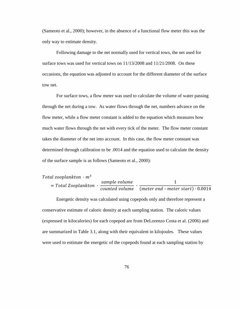
76
(Sameoto et al., 2000); however, in the absence of a functional flow meter this was the
only way to estimate density.
Following damage to the net normally used for vertical tows, the net used for
surface tows was used for vertical tows on 11/13/2008 and 11/21/2008. On these
occasions, the equation was adjusted to account for the different diameter of the surface
tow net.
For surface tows, a flow meter was used to calculate the volume of water passing
through the net during a tow. As water flows through the net, numbers advance on the
flow meter, while a flow meter constant is added to the equation which measures how
much water flows through the net with every tick of the meter. The flow meter constant
takes the diameter of the net into account. In this case, the flow meter constant was
determined through calibration to be .0014 and the equation used to calculate the density
of the surface sample is as follows (Sameoto et al., 2000):
Energetic density was calculated using copepods only and therefore represent a
conservative estimate of caloric density at each sampling station. The caloric values
(expressed in kilocalories) for each copepod are from DeLorenzo Costa et al. (2006) and
are summarized in Table 3.1, along with their equivalent in kilojoules. These values
were used to estimate the energetic of the copepods found at each sampling station by

77
calculating the total number of kilojoules per sub-sample and entering them into the
previous equations in place of the “Total Zooplankton” variable.
Sightings per unit effort and plankton characteristics
To examine the relationship between SPUE (sightings per unit effort) and
plankton characteristics, we compared SPUE to energetic density and proportions of C.
finmarchicus at vertical sampling stations. Only surveys from October – December were
included so that yearly plots had similar temporal extents. Only data from vertical
plankton tows were used, as these represented the majority of plankton tows during the
study period. Additionally, right whales were observed surface feeding on very few
occasional throughout the study period, suggesting that sub-surface plankton samples
were more likely to be representative of the whale’s target prey. However, this restriction
meant that 2003 was excluded from these plots due to the paucity of vertical tows from
that year.
Statistical analysis
All statistical analyses were performed using SPSS. To test for a difference in
caloric values between vertical and surface plankton tows, a univariate analysis of
variance (ANOVA) was carried out. The results of this test were used to justify
separating analyses by tow type in the following statistical tests. A binary logistic
regression was used to test the predictive value of caloric density of a station on whale
presence/absence at a station. Two tests were performed: one on vertical samples and

78
one on surface samples. A generalized linear model was used to test whether the station
type was a significant predictor of caloric density at the station. Here, caloric value was
the dependent variable and station type was the random factor. Station types included Rn
(Regular sampling station at which no whale was present in the vicinity), Rd (Regular
sampling station at which at least one right whale was present in the vicinity) and Sd
(Opportunistic sampling station chosen due to the presence of a right whale). Two tests
were performed: one on vertical samples and one on surface samples. Samples were
separated because a Levene’s (homogeneity of variance) test revealed that surface
samples had a different distribution than vertical samples.
Results
The effect of tow type (vertical or surface) on caloric value was found to be
significant (ANOVA, p=.015) with vertical tows having significantly smaller caloric
densities than surface tows (Table 3.2). In analysis of plankton characteristics in Jeffreys
Ledge, vertical and surface samples were analyzed separately, and in certain cases,
surface samples were omitted completely for reasons discussed in the methods section.
Sightings per unit effort and plankton characteristics
To examine the relationship between SPUE (sightings per unit effort) and
energetic density in Jeffreys Ledge, SPUE and mean energetic density (expressed in
kilojoules m-3
) from vertical tows were plotted against survey day on the same graph
(Figure 3.2). Plots were separated by survey season.

79
In some years, such as 2005, low overall SPUE was associated with low energetic
density in the study area. In 2004, overall SPUE values were relatively low, despite high
energetic density at some stations, while in 2007, the peak in SPUE was concurrent with
very low energetic density. 2006 was the only year in which peak SPUE corresponded
with high energetic density at some stations (Figure 3.2). A scatter plot of energetic
density and SPUE revealed no relationship between the two variables when all the years
were combined (Figure 3.3).
To examine the relationship between SPUE and species composition, SPUE and
the proportions of C. finmarchicus (Figure 3.4), Centropages spp. (Figure 3.6), and
Pseudocalanus spp.(Figure 3.8) in each sample were plotted against day of season.
SPUE was plotted on the same graphs. Plots were separated by survey season (Figures
3.4, 3.6, 3.8).
There appeared to be no relationship between the proportion of C. finmarchicus at
a station and the SPUE (Figures 3.4, 3.5). In 2005, SPUE was low throughout the season
despite high proportions of C.finmarchicus at many survey stations throughout the
season, whereas relative low proportions of C. finmarchicus in 2007 were measured
concurrently with peak SPUE values for that year. In most years, there was a large
variation in the proportions of C. finmarchicus observed at different sampling stations on
the same survey date.
There were no observable trends in the proportions of Centropages spp. during
the study period (Figures 3.6, 3.7). Except for 2004 and early 2005 when most stations
exhibited low proportions of Centropages spp., there was large variation in proportions of

80
Centropages spp. within and between survey dates and between years. There were no
observable changes in SPUE associated with changes in the proportion of Centropages
spp., although the small spike in SPUE in 2005 did coincide with a peak measurement of
Centropages spp. proportion for that year. Similar variation within and between years
existed in the proportions of Pseudocalanus spp.(Figure 3.8). Wide variation existed
within a survey date, throughout seasons and across the study period.
The proportion of C. finmarchicus, Centropages spp., and Pseudocalanus spp.
showed no trend against SPUE when all years in the study period were combined
(Figures 3.5, 3.7, 3.9).
Energetic density and whale presence/absence
A binary logistic regression was used to test the predictive value of the energetic
density of surface samples on whale presence/absence. While there was a significant
relationship between energetic density and whale presence/absence (p=.001)(Table 3.4),
energetic density correctly predicted whale absence 97.5% of the time but correctly
predicted whale presence only 25.6% of the time (Table 3.3).
Results were similar when vertical samples were tested. There was a significant
relationship between energetic density and whale presence absence (p=.028) (Table 3.6).
Energetic density could correctly predict whale absence 98.8% of the time, but the model
was not powerful in predicting whale presence (Table 3.5).
In both vertical and surface tows, low energetic density was a good predictor of
whale absence, but high energetic density was a poor predictor of whale presence.

81
Energetic density and station types
A generalized linear model was used to test whether the station type (Regular
station with no whales (Rn), Regular station with whales (Rd), Opportunistic station with
whales (Sd)) was a significant predictor of caloric density at the station. Testing surface
samples only, we found that both the Rd and the Rn stations have significantly less
energetic density than the opportunistic stations (p=.03; p<.001) (Table 3.7).
In a second generalized linear model testing only vertical samples (Table 3.8), Rd
and Sd stations were not significantly different, although there was a large standard error
for the Rd effect estimate. However, the Rn stations were found to have significantly
smaller caloric densities (B= -156.104) compared to the Sd stations (p=.003). In this
case, the station type could accurately predict the difference in caloric values between Sd
stations and Rn stations 85.1% of the time (Table 3.8).
Discussion
Sightings per unit effort and plankton characteristics
The finding that energetic density was significantly smaller in vertical samples
compared to surface samples was probably a result of the sampling methodology. In
most of the vertical samples, the net was dropped to a depth of 19 m, although in some
cases the net was dropped to 25 m or 50 m. Station A was the shallowest sampling
station, with an average depth of about 50 m; however, the remaining samples were taken
at locations where depths were far greater. Station C had an average depth of 180m, and

82
many opportunistic stations were in depths of 180 – 200 m. This means that vertical tows
were only sampling a small fraction of the water column. This is especially problematic
because from the late summer to mid-winter, stage V C. finmarchicus is known to go into
diapause, a dormant state that conserves energy during times of low food availability.
During these times of dormancy, diapausing C. finmarchicus settle at the bottom of the
water column (Hirche, 1996). In other habitats, such as the Bay of Fundy, right whales
are thought to target these energy-rich diapausing copepods, diving to depths exceeding
90 m (Baumgartner & Mate, 2003). Therefore, it is possible that vertical samples taken
in Jeffreys Ledge did not capture the layer of zooplankton that the whales were targeting.
The absence of a flow meter on the vertical net also likely caused an
underestimation of the plankton density, and by extension, the energetic density of the
vertical samples. As discussed in the methods, drift from the boat is likely to occur while
a vertical sample is being dropped, causing more water to flow through the net than is
captured by the equation (Sameoto et al., 2000).
These issues in sampling methodology also likely contributed to the lack of
correlation between sightings per unit effort, energetic density, and species composition.
It is possible that deep layers of diapausing copepods are what draw right whales to the
area, but that the lack of sampling range and precision do not allow us to measure the
relationship between SPUE and plankton characteristics. It is also possible that factors
which skew the calculation of SPUE contribute to this lack of correlation. Because
SPUE is calculated based on how many kilometers of trackline are surveyed , unusually
high SPUE values sometimes occur when a large amount of survey time is spent

83
photographing large aggregations of individuals, and a relatively small amount of time is
spent on the trackline.
It is also possible that food is not the primary factor drawing right whales to the
area. As discussed in section 1, Jeffreys Ledge and the surrounding areas have been
identified as a possible mating ground for right whales, so the lack of a relationship
between plankton characteristics and whale sightings might indicate that right whales are
using this habitat for purposes other than feeding.
Some patterns between energetic density and whale presence were observed from
the binary logistic regressions. However, while low energetic density appeared to be a
good predictor of whale absence, high energetic density was not powerful in predicting
whale presence. The lack of power of high energetic density at a station to predict whale
presence is most likely caused by the small sample size of stations at which whales were
present.
A generalized linear model also gave some support of a relationship between
whale presence and caloric density. Opportunistic stations had significantly higher
energetic density than both types of regular sampling stations (whale present vs. whale
absent) when surface tows were tested. In vertical samples, regular stations with no
whales had significantly lower energetic density than opportunistic stations. The
distinction between opportunistic samples and both types of regular sampling stations is
likely because opportunistic surface samples were most likely to be taken near whales
which were surface feeding, meaning that the researchers could more precisely target the

84
area where the plankton layer was likely to be dense by sampling as close to the whale as
possible.
The weak relationship between plankton characteristics and whale sightings is
likely due to one of two factors. Either the sampling methodology failed to capture the
layer of prey targeted by the whale, or the prey quality is not, in fact, the primary factor
drawing whales to the study area. Future studies should focus on targeting deeper layers
of plankton to characterize the quality of zooplankton for the entirety of the water
column. While net tows are the least technologically-advanced methods of evaluating
zooplankton density in a region, they are valuable in that they permit detailed analysis of
taxa, life stage, and gender of individual copepods at a specific location; however, they
are not able precisely target plankton layers concentrated at a specific depth, and samples
taken at deeper depths require winches and cables to retrieve the net. Future studies of
the plankton resource in Jeffreys Ledge should focus on targeting the depths in the water
column at which whales are likely to be feeding. An optical plankton counter (OPC)
might be useful in identifying the depths at which large concentrations of zooplankton
might be occurring in order to decide the depth to which the net will be dropped
(Sameoto et al., 2000)
Determining that food is not the primary reason drawing whales to the area would
be of equal value, lending further support to the idea that this habitat might be part of a
mating area for the species. As discussed in Chapter 2, the timing of right whale
occurrences in Jeffreys Ledge coincides with the time period during which conceptive
mating is thought to take place (Kraus et al., 2007). If more thorough plankton sampling

85
techniques were to continue to yield low values of energetic density in the study area, that
would provide support for the idea that right whales are using this habitat for reasons
other than foraging.
Alternately, this habitat could be a habitat with marginal food quality where right
whales occasionally stop and forage on their way to better feeding areas. It may be that
the occasional energy-rich plankton patch in Jeffreys Ledge might make it worthwhile for
right whales to forage in this region during times of year when plankton quality in other
habitats is also poor. Updating the plankton sampling regime to include more sampling
stations and to target specific depth would clarify which of these scenarios is the most
likely. Assessing the relationship between whale sightings and plankton quality could
potentially allow for predictions of whale aggregations, allowing conservation managers
to lower the risk of ship strikes and entanglement in fishing gear.
Conclusions
Technical facets of the plankton sampling methodology made it difficult to
establish a positive correlation between right whale SPUE and prey quality in Jeffreys
Ledge. However, we have shown a weak relationship between low energetic density and
right whale absence, as well as a significant difference in caloric densities at different
plankton sampling station types. These results suggest that more comprehensive
plankton sampling would be of value in determining the quality of the prey resource in
this region.

86
TABLES
Table 3.1. Estimate of species, stage and stage-specific energy density of copepods
(From DeLorenzo Costa et al., 2006).
Species/Stage/Sex
Caloric
Value(kCal)
Caloric
Value (kJ)
C. finmarchicus ≤IV 0.2644 1.1062496
C. finmarchicus ≥V 1.8623 7.7918632
C. finmarchicus Female 1.6346 6.8391664
C. finmarchicus Male 2.0977 8.7767768
Pseudocalanus spp. ≤IV 0.03 0.12552
Pseudocalanus spp. ≥V 0.1991 0.8330344
Centropages spp. ≤IV 0.08 0.33472
Centropages spp. V 0.0704 0.2945536
Centropages spp. Female 0.1562 0.6535408
Centropages spp. Male 0.1331 0.5568904
Acartia hudsonica 0.04 0.16736
Temora longicornus 0.12 0.50208
Tortanus discaudatus 0.2 0.8368
Oithona spp. 0.02 0.08368
Other 0.02 0.08368
Table 3.2. Results of a univariate analysis of variance testing the effect of tow type on energetic
density at a sampling station.
Parameter B SE T Sig.
Observed
Power*
Intercept 386.447 62.962 6.138 0 1.000
Vertical tow -196.354 80.165 -2.449 0.015 0.686
Surface tow 0**
*Computed using alpha=.05
**Parameter set to zero because it is redundant

87
Table 3.3. Logistic model from a Binary Logistic Regression measuring predictive
power of effect of energetic density of surface samples on whale presence/absence.
Table 3.4. Results of a binary logistic regression testing the effect of energetic density of
surface samples on whale presence/absence
B SE Wald df Sig. Exp(B)
Step 1 Energetic Density .001 .000 11.396 1 .001 1.001
Constant -1.582 .230 47.473 1 .000 .206
Table 3.5. Logistic model from a binary logistic regression measuring predictive power
of effect of energetic density of vertical samples on whale presence/absence.
Observed Predicted
Whale Presence Percentage
Correct Absent Present
Step 1 Absent 163 2 98.8
Present 84 7 7.7
Overall Percentage 66.4

88
Table 3.6. Results of a binary logistic regression testing the effect of energetic density of
vertical samples on whale presence/absence
B S.E. Wald df Sig. Exp(B)
Step 1 Energetic Density .001 .000 4.798 1 .028 1.001
Constant -.788 .156 25.632 1 .000 .455
Table 3.7. Results of a Generalized Linear Model testing the effect of station type on the
energetic density of surface samples. (Rd = Regular sampling station with whales
present; Rn=Regular sampling station with no whales present; Sd = Opportunistic
sampling station with whales present).
Paramete
r B SE t Sig.
Observe
d
Power*
Intercept
1192.892
181.872
6.559
0
1.000
Rd
-1067.18
486.884
-2.192
0.03
0.586
Rn
-1050.19
208.874
-5.028
0
0.999
Sd
0**
. . . .
*Computed using
alpha=.05
**Parameter set to zero because it is redundant
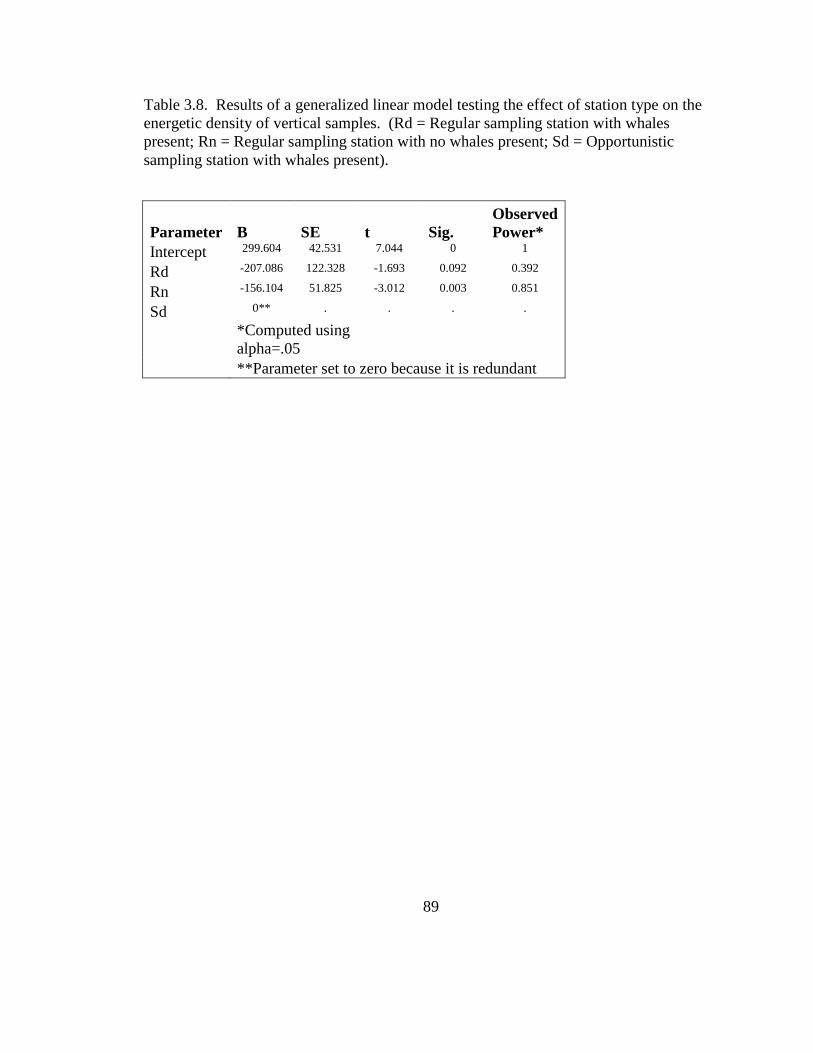
89
Table 3.8. Results of a generalized linear model testing the effect of station type on the
energetic density of vertical samples. (Rd = Regular sampling station with whales
present; Rn = Regular sampling station with no whales present; Sd = Opportunistic
sampling station with whales present).
Parameter B SE t Sig.
Observed
Power*
Intercept 299.604 42.531 7.044 0 1
Rd -207.086 122.328 -1.693 0.092 0.392
Rn -156.104 51.825 -3.012 0.003 0.851
Sd 0** . . . .
*Computed using
alpha=.05
**Parameter set to zero because it is redundant

90
FIGURES
Figure 3.1. Jeffreys Ledge survey area tracklines and regular sampling stations with
additional stations sampled by Provincetown Center for Coastal Studies (PCCS) in 2005
– 2006.
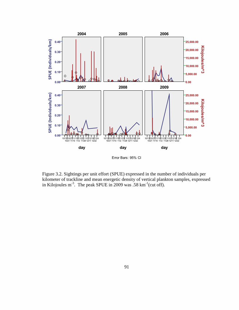
91
Figure 3.2. Sightings per unit effort (SPUE) expressed in the number of individuals per
kilometer of trackline and mean energetic density of vertical plankton samples, expressed
in Kilojoules m-3
. The peak SPUE in 2009 was .58 km-1
(cut off).

92
Figure 3.3. Scatter plot of energetic density (expressed in kilojoules m-3
) at a sampling
station and SPUE (expressed in number of individuals km-1
) for a survey date.

93
Figure 3.4. Sightings per unit effort (SPUE) expressed in the number of individuals per
kilometer of trackline and the proportion of C. finmarchicus in vertical samples. Each
point represents an individual vertical sample. The peak SPUE in 2009 was .58
individuals km-1
(cut off).

94
Figure 3.5. Scatter plot of the proportion of C. finmarchicus at a sampling station and
SPUE (expressed in number of individuals km-1
) for a survey date.

95
Figure 3.6. Sightings per unit effort (SPUE) expressed in the number of individuals per
kilometer of trackline and the proportion of Centropages spp. in vertical samples. Each
point represents an individual vertical sample. The peak SPUE in 2009 was .58
individuals km -1
(cut off).

96
Figure 3.7. Scatter plot of the proportion of Centropages spp. at a sampling station and
SPUE (expressed in number of individuals km-1
) for a survey date.

97
Figure 3.8. Sightings per unit effort (SPUE) expressed in the number of individuals per
kilometer of trackline and the proportion of Pseudocalanus spp. in vertical samples.
Each point represents an individual vertical sample. The peak SPUE in 2009 was .58
individuals km-1
(cut off).

98
Figure 3.9. Scatter plot of the proportion of Pseudocalanus spp. at a sampling station and
SPUE (expressed in number of individuals km-1
) for a survey date.

99
CHAPTER 4
RIGHT WHALE DISTRIBUTION IN JEFFREYS LEDGE: IDENTIFYING HOT
SPOTS AND ASSESSING THE EFFECT OF BATHYMETRIC FEATURES ON
RIGHT WHALE SIGHTINGS
Introduction
Jeffreys Ledge is approximately 54km long and is considered a complex glacial
deposit. The shallowest part of Jeffreys Ledge is characterized by depths of 45 – 61 m,
while the east and west sides of the ledge slope steeply to depth of up to 150 m (Weinrich
et al., 2000). The Jeffreys Ledge study area covers 2,022 km2, but right whale sightings
do not occur uniformly throughout the study area. Initial visualization of the sightings
data indicate that right whale sightings are most likely to occur off the northwest side of
the ledge (Figure 4.1). In this section, spatial statistics tools in ArcMap 10 will be used
to examine whether this clustering pattern is significantly different than what might be
expected from a random distribution of sightings, and hot and cold spots within the
region will be identified.
Hot spots refer to areas where features with high values cluster spatially, and cold
spots refer to areas where features of low values cluster spatially (ESRI, 2011).

100
Identifying hot and cold spots is a helpful research tool because by looking at where
features of high and low values cluster, there is the potential to identify the underlying
cause of that clustering pattern, based on location. Hot spot analysis is often used to set
conservation priorities by identifying areas of exceptionally high ecological importance
or vulnerability (Myers et al., 2000). In the case of the right whale, identifying such hot
spots can also be helpful to focus research and conservation efforts in the understudied
habitat of Jeffreys Ledge, and may provide insight into the factors affecting fine-scale
distribution of right whales. This analysis will also identify how hot and cold spots
change in size and location throughout the study period. Determining whether these hot
spot patterns are stable is important if future conservation decisions are to be informed by
these hot spots.
A second question that will be addressed is whether whale sightings are
influenced by bathymetric factors such as depth and slope. In some habitats, large
numbers of right whale sightings are often correlated with dense aggregations of
zooplankton, particularly calanoid copepods (Baumgartner et al., 2007). As discussed in
Chapter 2, attempts to correlate plankton densities with right whale sightings in Jeffreys
Ledge have been inconclusive (PCCS, 2008b; WCNE, 2008), possibly due to the fact that
the plankton layer that the whales are targeting may be too deep to be targeted by
traditional plankton tow methodologies employed .
Because a biological variable which can accurately predict right whale presence
has not yet been identified for this area, abiotic bathymetric features have the potential to
affect right whale sightings due to their role in influencing oceanographic patterns. The

101
bathymetry of the Gulf of Maine plays a role in the distribution of chlorophyll in the
water column (Fong et al., 1997). Oceanographic forces which affect primary
productivity can also, in turn, affect zooplankton population dynamics (Durbin, 1996).
Calanoid copepods are often found in areas of coastal upwelling where the interaction
between deep layers of nutrient rich water and coastal features leads to areas of high
productivity (Pinet, 2006; Miller, 2008).
Both depth and slope have been shown to affect the distribution of cetacean
species in various habitats. In many cetacean species including the sperm whale, dwarf
sperm whale, and several types of dolphins, depth and slope have been identified as
factors linked to species aggregations (Baumgartner et al., 2001; De Stephanis et al,
2008). In the shelf waters off the Western Antarctic Peninsula, areas of increasingly
slope are associated with both areas of increasing krill aggregation and whale distribution
(Friedlander et al., 2006). In other cetacean species such as the sperm whale, pygmy
sperm whale, In shelf-edge and deeper waters off the Northeastern United States, mean
sighting rates of both sperm and beaked whales are associated with canyon features, and
that association is thought to be a result of the interplay between both ephemeral and non-
ephemeral hydrographic features at the location resulting in the establishment of foraging
sites (Waring et al., 2001). Further, Southern right whales appear to show preferences for
areas of specific depths and sometimes slope on a fine scale. Elwen (2004) suggests that
the apparent preference by Southern right whale females with calves for slopes that are
neither very shallow nor very deep may reflect a preference for calmer waters. Calmer
waters are likely to deposit sediment in such a way that creates a gentle, but not too

102
shallow slope. This section will investigate whether such habitat preferences exist in the
Jeffreys Ledge habitat.
Methods
Only boat-based sightings of right whales collected by the Whale Center of New
England from 2003 - 2009 were used for these analyses. For details on data collection,
refer to the methods section of Chapter 2. All spatial analyses were performed in
ArcMap v. 10 and all regressions and generalized linear models were performed in SPSS.
Base map
Using ArcMap version 10.0, a vector-based bathymetry layer of the Gulf of
Maine from MassGIS was reprojected to the
NAD_1983_Stateplane_Massachusetts_Mainland_FIPS projection, which is a Lambert
Conformal Conical projection. Projections are used in cartography to address the
problem of working with a three-dimensional surface (the Earth’s surface) in two-
dimensional space by transforming a latitude and longitudinal position on the Earth’s
surface to a set of Cartesian coordinates (Longley et al., 2011). This projection is
appropriate for the mapping of states in the middle latitudes, and is used for areas that are
smaller than 30 degrees latitude. It preserves shape and provides minimal distortion of
area, and distance is preserved along parallels (Price, 2010).

103
To define the survey area, a polygon grid was created over the extent of the
survey area defined in Chapter 1. The grid was set so that each cell had an area of 2 km².
This grid size was chosen because every effort was made to obtain a right whale location
that was a close to the right whale itself, but when the location of a right whale is
recorded, that whale is within a 2 km radius of the recorded location.
To derive the sightings per unit effort (SPUE) value for each grid cell, a point
layer was imported where each point represented the number of whales seen at that
location on that survey date, divided by the total number of trackline kilometers surveyed
on that date. Using a spatial join, all of the points from the duration of the study period
were aggregated by each 2 km² grid cell such that each grid cell contained the sum of the
SPUE in that particular 2 km² area.
Hot spot analysis
The Hot Spot tool in ArcMap 10 uses the Getis-Ord Gi* statistic to identify hot
and cold spots within a region. The Gi* statistic returns a Z-score based on the value of a
feature and the values of neighboring features. In this case, each feature is a 2 km2 grid
cell with an associated summed SPUE value. A feature with a high value in close
proximity to cells of other high values will have a high positive Z-score, while a feature
with a low value in close proximity to other features with low values with have a low,
negative Z-score. Z-scores represent standard deviations associated with a normal
distribution. Z-scores with very high positive values or very low negative values are
associated with low p-values. A high positive Z-score and a low p-value indicate a

104
hotspot –a non-random clustering of high values, while a small Z score and a low p-value
indicate a cold spot—a non-random clustering of low values (ESRI, 2011).
To test the null hypothesis that there are no hot spots, only grid cells that
contained SPUE values greater than zero were selected. Inverse Distance was used as the
spatial characterization. This implies that every feature is potentially a neighbor of every
other feature, and was chosen as no physical boundaries prevent these kinds of
relationships in this environment. The distance band was set to the default, which is the
minimum distance needed so that each point has at least one neighbor (ESRI, 2011).
Each grid cell was weighted by the total SPUE in the cell.
The analysis was performed over the whole study period (2003 – 2009) as well as
on three year data intervals. Three year intervals were chosen because they contained
enough sightings data for meaningful analysis while allowing us to examine hot spots on
a finer temporal scale to see whether they changed over time. The tool requires a variety
of values in the variable to be analyzed (ESRI, 2011), and three years was the smallest
time interval over which a variety of values could be observed. In this analysis, the sum
of SPUE in each grid cell can be considered the independent variable and the resulting
Gi* score or Z-score in each grid cell is the dependent variable, as the analysis uses the
summed SPUE value per 2km2 grid cell as a weighting factor.

105
Regression analysis
To test whether or not right whale sightings were associated with bathymetric
features two types of regressions were performed on the data. An ordinary least squares
regression was performed to analyze the relationship between bathymetric features and
whale presence/absence, while a Generalized Linear Model was used to analyze the
relationship between bathymetric features and SPUE. For the binary logistic regression,
a Wald statistic was generated to test the significance of each individual parameter {{103
Sokal, R.R. 1995;}} and an exponentiation of the B coefficient (Exp(B)) was generated
because it is easier to interpret than the B coefficient (UCLA, 2007).
To prepare the data for these regressions, average values for depth and slope were
assigned to each grid cell. To accomplish this, separate rasters for both slope and depth
were created. To create a depth raster, an attribute was added to the polygon-based
bathymetry layer which averaged the high and low values for each depth range category.
Then, a raster was created using the average depth as the value for every cell. The cell
size was set to 350 m2, which was the finest-scale value allowed by the program, given
the complexity of the vector layer. To create a slope raster, the Slope tool in spatial
analyst was used to create a raster using the average depth raster as an input. The cell
size is also 350 m2 and each cell has a value for the average slope in degrees.
A point was placed in the center of each 2 km2 grid cell. Using the Extract Multi
Values to Point tool in the Extraction toolbox, depth and slope values from the depth and
slope from the 350 m2 rasters were extracted to the points at the center of each 2 km
2 grid
cell such that each 2 km2 grid cell had an associated slope and depth values defined by

106
that center point. The option to allow interpolation to the point was used so that the slope
and depth values across each cell were averaged for each center point. After this tool
was run, every 2km2 grid cell had 3 three values associated with it: average depth,
average slope and total SPUE. A table containing this information was imported into
SPSS where an additional field was added. For each grid cell, a value of 0 was assigned
if no whales were ever seen in the cell and a value of 1 was assigned if there had ever
been a whale observed in the cell.
Before attempting the regression analyses, a statistical test for multicollinearity
was performed in SPSS to confirm that slope and depth do not co-vary, as
multicollinearity can skew regression analyses. A Pearson’s Correlation Score of -.003
and a p-value of .94 suggested that covariance between slope and depth would not be
problematic in the following analyses.
A binary logistic regression was performed in SPSS to determine whether average
depth and slope in a 2km2 grid cell affected the probability of seeing a whale in that cell.
All cells within the study area were tested. A generalized linear model using a gamma
distribution with log link in SPSS was used to determine whether there was a relationship
between depth or slope and SPUE. Only grid cells in which whales were seen were
included in this analysis. This model was chosen due to the non-normality of the SPUE
data.

107
Results
Hot spot analysis
The Getis-Ord Gi* Hot Spot Analysis reveals a large hotspot located on the
northwestern edge of the ledge, and well a cold spot off the southeastern corner of the
ledge (Figure 4.2) Grid cells with high positive Z-scores and low p-values are considered
hot spots, meaning that they have high SPUE values and are in close proximity other cells
with high SPUE values. Grid cells with low negative Z-scores and low p-values are
considered cold spots, meaning that they have low SPUE values and are in close
proximity to other cells with low SPUE values.
Analysis over three-year intervals reveals a hot spot which changes in size,
location and intensity from 2003 – 2009. Cold spots are sparse in some years (Figures
4.3, 4.5 – 4.7) and non-existent in others (Figure 4.4), and in all years are lacking in
intensity, having only slightly negative Z-scores. The presence and location of a cold
spot in the map containing the entire study area is likely due to a larger sample size. In
the earlier years of the study period, the hotspot is small, and located off the southwestern
edge of the Ledge. As the years progress, the hotspot expands and moves towards the
northeast. The last three-year interval most closely resembles the hot spot present in the
hotspot analysis containing all seven years of data.

108
Regressions
Results of a binary logistic regression indicate that the probability of seeing a
whale within a given grid cell increases significantly with the average depth (p<.001),
but not slope in a cell (Table 4.1). Similarly, in areas where whales are present, a
generalized linear model reveals that SPUE is significantly higher with increasing cell
depth (p<.001), but not with slope or the interaction term (Table 4.2). The Wald statistic
value of 16.588 for that parameter also supports the significance of increasing depth with
slope. In the context of this analysis, the negative intercept or constant is meaningless
because a negative SPUE value is not possible. Negative intercepts and constants can
occur when the regression line moves farther away from the center of data (Freedman et
al., 2007).
Discussion
Hot spot analysis
The clustering and hot spot analysis showed statistically significant clustering and
hot spots off the northwest edge of Jeffreys Ledge where high sightings per unit effort
(SPUE) have occurred. The results of the hot spot analysis suggest that the null
hypothesis, that right whale SPUE is random throughout the study area, can be rejected.
The hot spot analysis identifies both hot spots, which are areas where high values (in this
case, high SPUE values) are spatially clustered, and cold spots, where low values of

109
SPUE are spatially clustered. Looking at the results of the Hot Spot analysis over three-
year intervals allowed us to see how hot spots changed over time.
An initial examination of the results shows a hot spot which changes in size as
well as location between 2003 and 2009. Between 2003 and 2005, only two grid cells
show a slightly significant hotspot, and these cells are much further to the southwest of
the large hotspot in the aggregated data. By the 2007 – 2009 interval, the hot spot was
larger, having more grid-cells with higher z-scores, and had shifted to the northeast.
Interestingly, the 2006 – 2008 interval shows several slightly significant cold
spots, while the aggregated data shows a much larger and more significant cold spot on
the other side of the ledge than the hotspot. This suggests that a survey is more likely to
observe high numbers of right whales off the northwest side of the ledge, to the west of
the westernmost trackline, while it is sightings are likely to be less frequent off the
northeast side of the ledge, to the east of the easternmost trackline.
Sightings of right whales were normalized by survey trackline effort due to
account for inconsistent survey effort between and within seasons. Because a primary
focus of these surveys was identifications data, one survey trackline (Track #3) was
surveyed more frequently than others to maximize the number of identification photos
obtained. Surprisingly, although this trackline was surveyed more than others because it
was believed that most sightings were occurring east of Jeffreys Ledge, this hot spot
analysis reveals that the highest sightings per unit effort occurred west of the ledge
between tracks 1 and 2.

110
Correcting sightings for effort alleviates some of the bias inherent in this survey
methodology. High SPUE values can occur when a large group of whales is seen after
spending very little time on the trackline and a long time capturing photos of each whale.
Very high SPUE values were characteristic of the 2009 season in which a large number
of surface active groups (SAGs) were observed and surveys were not completed due to
the time spent photographing individuals within these groups. It is possible that these
large values can at least partially account for the large hot spot seen towards the end of
the study period.
While the presence of a hot spot in this habitat can be useful in making future
survey effort more efficient; however, the changes in hot spot characteristics over shorter
time periods suggest that Jeffreys Ledge might be a more important habitat in some years
rather than others. Before restricting conservation efforts to a smaller segment of the
study area, more years of data should be included in the analysis to determine the long-
term stability of the hot spot.
Bathymetry
Both a binary logistic regression and a generalized linear model suggest that
depth, but not slope is a statistically significant predictor of the number of right whales in
an area. Bathymetric features were chosen as potential predictive factors because of the
characteristics of the right whales’ food source. It has been well-documented that many
species of zooplankton, including the copepod, vertically migrate throughout the day,
feeding at the surface during the night and migrating to deeper waters during the day to

111
avoid predators. Tarrant et al. (2008) sampled copepods in the Gulf of Maine in the
spring and found that the copepods sampled at depth were diapausing and had a larger oil
sac compared to copepods sampled at the surface. Similarly, studies by Baumgartner et
al. (2011) revealed that non-migrating copepods that remained in deep waters in the Great
South Channel had larger oil sac volumes, indicative of higher energetic content, than
migrating copepods and non-migrating copepods found at the surface. Right whales have
been documented feeding at depths of up to 200 meters in the Bay of Fundy
(Baumgartner & Mate, 2003), and it is possible that the correlations between right whale
sightings and increasing depths are related to the distribution of the planktonic resource
in deeper waters. However, many other factors not included in the model tested here,
including current speed and direction, sunlight, sea surface temperature, and nutrient load
may also play major roles in where plankton and right whales can be found in large
numbers.
Other facets of the methodology might also have influenced the results of both the
hot spot and the regression analyses. For example, although right whale sightings are
entered into the database as point features, their locations are not exact. The location is
determined by a GPS unit from a boat-based platform. As a result, the documented right
whale can be anywhere within an approximately 2 km radius of the documented location.
This is why 2 km was chosen as the grid size, however, that does not fully account for the
lack of precision in the whale’s location. Additionally, right whales generally do not stay
in the same location. Right whales in other foraging areas moved at an average of 1.1
km/h, and at greater speeds outside the foraging area (Mate, 1997). As their locations are

112
generally reported only once over the course of a survey, it is not possible to say whether
the whale is associated with a particular depth or slope for the duration of the
observation.
Finally, it is possible that the behavior of right whales causes the data to be
skewed. On Jeffreys Ledge, right whales are often observed on long (and presumably
deep) dives, which can exceed 30 minutes (Weinrich et al, 2000; WCNE, 2008). Because
they are detected visually, it is assumed that surveys underestimate the total number of
whales in any given area, as whales which may be on a long dive as the boat passes along
the trackline will remain undetected. It is possible that foraging behavior like long dives
may make a whale less likely to be detected than a whale that is engaging in surface
behavior such as surface feeding, surface social behavior, or travel. Future analyses
which incorporate observed behavior into a predictive model based on bathymetric
features may play a role in addressing this issue.
Future work must be done to confirm that deep basins play a role in zooplankton,
and by extension, right whale aggregation; however, depth appears to be a useful proxy in
predicting where right whales are likely to occur in the Jeffreys Ledge region.
Information on bathymetric preferences of right whales, used in conjunction with hot spot
visualization, can be helpful in focusing future conservation and research effort in this
region in order to further assess the importance of this habitat to the right whale.

113
Conclusions
Spatial analysis and spatial statistics tools are helpful in identifying patterns of
right whale habitat use in Jeffreys Ledge. We have identified a statistically significant
hot spot in the northwestern part of the study area which changed in size, location, and
intensity throughout the study period. Increasing the number of years involved in this
analysis could be useful in identifying long-term patterns of use in this habitat. We have
also used spatial data derived from a bathymetric layer of the Gulf of Maine to identify a
positive relationship between depth and right whale sightings in the region. In the
absence of a biological variable that can accurately predict right whale sightings, depth is
a useful and widely available predictive variable. Although the mechanism driving this
relationship is not certain, it further stresses the need for plankton sampling in this area
which targets the water column in its entirety.

114
TABLES
Table 4.1. Results of a binary logistic regression of the whale presence/absence in
relation to slope, depth and an interaction termin a 2km2 grid cell.
Table 4.2. Results of a generalized linear model of SPUE value in relation to slope,
depth and an interaction term in a 2km2 grid cell.
Parameter B SE Wald df Sig.
Constant -5.025 .3982 159.281 1 .000
Depth .011 .0029 15.100 1 .000
Slope .317 .3329 .909 1 .340
Depth*Slope -.002 .0026 .932 1 .334
Parameter B SE Wald
df Sig. Exp (B)
Constant -2.99 0.448 44.599 1 .000 0.05
Depth 0.014 0.003 16.588 1 .000 1.014
Slope 0.204 0.386 0.279 1 0.597 1.226
Depth* Slope -0.002 0.003 0.294 1 .588 0.998

115
FIGURES
Figure 4.1. Bathymetry of Jeffreys Ledge with boat-based whale sightings September
2003 – December 2009.

116
Figure 4.2. Results of Getis-Ord Gi* Hot Spot analysis of 2003 - 2009 SPUE. Cells with
high positive Z-scores are considered hotspots and cells with low negative Z-scores are
considered cold spots.
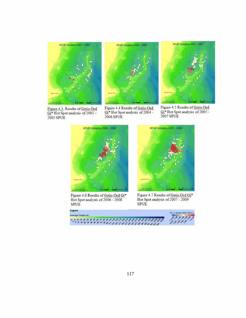
117

118
APPENDIX I
LIST OF ALL SURVEYS OF JEFFREYS LEDGE (JL) AND CAPE COD BAY (CCB)
DURING THE STUDY PERIOD BY THE WHALE CENTER OF NEW ENGLAND
(WCNE), NORTHEAST FISHERIES SCIENCE CENTER (NEFSC), AND
PROVINCETOWN CENTER FOR COASTAL STUDIES (PCCS)
Date Organization Platform Area
Survey
Completed? Flight Type*
Trackline km in
survey area
covered
9/30/2003 NEFSC Aerial JL Y Broadscale 22.3
10/9/2003 NEFSC Aerial JL N Broadscale 36.3
10/18/2003 NEFSC Aerial JL Y Broadscale 44.2
12/4/2003 NEFSC Aerial JL Y Focused (DAM) 70.72
2/12/2004 NEFSC Aerial JL Y Focused (DAM) 59.6
3/10/2004 NEFSC Aerial JL Y Focused (DAM) 256.25
3/30/2004 NEFSC Aerial JL Y Broadscale 38.2
4/17/2004 NEFSC Aerial JL Y Broadscale 10.7
4/25/2004 NEFSC Aerial JL Y Broadscale 34.3
5/12/2004 NEFSC Aerial JL Y Broadscale 41.7
10/14/2004 NEFSC Aerial JL N Focused (DAM) 22.6
10/26/2004 NEFSC Aerial JL Y Focused (DAM) 92.4
11/17/2004 NEFSC Aerial JL Y Broadscale 50.3
11/30/2004 NEFSC Aerial JL Y Broadscale 34.3
1/9/2005 NEFSC Aerial JL Y Broadscale 36.4
1/15/2005 NEFSC Aerial JL Y Broadscale 22.3
2/8/2005 NEFSC Aerial JL Y Broadscale 50.1
3/31/2005 NEFSC Aerial JL Y Broadscale 50.3
4/13/2005 NEFSC Aerial JL Y Broadscale 45
4/26/2005 NEFSC Aerial JL Y Broadscale 50.1
5/14/2005 NEFSC Aerial JL Y Broadscale 53.8
9/19/2005 NEFSC Aerial JL Y Broadscale 147.1
9/28/2005 NEFSC Aerial JL Y Broadscale 20.4
10/21/2005 NEFSC Aerial JL N Broadscale 26.9
10/28/2005 NEFSC Aerial JL Y Broadscale 53.8
11/18/2005 NEFSC Aerial JL Y Broadscale 10.7
11/19/2005 NEFSC Aerial JL Y Broadscale 38.2
12/21/2005 NEFSC Aerial JL Y Broadscale 34.3
1/29/2006 NEFSC Aerial JL Y Broadscale 49.4
2/21/2006 NEFSC Aerial JL Y Broadscale 67.9

119
3/19/2006 NEFSC Aerial JL Y Broadscale 38.2
4/26/2006 NEFSC Aerial JL Y Broadscale 34.3
10/3/2006 NEFSC Aerial JL Y Broadscale 34.3
10/17/2006 NEFSC Aerial JL Y Broadscale 50.3
11/25/2006 NEFSC Aerial JL Y Broadscale 34.2
11/27/2006 NEFSC Aerial JL Y Directed 127.3
12/11/2006 NEFSC Aerial JL Y Directed 132.4
1/4/2007 NEFSC Aerial JL Y Directed 16
1/22/2007 NEFSC Aerial JL N Directed 16
1/24/2007 NEFSC Aerial JL Y Directed 112.3
2/21/2007 NEFSC Aerial JL Y Directed 112.3
2/27/2007 NEFSC Aerial JL Y Broadscale 41.7
3/21/2007 NEFSC Aerial JL Y Directed 112.3
10/16/2007 NEFSC Aerial JL Y Sawtooth 203.6
11/5/2007 NEFSC Aerial JL Y Sawtooth 150.5
12/18/2007 NEFSC Aerial JL N Directed 0
1/13/2008 NEFSC Aerial JL Y Sawtooth 192.7
2/3/2008 NEFSC Aerial JL Y Sawtooth 192.7
2/29/2008 NEFSC Aerial JL Y Directed 209.2
2/29/2008 NEFSC Aerial JL Y Sawtooth 192.7
10/5/2008 NEFSC Aerial JL Y Sawtooth 99.7
10/21/2008 NEFSC Aerial JL Y Sawtooth 201.7
11/24/2008 NEFSC Aerial JL Y Sawtooth 209.2
1/26/2009 NEFSC Aerial JL N Sawtooth 176
2/10/2009 NEFSC Aerial JL Y Sawtooth 202.5
3/5/2009 NEFSC Aerial JL Y Sawtooth 196.3
10/27/2009 NEFSC Aerial JL Y Sawtooth 163.5
11/19/2009 NEFSC Aerial JL Y Sawtooth 167.2
1/5/2010 NEFSC Aerial JL Y Sawtooth 167.2
1/13/2010 NEFSC Aerial JL Y Sawtooth 83
1/28/2010 NEFSC Aerial JL N Sawtooth 88.4
2/28/2010 NEFSC Aerial JL N Jump Sawtooth 151.1
5/5/2010 NEFSC Aerial JL Y Jump Sawtooth 177
1/21/2004 PCCS Aerial CCB N 66.672
1/27/2004 PCCS Aerial CCB N 396.328
2/2/2004 PCCS Aerial CCB N 374.104
2/3/2004 PCCS Aerial CCB N 364.844
2/10/2004 PCCS Aerial CCB N 433.368
2/12/2004 PCCS Aerial CCB N 388.92
2/17/2004 PCCS Aerial CCB N 392.624

120
2/20/2004 PCCS Aerial CCB N 411.144
2/24/2004 PCCS Aerial CCB N 414.848
2/29/2004 PCCS Aerial CCB N 414.848
3/1/2004 PCCS Aerial CCB N 414.848
3/10/2004 PCCS Aerial CCB N 350.028
3/14/2004 PCCS Aerial CCB N 414.848
3/16/2004 PCCS Aerial CCB N 185.2
3/20/2004 PCCS Aerial CCB N 414.848
3/24/2004 PCCS Aerial CCB N 414.848
4/7/2004 PCCS Aerial CCB N 414.848
4/8/2004 PCCS Aerial CCB Y 435.22
4/10/2004 PCCS Aerial CCB Y 435.22
4/18/2004 PCCS Aerial CCB Y 435.22
4/21/2004 PCCS Aerial CCB N 414.848
4/25/2004 PCCS Aerial CCB N 414.848
5/5/2004 PCCS Aerial CCB Y 435.22
5/6/2004 PCCS Aerial CCB N 414.848
5/8/2004 PCCS Aerial CCB Y 435.22
5/10/2004 PCCS Aerial CCB N 414.848
1/2/2005 PCCS Aerial CCB Y 435.22
1/9/2005 PCCS Aerial CCB Y 435.22
1/11/2005 PCCS Aerial CCB Y 435.22
1/15/2005 PCCS Aerial CCB Y 435.22
1/30/2005 PCCS Aerial CCB Y 435.22
2/1/2005 PCCS Aerial CCB Y 435.22
2/2/2005 PCCS Aerial CCB N 435.22
2/7/2005 PCCS Aerial CCB Y 435.22
2/8/2005 PCCS Aerial CCB N 414.848
2/9/2005 PCCS Aerial CCB Y 435.22
2/14/2005 PCCS Aerial CCB N 414.848
2/17/2005 PCCS Aerial CCB Y 435.22
2/26/2005 PCCS Aerial CCB Y 435.22
2/28/2005 PCCS Aerial CCB Y 435.22
3/5/2005 PCCS Aerial CCB Y 435.22
3/7/2005 PCCS Aerial CCB Y 435.22
3/10/2005 PCCS Aerial CCB N 414.848
3/11/2005 PCCS Aerial CCB N 175.94
3/13/2005 PCCS Aerial CCB N 414.848
3/18/2005 PCCS Aerial CCB N 222.24
3/20/2005 PCCS Aerial CCB N 414.848

121
3/22/2005 PCCS Aerial CCB Y 435.22
3/26/2005 PCCS Aerial CCB N 350.028
3/27/2005 PCCS Aerial CCB N 414.848
4/1/2005 PCCS Aerial CCB N 414.848
4/5/2005 PCCS Aerial CCB Y 435.22
4/6/2005 PCCS Aerial CCB N 368.548
4/10/2005 PCCS Aerial CCB Y 435.22
4/16/2005 PCCS Aerial CCB N 414.848
4/17/2005 PCCS Aerial CCB Y 435.22
4/22/2005 PCCS Aerial CCB Y 435.22
4/26/2005 PCCS Aerial CCB N 31.484
5/3/2005 PCCS Aerial CCB N 414.848
5/5/2005 PCCS Aerial CCB Y 435.22
5/10/2005 PCCS Aerial CCB Y 435.22
1/10/2006 PCCS Aerial CCB Y 435.22
1/12/2006 PCCS Aerial CCB Y 435.22
1/17/2006 PCCS Aerial CCB N 414.848
1/22/2006 PCCS Aerial CCB N 414.848
1/24/2006 PCCS Aerial CCB N 414.848
1/29/2006 PCCS Aerial CCB Y 435.22
2/2/2006 PCCS Aerial CCB Y 435.22
2/4/2006 PCCS Aerial CCB Y 435.22
2/9/2006 PCCS Aerial CCB Y 437.072
2/16/2006 PCCS Aerial CCB Y 437.072
2/22/2006 PCCS Aerial CCB Y 437.072
2/23/2006 PCCS Aerial CCB Y 437.072
3/2/2006 PCCS Aerial CCB N 216.684
3/6/2006 PCCS Aerial CCB N 66.672
3/8/2006 PCCS Aerial CCB N 414.848
3/12/2006 PCCS Aerial CCB N 368.548
3/22/2006 PCCS Aerial CCB N 64.82
3/24/2006 PCCS Aerial CCB Y 435.22
3/25/2006 PCCS Aerial CCB Y 437.072
3/28/2006 PCCS Aerial CCB Y 437.072
3/29/2006 PCCS Aerial CCB Y 437.072
3/30/2006 PCCS Aerial CCB Y 437.072
4/3/2006 PCCS Aerial CCB N 414.848
4/10/2006 PCCS Aerial CCB Y 437.072
4/12/2006 PCCS Aerial CCB N 142.604
4/14/2006 PCCS Aerial CCB N 316.692

122
4/22/2006 PCCS Aerial CCB Y 435.22
4/26/2006 PCCS Aerial CCB N 216.684
4/27/2006 PCCS Aerial CCB Y 435.22
5/5/2006 PCCS Aerial CCB Y 435.22
5/6/2006 PCCS Aerial CCB Y 435.22
5/18/2006 PCCS Aerial CCB Y 435.22
1/24/2007 PCCS Aerial CCB N 414.848
1/27/2007 PCCS Aerial CCB N 66.672
2/7/2007 PCCS Aerial CCB N 414.848
2/10/2007 PCCS Aerial CCB Y 435.22
2/11/2007 PCCS Aerial CCB Y 435.22
2/21/2007 PCCS Aerial CCB N 414.848
2/22/2007 PCCS Aerial CCB Y 435.22
2/25/2007 PCCS Aerial CCB Y 435.22
2/27/2007 PCCS Aerial CCB N 414.848
3/1/2007 PCCS Aerial CCB Y 435.22
3/3/2007 PCCS Aerial CCB N 283.356
3/9/2007 PCCS Aerial CCB N 283.356
3/12/2007 PCCS Aerial CCB N 350.028
3/21/2007 PCCS Aerial CCB N 51.856
3/23/2007 PCCS Aerial CCB N 414.848
3/24/2007 PCCS Aerial CCB N 414.848
3/26/2007 PCCS Aerial CCB N 142.604
3/31/2007 PCCS Aerial CCB Y 435.22
4/1/2007 PCCS Aerial CCB Y 435.22
4/7/2007 PCCS Aerial CCB N 414.848
4/11/2007 PCCS Aerial CCB N 414.848
4/21/2007 PCCS Aerial CCB Y 435.22
4/22/2007 PCCS Aerial CCB Y 435.22
4/25/2007 PCCS Aerial CCB Y 435.22
4/26/2007 PCCS Aerial CCB N 414.848
5/5/2007 PCCS Aerial CCB N 414.848
5/7/2007 PCCS Aerial CCB Y 435.22
5/9/2007 PCCS Aerial CCB N 387.068
5/13/2007 PCCS Aerial CCB N 350.028
5/14/2007 PCCS Aerial CCB Y 435.22
1/5/2008 PCCS Aerial CCB Y 435.22
1/12/2008 PCCS Aerial CCB N 350.028
1/26/2008 PCCS Aerial CCB Y 435.22
2/3/2008 PCCS Aerial CCB Y 435.22

123
2/21/2008 PCCS Aerial CCB N 151.864
2/24/2008 PCCS Aerial CCB Y 435.22
2/29/2008 PCCS Aerial CCB N 414.848
3/6/2008 PCCS Aerial CCB N 225.944
3/11/2008 PCCS Aerial CCB N 233.352
3/14/2008 PCCS Aerial CCB N 194.46
3/18/2008 PCCS Aerial CCB Y 435.22
3/24/2008 PCCS Aerial CCB Y 435.22
3/27/2008 PCCS Aerial CCB N 246.316
4/8/2008 PCCS Aerial CCB N 137.048
4/9/2008 PCCS Aerial CCB N 174.088
4/10/2008 PCCS Aerial CCB N 66.672
4/11/2008 PCCS Aerial CCB N 151.864
4/14/2008 PCCS Aerial CCB N 166.68
4/15/2008 PCCS Aerial CCB N 292.616
4/19/2008 PCCS Aerial CCB N 357.436
4/21/2008 PCCS Aerial CCB N 350.028
4/23/2008 PCCS Aerial CCB N 174.088
5/1/2008 PCCS Aerial CCB Y 435.22
5/6/2008 PCCS Aerial CCB Y 435.22
5/15/2008 PCCS Aerial CCB Y 435.22
1/23/2009 PCCS Aerial CCB Y 435.22
1/26/2009 PCCS Aerial CCB Y 435.22
1/30/2009 PCCS Aerial CCB Y 435.22
2/2/2009 PCCS Aerial CCB Y 435.22
2/11/2009 PCCS Aerial CCB N 337.064
2/16/2009 PCCS Aerial CCB N 414.848
2/25/2009 PCCS Aerial CCB N 262.984
3/10/2009 PCCS Aerial CCB N 414.848
3/15/2009 PCCS Aerial CCB N 311.136
3/17/2009 PCCS Aerial CCB N 383.364
3/26/2009 PCCS Aerial CCB N 388.92
4/9/2009 PCCS Aerial CCB N 218.536
4/10/2009 PCCS Aerial CCB Y 435.22
4/14/2009 PCCS Aerial CCB N 383.364
4/17/2009 PCCS Aerial CCB Y 435.22
5/8/2009 PCCS Aerial CCB Y 435.22
5/11/2009 PCCS Aerial CCB Y 435.22
1/13/2010 PCCS Aerial CCB N 77.784
1/16/2010 PCCS Aerial CCB N 396.328

124
1/21/2010 PCCS Aerial CCB Y 435.22
1/28/2010 PCCS Aerial CCB N 212.98
2/2/2010 PCCS Aerial CCB Y 435.22
2/13/2010 PCCS Aerial CCB Y 435.22
2/21/2010 PCCS Aerial CCB N 206.6832
2/22/2010 PCCS Aerial CCB N 414.848
2/28/2010 PCCS Aerial CCB Y 435.22
3/2/2010 PCCS Aerial CCB Y 435.22
3/7/2010 PCCS Aerial CCB Y 435.22
3/10/2010 PCCS Aerial CCB Y 435.22
3/12/2010 PCCS Aerial CCB Y 435.22
3/19/2010 PCCS Aerial CCB Y 435.22
3/21/2010 PCCS Aerial CCB Y 435.22
3/25/2010 PCCS Aerial CCB N 331.508
3/28/2010 PCCS Aerial CCB Y 435.22
4/2/2010 PCCS Aerial CCB N 414.848
4/5/2010 PCCS Aerial CCB Y 435.22
4/8/2010 PCCS Aerial CCB N 85.192
4/12/2010 PCCS Aerial CCB Y 435.22
4/13/2010 PCCS Aerial CCB Y 435.22
4/18/2010 PCCS Aerial CCB Y 435.22
4/20/2010 PCCS Aerial CCB Y 435.22
5/5/2010 PCCS Aerial CCB Y 435.22
9/15/2003 WCNE Boat JL Y 151
9/22/2003 WCNE Boat JL Y 158
9/26/2003 WCNE Boat JL Y 151
9/29/2003 WCNE Boat JL Y 158
10/1/2003 WCNE Boat JL N 133.5
10/6/2003 WCNE Boat JL Y 158
10/9/2003 WCNE Boat JL N 132.5
10/14/2003 WCNE Boat JL Y 158
10/17/2003 WCNE Boat JL Y 158
10/20/2003 WCNE Boat JL Y 151
10/25/2003 WCNE Boat JL N 119
10/31/2003 WCNE Boat JL Y 151
11/2/2003 WCNE Boat JL Y 158
11/6/2003 WCNE Boat JL Y 151
11/7/2003 WCNE Boat JL Y 158
11/10/2003 WCNE Boat JL Y 158
11/11/2003 WCNE Boat JL Y 133

125
11/17/2003 WCNE Boat JL Y 158
11/18/2003 WCNE Boat JL Y 158
11/24/2003 WCNE Boat JL N 138.5
11/26/2003 WCNE Boat JL Y 151
12/5/2003 WCNE Boat JL Y 133
12/10/2003 WCNE Boat JL Y 158
9/15/04 WCNE Boat JL Y 158
9/21/04 WCNE Boat JL Y 151
9/24/04 WCNE Boat JL Y 133
9/27/04 WCNE Boat JL N 37
10/1/04 WCNE Boat JL N 103
10/4/04 WCNE Boat JL Y 151
10/8/04 WCNE Boat JL Y 133
10/13/04 WCNE Boat JL Y 158
10/14/04 WCNE Boat JL Y 133
10/29/04 WCNE Boat JL Y 133
11/2/04 WCNE Boat JL Y 151
11/4/04 WCNE Boat JL Y 133
11/10/04 WCNE Boat JL Y 151
11/16/04 WCNE Boat JL Y 133
11/18/04 WCNE Boat JL Y 151
11/19/04 WCNE Boat JL N 100
11/23/04 WCNE Boat JL N 151
11/27/04 WCNE Boat JL N 118
11/30/04 WCNE Boat JL Y 151
12/4/04 WCNE Boat JL Y 133
12/9/04 WCNE Boat JL Y 151
12/12/04 WCNE Boat JL N 44
12/16/04 WCNE Boat JL N 84
12/18/04 WCNE Boat JL Y 151
12/22/04 WCNE Boat JL Y 158
12/30/04 WCNE Boat JL Y 158
9/19/2005 WCNE Boat JL Y 151
9/23/2005 WCNE Boat JL Y 133
9/28/2005 WCNE Boat JL Y 158
10/3/2005 WCNE Boat JL N 84
10/18/2005 WCNE Boat JL Y 158
10/21/2005 WCNE Boat JL Y 133
10/28/2005 WCNE Boat JL Y 151
10/31/2005 WCNE Boat JL Y 158

126
11/5/2005 WCNE Boat JL N 55
11/8/2005 WCNE Boat JL N 125
11/19/2005 WCNE Boat JL Y 133
11/21/2005 WCNE Boat JL Y 151
11/26/2005 WCNE Boat JL Y 133
11/28/2005 WCNE Boat JL Y 158
12/5/2005 WCNE Boat JL N 34
12/12/2005 WCNE Boat JL Y 133
12/19/2005 WCNE Boat JL N 36
12/21/2005 WCNE Boat JL Y 133
12/28/2005 WCNE Boat JL Y 158
1/6/2006 WCNE Boat JL Y 133
1/10/2006 WCNE Boat JL Y 151
1/13/2006 WCNE Boat JL Y 158
1/17/2006 WCNE Boat JL Y 133
1/24/2006 WCNE Boat JL Y 151
10/19/06 WCNE Boat JL Y 133
10/27/06 WCNE Boat JL Y 151
10/31/06 WCNE Boat JL Y 133
11/5/06 WCNE Boat JL Y 158
11/6/06 WCNE Boat JL Y 133
11/11/06 WCNE Boat JL N 109
11/15/06 WCNE Boat JL Y 133
11/18/06 WCNE Boat JL N 114
11/20/06 WCNE Boat JL N 45
11/22/06 WCNE Boat JL N 137
11/27/06 WCNE Boat JL Y 133
12/11/06 WCNE Boat JL N 130
12/14/06 WCNE Boat JL Y 133
10/18/2007 WCNE Boat JL Y 151
10/22/2007 WCNE Boat JL Y 133
10/26/2007 WCNE Boat JL N 132
10/31/2007 WCNE Boat JL N 127
11/2/2007 WCNE Boat JL Y 151
11/5/2007 WCNE Boat JL N 82
11/9/2007 WCNE Boat JL N 144
11/12/2007 WCNE Boat JL Y 133
11/18/2007 WCNE Boat JL N 125
11/26/2007 WCNE Boat JL N 129
12/5/2007 WCNE Boat JL N 138

127
10/21/2008 WCNE Boat JL Y 133
10/24/2008 WCNE Boat JL Y 151
10/27/2008 WCNE Boat JL Y 133
10/31/2008 WCNE Boat JL N 94
11/3/2008 WCNE Boat JL N 90
11/4/2008 WCNE Boat JL Y 151
11/12/2008 WCNE Boat JL Y 133
11/13/2008 WCNE Boat JL N 128
11/21/2008 WCNE Boat JL N 44
11/24/2008 WCNE Boat JL N 116
11/30/2008 WCNE Boat JL N 106
12/3/2008 WCNE Boat JL N 128
12/6/2008 WCNE Boat JL N 120
10/21/2009 WCNE Boat JL N/A Directed 0
10/26/2009 WCNE Boat JL N 52
10/27/2009 WCNE Boat JL N 115
11/7/2009 WCNE Boat JL N 52
11/8/2009 WCNE Boat JL N 138
11/10/2009 WCNE Boat JL N 50
11/18/2009 WCNE Boat JL Y 133
11/19/2009 WCNE Boat JL Y 158
12/2/2009 WCNE Boat JL Y 133
*For NEFSC surveys only. All other surveys are the same throughout the study period.

128
APPENDIX II
RELATIONSHIPS BETWEEN SIGHTINGS PER UNIT EFFORT (SPUE) AND
EFFORT
Relationship between SPUE (sightings per unit effort) and total trackline effort for
Northeast Fisheries Science Center (NEFSC) aircraft-based surveys.
0
0.02
0.04
0.06
0.08
0.1
0.12
0.14
0.16
0 50 100 150 200 250 300 350 400 450
SP
UE
(In
div
idu
als
/km
)
Effort (Trackline km)
Jeffreys Ledge SPUE and Trackline
Effort (Aircraft-based)

129
Relationship between SPUE (sightings per unit effort) and total trackline effort for
Whale Center of New England (WCNE) boat-based surveys.
Relationship between SPUE (sightings per unit effort) and total trackline effort for
Provincetown Center for Coastal Studies (PCCS) aircraft-based surveys.
0
0.1
0.2
0.3
0.4
0.5
0.6
0.7
0 200 400 600 800 1000 1200 1400 1600
SP
UE
(In
div
idu
als
/km
)
Effort (Trackline km)
Jeffreys Ledge SPUE and Trackline Effort
(Boat-based)
0
0.5
1
1.5
2
2.5
0 500 1000 1500 2000 2500 3000 3500 4000
SP
UE
(In
div
idu
als
/km
)
Effort (Trackline km)
Cape Cod Bay SPUE and Trackline
Effort (Aircraft-based)

130
APPENDIX III
LIST OF ALL PLANKTON SAMPLES WITH STATION, STATION TYPE, TOW
TYPE, PROPORTIONS OF THREE MAJOR SPECIES, ORGANISM DENSITY AND
ENERGETIC DENSITY
Date Station
Station
Type
Tow
Type
Prop.
C.finmarchicus.
Proportion
Centropages
spp.
Proportion
Pseudocalanus
spp. Organisms m-3
Energetic
Density
(kJ m-3)
10/9/2003 B Rn surface 0.00 0.41 0.11 184.14 64.60
10/9/2003 Z Rn surface 0.03 0.62 0.17 4155.69 2765.12
10/9/2003 A Rn surface 0.10 0.62 0.18 138.73 120.07
10/9/2003 B Rn vertical 0.08 0.75 0.12 3971.65 3841.00
10/14/2003 A Rn surface 0.00 0.72 0.12 180.20 86.11
10/14/2003 B Rn surface 0.04 0.31 0.60 479.13 64.70
10/14/2003 W1 Sd surface 0.00 0.73 0.15 268.73 249.40
10/14/2003 W2 Sd surface 0.02 0.75 0.21 5340.97 7506.99
10/17/2003 B Rn surface 0.00 0.63 0.36 2114.87 2898.18
10/17/2003 A Rn surface 0.03 0.66 0.28 527.43 761.56
10/20/2003 A Rn surface 0.03 0.44 0.38 162.96 141.61
10/20/2003 B Rn surface 0.00 0.62 0.35 414.12 93.94
10/25/2003 A Rn surface 0.08 0.07 0.80 29.03 17.12
10/25/2003 B Rn surface 0.03 0.52 0.44 599.21 191.61
10/25/2003 W1 Sd surface 0.01 0.88 0.12 3426.90 2322.98
10/31/2003 A Rn surface 0.03 0.25 0.69 1018.60 202.27
10/31/2003 B Rn surface 0.10 0.08 0.75 57.77 11.99
11/2/2003 B Rn surface 0.02 0.63 0.35 1611.39 1676.18
11/2/2003 A Rn surface 0.16 0.18 0.57 337.15 430.74
11/2/2003 W1 Sd surface 0.06 0.80 0.14 3871.70 6775.20
11/6/2003 W1 Sd surface 0.99 0.00 0.00 1302.53 9547.44
11/6/2003 A Rn surface 0.31 0.20 0.46 592.41 1286.86
11/7/2003 A Rn surface 0.45 0.22 0.32 245.26 789.81
11/7/2003 B Rn surface 0.13 0.59 0.27 530.81 1550.99
11/7/2003 W1 Sd surface 0.44 0.15 0.41 2779.72 4163.61
11/7/2003 W2 Sd surface 0.58 0.12 0.22 63.48 97.09
11/10/2003 B Rn surface 0.03 0.34 0.62 533.64 245.57
11/10/2003 W1 Sd surface 0.06 0.26 0.68 221.44 128.96
11/10/2003 A Rn surface 0.20 0.18 0.62 1461.45 1744.13
11/10/2003 W2 Sd surface 0.08 0.06 0.71 16.19 6.50
11/11/2003 W1 Sd surface 0.09 0.35 0.54 175.58 60.68
11/11/2003 W2 Sd surface 0.52 0.15 0.31 854.90 631.66
11/11/2003 W3 Sd surface 0.61 0.17 0.21 913.31 1750.92
11/17/2003 B Rn surface 0.22 0.44 0.22 0.52 0.51
11/17/2003 W1 Sd surface 0.90 0.03 0.04 8.09 49.38
11/17/2003 W2 Sd surface 1.00 0.00 0.00 0.34 2.09

131
11/17/2003 W3 Sd surface 0.05 0.39 0.54 131.18 68.67
11/18/2003 W1 Sd surface 0.17 0.29 0.52 324.14 337.02
11/18/2003 A Rn surface 0.06 0.47 0.46 939.75 597.14
11/24/2003 A Rn surface 0.06 0.50 0.44 1423.55 694.96
11/24/2003 B Rd surface 0.07 0.49 0.43 149.32 113.35
11/24/2003 W1 Sd surface 0.15 0.40 0.41 19.01 25.12
11/26/2003 A Rn surface 0.09 0.50 0.39 740.94 1388.11
11/26/2003 B Rn surface 0.02 0.35 0.62 1042.12 671.94
11/26/2003 W1 Sd surface 0.08 0.30 0.61 341.74 160.58
12/5/2003 B Rn surface 0.04 0.26 0.68 81.51 30.83
12/5/2003 W1 Sd surface 0.01 0.18 0.76 18825.49 4729.64
12/5/2003 W2 Sd surface 0.00 0.16 0.84 5227.85 1698.74
12/10/2003 B Rn surface 0.10 0.27 0.54 31.45 19.34
12/10/2003 W1 Sd surface 0.55 0.15 0.28 20.14 67.63
12/10/2003 A Rn surface 0.04 0.43 0.48 984.16 530.87
12/10/2003 W2 Sd surface 0.00 0.66 0.30 969.67 1033.64
9/15/2004 A Rn surface 0.00 0.50 0.50 0.62 0.06
9/15/2004 B Rn vertical 0.33 0.11 0.56 0.98 0.61
9/15/2004 A Rn vertical 0.21 0.40 0.35 5.53 2.57
9/21/2004 B Rn surface 0.47 0.06 0.35 4.04 0.94
9/21/2004 A Rn vertical 0.00 0.60 0.40 0.45 0.27
9/21/2004 B Rn vertical 0.25 0.20 0.55 1.74 2.28
9/24/2004 W1 Sd vertical 0.56 0.00 0.33 0.76 0.62
9/27/2004 W1 Sd vertical 0.46 0.04 0.50 9.92 3.74
9/27/2004 A Rn vertical 0.12 0.12 0.76 1.89 1.05
9/27/2004 A Rn surface 0.34 0.43 0.20 2.73 1.21
9/27/2004 W1 Sd surface 0.66 0.06 0.28 427.74 104.92
10/1/2004 A Rn vertical 0.29 0.00 0.71 0.61 0.48
10/1/2004 A Rn surface 0.77 0.06 0.16 8.23 4.27
10/4/2004 B Rn vertical 0.48 0.03 0.47 508.69 1020.55
10/4/2004 A Rn vertical 0.56 0.07 0.34 3.41 3.41
10/13/2004 A Rn vertical 0.59 0.00 0.35 42.58 51.50
10/13/2004 B Rn vertical 0.76 0.02 0.13 580.35 655.29
10/13/2004 W1 Sd vertical 0.63 0.01 0.30 38.30 28.99
10/14/2004 W1 Sd vertical 0.92 0.00 0.06 2526.42 3576.95
11/2/2004 W1 Sd vertical 0.81 0.02 0.16 295.22 715.13
11/2/2004 B Rn vertical 0.59 0.02 0.35 304.31 565.34
11/2/2004 A Rn surface 0.37 0.09 0.09 87.13 63.23
11/10/2004 W1 Sd vertical 0.80 0.02 0.18 2252.01 6327.06
11/10/2004 B Rn vertical 0.85 0.01 0.12 656.30 1723.11
11/10/2004 A Rn vertical 0.86 0.00 0.05 86.11 148.06
11/10/2004 B Rn surface 0.91 0.00 0.03 99.58 323.16
11/16/2004 C Rn vertical 0.43 0.13 0.43 1315.88 1504.39
11/16/2004 W1 Sd vertical 0.80 0.02 0.18 160.78 373.48
11/16/2004 W2 Sd surface 0.86 0.00 0.12 2046.78 9357.17
11/16/2004 W2 Sd vertical 0.88 0.01 0.11 3583.04 15188.14

132
11/18/2004 W4 Sd vertical 0.60 0.00 0.39 1090.05 2858.61
11/18/2004 W4 Sd surface 0.81 0.00 0.18 7795.23 34557.35
11/18/2004 W2 Sd surface 0.93 0.00 0.07 2426.85 12243.25
11/18/2004 B Rn surface 0.57 0.31 0.07 1455.48 2344.57
11/18/2004 B Rn vertical 0.45 0.19 0.35 1755.25 2975.89
11/18/2004 W3 Sd surface 0.93 0.00 0.07 535.36 2617.99
11/18/2004 W1 Sd vertical 0.64 0.06 0.30 111.28 231.99
11/18/2004 C Rn vertical 0.54 0.03 0.43 302.03 518.78
11/23/2004 A Rn vertical 0.67 0.09 0.22 1067.34 3635.26
11/23/2004 D Rn vertical 0.76 0.04 0.19 268.73 1257.40
11/23/2004 W3 Sd surface 0.81 0.01 0.15 1964.96 2511.09
11/23/2004 W2 Sd surface 0.97 0.01 0.02 5948.30 34095.74
11/23/2004 W1 Sd surface 0.83 0.03 0.14 6970.34 32187.38
11/23/2004 A Rn surface 0.74 0.04 0.22 368.38 1376.43
11/27/2004 A Sd vertical 0.17 0.10 0.64 821.32 697.30
11/27/2004 W1 Sd vertical 0.28 0.13 0.58 429.96 336.07
11/27/2004 A Sd surface 0.26 0.08 0.61 124.83 79.86
11/30/2004 B Rn surface 0.50 0.10 0.13 4.39 3.96
11/30/2004 B Rn vertical 0.44 0.10 0.45 254.53 506.22
11/30/2004 C Rn vertical 0.56 0.07 0.37 1400.41 2284.28
12/4/2004 D Rn surface 0.65 0.03 0.29 9.42 27.39
12/4/2004 C Rn vertical 0.96 0.01 0.03 171.83 869.68
12/4/2004 D Rn vertical 0.83 0.04 0.13 89.42 435.67
12/9/2004 A Rn vertical 0.28 0.02 0.15 133.10 124.39
12/9/2004 C Rn vertical 0.89 0.00 0.09 160.86 474.52
12/9/2004 C Rn surface 0.25 0.25 0.25 0.29 0.60
12/12/2004 D Rn surface 0.55 0.02 0.41 16.16 44.06
12/12/2004 D Rn vertical 0.80 0.09 0.11 120.49 515.43
12/16/2004 D Rn vertical 0.46 0.14 0.37 33.31 86.20
12/18/2004 B Rn vertical 0.54 0.04 0.41 957.58 3214.15
12/18/2004 C Rn vertical 0.35 0.01 0.63 254.53 537.30
12/18/2004 C Rn surface 0.45 0.17 0.24 2.52 5.89
12/22/2004 D Rn vertical 0.66 0.10 0.23 82.79 291.98
12/22/2004 A Rn vertical 0.57 0.01 0.42 715.35 2968.52
12/22/2004 A Rn surface 0.87 0.00 0.13 1025.57 5804.73
12/30/2004 A Rn surface 0.70 0.04 0.24 56.19 249.92
12/30/2004 C Rn vertical 0.67 0.01 0.33 308.47 1498.16
12/30/2004 A Rn vertical 0.74 0.02 0.23 61.50 327.40
9/19/2005 C Rn vertical 0.09 0.65 0.25 12.85 9.71
9/19/2005 A Rn vertical 0.22 0.57 0.21 12.85 12.72
9/19/2005 C Rn surface 1.00 0.00 0.00 0.92 0.20
9/23/2005 C Rn surface 0.00 0.00 0.00 0.59 0.01
9/23/2005 D Rn vertical 0.17 0.50 0.25 3.29 1.42
9/28/2005 D Rn surface 0.02 0.93 0.03 80.90 37.38
9/28/2005 B Rn surface 0.00 1.00 0.00 3.78 0.77
10/3/2005 A Rn surface 0.50 0.50 0.00 1.61 0.27

133
10/18/2005 C Rn surface 0.64 0.09 0.27 124.83 79.86
10/18/2005 A Rn surface 0.34 0.05 0.57 243.75 73.30
10/21/2005 J1N Rn surface 0.18 0.69 0.11 16.16 44.06
10/21/2005 J3N Rn vertical 0.53 0.01 0.24 90.36 123.43
10/21/2005 J3M Rn vertical 0.82 0.00 0.12 399.94 1392.30
10/21/2005 J2N Rn vertical 0.48 0.06 0.39 280.08 269.06
10/21/2005 J1S Rn vertical 0.25 0.07 0.57 698.79 739.10
10/21/2005 J1N Rn vertical 0.31 0.26 0.36 1419.34 1218.53
10/21/2005 J3N Rn surface 0.36 0.02 0.61 0.92 0.20
10/21/2005 J3M Rn surface 0.55 0.00 0.44 56.19 249.92
10/21/2005 J3S Rn vertical 0.41 0.01 0.54 78.63 87.21
10/21/2005 J1S Rn surface 0.52 0.04 0.34 2.52 5.89
10/21/2005 J1M Rn surface 0.57 0.04 0.35 0.29 0.60
10/21/2005 D Rn surface 0.31 0.02 0.58 9.42 27.39
10/21/2005 C Rn surface 0.51 0.04 0.22 4.39 3.96
10/21/2005 J3S Rn surface 0.70 0.01 0.27 0.59 0.01
10/21/2005 J2N Rn surface 0.55 0.04 0.40 1025.57 5804.73
10/21/2005 J1M Rn vertical 0.57 0.01 0.33 524.21 1150.99
10/28/2005 B Rn surface 0.45 0.01 0.25 3.78 0.77
10/28/2005 B Rn vertical 0.55 0.02 0.40 74.70 166.48
10/28/2005 C Rn vertical 0.67 0.00 0.19 119.52 286.20
10/31/2005 W1 Sd vertical 0.62 0.00 0.37 42.83 55.23
10/31/2005 D Rn surface 0.86 0.00 0.11 80.90 37.38
10/31/2005 A Rn vertical 0.75 0.00 0.22 186.01 431.32
10/31/2005 D Rn vertical 0.80 0.00 0.18 191.24 537.75
11/5/2005 D Rn vertical 0.65 0.00 0.30 26.20 15.31
11/5/2005 C Rn vertical 0.42 0.01 0.54 109.81 312.71
11/5/2005 C Rn surface 0.63 0.02 0.31 1.61 0.27
11/8/2005 B Rn surface 0.76 0.02 0.15 243.75 73.30
11/8/2005 B Rn vertical 0.71 0.01 0.27 77.29 375.35
11/19/2005 J3M Rn surface 0.87 0.04 0.02 20.42 132.40
11/19/2005 J3N Rn vertical 0.24 0.01 0.60 86.30 164.48
11/19/2005 J3M Rn vertical 0.39 0.02 0.34 162.50 510.80
11/19/2005 J2S Rn vertical 0.16 0.00 0.74 107.74 139.34
11/19/2005 J2M Rn vertical 0.62 0.02 0.28 349.16 1478.76
11/19/2005 J1N Rn vertical 0.04 0.29 0.52 584.77 469.64
11/19/2005 J1M Rn vertical 0.04 0.16 0.68 893.24 729.34
11/19/2005 J3S Rn vertical 0.14 0.01 0.79 142.50 205.27
11/19/2005 J3N Rn surface 0.48 0.30 0.20 15.20 49.59
11/19/2005 J2N Rn vertical 0.14 0.08 0.71 119.22 164.79
11/19/2005 J2S Rn surface 0.72 0.08 0.10 25.50 48.71
11/19/2005 J2N Rn surface 0.13 0.71 0.15 28.79 30.50
11/19/2005 J2M Rn surface 0.50 0.28 0.10 28.84 101.45
11/19/2005 J1S Rn surface 0.23 0.55 0.10 544.86 990.77
11/19/2005 J1N Rn surface 0.53 0.35 0.03 161.19 636.58
11/19/2005 J1M Rn surface 0.56 0.24 0.07 135.63 520.49

134
11/19/2005 C Rn surface 1.00 0.00 0.00 0.17 1.30
11/19/2005 J3S Rn surface 0.39 0.21 0.31 4.49 9.11
11/19/2005 J1S Rn vertical 0.01 0.44 0.48 2441.26 1562.71
11/21/2005 A Rn vertical 0.13 0.27 0.60 1115.55 1440.37
11/21/2005 W1 Sd vertical 0.36 0.06 0.55 49.70 144.37
11/21/2005 C Rn vertical 0.42 0.05 0.51 35.76 117.61
11/21/2005 C Rn surface 0.26 0.13 0.50 5.08 8.53
11/26/2005 D Rd vertical 0.64 0.02 0.34 11.75 51.34
11/26/2005 C Rn vertical 0.07 0.13 0.79 56.87 63.87
11/26/2005 C Rn surface 0.13 0.28 0.56 9.62 6.15
11/28/2005 D Rn vertical 0.64 0.07 0.28 106.57 517.52
11/28/2005 A Rn vertical 0.15 0.26 0.56 76.59 126.53
11/28/2005 D Rn surface 0.36 0.12 0.51 32.58 78.89
12/5/2005 W1 Sd vertical 0.01 0.72 0.26 159.65 108.76
12/12/2005 C Rn vertical 0.31 0.21 0.46 48.51 126.62
12/12/2005 C Rn surface 0.18 0.10 0.62 6.34 5.56
12/19/2005 A Rn surface 0.37 0.51 0.09 57.57 200.04
12/19/2005 W1 Sd vertical 0.00 0.22 0.38 624.51 367.65
12/19/2005 A Rn vertical 0.12 0.56 0.29 132.33 183.79
12/21/2005 C Rn surface 0.06 0.31 0.07 7.22 4.60
12/21/2005 D Rn vertical 0.23 0.51 0.23 37.65 76.93
12/21/2005 C Rn vertical 0.06 0.14 0.73 130.31 142.60
12/28/2005 D Rn vertical 0.50 0.22 0.23 198.41 765.16
12/28/2005 W1 Sd vertical 0.84 0.03 0.09 48.51 282.40
12/28/2005 B Rn surface 0.08 0.41 0.08 29.77 28.85
12/28/2005 B Rn vertical 0.56 0.17 0.22 20.82 87.68
10/19/2006 D Rn vertical 0.01 0.38 0.60 525.90 397.68
10/19/2006 C Rn vertical 0.01 0.63 0.36 1354.59 904.67
10/19/2006 C Rn surface 0.00 0.77 0.15 160.11 269.22
10/27/2006 B Rn surface 0.03 0.38 0.55 26.87 9.67
10/27/2006 B Rn vertical 0.02 0.48 0.51 1603.60 1326.46
10/27/2006 C Rn vertical 0.07 0.51 0.41 303.29 334.61
10/31/2006 C Rn surface 0.04 0.43 0.53 23.59 8.61
10/31/2006 D Rn vertical 0.02 0.18 0.80 741.04 637.46
10/31/2006 C Rn vertical 0.04 0.38 0.57 153.14 128.29
10/31/2006 W1 Sd vertical 0.07 0.34 0.59 4581.72 5301.23
11/5/2006 A Rn surface 0.91 0.02 0.05 387.68 2350.92
11/5/2006 A Rn vertical 0.61 0.10 0.28 219.62 862.09
11/5/2006 B Rn vertical 0.07 0.43 0.49 1275.91 1358.13
11/6/2006 C Rn surface 0.23 0.25 0.52 56.17 22.39
11/6/2006 D Rn surface 0.03 0.47 0.47 13.26 1.09
11/6/2006 W1 Sd surface 0.02 0.55 0.40 519.47 98.29
11/6/2006 W2 Sd surface 0.01 0.79 0.20 283.92 205.84
11/11/2006 W1 Sd vertical 0.04 0.64 0.30 1607.59 1238.29
11/11/2006 W1 Sd surface 0.09 0.54 0.34 497.12 408.90
11/11/2006 C Rn vertical 0.07 0.66 0.26 248.01 273.28

135
11/15/2006 W1 Sd vertical 0.01 0.53 0.46 1462.17 1034.51
11/15/2006 C Rd vertical 0.02 0.54 0.43 129.23 86.68
11/15/2006 D Rd vertical
0.00 0.00
11/15/2006 W2 Sd vertical 0.07 0.58 0.34 565.74 564.70
11/18/2006 W1 Sd vertical 0.03 0.66 0.32 613.55 472.14
11/18/2006 B Rn surface 0.00 0.92 0.08 309.96 508.99
11/18/2006 B Rn vertical 0.04 0.75 0.22 228.59 197.00
11/18/2006 C Rn vertical 0.07 0.34 0.58 87.65 102.39
11/20/2006 W1 Sd vertical 0.02 0.68 0.30 2262.97 1644.65
11/20/2006 C Rn surface 0.03 0.82 0.11 47.53 117.25
11/20/2006 C Rn vertical 0.08 0.70 0.21 194.23 228.83
11/22/2006 D Rn vertical 0.11 0.65 0.23 20.32 26.76
11/22/2006 W2 Sd vertical 0.17 0.43 0.39 68.35 120.04
11/22/2006 W3 Sd vertical 0.02 0.61 0.37 130.73 98.27
11/22/2006 D Rn surface 0.00 0.89 0.11 66.02 217.18
11/27/2006 C Rn surface 0.01 0.59 0.34 17.26 26.08
11/27/2006 W1 Sd vertical 0.00 0.55 0.35 119.52 76.32
11/27/2006 C Rn vertical 0.03 0.63 0.32 276.40 228.04
11/27/2006 W2 Sd vertical 0.11 0.64 0.25 243.53 333.04
11/27/2006 D Rn vertical 0.05 0.19 0.73 59.96 66.87
12/11/2006 W1 Sd vertical 0.23 0.36 0.39 105.98 116.67
12/11/2006 W2 Sd vertical 0.03 0.14 0.81 491.54 263.87
12/11/2006 J1M Rn vertical 0.02 0.06 0.51 274.03 159.32
12/11/2006 D Rn vertical 0.42 0.23 0.34 24.70 84.99
12/11/2006 J3N Rn vertical 0.50 0.02 0.41 139.28 559.76
12/11/2006 W3 Sd vertical 0.14 0.12 0.70 316.74 317.23
12/11/2006 J3M Rn vertical 0.19 0.03 0.51 108.34 170.41
12/11/2006 J2S Rn vertical 0.01 0.79 0.17 102.19 54.01
12/11/2006 J2N Rn vertical 0.32 0.03 0.52 65.10 161.59
12/11/2006 J2M Rn vertical 0.09 0.16 0.54 35.20 37.33
12/11/2006 J1S Rn vertical 0.08 0.15 0.57 432.99 399.54
12/11/2006 J1N Rn vertical 0.03 0.51 0.32 257.37 168.78
12/11/2006 J3S Rn vertical 0.09 0.24 0.62 105.98 116.67
12/14/2006 D Rn vertical 0.53 0.15 0.31 3.09 6.34
12/14/2006 C Rn vertical 0.19 0.10 0.65 123.31 202.87
10/18/2007 W1 Sd surface 0.10 0.88 0.02 3796.23 3150.92
10/18/2007 A Rn surface 0.25 0.43 0.32 50.53 11.71
10/18/2007 W2 Sd surface 0.50 0.34 0.16 3142.38 5122.51
10/18/2007 A Rn vertical 0.16 0.04 0.80 5.68 22.26
10/18/2007 W3 Sd vertical 0.15 0.47 0.35 13.05 10.84
10/18/2007 W4 Sd vertical 0.22 0.11 0.63 218.13 143.28
10/22/2007 W1 Sd vertical 0.61 0.30 0.09 849.11 1223.37
10/22/2007 W2 Sd vertical 0.57 0.30 0.14 3466.17 8388.44
10/22/2007 D Rn vertical 0.31 0.36 0.23 20.32 14.58
10/22/2007 D Rn surface 0.31 0.57 0.10 2874.96 4673.93
10/22/2007 W3 Sd vertical 0.26 0.31 0.33 2121.53 2893.92

136
10/26/2007 A Rn vertical 0.11 0.18 0.64 91.63 62.03
10/26/2007 W4 Sd vertical 0.22 0.11 0.60 199.21 163.96
10/26/2007 W2 Sd vertical 0.46 0.43 0.11 5059.81 14381.27
10/26/2007 W1 Sd vertical 0.49 0.27 0.23 1928.31 5754.48
10/26/2007 C Rn vertical 0.23 0.46 0.31 273.71 285.97
10/26/2007 W3 Sd surface 0.52 0.33 0.12 2731.11 6514.04
10/26/2007 C Rn surface 0.02 0.82 0.14 1996.51 3320.58
10/31/2007 C Rn vertical 0.24 0.05 0.67 38.25 40.02
10/31/2007 D Rn vertical 0.28 0.45 0.22 883.97 1516.77
10/31/2007 D Rd surface 0.02 0.80 0.09 947.36 1681.53
10/31/2007 W1 Sd vertical 0.26 0.31 0.40 932.28 1584.23
10/31/2007 W2 Sd vertical 0.24 0.22 0.51 33.17 51.07
10/31/2007 W3 Sd vertical 0.22 0.24 0.50 26.39 28.69
11/2/2007 C Rn vertical 0.19 0.14 0.66 19.52 23.41
11/2/2007 B Rd vertical 0.04 0.56 0.39 352.19 198.30
11/2/2007 B Rd surface 0.04 0.83 0.12 438.83 250.20
11/5/2007 C Rd surface 0.06 0.90 0.03 949.67 545.08
11/5/2007 D Rn vertical 0.12 0.19 0.69 122.01 137.08
11/5/2007 W3 Sd vertical 0.09 0.72 0.18 71.71 51.72
11/5/2007 C Rd vertical 0.13 0.71 0.16 301.80 247.84
11/5/2007 W2 Sd vertical 0.21 0.34 0.42 448.21 558.32
11/9/2007 W3 Sd vertical 0.14 0.45 0.36 2.99 2.81
11/9/2007 W2 Sd vertical 0.10 0.72 0.17 3.29 3.29
11/9/2007 W1 Sd vertical 0.01 0.88 0.10 370.19 236.23
11/9/2007 C Rn vertical 0.18 0.39 0.40 17.53 18.13
11/9/2007 B Rn vertical 0.07 0.48 0.42 37.75 37.22
11/9/2007 B Rn surface 0.10 0.44 0.36 37.93 15.26
11/12/2007 W2 Sd vertical 0.04 0.88 0.05 502.99 390.64
11/12/2007 D Rn vertical 0.75 0.16 0.08 768.93 2946.46
11/12/2007 W1 Sd vertical 0.13 0.66 0.17 141.04 155.88
11/12/2007 W3 Sd vertical 0.10 0.85 0.03 737.06 830.03
11/12/2007 C Rn vertical 0.05 0.87 0.07 443.23 421.29
11/18/2007 B Rn surface 0.06 0.73 0.11 88.75 152.19
11/18/2007 B Rn vertical 0.23 0.64 0.09 372.51 719.04
11/18/2007 C Rd vertical 0.30 0.41 0.30 4.08 8.19
11/18/2007 W1 Sd vertical 0.77 0.10 0.13 207.17 962.32
11/18/2007 W2 Sd vertical 0.52 0.30 0.18 162.10 613.24
11/18/2007 W3 Sd vertical 0.15 0.62 0.22 88.45 114.75
11/18/2007 W4 Sd vertical 0.37 0.44 0.16 75.70 212.14
11/26/2007 C Rn vertical 0.08 0.55 0.34 1157.38 1042.76
11/26/2007 D Rn surface 0.55 0.03 0.03 93.53 346.99
11/26/2007 D Rn vertical 0.38 0.16 0.46 912.36 2714.94
11/26/2007 W1 Sd vertical 0.36 0.40 0.23 223.11 697.42
12/5/2007 C Rn vertical 0.11 0.62 0.26 337.06 406.98
12/5/2007 W1 Sd vertical 0.56 0.18 0.25 195.42 840.44
12/5/2007 B Rn surface 0.08 0.37 0.38 0.72 0.62

137
10/21/2008 C Rn vertical 0.04 0.60 0.35 123.71 92.26
10/21/2008 D Rn vertical 0.04 0.22 0.73 470.12 388.42
10/21/2008 W1 Sd vertical 0.01 0.09 0.88 39.04 25.73
10/24/2008 B Rn surface 0.01 0.13 0.11 5.61 1.62
10/24/2008 B Rn vertical 0.05 0.42 0.52 287.85 242.58
10/24/2008 C Rd vertical 0.11 0.24 0.64 709.17 953.35
10/27/2008 D Rn surface 0.00 0.37 0.07 23.34 15.80
10/27/2008 D Rn vertical 0.05 0.30 0.64 231.58 175.31
10/27/2008 C Rn vertical 0.00 0.30 0.66 1095.63 757.35
10/31/2008 C Rd vertical 0.07 0.41 0.52 1117.54 800.27
10/31/2008 A Rn surface 0.00 0.36 0.63 109.08 75.67
10/31/2008 A Rn vertical 0.01 0.51 0.40 2438.27 1350.24
11/3/2008 C Rd vertical 0.08 0.29 0.63 1081.68 913.37
11/3/2008 D Rn vertical 0.03 0.12 0.84 531.88 480.95
11/3/2008 C Rd surface 0.12 0.39 0.49 449.87 511.86
11/4/2008 A Rn vertical 0.16 0.10 0.70 8.77 5.16
11/4/2008 C Rn vertical 0.03 0.60 0.37 287.45 167.95
11/4/2008 W1 Sd vertical 0.01 0.55 0.42 739.05 490.65
11/4/2008 A Rn surface 0.00 0.01 0.71 209.36 56.93
11/4/2008 W2 Sd vertical 0.03 0.55 0.40 57.27 41.31
11/12/2008 W1 Sd vertical 0.03 0.36 0.61 613.55 455.29
11/12/2008 W2 Sd vertical 0.00 0.36 0.61 892.44 610.67
11/12/2008 D Rn vertical 0.04 0.47 0.48 935.27 741.16
11/12/2008 C Rn vertical 0.01 0.33 0.65 1075.71 785.66
11/12/2008 D Rd surface 0.01 0.44 0.44 107.98 53.76
11/13/2008 C Rn vertical 0.00 0.36 0.63 671.32 463.79
11/13/2008 C Rn surface 0.00 0.30 0.70 16887.23 12993.02
11/13/2008 W2 Sd vertical 0.02 0.60 0.37 827.70 546.56
11/13/2008 W1 Sd vertical 0.03 0.20 0.77 742.04 626.74
11/21/2008 W1 Sd vertical 0.01 0.79 0.19 654.39 400.85
11/24/2008 D Rn surface 0.36 0.30 0.34 70.39 130.19
11/24/2008 C Rd vertical 0.03 0.49 0.48 1010.97 815.42
11/24/2008 W1 Sd vertical 0.09 0.23 0.68 693.73 872.26
11/24/2008 D Rn vertical 0.13 0.24 0.63 523.91 783.03
11/30/2008 B Rn surface 0.16 0.66 0.17 361.30 661.78
11/30/2008 W2 Sd vertical 0.02 0.43 0.55 1048.82 857.07
11/30/2008 W1 Sd vertical 0.06 0.40 0.53 453.19 483.87
11/30/2008 C Rd vertical 0.01 0.60 0.39 266.54 183.30
11/30/2008 B Rn vertical 0.18 0.53 0.29 833.67 1379.62
12/3/2008 W4 Sd vertical 0.16 0.40 0.44 1414.36 2529.24
12/3/2008 W3 Sd vertical 0.02 0.55 0.42 194.82 149.25
12/3/2008 W2 Sd vertical 0.03 0.44 0.53 368.53 304.68
12/3/2008 W1 Sd vertical 0.01 0.59 0.40 679.79 455.78
12/3/2008 W5 Sd vertical 0.10 0.48 0.41 856.58 1099.16
12/6/2008 D Rn vertical 0.02 0.52 0.46 2446.24 1822.45
12/6/2008 W2 Sd vertical 0.09 0.21 0.68 224.11 277.56

138
12/6/2008 C Rn vertical 0.04 0.41 0.55 687.26 1137.36
12/6/2008 W1 Sd vertical 0.11 0.29 0.59 355.58 524.97
10/26/2009 W2 Sd vertical 0.06 0.64 0.29 756.98 715.80
10/26/2009 W1 Sd vertical 0.01 0.54 0.45 2143.45 1425.85
10/26/2009 A Rn vertical 0.05 0.63 0.30 1840.66 1706.56
10/26/2009 W3 Sd vertical 0.00 0.56 0.40 1195.23 736.54
10/26/2009 C Rn vertical 0.02 0.62 0.33 2267.95 1498.59
10/27/2009 C Rn surface 0.00 0.67 0.30 2337.06 4367.13
10/27/2009 C Rn vertical 0.02 0.59 0.38 653.39 418.52
10/27/2009 W1 Sd vertical 0.03 0.49 0.48 2717.16 1899.94
11/7/2009 C Rn surface 0.09 0.13 0.18 44.87 19.28
11/7/2009 W1 Sd vertical 0.26 0.25 0.47 331.68 576.52
11/7/2009 C Rn vertical 0.09 0.36 0.46 170.32 171.96
11/7/2009 A Rn vertical 0.07 0.54 0.39 1715.16 1624.84
11/8/2009 C Rn surface 0.01 0.18 0.10 18.42 6.17
11/8/2009 C Rn vertical 0.31 0.34 0.31 1073.72 2602.75
11/10/2009 A Rn surface 0.13 0.20 0.21 92.79 24.39
11/10/2009 C Rn vertical 0.04 0.74 0.19 547.81 329.01
11/10/2009 A Rn vertical 0.17 0.16 0.62 329.88 458.26
11/10/2009 B Rn vertical 0.08 0.15 0.75 394.43 416.53
11/18/2009 C Rn surface 0.01 0.54 0.16 145.23 148.99
11/18/2009 D Rn vertical 0.18 0.18 0.62 54.08 81.73
11/18/2009 C Rn vertical 0.01 0.49 0.44 549.81 333.04
11/19/2009 B Rn surface 0.00 0.23 0.25 5.31 1.73
11/19/2009 B Rn vertical 0.03 0.19 0.68 232.32 174.89
12/2/2009 W1 Sd vertical 0.05 0.12 0.83 330.68 312.48
12/2/2009 D Rn vertical 0.33 0.26 0.40 315.54 777.55
12/2/2009 C Rn vertical 0.07 0.11 0.82 541.84 448.99
12/2/2009 B Rn vertical 0.07 0.10 0.83 492.44 536.12

139
REFERENCES
Allen, M. C., Read, A. J., Gaudet, J., & Sayigh, L. S. (2001). Fine-scale habitat selection
of foraging bottlenose dolphins Tursiops truncatus near Clearwater, Florida. Marine
Ecology Progress Series, 222, 253-264.
Baumgartner, M. F., Cole, T. V. N., Campbell, R. G., Teegarden, G. J., & Durbin, E. G.
(2003). Associations between North Atlantic right whales and their prey, Calanus
finmarchicus, over diel and tidal time scales. Marine Ecology Progress Series, 264,
155-166.
Baumgartner, M. F., Lysiak, N. S. J., Schuman, C., Urban-Rich, J., & Wenzel, F. W.
(2011). Diel vertical migration behavior of Calanus finmarchicus and its influence
on right and sei whale occurrence. Marine Ecology Progress Series, 423, 167-184.
Baumgartner, M. F., & Mate, B. R. (2003). Summertime foraging ecology of North
Atlantic right whales. Marine Ecology Progress Series, 264, 123 – 135.
Baumgartner, M.F., Mayo, C.A., & Kenney, R.D. (2007). Enormous carnivores,
microscopic food, and a restaurant that’s hard to find. In Kraus, S. and Rolland, R.,
(Eds.), The urban whale (pp. 138 – 171). Cambridge: Harvard University Press.
Baumgartner, M. F., & Mate, B. R. (2005). Summer and fall habitat of North Atlantic
right whales (Eubalaena glacialis) inferred from satellite telemetry. Canadian
Journal of Fisheries and Aquatic Sciences, 62(3), 527.
Baumgartner, M. F., Mullin, K. D., May, L. N., & Leming, T. D. (2001). Cetacean
habitats in the northern Gulf of Mexico. Fishery Bulletin – National Oceanographic
and Atmospheric Administration, 99(2), 219-239.
Breed, G. A., Jonsen, I. D., Myers, R. A., Bowen, W. D., & Leonard, M. L. (2009). Sex-
specific, seasonal foraging tactics of adult grey seals (Halichoerus grypus) revealed
by state-space analysis. Ecology, 90(11), 3209-3221.

140
Brown, M., Brault, S., Hamilton, P., & Kenney, R. (5). Others (2001) sighting
heterogeneity of right whales in the western North Atlantic: 1980–1992. Journal of
Cetacean Resource Management (Special Issue), 2, 245-260.
Buckland, S. T., Anderson, D. R., Burnham, K. P., & Laake, J. L. (1993). Distance
sampling Wiley Online Library.
Cetacean and Turtle Assessment Program (CeTAP) (1982). A characterization of marine
mammals and turtles in the mid- and north Atlantic areas of the U.S. outer
continental shelf. Final Report to the U.S. Dept. of Interior. H.E. Winn, Scientific
Director.
Cole T.V., Gerrior P., & Merrick R.L. (2007). Methodologies of the NOAA National
Marine Fisheries Service aerial survey program for right whales (Eubalaena
glacialis) in the Northeast U.S., 1998-2006. US Department of Commerce, Northeast
Fisheries Science Center Reference Document 07-02; 11 p.
DeLorenzo Costa, A., Durbin, E.G., & Mayo, C.A. (2006). Variability in the nutritional
value of the major copepods in Cape Cod Bay (Massachusetts, USA) with
implications for right whales. Marine Ecology, 27(2), 109 – 123.
De Stephanis, R., Cornulier, T., Verborgh, P., Salazar Sierra, J., Pérez Gimeno, N., &
Guinet, C. (2008). Summer spatial distribution of cetaceans in the Strait of Gibraltar
in relation to the oceanographic context. Marine Ecology Progress Series, 353, 275-
288.
Durbin, E. (1996). Proceedings of the Gulf of Maine ecosystems and dynamics scientific
symposium and workshop: Zooplankton dynamics of the Gulf of Maine and Georges
Bank region. St. Andrews, New Brunswick.
Elwen, S. H., & Best, P. B. (2004). Environmental factors influencing the distribution of
Southern right whales (Eubalaena australis) on the south coast of South Africa II:
Within bay distribution. Marine Mammal Science, 20(3), 583-601.

141
Endangered Species Act (ESA) of 1973. § 16 U.S.C. § 1533 (2002), available at
<http://endangered.fws.gov/esa.html>
Environmental Systems Research Institute (ESRI) (2011). ArcMap 10 [computer
software].
Fong, D. A., Geyer, W. R., & Signell, R. P. (1997). The wind-forced response on a
buoyant coastal current: Observations of the Western Gulf of Maine plume. Journal
of Marine Systems, 12(1), 69-81.
Freedman, D., Pisani, R., & Purves, R. (2007). Statistics. New York: W. W. Norton &
Company.
Friedlaender, A. S., Halpin, P. N., Qian, S. S., Lawson, G. L., Wiebe, P. H., Thiele, D., &
Read, A. J. (2006). Whale distribution in relation to prey abundance and
oceanographic processes in shelf waters of the western Antarctic peninsula. Marine
Ecology Progress Series (317), 297-310.
Gerber, R.P. (2000). An identification manual to the coastal and estuarine
zooplankton of the Gulf of Maine region. Freeport: Freeport Village Press.
Hamilton, P.K., Knowlton, A.R., and Marx, M.K. Right whales in the urban ocean. In
Kraus, S. and Rolland, R., (Eds.), The urban whale (pp. 1-38). Cambridge:
Harvard University Press.
Hammond PS, Benke H, Berggren P, Borchers DL and others (1995). Distribution and
abundance of the harbour porpoise and other small cetaceans in the North Sea and
adjacent waters. Final Report to the European Commission under contract LIFE
92-2/UK/027, Brussels.
Hirche, H. (1996). Diapause in the marine copepod, Calanus finmarchicus—a review.
Ophelia (44), 129-143.

142
International Fund for Animal Welfare (IFAW) (2000). Logger 2000 [computer
software].
Johnson, W. S., Allen, D. M., & Fylling, M. (2005). Zooplankton of the Atlantic and Gulf
coasts: A guide to their identification and ecology. Baltimore: Johns Hopkins
University Press.
Kenney, R.D., Hyman, M.A.M., Owen, R.E., Scott, G. P., & Winn, H.E. (1986).
Estimation of prey densities required by western North Atlantic right whales.
Marine Mammal Science 2(1), 1 -13.
Kenney, R. D., Mayo, C. A., & Winn, H. E. (2001). Migration and foraging strategies at
varying spatial scales in western North Atlantic right whales: A review of
hypotheses. Journal of Cetacean Research and Management, (Special Issue 2), 251-
260.
Kraus, S.D., Pace, R. M. & Frasier, T. R. (2007). High investment, low return: The
strange case of reproduction in Eubalaena glacialis. In Kraus, S. and Rolland, R.,
(Eds.), The urban whale (pp. 172-199). Cambridge: Harvard University Press.
Longley, P.A., Goodchild, M., Maguire, D.J., & Rhind, D.D. (2011). Geographic
information systems and science. Hoboken: John Wiley & Sons.
Loseto, L. L. L. L. L., Richard, P. R. P., Stern, G. A. S. G. A., Orr, J. O. J., & Ferguson,
S. H. F. S. H. (2006). Segregation of Beaufort Sea beluga whales during the open-
water season. Canadian Journal of Zoology, 84(12), 1743-1751.
Main, M. B., Weckerly, F. W., & Bleich, V. C. (1996). Sexual segregation in ungulates:
New directions for research. Journal of Mammalogy, 449-461.
Marine Mammal Protection Act (MMPA) of 1972. § 16 U.S.C. § 31 (2007), available at
<http://www.nmfs.noaa.gov/pr/pdfs/laws/mmpa.pdf>

143
MassGIS (1999). Bathymetry of the Gulf of Maine.
<http://www.mass.gov/mgis/bathymgm.htm>
Mate, B. R. (1997). Satellite-monitored movements of the northern right whale. Journal
of Wildlife Management, 61(4), 1393.
Mayo, C.A. & Marx, M.K. (1990). Surface foraging behavior of the North Atlantic right
whale, Eubalaena glacialis, and associated zooplankton characteristics. Canadian
Journal of Zoology, 68(10), 2214 – 2220.
McCauley, E. (1984). The estimation of the abundance and biomass of zooplankton in
samples. A Manual on Methods for the Assessment of Secondary Productivity in
Fresh Waters.Blackwell Scientific, Oxford, UK, , 228-265.
McEwen, G. F., Johnson, M. W., & Folsom, T. R. (1954). A statistical analysis of the
performance of the folsom plankton sample splitter, based upon test observations.
Meteorology and Atmospheric Physics, 7(1), 502-527.
Merrick, R. L. (2005). Seasonal management areas to reduce ship strikes of northern right
whales in the Gulf of Maine. US Department of Commerce, Northeast Fisheries
Science Center Reference Document, 05-19.
Michaud, J. & Taggart, C.T. (2007). Lipid and gross energy content of North Atlantic
right whale food, Calanus finmarchicus, in the Bay of Fundy. Endangered
Species Research, 3(1), 77 – 94.
Miller, C.B. (2008). Biological oceanography. Malden: Blackwell Publishing.
Mitchell, E (1974). Proceedings from the Canadian Society of Zoologists Annual
Meeting, 1974: Trophic relationships and competition for food in northwest Atlantic
whales. Fredericton, New Brunswick.
Myers, N., Mittermeier, R. A., Mittermeier, C. G., da Fonseca, G. A., & Kent, J. (2000).
Biodiversity hotspots for conservation priorities. Nature, 403(6772), 853-858.

144
National Marine Fisheries Service (NMFS), National Oceanographic and Atmospheric
Administration (NOAA), Commerce. (1994). Designated Critical Habitat;
Northern Right Whale, Final Rule available at <
http://www.nmfs.noaa.gov/pr/pdfs/fr/fr59-28805.pdf>.
National Marine Fisheries Service (NMFS) (2010). North Atlantic right whale
(Eubalaena glacialis): Western Atlantic Stock. (Marine Mammal Stock
Assessment Report). Available at
<http://www.nmfs.noaa.gov/pr/pdfs/sars/ao2010whnr-w.pdf>
National Oceanic and Atmospheric Administration (NOAA). (1997) Taking of Marine
Mammals Incidental to Commercial Fishing Operations; Atlantic Large Whale
Take Reduction Plan Regulations, 50 CFR Part 229, 62 Federal Register 140, pp.
39157–39189.
Nousek McGregor, A.E. (2010). The cost of locomotion in North Atlantic right whales
(Eubalaena glacialis ). (Unpublished doctoral dissertation). Duke University,
Durham, NC.
Payne, P., Wiley, D., Young, S., Pittman, S., Clapham, P., & Jossi, J. (1990). Recent
fluctuations in the abundance of baleen whales in the southern Gulf of Maine in
relation to changes in selected prey. Fishery Bulletin, 88(4), 687-696.
Pendleton, D. E. (2009). Regional-scale mean copepod concentration indicates relative
abundance of North Atlantic right whales. Marine Ecology Progress Series, (378),
211.
Pershing, A. J., Record, N. R., Monger, B. C., Mayo, C. A., Brown, M. W., Cole, T. V.
N., Woodard, L. A. (2009). Model-based estimates of right whale habitat use in the
Gulf of Maine. Marine Ecology Progress Series, (378), 245-257.
Pinet, P. R. (2006). Invitation to Oceanography. Sudbury: Jones and Bartlett.
Price, M. (2010). Mastering ArcGIS. New York: McGraw Hill.

145
Provincetown Center for Coastal Studies (PCCS) (2003). Using zooplankton enumeration
to manage the Cape Cod Bay right whale critical habitat – 2003, Final Report to the
Massachusetts Division of Marine Fisheries. M.K. Bessinger, C.A. Mayo & M.W.
Brown.
Provincetown Center for Coastal Studies (PCCS). (2007). Surveillance, monitoring and
management of North Atlantic right whales in Cape Cod Bay and adjacent waters –
2007, Final Report to the Massachusetts Division of Marine Fisheries. N. Jaquet,
C.A. Mayo, D. Osterberg, C.L. Browning & M.K. Marx.
Provincetown Center for Coastal Studies (PCCS) (2008a). Surveillance, monitoring and
management of North Atlantic right whales in Cape Cod Bay and adjacent waters –
2008. Final Report to the Massachusetts Division of Marine Fisheries. R.H. Leeney,
K. Stamieszkin, N. Jaquet, C.A. Mayo, D. Osterberg & M.K. Marx.
Provincetown Center for Coastal Studies (PCCS) (2008b). Assessment of a right whale
feeding habitat: Jeffreys ledge 2005-2006. Report to the Marine Mammal
Commission. C.A. Mayo, D. J. Osterberg & M. K. Bessinger.
Provincetown Center for Coastal Studies (PCCS) (2010). Surveillance, monitoring and
management of North Atlantic right whales in Cape Cod Bay and adjacent waters
- 2010. Final Report to the Massachusetts Division of Marine Fisheries. K.
Stamieszkin, L. Ganley, C.A. Mayo, R.H. Leeney & M.K. Marx.
Reeves, R. R., Smith, T.D., & Josephson, E.A. (2007). Near-annihilation of a species:
right whaling in the North Atlantic. In Kraus, S. and Rolland, R., (Eds.), The
urban whale (pp. 39 - 74). Cambridge: Harvard University Press.
Rice, D. W. (1989). Sperm whale-Physeter macrocephalus Linnaeus, 1758. In: Ridgway,
S.H. & Harrison, R., (Eds.), Handbook of marine mammals. 4. River dolphins and
the larger toothed whales (pp. 177 – 233). London:Academic Press.

146
Rice, D. W., Wolman, A. A., & Braham, H. W. (1984). The gray whale, Eschrichtius
robustus. Marine Fisheries Review, 46(4), 7-14.
Right Whale Consortium (2011). <www.narwc.org>
Right Whale Consortium (2011). North Atlantic Right Whale Consortium Identification
Database 09/14/2011 (New England Aquarium, Boston, MA, U.S.A.).
Right Whale Consortium (2012). North Atlantic Right Whale Consortium Identification
Database 03/06/2012 (New England Aquarium, Boston, MA, U.S.A.).
Ruckstuhl, K. E., & Neuhaus, P. (2000). Sexual segregation in ungulates: A new
approach. Behaviour, 137(3), 361-377.
Ruckstuhl, K., & Neuhaus, P. (2002). Sexual segregation in ungulates: A comparative
test of three hypotheses. Biological Reviews, 77(1), 77-96.
Sameoto, D, Wiebe, P., Runge, J., Postel, L., Dunn, J., Miller, C., & Coombs, S. (2000).
Collecting zooplankton. In Harris, RP, Wiebe, PH, Lenz, J, Skjoldal, HR., &
Huntley, M. (Eds.), Zooplankton methodology manual (pp. 55 – 82). London:
Elsevier Academic Press.
Schilling, M. R., Seipt, I., Weinrich, M. T., Frohock, S. E., Kuhlberg, A. E., & Clapham,
P. J. (1992). Behavior of individually-identified sei whales Balaenoptera borealis
during an episodic influx into the southern Gulf of Maine in 1986. Fishery Bulletin –
National Oceanographic and Atmospheric Administration, 90, 749-749.
Silber, GK and S Bettridge. (2012). An Assessment of the Final Rule to Implement
Vessel Speed Restrictions to Reduce the Threat of Vessel Collisions with North
Atlantic Right Whales. U.S. Department of Commerce, NOAA Technical
Memorandum NMFS-OPR-48, 114 p.
Sokal, R. R., & Rohlf, F. J. (1995). Biometry: The principles and practice of statistics in
biological research. New York: W.H. Freeman.

147
Stevick, P.T., McConnell, B.J. & Hammond, P.S. (2002). Patterns of Movement. In
Hoelzel, A.R., (Ed.), Marine mammal biology: an evolutionary approach (pp. 185 –
216). Oxford: Blackwell Science.
Tarrant, A. M., Baumgartner, M. F., Verslycke, T., & Johnson, C. L. (2008). Differential
gene expression in diapausing and active Calanus finmarchicus (copepoda). Marine
Ecology Progress Series, 355, 193-207.
Teloni, V., Mark, J. P., Patrick, M. J. O., & Peter, M. T. (2008). Shallow food for deep
divers: Dynamic foraging behavior of male sperm whales in a high latitude habitat.
Journal of Experimental Marine Biology and Ecology, 354(1), 119-131.
Todd, C.D., M.S. Laverack and G.A. Boxshall. (1996). Coastal marine zooplankton.
Cambridge: Cambridge University Press.
UCLA (2007). Introduction to SAS. Academic Technology Services, Statistical
Consulting Group, available at <http://www.ats.ucla.edu/stat/sas/notes2/>.
.
Ward-Geiger, L. I., Silber, G. K., Baumstark, R. D., & Pulfer, T. L. (2005).
Characterization of ship traffic in right whale critical habitat. Coastal Management,
33(3), 263-278.
Waring, G., Hamazaki, T., Sheehan, D., Wood, G., & Baker, S. (2001). Characterization
of beaked whale (ziphiidae) and sperm whale (Physeter macrocephalus) summer
habitat in shelf‐edge and deeper waters off the northeast US. Marine Mammal
Science, 17(4), 703-717.
Whale Center of New England (WCNE) (2008). Weinrich, M., Sardi, K., Pekarcik, C., &
Tackaberry, J. (2008). Fall boat-based surveys on Jeffreys ledge for North Atlantic
right whales: Distribution, abundance, behavior, ecology, and photo-identification:
September 2004 - December 2007 with an emphasis on September 2004 - January
2006. Report to the National Marine Fisheries Service. M. Weinrich, K. Sardi, C.
Pekarcik & J. Tackaberry.

148
Weinrich, M. T., Kenney, R.D., & Hamilton, P.K. (2000). Right whales (Eubalaena
glacialis) on Jeffreys Ledge: A habitat of unrecognized importance? Marine
Mammal Science, 16(2), 326.
Whitehead, H. (2001). Analysis of animal movement using opportunistic individual
identifications: Application to sperm whales. Ecology, 82(5), 1417 – 1432.
Whitehead, H. (2009). SOCPROG programs: analyzing animal social structures.
Behavioral Ecology and Sociobiology, 63, 765-778.
Wilson, C.B. (1932). The Copepods of the Woods Hole Region Massachusetts. U.S.
National Museum Bulletin 158. U.S. Government Printing Office, Washington, D.C.
Wimmer, T., & Whitehead, H. (2004). Movements and distribution of northern
bottlenose whales, Hyperoodon ampullatus, on the scotian slope and in adjacent
waters. Canadian Journal of Zoology, 82(11), 1782-1794.
Wishner, K., Durbin, E., Durbin, A., Macaulay, M., Winn, H., & Kenney, R. (1988).
Copepod patches and right whales in the Great South Channel off New England.
Bulletin of Marine Science, 43(3), 825-844.