C. AndersenN. E. L. Nielsen

Investigating the potential of ultra-supercritical coal fired pow

er plants

FACE 10

June 2008

Óttar Kjartansson

Title : Investigating the potential of ultra-supercritical coal fired power plants

Project period : 10th SemesterProject start : February 4th 2008

Report submitted : June 3rd 2008Page count : 44Appendix : A-D

Supplement : Found on enclosed CDNumber printed : 3

Supervisor : Mads Pagh NielsenGroup : FACE10-D

Institute : AAU - Institute of Energy TechnologyWritten by : Ottar Kjartansson

Abstract

The main aspect of this project is to describe and model the water/steam cycle insuper critical pulverised coal fired power plants. Then use that model to investigatethe potential of a ultra-super critical pulverised coal fired power plant.The Unit 3 in Nordjyllandsværket is chosen as base for the modeling of a steam/watercycle in super critical power plant because of the high thermal efficiency and it isregarded for many as the state of the art super critical coal fired power plant.A model is developed and it is concluded that the model is fairly accurate, whencomparing the solutions from the model with design data from unit 3 in Nordjyllands-værket. The model is also verified by investigating the tendency for the solutions whenaltering the temperature and pressure inputs. The tendency is as expected.A investigation of the potential of ultra-super critical steam data is performed. Thetendency in the solutions is as expected and shows increased thermal efficiency whenthe temperature and pressure of the steam is increased. By raising the temperature from580 °C to 760 °C and the pressure out of the high pressure feedwater pump from 33MPa to 42 MPa, the thermal efficiency improves by about 4%.This improved efficiency is in accordance with resent literature on the subject andsupplements further to the verification of the model.

i

Preface

This report has been written under the Fluids and Combustion Engineering (FACE),graduate programme, 10th semester at the Institute of Energy Technology - AAU.

At his 8th semester, the author of this report was in a project group that did a investi-gation of a rotary regenerator at Vattenfalls power plant Nordjyllandsværket [Kjartanssonand Nielsen 2007]. At his 9th semester, the author had a internship at the same powerplant [Kjartansson 2007]. This project is greatly inspired from these two semesters.

The report consists of three parts; the main report, a set of appendixes and a CD-rom. On the CD-rom an electronic version of the report and a copy of the numericallydeveloped model can be found.

Tables and figures have been enumerated with the number of the chapter and the numberof the figure in that chapter, e.g. ”Figure 3.1”. This figure will be the first figure inchapter 3. Appendixes are indicated with letters, e.g. ”Appendix A”.Citations in the report are made in squared brackets, and give the authors last name andyear of publishing, e.g. [Jensen 1999].

This report is typeset in LATEX and compiled with LEd as editor.

ii

List of Figures

1.1 Overview over the main sources of energy in production of electricityin Denmark.[Dal and Zarnaghi 2007] . . . . . . . . . . . . . . . . . . . 4

1.2 Overview over assumed main sources of energy in production of electricityin Denmark.[Mantzos and Capros 2006] . . . . . . . . . . . . . . . . . 4

2.1 Evolution of yield stress as a function of temperature: solid circlesindicate measurements; solid line indicates mean Gaussian processespredictions; broken lines indicate predicted error bounds.[Tancret andBhadeshia 2003] . . . . . . . . . . . . . . . . . . . . . . . . . . . . . 8

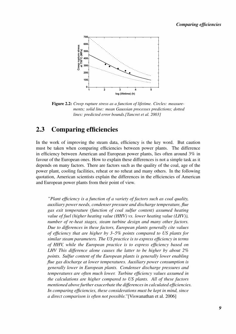
2.2 Creep rupture stress as a function of lifetime. Circles: measurements;solid line: mean Gaussian processes predictions; dotted lines: predictederror bounds.[Tancret et al. 2003] . . . . . . . . . . . . . . . . . . . . . 9

3.1 Overview over the power plant Nordjyllandsværket. The largest buildingis Unit 3.[Elsam 1998] . . . . . . . . . . . . . . . . . . . . . . . . . . 12

3.2 A representation of the water/steam cycle in Unit 3 in Nordjyllands-værket. . . . . . . . . . . . . . . . . . . . . . . . . . . . . . . . . . . 14

3.3 A T-s diagram over the water/steam cycle in Unit 3 in Nordjyllandsværket. 153.4 Flow diagram of the channels where the flue gas and air are lead before

and after the air preheater. . . . . . . . . . . . . . . . . . . . . . . . . 16

4.1 Flowchart that shows the process of building the model in EES. . . . . . 18

5.1 Diagram that shows overview over mass balances in the model. . . . . . 225.2 Diagram that shows overview over energy balances in the model. . . . . 225.3 Diagram that shows how the modules in the model are connected. Under

the name of the module are listed those variables that are input to themodel. . . . . . . . . . . . . . . . . . . . . . . . . . . . . . . . . . . . 23

5.4 Diagram over the turbine and its steam outlets. . . . . . . . . . . . . . . 245.5 Feedwater preheater. . . . . . . . . . . . . . . . . . . . . . . . . . . . 265.6 Bypass over the last three feedwater heat exchangers. . . . . . . . . . . 26

6.1 Key numbers in the water/steam cycle from the model when simulatingNJV3 at full load. . . . . . . . . . . . . . . . . . . . . . . . . . . . . . 30

6.2 T-s diagram over the water/steam cycle when simulating NJV3 at fullload. . . . . . . . . . . . . . . . . . . . . . . . . . . . . . . . . . . . . 31

iii

LIST OF FIGURES

7.1 Efficiency as a function of temperature from the boiler and pressurefrom the feedwater pumps. . . . . . . . . . . . . . . . . . . . . . . . . 36

7.2 Key numbers in the water/steam cycle from the model when simulating769 °C from the boiler and 42 MPa from the high pressure feedwaterpump. . . . . . . . . . . . . . . . . . . . . . . . . . . . . . . . . . . . 37

7.3 T-s diagram over the water/steam cycle when simulating 769 °C fromthe boiler and 42 MPa from the high pressure feedwater pump. . . . . . 38

A.1 Explanation of the crosses in the diagram window. . . . . . . . . . . . . 46A.2 Error message that is likely to come after changes in variables. . . . . . 46

D.1 This is the guy who makes it possible for ultra super critical powerplants to reach steam temperatures and pressures of 750°C/35MPa.Courtesy Franck Tancret . . . . . . . . . . . . . . . . . . . . . . . . . 59

iv

List of Tables

3.1 Main technical parameters for Nordjyllandsværket.[Elsam 1998] . . . . 133.2 Steam data for turbine inlets.[Elsam 1998] . . . . . . . . . . . . . . . . 14

5.1 Isentropic efficiency for each stage of the turbine in the model. . . . . . 25

6.1 Comparison of design data for NJV3 at 100% load and calculationsfrom the model. The difference is relative difference. . . . . . . . . . . 29

6.2 Stability test of the model when updating start guesses after every solution.When a solution is acquired, values for the chosen variables are logged,the start guesses are updated and the process is repeated. . . . . . . . . 32

7.1 Change in results when increasing pressure from the high pressurefeedwater pumps and temperature from the boiler. Values for the efficiencyare shown in figure 7.1. The values in this table are acquired from amore detailed table in appendix C. . . . . . . . . . . . . . . . . . . . . 36

A.1 Variables in the model that can be altered and their recommended lowerand upper values. . . . . . . . . . . . . . . . . . . . . . . . . . . . . . 46

C.1 Change in results when increasing pressure from the boiler feedwaterpumps and temperature from the boiler. . . . . . . . . . . . . . . . . . 58

LIST OF TABLES

vi

Contents

Abstract i

Preface ii

List of figures iii

List of tables v

Nomenclature 1Abbreviations . . . . . . . . . . . . . . . . . . . . . . . . . . . . . . . . . . . . . . . . . . . 2

1 Introduction 31.1 Problem orientation . . . . . . . . . . . . . . . . . . . . . . . . . . . . . . . . . . . . . 31.2 Problem definition . . . . . . . . . . . . . . . . . . . . . . . . . . . . . . . . . . . . . 51.3 Problem delimitation . . . . . . . . . . . . . . . . . . . . . . . . . . . . . . . . . . . . 5

2 Steam temperature and pressure 72.1 Introduction . . . . . . . . . . . . . . . . . . . . . . . . . . . . . . . . . . . . . . . . . 72.2 Improvements on boiler materials . . . . . . . . . . . . . . . . . . . . . . . . . . . . . 72.3 Comparing efficiencies . . . . . . . . . . . . . . . . . . . . . . . . . . . . . . . . . . . 92.4 Summary . . . . . . . . . . . . . . . . . . . . . . . . . . . . . . . . . . . . . . . . . . 10

3 Nordjyllandsværket 113.1 Introduction . . . . . . . . . . . . . . . . . . . . . . . . . . . . . . . . . . . . . . . . . 113.2 Unit 3 . . . . . . . . . . . . . . . . . . . . . . . . . . . . . . . . . . . . . . . . . . . . 123.3 Steam/water system . . . . . . . . . . . . . . . . . . . . . . . . . . . . . . . . . . . . . 133.4 Combustion air and flue gas . . . . . . . . . . . . . . . . . . . . . . . . . . . . . . . . . 153.5 Summary . . . . . . . . . . . . . . . . . . . . . . . . . . . . . . . . . . . . . . . . . . 16

4 Modelling the water/steam cycle 174.1 Introduction . . . . . . . . . . . . . . . . . . . . . . . . . . . . . . . . . . . . . . . . . 174.2 Formulating the model . . . . . . . . . . . . . . . . . . . . . . . . . . . . . . . . . . . 174.3 EES . . . . . . . . . . . . . . . . . . . . . . . . . . . . . . . . . . . . . . . . . . . . . 184.4 The foundation of the model . . . . . . . . . . . . . . . . . . . . . . . . . . . . . . . . 194.5 Summary . . . . . . . . . . . . . . . . . . . . . . . . . . . . . . . . . . . . . . . . . . 19

5 Presentation of the model 215.1 Introduction . . . . . . . . . . . . . . . . . . . . . . . . . . . . . . . . . . . . . . . . . 215.2 Mass balance . . . . . . . . . . . . . . . . . . . . . . . . . . . . . . . . . . . . . . . . 215.3 Energy balance . . . . . . . . . . . . . . . . . . . . . . . . . . . . . . . . . . . . . . . 225.4 Modules . . . . . . . . . . . . . . . . . . . . . . . . . . . . . . . . . . . . . . . . . . . 235.5 Summary . . . . . . . . . . . . . . . . . . . . . . . . . . . . . . . . . . . . . . . . . . 27

6 Verification of the model 296.1 Introduction . . . . . . . . . . . . . . . . . . . . . . . . . . . . . . . . . . . . . . . . . 296.2 Comparing design data for NJV3 with solutions from the model . . . . . . . . . . . . . 296.3 Comparing T-s diagrams from the model and NJV3. . . . . . . . . . . . . . . . . . . . . 316.4 Stability of the model . . . . . . . . . . . . . . . . . . . . . . . . . . . . . . . . . . . . 316.5 Summary . . . . . . . . . . . . . . . . . . . . . . . . . . . . . . . . . . . . . . . . . . 33

vii

CONTENTS

7 Ultra-super critical steam 357.1 Introduction . . . . . . . . . . . . . . . . . . . . . . . . . . . . . . . . . . . . . . . . . 357.2 Altering the steam data . . . . . . . . . . . . . . . . . . . . . . . . . . . . . . . . . . . 357.3 Summary . . . . . . . . . . . . . . . . . . . . . . . . . . . . . . . . . . . . . . . . . . 39

8 Conclusion 418.1 Primary conclusion . . . . . . . . . . . . . . . . . . . . . . . . . . . . . . . . . . . . . 418.2 Future work . . . . . . . . . . . . . . . . . . . . . . . . . . . . . . . . . . . . . . . . . 42

Bibliography 43

Appendix 45

A Model user guide 45A.1 About the model . . . . . . . . . . . . . . . . . . . . . . . . . . . . . . . . . . . . . . 45A.2 User guide . . . . . . . . . . . . . . . . . . . . . . . . . . . . . . . . . . . . . . . . . . 45

B Model code 47B.1 Introduction . . . . . . . . . . . . . . . . . . . . . . . . . . . . . . . . . . . . . . . . . 47B.2 Code . . . . . . . . . . . . . . . . . . . . . . . . . . . . . . . . . . . . . . . . . . . . . 47

C Investigating change in temperatures and pressure 57C.1 Introduction . . . . . . . . . . . . . . . . . . . . . . . . . . . . . . . . . . . . . . . . . 57C.2 Increasing the temperature and pressure . . . . . . . . . . . . . . . . . . . . . . . . . . 57

D Nickel based superalloy 59

viii

Nomenclature

Latin Letters

h Enthalpy kJ/kgm Mass flow rate kg/sm Mass kgP Pressure kPaQ Heat transfer rate kJ/ss Entropy kJ/kg·KT Temperature °CW Electric energy rate MW

Greek Letters

η Efficiency -

Subscripts

b Boilercond Condenser

el Electricityf w Feedwatergen Generatorhp High pressurei Inleto Outlet

reh Reheatingturb Turbine

1

Nomenclature

AbbreviationsCCGT Combined cycle gas turbineCHP Combined heat and powerEES Engineering Equation SolverHHV Higher heating valueHP High PressureLHV Lower heating valueLP Low PressureIAPWS International Association for the Properties of Water and SteamIGCC Integrated gasification combined cycleIP Intermediate PressureNJV3 Nordjyllandsværket unit 3PFBC Pressurised fluidised bed combustionUSC Ultra-supercriticalVHP Very High Pressure

2

1Introduction

1.1 Problem orientation1.2 Problem definition1.3 Problem delimitation

In this chapter, the background for the project is introduced. The energy situation inthe past and the future is discussed with focus on production of electricity from burningcoal.

1.1 Problem orientationAs our society develops, the demand for energy is constantly growing. The energysupply is expected to be constant and reliable. There is also a requirement that theenergy is environmental friendly or as little polluting as possible.In Europe the energy comes mainly from two sources; from nuclear power plants andburning fossil fuels (coal, oil and natural gas), but there is increasing focus on renewableenergy sources such as wind power and solar energy.For environmental reasons, nuclear power and fossil fuels are not popular as energysource, but it seams like the the western world is stuck with it. At least until the renew-able energy has developed to a stage, where it can provide enough energy so the otherless environmentally friendly methods can be taken out.

In Europe, most countries (inclusive Denmark) have signed the Kyoto protocol. Thosecountries have agreed to cut down CO2 equivalent emissions by 8%, expressed inrelation to emissions in a predefined base year or period. This reduction of CO2equivalent emissions is supposed to happen in the period of 2008 to 2012. [Kyo 2007]

In Denmark, the majority of the electricity production is based on coal fired powerplants [Dal and Zarnaghi 2007]. Efforts are constantly made to improve the efficiencyof the plants. In the period from 1990 to 2004 has the total efficiency of the Danishheat and power plants risen from 60% to 73% [Pedersen 2005]. Figure 1.1 givesoverview over how the energy sources for production of electricity in Denmark is di-vided between oil, natural gas, coal, waste burning and self sustainable sources from1990 to 2006. Figure 1.2 gives overview over how the energy sources for production ofelectricity in Denmark are assumed to develop until 2030.In Europe, solid fuels (hard coal and lignite) are projected to decrease somewhat by2020 and to come back almost to the level it was in 2006 by the year 2030. [Mantzos

3

Problem orientation

and Capros 2006]

70

80

90

100

Sources of energy in production of electricity in DenmarkOil

Gas

Coal

Waste burning

Selfsustainable

0

10

20

30

40

50

60

1990 1991 1992 1993 1994 1995 1996 1997 1998 1999 2000 2001 2002 2003 2004 2005 2006

%

Selfsustainable

Figure 1.1: Overview over the main sources of energy in production ofelectricity in Denmark.[Dal and Zarnaghi 2007]

60

70

80

90

100Assumed sources of energy in production

of electricity in DenmarkOil

Gas

Coal

Selfsustainable and waste

0

10

20

30

40

50

60

2000 2005 2010 2015 2020 2025 2030

%

Figure 1.2: Overview over assumed main sources of energy in production ofelectricity in Denmark.[Mantzos and Capros 2006]

The advantage of using coal as fuel is e.g. that it can be acquired from many locationsaround the world. This becomes valuable when compared to oil, of which a great dealcomes from areas where political instability has been long lasting.A big disadvantage of coal as a fuel is that the use of it involves a large amount ofCO2 emissions. Carbon dioxide is one of the greenhouse gases that contributes to thegreenhouse effect.

At the present stage, it is very likely that coal vil continue to be number one energysupply in production of electricity in Denmark. Therefore it is of outmost importance

4

Problem definition

to improve the efficiency of coal fired power plants and reduce the CO2 emissions. Thetendency is clearly moving in that direction.

1.2 Problem definitionThe main aspect of this project is to describe and model the water/steam cycle in supercritical pulverised coal fired power plants, and to investigate the future potential foroptimization of the process.

1.3 Problem delimitationThis project will have its main focus on the water/steam cycle in a super critical powerplant. More specific, it will be based on how the efficiency can be increased byimproving the steam data. The areas of interest within this project are as follows:

• Create a model of water/steam cycle in a super critical pulverised coal fired powerplant

• Utilise the model to investigate how a change into a ultra super critical powerplant, affects the efficiency.

5

Problem delimitation

6

2Steam temperature and pressure

2.1 Introduction2.2 Improvements on boiler materials2.3 Comparing efficiencies2.4 Summary

2.1 IntroductionThe increased cost of fuel along with the need to reduce CO2 emission, has providedan additional incentive to increase the efficiency of power plants. This chapter con-tains a literature study which has focus on what others have worked on, according toimprovements on super critical pulverised coal power plants.

2.2 Improvements on boiler materialsWhen improving the efficiency of a super critical pulverised coal power plant, the mainfocus has been on raising the temperature and pressure of the steam leaving the boilerinto the turbine. But this is not very simple. At temperatures over 400°C, there isincreased risk of damage on the piping from creep, cycle fatigue, creep fatigue anderosion-corrosion.[Wilcox 1992] The upper limit in temperature and pressure in super-critical power plants has been around 600°C/30MPa. But there is a great deal of effortmade to push these limits higher.

R. Viswanathan, K. Coleman and U. Rao have done a study on materials needed for theconstruction of the critical components of ultra-supercritical coal-fired boilers capableof operating with 760°C/35MPa steam. It is estimated that by raising the temperatureand pressure to these levels, will increase the efficiency from the average of 37% toapproximately 47% for a double reheat configuration in the USA. [Viswanathan et al.2006]

The European Union financed a AD700 project which Elsam coordinated. This projectinvolves about 40 companies representing actors in the European power industry. Theaim of the project is to raise the efficiency of a USC power plant above 50%. [Buggeet al. 2006]

7

Improvements on boiler materials

At Oak Ridge National Laboratory and University of Cincinnati, long-term tests ofmechanical properties of nickel-based alloys have been performed. These tests aremade with temperatures up to 800°C. [Shingledecker et al. 2006]

In China, experiments have been made on a nickel-based super-alloy. The purpose ofthis experiment was to find a suitable alloy for application in USC superheater tubesabove 750°C. [Zhao et al. 2006]

F. Tancret and H.K.D.H. Bhadeshiab have worked on a nickel based super alloy thatwould be affordable for power plant applications. The design requirements are a lifetimeof 100000 hours at 750°C under 100MPa. The design requirements also includedforgeability, weldability, corrosion resistance, and microstructural stability over longexposure at service temperature. This work resulted in a design of a nickel based alloy.A bar of this alloy has been fabricated and tested. Figures 2.1 and 2.2 show bothmodelled and measured results from the tests.

9

Figure 2: TEM micrograph of the fully heat-treated alloy.

Figure 3: Evolution of yield stress as a function of temperature. Circles: measurements; solid line: meanGaussian processes predictions; dotted lines: predicted error bounds.

0

200

400

600

800

1000

0 200 400 600 800 1000 1200

Temperature (°C)

Yie

ld s

tre

ss

(M

Pa

)

Figure 2.1: Evolution of yield stress as a function of temperature: solidcircles indicate measurements; solid line indicates meanGaussian processes predictions; broken lines indicate predictederror bounds.[Tancret and Bhadeshia 2003]

Notice in figure 2.1 how the strength is at first insensitive to temperature. It is first atabout 700°C the strength begins to drop.In figure 2.2 the circles represent five tests for creep at 320, 290, 260, 230 and 200 MPa.The test at 200 MPa was unloaded before fracture but the rupture time at 200 MPa isextrapolated to about 5000 hours. The measurements are all well over the 100 MPalimit and the modelling proposes that the alloy should withstand 100 MPa at 750°C.According to [Tancret and Bhadeshia 2003], is the target of a lifetime of 100000 hoursat 750°C under 100MPa, well attainable.

8

Comparing efficiencies

10

Figure 4: Creep rupture stress as a function of lifetime. Circles: measurements; solid line: mean Gaussianprocesses predictions; dotted lines: predicted error bounds.

Figure 5: SEM micrograph of the as-solidified alloy. The black line is the EDS scan path.

1 2 3 4 50

100

200

300

400

500

600

700

Cre

ep r

up

ture

str

ess

at 7

50°C

(M

Pa)

log (lifetime) (h)

Figure 2.2: Creep rupture stress as a function of lifetime. Circles: measure-ments; solid line: mean Gaussian processes predictions; dottedlines: predicted error bounds.[Tancret et al. 2003]

2.3 Comparing efficiencies

In the work of improving the steam data, efficiency is the key word. But cautionmust be taken when comparing efficiencies between power plants. The differencein efficiency between American and European power plants, lies often around 3% infavour of the European ones. How to explain these differences is not a simple task as itdepends on many factors. There are factors such as the quality of the coal, age of thepower plant, cooling facilities, reheat or no reheat and many others. In the followingquotation, American scientists explain the differences in the efficiencies of Americanand European power plants from their point of view.

”Plant efficiency is a function of a variety of factors such as coal quality,auxiliary power needs, condenser pressure and discharge temperature, fluegas exit temperature (function of coal sulfur content) assumed heatingvalue of fuel (higher heating value (HHV) vs. lower heating value (LHV)),number of re-heat stages, steam turbine design and many other factors.Due to differences in these factors, European plants generally cite valuesof efficiency that are higher by 3–5% points compared to US plants forsimilar steam parameters. The US practice is to express efficiency in termsof HHV, while the European practice is to express efficiency based onLHV This difference alone causes the latter to be higher by about 2%points. Sulfur content of the European plants is generally lower enablingflue gas discharge at lower temperatures. Auxiliary power consumption isgenerally lower in European plants. Condenser discharge pressures andtemperatures are often much lower. Turbine efficiency values assumed inthe calculations are higher compared to US plants. All of these factorsmentioned above further exacerbate the differences in calculated efficiencies.In comparing efficiencies, these considerations must be kept in mind, sincea direct comparison is often not possible.”[Viswanathan et al. 2006]

9

Summary

When the literature on the subject is studied, it must be kept in mind that peopleoften tend to favourite their ”home” technology, but whatever the reasons are for thedifference in the efficiency are, it is not simple to compare the efficiency of two powerplants.Because of this difficulties in comparing efficiencies between power plants, it is probablymore appropriate to focus on how each power plant can be improved rather than try tofigure out which one is ”best”. It must though be kept in mind that competition is oftena substantial drive in developing new techniques.

2.4 SummaryTo sum up, there is a lot of work done in the field of increasing the efficiency of asuper critical pulverised coal fired power plant. From these studies it seems likelythat the boilers in the nearest future will be build of a nickel-based super-alloy. Themaximum temperature/pressure will be around 700°C/35MPa and about 760°C reheattemperature. Higher reheat temperature is possible because of lower pressure. Thisimprovement of the steam data should be noticeable in better efficiency. One shouldthough be careful in comparing efficiencies between power plants, because of differentsituations and fuel.

10

3Nordjyllandsværket

3.1 Introduction3.1.1 Nordjyllandsværket

3.2 Unit 33.3 Steam/water system3.4 Combustion air and flue gas3.5 Summary

3.1 IntroductionThis chapter contains a brief description of the power plant Nordjyllandsværket Unit 3which is the base for the model in this project. The main technical parameters for theunit are discussed, followed by explanations of the water/steam cycle and the air andfluegas system.

3.1.1 NordjyllandsværketNordjyllandsværket is owned by Vattenfall, a Swedish multinational energy company.Vattenfall has operations in Denmark, Sweden, Poland and Germany and produces anddelivers electricity and heat to its customers.

Nordjyllandsværket is a combined heat and power plant which produces electricity tothe Danish power grid and district heating to Aalborg and part of the minor local townsin the area. There has been a power plant on the location since 1967 and in 1992decision was made to build a new supercritical coal fired unit. The building of this unitcalled Unit 3, was finished 1998 and is now the main unit in the power plant, see picture3.1. In table 3.1 the main technical parameters are given for Unit 3.

11

Unit 3

Figure 3.1: Overview over the power plant Nordjyllandsværket. The largestbuilding is Unit 3.[Elsam 1998]

3.2 Unit 3

Unit 3 in Nordjyllandsværket, shown on figure 3.1 is the coal fired power plant in theworld with the highest thermal efficiency (about 47%, relative to the heating valueof coal). This exceptional performance of unit 3 is largely due to favourable coolingconditions in Denmark where the cold seawater from the Limfjord can be used in thecondenser. If unit 3 would be situated at an inland location in the UK where a coolingtower would be required, it would operate with a maximum efficiency of approximately44-45%. [Watson 2005]The thermal efficiency is determined from the electric net output divided by the heattransfer rate provided to the boiler by the fuel, see equation 3.1.

η =Welectric

Q f uel(3.1)

The heat transfer rate is found from the lower heating value and the mass flow rate ofthe fuel (eq; 3.2).

Q f uel = m f uel ·LHVf uel (3.2)

12

Steam/water system

Technical parameters for Nordjyllandsværket Unit 3Total thermal efficiency with full heating output 90 %Thermal efficiency (condensation operation) 47 %Output, no district heating 411 MWeOutput, with district heating 340 MWeSteam cycle type Double reheat cycle with

advanced regenerationTemperature 580 °CPressure 290 barFuel Bituminous coalBoiler throughput of coals 117 t/hAir preheater RegenerativeCooling Sea water

Table 3.1: Main technical parameters for Nordjyllandsværket.[Elsam 1998]

This unit is a double reheat, supercritical power plant designed to supply both electricityand district heating. It has been in commercial operation since 1998. The plant isfired with bituminous coal as the main fuel and heavy fuel oil as the backup fuel. Asimilar plant, built in Skærbæk in southern Jutland, is identical to NJV3 but is firedwith natural gas as the main fuel and oil as the backup fuel. The unit in Skærbæk hasbeen in commercial operation since 1997. [Elsam 1998]

3.3 Steam/water system

The steam turbine is an impulse design which allows expansion from 28,500 kPa (boileroutlet) to 3 kPa (condenser inlet). A representation of the water/steam-cycle is givenin figure 3.2. In figure 3.2, numbers for bleeding of steam from the turbine to the feedwater preheaters are equivalent to the numbers on the T-s diagram in figure 3.3. Thesame applies to the letters shown on both figures.

From the boiler, the steam is lead to the VHP turbine. From the VHP turbine the steamis lead back to the boiler to be reheated for the first time. After the first reheating thesteam expands trough the HP turbine and is reheated for the second time. From thelatter reheating the steam is lead to the IP0 turbine. After the IP0 turbine the steamexpands trough the IP1 and IP2 turbines. From the IP turbines the steam is either leadto the LP turbines or the district heaters. If the steam is lead to the district heaters itcondenses there and from the district heaters it is lead to the feed water system. If thesteam is lead to the LP turbine it continues from there to the condenser. Depending onthe need for district heating, the amount of steam that is lead through the district heaterscan be controlled so that the flow is partially through the district heaters and partiallyto the LP turbines. After the condenser, the feed water is pumped back to the boilertrough a number of feed water heaters which get their heat from steam that bleeds fromthe turbine.

13

Steam/water system

Boiler

VHP HP IP0 IP2IP1 LP1 LP2 G

Figure 3.2: A representation of the water/steam cycle in Unit 3 in Nord-jyllandsværket.

After the high pressure feedwater pump, there is a option of bypassing the last threefeedwater heaters. Bypassing the feedwater heaters results in a less bleeding of steamfrom the turbine and therefore more power to the generator, but leads to slightly lessoverall efficiency of the power plant.In table 3.2 the main technical parameters are given for the turbine.

Technical parameters for turbineStage Pressure [kPa] Temperature[°C]VHP 28,500 580HP 7,400 580IP0 1,900 580IP 720 429LP1 150 233LP2 70 154

Table 3.2: Steam data for turbine inlets.[Elsam 1998]

In figure 3.3, a T-s diagram over the process in NJV3 is shown. The letters represent thefeed water preheaters and are also presented in the diagram in figure 3.2. The numbersstand for bleeding of steam from the turbine to the feed water preheaters and the samenumbers are also shown in figure 3.2.

14

Combustion air and flue gas

3200 kJ/kg

3400 kJ/kg

3600 kJ/kg

400

500

600

2

3

5

4

1

2600 kJ/kg

2800 kJ/kg

3000 kJ/kg

3200 kJ/kg

0

100

200

300

0 1 2 3 4 5 6 7 8 9

T (

C)

s (kJ/kg)

6

7

8

9

10A

B

C

D

E

F

G

H

I

JK

Figure 3.3: A T-s diagram over the water/steam cycle in Unit 3 in Nord-jyllandsværket.

3.4 Combustion air and flue gasEwen though the main focus in this project is on the water/steam circulaton, the air andflue gas system can not be left unmentioned. To get a high efficiency from a powerplant of this type, these systems must be designed to fit each other. On its way from theboiler, the flue gas heat exchanges with the feed water coming into the boiler. Becauseof the feedwater heaters the feedwater has a temperature close to 300 °C. That resultsin a high temperature of the fluegas flow leaving the boiler (about 370 °C). To utilisethe energy in the flue gas, a regenerative air preheater is used to transfer heat from theflue gas to the combustion air. A flow diagram over the air and fluegas system in NJV3is presented in figure 3.4.

The flue gas flows from the boiler to the air preheater through NOx removal and fromthere it is lead through a cleaning system before it is released into the atmospherethrough the stack. This cleaning system consists of electrostatic precipitator and fluegas desulphuration by wet scrubbing.Between the electrostatic precipitator and the induced draught fans, a part of the flue gasis recirculated to the boiler via the air preheater. The flue gas recirculation is primarilyused at low loads to maintain the volume flow through the boiler to ensure evenly spreadheat exchanging in the boiler.

The air intake is at the top of the boiler building in the warm zone around the boiler. Theair is lead through forced draught fans and splits up into primary air and combustionair, also called secondary air.

15

Summary

Air preheater

Electrostatic precipitator

SO2 removal (wet scrubbing)

Stack

Flue gas

Flue gas

Flue gasFlue gas

Recirculating flue gas

Recirculating flue gas

Primary air

Secondary air

Air intake

Secondary airPrim

ary air

Coal Mills

Boiler

De-NOx

Primary air

Secondary air

Steam air preheater

Induced draught

fans

Forced draught fans

Figure 3.4: Flow diagram of the channels where the flue gas and air are leadbefore and after the air preheater.

The primary air is lead to the air preheater where it is heated up before it is lead to thecoal mills where it is used to blow coal dust from the mills into the boiler. To preventthe coal dust from exploding, some of the primary air bypasses the air preheater to limitthe temperature of the air.The secondary air flows through a steam/air preheater on its way to the regenerativeair preheater. The steam/air preheater is only used at low loads. At low loads, thetemperature in the regenerative air preheater drops a little. A lower temperature inthe regenerative air preheater could create conditions where sulphur in the fluegascondenses and forms a sulphuric acid. That would create erosion problems in theregenerative air preheater. Therefore the steam/air preheater is used at low loads tomaintain the temperature in the regenerative air preheater over the sulphuric acid dewpoint. From the regenerative air preheater the secondary air is lead directly to the boilerto be used as combustion air. [Elsam 1998]

3.5 SummaryThe Unit 3 in Nordjyllandsværket is chosen as base for the modeling of a steam/watercycle in super critical power plant. NJV3 is chosen mainly because of the high thermalefficiency and it is regarded for many as the state of the art super critical coal firedpower plant.

16

4Modelling the water/steam cycle

4.1 Introduction4.2 Formulating the model4.3 EES

4.3.1 Fluid properties4.4 The foundation of the model4.5 Summary

4.1 IntroductionIn this chapter the development of the numerical model is explained. EngineeringEquation Solver is introduced as well and the background of the model is explained.

4.2 Formulating the modelProgramming this model is a highly iterative process. In the beginning it is definedwhat the model is supposed to do. This decision can change during the work on themodel.Deciding the variables and writing the equations is fairly straight forward but adjustmentand improvement is constantly done through out the modeling progress.In a model of this complexity, the model is very sensitive to the choice of start guessesof the modelling variables. These must be carefully chosen and often updated, evenafter minor changes in the model or the inputs to the model.A flowchart over the modelling process can be seen in figure 4.1.

17

EES

Model making

Decide the purpose of the

model

Decide the variables

Write the equations Test the model

Does the model

converge?

Utilise the model

Deside/update the start guesses

No

Yes

Reevaluate the purpose of the

model

Verify the modelIs the solution accepted?

No

Yes

Figure 4.1: Flowchart that shows the process of building the model in EES.

4.3 EESThe model is built in EES (Engineering Equation Solver). The basic function pro-vided by EES is the solution of a set of non-linear algebraic equations. EES can alsosolve differential equations, equations with complex variables, do optimization, pro-vide linear and non-linear regression, generate publication-quality plots, simplify un-certainty analyses and provide animations. EES uses a variant of Newton’s method tosolve systems of non-linear equations. [Klein 2004]When building a model such as this one in EES, great care must be taken when choosingstart guesses. If the start guesses are not properly chosen the model will not converge.

4.3.1 Fluid propertiesFor the properties of water and steam, EES has several different reference tables tochose between. In this case Steam IAPWS is chosen because it implements particularly

18

The foundation of the model

high accuracy thermodynamic properties of water at super critical conditions with the1995 Formulation for the Thermodynamic Properties of Ordinary Water Substance forGeneral and Scientific Use, issued by The International Association for the Propertiesof Water and Steam. Steam IAPWS uses slightly more computer power than the othertables, but its advantages are that it is more accurate at higher temperatures and pressures.

4.4 The foundation of the modelIn order to make the model realistic, technical parameters for the turbine in NJV3are used to calculate the isentropic efficiency of the turbine. These parameters aretemperature and pressure of the steam at the inlet of each stage of the turbine andare acquired from a poster published by Elsam 1998 at the beginning of commercialoperation of NJV3. [Elsam 1998] Table 3.2 lists those parameters for the steam.It was also necessary to make a few other ”qualified guesses”. One example, is thepressure loss over the boiler. Those numbers are taken from T-s diagram made byJeppe Grue. [Grue 2007] This T-s diagram can be seen in figure 3.3.The model is then verified by comparing data from the model with data for NJV3. Theverification of the model is done in section 6.2.

4.5 SummaryBuilding this model is an highly iterative procedure. During this process, the earlierwork is constantly evaluated and reevaluated. The model consists of more than 250equations and there are many opportunities to make mistakes. But finally it is assumedthat the model must be fairly accurate when comparing the solutions from the modelwith design data from NJV3.

19

Summary

20

5Presentation of the model

5.1 Introduction5.2 Mass balance5.3 Energy balance5.4 Modules

5.4.1 Boiler5.4.2 Turbine5.4.3 Generator5.4.4 Condenser5.4.5 Feedwater pumps5.4.6 Feedwater preheaters5.4.7 Bypass

5.5 Summary

5.1 IntroductionIn this chapter the structure of the model is explained.

5.2 Mass balanceIn the model, the energy balance over the boiler is applied to determine the mass flowrate of water/steam through the boiler. Then from that energy balance, and from energybalances over heat exchangers in the feedwater flow, all other mass flow rates in thesystem are deduced. This is complicated task because this is not a simple cycle. Thereare two reheat stages and ten steam outlets on the turbine for the purpose of preheatingthe feedwater.Apart from the energy balances, there are more than 20 equations of mass balances inthe model. Each mass flow rate has one variable name in the model and the same massflow rate variable name can thereby appear in several mass balances. By that, the massbalances are connected.In figure 5.1 the boundaries for the mass balances are shown. In appendix B theequations for the mass balance can be viewed, as they are grouped together at the begin-ning of the code.Additionally, there are restrictions on the mass flow rate variables in the model, primarilyto ensure that the flow is in the right direction.

21

Energy balance

Boiler

VHP HP IP0 IP2IP1 LP1 LP2 G

Feed pumpHigh pressure feed heaters

Condenser

Reheating 1 Reheating 2

1 3

2

4 5 67 8

9 10

ABC

D

EF

G

H

IJ

K

Figure 5.1: Diagram that shows overview over mass balances in the model.

5.3 Energy balance

The energy balances in the model set the mass flow rate trough various components inthe model. It can also work the other way around, the mass flow rate sets the value ofenthalpy of the flow in question by the energy balances. The boundaries for the energybalances are shown in figure 5.2. In appendix B the equations for the energy balancescan be found in the code in the modules they belong to.

G

Figure 5.2: Diagram that shows overview over energy balances in the model.

22

Modules

5.4 Modules

The model is built up of modules that are connected together. Each module representsa component in the water/steam cycle. In the diagram in figure 5.3 it is shown how themodules are connected. Note that the arrows in figure 5.3 do not indicate the directionof the flow but show where from, the modules get their inputs from. It should alsobe noted that many arrows for mass flow rate and enthalpy are not drawn in order tosimplify the diagram. For mass and energy balances figures 5.1 and 5.2 can be viewed.

BoilerMass flow rate coal

Boiler efficiencyPressureloss

Steam temperatur out

Reheating 1Steam temperatur out

Reheating 2Steam temperatur out

VHPTurbine pressure loss ratio

Isentropic efficiency

Pressure

Enthalpy

Temperature

Mass flow rate

HPTurbine pressure loss ratio

Isentropic efficiency

HPTurbine pressure loss ratio

Isentropic efficiency

IP0Turbine pressure loss ratio

Isentropic efficiency

IP1Turbine pressure loss ratio

Isentropic efficiency

IP2Turbine pressure loss ratio

Isentropic efficiency

LP1Isentropic efficiency

IP2Isentropic efficiency

GeneratorEfficiency

Heat transfer rate

CondenserPressureQuality

Main condensate pumpsPressure Specific volume

ATemperature difference

Quality

C

DQuality

Low pressure feed pumpsPressure

FTemperature difference

Quality

Boiler feed pumpsPressure

KTemperature difference

G

HQuality

Temperature difference

BypassBypass ratio

Bypass ratio

Figure 5.3: Diagram that shows how the modules in the model areconnected. Under the name of the module are listed those vari-ables that are input to the model.

23

Modules

5.4.1 BoilerIn this model, the temperature of the steam from the boiler, the throughput of coal, theheating value of the coal and boiler efficiency is given as input. The pressure of thesteam from the boiler is set by taking the pressure from the high pressure feedwaterpump and assuming about 14% pressure loss through the boiler. From the values oftemperature and pressure, the enthalpy of the steam is acquired.The heating value of the coal is set to be 28700 kJ/kg and that is within the limits forbituminous coal given by [Perry and Green 1997].

With these parameters it is possible to establish an energy balance for the boiler andcalculate the mass flow of water/steam through the boiler. In equation 5.1 the energybalance as it is in the model is given and from that energy balance the mass flow ratecan be isolated and found.

Qcoal ·ηb = msteamb · (hob−hib)+ mreh1 · (hiHP−hoV HP)+ mreh2 · (hiIP0−hoHP) (5.1)

The boiler module does not include variables for energy flow in form of air and flue gas.Instead these energy transfer rates are encountered for in the form of boiler efficiency.

5.4.2 Turbine

Boiler

VHP HP IP0 IP2IP1 LP1 LP2 G

Figure 5.4: Diagram over the turbine and its steam outlets.

Each stage of the turbine is handled as an independent module in the model. Inputsinto the turbine modules are mass flow rate into the turbine stage, enthalpy of the steamflowing into the turbine stage, isentropic efficiency, pressure loss ratio and pressure ofthe steam flowing into the turbine stage. Pressure loss ratio is the ratio of the pressureloss over the whole turbine.For each stage of the turbine, the heat transfer rate is calculated by multiplying the massflow rate with the change in enthalpy of the steam that flows through the turbine stage,equation 5.2.

Qturb = msteam ·∆hsteam (5.2)

Then the heat transfer rates for each stage, are added to get the heat transfer rate for thewhole turbine.

For the isentropic efficiency, a qualified guess is taken. There were four types of criteriathat had to be fulfilled in the decision of the isentropic efficiency.

24

Modules

• The net energy output from the system should match NJV3 at full load.

• The mass flow rate out of the boiler should match NJV3 at full load.

• The thermal efficiency should match NJV3 at full load.

• The T-s diagram from the model is to look like the T-s diagram for NJV3 in figure3.3.

The values for the first three items are listed in table 6.1 and are about 1% or less fromthe target. Regarding the last item, the two T-s diagrams in figures 3.3 and 6.2 can becompared to judge how similar they are.Table 5.1 shows the isentropic efficiencies for each stage of the turbine system.

Isentropic efficiencyVHP 93 %HP 93 %IP0 91 %IP1 90 %IP2 90 %LP1 90 %LP2 90 %

Table 5.1: Isentropic efficiency for each stage of the turbine in the model.

5.4.3 GeneratorThe output from the generator is calculated from total heat transfer rates from theturbine and the efficiency for the generator (equation 5.3).

Wel = ηgen · Qturb (5.3)

5.4.4 CondenserIn the condenser module, the pressure and the quality of the flow is determined from aT-s diagram provided by Jeppe Grue [Grue 2007].The mass flow rate and the temperature of the seawater that flows through the condenseris not accounted for in the condenser module. It is assumed that there is a balancebetween the heat produced by condensing the steam and the heat transfer from thecondenser by the seawater.

5.4.5 Feedwater pumpsThere are three modules for feedwater pumps in the model. Their pressure is set as it isin NJV3 but it can be altered to a value of choice.

25

Modules

5.4.6 Feedwater preheaters

The feedwater preheater modules calculate the increase of heat rate over the feedwaterpreheater. There are several variations and figure 5.5 and equation 5.4 give an exampleof the most simple one.

Feedwater inFeedwater out

Steam in

Figure 5.5: Feedwater preheater.

m f w in ·h f w in + msteam in ·hsteam in = m f w out ·h f w out (5.4)

There are also cases where the flows through the heat exchanger do not mix. In thosecases the assumption is taken that the temperature difference between the hot flow outof the heat exchanger and the cold flow into the heat exchanger is 5°C.

5.4.7 Bypass

There is a possibility of simulating bypass over the last three feedwater heat exchangersin the model (figure 5.6). The value for bypass can be set as 0 and 1 and anywhere therebetween for partial bypass. 0 is no bypass and 1 is full bypass.

BoilerVHP HP

Feed pumpHigh pressure feed heaters

Reheating 1

1 3

2

HIJK

Bypass

Figure 5.6: Bypass over the last three feedwater heat exchangers.

26

Summary

5.5 SummaryThe model is made up of modules. Each module bases its calculations on inputs fromother modules and constants set by the user of the model. Between the modules aremass and energy balances. These balances are connected when they involve the sameflow by using the same variable name for that flow.

27

Summary

28

6Verification of the model

6.1 Introduction6.2 Comparing design data for NJV3 with solutions from

the model6.3 Comparing T-s diagrams from the model and NJV3.6.4 Stability of the model6.5 Summary

6.1 IntroductionIn this chapter the model is verified by holding its solutions against known parametersfrom NJV3. Also the stability in the solutions is analysed to see if it is as expected.

6.2 Comparing design data for NJV3 with solutions fromthe model

To verify the validation of the model, it can be compared with design data for NJV3.When building the model, a effort was made to program the model to give resultsfor certain chosen variables as close as possible to design data for NJV3 as they arepresented in [Elsam 1998]. For this purpose, three variables were chosen; electricefficiency, steam mass flow from boiler and electric output from the generator. Thesevariables are listed in table 6.1.In diagram 6.1 the results from the model are displayed when the steam temperaturefrom the boiler is set to 580 °C, and the pressure from the feed pump is 33.000 kPa.

Verification of the modelNJV3 Model Difference

Efficiency, electric generation only 47% 48.13% 2.40%Max steam output from boiler 270 kg/s 272 kg/s 0.74%Output from generator 411 MW 407.3 MW 0.90%

Table 6.1: Comparison of design data for NJV3 at 100% load and calcula-tions from the model. The difference is relative difference.

29

Comparing design data for NJV3 with solutions from the model

File

:d:\

Skó

li\F

AC

E1

0\R

ep

ort

\mo

de

l\m

od

el.E

ES

24

.5.2

00

8 1

2:1

1:0

6

Pa

ge

1

EE

S V

er.

7.9

84

: #

21

80

: F

or

use

on

ly b

y s

tud

en

ts a

nd

fa

cu

lty a

t A

alb

org

Un

ive

rsity,

De

nm

ark

Bo

iler

VH

PH

PIP

0IP

2IP

1L

P1

LP

2G

Dis

tric

t heating

Feed p

um

pH

igh p

ressure

feed h

eate

rs

Condenser

Reheating 1

Reheating

2

Lim

fjord

en

13

2

45

67

8

910

AB

C

D

EF

G

H

IJ

K

Coal th

= 1

17

[ton/h

]

ηel =

0,4

813

Wel =

407,3

[M

W]

272

T[C

]P

[kP

a]

m[k

g/s

]h[k

J/k

g]

580

28500

352

7400

3398

3039

580

7400

3600

356,4

1900

3185

580

1900

3647

3

431,7

720

239,8

150

70

153,9

299,2

272

3336

2952

2811

24,0

8

2342

3

101

500

500

3300

33000

24,0

9

101,5

3300

356,4

1900

3185

272

299,2

33000

1324

1324

468,2

3374

3913

3913

304,2

2976

0,0

1127

0,0

1127

235,3

235,3

272

236,7

236,7

352

7400

3039

3300 1034

1070

33000

2722

39,2

245,9

1090

250,9

35,3

7

35,3

61,3

9

Qcoal =

846177 [

kJ/s

]

235,3

3489

505,8

1245

1012

234,7

640,1

3300

500

152,1

643,1

151,8

3300

153,4

648,6

205,1

30,1

4

431,7

720

3336

239,8

150

2952

3056

273,9

292,8

0,4

18

0,0

00135

1,6

97

38,5

3

204,7

26,5

5

176,5

161,6

200,2

200,2

203

204,7

204,7

200,2

88,9

935,3

1

2663

38,5

3

205,1

3300

643,2

152,2

0,4

18

273,9

663,1

157,2

620,8

147,3

70

153,9

2811

0,0

01599

2,8

74

203

620,7

500

500

131,9

147,3

329,0

9

121,9

590,6

140,3

2723

286,3

24,0

8

0

0B

ypass

33000

1070

245,9

0

So

lve

T-s

dia

gra

m

Figure 6.1: Key numbers in the water/steam cycle from the model when sim-ulating NJV3 at full load.

30

Comparing T-s diagrams from the model and NJV3.

6.3 Comparing T-s diagrams from the model and NJV3.The model generates a T-s diagram which is also helpful in determining if the model isreturning feasible results. The T-s diagram matching the diagram 6.1 is shown in figure6.2. The T-s diagram in figure 6.2 can also be compared with the T-s diagram from thepower plant Nordjyllandsværket shown in figure 3.3.File:d:\Skóli\FACE10\Report\model\model.EES 20.5.2008 22:15:27 Page 1

EES Ver. 7.984: #2180: For use only by students and faculty at Aalborg University, Denmark

0 1 2 3 4 5 6 7 8 90

100

200

300

400

500

600

700

800

s [kJ/kg-K]

T [

°C]

33000 kPa

3300 kPa

500 kPa

3 kPa

0,2 0,4 0,6 0,8

Model

Figure 6.2: T-s diagram over the water/steam cycle when simulating NJV3at full load.

Notice that there are two lines on the T-s diagram representing the steam flows throughthe IP and LP turbine stages.

6.4 Stability of the modelBecause EES is an numerical solver, the solutions from the model can vary dependingon the start guesses. To evaluate this phenomena in the model, a stability test wasperformed.In table 6.2 solutions for six variables are logged. These variables are; electric output,thermal efficiency, mass flow rate out of the boiler, mass flow rate into the condenser,mass flow rate into the feedwater preheater D and mass flow rate into the feedwaterpreheater H. The model is set to simulate NJV3 at full load and every time the modelconverged, the start guesses were updated.

31

Stability of the model

When updating the start guesses, the guess value of each variable is replaced withthe value determined in the last calculation. This should improve the computationalaccuracy of the model since it ensures that a consistent set of guess values is used inthe next calculation.

Stability testWel [MW] η [%] mo b [kg/s] mi cond [kg/s] mi D [kg/s] mi H [kg/s]

407.4 48.15 272 158.6 198.3 235.5408.2 48.24 272 159.9 199.5 235.5408.7 48.3 272 161.1 170.1 235.5408.4 48.26 272 160.5 177.8 235.5404.9 47.85 272 162.8 189.8 235.5404.2 47.77 272 163.2 190.3 235.5408.9 48.32 272 162.7 189.7 235.5409.4 48.38 272 162.7 189.7 235.6409.6 48.41 272 162.7 189.6 235.5403.9 47.73 272 163.8 190.9 235.5405.3 47.9 272 164.7 169.8 235.5407.7 48.18 272 164.4 169.8 235.5409.7 48.42 272 164.1 168.8 235.5409.3 48.37 272 163.1 169 235.5410.8 48.55 272 160.1 194.3 235.5410 48.45 272 158.8 193 235.5411.1 48.58 272 158.3 192.5 235.5410.6 48.53 272 158.8 190.1 235.5

1.76 1.76 0.00 3.96 16.58 0.04The range as a ratio of the mean value [%]

Table 6.2: Stability test of the model when updating start guesses after everysolution. When a solution is acquired, values for the chosen vari-ables are logged, the start guesses are updated and the process isrepeated.

At the bottom of table 6.2, the range of each column is given as percentage of the meanvalue, see equation 6.1. By that it is possible to compare the stability for differentvariable solutions regardless of different units and size of the scale.

Fluctuation =xmax − xmin

mean value·100 (6.1)

When viewing the solutions in table 6.2 it seems like the modules around the boiler(see fig. 5.3) give the most steady solutions. This is not surprising because it is in theboiler module where the governing inputs to the model are.There is always the same mass flow rate through the boiler, but this mass flow is notdistributed through the system in the same way in every calculation. The mass flow

32

Summary

rates through the bleeds from the turbine to the feedwater preheaters varies and thatresults in a varying mass flow rates of feedwater through the first feedwater preheaters.It is interesting to see so big fluctuation in the solution for the mass flow rate intofeedwater preheater D. This happens in spite of low values for the maximum relativeresidual and the maximum change in a variable value from one iteration to the next.These are respectively set to 10−6 and 10−9.

This variation in the mass flow rate through the first feedwater preheaters does not seemto affect the overall efficiency of the system much and there are also no major influenceson the T-s diagram. On the other hand one must be cautious when making assumptionsrelated to the mass flow rate in the system furthest from the boiler module, because offluctuations in these values.

6.5 SummaryIn this chapter the verification of the model has been discussed. The solutions from themodel are compared with design data and T-s diagram from NJV3 at full load. Thereis consistency between the model and the data for NJV3 at full load and that givesconfidence to work further with the model.The stability of the model is tested by evaluating the range of the solutions. The thermalefficiency which is regarded as one of the most interesting variables fluctuates within1% while other variables can vary much more. Therefore it is important to evaluate thefluctuations in those variables one wishes to investigate.

Another way of verifying the model, is to alter some variables and see if the resultshave the same tendency as expected. This is done in following chapter.

33

Summary

34

7Ultra-super critical steam

7.1 Introduction7.2 Altering the steam data

7.2.1 670°C and 42 MPa7.3 Summary

7.1 IntroductionIn this chapter a investigation of the potential of ultra-super critical steam data is per-formed. Results are presented for increased temperature from the boiler and pressurefrom the high pressure feedwater pumps.

7.2 Altering the steam dataIn order to investigate the influences of increasing the temperature and pressure of thesteam from the boiler, these values are increased gradually up to 760 °C and 42 MPa.In table 7.1 values are given for chosen inputs and outputs from the model. The inputsare temperature from the boiler and pressure from the high pressure feedwater pump.The outputs are output from generator, thermal efficiency, mass flow rate through theboiler and the mass flow rate through the condenser.The results were obtained by altering the values for temperature and pressure in theorder; Tout reh2, Tout reh1, Tin V HP and Php f w. Full table of results is given in appendixC.

When gathering the data in table 7.1 it became clear that a better convergence of themodel would be a great improvement of the model, as it took two and a half day to getthe solutions in the table.

In figure 7.1 it is shown that the results for the efficiency rises about 4% by elevating thetemperature and pressure to respectively 760 °C and 42 MPa. These results comply withwhat was expected and are also comparable to what other studies expect in efficiencywhen raising the temperature and pressure.

35

Altering the steam data

Increasing temperature and pressureTo b [°C] Php f w [kPa] Wel [MW] η [%] mi b [kg/s] mi cond [kg/s]

580 33000 407.4 48.15 272 158.6600 34000 412.8 48.79 267.4 159.6620 35000 412.6 48.76 261.6 158.8640 36000 418 49.4 255.8 154.5660 37000 423.9 50.1 249.3 154680 38000 424.6 50.18 246.7 152.4700 39000 426.2 50.37 241.8 148.8720 40000 429.2 50.72 237.1 146.3740 41000 435 51.41 232.2 147760 42000 441 52.12 227.6 143

Table 7.1: Change in results when increasing pressure from the high pressurefeedwater pumps and temperature from the boiler. Values for theefficiency are shown in figure 7.1. The values in this table areacquired from a more detailed table in appendix C.

change m_boiler W_el ETA m_incond T_inboiler T_out boilerP W_el ETA m_boiler

272 407,4 48,15 158,6 299,2 580 33000 407,4 48,15 272

600 (2) 269,9 407,4 48,14 157,8 299,2 600 34000 412,8 48,79 267,4

600 (1) 268,9 407,7 48,19 158,2 299,2 620 35000 412,6 48,76 261,6

600 (b) 267,1 412,6 48,76 159,1 299,2 640 36000 418 49,4 255,8

34000 267,4 412,8 48,79 159,6 299,2 660 37000 423,9 50,1 249,3

620 (2) 264,2 411,4 48,61 160 299,2 680 38000 424,6 50,18 246,7

620 (1) 263,2 413,6 48,88 157,2 299,2 700 39000 426,2 50,37 241,8

620 (b) 261,4 414,3 48,96 157,8 299,2 720 40000 429,2 50,72 237,1

35000 261,6 412,6 48,76 158,8 299,2 740 41000 435 51,41 232,2

630 (2) 260 413,1 48,82 158 299,2 760 42000 441 52,12 227,6

640 (2) 258,5 414,3 48,96 158,3 299,2

640 (1) 257,5 415,3 49,08 157,9 299,2

640 (b) 255,6 418,4 49,44 155,6 299,2

36000 255,8 418 49,4 154,5 299,2

650 (2) 254,3 420,1 49,65 156,1 299,252,00

52,50

650 (2) 254,3 420,1 49,65 156,1 299,2

660 (2) 254,5 419,6 49,59 156,2 299,2

660 (1) 253,5 420,2 49,66 156,2 299,2

660 (b) 249,5 423,5 50,05 153,9 299,1

37000 249,3 423,9 50,1 154 299,1

680 (2) 249,4 422,7 49,96 154 299,1

670 (1) 249,4 423,3 50,03 153,9 299,1

680 (1) 248 423,9 50,1 153,8 299,1

680 (b) 246,6 424,1 50,12 152,4 299

38000 246,7 424,6 50,18 152,4 299

700 (2) 244,3 425 50,23 151,1 299

700 (1) 243,3 425,8 50,32 150,7 299

700 (b) 241,6 425,8 50,32 148,6 299

39000 241,8 426,2 50,37 148,8 299

720 (2) 239,3 428,3 50,62 149,5 299

720 (1) 238,4 429,2 50,73 149,2 299

720 (b) 236,8 430,6 50,89 148,5 298,9

40000 237,1 429,2 50,72 146,3 299

740 (2) 234 429,7 50,78 144,9 299

47,50

48,00

48,50

49,00

49,50

50,00

50,50

51,00

51,50

52,00

560 580 600 620 640 660 680 700 720 740 760 780

Eff

icie

ncy

[%

]

Temperature out of the boiler [°C]

Figure 7.1: Efficiency as a function of temperature from the boiler andpressure from the feedwater pumps.

7.2.1 670°C and 42 MPaIn figure 7.2 the overall results are given for 760 °C from the boiler and 42 MPa fromthe high pressure feedwater pump. In figure 7.3 a T-s diagram for the same condition isshown.

36

Altering the steam data

File

:d:\

Skó

li\F

AC

E1

0\R

ep

ort

\in

ve

stig

atio

n\m

od

elIn

ve

stg

.EE

S3

1.5

.20

08

22

:55

:47

P

ag

e 1

EE

S V

er.

7.9

84

: #

21

80

: F

or

use

on

ly b

y s

tud

en

ts a

nd

fa

cu

lty a

t A

alb

org

Un

ive

rsity,

De

nm

ark

Bo

iler

VH

PH

PIP

0IP

2IP

1L

P1

LP

2G

Dis

tric

t heating

Feed p

um

pH

igh p

ressure

feed h

eate

rs

Condenser

Reheating 1

Reheating

2

Lim

fjord

en

13

2

45

67

8

910

AB

C

D

EF

G

H

IJ

K

Coal th

= 1

17

[ton/h

]

ηel =

0,5

212

Wel =

441 [

MW

]

227,7

T[C

]P

[kP

a]

m[k

g/s

]h[k

J/k

g]

760

36273

493,5

9418

3877

3402

760

9418

4019

501,3

2418

3505

760

2418

4055

3

589,3

916,4

363,2

190,9

89,0

9166,5

298,9

227,7

3675

3201

3024

24,0

8

2342

3

101

500

500

3300

42000

24,0

9

101,5

3300

501,3

2418

3505

298,9

42000

1320

1320

630,6

3738

4953

4953

303,9

2940

0,0

1372

0,0

1372

176,8

176,8

227,7

204,1

204,1

493,5

9418

3402

3300 1034

1081

42000

227,7239,2

247,8

1099

252,8

23,6

1

23,5

927,2

8

Qcoal =

846177 [

kJ/s

]

176,8

3863

674,6

1582

643,5

152,2

640,1

3300

500

152,1

643,1

151,8

3300

152,1

643,2

176,7

0,0

1922

589,3

916,4

3675

363,2

190,9

3201

3230

253,2

377,9

0,0

002613

0,0

001831

0,4

563

8,9

65

176,7

6,5

35

146,1

143

152

152

176,3

176,7

176,7

152

95,2

742,7

3

2674

8,9

65

176,7

3300

643,1

152,1

0,0

002613

253,2

663,1

157,1

633,5

150,3

89,0

9166,5

3024

23,6

3

0,6

779

152,7

263,3

500

500

193,6

62,8

329,0

9

121,9

252

60,1

1

2788

1358

24,0

8

0

0B

ypass

42000

1081

247,8

0

227,7

So

lve

T-s

dia

gra

m

Figure 7.2: Key numbers in the water/steam cycle from the model when simu-lating 769 °C from the boiler and 42 MPa from the high pressurefeedwater pump.

37

Altering the steam data

File:d:\Skóli\FACE10\Report\investigation\modelInvestg.EES 31.5.2008 22:55:48 Page 13

EES Ver. 7.984: #2180: For use only by students and faculty at Aalborg University, Denmark

0 1 2 3 4 5 6 7 8 90

100

200

300

400

500

600

700

800

s [kJ/kg-K]

T [

°C]

33000 kPa

3300 kPa

500 kPa

3 kPa

0,2 0,4 0,6 0,8

Model

Figure 7.3: T-s diagram over the water/steam cycle when simulating 769 °Cfrom the boiler and 42 MPa from the high pressure feedwaterpump.

38

Summary

7.3 SummaryIn this chapter a investigation of the potential of ultra-super critical steam data is per-formed. This investigation is done by making use of the model developed in this project.The tendency in the solutions is as expected and shows increased thermal efficiencywhen the temperature and pressure of the steam is increased. By raising the temperaturefrom 580 °C to 760 °C and the pressure out of the high pressure feedwater pump from33 MPa to 42 MPa, the thermal efficiency improves by about 4%.This improved efficiency is in accordance with resent literature on the subject andsupplements further to the verification of the model. It is though very time consum-ing to work with the model and if the model would converge more easily, more studiescould be made on this system in the same amount of time.

39

Summary

40

8Conclusion

8.1 Primary conclusion8.2 Future work

8.1 Primary conclusionThe main aspect of this project is to describe and model the water/steam cycle insuper critical pulverised coal fired power plants. Then use that model to investigatethe potential of a ultra-super critical pulverised coal fired power plant.

There is a lot of work done in the field of increasing the efficiency of a super criticalpulverised coal fired power plant. From these studies it seems likely that the boil-ers in the nearest future will be build of a nickel-based super-alloy. The maximumtemperature/pressure will be around 700°C/35MPa and about 760°C reheat temperature.Higher reheat temperature is possible because of lower pressure. This improvement ofthe steam data should be noticeable in better efficiency.

The Unit 3 in Nordjyllandsværket is chosen as base for the modeling of a steam/watercycle in super critical power plant. Unit 3 in Nordjyllandsværket is chosen mainly be-cause of the high thermal efficiency and it is regarded for many as the state of the artsuper critical coal fired power plant.

Building this model is an highly iterative procedure. During this process, the earlierwork is constantly evaluated and reevaluated. The model consists of more than 250equations and there are many opportunities to make mistakes. It is though concludedthat the model is fairly accurate when comparing the solutions from the model withdesign data from unit 3 in Nordjyllandsværket.The model is made up of modules. Each module bases its calculations on inputs fromother modules and constants set by the user of the model.

The model is verified by comparing the solutions from the model with design dataand T-s diagram from unit 3 in Nordjyllandsværket at full load. There is consistencybetween the model and the data for NJV3 at full load and that gives confidence to workfurther with the model. The model is also verified by investigating the tendency forthe solutions when altering the temperature and pressure inputs. The tendency is asexpected.

41

Future work

When altering the inputs to the model, it can get very difficult to get the model to con-verge. This has a great influence on the time required to get solutions from the modeland has limited the number of analyses done with the model.

A investigation of the potential of ultra-super critical steam data is performed. Thetendency in the solutions is as expected and shows increased thermal efficiency whenthe temperature and pressure of the steam is increased. By raising the temperature from580 °C to 760 °C and the pressure out of the high pressure feedwater pump from 33MPa to 42 MPa, the thermal efficiency improves by about 4%.This improved efficiency is in accordance with resent literature on the subject andsupplements further to the verification of the model.

In the introduction of this report the two areas of interest within this project are stated.These are modeling the water/steam cycle in a super critical coal fired power plantand utilise the model to investigate the thermal efficiency of a such power plant at aultra-super critical conditions. It is concluded that these tasks where achieved.

8.2 Future workThere are many more interesting studies that could be done with the model, beside thosedescribed in this report. These studies could be done with the model either directly orwith minor changes in the code. Few of these studies are mentioned in the following.

On the turbine there are ten steam outlets for the purpose of preheating the feedwater.It would be interesting to investigate if some of these steam outlets could be removedwith out substantial loss in efficiency. Either by blocking the steam outlet or lead thesteam out of the system for other purposes. Bypassing the feedwater preheaters is oneversion of this investigation.The performance of the system at part load could be investigated.The number of reheat stages could be investigated to determine how much each reheatstage influences the thermal efficiency.The cooling conditions could be investigated with focus on the difference between sum-mer and winter conditions or difference in climates and placement in the world.

From the above, it is clear that there is no shortage of useful exploitation of such amodel. The imagination is the only limit.

42

Bibliography

Kyoto Protocol Reference Manual on Accounting of Emissions and Assigned Amounts.United Nations, February 2007.

Jørgen Bugge, Sven Kjær, and Rudolph Blum. Energy, 31(10-11):1437–1445, 2006.

Peter Dal and Ali Zarnaghi. Energiproducenttælling 2006. Energistyrelsen,København, November 2007. URL http://www.ens.dk/sw11654.asp.

Elsam. Nordjyllandsværket unit 3. Poster, May 1998.

Jeppe Grue. T-s diagram, 2007.

Ottar Kjartansson. Analyse af høtryksfødevandsforvarmere og luftforvarmer pa nord-jyllandsværket - praktikrapport, Desember 2007.

Ottar Kjartansson and Niels E. L. Nielsen. Analytical and numerical investigation of arotary regenerator, May 2007.

S. A. Klein. EES Engineering Equation Solver for Microsoft Windows Operating Sys-tems Commercial and Professional Versions. F-Chart Software, 2004.

L. Mantzos and P. Capros. European Energy and Transport, Trends to 2030-update2005, 2006.

Klaus Balslev Pedersen, editor. Fald i CO2-udslip fra kraftværkerne, Oktober 2005.Danmarks Statistik.

Robert H. Perry and Don W. Green. Perry’s Chemical Engineers’ Handbook. McGraw-Hill, seventh edition, 1997.

John P. Shingledecker, Robert W. Swindeman, Quanyan Wu, and Vijay K. Vasudevan.STRENGTHENING ISSUES FOR HIGH-TEMPERATURE NI-BASED ALLOYSFOR USE IN USC STEAM CYCLES. 2006.

F. Tancret and H. Bhadeshia. An affordable creep-resistant nickel-base alloy for powerplant. PARSONS 2003: Sixth International Charles Parsons Turbine Conference,pages 525–535, 2003.

F. Tancret, T. Sourmail, MA Yescas, RW Evans, C. McAleese, L. Singh, T. Smeeton,and H. Bhadeshia. Design of a creep resistant nickel base superalloy for power plantapplications: Part 3-Experimental results. Materials Science and Technology, 19(3):296–302, 2003.

43

BIBLIOGRAPHY

R. Viswanathan, K. Coleman, and U. Rao. Materials for ultra-supercritical coal-firedpower plant boilers. International Journal of Pressure Vessels and Piping, 83(11-12):778–783, 2006.

Jim Watson. Advanced Cleaner Coal Technologies for Power Generation: Can theydeliver?, 2005.

Babcock & Wilcox. Steam its generation and use. The Babcock & Wilcox Company,40 edition, 1992. ISBN 0-9634570-0-4.

S.Q. Zhao, Y. Jiang, J.X. Dong, and X.S. Xie. Experimental investigation and thermo-dynamic calculation on phase precipitation of inconel 740. Acta Metallurgica Sinica,19(6):425–431, 2006.

44

AModel user guide

A.1 About the modelA.2 User guide

In this appendix a short user guide to the model is presented.

A.1 About the modelThis is a model over steam/water cycle in a super critical power plant, made by OttarKjartansson at his 10th semester under the Fluids and Combustion Engineering (FACE),graduate programme, in the Institute of Energy Technology - AAU.The model is based on the structure of unit 3 in the power plant Nordjyllandsværketdescribed in chapter 3For educational purposes, the model can be used without charge. Just make sure thatthe authors name is mentioned. For commercial use of the model, a permit from OttarKjartansson is required.

A.2 User guideIf you have little experience with EES it would be a good idea to have a look at themanual, e.g. [Klein 2004] to get started. It can be downloaded at http://fchart.com.

The model can be applied to investigate the consequences of different temperatures andpressures from the boiler on such a system described in this report. It is also possibleto simulate bypass over the last three feedwater heat exchangers.To do this it is most suitable to have the diagram window open and alter the values in thesquared boxes that can be found in the diagram, and then press the ”calculate” button.In table A.1 the variables are listed. It is recommended to stay within the restrictionsgiven in table A.1. It is possible to enter values that are lower or higher than those givenin table A.1 but it will probably be difficult to get the model to converge.

In the diagram window the solutions for temperature, pressure, mass flow rate andenthalpy are given in crosses for most of the flows (figure A.1). In the solution windowall solutions are displayed.

45

User guide

Temperature [ºC] Pressure [kPa]

Mass flow rate [kg/s] Enthalpy [kJ/kg]

Figure A.1: Explanation of the crosses in the diagram window.

It is also possible to make changes or improvements on the code in the equationswindow. These changes could be e.g. altering the heating value of the fuel or isen-tropic efficiency of the turbine. New modules or equations can also be added.

It is also possible to get a T-s diagram over the process by pressing the ”T-s diagram”button.The equation set can be visualised or modified by pressing ctrl+e and a formatted andeasier readable version is seen by pressing ctrl+f. To return to the diagram window,press ctrl+d.

Variables in the modelVariable Unit Lower UpperTemperature °C 400 1000Pressure kPa 10,000 50,000Bypass - 0 1Coal throughput ton/h 30 200

Table A.1: Variables in the model that can be altered and their recommendedlower and upper values.

When altering the variables, an error message like the one in figure A.2 may appear. Inthat case, try again until the model converges.

Figure A.2: Error message that is likely to come after changes in variables.

If a solution is then obtained, use Update Guesses in the Calculate menu to set the guessvalues of all variables to their current values. Repeat until the model is stable. To speedup this process it might be a good idea to do the changes in smaller steps. Still, this canbe very time consuming and patience is essential in this work.

46

BModel code

B.1 IntroductionB.2 Code

B.1 IntroductionIn this appendix the model code is presented as it is in the Equations Window in EES.

B.2 Code"This is a model over steam/water cycle in a super critical power plant,

made by Ottar Kjartansson at his 10th semester under the Fluids and

Combustion Engineering (FACE), graduate programme, at the Institute

of Energy Technology - AAU.

For educational purposes, the model can be used without charge. Just

make sure that the authors name is mentioned. For a commercial use

of the model, a permit from Ottar Kjartansson is required."

"Mass balance"

m_dot_steamboiler=m_dot_reh1+m_dot_bleed1

m_dot_steamboiler=m_dot_out_H

m_dot_reh2=m_dot_in_H

m_dot_bleed1+m_dot_bleed2=m_dot_bleed_1_2

m_dot_reh1=m_dot_bleed2+m_dot_bleed3+m_dot_reh2

m_dot_in_H+m_dot_bleed3+m_dot_bleed_1_2=m_dot_out_H

m_dot_in_H=m_dot_bleed4+m_dot_bleed5+m_dot_bleed6+m_dot_out_D

m_dot_reh2=m_dot_bleed4+m_dot_bleed5+m_dot_out_IP0

m_dot_in_G+m_dot_bleed4=m_dot_in_H

m_dot_out_D+m_dot_bleed5+m_dot_bleed6=m_dot_in_G

m_dot_in_G=m_dot_bleed5+m_dot_out_IP0

m_dot_out_D=m_dot_in_D+m_dot_bleed7

m_dot_in_C+m_dot_bleed8=m_dot_in_D

m_dot_in_D=m_dot_bleed8+m_dot_bleed9+m_dot_bleed10+m_dot_out_LP

m_dot_out_IP0=m_dot_bleed6+m_dot_bleed7+m_dot_bleed8+m_dot_out_IP1+m_dot_out_IP2

m_dot_out_IP1=m_dot_bleed9+m_dot_out_LP1

m_dot_out_IP2=m_dot_bleed10+m_dot_out_LP2

47

Code

m_dot_out_LP=m_dot_out_LP1+m_dot_out_LP2

m_dot_in_H=m_dot_bleed4+m_dot_bleed5+m_dot_bleed6+m_dot_bleed7+m_dot_bleed8+

m_dot_bleed9+m_dot_bleed10+m_dot_out_LP

m_dot_in_D=m_dot_bleed8+m_dot_out_IP1+m_dot_out_IP2

m_dot_in_D+m_dot_reh2=m_dot_bleed8+m_dot_out_IP1+m_dot_out_IP2+m_dot_in_H

m_dot_out_cond=m_dot_out_LP+m_dot_bleed10

"Boiler"

{Coal_th=117} "Boiler throughput coal t/h"

m_dot_coal=Coal_th*convert(ton/h;kg/s) "Coal massflow"

eta_boiler=0,952 "Boiler efficiency"

HV_coal=28700 "Heating Value coal"

Q_dot_coal=HV_coal*m_dot_coal "Rate of fuel energy input"

{T_out_boilersteam=580} "Steam temperature[C]"

{h_in_boiler=Enthalpy(Steam_IAPWS;T=T_out_K;P=P_fw_hp)} "Enthalpy"

h_out_boiler=Enthalpy(Steam_IAPWS;T=T_out_boilersteam;P=P_in_VHP) "Enthalpy"

Q_dot_coal*eta_boiler=m_dot_steamboiler*(h_out_boiler-h_in_boiler)+m_dot_reh1*

(h_in_HP-h_out_VHP)+m_dot_reh2*(h_in_IP0-h_out_HP)

{m_dot_steamboiler} "Steam massflow trough boiler"

{P_out_boiler=28500}

P_out_boiler=P_fw_hp-P_fw_hp*0,13636

T_in_boiler=Temperature(Steam_IAPWS;P=P_fw_hp;h=h_in_boiler)

Q_dot_boiler_out=m_dot_steamboiler*h_out_boiler+m_dot_reh1*h_in_HP+m_dot_reh2*

h_in_IP0-m_dot_steamboiler*h_in_boiler-m_dot_reh1*h_out_VHP-m_dot_reh2*h_out_HP

"VHP turbine"

P_in_VHP=P_out_boiler

{P_in_VHP=285*convert(bar;kPa)} "Inlet pressure[bar]"

s_in_VHP=Entropy(Steam_IAPWS;T=T_out_boilersteam;P=P_in_VHP) "Entropy"

{T_out_VHP=370} "Temperature"

{h_out_VHP=Enthalpy(Steam_IAPWS;T=T_out_VHP;P=P_in_HP)} "Enthalpy"

h_s_out_VHP=Enthalpy(Steam_IAPWS;P=P_in_HP;s=s_in_VHP) "Isentropic enthalpy"

{eta_s_VHP=(h_out_boiler-h_out_VHP)/(h_out_boiler-h_s_out_VHP)} "Isentropic efficiency"

eta_s_VHP=0,93

h_out_VHP=-eta_s_VHP*(h_out_boiler-h_s_out_VHP)+h_out_boiler

T_out_VHP=Temperature(Steam_IAPWS;P=P_in_HP;s=s_in_VHP)

Q_dot_VHP=m_dot_steamboiler*(h_out_boiler-h_out_VHP)

"Reheating 1"

{T_out_reh1=580}

"HP turbine"

{P_in_HP=74*convert(bar;kPa)} "Inlet pressure[bar]"

P_in_HP=(P_in_VHP-P_cond)-(P_in_VHP-P_cond)*0,740323542829070

h_in_HP=Enthalpy(Steam_IAPWS;T=T_out_reh1;P=P_in_HP) "Enthalpy"

48

Code

{h_out_HP=Enthalpy(Steam_IAPWS;T=T_out_HP;P=P_in_IP0)} "Enthalpy"

s_in_HP=Entropy(Steam_IAPWS;T=T_out_reh1;P=P_in_HP) "Entropy"

{T_out_HP=380} "Temperature"

{T_bleed2=480} "Temperature"

T_bleed2=(T_out_reh1+T_out_HP)/2

h_bleed2=Enthalpy(Steam_IAPWS;T=T_bleed2;s=s[3]) "Enthalpy"

P_HPbleed2=Pressure(Steam_IAPWS;T=T_bleed2;s=s[3]) "Pressure"

eta_s_HP=0,93

h_s_out_HP=Enthalpy(Steam_IAPWS;P=P_in_IP0;s=s_in_HP)

h_out_HP=-eta_s_HP*(h_in_HP-h_s_out_HP)+h_in_HP

T_out_HP=Temperature(Steam_IAPWS;P=P_in_IP0;s=s_in_HP)

Q_dot_HP=(m_dot_reh1-m_dot_bleed2)*(h_in_HP-h_out_HP)

"Reheating 2"

{T_out_reh2=580}

"IP0 turbine"

{P_in_IP0=19*convert(bar;kPa)} "Inlet pressure[bar]"

P_in_IP0=(P_in_VHP-P_cond)-(P_in_VHP-P_cond)*0,933326315050707

h_in_IP0=Enthalpy(Steam_IAPWS;T=T_out_reh2;P=P_in_IP0) "Enthalpy"

{T_bleed4=530}

T_bleed4=(T_out_reh2+T_in_IP)/2

h_bleed4=Enthalpy(Steam_IAPWS;T=T_bleed4;s=s[5])

P_IP0bleed4=Pressure(Steam_IAPWS;T=T_bleed4;s=s[5]) "Pressure"

h_s_out_IP0=Enthalpy(Steam_IAPWS;P=P_in_IP;s=s[5])

h_out_IP0=-eta_s_IP0*(h_in_IP0-h_s_out_IP0)+h_in_IP0

eta_s_IP0=0,91

Q_dot_IP0=(m_dot_reh2-m_dot_bleed4)*(h_in_IP0-h_in_IP)

"IP1/IP2"

{T_in_IP=429} "Temperature"

{T_in_IP=Temperature(Steam_IAPWS;P=P_in_IP;s=s[6])}

T_in_IP=Temperature(Steam_IAPWS;P=P_in_IP;h=h_out_IP0)

{P_in_IP=7,2*convert(bar;kPa)} "Pressure"

P_in_IP=(P_in_VHP-P_cond)-(P_in_VHP-P_cond)*0,974734182545531

{h_in_IP=Enthalpy(Steam_IAPWS;T=T_in_IP;P=P_in_IP)} "Enthalpy"

h_in_IP=h_out_IP0

{T_bleed6=330}

T_bleed6=(T_in_IP+T_in_LP2)/2

h_bleed6=Enthalpy(Steam_IAPWS;T=T_bleed6;s=s[6])

P_bleed6=Pressure(Steam_IAPWS;T=T_bleed6;s=s[6])

eta_s_IP1=0,9

eta_s_IP2=0,9

h_s_out_IP1=Enthalpy(Steam_IAPWS;P=P_in_LP1;s=s[6])

h_s_out_IP2=Enthalpy(Steam_IAPWS;P=P_in_LP2;s=s2[6])

49

Code

h_out_IP1=-eta_s_IP1*(h_in_IP-h_s_out_IP1)+h_in_IP

h_out_IP2=-eta_s_IP2*(h_in_IP-h_s_out_IP2)+h_in_IP

Q_dot_IP1=(m_dot_out_IP1+m_dot_bleed7)*(h_in_IP-h_in_LP1)

Q_dot_IP2=(m_dot_out_IP2+m_dot_bleed8)*(h_in_IP-h_in_LP2)

"LP1 turbine"

{P_in_LP1=1,5*convert(bar;kPa)} "Pressure"

P_in_LP1=(P_in_VHP-P_cond)-(P_in_VHP-P_cond)*0,994736288030319

{T_in_LP1=233}

T_in_LP1=Temperature(Steam_IAPWS;P=P_in_LP1;s=s[7])

{T_bleed9=81} "Temperature"

T_bleed9=(T_in_LP1+T_in_cond)/2

h_bleed9=Enthalpy(Steam_IAPWS;T=T_bleed9;x=1)

{h_in_LP1=Enthalpy(Steam_IAPWS;T=T_in_LP1;P=P_in_LP1)} "Enthalpy"

h_in_LP1=h_out_IP1

P_bleed9=Pressure(Steam_IAPWS;T=T_bleed9;h=h_bleed9)

eta_s_LP1=0,9

h_s_out_LP1=Enthalpy(Steam_IAPWS;P=P_cond;s=s[7])

h_out_LP1=-eta_s_LP1*(h_in_LP1-h_s_out_LP1)+h_in_LP1

Q_dot_LP1=(m_dot_out_IP1-m_dot_bleed9)*(h_in_LP1-h_out_LP1)

"LP2 turbine"

{P_in_LP2=0,7*convert(bar;kPa)} "Pressure"

P_in_LP2=(P_in_VHP-P_cond)-(P_in_VHP-P_cond)*0,997543601080816

{T_in_LP2=154} "Temperature"

s_out_LP2=Entropy(Steam_IAPWS;T=T_in_LP2;P=P_in_LP2)

T_in_LP2=Temperature(Steam_IAPWS;P=P_in_LP2;s=s_out_LP2)

{h_in_LP2=Enthalpy(Steam_IAPWS;T=T_in_LP2;P=P_in_LP2)} "Enthalpy"

h_in_LP2=h_out_IP2

{T_bleed10=46}

T_bleed10=(T_in_LP2+T_in_cond)/2

h_bleed10=Enthalpy(Steam_IAPWS;T=T_bleed10;s=s_out_LP2)

P_bleed10=Pressure(Steam_IAPWS;T=T_bleed10;s=s_out_LP2)

eta_s_LP2=0,9

h_s_out_LP2=Enthalpy(Steam_IAPWS;P=P_cond;s=s2[7])

h_out_LP2=-eta_s_LP2*(h_in_LP2-h_s_out_LP2)+h_in_LP2

Q_dot_LP2=(m_dot_out_IP2-m_dot_bleed10)*(h_in_LP2-h_out_LP2)

"Generator"

Q_dot_turbine=Q_dot_VHP+Q_dot_HP+Q_dot_IP0+Q_dot_IP1+Q_dot_IP2+Q_dot_LP1+Q_dot_LP2

eta_el=W_dot_el*convert(MW;kJ/s)/Q_dot_coal "Thermal efficiency condensation operation"

{W_dot_el=411} "Output"

W_dot_el=eta_gen*Q_dot_turbine*convert(kJ/s;MW)

eta_gen=0,9341 "Power factor"

50

Code

"Condenser"

T_in_cond=Temperature(Steam_IAPWS;P=P_cond;x=x_in_cond) "Temperature"

P_cond=0,03*convert(bar;kPa) "Pressure"

h_in_cond=Enthalpy(Steam_IAPWS;x=x_in_cond;P=P_cond) "Enthalpy"

h_out_cond=Enthalpy(Steam_iapws;x=0;P=P_cond) "Enthalpy"

x_in_cond=0,917 "Quality"

v_out_cond=Volume(Steam_IAPWS;P=P_cond;x=0)

T_out_cond_mix=Temperature(Steam_IAPWS;P=P_cond;h=h_out_cond_mix)

m_dot_out_LP*h_out_cond+m_dot_bleed10*h_bleed10_water=

m_dot_out_cond*h_out_cond_mix

"Main condensate pumps"

P_fw_cp=5*convert(bar;kPa) "Feed water pressure"

h_fw_cp=h_out_cond+w_in_fw_cp "Enthalpy"

w_in_fw_cp=v_out_cond*(P_fw_cp-P_cond)

T_out_fw_cp=Temperature(Steam_IAPWS;h=h_fw_cp;P=P_fw_cp)

"Preheater A"

T_bleed10_water=T_out_fw_cp+5

h_bleed10_water=Enthalpy(Steam_IAPWS;T=T_bleed10_water;x=0)

T_out_A=Temperature(Steam_IAPWS;P=P_fw_cp;h=h_out_A)

m_dot_out_cond*h_fw_cp+m_dot_bleed10*h_bleed10=

m_dot_out_cond*h_out_A+m_dot_bleed10*h_bleed10_water

"Preheater B"

m_dot_out_cond*h_out_A+m_dot_bleed9*h_bleed9=m_dot_in_C*h_in_C

"Preheater C"

T_in_C=Temperature(Steam_IAPWS;P=P_fw_cp;h=h_in_C)

m_dot_in_C*h_in_C+m_dot_bleed8*h_in_LP2=m_dot_in_D*h_in_D

"Feed water tank D"

v_out_D=Volume(Steam_IAPWS;P=P_fw_cp;x=0)

h_out_D=Enthalpy(Steam_iapws;x=0;P=P_fw_cp)

T_in_D=Temperature(Steam_IAPWS;P=P_fw_cp;h=h_in_D)

T_out_D=Temperature(Steam_IAPWS;P=P_fw_cp;h=h_out_D)

m_dot_in_D*h_in_D+m_dot_bleed7*h_in_LP1=m_dot_out_D*h_out_D

"Low pressure feed pumps"

P_fw_lp=33*convert(bar;kPa) "Feed water pressure"

w_in_fw_lp=v_out_D*(P_fw_lp-P_fw_cp)

h_fw_lp=h_out_D+w_in_fw_lp

T_out_fw_lp=Temperature(Steam_IAPWS;P=P_fw_lp;h=h_fw_lp)

51

Code

"Preheater E"

m_dot_out_D*h_fw_lp+m_dot_bleed5*h_in_IP+m_dot_bleed6*h_bleed6=m_dot_in_G*h_in_G

"Preheater F"

{T_in_F=T_in_G-30}

h_in_F=Enthalpy(Steam_IAPWS;T=T_in_F;P=P_fw_lp)

T_bleed5_water=T_in_F+5

h_bleed5_water=Enthalpy(Steam_IAPWS;T=T_bleed5_water;x=0)

m_dot_in_G*h_in_F+m_dot_bleed5*h_in_IP=

m_dot_in_G*h_in_G+m_dot_bleed5*h_bleed5_water

"Preheater G"

{T_in_G=T_in_H-15}

h_in_G=Enthalpy(Steam_IAPWS;T=T_in_G;P=P_fw_lp)

m_dot_in_G*h_in_G+m_dot_bleed4*h_bleed4=m_dot_in_H*h_in_H

"Feed water tank H"

v_out_H=Volume(Steam_IAPWS;P=P_fw_lp;x=0)

h_out_H=Enthalpy(Steam_iapws;x=0;P=P_fw_lp)

T_out_H=Temperature(Steam_IAPWS;P=P_fw_lp;h=h_out_H)

T_Hbleed_1_2=T_out_fw_hp+5

h_bleed_1_2=Enthalpy(Steam_iapws;T=T_Hbleed_1_2;x=0)

h_in_H*m_dot_in_H+h_out_HP*m_dot_bleed3+h_bleed_1_2*m_dot_bleed_1_2=

h_out_H*m_dot_out_H

T_in_H=Temperature(Steam_IAPWS;P=P_fw_lp;h=h_in_H){T_in_H=230}

"Boiler feed pumps"

{P_fw_hp=330*convert(bar;kPa)} "Feed water pressure"

w_in_fw_hp=v_out_H*(P_fw_hp-P_fw_lp)

h_fw_hp=h_out_H+w_in_fw_hp

T_out_fw_hp=Temperature(Steam_IAPWS;P=P_fw_hp;h=h_fw_hp)

"Bypass"

{b=0}

m_dot_in_K=m_dot_out_H*(1-b)

m_dot_out_H*(1-b)*h_out_K+m_dot_out_H*b*h_fw_hp=m_dot_out_H*h_in_boiler

m_dot_bypass=m_dot_out_H*b

"HP heaters"

m_dot_out_H*(1-b)*h_fw_hp+m_dot_bleed2*h_bleed2+m_dot_bleed1*h_out_VHP=

m_dot_out_H*(1-b)*h_out_K+m_dot_bleed_1_2*h_bleed_1_2

m_dot_out_H*(1-b)*h_fw_hp+m_dot_bleed2*h_out_K_steam+m_dot_bleed1*h_out_VHP=

m_dot_out_H*(1-b)*h_in_K+m_dot_bleed_1_2*h_bleed_1_2

52

Code

"Preheater K"

{T_in_K=292} "Temperature"

T_in_K=Temperature(Steam_IAPWS;P=P_fw_hp;h=h_in_K)

{v_1=Volume(Steam_IAPWS;x=0;P=P_fw_hp)}

{h_in_K=Enthalpy(Steam_IAPWS;T=T_in_K;P=P_fw_hp)} "Enthalpy"

T_out_K_steam=T_in_K+5 "Temperature"

h_out_K_steam=Enthalpy(Steam_IAPWS;T=T_out_K_steam;P=P_HPbleed2) "Enthalpy"

{T_out_K=300} "Temperature"

T_out_K=Temperature(Steam_IAPWS;P=P_fw_hp;h=h_out_K)

h_out_K=Enthalpy(Steam_IAPWS;T=T_out_K;P=P_fw_hp) "Enthalpy"

m_dot_out_H*(1-b)*(h_in_K-h_out_K)=m_dot_bleed2*(h_out_K_steam-h_bleed2)

"Arrays"

T[1]=T_out_boilersteam

T[2]=T_out_VHP

T[3]=T_out_reh1

T[4]=T_out_HP

T[5]=T_out_reh2

T[6]=T_in_IP

T2[6]=T_in_IP

T[7]=T_in_LP1

T2[7]=T_in_LP2

{T[8]=T_in_LP2}

T[9]=T_in_cond

T2[9]=T_in_cond

T[10]=T[9]

T[11]=T_out_cond_mix

T[12]=T_out_fw_cp

T[13]=T_out_A

T[14]=T_in_C

T[15]=T_in_D

T[16]=T_out_D

T[17]=T_out_fw_lp

T[18]=T_in_F

T[19]=T_in_G

T[20]=T_in_H

T[21]=T_out_H

T[22]=T_out_fw_hp

{T[23]}

T[24]=T_in_K

T[25]=T_out_K

T[26]=Temperature(Steam_IAPWS;P=P[26];s=s[26])

T[27]=Temperature(Steam_IAPWS;P=P[27];s=s[27])

T[28]=Temperature(Steam_IAPWS;P=P[28];s=s[28])

T[29]=Temperature(Steam_IAPWS;P=P[29];s=s[29])

53

Code

T[30]=Temperature(Steam_IAPWS;P=P[30];s=s[30])

T[31]=Temperature(Steam_IAPWS;P=P[31];s=s[31])

T[32]=Temperature(Steam_IAPWS;P=P[32];s=s[32])

T[33]=Temperature(Steam_IAPWS;P=P[33];s=s[33])

T[34]=Temperature(Steam_IAPWS;P=P[34];s=s[34])

T[35]=Temperature(Steam_IAPWS;P=P[35];s=s[35])

T[36]=Temperature(Steam_IAPWS;P=P[36];s=s[36])

T[37]=Temperature(Steam_IAPWS;P=P[37];s=s[37])

T[38]=Temperature(Steam_IAPWS;P=P[38];s=s[38])

T[39]=Temperature(Steam_IAPWS;P=P[39];s=s[39])

T[40]=Temperature(Steam_IAPWS;P=P[40];s=s[40])

s[1]=s_in_VHP

s[2]=entropy(Steam_IAPWS;h=h_out_VHP;P=P_in_HP)

s[3]=s_in_HP

s[4]=Entropy(Steam_IAPWS;h=h_out_HP;P=P_in_IP0)

s[5]=Entropy(Steam_IAPWS;T=T_out_reh2;P=P_in_IP0)

s[6]=Entropy(Steam_IAPWS;h=h_out_IP0;P=P_in_IP)

s2[6]=Entropy(Steam_IAPWS;h=h_out_IP0;P=P_in_IP)

s[7]=Entropy(Steam_IAPWS;h=h_out_IP1;P=P_in_LP1)

s2[7]=Entropy(Steam_IAPWS;h=h_out_IP2;P=P_in_LP2)

s[8]=Entropy(Steam_IAPWS;T=T_in_LP2;P=P_in_LP2)

s[9]=Entropy(Steam_IAPWS;h=h_out_LP1;P=P_cond)

s2[9]=Entropy(Steam_IAPWS;h=h_out_LP2;P=P_cond)

s[10]=Entropy(Steam_IAPWS;x=0;P=P_cond)

s[11]=Entropy(Steam_IAPWS;T=T_out_cond_mix;x=0)

s[12]=Entropy(Steam_IAPWS;T=T_out_fw_cp;P=P_fw_cp)

s[13]=Entropy(Steam_IAPWS;T=T_out_A;P=P_fw_cp)

s[14]=Entropy(Steam_IAPWS;T=T_in_C;P=P_fw_cp)

s[15]=Entropy(Steam_IAPWS;T=T_in_D;P=P_fw_cp)

s[16]=Entropy(Steam_IAPWS;x=0;P=P_fw_cp)

s[17]=Entropy(Steam_IAPWS;T=T_out_fw_lp;P=P_fw_lp)

s[18]=Entropy(Steam_IAPWS;T=T_in_F;P=P_fw_lp)

s[19]=Entropy(Steam_IAPWS;T=T_in_G;P=P_fw_lp)

s[20]=Entropy(Steam_IAPWS;T=T_in_H;P=P_fw_lp)

s[21]=Entropy(Steam_IAPWS;x=0;P=P_fw_lp)

s[22]=Entropy(Steam_IAPWS;T=T_out_fw_hp;P=P_fw_hp)

{s[23]}

s[24]=Entropy(Steam_IAPWS;T=T_in_K;P=P_fw_hp)

s[25]=Entropy(Steam_IAPWS;T=T_out_K;P=P_fw_hp)

s[26]=s[25]+(s[1]-s[25])/15

s[27]=s[26]+(s[1]-s[25])/15

s[28]=s[27]+(s[1]-s[25])/15

s[29]=s[28]+(s[1]-s[25])/15

s[30]=s[29]+(s[1]-s[25])/15

54

Code

s[31]=s[30]+(s[1]-s[25])/15

s[32]=s[31]+(s[1]-s[25])/15

s[33]=s[32]+(s[1]-s[25])/15

s[34]=s[33]+(s[1]-s[25])/15

s[35]=s[34]+(s[1]-s[25])/15

s[36]=s[35]+(s[1]-s[25])/15

s[37]=s[36]+(s[1]-s[25])/15

s[38]=s[37]+(s[1]-s[25])/15

s[39]=s[38]+(s[1]-s[25])/15

s[40]=s[39]+(s[1]-s[25])/15

P[26]=P_fw_hp-(P_fw_hp-P_out_boiler)/15

P[27]=P[26]-(P_fw_hp-P_out_boiler)/15

P[28]=P[27]-(P_fw_hp-P_out_boiler)/15

P[29]=P[28]-(P_fw_hp-P_out_boiler)/15

P[30]=P[29]-(P_fw_hp-P_out_boiler)/15

P[31]=P[30]-(P_fw_hp-P_out_boiler)/15

P[32]=P[31]-(P_fw_hp-P_out_boiler)/15

P[33]=P[32]-(P_fw_hp-P_out_boiler)/15

P[34]=P[33]-(P_fw_hp-P_out_boiler)/15

P[35]=P[34]-(P_fw_hp-P_out_boiler)/15

P[36]=P[35]-(P_fw_hp-P_out_boiler)/15

P[37]=P[36]-(P_fw_hp-P_out_boiler)/15

P[38]=P[37]-(P_fw_hp-P_out_boiler)/15

P[39]=P[38]-(P_fw_hp-P_out_boiler)/15

P[40]=P[39]-(P_fw_hp-P_out_boiler)/15

$SHOWWINDOW Diagram

{$SHOWWINDOW Equations}

{$SHOWWINDOW Plot}

55

Code

56

CInvestigating change in

temperatures and pressure

C.1 IntroductionC.2 Increasing the temperature and pressure

C.1 IntroductionIn this appendix a investigation of the potential of ultra-super critical steam data isperformed. Results are presented for increased temperature from the boiler and pressurefrom the high pressure feedwater pumps.

C.2 Increasing the temperature and pressureIn order to investigate the influences of increasing the temperature and pressure of thesteam from the boiler, these values are increased gradually up to 760 °C and 42 MPa. Intable C.1 values are given for chosen inputs and outputs from the model. The inputs aretemperature from the boiler and pressure from the high pressure feedwater pump. Theoutputs are mass flow rate through the boiler, output from generator, thermal efficiency,the mass flow rate through the condenser and the temperature of the feedwater into theboiler.The results were obtained by altering the values for temperature and pressure in theorder; Tout reh2, Tout reh1, Tin V HP and Php f w.

57

Increasing the temperature and pressure

Increasing temperature and pressureVariable Change mi b [kg/s] Wel [MW] η [%] mi cond [kg/s] Ti b [°C]

272 407.4 48.15 158.6 299.2Tout reh2[°C] 600 269.9 407.4 48.14 157.8 299.2Tout reh1[°C] 600 268.9 407.7 48.19 158.2 299.2Tin V HP[°C] 600 267.1 412.6 48.76 159.1 299.2Php f w[kPa] 34000 267.4 412.8 48.79 159.6 299.2Tout reh2[°C] 620 264.2 411.4 48.61 160 299.2Tout reh1[°C] 620 263.2 413.6 48.88 157.2 299.2Tin V HP[°C] 620 261.4 414.3 48.96 157.8 299.2Php f w[kPa] 35000 261.6 412.6 48.76 158.8 299.2Tout reh2[°C] 630 260 413.1 48.82 158 299.2Tout reh2[°C] 640 258.5 414.3 48.96 158.3 299.2Tout reh1[°C] 640 257.5 415.3 49.08 157.9 299.2Tin V HP[°C] 640 255.6 418.4 49.44 155.6 299.2Php f w[kPa] 36000 255.8 418 49.4 154.5 299.2Tout reh2[°C] 650 254.3 420.1 49.65 156.1 299.2Tout reh2[°C] 660 254.5 419.6 49.59 156.2 299.2Tout reh1[°C] 660 253.5 420.2 49.66 156.2 299.2Tin V HP[°C] 660 249.5 423.5 50.05 153.9 299.1Php f w[kPa] 37000 249.3 423.9 50.1 154 299.1Tout reh2[°C] 680 249.4 422.7 49.96 154 299.1Tout reh1[°C] 670 249.4 423.3 50.03 153.9 299.1Tout reh1[°C] 680 248 423.9 50.1 153.8 299.1Tin V HP[°C] 680 246.6 424.1 50.12 152.4 299Php f w[kPa] 38000 246.7 424.6 50.18 152.4 299Tout reh2[°C] 700 244.3 425 50.23 151.1 299Tout reh1[°C] 700 243.3 425.8 50.32 150.7 299Tin V HP[°C] 700 241.6 425.8 50.32 148.6 299Php f w[kPa] 39000 241.8 426.2 50.37 148.8 299Tout reh2[°C] 720 239.3 428.3 50.62 149.5 299Tout reh1[°C] 720 238.4 429.2 50.73 149.2 299Tin V HP[°C] 720 236.8 430.6 50.89 148.5 298.9Php f w[kPa] 40000 237.1 429.2 50.72 146.3 299Tout reh2[°C] 740 234 429.7 50.78 144.9 299Tout reh1[°C] 740 233.1 430.5 50.88 144.8 298.9Tin V HP[°C] 740 231.7 431.5 51 143.9 298.9Php f w[kPa] 41000 232.2 435 51.41 147 298.9Tout reh2[°C] 750 231.1 433.4 51.22 144.8 298.9Tout reh2[°C] 760 229.8 432.4 51.1 143.1 298.9Tout reh1[°C] 760 228.8 435.4 51.45 146.1 298.9Tin V HP[°C] 760 227.6 440.1 52.01 143.9 298.9Php f w[kPa] 42000 227.6 441 52.12 143 298.9

Table C.1: Change in results when increasing pressure from the boiler feed-water pumps and temperature from the boiler.

58

DNickel based superalloy

Figure D.1: This is the guy who makes it possible for ultra super criti-cal power plants to reach steam temperatures and pressures of750°C/35MPa. Courtesy Franck Tancret

59