Investigating the Local Atmospheric Response to a Realistic Shift in theOyashio Sea Surface Temperature Front

DIMITRY SMIRNOV AND MATTHEW NEWMAN

Cooperative Institute for Research in Environmental Sciences, University of Colorado, and NOAA/ESRL,

Boulder, Colorado

MICHAEL A. ALEXANDER

NOAA/ESRL, Boulder, Colorado

YOUNG-OH KWON

Woods Hole Oceanographic Institution, Woods Hole, Massachusetts

CLAUDE FRANKIGNOUL

LOCEAN/IPSL, Université Pierre et Marie Curie, Paris, France

(Manuscript received 15 April 2014, in final form 22 October 2014)

ABSTRACT

The local atmospheric response to a realistic shift of the Oyashio Extension SST front in the western North

Pacific is analyzed using a high-resolution (HR; 0.258) version of the global Community Atmosphere Model,

version 5 (CAM5). A northward shift in the SST front causes an atmospheric response consisting of a weak

surface wind anomaly but a strong vertical circulation extending throughout the troposphere. In the lower

troposphere, most of the SST anomaly–induced diabatic heating ( _Q) is balanced by poleward transient eddy

heat andmoisture fluxes. Collectively, this response differs from the circulation suggested by linear dynamics,

where extratropical SST forcing produces shallow anomalous heating balanced by strong equatorward cold

air advection driven by an anomalous, stationary surface low to the east. This latter response, however, is

obtained by repeating the same experiment except using a relatively low-resolution (LR; 18) version of

CAM5. Comparison to observations suggests that the HR response is closer to nature than the LR response.

Strikingly, HR and LR experiments have almost identical vertical profiles of _Q. However, diagnosis of the

diabatic quasigeostrophic vertical pressure velocity (v) budget reveals that HR has a substantially stronger

$2 _Q response, which togetherwith upper-levelmean differential thermal advection balances stronger vertical

motion. The results herein suggest that changes in transient eddy heat and moisture fluxes are critical to the

overall local atmospheric response to Oyashio Front anomalies, which may consequently yield a stronger

downstream response. These changes may require the high resolution to be fully reproduced, warranting

further experiments of this type with other high-resolution atmosphere-only and fully coupled GCMs.

1. Introduction

Large-scale extratropical ocean–atmosphere interaction

has long been recognized as dominated by atmo-

spheric forcing of the ocean (Davis 1976; Frankignoul

and Hasselmann 1977; Frankignoul 1985). However,

ocean–atmosphere coupling varies considerably across

the midlatitude ocean basins, with oceanic processes

likely to be more important to sea surface temperature

(SST) variability in the vicinity of the western boundary

currents (WBCs) and their associated SST fronts (Qiu

2000; Nonaka and Xie 2003; Small et al. 2008; Minobe

et al. 2010; Kwon et al. 2010). In the North Pacific, low-

frequencyWBCanomalies are primarily forced by previous

basin-scale wind stress fluctuations via oceanic Rossby

wave propagation (Frankignoul et al. 1997; Deser

Corresponding author address:Dimitry Smirnov, NOAA/ESRL,

325 Broadway, R/PSD1, Boulder, CO 80305.

E-mail: chillwx@gmail.com

1126 JOURNAL OF CL IMATE VOLUME 28

DOI: 10.1175/JCLI-D-14-00285.1

� 2015 American Meteorological Society

et al. 1999; Qiu 2000; Schneider and Miller 2001).

Smirnov et al. (2014) estimated that 40%–60% of SST

variability in the Kuroshio–Oyashio Extension (KOE)

region is driven by oceanic processes, whereas outside

of the KOE most SST variability is atmosphere driven.

A key outstanding question is the extent to which these

ocean-driven SST anomalies impact the atmosphere, be-

yond the basic thermodynamic air–sea coupling via tur-

bulent boundary layer heat flux exchange that operates

throughout the extratropics (Barsugli and Battisti 1998;

Frankignoul et al. 1998; Lee et al. 2008). The answer to

this question is key to the relevance of large-scale extra-

tropical coupled air–sea modes and could have re-

percussions on predictability, especially on decadal time

scales (Schneider and Miller 2001; Qiu et al. 2014).

Major storm tracks are organized along or just down-

stream of the main oceanic frontal zones (Nakamura

et al. 2004), suggesting that SST variations near the fronts

may affect storm-track activity and the westerly jets.

Some recent modeling and observational evidence sup-

ports the view that extratropical SST fronts affect the

climatological atmospheric state and its variability in the

North Pacific (Xu et al. 2011; Sasaki et al. 2012), North

Atlantic (Minobe et al. 2008; Minobe et al. 2010), South-

ern Ocean (Nonaka et al. 2009; Small et al. 2014), and

idealized aquaplanet experiments (Brayshaw et al. 2008;

Nakamura et al. 2008), although how this impact com-

pares to other topographic effects, including land–sea

contrasts, remains unclear (e.g., Saulière et al. 2012;Kaspi and Schneider 2013). Furthermore, a better de-

piction of an SST front improved the numerical simu-

lation of observed cyclones in several studies (Jacobs

et al. 2008; Booth et al. 2012). One approach to in-

vestigating the importance of SST fronts is to compare

the mean climates of a model run with or without a SST

front. However, by design, the smoothing functions of

such ‘‘front–no front’’ experiments result in SST anom-

alies with very large amplitude (exceeding 48C; cf. Fig. 2in Small et al. 2014), spatial extent (e.g., SST anomalies

that circumnavigate the earth in aquaplanet experi-

ments), or both, which are never realized in observations.

In this paper, we are interested in how realistic changes

in theOyashio Extension front, which is stronger than the

Kuroshio Extension front at the sea surface (Nonaka

et al. 2006; Frankignoul et al. 2011, hereafter FSKA11;

Taguchi et al. 2012), affect the atmosphere during boreal

winter, when ocean–atmosphere heat exchange is most

vigorous. There is growing evidence that KOE frontal

shifts—or alternatively SST anomalies in the KOE

region—have a significant influence on the large-scale

atmospheric circulation in theNorthernHemisphere (Liu

et al. 2006; Frankignoul and Sennéchael 2007; Qiu et al.

2007; Okajima et al. 2014). Using a lag of 2–6 months,

FSKA11 found that the Oyashio Extension SST frontal

shift tends to lead an atmospheric pattern resembling

the North Pacific Oscillation, a meridional dipole with

centers near the date line at approximately 358 and 608N.

However, the use of monthly averaged data and a short

record (1982–2008) resulted in a marginal signal to noise

ratio and showed some sensitivity to seasonality. An

even stronger sensitivity to seasonality, both in obser-

vations and in a coupled model, was shown by Taguchi

et al. (2012), who found a high over the Gulf of Alaska

and northward shift in the storm track in response to

positive KOE SST anomalies in January but not in

February. Gan and Wu (2013) observed a weakening of

the storm track when the KOE is anomalously warm

during early but not late winter. O’Reilly and Czaja

(2015) found that, when the Kuroshio Extension ex-

hibits a stronger SST front, the atmospheric heat trans-

port by transient eddies is increased in the western

Pacific and decreased in the east.

Theoretical and simple modeling studies of the extra-

tropics (Hoskins andKaroly 1981;Hendon andHartmann

1982; Hall et al. 2001) have shown that the large-scale

steady linear atmospheric response to an extratropical

SST anomaly, as represented by a low-level diabatic

heating anomaly, is a slightly downstream surface cyclonic

anomaly. Because of time-mean meridional temperature

gradients in the midlatitudes, this circulation balances the

SST-inducedwarmingwith cold air advection. This results

in subsidence (excluding boundary layer Ekman pump-

ing) over the SST anomaly, as column shrinking is re-

quired to conserve vorticity and balance the equatorward

flow, yielding a baroclinic structure with a downstream

upper-level high. This basic picture does not tend to

support a prominent large-scale atmospheric response to

extratropical SST forcing, in contrast to tropical SST

forcing of deep anomalous heating, which is balanced by

vertical motion whose corresponding upper-level vorticity

forcing yields a more pronounced downstream Rossby

wave response (Hoskins and Karoly 1981; Sardeshmukh

and Hoskins 1988).

The consensus view of the atmospheric response to

extratropical SST anomalies (e.g., Kushnir et al. 2002) has

been that nonlinear dynamics are essential for the atmo-

spheric response to be significant: specifically, transient

eddy vorticity fluxes must act both to amplify the down-

stream response andmodify it to be equivalent barotropic

(Ting 1991; Peng et al. 1997; Hall et al. 2001; Peng and

Robinson 2001; Watanabe et al. 2006). Unfortunately,

these studies have otherwise yielded inconsistent results,

so that their interpretation is complicated by sensitivity

to many other factors. For example, a pronounced de-

pendence on seasonality is common, possibly as a conse-

quence of the sensitivity of the downstream response to

1 FEBRUARY 2015 SM IRNOV ET AL . 1127

transient eddy feedbacks (Kushnir et al. 2002). Another

issue with past fixed SST experiments is that to get

a meaningful response, unrealistically strong SST anoma-

lies have oftenbeenprescribed [e.g., Peng et al. 1997; Inatsu

et al. 2003; Liu and Wu 2004; see also studies discussed by

Kushnir et al. (2002)]. This implies that realistic SST

anomalies would have caused a weak response, although

such an approach has been rationalized by suggesting that

insufficient model resolution has led to the systematic un-

derestimation of the eddy processes and their amplifying

effect. Peng et al. (1997) suggested that relatively higher-

resolution general circulation models (GCMs) tended to

give more consistent results in showing an anomalous

equivalent barotropic ridge downstream of positive SST

anomalies (broadly consistent with observations). How-

ever, at that time, even higher-resolution models had 281(;250km) resolution. More recently, Jung et al. (2012)

showed that reducing horizontal grid size from126 to 39km

in a global climate model produces large improvement in

its seasonal forecast skill, with much smaller additional

improvement when grid size is further decreased to 16km

and even 10km. Similar results are found for climate and

regional model representation of extratropical cyclone in-

tensity (e.g., Catto et al. 2010; Willison et al. 2013). Also,

higher-resolution regional models appear to better repre-

sent the impacts of SST fronts on the atmosphere (e.g.,

Doyle and Warner 1993; Taguchi et al. 2009; Woollings

et al. 2010; Brachet et al. 2012).

This study attempts to address the following: (i) Is

a state-of-the-art GCM able to produce a robust atmo-

spheric response to a realistic shift in the Oyashio SST

front? (ii) Does this response depend on the horizontal

resolution of the GCM? (iii) What physical mechanism(s)

governs the local atmospheric response? We investigate

the first question by prescribing an SST anomaly that

corresponds to an observed shift of theOyashioExtension

front, in the KOE region only, as forcing in a global

atmospheric GCM; the impact of resolution is then

addressed by running identical experimental ensembles

with either a 18 (;90km) or 0.258 (;23km) grid. Our

main finding is that higher atmospheric model resolution

in our experiment yields a strong remote atmospheric

response to anomalous surface heating from the Oyashio

SST frontal shift, not so much because remote feedbacks

are altered as because key aspects of the local response

over the western Pacific are extremely sensitive to model

resolution. Thus, in this paper we focus exclusively on

diagnosis of the local response, deferring the diagnosis of

the remote response to a companion paper.

The manuscript is structured as follows: In section 2,

we describe the model experimental design, including

how the SST forcing boundary condition is developed

and prescribed in the National Center for Atmospheric

Research Community Atmosphere Model, version 5

(CAM5) GCM, and discuss how we determine obser-

vational comparisons to the model results. In section 3,

the results of the Oyashio Extension frontal shift ex-

periments using CAM5 at high (0.258) and relatively low

(18) resolutions are presented. In section 4, we investigatethe physical mechanism associated with the atmospheric

response. A comparison with observations is presented in

section 5. Finally, in section 6, we summarize our findings,

highlight outstanding questions, and provide motivation

to study the remote response.

2. Experimental design

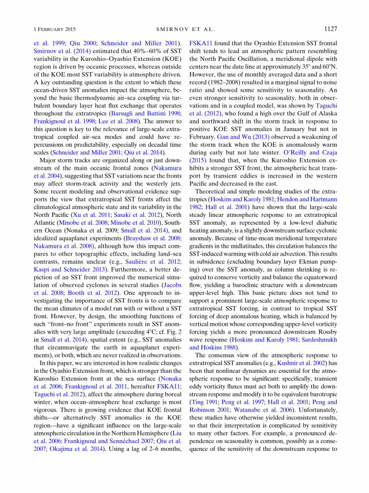
a. Specification of an appropriate Oyashio Extensionfrontal shift SST anomaly

The Oyashio Extension index (OEI), developed by

FSKA11, is based on the leading empirical orthogonal

function of the latitude of the maximum monthly aver-

agedmeridional SST gradient (SSTY) within the domain

358–478N, 1458–1708E. A regression of monthly aver-

aged SST anomalies on the OEI during the extended

winter period (November–March) from 1982 to 2008 is

shown in Fig. 1a. The polarity in Fig. 1a, which is asso-

ciated with a northward shift in the SST front, is called

the warm phase.

We are interested in the influence of this frontal shift

on the large-scale atmospheric circulation, so here we

force an AGCM with a prescribed SST anomaly corre-

sponding to the frontal shift. The risk in this approach is

that a substantial portion of the basinwide SST anomaly

(Fig. 1a) may reflect the SST response to atmospheric

changes forced by or contemporaneous with the Oyashio

Extension shift, which should not be included in a pre-

scribed SST experiment (Barsugli and Battisti 1998;

Bretherton and Battisti 2000). That is, we wish to pre-

scribe an SST anomaly that represents only oceanic

forcing of the atmosphere. To focus on the direct frontal

influence, we have applied the following to the anomaly

in Fig. 1a: Starting with the 1408E meridian and pro-

gressing eastward, a 61-point (15.258 span of latitude)

tapered cosine window (taper ratio is 0.5) is applied in

the meridional direction by centering it on the latitude

where the November–March-mean jSSTYj is maximized

and only if jSSTYj . 1.58C (100 km)21 (anomalies out-

side of the filter are set to zero). Next, because the fi-

nescale structure in Fig. 1a may be an artifact of the

short data record, a 5-point running mean filter is ap-

plied 20 times in the zonal direction only (to prevent

excessive smoothing of the SST front), and then the

resultant pattern is scaled by 3 to represent a 3s shift of

the OEI index. The final SST anomaly pattern, shown in

1128 JOURNAL OF CL IMATE VOLUME 28

Fig. 1b, has SST anomalies with a maximum amplitude

of ;1.5K but is limited to 1408–1708E. This region is

where Smirnov et al. (2014) (cf. their Fig. 5a) found

a significant fraction of the SST variability was forced

by the ocean, presumably reflecting anomalous heat

transport via oceanic advection or eddy activity.Abinned

scatterplot of point-by-point SSTY across the Oyashio

Extension front over the domain marked by the box in

Fig. 1b is shown in Fig. 1c. The OEI captures the north-

ward shifted SST front [;(38–48) farther north in the

FIG. 1. (a) November–March OEI SST regression. (b) Regression after multiplying (a) by 3

and then smoothing and applying cosine-taper filter (see text). (c) Scatter of point-by-point

2d(SST)/dy from 1458 to 1658E as a function of latitude (dots) for the warm (red; northward

Oyashio shift) and cold (blue) experiments. The black box shown in (b) shows the region used

for across-front zonal averages (1458–1658E) in subsequent figures.

1 FEBRUARY 2015 SM IRNOV ET AL . 1129

warm phase compared to the cold phase] and suggests

that the front is significantly broader inmeridional extent

during thewarmphase.However, note that themaximum

SST front strength is essentially unchanged [;3.68C(100km21)] between the warm and cold phases.

We determine how significant these modifications of

the original OEI pattern are by projecting the spatial

structure shown in Fig. 1b onto observations to create

a projected OEI (POEI) time series. The sensitivity of

this index to different time periods and resolution is then

assessed by comparing three versions constructed using

1) monthly and 2) daily averaged 0.258 resolution

NOAA optimum interpolation (OI; Reynolds et al.

2007) SST anomalies from 1982 to 2012 and 3) monthly

averaged 18 resolution objectively analyzed air–sea

fluxes (OAFlux; Yu and Weller 2007) SST anomalies

from 1958 to 2012. All resulting time series—called

POEI1, POEI2, and POEI3, respectively—are stan-

dardized to unit variance. During the overlapping pe-

riod (1982–2012), the two monthly averaged POEIs

based on different datasets (1 and 3) have a 0.98 corre-

lation. The correlation between the original OEI and

POEI1 is only 0.56, but the indices are more strongly

related (correlation of 0.77) when both are smoothed

with a 13-month running mean, suggesting that while

there may be nonnegligible differences between the two

indices on monthly to seasonal time scales they have

greater agreement on longer time scales. Moreover, the

POEI3, shown in Fig. 2, has a much longer decorrelation

time (7 months) compared to the OEI (3 months) so that

it may represent the most persistent portion of the OEI

SST anomaly and thus be more appropriate for a pre-

scribed SST anomaly experiment. Additionally, while

Fig. 1b corresponds to a 3s departure of the OEI, it

amounts to a 1.25s departure of the POEI3. The corre-

lation between the POEI1 (interpolated to daily values)

and daily POEI2 is 0.90, implying that in the daily index

submonthly variability does not obscure the longer time

scales. For reasons discussed in section 5, we use the daily

POEI2 (hereafter just POEI) as the basis for the obser-

vational comparison to the GCM simulations.

b. Model details and experimental design

The CAM5 GCM (Neale et al. 2010), coupled to the

Community Land Model version 2 and forced by pre-

scribed SST and sea ice, is used for all experiments in

this study. CAM5 is integrated with a finite-volume dy-

namical core and contains 30 unequally spaced vertical

levels using a hybrid pressure–sigma coordinate system.

Notably, there are approximately 8 levels within the

boundary layer (.800 hPa). We run two configurations

of the model: a high-resolution (HR) version with 0.258horizontal resolution and time step of 15min and

a (relatively) low-resolution (LR) version with 18 hori-zontal resolution and time step of 30min. All parame-

terization schemes are the same between the HR and

LR. Aside from the impacts of linearly interpolating the

HR initial and boundary data to the LR grid (slight

differences in regions of large topography), all other

facets of the two models are identical.

For both configurations, a 25-member ensemble of

control simulations is created in the following manner.

Using 1 November initial atmospheric conditions of

25 different years taken from a previous 0.258 CAM5

simulation (Wehner et al. 2015), we run the CAM5 from

1 November through 31 March forced by the climato-

logical, monthly averaged annual cycle of SST derived

from the 1982–2011 0.258 NOAA OI dataset. The same

initial land and sea ice condition are used for all en-

semble members. Next, two additional sets of ensembles

are conducted in very similar fashion as the control ex-

cept with the addition (warm) or subtraction (cold) of

FIG. 2. Standardized POEI3 (colors) based on the 18 OAFlux SST dataset for 1958–2012 and OEI

(without trend removal) from FSKA11 (black lines) for 1982–2012.

1130 JOURNAL OF CL IMATE VOLUME 28

the SST anomaly pattern shown in Fig. 1b. The SST

anomaly is constant and does not evolve with the annual

cycle, which can be justified by the relatively long 7-month

decorrelation time scale of the monthly POEI.

3. Atmospheric response to an Oyashio Extensionfrontal shift

Since we are interested in the equilibrium winter-

mean response to the Oyashio Extension shift, it is es-

sential to determine (and discard) the time required for

model spinup. Figure 3 shows that the transient atmo-

spheric response to the northward shift of the Oyashio

Extension SST front, as depicted by the spatial corre-

lation and spatial root-mean-square to the equilibrium

(December–March mean) across-front divergence, takes

about 15 days to reach quasi equilibrium in the HR sim-

ulation (in LR, this takes;20 days; not shown). A similar

spinup time is seen when analyzing the surface (16 days)

and the 2–6-day bandpass 850-hPa heat flux (y0T 0)(18 days; not shown). Importantly, in HR the response is

similar from month to month and is nearly linear when

comparing the warm–control and control–cold differences

separately (not shown). Thus, hereafter we only discuss

the mean December–March atmospheric response, de-

termined from themean difference between thewarm and

cold ensembles. Significance is assessed via the Student’s t

test assuming that the ensemblemembers are independent

from each other. Finally, since the SST anomaly (warm–

cold) in the model simulations represents a61.25s POEI

difference, the results displayed below have been rescaled

to represent a 1s change in the POEI.

The model responses of the HR (left) and LR (right)

simulations to the prescribed SST anomalies are shown

in Fig. 4. The top panels show the net turbulent heat flux

FIG. 3. (a) Mean response (contours with interval of 4 3 1027 s21) of the December–March

across-front (1458–1658E) divergence in the HR simulation [ordinate is pressure (hPa)]. Black dots

denote areas significant at the 95% confidence level. (b) Evolution of the 5-day running mean

response of across-front divergence. The thick (thin) line indicates the response pattern rms (pat-

tern correlation) with the equilibrium pattern in (a). The rms is normalized to 1 by the day 3 value.

In (a), red and blue bars denote the position of the SST anomaly.

1 FEBRUARY 2015 SM IRNOV ET AL . 1131

(THF; positive upward) and 950-hPa wind responses

for HR (Fig. 4a) and LR (Fig. 4b). Both simulations

generate a surface cyclone downstream of the SST

anomaly, consistent with the expected response to

a shallow extratropical heat source (Hoskins and

Karoly 1981; Hendon and Hartmann 1982; Peng et al.

1997; Hall et al. 2001; Deser et al. 2007; Smirnov and

Vimont 2012). However, the sea level pressure (SLP)

and near-surface wind responses are three to four

times stronger in the LR than in the HR simulation.

Furthermore, the LR surface anomalies are part of an

equivalent barotropic response throughout the entire

atmospheric column [not shown but similar to Pitcher

et al. (1988) and Kushnir and Lau (1992)], though it is

only statistically significant from the surface through

;600 hPa. However, there is no significant local

height response in HR west of the date line. Surpris-

ingly, the THF response in LR is 15%–20% greater

than in HR. This is consistent with much stronger cold

and dry air advection over the warm SST anomaly

induced by the stronger LR winds compared to the

HR. Consequently, while the surface heat fluxes in

both the LR andHR act to damp the SST anomaly, the

damping is stronger in LR. Based on the surface fluxes

alone, the SST anomaly would have an e-folding time

scale of 5 (4) months in the HR (LR) simulations.

FIG. 4. The mean December–March atmospheric response (warm–cold) to a shift in the Oyashio Extension SST front in (left) HR and

(right) LR simulations. (a),(b) Turbulent heat flux (colors; K m s21) and 950-hPa wind (vectors; m s21). Black thick vectors are significant

at the 95% confidence level. (c),(d) Zonally averaged (1458–1658E) across-front (y, v) circulation (vectors) and uE (colors) [ordinate is

pressure (hPa)]. Black thick vectors are significant at the 90% confidence level. The v component is multiplied by 2000 to aid in visualization.

(e),(f) The 850-hPa y0u0E (colorsKms21), where stippling denotes regions significant at the 95%confidence level. The black contours indicate

the mean climatological y0u0E. In all panels, the mean difference is divided by 2.5 to account for a 61.25s POEI SST anomaly.

1132 JOURNAL OF CL IMATE VOLUME 28

While the LR shows a stronger response in the local

horizontal circulation, the HR shows a substantially

stronger response in the vertical circulation. Figures 4c,d

show the response of the across-front zonally averaged

(1458–1658E; see box in Fig. 1b) circulation (y, v) and

equivalent potential temperature uE. Both HR (Fig. 4c)

and LR (Fig. 4d) show upward motion over the positive

SST anomalies, consistent with past studies (Feliks et al.

2004; Brachet et al. 2012), but this upward motion in HR

extends to the tropopause, whereas it is limited to the

lower troposphere in LR. In the upper troposphere the

circulation forms two cells with northward (southward)

flow north (south) of the front in HR, whereas the flow is

southward at all latitudes in LR. The larger low-level uEanomaly in HR over the warm SST, reflecting both

warmer temperatures and enhanced low-level moisture,

also reduces the low-level stability (not shown), in a re-

gion that is frequently convectively unstable (Czaja and

Blunt 2011; Sheldon and Czaja 2014). The zonal wind

response is weak in both simulations (not shown): in the

LR, zonal wind changes are less than about 1.5m s21 and

are consistent with the cyclonic circulation to the east,

while the HR zonal wind changes are of opposite sign

and even smaller.

In the western North Pacific, synoptic variability plays

a dominant role in transporting heat and moisture

(Nakamura et al. 2004; Newman et al. 2012; Kwon and

Joyce 2013). Comparing the control climates of HR and

LR (contours in Figs. 4e,f) with observations (see sec-

tion 5) shows HR underestimates 850-hPa transient

eddy meridional uE flux y0u0E (which is functionally

equivalent to moist static energy flux) in its core near

408N by only about 8% (54Kms21 in HR; 59Kms21 in

ERA-Interim) while LR (46Kms21) underestimates it

by 22%. Unfortunately, daily humidity fields were not

saved from the model output, so instead this eddy term

was determined from monthly averaged covariance as

y0u0E 5 yuE 2 y uE, which includes all submonthly vari-

ability and accounts for a majority of the total climato-

logical 850-hPa y0u0E east of Japan (not shown). Aside

from the stronger mean y0u0E in the storm-track core,

comparison of the HR and LR mean states does not

yield any other major differences.

Both the HR and LR exhibit a northward shift of the

y0u0E with a reduction south of the SST anomaly (Figs. 4e,f),

but the increase north of the SST anomaly is more than

3 times stronger in the HR experiment. The total y0u0Eresponse consists of roughly equal contributions from

heat and moisture fluxes (not shown). Most of the heat

flux response arises from the 2–6-day bandpass filtered,

or synoptic, time scales as shown in Fig. 5 for the thermal-

only component y0T 0 in HR (as noted above, the band-

pass moisture flux cannot be determined explicitly). In

LR the response is relatively shallow, confined mostly

below about 750 hPa, whereas in the HR run the re-

sponse is much deeper, extending well above 500 hPa, as

shown in the across-front vertical cross sections of y0u0E(Figs. 6a,b). Equally striking differences are seen in

submonthly y02 (Figs. 6c,d), which increases north of the

front in HR but decreases south of the front in LR. The

broadening of the storm track at upper levels in HR is

notable and consistent with a broader SST front (Fig. 1c)

but does not reach the 95% significance level. Note that

the upper-level y02 is about 20% stronger in the HR

control compared to the LR control (black contours in

Figs. 6c,d), though even HR still slightly underestimates

y02 in ERA-Interim (not shown).

Collectively, the HR simulation places a much greater

emphasis on eddy transport in a region where fluxes of

FIG. 5. (a) The total submonthly 850-hPa y0T 0 (Kms21) and its

contribution separated into the (b) 2–6-day and (c) 6–30-day bandpass

components in the HR simulation. Black dots denote regions that are

significant at the 95% confidence level. Note that daily specific hu-

midity output was not saved, precluding the same analysis on y0u0E.

1 FEBRUARY 2015 SM IRNOV ET AL . 1133

heat andmoisture occur predominantly with the passage

of warm and cold fronts (James 1995). To gauge how the

HR and LR treat such passages and their sensitivity to

the SST anomaly, Fig. 7 shows a composite of anomalous

SLP (contour) and 2–8-day bandpass-filtered 850-hPa

y0T 0 (color) when an atmospheric front appears in the

black box shown in Figs. 7a–d (we use y0T 0 instead of

y0u0E because daily q was not archived). Fronts are

identified in both the warm and cold simulations of HR

and LR when the thermal front parameter (TFP),

a scalar value based on the gradient of the magnitude of

6-hourly averaged 850-hPa potential temperature (see

Table 1 in Hewson 1998). Using a TFP exceedance

threshold value of 0.15K (100 km)22 (Renard and

Clarke 1965; Booth et al. 2012), a front is identified in

the box in Fig. 7 about 1 out of every 6 days. To avoid

very localized, potentially misleading features, this cri-

terion must be met at two or more neighboring grid

points. Figures 7a–d show that the composite SLP field is

characterized by a 6–7-hPa cyclonic anomaly within the

box with a 5–6-hPa anticyclonic anomaly ;208 east forboth the warm and cold simulations of HR and LR, with

y0T 0 consistent with northward advection of warm air in

a midlatitude cyclone’s warm sector. For fronts passing

through this box, y0T 0 is about 10% stronger in the HR

than LR simulations for both warm and cold phases

(cf. Figs. 7a,b; cf. Figs. 7c,d), even though the SLP

composites are nearly identical, similar to the difference

between the HR and LR control runs (the black con-

tours in Figs. 4e,f). However, for the warm minus cold

response (Figs. 7e,f), the SST anomaly has a much

greater impact on heat flux associated with frontal pas-

sage in the HR, with a dipole in the y0T 0 response

roughly straddling the SST front, while the LR only

captures the (weaker) southern portion of the response.

Both models have enhanced cloud formation and

precipitation resulting from the warm SST anomaly

though the response is shifted slightly poleward (and

consistent with a more robust storm-track shift) in HR

compared to LR (Fig. 8). However, while the magnitude

of the precipitation response is similar in HR and LR

(Figs. 8a,b), the precipitable water response in HR is

more than twice as large. There is also a corresponding

increase in the cloud water content in theHR simulation

(not shown). The much higher levels of PW and cloud

water are consistent with the increased transient eddy

moisture flux convergence in the HR simulation (not

shown but the differences are similar to Figs. 4e,f) as

well as the stronger advection of dry air from the

northeast and a weakening of the background westerlies

in the LR simulation (Figs. 4a,b). That is, even though

the precipitation response over the SST anomaly is

FIG. 6. Across-front mean December–March response (color shading) of (a),(b) y0u0E (shading interval is

0.8Kms21) and (c),(d) y0y0 (shading interval is 2m2 s22) in the (left) HR and (right) LR simulations. Stippling

denotes areas that are significant at the 95% confidence level. The thick black contours show the climatological

values from the (a),(c) HR and (b),(d) LR control simulations.

1134 JOURNAL OF CL IMATE VOLUME 28

similar, in LR there is a local balance between increased

evaporation and precipitation, while in HR storms

converge moisture into the storm track–jet stream that

can subsequently be transported downstream (not

shown but see Fig. 15a,b).

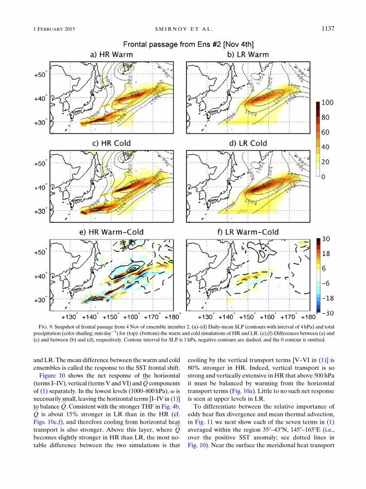
Figure 9 shows the stark difference in the SLP and

precipitation response from the standpoint of an individual

synoptic storm.This event is chosen from the 4th day of the

model runs (4 November) where a particular weather

feature could still be identified in all four simulations

(warm–cold and HR–LR). One caveat is that this may

not portray the sensitivity of the equilibrium response as

Fig. 3 showed this requires roughly 2 weeks. Nonethe-

less, Fig. 9 shows that HR depicts a slightly stronger

cyclone than LR, located near 408N, 1608E. HR contains

two frontal-like precipitation bands, while the LR shows

one main band in the immediate vicinity of the cyclone

center. However, the largest differences appear by taking

FIG. 7. (a)–(d) Composites of anomalous SLP (contours) and high-pass-filtered 850-hPa y0T 0(color shading; Kms21) on days where the

thermal front parameter (see text for additional information) exceeds 0.15K (100km)22 for the (a) warm and (c) cold HR simulations and

(b)warmand (d) coldLRsimulations. (e),(f)Differences of (a)2 (c) and (b)2 (d). In (e),(f), a thick contour encloses areas that exceed the 95%

significance based on a 1000-sampleMonte Carlo test. Note that SLP does not show up in (e),(f) because it does not meet the 95% significance

threshold (or even the 90% threshold). Black rectangle in (a)2(d) denotes the region where the front tracking is applied (see text).

1 FEBRUARY 2015 SM IRNOV ET AL . 1135

the warm–cold response. Figures 9e,f show that the

precipitation response in HR is roughly 4 times stronger

and more coherent than LR, though both models depict

a northward shift in precipitation to first order. Addi-

tionally, the HR shows a substantially stronger response

in SLP, with a 2–3-hPa dipole straddling the cyclone

center. Meanwhile, the LR shows a broader cyclonic

anomaly that is located much farther west. Figure 9 is

not meant to be a generalization across all synoptic

disturbances, but instead shows the surprising sensitivity

to atmospheric resolution at the frontal scale.

4. Diagnosis of physical mechanisms

In response to the poleward shift of the SST front, the

HR and LR simulations each, to different extents, de-

velop a near-surface cyclonic circulation to the east of

the warm SST anomaly, with enhanced uE, upward

motion, and transient eddy heat flux divergence above

the SST anomaly. However, the relative importance of

these processes is very different, such that, while the

LR primarily balances the warm SST by a mean cir-

culation change advecting cold and dry air southward,

the HR primarily balances the enhanced heat and

moisture through transient eddies transporting heat

and moisture northward, probably via frontal passages.

In this section, we further quantify these key differ-

ences by constructing budgets using the thermody-

namic and vertical velocity (v) equations.

a. Thermodynamic budget

First, we diagnose how heat is exchanged at the air–

sea interface and within the atmospheric column. The

processes that balance the diabatic heating _Q resulting

from the SST anomalies are determined from the time-

mean thermodynamic equation, written as

u›T

›xI

1›

›xu0T 0

II

1 y›T

›yIII

1›

›yy0T 0

IV

1

�v›T

›p2

k

pvT

�V

1

0@v0›T

0

›p2

k

pv0T 0

1A

VI

5 _Q

VII

, (1)

where overbars represent the ensemble climatological

mean for each month; primes represent departures from

thatmean, k5R/CP, whereR is 287 J kg21K21 andCP is

1004 J kg21K21; and all other terms assume their typical

meteorological conventions. The HR data are linearly

interpolated to the LR grid and the budget is calculated

for each month separately and then averaged to form

a December–March mean. Term VII is from direct

model output and the budget is nearly closed with the

residual being a few percent of the sum from the re-

maining terms, except in very close proximity to orog-

raphy. The warm and cold ensembles each have their

own climatological means, and we calculate each term

separately for the warm and cold ensembles of both HR

FIG. 8. Mean December–March response in (a),(b) total (convective1 stratiform) precipitation (mm day21) and

(c),(d) column-integrated precipitable water (mm) in the (a),(c) HR and (b),(d) LR simulations. Contours enclose

areas that are significant at the 95% confidence level.

1136 JOURNAL OF CL IMATE VOLUME 28

and LR. Themean difference between the warm and cold

ensembles is called the response to the SST frontal shift.

Figure 10 shows the net response of the horizontal

(terms I–IV), vertical (termsV andVI) and _Q components

of (1) separately. In the lowest levels (1000–800hPa), v is

necessarily small, leaving the horizontal terms [I–IV in (1)]

to balance _Q. Consistent with the stronger THF in Fig. 4b,_Q is about 15% stronger in LR than in the HR (cf.

Figs. 10e,f), and therefore cooling from horizontal heat

transport is also stronger. Above this layer, where _Q

becomes slightly stronger in HR than LR, the most no-

table difference between the two simulations is that

cooling by the vertical transport terms [V–VI in (1)] is

80% stronger in HR. Indeed, vertical transport is so

strong and vertically extensive inHR that above 500 hPa

it must be balanced by warming from the horizontal

transport terms (Fig. 10a). Little to no such net response

is seen at upper levels in LR.

To differentiate between the relative importance of

eddy heat flux divergence and mean thermal advection,

in Fig. 11 we next show each of the seven terms in (1)

averaged within the region 358–438N, 1458–1658E (i.e.,

over the positive SST anomaly; see dotted lines in

Fig. 10). Near the surface the meridional heat transport

FIG. 9. Snapshot of frontal passage from 4 Nov of ensemble member 2. (a)–(d) Daily-mean SLP (contours with interval of 4hPa) and total

precipitation (color shading; mmday21) for (top)–(bottom) the warm and cold simulations of HR and LR. (e),(f) Differences between (a) and

(c) and between (b) and (d), respectively. Contour interval for SLP is 1hPa, negative contours are dashed, and the 0 contour is omitted.

1 FEBRUARY 2015 SM IRNOV ET AL . 1137

terms largely balance _Q, but for the LR the mean

transport dominates the eddy transport whereas for the

HR the eddy transport is about 60% larger than the

mean transport (Fig. 11c) and has much greater vertical

extent. Recall that the total (i.e., submonthly) eddy re-

sponse is dominated by the 2–6-day synoptic time scales

(Fig. 5). In the middle and upper troposphere, the large

difference in the vertical transport between HR and LR

is due to themeanv circulation (Fig. 11d). For the LR in

this region, mean zonal and meridional terms are large

but mostly offset (cf. Figs. 11b,c), whereas the primary

HR balance is between the combined mean horizontal

and vertical transports. Overall, the thermodynamic

budget confirms that horizontal eddy transports (lower

troposphere) and strong vertical motion (middle tro-

posphere) are much more important for balancing _Q in

HR than in LR simulations.

b. Omega equation

The stronger v response in HR seen in Figs. 4c,d raises

the question of what physical mechanism(s) correspond to

this difference. To investigate, we calculate contributions

to v using a modified quasigeostrophic (QG) form of the

generalized v equation that includes diabatic effects

(Krishnamurti 1968; Trenberth 1978; Raisanen 1995).

Unlike past studies, such as Pauley and Nieman (1992)

and Raisanen (1995), we focus on the mean v as opposed

to an individual synoptic event. The modified QG v

equation can be written as

�s=21f 2

›2

›p2

�v5=2

264Vg �$

�2›f

›p

�I

1V 0g �$

�2›f0

›p

�II

375

1 f›

›p

"Vg �$(zg1 f )

III

1V0g �$z0gIV

#

2k

p=2 _Q

V

,

(2)

where s is the wintertime spatially varying December–

March-mean static stabilitys(x, y, p)52(RT/pu)/(›u/›p)

andf is the geopotential height. Terms I and II are themean

FIG. 10. Across-frontDecember–March-mean difference of the terms comprising the thermodynamic budget in (1)

for the (a),(c),(e) HR and (b),(d),(f) LR simulations [ordinate is pressure (hPa)]. (a),(b) Sum of all horizontal terms

(I–IV); (c),(d) sum of all vertical terms (V and VI); and (e),(f) diabatic heating (colors) and their Laplacian (con-

tours). The thin vertical dotted lines show the approximate latitudinal position (358–438N) of the positive SST

anomaly and are used for meridional averaging in Fig. 11.

1138 JOURNAL OF CL IMATE VOLUME 28

and eddy components of the differential thermal advec-

tion, while terms III and IV are the mean and eddy

components of the differential vorticity advection. Gen-

erally, thermal (vorticity) advection is more important in

the lower (mid and upper) troposphere; however, there is

often strong cancellation between the two (Hoskins et al.

1978; Billingsley 1998) and investigating each term sep-

arately may be beneficial.

The recalculated v response (vR) is accomplished via

successive relaxation by forcing with the sum of the rhs

of (2). Details of the calculation are in the appendix.

Figures 12a,b show the across-front response in v com-

pared with vR for HR and LR. There are regions where

vRdiffers from v, but generally this difference is less

than 20%. Over the warm SST (368–428N), vR over-

estimates the upward motion, but except near the tro-

popause this discrepancy is relatively small. Given this,

the vR response can be used as a proxy for v and

Figs. 12c–f show the dominant terms in (2); terms II

(eddy thermal), III (mean vorticity), and IV (eddy vor-

ticity) are small (less than one contour) and thus not

shown. Over the SST anomaly in the lower to middle

troposphere (from the surface to 500 hPa), the HR

simulation generates vertical motion that is about 40%

stronger than LR and is balanced by a stronger diabatic

term V. This might appear to contradict the earlier ob-

servation that the low-level LR heating is actually stronger

than HR (cf. Figs. 10e,f), but it is the finer-scale structure

of _Q as measured by =2 _Q (see dashed contours of

Figs. 10e,f) that is commensurately stronger in HR at

lower levels. That is, the narrowness of the diabatic heating

balances the stronger v field, though causality cannot be

determined via the diagnostic equation (2).

The other major difference between vR in the two

simulations is mainly in the middle and upper tropo-

sphere, where mean differential thermal advection [term

I in (2); Figs. 12c,d] generates stronger upwardmotion in

the HR simulation. Since this region has a significant

mean meridional temperature gradient and weak pole-

ward flow (not shown), enhanced upward motion could

be maintained by a shift in the temperature gradient

and/or by changes in the circulation. To determine

which is more important, we recalculate vR but using

several modified forms of term I, as shown in Fig. 13.

First, Fig. 13b shows that, when u and y are both set to be

their control climatological values, the vR response is

much weaker and nearly of opposite sign as the full term

I forcing (cf. Fig. 13a), implying that changes in themean

T field are an insignificant contributor to term I. Next,

when T is set to climatology (Fig. 13c), the vR is nearly

identical to full forcing, confirming that the anomalous

wind is responsible for balancing the upper-level vR.

Finally, when T and u are set to climatology (Fig. 13d),

FIG. 11. Vertical profiles of the heating rate response (Kday21)

arising from (a) horizontal (blue) and vertical (gray) transport,

diabatic processes (red). (b)–(d) Separation from (a) of the hori-

zontal component into mean (solid) and eddy (dash) components

for zonal and meridional transport, and into mean and eddy terms,

respectively. The thick (thin) lines are for HR (LR). Note the

different x-axis scale in (b)–(d) compared to (a).

1 FEBRUARY 2015 SM IRNOV ET AL . 1139

the resulting vR is almost identical to the full forcing,

showing that it is specifically the anomalous y that con-

tributes most strongly to balancing the upper-level vR in

HR. The impact of anomalous u is not negligible and has

about 20% of the impact of y but is shifted farther south

than the main region of upward motion seen in Fig. 13a.

5. Observational comparison

Properly diagnosing extratropical air–sea interactions

in observations is challenging. Simultaneous atmosphere–

ocean statistics can bemisleading because of the coupled

nature of the problem and the differing oceanic and

atmospheric dynamical time scales (Frankignoul and

Hasselmann 1977). To address this issue, empirical

analysis in the extratropics must include some temporal

lag that is longer than the intrinsic atmospheric persis-

tence of a few days to weeks (Frankignoul and Kestenare

2002) or, ideally, empirically estimate coupled air–sea

dynamics explicitly (Smirnov et al. 2014). This is difficult

in short datasets of a multivariate system in which slowly

evolving oceanic forcing may produce atmospheric re-

sponses coexisting with faster coupled air–sea variabil-

ity, as well as oceanic variability forced primarily by the

atmosphere, with corresponding spatial patterns that are

neither identical nor orthogonal.

As noted in the introduction, past observational

analyses on the impact of the Oyashio SST front find

pronounced signals but do not uniformly agree, espe-

cially concerning the remote atmospheric response. We

do not aim to solve that problem in this paper. However,

given the strong sensitivity of the results to model res-

olution, it is natural to askwhether the local atmospheric

response of either experiment is consistent with nature.

We do not expect an identical match of course, since

although the SST anomaly used in our experiment has

realistic amplitude and pattern it was held fixed and

specified only within the POEI region. Still, to create an

observational comparison to section 3, we have re-

gressed various atmospheric variables on the POEI for

FIG. 12. (left) HR and (right) LR simulations. (a),(b) Across-front mean vR (contours) and v–vR (contours–red:

positive; blue: negative), respectively. Contour interval is 0.005Pa s21. The contribution to vR decomposed into the

(c),(d) mean thermal and (e),(f) diabatic heating components. The eddy thermal, mean vorticity, and eddy vorticity

components are negligible (,1 contour) and are not shown. See (2) for terms.

1140 JOURNAL OF CL IMATE VOLUME 28

lags ranging from several days to 2 months, with the

POEI both leading and lagging the atmosphere, roughly

similar to the FSKA11 approach. We have also exam-

ined both daily and monthly averaged data. Choosing

one representative lag and data sampling interval is

difficult as no single lag time captures the response of all

variables, possibly because (i) there is a transient at-

mospheric response to the Oyashio Extension shift that

is dependent on lag and (ii) each atmospheric variable

decorrelates on a different time scale. For display pur-

poses, we show a lag regression of daily wintertime

(November–March) data when the POEI leads the at-

mosphere by 14 days, which should be long enough to

mainly capture the atmospheric response to the POEI

(as most atmospheric variables are nearly fully decor-

related after two weeks) and also seems appropriate

based on the earlier discussion of the model response

equilibration time (Fig. 3). For comparison, we also show

the simultaneous regression between the atmosphere and

the POEI but note that this is difficult to interpret since

it can contain both the forcing of and response to the

POEI SST anomaly.

In general, the regression amplitude depends on lag,

sometimes strongly, but the spatial structure is fairly con-

sistent. Using daily data resulted in a 20%–40% stronger

signal compared to using monthly data, but results

are otherwise qualitatively similar (not shown). ERA-

Interim does not have daily values of sensible and latent

heat flux, so the 18 OAFlux (Yu and Weller 2007)

dataset is used for these variables. Also, since El Niño–Southern Oscillation (ENSO) variability has a strong

teleconnection to the North Pacific (e.g., Alexander

et al. 2002), we remove the covariability with ENSO

from both the POEI and all atmospheric variables by

a linear regression using the daily Niño-3.4 index. Thisgenerally reduces the amplitude of regression co-efficients by up to 15% (mostly east of the date line) butleaves the spatial structures unchanged.

FIG. 13. (a) Mean thermal contribution to across-front vR response in the HR simulation (as in Fig. 12c but with

contour interval of 0.0025Pa s21). (b)–(e) As in (a), but setting to climatological values from the HR control sim-

ulations: (u, y), T, (T, u), and (T, y), respectively.

1 FEBRUARY 2015 SM IRNOV ET AL . 1141

Additionally, FSKA11 suggested that the meridionally

confined nature of the Oyashio Extension SST front vari-

ability could make it difficult to diagnose the atmospheric

response in coarse-resolution datasets. We compared the

across-front regression of pressure velocity (v; negative

upward) on the POEI using the 0.78 resolution ERA-

Interim (Uppala et al. 2008; http://data-portal.ecmwf.int/

data/d/interim_daily/) dataset with the 2.58 resolution Na-

tional Centers for Environmental Prediction Reanalysis 1

(NCEP-1; Kalnay et al. 1996) over the 1982–2012 period

and found a 40% stronger signal in the former (not

shown). Here we chose the enhanced ERA-Interim res-

olution (time range: 1979–present) over the longer data

record provided by NCEP-1 (time range: 1948–present).

With the many above caveats in mind, in Fig. 14 we

show the same fields as displayed in Fig. 4 but based on

regressions of observed data onto the daily POEI at

0-day (left) and 14-day lags (right). In the observed re-

gression, positive POEI values are associated with

strong THF from the ocean to atmosphere on the

southern periphery of the SST front (368–428N) roughly

at a rate of ;30Wm22 8C21, consistent with previous

estimates (Frankignoul and Kestenare 2002; Park et al.

2005). Note that weaker values in Fig. 14a appear to be

the result of the contemporaneous state of the POEI

and atmosphere, with larger values resulting when

the POEI leads THF by 14 days (Fig. 14b), consistent

with oceanic forcing of the atmosphere (see Fig. 21

in Frankignoul 1985). The 14-day regression (i) has

a 40% weaker uE signal and (ii) limits the up-

ward vertical motion to the immediate SST anomaly

region.

FIG. 14. Observational counterpart to Fig. 4 based on (left) simultaneous and (right) 14-day lagged regressions of the ERA-Interim

atmospheric variables on the daily POEI.

1142 JOURNAL OF CL IMATE VOLUME 28

In general, the observations seem more broadly con-

sistent with the HR than the LR model results. In terms

of the response to POEI SST anomalies, the observed

regression appears to have a broader area of upward

THF than either the HR or LR simulation, which could

be due to the limited spatial extent of the prescribed SST

anomaly in the model, but the observed and model

amplitudes appear comparable. The lack of significant

wind anomalies in the observed regression appears more

consistent with the HR, suggesting that LR may be

overemphasizing the importance of themean circulation

response in balancing anomalous heat from the SST.

Additionally, the vertical extent of the upward motion

over the SST anomaly in theHR resembles the observed

pattern, as does the upper-level outflow that is sym-

metric or slightly northward, whereas the LR (Fig. 4d)

has southward flow at all levels.

Finally, both the simultaneous and 14-day lag regression

(Figs. 14e,f; note that using lags of 21 and 28 days results in

a very similar pattern as the 14-day lag) indicate

a northward shift of y0u0E but primarily indicate

a much stronger reduction of y0u0E south of the SST

front, especially in Fig. 14f, which appears markedly

different from Fig. 14e and appears to better match

LR. However, we note that the divergence of y0u0Ecentered over the warm SST anomaly is the same in

both panels, with the location and amplitude better

matching the HR results (not shown). Collectively, it

appears the observed regressions better match HR

because of (i) significantly more active eddy heat

transport response and (ii) deeper response in v.

6. Discussion and conclusions

In a high-resolution (0.258) version of the NCAR

CAM5, a meridional shift of the Oyashio Extension SST

front is shown to locally force a robust atmospheric re-

sponse dominated by changes in the eddy heat and

moisture transports. However, in the corresponding low-

resolution (18) simulations, the local atmospheric re-

sponse exhibits strong heating by surface fluxes that is

balanced by the mean equatorward advection of cold air,

consistent with the paradigmof a steady linear response to

a near-surface heat source (seeHoskins andKaroly 1981).

In the higher-resolution simulation, we noted a sub-

stantially weaker surface circulation (Figs. 4a,b), stronger

and deeper vertical motion (Figs. 4c,d), and significantly

stronger transient eddy moist static energy flux as key

responses to the SST anomaly. Furthermore, it appeared

that the latter difference could be seen on average in in-

dividual synoptic fronts (Figs. 7 and 9).

A number of previous modeling studies have sug-

gested that heat from an extratropical SST anomaly is

transferred into the lower troposphere where it directly

forces the atmospheric response, with transient eddy

flux feedbacks primarily important for modifying the

downstream upper-level circulation anomaly (Peng

et al. 2003; Peng and Whitaker 1999; Hall et al. 2001;

Yulaeva et al. 2001; Kushnir et al. 2002). In contrast, we

find that transient eddies impact the local heat balance

through changes in the transient eddy moist static en-

ergy flux. That is, extratropical cyclones respond to the

underlying SST anomaly in the Oyashio Extension

front region by transportingmuch of the anomalous heat

northward, so that even under linear theory the weaker

residual heating could be expected to produce only

a weak surface low to the east. As the downstream low

and its southward advection of cold, dry air are reduced,

subsidence associated with vortex shrinking over the

heating region is also reduced.

Some issues in our experimental design limit in-

terpretation of our results. First, when comparing HR to

LR responses, the impact of better resolving the SST

gradient cannot be distinguished from intrinsic differ-

ences between the 0.258 and 18 versions of CAM5. This

issue could be addressed by rerunning the HR experi-

ments but with the 18 SST grid used by LR. Second,

because some of the SST anomaly in the central and

eastern Pacific related to an Oyashio Extension shift

(Fig. 1a) represents coupling to or forcing by the atmo-

sphere (Smirnov et al. 2014), we employed a conserva-

tive experimental approach by prescribing a very spatially

confined SST anomaly; however, this approach still ig-

nores potential feedbacks due to air–sea coupling. Also,

the model SST anomaly is held fixed in time, whereas in

observations its decorrelation time scale is 7 months and

in the HR it would have a ;5-month decorrelation time

scale if allowed to decay because of surface heat fluxes.

While it seems intuitive that the HR better resolves

frontal circulations and associated v, we have not de-

termined why the transient eddy heat and moisture flux

responses are so sensitive to model resolution. Moist

diabatic processes appear to affect how SST fronts could

influence extratropical cyclone development (Fig. 9; see

also Booth et al. 2012; Deremble et al. 2012; Willison

et al. 2013), and Willison et al. (2013) found increased

moist diabatic creation of potential vorticity during cy-

clogenesis between two regional model resolutions

roughly corresponding to our LR and HR models. Our

SST anomaly might be special in shape and/or location,

such that different SST anomalies in the HR model

would produce less dramatic results, although it seems

reasonable to suggest that locating the SST anomaly

within the climatological storm track yields a greater

impact on the transient eddy heat flux than elsewhere.

Moreover, our HR result could be unique to CAM5, so

it should be confirmed with other high-resolution

1 FEBRUARY 2015 SM IRNOV ET AL . 1143

GCMs. On the other hand, two recent GCM studies

have shown SST frontal anomalies to have similarly

pronounced impacts on transient eddy heat flux, as well

as relatively weaker impacts on meridional eddy wind

variance, in theNorth Pacific (Taguchi et al. 2009) and in

the North Atlantic (Small et al. 2014). Still, our HR re-

sults (especially Figs. 7 and 9) strongly suggest that better

understanding of how SST anomalies affect North Pacific

cyclogenesis, including associated heat and moisture

transports and how model resolution impacts the accu-

rate simulation of these processes, is essential to de-

termining the impact of Oyashio Extension frontal shifts

in nature.

Though the focus of this paper is on the local response

to the Oyashio Extension shift, it is arguably the remote

response that is more relevant to society since variability

in the Oyashio Extension frontal region projects onto

the larger-scale Pacific decadal oscillation (Mantua et al.

1997; Schneider and Cornuelle 2005; Kwon et al. 2010;

Newman 2013; Seo et al. 2014). Given the stronger and

deeper local atmospheric response in the HR simula-

tion, with a pronounced divergence anomaly located in

the jet core at around 300 hPa, it is not entirely surprising

that striking differences between HR and LR also exist

across the entire North Pacific basin, which is shown in

Fig. 15 for 800-hPa uE and 300-hPa geopotential height.

In HR, the uE response is stronger locally and extends

eastward across a substantial portion of the North Pa-

cific, culminating with a strong anomalous anticyclone in

the Gulf of Alaska and substantially reduced pre-

cipitation along the northwest coast of North American

(not shown). Meanwhile, in LR, there is no significant

response north of 408N but a weak response in the

subtropics as the anomalous local cyclonic circulation

advects relatively high uE air southward and eastward. A

full diagnosis of this remote response is underway.

Acknowledgments. The authors thank Justin Small

and ShoshiroMinobe for stimulating discussions, as well

as Hisashi Nakamura and two anonymous reviewers for

constructive suggestions. Michael Wehner provided the

0.258 initial condition files for CAM5.We also gratefully

acknowledge funding provided by NSF to DS and MN

(AGS CLD 1035325) and Y-OK and CF (AGS CLD

1035423) and by DOE to Y-OK (DE-SC0007052).

APPENDIX

Details of the Modified QG v Budget

Forcing terms I–IV in (2) only require f from which ugand yg and zg and their spatial and vertical derivatives are

approximated via a centered finite-difference scheme.

For the extended winter months (December–March) of

the simulations, forcing terms I and III are found by

separately averaging over the warm and cold ensembles

during that period. Meanwhile, terms II and IV require

anomalous values, which are found by removing the

monthly ensemble mean separately for the warm and

cold ensembles. Data are on 20 pressure levels that are

log–linearly interpolated from the model hybrid (pres-

sure and sigma) coordinates to pressure levels. Using

daily averages reduces the mean thermal andmomentum

covariance by 20% compared to 4 times daily data, but

the calculatedv response is only altered by less than 10%.

Thus, daily average data are used because of a substantial

reduction in required computational time. Furthermore,

the data are linearly interpolated to the LR ;(18 3 18)

FIG. 15. Mean December–March difference in (a),(b) 800-hPa uE and (c),(d) 300-hPa geopotential height over the

North Pacific for the (a),(c) HR and (b),(d) LR simulations. The black contour denotes areas significant at the 95%

confidence level based on a Student’s t test.

1144 JOURNAL OF CL IMATE VOLUME 28

grid. The effect of interpolation is only important in the

immediate vicinity of topography and influences vR less

than 3% across the ocean grid points (not shown).

To generate v from (2), successive relaxation is used

after imposing a zero boundary condition at the top and

bottom levels as well as the horizontal boundaries of

the domain [the domain is 158–658N, 1108–2008E; seeNieman (1990) for further details]. With this homoge-

neous boundary condition, the forcing from each term

can be linearly separated. With a relaxation parameter

(see Krishnamurti 1968; Nieman 1990) of 0.88, implying

‘‘underrelaxation,’’ 400 iterations are sufficient to de-

termine v. The recalculatedv (vR) is found for the warm

and cold ensembles of HR and LR separately, and then

the warm–cold difference is the response. Figures 12a,b

show that vR compares well with the model-generated

v, with a residual less than 10% for LR and 20% for HR

(except in the in localized regions in the upper levels; see

Figs. 12a,b). The differences could arise from the neglect

of friction terms, the use of daily averaged data that

would underestimate the impact of the covariance

terms, or from interpolation (only for HR as LR is cal-

culated on its native grid). Interestingly, using the full

wind (instead of the geostrophic wind) and including the

tilting and twisting terms in the v equation (Pauley and

Nieman 1992; Raisanen 1995) had very little impact on

vR (not shown), suggesting that the modified QG ap-

proximation with inclusion of diabatic heating yields

a satisfactory approximation. This may not be the case

on a storm-by-storm analysis.

REFERENCES

Alexander,M.A., I.Bladé,M.Newman, J.R.Lanzante,N.-C.Lau, and

J. D. Scott, 2002: The atmospheric bridge: The influence of ENSO

teleconnections on air–sea interaction over the global oceans.

J. Climate, 15, 2205–2231, doi:10.1175/1520-0442(2002)015,2205:

TABTIO.2.0.CO;2.

Barsugli, J., andD. Battisti, 1998: The basic effects of atmosphere–

ocean thermal coupling on midlatitude variability. J. Atmos.

Sci., 55, 477–493, doi:10.1175/1520-0469(1998)055,0477:

TBEOAO.2.0.CO;2.

Billingsley, D., 1998: A review of QG theory—Part III: A different

approach. Natl. Wea. Dig., 22, 3–10.

Booth, J. F., L. Thompson, J. Patoux, and K. A. Kelly, 2012: Sen-

sitivity of midlatitude storm intensification to perturbations in

the sea surface temperature near the Gulf Stream.Mon. Wea.

Rev., 140, 1241–1256, doi:10.1175/MWR-D-11-00195.1.

Brachet, S., F. Codron, Y. Feliks, M. Ghil, H. Le Treut, and

E. Simonnet, 2012: Atmospheric circulations induced by

a midlatitude SST front: A GCM study. J. Climate, 25, 1847–

1853, doi:10.1175/JCLI-D-11-00329.1.

Brayshaw,D. J., B.Hoskins, andM.Blackburn, 2008: The storm-track

response to idealized SST perturbations in an aquaplanet GCM.

J. Atmos. Sci., 65, 2842–2860, doi:10.1175/2008JAS2657.1.

Bretherton, C., and D. Battisti, 2000: Interpretation of the results

from atmospheric general circulation models forced by the

time history of the observed sea surface temperature distri-

bution. Geophys. Res. Lett., 27, 767–770, doi:10.1029/

1999GL010910.

Catto, J. L., L. C. Shaffrey, and K. I. Hodges, 2010: Can climate

models capture the structure of extratropical cyclones?

J. Climate, 23, 1621–1635, doi:10.1175/2009JCLI3318.1.

Czaja, A., and N. Blunt, 2011: A new mechanism for ocean–

atmosphere coupling in midlatitudes. Quart. J. Roy. Meteor.

Soc., 137, 1095–1101, doi:10.1002/qj.814.

Davis, R. E., 1976: Predictability of sea surface temperature and sea

level pressure anomalies over the North Pacific Ocean. J. Phys.

Oceanogr., 6, 249–266, doi:10.1175/1520-0485(1976)006,0249:

POSSTA.2.0.CO;2.

Deremble, B., G. Lapeyre, and M. Ghil, 2012: Atmospheric dy-

namics triggered by an oceanic SST front in a moist quasi-

geostrophic model. J. Atmos. Sci., 69, 1617–1632, doi:10.1175/

JAS-D-11-0288.1.

Deser, C., M. A. Alexander, and M. S. Timlin, 1999: Evidence for

a wind-driven intensification of the Kuroshio Current Exten-

sion from the 1970’s to the 1980’s. J. Climate, 12, 1697–1706,

doi:10.1175/1520-0442(1999)012,1697:EFAWDI.2.0.CO;2.

——, R. A. Tomas, and S. Peng, 2007: The transient atmospheric

circulation response to North Atlantic SST and sea ice

anomalies. J. Climate, 20, 4751–4767, doi:10.1175/JCLI4278.1.Doyle, J. D., and T. T. Warner, 1993: The impact of the sea surface

temperature resolution on mesoscale coastal processes during

GALE IOP 2. Mon. Wea. Rev., 121, 313–334, doi:10.1175/

1520-0493(1993)121,0313:TIOTSS.2.0.CO;2.

Feliks, Y., M. Ghil, and E. Simonnet, 2004: Low-frequency vari-

ability in the midlatitude atmosphere induced by an oce-

anic thermal front. J. Atmos. Sci., 61, 961–981, doi:10.1175/

1520-0469(2004)061,0961:LVITMA.2.0.CO;2.

Frankignoul, C., 1985: Sea surface temperature anomalies, plane-

tary waves, and air-sea feedback in the middle latitudes. Rev.

Geophys., 23, 357–390, doi:10.1029/RG023i004p00357.

——, and K. Hasselmann, 1977: Stochastic climate models, Part

II: Application to sea-surface temperature anomalies and

thermocline variability. Tellus, 29, 289–305, doi:10.1111/

j.2153-3490.1977.tb00740.x.

——, and E. Kestenare, 2002: The surface heat flux feedback. Part I:

Estimates from observations in the Atlantic and North Pacific.

Climate Dyn., 19, 633–647, doi:10.1007/s00382-002-0252-x.

——, andN. Sennéchael, 2007: Observed influence of North Pacific

SST anomalies on the atmospheric circulation. J. Climate, 20,

592–606, doi:10.1175/JCLI4021.1.

——, P. Muller, and E. Zorita, 1997: A simple model of the decadal

response of the ocean to stochastic wind forcing. J. Phys. Oce-

anogr., 27, 1533–1546, doi:10.1175/1520-0485(1997)027,1533:

ASMOTD.2.0.CO;2.

——,A.Czaja, andB. L’Hedever, 1998:Air–sea feedback in theNorth

Atlantic and surface boundary conditions for ocean models.

J. Climate, 11, 2310–2324, doi:10.1175/1520-0442(1998)011,2310:

ASFITN.2.0.CO;2.

——, N. Sennéchael, Y. Kwon, and M. Alexander, 2011: Influence

of the meridional shifts of the Kuroshio and the Oyashio Ex-

tensions on the atmospheric circulation. J. Climate, 24, 762–

777, doi:10.1175/2010JCLI3731.1.

Gan, B., and L. Wu, 2013: Seasonal and long-term coupling be-

tween wintertime storm tracks and sea surface temperature

in the North Pacific. J. Climate, 26, 6123–6136, doi:10.1175/

JCLI-D-12-00724.1.

Hall, N.M. J., J.Derome, andH. Lin, 2001: The extratropical signal

generated by a midlatitude SST anomaly. Part I: Sensitivity

1 FEBRUARY 2015 SM IRNOV ET AL . 1145

at equilibrium. J. Climate, 14, 2035–2053, doi:10.1175/

1520-0442(2001)014,2035:TESGBA.2.0.CO;2.

Hendon, H. H., and D. L. Hartmann, 1982: Stationary waves on

a sphere: Sensitivity to thermal feedback. J. Atmos. Sci., 39, 1906–

1920, doi:10.1175/1520-0469(1982)039,1906:SWOASS.2.0.CO;2.

Hewson, T. D., 1998: Objective fronts. Meteor. Appl., 5, 37–65,

doi:10.1017/S1350482798000553.

Hoskins, B. J., andD. J. Karoly, 1981: The steady linear response of

a spherical atmosphere to thermal and orographic forcing.

J.Atmos.Sci.,38,1179–1196, doi:10.1175/1520-0469(1981)038,1179:

TSLROA.2.0.CO;2.

——, I. Draghici, and H. C. Davies, 1978: A new look at the omega

equation.Quart. J. Roy. Meteor. Soc., 104, 31–38, doi:10.1002/

qj.49710443903.

Inatsu, M., H. Mukokougawa, and S.-P. Xie, 2003: Atmospheric

response to zonal variations in midlatitude SST: Transient and

stationary eddies and their feedback. J. Climate, 16, 3314–3329,

doi:10.1175/1520-0442(2003)016,3314:ARTZVI.2.0.CO;2.

Jacobs, N. A., S. Raman, G. M. Lackmann, and P. P. Childs Jr.,

2008: The influence of the Gulf Stream induced SST gradients

on the US East Coast winter storm of 24–25 January 2000. Int.

J. Remote Sens., 29, 6145–6174, doi:10.1080/01431160802175561.James, I. N., 1995: Introduction to Circulating Atmospheres. Cam-

bridge University Press, 422 pp.

Jung, T., and Coauthors, 2012: High-resolution global climate

simulations with the ECMWF model in Project Athena: Ex-

perimental design, model climate and seasonal forecast skill.

J. Climate, 25, 3155–3172, doi:10.1175/JCLI-D-11-00265.1.

Kalnay, E., and Coauthors, 1996: The NCEP/NCAR 40-Year Re-

analysis Project. Bull. Amer. Meteor. Soc., 77, 437–471,

doi:10.1175/1520-0477(1996)077,0437:TNYRP.2.0.CO;2.

Kaspi, Y., and T. Schneider, 2013: The role of stationary eddies in

shaping midlatitude storm tracks. J. Atmos. Sci., 70, 2596–

2613, doi:10.1175/JAS-D-12-082.1.

Krishnamurti, T. N., 1968: A diagnostic balance model for studies

of weather systems of low and high latitudes, Rossby num-

ber less than 1. Mon. Wea. Rev., 96, 197–207, doi:10.1175/

1520-0493(1968)096,0197:ADBMFS.2.0.CO;2.

Kushnir, Y., and N.-C. Lau, 1992: The general circulation model

response to aNorth Pacific SST anomaly:Dependence on time

scale and pattern polarity. J. Climate, 5, 271–283, doi:10.1175/

1520-0442(1992)005,0271:TGCMRT.2.0.CO;2.

——,W. Robinson, I. Bladé, N. Hall, S. Peng, and R. Sutton, 2002:

Atmospheric GCM response to extratropical SST anomalies:

Synthesis and evaluation. J. Climate, 15, 2233–2256, doi:10.1175/

1520-0442(2002)015,2233:AGRTES.2.0.CO;2.

Kwon, Y.-O., and T. Joyce, 2013: Northern Hemisphere winter

atmospheric transient eddy heat fluxes and the Gulf Stream

and Kuroshio–Oyashio Extension variability. J. Climate, 26,

9839–9859, doi:10.1175/JCLI-D-12-00647.1.

——,M.A. Alexander, N. A. Bond, C. Frankignoul, H. Nakamura,

B.Qiu, and L.A. Thompson, 2010: Role of theGulf Streamand

Kuroshio–Oyashio systems in large-scale atmosphere–ocean in-

teraction: A review. J. Climate, 23, 3249–3281, doi:10.1175/

2010JCLI3343.1.

Lee, D., Z. Liu, and Y. Liu, 2008: Beyond thermal interaction be-

tween ocean and atmosphere: On the extratropical climate

variability due to the wind-induced SST. J. Climate, 21, 2001–

2018, doi:10.1175/2007JCLI1532.1.

Liu, Q., N. Wen, and Z. Liu, 2006: An observational study of the

impact of the North Pacific SST on the atmosphere.Geophys.

Res. Lett., 33, L18611, doi:10.1029/2006GL026082.

Liu, Z., and L. Wu, 2004: Atmospheric response to North Pacific SST:

The role of ocean–atmosphere coupling. J.Climate, 17, 1859–1882,

doi:10.1175/1520-0442(2004)017,1859:ARTNPS.2.0.CO;2.

Mantua, N. J., S. R. Hare, Y. Zhang, J. M.Wallace, and R. C. Francis,

1997: A Pacific interdecadal climate oscillation with impacts on

salmon production. Bull. Amer. Meteor. Soc., 78, 1069–1079,

doi:10.1175/1520-0477(1997)078,1069:APICOW.2.0.CO;2.

Minobe, S., A. Kuwano-Yoshida, N. Komori, S. Xie, and R. Small,

2008: Influence of theGulf Stream on the troposphere.Nature,

452, 206–209, doi:10.1038/nature06690.

——, ——, M. Miyashita, H. Tokinaga, and S.-P. Xie, 2010: At-

mospheric response to the Gulf Stream: Seasonal variations.

J. Climate, 23, 3699–3719, doi:10.1175/2010JCLI3359.1.

Nakamura, H., T. Sampe, Y. Tanimoto, and A. Shimpo, 2004:

Observed associations among storm tracks, jet streams and

midlatitude oceanic fronts. Earth’s Climate: The Ocean-

Atmosphere Interaction, Geophys. Monogr., Vol. 147, Amer.

Geophys. Union, 329–346.

——, ——, A. Goto, W. Ohfuchi, and S.-P. Xie, 2008: On the im-

portance of mid-latitude oceanic frontal zones for the mean

state and dominant variability in the tropospheric circulation.

Geophys. Res. Lett., 35, L15709, doi:10.1029/2008GL034010.

Neale, R., and Coauthors, 2010: Description of the NCAR Com-

munity Atmosphere Model (CAM 5.0). NCAR Tech. Note

NCAR/TN-4861, 224 pp.

Newman, M., 2013: An empirical benchmark for decadal forecasts

of global surface temperature anomalies. J. Climate, 26, 5260–

5269, doi:10.1175/JCLI-D-12-00590.1.

——, G. N. Kiladis, K. M. Weickmann, F. M. Ralph, and P. D.

Sardeshmukh, 2012: Relative contributions of synoptic and

low-frequency eddies to time-mean atmospheric moisture

transport, including the role of atmospheric rivers. J. Climate,

25, 7341–7361, doi:10.1175/JCLI-D-11-00665.1.

Nieman, S. J., 1990: A diagnosis of non-quasigeostrophic vertical

motion for a model-simulated rapidly intensifying marine

extratropical cyclone. M.S. thesis, Department of Meteorol-

ogy, University of Wisconsin–Madison, 181 pp.

Nonaka, M., and S.-P. Xie, 2003: Covariations of SST and wind

over the Kuroshio and its extension: Evidence for ocean-to-

atmospheric feedback. J. Climate, 16, 1404–1413, doi:10.1175/

1520-0442(2003)16,1404:COSSTA.2.0.CO;2.

——, H. Nakamura, Y. Tanimoto, T. Kagimoto, and H. Sasaki,

2006: Decadal variability in the Kuroshio–Oyashio Extension

simulations in an eddy-resolving OGCM. J. Climate, 19, 1970–

1989, doi:10.1175/JCLI3793.1.

——, ——, B. Taguchi, N. Komori, A. Kuwano-Yoshida, and

K. Takaya, 2009: Air–sea heat exchanges characteristic of

a prominent midlatitude oceanic front in the south Indian

Ocean as simulated in a high-resolution coupled GCM.

J. Climate, 22, 6515–6535, doi:10.1175/2009JCLI2960.1.

Okajima, S., H. Nakamura, K. Nishii, T. Miyasaka, and A. Kuwano-

Yoshida, 2014: Assessing the importance of prominent warm

SST anomalies over the midlatitude North Pacific in forcing

large-scale atmospheric anomalies during 2011 summer and au-

tumn. J. Climate, 27, 3889–3903, doi:10.1175/JCLI-D-13-00140.1.

O’Reilly, C. H., andA. Czaja, 2015: The response of the Pacific storm

track and atmospheric circulation to Kuroshio Extension vari-

ability.Quart. J. Roy. Meteor. Soc., doi:10.1002/qj.2334, in press.

Park, S., C. Deser, and M. A. Alexander, 2005: Estimation of

the surface heat flux response to sea surface temperature

anomalies over the global oceans. J. Climate, 18, 4582–4599,

doi:10.1175/JCLI3521.1.

1146 JOURNAL OF CL IMATE VOLUME 28

Pauley, P.M., andS. J.Nieman, 1992:Acomparisonof quasigeostrophic

and nonquasigeostrophic vertical motions for a rapidly intensifying

marine extratropical cyclone. Mon. Wea. Rev., 120, 1108–1134,

doi:10.1175/1520-0493(1992)120,1108:ACOQAN.2.0.CO;2.

Peng, S., and J. S. Whitaker, 1999: Mechanisms determining the

atmospheric response to midlatitude SST anomalies. J. Cli-

mate, 12, 1393–1408, doi:10.1175/1520-0442(1999)012,1393:

MDTART.2.0.CO;2.

——, and W. A. Robinson, 2001: Relationships between atmo-

spheric internal variability and the responses to an extra-

tropical SST anomaly. J. Climate, 14, 2943–2959, doi:10.1175/

1520-0442(2001)014,2943:RBAIVA.2.0.CO;2.

——, ——, and M. P. Hoerling, 1997: The modeled atmospheric

response to midlatitude SST anomalies and its dependence on

background circulation states. J. Climate, 10, 971–987,

doi:10.1175/1520-0442(1997)010,0971:TMARTM.2.0.CO;2.

——, ——, and S. Li, 2003: Mechanisms for the NAO responses to

the North Atlantic SST tripole. J. Climate, 16, 1987–2004,

doi:10.1175/1520-0442(2003)016,1987:MFTNRT.2.0.CO;2.

Pitcher, E. J., M. L. Blackmon, G. T. Bates, and S. Muñoz, 1988:The effect of North Pacific sea surface temperature anomalies

on the January climate of a general circulation model. J. At-

mos. Sci., 45, 173–188, doi:10.1175/1520-0469(1988)045,0173:

TEONPS.2.0.CO;2.

Qiu, B., 2000: Interannual variability of the Kuroshio Extension

system and its impact on the wintertime SST field. J. Phys.

Oceanogr., 30, 1486–1502, doi:10.1175/1520-0485(2000)030,1486:

IVOTKE.2.0.CO;2.

——, N. Schneider, and S. Chen, 2007: Coupled decadal variability

in the North Pacific: An observationally constrained idealized

model. J. Climate, 20, 3602–3620, doi:10.1175/JCLI4190.1.

——, S. Chen, N. Schneider, andB. Taguchi, 2014: A coupled decadal

prediction of the dynamic state of the Kuroshio Extension sys-

tem. J. Climate, 27, 1751–1764, doi:10.1175/JCLI-D-13-00318.1.

Raisanen, J., 1995: Factors affecting synoptic-scale verticalmotions:A

statistical study using a generalized omega equation.Mon. Wea.

Rev., 123, 2447–2460, doi:10.1175/1520-0493(1995)123,2447:

FASSVM.2.0.CO;2.

Renard, R. J., and L. C. Clarke, 1965: Experiments in numerical

objective frontal analysis. Mon. Wea. Rev., 93, 547–556,

doi:10.1175/1520-0493(1965)093,0547:EINOFA.2.3.CO;2.

Reynolds, R. W., T. M. Smith, C. Liu, D. B. Chelton, K. S. Casey,

and M. G. Schlax, 2007: Daily high-resolution-blended ana-

lyses for sea surface temperature. J. Climate, 20, 5473–5496,

doi:10.1175/2007JCLI1824.1.

Sardeshmukh, P. D., and B. J. Hoskins, 1988: The generation of

global rotational flow by steady idealized tropical divergence.

J. Atmos. Sci., 45, 1228–1251, doi:10.1175/1520-0469(1988)045,1228:

TGOGRF.2.0.CO;2.

Sasaki, Y. N., S. Minobe, T. Asai, and M. Inatsu, 2012: Influence of

the Kuroshio in the East China Sea on the early summer (baiu)

rain. J. Climate, 25, 6627–6645, doi:10.1175/JCLI-D-11-00727.1.

Saulière, J., D. J. Brayshaw, B. Hoskins, and M. Blackburn, 2012:

Further investigation of the impact of idealized continents and

SST distributions on the Northern Hemisphere storm tracks.

J. Atmos. Sci., 69, 840–856, doi:10.1175/JAS-D-11-0113.1.

Schneider, N., and A. J. Miller, 2001: Predicting western North

Pacific ocean climate. J. Climate, 14, 3997–4002, doi:10.1175/

1520-0442(2001)014,3997:PWNPOC.2.0.CO;2.

——, and B. D. Cornuelle, 2005: The forcing of the Pacific decadal os-

cillation. J. Climate, 18, 4355–4373, doi:10.1175/JCLI3527.1.

Seo, H., Y.-O. Kwon, and J.-J. Park, 2014: On the effect of the East/

Japan Sea SST variability on the North Pacific atmospheric

circulation in a regional climate model. J. Geophys. Res., 119,

418–444, doi:10.1002/2013JD020523.

Sheldon, L., and A. Czaja, 2014: Seasonal and interannual vari-

ability of an index of deep atmospheric convection over the

western boundary currents. Quart. J. Roy. Meteor. Soc., 140,

22–30, doi:10.1002/qj.2103.

Small, R. J., and Coauthors, 2008: Air–sea interaction over ocean

fronts and eddies. Dyn. Atmos. Oceans, 45, 274–319,

doi:10.1016/j.dynatmoce.2008.01.001.

——, R. A. Tomas, and F. O. Bryan, 2014: Storm track response to

ocean fronts in a global high-resolution climate model. Cli-

mate Dyn., 43, 805–828, doi:10.1007/s00382-013-1980-9.

Smirnov, D., and D. J. Vimont, 2012: Extratropical forcing of

tropical Atlantic variability during boreal summer and fall.

J. Climate, 25, 2056–2076, doi:10.1175/JCLI-D-11-00104.1.

——,M.Newman, andM.A.Alexander, 2014: Investigating the role

of ocean–atmosphere coupling in the North Pacific Ocean.

J. Climate, 27, 592–606, doi:10.1175/JCLI-D-13-00123.1.

Taguchi, B., H. Nakamura, M. Nonaka, and S.-P. Xie, 2009: In-

fluences of the Kuroshio/Oyashio Extensions on air–sea heat

exchanges and storm-track activity as revealed in regional

atmospheric model simulations for the 2003/04 cold season.

J. Climate, 22, 6536–6560, doi:10.1175/2009JCLI2910.1.

——, ——,——, N. Komori, A. Kuwano-Yoshida, K. Takaya, and

A.Goto, 2012: Seasonal evolutions of atmospheric response to

decadal SST anomalies in the North Pacific subarctic frontal

zone: Observations and a coupled model simulation. J. Cli-

mate, 25, 111–139, doi:10.1175/JCLI-D-11-00046.1.

Ting, M., 1991: The stationary wave response to a midlatitude SST

anomaly in an idealized GCM. J. Atmos. Sci., 48, 1249–1275,

doi:10.1175/1520-0469(1991)048,1249:TSWRTA.2.0.CO;2.

Trenberth, K. E., 1978: On the interpretation of the diagnostic

quasi-geostrophic omega equation. Mon. Wea. Rev., 106, 131–

137, doi:10.1175/1520-0493(1978)106,0131:OTIOTD.2.0.CO;2.

Uppala, S., D. Dee, S. Kobayashi, P. Berrisford, and A. Simmons,

2008: Towards a climate data assimilation system: Status up-

date of ERA-Interim.ECMWFNewsletter,No. 115, European

Centre for Medium-Range Weather Forecasts, Reading,

United Kingdom, 12–18.

Watanabe,M., F. Jin, andL. Pan, 2006:Accelerated iterativemethod

for solving steady problems of linearized atmospheric models.

J. Atmos. Sci., 63, 3366–3382, doi:10.1175/JAS3807.1.

Wehner,M.F., andCoauthors, 2015:Theeffectofhorizontal resolutionon

simulation quality in theCommunityAtmosphericModel, CAM5.1.

J. Adv. Model. Earth Syst., doi:10.1002/2013MS000276, in press.

Willison, J.,W.A.Robinson, andG.M.Lackmann,2013:The importance

of resolving mesoscale latent heating in the North Atlantic storm

track. J. Atmos. Sci., 70, 2234–2250, doi:10.1175/JAS-D-12-0226.1.

Woollings, T., B. Hoskins, M. Blackburn, D. Hassell, and

K. Hodges, 2010: Storm track sensitivity to sea surface tem-

perature resolution in a regional atmosphere model. Climate

Dyn., 35, 341–353, doi:10.1007/s00382-009-0554-3.

Xu, H., M. Xu, S.-P. Xie, and Y. Wang, 2011: Deep atmospheric

response to the spring Kuroshio over the East China Sea.

J. Climate, 24, 4959–4972, doi:10.1175/JCLI-D-10-05034.1.

Yu, L., and R. Weller, 2007: Objectively analyzed air–sea heat

fluxes for the global ice-free oceans (1981–2005). Bull. Amer.

Meteor. Soc., 88, 527–539, doi:10.1175/BAMS-88-4-527.

Yulaeva, E., N. Schneider, D. Pierce, and T. Barnett, 2001: Mod-

eling of North Pacific climate variability forced by oceanic

heat flux anomalies. J. Climate, 14, 4027–4046, doi:10.1175/

1520-0442(2001)014,4027:MONPCV.2.0.CO;2.

1 FEBRUARY 2015 SM IRNOV ET AL . 1147