Investigating Polyhedra by Oracles and Analyzing...
203
Investigating Polyhedra by Oracles and Analyzing Simple Extensions of Polytopes Dissertation zur Erlangung des akademischen Grades doctor rerum naturalium (Dr. rer. nat.) von Dipl.-Comp.-Math. Matthias Walter geb. am 24. September 1986 in Wolmirstedt genehmigt durch die Fakultät für Mathematik der Otto-von-Guericke-Universität Magdeburg Gutachter: Prof. Dr. Volker Kaibel Otto-von-Guericke-Universität Magdeburg Prof. Dr. Marc Pfetsch Technische Universität Darmstadt eingereicht am: 16. Dezember 2015 Verteidigung am: 29. März 2016
Transcript of Investigating Polyhedra by Oracles and Analyzing...
Investigating Polyhedra by Oraclesand
Analyzing Simple Extensions ofPolytopes
Dissertationzur Erlangung des akademischen Grades
doctor rerum naturalium(Dr. rer. nat.)
von Dipl.-Comp.-Math. Matthias Waltergeb. am 24. September 1986 in Wolmirstedt
genehmigt durch die Fakultät für Mathematikder Otto-von-Guericke-Universität Magdeburg
Gutachter: Prof. Dr. Volker KaibelOtto-von-Guericke-Universität Magdeburg
Prof. Dr. Marc PfetschTechnische Universität Darmstadt
eingereicht am: 16. Dezember 2015Verteidigung am: 29. März 2016


Dedicated to Sarah.

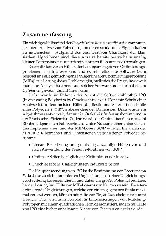
ZusammenfassungEin wichtiges Hilfsmittel der Polyedrischen Kombinatorik ist die computer-gestützte Analyse von Polyedern, um deren strukturelle Eigenschaftenzu untersuchen. Aufgrund des enumerativen Charakters der klas-sischen Algorithmen sind diese Ansätze bereits bei verhältnismäßigkleinen Dimensionen nur noch mit enormen Ressourcen zu bewältigen.
Da oft die konvexen Hüllen der Lösungsmengen von Optimierungs-problemen von Interesse sind und es sehr effiziente Software (zumBeispiel im Falle gemischt-ganzzahliger linearer Optimierungsprobleme(MIPs)) zur Lösung dieser Probleme gibt, stellt sich die Frage, inwieweitman eine Analyse basierend auf solcher Software, oder formal einemOptimierungsorakel, durchführen kann.
Dafür wurde im Rahmen der Arbeit die Softwarebibliothek IPO(Investigating Polyhedra by Oracles) entwickelt. Der erste Schritt einerAnalyse ist in dem meisten Fällen die Bestimmung der affinen Hülleeines Polyeders P ⊆ Rn, insbesondere der Dimension. Dazu wurde einAlgorithmus entwickelt, der mit 2n Orakel-Aufrufen auskommt und inder Praxis sehr effizient ist. Zudem wurde die Optimalität dieser Anzahlfür den allgemeinen Fall bewiesen. Unter Nutzung einer entsprechen-den Implementation und des MIP-Lösers SCIP wurden Instanzen derMIPLIB 2.0 betrachtet und Dimensionen verschiedener Polyeder be-stimmt:
• Lineare Relaxierung und gemischt-ganzzahlige Hüllen vor undnach Anwendung der Presolve-Routinen von SCIP.
• Optimale Seiten bezüglich der Zielfunktion der Instanz.
• Durch gegebene Ungleichungen induzierte Seiten.
Die Hauptanwendung von IPO ist die Bestimmung von Facetten vonP, da diese zu nicht dominierten Ungleichungen in einer Ungleichungs-beschreibung korrespondieren und daher ein großes Potential besitzen,bei der Lösung (mit Hilfe von MIP-Lösern) von Nutzen zu sein. Facetten-definierende Ungleichungen, welche von einem gegebenen Punkt maxi-mal verletzt werden, können mit Hilfe von Target-Cuts effektiv bestimmtwerden. Dies wird zum Beispiel für Linearisierungen von Matching-Polytopen mit einem quadratischen Term demonstriert, indem mit Hilfevon IPO eine bisher unbekannte Klasse von Facetten entdeckt wurde.
i
Zusätzlich zur Facetten- und Affine-Hülle-Bestimmung hat IPO einedritte Funktionalität, die die Überprüfung der Adjazenz zweier Eckenvon P betrifft. Diese ist äquivalent dazu, dass der Normalenkegel anihren Mittelpunkt (n − 1)-dimensional ist. Da man mit Hilfe einesOptimierungsorakels für P – ähnlich zu Target Cuts – ein Optimierungs-orakel für den betrachteten Normalenkegel konstruieren kann, reduziertsich das Adjazenzproblem ebenfalls auf das Affine-Hülle-Problem. ZurDemonstration wurden eine große Anzahl von Adjazenzen zufälligerEcken von TSP-Polytopen überprüft, wobei als Orakel die TSP-Softwareconcorde genutzt wurde.
Damit IPO grundsätzlich korrekt arbeitet, die Probleme jedoch mög-lichst effizient löst, wird an vielen Stellen sowohl rationale als auchGleitkomma-Arithmetik verwendet. Dies ist besonders bei Dimensio-nen größer als 500 enorm relevant, da hier gelegentlich exakte Zahlenmit Kodierungslängen von über 106 Bits auftreten. Um weiterhin diemeist laufzeitintensiven Orakelaufrufe zu sparen, erlaubt IPO die Nut-zung von Heuristiken, von denen außer der Zulässigkeit der ange-gebenen Lösungen nichts verlangt wird. So können beispielsweisedie gerundeten Lösungen von SCIP als heuristisch betrachtet und dieexakte Version von SCIP zur “Verifikation” genutzt werden.
Der zweite Teil der Arbeit fällt in das Forschungsgebiet der Erweiter-ten Formulierungen und basiert auf einem gemeinsam mit Volker Kaibelveröffentlichten Artikel. In diesem Gebiet geht es im Wesentlichendarum, ein gegebenes Polytop P als affine Projektion eines anderen Poly-tops Q mit möglichst wenigen Facetten darzustellen. Die größte Moti-vation hierfür ist die (in gewissem Sinne äquivalente) Frage, ob man einlineares Optimierungsproblem über P mit Hilfe von weiteren Variablenals ein lineares Optimierungsproblem darstellen kann, welches mit sehrwenigen Ungleichungen auskommt.
In der Arbeit wurde untersucht, inwieweit solche kompakten Dar-stellungen möglich sind, wenn man noch zusätzlich fordert, dass dasErweiterungspolytop Q ein einfaches Polytop ist, das gesuchte lineareOptimierungsproblem also nicht (primal) degeneriert ist. Einerseitshaben bereits bekannte Klassen von Erweiterungspolytopen diese Eigen-schaft, andererseits kann man für jedes Polytop zunächst ein einfachesErweiterungspolytop konstruieren. Die charakteristische Größe ist diesogenannte simple extension complexity, die die minimale Facettenzahl
ii
eines solchen einfachen Erweiterungspolytops angibt.Hierzu wurde eine Technik entwickelt, die es ermöglicht, aufgrund
von Eigenschaften des Graphen von P untere Schranken an diese Größezu bestimmen. Trotz der genannten positiven Beispiele stellt sich her-aus, dass die Eigenschaft sehr selten ist: Bereits wenig kompliziertePolytope, wie Hypersimplizes, die zudem nur schwach degeneriertsind, haben eine simple extension complexity in der Größenordnungder Anzahl der Ecken des Polytops, einer trivialen oberen Schranke.Wenig überraschend ist da, dass dies auch für zahlreiche kombina-torische Polytope der Fall ist, unter ihnen perfekte Matching-Polytopevollständiger und vollständiger bipartiter Graphen, Flusspolytope un-zerlegbarer azyklischer Netzwerke, Spannbaumpolytope vollständigerGraphen, sowie zufällige 0/1-Polytope mit gewissen Eckenanzahlen.Um die untere Schranke im Falle perfekter Matchings auf vollständigenGraphen zu beweisen, wurde ein Resultat von Padberg & Rao überAdjazenzbeziehungen entsprechender Polytope verbessert.
In einem kurzen Abschnitt dieses Teils wird charakterisiert, wannzwei der (wenigen) bekannten Methoden zur Konstruktion von Er-weiterten Formulierungen Einfachheit herstellen.
iii
SummaryAn important tool of Polyhedral Combinatorics is the computer-aidedanalysis of polyhedra for understanding their structural properties,which are often related to an underlying optimization problem. Dueto the enumerative nature of the classical algorithms for polyhedralanalysis this approach can often only be pursued for relatively smalldimensions or using an enormous amount of resources.
Since many polyhedra of interest are convex hulls of feasible sets ofoptimization problems and since there exists efficient software (e.g., incase of mixed-integer linear optimization problems (MIPs)) for solvingthese problems even in higher dimensions, it is a reasonable questionhow to carry out an analysis based on such software, or more formally,on an optimization oracle.
This thesis is accompanied by a software library IPO (InvestigatingPolyhedra by Oracles) specifically designed for this approach. A firststep in such an analysis is typically the computation of the affine hull of apolyhedron P ⊆ Rn, in particular its dimension. For this we developedan algorithm that needs at most 2n oracle calls and is very efficientin practice. We also prove that this number is the minimum in theworst case. Using our implementation and the MIP solver SCIP weinvestigated instances of the MIPLIB 2.0 and determined dimensionsof several polyhedra:
• Linear relaxations and mixed-integer hulls before and after apply-ing presolve routines of SCIP.
• Optimal faces with respect to the objective of the instance.
• Faces induced by given inequalities.
The main application of IPO is the detection of some of P’s facets sincethose correspond to undominated inequalities in an inequality descrip-tion, and hence usually have great potential of being useful during thesolving process (using a MIP solver). Facet-defining inequalities thatare maximally violated by a given point can be found efficiently us-ing Target Cuts. In particular, this is demonstrated for linearizations ofmatching polytopes with one quadratic term, for which we determineda new class of facets using IPO.
iv
In addition to facet- and affine-hull computations, IPO has a thirdcomponent that can check adjacency of two vertices of P. The latteris equivalent to the property that the dimension of the normal cone attheir barycenter is equal to n − 1. Since we can – similar to Target Cuts– construct an optimization oracle for this normal cone, this problemreduces to the affine-hull problem. Again for demonstration purposeswe tested a huge number of vertex pairs of TSP polytopes for adjacency,using the software concorde as an optimization oracle.
Since we strive for efficiency, but still want to ensure correct behaviorof IPO, we often use floating-point- and rational arithmetic. This is par-ticularly important for dimensions greater than 500 as then sometimesthe occurring exact numbers have encoding lengths of more than 106
bits. In order to save costly oracle calls, IPO allows to use heuristics fromwhich we do not require optimality of returned solutions. This way wecan use, for instance, the rounded (potentially incorrect) solutions ofSCIP and use the exact version of SCIP for verification purposes only.
The second part of the thesis belongs to the field of extended formu-lations and is based on a joint publication [41] with Volker Kaibel. Thefield basically captures how to describe a given polytope P as an affineprojection of another polytope Q with only few facets. The main moti-vation for this is the (in some sense equivalent) question of constructinga linear optimization problem for P with additional variables, but onlyfew inequalities.
In this work we consider the additional restriction of the extensionpolytope Q to be a simple polytope, that is, the linear optimization problemover Q has to be (primal) non-degenerate. On the one hand, some ofthe known classes of extension polytopes have this property, and onthe other hand, we can construct a simple extension for every polytope.The characteristic quantity for this task is the so-called simple extensioncomplexity that measures the minimum number of facets of such a simpleextension polytope Q.
To get a hand on this quantity we developed lower bounds that de-pend only on the graph of P. Despite the mentioned positive examples,it turns out that this property is very rare: Even very basic polytopeslike hypersimplices, which are only slightly degenerate, have a veryhigh simple extension complexity in the order of P’s number of ver-tices, a trivial upper bound. Having this in mind, it is not surprising
v
that this is also the case for other combinatorial polytopes, among themperfect-matching polytopes of complete and complete bipartite graphs,uncapacitated flow polytopes for nontrivially decomposable directedacyclic graphs, spanning-tree polytopes of complete graphs and ran-dom 0/1-polytopes with vertex numbers in a certain range. On ourway to obtain the result on perfect-matching polytopes we improveon a result of Padberg and Rao’s on the adjacency structures of thosepolytopes.
In a short section of this part we characterize when two of the (few)known methods for constructing extended formulations actually yieldsimple polytopes.
vi

AcknowledgementsThis thesis would not have been possible without the inspiring envi-ronment I found in the group of Volker Kaibel who guided me in theright directions by spreading good ideas, finding faults in the proofs orstopping me from wasting time on things that can’t work at all. He leftme a lot of room for my own research, but also spent a lot of time forsharing knowledge as well as writing- and presentation skills. I wantto thank my colleagues, especially Stefan Weltge, Ferdinand Thein, JanKrümpelmann and Julia Lange for making IMO such a great place tosuspend research for a coffee break. It was a particular pleasure to workin an office with Stefan who is the counterpart in a dream team in whichmaking math is true fun. Together with Volker at the blackboard weoften were completely absorbed, discussing with so much emotion thatother people on the floor surely suffered from our intensity. I also wantto thank Stefan and Volker for improving the quality of the manuscriptby thorough proofreading.
Traveling so much allowed me to get in touch with many remarkableand bright people in the field of integer programming and combinatorialoptimization. It was a pleasure to collaborate with Michele Conforti,Jon Lee and Klaus Truemper, and to have inspiring discussions withmany more. I particularly benefited from advice by Marc Pfetsch whotold me about an effective generation scheme for Target Cuts, previouswork on stabilized column generation and suggested the considerationof presolved MIP instances for my computational studies. Attendingmany great talks at several Aussois meetings, IPCOs and ISMPs clearlycoined my perspective on our field.
The computational aspect of this thesis builds on the work of manypeople. I thank Roland Wunderling for creating SoPlex, Tobias Achter-berg for creating SCIP and Ambros Gleixner for turning SoPlex into anexact arithmetic LP solver to which I had access in early developmentstages. Although I bothered Ambros with several bugs I could usuallyfind a corresponding fix at 5:331 the next day. General thanks go tothe whole development team of the SCIPOptSuite. I am grateful to BillCook who provided me with code I could turn into an exact arithmeticsolver for the traveling salesman problem, and to him and his coau-
1See commit 8efd6801ef46039f85b75ad04b09d26b4b15b989 of the SoPlex-repository.
vii

thors for their work on the concorde TSP solver. For helping me withstatistical issues I want to thank Martin Radloff.
Finally I want to say thank you to all my family. To my parentsGabriele and Karl-Heinz who always encouraged me to give way to mymathematical interests, to my brother Tobias who taught me program-ming when I was quite young, and to my wife Sarah and our son Lukas.The two probably have the smallest mathematical contribution amongthe people I listed here, but are nevertheless the most important ones inmy life, giving me nothing more than a home full of love.
viii
ContentsZusammenfassung . . . . . . . . . . . . . . . . . . . . . . . . . iSummary . . . . . . . . . . . . . . . . . . . . . . . . . . . . . . . ivAcknowledgements . . . . . . . . . . . . . . . . . . . . . . . . . vii
1 Introduction 11.1 Polyhedral Combinatorics . . . . . . . . . . . . . . . . . . 3
1.1.1 Investigating Polyhedra by Oracles . . . . . . . . 41.1.2 Analyzing Simple Extensions of Polytopes . . . . 4
1.2 Preliminaries . . . . . . . . . . . . . . . . . . . . . . . . . . 61.2.1 Basics . . . . . . . . . . . . . . . . . . . . . . . . . . 61.2.2 Vectors, Matrices and Linear Algebra . . . . . . . 71.2.3 Polyhedra . . . . . . . . . . . . . . . . . . . . . . . 71.2.4 Linear and Mixed-Integer Linear Optimization . . 91.2.5 Graphs . . . . . . . . . . . . . . . . . . . . . . . . . 91.2.6 Computational Complexity . . . . . . . . . . . . . 10
2 Investigating Polyhedra by Oracles 112.1 Motivation: Mixed-Integer Hulls . . . . . . . . . . . . . . 132.2 The Software Library IPO . . . . . . . . . . . . . . . . . . 17
2.2.1 Outline . . . . . . . . . . . . . . . . . . . . . . . . . 182.2.2 IPO’s User Interface . . . . . . . . . . . . . . . . . 20
2.3 Optimization Oracles . . . . . . . . . . . . . . . . . . . . . 212.3.1 Optimization Oracle for the Recession Cone . . . 222.3.2 Optimization Oracles for Projections of Polyhedra 222.3.3 Optimization Oracles for Faces of Polyhedra . . . 232.3.4 Corrector Oracle for Mixed-Integer Programs . . 25
2.4 Computing the Affine Hull . . . . . . . . . . . . . . . . . 272.4.1 A Basic Scheme . . . . . . . . . . . . . . . . . . . . 272.4.2 The Algorithm . . . . . . . . . . . . . . . . . . . . 292.4.3 A Lower Bound on the Number of Oracle Calls . 362.4.4 Heuristic Optimization Oracles . . . . . . . . . . . 38
ix
2.4.5 Implementation Details . . . . . . . . . . . . . . . 402.5 Computing Facets . . . . . . . . . . . . . . . . . . . . . . . 43
2.5.1 Polarity and Target Cuts . . . . . . . . . . . . . . . 432.5.2 An Equivalent Model . . . . . . . . . . . . . . . . 452.5.3 Extended Basic Solutions . . . . . . . . . . . . . . 482.5.4 Extracting Inequalities and Equations . . . . . . . 492.5.5 Computing Multiple Facets . . . . . . . . . . . . . 51
2.6 Identifying Vertices, Edges and Other Faces . . . . . . . . 532.6.1 The Smallest Containing Face . . . . . . . . . . . . 532.6.2 Detecting Vertices . . . . . . . . . . . . . . . . . . . 562.6.3 Detecting Edges and Extreme Rays . . . . . . . . . 572.6.4 Detecting Higher-Dimensional Faces . . . . . . . 592.6.5 Strengthening Inequalities . . . . . . . . . . . . . . 60
2.7 Solving the Polar Linear Programs . . . . . . . . . . . . . 612.7.1 The Separation Problem . . . . . . . . . . . . . . . 622.7.2 Stabilization . . . . . . . . . . . . . . . . . . . . . . 622.7.3 Cut Aging . . . . . . . . . . . . . . . . . . . . . . . 642.7.4 Effect of Stabilization and Cut Aging . . . . . . . . 64
2.8 Improving Readability of Equations and Inequalities . . 672.8.1 Manhattan Norm Problems . . . . . . . . . . . . . 682.8.2 Two Vectors: An Exact Algorithm . . . . . . . . . 692.8.3 A Fast Heuristic . . . . . . . . . . . . . . . . . . . . 792.8.4 Implementation . . . . . . . . . . . . . . . . . . . . 80
2.9 Computational Studies: Dimensions . . . . . . . . . . . . 812.9.1 Dimensions of Polyhedra from MIPLIB Instances 822.9.2 Dimensions of Optimal Faces . . . . . . . . . . . . 892.9.3 Faces Induced by Model Inequalities . . . . . . . . 93
2.10 Computational Study: Facets . . . . . . . . . . . . . . . . 992.10.1 Matching Polytopes with One Quadratic Term . . 992.10.2 Edge-Node-Polytopes . . . . . . . . . . . . . . . . 1042.10.3 Tree Polytopes . . . . . . . . . . . . . . . . . . . . . 108
2.11 Computational Study: Adjacency . . . . . . . . . . . . . . 1122.11.1 Heuristics and Oracles for TSP Polytopes . . . . . 1122.11.2 Experiment & Results . . . . . . . . . . . . . . . . 1132.11.3 Adjacent Tours with Common Edges . . . . . . . 115
x
CONTENTS
3 Analyzing Simple Extensions of Polytopes 1213.1 Introduction . . . . . . . . . . . . . . . . . . . . . . . . . . 1233.2 Constructions . . . . . . . . . . . . . . . . . . . . . . . . . 127
3.2.1 Reflections . . . . . . . . . . . . . . . . . . . . . . . 1273.2.2 Disjunctive Programming . . . . . . . . . . . . . . 130
3.3 Bounding Techniques . . . . . . . . . . . . . . . . . . . . . 1333.4 Hypersimplices . . . . . . . . . . . . . . . . . . . . . . . . 1403.5 Spanning Tree Polytopes . . . . . . . . . . . . . . . . . . . 1423.6 Flow Polytopes for Acyclic Networks . . . . . . . . . . . 1473.7 Perfect Matching Polytopes . . . . . . . . . . . . . . . . . 151
3.7.1 Complete Bipartite Graphs . . . . . . . . . . . . . 1533.7.2 Complete Nonbipartite Graphs . . . . . . . . . . . 1543.7.3 Adjacency Result . . . . . . . . . . . . . . . . . . . 155
3.8 A Question Relating Simple Extensions with Diameters . 164
Bibliography 167
Appendix 173A.1 Computational Studies: Dimensions . . . . . . . . . . . . 175
xi

xii
List of Figures2.1 Traditional work-flow in polyhedral combinatorics . . . 142.2 Proposed new work-flow in polyhedral combinatorics . . 152.3 Illustration of Example 2.3.1 . . . . . . . . . . . . . . . . . 242.4 Projection of unstabilized and stabilized solutions onto
two variables . . . . . . . . . . . . . . . . . . . . . . . . . 662.5 Illustration of Lemma 2.8.5 . . . . . . . . . . . . . . . . . . 712.6 Illustration of the instance from Example 2.8.9 . . . . . . 742.7 Illustration of the transformed instance from
Example 2.8.9 . . . . . . . . . . . . . . . . . . . . . . . . . 752.8 Distribution of original and presolved MIPLIB 2.0
instances by dimension ratio of hull and relaxation . . . . 872.9 Different running time distributions for affine hull
computation . . . . . . . . . . . . . . . . . . . . . . . . . . 882.10 Distribution of relaxations of original and presolved
MIPLIB 2.0 instances by relative dimension of the optimalface . . . . . . . . . . . . . . . . . . . . . . . . . . . . . . . 93
2.11 Distribution of original and presolved MIPLIB 2.0instances by relative dimension of the optimal face . . . . 94
2.12 Distribution of constraint dimensions for originalMIPLIB 2.0 instances . . . . . . . . . . . . . . . . . . . . . 96
2.13 Distribution of constraint dimensions for presolvedMIPLIB 2.0 instances . . . . . . . . . . . . . . . . . . . . . 97
2.14 ZIMPL model for matching problem with one quadraticterm . . . . . . . . . . . . . . . . . . . . . . . . . . . . . . . 101
2.15 Results for matching problem with one quadratic term . 1012.16 Illustration of Case (b) of Theorem 2.11.3 . . . . . . . . . 1172.17 Pair of tours not obtained from 2-matching adjacencies
by splitting . . . . . . . . . . . . . . . . . . . . . . . . . . . 119
3.1 Some reflections used for a 16-gon . . . . . . . . . . . . . 129
xiii
3.2 The sets F andV in the face lattice . . . . . . . . . . . . . 1353.3 Polytope Q from Example 3.3.5 and its projection P . . . 1383.4 Vertices of ∆n
k inV for a biclique . . . . . . . . . . . . . . 1413.5 Case 2 of Lemma 3.5.1 . . . . . . . . . . . . . . . . . . . . 1433.6 Construction for Theorem 3.5.2 . . . . . . . . . . . . . . . 1443.7 Construction for Case 1 in the proof of Theorem 3.6.1 . . 1493.8 Construction for Case 2 in the proof of Theorem 3.6.1 . . 1503.9 Lemma 3.7.5 for a 10-cycle and a 12-cycle . . . . . . . . . 1553.10 Construction in Lemma 3.7.7 with 3 outer cycles . . . . . 1583.11 A special case in the proof of Lemma 3.7.7 where M3 is
adjacent to M1 and M2 . . . . . . . . . . . . . . . . . . . . 1593.12 Modifications in Case 1 in the proof of Theorem 3.7.6 . . 1613.13 Modifications in Case 2 in the proof of Theorem 3.7.6 . . 162
xiv
List of Tables2.1 Effects of stabilization and cut aging . . . . . . . . . . . . 652.2 Dimensions for original MIPLIB 2.0 instances . . . . . . . 842.3 Dimensions for presolved MIPLIB 2.0 instances . . . . . . 852.4 Dimensions of optimal faces for original MIPLIB 2.0
instances . . . . . . . . . . . . . . . . . . . . . . . . . . . . 912.5 Dimensions of optimal faces for presolved MIPLIB 2.0
instances . . . . . . . . . . . . . . . . . . . . . . . . . . . . 922.6 Running times for different caching strategies . . . . . . . 982.7 Adjacency computation for random vertex pairs of TSP
polytopes . . . . . . . . . . . . . . . . . . . . . . . . . . . . 115
A.1 Statistics for relaxations of MIPLIB 2.0 instances . . . . . 176A.2 Timings for relaxations of MIPLIB 2.0 instances . . . . . . 177A.3 Statistics for MIPLIB 2.0 instances . . . . . . . . . . . . . . 178A.4 Timings for MIPLIB 2.0 instances . . . . . . . . . . . . . . 179A.5 Statistics for relaxations of presolved MIPLIB 2.0
instances . . . . . . . . . . . . . . . . . . . . . . . . . . . . 180A.6 Timings for relaxations of presolved MIPLIB 2.0
instances . . . . . . . . . . . . . . . . . . . . . . . . . . . . 181A.7 Statistics for presolved MIPLIB 2.0 instances . . . . . . . 182A.8 Timings for presolved MIPLIB 2.0 instances . . . . . . . . 183
xv

xvi

Chapter 1
Introduction
1

INTRODUCTION
2
1.1. POLYHEDRAL COMBINATORICS
INTRODUCTION:
1.1 Polyhedral Combinatorics
Many combinatorial optimization problems can be stated as the problemto find a subset F ⊆ E of a finite ground set having certain propertiessuch that a given cost function is minimized. If the cost function islinear, i.e., there exists a vector c ∈ RE such that the costs are
∑e∈F ce,
then we can formulate this as a linear optimization problem (LP)
min cᵀx subject to x ∈ conv.hullχ(F) ∈ 0, 1E | F ⊆ E is feasible
,
where χ(F) is F’s characteristic vector, i.e, χ(F)e = 1 holds if and only ife ∈ F holds and conv.hull (·) denotes the convex hull.
Such linear programming formulations are a standard tool to gainstructural insight, derive algorithms and to analyze complexity. In orderto solve such an LP we need to describe it by means of linear inequalities,i.e., Ax ≤ b, which is a nontrivial task in general: For many polyhedrafor which the associated optimization problem is solvable in polynomialtime such a description is known, but of exponential size (in the dimen-sion). Even worse, for NP-hard problems we should not expect thatwe can characterize such a description in a certain nice way, since thiswould imply NP = coNP, that is, every propositional tautology wouldhave a polynomial-size proof. Nevertheless, for practically solving theseproblems, good linear relaxations are important. Understanding thesepolytopes is (part of) the branch of discrete mathematics called Polyhe-dral Combinatorics. This thesis contributes with new techniques, resultsand software to this area.
3
INTRODUCTION
Investigating Polyhedra by Oracles
In the first part we address questions regarding the computer-aidedanalysis of polyhedra that are only implicitly defined by means of ablack-box algorithm (a so-called oracle) solving the optimization prob-lem. At first glance, this approach may seem rather complicated, but itis quite effective in practice if we have access to a solver for mixed-integerlinear optimization problems (MIPs). In this situation we can simply givea mathematical model as the input.
Fundamental work on this topic was done by Grötschel, Lovászand Schrijver in 1981, when they established the famous theorem on“equivalence of optimization and separation” [33]. It essentially statesthat solving the linear optimization problems over a rational polytopeP is equivalent (with respect to polynomial-time solvability) to finding,for a given rational point x, some hyperplane that separates x from P.From this result one can derive that one can carry out certain tasks likefinding facets, determining the dimension, or optimizing over faces ina theoretically efficient way (see Chapter 14 in Schrijver’s book [62]).Unfortunately, the result and its applications heavily depend on theEllipsoid method, a theoretically efficient, but practically almost uselessalgorithm.
In Chapter 2, we will present practically efficient algorithms for someof these problems, describe the underlying ideas, provide the readerwith proofs of correctness, and introduce a new software library IPO thatimplements them. Finally, we carry out small computational studies ondifferent problems showing the software’s capabilities and limitations.
Analyzing Simple Extensions of Polytopes
Chapter 3, the second part of this thesis, deals with our contributions tothe theory of extended formulations, a recently very active area of Polyhe-dral Combinatorics. Consider once again some polytope P associatedto a class of certain combinatorial sets. Even if a description of P by asystem of linear inequalities is known, it may still be impractically large.
Sometimes it is possible to write P as a projection of some other poly-tope Q that needs fewer inequalities for the price of a higher dimension,i.e., more variables. Then we call Q together with the projection map anextension of P. The theory of extended formulations mainly deals with
4
1.1. POLYHEDRAL COMBINATORICS
the question of the minimum number of inequalities actually required todescribe P, its so-called extension complexity.
Inspired by this phenomenon, one may even dare to ask for anextension polytope Q that is simple in the sense that every vertex of Q liesin exactly d facets, where d denotes the dimension of Q. Unfortunately,we should not be too optimistic when asking for few facets and non-degeneracy at the same time. It turns out that several well-understoodcombinatorial classes of polytopes do not have such an extension.
To prove such results we develop a technique for establishing lowerbounds on the extension complexity when only simple extensions arepermitted. In subsequent sections we apply it to different classes ofcombinatorial polytopes. In one particular case, namely for perfectmatching polytopes of complete graphs, we have to improve a resultof Padberg and Rao’s on adjacencies of perfect matchings [52] (see The-orem 3.7.6). All results of this chapter, except for Theorem 3.7.1, arealready published in the following article:
• Volker Kaibel and Matthias Walter: Simple extensions of polytopes.Mathematical Programming Series B, 154(1-2): 381–406, 2015.
5
INTRODUCTION
INTRODUCTION:
1.2 Preliminaries
In this section we introduce our basic notation without going into details.If appropriate, we point the reader to the relevant literature. Wheneverwe focus on a combinatorial problem, we will introduce the necessaryconcepts locally.
Basics
By R, Q, Z and N we denote the real numbers, the rationals, integersand the natural1 numbers, respectively (resp.). Using a “+” or “−” in thesubscript (e.g., R+ or R−), we denote the corresponding restrictions tonon-negative (resp. non-positive) numbers. We write [n] := 1, 2, . . . ,n.The greatest common divisor of two integers a and b is denoted bygcd(a, b). For two sets A,B we denote by A∆B := (A \ B) ∪ (B \ A) thesymmetric difference, and write A ∪· B for the disjoint union, i.e., weimplicitly require A∩B = ∅. As usual, the boundary, relative boundary,the interior and the relative interior of a set A are denoted by bd (A),relbd (A), int (A) and relint (A), respectively. By proj x(A) we denotethe orthogonal projection of a set A on the subspace indexed by thex-variables (which are clear from the context).
To state asymptotic behavior, we use the usual Bachmann-Landaunotation O (·), Ω (·), Θ (·) and o (·).
1Ignoring DIN norm 5473, we consider 0 not to be a natural number.
6
1.2. PRELIMINARIES
Vectors, Matrices and Linear Algebra
We make use of the standard scalar product 〈·, ·〉 in the Euclidean space.The zero vector in Rn and the m × n all-zeros matrix are denoted byOn and Om,n, respectively, where we omit the subscript whenever thedimension is clear. Similarly, the all-ones vector is 1 := 1n, and the i-thunit vector is denoted by e
(i). As already stated in the introduction, thecharacteristic vector χ(F) of a subset F ⊆ E is the binary vector withχ(F)e = 1 if and only if e ∈ F. For the product 〈v, χ(F)〉 we use thenotation v(F). The n × n unit matrix is denoted by In and transpositionof vectors and matrices by (·)ᵀ. For a matrix A ∈ Rm×n, a row subsetI ⊆ [m] and a column subset J ⊆ [n], we write AI,J for the submatrixindexed by the corresponding rows and columns. Instead of AI,[n] andA[m],J we also write AI,∗ and A∗,J, respectively, and for the single entriesAi, j we write Ai, j.
For the set of rows of a matrix A, considered as vectors, we writerows (A) and for the nullspace of A we write ker (A). The dimensiondim (X) of a set X ⊆ Rn is defined as the dimension of its affine hull(denoted by aff.hull (X)), i.e., the dimension of the smallest affine spacethat contains X. We say that X is full-dimensional if dim (X) = n holds.As usual, the linear hull (denoted by lin.hull (X)) is the set of all linearcombinations of elements of X.
Polyhedra
For precise definitions and basic properties of convex sets and polyhedrawe refer to [61] and [62], respectively. As already done in the introduc-tion, we write conv.hull (X) for the convex hull and conic.hull (X) forthe convex conic hull of X, respectively. A polyhedron P ⊆ Rn is theintersection of finitely many halfspaces, that is, P = x ∈ Rn
| Ax ≤ b forsome matrix A ∈ Rm×n and some vector b ∈ Rm. Polytopes are boundedpolyhedra or, equivalently, convex hulls of finitely many points. Wesay that a direction v ∈ Rn is unbounded with respect to (w.r.t.) P if P isnon-empty and x + λv ∈ P holds for some x ∈ P and for all λ ≥ 0. Theset recc (P) := v ∈ Rn
| v is unbounded w.r.t. P is the so-called recessioncone of P (which is a polyhedral cone). By Minkowski-Weyl’s Theorem(see Corollary 7.1b in [62]), every polyhedron P is the sum of a polytope
7
INTRODUCTION
and P’s recession cone, that is,
P = conv.hull (S) + conic.hull (R) for finite S ⊆ P and finite R ⊆ recc (P).
We call such a pair (S,R) an inner description of P, whereas we refer toAx ≤ b as an outer description. If S and R are sets of rational vectors,we say that P is a rational polyhedron. The lineality space, defined aslineal (P) := recc (P)∩ recc (−P), is the set of all directions correspondingto lines contained in P. We say that P is pointed if lineal (P) = O holds.
Farkas’ Lemma (see Corollary 7.1e in [62]) states that either the systemAx ≤ b (for A ∈ Rm×n and b ∈ Rm) has a solution or there exists anonnegative vector y with yᵀA = O and yᵀb < 0.
We say that an inequality 〈a, x〉 ≤ β (for a ∈ Rn and β ∈ R) is valid for apolyhedron P if it is satisfied by all points in P. A face of a polyhedron Pis a subset F ⊆ P that is induced by a valid inequality 〈a, x〉 ≤ β in the sensethat F =
x ∈ P | 〈a, x〉 = β
holds. For non-empty faces F we also say that
F is the a-maximum face of P since then clearly F = arg max 〈a, x〉 | x ∈ Pholds. The faces of a polyhedron P form a graded lattice L(P) (in thesense of a partially ordered set), ordered by inclusion (see [70]). The(d−1)-dimensional faces of a d-dimensional polyhedron are called facetsand the 0-dimensional faces are called vertices. Although vertices areformally singleton sets x for some x ∈ P, we usually just write x.The set of all vertices of a polyhedron P is denoted by vert (P). Notethat only pointed polyhedra actually have actually have vertices. Asmotivated in the introduction, 0/1-polytopes, that is, polytopes whosevertices have only 0/1-coordinates, are of special interest in PolyhedralCombinatorics. The bounded (resp. unbounded) 1-dimensional faces ofpointed polyhedra are called edges (resp. extreme rays). The set of direc-tion vectors corresponding to the extreme rays is denoted by ext.rays (P).The irredundant (that is, inclusion-wise minimal) inner description of apointed polyhedron P is the pair (vert (P) , ext.rays (P)).
For a polyhedron P ⊆ Rn and a point x ∈ P we will use the radialcone, defined as rad.conex(P) := conic.hull (P − x), and its polar conenml.conex(P) :=
y ∈ Rn
|⟨y, x − x
⟩≤ 0 for all x ∈ P
, called the normal
cone. Intuitively, the radial cone contains all directions one can go fromx without immediately leaving P, whereas the normal cone consists ofall objective vectors whose maximum face contains x.
In order to use (sets of) inequalities or equations as input or output
8
1.2. PRELIMINARIES
of algorithms, we will often consider system Ax ≤ b or Cx = d as objects,where we formally mean the pairs (A, b) and (C, d), respectively.
Linear and Mixed-Integer Linear OptimizationA linear optimization problem (LP) is an optimization problem of the form
max 〈c, x〉 subject to (s.t.) Ax ≤ b.
for a matrix A ∈ Rm×n and vectors b ∈ Rm and c ∈ Rn. Of course we canalso minimize, allow equations, “≥”-inequalities, or special inequalitieslike x ≥ O, so-called variable bounds. We often use the phrase of “opti-mizing over a polyhedron P” which means to solve linear optimizationproblems with P as the feasible region and arbitrary linear objectivefunctions.
A mixed-integer optimization problem (MIP) is an LP with the addi-tional restriction that a subset I ⊆ [n] of variables must be integral,that is, x ∈ I := x ∈ Rn
| xi ∈ Z for all i ∈ I holds. The feasible pointsare sometimes called integer-feasible to distinguish from LP-feasibility forwhich we ignore the integrality constraints. The special case of I = [n]is called just an integer program (IP).
A polyhedron P = x ∈ Rn| Ax ≤ b is called a linear relaxation of a
set X ⊆ I (w.r.t. I) if P ∩ I = X holds. Its corresponding mixed-integerhull is the set PI := conv.hull (P ∩ I), that is, PI = conv.hull (X).
GraphsMost of the combinatorial optimization problems we are concerned withare defined for graphs. We will only introduce notation here, and referto the books of Schrijver [63] and Korte and Vygen [47]. They are notgraph-theoretic, but introduce all concepts that are necessary to dealwith our problems.
We mostly deal with undirected graphs G = (V,E) consisting of aset V of nodes2 and a set E of edges, where an edge is a 2-element set ofnodes. In particular, all our graphs are simple (no edge exists twice) andloopless (edges connect distinct nodes). We often consider the completegraphs Kn with n nodes and all
(n2)
possible edges. We denote for a set
2Note that we only use the term “vertices” for the 0-dimensional faces of polyhedra.
9
INTRODUCTION
S ⊆ V of nodes by E[S] the set of edges whose endpoints lie in S. By δ(S)we denote the cut induced by S, that is, the set of edges having preciselyone endnode in S. We abbreviate δ(v) by δ(v) for single nodes v ∈ V.For an edge set F ⊆ E we denote by V(F) the set of all nodes of edges inF.
In Section 3.6 we also consider directed graphs G = (V,A) with nodesets V and arcs A which are pairs of nodes. We will introduce suitablenotation locally.
Another type of graphs we consider is the so-called 1-skeleton of apolytope whose nodes are the vertices and whose edges are the edges(1-dimensional faces) of the polytope.
Computational ComplexityAlthough we do not directly touch the field of computational complex-ity, we benefited a lot from it. As argued in the introduction we can use itto guide expectations on the possibility to characterize facial structuresof polyhedra. We won’t define the complexity classes, P, NP and coNPhere, but refer to standard literature [29], [7].
10
Chapter 2
Investigating Polyhedra byOracles
11
INVESTIGATING POLYHEDRA BY ORACLES
12
2.1. MOTIVATION: MIXED-INTEGER HULLS
INVESTIGATING POLYHEDRA BY ORACLES:
2.1 Motivation: Mixed-Integer Hulls
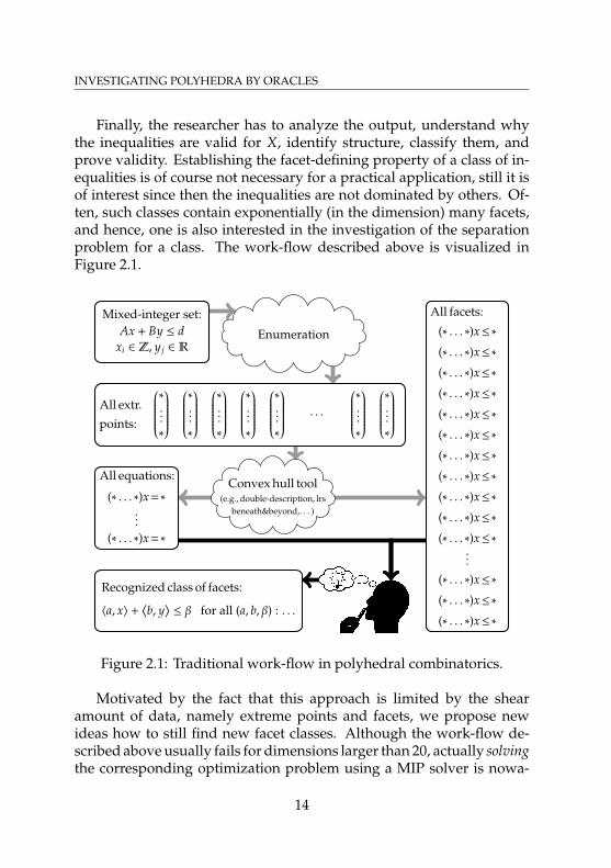
As described in the introduction, one goal of Polyhedral Combina-torics is to study (facial structures of) polytopes of which one implicitlyknows the extreme points. Since in most of the applications one alsoknows some linear relaxation, a MIP solver can be used to optimizeover the polytopes. In general, it is advantageous for a MIP solver ifthe relaxation approximates the corresponding mixed-integer hull verywell, where inequalities that are not dominated by others (e.g., withina bounding box) are particularly interesting. Geometrically, this meansthat the face induced by such an inequality is a facet. Hence, a typicaltask for researchers is to identify such facets for a given linear relaxation.
One way of doing this is to first compute all extreme points X ⊆ Rn ofthe mixed-integer hull, either by developing problem-specific softwareor by using tools that do this automatically for a given relaxation. Forthe latter task, there are many different types of algorithms and evenmore different implementations. For an overview and a comparison werefer to [8], where the authors compare all tools that are interfaced bythe polymake system [56]. Note that there are binary sets X ⊆ 0, 1n
for which every linear relaxation in the original space has exponentiallymany inequalities (see [42]), which is a problem for such tools since theyget such a relaxation as an input.
As a second step, this set X is usually given as input to some convexhull tool which computes a set of linear equations defining aff.hull (X)and one inequality representing each facet of conv.hull (X). Again, thereare many algorithms for this task, and we refer to [8] for a comparison.
13
INVESTIGATING POLYHEDRA BY ORACLES
Finally, the researcher has to analyze the output, understand whythe inequalities are valid for X, identify structure, classify them, andprove validity. Establishing the facet-defining property of a class of in-equalities is of course not necessary for a practical application, still it isof interest since then the inequalities are not dominated by others. Of-ten, such classes contain exponentially (in the dimension) many facets,and hence, one is also interested in the investigation of the separationproblem for a class. The work-flow described above is visualized inFigure 2.1.
Mixed-integer set:Ax + By ≤ d
xi ∈ Z, y j ∈ R
All extr.
points:
∗
...∗
∗
...∗
∗
...∗
∗
...∗
∗
...∗
∗
...∗
∗
...∗
. . .
All facets:
(∗ . . . ∗)x≤∗
(∗ . . . ∗)x≤∗
(∗ . . . ∗)x≤∗
(∗ . . . ∗)x≤∗
(∗ . . . ∗)x≤∗
(∗ . . . ∗)x≤∗
(∗ . . . ∗)x≤∗
(∗ . . . ∗)x≤∗
(∗ . . . ∗)x≤∗
(∗ . . . ∗)x≤∗
(∗ . . . ∗)x≤∗
(∗ . . . ∗)x≤∗
(∗ . . . ∗)x≤∗
(∗ . . . ∗)x≤∗
...
All equations:
(∗ . . . ∗)x = ∗
(∗ . . . ∗)x = ∗
...
Recognized class of facets:
〈a, x〉 +⟨b, y
⟩≤ β for all (a, b, β) : . . .
Enumeration
Convex hull tool(e.g., double-description, lrs
beneath&beyond,. . . )
Figure 2.1: Traditional work-flow in polyhedral combinatorics.
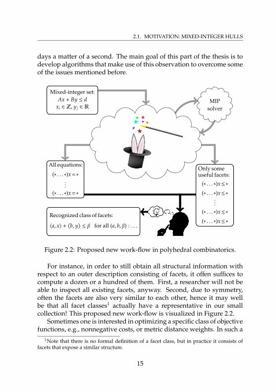
Motivated by the fact that this approach is limited by the shearamount of data, namely extreme points and facets, we propose newideas how to still find new facet classes. Although the work-flow de-scribed above usually fails for dimensions larger than 20, actually solvingthe corresponding optimization problem using a MIP solver is nowa-
14
2.1. MOTIVATION: MIXED-INTEGER HULLS
days a matter of a second. The main goal of this part of the thesis is todevelop algorithms that make use of this observation to overcome someof the issues mentioned before.
Mixed-integer set:Ax + By ≤ d
xi ∈ Z, y j ∈ R
Only someuseful facets:
(∗ . . . ∗)x≤∗
(∗ . . . ∗)x≤∗
(∗ . . . ∗)x≤∗
(∗ . . . ∗)x≤∗
...
All equations:
(∗ . . . ∗)x = ∗
(∗ . . . ∗)x = ∗
...
Recognized class of facets:
〈a, x〉 +⟨b, y
⟩≤ β for all (a, b, β) : . . .
MIPsolver
Figure 2.2: Proposed new work-flow in polyhedral combinatorics.
For instance, in order to still obtain all structural information withrespect to an outer description consisting of facets, it offen suffices tocompute a dozen or a hundred of them. First, a researcher will not beable to inspect all existing facets, anyway. Second, due to symmetry,often the facets are also very similar to each other, hence it may wellbe that all facet classes1 actually have a representative in our smallcollection! This proposed new work-flow is visualized in Figure 2.2.
Sometimes one is interested in optimizing a specific class of objectivefunctions, e.g., nonnegative costs, or metric distance weights. In such a
1Note that there is no formal definition of a facet class, but in practice it consists offacets that expose a similar structure.
15
INVESTIGATING POLYHEDRA BY ORACLES
case, there may exist many inequalities that define facets, but will neverbe relevant for objective functions from the respective class. The methodfor facet-detection we will present has the remarkable property that itmay be controlled by an objective vector. Hence, by choosing objectivevectors from the set of interesting ones we can at least slightly influencewhich facets will be detected.
16
2.2. THE SOFTWARE LIBRARY IPO
INVESTIGATING POLYHEDRA BY ORACLES:
2.2 The Software Library IPO
Motivated by the observations from the previous section we developedthe software library IPO (Investigating Polyhedra by Oracles, [67]). Wenow briefly describe its functionality, leaving the details for Sections 2.3–2.8.
The user has to provide IPO with a so-called optimization oracle,which is a black-box procedure for maximizing any given linear objec-tive function over a certain polyhedron. We will define this formallyin the next section. In principle this can be any algorithm that solvesa certain type of optimization problems, but in particular, it may be aMIP model together with a solver. For the latter case, IPO already in-terfaces the solver SCIP [1], which can solve an even broader problemclass than just MIPs. It does not matter whether the SCIP optimizationoracle was created for an explicit MIP or whether it uses so-called con-straint handlers that dynamically enforce some of the constraints, e.g.,by solving separation problems. Hence, one can also use oracles forproblems that allow no small LP relaxation. Since most of the MIPsolvers work with floating-point arithmetic, one may also use the exactMIP solver ExactSCIP (see [20], [64] and [19] for details) for numericallychallenging problems, taking a considerable increase in running timeinto account.
We assume that the oracle implicitly defines a polyhedron P :=conv.hull (S) + conic.hull (R), where S is the set of all points that theoracle may return as optimal, and R is the set of direction vectors thatthe oracle may return as unbounded directions. Note that just by this
17
INVESTIGATING POLYHEDRA BY ORACLES
definition P could be any convex closed set, a generalization not con-sidered here. A description of our requirements, including the one thatan oracle must not contradict its previous answers, can be found inSection 2.3.
In addition to user-written optimization oracles and the predefinedSCIPOptimizationOracle and ExactSCIPOptimizationOracle (inter-facing SCIP and ExactSCIP, respectively), the user can easily derivenew oracles from existing ones without much effort. Among those“wrapper” optimization oracles are the ones for the recession cone, forarbitrary faces and affine projections of the polyhedron defined by agiven oracle.
Outline
Using an optimization oracle for a polyhedron P ⊆ Rn, IPO can
• compute the affine hull of P in the sense that it returns (d + 1)many affinely independent points in P and (n − d) many linearlyindependent equations valid for P, where d is the dimension of P.The details are discussed in Section 2.4,
• compute a facet-defining inequality that is violated by a givenpoint. The technique is based on Target Cuts developed by Buch-heim, Liers and Oswald [15] in 2008, and presented in Section 2.5.
• compute facets that are “helpful” when maximizing a specifiedobjective vector c. More precisely, it iteratively solves LPs whoseinequalities correspond to some of P’s facets, until the currentoptimum is in P. As long as this is not the case, the procedurereturns violated facet-defining inequalities and adds them to theLP.
• check whether two given vertices of P are adjacent. In Section 2.6.2we reduce this problem to the next one:
• compute the smallest face of P containing a given point by meansof an inequality defining this face. Check whether a given pointis a vertex of P. Section 2.6 is dedicated to this topic.
18
2.2. THE SOFTWARE LIBRARY IPO
Section 2.7 deals with an auxiliary problem that needs to be solvedfor the facet-computation as well as for the computation of the smallestcontaining face. It is essentially the separation problem for the cone ofinequalities valid for a polyhedron.
In Section 2.8 we develop methods that linearly combine two integervectors in order to produce one of minimum Manhattan norm (withoutallowing the zero vector). This is useful to post-process IPO’s output:first, equations may be combined to become more readable. Second, theequations may be combined with a computed inequality to improve thereadability of the latter.
The capabilities of IPO are demonstrated in several small computa-tional studies. For the affine hull computations we considered the linearrelaxations and the mixed-integer hulls for a subset of the MIPLIB 2.0instances [14]. We computed their dimensions, the dimensions of theiroptimal faces and for the mixed-integer hulls also the dimensions ofthe faces induced by the inequality constraints specified in the modelinstance. The results are presented in Section 2.9.
For the facet computation we investigated integer hulls for severalinteger programs. First we considered polytopes associated to matchingproblems with objective functions consisting of a linear term plus asingle product term. Section 2.10 shows how we used IPO to computeseveral unclassified facets, and also contains proofs that the identifiedclasses indeed consists of valid facet-defining inequalities. As a secondexample we considered inequality constraints that link node sets andedge sets in different ways. We deal with outer descriptions of thecorresponding integer hulls and with computational complexity of theassociated optimization problems. IPO requires a fractional solutionto be cut off by a facet, and such a solution is sometimes hard to find.Hence, in a third example we present a strategy to come up with suchsolutions, in our case based on a polyhedral reduction from vertex coverto tree polytopes.
In our last experiment we used the famous solver concorde [4] as anoracle for the traveling salesman polytope to check many random vertexpairs for adjacency. We present some statistics, and describe a techniqueto produce adjacent pairs by node splitting.
19
INVESTIGATING POLYHEDRA BY ORACLES
IPO’s User InterfaceIn order to make IPO user-friendly, the following programs also belongto the library:
• ipo-facets: Input is any instance that SCIP can read, in partic-ular MIPs in LP or MPS format and models written in the ZIMPLmodelling language [45]. It uses the objective from the MIP tocompute “helpful” facets (see above).
• ipo-dimensions: Input is as for ipo-facets, together with achoice of whether it shall compute the dimension of the linearrelaxation, of the mixed-integer hull, of the optimal face of eitherof them, or of all faces induced by the inequality constraints givenin the model.
• ipo-smallest-face: Input is as for ipo-facets, together with apoint s ∈ P. It then computes the dimension of the smallest facethat contains s. This can be used to check adjacency of two vertices(e.g., s is their midpoint), as discussed in Section 2.6.3.
20
2.3. OPTIMIZATION ORACLES
INVESTIGATING POLYHEDRA BY ORACLES:
2.3 Optimization Oracles
In this section we will specify what IPO requires from an optimizationoracle in order to work correctly. Then we discuss how to derive from anoptimization oracle for a polyhedron those for related polyhedra (e.g.,faces and projections). In the last subsection we introduce a specialoptimization oracle that is helpful when analyzing mixed-integer hullswith the help of a floating-point based MIP solver.
A proper optimization oracle O for a rational polyhedron P ⊆ Rn isan oracle that can be called for any direction c ∈ Qn (we denote this byO(c)) and returns
• O(c).val = −∞ if P = ∅ holds,
• O(c).val = +∞ and a rational direction r := O(c).dir ∈ recc (P)satisfying 〈c, r〉 > 0 if sup 〈c, x〉 | x ∈ P = ∞,
• and δ := O(c).val ∈ Q and a rational point s := O(c).point ∈ Psatisfying 〈c, s〉 = δ = max 〈c, x〉 | x ∈ P otherwise.
In an implementation, such an oracle usually also has functionality toobtain P’s ambient dimension n, and hence we will always assume thatn is known.
We say thatO is finite if the set of all possible answers is finite, i.e., if
| O(c).dir | c ∈ Qn with O(c).val = +∞ | < ∞ and|O(c).point | c ∈ Qn with O(c).val , ±∞
| < ∞
21
INVESTIGATING POLYHEDRA BY ORACLES
hold. We will often use finiteness of oracles in order to prove terminationof our algorithms. In several cases we will not be able to give proofs onthe actual running time since we make heavy use of the Simplex methodfor which no polynomial-time version is known.
Many of the algorithms we present do not always require optimal-ity of the solutions returned by an oracle. Hence it is useful to alsoconsider oracles that still guarantee to return feasible solutions but notnecessarily return optimal ones. We call such an oracle a heuristic op-timization oracle (in contrast to proper optimization oracles). Often, ouralgorithms require optimality only in certain steps, so we can some-times make progress using a heuristic optimization oracle first withoutlosing correctness. A simple example is to use a standard MIP solver,which is prone to rounding errors triggered by float-point arithmetic,as a heuristic and a slower exact MIP solver as a proper optimizationoracle.
Optimization Oracle for the Recession Cone
Let O be an optimization oracle for a non-empty rational polyhedronP ⊆ Rn and let C := recc (P) be its recession cone. We can very easilyderive an optimization oracle OC for C from O:
Given a direction c ∈ Qm, call O(c). If O(c).val = +∞ holds, then OCalso returnsO(c).dir since the latter lies in C. Otherwise, i.e., ifO(c).val ,±∞holds, thenOC returnsO as the optimum point. The origin is optimalsince any point y ∈ C with a positive objective value would immediatelymake max 〈c, x〉 | x ∈ P unbounded because we have λy ∈ recc (P) forany λ ≥ 0, i.e., Owould have returned O(c).val = +∞.
Optimization Oracles for Projections of Polyhedra
Let O be an optimization oracle for a rational polyhedron P ⊆ Rn. Letfurthermore A ∈ Qm×n be a matrix and b ∈ Qm be a vector defining theprojection map π : Rn
→ Rm via π(x) := Ax + b. Let Q := π(P) be theimage of the projection.
In this case an optimization oracle OQ for Q can be obtained in astraight-forward way: Given a direction c ∈ Qm, call O(Aᵀc). Clearly,P = ∅ holds if and only if Q = ∅ holds. If O(Aᵀc).val = +∞ holds, thenOQ also returns an unbounded direction Ar with r = O(Aᵀc).dir. To
22
2.3. OPTIMIZATION ORACLES
see that this is correct, observe 〈c,Ar〉 = 〈Aᵀc, r〉 > 0 and consider somex ∈ P. For all λ ≥ 0 we have x + λr ∈ P, and hence (Ax + b) + λAr ∈ Q,i.e., Ar ∈ recc (Q). In the last case, i.e., if O(Aᵀc).val , ±∞ holds, thenOQ also returns a point π(s) with s = O(Aᵀc).point. This is justified bythe fact that for any x, x′ ∈ Rn we have
〈Aᵀc, x〉 ≤ 〈Aᵀc, x′〉 ⇐⇒ 〈c,Ax + b〉 ≤ 〈c,Ax′ + b〉 .
Optimization Oracles for Faces of Polyhedra
In contrast to the construction of an optimization oracle for a projectionof a polyhedron P, it is harder to create one for a face F of P ⊆ Rn
without relying on the equivalence of optimization and separation (seeChapter 14 in Schrijver’s book [63]). In contrast, note that creating aseparation oracle for a face from a separation oracle for the polyhedronis trivial.
One idea for a direct construction is to tilt a given objective vectorsuch that an optimal point is contained in F or an unbounded directionis also in the recession cone of F. Unfortunately, the last property istoo restrictive without further assumptions as shown in the followingexample.
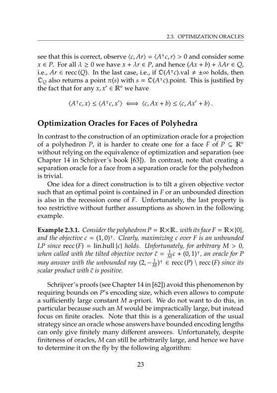
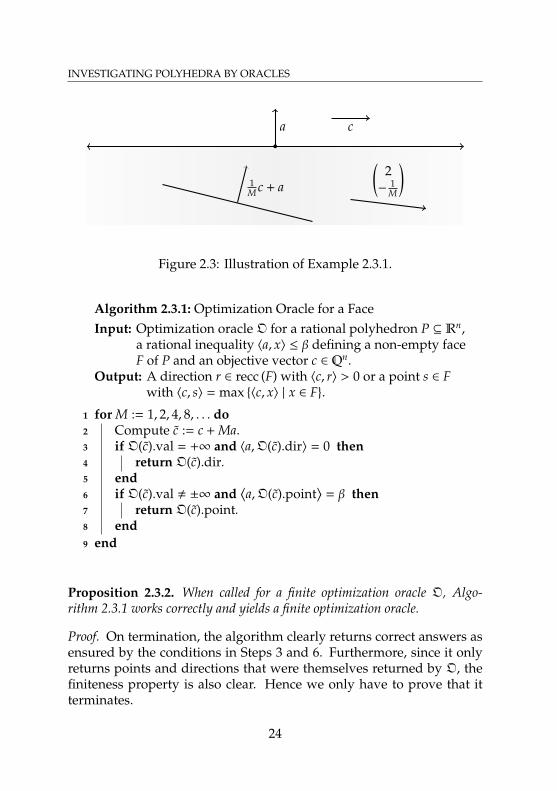
Example 2.3.1. Consider the polyhedron P = R×R− with its face F = R×0,and the objective c = (1, 0)ᵀ. Clearly, maximizing c over F is an unboundedLP since recc (F) = lin.hull c holds. Unfortunately, for arbitrary M > 0,when called with the tilted objective vector c = 1
M c + (0, 1)ᵀ, an oracle for Pmay answer with the unbounded ray (2,− 1
M )ᵀ ∈ recc (P) \ recc (F) since itsscalar product with c is positive.
Schrijver’s proofs (see Chapter 14 in [62]) avoid this phenomenon byrequiring bounds on P’s encoding size, which even allows to computea sufficiently large constant M a-priori. We do not want to do this, inparticular because such an M would be impractically large, but insteadfocus on finite oracles. Note that this is a generalization of the usualstrategy since an oracle whose answers have bounded encoding lengthscan only give finitely many different answers. Unfortunately, despitefiniteness of oracles, M can still be arbitrarily large, and hence we haveto determine it on the fly by the following algorithm:
23
INVESTIGATING POLYHEDRA BY ORACLES
a c
1M c + a
(2−
1M
)
Figure 2.3: Illustration of Example 2.3.1.
Algorithm 2.3.1: Optimization Oracle for a FaceInput: Optimization oracle O for a rational polyhedron P ⊆ Rn,
a rational inequality 〈a, x〉 ≤ β defining a non-empty faceF of P and an objective vector c ∈ Qn.
Output: A direction r ∈ recc (F) with 〈c, r〉 > 0 or a point s ∈ Fwith 〈c, s〉 = max 〈c, x〉 | x ∈ F.
1 for M := 1, 2, 4, 8, . . . do2 Compute c := c + Ma.3 if O(c).val = +∞ and 〈a,O(c).dir〉 = 0 then4 return O(c).dir.5 end6 if O(c).val , ±∞ and
⟨a,O(c).point
⟩= β then
7 return O(c).point.8 end9 end
Proposition 2.3.2. When called for a finite optimization oracle O, Algo-rithm 2.3.1 works correctly and yields a finite optimization oracle.
Proof. On termination, the algorithm clearly returns correct answers asensured by the conditions in Steps 3 and 6. Furthermore, since it onlyreturns points and directions that were themselves returned by O, thefiniteness property is also clear. Hence we only have to prove that itterminates.
24
2.3. OPTIMIZATION ORACLES
Let x ∈ F be some point in the non-empty face F and consider any
s ∈ P \ F. Define M(s) := 〈c,s−x〉+1β−〈a,s〉 (note that 〈a, s〉 < β holds). We now
observe that
⟨c + M(s)a, x − s
⟩=
⟨c, x − s
⟩+
⟨c, s − x
⟩+ 1
β − 〈a, s〉(β − 〈a, s〉) > 0
holds, i.e., no M greater than M(s) will yield s as a (c + Ma)-maximumpoint.
Also observe that for every direction r ∈ recc (P) \ recc (F) we have〈a, r〉 < 0. Hence, there exists a number ~M(r) > 0 with 〈c + ~M(r)a, r〉 ≥ 0.
Now consider an M∗ (from the algorithm) that is greater than M(s)for all (finitely many) points s that the oracle may return and greaterthan ~M(r) for all (finitely many) directions r that the oracle may return.For M∗, the conditions 〈a,O(c).dir〉 = 0 and
⟨a,O(c).point
⟩= β must be
satisfied by the arguments above.
Corrector Oracle for Mixed-Integer Programs
Since the polyhedra of our main interest are mixed-integer hulls, weoften use MIP solvers as heuristics and oracles. It is not straight-forwardto use a floating-point precision MIP solver for such a task as our oraclespecification requires them to return results in exact arithmetic. Clearly,for pure integer programs this is not an issue as we can simply roundthe returned vectors component-wise2.
In order to handle at least explicitly given mixed-integer programs,IPO implements a MixedIntegerProgramCorrectorOracle that doesthe following: Given an approximate solution (x, y) ∈ Rn
× Rd to theMIP max
〈c, x〉 +
⟨d, y
⟩| Ax + By ≤ g, y ∈ Zd
, it rounds y component-
wise to the nearest integer and obtains vector y ∈ Zd. Then, the LPmax
〈c, x〉 | Ax ≤ g − By
(with fixed y) is solved with SoPlex [68], which
can be configured to return exact solutions. This rational solution x isaugmented by y and returned. If the LP is unbounded, then the originalproblem is unbounded as well. If the LP is infeasible, an exception
2In general rounding may produce infeasible points, but in such a case we probablyhave numerical troubles, anyway.
25

INVESTIGATING POLYHEDRA BY ORACLES
is raised, since clearly the answer of the floating-point precision MIPsolver is not even approximately feasible.
26
2.4. COMPUTING THE AFFINE HULL
INVESTIGATING POLYHEDRA BY ORACLES:
2.4 Computing the Affine Hull
This section is dedicated to the following problem. Given an optimiza-tion oracleO for a rational polyhedron P ⊆ Rn, we want to determine P’saffine hull. A very obvious (and useful) certificate consists of an innerdescription, i.e., an affine basis of aff.hull (P) and an outer descriptionof aff.hull (P), i.e, an (irredundant) set of equations valid for P. We firstpresent a simple algorithm that produces such a certificate using at most2n + 1 oracle calls. In Section 2.4.2 we refine the algorithm to reduce thisnumber to 2n, also adding several other improvements. Section 2.4.3 isdedicated to the proof that that no oracle-based algorithm can do better.In order to exploit presence of heuristic optimization oracles we devel-oped an algorithm that first runs our refined algorithm for a heuristicoracle, and then tries to verify the k returned potential equations withonly k + 1 calls to a proper optimization oracle. This algorithm, togetherwith a proof that k + 1 calls are again best possible, is presented in Sec-tion 2.4.4. In Section 2.4.5 we give some insight in details of the softwareimplementation.
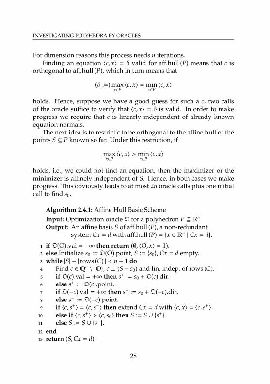
A Basic Scheme
We begin with a simple iterative scheme. It maintains a set S ⊆ Pof affinely independent points (initialized with a single point s0) and anon-redundant system Cx = d of equations valid for aff.hull (P) (initiallyempty), and either enlarges the set S by one point or extends the systemof equations by an equation until aff.hull (S) = x ∈ Rn
| Cx = d holds.
27
INVESTIGATING POLYHEDRA BY ORACLES
For dimension reasons this process needs n iterations.Finding an equation 〈c, x〉 = δ valid for aff.hull (P) means that c is
orthogonal to aff.hull (P), which in turn means that
(δ :=) maxx∈P〈c, x〉 = min
x∈P〈c, x〉
holds. Hence, suppose we have a good guess for such a c, two callsof the oracle suffice to verify that 〈c, x〉 = δ is valid. In order to makeprogress we require that c is linearly independent of already knownequation normals.
The next idea is to restrict c to be orthogonal to the affine hull of thepoints S ⊆ P known so far. Under this restriction, if
maxx∈P〈c, x〉 > min
x∈P〈c, x〉
holds, i.e., we could not find an equation, then the maximizer or theminimizer is affinely independent of S. Hence, in both cases we makeprogress. This obviously leads to at most 2n oracle calls plus one initialcall to find s0.
Algorithm 2.4.1: Affine Hull Basic SchemeInput: Optimization oracle O for a polyhedron P ⊆ Rn.Output: An affine basis S of aff.hull (P), a non-redundant
system Cx = d with aff.hull (P) = x ∈ Rn| Cx = d.
1 if O(O).val = −∞ then return (∅, 〈O, x〉 = 1).2 else Initialize s0 := O(O).point, S := s0, Cx = d empty.3 while |S| + | rows (C) | < n + 1 do4 Find c ∈ Qn
\ O, c ⊥ (S − s0) and lin. indep. of rows (C).5 if O(c).val = +∞ then s+ := s0 +O(c).dir.6 else s+ := O(c).point.7 if O(−c).val = +∞ then s− := s0 +O(−c).dir.8 else s− := O(−c).point.9 if 〈c, s+
〉 = 〈c, s−〉 then extend Cx = d with 〈c, x〉 = 〈c, s+〉.
10 else if 〈c, s+〉 > 〈c, s0〉 then S := S ∪ s+
.11 else S := S ∪ s−.12 end13 return (S,Cx = d).
28
2.4. COMPUTING THE AFFINE HULL
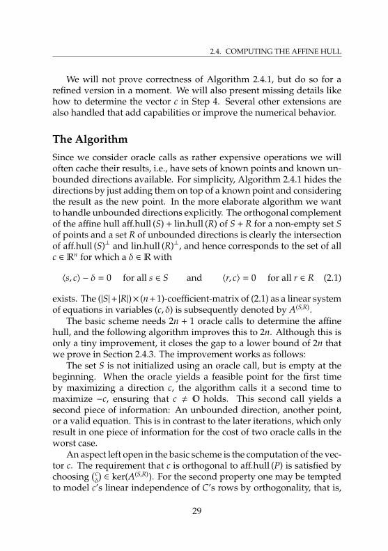
We will not prove correctness of Algorithm 2.4.1, but do so for arefined version in a moment. We will also present missing details likehow to determine the vector c in Step 4. Several other extensions arealso handled that add capabilities or improve the numerical behavior.
The Algorithm
Since we consider oracle calls as rather expensive operations we willoften cache their results, i.e., have sets of known points and known un-bounded directions available. For simplicity, Algorithm 2.4.1 hides thedirections by just adding them on top of a known point and consideringthe result as the new point. In the more elaborate algorithm we wantto handle unbounded directions explicitly. The orthogonal complementof the affine hull aff.hull (S) + lin.hull (R) of S + R for a non-empty set Sof points and a set R of unbounded directions is clearly the intersectionof aff.hull (S)⊥ and lin.hull (R)⊥, and hence corresponds to the set of allc ∈ Rn for which a δ ∈ R with
〈s, c〉 − δ = 0 for all s ∈ S and 〈r, c〉 = 0 for all r ∈ R (2.1)
exists. The (|S|+ |R|)× (n+1)-coefficient-matrix of (2.1) as a linear systemof equations in variables (c, δ) is subsequently denoted by A(S,R).
The basic scheme needs 2n + 1 oracle calls to determine the affinehull, and the following algorithm improves this to 2n. Although this isonly a tiny improvement, it closes the gap to a lower bound of 2n thatwe prove in Section 2.4.3. The improvement works as follows:
The set S is not initialized using an oracle call, but is empty at thebeginning. When the oracle yields a feasible point for the first timeby maximizing a direction c, the algorithm calls it a second time tomaximize −c, ensuring that c , O holds. This second call yields asecond piece of information: An unbounded direction, another point,or a valid equation. This is in contrast to the later iterations, which onlyresult in one piece of information for the cost of two oracle calls in theworst case.
An aspect left open in the basic scheme is the computation of the vec-tor c. The requirement that c is orthogonal to aff.hull (P) is satisfied bychoosing
(cδ
)∈ ker(A(S,R)). For the second property one may be tempted
to model c’s linear independence of C’s rows by orthogonality, that is,
29
INVESTIGATING POLYHEDRA BY ORACLES
to add the corresponding rows to A(S,R) and then search for an elementin the null space. This would certainly yield a correct algorithm, butcomputational experiments suggest that this has undesirable numericalconsequences: First, the underlying linear algebra has to handle rationalnumbers with much higher encoding lengths that can increase the run-ning time dramatically. Second, the normals of the final set of equationsthen constitute an orthonormal basis. For several applications such arequirement is not natural, and it is hard to post-process the equationsto make them easier to read (see Section 2.8). Instead of this directapproach, the following algorithm iterates over a set of basis elementsof A(S,R)’s null space and checks every candidate direction c for lineardependence of C’s rows. For this it maintains a column basis B ⊆ [n+1],an LU-factorization3 of A(S,R)
∗,B and a list L ⊆ [n + 1] \ B of indices thatinduce candidate directions. Since adding an equation does not changeA(S,R), the single loop of Algorithm 2.4.1 is split into two loops, where theinner loop iterates over the candidate directions, and the candidate listis reset in every iteration of the outer loop. This yields Algorithm 2.4.2.
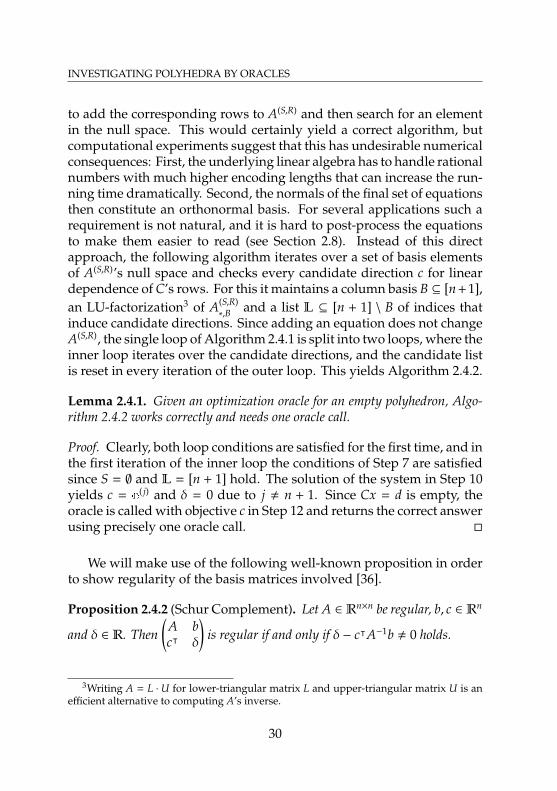
Lemma 2.4.1. Given an optimization oracle for an empty polyhedron, Algo-rithm 2.4.2 works correctly and needs one oracle call.
Proof. Clearly, both loop conditions are satisfied for the first time, and inthe first iteration of the inner loop the conditions of Step 7 are satisfiedsince S = ∅ and L = [n + 1] hold. The solution of the system in Step 10yields c = e
( j) and δ = 0 due to j , n + 1. Since Cx = d is empty, theoracle is called with objective c in Step 12 and returns the correct answerusing precisely one oracle call.
We will make use of the following well-known proposition in orderto show regularity of the basis matrices involved [36].
Proposition 2.4.2 (Schur Complement). Let A ∈ Rn×n be regular, b, c ∈ Rn
and δ ∈ R. Then(
A bcᵀ δ
)is regular if and only if δ − cᵀA−1b , 0 holds.
3Writing A = L · U for lower-triangular matrix L and upper-triangular matrix U is anefficient alternative to computing A’s inverse.
30
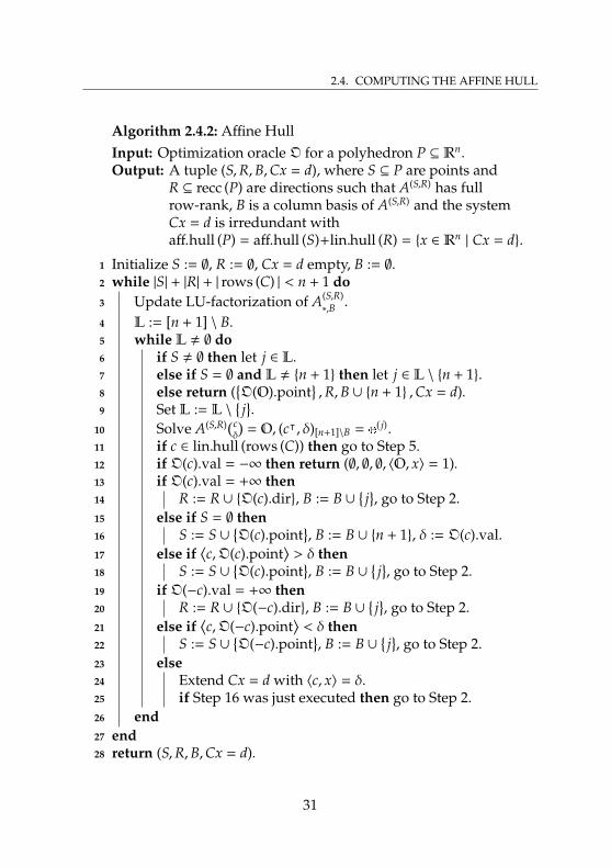
2.4. COMPUTING THE AFFINE HULL
Algorithm 2.4.2: Affine HullInput: Optimization oracle O for a polyhedron P ⊆ Rn.Output: A tuple (S,R,B,Cx = d), where S ⊆ P are points and
R ⊆ recc (P) are directions such that A(S,R) has fullrow-rank, B is a column basis of A(S,R) and the systemCx = d is irredundant withaff.hull (P) = aff.hull (S)+lin.hull (R) = x ∈ Rn
| Cx = d.
1 Initialize S := ∅, R := ∅, Cx = d empty, B := ∅.2 while |S| + |R| + | rows (C) | < n + 1 do3 Update LU-factorization of A(S,R)
∗,B .4 L := [n + 1] \ B.5 while L , ∅ do6 if S , ∅ then let j ∈ L.7 else if S = ∅ and L , n + 1 then let j ∈ L \ n + 1.8 else return (
O(O).point
,R,B ∪ n + 1 ,Cx = d).
9 Set L := L \j.
10 Solve A(S,R)(cδ
)= O, (cᵀ, δ)[n+1]\B = e
( j).11 if c ∈ lin.hull (rows (C)) then go to Step 5.12 if O(c).val = −∞ then return (∅, ∅, ∅, 〈O, x〉 = 1).13 if O(c).val = +∞ then14 R := R ∪ O(c).dir, B := B ∪
j, go to Step 2.
15 else if S = ∅ then16 S := S ∪
O(c).point
, B := B ∪ n + 1, δ := O(c).val.
17 else if⟨c,O(c).point
⟩> δ then
18 S := S ∪O(c).point
, B := B ∪
j, go to Step 2.
19 if O(−c).val = +∞ then20 R := R ∪ O(−c).dir, B := B ∪
j, go to Step 2.
21 else if⟨c,O(−c).point
⟩< δ then
22 S := S ∪O(−c).point
, B := B ∪
j, go to Step 2.
23 else24 Extend Cx = d with 〈c, x〉 = δ.25 if Step 16 was just executed then go to Step 2.26 end27 end28 return (S,R,B,Cx = d).
31
INVESTIGATING POLYHEDRA BY ORACLES
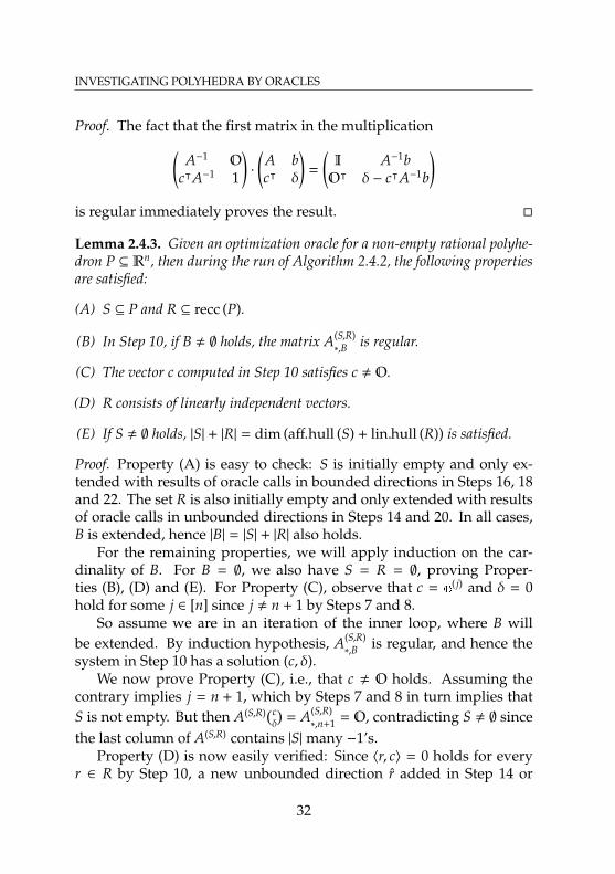
Proof. The fact that the first matrix in the multiplication(A−1 O
cᵀA−1 1
)·
(A bcᵀ δ
)=
(I A−1bOᵀ δ − cᵀA−1b
)is regular immediately proves the result.
Lemma 2.4.3. Given an optimization oracle for a non-empty rational polyhe-dron P ⊆ Rn, then during the run of Algorithm 2.4.2, the following propertiesare satisfied:
(A) S ⊆ P and R ⊆ recc (P).
(B) In Step 10, if B , ∅ holds, the matrix A(S,R)∗,B is regular.
(C) The vector c computed in Step 10 satisfies c , O.
(D) R consists of linearly independent vectors.
(E) If S , ∅ holds, |S| + |R| = dim (aff.hull (S) + lin.hull (R)) is satisfied.
Proof. Property (A) is easy to check: S is initially empty and only ex-tended with results of oracle calls in bounded directions in Steps 16, 18and 22. The set R is also initially empty and only extended with resultsof oracle calls in unbounded directions in Steps 14 and 20. In all cases,B is extended, hence |B| = |S| + |R| also holds.
For the remaining properties, we will apply induction on the car-dinality of B. For B = ∅, we also have S = R = ∅, proving Proper-ties (B), (D) and (E). For Property (C), observe that c = e
( j) and δ = 0hold for some j ∈ [n] since j , n + 1 by Steps 7 and 8.
So assume we are in an iteration of the inner loop, where B willbe extended. By induction hypothesis, A(S,R)
∗,B is regular, and hence thesystem in Step 10 has a solution (c, δ).
We now prove Property (C), i.e., that c , O holds. Assuming thecontrary implies j = n + 1, which by Steps 7 and 8 in turn implies thatS is not empty. But then A(S,R)(c
δ
)= A(S,R)
∗,n+1 = O, contradicting S , ∅ sincethe last column of A(S,R) contains |S|many −1’s.
Property (D) is now easily verified: Since 〈r, c〉 = 0 holds for everyr ∈ R by Step 10, a new unbounded direction r added in Step 14 or
32
2.4. COMPUTING THE AFFINE HULL
Step 20 must be linearly independent of R because 〈r, c〉 , 0 holds aswell.
If S = ∅ holds and the algorithm reaches Step 16, then after thisstep Property (E) is satisfied since |R| = dim (lin.hull (R)) holds by Prop-erty (D).
We now prove Property (E) if S , ∅ holds, including the case thatStep 16 was performed. In this case 〈c, s〉 = γ holds for all s ∈ S and〈c, r〉 = 0 holds for all r ∈ R. A new point s added in Step 18 or Step 22must be affinely independent of aff.hull (S) + lin.hull (R).
It remains to show Property (B). Iterations in which B is extendedtwice are handled one by one. Let B′ = B ∪
j
be the new basis and letS′, R′ be the new sets of points and unbounded directions, respectively.Note that we either have S′ = S and R′ = R ∪ r or S′ = S ∪ s andR′ = R. By induction we can assume that A(S,R)
∗,B is regular.
We first show regularity of A(S′,R′)∗,B′ for the case when S = ∅ and a point
is added in Step 16. A(S′,R′)∗,B′ is regular since it arises from A(S,R)
∗,B by addinga row and a (negative) unit column with the −1 in the new row.
We now show regularity of A(S′,R′)∗,B for the case when S = ∅ and
n + 1 < B hold and an unbounded directions r is added in Step 14 orStep 20. From O = A(S,R)(c
δ
)= A(S,R)
∗,B cB + A(S,R)∗, j we derive that
r j − rᵀBA(S,R)∗,B
−1A(S,R)∗, j = r j + 〈rB, cB〉 = 〈r, c〉 , 0
holds, where the last non-equality comes from the fact that r is un-bounded in direction c or −c. Thus, by Proposition 2.4.2, the matrixA(S′,R′)∗,B′ is regular.
We continue with the regularity of A(S′,R′)∗,B for the case when S , ∅
and n + 1 ∈ B hold and an unbounded direction r is added in Step 14 orStep 20. From O = A(S,R)(c
δ
)= A(S,R)
∗,B(cBδ
)+ A(S,R)
∗, j we derive that
r j −
(rB
0
)ᵀA(S,R)∗,B
−1A(S,R)∗, j = r j +
⟨(rB
0
),
(cB
δ
)⟩= 〈r, c〉 , 0
holds, where the last non-equality comes from the fact that r is un-bounded in direction c or −c. Again, by Proposition 2.4.2, the matrixA(S′,R′)∗,B′ is regular.
33
INVESTIGATING POLYHEDRA BY ORACLES
We finally show regularity of A(S′,R′)∗,B for the case when S , ∅ and
n + 1 ∈ B hold and a point s is added in Step 18 or Step 22. FromO = A(S,R)(c
δ
)= A(S,R)
∗,B(cBδ
)+ A(S,R)
∗, j we derive that
s j −
(sB
−1
)ᵀA(S,R)∗,B
−1A(S,R)∗, j = s j +
⟨(sB
−1
),
(cB
δ
)⟩= 〈s, c〉 − δ , 0
holds, where the last non-equality comes from the fact that s has c-value distinct from δ. Again, by Proposition 2.4.2, the matrix A(S′,R′)
∗,B′ isregular.
Lemma 2.4.4. Given an optimization oracle for a non-empty rational polyhe-dron P ⊆ Rn, then during the run of Algorithm 2.4.2 the system Cx = d isvalid for P, and the rows of C are linearly independent.
Proof. We prove the lemma by induction on the number of equations inCx = d, being trivially satisfied at the beginning.
Let Cx = d be non-redundant and valid for P, and consider equation〈c, x〉 = δ added in Step 24. Due to Step 11 we have that c is linearlyindependent from rows (C), and from Steps 17 and 21 we derive that〈c, x〉 ≤ δ and 〈c, x〉 ≥ δ are valid for P, which concludes the proof.
Lemma 2.4.5. Given an optimization oracle defining a non-empty rationalpolyhedron P ⊆ Rn, then during the run of Algorithm 2.4.2 we have
lin.hull(rows([C | d])) ⊆ ker(A(S,R)), (2.2)
and equality holds if and only if we have |S| + |R| + | rows (C) | = n + 1.
Proof. Since Cx = d is valid for P by Lemma 2.4.4 and since we haveS ⊆ P and R ⊆ recc (P) by Property (A) of Lemma 2.4.3, the relation(2.2) holds. Then, by linear independence of C’s rows (Lemma 2.4.4)and regularity of A(S,R)
∗,B (Lemma 2.4.3, Property (B)), we obtain the in-equality | rows (C) | ≤ dim ker(A(S,R)) = n + 1 − |S| − |R|. Hence, equalityis equivalent to the given condition, which concludes the proof.
Lemma 2.4.6. Given an optimization oracle defining a non-empty rationalpolyhedron P ⊆ Rn, then whenever the inner loop of Algorithm 2.4.2 is left,then the number of oracle calls made so far is bounded from above by the term2(|S| + |R| + | rows (C) | − 1) if S , ∅ holds, by |R| + 1 if we are in Step 8 andby |R| otherwise.
34
2.4. COMPUTING THE AFFINE HULL
Proof. We prove the lemma by induction on the number of times Step 13has been reached at the point of consideration (not necessarily with thecondition satisfied). It trivially holds after initialization.
Case 1: S = ∅.If Step 14 is executed, then both |R| and the number of oracle calls areincreased by 1. If Step 8 is executed, the number of calls is |R|+ 1 due tothe additional call in that step. Otherwise, S is for the first time extendedwith a point. Let k := |R| denote the number of unbounded directionsat that time. In the same iteration of the inner loop another point or adirection or an equation is added to S, R or Cx = d, respectively. Hence,when this loop is left we have called the oracle k + 2 times and observe|S| + |R| + | rows (C) | ≥ k + 2, which proves the claimed bound (usingk ≥ 0).
Case 2: S , ∅.In every iteration of the inner loop in which the oracle is called, it iscalled at most twice and S, R or Cx = d are extended, which proves theclaimed bound.
Theorem 2.4.7. Algorithm 2.4.2 is correct and needs at most 2n calls to thegiven optimization oracle for a rational polyhedron P ⊆ Rn.
Proof. By Lemma 2.4.1 we can assume P , ∅.We first prove the upper bound on the number of oracle calls. After
2n oracle calls |S| + |R| + | rows (C) | − 1 ≥ n holds by Lemma 2.4.6, andthus the condition of the outer loop in Step 2 is violated. Except forSteps 16 and 24 the condition is always checked before the next oraclecall. Step 16 is only executed after at most n executions of Step 14 (sincethen R already contains a basis of Rn), which takes only n oracle calls.Suppose the (2n)’th oracle call results in the execution of Step 24. By theabove reasoning we have |S| + |R| + | rows (C) | = n + 1 and Lemma 2.4.5then implies that for every
(cδ
)∈ ker(A(S,R)) the vector c is linearly depen-
dent of lin.hull (C). Hence, Step 11 ensures that no oracle call is triggeredbefore the condition in Step 2 is checked the next time. This concludesthe proof of the bound on the number of oracle calls.
We now show that the algorithm terminates. Suppose the contrary,and observe that the inner loop does not run forever since L is finiteand an element is removed in each iteration in Step 9. Furthermore,
35
INVESTIGATING POLYHEDRA BY ORACLES
Step 13 can only be reached finitely many times since the number oforacle calls is bounded. The only possibility to run forever is thus byhaving |S| + |R| + | rows (C) | < n + 1 and c ∈ lin.hull (rows (C)) for every(cδ
)∈ ker
(A(S,R)
)satisfied such that the algorithm leaves the inner loop
via Step 11. But both conditions contradict each other by Lemma 2.4.5.We finally show that the algorithm always returns the correct output
for P , ∅. If S = ∅ holds when we return, then it is in Step 8. We musthave Cx = d empty since adding an equation in Step 24 happens only ifS , ∅ holds. Hence, since c , O holds by Property (C) of Lemma 2.4.3,whenever j was removed from L in Step 9, an unbounded directionwas added to R in Step 13. Thus we have [n + 1] \ B = n + 1, showing|R| = n, i.e. recc (P) = Rn. The last oracle call in Step 8 then yields afeasible point and the returned basis is [n + 1].
Otherwise we return due to the violation of the outer loop’s condition|S|+ |R|+ | rows (C) | < n+1, i.e., (|S|−1)+ |R| ≤ dim (P) ≤ n−| rows (C) | issatisfied with equality. Hence, the returned objects determine P’s affinehull. Furthermore, by Property (B) of Lemma 2.4.3 the returned basis iscorrect.
A Lower Bound on the Number of Oracle CallsThe following theorem states that the number of oracle calls in Algo-rithm 2.4.2 is best possible.
Theorem 2.4.8. Every algorithm that computes the affine hull of any polyhe-dron P ⊆ Rn only by using an optimization oracle for P needs at least 2n oraclecalls in the worst case, even if the polyhedra are restricted to cones.
We will soon define the behavior of an oracle such that the algorithmcannot determine the affine hull after calling the oracle only 2n−1 times.The oracle then implicitly defines a polyhedron P that will be a conehaving the property in the following proposition.
Proposition 2.4.9. Let A ∈ Rm×n be such that 〈Ai,∗,A j,∗〉 ≥ 0 holds for everyi, j ∈ [m]. Then the cone C = x ∈ Rn
| Ax ≤ O is full-dimensional.
Proof of Proposition 2.4.9. Let 〈a, x〉 = 0 be an equation valid for C, i.e.,max 〈±a, x〉 | x ∈ C = 0 holds (note that O ∈ C). We want to prove thata = O holds showing that 〈O, x〉 = 0 is the only equation valid for C.
36
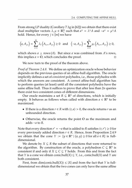
2.4. COMPUTING THE AFFINE HULL
From strong LP duality (Corollary 7.1g in [62]) we obtain that there existdual multiplier vectors λ, µ ∈ Rm
+ such that aᵀ = λᵀA and −aᵀ = µᵀAhold. Hence, for every j ∈ [m] we have⟨
a,A j,∗
⟩=
m∑i=1
λi
⟨Ai,∗,A j,∗
⟩≥ 0 and
⟨−a,A j,∗
⟩=
m∑i=1
µi
⟨Ai,∗,A j,∗
⟩≥ 0,
which shows a ⊥ rows (A). But since a was combined from A’s rows,this implies a = O, which concludes the proof.
We now turn to the proof of the theorem above.
Proof of Theorem 2.4.8. We define an optimization oracle whose behaviordepends on the previous queries of an affine-hull algorithm. The oracleimplicitly defines a set of consistent polyhedra, i.e., those polyhedra withwhich the answers are consistent. A correct affine-hull algorithm hasto perform queries (at least) until all the consistent polyhedra have thesame affine hull. Thus it suffices to prove that after less than 2n queriesthere exist two consistent cones of different dimensions.
Our oracle maintains a set R ⊆ Rn of directions, which is initiallyempty. It behaves as follows when called with direction a ∈ Rn to bemaximized.
• If there is a direction r ∈ R with 〈r, a〉 > 0, the oracle returns r as anunbounded direction.
• Otherwise, the oracle returns the point O as the maximum andadds −a to R.
Note that every direction r′ = −a that is added to R satisfies 〈r, r′〉 ≥ 0 forevery previously added direction r ∈ R. Hence, from Proposition 2.4.9we obtain that the cone Y :=
y ∈ Rn
|⟨a, y
⟩≥ 0 for all a ∈ R
is full-
dimensional.We denote by X ⊆ R the subset of directions that were returned to
the algorithm. By construction of the oracle, a polyhedron C ⊆ Rn isconsistent if and only if X ⊆ C ⊆ Y holds. From this and from the factthat Y is a cone we obtain conic.hull(X) ⊆ Y, i.e., conic.hull(X) and Y areboth consistent.
First, from dim(conic.hull(X)) ≤ |X| and from the fact that Y is full-dimensional we obtain that the two cones can only have the same affine
37
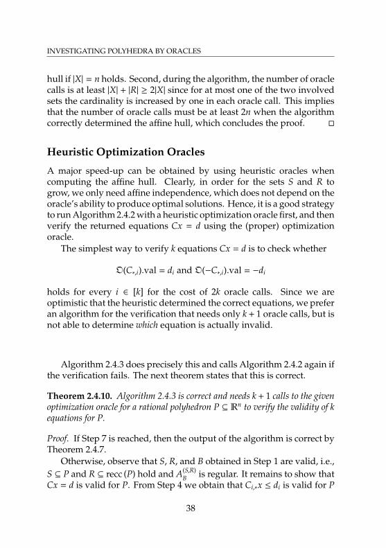
INVESTIGATING POLYHEDRA BY ORACLES
hull if |X| = n holds. Second, during the algorithm, the number of oraclecalls is at least |X| + |R| ≥ 2|X| since for at most one of the two involvedsets the cardinality is increased by one in each oracle call. This impliesthat the number of oracle calls must be at least 2n when the algorithmcorrectly determined the affine hull, which concludes the proof.
Heuristic Optimization Oracles
A major speed-up can be obtained by using heuristic oracles whencomputing the affine hull. Clearly, in order for the sets S and R togrow, we only need affine independence, which does not depend on theoracle’s ability to produce optimal solutions. Hence, it is a good strategyto run Algorithm 2.4.2 with a heuristic optimization oracle first, and thenverify the returned equations Cx = d using the (proper) optimizationoracle.
The simplest way to verify k equations Cx = d is to check whether
O(C∗,i).val = di and O(−C∗,i).val = −di
holds for every i ∈ [k] for the cost of 2k oracle calls. Since we areoptimistic that the heuristic determined the correct equations, we preferan algorithm for the verification that needs only k + 1 oracle calls, but isnot able to determine which equation is actually invalid.
Algorithm 2.4.3 does precisely this and calls Algorithm 2.4.2 again ifthe verification fails. The next theorem states that this is correct.
Theorem 2.4.10. Algorithm 2.4.3 is correct and needs k + 1 calls to the givenoptimization oracle for a rational polyhedron P ⊆ Rn to verify the validity of kequations for P.
Proof. If Step 7 is reached, then the output of the algorithm is correct byTheorem 2.4.7.
Otherwise, observe that S, R, and B obtained in Step 1 are valid, i.e.,S ⊆ P and R ⊆ recc (P) hold and A(S,R)
B is regular. It remains to show thatCx = d is valid for P. From Step 4 we obtain that Ci,∗x ≤ di is valid for P
38
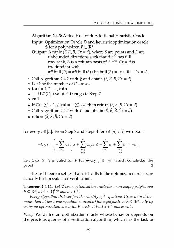
2.4. COMPUTING THE AFFINE HULL
Algorithm 2.4.3: Affine Hull with Additional Heuristic OracleInput: Optimization Oracle O and heuristic optimization oracle
H for a polyhedron P ⊆ Rn.Output: A tuple (S,R,B,Cx = d), where S are points and R are
unbounded directions such that A(S,R) has fullrow-rank, B is a column basis of A(S,R), Cx = d isirredundant withaff.hull (P) = aff.hull (S)+lin.hull (R) = x ∈ Rn
| Cx = d.
1 Call Algorithm 2.4.2 with H and obtain (S,R,B,Cx = d).2 Let k be the number of C’s rows.3 for i = 1, 2, . . . , k do4 if O(Ci,∗).val , di then go to Step 7.5 end6 if O(−
∑ki=1 Ci,∗).val = −
∑ki=1 di then return (S,R,B,Cx = d)
7 Call Algorithm 2.4.2 with O and obtain (S, R, B, Cx = d).8 return (S, R, B, Cx = d)
for every i ∈ [n]. From Step 7 and Steps 4 for i ∈ [n] \j
we obtain
−C j,∗x =
− n∑i=1
Ci,∗
x +
n∑i=1i, j
Ci,∗x ≤ −n∑
i=1
di +
n∑i=1i, j
di = −d j,
i.e., C j,∗x ≥ d j is valid for P for every j ∈ [n], which concludes theproof.
The last theorem settles that k + 1 calls to the optimization oracle areactually best possible for verification.
Theorem 2.4.11. LetO be an optimization oracle for a non-empty polyhedronP ⊆ Rn, let C ∈ Qk×n and d ∈ Qk.
Every algorithm that verifies the validity of k equations Cx = d (or deter-mines that at least one equation is invalid) for a polyhedron P ⊆ Rn only byusing an optimization oracle for P needs at least k + 1 oracle calls.
Proof. We define an optimization oracle whose behavior depends onthe previous queries of a verification algorithm, which has the task to
39
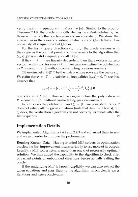
INVESTIGATING POLYHEDRA BY ORACLES
verify the k := n equations xi = 0 for i ∈ [n]. Similar to the proof ofTheorem 2.4.8, the oracle implicitly defines consistent polyhedra, i.e.,those with which the oracle’s answers are consistent. We show thatafter n queries there exist consistent polyhedra P and Q such that P doesnot satisfy all n equations, but Q does.
For the first n query directions c1, . . . , cn, the oracle answers withthe origin as the optimal point, and thus reveals to the algorithm that〈ci, x〉 ≤ 0 is a valid inequality for all i ∈ [n].
If the ci (i ∈ [n]) are linearly dependent, then there exists a nonzerovector v with v ⊥ ci for every i ∈ [n]. We can now define the polyhedronas P := conic.hull(v) without contradicting previous answers.
Otherwise, let T ∈ Qn×n be the matrix whose rows are the vectors cᵀi .We claim that v := −T−1
1n satisfies all inequalities 〈ci, x〉 ≤ 0. To see this,observe that
〈ci, v〉 = −⟨ci,T−1
1n
⟩= −
⟨e
(i),1n
⟩≤ 0
holds for all i ∈ [n]. Thus we can again define the polyhedron asP := conic.hull(v) without contradicting previous answers.
In both cases the polyhedra P and Q := O are consistent. Since Pdoes not satisfy all the given equations (note that dim P = 1 holds), butQ does, the verification algorithm can not correctly terminate after thefirst n queries.
Implementation Details
We implemented Algorithms 2.4.2 and 2.4.3 and enhanced them in sev-eral ways in order to improve the performance.
Reusing Known Data. Having in mind MIP solvers as optimizationoracles, the first improvement idea is certainly to use more of its output:Usually, a MIP solver returns more than one (not necessarily optimal)solution. We thus added the capability to the algorithm to check a setof cached points or unbounded directions before actually calling theoracle.
If the underlying MIP is known explicitly we can also extract thegiven equations and pass them to the algorithm, which clearly savesiterations and hence oracle calls.
40
2.4. COMPUTING THE AFFINE HULL
Similarly, if we computed the affine hull of a polyhedron P we mayafterwards compute the affine hull of one of its faces. In this case wereuse all valid equations and fill the cache of points and directions withthose feasible for the face.
Precomputing With Floating Point Arithmetic. Computational evi-dence shows that for larger dimensions the linear algebra part of thealgorithm can be quite time-consuming due to exact arithmetic. Thereare several steps in Algorithm 2.4.2 in which we could improve the speedby precomputing certain data with floating-point arithmetic followedby an exact computation of the interesting parts.
A first application of this technique is the mentioned cache of pointsand unbounded directions. We are given a set S′ ⊆ Qn of points, adirection vector c ∈ Qn and a number δ ∈ Q, defining a hyperplaneH = x ∈ Rn
| 〈c, x〉 = δ. The task is to find out whether there existsa point s′ ∈ S′ \ H. For this we first sort S′ by increasing sparsityand compute the approximate scalar products in that order using thefloating-point representations c of c and s′ of s′ for all s′ ∈ S′. If anapproximate scalar product satisfies |
⟨c, s′
⟩− δ| ≥ τ for some threshold
parameter τ > 0, then we recompute the scalar product exactly and, ifdifferent from δ, return the current point. Otherwise we increase τ by afactor of 10, that is, we do not trust floating-point results in this order ofmagnitude anymore. Sorting S′ prior to searching allows us to stop thesearch as soon as we find a suitable point since all points that we wouldinspect later have no better sparsity. If we do not succeed with thisstrategy, we also try the point with the largest approximate distance toH. Of course it may happen that there exists a point s′ ∈ S′ \H, but ouralgorithm is unable to find it. The algorithm for unbounded directionsis very similar and we refer to the source code.
A second application is the selection of the index j in Steps 6 and 7of Algorithm 2.4.2. Different indices j yield different directions c and,once again, we prefer sparse vectors for different reasons: On the onehand, the oracle may be faster to maximize a sparse objective vector,e.g., if c is a unit vector then the task is to check whether a variablebound is tight. On the other hand, some of the directions may end upas equation normals, and a user is probably more interested in a sparseset of equations valid for P.
Since the computation of a single direction can be already be very
41

INVESTIGATING POLYHEDRA BY ORACLES
expensive (see Figure 2.9 in Section 2.9.1) we again compute all di-rections using floating-point arithmetic and (approximately) determinetheir sparsity. For this we declare a number with absolute value lessthan 10−7 as zero4.
4This value was determined in order to get a good approximation of the true sparsity.
42
2.5. COMPUTING FACETS
INVESTIGATING POLYHEDRA BY ORACLES:
2.5 Computing Facets
This section is dedicated to the problem of finding facets of a polyhe-dron P, again specified by means of an optimization oracle O. We firstdescribe the main idea from a geometric point of view and present anequivalent model that is more attractive from a computational stand-point. We only sketch how the oracle is actually used to solve the model,since we need to solve a similar one for a related problem, and hencediscuss the details in Section 2.7, dedicated to this topic.
After establishing the correctness of the model we discuss a technicalproblem that arises, suggest how to resolve it and finally consider detailsconcerning the actual derivation of the facets.
Polarity and Target CutsSince we want to start with a geometric intuition, we consider a full-dimensional polyhedron P ⊆ Rn that contains the originO in its interior.The polar P∗ of P is defined as the set
P∗ :=y ∈ Rn
|⟨y, x
⟩≤ 1 for all x ∈ P
.
From basic convex geometry we know several basic properties that willturn out to be very useful for us.
Proposition 2.5.1 (Theorem 9.1 and Corollary 9.1a in [62]). Let P ⊆ Rn
be a full-dimensional pointed polytope with O ∈ int (P). Then
(i) P∗ is a again a full-dimensional pointed polytope,
43
INVESTIGATING POLYHEDRA BY ORACLES
(ii)⟨x, y
⟩≤ 1 is valid for all y ∈ P∗ if and only if x ∈ P holds, and
(iii)⟨y, x
⟩≤ 1 induces a facet of P if and only if y is a vertex of P∗.
Since we are interested in facets of P, Proposition 2.5.1 (iii) tells usthat we want to find vertices of P∗. In order to find a specific facet,namely one that separates a point x ∈ Rn from P, we can solve thefollowing problem.
max⟨x, y
⟩(2.3)
s.t.⟨x, y
⟩≤ 1 for all x ∈ P (2.4)
y ∈ Rn (2.5)
Note that formally this is not an LP since in general it contains infinitelymany constraints. It is not too hard to see that we can restrict Con-straint (2.4) to those x ∈ P that are vertices. By Proposition 2.5.1 (iii)a vertex solution y of Problem (2.3)–(2.5) corresponds to a facet of P.Furthermore, if the maximum objective is larger than 1, i.e.,
⟨x, y
⟩> 1
holds, then the facet-defining inequality⟨y, x
⟩≤ 1 of P is violated by
x. On the other hand, if the maximum objective is at most 1, that is,⟨x, y
⟩≤ 1 holds for all y ∈ P∗, then again by Proposition 2.5.1 (iii) there
is no facet-defining inequality (and hence no valid inequality at all) thatseparates x from P.
Using Proposition 2.5.1 (ii) we can show that the separation problemfor Inequalities (2.4) is essentially the optimization problem over P,which we can solve by means of our optimization oracle. More precisely,if we have a partial outer description of LP (2.3)–(2.5), then we can decideby one call to the optimization oracle for P whether the current solutiony is feasible, obtaining a violated inequality if this is not the case. Thedetails of this procedure including the exact usage of our optimizationoracle are discussed in the dedicated Section 2.7.
Note that we do not require the oracle to return vertex solutions, sinceour (partial) outer description of P∗ is allowed to contain non-facet-defining inequalities, too. On the other hand, it is necessary that wecompute a vertex solution y as only those correspond to facets of P.
If P does not contain O in its interior we can simply shift it by some
44
2.5. COMPUTING FACETS
vector o ∈ int (P), which yields the following LP
max⟨x − o, y
⟩(2.6)
s.t.⟨s − o, y
⟩≤ 1 for all s ∈ S (2.7)
y ∈ Rn, (2.8)
where S ⊆ P is a (finite) superset of P’s vertices.The ideas we just introduced are not new. To the best of our knowl-
edge, Applegate, Bixby, Chvátal and Cook [3] were the first to developcutting plane methods based on optimization oracles. Their Local Cutprocedure uses a different objective function, which does not necessarilyyield facet-defining inequalities. Hence, they describe a tilting proce-dure that allows them to generate facets for small subproblems of thetraveling salesman problem (TSP), which are in turn lifted to inequali-ties valid for the TSP-polytope. Later, Buchheim, Liers and Oswald [15]revisited this idea and came up with the Target Cuts for which they useda variant of LP (2.6)–(2.8).
An Equivalent ModelThe LP (2.6)–(2.8) in principle works for our purposes, except that werestricted ourself to full-dimensional pointed polytopes. Unfortunately,interior points of (combinatorial) polyhedra are typically very densevectors, which implies that the matrix of the LP’s inequality system is avery dense matrix in general. Since the running time of state-of-the-artLP solvers critically depends on the number of nonzeros of the problemmatrix (see, e.g., [66] and [65]), it is obvious that this LP is numericallynot very attractive.
Luckily, there is a transformation, communicated by Marc Pfetsch,that yields an equivalent LP in which the interior point o appears in onlyone inequality.
max 〈x, a〉 − β (2.9)s.t. 〈s, a〉 − β ≤ 0 for all s ∈ S (2.10)
〈r, a〉 ≤ 0 for all r ∈ R (2.11)〈x − o, a〉 ≤ 1 (2.12)
a ∈ Rn, β ∈ R (2.13)
45
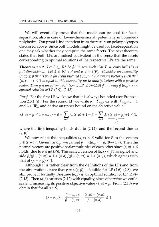
INVESTIGATING POLYHEDRA BY ORACLES
We will eventually prove that this model can be used for facet-separation, also in case of lower-dimensional (potentially unbounded)polyhedra. Our proof is independent from the results on polar polytopesdiscussed above. Since both models might be used for facet-separationone may ask whether they compute the same facets. The next theoremstates that both LPs are indeed equivalent in the sense that the facetscorresponding to optimal solutions of the respective LPs are the same.
Theorem 2.5.2. Let S ⊆ Rn be finite sets such that P = conv.hull (S) isfull-dimensional. Let x ∈ Rn
\ P and o ∈ int (P). Consider an inequality〈a, x〉 ≤ β that is valid for P but violated by x, and the unique vector y such that⟨y, x − o
⟩≤ 1 is equal to this inequality up to multiplication with a positive
scalar. Then y is an optimal solution of LP (2.6)–(2.8) if and only if (a, β) is anoptimal solution of LP (2.9)–(2.13).
Proof. For the first LP we know that it is always bounded (see Proposi-tion 2.5.1 (i)). For the second LP we write o =
∑s∈S λss with
∑s∈S λs = 1
and λ ∈ RS+, and derive an upper bound on the objective value
〈x, a〉 − β ≤ 1 + 〈o, a〉 − β =∑s∈S
λs 〈s, a〉 + 1 − β =∑s∈S
λs (〈s, a〉 − β)︸ ︷︷ ︸≤ 0
+1 ≤ 1,
where the first inequality holds due to (2.12), and the second due to(2.10).
We now relate the inequalities 〈a, x〉 ≤ β valid for P to the vectorsy ∈ (P−o)∗. Given a and β, we can set y = π(a, β) := a/(β−〈o, a〉. Then thenormal vectors are positive scalar multiples of each other since 〈a, o〉 < βholds (due to o ∈ int (P)). This scaled version of 〈a, x〉 ≤ β has right-handside β/(β − 〈o, a〉) = 1 + 〈o, a〉 /(β − 〈o, a〉) = 1 +
⟨o, y
⟩, which agrees with
that of⟨x − o, y
⟩≤ 1.
Although it is rather clear from the definitions of the LPs and fromthe observation above that y = π(a, β) is feasible for LP (2.6)–(2.8), westill prove it formally. Assume (a, β) is an optimal solution of LP (2.9)–(2.13). Then (a, β) satisfies (2.12) with equality, since otherwise we couldscale it, increasing its positive objective value 〈x, a〉 − β. From (2.10) weobtain that for all s ∈ S,⟨
s − o, y⟩
=〈s − o, a〉β − 〈o, a〉
=〈s, a〉 − 〈o, a〉β − 〈o, a〉
≤ 1
46
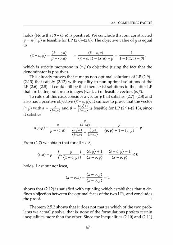
2.5. COMPUTING FACETS
holds (Note that β− 〈a, o〉 is positive). We conclude that our constructedy = π(a, β) is feasible for LP (2.6)–(2.8). The objective value of y is equalto ⟨
x − o, y⟩
=〈x − o, a〉β − 〈o, a〉
=〈x − o, a〉
〈x − o, a〉 − 〈x, a〉 + β=
11 − (〈x, a〉 − β)
,
which is strictly monotone in (a, β)’s objective (using the fact that thedenominator is positive).
This already proves that π maps non-optimal solutions of LP (2.9)–(2.13) that satisfy (2.12) with equality to non-optimal solutions of theLP (2.6)–(2.8). It could still be that there exist solutions to the latter LPthat are better, but are no images (w.r.t. π) of feasible vectors (a, β).
To rule out this case, consider a vector y that satisfies (2.7)–(2.8) andalso has a positive objective
⟨x − o, y
⟩. It suffices to prove that the vector
(a, β) with a =y
〈x−o,y〉and β =
〈o,y〉+1
〈x−o,y〉is feasible for LP (2.9)–(2.13), since
it satisfies
π(a, β) =a
β − 〈o, a〉=
y
〈x−o,y〉
〈o,y〉+1
〈x−o,y〉−〈o,y〉〈x−o,y〉
=y⟨
o, y⟩
+ 1 −⟨o, y
⟩ = y
From (2.7) we obtain that for all s ∈ S,
〈s, a〉 − β =
⟨s,
y⟨x − o, y
⟩⟩ − ⟨o, y
⟩+ 1⟨
x − o, y⟩ =
⟨s − o, y
⟩− 1⟨
x − o, y⟩ ≤ 0
holds. Last but not least,
〈x − o, a〉 =
⟨x − o, y
⟩⟨x − o, y
⟩ = 1
shows that (2.12) is satisfied with equality, which establishes that π de-fines a bijection between the optimal faces of the two LPs, and concludesthe proof.
Theorem 2.5.2 shows that it does not matter which of the two prob-lems we actually solve, that is, none of the formulations prefers certaininequalities more than the other. Since the Inequalities (2.10) and (2.11)
47
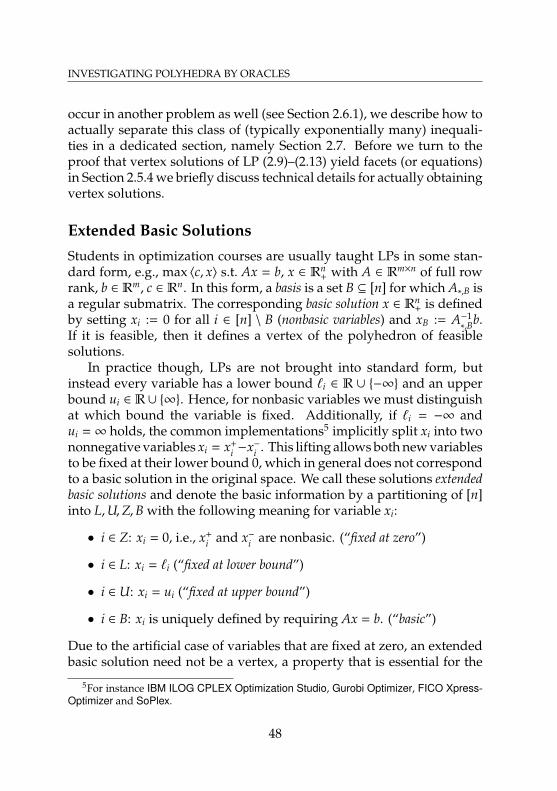
INVESTIGATING POLYHEDRA BY ORACLES
occur in another problem as well (see Section 2.6.1), we describe how toactually separate this class of (typically exponentially many) inequali-ties in a dedicated section, namely Section 2.7. Before we turn to theproof that vertex solutions of LP (2.9)–(2.13) yield facets (or equations)in Section 2.5.4 we briefly discuss technical details for actually obtainingvertex solutions.
Extended Basic Solutions
Students in optimization courses are usually taught LPs in some stan-dard form, e.g., max 〈c, x〉 s.t. Ax = b, x ∈ Rn
+ with A ∈ Rm×n of full rowrank, b ∈ Rm, c ∈ Rn. In this form, a basis is a set B ⊆ [n] for which A∗,B isa regular submatrix. The corresponding basic solution x ∈ Rn
+ is definedby setting xi := 0 for all i ∈ [n] \ B (nonbasic variables) and xB := A−1
∗,Bb.If it is feasible, then it defines a vertex of the polyhedron of feasiblesolutions.
In practice though, LPs are not brought into standard form, butinstead every variable has a lower bound `i ∈ R ∪ −∞ and an upperbound ui ∈ R∪ ∞. Hence, for nonbasic variables we must distinguishat which bound the variable is fixed. Additionally, if `i = −∞ andui = ∞ holds, the common implementations5 implicitly split xi into twononnegative variables xi = x+
i −x−i . This lifting allows both new variablesto be fixed at their lower bound 0, which in general does not correspondto a basic solution in the original space. We call these solutions extendedbasic solutions and denote the basic information by a partitioning of [n]into L,U,Z,B with the following meaning for variable xi:
• i ∈ Z: xi = 0, i.e., x+i and x−i are nonbasic. (“fixed at zero”)
• i ∈ L: xi = `i (“fixed at lower bound”)
• i ∈ U: xi = ui (“fixed at upper bound”)
• i ∈ B: xi is uniquely defined by requiring Ax = b. (“basic”)
Due to the artificial case of variables that are fixed at zero, an extendedbasic solution need not be a vertex, a property that is essential for the
5For instance IBM ILOG CPLEX Optimization Studio, Gurobi Optimizer, FICO Xpress-Optimizer and SoPlex.
48
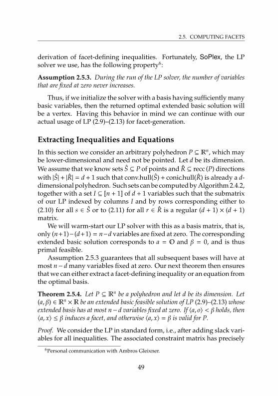
2.5. COMPUTING FACETS
derivation of facet-defining inequalities. Fortunately, SoPlex, the LPsolver we use, has the following property6:
Assumption 2.5.3. During the run of the LP solver, the number of variablesthat are fixed at zero never increases.
Thus, if we initialize the solver with a basis having sufficiently manybasic variables, then the returned optimal extended basic solution willbe a vertex. Having this behavior in mind we can continue with ouractual usage of LP (2.9)–(2.13) for facet-generation.
Extracting Inequalities and EquationsIn this section we consider an arbitrary polyhedron P ⊆ Rn, which maybe lower-dimensional and need not be pointed. Let d be its dimension.We assume that we know sets S ⊆ P of points and R ⊆ recc (P) directionswith |S|+ |R| = d + 1 such that conv.hull(S) + conic.hull(R) is already a d-dimensional polyhedron. Such sets can be computed by Algorithm 2.4.2,together with a set I ⊆ [n + 1] of d + 1 variables such that the submatrixof our LP indexed by columns I and by rows corresponding either to(2.10) for all s ∈ S or to (2.11) for all r ∈ R is a regular (d + 1) × (d + 1)matrix.
We will warm-start our LP solver with this as a basis matrix, that is,only (n+1)−(d+1) = n−d variables are fixed at zero. The correspondingextended basic solution corresponds to a = O and β = 0, and is thusprimal feasible.
Assumption 2.5.3 guarantees that all subsequent bases will have atmost n− d many variables fixed at zero. Our next theorem then ensuresthat we can either extract a facet-defining inequality or an equation fromthe optimal basis.
Theorem 2.5.4. Let P ⊆ Rn be a polyhedron and let d be its dimension. Let(a, β) ∈ Rn
×R be an extended basic feasible solution of LP (2.9)–(2.13) whoseextended basis has at most n− d variables fixed at zero. If 〈a, o〉 < β holds, then〈a, x〉 ≤ β induces a facet, and otherwise 〈a, x〉 = β is valid for P.
Proof. We consider the LP in standard form, i.e., after adding slack vari-ables for all inequalities. The associated constraint matrix has precisely
6Personal communication with Ambros Gleixner.
49
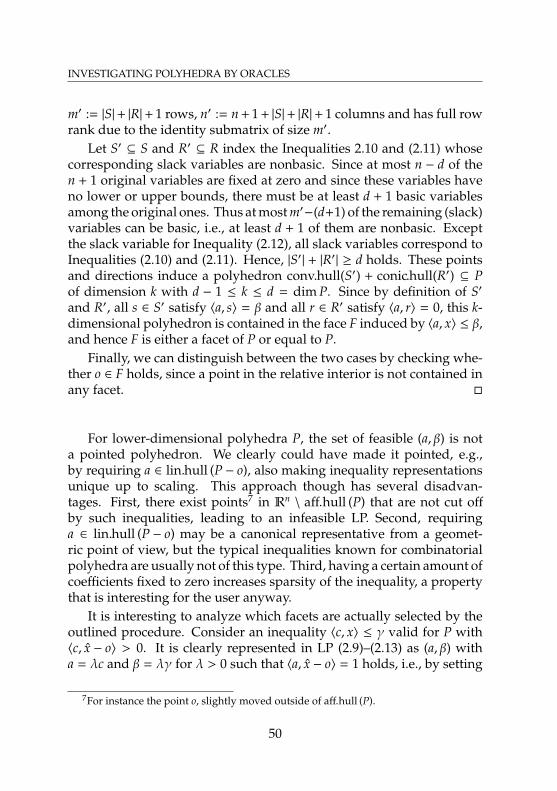
INVESTIGATING POLYHEDRA BY ORACLES
m′ := |S|+ |R|+ 1 rows, n′ := n + 1 + |S|+ |R|+ 1 columns and has full rowrank due to the identity submatrix of size m′.
Let S′ ⊆ S and R′ ⊆ R index the Inequalities 2.10 and (2.11) whosecorresponding slack variables are nonbasic. Since at most n − d of then + 1 original variables are fixed at zero and since these variables haveno lower or upper bounds, there must be at least d + 1 basic variablesamong the original ones. Thus at most m′−(d+1) of the remaining (slack)variables can be basic, i.e., at least d + 1 of them are nonbasic. Exceptthe slack variable for Inequality (2.12), all slack variables correspond toInequalities (2.10) and (2.11). Hence, |S′| + |R′| ≥ d holds. These pointsand directions induce a polyhedron conv.hull(S′) + conic.hull(R′) ⊆ Pof dimension k with d − 1 ≤ k ≤ d = dim P. Since by definition of S′
and R′, all s ∈ S′ satisfy 〈a, s〉 = β and all r ∈ R′ satisfy 〈a, r〉 = 0, this k-dimensional polyhedron is contained in the face F induced by 〈a, x〉 ≤ β,and hence F is either a facet of P or equal to P.
Finally, we can distinguish between the two cases by checking whe-ther o ∈ F holds, since a point in the relative interior is not contained inany facet.
For lower-dimensional polyhedra P, the set of feasible (a, β) is nota pointed polyhedron. We clearly could have made it pointed, e.g.,by requiring a ∈ lin.hull (P − o), also making inequality representationsunique up to scaling. This approach though has several disadvan-tages. First, there exist points7 in Rn
\ aff.hull (P) that are not cut offby such inequalities, leading to an infeasible LP. Second, requiringa ∈ lin.hull (P − o) may be a canonical representative from a geomet-ric point of view, but the typical inequalities known for combinatorialpolyhedra are usually not of this type. Third, having a certain amount ofcoefficients fixed to zero increases sparsity of the inequality, a propertythat is interesting for the user anyway.
It is interesting to analyze which facets are actually selected by theoutlined procedure. Consider an inequality 〈c, x〉 ≤ γ valid for P with〈c, x − o〉 > 0. It is clearly represented in LP (2.9)–(2.13) as (a, β) witha = λc and β = λγ for λ > 0 such that 〈a, x − o〉 = 1 holds, i.e., by setting
7For instance the point o, slightly moved outside of aff.hull (P).
50
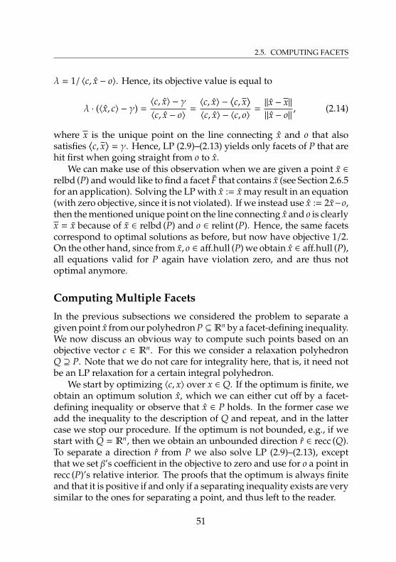
2.5. COMPUTING FACETS
λ = 1/ 〈c, x − o〉. Hence, its objective value is equal to
λ · (〈x, c〉 − γ) =〈c, x〉 − γ〈c, x − o〉
=〈c, x〉 −
⟨c, x
⟩〈c, x〉 − 〈c, o〉
=||x − x||||x − o||
, (2.14)
where x is the unique point on the line connecting x and o that alsosatisfies
⟨c, x
⟩= γ. Hence, LP (2.9)–(2.13) yields only facets of P that are
hit first when going straight from o to x.We can make use of this observation when we are given a point x ∈
relbd (P) and would like to find a facet F that contains x (see Section 2.6.5for an application). Solving the LP with x := x may result in an equation(with zero objective, since it is not violated). If we instead use x := 2x−o,then the mentioned unique point on the line connecting x and o is clearlyx = x because of x ∈ relbd (P) and o ∈ relint (P). Hence, the same facetscorrespond to optimal solutions as before, but now have objective 1/2.On the other hand, since from x, o ∈ aff.hull (P) we obtain x ∈ aff.hull (P),all equations valid for P again have violation zero, and are thus notoptimal anymore.
Computing Multiple Facets
In the previous subsections we considered the problem to separate agiven point x from our polyhedron P ⊆ Rn by a facet-defining inequality.We now discuss an obvious way to compute such points based on anobjective vector c ∈ Rn. For this we consider a relaxation polyhedronQ ⊇ P. Note that we do not care for integrality here, that is, it need notbe an LP relaxation for a certain integral polyhedron.
We start by optimizing 〈c, x〉 over x ∈ Q. If the optimum is finite, weobtain an optimum solution x, which we can either cut off by a facet-defining inequality or observe that x ∈ P holds. In the former case weadd the inequality to the description of Q and repeat, and in the lattercase we stop our procedure. If the optimum is not bounded, e.g., if westart with Q = Rn, then we obtain an unbounded direction r ∈ recc (Q).To separate a direction r from P we also solve LP (2.9)–(2.13), exceptthat we set β’s coefficient in the objective to zero and use for o a point inrecc (P)’s relative interior. The proofs that the optimum is always finiteand that it is positive if and only if a separating inequality exists are verysimilar to the ones for separating a point, and thus left to the reader.
51
INVESTIGATING POLYHEDRA BY ORACLES
Using this strategy we typically obtain several facets until we even-tually find a point x ∈ P. This iteration number clearly depends on thetightness of the relaxation Q: If Q does not approximate P in a reasonableway, then many iterations are needed, which is not bad by itself, but ithappens frequently that the procedure yields many trivial facets beforeactually computing an interesting one. On the other hand, if the opti-mum objective value (w.r.t. c) over Q is equal to that of P, then we mightnot learn anything new. To cope with this problem there are two ways,which can also be combined. One simple trick is to weaken the relax-ation by simply relaxing right-hand side vectors. Although in this caseIPO may just return the original inequalities, it sometimes happens thata different inequality is obtained. The other approach is to try differentobjective vectors. In fact it may even require some mathematical workin order to come up with such bad objective vectors, or at least usefulparameters to randomly generate them. For instance, in Section 2.10.3we consider a polyhedral reduction of vertex cover polytopes to treepolytopes that can be used to come up with objective vectors that yieldfractional solutions, and hence allow IPO to detect new facets of thelatter polytopes.
52

2.6. IDENTIFYING VERTICES, EDGES AND OTHER FACES
INVESTIGATING POLYHEDRA BY ORACLES:
2.6 Identifying Vertices, Edges andOther Faces
The goal of this section is to devise practical algorithms that solve thefollowing problem. Given an optimization oracle O for a rational poly-hedron P ⊆ Rn, as well as finite sets S ⊆ P and R ⊆ recc (P), decidewhether F := conv.hull (S) + conic.hull (R) is a face of P. A related taskis to ask for the smallest face F containing F, and particular cases are tocheck whether a given point s ∈ P defines a vertex and to check whethertwo vertices s1, s2 of P are adjacent (i.e., conv.hull (s1, s2) defines an edge).
All these problems can be solved in time polynomial in n, the encod-ing length of P and the running-time of O using the ellipsoid method[62]. Schrijver presents algorithms for related problems, but – althoughthey run in polynomial-time – they make use of the equivalence of op-timization and separation multiple times in a nested manner, which isimpractical even if one replaces the ellipsoid method by some practicallyefficient method.
Let, throughout this section, S,R ⊆ Qn be given finite sets, and O begiven. We will always assume that ∅ , S ⊆ P and R ⊆ recc (P) hold.
The Smallest Containing Face
We begin with an algorithm that determines a vector c whose associatedoptimal face F := arg max 〈c, x〉 | x ∈ P is the smallest face containing F.
A first useful observation, stated in the next lemma, is that it suffices
53
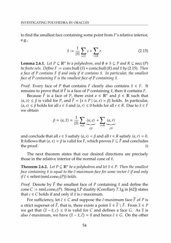
INVESTIGATING POLYHEDRA BY ORACLES
to find the smallest face containing some point from F’s relative interior,e.g.,
x :=1|S|
∑s∈S
s +∑r∈R
r. (2.15)
Lemma 2.6.1. Let P ⊆ Rn be a polyhedron, and ∅ , S ⊆ P and R ⊆ recc (P)be finite sets. Define F := conv.hull (S) + conic.hull (R) and x by (2.15). Thena face of P contains F if and only if it contains x. In particular, the smallestface of P containing F is the smallest face of P containing x.
Proof. Every face of P that contains F clearly also contains x ∈ F. Itremains to prove that if F is a face of P containing x, then it contains F.
Because F is a face of P, there exist a ∈ Rn and β ∈ R such that〈a, x〉 ≤ β is valid for P, and F =
x ∈ P | 〈a, x〉 = β
holds. In particular,
〈a, s〉 ≤ β holds for all s ∈ S and 〈a, r〉 ≤ 0 holds for all r ∈ R. Due to x ∈ Fwe obtain
β = 〈a, x〉 =1|S|
∑s∈S
〈a, s〉︸︷︷︸≤β
+∑r∈R
〈a, r〉︸︷︷︸≤0
and conclude that all s ∈ S satisfy 〈a, s〉 = β and all r ∈ R satisfy 〈a, r〉 = 0.It follows that 〈a, x〉 = β is valid for F, which proves F ⊆ F and concludesthe proof.
The next theorem states that our desired directions are preciselythose in the relative interior of the normal cone of x.
Theorem 2.6.2. Let P ⊆ Rn be a polyhedron and let x ∈ P. Then the smallestface containing x is equal to the c-maximum face for some vector c if and onlyif c ∈ relint (nml.conex(P)) holds.
Proof. Denote by F the smallest face of P containing x and define thecone C := nml.conex(P). Strong LP duality (Corollary 7.1g in [62]) statesthat c ∈ C holds if and only if x is c-maximum.
For sufficiency, let c ∈ C and suppose the c-maximum face F of P isa strict superset of F, that is, there exists a point x ∈ F \ F. From x ∈ Pwe get that
⟨x − x, c
⟩≤ 0 is valid for C and defines a face G. As x is
also c-maximum, we have⟨x − x, c
⟩= 0 and hence c ∈ G. On the other
54
2.6. IDENTIFYING VERTICES, EDGES AND OTHER FACES
hand, since F , F holds, there exists a facet-defining inequality 〈a, x〉 ≤ βsatisfied with equality by F (in particular by x), but not by x. This inturn implies
⟨x − x, a
⟩< 0, i.e., a < G. Hence, G is a proper face of C and
we obtain c < relint (C).For necessity, let c ∈ C \ relint (C), that is, there exists a proper face
G of C induced by the inequality 〈v, c〉 ≤ 0 valid for C with 〈v, c〉 = 0.This implies that v ∈ rad.conex(P), i.e., we can assume v to be scaledsuch that x := x + v ∈ P holds. Since G is a proper face, there exists adirection a ∈ C \ G that is a normal vector of a facet of P containing x,i.e., for some β ∈ R, 〈a, x〉 ≤ β is valid for P, 〈v, a〉 < 0, and 〈a, x〉 = βhold. From 〈v, a〉 < 0 we obtain
⟨a, x
⟩< β, which proves x ∈ P \ F. Since⟨
c, x⟩
= 〈c, x〉 holds, the c-maximum face of P must be strictly larger thanF. This concludes the proof.
Luckily, we can compute a relative interior point of a polyhedron ifwe can optimize over it by invoking Algorithm 2.4.2 from Section 2.4.Note that in the case of a cone, “optimizing” essentially means to com-pute for a given objective vector an unbounded direction with positivescalar product or return the zero vector as the optimal point. In order tooptimize a linear function 〈v, ·〉 over the normal cone of a given point xwe will use the following LP that is based on the definition of a normalcone.
max 〈v, c〉 (2.16)s.t. 〈s, c〉 − δ ≤ 0 for all s ∈ vert (P) (2.17)
〈r, c〉 ≤ 0 for all r ∈ ext.rays (P) (2.18)〈x, c〉− δ = 0 (2.19)
c ∈ Rn, δ ∈ R (2.20)
Note that the projection of the set of feasible (c, δ) onto the c-space is anisomorphism due to Equation (2.19), and hence the relative interior ofthe feasible region is projected onto the relative interior of the normalcone. Techniques to solve this LP efficiently are described in Section 2.7.
Suppose we know the inequality 〈c, x〉 ≤ δ that induces our desiredface and we want to determine its dimension (e.g., in order to checkwhether a given point is a vertex). For this we could turn our optimiza-tion oracle for P into one for F (see Section 2.3.3) and compute F’s affine
55
INVESTIGATING POLYHEDRA BY ORACLES
hull. The next proposition states that we can calculate the dimensionfrom that of the normal cone we used to compute c.
Proposition 2.6.3. Let P ⊆ Rn be a polyhedron, let x ∈ P, and let F be thesmallest face of P containing x. Then lin.hull
(F − x
)= nml.conex(P)⊥ holds
and hence the dimension of F is equal to n − dim (nml.conex(P)).
Proof. Let v ∈ (F − x). Since F is the smallest face of P containing x, wehave x ∈ relint(F), and hence there exists λ > 0 such that (x − λv) ∈ Fholds, proving v,−v ∈ rad.conex(P), which implies v ⊥ nml.conex(P).
Let the equation 〈v, x〉 = 0 be valid for nml.conex(P). Hence, wehave v ∈ lineal (rad.conex(P)), which proves (x + λv), (x − λv) ∈ P forsufficiently small λ > 0. Let a ∈ Rn, β ∈ R be such that 〈a, x〉 ≤ βis valid for P, and F = arg max 〈a, x〉 | x ∈ P holds. From 〈a, x〉 = β,〈a, x + λv〉 ≤ β and 〈a, x − λv〉 ≤ β it follows that 〈a, v〉 = 0 holds, that is,v ∈ lin.hull(F − x) holds, which concludes the proof.
The results of this section, together with Theorem 2.4.7 directly yieldthe correctness of the following algorithm:
Algorithm 2.6.1: Smallest Containing FaceInput: Optimization oracleO for a polyhedron P ⊆ Rn and x ∈ POutput: A vector c whose maximum face F of P is the smallest
face containing x, and the dimension dim F of that face.
1 Using O and LP (2.16)–(2.20), construct an optimization oracleOC for C := nml.conex(P) (see Section 2.7).
2 Call Algorithm 2.4.2 with OC and obtain (S,R,B,Ax = b).3 Compute a relative interior point c of C by Equation (2.15).4 return (c, | rows (A) | − 1).
Detecting VerticesWith Proposition 2.6.3 at hand we can easily check if a given point s ∈ Pis a vertex of P. For this we simply compute the dimension of the normalcone at s, which is equal to the ambient dimension n if and only if s isa vertex. The next observation shows that we still have to be careful,though.
56
2.6. IDENTIFYING VERTICES, EDGES AND OTHER FACES
Observation 2.6.4. Let P ⊆ Rn be a polytope and let x < P. Then
C :=c ∈ Rn
| ∃δ satisfying (2.17), (2.18) and (2.19)
is full-dimensional.
Proof. From x < P we conclude that there exists a separating hyper-plane, i.e., there exists c ∈ Rn with 〈c, x〉 > max 〈c, x〉 | x ∈ P. SinceP is bounded, any sufficiently small perturbation c of c has the sameproperty. This concludes the proof since c and all c are contained inC.
Suppose we accidentally call Algorithm 2.6.1 for a point x < P. Thenwe would conclude x to be a vertex, although it is not even containedin P. Hence we have to ensure x ∈ P beforehand.
Detecting Edges and Extreme RaysSuppose we are given two vertices s1 and s2 of P and want to test whetherF := conv.hull (s1, s2) is an edge of P. By Lemma 2.6.1 we just have todetermine the dimension of the smallest face containing x := 1
2 s1 + 12 s2
since this smallest face is 1-dimensional if and only if F is an edge.The situation is similar for extreme rays: For given vertex s ∈ P and
extreme ray r ∈ recc (P) we only have to check whether the smallest facecontaining s + r is 1-dimensional.
We now discuss how to obtain certificates for the two situations.Suppose the algorithm determines that F is indeed 1-dimensional, thatis, the normal cone C of x is at least (n− 1)-dimensional (in fact dim C =n−1 holds since 〈s1 − s2, c〉 = 0 is valid for C). The certificate for this factis a set of (n − 1) linearly independent rays r1, . . . , rn−1 ∈ C. Note thatAlgorithm 2.4.2 actually computes these rays. In order to verify sucha certificate, the user has to test for linear independence and to checkthat each of the ri’s is in the normal cone, which in turn can be done bymaximizing 〈ri, x〉 over P (and verifying that the maximum is equal to〈ri, x〉).
Suppose the algorithm determines that F is higher-dimensional. Avery practical certificate, often used in proofs for non-adjacency, is towrite x as a nontrivial convex combination of points in P plus a coniccombination of extreme rays of P. We now describe how to obtain such
57
INVESTIGATING POLYHEDRA BY ORACLES
a certificate while running Algorithm 2.6.1. Since F is not an edge, thereexists an equation 〈w, c〉 = 0 valid for all c ∈ C such that w is not parallelto (s2 − s1). Algorithm 2.4.2 obtains this equation by maximizing andminimizing 〈w, c〉 over C. According to the construction of OC in Step 1of Algorithm 2.6.1, this is done by solving two of the LPs (2.16)–(2.20).We now consider the dual of this LP:
min 0 (2.21)
s.t.∑
s∈vert(P)
sλs +∑
r∈ ext.rays(P)
rµr + xξ = v (2.22)∑s∈vert(P)
−λs − ξ = 0 (2.23)
λ ∈ Rvert(P)+ , µ ∈ R
ext.rays(P)+ , ξ ∈ R (2.24)
The next proposition states that the two sets of dual values obtained forv ∈ w,−w yield our desired convex combination.
Proposition 2.6.5. Let P ⊆ Rn be a pointed polyhedron, and let F ⊆ Rn bea face of P of dimension at least 2. Let s1, s2 ∈ F be two vertices such thattheir barycenter x is in F’s relative interior, and let w ∈ lin.hull (F − x) be adirection valid for F. Let furthermore (λ+, µ+, ξ+) and (λ−, µ−, ξ−) be optimalsolutions of LP (2.21)–(2.24) for v = +w and v = −w, respectively. Then
x =∑
s∈vert(P)
λ+s + λ−s−ξ+ − ξ−
s +∑
r∈ ext.rays(P)
µ+r + µ−r−ξ+ − ξ−
r (2.25)
holds. Furthermore, if w is not parallel to (s2 − s1), then the combination is notthe trivial one x = 1
2 s1 + 12 s2.
Proof. We will first prove that the LP (2.21)–(2.24) is feasible. Due tox ∈ relint (F), we have that for v ∈ +w,−w, v lies in the radial cone ofx w.r.t. P, that is, there exist λ ∈ Rvert(P)
+ and µ ∈ Rext.rays(P)+ that satisfy∑
s∈vert(P)(s − x)λs +∑
r∈ ext.rays(P) rµr = v. By setting ξ according to (2.23),we obtain the two feasible solutions.
Let (λ+, µ+, ξ+) and (λ−, µ−, ξ−) be optimal solutions of LP (2.21)–(2.24) for v = +w and v = −w, respectively. From (2.23) and (2.24)we get that ξ+ and ξ− must be nonpositive. Furthermore, (ξ+ + ξ−) is
58
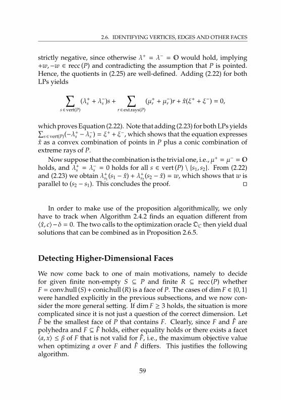
2.6. IDENTIFYING VERTICES, EDGES AND OTHER FACES
strictly negative, since otherwise λ+ = λ− = O would hold, implying+w,−w ∈ recc (P) and contradicting the assumption that P is pointed.Hence, the quotients in (2.25) are well-defined. Adding (2.22) for bothLPs yields∑
s∈vert(P)
(λ+s + λ−s )s +
∑r∈ ext.rays(P)
(µ+r + µ−r )r + x(ξ+ + ξ−) = 0,
which proves Equation (2.22). Note that adding (2.23) for both LPs yields∑s∈vert(P)(−λ+
s −λ−s ) = ξ+ + ξ−, which shows that the equation expresses
x as a convex combination of points in P plus a conic combination ofextreme rays of P.
Now suppose that the combination is the trivial one, i.e.,µ+ = µ− = Oholds, and λ+
s = λ−s = 0 holds for all s ∈ vert (P) \ s1, s2. From (2.22)and (2.23) we obtain λ+
s1(s1 − x) + λ+
s2(s2 − x) = w, which shows that w is
parallel to (s2 − s1). This concludes the proof.
In order to make use of the proposition algorithmically, we onlyhave to track when Algorithm 2.4.2 finds an equation different from〈x, c〉−δ = 0. The two calls to the optimization oracleOC then yield dualsolutions that can be combined as in Proposition 2.6.5.
Detecting Higher-Dimensional Faces
We now come back to one of main motivations, namely to decidefor given finite non-empty S ⊆ P and finite R ⊆ recc (P) whetherF = conv.hull (S) + conic.hull (R) is a face of P. The cases of dim F ∈ 0, 1were handled explicitly in the previous subsections, and we now con-sider the more general setting. If dim F ≥ 3 holds, the situation is morecomplicated since it is not just a question of the correct dimension. LetF be the smallest face of P that contains F. Clearly, since F and F arepolyhedra and F ⊆ F holds, either equality holds or there exists a facet〈a, x〉 ≤ β of F that is not valid for F, i.e., the maximum objective valuewhen optimizing a over F and F differs. This justifies the followingalgorithm.
59
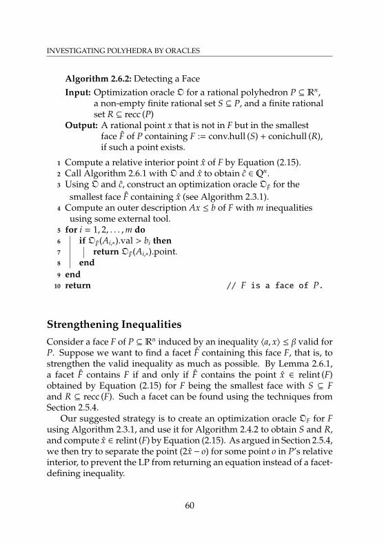
INVESTIGATING POLYHEDRA BY ORACLES
Algorithm 2.6.2: Detecting a FaceInput: Optimization oracle O for a rational polyhedron P ⊆ Rn,
a non-empty finite rational set S ⊆ P, and a finite rationalset R ⊆ recc (P)
Output: A rational point x that is not in F but in the smallestface F of P containing F := conv.hull (S) + conic.hull (R),if such a point exists.
1 Compute a relative interior point x of F by Equation (2.15).2 Call Algorithm 2.6.1 with O and x to obtain c ∈ Qn.3 Using O and c, construct an optimization oracle OF for the
smallest face F containing x (see Algorithm 2.3.1).4 Compute an outer description Ax ≤ b of F with m inequalities
using some external tool.5 for i = 1, 2, . . . ,m do6 if OF(Ai,∗).val > bi then7 return OF(Ai,∗).point.8 end9 end
10 return // F is a face of P.
Strengthening InequalitiesConsider a face F of P ⊆ Rn induced by an inequality 〈a, x〉 ≤ β valid forP. Suppose we want to find a facet F containing this face F, that is, tostrengthen the valid inequality as much as possible. By Lemma 2.6.1,a facet F contains F if and only if F contains the point x ∈ relint (F)obtained by Equation (2.15) for F being the smallest face with S ⊆ Fand R ⊆ recc (F). Such a facet can be found using the techniques fromSection 2.5.4.
Our suggested strategy is to create an optimization oracle OF for Fusing Algorithm 2.3.1, and use it for Algorithm 2.4.2 to obtain S and R,and compute x ∈ relint (F) by Equation (2.15). As argued in Section 2.5.4,we then try to separate the point (2x− o) for some point o in P’s relativeinterior, to prevent the LP from returning an equation instead of a facet-defining inequality.
60
2.7. SOLVING THE POLAR LINEAR PROGRAMS
INVESTIGATING POLYHEDRA BY ORACLES:
2.7 Solving the Polar Linear Programs
We already encountered two situations, namely the computation offacets (see Section 2.5.2) and of the smallest containing face (see Sec-tion 2.6.1), in which we searched for certain inequalities valid for arational non-empty polyhedron P using a linear program, where P isgiven by an optimization oracle. In both applications the LP consistedof the following inequalities in addition to only a few others.
〈s, a〉 − β ≤ 0 for all s ∈ S (2.26)〈r, a〉 ≤ 0 for all r ∈ R (2.27)
Here, S ⊇ vert (P) is a finite superset of P’s vertices, while R ⊇ ext.rays (P)is a finite superset of its extreme rays. We furthermore assume that theorigin (a, β) = (O, 0) is feasible, i.e., none of the additional constraintscuts it off.
This section deals with different aspects for solving such linear pro-grams in practice. We first settle how to solve the separation problemfor both constraints using O. It allows us to start with only a few (oreven none) of the inequalities, adding inequalities that are violated bythe current solution until all are satisfied. Despite this lazy addition,the LPs may become very large in terms of rows, and hence we imple-mented a so-called cut aging strategy that is described in the second part.In the last part we discuss stabilization, a technique that is applied tocontain tailing-off effects.
61
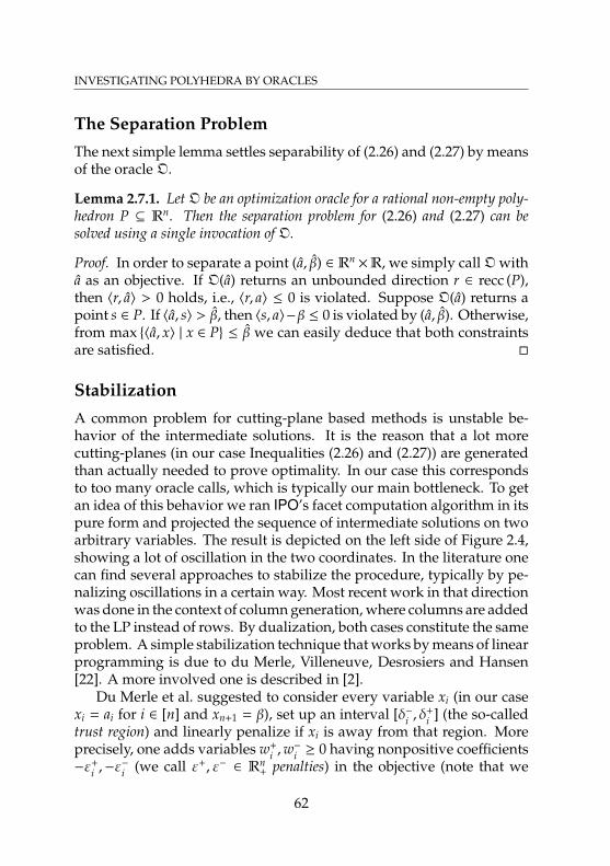
INVESTIGATING POLYHEDRA BY ORACLES
The Separation Problem
The next simple lemma settles separability of (2.26) and (2.27) by meansof the oracle O.
Lemma 2.7.1. LetO be an optimization oracle for a rational non-empty poly-hedron P ⊆ Rn. Then the separation problem for (2.26) and (2.27) can besolved using a single invocation of O.
Proof. In order to separate a point (a, β) ∈ Rn×R, we simply callOwith
a as an objective. If O(a) returns an unbounded direction r ∈ recc (P),then 〈r, a〉 > 0 holds, i.e., 〈r, a〉 ≤ 0 is violated. Suppose O(a) returns apoint s ∈ P. If 〈a, s〉 > β, then 〈s, a〉−β ≤ 0 is violated by (a, β). Otherwise,from max 〈a, x〉 | x ∈ P ≤ β we can easily deduce that both constraintsare satisfied.
Stabilization
A common problem for cutting-plane based methods is unstable be-havior of the intermediate solutions. It is the reason that a lot morecutting-planes (in our case Inequalities (2.26) and (2.27)) are generatedthan actually needed to prove optimality. In our case this correspondsto too many oracle calls, which is typically our main bottleneck. To getan idea of this behavior we ran IPO’s facet computation algorithm in itspure form and projected the sequence of intermediate solutions on twoarbitrary variables. The result is depicted on the left side of Figure 2.4,showing a lot of oscillation in the two coordinates. In the literature onecan find several approaches to stabilize the procedure, typically by pe-nalizing oscillations in a certain way. Most recent work in that directionwas done in the context of column generation, where columns are addedto the LP instead of rows. By dualization, both cases constitute the sameproblem. A simple stabilization technique that works by means of linearprogramming is due to du Merle, Villeneuve, Desrosiers and Hansen[22]. A more involved one is described in [2].
Du Merle et al. suggested to consider every variable xi (in our casexi = ai for i ∈ [n] and xn+1 = β), set up an interval [δ−i , δ
+i ] (the so-called
trust region) and linearly penalize if xi is away from that region. Moreprecisely, one adds variables w+
i ,w−
i ≥ 0 having nonpositive coefficients−ε+
i ,−ε−
i (we call ε+, ε− ∈ Rn+ penalties) in the objective (note that we
62
2.7. SOLVING THE POLAR LINEAR PROGRAMS
maximize) and adds constraints xi ≤ w+i + δ+
i and xi ≥ −w−i + δ−i . Nowif xi ∈ [δ−i , δ
+i ] holds, then both extra variables can be set to zero for no
cost. But if xi is outside the trust region, e.g., if xi > δ+i , then the LP has
to pay the costs for each unit of w+i = xi − δ+
i .Clearly one has to come up with update strategies for the trust
regions (as we don not know the right value of xi in advance) andfor the penalty values. Moreover, in the mentioned papers the authorscan usually specify certain initial values since they consider specificproblems. We are not in this situation as we do not know the sizes ofour inequalities’ coefficients a priori. This is particularly important forthe penalties: If they are too large, the solution is bound to the trustregion, and if they are too small, we do not stabilize at all. In order tocalibrate the penalty values we decided to start with an initially largeuniform penalty value ε ≥ 0 (that is, every w±i -variable has objectivevalue −ε) and the trivial interval [0, 0]. This will lead to the origin (i.e.,a = O, β = 0) as the optimal solution. As long as this is the case wedecrease ε by 50 %, until the optimum is different from the origin.
A very interesting observation that we made is that by just contin-uing this “calibration” we can already reduce the number of iterationssignificantly. So suppose we actually obtained an optimal solution thatis not equal to the origin. Then we separate inequalities as long as possi-ble, that is, either until the optimum is again equal to the origin, or untilthe current solution is indeed feasible. After this separation sequencewe decrease ε further and repeat. Finally, ε will be very small, havingno impact on the solution, we can set it to zero and obtain the originalLP.
Since a thorough investigation of stabilization approaches and corre-sponding update strategies is out of the scope of this thesis, we decidedto keep this behavior. At the end of this section we will present compu-tational results for an example instance that justify this decision.
In order to obtain correct solutions we eventually have to solve the LPwith exact arithmetic. But in fact we do not care about exactly computedstabilization values w±i and also not about the precision of the computedintermediate solutions. This motivates to run the described stabilizationprocedure with floating-point precision only and then warm-start a non-stabilized procedure that uses exact arithmetic. To carry out the warm-start we only have to extract those points S and directions R that were
63
INVESTIGATING POLYHEDRA BY ORACLES
required to prove optimality of the stabilization LP, i.e., those for whichthe corresponding slack variables were nonbasic. In our experiments,this strategy worked well in the sense that we rarely had to add moreinequalities to the LP after the warm-start.
Cut Aging
Despite stabilization, usually many cutting planes need to be separated,in particular more than actually needed to assert optimality. Accordingto our knowledge, all state-of-the-art solvers implement an aging strat-egy, which is a simple heuristic that removes inequalities from the LPthat were not useful for a certain number of cut rounds. For this, onetypically maintains a number called the age of a row. If a row is not “use-ful”, its age is incremented, while the age is set to zero for useful ones.The maximum age of a row is 20 by default, but can be specified by theuser. We do not maintain a cut pool, that is, we do not explicitly collectthe removed inequalities. Instead we store the set of known points anddirections returned by the oracle and search among those for violatedinequalities before calling the oracle. Hence, re-adding inequalities thatwere removed due to aging is not a costly operation.
The cutting-plane procedure might get stuck in the sense that itonly adds back inequalities that were removed due to aging withoutmaking any progress. If the number of rounds in which only knowninequalities are added and the objective did not improve exceeds themaximum age, then this age is increased. This strategy guarantees thatwe will eventually terminate. IPO considers a row as “useful” if its dualis nonzero, which is the same strategy that is implemented in SCIP.
Effect of Stabilization and Cut Aging
We consider, as an example instance, an integer program with 105 vari-ables over the master edge cover polytope, defined in Section 2.10.2, for thecomplete graph with 14 nodes. For a fixed random objective, IPO de-tected six facets and we report statistics for the whole facet-computation.Note that we just want to illustrate the effect of stabilization and cut ag-ing, and by no means claim that the effects will be the same (or similar)for other polyhedra. In fact they will highly depend on the dimensionand the relative running times of heuristics and oracles.
64
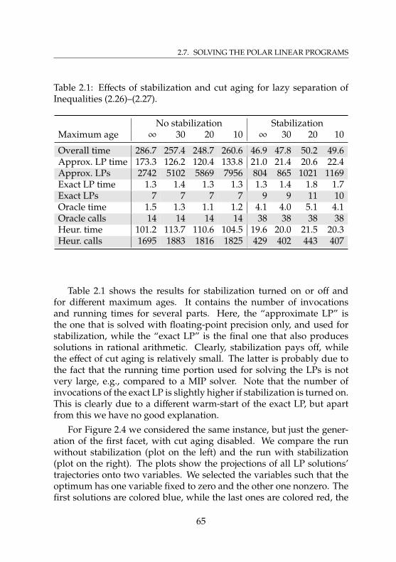
2.7. SOLVING THE POLAR LINEAR PROGRAMS
Table 2.1: Effects of stabilization and cut aging for lazy separation ofInequalities (2.26)–(2.27).
No stabilization StabilizationMaximum age ∞ 30 20 10 ∞ 30 20 10
Overall time 286.7 257.4 248.7 260.6 46.9 47.8 50.2 49.6Approx. LP time 173.3 126.2 120.4 133.8 21.0 21.4 20.6 22.4Approx. LPs 2742 5102 5869 7956 804 865 1021 1169Exact LP time 1.3 1.4 1.3 1.3 1.3 1.4 1.8 1.7Exact LPs 7 7 7 7 9 9 11 10Oracle time 1.5 1.3 1.1 1.2 4.1 4.0 5.1 4.1Oracle calls 14 14 14 14 38 38 38 38Heur. time 101.2 113.7 110.6 104.5 19.6 20.0 21.5 20.3Heur. calls 1695 1883 1816 1825 429 402 443 407
Table 2.1 shows the results for stabilization turned on or off andfor different maximum ages. It contains the number of invocationsand running times for several parts. Here, the “approximate LP” isthe one that is solved with floating-point precision only, and used forstabilization, while the “exact LP” is the final one that also producessolutions in rational arithmetic. Clearly, stabilization pays off, whilethe effect of cut aging is relatively small. The latter is probably due tothe fact that the running time portion used for solving the LPs is notvery large, e.g., compared to a MIP solver. Note that the number ofinvocations of the exact LP is slightly higher if stabilization is turned on.This is clearly due to a different warm-start of the exact LP, but apartfrom this we have no good explanation.
For Figure 2.4 we considered the same instance, but just the gener-ation of the first facet, with cut aging disabled. We compare the runwithout stabilization (plot on the left) and the run with stabilization(plot on the right). The plots show the projections of all LP solutions’trajectories onto two variables. We selected the variables such that theoptimum has one variable fixed to zero and the other one nonzero. Thefirst solutions are colored blue, while the last ones are colored red, the
65
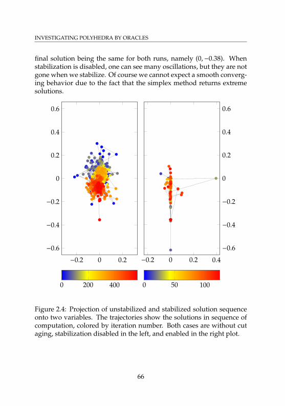
INVESTIGATING POLYHEDRA BY ORACLES
final solution being the same for both runs, namely (0,−0.38). Whenstabilization is disabled, one can see many oscillations, but they are notgone when we stabilize. Of course we cannot expect a smooth converg-ing behavior due to the fact that the simplex method returns extremesolutions.
−0.2 0 0.2
−0.6
−0.4
−0.2
0
0.2
0.4
0.6
0 200 400
−0.2 0 0.2 0.4
−0.6
−0.4
−0.2
0
0.2
0.4
0.6
0 50 100
Figure 2.4: Projection of unstabilized and stabilized solution sequenceonto two variables. The trajectories show the solutions in sequence ofcomputation, colored by iteration number. Both cases are without cutaging, stabilization disabled in the left, and enabled in the right plot.
66
2.8. IMPROVING READABILITY OF EQUATIONS AND INEQUALITIES
INVESTIGATING POLYHEDRA BY ORACLES:
2.8 Improving Readability ofEquations and Inequalities
The main use case for IPO is the computation of equations and in-equalities valid for a polyhedron of interest with the goal that the userhopefully understands and generalizes them. As this final step is clearlynot mechanical, the actual representation of these objects matters a lot.First we only consider integral representations, that is, all equationsand inequalities presented to a user must have integral normal vectors.Second, we believe that verifying the validity of an equation or an in-equality by hand usually requires a certain amount of time per nonzero,and that the effort for larger (absolute values of) coefficients is higher.In case of complicated coefficients a user may even think that thereare number-theoretic reasons for the validity, although there could be asimple combinatorial explanation. This motivates our decision to prefersparse normal vectors over dense ones, but also try to avoid large co-efficients. For equations we already designed the affine-hull algorithmsuch that sparse objective vectors are preferred (see Section 2.4.5).
In this section we consider a simple technique to post-process equa-tions and inequalities to find a nicer representation. For this we try tominimize Manhattan norms ||a||1 :=
∑ni=1 |ai| of the corresponding normal
vectors a ∈ Zn. It clearly avoids coefficients of large absolute value, butalso cares a bit for sparsity, e.g., in contrast to the maximum norm. Sincefinding normal vectors with a global minimum norm is hard (and outof the scope of this thesis), we present a local-improvement heuristic.
67
INVESTIGATING POLYHEDRA BY ORACLES
Manhattan Norm ProblemsImproving the readability of a set of given equations as discussed aboveis essentially the following problem.
Problem 2.8.1 (`1-shortest Basis). Given a vector space V ⊆ Qn by meansof a rational basis, find an integral basis v1, . . . , vk ∈ Z
n of V whose sum of`1-norms
∑ki=1 ||vi||1 is minimum.
Although we are not aware of an NP-hardness proof, there is a resultby Haviv and Regev [35], who showed that unless NP ⊆ RP8 holds, thereis no polynomial-time constant-factor approximation algorithm for theshortest vector problem for the `1-norm. It is not too hard to see that anoptimum solution to Problem 2.8.1 always contains a vector of minimum`1-norm since otherwise we could add to to the basis and remove anyother linearly dependent vector. Note that Haviv and Regev’s resultholds for any `p norm for 1 ≤ p ≤ ∞.
Short integral vectors in the span of the equations’ normal vectorsand the normal vector of a given inequality are only useful if we canactually replace the latter by such a short vector. Let v1, . . . , vk be a basisof any subspace V of Rn. We say that a vector v ∈ V depends on vi(w.r.t. this basis) if the multiplier λi in the (unique) linear combinationv =
∑ki=1 λivi is nonzero. Assuming that v2, . . . , vk are the equations’
normals, and that v1 is that of a given inequality, our problem of interestis as follows.
Problem 2.8.2 (`1-shortest Vector with One Dependency). Given a vectorspace V ⊆ Qn by means of a basis v1, . . . , vk ∈ Z
n, find a vector v ∈ Zn\ O
of minimum `1-norm which depends on v1.
It is again not hard to see this new problem is not simpler than theshortest vector problem: We reorder the vectors v1, . . . , vk in k ways suchthat the first vector is always a different one, and solve Problem 2.8.2 foreach of these instances. Then, among the k solutions we will find ourshortest vector since it must depend on some of the vi.
Due to the hardness of these problems we decided to implement alocal improvement heuristic that we present in the next section.
8RP consists of those decision problems that can be solved in polynomial time on arandomized Turing machine.
68
2.8. IMPROVING READABILITY OF EQUATIONS AND INEQUALITIES
Two Vectors: An Exact AlgorithmOur main result in this section is the following theorem that enables usto approximately reduce the `1-norm sum of a basis by iteratively con-sidering pairs of basis vectors, solving the corresponding subproblemto optimality and replacing one of the vectors by the solution.
Theorem 2.8.3. Problem 2.8.2 for k = 2 can be solved in polynomial time.
Let us first start with a simple lemma that tells us how to reduce theproblem to one where we only have to consider integral combinations ofthe vectors. This is ensured by replacing them by a lattice basis of theirspan.
Lemma 2.8.4. Let u, v ∈ Zn be two linearly independent vectors, and let the
matrix H =
(α 0β γ
)∈ Z2×2 be such that [H | O2×(n−2)] is the Hermite normal
form of(vᵀ
uᵀ
)∈ Z2×n. Then v = 1
α v and u = 1αγ (αu − βv) are a lattice basis
of lin.hull (u, v) ∩ Zn and a vector (λu + µv) depends on u if and only if itdepends on u.
Proof. Let U ∈ Zn×n be the unimodular matrix such that we have[H | O2×(n−2)
]=
(vᵀ
uᵀ
)·Uᵀ,
which implies αe(1) = Uv and βe(1) +γe(2) = Uu. From the first equationwe derive Uv = e
(1) and from both equations we obtain
Uu =1αγ
(αUu − βUv) =1αγ
(αβe(1) + αγe(2)− αβe(1)) = e
(2).
Since U is unimodular (in particular, U−1∈ Zn×n), the vectors u and v are
integral. Consider any pair of multipliersλ, µ ∈ R for which w = λu+µvis an integral vector. Since then also Uw = λUu + µUv = λe(2) + µe(1)
is an integral vector, λ and µ must be integers and thus u and v form alattice basis.
We now prove the dependency property. A vector w does not dependon u w.r.t. the basis u, v if and only if it is a multiple of v. Similarly, w
69
INVESTIGATING POLYHEDRA BY ORACLES
does not depend on u w.r.t. the basis u, v if and only if it is a multiple ofv. Since v = 1
α v holds, the dependency properties are also equivalent,which concludes the proof.
For the rest of this section we can now assume that u, v ∈ Zn are alattice basis and we want to find integral multipliers λ, µwith λ , 0 suchthat
||λu + µv||1 =
n∑i=1
|λui + µvi| (2.28)
is minimum. Since (λ, µ) and (−λ,−µ) have the same objective values,we will even requireλ ≥ 1. One may be afraid of doing a case distinctionin order to resolve the n absolute value expressions in (2.28) since inprinciple this results in 2n cases. It turns out that this combinatorialexplosion does not occur because the sign of λui + µvi depends on thecomparison of µ/λ with −ui/vi for every i ∈ [n]. This leaves at mostn + 1 intervals such that for all λ, µ (with λ ≥ 1) such that µ/λ is in oneinterval, the objective function (2.28) is linear. This observation is madeprecise in the following lemma.
Lemma 2.8.5. Let u, v ∈ Zn be two linearly independent vectors and let−∞ = q0 < q1 < . . . < qk−1 < qk = ∞ be the sorted elements of the setQ :=
−
uivi| i ∈ [n] with vi , 0
∪ ±∞. Then the sign pattern of λu + µv is
constant over all multiplier pairs (λ, µ) with λ > 0 for which µ/λ is in anyfixed interval [q j−1, q j] for j ∈ [k].
Proof. Let (λ, µ) and (λ′, µ′) with λ, λ′ > 0 be two such multiplier pairssatisfying µ
λ ,µ′
λ′ ∈ [q j−1, q j] for some j ∈ [k], but with different signs onposition i: λui + µvi < 0 < λ′ui + µ′vi. We have vi , 0 since otherwiseλui < 0 < λ′ui holds, contradicting λ, λ′ > 0.
Hence − uivi∈ Q, that is, µλ and µ′
λ′ are either both less than or equal to
−uivi
or both greater than − uivi
. This implies that µλ + uivi
and µ′
λ′ +uivi
have thesame sign, which in turn implies that λui + µvi and λ′ui + µ′vi have thesame sign (using the fact that λ, λ′ > 0). This concludes the proof.
70
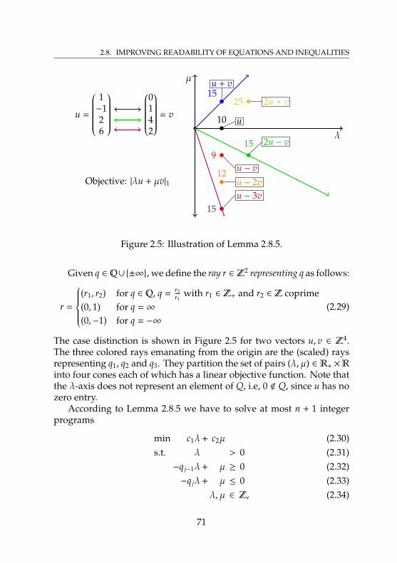
2.8. IMPROVING READABILITY OF EQUATIONS AND INEQUALITIES
λ
µ
10 u
15u + v
15 2u − v
15u − 3v
12u − 2v
9u − v
25 2u + vu =
1−126
0142
= v
Objective: |λu + µv|1
Figure 2.5: Illustration of Lemma 2.8.5.
Given q ∈ Q∪±∞, we define the ray r ∈ Z2 representing q as follows:
r =
(r1, r2) for q ∈ Q, q = r2
r1with r1 ∈ Z+ and r2 ∈ Z coprime
(0, 1) for q = ∞
(0,−1) for q = −∞
(2.29)
The case distinction is shown in Figure 2.5 for two vectors u, v ∈ Z4.The three colored rays emanating from the origin are the (scaled) raysrepresenting q1, q2 and q3. They partition the set of pairs (λ, µ) ∈ R+ ×Rinto four cones each of which has a linear objective function. Note thatthe λ-axis does not represent an element of Q, i.e, 0 < Q, since u has nozero entry.
According to Lemma 2.8.5 we have to solve at most n + 1 integerprograms
min c1λ+ c2µ (2.30)s.t. λ > 0 (2.31)−q j−1λ+ µ ≥ 0 (2.32)−q jλ+ µ ≤ 0 (2.33)
λ, µ ∈ Z, (2.34)
71
INVESTIGATING POLYHEDRA BY ORACLES
where c is a suitable objective function we will specify later and j ∈ [k].Note that (2.31) is a strict inequality constraint that could also be replacedby λ ≥ 1. Since integer programming is polynomial-time solvable infixed dimension (see [48]) these IPs can be solved in polynomial time,which proves Theorem 2.8.3.
For efficiency reasons, instead of solving IP (2.30)–(2.34) by a generalalgorithm we will now devise a problem-specific approach. Since wecan evaluate objective for the pairs (λ, µ) with µ/λ = qi for some i ∈[k − 1] directly, we can restrict our search for (integral) λ, µ satisfying−q j−1λ+µ > 0 and−q jλ+µ < 0, which impliesλ > 0. To see this, observethat the cone whose extreme rays are the rays representing q j−1 and q j iscontained in R+ ×R, and hence its interior is contained in R>0 ×R. Thenext lemma captures the objective function representing ||λu + µv||1 forsuch a cone.
Lemma 2.8.6. Let u, v ∈ Zn be two linearly independent vectors and let−∞ = q0 < q1 < . . . < qk−1 < qk = ∞ be as in Lemma 2.8.5. Consider a fixedj ∈ [k] and define
I+j :=
i ∈ [n] | vi > 0,−
ui
vi≤ q j−1 or vi < 0,−
ui
vi≥ q j or vi = 0,ui > 0
I−j :=
i ∈ [n] | vi < 0,−
ui
vi≤ q j−1 or vi > 0,−
ui
vi≥ q j or vi = 0,ui < 0
.
Then all (λ, µ) ∈ R>0 ×R with q j−1 ≤ µ/λ ≤ q j satisfy
||λu + µv||1 =∑i∈I+
j
(λui + µvi) −∑i∈I−j
(λui + µvi).
Proof. We have to prove that I+j (resp. I−j ) contains the set of i ∈ [n] for
which wi := λui + µvi is positive (resp. negative). Suppose λui + µvi > 0holds. If vi = 0, then the sign of wi agrees with the sign of ui. Otherwise,the condition is equivalent to vi(
uivi
+µλ ) > 0. For vi > 0 (resp. vi < 0) this
implies − uivi<
µλ (resp. − ui
vi>
µλ ). Using the fact that − ui
viis equal to q`
for some ` ∈ [k − 1], we observe that this is equivalent to − uivi≤ q j−1 for
vi > 0 and to − uivi≥ q j for vi < 0. This proves the statement for positive
λui + µvi, the case of negative λui + µvi being similar.
72
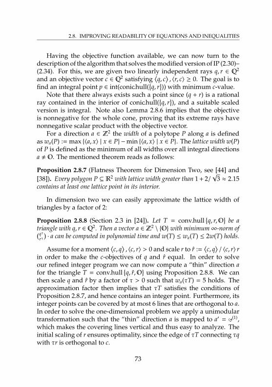
2.8. IMPROVING READABILITY OF EQUATIONS AND INEQUALITIES
Having the objective function available, we can now turn to thedescription of the algorithm that solves the modified version of IP (2.30)–(2.34). For this, we are given two linearly independent rays q, r ∈ Q2
and an objective vector c ∈ Q2 satisfying⟨q, c
⟩, 〈r, c〉 ≥ 0. The goal is to
find an integral point p ∈ int(conic.hull(q, r
)) with minimum c-value.
Note that there always exists such a point since (q + r) is a rationalray contained in the interior of conic.hull(
q, r
), and a suitable scaled
version is integral. Note also Lemma 2.8.6 implies that the objectiveis nonnegative for the whole cone, proving that its extreme rays havenonnegative scalar product with the objective vector.
For a direction a ∈ Z2 the width of a polytope P along a is definedas wa(P) := max 〈a, x〉 | x ∈ P −min 〈a, x〉 | x ∈ P. The lattice width w(P)of P is defined as the minimum of all widths over all integral directionsa , O. The mentioned theorem reads as follows:
Proposition 2.8.7 (Flatness Theorem for Dimension Two, see [44] and[38]). Every polygon P ⊆ R2 with lattice width greater than 1 + 2/
√3 ≈ 2.15
contains at least one lattice point in its interior.
In dimension two we can easily approximate the lattice width oftriangles by a factor of 2:
Proposition 2.8.8 (Section 2.3 in [24]). Let T = conv.hullq, r,O
be a
triangle with q, r ∈ Q2. Then a vector a ∈ Z2\ O with minimum∞-norm of(qᵀ
rᵀ)· a can be computed in polynomial time and w(T) ≤ wa(T) ≤ 2w(T) holds.
Assume for a moment⟨c, q
⟩, 〈c, r〉 > 0 and scale r to r :=
⟨c, q
⟩/ 〈c, r〉 r
in order to make the c-objectives of q and r equal. In order to solveour refined integer program we can now compute a “thin” direction afor the triangle T = conv.hull
q, r,O
using Proposition 2.8.8. We can
then scale q and r by a factor of τ > 0 such that wa(τT) = 5 holds. Theapproximation factor then implies that τT satisfies the conditions ofProposition 2.8.7, and hence contains an integer point. Furthermore, itsinteger points can be covered by at most 6 lines that are orthogonal to a.In order to solve the one-dimensional problem we apply a unimodulartransformation such that the “thin” direction a is mapped to a′ = e
(1),which makes the covering lines vertical and thus easy to analyze. Theinitial scaling of r ensures optimality, since the edge of τT connecting τqwith τr is orthogonal to c.
73
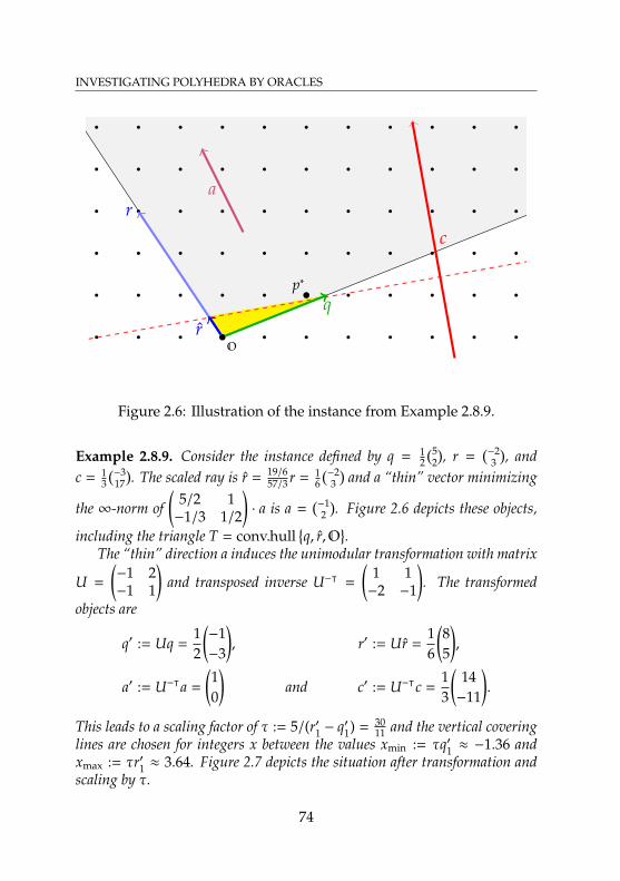
INVESTIGATING POLYHEDRA BY ORACLES
O
q
r
r
c
a
p∗
Figure 2.6: Illustration of the instance from Example 2.8.9.
Example 2.8.9. Consider the instance defined by q = 12(5
2), r =
(−23), and
c = 13(−317). The scaled ray is r = 19/6
57/3 r = 16(−23)
and a “thin” vector minimizing
the ∞-norm of(
5/2 1−1/3 1/2
)· a is a =
(−12). Figure 2.6 depicts these objects,
including the triangle T = conv.hullq, r,O
.
The “thin” direction a induces the unimodular transformation with matrix
U =
(−1 2−1 1
)and transposed inverse U−ᵀ =
(1 1−2 −1
). The transformed
objects are
q′ := Uq =12
(−1−3
), r′ := Ur =
16
(85
),
a′ := U−ᵀa =
(10
)and c′ := U−ᵀc =
13
(14−11
).
This leads to a scaling factor of τ := 5/(r′1 − q′1) = 3011 and the vertical covering
lines are chosen for integers x between the values xmin := τq′1 ≈ −1.36 andxmax := τr′1 ≈ 3.64. Figure 2.7 depicts the situation after transformation andscaling by τ.
74
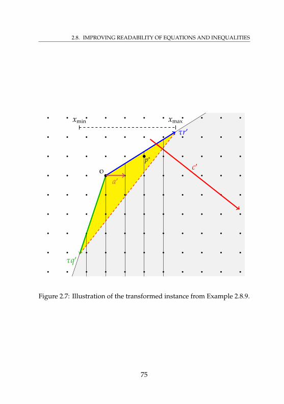
2.8. IMPROVING READABILITY OF EQUATIONS AND INEQUALITIES
O
τq′
τr′
c′
a′
p∗
xmin xmax
Figure 2.7: Illustration of the transformed instance from Example 2.8.9.
75
INVESTIGATING POLYHEDRA BY ORACLES
The following algorithm makes these ideas precise:
Lemma 2.8.10. Algorithm 2.8.1 is correct and runs in polynomial time.
Proof. By Proposition 2.8.8, Step 4 can be carried out in polynomialtime and the vector a satisfies w(T) ≤ wa(T) ≤ 2w(T) for the triangleT := conv.hull
q, r,O
. By construction a is primitive, i.e., gcd(a1, a2) = 1
holds. Hence, Step 6 can be performed using the extended Euclideanalgorithm. The (unimodular) transformation in Step 7 transforms therays in such a way that the direction a corresponds to a′ := (1, 0). Observethat
⟨U−ᵀc,Up
⟩=
⟨c, p
⟩holds for all points p, i.e., the new objective
vector c′ corresponds to c after the transformation.If
⟨c, q
⟩, 〈c, r〉 > 0 does not hold, we can assume w.l.o.g. that 〈c, r〉 = 0
holds. In this case, every feasible point p with⟨a, p
⟩= 1 is optimal.
Hence, after the transformation, any point (x, y) with x = 1 is suitable,and the algorithm will find it since Step 17 is executed due to c′2 = 0.
If⟨c, q
⟩, 〈c, r〉 > 0 holds, we have
⟨c′, q′
⟩= 〈c′, r′〉 due to the prelim-
inary scaling in Step 3. The factor τ > 0 computed in Step 11 ensuresthat wa(τT) = 5 holds, ensuring that τT satisfies the condition of Propo-sition 2.8.7 and hence contains an integer point. By unimodularity ofthe transformation, also τT′ (with T′ :=
Up | p ∈ T
) contains an integer
point. Furthermore, the integer points in τT′ can be covered by at mostsix vertical lines with x-coordinates between xmin and xmax. It is easyto verify that Steps 14–17 find for a specified x ∈ Z an integer y suchthat (x, y) ∈ int(conic.hull
q′, r′,O
) is of minimum c′-value (if such a
y exists). Note that by the definition of Y we do not necessarily have(x, y) ∈ τT′. If a y exists, its objective value
⟨c,U−1(x, y)ᵀ
⟩=
⟨c′, (x, y)ᵀ
⟩is compared to that of an already known best solution.
It remains to show optimality, i.e., that an optimal point is amongthose considered. Suppose an optimal point p∗ lies outside of τT′. Sincethe line connecting q′ and r′ is orthogonal to c′ due to
⟨c′, q′
⟩= 〈c′, r′〉,
observe that c′ is the normal vector of this edge of τT′. Hence, any pointinside of T′ has better objective than p∗, which concludes the proof.
76
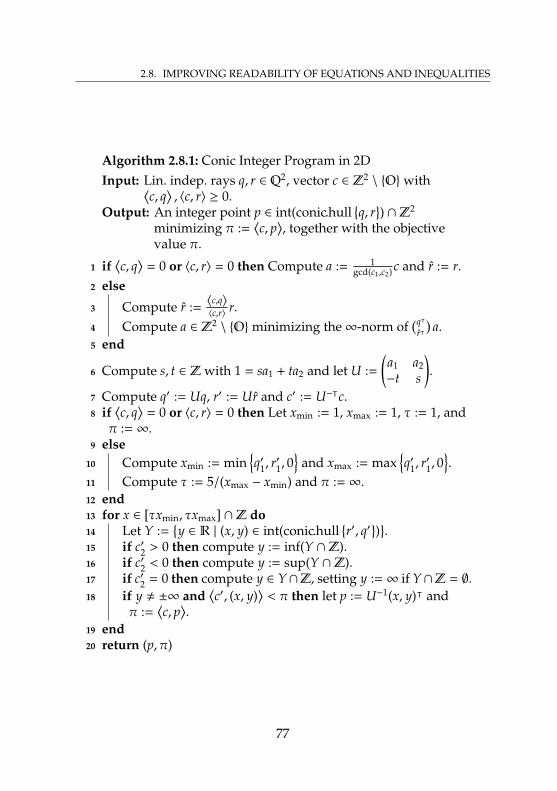
2.8. IMPROVING READABILITY OF EQUATIONS AND INEQUALITIES
Algorithm 2.8.1: Conic Integer Program in 2DInput: Lin. indep. rays q, r ∈ Q2, vector c ∈ Z2
\ Owith⟨c, q
⟩, 〈c, r〉 ≥ 0.
Output: An integer point p ∈ int(conic.hullq, r
) ∩Z2
minimizing π :=⟨c, p
⟩, together with the objective
value π.
1 if⟨c, q
⟩= 0 or 〈c, r〉 = 0 then Compute a := 1
gcd(c1,c2) c and r := r.2 else
3 Compute r := 〈c,q〉〈c,r〉 r.
4 Compute a ∈ Z2\ Ominimizing the∞-norm of
(qᵀ
rᵀ)
a.5 end
6 Compute s, t ∈ Zwith 1 = sa1 + ta2 and let U :=(a1 a2−t s
).
7 Compute q′ := Uq, r′ := Ur and c′ := U−ᵀc.8 if
⟨c, q
⟩= 0 or 〈c, r〉 = 0 then Let xmin := 1, xmax := 1, τ := 1, and
π := ∞.9 else
10 Compute xmin := minq′1, r
′
1, 0
and xmax := maxq′1, r
′
1, 0.
11 Compute τ := 5/(xmax − xmin) and π := ∞.12 end13 for x ∈ [τxmin, τxmax] ∩Z do14 Let Y :=
y ∈ R | (x, y) ∈ int(conic.hull
r′, q′
).
15 if c′2 > 0 then compute y := inf(Y ∩Z).16 if c′2 < 0 then compute y := sup(Y ∩Z).17 if c′2 = 0 then compute y ∈ Y∩Z, setting y := ∞ if Y∩Z = ∅.18 if y , ±∞ and
⟨c′, (x, y)
⟩< π then let p := U−1(x, y)ᵀ and
π :=⟨c, p
⟩.
19 end20 return (p, π)
77
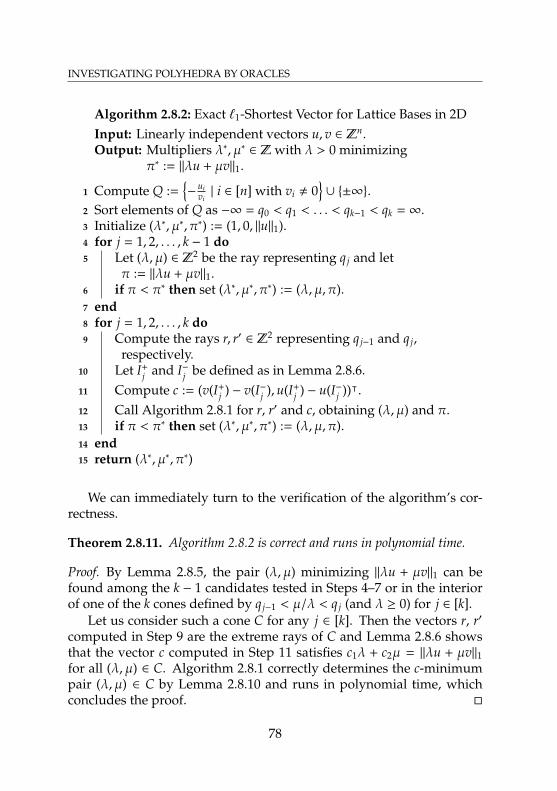
INVESTIGATING POLYHEDRA BY ORACLES
Algorithm 2.8.2: Exact `1-Shortest Vector for Lattice Bases in 2DInput: Linearly independent vectors u, v ∈ Zn.Output: Multipliers λ∗, µ∗ ∈ Zwith λ > 0 minimizing
π∗ := ||λu + µv||1.
1 Compute Q :=−
uivi| i ∈ [n] with vi , 0
∪ ±∞.
2 Sort elements of Q as −∞ = q0 < q1 < . . . < qk−1 < qk = ∞.3 Initialize (λ∗, µ∗, π∗) := (1, 0, ||u||1).4 for j = 1, 2, . . . , k − 1 do5 Let (λ, µ) ∈ Z2 be the ray representing q j and let
π := ||λu + µv||1.6 if π < π∗ then set (λ∗, µ∗, π∗) := (λ, µ, π).7 end8 for j = 1, 2, . . . , k do9 Compute the rays r, r′ ∈ Z2 representing q j−1 and q j,
respectively.10 Let I+
j and I−j be defined as in Lemma 2.8.6.11 Compute c := (v(I+
j ) − v(I−j ),u(I+j ) − u(I−j ))ᵀ.
12 Call Algorithm 2.8.1 for r, r′ and c, obtaining (λ, µ) and π.13 if π < π∗ then set (λ∗, µ∗, π∗) := (λ, µ, π).14 end15 return (λ∗, µ∗, π∗)
We can immediately turn to the verification of the algorithm’s cor-rectness.
Theorem 2.8.11. Algorithm 2.8.2 is correct and runs in polynomial time.
Proof. By Lemma 2.8.5, the pair (λ, µ) minimizing ||λu + µv||1 can befound among the k − 1 candidates tested in Steps 4–7 or in the interiorof one of the k cones defined by q j−1 < µ/λ < q j (and λ ≥ 0) for j ∈ [k].
Let us consider such a cone C for any j ∈ [k]. Then the vectors r, r′
computed in Step 9 are the extreme rays of C and Lemma 2.8.6 showsthat the vector c computed in Step 11 satisfies c1λ + c2µ = ||λu + µv||1for all (λ, µ) ∈ C. Algorithm 2.8.1 correctly determines the c-minimumpair (λ, µ) ∈ C by Lemma 2.8.10 and runs in polynomial time, whichconcludes the proof.
78
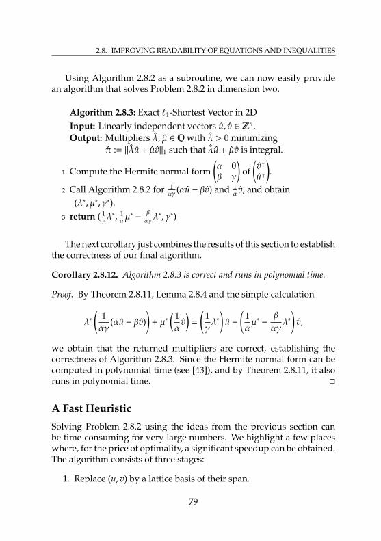
2.8. IMPROVING READABILITY OF EQUATIONS AND INEQUALITIES
Using Algorithm 2.8.2 as a subroutine, we can now easily providean algorithm that solves Problem 2.8.2 in dimension two.
Algorithm 2.8.3: Exact `1-Shortest Vector in 2DInput: Linearly independent vectors u, v ∈ Zn.Output: Multipliers λ, µ ∈ Qwith λ > 0 minimizing
π := ||λu + µv||1 such that λu + µv is integral.
1 Compute the Hermite normal form(α 0β γ
)of
(vᵀ
uᵀ
).
2 Call Algorithm 2.8.2 for 1αγ (αu − βv) and 1
α v, and obtain(λ∗, µ∗, γ∗).
3 return ( 1γλ∗, 1αµ∗−
βαγλ
∗, γ∗)
The next corollary just combines the results of this section to establishthe correctness of our final algorithm.
Corollary 2.8.12. Algorithm 2.8.3 is correct and runs in polynomial time.
Proof. By Theorem 2.8.11, Lemma 2.8.4 and the simple calculation
λ∗(
1αγ
(αu − βv))
+ µ∗( 1α
v)
=
(1γλ∗
)u +
(1αµ∗ −
β
αγλ∗
)v,
we obtain that the returned multipliers are correct, establishing thecorrectness of Algorithm 2.8.3. Since the Hermite normal form can becomputed in polynomial time (see [43]), and by Theorem 2.8.11, it alsoruns in polynomial time.
A Fast Heuristic
Solving Problem 2.8.2 using the ideas from the previous section canbe time-consuming for very large numbers. We highlight a few placeswhere, for the price of optimality, a significant speedup can be obtained.The algorithm consists of three stages:
1. Replace (u, v) by a lattice basis of their span.
79
INVESTIGATING POLYHEDRA BY ORACLES
2. Find (at most n+1) regions for the multipliers (λ, µ) having a linearobjective.
3. For each region, solve the corresponding integer program withtwo variables.
Clearly, if we skip Step 1, we do not reach all possible combinationsλu + µv ∈ Zn in general. Still, all produced solutions are valid.
The most time-consuming step is Step 3, and we can save a lot ofcomputation time if we restrict our search only to those pairs (λ, µ) withλ/µ ∈ Q. Although this clearly limits the set of vectors w = λu+µv ∈ Zn
considered, every w having an entry wi = 0 with ui, vi , 0 is checked. Inparticular, if there is a combination that is much sparser than u and v,the heuristic will still consider it.
ImplementationThe problem considered in this section is clearly not central to this thesis,and hence we spent only a limited amount of time on the implementa-tion. One of the simplest ideas for using the algorithms is to repeatedlycheck pairs of vectors for possible norm reductions until no such im-provement is possible. IPO contains precisely this functionality, exceptthat it works in two rounds: in the first round, the cheaper heuristicis run, and in the second round, the more expensive Algorithm 2.8.3 istried.
We did not carry out a computational study, but would like to men-tion that our observations are moderate: Running the heuristic does nottake a lot of time, which is why we sticked to the simple pair-checkingstrategy described in the previous paragraph. Furthermore, for vectorswith less than 20 coefficients it produces good results in the sense thatwe could not improve them by looking at the results. For dense vectorsusually not much changes, but in general it is hard to judge the results,as we do not know the optimal bases.
80
2.9. COMPUTATIONAL STUDIES: DIMENSIONS
INVESTIGATING POLYHEDRA BY ORACLES:
2.9 Computational Studies:Dimensions
In this section we describe results of three experiments we conductedon some well-known benchmark MIPs. In Section 2.9.1 we report on thedimensions of polyhedra related to the instances, and discuss particularcases that give insight into the capabilities and limitations of our im-plementation. In Section 2.9.2 we consider the maximum faces for theobjectives specified in the respective instances. For the last experiment,presented in Section 2.9.3, we use our code to analyze the inequalityconstraints of the mentioned instances with respect to the dimensionsof the induced faces.
Hardware. The experiments were conducted on a 64-bit Intel i3-2310MCPU at 2.1 GHz with 3 MB cache and 4 GB main memory.
Software. As an exact LP solver we used the development versionof SoPlex from January 2015. IPO was compiled with GCC 4.6.39 andlinked to the external libraries GMP 3.5.210. As an oracle we used theexact MIP solver ExactSCIP 3.0.0 linked to GMP 4.3.1 (the recommendedversion for ExactSCIP), MPFR 2.4.211, QSopt_ex 2.5.10 (see [6, 5]), andEGlib-2.6.2012. Using IPO’s MixedIntegerProgramCorrectorOracle on
9GCC, the GNU Compiler Collection, available at http://gcc.gnu.org/10The GNU Multiple Precision Arithmetic Library, available at http://gmplib.org/11The GNU MPFR Library, available at http://www.mpfr.org/12EGlib, available at http://www.dii.uchile.cl/~daespino/EGlib_doc/main.html
81
INVESTIGATING POLYHEDRA BY ORACLES
top of SCIP-3.1.1, the approximate oracle we used, we could turn thefloating-point solutions into rational ones (see Section 2.3.4).
Dimensions of Polyhedra from MIPLIB Instances
In order to demonstrate the capabilities and also the limitations of ourimplementation of Algorithm 2.4.3 we computed the affine hulls for var-ious polyhedra stemming from the MIPLIB 2.0. We selected all instanceswith at most 1000 variables that are solved exactly within 5 minutes, sincethe running time of the algorithm depends on the ambient dimensionand on the running time of the oracle. For each instance we consideredthe linear relaxation P, the linear relaxation Q of the presolved instanceand their respective mixed-integer hulls PI and QI. The presolve wasdone by SCIP using default settings in floating-point arithmetic.
First, we ran our implementation of the affine hull algorithm tocompute the dimensions of these polyhedra. One goal was to showthat we can compute the affine hull of polyhedra associated to MIPswith several dozens – and in some cases also hundreds – of variables.Second, we were curious about how well the affine hull of the mixed-integer hull is actually known just from the model. To be more precise,denote by n′ the initially known upper bound on the dimension, i.e.,the ambient dimension n minus the number of irredundant equationsexplicitly stated in the MIP (or −1 if a trivially violated equation isgiven). The two simple inequalities
n′ ≥ dim P ≥ dim PI
are clearly valid, and we were curious how often they are actually tight.Tables 2.2 and 2.3 report the main results of this experiment. For
more detailed statistics, e.g., time measurements for different parts of thealgorithm, we refer to Tables A.1–A.8. Note that all timings displayedin tables and figures are in seconds.
The numbers showing dim P (resp. dim Q) are colored red if theydiffer from n′, i.e., if an inequality (or bound) constraint of the relaxationis satisfied with equality by all LP solutions. Similarly, the numbersshowing dim PI (resp. dim QI) are colored green if they differ from dim P(resp. dim Q).
82
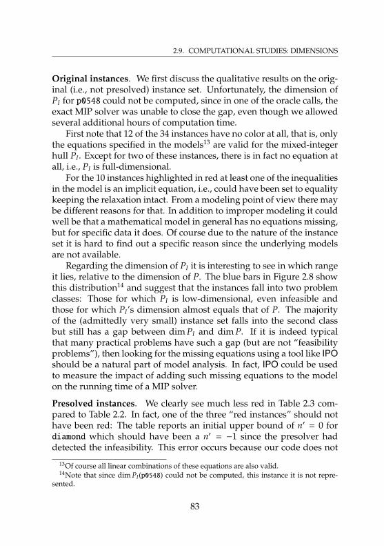
2.9. COMPUTATIONAL STUDIES: DIMENSIONS
Original instances. We first discuss the qualitative results on the orig-inal (i.e., not presolved) instance set. Unfortunately, the dimension ofPI for p0548 could not be computed, since in one of the oracle calls, theexact MIP solver was unable to close the gap, even though we allowedseveral additional hours of computation time.
First note that 12 of the 34 instances have no color at all, that is, onlythe equations specified in the models13 are valid for the mixed-integerhull PI. Except for two of these instances, there is in fact no equation atall, i.e., PI is full-dimensional.
For the 10 instances highlighted in red at least one of the inequalitiesin the model is an implicit equation, i.e., could have been set to equalitykeeping the relaxation intact. From a modeling point of view there maybe different reasons for that. In addition to improper modeling it couldwell be that a mathematical model in general has no equations missing,but for specific data it does. Of course due to the nature of the instanceset it is hard to find out a specific reason since the underlying modelsare not available.
Regarding the dimension of PI it is interesting to see in which rangeit lies, relative to the dimension of P. The blue bars in Figure 2.8 showthis distribution14 and suggest that the instances fall into two problemclasses: Those for which PI is low-dimensional, even infeasible andthose for which PI’s dimension almost equals that of P. The majorityof the (admittedly very small) instance set falls into the second classbut still has a gap between dim PI and dim P. If it is indeed typicalthat many practical problems have such a gap (but are not “feasibilityproblems”), then looking for the missing equations using a tool like IPOshould be a natural part of model analysis. In fact, IPO could be usedto measure the impact of adding such missing equations to the modelon the running time of a MIP solver.
Presolved instances. We clearly see much less red in Table 2.3 com-pared to Table 2.2. In fact, one of the three “red instances” should nothave been red: The table reports an initial upper bound of n′ = 0 fordiamond which should have been a n′ = −1 since the presolver haddetected the infeasibility. This error occurs because our code does not
13Of course all linear combinations of these equations are also valid.14Note that since dim PI(p0548) could not be computed, this instance it is not repre-
sented.
83
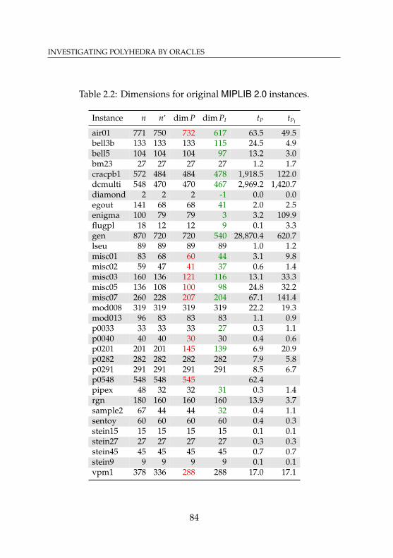
INVESTIGATING POLYHEDRA BY ORACLES
Table 2.2: Dimensions for original MIPLIB 2.0 instances.
Instance n n′ dim P dim PI tP tPI
air01 771 750 732 617 63.5 49.5bell3b 133 133 133 115 24.5 4.9bell5 104 104 104 97 13.2 3.0bm23 27 27 27 27 1.2 1.7cracpb1 572 484 484 478 1,918.5 122.0dcmulti 548 470 470 467 2,969.2 1,420.7diamond 2 2 2 -1 0.0 0.0egout 141 68 68 41 2.0 2.5enigma 100 79 79 3 3.2 109.9flugpl 18 12 12 9 0.1 3.3gen 870 720 720 540 28,870.4 620.7lseu 89 89 89 89 1.0 1.2misc01 83 68 60 44 3.1 9.8misc02 59 47 41 37 0.6 1.4misc03 160 136 121 116 13.1 33.3misc05 136 108 100 98 24.8 32.2misc07 260 228 207 204 67.1 141.4mod008 319 319 319 319 22.2 19.3mod013 96 83 83 83 1.1 0.9p0033 33 33 33 27 0.3 1.1p0040 40 40 30 30 0.4 0.6p0201 201 201 145 139 6.9 20.9p0282 282 282 282 282 7.9 5.8p0291 291 291 291 291 8.5 6.7p0548 548 548 545 62.4pipex 48 32 32 31 0.3 1.4rgn 180 160 160 160 13.9 3.7sample2 67 44 44 32 0.4 1.1sentoy 60 60 60 60 0.4 0.3stein15 15 15 15 15 0.1 0.1stein27 27 27 27 27 0.3 0.3stein45 45 45 45 45 0.7 0.7stein9 9 9 9 9 0.1 0.1vpm1 378 336 288 288 17.0 17.1
84
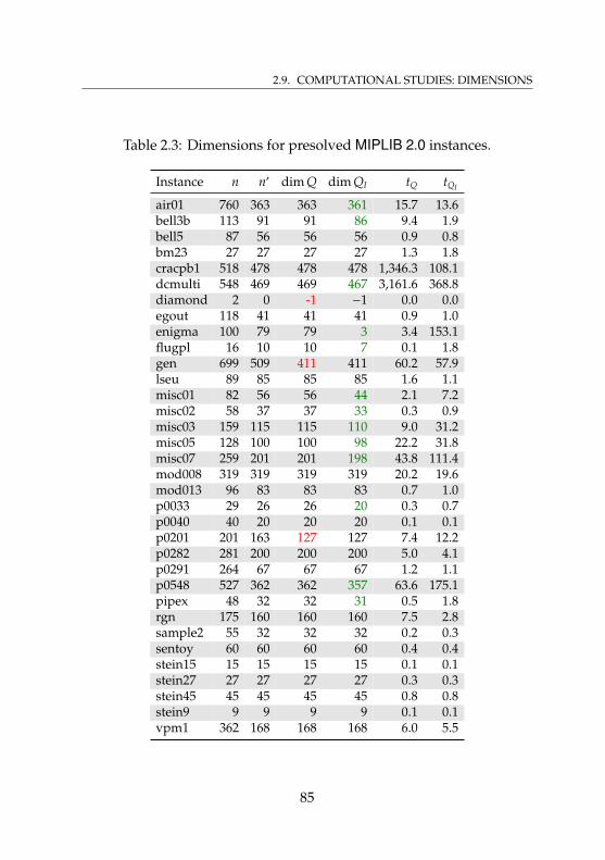
2.9. COMPUTATIONAL STUDIES: DIMENSIONS
Table 2.3: Dimensions for presolved MIPLIB 2.0 instances.
Instance n n′ dim Q dim QI tQ tQI
air01 760 363 363 361 15.7 13.6bell3b 113 91 91 86 9.4 1.9bell5 87 56 56 56 0.9 0.8bm23 27 27 27 27 1.3 1.8cracpb1 518 478 478 478 1,346.3 108.1dcmulti 548 469 469 467 3,161.6 368.8diamond 2 0 -1 −1 0.0 0.0egout 118 41 41 41 0.9 1.0enigma 100 79 79 3 3.4 153.1flugpl 16 10 10 7 0.1 1.8gen 699 509 411 411 60.2 57.9lseu 89 85 85 85 1.6 1.1misc01 82 56 56 44 2.1 7.2misc02 58 37 37 33 0.3 0.9misc03 159 115 115 110 9.0 31.2misc05 128 100 100 98 22.2 31.8misc07 259 201 201 198 43.8 111.4mod008 319 319 319 319 20.2 19.6mod013 96 83 83 83 0.7 1.0p0033 29 26 26 20 0.3 0.7p0040 40 20 20 20 0.1 0.1p0201 201 163 127 127 7.4 12.2p0282 281 200 200 200 5.0 4.1p0291 264 67 67 67 1.2 1.1p0548 527 362 362 357 63.6 175.1pipex 48 32 32 31 0.5 1.8rgn 175 160 160 160 7.5 2.8sample2 55 32 32 32 0.2 0.3sentoy 60 60 60 60 0.4 0.4stein15 15 15 15 15 0.1 0.1stein27 27 27 27 27 0.3 0.3stein45 45 45 45 45 0.8 0.8stein9 9 9 9 9 0.1 0.1vpm1 362 168 168 168 6.0 5.5
85
INVESTIGATING POLYHEDRA BY ORACLES
check explicitly whether the initial set of equations contains a triviallyviolated equation. Hence, only the two presolved instances gen andp0201 do not contain all equations necessary to describe the affine hullof the relaxation. This is a sign that in general the presolver does agood job in detecting inequalities that are satisfied with equality by allsolutions.
The red bars in Figure 2.8 correspond to the presolved instances. Weobserve that almost two thirds of the instances have dim Q = dim QI.This shows the effects of the so-called “dual tightening” and “dual fix-ing” operations, which are the presolve techniques that are allowedto cut off integer-feasible points as long as at least one optimal solu-tion remains feasible15. For example, the dimensions of PI(air01) andQI(air01) are 617 and 361, respectively, that is, many feasible solutionshave been cut off.
Large encoding lengths. We now turn to the quantitative results. Themost prominent case is clearly instance gen for which the computationof dim P needed more than 8 hours, whereas the computation of dim PIwas performed in less than 11 minutes. This already indicates that theissue cannot be the running time of the heuristic or the oracle.
Figure 2.9 displays the relative amounts of running time used for thedifferent components of Algorithm 2.4.3 for some instances and somemodifications of the algorithm.
Since the heuristic for P(gen) only has to solve an LP, the majorityof running time is spent for the linear algebra parts, in particular thecomputation of the direction vectors, the most complicated one havingan encoding length of almost 20 million bits. In order to avoid manycomputations with such huge numbers, IPO heuristically selects thenext nonbasic index in Steps 6 and 7 of Algorithm 2.4.2 such that thecorresponding direction vector becomes as sparse as possible. Sparsityof the directions is also interesting for the user since sparse equations aretypically easier to understand. This is done by computing all directionsfirst in floating-point precision and estimating the number of nonzeros16.First, observe that the overhead of this effort is relatively small, as inonly very few cases the time spent for the approximate directions is as
15The term “dual” comes from the fact that such an operation must take the objectiveinto account.
16Experiments suggested to consider numbers smaller than 10−7 as zero.
86
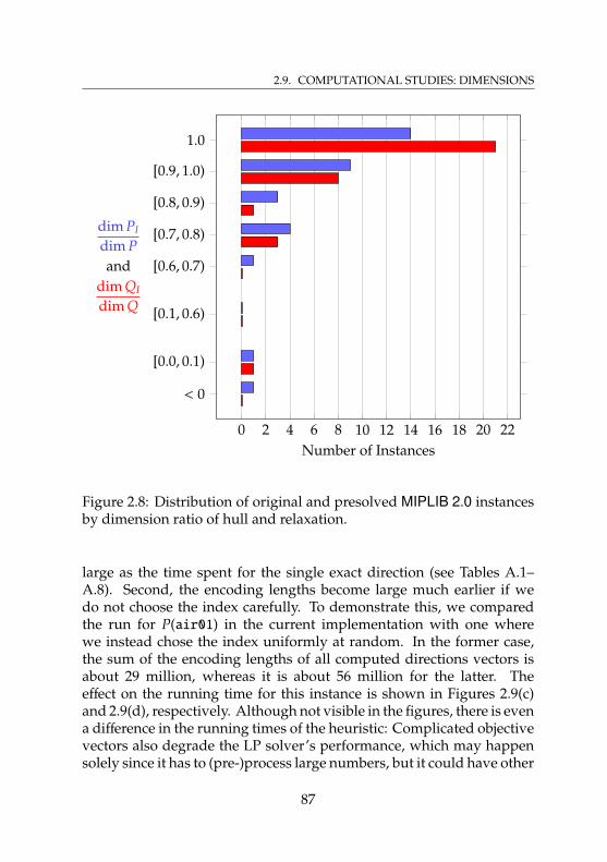
2.9. COMPUTATIONAL STUDIES: DIMENSIONS
0 2 4 6 8 10 12 14 16 18 20 22
< 0
[0.0, 0.1)
[0.1, 0.6)
[0.6, 0.7)
[0.7, 0.8)
[0.8, 0.9)
[0.9, 1.0)
1.0
Number of Instances
dim PI
dim Pand
dim QI
dim Q
Figure 2.8: Distribution of original and presolved MIPLIB 2.0 instancesby dimension ratio of hull and relaxation.
large as the time spent for the single exact direction (see Tables A.1–A.8). Second, the encoding lengths become large much earlier if wedo not choose the index carefully. To demonstrate this, we comparedthe run for P(air01) in the current implementation with one wherewe instead chose the index uniformly at random. In the former case,the sum of the encoding lengths of all computed directions vectors isabout 29 million, whereas it is about 56 million for the latter. Theeffect on the running time for this instance is shown in Figures 2.9(c)and 2.9(d), respectively. Although not visible in the figures, there is evena difference in the running times of the heuristic: Complicated objectivevectors also degrade the LP solver’s performance, which may happensolely since it has to (pre-)process large numbers, but it could have other
87
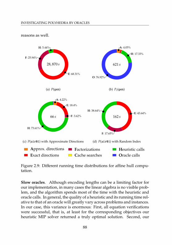
INVESTIGATING POLYHEDRA BY ORACLES
reasons as well.
E: 68.31%
F: 25.94%
H: 5.44%
28, 870 s
(a) P(gen)
A: 4.05%
H: 17.33%
O: 76.92%
621 s
(b) PI(gen)
A: 4.22%
E: 18.4%
F: 3.62%
H: 73.61%
66 s
(c) P(air01) with Approximate Directions
E: 43.64%
F: 17.65%
H: 38.64%
162 s
(d) P(air01) with Random Index
Approx. directions Factorizations Heuristic callsExact directions Cache searches Oracle calls
Figure 2.9: Different running time distributions for affine hull compu-tation.
Slow oracles. Although encoding lengths can be a limiting factor forour implementation, in many cases the linear algebra is no visible prob-lem, and the algorithm spends most of the time with the heuristic andoracle calls. In general, the quality of a heuristic and its running time rel-ative to that of an oracle will greatly vary across problems and instances.In our case, this variance is enormous: First, all equation verificationswere successful, that is, at least for the corresponding objectives ourheuristic MIP solver returned a truly optimal solution. Second, our
88
2.9. COMPUTATIONAL STUDIES: DIMENSIONS
exact MIP solver ExactSCIP is very slow. Often, finding a primal so-lution at all takes several minutes, if not hours. This is due to the factthat ExactSCIP has no primal heuristics, i.e., it finds solutions only asLP solutions during branch & bound. Furthermore, since IPO accessesExactSCIP using an external call, it cannot make use of warm-start fea-tures. If linear algebra becomes no issue, then the typical running timeprofile looks like the one in Figure 2.9(b).
We also tried to compute the affine hull for some instances withouta heuristic, but the results are not very surprising: For some easy in-stances, there is almost no visible effect, for hard instances, it would havetaken days to compute the affine hull. Furthermore, since ExactSCIPsometimes has trouble to close the gap17 or to find a feasible solution,we observe dramatic running-time differences among the oracle callsfor single instances already.
Dimensions of Optimal Faces
In addition to the affine hull computations of P, PI, Q and QI we also useIPO to compute the dimensions of the optimal faces of the four polyhe-dra for the objectives specified in the respective instances. Clearly, forthe empty polyhedron associated to instance diamond, the optimal faceis also empty. In addition to this, several cells in the Tables 2.4 and 2.5 areempty. Due to the maximum allowed time of 1 hour per oracle call, thecomputations failed for PI(bell3b), PI(bell5), PI(dcmulti), PI(egout),PI(p0548), QI(p0548) and QI(vpm1).
Tables 2.4 and 2.5 report the results of this experiment. In particu-lar for the mixed-integer hulls the running times are very large. Thisis mostly due to the fact that because of small resulting dimensions,the algorithm has to verify many equations, most of them being fixedvariables. Despite the simplicity of the objective vectors the exact MIPsolver sometimes needs a lot of time. In fact, the dual bound is oftenoptimal very early, but the solver fails to find a feasible solution (whichis also optimal if the equation is correct).
A first observation is that, regardless of the instance type, most of theoptimal faces are either high-dimensional or very low-dimensional. To
17There are cases where SCIP states a gap of 0.0 % and still continues to branch, and weverified that there is still a tiny difference between the primal and dual bounds.
89
INVESTIGATING POLYHEDRA BY ORACLES
make this more precise we produced Figures 2.11 and 2.10 for which wegrouped the instances according to the dimension of the optimal facerelative to the dimension of the host polyhedron.
Relaxations. For the linear relaxations P and Q we observe that 6 ofthe 33 feasible18 instances have high-dimensional optimal faces, and theremaining 27 instances have optimal faces of dimension less that onethird of that of P, or Q, respectively. In particular, 10 (resp. 12) of themare even 0-dimensional, that is, they have a unique LP optimum. Rea-sons for having high-dimensional optimal faces may be very symmetricmodels or very simple (e.g., sparse) objectives.
Symmetry may be a disadvantage of an LP model, as for examplecutting planes may cut off several LP-optimal solutions, but as long asthey do not cut off all of them, there is either no dual improvement, orone needs many cutting planes to make progress. Hence, in order toanalyze problems for which such a behavior is observed, a researchermay use IPO to check the dimension of the optimal face of the linearrelaxation.
Mixed-Integer Hulls. As mentioned at the beginning of this section wehad trouble to compute the dimensions of the optimal faces for severalinstances. For this reason we only used those 27 instances19 for whichwe had results for both, the original and the presolved when creatingFigure 2.11. There are again only small differences between the originaland the presolved instances. During presolve the polyhedron itself andthe optimal face can be cut, reducing the respective dimensions. Asexpected, there are no serious changes with respect to the dimensionratio, since usually the presolvers cannot reduce the main dimension tothe order of magnitude of the optimal face if the latter is rather small.Since there is no general relationship between the optimal faces of linearrelaxations and their mixed-integer hulls, it is somewhat interestingthat the four instances with largest ratio are also among the group of sixinstances for which the relaxations had a ratio of more than 70 %. Amongthe latter are enigma whose mixed-integer hull is only 3-dimensional,reducing the ratio to a third, as well as cracpb1, for which the optimalface dimensions for the mixed-integer hulls were 202, while those for
18We excluded the infeasible instance diamond.19In addition to the infeasible instance diamond we excluded bell3b, bell5, dcmulti,egout, p0548 and vpm1.
90
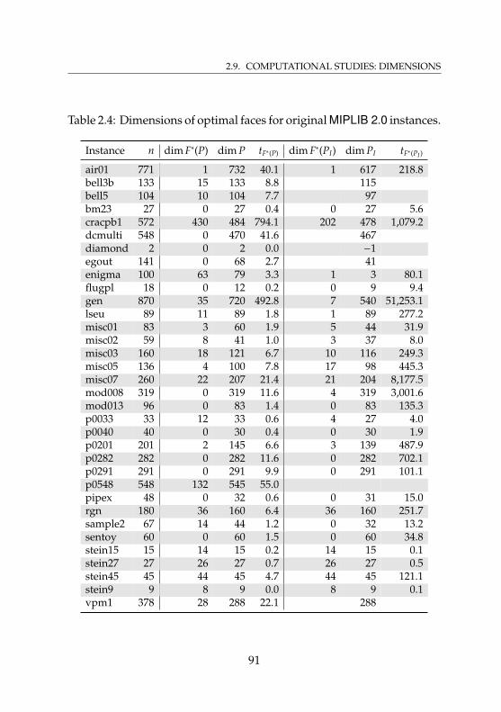
2.9. COMPUTATIONAL STUDIES: DIMENSIONS
Table 2.4: Dimensions of optimal faces for original MIPLIB 2.0 instances.
Instance n dim F∗(P) dim P tF∗(P) dim F∗(PI) dim PI tF∗(PI )
air01 771 1 732 40.1 1 617 218.8bell3b 133 15 133 8.8 115bell5 104 10 104 7.7 97bm23 27 0 27 0.4 0 27 5.6cracpb1 572 430 484 794.1 202 478 1,079.2dcmulti 548 0 470 41.6 467diamond 2 0 2 0.0 −1egout 141 0 68 2.7 41enigma 100 63 79 3.3 1 3 80.1flugpl 18 0 12 0.2 0 9 9.4gen 870 35 720 492.8 7 540 51,253.1lseu 89 11 89 1.8 1 89 277.2misc01 83 3 60 1.9 5 44 31.9misc02 59 8 41 1.0 3 37 8.0misc03 160 18 121 6.7 10 116 249.3misc05 136 4 100 7.8 17 98 445.3misc07 260 22 207 21.4 21 204 8,177.5mod008 319 0 319 11.6 4 319 3,001.6mod013 96 0 83 1.4 0 83 135.3p0033 33 12 33 0.6 4 27 4.0p0040 40 0 30 0.4 0 30 1.9p0201 201 2 145 6.6 3 139 487.9p0282 282 0 282 11.6 0 282 702.1p0291 291 0 291 9.9 0 291 101.1p0548 548 132 545 55.0pipex 48 0 32 0.6 0 31 15.0rgn 180 36 160 6.4 36 160 251.7sample2 67 14 44 1.2 0 32 13.2sentoy 60 0 60 1.5 0 60 34.8stein15 15 14 15 0.2 14 15 0.1stein27 27 26 27 0.7 26 27 0.5stein45 45 44 45 4.7 44 45 121.1stein9 9 8 9 0.0 8 9 0.1vpm1 378 28 288 22.1 288
91
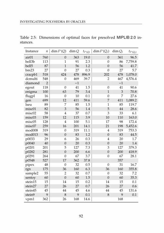
INVESTIGATING POLYHEDRA BY ORACLES
Table 2.5: Dimensions of optimal faces for presolved MIPLIB 2.0 in-stances.
Instance n dim F∗(Q) dim Q tF∗(Q) dim F∗(QI) dim QI tF∗(QI )
air01 760 0 363 19.0 0 361 96.5bell3b 113 1 91 2.3 0 86 7,759.8bell5 87 1 56 1.2 0 56 41.7bm23 27 0 27 0.3 0 27 5.7cracpb1 518 424 478 896.9 202 478 1,078.0dcmulti 548 0 469 39.7 2 467 4,576.4diamond 2 −1 −1egout 118 0 41 1.5 0 41 90.6enigma 100 63 79 3.4 1 3 70.8flugpl 16 0 10 0.1 0 7 27.6gen 699 12 411 59.6 7 411 1,089.2lseu 89 7 85 1.5 1 85 119.7misc01 82 3 56 1.4 5 44 28.6misc02 58 4 37 0.7 3 33 6.1misc03 159 12 115 3.9 10 110 163.0misc05 128 4 100 5.1 17 98 172.4misc07 259 16 201 14.1 21 198 5,452.6mod008 319 0 319 11.1 4 319 753.3mod013 96 0 83 1.2 0 83 44.5p0033 29 6 26 0.3 4 20 1.7p0040 40 0 20 0.3 0 20 1.4p0201 201 5 127 7.3 3 127 379.3p0282 281 0 200 6.6 0 200 418.9p0291 264 0 67 3.7 0 67 28.1p0548 527 17 362 37.8 357pipex 48 0 32 0.5 0 31 16.7rgn 175 36 160 6.3 36 160 355.8sample2 55 2 32 0.7 0 32 7.2sentoy 60 0 60 1.5 0 60 35.3stein15 15 14 15 0.2 14 15 0.1stein27 27 26 27 0.7 26 27 0.6stein45 45 44 45 4.6 44 45 131.6stein9 9 8 9 0.1 8 9 0.1vpm1 362 26 168 14.6 168
92
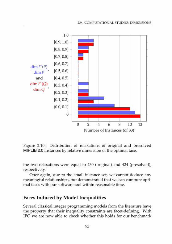
2.9. COMPUTATIONAL STUDIES: DIMENSIONS
0 2 4 6 8 10 12
0
(0.0, 0.1)
[0.1, 0.2)
[0.2, 0.3)
[0.3, 0.4)
[0.4, 0.5)
[0.5, 0.6)
[0.6, 0.7)
[0.7, 0.8)
[0.8, 0.9)
[0.9, 1.0)
1.0
Number of Instances (of 33)
dim F∗(P)dim P
,
anddim F∗(Q)
dim Q,
Figure 2.10: Distribution of relaxations of original and presolvedMIPLIB 2.0 instances by relative dimension of the optimal face.
the two relaxations were equal to 430 (original) and 424 (presolved),respectively.
Once again, due to the small instance set, we cannot deduce anymeaningful relationships, but demonstrated that we can compute opti-mal faces with our software tool within reasonable time.
Faces Induced by Model Inequalities
Several classical integer programming models from the literature havethe property that their inequality constraints are facet-defining. WithIPO we are now able to check whether this holds for our benchmark
93
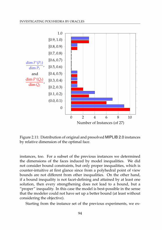
INVESTIGATING POLYHEDRA BY ORACLES
0 2 4 6 8 10
0
(0.0, 0.1)
[0.1, 0.2)
[0.2, 0.3)
[0.3, 0.4)
[0.4, 0.5)
[0.5, 0.6)
[0.6, 0.7)
[0.7, 0.8)
[0.8, 0.9)
[0.9, 1.0)
1.0
Number of Instances (of 27)
dim F∗(PI)dim PI
,
anddim F∗(QI)
dim QI,
Figure 2.11: Distribution of original and presolved MIPLIB 2.0 instancesby relative dimension of the optimal face.
instances, too. For a subset of the previous instances we determinedthe dimensions of the faces induced by model inequalities. We didnot consider bound constraints, but only proper inequalities, which iscounter-intuitive at first glance since from a polyhedral point of viewbounds are not different from other inequalities. On the other hand,if a bound inequality is not facet-defining and attained by at least onesolution, then every strengthening does not lead to a bound, but a“proper” inequality. In this case the model is best-possible in the sensethat the modeler could not have set up a better bound (at least withoutconsidering the objective).
Starting from the instance set of the previous experiments, we ex-
94
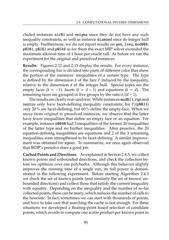
2.9. COMPUTATIONAL STUDIES: DIMENSIONS
cluded instances air01 and enigma since they do not have any suchinequality constraints, as well as instance diamond since its integer hullis empty. Furthermore, we do not report results on gen, lseu, mod008,p0201, p0282 and p0548 as for them the exact MIP solver exceeded themaximum allowed time of 1 hour per oracle call. As before we ran theexperiment for the original and presolved instances.
Results. Figures 2.12 and 2.13 display the results. For every instance,the corresponding bar is divided into parts of different color that showthe portion of the instances’ inequalities of a certain type. The typeis defined by the dimension k of the face F induced by the inequality,relative to the dimension d of the integer hull. Special types are theempty faces (k = −1), facets (k = d − 1) and equations (k = d). Theremaining faces are grouped in five groups by the ratio k/(d − 1).
The results are clearly non-uniform: While instances mod013, rgn andsentoy only have facet-defining inequality constraints, for PI(p0033)only 20 % are facet-defining, but 60 % define the empty-face. When wemove from original to presolved instances, we observe that the latterhave fewer inequalities that define an empty face or an equation. Forexample, instance p0040 had 3 inequalities of the former, 20 inequalitiesof the latter type and no further inequalities. After presolve, the 20equation-defining inequalities are equations and 2 of the 3 remaininginequalities were strengthened to be facet-defining. A similar improve-ment was obtained for egout. To summarize, we once again observedthat SCIP’s presolve does a good job.
Cached Points and Directions. As explained in Section 2.4.5, we collectknown points and unbounded directions, and check the collection be-fore we optimize over our polyhedra. Although this behavior slightlyimproves the running time of a single run, its full power is demon-strated in the following experiment. Before starting Algorithm 2.4.3we check the set of known points (and similarly the set of known un-bounded directions) and collect those that satisfy the current inequalitywith equality. Depending on the inequality and the number of so-farcollected points, these can be many, which reduces the number of calls tothe heuristic. In fact, sometimes we can start with thousands of points,and have to take care that searching the cache is fast enough. For thesesituations we developed a floating-point based selection of candidatepoints, which avoids to compute one scalar product per known point in
95
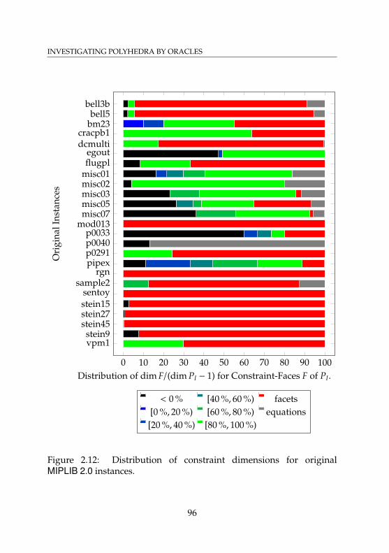
INVESTIGATING POLYHEDRA BY ORACLES
0 10 20 30 40 50 60 70 80 90 100
bell3bbell5
bm23cracpb1dcmulti
egoutflugpl
misc01misc02misc03misc05misc07
mod013p0033p0040p0291pipex
rgnsample2
sentoystein15stein27stein45stein9vpm1
Distribution of dim F/(dim PI − 1) for Constraint-Faces F of PI.
Ori
gina
lIns
tanc
es
< 0 % [40 %, 60 %) facets[0 %, 20 %) [60 %, 80 %) equations
[20 %, 40 %) [80 %, 100 %)
Figure 2.12: Distribution of constraint dimensions for originalMIPLIB 2.0 instances.
96
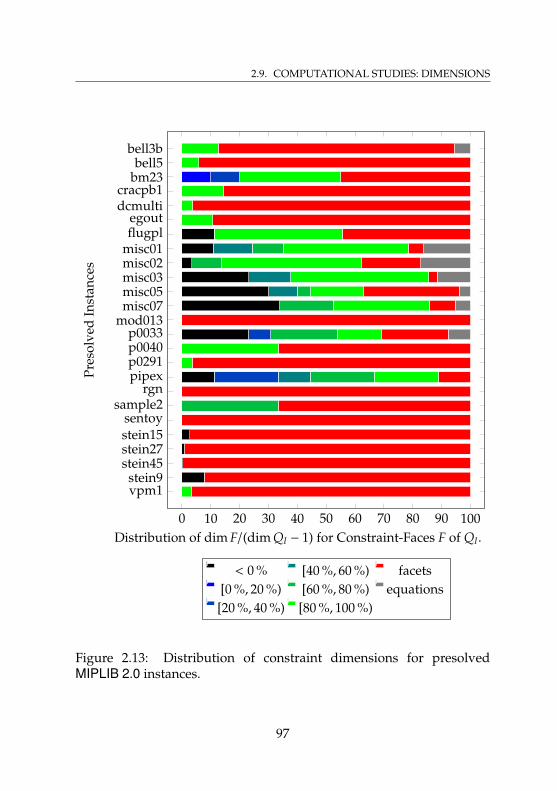
2.9. COMPUTATIONAL STUDIES: DIMENSIONS
0 10 20 30 40 50 60 70 80 90 100
bell3bbell5
bm23cracpb1dcmulti
egoutflugpl
misc01misc02misc03misc05misc07
mod013p0033p0040p0291pipex
rgnsample2
sentoystein15stein27stein45stein9vpm1
Distribution of dim F/(dim QI − 1) for Constraint-Faces F of QI.
Pres
olve
dIn
stan
ces
< 0 % [40 %, 60 %) facets[0 %, 20 %) [60 %, 80 %) equations
[20 %, 40 %) [80 %, 100 %)
Figure 2.13: Distribution of constraint dimensions for presolvedMIPLIB 2.0 instances.
97
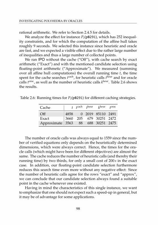
INVESTIGATING POLYHEDRA BY ORACLES
rational arithmetic. We refer to Section 2.4.5 for details.We analyze the effect for instance PI(p0291), which has 252 inequal-
ity constraints, and for which the computation of the affine hull takesroughly 9 seconds. We selected this instance since heuristic and oracleare fast, and we expected a visible effect due to the rather large numberof inequalities and thus a large number of collected points.
We ran IPO without the cache (“Off”), with cache search by exactarithmetic (“Exact”) and with the mentioned candidate selection usingfloating-point arithmetic (“Approximate”). We measured (summingover all affine hull computations) the overall running time t, the timespent for the cache searches tcach, for heuristic calls theur and for oraclecalls torac, as well as the number of heuristic calls kheur. Table 2.6 showsthe results.
Table 2.6: Running times for PI(p0291) for different caching strategies.
Cache t tcach theur kheur torac
Off 4858 0 2019 85110 2491Exact 3660 205 679 30251 2472Approximate 3563 88 688 30251 2475
The number of oracle calls was always equal to 1559 since the num-ber of verified equations only depends on the heuristically determineddimensions, which were always correct. Hence, the times for the ora-cle calls (which might have been for different objectives) are almost thesame. The cache reduces the number of heuristic calls (and thereby theirrunning time) by two thirds, for only a small cost of 200 s in the exactcase. In addition, our floating-point candidate selection furthermorereduces this search time even more without any negative effect: Sincethe number of heuristic calls agree for the rows “exact” and “approx”,we can conclude that our candidate selection always found a suitablepoint in the cache whenever one existed.
Having in mind the characteristics of this single instance, we wantto emphasize that one should not expect such a speed-up in general, butit may be of advantage for some applications.
98
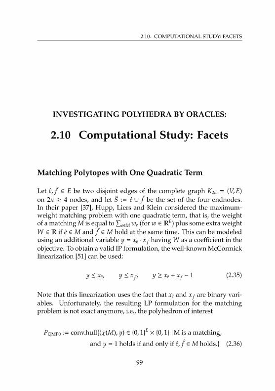
2.10. COMPUTATIONAL STUDY: FACETS
INVESTIGATING POLYHEDRA BY ORACLES:
2.10 Computational Study: Facets
Matching Polytopes with One Quadratic Term
Let e, f ∈ E be two disjoint edges of the complete graph K2n = (V,E)on 2n ≥ 4 nodes, and let S := e ∪ f be the set of the four endnodes.In their paper [37], Hupp, Liers and Klein considered the maximum-weight matching problem with one quadratic term, that is, the weightof a matching M is equal to
∑e∈M we (for w ∈ RE) plus some extra weight
W ∈ R if e ∈ M and f ∈ M hold at the same time. This can be modeledusing an additional variable y = xe · x f having W as a coefficient in theobjective. To obtain a valid IP formulation, the well-known McCormicklinearization [51] can be used:
y ≤ xe, y ≤ x f , y ≥ xe + x f − 1 (2.35)
Note that this linearization uses the fact that xe and x f are binary vari-ables. Unfortunately, the resulting LP formulation for the matchingproblem is not exact anymore, i.e., the polyhedron of interest
PQMP0 := conv.hull(χ(M), y) ∈ 0, 1E × 0, 1 |M is a matching,
and y = 1 holds if and only if e, f ∈M holds. (2.36)
99
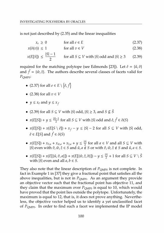
INVESTIGATING POLYHEDRA BY ORACLES
is not just described by (2.35) and the linear inequalities
xe ≥ 0 for all e ∈ E (2.37)x(δ(v)) ≤ 1 for all v ∈ V (2.38)
x(E[S]) ≤|S| − 1
2for all S ⊆ V with |S| odd and |S| ≥ 3 (2.39)
required for the matching polytope (see Edmonds [23]). Let e = u, vand f = w, z. The authors describe several classes of facets valid forPQMP0:
• (2.37) for all e ∈ E \e, f
• (2.38) for all v ∈ V
• y ≤ xe and y ≤ x f
• (2.39) for all S ⊆ V with |S| odd, |S| ≥ 3, and S * S
• x(E[S]) + y ≤ |S|−12 for all S ⊆ V with |S| odd and e, f ∈ δ(S)
• x(E[S]) + x(E[S \ e]) + x f − y ≤ |S| − 2 for all S ⊆ V with |S| odd,
e ∈ E[S] and f ∈ δ(S)
• x(E[S]) + xv,a + xw,a + xz,a + y ≤ |S|2 for all a ∈ V and all S ⊆ V with|S| even with v, w, z ∈ S and u, a < S or with v, w, z < S and u, a ∈ S.
• x(E[S]) + x(E[u, v, a]) + x(E[w, z, b]) − y ≤ |S|2 + 1 for all S ⊆ V \ Swith |S| even and all a, b ∈ S.
They also note that the linear description of PQMP0 is not complete. Infact in Example 1 in [37] they give a fractional point that satisfies all theabove inequalities, but is not in PQMP0. As an argument they providean objective vector such that the fractional point has objective 11, andthey claim that the maximum over PQMP0 is equal to 10, which wouldhave proved that the point lies outside the polytope. Unfortunately, themaximum is equal to 12, that is, it does not prove anything. Neverthe-less, the objective vector helped us to identify a yet unclassified facetof PQMP0. In order to find such a facet we implemented the IP model
100
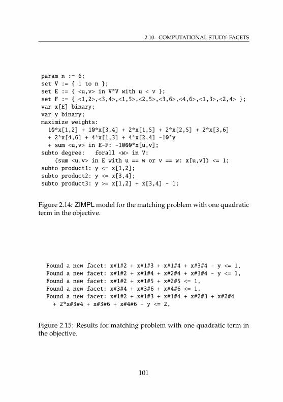
2.10. COMPUTATIONAL STUDY: FACETS
param n := 6;set V := 1 to n ;set E := <u,v> in V*V with u < v ;set F := <1,2>,<3,4>,<1,5>,<2,5>,<3,6>,<4,6>,<1,3>,<2,4> ;var x[E] binary;var y binary;maximize weights:10*x[1,2] + 10*x[3,4] + 2*x[1,5] + 2*x[2,5] + 2*x[3,6]+ 2*x[4,6] + 4*x[1,3] + 4*x[2,4] -10*y+ sum <u,v> in E-F: -1000*x[u,v];
subto degree: forall <w> in V:(sum <u,v> in E with u == w or v == w: x[u,v]) <= 1;
subto product1: y <= x[1,2];subto product2: y <= x[3,4];subto product3: y >= x[1,2] + x[3,4] - 1;
Figure 2.14: ZIMPL model for the matching problem with one quadraticterm in the objective.
Found a new facet: x#1#2 + x#1#3 + x#1#4 + x#3#4 - y <= 1,Found a new facet: x#1#2 + x#1#4 + x#2#4 + x#3#4 - y <= 1,Found a new facet: x#1#2 + x#1#5 + x#2#5 <= 1,Found a new facet: x#3#4 + x#3#6 + x#4#6 <= 1,Found a new facet: x#1#2 + x#1#3 + x#1#4 + x#2#3 + x#2#4+ 2*x#3#4 + x#3#6 + x#4#6 - y <= 2,
Figure 2.15: Results for matching problem with one quadratic term inthe objective.
101
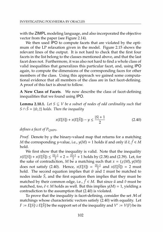
INVESTIGATING POLYHEDRA BY ORACLES
with the ZIMPL modeling language, and also incorporated the objectivevector from the paper (see Figure 2.14).
We then used IPO to compute facets that are violated by the opti-mum of the LP relaxation given in the model. Figure 2.15 shows therelevant lines of the output. It is not hard to check that the first fourfacets in the list belong to the classes mentioned above, and that the lastfacet does not. Furthermore, it was also not hard to find a whole class ofvalid inequalities that generalizes this particular facet, and, using IPOagain, to compute the dimensions of the corresponding faces for othermembers of the class. Using this approach we gained some computa-tional evidence that all members of the class are in fact facet-defining.A proof of this fact is about to follow.
A New Class of Facets. We now describe the class of facet-defininginequalities that we found using IPO.
Lemma 2.10.1. Let S ⊆ V be a subset of nodes of odd cardinality such thatS ∩ S = w, z holds. Then the inequality
x(E[S]) + x(E[S]) − y ≤|S| + 1
2(2.40)
defines a facet of PQMP0.
Proof. Denote by y the binary-valued map that returns for a matchingM the corresponding y-value, i.e., y(M) = 1 holds if and only if e, f ∈Mhold.
We first show that the inequality is valid. Note that the inequalityx(E[S]) + x(E[S]) ≤ |S|−1
2 + 2 = |S|+12 + 1 holds by (2.38) and (2.39). Let, for
the sake of contradiction, M be a matching such that x = (χ(M), y(M))does not satisfy (2.40). Hence, x(E[S]) = |S|−1
2 and x(E[S]) = 2 musthold. The second equation implies that w and z must be matched tonodes inside S, and the first equation then implies that they must bematched by their common edge, i.e., f ∈ M. But since u and v must bematched, too, e ∈M holds as well. But this implies y(M) = 1, yielding acontradiction to the assumption that (2.40) is violated.
To prove that the inequality is facet-defining, consider the setM ofmatchings whose characteristic vectors satisfy (2.40) with equality. LetF := E[S]∪E[S] be the support set of the inequality and V′ := V(F) be its
102
2.10. COMPUTATIONAL STUDY: FACETS
node set. Using the fact that the inequality is equal to x(F)+x f −y ≤ |S|+12 ,
it is easy to see thatM contains all matchings M satisfying
(a) |M ∩ F| = |S|+12 , or
(b) |M ∩ F| = |S|−12 , f ∈M and e <M.
(2.41)
Let 〈c, x〉 + δy ≤ γ be an inequality that dominates (2.40), that is, it isvalid for PQMP0 and satisfied with equality by the vectors (χ(M), y(M))for all matchings M ∈ M.
We first show that ce = 0 holds for edges e ∈ E \ F by specifyinga matching M ∈ M with M ∪ e ∈ M. We just describe the requiredproperties of M, and leave the actual constructions to the reader. Wedistinguish three cases:
• e ∈ E[V \ V′]: Consider any near-perfect matching M of F, that is, amatching that matches all nodes except for one. It satisfies M ∈ Mand M ∪ e ∈ M by (2.41 a).
• e ∈ δ(V′): Let a ∈ e ∩ V′ be the connecting node and consider anyperfect matching M of F[V′\a] It satisfies M ∈ M and M∪e ∈ Mby (2.41 a).
• e ∈ E[V′] \ F: We can assume e = u, a for some node a ∈ S \ w, zsince the case of v, a is symmetric. Consider any perfect matchingM of F[S \ a] that contains f . It satisfies M ∈ M and M ∪ e ∈ Mby (2.41 b).
We now show that ce = c f holds for all pairs of (distinct) edges in F \
f.
Since the line graph of F \
f
is connected, we only have to show thisproperty for edges that intersect. Denote by a ∈ e∩ f such a node and bybe, b f the endnodes of edges e and f , respectively. To prove the equationit suffices to specify a matching M with M ∪ e ∈ M and M ∪
f∈ M.
Using (2.41 a), one only has to verify the existence of a perfect matchingM in F[V′ \ a, be, b f ], since in this case we have |M| + 1 = |S|−1
2 + 1. Thisstep is straight-forward and left to the reader.
We now know that our dominating inequality is of the form
x(E[S] \ f ) + x(E[S] \ f ) + c f x f + δy ≤ γ.
103
INVESTIGATING POLYHEDRA BY ORACLES
We continue by showing that c f = 2cu,w holds. Let M be a near-perfectmatching of E[S \ w, z]. Since it does not contain e, by (2.41 b) we getthat M∪ f ∈ M holds. From (2.41 a) we obtain M∪ u, w, v, z ∈ M.Hence the two corresponding inequalities are satisfied with equality,and their comparison yields the desired equation c f − cu,w + cv,z = 0.
Let again M be a near-perfect matching of E[S] that contains f . Sinceit does not contain e, by (2.41 b) we get that M ∈ M holds. From(2.41 a) we furthermore get that M ∪ e ∈ M holds. From y(M) = 0 andy(M ∪ e) = 1, comparing the corresponding inequalities, we get theequation ce + δ = 0.
Hence, up to scaling, the coefficient vector of the dominating in-equality is equal to the one of (2.40). This, together with the fact thatthe right-hand side of (2.40) cannot be decreased further, proves that theinequality is facet-defining.
It is not clear whether we now have a complete description of PQMP0,and we leave a proof or disproof of this fact to the authors of [37] andto the interested reader.
Edge-Node-PolytopesMany combinatorial optimization problems on undirected graphs con-sider certain subsets of nodes or edges. This can be modeled with0/1-variables in the edge space or in the node space. Sometimes one cangeneralize them by adding variables of the other type and linking themappropriately. Motivated by this we are interested in certain types oflinks between edge- and node-subsets. More precisely, for nodes V andedges E of the complete graph on n nodes we are interested in descrip-tions of the convex hulls of characteristic vectors of pairs (F,W) ⊆ E×Vsatisfying a subset of the following restrictions:
(i) f ∈ F for f = u, v implies u, v ∈W.
(ii) w ∈W implies f ∈ F for some edge f ∈ δ(w).
Clearly, the variables have to satisfy the trivial bound constraints:
0 ≤ xe ≤ 1 for all e ∈ E (2.42)0 ≤ yv ≤ 1 for all v ∈ V (2.43)
104
2.10. COMPUTATIONAL STUDY: FACETS
If we just enforce Constraint (i), then we obtain a system with totallyunimodular problem matrix and an integral right-hand side,
xe ≤ yv for all v ∈ e ∈ E, (2.44)
that is, an integral polytope (see Chapter 19 in [62] for a definition andproperties). It is known as the subgraph polytope (see [18] for an extensionand applications).
On the other hand, if we just enforce Constraint (ii) using the obviousinequalities
yv ≤ x(δ(v)) for all v ∈ V, (2.45)
then we observe that the resulting polytope is not integral. Its integerhull is a polytope whose faces obtained by fixing all y-variables (to 0 or1) and by fixing some of the x-variables to 0 are edge-cover polytopes, i.e.,the convex hulls of characteristic vectors of edge covers. Hence, we call
P masteredge-cov (n) := conv.hull(χ(F), χ(W)) ∈ 0, 1E × 0, 1V |
F ∩ δ(w) , ∅ for all w ∈W
the master edge cover polytope, since by taking appropriate faces one ob-tains the edge cover polytopes for all graphs with at most n nodes. UsingIPO we detected the following class of inequalities valid for P master
edge-cov (n):
y(S) ≤ x(δ(S) ∪ E[S]) +|S| − 1
2for all S ⊆ V with |S| odd (2.46)
As in the previous section, it is not hard to establish that these in-equalities are even facet-defining:
Theorem 2.10.2. Let (V,E) be the complete graph on n nodes. Then Inequal-ity (2.46) is facet-defining for P master
edge-cov (n) for every S $ V with |S| odd.
Proof. Let S $ V be an odd set and define H := δ(S) ∪ E[S]. To provevalidity of (2.46), consider a feasible point (x, y) ∈ 0, 1E × 0, 1V. Foreach w ∈ S with yw = 1 there must exist an edge f ∈ H with x f = 1 thatcan compensate this y-value in the sum y(S) − x(H). Since such an edgehas two endnodes, the edges f ∈ H with x f = 1 compensate at least half
105
INVESTIGATING POLYHEDRA BY ORACLES
of the overall y-values y(S), that is, y(S)− x(H) ≤ |S|2 . Since |S| is odd andsince the coefficient vector is integral we can round this number downwhich yields Inequality (2.46).
To prove that the inequality is facet-defining, consider the set X offeasible pairs (F,W) ⊆ E × V for which (χ(F), χ(W)) satisfies Inequal-ity (2.46) with equality. Let 〈c, x〉 +
⟨d, y
⟩≤ γ be an inequality that
dominates Inequality (2.46) for S, that is, it is valid for P masteredge-cov (n), and
satisfied with equality by the vectors (χ(F), y(W)) for all pairs (F,W) ∈ X.We first consider the zero coefficients. Let v ∈ V \ S, w ∈ S and
let e = v,w be the connecting edge. Let M ⊆ E[S \ w] be a perfectmatching of the nodes S \ w. We have (M ∪ e ,S) ∈ X as well as(M ∪ e ,S ∪ v) ∈ X, because 〈χ(S), χ(S ∪ v)〉 = 〈χ(S), χ(S)〉 = |S| and〈χ(H), χ(M ∪ e〉 = |M|+ 1 = |S|+1
2 hold (note that |S| − |S|+12 = |S|−1
2 holds),proving dv = 0.
Also note that this proves X , ∅, that is, the constant |S|−12 in (2.46)
cannot be decreased. Let f ∈ δ(v) \ H be an edge incident to v butnot to S. By a similar argument, we observe that (M ∪ e ,S) ∈ Xand (M ∪
e, f
,S) ∈ X holds, proving c f = 0. Next, consider an edge
e = v,w ∈ H with v ∈ S. Let M ⊆ E[S \ v] be a perfect matching of thenodes S \ v. Similar to the above arguments we have (M ∪ e ,S) ∈ Xand (M,S \ v) ∈ X, proving that ce + dv = 0 holds. If w is also a nodein S, then this proves dw = −ce = dv, which in turn yields that du = −c ffor all u ∈ S and all f ∈ H. Hence, c and d are unique up to scaling, thatis, the inequality 〈c, x〉+
⟨d, y
⟩≤ γ cannot strictly dominate (2.46), which
concludes the proof.
We would also like to mention that optimizing over P masteredge-cov (n) is an
easy problem using a reduction to minimum weight matching: we justhave to replace every edge e = u, v of our graph by a path u-(e,u)-(e, v)-vof length three (adding two nodes (e,u) and (e, v) per edge). It is not toohard to see that the matching polytope of this auxiliary graph projectsdown to P master
edge-cov (n) using the projection defined by xe = 1− z(e,u),(e,v) forall e = u, v ∈ E and yv =
∑e∈δ(v) z(e,v),v for all v ∈ V, where z denotes
matching-variables for the auxiliary graph.Hence, a complete description of P master
edge-cov (n) is conceivable, andsince the descriptions of edge-cover polytopes arise as special cases, webelieve that the following holds:
106
2.10. COMPUTATIONAL STUDY: FACETS
Conjecture 2.10.3. Let (V,E) be the complete graph on n nodes. We then have
P masteredge-cov (n) =
(x, y) ∈ [0, 1]E
× [0, 1]V| (x, y) satisfies (2.46)
.
Finally, we show that enforcing Constraints (i) and (ii) at the sametime (which models that W consists of all nodes of the edges in F, i.e.,W = V(F)), yields an NP-hard problem. For a given graph G = (V,E),edge weights w ∈ RE and node weights p ∈ RV, the induced-nodesetproblem consists of finding a subset F ⊆ E of edges such that the sum ofthe edge weights w(F) plus the node weights p(V(F)) is minimum. Wecall (V(F),F) an induced-nodeset pair.
Theorem 2.10.4. The induced-nodeset problem is NP-hard.
Proof. We reduce the vertex cover problem that consists of finding, for agiven graph G = (V,E), a minimum cardinality vertex cover (a subset ofnodes W ⊆ V such that every edge in E is incident to at least one of thenodes in W).
Let G = (V,E) be an instance of the vertex cover problem. Considerthe graph G = (V∪E, E) with the edge set E := v, e | v ∈ e ∈ E, obtainedfrom G by splitting every edge. Define edge weights p := OE and nodeweights qv := 1 for all v ∈ V, and qe := −|V| − 1 for all e ∈ E. We claimthat the size of the minimum cardinality vertex cover in G is equal to theminimum weight of an induced-nodeset pair for the instance (G, p, q)plus (|V| + 1) · |E|.
To this end, let W ⊆ V be a minimum vertex cover, in particular onethat contains no isolated nodes. For the node set W ∪ E there exists anedge set F := w, e | w ∈ e ∈ E and w ∈W that induces it. The induced-nodeset pair (W,F) clearly has weight |W| − (|V| + 1) · |E|.
Let (V(F),F) be a minimum weight induced-nodeset pair in G. It iseasy to see that due to the small weights, V(F) must contain all nodese ∈ E. Hence, for every u, v ∈ E, F must contain the edge v, u, v orthe edge u, u, v (or both). In the first situation, V(F) contains v, andin the second, V(F) contains u. To summarize, for every edge e ∈ E of G,V(F) must contain at least one endpoint, that is, V(F) is a vertex cover,whose weight is equal to |V(F)|. This concludes the proof, since theconstruction of the instance (G, p, q) can be done in polynomial time.
107
INVESTIGATING POLYHEDRA BY ORACLES
Tree PolytopesIn this subsection we consider the tree polytopes for complete graphsKn = (Vn,En) on n nodes, defined as
Ptree (n) := conv.hull(χ(F), χ(W)) ∈ 0, 1En×0, 1Vn | (W,F) is a tree ,
where we consider pairs (v , ∅) for nodes v ∈ Vn and also (∅, ∅) as trees.Defining the pair of empty sets as a tree has not much effect, except thatit makes the polytope full-dimensional and hence the representation offacets unique up to scaling. Such polytopes are interesting since the facesobtained by setting some edge-variables to 0 and some node-variablesto 1 can be projected down to Steiner tree polytopes. Furthermore, thewell-known relaxation
x(E[S]) ≤ y(S \ s) for all s ∈ S ⊆ V (2.47)x(E) ≥ y(V) − 1 (2.48)
xe ≥ 0 for all e ∈ E (2.49)yv ≤ 1 for all y ∈ V (2.50)
is very strong, at least for solving Steiner tree problems. We refer to [32]for a theoretical comparison of relaxations and to [46] for a computa-tional study in which an equally strong model is used. The face of thisrelaxation obtained by fixing a set of edge-variables to 0 such that theremaining ones form a 2-tree (a graph constructed from a single edgeby successively adding nodes and connecting them to precisely two ofthe previous nodes), is integral [49].
Clearly, optimizing over Ptree (n) is NP-hard since it subsumes solv-ing Steiner tree problems. In a moment we will present a well-knownhardness reduction from the vertex cover problem that is “polyhedral”,i.e., we can find for every graph G = (V,E) a number n that is polyno-mial in |V| and |E| such that a certain face of Ptree (n) projects down to thevertex cover polytope20 of G. Having the strength of the relaxation inmind, this is a win-win situation in the following sense: Either the pro-jection of the relaxation yields a relaxation of the vertex cover polytopethat is also strong in practice or we obtain an objective vector whosemaximization over (2.47)–(2.50) yields a fractional point. In the latter
20The vertex cover polytope is the convex hull of characteristic vectors of vertex covers
108
2.10. COMPUTATIONAL STUDY: FACETS
case we can use IPO to learn a new facet. Note that Bazzi et al. [12]recently proved that no polynomial-size linear relaxation approximatesthe vertex cover polytope very well in every direction. Our relaxation iscertainly not of polynomial size, but the same reduction works for theSteiner arborescence polytope, which has a polynomial-size extendedformulation using flow variables (see [32]) and yields equally strongLP solutions. Hence, the mentioned negative result also applies to treepolytopes.
We now describe the mentioned reduction. For a graph G = (V,E)we construct an auxiliary graph G = (V, E) by replacing every edge by a2-path and adding a root node r that is connected to all original nodes,and define a set T of “terminal nodes”.
V := V ∪ E ∪ r
E := v, e | v ∈ e ∈ E ∪ v, r | v ∈ V
T := E ∪ r
We claim that for every tree (W, F) in G satisfying W ⊇ T the set W ∩ Vis a vertex cover of G. To prove this, we just have to convince ourselvesthat every edge e ∈ E is covered. Clearly, since every split node e of G isa terminal, i.e., e ∈ T holds, at least one of e’s endnodes must be part ofthe tree.
Furthermore, for every vertex cover W ⊆ V of G we consider the setW := W ∪ T and observe that G[W] is connected. This proves that thereexists a tree in G whose node set is equal to W.
By embedding G into the complete graph on n = |V|nodes we get thatthe tree polytope Ptree (n) has a face (obtained by fixing edge-variablesfor edges not in E to 0 and node-variables for nodes in T to 1) thatprojects to the vertex cover polytope of G. Clearly, the map is just theprojection onto the node-variables for nodes in V.
We implemented a separation routine for Inequalities (2.47), basedon the fact that the separation problem can be solved by optimizingover the subgraph polytope defined in Section 2.10.2. Using SCIP andIPO we computed facets of the image of the relaxation’s projection ontothe y-variables.
Unfortunately, computational evidence suggests that the projectionalways yields a very weak relaxation for the vertex cover polytopes,
109
INVESTIGATING POLYHEDRA BY ORACLES
namely the one consisting of just the inequalities yu + yv ≥ 1 for everyedge u, v ∈ E. Hence we considered complete graphs G and the strongclique inequalities y(V) ≥ |V| − 1. Since they are not valid for the projec-tion of the relaxation, their lifted version is also not valid for the treepolytope. Thus we were able to use the corresponding normal vector asan objective for IPO’s facet computation.
For the clique with 3 nodes we obtained the following facet of Ptree (7)(with nodes indexed from 1 to 7):
(x1,4 + x4,2) + (x1,5 + x5,3) + (x2,6 + x6,3) + x(E[1, 2, 3, 7])≤ 2y1 + 2y2 + 2y3 + y7
For the clique with 4 nodes, IPO found more than a dozen facets ofPtree (11), already with different types of coefficient patterns. Two ofthem are very similar to the above inequality:
(x1,4 + x4,2) + (x1,5 + x5,3) + (x2,6 + x6,3) + x(E[1, 2, 3, 7, 8, 9, 10])≤ 2y1 + 2y2 + 2y3 + y7 + y8 + y9 + y10
(x1,4 + x4,2) + (x1,5 + x5,3) + (x2,6 + x6,3) + x(E[1, 2, 3, 7, 8, 9, 10, 11])≤ 2y1 + 2y2 + 2y3 + y7 + y8 + y9 + y10 + y11
This pattern suggests that the core of these inequalities is
(x1,4 + x4,2) + (x1,5 + x5,3) + (x2,6 + x6,3) + x(E[1, 2, 3])≤ 2y1 + 2y2 + 2y3.
Taking one more computed inequality
(x1,5 + x5,2) + (x1,6 + x6,3) + (x1,7 + x7,4) + (x2,8 + x8,3) + (x2,9 + x9,4)+ (x3,10 + x10,4) + x(E[1, 2, 3, 4]) ≤ 3y1 + 3y2 + 3y3 + 3y4
into account we can conjecture the following:
Conjecture 2.10.5. Let n, k,∈N and ` ∈ Z+ with k ≥ 2 and k + ` +(k
2)≤ n.
Let v1, . . . , vk, u1, . . .u`, and wi, j for i, j ∈ [k] with i < j be distinct nodes of
110
2.10. COMPUTATIONAL STUDY: FACETS
Kn. Let U := u1, . . . ,u`. Then the inequality∑i, j∈[k],i< j
(xvi,wi, j+xwi, j,v j )+x(E[v1, . . . vk∪U]) ≤ (k−1)·y(v1, . . . , vk)+y(U)
is valid and facet-defining for Ptree (n).
Note that for k = 1 and ` ∈ N this yields an inequality of type(2.47). We conclude this section by leaving the proof (or disproof) to theinterested reader.
111
INVESTIGATING POLYHEDRA BY ORACLES
INVESTIGATING POLYHEDRA BY ORACLES:
2.11 Computational Study: Adjacency
In this section we consider the symmetric traveling salesman polytopefor the complete graph Kn = (V,E) on n nodes (for n ≥ 3), defined as
Pn := conv.hullχ(T) ∈ 0, 1E | T is a tour in Kn
,
where tours are cycles that visit every node exactly once. Using ap-propriate heuristics and oracles we show how to test two tours (Hamil-tonian cycles) for adjacency quickly using Algorithm 2.6.1 from Sec-tion 2.6.1. This work is motivated by the question regarding the di-ameter of (the 1-skeleton of) Pn, raised by Grötschel and Padberg [34]in 1985. We do not make direct progress on this question, but makean observation on the existence of adjacencies that do not belong to acertain class.
Heuristics and Oracles for TSP PolytopesThe first oracle we use is the famous software concorde [4]. With asimple Python21 wrapper that creates the instance file for each oraclecall we have access to this very fast oracle. Note that, since the travelingsalesman problem is usually stated as a minimization problem, we usethis notion as well, although in practice IPO’s oracles only maximize.
Unfortunately, concorde relies on 32-bit integer arithmetic and canthus handle only integral objectives of small encoding length. In or-
21Python, available at http://www.python.org/
112
2.11. COMPUTATIONAL STUDY: ADJACENCY
der to still allow correct behavior, we created another oracle that, ifthe encoding lengths are small, calls concorde, and otherwise runs anenumeration-based exact algorithm in exact arithmetic. An efficientimplementation (using limited precision) was available to us as a cour-tesy of William J. Cook. Since the enumeration algorithm needs goodprimal bounds, that is, tours with good objective value, for effectivepruning, it runs a heuristic beforehand. We turned this heuristic into anIPO heuristic that allows us to speed-up our affine hull and adjacencycomputations. The details are as follows:
Heuristic. For small numbers of nodes, a very simple heuristic worksquite well. Starting from some node s, a tour is built by always choosingthe nearest neighbor. Then, 2-opt local improvement steps, modifyingthe tour by replacing two edges by two cheaper edges, are carried outas long as possible. This is repeated for each possible starting node s,and the best tour is taken.
Enumeration. The exact algorithm consists of a routine that, given asimple path W in Kn and a primal bound δ ∈ R, enumerates all tours inKn that contain W as a subpath. It does this by connecting W’s endnodet to every other node v that is not already covered by W, and calls itselfrecursively with the path W ∪ t, v. In order to avoid exploration ofthe whole search space, the algorithm stops searching for path W if theweight of W plus the weight of the minimum-weight tree that spans thenodes outside of W and the two endnodes of W is greater than or equalto δ. This is correct since every tour T ⊇ W induces such a tree, andthus, the weight of T \W is at least as large as the minimum value. Ifthe routine reaches a state where W covers all nodes, then the endnodess, t are connected and the resulting weight δ′ is compared to δ. If δ′ < δholds, δ is replaced by δ′ and the best known tour is replaced by W∪s, t.In order to avoid spanning tree computations for the same node set, ahash is used that maps the set of spanned nodes to the correspondingweight.
Experiment & Results
We use our tool to estimate the degrees of Pn’s vertices, which are all thesame (for a certain n) for symmetry reasons.
113
INVESTIGATING POLYHEDRA BY ORACLES
Our experiment is designed as follows. First, we fix a tour T0.Second, for N = 10000 repetitions, we sample a tour T , T0 in Knuniformly at random, and check whether it is adjacent to T0. We thencount the number k of positive answers, that is, detected edges.
In order to get a sense of how precise the approximations of thedegrees actually are, we apply some standard techniques from statistics.As we select the candidate tours independently uniformly at random,we have a binomial distribution X for N experiments with a successprobability p that is equal to the relative degree of each tour. Clearly,our best estimate for p is the fraction p := k/N. The expected value ofX is equal to p · N, and its standard deviation equals σ :=
√p(1 − p)/N.
We can thus approximate X−pNσ by the normal distribution with mean
0 and standard deviation 1. For the latter we know the confidenceintervals, from which we can compute the error intervals for X fora certain confidence. The resulting interval for a confidence level of
99 % (with so-called Z-value 2.5759) is thus p ± 2.5759√
p(1−p)N . If we
approximate p by p, we obtain for the relative error the following formula:
εrel99%(k,N) ≈
2.5759 ·√
p·(1−p)N
p= 2.5759 ·
√N − k
kN(2.51)
Table 2.7 shows the results of this experiment, where τ is the numberof tours that were computed22 during the run of IPO and νn = 1
2 (n − 1)!denotes the number of all tours. The column labeled t shows the time periteration (in seconds), and the columns labeled tLP, theur, torac, tcach denotethe proportions used for the LP computations, heuristic calls, oraclecalls and cache searches, respectively. Furthermore, εrel
99% was computedby (2.51).
A first observation is that the relative degree k/105 decreases, butquite slowly. In particular, it seems that k won’t get below
√νn, which
would have been a simple reason for the diameter of Pn to be greaterthan 2 (see [25]), disproving a conjecture by Grötschel and Padberg. Wecan trust the values up to a certain error: For example, assume that therelative degree for n = 15 is indeed equal to 0.59 %, then in 99 % of the
22Note that the tours corresponding to the input vertices are not considered here.
114
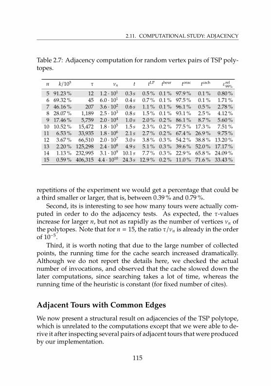
2.11. COMPUTATIONAL STUDY: ADJACENCY
Table 2.7: Adjacency computation for random vertex pairs of TSP poly-topes.
n k/105 τ νn t tLP theur torac tcach εrel99%
5 91.23 % 12 1.2 · 101 0.3 s 0.5 % 0.1 % 97.9 % 0.1 % 0.80 %6 69.32 % 45 6.0 · 101 0.4 s 0.7 % 0.1 % 97.5 % 0.1 % 1.71 %7 46.16 % 207 3.6 · 102 0.6 s 1.1 % 0.1 % 96.1 % 0.5 % 2.78 %8 28.07 % 1,189 2.5 · 103 0.8 s 1.5 % 0.1 % 93.1 % 2.5 % 4.12 %9 17.46 % 5,759 2.0 · 104 1.0 s 2.0 % 0.2 % 86.1 % 8.7 % 5.60 %
10 10.52 % 15,472 1.8 · 105 1.5 s 2.3 % 0.2 % 77.5 % 17.3 % 7.51 %11 6.53 % 33,935 1.8 · 106 2.1 s 2.7 % 0.2 % 67.4 % 26.9 % 9.75 %12 3.67 % 66,510 2.0 · 107 3.0 s 3.8 % 0.3 % 54.2 % 38.8 % 13.20 %13 2.20 % 125,298 2.4 · 108 4.9 s 5.1 % 0.3 % 39.6 % 52.0 % 17.17 %14 1.13 % 232,995 3.1 · 109 10.1 s 7.7 % 0.3 % 22.9 % 65.8 % 24.09 %15 0.59 % 406,315 4.4 · 1010 24.3 s 12.9 % 0.2 % 11.0 % 71.6 % 33.43 %
repetitions of the experiment we would get a percentage that could bea third smaller or larger, that is, between 0.39 % and 0.79 %.
Second, its is interesting to see how many tours were actually com-puted in order to do the adjacency tests. As expected, the τ-valuesincrease for larger n, but not as rapidly as the number of vertices νn ofthe polytopes. Note that for n = 15, the ratio τ/νn is already in the orderof 10−5.
Third, it is worth noting that due to the large number of collectedpoints, the running time for the cache search increased dramatically.Although we do not report the details here, we checked the actualnumber of invocations, and observed that the cache slowed down thelater computations, since searching takes a lot of time, whereas therunning time of the heuristic is constant (for fixed number of cites).
Adjacent Tours with Common Edges
We now present a structural result on adjacencies of the TSP polytope,which is unrelated to the computations except that we were able to de-rive it after inspecting several pairs of adjacent tours that were producedby our implementation.
115
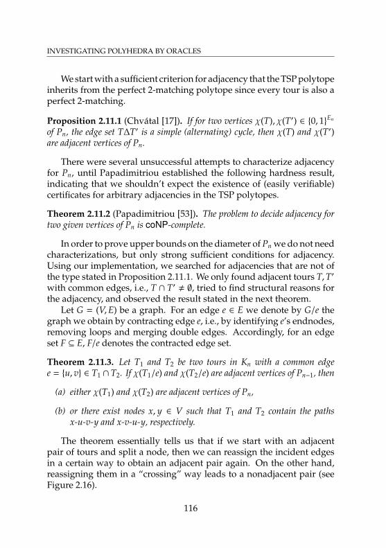
INVESTIGATING POLYHEDRA BY ORACLES
We start with a sufficient criterion for adjacency that the TSP polytopeinherits from the perfect 2-matching polytope since every tour is also aperfect 2-matching.
Proposition 2.11.1 (Chvátal [17]). If for two vertices χ(T), χ(T′) ∈ 0, 1En
of Pn, the edge set T∆T′ is a simple (alternating) cycle, then χ(T) and χ(T′)are adjacent vertices of Pn.
There were several unsuccessful attempts to characterize adjacencyfor Pn, until Papadimitriou established the following hardness result,indicating that we shouldn’t expect the existence of (easily verifiable)certificates for arbitrary adjacencies in the TSP polytopes.
Theorem 2.11.2 (Papadimitriou [53]). The problem to decide adjacency fortwo given vertices of Pn is coNP-complete.
In order to prove upper bounds on the diameter of Pn we do not needcharacterizations, but only strong sufficient conditions for adjacency.Using our implementation, we searched for adjacencies that are not ofthe type stated in Proposition 2.11.1. We only found adjacent tours T,T′
with common edges, i.e., T ∩ T′ , ∅, tried to find structural reasons forthe adjacency, and observed the result stated in the next theorem.
Let G = (V,E) be a graph. For an edge e ∈ E we denote by G/e thegraph we obtain by contracting edge e, i.e., by identifying e’s endnodes,removing loops and merging double edges. Accordingly, for an edgeset F ⊆ E, F/e denotes the contracted edge set.
Theorem 2.11.3. Let T1 and T2 be two tours in Kn with a common edgee = u, v ∈ T1 ∩ T2. If χ(T1/e) and χ(T2/e) are adjacent vertices of Pn−1, then
(a) either χ(T1) and χ(T2) are adjacent vertices of Pn,
(b) or there exist nodes x, y ∈ V such that T1 and T2 contain the pathsx-u-v-y and x-v-u-y, respectively.
The theorem essentially tells us that if we start with an adjacentpair of tours and split a node, then we can reassign the incident edgesin a certain way to obtain an adjacent pair again. On the other hand,reassigning them in a “crossing” way leads to a nonadjacent pair (seeFigure 2.16).
116
2.11. COMPUTATIONAL STUDY: ADJACENCY
u v
x y
Figure 2.16: Illustration of Case (b) of Theorem 2.11.3.
Proof. We can identify Kn/e with Kn−1 in a natural way, and hence con-sider T1/e and T2/e as tours in Kn−1. Throughout the proof we willdenote by u&v the node to which e was contracted in Kn/e.
We consider the face F := x ∈ Pn | xe = 1 of Pn and the projectionmap π : RE
→ RE/u,v defined via
π(x)e =
xe if u&v < exw,u + xw,v if e = w,u&v .
It is not hard to see that π projects vertices of F to vertices of Pn−1, i.e.,considering tours in Kn that contain e, and interpreting them as tours inKn/e. In fact every vertex of F is projected to a vertex of Pn−1 this way.
We claim that for any tour T in Kn/e there are precisely two tours T′
in Kn for which π(χ(T′)) = χ(T) holds. To see this, let W = x-(u&v)-y bethe 2-path in T with u&v as the inner node. Then T′ must be equal toone of the tours
(T \W) ∪x,u , e,
v, y
and (T \W) ∪
x, v , e,
u, y
, (2.52)
since e ∈ T′ must hold and there are only these two possibilities toproperly connect e to T \ W. Hence the preimage of χ(T) under π(intersected with Pn) is an edge of F whose vertices correspond to thetwo possible tours T′.
From the latter (observing thatπ : F→ Pn−1 maps vertices to vertices)we get that the preimage of our given edge conv.hull χ(T1/e), χ(T2/e)
117
INVESTIGATING POLYHEDRA BY ORACLES
under π (again intersected with Pn) is a polytope G with four vertices.These vertices must be the characteristic vectors of T1, T′1, T2 and T′2,where T′1 and T′2 are tours such that the contraction of e maps T1,T′1 toT1/e, and T2,T′2 to T2/e, respectively.
We will now prove that if (b) holds, then (a) cannot hold. So assumethat T1 = W1 ∪·
x,u , e,
v, y
and that T2 = W2 ∪·
x, v , e,
u, y
hold.
From T1/e = T′1/e we obtain T′1 = W1 ∪·x, v , e,
u, y
, while from
T2/e = T′2/e we obtain T′2 = W2 ∪·x,u , e,
v, y
. This already proves
W1 ,W2 since otherwise T1 = T′2 would contradict the fact that the fourtours correspond to distinct vertices of G. Counting edges immediatelyyields
12χ(T1) +
12χ(T2) =
12χ(T′1) +
12χ(T′2), (2.53)
which proves the nonadjacency of χ(T1) and χ(T2).Now suppose (a) does not hold, that is, χ(T1) and χ(T2) are not
adjacent. Since the only polytopes with four vertices are 3-simplices andquadrilaterals, and since simplices have no non-adjacencies, G must bea quadrilateral. Because G is also a 0/1-polytope, its diagonals intersectin their barycenters, that is, Equation (2.53) holds, and in particularT1∆T2 = T′1∆T′2 must hold. From (2.52) we know that T1∆T′1 and T2∆T′2are 4-cycles having e as a chord. Now (2.53) implies that the cycles mustbe the same, i.e., T1∆T′1 = T2∆T′2. Let x and y be the nodes of this cyclethat are not incident to e, ordered such that T1 contains the path x-u-v-y.From (2.52) we obtain that T′1 contains the path x-v-u-y. In particular,the edge x,u is contained in T1 \ T′1, and once again by (2.53), x,ucannot be contained in T2. Hence, T2 must contain the path x-v-u-y.
There are adjacencies that are not inherited from the perfect 2-matching polytope, but can be explained using Proposition 2.11.1 andTheorem 2.11.3. One may be brave to conjecture that maybe all adja-cencies of the TSP polytope are either of 2-matching type or stem fromthose by splitting. But once again, since a series of contractions wouldbe a short certificate, the hardness result in Theorem 2.11.2 states thatwe should not expect such a result. In other words we might expectthat there exist pairs of adjacent vertices χ(T1) and χ(T2) of Pn (for somen ∈ N) that are not adjacent in the 2-matching polytope, and no mat-
118
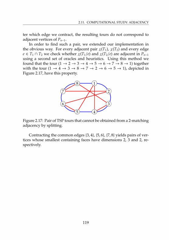
2.11. COMPUTATIONAL STUDY: ADJACENCY
ter which edge we contract, the resulting tours do not correspond toadjacent vertices of Pn−1.
In order to find such a pair, we extended our implementation inthe obvious way. For every adjacent pair χ(T1), χ(T2) and every edgee ∈ T1 ∩ T2 we check whether χ(T1/e) and χ(T2/e) are adjacent in Pn−1using a second set of oracles and heuristics. Using this method wefound that the tour (1 → 2 → 3 → 4 → 5 → 6 → 7 → 8 → 1) togetherwith the tour (1 → 4 → 3 → 8 → 7 → 2 → 6 → 5 → 1), depicted inFigure 2.17, have this property.
1
2
3
45
6
7
8
Figure 2.17: Pair of TSP tours that cannot be obtained from a 2-matchingadjacency by splitting.
Contracting the common edges 3, 4, 5, 6, 7, 8 yields pairs of ver-tices whose smallest containing faces have dimensions 2, 3 and 2, re-spectively.
119

ANALYZING SIMPLE EXTENSIONS OF POLYTOPES
120
Chapter 3
Analyzing SimpleExtensions of Polytopes
121
ANALYZING SIMPLE EXTENSIONS OF POLYTOPES
122
3.1. INTRODUCTION
ANALYZING SIMPLE EXTENSIONS OF POLYTOPES:
3.1 Introduction
With respect to both structural and algorithmic aspects, linear optimiza-tion over a polytope P can be replaced by linear optimization over any(usually higher dimensional) polytope Q of which P can be obtained asthe image under a linear map (which we refer to as a projection). Such apolytope Q (along with a suitable projection) is called an extension of P.
Defining the size of a polytope as its number of facets, the smallestsize of any extension of the polytope P is known as the extension com-plexity xc (P) of P. It has turned out in the past that for several importantpolytopes related to combinatorial optimization problems the extensioncomplexity is bounded polynomially in the dimension, although outerdescriptions in the original space require exponentially many inequali-ties. One of the most prominent examples is the spanning tree polytopeof the complete graph Kn on n nodes, which has extension complexityO(n3) [50].
After Rothvoss [58] showed that there are 0/1-polytopes whose exten-sion complexities cannot be bounded polynomially in their dimensions,in 2012, Fiorini, Massar, Pokutta, Tiwary and de Wolf [27] could provethat the extension complexities of some concrete and important exam-ples of polytopes like traveling salesman polytopes cannot be boundedpolynomially. Similar results have then also been deduced for severalother polytopes associated with NP-hard optimization problems, e.g.,by Avis and Tiwary [9] and Pokutta and van Vyve [55]. Rothvoss [59]recently showed that also the perfect matching polytope of the com-plete graph (with an even number of nodes) has exponential extension
123
ANALYZING SIMPLE EXTENSIONS OF POLYTOPES
complexity, thus exhibiting the first polytope with this property that isassociated with a polynomial-time solvable optimization problem.
The first fundamental research with respect to understanding exten-sion complexities was Yannakakis’ seminal paper [69] of 1991. Observ-ing that many of the nice and small extensions that are known (e.g., thepolynomial size extension of the spanning tree polytope of Kn mentionedabove) have the nice property of being symmetric in a certain sense, hederived lower bounds on extensions with that special property. In par-ticular, he already proved that both perfect matching polytopes as wellas traveling salesman polytopes do not have polynomial size symmetricextensions.
It turned out that requiring symmetry in principle actually canmake a huge difference for the minimum sizes of extensions (thoughnowadays we know that this is not really true for traveling sales-man and perfect matching polytopes). For instance, Kaibel, Theis andPashkovich [40] showed that the polytope associated with the match-ings of size blog nc in Kn has polynomially bounded extension complex-ity although it does not admit symmetric extensions of polynomial size.Another example is provided by the permutahedron, which has exten-sion complexity Θ
(n log n
)[31], while every symmetric extension of it
has size Ω(n2) [54].These examples show that imposing the restriction of symmetry may
severely influence the smallest possible sizes of extensions. In this chap-ter, we investigate another type of restrictions on extensions, namely theone arising from requiring the extension to be a non-degenerate poly-tope. A d-dimensional polyhedron is called simple if every vertex iscontained in exactly d facets. We denote by sxc (P) the simple extensioncomplexity, i.e., the smallest size of any simple extension of the poly-tope P.
From a practical point of view, simplicity is an interesting propertysince it is the geometric interpretation of primal non-degeneracy of lin-ear programs. In addition, large parts of combinatorial/extremal theoryof polytopes deal with simple polytopes. Furthermore, as with otherrestrictions like symmetry, there indeed exist nice examples of simpleextensions of certain polytopes relevant in optimization. For instance,generalizing the well-known fact that the permutahedron is a zonotope,Wolsey showed in the late 80’s (personal communication) that, for ar-
124
3.1. INTRODUCTION
bitrary processing times, the completion-time polytope for n jobs is aprojection of an O(n2)-dimensional cube. The main results of this chap-ter show, however, that for several polytopes relevant in optimization(among them both perfect matching polytopes and spanning tree poly-topes) insisting on simplicity enforces very large sizes of the extensions.More precisely, we establish that for the following polytopes the sim-ple extension complexity equals their number of vertices (note that thenumber of vertices of P is a trivial upper bound for sxc (P), realized bythe extension obtained from writing P as the convex hull of its vertices):
• Perfect matching polytopes of complete graphs (Theorem 3.7.3)
• Perfect matching polytopes of complete bipartite graphs (Theo-rem 3.7.1)
• Uncapacitated flow polytopes of non-decomposable acyclic net-works (Theorem 3.6.1)
• (Certain) random 0/1-polytopes (Theorem 3.3.8)
• Hypersimplices (Theorem 3.4.1)
Furthermore, we prove that
• the spanning tree polytope of the complete graph with n nodes hassimple extension complexity at least Ω(2n−o(n)) (Theorem 3.5.2).
The chapter is structured as follows: We first focus on known con-struction techniques, and characterize when reflections and disjunctiveprogramming yield simple extensions (Section 3.2). We continue withsome techniques to bound the simple extension complexity of a polytopefrom below (Section 3.3). Then we deduce our results on hypersimplices(Section 3.4), spanning tree polytopes (Section 3.5), flow polytopes (Sec-tion 3.6) and perfect matching polytopes (Section 3.7). The core of thelatter part is a strengthening of a result of Padberg and Rao’s [52] on ad-jacencies in the perfect matching polytope (Theorem 3.7.6), which maybe of independent interest.
Let us end this introduction by remarking that the concept of simpli-cial extensions is not interesting. To see this, observe that any d-polytopeQ with N vertices has at least d · N facet-vertex incidences since everyvertex lies in at least d facets. On the other hand, if Q is simplicial (i.e.,
125
ANALYZING SIMPLE EXTENSIONS OF POLYTOPES
all facets are simplices) and has f facets, the number of facet-vertex in-cidences is equal to d · f , proving f ≥ N. For every polytope P with Nvertices, every extension polytope has at least N vertices, and hence asmallest possible simplicial extension polytope of P is the simplex withN vertices.
126
3.2. CONSTRUCTIONS
ANALYZING SIMPLE EXTENSIONS OF POLYTOPES:
3.2 Constructions
There are three major techniques for constructing extended formula-tions, namely dynamic programming, disjunctive programming andreflections. Extensions based on dynamic programs yield network flowpolytopes for acyclic graphs, which are not simple in general and alsohave large simple extension complexities (see Section 3.6).
In this section we characterize for the other two techniques men-tioned above in which cases the produced extensions are simple.
Reflections
Let P = x ∈ Rn| Ax ≤ b be a polytope and let H≤ =
x ∈ Rn
| 〈a, x〉 ≤ β
be a halfspace in Rn (in particular we assume a , O). Denoting byP1 := P ∩H≤ the intersection of the polytope with the halfspace and byP2 the image of P1 under reflection at the boundary hyperplane H= ofH≤, we call conv.hull(P1 ∪ P2) the reflection of P at H≤. The technique in[39] provides an extended formulation for this polytope.
Proposition 3.2.1 (Kaibel & Pashkovich [39]). The polytope Q defined by
Q = (x, y) ∈ Rn+n| Ay ≤ b,
⟨a, y
⟩≤ 〈a, x〉 ≤ 2β −
⟨a, y
⟩,
(x − y) ∈ lin.hull (a)
together with the projection onto the x-space is an extension of the polytopeconv.hull (P1 ∪ P2).
127
ANALYZING SIMPLE EXTENSIONS OF POLYTOPES
Our contribution is the next theorem that clarifies under which cir-cumstances Q is a simple polytope.
Theorem 3.2.2. Let Q be the extension polytope for the reflection of P at H≤as defined in this subsection, let P1 := P ∩ H≤, and let F := P1 ∩ H= be theintersection of P1 with the reflection hyperplane. Then Q is simple if and onlyif P1 is simple and either P1 = F, or F is a facet of P1 or F = ∅.
Proof. We first observe that the faces
Q1 := Q ∩(x, y) ∈ Rn
×Rn|⟨a, y
⟩= 〈a, x〉
Q2 := Q ∩
(x, y) ∈ Rn
×Rn| 〈a, x〉 = 2β −
⟨a, y
⟩of Q are both affinely isomorphic to P1. Thus Q can only be simple ifP1 is so. If P1 ⊆ H= holds, Q = Q1 = Q2 and Q is simple if and onlyif P1 is simple, proving the equivalence in case P1 = F. Otherwise, letd := dim P1 and observe that dim Q = d + 1 holds because Q1 and Q2are proper faces of Q and Q’s dimension cannot be larger than d + 1.Furthermore, (x, y) ∈ Q1 ∩ Q2 holds if and only if 〈a, x〉 = β is satisfied,hence Q1 ∩Q2 is affinely isomorphic to F. Define k := dim F.
We now assume that Q is simple and F , ∅, i.e., k ≥ 0 holds. Letv be any vertex of Q1 ∩ Q2. Since Q is simple and of dimension d + 1,v has d + 1 adjacent vertices, k of which lie in Q1 ∩ Q2 (isomorphic toF). Furthermore, v has d neighbors in Qi for i = 1, 2. Hence, k of thesevertices lie in Q1 ∩ Q2, d − k lie in Q1 \ Q2 and d − k lie in Q2 \ Q1. Theresulting equation k + (d − k) + (d − k) = d + 1 yields k = d − 1, i.e., F is afacet of P1. This proves necessity of the condition.
To prove sufficiency, from now on assume that P1 is simple anddim Q = d + 1 holds. We prove that every vertex (x, y) of Q not lying inQ1∩Q2 lies in at most (thus, exactly) d + 1 facets of Q. First, y can satisfyat most d inequalities of Ay ≤ b with equality because P1 is simple.Second, (x, y) can satisfy at most one of the other two inequalities withequality since otherwise, 〈a, x〉 = β would hold, contradicting the factthat (x, y) < Q1 ∩Q2. Hence, the vertex lies in at most d + 1 facets, whichproves the claim. This already proves that Q is simple in the case F = ∅,since then there are no further vertices.
It remains to show that if F is a facet of P1 then every vertex (x, y) ofQ1 ∩Q2 has at most d + 1 neighbors in Q. In this case, Q1 ∩Q2 is a facetof Q1 and of Q2, which in turn are facets of Q. Since Q1 ∩Q2 is a facet of
128
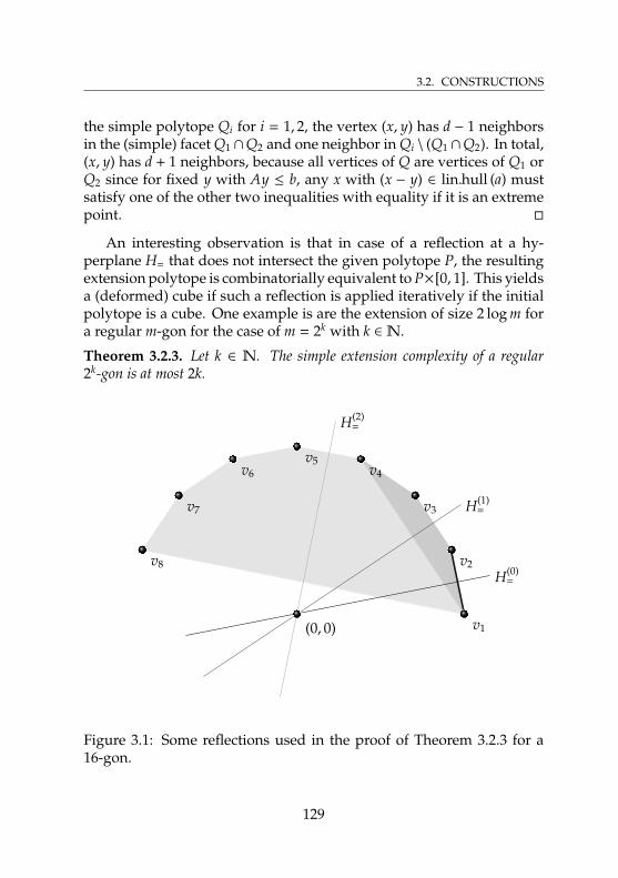
3.2. CONSTRUCTIONS
the simple polytope Qi for i = 1, 2, the vertex (x, y) has d − 1 neighborsin the (simple) facet Q1 ∩Q2 and one neighbor in Qi \ (Q1 ∩Q2). In total,(x, y) has d + 1 neighbors, because all vertices of Q are vertices of Q1 orQ2 since for fixed y with Ay ≤ b, any x with (x − y) ∈ lin.hull (a) mustsatisfy one of the other two inequalities with equality if it is an extremepoint.
An interesting observation is that in case of a reflection at a hy-perplane H= that does not intersect the given polytope P, the resultingextension polytope is combinatorially equivalent to P×[0, 1]. This yieldsa (deformed) cube if such a reflection is applied iteratively if the initialpolytope is a cube. One example is are the extension of size 2 log m fora regular m-gon for the case of m = 2k with k ∈N.
Theorem 3.2.3. Let k ∈ N. The simple extension complexity of a regular2k-gon is at most 2k.
H(2)=
H(1)=
H(0)=
v1
v2
v3
v4v5
v6
v7
v8
(0, 0)
Figure 3.1: Some reflections used in the proof of Theorem 3.2.3 for a16-gon.
129
ANALYZING SIMPLE EXTENSIONS OF POLYTOPES
Proof. We recursively define a series of polytopes as follows: The initial(simple) polytope is P(0) := (1, 0)ᵀ, i.e., a single point. Since the exten-sions we construct are located in increasingly higher-dimensional spaceswe write coordinates as (x, y, z)ᵀ ∈ R ×R ×R∗, where the dimension ofthe z-space increases, initially being zero.
We now define for i = 0, 1, 2, . . . , k − 1 the polytope P(i+1) as thereflection of P(i) at the halfspace
H(i)≤
:= (x, y, z) ∈ R ×R ×R∗ |
− sin((2i− 1) · π/2k)x + cos((2i
− 1) · π/2k)y ≤ 0.
Theorem 3 in [39] shows that P(k) is an extension of a regular 2k-gon. If welabel the vertices of this 2k-gon with v1, v2, . . . , v2k in counter-clockwiseorder starting with v1 = (1, 0)ᵀ, the proof even shows that the projectionof P(i) onto the first two coordinates equals the convex hull of the verticesv1, v2, . . . , v2i . Now for every i = 0, 1, . . . , k − 1, the polytope P(i) does notintersect H(i)
= since the projection of such an intersection point would lieoutside the mentioned convex hull.
This ensures that by induction all polytopes P(i) for i = 0, 1, 2, . . . , kare simple by Theorem 3.2.2 and that the last polytope P(k) is a simpleextension of the regular 2k-gon.
Disjunctive Programming
The third major technique to construct extended formulations is bymeans of disjunctive programming, introduced by Balas [10],[11]. We onlyconsider the special case of a disjunction of two polytopes P1,P2 ⊆ Rn
and are interested in an extension of the convex hull of the union of thetwo.
A helpful tool is the homogenization homog(P) of a polytope P, definedas homog(P) := conic.hull (P × 1). We say that a pointed polyhedralcone C is weakly simple if every extreme ray of C lies in exactly dim (C)−1 facets and strongly simple if C is a simple polyhedron. Clearly, astrongly simple cone is also weakly simple. Furthermore, if we haveC = homog(P) then C is weakly simple if and only if P is simple and C isstrongly simple if and only if P is a simplex. We will need the followinglemma about weak simplicity of cartesian products of cones.
130
3.2. CONSTRUCTIONS
Lemma 3.2.4. Given two pointed polyhedral cones C1 ⊆ Rn1 , C2 ⊆ Rn2 , theirproduct cone C := C1 × C2 ⊆ Rn1+n2 is weakly simple if and only if both C1and C2 are strongly simple.
Proof. It is easy to check that C1 ×C2 = (x1, x2) ∈ Rn1+n2 | xi ∈ Ci i = 1, 2is a pointed polyhedral cone again. Furthermore, the faces of C1 × C2are exactly the products of faces of C1 and C2, their dimensions add up,and a face F1 × F2 of C1 × C2 is contained in another face G1 × G2 if andonly if F1 ⊆ G1 and F2 ⊆ G2 hold.
Hence, the extreme rays of C1×C2 are either products of extreme raysof C1 withOn2 or products ofOn1 with extreme rays of C2. Similarly, thefacets of C1 × C2 are either products of facets of C1 with C2 or productsof C1 with facets of C2.
We consider an extreme ray of C, w.l.o.g. of the form r ×On2 , wherer is an extreme ray of C1. It is clearly contained in the facets F1 × C2,where F1 is a facet of C1 containing r. For every facet F2 of C2, we haveOn2 ⊆ F2 and hence C1 × F2 contains r ×On2 .
Thus, if r is contained in k facets of C1 and C2 has ` facets then r×On2
is contained in k + ` facets of C1 × C2.We always have k ≥ dim C1 − 1 and ` ≥ dim C2 since C1 and C2 are
pointed polyhedral cones. Hence, k + ` ≥ dim C1 + dim C2 − 1 holdsand we have equality if and only if k = dim C1 − 1 and ` = dim C2 aresatisfied, and hence C1 and C2 are strongly simple.
We now turn to the mentioned extension of P = conv.hull (P1 ∪ P2)using disjunctive programming. Define
Q =(x1, λ1, x2, λ2) ∈ homog (P1) × homog (P2) | λ1 + λ2 = 1
.
It is well-known that Q together with the projection (x1, λ1, x2, λ2) 7→x1 +x2 yields an extension of P. We now characterize when Q is a simplepolytope.
Theorem 3.2.5. The extension polytope Q of the disjunctive program forthe polytope P = conv.hull (P1 ∪ P2) is simple if and only if P1 and P2 aresimplices.
131
ANALYZING SIMPLE EXTENSIONS OF POLYTOPES
Proof. As Q is the intersection of the pointed cone C = homog (P1) ×homog (P2) with the hyperplane defined by λ1 +λ2 = 1 (which does notcontain any of C’s extreme rays), we know that Q is simple if and onlyif C is weakly simple. Now Lemma 3.2.4 yields the result.
132
3.3. BOUNDING TECHNIQUES
ANALYZING SIMPLE EXTENSIONS OF POLYTOPES:
3.3 Bounding Techniques
Let P ⊆ Rn be a polytope with N vertices.
Clearly, P is the set of all convex combinations of its vertices, imme-diately providing an extended formulation of size N:
P = proj x(x, y) ∈ Rn×Rvert(P)
+ | x =∑
v∈vert(P)
yvv,∑
v∈vert(P)
yv = 1
Note that this trivial extension is simple since the extension is an (N − 1)-dimensional simplex.
An easy observation for extensions P = π(Q) with Q ⊆ Rd andπ : Rd
→ Rn is that the assignment F 7→ π−1(F) ∩Q =y ∈ Q | π(y) ∈ F
defines a map j which embeds L(P) into L(Q), i.e., it is one-to-oneand preserves inclusion in both directions (see [26]). Note that thisembedding furthermore satisfies j(F ∩ F′) = j(F) ∩ j(F′) for all faces F,F′
of P (where the nontrivial inclusion j(F) ∩ j(F′) ⊆ j(F ∩ F′) follows fromπ( j(F)∩ j(F′)) ⊆ π( j(F))∩π( j(F′)) = F∩F′). We use the shorthand notationj(v) := j(v) for vertices v of P.
We consider the face-vertex non-incidence graph GN (P), a bipartitegraph having the faces and the vertices of P as the node set and edgesF, v for all v < F (where v is a vertex and F is a face of P). Every facetf of an extension induces two node sets of this graph in the following
133
ANALYZING SIMPLE EXTENSIONS OF POLYTOPES
way:
F ( f ) :=F face of P | j(F) ⊆ f
V( f ) :=
v vertex of P | j(v) * f
(3.1)
We call F ( f ) and V( f ) the set of faces (resp. vertices) induced by the facetf (with respect to the extension P = π(Q)). Typically, the extension andthe facet f are fixed and we just write F (resp.V). It may happen thatV( f ) is equal to the whole vertex set, e.g., if f projects into the relativeinterior of P. IfV( f ) is a proper subset of the vertex set we call facet fproper.
For each facet f of an extension of P the face and vertex sets F ( f ),V( f ) together induce a biclique (i.e., complete bipartite subgraph) inGN (P). It follows from Yannakakis [69] that every edge in GN (P) iscovered by at least one of those induced bicliques. We provide a briefcombinatorial argument for this (in particular showing that we canrestrict to proper facets) in the proof of the following proposition.
Proposition 3.3.1. Let P be a polytope and Q be an extension with P = π(Q).Then the subgraph of GN (P) induced by F ( f ) ∪· V( f ) is a biclique for everyfacet f of Q. Furthermore, every edge F, v of GN (P) is covered by at least oneof the bicliques induced by a proper facet.
Proof. Let f be one of the facets and assume that an edge F, v withF ∈ F ( f ) and v ∈ V( f ) is not present in GN (P), i.e., v ∈ F. From v ∈ F weobtain j(v) ⊆ j(F) ⊆ f , a contradiction to v ∈ V( f ).
To prove the second statement, let F, v be any edge of GN (P), i.e.,v < F. Observe that the preimages G := j(F) and g := j(v) are alsonot incident (i.e., g * G) since j is a lattice embedding. As G is theintersection of all facets of Q it is contained in (the face-lattice of apolytope is coatomic), there must be at least one facet f containing Gbut not g (since otherwise g would be contained in G), yielding F ∈ F ( f )and v ∈ V( f ).
If F , ∅, any vertex w ∈ F satisfies j(w) ⊆ G ⊆ f and hence f is aproper facet. If F = ∅, let w be any vertex of P distinct from v. Thepreimages j(v) and j(w) clearly satisfy j(v) * j(w). Again, since the face-lattice of Q is coatomic, there exists a facet f with j(w) ⊆ f but j(v) * f .
134
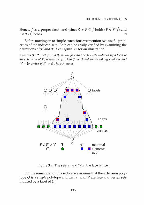
3.3. BOUNDING TECHNIQUES
Hence, f is a proper facet, and (since ∅ , F ⊆ f holds) F ∈ F ( f ) andv ∈ V( f ) holds.
Before moving on to simple extensions we mention two useful prop-erties of the induced sets. Both can be easily verified by examining thedefinitions of F andV. See Figure 3.2 for an illustration.
Lemma 3.3.2. Let F and V be the face and vertex sets induced by a facet ofan extension of P, respectively. Then F is closed under taking subfaces andV =
v vertex of P | v <
⋃F∈F F
holds.
P
∅
facets
vertices
edges
F < F ∪V V F maximalelementsin F
Figure 3.2: The sets F andV in the face lattice.
For the remainder of this section we assume that the extension poly-tope Q is a simple polytope and that F and V are face and vertex setsinduced by a facet of Q.
135
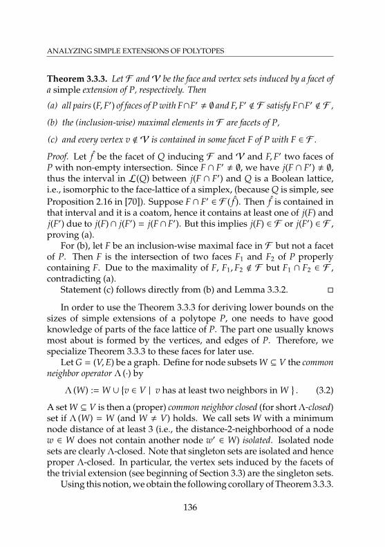
ANALYZING SIMPLE EXTENSIONS OF POLYTOPES
Theorem 3.3.3. Let F andV be the face and vertex sets induced by a facet ofa simple extension of P, respectively. Then
(a) all pairs (F,F′) of faces of P with F∩F′ , ∅ and F,F′ < F satisfy F∩F′ < F ,
(b) the (inclusion-wise) maximal elements in F are facets of P,
(c) and every vertex v <V is contained in some facet F of P with F ∈ F .
Proof. Let f be the facet of Q inducing F and V and F,F′ two faces ofP with non-empty intersection. Since F ∩ F′ , ∅, we have j(F ∩ F′) , ∅,thus the interval in L(Q) between j(F ∩ F′) and Q is a Boolean lattice,i.e., isomorphic to the face-lattice of a simplex, (because Q is simple, seeProposition 2.16 in [70]). Suppose F ∩ F′ ∈ F ( f ). Then f is contained inthat interval and it is a coatom, hence it contains at least one of j(F) andj(F′) due to j(F)∩ j(F′) = j(F∩ F′). But this implies j(F) ∈ F or j(F′) ∈ F ,proving (a).
For (b), let F be an inclusion-wise maximal face in F but not a facetof P. Then F is the intersection of two faces F1 and F2 of P properlycontaining F. Due to the maximality of F, F1,F2 < F but F1 ∩ F2 ∈ F ,contradicting (a).
Statement (c) follows directly from (b) and Lemma 3.3.2.
In order to use the Theorem 3.3.3 for deriving lower bounds on thesizes of simple extensions of a polytope P, one needs to have goodknowledge of parts of the face lattice of P. The part one usually knowsmost about is formed by the vertices, and edges of P. Therefore, wespecialize Theorem 3.3.3 to these faces for later use.
Let G = (V,E) be a graph. Define for node subsets W ⊆ V the commonneighbor operator Λ (·) by
Λ (W) := W ∪v ∈ V | v has at least two neighbors in W
. (3.2)
A set W ⊆ V is then a (proper) common neighbor closed (for short Λ-closed)set if Λ (W) = W (and W , V) holds. We call sets W with a minimumnode distance of at least 3 (i.e., the distance-2-neighborhood of a nodew ∈ W does not contain another node w′ ∈ W) isolated. Isolated nodesets are clearly Λ-closed. Note that singleton sets are isolated and henceproper Λ-closed. In particular, the vertex sets induced by the facets ofthe trivial extension (see beginning of Section 3.3) are the singleton sets.
Using this notion, we obtain the following corollary of Theorem 3.3.3.
136
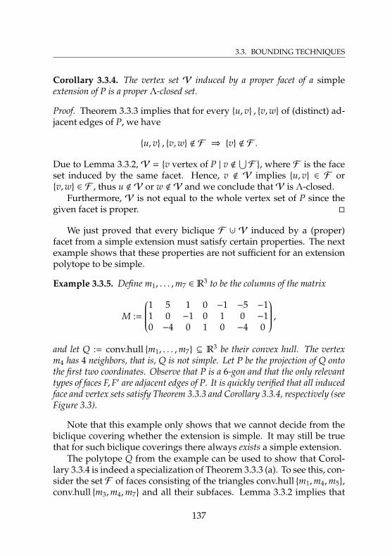
3.3. BOUNDING TECHNIQUES
Corollary 3.3.4. The vertex set V induced by a proper facet of a simpleextension of P is a proper Λ-closed set.
Proof. Theorem 3.3.3 implies that for every u, v , v,w of (distinct) ad-jacent edges of P, we have
u, v , v,w < F ⇒ v < F .
Due to Lemma 3.3.2,V = v vertex of P | v <⋃F , where F is the face
set induced by the same facet. Hence, v < V implies u, v ∈ F orv,w ∈ F , thus u <V or w <V and we conclude thatV is Λ-closed.
Furthermore, V is not equal to the whole vertex set of P since thegiven facet is proper.
We just proved that every biclique F ∪· V induced by a (proper)facet from a simple extension must satisfy certain properties. The nextexample shows that these properties are not sufficient for an extensionpolytope to be simple.
Example 3.3.5. Define m1, . . . ,m7 ∈ R3 to be the columns of the matrix
M :=
1 5 1 0 −1 −5 −11 0 −1 0 1 0 −10 −4 0 1 0 −4 0
,and let Q := conv.hull m1, . . . ,m7 ⊆ R3 be their convex hull. The vertexm4 has 4 neighbors, that is, Q is not simple. Let P be the projection of Q ontothe first two coordinates. Observe that P is a 6-gon and that the only relevanttypes of faces F,F′ are adjacent edges of P. It is quickly verified that all inducedface and vertex sets satisfy Theorem 3.3.3 and Corollary 3.3.4, respectively (seeFigure 3.3).
Note that this example only shows that we cannot decide from thebiclique covering whether the extension is simple. It may still be truethat for such biclique coverings there always exists a simple extension.
The polytope Q from the example can be used to show that Corol-lary 3.3.4 is indeed a specialization of Theorem 3.3.3 (a). To see this, con-sider the set F of faces consisting of the triangles conv.hull m1,m4,m5,conv.hull m3,m4,m7 and all their subfaces. Lemma 3.3.2 implies that
137
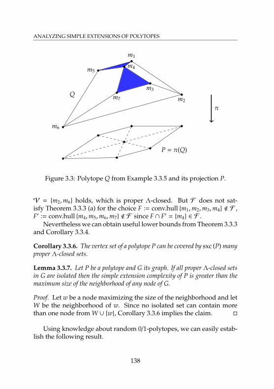
ANALYZING SIMPLE EXTENSIONS OF POLYTOPES
m1
m2
m3
m4m5
m6
m7
π
Q
P = π(Q)
Figure 3.3: Polytope Q from Example 3.3.5 and its projection P.
V = m2,m6 holds, which is proper Λ-closed. But F does not sat-isfy Theorem 3.3.3 (a) for the choice F := conv.hull m1,m2,m3,m4 < F ,F′ := conv.hull m4,m5,m6,m7 < F since F ∩ F′ = m4 ∈ F .
Nevertheless we can obtain useful lower bounds from Theorem 3.3.3and Corollary 3.3.4.
Corollary 3.3.6. The vertex set of a polytope P can be covered by sxc (P) manyproper Λ-closed sets.
Lemma 3.3.7. Let P be a polytope and G its graph. If all proper Λ-closed setsin G are isolated then the simple extension complexity of P is greater than themaximum size of the neighborhood of any node of G.
Proof. Let w be a node maximizing the size of the neighborhood and letW be the neighborhood of w. Since no isolated set can contain morethan one node from W ∪ w, Corollary 3.3.6 implies the claim.
Using knowledge about random 0/1-polytopes, we can easily estab-lish the following result.
138
3.3. BOUNDING TECHNIQUES
Theorem 3.3.8. There is a constant σ > 0 such that a random d-dimensional0/1-polytope P with at most 2σd vertices asymptotically almost surely has asimple extension complexity equal to its number of vertices.
Proof. One of the main results of Gillmann’s thesis (See Theorem 3.37in [30] for k = 2) is that there is such a σ ensuring that a random d-dimensional 0/1-polytope P with at most 2σd vertices asymptoticallyalmost surely has every pair of vertices adjacent. Since in this situationthe only proper Λ-closed sets are the singletons, Corollary 3.3.6 yieldsthe claim.
139
ANALYZING SIMPLE EXTENSIONS OF POLYTOPES
ANALYZING SIMPLE EXTENSIONS OF POLYTOPES:
3.4 Hypersimplices
Let ∆nk denote the k-hypersimplex in Rn for some k ∈ 0, 1, 2, . . . ,n,
i.e., the 0/1-cube intersected with the hyperplane 〈1n, x〉 = k. Note thatits vertices are all 0/1-vectors with exactly k 1’s, since the above linearsystem is totally unimodular (a row of ones together with two unitmatrices). It follows from the knowledge about edges and 2-faces ofthe cube that two vertices of ∆n
k are adjacent if and only if they differ inexactly two coordinates. In other words, all neighbors of a vertex x canbe obtained by replacing a 1 by a 0 at some index and a 0 by a 1 at someother index. Observe that ∆n
k is almost simple for 2 ≤ k ≤ n − 2 in thesense that its dimension is n− 1, but every vertex lies in exactly n facets.With this in mind, the following result may seem somewhat surprising.
Theorem 3.4.1. Let 1 ≤ k ≤ n − 1. The simple extension complexity of∆n
k ⊆ Rn is equal to its number of vertices
(nk).
Proof. The case of k = 1 or k = n − 1 is clear since then ∆nk is an (n − 1)-
dimensional simplex.Let 2 ≤ k ≤ n − 2 and F andV be face and vertex sets induced by a
proper facet of a simple extension of ∆nk .
Since every vertex v of ∆nk has vi = 0 or vi = 1, at most one of the
facets xi ≥ 0 or xi ≤ 1 can be in F for every i ∈ [n] (otherwiseV wouldbe empty). We can partition [n] into L ∪· U ∪· R such that L (resp. U)contains those indices i ∈ [n] such that the facet corresponding to xi ≥ 0(resp. xi ≤ 1) is in F and R contains the remaining indices. Lemma 3.3.2
140
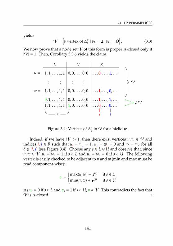
3.4. HYPERSIMPLICES
yieldsV =
v vertex of ∆n
k | vL = 1, vU = O. (3.3)
We now prove that a node setV of this form is proper Λ-closed only if|V| = 1. Then, Corollary 3.3.6 yields the claim.
L U R
1, 1, . . . , 1, 1
......
1, 1, . . . , 1, 1
0, 0, . . . , 0, 0
......
0, 0, . . . , 0, 0
. . . , 0, . . . , 1, . . .
. . . , 1, . . . , 0, . . .
0, 1, . . . , 1, 1 0, 0, . . . , 0, 0 . . . , 1, . . . , 1, . . .1, 1, . . . , 1, 1 1, 0, . . . , 0, 0 . . . , 0, . . . , 0, . . .
V
u =
w =
i j
v <V
s
Figure 3.4: Vertices of ∆nk inV for a biclique.
Indeed, if we have |V| > 1, then there exist vertices u,w ∈ V andindices i, j ∈ R such that ui = w j = 1, u j = wi = 0 and u` = w` for all` < i, j (see Figure 3.4). Choose any s ∈ L ∪· U and observe that, sinceu,w ∈ V, us = ws = 1 if s ∈ L and us = ws = 0 if s ∈ U. The followingvertex is easily checked to be adjacent to u and w (min and max must beread component-wise):
v :=
max(u,w) − e(s) if s ∈ Lmin(u,w) + e
(s) if s ∈ U
As vs = 0 if s ∈ L and vs = 1 if s ∈ U, v <V. This contradicts the fact thatV is Λ-closed.
141
ANALYZING SIMPLE EXTENSIONS OF POLYTOPES
ANALYZING SIMPLE EXTENSIONS OF POLYTOPES:
3.5 Spanning Tree Polytopes
In this section we bound the simple extension complexity of the span-ning tree polytope Pspt (Kn) of the complete graph Kn with n nodes. Inorder to highlight different perspectives we mention three equivalentadjacency characterizations that all follow from the fact that the span-ning tree polytope is the base polytope of a graphic matroid (see [63],Theorem 40.6.). The vertices corresponding to spanning trees T and T′
are adjacent in the spanning tree polytope if and only if . . .
• . . . |T∆T′| = 2 holds.
• . . . T′ arises from T by removing one edge and reconnecting thetwo connected components by another edge.
• . . . T′ arises from T by adding one additional edge and removingany edge from the cycle that this edge created.
From the third statement it is easy to see that the maximum degreeof the 1-skeleton of Pspt (Kn) is in O(n3), since there are O(n2) possiblechoices for the additional edge, each of which yields O (n) choices for acycle-edge to remove.
Lemma 3.5.1. All proper Λ-closed sets in the graph of Pspt (Kn) are isolated.
Proof. Throughout the proof, we will identify vertices with the corre-sponding spanning trees.
142
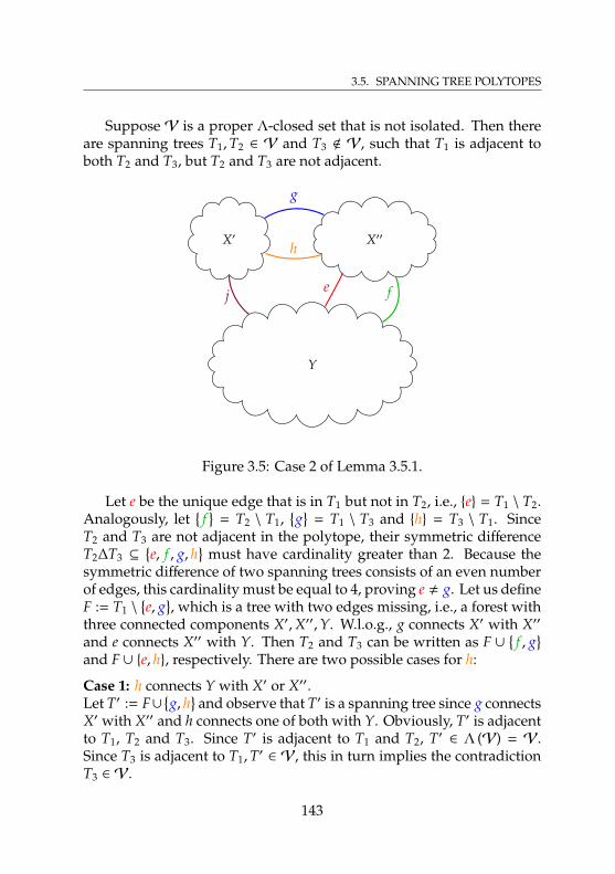
3.5. SPANNING TREE POLYTOPES
Suppose V is a proper Λ-closed set that is not isolated. Then thereare spanning trees T1,T2 ∈ V and T3 < V, such that T1 is adjacent toboth T2 and T3, but T2 and T3 are not adjacent.
X′ X′′
Y
e f
g
h
j
Figure 3.5: Case 2 of Lemma 3.5.1.
Let e be the unique edge that is in T1 but not in T2, i.e., e = T1 \ T2.Analogously, let
f
= T2 \ T1,g
= T1 \ T3 and h = T3 \ T1. SinceT2 and T3 are not adjacent in the polytope, their symmetric differenceT2∆T3 ⊆
e, f , g, h
must have cardinality greater than 2. Because the
symmetric difference of two spanning trees consists of an even numberof edges, this cardinality must be equal to 4, proving e , g. Let us defineF := T1 \
e, g
, which is a tree with two edges missing, i.e., a forest with
three connected components X′,X′′,Y. W.l.o.g., g connects X′ with X′′
and e connects X′′ with Y. Then T2 and T3 can be written as F ∪f , g
and F ∪ e, h, respectively. There are two possible cases for h:
Case 1: h connects Y with X′ or X′′.Let T′ := F∪
g, h
and observe that T′ is a spanning tree since g connects
X′ with X′′ and h connects one of both with Y. Obviously, T′ is adjacentto T1, T2 and T3. Since T′ is adjacent to T1 and T2, T′ ∈ Λ (V) = V.Since T3 is adjacent to T1,T′ ∈ V, this in turn implies the contradictionT3 ∈ V.
143
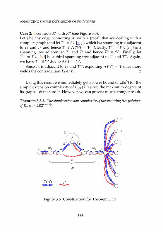
ANALYZING SIMPLE EXTENSIONS OF POLYTOPES
Case 2: h connects X′ with X′′ (see Figure 3.5).Let j be any edge connecting X′ with Y (recall that we dealing with acomplete graph) and let T′ := F∪
g, j
, which is a spanning tree adjacent
to T1 and T2 and hence T′ ∈ Λ (V) = V. Clearly, T′′ := F ∪e, j
is a
spanning tree adjacent to T1 and T′ and hence T′′ ∈ V. Finally, letT′′′ := F ∪
h, j
be a third spanning tree adjacent to T′ and T′′. Again,
we have T′′′ ∈ V due to Λ (V) =V.Since T3 is adjacent to T1 and T′′′, exploiting Λ (V) = V once more
yields the contradiction T3 ∈ V.
Using this result we immediately get a lower bound of Ω(n3) for thesimple extension complexity of Pspt (Kn) since the maximum degree ofits graph is of that order. However, we can prove a much stronger result.
Theorem 3.5.2. The simple extension complexity of the spanning tree polytopeof Kn is in Ω(2n−o(n)).
U
s w1 x
y
z wk t
v1
v2
...a
b
c
W
T(W) T′
Figure 3.6: Construction for Theorem 3.5.2.
144
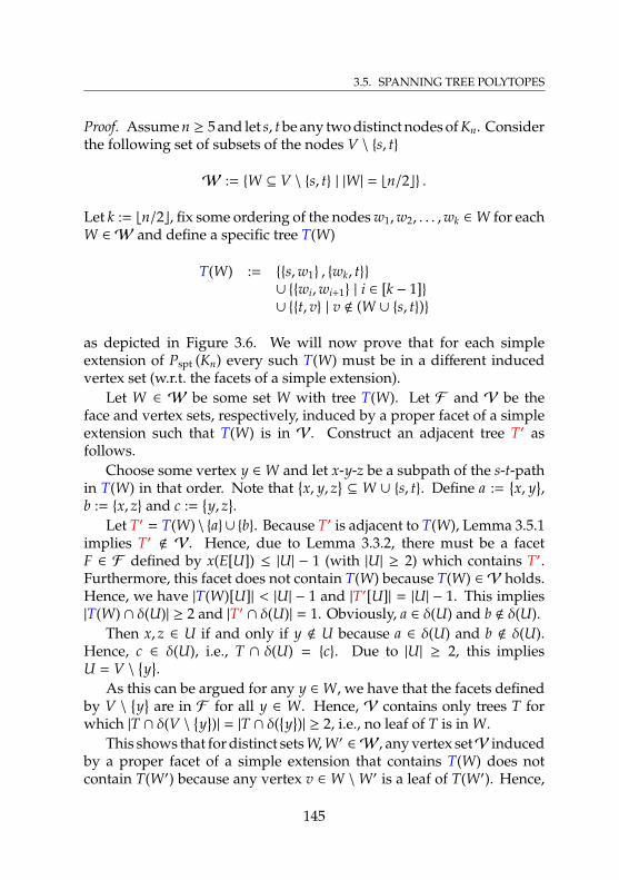
3.5. SPANNING TREE POLYTOPES
Proof. Assume n ≥ 5 and let s, t be any two distinct nodes of Kn. Considerthe following set of subsets of the nodes V \ s, t
W := W ⊆ V \ s, t | |W| = bn/2c .
Let k := bn/2c, fix some ordering of the nodes w1,w2, . . . ,wk ∈W for eachW ∈ W and define a specific tree T(W)
T(W) := s,w1 , wk, t∪ wi,wi+1 | i ∈ [k − 1]∪ t, v | v < (W ∪ s, t)
as depicted in Figure 3.6. We will now prove that for each simpleextension of Pspt (Kn) every such T(W) must be in a different inducedvertex set (w.r.t. the facets of a simple extension).
Let W ∈ W be some set W with tree T(W). Let F and V be theface and vertex sets, respectively, induced by a proper facet of a simpleextension such that T(W) is in V. Construct an adjacent tree T′ asfollows.
Choose some vertex y ∈W and let x-y-z be a subpath of the s-t-pathin T(W) in that order. Note that
x, y, z
⊆ W ∪ s, t. Define a :=
x, y
,
b := x, z and c :=y, z
.
Let T′ = T(W) \ a∪ b. Because T′ is adjacent to T(W), Lemma 3.5.1implies T′ < V. Hence, due to Lemma 3.3.2, there must be a facetF ∈ F defined by x(E[U]) ≤ |U| − 1 (with |U| ≥ 2) which contains T′.Furthermore, this facet does not contain T(W) because T(W) ∈ V holds.Hence, we have |T(W)[U]| < |U| − 1 and |T′[U]| = |U| − 1. This implies|T(W) ∩ δ(U)| ≥ 2 and |T′ ∩ δ(U)| = 1. Obviously, a ∈ δ(U) and b < δ(U).
Then x, z ∈ U if and only if y < U because a ∈ δ(U) and b < δ(U).Hence, c ∈ δ(U), i.e., T ∩ δ(U) = c. Due to |U| ≥ 2, this impliesU = V \
y.
As this can be argued for any y ∈W, we have that the facets definedby V \
y
are in F for all y ∈ W. Hence, V contains only trees T forwhich |T ∩ δ(V \
y)| = |T ∩ δ(
y)| ≥ 2, i.e., no leaf of T is in W.
This shows that for distinct sets W,W′∈ W, any vertex setV induced
by a proper facet of a simple extension that contains T(W) does notcontain T(W′) because any vertex v ∈ W \W′ is a leaf of T(W′). Hence,
145

ANALYZING SIMPLE EXTENSIONS OF POLYTOPES
the number of simple bicliques is at least
|W| =
(n − 2bn/2c
)∈ Ω(2n−o(n)).
146
3.6. FLOW POLYTOPES FOR ACYCLIC NETWORKS
ANALYZING SIMPLE EXTENSIONS OF POLYTOPES:
3.6 Flow Polytopes for AcyclicNetworks
Many extended formulations model the solutions to the original formu-lation via a path in a specifically constructed directed acyclic graph. Asimple example is the linear-size formulation for the parity polytope byCarr and Konjevod [16], and a more elaborate one is the approximateformulation for 0/1-knapsack polytopes by Bienstock [13].
Let D = (V,A) be a directed acyclic graph with fixed source s ∈ Vand sink t ∈ V (t , s). By Ps,t (D) we denote the arc-sets of s-t-paths inD. For some path P ∈ Ps,t (D) and nodes u, v ∈ V(P), we denote by P|(u,v)the subpath of P going from u to v if it exists.
For acyclic graphs, the convex hull of the characteristic vectors of alls-t-paths is equal to the uncapacitated s-t-flow polytope Ps-t-flow (D) withflow-value 1, since the linear description of the latter is totally unimod-ular. The inequalities in this description correspond to nonnegativityconstraints of the arc variables, and a vertex corresponding to the pathP is obviously non-incident to a facet corresponding to ya ≥ 0 if andonly if a ∈ P holds. Adjacency in the path polytope was characterizedby Gallo and Sodini [28], and can be stated as follows: Two s-t-pathsP,P′ correspond to adjacent vertices of the polytope if and only if theirsymmetric difference consists of two paths from x to y (x, y ∈ V, x , y)without common inner nodes. In other words, they must split andmerge exactly once.
Such a network formulation can be easily decomposed into two
147
ANALYZING SIMPLE EXTENSIONS OF POLYTOPES
independent formulations if a node v exists such that every s-t-pathtraverses v. We are now interested in the simple extension complexitiesof flow polytopes of s-t-networks that cannot be decomposed in such atrivial way. Our main result in this section is the following:
Theorem 3.6.1. Let D = (V,A) be a directed acyclic graph with source s ∈ Vand sink t ∈ V such that for every node v ∈ V \ s, t there exists an s-t-path in D that does not traverse v. Then the simple extension complexity ofPs-t-flow (D) ⊆ RA
+ is equal to the number of distinct s-t-paths |Ps,t (D) |.
Proof. Let F and V be the face and vertex sets induced by a properfacet of a simple extension of Ps-t-flow (D), respectively. The goal is toprove |V| = 1. Let us assume for the sake of contradiction |V| ≥ 2. ByTheorem 3.3.3 (b), the (inclusion-wise) maximal faces inF are facets. Let∅ , B′ ⊆ A be the arc set corresponding to these facets. By Lemma 3.3.2,V is the set of (characteristic vectors of) paths P ∈ Ps,t (D) satisfyingP ⊇ B′. Let B ⊆ A be the set of arcs common to all such paths and notethat B ⊇ B′ , ∅ by definition of B′.
By construction, for any path P ∈ V and any arc a ∈ P \B, there is analternative path P′ ∈ V with a < P′.
Let us fix one of the paths P ∈ V. Let, without loss of generality,(x′, x) ∈ B be such that the arc of P leaving x (exists and) is not in B. Ifsuch an arc does not exist, since B , P, there must be an arc (x, x′) ∈ Bsuch that the arc of P entering x is not in B. In this case, revert thedirections of all arcs in D and exchange the roles of s and t, and applythe following arguments to the new network. Let y be the first nodeon P|(x,t) different from x and incident to some arc in B or, if no such yexists, let y := t. Paths in V must leave x and enter y but may differin-between. The set of traversed nodes is defined as
S :=v ∈ V \
x, y
| ∃ x-v-y-path in D
.
By construction, x < s, t and by the assumptions of the Theorem thereexists a path P′ ∈ Ps,t (D) that does not traverse x. Let s′ be the last nodeon P|(s,x) that is traversed by P′. Analogously, let t′ be the first node ofV(P|(x,t)) ∪ S that is traversed by P′. Note that t′ , x since t′ is traversedby P′ but x is not. We now distinguish two cases for which we showthatV is not Λ-closed yielding a contradiction to Corollary 3.3.4:
148
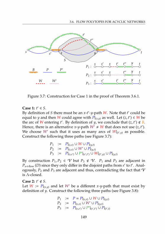
3.6. FLOW POLYTOPES FOR ACYCLIC NETWORKS
S
s tx ys′
t′
t′′
s s′ x t′′ yt′ t
s s′ x yt′′ t
s s′ t′ t′′ y t
B P P′
W W′
P1 :
P2 :
P3 :
Figure 3.7: Construction for Case 1 in the proof of Theorem 3.6.1.
Case 1: t′ ∈ S.By definition of S there must be an x-t′-y-path W. Note that t′ could beequal to y and then W could agree with P|(x,y) as well. Let (z, t′) ∈ W bethe arc of W entering t′. By definition of y, we conclude that (z, t′) < B.Hence, there is an alternative x-y-path W′ , W that does not use (z, t′).We choose W′ such that it uses as many arcs of W|(t′,y) as possible.Construct the following three paths (see Figure 3.7):
P1 := P|(s,x) ∪W ∪ P|(y,t)P2 := P|(s,x) ∪W′
∪ P|(y,t)P3 := P|(s,s′) ∪ P′|(s′,t′) ∪W|(t′,y) ∪ P|(y,t)
By construction P1,P2 ∈ V but P3 < V. P1 and P3 are adjacent inPs-t-flow (D) since they only differ in the disjoint paths from s′ to t′. Anal-ogously, P2 and P3 are adjacent and thus, contradicting the fact that Vis Λ-closed.
Case 2: t′ < S.Let W := P|(x,y) and let W′ be a different x-y-path that must exist bydefinition of y. Construct the following three paths (see Figure 3.8):
P1 := P = P|(s,x) ∪W ∪ P|(y,t)P2 := P|(s,x) ∪W′
∪ P|(y,t)P3 := P|(s,s′) ∪ P′|(s′,t′) ∪ P|(t′,t)
149
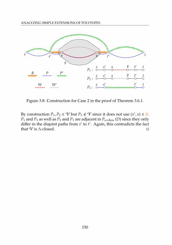
ANALYZING SIMPLE EXTENSIONS OF POLYTOPES
S
s tx ys′ t′
s s′ x y t′ t
s s′ x y t′ t
s s′ t′ t
B P P′
W W′
P1 :
P2 :
P3 :
Figure 3.8: Construction for Case 2 in the proof of Theorem 3.6.1.
By construction P1,P2 ∈ V but P3 < V since it does not use (x′, x) ∈ B.P1 and P3 as well as P2 and P3 are adjacent in Ps-t-flow (D) since they onlydiffer in the disjoint paths from s′ to t′. Again, this contradicts the factthatV is Λ-closed.
150
3.7. PERFECT MATCHING POLYTOPES
ANALYZING SIMPLE EXTENSIONS OF POLYTOPES:
3.7 Perfect Matching Polytopes
The matching polytope and the perfect matching polytope of a graph G =(V,E) are defined as
Pmatch (G) := conv.hullχ(M) |M matching in G
and
Pperfmatch (G) := conv.hull
χ(M) |M perfect matching in G
,
where χ(M) ∈ 0, 1E is the characteristic vector of the set M ⊆ E, i.e.,χ(M)e = 1 if and only if e ∈ M. Edmonds [23] showed that Pperf
match (G) isthe set of x ∈ RE satisfying
xe ≥ 0 for all e ∈ E (3.4)x(δ(v)) = 1 for all v ∈ V (3.5)
x(δ(U)) ≥ 1 for all U ⊆ V with |U| odd. (3.6)
If G is bipartite then only the nonnegativity constraints (3.4) and degreeconstraints (3.5) are required because the constraint matrix is totallyunimodular.
Clearly, the symmetric difference M∆M′ of two perfect matchingsis always a disjoint union of alternating cycles, so-called M-M′-cycles.Chvátal [17] showed that (the vertices corresponding to) two perfectmatchings M and M′ are adjacent if and only if M∆M′ forms a singlealternating cycle.
This section establishes the simple extension complexities of the per-fect matching polytopes (yielding lower bounds for the correspond-
151
ANALYZING SIMPLE EXTENSIONS OF POLYTOPES
ing matching polytopes’ simple extension complexities) of two graphclasses: Subsection 3.7.1 addresses the complete bipartite graphs Kn,nwith n nodes on both sides of the bipartition. Subsection 3.7.2 reducesthe question for complete graphs K2n with 2n nodes to an adjacencyresult on Pperf
match (K2n). The latter is then established in Subsection 3.7.3.
152
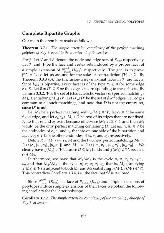
3.7. PERFECT MATCHING POLYTOPES
Complete Bipartite GraphsOur main theorem here reads as follows:
Theorem 3.7.1. The simple extension complexity of the perfect matchingpolytope of Kn,n is equal to the number n! of its vertices.
Proof. Let V and E denote the node and edge sets of Kn,n, respectively.Let F and V be the face and vertex sets induced by a proper facet ofa simple extension of Pperf
match
(Kn,n
), respectively. The goal is to prove
|V| = 1, so let us assume for the sake of contradiction |V| ≥ 2. ByTheorem 3.3.3 (b), the (inclusion-wise) maximal faces in F are facets.Since Kn,n is bipartite, every facet is of the type xe ≥ 0 for some edgee ∈ E. Let ∅ , D′ ⊆ E be the edge set corresponding to these facets. ByLemma 3.3.2,V is the set of (characteristic vectors of) perfect matchingsM ⊆ E satisfying M ⊇ D′. Let D ⊇ D′ be the set of fixed edges, i.e., edgescommon to all such matchings, and note that D is not the empty set,since D′ is not.
Let M1 be a perfect matching with χ(M1) ∈ V, let e0 ∈ D be somefixed edge, and let e1, e2 ∈ M1 \D be two of its edges that are not fixed.Note that e1 and e2 exist because otherwise |M1 \ D| ≤ 1 and then M1would be the only perfect matching containing D. Let u0,u1,u2 ∈ V bethe endnodes of e0, e1 and e2 that are on one side of the bipartition andv0, v1, v2 ∈ V be the other endnodes of e0, e1 and e2, respectively.
Define R := M1 \ e0, e1, e2 and the two new perfect matchings M2 :=R ∪ e0, u1, v2 , u2, v1 and M3 := R ∪ u0, v1 , u1, v2 , u2, v0. Weclearly have χ(M2) ∈ V because D ⊆ M2 holds and χ(M3) < V, becausee0 <M3.
Furthermore, we have that M1∆M3 is the cycle u0-v0-u2-v2-u1-v1-u0 and that M2∆M3 is the cycle u0-v0-u2-v1-u0, that is, M3 (satisfyingχ(M3) <V) is adjacent to both M1 and M2 (satisfying χ(M1), χ(M2) ∈ V).This contradicts Corollary 3.3.4, i.e., the fact thatV is Λ-closed.
Since Pperfmatch
(Kn,n
)is a face of Pmatch
(Kn,n
)and simple extensions of
polytopes induce simple extensions of their faces we obtain the follow-ing corollary for the latter polytope.
Corollary 3.7.2. The simple extension complexity of the matching polytope ofKn,n is at least n!.
153
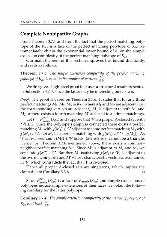
ANALYZING SIMPLE EXTENSIONS OF POLYTOPES
Complete Nonbipartite GraphsFrom Theorem 3.7.1 and from the fact that the perfect matching poly-tope of the Kn,n is a face of the perfect matching polytope of K2n weimmediately obtain the exponential lower bound of n! on the simpleextension complexity of the perfect matching polytope of K2n.
Our main theorem of this section improves this bound drastically,and reads as follows:
Theorem 3.7.3. The simple extension complexity of the perfect matchingpolytope of K2n is equal to its number of vertices (2n)!
n!·2n .
We first give a high-level proof that uses a structural result presentedin Subsection 3.7.3, since the latter may be interesting on its own.
Proof. The proof is based on Theorem 3.7.6. It states that for any threeperfect matchings M1, M2, M3 in K2n, where M1 and M2 are adjacent (i.e.,the corresponding vertices are adjacent), M3 is adjacent to both M1 andM2 or there exists a fourth matching M′ adjacent to all three matchings.
Let P = Pperfmatch (K2n) and suppose thatV is a proper Λ-closed set with
|V| ≥ 2. Since the polytope’s graph is connected there exists a perfectmatching M1 withχ(M1) <V adjacent to some perfect matching M2 withχ(M2) ∈ V. Let M3 be a perfect matching with χ(M3) ∈ V \ χ(M2). AsV is Λ-closed and χ(M3) ∈ V holds, M1,M2,M3 cannot be a triangle.Hence, by Theorem 3.7.6 mentioned above, there exists a common-neighbor perfect matching M′. Since M′ is adjacent to M2 and M3 weconclude χ(M′) ∈ V. But then M1 (satisfying χ(M1) < V) is adjacent tothe two matchings M2 and M′whose characteristic vectors are containedinV, which contradicts the fact thatV is Λ-closed.
Hence all proper Λ-closed sets are singletons, which implies theclaim due to Corollary 3.3.6.
Since Pperfmatch (K2n) is a face of Pmatch (K2n) and simple extensions of
polytopes induce simple extensions of their faces we obtain the follow-ing corollary for the latter polytope.
Corollary 3.7.4. The simple extension complexity of the matching polytope ofK2n is at least (2n)!
n!·2n .
154
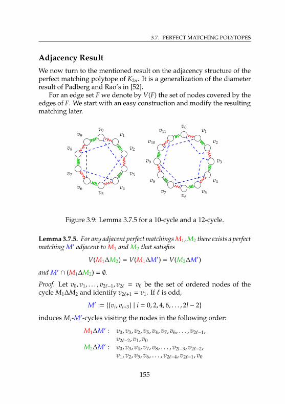
3.7. PERFECT MATCHING POLYTOPES
Adjacency ResultWe now turn to the mentioned result on the adjacency structure of theperfect matching polytope of K2n. It is a generalization of the diameterresult of Padberg and Rao’s in [52].
For an edge set F we denote by V(F) the set of nodes covered by theedges of F. We start with an easy construction and modify the resultingmatching later.
v0 v1
v2
v3
v4
v5v6v7
v8
v9
v10
v11v0v1
v2
v3
v4v5
v6
v7
v8
v9
Figure 3.9: Lemma 3.7.5 for a 10-cycle and a 12-cycle.
Lemma 3.7.5. For any adjacent perfect matchings M1, M2 there exists a perfectmatching M′ adjacent to M1 and M2 that satisfies
V(M1∆M2) = V(M1∆M′) = V(M2∆M′)
and M′ ∩ (M1∆M2) = ∅.
Proof. Let v0, v1, . . . , v2`−1, v2` = v0 be the set of ordered nodes of thecycle M1∆M2 and identify v2`+1 = v1. If ` is odd,
M′ := vi, vi+3 | i = 0, 2, 4, 6, . . . , 2l − 2
induces Mi-M′-cycles visiting the nodes in the following order:
M1∆M′ : v0, v3, v2, v5, v4, v7, v6, . . . , v2`−1,v2`−2, v1, v0
M2∆M′ : v0, v3, v4, v7, v8, . . . , v2l−3, v2`−2,v1, v2, v5, v6, . . . , v2`−4, v2`−1, v0
155
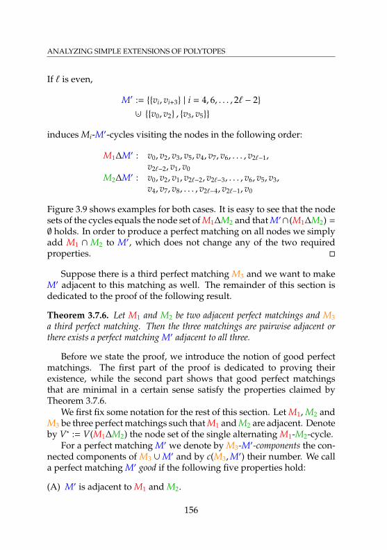
ANALYZING SIMPLE EXTENSIONS OF POLYTOPES
If ` is even,
M′ := vi, vi+3 | i = 4, 6, . . . , 2` − 2∪· v0, v2 , v3, v5
induces Mi-M′-cycles visiting the nodes in the following order:
M1∆M′ : v0, v2, v3, v5, v4, v7, v6, . . . , v2`−1,v2`−2, v1, v0
M2∆M′ : v0, v2, v1, v2`−2, v2`−3, . . . , v6, v5, v3,v4, v7, v8, . . . , v2`−4, v2`−1, v0
Figure 3.9 shows examples for both cases. It is easy to see that the nodesets of the cycles equals the node set of M1∆M2 and that M′∩(M1∆M2) =∅ holds. In order to produce a perfect matching on all nodes we simplyadd M1 ∩ M2 to M′, which does not change any of the two requiredproperties.
Suppose there is a third perfect matching M3 and we want to makeM′ adjacent to this matching as well. The remainder of this section isdedicated to the proof of the following result.
Theorem 3.7.6. Let M1 and M2 be two adjacent perfect matchings and M3a third perfect matching. Then the three matchings are pairwise adjacent orthere exists a perfect matching M′ adjacent to all three.
Before we state the proof, we introduce the notion of good perfectmatchings. The first part of the proof is dedicated to proving theirexistence, while the second part shows that good perfect matchingsthat are minimal in a certain sense satisfy the properties claimed byTheorem 3.7.6.
We first fix some notation for the rest of this section. Let M1, M2 andM3 be three perfect matchings such that M1 and M2 are adjacent. Denoteby V∗ := V(M1∆M2) the node set of the single alternating M1-M2-cycle.
For a perfect matching M′ we denote by M3-M′-components the con-nected components of M3 ∪M′ and by c(M3,M′) their number. We calla perfect matching M′ good if the following five properties hold:
(A) M′ is adjacent to M1 and M2.
156
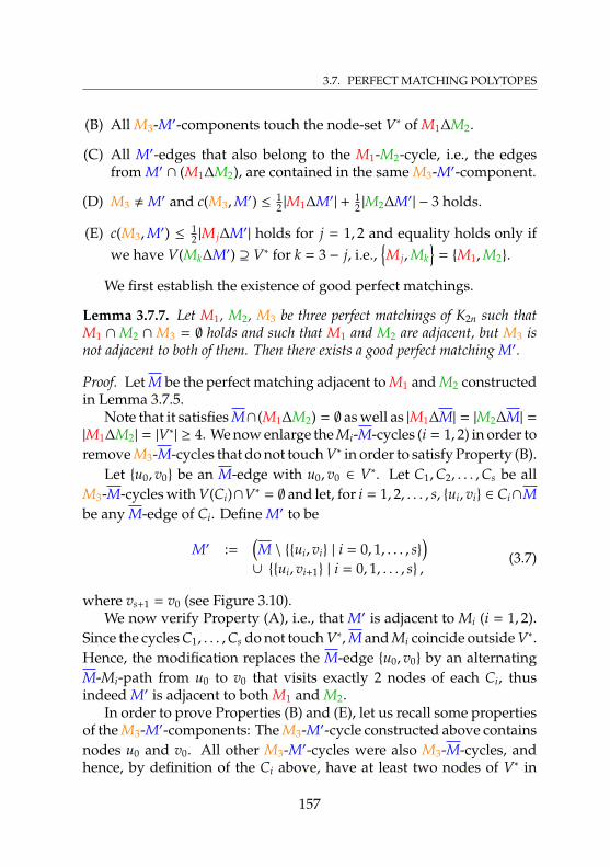
3.7. PERFECT MATCHING POLYTOPES
(B) All M3-M′-components touch the node-set V∗ of M1∆M2.
(C) All M′-edges that also belong to the M1-M2-cycle, i.e., the edgesfrom M′ ∩ (M1∆M2), are contained in the same M3-M′-component.
(D) M3 ,M′ and c(M3,M′) ≤ 12 |M1∆M′| + 1
2 |M2∆M′| − 3 holds.
(E) c(M3,M′) ≤ 12 |M j∆M′| holds for j = 1, 2 and equality holds only if
we have V(Mk∆M′) ⊇ V∗ for k = 3 − j, i.e.,M j,Mk
= M1,M2.
We first establish the existence of good perfect matchings.
Lemma 3.7.7. Let M1, M2, M3 be three perfect matchings of K2n such thatM1 ∩M2 ∩M3 = ∅ holds and such that M1 and M2 are adjacent, but M3 isnot adjacent to both of them. Then there exists a good perfect matching M′.
Proof. Let M be the perfect matching adjacent to M1 and M2 constructedin Lemma 3.7.5.
Note that it satisfies M∩(M1∆M2) = ∅ as well as |M1∆M| = |M2∆M| =|M1∆M2| = |V∗| ≥ 4. We now enlarge the Mi-M-cycles (i = 1, 2) in order toremove M3-M-cycles that do not touch V∗ in order to satisfy Property (B).
Let u0, v0 be an M-edge with u0, v0 ∈ V∗. Let C1,C2, . . . ,Cs be allM3-M-cycles with V(Ci)∩V∗ = ∅ and let, for i = 1, 2, . . . , s, ui, vi ∈ Ci∩Mbe any M-edge of Ci. Define M′ to be
M′ :=(M \ ui, vi | i = 0, 1, . . . , s
)∪ ui, vi+1 | i = 0, 1, . . . , s ,
(3.7)
where vs+1 = v0 (see Figure 3.10).We now verify Property (A), i.e., that M′ is adjacent to Mi (i = 1, 2).
Since the cycles C1, . . . ,Cs do not touch V∗, M and Mi coincide outside V∗.Hence, the modification replaces the M-edge u0, v0 by an alternatingM-Mi-path from u0 to v0 that visits exactly 2 nodes of each Ci, thusindeed M′ is adjacent to both M1 and M2.
In order to prove Properties (B) and (E), let us recall some propertiesof the M3-M′-components: The M3-M′-cycle constructed above containsnodes u0 and v0. All other M3-M′-cycles were also M3-M-cycles, andhence, by definition of the Ci above, have at least two nodes of V∗ in
157
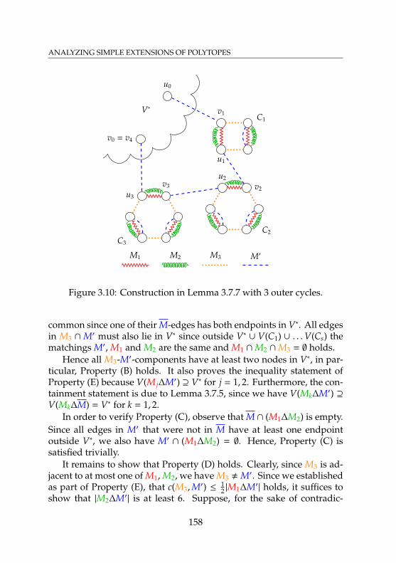
ANALYZING SIMPLE EXTENSIONS OF POLYTOPES
v1
u1
C1
v2
u2
C2
v3
u3
C3
V∗
u0
v0 = v4
M1 M2 M3 M′
Figure 3.10: Construction in Lemma 3.7.7 with 3 outer cycles.
common since one of their M-edges has both endpoints in V∗. All edgesin M3 ∩M′ must also lie in V∗ since outside V∗ ∪ V(C1) ∪ . . .V(Cs) thematchings M′, M1 and M2 are the same and M1 ∩M2 ∩M3 = ∅ holds.
Hence all M3-M′-components have at least two nodes in V∗, in par-ticular, Property (B) holds. It also proves the inequality statement ofProperty (E) because V(M j∆M′) ⊇ V∗ for j = 1, 2. Furthermore, the con-tainment statement is due to Lemma 3.7.5, since we have V(Mk∆M′) ⊇V(Mk∆M) = V∗ for k = 1, 2.
In order to verify Property (C), observe that M ∩ (M1∆M2) is empty.Since all edges in M′ that were not in M have at least one endpointoutside V∗, we also have M′ ∩ (M1∆M2) = ∅. Hence, Property (C) issatisfied trivially.
It remains to show that Property (D) holds. Clearly, since M3 is ad-jacent to at most one of M1, M2, we have M3 ,M′. Since we establishedas part of Property (E), that c(M3,M′) ≤ 1
2 |M1∆M′| holds, it suffices toshow that |M2∆M′| is at least 6. Suppose, for the sake of contradic-
158
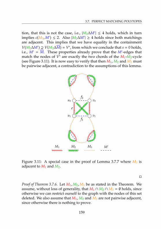
3.7. PERFECT MATCHING POLYTOPES
tion, that this is not the case, i.e., |M2∆M′| ≤ 4 holds, which in turnimplies c(M3,M′) ≤ 2. Also |M2∆M′| ≥ 4 holds since both matchingsare adjacent. This implies that we have equality in the containmentV(M2∆M′) ⊇ V(M2∆M) = V∗, from which we conclude that s = 0 holds,i.e., M′ = M. These properties already prove that the M′-edges thatmatch the nodes of V∗ are exactly the two chords of the M1-M2-cycle(see Figure 3.11). It is now easy to verify that then M1, M2 and M3 mustbe pairwise adjacent, a contradiction to the assumptions of this lemma.
u1
u2
v1
v2
f1
f2
e
M1 M2 M3 M′
Figure 3.11: A special case in the proof of Lemma 3.7.7 where M3 isadjacent to M1 and M2.
Proof of Theorem 3.7.6. Let M1,M2,M3 be as stated in the Theorem. Weassume, without loss of generality, that M1 ∩M2 ∩M3 = ∅ holds, sinceotherwise we can restrict ourself to the graph with the nodes of this setdeleted. We also assume that M1, M2 and M3 are not pairwise adjacent,since otherwise there is nothing to prove.
159
ANALYZING SIMPLE EXTENSIONS OF POLYTOPES
In this situation, Lemma 3.7.7 guarantees the existence of a goodperfect matching. Let M′ be a good perfect matching with minimumc(M3,M′). If c(M3,M′) = 1 holds, M′ is adjacent to M3 (and also adjacentto M1 and M2 by Property (A)) and we are done. Hence, for the sakeof contradiction, we from now on assume that c(M3,M′) is at least 2.The strategy is to construct another good matching M∗ with c(M3,M∗) <c(M3,M′).
Due to Property (C), there exists an M3-M′-component C containingall edges (if any) from M′ ∩ (M1∆M2). M1∆M2 is a single cycle visitingall nodes in V∗ all of which are in some M3-M′-component as they arematched by M′. Thus, by Property (B), the component C is connectedto at least one other M3-M′-component by an edge from M1-M2. Let uschoose such an edge e ∈ M j \Mk for some j = 1, 2 and k = 3 − j, andif such edges exist for both values of j, choose e such that |M j∆M′| ismaximum.
We claim that |M j∆M′| ≥ 6 holds. Suppose, for the sake of contradic-tion, |M j∆M′| = 4. Property (E) implies that c(M3,M′) ≤ 2 holds. Sincec(M3,M′) ≥ 2 also holds, we have equality and then Property (E) impliesthat the Mk-M′-cycle covers all nodes in V∗. This cycle connects the onlytwo M3-M′-components C and C′ via at least two Mk-edges f , f ′ since theM′-edges of the cycle are inside their respective components. Note that|Mk∆M′| ≥ 2c(M3,M′) + 6 − |M j∆M′| ≥ 6 holds by Property (D). Hence,by the maximality assumption for the choice of edge e, this implies thatthere is no edge in Mk \ M j that connects C to C′. Since f , f ′ ∈ Mk
both connect C to C′, it follows that f , f ′ ∈ M j holds as well. Because|M j∆M′| = 4 holds we have M j \M′ =
f , f ′
. Hence, the alternating
M j-M′-cycle of length 4 is also an alternating Mk-M′-cycle. But the latterhas at least length 6 as argued above, which yields a contradiction.
To summarize, we now have two distinct M3-M′-components C andC′ connected by an edge e ∈M j\Mk for some j = 1, 2 such that |M j∆M′| ≥6 holds and all edges from M′ ∩ (M1∆M2) (if any) are in C.
Let u1 ∈ V(C) and u2 ∈ V(C′) be the endpoints of edge e. Let f1 =u1, v1 , f2 = u2, v2 ∈ M′ be the edges matching u1 and u2. We clearlyhave v1 ∈ V(C) and v2 ∈ V(C′) as well since f1 and f2 are contained intheir respective M3-M′-components. In particular we have f1, f2 , e andu1,u2, v1, v2 are pairwise distinct nodes. Because f2 < M j (e ∈ M j and
160
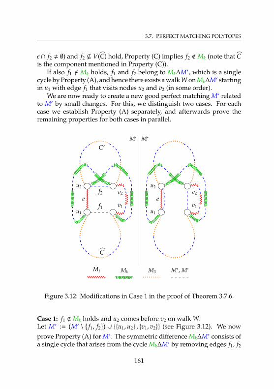
3.7. PERFECT MATCHING POLYTOPES
e∩ f2 , ∅) and f2 * V(C) hold, Property (C) implies f2 <Mk (note that Cis the component mentioned in Property (C)).
If also f1 < Mk holds, f1 and f2 belong to Mk∆M′, which is a singlecycle by Property (A), and hence there exists a walk W on Mk∆M′ startingin u1 with edge f1 that visits nodes u2 and v2 (in some order).
We are now ready to create a new good perfect matching M∗ relatedto M′ by small changes. For this, we distinguish two cases. For eachcase we establish Property (A) separately, and afterwards prove theremaining properties for both cases in parallel.
M′ M∗
u1
u2
v1
v2
ef1
f2
C
C′
u1
u2
v1
v2
e
M j Mk M3 M′, M∗
Figure 3.12: Modifications in Case 1 in the proof of Theorem 3.7.6.
Case 1: f1 <Mk holds and u2 comes before v2 on walk W.Let M∗ :=
(M′ \
f1, f2
)∪ u1,u2 , v1, v2 (see Figure 3.12). We now
prove Property (A) for M∗. The symmetric difference Mk∆M∗ consists ofa single cycle that arises from the cycle Mk∆M′ by removing edges f1, f2
161
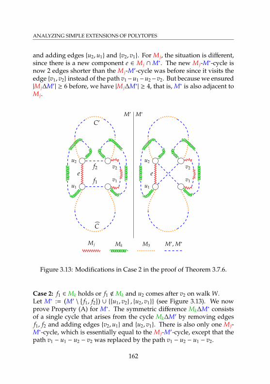
ANALYZING SIMPLE EXTENSIONS OF POLYTOPES
and adding edges u2,u1 and v2, v1. For M j, the situation is different,since there is a new component e ∈ M j ∩M∗. The new M j-M∗-cycle isnow 2 edges shorter than the M j-M′-cycle was before since it visits theedge v1, v2 instead of the path v1−u1−u2−v2. But because we ensured|M j∆M′| ≥ 6 before, we have |M j∆M∗| ≥ 4, that is, M∗ is also adjacent toM j.
M′ M∗
u1
u2
v1
v2
ef1
f2
C
C′
u1
u2
v1
v2
e
M j Mk M3 M′, M∗
Figure 3.13: Modifications in Case 2 in the proof of Theorem 3.7.6.
Case 2: f1 ∈Mk holds or f1 <Mk and u2 comes after v2 on walk W.Let M∗ :=
(M′ \
f1, f2
)∪ u1, v2 , u2, v1 (see Figure 3.13). We now
prove Property (A) for M∗. The symmetric difference Mk∆M∗ consistsof a single cycle that arises from the cycle Mk∆M′ by removing edgesf1, f2 and adding edges v2,u1 and u2, v1. There is also only one M j-M∗-cycle, which is essentially equal to the M j-M′-cycle, except that thepath v1 − u1 − u2 − v2 was replaced by the path v1 − u2 − u1 − v2.
162
3.7. PERFECT MATCHING POLYTOPES
In Case 1 as well as in Case 2, M∗ is again a perfect matching sinceM′ was a perfect matching and they differ only in the way the nodesu1,u2, v1, v2 are matched. Furthermore, M∗ connects the two componentsC and C′, that is, c(M3,M∗) = c(M3,M′)−1. In order to create the desiredcontradiction to the minimality of c(M3,M′), it remains to prove that M∗
satisfies Properties (B),(C), (D) and (E).Property (B) is satisfied for M∗ because V(C) is contained in an M3-
M∗-component and all edges in M∗ \M′ are contained in the same com-ponent.
Property (C) is also satisfied for M∗ since all M∗-edges that were notM′-edges before, are contained in cycle C (which was by definition theonly M3-M′-cycle containing edges in M′ ∩ (M1∆M2)).
We now prove that Property (D) is satisfied for M∗. We have
c(M3,M∗) + 3 = c(M3,M′) + 3 − 1 ≤12|M1∆M′| +
12|M2∆M′| − 1
=12|Mk∆M′| +
12|M j∆M′| − 1
≤12|Mk∆M∗| +
12
(|M j∆M∗| + 2
)− 1
=12|M1∆M∗| +
12|M2∆M∗|,
where the first inequality is due to Property (D) for M′ and the lastinequality comes from the fact that in Case 1, M j∆M∗ has two feweredges than M j∆M′ and in Case 2, the cardinalities agree.
By similar arguments, c(M3,M∗) ≤ 12 |Mi∆M∗| holds for i = 1, 2. In or-
der to prove that Property (E) is satisfied for M∗, assume that c(M3,M∗) =12 |Mi∆M∗| holds for some i ∈ 1, 2. Due to c(M3,M∗) = c(M3,M′)− 1, thisimplies i = j and we are in Case 1 since only there |Mi∆M∗| is less than|Mi∆M′|, and also have c(M3,M′) = 1
2 |M j∆M′|. Property (E) of M′ guar-antees that V(Mk∆M′) ⊇ V∗ holds. But since the node sets of Mk∆M′
and Mk∆M∗ are the same, we also have V(Mk∆M∗) ⊇ V∗.We proved that M∗ is a good perfect matching, yielding the required
contradiction to the minimality assumption of c(M3,M′) which com-pletes the proof.
163
ANALYZING SIMPLE EXTENSIONS OF POLYTOPES
ANALYZING SIMPLE EXTENSIONS OF POLYTOPES:
3.8 A Question Relating SimpleExtensions with Diameters
Let us make a brief digression on the potential relevance of simple exten-sions with respect to questions related to the diameter of a polytope, i.e.,the maximum distance (minimum number of edges on a path) betweenany pair of vertices in the graph of the polytope. We denote by ∆(d,m)the maximum diameter of any d-dimensional polytope with m facets.It is well-known that ∆(d,m) is attained by simple polytopes. A neces-sary condition for a polynomial time variant of the simplex-algorithmto exist is that ∆(d,m) is bounded by a polynomial in d and m (thus by apolynomial in m). In fact, in 1957 Hirsch even conjectured (see [21]) that∆(d,m) ≤ m − d holds, which has only rather recently been disprovedby Santos [60]. However, still it is even unknown whether ∆(d,m) ≤ 2mholds true, and the question, whether ∆(d,m) is bounded polynomially(i.e., whether the polynomial Hirsch-conjecture is true) is a major openproblem in Discrete Geometry.
In view of the fact that linear optimization over a polytope can beperformed by linear optimization over any of its extensions, a reason-able relaxed version of this question might be to ask whether everyd-dimensional polytope P with m facets admits an extension whose sizeand diameter both are bounded polynomially in m. Stating the relaxedquestion in this naive way, the answer clearly is positive, as one mayconstruct an extension by forming a pyramid over P (after embedding Pinto Rdim(P)+1), which has diameter two. However, in some accordance
164
3.8. A QUESTION RELATING SIMPLE EXTENSIONS WITH DIAMETERS
with the way the simplex algorithm works by pivoting between basesrather than only by proceeding along edges, it seems to make senseto require the extension to be simple (which a pyramid, of course, ingeneral is not). But still, this is not yet a useful variation, since ourresult on flow polytopes (see Theorem 3.6.1) shows that there are poly-topes that even do not admit a polynomial (in the number of facets) sizesimple extension at all. Therefore, we propose to investigate the follow-ing question, whose positive answer would be implied by establishingthe polynomial Hirsch-conjecture (as every polytope is an extension ofitself).
Question 3.8.1. Does there exist a polynomial q such that every simplepolytope P with m facets has a simple extension Q with at most q(m) manyfacets and diameter at most q(m)?
In order to make progress on this question, one might want to inves-tigate the face-lattice embeddings for projections of simple extensionsof simple polytopes. On the one hand, all lower bounds we obtainedin this chapter are for a non-simple polytope. On the other hand, allconstructive results are for simple polytopes, e.g., the completion-timepolytopes mentioned in the introduction (see Corollary 4.5 in [57] for aproof of this fact).
165

ANALYZING SIMPLE EXTENSIONS OF POLYTOPES
166
Bibliography[1] Tobias Achterberg. SCIP: Solving constraint integer programs.
Math. Program. Ser. C, 1(1):1–41, 2009.
[2] Hatem Ben Amor and Jacques Desrosiers. A proximal trust-regionalgorithm for column generation stabilization. Computers & Oper-ations Research, 33(4):910 – 927, 2006.
[3] David Applegate, Robert Bixby, Vašek Chvátal, and William Cook.Computational Combinatorial Optimization: Optimal or Provably Near-Optimal Solutions, chapter TSP Cuts Which Do Not Conform to theTemplate Paradigm, pages 261–303. Springer Berlin Heidelberg,Berlin, Heidelberg, 2001.
[4] David L. Applegate, Robert E. Bixby, Vasek Chvátal, and William J.Cook. Concorde TSP solver,http://www.math.uwaterloo.ca/tsp/concorde.html, 2006.
[5] David L. Applegate, William Cook, Sanjeeb Dash, and Daniel G.Espinoza. QSopt_ex,http://www.dii.uchile.cl/daespino/ESolver_doc/main.html,2007.
[6] David L. Applegate, William Cook, Sanjeeb Dash, and Daniel G.Espinoza. Exact solutions to linear programming problems. Oper-ations Research Letters, 35(6):693 – 699, 2007.
[7] Sanjeev Arora and Boaz Barak. Computational complexity: a modernapproach. Cambridge University Press, 2009.
[8] Benjamin Assarf, Ewgenij Gawrilow, Katrin Herr, MichaelJoswig, Benjamin Lorenz, Andreas Paffenholz, and Thomas Rehn.polymake in linear and integer programming. arXiv preprintarXiv:1408.4653, 2014.
167
[9] David Avis and Hans Raj Tiwary. On the extension complexityof combinatorial polytopes. In Fedor V. Fomin, Rusins Freivalds,Marta Z. Kwiatkowska, and David Peleg, editors, Automata, Lan-guages, and Programming, volume 7965 of Lecture Notes in ComputerScience, pages 57–68. Springer Berlin Heidelberg, 2013.
[10] Egon Balas. Disjunctive programming: Properties of the convexhull of feasible points. MSRR 348, Carnegie Mellon University,1974.
[11] Egon Balas. Disjunctive programming. In P.L. Hammer, E.L. John-son, and B.H. Korte, editors, Discrete Optimization II, volume 5 ofAnnals of Discrete Mathematics, pages 3 – 51. Elsevier, 1979.
[12] Abbas Bazzi, Samuel Fiorini, Sebastian Pokutta, and Ola Svensson.No small linear program approximates vertex cover within a factor2 − ε. arXiv:1503.00753, 2015.
[13] Daniel Bienstock. Approximate formulations for 0-1 knapsack sets.Operations Research Letters, 36(3):317 – 320, 2008.
[14] Robert E. Bixby, E. Andrew Boyd, and Ronni R. Indovina. Miplib:A test set of mixed-integer programming problems. SIAM News,25, 1992.
[15] Christoph Buchheim, Frauke Liers, and Marcus Oswald. Local cutsrevisited. Operations Research Letters, 36(4):430 – 433, 2008.
[16] Robert D. Carr and Goran Konjevod. Polyhedral combinatorics.In H. J. Greenberg, editor, Tutorials on Emerging Methodologies andApplications in Operations Research, volume 76 of International Seriesin Operations Research & Management Science, chapter 2, pages 1–46.Springer, 2005.
[17] Vasek Chvátal. On certain polytopes associated with graphs. J.Combin. Theory Ser. B, 18(2):138 – 154, 1975.
[18] Michele Conforti, Volker Kaibel, Matthias Walter, and StefanWeltge. Subgraph polytopes and independence polytopes of countmatroids. Operations Research Letters, 43(5):457 – 460, Sep 2015.
168
BIBLIOGRAPHY
[19] William Cook, Thorsten Koch, Daniel E Steffy, and Kati Wolter.A hybrid branch-and-bound approach for exact rational mixed-integer programming. Mathematical Programming Computation,5(3):305–344, 2013.
[20] William Cook, Thorsten Koch, DanielE. Steffy, and Kati Wolter.An exact rational mixed-integer programming solver. In OktayGünlük and GerhardJ. Woeginger, editors, Integer Programming andCombinatoral Optimization, volume 6655 of Lecture Notes in ComputerScience, pages 104–116. Springer Berlin Heidelberg, 2011.
[21] George B. Dantzig. Linear Programming and Extensions. Princetonlandmarks in mathematics and physics. Princeton University Press,1963.
[22] Olivier du Merle, Daniel Villeneuve, Jacques Desrosiers, and PierreHansen. Stabilized column generation. Discrete Mathematics,194(1–3):229 – 237, 1999.
[23] Jack Edmonds. Maximum matching and a polyhedron with 0, 1-vertices. Journal of Research of the National Bureau of Standards B,69:125–130, 1965.
[24] Friedrich Eisenbrand and Sören Laue. A faster algorithm for two-variable integer programming. In Algorithms and Computation,pages 290–299. Springer, 2003.
[25] Paul Erdös, Siemion Fajtlowicz, and Alan J Hoffman. Maximumdegree in graphs of diameter 2. Networks, 10(1):87–90, 1980.
[26] Samuel Fiorini, Volker Kaibel, Kanstantsin Pashkovich, andDirk Oliver Theis. Combinatorial bounds on nonnegative rankand extended formulations. Discrete Math., 313(1):67–83, 2013.
[27] Samuel Fiorini, Serge Massar, Sebastian Pokutta, Hans Raj Ti-wary, and Ronald de Wolf. Linear vs. semidefinite extended for-mulations: exponential separation and strong lower bounds. InHoward J. Karloff and Toniann Pitassi, editors, STOC, pages 95–106. ACM, 2012.
169
[28] Giorgio Gallo and Claudio Sodini. Extreme points and adjacencyrelationship in the flow polytope. Calcolo, 15:277–288, 1978.
[29] Michael R. Garey and David S. Johnson. Computers and Intractabil-ity: A Guide to the Theory of NP-Completeness. W. H. Freeman, 1979.
[30] Rafael Gillmann. 0/1-Polytopes Typical and Extremal Properties. PhDthesis, Technische Universität Berlin, 2007.
[31] Michel Goemans. Smallest compact formulation for the permuta-hedron. http://www-math.mit.edu/~goemans/publ.html, 2009.
[32] Michel X. Goemans and Young-Soo Myung. A Catalog of SteinerTree Formulations. Networks, 23(1):19–28, 1993.
[33] Martin Grötschel, László Lovász, and Alexander Schrijver. Theellipsoid method and its consequences in combinatorial optimiza-tion. Combinatorica, 1(2):169–197, 1981.
[34] Martin Grötschel and Manfred W. Padberg. Polyhedral theory.In E. L. Lawler, Jan Karel Lenstra, A. H. G. Rinnooy Kan, andD. B. Shmoys, editors, The traveling salesman problem: a guided tourof combinatorial optimization, Wiley Interscience Series in DiscreteMathematics, page 476. John Wiley & Sons, Inc., 1985.
[35] Ishay Haviv and Oded Regev. Tensor-based hardness of the short-est vector problem to within almost polynomial factors. In Proceed-ings of the thirty-ninth annual ACM symposium on Theory of computing,pages 469–477. ACM, 2007.
[36] Emilie V. Haynsworth. On the schur complement. Basel Mathemat-ical Notes, 20, 1968.
[37] Lena Hupp, Laura Klein, and Frauke Liers. An exact solutionmethod for quadratic matching: The one-quadratic-term techniqueand generalisations. Discrete Optimization, 18:193 – 216, 2015.
[38] Cor A. J. Hurkens. Blowing up convex sets in the plane. LinearAlgebra Appl., 134:121–128, 1990.
170
BIBLIOGRAPHY
[39] Volker Kaibel and Kanstantsin Pashkovich. Constructing extendedformulations from reflection relations. In O. Günlük and G. Woeg-inger, editors, Integer Programming and Combinatorial Optimization.Proceedings of IPCO XV, New York, NY, volume 6655 of Lecture Notesin Computer Science, pages 287–300. Springer, 2011.
[40] Volker Kaibel, Kanstantsin Pashkovich, and Dirk Oliver Theis.Symmetry matters for sizes of extended formulations. SIAM J.Disc. Math., 26(3):1361–1382, 2012.
[41] Volker Kaibel and Matthias Walter. Simple extensions of polytopes.Math. Program. Ser. B, 154(1-2):381–406, 2015.
[42] Volker Kaibel and Stefan Weltge. Lower bounds on the sizes ofinteger programs without additional variables. Math. Program. Ser.B, 154(1-2):407–425, 2015.
[43] Ravindran Kannan and Achim Bachem. Polynomial algorithmsfor computing the smith and hermite normal forms of an integermatrix. siam Journal on Computing, 8(4):499–507, 1979.
[44] Ravindran Kannan and László Lovász. Covering minima andlattice-point-free convex bodies. Annals of Mathematics, 128:577–602, 1988.
[45] Thorsten Koch. ZIMPL user guide. Technical report, Konrad-Zuse-Zentrum für Informationstechnik, 2001.
[46] Thorsten Koch and Alexander Martin. Solving Steiner Tree Prob-lems in Graphs to Optimality. Networks, 32(3):207–232, 1998.
[47] Bernhard Korte and Jens Vygen. Combinatorial Optimization, vol-ume 21. Springer, fifth edition, 2012.
[48] Hendrik W. Lenstra, Jr. Integer programming with a fixed numberof variables. Mathematics of Operations Research, 8(4):538–548, 1983.
[49] François Margot, Alain Prodon, and Thomas M. Liebling. Treepolytope on 2-trees. Mathematical Programming, 63(1-3):183–191,1994.
171
[50] R. Kipp Martin. Using separation algorithms to generate mixedinteger model reformulations. Oper. Res. Lett., 10(3):119–128, 1991.
[51] Garth P. McCormick. Computability of global solutions to fac-torable nonconvex programs: Part i — convex underestimatingproblems. Mathematical Programming, 10(1):147–175, 1976.
[52] Manfred W. Padberg and Mendu Rammohan Rao. The travellingsalesman problem and a class of polyhedra of diameter two. Math.Program., 7:32–45, 1974. 10.1007/BF01585502.
[53] Christos H. Papadimitriou. The adjacency relation on the travel-ing salesman polytope is np-complete. Mathematical Programming,14(1):312–324, 1978.
[54] Kanstantsin Pashkovich. Tight lower bounds on the sizes of sym-metric extensions of permutahedra and similar results. Mathematicsof Operations Research, 39(4):1330–1339, 2014.
[55] Sebastian Pokutta and Mathieu Van Vyve. A note on the extensioncomplexity of the knapsack polytope. Oper. Res. Lett., 41(4):347–350,2013.
[56] The polymake team. polymake, http://www.polymake.org, 2015.
[57] Maurice Queyranne. Structure of a simple scheduling polyhedron.Math. Program., 58(1-3):263–285, 1993.
[58] Thomas Rothvoss. Some 0/1 polytopes need exponential size ex-tended formulations. Mathematical Programming, 142(1-2):255–268,2013.
[59] Thomas Rothvoss. The matching polytope has exponential exten-sion complexity. In Proceedings of the 46th Annual ACM Symposiumon Theory of Computing, STOC ’14, pages 263–272, New York, NY,USA, 2014. ACM.
[60] Francisco Santos. A counterexample to the hirsch conjecture. An-nals of Mathematics. Second Series, 176(1):383–412, 2012.
[61] Rolf Schneider. Convex bodies: the Brunn–Minkowski theory. Number151. Cambridge University Press, 2013.
172
BIBLIOGRAPHY
[62] Alexander Schrijver. Theory of linear and integer programming. JohnWiley & Sons, Inc., New York, NY, USA, 1986.
[63] Alexander Schrijver. Combinatorial Optimization – Polyhedra andEfficiency. Springer, 2003.
[64] Daniel E. Steffy and Kati Wolter. Valid linear programming boundsfor exact mixed-integer programming. INFORMS Journal on Com-puting, 25(2):271–284, 2013.
[65] Leena M. Suhl and Uwe H. Suhl. A fast LU update for linearprogramming. Annals of Operations Research, 43(1):33–47, 1993.
[66] Uwe H. Suhl and Leena M. Suhl. Computing Sparse LU Factoriza-tions for Large-Scale Linear Programming Bases. ORSA Journal onComputing, 2(4):325–335, 1990.
[67] Matthias Walter. IPO – Investigating Polyhedra by Oracles,http://polyhedra-oracles.bitbucket.org/, 2016.
[68] Roland Wunderling. Paralleler und objektorientierter Simplex-Algorithmus. PhD thesis, ZIB, 1997.
[69] Mihalis Yannakakis. Expressing combinatorial optimization prob-lems by linear programs. J. Comput. Syst. Sci., 43(3):441–466, 1991.
[70] Günter M. Ziegler. Lectures on Polytopes (Graduate Texts in Mathe-matics). Springer, 2001.
173

APPENDIX
174
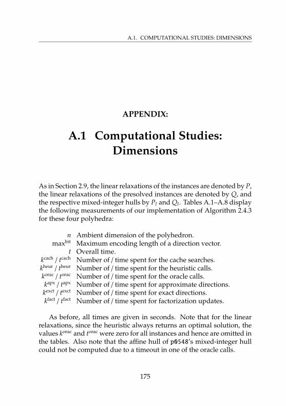
A.1. COMPUTATIONAL STUDIES: DIMENSIONS
APPENDIX:
A.1 Computational Studies:Dimensions
As in Section 2.9, the linear relaxations of the instances are denoted by P,the linear relaxations of the presolved instances are denoted by Q, andthe respective mixed-integer hulls by PI and QI. Tables A.1–A.8 displaythe following measurements of our implementation of Algorithm 2.4.3for these four polyhedra:
n Ambient dimension of the polyhedron.maxbit Maximum encoding length of a direction vector.
t Overall time.kcach / tcach Number of / time spent for the cache searches.kheur / theur Number of / time spent for the heuristic calls.korac / torac Number of / time spent for the oracle calls.kapx / tapx Number of / time spent for approximate directions.kexct / texct Number of / time spent for exact directions.kfact / tfact Number of / time spent for factorization updates.
As before, all times are given in seconds. Note that for the linearrelaxations, since the heuristic always returns an optimal solution, thevalues korac and torac were zero for all instances and hence are omitted inthe tables. Also note that the affine hull of p0548’s mixed-integer hullcould not be computed due to a timeout in one of the oracle calls.
175
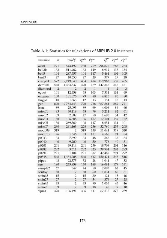
APPENDIX
Table A.1: Statistics for relaxations of MIPLIB 2.0 instances.
Instance n maxbitP kcach
P kheurP kapx
P kexctP kfact
P
air01 771 544,192 750 769 296,827 768 733bell3b 133 511,962 133 149 8,912 133 134bell5 104 287,557 104 117 5,461 104 105bm23 27 40,650 27 28 379 27 28cracpb1 572 2,749,540 484 484 159,963 557 485dcmulti 548 4,434,537 470 479 147,346 547 471diamond 2 2 2 1 4 2 3egout 141 12,458 68 103 7,311 131 69enigma 100 181,576 79 80 4,820 90 80flugpl 18 1,365 12 13 151 18 13gen 870 19,784,443 720 726 367,561 869 721lseu 89 25,093 89 99 4,006 89 90misc01 83 30,118 68 79 3,211 82 61misc02 59 2,882 47 58 1,600 54 42misc03 160 106,686 136 152 12,101 159 122misc05 136 289,569 108 117 8,651 131 101misc07 260 291,163 228 256 32,760 255 208mod008 319 2 319 638 51,041 319 320mod013 96 1,646 83 131 4,566 91 84p0033 33 7,699 33 48 562 33 34p0040 40 9,200 40 50 776 40 31p0201 201 49,114 201 259 18,706 201 146p0282 282 3,611 282 323 39,904 282 283p0291 291 1,104 291 337 42,487 291 292p0548 548 1,484,208 548 612 150,421 548 546pipex 48 22,575 32 28 1,041 47 33rgn 180 265,958 160 168 16,081 179 161sample2 67 347 44 50 2,003 62 45sentoy 60 2 60 60 1,831 60 61stein15 15 2 15 30 121 15 16stein27 27 2 27 54 379 27 28stein45 45 2 45 90 1,036 45 46stein9 9 2 9 18 46 9 10vpm1 378 106,491 336 411 67,537 377 289
176
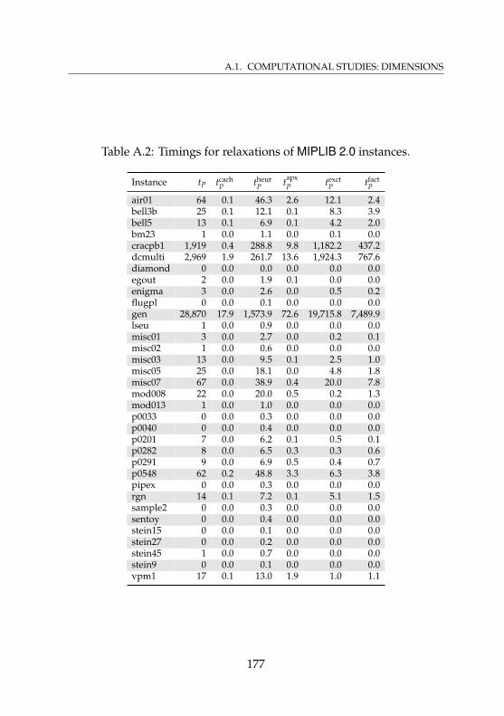
A.1. COMPUTATIONAL STUDIES: DIMENSIONS
Table A.2: Timings for relaxations of MIPLIB 2.0 instances.
Instance tP tcachP theur
P tapxP texct
P tfactP
air01 64 0.1 46.3 2.6 12.1 2.4bell3b 25 0.1 12.1 0.1 8.3 3.9bell5 13 0.1 6.9 0.1 4.2 2.0bm23 1 0.0 1.1 0.0 0.1 0.0cracpb1 1,919 0.4 288.8 9.8 1,182.2 437.2dcmulti 2,969 1.9 261.7 13.6 1,924.3 767.6diamond 0 0.0 0.0 0.0 0.0 0.0egout 2 0.0 1.9 0.1 0.0 0.0enigma 3 0.0 2.6 0.0 0.5 0.2flugpl 0 0.0 0.1 0.0 0.0 0.0gen 28,870 17.9 1,573.9 72.6 19,715.8 7,489.9lseu 1 0.0 0.9 0.0 0.0 0.0misc01 3 0.0 2.7 0.0 0.2 0.1misc02 1 0.0 0.6 0.0 0.0 0.0misc03 13 0.0 9.5 0.1 2.5 1.0misc05 25 0.0 18.1 0.0 4.8 1.8misc07 67 0.0 38.9 0.4 20.0 7.8mod008 22 0.0 20.0 0.5 0.2 1.3mod013 1 0.0 1.0 0.0 0.0 0.0p0033 0 0.0 0.3 0.0 0.0 0.0p0040 0 0.0 0.4 0.0 0.0 0.0p0201 7 0.0 6.2 0.1 0.5 0.1p0282 8 0.0 6.5 0.3 0.3 0.6p0291 9 0.0 6.9 0.5 0.4 0.7p0548 62 0.2 48.8 3.3 6.3 3.8pipex 0 0.0 0.3 0.0 0.0 0.0rgn 14 0.1 7.2 0.1 5.1 1.5sample2 0 0.0 0.3 0.0 0.0 0.0sentoy 0 0.0 0.4 0.0 0.0 0.0stein15 0 0.0 0.1 0.0 0.0 0.0stein27 0 0.0 0.2 0.0 0.0 0.0stein45 1 0.0 0.7 0.0 0.0 0.0stein9 0 0.0 0.1 0.0 0.0 0.0vpm1 17 0.1 13.0 1.9 1.0 1.1
177
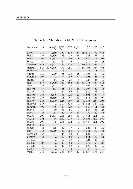
APPENDIX
Table A.3: Statistics for MIPLIB 2.0 instances.
Instance n maxbitPI
kcachPI
kheurPI
koracPI
kapxPI
kexctPI
kfactPI
air01 771 9,859 750 876 134 285,672 770 618bell3b 133 145,456 133 123 19 8,741 133 116bell5 104 47,613 104 99 8 5,537 104 98bm23 27 221 27 16 0 379 27 28cracpb1 572 103,921 484 435 7 159,414 553 479dcmulti 548 2,790,396 470 251 4 147,106 547 468diamond 2 2 1 1 1 3 1 0egout 141 7,029 68 120 28 5,103 129 42enigma 100 2 79 155 77 398 83 4flugpl 18 14 12 23 4 127 18 10gen 870 49,509 720 962 181 324,271 869 541lseu 89 4,393 89 77 0 4,006 89 90misc01 83 241 68 88 25 2,707 82 45misc02 59 97 47 62 11 1,518 55 38misc03 160 8,876 136 128 21 11,891 159 117misc05 136 26,439 108 67 11 8,576 134 99misc07 260 40,670 228 197 25 32,335 257 205mod008 319 2 319 638 0 51,041 319 320mod013 96 936 83 129 0 4,566 91 84p0033 33 30 33 51 7 547 33 28p0040 40 111 40 48 11 776 40 31p0201 201 27,841 201 253 63 18,411 201 140p0282 282 86 282 318 0 39,904 282 283p0291 291 78 291 332 0 42,487 291 292p0548 548pipex 48 526 32 17 2 1,024 47 32rgn 180 86,119 160 158 0 16,081 179 161sample2 67 164 44 58 13 1,684 66 33sentoy 60 2 60 60 0 1,831 60 61stein15 15 2 15 30 0 121 15 16stein27 27 2 27 54 0 379 27 28stein45 45 2 45 90 0 1,036 45 46stein9 9 2 9 18 0 46 9 10vpm1 378 6,172 336 547 49 67,537 376 289
178
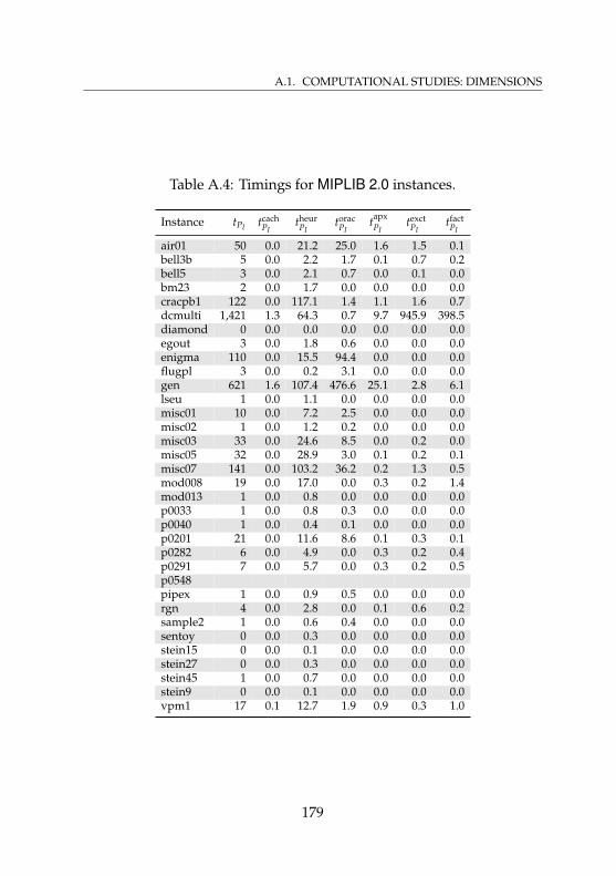
A.1. COMPUTATIONAL STUDIES: DIMENSIONS
Table A.4: Timings for MIPLIB 2.0 instances.
Instance tPI tcachPI
theurPI
toracPI
tapxPI
texctPI
tfactPI
air01 50 0.0 21.2 25.0 1.6 1.5 0.1bell3b 5 0.0 2.2 1.7 0.1 0.7 0.2bell5 3 0.0 2.1 0.7 0.0 0.1 0.0bm23 2 0.0 1.7 0.0 0.0 0.0 0.0cracpb1 122 0.0 117.1 1.4 1.1 1.6 0.7dcmulti 1,421 1.3 64.3 0.7 9.7 945.9 398.5diamond 0 0.0 0.0 0.0 0.0 0.0 0.0egout 3 0.0 1.8 0.6 0.0 0.0 0.0enigma 110 0.0 15.5 94.4 0.0 0.0 0.0flugpl 3 0.0 0.2 3.1 0.0 0.0 0.0gen 621 1.6 107.4 476.6 25.1 2.8 6.1lseu 1 0.0 1.1 0.0 0.0 0.0 0.0misc01 10 0.0 7.2 2.5 0.0 0.0 0.0misc02 1 0.0 1.2 0.2 0.0 0.0 0.0misc03 33 0.0 24.6 8.5 0.0 0.2 0.0misc05 32 0.0 28.9 3.0 0.1 0.2 0.1misc07 141 0.0 103.2 36.2 0.2 1.3 0.5mod008 19 0.0 17.0 0.0 0.3 0.2 1.4mod013 1 0.0 0.8 0.0 0.0 0.0 0.0p0033 1 0.0 0.8 0.3 0.0 0.0 0.0p0040 1 0.0 0.4 0.1 0.0 0.0 0.0p0201 21 0.0 11.6 8.6 0.1 0.3 0.1p0282 6 0.0 4.9 0.0 0.3 0.2 0.4p0291 7 0.0 5.7 0.0 0.3 0.2 0.5p0548pipex 1 0.0 0.9 0.5 0.0 0.0 0.0rgn 4 0.0 2.8 0.0 0.1 0.6 0.2sample2 1 0.0 0.6 0.4 0.0 0.0 0.0sentoy 0 0.0 0.3 0.0 0.0 0.0 0.0stein15 0 0.0 0.1 0.0 0.0 0.0 0.0stein27 0 0.0 0.3 0.0 0.0 0.0 0.0stein45 1 0.0 0.7 0.0 0.0 0.0 0.0stein9 0 0.0 0.1 0.0 0.0 0.0 0.0vpm1 17 0.1 12.7 1.9 0.9 0.3 1.0
179
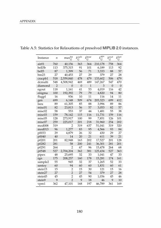
APPENDIX
Table A.5: Statistics for Relaxations of presolved MIPLIB 2.0 instances.
Instance n maxbitQ kcach
Q kheurQ kapx
Q kexctQ kfact
Q
air01 760 40,156 363 364 210,178 758 364bell3b 113 375,315 91 101 6,189 113 92bell5 87 1,399 56 71 3,333 88 57bm23 27 40,453 27 29 379 27 28cracpb1 518 2,559,840 478 479 133,602 506 479dcmulti 548 4,508,942 469 489 147,267 547 470diamond 2 0 0 1 3 0 0egout 118 1,161 41 53 4,019 116 42enigma 100 192,392 79 79 4,820 94 80flugpl 16 936 10 11 116 14 11gen 699 6,148 509 674 203,323 699 412lseu 89 61,305 85 88 3,996 89 86misc01 82 23,813 56 57 3,053 82 57misc02 58 553 37 44 1,481 55 38misc03 159 78,142 115 116 11,731 159 116misc05 128 273,917 100 99 7,851 126 101misc07 259 225,017 201 218 31,960 254 202mod008 319 2 319 637 51,041 319 320mod013 96 1,277 83 95 4,566 93 84p0033 29 4,879 26 32 430 29 27p0040 40 14 20 21 611 39 21p0201 201 82,948 163 202 17,527 201 128p0282 281 58 200 241 36,301 281 201p0291 264 2 67 96 15,478 264 68p0548 527 2,704,204 362 381 125,434 527 363pipex 48 25,695 32 33 1,041 47 33rgn 175 208,257 160 178 15,281 174 161sample2 55 945 32 37 1,265 52 33sentoy 60 94 60 60 1,831 60 61stein15 15 2 15 30 121 15 16stein27 27 2 27 54 379 27 28stein45 45 2 45 90 1,036 45 46stein9 9 2 9 18 46 9 10vpm1 362 47,101 168 197 46,789 361 169
180
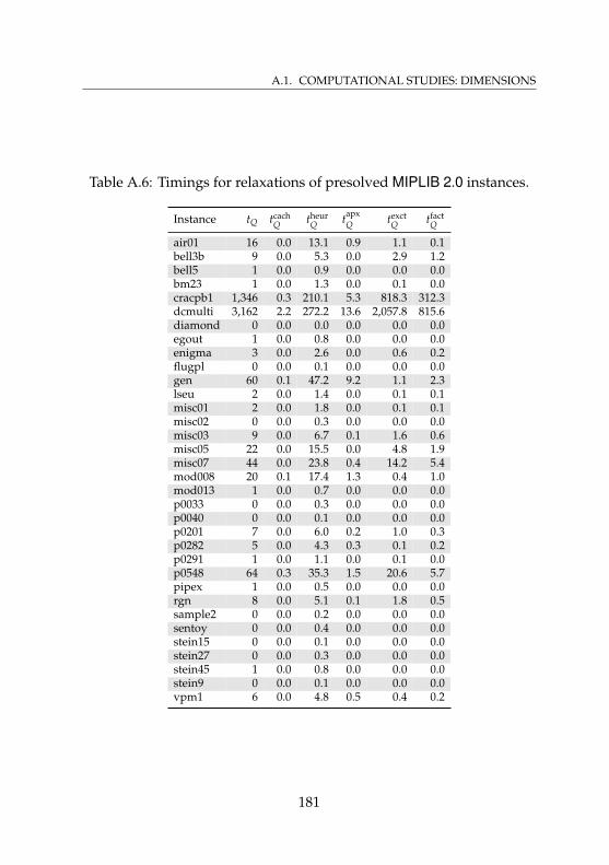
A.1. COMPUTATIONAL STUDIES: DIMENSIONS
Table A.6: Timings for relaxations of presolved MIPLIB 2.0 instances.
Instance tQ tcachQ theur
Q tapxQ texct
Q tfactQ
air01 16 0.0 13.1 0.9 1.1 0.1bell3b 9 0.0 5.3 0.0 2.9 1.2bell5 1 0.0 0.9 0.0 0.0 0.0bm23 1 0.0 1.3 0.0 0.1 0.0cracpb1 1,346 0.3 210.1 5.3 818.3 312.3dcmulti 3,162 2.2 272.2 13.6 2,057.8 815.6diamond 0 0.0 0.0 0.0 0.0 0.0egout 1 0.0 0.8 0.0 0.0 0.0enigma 3 0.0 2.6 0.0 0.6 0.2flugpl 0 0.0 0.1 0.0 0.0 0.0gen 60 0.1 47.2 9.2 1.1 2.3lseu 2 0.0 1.4 0.0 0.1 0.1misc01 2 0.0 1.8 0.0 0.1 0.1misc02 0 0.0 0.3 0.0 0.0 0.0misc03 9 0.0 6.7 0.1 1.6 0.6misc05 22 0.0 15.5 0.0 4.8 1.9misc07 44 0.0 23.8 0.4 14.2 5.4mod008 20 0.1 17.4 1.3 0.4 1.0mod013 1 0.0 0.7 0.0 0.0 0.0p0033 0 0.0 0.3 0.0 0.0 0.0p0040 0 0.0 0.1 0.0 0.0 0.0p0201 7 0.0 6.0 0.2 1.0 0.3p0282 5 0.0 4.3 0.3 0.1 0.2p0291 1 0.0 1.1 0.0 0.1 0.0p0548 64 0.3 35.3 1.5 20.6 5.7pipex 1 0.0 0.5 0.0 0.0 0.0rgn 8 0.0 5.1 0.1 1.8 0.5sample2 0 0.0 0.2 0.0 0.0 0.0sentoy 0 0.0 0.4 0.0 0.0 0.0stein15 0 0.0 0.1 0.0 0.0 0.0stein27 0 0.0 0.3 0.0 0.0 0.0stein45 1 0.0 0.8 0.0 0.0 0.0stein9 0 0.0 0.1 0.0 0.0 0.0vpm1 6 0.0 4.8 0.5 0.4 0.2
181
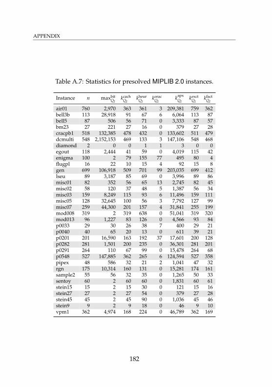
APPENDIX
Table A.7: Statistics for presolved MIPLIB 2.0 instances.
Instance n maxbitQI
kcachQI
kheurQI
koracQI
kapxQI
kexctQI
kfactQI
air01 760 2,970 363 361 3 209,381 759 362bell3b 113 28,918 91 67 6 6,064 113 87bell5 87 506 56 71 0 3,333 87 57bm23 27 221 27 16 0 379 27 28cracpb1 518 132,385 478 432 0 133,602 511 479dcmulti 548 2,152,153 469 133 3 147,106 548 468diamond 2 0 0 1 1 3 0 0egout 118 2,444 41 59 0 4,019 115 42enigma 100 2 79 155 77 495 80 4flugpl 16 22 10 15 4 92 15 8gen 699 106,918 509 701 99 203,035 699 412lseu 89 3,187 85 69 0 3,996 89 86misc01 82 352 56 65 13 2,745 82 45misc02 58 120 37 48 5 1,387 56 34misc03 159 8,249 115 93 6 11,496 159 111misc05 128 32,645 100 56 3 7,792 127 99misc07 259 44,300 201 157 4 31,841 255 199mod008 319 2 319 638 0 51,041 319 320mod013 96 1,227 83 126 0 4,566 93 84p0033 29 30 26 38 7 400 29 21p0040 40 65 20 13 0 611 39 21p0201 201 16,590 163 192 37 17,601 200 128p0282 281 1,501 200 235 0 36,301 281 201p0291 264 110 67 99 0 15,478 264 68p0548 527 147,885 362 265 6 124,594 527 358pipex 48 586 32 21 2 1,041 47 32rgn 175 10,314 160 131 0 15,281 174 161sample2 55 56 32 35 0 1,265 50 33sentoy 60 2 60 60 0 1,831 60 61stein15 15 2 15 30 0 121 15 16stein27 27 2 27 54 0 379 27 28stein45 45 2 45 90 0 1,036 45 46stein9 9 2 9 18 0 46 9 10vpm1 362 4,974 168 224 0 46,789 362 169
182
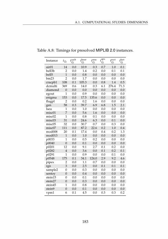
A.1. COMPUTATIONAL STUDIES: DIMENSIONS
Table A.8: Timings for presolved MIPLIB 2.0 instances.
Instance tQI tcachQI
theurQI
toracQI
tapxQI
texctQI
tfactQI
air01 14 0.0 10.9 0.3 0.7 1.0 0.1bell3b 2 0.0 1.4 0.2 0.0 0.1 0.1bell5 1 0.0 0.8 0.0 0.0 0.0 0.0bm23 2 0.0 1.7 0.0 0.0 0.0 0.0cracpb1 108 0.1 105.3 0.0 0.8 1.4 0.5dcmulti 369 0.6 14.0 0.3 6.1 276.4 71.3diamond 0 0.0 0.0 0.0 0.0 0.0 0.0egout 1 0.0 0.9 0.0 0.0 0.0 0.0enigma 153 0.0 17.5 135.6 0.0 0.0 0.0flugpl 2 0.0 0.2 1.6 0.0 0.0 0.0gen 58 0.3 39.7 6.9 6.8 1.5 2.1lseu 1 0.0 1.0 0.0 0.0 0.0 0.0misc01 7 0.0 5.6 1.6 0.0 0.0 0.0misc02 1 0.0 0.8 0.1 0.0 0.0 0.0misc03 31 0.0 24.6 6.3 0.0 0.1 0.0misc05 32 0.0 30.7 0.7 0.0 0.3 0.0misc07 111 0.0 87.2 22.6 0.2 1.0 0.4mod008 20 0.1 17.4 0.0 0.4 0.2 1.3mod013 1 0.0 1.0 0.0 0.0 0.0 0.0p0033 1 0.0 0.5 0.2 0.0 0.0 0.0p0040 0 0.0 0.1 0.0 0.0 0.0 0.0p0201 12 0.0 9.1 2.7 0.1 0.2 0.0p0282 4 0.0 3.6 0.0 0.1 0.2 0.1p0291 1 0.0 0.9 0.0 0.0 0.1 0.0p0548 175 0.1 34.1 124.0 2.9 9.2 4.6pipex 2 0.0 1.1 0.7 0.0 0.0 0.0rgn 3 0.0 2.5 0.0 0.1 0.1 0.1sample2 0 0.0 0.3 0.0 0.0 0.0 0.0sentoy 0 0.0 0.4 0.0 0.0 0.0 0.0stein15 0 0.0 0.1 0.0 0.0 0.0 0.0stein27 0 0.0 0.3 0.0 0.0 0.0 0.0stein45 1 0.0 0.8 0.0 0.0 0.0 0.0stein9 0 0.0 0.1 0.0 0.0 0.0 0.0vpm1 6 0.1 4.5 0.0 0.3 0.3 0.2
183