Inverted Linear Halbach Array for Separation of Magnetic ...
88
Oberlin College Honors Thesis Inverted Linear Halbach Array for Separation of Magnetic Nanoparticles Author: Chetan Poudel Advisor: Dr. Yumi Ijiri A thesis submitted in fulfillment of the requirements for the Honors program in Physics in the Department of Physics and Astronomy May 2014
-
Upload
truonghuong -
Category
Documents
-
view
226 -
download
2
Transcript of Inverted Linear Halbach Array for Separation of Magnetic ...

Oberlin College
Honors Thesis
Inverted Linear Halbach Array forSeparation of Magnetic
Nanoparticles
Author:
Chetan Poudel
Advisor:
Dr. Yumi Ijiri
A thesis submitted in fulfillment of the requirements
for the Honors program in Physics
in the
Department of Physics and Astronomy
May 2014

Executive Summary
Inverted Linear Halbach Array for Separation of Magnetic Nanoparticles
by Chetan Poudel
Magnetic nanoparticles are extremely tiny particles that act like compass needles
in that they can be influenced by larger magnets. These nanoparticles can in turn
interact with other particles near them, influencing their directions and arrangements.
Usually, these particles are suspended in a fluid for use in biomedical applications.
However, most of these applications can work well only if we can ensure that these
particles are uniform, not just in their size but also in their magnetic properties.
Therefore, separations and purifications of these particles are of utmost importance
if we are to make use of these applications.
In this thesis, we describe our creation of a new device and method for separating
magnetic nanoparticles. This device uses a special arrangement of magnets that can
influence a mixture of particles flowing on top of them. This influence causes larger
and more magnetic particles to separate away from the smaller and less magnetic
particles. Therefore, upon flowing one mixture containing small and large particles
through the device, one can obtain two separated solutions: one with only small
particles and one with only large particles, both more uniform than the mixture we
started out with.
We investigate the separation process by first examining the general interactions
of nanoparticles with magnets. We also describe in detail how we investigate the
properties of the nanoparticle mixtures. In our experiments, we find that the device
can separate some types of particle mixtures fully and some only partially. We try to
explain why this may be so. Finally, we establish how efficiently the device performs
and the ways to improve its performance in future experiments. We conclude by
mentioning ongoing and future work that could be done to enhance the workings of
our device to reach our goal of separating nanoparticles for use in desired biomedical
applications.

Acknowledgements
I would first and foremost like to extend my deepest gratitude to my advisor,
Professor Yumi Ijiri, for giving me the opportunity to work in her lab. Her guidance,
teaching, encouragement and her patience in letting me figure out scientific prob-
lems and conduct experiments on my own have been invaluable to my growth as a
researcher. I also very much appreciate the time she put into helping me edit most
of the writing in this thesis.
I would also like to thank my lab partner, Kathryn Hasz, for being a great friend
throughout. Thanks for all the baked desserts and for putting up with, and perhaps
even enjoying, my pop music and strange ideas in lab. Many thanks also for her help
with developing a new framework to analyze my experimental data.
In addition, I would like to thank my other wonderful physics friends Dagmawi
Gebreselasse, David Morris, Jocienne Nelson, Ben Lemberger, Elizabeth Garbee,
Zach Mark, Sujoy Bhattacharya, Mattie Dedoes, Noah Jones, Mike Rowan, Elizabeth
Gilmour and Sam Berney for spending many nights tackling arduous problems sets
together and for all the fun we had in Wright. Thanks to the juniors Greg Stevens,
Cooper McDonald, Donal Sheets, Dan Bloch, Dan Barella and Dan Laufer for the
amusing discussions. I would also like to acknowledge Jason Stalnaker and all other
professors of the Oberlin Physics department for being such excellent resources and
perpetually challenging and stretching my knowledge. Thanks to Bill Marton for his
excellent machining work on many projects and to Diane for taking care of us all.
Many thanks to my girlfriend Valerie Feerer for her love and to my housemates
and friends Cuyler, Tania, Clara, Pete, Steve, Ren and Shiva for keeping me going.
Finally, I am very grateful for the constant encouragement and frequent calls from
my loving family and relatives, while I lived thousands of miles away and kept staying
at Oberlin for many summers and winters doing research without coming home.
This work was partially supported by NSF grant DMR-1104489, NIH CA62349,
a Great Lakes College Association New Directions Initiative Award, the Cleveland
Clinic, and an Oberlin College Research Status Award. The research made use of
equipment obtained from NSF DMR-0922588 and DUE-9950606.
ii

Contents
Abstract i
Acknowledgements ii
List of Figures v
List of Tables viii
Abbreviations ix
Symbols and Units ix
Glossary and Physical Constants xi
1 Motivation and Approach 1
1.1 Colloidal magnetic fluids and nanoparticles . . . . . . . . . . . . . . . 1
1.2 Separation of magnetic nanoparticles . . . . . . . . . . . . . . . . . . 3
1.3 Introduction and applications of the Halbach magnet array . . . . . . 6
2 Theory 9
2.1 Types of magnetism . . . . . . . . . . . . . . . . . . . . . . . . . . . 9
2.2 Superparamagnetism . . . . . . . . . . . . . . . . . . . . . . . . . . . 11
2.3 Theory of magnetic separation . . . . . . . . . . . . . . . . . . . . . . 14
2.4 Theory of small angle x-ray scattering . . . . . . . . . . . . . . . . . 17
3 The Halbach Array: Design, Construction and Characterization 22
3.1 Finite Element Modeling . . . . . . . . . . . . . . . . . . . . . . . . . 22
3.2 Computer aided designs of magnet array and flow channels . . . . . . 24
3.3 Device construction . . . . . . . . . . . . . . . . . . . . . . . . . . . . 26
3.4 Characterization of constructed Halbach array . . . . . . . . . . . . . 27
3.5 Implications for magnetic separation . . . . . . . . . . . . . . . . . . 30
4 Experimental Procedures 35
4.1 Nanoparticle synthesis and procurement . . . . . . . . . . . . . . . . 35
iii

Contents iv
4.2 Structural Characterization . . . . . . . . . . . . . . . . . . . . . . . 37
4.2.1 Transmission Electron Microscopy and image analysis . . . . . 37
4.2.2 Small angle x-ray scattering . . . . . . . . . . . . . . . . . . . 38
4.2.3 Curve fitting using NANO-Solver and NIST SANS macros . . 40
4.3 Magnetic Characterization using a VSM . . . . . . . . . . . . . . . . 41
4.4 Nanoparticle separation procedures . . . . . . . . . . . . . . . . . . . 42
5 Results and Analysis 45
5.1 Structural characterization results of nanoparticle suspensions . . . . 45
5.1.1 TEM results of Sigma-Aldrich’s and Anna-Samia’s nanoparticles 46
5.1.2 SAXS results of stock suspensions and mixtures . . . . . . . . 49
5.2 Magnetic characterization results of nanoparticle suspensions . . . . . 52
5.3 Separation results . . . . . . . . . . . . . . . . . . . . . . . . . . . . . 53
5.3.1 Toluene-based nanoparticle suspensions . . . . . . . . . . . . . 54
5.3.2 Water-based nanoparticle suspensions . . . . . . . . . . . . . . 59
5.4 ROC Analysis . . . . . . . . . . . . . . . . . . . . . . . . . . . . . . . 61
6 Conclusions and Future Work 64
6.1 Conclusions . . . . . . . . . . . . . . . . . . . . . . . . . . . . . . . . 64
6.2 Ongoing and Future Work . . . . . . . . . . . . . . . . . . . . . . . . 65
A Solidworks CAD Designs 73

List of Figures
2.1 Magnetic responses associated with different classes of magnetic ma-terials. . . . . . . . . . . . . . . . . . . . . . . . . . . . . . . . . . . . 10
2.2 Magnetic domains of ferromagnetic materials in the absence and pres-ence of applied magnetic fields. . . . . . . . . . . . . . . . . . . . . . 11
2.3 A plot of the Langevin function allows us to distinguish between sam-ples differing in their particle moments and magnetizations. . . . . . . 14
2.4 Schematic of x-ray scattering showing angle 2θ between the sourcebeam and the scattered beam received by the detector. . . . . . . . . 17
2.5 Schematic of x-ray scattering showing initial and final wave-vectorsand the scattering vector Q . . . . . . . . . . . . . . . . . . . . . . . 18
2.6 Theoretical plot of x-ray scattering intensity from perfectly sphericalparticles. . . . . . . . . . . . . . . . . . . . . . . . . . . . . . . . . . . 20
2.7 Theoretical plot of x-ray scattering intensity from a lognormal distri-bution of spheres. . . . . . . . . . . . . . . . . . . . . . . . . . . . . . 21
3.1 Finite element method model of the Halbach array, showing magneti-zation orientation of successive magnets. . . . . . . . . . . . . . . . . 24
3.2 Array-channel assembly design with toluene-compatible glass channel. 25
3.3 Array-channel assembly with water-compatible Plexiglas channel. . . 25
3.4 The constructed linear Halbach magnet array with 47 NdFeB magnetsheld together by set screws and an aluminum frame. . . . . . . . . . . 26
3.5 The toluene-compatible glass channel during a separation process showsdark bands where nanoparticles are aggregating. . . . . . . . . . . . . 27
3.6 The water-compatible Plexiglas channel during a similar separationprocess. . . . . . . . . . . . . . . . . . . . . . . . . . . . . . . . . . . 27
3.7 Comparison of the modeled and measured values of the normal com-ponent of the B field along the length of the magnet array at differentdistances away from the array. . . . . . . . . . . . . . . . . . . . . . . 28
3.8 Comparison of the modeled and measured values of the normal com-ponent of the B field, and the corresponding gradient values along thelength of the magnet array at a distance 0.3 cm from the low flux sideof the array. . . . . . . . . . . . . . . . . . . . . . . . . . . . . . . . . 28
3.9 Plot of the B field along the length of the magnet array at four differentdistances relevant for separation away from the array, as modeled withFEMMView. . . . . . . . . . . . . . . . . . . . . . . . . . . . . . . . . 29
3.10 Comparison of field gradient as a function of average B field for thehigh and low flux sides of the Halbach array and for a single magnet. 30
v

List of Figures vi
3.11 Plot of the (a) averaged B field and (b) gradient of B in the direc-tion perpendicular to the surface of the magnet array as a function ofdistance above the array in the low flux side. . . . . . . . . . . . . . . 31
3.12 Schematic of separation showing field and particle behavior at differentdistances away from the array. . . . . . . . . . . . . . . . . . . . . . . 31
3.13 Schematic of separation at an optimal distance and complications thatcould arise. . . . . . . . . . . . . . . . . . . . . . . . . . . . . . . . . 33
4.1 Stages of TEM image analysis performed using ImageJ analysis software. 38
4.2 Configuration of SAXS geometry attachments in the XRD. . . . . . . 39
4.3 Lakeshore 7307 Vibrating Sample Magnetometer at Oberlin College. . 42
4.4 A schematic of multiple passes showing desired filtrates and residuesproduced in each step, along with discarded products. . . . . . . . . . 43
5.1 TEM images of Sigma Aldrich’s A7 and A20 nanoparticles after Im-ageJ processing. . . . . . . . . . . . . . . . . . . . . . . . . . . . . . . 46
5.2 Lognormal fit to the histogram data combined from four images of A7particles purchased from Sigma-Aldrich. . . . . . . . . . . . . . . . . 47
5.3 Lognormal fit to the histogram data combined from three images ofA20 nanoparticles purchased from Sigma-Aldrich. . . . . . . . . . . . 48
5.4 Small angle x-ray scattering results of four Sigma-Aldrich stock sus-pensions show variations in SAXS patterns, relating to their particlesize and dispersion. . . . . . . . . . . . . . . . . . . . . . . . . . . . . 49
5.5 Small angle x-ray scattering results of Anna Samia’s two stock suspen-sions dried to powder form. . . . . . . . . . . . . . . . . . . . . . . . 50
5.6 SAXS results of mixtures containing different proportions of SigmaAldrich’s 7nm and 20nm particles. The fit parameters have been ob-tained using NANO-Solver software. . . . . . . . . . . . . . . . . . . . 51
5.7 Magnetometry of Sigma-Aldrich’s stock suspensions gives mass mag-netizations that can be compared to that of pure bulk magnetite toassess the ”magnetic quality” of the samples. . . . . . . . . . . . . . . 52
5.8 Magnetometry results of Anna Samia’s stock suspensions allow similarcomparison of mass magnetization of samples to that of bulk magnetite. 53
5.9 SAXS curves and particle distributions of Sigma Aldrich’s A7 and A20suspensions, mixtures and their post-sort filtrate. The fits have beenobtained using NANO-Solver software. . . . . . . . . . . . . . . . . . 55
5.10 SAXS curves and particle distributions of Sigma Aldrich’s A6 and A16suspensions, mixtures and their post-sort filtrates and residues. Thefits have been obtained using NANO-Solver software. . . . . . . . . . 56
5.11 SAXS curves and particle distributions of Sigma Aldrich’s A7 and A16suspensions, mixture and the multiple pass post-sort filtrate. The fitshave been obtained using NANO-Solver software. . . . . . . . . . . . 57
5.12 Particle distributions of stock, filtrate and residue from purificationattempts on a new Sigma-Aldrich batch of particles. . . . . . . . . . . 59
5.13 SAXS curves of Anna Samia’s particles during different stages of theseparation process. Solid curves are fits to NIST SANS macros. . . . 60

List of Figures vii
5.14 ROC curves for the Halbach array’s separation performance with dif-ferent particle mixtures. . . . . . . . . . . . . . . . . . . . . . . . . . 63
6.1 Using height adjustment platforms for finer control of array-channeldistance. . . . . . . . . . . . . . . . . . . . . . . . . . . . . . . . . . . 65
A.1 Design of Plexiglas channel base for the toluene-compatible glass channel. 73
A.2 Design of Plexiglas top plate for the water-compatible flow channel. . 74
A.3 Design of stainless steel bottom plate for the water-compatible flowchannel. . . . . . . . . . . . . . . . . . . . . . . . . . . . . . . . . . . 75
List of Tables
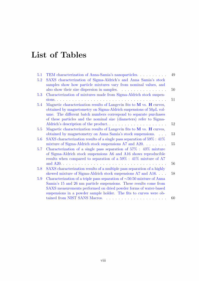
5.1 TEM characterization of Anna-Samia’s nanoparticles. . . . . . . . . . 49
5.2 SAXS characterization of Sigma-Aldrich’s and Anna Samia’s stocksamples show how particle mixtures vary from nominal values, andalso show their size dispersion in samples. . . . . . . . . . . . . . . . 50
5.3 Characterization of mixtures made from Sigma-Aldrich stock suspen-sions. . . . . . . . . . . . . . . . . . . . . . . . . . . . . . . . . . . . . 51
5.4 Magnetic characterization results of Langevin fits to M vs. H curves,obtained by magnetometry on Sigma-Aldrich suspensions of 50µL vol-ume. The different batch numbers correspond to separate purchasesof these particles and the nominal size (diameters) refer to Sigma-Aldrich’s description of the product. . . . . . . . . . . . . . . . . . . . 52
5.5 Magnetic characterization results of Langevin fits to M vs. H curves,obtained by magnetometry on Anna Samia’s stock suspensions. . . . 53
5.6 SAXS characterization results of a single pass separation of 59% : 41%mixture of Sigma-Aldrich stock suspensions A7 and A20. . . . . . . . 55
5.7 Characterization of a single pass separation of 57% : 43% mixtureof Sigma-Aldrich stock suspensions A6 and A16 shows reproducibleresults when compared to separation of a 59% : 41% mixture of A7and A20. . . . . . . . . . . . . . . . . . . . . . . . . . . . . . . . . . . 56
5.8 SAXS characterization results of a multiple pass separation of a highlyskewed mixture of Sigma-Aldrich stock suspensions A7 and A16. . . . 58
5.9 Characterization of a triple pass separation of ∼50:50 mixture of AnnaSamia’s 15 and 26 nm particle suspensions. These results come fromSAXS measurements performed on dried powder forms of water-basedsuspensions in a powder sample holder. The fits to curves were ob-tained from NIST SANS Macros. . . . . . . . . . . . . . . . . . . . . 60
viii
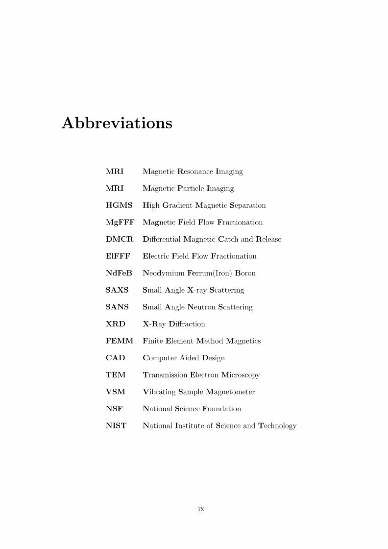
Abbreviations
MRI Magnetic Resonance Imaging
MRI Magnetic Particle Imaging
HGMS High Gradient Magnetic Separation
MgFFF Magnetic Field Flow Fractionation
DMCR Differential Magnetic Catch and Release
ElFFF Electric Field Flow Fractionation
NdFeB Neodymium Ferrum(Iron) Boron
SAXS Small Angle X-ray Scattering
SANS Small Angle Neutron Scattering
XRD X-Ray Diffraction
FEMM Finite Element Method Magnetics
CAD Computer Aided Design
TEM Transmission Electron Microscopy
VSM Vibrating Sample Magnetometer
NSF National Science Foundation
NIST National Institute of Science and Technology
ix

Symbols and Units
m magnetic moment emu or erg/gauss
M mass magnetization emu/g
H applied magnetic field Oersted(Oe)
B magnetic flux density Gauss
χ magnetic susceptibility dimensionless
K magnetic anisotropy erg/cm3
Φ magnetic flux maxwell
σ saturation magnetization emu/g
Fm magnetic force erg
η viscosity centipoise (cP)
vp velocity of particle µm/s
Q scattering vector Angstrom−1 or A−1
I(Q) scattering intensity arbitrary units
x

Glossary and Physical Constants
Boltzmann’s constant kB = 1.38× 10⁻²³ J/K
Permeability of vacuum µ0 = 4π × 10−7 N/A2 in SI or 1 in CGS
Avogadro’s constant NA = 6.022 136 7(36)× 1023 mol−1
Bohr magneton µb = 9.27× 10⁻²¹ emu
Room temperature T = 298 K
Viscosity of toluene ηtoluene = 0.580 cP
Viscosity of water ηwater = 1.00 cP at room temperature
xi

Dedicated to Buwa, Baba, Mamu and Saugat. . .
xii

Chapter 1
Motivation and Approach
1.1 Colloidal magnetic fluids and nanoparticles
Magnetic fluids are stable colloidal suspensions of nano-sized particles of mag-
netic materials in a carrier liquid. Such artificial strongly magnetic fluids were first
synthesized in the 1960s, with an unprecedented amount of research that followed in
later years [1, 2]. The small size and magnetic characteristics of these nanoparticles
in fluid have opened up a wide range of very interesting and promising applications,
especially in biomedicine.
Biomedical nanomagnetics is the name given to the multidisciplinary research
area studying magnetic nanoparticles for their applications in diagnostic imaging,
targeted drug delivery, cancer therapy and hyperthermia [3]. The nanometer dimen-
sions of these particles allow them to interact with biological entities like cells and
molecules. The nanoparticles can be coated with some specific biomolecules to allow
uptake into the body and for selective interactions with other biomolecules. The
nanoparticles can also be tagged with fluorescent markers (like green fluorescent pro-
teins) and be attached to selected cells for optical imaging [4]. Some nanoparticles
also form excellent contrast agents for in vitro magnetic resonance imaging (MRI)
or magnetic particle imaging (MPI) [5]. The nanoparticles can be manipulated with
external field gradients to for guide the transport of drugs or genes to targeted sites
in the body [6]. Introducing and attaching colloidal magnetic nanoparticles, whose
magnetic susceptibility exceeds that of other intact cells by several orders of magni-
tude, into some biological membranes offers magnetic control of selected cells from
the outside. Magnetic nanoparticles also respond to an alternating or time-varying
1

Chapter 1. Motivation and Approach 2
magnetic field, with an advantageous transfer of energy from an exciting field to the
nanoparticle. This release of energy can be exploited to heat up the particles and
surrounding tissue by heat transfer. This technique in cancer therapy, which is called
hyperthermia, can strongly supplement chemotherapy, destroying tumor tissues in a
localized fashion inside the body [7].
In all major clinical applications of magnetic fluids, the ability to control im-
portant parameters like imaging resolution, payload delivery, transport efficiency and
temperature is crucial. Achieving this control depends critically upon the ability to
obtain superior quality nanoparticle samples, with high uniformity in particle size
and in magnetic properties. This is because a non-uniform distribution of billions
of particles will cause the response of a certain group of particles to be vastly dif-
ferent from other particles in the same sample, causing uncontrolled and unintended
consequences. There is an obvious advantage in having a narrow distribution in
particle-size and magnetization since large deviations can adversely affect the per-
formance, especially in applications where the nanoparticles are subjected to large
fields or field gradients.
However, the synthesis of nanoparticles for use in these applications is a difficult
and sensitive chemical process that requires a judicious selection of reaction condi-
tions to promote nucleation on preformed nanocrystal seeds into the final product.
Even then, a number of parameters in the synthesis like heating temperature, seed
size, seed crystallinity, solvent polarity, stabilizer concentration all influence the final
product morphology [8]. Some highly optimized syntheses of nanoparticles can and
have yielded samples with very narrow size distributions but the problem of irrepro-
ducibility of similar ‘monodisperse’ samples is often-overlooked in these syntheses.
It might also be the case that even though samples appear to be monodisperse in
size, heterogeneities still exist in composition and crystallinity among particles in
the solution. In the absence of methods for accessing and assuring the purity of
these synthesized products, the ultimate use of magnetic nanoparticles in biomedi-
cal applications cannot be validated and therefore is likely to be limited. Therefore,
post-synthesis purification and separation is of paramount importance for expanding
the potentials of magnetic nanoparticles in medical and biodiagnostic applications.

Chapter 1. Motivation and Approach 3
1.2 Separation of magnetic nanoparticles
Unfortunately, post-synthetic separation and purification methods for use with
small colloidal nanoparticles are scarce in nanoparticle synthesis literature. There
exist comparatively only a few sorting methods, which are typically quite tedious,
and even then mostly based on size-based selection and not based on magnetic char-
acteristics. The application of analytical separations has largely been limited to
larger micron-sized particles and biological cells despite the promising applications of
smaller nanoparticles in emerging technologies. Even while some nanoparticle purifi-
cation methodologies exist, a well-quantified and characterized separation of colloidal
nanoparticles is rarely practiced. We briefly review the few existing techniques and
methods used in purification or separation of magnetic nanoparticles, first starting
with magnetic-based methods using magnetic fields and gradients of simple mag-
nets, high gradient magnetic separation (HGMS), magnetic field flow fractionation
(MgFFF), and differential magnetic catch and release (DMCR). We then briefly ex-
plore the manipulation of nanoparticles using microfluidic channels, electric fields
and other solely size-based separation techniques.
Most separation procedures of magnetic nanoparticles involve recovery or con-
trol of the motion of the superparamagnetic particles and so magnetophoresis is an
essential step, for which magnetic gradients are employed. The simplest and crud-
est way to do this would be to use a simple permanent magnet near a nanoparticle
suspension. The problem with a simple magnet is the high field and low gradient
it provides, magnetizing and accumulating all particles towards it, without any se-
lective sorting criteria. If this magnet is placed sufficiently far enough to cause a
weak field to magnetize only the more magnetic particles, the field gradient which
influences the magnetophoretic particle velocities becomes so low that the process of
separation takes an incredibly long time (a few days for one sample), making it very
inconvenient or of not much use.
Some better methods like high gradient magnetic separation (HGMS), magnetic
field flow fractionation (MgFFF) and differential magnetic catch and release (DMCR)
use flow based techniques in conjunction with applied magnetic fields [9]. HGMS
methods use various flow channel geometries and columns packed with micron sized
magnetic wires that can be magnetized with a powerful electromagnet to create very
inhomogeneous magnetic fields of 1 to 2 Tesla with a high gradient (greater than
1000 T/m) for high throughput. HGMS is common in separation of micron-scale or

Chapter 1. Motivation and Approach 4
larger particles but a similar theoretical framework could be utilized for separation of
magnetic nanoparticles [10]. HGMS is best suited for separating nanoparticles out of
a mixture of magnetic and non-magnetic particles, in applications relating to water
purification and removal of toxic waste [11], and not so much for sorting between two
different particle distributions originating from the same mixture. That is because
even through HGMS guarantees high magnetophoretic particle velocity, the high
gradient sources necessarily consist of a large field that magnetizes all particles and
causes them all to be trapped in the separating column, without enough sensitivity
to discriminate between particles in the mixture [12]. A research group [13] has
recently demonstrated good separation efficiency and yield in sorting several different
populations from a complex mixture of nanoparticles less than 20 nm in size using
variable field applications in a conventional HGMS. This is an exciting result for
the use of an HGMS method, but they too report difficulties with separating larger
nanocrystals from each other.
MgFFF is another separation and characterization technique, which is better for
sorting of magnetic nanoparticles in that it can distinguish different magnetic particle
components that vary in their magnetic material content from the same mixture
[14]. In MgFFF, the interplay of hydrodynamic and magnetic forces elutes magnetic
particles at different times at the outlet (similar to a chromatography technique) as
they flow along a thin, parallel-walled channel, on which a magnetic field or gradient
is applied perpendicularly. Knowing the magnetic properties of the core material,
MgFFF can be used to roughly calculate the size distribution as well as the mean
size of magnetic cores of particles. However, careful examination of this method
reveals a number of significant problems. MgFFF involves indirect characterization
of the particles using calculations of observed elution time [15]. Such indirect size
distribution calculations are only accurate to the extent that particle size scales with
the core size. If most particles in the sample have a magnetically dead layer while
still being large in size, MgFFF will tend to underestimate the sample’s average
particle size. Multiple MgFFF attempts have also failed because of difficulty in
creating uniform field arrangements throughout the channel. Some groups have used
a quadrupole MgFFF system [10, 16] to create uniform radially symmetric regions
in the flow channel to remedy this problem but it stills seem to work best only for
bigger nanoparticles hundreds of nanometers in diameter. Being able to sort smaller
nanoparticles in the 5 nm - 50 nm range would be much more desirable for biomedical
applications in cellular transport and magnetic targeting.

Chapter 1. Motivation and Approach 5
Differential magnetic catch and release (DMCR) is a relatively new technique
[17] that tries to focus on separating polydisperse magnetic nanoparticles with sizes
less than 20 nm into monodisperse fractions that are compatible for bioanalysis and
medical applications. DMCR separates particles in the mobile phase using differential
applied magnetic forces to trap and retain flowing nanoparticles against the wall of
an open tubular capillary wrapped between two narrowly spaced electromagnetic
poles. Despite the method’s successful demonstration of separation of three sizes
of magnetic nanoparticles with small differences in diameter and of reduction in size
distribution of particles, there are a number of problems that arise in this technique as
well. First of all, it uses very high tunable fields in the order of Teslas that requires
a powerful expensive electromagnet using high voltage and chillers. On the other
hand, this method uses an injection volume of ∼1 µL and separates the volume into
monodisperse fractions in around 25 to 100 minutes [18]. This would take a thousand
times longer to separate usable milliliter amounts of sample, especially if the yields
of nanoparticles are as low as reported. Therefore, it seems to be a good process for
demonstrating magnetic separation but is in no way a time efficient or easily scalable
technique.
Another large research area where size-based and magnetic nanoparticle sepa-
rations have been tested is in microfluidics or ”lab on a chip” technologies. These
microchannels allow analysis of exceedingly small quantities of sample with low cost,
portability and remarkable high resolution [9]. Descroix and co-workers [19] devel-
oped a microchip for trapping and releasing 30 nm diameter iron oxide nanoparticles
at high gradient and flow rates of tens of µL in an hour. Taking heed of the through-
put rate, we can very well see that although microfluidics may be useful to obtain
minuscule amounts of very uniform samples, it cannot be utilized for manipulation of
particle solutions in large scales. Electric field flow fraction (ElFFF) methods [20] us-
ing electric fields for elution-based separations of nanoparticles are also of increasing
use but they suffer from other limitations in that only size-based separation of large
charged nanoparticles are possible. Even small pH changes or changes in solvent and
surface chemistry can result in aggregation, degradation in these methods. Similarly,
there are various other methods of fine size separation for nanomaterials including
centrifugation [21], salts-based selective precipitation [22], size exclusion chromatog-
raphy [23], and diafiltration [24], but these processes do not take advantage of the
magnetic properties of iron oxide nanoparticles and are thus of limited use in creating
samples for use in magnetic field based biomedical applications.

Chapter 1. Motivation and Approach 6
Although quite a bit of research work on nanoparticle separations has been
done, we can clearly see that a well-characterized and high-throughput separation of
colloidal magnetic nanoparticles in a size regime where they can be of great use to
biomedical applications is rarely practiced.
1.3 Introduction and applications of the Halbach
magnet array
Our research project considers a novel idea to fill these gaps in the field of size-
based and magnetic separation of small colloidal nanoparticle suspensions, utilizing
a well-established technology cleverly refashioned to suit our purpose of nanoparti-
cle sorting. Our method also employs rigorous and well-defined characterization of
nanoparticle suspensions throughout the process to quantify separation success. The
aim of the project is simple: to take nanoparticle samples with particle sizes varying
from around 5 nm to 30 nm synthesized without magnetic and size uniformity and
transform them into uniform well-characterized samples usable for aforementioned
important biomedical applications.
Our idea came out of research work in tailored high magnetic fields and high
flux used by Klaus Halbach [25] in designing synchrotron magnets, and in magnetic
levitation systems. The importance of tailored homogeneous fields and gradients
to magnetic sorting technology has already been established before. While such
adjustable field sources are typically electromagnets powered by large amounts of
power (typically more than a thousand watts and a chiller to keep the electromagnet
from heating) [26], the discovery of Neodymium Iron Boron (NdFeB) permanent
magnets with high coercivity and remanence properties made them viable alternatives
to powered sources for these same applications [27]. We examined an important
class of such permanent magnet designs described by Mallinson [28], based on a
particular arrangement of permanent magnets in an alternating pattern. This special
arrangement gave the design a unique and counter-intuitive ability to confine most
of the magnetic flux to only one side of the design while keeping the magnetic field
profile considerably more spatially uniform throughout the structure on either face
compared to simpler magnet arrays. Mallinson showed the field would be confined
in this way if the component of magnetization were any Hilbert transform pair, the

Chapter 1. Motivation and Approach 7
simplest of which is v = sin(x)i + cos(x)j, where v is the magnetization vector and
x is the position along the design.
The concept of one-sided flux structures, now referred to as ‘Halbach arrays’,
is not new. Many of its characteristics are known in the context of devices such as
magnetic recording tape, refrigerator magnets, and even in drug targeting and cell
separation [29]. One proposed usage of Halbach arrays is in creating a magnetic
bandage for targeting and controlling the delivery of therapeutic agents into tumor
sites. Research groups [30, 31] have discovered that a Halbach array configuration of
magnets placed near a small tumor yields the best trapping characteristics (large and
uniform force distributions) and maximal pulling and pushing forces, outperforming
benchmark magnets of similar size and strength, to magnetostatically control small
highly magnetic particles injected into the region of interest. The particles could
then slowly release chemotherapeutic drugs, or radiate tissues using beta emitters
in them or induce localized hyperthermia on application of an alternating magnetic
field. When the Halbach array is finally removed, the particles redistribute into the
blood supply and then be cleared out. Halbach arrays have recently also been used
to continuously sort micrometer-sized magnetic particles with a fluid channel placed
over the high flux side of the array [32].
However, to the best of my knowledge, the low flux side of the Halbach array has
never been previously considered for any purpose. Our investigations have revealed
that the low flux side of the array contains two things that are rarely seen in conjunc-
tion: a low field value coupled with large field gradients over single magnet arrange-
ments. In addition, the linear Halbach arrangement we created through appropriate
modulation of the magnetization vectors of individual magnets produced substan-
tially uniform fields and gradients for planes parallel to the array. We have found
that these field and gradient profiles can be exploited to perform well-characterized
and replicable procedures of magnetic separations of nanoparticles in the size range
of a few nanometers, which as we described earlier, is an ideal size range for many
biomedical applications of nanoparticles.
In the next few chapters, we will delve into the particulars of our magnetic sepa-
ration approach using the aforementioned advantages of the low flux side or inverted
side of the Halbach array. In Chapter 2, we will develop a theoretical framework
to understand the responses of nanoparticles in magnetic fields and the underlying
physics used in magnetic separation. In Chapter 3, we will go into the details of

Chapter 1. Motivation and Approach 8
design, construction and characterization of the Halbach array fashioned for our sep-
aration purpose. Chapter 4 will include discussions of the nanoparticle samples we
used, and the experimental setup and procedures used in the collection and charac-
terization of our data. In Chapter 5, we will present and analyze our results from
typical experiments performed using the array and the importance of those results.
We will also provide a quantified analysis of the device performance using data from
all our separation experiments to inform the reader of ways to maximize separation
efficiency in future experiments. We conclude in Chapter 6 by briefly recounting our
separation method and its utility, our most important results, and the future work
that could to be done to firmly establish and expand on some of our exciting results.

Chapter 2
Theory
This chapter reviews the fundamental theory of magnetism and the special case
of nanoparticle magnetism to understand the theory behind our magnetic separa-
tion approach. Later, particular attention is paid to explaining the theoretical basis
for small angle x-ray scattering measurements that constitute our primary analysis
method.
2.1 Types of magnetism
To understand in detail how a magnetic sorting approach might work, we first
review the fundamental concepts of magnetism to understand the responses of mag-
netic nanoparticles in the presence of magnetic fields [33]. Further details can be
found in one of the many books on magnetism [34, 35, 36].
All materials are magnetic to some extent, with their magnetic responses de-
pending upon the material’s atomic structure and temperature. The magnetization
of these materials is given by the vector sum of all individual magnetic moments m
in a volume V of the material:
M =Σm
V(2.1)
If any material is placed in an applied magnetic field of strength H, the individual
atomic moments in the material will contribute to its overall response called the
magnetic induction B where:
B = µ0(H + M) (2.2)
9

Chapter 2. Theory 10
and µ0 is the permeability of free space. All materials may then be conveniently
classified in terms of a tensor called their volumetric magnetic susceptibility χ, where
M = χH (2.3)
describes the magnetization induced in a material by H. In CGS units, χ is dimen-
sionless, B is measured in Gauss(G), H in Oersted(Oe) and mass magnetization M in
emu/g. Materials show a wide range of magnetic behavior, with most only exhibiting
weak magnetism, and even then only in the presence of an external applied magnetic
field. These are particles with non-interacting spins characterized by a linear suscep-
tibility, classified either as paramagnets (PM), for which χ falls in the range 10−6 to
10−1, or as diamagnets (DM), with χ in the range −10−6 to −10−3, whose M vs. H
curves are shown in Figure 2.1 (A), (B).
Hc
~1/100 for scale of C
~1/1000 for scale of C
(A) (B)
(C) (D)
Figure 2.1: Magnetic responses associated with different classes of magneticmaterials. M vs. H curves are shown for diamagnetic (DM) and paramagnetic(PM) materials, for multidomain larger ferromagnetic (FM) particles and for smallnanometer-sized superparamagnetic (SPM) particles.
However, some materials are magnetic even without an applied field and can
be viewed as a collection of various magnetic regions called domains, separated by
domain walls, with each domain consisting of moments lined up in a certain direction
with respect to the external applied field, as shown in Figure 2.2.

Chapter 2. Theory 11
Figure 2.2: Magnetic domains of ferromagnetic materials in the absence (left)and presence (right) of a strong applied magnetic field in the upward direction.There are differences in size and number of domains in the two cases.
These materials exhibit ordered magnetic states, interactions between individual
moments, and a finite intrinsic coercivity Hc which refers to how strongly the material
resists demagnetization, given by the magnitude of external field applied in a reverse
direction to bring the magnetization from saturation back to zero, shown in Figure
2.1 (C). Another distinguishing feature is that the M vs. H curves of these materials
exhibit hysteresis - the material follows a different curve during demagnetization than
it does when being magnetized, leading to a closed loop as shown in Figure 2.1 (FM).
This hysteretic behavior is caused due to rotation in magnetization of moments and
change in size or number of magnetic domains when the applied field is increased,
which isn’t exactly reversed when the applied field is later decreased. The materials
exhibiting these properties are classified as ferromagnets, where the prefix refers to
the nature of the coupling interaction between the electrons within the material.
This coupling can give rise to large spontaneous magnetizations; in ferromagnets M
is typically 104 times larger than would appear otherwise.
2.2 Superparamagnetism
If we now reduce the size of ferromagnetic materials to length scales of domain
wall widths or nanometer dimensions, we ultimately reach a size where it is more
energetically favorable for the particle to first have a single magnetic domain. Then
the thermal energy (kBT = 4.01 × 10⁻²¹ J, at T=300 K where kB is the Boltzmann
constant of value 1.38×10⁻²³J/K) becomes greater than the anisotropy energy bar-
rier KV (where K is the magnetic anisotropy of the material and V is the volume
of the particle), causing the magnetization direction of the nanoparticle to random-
ize. The anisotropy energy barrier for a small magnetic particle, which is the energy
that must be exceeded to cause magnetic direction reversal by a spin-flip, is loosely

Chapter 2. Theory 12
speaking, a product of the square of the saturation magnetization (M) and its vol-
ume (V ∼ d3) [37]. As a first approximation of the characteristic particle size when
this spin-flip energy barrier is attained, we can set the simple magnetization reversal
energy equal to the thermal energy, i.e. M2d3 ∼ kBT ∼ 4.01 × 10⁻²¹ J at room tem-
perature. For typical nanosized ferromagnets, we can obtain a characteristic length
of diameters less than 30 nm, below which ferromagnetism gives way to this unique
behavior such that when no external magnetic field is applied, the average magnetiza-
tion measured in a finite time interval (typically, 100 s) is zero. Such materials show
no intrinsic coercivity and behave as paramagnets with a huge moment, which is why
they are called superparamagnets (SPM in Figure 2.1). The nanoparticles generally
used for biomedical applications and the particles used in our magnetic separation
techniques span this size range of less than 30 nm and are thus all superparamag-
netic. It may be important to note that in practice, the particle size regime where
super-paramagnetism becomes relevant is found to vary among different materials so
it might be different for iron oxide nanoparticles than it would be for other oxide
nanoparticles.
In a colloidal magnetic fluid, each nanoparticle carrying a magnetic moment m
can then be treated as a small thermally agitated magnet in the carrier liquid. Each
particle in this fluid is randomly oriented in the absence of an applied magnetic field,
and the fluid has no net magnetization. For ordinary field strengths, the tendency of
the moments to align with the applied field is partially overcome by thermal agitation
and as the magnitude of the applied field is increased, the particles become more
and more aligned with the field direction. At higher field strengths, the particles
may be fully aligned, with the magnetization achieving its saturation value. The
usefulness of single domain magnetic nanoparticles lies in the fact that the particle’s
moment is about 105 times larger than that of transition or rare-earth metal ions.
Therefore, when exposed to an external magnetic field, the whole colloidal solution
behaves paramagnetically, with susceptibilities χ exceedingly high by similar order
of magnitude, which is why saturation of magnetization in these particles can be
reached in fields as relatively low as about .1 Tesla or 1 kGauss.
The superparamagnetic response of magnetic nanoparticles can be understood
from some simple statistical mechanics considerations, assuming negligible particle-
particle magnetic interaction. We know that in dilute superparamagnetic fluids,
saturation is reached simply by rotation of all independent particle moments to align
with the field direction to give a saturation magnetic moment. Starting with initial

Chapter 2. Theory 13
conditions, we can consider a particle with moment of m initially directed at an angle
θ to an applied field H. Assuming no anisotropic energy terms, the energy of this
particle will be given by the well-known classical Zeeman energy term -mHCosθ[38].
If we have an assembly of particles at temperature T that have reached thermody-
namic equilibrium with the field, there will be a Boltzmann’s distribution of θ’s over
the particle assembly. The fraction of the total magnetization aligned by the field
is calculated by averaging Cosθ over the Boltzmann distribution, which yields an
integral expression
m =< mCosθ >=
∫ π0mCosθ e
mHCosθkBT Sinθdθ∫ π
0emHCosθkBT Sinθdθ
(2.4)
If we introduce a ratio between the energy of a particle in the applied magnetic
field H and its thermal energy as α = mHkBT
, then the above expression may be written
as
m =
∫ π0mCosθ eαCosθ dCosθ∫ π
0eαCosθ dCosθ
(2.5)
m =m
α
∫ α−α xe
x dx∫ α−α e
x dx(2.6)
where x = αCosθ. When the integrations are carried out, the result is given by
m = mL(α) = m
[cothα− 1
α
]= Nm
[coth
(mH
kBT
)− kBT
mH
](2.7)
which is commonly referred to as the Langevin function. N is the total number
of magnetic nanoparticles in the sample, kB is the Boltzmann’s constant and T is the
temperature. Once could also decide to write the moment of a particle as m= n µB
where n is the number of Bohr magnetons in a representative particle and µB is the
Bohr magneton.
A Langevin function is traditionally used to fit the curve of magnetization or
magnetic moment vs. applied field (M vs. H curve) for superparamagnetic nanopar-
ticles. The fit allows us to extract information about the saturation mass magnetiza-
tion of the particle’s material and the magnetic moment per average particle. A plot
of the Langevin function for different magnetization and particle moment values is
shown in Figure 2.3.

Chapter 2. Theory 14
-10 000 -5000 5000 10 000 Applied Field
-50
50
Magnetization
Figure 2.3: A plot of the Langevin function allows us to distinguish between sam-ples differing in their particle moments and magnetizations. Nanoparticle samplesthat differ in their saturation magnetization values are represented by dashed redand green curves, where dashed red has a higher magnetization. Similarly, sampleswith the same magnetization but differing in their particle moments are repre-sented by dashed red and solid blue curves, where blue represents a sample with asmaller value of magnetic moment per particle.
The magnetization of the sample may be calculated by dividing the total mo-
ment of the sample by the volume of suspended magnetic material. Sometimes if a
magnetic nanoparticle exhibits a core shell structure, made of magnetically differen-
tiable materials like magnetite (Fe3O4) and maghemite (γ-Fe2O3), one can roughly
estimate the core shell dimensions using information extracted from the Langevin fit-
ting. However, when working with superparamagnetic nanoparticles, one needs to be
careful of the possibility of significant variation in values of saturation magnetization
between individual particles and bulk, leading to erroneous conclusions.
2.3 Theory of magnetic separation
A single domain, isolated magnetic particle of total magnetic moment m in an
inhomogeneous applied field H0 experiences a magnetic force:
Fm = (m • ∇)H0 (2.8)
where ∇ is the gradient operator evaluated at the location of the particle [39]. In the
case of a magnetic nanoparticle suspended in a very weakly diamagnetic or param-
agnetic medium such as toluene or water, the total moment on the particle can be
written as m = Vm M, where Vm is the magnetic volume of the particle and M is its

Chapter 2. Theory 15
volumetric magnetization. Furthermore, provided there are no time-varying electric
fields of currents in the medium, we can apply Maxwell’s equation ∇× H0 = 0 to
the mathematical identity:
(m • ∇)H0 = ∇(m •H0)−H0 • ∇m−m× (∇×H0)−H0 × (∇×m) (2.9)
For constant m this simplifies to:
(m • ∇)H0 = ∇(m •H0)−m× (∇×H0) (2.10)
When there is no flow of electric current, ∇ ×H0 is identically zero, and therefore
for a dipole of fixed moment m the force can be written as
Fm = ∇(m •H0) (2.11)
This relation summarizes the force on a single particle of fixed moment as a function
of its orientation and position in the applied field H0. Also, this relation shows that
a spatially varying magnetic field is required to create a magnetic force, which is the
only parameter controlled by the magnet design; the other term depends on the size
and material properties of the particles.
For a particle in solution of viscosity η, this force may be opposed by a resulting
Stokes’ drag force of
Fd = −3πηdpvp (2.12)
where dp is the effective particle diameter in solution, and vp is its velocity. For
Fd + Fm = 0 (2.13)
the particle achieves a steady state vp which, for sufficiently large m and large gradient
in field, may be sizeable enough to allow for separation of the particle in a magnetic
separation process. It is important to note that the largest magnetostatic forces
on the particles will be at the region closest to the magnet. This is because the
magnetic field is highest adjacent to the magnets, causing greatest magnetization of
the particles and thus exerting the greatest magnetic force. It is not surprising then
that particles will move towards the magnet not because of gravitational settling
(since gravity is a much smaller force on the particle), but primarily due to magnetic
causes.

Chapter 2. Theory 16
In addition to a single particle interaction with the applied field, we must also
consider the possibility of inter-particle interactions in the presence of an applied
field, so far ignored. For two magnetic nanoparticles, the dipole-dipole energy [39]
can be calculated by
Udd =πµ0M
2d6m72(dm + 2δ)3
(2.14)
where the particles have magnetization values of M, magnetic diameter dm and non-
magnetic coating thickness δ. Note that the magnetic diameter dm may be signif-
icantly different from the effective particle diameter in solution dp, as the particles
may have a sizeable portion that is not magnetic as a result of surface effects or more
simply due to a surfactant coating.
The dipole-dipole interaction energy between particles Udd and the thermal en-
ergy kBT come to be around similar values for magnetic nanoparticles. These energies
compete to determine whether particles will aggregate or flow freely exhibiting Brow-
nian motion in the magnetic colloid. The tendency for superparamagnetic particles
to aggregate is expected to increase with particle size, in part due to greater magneti-
zation in larger particles caused by larger magnetic susceptibilities [40]. In addition,
Begin-Colin and co-workers indicate that smaller sizes of iron oxide crystals are en-
riched in the less magnetic iron oxide called maghemite (γ-Fe2O3) as opposed to the
more magnetic magnetite (Fe3O4) which may decrease their magnetic moment and
contribute to minimal aggregation due to reduced response to external fields [41].
Once the field is removed, particle interactions immediately diminish and the
observed aggregate structures dissolve into the suspension. This is also an essential
difference between dispersion of superparamagnetic and ferromagnetic particles: in
the case of particles with a permanent dipole (ferromagnetic particles), aggregates
would still be observed in the absence of magnetic field due to the remanent dipole-
dipole interaction. The reversible field-induced aggregation in superparamagnetic
nanoparticles helps to dramatically enhance magnetophoresis, which is the move-
ment of particles in an applied field gradient. According to Camacho et al. [40],
initially the magnetophoretic velocity of the particles is very slow, but large chain-
like aggregates are rapidly formed, moving fast and colliding with other aggregates
to produce even larger structures at faster velocity. This increase in magnetophoretic
velocity increases the throughput of methods that employ such reversible aggregation
by orders of magnitude.

Chapter 2. Theory 17
2.4 Theory of small angle x-ray scattering
Small angle x-ray scattering (SAXS) is a widely used and well understood wave-
diffraction method for studying the structure and ordering of matter. This method
of elastic scattering is used in various branches of science and technology, including
condensed matter phyics, biophysics, polymer science, and metallurgy. In small angle
x-ray diffraction experiments, a primary beam of x-rays influences a studied object,
and the scattering pattern is analyzed in the range of 2θ from 0 to around 5 degrees,
where 2θ is the angle between the source and the detector as shown in Figure 2.4.
This analysis provides information on the structure of a substance with a spatial
Figure 2.4: Schematic of x-ray scattering showing angle 2θ between the sourcebeam and the scattered beam received by the detector.
resolution from 10 A to thousands of Angstroms. Below, we review the basic theory
of stationary scattering result with no time dependence in the elastic scattering case
where the wavelength of the x-ray and magnitude of the wavevector | k |= 2πλ
does
not change upon scattering. We describe the form factor for spherical particles and
obtain an expression for scattering intensity observed in all our experimental plots.
Further information can be found in any of the various texts on small angle X-ray
scattering [42, 43, 44].
X-ray scattering occurs when particles differing in electron density from their
surrounding matrix are irradiated with monochromatic x-rays, modeled as a plane
wave ψ = ei(k·r−ωt) where k is the wave vector, r is the path difference between the
wave and a scattering origin, and ω is the angular frequency of the x-ray. If the final
wavevector kf is deflected at an angle 2θ from the initial wavevector ki, assume Q is
the scattering vector given by the difference between the final and inital wavevectors,
shown in Figure 2.5 and defined by:
Q = kf − ki and Q =4π
λsinθ (2.15)

Chapter 2. Theory 18
Figure 2.5: Schematic of x-ray scattering showing initial and final wavevectorski and kf and the scattering vector Q
Unlike the incident beam which is collimated, the intensity of the outgoing
wave per unit area will fall dramatically after scattering. Due to the phase change
introduced from our nanoparticle sample at distance r, the scattered wave will take
the general form:
ψf = ψ0G(λ, θ)eik·r
r(2.16)
where ψ0 ensures that the rate of scattering is proportional to the incident flux, and
the function G(λ, θ) tells us about the chances that a wave of given wavelength λ
is deflected in a certain direction θ from the incident wave direction. For any real
sample radiated with a beam of x-rays, the challenge for finding the pattern that will
result is summing up all the n scattered waves from each individual scattering event
to produce a complete scattered intensity profile. The amplitude of the resulting
wave in the direction of Q, notated as F(Q), gives the diffraction pattern in Q-space
detected in experiments:
F (Q) =n∑0
e−iQ·rn (2.17)
where F(Q) is the Fourier transform of the electron density fluctuations within the
object depending on the form of particles. Typically in the study of crystal diffrac-
tion, the scattering amplitude F(Q) is given by the product of the form factor f(Q)
and the structure factor S(Q). The form factor is a measure of the particle shape
and composition, while the structure factor which is a measure of the arrangement
of scattering sources. In our case, the structure factor will not contribute to the
scattering amplitude because our samples are magnetic particle colloids randomly
suspended in medium and not arranged in any regular order. Therefore, the scatter-
ing intensity I(Q), which is the square of the scattering amplitude, depends purely
on the form factor squared.
F (Q) = f(Q)S(Q) (2.18)
I(Q) ∝ |F (Q)|2 ∝ |f(Q)|2 (2.19)

Chapter 2. Theory 19
To understand what sets the F(Q) and how it relates to electron density in a
sample, we can look at the atomic cross section of the material, following the method
of Windsor [45]. If a sample contains N atoms of type i, each with atomic cross
sections dσ/dΩi, atomic density di and atomic weight Ai, then the cross section for
some macroscopic portion of sample is given by
dE/dΩ =n∑0
(NAdiAi
)dσ/dΩi (2.20)
where NA is Avogadro’s number. The atomic cross section can be thought of as the
total amount of material in a given volume that will scatter the incoming beam. This
quantity, integrated over all dΩ and multiplied by 4π will give the exact fraction of
the beam scatter by the sample. The uneven distribution of particles in space leads
to a collection of scattered phases within the sample. For each distinct phase j, it is
possible to define a scattering length density, essentially an average scattering length
density ρj in terms of a bound coherent scattering length bj:
ρj =NAdibjAi
(2.21)
If the sample is assumed to be in a medium of scattering length density ρ0 such
that the difference of electron density is ∆ρ=ρ− ρ0, the macroscopic cross section in
Equation 2.20 gives rise to the form factor due to the particle shape and composition
integrated over the particle volume:
f(Q) =1
V
∫V
∆ρ(r)eiQ·rdr (2.22)
There are many common particle structures for which the form factors have
been derived. One of the simplest systems, a hard sphere, has been derived below
since it is the structure of most relevance for our nanoparticle structure. Using an

Chapter 2. Theory 20
approximation and substituting it in Equation 2.22:
〈eiQ·r〉 =sin(Q · r)
Q · r(2.23)
|f(Q)|2 =1
V|∆ρ|2
∣∣∣∣∫ R
0
sin(Q · r)
Q · rdr
∣∣∣∣2 (2.24)
|f(Q)|2 =1
V|∆ρ|2
∣∣∣∣ 3
(Q ·R)3[sin(Q ·R)−Q ·Rcos(Q ·R)]
∣∣∣∣2 (2.25)
|f(Q)|2 = |∆ρ|2∣∣∣∣ 4π
(Q)3
(sin
[Q ·D
2
]− Q ·D
2cos
[Q ·D
2
])∣∣∣∣2 (2.26)
where R is the radius of a nanoparticle in the sample and D is the diameter. A
theoretical plot of this scattering intensity with respect to Q for two different sizes of
perfectly spherical particles is given in Figure 2.6. The pronounced minima seen in the
figure are rare for experimental results due to a distribution of radii and imperfectly
shaped particles.
Figure 2.6: Theoretical plot of x-ray scattering intensity from perfectly spherical20 nm and 7 nm particles as modeled by Equation 2.26.
Typically when we are dealing with a sample of large number of nanoparticles,
we assume that these particles have a distribution of particle sizes. Let us assume
these sizes are distributed according to the Γ-distribution function P(D, D0, σ) rep-
resented by Equation 2.27 where D0 is the average diameter of particles, and σ is the
normalized variance:
P (D,D0, σ) =1
Γ(1/σ2)
[1
σ2D0
](1/σ2)
D−1+1/σ2
exp
[− D
σ2D0
](2.27)

Chapter 2. Theory 21
Then the final expression for scattering intensity is I( ~Q) = |F(Q, D0, σ)| 2 given by
Equation 2.28:
= |∆ρ|2∣∣∣∣ 4π
(Q)3
(sin
[Q ·D
2
]− Q ·D
2cos
[Q ·D
2
])∣∣∣∣2 × P (D,D0, σ)D3
0
D3dD (2.28)
Therefore, when SAXS measurements of nanoparticles are carried out in the
transmission geometry, the scattering intensity can be modeled by Equation 2.28. If
we assume that the particle sizes are arranged according to a lognormal distribution
function, which is another size distribution function commonly used in the analysis of
nanoparticle sizes, we can simply replace the gamma distribution function with the
lognormal distribution in Equation 2.28. A theoretical plot is shown below in Figure
2.7 depicting scattering intensity vs. angle (converted from Q using Equation 2.15)
from a lognormal distribution of Fe3O4 spheres with average diameters of 7 nm and
20 nm and dispersion of 10%, each suspended in a toluene medium. The sharpness
of minima helps to characterize the size distribution of particles. Notice that the
sharp minima associated with perfect spheres is now much less pronounced due to
the distribution of sizes and the liquid medium.
10-1
100
101
102
103
104
105
Sca
tter
ing
inte
nsi
ty (
arb
itra
ry u
nit
s)
0.12 3 4 5 6 7 8 9
12 3 4 5
Angle (2q)
For lognormal distribution of spheres with average 20 nm diameter and 10% dipersion
For lognormal distribution of spheres with average 7 nm diameter and 10% dispersion
Figure 2.7: Theoretical plot of x-ray scattering intensity from a lognormal dis-tribution of spheres with average diameters 7 and 20 nm and 10% dispersion.

Chapter 3
The Halbach Array: Design,
Construction and Characterization
We have investigated the modeling, design, construction and characterization of
a linear Halbach arrangement of permanent magnets. This magnet array has been
shown to exert small spatially uniform magnetic field while at the same time obtaining
a large magnetic gradient, within the physical constraints imposed by Maxwell’s
magnetostatic equations. In the sections below, we explain in detail the modeling of
the magnet array behavior using finite element modeling, along with the designing
of the array and associated flow channels using specialized CAD software. We then
outline the actual construction of the linear Halbach array before investigating its
field measurements, the array behavior and its implications for magnetic separation.
3.1 Finite Element Modeling
As described earlier, we hypothesized that the low flux side of a linear Halbach
array could provide characteristics desirable for magnetic separation of nanoparticles,
such as high magnetic field gradient and low field. To develop the concept further,
we used finite element modeling to simulate the magnetic field and gradient profiles
across a linear Halbach array model. The modeling was performed using FEMMView
(Finite Element Method Magnetics) software [46] that solves two dimensional pla-
nar electromagnetic problems and in our case, linear magnetostatic problems using
22

Chapter 3. The Halbach Array: Design, Construction and Characterization 23
differential equations and the standard Maxwell’s equations [36]:
∇×H = J = 0 (3.1)
B = µ0(H + M) (3.2)
∇ •B = 0 (3.3)
where J is the current density which is zero in our case and other symbols have
already been defined earlier. These equations hold true in vacuum as well as in
materials (air and liquid), and for electromagnetism and permanent magnets (mag-
netization M 6= 0). Since it is typically very difficult to get closed-form solutions for
all but the simplest geometries, finite elements uses the concept of breaking down
the problem into a large discrete number of simple triangular regions over which the
”true solution” for the desired potential is approximated by a very simple function.
This discretization essentially forms a large but easy linear algebra problem solved
by minimizing the error between the exact differential equation and the approximate
differential equation as written in terms of linear trial functions.
For our model, 47 blocks were arranged linearly and each block was assigned the
property of uniformly magnetized Neodymium Iron Boron (NdFeB) magnets, which
are a class of commonly found permanent magnets that can be made into various
different sizes and shapes and can be magnetized with very specific magnetization
directions. The magnetization direction of successive magnets in the array differed by
90 degrees in a regular pattern. Figure 3.1 shows magnetic field lines from the linear
magnet array model that was created using FEMMView. Although we designed the
model starting out with all magnets at the same level, measurement of the normal
B field from the physical array constructed using this model suggested that every
other magnet (with their magnetizations directions horizontal) had shifted 5% from
the original structure. The model was then adjusted to account for such a shift, with
the final model shown in the inset of Figure 3.1 The calculated magnetic flux density
data were extracted from the modeling software and imported into the graphing and
data analysis software package Igor Pro.

Chapter 3. The Halbach Array: Design, Construction and Characterization 24
Figure 3.1: (a) Finite element method model of the Halbach array. (b) MagnifiedHalbach array profile to show magnetization orientation of successive magnets.
3.2 Computer aided designs of magnet array and
flow channels
Computer-aided designs (CAD) were made using Solidworks Premium 2013, a
3D mechanical solid modeler CAD program that allowed to easily create models and
assemblies of parts. Designs of the magnet array were created in SolidWorks by
our collaborators in Cleveland Clinic’s Lerner Research Institute before the actual
construction of the device. They also designed an associated toluene-compatible flow
channel with layers of different materials that could be sandwiched together and held
tightly by screws to prevent leaks in the system. This channel contains a Viton rubber
gasket sandwiched between a stainless steel base and a borosilicate glass top plate.
All three of these materials were chosen for excellent corrosion resistance to toluene
and can also be used for aqueous suspension separations. A Plexiglas cover (design
shown in Appendix A) sits on top and holds down all the components tightly using 22
large screws to prevent leaks while also allowing to view separation progress during
liquid flow. This assembly with different component layers including the magnet
array is shown in Figure 3.2. Based on this design, we describe the materials and
dimensions used in the actual construction of this channel in Section 3.3.
We later designed a second water-compatible Plexiglas channel (design in Ap-
pendix A), shown in Figure 3.3 consisting of thinner medical grade silicone gasket
sandwiched between a transparent Plexiglas top plate and a stainless steel bottom
plate. The lower surface of the bottom plate was designed to be extremely thin,
about 0.13 cm, allowing us to access higher fields and gradients closer to the ar-
ray when particles flow on top of this plate. These materials were chosen for water

Chapter 3. The Halbach Array: Design, Construction and Characterization 25
Figure 3.2: Array-channel assembly design with toluene-compatible glass channel.
Figure 3.3: Array-channel assembly design with water-compatible Plexiglas chan-nel.

Chapter 3. The Halbach Array: Design, Construction and Characterization 26
compatibility, the ability to view separation progress during liquid flow, and resis-
tance to cracking under pressure. These considerations limited our selection of top
plates to a few transparent machinable plastics, among which all of them corroded in
contact with toluene or organic solvents. Therefore, this new channel is only water-
compatible and cannot be used with toluene suspensions. However, it is lighter, more
portable, and can easily be lifted to change array-channel distance during a separa-
tion without any leaks and without having to unscrew the 22 large screws that held
the toluene-compatible channel.
3.3 Device construction
As shown in Figure 3.4, an inverted Halbach array has been constructed with 47
nickel-plated Nd-Fe-B magnets (42 MGOe energy product, K&J Magnetics, Inc), each
with dimensions of 0.64 cm (width) 0.64 cm (height) 5.08 cm (length) and magnetized
through a 0.64 cm dimension. Across the array, the magnetization direction of each
magnet is rotated by 90 degrees. The magnets are held in place with set screws
and an aluminum frame, but there are height variations from magnet to magnet of
around 5%, which have been accounted for in our FEMM model as well. The array
dimensions have been chosen to make use of readily obtainable magnets and other
materials.
Figure 3.4: The constructed linear Halbach magnet array with 47 NdFeB magnetsheld together by set screws and an aluminum frame.
Figure 3.5 depicts banding patterns due to toluene-based nanoparticle aggrega-
tion in our first flow channel. The channel has dimensions of 23.3 cm (length) 1.27
cm (width) 0.025 cm (thickness), with an inlet to outlet distance of 22.9 cm. FEP
Teflon tubing (0.08 cm inner diameter) has been used for the inlet and outlet, with
magnetic suspensions injected or withdrawn using a syringe pump (Harvard Appa-
ratus Syringe Pump 11 Elite). Additional stainless steel spacer plates can be used to
adjust the distance of the channel from the array.

Chapter 3. The Halbach Array: Design, Construction and Characterization 27
Figure 3.5: The toluene-compatible glass channel on top of the Halbach arrayduring a separation process shows aggregation of nanoparticles at distinct locationsabove the array where gradient of the field is highest.
Our second flow channel is depicted in Figure 3.6, with similar banding patterns
seen in the case of water-based suspensions.
Figure 3.6: The water-compatible glass channel during a similar separation pro-cess. This design is lighter, more portable and easily allows adjusting distancesbetween the array and channel, even during separations.
3.4 Characterization of constructed Halbach array
The validity of the finite element modeling, described earlier in section 3.1, has
been tested by measuring the magnetic field normal to the magnet assembly with
a Hall effect gaussmeter (Lakeshore 410 gaussmeter) for several distances above the
array parallel to the surface as shown in Figure 3.7. Through the central portion
of the array, there is relatively good agreement between the measured and modeled
values of the normal component of B.
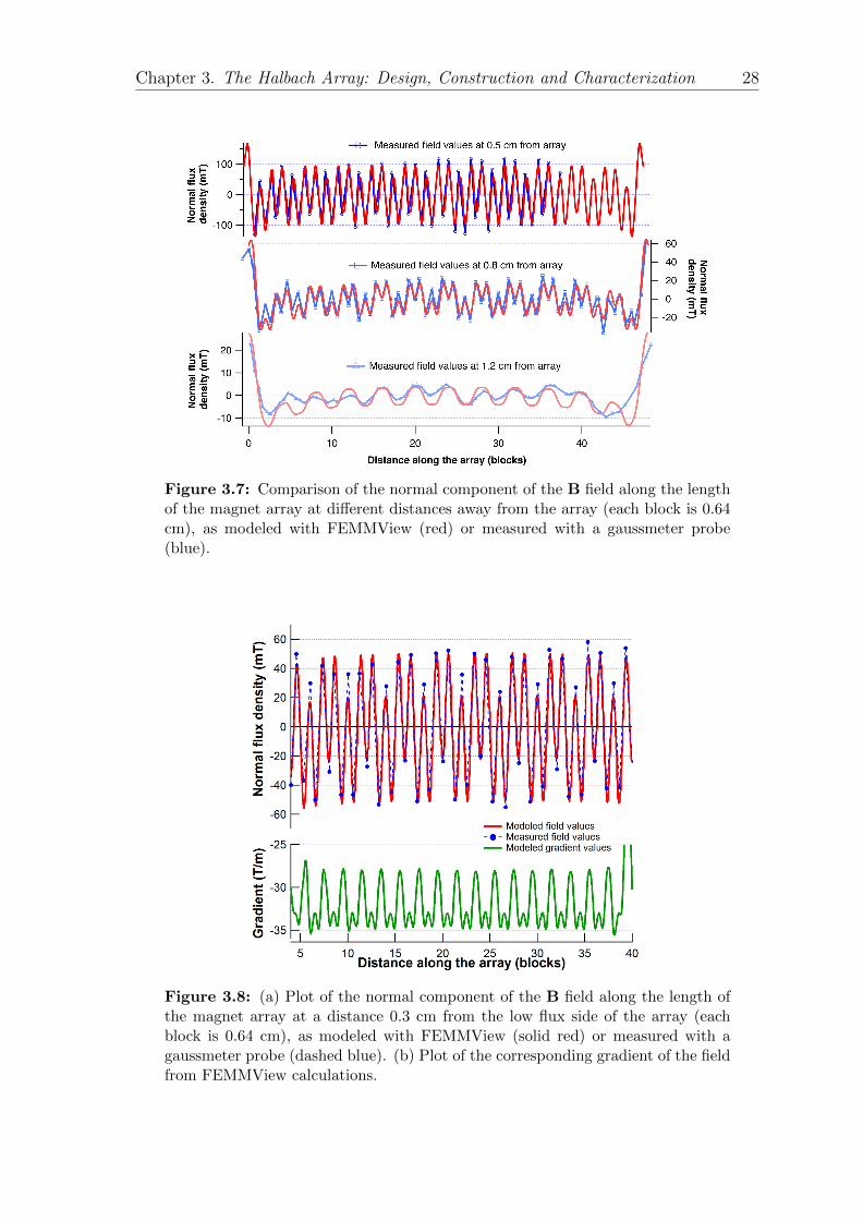
Figure 3.8 shows the data for the normal component of the field measured at a
distance of 0.3 cm from the magnet array surface (dashed blue), a distance commonly
used for many of our nanoparticle separations where the average peak field value has
been found to be approximately 50 mT. Also shown in the figure are the results of
finite element method calculations performed with FEMMView software, indicating
the predicted field value(solid red). The gradient(green) has an average value of 32
T/m at that height.
Chapter 3. The Halbach Array: Design, Construction and Characterization 28
Figure 3.7: Comparison of the normal component of the B field along the lengthof the magnet array at different distances away from the array (each block is 0.64cm), as modeled with FEMMView (red) or measured with a gaussmeter probe(blue).
Figure 3.8: (a) Plot of the normal component of the B field along the length ofthe magnet array at a distance 0.3 cm from the low flux side of the array (eachblock is 0.64 cm), as modeled with FEMMView (solid red) or measured with agaussmeter probe (dashed blue). (b) Plot of the corresponding gradient of the fieldfrom FEMMView calculations.

Chapter 3. The Halbach Array: Design, Construction and Characterization 29
The good agreement between modeling and measurement results at multiple
distances from the array provides evidence that the model is faithful to actual device
characteristics, allowing us to use the finite element model for further pertinent cal-
culations. The field data from the model plotted in Figure 3.9 shows slight variations
but in general, good uniformity in B field along the entire horizontal distance of the
array. At distances very close to the array, there is much greater variation in the B
field but the array still maintains uniformity in peak field values. However, at the
two ends of the array (the last 2.5 cm on each side), fringe effects occur making the
field highly irregular (not shown in figure) but for our separations, the flow channel
location and its width and length have been chosen to be in the uniform field region
to avoid these end effects.
200
150
100
50
0
Mo
del
ed B
fie
ld v
alu
es (
mT
)
403020100
Distance along the array (magnet blocks)
At 0.13 cm from array
At 0.15 cm from array
At 0.3 cm from array
At 0.45 cm from array
Figure 3.9: Plot of the B field along the length of the magnet array at fourdifferent distances relevant for separation away from the array, as modeled withFEMMView. The highest field values are reached in the new Plexiglas channelwhen used without spacers, while the three lower field values are reached withthe old glass channel when 1, 2 and 3 spacers, each of thickness 0.15 cm restunderneath.
FEMMView modeling results have also confirmed the utility of our approach in
using the low flux side of the Halbach array, in comparison to the expected behavior
for a single magnet or the high flux side of the array. We can see in Figure 3.10 that
the gradients for low flux side of the Halbach array are significantly higher for the
same values of field - which supports the central premise of this separation approach,
namely that a high field gradient ∼30 T/m can be achieved in low field ∼50 mT. In
addition, the array provides a large region for separation of nanoparticle suspensions
as opposed to a very small region above a single magnet.

Chapter 3. The Halbach Array: Design, Construction and Characterization 30
Figure 3.10: Comparison of field gradient as a function of average B field for thehigh and low flux sides of the Halbach array and for a single magnet shows theutility of using the low flux side.
The significantly higher gradient at the low flux side for the same medium and
set of particles increases the flow rate of the particles linearly as given by modification
of Eqn 2.13 on page 15 into
vp =∇(m •B)
3πηdp(3.4)
Based on the field values we are using, a three to sixfold higher gradient makes
each separation 3 to 6 times faster. Therefore our idea of a high throughput separation
process of magnetic particles is best served by using the low flux side of the array.
When we are using the array in the low flux side, the average B field and field
gradient of the array both get changed just by changing the distance of the channel
from the array surface. Figure 3.11 presents the values of magnetic field and gradient
along the channel as a function of the array-channel distance calculated using our
model. Consider, for example, a decrease in the distance between the array and the
channel. This increases the field gradient and thus increases the force on a suspension
of nanoparticles (Eqn 2.8), making the separation faster.
3.5 Implications for magnetic separation
Next, we develop a schematic of separation process and particle behavior in a
channel placed at different distance from the Halbach array using the concepts of mag-
netic force and dipole-dipole energy and using a number of generalized assumptions.
First, we can assume that the magnetic field generated by the Halbach magnet array
is uniform throughout the horizontal distance of the array and inversely proportional

Chapter 3. The Halbach Array: Design, Construction and Characterization 31
Figure 3.11: Plot of the (a) averaged B field and (b) gradient of B in the directionperpendicular to the surface of the magnet array as a function of distance abovethe array in the low flux side.
to distance from the array (supposedly located right below the schematic) as shown
in Figure 3.12, where the field strength is higher in the bottom strip than in the top
strip. The channel full of particles can be situated at different distances from the
magnet array. Noting the directly proportional relation between Udd and magnetiza-
tion M in Equation 2.14, we can infer that Udd between particles will be greatest at a
region closest to the magnet array where particles experience the greatest magnetic
fields and get most magnetized.
Figure 3.12: Schematic of separation showing field and particle behavior at dif-ferent distances away from the array: the bottom strip represents highest fieldand gradient values, both of which decline as we move up and away from the ar-ray. Sorting close to the array near the bottom leads to maximum aggregationof particles while sorting far away from the array leads to minimum aggregation.Somewhere in between, we expect an optimum distance where aggregation of moremagnetic particles and random flow of less magnetic particles can be expected.
Next, we can make the assumption that magnetization of particles scales with
size, which is a reasonable assumption to make for particle suspensions manufactured
using the same synthesis process [40]. For a mixed suspension of large (red) and small

Chapter 3. The Halbach Array: Design, Construction and Characterization 32
(blue) particles flowing in the channel in moderate (middle strip) to high magnetic
fields (bottom strip), Udd for larger particles can become much greater than thermal
fluctuations of order kBT. This may result in a distribution of clustered and chained
large nanoparticles at the bottom of the channel. On the contrary, for small parti-
cles, thermal energy dominates the dipole-dipole interaction energy and prevents the
particles from clustering to each other, letting them flow freely through the fluid.
There are some trade-offs to balance here in terms of what particles we would
like to isolate in the post-sort filtrate and post-sort residues and the quality (in
uniformity) of these filtrates and residues. This balance depends critically upon the
distance of the channel from the magnet array since this distance not only alters the
gradient and magnetic force experienced by the particles as described before, but also
the magnetization and dipole-dipole interactions between individual particles due to
change in field.
Doing a separation too close to the array (bottom strip) strengthens the dipole-
dipole interactions between all particles and brings about the complication and un-
desirable effect of particle aggregates interacting with both large and small particles.
This traps even some smaller particles in the residue instead of letting them flow
freely into the filtrate. This might produce a good filtrate by letting only small parti-
cles flow freely but will surely reduce the uniformity of the residue. Similarly, placing
the channel far away from the array (top strip) reduces the dipole-dipole interactions
and brings about another undesirable effect of even large particles not being trapped
in the array as residue, and just flowing through to the filtrate instead. In this case,
the residue might contain only some larger particles that clumped, making it more
uniform but the quality of the filtrate is compromised.
Another schematic, Figure 3.13 (c), shows explicitly the nanoparticle suspen-
sion flow and the effect of locating a channel in an ideal sorting situation, with large
particles trapped in periodic locations along the array where both gradient and field
are greatest. However, even when the optimal distance has been calculated and used,
some of our assumptions about the particles can go awry, leading to sub-optimal
sorting conditions. Say for example, that the assumption of particle magnetization
scaling with size is defective, meaning that there are some large particles with mag-
netization comparable to or weaker than the smaller particles and that there are
some small particles with very high magnetization. In this case, the small particles
can potentially start interacting with a cluster of large chained nanoparticles if the
dipole-dipole energy between the particle-cluster combination exceeds the thermal

Chapter 3. The Halbach Array: Design, Construction and Characterization 33
energy. Different-sized nanoparticles could be entangled or trapped inside this clus-
ter as it forms, making the separation process more challenging. Similarly, there
might be larger particles with smaller values of magnetization that never get trapped
at the base but instead, flow out along with the smaller particles even when we are
at an optimum distance. The schematic in Figure 3.13 (d), shows the result of these
various complications that could occur when working with particles originating from
mixtures synthesized at different times.
Figure 3.13: Schematic of separation at an optimal distance and complicationsthat could arise: (a) Placing the channel at an optimal distance. (b) Flowinga mixed suspension with large and small nanoparticles into the channel from aninlet. (c) Ideal sort behavior with smaller particles flowing out of the outlet as fil-trate while larger particles aggregate at highest gradient locations above the array.(d) Complications that could arise even at optimal sorting distance if magneticproperties of nanoparticles were not size-dependent.
Resolving these issues might require multiple passes of the sample through the
array at different distances or obtaining samples that are uniform for at least one of

Chapter 3. The Halbach Array: Design, Construction and Characterization 34
the parameters of size or magnetization. Finding the best distance for performing
a separation of each pre-sort solution also requires magnetic and structural char-
acterization of the pre-sort beforehand and careful optimization calculations based
on the characterization results. The following chapters discuss these magnetic and
structural characterization procedures and the optimizations that need to be done in
preparation for separation experiments.

Chapter 4
Experimental Procedures
This chapter outlines the experimental procedures used for nanoparticle prepa-
ration, structural and magnetic characterization, and separation via the constructed
Halbach array.
4.1 Nanoparticle synthesis and procurement
In most biomedical applications of magnetic fluids, the magnetic materials used
are generally different types of iron oxides or ferrites because they demonstrate min-
imal toxicity inside the body. By far the most commonly used ferrites are magnetite
(Fe3O4) and maghemite (γ-Fe2O3). Because magnetite can be oxidized to maghemite
with only a small reduction in magnetic moment, the actual structure of particles
in magnetic fluids usually involves the presence of both ferrites in an undefined ra-
tio. For most applications, it is absolutely essential that magnetic particles be stable
in suspension with regard to temperature changes and in the presence of uniform
or non-uniform magnetic fields. In order to avoid settling or coagulation of parti-
cles, two different approaches are commonly used. The particle surface can either
be coated with long organic chain molecule surfactants to produce a steric hindrance
between particles or the particle surface can be charged to produce an electrostatic
repulsion. In our study, we used both kinds of particles stabilized with such surface
modifications.
35

Chapter 4. Experimental Procedures and Characterization 36
The nanoparticle samples for the purposes of our study were obtained from two
primary sources: Sigma-Aldrich company and a research group at Case Western Re-
serve University (CWRU). Preliminary testing of array performance and characteri-
zation sensitivity was performed using commercial iron oxide nanoparticles purchased
from Sigma-Aldrich (product number 700320 and 700304). These relatively monodis-
perse particles were synthesized using a size-controlled method in accordance with
Sun et al. [47], which involved a high-temperature solution phase reaction of iron
(III) acetylacetonate in phenyl ether in the presence of hexadecanediol, oleic acid, and
oleylamine. Small 7 nm Fe3O4 nanoparticles obtained midway in the reaction were
used as seeds to grow larger nanoparticles in the precursors solution, giving rise to
the 19 nm Fe3O4 nanoparticles reported by Gu et al [48]. From TEM, Sigma-Aldrich
reported our manufactured nanoparticles to be of nominal sizes of 5 (±1) and 20
(±2) nm diameters, with a 1.5 nm thick coating of oleic acid as surfactant to avoid
agglomeration. The particles were suspended in toluene with an initial concentration
of 5 mg/mL, but could be diluted for separations by simply adding desired amounts
of pure toluene without facing any settling problems.
Additional nanoparticle samples were obtained from Professor Anna Samia and
her students at CWRU. While both toluene-based and water-based particles were
obtained, we only dealt with Samia’s water-based particles as they were closer to
the sample types used in biomedical applications. Samia et al.’s paper [49] describes
the synthesis of both these kinds of particles in detail. The toluene-based parti-
cles were synthesized using iron oleate, oleic acid, hexane and octadecene at a high
temperature before cooling, washing with ethanol and centrifugation. Different sizes
of nanoparticles were prepared by varying the relative amounts of oleic acid and
iron precursor. The water-based particles were modified from the toluene-based sus-
pension using aqueous basic reagents like ammonium hydroxide along with butanol,
ethylamine and succinic anhydride. After these modifications, the particles were held
suspended in water by repulsive electrostatic interactions over the pH range of 5 to
12, with an initial concentration of 5 mg/mL. A Beckman pH meter indicated a pH of
10.9 for our obtained water-based particles. Dilutions of these water-based samples
for separations required careful monitoring of pH since pH disturbances disrupted
electrostatic interactions causing large numbers of particles to quickly crash out of
suspension. This settling was avoided by adding pre-made pH matched (pH 10.9)
aqueous solution of sodium hydroxide (NaOH) in desired amounts.
These particles were selected for their ideal uniform spherical shape for which

Chapter 4. Experimental Procedures and Characterization 37
small angle scattering curves can be readily modeled. In addition, working with
Samia’s water-based particles allowed us to test our improved channel made of Plex-
iglas and compatible only with water-based particles.
4.2 Structural Characterization
Structural characterization of magnetic nanoparticles to infer the particle size,
shape and dispersion, is generally performed by analyzing transmission electron mi-
croscopy (TEM) images. Complementing a detailed TEM analysis, the structural
properties of these particles can also be investigated, on both powder samples and
liquid samples, using small angle x-ray scattering (SAXS) with an x-ray diffrac-
tometer (XRD) [50]. In fact, TEM image analysis only uses a small portion of the
nanoparticle sample while small angle x-ray scattering allows characterization of the
entire sample. This makes SAXS a more useful method for characterizing the total
behavior of a sample of nanoparticles and we made extensive use of this technique as
opposed to TEM image analysis. Here we review the methods followed and later we
present data from both analyses in the results chapter.
4.2.1 Transmission Electron Microscopy and image analysis
Transmission Electron Microscopy is an imaging technique in which a beam of
electrons is transmitted through an ultra-thin electron-dense specimen, interacting
with the specimen as it passes through. TEM provides significantly higher resolu-
tion than optical microscopy and can be used to photograph nanostructures. TEM
imaging was performed in Carnegie Mellon University by our collaborators on the
commercial Sigma-Aldrich particles. Multiple images of the two samples were taken
to cover a greater sample population. These images were then analyzed using Im-
ageJ [51], an open-source image processing and analysis software developed by the
National Institute of Health (NIH). ImageJ allowed us to remove the background
and increase contrast so particles could be clearly distinguished and approximated
as ellipses to calculate diameters of the suspended particles, as shown in Figure 4.1.

Chapter 4. Experimental Procedures and Characterization 38
Figure 4.1: Two stages of Transmissions Electron Microscopy(TEM) image anal-ysis performed using ImageJ analysis software. The picture to the right shows theparticles in the left approximated as ellipses to extract diameter and distributionparameters.
Once the diameter values were obtained, a normalized histogram of particle
diameters was created and fit to a lognormal distribution, given by
y = y0 + A exp
[−ln(x/x0)
width
2]
(4.1)
where y0 is related to the offset due to background, A gives the peak probability of
the peak of the normalized histogram, x0 is the average particle diameter, and width
=√
2(dispersion) gives us information about the size dispersion of the particles. Our
collaborators at Case Western performed similar analyses on their own particles and
provided us with their results.
4.2.2 Small angle x-ray scattering
Structural characterizations were performed using a Rigaku Ultima IV 285mm
X-ray diffractometer (acquired through NSF grant DMR-0922588 at Oberlin College)
in the small angle X-ray scattering (SAXS) configuration. This compact XRD ma-
chine consists of a copper Kα x-ray vacuum tube coupled with a high-voltage power
source to produce an x-ray beam of known wavelength and a sensitive detector to
register scattered x-rays. The Ultima IV model also possesses interchangeable slit
boxes with incident and receiving height limiting slits to eliminate non-correlated

Chapter 4. Experimental Procedures and Characterization 39
scattered x-rays and direct the beam towards the sample stage to produce highly col-
limated x-rays. This XRD machine has numerous advantages including automated
self-alignment and multiple attachment capabilities. The sample stage is held sta-
tionary while the x-ray tube and detector are moved in synchronicity to allow for
easier measurement of powder and liquid samples.
For performing a small angle X-ray scattering experiment using the Ultima IV
XRD, special SAXS geometry attachments are required. The SAXS geometry kit
consists of SAXS sample holder, SAXS sample stage, vacuum path, and SAXS liquid
and powder sample holders in addition to the standard X-ray setup. A diagram of
this SAXS configuration put together in place into the XRD unit is seen in Figure
4.2. The vacuum path is an aluminum box kept under vacuum with x-ray transparent
windows that reduces the amount of scattering from air separating the sample and
detector. Unlike the standard sample stage using a reflection geometry, the SAXS
stage utilizes transmission of the x-ray beam through the sample material to the
detector, with detected beam intensity depending on size of the sample.
Figure 4.2: Configuration of SAXS geometry attachments in the XRD.
The viability of SAXS in the liquid phase using stainless steel liquid sample
holders was tested by Rob Bond [52]. His results proved that successful SAXS pat-
terns could be obtained under 300 minutes using a stainless steel design holder with
screws and kapton windows for holding toluene-based particles.

Chapter 4. Experimental Procedures and Characterization 40
However, for the water-based particles, we used a standard SAXS powder sample
holder after drying the suspension to powder form on a mylar cutout in a crucible.
The x-rays caused these water-based particles to crash out of solution during SAXS
scans by interfering with the charge distributions that held the particles suspended.
Therefore, scans of only their powder forms could be performed. All SAXS measure-
ments were taken from 0.1 to 4 degrees 2θ with a step size of 0.02 degrees and a
count rate of 1 minute per point, making each scan last about 200 minutes. The fits
to measured curves were obtained using two different software: NANO-Solver and
NIST SANS macros.
4.2.3 Curve fitting using NANO-Solver and NIST SANS
macros
The Rigaku Ultima IV has an optional proprietary software package to interpret
scattering data. The software, NANO-Solver version 3.7 [53], fits SAXS results to a
model of spherical particles in a medium with a gamma (Γ) distribution of particle
sizes. After the fit, it returns values for particle size, size distribution, packing frac-
tion, nearest neighbor distance, and other quantities of interest. NANO-Solver also
has the ability to account for two-phase systems by allowing the input of scattering
length densities for both particle and solution. The Γ distribution function used in
this software for analysis is expressed by Equation 2.27, the same equation used in
the derivation of the final expression for scattering intensity.
If D is the independent size variable, D0 is the average diameter when the scatter-
ing particles are spherical and M is the parameter of size distribution, then Mnorm[%]
gives the particle size dispersion when normalized by average size:
Mnorm[%] =
√〈δD2〉D0
× 100 =1√M× 100 (4.2)
Despite the user-friendly platform of the proprietary software, NANO-Solver’s
fitting algorithms are not published, prohibiting a mathematical evaluation of the
accuracy of its fit results. In addition, the program is not robust enough to deal with
powder scan results. To test the accuracy of NANO-Solver predictions and to provide
a framework to fit results from our powder scans, we used an open-sourced package
from the National Institute of Science and Technology (NIST) that comes with the

Chapter 4. Experimental Procedures and Characterization 41
Igor Pro data analysis software called NIST SANS macros [54], used predominantly
for analysis of small angle neutron scattering (SANS) data, but which have been
adapted for SAXS data.
The particle size distribution results from curve fits to NANO-Solver’s gamma
distribution and to NIST SANS macro’s log-normal sphere model were reported by
Kathryn Hasz [55] to agree within error for multiple SAXS datasets. These datasets
included measured SAXS data of Sigma-Aldrich stock suspensions with a single mean
particle size and of mixed suspensions with particles of multiple mean sizes. One
important difference is that unlike NANO-Solver, NIST SANS macros allowed using
the same framework that was verified to work for liquid samples, to then analyze
SAXS data on powders of Anna-Samia’s particles. The credibility of SAXS analysis
using NIST SANS macros was further confirmed by good agreement with results from
TEM on Anna-Samia’s particles, shown later in the results section.
4.3 Magnetic Characterization using a VSM
The magnetic characterization of a magnetic fluid by plotting its magnetization
curve can give us a rough idea about the magnetization of individual average nanopar-
ticles in a sample and can allow distinguishing between solutions with different metals
oxides. Magnetic characterization of samples was performed using a Lakeshore 7307
Vibrating Sample Magnetometer (VSM) shown in Figure 4.3, acquired using the NSF
grant DMR-1104489 at Oberlin College. A VSM is based on the concept of Faraday’s
law of induction, which states that a time-varying magnetic flux induces a voltage
signal in a detection coil nearby. In our magnetometer, magnetic fields of upto 1
Tesla applied to the vibrating sample were created using a large electromagnet. High
voltage systems, fitted with cooling water, were in place to generate the large field.
Although various temperature control settings were available, we performed all our
measurements at room temperature.
The device’s position and alignment were calibrated using a ferromagnetic Nickel
standard of known magnetization in a field high enough to saturate the moment.
Before measurement of any sample, careful adjustments were made to the already
calibrated device to center the sample holder. Magnetic nanoparticle suspensions,
placed in a holder and connected to a sample rod, were then vibrated back and
forth in a region surrounded by several detection or pickup coils. This vibrating

Chapter 4. Experimental Procedures and Characterization 42
magnetic sample resulted in time-varying magnetic flux, inducing an electric voltage
signal through the pickup coils proportional to the sample’s magnetic moment. This
voltage signal was processed through a lock-in amplifier and other electronics built
into the VSM. The Lakeshore 7307 VSM with accompanying IdeasVSM software were
designed with a high level of automation, so the voltage signals were interpreted and
the M vs. H curve of each sample directly plotted by the software, with remarkable
reproducibility. The data points generated allowed us to easily calculate the sample’s
magnetization using the Langevin function given by Equation 2.7.
Figure 4.3: Lakeshore 7307 Vibrating Sample Magnetometer at Oberlin College.
For all our samples, we started out with a 50 µL volume of suspension and
placed it in a Kel-F plastic holder made to hold liquid samples. Magnetic moment
responses of ∼10−3 emu were reported for each sample, well above the 5 × 10⁻⁵ emu
noise threshold of our magnetometer.
4.4 Nanoparticle separation procedures
In preparation for magnetic separation of nanoparticle suspensions using the
Halbach array-channel assembly, magnetic nanoparticle stock solutions were struc-
turally characterized using TEM and SAXS and magnetically characterized using
magnetometry. Using results from the magnetic and structural characterization for
any set of particle mixtures, calculations were done to figure out optimal field values

Chapter 4. Experimental Procedures and Characterization 43
such that dipole-dipole interaction energy for larger particles at that field value ex-
ceeded kBT by a few times, while Udd for smaller particles was still less than kBT.
Once the optimum field value was calculated, an appropriate number of spacers were
used underneath the channel to reach the necessary field. Finite element model cal-
culations helped here by providing information about the ideal separation distance,
along with the gradient value at the relevant field which allowed us to calculate the
flow rate using Equation 3.4. A separation setup was then established with relevant
flow channels at the right distances based on the samples to be used.
Once the separation setup was established, a mixture of two different stock
suspensions was created and characterized using SAXS to get information about the
pre-sort. It was then diluted, inserted into a syringe and pumped through the channel
inlet at accurate flow rates using a syringe pump (Harvard Apparatus Syringe pump
11 Elite). The filtrate was collected from the outlet in a small vial and the residue
was withdrawn from the channel at a high flow rate. Both the post-sort filtrate and
residue were then characterized using SAXS to obtain volume fraction information
to see how successful the single pass separation went.
Figure 4.4: A schematic of multiple passes showing desired filtrates and residuesproduced in each step, along with the starred discarded products.
For multiple passes, the filtrates and residues from the single pass were passed
through the array again separately, each giving rise to their own filtrates and residues,
as shown in Figure 4.4. We would expect Filtrate 2 obtained from double pass
to be more enriched in smaller particles than Filtrate 1. Few large particles with
magnetization comparable to smaller particles might have entered into Filtrate 1
after a single pass but would hopefully be caught in the double pass as Residue 2*.
Similarly, Filtrate 2* would most likely contain smaller particles with higher than
usual magnetizations. The starred filtrates and residues would then mostly be a

Chapter 4. Experimental Procedures and Characterization 44
collection of the few undesirable particles responsible for increasing magnetic and
size variations of the mixture, and they can thus be discarded. When analyzing
separation efficiency of the double pass, we have compared between Filtrate 2 and
Residue 2 results as being the yields of that pass. Similarly, we have compared
between Filtrate 3 and Residue 3 as yields of the triple pass.

Chapter 5
Results and Analysis
The results from structural and magnetic characterizations of magnetic nanopar-
ticle suspensions and results of separation experiments have been presented, inter-
preted and discussed here. Later, a quantitative way to assess device performance
based on use of various particle mixtures and number of passes has been explored
through receiver operating characteristic curves.
5.1 Structural characterization results of nanopar-
ticle suspensions
Structural characterization has been conducted using Transmission Electron Mi-
croscopy (TEM) and Small Angle X-ray Scattering (SAXS) techniques on Sigma-
Aldrich’s and Anna Samia’s nanoparticle suspensions. SAXS curves of distinct par-
ticle stock suspensions have been experimentally found to be distinct and their be-
havior as expected for each suspension. NANO-Solver and our NIST SANS model’s
capapabilities have allowed us to pinpoint to a certain level of accuracy the types
and volume fractions of different particles the suspensions contained, matching up
quite well with information known about the stock suspensions used to create those
mixtures.
45

Chapter 5. Results and Analysis 46
5.1.1 TEM results of Sigma-Aldrich’s and Anna-Samia’s nanopar-
ticles
Transmission Electron Microscopy image analysis has been performed on the
imaging results received from Carnegie Mellon for two of our batch I samples - A7
and A20 (Sigma Aldrich’s nominal 5 ± 1 nm and 20 ± 2 nm diameter particles).
ImageJ software’s image processing capabilities have allowed us to remove the grainy
background of the carrier fluid and surfactant (toluene and oleic acid in our case),
and increase contrast of the particles. Pixelated grains below a certain threshold size
of 3 nm have been discarded for our analysis since they were most probably products
of background noise. Representative images of the A7 and A20 samples after they
have been processed are given below in Figure 5.1.
Figure 5.1: TEM images of Sigma Aldrich’s A7 (shown in a) and A20 (shown inb) nanoparticles after ImageJ processing.
The smaller particle stock suspension (image a) seems to have contamination of
a few big particles in it, and the larger particle stock seems to have a contamination
of smaller particles in it. Although this points to the possibility of contamination of
samples in the sample holder when performing the imaging experiments, it probably
stems from the synthesis process of these nanoparticles. Gu et al. [48] describes the
synthesis of monodisperse Fe3O4 nanoparticles in which 7 nm nanoparticles are used
as seeds to grow larger nanoparticles in the precursor solution. The contamination
of small particles in the large particle stock (image b) then makes sense in terms
of looking at these particles as leftover seeds from the synthesis that did not grow
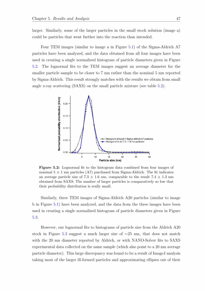
Chapter 5. Results and Analysis 47
larger. Similarly, some of the larger particles in the small stock solution (image a)
could be particles that went further into the reaction than intended.
Four TEM images (similar to image a in Figure 5.1) of the Sigma-Aldrich A7
particles have been analyzed, and the data obtained from all four images have been
used in creating a single normalized histogram of particle diameters given in Figure
5.2. The lognormal fits to the TEM images suggest an average diameter for the
smaller particle sample to be closer to 7 nm rather than the nominal 5 nm reported
by Sigma-Aldrich. This result strongly matches with the results we obtain from small
angle x-ray scattering (SAXS) on the small particle mixture (see table 5.2).
Figure 5.2: Lognormal fit to the histogram data combined from four images ofnominal 5 ± 1 nm particles (A7) purchased from Sigma-Aldrich. The fit indicatesan average particle size of 7.3 ± 1.6 nm, comparable to the result 7.4 ± 1.3 nmobtained from SAXS. The number of larger particles is comparatively so low thattheir probability distribution is really small.
Similarly, three TEM images of Sigma-Aldrich A20 particles (similar to image
b in Figure 5.1) have been analyzed, and the data from the three images have been
used in creating a single normalized histogram of particle diameters given in Figure
5.3.
However, our lognormal fits to histograms of particle size from the Aldrich A20
stock in Figure 5.3 suggest a much larger size of ∼25 nm, that does not match
with the 20 nm diameter reported by Aldrich, or with NANO-Solver fits to SAXS
experimental data collected on the same sample (which also point to a 20 nm average
particle diameter). This large discrepancy was found to be a result of ImageJ analysis
taking most of the larger ill-formed particles and approximating ellipses out of their

Chapter 5. Results and Analysis 48
Figure 5.3: Lognormal fit to the histogram data combined from three images ofnominal (20 ± 2) nm particles (A20) purchased from Sigma-Aldrich indicates anaverage particle size of 25.6 nm, with a contamination of smaller 7.3 nm particles.
major diameter, making our entire analysis to be skewed towards a larger diameter
size. In addition, TEM is an imaging technique that relies on selectively sampling
a few hundred particles that do not overlap during imaging to make a quantitative
statement about billions and billions of particles. Therefore, TEM results generally
have a sampling bias and are useful for determining particle shapes and at best,
providing a rough estimate of particle size.
Despite this discrepancy, the dispersions for both samples obtained from TEM
analysis seem to point towards results similar to those obtained from SAXS fits. For
the A20 stock suspension, isolating bigger particles from the TEM image and fitting
them to a lognormal separately results in a smaller dispersion (∼6%) than that given
by SAXS (∼9%), which makes sense because SAXS scans the entire suspension of
20 nm particles with few 7 nm seeds interspersed in them, averaging to a larger
dispersion. The results from the two structural characterization techniques typically
complement each other and help make greater sense of the data.
Results from TEM image analysis of Anna Samia’s particles performed by our
collaborators have also been reported during sample procurement (Table 5.1), and
they agree well with SAXS results that we have performed (see Table 5.2).

Chapter 5. Results and Analysis 49
Samples DesignatedName
Measured averageparticle size
Anna Samia S15 14.9 ± 0.9 nm
S26 24.0 ± 1.5 nm
Table 5.1: TEM characterization of Anna-Samia’s nanoparticles.
5.1.2 SAXS results of stock suspensions and mixtures
After TEM analysis on each of our stock suspensions, the validity of TEM
results has been confirmed by using our primary analysis technique of small angle
x-ray scattering. Figure 5.4 shows SAXS measurement results on four Sigma-Aldrich
stocks solutions suspended in toluene and measured in our liquid sample holder.
Similarly, Figure 5.5 shows SAXS measurements on two of Anna Samia’s particles
dried to a powder form and measured in the powder sample holder.
Figure 5.4: Small angle x-ray scattering results of four Sigma-Aldrich stock sus-pensions used in our separations show variations in SAXS patterns, relating totheir particle size and dispersion. The fits to measured curves have been obtainedusing NANO-Solver software.
Table 5.2 contains a list of information extracted from fits to SAXS results on
stock suspensions of Sigma-Aldrich and dried powders of Anna Samia’s nanoparti-
cles. The SAXS data for Sigma-Aldrich’s suspensions have been fitted using NANO-
Solver’s gamma distribution (see Equation 2.27) and Anna Samia’s dried powders
to NIST SANS macro’s lognormal sphere model. The fits allow us to see variations
between individual Aldrich batches even though they were the same product, just
purchased at different times. A number of SAXS characterization tests have been
performed on each of these samples over the course of many separations, yielding
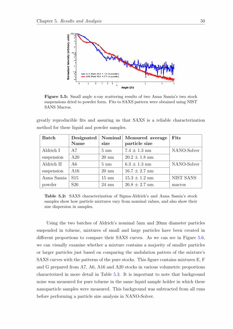
Chapter 5. Results and Analysis 50
Figure 5.5: Small angle x-ray scattering results of two Anna Samia’s two stocksuspensions dried to powder form. Fits to SAXS pattern were obtained using NISTSANS Macros.
greatly reproducible fits and assuring us that SAXS is a reliable characterization
method for these liquid and powder samples.
Batch DesignatedName
Nominalsize
Measured averageparticle size
Fits
Aldrich I A7 5 nm 7.4 ± 1.3 nm NANO-Solver
suspension A20 20 nm 20.2 ± 1.8 nm
Aldrich II A6 5 nm 6.3 ± 1.3 nm NANO-Solver
suspension A16 20 nm 16.7 ± 2.7 nm
Anna Samia S15 15 nm 15.3 ± 1.2 nm NIST SANS
powder S26 24 nm 26.8 ± 2.7 nm macros
Table 5.2: SAXS characterization of Sigma-Aldrich’s and Anna Samia’s stocksamples show how particle mixtures vary from nominal values, and also show theirsize dispersion in samples.
Using the two batches of Aldrich’s nominal 5nm and 20nm diameter particles
suspended in toluene, mixtures of small and large particles have been created in
different proportions to compare their SAXS curves. As we can see in Figure 5.6,
we can visually examine whether a mixture contains a majority of smaller particles
or larger particles just based on comparing the undulation patters of the mixture’s
SAXS curves with the patterns of the pure stocks. This figure contains mixtures E, F
and G prepared from A7, A6, A16 and A20 stocks in various volumetric proportions
characterized in more detail in Table 5.3. It is important to note that background
noise was measured for pure toluene in the same liquid sample holder in which these
nanoparticle samples were measured. This background was subtracted from all runs
before performing a particle size analysis in NANO-Solver.

Chapter 5. Results and Analysis 51
Figure 5.6: Small angle x-ray scattering results of mixtures containing differentproportions of Sigma Aldrich’s 7nm and 20nm particles. The fit parameters havebeen obtained using NANO-Solver software.
LetterDesignation
Stock suspensionsmixed
Measured averageparticle size
Volumefraction
E A7 and A20 7.6 ± 1.7 nm 59%
20.3 ± 1.7 nm 41%
F A6 and A20 6.3 ± 1.3 nm 85%
18.3 ± 2.7 nm 15%
G A7 and A16 7.2 ± 1.0 nm 10%
16.6 ± 2.9 nm 90%
Table 5.3: Characterization of mixtures made from Sigma-Aldrich stock suspen-sions.

Chapter 5. Results and Analysis 52
5.2 Magnetic characterization results of nanopar-
ticle suspensions
The net moment of particle stock suspensions as a function of applied magnetic
field has been measured using a Lakeshore 7307 VSM, with the suspensions showing
superparamagnetic-like behavior. 50 µL volume of each of the 5 mg/mL concentrated
suspensions were used for measurement. Figure 5.7 illustrates the plots of mass
magnetization (measured in emu/g) vs. applied field (measured in Oersteds) along
with their Langevin fits (Eqn 2.7) for each of the four stock suspensions we purchased
from Sigma-Aldrich to be used in our separation experiments. In addition, the results
from Langevin fitting to those curves have been summarized in Table 5.4 to give the
mass magnetization of the solution and moment per average individual particle.
Figure 5.7: Magnetometry of Sigma-Aldrich’s stock suspensions gives mass mag-netizations that can be compared to that of pure bulk magnetite (91 emu/g) toassess the ”magnetic quality” of the samples.
Batch SampleLabel
Nominalsize
Massmagnetization
(emu/g)
Moment perparticle (Bohrmagnetons)
I A7 5 nm 18.8 ± .2 7.4× 10³
A20 20 nm 16.4 ± 0.2 1.5× 10⁴
II A6 5 nm 58 ± .5 4.7× 10³
A16 20 nm 23.2 ± .1 4.1× 10⁴
Table 5.4: Magnetic characterization results of Langevin fits to M vs. H curves,obtained by magnetometry on Sigma-Aldrich suspensions of 50µL volume. Thedifferent batch numbers correspond to separate purchases of these particles andthe nominal size (diameters) refer to Sigma-Aldrich’s description of the product.

Chapter 5. Results and Analysis 53
Similarly, Figure 5.8 shows the plots of mass magnetization (measured in emu/g)
vs. applied field (measured in Oersted) along with their Langevin fits for two of
Anna Samia’s water based stock nanoparticle suspensions we used in our separation
experiments. The Langevin fits have been plotted as well, and the data from those
fits are in Table 5.5.
Figure 5.8: Magnetometry results of Anna Samia’s stock suspensions allow similarcomparison of mass magnetization of samples to that of bulk magnetite.
Stocksuspensions
Total magneticmoment (emu/g)
Moment per particle(Bohr magnetons)
Anna Samia’s15.3 nm stock
59.2 ± 0.1 6.9× 10⁴
Anna Samia’s26.8 nm stock
36.0 ± 0.2 1.6× 10⁵
Table 5.5: Magnetic characterization results of Langevin fits to M vs. H curves,obtained by magnetometry on Anna Samia’s stock suspensions.
These data about moment per particle and mass magnetization extracted from
the Langevin fits to measured values, along with the particle size data from SAXS
fits provide us with enough information to calculate relevant array-channel distances
for each separation process that use these samples.
5.3 Separation results
To test the performance of the constructed array with previously characterized
nanoparticle stock suspensions, we have conducted a series of separation experiments

Chapter 5. Results and Analysis 54
and then used SAXS as a post-separation analysis method to quantify degree of
separation. Single pass experiments have been performed by passing the mixed sus-
pensions once through the channel at optimal distances above the array and then
characterizing the post-sort filtrate and residue. Multiple pass experiments have also
been performed to test the limits of the device by passing the post-sort filtrate and
residues from the single pass through the array multiple times. The rate of passing
solutions through the channel has been calculated using Equation 3.4 for each set of
separations.
First we summarize our results from separations of toluene-based suspensions
from Aldrich that use our toluene-compatible glass channel. Later, we discuss results
from separation of water-based suspensions from Anna Samia that use our water-
compatible Plexiglas channel.
5.3.1 Toluene-based nanoparticle suspensions
Our first separation has been done using Sigma-Aldrich’s batch I 7.4 nm and
20.2 nm (samples A7 and A20) toluene-based particles mixed in a 59% A7 and 41%
A20 ratio by volume. Based on SAXS and magnetometry characterization results
from Tables 5.2 and 5.4, the optimal field has been calculated to be ∼110 mT with
channel distance at 0.15 cm steel plate away from the array. Flow rate has been
calculated to be below .2 mL/min so a rate of 0.1 mL/min has been used. This takes
around 20 minutes to sort a diluted 2 mL pre-sort mixture.
As shown in Figure 5.9, SAXS measurements of the unmixed suspensions clearly
indicate differences in the form factor beating as expected for nanoparticles of dif-
ferent diameters (patterns 1 and 4). The mixture of the two (pattern 3) displays an
intermediate pattern. Single pass of this mixture 3 has led to a significant change in
small angle scattering of the analyte/filtrate (pattern 2). On doing a NANO-Solver fit
to extract quantitative data, the 7 nm particles in the filtrate have showed substantial
enrichment starting from a volume fraction of only 59% in the original mixture to
81% just after a single pass. These results have been quantified in Table 5.6 and are
exciting in that just a 20 minute single pass processing of a 2 mL pre-sort mixture
can cause a big difference in the sample composition. In addition, separation success
could be seen roughly even from the color of the sample. The 7 nm pure stock solu-
tion (1) looks much lighter than the 20 nm stock solution (4). Their mixture is still

Chapter 5. Results and Analysis 55
dark (3) but on separation, the filtrate (2) shows a much lighter coloration, closer to
(1) and indicative of a large volume fraction of the smaller 7 nm particles in it.
Figure 5.9: SAXS curves (left) and particle distributions (right) of SigmaAldrich’s A7 and A20 suspensions, mixtures and their post-sort filtrate. The fitshave been obtained using NANO-Solver software.
Solution Measured averageparticle size
Volumefraction
7.4 nm stock solution (A7) 7.4 ± 1.3 nm
20.2 nm stock solution (A20) 20.2 ± 1.8 nm
Pre-sort mixture (A7+A20) 7.6 ± 1.7 nm 59%
20.3 ± 1.7 nm 41%
Post-sort filtrate 7.2 ± 2.2 nm 81%
20.4 ± 2.4 nm 19%
Table 5.6: SAXS characterization results of a single pass separation of 59% : 41%mixture of Sigma-Aldrich stock suspensions A7 and A20.
One concerning piece of information in this characterization of post-sort filtrate
is its rise in dispersion, making it much less uniform than the stock solution we started
out with. This certainly makes the filtrate sample not very usable for a number of
applications. This increase in dispersion is most probably due to the non-uniform 7
nm contaminants present in the A20 stock solution, which must have gone into the
filtrate.
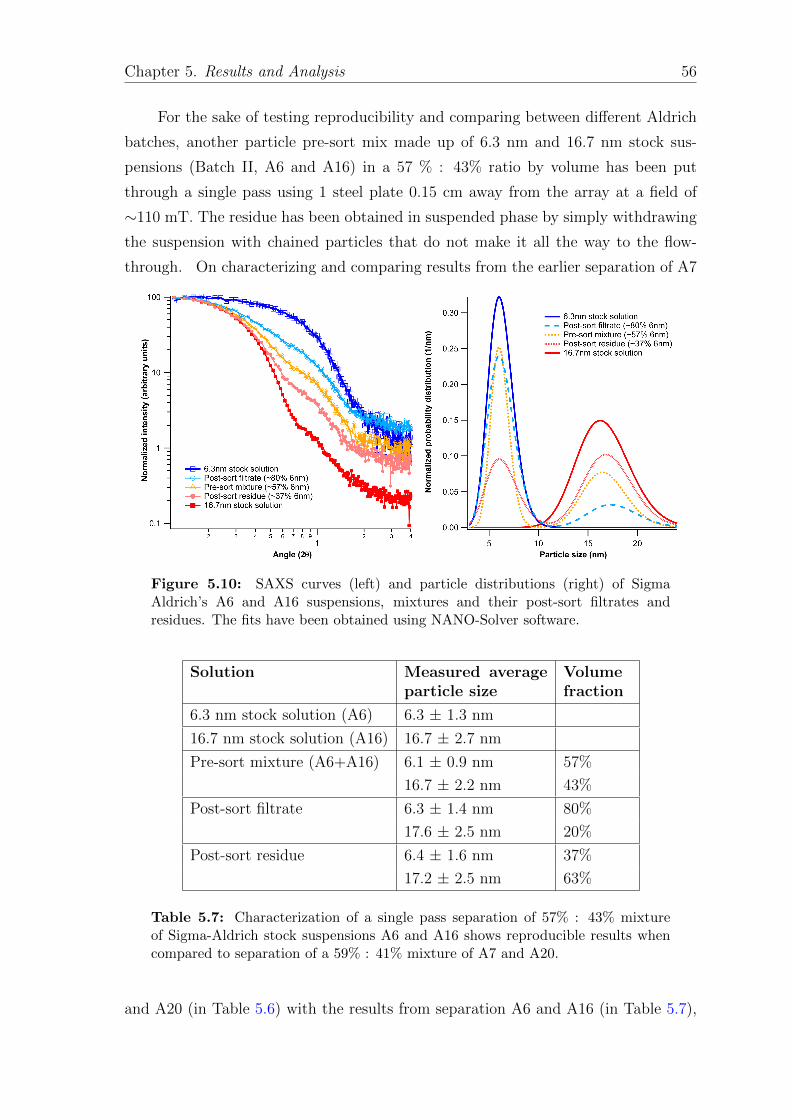
Chapter 5. Results and Analysis 56
For the sake of testing reproducibility and comparing between different Aldrich
batches, another particle pre-sort mix made up of 6.3 nm and 16.7 nm stock sus-
pensions (Batch II, A6 and A16) in a 57 % : 43% ratio by volume has been put
through a single pass using 1 steel plate 0.15 cm away from the array at a field of
∼110 mT. The residue has been obtained in suspended phase by simply withdrawing
the suspension with chained particles that do not make it all the way to the flow-
through. On characterizing and comparing results from the earlier separation of A7
Figure 5.10: SAXS curves (left) and particle distributions (right) of SigmaAldrich’s A6 and A16 suspensions, mixtures and their post-sort filtrates andresidues. The fits have been obtained using NANO-Solver software.
Solution Measured averageparticle size
Volumefraction
6.3 nm stock solution (A6) 6.3 ± 1.3 nm
16.7 nm stock solution (A16) 16.7 ± 2.7 nm
Pre-sort mixture (A6+A16) 6.1 ± 0.9 nm 57%
16.7 ± 2.2 nm 43%
Post-sort filtrate 6.3 ± 1.4 nm 80%
17.6 ± 2.5 nm 20%
Post-sort residue 6.4 ± 1.6 nm 37%
17.2 ± 2.5 nm 63%
Table 5.7: Characterization of a single pass separation of 57% : 43% mixtureof Sigma-Aldrich stock suspensions A6 and A16 shows reproducible results whencompared to separation of a 59% : 41% mixture of A7 and A20.
and A20 (in Table 5.6) with the results from separation A6 and A16 (in Table 5.7),

Chapter 5. Results and Analysis 57
we can see that both the pre-sort mixtures have started out with a relatively equal
proportion of smaller and larger particle stocks by volume and have both resulted in
a substantial enrichment of small particles in the post-sort filtrate, yielding a solution
of ∼80% small particles by volume. This is an important result demonstrating the
reproducibility and reliability of our separation technique and the level of control
we have over each separation, distinguishing it from commonly used techniques of
magnetic separation which can be highly random in their performance.
Seeing that single passes could only get us to around 80% small particles in
the post-sort filtrate, pre-sort mixtures have been passed through the array multiple
times to obtain post-sort filtrates, and then characterized to see if the fraction of
small particles would increase beyond 80%. It has been found that multiple passes
of Sigma-Aldrich do improve the volume fraction of small particles in the filtrate but
cannot do so beyond the high limits of around 88%. However, an exciting result
is that even pre-sorts with substantially low volume fraction of small particles can
be enriched to reach the those high limits. The separation below describes such an
enrichment.
Figure 5.11: SAXS curves (left) and particle distributions (right) of SigmaAldrich’s A7 and A16 suspensions, mixture and the multiple pass post-sort fil-trate. The fits have been obtained using NANO-Solver software.
Multiple pass separations of a highly skewed pre-sort mixture of 10% A6 and
90% A16 suspensions have been performed, again at ∼110 mT fields, where a massive
enrichment of small particles in the filtrate has been seen leading to an 87% by volume
of the A6 particles, as shown in Figure 5.11 and Table 5.8. The 20% dispersion of
small particles seen in the stock solution was preserved in the filtrate, while the
dispersion of larger particles was reduced to ∼3%, meaning that only a fraction of
the larger particles with unusually low magnetization could not be filtered by this
process.
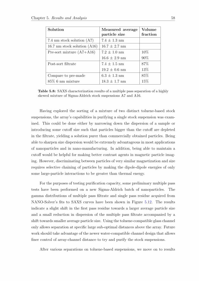
Chapter 5. Results and Analysis 58
Solution Measured averageparticle size
Volumefraction
7.4 nm stock solution (A7) 7.4 ± 1.3 nm
16.7 nm stock solution (A16) 16.7 ± 2.7 nm
Pre-sort mixture (A7+A16) 7.2 ± 1.0 nm 10%
16.6 ± 2.9 nm 90%
Post-sort filtrate 7.4 ± 1.5 nm 87%
19.2 ± 0.6 nm 13%
Compare to pre-made 6.3 ± 1.3 nm 85%
85% 6 nm mixture 18.3 ± 1.7 nm 15%
Table 5.8: SAXS characterization results of a multiple pass separation of a highlyskewed mixture of Sigma-Aldrich stock suspensions A7 and A16.
Having explored the sorting of a mixture of two distinct toluene-based stock
suspensions, the array’s capabilities in purifying a single stock suspension was exam-
ined. This could be done either by narrowing down the dispersion of a sample or
introducing some cutoff size such that particles bigger than the cutoff are depleted
in the filtrate, yielding a solution purer than commercially obtained particles. Being
able to sharpen size dispersion would be extremely advantageous in most applications
of nanoparticles and in nano-manufacturing. In addition, being able to maintain a
cutoff would be helpful for making better contrast agents in magnetic particle imag-
ing. However, discriminating between particles of very similar magnetization and size
requires selective chaining of particles by making the dipole-dipole energies of only
some large-particle interactions to be greater than thermal energy.
For the purposes of testing purification capacity, some preliminary multiple pass
tests have been performed on a new Sigma-Aldrich batch of nanoparticles. The
gamma distributions of multiple pass filtrate and single pass residue acquired from
NANO-Solver’s fits to SAXS curves have been shown in Figure 5.12. The results
indicate a slight shift in the first pass residue towards a larger average particle size
and a small reduction in dispersion of the multiple pass filtrate accompanied by a
shift towards smaller average particle size. Using the toluene-compatible glass channel
only allows separation at specific large sub-optimal distances above the array. Future
work should take advantage of the newer water-compatible channel design that allows
finer control of array-channel distance to try and purify the stock suspensions.
After various separations on toluene-based suspensions, we move on to results

Chapter 5. Results and Analysis 59
Figure 5.12: Particle distributions of stock, filtrate and residue from purificationattempts on a new Sigma-Aldrich batch of particles.
obtained from separation experiments on Anna Samia’s water-based nanoparticle
suspensions.
5.3.2 Water-based nanoparticle suspensions
After acquiring water-based particles from Anna Samia and her students at
CWRU, multiple pass separations have been tested with a new water-compatible
Plexiglas channel at a higher field and gradient than allowed by the older glass chan-
nel. Anna Samia’s nanoparticle suspensions, as opposed to Sigma-Aldrich’s, have the
advantage of tighter distributions of particle sizes without any size overlaps, along
with very different magnetizations of the two suspensions. This type of particle be-
havior makes it much easier to sort the two fractions, even with a device that has
less discriminating capacity.
Calculations from magnetometry results of the pure samples suggest using more
than 2 plates under the channel for a total array-channel distance of greater than .30
cm at fields of ∼50 mT to prevent significant dipole-dipole interactions between small
and large nanoparticles while still causing significant clumping of larger particles. A
roughly 50:50 ratio mixture of 15.3 nm and 26.8 nm stocks has been created and
diluted to make it amenable for separation. After SAXS characterization of the
initial mixture, first and second passes have been done with 2 plates underneath
the new channel. SAXS scans of first and second pass filtrates indicated enrichment
of small particles from the initial 54% to 66% to 90%, while larger particles were
enriched in the residue from an initial 46% to 75% in the first pass. To improve the
quality of filtrate in the 3rd pass, the separation has been started out with a single
plate below the channel to let the remaining big particles chain, and plates have been

Chapter 5. Results and Analysis 60
Figure 5.13: SAXS curves of Anna Samia’s particles during different stages ofthe separation process. Solid curves are fits to NIST SANS macros.
Solutions Measured averageparticle size
Volumefraction
15.3 nm stock solution (S15) 15.3 ± 1.2 nm
3rd pass filtrate 14.8 ± 1.4 nm 100%
1st pass filtrate 14.8 ± 1.5 nm 66%
26.7 ± 2.4 nm 44%
Mixture of two pure samples 14.8 ± 0.9 nm 54%
(S15+S26) 27.0 ± 1.6 nm 46%
1st pass residue 15.0 ± 0.8 nm 25%
26.5 ± 2.1 nm 75%
3rd pass residue 15.1 ± 0.5 nm 2%
27.2 ± 2.4 nm 98%
26.8 nm stock solution (S26) 26.8 ± 2.7 nm
Table 5.9: Characterization of a triple pass separation of ∼50:50 mixture ofAnna Samia’s 15 and 26 nm particle suspensions. These results come from SAXSmeasurements performed on dried powder forms of water-based suspensions in apowder sample holder. The fits to curves were obtained from NIST SANS Macros.

Chapter 5. Results and Analysis 61
added one by one to slowly let out smaller particles that might have been trapped in
the chain. A similar process for the residue has led to the final result of 100% 14.8
nm in the filtrate and 98% 27.2 nm in the residue, an almost perfect separation of
particles.
After having obtained SAXS characterization results from a number of separa-
tion experiments using the Halbach array and after having discussed them separately,
we would like to develop a quantitative way to assess the overall performance of our
device taking into account not just the separation experiments highlighted above but
all our recorded separation datasets with the device. The section below provides the
methodology for such an analysis.
5.4 ROC Analysis
Receiver Operating characteristic (ROC) analysis is a statistical methodology
that comes out of signal detection theory, and is commonly used in the analysis
of medical imaging technology [56, 57] . It is used to evaluate the discriminatory
performance of medical imaging tests to be able to sort images by presence or absence
of tumors, essentially “signals” or “noise” [58]. We have adapted the ROC analysis
procedures in the case of our Halbach device, using the volume fractions from SAXS
characterizations of the filtrate and residue for each separation. Such an analysis will
be able to examine the array’s performance in different separation conditions through
several possible sorting outcomes and find optimal procedures for future nanoparticle
sorts.
When considering the results of a particular test or sort in two populations of
small and large particles, we will rarely observe a perfect separation between the
two groups with all small particles ending up in the filtrate and all large particles
in the residue. If we assume that we’re trying to separate small particles out of a
mixture of small and large particles, then for every possible outcome of sorting we can
identify four cases. There will be small particles in the filtrate (true positive), large
particles in the filtrate (false positive), large particles in the residue (true negative)
and small particles in the residue (false negative). The most commonly used figures-
of-merit for sorting accuracy are “sensitivity” or the true positive fraction (TPF),
and “specificity” of the sort [56]. In our case, sensitivity is the probability that small
particles end up in the filtrate and specificity is the probability that large particles

Chapter 5. Results and Analysis 62
end up in the residue, given by the equations below:
Sensitivity(TPF ) =TP
TP + FN=
FiltratesmallFiltratesmall +Residuesmall
(5.1)
Specificity =TN
TN + FP=
ResiduelargeResiduelarge + Filtratelarge
(5.2)
FPF = 1− Specificity (5.3)
An ROC curve is a plot of the true positive fraction (TPF) in the y-axis with
respect to the false positive fraction (FPF) in the x-axis. A diagonal line in this plot
represents a completely random mix where no discrimination of particles is achieved.
Similarly, a point on the top left of the plot represents the best possible discrimination
of particle mixtures where all small particles end up in the filtrate and all large
particles end up in the residue.
In Figure 5.14, datapoints for each of our separation experiments have been
plotted according to the procedure described above, to assess our Halbach device
performance on various particle mixtures using single and multiple passes at differ-
ent array-channel locations. For single passes, each individual data point in the plot
represents the characterization results of filtrate and residue obtained from a single
separation performed with the array. For multiple passes, each datapoint represents
characterization results of filtrate and residue obtained from two distinct separations,
one done on the single pass filtrate and one on the single pass residue, as explained
in Figure 4.4. Our separations can be categorized into four different cases, each con-
taining datapoints with similar levels of separation success. Excluding the diagonal
line, four different curves have been created in the figure, just as a guide to the eye
for visually separating the four cases. There are a few general statements that could
be made from the analysis of these curves, explained below.
Single passes of ∼50:50 mixtures of particles at sub-optimal heights yield poor
separation results compared to single passes of similar mixtures performed at optimal
height, which can be seen visually by comparing the lower two curves in the plot.
The correct adjustment of height seems to be very important for maximizing the sort
ratio of particles to reach a desired level of separation. There is ongoing work to
optimize and obtain finer control of array-channel distance using a height-adjustable
channel configuration for the water-based nanoparticle separations, as explained later
in Chapter 6.

Chapter 5. Results and Analysis 63
Figure 5.14: ROC curves for the Halbach array’s separation performance withdifferent particle mixtures at different array-channel distances.
We can also see in the Figure that multiple passes of mixtures significantly
improve the array’s separation performance, when compared to single passes of the
same mixtures. This is seen visually as the jump from the green curve for single
pass of Sigma-Aldrich suspensions to the red curve for multiple passes. Both curves
represent separations done at the optimal distance from the array.
Using nanoparticle samples from two different sources has allowed us to compare
the device’s ease of separation or success based upon the quality of samples. With
Sigma-Aldrich’s 50:50 mixture, multiple passes (at least three) were required to reach
the red curve while just a double pass of Anna Samia’s particle mixture seemed to
get us to the same level of sorting performance. Likewise, just a triple pass of Anna
Samia’s particles leads to an almost perfect separation with 100% small particles in
the filtrate and 98% large particles in the residue according to our SAXS results,
shown by the top blue curve. It does make sense that a device with the capacity
to discriminate between nanoparticles based upon their size and magnetic properties
does better when particles are clearly very distinct in these characteristics.
Thus, we can see that ROC curves can offer a quantitative description of our
device’s separation performance in different circumstances by examining several pos-
sible outcomes. Furthermore, an ROC analysis can offer us strategies to pursue for
future separations of nanoparticles to maximize sort ratio and efficiency.

Chapter 6
Conclusions and Future Work
6.1 Conclusions
Magnetic nanoparticles smaller than 30 nm are particularly important for biomed-
ical applications. This thesis has demonstrated the utility of our novel method for
separating suspensions of small magnetic nanoparticles in that size regime, based on
their size and magnetic moments. Our design and construction of an inverted linear
Halbach array has showed that its low flux side contained a low magnetic field with
a high field gradient in conjunction, two things that are critical for our method of
magnetic separation to work. The magnetic characteristics of the assembly have also
agreed well with finite element method calculations and thus allowed for accurate
modeling of magnetic forces.
We have also outlined some of the important results obtained using our device
in the separation of Sigma-Aldrich’s toluene-based particles and Anna Samia’s water-
based particles. We have found out that multiple passes of particle suspensions, when
compared to single passes through the device, improved sorting ratios of particles.
However, multiple passes of particle suspensions could only discrimate them upto a
certain level if suspensions had possible non-correlated variations in size and magnetic
moments. In these sorts, we have realized that being at sub-optimal field and gradient
values adversely affected sorting efficiency and that sort ratio could be improved
significantly by being at the calculated optimal array-channel distance. In addition,
we have discovered that mixtures containing two particle distributions around average
sizes separated by 10 nm, having clear differences in their magnetic moments, could
be sorted almost perfectly by our device in just three passes.
64
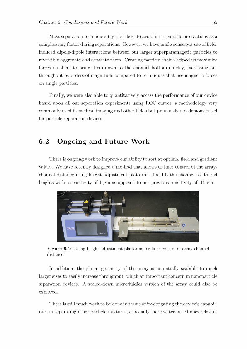
Chapter 6. Conclusions and Future Work 65
Most separation techniques try their best to avoid inter-particle interactions as a
complicating factor during separations. However, we have made conscious use of field-
induced dipole-dipole interactions between our larger superparamagetic particles to
reversibly aggregate and separate them. Creating particle chains helped us maximize
forces on them to bring them down to the channel bottom quickly, increasing our
throughput by orders of magnitude compared to techniques that use magnetic forces
on single particles.
Finally, we were also able to quantitatively access the performance of our device
based upon all our separation experiments using ROC curves, a methodology very
commonly used in medical imaging and other fields but previously not demonstrated
for particle separation devices.
6.2 Ongoing and Future Work
There is ongoing work to improve our ability to sort at optimal field and gradient
values. We have recently designed a method that allows us finer control of the array-
channel distance using height adjustment platforms that lift the channel to desired
heights with a sensitivity of 1 µm as opposed to our previous sensitivity of .15 cm.
Figure 6.1: Using height adjustment platforms for finer control of array-channeldistance.
In addition, the planar geometry of the array is potentially scalable to much
larger sizes to easily increase throughput, which an important concern in nanoparticle
separation devices. A scaled-down microfluidics version of the array could also be
explored.
There is still much work to be done in terms of investigating the device’s capabil-
ities in separating other particle mixtures, especially more water-based ones relevant

Bibliography 66
for biomedical applications. Having obtained good results in separating particle dis-
tributions around average sizes differing by 10 nm, we would like to push the device
further to sort mixtures with average sizes differing by less than 10 nm. In addition,
future work could also be focused on figuring out the best ways to sort mixtures
containing multiple particle distributions.
The work outlined here should continue to provide valuable insights for improv-
ing techniques of magnetic separation of nanoparticles in the future. These first
investigations of the low flux side of the Halbach array have revealed qualities diffi-
cult to create using other means. Therefore, it may guide others in making use of its
interesting magnetic characteristics for other applications as well.

Bibliography
[1] S. Odenbach. Colloidal Magnetic Fluids. Springer, 2009 (page 1).
[2] E. Blums, A. Cebers, and M. Maiorov. Magnetic Fluids. Berlin: Walter de
Gruyter, 1997, p. 416 (page 1).
[3] K. M. Krishnan. Biomedical Nanomagnetics: A Spin Through Possi-
bilities in Imaging, Diagnostics, and Therapy. IEEE Transactions on
Magnetics 46.7 (2010), pp. 2523–2558. doi: 10.1109/TMAG.2010.2046907
(page 1).
[4] X. Michalet, F. F. Pinaud, L. A. Bentolila, J. M. Tsay, S. Doose, J. J. Li, G.
Sundaresan, A. M. Wu, S. S. Gambhir, and S. Weiss. Quantum Dots for Live
Cells, in Vivo Imaging, and Diagnostics. 307.5709 (2005), pp. 538–544.
doi: 10.1126/science.1104274 (page 1).
[5] H. B. Na, I. C. Song, and T. Hyeon. Inorganic Nanoparticles for MRI
Contrast Agents. Advanced Materials 21.21 (2009), pp. 2133–2148 (page 1).
[6] Q. A. Pankhurst, N. K. T. Thanh, S. K. Jones, and J. Dobson. Progress
in applications of magnetic nanoparticles in biomedicine. Journal of
Physics D: Applied Physics 42.22 (2009), p. 224001. doi: 10.1088/0022-
3727/42/22/224001 (page 1).
[7] A. Ito, M. Shinkai, H. Honda, and T. Kobayashi. Medical application of
functionalized magnetic nanoparticles. Journal of Bioscience and Bio-
engineering 100.1 (2005), pp. 1–11 (page 2).
[8] J. S. Beveridge, M. R. Buck, J. F. Bondi, R. Misra, P. Schiffer, R. E. Schaak, and
M. E. Williams. Purification and Magnetic Interrogation of Hybrid Au-
Fe3O4 and FePt-Fe3O4 Nanoparticles. Angewandte Chemie International
Edition 50.42 (2011), pp. 9875–9879. doi: 10.1002/anie.201104829 (page 2).
67

Bibliography 68
[9] J. R. Stephens, J. S. Beveridge, and M. E. Williams. Analytical methods
for separating and isolating magnetic nanoparticles. Physical Chemistry
Chemical Physics 14.10 (2012), pp. 3280–3289. doi: 10.1039/c2cp22982j
(pages 3, 5).
[10] P. S. Williams, F. Carpino, and M. Zborowski. Magnetic Nanoparticle Drug
Carriers and Their Study by Quadrupole Magnetic Field-Flow Frac-
tionation. Mol.Pharmaceutics 6.5 (2009), pp. 1290–1306 (page 4).
[11] C. T. Yavuz et al. Low-field magnetic separation of monodisperse Fe3O4
nanocrystals. Science 314.5801 (2006), pp. 964–967. doi: 10.1126/science.
1131475 (page 4).
[12] G. D. Moeser, K. A. Roach, W. H. Green, T. Alan Hatton, and P. E. Laibi-
nis. High-gradient magnetic separation of coated magnetic nanopar-
ticles. AIChE Journal 50.11 (2004), pp. 2835–2848. doi: 10.1002/aic.10270
(page 4).
[13] J. T. Mayo, S. L. Seung, C. T. Yavuz, W. W. Yu, A. Prakash, J. C. Falkner,
and V. L. Colvin. A multiplexed separation of iron oxide nanocrystals
using variable magnetic fields. Nanoscale 3.11 (2011), pp. 4560–4563. doi:
10.1039/c1nr10671f (page 4).
[14] F. Carpino, L. Moore, M. Zborowski, J. Chalmers, and P. Williams. Analy-
sis of magnetic nanoparticles using quadrupole magnetic field-flow
fractionation. Journal of Magnetism and Magnetic Materials 293.1 (2005),
pp. 546–552 (page 4).
[15] P. S. Williams, F. Carpino, and M. Zborowski. Characterization of mag-
netic nanoparticles using programmed quadrupole magnetic field-
flow fractionation. Philosophical Transactions of the Royal Society London,
Series A (Mathematical, Physical and Engineering Sciences) 368.1927 (2010),
pp. 4419–4437. doi: 10.1098/rsta.2010.0133 (page 4).
[16] P. S. Williams, F. Carpino, and M. Zborowski. Quadrupole magnetic field-
flow fractionation: A novel technique for the characterization of mag-
netic nanoparticles. Journal of Magnetism and Magnetic Materials 311.1
(2007), pp. 383–387. doi: 10.1016/j.jmmm.2006.11.162 (page 4).
[17] J. S. Beveridge, J. R. Stephens, A. H. Latham, and M. E. Williams. Dif-
ferential Magnetic Catch and Release: Analysis and Separation of
Magnetic Nanoparticles. Analytical Chemistry 81.23 (2009), pp. 9618–9624
(page 5).

Bibliography 69
[18] J. S. Beveridge, J. R. Stephens, and M. E. Williams. Differential magnetic
catch and release: experimental parameters for controlled separation
of magnetic nanoparticles. Analyst 136.12 (2011), pp. 2564–2571 (page 5).
[19] B. Teste, F. Malloggi, A.-L. Gassner, T. Georgelin, J.-M. Siaugue, A. Varenne,
H. Girault, and S. Descroix. Magnetic core shell nanoparticles trapping
in a microdevice generating high magnetic gradient. Lab Chip 11 (5
2011), pp. 833–840. doi: 10.1039/C0LC00510J (page 5).
[20] N. Tri, K. Caldwell, and R. Beckett. Development of Electrical Field-
Flow Fractionation. Analytical Chemistry 72.8 (2000), pp. 1823–1829. doi:
10.1021/ac990822i (page 5).
[21] J. A. Jamison, K. M. Krueger, C. T. Yavuz, J. T. Mayo, D. LeCrone, J. J.
Redden, and V. L. Colvin. Size-Dependent Sedimentation Properties of
Nanocrystals. ACS Nano 2.2 (2008), pp. 311–319. doi: 10.1021/nn700144m
(page 5).
[22] C.-L. Wang, M. Fang, S.-H. Xu, and Y.-P. Cui. Salts-Based Size-Selective
Precipitation: Toward Mass Precipitation of Aqueous Nanoparticles.
Langmuir 26.2 (2010), pp. 633–638. doi: 10.1021/la903986v (page 5).
[23] A. M. Al-Somali, K. M. Krueger, J. C. Falkner, and V. L. Colvin. Recycling
Size Exclusion Chromatography for the Analysis and Separation of
Nanocrystalline Gold. Analytical Chemistry 76.19 (2004), pp. 5903–5910.
doi: 10.1021/ac049355h (page 5).
[24] S. F. Sweeney, G. H. Woehrle, and J. E. Hutchison. Rapid Purification
and Size Separation of Gold Nanoparticles via Diafiltration. Journal of
the American Chemical Society 128.10 (2006), pp. 3190–3197. doi: 10.1021/
ja0558241 (page 5).
[25] K. Halbach. Design of permanent multipole magnets with oriented
rare earth cobalt material. Nuclear Instruments and Methods 169.1 (1980),
pp. 1–10 (page 6).
[26] R. Bjork, C. R. H. Bahl, A. Smith, and N. Pryds. Comparison of adjustable
permanent magnetic field sources. Journal of Magnetism and Magnetic
Materials 322.22 (2010), pp. 3664–3671. doi: 10.1016/j.jmmm.2010.07.022
(page 6).

Bibliography 70
[27] J. Hilton and S. McMurry. An adjustable linear Halbach array. Journal of
Magnetism and Magnetic Materials 324.13 (2012), pp. 2051 –2056. doi: http:
//dx.doi.org/10.1016/j.jmmm.2012.02.014 (page 6).
[28] J. C. Mallinson. One-sided fluxes-a magnetic curiosity? IEEE Transac-
tions on Magnetics Mag-9.4 (1973), pp. 678–682 (page 6).
[29] P. Babinec, A. Krafck, M. Babincova, and J. Rosenecker. Dynamics of mag-
netic particles in cylindrical Halbach array: implications for mag-
netic cell separation and drug targeting. 2010 (page 7).
[30] M. E. Hayden and U. O. Hafeli. ’Magnetic bandages’ for targeted delivery
of therapeutic agents. Journal of Physics: Condensed Matter 18.38 (2006).
doi: 10.1088/0953-8984/18/38/S23 (page 7).
[31] A. Sarwar, A. Nemirovski, and B. Shapiro. Optimal Halbach permanent
magnet designs for maximally pulling and pushing nanoparticles.
Journal of Magnetism and Magnetic Materials 324.5 (2012), pp. 742–754. doi:
10.1016/j.jmmm.2011.09.008 (page 7).
[32] M. Hoyos, L. Moore, P. S. Williams, and M. Zborowski. The use of a linear
Halbach array combined with a step-SPLITT channel for continuous
sorting of magnetic species. Journal of Magnetism and Magnetic Materials
323.10 (2011), pp. 1384–1388. doi: 10.1016/j.jmmm.2010.11.051 (page 7).
[33] Q. A. Pankhurst, J Connolly, and J. S K Jones and. Applications of mag-
netic nanoparticles in biomedicine. Journal of Physics D: Applied Physics
36.13 (2003), R167 (page 9).
[34] R. C. O’Handley. Modern Magnetic Materials: Principles and Appli-
cations. Wiley, 1999 (page 9).
[35] E. du Tremolet de Lacheisserie, D. Gignoux, and M. Schlenker. Magnetism:
Fundamentals, Materials and Applications. Springer, 2002 (page 9).
[36] B. D. Cullity and C. D. Graham. Introduction to Magnetic Materials.
Wiley, 2009 (pages 9, 23).
[37] F. Himpsel, J. Ortega, G. Mankey, and R. Willis. Magnetic nanostructures.
Advances in physics 47.4 (1998), pp. 511–597 (page 12).
[38] C. P. Bean and J. D. Livingston. Superparamagnetism. Journal of Applied
Physics 30.4 (1959), S120–S129 (page 13).
[39] R. E. Rosensweig. Ferrohydrodynamics. Mineola, N.Y.: Dover Publications,
1997 (pages 14, 16).

Bibliography 71
[40] G. De Las Cuevas, J. Faraudo, and J. Camacho. Low-Gradient Magne-
tophoresis through Field-Induced Reversible Aggregation. The Journal
of Physical Chemistry C 112.4 (2008), pp. 945–950. doi: 10.1021/jp0755286
(pages 16, 31).
[41] A. Demortiere, P. Panissod, B. P. Pichon, G. Pourroy, D. Guillon, B. Donnio,
and S. Begin-Colin. Size-dependent properties of magnetic iron oxide
nanocrystals. Nanoscale 3 (1 2011), pp. 225–232. doi: 10.1039/C0NR00521E
(page 16).
[42] D. S. Sivia. Elementary scattering theory : for X-ray and neutron
users. Oxford; New York: Oxford University Press, 2011, p. 201 (page 17).
[43] O. Glatter and O. Kratky. Small angle x-ray scattering. Place of Pub-
lication: London, UK. Country of Publication: UK.: Academic Press, 1982
(page 17).
[44] D. I. Svergun, L. A. Fegin, and G. W. Taylor. Structure Analysis by Small-
angle X-ray and Neutron Scattering. Kluwer Academic Pub, 1987 (page 17).
[45] C. Windsor. An Introduction to Small-Angle Neutron-Scattering. Jour-
nal of Applied Crystallography 21 (1988), pp. 582–588 (page 19).
[46] D. Meeker. Finite element method magnetics. Version 4.2 (1 April 2009 Build).
2010 (page 22).
[47] S. Sun and H. Zeng. Size-Controlled Synthesis of Magnetite Nanoparti-
cles. Journal of the American Chemical Society 124.28 (2002), pp. 8204–8205.
doi: 10.1021/ja026501x (page 36).
[48] H.-C. Gu, L. Zhang, and R. He. Oleic acid coating on the monodisperse
magnetite nanoparticles. Applied Surface Science 253.5 (2006), pp. 2611–
2617. doi: 10.1016/j.apsusc.2006.05.023 (pages 36, 46).
[49] Z. Feng, S. Zhu, D. R. M. de Godoi, A. C. S. Samia, and D. Scherson. Adsorp-
tion of Cd2+ on Carboxyl-Terminated Superparamagnetic Iron Ox-
ide Nanoparticles. Analytical Chemistry 84.8 (2012), pp. 3764–3770 (page 36).
[50] A. Sasaki. Size Distribution Analysis of Nanoparticles Using Small An-
gle X-ray Scattering Technique. The Rigaku Journal 22.1 (2005), pp. 31–
38 (page 37).
[51] W. Rasband. ImageJ. U. S. National Institutes of Health, Maryland, USA,
1997-2014. url: http://imagej.nih.gov/ij/ (page 37).

Bibliography 72
[52] R. Bond. “Liquid Phase Small Angle X-ray Scattering of Iron Oxide
Nanoparticles”. Senior Thesis, Oberlin College. 2014 (page 39).
[53] NANO-Solver: Particle size and pore size analysis software. Rigaku Corpo-
ration. url: http : / / www . rigaku . com / service / software / nanosolver
(page 40).
[54] S. Kline. Reduction and analysis of SANS and USANS data using
Igor Pro, journal=Journal of applied crystallography. 39.6 (2006), pp. 895–
900 (page 41).
[55] K. Hasz. “Polarization Analyzed Small Angle Neutron Scattering of
Ferrite Nanoparticles”. Honors Thesis, Oberlin College. 2014 (page 41).
[56] Receiver Operating Characteristic Analysis in Medical Imaging. Jour-
nal of the ICRU 8.1 (2008). doi: 10.1093/jicru/ndn003 (page 61).
[57] C. Metz. Roc Methodology in Radiologic Imaging. Investigative radiology
21.9 (1986), pp. 720–733 (page 61).
[58] J. A. Swets. Measuring the Accuracy of Diagnostic Systems. Science
240.4857 (1988), pp. 1285–1293 (page 61).

Appendix A
Solidworks CAD Designs
Figures of CAD designs of the channel base for the older toluene-compatible
glass channel, and the top and bottom plates for the new water-compatible Plexiglas
channel have been included in this Appendix.
12.000
3.025
0.75
0
scale: 1:3
0.25
0
# 1 ( 0.228 )
drill thru
22 plcs
0.125drill thru6 places
0.25
0
0 0.37
5
1.37
5
2.50
0
3.75
0
5.00
0
6.25
0
7.50
0
8.75
0
10.0
00
11.2
50
12.5
00
13.0
00
0
1.92
5
2.12
5
2.32
5
10.9
25
11.1
25
11.3
250.
050
0.763
1.500
0.763
0.75
0
Cleveland ClinicBME Department
Bottom PlateSCALE: 1:2except wherenoted
SIZE DWG. NO.
AREV.
MATERIAL: acrylic or polycarbonate
FINISH --
DO NOT SCALE DRAWINGAPPLICATION
USED ONNEXT ASSY
DIMENSIONS ARE IN INCHESTOLERANCES: standardFRACTIONALANGULAR: MACH BEND TWO PLACE DECIMAL THREE PLACE DECIMAL
NAME DATE
Drawn: Lee Moore216-445-3230
ENG APPR.
MFG APPR.
Q.A.
SHEET 1 OF 1WEIGHT:
COMMENTS:
THE INFORMATION CONTAINED IN THISDRAWING IS THE SOLE PROPERTY OF<INSERT COMPANY NAME HERE>. ANY REPRODUCTION IN PART OR AS A WHOLEWITHOUT THE WRITTEN PERMISSION OF<INSERT COMPANY NAME HERE> IS PROHIBITED.
PROPRIETARY AND CONFIDENTIAL
Figure A.1: Design of Plexiglas channel base for the toluene-compatible glasschannel, with holes for 22 large aluminium screws to hold the system tight andprevent leaks of nanoparticle suspensions.
73

Appendix A. Solidworks CAD Designs 74
1.10
0.1
6
4 X
R0.
10
2.10 2.10 2.10 2.10 2.10
14 x clearance holes for 6-32 THRU ALL
2 x0.06 (under but
not over) THRU ALL
0.25 0.25
1.4
5
0.5
6 0.5
6 0.1
6
0.7
5
0.75
0.2
5 0.5
0 0.2
5 9.90
11.00
0.2
5
11.00
9.90
0.75
0.2
5 1.45
ISOMETRIC VIEW
By Chetan PoudelJuly 3, 2013
SIDE VIEWS
TOP VIEW
top plate drawingWEIGHT:
A4
SHEET 1 OF 1SCALE: 1:2 in all drawings
DWG NO.
TITLE:
REVISIONDO NOT SCALE DRAWING
MATERIAL: Plexiglass
DATESIGNATURENAME
DEBUR AND BREAK SHARP EDGES
FINISH:UNLESS OTHERWISE SPECIFIED:DIMENSIONS ARE IN MILLIMETERSSURFACE FINISH:TOLERANCES: LINEAR: ANGULAR:
Q.A
MFG
APPV'D
CHK'D
DRAWN
Figure A.2: Design of Plexiglas top plate for the water-compatible flow channel.

Appendix A. Solidworks CAD Designs 75
11.00
1.45
0.2
5
10.00
0.80
0.2
0
ISOMETRIC VIEW
0.5
6 0
.56
14 x clearance holes for 6-32 0
.16
0.1
6
0.8
0
R0.
10
0.2
0
clearance hole for 6-32
0.25
recess for 6-32 socket head
clea
ranc
e 0.
15 0.80
0.25 2.10 2.10 2.10 2.10 2.10 0.25
recess for 6-32 socket head
scale 2:1
TOP VIEW
BOTTOM VIEW
SIDE VIEW
bottom plate drawingWEIGHT:
A4
SHEET 1 OF 1SCALE: 1:2 unless otherwise mentioned
DWG NO.
TITLE:
REVISIONDO NOT SCALE DRAWING
MATERIAL: Stainless Steel 316
DATESIGNATURENAME
DEBUR AND BREAK SHARP EDGES
FINISH:UNLESS OTHERWISE SPECIFIED:DIMENSIONS ARE IN MILLIMETERSSURFACE FINISH:TOLERANCES: LINEAR: ANGULAR:
Q.A
MFG
APPV'D
CHK'D
DRAWN By Chetan PoudelJuly 3, 2013
Figure A.3: Design of stainless steel bottom plate for the water-compatible flowchannel such that the Plexiglas top plate fits tightly into .