Computers & Geosciences 36 (2010) 1474–1483

Contents lists available at ScienceDirect

Computers & Geosciences

0098-30

doi:10.1

n Corr

Investig

de Mon

fax: +5

E-m1 Te

journal homepage: www.elsevier.com/locate/cageo

Inversion of a velocity model using artificial neural networks

Aaron Moya a,b,n, Kojiro Irikura a,c,1

a Disaster Prevention Research Institute, Gokasho, Uji, Kyoto 611-0011, Japanb Laboratorio de Ingenierıa Sısmica, Instituto de Investigaciones en Ingenierıa, Universidad de Costa Rica. Apdo. 3620-60 San Pedro de Montes de Oca, San Jose, Costa Ricac Disaster Prevention Research Center, Aichi Institute of Technology Toyota, Aichi 470-0392, Japan

a r t i c l e i n f o

Article history:

Received 6 June 2008

Received in revised form

4 August 2009

Accepted 29 August 2009

Keywords:

Velocity model

Simulation

Neural networks

Synthetic waveforms

Inversion

Algorithm

04/$ - see front matter & 2010 Elsevier Ltd. A

016/j.cageo.2009.08.010

esponding author at: Laboratorio de Inge

aciones en Ingenierıa, Universidad de Costa R

tes de Oca, San Jose, Costa Rica. Tel.: +506 22

06 2224 2619.

ail address: aaronm@inii.ucr.ac.cr (A. Moya).

l.: +81 565 43 3855/774 38 3348; fax: +81 5

a b s t r a c t

We present a velocity model inversion approach using artificial neural networks (NN). We selected four

aftershocks from the 2000 Tottori, Japan, earthquake located around station SMNH01 in order to

determine a 1D nearby underground velocity model. An NN was trained independently for each

earthquake-station profile. We generated many velocity models and computed their corresponding

synthetic waveforms. The waveforms were presented to NN as input. Training consisted in associating

each waveform to the corresponding velocity model. Once trained, the actual observed records of the

four events were presented to the network to predict their velocity models. In that way, four 1D profiles

were obtained individually for each of the events. Each model was tested by computing the synthetic

waveforms for other events recorded at SMNH01 and at two other nearby stations: TTR007 and TTR009.

& 2010 Elsevier Ltd. All rights reserved.

1. Introduction

Scientists use both forward and backward numerical methodsto model an earthquake rupture process. Source inversion resultsbecome the input to other programs such as finite differencemethods (FDM) to refine the velocity model and explain damagedistribution areas in terms of ground motion amplification effects.Starting with an initial model, the source parameters arecontinuously adjusted until the differences between observedand synthetic seismograms are minimal.

The agreement between observation and synthetic data ismuch influenced by the propagation path, specifically the depthsof the layers and also the P and S-wave velocities. Accurateknowledge of the velocity model becomes as important as thesource itself for calculating synthetic seismograms. Seismicreflection surveys are a straightforward method to obtain under-ground velocity values and layer thicknesses. Such surveys oftenyield many detailed 2D sections that later can be interpolated toconstruct a 3D velocity model (e.g. Fisher et al., 2003; Stephensonet al., 2000). The surveys, though reliable, have the inconveniencethat they are generally expensive and difficult to deploy in highlypopulated or underwater areas.

ll rights reserved.

nierıa Sısmica, Instituto de

ica. Apdo. 3620-60 San Pedro

53 7331;

65 43 3865/774 38 4030.

Alternatively, the P and S arrival times from small earthquakescan be used to construct velocity models using travel timeinversion techniques (Musumeci et al., 2003). Those methodshave the advantage that a lot of information is generally availablefrom seismological centers and can be applied over extensiveregions. In this study, we consider not only the arrival times toperform the inversion but the waveform itself. The idea of usingwaveforms to determine a velocity model has been applied byother researchers. Chen et al. (2000) used a combination of 1Dand 2D models using whole seismograms to refine a 2D basinstructure in the Los Angeles area, California, using geneticalgorithms. Satoh et al. (2001) used a trial-and-error techniqueto fit synthetic waveforms in order to refine a 3D velocity modelin the Sendai basin, Japan. Our approach deviates from othertechniques in that we use a neural network (NN) as a patternrecognition tool that will be trained to associate waveforms totheir specific velocity models.

NN has proven to be a powerful tool in pattern recognitionapplications (Rogers, 1997). In seismology, they have been appliedin tasks such as arrival picking (Dai and MacBeth, 1997),discrimination between earthquake signals and explosions (DelPezzo et al., 2003; Dysart and Pulli, 1990), and earthquake riskevaluation (Giacinto et al., 1997). Roth and Tarantola (1994)applied NN to determine velocity profiles from seismic sectionsused in exploration seismology. Their velocity profile consisted ofeight layers each of which had a fixed thickness. They generatedmany synthetic seismograms to train the network by solving thewave equation. They used a ray-tracing approximation and aRicker wavelet as the source. The network was expected to predict

Dendrites

Nomenclature

NN Neural networksZ learning rate (constant value)dj error (difference between predicted and actual out-

put) of unit j

tj actual output of unit j

oj output of the preceding unit j

i index of a predecessor to the current unit j with linkoij from i to j

j index of the current unitk index of a successor to the current unit j with link ojk

from j to k

A. Moya, K. Irikura / Computers & Geosciences 36 (2010) 1474–1483 1475

the corresponding velocity values for each layer when a givenseismic section was presented as input.

Here we also trained an NN using synthetic data, but ourpurpose was to apply the method actually to earthquake recordsand not to seismic sections. We used the discrete wave numbermethod (Bouchon, 1981) to generate the synthetic seismogramsand included the focal mechanism solution as the source term.Our velocity model consisted of four layers: layer 1 (surface), layer2, layer 3, and layer 4 (bottom layer). The interfaces betweenlayers 1 and 2, and between layers 2 and 3 were set variablesbesides the velocities of layers 1, 2 and 3. Layer 4 was set constantat 20.0 km depth.

Four independent 1D models were obtained for previouslyselected earthquakes recorded at the same station. The earth-quakes were located at different depths and azimuths. We wereinterested in observing whether the models would be verydifferent among themselves or whether they would share enoughsimilarities in order to get a compromised final model. Eachmodel was tested also by simulating other earthquakes not usedduring the inversion. We compared the synthetic waveform to theobserved records at the target station as well as at TTR007 andTTR009 stations.

SynapseCell body

Axon

Nucleus

Input layer Output layer

Input unit 1

Input unit 2 Output unit

Input unit 3

Hid

den

laye

r

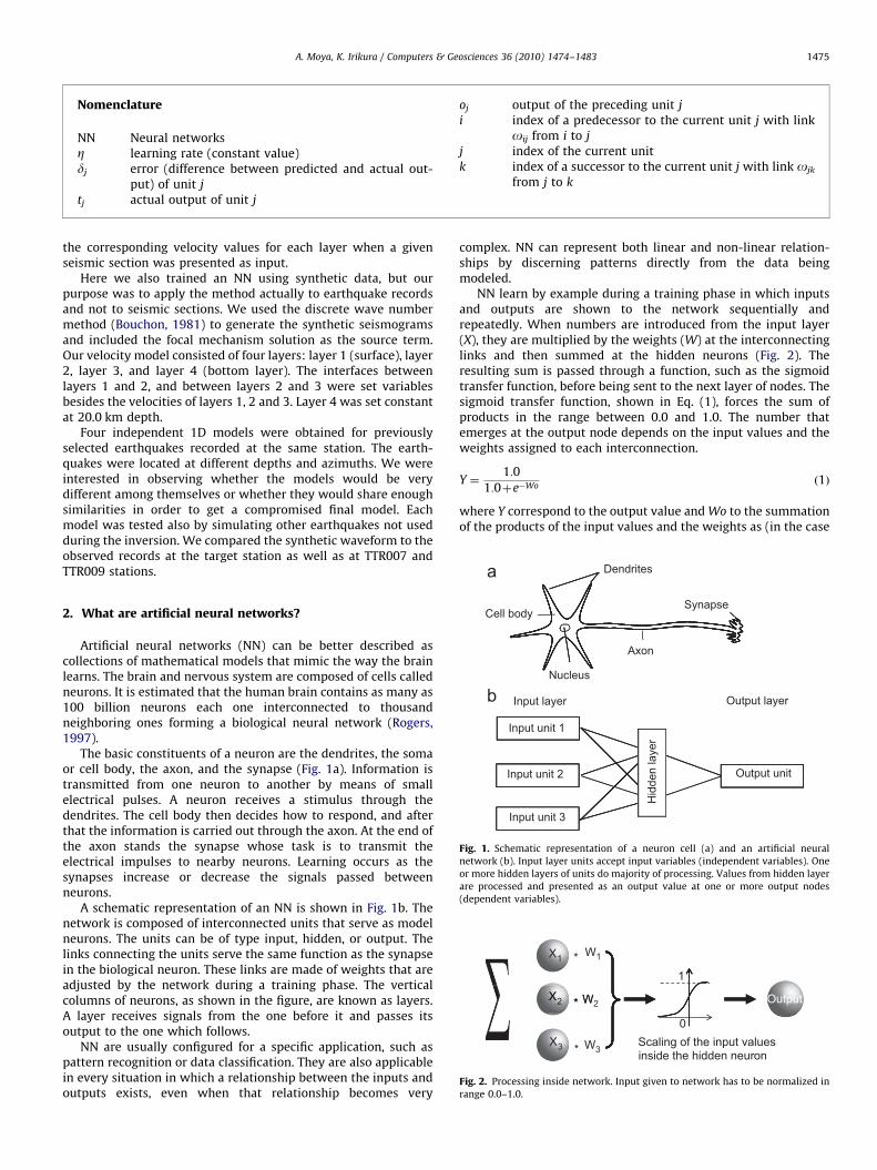
Fig. 1. Schematic representation of a neuron cell (a) and an artificial neural

network (b). Input layer units accept input variables (independent variables). One

or more hidden layers of units do majority of processing. Values from hidden layer

are processed and presented as an output value at one or more output nodes

(dependent variables).

X1 W1*1

X W*X2 W2 Output*

0X3 W3

Scaling of the input values * inside the hidden neuron

Fig. 2. Processing inside network. Input given to network has to be normalized in

range 0.0–1.0.

2. What are artificial neural networks?

Artificial neural networks (NN) can be better described ascollections of mathematical models that mimic the way the brainlearns. The brain and nervous system are composed of cells calledneurons. It is estimated that the human brain contains as many as100 billion neurons each one interconnected to thousandneighboring ones forming a biological neural network (Rogers,1997).

The basic constituents of a neuron are the dendrites, the somaor cell body, the axon, and the synapse (Fig. 1a). Information istransmitted from one neuron to another by means of smallelectrical pulses. A neuron receives a stimulus through thedendrites. The cell body then decides how to respond, and afterthat the information is carried out through the axon. At the end ofthe axon stands the synapse whose task is to transmit theelectrical impulses to nearby neurons. Learning occurs as thesynapses increase or decrease the signals passed betweenneurons.

A schematic representation of an NN is shown in Fig. 1b. Thenetwork is composed of interconnected units that serve as modelneurons. The units can be of type input, hidden, or output. Thelinks connecting the units serve the same function as the synapsein the biological neuron. These links are made of weights that areadjusted by the network during a training phase. The verticalcolumns of neurons, as shown in the figure, are known as layers.A layer receives signals from the one before it and passes itsoutput to the one which follows.

NN are usually configured for a specific application, such aspattern recognition or data classification. They are also applicablein every situation in which a relationship between the inputs andoutputs exists, even when that relationship becomes very

complex. NN can represent both linear and non-linear relation-ships by discerning patterns directly from the data beingmodeled.

NN learn by example during a training phase in which inputsand outputs are shown to the network sequentially andrepeatedly. When numbers are introduced from the input layer(X), they are multiplied by the weights (W) at the interconnectinglinks and then summed at the hidden neurons (Fig. 2). Theresulting sum is passed through a function, such as the sigmoidtransfer function, before being sent to the next layer of nodes. Thesigmoid transfer function, shown in Eq. (1), forces the sum ofproducts in the range between 0.0 and 1.0. The number thatemerges at the output node depends on the input values and theweights assigned to each interconnection.

Y ¼1:0

1:0þe�Woð1Þ

where Y correspond to the output value and Wo to the summationof the products of the input values and the weights as (in the case

A. Moya, K. Irikura / Computers & Geosciences 36 (2010) 1474–14831476

of Fig. 2) given by

Wo¼ X1W1þX2W2þX3W3 ð2Þ

At first, the outputs produced by NN consist of arbitrarynumbers. Over time, as cases are reintroduced repeatedlyhundreds or thousands of times, NN begin to get some of theanswers right. The training algorithm continues to change theweights until most of the answers are correct. Training can bestopped when NN reach a certain minimum error (specified bythe user) or after a given number of iterations (this is our case).

3. The backpropagation algorithm

NN use many different algorithms for training, we used thebackpropagation algorithm. In backpropagation, the input patternis presented at the input layer and the network runs normally tosee what output it produces. The predicted output is compared tothe desired output. The differences between predicted and desiredoutput form an ‘‘error pattern.’’ The error pattern is used to adjustthe weights so that the error would be reduced the next time thesame pattern is presented at the input layer.

When training begins, the links in the backpropagation neuralnetwork have their values initially set to random numbers. Theway in which the weights are updated follows what is calledgeneralized delta-rule (Zell et al., 1991, SNNSv4.2):

Dwij ¼ Zdjoi

dj ¼f 0jðnetjÞðtj�ojÞ if unit j is an output�unit

f 0jðnetjÞP

kdk ojk if unit j is a hidden�unit

(ð3Þ

where f0j is the network, oij is weight of the link from unit i to unitj, netj is input in unit j, Z is the learning rate (constant value), d isthe error (difference between predicted and actual output) of unitj, tj is the actual output of unit j, oj is the output of the precedingunit j, i is the index of a predecessor to the current unit j with linkojk from i to j, j is the index of the current unit, k is the index of asuccessor to the current unit j with link ojk from j to k.

Fig. 3. Location of SMNH01 station and four selected events for inversion (circles with cr

as a star. Two other nearby stations are also shown: TTR007 and TTR009 which belon

The learning rate, Z, is a quantity that specifies the proportionof the error derivative by which the weights will be adjustedduring training. If the learning rate is chosen too large then thelearning process may diverge, but if the learning rate is too lowthen convergence can take an extremely long time.

If local minima were along the path of the error surface, thenetwork could get trapped. One way to overcome this problem isby using what is called a momentum term as part of the weightschange. Each link has a given value assigned to it, its weight. Thatvalue changes every time a new pattern is presented at the inputunits. The momentum term, m, is a percentage of a link value’sprevious weight change to the actual change. In other words,every time there is a change in the weights (link values), apercentage of the previous weight is added to the new weight.

Dwijðtþ1Þ ¼ ZdjoiþmDwijðtÞ ð4Þ

where wij is weight of the link from unit i to unit j, D correspondsto the change added to the previous link’s value, and m is themomentum term.

4. Data preparation

As it was mentioned before, in order to train NN, a large dataset was needed from which the network could learn to associate aparticular waveform to its corresponding velocity model. Becausesuch database was not available from observed records, it wasnecessary to use synthetic waveforms instead.

To compute synthetic seismograms, we used the discrete wavenumber method (Bouchon, 1981). The synthetics were computedfor four selected aftershocks of the Tottori earthquake recorded atSMNH01 station. The Tottori earthquake occurred on October 6,2000, and it had a Mw 6.6 (Fig. 3). The strike-slip fault did notreach the surface, but results from waveform inversion indicatedthat the rupture extended 33 km long by 21 km deep (Iwata andSekiguchi, 2002; Pulido, 2004; Peyrat and Olsen, 2004) in aNW�SE direction. Two strong motion networks recorded themany aftershocks: KiK-net (which has both borehole and surface

oss). Aftershocks of 2000 Tottori earthquake are shown as white circles, mainshock

g to K-Net network.

A. Moya, K. Irikura / Computers & Geosciences 36 (2010) 1474–1483 1477

instruments) and K-NET (only surface instruments). To conductthis study, station SMNH01 was chosen for two reasons:

1.

TabFoc

N

(a

(a

TabVel

La

TabDep

sec

La

TabSou

use

N

(a

(a

It was located in the middle of the rupture zone. This impliedthat many earthquakes were recorded there allowing us toretrieve single 1D models from different azimuths.

2.

It was a KiK-net station. We could simulate the boreholerecords instead of the surface ones in order to avoidamplification effects due to surface geology.

Table 1a shows the source parameters for the earthquakes weselected. The selection was based on the proximity from theevents to the station along the rupture area, and also on whetheror not the waveform had a simple shape in the frequency range ofinterest. The acceleration records were integrated using SAC2000(Goldstein et al., 2003) to obtain velocity and filtered in the range0.3–1.0 Hz in time domain using a bandpass filter.

In determining a velocity model by waveform modeling, wehave to consider that the fitting is not only sensitive to the

le 1bal mechanism parameters for earthquakes used in this study.

o. Event Strike1 Dip1 Rake1 Strike2 Dip2 Rake2

1 Oct-07–06:22 253 74 �161 158 72 �17

2 Oct-17–22:17 309 87 18 218 72 177

3 Oct-18–23:39 258 69 �157 159 69 �22

4 Nov-03–16:53 166 88 �9 257 81 �178

)5 Oct-07–04:59 50 51 125 181 51 55

)6 Oct-12–17:07 169 85 �8 259 82 �175

a Not used for inversion, only for testing the results.

le 2aocity model from Ito et al., 1995.

yer no. Depth (km) P-velocity

(km/s)

S-velocity

(km/s)

r (g/cm3) Qp Qs

1 0 5.500 3.179 2.6 400 200

2 2.0 6.060 3.497 2.7 550 270

3 16.0 6.600 3.815 2.8 800 400

4 38.0 8.000 4.624 3.1 1000 500

le 2bth and velocity ranges for constructing velocity models for inversion. h indicates d

ond layer) as well as a to the P-wave velocity and b to S-wave velocity. Values for

yer no. Depth (km) P-velocity (km/s)

1 0 0.5oa1o2.0

2 0.1oh1–2o1.0 2.0oa2o4.0

3 1.0oh2–3o6.0 4.0oa3o6.0

4 20.0 7.0

le 1arce parameters for earthquakes used in this study. Event #5 and #6 are not

d for inversion but for later testing (see section on results).

o. Event Lat Lon Depth (km) Mw

1 Oct-07–06:22 35.3105 133.3269 7.9 3.8

2 Oct-17–22:17 35.1898 133.4336 12.1 4.3

3 Oct-18–23:39 35.2246 133.2968 7.3 3.7

4 Nov-03–16:53 35.3579 133.2975 8.8 3.5

)5 Oct-07–04:59 35.2865 133.3632 6.8 4.4

)6 Oct-12–17:07 35.3338 133.3202 10.54 3.5

a Not used for inversion, only for testing the results.

velocity and depth of the layers, but also to the focal mechanismof the earthquake. For that reason, information from the focalmechanism was not set variable, and for each event it was fixed tothe value reported by F-net project. The F-net project determinesmoment tensor solutions for earthquakes nationwide using abroadband network. The values for the strike, dip, and rake for theselected earthquakes are given in Table 1b.

Ito et al. (1995) determined the velocity model around theTottori region (Table 2a). Based on their model, we constructed afour-layer velocity model from which synthetics were generatedsemi-randomly by changing the values of the target parameterswithin the ranges given in Table 2b. Our model considered thesame Q values as Ito et al. (1995) where Qs=0.5Qp.

The target parameters were the depth at the interface betweenlayers 1 and 2 (h1�2), layers 2 and 3 (h2�3), and the P-wavevelocity of the first (a1), second (a2), and third (a3) layers. The S-wave velocity of the first layer was taken as b=a/2 (Kitsunezakiet al., 1990; Ludwig et al., 1970) and as b¼ a=

ffiffiffi3p

for the rest. Intotal we wanted to determine five unknowns.

In our model the bottom layer reaches out to 20 km depthbecause our deepest event is located at 12.1 km (Table 1). Thesource was modeled as a ramp function with a half rise-time of0.5 s. The duration of the synthetic was 38.5 s sampled every0.15 s (i.e. the delta t was 0.15). If we inverted the threecomponents as such, there would be 256 (38.5/0.15) units percomponent or 768 input units from the three components perevent. In order to reduce that number, we took a time window ofapproximately 80 points (or 12 s) around the maximum ampli-tude of the vectorial summation for the three components (Fig. 4)estimated as

OðtÞ ¼

ffiffiffiffiffiffiffiffiffiffiffiffiffiffiffiffiffiffiffiffiffiffiffiffiffiffiffiffiffiffiffiffiffiffiffiffiffiffiffixðtÞ2þyðtÞ2þzðtÞ2

qð5Þ

where x(t) and y(t) correspond to the horizontal components ofthe records and z(t) to the vertical component. Using 12 s windowwould be enough to cover the whole S-wave arrival part of thesignal.

epth ranges for corresponding layers (i.e. 1–2 means interface between first and

density and Q factors were taken from Ito et al., 1995 model.

S-velocity (km/s) r (g/cm3) Qp Qs

b1=a1/2 2.6 400 200

b2 ¼ a2=ffiffiffi3p

2.6 400 200

b3 ¼ a3=ffiffiffi3p

2.7 550 270

4.0 2.8 800 400

Input units = O(t)

Depth

Velocity

Fig. 4. Schematic representation of inversion procedure in this study. Input units

correspond to vectorial summation of waveform, O(t). During training, network

learns to associate a particular input waveform to corresponding output velocity

model.

A. Moya, K. Irikura / Computers & Geosciences 36 (2010) 1474–14831478

5. Learning a task

In order to properly train the network, we constructed a totalset of 1000 velocity models with their correspondent waveformsfor each earthquake-station pair. We subdivided those 1000models into three subsets. We used 800 models for training, 100models for validating, and 100 models for testing. The meaning ofeach subset is explained hereafter.

The training data set is made of the models the networkactually uses for learning. It is from that data set that the networkderives the necessary rules to decrease the global mean squarederror (MSE). The MSE is defined as

MSE¼

P½xo�xp�

2

n�p½6�

where xo is the actual output (original depth and velocity values),xp is the predicted output (predicted depth and velocity values)by the network, n is the number of observations and p thenumber of parameters (weights) (Zell et al., 1991, SNNSv4.2). Thenetwork adjusts the weights (or links) between connecting unitsas the patterns are presented over and over again until trainingfinishes.

0.07

0.06

0.05

0.04

Err

or

0.03

0.02

0.010 20000 40000

Ep

Fig. 5. Evolution of residual during learning process of NN for selected events. P

Table 3Comparison of original values and predicted values for selected patterns after network

Pattern Vp layer 1 Vp layer 2 Vp laye

Origin Predic Origin Predic Origin

1 577.2 858.4 3519.8 3388.0 6635.9

12 1316.8 991.3 2432.2 2831.1 7267.0

36 1035.8 913.6 1698.3 1769.5 6887.8

74 1108.4 918.1 2125.5 2085.8 7514.9

The validation data set is composed of models not used duringtraining. Using this set, we can gain insight into the performance ofthe network while it is still learning. As training goes on, every certainnumber of epochs (20 in our case) the process is momentarily paused.The validation set is presented to the network, which according towhat it has learned up to that point, tries to compute the error. Afterthat, the validating data set is removed and learning proceeds withthe training data set. The validation error has no effect on thenetwork’s weights, but it can be used to decide when to stop thelearning process and avoid what is called overtraining. Overtraining

occurs when an NN starts to memorize only a few patterns from thetraining data thus loosing its ability to generalize. In other words,overtraining can make the network yield the same result regardlessof the input data set—i.e. yield a constant velocity model. Byinspecting the error from the validating data set is how we can tellwhether the network has started to memorize (overtrain) or not.

The testing data set is a small data set used at the end, when thenetwork has finished the learning process and the weights do notchange anymore. It was used to examine the performance of thenetwork in its final stage. From the values predicted by thenetwork (i.e. the depths and velocities of the predicted model), wecomputed the synthetic waveforms and compared them to theones from the original models.

och

60000 80000 100000

Oct07-06:22

Oct17-22:17Oct18-23:39

Nov03-16:53

lots correspond to the validation data set for each one of the events given.

finished training. These models were obtained from testing (synthetic) data set.

r 3 Depth layer 1–2 Depth layer 2–3

Predic Origin Predic Origin Predic

6599.4 1005.7 1374.2 3846.7 4117.9

7358.1 80.1 488.7 7079.6 7333.6

7034.1 1107.1 770.4 7724.7 8124.2

7385.1 796.6 746.0 7568.8 7684.9

A. Moya, K. Irikura / Computers & Geosciences 36 (2010) 1474–1483 1479

Inputs and outputs needed to be scaled in the range 0.0–1.0.Stuttgart Neural Network Simulator User Manual, 2000 (Zell et al.,1991) software was used to train the network. We selected abackpropagation algorithm with a momentum term as thetraining function. We used a learning rate of 0.005 andmomentum term of 0.001. Each network was trained for a totalof 100,000 epochs or iterations. The error shown in Fig. 5corresponds to the one from the validating data set aspreviously discussed. It is interesting to note that the tendencyis similar for three events but very different for the Oct-17–22:17one, which is also the farthest earthquake from the target station.

Predictedd2Observed

d1

v3

v2

v1Cat

egor

y (v

= ve

loci

ty,

d=de

pth)

0 2000 4000 6000 8000Velocity (m/s) - Depth (m)

Fig. 6. Comparison of results for pattern # 1. Observed and predicted model are

similar.

Table 4Resultant models predicted by NN after presenting observed waveforms as input

values.

Parameter Earthquake’s date

Nov-03/16:53 Oct-07/06:22 Oct-18/23:39 Oct-17/22:17

Model A Model B Model C Model D

a1 (m/s) 1839 1209 1985 1927

a2 (m/s) 4212 5027 3957 5323

a3 (m/s) 5877 5888 6330 6373

h1–2 (m) 201 123 387 186

h2–3 (m) 3734 4562 1950 6774

Fig. 7. Waveform fitting between observed (light-gray line) and predicted

We used a single hidden layer with 10 hidden units. There arenot specific rules to define the number of units in this layer exceptby trial-and-error. In general, using a large number of hiddenunits is not recommended since it increases the degrees offreedom (i.e. larger number of links between input–hidden–output layers to be determined) of the task. In this particular caseof velocity model inversion, computation time significantlyincreased when numbers larger than 10 units were used. It wasobserved that the final error was only slightly smaller when largerthe number of hidden nodes was used. Using 10 hidden unitsyielded satisfactory results.

6. Results

Once training was finished, we examined the performanceof the network using the testing data set. We show thecomparison between the original values for four selected patternsagainst the values predicted by using NN in Table 3. Fig. 6shows the plot of pattern 1 where it is clear that the modelproposed by NN is very close to the original one. The fitting isnever exact, but the results given by the inversion are similar tothe observed ones.

After inspecting the result with the testing data set, wepresented the network the actual observed records of the firstfour aftershocks listed in Table 1. The values of each best fittingmodel are given in Table 4. Using those velocity models, wecomputed synthetic waveforms and compared the results withthe observed records in Fig. 7.

The fitting between observed and synthetic records is good inall models for the NS and EW components for the S-wave part.The vertical component is more difficult to fit in models A, B, andC. Model D seems to be the one that best explains observationeven in the vertical component.

Fig. 8 shows a map where we have drawn the profiles obtainedfor each of the four events in Table 1. The figure also shows thelocation of events Oct-12/17:07 and Oct-07/04:59 given in thesame table as well as stations TTR007 and TTR009. Using stationSMNH001, we calculated synthetic waveforms each event usingthe four models we obtained in the inversion. The idea was to testhow well each model performed with different events. The result

(solid black line) records for each one of four events given in Table 1.

A. Moya, K. Irikura / Computers & Geosciences 36 (2010) 1474–14831480

after using event #5 (Oct-07/04:59) is shown in Fig. 9. The best fitis obtained when synthetics are computed using models A and D.

In a similar way, we calculated synthetics for event #6 (Oct-12/17:07 in Table 1). Unlike event #5, event #6 was also recordedat TTR007 and TTR009. The epicenter of this event was locatedbetween models A and B (Fig. 8), so we were expecting to observea better fitting when using either model. However, as shown inFig. 10, the fitting was slightly better when using models C or Dinstead. The amplitudes of the NS components are overestimatedin all cases and the EW component at TTR009 shows the largestmismatch.

One possibility for those differences with respect to event #5could be related to the magnitude and depth of event #6. As

Fig. 8. Location of events #5 and #6 from Table 1 along

Fig. 9. Waveform fitting for event #5 from Table 1 at station SMNH001 using four m

observed record by solid line. Amplitude is given in cm/s for this event to left side of

Table 1 shows, event #6 is smaller in magnitude and is located ata greater depth than event #5. The amplitude of the waveformshould be smaller compared to other earthquakes used fortraining. NN might not have been properly trained to handlesuch smaller amplitudes.

The fitting of the four selected events, using their correspond-ing velocity models, was also tested at nearby TTR007 and TTR009stations. Those sites are part of the K-Net network and have noborehole instruments only surface ones. Fig. 11 shows thewaveform fittings. The results in those stations show cleardifferences between observation and synthetics except for event#4 (Model D). For event #4, the fitting is good in all three stationsexcept for the NS component in TTR009.

velocity models obtained by NN for first four events.

odels obtained from inversion. Synthetic waveform is given by dotted line while

figure.

Fig. 10. Waveform fitting for event #6 from Table 1 at station SMNH001, TTR007 and TTR009. Synthetic waveform is given by dotted line while observed record by solid

line. Amplitude is given in cm/s and time in s. Each model is indicated below each set of stations for the NS, EW, and UD components from left to right, respectively. Stations

names are indicated to left of figure. SMNH01 is plotted as SMND01 to indicate that borehole record was used.

A. Moya, K. Irikura / Computers & Geosciences 36 (2010) 1474–1483 1481

7. Discussion and recommendations

NN were used as a tool to construct a velocity model usingwaveform data. In this study, we have assumed that the locationof the hypocenter was fixed and inverted only the depth andvelocities of the layers. However, we have to consider that theoriginal hypocenter determination (the one reported by F-net)depends on the original velocity model. It would seem thatthis is a loop because hypocenter locations are model dependentand in this work a fixed hypocenter location is used to estimate avelocity model. This would be certainly a problem in the casewe were inverting the original model used by F-net (Kubo et al.,2002), but we are not. We are using NN to estimate a different(or a more refined) velocity model in a local area that isconstrained to the aftershock region of the Tottori earthquake.

The validity of the refined model would be dependent on theseismic network spatial density or to the four profiles we havecomputed.

Moment tensor is another quantity that is model dependentand using a fixed value for our inversion technique could result inan unstable solution. This can be solved by considering that F-netuses long period surface waves to compute the moment tensor.The estimated number of broadband stations used in thecalculation is around 70 according to their homepage (http://www.hinet.bosai.go.jp/f-net/event/dreger.php?LANG=en). Our in-version focuses on the waveform fitting of body waves fromstrong motion recordings near the rupture area. We are alsoworking in a different frequency band (0.3–1.0 Hz).

NN were able to predict the corresponding velocity models inthe 1D case when synthetic data were used. They were also able

Fig. 11. Waveform fitting for events #1, #2, #3, and #4 from Table 1 at stations TTR007 and TTR009 using velocity models computed from NN. Synthetic waveform is given

by dotted line while observed record by solid line. Amplitude is given in cm/s and time in s. Each model is indicated below each set of stations for NS, EW, and UD

components from left to right, respectively. Stations names are indicated to left of figure.

A. Moya, K. Irikura / Computers & Geosciences 36 (2010) 1474–14831482

to predict a velocity model from the observed records that yieldedreasonable synthetic waveforms (particularly the first arrivalsof P and S waves). Much of the different capabilities of NN werenot explored, such as the use of different training algorithms,neural architecture, number of hidden units, etc., which mayimprove the results.

According to the different models obtained for the 1D case,model D seemed to be the one that better explained the syntheticsand observed records near SMNH01 station. This, however, cannotbe conclusive until further analyses are carried out using not onlythe records at SMNH01 but also the ones at TTR007 and TTR009 inthe inversion procedure. The tests presented using earthquakes

other than the ones for creating the models (i.e. the four events totrain the network) do not show perfect agreement betweenobserved and synthetic records. One of the reasons was probablythe low amplitude of the waveform due to the small magnitudeand greater depth for one of the earthquakes compared to theones used for training the net. Those misfits probably suggest thata more realistic 2D or even 3D model could be used instead of asimple 1D model. In fact, the poor fitting for the NS component atTTR009 observed in Figs. 10 and 11 may be pointing in thatdirection.

Addition of white noise to the synthetic data sets used fortraining, validation, and testing should be taken into account in

A. Moya, K. Irikura / Computers & Geosciences 36 (2010) 1474–1483 1483

future inversions with NN. In the present study this was notchecked due to the low frequency band we considered.

8. Conclusions

The neural network approach that we have implemented inthis study seems to be a good alternative to retrieve velocitymodels provided certain requirements are met (such as theavailability of high quality data, initial information of a velocitymodel, etc.). The method was presented for a 1D case and it wastested using real (observed) records.

In our neural network approach we tried to obtain what iscalled continuous output which meant that we did not use neuralnetworks to perform a classification or sorting task but to retrieveactual values. In general, we believe that the answer given by NNis in most cases a good approximation to the true solution asshown by the fitting of the waveforms.

In the case of 1D modeling, we obtained four different velocityprofiles for the same station. We observed that the velocity modelcorresponding to model D seemed to be the one that bestexplained the data when different earthquakes (at differentstations as well) were simulated. However, as the waveformfittings were not exact, just approximations, we decided not toadopt a single velocity model until further testing was conducted.Such testing could involve other profiles in addition to stationSMNH01 and nearby stations as well.

In training neural networks for velocity model inversion, it issuggested that repetition of the same pattern be avoided into thetraining data set. In other words, it should be necessary that thetraining data set contained as many different patterns as possiblefor the network to properly generalize from it. Because this wasnot checked for in this study, we believe that the solutions couldbe further improved by careful examination of the input data set.

Given the fact that they are generally good at approximating asolution to its true value, combining the result of NN with agenetic algorithm could probably further enhance the effective-ness of the method as well as the use of different learningalgorithms (not just backpropagation), different network designs(number of hidden units or hidden layers or full connecting versusshortcut connecting links), and number of parameters to bedetermined (output units).

It would be necessary to examine whether the learning rateor momentum term could be different for different eventsor whether it could have any relation with the magnitude anddepth.

Acknowledgements

The waveform data used was provided by K-NET, KiK-netwhich belongs to the National Research Institute for Earth Scienceand Disaster Prevention (NIED). Seismic moments were obtainedfrom F-net (NEID). We wish to thank two referees for their carefuland critical review of the original manuscript. The study wascompleted while one of the authors (A. Moya) was a student atKyoto University and it was partially supported by a Grant-In-Aidfor Scientific Research from the Ministry of Education, Science,Sports, and Culture of Japan.

References

Bouchon, M., 1981. A simple method to calculate Greens functions for elasticlayered media. Bulletin of the Seismological Society of America 71, 959–971.

Chen, J., Helmberger, D.V., Wald, D.J., 2000. Basin structure estimation bywaveform modeling: forward and inverse methods. Bulletin of the Seismolo-gical Society of America 90, 964–976.

Dai, H., MacBeth, C., 1997. The application of a back-propagation algorithm toautomatic picking seismic arrivals from single-component recordings. Journalof Geophysical Research 102, 15105–15113.

Del Pezzo, E., Esposito, A., Giudicepietro, F., Marianro, M., Martini, M., Scarpetta, S.,2003. Discrimination of earthquakes and underwater explosions using neuralnetworks. Bulletin of the Seismological Society of America 93, 215–223.

Dysart, P.S., Pulli, J.J., 1990. Regional seismic 9event classification at the Noressarray: seismological measures and the use of trained networks. Bulletin of theSeismological Society of America 80, 1910–1933.

Fisher, M.A., Norwark, W.R., Bohannon, R.G., Sliter, R.W., Calvert, A.J., 2003.Geology of the continental margin beneath Santa Monica bay, southernCalifornia, from seismic-reflection data. Bulletin of the Seismological Society ofAmerica 93, 1955–1983.

Giacinto, G., Paolucci, R., Roli, F., 1997. Application of neural networks andstatistical pattern recognition algorithms to earthquake risk evaluations.Pattern Recognition Letters 18, 1353–1362.

Goldstein, P., Dodge, D., Firpo, M., Minner, L., 2003. SAC2000: Signal processing andanalysis tools for seismologists and engineers. In: Lee, W., Kanamori, H.,Jennings, P.C., Kisslinger, C. (Eds.), The IASPEI (International Association ofSeismology and Physics of Earth Interior) International Handbook of Earth-quake and Engineering Seismology. Academic Press, London, pp. 1613–1614.

Ito, K., Matsumura, K., Wada, H., Hirano, N., Nakao, S., Shibutani, T., Nishigami, K.,Katao, H., Takeuchi, F., Watanabe, K., Watanabe, H., Negishi, H., 1995.Seismogenic layer of the crust in the inner zone of southwest Japan. AnnalsDisaster Prevention Research Institute (Kyoto University) 38 B-1, 209–219.

Iwata, T., Sekiguchi, H., 2002. Source model of the 2000 Tottori-ken Seibuearthquake and near-source strong ground motion. In: Proceedings of the 11thJapan Earthquake Engineering Symposium (In Japanese), Tokyo, Japan, pp.125–128.

Kitsunezaki, C., Goto, N., Kobayashi, Y., Ikawa, T., Horike, H., Saito, T., Kurota, T.,Yamane, K., Okuzumi, K., 1990. Estimation of P and S-wave velocities in deepsoil deposits for evaluating ground vibrations in earthquake. Journal of JapanSociety for Natural Disaster Science 9 (3), 1–17 in Japanese.

Kubo, A., Fukuyama, E., Kawai, H., Nonomura, K., 2002. NIED (National ResearchInstitute for Earth Science and Disaster Prevention) seismic moment tensorcatalogue for regional earthquakes around Japan: quality test and application.Tectonophysic 356, 23–48.

Ludwig, W.J., Nafe, J.E., Drake, C.L., 1970. Seismic refraction. In: Maxwell, A.E. (Ed.),The Sea. Wiley-Interscience, New York, pp. 53–84.

Musumeci, C., Graziqa, G.D., Gresta, S., 2003. Minimun 1-D velocity modelsoutheastern Sicily (Italy) from local earthquake data: an improvement inlocation accuracy. Journal of Seismology 7, 469–478.

Pulido, N., 2004. Broadband frequency asperity parameters of crustal earthquakesfrom inversion of near-fault ground motion. In: Proceedings of the 13th WorldConference on Earthquake Engineering, Vancouver, B.C., Canada. Paper No.751. /http://www.j-shis.bosai.go.jp/staff/nelson/papers/Pulido_WCEE_2004.pdfS.

Peyrat, S., Olsen, K.B., 2004. Nonlinear dynamic inversion of the 2000 westernTottori, Japan, earthquake. Geophysical Research Letters 31, L05604,doi:10.1029/2003GL019058.

Rogers, J., 1997. Object-Oriented Neural Networks in C++. Academic Press, UnitedStates of America 310pp.

Roth, G., Tarantola, A., 1994. Neural network and inversion of seismic data. Journalof Geophysical Research 99, 6753–6768.

Satoh, H., Kawase, H., Sato, T., Pitarka, A., 2001. Three-dimensional finite-differencewaveform modeling of strong motions observed in the Sendai basin, Japan.Bulletin of the Seismological Society of America 91, 812–825.

Stephenson, W.J., Williams, R.A., Odum, J.K., Worley, D.M., 2000. High-resolutionseismic reflection surveys and modeling across an area of high damage fromthe 1994 Northridge earthquake, Sherman Oaks, California. Bulletin of theSeismological Society of America 90, 643–654.

Stuttgart Neural Network Simulator User Manual, 2000. Version 4.2, University ofStuttgart, University of Tubingen, Germany, p. 350, /http://www.ra.cs.uni-tuebingen.de/SNNS/S. [Accessed January 18, 2010].

Zell, A., Mache, N., Sommer, T., Korb, T., 1991. Recent developments of the SNNS(Stuttgart Neural Network Simulator) neural network simulator. In: Proceed-ings of Application of Neural Networks Conference, SPIE (The InternationalSociety for Optical Engineering), Vol. 1469, Aerospace Sensing InternationalSymposium, Orlando, Florida, United States of America, pp. 708–719.