Inversion Bay©sienne: illustration sur des probl¨mes
227
HAL Id: tel-00819179 https://tel.archives-ouvertes.fr/tel-00819179 Submitted on 30 Apr 2013 HAL is a multi-disciplinary open access archive for the deposit and dissemination of sci- entific research documents, whether they are pub- lished or not. The documents may come from teaching and research institutions in France or abroad, or from public or private research centers. L’archive ouverte pluridisciplinaire HAL, est destinée au dépôt et à la diffusion de documents scientifiques de niveau recherche, publiés ou non, émanant des établissements d’enseignement et de recherche français ou étrangers, des laboratoires publics ou privés. Inversion Bayésienne : illustration sur des problèmes tomographiques et astrophysiques Thomas Rodet To cite this version: Thomas Rodet. Inversion Bayésienne : illustration sur des problèmes tomographiques et astro- physiques. Traitement du signal et de l’image. Université Paris Sud - Paris XI, 2012. <tel-00819179>
Transcript of Inversion Bay©sienne: illustration sur des probl¨mes

HAL Id: tel-00819179https://tel.archives-ouvertes.fr/tel-00819179
Submitted on 30 Apr 2013
HAL is a multi-disciplinary open accessarchive for the deposit and dissemination of sci-entific research documents, whether they are pub-lished or not. The documents may come fromteaching and research institutions in France orabroad, or from public or private research centers.
L’archive ouverte pluridisciplinaire HAL, estdestinée au dépôt et à la diffusion de documentsscientifiques de niveau recherche, publiés ou non,émanant des établissements d’enseignement et derecherche français ou étrangers, des laboratoirespublics ou privés.
Inversion Bayésienne : illustration sur des problèmestomographiques et astrophysiques
Thomas Rodet
To cite this version:Thomas Rodet. Inversion Bayésienne : illustration sur des problèmes tomographiques et astro-physiques. Traitement du signal et de l’image. Université Paris Sud - Paris XI, 2012. <tel-00819179>

N d’ordre :
Université Paris-Sud 11Faculté des sciences d’Orsay
Mémoirepour obtenir
L’habilitation à diriger des recherches
préparé au laboratoire des signaux et systèmesdans le Groupe des Problèmes Inverses
soutenue publiquement
par
Thomas RODET
le 20 novembre 2012
Inversion Bayésienne :
illustration sur des problèmestomographiques et astrophysiques
JURY
Mme. Laure BLANC-FERRAUD RapporteurM. Christophe COLLET RapporteurMme. Sylvie ROQUES RapporteurMme. Irène BUVAT PrésidenteM. Hichem SNOUSSI ExaminateurM. Eric WALTER Examinateur


Remerciements
Avant toute chose, à l’ocassion de cette HdR, je souhaite ici exprimer mes plus sincères remercie-ments :
à Laure BLANC-FERAUD, Directrice de Recherche CNRS à I3S, Sylvie ROQUES, Directrice de Re-cherche CNRS au LATT et Christophe COLLET, Professeur à l’Université de Strasbourg au LSIIT pouravoir accepté la lourde tâche d’être rapporteur de ce manuscrit. Leurs conseils et leurs remarques m’ontété très utiles.
À Irène BUVAT, Directrice de Recherche CNRS à IMNC, présidente du jury de cette HdR, pour sonexamen minutieux et ses remarques pertinentes.
À Hichem SNOUSSI, Professeur à l’Université Technologique de Troyes au LM2S, qui m’a faitl’honneur d’être examinateur de ce travail.
À Eric WALTER, Directeur de Recherche CNRS à double titre, pour avoir accepté d’être examinateuret pour m’avoir acceuilli très chaleureusement lors de mon arrivé au L2S. J’ai apprécié pendant ses deuxmandats de directeur de laboratoire, ses qualités humaines hors du commun.
À Silviu NICULESCU, Directeur de Recherche CNRS, actuel directeur du L2S, pour son travailconstant pour le rayonnement de notre laboratoire, et pour l’aide qu’il m’a apportée pour développerle groupe des problèmes inverses.
Ce retour sur le travail que j’ai mené ces dix dernières années m’amène à penser que les qualitéspersonnelles passent en grande partie par des recontres. De ce point de vue, j’ai eu la chance de croiserMichel DEFRISE et Guy DEMOMENT, qui sont des chercheurs execptionnels autant d’un point de vuescientifique que d’un point de vue humain. Ils restent pour moi des références en terme de déontologie.
Je tiens aussi à exprimer ma reconnaissance à Alain ABERGEL, qui depuis mon recrutement n’apas cessé de me soutenir. Je le remercie aussi pour les rudiments d’astrophysique qu’il m’a appris avecpatience.
Merci également, à Jean–François GIOVANNELLI pour m’avoir accueilli au Groupe Problèmes In-verses qu’il dirigeait à l’époque, et pour m’avoir converti à l’inférence Bayésienne à force de discussionsphilosophiques au café.
Aux membres actuels du Groupe Problèmes Inverses, en particulier aux permanents Aurélia FRAYSSE,Nicolas GAC, Matthieu KOWALSKI, Ali MOHAMMAD-DJAFARI, Hélène PAPADOPOULOS avec lesquelsj’ai de nombreux échanges, en particulier pour les choix pour l’équipe.
Aux thésards que j’ai (eu) la chance d’encadrer : Nicolas BARBEY, François ORIEUX, Caifang CAI,Yuling ZHENG et Long CHEN. Beaucoup de leur travail est présent dans ce document mais surtout ilsm’ont appris à diriger des recherches.
A tous les membres du GPI qui sont passés dans la salle des machines avec moi Olivier, Mehdi,Aurélien, Boris, Fabrice, Patrice, Sofia, Nadia, Hachem, Diarra, Doriano, Sha, Ning, Thomas, Leila,Mircea. Merci de toutes ces discussions à travers lesquelles j’ai pu découvrir une partie des cultures dessept nationalités dont vous provenez.
Enfin, je remercie ma femme Cécile pour son soutien et ses relectures minutieuses de ce manuscrit.
ii


Table des matières
Table des figures v
Avant propos 1
I Parcours Professionnel 3
1 Curriculum Vitae 51.1 État Civil . . . . . . . . . . . . . . . . . . . . . . . . . . . . . . . . . . . . . . . . . . 5
1.1.1 Situation actuelle . . . . . . . . . . . . . . . . . . . . . . . . . . . . . . . . . . 51.2 Titres Universitaires . . . . . . . . . . . . . . . . . . . . . . . . . . . . . . . . . . . . 51.3 Parcours . . . . . . . . . . . . . . . . . . . . . . . . . . . . . . . . . . . . . . . . . . . 51.4 Activités d’enseignement . . . . . . . . . . . . . . . . . . . . . . . . . . . . . . . . . . 61.5 Activités liées à l’administration . . . . . . . . . . . . . . . . . . . . . . . . . . . . . . 61.6 Activités liées à la recherche . . . . . . . . . . . . . . . . . . . . . . . . . . . . . . . . 71.7 Collaborations . . . . . . . . . . . . . . . . . . . . . . . . . . . . . . . . . . . . . . . . 71.8 Encadrements . . . . . . . . . . . . . . . . . . . . . . . . . . . . . . . . . . . . . . . . 7
1.8.1 Post-doctorat et ATER. . . . . . . . . . . . . . . . . . . . . . . . . . . . . . . . 71.8.2 Doctorants . . . . . . . . . . . . . . . . . . . . . . . . . . . . . . . . . . . . . 81.8.3 Stagiaires . . . . . . . . . . . . . . . . . . . . . . . . . . . . . . . . . . . . . . 9
1.9 Liste de publications . . . . . . . . . . . . . . . . . . . . . . . . . . . . . . . . . . . . 101.9.1 Articles de revues internationales avec comité de lecture . . . . . . . . . . . . . 101.9.2 Articles de revues internationales à paraître ou soumis . . . . . . . . . . . . . . 111.9.3 Communications internationales dans des congrès avec comité de lecture et actes 111.9.4 Communications nationales dans des congrès avec comité de lecture et actes . . 131.9.5 Brevets . . . . . . . . . . . . . . . . . . . . . . . . . . . . . . . . . . . . . . . 131.9.6 Thèse . . . . . . . . . . . . . . . . . . . . . . . . . . . . . . . . . . . . . . . . 14
II Synthèse des travaux de recherches 15
2 Tomographie 172.1 Introduction . . . . . . . . . . . . . . . . . . . . . . . . . . . . . . . . . . . . . . . . . 17
2.1.1 Cadre général et définitions . . . . . . . . . . . . . . . . . . . . . . . . . . . . 172.1.2 Inversion tomographique analytique . . . . . . . . . . . . . . . . . . . . . . . . 182.1.3 Inversion statistique . . . . . . . . . . . . . . . . . . . . . . . . . . . . . . . . 202.1.4 Étude empirique sur les similitudes entre les approches analytiques et les ap-
proches statistiques . . . . . . . . . . . . . . . . . . . . . . . . . . . . . . . . . 222.1.5 Discussion . . . . . . . . . . . . . . . . . . . . . . . . . . . . . . . . . . . . . 26
iv

TABLE DES MATIÈRES v
2.2 Deux exemples illustrant l’apport des approches statistiques lorsque le modèle de forma-tion des données est non linéaire . . . . . . . . . . . . . . . . . . . . . . . . . . . . . . 282.2.1 Artefacts causés par la linéarisation de la loi de Beer Lambert . . . . . . . . . . 282.2.2 Résolution du problème de durcissement de spectre de la source de rayons X . . 31
2.3 Problème de la reconstruction 3D de la couronne solaire . . . . . . . . . . . . . . . . . 352.3.1 Problématiques en traitement du signal . . . . . . . . . . . . . . . . . . . . . . 372.3.2 Première approche : paramétrisation des plumes polaires . . . . . . . . . . . . . 382.3.3 Deuxième approche : identification comme un problème de séparation de sources 41
3 Bayesien Variationnel 453.1 Introduction . . . . . . . . . . . . . . . . . . . . . . . . . . . . . . . . . . . . . . . . . 453.2 Méthodologie bayésienne variationelle . . . . . . . . . . . . . . . . . . . . . . . . . . . 463.3 Gradient exponentiel pour le bayésien variationnel . . . . . . . . . . . . . . . . . . . . 473.4 Application à la reconstruction-séparation de composantes astrophysiques . . . . . . . . 49
3.4.1 Modèle direct : . . . . . . . . . . . . . . . . . . . . . . . . . . . . . . . . . . . 503.4.2 Lois a priori : . . . . . . . . . . . . . . . . . . . . . . . . . . . . . . . . . . . . 513.4.3 Loi a posteriori : . . . . . . . . . . . . . . . . . . . . . . . . . . . . . . . . . . 52
3.5 Mise en œuvre de l’approche bayésienne variationnelle . . . . . . . . . . . . . . . . . . 523.5.1 Étude de la séparabilité . . . . . . . . . . . . . . . . . . . . . . . . . . . . . . . 523.5.2 Mise à jour des lois approchantes : . . . . . . . . . . . . . . . . . . . . . . . . . 53
3.6 Résultats . . . . . . . . . . . . . . . . . . . . . . . . . . . . . . . . . . . . . . . . . . . 563.6.1 Données simulées . . . . . . . . . . . . . . . . . . . . . . . . . . . . . . . . . . 563.6.2 Données réelles . . . . . . . . . . . . . . . . . . . . . . . . . . . . . . . . . . . 58
3.7 Conclusion . . . . . . . . . . . . . . . . . . . . . . . . . . . . . . . . . . . . . . . . . 59
4 Perspectives 634.1 Inversion de données astrophysiques . . . . . . . . . . . . . . . . . . . . . . . . . . . . 634.2 Inversion de données tomographiques . . . . . . . . . . . . . . . . . . . . . . . . . . . 644.3 Méthodologie bayésienne variationnelle . . . . . . . . . . . . . . . . . . . . . . . . . . 654.4 Sélection de modèles . . . . . . . . . . . . . . . . . . . . . . . . . . . . . . . . . . . . 67
Bibliographie 71
III Sélection d’articles 80

Table des figures
2.1 Visualisation des coefficients de la matrice (HtH)−1 . . . . . . . . . . . . . . . . . . . 23
2.2 (a) Réponse impulsionnelle du filtre de reconstruction (b) Transformée de Fourier de laréponse impulsionnelle . . . . . . . . . . . . . . . . . . . . . . . . . . . . . . . . . . . 23
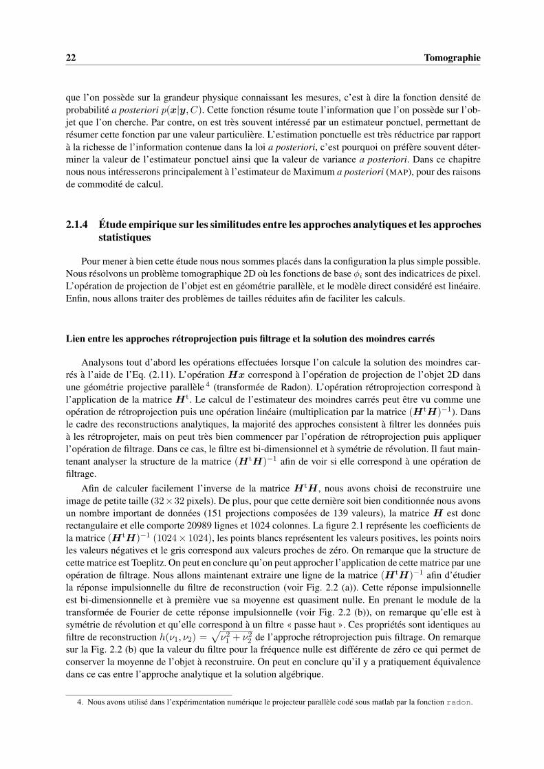
2.3 Visualisation des coefficients de la matrice (HHt)−1 . . . . . . . . . . . . . . . . . . . 24
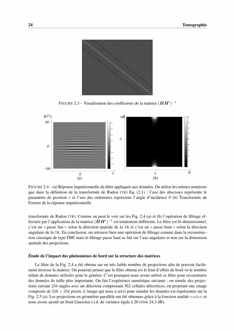
2.4 (a) Réponse impulsionnelle du filtre appliquée aux données. On utilise les mêmes nota-tions que dans la définition de la transformée de Radon (TR) Eq. (2.1) : l’axe des abs-cisses représente le paramètre de position s et l’axe des ordonnées représente l’angled’incidence θ (b) Transformée de Fourier de la réponse impulsionnelle . . . . . . . . . . 24
2.5 (a) Image vraie (b) rétroprojection uniquement (c) inversion de la transformée de Radon(filtre rampe) (d) rétroprojection filtrée en utilisant le filtre identifié à partir d’un petitproblème. . . . . . . . . . . . . . . . . . . . . . . . . . . . . . . . . . . . . . . . . . . 25
2.6 (a) Image vraie utilisée pour faire les simulations (b) Reconstruction de données pré-traitées avec l’algorithme FBP (c) Représentation sous forme d’un sinogramme de y
(données pré-traitées) (d) Minimum du critère des moindres carrés régularisés où lesdonnées pré-traitées les plus bruitées ont été supprimées. . . . . . . . . . . . . . . . . . 29
2.7 Tracés d’une projection pour un angle arbitrairement fixé. En bleu simulation sans bruit.En rouge simulation avec bruit (a) mesure de l’énergie déposée sur le détecteur (b) don-nées après pré-traitement Eq. (2.18). . . . . . . . . . . . . . . . . . . . . . . . . . . . . 30
2.8 Reconstruction polychromatique à partir de données simulées pour une tension de gé-nérateur de 70 et 150 keV . La première ligne correspond à l’abondance d’eau et ladeuxième à l’abondance d’os. (a) (e) sont les abondances de référence utilisées pourles simulations (b) (f) sont les résultats obtenus avec la méthode MCPS (c) (g) sont lesrésultats obtenus en inversant le problème décrit par les équations (2.25) et (2.26) (d) (h)correspondent aux profils extraits des images selon la ligne rouge ; les traits noirs corres-pondent à la référence, les traits bleus à la méthode de reconstruction puis séparation etles traits rouges à l’inversion du modèle non linéaire. . . . . . . . . . . . . . . . . . . . 35
2.9 Reconstruction polychromatique à partir de données réelles sur fantôme physique trèsproche des simulations pour des tensions de générateur de 70 et 150 keV . La premièreligne correspond à l’abondance d’eau et la deuxième à l’abondance d’os. (a) (d) ap-proche MCPS (b) (e) inversion du modèle non-linéaire (d) (h) correspondent aux profilsextraits des images selon la ligne rouge ; les traits bleus correspondent à la méthode dereconstruction puis séparation et les traits rouges à l’inversion du modèle non linéaire. . . 36
2.10 Position des satellites STEREO A et STEREO B par rapport au soleil . . . . . . . . . . 37
2.11 Image à 17,1 nm du pôle nord du soleil à l’aide de l’instrument EUVI. On voit clairementdes structures verticales lumineuses correspondant aux plumes polaires . . . . . . . . . 37
vi
TABLE DES FIGURES vii
2.12 Reconstruction en utilisant notre première approche : la première ligne correspond auxvaleurs que nous avons utilisées pour faire les simulations, la deuxième ligne correspondà des estimations : (a) image morphologique vraie : elle est composée de trois tâchesGaussiennes, (b) segmentation en zones possédant la même dynamique d’évolution, (c)valeur du gain γ en fonction du temps d’acquisition : les couleurs courbes correspondentaux couleurs de la segmentation de la figure (b), (d) reconstruction statique en utilisantune approche filtrage-rétroprojection classique, (e) estimation de la morphologie avecnotre première approche, (f) estimation de la dynamique temporelle. . . . . . . . . . . . 40
2.13 Reconstruction de données réelles en utilisant un seul satellite. Visualisation d’une seulecoupe au dessus du pôle nord : (a) segmentation des plumes définies manuellement, (b)évolution temporelle, (c) reconstruction par un algorithme de filtrage-rétroprojection, (d)reconstruction de la composante morphologique. . . . . . . . . . . . . . . . . . . . . . 41
2.14 Simulation des données : (a) composante morphologique e2, (b) composante morpho-logique e3, (c) composante statique e1, (d) évolution dynamique α associée à e2, (e)évolution dynamique β associée à e3, (f) sinogramme légèrement bruité y . . . . . . . . 43
2.15 Comparaison entre une reconstruction de type filtrage rétroprojection (f) et notre nou-velle approche (a)-(e) : (a) estimation de la composante morphologique e2, (b) estima-tion de la composante morphologique e3, (c) estimation de composante statique e1, (d)estimation de l’évolution dynamique α associée à e2, (e) estimation de l’évolution dy-namique β associée à e3, (f) reconstruction par une approche classique de filtrage rétro-projection (fonction iradon de matlab). . . . . . . . . . . . . . . . . . . . . . . . . . 44
3.1 Composante étendue s : (a) vraie carte utilisée pour simuler les données (b) carte recons-truite avec notre approche . . . . . . . . . . . . . . . . . . . . . . . . . . . . . . . . . 57
3.2 Composante impulsionnelle : (a) vraie carte utilisée pour simuler les données (b) cartereconstruite avec notre approche. . . . . . . . . . . . . . . . . . . . . . . . . . . . . . 58
3.3 Comparaison de différents estimateurs sur la somme des deux composantes : (a) Vraiecarte, (b) carte reconstruite avec le pipeline officiel de l’ESA, (c) carte reconstruite sansbi-modèle avec un a priori de douceur (d) carte reconstruite en utilisant un bi-modèle . . 60
3.4 Reconstruction d’une image de sources ponctuelles : (a) répartition spatiale des sources,vraie position (carré rouge), position estimée (croix bleue), (b) amplitude des treizesources dans un ordre arbitraire. . . . . . . . . . . . . . . . . . . . . . . . . . . . . . . 61
3.5 Profil d’une source : (ligne continue) vrai ciel, (ligne plus carrés) algorithme de l’ESA,(ligne plus croix) reconstruction sans bi-modèle avec un a priori de douceur, (ligne plustriangle) reconstruction en utilisant un bi-modèle . . . . . . . . . . . . . . . . . . . . . 61
3.6 Visualisation de la somme des deux composantes sur les données réelles reconstruites :(a) reconstruction à l’aide de l’algorithme de l’ESA (b) reconstruction bayésienne varia-tionnelle avec bi-modèle . . . . . . . . . . . . . . . . . . . . . . . . . . . . . . . . . . 62
3.7 Reconstruction de données réelles avec notre approche : (a) composante impulsionnelle,(b) composante étendue . . . . . . . . . . . . . . . . . . . . . . . . . . . . . . . . . . 62
4.1 Débruitage d’image : (a) Données bruitées SNR 20 db, (b) seuillage dur avec le seuiluniversel SNR 21,97 db, (c) meilleure image obtenue avec le seuillage dur 28,00 db, (d)notre approche qui détermine des «seuils» adaptatifs 27,35 db . . . . . . . . . . . . . . 66
4.2 Zoom correspondant au carré rouge dans la figure 4.1 : (a) meilleure image obtenue avecle seuillage dur, (b) notre approche . . . . . . . . . . . . . . . . . . . . . . . . . . . . . 67
Avant propos
Dans ce manuscrit, je vais décrire mes activités de recherche de ces neuf dernières années au sein duGroupe Problèmes Inverses.
Tout d’abord, j’exposerai un Curriculum Vitae assez succinct où mes encadrements et mes publica-tions seront mise en avant.
Puis, je présenterai de manière non exhaustive mes travaux de recherche. Je commencerai par pré-ciser ma démarche lorsque je suis confronté à la résolution d’un problème inverse (Chap. 2). Dans cechapitre, je traiterai de l’inversion tomographique et j’illustrerai comment utiliser les principaux leviersqui permettent d’améliorer la qualité de l’estimation : l’amélioration du modèle direct, le choix pertinentde la paramétrisation des inconnues et la détermination de l’information a priori à prendre en compte.Dans le chapitre 3, j’exposerai ma contribution à la méthodologie bayésienne variationnelle, approchequi permet de résoudre efficacement des problèmes inverses comportant un grand nombre d’inconnues.J’illustrerai l’efficacité de l’approche en résolvant un problème estimation-séparation de composantes as-trophysiques. J’exposerai la résolution de ce problème de manière détaillée afin d’appréhender le travailnécessaire à sa mise en œuvre. Cette méthode est le point de départ de la majorité de mes perspectivesde recherche exposées dans le chapitre 4.
Dans la dernière partie, j’ai sélectionné quelques uns de mes articles afin de représenter de manièreplus exhaustive que dans la partie II mes travaux de recherche. En effet, cette deuxième partie n’exposerani mes travaux sur la déconvolution myope [101] 1 (reproduit à la page 137), ni ceux sur l’inversion surrésolue issue de données d’un spectro-imageur [118] (reproduit à la page 154), ni ceux sur la recons-truction sur-résolue des données issues de détecteurs infrarouge bolométriques [102] (reproduit à la page119).
1. Les références sur des travaux auxquels j’ai contribué sont en gras dans le texte
1


Première partie
Parcours Professionnel
3

4

Chapitre 1
Curriculum Vitae
1.1 État Civil
Thomas RODET Né le 3 juin 1976Laboratoire des Signaux et Systèmes Nationalité françaiseSupélec, Plateau de Moulon, 91192 Gif–sur–Yvette, Cedex MariéTél. : 01 69 85 17 47 Trois enfantsMél. : [email protected] : http ://thomas.rodet.lss.supelec.fr/
1.1.1 Situation actuelle
Maître de conférences à l’Université Paris-Sud 11, section CNU 61, affecté au L2S depuis septembre2003.
1.2 Titres Universitaires
1999 - 2002 : Thèse de Doctorat en traitement du signal de l’Institut National Polytechnique de Gre-noble (INPG), intitulée « Algorithmes rapides de Reconstruction en tomographie par compressiondes calculs. Application à la tomofluoroscopie », soutenue la 18 octobre 2002, devant le jury com-posé de :– Pierre Yves COULON, Professeur, INPG (Président)– Michel BARLAUD, Professeur, Université de Nice-Sophia Antipolis (Rapporteur)– Michel DEFRISE, Directeur de Recherche, Univ. Libre de Belgique (Rapporteur)– Laurent DESBAT, Professeur, Université Joseph Fourier (UJF), (Directeur de thèse)– Pierre GRANGEAT, Expert senior, Commissariat à l’Énergie Atomique, (CEA), (Co-directeur de
thèse)– Françoise PEYRIN, Directrice de Recherche, CNRS, CREATIS, (Examinatrice)
1999 : Obtention du DEA «image de» l’Université Jean Monnet de Saint Étienne.
1999 : Ingénieur de l’École Supérieure de Chimie Physique Électronique de Lyon.
1.3 Parcours
2011 : Obtention d’un demi CRCT, séjour de 6 mois au Laboratoire Informatique Gaspard Monge(LIGM UMR 8049, Marne la Vallée).
2002 - 2003 : Étude post doctorale à la Vriej Universiteit Brussel.
5
6 Curriculum Vitae
1.4 Activités d’enseignement
– Coordinateur de l’équipe d’enseignants (2 Pr, 4 MdC, 1 ATER, 4 moniteurs) de traitement dusignal depuis 2009.
– Création de deux nouveaux enseignements de traitement du signal pour des astrophysiciens (M2Pet M2R).
– Création de projets d’informatique pluridisciplinaires (chimie des matériaux, traitement du signal,traitement de l’image).
– Responsable de quatre enseignements (gestion d’une équipe pédagogique de cinq personnes).– Enseignement de traitement du signal , de probabilité, d’informatique (langages de programmation
C et Java).– Production de polycopiés :
– Transformation d’un signal, théorie de l’échantillonnage, analyse temps-fréquence, transforméeen ondelettes, M2 P IST Capteur (18 pages)
– Outils de traitement du signal, transformée en ondelettes et problèmes inverses, M2R Astrono-mie et Astrophysique (52 pages).
– Inversion de données en imagerie, M1 IST EU 453 (40 pages)– Initiation à la programmation : Scilab, L2 Phys 230 (21 pages)– C dans la poche, L3 PIST 306 (31 pages)
– J’enseigne dans des formations très variées en terme de public :– Deuxième année de Licence de Physique,– Troisième année de Licence de Physique parcours Information, Systèmes et Technologie (IST),– Première et deuxième année du Master IST,– Deuxième année du Master de Recherche Astronomie et Astrophysique,– Troisième et quatrième années à Polytech Paris-Sud,– École doctorale d’Astronomie et d’Astrophysique d’Ile de France.– Formation continue et dernière année formation initiale à Supélec.
1.5 Activités liées à l’administration
– Co-responsable du parcours L3 Physique IST, refonte de l’emploi du temps du premier semestre(2011-2012).
– Co-responsable du Parcours Réseau et Telecom du Master IST (2012-).– Membre élu du conseil de perfectionnement de l’IFIPS de 2006 à 2010.– Membre élu au conseil du laboratoire depuis janvier 2010.– Membre élu à la CCSU 60/61/62 depuis 2010.– Membre du bureau de la sous-CCSU 61 depuis 2010.– Membre élu des CS-61 à l’UPS (2004 - 2007).– Membre extérieur du comité de sélection 61 sur le poste MCF 566 à l’école centrale de Nantes
(2011)– Membre interne dans quatre comités de sélection 61 (sur les postes 209, 417, 2197, 4058).– Membre du conseil scientifique du Groupement d’Intérêt Scientifique (GIS) « Signaux, Images et
Commande optimale des procédés(SIC) » entre EDF et Supélec.– Forte implication dans la définition de la politique informatique du L2S (définition d’un système
commun pour les postes de travail, achat d’un cluster de 64 coeurs de calcul).
I-1.6 Activités liées à la recherche 7
1.6 Activités liées à la recherche
– Responsable du Groupe Problèmes Inverses depuis juin 2008, le groupe est constitué de 6 per-manents (1 DR CNRS, 1 CR CNRS, 4 MdC), 9 thésards, 1 ATER. Gestion du budget, animationscientifique, organisation de séminaires internes, entretien du parc informatique, accueil des nou-veaux entrants, rédaction des rapports d’activité, demande de nouveaux postes, réponse aux appelsà projets etc...
– Quatre jours d’échanges avec un parlementaire (le sénateur maire Michel HOUEL), et un membrede l’Académie des Sciences (Odile MACCHI). Le but était de sensibiliser les parlementaires aumétier de chercheur et au rôle de la recherche en France.
– Président du Jury de la thèse de J. SCHMITT soutenue le 7/12/2011 devant le jury composé d’A.BIJAOUI (Rapporteur), G. FAY, I. GRENIER (Co-directeur), M. NGUYEN-VERGER (Rapporteur),T. RODET (Président) et J.-L. STARCK (Directeur de thèse).
– Titulaire de la Prime d’Excellence Scientifique (PES) depuis le 1er octobre 2009.– Organisation des séminaires d’audition informels pour les concours de Maître de Conférences et
Professeur des Universités en mai 2009.– Premier inventeur de deux brevets dont un étendu à l’international.– Expert ANR : blanc, jeune chercheur et Astrid.– Relecteur auprès de : IEEE Trans. on Medical Imaging, IEEE Trans. on Signal Processing, IEEE
Journal of Selected Topics in Signal Processing, Optical Engineering, Applied Optics, Optics Ex-press, The Journal of Electronic Imaging et The Journal of X-Ray Science and Technology.
– Relecteur pour les conférences : Gresti et ICIP.
1.7 Collaborations
– Très forte collaboration avec l’Institut d’Astrophysique Spatiale (IAS) (depuis 2003).Collaborateur privilégié de l’IAS dans les projets suivants :– Consultant en traitement du signal pour le Projet EUCLID.– Consultant en traitement du signal pour le consortium SPIRE de la mission Herschel ESA.– Expert en traitement de données pour le projet prospectif de détection d’eau dans l’atmosphère
des planètes extra-solaires, projet Darwin.– Collaboration avec le groupe de physique solaire de l’IAS, le Centre National d’Études Spatiales
(CNES) et la société Collecte Localisation Satellites (CLS) sur le projet STEREO.– Collaboration avec le LIGM, dépôt d’une ANR blanche 2011.– Collaboration avec l’ONERA Palaiseau dépôt d’une ANR blanche 2011.– Collaboration avec Arcellor Mittal, dépôt d’une ANR industrielle 2011.– Collaboration avec le LGEP projet Carnot C3S MillTER.– Collaboration internationale avec la Vriej Universiteit Brussel (depuis 2002).– Projet industriel avec Trophy (Kodak Dental System) (2011-).– Participation au projet européen DynCT (1999-2002).
1.8 Encadrements
1.8.1 Post-doctorat et ATER.
1. Nom : Boujemaa AIT EL FQUIH
Thème : Approches bayésiennes variationnelles récursives.Encadrement : T. RODET
Cadre : ATER temps plein à l’Université Paris-Sud 11

8 Curriculum Vitae
Période : 01 septembre 2009, durée 12 moisSituation actuelle : Post doctorant au CEA
Publications : [C4]
2. Nom : Hacheme AYASSO
Thème : Inversion des données SPIRE/Herschel.Encadrement : A. Abergel (1/2) et T. RODET (1/2)Cadre : Post doctorant consortium SPIREPériode : 01 décembre 2010, durée 21 moisSituation actuelle : Maître de conférences à Grenoble (UJF)Publications : [A1,S2]
1.8.2 Doctorants
1. Nom : Nicolas BARBEY
Titre : Détermination de la structure tridimensionnelle de la couronne solaire à partir d’images desmissions spatiales SoHO et STEREO.Encadrement : F. Auchère (2/5), J.-C. Vial (1/5) et T. Rodet (2/5)Cadre : Thèse Cifre CNES- CLSSoutenance : le 19 novembre 2008 devant le jury composé de :– Alain ABERGEL, Professeur, Université Paris-Sud 11, (Président)– Jérôme IDIER, Directeur de Recherche, CNRS IRCCYN, (Rapporteur)– Craig DEFOREST, Chercheur, Southwest Research Institute, (Rapporteur)– Jean-Claude VIAL, Directeur de Recherche, CNRS (Directeur de thèse)– Frédéric AUCHÈRE, Astronome adjoint, Univ. Paris Sud 11 (Co-encadrant)– Thomas RODET, Maître de conférences, Univ. Paris Sud 11, (Co-encadrant)Situation actuelle : CDI dans une SSIIPublications : [A4, C14, CN5]
2. Nom : François ORIEUX
Titre : Inversion bayésienne myope et non-supervisée pour l’imagerie sur-résolue. Application àl’instrument SPIRE de l’observatoire spatial Herschel.Encadrement : A. Abergel ( 15% ), J.-F. Giovannelli ( 50% ) et T. Rodet ( 35% )Cadre : Allocation ministérielleSoutenance : le 16 novembre 2009 devant le jury composé de :– Alain ABERGEL, Professeur, Université Paris-Sud 11, (Co-encadrant)– Jean–François GIOVANNELLI, Professeur, Université Bordeaux 1 (Directeur de thèse)– Jérôme IDIER, Directeur de Recherche, CNRS IRCCYN, (Rapporteur)– Guy LE BESNERAIS, Chercheur, ONÉRA (Examinateur)– Thomas RODET, Maître de conférences, Université Paris-Sud 11, (Co-encadrant)– Sylvie ROCQUES, Directeur de Recherche, CNRS LATT, (Rapporteur)– Eric THIÉBAUT, Astronome adjoint, Observatoire de Lyon, (Examinateur)Situation actuelle : Ingénieur de Recherche à l’Institut d’Astrophysique de ParisPublications :[S4, A1, A2, C8, C10, C11, C12, CN4]
3. Nom : Caifang CAI
Titre : Approches bayésiennes pour la reconstruction des fractions d’os et d’eau à partir de donnéestomographiques polychromatiques.Encadrement : A. Djafari (3/10), S. Legoupil (2/10) et T. Rodet (1/2)Cadre : thèse CEA-DGA
Soutenance : prévue en novembre 2012Publications : [C2, C6]

I-1.8 Encadrements 9
4. Nom : Yuling ZHENG
Titre : Nouvelles méthodes bayésiennes variationnelles.Encadrement : A. Fraysse (2/5) et T. Rodet (3/5)Cadre : Allocation ministérielleSoutenance : prévue en octobre 2014Publications : Néant
5. Nom : Long CHENG
Titre : Approches statistiques dédiées à la reconstruction d’images de la mâchoire.Encadrement : N. Gac (1/5), C. Maury (1/5) et T. Rodet (3/5)Cadre : Cifre avec la société Trophy Dental SystemSoutenance : prévue en décembre 2014Publications : Néant
1.8.3 Stagiaires
1. Nom : Alex GILBERT
Niveau : deuxième année de l’ESIEE (Marne la Vallée) (bac +4)Sujet : La reconstruction de cartes infrarouges étendues (mips/Spitzer).Encadrement : T. RodetPériode : mai 2004, 3 moisPublications : Néant
2. Nom : Guillaume BITTOUN
Niveau : deuxième année de FIUPSO (Université Paris-Sud 11)Sujet : La reconstruction tomographique de plumes solaires.Encadrement : T. RodetPériode : mai 2005, 3 moisPublications : Néant
3. Nom : François ORIEUX
Niveau : troisième année ESEO AngersSujet : L’inversion de données issues du spectro-imageur (IRS/Spitzer).Encadrement : J.-F. Giovannelli (1/10) et T. Rodet (9/10)Période : mars 2006, 5 moisPublications : [A3]
4. Nom : Anne-Aelle DRILLIEN
Niveau : M1 Physique et application (Université Paris-Sud 11)Sujet : Évaluation de la résolution d’un algorithme de sur résolution.Encadrement : T. RodetPériode : mai 2007, 3 moisPublications : Néant
5. Nom : Yuling ZHENG
Niveau : L3 Physique parcours IST (Université Paris-Sud 11)Sujet : Approche bayésienne variationnelle appliquée à la déconvolution impulsionnelle.Encadrement : T. RodetPériode : septembre 2008, 3 moisPublications : [CN3]
6. Nom : Belkacem KHERRAB
Niveau : M2R IST spécialité Automatique et Traitement du Signal et des Images (Université Paris-Sud 11)
10 ARTICLES DE REVUES INTERNATIONALES AVEC COMITÉ DE LECTURE
Sujet : La résolution d’un problème de séparation de sources étendues, appliquée à la reconstruc-tion 3D dynamique de l’atmosphère solaire à partir des données STEREO.Encadrement : T. RodetPériode : avril 2009, 5 moisPublications : [C9]
7. Nom : Cyril DELESTRE
Niveau : M1 IST (Université Paris-Sud 11)Sujet : Simulation d’une caméra teraHetz (infra-rouge) pour développer des systèmes de sécuritédans les aéroports.Encadrement : T. RodetPériode : mai 2010, 3 moisPublications : Néant
8. Nom : Yuling ZHENG
Niveau : M1 IST (Université Paris-Sud 11)Sujet : Approches statistiques pour la réduction des artefacts métalliques.Encadrement : T. RodetPériode : mai 2010, 3 moisPublications : [C6]
9. Nom : Long CHEN
Niveau : M2R IST Spécialité Automatique et Traitement du Signal et des ImagesSujet : La reconstruction tomographique 3D en imagerie dentaire.Encadrement : N. Gac (3/10) et T. Rodet (7/10)Période : mars 2011, 6 moisPublications : Néant
10. Nom : Leila GHARSALLI
Niveau : M2R Mathématiques / Vision / Apprentissage (ENS Cachan)Sujet : Les nouveaux algorithmes bayésiens variationnels accélérés en utilisant des outils d’analysefonctionnelle.Encadrement : A. Fraysse (4/5) et T. Rodet (1/5)Période : avril 2011, 6 moisPublications : Néant
1.9 Liste de publications
Les références surmontées d’une étoile ⋆ concernent mon travail de thèse.
1.9.1 Articles de revues internationales avec comité de lecture
[A1] F. Orieux, J.-F. Giovannelli, T. Rodet, A. Abergel, H. Ayasso et M. Husson, « Superresolutionin map-making based on physical instrument model and regularized inversion. Application toSPIRE/Herschel. », Astronomy & Astrophysics, vol. 539, n˚A38, pp. 16, mars 2012.
[A2] F. Orieux, J.-F. Giovannelli et T. Rodet, « Bayesian estimation of regularization and point spreadfunction parameters for Wiener–Hunt deconvolution », Journal of the Optical Society of America(A), vol. 27, n˚7, pp. 1593–1607, 2010.
[A3] T. Rodet, F. Orieux, J.-F. Giovannelli et A. Abergel, « Data inversion for over-resolved spectralimaging in astronomy », IEEE Journal of Selected Topics in Signal Processing, vol. 2, n˚5, pp. 802–811, octobre 2008.
ARTICLES DE REVUES INTERNATIONALES À PARAÎTRE OU SOUMIS 11
[A4] N. Barbey, F. Auchère, T. Rodet et J.-C. Vial, « A time-evolving 3D method dedicated to thereconstruction of solar plumes and results using extreme ultra-violet data », Solar Physics, vol. 248,n˚2, pp. 409–423, avril 2008.
[A5] G. Lagache, N. Bavouzet, N. Fernandez-Conde, N. Ponthieu, T. Rodet, H. Dole, M.-A. Miville-Deschênes et J.-L. Puget, « Correlated anisotropies in the cosmic far-infrared background detectedby the multiband imaging photometer for spitzer : First constraint on the bias », The AstrophysicalJournal Letters, vol. 665, n˚2, pp. 89–92, août 2007.
[A6] T. Rodet, F. Noo et M. Defrise, « The cone–beam algorithm of Feldkamp, Davis, and Kresspreserves oblique line integral », Medical Physics, vol. 31, n˚7, pp. 1972–1975, juillet 2004.
[A7] H. Kudo, T. Rodet, F. Noo et M. Defrise, « Exact and approximate algorithms for helical cone-beam CT », Physics in Medicine and Biology, vol. 49, n˚13, pp. 2913–2931, juillet 2004.
[A8]⋆ T. Rodet, P. Grangeat et L. Desbat, « Multichannel algorithm for fast reconstruction », Physics inMedicine and Biology, vol. 47, n˚15, pp. 2659–2671, August 2002.
[A9]⋆ P. Grangeat, A. Koenig, T. Rodet et S. Bonnet, « Theoretical framework for a dynamic cone–beamreconstruction algorithm based on a dynamic particle model », Physics in Medicine and Biology,vol. 47, n˚15, pp. 2611–2625, August 2002.
1.9.2 Articles de revues internationales à paraître ou soumis
[S1] A. Fraysse et T. Rodet, « A measure-theoretic variational bayesian algorithm for large dimensionalproblems. », Soumis à SIAM Imaging Sciences, 36 pages, 2012.
[S2] H. Ayasso, T. Rodet et A. Abergel, « A variational bayesian approach for unsupervised super-resolution using mixture models of point and smooth sources applied to astrophysical mapma-king », en révision dans Inverse Problems, 33 pages, 2012.
[S3] C. Cai, T. Rodet, S. Legoupil et A. Mohammad-Djafari, « Bayesian reconstruction of water andbone fractions in polychromatic multi-energy computed tomography », Soumis à Medical Physics,2012.
[S4] F. Orieux, J.-F. Giovannelli, T. Rodet et A. Abergel, « Estimation of hyperparameters and instru-ment parameters in regularized inversion. illustration for SPIRE/Herschel map making. », Soumisà Astronomy & Astrophysics, 15 pages, 2012.
1.9.3 Communications internationales dans des congrès avec comité de lecture et actes
[C1] E. Dupraz, F. Bassi, T. Rodet et M. Kieffer, « Distributed coding of sources with bursty correla-tion », in Proceedings of the International Conference on Acoustic, Speech and Signal Processing,Kyoto, Japan, 2012, pp. 2973 – 2976.
[C2] C. Cai, A. Mohammad-Djafari, S. Legoupil et T. Rodet, « Bayesian data fusion and inversion inX–ray multi–energy computed tomography », in Proceedings of the International Conference onImage Processing, septembre 2011, pp. 1377 – 1380.
[C3] A. Fraysse et T. Rodet, « A gradient-like variational bayesian algorithm », in Proceedings ofIEEE Statistical Signal Processing Workshop (SSP), Nice, France, juin 2011, n˚S17.5, pp. 605 –608.
[C4] B. Ait el Fquih et T. Rodet, « Variational bayesian Kalman filtering in dynamical tomography », inProceedings of the International Conference on Acoustic, Speech and Signal Processing, Prague,mai 2011, n˚Id 2548, pp. 4004 - 4007.
[C5] M. Kowalski et T. Rodet, « An unsupervised algorithm for hybrid/morphological signal decom-position », in Proceedings of the International Conference on Acoustic, Speech and Signal Pro-cessing, Prague, mai 2011, n˚Id 2155, pp. 4112 – 4115.

12COMMUNICATIONS INTERNATIONALES DANS DES CONGRÈS AVEC COMITÉ DE
LECTURE ET ACTES
[C6] Y. Zheng, C. Cai et T. Rodet, « Joint reduce of metal and beam hardening artifacts using multi-energy map approach in X-ray computed tomography », in Proceedings of the InternationalConference on Acoustic, Speech and Signal Processing, mai 2011, n˚Id 3037, pp. 737–740.
[C7] P. Guillard, T. Rodet, S. Ronayette, J. Amiaux, A. Abergel, V. Moreau, J.-L. Auguères, A. Ben-salem, T. Orduna, C. Nehmé, A. R. Belu, E. Pantin, P.-O. Lagage, Y. Longval, A. C. H. Glasse,P. Bouchet, C. Cavarroc, D. Dubreuil et S. Kendrew, « Optical performance of the JWST/MIRIflight model : characterization of the point spread function at high resolution », in Space Teles-copes and Instrumentation 2010 : Optical, Infrared, and Millimeter Wave (Proceedings Volume),San Diego, California, USA, juillet 2010, vol. 7731.
[C8] F. Orieux, T. Rodet et J.-F. Giovannelli, « Instrument parameter estimation in bayesian convexdeconvolution », in Proceedings of the International Conference on Image Processing, HongKong, Hong-Kong, décembre 2010, pp. 1161 – 1164.
[C9] B. Kherrab, T. Rodet et J. Idier, « Solving a problem of sources separation stemming from alinear combination : Applied to the 3D reconstruction of the solar atmosphere », in Proceedingsof the International Conference on Acoustic, Speech and Signal Processing, Dallas, USA, 2010,pp. 1338 – 1341.
[C10] F. Orieux, J.-F. Giovannelli et T. Rodet, « Deconvolution with gaussian blur parameter and hy-perparameters estimation », in Proceedings of the International Conference on Acoustic, Speechand Signal Processing, Dallas, USA, 2010, pp. 1350 – 1353.
[C11] T. Rodet, F. Orieux, J.-F. Giovannelli et A. Abergel, « Data inversion for hyperspectral objectsin astronomy », in Proc. of IEEE International Workshop on Hyperspectral Image and SignalProcessing (WHISPERS 2009), Grenoble France, août 2009.
[C12] F. Orieux, T. Rodet et J.-F. Giovannelli, « Super–resolution with continuous scan shift », inProceedings of the International Conference on Image Processing, Cairo, Egypt, novembre 2009,pp. 1169 – 1172.
[C13] Y. Grondin, L. Desbat, M. Defrise, T. Rodet, N. Gac, M. Desvignes et S. Mancini, « Data sam-pling in multislice mode PET for multi-ring scanner », in Proceedings of IEEE Medical ImagingConference, San Diego, CA, USA, 2006, vol. 4, pp. 2180–2184.
[C14] N. Barbey, F. Auchère, T. Rodet, K. Bocchialini et J.-C. Vial, « Rotational Tomography of theSolar Corona-Calculation of the Electron Density and Temperature », in SOHO 17 - 10 Years ofSOHO and Beyond, H. Lacoste, Ed., Noordwijk, juillet 2006, ESA Special Publications, pp. 66–68, ESA Publications Division.
[C15] A. Coulais, J. Malaizé, J.-F. Giovannelli, T. Rodet, A. Abergel, B. Wells, P. Patrashin, H. Ka-neda et B. Fouks, « Non-linear transient models and transient corrections methods for IR low-background photo-detectors », in Astronomical Data Analysis Software & Systems 13, Strasbourg,octobre 2003.
[C16] H. Kudo, F. Noo, M. Defrise et T. Rodet, « New approximate filtered backprojection algorithmfor helical cone-beam CT with redundant data », in Proceedings of IEEE Medical Imaging Confe-rence, octobre 2003, vol. 5, pp. 3211 – 3215.
[C17]⋆ T. Rodet, L. Desbat et P. Grangeat, « Parallel algorithm based on a frequential decompositionfor dynamic 3D computed tomography », in International Parallel and Distributed ProcessingSymposium (IPDPS 2003), Nice, France, 2003, n˚237, p. 7.
[C18]⋆ T. Rodet, P. Grangeat et L. Desbat, « A fast 3D reconstruction algorithm based on the compu-tation compression by prediction of zerotree wavelet », in Fully 3D Reconstruction in Radiologyand Nuclear Medicine, Saint Malo, France, juin 2003, vol. 7, pp. 135–138.

COMMUNICATIONS NATIONALES DANS DES CONGRÈS AVEC COMITÉ DE LECTUREET ACTES 13
[C19] T. Rodet, F. Noo, M. Defrise et H. Kudo, « Exact and approximate algorithms for helical cone–beam CT », in Fully 3D Reconstruction in Radiology and Nuclear Medicine, Saint Malo, France,juin 2003, n˚Mo-AM1-3, pp. 17–20.
[C20] T. Rodet, J. Nuyts, M. Defrise et C. Michel, « A study of data sampling in PET with planar detec-tors », in Proceedings of IEEE Medical Imaging Conference, Portland, Oregon, USA, novembre2003, n˚M8-8.
[C21]⋆ T. Rodet, P. Grangeat et L. Desbat, « Multifrequential algorithm for fast reconstruction », inFully 3D Reconstruction in Radiology and Nuclear Medicine, Pacific Grove CA ,USA, 2001,vol. 6, pp. 17–20.
[C22]⋆ P. Grangeat, A. Koenig, T. Rodet et S. Bonnet, « Theoretical framework for a dynamic cone–beam reconstruction algorithm based on a dynamic particle model », in Fully 3D Reconstructionin Radiology and Nuclear Medicine, 2001, pp. 171–174.
[C23]⋆ T. Rodet, P. Grangeat et L. Desbat, « A new computation compression scheme based on amultifrequential approach », in Proceedings of IEEE Medical Imaging Conference, 2000, vol. 15,pp. 267–271.
1.9.4 Communications nationales dans des congrès avec comité de lecture et actes
[CN1] M. Kowalski et T. Rodet, « Un algorithme de seuillage itératif non supervisé pour la décompo-sition parcimonieuse de signaux dans des unions de dictionnaires », in Actes du 23 e colloqueGRETSI, Bordeaux, France, septembre 2011, p. ID46.
[CN2] A. Fraysse et T. Rodet, « Sur un nouvel algorithme bayésien variationnel », in Actes du 23 e
colloque GRETSI, Bordeaux, France, septembre 2011, p. ID91.
[CN3] T. Rodet et Y. Zheng, « Approche bayésienne variationnelle : application à la déconvolutionconjointe d’une source ponctuelle dans une source étendue. », in Actes du 22 e colloque GRETSI,septembre 2009, p. ID432.
[CN4] F. Orieux, T. Rodet, J.-F. Giovannelli et A. Abergel, « Inversion de données pour l’imageriespectrale sur-résolus en astronomie », in Actes du 21 e colloque GRETSI, Troyes, septembre2007, pp. 717–720.
[CN5] N. Barbey, F. Auchère, T. Rodet et . J.-C. Vial, « Reconstruction tomographique de séquencesd’images 3D. Application aux données SOHO/STEREO », in Actes du 21 e colloque GRETSI,septembre 2007, pp. 709–712.
[CN6] T. Rodet, A. Abergel, H. Dole et A. Coulais, « Inversion de données infrarouges issues dutélescope Spitzer », in Actes du 20 e colloque GRETSI, septembre 2005, vol. 1, pp. 133–136.
[CN7]⋆ T. Rodet, P. Grangeat et L. Desbat, « Algorithme rapide de reconstruction tomographique basésur la compression des calculs par ondelettes », in Actes du 19 e colloque GRETSI, Paris, France,2003, p. ID297.
[CN8]⋆ T. Rodet, P. Grangeat et L. Desbat, « Reconstruction accélérée par compression de calculsutilisant une approche fréquentielle », in Actes du 18 e colloque GRETSI, Toulouse, France,2001, p. ID168.
1.9.5 Brevets
[B1] T. Rodet, P. Grangeat et L. Desbat, « Procédé de reconstruction accéléré d’une image tridimen-sionnelle », Brevet Français n 00 07278 0, CEA, Juin 2000.
[B2] T. Rodet, P. Grangeat et L. Desbat, « Procédé de reconstruction accéléré d’une image à partird’un jeu de projections par application d’une transformée en ondelettes », Brevet Français n 0212925 2, CEA, octobre 2002.

14 THÈSE
1.9.6 Thèse
[Th1]⋆ T. Rodet. Algorithmes rapides de reconstruction en tomographie par compression des calculs.Application à la tomofluoroscopie 3D. Thèse de Doctorat, Institut National Polytechnique deGrenoble, octobre 2002.

Deuxième partie
Synthèse des travaux de recherches
15

16
Chapitre 2
Tomographie
2.1 Introduction
Un nom qui recouvre des problématiques variées :
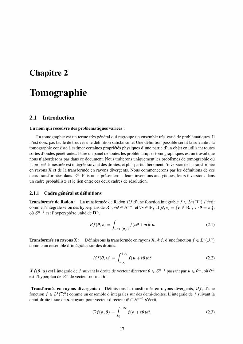
La tomographie est un terme très général qui regroupe un ensemble très varié de problématiques. Iln’est donc pas facile de trouver une définition satisfaisante. Une définition possible serait la suivante : latomographie consiste à estimer certaines propriétés physiques d’une partie d’un objet en utilisant toutessortes d’ondes pénétrantes. Faire un panel de toutes les problématiques tomographiques est un travail quenous n’aborderons pas dans ce document. Nous traiterons uniquement les problèmes de tomographie oùla propriété mesurée est intégrée suivant des droites, et plus particulièrement l’inversion de la transforméeen rayons X et de la transformée en rayons divergents. Nous commencerons par les définitions de cesdeux transformées dans Rn. Puis nous présenterons leurs inversions analytiques, leurs inversions dansun cadre probabiliste et le lien entre ces deux cadres de résolution.
2.1.1 Cadre général et définitions
Transformée de Radon : La transformée de Radon Rf d’une fonction intégrable f ∈ L1(Rn) s’écritcomme l’intégrale selon des hyperplans deRn, ∀θ ∈ Sn−1 et ∀s ∈ R, Π(θ, s) = r ∈ Rn, r ·θ = s ,où Sn−1 est l’hypersphère unité deRn.
Rf(θ, s) =
∫
u∈Π(θ,s)f(sθ + u)du (2.1)
Transformée en rayons X : Définissons la transformée en rayons X, Xf , d’une fonction f ∈ L1(Rn)comme un ensemble d’intégrales sur des droites.
X f(θ,u) =∫ +∞
−∞f(u+ tθ)dt (2.2)
X f(θ,u) est l’intégrale de f suivant la droite de vecteur directeur θ ∈ Sn−1 passant par u ∈ θ⊥, où θ⊥
est l’hyperplan deRn de vecteur normal θ.
Transformée en rayons divergents : Définissons la transformée en rayons divergents, Df , d’unefonction f ∈ L1(Rn) comme un ensemble d’intégrales sur des demi-droites. L’intégrale de f suivant lademi-droite issue de a et ayant pour vecteur directeur θ ∈ Sn−1 s’écrit,
Df(a,θ) =∫ +∞
0f(a+ tθ)dt. (2.3)
17

18 Tomographie
On s’intéressera particulièrement à cette transformée car c’est elle qui décrit le plus de systèmesmédicaux. En effet, dans ces systèmes, la source de rayonnement peut souvent être considérée commeponctuelle. Elle est représentée par a dans l’Eq. (2.3). De plus, un système d’acquisition permet demesurer simultanément l’intégrale de l’objet f sur un ensemble de demi-droites. La transformée enrayons divergents dépend de la trajectoire de a, nous allons considérer dans la suite que cette trajectoireest a(·) une courbe paramétrée par le scalaire λ.
Cas particulier d’un objet bi-dimensionnel (2D) n = 2 :
Dans ce cas le vecteur unitaire θ se réduit à un angle θ ∈ [0, 2π] et la transformée en rayons X estconfondue avec la transformée de Radon. Pour reconstruire exactement f , il faut mesurer Rf pour tousles couples (θ, s) appartenant au domaine [0, π]×R, [112].
Pour ce qui est de la transformée en rayons divergents, la reconstruction dépend de la trajectoire.Lorsque a(λ) suit une trajectoire circulaire autour de l’objet (trajectoire la plus utilisée en 2D), lesconditions pour une reconstruction exacte consiste à faire un peu plus d’un tour « Short Scan » (pourplus de détails voir [106] [115] 1). Lorsque l’on veut reconstruire uniquement une partie d’un objet ou unobjet allongé, on peut utiliser moins d’un demi tour c’est ce qu’ont montré F. NOO et al dans [97].
Cas particulier d’un objet tridimensionnel (3D) n = 3 :
Ce cas est celui que nous développerons principalement dans la suite de ce manuscrit. En effet,les objets que l’on veut imager en pratique, des patients, des pièces pour le contrôle non destructif,l’atmosphère du soleil, sont tous des objets 3D.
À ma connaissance, il n’y a pas de système qui permette de mesurer directement la transformée deRadon pour n = 3, car l’acquisition des intégrales de l’objet 3D selon des plans, posent de nombreuxproblèmes. On s’intéressera uniquement à la transformée en rayons X et à la transformée en rayonsdivergents. On rencontre la transformée en rayons X lorsque l’on résout des problèmes de Tomographieà Émission de Positron (TEP). Dans ce cas, la reconstruction exacte est mathématiquement possible siles données vérifient les conditions d’Orlov [103], c’est à dire si le vecteur θ décrit un grand cercle 2.
Comme dans le cas 2D, c’est la transformée en rayons divergents qui correspond à la plus grandediversité d’applications : scanners médicaux, imagerie dentaire, imagerie de l’atmosphère solaire, scan-ner pour des petits animaux, appareil de contrôle non destructif etc... Pour cette transformée, l’obtentiond’une reconstruction théoriquement exacte est possible si les données respectent la condition de Tuy[136]. Pour vérifier cette condition il faut que pour chaque point de l’objet à reconstruire tous les plansqui passent par ce point coupent la trajectoire de la source en au moins un point. On parle alors detrajectoire complète.
Au delà des conditions de reconstruction exacte se pose aussi le problème du choix des fréquencesd’échantillonnage de la transformée de Radon. Ce problème est très bien décrit dans l’habilitation àdiriger des recherches de L. DESBAT [43]. Nous y avons contribué [117][67] dans le cas de l’imagerieTEP en faisant une étude sur l’impact de l’utilisation de schémas d’échantillonnage efficace introduitsdans [42], et en particulier l’étude de la robustesse au bruit de mesure de ces approches.
2.1.2 Inversion tomographique analytique
Inversion de la transformée en rayons X
Si l’on a acquis des données sur un grand cercle (vérifiant les conditions Orlov), le problème d’in-version de la transformée en rayons X 3D (n = 3), peut se factoriser comme N problèmes d’inversion
1. Les références sur des travaux auxquels j’ai contribué sont en gras dans le texte2. cercle dont le plan générateur contient le centre de la sphère

II-2.1 Introduction 19
de la transformée en rayons X 2D (n = 2). De plus, nous avons vu dans le § 2.1.1 que cette transforméen rayons X 2D était équivalente à la transformée de Radon (TR) 2D. Son inversion a été introduite parJ. RADON en 1917 [112].
f(r1, r2) =1
2(2π)−1
∫ 2π
0
∫
R
e2jπσ(r1 cos θ+r2 sin θ)|σ|Rf(θ, σ)dσdθ (2.4)
avec Rf la transformée de Fourier de la transformée de Radon par rapport au deuxième paramètre(Rf(θ, ·)).
Nous exposons ci-dessus un algorithme de reconstruction de type filtrage rétroprojection. Dansl’Eq. (2.4), l’intégrale en σ et le produit par |σ| correspondent à une opération de filtrage par un filtre« passe haut » (la fréquence nulle est mise à zéro et les hautes fréquences sont amplifiées). L’intégrale enθ correspond à l’étape de rétroprojection. Il existe d’autres types d’algorithmes analytiques de recons-truction comme l’approche rétroprojection puis filtrage ou la reconstruction dans le domaine de Fourier[17]. Ces autres approches sont moins répandues car elles sont plus coûteuses en temps de calcul pourune sensibilité au bruit souvent plus importante.
Pour implanter les approches sur des calculateurs, on doit discrétiser l’Eq. (2.4). On échantillonnealors uniformément la dimension angulaire θ et les dimension spatiales s, r1 et r2. Les intégrales sontremplacées par des sommes. L’opération de filtrage est aussi discrétisée. Elle est très souvent réaliséedans le domaine de Fourier car le noyau de convolution est de grande taille. Enfin, on discrétise l’opéra-tion de rétroprojection. De nombreux travaux portent sur l’accélération et la discrétisation des opérateursde projection [125] [75] et de rétroprojection [59][120][35], nous évoquerons ceux-ci dans la partie 2.1.3.
Inversion de la transformée en rayons divergents pour n = 3 (3D)
La trajectoire circulaire : La trajectoire la plus naturelle est bien sûr la trajectoire circulaire. Maiscette trajectoire ne vérifie pas les conditions de Tuy. Les reconstructions que l’on peut faire seront doncmathématiquement approchées. L’approche la plus répandue pour cette trajectoire est l’algorithme FDKintroduit par FELDKAMP DAVIS et KRESS [48]. Bien que les reconstructions soient approchées nousavons montré [116] (reproduit à la page 184) que les intégrales sur les lignes obliques les plus prochesde l’axe perpendiculaire à la trajectoire étaient exactes.
La trajectoire hélicoïdale : Dans ce cas la courbe paramétrée est définie de la façon suivante
a(λ) =
R cosλR sinλ
h λ2π
,
avec R le rayon de l’hélice, λ un angle en radian et h son pas («pitch» en anglais). Cette trajectoirepermet une reconstruction exacte, et elle est mise en œuvre facilement comme la composition d’unetrajectoire circulaire avec une translation uniforme. De ce fait, c’est la trajectoire complète au sens deTuy la plus utilisée. Déterminer une formule exacte de type filtrage rétroprojection est quelque chose detrès difficile. En effet, certains plans passant par un point r fixé coupent trois fois la trajectoire 3 alorsque d’autres ne la coupent qu’une fois. Cela conduit indirectement à ce que la transformée de Radon 3Dest mesurée une ou trois fois selon les plans considérés. C’est seulement en 2002 que A. KATSEVICH
a trouvé un algorithme de reconstruction exacte [78]. Son principe est de trouver des directions de fil-trage particulières qui permettent de pondérer les plans par -1 ou 1. Cette pondération des plans permetde résoudre la dissymétrie de redondance entre les différents plans et ainsi d’avoir une formule d’inver-sion exacte. La formule d’inversion associée à l’algorithme de Katsevich est la suivante en utilisant les
3. uniquement la portion la plus faible permettant de faire la reconstruction appelée le PI-segment[33]

20 Tomographie
notations de l’article de H. KUDO [83] :
f(r) =
∫
Λ(r)
1
R− r1 cosλ− r2 sinλgF (r, λ, U(r, λ), V (r, λ))dλ (2.5)
où , r = (r1, r2, r3)t, Λ(r) = [λb(r), λt(r)] est le PI-segment [33] correspondant au point r. C’est
l’unique segment sur un tour d’hélice où les deux vecteurs (−−−−−→a(λb), r) et (
−−−−−→r,a(λt)) sont colinéaires. De
plus U(r, λ) et V (r, λ) sont les coordonnées détecteur de l’intersection entre la droite issue de a(λ) etpassant par r et le plan détecteur. L’intégrale de l’Eq. (2.5) correspond à l’opération de rétroprojection.gF correspond aux données filtrées
gF (r, λ, u′, v′) =1
2π
∫
R
h(u′ − u)gD(λ, u, v′ − (u′ − u) tan η(λ, r))du (2.6)
avec h(t) le filtre associé à la transformée de Hilbert, et v′ − (u′ − u) tan η(λ, r) définissant la ligne defiltrage permettant de résoudre le problème de redondance associé à l’acquisition des mesures dans lagéométrie hélicoïdale. Enfin gD correspond à la dérivée des projections,
gD(λ, u, v) =R√
R2 + u2 + v2
(∂
∂λ+R2 + u2
R2
∂
∂u+uv
R
∂
∂v
)Df(a(λ), u, v) (2.7)
Ce travail a été une grande avancée pour la communauté. Par contre toutes les données acquises nesont pas utilisées. C’est pourquoi, il y a eu beaucoup de travaux sur les méthodes approchées [82][77][132]même après 2002 pour concevoir des méthodes qui utilisent toutes les données acquises et qui sont doncmoins sensibles au bruit [16][83] (reproduit à la page 190).
Autres trajectoires : Il existe aussi des travaux sur d’autres trajectoires qui sont complètes au sens deTuy, comme par exemple la trajectoire cercle + droite [135]. Mais cette dernière, du fait de sa dissymétrie,rend les reconstructions instables dans certaines zones.
En revanche la trajectoire «saddle» qui a une forme de selle de cheval ou de chips a de bonnespropriétés en particulier pour l’imagerie cardiaque [104].
2.1.3 Inversion statistique
On considère ici que les données collectées, y ∈ RM , sont discrètes et que l’objet à reconstruire,bien que continu, est représenté par un nombre fini de coefficients de base.
f(r) =∑
i
xiφi(r),
où xi représente le ie coefficient de décomposition associé à la fonction de base φi. L’ensemble des φiforme une base ou une famille génératrice de L2(R). Dans la plupart des cas, les fonctions φi sont desindicatrices de pixels ou de voxels, mais on peut aussi utiliser des fonctions Kaiser Bessel [85][89] ou desGaussiennes [118]. On obtient dans tous les cas une relation entre des grandeurs discrètes, les données yet les coefficients de décomposition x = (x1, . . . , xi, . . . , xN )t,
y = H(x) + b. (2.8)
On désigne par H le modèle direct, x ∈ RN les coefficients et par b le bruit. Le modèle direct peutêtre linéaire ou non en fonction des cas. On étudiera des modèles directs non linéaires dans le cadre del’imagerie médicale dans le § 2.2. Le modèle direct ne représente pas strictement la réalité physique dumode d’acquisition. On utilise souvent des modèles simplifiés afin de faciliter la mise en œuvre et pourque le calcul de la sortie modèle H(x) soit suffisamment rapide. Par conséquent, le bruit b modélisel’incertitude sur les mesures due à certaines propriétés physiques des détecteurs mais aussi aux erreurscausées par l’utilisation d’un modèle simplifié.
II-2.1 Introduction 21
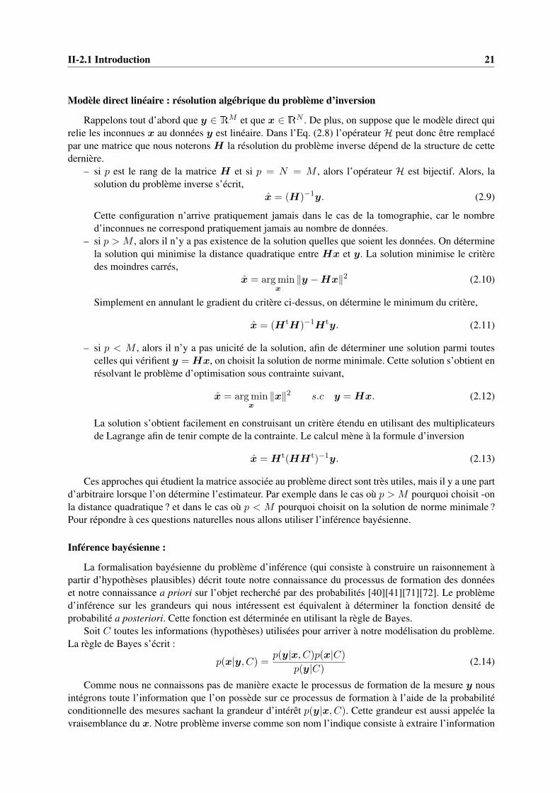
Modèle direct linéaire : résolution algébrique du problème d’inversion
Rappelons tout d’abord que y ∈ RM et que x ∈ RN . De plus, on suppose que le modèle direct quirelie les inconnues x au données y est linéaire. Dans l’Eq. (2.8) l’opérateur H peut donc être remplacépar une matrice que nous noterons H la résolution du problème inverse dépend de la structure de cettedernière.
– si p est le rang de la matrice H et si p = N = M , alors l’opérateur H est bijectif. Alors, lasolution du problème inverse s’écrit,
x = (H)−1y. (2.9)
Cette configuration n’arrive pratiquement jamais dans le cas de la tomographie, car le nombred’inconnues ne correspond pratiquement jamais au nombre de données.
– si p > M , alors il n’y a pas existence de la solution quelles que soient les données. On déterminela solution qui minimise la distance quadratique entre Hx et y. La solution minimise le critèredes moindres carrés,
x = argminx
‖y −Hx‖2 (2.10)
Simplement en annulant le gradient du critère ci-dessus, on détermine le minimum du critère,
x = (HtH)−1Hty. (2.11)
– si p < M , alors il n’y a pas unicité de la solution, afin de déterminer une solution parmi toutescelles qui vérifient y = Hx, on choisit la solution de norme minimale. Cette solution s’obtient enrésolvant le problème d’optimisation sous contrainte suivant,
x = argminx
‖x‖2 s.c y = Hx. (2.12)
La solution s’obtient facilement en construisant un critère étendu en utilisant des multiplicateursde Lagrange afin de tenir compte de la contrainte. Le calcul mène à la formule d’inversion
x = Ht(HHt)−1y. (2.13)
Ces approches qui étudient la matrice associée au problème direct sont très utiles, mais il y a une partd’arbitraire lorsque l’on détermine l’estimateur. Par exemple dans le cas où p > M pourquoi choisit -onla distance quadratique ? et dans le cas où p < M pourquoi choisit on la solution de norme minimale ?Pour répondre à ces questions naturelles nous allons utiliser l’inférence bayésienne.
Inférence bayésienne :
La formalisation bayésienne du problème d’inférence (qui consiste à construire un raisonnement àpartir d’hypothèses plausibles) décrit toute notre connaissance du processus de formation des donnéeset notre connaissance a priori sur l’objet recherché par des probabilités [40][41][71][72]. Le problèmed’inférence sur les grandeurs qui nous intéressent est équivalent à déterminer la fonction densité deprobabilité a posteriori. Cette fonction est déterminée en utilisant la règle de Bayes.
Soit C toutes les informations (hypothèses) utilisées pour arriver à notre modélisation du problème.La règle de Bayes s’écrit :
p(x|y, C) = p(y|x, C)p(x|C)p(y|C) (2.14)
Comme nous ne connaissons pas de manière exacte le processus de formation de la mesure y nousintégrons toute l’information que l’on possède sur ce processus de formation à l’aide de la probabilitéconditionnelle des mesures sachant la grandeur d’intérêt p(y|x, C). Cette grandeur est aussi appelée lavraisemblance du x. Notre problème inverse comme son nom l’indique consiste à extraire l’information
22 Tomographie
que l’on possède sur la grandeur physique connaissant les mesures, c’est à dire la fonction densité deprobabilité a posteriori p(x|y, C). Cette fonction résume toute l’information que l’on possède sur l’ob-jet que l’on cherche. Par contre, on est très souvent intéressé par un estimateur ponctuel, permettant derésumer cette fonction par une valeur particulière. L’estimation ponctuelle est très réductrice par rapportà la richesse de l’information contenue dans la loi a posteriori, c’est pourquoi on préfère souvent déter-miner la valeur de l’estimateur ponctuel ainsi que la valeur de variance a posteriori. Dans ce chapitrenous nous intéresserons principalement à l’estimateur de Maximum a posteriori (MAP), pour des raisonsde commodité de calcul.
2.1.4 Étude empirique sur les similitudes entre les approches analytiques et les approchesstatistiques
Pour mener à bien cette étude nous nous sommes placés dans la configuration la plus simple possible.Nous résolvons un problème tomographique 2D où les fonctions de base φi sont des indicatrices de pixel.L’opération de projection de l’objet est en géométrie parallèle, et le modèle direct considéré est linéaire.Enfin, nous allons traiter des problèmes de tailles réduites afin de faciliter les calculs.
Lien entre les approches rétroprojection puis filtrage et la solution des moindres carrés
Analysons tout d’abord les opérations effectuées lorsque l’on calcule la solution des moindres car-rés à l’aide de l’Eq. (2.11). L’opération Hx correspond à l’opération de projection de l’objet 2D dansune géométrie projective parallèle 4 (transformée de Radon). L’opération rétroprojection correspond àl’application de la matrice Ht. Le calcul de l’estimateur des moindres carrés peut être vu comme uneopération de rétroprojection puis une opération linéaire (multiplication par la matrice (HtH)−1). Dansle cadre des reconstructions analytiques, la majorité des approches consistent à filtrer les données puisà les rétroprojeter, mais on peut très bien commencer par l’opération de rétroprojection puis appliquerl’opération de filtrage. Dans ce cas, le filtre est bi-dimensionnel et à symétrie de révolution. Il faut main-tenant analyser la structure de la matrice (HtH)−1 afin de voir si elle correspond à une opération defiltrage.
Afin de calculer facilement l’inverse de la matrice HtH , nous avons choisi de reconstruire uneimage de petite taille (32×32 pixels). De plus, pour que cette dernière soit bien conditionnée nous avonsun nombre important de données (151 projections composées de 139 valeurs), la matrice H est doncrectangulaire et elle comporte 20989 lignes et 1024 colonnes. La figure 2.1 représente les coefficients dela matrice (HtH)−1 (1024× 1024), les points blancs représentent les valeurs positives, les points noirsles valeurs négatives et le gris correspond aux valeurs proches de zéro. On remarque que la structure decette matrice est Toeplitz. On peut en conclure qu’on peut approcher l’application de cette matrice par uneopération de filtrage. Nous allons maintenant extraire une ligne de la matrice (HtH)−1 afin d’étudierla réponse impulsionnelle du filtre de reconstruction (voir Fig. 2.2 (a)). Cette réponse impulsionnelleest bi-dimensionnelle et à première vue sa moyenne est quasiment nulle. En prenant le module de latransformée de Fourier de cette réponse impulsionnelle (voir Fig. 2.2 (b)), on remarque qu’elle est àsymétrie de révolution et qu’elle correspond à un filtre « passe haut ». Ces propriétés sont identiques aufiltre de reconstruction h(ν1, ν2) =
√ν21 + ν22 de l’approche rétroprojection puis filtrage. On remarque
sur la Fig. 2.2 (b) que la valeur du filtre pour la fréquence nulle est différente de zéro ce qui permet deconserver la moyenne de l’objet à reconstruire. On peut en conclure qu’il y a pratiquement équivalencedans ce cas entre l’approche analytique et la solution algébrique.
4. Nous avons utilisé dans l’expérimentation numérique le projecteur parallèle codé sous matlab par la fonction radon.

II-2.1 Introduction 23
FIGURE 2.1 – Visualisation des coefficients de la matrice (HtH)−1
1
2
3
4
5
6
7
8
9
10
11
x 10−4
0
0 ν
ν
1
2
(a) (b)
FIGURE 2.2 – (a) Réponse impulsionnelle du filtre de reconstruction (b) Transformée de Fourier de laréponse impulsionnelle
Lien entre les approches filtrage puis rétroprojection et la solution de norme minimale
La solution de norme minimale consiste à faire une opération linéaire sur les données (applicationde la matrice (HHt)−1) puis de rétroprojeter le résultat. Nous allons maintenant décrire l’expériencemenée afin d’identifier l’opération effectuée lorsque nous appliquons la matrice (HHt)−1 : commeprécédemment, nous avons choisi une configuration où la matrice HHt est de petite taille pour êtrefacilement inversible. Nous avons un nombre de mesures réduit (529), celles-ci sont composées de 23angles de projections uniformément répartis sur [0, π[. Afin que la matrice HHt soit bien conditionnéenous avons défini une image relativement grande (151× 151 = 22801 pixels 5). La figure 2.3 représenteles coefficients de la matrice (HHt)−1. On remarque visuellement que cette matrice peut être approchéepar une matrice Toeplitz. L’obtention de la solution de norme minimale correspond à un algorithme detype filtrage (multiplication par la matrice (HHt)−1 puis rétroprojection (multiplication par la matriceHt). Nous avons extrait une ligne de la matrice (HHt)−1 afin de visualiser la réponse impulsionnelledu filtre (voir Fig. 2.4 (a)) et le module de sa transformée de Fourier (voir Fig. 2.4 (b)). Dans ce cas laréponse impulsionnelle est très différente des approches filtrage rétroprojection. En effet, dans ces ap-proches on applique le même filtre rampe (dont la transformée de Fourier est égale à |σ|) sur toutes lesprojections de manière identique. De manière schématique, on corrige l’effet passe bas dû à l’intégrationde la transformée de Radon par un filtrage « passe haut » (filtre rampe) sur la variable spatiale s de la
5. Un nombre impaire de pixels dans l’images permet de limiter les symétrie du problème de projection permet d’avoir unematrice HH
t ayant un meilleur conditionnement.
24 Tomographie
FIGURE 2.3 – Visualisation des coefficients de la matrice (HHt)−1
0
−90
90
−0.3
−0.2
−0.1
0
0.1
0.2
0.3
0.4
s0
θ (°)
0
5
10
15
20
25
30
35
40
45
0
0
νθ
σ(a) (b)
FIGURE 2.4 – (a) Réponse impulsionnelle du filtre appliquée aux données. On utilise les mêmes notationsque dans la définition de la transformée de Radon (TR) Eq. (2.1) : l’axe des abscisses représente leparamètre de position s et l’axe des ordonnées représente l’angle d’incidence θ (b) Transformée deFourier de la réponse impulsionnelle
transformée de Radon (TR). Comme on peut le voir sur les Fig. 2.4 (a) et (b) l’opération de filtrage ef-fectuée par l’application de la matrice (HHt)−1 est totalement différente. Le filtre est bi-dimensionnel,c’est un « passe bas » selon la direction spatiale de la TR et c’est un « passe haut » selon la directionangulaire de la TR. En conclusion, on retrouve bien une opération de filtrage comme dans la reconstruc-tion classique de type FBP, mais le filtrage passe haut se fait sur l’axe angulaire et non sur la dimensionspatiale des projections.
Étude de l’impact des phénomènes de bord sur la structure des matrices
Le filtre de la Fig. 2.4 a été obtenu sur un très faible nombre de projections afin de pouvoir facile-ment inverser la matrice. On pourrait penser que le filtre obtenu est le fruit d’effets de bord vu le nombreréduit de données utilisées pour le générer. C’est pourquoi nous avons utilisé ce filtre pour reconstruiredes données de taille plus importante. On fait l’expérience numérique suivante : on simule des projec-tions suivant 256 angles avec un détecteur comprenant 362 cellules détectrices, en projetant une imagecomposée de 256× 256 pixels. L’image qui nous a servi pour simuler les données est représentée sur laFig. 2.5 (a). Les projections en géométrie parallèle ont été obtenues grâce à la fonction matlab radon etnous avons ajouté un bruit Gaussien i.i.d. de variance égale à 20 (SNR 24,3 dB).

II-2.1 Introduction 25
50 100 150 200 250
50
100
150
200
250
50 100 150 200 250
50
100
150
200
250
(a) (b)
50 100 150 200 250
50
100
150
200
250
50 100 150 200 250
50
100
150
200
250
(c) (d)
FIGURE 2.5 – (a) Image vraie (b) rétroprojection uniquement (c) inversion de la transformée de Radon(filtre rampe) (d) rétroprojection filtrée en utilisant le filtre identifié à partir d’un petit problème.
On compare les approches suivantes : uniquement l’opération de rétroprojection (Fig. 2.5 (b)), lareconstruction avec l’algorithme classique FBP (fonction matlab iradon) en utilisant uniquement lefiltre rampe (Fig. 2.5 (c)) et une approche filtrage rétroprojection en utilisant le filtre de la Fig. 2.4 (a)(Fig. 2.5 (d)). En comparant les Figs 2.5 (b) et (d), on voit clairement que le filtre garde des propriétésde reconstruction et que l’image de la Fig. 2.5 (d) possède des structures plus hautes fréquences queuniquement l’opération de rétroprojection. De plus lorsqu’on compare les résultats de reconstruction del’approche FBP avec le nouveau filtre on observe un effet régularisant qui est dû à l’opération passebas sur les projections. Il est normal d’avoir un effet régularisant car on a déduit le filtre à partir d’unesolution de norme minimale.
Conclusion :
Cette petite étude nous a permis de voir qu’il y avait un lien assez fort dans le cas de la géométrieparallèle entre les approches analytiques et les approches algébriques. Cette étude est plus une illus-tration pédagogique qu’un véritable travail de recherche, mais elle permet d’ouvrir des perspectives derecherches intéressantes. Il serait très utile d’avoir des approches intermédiaires entre les approches ana-lytiques et les approches algébriques afin d’avoir des approches plus précises que les approches analy-tiques et moins coûteuses en temps de calcul que les approches algébriques. Pour cela, il faudrait étudierles matrices (HHt)−1 lorsque la géométrie est divergente, lorsque la source ne peut pas être considérée

26 Tomographie
comme ponctuelle, etc.... À partir de ces études on déterminerait de nouveaux filtres de reconstructionqui pourraient tenir compte partiellement d’une source de rayons X non ponctuelle.
2.1.5 Discussion
Nous évoquerons ici les avantages et les inconvénients des approches analytiques et statistiques àtravers leurs applications à l’imagerie médicale en rayons X, car ce domaine couvre la majorité desproblèmes rencontrés dans l’inversion tomographique.
Apport des approches analytiques
Les approches analytiques restent les méthodes de référence dans pratiquement tous les systèmesmédicaux. Elles sont relativement faciles à mettre en œuvre. De plus, elles sont très efficaces en terme detemps de calcul, et assez économes en ressource mémoire. En effet, les approches analytiques nécessitentune étape de filtrage puis une étape de rétroprojection. La complexité dans le cas d’une reconstruction2D d’une image N ×N à partir de mesures M ×N est en O(MN log2N) opérations élémentaires et lacomplexité de la rétroprojection est en O(MN2) opérations élémentaires. De plus, ces algorithmes sontrelativement peu coûteux en terme de ressources mémoires car on peut traiter les données séquentielle-ment. La mémoire vive utilisée correspond seulement à la taille de l’image ou du volume que l’on veutreconstruire et les données uniquement à un ou deux angles différents. Avec l’évolution des détecteurs,l’imagerie est principalement 3D et le nombre de mesures est croissant. De plus, le temps de reconstruc-tion doit être le plus court possible pour recevoir un plus grand nombre de patients. Ces approches sonttrès adaptées lorsque le modèle direct est une intégration d’une propriété physique (modèle linéaire), quel’échantillonnage angulaire est régulier, et que la trajectoire de la source de rayons X est complète ausens de Tuy.
Problèmes de discrétisation des formules analytiques
Des artefacts apparaissent sur les reconstructions lorsque les conditions exposées ci-dessus ne sontpas remplies. Si le modèle direct reste linéaire mais que la matrice (HHt)−1 n’a plus une structureinvariante, on peut voir apparaître des artefacts pour les raisons suivantes :
– Les données ont une couverture angulaire limitée (moins de 180˚) : par exemple la tomosynthèse[13].
– L’échantillonnage angulaire est non uniforme.– Il y a des cellules détectrices défectueuses.– Le vieillissement des détecteurs conduit à une modification des gains détecteurs, qui provoque des
artefacts en anneau.
Problèmes lorsque le processus de formation des données n’est plus linéaire
Des artefacts apparaissent aussi lorsque le modèle direct n’est plus linéaire. Dans le cas de l’imagerieà rayons X, la loi de Beer Lambert (2.15) n’est pas linéaire à cause de l’exponentielle.
I(λ, p) = Ise−
∫L(λ,p) µ(r)dr (2.15)
avec L(λ, p) le segment de droite issu de la source a(λ) et passant par la cellule détectrice p, µ l’at-ténuation des matériaux traversés et Is l’énergie émise par la source de rayons X. Afin de linéariser leproblème, on prend le logarithme des mesures, mais cette opération modifie les propriétés statistiques dubruit, ce qui amplifie très fortement ce dernier lorsque l’on est en présence d’objets de forte atténuationcomme nous le verrons dans le § 2.2.1.
II-2.1 Introduction 27
Une autre cause de non linéarité provient du fait que les sources de rayons X ne sont pas monochro-matiques sauf cas particulier (rayonnement synchrotron). L’hypothèse d’une source monochromatiquefaite par les approches analytiques provoque des artefacts de durcissement de spectre. Nous verrons plusprécisément dans le § 2.2.2 comment les approches statistiques peuvent partiellement s’affranchir de ceproblème.
Les approches analytiques supposent aussi que l’objet est immobile pendant l’acquisition. Le mou-vement de l’objet pendant l’acquisition des projections provoque des artefacts importants. Nous verronsdans le § 2.3 que dans le cadre de l’inversion tomographique de données issues de la couronne solaire,on peut résoudre ce problème lorsque « le mouvement » a une structure particulière.
Difficulté pour intégrer des informations a priori aux approches analytiques
Les problèmes tomographiques sont mal posés au sens d’Hadamard. L’inversion a tendance à am-plifier le bruit présent dans les données. Pour palier ce problème, il faut introduire de l’information apriori. Malheureusement dans les approches analytiques, la seule information a priori exploitable, estla douceur (ou la régularité spatiale) de la solution. Cette régularité est imposée à l’aide d’opérations defiltrage sur la reconstruction (post filtrage) ou directement sur les données avant d’appliquer le filtre dereconstruction (pré-traitement).
À l’inverse les approches statistiques peuvent tenir compte d’une plus grande variété d’informationa priori. Par exemple, on peut favoriser les solutions régulières par morceaux en utilisant un a prioriintroduisant de la parcimonie sur le gradient de l’objet (Variation Totale), ou favoriser les objets com-posés d’un nombre connu de matériaux différents à l’aide d’une loi a priori formée d’un mélange deGaussiennes. Ces a priori permettent de mieux préserver les contours présents dans les images qu’un apriori de douceur tout en réduisant le bruit dans les reconstructions.
Limitations des approches statistiques
Il existe bien des facteurs qui limitent la qualité des images reconstruites, mais dans la majoritédes problèmes tomographiques difficiles (forte non linéarité, données avec un mauvais SNR, couvertureangulaire limitée) les approches statistiques fournissent des images de meilleure qualité que celles ana-lytiques.
Le principale verrou qui limite l’utilisation de ces approches est le temps de calcul qui est très im-portant. Comme l’estimateur est calculé de manière itérative, que chaque itération nécessite deux à troisfois plus d’opérations élémentaires qu’une inversion analytique et qu’il faut entre 150 et 3000 itérationspour arriver à la convergence, le temps de calcul est plus important de 2 à 3 ordres de grandeur. Le tempsde calcul est vraiment le talon d’Achile de ces approches.
Les raisons de la démocratisation des approches statistiques dans les systèmes d’imagerie médicale
Il y a principalement deux raisons au développement de ces approches :– La démocratisation dans les pays développés du recours à l’imagerie médicale, entraîne une hausse
du nombre d’examens par patient. L’irradiation de la population est en constante augmentation.Si cette augmentation persiste dans les années futures, on pourrait être confronté à un problèmede santé publique. La réduction drastique des doses délivrées aux patients est donc un sujet depremière importance pour l’imagerie à rayons X. Les approches statistiques permettent d’avoirune meilleur robustesse au bruit de mesures que les approches analytiques.
– Comme nous venons de le voir le temps de calcul des approches statistiques est trop importantpour que les systèmes d’imagerie médicale soient économiquement viables.Le développement de la puissance de calcul des ordinateurs associés à l’utilisation de FPGA pourla reconstruction tomographique [110] permettent d’obtenir des temps de calcul plus raisonnables.

28 Tomographie
De plus, le développement des cartes graphiques conçues pour générer des images de synthèse àhaut débit afin de permettre aux joueurs d’être plongés dans un monde tridimensionnel, peuventêtre utilisés désormais pour faire du calcul scientifique. Ces cartes sont de réels calculateurs pos-sédant jusqu’à 1500 cœurs de calcul. Le problème du rendu d’une scène 3D est similaire à unproblème de projection tomographique : on a une ou plusieurs sources ponctuelle de lumière et onveut former une image 2D à partir d’une scène 3D. Comme la géométrie projective est très sem-blable entre les deux problèmes, on peut utiliser de manière très efficace les cartes graphiques afinde calculer la projection et la rétroprojection tomographique [59, 120]. Ces cartes graphiques sontdes calculateurs ayant une architecture de type pipeline permettant de traiter un flot très importantde données. Á l’inverse d’un super calculateur la structure particulière des cartes graphiques nepermet pas d’avoir de bonnes performances sur tous les problèmes de calculs scientifiques. Parcontre, l’énorme avantage des cartes graphiques est qu’elles sont bon marché et que le coût defonctionnement est relativement faible (pas besoin de salle climatisée et insonorisée).
2.2 Deux exemples illustrant l’apport des approches statistiques lorsquele modèle de formation des données est non linéaire
2.2.1 Artefacts causés par la linéarisation de la loi de Beer Lambert
On se place dans cette partie dans le cas où la source de rayons X est monochromatique et les photonspossèdent tous l’énergie ǫ0. Dans ce cas l’Eq. (2.15) devient :
I(λ, s) = Is(ǫ0)e−
∫L(λ,s) µ(ǫ0,r)dr (2.16)
De plus les mesures sont entachées de bruit :
Im(λ, s) = I(λ, s) + η(λ, s). (2.17)
Le bruit η(λ, p) modélise un ensemble de phénomènes variés. Tout d’abord les photons X ont une cer-taine probabilité d’être absorbés par le scintillateur 6, ce phénomène conduit à ce que les données suiventune loi de Poisson. De plus, l’électronique de lecture et la quantification conduisent à commettre deserreurs. De manière générale ces sources d’erreurs sont souvent modélisées par un bruit Gaussien. Il fautaussi ajouter toutes les erreurs de modélisation dues aux hypothèses simplificatrices : la non prise encompte de la diffusion et la connaissance imparfaite de Is l’intensité de la source de rayons X. Il y a deuxcauses à la mauvaise connaissance de Is : elle est mesurée avec un détecteur imparfait et elle peut varierau cours de l’acquisition. La complexité et la diversité des phénomènes perturbateurs nous conduisentà penser que la modélisation du bruit devrait se faire au prix d’une loi très complexe. En pratique, onutilise des modèles avec des lois simples pour réduire la complexité des approches.
On voit dans l’Eq. (2.16) que la partie intégrale est une opération linéaire que nous allons modéliserpar une matrice après discrétisation. La non linéarité de la loi Beer Lambert vient de l’exponentielle.L’approche classique consiste à linéariser le problème. Pour cela, un pré-traitement détermine l’atténua-tion du faisceau de rayons X à partir de l’énergie déposée par les photons détectés :
y(λ, s) = log
(Is
Im(λ, s)
). (2.18)
Ce pré-traitement entraîne des artefacts en étoile lorsqu’il y a une zone dans l’image possédant une forteatténuation (voir figure 2.6 (b)). Ensuite, on considère le modèle suivant :
y(λ, s) =
∫
L(λ,s)µ(ǫ0, r)dr + b(λ, s) (2.19)
= Df(a(λ), s) + b(λ, s), (2.20)
6. Il est souvent composé d’un cristal qui absorbe les photons X et qui réémet des photons visibles

II-2.2 Deux exemples illustrant l’apport des approches statistiques lorsque le modèle de formationdes données est non linéaire 29
Dans les approches analytiques toutes les données ont le même poids ce qui correspond à un bruit b(λ, s)Gaussien indépendant identiquement distribué (i.i.d.) dans une interprétation statistique. D’autres ap-proches statistiques considèrent que y(λ, s) suit une loi de Poisson. Dans les deux cas, on néglige l’effetdu pré-traitement sur la statistique du bruit. Le problème apparaît (voir Fig. 2.6 (b) et (c)) lorsque queles flux de photons I(λ, s) sont faibles. Dans ce cas, d’une part l’énergie du bruit peut être supérieureau signal d’intérêt et d’autre part les faibles énergies mesurées correspondent à des fortes atténuations. Ily a donc une amplification importante du bruit causée par le pré-traitement non linéaire. Ce phénomèneest illustré sur la Fig. 2.7. Nous avons fait l’expérience numérique suivante : on a simulé des projectionsparallèles de l’objet 2D de la Fig. 2.6 (a) auxquelles nous avons ajouté du bruit Poissonnien et du bruitGaussien d’un niveau relativement faible (Fig. 2.6 (c)). Le résultat du pré-traitement est visualisé sur laFig. 2.7 (b). On voit très clairement qu’autour du pixel 150 le bruit a été très fortement amplifié et onremarque sur le tracé d’une projection (Fig. 2.7 (a)) que cela correspond à un niveau de flux faible. Àl’inverse autour du pixel 25 (abscisse de la Fig. 2.7 (b)) le niveau du bruit est inchangé voir atténué parle pré-traitement et on remarque que cela correspond à une zone de fort flux sur la Fig. 2.7 (a).
(a) (b)
20 40 60 80 100 120 140 160 180
50
100
150
200
250
300
350
(c) (d)
FIGURE 2.6 – (a) Image vraie utilisée pour faire les simulations (b) Reconstruction de données pré-traitées avec l’algorithme FBP (c) Représentation sous forme d’un sinogramme de y (données pré-traitées) (d) Minimum du critère des moindres carrés régularisés où les données pré-traitées les plusbruitées ont été supprimées.

30 Tomographie
50 100 150 200 250 300 350
0.20.40.60.8
1
(a)
50 100 150 200 250 300 3500
200
400
600
(b)
FIGURE 2.7 – Tracés d’une projection pour un angle arbitrairement fixé. En bleu simulation sans bruit.En rouge simulation avec bruit (a) mesure de l’énergie déposée sur le détecteur (b) données après pré-traitement Eq. (2.18).
Réduction de ces artefacts
La réduction de ces artefacts passe par la prise en compte de la loi Beer Lambert Eq. (2.16) et parune modélisation assez fine du bruit η.
Détermination du modèle d’incertitude sur les mesures : On remarque dans la littérature que lamodélisation retenue pour le bruit est Poissonnienne [98][99][46][45] dans une grande majorité des ap-proches. Ce choix semble légitime car le processus de détection des photons est Poissonnien. Mais onpeut opposer deux arguments à ce choix : premièrement dans la tomographie à rayons X il y a beaucoupde photons qui frappent les détecteurs et le processus Poissonnien peut être approché très précisémentpar une Gaussienne ; deuxièmement, comme nous l’avons déjà exposé dans le § 2.2.1, les sources d’in-certitude sur les mesures sont multiples, la loi résultante n’est donc ni Gaussienne, ni Poissonnienne.C’est pourquoi, dans le § 2.2.2 nous avons choisi de modéliser l’incertitude sur les mesures par un bruitblanc Gaussien donc la variance dépend du flux mesuré par le détecteur. De ce fait on tire parti de la sim-plicité de la loi Gaussienne tout en ayant une modélisation plus fine que les approches utilisant une loide Poissonnien. Notons qu’il existe un faible nombre de travaux utilisant un modèle composite associantun bruit Poissonnien et un bruit Gaussien [54].
Différentes stratégies d’inversion : Schématiquement on peut diviser l’état de l’art en deux grandesfamilles : les approches qui cherchent à inverser le problème non-linéaire et les approches qui gardentle pré-traitement mais qui vont essayer de tenir compte de l’amplification du bruit en pondérant ou enéliminant des données extrêmement bruitées.
L’inversion du problème non-linéaire avec un bruit Poissonnien est un problème d’optimisation com-plexe. L’optimisation directe n’est pas réalisable. C’est pourquoi, dans [45][46] les auteurs utilisent une

II-2.2 Deux exemples illustrant l’apport des approches statistiques lorsque le modèle de formationdes données est non linéaire 31
famille de fonctions majorantes plus facilement minimisables (les "surogate") pour approcher itérative-ment le critère cible. Dans le même esprit, J. NUYTS [99][98][36][37] fait une approximation quadratiqueséparable du critère puis il utilise une approche de descente de gradient pour minimiser ce nouveau cri-tère. Il est bien évident que, comme dans l’approche précédente, le critère quadratique approchant estmodifié à chaque itération. Nous avons contribué dans [144] en inversant le problème non-linéaire avecun bruit Gaussien. Dans ce cas nous avons une expression explicite du gradient du critère. Nous avonsdéveloppé un algorithme de descente de type gradient conjugué. Par contre, nous avons été obligés defaire une approximation quadratique du critère afin de déterminer un pas de descente efficace. Enfin, dansle cadre de la thèse de Caifang CAI nous avons résolu le même problème avec un bruit Gaussien dontla variance est différente pour chaque donnée et nous estimons ces variances au cours de l’algorithmeitératif [20].
La deuxième famille d’approches consiste à pré-traiter les données en tenant compte de l’amplifi-cation du bruit. Une première approche consiste à éliminer les données qui sont trop corrompues parle bruit. De manière générale ces données correspondent à des objets très fortement atténuants dont lareconstruction avec précision n’est pas très utile. Pour ce faire on applique un seuil sur les données pré-traitées. Nous avons appliqué cette approche sur les données simulées de la Fig. 2.6. Dans ce cas, onobtient des résultats assez satisfaisants (voir Fig. 2.6 (d)). Mais cette approche dépend d’un seuil quin’est pas facile à régler quand les images ont une structure complexe (images réelles), de plus il restedes artefacts résiduels (voir Fig. 2.6 (d)). Dans [53][134] les auteurs affectent une confiance différenteà chaque mesure pré-traitée en fonction de leur amplitude. Pour cela, on construit une vraisemblanceGaussienne qui possède une variance différente pour chaque mesure y. Cette vraisemblance correspondà un critère des moindres carrés pondérés [53] ("Weighted Least Square"). Cette approche est plus soupleque la précédente car elle ne nécessite pas de décision brutale. La qualité de reconstruction de cette ap-proche est un petit peu plus faible que les approches visant à inverser le problème non linéaire, parcontre, comme le critère à optimiser est quadratique, les algorithmes utilisés sont plus efficaces et plusfacilement parallèlisables.
2.2.2 Résolution du problème de durcissement de spectre de la source de rayons X
Les artefacts de durcissement de spectre sont particulièrement difficiles à éliminer par des approchesclassiques de traitement d’image car ils sont aux mêmes fréquences que les signaux d’intérêt. Toutes lesapproches de filtrage sont donc inefficaces. Un des artefacts symptomatique du durcissement de spectreest l’artefact « coupe ». Il se manifeste de la façon suivante : au lieu de reconstruire un objet ayant unniveau uniforme, la reconstruction présente une atténuation plus faible au centre de l’objet et plus fortesur les bords. Ce phénomène provient du fait que les générateurs de rayons X produisent des spectresd’émission continus de zéro jusqu’à la tension d’accélération des électrons. Les approches classiques dereconstruction supposent que l’on reconstruit l’image à l’énergie moyenne du spectre d’émission. On saittous que les photons de faible énergie sont beaucoup plus atténués que ceux possédant une énergie im-portante, lorsqu’un rayon traverse le bord de l’objet, son spectre d’émission est pratiquement inchangé etl’atténuation est correctement estimée. Par contre lorsqu’un rayon passe au centre de l’objet, l’atténuationest tellement importante que pratiquement aucun photon de faible énergie ne le traverse, la proportion dephotons haute énergie devient donc majoritaire. On dit que le spectre est durci car son énergie moyenne aaugmenté. Comme l’atténuation des matériaux peut être considérée comme inversement proportionnelleà l’énergie moyenne du spectre, il y a une sous estimation de l’atténuation au centre de l’objet. On peutvoir cet effet sur la gauche du profil de la Fig. 2.8 (h). Afin de bien comprendre la problématique du dur-cissement de spectre, nous allons présenter les principes de base de l’interaction rayonnement-matière.Nous exposerons ensuite différentes paramétrisations de l’objet inconnu ainsi que les hypothèses asso-ciées. Puis, nous présenterons quelques résultats de reconstruction sur des données simulées et sur desdonnées réelles.

32 Tomographie
Interaction rayonnement-matière
Comme nous l’avons vu dans l’Eq. (2.16) la loi Beer Lambert relie l’atténuation aux mesures, maiselle correspond uniquement a une loi empirique qui exprime le ratio entre les photons émis par la sourceet ceux détectés par le capteur. Cette atténuation des photons provient de différents phénomènes de laphysique de l’interaction entre le rayonnement et la matière.
Dans la gamme de rayonnements qui nous intéresse (photons possédant une énergie entre 5 et 500keV ), il y a principalement trois types d’interaction rayonnement-matière 7 :
– l’effet photoélectrique : le photon X frappe un atome, ce dernier est absorbé et un électron estéjecté.
– la diffusion Rayleigh (ou diffusion élastique) : le photon X rebondit sur l’atome sans perdre d’éner-gie.
– la diffusion Compton (ou diffusion inélastique) : le photon X donne de l’énergie à un électronfaiblement lié à l’atome. Il y a donc transfert d’énergie entre le photon et l’électron. Le photonX perd une partie de son énergie. En moyenne, l’angle de diffusion est proportionnel à l’énergietransmise à l’électron.
La probabilité d’une interaction rayonnement-matière dépend bien évidemment de la densité desatomes, mais aussi du type d’atomes. En première approximation, on peut utiliser un modèle qui dépenduniquement du numéro atomique des atomes considérés.
Loi Beer-Lambert généralisée
Si on fait l’hypothèse que tous les rayons diffusés ne sont pas détectés, alors, pour des photonsd’une énergie ǫ, on peut modéliser toutes les interactions rayonnement-matière par la loi Beer-Lambertgénéralisée où l’atténuation µ(ǫ, r) dépend de l’énergie du faisceau incident :
I(λ, s) =
∫
R
S(ǫ)Is(ǫ)e−
∫L(λ,s) µ(ǫ,r)drdǫ (2.21)
où Is(ǫ) correspond au spectre émis par la source et S(ǫ) correspond à la sensibilité du détecteur en fonc-tion de l’énergie ǫ des photons incidents. La difficulté ici est de reconstruire µ(ǫ, r) car il y a beaucoupde degrés de liberté vis à vis des mesures acquises.
Paramétrisations de l’inconnue
Le but de ces paramétrisations est de limiter le nombre de degrés de liberté du problème. Ces pa-ramétrisations impliquent certaines hypothèses sur les objets et la physique de détection. Tout d’abord,on considère dans toutes les approches qu’aucun photon diffusé n’arrive sur le capteur (nous verrons àla fin de cette partie, bien que cette hypothèse ne soit pas très réaliste, qu’il est très difficile de trouverune paramétrisation permettant de s’en affranchir). Dans la littérature, il y a principalement deux typesde paramétrisation :
– une approche proposée par B. DE MAN [34] qui suppose que l’atténuation peut être vue commeune combinaison linéaire de deux fonctions φ(ǫ) et ψ(ǫ)
µ(ǫ, r) = a(r)φ(ǫ) + b(r)ψ(ǫ) (2.22)
où φ(ǫ) représente le comportement photoélectrique et ψ(ǫ) la diffusion Compton. Dans les gam-mes d’énergie qui nous intéressent, on a des modélisations analytiques pour déterminer φ(ǫ) etψ(ǫ) relativement précisément. Il ne reste plus qu’à déterminer les coefficients a(r) et b(r) enchaque point r. Ici, les différentes valeurs des coefficients correspondent à des matériaux diffé-rents. B. DE MAN est allé plus loin pour contraindre encore plus le problème. Il a considéré que
7. Nous ne nous intéresserons pas à la production paire qui survient dans des gammes d’énergie supérieures à 1 000 keV
II-2.2 Deux exemples illustrant l’apport des approches statistiques lorsque le modèle de formationdes données est non linéaire 33
l’on pouvait identifier les matériaux présents, uniquement à partir de leurs atténuations à l’énergieà 70 keV :
µ(ǫ, r) = a(µ70(r))φ(ǫ) + b(µ70(r))ψ(ǫ) (2.23)
où a(µ70(r)) et b(µ70(r)) sont des fonctions analytiques de µ70(r). De cette manière il suffit dedéterminer l’atténuation à 70 keV .
– Une deuxième approche consiste à considérer que l’objet est une combinaison linéaire de ma-tériaux référence. Cette approche est très utilisée dans la reconstruction à partir de deux énergies[73][126][65]. Récemment, une approche de factorisation en matrice creuse de faible rang à permisd’avoir une plus grande diversité de matériaux [60]. Dans le contexte d’une application médicale,les matériaux référence les plus naturels sont l’eau et l’os :
µ(ǫ, r) = a(r)µeau(ǫ) + b(r)µos(ǫ) (2.24)
L’atténuation des matériaux référence en fonction de l’énergie est connue il suffit donc de déter-miner les coefficients linéaires a(r) et b(r) qui correspondent à l’abondance des différents ma-tériaux. D’un côté cette approche permet de décrire une moins grande variété de matériaux quela précédente ; par contre, elle permet d’avoir un modèle d’atténuation plus fidèle pour les maté-riaux référence, par exemple elle peut tenir compte de la diffusion Rayleigh. De plus, il permetde connaître l’abondance de deux matériaux référence et de réduire des artefacts dus au durcis-sement de spectre. La connaissance de l’abondance d’os peut se révéler très intéressante pour lesuivi de l’ostéoporose. C’est pourquoi dans le cadre de la thèse de Caifang CAI nous avons choisice deuxième modèle [19][20].
Remarque 1 Comme nous l’avons vu précédemment, les deux modèles ci-dessus font l’hypothèse qu’au-cun photon diffusé n’est détecté. Cette hypothèse est vérifiée s’il y a uniquement des diffusions simples 8
et que le détecteur est à une distance infinie de l’objet. En pratique il y a forcément des diffusions mul-tiples 9, par contre ils ont une plus grande probabilité d’être atténués car à chaque diffusion Comptonles photons perdent de l’énergie. Finalement, l’énergie détectée issue des diffusions multiples est dans laplupart des cas négligeable. Dans les systèmes d’imagerie médicale 3D, le détecteur est très proche dupatient. En effet, comme la paire source-détecteur tourne autour du patient, il faut que le détecteur soitproche du patient pour des considérations mécaniques et d’encombrement. En conséquence, pour lessystèmes possédant des détecteurs plats grand champ, l’énergie des photons diffusés représente jusqu’à25 % de l’énergie mesurée.
Cette fraction de photons détectés est très dure à déterminer car elle dépend de la géométrie d’acqui-sition mais aussi de la composition de l’objet (position relative des matériaux très diffusants par rapportaux matériaux très absorbants). De ce fait, produire un modèle précis qui tient compte uniquement de lafraction non détectée des photons diffusés est un problème ouvert.
Utilisation d’un système de tomographie à rayons X pour obtenir de la diversité d’information
Nous voulons donc reconstruire deux cartes correspondant à l’abondance d’os et l’abondance d’eau.Pour faire cette séparation en deux matériaux nous devons obtenir des données pouvant les discriminer.Nous avons donc acquis des mesures en faisant varier la tension de la source de rayons X pour quele spectre d’émission Is(ǫ) soit modifié. Nous avons choisi les tensions 70 keV et 150 keV , car lesspectres générés sont suffisamment différents. De plus, ces tensions sont facilement applicables sur desgénérateurs médicaux standards. En intégrant le modèle de matériaux Eq. (2.24) dans l’Eq. (2.21) et en
8. Diffusion simple : un photon qui diffuse qu’une fois9. Diffusion multiple : un photon qui diffuse au moins deux fois

34 Tomographie
faisant varier le spectre de la source, on obtient le couple d’équations suivant :
I70(λ, s) =
∫
R
S(ǫ)Is70(ǫ)e−µeau(ǫ)
∫L(λ,s) a(r)dre
−µos(ǫ)∫L(λ,s) b(r)drdǫ (2.25)
I150(λ, s) =
∫
R
S(ǫ)Is150e−µeau(ǫ)
∫L(λ,s) a(r)dre
−µos(ǫ)∫L(λ,s) b(r)drdǫ (2.26)
avec Is70 (resp. Is150) l’énergie délivrée par la source de rayons X pour une tension à l’anode de 70keV (resp. 150 keV ). On voit clairement que ce modèle est non linéaire à cause de la présence duterme exponentiel. Contrairement au cas du § 2.2.1, les approches de type moindres carrés pondérés sontmoins faciles à mettre en œuvre du fait de la présence de l’intégrale suivant l’énergie ǫ. Nous allonsdonc inverser ce modèle non linéaire. Suite à la discussion du § 2.2.1, on considère que les donnéesmesurées sont entachées d’un bruit blanc Gaussien de variance proportionnelle à sa moyenne. On choisitun a priori favorisant la parcimonie dans l’image des gradients des abondances. Afin de préserver ladifférentiabilité du critère, la norme L1 est remplacée par la fonction potentielle de Huber.
Une fois que la loi a posteriori est déterminée en utilisant la règle de Bayes, Eq. (2.14), nous avonschoisi de calculer le Maximum a posteriori (MAP). Nous devons résoudre un problème d’optimisationqui est en fait non convexe à cause de la non-linéarité du problème direct et de l’indétermination partiellepour la séparation des deux composantes. Néanmoins, nous avons résolu ce problème d’optimisation enutilisant une approche de descente à pas adaptatif [20]. Nous n’avons donc aucune garantie de conver-gence de cette approche vers le minimum global du critère, mais de manière pratique nous avons initialiséles inconnues par des zéros et les résultats lorsque l’algorithme a convergé, ont toujours été conformes ànos attentes.
Résultats
Afin de valider cette approche décrite dans [20], nous avons fait une expérience numérique (Fig. 2.8)et une expérimentation sur des données réelles (Fig. 2.9). Lors de ces deux expériences, nous avonscherché à être dans les mêmes conditions avec des fantômes les plus proches possibles. Nous avonsfabriqué un fantôme composé d’un grand cylindre d’eau (Fig. 2.8 (a)). Ce dernier est percé de 4 quatrecavités :
– à droite, nous avons de l’air : Fig. 2.8 (a)– en bas, nous avons de l’eau salée : Fig. 2.8 (a)– en haut, nous avons de l’«os» 10 : Fig. 2.8 (e)– à gauche, nous avons un anneau d’aluminium : Fig. 2.8 (e).Afin de comparer les performances de notre approche, nous avons développé une approche simi-
laire aux travaux de Granton [65]. Cette approche que nous nommerons Moindres Carrés Pondérés avecSéparation (MCPS), consiste à reconstruire de manière indépendante les deux jeux de données pourune tension au générateur de rayons X de 70 keV (resp. 150 keV ), puis de déterminer de l’abondancede chaque matériau en résolvant un problème de séparation de sources. Le problème de séparation estrésolu en calculant la solution d’un critère des moindres carrés pondérés [19].
Comme nous pouvons le voir, en particulier sur les Figs. 2.8 (f) et (h), la méthode MCPS ne résout pasle problème de durcissement de spectre : il y a des artefacts symptomatiques du durcissement de spectre.On voit un effet « coupe » (l’atténuation au centre est sous évaluée par rapport au bord de l’objet) surle profil passant dans l’aluminium. De plus, la séparation entre les matériaux n’est pas parfaite, unepartie importante de l’atténuation de l’os a été expliquée dans l’image d’eau voir Figs. 2.8 (b) et (d). Cesartefacts n’apparaissent pas dans notre nouvelle approche, les niveaux sont respectés et la séparation estbien meilleure que pour l’approche MCPS (voir Figs. 2.8 (c), (d), (g) et (h)).
10. Pour des raisons d’expérimentation nous avons pris de Hydroxyapatite, matériau dont les propriétés sont très proches del’os.
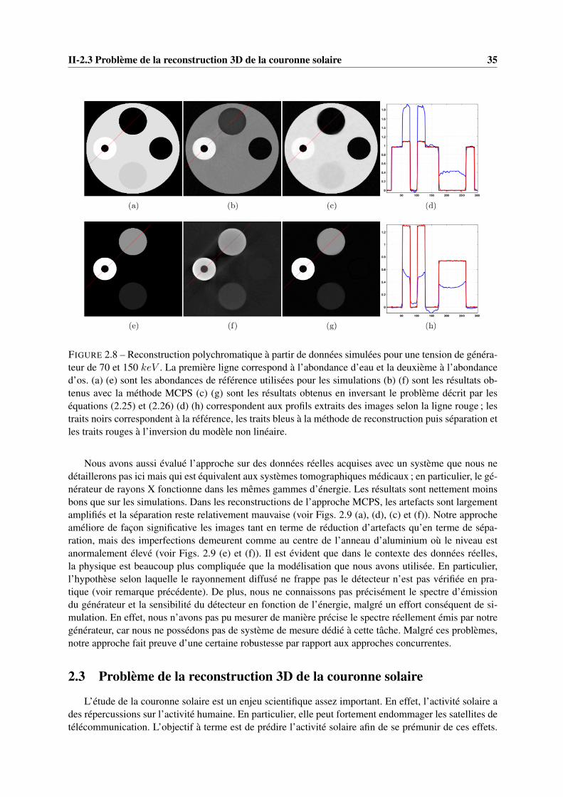
II-2.3 Problème de la reconstruction 3D de la couronne solaire 35
FIGURE 2.8 – Reconstruction polychromatique à partir de données simulées pour une tension de généra-teur de 70 et 150 keV . La première ligne correspond à l’abondance d’eau et la deuxième à l’abondanced’os. (a) (e) sont les abondances de référence utilisées pour les simulations (b) (f) sont les résultats ob-tenus avec la méthode MCPS (c) (g) sont les résultats obtenus en inversant le problème décrit par leséquations (2.25) et (2.26) (d) (h) correspondent aux profils extraits des images selon la ligne rouge ; lestraits noirs correspondent à la référence, les traits bleus à la méthode de reconstruction puis séparation etles traits rouges à l’inversion du modèle non linéaire.
Nous avons aussi évalué l’approche sur des données réelles acquises avec un système que nous nedétaillerons pas ici mais qui est équivalent aux systèmes tomographiques médicaux ; en particulier, le gé-nérateur de rayons X fonctionne dans les mêmes gammes d’énergie. Les résultats sont nettement moinsbons que sur les simulations. Dans les reconstructions de l’approche MCPS, les artefacts sont largementamplifiés et la séparation reste relativement mauvaise (voir Figs. 2.9 (a), (d), (c) et (f)). Notre approcheaméliore de façon significative les images tant en terme de réduction d’artefacts qu’en terme de sépa-ration, mais des imperfections demeurent comme au centre de l’anneau d’aluminium où le niveau estanormalement élevé (voir Figs. 2.9 (e) et (f)). Il est évident que dans le contexte des données réelles,la physique est beaucoup plus compliquée que la modélisation que nous avons utilisée. En particulier,l’hypothèse selon laquelle le rayonnement diffusé ne frappe pas le détecteur n’est pas vérifiée en pra-tique (voir remarque précédente). De plus, nous ne connaissons pas précisément le spectre d’émissiondu générateur et la sensibilité du détecteur en fonction de l’énergie, malgré un effort conséquent de si-mulation. En effet, nous n’avons pas pu mesurer de manière précise le spectre réellement émis par notregénérateur, car nous ne possédons pas de système de mesure dédié à cette tâche. Malgré ces problèmes,notre approche fait preuve d’une certaine robustesse par rapport aux approches concurrentes.
2.3 Problème de la reconstruction 3D de la couronne solaire
L’étude de la couronne solaire est un enjeu scientifique assez important. En effet, l’activité solaire ades répercussions sur l’activité humaine. En particulier, elle peut fortement endommager les satellites detélécommunication. L’objectif à terme est de prédire l’activité solaire afin de se prémunir de ces effets.

36 Tomographie
FIGURE 2.9 – Reconstruction polychromatique à partir de données réelles sur fantôme physique trèsproche des simulations pour des tensions de générateur de 70 et 150 keV . La première ligne correspondà l’abondance d’eau et la deuxième à l’abondance d’os. (a) (d) approche MCPS (b) (e) inversion dumodèle non-linéaire (d) (h) correspondent aux profils extraits des images selon la ligne rouge ; les traitsbleus correspondent à la méthode de reconstruction puis séparation et les traits rouges à l’inversion dumodèle non linéaire.
Pour cela, il faut comprendre les mécanismes physiques sous-jacents. On peut citer deux phénomènesdont on ne connaît pas l’origine. Premièrement, la température de la couronne solaire est d’environ unmillion de kelvins alors que la surface est uniquement de 5800 kelvins. Plusieurs théories [3][22] ontété développées mais aucune n’a encore pu être validée par des observations. Deuxièmement, la vitessedu vent solaire rapide est encore inexpliquée. Le vent solaire est un flux continu de particules chargéesqui émane du soleil. Il y a un vent lent (400 km/s) issu des régions équatoriales et un vent rapide (750km/s) issu des pôles [49].
Mission STEREO
Afin de mieux comprendre le fonctionnement du soleil, des missions d’observation de son activitéont été lancées ces dernières années : Solar and Heliospheric Observatory (SoHO) en 1995 et STEREOen 2006. Le but de la mission STEREO est de reconstruire la structure 3D de la couronne solaire. Pourcela, on souhaite avoir deux mesures simultanées sous deux angles de vue différents du soleil. Cette mis-sion a consisté à envoyer deux satellites quasiment identiques (STEREO A et STEREO B). Ces satellitess’écartent l’un de l’autre au court de la mission afin d’avoir des angles de vue de plus en plus différents etdonc une plus grande diversité d’information (voir Fig. 2.10). A l’intérieur de chaque satellite sont em-barqués plusieurs instruments : deux coronographes champ proche COR1 et COR2, deux coronographesgrand champ H1 et H2 qui peuvent couvrir toute la zone entre le Soleil et la Terre et les EUVI (ExtremeUltraViolet Imager) qui sont quatre imageurs qui observent dans l’extrême ultraviolet. Les quatre ima-geurs EUVI observent aux longueurs d’ondes 17,1 nm, 19,5 nm, 28,4 nm et 30,4 nm. Chaque longueurd’onde correspond à une raie de désexcitation d’un ion particulier qui est présent uniquement si le plasmaatteint une température particulière (17,1 nm, ions Fe IX et Fe X, Te ≈ 106K ; 19,5 nm, ion Fe XIITe ≈ 1, 6 × 10⁶K ; 28,4 nm ion Fe XV,Te ≈ 2 × 10⁶K ; 30,4 nm, ion He II, Te ≈ 8 × 10⁴K ). On

II-2.3 Problème de la reconstruction 3D de la couronne solaire 37
STEREO B
STEREO A
Terre
Soleil
FIGURE 2.10 – Position des satellites STEREO A et STEREO B par rapport au soleil
peut donc accéder à la densité du plasma à différentes altitudes dans la couronne proche du soleil (tem-pérature entre 1 et 2 millions de degrés Kelvin). Nous nous intéresserons ici uniquement aux donnéesEUVI bien que l’approche que nous allons présenter pourrait facilement être applicable sur les donnéesdes coronographes (voir thèse de Nicolas BARBEY [11]). L’image formée (voir Fig. 2.11) sur le planfocal du détecteur est acquise à l’aide d’un capteur CCD. Chaque pixel détecteur intègre tous les photonsarrivant dans le télescope pour une direction donnée. Cette mesure est donc l’intégrale selon une droitede la propriété d’émissivité qui nous intéresse. Enfin, l’atténuation à ces longueurs d’ondes des photonsultraviolets par l’atmosphère solaire est négligeable, on peut donc considérer chaque image Fig. 2.11comme une projection tomographique de l’émissivité de la couronne solaire.
FIGURE 2.11 – Image à 17,1 nm du pôle nord du soleil à l’aide de l’instrument EUVI. On voit clairementdes structures verticales lumineuses correspondant aux plumes polaires
2.3.1 Problématiques en traitement du signal
L’objectif astrophysique est la connaissance de la structure 3D de la couronne solaire, et en particulierla forme des plumes polaires. Ce sont des structures fines qui sont sur les pôles du soleil Fig. 2.11. Leursmorphologies ainsi que leurs paramètres physiques (densité et température du plasma) sont des élémentstrès importants pour expliquer la présence du vent rapide.
Tout d’abord, nous connaissons simultanément deux projections de notre objet d’intérêt grâce à STE-REO A et STEREO B, mais cette information est trop lacunaire pour faire une reconstruction précise del’objet. On utilise aussi la rotation du soleil sur lui même pour acquérir d’autres angles de projection. Sa

38 Tomographie
période de rotation au pôle est d’environ 27 jours [140]. L’un des problèmes que l’on n’ abordera pasici est que la rotation du Soleil n’est pas solide mais différentielle, c’est à dire que la période de rotationà l’équateur est plus rapide que celle aux pôles [140]. Pour les structures du soleil qui nous intéressentici, nous avons une difficulté supplémentaire : la durée d’apparition d’une plume polaire peut être trèscourte (2 jours) au regard de la période de rotation du soleil. L’hypothèse implicite de la reconstructiontomographique est que l’objet n’évolue pas au court de l’acquisition. Cette évolution rapide déforme lesstructures et crée des artefacts très importants dans les images. Afin de pouvoir tirer des conclusionsastrophysiques des reconstructions tomographiques, nous devons résoudre un problème de tomographiedynamique.
La littérature dans ce domaine est assez abondante pour le domaine de l’imagerie médicale [14, 121,143, 138, 69]. Dans ce contexte la tomographie dynamique est utilisée pour s’affranchir des mouvementsdu patient. Le mouvement le plus étudié est le mouvement cardiaque [69, 1]. La difficulté de ce mouve-ment est sa rapidité, mais il a l’avantage d’être périodique. Pratiquement l’ensemble des approches utilisece caractère périodique du mouvement. On acquiert un grand nombre de périodes et on sélectionne lesdonnées associées à la même phase cardiaque [69, 1]. Cette approche est très efficace et permet de sup-primer la majeure partie des artefacts. Cette hypothèse est malheureusement inutilisable dans notre cas.La tomographie dynamique est aussi utilisée dans le cas du mouvement respiratoire. Ce dernier n’est pasforcément périodique, mais on peut soit mesurer le mouvement à partir d’une mesure extérieure [138],soit faire une estimation du mouvement [64][14][143], car il est relativement lent.
Dans le domaine de l’astrophysique solaire, bien que la reconstruction tomographique soit connuedepuis plus de 60 ans [137], le nombre de travaux est relativement faible. Cela s’explique facilementpar la difficulté du problème associé à la communauté scientifique nettement plus réduite qu’en ima-gerie médicale. R. FRAZIN s’est intéressé au problème de la reconstruction dynamique de la couronnesolaire [57, 58]. Il a cherché à reconstruire des structures présentes dans la haute atmosphère qui ont uneévolution plus lente que nos plumes. Sa résolution repose sur l’introduction d’une information a prioride douceur selon l’axe temporel de l’objet 4D à reconstruire. D’autres travaux ont consisté à définirun a priori selon des directions en accord avec un modèle de MagnétoHydroDynamique (MHD) de lacouronne solaire [141].
2.3.2 Première approche : paramétrisation des plumes polaires
Le problème de reconstruction dynamique de la couronne solaire est extrêmement mal posé car ona dans les meilleures configurations 50 fois plus d’inconnues que de données. Ces travaux se sont faitdans le cadre de la thèse de N. BARBEY, et sont détaillés dans [12] (reproduit à la page 166). L’inversionde ce problème passe donc par l’introduction d’informations a priori très contraignantes. Pour ce faire,nous faisons l’hypothèse que la morphologie des plumes ne varie pas sur 13,5 jours. Cette modélisationde l’évolution des plumes vient de la supposition que les plumes sont tubulaires et suivent les lignes dechamps magnétiques du Soleil [86, 39]. Par contre, nous allons faire évoluer l’intensité de chaque plumeau cours du temps. Notre objet 3D + T que l’on note x va être paramétré à l’aide d’une composantemorphologique 3D notée e et des intensités variant dans le temps γ. La nouvelle paramétrisation duproblème est décrite par l’équation
x(~r, t) = e(~r).×Lγ(t). (2.27)
Dans notre paramétrisation nous avons besoin de connaître une segmentation de chaque plume (Fig.2.12 (b)). Cette segmentation est contenue dans la matrice L. De plus, l’opération .× fait le produit termeà terme des vecteurs. Afin de contraindre suffisamment le problème nous avons considéré au maximum4 ou 5 plumes actives.

II-2.3 Problème de la reconstruction 3D de la couronne solaire 39
Inversion :
On considère, un modèle direct linéaire correspondant à la transformée en rayons divergents. Nousmodéliserons une projection à un instant t donné par la matrice Ht.
y(t) = Ht (e.×Lγ(t)) + b(t) (2.28)
avec b(t) un bruit Gaussien i.i.d. de variance σ2b . On déduit que la vraisemblance p(y|e,γ, σb) suitune loi Gaussienne. Afin d’avoir une optimisation efficace dans un contexte où la taille des reconstruc-tions est importante (problème 3D + T), nous avons choisi des a priori conjugués avec la vraisemblance.
Pour ce qui est de la composante morphologique, nous avons choisi d’introduire une information dedouceur à travers un a priori Gaussien corrélé,
p(e|σe) ∝ exp(−‖Dee‖22σ2e
) (2.29)
où la matrice de corrélation est égale à (DteDe)
−1 et où D est la matrice des différences finies entrepixels voisins.
Pour ce qui est de la composante temporelle, on considère que la fluctuation est relativement douce.De plus, pour lever une indétermination du problème, on ajoute un terme de rappel à la valeur 1. Onfavorisera donc les solutions dont la valeur multiplicative est proche de 1, en utilisant la loi a priorisuivante :
p(γ|σγ , σ1) ∝ exp(−‖Dtγ‖22σ2γ
− ‖γ − 1‖22σ21
), (2.30)
où la matrice Dt correspond aux différences finies selon la dimension temporelle.En utilisant la règle de Bayes (2.14), on obtient la loi a posteriori jointe suivante :
p(e,γ|y, σγ , σ1, σe, σb) ∝ exp
(−‖y −H(e.×Lγ)‖
2σ2b− ‖Dee‖2
2σ2e− ‖Dtγ‖2
2σ2γ− ‖γ − 1‖2
2σ21
)(2.31)
Le modèle étant bilinéaire, la loi jointe p(e,γ|y, . . .) n’est pas Gaussienne. Par contre les lois condi-tionnelles p(e|γ,y, . . .) et p(γ|e,y, . . .) sont Gaussiennes. Nous allons, pour des questions d’effica-cité de calculs, choisir l’estimateur du maximum a posteriori. Puis nous utiliserons une procédure demaximisation alternée afin de trouver un optimum local. En effet, cette approche ne nous garantit pasde déterminer l’optimum global du critère conjoint. Comme la dimension du vecteur γ est faible, saminimisation connaissant e peut se faire en appliquant directement la formule analytique d’inversion(Eq. (2.11)). Pour ce qui est de l’optimisation suivant la composante morphologique la dimension duproblème nous contraint à utiliser une approche de descente suivant une direction liée au gradient ducritère. Nous procédons ensuite avec un schéma de minimisation alternée où le critère d’arrêt repose surla norme de la mise à jour inférieure à une constante ǫ pendant au moins trois itérations.
Résultats sur des données simulées :
Nous avons simulé des données en utilisant notre modèle de l’Eq. (2.27) composé de trois plumes.La composante morphologique est représentée sur la Fig. 2.12 (a), et l’évolution temporelle de chaqueplume sur la Fig. 2.12 (c). Nous avons simulé les données avec les mêmes configurations que pour unjeu de données réelles et nous avons ajouté un bruit Gaussien avec une variance équivalente à celleprésente sur les données réelles. Nous avons comparé notre approche (Fig. 2.12 (e) et Fig. 2.12 (f)) avecla reconstruction de type filtrage rétroprojection Eq. (2.4) sur la Fig. 2.12 (d). Il apparaît clairement surla Fig. 2.12 (d) que la non prise en compte de l’évolution temporelle crée des artefacts très importantset que les structures ne peuvent pas être reconstruites de manière précise. L’approche proposée permetbien de reconstruire de manière fidèle la composante morphologique (Fig. 2.12 (e)) et de manière assezfidèle l’allure des évolutions temporelles de chaque plume. Par contre, les valeurs des gains ne sont pascorrectement estimées à cause de l’indétermination du modèle à une constante multiplicative près.

40 Tomographie
(a) (b) (c)
(d) (e) (f)
FIGURE 2.12 – Reconstruction en utilisant notre première approche : la première ligne correspond auxvaleurs que nous avons utilisées pour faire les simulations, la deuxième ligne correspond à des estima-tions : (a) image morphologique vraie : elle est composée de trois tâches Gaussiennes, (b) segmenta-tion en zones possédant la même dynamique d’évolution, (c) valeur du gain γ en fonction du tempsd’acquisition : les couleurs courbes correspondent aux couleurs de la segmentation de la figure (b), (d)reconstruction statique en utilisant une approche filtrage-rétroprojection classique, (e) estimation de lamorphologie avec notre première approche, (f) estimation de la dynamique temporelle.
Résultats sur des données réelles :
Nous avons appliqué notre approche à des données réelles issues d’un seul satellite car au moment deces travaux la calibration photométrique entre les deux satellites n’était pas encore faite. Pour appliquernotre approche, on suppose que l’on connaît la segmentation des différentes plumes qui composent l’at-mosphère. Pour déterminer cette segmentation (Fig. 2.13 (a)), on fait une première reconstruction avecune approche filtrage rétroprojection (Fig. 2.13 (c)). On identifie les structures les plus lumineuses puis ondétermine manuellement le contour des plumes. L’estimation des évolutions temporelles (Fig. 2.13 (b))est cohérente avec ce que nous attendions. L’estimation de la composante morphologique (Fig. 2.13 (d))est plus contrastée que l’approche classique (Fig. 2.13 (c)). De plus, les valeurs négatives dans l’imagesont beaucoup moins nombreuses que dans l’approche classique. Tous ces éléments nous laissent penserque notre estimation est plus proche de la réalité que celle de la méthode de filtrage rétroprojection.
Conclusions :
Au regard de ces premiers résultats, la paramétrisation qui sépare la composante morphologiquede l’évolution temporelle paraît très pertinente. Les résultats sur des données simulées sont concluantset ceux sur des données réelles sont encourageants à bien des égards. Par contre, le point négatif del’approche est de considérer que la segmentation des différentes plumes est connue au moment de l’es-timation. Il est bien évident qu’une erreur d’estimation est très préjudiciable sur la qualité de la recons-truction finale. C’est pourquoi nous avons continué des travaux après la fin de la thèse de N. BARBEY
afin de s’affranchir cette hypothèse.
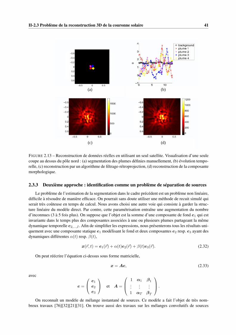
II-2.3 Problème de la reconstruction 3D de la couronne solaire 41
(a)
(c)
(b)
(d)
FIGURE 2.13 – Reconstruction de données réelles en utilisant un seul satellite. Visualisation d’une seulecoupe au dessus du pôle nord : (a) segmentation des plumes définies manuellement, (b) évolution tempo-relle, (c) reconstruction par un algorithme de filtrage-rétroprojection, (d) reconstruction de la composantemorphologique.
2.3.3 Deuxième approche : identification comme un problème de séparation de sources
Le problème de l’estimation de la segmentation dans le cadre précédent est un problème non linéaire,difficile à résoudre de manière efficace. On pourrait sans doute utiliser une méthode de recuit simulé quiserait très coûteuse en temps de calcul. Nous avons choisi une autre voie qui consiste à garder la struc-ture linéaire du modèle direct. Par contre, cette paramétrisation entraîne une augmentation du nombred’inconnues (3 à 5 fois plus). On suppose que l’objet est la somme d’une composante de fond e1 qui estinvariante dans le temps plus des composantes associées à une ou plusieurs plumes partageant la mêmedynamique temporelle e2,...,I . Afin de simplifier les expressions, nous présenterons tous les résultats uni-quement avec une composante statique e1 modélisant le fond et deux composantes e2 resp. e3 ayant desdynamiques différentes α(t) resp. β(t),
x(~r, t) = e1(~r) + α(t)e2(~r) + β(t)e3(~r). (2.32)
On peut réécrire l’équation ci-dessus sous forme matricielle,
x = Ae, (2.33)
avec
e =
e1e2e3
et A =
1 α1 β1...
......
1 αT βT
.
On reconnaît un modèle de mélange instantané de sources. Ce modèle a fait l’objet de très nom-breux travaux [76][32][21][31]. On trouve aussi des travaux sur les mélanges convolutifs de sources
42 Tomographie
[107][94][93], mais à notre connaissance il n’existe quasiment pas de travaux sur les mélanges linéairesde sources. C’est pourtant le problème auquel nous sommes confrontés car nous devons appliquer lamatrice de projection H à l’Eq. (2.33),
y = HAe+ b. (2.34)
b est ici un bruit Gaussien i.i.d. de variance σ2b . On déduit que la vraisemblance p(y|e,A, σb) est Gaus-sienne.
Comme nous l’avons dit au début de cette partie, l’idée de cette approche est de garder un modèlelinéaire, mais en contrepartie le nombre de paramètres inconnus est bien plus important (trois fois plusdans notre cas). Nous devons donc introduire une quantité d’information a priori importante. La pa-ramétrisation ne permettant pas de réduire suffisamment les degrés de liberté, nous allons utiliser uneinformation a priori de parcimonie sur la composante morphologique des plumes e2 et e3 au moyend’une loi à queue lourde. Notre choix s’est porté sur la loi de Student T car elle peut être générée commeun mélange infini de Gaussienne. Cette propriété va nous permettre d’utiliser uniquement des a prioriconjugués avec la vraisemblance. Cette propriété nous permet d’avoir des lois a posteriori condition-nelles dans des familles connues. Nous pourrons donc utiliser des approches bayésiennes variationellesdécrites dans le chapitre 3 pour résoudre notre problème d’inférence.
Les différentes lois a priori utilisées :– pour les composantes morphologiques des plumes, exprimons ici la loi de e2 :
p(e2(i)|λ, ν) = St(e2(i)|λ, ν)
=
∫
R
p(e2(i)|a2(i), λ) p(a2(i) | ν) da2(i)
=
∫
R
N(e2(i)|0, (a2(i) ∗ λ)−1
)G(a2(i)|
ν
2,ν
2
)da2(i) (2.35)
où St(·|λ, ν) 11 est une loi de Student centrée, N (·|m,σ2) est une loi Gaussienne de moyenne met de variance σ2 et G(·|p1, p2) 12 est une loi Gamma centrée de paramètres p1 et p2. On choisitla même loi avec les mêmes valeurs de paramètres pour e3. Nous allons estimer les précisions(l’inverse de la variance) des lois Gaussiennes a2 et a3 au lieu de les marginaliser pour conserverla conjugaison des a priori (pour plus de précision, cette approche est décrite dans le chap. 3,§ 3.3).
– pour les composantes dynamiques des plumes (α,β) nous utilisons une information de douceur,
p(α,β|σt) ∝ exp(−‖Dtα‖2 + ‖Dtβ‖22σ2t
) (2.36)
– pour la composante de fond e1, nous utiliserons une information de douceur spatiale,
p(e1|σe) ∝ exp(−‖Dee1‖22σ2e
) (2.37)
Loi a posteriori :
p(e1, e2, e2,a2,a3,α,β|y, σb, σt, σe, λ, ν) (2.38)
∝ p(y|e1, e2, e3,α,β, σb)p(e1|σe)p(e2|a2, λ)p(a2|ν) (2.39)
p(e3|a3, λ)p(a3|ν)p(α,β|σt) (2.40)
On utilise l’algorithme 2 décrit dans le Chap. 3, § 3.5.1. L’initialisation est faite par des zéros pour lacomposante de fond et par une approche filtrage rétroprojection pour les composantes morphologiquesdes plumes, enfin, les composantes dynamiques sont initialisées par des 1.
11. St(x|λ, ν) ∝(
1 + λνx2
)− ν+1
2
12. G(x|p1, p2) ∝ xp1−1 exp [−p2x]

II-2.3 Problème de la reconstruction 3D de la couronne solaire 43
20 40 60 80 100 120
20
40
60
80
100
1200
1
2
3
4
5
20 40 60 80 100 120
20
40
60
80
100
1200
1
2
3
4
5
20 40 60 80 100 120
20
40
60
80
100
1200
0.2
0.4
0.6
0.8
1
(a) (b) (c)
0 50 100 150 2000
0.2
0.4
0.6
0.8
1
1.2
1.4
0 50 100 150 2000
0.2
0.4
0.6
0.8
1
1.2
1.4
20 40 60 80 100 120 140 160 180
20
40
60
80
100
120
140
160
1800
10
20
30
40
50
60
70
(d) (e) (f)
FIGURE 2.14 – Simulation des données : (a) composante morphologique e2, (b) composante morpholo-gique e3, (c) composante statique e1, (d) évolution dynamique α associée à e2, (e) évolution dynamiqueβ associée à e3, (f) sinogramme légèrement bruité y
Premiers résultats sur des données simulées :Ces travaux sont encore à un stade préliminaire, ils ont débouché uniquement sur une communication
dans une conférence internationale [79]. Il manque un travail important de validation sur des donnéesréelles pour qu’ils soient aboutis. Afin de montrer la faisabilité de l’approche, nous avons fait l’expériencenumérique suivante : nous avons simulé des données en géométrie parallèle à partir d’un objet 2D + T128× 128× 180. Cet objet comporte trois composantes :
– le fond qui est invariant dans le temps et qui est relativement régulier (Fig. 2.14 (c)),– une première composante dynamique composée de deux plumes (Fig. 2.14 (a)) qui suit l’évolution
dynamique représentée sur la Fig. 2.14 (d).– une deuxième composante dynamique aussi composée de deux plumes dont l’une est superposée
avec le fond (Fig. 2.14 (b) et (c)). L’évolution dynamique de cette composante est représentée surla Fig. 2.14 (e), elle est en opposition de phase par rapport à l’autre composante dynamique.
Les données sont représentées sur la Fig. 2.14 (f). Il y a une projection tous les degrés. Nous avons ajoutédu bruit Gaussien i.i.d. de variance égale à 10. On voit clairement des évanouissements des structuresdynamiques dans le sinogramme (Fig. 2.14 (f)). La difficulté de ce problème inverse est directementvisible sur la Fig. 2.14. On cherche à retrouver les images des Figs. 2.14 (a)-(c) et les signaux représentéssur les Figs. 2.14 (d) et (e) uniquement à partir du sinogramme de la Fig. 2.14 (f).
On commence par faire une première reconstruction avec une approche filtrage rétroprojection (Fig.2.15 (f)). On observe que la composante statique est parfaitement reconstruite. Par contre, l’inconsis-tance dans les données due aux composantes dynamiques provoque de sévères artefacts en étoile autourdes plumes. Suite à l’utilisation de l’algorithme 2 page 49 adapté à notre problème, nous obtenons deslois approchantes pour chaque paramètre. Nous représentons sur les Figs. 2.15 (a), (b), (c), (d) et (e) lamoyenne de ces lois. On remarque que l’estimation du fond (Fig. 2.15 (c)) représentée avec la mêmeéchelle de couleurs est de bien meilleure qualité. Les artefacts sont très fortement réduits, les valeursnégatives sont quasiment inexistantes. Si on compare par rapport à l’image vraie (Fig. 2.14 (c)) on voit

44 Tomographie
20 40 60 80 100 120
20
40
60
80
100
1200
0.5
1
1.5
2
2.5
3
3.5
4
4.5
20 40 60 80 100 120
20
40
60
80
100
1200
1
2
3
4
5
6
20 40 60 80 100 120
20
40
60
80
100
120 −0.4
−0.2
0
0.2
0.4
0.6
0.8
1
(a) (b) (c)
0 50 100 150 200−0.5
0
0.5
1
1.5
2
2.5
0 50 100 150 2000
0.2
0.4
0.6
0.8
1
1.2
1.4
1.6
1.8
20 40 60 80 100 120
20
40
60
80
100
120−0.4
−0.2
0
0.2
0.4
0.6
0.8
1
(d) (e) (f)
FIGURE 2.15 – Comparaison entre une reconstruction de type filtrage rétroprojection (f) et notre nouvelleapproche (a)-(e) : (a) estimation de la composante morphologique e2, (b) estimation de la composantemorphologique e3, (c) estimation de composante statique e1, (d) estimation de l’évolution dynamiqueα associée à e2, (e) estimation de l’évolution dynamique β associée à e3, (f) reconstruction par uneapproche classique de filtrage rétroprojection (fonction iradon de matlab).
que l’introduction de l’information a priori de douceur nous fait légèrement sous estimer le maximumde l’image. De plus, on voit en haut à gauche qu’à l’endroit où la plume est superposée au fond, ily a un trou dans l’estimation du fond. L’approche lors de la séparation a préféré mettre tout le signaldans la composante dynamique. En ce qui concerne les composantes associées aux plumes, l’approchea très bien séparé les deux composantes dynamiques (rappelons que l’initialisation de ces composantesest identique ; on utilise l’image de la Fig. 2.15 (f) pour la partie morphologique et 1 pour l’évolutiontemporelle). De plus les plumes sont correctement positionnées et l’allure des évolutions dynamiquesFig. 2.15 (d) (resp. Fig. 2.15 (e)) sont très proches des vraies Fig. 2.14 (d) (resp. Fig. 2.14 (e)). Il y auniquement une erreur relativement importante autour de la projection 90 très visible sur la Fig. 2.15 (e).Cette projection correspond à une intégration suivant des lignes horizontales. Dans ce cas, il y a clai-rement une indétermination dans le problème de séparation que l’information a priori que nous avonsintroduite ne peut que partiellement lever. Enfin, les composantes morphologiques reconstruites ont unsupport plus petit que les images de départ. L’introduction de l’information de parcimonie a contraintles faibles valeurs des composantes associées aux plumes de se retrouver dans l’image du fond. On voitdes artefacts résiduels autour de l’emplacement des plumes sur la Fig. 2.15 (c) causés par cette mauvaiseestimation.

Chapitre 3
Bayesien Variationnel
3.1 Introduction
Problématique liée à résolution de problèmes inverses de grande dimension
Comme on a pu le voir dans le chapitre précédent, les problèmes inverses sont souvent de très grandesdimensions (plus d’un millions d’inconnues). On peut citer par exemple, les problèmes de reconstructions3D, 3D + T ou 2D mettant en jeu de grand détecteurs (ex : les CCD 4096× 4096 sont couramment dansl’imagerie satellitaire).
Dans beaucoup d’applications le besoin d’avoir des approches non-supervisées se fait sentir. Dansces approches, les paramètres qui règlent le compromis entre l’information apportée par les donnéeset l’information a priori, sont aussi estimés. Nous appellerons dans la suite ces paramètres, hyperpara-mètres, car ils ne correspondent pas à la grandeur d’intérêt du problème inverse. Dans un cadre bayésien,l’estimation des hyperparamètres passe par l’introduction d’une loi a priori sur ces hyperparamètresqui conduit à une loi a posteriori jointe. Ces approches s’appellent «bayésiennes hiérarchiques». Unefois la loi a posteriori obtenue, on cherche un estimateur ponctuel. On a principalement le choix entrele maximum ou la moyenne a posteriori. L’obtention du maximum a posteriori est équivalent à un pro-blème d’optimisation du critèreQ(w) = − log
(p(w|y)
). Le critère que l’on optimise est en général non
convexe lorsqu’on estime conjointement les hyperparamètres. L’optimisation non-convexe étant délicateen pratique, beaucoup de travaux récents ont choisi de calculer l’estimateur de la moyenne a posterioripar une approche stochastique.
État de l’art
Les méthodes les plus utilisées pour obtenir l’estimateur de la moyenne a posteriori, sont les ap-proches de calculs stochastiques de type Monte Carlo «Markov Chain» (MCMC) [113][114][90]. L’idéedes MCMC est de générer une chaîne d’échantillons qui converge asymptotiquement vers des échan-tillons sous la loi cible (loi a posteriori). On conserve ensuite uniquement les échantillons sous la loia posteriori obtenus après un certain temps, appelé temps de chauffe. En faisant la moyenne empiriqued’un grand nombre de ces échantillons, on obtient un très bon estimateur de la moyenne a posteriori. Ily a principalement deux types d’algorithmes MCMC : les algorithmes de Hasting-Metropolis et l’échan-tillonnage de Gibbs. Le principe des méthodes de Hasting-Metropolis est de générer un échantillon sousune loi plus simple que l’on peut échantillonner facilement. Cet échantillon est alors accepté avec unecertaine probabilité. La principale limitation de cette méthode est la dimension de l’espace à explorerqui peut devenir importante quand le nombre d’inconnues augmente. Il est donc quasiment impossiblede trouver une loi de proposition suffisamment proche de la loi cible sur un problème de grande di-mension. En ce qui concerne l’échantillonneur de Gibbs, son principe est de tirer des échantillons sousdes lois conditionnelles. Lorsque la chaîne a convergé, l’algorithme génère des échantillons sous la loi
45

46 Bayesien Variationnel
a posteriori jointe. Dans un problème avec un grand nombre d’inconnues, cet algorithme converge ex-trêmement lentement si on échantillonne conditionnellement inconnue par inconnue. Il est par contreefficace lorsque l’on peut échantillonner conjointement un grand nombre d’inconnues, ce qui est le cas sila loi jointe est séparable ou si elle est Gaussienne avec une matrice de covariance facilement inversible.Par exemple, il y a de nombreuses approches bayésiennes développées dans le cas de la déconvolution[90][61][101] 1, car la matrice de covariance est diagonalisable par transformée de Fourier (sous approxi-mation circulante). Par contre, il est extrêmement difficile de générer un échantillon vectoriel de grandedimension efficacement sous une loi corrélée si la matrice de covariance n’a pas de structure particulièrequi la rend facilement inversible ou si l’inverse de la matrice de covariance n’est pas creuse.
D. MACKAY a proposé en 1995 une alternative à ces méthodes d’échantillonnage : le bayésien va-riationnel [88]. Il s’est inspiré des approches en champ moyen «mean field» développées en physiquestatistique [105]. Cette approche a aussi été introduite sous une autre forme dans la communauté desinformaticiens [74]. Dans le domaine du traitement du signal, cette méthodologie a été appliquée à dif-férents sujets comme la séparation de sources [91][28], le choix de modèles pour décomposer un signalcomme une somme de signaux AR [92], la réduction d’images hyper spectrales [9], les problèmes d’ap-prentissage dans des dictionnaires en utilisant la parcimonie [142][124], les problèmes de déconvolu-tion [25][8] et le problème de déconvolution myope d’un flou dû au mouvement du photographe [50].L’approche bayésienne variationnelle est moins générique que les approches MCMC, et en théorie plusapproximative, mais elle est plus efficace en pratique surtout en grande dimension. Elle est limitée carelle ne permet de résoudre des problèmes inverses que lorsque la loi a posteriori appartient à une famillede lois conjuguées avec la vraisemblance. Cependant, comme les calculs sont analytiques, la vitesse deconvergence est nettement plus rapide que les approches MCMC. L’idée de cette méthodologie est d’ap-procher la loi a posteriori par des lois séparables. On cherche donc la fonction séparable qui est la plusproche de la loi a posteriori au sens de la divergence de Kullback-Leiber. Il faut donc résoudre un pro-blème d’optimisation dans un espace de dimension infinie, à savoir un espace fonctionnel. En pratique,la minimisation de la fonctionnelle se fait composante séparable par composante séparable, de manièrealternée. Cette minimisation est une version fonctionnelle de l’algorithme de minimisation de Gauss-Seidel dans un espace de dimension finie [96]. Lorsque l’on a un très grand nombre de composantesséparables, l’algorithme devient très lent.
Contributions
Il y a une réelle difficulté à développer des approches non supervisées pour les problèmes inverses detrès grande dimension. L’algorithme que nous avons proposé dans [56] (reproduit à la page 81) permetde s’affranchir de ce problème de dimension dans de très nombreux cas. L’idée est de transposer lesapproches classiques de descente de gradient à pas optimal, bien connue dans les espace de dimensionfinie [96], à l’espace des distribution de probabilité, qui est de dimension infinie. Nous avons aussi, établiune preuve de convergence de notre algorithme dans ces travaux. Nous exposerons brièvement dans cechapitre l’approche bayésienne variationnelle classique § 3.2, puis notre nouvel algorithme dans le § 3.3.Nous appliquerons cette méthodologie à un problème conjoint de reconstruction sur-résolue associé à unproblème de séparation de composante dans le contexte de l’imagerie astrophysique. Nous finirons parprésenter des résultats de notre approche sur des données simulées et réelles.
3.2 Méthodologie bayésienne variationelle
Nous décrivons ici l’approche bayésienne variationnelle classique introduite par D. MACKAY [88].Dans cette partie, afin d’avoir une présentation générale des approches nous noterons par y ∈ RM levecteur de dimension M contenant les données et nous noterons par w ∈ RN le vecteur rassemblant
1. Les références sur des travaux auxquels j’ai contribué sont en gras dans le texte
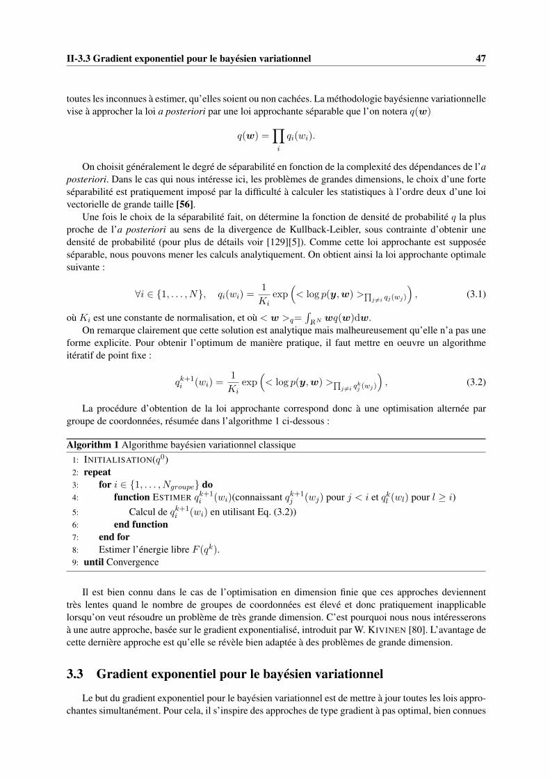
II-3.3 Gradient exponentiel pour le bayésien variationnel 47
toutes les inconnues à estimer, qu’elles soient ou non cachées. La méthodologie bayésienne variationnellevise à approcher la loi a posteriori par une loi approchante séparable que l’on notera q(w)
q(w) =∏
i
qi(wi).
On choisit généralement le degré de séparabilité en fonction de la complexité des dépendances de l’aposteriori. Dans le cas qui nous intéresse ici, les problèmes de grandes dimensions, le choix d’une forteséparabilité est pratiquement imposé par la difficulté à calculer les statistiques à l’ordre deux d’une loivectorielle de grande taille [56].
Une fois le choix de la séparabilité fait, on détermine la fonction de densité de probabilité q la plusproche de l’a posteriori au sens de la divergence de Kullback-Leibler, sous contrainte d’obtenir unedensité de probabilité (pour plus de détails voir [129][5]). Comme cette loi approchante est supposéeséparable, nous pouvons mener les calculs analytiquement. On obtient ainsi la loi approchante optimalesuivante :
∀i ∈ 1, . . . , N, qi(wi) =1
Kiexp
(< log p(y,w) >∏
j 6=i qj(wj)
), (3.1)
où Ki est une constante de normalisation, et où < w >q=∫RN wq(w)dw.
On remarque clairement que cette solution est analytique mais malheureusement qu’elle n’a pas uneforme explicite. Pour obtenir l’optimum de manière pratique, il faut mettre en oeuvre un algorithmeitératif de point fixe :
qk+1i (wi) =
1
Kiexp
(< log p(y,w) >∏
j 6=i qkj (wj)
), (3.2)
La procédure d’obtention de la loi approchante correspond donc à une optimisation alternée pargroupe de coordonnées, résumée dans l’algorithme 1 ci-dessous :
Algorithm 1 Algorithme bayésien variationnel classique
1: INITIALISATION(q0)2: repeat3: for i ∈ 1, . . . , Ngroupe do4: function ESTIMER qk+1
i (wi)(connaissant qk+1j (wj) pour j < i et qkl (wl) pour l ≥ i)
5: Calcul de qk+1i (wi) en utilisant Eq. (3.2))
6: end function7: end for8: Estimer l’énergie libre F (qk).9: until Convergence
Il est bien connu dans le cas de l’optimisation en dimension finie que ces approches deviennenttrès lentes quand le nombre de groupes de coordonnées est élevé et donc pratiquement inapplicablelorsqu’on veut résoudre un problème de très grande dimension. C’est pourquoi nous nous intéresseronsà une autre approche, basée sur le gradient exponentialisé, introduit par W. KIVINEN [80]. L’avantage decette dernière approche est qu’elle se révèle bien adaptée à des problèmes de grande dimension.
3.3 Gradient exponentiel pour le bayésien variationnel
Le but du gradient exponentiel pour le bayésien variationnel est de mettre à jour toutes les lois appro-chantes simultanément. Pour cela, il s’inspire des approches de type gradient à pas optimal, bien connues
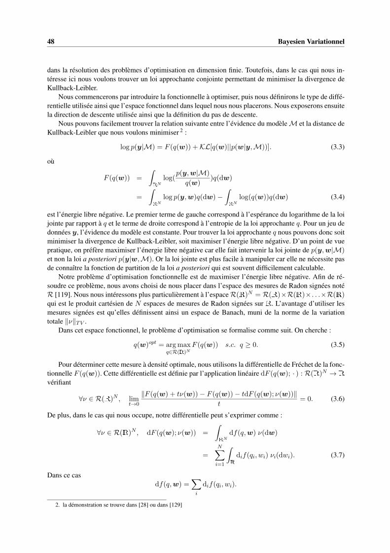
48 Bayesien Variationnel
dans la résolution des problèmes d’optimisation en dimension finie. Toutefois, dans le cas qui nous in-téresse ici nous voulons trouver un loi approchante conjointe permettant de minimiser la divergence deKullback-Leibler.
Nous commencerons par introduire la fonctionnelle à optimiser, puis nous définirons le type de diffé-rentielle utilisée ainsi que l’espace fonctionnel dans lequel nous nous placerons. Nous exposerons ensuitela direction de descente utilisée ainsi que la définition du pas de descente.
Nous pouvons facilement trouver la relation suivante entre l’évidence du modèleM et la distance deKullback-Leibler que nous voulons minimiser 2 :
log p(y|M) = F (q(w)) +KL[q(w)||p(w|y,M))]. (3.3)
où
F (q(w)) =
∫
RN
log(p(y,w|M)
q(w))q(dw)
=
∫
RN
log p(y,w)q(dw)−∫
RN
log(q(w))q(dw) (3.4)
est l’énergie libre négative. Le premier terme de gauche correspond à l’espérance du logarithme de la loijointe par rapport à q et le terme de droite correspond à l’entropie de la loi approchante q. Pour un jeu dedonnées y, l’évidence du modèle est constante. Pour trouver la loi approchante q nous pouvons donc soitminimiser la divergence de Kullback-Leibler, soit maximiser l’énergie libre négative. D’un point de vuepratique, on préfère maximiser l’énergie libre négative car elle fait intervenir la loi jointe de p(y,w|M)et non la loi a posteriori p(y|w,M). Or la loi jointe est plus facile à manipuler car elle ne nécessite pasde connaître la fonction de partition de la loi a posteriori qui est souvent difficilement calculable.
Notre problème d’optimisation fonctionnelle est de maximiser l’énergie libre négative. Afin de ré-soudre ce problème, nous avons choisi de nous placer dans l’espace des mesures de Radon signées notéR [119]. Nous nous intéressons plus particulièrement à l’espaceR(R)N = R(R)×R(R)× . . .×R(R)qui est le produit cartésien de N espaces de mesures de Radon signées sur R. L’avantage d’utiliser lesmesures signées est qu’elles définissent ainsi un espace de Banach, muni de la norme de la variationtotale ‖ν‖TV .
Dans cet espace fonctionnel, le problème d’optimisation se formalise comme suit. On cherche :
q(w)opt = argmaxq∈R(R)N
F (q(w)) s.c. q ≥ 0. (3.5)
Pour déterminer cette mesure à densité optimale, nous utilisons la différentielle de Fréchet de la fonc-tionnelle F (q(w)). Cette différentielle est définie par l’application linéaire dF (q(w); · ) : R(R)N → Rvérifiant
∀ν ∈ R(R)N , limt→0
‖F (q(w) + tν(w))− F (q(w))− tdF (q(w); ν(w))‖t
= 0. (3.6)
De plus, dans le cas qui nous occupe, notre différentielle peut s’exprimer comme :
∀ν ∈ R(R)N , dF (q(w); ν(w)) =
∫
RN
df(q,w) ν(dw)
=N∑
i=1
∫
R
dif(qi, wi) νi(dwi). (3.7)
Dans ce casdf(q,w) =
∑
i
dif(qi, wi).
2. la démonstration se trouve dans [28] ou dans [129]
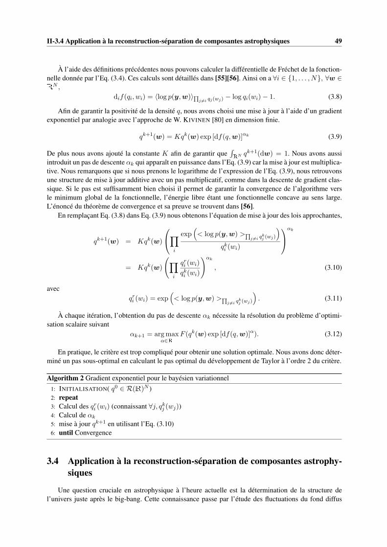
II-3.4 Application à la reconstruction-séparation de composantes astrophysiques 49
À l’aide des définitions précédentes nous pouvons calculer la différentielle de Fréchet de la fonction-nelle donnée par l’Eq. (3.4). Ces calculs sont détaillés dans [55][56]. Ainsi on a ∀i ∈ 1, . . . , N, ∀w ∈R
N ,
dif(qi, wi) = 〈log p(y,w)〉∏j 6=i qj(wj) − log qi(wi)− 1. (3.8)
Afin de garantir la positivité de la densité q, nous avons choisi une mise à jour à l’aide d’un gradientexponentiel par analogie avec l’approche de W. KIVINEN [80] en dimension finie.
qk+1(w) = Kqk(w) exp [df(q,w)]αk (3.9)
De plus nous avons ajouté la constante K afin de garantir que∫RN q
k+1(dw) = 1. Nous avons aussiintroduit un pas de descente αk qui apparaît en puissance dans l’Eq. (3.9) car la mise à jour est multiplica-tive. Nous remarquons que si nous prenons le logarithme de l’expression de l’Eq. (3.9), nous retrouvonsune structure de mise à jour additive avec un pas multiplicatif, comme dans la descente de gradient clas-sique. Si le pas est suffisamment bien choisi il permet de garantir la convergence de l’algorithme versle minimum global de la fonctionnelle, l’énergie libre étant une fonctionnelle concave au sens large.L’énoncé du théorème de convergence et sa preuve se trouvent dans [56].
En remplaçant Eq. (3.8) dans Eq. (3.9) nous obtenons l’équation de mise à jour des lois approchantes,
qk+1(w) = Kqk(w)
∏
i
exp(< log p(y,w) >∏
j 6=i qkj (wj)
)
qki (wi)
αk
= Kqk(w)
(∏
i
qri (wi)
qki (wi)
)αk
, (3.10)
avecqri (wi) = exp
(< log p(y,w) >∏
j 6=i qkj (wj)
). (3.11)
À chaque itération, l’obtention du pas de descente αk nécessite la résolution du problème d’optimi-sation scalaire suivant
αk+1 = argmaxα∈R
F (qk(w) exp [df(q,w)]α). (3.12)
En pratique, le critère est trop compliqué pour obtenir une solution optimale. Nous avons donc déter-miné un pas sous-optimal en calculant le pas optimal du développement de Taylor à l’ordre 2 du critère.
Algorithm 2 Gradient exponentiel pour le bayésien variationnel
1: INITIALISATION( q0 ∈ R(R)N )2: repeat3: Calcul des qri (wi) (connaissant ∀j, qkj (wj))4: Calcul de αk
5: mise à jour qk+1 en utilisant l’Eq. (3.10)6: until Convergence
3.4 Application à la reconstruction-séparation de composantes astrophy-siques
Une question cruciale en astrophysique à l’heure actuelle est la détermination de la structure del’univers juste après le big-bang. Cette connaissance passe par l’étude des fluctuations du fond diffus

50 Bayesien Variationnel
cosmologique afin d’en extraire l’information liée à l’énergie fossile. Les modèles cosmologiques uti-lisent le spectre du fond diffus. Cependant, la présence d’avant plans (étoiles, galaxies non résolues)biaise son estimation. L’objectif de notre approche est de pouvoir séparer les étoiles du fond.
Nous voulons donc construire une méthode permettant à la fois de faire une inversion sur-résolue etnon supervisée, et de résoudre conjointement un problème de séparation entre une source étendue corré-lée et une source impulsionnelle séparable. La méthode développée doit de plus être rapide et efficace surdes données de grandes tailles. Typiquement, pour les données réelles issues du satellite, il y a jusqu’à100 millions de données et 50 millions d’inconnues à traiter.
3.4.1 Modèle direct :
Nous cherchons une image infrarouge composée de sources ponctuelles, étoiles et galaxies non réso-lues par l’instrument, et d’une composante étendue qui correspond au fond diffus cosmologique. L’idéeest de reconstruire la grandeur observée comme la somme de deux composantes, cette idée était déjàprésente dans [30][38][62]. Nous considérons donc que notre image d’intérêt x ∈ RN comprend deuxcomposantes, une image lisse s et une image de pics p. Le modèle du ciel s’écrit alors
x = s+ p.
Nous l’intéressons ici aux données issues du télescope Herschel et plus particulièrement de l’imageurinfrarouge lointain (λ = 250µm ou λ = 350µm ou λ = 500µm) SPIRE.
Les observations sont données par plusieurs balayages du ciel horizontaux ou/et verticaux. Cet ima-geur est composé de détecteurs bolométriques répartis suivant une grille hexagonale. De plus, il y a unsous échantillonnage dû à l’encombrement de chaque bolomètre. La mesure du ciel est faite grâce à uneprocédure de balayage du ciel sub-pixellique. Le modèle prend aussi en compte la réponse optique del’instrument, donnée par la somme de la réponse des miroirs et des cornets qui fonctionnent comme desantennes permettant de concentrer l’onde électromagnétique. Nous considérons que la réponse du téles-cope correspond à la convolution du ciel par une réponse impulsionnelle supposée connue. Ce modèledirect a été développé dans le cadre de la thèse de François ORIEUX (pour plus de détails sur ce pointvoir [100][102]). Les données sont aussi entachées d’une erreur ǫ. La relation qui lie les données, notéesy ∈ RM , au ciel x est donc la suivante
y = Hx+ ǫ = H(s+ p) + ǫ (3.13)
Cette erreur ǫ est décomposable en deux parties : une erreur de mesure reproductible (offset) o qui estestimable et une erreur que l’on considère comme un bruit blanc Gaussien centré b d’inverse variance(précision) γb. On peut supposer sans introduire trop d’erreur de modélisation que les offsets sont in-dépendants d’un bolomètre à l’autre et qu’ils sont identiques pour chaque bolomètre pendant une phased’acquisition. La dimension du vecteur d’offset (Nbalayage × Nbolometres) est donc très inférieure aunombre de mesures. De plus, la stratégie de mesure rend les données redondantes, chaque pixel du cielétant vu plusieurs fois par les capteurs (bolomètres) à des instants différents. Tout cela fait que le pro-blème d’estimation des offsets est bien posé. Si on introduit une matrice de réplication des offsets, R,qui duplique les offsets afin d’avoir une valeur par mesure, l’équation (3.13) devient
y = H(s+ p) +Ro+ b. (3.14)
Comme le bruit est Gaussien, en utilisant l’Eq. (3.14) on détermine la vraisemblance de s, p et o :
Pr(y|p, s,o, γb) ∝ exp[−1
2γb‖y −Hs−Hp−Ro‖2] (3.15)

II-3.4 Application à la reconstruction-séparation de composantes astrophysiques 51
3.4.2 Lois a priori :
Ces lois a priori vont modéliser l’information que l’on va introduire pour séparer les deux compo-santes (impulsionnelle et douce). En effet, lorsqu’on regarde l’équation (3.14) on s’aperçoit aisémentqu’il y a indétermination entre s et p. La séparation entre les deux composantes ne proviendra doncque de l’information a priori. C’est pourquoi, il faut qu’a priori, l’information soit suffisamment dis-criminante. On choisit ici une loi corrélée Gaussienne pour la composante douce s et une loi à lourdequeue séparable pour la composante impulsionnelle p. Ces lois sont par exemple, la loi de Laplace, la loiBernoulli Gaussien [111][63], les mélanges finis de Gaussiennes [131][70], la loi de Cauchy, les lois α-stables et plus généralement, certaines lois de la famille des mélanges infinis de Gaussiennes (GaussianScale Mixture GSM) [139][23].
Une autre propriété importante pour le choix de nos a priori est qu’ils soient conjugués avec lavraisemblance. Cette propriété assure que l’a posteriori corresponde à des lois connues et donc que sescumulants soient facilement calculables. Ces contraintes nous conduisent aux choix suivants :
– La loi a priori sur les offsets o est une loi Gaussienne iid de moyenne om et d’inverse variance γo :
Pr(o|om, γo) ∝ exp[−1
2γo‖o− om‖2]
– La loi a priori pour s est une loi Gaussienne corrélée d’inverse variance γs et de matrice decovariance (γsD
tD)−1 :
Pr(s|γs) ∝ exp[−1
2γs‖Ds‖2]
où D est la matrice des différences finies.– La loi a priori pour p est une loi de Student-t iid.
Pr(p|ν, λ) ∝∏
i
(1 +
λ
νp2i
)− ν+12
.
Nous avons choisi cette loi à queue lourde plutôt qu’une loi de Laplace [27] ou qu’une loi α-stablecar elle peut s’écrire comme un mélange infini de Gaussiennes (GSM) faisant intervenir une loiGamma,
Pr(pi|ν, λ) =∫
R
Pr(pi|ai, λ) Pr(ai|ν)daiavec
Pr(pi|ai, λ) = N (0, (λai)−1),
Pr(ai|ν) = Gamma(ν
2,ν
2).
Remarque 2 En utilisant ce problème étendu, on définit la loi de Student-t comme un mélange infini deGaussiennes centrées. En remplaçant la loi Gamma par d’autres lois, on peut obtenir d’autres types deprobabilités telles que les lois de Laplace, voir [139].
L’idée introduite par [25] pour la résolution de problèmes inverses est d’introduire des variables cachéesa correspondant à la précision des lois Gaussiennes. On va donc résoudre un problème étendu danslequel l’on estimera la composante lisse s, la composante impulsionnelle p, et la précision a de cettecomposante impulsionnelle. Comme souvent, nous prenons le parti de résoudre un problème étendupossédant plus d’inconnues et dans lequel nous devons estimer aussi des variables cachées a. Nousestimons maintenant trois fois plus d’inconnues que de données. La contrepartie est que l’on a un aposteriori Gaussien pour s,p et Gamma pour a.
Pr(s,p,a|γs, ν, λ) = Pr(s|γs) Pr(p,a|ν, λ) = Pr(s|γs) Pr(p|a, λ) Pr(a|ν) (3.16)

52 Bayesien Variationnel
Notons ici, que l’on aurait pu introduire des variables cachées discrètes, cela nous aurait conduit àune loi a priori mélange de Gaussiennes comme dans [70][6], ou Bernoulli Gaussien [111][81].
Maintenant que nous avons défini des lois a priori conjuguées avec la vraisemblance, nous sommessûr que les lois a posteriori conditionnelles appartiendront à des familles connues. L’application de laméthodologie bayésienne variationnelle présentée dans la partie 3.2 est donc possible. Grâce à cela,l’optimisation des lois approchantes se fera à travers les paramètres de ces lois, ce qui facilite l’implé-mentation des méthodes.
3.4.3 Loi a posteriori :
Pour obtenir la loi a posteriori, nous utilisons la règle de Bayes. On déduit donc des équations (3.15)et (3.16) la loi a posteriori étendue pour (s,p,a,o)
Pr(s,p,a,o|y, γb, γs, ν, λ, om, γo,M) ∝ exp−1
2
[γb‖y −Hs−Hp−Ro‖2
+γs‖Ds‖2 + γo‖o− om‖2]∏
i
√ai exp
[−1
2p2i aiλ
]a
ν2−1
i exp
[−1
2νai
](3.17)
oùM est le modèle choisi.
3.5 Mise en œuvre de l’approche bayésienne variationnelle
3.5.1 Étude de la séparabilité
En étudiant la loi a posteriori Eq. (3.17), on remarque que la loi conditionnelle
Pr(a|s,p,y,o, γb, γs, ν, λ,M)
est séparable, ce qui n’est pas le cas pour les autres lois conditionnelles :
Pr(s|a,p,y,o, γb, γs, ν, λ,M),
Pr(p|a, s,y,o, γb, γs, ν, λ,M),
Pr(o|a, s,y,p, γb, γs, ν, λ,M).
De plus, nous allons traiter un volume de données important (4 millions de données) et nous avons unnombre d’inconnues aussi très grand, à savoir 3 × 700000 inconnues. C’est pourquoi nous avons choiside prendre des lois approchantes toutes séparables afin de réduire le coût de calcul et la taille mémoirenécessaire. En effet, le stockage de la loi vectorielle impose au minimum le stockage d’une matrice decovariance de taille N2. Nous allons donc appliquer les méthodologies présentées dans les parties 3.2 et3.3. En prenant w = (s,p,a,o), la loi approchante q s’écrit dans ce cas :
q(s,p,a,o) =∏
i
qsi(si)∏
j
qpj (pj)∏
k
qak(ak)∏
l
qol(ol) (3.18)
Rappelons que l’objectif est de trouver la loi approchante q maximisant l’énergie libre négative del’Eq. (3.4). Pour ce faire, nous allons utiliser une procédure alternée décrite dans l’algorithme ci-dessous :

II-3.5 Mise en œuvre de l’approche bayésienne variationnelle 53
Algorithm 3 Algorithme d’inversion du bi-modèle
1: INITIALISATION(q0s, q0p, q
0a, q
0o)
2: repeat3: function MISE À JOUR DE LA LOI DE a(qkp)4: Approche bayésienne variationnelle classique algorithme 15: end function6: function MISE À JOUR DE LA LOI DE p(qks , q
ko, q
k+1a )
7: Approche gradient exponentiel algorithme 28: end function9: function MISE À JOUR DE LA LOI DE s(qko, q
k+1p )
10: Approche gradient exponentiel algorithme 211: end function12: function MISE À JOUR DE LA LOI DE o(qk+1
s , qk+1p )
13: Approche gradient exponentiel algorithme 214: end function15: until Convergence
3.5.2 Mise à jour des lois approchantes :
Comme nous avons choisi des a priori conjugués, nous savons que la loi optimale appartient forcé-ment à la même famille que la loi a posteriori. Nous choisissons donc des lois approchantes q dans lamême famille que la loi a posteriori. On en déduit donc que les lois approchantes q(s) et q(p) seront desGaussiennes tandis que la loi approchante q(a) appartiendra à la famille des lois Gamma. Comme nousl’avons vu dans la partie précédente nous avons choisi le degré de séparabilité maximum afin de limiterle coût de calcul. Les lois approchantes à l’itération k sont donc définies comme suit :
qkor(or) = N (mok(r), Υo2k (r)),
qksi(si) = N (msk(i), Υs2k (i)),
qkpj (pj) = N (mpk(j), Υp2k (j)),
qkal(al) = Gamma(αk(l),γk(l)).
avec mo, ms (resp. mp) le vecteur de moyenne des lois Gaussiennes approchantes de o, s (resp. p)et Υo , Υs (resp. Υp ) le vecteur des écarts types des lois Gaussiennes approchantes de o, s resp. p.
Mise à jour de la loi de a
Si on examine finement la loi a posteriori de l’Eq. (3.17), on remarque que la loi conditionnellede a est déjà séparable. La mise à jour des ai peut donc se faire de façon indépendante dans l’approchebayésienne variationnelle «classique». Dans ce cas l’algorithme 2 est inutile. C’est pourquoi, nous allons

54 Bayesien Variationnel
utiliser l’algorithme 1. Les équations (3.2) et (3.17) nous donnent ∀i ∈ 1, . . . , N,
qk+1i (ai) =
1
Kiexp
(< log p(y, s,p,a) >∏
j 6=i qkj (aj)q
k(s)qk(p)qk(o)
)
∝ exp
((ν
2− 1
2) log(ai)
−∫(p2i aiλ
2+ ai
ν
2)∏
l
qkl (pl)∏
j 6=i
qkj (aj)dpda
)
∝ exp
((ν
2− 1
2) log(ai)− ai
ν
2−∫p2i aiλ
2qki (pi)dpi
)
∝ exp
((ν
2− 1
2) log(ai)− ai
ν
2− (Υp2
k (i) +mp2k(i))aiλ
2
)
∝ aν2− 1
2i exp
(−ai
[ν2+
(Υp2k (i) +mp2
k(i))λ
2
])(3.19)
On en déduit les équations de mise à jour des paramètres de la loi Gamma :
∀i ∈ 1, . . . , N, αk+1(i) =ν
2+
1
2, (3.20)
γk+1(i) =ν
2+λ(Υp2
k (i) +mp2k(i))
2. (3.21)
Mise à jour de la loi de p
Contrairement au cas précédent, la loi a posteriori conditionnelle de p n’est pas séparable, nousallons donc utiliser l’algorithme 2 afin de mettre à jour notre loi approchante. La première étape de cetalgorithme est de calculer la densité intermédiaire qrp Eq. (3.11) qui appartient à la même famille que qp.On a pour tout i appartenant à 1, . . . , N :
qrpi(pi) = exp(< log p(y,p, s,a) >∏
j 6=i qkpj
(pj)qk(s)qk(o)qk+1(a)
)
∝ exp
[−∫ (
γb‖y −Hs−Hp−Ro‖22
+λp2i ai2
)
∏
j 6=i
qkpj (pj)qk(s)qk(o)qk+1(a)dpdsdoda
]
∝ exp
[−∫ (
γbpTHTHp− 2γbp
THT (y −Hs−Rmok)
2
+λp2i ai2
)∏
j 6=i
qkpj (pj)qk(s)qk+1(a)dpdsda
]
∝ exp
[− γb
2
(p2i diag(H
TH)− 2pi
(HT (y −Hmsk −Rmok)
)i
+2pi(HTH − diag(HTH))mpk
)+λ p2iαk+1(i)
2γk+1(i)
](3.22)
où diag(A) est un vecteur composé des éléments diagonaux de la matrice A. On remarque que qrp resteGaussienne de moyenne mpr et de variance Υp2
r , ces paramètres prenant alors les valeurs suivantes :
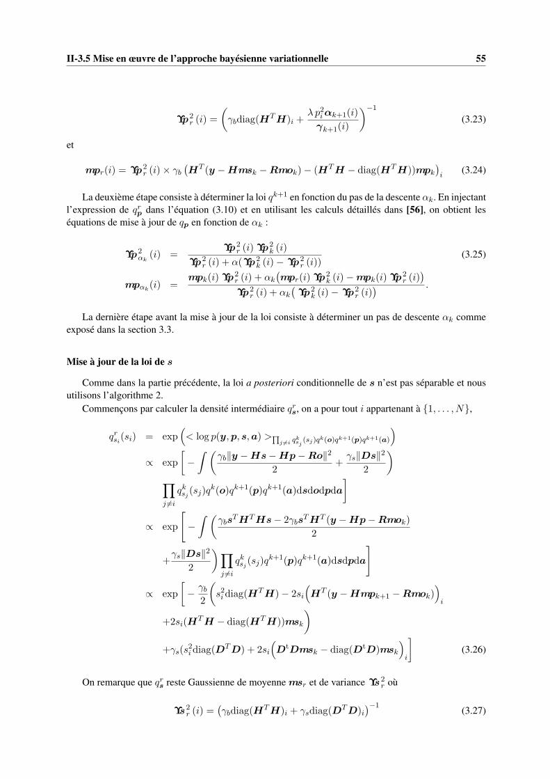
II-3.5 Mise en œuvre de l’approche bayésienne variationnelle 55
Υp2r (i) =
(γbdiag(H
TH)i +λ p2iαk+1(i)
γk+1(i)
)−1
(3.23)
et
mpr(i) = Υp2r (i)× γb
(HT (y −Hmsk −Rmok)− (HTH − diag(HTH))mpk
)i
(3.24)
La deuxième étape consiste à déterminer la loi qk+1 en fonction du pas de la descente αk. En injectantl’expression de qrp dans l’équation (3.10) et en utilisant les calculs détaillés dans [56], on obtient leséquations de mise à jour de qp en fonction de αk :
Υp2αk
(i) =Υp2
r (i) Υp2k (i)
Υp2r (i) + α(Υp2
k (i)− Υp2r (i))
(3.25)
mpαk(i) =
mpk(i) Υp2r (i) + αk
(mpr(i) Υp
2k (i)−mpk(i) Υp
2r (i)
)
Υp2r (i) + αk
(Υp2
k (i)− Υp2r (i)
) .
La dernière étape avant la mise à jour de la loi consiste à déterminer un pas de descente αk commeexposé dans la section 3.3.
Mise à jour de la loi de s
Comme dans la partie précédente, la loi a posteriori conditionnelle de s n’est pas séparable et nousutilisons l’algorithme 2.
Commençons par calculer la densité intermédiaire qrs, on a pour tout i appartenant à 1, . . . , N,
qrsi(si) = exp(< log p(y,p, s,a) >∏
j 6=i qksj(sj)qk(o)qk+1(p)qk+1(a)
)
∝ exp
[−∫ (
γb‖y −Hs−Hp−Ro‖22
+γs‖Ds‖2
2
)
∏
j 6=i
qksj (sj)qk(o)qk+1(p)qk+1(a)dsdodpda
]
∝ exp
[−∫ (
γbsTHTHs− 2γbs
THT (y −Hp−Rmok)
2
+γs‖Ds‖2
2
)∏
j 6=i
qksj (sj)qk+1(p)qk+1(a)dsdpda
]
∝ exp
[− γb
2
(s2i diag(H
TH)− 2si
(HT (y −Hmpk+1 −Rmok)
)i
+2si(HTH − diag(HTH))msk
)
+γs(s2i diag(D
TD) + 2si
(DtDmsk − diag(DtD)msk
)i
](3.26)
On remarque que qrs reste Gaussienne de moyenne msr et de variance Υs2r où
Υs2r (i) =
(γbdiag(H
TH)i + γsdiag(DTD)i
)−1(3.27)

56 Bayesien Variationnel
et
msr(i) = Υs2r (i)× γb
[HT (y −Hmpk+1 −Rmok) (3.28)
− (HTH − diag(HTH))msk −γsγb
(DTD − diag(DTD))msk
]
i
On remarque ici que la variance est constante ce qui facilite le calcul. Le reste des calculs est similaireà la partie 3.5.2.
Calcul de mise à jour de la loi de o
En procédant de manière identique aux parties précédentes, on obtient les équations de mise à joursuivantes pour les paramètres de la loi intermédiaire :
Υo2r (i) =
(γbdiag(R
TR)i + γo)−1
(3.29)
et
mor(i) = Υo2r (i)× γb
[RT (y −Hmpk −Hmsk) +
γsγbom
]
i
(3.30)
3.6 Résultats
Cette partie vise à montrer, d’une part l’efficacité de l’approche gradient exponentiel pour résoudre demanière non-supervisée des problèmes de grande dimension et d’autre part le pouvoir de séparation entreles avant plans (composante impulsionnelle) et le fond diffus cosmologique (composante régulière). Pource faire, nous allons dans un premier temps simuler des données dans la configuration de données réelles,c’est-à-dire qu’il y a 4 millions d’observations pour estimer 700 000 inconnues. Nous avons simulé àpartir d’une carte d’émission étendue mesurée par Herschel, à laquelle nous avons ajouté des sourcesponctuelles. Après cette validation, nous avons appliqué notre approche à des données réelles. Nousverrons que l’apport de notre approche en terme de résolution et de correction d’artefacts est flagrant.
Tout d’abord, un des points que nous n’avons pas abordé dans ce chapitre, est le réglage des hyper-paramètres. Ce réglage est particulièrement fastidieux dans le cas de la reconstruction et de la séparationconjointe de deux composantes car il y a alors quatre paramètres à régler, à savoir γb, γo, γs et λ. Onconsidère ici que le paramètre de forme de la loi de Student ν n’a pas besoin d’être réglé, il suffit deprendre une valeur permettant de favoriser les impulsions. Nous avons donc développé une approche oùles quatre hyperparamètres cités ci-dessus sont estimés conjointement aux deux cartes s, p et aux offsetso.
3.6.1 Données simulées
Nous présentons ici deux expérimentations numériques. Dans ces expériences, nous avons construitune image vraie à partir de deux composantes puis nous avons généré des données à l’aide de notremodèle direct en ajoutant un bruit blanc Gaussien identiquement distribué. Dans ces cas, nous n’avonspas ajouté d’offset o afin de rendre l’analyse des résultats plus facile.
La première expérimentation est une simulation réaliste. On a donc pris comme vraie carte d’émis-sion étendue, une carte reconstruite via le code officiel du consortium Herschel à partir de données réelles(voir figure 3.1 (a)). Puis, nous avons ajouté des sources qui sont légèrement étendues, à savoir un disquede 5 pixels sur-résolu de diamètre, voir figure 3.2 (a)). Nous avons ensuite simulé des données grâce à

II-3.6 Résultats 57
notre modèle direct puis nous avons ajouté un bruit Gaussien iid d’écart type 0, 035, qui correspond auniveau de bruit observé sur les données réelles.
La deuxième expérience numérique a comme objectif de tester le fonctionnement de l’approchequand la composante étendue est nulle et de vérifier que la position des sources est bien retrouvée et quela photométrie, i.e. l’énergie de la source, est conservée.
Simulation réaliste
Un point particulièrement important pour les approches bayésiennes variationnelles est l’initialisa-tion. Dans cet exemple, nous avons initialisé les moyennes mp à zéro et ms avec la carte issue del’algorithme de ESA déconvoluée. Les variances ont été initialisées à partir d’une estimation empiriquede la variance du bruit, σb, obtenu par le résidu issu de l’initialisation des moyennes. On prend alorsΥp égal à σb et Υs égal à σb/10. Après convergence, lorsque l’évolution de l’énergie libre négative estinférieure à un seuil déterminé, nous obtenons les résultats des figures 3.1 (b) et 3.2 (b).
(a) (b)
FIGURE 3.1 – Composante étendue s : (a) vraie carte utilisée pour simuler les données (b) carte recons-truite avec notre approche
On remarque que nous avons bien séparé la composante étendue de la composante impulsionnelle.Au delà de la séparation des sources, on arrive aussi à augmenter la qualité d’image reconstruite. Pourvoir cela, nous sommons la composante étendue et la composante impulsionnelle et nous comparons lerésultat obtenu, figure 3.3 (d), avec la méthode fournie par l’ESA, figure 3.3 (b), et une méthode où lavraisemblance est identique à notre approche mais où l’on utilise un a priori Gaussien sur les gradientsde l’image, figure 3.3 (c). On voit clairement que l’a priori favorisant les impulsions permet d’exploiterau maximum le modèle sur-résolu. De plus, la composante impulsionnelle est très proche de la vraie,voir figure 3.3 (a).
Étude de la reconstruction des pics
Cette deuxième étude a deux objectifs. D’une part, nous voulons déterminer le comportement de laméthode en l’absence de composante étendue. D’autre part, nous souhaitons obtenir un résultat quan-titatif sur la qualité de reconstruction des pics, leur position et le respect de la photométrie (énergie
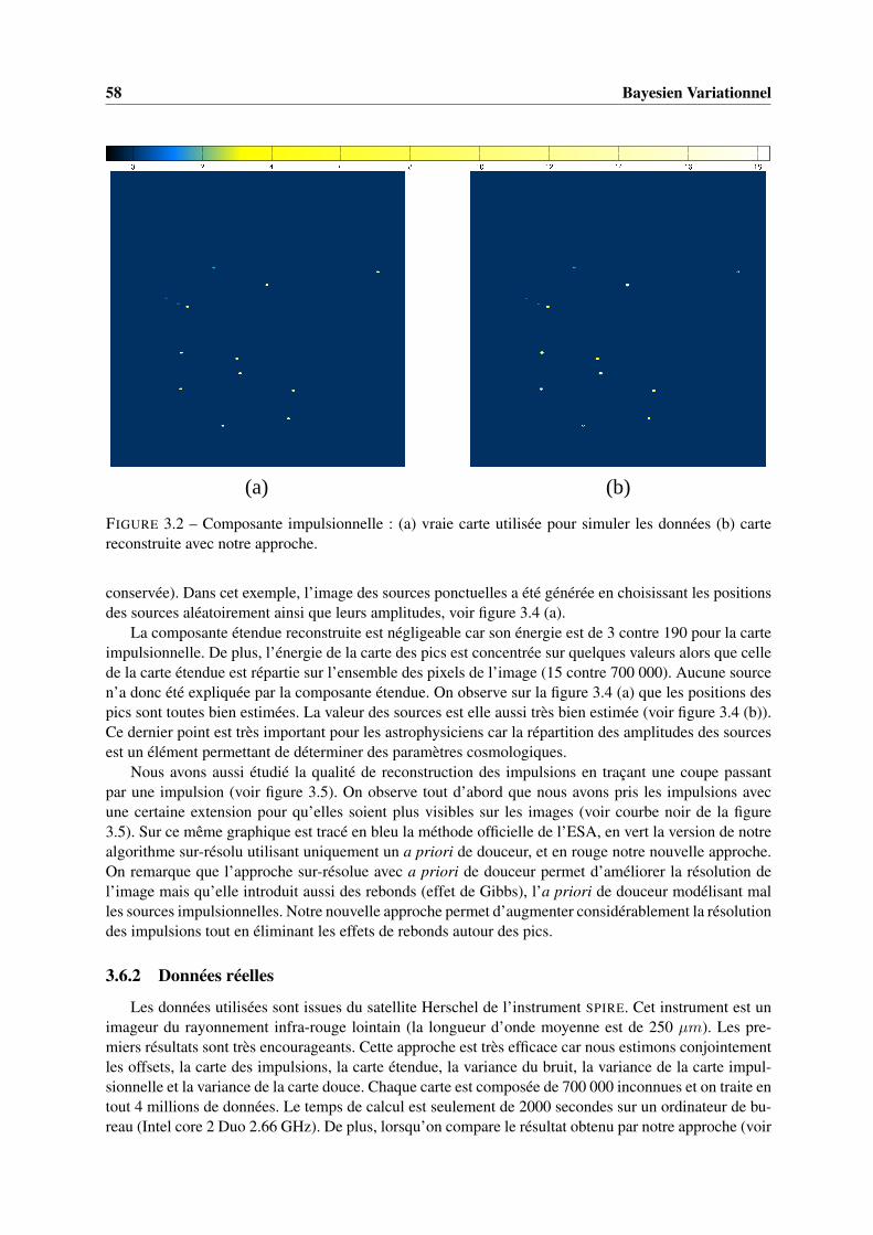
58 Bayesien Variationnel
(b)(a)
FIGURE 3.2 – Composante impulsionnelle : (a) vraie carte utilisée pour simuler les données (b) cartereconstruite avec notre approche.
conservée). Dans cet exemple, l’image des sources ponctuelles a été générée en choisissant les positionsdes sources aléatoirement ainsi que leurs amplitudes, voir figure 3.4 (a).
La composante étendue reconstruite est négligeable car son énergie est de 3 contre 190 pour la carteimpulsionnelle. De plus, l’énergie de la carte des pics est concentrée sur quelques valeurs alors que cellede la carte étendue est répartie sur l’ensemble des pixels de l’image (15 contre 700 000). Aucune sourcen’a donc été expliquée par la composante étendue. On observe sur la figure 3.4 (a) que les positions despics sont toutes bien estimées. La valeur des sources est elle aussi très bien estimée (voir figure 3.4 (b)).Ce dernier point est très important pour les astrophysiciens car la répartition des amplitudes des sourcesest un élément permettant de déterminer des paramètres cosmologiques.
Nous avons aussi étudié la qualité de reconstruction des impulsions en traçant une coupe passantpar une impulsion (voir figure 3.5). On observe tout d’abord que nous avons pris les impulsions avecune certaine extension pour qu’elles soient plus visibles sur les images (voir courbe noir de la figure3.5). Sur ce même graphique est tracé en bleu la méthode officielle de l’ESA, en vert la version de notrealgorithme sur-résolu utilisant uniquement un a priori de douceur, et en rouge notre nouvelle approche.On remarque que l’approche sur-résolue avec a priori de douceur permet d’améliorer la résolution del’image mais qu’elle introduit aussi des rebonds (effet de Gibbs), l’a priori de douceur modélisant malles sources impulsionnelles. Notre nouvelle approche permet d’augmenter considérablement la résolutiondes impulsions tout en éliminant les effets de rebonds autour des pics.
3.6.2 Données réelles
Les données utilisées sont issues du satellite Herschel de l’instrument SPIRE. Cet instrument est unimageur du rayonnement infra-rouge lointain (la longueur d’onde moyenne est de 250 µm). Les pre-miers résultats sont très encourageants. Cette approche est très efficace car nous estimons conjointementles offsets, la carte des impulsions, la carte étendue, la variance du bruit, la variance de la carte impul-sionnelle et la variance de la carte douce. Chaque carte est composée de 700 000 inconnues et on traite entout 4 millions de données. Le temps de calcul est seulement de 2000 secondes sur un ordinateur de bu-reau (Intel core 2 Duo 2.66 GHz). De plus, lorsqu’on compare le résultat obtenu par notre approche (voir

II-3.7 Conclusion 59
figure 3.6 (b)) avec le résultat obtenu par l’algorithme de l’ESA (voir figure 3.6 (a)), on remarque quela résolution est nettement plus importante. Notre méthode, grâce à l’estimation conjointe des offsets,élimine aussi les effets systématiques (oscillations sur le bord des images).
En plus du gain en résolution, nous avons séparé les sources ponctuelles ou légèrement étenduesd’un fond continu. Ces sources sont des galaxies lointaines non résolues par l’instrument. On remarqueque certaines de ces sources non résolues sont expliquées par deux ou trois impulsions. Enfin, grâce àl’estimation conjointe des sources et de la carte étendue, on peut détecter des sources d’amplitude beau-coup plus faible qu’avec des approches de type “clean”. Comme ces approches se basent sur l’estimationd’un maximum dans une carte de résidus, les sources faibles sont détectées lorsque la carte étendue a unniveau important, ce qui n’est pas le cas lorsque le niveau de la carte étendue est faible. Dans ce cadre,notre méthode est donc particulièrement intéressante car elle s’affranchit de ce problème.
3.7 Conclusion
Dans ce chapitre, nous avons montré comment les approches bayésiennes, et plus particulièrementl’approche basée sur le gradient exponentiel adapté au bayésien variationnel, peuvent être utilisées dansle cadre de la reconstruction d’images issues de télescope spatiaux. Plus particulièrement, la méthodedétaillée ici permet de résoudre des problèmes inverses de très grandes dimensions. En effet, on recons-truit ici des cartes de 700 000 pixels avec un ordinateur de bureau, voire 50 millions de pixels sur dessuper-calculateurs. Nous avons montré comment cette approche récente permet de résoudre un problèmed’estimation sur-résolue conjointement à de la séparation de deux composantes : une composante lissereprésentant le fond diffus cosmologique et une composante impulsionnelle, l’avant plan. Cette approchea été mise en œuvre dans le cadre d’un algorithme non supervisé, en exploitant le caractère très parci-monieux de la carte de sources impulsionnelles. Les résultats sur données simulées sont conformes à nosattentes et les résultats sur données réelles sont très bons car nous sommes arrivés à modéliser les effetsprépondérants qui dégradent les reconstructions, en particulier la présence d’offsets sur les bolomètres.Cette approche bayésienne est très prometteuse car elle permet d’étendre les approches non superviséesexploitant de la parcimonie aux problèmes de très grande dimension.

60 Bayesien Variationnel
(b)(a)
(c) (d)
FIGURE 3.3 – Comparaison de différents estimateurs sur la somme des deux composantes : (a) Vraiecarte, (b) carte reconstruite avec le pipeline officiel de l’ESA, (c) carte reconstruite sans bi-modèle avecun a priori de douceur (d) carte reconstruite en utilisant un bi-modèle
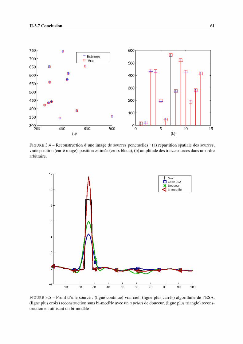
II-3.7 Conclusion 61
FIGURE 3.4 – Reconstruction d’une image de sources ponctuelles : (a) répartition spatiale des sources,vraie position (carré rouge), position estimée (croix bleue), (b) amplitude des treize sources dans un ordrearbitraire.
FIGURE 3.5 – Profil d’une source : (ligne continue) vrai ciel, (ligne plus carrés) algorithme de l’ESA,(ligne plus croix) reconstruction sans bi-modèle avec un a priori de douceur, (ligne plus triangle) recons-truction en utilisant un bi-modèle

62 Bayesien Variationnel
(a) (b)
FIGURE 3.6 – Visualisation de la somme des deux composantes sur les données réelles reconstruites :(a) reconstruction à l’aide de l’algorithme de l’ESA (b) reconstruction bayésienne variationnelle avecbi-modèle
(b)(a)
FIGURE 3.7 – Reconstruction de données réelles avec notre approche : (a) composante impulsionnelle,(b) composante étendue

Chapitre 4
Perspectives
4.1 Inversion de données astrophysiques
Inversion sur-résolue de données issues d’un Spectro-imageur
Nous avons eu de très bons résultats sur l’inversion des données du spectro-imageur IRS/SPITZER.Ce travail a fait l’objet d’une publication dans IEEE Journal of Selected Topics in Signal Processing[118] (reproduit à la page 154). Dans ce travail, la composante spectrale des données est obtenue grâceà un réseau de diffraction placé sur le plan focal du détecteur. Dans les missions lancées récemment :HERCHEL (FTS) ou Mars Express (PFS), on utilise des spectro-imageurs à transformée de Fourier. Leprincipe de ces spectro-imageurs est comparable à celui d’un interféromètre de Michelson. Cette configu-ration leur confère une très bonne résolution et un faible encombrement. L’objectif serait de développerun modèle direct précis comme dans le cas d’IRS, mais aussi de développer une approche bayésienne va-riationnelle permettant d’avoir une solution non-supervisée en un temps réduit. Ces travaux permettrontde tirer le maximum d’information des mesures réalisées. De plus, cette action participera à la diffusiondes approches statistiques dans la communauté des astrophysiciens.
Échantillonnage adaptatif
Les avancées récentes en inférence bayésienne, ont permis de résoudre des nouveaux problèmes quiconstruisent en temps réel un schéma d’échantillonnage optimal vis à vis de l’objet que l’on est en trainde reconstruire («Experimental Design»). Ce problème revient à répondre à la question suivante : Sa-chant que l’on a déjà fait N mesures de notre objet d’intérêt, où doit-on faire la N + 1e mesure pourque cette dernière soit la plus informative possible ? Ces approches ont déjà été introduites par M. Seegerdans le cadre des données IRM [123] et dans un cadre plus général de problèmes de grandes dimensions[122]. Les approches de M. Seeger sont conditionnées par l’utilisation d’un type d’a priori particulierfavorisant la parcimonie. L’approche bayésienne variationnelle permet aussi de résoudre ce problèmed’«Experimental Design», car elle fournit des lois simples appartenant à des familles connues donc fa-cilement marginalisables. L’utilisation d’une plus grande variété de lois a priori et de vraisemblancesserait donc rendue possible par cette approche. Enfin, il serait très pertinent d’appliquer cette méthodo-logie dans le contexte de fabrication de cartes astrophysiques. En effet, pour des raisons de protectioncontre le rayonnement solaire, il y a un laps de temps important entre deux séries de mesures d’une mêmecarte. L’idée serait, après une première acquisition, de déterminer la configuration de mesure optimalepermettant de mesurer uniquement les données nécessaires et ainsi gagner du temps d’acquisition qui estextrêmement coûteux sur ce type d’instrument (la minute de mesure sur le satellite Herschel revient àenviron 7 000 euros).
63

64 Perspectives
4.2 Inversion de données tomographiques
Utilisation du rayonnement diffusé pour discriminer des matériaux
Nous avons présenté dans le § 2.2.2 une méthode permettant de discriminer différents matériaux enutilisant leurs différences d’atténuation en fonction de l’énergie de photon. Une des limitations de cetteapproche est que, pour certains matériaux, la différence d’atténuation est très faible. Par exemple, dansle contexte du contrôle des bagages dans les aéroports, les shampoings ont une atténuation très prochedu plastique (l’explosif).
L’idée serait d’utiliser la différence de diffusion des matériaux pour les séparer. Il faut tout d’abordacquérir une partie du rayonnement diffusé pour avoir un espoir de pouvoir remonter à la fraction derayonnement diffusé en chaque point de l’objet. Il existe des systèmes tomographiques où l’on peut faci-lement mesurer le rayonnement diffusé. Par exemple, les tomographes à faisceau d’électrons «ElectronBeam Computed Tomography» (EBCT) sont constitués d’un anneau de détecteur fixe et le déplacementde la source de rayons X provient du déplacement d’un faisceau d’électrons sur une anode circulaireen périphérie de l’anneau de détection. Ces tomographes sont très utilisés en imagerie cardiaque [4].Le temps d’acquisition d’un jeu de données complètes est inférieur à un cycle cardiaque. La présencede l’anneau complet de détection permet de mesurer simultanément le rayonnement direct sur une por-tion de l’anneau et une partie du rayonnement diffusé sur une autre portion. On peut bien sûr concevoird’autres systèmes tomographiques possédant la même propriété.
Il faut ensuite pouvoir, à partir de ces mesures, connaître la fraction diffusé en chaque point del’image. Pour ce faire, on peut appliquer une approche de type Monte Carlo comme ce qui a été proposédans le cas de l’imagerie PET quantitative [84]. On peut aussi concevoir des méthodes d’inversion ens’inspirant des travaux de M. NGUYEN sur l’imagerie SPECT [95]. En réalité, la connaissance de ladiffusion a un intérêt supplémentaire en plus de son pouvoir de discrimination : elle permet de détermi-ner précisément l’atténuation effective des matériaux qui composent l’objet, car, comme nous l’avonsexpliqué dans la remarque du § 2.2.2, il est important de connaître la fraction de rayonnement diffuséqui se mélange au rayonnement direct dans nos mesures. Dans ce contexte, le développement d’uneméthode d’estimation de l’abondance de différents matériaux en utilisant conjointement l’informationd’atténuation et de diffusion paraît très pertinente.
Traitement récursif des données tomographiques 3D + T
Comme nous l’avons vu dans le § 2.3, la reconstruction 3D + T de la couronne solaire nécessiteun temps de calcul très important. De plus, les satellites STEREO A et STEREO B délivrent un flotquasiment continu de mesures. Dans le cadre de l’imagerie médicale nous avons affaire au même typede problème lorsque l’on veut développer un système de tomofluoroscopie 3D [115][64][15]. Dans lesdeux exemples précédents, on aimerait appliquer une approche de type filtre de Kalman afin de réduire lecoût de calcul et d’avoir une approche cohérente pour reconstruire un flot continu de données. Malheu-reusement le nombre d’inconnues est très important, donc la matrice de covariance des estimées n’estpas stockable en mémoire vive. En conséquence la mise à jour récursive de la matrice de covariance estimpossible, car nous devons calculer son inverse à chaque itération. Les travaux de BUTULA et al. [18]résolvent partiellement ce problème de mise à jour en estimant de manière empirique la nouvelle matricede covariance à partir d’un ensemble d’échantillons qui ont été mis à jour. Cependant, cette approchefonctionne uniquement sur des problèmes de dimension encore trop faible. De plus, contrairement à l’es-timation d’une moyenne, il faut beaucoup d’échantillons pour estimer de manière fiable une matrice decovariance de grande dimension.
L’approche que l’on propose consiste à se placer dans un cadre bayésien variationnel. En effet, onpeut y développer facilement des approches récursives [129][130]. Si l’on choisit un degré de séparabi-lité maximum associé à l’approche que nous avons exposée dans le chapitre 3 [56], on s’affranchit de

II-4.3 Méthodologie bayésienne variationnelle 65
la matrice de covariance. La mise à jour de la matrice de covariance est remplacée par la mise à jourd’un vecteur de variance qui a la même taille que le vecteur des inconnues. Des résultats préliminairesde cette approche ont déjà été présentés sur un problème 2D + T à «the International Conference Acous-tics, Speech and Signal Processing» [2]. Il serait intéressant d’appliquer cette approche sur des donnéesréelles 3D + T, afin de comparer les performances de cette nouvelle approche par rapport à celles exis-tantes. Dans ces premiers travaux, nous avons uniquement résolu un problème où la loi a posteriori étaitGaussienne (ce qui correspond au filtre de Kalman), il serait très intéressant d’appliquer l’approche pourdes lois a posteriori non Gaussiennes comme par exemple celles présentées dans le § 2.3.3 et le § 3.4.Cette approche pourrait palier les problèmes rencontré avec le filtrage particulaire [44] lorsque le nombred’inconnues est trop important.
4.3 Méthodologie bayésienne variationnelle
Amélioration de l’approche gradient
Ce travail se fera dans le cadre de la thèse de Yuling Zheng. Il s’inscrit dans la continuité du travaildéjà entamé sur l’accélération des approches bayésiennes variationnelles exposées dans le chapitre 3 etl’article [56]. Dans ces travaux, nous avons déterminé le gradient de notre fonctionelle puis un pas sousoptimum de descente. Dans le cas de l’optimisation en dimension finie pour accélérer les algorithmes dedescente, on peut soit appliquer un préconditionneur, soit déterminer un pas de descente optimum, soitdéterminer une direction de descente plus efficace que l’opposé du gradient. Nous travaillerons ici sur lechoix de la direction de descente. Une première idée serait d’utiliser des directions de descente conju-guées (gradient conjugué) car c’est l’approche la plus répandue en dimension finie. La transposition decette approche dans notre problème d’optimisation fonctionnelle est beaucoup plus compliquée qu’il n’yparait. En effet, l’espace dans lequel nous cherchons à optimiser n’est pas un espace vectoriel, donc iln’existe pas de produit scalaire donc pas de conjugaison. L’idée est de transposer les approches de des-cente à mémoire qui sont clairement exposées dans la thèse d’E. CHOUZENOUX [29]. Ces algorithmesréduisent de manière importante le nombre d’itérations mais le coût de calcul d’une itération augmenteaussi fortement. Il faudra donc déterminer si ces méthodes sont pertinentes pour notre problème d’opti-misation.
Estimation robuste
On pourrait appliquer l’algorithme présenté dans le chapitre 3 à l’estimation robuste. En effet, dansbeaucoup de systèmes nous voulons avoir une estimation qui est robuste aux données aberrantes. L’uti-lisation d’une vraisemblance gaussienne ne permet pas d’avoir une telle propriété. L’idée est de trouverune vraisemblance possédant des bonnes propriétés de conjugaison, ce qui est une condition nécessairepour pouvoir appliquer l’approche bayésienne variationnelle. La vraisemblance doit être une loi à queuelourde afin de posséder la propriété de robustesse. Dans le cas de mesures positives nous pouvons sansdoute obtenir de bons résultats en utilisant une vraisemblance Gamma.
Approches bayesiennes variationnelles et dictionnaire à base d’ondelettes
Nous pouvons aussi appliquer notre nouvelle méthodologie bayésienne variationnelle aux diction-naires fortement redondants par exemple les ondelettes non décimées. Les ondelettes non décimées sontdéjà très largement utilisées dans le domaine du débruitage d’images [24]. Il est évident qu’un schémaoptimal de seuillage des coefficients d’ondelettes est de déterminer un seuil par type de coefficient (type,échelle). La difficulté de cette approche réside dans le fait qu’il faut déterminer un nombre important deseuils (environ 10 seuils pour seulement trois niveaux décomposition). Lorsque l’on résout un problème

66 Perspectives
de débruitage, on peut utiliser les méthodes d’approximation de l’erreur quadratique moyenne en utili-sant le lemme de Stein [87] qui donnent de très bon résultats. Ces approches restent applicables dans lecas de la déconvolution [26][109], par contre on ne peut pas les appliquer à des problèmes inverses degrande dimension.
(a) (b)
(c) (d)
FIGURE 4.1 – Débruitage d’image : (a) Données bruitées SNR 20 db, (b) seuillage dur avec le seuiluniversel SNR 21,97 db, (c) meilleure image obtenue avec le seuillage dur 28,00 db, (d) notre approchequi détermine des «seuils» adaptatifs 27,35 db
Nous avons développé une approche permettant d’estimer conjointement les coefficients d’onde-lettes et les paramètres pour chaque type d’ondelette. Pour l’instant, nous avons uniquement fait uneexpérimentation sur un problème de débruitage d’image. Les données bruitées de la Fig. 4.1 (a) ont étéobtenues en ajoutant un bruit i.i.d. Gaussien à l’image Lena afin d’obtenir un SNR de 20 db. On utilise

II-4.4 Sélection de modèles 67
(a) (b)
FIGURE 4.2 – Zoom correspondant au carré rouge dans la figure 4.1 : (a) meilleure image obtenue avecle seuillage dur, (b) notre approche
un dictionnaire d’ondelettes basé sur une transformée non décimée (Symlet 4).On compare notre approche Fig. 4.1 (d) avec le seuillage dur sur le même dictionnaire utilisant le
seuil universel Fig. 4.1(b) et en utilisant le seuil qui minimise le SNR Fig. 4.1(c) 1. On observe que notreapproche permet d’avoir une qualité d’image comparable (SNR 27,35 db contre SNR 28 db en utilisant lemeilleur seuil). De plus, quand on regarde les zooms sur la Fig. 4.2 (a) et la Fig. 4.2 (b), on observe queles artefacts de seuillage dur sont moins visibles dans notre approche.
Le travail qui reste à mener, seraient dans un premier temps de comparer notre méthode avec lesapproches utilisant le lemme de Stein. Ensuite, on pourrait appliquer cette approche à des problèmes in-verses linéaires (déconvolution, inpainting, sur-résolution, inversion de données tomographiques etc....).
4.4 Sélection de modèles
Dans cette partie, nous aborderons le choix (ou la sélection) de modèles dans deux cas distincts.Le premier correspond au choix entre un petit nombre de modèles connus à l’avance. L’objectif est dedéterminer le meilleur modèle vis à vis des données collectées. Dans le deuxième cas, le nombre de mo-dèles concurrents est théoriquement infini. Il s’agit de déterminer la paramétrisation discrète (calculableet stockable sur un ordinateur) associée à une grandeur observée continue. Le choix du modèle dans cecas revient à choisir le nombre de paramètres qui vont décrire la grandeur continue.
Choix entre un faible nombre de modèles
Le choix entre les différents modèles se fait en calculant l’évidence p(y|Mi) de chaque modèle. Lemodèle qui maximise l’a posteriori du modèle sera retenu. L’a posteriori du modèle se détermine à uneconstante près très simplement comme le produit de l’évidence par l’a priori sur le modèle. En pratique, ilest très difficile de calculer l’évidence d’un modèle, car on connaît de manière explicite uniquement la loi
1. il faut connaître la vraie image pour obtenir ce résultat
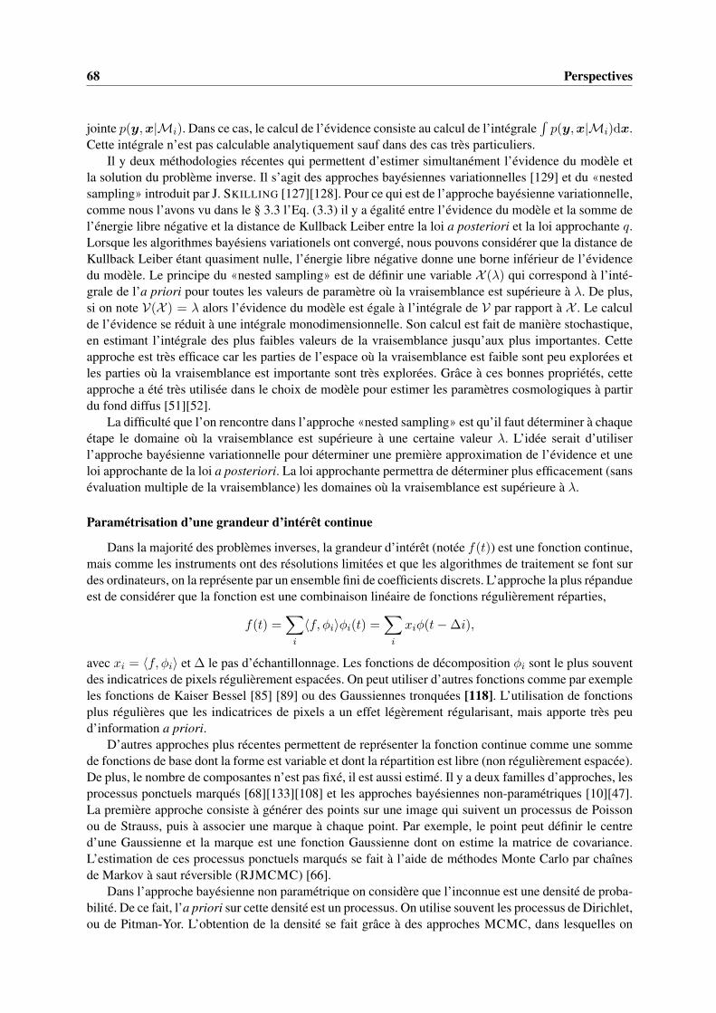
68 Perspectives
jointe p(y,x|Mi). Dans ce cas, le calcul de l’évidence consiste au calcul de l’intégrale∫p(y,x|Mi)dx.
Cette intégrale n’est pas calculable analytiquement sauf dans des cas très particuliers.Il y deux méthodologies récentes qui permettent d’estimer simultanément l’évidence du modèle et
la solution du problème inverse. Il s’agit des approches bayésiennes variationnelles [129] et du «nestedsampling» introduit par J. SKILLING [127][128]. Pour ce qui est de l’approche bayésienne variationnelle,comme nous l’avons vu dans le § 3.3 l’Eq. (3.3) il y a égalité entre l’évidence du modèle et la somme del’énergie libre négative et la distance de Kullback Leiber entre la loi a posteriori et la loi approchante q.Lorsque les algorithmes bayésiens variationels ont convergé, nous pouvons considérer que la distance deKullback Leiber étant quasiment nulle, l’énergie libre négative donne une borne inférieur de l’évidencedu modèle. Le principe du «nested sampling» est de définir une variable X (λ) qui correspond à l’inté-grale de l’a priori pour toutes les valeurs de paramètre où la vraisemblance est supérieure à λ. De plus,si on note V(X ) = λ alors l’évidence du modèle est égale à l’intégrale de V par rapport à X . Le calculde l’évidence se réduit à une intégrale monodimensionnelle. Son calcul est fait de manière stochastique,en estimant l’intégrale des plus faibles valeurs de la vraisemblance jusqu’aux plus importantes. Cetteapproche est très efficace car les parties de l’espace où la vraisemblance est faible sont peu explorées etles parties où la vraisemblance est importante sont très explorées. Grâce à ces bonnes propriétés, cetteapproche a été très utilisée dans le choix de modèle pour estimer les paramètres cosmologiques à partirdu fond diffus [51][52].
La difficulté que l’on rencontre dans l’approche «nested sampling» est qu’il faut déterminer à chaqueétape le domaine où la vraisemblance est supérieure à une certaine valeur λ. L’idée serait d’utiliserl’approche bayésienne variationnelle pour déterminer une première approximation de l’évidence et uneloi approchante de la loi a posteriori. La loi approchante permettra de déterminer plus efficacement (sansévaluation multiple de la vraisemblance) les domaines où la vraisemblance est supérieure à λ.
Paramétrisation d’une grandeur d’intérêt continue
Dans la majorité des problèmes inverses, la grandeur d’intérêt (notée f(t)) est une fonction continue,mais comme les instruments ont des résolutions limitées et que les algorithmes de traitement se font surdes ordinateurs, on la représente par un ensemble fini de coefficients discrets. L’approche la plus répandueest de considérer que la fonction est une combinaison linéaire de fonctions régulièrement réparties,
f(t) =∑
i
〈f, φi〉φi(t) =∑
i
xiφ(t−∆i),
avec xi = 〈f, φi〉 et ∆ le pas d’échantillonnage. Les fonctions de décomposition φi sont le plus souventdes indicatrices de pixels régulièrement espacées. On peut utiliser d’autres fonctions comme par exempleles fonctions de Kaiser Bessel [85] [89] ou des Gaussiennes tronquées [118]. L’utilisation de fonctionsplus régulières que les indicatrices de pixels a un effet légèrement régularisant, mais apporte très peud’information a priori.
D’autres approches plus récentes permettent de représenter la fonction continue comme une sommede fonctions de base dont la forme est variable et dont la répartition est libre (non régulièrement espacée).De plus, le nombre de composantes n’est pas fixé, il est aussi estimé. Il y a deux familles d’approches, lesprocessus ponctuels marqués [68][133][108] et les approches bayésiennes non-paramétriques [10][47].La première approche consiste à générer des points sur une image qui suivent un processus de Poissonou de Strauss, puis à associer une marque à chaque point. Par exemple, le point peut définir le centred’une Gaussienne et la marque est une fonction Gaussienne dont on estime la matrice de covariance.L’estimation de ces processus ponctuels marqués se fait à l’aide de méthodes Monte Carlo par chaînesde Markov à saut réversible (RJMCMC) [66].
Dans l’approche bayésienne non paramétrique on considère que l’inconnue est une densité de proba-bilité. De ce fait, l’a priori sur cette densité est un processus. On utilise souvent les processus de Dirichlet,ou de Pitman-Yor. L’obtention de la densité se fait grâce à des approches MCMC, dans lesquelles on

II-4.4 Sélection de modèles 69
utilise des échantillonneurs spécifiques («stick-breaking») afin de gérer les problèmes de troncature deslois.
La limitation de ces approches réside dans la complexité de calculs lorsque que le nombre de fonc-tions de base devient élevé (> 10 000). L’idée serait par exemple d’étendre le modèle de reconstructionet de séparation conjointe de sources ponctuelles et de sources étendues décrit dans [7] par un modèlevariationnel pour la composante étendue et un modèle non paramétrique pour la composante impulsion-nelle. Nous limiterions ainsi le nombre de fonctions de base et nous pourrions accéder comme cela à laposition des étoiles avec une précision sub-pixelique. Des premiers travaux sur des modèles très simples(AR) ont déjà proposé de combiner non paramétrique et bayésien variationnel [92].

70 Perspectives

Bibliographie
[1] S. Achenbach, D. Ropers, A. Kuettner, T. Flohr, B. Ohnesorge, H. Bruder, H. Theessen, M. Kara-kaya, W. G. Daniel, W. Bautz, et al. Contrast-enhanced coronary artery visualization by dual-source computed tomography-initial experience. European Journal of Radiology, 57(3) :331–335,2006.
[2] B. Ait el Fquih and T. Rodet. Variational bayesian Kalman filtering in dynamical tomography. InProceedings of the International Conference on Acoustic, Speech and Signal Processing, pages4004 – 4007, Prague, mai 2011.
[3] H. Alfvén. Existence of electromagnetic-hydrodynamic waves. Nature, 150(3805) :405–412,1942.
[4] Y. Arad, L. A. Spadaro, K. Goodman, D. Newstein, and A. D. Guerci. Prediction of coronaryevents with electron beam computed tomography. Journal of the American College of Cardiology,36(4) :1253–1260, 2000.
[5] H. Ayasso. Une approche bayésienne de l’inversion. Application à l’imagerie de diffraction dansles domaines micro-onde et optique. Thèse de Doctorat, Université Paris Sud, décembre 2010.
[6] H. Ayasso and A. Mohammad-Djafari. Joint NDT image restoration and segmentation usinggauss-markov-potts prior models and variational bayesian computation. IEEE Transactions onImage Processing, 19(9) :2265 – 2277, septembre 2010.
[7] H. Ayasso, T. Rodet, and A. Abergel. A variational bayesian approach for unsupervised super-resolution using mixture models of point and smooth sources applied to astrophysical mapmaking.Technical report, LSS, 33 pages, 2012. Submitted to Inverses Problem.
[8] S. D. Babacan, R. Molina, and A. K. Katsaggelos. Variationnal Bayesian Blind DeconvolutionUsing a Total Variation Prior. IEEE Transactions on Image Processing, 18(1) :12–26, janvier2009.
[9] N. Bali and A. Mohammad-Djafari. Bayesian approach with hidden Markov modeling and meanfield approximation for hyperspectral data analysis. IEEE Transactions on Image Processing,17(2) :217–225, Feb. 2008.
[10] E. Barat, T. Dautremer, and T. Montagu. Nonparametric bayesian inference in nuclear spectro-metry. In Proceedings of IEEE Medical Imaging Conference, volume 1, pages 880–887. IEEE,2007.
[11] N. Barbey. Détermination de la structure tridimensionnelle de la couronne solaire à partird’images des missions spatiales SoHO et STEREO. Thèse de Doctorat, Université Paris–sud 11,Orsay, décembre 2008.
[12] N. Barbey, F. Auchère, T. Rodet, and J.-C. Vial. A time-evolving 3D method dedicated tothe reconstruction of solar plumes and results using extreme ultra-violet data. Solar Physics,248(2) :409–423, avril 2008.
[13] P. Bleuet. Reconstruction 3D par tomosynthèse généralisée. Application à l’imagerie médicalepar rayons X. Thèse de Doctorat, Institut National des Sciences Appliquées de Lyon, 2002.
71
72 BIBLIOGRAPHIE
[14] C. Blondel, R. Vaillant, G. Malandain, and N. Ayache. 3D tomographic reconstruction of coronaryarteries using a precomputed 4D motion field. Physics in Medicine and Biology, 49 :2197–2208,2004.
[15] S. Bonnet, A. Koenig, S. Roux, P. Hugonnard, R. Guillemaud, and P. Grangeat. Dynamic X-raycomputed tomography. Proceedings of the IEEE, 91(10) :1574–1587, 2003.
[16] C. Bontus, T. Kohler, and R. Proksa. EnPiT : filtered back-projection algorithm for helical CTusing an n-Pi acquisition. IEEE Transactions on Medical Imaging, 24(8) :977–986, 2005.
[17] D. Brasse, P. E. Kinahan, R. Clackdoyle, M. Defrise, C. Comtat, and D. W. Townsend. Fast fully3-D image reconstruction in PET using planograms. IEEE Transactions on Medical Imaging,23(4) :413–425, avril 2004.
[18] M. D. Butala, F. Kamalabadi, R. A. Frazin, and Y. Chen. Dynamic tomographic imaging of thesolar corona. IEEE Journal of Selected Topics in Signal Processing, 2(5) :755–766, 2008.
[19] C. Cai, A. Mohammad-Djafari, S. Legoupil, and T. Rodet. Bayesian data fusion and inversion inX–ray multi–energy computed tomography. In Proceedings of the International Conference onImage Processing, pages 1377 – 1380, septembre 2011.
[20] C. Cai, T. Rodet, S. Legoupil, and A. Mohammad-Djafari. Bayesian reconstruction of water andbone fractions in polychromatic multi-energy computed tomography. Soumis à Medical Physics,2012.
[21] J.-F. Cardoso. Blind signal separation : statistical principles. Proceedings of the IEEE, 9 :2009–2025, 1998.
[22] P. J. Cargill and J. A. Klimchuk. Nanoflare heating of the corona revisited. The AstrophysicalJournal, 605 :911–920, 2004.
[23] F. Champagnat and J. Idier. A connection between half-quadratic criteria and EM algorithm. IEEESignal Processing Letters, 11(9) :709–712, septembre 2004.
[24] S. G. Chang, B. Yu, and M. Vetterli. Adaptive wavelet thresholding for image denoising andcompression. IEEE Transactions on Image Processing, 9(9) :1532–1546, 2000.
[25] G. Chantas, N. Galatsanos, A. Likas, and M. Saunders. Variational Bayesian image restora-tion based on a product of t-distributions image prior. IEEE Transactions on Image Processing,17(10) :1795–1805, octobre 2008.
[26] C. Chaux, L. Duval, A. Benazza-Benyahia, and J.-C. Pesquet. A nonlinear stein based estimatorfor multichannel image denoising. IEEE Transactions on Signal Processing, 56(8) :3855–3879,août 2008.
[27] S. S. Chen, D. L. Donoho, and M. A. Saunders. Atomic decomposition by basis pursuit. Technicalreport, Stanford University, février 1996.
[28] R. A. Choudrey. Variational Methods for Bayesian Independent Component Analysis. Thèse deDoctorat, University of Oxford, 2002.
[29] E. Chouzenoux. Recherche de pas par Majoration-Minoration. Application à la résolution deproblèmes inverses. Thèse de Doctorat, École Centrale de Nantes, 2010.
[30] P. Ciuciu, J. Idier, and J.-F. Giovannelli. Analyse spectrale non paramétrique haute résolution. InActes du 17 e colloque GRETSI, pages 721–724, Vannes, septembre 1999.
[31] P. Comon and C. Jutten. Handbook of Blind Source Separation : Independent component analysisand applications. Academic Press, 2010.
[32] P. Comon, C. Jutten, and J. Herault. Blind separation of sources, part II : Problems statement.Signal processing, 24(1) :11–20, 1991.

BIBLIOGRAPHIE 73
[33] P. E. Danielsson, P. Edholm, J. Eriksson, and M. Magnusson. Towards exact reconstruction forhelical cone-beam scanning of long objects. a new detector arrangement and a new completenesscondition. In DW Townsend and PE Kinahan, editors, Proc. 1997 Meeting on Fully 3D ImageReconstruction in Radiology and Nuclear Medicine, pages 141–144, 1997.
[34] B. De Man. Iterative Reconstruction for Reduction of Metal Artifacts in Computed Tomography.Thèse de Doctorat, Katholieke Universiteit Leuven (Belgium), 2001.
[35] B. De Man and S. Basu. Distance-driven projection and backprojection in three dimensions.Physics in Medicine and Biology, 49(11) :2463–75, juin 2004.
[36] B. De Man, J. Nuyts, P. Dupont, G. Marchal, and P. Suetens. Reduction of metal streak arti-facts in x-ray computed tomography using a transmission maximum a posteriori algorithm. InProceedings of IEEE Medical Imaging Conference, volume 2, pages 850–854. IEEE, 1999.
[37] B. De Man, J. Nuyts, P. Dupont, G. Marchal, and P. Suetens. An iterative maximum-likelihoodpolychromatic algorithm for CT. IEEE Transactions on Medical Imaging, 20(10) :999–1008,2001.
[38] C. De Mol and M. Defrise. Inverse imaging with mixed penalties. In URSI Symposium on Elec-tromagnetic Theory, pages 798–800, Pisa Italie, 2004. Ed. PLUS Univ. Pisa.
[39] G. Del Zanna, B. J. I. Bromage, and H. E. Mason. Spectroscopic characteristics of polar plumes.Astronomy and Astrophysics, 398(2) :743–761, 2003.
[40] G. Demoment. Image reconstruction and restoration : Overview of common estimation struc-ture and problems. IEEE Transactions on Acoustics, Speech and Signal Processing, ASSP-37(12) :2024–2036, décembre 1989.
[41] G. Demoment, J. Idier, J.-F. Giovannelli, and A. Mohammad-Djafari. Problèmes inverses entraitement du signal et de l’image. volume TE 5 235 of Traité Télécoms, pages 1–25. Techniquesde l’Ingénieur, Paris, 2001.
[42] L. Desbat. Efficient sampling on coarse grids in tomography. Inverse Problems, 9 :1141–1148,1993.
[43] L. Desbat. Échantillonnage efficace en tomographie. Habilitation à diriger des recherches, Uni-versité Joseph Fourier - Grenoble I, Octobre 1997.
[44] A. Doucet, S. Godsill, and C. Andrieu. On sequential Monte Carlo sampling methods for Bayesianfiltering. Statistics and Computing, 10(3) :197–208, 2000.
[45] I. A. Elbakri and J. A. Fessler. Segmentation-free statistical image reconstruction for polyenergeticX-ray computed tomography with experimental validation. Physics in Medicine and Biology,48 :2453, 2003.
[46] H. Erdogan and J. A. Fessler. Monotonic algorithms for transmission tomography. IEEE Tran-sactions on Medical Imaging, 18(9) :801–814, septembre 1999.
[47] M. D. Fall. Modélisation stochastique de processus pharmaco-cinétiques, applications à la re-construction tomographique par émission de positrons (TEP) spatio-temporelle. Thèse de Docto-rat, Université Paris-Sud 11, 2012.
[48] L. A. Feldkamp, L. C. Davis, and J. W. Kress. Practical cone-beam algorithm. Journal of theOptical Society of America (A), 1(6) :612–619, 1984.
[49] U. Feldman, E. Landi, and N. A. Schwadron. On the sources of fast and slow solar wind. Journalof Geophysical Research, 110(A07109) :1–12, 2005.
[50] R. Fergus, B. Singh, A. Hertzmann, S. T. Roweis, and W. T. Freeman. Removing camera shakefrom a single photograph. ACM Transactions on Graphics (TOG), 25(3) :787–794, 2006.

74 BIBLIOGRAPHIE
[51] F. Feroz and M. P. Hobson. Multimodal nested sampling : an efficient and robust alternative toMarkov Chain Monte Carlo methods for astronomical data analyses. Monthly Notices of the RoyalAstronomical Society, 384(2) :449–463, 2008.
[52] F. Feroz, M. P. Hobson, and M. Bridges. MultiNest : an efficient and robust bayesian inferencetool for cosmology and particle physics. Monthly Notices of the Royal Astronomical Society,398(4) :1601–1614, 2009.
[53] J. A. Fessler. Penalized weighted least-squares image reconstruction for positron emission tomo-graphy. IEEE Transactions on Medical Imaging, 13(2) :290–300, 1994.
[54] J. A. Fessler, I. A. Elbakri, P. Sukovic, and N. H. Clinthorne. Maximum-likelihood dual-energytomographic image reconstruction. In SPIE Medical Imaging. spie, 2002.
[55] A. Fraysse and T. Rodet. A gradient-like variational bayesian algorithm. In Proceedings of IEEEStatistical Signal Processing Workshop (SSP), number S17.5, pages 605 – 608, Nice, France, juin2011.
[56] A. Fraysse and T. Rodet. A measure-theoretic variational bayesian algorithm for large di-mensional problems. Technical report, LSS UMR 8506, 36 pages, 2012. http ://hal.archives-ouvertes.fr/docs/00/70/22/59/PDF/var_bayV8.pdf.
[57] R. A. Frazin. Tomography of the Solar Corona. I. A Robust, Regularized, Positive EstimationMethod. Astrophysical Journal, 530 :1026–1035, février 2000.
[58] R. A. Frazin and P. Janzen. Tomography of the Solar Corona. II. Robust, Regularized, PositiveEstimation of the Three-dimensional Electron Density Distribution from LASCO-C2 PolarizedWhite-Light Images. Astrophysical Journal, 570 :408–422, mai 2002.
[59] N. Gac, A. Mohammad-Djafari, A. Vabre, and F. Buyens. GPU implementation of a 3D bayesianCT algorithm and its application on real foam reconstruction. In First international conference onimage formation in X-ray computes tomography, Salt lake city, USA, June 2010.
[60] H. Gao, H. Yu, and G. Wang. Multi-energy CT based on a prior rank, intensity and sparsitymodel (PRISM). In Meeting on Fully Three-Dimensional Image Reconstruction in Radiology andNuclear Medicine, pages 124–7, Postdam, Germany, juillet 2011.
[61] J.-F. Giovannelli. Unsupervised bayesian convex deconvolution based on a field with an explicitpartition function. IEEE Transactions on Image Processing, 17(1) :16–26, janvier 2008.
[62] J.-F. Giovannelli and A. Coulais. Positive deconvolution for superimposed extended source andpoint sources. Astronomy and Astrophysics, 439 :401–412, 2005.
[63] Y. Goussard, G. Demoment, and F. Monfront. Maximum a posteriori dectection-estimation ofBernoulli-Gaussian processes. Mathematics in Signal Processing II. Clarendon Press, Oxford,UK, 1990.
[64] P. Grangeat, A. Koenig, T. Rodet, and S. Bonnet. Theoretical framework for a dynamic cone–beamreconstruction algorithm based on a dynamic particle model. Physics in Medicine and Biology,47(15) :2611–2625, August 2002.
[65] P. V. Granton, S. I. Pollmann, N. L. Ford, M. Drangova, and D. W. Holdsworth. Implementationof dual-and triple-energy cone-beam micro-CT for postreconstruction material decomposition.Medical Physics, 35 :5030–42, 2008.
[66] P. J. Green. Reversible jump MCMC computation and Bayesian model determinaion. Biometrika,82(4) :711–732, 1995.
[67] Y. Grondin, L. Desbat, M. Defrise, T. Rodet, N. Gac, M. Desvignes, and S. Mancini. Data sam-pling in multislice mode PET for multi-ring scanner. In Proceedings of IEEE Medical ImagingConference, volume 4, pages 2180–2184, San Diego, CA, USA, 2006.

BIBLIOGRAPHIE 75
[68] O. Häggström, M.-C. N. M. Van Lieshout, and J. Møller. Characterization results and Markovchain Monte Carlo algorithms including exact simulation for some spatial point processes. Ber-noulli, 5(4) :641–658, 1999.
[69] C. Hong, C. R. Becker, A. Huber, U. J. Schoepf, B. Ohnesorge, A. Knez, R. Brüning, and M. F.Reiser. ECG-gated reconstructed multi-detector row CT coronary angiography : Effect of varyingtrigger delay on image quality. Radiology, 220(3) :712–717, 2001.
[70] M. M. Ichir and A. Mohammad-Djafari. Hidden Markov models for wavelet-based blind sourceseparation. IEEE Transactions on Image Processing, 15(7) :1887–1899, July 2006.
[71] J. Idier, editor. Approche bayésienne pour les problèmes inverses. Traité IC2, Série traitement dusignal et de l’image, Hermès, Paris, 2001.
[72] J. Idier, editor. Bayesian Approach to Inverse Problems. ISTE Ltd and John Wiley & Sons Inc.,London, 2008.
[73] S. M. Johnston, G. A. Johnson, and C. T. Badea. A material decomposition method for dual energymicro-CT. In Proceedings of SPIE, volume 725841, pages 1–12, 2009.
[74] M. I. Jordan, Z. Ghahramani, T. S. Jaakkola, and L. K. Saul. An Introduction to variationalMethods for Graphical Models. Machine Learning, 37(2) :183–233, 1999.
[75] P. M. Joseph. An improved algorithm for reprojecting rays through pixel images. IEEE Transac-tions on Medical Imaging, MI-1(3) :192–196, mars 1982.
[76] C. Jutten and J. Herault. Blind separation of sources, part I : An adaptive algorithm based onneuromimetic architecture. Signal Processing, 24(1) :1–10, 1991.
[77] M. Kachelrieß, S. Schaller, and W. A. Kalender. Advanced single-slice rebinning in cone-beamspiral CT. Medical Physics, 27 :754, 2000.
[78] A. Katsevich. Theoretically exact filtered backprojection-type inversion algorithm for spiral CT.SIAM Journal on Applied Mathematics, pages 2012–2026, 2002.
[79] B. Kherrab, T. Rodet, and J. Idier. Solving a problem of sources separation stemming from a linearcombination : Applied to the 3D reconstruction of the solar atmosphere. In Proceedings of theInternational Conference on Acoustic, Speech and Signal Processing, pages 1338 – 1341, Dallas,USA, 2010. DOI : 10.1109/ICASSP.2010.5495439.
[80] J. Kivinen and M. Warmuth. Exponentiated gradient versus gradient descent for linear predictors.Information and Computation, 132(1) :1–63, 1997.
[81] M. Kowalski and T. Rodet. An unsupervised algorithm for hybrid/morphological signal decompo-sition. In Proceedings of the International Conference on Acoustic, Speech and Signal Processing,number Id 2155, pages 4112 – 4115, Prague, mai 2011.
[82] H. Kudo, F. Noo, and M. Defrise. Quasi-exact filtered backprojection algorithm for long-objectproblem in helical cone-beam tomography. IEEE Transactions on Medical Imaging, 19(9) :902–921, 2000.
[83] H. Kudo, T. Rodet, F. Noo, and M. Defrise. Exact and approximate algorithms for helical cone-beam CT. Physics in Medicine and Biology, 49(13) :2913–2931, juillet 2004.
[84] D. Lazaro, Z. El Bitar, V. Breton, D. Hill, and I. Buvat. Fully 3D Monte Carlo reconstruction inSPECT : a feasibility study. Physics in Medicine and Biology, 50 :3739–54, 2005.
[85] R. M. Lewitt. Alternative to voxels for image representation in iterative reconstruction algorithms.Physics in Medicine and Biology, 37 :705–716, 1992.
[86] A. Llebaria, P. Lamy, C. E. DeForest, and S. Koutchmy. Time domain analysis of polar plumesobserved with LASCO-C2 and EIT. In Solar Jets and Coronal Plumes, volume 421, pages 87–92,1998.
76 BIBLIOGRAPHIE
[87] F. Luisier, T. Blu, and M. Unser. Image denoising in mixed Poisson-Gaussian noise. IEEE Tran-sactions on Image Processing, 20(3) :696 – 708, 2010.
[88] D. J. C. MacKay. Ensemble learning and evidence maximization.http ://citeseerx.ist.psu.edu/viewdoc/summary ?doi=10.1.1.54.4083, 1995.
[89] S. Matej and R. M. Lewitt. Practical considerations for 3-D image reconstruction using sphericallysymmetric volume elements. IEEE Transactions on Medical Imaging, 15 :68–78, janvier 1996.
[90] V. Mazet. Développement de méthodes de traitement de signaux spectroscopiques : estimation dela ligne de base et du spectre de raies. Thèse de Doctorat, Université Henri Poincaré, Nancy 1,2005.
[91] J.W Miskin. Ensemble Learning for Independent Component Analysis. Thèse de Doctorat, Uni-versity of Cambridge, http://www.inference.phy.cam.ac.uk/jwm1003/, 2000.
[92] K. Morton, P. Torrione, and L. Collins. Variational bayesian learning for mixture autoregressivemodels with uncertain-order. IEEE Transactions on Signal Processing, 59(6) :2614–2627, 2011.
[93] E. Moulines, J.-F. Cardoso, and E. Gassiat. Maximum likelihood for blind separation and decon-volution of noisy signals using mixture models. In Proceedings of the International Conferenceon Acoustic, Speech and Signal Processing, Munich, Allemagne, avril 1997.
[94] N. Murata, S. Ikeda, and A. Ziehe. An approach to blind source separation based on temporalstructure of speech signals. Neurocomputing, 41(1) :1–24, 2001.
[95] M. K. Nguyen and T. T. Truong. On an integral transform and its inverse in nuclear imaging.Inverse Problems, 18 :265, 2002.
[96] J. Nocedal and S. J. Wright. Numerical Optimization. Series in Operations Research. SpringerVerlag, New York, 2000.
[97] F. Noo, M. Defrise, R. Clackdoyle, and H. Kudo. Image reconstruction from fan-beam projectionson less than a short scan. Physics in Medicine and Biology, 47 :2525–2546, 2002.
[98] J. Nuyts, P. Dupont, S. Stroobants, R. Benninck, L. Mortelmans, and P. Suetens. Simultaneousmaximum a posteriori reconstruction of attenuation and activity distributions from emission sino-grams. IEEE Transactions on Medical Imaging, 18(5) :393–403, 1999.
[99] J. Nuyts, B. D. Man, P. Dupont, M. Defrise, P. Suetens, and L. Mortelmans. Iterative reconstructionfor helical CT : a simulation study. Physics in Medicine and Biology, 43 :729, 1998.
[100] F. Orieux. Inversion bayésienne myope et non-supervisée pour l’imagerie sur-résolue. Applicationà l’instrument SPIRE de l’observatoire spatial Herschel. Thèse de Doctorat, Université Paris-Sud11, novembre 2009.
[101] F. Orieux, J.-F. Giovannelli, and T. Rodet. Bayesian estimation of regularization and point spreadfunction parameters for Wiener–Hunt deconvolution. Journal of the Optical Society of America(A), 27(7) :1593–1607, 2010.
[102] F. Orieux, J.-F. Giovannelli, T. Rodet, A. Abergel, H. Ayasso, and M. Husson. Superresolutionin map-making based on physical instrument model and regularized inversion. Application toSPIRE/Herschel. Astronomy and Astrophysics, 539(A38) :16, mars 2012.
[103] S. S. Orlov. Theory of three dimensional reconstruction. I. Conditions for a complete set ofprojections. Soviet Physics Crystallography, 20(3) :312–314, 1975.
[104] J. D. Pack, F. Noo, and H. Kudo. Investigation of saddle trajectories for cardiac CT imaging incone-beam geometry. Physics in Medicine and Biology, 49 :2317, 2004.
[105] G. Parisi. Statistical field theory. Addison Wesley, Redwood City,CA, 1988.
[106] D. L. Parker. Optimal short scan convolution reconstruction for fan-beam CT. Medical Physics,9(2) :245–257, 1982.

BIBLIOGRAPHIE 77
[107] L. Parra and C. Spence. Convolutive blind separation of non-stationary sources. IEEE Transac-tions on Speech and Audio Processing, 8(3) :320–327, 2000.
[108] G. Perrin, X. Descombes, and J. Zerubia. A marked point process model for tree crown extractionin plantations. In Proceedings of the International Conference on Image Processing, volume 1,pages I–661. IEEE, 2005.
[109] J.-C. Pesquet, A. Benazza-Benyahia, and C. Chaux. A SURE approach for digital signal/imagedeconvolution problems. IEEE Transactions on Signal Processing, 57(12) :4616–4632, décembre2009.
[110] F. Pfanner, M. Knaup, and M. Kachelriess. High performance parallel backprojection on FPGA.In 3rd Workshop on High Performance Image Reconstruction, pages 23–26, Postdam, Germany,juillet 2011.
[111] O. Rabaste and T. Chonavel. Estimation of multipath channels with long impulse response at lowSNR via an MCMC method. IEEE Transactions on Signal Processing, 55(4) :1312 – 1325, avril2007.
[112] J. Radon. Über die bestimmung von funktionen durch ihre integralwerte längs gewisser mannig-faltigkeiten. Berichte Sächsische Akademie der Wissenschaften, Math.-Phys., 69 :262–267, 1917.
[113] C. Robert. Simulations par la méthode MCMC. Economica, Paris, 1997.
[114] C. P. Robert and G. Casella. Monte-Carlo Statistical Methods. Springer Texts in Statistics. Sprin-ger, New York, NY, USA, 2000.
[115] T. Rodet. Algorithmes rapides de reconstruction en tomographie par compression des calculs.Application à la tomofluoroscopie 3D. Thèse de Doctorat, Institut National Polytechnique deGrenoble, octobre 2002.
[116] T. Rodet, F. Noo, and M. Defrise. The cone–beam algorithm of Feldkamp, Davis, and Kresspreserves oblique line integral. Medical Physics, 31(7) :1972–1975, juillet 2004.
[117] T. Rodet, J. Nuyts, M. Defrise, and C Michel. A study of data sampling in PET with planardetectors. In Proceedings of IEEE Medical Imaging Conference, number M8-8, Portland, Oregon,USA, novembre 2003.
[118] T. Rodet, F. Orieux, J.-F. Giovannelli, and A. Abergel. Data inversion for over-resolved spectralimaging in astronomy. IEEE Journal of Selected Topics in Signal Processing, 2(5) :802–811,octobre 2008.
[119] W. Rudin. Real and complex analysis. McGraw-Hill Book Co., New York, 1987.
[120] S. Sawall, L. Ritschl, M. Knaup, and M. Kachelriess. Performance comparison of openCL andCUDA by benchmarking an optimized perspective backprojection. In 3rd Workshop on highPerformance Image Reconstruction, pages 15–18, Postdam, Germany, juillet 2011.
[121] D. Schafer, J. Borgert, V. Rasche, and M. Grass. Motion-compensated and gated cone beamfiltered back-projection for 3-D rotational X-ray angiography. IEEE Transactions on MedicalImaging, 25(7) :898–906, 2006.
[122] M. Seeger and Nickisch H. Large scale bayesian inference and experimental design for sparselinear models. SIAM Journal on Imaging Sciences, 4(1) :166–199, 2011.
[123] M. Seeger, H. Nickisch, R. Pohmann, and B. Schoelkopf. Optimization of k-space trajectoriesfor compressed sensing by bayesian experimental design. Magnetic Resonance in Medicine,63(1) :116–126, 2009.
[124] M. Seeger and D. P. Wipf. Variational bayesian inference techniques. IEEE Signal ProcessingMagazine, 27(6) :81–91, november 2010.
78 BIBLIOGRAPHIE
[125] R. L. Siddon. Fast calculation of the exact radiological path for a three-dimensional CT array.Medical Physics, 12 :252–255, 1985.
[126] E. Y. Sidky, Y. Zou, and X. Pan. Impact of polychromatic X-ray sources on helical, cone-beamcomputed tomography and dual-energy methods. Physics in Medicine and Biology, 49 :2293,2004.
[127] J. Skilling. Nested sampling. In American Institute of Physics Conference Proceedings, volume735, page 395, 2004.
[128] J. Skilling. Nested sampling for general bayesian computation. Bayesian Analysis, 1(4) :833–860,2006.
[129] V. Smidl and A. Quinn. The variational Bayes Method in Signal Processing. Springer, 2006.
[130] V. Smidl and A. Quinn. Variational bayesian filtering. IEEE Transactions on Signal Processing,56(10) :5020–5030, octobre 2008.
[131] H. Snoussi and A. Mohammad-Djafari. Bayesian unsupervised learning for source separation withmixture of gaussians prior. International Journal of VLSI Signal Processing Systems, 37 :263–279,2004.
[132] K. Sourbelle, H. Kudo, G. Lauritsch, K. C. Tam, M. Defrise, and F. Noo. Performance evaluationof exact cone-beam algorithms for the long-object problem in spiral computed tomography. InFully 3D Reconstruction in Radiology and Nuclear Medicine, pages id 7–10, Pacific Grove CAUSA, novembre 2001.
[133] R. Stoica, X. Descombes, and J. Zerubia. A Gibbs point process for road extraction from remotelysensed images. International Journal of Computer Vision, 57(2) :121–136, 2004.
[134] P. Sukovic and N. H. Clinthorne. Penalized weighted least-squares image reconstruction for dualenergy X-ray transmission tomography. IEEE Transactions on Medical Imaging, 19(11) :1075–1081, 2000.
[135] K. C. Tam, G. Lauritsch, K. Sourbelle, F. Sauer, and B. Ladendorf. Exact (spiral+ circles) scanregion-of-interest cone beam reconstruction via backprojection. IEEE Transactions on MedicalImaging, 19(5) :376–383, 2000.
[136] H. Tuy. An inversion formula for cone-beam reconstruction. SIAM Journal of Applied Mathema-tics, 43 :546–552, 1983.
[137] H. C. Van de Hulst. The electron density of the solar corona. Bulletin of the Astronomical Institutesof the Netherlands, 11 :135–149, 1950.
[138] S. S. Vedam, P. J. Keall, V. R. Kini, H. Mostafavi, H. P. Shukla, and R. Mohan. Acquiring afour-dimensional computed tomography dataset using an external respiratory signal. Physics inMedicine and Biology, 48 :45–62, 2003.
[139] M. J. Wainwright and E. P. Simoncelli. Scale mixtures of gaussians and the statistics of naturalimages. Advances in Neural Information Processing Systems, 12(1) :855–861, 2000.
[140] F. Ward. Determination of the solar-rotation rate from the motion of identifiable features. TheAstrophysical Journal, 145 :416–425, 1966.
[141] T. Wiegelmann and B. Inhester. Magnetic modeling and tomography : First steps towards aconsistent reconstruction of the solar corona. Solar Physics, 214 :287–312, juin 2003.
[142] D. P. Wipf and B. D. Rao. Sparse Bayesian learning for basis selection. IEEE Transactions onSignal Processing, 52(8) :2153–2164, 2004.
[143] H. Yu and G. Wang. Data consistency based rigid motion artifact reduction in fan-beam CT. IEEETransactions on Medical Imaging, 26(2) :249–260, 2007.

BIBLIOGRAPHIE 79
[144] Y. Zheng, C. Cai, and T. Rodet. Joint reduce of metal and beam hardening artifacts using multi-energy map approach in X-ray computed tomography. In Proceedings of the International Confe-rence on Acoustic, Speech and Signal Processing, number Id 3037, pages 737–740, mai 2011.

Troisième partie
Sélection d’articles
80

,A measure-theoretic variational bayesian algorithm for large dimensional problems 81
A. Fraysse et T. Rodet, « A measure-theoretic variational bayesian algorithm for large dimensionalproblems. », Soumis à SIAM Imaging Sciences, 36 pages, 2012.

82 Sélection d’articles
,A measure-theoretic variational bayesian algorithm for large dimensional problems 83
A MEASURE-THEORETIC VARIATIONAL BAYESIANALGORITHM FOR LARGE DIMENSIONAL PROBLEMS.
A. FRAYSSE AND T. RODET∗
Abstract. In this paper we provide an algorithm allowing to solve the variational Bayesianissue as a functional optimization problem. The main contribution of this paper is to transpose aclassical iterative algorithm of optimization in the metric space of measures involved in the Bayesianmethodology. Once given the convergence properties of this algorithm, we consider its application tolarge dimensional inverse problems, especially for unsupervised reconstruction. The interest of ouralgorithm is enhanced by its application to large dimensional linear inverse problems involving sparseobjects. Finally, we provide simulation results. First we show the good numerical performances ofour method comparatively with classical ones on a small example. On a second time we treat a largedimensional dictionary learning problem.
keywords: ill-posed inverse problems, variational bayesian methodol-ogy, sparse signal reconstruction, infinite dimensional convex optimization
1. Introduction. The recent development of information technologies has in-creased the expansion of inverse problems for very large dimensional datasets. Indeedwhereas the 90’s decade have seen the introduction of image reconstruction problems,the current main interest is on 3D sequences (3D + T), thus on large dimensional setsof data. There is therefore a significant growth in the number of measurements in theinvolved problems. One has frequently to treat the reconstruction of more than onemillion data. At the same time, the signal processing techniques have helped to over-come the limitations of measuring instruments as they supplied the design of systemsinvolving indirect measures. These new equipments introduced in exchange novel sig-nal processing challenges, such as super resolution deconvolution, source separationor tomographic reconstruction. All these problems are ill posed, the only informationcontained in the data and in the model of acquisition are not sufficient to obtain agood estimation of the unknown objects.
To solve these ill-posed problems, we introduce an a priori information on thedata. The Bayesian approach appearing in this paper consists in a modelisation ofsource of information as probability density functions [7, 19, 12]. This approach allowsthe development of unsupervised methods, such that the parameters of probabilitydistributions (mean, variance, etc. ..), also called hyperparameters, are adjustedautomatically. These hyperparameters can tune the trade-off between informationcoming from data (likelihood) and a priori information. We call these methods ”fullyBayesian” as they consist in a construction of a posterior distribution from the like-lihood and from the prior information thanks to the Bayes rule. In general, thisposterior distribution is known up to a constant of proportionality K. In order todetermine an estimation of the unknown object, the posterior law is summed up by apoint: generally, the maximum a posteriori (MAP) or the posterior mean (PM) arechosen. The maximization of the posterior law leads to an non convex optimizationissue. In the posterior mean case, we must calculate an integral. When the constantK is unknown, we cannot determine analytically this solution. Therefore, a classicalway to determine this posterior mean is to perform an empirical mean of sample under
∗L2S, SUPELEC, CNRS, University Paris-Sud, 3 rue Joliot-Curie, 91190 Gif-Sur-Yvette,FRANCE. email:[email protected]
1

84 Sélection d’articles
the posterior law thanks to stochastic Markov Chain Monte Carlos (MCMC) [30, 31].In the MCMC principle a Markov chain is generated which converges asymptoticallyto a sample of the desired distribution. After a sufficient time, the so called burningtime, one retains only the samples of the Markov chain close to the posterior distribu-tion. There are two main types of MCMC methods, algorithms of Metropolis-Hastingsand Gibbs sampler [31]. However for large dimensional problems involving compli-cated covariance matrix, MCMC methods fail to give an acceptable approximation.Furthermore these methods need a long time solely to explore the space of possibilities.
Therefore D. MacKay, inspired by statistical physics works, introduced the varia-tional Bayesian inference as an alternative method to MCMC, see [20]. This method-ology was ever since involved in computer science such as in [14] and in signal pro-cessing, for different applications such as: source separation using ICA [21, 6], Mix-ture Models estimation [24], hyperspectral imaging reduction [3], deconvolution [4, 2]recursive methods [35, 36]. More recently a sparse bayesian methodology using aLaplace prior was developed by Seeger [33, 34]. The main outline of the variationalBayesian methodology is to determine an approximation the posterior distributionby the closest separable law, in terms of Kullback-Leiber divergence. Thanks to thismethod, the initial inverse problem appears as a convex optimization problem in afunction space. Classical variational approach gives then an analytical approximationof the posterior. However, this solution has no explicit forms. For large dimensionalproblems this turn out to be an important drawback.
The goal of this paper is to construct an iterative algorithm able to provide ina reduced computation time a close approximation of the solution of this variationalproblem. The main principle is to adapt a classical optimization algorithm, the gra-dient descent method, [27], to the space of probability distributions.
The second contribution consists in the application of the mentioned methodologyto inverse problems corresponding to linear Gaussian white noise model. This modelcan be applied for instance for deconvolution, super-resolution, tomography, or sourceseparation. Concerning the prior distribution, we emphasize on sparse information.
The sparse prior information is classically introduced by heavy-tailed distribu-tions. These distributions can be for instance Laplace [40], Bernoulli Gaussian law[29, 10, 18], mixtures of Gaussian [37, 11], Cauchy distribution, or α-stable distribu-tions. Recently, the Gaussian Scale Mixture class was introduced in [38] as a model ofwavelet coefficients of natural images. This class of probability densities generalizesthe previous ones. The main advantage of Gaussian Scale Mixture is that they canbe easily written as Gaussian distribution, conditioned by an hidden variable andthus enable the use of Gaussian based tools. In our context, we consider that thesparsity information can be modeled by the family of Gaussian Scale Vector Mixturedistribution introduced in [13]. In this case, such as Chantas et al. in [4], we definean extended problem where hidden variables have also to be estimated.
This article is divided as follows. In Section 2 we present the optimization algo-rithm in probability density space involved in the paper whereas Section 3 presentsour algorithm, based on its application to the classical variational Bayesian approach.Thus, in Section 4 we apply our new method for inverse problems with a Gaussianlikelihood and a prior in the Gaussian Scale Vector Mixture (GSVM) family andpresent our supervised and unsupervised algorithms. In section 5, we present simula-tion results, first on a tomographic example where the a priori information promotes
2
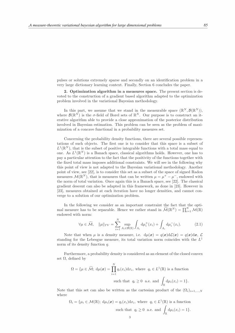
,A measure-theoretic variational bayesian algorithm for large dimensional problems 85
pulses or solutions extremely sparse and secondly on an identification problem in avery large dictionary learning context. Finally, Section 6 concludes the paper.
2. Optimization algorithm in a measures space. The present section is de-voted to the construction of a gradient based algorithm adapted to the optimizationproblem involved in the variational Bayesian methodology.
In this part, we assume that we stand in the measurable space (RN ,B(RN)),where B(RN) is the σ-field of Borel sets of RN . Our purpose is to construct an it-erative algorithm able to provide a close approximation of the posterior distributioninvolved in Bayesian estimation. This problem can be seen as the problem of maxi-mization of a concave functional in a probability measures set.
Concerning the probability density functions, there are several possible represen-tations of such objects. The first one is to consider that this space is a subset ofL1(RN ), that is the subset of positive integrable functions with a total mass equal toone. As L1(RN ) is a Banach space, classical algorithms holds. However, one has topay a particular attention to the fact that the positivity of the functions together withthe fixed total mass imposes additional constraints. We will see in the following whythis point of view is not adapted to the Bayesian variational methodology. Anotherpoint of view, see [22], is to consider this set as a subset of the space of signed RadonmeasuresM(RN ), that is measures that can be written µ = µ+ − µ−, endowed withthe norm of total variation. Once again this is a Banach space, see [22]. The classicalgradient descent can also be adapted in this framework, as done in [23]. However in[23], measures obtained at each iteration have no longer densities, and cannot con-verge to a solution of our optimization problem.
In the following we consider as an important constraint the fact that the opti-mal measure has to be separable. Hence we rather stand in M(RN ) =
∏Ni=1M(R)
endowed with norm:
∀µ ∈ M, ‖µ‖TV =
N∑
i=1
supAi∈B(R)
∫
Ai
dµ+i (xi) +
∫
Ai
dµ−i (xi). (2.1)
Note that when µ is a density measure, i.e. dµ(x) = q(x)dL(x) = q(x)dx, Lstanding for the Lebesgue measure, its total variation norm coincides with the L1
norm of its density function q.
Furthermore, a probability density is considered as an element of the closed convexset Ω, defined by
Ω = µ ∈ M; dµ(x) =
N∏
i=1
qi(xi)dxi, where qi ∈ L1(R) is a function
such that qi ≥ 0 a.e. and
∫
R
dµi(xi) = 1.
Note that this set can also be written as the cartesian product of the (Ωi)i=1,...,N
where
Ωi = µi ∈ M(R); dµi(x) = qi(xi)dxi, where qi ∈ L1(R) is a function
such that qi ≥ 0 a.e. and
∫
R
dµi(xi) = 1.3

86 Sélection d’articles
Hence our purpose is, given a concave functional F : M → R, to define analgorithm which approximates a probability measure µopt solution of
µopt = argmaxµ∈Ω
F (µ). (2.2)
This problem can be seen as a constrained convex optimization problem in theinfinite dimensional Banach space (M, ‖.‖TV ).
In this framework, most results of optimization are based on duality results, seefor instance [16, 5]. In the present paper we consider a gradient-like descent algorithmdefined directly on the probability measures set.
Let us introduce some notations from [22]. Let F : M → R. As M is a Ba-
nach space, one can compute its Frechet derivative at µ ∈ M as the bounded linearfunctional dFµ(.) : M → R satisfying
F (µ+ ν)− F (µ)− dFµ(ν) = o(‖ν‖TV ), when ‖ν‖ → 0.
In the following we also consider the Gateaux derivative of F :
∀ν ∈ M, ∂Fµ(ν) = limt→0
F (µ+ tν)− F (µ)t
.
In some cases, see [22], one can find a function df : M× RN → R continuous,
such that
∀ν ∈ M, ∂Fµ(ν) =
∫
RN
df(µ,x)dν(x). (2.3)
Consider an auxiliary concave functional G : M → R. An important propertyappearing in the following is that the Frechet differential of G is L-Lipschitz on Ω, i.e.
∀(µ1, µ2) ∈ Ω2, ∀ν ∈ M |dGµ1(ν)− dGµ2
(ν)| ≤ L‖ν‖TV ‖µ1 − µ2‖TV . (2.4)
The Lipschitz differential condition of G together with its concavity implies that,see [26] for instance,
∀(µ1, µ2) ∈ Ω2, 0 ≥ G(µ1)−G(µ2)− dGµ2(µ1 − µ2) ≥ −L‖µ1 − µ2‖2TV . (2.5)
Furthermore we say that a function F is twice differentiable at µ ∈ M, in thesense of Gateaux, if
∀(ν1, ν2) ∈ M2, ∂2Fµ(ν1, ν2) = limt→0
dFµ+tν1 (ν2)− dFµ(ν2)
t.
If it exists, ∂2F is a bilinear application from M × M to R. If F is a concavefunctional, this second-order derivative must satisfy for every µ ∈ M,
∀ν ∈ M, ∂2Fµ(ν, ν) ≤ 0. (2.6)
Our purpose is to construct an iterative algorithm providing a density at eachiteration and approximating the solution of (2.2) for a certain class of functions F .The key principle of our method is given by the Radon-Nikodym theorem, see [32]
for instance. Let k ≥ 0 be an integer and assume that µk ∈ M is a probability
4

,A measure-theoretic variational bayesian algorithm for large dimensional problems 87
measure absolutely continuous respectively to the Lebesgue measure. In order to keepa measure absolutely continuous with respect to the Lebesgue measure we constructµk+1 ∈ M as a measure absolutely continuous with respect to µk. In this case, theRadon-Nikodym theorem ensures that this measure should be written as
dµk+1(x) = hk(x)dµk(x), (2.7)
where hk ∈ L1(µk) is a positive function. Our aim is thus to determine a functionhk ∈ L1(µk) which ensures that F (µk+1) ≥ F (µk). Following the classical schemegiven by the gradient descent method, hk is given as a function of the derivative of Fat µk and, according to our structure, by
hk(x) = Kk(αk) exp(αkdf(µk,x)), (2.8)
where df is defined by (2.3) whereas αk > 0 is the algorithm step-size at iterationk and Kk(αk) is the normalization constant such that
∫RN dµk+1(x) = 1. We also
impose the convention that hk(x) =∞ when exp(αkdf(µk,x)) is not integrable. One
can see that as soon as µ0 can be written as µ0 = q0dx where q0 a positive density, socan be each µk. We thus can consider in the following that dµk = qkdx. This choiceof h is motivated by the positive, integrable assumption together with, as mentionedearlier, its coherence with the structure of the gradient descent method. This descentalgorithm is defined as the “exponentiated gradient” descent in [17]. Since [17] it hasbeen widely studied in the context of machine learning even in the Bayesian frame-work, see [9] for instance.
The optimization algorithm involved in this paper is the following:
Algorithm 1 Exponentiated Gradient algorithm
1: Initialize( µ0 ∈ Ω)2: repeat3: Compute df(µk,x)4: Compute αk = argmaxαKk(α) exp(αdf(µ
k, .))µk
5: Compute µk+1 = Kk(αk) exp(αkdf(µk, .))µk
6: until Convergence
In order to determine the convergence properties of this exponentiated gradientmethod in our context, let us define the hypotheses that we impose on the functionalF .
Assumption 1. Let F : M → R be a concave functional. We say that F satisfiesAssumption 1 if:
(i) F can be written as F = G +H where G is a concave L-Lipschitz Frechet-differentiable functional whereas H corresponds to the entropy of the proba-bility measure, that is the Kullback-Leibler divergence from this measure tothe Lebesgue measure.
(ii) F is twice differentiable in the sense of Gateaux and its first order derivativesatisfies Equation (2.3).
(iii) lim‖µ‖→∞ F (µ) = −∞.Remark 1. The two points (ii), (iii) of the definition of hypothesis 1 just ensure
that the optimal stepsize αk defined in our algorithm indeed exists. Concerning hy-pothesis (i), it can be replaced by the more restrictive hypothesis that F is L-Lipschitz
5

88 Sélection d’articles
Frechet differentiable. Note that as our purpose is to construct measures with a den-sity, the term H also corresponds to the entropy of the density function.
Let us now state the convergence result.Theorem 2.1. Let F be a concave functional satisfying Assumption 1 of Def-
inition 1. Let αk be the optimal stepsize of Algorithm 1, for every k ≥ 0. Thenthe sequence (µk)k≥0 of elements of M given by µk+1 = Kk(αk) exp(αkdf(µ
k, .))µk
converges to a maximizer of F on Ω.Proof. The proof of this theorem involves two main steps. In a first step we prove
that the sequence (F (µk))k∈N is an increasing sequence. This ensures in a secondtime to infer the convergence of the sequence (µk)k≥0 to a solution of (2.2).
Lemma 2.2. Let F be a functional satisfying Hypothesis 1. Let also (µk)k∈N bethe sequence provided by Algorithm 1. Then
∃α0 > 0, ∀α ∈ (0, α0) F (µα)− F (µk) ≥ 0. (2.9)
Proof.Let k > 0 be fixed and µk be given. For every α ≥ 0 we define µα as the
measure defined for all x ∈ RN by dµα(x) = Kk(α) exp(αdf(µ
k,x))dµk(x) :=hα(µ
k,x)dµk(x).We define furthermore gk(α) := F (µα). Thus gk is a function from R
+ to R twicedifferentiable and αopt is an optimal step-size if gk(αopt) = max gk(α), i.e.
αopt = argmaxα
gk(α). (2.10)
The fact that F (µ)→ −∞ when ‖µ‖ → ∞ ensures that we can find an αopt, notnecessarily unique, such that
∀α > 0, F (µα) ≤ F (µαopt). (2.11)
Let α > 0 be given and consider the decomposition given by point (i) of Definition1. Thanks to Equation (2.5) one has
G(µα) ≥ G(µk) + dGµk(µα − µk)− L‖µα − µk‖2TV . (2.12)
Furthermore, as µα = hα(µk, .)µk and µk is a probability measure one can notice
that
−L‖µα − µk‖2TV = −L‖hα(µk, .)− 1‖2L1(µk) ≥ −L‖hα(µk, .)− 1‖2L2(µk). (2.13)
Furthermore,
H(µα) = −∫
RN
ln
(dµα
dL
)dµα(x)
= H(µk)−∫
RN
ln(hα(µk,x))dµα(x)−
∫
RN
ln
(dµk
dL
)(hα(µ
k,x)− 1)dµk(x).
Following the development made in [8] for simple functions, the Gateaux deriva-tive at qk of the entropy H : L1 → R
+ in direction h ∈ L1 is given by
∂Hqk(h) = −∫(ln(qk(x)) + 1)h(x)d(x),
6

,A measure-theoretic variational bayesian algorithm for large dimensional problems 89
as soon as qk + h cannot be negative. A similar approach in M ensures that
∂Hµk(µα − µk) =
∫
RN
(− ln
(dµk
dL
)− 1)(hα(µ
k,x)− 1)dµk(x), (2.14)
as µk + (µα − µk) is obviously always positive.This entails
H(µα) ≥ H(µk)−∫
RN
ln(hα(µk,x))dµα(x) + ∂Hµk(µα − µk). (2.15)
Finally, from (2.12), (2.13) and (2.15) one has
F (µα)−F (µk) ≥ ∂Fµk(µα−µk)−L‖hα(µk, .)− 1‖2L2(µk)−∫
RN
ln(hα(µk,x))dµα(x).
(2.16)Finally, F (µα)− F (µk) is positive if the right side of Equation (2.16) is positive.
This part being quite technical it is reported to Appendix 7.1.
Lemma 2.2 ensures that for α > 0 small enough, F (µα) ≥ F (µk). As we chooseµk+1 = µαopt , where αopt is defined by (2.10), we obviously have F (µk+1) ≥ F (µk).
Finally the sequence (F (µk))k∈N is increasing and upper bounded in R, so con-vergent, it thus also satisfies that F (µk+1)− F (µk)→ 0.
In order to conclude we have to show that (µk)k∈N indeed converges to a maximum
of F on Ω. But, for every k ≥ 0, µk ∈ Ω, which is a bounded set in M and thus inM(RN ). Furthermore, this last one is the dual of C0, the space of continuous functionsthat tend to zero at infinity, which is a separable Banach space. As a consequenceof the Banach-Alaoglu Theorem, see [32] for instance, there exists µlim ∈ M and asubsequence (µkn)n∈N such that for every continuous function that goes to zero atinfinity f ,
∫f(x)µkn(dx)→
∫f(x)µlim(dx).
i.e. when k →∞, we have µkn ∗ µlim ∈ Ω.
From Lemma 2.2 we know that there exists α0 > 0 such that
F (µk+1) = gk(αopt) ≥ gk(α), ∀α ∈ (0, α0).
However the analytic form of αopt is not attainable. We thus approximate it by acalculable αsubopt, not necessarily smaller than α0. In order to determine this αsubopt
we can notice that the Taylor-Young formula gives, for α small enough,
gk(α) = gk(0) + αg′k(0) +α2
2g′′k (0) + α2ε(α) := ϕk(α) + α2ε(α), (2.17)
where ε(α)→ 0 when α→ 0.Let us determine the derivative of g. For this purpose, we have to determine the
derivative of the function g : α 7→ hα(µk, .). As hα(µ
k,x) = Kk(α)eαdf(µk,x), its
derivative is given by
7

90 Sélection d’articles
∀x ∈ RN , g′(α)(x) = K ′
k(α)eαdf(µk,x) + df(µk,x)Kk(α)e
αdf(µk,x).
As α is supposed to be close to zero, one can assume that it is not greater thanone and the Lebesgue’s Theorem thus yields
K ′k(α) = −
∫df(µk,x)Kk(α)e
αdf(µk,x)dµk(x)(∫eαdf(µk,x)dµk(x)
)2 = −Kk(α)
∫df(µk,x)hα(µ
k,x).
Finally one obtains that
∀x ∈ RN , g′(α)(x)dµk(x) = dµα(x)
(df(µk,x)−
∫
RN
df(µk,y)dµα(y)
). (2.18)
And
g′k(α) = ∂Fµα(g′(α)µk) =
∫
RN
df(µα,x)
(df(µk,x)−
∫
RN
df(µk,y)µα(dy)
)dµα(x),
and
g′k(0) = ∂Fµk(g′(0)µk) =
∫
RN
df(µk,x)
(df(µk,x)−
∫
RN
df(µk,y)µk(dy)
)dµk(x)
=
∫
RN
df(µk,x)2µk(dx)−(∫
RN
df(µk,y)dµk(y)
)2
(2.19)
The critical point of ϕk(α) is αsubopt = − g′k(0)
g′′k(0) , as soon as g′′k (0) 6= 0, which gives
in (2.17):
gk(αsubopt) = gk(0)−g′k(0)
2
2g′′k(0)+ α2ε(α), (2.20)
and by construction of F (µk+1),
F (µk+1) ≥ gk(αsubopt) = gk(0)−g′k(0)
2
2g′′k (0)+ α2ε(α) = F (µk)− g′k(0)
2
2g′′k (0)+ α2ε(α).
As F (µk+1)− F (µk)→ 0, obviously limk→∞
g′k(0)
2
2g′′k(0) = 0. Let us consider the conver-
gent subsequence (kn)n∈N and denote by (αkn)n∈N the sequence defined ∀n ∈ N by
γkn= αsubopt. Hence, − g′
kn(0)2
g′′kn
(0) = g′kn(0)γkn
→ 0. As df is supposed to be continu-
ous, the sequence (g′kn(0))n∈N is convergent and either γkn
→ 0 or g′kn(0) → 0. Let
us assume that γkn→ 0 and that g′kn
(0) → l 6= 0. Let β > 0 be given. As γkn→ 0
we have, for n large enough that
gkn(γkn
β)− gkn
(0) =γkn
βg′kn
(0) +γ2kn
2β2g′′kn
(0) + γ2knε(γkn
)
=γkn
βg′kn
(0)
(1− 1
2β
)+ γ2kn
ε(γkn).
8

,A measure-theoretic variational bayesian algorithm for large dimensional problems 91
Hence,
gkn(γkn
β )− gkn(0)
γkn/β
= g′kn(0)
(1− 1
2β
)+ γkn
ε(γkn), (2.21)
and when n tends to infinity, γkntends to zero, and taking limits in (2.21) one obtains
l = l
(1− 1
2β
),
which is impossible as soon as β 6= 12 . Hence, g
′kn(0)→ 0 when n→∞.
Furthermore,
g′k(0) =
∫
RN
df(µk,x)2µk(dx)−(∫
RN
df(µk,y)µk(dy)
)2
.
Hence, for n large enough,
‖df(µkn , .)‖2L2(µkn ) − ‖df(µkn , .)‖2L1(µkn ) → 0,
and thus df(µkn , .) converges to a constant λ, independent of x ∈ RN .
Let ν be any element of Ω. Applying the Main Value Theorem to the real valuedfunction f(θ) = F (θµlim + (1− θ)ν) we see that
F (ν) = F (µlim) + dFµlim(ν − µlim) +1
2∂2Fµ(ν − µlim, ν − µlim),
where µ = θ0ν + (1− θ0)µlim and θ0 ∈ (0, 1) is fixed.As ∂Fµlim(ν − µk) = 0, and from concavity of F we have
F (ν) ≤ F (µlim) ∀ν ∈ Ω,
which means that F (µlim) is a maximum of F over Ω.
In the present part we have presented an algorithm adapted to the space of prob-ability measures. Our main interest is its application in the context of variationalBayesian methodology. For the sake of completeness, let us remind this methodologyintroduced in [20].
3. Our Variational Bayesian Algorithm. For the sake of simplicity, we con-sider in the following density functions q instead of the corresponding measures µ. Wedenote by y ∈ R
M theM dimensional vector containing the data information whereasw ∈ R
N represents the vector to be estimated, which is considered as a realizationof a random vector W . We also denote by p the prior probability density function(p.d.f.) of W . The Bayes rule entails that this prior distribution is closely relatedto the posterior one, p(w|y), up to a normalization constant. Even in simple casesthis posterior may not be separable. Hence, in the variational Bayesian framework,we approximate it by a separable probability density
q(w) =∏
i
qi(wi). (3.1)
9

92 Sélection d’articles
Taking separable laws obviously simplify the problem even if it introduces someapproximation errors.
Therefore, we want to determine a separable probability density function q closeof the true posterior, in the sense defined by the Kullback-Leibler divergence, see [35]for instance. The optimal approximating density q is given by
∀i ∈ 1, . . . , N, qi(wi) = Kik exp
(< ln p(y,w) >∏
j 6=i qj
), (3.2)
whereKik is the normalization constant and< ln p(y,w) >∏
j 6=i qj=∫RN−1 ln p(y,w)
∏j 6=i qj(wj)
is the mean of ln p(y,w) under the probability∏
j 6=i qj .
Although this solution is obtained analytically, Equation (3.2) clearly does nothave an explicit form. In order to have implementable methods a first step is toconsider conjugate priors. Hence the optimization turns out to an update of thedistribution parameters. However even for conjugate priors, this solution is hardlytractable in practice, and is thus approximated by iterative fixed points methods. InEquation (3.2), the calculus of qi imposes the knowledge of all qj for j different fromi, and this optimization is either performed alternatively or by group of coordinate.In both cases, the computation complexity can be important.
For large dimensional problems these methods are not tractable in practice. Ourpurpose is thus to solve the functional optimization problem given by the Bayesianvariational method in an efficient way thanks to the algorithm defined in Section 2.
3.1. Variational Bayesian Exponentiated Gradient Algorithm. In thissection we define an iterative method which allows to compute efficiently at each iter-ation each qi independently of the others in order to decrease the computational costof one iteration.
A first step in this part is to rewrite the minimization problem as a convex op-timization problem independent of the posterior distribution to be approximated.Instead of minimizing the Kullback-Leibler divergence, we thus remark, as in [6], that
ln p(y) = lnp(y,w)
p(w|y) , (3.3)
where w is the vector of hidden variables and parameters.
As the log-likelihood ln p(y) in (3.3) does not depends on w one can write
ln p(y) = F(q) +KL[q||p(.|y))].
In this case,
F(q) =∫
RN
q(w) ln(p(y,w)
q(w))dw, (3.4)
is the negative free energy. Thus minimizing the Kullback-Leibler divergence is obvi-ously equivalent to maximize this negative free entropy.
10

,A measure-theoretic variational bayesian algorithm for large dimensional problems 93
Therefore in the following we will consider the problem of maximizing
F(q) =∫
RN
ln p(y,w)q(w)dw −∫
RN
ln(q(w))q(w)dw
= 〈ln p(y, .)〉q +H(q),(3.5)
where
H(q) = −∫
RN
ln(q(w))q(w)dw,
is the entropy of q. The main advantage of this approach is that the objective func-tional does not depend on the true posterior anymore but only on the joint distributionp(y, .), which is more easily tractable.
One can also notice that the problem of finding
qopt = argmaxq p.d.f.
F(q) (3.6)
is equivalent to the problem of finding
µopt = argmaxµ∈Ω
F (µ). (3.7)
Where the functional F is defined by ∀µ ∈ Ω, such that q is the density of µby F (µ) = F(q). Furthermore the corresponding function F satisfies hypothesis 1.Note that in the following we consider that . Hence we can apply Theorem 2.1 in thiscontext.
Remark 2. As mentioned, a classical method in our context is to consider eachdensity function q as a L1(RN ) function and to apply classical algorithms. In thepresent framework, taking the non-negativity and the total mass assumptions intoaccount, the algorithm involved is given by the projected gradient method which gives:
∀w ∈ RN qk+1(w) = PΘ(q
k(w) + ρkf(qk,w)), (3.8)
where PΘ is the projector operator on the subspace Θ = q ∈ L1(RN ); q(w) ≥0 and ‖q‖L1 = 1.
However, this algorithm requires that f(qk,w) ∈ L1(RN ) which is not the case ingeneral.
Hence, we apply the algorithm introduced in Section 2 to the Variational Bayesianframework of Section 3. We consider
F(q) = 〈ln p(y, .)〉q +H(q).
In this case, the Gateaux differential of F (µ) = F(q) at µ ∈ Ω separable is givenby dFµ(ν) =
∑i
∫RN f(qi, xi)νi(dx) where
∀i ∈ 1, . . . , N, ∀w ∈ RN , f(qi, wi) = 〈ln p(y,w)〉∏
j 6=iqj − ln qi(wi)− 1.
Let k ≥ 0 be given and qk be constructed. Following the scheme defined byAlgorithm 1 and Equation (2.8), at the following iteration we consider qα given, for
11

94 Sélection d’articles
α > 0, by
∀w ∈ RN , qα(w) = Kkq
k exp[αkf(q
k,w)]
(3.9)
= Kkqk(w)
∏
i
exp(< ln p(y,w) >∏
j 6=iqkj(wj)
)
qki (wi)
αk
= Kkqk(w)
(∏
i
qri (wi)
qki (wi)
)αk
(3.10)
where Kk is the normalization constant and qr is an intermediate measure given by
∀i ∈ 1, . . . , N, qri (wi) = exp(< ln p(y,w) >∏
j 6=i qkj(wj)
)
The main challenge is to determine the optimal value of α > 0. This optimal valueshould satisfy g′k(αopt) = 0. However, this quantity is hardly tractable in practice.Therefore, we consider instead the suboptimal value given by
αsubopt = −g′k(0)
g′′k (0), (3.11)
when g′′k (0) 6= 0. This leads to the main algorithm of this paper.
Algorithm 2 Variational Bayesian Exponentiated Gradient Like Algorithm
1: Initialize( q0 ∈ Θ)2: repeat3: function Iteration( Compute qk+1 = Kkq
k exp[αkf(q
k,w)])
4: Compute qri (wi) = exp(< ln p(y,w) >∏
j 6=iqkj(wj)
)for every i = 1, . . . , N
5: Compute αsubopt = − g′(0)g′′(0)
6: Compute qαsubopt(w) = qk(w)(
qr(w)qk(w)
)αsubopt
.
7: Take qk+1 = qαsubopt .8: end function9: until Convergence
4. Application to linear inverse problems.
4.1. Statement of the problem. The following of this paper presents theapplication of Algorithm 2 to linear inverse ill-posed problems. More precisely weconsider its implementation for Bayesian study of heavy-tailed information. Themodel of observations chosen in the following is given by
y = Hx+ b, (4.1)
where y ∈ RM is the vector of observations given as a linear function of the unknowns
vector x ∈ RN to be estimated. Here, b ∈ R
M is the noise vector whereas H is amatrix in MN×M . We also suppose that x is a realization of a random vector X.
12

,A measure-theoretic variational bayesian algorithm for large dimensional problems 95
In the following we stand in a white noise model which induces that the noise issupposed to be an iid Gaussian vector N (0, σ2
bI). We can deduct easily the likelihood
p(y|x) = (2πσ2b )
−M/2 exp
[−‖y −Hx‖2
2σ2b
]. (4.2)
Concerning the prior distribution we choose to take sparsity into account by consid-ering X distributed following a separable heavy tailed distribution. The most generalcase is given by Gaussian Vector Scale Mixture (GVSM) defined in [13]. In this case,for i = 1, . . . , N , we suppose that Xi ∼ Ui/
√Zi where U ∼ N (0, σ2
sI), Z =∏Zi
is a positive random vector of independent positive coordinates and U and Z areindependents. As a consequence the density of X is given in an integral form as
∀i ∈ 1, . . . , N, p(xi) =
∫
R
√zi
(2π)1/2σse−
zix2i
2σ2s φzi(zi)dzi.
Note that in the definition, for the sake of simplicity, we consider Z as a precisionparameter and not as a dilatation one. Gaussian Vector Scale Mixture form a largeclass of nongaussian random variables recently developed as a model of wavelet coef-ficients of natural images, see [38]. The main interest of this model is, by solving anextended problem due to the presence of a hidden random vector Z, to allow the useof Bayesian hierarchic approaches.
The Gaussian Scale Mixture family offers a large class of random variables in-cluding Gaussian mixing, when Z ∼ ZI a discrete random vector or Student laws ifall Zi are Gamma random variables. With different hypothesis on the distribution ofZ one can also define Generalized Gaussian distributions or α-stable ones, see [38].Indeed GSM offer a simple representation of a large class of nongaussian probabilitydistributions, which justify the increasing interest on this model.
In our context, we choose to consider Z as a independent Gamma random vector,i.e. for i = 1, . . . , N , we have Zi ∼ G(ai, bi) and
∀i ∈ 1, . . . , N, p(xi) =bai
i
Γ(ai)
∫
R
√zi
(2π)1/2σse−
zix2i
2σ2s zai−1
i e−zibidzi. (4.3)
For ai = bi =ν2 , the p.d.f. of X corresponds to a Student-t distribution, as in the
model used in [4]. This model of Z ensures that X satisfies the conjugate priorscondition.
One can easily check that when the prior information is given by (4.3), Equation(4.2) gives the following posterior distribution
p(x, z|y) ∝ σ−Mb exp
[−‖y −Hx‖2
2σ2b
] N∏
i=1
√zi
σsexp
[−zix
2i
2σ2s
]bai
i zai−1i e−zibi
Γ(ai). (4.4)
Considering that we do not know the involved constants and that the mixingmatrix H is high dimensional, this posterior distribution cannot be evaluated directly.
4.2. Numerical implementation. The aim of variational Bayesian methodol-ogy and therefore of our method in the context established in part 4 is the approxima-tion of the posterior p.d.f given by (4.4) by a separable one q(x, z) =
∏i qi(xi)
∏j qj(zj).
13

96 Sélection d’articles
As we have chosen conjugate prior for X and Z, the optimum approximating distri-bution of X is known to belong to a Gaussian family, whereas the p.d.f. of Z belongsto a Gamma one.
qk(x) =∏
i
N (mk(i),σ2k(i))
qk(z) =∏
j
G(ak(j), bk(j))
Hence at the initialization stage, we consider
q0(x) = N (m0,Diag(σ20))
q0(z) =∏
j
G(a0(j), b0(j))
where Diag(v) is a diagonal matrix with v on its diagonal, and σ20 ∈ R
N is the vectorof initial variances.
Our minimization problem can be analyzed following the alternate iterative scheme:
qk+1(z) = argmaxq(z)
F(qk(x)q(z)
)
qk+1(x) = argmaxq(x)
F(q(x)qk+1(z)
)
4.2.1. Approximation of q. One can see in Equation (4.4) that the condi-tional posterior p(z|x,y) is separable. In this case the classical Bayesian variationalapproach is efficient enough to be implemented directly. Actually for i = 1, . . . , N ,qk+1i (zi) does not depend on other coordinates. Hence all the zi can be computedsimultaneously, knowing only q(x). Thanks to the classical Bayesian variational ap-proach [20] described in Section 3, we deduce qk+1 thanks to Equation (3.2) andEquation (4.4), for every i = 1, . . . , N
qk+1i (zi) = exp
(< ln p(y,x, z) >∏
j 6=iqkj(zj)qk(x)
)(4.5)
∝ exp
(ai −
1
2) ln(zi)−
∫(x2i zi2σ2
s
+ zibi)∏
l
qkl (xl)∏
j 6=i
qkj (zj)dxdz
∝ exp
((ai −
1
2) ln(zi)− zibi −
∫x2i zi2σ2
s
qki (xi)dxi
)
∝ exp
((ai −
1
2) ln(zi)− zibi −
(σ2k(i) +m2
k(i))zi2σ2
s
)
∝ zai−12
i exp
(−zi[bi +
(σ2k(i) +m2
k(i))
2σ2s
])(4.6)
This entails that qk+1i (zi) corresponds to a Gamma p.d.f. of parameters:
∀i ∈ 1, . . . , N, ak+1(i) = ai +1
2, (4.7)
bk+1(i) =m2
k(i) + σ2k(i)
2σ2s
+ bi. (4.8)
14

,A measure-theoretic variational bayesian algorithm for large dimensional problems 97
4.2.2. Approximation of q by Algorithm 2. Let us assume that we start witha Gaussian p.d.f. q0(x) with meanm0 and covariance matrix Diag(σ2
0). At each itera-tion we determine the approximation of qk(x) thanks to our method. At each iteration
k+1, we define an auxiliary measure qr(x) by qri (xi) = exp(〈ln p(y,x, z)〉∏
j 6=iqkj(xj)qk+1(z)
).
Hence ∀i ∈ 1, . . . , N,
qri (xi) = exp(< ln p(y,x, z) >∏
j 6=i qkj(xj)qk+1(z)
)(4.9)
∝ exp
−
∫ (‖y −Hx‖22σ2
b
+x2i zi2σ2
s
)∏
j 6=i
qkj (xj)qk+1(z)dxdz
∝ exp
−
∫ (xTHTHx− 2xTHTy
2σ2b
+x2i zi2σ2
s
)∏
j 6=i
qkj (xj)qk+1(zi)dxdzi
∝ exp
[− 1
2σ2b
(x2i diag(H
TH)i − 2xi(HTy)i + 2xi(H
THmk)i
−2xidiag(HTH))imk(i))+
x2iak+1(i)
2σ2sbk+1(i)
](4.10)
where diag(A) is the vector composed by the diagonal entries of A. Note that qr(x)corresponds, up to the normalization term, to a Gaussian distribution with mean mr
and variance σ2r, where, for every i = 1, . . . , N ,
σ2r(i) =
(diag(HTH)i
σ2b
+ak+1(i)
bk+1(i)σ2s
)−1
(4.11)
and
mr(i) = σ2r(i)×
(HTy − (HTH − diag(HTH))mk
σ2b
)
i
(4.12)
Therefore, by Equation (3.10), we have for every i = 1, . . . , N ,
qαi (xi) = Kkqki (xi)
(qri (xi)
qki (xi)
)α
=
√σ2
k(i)
σ2r(i)
α
Kk exp
[− (xi −mk(i))
2
2σ2k(i)
]exp
[−αx
2i (σ
2k(i)− σ2
r(i))
2σ2r(i)σ
2k(i)
]
× exp
[−α−2xi(mr(i)σ
2k(i)−mk(i)σ
2r(i)) +mr(i)
2σ2k(i)−mk(i)
2σ2r(i)
2σ2r(i)σ
2k(i)
]
=
√σ2
k(i)
σ2r(i)
α
Kk exp
[−1
2
(x2i
σ2r(i) + α(σ2
k(i)− σ2r(i))
σ2r(i)σ
2k(i)
)]
× exp
[−1
2
(−2xi
mk(i)σ2r(i) + α(mr(i)σ
2k(i)−mk(i)σ
2r(i))
σ2r(i)σ
2k(i)
+ t(α)
)]
where qα is defined in Section 5.1.1, and t(α) = αmr(i)
2σ
2k(i)−mk(i)
2σ
2r(i)
2σ2r(i)σ
2k(i)
is a
constant. Finally, qαi (x) is still a Gaussian p.d.f. with parameters mα and Diag(σ2α)
15

98 Sélection d’articles
satisfying:
σ2α(i) =
σ2r(i)σ
2k(i)
σ2r(i) + α(σ2
k(i)− σ2r(i))
(4.13)
mα(i) =mk(i)σ
2r(i) + α(mr(i)σ
2k(i)−mk(i)σ
2r(i))
σ2r(i) + α(σ2
k(i)− σ2r(i))
. (4.14)
In order to construct qk+1 we choose in the previous equation α = αsubopt definedin Equation (3.11).
Finally, we obtain the following algorithm.
Algorithm 3 Supervised Sparse Reconstruction algorithm (SSR)
1: Initialize(q0, q0)2: repeat3: function Estimate qk+1(z)(qk(x))4: update ak+1 by Equation (4.7)5: update bk+1 by Equation (4.8)6: end function7: function Estimate qk+1(x)(qk+1(z))8: compute qr(x)← (mr,σ
2r) by Equation (4.12) and Equation (4.11)
9: compute αsubopt
10: compute qα(x)← (mα,σ2α) by Equation (4.14) and Equation (4.13)
11: end function12: until Convergence
4.3. Unsupervised algorithm. The algorithm described in the previous partis not a fully Bayesian one as it still depends on some parameters, namely the param-eters induced by the model (4.1) and (4.3). We see in the following how this methodcan be extended to an unsupervised one by estimating these parameters. The param-eters of the underlying Gamma random variable are not estimated in the following asthey define the sharpness of the prior distribution. We thus only estimate the varianceparameter of this prior together with the trade off between the prior and the noise.
The main interest of the variational Bayesian approach introduced by D. MacKay[20] and involved in this paper is its flexibility. That is an unsupervised algorithm canbe easily deduced from the method proposed in Section 4.2, by considering that the pa-rameters are realizations of a random variable with a given Jeffrey’s prior distribution.
In order to simplify the different expressions, we introduce in the following thenotations γb = 1/σ2
b and γs = 1/σ2s . Hence, γb and γs are the precision parameters
of the noise and of the prior distribution. From now on they are also assumed to berandom variable with Gamma prior of parameters (ab, bb) resp. (as, bs). As we donot have information on these precision parameters γb and γs, this prior is obtainedby fixing (ab = 0, bb = 0) resp. (as = 0, bs = 0).
With these assumptions, the posterior distribution from Equation (4.4) can be
16

,A measure-theoretic variational bayesian algorithm for large dimensional problems 99
written as
p(x, z, γb, γs|y) ∝ γM2
b exp
[−γb‖y −Hx‖2
2
]γ
N2s
∏
i
√zi exp
[−γszix
2i
2
]bai
i zai−1i e−zibi
Γ(ai)
× bab
b γab−1b e−γbbb
Γ(ab)
bass γ
as−1s e−γsbs
Γ(as).
(4.15)
As in the previous section, the conditional posterior p(z, γb, γs|x,y) is separableand can be approximated thanks to the classical variational Bayesian approach. Onceagain only the distribution of X needs the use of Algorithm 2. Here the alternateoptimization scheme to carry out is:
qk+1(z) = argmaxq(z)
F(qk(x)q(z)qkb (γb)q
ks (γs)
)
qk+1(x) = argmaxq(x)
F(q(x)qk+1(z)qkb (γb)q
ks (γs)
)
qk+1b (γb) = argmax
q(γb)
F(qk+1(x)qk+1(z)qb(γb)q
ks (γs)
)
qk+1s (γs) = argmax
q(γs)
F(qk+1(x)qk+1(z)qk+1
b (γb)qs(γs))
4.3.1. Optimization of the approximate p.d.f. qb. Concerning the randomvectors Z and X, the updating process follows the same scheme than the supervisedcase, see Section 4.2, and are not recalled here. The main differences reside in theupdate of the parameters distributions.
As the distributions of γb and γs are supposed to be Gamma, which is coherentwith the conjugate priors hypothesis, at each iteration we just adapt the parameters.Hence we initialize our algorithm by considering that
q0b (γb) = G(a0b , b0b)At iteration k + 1 we consider the maximum of the free energy from Equation (3.2)which gives
qk+1b (γb) ∝ exp
[< ln Pr(x,y, z, γb, γs) >∏
jqk+1
j(xj)
∏jqk+1
j(zj)qks (γs)
]
∝ exp
[< (
M
2+ ab − 1) ln(γb)− γb(
‖y −Hx‖22
+ bb) >∏jqk+1
j(xj)
]
∝ exp
[(M
2+ ab − 1) ln(γb)
−γb(12‖y −Hmk+1‖2 +
1
2
N∑
i=1
diag(HtH
)iσ2
k+1(i) + bb
)]
So qk+1b (γb) is a Gamma p.d.f. of parameters:
ak+1b =
M
2+ ab (4.16)
bk+1b =
1
2‖y −Hmk+1‖2 +
1
2
N∑
i=1
diag(HtH
)iσ2
k+1(i) + bb (4.17)
17

100 Sélection d’articles
4.3.2. Optimization of the approximate p.d.f. qs. As for γb, the approxi-mation of qs is performed in the family of Gamma distributions. Hence at the initial-ization step we assume that
q0s(γs) = G(a0s, b0s)
and at iteration k + 1, thanks again to Equation (3.2) we obtain
qk+1s (γs) ∝ exp
[< ln Pr(x,y, z, γb, γs|I) >∏
j qk+1
j(xj)
∏j qk+1
j(zj)q
k+1
b(γb)
]
∝ exp
[< (
N
2+ as − 1) ln(γs)− γs(
1
2
N∑
i=1
zix2i + bs) >∏
jqk+1
j(xj)q
k+1
j(zj)
]
∝ exp
[< (
N
2+ as − 1) ln(γs)− γs(
1
2
N∑
i=1
ak+1(i)
bk+1(i)(m2
k+1(i) + σ2k+1(i)) + bs)
]
So qk+1s (γs) is a Gamma p.d.f. and its parameters are deduced by identification.
ak+1s =
N
2+ as (4.18)
bk+1s =
1
2
N∑
i=1
ak+1(i)
bk+1(i)(m2
k+1(i) + σ2k+1(i)) + bs (4.19)
Finally the algorithm performed can be summed up as follows.
Algorithm 4 UnSupervised Sparse Reconstruction algorithm (USSR)
1: Initialize(q0, q0, q0b , q0s)
2: repeat3: function Estimate qk+1(z)(qk(x), qkb (γb), q
ks (γs))
4: update ak+1 using Equation (4.7)5: update bk+1 using Equation (4.8)6: end function7: function Estimate qk+1(x)(qk+1(z), qkb (γb), q
ks (γs))
8: compute qr(x)← (mr,σ2r) using Equation (4.12) and Equation (4.11)
9: compute αsubopt
10: compute qα(x)← (mα,σ2α) using Equation (4.14) and Equation (4.13)
11: end function12: function Estimate qk+1
b (γb)(qk+1(z), qk+1(x))
13: update ak+1b using Equation (4.16)
14: update bk+1b using Equation (4.17)
15: end function16: function Estimate qk+1
s (γs)(qk+1(z), qk+1(x))
17: update ak+1s using Equation (4.18)
18: update bk+1s using Equation (4.19)
19: end function20: until Convergence
5. Simulations. This section is devoted to numerical validations of the methodproposed in this paper. For the sake of completeness we will treat two cases. The
18

,A measure-theoretic variational bayesian algorithm for large dimensional problems 101
first one is given by a noisy tomographic problem in a small dimensional case. Thisexample allows a comparison of our method with classical reconstruction ones. In asecond example, we will see a component identification problem in a large dimensionaldataset. This second case ensures that the method proposed in this paper is valid forlarge dimensional cases.
The first inverse problem considered is given by a tomographic example. The goalis to enhance the accuracy and the effectiveness of our approach, by comparison withclassical ones, such as classical Variational Bayesian methods or Monte Carlos MarkovChain (MCMC) methods. From the limitations of these concurrent approaches, wechoose to consider only a small dimensional inverse problem (4096 unknowns), andthus to invert the Radon transform of a small sparse image (64× 64 pixels).
The second experimental result is devoted to a relatively large inverse problem(≈ 300000 unknowns). In this case, the problem is to identify different components ina dictionary learning process. This problem is performed in a very noisy environment,such as the signal to noise ratio can take negative values. This signal processingproblem can appear for instance in astrophysical context (detection of gravitationalwaves [28]) or in radar imaging [39, 1].
In both cases the sparsity information is introduced by an iid Student’t prior.This prior is a particular case of GSM. In the following we fix ai =
ν2 and bi =
ν2 in
Equation (4.4).
5.1. Tomographic example. For the sake of completeness, a short descriptionof the comparative approaches is given, enhancing the main differences between them.In a second part, we describe the phantom together with the simulation parametersand the results.
5.1.1. Algorithms descriptions.
Filtered Back Projection (FBP). Filtered Back Projection is the classical ap-proach to invert the Radon transform [25, 15]. This algorithm is obtained by samplingthe continuous inversion formula. Each line of the sinogram (see Fig. 5.1) is filteredwith a ramp filter. The filtered data are backprojected. The discrete version of thebackprojection operator is given by Ht.
Monte Carlos Markov Chain. The MCMCmethod contains a large class of Bayesianalgorithms [31]. In the following we consider the Gibbs algorithm for its efficiencywhen the size of the problem increases. The principle is to obtain samples of theposterior law given by Equation (4.4) by an alternate sampling with conditional laws.The algorithm is as follows:
(i) zk sampled with p(z|y,xk−1)(ii) xk sampled with p(x|y, zk)(iii) go to i) until convergence of the Markov chain.
As the conditional law p(z|y,xk−1) is a separable Gamma distribution, the com-putation of the sample zk is easy. Furthermore p(x|y, zk) is a correlated Gaussiandistribution with a covariance matrix Rk = M t
kMk = [ 1σ2b
HtH + 1σ2sDiag(zk)]−1 and
a mean mk = 1σ2b
RkHty. The sampling under this correlated distribution is per-
formed by sampling a vector of centered iid Gaussian random variables with variance1. Afterward this vector is multiplied by the correlation matrix Mk and added tomk.
19

102 Sélection d’articles
Remark 3. At each sampling iteration the covariance matrix of size N ×N haveto be inverted.
Classical Bayesian Variational approach. This method was already described inSection 3. In the alternate gradient descent algorithm, one can chose the degreeof separability of the approximative distribution. In the following we consider twocases. In the first case, the so called VBBloc, we consider that the separation of theapproximating law is only between x and z. This leads to consider the approximatingdistribution as:
q(x, z) = q(x)q(z)
and
q(x) = N (m,R)
q(z) = G(a, b)Thus, with Equation (3.2), we obtain ∀i ∈ 1, . . . , N the following updating equa-tions:
a(i) =ν
2+
1
2,
bk+1(i) =ν
2+
m2k(i) + diag(Rk)(i)
2σ2s
Rk+1 =
(1
σ2s
Diag(a/bk+1) +1
σ2b
HtH
)−1
mk+1 =1
σ2b
Rk+1Hty.
Remark 4. At each step, the updating of the covariance matrix requires the in-version of a N × N matrix, but the convergence rate is better than for the MCMCapproach. To overcome the limit given by a matrix inversion in the classical varia-tional Bayesian framework, we can construct an approximative distribution separableon x. Hence, we estimate a vector of variance instead of the matrix of covariance.This approach is called VBComp in the following.
q(x, z) = Πiqi(xi)q(z)
In this case Equation (3.2) give the following updating equations, ∀i ∈ 1, . . . , N:
a(i) =ν
2+
1
2,
bk+1(i) =ν
2+
m2k(i) + σ2
k(i)
2σ2s
And, for every i ∈ 1, . . . , N:
σ2k+1(i) =
(1
σ2s
a(i)/bk+1(i) +1
σ2b
(HtH)(i,i)
)−1
mk+1(i) =σ2
k+1(i)
σ2b
(Hty(i)− (d(i)− (HtH)(i,i)mk(i)))
d = HtHmk
Remark 5. For each pixel xi, the corresponding value of d = HtHmk must bedetermined.
20

,A measure-theoretic variational bayesian algorithm for large dimensional problems 103
Coordinate (28,28) (25,28) (28,25) (40,28) (32,38) (48,48) (8,52)Value 1 1 1 0.5 0.7 0.8 0.6
Table 5.1
Peaks definition in the phantom
5.1.2. Simulation configuration. The test image is given by a sparse phan-tom, composed of 7 peaks on a grid 64× 64 (see Tab. 5.1 and Fig. 5.2(a)). We havesimulated data in a parallel beam geometry. These projections are collected from 32angles θ, uniformly spaced over [0, 180[. Each projection is composed of 95 detectorcells. We add a white Gaussian noise (iid) with standard deviation equal to 0.3 (seeFig. 5.1). Data have thus a relatively bad signal to noise ratio and the number of un-knowns is larger than the number of data, which leads to an ill-posed inverse problem.
s10 20 30 40 50 60 9070 800
θ
45
90
180
135
Fig. 5.1. Data collected : sinogram composed of 32 angles and 95 detector cells.
5.1.3. Results and discussion. In this section, we expose the inversion of a to-mographic problem with the approaches described earlier. All the iterative approachesare initialized with a zero mean and a variance equal to one, and the hyperparam-eters σ2
b , σ2s and ν are respectively fixed to 1, 0.05 and 0.1. The original image and
its different reconstructions are summed up on Fig. 5.2. A comparison of Fig. 5.2(b) with 5.2 (c), 5.2 (d) and 5.2 (e) clearly shows that the analytical inversion of theRadon transform performed by Filtered Back Projection (FBP) is less robust to noisethan Bayesian approaches. Asymptotically, in Bayesian cases, theoretical results arefavorable to the MCMC approach, as it does not need any approximation. In prac-tice, the number of samples is too small to fit with the asymptotic results of MCMCmethods, which explains the bad reconstruction observed in Fig. 5.2(c). Finally, theSupervised Sparse Reconstruction (SSR) (see Fig. 5.2(f)) has the same reconstructionquality than the classical variational Bayesian approaches (see VBBloc Fig. 5.2(d)and VBComp Fig. 5.2(e)). However when we compare the execution time (see Tab.5.2), we see that our approach is 10 time faster than the VBBloc approach, 40 timefaster than the VBComp approach and 370 faster than the MCMC approach for thissmall inverse problem. Moreover this ratio increases with the size of the problemas both MCMC and classical variational Bayesian need the inversion of a covariancematrix at each iteration, which is not the case for our algorithm.
5.1.4. Hyperparameters estimation. As seen in the section 4.2, our approachis defined in a fully Bayesian framework. We thus estimate the values of hyperparam-eters in introducing a non informative Jeffrey’s prior, as described in Part 4.3. Weestimate thus the trade off between the likelihood and the prior through the estimationof σ2
b and σ2s . Hence, we apply the algorithm UnSupervised Sparse Reconstruction
(USSR) (see Algorithm 4) in our tomographic dataset. As for the previous simulation,
21
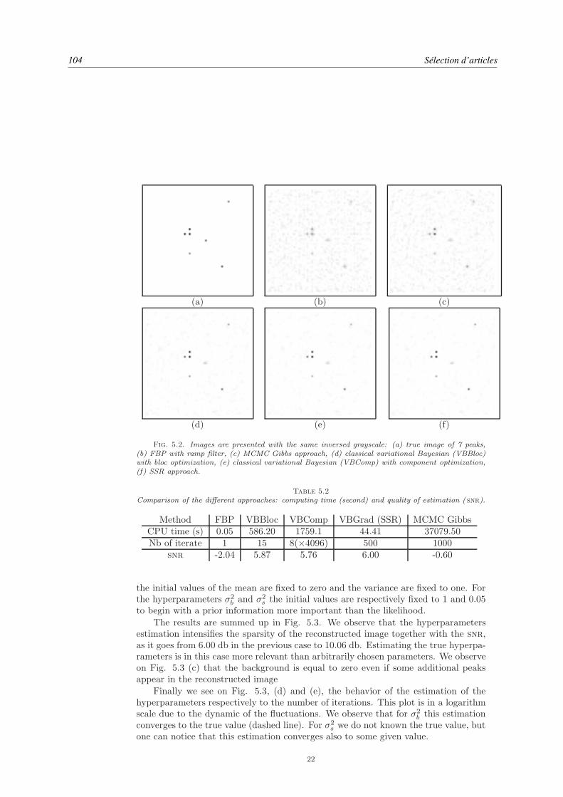
104 Sélection d’articles
(a) (b) (c)
(d) (e) (f)
Fig. 5.2. Images are presented with the same inversed grayscale: (a) true image of 7 peaks,(b) FBP with ramp filter, (c) MCMC Gibbs approach, (d) classical variational Bayesian (VBBloc)with bloc optimization, (e) classical variational Bayesian (VBComp) with component optimization,(f) SSR approach.
Table 5.2
Comparison of the different approaches: computing time (second) and quality of estimation ( snr).
Method FBP VBBloc VBComp VBGrad (SSR) MCMC GibbsCPU time (s) 0.05 586.20 1759.1 44.41 37079.50Nb of iterate 1 15 8(×4096) 500 1000
snr -2.04 5.87 5.76 6.00 -0.60
the initial values of the mean are fixed to zero and the variance are fixed to one. Forthe hyperparameters σ2
b and σ2s the initial values are respectively fixed to 1 and 0.05
to begin with a prior information more important than the likelihood.
The results are summed up in Fig. 5.3. We observe that the hyperparametersestimation intensifies the sparsity of the reconstructed image together with the snr,as it goes from 6.00 db in the previous case to 10.06 db. Estimating the true hyperpa-rameters is in this case more relevant than arbitrarily chosen parameters. We observeon Fig. 5.3 (c) that the background is equal to zero even if some additional peaksappear in the reconstructed image
Finally we see on Fig. 5.3, (d) and (e), the behavior of the estimation of thehyperparameters respectively to the number of iterations. This plot is in a logarithmscale due to the dynamic of the fluctuations. We observe that for σ2
b this estimationconverges to the true value (dashed line). For σ2
s we do not known the true value, butone can notice that this estimation converges also to some given value.
22

,A measure-theoretic variational bayesian algorithm for large dimensional problems 105
(a) (b) (c)
0 200 400 600 800 1000−3
−2
−1
0
1
2
3
nb of iterations0 200 400 600 800 1000
−10
−8
−6
−4
−2
0
nb of iterations
(d) (e)
Fig. 5.3. Results with hyperparameters estimation: (a) True image, (b) reconstructed imagewith SSR algorithm (hyperparameters are fixed), (c) reconstructed image with USSR (image andhyperparameters are estimated jointly), (d) logarithm of σ2
bduring the iterations the dashed line
correspond to the true value, (e) logarithm of σ2s during the iterations
5.2. Component identification (denoising). As enhanced by the previoussimulation, our method can be more efficient than classical ones on relatively smallproblem (4096 unknowns). But its main advantage is that it allows to address largerproblems (≈ 300000 unknowns in the present case). In the present part, our purposeis to treat an identification problem on a dictionary decomposition. More precisely,we identify many chirps function ψk(t) in a linear mixture. This identification issueappears for instance in astrophysics, in order to detect gravitational waves [28] or inradar imaging [39, 1]. Unfortunately, this mixture is corrupted by noise and spurioussignal. To identify each chirps in the mixture and to remove the effect of the spurioussignal, we develop a dictionary learning approach. To build our dictionary we makethe following assumptions : all chirps have the same duration TChirp, the chirps rateζ is digitalized on very few values (eight in the present case), the spurious signal canbe represented on very few coefficients of Discrete Fourier Transform and the noiseis white and Gaussian. However, we do not make any assumption on the variance ofthe noise or on the number of chirp functions in the mixture.
In the following section, we present the formalism of the dictionary learning ap-proach. After that, we expose the simulation condition. Then, we illustrate theefficiency of our approach with three numerical experiments. In the first one, we con-sider a nominal case to study the quality of estimation. After what, we study a limitcase with a very high level of noise (snr at -5 db), in order to illustrate the robustnessof our approach with regard to noise. In the last experiment, we study the behavior
23

106 Sélection d’articles
of the reconstruction quality when the number of chirp functions or the noise levelincrease.
5.2.1. Dictionary decomposition. In this section the signal considered, de-noted by s(t), is obtained by the following dictionary decomposition.
s(t) =
Nfreq∑
i=1
(ui + jvi)φi(t) +
Ntrans∑
l=1
Nrate∑
k=1
cl,kψk(t− l∆t), (5.1)
where
φi(t) = exp [2jπfit] ,
corresponds to a pure frequency fi with j2 = −1 whereas
ψk(t) = cos(2π(f0t+1
2t2ζk))Π0,TChirp
(t)
corresponds to the chirps components. Here, f0 is the starting frequency (at time t =0), ζk is the chirp rate, that is the increasing rate of the frequency, Π(t) is a gate func-tion, TChirp is the duration of the chirp, ∆t is the shift between two chirps functionsand tl = l∆t is the first time where the ψk(t−l∆t) is not null. We merge all the dictio-nary’s coefficients in a single vector x = (u1, . . . , uNfreq, v1, . . . , vNfreq, c1,1, . . . , cNtrans,Nrate)
t.Where Nfreq is the number of pure frequency functions contained on the dictionarywhereas Ntrans is the number of chirp shifts and Nrate is the number of chirp rate.Moreover, we store sampled version of functions φi and ψl,k into a matrix H . Hence,the sampled version of Equation (5.1) is given by
s = Hx, (5.2)
where s = (s(t0), . . . , s(tN ))t.
The measurement of the signal s is also corrupted by an iid Gaussian noise b witha variance σ2
b , such that the observations are given by
y = s+ b = Hx+ b. (5.3)
In the following, the dictionary is composed of chirp functions with only 8 differentchirp rates (Nrate = 8). The frequency f0 is equal to 5 000 hz, the chirp rates ζk areuniformly spaced between 6 000 and 20 000 hz, the shift parameters ∆t is fixed up toa sampling period (Te = 1/Fe). Finally, the duration of the chirp (TChirp) is equal tothe half time of the measurements (Tmes).
Remark 6. Our dictionary is redundant as the number of coefficients is 4.5times greater than the number of observations. Thus, the component identification isan ill-posed problem.
5.2.2. Common simulation conditions. Simulated data are composed by thesum of NCos cosine functions with different frequencies and NChirp chirp functionstaken in our dictionary. The simulated data are sampled at a frequency Fe = 44khz,and they are composed of N = 216 points, thus the duration of measurement Tmes isequal to 1.5 second.
24

,A measure-theoretic variational bayesian algorithm for large dimensional problems 107
Table 5.3
Parameters of the different components
type of function Amplitude frequency (hz) rate (hz) first time (s)cosine 1 5169.7 - -cosine 0.8 4834 - -Chirp 1.4 - 8000 0.2Chirp 1.4 - 10000 0.25Chirp 1.0 - 16000 0.22Chirp 1.0 - 20000 0.5Chirp 1.2 - 10000 0.4Chirp 1.0 - 18000 0.41Chirp 1.0 - 20000 0.6Chirp 1.4 - 8000 0.3
0 0.5 1 1.5−15
−10
−5
0
5
10
15
time in second0 1 2 3 4 5
x 104
0
0.5
1
1.5
2
2.5
3
3.5x 10
4
frequency in hertz time in second
freq
uenc
y in
her
tz
0 0.5 10
0.5
1
1.5
2
2.5
3
3.5
4
x 104
(a) (b) (c)
Fig. 5.4. Data in different fields: (a) time, (b) frequency, (c) time-frequency
5.2.3. First result. The simulated data are composed of two cosine functionsand eight chirp functions, the parameters of all this functions are given in Tab. 5.3.Once again simulated data have a relatively bad snr, at 5.68 db in this case. Theyare plotted in Fig. 5.4 (a), whereas their Fourier transform are given in Fig. 5.4(b) and their time-frequency transform, computed with a STFT (Short Time FourierTransform) are on Fig. 5.4(c). We can see in the time frequency representation thatthere are overlaps between the different components making the identification harder.
Moreover this inverse problem is treated with the unsupervised approach given byAlgorithm 4. Our algorithm was launched with the shape parameter of the Student’tequals to ν = 0.01 in order to introduce a very sparse prior. The initializationparameters are:
• The mean of q0(x), m0 = 0,• the variance of q0(x), σ2
0 = 1,• the mean of q0b (γb), is equal to 10−5,• the mean of q0s(γs), is equal to 105.
After 400 iterations (316 s), the algorithm (USSR) converges to a stable solu-tion. It gives parameters of different approximated laws. We consider here that theestimation x is obtained by taking the posterior mean for the coefficients (see Fig.5.5).
Fig. 5.5 (a) represents the real part of the Fourier coefficients (the vector u isthe Equation (5.1)). We recognize the Fourier transform of the two cosine functions.Moreover, when we compare Fig. 5.5 (a) with the Fourier transform of the data, Fig.
25
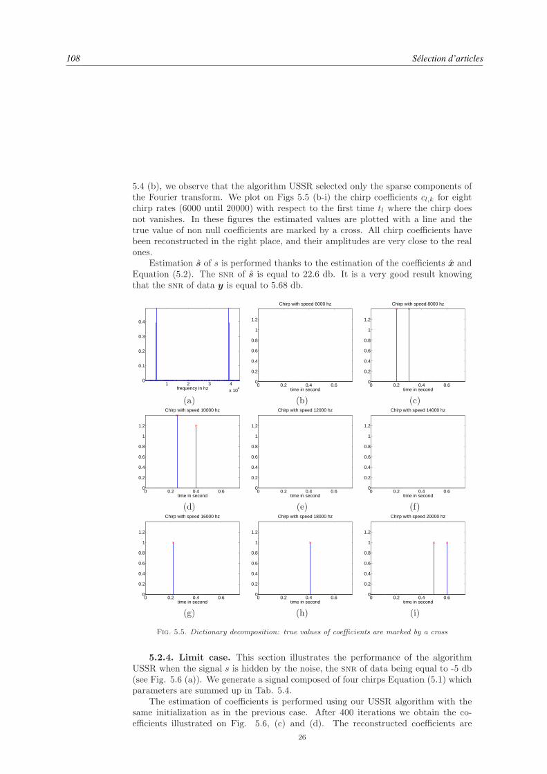
108 Sélection d’articles
5.4 (b), we observe that the algorithm USSR selected only the sparse components ofthe Fourier transform. We plot on Figs 5.5 (b-i) the chirp coefficients cl,k for eightchirp rates (6000 until 20000) with respect to the first time tl where the chirp doesnot vanishes. In these figures the estimated values are plotted with a line and thetrue value of non null coefficients are marked by a cross. All chirp coefficients havebeen reconstructed in the right place, and their amplitudes are very close to the realones.
Estimation s of s is performed thanks to the estimation of the coefficients x andEquation (5.2). The snr of s is equal to 22.6 db. It is a very good result knowingthat the snr of data y is equal to 5.68 db.
1 2 3 4x 10
4
0
0.1
0.2
0.3
0.4
frequency in hz0 0.2 0.4 0.6
0
0.2
0.4
0.6
0.8
1
1.2
Chirp with speed 6000 hz
time in second0 0.2 0.4 0.6
0
0.2
0.4
0.6
0.8
1
1.2
Chirp with speed 8000 hz
time in second
(a) (b) (c)
0 0.2 0.4 0.60
0.2
0.4
0.6
0.8
1
1.2
Chirp with speed 10000 hz
time in second0 0.2 0.4 0.6
0
0.2
0.4
0.6
0.8
1
1.2
Chirp with speed 12000 hz
time in second0 0.2 0.4 0.6
0
0.2
0.4
0.6
0.8
1
1.2
Chirp with speed 14000 hz
time in second
(d) (e) (f)
0 0.2 0.4 0.60
0.2
0.4
0.6
0.8
1
1.2
Chirp with speed 16000 hz
time in second0 0.2 0.4 0.6
0
0.2
0.4
0.6
0.8
1
1.2
Chirp with speed 18000 hz
time in second0 0.2 0.4 0.6
0
0.2
0.4
0.6
0.8
1
1.2
Chirp with speed 20000 hz
time in second
(g) (h) (i)
Fig. 5.5. Dictionary decomposition: true values of coefficients are marked by a cross
5.2.4. Limit case. This section illustrates the performance of the algorithmUSSR when the signal s is hidden by the noise, the snr of data being equal to -5 db(see Fig. 5.6 (a)). We generate a signal composed of four chirps Equation (5.1) whichparameters are summed up in Tab. 5.4.
The estimation of coefficients is performed using our USSR algorithm with thesame initialization as in the previous case. After 400 iterations we obtain the co-efficients illustrated on Fig. 5.6, (c) and (d). The reconstructed coefficients are
26

,A measure-theoretic variational bayesian algorithm for large dimensional problems 109
Table 5.4
Parameters of the different components
type of function Amplitude Chirp rate (hz) first time (s)Chirp 0.9526 16000 0.1530Chirp 1.1606 16000 0.1945Chirp 0.7369 18000 0.2000Chirp 1.1724 18000 0.1865
represented by a line and the true values of the coefficients are marked by a cross.We observe that all coefficients are in the right place and that the peaks amplitudesare systematically underestimated, but the estimated values are relatively close to thetrue ones. Fig. 5.6 (b) points out the estimator s. We see that the shape of the signalis close to the true one, and that when the signal is missing, between 1 and 1,45 s,the level of the residual noise is relatively low.
Table 5.5
Signal to Noise Ratio ( snr) in db
data USSR approach best Wiener filter best wavelet soft threshold-5.0 15.05 1.1941 1.8677
In Tab. 5.5 we compare the reconstructed signal s with the reconstruction ob-tained with two classical denoising approaches, namely the Wiener filter and the softwavelet shrinkage, with the four vanishing moments symmlet. In these two meth-ods, we furthermore have to tune a parameter which is the correlation power for theWiener filter and the threshold for the soft wavelet shrinkage. Hence we choose thevalue of this hyperparameter which minimizes the Signal to Noise Ratio (snr). Unlikein the USSR approach, we thus have to we know the true signal in order to tune thisparameter. Furthermore, our approach increases hugely the snr (20 db), thus thenoise level is divided by 100 whereas the classical methods reduce the noise only by afactor 4 or 5. This example enhances the efficiency of the dictionary decompositionin the denoising context.
5.2.5. Behavior of our method versus level of noise and number of com-ponents. In this part, we perform the study of the robustness of the USSR algorithmregarding Signal to Noise Ratio. This simulation allows a better understanding of thereconstruction properties of our method.
Simulations. In the following we consider simulated data with 6 different snr
(−5,−2, 1, 2, 5, 10) and with low (4) and high (16) number of components. For eachsnr and each number of components, we simulate 30 set of data, the components ofthe signal being randomly chosen between 1 and 9. If the number is equal to 1, weconsider a cosine function with a frequency fi is uniformly taken between 0 and thesampling frequency (Fe= 44 khz), and an amplitude randomly chosen between 0.6and 1.4. If the number is equal to 2 resp. 3, . . . , 9, we simulate a chirp function witha chirp rate ζk equal to 6000 resp. 8000, . . . , 20000. The first time of the chirp tl isuniformly taken between 0.1 and 0.6 second, and as previously, the amplitude cl,k israndomly chosen between 0.6 and 1.4.
Reconstruction. We reconstruct this 360 sets of data by the algorithm USSRtaking the same configuration and the same initialization as in previous cases.
27

110 Sélection d’articles
0.2 0.4 0.6 0.8 1 1.2 1.4
−6
−4
−2
0
2
4
6
8
time in second0.2 0.4 0.6 0.8 1 1.2 1.4
−6
−4
−2
0
2
4
6
8
time in second
(a) (b)
0 0.2 0.4 0.60
0.2
0.4
0.6
0.8
1
1.2
Chirp with speed 16000 hz
time in second0 0.2 0.4 0.6
0
0.2
0.4
0.6
0.8
1
1.2
Chirp with speed 18000 hz
time in second
(c) (d)
Fig. 5.6. Limit case: (a) data and true signal, (b) reconstructed signal
The results are summed up on Fig 5.7 (a-d). Each point of the plot is computedby averaging the result of 30 reconstructions. In Fig 5.7 (a), resp. (b), we plot the truepositive proportion, resp. false positive proportion, of the significant reconstructedcoefficients1. At first sight we see that there are no false positive with our approach.Indeed, as the approach is unsupervised with a sparsity prior, the coefficients with lowenergy are considered as noise. Moreover we can reconstruct 16 components withoutlost when the snr is greater or equal to 5 db and resp. 4 components when the snr
is greater to 1 db. Fig. 5.7 shows that the reconstruction is more difficult when thenumber of components increases.
Fig. 5.7 (c) is obtained by calculating the snr of the reconstructed signal s. Weobserve a quite linear behavior. For 4 components the gain is of 17 db whereas for16 components we gain 11.5 db. Finally, Fig. 5.7 (d) exposes the quadratic error ofthe peaks amplitude. There are here two cases. When all the components are foundthis error is linear (see Fig. 5.7 (d) the bottom curve when snr> 1) but it increasesmore rapidly when some components are not found (see Fig. 5.7 (d) the bottom curvewhen snr< 1).
6. Conclusion. In this paper, we have defined an iterative algorithm based onthe descent gradient principle and adapted to the context of variational Bayesianmethods. The main interest of this algorithm is that it converges faster than theclassical Bayesian methods and allows an use on large dimensional datasets. We havefurthermore give its implementation in the case of white noise model when the priorinformation enhances some sparse behavior. A small tomographic application allowsus to compare our method with classical ones. We see that even in small cases, ouralgorithm can be faster than classical ones. A second simulation part, corresponding
1the significant coefficients are obtained by applying a threshold equal to 0.2 on the coefficientsvector. This threshold is equal to the third of the minimum value of the true non zero coefficients.
28

,A measure-theoretic variational bayesian algorithm for large dimensional problems 111
−5 0 5 100
20
40
60
80
100
SNR in db
Proportion of true positive
NbComp=4NbComp=16
−5 0 5 100
20
40
60
80
100
SNR in db
Proportion of false positive
NbComp=4NbComp=16
(a) (b)
−5 0 5 100
5
10
15
20
25
30
SNR in db
Rec
onst
ruct
ed S
NR
in d
b
NbComp=4NbComp=16
−5 0 5 1010
−6
10−4
10−2
100
SNR in db
Qua
drat
ic e
rror
of a
mpl
itude
NbComp=4NbComp=16
(c) (d)
Fig. 5.7. Study of Robustness versus noise, each point of the curve being is calculated byaveraging 30 reconstructions with components randomly chosen: (a) True positive proportion of thesignificant reconstructed coefficients, (b) False positive proportion of the significant reconstructedcoefficients, (c) snr of the estimated signal s, (d) Quadratic error of the peaks amplitude
to a dictionary identification allows to understand the behavior of our method for largedimensional problems. Once again this method has good reconstruction properties inthis case.
7. Annexe.
7.1. Proof of Lemma 2.2. In order to ensure that for small values of α, wehave F (µα) > F (µk), we show that the right part of Equation (2.16),
F (µα)−F (µk) ≥ ∂Fµk(µα−µk)−L‖hα(µk, .)−1‖2L2(µk)−∫
RN
(αdf(µk,x)+lnKk(α))dµα(x),
is positive.
First, one can notice that
−∫
RN
ln(hα(µk,x))dµα(x) = −
∫
RN
(αdf(µk,x)+lnKk(α))hαdµk(x) = −α
(∫
RN
df(µk,x)hαdµk(x)−
But Jensen’s inequality ensures that
lnKk(α) ≤ −α∫
RN
df(µk,x)dµk(x). (7.1)
29

112 Sélection d’articles
Which leads to
−∫
RN
ln(hα(µk,x))dµα(x) ≥ −α
∫
RN
df(µk,x)(hα(µk,x)− 1)dµk(x). (7.2)
Hence,
∂Fµk(µα − µk)−∫
RN
ln(hα(µk,x))dµα(x) ≥
∫
RN
(1− α)df(µk,x)(hα(µk,x)− 1)dµk(x)
=1− αα
∫
RN
(αdf(µk,x) + lnKk(α))(hα(µk,x)− 1)dµk(x)−
∫
RN
(1− α) lnKk(α)
α(hα(µ
=1− αα
∫
RN
(αdf(µk,x) + lnKk(α))(hα(µk,x)− 1)dµk(x),
as (1−α) lnKk(α)α is constant and
∫RN (hα(µ
k,x)− 1)dµk(x) = 0.Finally,
dFµk(µα − µk)− L‖hα − 1‖2L2(µk) −∫
RN
(αdf(µk,x) + lnKk(α))dµα(x)
≥∫
RN
((αdf(µk,x) + lnKk(α))(
1
α− 1)− L(hα(µk,x)− 1)
)(hα(µ
k,x)− 1)dµk(x)
=
∫
x:αdf(µk,x)+lnKk(α)>0
((αdf(µk,x) + lnKk(α))(
1
α− 1)− L(hα(µk,x)− 1)
)(hα(µ
k,x)− 1)dµk(x
+
∫
x:αdf(µk,x)+lnKk(α)≤0
((αdf(µk,x) + lnKk(α))(
1
α− 1)− L(hα(µk,x)− 1)
)(hα(µ
k,x)− 1)dµk(x)
(7.3)
Let us consider each integrals appearing in Eq. (7.3) separately. First, let usnotice that if αdf(µk,x) + lnKk(α) < 0 then so is hα(µ
k, .) − 1. Furthermore, forevery α > 0 and x ∈ R
N , we have hα(µk, .) − 1 ≥ αdf(µk,x) + lnKk(α). Hence if
x ∈ RN is such that αdf(µk,x) + lnKk(α) < 0 then
((αdf(µk,x) + lnKk(α))(
1
α− 1)− L(hα(µk,x)− 1)
)(hα(µ
k,x)−1) ≥ (hα(µk,x)−1)2
(1
α− 1− L
),
which is positive as soon as α ≤ 11+L .
Consider now that x ∈ RN is such that αdf(µk,x) + lnKk(α) ≥ 0. The Mean
Value Theorem applied to the function exponential ensures that one can find, forevery x ∈ R
N and α > 0 a θ(x, α) ∈ (0, αdf(µk,x) + lnKk(α)) such that
hα(µk,x) = eαdf(µ
k,x)+lnKk(α) = 1 + (αdf(µk,x) + lnKk(α))eθ(x,α).
This entails that((αdf(µk,x) + lnKk(α))(
1
α− 1)− L(hα(µk,x)− 1)
)= (αdf(µk,x)+lnKk(α))(
1
α−1−Leθ(x,α)).
Furthermore, Jensen’s inequality ensures that
0 ≤ αdf(µk,x) + lnKk(α) ≤ α(df(µk,x)−
∫
RN
df(µk,x)dµk(x)
).
30

,A measure-theoretic variational bayesian algorithm for large dimensional problems 113
Thus
df(µk,x)−∫
RN
df(µk,x)dµk(x) ≥ 0.
And
1 ≤ eθ(x,α) ≤ hα(µk,x) ≤ eα(df(µk,x)−∫RN
df(µk,x)dµk(x)),
which leads to
1
α− 1− Leα(df(µk,x)−
∫RN
df(µk,x)dµk(x)) ≤ 1
α− 1− Leθ(x,α) ≤ 1
α− 1− L.
Concerning the left part of the previous equation one can notice that the function ofα defined here is positive for small positive values of α. Hence there exists a valueα0 > 0 such that for every α ≤ α0,
1
α− 1− Leα(df(µk,x)−
∫RN
df(µk,x)dµk(x)) ≥ 0.
Finally one has that there exists α0 ≥ 0 such that
∀α ≤ α0, dFµk(µα−µk)−L‖hα−1‖2L2(µk)−∫
RN
(αdf(µk,x)+lnKk(α))dµα(x) ≥ 0.
(7.4)
7.2. Optimization of the parameter α. In order to obtain the optimal valueof α > 0, we have to optimize
gk(α) = F (qα) =
∫
RN
∫
RN
ln p(x,y, z)qα(x)qk(z)dxdz−∫
RN
∫
RN
ln(qα(x)qk(z))qα(x)qk(z)dxdz.
Let us compute F (qα). To achieve this, we first notice that
ln p(x,y, z) = C−xTHTHx− 2xTHTy + yTy
2σ2b
+∑
i
1
2ln(zi/σ
2s)−
zix2i
2σ2s
+(ai−1) ln(zi)−zibi,
where C is a positive constant. Thus
∫
RN
∫
RN
ln p(x,y, z)qα(x)qk(z)dxdz = C −∫
RN
∫
RN
xTHTHx− 2xTHTy
2σ2b
∏qαj (xj)q
k(z)dxdz
+∑
i
∫
R
1
2ln(zi/σ
2s)q
ki (zi)dzi +
∑
i
∫
R
((ai − 1) ln(zi)− zibi
)qk(zi)
−∑
i
∫
R2
zix2i
2σsqki (zi)dxidzi
We have thus five terms:
31
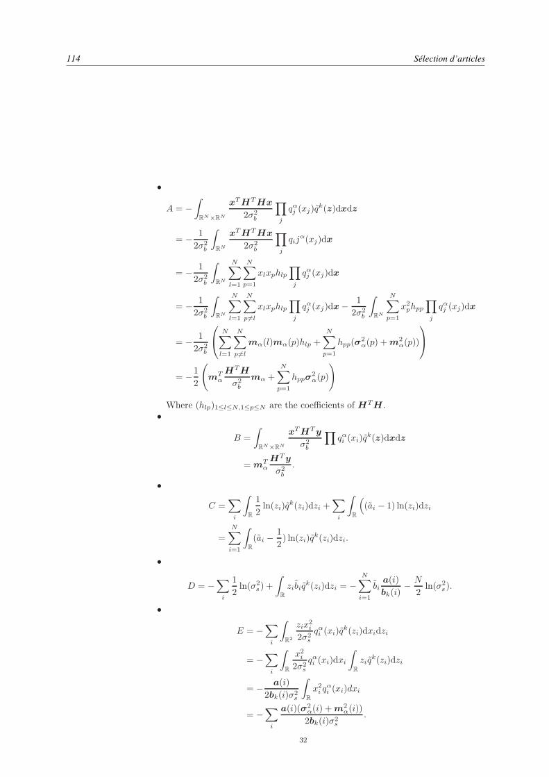
114 Sélection d’articles
•
A = −∫
RN×RN
xTHTHx
2σ2b
∏
j
qαj (xj)qk(z)dxdz
= − 1
2σ2b
∫
RN
xTHTHx
2σ2b
∏
j
qijα(xj)dx
= − 1
2σ2b
∫
RN
N∑
l=1
N∑
p=1
xlxphlp∏
j
qαj (xj)dx
= − 1
2σ2b
∫
RN
N∑
l=1
N∑
p6=l
xlxphlp∏
j
qαj (xj)dx−1
2σ2b
∫
RN
N∑
p=1
x2phpp∏
j
qαj (xj)dx
= − 1
2σ2b
N∑
l=1
N∑
p6=l
mα(l)mα(p)hlp +
N∑
p=1
hpp(σ2α(p) +m2
α(p))
= −1
2
(mT
α
HTH
σ2b
mα +
N∑
p=1
hppσ2α(p)
)
Where (hlp)1≤l≤N,1≤p≤N are the coefficients of HTH .•
B =
∫
RN×RN
xTHTy
σ2b
∏qαi (xi)q
k(z)dxdz
= mTα
HTy
σ2b
.
•
C =∑
i
∫
R
1
2ln(zi)q
k(zi)dzi +∑
i
∫
R
((ai − 1) ln(zi)dzi
=
N∑
i=1
∫
R
(ai −1
2) ln(zi)q
k(zi)dzi.
•
D = −∑
i
1
2ln(σ2
s ) +
∫
R
zibiqk(zi)dzi = −
N∑
i=1
bia(i)
bk(i)− N
2ln(σ2
s ).
•
E = −∑
i
∫
R2
zix2i
2σ2s
qαi (xi)qk(zi)dxidzi
= −∑
i
∫
R
x2i2σ2
s
qαi (xi)dxi
∫
R
ziqk(zi)dzi
= − a(i)
2bk(i)σ2s
∫
R
x2i qαi (xi)dxi
= −∑
i
a(i)(σ2α(i) +m2
α(i))
2bk(i)σ2s
.
32

,A measure-theoretic variational bayesian algorithm for large dimensional problems 115
Furthermore, concerning the entropy we have
H(X,Z) =N∑
i=1
H(qα(xi)) +N∑
i=1
H(qk(zi)).
And,
H(qα(xi)) =1
2(1 + ln(2πσ2
α(i))),
H(qk(zi)) = −∫
R
(a(i)− 1) ln(zi)qk(zi)dzi + Const.
From Equation (4.7) we have a(i) = ai +12 and
C+
N∑
i=1
H(qk(zi)) =N∑
i=1
N∑
i=1
∫
R
(ai−1
2) ln(zi)q
k(zi)dzi−∫
R
(ai+1
2−1) ln(zi)qk(zi)dzi+Const = Const
Finally, the negative free entropy is
F (qα) = A+B +D + E +∑
i
H(xi) + Const, (7.5)
Let us determine the critical values of gk(α) = F (qα) and their signs.As one can see, the derivative of gk(α) is closely related to the derivatives of σ2
α(i)and mα(i) which, for i = 1, . . . , N , are given by
dσ2α(i)
dα=−σ2
k(i)σ2r(i)(σ
2k(i)− σ2
r(i))
(σ2r(i) + α(σ2
k(i)− σ2r(i)))
2, (7.6)
whereas
dmα(i)
dα=
σ2r(i)σ
2k(i)(mr(i)−mk(i))
(σ2r(i) + α(σ2
k(i)− σ2r(i)))
2. (7.7)
And the second order derivatives are
d2σ2α(i)
dα2=
2σ2k(i)σ
2r(i)(σ
2k(i)− σ2
r(i))2
(σ2r(i) + α(σ2
k(i)− σ2r(i)))
3(7.8)
and,
d2mα(i)
dα2=
2σ2r(i)σ
2k(i)(mr(i)−mk(i))(σ
2r(i)− σ2
k(i))
(σ2r(i) + α(σ2
k(i)− σ2r(i)))
3. (7.9)
This entails that the first order derivative of g satisfies
g′(α) =
N∑
i=1
− 1
σ2b
N∑
p=1
dmα(i)
dαmα(p)hip
− hii2σ2
b
dσ2α(i)
dα+
dmα(i)
dα
(HTy
σ2b
)
i
− a(i)
2bk(i)σ2s
dσ2α(i)
dα− a(i)mα(i)
bk(i)σ2s
dmα(i)
dα+
dσ2α(i)/dα
4πσ2α(i)
(7.10)
33
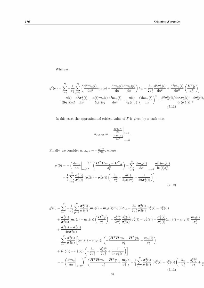
116 Sélection d’articles
Whereas,
g′′(α) =
N∑
i=1
− 1
σ2b
N∑
p=1
(d2mα(i)
dα2mα(p) +
dmα(i)
dα
dmα(p)
dα
)hip −
hii2σ2
b
d2σ2α(i)
dα2+
d2mα(i)
dα2
(HTy
σ2b
)
i
− a(i)
2bk(i)σ2s
d2σ2α(i)
dα2− a(i)mα(i)
bk(i)σ2s
d2mα(i)
dα2− a(i)
bk(i)σ2s
(dmα(i)
dα
)2
+d2σ2
α(i)/dα2σ2
α(i)− dσ2α(i)/
4π(σ2α(i))
2
(7.11)
In this case, the approximated critical value of F is given by α such that
αsubopt = −dF (qα)
dα
∣∣∣α=0
d2F (qα)dα2
∣∣∣α=0
.
Finally, we consider αsubopt = − g′(0)g′′(0) , where
g′(0) = −(dmα
dα
∣∣∣∣α=0
)T (HTHmk −HTy
σ2b
)−
N∑
i=1
dmα(i)
dα
∣∣∣∣α=0
a(i)mk(i)
bk(i)σ2s
+1
2
N∑
i=1
σ2k(i)
σ2r(i)
(σ2r(i)− σ2
k(i))
(−hiiσ2b
− a(i)
bk(i)σ2s
+1
2πσ2k(i)
)].
(7.12)
g′(0) =
N∑
i=1
− 1
σ2b
N∑
p=1
σ2k(i)
σ2r(i)
(mr(i)−mk(i))m0(p)hip −hii2σ2
b
σ2k(i)
σ2r(i)
(σ2r(i)− σ2
k(i))
+σ2
k(i)
σ2r(i)
(mr(i)−mk(i))
(HTy
σ2b
)
i
− aki bki
2σ2s
σ2k(i)
σ2r(i)
(σ2r(i)− σ2
k(i))−σ2
k(i)
σ2r(i)
(mr(i)−mk(i))m0(i)
σ2s
+σ2
r(i)− σ2k(i)
4πσ2r(i)
=
N∑
i=1
σ2k(i)
σ2r(i)
[(mr(i)−mk(i))
(− (HTHmk −HTy)i
σ2b
− mk(i)
σ2s
)
+ (σ2r(i)− σ2
k(i))
(− hii2σ2
b
− aki bki
2σ2s
+1
4πσ2k(i)
)]
= −(dmα
dα
∣∣∣∣α=0
)T (HTHmk −HTy
σ2b
+mk
σ2s
)+
1
2
N∑
i=1
σ2k(i)
σ2r(i)
(σ2r(i)− σ2
k(i))
(−hiiσ2b
− aki bki
σ2s
+2π
(7.13)
34
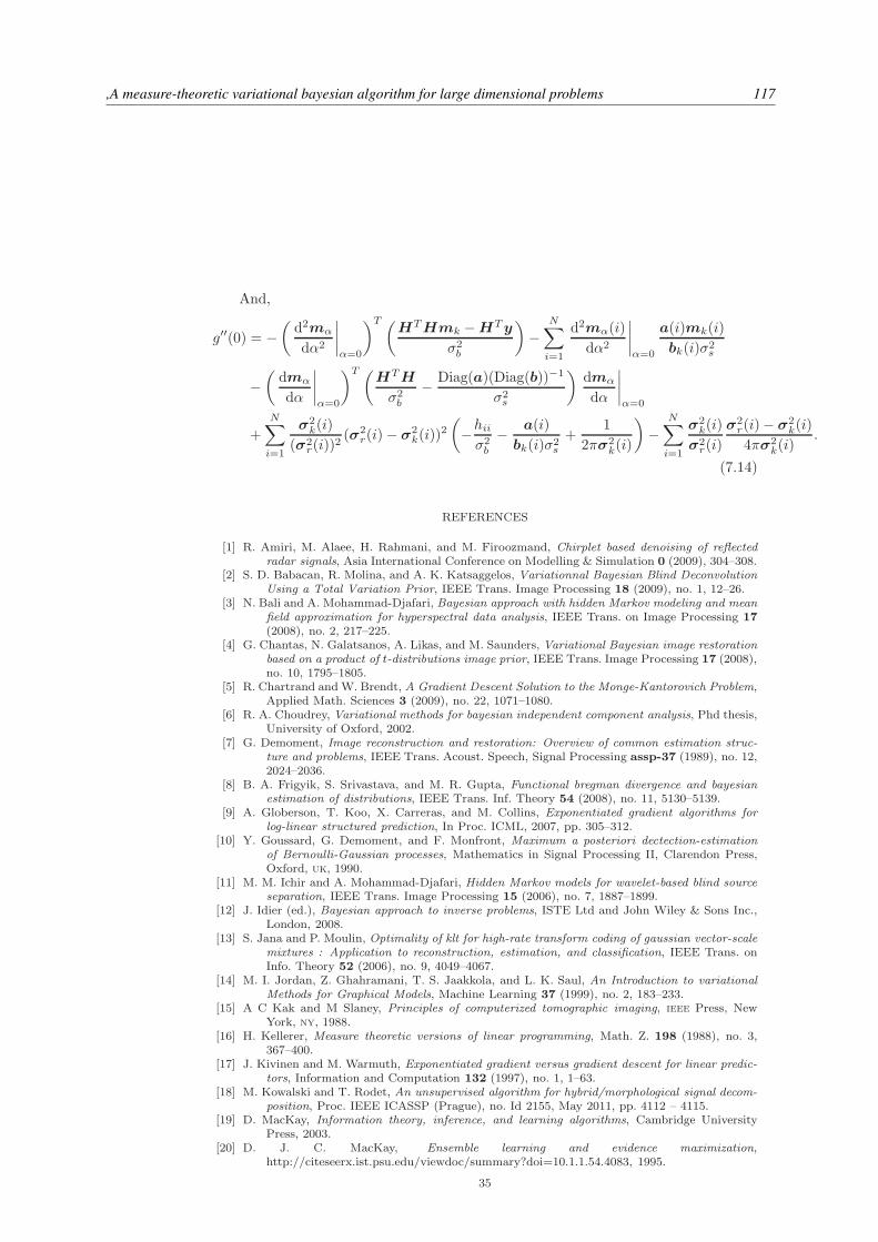
,A measure-theoretic variational bayesian algorithm for large dimensional problems 117
And,
g′′(0) = −(d2mα
dα2
∣∣∣∣α=0
)T (HTHmk −HTy
σ2b
)−
N∑
i=1
d2mα(i)
dα2
∣∣∣∣α=0
a(i)mk(i)
bk(i)σ2s
−(dmα
dα
∣∣∣∣α=0
)T (HTH
σ2b
− Diag(a)(Diag(b))−1
σ2s
)dmα
dα
∣∣∣∣α=0
+
N∑
i=1
σ2k(i)
(σ2r(i))
2(σ2
r(i)− σ2k(i))
2
(−hiiσ2b
− a(i)
bk(i)σ2s
+1
2πσ2k(i)
)−
N∑
i=1
σ2k(i)
σ2r(i)
σ2r(i)− σ2
k(i)
4πσ2k(i)
.
(7.14)
REFERENCES
[1] R. Amiri, M. Alaee, H. Rahmani, and M. Firoozmand, Chirplet based denoising of reflectedradar signals, Asia International Conference on Modelling & Simulation 0 (2009), 304–308.
[2] S. D. Babacan, R. Molina, and A. K. Katsaggelos, Variationnal Bayesian Blind DeconvolutionUsing a Total Variation Prior, IEEE Trans. Image Processing 18 (2009), no. 1, 12–26.
[3] N. Bali and A. Mohammad-Djafari, Bayesian approach with hidden Markov modeling and meanfield approximation for hyperspectral data analysis, IEEE Trans. on Image Processing 17
(2008), no. 2, 217–225.[4] G. Chantas, N. Galatsanos, A. Likas, and M. Saunders, Variational Bayesian image restoration
based on a product of t-distributions image prior, IEEE Trans. Image Processing 17 (2008),no. 10, 1795–1805.
[5] R. Chartrand and W. Brendt, A Gradient Descent Solution to the Monge-Kantorovich Problem,Applied Math. Sciences 3 (2009), no. 22, 1071–1080.
[6] R. A. Choudrey, Variational methods for bayesian independent component analysis, Phd thesis,University of Oxford, 2002.
[7] G. Demoment, Image reconstruction and restoration: Overview of common estimation struc-ture and problems, IEEE Trans. Acoust. Speech, Signal Processing assp-37 (1989), no. 12,2024–2036.
[8] B. A. Frigyik, S. Srivastava, and M. R. Gupta, Functional bregman divergence and bayesianestimation of distributions, IEEE Trans. Inf. Theory 54 (2008), no. 11, 5130–5139.
[9] A. Globerson, T. Koo, X. Carreras, and M. Collins, Exponentiated gradient algorithms forlog-linear structured prediction, In Proc. ICML, 2007, pp. 305–312.
[10] Y. Goussard, G. Demoment, and F. Monfront, Maximum a posteriori dectection-estimationof Bernoulli-Gaussian processes, Mathematics in Signal Processing II, Clarendon Press,Oxford, uk, 1990.
[11] M. M. Ichir and A. Mohammad-Djafari, Hidden Markov models for wavelet-based blind sourceseparation, IEEE Trans. Image Processing 15 (2006), no. 7, 1887–1899.
[12] J. Idier (ed.), Bayesian approach to inverse problems, ISTE Ltd and John Wiley & Sons Inc.,London, 2008.
[13] S. Jana and P. Moulin, Optimality of klt for high-rate transform coding of gaussian vector-scalemixtures : Application to reconstruction, estimation, and classification, IEEE Trans. onInfo. Theory 52 (2006), no. 9, 4049–4067.
[14] M. I. Jordan, Z. Ghahramani, T. S. Jaakkola, and L. K. Saul, An Introduction to variationalMethods for Graphical Models, Machine Learning 37 (1999), no. 2, 183–233.
[15] A C Kak and M Slaney, Principles of computerized tomographic imaging, ieee Press, NewYork, ny, 1988.
[16] H. Kellerer, Measure theoretic versions of linear programming, Math. Z. 198 (1988), no. 3,367–400.
[17] J. Kivinen and M. Warmuth, Exponentiated gradient versus gradient descent for linear predic-tors, Information and Computation 132 (1997), no. 1, 1–63.
[18] M. Kowalski and T. Rodet, An unsupervised algorithm for hybrid/morphological signal decom-position, Proc. IEEE ICASSP (Prague), no. Id 2155, May 2011, pp. 4112 – 4115.
[19] D. MacKay, Information theory, inference, and learning algorithms, Cambridge UniversityPress, 2003.
[20] D. J. C. MacKay, Ensemble learning and evidence maximization,http://citeseerx.ist.psu.edu/viewdoc/summary?doi=10.1.1.54.4083, 1995.
35
118 Sélection d’articles
[21] J.W Miskin, Ensemble learning for independent component analysis, Phd thesis, University ofCambridge, http://www.inference.phy.cam.ac.uk/jwm1003/, 2000.
[22] I. Molchanov, Tangent sets in the space of measures: with applications to variational analysis,J. Math. Anal. Appl. 249 (2000), no. 2, 539–552.
[23] I. Molchanov and S. Zuyev, Steepest descent algorithms in a space of measures, Statistics andComputing 12 (2002), 115–123.
[24] K. Morton, P. Torrione, and L. Collins, Variational bayesian learning for mixture autoregressivemodels with uncertain-order, IEEE Trans. Signal Processing 59 (2011), no. 6, 2614–2627.
[25] F. Natterer, Algorithms in tomography, Clarendon Press, 1997.[26] Y. Nesterov, Smooth minimization of non-smooth functions, Mathematical Programming 103
(2005), no. 1, 127–152.[27] J. Nocedal and S. J. Wright, Numerical optimization, Series in Operations Research, Springer
Verlag, New York, 2000.[28] A. Pai, E. Chassande-Mottin, and O. Rabaste, Best network chirplet chain: Near-optimal
coherent detection of unmodeled gravitational wave chirps with a network of detectors,Phys. Rev. D 77 (2008), no. 062005, 1–22, Also available at gr-qc/0708.3493.
[29] O. Rabaste and T. Chonavel, Estimation of multipath channels with long impulse response atlow SNR via an MCMC method, IEEE Trans. Signal Processing 55 (2007), no. 4, 1312 –1325.
[30] C. Robert, Simulations par la methode MCMC, Economica, Paris, France, 1997.[31] C. P. Robert and G. Casella, Monte-Carlo statistical methods, Springer Texts in Statistics,
Springer, New York, ny, 2000.[32] W. Rudin, Real and complex analysis, McGraw-Hill Book Co., New York, 1987.[33] M. Seeger, Bayesian inference and optimal design for sparse linear model, Jour. of Machine
Learning Research 9 (2008), 759–813.[34] M. Seeger and D. P. Wipf, Variational bayesian inference techniques, IEEE Trans. Signal
Processing Mag. 27 (2010), no. 6, 81–91.[35] V. Smidl and A. Quinn, The variational bayes method in signal processing, Springer, 2006.[36] , Variational bayesian filtering, IEEE Trans. Signal Processing 56 (2008), no. 10, 5020–
5030.[37] H. Snoussi and A. Mohammad-Djafari, Bayesian unsupervised learning for source separation
with mixture of gaussians prior, International Journal of VLSI Signal Processing Systems37 (2004), no. 2-3, 263–279.
[38] M. J. Wainwright and E. P. Simoncelli, Scale mixtures of gaussians and the statistics of naturalimages, Advances in Neural Information Processing Systems 12 (2000), no. 1, 855–861.
[39] G. Wang and Z. Bao, Inverse synthetic aperture radar imaging of maneuvering targets basedon chirplet decomposition, Opt. Eng. 38 (1999), no. 1534.
[40] M. Zibulevsky and M. Elad, L1-l2 optimization in signal and image processing, IEEE SignalProcessing Magazine (2010), 76–88.
36

Superresolution in map-making based on physical instrument model and regularized inversion. Application toSPIRE/Herschel. 119
F. Orieux, J.-F. Giovannelli, T. Rodet, A. Abergel, H. Ayasso et M. Husson, « Superresolution inmap-making based on physical instrument model and regularized inversion. Application to SPIRE/Herschel. »,Astronomy & Astrophysics, vol. 539, n˚A38, pp. 16, mars 2012.

120 Sélection d’articles
Superresolution in map-making based on physical instrument model and regularized inversion. Application toSPIRE/Herschel. 121
A&A 539, A38 (2012)DOI: 10.1051/0004-6361/201116817c© ESO 2012
Astronomy&
Astrophysics
Super-resolution in map-making based on a physical instrument
model and regularized inversion
Application to SPIRE/Herschel
F. Orieux1, J.-F. Giovannelli1,2, T. Rodet1, A. Abergel3, H. Ayasso3, and M. Husson3
1 Laboratoire des Signaux et Systèmes ( – Supélec – Univ. Paris-Sud 11), Plateau de Moulon, 91192 Gif-sur-Yvette, Francee-mail: [orieux;rodet]@lss.supelec.fr
2 Univ. Bordeaux, IMS, UMR 5218, 33400 Talence, Francee-mail: [email protected]
3 Institut d’Astrophysique Spatiale ( – Univ. Paris-Sud 11), 91 405 Orsay, Francee-mail: [email protected]
Received 3 March 2011 / Accepted 5 December 2011
ABSTRACT
We investigate super-resolution methods for image reconstruction from data provided by a family of scanning instruments like theHerschel observatory. To do this, we constructed a model of the instrument that faithfully reflects the physical reality, accurately takingthe acquisition process into account to explain the data in a reliable manner. The inversion, i.e. the image reconstruction process,is based on a linear approach resulting from a quadratic regularized criterion and numerical optimization tools. The applicationconcerns the reconstruction of maps for the SPIRE instrument of the Herschel observatory. The numerical evaluation uses simulatedand real data to compare the standard tool (coaddition) and the proposed method. The inversion approach is capable to restore spatialfrequencies over a bandwidth four times that possible with coaddition and thus to correctly show details invisible on standard maps.The approach is also applied to real data with significant improvement in spatial resolution.
Key words. methods: numerical – techniques: photometric – methods: data analysis – techniques: image processing –instrumentation: photometers – techniques: high angular resolution
1. Introduction
Map making is a critical step in the processing of astronomicaldata of various imaging instruments (interferometers, telescopes,spectro-imager, etc.), and two recent special issues have beenpublished (Leshem et al. 2010, 2008) on the subject. Becausethe observed sky may contain structures of various scales, fromextended emission to point sources, the challenge is to design re-construction methods that deliver maps that are photometricallyvalid for the broadest range of spatial frequencies.
For long-wavelength instruments, be they ground based(SCUBA/JCMT, LABOCA/APEX, etc.), on-board balloons(Archeops, BLAST, etc.) or space borne (IRAS, ISO, Spitzer,WMAP, Planck, Herschel, etc.), the task is especially challeng-ing for two reasons. First, the physical resolution is poor at thesewavelengths. Second, the distance between the detectors of theseinstruments generally prevents a proper sampling of the focalplane, given the maximum spatial frequency allowed by the op-tical response. Therefore, specific scanning strategies have tobe defined, which depend on the detector positions and need tobe closely combined with a well-designed image reconstructionmethod.
The Herschel Space Observatory (Pilbratt et al. 2010) waslaunched in May 2009 together with the Planck satellite. It con-tinuously covers the 55–672µm spectral range with its veryhigh spectral resolution spectrometer HIFI (de Graauw et al.2010) and its two photometers / medium resolution spectrome-ters PACS (Poglitsch et al. 2010) and SPIRE (Griffin et al. 2010).
With a 3.5 m primary mirror, Herschel is the largest space tele-scope launched to date. In order to take full advantage of thetelescope size, the accurate representation and processing of thehighest spatial frequencies presents a particular challenge. Tothis end, two step-by-step photometer pipelines have been de-veloped by the instrument consortia by Griffin et al. (2008) forSPIRE and by Wieprecht et al. (2009) for PACS: they produceflux density timelines corrected for various effects, calibratedand associated with sky coordinates (level-1 products), then pro-duce maps (level-2 products). An important step is the correctionof the 1/ f noise components, which can be correlated or uncor-related between bolometers. For SPIRE, a significant fraction ofthe correlated component is processed using the signals deliv-ered by blind bolometers. For PACS, it is currently processedusing different kinds of filtering. The glitches caused by the de-posit of thermal energy by ionizing cosmic radiation are flaggedor corrected. Finally, the timeline outputs can be simply coad-ded on a spatial grid to produce “naive maps”, with a roundedpointing approximation. Maximum likelihood approaches withthe same coaddition algorithm, namely MADmap (Cantalupoet al. 2010) and SANEPIC (Patanchon et al. 2008) have alsobeen developed to compute maps, using the spatial redundancyto correct for the 1/ f noise.
There are several drawbacks to these pipelines. First, be-cause they work on a step-by-step basis, the performance of thewhole process is limited by the step with the worst performance.Second, the ultimate performance of one step is out of reach be-cause only a reduced part of the available information is handed
Article published by EDP Sciences A38, page 1 of 16

122 Sélection d’articles
A&A 539, A38 (2012)
over from the previous step. This mean that better perfomancescan be achieved by a more global approach. More important, theinstrument and the telescope properties (mainly the diffraction)are not taken into account, which is why the maps are unavoid-ably smoothed by the Point Spread Function (PSF), whereas thescanning strategy allows higher spatial frequencies to be indi-rectly observed.
To overcome these limitations, we resorted to an inverseproblem approach (Idier 2008) that is based on an instrumentmodel and an inverson method.
– It requires an instrument model that faithfully reflects thephysical reality to distinguish in the observations betweenwhat is caused by the instrument and what is due to the ac-tual sky. To this end, an important contribution of our paper isan analytical instrument model based on a physical descrip-tion of the phenomena as functions of continuous variables.Moreover, it includes scanning strategy, mirror, wavelengthfilter, feedhorns, bolometers and read-out electronics. Thepoint for the resolution is the following. On the one hand,the field of view is covered by hexagonally packed feedhorn-coupled bolometers, the sampling period is twice the PSFwidth, which potentially lead to spectral aliasing for wide-band objects. On the other hand, the scanning strategy witha pointing increment lower than the bolometer spacing intro-duces an higher equivalent sampling frequency. Therefore,it is crucial to properly take into account the scanning strat-egy and the whole instrument including irregular samplingto obtain super-resolution (see also the analysis in Orieuxet al. 2009). To the best of our knowledge, a physical modelof the instrument this accurate has never been used in a mapmaking method.
– The inversion of our instrument model constitutes an ill-posed problem (Idier 2008) because of the deficit of availableinformation induced by convolution with the instrument PSF.Moreover, the ill-posedness becomes all the more marked asthe resolution requirement increases. The inversion methodsmust therefore exploit other information by regularization tocompensate for the deficits in the observations. Each recon-struction method is therefore specialized for a certain classof maps (point sources, diffuse emission, superposition ofthe two, etc.) according to the information that is included.From this standpoint, the present paper is essentially devotedto extended emission.The method is linear w.r.t. the data for the sake of simplicityand computational burden. From the methodological pointof view, it is built within the framework of quadratic regular-ization (Tikhonov & Arsenin 1977; Andrews & Hunt 1977).It relies on a criterion involving an adequation measure (ob-served data vs model output) and a spatial smoothness mea-sure. From a numerical standpoint, we resort to a gradient-based optimisation algorithm (Nocedal & Wright 2000) tocompute the map.Moreover, in as much as it relies on two sources of infor-mation, the method is based on a trade-off tuned by meansof an hyperparameter. It is empirically set in the present pa-per and work in progress, based on Robert & Casella (2000)and Orieux et al. (2010), is devoted to the question of thehyperparameter and instrument parameter auto-calibration(myopic and unsupervised inversion).
One of the most striking results of our research is the correctrestoration of small-scale structures (wide-band), which are notdetectable on naive maps. This result is reached thanks to the de-veloped instrument model together with the used inversion: they
jointly enable the proposed method to reduce instrument effects,overtake instrument limitations and restore high spatial frequen-cies.
In the image processing community, these capabilities arereferred to as super-resolution (Park et al. 2003) and we werepartly inspired by recent developments in this field. They areusually based on various (scene or camera) motion or scan-ning strategy. Some of them account for possible rotation (Elad& Feuer 1999) and/or a magnifying factor (Rochefort et al.2006). Other approaches introduce an edge-preserving prior(Nguyen et al. 2001; Woods et al. 2006). These works rely onthe description of the unknown object as a function of con-tinuous variables that is decomposed on pixel indicator basis(Hardie et al. 1997; Patti et al. 1997), on a truncated discreteFourier basis (Vandewalle et al. 2007), on a family of regularlyshifted Gaussian functions (Rodet et al. 2008), or spline fam-ily (Rochefort et al. 2006). Other approaches have been pro-posed, based on shift-and-add step (Farsiu et al. 2004) followedby a deconvolution step (Molina & Ripley 1989). Finally, severalcontributions are devoted to the performance of super-resolutionapproaches (Champagnat et al. 2009; Orieux et al. 2009).
The paper is organized as follows. The instrument model de-scribing the relationship between the measured data and the un-known sky is presented in Sect. 2. Section 3 details the methodthat we propose to inverse the data and compute high-resolutionmaps. Finally, Sect. 4 presents experimental results, first on sim-ulated data (Sect. 4.1), then on real data (Sect. 4.2).
2. Instrument model
The prime objective of the instrument model is the reproduc-tion of observed data taking into account the physics of theacquisition. In addition, the reconstruction algorithms use theinstrument model many times, it is therefore necessary to adopthypotheses and approximations to the reduce computational bur-den. This is one of the differences to a simulator (Sibthorpe et al.2009; Sibthorpe & Griffin 2006), which is designed to be runonce per data set.
2.1. Physical models
2.1.1. Mode of observation
The sky, X(α, β, λ), is characterized by two spatial dimensions(α, β) and one spectral dimension λ. To model telescope trans-lations, we used a frame of reference defined by the instrument.The map at the input is time-dependent and can be written
X(α, β, λ, t) = X(α − pα(t), β − pβ(t), λ
), (1)
where α and β define the central angular position of the observa-tion and (pα(t), pβ(t)) the translations into the two directions asa function of time t.
Here, we present only the “Large map” protocol. Data wereacquired over a complete observation sequence composed of twoalmost perpendicular directions and several scans back and forthfor each of the two directions. The pointing acceleration anddeceleration phases were not included in the zone of interestand there was no rotation during the observation sequence. Thepointing functions are therefore written
pα(t) = vαt + cα and pβ(t) = vβt + cβ (2)
for scanning at a constant velocity (vα, vβ). The pointing accuracyis of the order of a few seconds of arc. This protocol enables us
A38, page 2 of 16

Superresolution in map-making based on physical instrument model and regularized inversion. Application toSPIRE/Herschel. 123
F. Orieux et al.: Super-resolution: instrument model and regularized inversion
to introduce spatial redundancy, which is an essential elementfor the reconstruction of a sky at a resolution greater than the de-tector spatial sampling period (Orieux et al. 2009; Champagnatet al. 2009).
2.1.2. Optics
The Herschel Telescope is a classical Cassegrain instrumentwith a 3.5 m diameter primary mirror and a 308 mm diametersecondary mirror. The SPIRE photometer has three channelsfor a single field of view. The light is split by a combina-tion of dichroics and flat-folding mirrors. The spectral channelsare defined by a sequence of metal mesh filters and the reflec-tion/transmission edges of the dichroics. They are centred at ap-proximately 250, 350 and 500µm (noted as PSW, PMW andPLW respectively). We assumed the overall transmission curvesof the wavelength filter hk(λ), for k = 1, 2, 3, as given by theSPIRE Observers’ Manual (no analytical form is available).
The three detector arrays contain 139 (250µm), 88 (350µm)and 43 (500µm) bolometers, each coupled to the telescope beamwith hexagonally close-packed circular feedhorns. The beamsolid angle is apodized by a bell-shaped weight whose widthincreases with λ. Efforts have been made to correctly integratethe feedhorns in the instrument model but the detailed couplingof feedhorns on incoming radiation is, to the best of our knowl-edge (Griffin et al. 2002), not fully understood at present.
Our final choice as an effective PSF for the telescope coupledwith feedhorns was a Gaussian shape ho(α, β, λ). This choice hastwo advantages: (i) it allows a closed equation for the instrumentmodel (see Sect. 2.2), and (ii) it agrees with the response mea-sured from observations of Neptune (Griffin et al. 2010). As afirst approach, we assumed isotropic Gaussians with standarddeviations σo(λ) = cλ proportional to the wavelength since thewidth of the beam varies almost linearly with the wavelength.The widths obtained are close to the FWHM measured on thesky with 18.1′′, 25.2′′, and 36.9′′ at 250 µm, 350 µm and 500 µm,respectively (Griffin et al. 2010). The feedhorn diameter is 2Fλ,which introduces a detector spatial sampling period of 2Fλ (50′′
for the 350µm array, or equivalently with sampling frequencyfs ≈ 0.02 arcsec−1).
The output after each feedhorn is then written as a 2D con-volution of the input X(α, β, λ, t) and the effective PSF ho in ad-dition to the hk wavelength filter
Xlmk (λ, t) = hk(λ)
X (α, β, λ, t)
× ho (α − αlm, β − βlm, λ) dαdβ (3)
where (αlm, βlm) is the direction pointed at by the feedhorn (l,m),for l = 1, . . . L and m = 1, . . .M. The k subscript can be safelyremoved from Xlm
ksince each spectral band is processed sepa-
rately. Finally, the optics was modelled as a linear invariant sys-tem w.r.t. continuous variable.
2.1.3. Bolometers
To set up the bolometer model, we took the thermal model ofSudiwala et al. (2002), which was also used in the simulator de-veloped by Sibthorpe et al. (2009). Bolometers absorb the entirereceived radiation
Plm(t) =
∫
λ
Xlm(λ, t) dλ, (4)
and this power provides the system excitation. The temperatureT lm(t) determines the system output. The link between the inputP(t) and the response T (t) is described by the differential equa-tion deduced from a thermal balance,
CdT
dt−
R(T )V2p
R2c
+G0
T ν0(ν + 1)
(T ν+1 − T ν+1
0
)= P,
where C is the heat capacity of the bolometer, R(T ) is its resis-tivity, T0 is the temperature of the thermal bath, ν is a physi-cal parameter that depends on the bolometer, G0 is the thermalconductance (at temperature T0) and Vp and Rc are the polar-ization voltage and charge. No explicit solution of this equa-tion is available in the literature. Sudiwala’s approach (Sudiwalaet al. 2002), which we adopted here, is to linearize this equationaround an operating point (T , P). In the following, we consideronly the variable part of the flux and exclude the constant partthat defines the operating point. All constants are defined withrespect to the operating point.
For SPIRE, most of the observations should be carried outin the linear regime (Griffin 2006, 2007). We therefore consid-ered that a development is sufficient to model the bolometer be-haviour correctly. Then, knowing the variations of the resistivityR(T ) with temperature, it is possible to determine the tension atthe terminals. This first-order development models the bolome-ter as a first-order, low-pass filter with an impulse response
hb(t) = S exp [−t/τ] , (5)
where the gain S and the time constant τ depend on the physicalparameters in the differential equation (Sudiwala et al. 2002).The values of these parameters are defined with respect to theoperating point and correspond to the official SPIRE character-istics (Griffin 2006, 2007). The output voltage around the oper-ating point can then be written as a function of the incident flux,
ylm(t) =
∫
t′
∫
λ
Xlm(λ, t′)hb(t′ − t)dt′ dλ. (6)
Finally, downstream, we have the read-out electronics,composed of several stages (modulation, amplification, low-passfilter, demodulation, quantification). However, except for thelow-pass filters, they seem to have negligible effects to the otherelements and are not included in our model. The equations arenevertheless available (Griffin 2007) and it is possible to inte-grate them into the model.
The low-pass filters introduce a delay on the data with re-spect to the telescope position along the scan. As a trade-offbetween model accuracy and computational burden, we havechosen to model the combination of the low-pass filter and thebolometer as a unique first-order filter. The time constant1 value(0.2 s) is taken to be representative of the combination.
Finally, we accounted for regular time sampling that takesthe values at times t = nTs (with a sampling frequency Fs =
1/Ts ≈ 30 Hz) and then ynlm= ylm(nTs), for n = 1, . . .N. Given
the scanning speed of 30′′ s−1 this induces a spatial sampling pe-riod of 2′′ between two succesive time samples for one bolome-ter, while the detector sampling period is 50′′ for the 350µmarray.
1 For the illustration on real data in Sect. 4.2, the correction of thelow-pass filter was performed using the Herschel Interactive ProcessingEnvironment (Ott 2010), and the time constant of the first-order low-pass filter was set to the time constant for the bolometer alone (5.7 ms).
A38, page 3 of 16

124 Sélection d’articles
A&A 539, A38 (2012)
2.1.4. Complete model equation
Adding these elements yields the equation of the acquisitionchain. For a spectral channel k, the time signal at the bolome-ter (l,m) at time n is
ynlm =
hk(λ)
X(α − pα(t), β − pβ(t), λ
)
× ho(α − αlm, β − βlm, λ) dα dβ hb(nTs − t) dλ dt. (7)
This equation introduces four integrals: two from the optics (spa-tial convolution), one from the spectral integration, and one fromthe time convolution. This is the fundamental equation of theinstrument model since it describes the data yn
lmbolometer by
bolometer at each instant as a function of the sky X(α, β, λ). Itshould be noted that this model includes the discretization pro-cess (and possible aliasing) in the sense that the data yn
lmis a
discret set and X is a function of continuous variables.
2.1.5. Super-resolution sky model
The model of the sky is an important element for the recon-struction method. As stated in the introduction and presentedin Sect. 2.1.1, the sub-pixel scanning strategy should allowfor reverse aliasing and enable to estimate a super-resolvedsky (Orieux et al. 2009). The model of X must therefore be suit-able for super-resolved reconstruction and, in particular, allowsa fine description of the physical reality and integration with theinstrument model.
Firstly, unlike conventional models of SPIRE (Sibthorpeet al. 2009; Cantalupo et al. 2010), we considered the sky spec-trum within each channel. The emission observed by SPIRE ismainly caused by thermal equilibrium (between emission andabsorption of UV and visible photons from incident radiation),and the intensities can be written
Iλ = τλ0×
(λ
λ0
)−β× Bλ(T ), (8)
where τλ0is the optical depth at wavelength λ0, β is the spec-
tral index, Bλ is the Planck function, and T the dust temperature.The SPIRE data alone do not allow the proper measurement ofthe dust temperature (the combination of SPIRE and PACS ismandatory, Abergel et al. 2010), consequently we decided to ex-clude the dust temperature in our sky model and work in theRayleigh-Jeans approximation, so that Bλ(T ) ∝ λ−4. Moreover,we assumed β = 2, which is the “standard” value of the diffuseISM (e.g., Boulanger et al. 1996). Finally, we have
X(α, β, λ) = λ−X(α, β) (9)
with = 6. However, as we will see in Sect. 2.2, the wavelengthintegration of the acquisition model will be performed numeri-cally. In other words, the spectrum profile can be set adequatelywith the available knowledge of the observed sky.
Secondly, X(α, β) was generated onto a family of functionsregularly shifted in space: ψi j(α, β) = ψ(α − iδα, β − jδβ) whereψ is an elementary function and (δα, δβ) are the shifts betweenthe ψi j in (α, β). We then obtain
X(α, β) =∑
i j
xi j ψ(α − iδα, β − jδβ), (10)
where ψ is the generating function and xi j are the coefficients.In addition, the axis α is determined by the first scan of theobservation.
One of the purposes of this model is to describe maps witharbitrary fine details, that is to say, arbitrary wide band. Withinthis model, the usual function ψ is the cardinal sine with shiftand width adapted to the target band. However, cardinal sinesrequire analytical calculations that cannot be made explicit. Tolighten the computational burden, we chose Gaussian ψ func-tions. These functions are parametrized by their spatial shifts(δα, δβ) and their standard deviations (σα, σβ). The parameters(δα, δβ) are chosen to be equal to the inverse of the target bandwidth as for the cardinal sines. In the numerical processing ofSect. 4, the values of (δα, δβ) are equal to the sampling period of2′′ induced by the scanning scheme of the “Large map” proto-col (Orieux 2009). For the Gaussian function width parameters(σα, σβ), we determined the value that minimizes the differencebetween the width at half-maximum of the cardinal sine and theGaussian: σα/β ≈ 0.6 δα/β in a similar manner in α and β.
2.2. Explicit calculation of the acquisition model
Given the linearity of the instrument model (7) and the skymodel (9), (10), the instrument output for a given sky is
ynlm =
∑
i j
xi j
∫λ−hk(λ)
ho(α − αlm, β − βlm, λ)
× ψ(α − iδα − pα(t), β − jδβ − pβ(t)
)dαdβ hb(nTs − t) dt dλ.
(11)
Thus, to obtain the contribution of a sky coefficient xi j to a dataitem yn
lm, it is necessary to calculate four integrals, whose dis-
cretization by brute force would result in time-consuming nu-merical computations.
Concerning the optics, the convolution of the functionψwiththe optical response ho appears in Eq. (11) and, because these areGaussians, the convolution can be made explicit
ψ
(α − iδα − pα, β − jδβ − pβ
)ho(α − αlm, β − βlm) dαdβ ∝
exp
⎡⎢⎢⎢⎢⎢⎣−(pα + iδα − αlm)2
2Σ2α
−(pβ + jδβ − βlm)2
2Σ2β
⎤⎥⎥⎥⎥⎥⎦ (12)
with, in a similar manner in α and β: Σ2α/β= σ2
α/β+ σ2
o.
For the integral over time, only the constant velocity phasescan be explicitly described for the “Large map” protocol. Tointegrate over time in (11), we used the expressions of (2) forpα(t) and pβ(t), which gives
∑
i j
xi j
∫λ−hk(λ)
∫exp
[− (vαt + cα + iδα − αlm)2
2Σ2α
]
× exp
⎡⎢⎢⎢⎢⎢⎣−(vβt + cβ + jδβ − βlm)2
2Σ2β
⎤⎥⎥⎥⎥⎥⎦ hb(nTs − t) dt dλ. (13)
A38, page 4 of 16

Superresolution in map-making based on physical instrument model and regularized inversion. Application toSPIRE/Herschel. 125
F. Orieux et al.: Super-resolution: instrument model and regularized inversion
It can be shown that explicit integration can be performed byincluding the Gaussians and the bolometer response (see detailsof the calculations in Appendix B, and the model becomes
ynlm =
S
2√
2πΣv
∑
i j
xi j
∫λ−hk(λ)
× erfcx
⎛⎜⎜⎜⎜⎜⎝ΣαΣβ√
2τΣv−Σβvα(oα + nTsvα)√
2ΣαΣv−Σαvβ(oβ + nTsvβ)√
2ΣβΣv
⎞⎟⎟⎟⎟⎟⎠
× exp
⎡⎢⎢⎢⎢⎢⎢⎢⎢⎣−(oα + nTsvα)
2
2Σ2α
−
(oβ + nTsvβ
)2
2Σ2β
⎤⎥⎥⎥⎥⎥⎥⎥⎥⎦ dλ. (14)
In this equation, the angles oα and oβ are defined by oα = cα +
iδα − αlm and oβ = cβ + jδβ − βlm. Moreover, Σ2v = Σ
2βv
2α + Σ
2αv
2β.
The data point ynlm
does not depend directly on the “scan-ning time” t because it is integrated. It depends on time throughthe sampling instant n occuring only in nTsvα,β, i.e. a distance.
In practice, the sampling period along the scans Ts
√v2α + v
2β
is
much shorter than the sampling period of the detecteor array.Thus, this properly modelled sampling scheme is a key elementfor reconstruction with an higher resolution.
In addition, the time constant of the bolometer and the elec-tronics τ appears only in the argument of the function erfcx. It isconsequently through this function that the bolometers and theelectronics influence the spatial response.
The dependence on the wavelength through σo(λ) precludesexplicit integration with respect to λ. However, the integral de-pends neither on the data nor on the unknown object but only onthe protocol. Accordingly, for a given protocol, these integralscan be calculated once and for all. Finally, the work describedabove allow three explicit intergration of the four introduced bythe initial model.
Equation (14) models the acquisition of the data item ynlm
attime n by bolometer (l,m) from the coefficients xi j. These equa-tions can be written
ynlm =
∑
i j
xi jHlmn(ψi j), (15)
whereH is calculated from Eq. (14). The model is linear and wecan therefore write
y =Hx, (16)
where y and x are vectors of size LMN and IJ, and H is aLMN × IJ matrix, each row of which can be deduced from (14)by varying l,m, n for fixed i, j.
2.3. Invariant structure
Initially, the physical model (7) is based on convolutive (soinvariant) transforms w.r.t. continuous variables. However, thediscretization operation is inhomogeneous, consequently the in-variance property does not hold anymore, which lead to longcomputational time. Nevertheless, the trace of this initial invari-ance can still be perceived because H is a sum of terms at differ-ent spatial positions of the Gaussians (cf. Eq. (14)). Because theproblem is now discretized, we seek to bring out an invarianceby quantified shifts in
cα + iδα + nTsvα − αlm
for the α direction, and similarly for β. With the approximationthat the terms are multiples of a common factor ∆α, the continu-ous shift is
oα + nTsvα = (n0 + in1 + nn2 − ln3 − mn4)∆α.
The pointed directions are therefore rounded to match the gridof sky. The MADmap and SANEPIC methods use this idea butthere is a notable difference: they perform the operation on alow-resolution grid, which limits the map resolution. In con-trast, the developments proposed here exploit the idea of a high-resolution grid, enabling super-resolution reconstruction. By act-ing in the same way in the β direction, we have
ynlm =
∑
i j
xi jH((n0 + in1 + nn2 − ln3 − mn4)∆α,
(n′0 + in′1 + nn′2 − ln3 − mn4)∆β)
(17)
and by computing the discrete convolution, we obtain
y(i′, j′) =∑
i j
xi jH((i − i′)∆α, ( j − j′)∆β
). (18)
Therefore, ynlm= y(i′, j′) if, and only if,
i − i′ = in1 + ln3 + mn4 − nn2 − n0 (19)
j − j′ = jn′1 + ln3 + mn4 − nn′2 − n′0. (20)
In these conditions, the data y, for a given scanning directionare computed by discrete convolution (18) followed by (inhomo-geneous) down-sampling defined by (19), (20), which is muchmore efficient than using a generic linear model (16). First of all,the decomposition by convolution then decimation is faster thanthe direct calculation and, what is more, the convolution can becomputed by FFT. Finally, given that only the impulse responseis necessary, there is no need to compute and store all elementsof the matrix.
In this form, some computations may be made even thoughthey are useless, because the convolution is performed for allindices, whereas only some of them are used. In practice, theexcess computation is reduced because we chose shifts (δα, δβ)close to the sampling period induced by the scanning scheme.Almost all convolution results are observed, from 1 to 7 timesfor PSW as illustrated in Fig. 1.
There is, however, the disadvantage that the bolometer po-sitions are approximated. Yet these positions are important be-cause they allow to best exploit the data and to properly managethe information needed to estimate high frequencies. We chosea step ∆ that is close to the sampling period along the scan, i.e.∆ ≈ 2′′. The error introduced is therefore small. This can be seento be all the more valid when we consider the expected level ofnoise and telescope pointing errors, which are of the same orderof magnitude, 2′′.
Finally, the initial model (16) is decomposed in the dis-crete convolution defined by (18) following the (inhomoge-neous) down-sampling defined by (19), (20), that is to say, His factorised and
y =Hx = PHcx, (21)
where Hc is a convolution matrix and P a pointing matrix thattakes the values observed after convolution. It has one, and onlyone, “1” per row because each data item can only come from oneposition. Some columns may be entirely zero because certain co-efficients may not be observed. Conversely, some columns maycontain several “1” because certain coefficients may be observedseveral times.
A38, page 5 of 16

126 Sélection d’articles
A&A 539, A38 (2012)
Fig. 1. Factorised physical model (PSW detector, velocity of 30′′/s to-wards the left): map of spatial redundancies P (left) and spatial impulseresponse Hc (right). The spatial scales are different for better visualisa-tion of the impulse response.
To summarize, using an approximation of the pointed di-rection, we have separated the model H into two sub-modelsH = PHc, where Hc is invariant and P contains the non-invariant structure. This decomposition is broadly similar to theone generally found in super-resolution in the field of image pro-cessing (see references in the introduction).
Figure 1 presents this decomposition for the PSW detectorwith a velocity of 30′′/s towards the left: spatial redundancy con-tained in P (the blacker the pixel, the more often it was ob-served) and spatial impulse response (the time response of thebolometer and the electronics is clearly visible as the spatial ex-tent of the Gaussian lobe).
2.4. Conclusion
We have constructed a linear instrument model from the phys-ical description of the phenomena involved during acquisition:scanning, optics, filters, bolometers, and electronics were takeninto account, together with a description of the sky in continuousvariables in the three dimensions. We next explicitly describedcertain calculations and approximated the model in a factorisedform to lighten the numerical computational burden.
The proposed model differs from those currently used inSANEPIC (Patanchon et al. 2008) or MADmap (Cantalupo et al.2010) in that it includes the physics of acquisition. Moreover,unlike monochromatic models (Sibthorpe et al. 2009), the skymodel extends spectrally across the whole channel. Again, un-like (Sibthorpe et al. 2009), our bolometer model is linearized,which simplifies the developments and allows the bolometertime response to be made explicit.
Finally, the consistent, global definition of the acquisition al-lows the over-sampling to be directly exploited and a processingmethod to be designed that uses these properties to estimate thesky at higher resolution than the detector sampling period.
3. Data inversion for high-resolution maps
The previous section was dedicated to the instrument model andwe deduced the relationship between the measured data z andthe unknown sky X or its coefficients x through
z = HX + o + n =Hx + o + n. (22)
The matrix H is relatively complex and high-dimensional, butthe forward model (16) remains linear. The terms o and n
account for measurement and modelling errors and quantify thedata uncertainties. The term o is the noise mean (offset) and nis a zero-mean white and stationnary Gaussian noise with vari-ance σ2
n. We assumed that each bolometer denoted b is affectedby an unknown offset ob. Equation (16) can be rewritten for thebolometer b
zb =Hbx + ob + nb, (23)
where zb contains data from bolometer b, Hb is the correspond-ing part of the instrument model and (nb, ob) accounts for errorsof the bolometer b. This section presents the method to estimatethe unknown x and the offsets o from the data z.
We tackled the map-making question in an inverse prob-lem framework. Abundant literature is available on the sub-ject (Idier 2008; Demoment 1989; Tikhonov & Arsenin 1977;Twomey 1962). As presented in the previous section, the instru-ment model embeds convolutions and low-pass systems. The in-verse problem is ill-posed (Park et al. 2003) and this is partic-ularly true when super-resolution is intended. In this context, anaive inversion, such as a least-squares solution, would lead toan unacceptably noisy and unstable solution.
A usual class of solutions relies on regularization, i.e. the in-troduction of prior information on the unknown object x to com-pensate for the lack of information in the data. A consequenceof regularization is that reconstruction methods are specific toa class of (sky) maps, according to the introduced informa-tion. From this standpoint, the present paper considers extendedsources and relatively spatially regular maps.
Since it is defined as a function of continuous variables, theregularity can be measured by the squared energy2 of derivativesofX. For first derivatives in both directions, it can be shown (seeAppendix A) that
∥∥∥∥∥∂X(α, β)
∂α
∥∥∥∥∥2
+
∥∥∥∥∥∂X(α, β)
∂β
∥∥∥∥∥2
= xt(Dα +Dβ
)x, (24)
where D =Dα +Dβ is obtained from the sum of the autocorre-lation of the derivative of ψ with respect to α and β and is sim-ilar to a discrete gradient operator. This relation illustrates theequivalence between the measure on the continuous function Xand the measure on coefficient x, thanks to the use of a Gaussiangenerating function.
With the regularity measure (24) and the white Gaussianmodel hypothesis for n, the regularized least-squares criterion is
JX(X,o) = ‖z −HX − o‖2
+ µ
(∥∥∥∥∥∂X(α, β)
∂α
∥∥∥∥∥2
+
∥∥∥∥∥∂X(α, β)
∂β
∥∥∥∥∥2)· (25)
Another consequence of ill-posedness and regularization is theneed to tune the compromise between different sources of in-formation. The hyperparameter µ tunes this trade-off. WithEqs. (22) and (24), we obtain a regularized least-squares crite-rion that depends only on the coefficients
Jx(x,o) = ‖z −Hx − o‖2 + µxtDx, (26)
the desired map is defined as the minimizer
x, o = arg minx,o
Jx(x,o).
2 As an alternative, a non-quadratic norm of the derivative, e.g. convexpenalty, could also be used. Its interest is less penalization of high gra-dients in the map. Unfortunately, the measure on coefficients is no moreexplicit.
A38, page 6 of 16
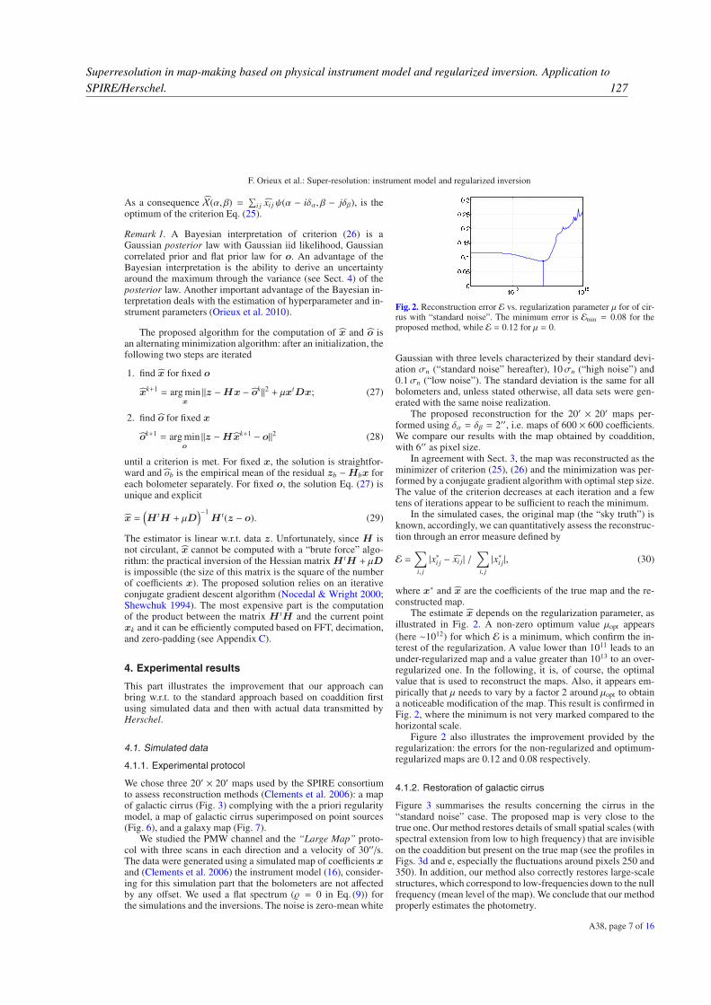
Superresolution in map-making based on physical instrument model and regularized inversion. Application toSPIRE/Herschel. 127
F. Orieux et al.: Super-resolution: instrument model and regularized inversion
As a consequence X(α, β) =∑
i j xi j ψ(α − iδα, β − jδβ), is theoptimum of the criterion Eq. (25).
Remark 1. A Bayesian interpretation of criterion (26) is aGaussian posterior law with Gaussian iid likelihood, Gaussiancorrelated prior and flat prior law for o. An advantage of theBayesian interpretation is the ability to derive an uncertaintyaround the maximum through the variance (see Sect. 4) of theposterior law. Another important advantage of the Bayesian in-terpretation deals with the estimation of hyperparameter and in-strument parameters (Orieux et al. 2010).
The proposed algorithm for the computation of x and o isan alternating minimization algorithm: after an initialization, thefollowing two steps are iterated
1. find x for fixed o
xk+1 = arg minx
‖z −Hx − ok‖2 + µxtDx; (27)
2. find o for fixed x
ok+1 = arg mino
‖z −Hxk+1 − o‖2 (28)
until a criterion is met. For fixed x, the solution is straightfor-ward and ob is the empirical mean of the residual zb −Hbx foreach bolometer separately. For fixed o, the solution Eq. (27) isunique and explicit
x =(H tH + µD
)−1H t(z − o). (29)
The estimator is linear w.r.t. data z. Unfortunately, since H isnot circulant, x cannot be computed with a “brute force” algo-rithm: the practical inversion of the Hessian matrix H tH + µDis impossible (the size of this matrix is the square of the numberof coefficients x). The proposed solution relies on an iterativeconjugate gradient descent algorithm (Nocedal & Wright 2000;Shewchuk 1994). The most expensive part is the computationof the product between the matrix H tH and the current pointxk and it can be efficiently computed based on FFT, decimation,and zero-padding (see Appendix C).
4. Experimental results
This part illustrates the improvement that our approach canbring w.r.t. to the standard approach based on coaddition firstusing simulated data and then with actual data transmitted byHerschel.
4.1. Simulated data
4.1.1. Experimental protocol
We chose three 20′ × 20′ maps used by the SPIRE consortiumto assess reconstruction methods (Clements et al. 2006): a mapof galactic cirrus (Fig. 3) complying with the a priori regularitymodel, a map of galactic cirrus superimposed on point sources(Fig. 6), and a galaxy map (Fig. 7).
We studied the PMW channel and the “Large Map” proto-col with three scans in each direction and a velocity of 30′′/s.The data were generated using a simulated map of coefficients xand (Clements et al. 2006) the instrument model (16), consider-ing for this simulation part that the bolometers are not affectedby any offset. We used a flat spectrum ( = 0 in Eq. (9)) forthe simulations and the inversions. The noise is zero-mean white
Fig. 2. Reconstruction error E vs. regularization parameter µ for of cir-rus with “standard noise”. The minimum error is Emin = 0.08 for theproposed method, while E = 0.12 for µ = 0.
Gaussian with three levels characterized by their standard devi-ation σn (“standard noise” hereafter), 10σn (“high noise”) and0.1σn (“low noise”). The standard deviation is the same for allbolometers and, unless stated otherwise, all data sets were gen-erated with the same noise realization.
The proposed reconstruction for the 20′ × 20′ maps per-formed using δα = δβ = 2′′, i.e. maps of 600 × 600 coefficients.We compare our results with the map obtained by coaddition,with 6′′ as pixel size.
In agreement with Sect. 3, the map was reconstructed as theminimizer of criterion (25), (26) and the minimization was per-formed by a conjugate gradient algorithm with optimal step size.The value of the criterion decreases at each iteration and a fewtens of iterations appear to be sufficient to reach the minimum.
In the simulated cases, the original map (the “sky truth”) isknown, accordingly, we can quantitatively assess the reconstruc-tion through an error measure defined by
E =∑
i, j
|x∗i j − xi j| /∑
i, j
|x∗i j|, (30)
where x∗ and x are the coefficients of the true map and the re-constructed map.
The estimate x depends on the regularization parameter, asillustrated in Fig. 2. A non-zero optimum value µopt appears
(here ∼1012) for which E is a minimum, which confirm the in-terest of the regularization. A value lower than 1011 leads to anunder-regularized map and a value greater than 1013 to an over-regularized one. In the following, it is, of course, the optimalvalue that is used to reconstruct the maps. Also, it appears em-pirically that µ needs to vary by a factor 2 around µopt to obtaina noticeable modification of the map. This result is confirmed inFig. 2, where the minimum is not very marked compared to thehorizontal scale.
Figure 2 also illustrates the improvement provided by theregularization: the errors for the non-regularized and optimum-regularized maps are 0.12 and 0.08 respectively.
4.1.2. Restoration of galactic cirrus
Figure 3 summarises the results concerning the cirrus in the“standard noise” case. The proposed map is very close to thetrue one. Our method restores details of small spatial scales (withspectral extension from low to high frequency) that are invisibleon the coaddition but present on the true map (see the profiles inFigs. 3d and e, especially the fluctuations around pixels 250 and350). In addition, our method also correctly restores large-scalestructures, which correspond to low-frequencies down to the nullfrequency (mean level of the map). We conclude that our methodproperly estimates the photometry.
A38, page 7 of 16
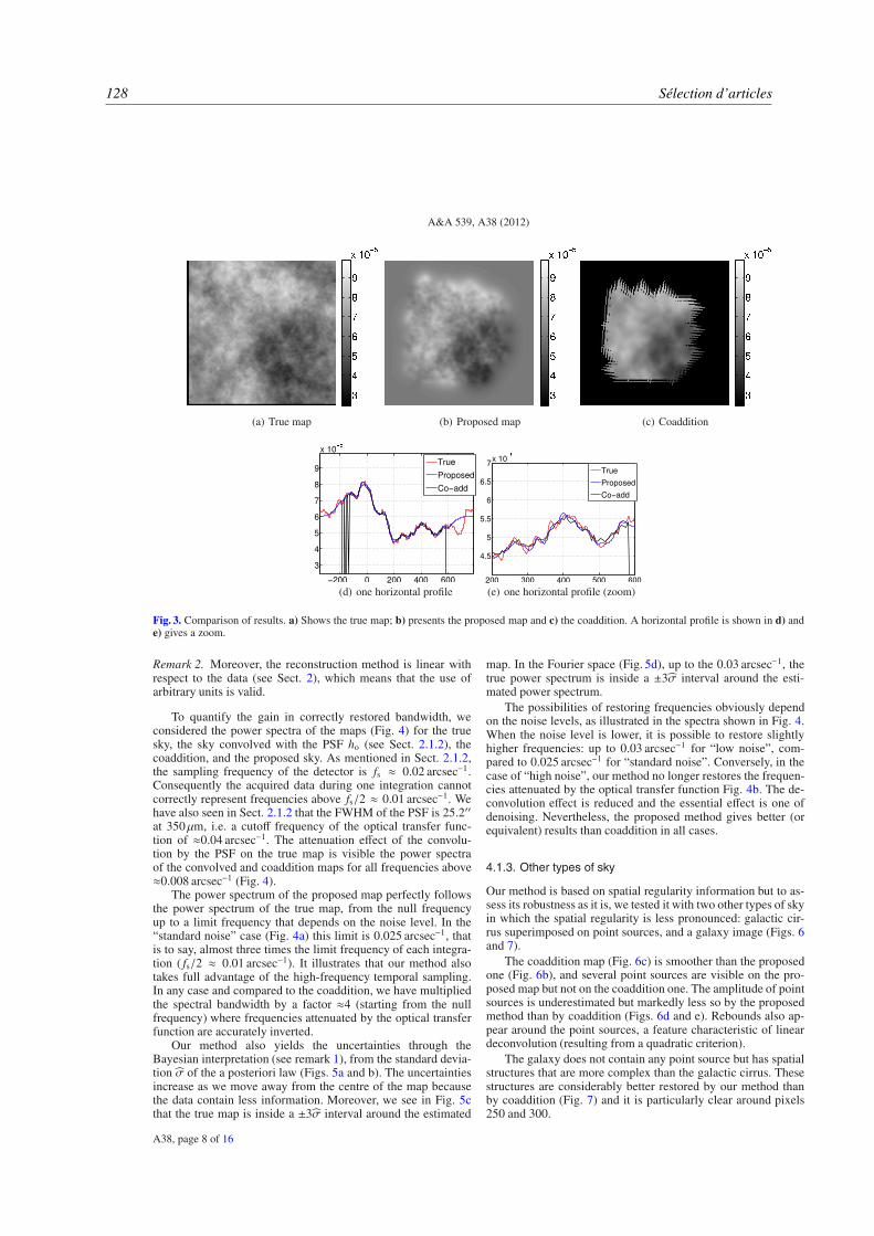
128 Sélection d’articles
A&A 539, A38 (2012)
(a) True map (b) Proposed map (c) Coaddition
(d) one horizontal profile (e) one horizontal profile (zoom)
Fig. 3. Comparison of results. a) Shows the true map; b) presents the proposed map and c) the coaddition. A horizontal profile is shown in d) ande) gives a zoom.
Remark 2. Moreover, the reconstruction method is linear withrespect to the data (see Sect. 2), which means that the use ofarbitrary units is valid.
To quantify the gain in correctly restored bandwidth, weconsidered the power spectra of the maps (Fig. 4) for the truesky, the sky convolved with the PSF ho (see Sect. 2.1.2), thecoaddition, and the proposed sky. As mentioned in Sect. 2.1.2,the sampling frequency of the detector is fs ≈ 0.02 arcsec−1.Consequently the acquired data during one integration cannotcorrectly represent frequencies above fs/2 ≈ 0.01 arcsec−1. Wehave also seen in Sect. 2.1.2 that the FWHM of the PSF is 25.2′′
at 350µm, i.e. a cutoff frequency of the optical transfer func-tion of ≈0.04 arcsec−1. The attenuation effect of the convolu-tion by the PSF on the true map is visible the power spectraof the convolved and coaddition maps for all frequencies above≈0.008 arcsec−1 (Fig. 4).
The power spectrum of the proposed map perfectly followsthe power spectrum of the true map, from the null frequencyup to a limit frequency that depends on the noise level. In the“standard noise” case (Fig. 4a) this limit is 0.025 arcsec−1, thatis to say, almost three times the limit frequency of each integra-tion ( fs/2 ≈ 0.01 arcsec−1). It illustrates that our method alsotakes full advantage of the high-frequency temporal sampling.In any case and compared to the coaddition, we have multipliedthe spectral bandwidth by a factor ≈4 (starting from the nullfrequency) where frequencies attenuated by the optical transferfunction are accurately inverted.
Our method also yields the uncertainties through theBayesian interpretation (see remark 1), from the standard devia-tion σ of the a posteriori law (Figs. 5a and b). The uncertaintiesincrease as we move away from the centre of the map becausethe data contain less information. Moreover, we see in Fig. 5cthat the true map is inside a ±3σ interval around the estimated
map. In the Fourier space (Fig. 5d), up to the 0.03 arcsec−1, thetrue power spectrum is inside a ±3σ interval around the esti-mated power spectrum.
The possibilities of restoring frequencies obviously dependon the noise levels, as illustrated in the spectra shown in Fig. 4.When the noise level is lower, it is possible to restore slightlyhigher frequencies: up to 0.03 arcsec−1 for “low noise”, com-pared to 0.025 arcsec−1 for “standard noise”. Conversely, in thecase of “high noise”, our method no longer restores the frequen-cies attenuated by the optical transfer function Fig. 4b. The de-convolution effect is reduced and the essential effect is one ofdenoising. Nevertheless, the proposed method gives better (orequivalent) results than coaddition in all cases.
4.1.3. Other types of sky
Our method is based on spatial regularity information but to as-sess its robustness as it is, we tested it with two other types of skyin which the spatial regularity is less pronounced: galactic cir-rus superimposed on point sources, and a galaxy image (Figs. 6and 7).
The coaddition map (Fig. 6c) is smoother than the proposedone (Fig. 6b), and several point sources are visible on the pro-posed map but not on the coaddition one. The amplitude of pointsources is underestimated but markedly less so by the proposedmethod than by coaddition (Figs. 6d and e). Rebounds also ap-pear around the point sources, a feature characteristic of lineardeconvolution (resulting from a quadratic criterion).
The galaxy does not contain any point source but has spatialstructures that are more complex than the galactic cirrus. Thesestructures are considerably better restored by our method thanby coaddition (Fig. 7) and it is particularly clear around pixels250 and 300.
A38, page 8 of 16

Superresolution in map-making based on physical instrument model and regularized inversion. Application toSPIRE/Herschel. 129
F. Orieux et al.: Super-resolution: instrument model and regularized inversion
(a) Standard noise (b) High noise (c) Low noise
Fig. 4. Circular means of power spectra for the three levels of noise (standard deviations: σn, 10σn and 0.1σn). The parameter µ is chosen to beoptimal each time from the point of view of the error E (Eq. (30)).
(a) σ map (b) σ map profile
(c) Map profile ±3σ (d) Power spectra ±3σ
Fig. 5. Uncertainty provided by the a posteriori standard deviation σ. a) Shows the map of the standard deviation for each pixel and b) gives aprofile. c) Shows a profile of the true map as a solid line and the two dashed lines give a ±3σ interval around the estimated map. d) Shows thepower spectrum of the true map as a solid red line and the two dashed lines give a ±3σ interval around the estimated power spectrum in the“standard noise” case.
In conclusion, the proposed method is flexible and shows agood restoration capacity for various types of maps. In particu-lar, it possesses a certain robustness compared to an input skypresenting characteristics that are poorly taken into account bythe a priori model based on regularity information. It provides asky that is closer to the real one than that obtained by coaddition,even in the least favourable cases.
4.2. Processing real data
We conducted tests with real data of the reflection nebulaNGC 7023 and of the Polaris flare (which is a high Galactic
latitude cirrus cloud) performed during the science demonstra-tion phase of Herschel and already presented in (Abergel et al.2010) and (Miville-Deschênes et al. 2010), respectively. In orderto run our algorithm, we took the level-1 files processed usingHIPE. The true sky is not known, of course, so the value of theregularization parameter was fixed for each of the spectral chan-nels by a trade-off between the gain in spectral resolution andthe amplification of the noise.
Figures 8 to 12 illustrate the results for NGC 7023 and thePolaris flare. The gain in spatial resolution is spectacular in thethree channels. It is interesting to note that the map of NGC 7023
A38, page 9 of 16

130 Sélection d’articles
A&A 539, A38 (2012)
(a) True map (b) Proposed (c) Coaddition
(d) one horizontal profile (e) one horizontal profile (zoom)
Fig. 6. Restoration of cirrus superimposed on point sources.
(a) True map (b) Proposed (c) Coaddition
(d) one horizontal profile (e) one horizontal profile (zoom)
Fig. 7. Restoration of galaxy.
A38, page 10 of 16

Superresolution in map-making based on physical instrument model and regularized inversion. Application toSPIRE/Herschel. 131
F. Orieux et al.: Super-resolution: instrument model and regularized inversion
Fig. 8. Central part (23′× 23′) of NGC 7023 in the three channels PSW, PMW and PLW (left, middle and right, respectively). Top panels: coaddedmaps; bottom panels: proposed maps.
Fig. 9. Profiles along the three sections shown in the top left panel of Fig. 8. Each panel shows the profiles within the PSW, PMW and PLWchannels, offset for clarity from bottom to top, respectively. Left panel: horizontal profile; central and right panels: vertical profiles. Black:coadded maps, blue: proposed maps.
obtained by our method in the longest wavelength channel(500µm, PLW channel) shows spatial structures that are not vis-ible in the coaddition but are real since they are visible at shorterwavelengths (250µm, PSW channel), as illustrated for instancein the right panel of Fig. 9. The same panel also shows that neg-ative rebounds appear on the sharpest side of the brightest fila-ment of NGC 7023. This filament is the narrowest structure ofthe map and its width is comparable to the width of the PSF.Similar rebounds were also seen in our simulations with pointsources (Fig. 6). The Polaris flare does not contain comparablebright and narrow filament, so the proposed map does not present
this kind of artefact. The zoom on a 10′ × 10′ square (Fig. 11)illustrates the gain in angular resolution for faint structures.
Figure 12 shows that the power spectra of the proposedmaps of the Polaris flare in the three channels follow the ex-pected power law that is typical of the infrared emission of highGalactic cirrus P(k) α kγ with γ = −2.7 (e.g., Miville-Deschêneset al. 2010) on a frequency range from 10−3 to 3×10⁻² arcsec−1.For the simulated data of our Sect. 4.1, the attenuation effect ofthe convolution by the PSF is accurately inverted up to the fre-quency where the noise is dominant. Thanks to this correction,the contrast of the small-scale structures is enhanced (Figs. 10
A38, page 11 of 16
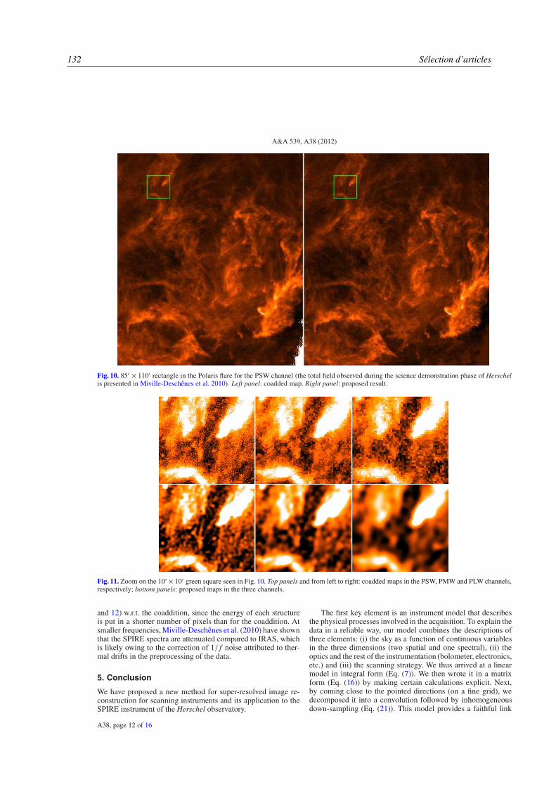
132 Sélection d’articles
A&A 539, A38 (2012)
Fig. 10. 85′ × 110′ rectangle in the Polaris flare for the PSW channel (the total field observed during the science demonstration phase of Herschelis presented in Miville-Deschênes et al. 2010). Left panel: coadded map. Right panel: proposed result.
Fig. 11. Zoom on the 10′ × 10′ green square seen in Fig. 10. Top panels and from left to right: coadded maps in the PSW, PMW and PLW channels,respectively; bottom panels: proposed maps in the three channels.
and 12) w.r.t. the coaddition, since the energy of each structureis put in a shorter number of pixels than for the coaddition. Atsmaller frequencies, Miville-Deschênes et al. (2010) have shownthat the SPIRE spectra are attenuated compared to IRAS, whichis likely owing to the correction of 1/ f noise attributed to ther-mal drifts in the preprocessing of the data.
5. Conclusion
We have proposed a new method for super-resolved image re-construction for scanning instruments and its application to theSPIRE instrument of the Herschel observatory.
The first key element is an instrument model that describesthe physical processes involved in the acquisition. To explain thedata in a reliable way, our model combines the descriptions ofthree elements: (i) the sky as a function of continuous variablesin the three dimensions (two spatial and one spectral), (ii) theoptics and the rest of the instrumentation (bolometer, electronics,etc.) and (iii) the scanning strategy. We thus arrived at a linearmodel in integral form (Eq. (7)). We then wrote it in a matrixform (Eq. (16)) by making certain calculations explicit. Next,by coming close to the pointed directions (on a fine grid), wedecomposed it into a convolution followed by inhomogeneousdown-sampling (Eq. (21)). This model provides a faithful link
A38, page 12 of 16
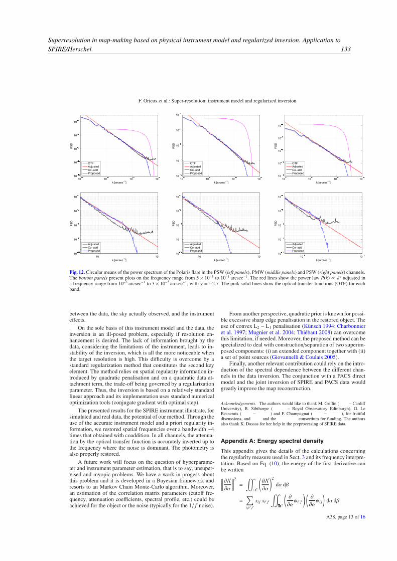
Superresolution in map-making based on physical instrument model and regularized inversion. Application toSPIRE/Herschel. 133
F. Orieux et al.: Super-resolution: instrument model and regularized inversion
Fig. 12. Circular means of the power spectrum of the Polaris flare in the PSW (left panels), PMW (middle panels) and PSW (right panels) channels.The bottom panels present plots on the frequency range from 5 × 10⁻³ to 10−1 arcsec−1. The red lines show the power law P(k) ∝ kγ adjusted ina frequency range from 10−3 arcsec−1 to 3 × 10⁻² arcsec−1, with γ = −2.7. The pink solid lines show the optical transfer functions (OTF) for eachband.
between the data, the sky actually observed, and the instrumenteffects.
On the sole basis of this instrument model and the data, theinversion is an ill-posed problem, especially if resolution en-hancement is desired. The lack of information brought by thedata, considering the limitations of the instrument, leads to in-stability of the inversion, which is all the more noticeable whenthe target resolution is high. This difficulty is overcome by astandard regularization method that constitutes the second keyelement. The method relies on spatial regularity information in-troduced by quadratic penalisation and on a quadratic data at-tachment term, the trade-off being governed by a regularizationparameter. Thus, the inversion is based on a relatively standardlinear approach and its implementation uses standard numericaloptimization tools (conjugate gradient with optimal step).
The presented results for the SPIRE instrument illustrate, forsimulated and real data, the potential of our method. Through theuse of the accurate instrument model and a priori regularity in-formation, we restored spatial frequencies over a bandwidth ∼4times that obtained with coaddition. In all channels, the attenua-tion by the optical transfer function is accurately inverted up tothe frequency where the noise is dominant. The photometry isalso properly restored.
A future work will focus on the question of hyperparame-ter and instrument parameter estimation, that is to say, unsuper-vised and myopic problems. We have a work in progess aboutthis problem and it is developed in a Bayesian framework andresorts to an Markov Chain Monte-Carlo algorithm. Moreover,an estimation of the correlation matrix parameters (cutoff fre-quency, attenuation coefficients, spectral profile, etc.) could beachieved for the object or the noise (typically for the 1/ f noise).
From another perspective, quadratic prior is known for possi-ble excessive sharp edge penalisation in the restored object. Theuse of convex L2 − L1 penalisation (Künsch 1994; Charbonnieret al. 1997; Mugnier et al. 2004; Thiébaut 2008) can overcomethis limitation, if needed. Moreover, the proposed method can bespecialized to deal with construction/separation of two superim-posed components: (i) an extended component together with (ii)a set of point sources (Giovannelli & Coulais 2005).
Finally, another relevant contribution could rely on the intro-duction of the spectral dependence between the different chan-nels in the data inversion. The conjunction with a PACS directmodel and the joint inversion of SPIRE and PACS data wouldgreatly improve the map reconstruction.
Acknowledgements. The authors would like to thank M. Griffin ( – CardiffUniversity), B. Sibthorpe ( – Royal Observatory Edinburgh), G. LeBesnerais ( – ) and F. Champagnat ( – ), for fruitfuldiscussions, and and the consortium for funding. The authorsalso thank K. Dassas for her help in the preprocessing of SPIRE data.
Appendix A: Energy spectral density
This appendix gives the details of the calculations concerningthe regularity measure used in Sect. 3 and its frequency interpre-tation. Based on Eq. (10), the energy of the first derivative canbe written
∥∥∥∥∥∂X∂α
∥∥∥∥∥2
=
2
(∂X∂α
)2
dα dβ
=∑
i ji′ j′
xi j xi′ j′
2
(∂
∂αψi′ j′
) (∂
∂αψi j
)dα dβ.
A38, page 13 of 16

134 Sélection d’articles
A&A 539, A38 (2012)
By noting the derivative ψ′α = ∂ψ/∂α, we obtain the autocor-relation Ψα = ψ
′α ⋆ ψ
′α of the first derivative of the generating
function and we have
∥∥∥∥∥∂X∂α
∥∥∥∥∥2
=∑
i ji′ j′
xi j xi′ j′
2
ψ′α(α − i′δα, β − j′δβ
)
ψ′α(α − iδα, β − jδβ
)dα dβ
=∑
i ji′ j′
xi j xi′ j′[ψ′α ⋆ ψ
′α
] (i′ − i)δα, ( j′ − j)δβ
=∑
i ji′ j′
xi j xi′ j′Ψα
(i′ − i)δα, ( j′ − j)δβ
. (A.1)
As there is a finite number of coefficients xi j, the measure can beput in the form of a quadratic norm
∥∥∥∥∥∂X∂α
∥∥∥∥∥2
= xtDαx
where the matrix Dα is obtained from Ψα. Considering the in-variant structure of (A.1), the matrix Dα has a Tœplitz structure.The calculation is performed by discrete convolution and can becomputed by FFT.
By introducing the dimension β,
∥∥∥∥∥∂X∂α
∥∥∥∥∥2
+
∥∥∥∥∥∂X∂β
∥∥∥∥∥2
= xtDαx + xtDβx.
The quadratic regularity measure on the function X with contin-uous variables is expressed through a quadratic regularity mea-sure on the coefficients x.
The autocorrelation Fourier transform (FT) is the energyspectral density, i.e. the squared modulus of the FT of ψ′α
Ψα( fα, fβ) =
2
Ψα(α, β)e−2 jπ(α fα+β fβ) dα dβ
=
∣∣∣∣∣
2
ψ′α(α, β)e−2 jπ(α fα+β fβ) dα dβ
∣∣∣∣∣2
= 4π2 f 2α
∣∣∣∣ψ( fα, fβ)
∣∣∣∣2
,
whereψ is the FT of ψ. When the dimension β is introduced, the
a priori energy spectral density for the sky naturally has circularsymmetry
Ψ( fα, fβ) = 4π2
(f 2α + f 2
β
) ∣∣∣∣ψ( fα, fβ)
∣∣∣∣2
. (A.2)
This calculation brings out the frequency structure introduced apriori for the sky according to the chosen function ψ. This is a
high-pass structure since the factor f 2α + f 2
β tends to cancelΨ
around zero, which is consistent with a regularity measure.
Appendix B: Explicit calculation of the model
In order to integrate over time in (13), we use the expressionsof (2) for pα(t) and pβ(t), which give
1
2π
1
ΣαΣβ
∫
t
exp
[−1
2
(vαt + cα + αi j − αlm)2
Σ2α
]
× exp
⎡⎢⎢⎢⎢⎢⎣−1
2
(vβt + cβ + βi j − βlm)2
Σ2β
⎤⎥⎥⎥⎥⎥⎦ hb(nTs − t) dt.
With the bolometer response
hb(nTs − t) = [0 +∞[(nTs − t)S exp
[−nTs − t
τ
],
we have
1
2π
S
ΣαΣβexp
[−nTs
τ
] ∫ nTs
−∞exp
[−1
2
(vαt + oα)2
Σ2α
]
× exp
⎡⎢⎢⎢⎢⎢⎣−1
2
(vβt + oβ)2
Σ2β
⎤⎥⎥⎥⎥⎥⎦ exp
[t
τ
]dt (B.1)
with oα = cα + αi j − αlm and oβ = cβ + β
i j − βlm. This is theintegration of a truncated Gaussian since the argument of theexponential is a quadratic form w.r.t. t.
B.1. Calculation of the argument
Here, we express the quadratic form in question
n(t) = τΣ2β(vαt + oα)
2 + τΣ2α(vβt + oβ)
2 − 2Σ2αΣ
2βt.
Expanding and factorizing the numerator n(t) gives
n(t) = τΣ2β
(v2αt
2 + 2vαoαt + o2α
)
+ τΣ2α
(v2βt
2 + 2vβoβt + o2β
)− 2Σ2
αΣ2βt
=((t + a)2 + b − a2
)/Σ2
with the constants a = Σ2(τΣ2βvαoα + τΣ
2αvβoβ − Σ2
αΣ2β
), b =
τΣ2(Σ2βo
2α + Σ
2αo
2β
)and Σ−2 = τ
(Σ2βv
2α + Σ
2αv
2β
). Putting this t-
quadratic form into the integral, we obtain
1
2πS
√πτΣ√
2exp
⎡⎢⎢⎢⎢⎢⎣−nTs
τ− 1
2
b − a2
Σ2Σ2αΣ
2βτ
⎤⎥⎥⎥⎥⎥⎦
×⎛⎜⎜⎜⎜⎜⎝1 + erf
⎛⎜⎜⎜⎜⎜⎝nTs + a√
2τΣΣαΣβ
⎞⎟⎟⎟⎟⎟⎠⎞⎟⎟⎟⎟⎟⎠ , (B.2)
where the function erf is defined by
erf(x) =2√π
∫ x
0
e−θ2
dθ = −erf(−x).
This expression can be simplified by using the functionerfcx(x) = exp(x2)(1 − erf(x)).
B.2. Argument of the exponential
For the sake of notational simplcity, let us note S = Σ2Σ2αΣ
2β. The
argument of the function exp then is
nTs
τ− b − a2
2Σ2Σ2αΣ
2βτ= −nTs
τ− b − a2
2S τ
+
(n2T 2
s
2S τ− n2T 2
s
2S τ
)+
(2nTsa
2S τ− 2nTsa
2S τ
)
and then
nTs
τ− b − a2
2Σ2Σ2αΣ
2βτ= −nTs
τ− b + 2nTsa + n2T 2
s
2S τ+
(nTs + a√
2S τ
)2
·
A38, page 14 of 16

Superresolution in map-making based on physical instrument model and regularized inversion. Application toSPIRE/Herschel. 135
F. Orieux et al.: Super-resolution: instrument model and regularized inversion
So, by injecting this expression in (B.2), the function erfcx ap-pears
exp
[−nTs
τ− b − a2
2S τ
] (1 + erf
(nTs + a√
2S τ
))=
exp
[−nTs
τ− b + 2nTsa + n2T 2
s
2S τ
]erfcx
(−nTs + a√
2S τ
)·
The values of S , a and b can be replaced. First of all, the argu-ment of the exponential is
− nTs
τ−τΣ2
(Σ2βo2α + Σ
2αo
2β
)
2Σ2Σ2αΣ
2βτ
−2nTsΣ
2(τΣ2βvαoα + τΣ
2αvβoβ − Σ2
αΣ2β
)
2Σ2Σ2αΣ
2βτ
− n2T 2s
2S τ=
− nTs
τ− o2
α
2Σ2α
−o2β
2Σ2β
− 2nTsvαoα
2Σ2α
−2nTsvβoβ
2Σ2β
+nTs
τ− n2T 2
s
2Σ2Σ2αΣ
2βτ, (B.3)
and the terms nTs/τ simplify. We then use the expression for Σ2
n2T 2s
2Σ2Σ2αΣ
2βτ=
n2T 2s v
2α
2Σ2α
+n2T 2
s v2β
2Σ2β
,
to obtain two perfect squares. Finally the argument of the expo-nential (B.3) in (B.2) is
− (oα + nTsvα)2
2Σ2α
−
(oβ + nTsvβ
)2
2Σ2β
, (B.4)
which is exactly the argument of a bivariate Gaussian. Weagain find the same standard deviations Σα and Σβ. However,the response of the optics, initially (oα, oβ), is now shifted by(nTsvα, nTsvβ), i.e. the pointing difference between two succes-sive time samples.
B.3. Argument of the function erfcx and final expression
Another term is needed to know the global response. It comesfrom the function erfcx, which corresponds to the influence ofthe bolometer. The argument of the function erfcx is
− nTs + a√
2τΣΣαΣβ=ΣαΣβ√
2τΣv−
Σβvα(oα + nTsvα)√2ΣαΣv
−Σαvβ(oβ + nTsvβ)√
2ΣβΣv, (B.5)
where Σ2v = Σ
2βv2α + Σ
2αv
2β, and what is of interest here is that the
same factors are found in the argument of the exponential. Toknow the global response, we need to bring everything together.
By injecting the expressions of the arguments (B.4) and (B.5),we obtain
1
2πS
√πτΣ√
2exp
⎡⎢⎢⎢⎢⎢⎣nTs
τ− 1
2
b − a2
Σ2Σ2αΣ
2βτ
⎤⎥⎥⎥⎥⎥⎦
×⎛⎜⎜⎜⎜⎜⎝1 + erf
⎛⎜⎜⎜⎜⎜⎝nTs + a√
2τΣΣαΣβ
⎞⎟⎟⎟⎟⎟⎠⎞⎟⎟⎟⎟⎟⎠ =
× S
2√
2πΣvexp
⎡⎢⎢⎢⎢⎢⎢⎢⎢⎣−(oα + nTsvα)
2
2Σ2α
−
(oβ + nTsvβ
)2
2Σ2β
⎤⎥⎥⎥⎥⎥⎥⎥⎥⎦
×erfcx
⎛⎜⎜⎜⎜⎜⎝ΣαΣβ√
2τΣv−Σβvα(oα + nTsvα)√
2ΣαΣv−Σαvβ(oβ + nTsvβ)√
2ΣβΣv
⎞⎟⎟⎟⎟⎟⎠
with, similarly for α and β: Σ2α/β= σ2
α/β+ σ2
o, which finishes the
integration of (13) over time.
Appendix C: Direct model computation algorithm
This part gives some more details on the concrete computation ofa model output Hx of Sect. 2.3. First of all, there are four differ-ent impulse responses whatever the number of scans. For scansin the same direction, the response is the same. Thus we can con-struct four different convolution matrices Hi for i = 1, 2, 3, 4 andapply four different discrete convolutions to the coefficients x.
We can also deduce the structure of the transpose of themodel H t = H t
cPt. The matrix P t is a data summation/zero
padding matrix (addition of the data that possess the same point-ing while setting the other coefficients to zero), and H t
c cor-responds to a convolution with the space reversal impulse re-sponses.
The product by P t is very similar to the construction of anaive map except that the data are added rather than averaged.Also, the operation is done by velocity and not globally. Finally,the products by Hc and H t
c are convolutions computed by FFT.
References
Abergel, A., Arab, H., Compiègne, M., et al. 2010, A&A, 518, L96Andrews, H. C., & Hunt, B. R. 1977, Digital Image Restoration (Englewood
Cliffs, : Prentice-Hall)Boulanger, F., Abergel, A., Bernard, J., et al. 1996, A&A, 312, 256Cantalupo, C. M., Borrill, J. D., Jaffe, A. H., Kisner, T. S., & Stompor, R. 2010,
ApJS, 187, 212Champagnat, F., Le Besnerais, G., & Kulcsár, C. 2009, J. Opt. Soc. Am. A, 26,
1730Charbonnier, P., Blanc-Féraud, L., Aubert, G., & Barlaud, M. 1997, IEEE Trans.
Image Processing, 6, 298Clements, D., Chanial, P., Bendo, G., et al. 2006, Mapmaking Algorithm
Review Report, Tech. Rep., Astrophysics group at Imperial College Londonde Graauw, T., Helmich, F. P., Phillips, T. G., et al. 2010, A&A, 518, L6Demoment, G. 1989, IEEE Trans. Acoust. Speech, Signal Processing, -37,
2024Elad, M., & Feuer, A. 1999, IEEE Trans. Image Processing, 8, 387Farsiu, S., Robinson, M., Elad, M., & Milanfar, P. 2004, Image Processing, IEEE
Transactions on, 13, 1327Giovannelli, J.-F., & Coulais, A. 2005, A&A, 439, 401Griffin, M. J. 2006, Revised Photometer sensitivity model, working version after
sensitivity review meetingGriffin, M. J. 2007, The SPIRE Analogue Signal Chain and Photometer Detector
Data Processing Pipeline, Tech. Rep., University of Wales CardiffGriffin, M. J., Bock, J. J., & Gear, W. K. 2002, Appl. Opt., 41, 6543Griffin, M., Swinyard, B., Vigroux, L., et al. 2008, in SPIE Conf., 7010Griffin, M. J., Abergel, A., Abreu, A., et al. 2010, A&A, 518, L3Hardie, R. C., Barnard, K. J., & Armstrong, E. E. 1997, IEEE Trans. Image
Processing, 6, 1621
A38, page 15 of 16

136 Sélection d’articles
A&A 539, A38 (2012)
Idier, J., 2008, Bayesian Approach to Inverse Problems (London: ISTE Ltd andJohn Wiley & Sons Inc.)
Künsch, H. R. 1994, Ann. Inst. Stat. Math., 46, 1Leshem, A., Christou, J., Jeffs, B. D., Kuruoglu, E., & van der Veen, A. J. 2008,
IEEE Journal of Selected Topics in Signal Processing, 2Leshem, A., Kamalabadi, F., Kuruoglu, E., & van der Veen, A.-J. 2010, Signal
Processing Magazine, 27Miville-Deschênes, M., Martin, P. G., Abergel, A., et al. 2010, A&A, 518, L104Molina, R., & Ripley, B. D. 1989, J. Appl. Stat., 16, 193Mugnier, L., Fusco, T., & Conan, J.-M. 2004, J. Opt. Soc. Amer., 21, 1841Nguyen, N., Milanfar, P., & Golub, G. 2001, IEEE Trans. Image Processing, 10,
573Nocedal, J., & Wright, S. J. 2000, Numerical Optimization, Series in Operations
Research (New York: Springer Verlag)Orieux, F. 2009, Ph.D. Thesis, Université Paris-Sud 11Orieux, F., Rodet, T., & Giovannelli, J.-F. 2009, in Proc. of IEEE International
Conference on Image Processing (ICIP 2009), Cairo, EgyptOrieux, F., Giovannelli, J.-F., & Rodet, T. 2010, J. Opt. Soc. Am. A, 27, 1593Ott, S. 2010, in Astronomical Data Analysis Software and Systems XIX, ed.
Y. Mizumoto, K.-I. Morita, & M. Ohishi, ASP Conf. Ser., 434, 139Park, S. C., Park, M. K., & Kang, M. G. 2003, IEEE Trans. Signal Processing
Mag., 21Patanchon, G., Ade, P. A. R., Bock, J. J., et al. 2008, ApJ, 681, 708Patti, A. J., Sezan, M. I., & Tekalp, A. M. 1997, IEEE Trans. Image Processing,
6, 1064Pilbratt, G. L., Riedinger, J. R., Passvogel, T., et al. 2010, A&A, 518, L1
Poglitsch, A., Waelkens, C., Geis, N., et al. 2010, A&A, 518, L2Robert, C. P., & Casella, G. 2000, Monte-Carlo Statistical Methods, Springer
Texts in Statistics (New York, : Springer)Rochefort, G., Champagnat, F., Le Besnerais, G., & Giovannelli, J.-F. 2006,
IEEE Trans. Image Processing, 15, 3325Rodet, T., Orieux, F., Giovannelli, J.-F., & Abergel, A. 2008, IEEE J. Selec.
Topics in Signal Proc., 2, 802Shewchuk, J. R. 1994, An Introduction to the Conjugate Gradient Method
Without the Agonizing Pain, Tech. Rep., Carnegie Mellon UniversitySibthorpe, B., & Griffin, M. J. 2006, Spire Photometer Simulator, Tech. Rep.,
University of Wales CardiffSibthorpe, B., Chanial, P., & Griffin, M. J. 2009, A&A, 503, 625Sudiwala, R. V., Griffin, M. J., & Woodcraft, A. L. 2002, International Journal
of Infrared and Millimeter Waves, 23, 545Thiébaut, E. 2008, in Astronomical Telescopes and Instrumentation, Proc. SPIE,
7013, 70131–ITikhonov, A., & Arsenin, V. 1977, Solutions of Ill-Posed Problems (Washington, : Winston)
Twomey, S. 1962, J. Assoc. Comp. Mach., 10, 97Vandewalle, P., Sbaiz, L., Vandewalle, J., & Vetterli, M. 2007, IEEE Trans.
Signal Processing, 55, 3687Wieprecht, E., Schreiber, J., de Jong, J., et al. 2009, in ASP Conf. Ser., ed.
D. A. Bohlender, D. Durand, & P. Dowler, 411, 531Woods, N. A., Galatsanos, N. P., & Katsaggelos, A. K. 2006, IEEE Trans. Image
Processing, 15, 201
A38, page 16 of 16

Bayesian estimation of regularization and point spread function parameters for Wiener–Hunt deconvolution 137
F. Orieux, J.-F. Giovannelli et T. Rodet, « Bayesian estimation of regularization and point spreadfunction parameters for Wiener–Hunt deconvolution », Journal of the Optical Society of America (A),vol. 27, n˚7, pp. 1593–1607, 2010.

138 Sélection d’articles
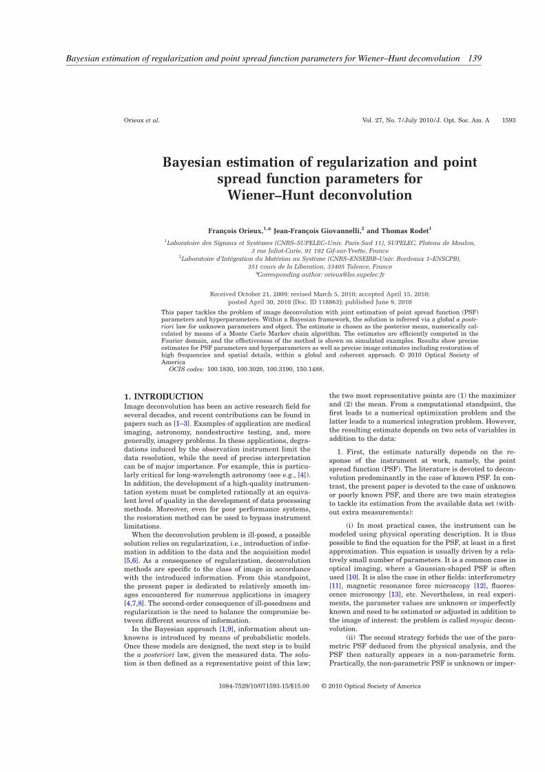
Bayesian estimation of regularization and point spread function parameters for Wiener–Hunt deconvolution 139
Bayesian estimation of regularization and pointspread function parameters for
Wiener–Hunt deconvolution
François Orieux,1,* Jean-François Giovannelli,2 and Thomas Rodet1
1Laboratoire des Signaux et Systèmes (CNRS–SUPELEC–Univ. Paris-Sud 11), SUPELEC, Plateau de Moulon,
3 rue Joliot-Curie, 91 192 Gif-sur-Yvette, France2Laboratoire d’Intégration du Matériau au Système (CNRS–ENSEIRB–Univ. Bordeaux 1–ENSCPB),
351 cours de la Liberation, 33405 Talence, France*Corresponding author: [email protected]
Received October 21, 2009; revised March 5, 2010; accepted April 15, 2010;
posted April 30, 2010 (Doc. ID 118863); published June 9, 2010
This paper tackles the problem of image deconvolution with joint estimation of point spread function (PSF)parameters and hyperparameters. Within a Bayesian framework, the solution is inferred via a global a poste-riori law for unknown parameters and object. The estimate is chosen as the posterior mean, numerically cal-culated by means of a Monte Carlo Markov chain algorithm. The estimates are efficiently computed in theFourier domain, and the effectiveness of the method is shown on simulated examples. Results show preciseestimates for PSF parameters and hyperparameters as well as precise image estimates including restoration ofhigh frequencies and spatial details, within a global and coherent approach. © 2010 Optical Society ofAmerica
OCIS codes: 100.1830, 100.3020, 100.3190, 150.1488.
1. INTRODUCTIONImage deconvolution has been an active research field forseveral decades, and recent contributions can be found inpapers such as [1–3]. Examples of application are medicalimaging, astronomy, nondestructive testing, and, moregenerally, imagery problems. In these applications, degra-dations induced by the observation instrument limit thedata resolution, while the need of precise interpretationcan be of major importance. For example, this is particu-larly critical for long-wavelength astronomy (see e.g., [4]).In addition, the development of a high-quality instrumen-tation system must be completed rationally at an equiva-lent level of quality in the development of data processingmethods. Moreover, even for poor performance systems,the restoration method can be used to bypass instrumentlimitations.
When the deconvolution problem is ill-posed, a possiblesolution relies on regularization, i.e., introduction of infor-mation in addition to the data and the acquisition model[5,6]. As a consequence of regularization, deconvolutionmethods are specific to the class of image in accordancewith the introduced information. From this standpoint,the present paper is dedicated to relatively smooth im-ages encountered for numerous applications in imagery[4,7,8]. The second-order consequence of ill-posedness andregularization is the need to balance the compromise be-tween different sources of information.
In the Bayesian approach [1,9], information about un-knowns is introduced by means of probabilistic models.Once these models are designed, the next step is to buildthe a posteriori law, given the measured data. The solu-tion is then defined as a representative point of this law;
the two most representative points are (1) the maximizerand (2) the mean. From a computational standpoint, thefirst leads to a numerical optimization problem and thelatter leads to a numerical integration problem. However,the resulting estimate depends on two sets of variables inaddition to the data:
1. First, the estimate naturally depends on the re-sponse of the instrument at work, namely, the pointspread function (PSF). The literature is devoted to decon-volution predominantly in the case of known PSF. In con-trast, the present paper is devoted to the case of unknownor poorly known PSF, and there are two main strategiesto tackle its estimation from the available data set (with-out extra measurements):
(i) In most practical cases, the instrument can bemodeled using physical operating description. It is thuspossible to find the equation for the PSF, at least in a firstapproximation. This equation is usually driven by a rela-tively small number of parameters. It is a common case inoptical imaging, where a Gaussian-shaped PSF is oftenused [10]. It is also the case in other fields: interferometry[11], magnetic resonance force microscopy [12], fluores-cence microscopy [13], etc. Nevertheless, in real experi-ments, the parameter values are unknown or imperfectlyknown and need to be estimated or adjusted in addition tothe image of interest: the problem is called myopic decon-volution.
(ii) The second strategy forbids the use of the para-metric PSF deduced from the physical analysis, and thePSF then naturally appears in a non-parametric form.Practically, the non-parametric PSF is unknown or imper-
Orieux et al. Vol. 27, No. 7 /July 2010 /J. Opt. Soc. Am. A 1593
1084-7529/10/071593-15/$15.00 © 2010 Optical Society of America

140 Sélection d’articles
fectly known and needs to be estimated in addition to theimage of interest: the problem is referred to as blind de-convolution, for example in interferometry [14–17].
From an inference point of view, the difficulty of bothmyopic and blind problems lies in the possible lack of in-formation, resulting in ambiguity between image andPSF, even in the noiseless case. In order to resolve theambiguity, information must be added [3,18], and it iscrucial to make inquiries based on any available source ofinformation. To this end, the knowledge of the parametricPSF represents a valuable means to structure the prob-lem and possibly resolve the degeneracies. Moreover, dueto the instrument design process, a nominal value as wellas an uncertainty are usually available for the PSF pa-rameters. In addition, from a practical and algorithmicstandpoint, the myopic case, i.e., the case of parametricPSF, is often more difficult due to the non-linear depen-dence of the observation model with respect to the PSFparameters. In contrast, the blind case, i.e., the case ofnon-parametric PSF, yields a simpler practical and algo-rithmic problem since the observation model remains lin-ear w.r.t. the unknown elements given the object. Despitethe superior technical difficulty, the present paper is de-voted to the myopic format since it is expected to be moreefficient than the blind format from an information stand-point. Moreover, the blind case has been extensively stud-ied, and a large number of papers are available [19–21],while the myopic case has been less investigated, thoughit is of major importance.
2. Second, the solution depends on the probability lawparameters called hyperparameters (means, variances,parameters of correlation matrix, etc.). These parametersadjust the shape of the laws, and at the same time theytune the compromise between the information providedby the a priori knowledge and the information providedby the data. In real experiments, their values are un-known and need to be estimated: the problem is called un-
supervised deconvolution.
For both families of parameters (PSF parameters andhyperparameters), two approaches are available. In thefirst one, the parameter values are empirically tuned orestimated in a preliminary step (with maximum likeli-hood [7] or calibration [22] for example); then the valuesare used in a second step devoted to image restorationgiven the parameters. In the second step, the parametersand the object are jointly estimated [2,19].
For the myopic problem, Jalobeanu et al. [23] addressthe case of a symmetric Gaussian PSF. The width param-eter and the noise variance are estimated in a prelimi-nary step by maximum likelihood. A recent paper [24] ad-dresses the estimation of a Gaussian blur parameter, asin our experiment, with an empirical method. They foundthe Gaussian blur parameter by minimizing the absolutevalue of the second derivative (Laplacian) of the restoredimages.
The present paper addresses the myopic and unsuper-vised deconvolution problem. We propose a new methodthat jointly estimates the PSF parameters, the hyperpa-rameters, and the image of interest. It is built in a coher-ent and global framework based on an extended a poste-
riori law for all the unknown variables. The posterior law
is obtained via the Bayes rule, founded on a priori laws:Gaussian for image and noise, uniform for PSF param-eters, and gamma or Jeffreys for hyperparameters.
Regarding the image prior law, we have paid special at-tention to the parameterization of the covariance matrixin order to facilitate law manipulations such as integra-tion, conditioning, and hyperparameter estimation. Thepossible degeneracy of the a posteriori law in some limitcases is also studied.
The estimate is chosen as the mean of the posterior lawand is computed using Monte Carlo simulations. To thisend, Monte Carlo Markov chain (MCMC) algorithms [25]enable one to draw samples from the posterior distribu-tion despite its complexity and especially the non-lineardependence w.r.t. the PSF parameters.
The paper is structured in the following manner. Sec-tion 2 presents the notation and describes the problem.The three following sections describe our methodology:first the Bayesian probabilistic models are detailed inSection 3, then a proper posterior law is established inSection 4; and an MCMC algorithm to compute the esti-mate is described in Section 5. Numerical results are pre-sented in Section 6. Finally, Section 7 is devoted to theconclusion and perspectives.
2. NOTATION AND CONVOLUTION MODEL
Consider N-pixel real square images represented in lexi-cographic order by vector xR
N, with generic elementsxn. The forward model is written
y = Hwx + , 1
where yRN is the vector of data, Hw a convolution ma-
trix, x the image of interest, and the modelization errorsor the noise. Vector wR
P stands for the PSF param-eters, such as width or orientation of a Gaussian PSF.
The matrix Hw is block-circulant with circulant-block(BCCB) for computational efficiency of the convolution inthe Fourier space. The diagonalization [26] of Hw is writ-ten H=FHwF†, where F is the unitary Fourier matrixand † is the transpose conjugate symbol. The convolutionin the Fourier space, is then
y = Hx + , 2
where x=Fx, y=Fy and =F are the 2D discrete Fouriertransform (DFT-2D) of image, data, and noise, respec-tively.
Since H is diagonal, the convolution is computed witha term-wise product in the Fourier space. There is a strictequivalence between a description in the spatial domain[Eq. (1)] and in the Fourier domain [Eq. (2)]. Conse-quently, for coherent description and computational effi-ciency, all the developments are equally done in the spa-tial space or in the Fourier space.
For notational convenience, let us introduce the compo-nent at null frequency x0R and the vector of componentat non-null frequencies x*C
N−1 so that the whole set ofcomponents is written x= x0 , x*.
Let us denote 1 the vector of N components equal to1/N, so that 1
tx is the empirical mean level of the image.
The Fourier components are the 1n, and we have 10=1 and
1594 J. Opt. Soc. Am. A/Vol. 27, No. 7 /July 2010 Orieux et al.

Bayesian estimation of regularization and point spread function parameters for Wiener–Hunt deconvolution 141
1n=0 for n0. Moreover, 1=F11tF† is a diagonal matrix
with only one non-null coefficient at null frequency.
3. BAYESIAN PROBABILISTIC MODEL
This section presents the prior law for each set of param-eters. Regarding the image of interest, in order to accountfor smoothness, the law introduces high-frequency penal-ization through a differential operator on the pixel. A con-jugate law is proposed for the hyperparameters, and auniform law is considered for the PSF parameters.
Moreover, we have paid special attention to the imageprior law parameterization. In Subsection 3.A we presentseveral parameterizations in order to facilitate law ma-nipulations such as integration, conditioning, and hyper-parameter estimation. Moreover, the correlation matrix ofthe image law may become singular in some limit cases,resulting in a degenerated prior law [when px=0 for allxR
N]. Based on this parameterization, in Section 4 westudy the degeneracy of the posterior in relation to the pa-rameters of the prior law.
A. Image Prior LawThe probability law for the image is a Gaussian field witha given precision matrix P parameterized by a vector .The pdf reads
px = 2−N/2 detP1/2 exp−1
2xtPx . 3
For computational efficiency, the precision matrix is de-signed (or approximated) in a toroidal manner, and it isdiagonal in the Fourier domain P=FPF†. Thus, the lawfor x also is written
px = 2−N/2 detFdetP1/2 detF†
exp−1
2xtF†PFx , 4
=2−N/2 detP1/2 exp−1
2x†Px , 5
and it is sometimes referred to [27] as a Whittle approxi-mation (see also [28], p. 133) for the Gaussian law. Thefilter obtained for fixed hyperparameters is also theWiener–Hunt filter [29], as described in Subsection 5.A,below.
This paper focuses on smooth images and thus on posi-tive correlation between pixels. It is introduced by high-frequency penalty using any circulant differential opera-tor: pth differences between pixels, Laplacian and Sobel,among others. The differential operator is denoted by D
and its diagonalized form by D=FDF†. Then, the preci-sion matrix is written P=1DtD, and its Fourier counter-part is written
P = 1D† D = diag0,1d12, . . . ,1dN−12, 6
where 1 is a positive scale factor, diag builds a diagonal
matrix from elementary components, and dn is the nthDFT-2D coefficient of D.
Under this parameterization of P, the first eigenvalueis equal to zero, corresponding to the absence of penaltyfor the null frequency x0, i.e., no information is accountedfor about the empirical mean level of the image. As a con-sequence, the determinant vanishes, detP=0, resultingin a degenerated prior. To manage this difficulty, severalapproaches have been proposed.
Some authors [2,30] still use this prior despite its de-generacy, and this approach can be analyzed in two ways:
1. On the one hand, this prior can be seen as a non-degenerated law for x*, the set of non-null frequency com-ponents only. In this format, the prior does not affect anyprobability for the null frequency component, and theBayes rule does not apply to this component. Thus, thisstrategy yields an incomplete posterior law, since the nullfrequency is not embedded in the methodology.
2. On the other hand, this prior can be seen as a de-generated prior for the whole set of frequencies. The ap-plication of the Bayes rule is then somewhat confusingdue to degeneracy. In this format, the posterior law can-not be guaranteed to remain non-degenerated.
In any case, neither of the two standpoints yields a pos-terior law that is both non-degenerated and addresses thewhole set of frequencies.
An alternative parameterization relies on the energy ofx. An extra term 0I, tuned by 00, in the precision ma-trix [31], introduces information for all the frequencies in-cluding x0. The precision matrix is written
P = 0I + 1D† D = diag0,0 + 1d12, . . . ,0 + 1dN−12
7
with a determinant
detP = n=0
N−1
0 + 1dn2. 8
The obtained Gaussian prior is not degenerated and un-doubtedly leads to a proper posterior. Nevertheless, thedeterminant Eq. (8) is not separable in 0 and 1. Conse-quently, the conditional posterior for these parameters isnot a classical law, and future development will be moredifficult. Moreover, the non-null frequencies x* are con-trolled by two parameters, 0 and 1:
px0,1 = px00px*0,1. 9
The proposed approach to manage the degeneracy re-lies on the addition of a term for the null frequency only,1=diag1,0, . . . ,0:
P = 01
†1 + 1D† D . = diag0,1d12, . . . ,1dN−12.
10
The determinant has a separable expression,
detP = 01N−1
n=1
N−1
dn2, 11
i.e., the precision parameters have been factorized. In ad-dition, each parameter controls a different set of frequen-cies:
Orieux et al. Vol. 27, No. 7 /July 2010 /J. Opt. Soc. Am. A 1595

142 Sélection d’articles
px0,1 = px00px*1,
where 0 drives the empirical mean level of the image x0
and 1 drives the smoothness x* of the image. With theFourier precision structure of Eq. (10), we have the non-degenerated prior law for the image that addresses sepa-rately all the frequencies with a factorized partition func-tion w.r.t. 0 ,1:
px0,1 = 2−N/2n=1
N−1
dn01/21
N−1/2
exp−0
2x02 −
1
2D*x*2 , 12
where D* is obtained from D without the first line andcolumn. The next step is to write the a priori law for thenoise in an explicit form and the other parameters, in-cluding the law parameters and the instrument param-eters w.
B. Noise and Data LawsFrom a methodological standpoint, any statistic can be in-cluded for errors (measurement and model errors). It ispossible to account for correlations in the error process orto account for a non-Gaussian law, e.g., Laplacian law,generalized Gaussian law, or other laws based on a robustnorm. In the present paper, the noise is modeled as zero-mean white Gaussian vector with unknown precision pa-rameter :
p = 2−N/2N/2 exp−
22 . 13
Consequently, the likelihood for the parameters given theobserved data is written
pyx,,w = 2−N/2N/2 exp−
2y − Hwx2 . 14
It naturally depends on the image x, on the noise param-eter , and the PSF parameters w embedded in Hw. Itclearly involves a least-squares discrepancy that can berewritten in the Fourier domain: y−Hwx2= y−Hx2.
C. Hyperparameter LawA classical choice for the hyperparameter law relies onthe conjugate prior [32]: the conditional posterior for thehyperparameters is in the same family as its prior. It re-sults in practical and algorithmic facilities: update of thelaws amounts to update of a small number of parameters.
The three parameters 0, 1, and are precision pa-rameters of Gaussian laws Eq. (12) and (14); a conjugatelaw for these parameters is the gamma law (see AppendixB). Given parameters i ,i, for i=0, 1 or , the pdf reads
pi =1
i
ii
i
i−1exp− i/i, ∀ i 0,+ .
15
In addition to computational efficiency, the law allowsfor non-informative priors. With specific parameter val-ues, one obtains two improper non-informative priori: the
Jeffreys law p=1/ and the uniform law p=U0,+ with i ,i set to 0,+ and 1,+, respec-tively. The Jeffreys law is a classical law for the precisionsand is considered non-informative [33]. This law is alsoinvariant to power transformations: the law of n [33,34]is also a Jeffreys law. For these reasons development isdone using the Jeffreys law.
D. PSF Parameter LawRegarding the PSF parameters w, we consider that theinstrument design process or a physical study provides anominal value w with uncertainty , that is, w w− ,w+. The “Principle of Insufficient Reason” [33]leads to a uniform prior on this interval:
pw = Uw,w, 16
where Uw, is a uniform pdf on w− ,w+. Neverthe-less, within the proposed framework, the choice is not lim-ited and other laws, such as Gaussian, are possible. Inany case, other choices do not allow easier computationbecause of the non-linear dependency of the observationmodel w.r.t. PSF parameters.
4. PROPER POSTERIOR LAW
At this point, the prior law of each parameter is available:the PSF parameters, the hyperparameters, and the im-age. Thus, the joint law for all the parameters is built bymultiplying the likelihood Eq. (14) and the a priori lawsEq. (12), (15), and (16):
px,,0,1,w, y
= pyx,,wpx0,1pp0p1pw 17
and explicitly
px,,0,1,w, y
=
2−Nn=1
N−1dn
0
001
11
+N/2−10
0−1/21
1+N−1/2−1
exp−
−0
0
−1
1Uw,w
exp−
2y − Hx2 −
0
2x02 −
1
2Dx2 . 18
According to the Bayes rule, the a posteriori law reads
px,,0,1,wy =px,,0,1,w, y
py, 19
where py is a normalization constant
py = py,x,,wdxddw. 20
As described before, setting 0=0 leads to degeneratedprior and joint laws. However, when the observation sys-tem preserves the null frequency, 0 can be considered anuisance parameter. In addition, only prior informationon the smoothness is available.
1596 J. Opt. Soc. Am. A/Vol. 27, No. 7 /July 2010 Orieux et al.

Bayesian estimation of regularization and point spread function parameters for Wiener–Hunt deconvolution 143
In Bayesian framework, a solution to eliminate the nui-sance parameters is to integrate them out in the a poste-
riori law. According to our parameterization in Subsection3.A, the integration of 0 is the integration of a gammalaw. Application of Appendix B.1 on 0 in the a posteriori
law Eq. (19) provides
px,,1,wy
=px0py,x*,,1,wx0
px0py,x*,,1,wx0dd1dwdx*dx0
21
with
px0 = px00p0d0 = 1 +0x0
2
2−0−1/2
. 22
Now the parameter is integrated, and the parameters 0
and 0 are set to remove the null frequency penalization.Since we have 00 and 00 we get 1+0x0
2 /2−0−1/2
1, and the joint law is majored:
1 +0x0
2
2−0−1/2
py,x*,,1,wx0 py,x*,,1,wx0.
23
Consequently, by the dominated convergence theorem[35], the limit of the law with 0→1 and 0→0 can beplaced under the integral sign at the denominator. Thenthe null-frequency penalization px0 from the numeratorand denominator are removed. This is equivalent to theintegration of the 0 parameter under a Dirac distribution(see Appendix B). The equation is simplified, and the in-tegration with respect to x0 in the denominator Eq. (20)
R
pyx,,wpx*1p1,,wdx0 R
py0x0,,wdx0
24
R
exp−
2y0 − h0x02dx0 25
converges if and only if h00: the null frequency is ob-served. If this condition is met, Eq. (21) with 0=0 and0=1 is a proper posterior law for the image, the precisionparameters, and the PSF parameters. In other words, ifthe average is observed, the degeneracy of the a priori lawis not transmitted to the a posteriori law.
Then, the obtained a posteriori law is written
px,,1,wy =px,,1,w, y
py
+N/2−11
1+N−1/2−1Uw,wexp−
2y
− Hx2 −1
2D*x*2exp−
−1
1 .
26
Finally, inference is done on this law Eq. (26). If the nullfrequency is not observed, or information must be added,the previous Eq. (19) can be used.
5. POSTERIOR MEAN ESTIMATOR ANDLAW EXPLORATION
This section presents the algorithm to explore the poste-rior law Eq. (19) or Eq. (26) and to compute an estimate ofthe parameters. For this purpose, Monte Carlo Markovchain is used to provide samples. First, the obtainedsamples are used to compute different moments of thelaw. Afterward, they are also used to approximate mar-ginal laws as histograms. These two representations arehelpful for analyzing the a posteriori law, the structure ofthe available information, and the uncertainty. They areused in Subsection 6.C.2 to illustrate the mark of the am-biguity in the myopic problem.
Here, the samples of the a posteriori law are obtainedby a Gibbs sampler [25,36,37]: it consists in iterativelysampling the conditional posterior law for a set of param-eters given the other parameters (obtained at previous it-eration). Typically, the sampled laws are the law of x, i,and w. After a burn-in time, the complete set of samplesare under the joint a posteriori law. The next three sub-sections present each sampling step.
A. Sampling the ImageThe conditional posterior law of the image is a Gaussianlaw:
xk+1 pxy,k,0
k,1k,wk 27
Nk+1,k+1. 28
The covariance matrix is diagonal and is written
k+1 = kH
k2 + 0k1
2 + 1kD2−1, 29
and the mean
k+1 = kk+1H
†ky, 30
where † is the transpose conjugate symbol. The vectork+1 is the regularized least-square solution at the cur-rent iteration (or the Wiener–Hunt filter). Clearly, if the
null frequency is not observed, h0=0 and if 0=0, the co-variance matrix is not invertible and the estimate is notdefined as described Section 4.
Finally, since the matrix is diagonal, the sample xk+1
is obtained by a term-wise product of F (where is whiteGaussian) with the standard deviation matrix k+11/2
Orieux et al. Vol. 27, No. 7 /July 2010 /J. Opt. Soc. Am. A 1597
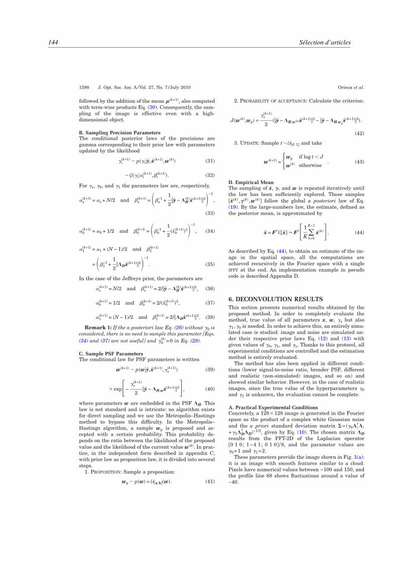
144 Sélection d’articles
followed by the addition of the mean k+1, also computedwith term-wise products Eq. (30). Consequently, the sam-pling of the image is effective even with a high-dimensional object.
B. Sampling Precision ParametersThe conditional posterior laws of the precisions aregamma corresponding to their prior law with parametersupdated by the likelihood
ik+1 piy,xk+1,wk 31
Giik+1,i
k+1. 32
For , 0, and 1 the parameters law are, respectively,
k+1 = + N/2 and
k+1 = −1 +
1
2y − H
kxk+12−1
,
33
0k+1 = 0 + 1/2 and 0
k+1 = 0−1 +
1
2x0
k+12−1
, 34
1k+1 = 1 + N − 1/2 and 1
k+1
= 1−1 +
1
2Dxk+12−1
. 35
In the case of the Jeffreys prior, the parameters are
k+1 = N/2 and
k+1 = 2/y − Hkxk+12, 36
0k+1 = 1/2 and 0
k+1 = 2/x0k+12, 37
1k+1 = N − 1/2 and 1
k+1 = 2/Dxk+12. 38
Remark 1: If the a posteriori law Eq. (26) without 0 is
considered, there is no need to sample this parameter [Eqs.
(34) and (37) are not useful] and 0k=0 in Eq. (29).
C. Sample PSF ParametersThe conditional law for PSF parameters is written
wk+1 pwy,xk+1,k+1 39
exp−
k+1
2y − H,wxk+12 , 40
where parameters w are embedded in the PSF H. Thislaw is not standard and is intricate: no algorithm existsfor direct sampling and we use the Metropolis–Hastingsmethod to bypass this difficulty. In the Metropolis–Hastings algorithm, a sample wp is proposed and ac-cepted with a certain probability. This probability de-pends on the ratio between the likelihood of the proposedvalue and the likelihood of the current value wk. In prac-tice, in the independent form described in appendix C,with prior law as proposition law, it is divided into severalsteps.
1. PROPOSITION: Sample a proposition:
wp pw = Ua bw. 41
2. PROBABILITY OF ACCEPTANCE: Calculate the criterion:
Jwk,wp =
k+1
2y − H,wkxk+12 − y − H,wp
xk+12.
42
3. UPDATE: Sample t U0 1 and take
wk+1 = wp if log t J
wk otherwise . 43
D. Empirical MeanThe sampling of x, , and w is repeated iteratively untilthe law has been sufficiently explored. These samplesxk ,k ,wk follow the global a posteriori law of Eq.(19). By the large-numbers law, the estimate, defined asthe posterior mean, is approximated by
x = F†Ex F† 1
Kk=0
K−1
xk . 44
As described by Eq. (44), to obtain an estimate of the im-age in the spatial space, all the computations areachieved recursively in the Fourier space with a singleIFFT at the end. An implementation example in pseudocode is described Appendix D.
6. DECONVOLUTION RESULTS
This section presents numerical results obtained by theproposed method. In order to completely evaluate themethod, true value of all parameters x, w, but also1 ,0 is needed. In order to achieve this, an entirely simu-lated case is studied: image and noise are simulated un-der their respective prior laws Eq. (12) and (13) withgiven values of 0, 1, and . Thanks to this protocol, allexperimental conditions are controlled and the estimationmethod is entirely evaluated.
The method has also been applied in different condi-tions (lower signal-to-noise ratio, broader PSF, differentand realistic (non-simulated) images, and so on) andshowed similar behavior. However, in the case of realisticimages, since the true value of the hyperparameters 0
and 1 is unknown, the evaluation cannot be complete.
A. Practical Experimental ConditionsConcretely, a 128128 image is generated in the Fourierspace as the product of a complex white Gaussian noiseand the a priori standard deviation matrix = 0
1
†1
+1D† D−1/2, given by Eq. (10). The chosen matrix D
results from the FFT-2D of the Laplacian operator0 1 0; 1−4 1; 0 1 0 /8, and the parameter values are0=1 and 1=2.
These parameters provide the image shown in Fig. 1(a):it is an image with smooth features similar to a cloud.Pixels have numerical values between −100 and 150, andthe profile line 68 shows fluctuations around a value of−40.
1598 J. Opt. Soc. Am. A/Vol. 27, No. 7 /July 2010 Orieux et al.

Bayesian estimation of regularization and point spread function parameters for Wiener–Hunt deconvolution 145
The a priori law for the hyperparameters are set to thenon-informative Jeffreys law by fixing the i ,i to 0,+, as explained in Subsection. 3.C. In addition, the PSFis obtained in the Fourier space by discretization of a nor-malized Gaussian shape,
h, = exp− 222w cos2 + w sin2
+ 2w sin2 + w cos2
+ 2 sin cos w − w, 45
Fig. 1. (a) 128128 sample of the a priori law for the object with 0=1 and 1=2. (b) Data computed with the PSF shown in Fig. 2. (c)and (d) Estimates with non-myopic and the myopic estimate, respectively. Profiles correspond to the 68th line of the image.
Orieux et al. Vol. 27, No. 7 /July 2010 /J. Opt. Soc. Am. A 1599

146 Sélection d’articles
with frequencies , −0.5;0.52. This low-pass filter,illustrated in Fig. 2, is controlled by three parameters:
• Two width parameters w and w set to 20 and 7, re-spectively. Their a priori laws are uniform: pw=U19 21w and pw=U6 8w corresponding to anuncertainty of about 5% and 15% around the nominalvalue (see Subsection 3.D).
• A rotation parameter set to /3. The a priori law isalso uniform: p=U/4 /2, corresponding to 50%uncertainty.
Then, the convolution is computed in the Fourier space,and the data are obtained by adding a white Gaussiannoise with precision =0.5. Data are shown Fig. 1(b):they are naturally smoother than the true image, and thesmall fluctuations are less visible and are corrupted bythe noise. The empirical mean level of the image is cor-rectly observed (the null frequency coefficient of Hw is
h0=1) so the parameter 0 is considered a nuisance pa-rameter. Consequently it is integrated out under a Diracdistribution (see Section 4). This is equivalent to fix itsvalue to 0 in the algorithm of Appendix D, line 4.
Finally, the method is evaluated on two different situ-ations.
1. The unsupervised and non-myopic case: the param-eters w are known. Consequently, there is no M.H. step(Subsection 5.C): lines 9–16 are ignored in the algorithmof Appendix D, and w is set to its true value. To obtainsufficient law exploration, the algorithm is run until thedifference between two successive empirical means is lessthan 10−3. In this case, 921 samples are necessary, andthey are computed in approximately 12 s on a processorat 2.66 GHz with Matlab,
2. The unsupervised and myopic case: all the param-eters are estimated. To obtain sufficient law exploration,the algorithm is run until the difference between two suc-cessive empirical means is less than 510−5. In this case,18, 715 samples are needed, and they are computed in ap-proximately 7 min.
Remark: The algorithm has also been run for up to
1,000,000 samples, in both cases, without perceptible
qualitative changes.
B. Estimation Results
1. ImagesThe two results for the image are given Figs. 1(c) and 1(d)for the non-myopic and the myopic cases, respectively.
The effect of deconvolution is notable on the image, aswell as on the shown profile. The object is correctly posi-tioned, the orders of magnitude are respected, and themean level is correctly reconstructed. The image is re-stored, more details are visible, and the profiles are closermatches to the true image than are the data. More pre-cisely, pixels 20–25 of the 68th line of the image in Fig. 1show the restoration of the original dynamic, whereas it isnot visible in the data. Between pixels 70 and 110, fluc-tuations not visible in the data are also correctly restored.
In order to visualize and study the spectral contents ofthe images, the circular average of the empirical powerspectral density is considered and is called “spectrum”hereafter. The subjacent spectral variable is a radial fre-quency f, such as f2=
2 +2. The spectra of the true object,
data, and restored object are shown Figs. 3(a) and 3(b) inthe non-myopic and myopic cases, respectively. It is clearthat the spectrum of the true image is correctly retrieved,in both cases, up to the radial frequency f0.075. Abovethis frequency, noise is clearly dominant and informationabout the image is almost lost. In other words, themethod produces correct spectral equalization in theproperly observed frequency band. The result is expectedfrom the Wiener–Hunt method, but the achievement isthe joint estimation of hyperparameter and instrumentparameters in addition to the correct spectral equaliza-tion.
Concerning a comparison between non-myopic andmyopic cases, there is no visual difference. The spectra in
Fig. 2. PSF with w=20, w=7 and = /3. The x axis and yaxis are reduced frequency.
Fig. 3. Circular average of the empirical power spectral densityof the image, the convolved image, the data (convolved image cor-rupted by noise), and the estimates, in radial frequency with they axis in logarithmic scale. The x axis is the radial frequency.
1600 J. Opt. Soc. Am. A/Vol. 27, No. 7 /July 2010 Orieux et al.

Bayesian estimation of regularization and point spread function parameters for Wiener–Hunt deconvolution 147
Figs. 3(a) and 3(b) in the non-myopic and myopic cases,respectively, are visually indistinguishable. This is alsothe case when comparing Figs. 1(c) and 1(d) and espe-cially, the 68th line. From a more precise quantitativeevaluation, a slight difference is observed is and detailedbelow.
In order to quantify performance, a normalized Euclid-ean distance
e = x − x*/x* 46
between an image x and the true image x* is considered.It is computed between the true image and the estimatedimages as well as between the true image and the data.Results are reported in Table 1 and confirm that the de-convolution is effective with an error of approximately 6%in the myopic case compared with 11% for the data. Bothnon-myopic and myopic deconvolution reduce error by afactor of 1.7 with respect to the observed data.
Regarding a comparison between the non-myopic andmyopic cases, the errors are almost the same, with aslightly lower value for the non-myopic case, as expected.This difference is consistent with the intuition: more in-formation is injected in the non-myopic case through thetrue PSF parameter values.
2. Hyperparameters and Instrument ParametersConcerning the other parameters, their estimates areclose to the true values and are reported in Table 2. The estimate is very close to the true value with ˆ =0.49instead of 0.5 in the two cases. The error for the PSF pa-rameters are 0.35%, 2.7%, and 1.9% for w, w, and , re-spectively. The value of 1 is underestimated in the twocases, with approximately 1.7 instead of 2. All the truevalues fall in the ±3 interval.
In order to deepen the numerical study, the paperevaluates the capability of the method to accurately selectthe best values for hyperparameters and instrument pa-rameters. To this end, we compute the estimation errorEq. (46) for a set of “exhaustive” values of the parameters ,1 ,w ,w ,. The protocol is the following: (1) choosea new value for a parameter (, for example) and fix theother parameters to the value provided by our algorithm,
(2) compute the Wiener–Hunt solution (Subsection 5.A),and (3) compute the error index.
Results are reported in Fig. 4. In each case, smoothvariation of error is observed when varying hyperparam-eters and instrument parameters, and unique optimum isvisible. In this way, one can find the values of the param-eters that provide the best Wiener–Hunt solution whenthe true image x* is known. This is reported in Table 1and shows almost imperceptible improvement: optimiza-tion of the parameters (based on the true image x*) allowsnegligible improvement (smaller than 0.02% as reportedin Table 1).
Thus the main conclusion is that the proposed unsuper-vised and myopic approach is a relevant tool for tuningparameters: it works (without knowledge of the true im-age) as well as being an optimal approach (based on theknowledge of the true image).
C. A Posteriori Law CharacteristicsThis section describes the a posteriori law using histo-grams, means and variances of the parameters. Thesample histograms, Figs. 5 and 6, provide an approxima-tion of the marginal posterior law for each parameter.Tables 1 and 2 report the variance for the image and lawparameters respectively and thus allow to quantify theuncertainty.
1. Hyperparameter CharacteristicsThe histograms for and 1, Fig. 5, are concentratedaround a mean value in both non-myopic and myopiccases. The variance for is lower than the one for 1, andit can be explained as follows.
The observed data are directly affected by noise(present at the system output), whereas they are indi-rectly affected by the object (present at the system input).The convolution system damages the object and not thenoise: as a consequence, the parameter (which drivesnoise law) is more reliably estimated than 1 (whichdrives object law).
A second observation is the smaller variance for 1 inthe non-myopic case, Fig. 5(c), than in the myopic case,Fig. 5(d). This is the consequence of the addition of infor-mation in the non-myopic case w.r.t. the myopic one,through the value of the PSF parameters. In the myopiccase, the estimates are based on the knowledge of an in-terval for the values of the instrument parameters,whereas in the non-myopic case, the estimates are basedon the true values of the instrument parameters.
Table 1. Error e [Eq. (46)] and Averaged Standard
Deviation of the Posterior Image Lawa
Data Non-myopic Myopic Best
Error e 11.092 % 6.241 % 6.253 % 6.235 %
of x law – 3.16 3.25 –
a
The “Best” error has been obtained with the knowledge of the true image.
Table 2. Quantitative Evaluation: True and Estimated Values of Hyperparameters and PSF Parameters
Case
± 1± w± w± ±
True Value 0.5 2 20 7 1.05 /3
Non-myopic Estimate 0.49±0.0056 1.78±0.14 – – –
Error 2.0 % 11 % – – –
Myopic Estimate 0.49±0.0056 1.65±0.15 20.07±0.53 7.19±0.38 1.03±0.04
Error 2.0 % 18 % 0.35 % 2.7 % 1.9 %
Orieux et al. Vol. 27, No. 7 /July 2010 /J. Opt. Soc. Am. A 1601

148 Sélection d’articles
2. PSF Parameter CharacteristicsFigure 6 gives histograms for the three PSF parametersand their appearance is quite different from the one forthe hyperparameters. The histograms for w and w,Figs. 6(a) and 6(b), are not as concentrated as the one ofFig. 5 for hyperparameters. Their variances are quitelarge with respect to the interval of the prior law. In con-trast, the histogram for the parameter , Fig. 6(c), has thesmallest variance. It is analyzed as a consequence of alarger sensitivity of the data w.r.t. the parameter thanw.r.t. the parameters w and w. In an equivalent man-ner, the observed data are more informative about the pa-rameter than about the parameters w and w.
3. Mark of the Myopic AmbiguityFinally, a correlation between parameters 1 ,w and1 ,w is visible on their joint histograms, Fig. 7. It canbe interpreted as a consequence of the ambiguity in theprimitive myopic deconvolution problem, in the followingmanner: the parameters 1 and w both participate in theinterpretation of the spectral content of data, 1, as ascale factor and w as a shape factor. An increase of w orw results in a decrease of the cutoff frequency of the ob-servation system. In order to explain the spectral contentof a given data set, the spectrum of the original imagemust contain more high frequencies, i.e., a smaller 1.This is also observed on the histogram illustrated, Fig.7(a)
D. MCMC Algorithm CharacteristicsGlobally, the chains of Figs. 5 and 6, have a Markov fea-ture (correlated) and explore the parameter space. Theyhave a burn-in period followed by a stationary state. Thischaracteristic has always been observed regardless of theinitialization. For fixed experimental conditions, the sta-tionary state of multiple runs was always around thesame value. Considering different initializations, the onlyvisible change is on the length of the burn-in period.
More precisely, the chain of is concentrated in asmall interval, the burn-in period is very short (fewer
Fig. 4. (Color online) Computation of the best parameters in the sense e, Eq. (46). The symbol is the minimum and the dot is theestimated value with our approach. The y axes of and 1 are in logarithmic scale.
Fig. 5. Histograms and chains for the non-myopic case [(a) and(c)] and the myopic case [(b) and (d)] for and 1, respectively.The symbol on the y axes localizes the initial value, and thedashed line corresponds to the true value. The x axes are the it-eration’s index for the chains (bottom of figures) and the param-eter value for the histograms (top of figures).
1602 J. Opt. Soc. Am. A/Vol. 27, No. 7 /July 2010 Orieux et al.

Bayesian estimation of regularization and point spread function parameters for Wiener–Hunt deconvolution 149
than 10 samples), and its evolution seems independent ofthe other parameters. The chain of 1 has a larger explo-ration, the burn-in period is longer (approximately 200samples), and the histogram is larger. This is in accor-dance with the analysis of Subsection 6.C.1.
Regarding PSF parameters, the behavior is differentfor w ,w and . The chain of the two width parametershas a very good exploration of the parameter space with aquasi-instantaneous burn-in period. Conversely, the chainof is more concentrated, and its burn-in period is ap-proximately 4,000 samples. This is also in accordancewith previous analysis (Subsection 6.C.2).
Acceptance rates in the Metropolis–Hastings algorithmare reported in Table 3: they are quite small, especiallyfor the rotation parameter. This is due to the structure ofthe implemented algorithm: an independent Metropolis–Hastings algorithm with the prior law as a propositionlaw. The main advantage of this choice is its simplicity,but as a counterpart, a high rejection rate is observed dueto a large a priori interval for the angle parameter. A fu-ture study will be devoted to the design of a more accurateproposition law.
E. Robustness of Prior Image ModelFigure 8 illustrates the proposed method on a more real-istic image with heterogeneous spatial structures. Theoriginal is the Lena image, and the data have been ob-tained with the same Gaussian PSF and also with corrup-tion by white Gaussian noise. Figure 8(b) shows that therestored image is closer to the true one than are the data.Smaller structures are visible and edges are sharper, forexample, around pixel 200. The estimated parameters areˆ =1.98 while the true value is
*=2. Concerning the PSFparameters, the results are wˆ =19.3, wˆ =7.5 and
=1.15, while the true values are, respectively, w* =20,
w* =7 and *=1.05 as in Subsection 6.B. Here again, the
estimated PSF parameters are close to the true values,giving an initial assessment of the capability of themethod in a more realistic context.
7. CONCLUSION AND PERSPECTIVES
This paper presents a new global and coherent method formyopic and unsupervised deconvolution of relativelysmooth images. It is built within a Bayesian framework
Table 3. Acceptance Rate
Parameter
w w
Acceptance rate 14.50 % 9.44 % 2.14 %
Fig. 6. Histogram and chain for the PSF parameters (a) w, (b) w, and (c) . The symbol on the y axes localizes the initial value, andthe dashed line corresponds to the true value. The x axis for the histograms and the y axis of the chain are limits of the a priori law.
Fig. 7. Joint histograms for the couple (a) 1 ,w and (b)1 ,w. The x and y axes are the parameter values.
Orieux et al. Vol. 27, No. 7 /July 2010 /J. Opt. Soc. Am. A 1603

150 Sélection d’articles
and a proper extended a posteriori law for the PSF pa-rameters, the hyperparameters, and the image. The esti-mate, defined as the posterior mean, is computed bymeans of an MCMC algorithm in less than a few minutes.
Numerical assessment attests that the parameters ofthe PSF and the parameters of the prior laws are pre-cisely estimated. In addition, results also demonstratethat the myopic and unsupervised deconvolved image iscloser to the true image than are the data and shows truerestored high frequencies as well as spatial details.
The paper focuses on a linear invariant model often en-countered in astronomy, medical imaging, and nonde-structive testing and especially in optical problems. Non-invariant linear models can also be considered in order toaddress other applications such as spectrometry [4] orfluorescence microscopy [13]. The loss of the invarianceproperty precludes entirely Fourier-based computations,but the methodology remains valid and practicable. Inparticular, it is possible to draw samples of the image bymeans of an optimization algorithm [38].
Gaussian law, related to L2 penalization, is known forpossible excessive sharp edges penalization in the re-stored object. The use of convex L2−L1 penalization[39–41] or non-convex L2−L0 penalization [42] can over-come this limitation. In these cases a difficulty occurs inthe development of myopic and unsupervised deconvolu-tion: the partition function of the prior law for the imageis in intricate or even unknown dependency w.r.t. the pa-rameters [1,7,43]. However a recent paper [41] overcomes
the difficulty, resulting in an efficient unsupervised de-convolution, and we plan to extend this work for the myo-pic case.
Regarding noise, Gaussian likelihood limits robustnessto outliers or aberrant data, and it is possible to appeal toa robust law such as Huber penalization in order to by-pass the limitation. Nevertheless, the partition functionfor the noise law is again difficult or impossible to man-age, and it is possible to resort to the idea proposed in [41]to overcome the difficulty.
Finally, estimation of the parameters of the correlationmatrix (cutoff frequency, attenuation coefficients, etc.) ispossible within the same methodological framework. Thiscould be achieved for the correlation matrix of the objector the noise. As for the PSF parameters, the approachcould rely on an extended a posteriori law, including thenew parameters and a Metropolis–Hastings sampler.
APPENDIX A: LAW IN FOURIERSPACE
For a Gaussian vector x N ,, the law for x=Fx (theFFT of x) is also Gaussian, whose first two moments arethe following:
• The mean is
= Ex = FEx = F. A1
Fig. 8. (Color online) (a) Observed image and (b) restored image. Profiles correspond to the 68th line. The solid curve is the true profile,and the dashed curve correspond to (a) data and (b) estimated profiles.
1604 J. Opt. Soc. Am. A/Vol. 27, No. 7 /July 2010 Orieux et al.

Bayesian estimation of regularization and point spread function parameters for Wiener–Hunt deconvolution 151
• The covariance matrix is
= Ex − x − † = FF†. A2
Moreover, if the covariance matrix is circulant, it iswritten
= FF† = , A3
i.e., the covariance matrix is diagonal.
APPENDIX B: GAMMA PROBABILITYDENSITY
1. DefinitionThe gamma pdf for 0, with given parameter 0 and0, is written
G, =1
−1 exp− /. B1
Table 4 gives three limit cases for ,. The followingproperties hold:
• The mean is EG=.• The variance is VG=2.• The maximizer is −1 if and only if 1.
2. MarginalizationFirst consider an N-dimensional zero-mean Gaussian vec-tor with a given precision matrix with 0. The pdfreads
px = 2−N/2N/2 det1/2 exp− xtx/2. B2
So consider the conjugate pdf for as a gamma law withparameters , (see Appendix B.1). The joint law forx , is the product of the pdf given by Eqs. (B1) and (B2):px ,=px p. The marginalization of the joint law isknown [44]:
px =R+
pxpd
=N/2 det1/2 + N/2
2N/21 +
xtx
2−−N/2
,
B3
which is an N-dimensional t-Student law of 2 degrees offreedom with a precision matrix. Finally, the condi-tional law reads
px =2−N/2 det1/2
+N/2−1 exp− xtx/2 + 1/.
B4
Thanks to conjugacy, it is also a gamma pdf with param-
eters , given by =+N /2 and −1=−1+2/ xtx.
APPENDIX C: METROPOLIS–HASTINGSALGORITHM
The Metropolis–Hastings algorithm provides samples of atarget law fw that cannot be directly sampled but can beevaluated, at least up to a multiplicative constant. Using
the so called “instrument law” qwp wt, samples of thetarget law are obtained by the following iterations:
1. Sample the proposition wp qwp wt.2. Compute the probability:
= min fwp
fwt
qwtwp
qwpwt,1 . C1
3. Take
wt+1 = wp with probability
wt with 1 − probability . C2
At convergence, the samples follow the target law fw[25,36]. When qwp wt=qwp the algorithm is namedindependent Metropolis–Hastings. In addition, if the in-strument law is uniform, the acceptance probability be-comes simpler:
= min fwp
fwt,1 . C3
APPENDIX D
Pseudo-code algorithm. gamrnd, rand and randn drawsamples of the gamma-variable, uniform-variable, andzero-mean unit-variance white complex Gaussian vector,respectively.
Table 4. Specific Laws Obtained As Limit of the
Gamma PDF
Law
Jeffreys 0
Uniform 1
Dirac – 0
Orieux et al. Vol. 27, No. 7 /July 2010 /J. Opt. Soc. Am. A 1605
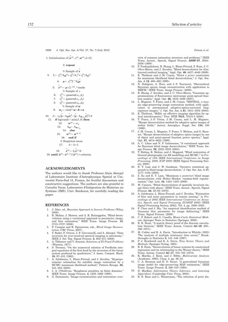
152 Sélection d’articles
1: Initialization of xo
0 ,0 ,w0 ,k=0
2: repeat
% Sample of xo
3: ←kH2+0
k12+1
kD2
4: ←k−1H
* yo
5: xo
k←+−1/2 . *randn
% Sample of
6: k←gamrnd ,
7: 1k←gamrnd1 ,1
8: 0k←gamrnd0 ,0
% Sample of w
9: wp←rand* a−b+a
10: J←yo
−Hxo
2− yo
−H,wpxo
2 /2
11: if logrand minJ ,0 then
12: wk←wp
13: H←H,wp
14: else
15: wk←wk−1
16: end if
% Empirical mean
17: k←k+1
18: xo
k←ixo
i /k
19: until xk− xk−1 / xkcriterion
ACKNOWLEDGMENTS
The authors would like to thank Professor Alain Abergelof Laboratoire Institute d’Astrophysique Spatial at Uni-versité Paris-Sud 11, France, for fruitful discussions andconstructive suggestions. The authors are also grateful toCornelia Vacar, Laboratoire d’Intégration du Matériau auSystème (IMS), Univ. Bordeaux, for carefully reading thepaper.
REFERENCES1. J. Idier, ed., Bayesian Approach to Inverse Problems (Wiley,
2008).2. R. Molina, J. Mateos, and A. K. Katsaggelos, “Blind decon-
volution using a variational approach to parameter, image,and blur estimation,” IEEE Trans. Image Process. 15,3715–3727 (2006).
3. P. Campisi and K. Egiazarian, eds., Blind Image Deconvo-lution (CRC Press, 2007).
4. T. Rodet, F. Orieux, J.-F. Giovannelli, and A. Abergel, “Datainversion for over-resolved spectral imaging in astronomy,”IEEE J. Sel. Top. Signal Process. 2, 802–811 (2008).
5. A. Tikhonov and V. Arsenin, Solutions of Ill-Posed Problems(Winston, 1977).
6. S. Twomey, “On the numerical solution of Fredholm inte-gral equations of the first kind by the inversion of the linearsystem produced by quadrature,” J. Assoc. Comput. Mach.10, 97–101 (1962).
7. A. Jalobeanu, L. Blanc-Féraud, and J. Zerubia, “Hyperpa-rameter estimation for satellite image restoration by aMCMC maximum likelihood method,” Pattern Recogn. 35,341–352 (2002).
8. J. A. O’Sullivan, “Roughness penalties on finite domains,”IEEE Trans. Image Process. 4, 1258–1268 (1995).
9. G. Demoment, “Image reconstruction and restoration: over-
view of common estimation structure and problems,” IEEETrans. Acoust., Speech, Signal Process. ASSP-37, 2024–2036 (1989).
10. P. Pankajakshani, B. Zhang, L. Blanc-Féraud, Z. Kam, J.-C.Olivo-Marin, and J. Zerubia, “Blind deconvolution for thin-layered confocal imaging,” Appl. Opt. 48, 4437–4448 (2009).
11. E. Thiébaut and J.-M. Conan, “Strict a priori constraintsfor maximum likelihood blind deconvolution,” J. Opt. Soc.Am. A 12, 485–492 (1995).
12. N. Dobigeon, A. Hero, and J.-Y. Tourneret, “HierarchicalBayesian sparse image reconstruction with application toMRFM,” IEEE Trans. Image Process. (2009).
13. B. Zhang, J. Zerubia, and J.-C. Olivo-Marin, “Gaussian ap-proximations of fluorescence microscope point-spread func-tion models,” Appl. Opt. 46, 1819–1829 (2007).
14. L. Mugnier, T. Fusco, and J.-M. Conan, “MISTRAL: a myo-pic edge-preserving image restoration method, with appli-cation to astronomical adaptive-optics-corrected long-exposure images,” J. Opt. Soc. Am. A 21, 1841–1854 (2004).
15. E. Thiébaut, “MiRA: an effective imaging algorithm for op-tical interferometry,” Proc. SPIE 7013, 70131-I (2008).
16. T. Fusco, J.-P. Véran, J.-M. Conan, and L. M. Mugnier,“Myopic deconvolution method for adaptive optics images ofstellar fields,” Astron. Astrophys. Suppl. Ser. 134, 193(1999).
17. J.-M. Conan, L. Mugnier, T. Fusco, V. Michau, and G. Rous-set, “Myopic deconvolution of adaptive optics images by useof object and point-spread function power spectra,” Appl.Opt. 37, 4614–4622 (1998).
18. A. C. Likas and N. P. Galatsanos, “A variational approachfor Bayesian blind image deconvolution,” IEEE Trans. Im-age Process. 52, 2222–2233 (2004).
19. T. Bishop, R. Molina, and J. Hopgood, “Blind restoration ofblurred photographs via AR modelling and MCMC,” in Pro-ceedings of 15th IEEE International Conference on ImageProcessing, 2008, ICIP 2008 (IEEE Signal Processing Soci-ety, 2008).
20. E. Y. Lam and J. W. Goodman, “Iterative statistical ap-proach to blind image deconvolution,” J. Opt. Soc. Am. A 17,1177–1184 (2000).
21. Z. Xu and E. Y. Lam, “Maximum a posteriori blind imagedeconvolution with Huber–Markov random-field regular-ization,” Opt. Lett. 34, 1453–1455 (2009).
22. M. Cannon, “Blind deconvolution of spatially invariant im-age blurs with phase,” IEEE Trans. Acoust., Speech, SignalProcess. 24, 58–63 (1976).
23. A. Jalobeanu, L. Blanc-Feraud, and J. Zerubia, “Estimationof blur and noise parameters in remote sensing,” in Pro-ceedings of 2002 IEEE International Conference on Acous-tics, Speech, and Signal Processing (ICASSP 2002) (IEEESignal Processing Society, 2002), Vol. 4, pp. 3580–3583.
24. F. Chen and J. Ma, “An empirical identification method ofGaussian blur parameter for image deblurring,” IEEETrans. Signal Process. (2009).
25. C. P. Robert and G. Casella, Monte-Carlo Statistical Meth-ods, Springer Texts in Statistics (Springer, 2000).
26. B. R. Hunt, “A matrix theory proof of the discrete convolu-tion theorem,” IEEE Trans. Autom. Control AC-19, 285–288 (1971).
27. M. Calder and R. A. Davis, “Introduction to Whittle (1953)‘The analysis of multiple stationary time series’,” Break-throughs in Statistics 3, 141–148 (1997).
28. P. J. Brockwell and R. A. Davis, Time Series: Theory andMethods (Springer-Verlag, 1991).
29. B. R. Hunt, “Deconvolution of linear systems by constrainedregression and its relationship to the Wiener theory,” IEEETrans. Autom. Control AC-17, 703–705 (1972).
30. K. Mardia, J. Kent, and J. Bibby, Multivariate Analysis(Academic, 1992), Chap. 2, pp. 36–43.
31. C. A. Bouman and K. D. Sauer, “A generalized Gaussianimage model for edge-preserving MAP estimation,” IEEETrans. Image Process. 2, 296–310 (1993).
32. D. MacKay, Information Theory, Inference, and LearningAlgorithms (Cambridge Univ. Press, 2003).
33. R. E. Kass and L. Wasserman, “The selection of prior dis-
1606 J. Opt. Soc. Am. A/Vol. 27, No. 7 /July 2010 Orieux et al.

Bayesian estimation of regularization and point spread function parameters for Wiener–Hunt deconvolution 153
tributions by formal rules,” J. Am. Stat. Assoc. 91, 1343–1370 (1996).
34. E. T. Jaynes, Probability Theory: The Logic of Science (Cam-bridge Univ. Press, 2003).
35. S. Lang, Real and Functional Analysis (Springer, 1993).36. P. Brémaud, Markov Chains. Gibbs Fields, Monte Carlo
Simulation, and Queues, Texts in Applied Mathematics 31(Springer, 1999).
37. S. Geman and D. Geman, “Stochastic relaxation, Gibbs dis-tributions, and the Bayesian restoration of images,” IEEETrans. Pattern Anal. Mach. Intell. 6, 721–741 (1984).
38. P. Lalanne, D. Prévost, and P. Chavel, “Stochastic artificialretinas: algorithm, optoelectronic circuits, and implementa-tion,” Appl. Opt. 40, 3861–3876 (2001)
39. H. R. Künsch, “Robust priors for smoothing and image res-toration,” Ann. Inst. Stat. Math. 46, 1–19 (1994).
40. P. Charbonnier, L. Blanc-Féraud, G. Aubert, and M. Bar-laud, “Deterministic edge-preserving regularization in com-puted imaging,” IEEE Trans. Image Process. 6, 298–311(1997).
41. J.-F. Giovannelli, “Unsupervised Bayesian convex deconvo-lution based on a field with an explicit partition function,”IEEE Trans. Image Process. 17, 16–26 (2008).
42. D. Geman and C. Yang, “Nonlinear image recovery withhalf-quadratic regularization,” IEEE Trans. Image Process.4, 932–946 (1995).
43. X. Descombes, R. Morris, J. Zerubia, and M. Berthod, “Es-timation of Markov random field prior parameters usingMarkov chain Monte Carlo maximum likelihood,” IEEETrans. Image Process. 8, 954–963 (1999).
44. G. E. P. Box and G. C. Tiao, Bayesian Inference in Statisti-cal Analysis (Addison-Wesley, 1972).
Orieux et al. Vol. 27, No. 7 /July 2010 /J. Opt. Soc. Am. A 1607

154 Sélection d’articles
T. Rodet, F. Orieux, J.-F. Giovannelli et A. Abergel, « Data inversion for over-resolved spectralimaging in astronomy », IEEE Journal of Selected Topics in Signal Processing, vol. 2, n˚5, pp. 802–811,octobre 2008.

Data inversion for over-resolved spectral imaging in astronomy 155

156 Sélection d’articles
SUBMITTED TO IEEE JOURNAL OF SELECTED TOPICS IN SIGNAL PROCESSING 1
Data inversion for over-resolved spectral imagingin astronomy
T. Rodet, F. Orieux, J.-F. Giovannelli and A. Abergel
Abstract—We present an original method for reconstructinga three-dimensional object having two spatial dimensions andone spectral dimension from data provided by the infraredslit spectrograph on board the Spitzer Space Telescope. Duringacquisition, the light flux is deformed by a complex processcomprising four main elements (the telescope aperture, theslit,the diffraction grating and optical distortion) before it r eachesthe two-dimensional sensor.
The originality of this work lies in the physical modelling, inintegral form, of this process of data formation in continuousvariables. The inversion is also approached with continuousvariables in a semi-parametric format decomposing the objectinto a family of Gaussian functions. The estimate is built inadeterministic regularization framework as the minimizer of aquadratic criterion.
These specificities give our method the power to over-resolve.Its performance is illustrated using real and simulated data.We also present a study of the resolution showing a 1.5-foldimprovement relative to conventional methods.
Index Terms—inverse problems, bayesian estipmation, over-resolved imaging, spectral imaging, irregular sampled, interpo-lation, IRS Spitzer.
I. I NTRODUCTION
Since the end of the 1970’s, infra-red to millimetric obser-vations of the sky from space have brought about a revolutionin practically all fields of astrophysics. It has become possibleto observe distant galaxies, perform detailed physicochemicalstudies of interstellar matter. Observations in the far infra-red are now possible thanks to new types of sensors (Ge:GaSi:As semiconductors and bolometer arrays). The properties ofthese new sensors encouraged the astrophysicists of the Institutd’Astrophysique Spatiale (IAS) to work with researchers atthe Laboratoire des Signaux et Systèmes (L2S) in order todevelop suitable processing methods. The spectral imagingwork presented here was carried out in the framework of thiscooperative effort. The aim is to reconstruct an over-resolvedobject having two spatial dimensions (α, β)1 and one spectraldimensionλ. Data provided by the Infrared Spectrograph(IRS) [1] on board the american Spitzer Space Telescopelaunched in 2003 are used to illustrate our work. Several setsof two-dimensional data are delivered by the Spitzer ScienceCenter (SSC), each set being the result of an acquisition for
T. Rodet, F. Orieux, J.-F. Giovannelli are with the Laboratoire desSignaux et Systèmes (CNRS – Supélec – UPS), Supélec, Plateau deMoulon, 3 rue Joliot-Curie, 91192 Gif-sur-Yvette Cedex, France. E-mail:orieux,rodet,[email protected].
A. Abergel is with the Institut d’Astrophysique Spatiale, bati-ment 121, Université Paris Sud 11, 91405 Orsay Cedex. E-mail:[email protected].
1In this paper, the spatial dimensions are angles in radian
a given satellite pointing direction. The data were acquiredusing a slit spectrograph, the operation of which is describedin detail in part II. This instrument is located in the focalplane of the telescope. When the telescope is pointed towardsa region of the sky, the spectrograph slit selects a direction ofspaceα. The photon flux is then dispersed perpendicularly tothe slit direction with a diffraction grating. The measurementis made using a two-dimensional sensor. A signal containingone spatial dimensionα and the spectral dimensionλ isthus obtained. The second spatial dimensionβ is obtainedby scanning the sky (modifying telescope pointing). Thisscanning has two notable characteristics:
• it is irregular, because the telescope control is not perfect;• it is, however, measured with sub-pixel accuracy (eighth
of a pixel).
In addition, for a given pointing direction, : the telescopeoptics, the slit width and the sensor integration limit the spatialresolution while the grating, the slit and the sensor integrationlimit the spectral resolution. The specificity of systems ofthistype is that the width of impulse response depends on thewavelength. A phenomenon of spectral also aliasing appearsfor the shortest wavelengths. Finally, the scanning results inirregular sampling along the spatial directionβ. The problemto be solved is thus one of inverting the spectral aliasing(i.e. the over-resolution) using a finite number of discretedataprovided by a complex system. The solution proposed here isbased on precise modelling of the instrument and, in particular,the integral equations containing the continuous variables (α,β andλ) of the optics and sensing system. The model input isnaturally a function of these continuous variablesφ(α, β, λ)and the output is a finite sety of discrete data items.
The approach used for solving the inverse problem, i.e.reconstructing an object having three continuous variablesfrom the discrete data
• comes within the framework of regularization by penal-ization;
• uses a semi-parametric format where the object is decom-posed into a family of functions.
There is a multitude of families of functions available(possibly forming a basis of the chosen functional space).The most noteworthy are Shannon, Fourier, wavelet and pixel-indicator families or those of spline, Gaussian Kaiser-Bessel,etc. Work on 3D tomographic reconstruction has used a familyof Kaiser-Bessel functions having spherical symmetry in orderto calculate the projections more efficiently [2], [3], [4],[5].In a different domain, the signal processing community hasbeen working on the reconstruction of over-resolved images

Data inversion for over-resolved spectral imaging in astronomy 157
2 SUBMITTED TO IEEE JOURNAL OF SELECTED TOPICS IN SIGNAL PROCESSING
from a series of low resolution images [6]. A generic directmodel can be described [6], starting with a continuous scene,to which are appliedk shift or deformation operators includingat least one translation. This step givesk deformed, high-resolution images. A convolution operator modelling the opticsand sensor cells is then applied to each of the images. Aftersubsampling, thek low-resolution images that constitute thedata are obtained. Recent work on the direct model has mainlyconcerned modelling the shift by introducing a rotation of theimage [7], [8] and a magnifying factor [9]. Other works havemodelled the shift during sensor integration by modifying theconvolution operator [10]. To the best of our knowledge, inmost works, the initial discretization step is performed onpixel indicators [11], [7], [10], [8], [6], [12]. On this point,a noteworthy contribution has been made by P. Vandewalleetal. who discretize the scene on a truncated discrete Fourierbasis [13]. However, their decomposition tends to make theimages periodic leading to create artefacts on the image side.Thus we have decided not to use this approach. Recently, theproblem of X-ray imaging spectroscopy has been solved inthe Fourier space [14], but each spectral component has beenestimated independantly.
The two major contributions of our paper are (1) the mod-elling of the measurement system as a whole with continuousvariables and (2) the continuous variable decomposition ofthe three dimensional object over a family of Gaussian func-tions. Modelling with continuous variables enables a faithfuldescription to be made of the physical phenomena involvedin the acquisition and avoids to carry out any prior datainterpolation. In our case, computing the model output requiressix integrals (two for the response of the optics, two for thegrating response, and two for the sensor integration) and thechoice of a Gaussian family allows five of these six integralsto be explicitly stated. Our paper is organised as follows:
Part II describes the continuous model of the instrumentcomprising: the diffraction at the aperture, the truncation bythe slit, the response of the grating, the distortion of the lightflux, the sensor integration and the scanning of the sky. Inpart III, the object with continuous variables is decomposedover a family of Gaussian functions. The aperture and gratingresponses are approximated by Gaussian functions. This partconcludes with the obtention of a precise, efficient modelof the measuring system. The inverse problem is solved ina regularized framework in part IV. Finally, part V givesan evaluation of the resolving power of the method and acomparison with a standard data co-addition method usingboth simulated and real data.
II. CONTINUOUS DIRECT MODEL
The aim of the instrument model is to reproduce the data,y, acquired by the spectral imager from a fluxφ(α, β, λ) ofincoherent light. Fig. 1 illustrates the instrument model forone acquisition (the telescope remains stationary). To simplify,we present the scanning procedure in section II-D. First, wehave the response of the primary mirror (aperture), whichcorresponds to a convolution. Second, there is a truncationdue to a rectugular slit. Third, a grating disperses the light.
Finnally, the sensor integration provides the discrete data y.Distortion of the luminous flux is modelled in the sensorintegration.
Fig. 1. Block diagram of the direct model for one acquisition: from acontinuously defined skyφ to a discrete outputy describing the data. Theflux φf is a convolution of the fluxφ and the PSF of the primary miror.φf
is truncated by a rectangular slit and is dispersed by the gratting. Finally, thesensor provide a discrete outputy.
A. Aperture diffraction
Under some hypotheses, the propagation of a light wavewhich passes through an aperture is determined by FRESNEL
diffraction [15] and the result in the focal plane is a convolu-tion of the input fluxφ with the Point Spread Function (PSF)ha illustrated in Fig. 2 for a circular aperture. This PSF, whichis a low pass filter, has a width proportional to the wavelengthof the incident flux. For a circular aperture, it can be written:
ha(α, β, λ) = A
[2J1(πD
√α2 + β2/λ)
πD√α2 + β2/λ
]2(1)
whereJ1 is the first order Bessel function of the first kind,Ais an amplitude factor andD is the diameter of the mirror.
Fig. 2. Profile of anAiry disk (PSF for a circular aperture) for twowavelengths.
The flux in the focal plane,φf , is written in integral form:
φf (α′, β′, λ) =
∫∫
α,β
φ(α, β, λ)ha(α − α′, β − β′, λ) dα dβ
(2)
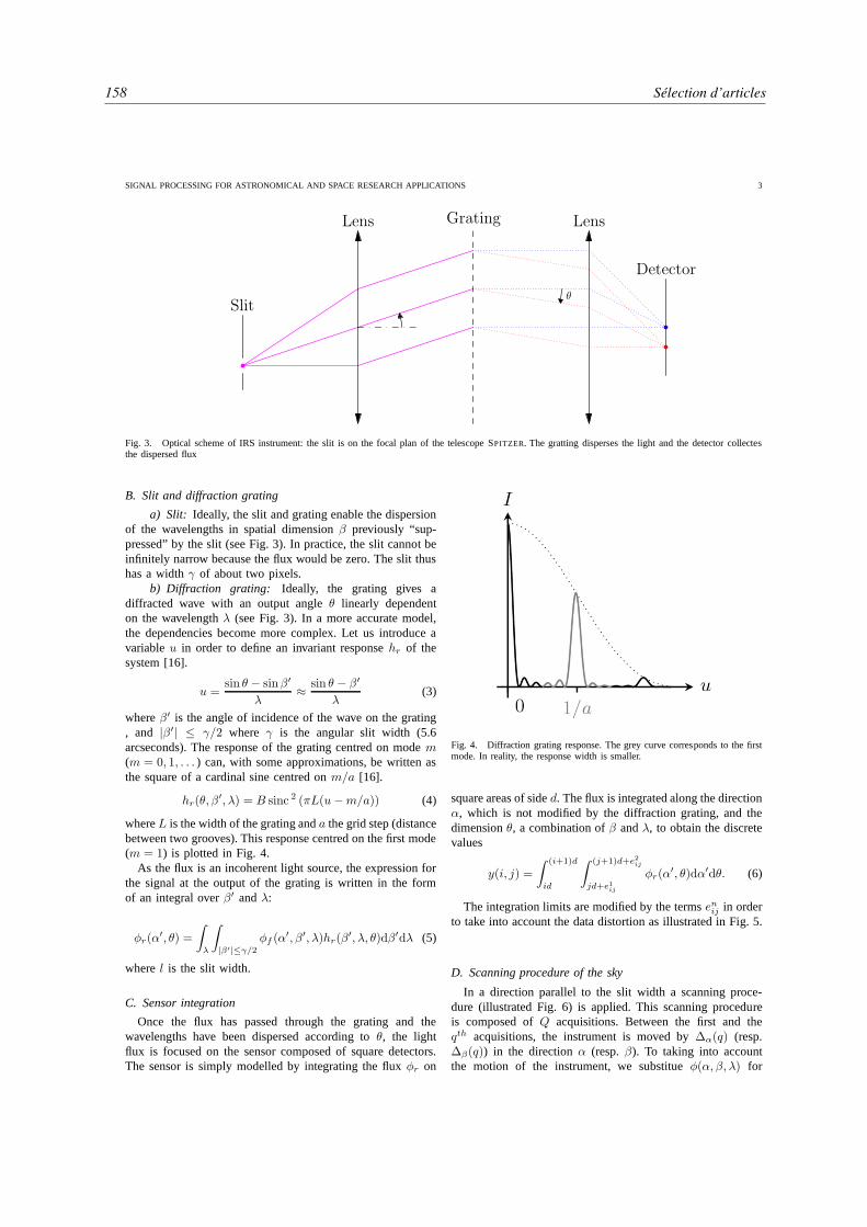
158 Sélection d’articles
SIGNAL PROCESSING FOR ASTRONOMICAL AND SPACE RESEARCH APPLICATIONS 3
θ
Lens Grating Lens
Detector
Slit
Fig. 3. Optical scheme of IRS instrument: the slit is on the focal plan of the telescope SPITZER. The gratting disperses the light and the detector collectesthe dispersed flux
B. Slit and diffraction grating
a) Slit: Ideally, the slit and grating enable the dispersionof the wavelengths in spatial dimensionβ previously “sup-pressed” by the slit (see Fig. 3). In practice, the slit cannot beinfinitely narrow because the flux would be zero. The slit thushas a widthγ of about two pixels.
b) Diffraction grating: Ideally, the grating gives adiffracted wave with an output angleθ linearly dependenton the wavelengthλ (see Fig. 3). In a more accurate model,the dependencies become more complex. Let us introduce avariableu in order to define an invariant responsehr of thesystem [16].
u =sin θ − sinβ′
λ≈ sin θ − β′
λ(3)
whereβ′ is the angle of incidence of the wave on the grating, and |β′| ≤ γ/2 where γ is the angular slit width (5.6arcseconds). The response of the grating centred on modem(m = 0, 1, . . . ) can, with some approximations, be written asthe square of a cardinal sine centred onm/a [16].
hr(θ, β′, λ) = B sinc 2 (πL(u−m/a)) (4)
whereL is the width of the grating anda the grid step (distancebetween two grooves). This response centred on the first mode(m = 1) is plotted in Fig. 4.
As the flux is an incoherent light source, the expression forthe signal at the output of the grating is written in the formof an integral overβ′ andλ:
φr(α′, θ) =
∫
λ
∫
|β′|≤γ/2
φf (α′, β′, λ)hr(β
′, λ, θ)dβ′dλ (5)
wherel is the slit width.
C. Sensor integration
Once the flux has passed through the grating and thewavelengths have been dispersed according toθ, the lightflux is focused on the sensor composed of square detectors.The sensor is simply modelled by integrating the fluxφr on
Fig. 4. Diffraction grating response. The grey curve corresponds to the firstmode. In reality, the response width is smaller.
square areas of sided. The flux is integrated along the directionα, which is not modified by the diffraction grating, and thedimensionθ, a combination ofβ andλ, to obtain the discretevalues
y(i, j) =
∫ (i+1)d
id
∫ (j+1)d+e2ij
jd+e1ij
φr(α′, θ)dα′dθ. (6)
The integration limits are modified by the termsenij in orderto take into account the data distortion as illustrated in Fig. 5.
D. Scanning procedure of the sky
In a direction parallel to the slit width a scanning proce-dure (illustrated Fig. 6) is applied. This scanning procedureis composed ofQ acquisitions. Between the first and theqth acquisitions, the instrument is moved by∆α(q) (resp.∆β(q)) in the directionα (resp.β). To taking into accountthe motion of the instrument, we substitueφ(α, β, λ) for
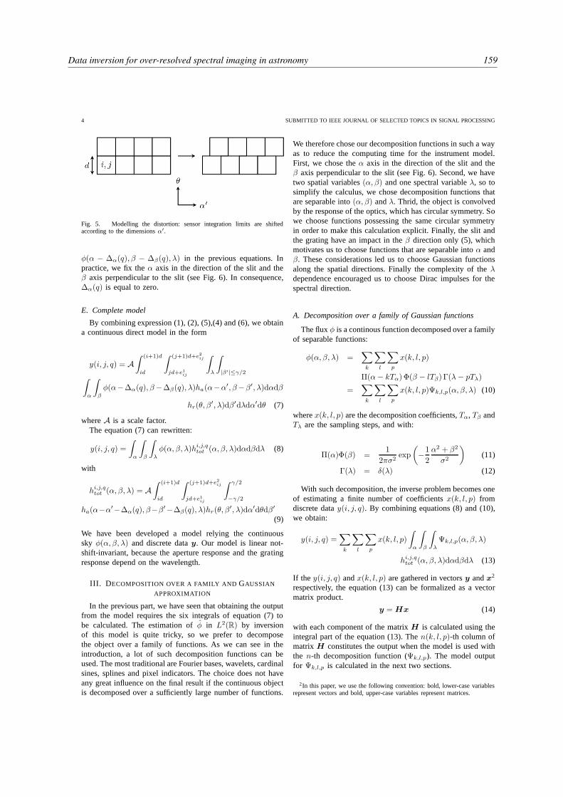
Data inversion for over-resolved spectral imaging in astronomy 159
4 SUBMITTED TO IEEE JOURNAL OF SELECTED TOPICS IN SIGNAL PROCESSING
Fig. 5. Modelling the distortion: sensor integration limits are shiftedaccording to the dimensionsα′.
φ(α − ∆α(q), β − ∆β(q), λ) in the previous equations. Inpractice, we fix theα axis in the direction of the slit and theβ axis perpendicular to the slit (see Fig. 6). In consequence,∆α(q) is equal to zero.
E. Complete model
By combining expression (1), (2), (5),(4) and (6), we obtaina continuous direct model in the form
y(i, j, q) = A∫ (i+1)d
id
∫ (j+1)d+e2ij
jd+e1ij
∫
λ
∫
|β′|≤γ/2∫
α
∫
β
φ(α−∆α(q), β−∆β(q), λ)ha(α−α′, β−β′, λ)dαdβ
hr(θ, β′, λ)dβ′dλdα′dθ (7)
whereA is a scale factor.The equation (7) can rewritten:
y(i, j, q) =
∫
α
∫
β
∫
λ
φ(α, β, λ)hi,j,qtot (α, β, λ)dαdβdλ (8)
with
hi,j,qtot (α, β, λ) = A∫ (i+1)d
id
∫ (j+1)d+e2ij
jd+e1ij
∫ γ/2
−γ/2
ha(α−α′−∆α(q), β−β′−∆β(q), λ)hr(θ, β′, λ)dα′dθdβ′
(9)
We have been developed a model relying the continuoussky φ(α, β, λ) and discrete datay. Our model is linear not-shift-invariant, because the aperture response and the gratingresponse depend on the wavelength.
III. D ECOMPOSITION OVER A FAMILY AND GAUSSIAN
APPROXIMATION
In the previous part, we have seen that obtaining the outputfrom the model requires the six integrals of equation (7) tobe calculated. The estimation ofφ in L2(R) by inversionof this model is quite tricky, so we prefer to decomposethe object over a family of functions. As we can see in theintroduction, a lot of such decomposition functions can beused. The most traditional are Fourier bases, wavelets, cardinalsines, splines and pixel indicators. The choice does not haveany great influence on the final result if the continuous objectis decomposed over a sufficiently large number of functions.
We therefore chose our decomposition functions in such a wayas to reduce the computing time for the instrument model.First, we chose theα axis in the direction of the slit and theβ axis perpendicular to the slit (see Fig. 6). Second, we havetwo spatial variables(α, β) and one spectral variableλ, so tosimplify the calculus, we chose decomposition functions thatare separable into(α, β) andλ. Thrid, the object is convolvedby the response of the optics, which has circular symmetry. Sowe choose functions possessing the same circular symmetryin order to make this calculation explicit. Finally, the slit andthe grating have an impact in theβ direction only (5), whichmotivates us to choose functions that are separable intoα andβ. These considerations led us to choose Gaussian functionsalong the spatial directions. Finally the complexity of theλdependence encouraged us to choose Dirac impulses for thespectral direction.
A. Decomposition over a family of Gaussian functions
The fluxφ is a continous function decomposed over a familyof separable functions:
φ(α, β, λ) =∑
k
∑
l
∑
p
x(k, l, p)
Π(α− kTα)Φ(β − lTβ) Γ(λ− pTλ)
=∑
k
∑
l
∑
p
x(k, l, p)Ψk,l,p(α, β, λ) (10)
wherex(k, l, p) are the decomposition coefficients,Tα, Tβ andTλ are the sampling steps, and with:
Π(α)Φ(β) =1
2πσ2exp
(−1
2
α2 + β2
σ2
)(11)
Γ(λ) = δ(λ) (12)
With such decomposition, the inverse problem becomes oneof estimating a finite number of coefficientsx(k, l, p) fromdiscrete datay(i, j, q). By combining equations (8) and (10),we obtain:
y(i, j, q) =∑
k
∑
l
∑
p
x(k, l, p)
∫
α
∫
β
∫
λ
Ψk,l,p(α, β, λ)
hi,j,qtot (α, β, λ)dαdβdλ (13)
If the y(i, j, q) andx(k, l, p) are gathered in vectorsy andx2
respectively, the equation (13) can be formalized as a vectormatrix product.
y = Hx (14)
with each component of the matrixH is calculated using theintegral part of the equation (13). Then(k, l, p)-th column ofmatrix H constitutes the output when the model is used withthe n-th decomposition function (Ψk,l,p). The model outputfor Ψk,l,p is calculated in the next two sections.
2In this paper, we use the following convention: bold, lower-case variablesrepresent vectors and bold, upper-case variables represent matrices.

160 Sélection d’articles
SIGNAL PROCESSING FOR ASTRONOMICAL AND SPACE RESEARCH APPLICATIONS 5
B. Impulse responses approximated by Gaussian functions
1) Approximation of the PSF :Equation (2) comes downto convolutions of a squared Bessel function and Gaussians.This integral is not explicit and, in order to carry out thecalculations, the PSF is approximated by a Gaussian
ha(α, β, λ) =1
2πσ2λ
exp
(−1
2
α2 + β2
σ2λ
)
with a standard deviationσλ depending on the wavelength.Indeed, the Bessel functions cross zero at the first timein 1.22λ/D. σλ is determined numerically by minimiz-ing the quadratic error between the Gaussian kernel andthe squared Bessel function, which gives for our instru-ment σλ ≈ λ/2. The relative quadratic errorerrL2 =‖Bessel− Gaussian‖22 / ‖Bessel‖22 is equal to0.15% for ourinstrument. If we caculate the relative absolute errorerrL1 =‖Bessel− Gaussian‖1 / ‖Bessel‖1, we obtain 5 %. We canconclude that most of the energy of the squared bessel functionis localized in the primary lobe. Another advantage of usingthe Gaussian approximation is that the convolution kernel isseparable intoα andβ. Finally, the result of the convolutionof two Gaussian functions is a standard one and is also aGaussian:
ha(α, β, λ)⋆Π(α)Φ(β) =1
2π(σ2λ + σ2)
exp
(− α′2 + β′2
2(σ2λ + σ2)
)
(15)
2) Approximation of the grating response:The presenceof the slit means that integral (5) is bounded overβ′ andis not easily calculable. Since the preceding expressions useGaussian functions, we approximate the squared cardinal sineby a Gaussian to make the calculations easier:
sinc2(πL
(sin θ − β′
λ− m
a
))≈
1√2πλσs
exp
(−1
2
( sin θ−β′
λ − ma )
2
σ2s
)(16)
σs is determined numerically by minimizing the quadraticerror between the Gaussian kernel and the squared cardinalsine, which gives for our instrumentσs ≈ 25.5 m−1. Therelative errors made are larger than the bessel case (errL2 =0.43%, errL1 = 10.7%), but this Gaussian approximation ofthe grating response allows the fluxφr coming out of thegrating to be known explicitly.
The error introduced here is larger than for the Gaussianapproximation of the PSF described in the previous section.However, our goal is to have a good model of the spatialdimension of the array. Furthermore, with respect to thecurrent method, the fact of taking the response of the gratinginto consideration, even as an approximation, is already astrong improvement.
φr(α′, θ) =
∫
λ
∫ γ/2
−γ/2
∫
α
∫
β
Π(α − αk)Φ(β − βl −∆β(q))
Γ(λ− λp)ha(α− α′, β − β′, λ)hr(θ, β′, λ)
dαdβdβ′dλ
= A exp
(− (α′ − αk)
2
2(σ2λ + σ2)
)exp
(− (sin θ − ν)2
2Σ2
)
×[erf
(γ/2− µΣ′√2
)− erf
(−γ/2− µΣ′√2
)](17)
with
A =1
4π
√1
(σ2λ + σ2)(σ2
λ + σ2 + λ2pσ2s)
Σ2 = (σ2λ + σ2) + λ2pσ
2s
ν =mλpa
+ βl +∆β(q)
Σ′ =
√σ2λ + σ2λpσs√
σ2λ + σ2 + λ2pσ
2s
µ =
(sin θ − mλp
a
)(σ2
λ + σ2)
(σ2λ + σ2) + λ2pσ
2s
erf(a) =2√π
∫ a
0
e−t2dt
In equation (17), it can be seen thatφr is separable intoα′
andθ. Let us introduce the functionsf andg such that:
φr(α′, θ) = Af(α′)g(θ) (18)
C. Sensor integration
First, we calculate the sensor integration in theα′ direction.
∫ (j+1)d+e2ij
jd+e1ij
f(α′)dα′ =
K[
erf
((j + 1)d+ e2ij − αk√
2(σ2λ + σ2)
)− erf
(jd+ e1ij − αk√
2(σ2λ + σ2)
)]
(19)
with K =√π(σ2
λ + σ2)/2The integral ofg is calculated numerically as the presence
of erf functions in equation (17) does not allow analyticalcalculations.
We obtain the expression for then-th column of matrixH ,which now contains only a single integral:
y(i, j, q) = AK∫ (i+1)d
id
g(θ)dθ
×[
erf
((j + 1)d+ e2ij − αk√
2(σ2λ + σ2)
)− erf
(jd+ e1ij − αk√
2(σ2λ + σ2)
)]
(20)
Using expression (20), the elements of matrixH are pre-computed relatively rapidly. Thanks to the sparsity of thematrix H to calculate the model output of Eq. (14).

Data inversion for over-resolved spectral imaging in astronomy 161
6 SUBMITTED TO IEEE JOURNAL OF SELECTED TOPICS IN SIGNAL PROCESSING
IV. I NVERSION
The previous sections build the relationship (14) betweenthe object coefficients and the data: it describes a complexinstrumental model but remains linear. The problem of input(sky) reconstruction is a typical inverse problem and theliterarure on the suject is abundant.
The proposed inversion method resorts to linear processing.It is based on conventional approaches described in bookssuch [17], [18] or more recently [19]. In this framework, thereader may also consider [20], [21] for inversion based onspecific decomposition. These methods rely on a quadraticcriterion
J(x) = ||y −Hx||2 + µαβ ||Dαβx||2 + µλ||Dλx||2 . (21)
It involves a least squares term and two penality termsconcerning the differences between neighbouring coefficients:one for the two spatial dimensions and one for the spectraldimension. They are weighted byµαβ and µλ, respectively.The estimatex is chosen as the minimizer of this criterion. Itis thus explicit and linear with respect to the data:
x =(HtH + µαβD
tαβDαβ + µλD
tλDλ
)−1Hty (22)
and depends on the two regularization parametersµαβ andµλ.
Remark 1 — This estimator can be interpreted in aBayesian framework [22] based on Gaussian models for theerrors and the object. As far as the errors are concerned, themodel is a white noise. As far as the object is concerned, themodel is correlated and the inverse of the correlation matrixis proportional toµαβD
tαβDαβ+µλD
tλDλ, i.e., it is a Gauss
markov field. In this framework, the estimate maximizes the aposteriori law.
Remark 2 — Many works in the field of over-resolvedreconstruction concern edge preserving priors [23], [11], [7],[24], [25], [12]. In our application here, smooth interstellardust clouds are under study, so preservation of edges is notappropriate. For the sake of simplicity of implementation, wechose a Gaussian object prior.
The minimizer x given by relation (22) is explicit but,in practice, it cannot be calculated on standard computers,because the matrix to be inverted is too large. The solutionx
is therefore computed by a numerical optimization algorithm.Practically, the optimization relies on a standard gradientdescent algorithm [26], [27]. More precisely, the directiondescent is a approximate conjugate gradient direction [28]andthe optimal step of descent is used. Finally, we initialise themethod with zero (x = 0).
V. RESULTS
As we have presented in part III theα andβ axis are fix(see Fig. 6, right). The real data is composed of 23 acquisitionshaving a spatial dimensionα′ and a spectral dimensionθ ofwavelength between 7.4 and 15.3µm (each acquisition is animage composed of38 × 128 detector cells, see Fig. 6, left).Between two acquisitions, the instrument is moved by half a
Fig. 6. Acquisition. The left-hand image represents the data acquiredfor one pointing position: the vertical axis shows the spectral dimensionθand the horizontal axis is the spatial dimensionα′. The slit is representedschematically by a rectangle in the middle. The right-hand image illustratesthe scanning strategy in theβ direction.
slit width in theβ direction. Fig. 6, right, shows the scanningprocedure applied to the Horsehead nebula [29].
Our results (Fig. 8(b), solid line on Fig. 9 and Fig. 10(b))can be compared with those obtained with the conventionalprocessing (Fig. 8(c), dotted line on Fig. 9 and Fig. 10(a)).For the conventional processing (described in Compiègne etal. 2007 [29]) an image of the slit is simply extracted for eachwavelength from the data taken after each acquisition (e.g.leftpanel of Fig. 6) and projected and co-added on the output skyimage, without any description of the instrument properties.
A. Simulated data
In our first experiment, we reconstruct data simulated usingour direct model. We choose an object with the same spatialmorphology and the same spectral content as the Horseheadnebula (see Fig. 8(a)). However, in order to tune the regulariza-tion coefficient, we perform a large number of reconstructions.Thus, we need to simulate a problem smaller than in our realcase. The data are composed of 14 acquisitions, and the virtualdetector contained18× 40 pixels. We choose to reconstruct avolume with 15870 gaussians distributed on a cartesian grid23 × 23 × 30. Finally, we add to the output of the model awhite Gaussian noise with the same variance as the real data.
The results contain a set of 30 images (see Fig. 7). Fig.8(b) and solid line on Fig.9 illustrate our result for onewavelength (8.27µm) and one pixel, respectively. The imagecomputed with our method (Fig. 8(b)) appears comparableto the true image (Fig. 8(a)), while the image computedwith the conventional processing (Fig. 8(c)) is smoother. Acomparison of solid line and dotted line in Fig. 9 clearly alsoshows that our method provides a spectrum comparable to thetrue spectrum, while the peaks obtained with the conventionalprocessing are too broad.
Our sky estimation depends on the regularization coeffi-cientsµαβ and µλ. We tune this parameters by minimizingnumerically the quadratic error between the estimated objectand the real object were selected. In this experiment we obtainµαβ = 0.01, µλ = 0.005.
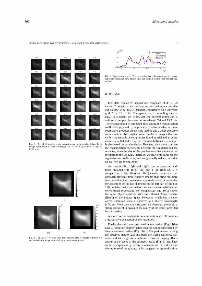
162 Sélection d’articles
SIGNAL PROCESSING FOR ASTRONOMICAL AND SPACE RESEARCH APPLICATIONS 7
7.40 7.46 7.52 7.59 7.65
7.71 7.77 7.83 7.90 7.96
8.02 8.08 8.14 8.21 8.27
8.33 8.39 8.45 8.52 8.58
8.64 8.70 8.76 8.83 8.89
8.95 9.01 9.07 9.14 9.20
Fig. 7. Set of 30 images of our reconstruction from simulateddata. Eachimage corresponds to one wavelength for 7.4 to 9.2µm with a step of0.062µm.
0
0.5
1
1.5
2
x 1011
(a)
0
5
10
15
20x 10
10
(b)
0
2
4
6
8
10
12
14
x 1010
(c)
Fig. 8. Image atλ = 8.27µm:, (a) simulated sky, (b) image estimated byour method, (c) image estimated by a conventional method.
7.5 8 8.5 9
x 10−6
0.5
1
1.5
2x 10
11
TrueOur methodStandard
Fig. 9. Spectrum of a pixel. The curves abscissa is the wavelenght in meters:solid line: simulated sky, dashed line: our method, dotted line: conventionalmethod.
B. Real data
Eeal data contain 23 acquisitions composed of38 × 128values. To obtain a over-resolved reconstruction, we describeour volume with 587264 gaussians destributes on a cartesiangrid 74 × 62 × 128. The spatial(α, β) sampling step isequal to a quater slit width, and the spectral dimension isuniformly sampled between the wavelength 7.4 and 15.3µm.The reconstruction is computed after setting the regularizationcoefficientsµαβ andµλ empirically. Too low a value for thesecoefficients produces an unstable method and a quasi explosivereconstruction. Too high a value produces images that arevisibly too smooth. A compromise found by trial and error ledus toµαβ = 0.3 andµλ = 0.7. The ratio betweenµαβ andµλ
is also based on our simulation. However, we cannot comparethe regularization coefficients between the simulated and thereal case, since the size of the problem modifies the weigth ofthe norm in the Eq. (21). Pratically, we take large value for theregularization coefficients, and we gradually reduce the valueup that we are seeing noise.
Our results (Fig. 10(b) and 11(b)) can be compared withthose obtained with (Fig. 10(a) and 11(a), from [29]). Acomparison of Fig. 10(a) and 10(b) clearly shows that ourapproach provides more resolved images that bring out morestructures than the conventional approach. Note, in particular,the separation of the two filaments on the left part of the Fig.10(b) obtained with our method, which remains invisible afterconventional processing. For comparison, Fig. 10(c) showsthe same object observed with the Infrared Array Camera(IRAC) of the Spitzer Space Telescope which has a betternative resolution since it observes at a shorter wavelength(4.5µm). Here the same structures are observed, providing astrong argument in favour of the reality of the results providedby our method.
A more precise analysis is done in section V-C. It providesa quantitative evaluation of the resolution.
Finally, the spectra reconstructed by our method (Fig. 11(b))have a resolution slightly better than the one reconstructed bythe conventional method (Fig. 11(a)). The peaks characterizingthe observed matter (gas and dust) are well positioned, nar-rower and with a greater amplitude. However, ringing effectsappear at the bases of the strongest peaks (Fig. 11(b)). Theycould be explained by an over-evaluation of the widthσs ofthe response of the grating, or by the gaussian approximation.
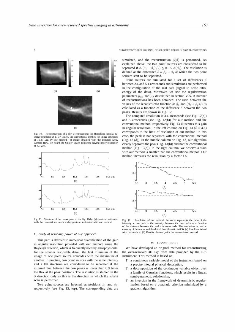
Data inversion for over-resolved spectral imaging in astronomy 163
8 SUBMITTED TO IEEE JOURNAL OF SELECTED TOPICS IN SIGNAL PROCESSING
0
20
40
60
80
100
(a)
0
20
40
60
80
100
(b)
(c)
Fig. 10. Reconstruction of a skyφ representing the Horsehead nebula: (a)image estimated at 11.37µm by the conventional method (b) image estimatedat 11.37µm by our method, (c) image obtained with the Infrared ArrayCamera IRAC on board the Spitzer Space Telescope having better resolutionat 4.5µm.
20 40 60 80 100 1200
50
100
7.4 8.6 9.9 11.1 12.4 13.6 14.8µ m
50
0
100
(a)
20 40 60 80 100 1200
50
100
µ m
50
0
100
7.4 8.6 9.9 11.1 12.4 13.6 14.8
(b)
Fig. 11. Spectrum of the center point of the Fig. 10(b): (a) spectrum estimatedwith the conventional method (b) spectrum estimated with our method.
C. Study of resolving power of our approach
This part is devoted to numerical quantification of the gainin angular resolution provided with our method, using theRayleigh criterion, which is frequently used by astrophysicists:for the smaller resolvable detail, the first minimum of theimage of one point source coincides with the maximum ofanother. In practice, two point sources with the same intensityand a flat strectrum are considered to be separated if theminimal flux between the two peaks is lower than 0.9 timesthe flux at the peak positions. The resolution is studied in theβ direction only as this is the direction in which the subslitscan is performed.
Two point sources are injected, at positionsβ1 and β2,respectively (see Fig. 13, top). The corresponding data are
simulated, and the reconstructionφ(β) is performed. Asexplained above, the two point sources are considered to beseparated ifφ([β1 + β2] /2) ≤ 0.9× φ(β1). The resolution isdefined as the differenceδ = β2 − β1 at which the two pointsources start to be separated.
Point sources are simulated for a set of differencesδbetween 2.4 and 5.4 arcseconds and simulations are performedin the configuration of the real data (signal to noise ratio,energy of the data). Moreover, we use the regularizationparametersµαβ andµλ determined in section V-A. A numberof reconstructions has been obtained. The ratio between thevalues of the reconstructed function atβ1 and(β1 + β2)/2 iscalculated as a function of the differenceδ between the twopeaks. Results are shown in Fig. 12.
The computed resolution is 3.4 arcseconds (see Fig. 12(a))and 5 arcseconds (see Fig. 12(b)) for our method and theconventional method, respectively. Fig. 13 illustrates this gainin angular resolution. In the left column on Fig. 13 (δ = 3.4)corresponds to the limit of resolution of our method. In thiscase, the peak is not separated with the conventional method(Fig. 13 (d)). In the middle column on Fig. 13, our algorithmclearly separates the peak (Fig. 13(h)) and not the conventionalmethod (Fig. 13(e)). In the right column, we observe a stainwith our method is smaller than the conventional method. Ourmethod increases the resolution by a factor 1.5.
2.5 3 3.5 4 4.5 5 5.50
0.5
1
(a)
2.5 3 3.5 4 4.5 5 5.50
0.5
1
(b)
Fig. 12. Resolution of our method: the curve represents the ratio of theintensity at one peak to the intensity between the two peaks as a functionof the distance between the peaks in arcseconds. The resolution is read atcrossing of this curve and the dotted line (the ratio is 0.9).(a) Results obtainedwith our method. (b) Results obtained with the conventionalmethod.
VI. CONCLUSIONS
We have developed an original method for reconstructingthe over-resolved 3D sky from data provided by the IRSinstrument. This method is based on:
1) a continuous variable model of the instrument based ona precise integral physical description,
2) a decomposition of the continuous variable object overa family of Gaussian functions, which results in a linear,semi-parametric relationship,
3) an inversion in the framework of deterministic regular-ization based on a quadratic criterion minimized by agradient algorithm.
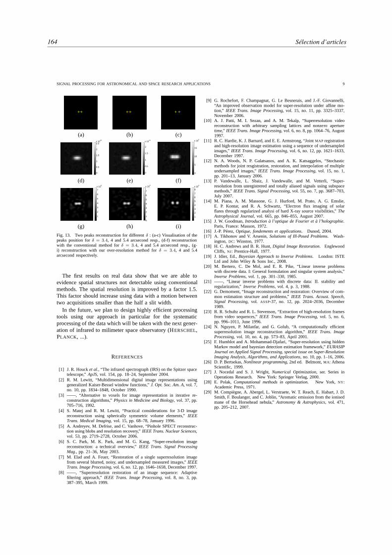
164 Sélection d’articles
SIGNAL PROCESSING FOR ASTRONOMICAL AND SPACE RESEARCH APPLICATIONS 9
(a) (b) (c)
0
0.5
1
1.5
2
2.5x 10
10
0
0.5
1
1.5
2
x 1010
0
5
10
15
x 109
(d) (e) (f)
1
2
3
4
5
6
7
x 109
0
1
2
3
4
5
6
7
x 109
1
2
3
4
5
6
7
8x 10
9
(g) (h) (i)
Fig. 13. Two peaks reconstruction for differentδ : (a-c) Visualisation of thepeaks position forδ = 3.4, 4 and 5.4 arcsecond resp., (d-f) reconstructionwith the conventional method forδ = 3.4, 4 and 5.4 arcsecond resp., (g-i) reconstruction with our over-resolution method forδ = 3.4, 4 and 5.4arcsecond respectively.
The first results on real data show that we are able toevidence spatial structures not detectable using conventionalmethods. The spatial resolution is improved by a factor 1.5.This factor should increase using data with a motion betweentwo acquisitions smaller than the half a slit width.
In the future, we plan to design highly efficient processingtools using our approach in particular for the systematicprocessing of the data which will be taken with the next gener-ation of infrared to milimeter space observatory (HERSCHEL,PLANCK , ...).
REFERENCES
[1] J. R. Houcket al., “The infrared spectrograph (IRS) on the Spitzer spacetelescope,”ApJS, vol. 154, pp. 18–24, September 2004.
[2] R. M. Lewitt, “Multidimensional digital image representations usinggeneralized Kaiser-Bessel window functions,”J. Opt. Soc. Am. A, vol. 7,no. 10, pp. 1834–1848, October 1990.
[3] ——, “Alternative to voxels for image representation in iterative re-construction algorithms,”Physics in Medicine and Biology, vol. 37, pp.705–716, 1992.
[4] S. Matej and R. M. Lewitt, “Practical considerations for3-D imagereconstruction using spherically symmetric volume elements,” IEEETrans. Medical Imaging, vol. 15, pp. 68–78, January 1996.
[5] A. Andreyev, M. Defrise, and C. Vanhove, “Pinhole SPECT reconstruc-tion using blobs and resolution recovery,”IEEE Trans. Nuclear Sciences,vol. 53, pp. 2719–2728, October 2006.
[6] S. C. Park, M. K. Park, and M. G. Kang, “Super-resolution imagereconstruction: a technical overview,”IEEE Trans. Signal ProcessingMag., pp. 21–36, May 2003.
[7] M. Elad and A. Feuer, “Restoration of a single superresolution imagefrom several blurred, noisy, and undersampled measured images,” IEEETrans. Image Processing, vol. 6, no. 12, pp. 1646–1658, December 1997.
[8] ——, “Superresolution restoration of an image sequence:Adaptivefiltering approach,”IEEE Trans. Image Processing, vol. 8, no. 3, pp.387–395, March 1999.
[9] G. Rochefort, F. Champagnat, G. Le Besnerais, and J.-F. Giovannelli,“An improved observation model for super-resolution underaffine mo-tion,” IEEE Trans. Image Processing, vol. 15, no. 11, pp. 3325–3337,November 2006.
[10] A. J. Patti, M. I. Sezan, and A. M. Tekalp, “Superresolution videoreconstruction with arbitrary sampling lattices and nonzero aperturetime,” IEEE Trans. Image Processing, vol. 6, no. 8, pp. 1064–76, August1997.
[11] R. C. Hardie, K. J. Barnard, and E. E. Armstrong, “JointMAP registrationand high-resolution image estimation using a sequence of undersampledimages,”IEEE Trans. Image Processing, vol. 6, no. 12, pp. 1621–1633,December 1997.
[12] N. A. Woods, N. P. Galatsanos, and A. K. Katsaggelos, “Stochasticmethods for joint resgistration, restoration, and interpolation of multipleundersampled images,”IEEE Trans. Image Processing, vol. 15, no. 1,pp. 201–13, January 2006.
[13] P. Vandewalle, L. Sbaiz, J. Vandewalle, and M. Vetterli, “Super-resolution from unregistrered and totally aliased signalsusing subspacemethods,”IEEE Trans. Signal Processing, vol. 55, no. 7, pp. 3687–703,July 2007.
[14] M. Piana, A. M. Massone, G. J. Hurford, M. Prato, A. G. Emslie,E. P. Kontar, and R. A. Schwartz, “Electron flux imaging of solarflares through regularized analysi of hard X-ray source visibilities,” TheAstrophysical Journal, vol. 665, pp. 846–855, August 2007.
[15] J. W. Goodman,Introduction à l’optique de Fourier et à l’holographie.Paris, France: Masson, 1972.
[16] J.-P. Pérez,Optique, fondements et applications. Dunod, 2004.[17] A. Tikhonov and V. Arsenin,Solutions of Ill-Posed Problems. Wash-
ington, DC: Winston, 1977.[18] H. C. Andrews and B. R. Hunt,Digital Image Restoration. Englewood
Cliffs, NJ: Prentice-Hall, 1977.[19] J. Idier, Ed.,Bayesian Approach to Inverse Problems. London: ISTE
Ltd and John Wiley & Sons Inc., 2008.[20] M. Bertero, C. De Mol, and E. R. Pike, “Linear inverse problems
with discrete data. I: General formulation and singular system analysis,”Inverse Problems, vol. 1, pp. 301–330, 1985.
[21] ——, “Linear inverse problems with discrete data: II. stability andregularization,”Inverse Problems, vol. 4, p. 3, 1988.
[22] G. Demoment, “Image reconstruction and restoration: Overview of com-mon estimation structure and problems,”IEEE Trans. Acoust. Speech,Signal Processing, vol. ASSP-37, no. 12, pp. 2024–2036, December1989.
[23] R. R. Schultz and R. L. Stevenson, “Extraction of high-resolution framesfrom video sequences,”IEEE Trans. Image Processing, vol. 5, no. 6,pp. 996–1011, June 1996.
[24] N. Nguyen, P. Milanfar, and G. Golub, “A computationally efficientsuperresolution image reconstruction algorithm,”IEEE Trans. ImageProcessing, vol. 10, no. 4, pp. 573–83, April 2001.
[25] F. Humblot and A. Mohammad-Djafari, “Super-resolution using hiddenMarkov model and bayesian detection estimation framework,” EURASIPJournal on Applied Signal Processing, special issue on Super-ResolutionImaging Analysis, Algorithms, and Applications, no. 10, pp. 1–16, 2006.
[26] D. P. Bertsekas,Nonlinear programming, 2nd ed. Belmont,MA : AthenaScientific, 1999.
[27] J. Nocedal and S. J. Wright,Numerical Optimization, ser. Series inOperations Research. New York: Springer Verlag, 2000.
[28] E. Polak, Computational methods in optimization. New York, NY:Academic Press, 1971.
[29] M. Compiègne, A. Abergel, L. Verstraete, W. T. Reach, E.Habart, J. D.Smith, F. Boulanger, and C. Joblin, “Aromatic emission fromthe ionisedmane of the Horsehead nebula,”Astronomy & Astrophysics, vol. 471,pp. 205–212, 2007.

Data inversion for over-resolved spectral imaging in astronomy 165
10 SUBMITTED TO IEEE JOURNAL OF SELECTED TOPICS IN SIGNAL PROCESSING
Thomas Rodetwas born in Lyon, France, in 1976.He received the Doctorat degree at Institut NationalPolytechnique de Grenoble, France, in 2002.
He is presently assistant professor in the Dé-partement de Physique at Université Paris-Sud 11and researcher with the Laboratoire des Signaux etSystèmes (CNRS - Supélec - UPS). He is interestedin tomography methods and Bayesian methods forinverse problems in astrophisical problems (inver-sion of data taken from space observatory: Spitzer,Herschel, SoHO, STEREO).
François Orieux was born in Angers, France,in 1981. He graduated from the École Supérieured’Électronique de l’Ouest in 2006 and obtain theM. S. degree from the University of Rennes 1. Hecurrently pursuing the Ph. D. degree at the UniversitéParis-Sud 11. His research interests are statisticalimage processing and Bayesian methods for inverseproblems.
Jean-François Giovannelli was born in Béziers,France, in 1966. He graduated from the École Na-tionale Supérieure de l’Électronique et de ses Ap-plications in 1990. He received the Doctorat degreein physics at Université Paris-Sud, Orsay, France, in1995.
He is presently assistant professor in the Dé-partement de Physique at Université Paris-Sud andresearcher with the Laboratoire des Signaux et Sys-tèmes (CNRS - Supélec - UPS). He is interestedin regularization and Bayesian methods for inverse
problems in signal and image processing. Application fieldsessentiallyconcern astronomical, medical and geophysical imaging.
Alain Abergel was born in Paris, France, in 1959.He received the Doctorat degree in astrophysicsat the Paris 6 University, France, in 1987, and ispresently Professor in Physics and Astronomy atthe Paris-Sud University. He is interested in theinterstellar medium of galaxies, and uses data takenfrom long wavelength space observatories (IRAS,COBE, ISO, Spitzer, ... ). He is Co-investigatorfor the Spectral and Photometric Imaging Receiver(SPIRE) instrument on-board the European SpaceAgency’s Herschel Space Observatory.

166 Sélection d’articles
N. Barbey, F. Auchère, T. Rodet et J.-C. Vial, « A time-evolving 3D method dedicated to the re-construction of solar plumes and results using extreme ultra-violet data », Solar Physics, vol. 248, n˚2,pp. 409–423, avril 2008.

A time-evolving 3D method dedicated to the reconstruction of solar plumes and results using extreme ultra-violetdata 167

168 Sélection d’articles
arX
iv:0
802.
0113
v1 [
astr
o-ph
] 1
Feb
200
8
Solar PhysicsDOI: 10.1007/•••••-•••-•••-••••-•
A Time-Evolving 3D Method Dedicated to the
Reconstruction of Solar Plumes and Results
Using Extreme Ultra-Violet Data
Nicolas Barbey∗†· Frédéric Auchère∗
·
Thomas Rodet† · Jean -Claude Vial∗
Received: 9 May 2007 / Accepted: 24 January 2008
c© Springer ••••
Abstract An important issue in the tomographic reconstruction of the solar polesis the relatively rapid evolution of the polar plumes. We demonstrate that it ispossible to take into account this temporal evolution in the reconstruction. Thedifficulty of this problem comes from the fact that we want a 4D reconstruction (threespatial dimensions plus time) while we only have 3D data (2D images plus time).To overcome this difficulty, we introduce a model that describes polar plumes asstationary objects whose intensity varies homogeneously with time. This assumptioncan be physically justified if one accepts the stability of the magnetic structure. Thismodel leads to a bilinear inverse problem. We describe how to extend linear inversionmethods to these kinds of problems. Studies of simulations show the reliability of ourmethod. Results for SOHO/EIT data show that we are able to estimate the temporalevolution of polar plumes in order to improve the reconstruction of the solar polesfrom only one point of view. We expect further improvements from STEREO/EUVIdata when the two probes will be separated by about 60.
1. Introduction
A method known as solar rotational tomography has been used to retrieve the 3Dgeometry of the solar corona (Frazin 2000; Frazin and Janzen 2002). This methodassumes the stability of the structures during the time necessary to acquire thedata. Since we generally have only one point of view at our disposal, about 15days are required to have data for half a solar rotation at the poles. Here, we focusour study on solar polar plumes. They are bright, radial, coronal ray structureslocated at the solar poles in regions of open magnetic field. The study of plumes isof great interest since it may be the key to the understanding of the accelerationof the fast component of the solar wind (Teriaca et al., 2003). However the three-dimensional shape of these structures is poorly known and different assumptions have
∗Institut d’Astrophysique Spatiale, Université Paris-Sud, Orsay, Franceemail: [email protected], [email protected], [email protected]
†Laboratoire des Signaux et Systemes, Supéléc, Gif-sur-Yvette, Franceemail: [email protected], [email protected]

A time-evolving 3D method dedicated to the reconstruction of solar plumes and results using extreme ultra-violetdata 169
N. Barbey et al.
been made, e.g. Gabriel et al., 2005; Llebaria, Saez, and Lamy, 2002. The plumes
are known to evolve with a characteristic time of approximately 24 hours on spatial
scales typical of Extreme ultra-violet Imaging Telescope (SOHO/EIT) data (2400
km) (DeForest, Lamy, and Llebaria, 2001). Consequently the stability assumption
made in rotational tomography fails. Fortunately, the Solar TErestrial RElations
Observatory (STEREO) mission consists of two identical spacecraft STEREOA and
STEREOB which take pictures of the Sun from two different points of view. With the
SOHO mission still operating, this results in three,simultaneous points of view. Three
viewpoints help to improve the reconstruction of the plumes, but they are still not
enough to use standard tomographic algorithms. The problem is underdetermined
and consequently one has to add a priori information in order to overcome the lack
of information. This leads to challenging and innovative signal analysis problems.
There are different ways to deal with underdetermination depending on the kind of
object to be reconstructed. Interestingly the field of medical imaging faces the same
kind of issues. In cardiac reconstruction, authors make use of the motion periodicity
in association with a high redundancy of the data (Grass et al., 2003; Kachelriess,
Ulzheimer, and Kalender, 2000). If one can model the motion as an affine transfor-
mation, and if one assumes that we know this transformation, one can obtain an
analytic solution (Ritchie et al., 1996; Roux et al., 2004).
In solar tomography, the proposed innovative approaches involve the use of ad-
ditional data such as magnetic-field measurements in the photosphere (Wiegelmann
and Inhester, 2003) or data fusion (Frazin and Kamalabadi, 2005). Attempts have
been made by Frazin et al. (2005) to treat temporal evolution using Kalman filtering.
Since polar plumes have apparently a local, rapid, and aperiodic temporal evo-
lution, we developed as in the previously referenced work, a model based on the
specifics of the object we intend to reconstruct (preliminary results can be found in
Barbey et al., (2007). Plumes have an intensity which evolves rapidly with time,
but their position can be considered as constant. This hypothesis is confirmed by
previous studies of the plumes such as DeForest, Lamy, and Llebaria (2001). The
model is made up of an invariant morphological part (x) multiplied by a gain term
(θt) that varies with time. Only one gain term is associated with each plume in order
to constrain the model. So we assume that the position of each plume in the scene
is known. This model is justified if we consider polar plumes to be slowly evolving
magnetic structures in which plasma flows.
Thanks to this model we can perform time-evolving three-dimensional tomogra-
phy of the solar corona using only extreme ultra-violet images. Furthermore, there is
no complex, underlying physical model. The only assumptions are the smoothness of
the solution, the area-dependant evolution model, and the knowledge of the plume
position. These assumptions allow us to consider a temporal variation of a few days,
while assuming only temporal smoothness would limit variations to the order of one
solar rotation (about 27 days). To our knowledge, the estimation of the temporal
evolution has never been undertaken in tomographic reconstruction of the solar
corona.
We first explain our reconstruction method in a Bayesian framework (Section
2). We then test the validity of our algorithm with simulated data (Section 3). An
example of a reconstruction on real SOHO/EIT data is shown in Section 4. Results
are discussed in Section 5. We conclude in Section 6.
barbey_SPfullpaper.tex; 4/02/2008; 5:12; p.2

170 Sélection d’articles
A Time-Evolving 3D Method Dedicated to the Reconstruction of Solar Plumes
Figure 1. Scheme of the data acquisition geometry. (O; x, y, z) defines the Carrington helio-centric frame of reference. S is the spacecraft considered. φ is the latitude, and θ the longitudeof this spacecraft. V is the virtual detector.
2. Method
Tomographic reconstruction can be seen as an inverse problem, the direct problembeing the acquisition of data images knowing the emission volume density of theobject (Section 2.1). If the object is evolving during the data acquisition, the inverseproblem is highly underdetermined. So our first step is to redefine the direct problemthanks to a reparametrization, in order to be able to define more constraints (Section2.2). Then, we place ourselves in the Bayesian inference framework in which dataand unknowns are considered to be random variables. The solution of the inverseproblem is chosen to be the maximum a posteriori (Section 2.3). This leads to acriterion that we minimize with an alternate optimization algorithm (Section 2.4).
2.1. Direct Problem
The geometrical acquisition is mathematically equivalent to a conical beam dataacquisition with a virtual spherical detector (see Figure 1). In other words, the stepbetween two pixels vertically and horizontally is constant in angle. The angle of thefull field of view is around 45 minutes. In order to obtain an accurate reconstruc-tion, we take into account the exact geometry, which means the exact position andorientation of the spacecraft relatively to Sun center. We approximate integration ofthe emission in a flux tube related to a pixel by an integration along the line of sightgoing through the middle of that pixel. We choose to discretize the object in theusual cubic voxels. x is a vector of size N containing the values of all voxels. In thesame way, we define the vector of data yt of size M at time t. Since the integrationoperator is linear, the projection can be described by a matrix Pt. We choose nt tobe an additive noise:
yt = Ptxt + nt, ∀t ∈ [1, ..., T ] (1)
Pt is the projection matrix at time t of size M ×N which is defined by the positionand the orientation of the spacecraft at this time. Its transpose is the backprojec-tion matrix. Note that a uniform sampling in time is not required. In order to beable to handle large problems with numerous well-resolved data images and a largereconstruction cube, we chose not to store the whole projection matrix. Instead,
barbey_SPfullpaper.tex; 4/02/2008; 5:12; p.3

A time-evolving 3D method dedicated to the reconstruction of solar plumes and results using extreme ultra-violetdata 171
N. Barbey et al.
we perform the projection operation (Px) or its transpose each time it is neededat each iteration. Thus, we need a very efficient algorithm. We developed a codewritten in C which performs the projection operation. It makes use of the geometricalparameters given in the data headers in order to take into account the exact geometry(conicity, position, and orientation of the spacecraft). To keep this operation fast,we implemented the Siddon algorithm (Siddon, 1985). It allows a fast projection orbackprojection in the case of cubic voxels (Cartesian grid). Since we focus on a smallregion at the poles, we consider that we do not need to use a spherical grid whichwould require a more time-consuming projection algorithm.
We take into account the fact that the field of view is conical. Despite the factthat the acquisition is very close to the parallel acquisition geometry, it is sufficientto introduce an error of several voxels of size 0.01 solar radius from one side to theother of a three solar radii reconstructed cube.
2.2. Modeling of the Temporal Evolution
With this model, the inverse problem is underdetermined since we have at mostthree images at one time and we want to reconstruct the object with its temporalevolution. In order to do so, we first redefine our unknowns to separate temporalevolution from spatial structure. We introduce a new set of variables gt of size N
describing the temporal evolution and require that x does not depend on time:
yt = Pt(x gt) + nt (2)
with being the term-by-term multiplication of vectors. This operator is clearlybilinear. However, this model would increase the number of variables excessively.So, we need to introduce some other kind of a priori into our model. We makethe hypothesis that all of the voxels of one polar plume have the same temporalevolution:
gt = Lθt (3)
The matrix L of size N × P (P being the number of areas) localizes areas wherethe temporal evolution is identical. Each column of L is the support function of oneof the plumes. We would like to stress that in our hypothesis, those areas do notmove relative to the object. In other words, L does not depend on time. Localizingthese areas defines L and only leaves P T variables to estimate. We redefined ourproblem in a way that limits the number of parameters to estimate but still allowsmany solutions. Furthermore, the problem is linear in x knowing θ and linear in θ
knowing x. It will simplify the inversion of the problem as we shall see later. Note,however that the uniqueness of a solution (x, θ) is not guaranteed with bilinearitydespite its being guaranteed in the linear case. This example shows that A can bechosen arbitrarily without changing the closeness to the data: xg = (Ax)(A−1g),where A is a real constant. Introducing an a priori of closeness to 1 for θ would allowus to deal with this indeterminacy in principle. But note that this indeterminacy isnot critical since the physical quantity of interest is only the product x g. Féron,Duchêne, and Mohammad-Djafari (2005) present a method which solves a bilinearinversion problem in the context of microwave tomography.
We do not deal with the estimation of the areas undergoing evolution, but weassume in this paper that the localization is known. This localization can be achieved
barbey_SPfullpaper.tex; 4/02/2008; 5:12; p.4

172 Sélection d’articles
A Time-Evolving 3D Method Dedicated to the Reconstruction of Solar Plumes
using other sources of information, e.g. stereoscopic observations. We expect to beable to locate the areas using some other source of information.
We can regroup the equations of the direct problem. We have two ways to do so,each emphasizing the linearity throughout one set of variables.
y = Uxθ + n
y1
...yT
=
P1XL 0
. . .
0 PTXL
θ1
...θT
+
n1
...nT
(4)
with X = diag(x), the diagonal matrix defined by x. x is of size N , y and n are ofsize M T , θ is of size P T and Ux is of size M T × P T .
Similarly,
y = Vθx+ n
with Vθ =
P1diag(Lθ1) 0
. . .
0 PTdiag(LθT )
Id...Id
(5)
with Id the identity matrix of size M ×M . Vθ is of size MT ×N .
2.3. Inverse Problem
In Bayes’ formalism, solving an inverse problem consists in knowing the a posteriori(the conditional probability density function of the parameters, the data being given).To do so we need to know the likelihood (the conditional probability density functionof the data knowing the parameters) and the a priori (the probability density func-tion of the parameters). An appropriate model is a Gaussian, independent, identicallydistributed (with the same variance) noise n. The likelihood function is deduced fromthe noise statistic:
f(y|x,θ, σn,M) = K1 exp
(−‖y −Uxθ‖
2
2σ2n
)(6)
M = [P ,L] describing our model (the projection algorithm and parameters and thechoice of the plume position). We assume that the solution is smooth spatially andtemporally, so we write the a priori as follows:
f(x|σx) = K2 exp
(−‖Drx‖
2
2σ2x
)and f(θ|σθ) = K3 exp
(−‖Dtθ‖
2
2σ2θ
)(7)
Dr and Dt are discrete differential operators in space and time. Bayes’ theoremgives us the a posteriori law if we assume that the model M is known as well as thehyperparameters H = [σn, σx, σθ ]:
f(x,θ|y,H,M) =f(y|x,θ, σn,M)f(x|σx)f(θ|σθ)
f(y|H,M)(8)
barbey_SPfullpaper.tex; 4/02/2008; 5:12; p.5

A time-evolving 3D method dedicated to the reconstruction of solar plumes and results using extreme ultra-violetdata 173
N. Barbey et al.
We need to choose an estimator. It allows us to define a unique solution instead ofhaving a whole probability density function. We then choose to define our solutionas the maximum a posteriori. which is given by:
(xMAP
, θMAP) = argmax
x,θf(y|x,θ, σn,M)f(x|σx)f(θ|σθ) (9)
since f(y|M) is a constant. Equation (9) can be rewritten as a minimization problem:
(xMAP
, θMAP) = argmin
x,θJ(x,θ) (10)
with:
J(x,θ) = −2σn log f(x,θ|y,M,H) = ‖y −Uxθ‖2 + λ‖Drx‖
2 + µ‖Dtθ‖2 (11)
λ =σ2n
σ2x
and µ =σ2n
σ2α
are user-defined hyperparameters.
The equivalence of Equations (9) and (10) has been proved by Demoment (1989).Note that the solution does not have to be very smooth. It mostly depends on
the level of noise since noise increases the underdetermination of the problem as ithas been shown by the definition of λ and µ.
2.4. Criterion Minimization
The two sets of variables x and θ are very different in nature. However, thanksto the problem’s bilinearity, one can easily estimate one set while the other is fixed.Consequently we perform an iterative minimization of the criterion, and we alternateminimization of x and θ. At each step n we perform:
θn+1 = argmin
θ
J(xn, θ) and x
n+1 = argminx
J(x,θn+1) (12)
The two subproblems are formally identical. However, θ is much smaller than x.This is of the utmost practical importance since one can directly find the solution onθ by using the pseudo-inverse method. x is too big for this method, and we have touse an iterative scheme such as the conjugate-gradient to approximate the minimum.These standard methods are detailed in Appendices A and B.
2.5. Descent Direction Definition and Stop Threshold
We choose to use an approximation of the conjugate-gradient method that is knownto converge much more rapidly than the simple gradient method (Nocedal andWright, 2000; Polak and Ribière, 1969).
dp+1 = dp + bp∇x J |x=xp
bp =〈∇x J|
x=xp ,∇x J|
x=xp−1〉
‖∇x J|x=x
p−1‖2
(13)
Since the minimum is only approximately found, we need to define a thresholdwhich we consider to correspond to an appropriate closeness to the data in order to
barbey_SPfullpaper.tex; 4/02/2008; 5:12; p.6
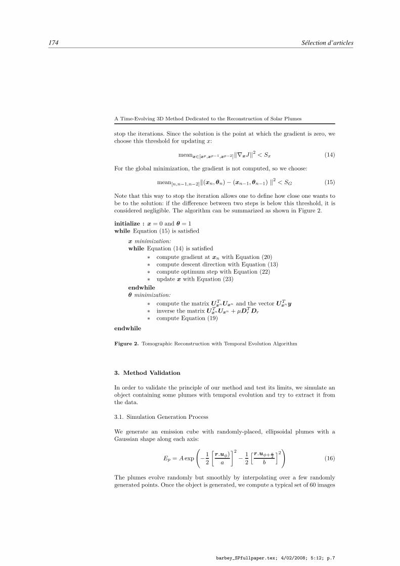
174 Sélection d’articles
A Time-Evolving 3D Method Dedicated to the Reconstruction of Solar Plumes
stop the iterations. Since the solution is the point at which the gradient is zero, wechoose this threshold for updating x:
meanx∈[xp,xp−1,xp−2]‖∇xJ‖2< Sx (14)
For the global minimization, the gradient is not computed, so we choose:
mean[n,n−1,n−2]‖(xn, θn)− (xn−1, θn−1) ‖2< SG (15)
Note that this way to stop the iteration allows one to define how close one wants tobe to the solution: if the difference between two steps is below this threshold, it isconsidered negligible. The algorithm can be summarized as shown in Figure 2.
initialize : x = 0 and θ = 1while Equation (15) is satisfied
x minimization:while Equation (14) is satisfied
∗ compute gradient at xn with Equation (20)∗ compute descent direction with Equation (13)∗ compute optimum step with Equation (22)∗ update x with Equation (23)
endwhileθ minimization:
∗ compute the matrix UTxnUxn and the vector UT
xny
∗ inverse the matrix UTxnUxn + µDT
r Dr
∗ compute Equation (19)
endwhile
Figure 2. Tomographic Reconstruction with Temporal Evolution Algorithm
3. Method Validation
In order to validate the principle of our method and test its limits, we simulate anobject containing some plumes with temporal evolution and try to extract it fromthe data.
3.1. Simulation Generation Process
We generate an emission cube with randomly-placed, ellipsoidal plumes with aGaussian shape along each axis:
Ep = A exp
(−1
2
[r.uφ)
a
]2−
1
2
[r.uφ+π2
b
]2)(16)
The plumes evolve randomly but smoothly by interpolating over a few randomlygenerated points. Once the object is generated, we compute a typical set of 60 images
barbey_SPfullpaper.tex; 4/02/2008; 5:12; p.7

A time-evolving 3D method dedicated to the reconstruction of solar plumes and results using extreme ultra-violetdata 175
N. Barbey et al.
equally spaced along 180 using our projector algorithm. A Gaussian random noiseis added to the projections with a signal to noise ratio (SNR) of five. The simulation
parameters are summarized in Table 1.
Table 1. Simulation Definition: Plumes Parameters
Plume Semimajor Semiminor φ x0 y0 IntensityNumber Axis a Axis b (A)
1 4.8 4.2 1.2 29 29 329
2 5.6 3.3 1.1 23 33 430
3 5.2 4.8 0.1 40 42 723
3.2. Results Analysis
We now compare our results (Figure 3) with a filtered back-projection (FBP) algo-
rithm. This method is explained by Natterer (1986) and Kak and Slaney (1987).By comparing the simulation and the reconstruction in Figure 3, we can see the
quality of the temporal evolution estimation. The shape of the intensity curves is well
reproduced except for the first plume in the first ten time steps where the intensity isslightly underestimated. This corresponds to a period when plume 1 is hidden behind
plume 2. Thus, our algorithm attributes part of the plume 1 intensity to plume 2.Let us note that this kind of ambiguity will not arise in the case of observations frommultiple points of view such as STEREO/EUVI observations. The indeterminacy of
the problem is due to its bilinearity discussed in Section 2.2. This allows the algorithmto attribute larger values to the θ parameters and to compensate by decreasing the
corresponding x. This is not a drawback of the method since it allows discontinuitiesbetween plumes and interplumes. The only physical value of interest is the productx g.
Figure 4 shows the relative intensity of the plumes at different times. One cancompare with the reconstruction. One way to quantify the quality of the reconstruc-tion is to compute the distance (quadratic norm of the difference) between the real
object and the reconstructed one. Since the FBP reconstruction does not actuallycorrespond to a reconstruction at one time, we evaluate the minimum of the distances
at each time. We find it to be 3000. This is to be compared with a value of 700 withour algorithm, which is much better.
Table 2. Simulation Definition: Geometric Parameters
cube size cube number pixel projection(solar radii) of voxels size (radians) number of pixels
1× 1× 0.05 64 × 64 × 4 5× 10−5 × 5× 10−5 128 × 8
barbey_SPfullpaper.tex; 4/02/2008; 5:12; p.8

176 Sélection d’articles
A Time-Evolving 3D Method Dedicated to the Reconstruction of Solar Plumes
x axis in solar radii
y ax
is in
sol
ar r
adii
−0.5 0 0.5
−0.5
0
0.5
0
100
200
300
400
x axis in solar radii
y ax
is in
sol
ar r
adii
−0.5 0 0.5
−0.5
0
0.50
100
200
300
400
500
600
700
x axis in solar radii
y ax
is in
sol
ar r
adii
−0.5 0 0.5
−0.5
0
0.5 0
50
100
150
(a) x with a FBP algorithm (b) Simulated x (c) x with our algorithm
x axis in solar radii
y ax
is in
sol
ar r
adii
−0.5 0 0.5
−0.5
0
0.52 4 6 8 10 12 14
0
0.2
0.4
0.6
0.8
1
Time in days
θ
backgroundplume 1plume 2plume 3
2 4 6 8 10 12 140.5
1
1.5
2
2.5
3
3.5
4
Time in days
θ
backgroundplume 1plume 2plume 3
(d) Chosen temporal areas (e) Simulated θ (f) θ with our algorithm
Figure 3. Comparison of a standard FBP method (a), the real simulated object (b), and theobject reconstructed with our method (c). The object is reconstructed using 60 projectionsregularly spaced over 180. The areas of homogeneous temporal evolution (e) are the same inthe simulation and the reconstruction. We associated one time per projection to define θ inthe simulation (e) and our reconstruction (f). The time scale is in days assuming a rotationspeed of half a rotation in 14 days. x is the spatial distribution of the emission density volume.θ is a gain representing the emission variation over time. Except for the FBP reconstruction,only the product x θ has physical dimensions. The spatial scales are given in solar radiiand centered on the solar axis of rotation. (a), (b) and (c) are slices of 3D cubes at the samez = 0.1R⊙. Emission densities (arbitrary units) are scaled in the color bars in the right-endside of (a), (b), (c).
x axis in solar radii
y ax
is in
sol
ar r
adii
−0.5 0 0.5
−0.5
0
0.5 0
100
200
300
400
500
x axis in solar radii
y ax
is in
sol
ar r
adii
−0.5 0 0.5
−0.5
0
0.5 0
100
200
300
400
500
x axis in solar radii
y ax
is in
sol
ar r
adii
−0.5 0 0.5
−0.5
0
0.5 0
100
200
300
400
500
(a) Simulation at 10∆T (b) Simulation at 30∆T (c) Simulation at 50∆T
x axis in solar radii
y ax
is in
sol
ar r
adii
−0.5 0 0.5
−0.5
0
0.5 0
100
200
300
400
500
x axis in solar radii
y ax
is in
sol
ar r
adii
−0.5 0 0.5
−0.5
0
0.5 0
100
200
300
400
500
x axis in solar radii
y ax
is in
sol
ar r
adii
−0.5 0 0.5
−0.5
0
0.5 0
100
200
300
400
500
(d) Result at 10∆T (e) Result at 30∆T (f) Result at 50∆T
Figure 4. Comparison of xg simulated and reconstructed at different times. ∆T is the timebetween two data images (5.6 hours). Distances are in solar radii. Values represent the volumeemission density. All of this images are slices of 3D cubes at the same z = 0.1R⊙.
barbey_SPfullpaper.tex; 4/02/2008; 5:12; p.9
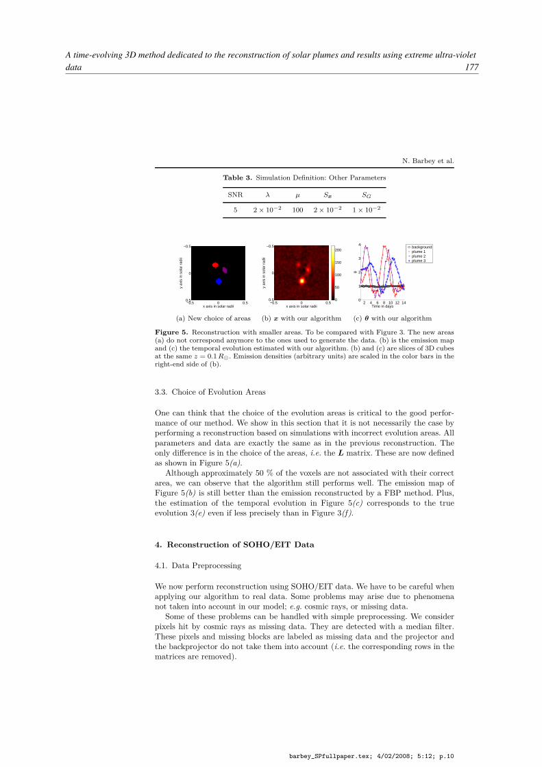
A time-evolving 3D method dedicated to the reconstruction of solar plumes and results using extreme ultra-violetdata 177
N. Barbey et al.
Table 3. Simulation Definition: Other Parameters
SNR λ µ Sx SG
5 2× 10⁻² 100 2× 10⁻² 1× 10⁻²
x axis in solar radii
y ax
is in
sol
ar r
adii
−0.5 0 0.5
−0.5
0
0.5
x axis in solar radii
y ax
is in
sol
ar r
adii
−0.5 0 0.5
−0.5
0
0.5 0
50
100
150
200
2 4 6 8 10 12 140
1
2
3
4
Time in days
θ
backgroundplume 1plume 2plume 3
(a) New choice of areas (b) x with our algorithm (c) θ with our algorithm
Figure 5. Reconstruction with smaller areas. To be compared with Figure 3. The new areas(a) do not correspond anymore to the ones used to generate the data. (b) is the emission mapand (c) the temporal evolution estimated with our algorithm. (b) and (c) are slices of 3D cubesat the same z = 0.1R⊙. Emission densities (arbitrary units) are scaled in the color bars in theright-end side of (b).
3.3. Choice of Evolution Areas
One can think that the choice of the evolution areas is critical to the good perfor-mance of our method. We show in this section that it is not necessarily the case byperforming a reconstruction based on simulations with incorrect evolution areas. Allparameters and data are exactly the same as in the previous reconstruction. Theonly difference is in the choice of the areas, i.e. the L matrix. These are now definedas shown in Figure 5(a).
Although approximately 50 % of the voxels are not associated with their correctarea, we can observe that the algorithm still performs well. The emission map ofFigure 5(b) is still better than the emission reconstructed by a FBP method. Plus,the estimation of the temporal evolution in Figure 5(c) corresponds to the trueevolution 3(e) even if less precisely than in Figure 3(f).
4. Reconstruction of SOHO/EIT Data
4.1. Data Preprocessing
We now perform reconstruction using SOHO/EIT data. We have to be careful whenapplying our algorithm to real data. Some problems may arise due to phenomenanot taken into account in our model; e.g. cosmic rays, or missing data.
Some of these problems can be handled with simple preprocessing. We considerpixels hit by cosmic rays as missing data. They are detected with a median filter.These pixels and missing blocks are labeled as missing data and the projector andthe backprojector do not take them into account (i.e. the corresponding rows in thematrices are removed).
barbey_SPfullpaper.tex; 4/02/2008; 5:12; p.10
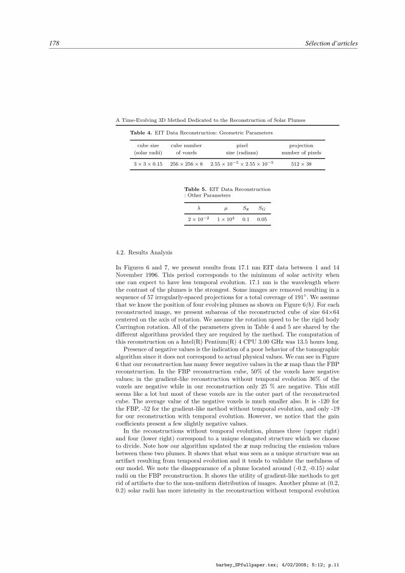
178 Sélection d’articles
A Time-Evolving 3D Method Dedicated to the Reconstruction of Solar Plumes
Table 4. EIT Data Reconstruction: Geometric Parameters
cube size cube number pixel projection(solar radii) of voxels size (radians) number of pixels
3× 3× 0.15 256 × 256 × 8 2.55× 10−5 × 2.55× 10−5 512 × 38
Table 5. EIT Data Reconstruction: Other Parameters
λ µ Sx SG
2× 10⁻² 1× 10⁴ 0.1 0.05
4.2. Results Analysis
In Figures 6 and 7, we present results from 17.1 nm EIT data between 1 and 14November 1996. This period corresponds to the minimum of solar activity whenone can expect to have less temporal evolution. 17.1 nm is the wavelength wherethe contrast of the plumes is the strongest. Some images are removed resulting in asequence of 57 irregularly-spaced projections for a total coverage of 191. We assumethat we know the position of four evolving plumes as shown on Figure 6(b). For eachreconstructed image, we present subareas of the reconstructed cube of size 64×64centered on the axis of rotation. We assume the rotation speed to be the rigid bodyCarrington rotation. All of the parameters given in Table 4 and 5 are shared by thedifferent algorithms provided they are required by the method. The computation ofthis reconstruction on a Intel(R) Pentium(R) 4 CPU 3.00 GHz was 13.5 hours long.
Presence of negative values is the indication of a poor behavior of the tomographicalgorithm since it does not correspond to actual physical values. We can see in Figure6 that our reconstruction has many fewer negative values in the x map than the FBPreconstruction. In the FBP reconstruction cube, 50% of the voxels have negativevalues; in the gradient-like reconstruction without temporal evolution 36% of thevoxels are negative while in our reconstruction only 25 % are negative. This stillseems like a lot but most of these voxels are in the outer part of the reconstructedcube. The average value of the negative voxels is much smaller also. It is -120 forthe FBP, -52 for the gradient-like method without temporal evolution, and only -19for our reconstruction with temporal evolution. However, we notice that the gaincoefficients present a few slightly negative values.
In the reconstructions without temporal evolution, plumes three (upper right)and four (lower right) correspond to a unique elongated structure which we chooseto divide. Note how our algorithm updated the x map reducing the emission valuesbetween these two plumes. It shows that what was seen as a unique structure was anartifact resulting from temporal evolution and it tends to validate the usefulness ofour model. We note the disappearance of a plume located around (-0.2, -0.15) solarradii on the FBP reconstruction. It shows the utility of gradient-like methods to getrid of artifacts due to the non-uniform distribution of images. Another plume at (0.2,0.2) solar radii has more intensity in the reconstruction without temporal evolution
barbey_SPfullpaper.tex; 4/02/2008; 5:12; p.11
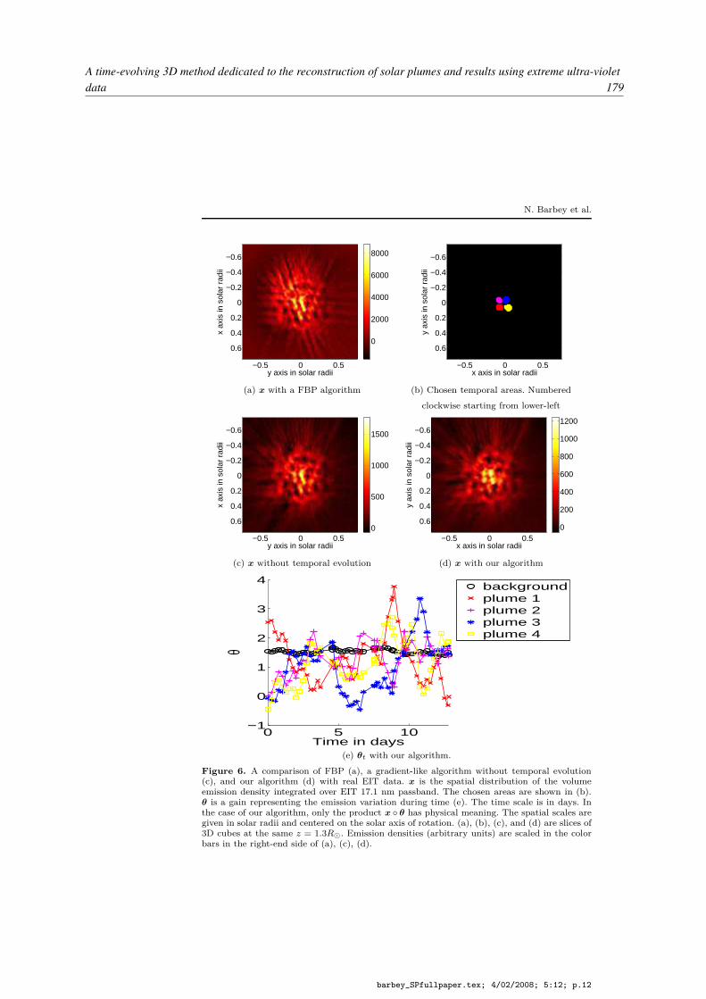
A time-evolving 3D method dedicated to the reconstruction of solar plumes and results using extreme ultra-violetdata 179
N. Barbey et al.
y axis in solar radii
x ax
is in
sol
ar r
adii
−0.5 0 0.5
−0.6
−0.4
−0.2
0
0.2
0.4
0.60
2000
4000
6000
8000
x axis in solar radii
y ax
is in
sol
ar r
adii
−0.5 0 0.5
−0.6
−0.4
−0.2
0
0.2
0.4
0.6
(a) x with a FBP algorithm (b) Chosen temporal areas. Numbered
clockwise starting from lower-left
y axis in solar radii
x ax
is in
sol
ar r
adii
−0.5 0 0.5
−0.6
−0.4
−0.2
0
0.2
0.4
0.60
500
1000
1500
x axis in solar radii
y ax
is in
sol
ar r
adii
−0.5 0 0.5
−0.6
−0.4
−0.2
0
0.2
0.4
0.60
200
400
600
800
1000
1200
(c) x without temporal evolution (d) x with our algorithm
0 5 10−1
0
1
2
3
4
Time in days
θ
backgroundplume 1plume 2plume 3plume 4
(e) θt with our algorithm.
Figure 6. A comparison of FBP (a), a gradient-like algorithm without temporal evolution(c), and our algorithm (d) with real EIT data. x is the spatial distribution of the volumeemission density integrated over EIT 17.1 nm passband. The chosen areas are shown in (b).θ is a gain representing the emission variation during time (e). The time scale is in days. Inthe case of our algorithm, only the product x θ has physical meaning. The spatial scales aregiven in solar radii and centered on the solar axis of rotation. (a), (b), (c), and (d) are slices of3D cubes at the same z = 1.3R⊙. Emission densities (arbitrary units) are scaled in the colorbars in the right-end side of (a), (c), (d).
barbey_SPfullpaper.tex; 4/02/2008; 5:12; p.12

180 Sélection d’articles
A Time-Evolving 3D Method Dedicated to the Reconstruction of Solar Plumes
x axis in solar radii
y ax
is in
sol
ar r
adii
−0.5 0 0.5
−0.6
−0.4
−0.2
0
0.2
0.4
0.6
0
500
1000
1500
2000
2500
x axis in solar radii
y ax
is in
sol
ar r
adii
−0.5 0 0.5
−0.6
−0.4
−0.2
0
0.2
0.4
0.6
0
500
1000
1500
2000
2500
x axis in solar radii
y ax
is in
sol
ar r
adii
−0.5 0 0.5
−0.6
−0.4
−0.2
0
0.2
0.4
0.6
0
500
1000
1500
2000
2500
(a) Reconstruction at t25 (b) Reconstruction at t35 (c) Reconstruction at t45
(6 days) (8.5 days) (9.8 days)
Figure 7. Reconstruction of x g at different times. Distances are in solar radii. Valuesrepresent the volume emission density integrated over the EIT 17.1 nm passband. All of theseimages are slices of 3D cubes at the same z = 1.3R⊙.
than with our algorithm. It illustrates how temporal evolution can influence thespatial reconstruction.
5. Discussion
The major feature of our approach is the quality of our reconstruction, which ismuch improved with respect to FBP reconstruction, as demonstrated by the smallernumber of negative values and the increased closeness to the data. Let us now discussthe various assumptions that have been made through the different steps of themethod.
The strongest assumption we made, in order to estimate the temporal evolution ofpolar plumes, is the knowledge of the plume position. Here, we choose to define theplumes as being the brightest points in a reconstruction without temporal evolution.The choice is not based on any kind of automatic threshold. The areas are entirelyhand-chosen by looking at a reconstruction. It is possible that these areas do notcorrespond to the actual physical plumes, they could correspond to areas presentingincreased emission during half a rotation. Note that this is biased in favor of plumescloser to the axis of rotation since, along one slice of the reconstructed cartesiancube, their altitude is lower and thus, their intensity is higher. In order to haveconstant altitude maps one would have to carry out the computation on a sphericalgrid or to interpolate afterwards onto such a grid. For this reconstruction examplewe are aware that we did not locate all of the plumes but only tried to find a few. Itwould be interesting to try to locate the plumes using other data or with a methodestimating their positions and shapes.
The method involves hyperparameters which we choose to set manually. Thereare methods to estimate hyperparameters automatically such as the L-curve method,the cross-validation method (Golub, Heath, and Wahba, 1979) or the full-bayesianmethod (Higdon et al., 1997; Champagnat, Goussard, and Idier, 1996). We per-formed reconstructions using different hyperparameter values. We then looked atthe reconstruction to see if the smoothness seemed exaggerated or if the noise wereamplified in the results. This allowed us to reduce the computational cost and doesnot really put the validity of the method into question.
One possible issue with this algorithm is the non-convexity of our criterion. Thiscan lead to the convergence to a local minimum that does not correspond to the
barbey_SPfullpaper.tex; 4/02/2008; 5:12; p.13

A time-evolving 3D method dedicated to the reconstruction of solar plumes and results using extreme ultra-violetdata 181
N. Barbey et al.
desired solution defined as the global minimum of the criterion. One way to test thiswould be to change the initialization many times.
We chose the speed of rotation of the poles to be the Carrington rotation speed.But the speed of the polar structures has not been measured precisely to our knowl-edge and could affect drastically the reconstruction. This is an issue shared by alltomographic reconstructions of the Sun.
In the current approach, we need to choose on our own the position of the time-evolving areas which are assumed to be plumes. This is done by assuming that moreintense areas of a reconstruction without temporal evolution correspond to plumepositions. A more rigorous way would be to try to use other sources of information totry to localize the plumes. Another, self-consistent way, would be to develop a methodthat jointly estimates the position of the plumes in addition to the emission (x) andthe time evolution (θ). We could try to use the results of Yu and Fessler (2002)who propose an original approach in order to reconstruct a piece-wise homogeneousobject while preserving edges. The minimization is alternated between an intensitymap and boundary curves. The estimation of the boundary curves is made usinglevel sets technics ((Yu and Fessler, 2002) and references therein). It would also bepossible to use a Gaussian mixture model (Snoussi and Mohammad-Djafari, 2007).
6. Conclusion
We have described a method that takes into account the temporal evolution of polarplumes for tomographic reconstruction near the solar poles. A simple reconstructionbased on simulations demonstrates the feasibility of the method and its efficiency inestimating the temporal evolution assuming that parameters such as plume positionor rotation speed are known. Finally we show that it is possible to estimate thetemporal evolution of the polar plumes with real data.
In this study we limited ourselves to reconstruction of images at 17.1 nm butone can perform reconstructions at 19.5 nm and 28.4 nm as well. It would allow usto estimate the temperatures of the electrons as in Frazin, Kamalabadi, and Weber(2005) or Barbey et al. (2006).
Acknowledgements Nicolas Barbey acknowledges the support of the Centre Nationald’Études Spatiales and the Collecte Localisation Satellites. The authors thank the referee fortheir useful suggestions for the article.
Appendix
A. Pseudo-Inverse Minimization
We want to minimize:
J = ‖y −Uxnθ‖2 + λ‖Drxn‖2 + µ‖Dtθ‖
2 (17)
The second term does not depend on θ. Due to the strict convexity of the crite-rion, the solution is a zero of the gradient. Since the criterion is quadratic, one canexplicitly determine the solution:
∇θJ |θ=θn+1 = 2UTxn
(Uxnθ
n+1 − y
)+ 2µDT
t Dtθn+1 = 0 (18)
barbey_SPfullpaper.tex; 4/02/2008; 5:12; p.14

182 Sélection d’articles
A Time-Evolving 3D Method Dedicated to the Reconstruction of Solar Plumes
from which we conclude:
θn+1 =
[U
TxnUxn + µD
Tt Dt
]−1
UTxny (19)
B. Gradient-like Method
In this method we try to find an approximation of the minimum by decreasing thecriterion iteratively. The problem is divided in two subproblems: searching for thedirection and searching for the step of the descent. In gradient-like methods, theconvergence is generally guaranteed ultimately to a local minimum. But since thecriterion is convex, the minimum is global. To iterate, we start at an arbitrary point(x0) and go along a direction related to the gradient. The gradient at the pth stepis:
∇xJ |x=xp = 2V Tθn+1 (Vθn+1x
p − y) + 2λDTr Drx
p (20)
Once the direction is chosen, searching for the optimum step is a linear minimizationproblem of one variable:
ap+1OPT = argmin
aJ(xp + ad
p+1) (21)
which is solved by:
ap+1OPT = −
1
2
dp+1 ∇xJ |x=xp
‖Vθn+1dp+1‖2 + λ‖Drdp+1‖2(22)
We can write the iteration:
xp+1 = x
p + ap+1OPTd
p+1 (23)
References
Barbey, N., Auchére, F., Rodet, T., Bocchialini, K., Vial, J.C.: 2006, Rotational Tomog-raphy of the Solar Corona-Calculation of the Electron Density and Temperature. In:Lacoste, H. (ed.) SOHO 17 - 10 Years of SOHO and Beyond. ESA Special Publications.ESA Publications Division, Noordwijk, 66 – 68.
Barbey, N., Auchère, F., Rodet, T., Vial, .J.C.: 2007, Reconstruction Tomographique deSéquences d’Images 3D - Application aux Données SOHO/STEREO. In: Actes de GRETSI
2007., 709 – 712.Champagnat, F., Goussard, Y., Idier, J.: 1996, Unsupervised deconvolution of sparse spike
trains using stochastic approximation. IEEE Transactions on Signal Processing 44(12),2988 – 2998.
DeForest, C.E., Lamy, P.L., Llebaria, A.: 2001, Solar Polar Plume Lifetime and Coronal HoleExpansion: Determination from Long-Term Observations. Astrophys. J. 560, 490 – 498.
Demoment, G.: 1989, Image reconstruction and restoration: Overview of common estimationstructure and problems. IEEE Transactions on Acoustics, Speech and Signal Processing
37(12), 2024 – 2036.Féron, O., Duchêne, B., Mohammad-Djafari, A.: 2005, Microwave imaging of inhomogeneous
objects made of a finite number of dielectric and conductive materials from experimentaldata. Inverse Problems 21(6), S95 – S115.
Frazin, R.A.: 2000, Tomography of the Solar Corona. I. A Robust, Regularized, PositiveEstimation Method. Astrophys. J. 530, 1026 – 1035.
barbey_SPfullpaper.tex; 4/02/2008; 5:12; p.15
A time-evolving 3D method dedicated to the reconstruction of solar plumes and results using extreme ultra-violetdata 183
N. Barbey et al.
Frazin, R.A., Butala, M.D., Kemball, A., Kamalabadi, F.: 2005, Time-dependent Recon-struction of Nonstationary Objects with Tomographic or Interferometric Measurements.Astrophys. J. 635(2), L197 – L200.
Frazin, R.A., Janzen, P.: 2002, Tomography of the Solar Corona. II. Robust, Regularized,Positive Estimation of the Three-dimensional Electron Density Distribution from LASCO-C2 Polarized White-Light Images. Astrophys. J. 570, 408 – 422.
Frazin, R.A., Kamalabadi, F.: 2005, Rotational Tomography For 3D Reconstruction Of TheWhite-Light And Euv Corona In The Post-SOHO Era. Solar Phys. 228, 219 – 237.
Frazin, R.A., Kamalabadi, F., Weber, M.A.: 2005, On the Combination of Differential EmissionMeasure Analysis and Rotational Tomography for Three-dimensional Solar EUV Imaging.Astrophys. J. 628, 1070 – 1080.
Gabriel, A.H., Abbo, L., Bely-Dubau, F., Llebaria, A., Antonucci, E.: 2005, Solar Wind Outflowin Polar Plumes from 1.05 to 2.4 Rsolar. Astrophys. J. 635, L185 – L188.
Golub, G.H., Heath, M., Wahba, G.: 1979, Generalized cross-validation as a method forchoosing a good ridge parameter. Technometrics 21(2), 215 – 223.
Grass, M., Manzke, R., Nielsen, T., KoKen, P., Proksa, R., Natanzon, M., Shechter, G.: 2003,Helical cardiac cone beam reconstruction using retrospective ECG gating. Phys. Med. Biol.48, 3069 – 3083.
Higdon, D.M., Bowsher, J.E., Johnson, V.E., Turkington, T.G., Gilland, D.R., Jaszczak, R.J.:1997, Fully Bayesian estimation of Gibbs hyperparameters for emission computed tomog-raphy data. IEEE Transactions on Medical Imaging 16(5), 516 – 526.
Kachelriess, M., Ulzheimer, S., Kalender, W.: 2000, ECG-correlated imaging of the heart withsubsecond multislice spiral CT. IEEE Transactions on Medical Imaging 19(9), 888 – 901.
Kak, A.C., Slaney, M.: 1987, Principles of computerized tomographic imaging. IEEE Press,
New York.
Llebaria, A., Saez, F., Lamy, P.: 2002, The fractal nature of the polar plumes. In: Wilson, A.(ed.) ESA SP-508: From Solar Min to Max: Half a Solar Cycle with SOHO., 391 – 394.
Natterer, F.: 1986, The Mathematics of Computerized Tomography. John Wiley.Nocedal, J., Wright, S.J.: 2000, Numerical optimization. Series in Operations Research.
Springer Verlag, New York.Polak, E., Ribière, G.: 1969, Note sur la convergence de méthodes de directions conjuguées.
Rev. Française d’Informatique Rech. Opérationnelle 16, 35 – 43.Ritchie, C.J., Crawford, C.R., Godwin, J.D., King, K.F., Kim, Y.: 1996, Correction of com-
puted tomography motion artifacts using pixel-specific backprojection. IEEE Med. Imag.
15(3), 333 – 342.Roux, S., Debat, L., Koenig, A., Grangeat, P.: 2004, Exact reconstruction in 2d dynamic CT:
compensation of time-dependent affine deformations. Phys. Med. Biol. 49(11), 2169 – 2182.Siddon, R.L.: 1985, Fast calculation of the exact radiological path for a three-dimensional CT
array. Medical Physics 12, 252 – 255.Snoussi, H., Mohammad-Djafari, A.: 2007, Estimation of structured Gaussian mixtures: the
inverse EM algorithm. IEEE Trans. on Signal Processing 55(7), 3185 – 3191.Teriaca, L., Poletto, G., Romoli, M., Biesecker, D.A.: 2003, The Nascent Solar Wind: Origin
and Acceleration. Astrophys. J. 588, 566 – 577.Wiegelmann, T., Inhester, B.: 2003, Magnetic modeling and tomography: First steps towards
a consistent reconstruction of the solar corona. Solar Physics 214, 287 – 312.Yu, D., Fessler, J.: 2002, Edge-preserving tomographic reconstruction with nonlocal regular-
ization. IEEE Med. Imag. 21, 159 – 173.
barbey_SPfullpaper.tex; 4/02/2008; 5:12; p.16

184 Sélection d’articles
T. Rodet, F. Noo et M. Defrise, « The cone–beam algorithm of Feldkamp, Davis, and Kress preservesoblique line integral », Medical Physics, vol. 31, n˚7, pp. 1972–1975, juillet 2004.

The cone–beam algorithm of Feldkamp, Davis, and Kress preserves oblique line integral 185

186 Sélection d’articles
The cone-beam algorithm of Feldkamp, Davis, and Kress preserves obliqueline integrals
Thomas RodetDepartment of Nuclear Medicine, Vrije Universiteit Brussel,AZ-VUB, B-1090 Brussels, Belgium
Frederic NooDepartment of Radiology, University of Utah, Salt Lake City, Utah 84112
Michel Defrisea)
Department of Nuclear Medicine, Vrije Universiteit, Brussel, AZ-VUB, B-1090 Brussels, Belgium
~Received 2 January 2004; revised 23 March 2004; accepted for publication 20 April 2004;published 17 June 2004!
The algorithm of Feldkamp, Davis, and Kress@J. Opt. Soc. Am. A1, 612–619~1984!# is a widelyused filtered-backprojection algorithm for three-dimensional image reconstruction from cone-beam~CB! projections measured with a circular orbit of the x-ray source. A well-known property of thisapproximate algorithm is that the integral of the reconstructed image along anyaxial line orthogo-nal to the plane of the orbit is exact when the cone-beam projections are not truncated. We gener-alize this result to oblique line integrals, thus providing an efficient method to compute syntheticradiographs from cone-beam projections. Our generalized result is obtained by showing that theFDK algorithm is invariant under transformations that map oblique lines onto axial lines. ©2004American Association of Physicists in Medicine. @DOI: 10.1118/1.1759828#
I. INTRODUCTION
The algorithm of Feldkamp, Davis, and Kress~FDK1! wasintroduced in 1984 to reconstruct cone-beam~CB! projec-tions measured with a circular orbit of the x-ray sourcearound the object. Despite considerable progress in thetheory of CB reconstruction~see, e.g., Ref. 2!, and despite itsapproximate character, the FDK algorithm is still widelyused, either in its original form, or in various extensionsdeveloped for improved accuracy3 or for helical cone-beamCT.4–6 Applications include cardiac CT, small animal imag-ing, or radiotherapy. This lasting popularity stems from thesimplicity and ease of implementation of the algorithm andfrom its good robustness to the CB artefacts caused by theincompleteness of the circular orbit.7,8 The good accuracy ofthe FDK algorithm is often related to three well-known prop-erties, which were derived in the original paper.1
~1! The reconstruction is exact in the plane of the circularorbit of the x-ray source.
~2! The reconstruction is exact for any object which is in-variant for translations in theaxial direction orthogonalto the plane of the orbit.
~3! The integral of the reconstructed image along anyaxialline orthogonal to the plane of the orbit is exact, i.e., thevalue of that integral coincides with the value of thecorresponding line integral of the actual object.
In this paper, we generalize the latter property by showingthat the FDK reconstruction also preserves the value of inte-grals alongoblique lines that are not orthogonal to the circu-lar orbit plane. This result provides additional insight into theaccuracy of the FDK reconstructions and of synthetic projec-tions@such as Digitally Reconstructed Radiographs~DRR! inradiotherapy# which can be calculated from these reconstruc-tions. Although this property has never, to our knowledge,
been mentioned, the very possibility of calculating obliqueline integrals from circular CB data has previously beendemonstrated by Chen, Patch, and Trofimov. Chen9 recon-structs an oblique line integral by integrating the ramp fil-tered three-dimensional~3D! radon transform for all planescontaining the line. The ramp filtered 3-D radon transformcan be calculated for a given plane using any CB projectionmeasured for a vertex located in the plane, by using Smith’sintermediate function.12 In Patch,10 CB projections are syn-thetized for any vertex located within the disk defined by thecircular orbit. The computation is achieved by solving John’sequation for the three-dimensional x-ray transform, using themeasured projections as boundary values. In Trofimov,11 atheorem supporting the results in Patch, Chen, and this paperwas given without the specification of an algorithm for theeffective computation of line integrals. In this paper we showthat the FDK algorithm allows the computation of obliqueline integrals. After introducing the FDK algorithm in Sec.II, we demonstrate in Sec. III the invariance of this algorithmfor some affine transformation. This serves in Sec. IV toprove the preservation of oblique line integrals when twoconditions are satisfied.
~i! The cone-beam projections are not truncated;~ii ! the angle between the line and the axial direction does
not exceed a maximum value that will be specified inSec. IV.
II. THE FDK ALGORITHM
We consider the reconstruction of a smooth functionffrom CB projections measured for cone vertices on a cen-tered circle in the planez50. To locate points in the field-of-view, vector notationsrW5x1W x1y1W y will be used for thetransaxial components, while the axial coordinatez will be
1972 1972Med. Phys. 31 „7…, July 2004 0094-2405 Õ2004Õ31„7…Õ1972Õ4Õ$22.00 © 2004 Am. Assoc. Phys. Med.

The cone–beam algorithm of Feldkamp, Davis, and Kress preserves oblique line integral 187
written separately. Thus, we write the density function asf (rW,z), and throughout the paperrW will denote a vector or-thogonal to the axis 1W
z of the scan.We assume that the functionf is smooth and vanishes
outside the cylinder,
V f5$~rW,z!PR3u irWi<RFOV , uzu<HFOV%. ~1!
The position of the cone vertex is
aW ~l !5R1W w~l !, lP@0,2p !, ~2!
wherel is the angle describing the rotation of the cone ver-tex, R.RFOV is the radius of the orbit, and
1W w~l !5cosl 1W x1sinl 1W y ~3!
is a unit vector pointing from the origin of the coordinatesystem towards the cone vertex.
We consider a flat area detector which rotates with thecone vertex. At angular positionl, the detector is parallel tothe z-axis and to the vectoraW 8(l) tangent to the circle. Tosimplify the derivations, we assume that the distance fromaW (l) to the detector isR, i.e., the detector contains the ro-tation axis 1W z . Detector pixels are located with Cartesiancoordinatesu and v measured along two orthogonal unitvectors in the planeD~l! containing the flat area detector:
1W u~l !52sinl 1W x1cosl 1W y , 1Wv51W z . ~4!
Thus, u is the transaxial coordinate~‘‘detector element’’!whereasv is the axial coordinate~‘‘detector row’’!. The ori-gin (u,v)5(0,0) is at the orthogonal projection ofaW (l) ontoD~l!.
The CB projection for vertex positionl is the set of lineintegralsgmeas(u,v,l) connectingaW (l) to points (u,v) inD~l!. Throughout the paper, we use modified datag(l,u,v)obtained by applying the usual FDK weight to the measureddata:
g~l,u,v !5
1
AR21u2
1v2
gmeas~l,u,v !
5E0
`
dl f „XW ~l,u,l !,lv…, ~5!
with (u,v)P@2uD ,uD#3@2vD ,vD# and
XW ~l,u,l !5~12 l !R1W w~l !1 lu1W u~l !. ~6!
In practice the limits of the integral overl in Eq. ~5! are ofcourse finite, and are determined by the radius of the FOV.We assume below that the projections are not truncated, i.e.,the shadow of the cylindrical FOV is always containedwithin the detector. This requires
uD>umax5RRFOV
AR22RFOV
2, vD>vmax5
RHFOV
R2RFOV. ~7!
The FDK algorithm1 is an empirical 3-D extension of thestandard 2-D fan-beam filtered-backprojection algorithm.13
The reconstructed image is given by a CB backprojection:
f FDK~rW,z!5
1
2E
0
2p
dlR3
„R2rW•1W w~l !…2gF~l,U,V!,
irWi,R, ~8!
where
U5U~rW,l !5
RrW•1W u~l !
R2rW•1W w~l !,
~9!
V5V~rW,z,l !5
Rz
R2rW•1W w~l !,
are such that the ray defined byl, U, V contains the point(rW,z). The filtered projections are given by
gF~l,u,v !5E2umax
umaxdu8hR~u2u8!g~l,u8,v !. ~10!
This is a 1-D convolution of each detector rowv5const withthe kernelhR(u) of the ramp filter~the inverse 1-D Fouriertransform ofunu!.
The FDK reconstruction is defined only forirWi,R be-cause the magnification weight in Eq.~8! is singular whenrW5aW (l) for somel. In addition,f FDK(rW,z) vanishes outsidea volumeVFDK limited by two conical surfaces:
f FDK~rW,z!50 when ~rW,z!¹VFDKªH ~rW,z!u irWi,R
and uzu,vmaxS 11
irWi
R D J . ~11!
This property is verified by noting that the filtering in Eq.~10! is done row by row, and thatuV(rW,z,l)u>Ruzu/(R1irWi).
Feldkampet al.1 showed that their algorithm preservesthe value of axial line integrals when the CB projections arenot [email protected]., when Eq.~7! is satisfied#. Specifically,they showed that for anyrW0 with irW0i,R,
E(rW0 ,z)PVFDK
dz fFDK~rW0 ,z!5E2HFOV
HFOVdz f~rW0 ,z!. ~12!
On the left hand side of this equation, the FDK reconstruc-tion must be integrated over the whole supportVFDK , i.e.,over the range
2vmaxS 11
irW0i
R D<z<vmaxS 11
irW0i
R D . ~13!
Thus, in order to use Eq.~12!, the computation of the FDKreconstruction must not be restricted to the cylindrical sup-port V f of the object, but must include all ‘‘artifacts.’’
1973 Rodet, Noo, and Defrise: The FDK algorithm preserves oblique line integrals 1973
Medical Physics, Vol. 31, No. 7, July 2004
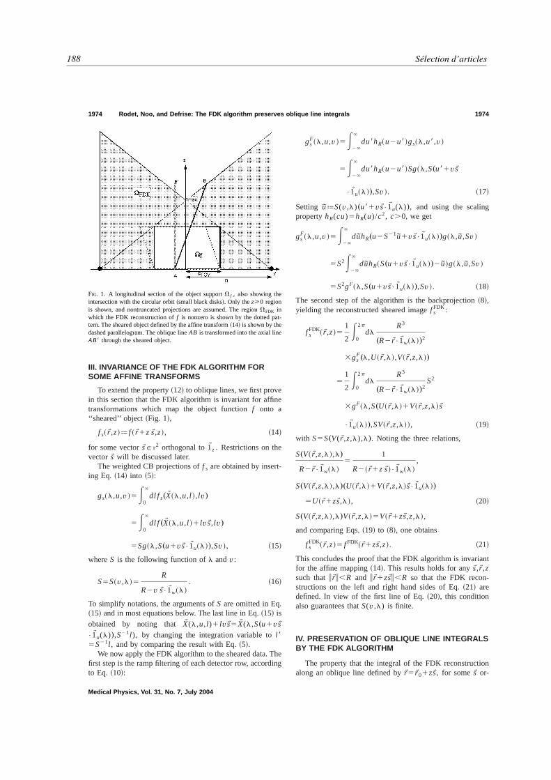
188 Sélection d’articles
III. INVARIANCE OF THE FDK ALGORITHM FORSOME AFFINE TRANSFORMS
To extend the property~12! to oblique lines, we first provein this section that the FDK algorithm is invariant for affinetransformations which map the object functionf onto a‘‘sheared’’ object~Fig. 1!,
f s~rW,z!ª f ~rW1z sW,z!, ~14!
for some vectorsWPr2 orthogonal to 1W
z . Restrictions on thevectorsW will be discussed later.
The weighted CB projections off s are obtained by insert-ing Eq. ~14! into ~5!:
gs~l,u,v !5E0
`
dl f s„XW ~l,u,l !,lv…
5E0
`
dl f „XW ~l,u,l !1 lvsW,lv…
5Sg~l,S„u1vsW•1W u~l !…,Sv !, ~15!
whereS is the following function ofl andv:
S5S~v,l !5
R
R2v sW•1W w~l !. ~16!
To simplify notations, the arguments ofS are omitted in Eq.~15! and in most equations below. The last line in Eq.~15! isobtained by noting thatXW (l,u,l )1 lvsW5XW (l,S„u1vsW
•1W u(l)…,S21l ), by changing the integration variable tol 85S21l , and by comparing the result with Eq.~5!.
We now apply the FDK algorithm to the sheared data. Thefirst step is the ramp filtering of each detector row, accordingto Eq. ~10!:
gsF~l,u,v !5E
2`
`
du8hR~u2u8!gs~l,u8,v !
5E2`
`
du8hR~u2u8!Sg~l,S„u81vsW
•1W u~l !…,Sv !. ~17!
Setting uªS(v,l)„u81vsW•1W u(l)…, and using the scalingpropertyhR(cu)5hR(u)/c2, c.0, we get
gsF~l,u,v !5E
2`
`
duhR„u2S21u1vsW•1W u~l !…g~l,u,Sv !
5S2E2`
`
duhR~S„u1vsW•1W u~l !…2u!g~l,u,Sv !
5S2gF~l,S„u1vsW•1W u~l !…,Sv !. ~18!
The second step of the algorithm is the backprojection~8!,yielding the reconstructed sheared imagef s
FDK :
f sFDK
~rW,z!5
1
2E
0
2p
dlR3
„R2rW•1W w~l !…2
3gsF„l,U~rW,l !,V~rW,z,l !…
5
1
2E
0
2p
dlR3
„R2rW•1W w~l !…2S2
3gF~l,S„U~rW,l !1V~rW,z,l !sW
•1W u~l !…,SV~rW,z,l !!, ~19!
with S5S„V(rW,z,l),l…. Noting the three relations,
S„V~rW,z,l !,l…
R2rW•1W w~l !5
1
R2~rW1z sW !•1W w~l !,
S„V~rW,z,l !,l…„U~rW,l !1V~rW,z,l !sW•1W u~l !…
5U~rW1zsW,l !, ~20!
S„V~rW,z,l !,l…V~rW,z,l !5V~rW1zsW,z,l !,
and comparing Eqs.~19! to ~8!, one obtains
f sFDK
~rW,z!5 f FDK~rW1zsW,z!. ~21!
This concludes the proof that the FDK algorithm is invariantfor the affine mapping~14!. This results holds for anysW,rW,zsuch thatirWi,R and irW1zsWi,R so that the FDK recon-structions on the left and right hand sides of Eq.~21! aredefined. In view of the first line of Eq.~20!, this conditionalso guarantees thatS(v,l) is finite.
IV. PRESERVATION OF OBLIQUE LINE INTEGRALSBY THE FDK ALGORITHM
The property that the integral of the FDK reconstructionalong an oblique line defined byrW5rW01zsW, for somesW or-
FIG. 1. A longitudinal section of the object supportV f , also showing theintersection with the circular orbit~small black disks!. Only thez>0 regionis shown, and nontruncated projections are assumed. The regionVFDK inwhich the FDK reconstruction off is nonzero is shown by the dotted pat-tern. The sheared object defined by the affine transform~14! is shown by thedashed parallelogram. The oblique lineAB is transformed into the axial lineAB8 through the sheared object.
1974 Rodet, Noo, and Defrise: The FDK algorithm preserves oblique line integrals 1974
Medical Physics, Vol. 31, No. 7, July 2004
The cone–beam algorithm of Feldkamp, Davis, and Kress preserves oblique line integral 189
thognal to 1W z , is exact is a direct consequence of the invari-ance property derived in the previous section. Indeed, we canwrite
E2`
`
dz fFDK~rW01zsW,z!5E2`
`
dz fsFDK
~rW0 ,z!
5E2`
`
dz fs~rW0 ,z!
5E2`
`
dz f~rW01zsW,z!, ~22!
where the first equality uses Eq.~21!. The second equalityfollows from the fact thatf s
FDK is obtained by applying theFDK algorithm to the CB projections off s , and from thepreservation of axial line integrals by this algorithm. The lastequality is obtained using the definition of the mapping~14!.
Let us now discuss the conditions of validity of our mainresult. Equation~22! assumes that the relation~21! holds forall points of the oblique line for whichf FDK(rW,z)Þ0. Thiscondition requires that the intersections of the oblique linewith the boundaries of the supportVFDK of f FDK(rW,z) areboth on the lower or upper conical surface@see Eq.~11!#, andnot on the lateral surface of the cylinder of radiusR, wheref FDK is not defined. Hence the intersections of the obliqueline of parametric equation (rW01zsW,z) with the cylinder ofradius R must both be located atuzu.2vmax. One easilychecks that this condition is satisfied whenirW0i,R and
2isWivmax,AR22irW0i2
1
~rW0•sW !2
isWi2 2
urW0•sWu
isWi. ~23!
Equation ~23! also implies that the support of the shearedobject f s(rW,z) is contained within the cylinder of radiusR,thus guaranteeing thatf s
FDK(rW,z) is well-defined. To verifythis statement, note that
f s~rW,z!Þ0→~rW1zsW,z!PV f→uzu<HFOV
and
irW1zsWi<RFOV . ~24!
Therefore,
f s~rW,z!Þ0→irWi25irW1zsWi2
1isWi2z222zsW•~rW1zsW !
<RFOV2
1S R2RFOV
2HFOVD 2
HFOV2
12R2RFOV
2HFOVHFOVRFOV
5
~R1RFOV!2
4,R2, ~25!
where we have used the fact that condition~23!, with vmax
from Eq. ~7!, implies isWi,R/(2vmax)5(R2RFOV)/(2HFOV). We finally conclude that Eq.~23! is asufficient condition of validity for Eq.~22!.
V. CONCLUSION
We have shown that the filtered-backprojection algorithmof Feldkamp, Davis, and Kress for circular cone-beam recon-struction preserves the values of oblique line integrals,thereby generalizing the well-known property that axial lineintegrals are preserved. This property provides new insightinto the accuracy of this widely used algorithm, and it alsosuggests an efficient way of calculating synthetic radiographsfrom CB data. The property only holds when the CB projec-tions are not truncated and it requires an additional conditionon the angle between the line and the axial direction. Itspractical significance, therefore, mainly concerns the imag-ing of small animals and of isolated tissue samples, whichcan be put on blocks of material with very low attenuation tomeet the hypothesis of nontruncation.
a!Electronic mail: [email protected]. A. Feldkamp, L. C. Davis, and J. W. Kress, ‘‘Practical cone-beamalgorithm,’’ J. Opt. Soc. Am. A1, 612–619~1984!.
2A. Katsevich, ‘‘Improved exact FBP algorithm for spiral CT,’’ Adv. Appl.Math. ~submitted!; also see ‘‘Analysis of an exact inversion algorithm forspiral cone-beam CT,’’ Phys. Med. Biol.47, 2583–2597~2002!.
3M. Grass, T. Ko¨hler, and R. Proksa, ‘‘3D cone-beam CT reconstructionfor circular trajectories,’’ Phys. Med. Biol.45, 329–348~2000!.
4H. Kudo and T. Saito, ‘‘Helical-scan computed tomography using cone-beam projections,’’Conference Record of the 1991 IEEE MedicalImag-ing Conference, Santa Fe, NM, 1992, pp. 1958–1962.
5G. Wang, T. H. Lin, P. Cheng, and D. M. Shinozaki, ‘‘A general cone-beam reconstruction algorithm,’’ IEEE Trans. Med. ImagingMI-12 ,486–496~1993!.
6X. Yan and R. M. Leahy, ‘‘Cone-beam tomography with circular, ellipti-cal and spiral orbits,’’ Phys. Med. Biol.37, 493–506~1992!.
7H. Tuy, ‘‘An inversion formula for cone-beam reconstruction,’’ SIAM~Soc. Ind. Appl. Math.! J. Appl. Math.43, 546–552~1983!.
8P. Grangeat, ‘‘Mathematical framework of cone-beam 3D reconstructionvia the first derivative of the Radon transform,’’Mathematical Methods inTomography, Lecture Notes in Mathematics, edited by G. T. Herman, A.K. Louis, and F. Natterer~Springer-Verlag, Berlin, 1991!, Vol. 1497, pp.66–97.
9J. Chen, ‘‘A theoretical framework of regional cone-beam tomography,’’IEEE Trans. Med. ImagingMI-11 , 342–351~1992!.
10S. K. Patch, ‘‘Consistency conditions upon 3D CT data and the waveequation,’’ Phys. Med. Biol.47, 2637–2650~2002!.
11O. E. Trofimov, ‘‘Virtual beam~x-ray! projections,’’Proceedings of the2003 International Conference on Fully 3D Reconstruction in Radiologyand Nuclear Medicine, Saint-Malo, France, edited by Y. Bizais, 2003.
12B. D. Smith, ‘‘Image reconstruction from cone-beam projections—Necessary and sufficient conditions and reconstruction methods,’’ IEEETrans. Med. ImagingMI-4 , 14–25~1985!.
13F. Natterer,The Mathematics of Computerized Tomography ~Wiley, NewYork, 1986!.
1975 Rodet, Noo, and Defrise: The FDK algorithm preserves oblique line integrals 1975
Medical Physics, Vol. 31, No. 7, July 2004

190 Sélection d’articles
H. Kudo, T. Rodet, F. Noo et M. Defrise, « Exact and approximate algorithms for helical cone-beamCT », Physics in Medicine and Biology, vol. 49, n˚13, pp. 2913–2931, juillet 2004.

Exact and approximate algorithms for helical cone-beam CT 191

192 Sélection d’articles
Exact and approximate algorithms for helical cone-beam CT
Hiroyuki Kudo1, Thomas Rodet2, Frederic Noo3, Michel Defrise2
1 Dept. of Computer Science, Graduate School of Systems and Information Engineering,
University of Tsukuba, Japan2Dept. of Nuclear Medicine, Vrije Universiteit Brussel, AZ-VUB, B-1090 Brussels, Belgium
3 Dept. of Radiology, University of Utah, Salt-Lake City, Utah.
April 27, 2004
Abstract
This paper concerns image reconstruction for helical x-ray transmission tomography (CT) with multi-
row detectors. We introduce two approximate cone-beam (CB) filtered-backprojection (FBP) algo-
rithms of the Feldkamp type, obtained by extending to three dimensions (3D) two recently proposed
exact FBP algorithms for 2D fan-beam reconstruction. The new algorithms are similar to the stan-
dard Feldkamp-type FBP for helical CT. In particular, they can reconstruct each transaxial slice
from data acquired along an arbitrary segment of helix, thereby efficiently exploiting the available
data. In contrast with the standard Feldkamp-type algorithm, however, the redundancy weight is
applied after filtering, allowing a more efficient numerical implementation. To partially alleviate the
CB artefacts, which increase with increasing values of the helical pitch, a frequency-mixing method
is proposed. This method reconstructs the high frequency components of the image using the longest
possible segment of helix, whereas the low frequencies are reconstructed using a minimal, short-scan,
segment of helix to minimize CB artefacts. The performance of the algorithms is illustrated using
simulated data.
1 Introduction
This paper concerns the image reconstruction problem for helical x-ray transmission tomog-raphy (CT) with multi-row detectors. An exact solution to this problem has been recentlyintroduced by Katsevich (2002, 2002a, 2003) and leads to an efficient filtered-backprojection(FBP) algorithm for the reconstruction of a 3D function from axially truncated cone-beam(CB) projections acquired with a helical path of the x-ray source relative to the patient. Inthis algorithm, the CB projections are first differentiated with respect to the helical pathlength; a 1D Hilbert filter is then applied along one or several families of straight lines inthe detector, and the filtered CB projections are finally backprojected as in the well-knownalgorithm of Feldkamp, Davis and Kress (1984).
1

Exact and approximate algorithms for helical cone-beam CT 193
One of the key points in the derivation of Katsevich’s algorithm is the definition offamilies of filtering lines that guarantee exact reconstruction, allow the handling of axiallytruncated projections, and efficiently use the available detector area to optimize the signal-to-noise ratio (SNR). To date, families of filtering lines that yield exact reconstruction have beendefined only for two specific cases, referred to here for convenience as the PI-reconstructionand the 3 PI-reconstruction. With the PI-reconstruction, each point in the image volumeis reconstructed using the segment of helix bounded by the PI-line of the point1. This isthe smallest helix segment compatible with exact reconstruction, and therefore, when thedetector size is fixed, the PI-reconstruction allows to maximize the helical pitch. The 3 PI-reconstruction reconstructs each point P from a longer segment of helix bounded by a linecontaining P and two points of the helix with an axial separation comprised between oneand two times the pitch. As with the PI reconstruction, however, the 3 PI-reconstructionmakes efficient use of the available detector area only for a well defined value of the helicalpitch.
Thus being restricted to these two specific cases, the exact algorithms known to datedo not allow optimal data utilization with arbitrary values of the helical pitch, for a fixedsize of the detector. This motivates continuing research on approximate algorithms that canmore easily be adapted to general configurations. Two approaches have been proposed sofar:
• Generalizations (Stierstorfer et al 2002, Tang 2003, Flohr et al 2003) of the advancedsingle slice rebinning algorithm (Larson et al 1998, Heuscher 1999, Noo et al 1999,Kachelriess et al 2000, Defrise et al 2001, 2003),
• Generalizations of the FDK algorithm (Feldkamp et al 1984) for helical data (Kudoand Saito 1992, Wang et al 1993, Yan and Leahy 1992).
The second approach will be discussed in this paper. The approximate algorithms of the FDKtype are derived by extending to 3D standard algorithms for 2D fan-beam reconstruction.Specifically, an exact 2D fan-beam inversion formula is first written for each point P =(x0, y0, z0), assuming a virtual circular orbit contained in the transaxial plane z = z0. Theray-sums required by this 2D fan-beam inversion formula are then replaced by measuredray-sums diverging from locations of the x-ray source along its circular or helical path. The2D fan-beam backprojection is thereby converted into a 3D cone-beam backprojection, whilethe ramp filtering remains the same as in the 2D case (the nature of the lines in the detectoralong which the filter is applied will be discussed below).
This strategy has been applied to circular and to helical CT, starting either from a full-scan fan-beam reconstruction (360 degree) or from a short-scan reconstruction. In the lattercase, data redundancy is handled using the weighting proposed by Parker (1982). Parker’sweighting for data redundancy, however, can be generalized to arbitrary angular ranges, upto 360 degrees (Silver 2000), and possibly exceeding 360 degrees. Extending the resulting
1The PI-line of a point P is the unique line through P that connects two points of the helix separatedaxially by less than one pitch.
2

194 Sélection d’articles
algorithms to 3D in the same way as for the standard FDK method leads to an approximateCB-CT algorithm in which each point P = (x0, y0, z0) is reconstructed from a segment ofhelix centered, axially, at z = z0. The length of the helix segment is arbitrary, provided itis larger than the short-scan segment and does not exceed the maximum size allowed by thedetector size.
Besides its approximate nature, the main drawback of the FDK type approach forhelical CB-CT is that the cone-beam projections must be filtered more than once (Kudo etal 1999). This property is due to the fact that the projections must be multiplied by Parker’sweight prior to filtering (see Parker 1982 and Wesarg et al 2002). But Parker’s weight dependson the location of the x-ray source relative to the segment of helix used for reconstruction,and since this segment is centered on the transaxial slice z0, the weight applied to a givendetector row depends on the slice z0 to which this row contributes. Therefore, each rowmust be weighted and then filtered, once for each image slice onto which it is backprojected.This added computational complexity is only avoided when the segment of helix used forreconstruction is an integer multiple of 2π since Parker’s weight is constant in that case.
In this paper, we introduce two approximate algorithms for helical CB-CT which canbe applied to arbitrary helix segments. These algorithms are obtained by extending to 3D,in the same way as above, two recently discovered 2D fan-beam reconstruction algorithms(Noo et al 2002, Kudo et al 2002) based on a relation between fan-beam projections andparallel-beam projections (Hamaker et al 1980). The main property of these algorithms isthat the redundancy weight is applied after filtering. This property allows to filter eachprojection only once, hence considerably simplifying the extension to helical CT.
The paper is organized as follows. After introducing notations in section 2, the twofan-beam FBP algorithms are described in section 3, and are then extended in section 4to helical CT. The link between the resulting approximate algorithms and exact CB-FBPmethods is discussed in section 5, allowing a characterization of the approximation in terms ofthe 3D Radon transform. The link with the exact methods will also provide some motivationfor selecting filtering lines in FDK type algorithms that are parallel to the tangent to thehelix, as originally proposed by Yan and Leahy (1992). These results naturally lead to anew algorithm, described in section 6. This algorithm reconstructs the low- and the high-frequency components of the object using respectively a short and a longer helix segment;this technique efficiently exploits the available detector data while minimizing the cone-beam artefacts due to the approximate character of the FDK algorithms. Finally, in section7, results with simulated data illustrate the accuracy of the proposed methods and theirpotential to reduce image noise by using redundant CB data in an efficient way.
2 The helical CT data and the 3D x-ray transform
Figure 1 illustrates the data acquisition geometry. We use f(~r) with ~r = (x, y, z) to describethe density function to be reconstructed and assume that this function is smooth and vanishes
3

Exact and approximate algorithms for helical cone-beam CT 195
outside the cylinder
Ω =
(x, y, z) ∈ IR3∣
∣
∣ x2 + y2 ≤ R2FOV
. (1)
We will write equivalently f(~r) = f(x, y, z). Physically, Ω represents the field-of-view of thescanner.
To reconstruct f(~r), we measure CB projections for cone vertices on the helical path~a(λ) oriented along the z-axis:
~a(λ) = (R cos λ,R sinλ, hλ) (2)
where λ ∈ IR is the angle describing the rotation of the cone vertex, R > RFOV is the radiusof the helix and P = 2πh is its pitch. In CT, the cone vertex represents the position of thex-ray source relative to the object or patient.
As illustrated in figure 1, we consider a flat area detector which moves with the conevertex. At angular position λ, the detector is parallel to the z-axis and to the vector ~a′(λ) =d~a(λ)/dλ tangent to the helix. To simplify the derivations, we assume below that the distancefrom ~a(λ) to the detector is R, i.e. the detector contains the z-axis2. To locate detectorpixels in space, we introduce cartesian coordinates u and v in the plane D(λ) containing thearea detector. These coordinates are measured along two orthogonal unit vectors ~1u and ~1v
in D(λ), with ~1v parallel to the axis of the helix:
~1u(λ) = (− sinλ, cos λ, 0) ~1v(λ) = (0, 0, 1) (3)
The origin (u, v) = (0, 0) is at the orthogonal projection of ~a(λ) onto D(λ), and the measuredrange is (u, v) ∈ [−uD, uD]× [−vD, vD]. We assume that the detector is large enough to avoid
truncation along the u axis, so that uD ≥ um = RRFOV /√
R2 −R2FOV .
The CB projection for vertex position λ is the set of line integrals g(u, v, λ) whichconnect ~a(λ) to points (u, v) in D(λ):
g(λ, u, v) =√
R2 + u2 + v2
∫ l0(u)+∆l(u)
l0(u)−∆l(u)dl f
(
X(λ, u, l), Y (λ, u, l), hλ + lv)
(4)
with (u, v) ∈ [−uD, uD] × [−vD, vD] and
X(λ, u, l) = R cos λ+ l(−R cos λ− u sinλ)
Y (λ, u, l) = R sinλ+ l(−R sinλ+ u cos λ) (5)
The limits of the integral in equation (4) are determined by the intersection of the ray withthe boundary of the cylindrical field-of-view Ω:
l0(u) = R2/(R2 + u2) , ∆l(u) =√
(u2m − u2)(R2 −R2
FOV )/(R2 + u2) (6)
2Scaling all equations by substituting u → uR/D and v → vR/D is sufficient to describe the case of aplane detector located at a distance D from the vertex.
4

196 Sélection d’articles
This paper deals with the reconstruction of f(x, y, z) from the cone-beam projectionsacquired on a helix segment λ ∈ Λ(z) = [z/h − ∆Λ/2, z/h + ∆Λ/2] centered axially on theslice z and having a specified angular range ∆Λ. As outlined in the introduction, approx-imate solutions to this problem will be defined by first considering in the next section thereconstruction of a transaxial slice z = z0 from its 2D Radon transform.
3 Two-dimensional fan-beam reconstruction with redundant
data
The 2D Radon transform of a slice f(x, y)3 will be parametrized using the fan-beam samplingdefined by restricting to 2D the 3D geometry of equation (4):
g(λ, u) =√
R2 + u2
∫ l0(u)+∆l(u)
l0(u)−∆l(u)dl f
(
X(λ, u, l), Y (λ, u, l))
|u |≤ um, λ ∈ Λ (7)
These data correspond to a set of ray-sums diverging from locations of the x-ray sourcealong a segment of circle ~a2D(λ) = (R cos λ,R sinλ), λ ∈ Λ = [−∆Λ/2,+∆Λ/2]. The length
∆Λ of this segment must be such that any line crossing Ω2D =
(x, y) ∈ IR2∣
∣
∣x2 + y2 ≤R2
FOV
intersects the circle segment at least once (Natterer 1986). This 2D data sufficiency
condition is satisfied when the segment is not smaller than the short-scan segment, i.e. when∆Λ ≥ π + 2arcsin(RFOV /R). In this paper, however, we consider larger segments whichmay exceed 2π, even though this makes little sense in a 2D context. In this case, the dataare redundant and the number N(λ, u) of intersections between a ray-sum parameterized by(λ, u) and the circle segment is not constant. To account for this redundancy, one introducesa smooth normalization function w(λ, u) such that for any pair (λ ∈ Λ, u ∈ [−um, um]),
N(λ,u)∑
j=1
w(λj , uj) = 1 (8)
where ~a2D(λj), j = 1, · · · , N(λ, u) are the intersections of the ray (λ, u) with the circle seg-ment ~a2D(Λ), and uj , j = 1, · · · , N(λ, u) are the corresponding detector coordinates, sothat all rays (λj , uj), j = 1, · · · , N(λ, u) coincide. The simplest normalization function isw(λ, u) = 1/N(λ, u) but differentiable functions are prefered for better numerical stability,and are even required by some algorithms.
Starting from the standard FBP algorithm for the inversion of the Radon transformwith parallel-beam parameterization, inversion formulae for fan-beam data have been derivedby exploiting relations linking the fan-beam data g(λ, u), equation (7), to parallel-beam data
p(s, ~n) =
∫
Ω2D
d~rf(~r) δ(s − ~n · ~r) (9)
3We consider in this section a fixed slice z = 0 and drop the third argument of f .
5
Exact and approximate algorithms for helical cone-beam CT 197
with the well-known relation between the parallel-beam and fan-beam parameters
~n = (−R sinλ+ u cos λ,R cos λ+ u sinλ)/√
R2 + u2
s = Ru/√
R2 + u2 (10)
Three such 2D fan-beam inversion formulae are given below:
• FBP-1: Using the direct link p(s, ~n) = g(λ, u), one gets the standard fan-beam FBP(Parker 1982):
f(x, y) =
∫
Λdλ
R2
(R− x cos λ− y sinλ)2gF1 (λ,U(x, y, λ)) (11)
whereU(x, y, λ) = R(−x sinλ+ y cos λ)/(R − x cos λ− y sinλ) (12)
is such that the ray defined by (λ,U(x, y, λ)) contains the point (x, y). The filteredprojections are given by
gF1 (λ, u′) =
∫ um
−um
du hR(u′ − u)w(λ, u)R√
R2 + u2g(λ, u) (13)
where hR(u) is the kernel of the ramp filter, hR(u) =∫∞−∞ dν |ν| exp(2πiνu).
• FBP-2: Using the relation of Hamaker (1980) between the Hilbert transforms of p(s, ~n)and of g(λ, u), one obtains (Kudo et al 2002):
f(x, y) =
∫
Λdλ
R2
(R− x cos λ− y sinλ)2
w(λ,U) gF2R(λ,U)
+∂w(λ, u)
∂u
∣
∣
∣
u=UgF2H(λ,U)
(14)
where U = U(x, y, λ) is as in equation (12), and the two filtered fan-beam projectionsare given by
gF2R(λ, u′) =
∫ um
−um
du hR(u′ − u)R√
R2 + u2g(λ, u) (15)
gF2H(λ, u′) =
1
2π
∫ um
−um
du hH(u′ − u)R√
R2 + u2g(λ, u) (16)
where hH(u) =∫∞−∞ dν (−i) sign(ν) exp(2πiνu) is the kernel of the Hilbert transform.
• FBP-3: Finally, the derivative of Hamaker’s relation with respect to λ leads to a thirdinversion formula (Noo et al 2002):
f(x, y) =
∫
Λdλ
1
R− x cos λ− y sinλw(λ,U) gF
3 (λ,U) (17)
6

198 Sélection d’articles
where again U = U(x, y, λ), and
gF3 (λ, u′) =
1
2π
∫ um
−um
du hH(u′ − u)R√
R2 + u2
(
∂
∂λ+R2 + u2
R
∂
∂u
)
g(λ, u) (18)
Note that this last formula involves the first power of the magnification weight in thebackprojection.
Compared to standard fan-beam FBP, the last two algorithms have two importantadvantages. The first one is that the exact reconstruction of a point (x, y) requires thenormalisation condition (8) to be satisfied only for all rays containing (a neighbourhoodof) that point. Therefore, some subset of the FOV Ω2D can be reconstructed from fan-beam data acquired along a segment of circle shorter than the short-scan segment π +2arcsin(RFOV /R) (Noo et al 2002). In contrast, the standard fan-beam reconstructionFBP-1 requires measuring all rays through the object, even if only part of the FOV needsto be reconstructed. The length of the circle segment must then be at least a short-scanπ + 2arcsin(RFOV /R).
The second property of the algorithms FBP-2 and FBP-3 is that the redundancyweight w(λ, u), or its derivative, is applied after filtering the data, in contrast with thestandard fan-beam FBP of equation (13). As will be seen in the next section, this propertysimplifies the extension to helical cone-beam data.
4 Two new Feldkamp-type algorithms for helical CT
In this section we extend the 2D fan-beam FBP algorithms to reconstruct the helical cone-beam data defined by equation (4). This empirical extension follows the same approach asthat leading to the classical Feldkamp algorithms (Feldkamp et al 1984).
Each transaxial slice z is reconstructed by backprojecting the filtered cone-beam pro-jections acquired on the helix segment Λ(z) = [z/h−∆Λ/2, z/h+ ∆Λ/2] according to equa-tions (11), (14) and (17) for the three fan-beam algorithms respectively. Because we aredealing with cone-beam data g(λ, u, v) instead of fan-beam data g(λ, u), the axial detectorvariable v must be inserted into these equations. This is done by choosing v in such a waythat f(~r) is reconstructed by summing filtered ray-sums containing the point ~r.
The filtering of the fan-beam projections in equations (13), (15), (16) and (18) isextended to cone-beam projections with three modifications:
1. The weighting factors R/√R2 + u2 are replaced by R/
√R2 + u2 + v2,
2. The derivative ∂/∂λ+(R2+u2)/R ∂/∂u in equation (18) is a derivative with respect tothe parameter λ for a fixed direction of the ray. It is replaced in 3D by the correspondingderivative at fixed spatial direction, which is ∂/∂λ+ (R2 + u2)/R ∂/∂u+ (uv/R)∂/∂v,
7

Exact and approximate algorithms for helical cone-beam CT 199
3. The direction in the detector along which the ramp and Hilbert filters must be appliedis not defined unambiguously when extending empirically the algorithms to 3D. Forthe usual helical Feldkamp algorithm, the ramp filter has been applied either along the~1u axis orthogonal to the helix axis z (Kudo and Saito 1992, Wang et al 1993), or alongan axis ~1ur rotated by an angle η = arctan(h/R) with respect to the u axis (Yan andLeahy 1992):
~1ur = cos η ~1u + sin η ~1v = (− cos η sinλ, cos η cos λ, sin η) (19)
This axis ~1ur is parallel to the tangent ~a′(λ) to the helix at the vertex considered(we omit for simplicity the dependence of these unit vectors on λ). Several studies(Turbell and Danielsson 1999, Sourbelle and Kalender 2003) indicate that filteringalong ~1ur instead of ~1u significantly reduces cone-beam artefacts, and this approachwill be selected in this paper.
We are now ready to define the three Feldkamp-type algorithms:
• FDK-1 The standard FDK algorithm is the 3D extension of FBP-1:
f(~r) =
∫
Λ(z)dλ
R2
(R− x cos λ− y sinλ)2gF1 (λ,U, V ) (20)
where U = U(x, y, λ) as in the previous section and
V = V (x, y, z, λ) = R(z − hλ)/(R − x cos λ− y sinλ) (21)
is such that the ray defined by λ,U, V contains the point ~r = (x, y, z). The filteredprojections are given by,
gF1 (λ, u′, v′) =
∫ um
−um
du hR(u′ − u) gw(λ, u, v′ − (u′ − u) tan η) (22)
where gw(λ, u, v) are the cone-beam data multiplied by the usual Feldkamp’s weightand by the redundancy weight,
gw(λ, u, v) =R√
R2 + u2 + v2w(λ− z/h, u) g(λ, u, v) (23)
where w is any solution to the normalization condition (8). Note that w was defined foran angular range [−∆Λ/2,+∆Λ/2], and therefore its first argument in equation (23) isshifted by −z/h to center the angular range on the center of the helix segment Λ(z)used to reconstruct slice z. This dependence on z in equations (23) and (22) impliesthat each row in a cone-beam projection must be filtered more than once (unless∆Λ = 2π, 4π, · · ·). This drawback is avoided with the two new algorithms presentedbelow.
8
200 Sélection d’articles
• FDK-2 The first new algorithm is derived from FBP-2:
f(~r) =
∫
Λ(z)dλ
R2
(R − x cos λ− y sinλ)2× (24)
(
w(λ− z/h,U) gF2R(λ,U, V ) +
∂w(λ − z/h, u)
∂u
∣
∣
∣
u=UgF2H(λ,U, V )
)
with U = U(x, y, λ) and V = V (x, y, z, λ) as before, and the filtered projections
gF2R(λ, u′, v′) =
∫ um
−um
du hR(u′ − u) gw(λ, u, v′ − (u′ − u) tan η)
gF2H(λ, u′, v′) =
1
2π
∫ um
−um
du hH(u′ − u) gw(λ, u, v′ − (u′ − u) tan η) (25)
where gw(λ, u, v) are the cone-beam data multiplied by the usual Feldkamp weight,
gw(λ, u, v) =R√
R2 + u2 + v2g(λ, u, v) (26)
• FDK-3 The second new algorithm is derived from FBP-3:
f(~r) =
∫
Λ(z)dλ
1
R− x cos λ− y sinλw(λ− z/h,U) gF
3 (λ,U, V ) (27)
with the same U and V as above, and
gF3 (λ, u′, v′) =
1
2π
∫ um
−um
du hH(u′ − u) gw(λ, u, v′ − (u′ − u) tan η) (28)
where gw is obtained by differentiating and weighting the cone-beam projections:
gw(λ, u, v) =R√
R2 + u2 + v2
(
∂
∂λ+R2 + u2
R
∂
∂u+uv
R
∂
∂v
)
g(λ, u, v) (29)
The three algorithms above yield exact reconstruction when f(~r) = f(x, y) is indepen-dent of z. To prove this assertion, it is sufficient to note that the fan-beam data g2D(λ, u) ofany slice z = const. of a z-homogeneous 3D object are related to the cone-beam data (4) byg(λ, u, v) =
√R2 + u2 + v2 g2D(λ, u)/
√R2 + u2. Inserting this equation into the algorithms
FDK-1,2,3, one obtains4 the algorithms FBP-1,2,3 respectively, applied to the data g2D.The fact that these fan-beam algorithms are exact then proves the assertion.
4To guarantee this property, the filtering in equations (22),(25) and (28) is written with u, v′−(u′−u) tan ηinstead of u′ − (u − u′) cos η, v′ − (u′ − u) sin η. The two expressions give identical results with the Hilbertfilter, but differ by a scaling factor | cos η| with the ramp filter.
9

Exact and approximate algorithms for helical cone-beam CT 201
5 Link with the exact algorithm of Katsevich
The three algorithms in the previous section can reconstruct each slice from data acquiredalong an arbitrary segment of helix. This versatility allows the detector data to be exploitedin an efficient way without being restricted to specific configurations such as the PI- or the3 PI-windows used by the Katsevich algorithms. In contrast with the latter algorithms,however, FDK-type methods are not exact and their accuracy decreases with increasinghelical pitch or with increasing range ∆Λ. A characterization of the approximation providesinsight into the nature of the expected reconstruction artefacts. In this section, such acharacterization is obtained for the FDK-3 algorithm, using the link between this algorithmand the 3D Radon transform of f(~r).
We start from the general inversion formula of Katsevich (2002), which can be rewrittenin terms of planar detector coordinates as (see Bontus et al 2003 and the appendix in Packet al 2003):
fM (~r) =
∫
IRdλ
1
R− x cos λ− y sinλwM (λ,~r) gF (~r, λ, U, V ) (30)
with the same U and V as above, and
gF (~r, λ, u′, v′) =1
2π
∫ um
−um
du hH(u′ − u) gw(λ, u, v′ − (u′ − u) tan η(λ,~r)) (31)
with gw given by equation (29). Comparison with equations (27) and (28) shows that thisalgorithm is similar to FDK-3, with two differences:
• The segment of helix Λ(~r) used to reconstruct a point ~r is allowed to depend on x, y, zand not only on the slice z. In equation (30) this segment is defined implicitly by theweighting function wM , as Λ(~r) = λ ∈ IR | wM (λ,~r) 6= 0.
• The direction along which the Hilbert filter is applied in the detector is no longerconstant and is defined by the angle η(λ,~r)5.
As shown in (Katsevich 2003) the algorithm (30),(31) is equivalent to an inversion ofthe second derivative of the 3D Radon transform of f , in which each plane Π(~r, ~θ) containing~r and normal to a unit vector ~θ ∈ S2 is weighted by a factor M(~r, ~θ):
fM(~r) =−1
8π2
∫
S2
d~θ M(~r, ~θ)∂2Rf(~θ, ρ)
∂ρ2
∣
∣
∣
ρ=~θ·~r(32)
where S2 is the unit sphere and Rf(~θ, ρ) is the 3D Radon transform of f . The link withequation (30) is given by
M(~r, ~θ) =
N(~r,~θ)∑
j=1
wM (λj, ~r) sign(~a′(λj) · ~θ) sign(~ξ(λj , ~r) · ~θ) (33)
5Via this dependence of η on ~r, the filtered projection depends on the point ~r, hence the algorithm entailsin general repeated filtering of each cone-beam projection for each point ~r, unless η depends on ~r only throughU(x, y, λ), V (x, y, z, λ).
10

202 Sélection d’articles
where the sum is over all intersections ~a(λj), j = 1, · · · , N(~r, ~θ) of the plane Π(~r, ~θ) withthe helix segment ~a[Λ(~r)] defined by the support of wM (λ,~r) with respect to λ. The vector~ξ(~r, λ) in equation (33) is defined by
~ξ(~r, λ) = cos η(λ,~r)~1u(λ) + sin η(λ,~r)~1v(λ) (34)
For a specific choice of wM (λ,~r) and η(λ,~r), the corresponding weighting of the Radon planecan be calculated using equation (33). The algorithm provides an exact reconstruction atpoint ~r if M(~r, ~θ) = 1 for any ~θ ∈ S2. When M(~r, ~θ) 6= 1, the algorithm is approximateand the reconstruction artefacts around a point ~r can be characterized geometrically byanalysing the deviation |M(~r, ~θ) − 1| as function of the orientation ~θ of the Radon planethrough ~r. Specifically, a surface of discontinuity (or of rapid variation) of f at point ~r,which is orthogonal to some direction ~θ, will be reconstructed accurately only if M(~r, ~θ)does not significantly differ from 1.
5.1 The Katsevich algorithm for PI-reconstruction
The exact algorithm of Katsevich corresponds to the following choice for wM and ~ξ:
• Λ(~r) = [λb(~r), λt(~r)] is the PI-segment of point ~r, defined by the unique (Edholm etal 1997) pair of vertices such that λb < λt < λb + 2π and the three points ~a(λb),~a(λt)and ~r are colinear. Thus,
wM (λ,~r) =
1 λb(~r) ≤ λ ≤ λt(~r)0 otherwise
(35)
The planes Π(~r, ~θ) have either one or three intersections with Λ(~r), i.e. N(~r, ~θ) = 1 or3.
• ~ξ(~r, λ) is a vector along the intersection of the detector plane with a plane containingthe four points ~r,~a(λ),~a(λ+ s) and ~a(λ+ 2s). It can be shown that ~ξ is unique if s isrestricted to the PI-interval λb(~r) ≤ λ+ 2s ≤ λt(~r).
The algorithm defined by equations (30) and (31) with the above choice of wM and~ξ admits an efficient implementation because wM (λ,~r) and the direction of filtering η(λ,~r)depend on ~r only through the coordinates U and V of the projection of ~r onto the detector.Specifically,
wM (λ,~r) =
1 −VTam(−U) ≤ λ ≤ VTam(U)0 otherwise
(36)
with
VTam(U) = h(1 +U2
R2)(π
2− arctan
U
R) (37)
i.e. wM is equal to 1 if the projection of ~r is inside Tam’s window and zero otherwise, wherethe Tam window (Tam et al 1998) is the detector area bounded by the projection onto the
11
Exact and approximate algorithms for helical cone-beam CT 203
detector of the helix turns directly below and above the source position. The Hilbert filter inequation (31) is applied along a family of straight lines in the detector. These lines dependon a parameter s and are defined by
Ls : v = hs+ uh
Rs cot s − π ≤ s ≤ π (38)
This line is the intersection of the detector plane with the plane defined by ~a(λ), ~a(λ+s) and~a(λ+2s). A point ~r is reconstructed using the data filtered along the line Ls that correspondsto the smallest value of |s| such that (U(~r, λ), V (~r, λ)) ∈ Ls, and tan η(λ,~r) = (hs cot s)/R.
5.2 The FDK-3 algorithm for an arbitrary helix segment
The Feldkamp-type algorithm FDK-3 in section 4 can be seen by direct substitution to bethe general algorithm of equations (30),(31) with η(λ,~r) = arctan(h/R) and
wM (λ,~r) =
w(λ,U(x, y, λ)) if λ ∈ Λ(z)0 otherwise
(39)
where Λ(z) = [z/h−∆Λ/2, z/h+ ∆Λ/2] and w(λ, u) is the weighting function introduced insection 3. Equation (33) then becomes
M(~r, ~θ) =
N(~r,~θ)∑
j=1
w(λj − z/h,U(x, y, λj)) (40)
By construction of the fan-beam redundancy weight (see equation (8)), M(~r, ~θ) = 1for all planes parallel to the z axis ~1z, i.e. such that ~θ · ~1z = 0. For other planes M maydiffer from 1, and the algorithm FDK-3 is therefore approximate.
6 Frequency-Mixing approach
The FDK-type approximate algorithms (FDK-1,2,3) described in section 4 work well whenthe segment of helix Λ(z) used to reconstruct each transaxial slice z is not too long and thepitch 2πh is moderate. In this case the rays used to reconstruct a point ~r can be treated to agood approximation as if they were all lying in the same plane. When the segment length ∆Λ
or the pitch 2πh become too large, this approximation breaks down, leading to unacceptableartefacts. This section proposes an empirical, but simple and effective, method which reducesthese cone-beam artefacts and allows an improved compromise between image accuracy andimage noise for a selected value of ∆Λ. This approach was originally disclosed in (Kudoet al 2003), and independently proposed by Shechter et al (2003) for the rebinning-typealgorithms.
The proposed method is based on the same idea as the pseudo-FBP algorithm devel-oped by Tanaka et al (1992) for 3-D positron emission tomography. The key observation is
12

204 Sélection d’articles
that the accuracy of FDK-type reconstructions can be analysed in terms of the 3D Radontransform of the object. Specifically, as shown in section 5, the major artefacts caused bythe algorithms FDK-3 arise from the incorrect redundancy handling of Radon planes whichare nearly orthogonal to the z-axis (see also figure 2 in section 7.1). Owing to the centralsection theorem for the 3D Radon transform, this means that the local modulation transferfunction (MTF) of the reconstruction algorithm deviates from unity mainly within a cone offrequencies which is centered at the origin and is directed along the z-axis. This cone cor-responds to low frequencies with respect to x and y. In contrast, the noise in tomographicreconstruction essentially affects the high spatial frequencies.
This observation suggests the following frequency-mixing method to reduce the cone-beam artefacts while at the same time optimizing image noise. First, the projection datag(λ, u, v) are decomposed into high- and low-frequency components gH(λ, u, v) and gL(λ, u, v)with respect to the detector coordinate u. The high-frequency component gH(λ, u, v) is thenreconstructed using a long segment of helix (i.e. a large value of ∆Λ) which maximally utilizesthe available detector data. On the contrary, the low-frequency component gL(λ, u, v) isreconstructed with a small value of ∆Λ (e.g. a short-scan segment) so as to minimize the cone-beam artefacts. Finally, the two reconstructed components fH(~r) and fL(~r) are summed upto obtain f(~r). This approach can be applied to any of the FDK-1,2,3 algorithms.
The cone-beam problem is not a convolution problem and therefore the decompositioninto low- and high-frequency components is not strictly valid6. To minimize possible errorsdue by this limitation, and also to minimize discretization errors, the frequency splittingshould not be sharp. Our current implementation uses the same Gaussian filter as Tanakaet al (1992) to decompose the projection data:
gL(λ, u′, v) =
∫ um
−um
1√2πσ2
e−(u′−u)2/(2σ2)g(λ, u, v)du
gH(λ, u, v) = g(λ, u, v) − gL(λ, u, v) (41)
The filter parameter σ corresponds to the inverse of a smooth cut-off frequency, and isdetermined empirically.
7 Results
7.1 The Radon weighting in the FDK-3 algorithm
The Radon weighting function M(~r, ~θ) was calculated using equation (40). The radius ofthe helix was R = 400 mm and the pitch was P = 46.28 mm. Each image in figure 2 showsthe Radon weight for all planes containing the point ~r = (x = 0, y = −90 mm , z = 0),reconstructed from a helix segment centered on the slice z = 0 and of length 1.5π or 3π. The
6More precisely, gH(λ, u, v) and gL(λ, u, v) do not separately satisfy the data consistency conditions.
13

Exact and approximate algorithms for helical cone-beam CT 205
redundancy weight is defined as the following solution to equation (8):
w(λ, u) =c(λ)
∑N(λ,u)j=1 c(λj)
λ ∈ Λ = [−∆Λ/2,+∆Λ/2] (42)
where N(λ, u) and λj are defined as in section 3, and c(λ) is any smooth function whichvanishes at the extremities of the helix segment. We use
c(λ) =
1 if |λ| ≤ ∆Λ/2 −m
sin2(
π2
∆Λ/2−|λ|m
)
otherwise(43)
The width of the transition region was m = 0.50 radian. The same weighting function wasused for all simulations.
In figure 2, the vertical axis in each image is ~θ · ~1z, the cosine of the polar angle ofthe unit vector ~θ perpendicular to a Radon plane. In all cases, M(~r, ~θ) = 1 on the centralrow, which corresponds to planes parallel to the axis of the helix: these planes are exactlynormalized by the fan-beam weight w. The closer the plane is to an endpoint of the helix,the larger the deviation from M = 1, with the maximum deviations occuring for planes thatare orthogonal to the axis of the helix (i.e. occuring in the first and last rows of each image).
7.2 The HEAD phantom
Helical data have been simulated for the FORBILD (www.imp.uni-erlangen.de/forbild) HEADphantom (Schaller 1998). The HEAD phantom was scaled by a factor 0.736, and four co-centric thin disks (radius 14.7 mm, thickness 3 mm, spacing 6 mm) were added to betterelicit the cone-beam artefacts. The simulated value of each detector pixel was the average of9 analytically calculated line integrals of the phantom. These lines intersected the detectorin 9 points uniformly distributed over the corresponding detector pixel, so as to roughlysimulate the effect of the point spread function of the detector. The focus of the x-ray sourcewas treated as a single point.
The parameters of the simulation and of the reconstruction are summarized in table 1.The ramp and Hilbert filters were apodized with a Hamming window cut-off at the Nyquistfrequency. The derivatives were discretized with a kernel −1, 1. Figures 4 and 3 illustratethe good agreement between the reconstructions obtained with the two new algorithms andthe expected degradation of image quality with increasing length of the helix segment. Thisdegradation is most evident at the level of the disk structures, as expected from the resultin section 6. Note that in this simulation, the pitch was fixed, and the cone-angle wasmodified so that the used helix segment varies between 1.5π and 3π. This is different froman actual CT system, in which the cone-angle is fixed and the maximum usable helix segmentis determined by the pitch.
For comparison, figure 5 shows the same longitudinal section as in figure 4, recon-structed with the exact algorithm of Katsevich and with the usual helical FDK algorithm
14

206 Sélection d’articles
Table 1: Simulation and reconstruction parameters.
phantom HEAD SPHERES
R (mm) 400 400P = 2πh (mm) 46.28 46.28
projections per turn 1200 1200helix turns 3.5 3.5
image dimensions 400x400x200 128x128x128voxel size ∆x = ∆y = ∆z (mm) 0.50 0.05
projection dimensions 400x200 400x200proj. pixel size ∆u = ∆v (mm) 0.50 0.50
Table 2: Reconstruction times (hours).
1.5π 3π
FDK-1 3.7 9.2FDK-2 2.4 4.9FDK-3 2.2 4.6
FDK-1 applied to a helix segment of 3π. Note the similarity of the three algorithms FDK-
1,2,3.The reconstruction times are given in table 2 for an Alpha 21264 processor (667 MHz)
with 512 Mbytes memory. The longer time required by FDK-1 is due to the repeatedfiltering of each projection row. The Katsevich algorithm uses a minimum set of data andtook 2.9 hours.
7.3 Resolution phantom
The reconstructed resolution was investigated by simulating helical data for 5 spheres ofdiameter 2 mm, with centers in the transaxial section z = 0. One sphere is located at thecenter, the other four are centered respectively at x = 0, y = 90 mm (North), x = 90 mm,y = 0 (East), x = 0, y = −90 mm (South), and x = −90 mm, y = 0 (West). The intersectionof the helix with the slice z = 0 is located at x = 0, y = −400 mm and is therefore nearest tothe ”South” source. After reconstruction, each reconstructed sphere was compared with theexact image of the sphere that has been convolved with a 3D gaussian kernel. This kernelwas characterized by its three half-axes (converted to FWHM values) and by the orientationof these axes, specified by three angles. These six parameters were determined to optimizethe fit between the reconstruction and its model. The results are shown in tables 3 and 4for the algorithms FDK-2 and FDK-3 and are summarized graphically in figure 6, where
15

Exact and approximate algorithms for helical cone-beam CT 207
Table 3: PSF 3D measured in different location for FDK-2. The last column gives the rootmean square deviation between the reconstructed and modelled PSF.Helix location σx (pixels) σy (pixels) σz (pixels) θ () φ () ψ () fit (in %)
1.5π center 8.4 8.4 5.4 -3 3 9 2.631.5π east 6.6 9.1 5.2 -3 37.0 3 3.011.5π north 10.5 7.7 6.1 -3 0.0 0.0 2.291.5π west 6.6 9.1 5.2 -3 -37.0 -3 2.721.5π south 6.2 7.8 4.6 -3 0.0 0.0 2.75
3π center 8.4 8.4 5.4 -3 3 -86 2.673π east 7.5 8.4 5.4 -6 -25.8 0.0 2.573π north 7.5 7.6 5.1 -3 3 -9 2.633π west 7.5 8.4 5.4 -6 25.8 0.0 2.673π south 9.0 7.6 5.5 -3 0.0 0.0 2.49
Table 4: PSF 3D measured in different location for FDK-3. The last column gives the rootmean square deviation between the reconstructed and modelled PSF.Helix location σx (pixels) σy (pixels) σz (pixels) θ () φ () ψ () fit (in %)
1.5π center 9.2 9.1 6.2 -3 0.0 23 2.181.5π east 7.6 10.6 5.6 -3 29.0 0.0 2.161.5π north 12.3 8.4 6.5 0.0 0.0 0.0 1.701.5π west 7.7 10.5 5.7 -3 -29.0 0.0 2.041.5π south 8.1 8.5 5.0 -3 0.0 0.0 1.96
3π center 9.2 9.1 6.3 -3 0.0 8.6 2.213π east 8.3 10.2 5.8 -6 -11.5 0.0 1.863π north 9.4 8.3 5.5 0.0 0.0 0.0 1.853π west 8.3 10.2 5.7 -6 11.5 0.0 1.923π south 10.8 8.2 5.9 -3 0.0 0.0 1.81
transaxial isocontours of the gaussian fit of the point response function are represented forthe five positions and for two segment lengths ∆Λ = 1.5π and 3π. The anisotropy andinhomogeneity of the resolution can be understood qualitatively by analyzing the relativeposition of the helix segment with respect to the various cylinders, taking into account thedegradation of the spatial resolution at increasing distances from the source. Note that thefact that the algorithms FDK-2 and FDK-3 respectively apply a quadratic and a linearmagnification weight for cone-beam backprojection does not seem to significantly influencethe spatial variations or the anisotropy of the resolution.
16

208 Sélection d’articles
7.4 Noise and the Frequency-Mixing algorithm
Increasing the helix segment used for reconstruction incorporates a larger fraction of theavailable detector data, and thereby improves the image SNR. This is illustrated for theFDK-2 algorithm in the first row of figure 7, where pseudo-random Poisson noise has beenadded to the simulated data of the HEAD phantom, corresponding to an average incidentflux of 200000 photons per detector pixel. Even though a quantitative analysis is beyond thescope of this paper, it is clear that image noise is significantly lower with the 3π acquisition.The noise behaviour of the algorithms FDK-2 and FDK-3 is similar (data not shown).
The Katsevich algorithm reconstructs each point using a PI-segment of helix, thelength of which varies between π and 1.5π, resulting in an increased noise compared to theFDK-2 reconstruction.
Figure 7 also illustrates the validity of the frequency-mixing approach (section 6) whenapplied to FDK-2. The parameter σ in equation (41) was fixed as σ =
√2/(0.5π νN ) where
νN = 1/(2∆u) is the Nyquist frequency for the sampling in u. With the large pitch used inthis simulation, the reconstruction from a 3π segment with the FDK-2 algorithm producedartefacts around the high-contrast structures inside the phantom. These artefacts can besuppressed by using non-redundant short-scan data (FDK-2 with a 1.5π segment, or theKatsevich algorithm), but the price to pay is a significant increase of the noise level. Asillustrated, the Frequency-Mixing algorithm yields the best of the two methods by yieldinga reconstruction with largely suppressed artefacts and with a low noise level. Worth notingis the fact that the computational time required by this algorithm was only 20% longer thanfor the algorithm with redundant data. This is thanks to the fact that the filtered high- andlow-frequency components can be added after multiplication by the respective weights, andthen backprojected simultaneously.
8 Discussions and conclusions
We have presented two approximate algorithms (FDK-2 and FDK-3) for helical cone-beamdata acquired along a helix segment of arbitrary length. These algorithms are similar to thestandard Feldkamp method (FDK-1) and have similar performance in terms of accuracyand noise behaviour. In contrast with the Feldkamp method, however, the new algorithmsapply the Parker-like redundancy weight after filtering; this property allows a more efficientnumerical implementation (see table 2) because each cone-beam projection needs only befiltered once.
Just as for the standard method (FDK-1), the cone-beam artefacts observed withthe two new algorithms increase when the length of the helix segment is increased. Thesecond contribution of this paper aims at suppressing these artefacts without losing thebenefit of an efficient data utilization. This is achieved by the frequency-mixing methodproposed in section 6. This methods reconstructs separately the low and the high spatialfrequency components of the image, using respectively a short helix segment (to minimizethe cone-beam artefacts) and a longer helix segment (to minimize high frequency noise).
17
Exact and approximate algorithms for helical cone-beam CT 209
This approach can be applied to any approximate algorithm, although the evaluation in thispaper is done with the FDK-2 algorithm only. The results in section 7.4 demonstrate thepotential of this method and its numerical efficiency.
Even though the Feldkamp-type algorithms allow to use an arbitrary segment of helix,data utilization is not yet optimal, because a fixed helix segment is used for each slice, andthe number of detector rows must be sufficient to provide all required data for the whole slice.This constraint restricts the length of the usable helix segment. Taguchi et al (2003) recentlyproposed to overcome this limitation by extrapolating the data axially, thereby allowing theuse of a longer segment of helix, such that each detected ray-sum is incorporated into thereconstruction. The two new algorithms presented here suggest an alternative approach:because the redundancy weight is applied after filtering, it becomes possible, numerically, touse a different weight for each pixel in the slice, so as to further improve data utilization.This approach will be investigated in future work.
References
[1] Bontus C, Kohler T, and Proksa R 2003 A quasiexact reconstruction algorithm forhelical CT using a 3-Pi acquisition Med. Phys. 30 2493-2502
[2] Danielsson P E, Edholm P, Eriksson J and Magnusson Seger M 1997 Towards exact re-construction for helical cone-beam scanning of long objects. A new detector arrangementand a new completeness condition, Proc. 1997 Meeting on Fully 3D Image Reconstruc-tion in Radiology and Nuclear Medicine (Pittbsurgh, PA), ed D W Townsend and PKinahan, 141-4.
[3] Defrise M, Noo F and Kudo H 2001 Rebinning based algorithms for helical cone-beamCT Phys. Med. Biol. 46 2911-2937
[4] Defrise M, Noo F and Kudo H 2003 Improved two-dimensional rebinning of helicalcone-beam computerized tomography data using John’s equation Inverse Problems 19
S41-S54
[5] Feldkamp L A, Davis L C and Kress J W 1984 Practical cone-beam algorithm J. Opt.Soc. Am. A6 612-619
[6] Flohr Th, Stierstorfer K, Bruder H, Simon J, Polacin A and Schaller S 2003 Imagereconstruction and image quality evaluation for a 16-slice CT scanner Med. Phys. 30
832-845
[7] Hamaker C, Smith K T, Solmon D C and Wagner S L 1980 The divergent beam x-raytransform Rocky Mountain J. Math. 10 253-83
[8] Heuscher D 1999 Helical cone beam scans using oblique 2D surface reconstructionRecords of the 1999 Int. Meeting on 3D Image Reconstruction 204-207
18

210 Sélection d’articles
[9] Kachelriess M, Schaller S and Kalender W 2000 Advanced single-slice rebinning in cone-beam spiral CT Med. Phys. 27 754-772
[10] Katsevich A 2002 Improved exact FBP algorithm for spiral CT, submitted to Adv. Appl.Math.
[11] Katsevich A 2002a Analysis of an exact inversion algorithm for spiral cone-beam CTPhys. Med. Biol. 47 2583-2597.
[12] Katsevich A 2003 A general scheme for constructing inversion algorithms for cone-beamCT Int. J. of Math. and Math. Sc. 21 1305-21
[13] Kudo H and Saito T 1992 Helical-scan computed tomography using cone-beam projec-tions Conf. Rec. 1991 IEEE Med. Imag. Conf. (Santa Fe, NM) 1958-1962
[14] Kudo H, Park S, Noo F and Defrise M 1999 Performance of quasi-exact cone-beamfiltered-backprojection algorithms for axially truncated helical data IEEE Trans. Nucl.Sc. NS-46 608-17
[15] Kudo H, Noo F, Defrise M and Clackdoyle R 2002 New super-short-scan algorithms forfan-beam and cone-beam reconstruction, records of the 2002 IEEE Nuclear Science andMedical Imaging Symposium (paper M5-3, CD-ROM, ISBN 0-7803-7637-4).
[16] Kudo H, Noo F, Defrise M and Rodet T 2003 New approximate filtered backprojectionalgorithm for helical cone-beam CT with redundant data records of the 2003 IEEE Nu-clear Science and Medical Imaging Symposium (paper M14-330, CD-ROM, to appear).
[17] Larson G L, Ruth C C and Crawford C R 1998 Nutating slice CT image reconstruction.Patent Application WO 98/44847.
[18] Natterer F 1986 The Mathematics of Computerized Tomography, Wiley.
[19] Noo F, Defrise M and Clackdoyle R 1999 Single-slice rebinning for helical cone-beamCT Phys. Med. Biol. 44 561-570
[20] Noo F, Defrise M, Clackdoyle R and Kudo H 2002 Image reconstruction from fan-beamprojections on less than a short-scan Phys. Med. Biol. 47 2525-46
[21] Pack J D, Noo F and Kudo H 2003 Investigation of saddle trajectories for cardiac CTimaging in cone-beam geometry, submitted to Phys. Med. Biol.
[22] Parker D L 1982 Optimal short scan convolution reconstruction for fan-beam CT Med.Phys. 9 254-257
[23] Schaller S 1998 Practical image reconstruction for cone-beam tomography PhD thesisUniversity of Erlangen
19
Exact and approximate algorithms for helical cone-beam CT 211
[24] Shechter G, Altman A, Koehler T and Proksa R 2003 High-resolution images of conebeam collimated CT scans records of the 2003 IEEE Nuclear Science and Medical Imag-ing Symposium (paper M11-323, CD-ROM, to appear).
[25] Silver M D 2000 A method for including redundant data in computed tomography, Med.Phys. 27 773-774
[26] Sourbelle K and Kalender W 2003 Generalization of Feldkamp reconstruction for clinicalspiral cone-beam CT Proc. 2003 Meeting on Fully 3D Image Reconstruction in Radiologyand Nuclear Medicine (St Malo, France), ed Y Bizais.
[27] Stierstorfer K, Flohr T and Bruder H 2002 Segmented multi-plane reconstruction: anovel approximate reconstruction scheme for multi-slice spiral CT Phys. Med. Biol. 47
2571-2581
[28] Taguchi K, Chiang B and Silver M 2003 New weighting scheme for cone-beam helicalCT to reduce the image noise, Proc. 2003 Meeting on Fully 3D Image Reconstructionin Radiology and Nuclear Medicine (St Malo, France), ed Y Bizais.
[29] Tam K C, Samarasekera S and Sauer K 1998 Exact cone-beam CT with a spiral scanPhys. Med. Biol. 43 1015-24
[30] Tanaka E, Mori S, Shimizu K, Yoshikawa E, Yamashita T and Murayama H 1992Moving slice septa and pseudo 3-D reconstruction for multi-ring PET Phys. Med. Biol.37 661-672
[31] Tang X 2003 Matched view weighting in tilted-plane-based reconstruction algorithmsto suppress helical artifacts and optimize noise characteristics Med. Phys. 30 2912-2918
[32] Turbell H and Danielsson P E 1999 An improved PI-method for reconstruction fromhelical cone-beam projections records of the 1999 IEEE Nuclear Science and MedicalImaging Symposium (Seattle, WA), paper M2-7.
[33] Wang G, Lin T H, Cheng P and Shinozaki D M 1993 A general cone-beam reconstructionalgorithm IEEE Trans Med Imag MI-12 486-496
[34] Wesarg S, Ebert M and Bortfeld T 2002 Parker weights revisited Med. Phys. 29 372-378
[35] Yan X and Leahy R M 1992 Cone-beam tomography with circular, elliptical and spiralorbits Phys. Med. Biol. 37 493-506
20
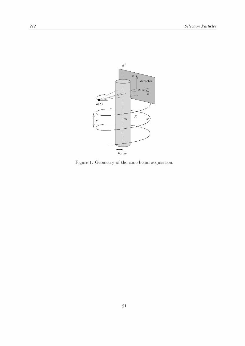
212 Sélection d’articles
R
RF OV
P
~a(λ)
detector
z
v
u
Figure 1: Geometry of the cone-beam acquisition.
21

Exact and approximate algorithms for helical cone-beam CT 213
(a) helix segment 1.5π, min=0.77, max=1.24 (b) helix segment 3π, min=0.33, max=1.33
Figure 2: Total Radon weight M(~r, ~θ) (eq. (40)) at ~r = (0,−90 mm, 0). The horizontaland the vertical axes are respectively the azimutal angle and the cosine of the polar angleassociated to ~θ. The grey scale range is [0.9, 1.1]. The minimum and the maximum of Mare indicated in the sub-legend.
22

214 Sélection d’articles
(a) FDK2 1.5π (b) FDK2 2π (c) FDK2 3π
(d) FDK3 1.5π (e) FDK3 2π (f) FDK3 3π
Figure 3: Transaxial slice z = −21.5 mm of the HEAD phantom reconstructed with thealgorithms FDK-2 and FDK-3. The grey scale range is [1.01, 1.09].
23
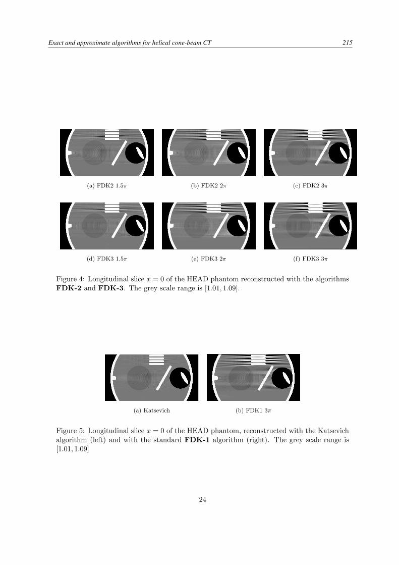
Exact and approximate algorithms for helical cone-beam CT 215
(a) FDK2 1.5π (b) FDK2 2π (c) FDK2 3π
(d) FDK3 1.5π (e) FDK3 2π (f) FDK3 3π
Figure 4: Longitudinal slice x = 0 of the HEAD phantom reconstructed with the algorithmsFDK-2 and FDK-3. The grey scale range is [1.01, 1.09].
(a) Katsevich (b) FDK1 3π
Figure 5: Longitudinal slice x = 0 of the HEAD phantom, reconstructed with the Katsevichalgorithm (left) and with the standard FDK-1 algorithm (right). The grey scale range is[1.01, 1.09]
24

216 Sélection d’articles
1.5 3 π π
1.5 3 ππ
Figure 6: Schematic representation of the iso-contour lines of the response function of thealgorithms FDK-2 (top) and FDK-3 (bottom). The segment of helix used to reconstructslice z = 0 is represented, with the full and dotted lines corresponding respectively to thehalf segments located above and below the slice. In each case, the segment is centered atthe South.
25

Exact and approximate algorithms for helical cone-beam CT 217
(a) FDK2 1.5π (b) FDK2 3π
(c) Katsevich (d) Frequency mixing 3π
Figure 7: Longitudinal slice x = 0 of the HEAD phantom, reconstructed from the noisyprojection data. The grey scale range is [1.0, 1.1].
26

218 Sélection d’articles