Inverse problems

Regularization Lecture 3

Nikolai Piskunov 2014

Regularization •  An ill-posed problem can be made

well-posed by restricting a subset of possible solutions

•  Two questions: – How to make sure the subset contains

only one solution? – Will that be the “correct” one?

•  We can choose a strategy and try to answer those question for specific method.

Two methods: 1.  Search for quasi-solution. Quasi-

solution is the solution that is searched for on a subset of all possible solutions.

2.  Replacing the original problem with a similar well-posed problem. We replace the kernel with the one that gives very close g’s for the same f ’s but is well behaved.

• Quasi-solutions. One typical problem that is often solved with this method is deconvolution or the removal of the instrumental profile. The original signal is registered by an equipment described with a PSF : The PSF (kernel) usually quickly drops away from the center but never goes below zero.

∫+∞

∞−

−= dyyfyxKxg )()()()(xK

In many cases a Gaussian is a good model for the PSF: The Fourier transform is defined as:

2)/(1)( δ−

δπ= xexK

∫

∫∞+

∞−

ω−

π

−

+∞

∞−

ω

π

ωω≡=

≡=ω

defftf

dtetfff

ti

ti

)(F)(

)(F)(

211

21

One interesting property of Fourier transform is relevant for the convolution: Another interesting property is that the Fourier transform of a Gaussian is a Gaussian. Assuming that we know the instrumental profile (PSF) we can formally perform deconvolution:

⎥⎦

⎤⎢⎣

⎡−=ω⋅ω ∫

+∞

∞−

dyyvyxuvu )()(F)()(

[ ]Kgxf FFF)( 1−=

In practice, the and are known on a discrete grid with certain measurement errors. The noise has frequency-independent spectrum, so the Fourier transform of the kernel and the measurements would look something like this:

g K

Kernel

Measurements

K g

Ratio g K

Quasi-solution: Let’s restrict ourselves with solutions containing only low frequencies, for example, from 0 up to the point where the transform of the kernel becomes equal to . In more sophisticated cases one may try to create a model for the noise spectrum and use that for the cut-off. The solution is stable and unique and it will actually approach the true f, as the S/N is improved. Note, that narrow spectrum of K means that the kernel decays slowly making our constraints on the solution more strict.

g

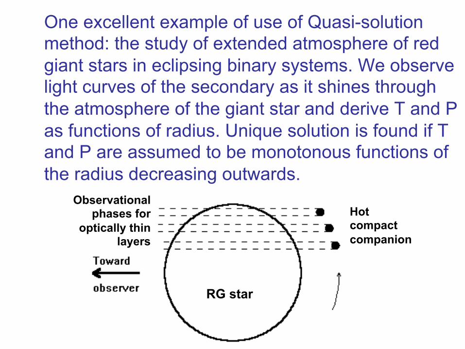
One excellent example of use of Quasi-solution method: the study of extended atmosphere of red giant stars in eclipsing binary systems. We observe light curves of the secondary as it shines through the atmosphere of the giant star and derive T and P as functions of radius. Unique solution is found if T and P are assumed to be monotonous functions of the radius decreasing outwards.

RG star

Hot compact companion

Observational phases for

optically thin layers

Let look at the iterations: •  Get T(r) and P(r) from a model

atmosphere •  Compute molecular-ionization equilibrium

to get partial number densities •  Get opacities and optical path •  Adjust source function, get new

temperature structure •  Re-compute model atmosphere •  Iterate

Regularized functional •  We are going to replace the functional

which results in an ill-posed problem with another functional which is close, has better properties and behaves in a predictable way.

•  Strictly speaking we want to replace with where for measurement error there are numbers and such that for all measurements within the error bars the solutions minimizing form a compact set around the true solution:

)( fΦ

Φ

),( ΛΩ f 0>δ0>εΛ

δ<− trueggΩ

ε<− trueff

One example of using regularization in numerical methods is the approximate calculation of derivative: Assuming that a sequence of f will converge to the true derivative as we find an ill-posed problem. If a numerical representation can be split in a true value and rounding error then the approximation can be re-written as: and but

Δ

−Δ+≈=

)()()( xgxgdxdgxf

0→Δ

egg tm +=

0

( ) ( ) ( ) ( ) ( )

( ) ( )

m m t t

t t

g x g x g x g x e x

g x g x dgdx

δΔ→

+Δ − +Δ −= +

Δ Δ Δ+Δ −

⎯⎯⎯→ →∞Δ Δ

•  In order to keep our estimate reasonable we have to keep . For smaller the errors will dominate our estimates.

•  We can generalize this idea and introduce a positive functional that is defined for all f ’s and has a property that for a given only a compact subset of f ’s fulfills the condition:

•  The compactness means that for a given d any pair of f ‘s such that: and is closer than certain and for

( )δ δΔ = Λ >Δ

),( ΛfRd

df <Λ),(R

df <)( 1Rdf <)( 2R

21 ff −>ε0 ,0 →ε→d

•  In 1943 Tikhonov proved that if such can be found is a regularized functional, stable against small perturbations in g’s.

•  The idea behind is that we may have many solutions f such that but only a compact number of them will result in small ‘s. If more then one solution exists they would be close to each other and can be selected such as to make the solution unique.

δ<− mgfK

)()(),( fff R⋅Λ+Φ≡ΛΩ

R

RΛ

is called the regularizing functional. Now instead of solving the problem searching for minimum of , we will search for the minimum of . One can also think of this as of conditional minimization where the relative weight of additional condition(s) is determined by Lagrangian multiplier also known as the regularization parameter. We would like to find the regularization function such that it will make the search for minimum of a well-posed problem while can be adjusted depending on measurements to ensure uniqueness.

R

ΦΩ

Λ

Ω Λ

3 big questions:

•  Is there a general form of that will ensure the stability and uniqueness of the solution?

•  How do we choose the regularization parameter ?

•  Can we say anything about the relation between the properties of g’s and resulting solution for f ’s minimizing ?

Λ

R

Ω

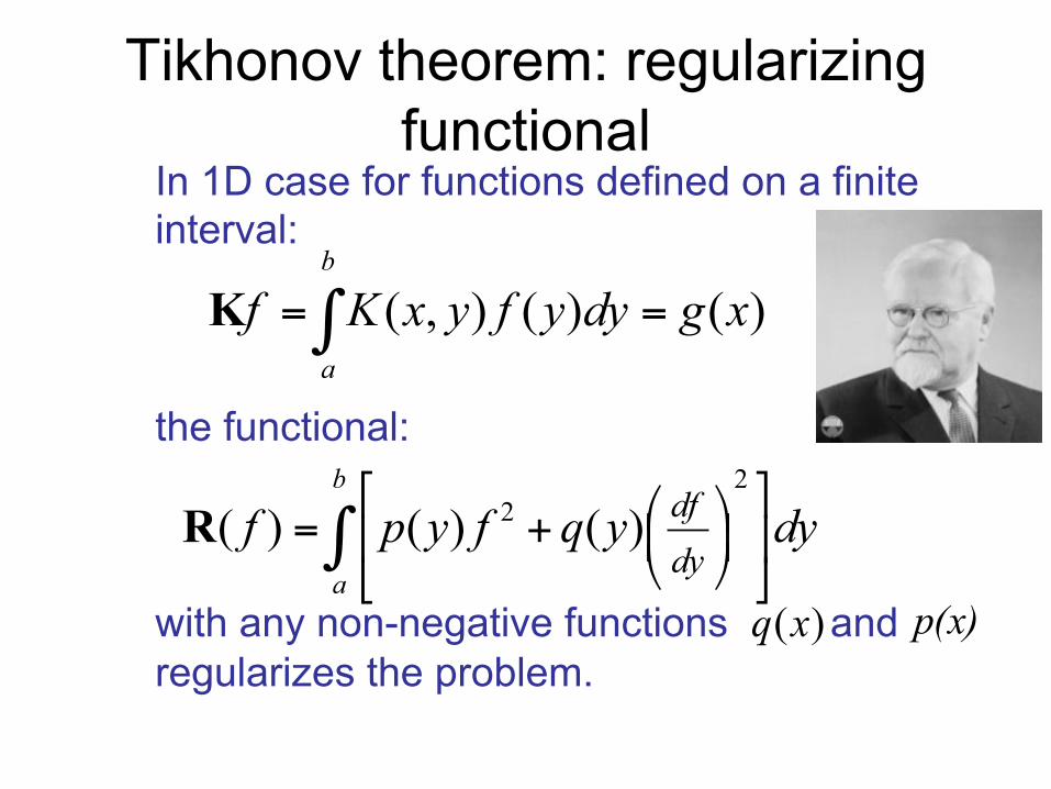
Tikhonov theorem: regularizing functional

In 1D case for functions defined on a finite interval: the functional: with any non-negative functions and regularizes the problem.

∫ ⎥⎦

⎤⎢⎣

⎡⎟⎠⎞

⎜⎝⎛+=

b

a

dyyqfypfdydf

22 )()()(R

∫ ==b

a

xgdyyfyxKf )()(),(K

)(xq p(x)

Can we prove that? For a linear operator: Yes. Suppose we have two different solutions and that minimize . Let’s construct a linear combination: The regularized functional becomes now a simple quadratic function of : with: Thus has only one minimum!

1f2f

)( 121 ffff −⋅β+=

β2( ) K( ) R( )f g f A B Cβ β βΩ = − + = + +

( )

( ) ( )

2

2 1

2 22 1 2 1

( , )

0

b b

a a

b

a

C K x y f f dy dx

p f f q f f dy

⎧ ⎫⎪ ⎪= ⋅ − +⎨ ⎬

⎪ ⎪⎩ ⎭

⎡ ⎤ʹ′ ʹ′+ ⋅ − + ⋅ − >⎣ ⎦

∫ ∫

∫)(βΩ

Ω

•  In case of nonlinear kernel the prove is not that easy. One can define special classes of kernels for which the uniqueness can be proven. One class important for astrophysical applications is when the kernel is a monotonous in f .

•  The regularization parameter in theory can be predicted if the error bars of the measurements are known. Unfortunately, in practice the model often contains additional tuning parameters, systematic errors etc. Instead we adjust as we approach the solution.

Λ

Λ

•  The regularizing functional above is called Tikhonov regularization. Other regularizing functional forms: –  Maximum entropy (MEM) –  Maximum likelyhood

•  MEM. Entropy in information theory has been introduced by Shannon in 1948 as the information content of the probability distribution: The information content does not depend on the physical units so are unitless, e.g.:

∑−= iii mpp logS

∑=

iN

ii f

fp 1

ip

•  The regularization is achieved by maximizing the entropy so the regularized functional will be:

•  Home work: Implement Tikhonov regularization assuming and and MEM regularization.

∑Λ+−=Ω ii ppgKff log)(

0)( =xp 1)( =xq