Inverse Problems in Structural Mechanics

by

Jing Li

Dissertation submmitted to the Faculty of

Virginia Polytechnic Institute and State University

in partial fulfillment of the requirements for the degree of

Doctor of Philosophy

in

Aerospace Engineering

Advisory Committee

Rakesh K. Kapania, Chairman

Romesh C. Batra

Raymond H. Plaut

Robert L. West

Mayuresh Patil

December 2005

Blacksburg, Virginia

Keywords: inverse problems, unitized structures, load updating, finite element models,

fiber optic sensors, placement optimization, genetic algorithms, panel optimization

Copyright c© 2005, Jing Li

Inverse Problems in Structural Mechanics

Jing Li

Virginia Polytechnic Institute and State UniversityBlacksburg, VA 24061-0203

(ABSTRACT)

This dissertation deals with the solution of three inverse problems in structural mechanics.

The first one is load updating for finite element models (FEMs). A least squares fitting is

used to identify the load parameters. The basic studies are made for geometrically linear and

nonlinear FEMs of beams or frames by using a four-noded curved beam element, which, for a

given precision, may significantly solve the ill-posed problem by reducing the overall number

of degrees of freedom (DOF) of the system, especially the number of the unknown variables

to obtain an overdetermined system. For the basic studies, the unknown applied load within

an element is represented by a linear combination of integrated Legendre polynomials, the

coefficients of which are the parameters to be extracted using measured displacements or

strains. The optimizer L-BFGS-B is used to solve the least squares problem.

The second problem is the placement optimization of a distributed sensing fiber optic

sensor for a smart bed using Genetic Algorithms (GA), where the sensor performance is

maximized. The sensing fiber optic cable is represented by a Non-uniform Rational B-

Splines (NURBS) curve, which changes the placement of a set of infinite number of the

infinitesimal sensors to the placement of a set of finite number of the control points. The

sensor performance is simplified as the integration of the absolute curvature change of the

fiber optic cable with respect to a perturbation due to the body movement of a patient. The

smart bed is modeled as an elastic mattress core, which supports a fiber optic sensor cable.

The initial and deformed geometries of the bed due to the body weight of the patient are

calculated using MSC/NASTRAN for a given body pressure. The deformation of the fiber

optic cable can be extracted from the deformation of the mattress. The performance of the

fiber optic sensor for any given placement is further calculated for any given perturbation.

The third application is stiffened panel optimization, including the size and placement

optimization for the blade stiffeners, subject to buckling and stress constraints. The present

work uses NURBS for the panel and stiffener representation. The mesh for the panel is

generated using DistMesh, a triangulation algorithm in MATLAB. A NASTRAN/MATLAB

interface is developed to automatically transfer the data between the analysis and opti-

mization processes respectively. The optimization consists of minimizing the weight of the

stiffened panel with design variables being the thickness of the plate and height and width

of the stiffener as well as the placement of the stiffeners subjected to buckling and stress

constraints under in-plane normal/shear and out-plane pressure loading conditions.

Dedication

To the Almighty God Father, and His Son Jesus Christ;To my parents, Zhenyu Li and Yulan Che,

To my mother-in-law, Guilan Zhang,To my wife, Xiuli Lu,

To my daughters, Suo Li and Rebekah Li

“I can do all things in Christ who strengthens me...”– BIBLE: Phillipians 4:13

Acknowledgments

I am grateful to my advisor, Dr. Rakesh K. Kapania, for giving me a valuable opportunity

to work with him and to gain broad experience through many exciting projects, and for his

valuable support and encouraging advice throughout the program. I also want to express my

gratefulness to Drs. Raymond H. Plaut, Romesh C. Batra, Robert L. West and Mayuresh

Patil for serving as committee members and giving me valuable input through the committee

meetings or course work.

I have been so fortunate to have my parents, Zhenru Li and Yulan Che, my mother-in-law

Guilan Zhang, and deeply grateful for their unchanging love and support. I want to express

my deep thanks to my wife, Xiuli Lu, for her precious love, encouragement, and sacrifice,

and my daughters, Suo and Rebekah, for their everlasting smile and good health.

Thanks are also due to many colleagues in our department throughout the program for

their valuable company and encouragement, especially to Yong Yook Kim, Jeffrey M.K.

Chock, Dhaval Makhecha, Sameer Mulani, Sumit Vasudeva, Hazem Soliman, and Hitesh

Kapoor.

I also want to acknowledge the financial support through all years for my studies and

researches from the project sponsored by a grant (CDAAH04-95-1-0175) from the Army

Research Office with Dr. Gary Anderson as the grant monitor, from the project of Java

Applets for Engineering Education funded by the National Science Foundation, from the

assistance and funding of ADOPTECH, Inc., of Blacksburg, Virginia, through Dr. Scott

Ragon, from the project funded by Virginia Tech Applied Biosciences Center (VT ABC)

at Virginia Polytechnic Institute and State University through Dr. William Spillman, Jr.,

and from the project funded from NASA Langley and the National Institute of Aerospace

for funding the project with Drs. Davis Brake, and Karen Taminger as grant monitors.

Finally and uttermost, I’d thank the Almighty God and His Christ Jesus for the salvation

and spiritual comfort during my hardest time.

God bless you and thank you all,

Jing Li

iv

Table of Contents

Title Page 1

Abstract ii

Dedication iii

Acknowledgements iv

Table of Contents v

List of Figures viii

List of Tables xiv

Introduction 1

1.1 Inverse Problems . . . . . . . . . . . . . . . . . . . . . . . . . . . . . . . . . 1

1.2 Regularization Methods . . . . . . . . . . . . . . . . . . . . . . . . . . . . . 5

1.3 Present Work . . . . . . . . . . . . . . . . . . . . . . . . . . . . . . . . . . . 9

Load Updating for Finite Element Models 11

2.1 An Overview . . . . . . . . . . . . . . . . . . . . . . . . . . . . . . . . . . . 12

2.2 Theory . . . . . . . . . . . . . . . . . . . . . . . . . . . . . . . . . . . . . . . 18

2.2.1 Load Representation within an Element . . . . . . . . . . . . . . . . 18

2.2.2 Load Updating for Nonlinear FEM . . . . . . . . . . . . . . . . . . . 19

2.2.3 Constraints on Load Distribution . . . . . . . . . . . . . . . . . . . . 23

2.3 Examples . . . . . . . . . . . . . . . . . . . . . . . . . . . . . . . . . . . . . 26

2.3.1 The Effect of Measurement Methods: Absolute Error and Relative Error 28

2.3.2 The Effect of the Order of Integrated Legendre Polynomials . . . . . 30

2.3.3 The Effect of Element Size . . . . . . . . . . . . . . . . . . . . . . . . 32

2.3.4 The Effect of Density of Measured Points . . . . . . . . . . . . . . . . 34

2.3.5 The Effect of Enforcing Smoothing and C0 Continuity . . . . . . . . 36

2.3.6 An Application to a Portal Frame . . . . . . . . . . . . . . . . . . . . 37

2.3.7 An Application to Highly Oscillating Load Updating . . . . . . . . . 38

2.3.8 Measured Strains Based Load Updating . . . . . . . . . . . . . . . . 40

2.3.9 An Application to Geometrically Nonlinear Beam . . . . . . . . . . . 40

2.4 Conclusions . . . . . . . . . . . . . . . . . . . . . . . . . . . . . . . . . . . . 45

TABLE OF CONTENTS vi

Placement Optimization of Fiber Optic Sensors 48

3.1 An Overview . . . . . . . . . . . . . . . . . . . . . . . . . . . . . . . . . . . 49

3.2 Description of the Problem . . . . . . . . . . . . . . . . . . . . . . . . . . . . 53

3.2.1 Objective/Sensor Performance Function . . . . . . . . . . . . . . . . 53

3.2.2 Design Variables/Placement Representation . . . . . . . . . . . . . . 54

3.2.3 Constraints . . . . . . . . . . . . . . . . . . . . . . . . . . . . . . . . 56

3.3 Procedure and Implementation . . . . . . . . . . . . . . . . . . . . . . . . . 57

3.3.1 Procedure . . . . . . . . . . . . . . . . . . . . . . . . . . . . . . . . . 57

3.3.2 Implementation . . . . . . . . . . . . . . . . . . . . . . . . . . . . . . 61

3.4 Placement Optimization of the Fiber Optic Sensors for a Smart Bed by GA . 62

3.4.1 A Very Simple Breeding Algorithm . . . . . . . . . . . . . . . . . . . 62

3.4.2 Coding/Decoding . . . . . . . . . . . . . . . . . . . . . . . . . . . . . 63

3.4.3 Fitness Function . . . . . . . . . . . . . . . . . . . . . . . . . . . . . 64

3.4.4 Examples . . . . . . . . . . . . . . . . . . . . . . . . . . . . . . . . . 65

3.5 Conclusions . . . . . . . . . . . . . . . . . . . . . . . . . . . . . . . . . . . . 67

Optimal Design of Unitized Panels with Curvilinear Stiffeners 71

4.1 An Overview . . . . . . . . . . . . . . . . . . . . . . . . . . . . . . . . . . . 71

4.2 Methodology, Procedure, and Capability . . . . . . . . . . . . . . . . . . . . 73

4.2.1 Methodology . . . . . . . . . . . . . . . . . . . . . . . . . . . . . . . 73

4.2.2 Procedure . . . . . . . . . . . . . . . . . . . . . . . . . . . . . . . . . 74

4.2.3 Capability and Limitation . . . . . . . . . . . . . . . . . . . . . . . . 75

4.3 Mathematical Aspects of Optimization of Stiffened Panels . . . . . . . . . . 75

4.3.1 Formulation of Optimization of Stiffened Panels . . . . . . . . . . . . 75

4.3.2 Convergence of Optimization of Stiffened Panels . . . . . . . . . . . . 76

4.3.3 NURBS Representation of Stiffened Panels . . . . . . . . . . . . . . . 79

4.3.4 Finite Element Meshing and Mapping . . . . . . . . . . . . . . . . . . 82

4.4 Numerical Studies on Optimal Blade Stiffened Panel Designs . . . . . . . . . 82

4.4.1 Orientation Effects . . . . . . . . . . . . . . . . . . . . . . . . . . . . 84

4.4.2 Spacing Effects . . . . . . . . . . . . . . . . . . . . . . . . . . . . . . 88

4.4.3 Location Effects . . . . . . . . . . . . . . . . . . . . . . . . . . . . . . 88

4.4.4 Curvature Effects . . . . . . . . . . . . . . . . . . . . . . . . . . . . . 88

4.5 Conclusions and Future Work . . . . . . . . . . . . . . . . . . . . . . . . . . 106

Summary and Conclusions 119

Legendre Polynomials 124

Load Coefficient Matrix at the Element Level 126

TABLE OF CONTENTS vii

The Derivatives of the Displacements with Respective to Load CoefficientVector 130

The Derivatives of the Strains with Respect to Load Coefficient Vector 132

References 134

Vita 142

List of Figures

Figure 1.1 A spring-mass-damper system.. . . . . . . . . . . . . . . . . . . . . . . . 2

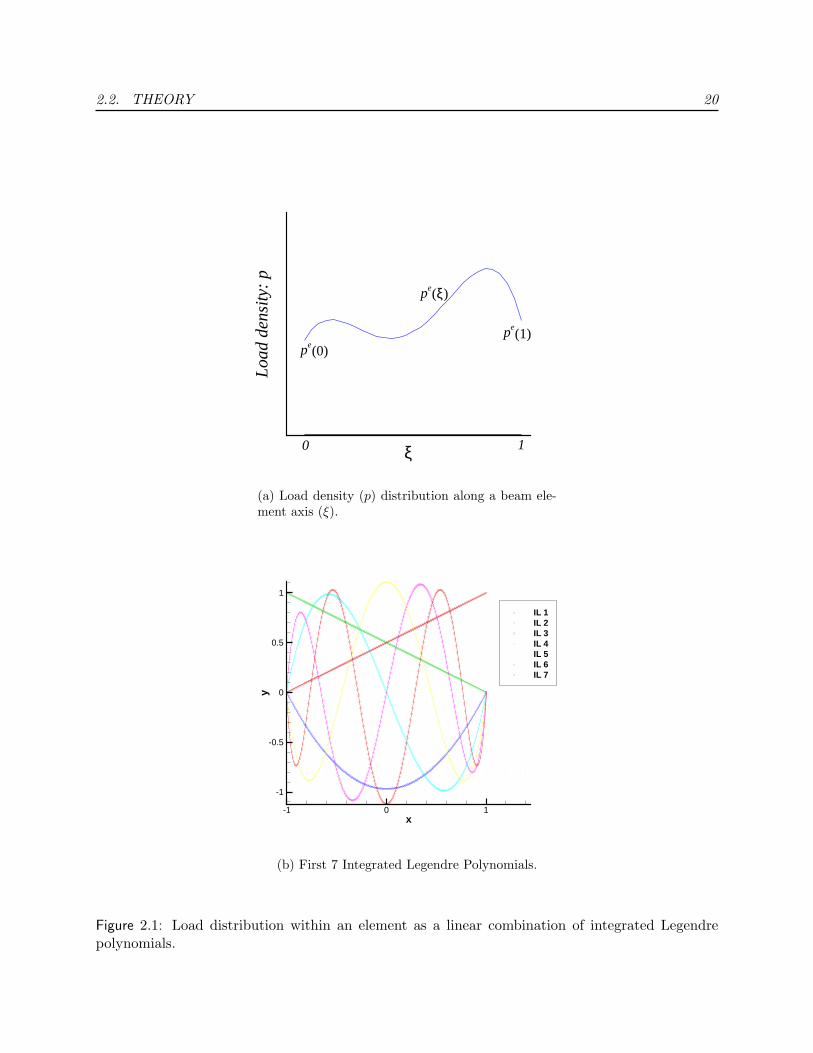
Figure 2.1 Load distribution within an element as a linear combination of integrated

Legendre polynomials.. . . . . . . . . . . . . . . . . . . . . . . . . . . . . . . . 20

Figure 2.2 A need for constraints on the extracted load.. . . . . . . . . . . . . . . . 25

Figure 2.3 A comparison of the extracted loads for a cantilever beam with absolute

or relative error between the calculated and measured displacements at 9 points.

The applied reference load was uniformly distributed and the extracted load

within an element was also assumed to be uniformly distributed. Eight four-

noded curved beam elements were used to model the beam. The extracted load

with relative error of displacements was closer to the applied reference load than

that with absolute error of displacements.. . . . . . . . . . . . . . . . . . . . . . 29

Figure 2.4 Extracted load for a cantilever beam subjected to a uniform reference

load as a function of number of integrated Legendre polynomials. Polynomials

up to degree 3 extracted the load perfectly. Higher-order polynomials gave a

relatively large oscillating error around the reference load.. . . . . . . . . . . . . 31

Figure 2.5 Extracted load for a cantilever beam as a function of number of elements.

The load within each element was assumed to be uniformly distributed. . . . . . 33

Figure 2.6 Extracted load for a cantilever beam as a function of number of measured

points. The applied reference load was uniformly, linearly or Sinusoidally dis-

tributed, but the load within each of the elements was assumed to be uniformly

distributed.. . . . . . . . . . . . . . . . . . . . . . . . . . . . . . . . . . . . . . 35

Figure 2.7 Constraining the extracted load through the enforcement of load smooth-

ing within an element and C0 between two adjacent elements: λS, λC0 = 1× 103

continuity. The applied reference load was linearly distributed but a linear com-

bination of first 4 integrated Legendre polynomials (highest degree is 3) was used

to represent the load distribution over an element for load extraction. Eight el-

ements were used to model the beam.. . . . . . . . . . . . . . . . . . . . . . . . 37

Figure 2.8 Extracting in-plane and out-plane loads for a portal frame.. . . . . . . . 38

LIST OF FIGURES ix

Figure 2.9 Extracting highly oscillating load for a cantilever beam. The applied

reference load (RL) was sinusoidally distributed with unit mean value. The

extracted load (EL) was assumed uniformly distributed within an element. (a)

The RL had 3 sine waves. 60 elements were used. The EL agreed well with the

RL. (b) The RL had 6 sine waves. 120 elements were used. The EL agreed well

with the RL at first 3 sine waves near the fixed end but tended to be close to

the unit mean value of the RL at the other 3 sine waves near the free end. (c)

The applied load had 12 sine waves and unit mean value. 240 (120) elements

were used. The EL agreed well with the RL at only 1.5 sine waves near the fixed

end but tended to be close to the unit mean value of the RL near the free end.

Results using both 120 and 240 elements are almost identical.. . . . . . . . . . . 39

Figure 2.10 Extracting loads of different distributions for a cantilever beam with mea-

sured bending strains at 3 Gaussian points in each of the 8 elements. Load within

each element was assumed to be uniform.. . . . . . . . . . . . . . . . . . . . . . 41

Figure 2.11 Extracting uniform self-weight type load for a cantilever beam. Eight

finite elements were used to model the beam.. . . . . . . . . . . . . . . . . . . . 43

Figure 2.12 Extracting uniform snow loads of type II-n (non-conservative consider-

ation) as compared with type II-c (conservative consideration) for a cantilever

beam. Eight finite elements were used to model the beam.. . . . . . . . . . . . 44

Figure 2.13 Extracting uniform pressure load for a cantilever beam with different

choices of displacement measurements. Eight finite elements were used. The

unknown axial displacements are set to zero in the figure. The TD were measured

at all the 25 nodes. TD: transverse displacements; RL: reference load; AD: axial

displacements. DS: design stepsize; LUI: load updating iterations.. . . . . . . . 46

Figure 3.1 A schematic diagram of the smart bed. The distributed sensing fiber

optic cable is stitched on the bed surface.. . . . . . . . . . . . . . . . . . . . . . 52

Figure 3.2 A possible fiber optic sensor placement represented by a NURBS curve.. 55

Figure 3.3 Chart for optimal placement of the fiber optic sensor.. . . . . . . . . . . 58

Figure 3.4 Body pressure and deformation of the soft cored mattress. The pressure

P has a unit of N/cm2.. . . . . . . . . . . . . . . . . . . . . . . . . . . . . . . . 60

Figure 3.5 A placement of a fiber optic sensor for a smart bed represented by a

NURBS curve with 6 control points. Adopted from Fig. 3.7b.. . . . . . . . . . . 63

Figure 3.6 Placement optimization of a fiber optic sensor for a smart bed by GA.. . 65

Figure 3.7 A 3-D view of the initial placement and updated placement. The per-

turbed (dashed) and unperturbed (solid) fiber curve shapes of the optimal place-

ment of the fiber optic sensor. . . . . . . . . . . . . . . . . . . . . . . . . . . . . 68

Figure 3.8 Placement optimization of a fiber optic sensor for a smart bed by GA.. . 69

LIST OF FIGURES x

Figure 3.9 A 3-D view of the initial placement and updated placement. The per-

turbed (dashed) and unperturbed (solid) fiber curve shapes of the optimal place-

ment of the fiber optic sensor.. . . . . . . . . . . . . . . . . . . . . . . . . . . . 70

Figure 4.1 A curved panel with arbitrarily oriented stiffeners and its finite element

mesh.. . . . . . . . . . . . . . . . . . . . . . . . . . . . . . . . . . . . . . . . . . 73

Figure 4.2 NURBS representation for stiffeners’ reference curves.. . . . . . . . . . . 80

Figure 4.3 NURBS representation for panel’s reference surface.. . . . . . . . . . . . 80

Figure 4.4 The meshing and mapping of a stiffened panel with a central hole.. . . . 83

Figure 4.5 Geometrical dimensions (a = 2.54m; b = 2.54m), pure shear loading

(Qxy = 250kN/m), and simply supported conditions of a blade stiffened panel.

Both stiffeners and plate are made out of aluminum. Initial size and bounds:

t0 = w0 = 0.005m; h0 = 5w0; tb = wb = [0.0001, 0.1]m; hb = [0.0001, 0.5]m.. . . . 85

Figure 4.6 Effects of orientations of the stiffeners on the optimal designs. Orientation

I: Mmin = 224kg.. . . . . . . . . . . . . . . . . . . . . . . . . . . . . . . . . . . . 86

Figure 4.7 Effects of orientations of the stiffeners on the optimal designs. Orientation

II: Mmin = 144kg.. . . . . . . . . . . . . . . . . . . . . . . . . . . . . . . . . . . 87

Figure 4.8 Effects of spacing of the stiffeners on the optimal designs. Spacing II:

Mmin = 101kg.. . . . . . . . . . . . . . . . . . . . . . . . . . . . . . . . . . . . . 89

Figure 4.9 Effects of location of the stiffeners on the optimal designs. Location I:

Mmin = 144kg; Location II: Mmin = 186kg.. . . . . . . . . . . . . . . . . . . . . 90

Figure 4.10 One design parameter α controls the motions of two mid control points

x1 and x2 starting from x10 and x2

0 and by αd1 and αd2 for stiffeners 1 and 2,

respectively.. . . . . . . . . . . . . . . . . . . . . . . . . . . . . . . . . . . . . . 92

Figure 4.11 Effects of curvature of the stiffeners on the optimal designs. α = −0.3:

Mmin = 240kg.. . . . . . . . . . . . . . . . . . . . . . . . . . . . . . . . . . . . . 93

Figure 4.12 Effects of curvature of the stiffeners on the optimal designs. α = 0.0:

Mmin = 220kg.. . . . . . . . . . . . . . . . . . . . . . . . . . . . . . . . . . . . . 94

Figure 4.13 Effects of curvature of the stiffeners on the optimal designs. α = 0.8:

Mmin = 178kg.. . . . . . . . . . . . . . . . . . . . . . . . . . . . . . . . . . . . . 95

Figure 4.14 Diagram of minimum mass vs. shape design parameter α. Two minima

are found. One corresponds to straight stiffeners at about α = 0.0 with mini-

mum mass Mmin = 220kg. The global optimal shape corresponds to curvilinear

stiffeners at about α = 0.8 with a minimum mass Mmin = 178kg, which is the

minimum of the two minima.. . . . . . . . . . . . . . . . . . . . . . . . . . . . . 96

LIST OF FIGURES xi

Figure 4.15 Geometrical dimensions (a = 2.54m; b = 2.54m), bi-normal loading

(Nx = 250kN/m; Ny = 0.2Nx), and simply-supported conditions of a blade

stiffened panel. Both stiffeners and plate are made out of aluminum. Initial

size and bounds: t0 = w0 = 0.005m; h0 = 5w0; tb = wb = [0.0001, 0.1]m;

hb = [0.0001, 0.5]m.. . . . . . . . . . . . . . . . . . . . . . . . . . . . . . . . . . 97

Figure 4.16 Location 1: The end points of the two stiffeners are close to the up-

per/lower edges of the panel and 13/15b apart from each other. One design

parameter α controls the motions of two mid control points x1 and x2 starting

from x10 and x2

0 and by α1d1 and α2d

2 for stiffeners 1 and 2, respectively.. . . . 98

Figure 4.17 Location I: effects of curvature of the stiffeners on the optimal designs.. . 99

Figure 4.18 Location I: Diagram of minimum mass vs. shape design parameter α.

The global optimal shape is achieved at about α = 1.60 with a minimum mass

Mmin = 245kg. The maximum number of iterations for size optimization is set

to be 50 and 100.. . . . . . . . . . . . . . . . . . . . . . . . . . . . . . . . . . . 100

Figure 4.19 Location II: The end points of the two stiffeners are close to the up-

per/lower edges of the panel and 7/15b apart from each other. One design

parameter α controls the motions of two mid control points x1 and x2 starting

from x10 and x2

0 and by α1d1 and α2d

2 for stiffeners 1 and 2, respectively. Also

see Fig. 4.16.. . . . . . . . . . . . . . . . . . . . . . . . . . . . . . . . . . . . . . 101

Figure 4.20 Location II: Diagram of minimum mass vs. shape design parameter α.

The global optimal shape is achieved at about α = 0.10 with a minimum mass

Mmin = 197kg (compared with straight stiffeners α = 0.0 with Mmin = 205kg).

The maximum number of iterations for size optimization is set to be 100.. . . . 102

Figure 4.21 Location III: The end points of the two stiffeners are close to the up-

per/lower edges of the panel and 5/15b apart from each other. One design

parameter α controls the motions of two mid control points x1 and x2 starting

from x10 and x2

0 and by α1d1 and α2d

2 for stiffeners 1 and 2, respectively. Also

see Fig. 4.16.. . . . . . . . . . . . . . . . . . . . . . . . . . . . . . . . . . . . . . 103

Figure 4.22 Location 3: Diagram of minimum mass vs. shape design parameter α.

The global optimal shape is achieved at about α = 0.0 with a minimum mass

Mmin = 185kg. The maximum number of iterations for size optimization is set

to be 100.. . . . . . . . . . . . . . . . . . . . . . . . . . . . . . . . . . . . . . . 104

Figure 4.23 One design parameter α controls the shapes of the NURBS curves of four

stiffeners, which are initially straight (α = 0.0) and evenly spaced.. . . . . . . . 105

LIST OF FIGURES xii

Figure 4.24 A comparison of diagrams of minimum mass vs. shape design parameter

α before and after the improvement of the convergence. After the improvement

of the convergence, three local minima are found. One corresponds to straight

stiffeners at about α = 0.0 with a minimum mass Mmin = 213kg which is also the

global minimum. The other two local minima correspond to curvilinear stiffeners

at about α = 0.275 with a minimum mass Mmin = 223kg, and at about α = 0.875

with a minimum mass Mmin = 235kg.. . . . . . . . . . . . . . . . . . . . . . . . 106

Figure 4.25 A comparison of optimal designs before and after the improvement of the

convergence.. . . . . . . . . . . . . . . . . . . . . . . . . . . . . . . . . . . . . . 107

Figure 4.26 A comparison of the first four buckling modes before and after the im-

provement of the convergence.. . . . . . . . . . . . . . . . . . . . . . . . . . . . 108

Figure 4.27 A comparison of the design histories before and after the improvement of

the convergence.. . . . . . . . . . . . . . . . . . . . . . . . . . . . . . . . . . . . 109

Figure 4.28 One design parameter α controls the shapes of the NURBS curves of four

stiffeners, which are initially straight (α = 0.0) and evenly spaced.. . . . . . . . 110

Figure 4.29 Variation of minimum mass vs. shape design parameter α. The global

optimal shape is achieved at about α = 0.0 with a minimum mass Mmin = 190kg.

An inclusion of a central hole of radius 0.3m results in curvilinear stiffeners as

the global optimal placement, achieved at about α = −0.0725 with a minimum

mass Mmin = 182kg.. . . . . . . . . . . . . . . . . . . . . . . . . . . . . . . . . . 111

Figure 4.30 A comparison of optimal designs before and after the inclusion of the

central cutout of radius 0.3m.. . . . . . . . . . . . . . . . . . . . . . . . . . . . 112

Figure 4.31 A comparison of first four buckling modes before and after the inclusion

of the central cutout of radius 0.3m.. . . . . . . . . . . . . . . . . . . . . . . . . 113

Figure 4.32 A comparison of design histories before and after the inclusion of the

central cutout of radius 0.3m.. . . . . . . . . . . . . . . . . . . . . . . . . . . . 114

Figure 4.33 Geometrical dimensions (a = 2.54m; b = 2.54m), bi-normal and shear

loading (Nx = 250kN/m; Ny = 0.2Nx; Qxy = 0.5Nx; Py = 0), and simply

supported conditions of a blade stiffened panel. Both stiffeners and plate are

made out of aluminum. Initial size and bounds: t0 = w0 = 0.005m; h0 = 5w0;

tb = wb = [0.0001, 0.1]m; hb = [0.0001, 0.5]m.. . . . . . . . . . . . . . . . . . . . 115

Figure 4.34 Design parameter α1 controls the motions of two mid control points x1 and

x2 starting from x10 and x2

0 by α1d11 and α1d

21 for stiffeners 1 and 2, respectively.

Design parameter α2 controls the motions of two mid control points x3 and x4

starting from x30 and x4

0 by α2d32 and α2d

42 for stiffeners 3 and 4, respectively.. . 115

LIST OF FIGURES xiii

Figure 4.35 Design space of two design parameters: α1 = X and α2 = Y , with

corresponding minimum mass: Mmin = Z. Two local minima are found as shown

as the dark squares inside the circles from 17 discrete points on the 11×11 grids.

The maximum number of iterations for size optimization is set to be 100.. . . . 116

Figure 4.36 Two local minima vs. two design parameters.. . . . . . . . . . . . . . . . 117

Figure 4.37 First four buckling modes for minimum 1 and minimum 2.. . . . . . . . 118

List of Tables

Table 2.1 EExtload vs. absolute and relative displacement measurements.. . . . . . . . . 30

Table 2.2 EExtload vs. the degree of Integrated Legendre polynomial within one element.. 31

Table 2.3 EExtload vs. the number of elements (Nelm).. . . . . . . . . . . . . . . . . . . 32

Table 2.4 EExtload vs. the number of measured points (Nm).. . . . . . . . . . . . . . . 36

Table 3.1 Latex Mattress Core Fact Sheet.. . . . . . . . . . . . . . . . . . . . . . . 59

Table 3.2 Latex Mattress Core Fact Sheet.. . . . . . . . . . . . . . . . . . . . . . . 60

Chapter 1

Introduction

Driven by the needs from applications in both industry and other sciences, the field of

inverse problems has undergone a tremendous growth during the last two decades (Engl and

Kugler, 2003). However, studies on inverse problems in structural mechanics can be traced

back to as far as 1904 when Michell (1904) dealt with the optimum layout of a plane truss.

The work by Schmitt (1960) is frequently viewed as the start of modern structural opti-

mization in the 1960’s when computer-aided structural analysis and numerical optimization

techniques became accessible. Though the studies on modern structural optimization has

been undertaken for more than three decades, the terminology of inverse problems has not

been widely used.

1.1 Inverse Problems

Inverse problems arise whenever one searches for causes of observed or desired effects (Engl

and Kugler, 2003). Accordingly, direct or forward problems are to find the effects with given

causes.

In the field of structural mechanics, the causes more often refer to structural and load

parameters, and the effects are structural responses. Therefore, structural analysis for re-

sponses under given structures and loads are usually called direct or forward problems, while

structural optimizations and identifications for structural and load parameters that cause

the observed or desired responses are inverse problems.

1

1.1. INVERSE PROBLEMS 2

To illustrate, refer Fig. 1.1 for a spring-mass-damper dynamic system, which can be de-

scribed in the form of linear dynamic state equation, noticing the time t derivative notations:

x = ∂x∂t

and x = ∂2x∂t2

for any entity x:

Figure 1.1: A spring-mass-damper system.

Mu + Cu + Ku = P (1.1)

with initial conditions for displacement u and velocity u:

u|t=t0 = u0; u|t=t0 = v0 (1.2)

Then, as examples, we can define one of the simplest forward problems as:

1.1. INVERSE PROBLEMS 3

• Forward problem 1: Given the mass M, damping C, spring constant or system stiff-

ness K, initial conditions as in Eq. (1.2), and the external load P, find the displacement

response u for t ≥ t0.

and some inverse problems:

• Inverse problem 1: Given the displacement response u for t ≥ t0 and v0, and the

external load P, find the mass M, damping C, and system stiffness K.

• Inverse problem 2: Given the displacement response u for t ≥ t0 and v0, as well as

the mass M, damping C, and system stiffness K, find the external load P.

Inverse problem 1 is often viewed as a formulation of structural parameter identification

(Trivailo et al., 2004) or structural model updating (Mottershead and Friswell, 1993; Friswell

and Mottershead, 1995; Ahmadian et al., 1998; Avitabile, 2000). Inverse problem 2 is a

formulation for load parameter identification or load updating (Chock and Kapania, 2003;

Chock and Kapania, 2004).

Though many inverse problems in structural mechanics are formulated on the continuous

setting, and evaluated on the discrete setting based on FEM or boundary element methods

(BEM) (Bonnet and Constantinescu, 2005), both of the above inverse problem formulations

are discrete formulations (Mroz and Garstecki, 2005) or based on discrete linear model

equations (Hansen and O’Leary, 1993), for example, finite element models or methods (FEM)

(Mottershead and Friswell, 1993; Friswell and Mottershead, 1995; Gladwelly, 1997; Avitabile,

2000; Chock and Kapania, 2003; Chock and Kapania, 2004; Maincon, 2004a; Maincon,

2004b; Maree and Maincon, 2004; Barnardo and Maincon, 2004; Trivailo et al., 2004; Mroz

and Garstecki, 2005).

The solutions of most inverse problems lack uniqueness, which violates the second of the

three Hadamard well-posed conditions (Engl and Kugler, 2003):

1.1. INVERSE PROBLEMS 4

1. for all admissible data, a solution exists,

2. for all admissible data, the solution is unique and

3. the solution depends continuously on the data.

A violation of any of the three conditions (first two describe the identifiability and

third one is about stability) makes the inverse problems ill-posed or ill-conditioned. Non-

uniqueness is sometimes an advantage, and allows to choose among several strategies for a

desired effect (Engl and Kugler, 2003). For instance, an infinite number of the solutions

of inverse problems is useful in many design problems as it gives one the freedom to find

the optimal solutions among all possible solutions when further desired effects, such as the

requests to minimize or maximize some cost or objective function E subjected to certain

constraints, are provided. Then, inverse problems 1 and 2 can be further formulated into

two optimization problems:

• Inverse problem 1a: Given the displacement response u and other possible con-

straints for t ≥ t0 and v0, and the external load P, find the optimal mass M, damping

C, and system stiffness K to minimize or maximize E = E(M,C,K)

• Inverse problem 2a: Given the displacement response u and other possible con-

straints for t ≥ t0 and v0, as well as the mass M, damping C, and system stiffness K,

find the optimal external load P minimize or maximize E = E(P).

Inverse problem 1a includes a conventional structural optimization formulation subjected

to a constraint on the displacement response. Therefore, we have established the idea that

structural optimization is a special application field of inverse problems in structural mechan-

ics. Inverse problem 2a covers a seemingly new optimization formulation where the design

variables are loads or load parameters, instead of structural parameters. In fact, actual load

updating or identification is often formulated as some form of an optimization problem with

1.2. REGULARIZATION METHODS 5

load or load parameters as design variables employed to minimize, for example, the error be-

tween the given observed displacement response based on measurement and the calculated or

predicted displacement response of a structural (FEM) model under an approximated load.

Mroz and Garstecki (2005) gave some interesting inverse problem formulations for optimal

loading conditions in the design and identification of structures, which is a kind of mixed

formulation of inverse problems 1a and 2a.

An inverse problem is not only often formulated as a numerical optimization problem, but

also has some kind of numerical optimization technique as a solution approach. Ring (1999),

Ewing et al. (1999), Rattray et al. (1999), Avitabile (2000), and Chock and Kapania (2003)

were concerned with or used least squares formulation. For the solutions of their inverse

problems, Dunn (1976), Chiroiu et al. (2000), Kim and Kapania (2004), Trivailo et al.

(2004), and Trivailo et al. (2004) used Neural Networks and Genetic Algorithms; Brakhage

(1987), Hanke (1995), Rieder (1999), Burger and Muhlhuber (2002), Chock and Kapania

(2003), and Feijoo et al. (2004) used gradient based methods.

It should also be noted that in general the solutions of the optimization problems such

as inverse problem 1a or 2a are still nonunique. The number of optimization solutions can

be both finite and infinite. In the former case, some global optimization techniques are often

needed. In the latter case, there is a need to use further priori information to add some

constraints to obtain a unique solution.

1.2 Regularization Methods

In many practical inverse problems, however, non-uniqueness of the solutions or other ill-

conditioned solutions is not desired. In practice, one has only data with noise due to errors

in the measurements and inaccuracies of the model itself (Engl and Kugler, 2003). Then, in

case of a violation of the third Hadamard condition (i.e. the solution depends continuously on

1.2. REGULARIZATION METHODS 6

the data), even a small error in data will make algorithms developed for well-posed problems

fail if the instability is not desired, since data and round-off errors may be amplified by an

arbitrarily large factor (Engl and Kugler, 2003).

In order to overcome these instabilities one has to use regularization methods, which in

general terms replace an ill-posed problem by a family of neighboring well-posed problems

(Engl and Kugler, 2003) or filter out the influence of noise (Hansen and O’Leary, 1993).

To illustrate, consider a parameter identification problem with an observable entity y

of dimension m, which is in general a nonlinear function of an unknown parameter x of

dimension n to be identified:

y ≡ y0 + e = f(x) (1.3)

or in the linear case f(x) = Tx:

Tx = y0 + e ≡ y (1.4)

Here, T is a linear operator of dimension m × n, y0 is the true data, and e is the unknown

noise.

Well-known regularization methods for linear inverse problems are Tikhonov regulariza-

tion and the truncated singular value decomposition (SVD) (Hansen and O’Leary, 1993;

Engl and Kugler, 2003). We can illustrate both methods using the SVD of matrix T . A

non-negative real number σ is a singular value for T (its conjugate is T ∗) if there exist

non-zero vectors u of dimension m and v of dimension n such that

Tv = σu and T ∗u = σv (1.5)

Then, the theorem of SVD states that

T =n∑

i=1

σiuivTi (1.6)

1.2. REGULARIZATION METHODS 7

Here, the left and right singular vectors u and v are orthonormal, and the singular values

σi are nonnegative and non-increasing numbers, i.e., σ1 ≥ σ2 ≥ · · · ≥ σn ≥ 0 (Hansen and

O’Leary, 1993; Engl and Kugler, 2003). Common for all discrete ill-posed problems is that

the matrix T has a cluster of singular values at zero and that the size of this cluster increases

when the dimension m or n is increased (Hansen and O’Leary, 1993).

Using the SVD of T , the least squares solution to Eq. (1.4), i.e. the one obtained by

solving the unconstrained minimization problem:

minx‖Tx− y‖2 (1.7)

can be written in the form

xLSQ =n∑

i=1

αi

σi

vi (1.8)

where αi = uTi y (Hansen and O’Leary 1993).

It is obvious from Eq. (1.8) that a direct use of the least squares solution xLSQ leads to the

trouble that error in the directions corresponding to small singular values is greatly magnified

and overwhelms the information contained in the directions corresponding to larger singular

values. To overcome this problem, it is necessary to incorporate filter factors 0 ≤ fi ≤ 1, to

obtain the modified solution:

xfiltered =n∑

i=1

fiαi

σi

vi (1.9)

The most popular regularization method is the one due to Tikhonov and Arsenin (1977),

which turns to find the solution xλ to solve the minimization problem

minx

(‖Tx− y‖22 + λ2 ‖x‖2

2) (1.10)

1.2. REGULARIZATION METHODS 8

which is equivalent to choosing the filter factor:

fi =σ2

i

λ2 + σ2i

(1.11)

Here, the parameter λ controls how much weight is given to minimization of ‖x‖2 relative

to minimization of the residual norm.

Another widely used method is the truncated SVD, where one simply truncates the

summation in Eq. (1.8) at an upper limit k ≤ n, before the small singular values start to

dominate (Hansen and O’Leary, 1993), or equivalently speaking, let the small singular values

(“high frequencies”) be filtered out by a “low-pass filter” (Engl and Kugler, 2003).

In addition to noisy-data problems, the Tikhonov regularization method is often used

for the class of non-unique solution problems due to rank-deficient or even underdetermined

LSQ problems (Schulze and Sachs, 2002; Eriksson and Gulliksson, 2003), where the number

of the unknown variables n is larger than that of the data points m.

Noticing Eq. 1.3, the nonlinear counterpart of Eq. 1.7 is

minx‖f(x)− y‖2 (1.12)

the corresponding LSQ minimization formulation with the Tikhonov regularization is

minx

(‖f(x)− y‖22 + λ2 ‖x‖2

2) (1.13)

which is equivalent to the constrained minimization problem:

min ‖x‖22

s.t. minx‖f(x)− y‖2 (1.14)

For the underdetermined LSQ problem, Eq. 1.13 or 1.14 can be solved by some iterative

1.3. PRESENT WORK 9

algorithm, e.g. the inexact Gauss-Newton method (Schulze and Sachs, 2002) or truncated

Gauss-Newton method (Eriksson and Gulliksson, 2003).

1.3 Present Work

While structural mechanics includes elasticity, plasticity, plates and shells, vibrations, aeroe-

lasticity, finite element methods, structural stability, optimal design, fracture mechanics and

composite materials, etc., in the current work, however, we address three inverse problems

in a discrete setting.

The first problem (Chapter 2) is load updating for finite element models. The theory part

includes the extracted load representation within an element, load updating for nonlinear

FEM, and constraints on load distribution. Through a relative model order analysis, the

benefits for solving load updating problems using the relative deformation measurement,

the polynomials of lower orders, the elements of larger sizes, and the deformation of denser

measured points are studied for linear responses under the applied loads of different types. It

is confirmed that using the reduced number of unknown variables to obtain an overdetermined

inverse problem helps get unique and stable extracted loads. Various applications are given.

The second one (Chapter 3) is placement optimization of a fiber optic sensor for an

Integrated Smart-bedTM (Spillman Jr. et al., 2004). A description of the problem is first

given for the objective/sensor performance and constraints on the placement optimization

of a distributed sensing optical fiber. The procedure and implementation are described. An

example is given for the placement optimization of the fiber optic sensor for a smart bed using

a very simple breeding genetic algorithm for the multiple solution problems. The reduced

number of the unknown variables is realized by using the finite number of the control points

of the NURBS representation for the distributed sensing fiber optic cable.

The third one (Chapter 4) is stiffened panel optimization. An integrated approach is

1.3. PRESENT WORK 10

adopted to use the available capabilities. The mathematical aspects include the formulation

and convergence of the stiffened panel optimization. Numerical studies are made on optimal

blade stiffened panel designs. The effects of the orientation, spacing, location and curvature

of the stiffeners are studied. The slow and unstable convergence due to the ill-conditions

is solved mainly by reducing the condition number of the Hessian for the objective, and

some scaling and shifting to both the objective and constraint functions to have a balanced

weights or multipliers for an extended Lagrangian formulation.

A brief literature review is given in the individual chapters of the three application fields.

Chapter 2

Load Updating for Finite Element

Models

A measurement-based load updating method for finite element models subjected to static

loads was studied using a four-noded curved beam element for large displacements/ rotations

and a gradient-based variable metric optimizer. Finite element analysis was used to numeri-

cally calculate the geometrically linear and nonlinear responses and their sensitivities under

a given load. The optimizer was used to recursively update the load so that it minimized

the square of the difference between the calculated and pre-filtered/noise-free measured (dis-

placement or strain) data. For the basic studies, the extracted load was represented within

an element by a linear combination of integrated Legendre polynomials, the coefficients of

which were taken as design variables of the least-squares problem. Through a relative model

order analysis, the benefits for solving load updating problems using the relative deformation

measurement, the polynomials of lower orders, the elements of larger sizes (because of using

the high precision four-noded beam element), and the deformation of denser measured points

were studied for linear responses under the applied loads of different types. It was confirmed

that using the reduced number of unknown variables to obtain an overdetermined inverse

problem helps get unique and stable extracted loads. Though this conclusion was verified

mainly through illustrative examples for a cantilever beam, it was generally applicable to

other load updating or inverse problems. Further examples were given for a 3D portal frame

load updating, extracting highly oscillating loads, and a strain-based cantilever beam load

updating. The final examples were load updating for geometrically nonlinear finite element

models under under self-weight, snow and/or pressure loads.

11

2.1. AN OVERVIEW 12

2.1 An Overview

Finite element analysis (FEA) has long been one of the generally accepted tools for structural

analysis. While differences between real testing and FEA are usually reduced using system

identification, much effort has been focused on the increasing accuracy of the mathematical

model of the structure from the point of view of updating the finite element model (FEM)

of the structure itself under given applied loads.

However, simply updating the FEM itself is not sufficient to satisfactorily reduce the

differences between the observed experimental data and numerically calculated results based

on FEA if the applied loads are not exactly known. Also, operational loads, such as self-

weight, snow, waves, winds, etc., either dynamic or static, are usually not simply or directly

measurable. Therefore, it is an appealing alternative to use the indirect or inverse method to

determine or update the approximate applied loads based on the actually measured responses

of the structure under realistic working conditions by identifying load parameters of the

established load model. In other words, we seek to reduce those differences by modifying

not the FEM of the structural system, but the loading that the structure is subjected to

such that the experimental and the finite element responses match in the least-squares sense

(Rattray et al., 1999; Avitabile, 2000; Chock and Kapania, 2003).

The load updating is a special application of system identifications in the growing field of

inverse problems, which arise whenever one searches for causes of observed or desired effects

(Engl and Kugler, 2003). Therefore, an examination of the literature in terms of inverse

problems aids us in determining the most appropriate methodology for load updating.

In most formulations, the load identification process requires the inversion of the global

matrix, which tends to be very ill conditioned. That is, very small errors in measurements

propagate into large errors in estimated forces, especially at frequencies close to the resonance

and ant-resonance conditions (Starkey and Merrill, 1989). On the other hand, in many

2.1. AN OVERVIEW 13

practical inverse problems, one aims to retrieve a model that has infinitely many DOFs from

a finite amount of data, which leads to the non-uniqueness of the solutions of the rank-

deficient or underdetermined problems (Schulze and Sachs, 2002; Eriksson and Gulliksson,

2003). Therefore, solving an inverse problem entails more than estimating a model: any

inversion is not complete without a description of the class of models that is consistent with

the data (Snieder, 1998).

The process to overcome this difficulty is called regularization, which is to replace an

ill-posed problem by a family of neighboring well-posed problems (Engl and Kugler, 2003)

or filter out the influence of noise (Hansen and O’Leary, 1993).

The singular-value decomposition (SVD) technique (Elliott et al., 1988; Chock and Ka-

pania, 2003) along with the pseudo-inverse technique (Fabunmi, 1986) provides the funda-

mental theory and methods to overcome ill-conditioning for most linear inverse problems.

The pure SVD method gives a direct solution of a direct least-squares formulation. Associ-

ated with the SVD technique are two well-known regularization methods for linear inverse

problems, the Tikhonov regularization (Tikhonov and Arsenin, 1977) and the truncated sin-

gular value decomposition (SVD) (Hansen and O’Leary, 1993; Engl and Kugler, 2003). The

Tikhonov regularization is to add a constraint term to the pure least-squares formulation,

an approach that can be readily extended to the solution to the nonlinear inverse problems.

The truncated SVD method is to truncate off all the terms of zero or close-to-zero singular

values.

Smoothing or filtering either the (noisy) data or the (oscillating) solution (Louis, 1999),

using over-specified or overdetermined boundary data for complete data (Bonnet and Con-

stantinescu, 1996) and many boundary measurements (Eller, 1996), etc., are alternative

and intuitive approaches to regularize the ill-posed inverse problems, and overcome oscillat-

ing, arbitrary and/or unique solution problems. A prior information (Sabatier, 1995; Kaipio

et al., 1999) and a richly measured or experimental data helps one to establish unique results

or solve identification problems.

2.1. AN OVERVIEW 14

A regularization effect can already be obtained by a finite-dimensional approximation of

the problem, where the approximation level plays the role of the regularization parameter

(Engl and Kugler, 2003). At least for severely ill-posed problems the dimension of the

problem has to be low in order to keep the total extracted error small (Engl and Kugler, 2003).

The number of zero singular values increases when the size of the inverse problem increases

(Hansen and O’Leary, 1993). For this reason, the formulation of the inverse problems, for

example, load updating or identification on the discrete setting, such as based on FEM,

is advantageous. The FEM often includes a large number of degrees-of-freedom (DOF),

although most of them are not necessarily needed, especially those to which no forces are

applied and those for which no responses are measured. To estimate the loads, the FEM has

to be reduced by model reduction techniques so that responses need only be measured at a

limited number of sites (Chen and Geradin, 1996).

For almost all inverse problems, optimization is not only a formulation, but also a solution

technique. Ewing et al. (1999), Rattray et al. (1999), Ring (1999), Avitabile (2000), and

Chock and Kapania (2003), etc., used least-squares formulation, which is to define an error

that characterizes the quality of the model with respect to the experimental data and then

to minimize this error. In solving their inverse problems, Dunn (1976), Chiroiu et al. (2000),

Trivailo et al. (2004), and Trivailo et al. (2004), etc., used the Neural Network and Genetic

Algorithms; Hanke (1995), Rieder (1999), Burger and Muhlhuber (2002), Chock and Kapania

(2003) and Feijoo et al. (2004), etc., used gradient based methods.

While a nonlinear inverse problem is usually solved by the iterative algorithms (Schulze

and Sachs, 2002; Eriksson and Gulliksson, 2003; Engl and Kugler, 2003), including various

optimization methods, its ill-posedness may be more severe than for linear problems as

nonlinear error propagation is a difficult problem (Snieder, 1998). In the field of elasticity or

structures, examples of handling nonlinear inverse problem were given by Ewing et al. (1999)

for nonlinear beam cross-sectional property estimation, Chiroiu et al. (2000) for material

constants extraction, Hasanov and Mamedov (1994) for identifying elasto-plastic properties

2.1. AN OVERVIEW 15

of a plate, and Ring (1999) for load identification.

The identification of applied loads using measured response is not a new concept. We can

easily list some early works in the literature. Pilkey and Kalinowski (1972) deal with iden-

tification of shock and vibration forces. Hillary and Ewins (1984) were concerned with the

use of strain gauges in force determination and frequency response function measurements.

Gregory et al. (1986) studied experimental determination of the dynamic forces acting on

non-rigid bodies. Stevens (1987) presented an overview on force identification problems.

Wang et al. (1987) coped with force identification from structural response. Starkey and

Merrill (1989) addressed the ill-conditioned nature of indirect force-measurement techniques.

Besides, the following earlier and recent works may present a clear picture in the field of

load updating or identification for structures.

Park and Park (1994) dealt with transient response of an impacted beam and indirect

impact force (location and time history) identification using wave propagation theory and

strain measurements.

Chen and Geradin (1996) identified the dynamic force for beamlike structures by dividing

the entire structure into substructures according to the excitation locations and the measured

response sites, and then represented each substructure by an equivalent element. Therefore,

the resulting model only retained the DOFs associated with the excitation and the measured

responses and the DOFs corresponding to the boundaries of the structures. They tried

to avoid the processes of modal parameter extraction, global matrix inversion, and model

reduction.

Johnson (1998c) used system informatics to derive necessary and sufficient conditions

to ensure convergence of the loads determined by solving the underlying inverse problem.

On the basis that a system is a superposition of signals, Johnson (1998b) developed a force

2.1. AN OVERVIEW 16

and moment identification method using basis functions chosen to represent desired charac-

teristics of time variations of loadings in a general class of linear (linearized) dynamic and

vibration problems with multiple-inputs and multiple-measurements. Johnson (1998a) ap-

plied the above developed methodologies to the identification of the unknown, immeasurable

static load distributions on beams, from measurements of beam static deflections. He noted

the difficulties in identifying a system near the applied boundary conditions and presented

a method for inverse problem solutions.

Ring (1999) identified the unknown load for a steel-concrete composite beam using the

measured inclination (or slope) along the axis of the beam. A nonlinear, non-smooth consti-

tutive relation was used to model the partial breaking of the pile at points where the bending

moment exceeds a critical value. A two-step approach for the inverse problem was consid-

ered. In the first step the broken and unbroken parts of the beam were determined from the

solution of a regularized least-squares problem, where a total variation type regularization

term was used. In the second step a linearly constrained least-squares problem was solved.

Existence, stability and convergence results were presented.

Law and Fang (2001) used the dynamic programming technique to overcome a common

weakness of large fluctuations in the identified load results. The forces in the state-space for-

mulation of the dynamic system are identified in the time domain using a recursive formula

based on several distributed sensor measurements, and responses of the structure are recon-

structed using the identified forces for comparison. Like all inverse problems, the compu-

tation is ill-conditioned. However, the dynamic programming technique inherently provides

bounds to the ill-conditioned forces.

Chock and Kapania (2003) addressed the importance of load updating for FEM and

its application in engineering. They gave a relatively extensive survey of the load updating

relevant literature in the time domain as the literature for static load updating was rare. They

applied the achievements in time domain to the static load updating problem, and specially

dealt with the load updating for linear FEM of one-dimensional beam problems. The classical

2.1. AN OVERVIEW 17

least-squares fitting method was used to minimize the error between the measured and

analytical displacements. The load distribution was taken element-wise and assumed to be

the linear combination of integrated Legendre polynomials with the coefficients as the known

parameters to be identified. The conditioning number of the resulting system equations was

examined and provided a solution method more robust through the use of singular value

decomposition. This work was extended from a one-dimensional beam to a two-dimensional

plate and initial results on the plate were discussed (Chock and Kapania, 2004).

Our current work presents load identification/updating for geometrically nonlinear FEM

of beams and frames subjected to static loading, modeled by using a four-noded curved

beam element (Kapania and Li, 2003b; Kapania and Li, 2003a). Using this element makes

it possible to have a system of lower dimension as it requires fewer elements to predict the

responses in higher precision and makes solving the hard nonlinear inverse problems easier

for the given but limited data points if the number of the unknown load parameters is

proportional to the number of elements.

The optimizer L-BFGS-B (Byrd et al., 1995; Zhu et al., 1994), a limited-memory quasi-

Newton code for large-scale bound-constrained or unconstrained optimization, is used to

solve the pre-conditioned least-squares problem. Though the bound-constraints on the design

variables could play an important role in the regularization, this capability is not addressed

for the current studies. A unique solution for an underdetermined system, however, is

obtained numerically using this iteration-based optimizer by starting from an approximate

uniform load determined by the priori information. If no priori information is known, the

approximate load is assumed to vanish. Starting from a uniform load with a small design

stepsize can prevent the procedure from stopping at a wildly oscillating solution.

Simplified static load models for self-weight, snow and pressure loads (Kapania and Li,

2003a) with uniform, linear or sinusoidal distribution are used for assumed operational loads

at the global level. For the basic studies on the load updating, the extracted applied load

is represented elementwise by a linear combination of the so-called integrated Legendre

2.2. THEORY 18

polynomials, though an across-element representation of the load is recommended for further

studies to avoid the oscillations in the solution by reducing the unnecessary inverse problem

model DOFs. The coefficients of integrated Legendre polynomials are the parameters to be

extracted using measured displacements or strains.

We assume that the measured data are noise-free, and therefore do not directly use the

general Tikhonov-like regularization though we could use it for the underdetermined system

to have a unique solution. For the basic studies, however, we address the benefits for solving

the load updating problems using the relative measurement method, the fewer four-noded

beam elements, polynomials of lower order, and richer measured data, smoothing, and en-

forcing C0 continuity to reduce the relative model order to the extent that an overdetermined

inverse problem is obtained.

Illustrative examples of linear and nonlinear FEM are given for beams in planar loading

cases and a portal frame for a 3-D loading case.

2.2 Theory

2.2.1 Load Representation within an Element

We assume that a load density function p(ξ) (ξ ∈ [0, 1]) over the beam element (Fig. 2.1a)

can be represented by a linear combination of a set of basis functions Pα(ξ):

p(ξ) =Nc∑

α=1

cαPα(ξ); (2.1)

here cα are unknown load coefficients.

Though increasing the number, Nc, of basis functions over an element will allow a more

2.2. THEORY 19

accurate prediction of the element loading, it has its limits due to the accuracy of the

element used. In this study, we follow the work by Chock and Kapania (2003), and use

integrated Legendre polynomials as basis functions to represent the load distribution within

an element. Refer to Fig. 2.1(b) and Appendix A for the shapes and definitions of the first

seven integrated Legendre polynomials, respectively.

2.2.2 Load Updating for Nonlinear FEM

In general, for our geometrically nonlinear FEM in the 3-D case, we can start with the state

equation of a nonlinear structural system (Kapania and Li, 2003a)

R(a, c, λ) = qint(a)− λqext0(a, c) = 0. (2.2)

where R is the residual vector, qint the nodal internal force vector, qext0 the nodal external

load vector calculated at the applied load level, λ the proportional nodal loading factor;

a = a(c, λ) the nodal displacement vector, and c the load (force) coefficient vector, which

is further determined by the unknown load design (coefficient) vector x with independent

components. Now, we have the global entities in component forms:

R =

R1

R2

...

RNa

, qint =

qint1

qint2

...

qintNa

, qext0 =

qext01

qext02

...

qext0Na

, δa =

δa1

δa2

...

δaNa

, and x =

x1

x2

...

xNx

(2.3)

Note that Na ≡ Ndof , the total DOFs of the finite element system; Nx is the total number

of the independent load (force) coefficients or unknown load design variables.

Let am represent the measured displacement response and a the calculated displacement

2.2. THEORY 20

ξ

Loa

dde

nsity

:p

pe(0)

(1)pe

pe(ξ)

0 1

(a) Load density (p) distribution along a beam ele-ment axis (ξ).

x

y

-1 0 1

-1

-0.5

0

0.5

1

IL 1IL 2IL 3IL 4IL 5IL 6IL 7

(b) First 7 Integrated Legendre Polynomials.

Figure 2.1: Load distribution within an element as a linear combination of integrated Legendrepolynomials.

2.2. THEORY 21

response. The square of the error, Ea, is given as

Ea =1

2mete (2.4)

where the vector e is defined as

e = a− am (2.5)

and m is the number of the measured data. Since the response can be measured only at a

limited number of points, the dimensions of vectors a and am will be different. We have to

reduce the dimension of a to that of am if we consider am to be fully populated. Thus we

can use a transformation matrix T onto a, so that Eq. (2.4) becomes

Ea =1

2m‖Ta− am‖2

2 =1

2mete (2.6)

where the vector e is defined as

e = Ta− am =

aI1 − amI1

aI2 − amI2

...

aIm − amIm

(2.7)

where subscript indices I1, I2, ..., Im give the corresponding locations at the array a. An

alternative way to measure the error is in the relative sense,

e =

aI1

amI1− 1

aI2

amI2− 1

...

aIm

amIm− 1

(2.8)

which makes smaller measured displacements and their gradients treated equally, or they

would be ignored because of being truncated off due to the limited machine precision. e

2.2. THEORY 22

relates to e by

e = Dame; or e = D−1am

e (2.9)

where

Dam =

amI1 0 · · · 0

0 amI2 · · · 0...

.... . .

...

0 0 · · · amIm

; or D−1am

=

1

amI10 · · · 0

0 1amI2

· · · 0...

.... . .

...

0 0 · · · 1amIm

(2.10)

Now, the least-squares problem of the load updating for the nonlinear FEM is to find the

load (force) coefficient vector x that will

minimize E = Ea (2.11)

which requires that the variation of E with respect to x vanish, noticing Eq. (C.10) in

Appendix C:

δxE =1

metδxe =

1

metTδxa =

1

mE,xδx = 0 (2.12)

or equivalently, the sensitivity of the square of the displacement response error with respect

to load (force) coefficient vector c or x to vanish:

E,x = ete,x = 0 (2.13)

e,x = Ta,x (2.14)

where a,x = λK−1T qext0,x, as given in Eq. (C.11) of Appendix C, is the sensitivity of the

displacement vector a with respect to the load (force) coefficient vector x, KT is the tangent

stiffness matrix, and qext0,x is the global load (force) coefficient matrix, assembled from

element force coefficient matrices as given in Eqs. (B.15-B.21) of Appendix B.

For linear FEM, K−1T is constant and therefore e,x is constant with respect to the load

2.2. THEORY 23

(force) coefficients. Equation (2.13) can be transformed to a linear equation system with

symmetric coefficient matrix. For the geometrically nonlinear FEM, however, the relation-

ships between responses and loads are no longer proportional, i.e., K−1T and e,x are no

longer constant. Therefore, one needs to recursively solve a nonlinear system state equation

within an unconstrained nonlinear programming problem or sequential unconstrained non-

linear programming problems as described in Eq. (2.11). In each load updating step, one

must re-analyze the geometrically nonlinear problem for both structural responses and their

sensitivities with respect to the load (force) coefficients.

The ARCHCODE, a FORTRAN FEA code with the four-noded curved beam element

first implemented in Kapania and Li (2003a), is extended and used to predict the linear and

geometrically nonlinear responses and their sensitivities with respect to the load coefficients.

2.2.3 Constraints on Load Distribution

The load updating problem usually has an infinite number of solutions due to the rank-

deficient and underdetermined nature of the inverse problem. Most of the solutions may not

be practical or useful for the realistic applications at hand. Therefore, it is often necessary

to set certain constraints on the load distribution. For example, if we know beforehand

that the load over an element should be smooth or close to a linear distribution, and/or

the load across two adjacent beam elements should be continuous or almost continuous, we

can enforce load smoothing within an element and/or C0 continuity across two adjacent

elements. Then, the objective function of the scaled (Banks, 2002) and mixed (Ewing et al.,

1999) least-squares problem in Eq. (2.11) becomes

E = λaEa + λTET + λSES + λC0EC0 (2.15)

2.2. THEORY 24

where

ET =1

2Nelm

Nelm∑e=1

∫ 1

0

[pe(ξ)− pe∗(ξ)]2dξ (2.16)

is the general term for the Tikhonov regularization to handle both the noisy data problem

and the nonunique solutions problem, and reflects the average value of the difference between

the predicted load distribution pe(ξ) and the approximate one pe∗(ξ)1 (Banks, 2002; Eriksson

and Gulliksson, 2003);

ES =1

2Nelm

Nelm∑e=1

∫ 1

0

[pe(ξ)− (1− ξ)pe(0)− ξpe(1)]2dξ (2.17)

is the smoothing term, and reflects the average value of the extracted load error he(ξ) com-

pared to the linear distribution over an element, as seen in Fig. 2.2 (a), and

EC0 =1

2(Nelm − 1)

Nelm−1∑e=1

[pe(1)− pe+1(0)]2 (2.18)

reflects the average load discontinuity between two adjacent elements, as seen in Fig. 2.2 (b).

λa is the least-squares scale factor, and λT, λS, and λC0 are the corresponding multipliers

or regularization factors for the Tikhonov regularization term ET, smoothing term ES, and

C0 continuity term EC0 , respectively. Note that ES and EC0 are special cases of the general

Tikhonov regularization term ET.

Though both the effect of the noise in the measured data can be filtered out and a

smooth unique solution can be obtained using the general Tikhonov regularization, in this

study, however, the noise in the measured data is not considered as we address the benefits

for solving the load updating problems using the relative measurement, fewer four-noded

beam elements, polynomials of lower order, and richer measured data, solution smoothing

(Louis, 1999), and enforcing C0 continuity.

1For a classical Tikhonov regularization method, the approximate applied load term is assumed to bepe∗(ξ) = 0. If an approximate applied load is known from a priori information, the resulted extracted loadmay be closer to the actual applied load for a given regularization effect.

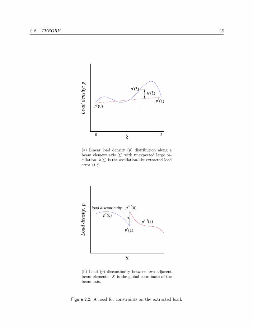
2.2. THEORY 25

ξ

Loa

dde

nsity

:p

pe(0)

(1)pe

pe(ξ)he(ξ)

0 1

(a) Linear load density (p) distribution along abeam element axis (ξ) with unexpected large os-cillation. h(ξ) is the oscillation-like extracted loaderror at ξ.

X

Loa

dde

nsity

:p

pe

pe+1(0)

(1)

pe+1(ξ)

pe(ξ)

load discontinuity

(b) Load (p) discontinuity between two adjacentbeam elements. X is the global coordinate of thebeam axis.

Figure 2.2: A need for constraints on the extracted load.

2.3. EXAMPLES 26

The optimizer L-BFGS-B (version 2.1) (Byrd et al., 1995; Zhu et al., 1994), a limited-

memory quasi-Newton code for large-scale bound-constrained or unconstrained optimization,

is used to solve the scaled and mixed least-squares problem Eq. 2.15. Though the bound-

constraints on the design variables could play an important role in the regularization, this

capability is not addressed for the current studies. A unique solution for the underdetermined

system (when a Tikhonov regularization is not used) is obtained numerically using this

iteration-based optimizer by starting from an approximate uniform load determined by the

priori information. If no priori information is known, the approximate load is assumed to

vanish. Starting from a uniform load with a small design stepsize can prevent the procedure

from stopping at a wildly oscillating solution.

2.3 Examples

In all the numerical examples for the solutions of the LSQ problem Eq. 2.15 by the optimizer

L-BFGS-B, the initial design variables are uniformly set to zero, which means the load

updating procedure starts at a zero level load.

Unless mentioned otherwise, no Tikhonov regularization is used, i.e., λT = 0, λS = 0,

and λC0 = 0.

The procedure terminates if 1) the total number of the function E and the gradient E,x

evaluations exceeds 999 or 2) the projected gradient projE,x (Zhu et al., 1994; Byrd et al.,

1995) is small enough: |projE,x|/(λa + |E|) < εg, or 3) the function value E is small enough:

|E| /λa ≤ εf . Then, the procedure is considered converged. The parameters are chosen

as follows except when stated otherwise: λa = 1 × 1014, εg = 1 × 10−14, εf = 1 × 10−3,

and the machine precision of the computer (Intel Pentium III, 600MHz, 128MB RAM) is

εM = 2.22× 10−16. Referring to Eq. 2.15, we know that E is the scaled least squares. λa is

the scalar of the squared difference between the calculated and measured deformations. εg

2.3. EXAMPLES 27

and εf are, respectively, the relative tolerances of projE,x with respect to λa + |E| and E

with respect to the scalar λa.

In addition to the above termination criteria, for nonlinear examples, the procedure stops

when the step size ‖xcurrent − xprevious‖2 ≤ εstep = 1× 10−3.

We will use the vertical (and horizontal for nonlinear case) nodal displacements under the

reference load as the measured displacements and extract the load distribution with given

direction. In the load updating procedure, the load distribution within an element is repre-

sented by the linear combination of up to six integrated Legendre polynomials while within

the four-noded curved beam FEA procedure, the load distribution is always represented by

cubic Lagrangian interpolation of the four nodal values.

In the results of all the examples, described in the following, X, Y and Z are the position

coordinates of the beam or frame in a 3-D space. Displacements share the same scale as the

position coordinates. When properly scaled, load density p and/or bending strain κ may

share the same axis as the position coordinates. For example, Y (p×10−1) or Y (p×10−1, κ×

10−2) means that p × 10−1 or κ × 10−2 share the same scale as position or displacement

coordinate Y : 10 units of p and/or 100 units of κ equal 1 unit of Y .

For the model order analysis, instead of a standard ANOVA (Analysis of Variance) (Miller

et al., 1997; Bates and Watts, 1988; Walpole and Myers, 1989), the relative model order or

relative number of the unknown variables is used and defined as the ratio of the number of

the independent unknown load coefficients Nx to the number of measured data Nm:

Nxm =

Nx

Nm

=Nelm(1 + degree of IL polynomials)

Nm

(2.19)

When Nxm < 1, the inverse problem is potentially overdetermined with a unique solution; but

when Nxm > 1, the inverse problem is underdetermined with non-uniqueness of the solutions.

The extracted load error variance is defined as the average extracted load error over the

2.3. EXAMPLES 28

beam length:

EExtload =

1

L

Nelm∑e=1

∫ 1

0

[peext(ξ)− pe

ref(ξ)]2dξ (2.20)

where peext and pe

ref are extracted load density and reference applied load density over element

e, respectively.

The basic studies are made for a planar uniform cantilever beam subjected to distributed

load: the load density p has units of (EI/L3). L = 0.5. Three kinds of load distribution of

reference load will studied: uniformly, linearly, and/or sinusoidally distributed.

2.3.1 The Effect of Measurement Methods: Absolute Error and

Relative Error

This example was used to compare the extracted loads obtained using two different displace-

ment measurements. One was the absolute measurement, and the other was the relative

measurement. As shown in Fig. 2.3 and Table 2.1, the load updating problem remains

overdetermined (the relative model order Nxm = Nx

Nm= 8/9) though the 9 measured displace-

ment components are only taken at the two ends of the beam and 7 joint points of the 8

beam elements. It implies that there is a unique LSQ solution.

As seen in Fig. 2.3, when the absolute displacement ai is used, the displacement error

ai − ami and its gradient ai,x with respect to the load x close to the fixed end are smaller.

This would make the load stop at a low level x. When the relative displacement ai/ami is

used, however, its gradient ai,x/ami with respect to the load x is larger if ami is smaller. This

would make the load stop at a higher level x/ami. It is concluded that calculating the error

between the calculated and measured displacements in the relative sense (Eq. 2.8) is better

than in the absolute sense (Eq. 2.7). By increasing the accuracy from εg = 1 × 10−9 to

εg = 1 × 10−14 (which is closer to the machine precision εM = 2.22 × 10−16), the extracted

load agrees perfectly with the reference applied load.

2.3. EXAMPLES 29

X

Y(p

×10

-1)

0 0.1 0.2 0.3 0.4 0.5-0.1

0

0.1

0.2

0.3

0.4 Initial shapeReference loadMeasured displacementShape under extracted loadExtracted load, absolute error,λa=1, εg = 10-9

Extracted load, relative error,λa=1, εg = 10-9

Extracted load, relative error,λa=1, εg = 10-14

Figure 2.3: A comparison of the extracted loads for a cantilever beam with absolute or relative errorbetween the calculated and measured displacements at 9 points. The applied reference load wasuniformly distributed and the extracted load within an element was also assumed to be uniformlydistributed. Eight four-noded curved beam elements were used to model the beam. The extractedload with relative error of displacements was closer to the applied reference load than that withabsolute error of displacements.

2.3. EXAMPLES 30

Table 2.1: EExtload vs. absolute and relative displacement measurements.

Measurement Absolute Relative displacement Relative displacementmethod displacement εg = 1× 10−9 εg = 1× 10−14

Nxm = Nx

Nm8/9 8/9 8/9

EExtload 6.229× 10−2 2.219× 10−2 1.225× 10−10

In all the examples that fellow, the relative measurement is used.

2.3.2 The Effect of the Order of Integrated Legendre Polynomials

Since the extracted load within an element is represented by a linear combination of in-

tegrated Legendre polynomials, a numerical investigation was made on a single elemented

cantilever beam of 4 nodes and 4 measured displacement components to see the effect of

different orders of the polynomials on the extracted load for a uniformly distributed refer-

ence load, as shown in Fig. 2.4 and Table 2.2. The results show that when the order of

polynomials is small enough as to make the problem determined or overdetermined, i.e.,

Nxm = Nx

Nm≤ 1, the applied load can be better extracted. An increase in the order of

polynomials does not always result in a better extracted load. Instead, a higher order of

polynomials introduces more unknowns, tends to make the problem underdetermined, and

results in oscillating extracted loads.

2.3. EXAMPLES 31

0 0 0 0 0 0 0 0 0 0 01 1 1 12 2 2 2 2 2 23 3

X

Y(p

×10

-1)

0 0.1 0.2 0.3 0.4 0.5

0

0.1

0.2

0.3

0.4

Initial shapeReference loadMeasured displacementShape under extracted loadExtracted load, 0 IL: constantExtracted load, 1 IL: linearExtracted load, 2 IL: quadraticExtracted load, 3 IL: cubicExtracted load, 4 ILExtracted load, 5 ILExtracted load, 6 IL

0

1

2

3

Figure 2.4: Extracted load for a cantilever beam subjected to a uniform reference load as a functionof number of integrated Legendre polynomials. Polynomials up to degree 3 extracted the loadperfectly. Higher-order polynomials gave a relatively large oscillating error around the referenceload.

Table 2.2: EExtload vs. the degree of Integrated Legendre polynomial within one element.

Degree of IL 0 1 2 3 4 5 6

Nxm = Nx

Nm1/4 2/4 3/4 4/4 5/4 6/4 7/4

EExtload 0.000 0.000 0.000 8.864 1.436 1.565 1.294

(Uniform load) ×10−4 ×10−2 ×10−2 ×10−2

2.3. EXAMPLES 32

2.3.3 The Effect of Element Size

Refer to Fig. 2.5 and Table 2.3. The extracted loads for applied reference loads with uniform,

linear and sinusoidal distributions were investigated as functions of the number of elements

used. The number of elements used was 1, 2, 4 and 8, respectively. The extracted load

within an element was assumed constant. In all the cases shown in the figure and table,

the measured data were taken only at 4 points except for Fig. 2.5(d). It appears that

Table 2.3: EExtload vs. the number of elements (Nelm).

Nelm 1 2 4 8

Nxm = Nx

Nm1/4 2/4 4/4 8/4

EExtload 0.000 0.000 0.000 0.000

(Uniform load)

EExtload 2.575 1.187 1.300 1.357

(Linear load) ×10−2 ×10−2 ×10−2 ×10−2

EExtload 2.190 3.501 1.771 1.532

(Sine load) ×10−2 ×10−2 ×10−2 ×10−2

the problem is determined or overdetermined for all cases except for the case of 8 elements

and better extracted loads are expected. However, as the constant extracted loads of fewer

elements cannot better represent the non-uniform load distributions, the extracted load

errors tend to be dominant.

Therefore, an increase in the number of finite elements does not help in extracting a load

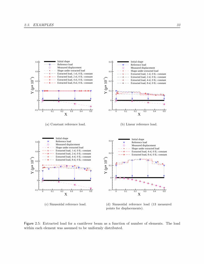
2.3. EXAMPLES 33

1 12 24 48 8

X

Y(p

×10

-1)

0 0.1 0.2 0.3 0.4 0.5-0.1

0

0.1

0.2

0.3

0.4 Initial shapeReference loadMeasured displacementShape under extracted loadExtracted load, 1 el, 0 IL: constantExtracted load, 2 el, 0 IL: constantExtracted load, 4 el, 0 IL: constantExtracted load, 8 el, 0 IL: constant

1

2

4

8

(a) Constant reference load.

1 1

2

24

48 8

X

Y(p

×10

-1)

0 0.1 0.2 0.3 0.4 0.5-0.1

0

0.1

0.2

0.3

0.4 Initial shapeReference loadMeasured displacementShape under extracted loadExtracted load, 1 el, 0 IL: constantExtracted load, 2 el, 0 IL: constantExtracted load, 4 el, 0 IL: constantExtracted load, 8 el, 0 IL: constant

1

2

4

8

(b) Linear reference load.

1 1

2

244

8

8

X

Y(p

×10

-1)

0 0.1 0.2 0.3 0.4 0.5-0.1

0

0.1

0.2

0.3

0.4

Initial shapeReference loadMeasured displacementShape under extracted loadExtracted load, 1 el, 0 IL: constantExtracted load, 2 el, 0 IL: constantExtracted load, 4 el, 0 IL: constantExtracted load, 8 el, 0 IL: constant

1

2

4

8

(c) Sinusoidal reference load.

4 488

X

Y(p

×10

-1)

0 0.1 0.2 0.3 0.4 0.5-0.1

0

0.1

0.2

0.3Initial shapeReference loadMeasured displacementShape under extracted loadExtracted load, 4 el, 0 IL: constantExtracted load, 8 el, 0 IL: constant

4

8

(d) Sinusoidal reference load (13 measuredpoints for displacements).

Figure 2.5: Extracted load for a cantilever beam as a function of number of elements. The loadwithin each element was assumed to be uniformly distributed.

2.3. EXAMPLES 34

closer to the reference load though it has a potential to better represent the non-uniform

distribution of an applied load. Instead, the minimum number of elements that meets the

requirement of the accuracy of FEA may get the extracted load closest to the reference load

for a given number and distribution of measured points over the beam. This makes using a

high precision four-noded beam element advantageous because one can use fewer elements

to obtain a regularization effect by turning the problem to be an overdetermined one.

Increasing the number of elements seemingly tends to improve the quality of the extracted

load far off the supporting boundaries. In fact, the better extracted load was obtained

more due to a better representation of the load distribution. The extracted load got worse

near the boundaries as the number of elements increased due to the limited number of the

measured points. This conclusion is seemingly contrary to the previous observation (Chock

and Kapania, 2003) that aimed at reducing the boundary effect (Johnson, 1998a; Chock

and Kapania, 2003) by increasing the number of elements near the boundaries. In fact, the

reduced boundary effect was more due to an increase in the noise-free measured data (and

reduced model order) near the boundaries. Compare Fig. 2.5(c) and Fig. 2.5(d).

2.3.4 The Effect of Density of Measured Points

Generally speaking, the more information about the structural model, load, and response is

known, the better the extracted load tends to be. Therefore, we expect that an increase of

the local and global density of noise-free measured points does help in bringing the extracted

load closer to the reference load (under which the measured data are taken).

The extracted loads for the uniformly, linearly and sinusoidally distributed reference

loads, respectively, with constant extracted load within an element are presented as functions

of the number of measured points in Fig. 2.6 and Table 2.4 (for linear reference load), in

which eight elements were used and the number of measured points is 4, 7, 13, and 25,

respectively. Obviously, more measured points tend to improve the quality of the extracted

2.3. EXAMPLES 35

X

Y(p

×10

-1)

-0.1 0 0.1 0.2 0.3 0.4 0.5-0.1

0

0.1

0.2

0.3Initial shapeReference loadMeasured displacementShape under extracted loadExtracted load, 8 el - 4 pt, 0 IL: constantExtracted load, 8 el - 25 pt, 0 IL: constant

(a) Constant reference load

X

Y(p

×10

-1)

0 0.1 0.2 0.3 0.4 0.5-0.1

0

0.1

0.2

0.3

0.4 Initial shapeReference loadMeasured displacementShape under extracted loadExtracted load, 8 el - 4 pt, 0 IL: constantExtracted load, 8 el - 7 pt, 0 IL: constantExtracted load, 8 el - 13 pt, 0 IL: constantExtracted load, 8 el - 25 pt, 0 IL: constant

(b) Linear reference load: Full beam.

X

Y(p

×10

-1)

0 0.05 0.1

0

0.01

0.02

0.03

0.04

0.05

0.06

0.07

0.08

0.09

0.1

0.11

0.12

0.13

0.14

(c) Linear reference load: Close-up at fixedend.

X

Y(p

×10

-1)

-0.1 0 0.1 0.2 0.3 0.4 0.5-0.1

0

0.1

0.2

0.3

Initial shapeReference loadMeasured displacementShape under extracted loadExtracted load, 8 el - 4 pt, 0 IL: constantExtracted load, 8 el - 25 pt, 0 IL: constant

(d) Sinusoidal reference load

Figure 2.6: Extracted load for a cantilever beam as a function of number of measured points. Theapplied reference load was uniformly, linearly or Sinusoidally distributed, but the load within eachof the elements was assumed to be uniformly distributed.

2.3. EXAMPLES 36

load, especially near the boundaries, without increasing the number of elements, which tends

to reduce the problem to be overdetermined or more overdetermined (Nxm < 1).

Table 2.4: EExtload vs. the number of measured points (Nm).

Nm 4 7 13 25

Nxm = Nx

Nm8/4 8/7 8/13 8/25

EExtload 1.357 8.766 2.706 2.705

(Linear load) ×10−2 ×10−3 ×10−3 ×10−3

2.3.5 The Effect of Enforcing Smoothing and C0 Continuity

When a polynomial of higher order is assumed within an element for extracting a load, the

resulting extracted load will have unexpected oscillation within an element and discontinuity

between two adjacent elements. Therefore, it may be useful to enforce C0 continuity and

load smoothing. The illustrative example was a planar uniform cantilever beam subjected

to linearly distributed load. Refer to Fig. 2.7. Eight four-noded beam elements (Nelm = 8)

were used. The Nm = 25 measured displacement components were taken from all of the

available nodes (Nnode = 3Nelm + 1 = 25). The first 4 integrated Legendre polynomials

were used for the extracted load representation within an element. Therefore, the problem

is underdetermined at the begining as the relative model order Nxm = Nx

Nm= 8× (1+3)/25 =

32/25 > 1. When only the C0 continuity is enforced, it equivalently adds Nelm − 1 = 7

constraints to the model. This only brings the model to appear barely determined Nxm =

(32− 7)/25 = 1. Although the load discontinuity disappears, the extracted load oscillation

still exists. It implies that the problem remains ill-posed. When both the C0 continuity and

2.3. EXAMPLES 37

X

Y(p

×10

-1)

0 0.1 0.2 0.3 0.4 0.5

0

0.05

0.1

0.15

Initial shapeReference loadMeasured displacementShape under extracted loadExtracted load, 3 ILExtracted load, C0, λC0 = 103

Extracted load, smoothing + C0

Figure 2.7: Constraining the extracted load through the enforcement of load smoothing within anelement and C0 between two adjacent elements: λS , λC0 = 1×103 continuity. The applied referenceload was linearly distributed but a linear combination of first 4 integrated Legendre polynomials(highest degree is 3) was used to represent the load distribution over an element for load extraction.Eight elements were used to model the beam.

load smoothing are enforced, it equivalently adds Nelm − 1 + Nelm = 15 constraints to the

model. This brings the model to appear overdetermined Nxm = (32 − 15)/25 = 17/25 < 1.

Both the load discontinuity and oscillation disappear!

2.3.6 An Application to a Portal Frame

After the basic studies on the load updating for finite element models were for a cantilever

beam using the four-noded beam element, the proposed approach and recommendations

were applied to extract loads acting on a portal frame with a height of unit length and

a span of 2 units. The load density p has units of EI/h3 where h is the height of the

frame. Note that both the applied load and deformation are out of plane. One element

was used for each of the two columns (under linearly distributed load with 1 unit of load

at one end and 0.5 at the other end) and two elements were used for the top beam (under

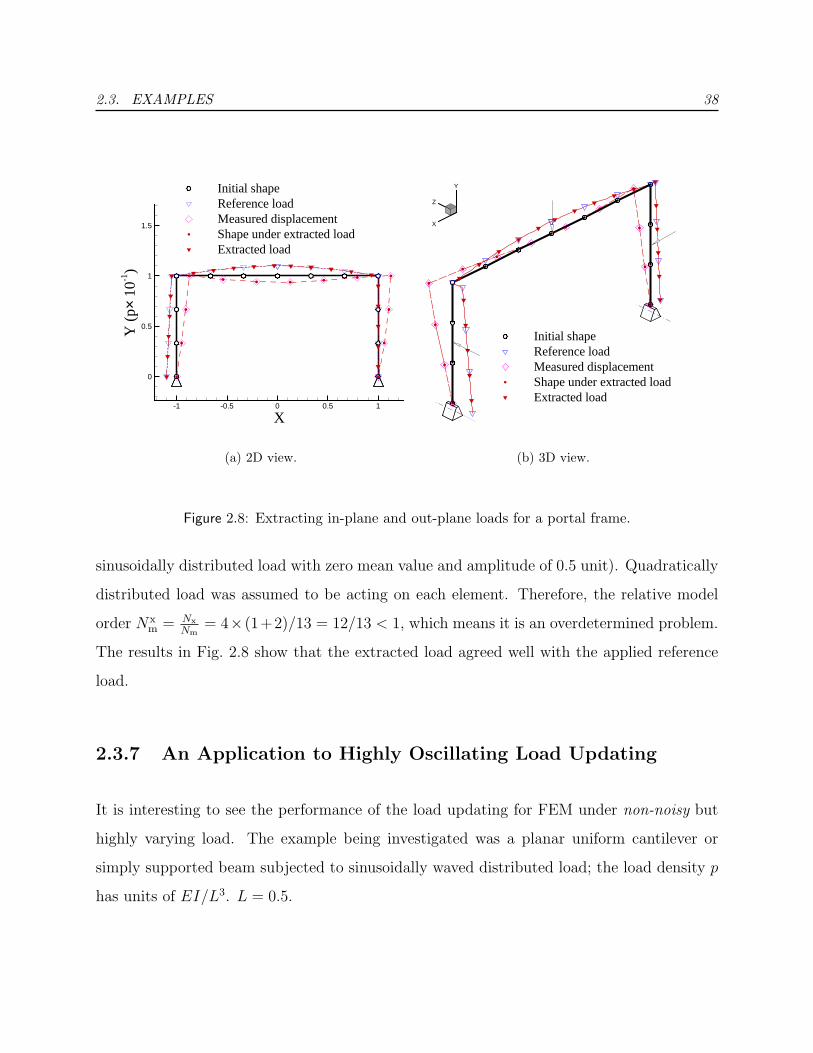
2.3. EXAMPLES 38

X

Y(p

×10

-1)

-1 -0.5 0 0.5 1

0

0.5

1

1.5

Initial shapeReference loadMeasured displacementShape under extracted loadExtracted load

(a) 2D view.

Y

Z

X

Initial shapeReference loadMeasured displacementShape under extracted loadExtracted load

(b) 3D view.

Figure 2.8: Extracting in-plane and out-plane loads for a portal frame.

sinusoidally distributed load with zero mean value and amplitude of 0.5 unit). Quadratically

distributed load was assumed to be acting on each element. Therefore, the relative model

order Nxm = Nx

Nm= 4× (1+2)/13 = 12/13 < 1, which means it is an overdetermined problem.

The results in Fig. 2.8 show that the extracted load agreed well with the applied reference

load.

2.3.7 An Application to Highly Oscillating Load Updating

It is interesting to see the performance of the load updating for FEM under non-noisy but

highly varying load. The example being investigated was a planar uniform cantilever or

simply supported beam subjected to sinusoidally waved distributed load; the load density p

has units of EI/L3. L = 0.5.

2.3. EXAMPLES 39

X

Y(p

×10

-1)

0 0.1 0.2 0.3 0.4 0.5-0.1

0

0.1

0.2

0.3

0.4

0.5Initial shapeReference loadMeasured displacementExtracted load, 0 IL: constantShape under extracted load

(a)

XY

(p×

10-1)

0 0.1 0.2 0.3 0.4 0.5-0.1

0

0.1

0.2

0.3

0.4

0.5 Initial shapeReference loadMeasured displacementExtracted load, 0 IL: constantShape under extracted load

(b)

X

Y(p

×10

-1)

0 0.1 0.2 0.3 0.4 0.5-0.1

0

0.1

0.2

0.3

0.4

0.5 Initial shapeReference loadMeasured displacementExtracted load, 240 el, 0 IL: constantExtracted load, 120 el, 0 IL: constantShape under extracted load

(c)

Figure 2.9: Extracting highly oscillating load for a cantilever beam. The applied reference load(RL) was sinusoidally distributed with unit mean value. The extracted load (EL) was assumeduniformly distributed within an element. (a) The RL had 3 sine waves. 60 elements were used.The EL agreed well with the RL. (b) The RL had 6 sine waves. 120 elements were used. The ELagreed well with the RL at first 3 sine waves near the fixed end but tended to be close to the unitmean value of the RL at the other 3 sine waves near the free end. (c) The applied load had 12sine waves and unit mean value. 240 (120) elements were used. The EL agreed well with the RLat only 1.5 sine waves near the fixed end but tended to be close to the unit mean value of the RLnear the free end. Results using both 120 and 240 elements are almost identical.

2.3. EXAMPLES 40

For all the cases shown in Fig. 2.9, a constant extracted load was assumed for each four-

noded beam element and the measured displacement components were taken at all available

nodes. As a large number of elements was used, the relative model order was Nxm ≈ 1/3 < 1.

It means the problem is very overdetermined.

The results for the cantilever beam show that the load updating using the four-noded

beam element is able to extract the applied load for moderately waved load, but only good

to extract the mean value of the highly waved load. In other words, the load updating tends

to extract the average part of the applied load but filters out the highly oscillating part of

the load. This numerical “damping” effect may be contributed to the truncated errors due

to the limited machine precision. Figure 2.9 shows the results for the cantilever beam.

2.3.8 Measured Strains Based Load Updating

A planar uniform cantilever beam subjected to distributed load: the load density p has units

of EI/L3. L = 0.5. The measured data were the bending strains taken at 3 Gaussian

points of each of the 8 four-noded beam elements. Therefore, the relative model order

was Nxm = 8/(8 × 3) = 1/3 < 1, implying an overdetermined problem. The sensitivities

of the strains with respect to the assumed load coefficients were calculated according to

the method explained in Appendix D. While the uniformly distributed load was assumed

within a single element, the applied reference load was uniformly, linearly and sinusoidally

distributed, respectively, as shown in Fig. 2.10. The results show that the extracted load

agreed well with the applied load.

2.3.9 An Application to Geometrically Nonlinear Beam

Thus far, we have extracted loads acting on beams and frames assuming that the beam or

the frame behaves linearly. The approach was also used to extract loads under which the

2.3. EXAMPLES 41

X

Y(p

×10

-1,κ

×10

-1)

0 0.1 0.2 0.3 0.4 0.5-0.1

0

0.1

0.2

0.3

0.4

0.5Initial shapeReference loadMeaured bending strainExtracted loadBending strain under extracted loadShape under extracted load

(a) Uniformly distributed.

X

Y(p

×10

-1,κ

×10

-1)

0 0.1 0.2 0.3 0.4 0.5-0.1

0

0.1

0.2

0.3

0.4

0.5

Initial shapeReference loadMeaured bending strainExtracted loadBending strain under extracted loadShape under extracted load

(b) Linearly distributed.

X

Y(p

×10

-1,κ

×10

-1)

0 0.1 0.2 0.3 0.4 0.5-0.1

0

0.1

0.2

0.3

0.4

0.5Initial shapeReference loadMeaured bending strainExtracted loadBending strain under extracted loadShape under extracted load

(c) Sinusoidally distributed.

Figure 2.10: Extracting loads of different distributions for a cantilever beam with measured bendingstrains at 3 Gaussian points in each of the 8 elements. Load within each element was assumed tobe uniform.

2.3. EXAMPLES 42

response can be nonlinear. The finite element used in this study is capable of simulating

geometrically nonlinear behavior. The capability to extract loads that lead to a nonlinear

behavior was investigated for a cantilever beam subjected to self-weight, snow load, and

pressure load. For a nonlinear behavior, the axial displacement of the beam cannot be

ignored, while it is ignored for a linear case. It should, however, be pointed out that it would

be rather difficult to measure the axial displacement. Therefore, we investigated the role of

measuring the axial displacement along with the transverse displacement.

The example being investigated was a planar uniform cantilever beam subjected to uni-

formly distributed load: the load density p = 5 has units of EI/L3. L = 0.5.

In all cases, a uniform extracted load was assumed for each of eight four-noded beam

elements. The measured displacements were taken from all the 25 nodes. The problem was

overdetermined for all cases as the relative model order Nxm ≤ 8/(8× 3 + 1) ≈ 1/3 < 1. The

full Newton-Raphson approach (Kapania and Li, 2003b) with 10 equal load steps was used

to solve the geometrically nonlinear problem.

Self weight load

For self-weight type load, the extracted load agrees well with the reference applied load

when transverse displacement alone is taken as measured data, which is as good as when

both transverse and axial displacement are used (see Fig. 2.11).

Snow load

For snow type load (type II-n as compared with type II-c) (Kapania and Li, 2003a), the

extracted load agrees well also with the reference applied load when transverse displacement

alone is taken as the measured data, which is as good as when both transverse and axial

displacement are used ( Fig. 2.12).

2.3. EXAMPLES 43

X

Y(p

×10

-2)

0 0.1 0.2 0.3 0.4 0.5-0.3

-0.2

-0.1

0

0.1

0.2Initial shapeReference loadMeasured displacementExtracted loadShape under extracted load

(a) The applied load was extracted usingtransverse displacements only (the unknownaxial displacements are set to zero in the fig-ure) of all the 25 nodes. The extraction re-quired 45.59 seconds of CPU time, 28 nonlin-ear finite element analyses and 21 load updat-ing iterations, stopping when the design stepsize was 0.00019.

X

Y(p

×10

-2)

0 0.1 0.2 0.3 0.4 0.5-0.3

-0.2

-0.1

0

0.1

0.2

Initial shapeReference loadMeasured displacementExtracted loadShape under extracted load

(b) The applied load was extracted usingboth transverse and axial displacement com-ponents of all the 25 nodes. The extrac-tion required 45.58 seconds of CPU time, 15nonlinear FEA and 11 load updating itera-tions, stopping when the design step size was0.00063.

Figure 2.11: Extracting uniform self-weight type load for a cantilever beam. Eight finite elementswere used to model the beam.

2.3. EXAMPLES 44

X

Y(p

×10

-2)

0 0.1 0.2 0.3 0.4 0.5-0.3

-0.2

-0.1

0

0.1

0.2

Initial shapeReference loadMeasured displacementExtracted loadShape under extracted loadShape under conservative load

II-n

II-c

(a) The applied load was extracted usingtransverse displacements only (the unknownaxial displacements are set to zero in thefigure) of all the 25 nodes. The extrac-tion required 57.30 seconds of CPU time, 23nonlinear FEA and 17 load updating itera-tions, stopping when the design step size was0.00045.

X

Y(p

×10

-2)

0 0.1 0.2 0.3 0.4 0.5-0.3

-0.2

-0.1

0

0.1

0.2

Initial shapeReference loadMeasured displacementExtracted loadShape under extracted load

(b) The applied load was extracted usingboth transverse and axial displacement com-ponents of all the 25 nodes. The extractionrequired 44.26 seconds of CPU time, 16 non-linear FEA and 12 load updating iterations,stopping when the design step size was 0.0006.

Figure 2.12: Extracting uniform snow loads of type II-n (non-conservative consideration) as com-pared with type II-c (conservative consideration) for a cantilever beam. Eight finite elements wereused to model the beam.

2.4. CONCLUSIONS 45

Pressure load

For pressure type load, we found that when only transverse displacement was taken as the

measured data, the load updating procedure failed to converge to a satisfactory solution for

the given load level (Fig. 2.13a). However, simply adding an axial measured displacement

at the free end (Fig. 2.13b), the extraction not only converged to the expected solution, but

the extracted results are also as good as when both the transverse and axial displacements

at all the 25 points are taken as the measured data (Fig. 2.13c).

2.4 Conclusions

The load updating for geometrically linear and nonlinear beams/frames with the given noise-

free measured deformation has been studied by the use of a four-noded curved beam element

and the optimizer L-BFGS-B.

For the basic studies, the extracted load was represented within an element by a linear

combination of integrated Legendre polynomials, the coefficients of which were taken as

design variables of the least-squares problem.

Through a relative model order analysis, the benefits for solving load updating problems

using the relative deformation measurement, the polynomials of lower orders, the elements

of larger sizes (because of using the high precision four-noded beam element), and the defor-

mation of denser measured points were studied for linear responses under the applied loads

of different types.

It was confirmed that using the reduced number of unknown variables to obtain an

overdetermined inverse problem helps get unique and stable extracted loads. Though this

conclusion was verified mainly through illustrative examples for a cantilever beam, it was

generally applicable to other load updating or inverse problems.

2.4. CONCLUSIONS 46

X

Y(p

×10

-3)

-0.1 0 0.1 0.2 0.3 0.4 0.5 0.6-0.3

-0.2

-0.1

0

0.1

0.2

0.3

Initial shapeReference loadMeasured displacementExtracted loadShape under extracted load

(a) The RL failed to be extracted using TDonly. It stopped when DS was 1.114×10−12

but the objective did not converge to zerothough each nonlinear FEA converged!

XY

(p×

10-2)

0 0.1 0.2 0.3 0.4 0.5-0.3

-0.2

-0.1

0

0.1

0.2Initial shapeReference loadMeasured displacementExtracted loadShape under extracted load

(b) The RL was extracted using TD and ADmeasured only at the free-end. It took 28.98seconds of CPU time, 18 FEA and 14 LUI,stopping when DS was 0.00079.

X

Y(p

×10

-2)

0 0.1 0.2 0.3 0.4 0.5-0.3

-0.2

-0.1

0

0.1

0.2

Initial shapeReference loadMeasured displacementExtracted loadShape under extracted load

(c) The RL was extracted using all TD andAD. It took 32.96 seconds of CPU time, 20FEA and 12 LUI, stopping when DS was0.00065

Figure 2.13: Extracting uniform pressure load for a cantilever beam with different choices of dis-placement measurements. Eight finite elements were used. The unknown axial displacements areset to zero in the figure. The TD were measured at all the 25 nodes. TD: transverse displacements;RL: reference load; AD: axial displacements. DS: design stepsize; LUI: load updating iterations.

2.4. CONCLUSIONS 47

Application examples were given for a 3D portal frame load updating, extracting highly

oscillating loads, and a strain-based cantilever beam load updating, and load updating for

geometrically nonlinear finite element models under under self-weight, snow and/or pressure

loads.

The extraction of highly varying applied load shows that the load updating for FEM

using the four-noded beam element is able to extract moderate waved load, but only extract

the average part of the load and filter off the highly oscillating part. This damping effect is

due to the truncated error of numerical implementation.

For a linear FEM, using only transverse components of the displacements are enough to

extract the applied load of a cantilever beam or simply-supported beam. However, for a

geometrically nonlinear FEM, both transverse and axial components of the displacement at

the measured points have to be used for a higher load level, especially for pressure load.

Present conclusions may be applied to the measurement based load updating for general

finite element models when the measured data are pre-smoothed or the noise in the data is

pre-filtered off.

Chapter 3

Placement Optimization of Fiber

Optic Sensors

We address the methodology and implementation for the placement optimization of a

distributed sensing fiber optic sensor using a simple breeding Genetic Algorithm (GA). The

sensor consists of an infinite number of infinitesimal sensors continuously connected together,

and its total output is proportional to the absolute value of the first time derivative of the

integrated spatial perturbation along the fiber. For the placement optimization, the sensor

performance is simplified as the full length integration of the absolute curvature change of

the fiber optic cable due to the perturbation on the deformed shape of the fiber optic cable.

The sensing optical fiber curve is represented by Non-Uniform Rational B-Splines (NURBS).

The coordinates of the control points of the NURBS curve are the design variables, coded as

genes of a chromosome string in the GA. The constraints include the maximum length and

maximum initial curvature of the fiber optic cable. As an application example for a clinical

smart bed, the deformation of the fiber optic cable is calculated from the deformation of

the mattress surface by the assumption that the fiber optic cable remains adhered to the

mattress surface, while the deformation of the foam-cored mattress is calculated using the

finite element code MSC.NASTRAN under given body pressure distributions. An interactive

Java tool was developed for the implementation of the placement optimization of the fiber

optic sensor. Illustrative examples are presented to demonstrate the validity of the approach

and usefulness of the tool. Though the specific example is for clinical use, the fiber optic

sensor and associated placement methodology can also be used in pilot/passenger seats and

structures for flight vehicles.

48

3.1. AN OVERVIEW 49

3.1 An Overview

Sensor placement or sensor location design is an important issue that engineers must address

in solving problems like identification, analysis, control, and health monitoring of various

structures. Such structures include aerospace crafts, bridges, and offshore platforms, as well

as human bodies in clinical areas. There are often many limitations in sensor placement.

For example, the number of available sensors is limited and their positions essentially fixed

in service (Abdullah et al., 2001; Guo et al., 2004). In such situations, sensor placement

becomes a critical issue which governs the success and failure of the target purpose.

Though there are many types of sensors/actuators for structural health management

technology for non-aerospace and aerospace vehicles including fiber optic sensors, active

and passive acoustic sensors, electromagnetic sensors, wireless sensing systems, MEMS, and

nanosensors (Prosser, 2003), the algorithms for optimal placement of actuators and sensors

appear to be very similar regardless of the application (Padula and Kincaid, 1999). All can

be posed as selecting a subset of locations from a large set of candidate locations (Padula

and Kincaid, 1999). Therefore, it is useful to review some literature on sensor placement in

other fields for the sensor placement of the specific kind.

Methods have been developed to optimally place sensors to address the identification and

control of dynamic structures by Udwadia and Garba (1985) and Lim (1991), etc. Kammer

(1991b) proposed an effective independence algorithm based on the contribution of each

sensor location to the linear independence of the identified modes. The initial candidate set

of sensor locations was quickly reduced to the number of available sensors. Kammer (1991a)

dealt with the effect of sensor error on sensor placement. He also reported many earlier work

on the optimal placement of sensors for identification and control from a control dynamics

standpoint, and some smaller amount of work considering optimal sensor placement for

identification from a structural dynamics point of view. Kammer and Brillhart (1994) studied

optimal sensor placement for modal identification using system-realization methods. The

3.1. AN OVERVIEW 50

sensor placement method maximized spatial independence and signal strength of targeted

mode shapes by maximizing the determinant of an associated Fisher information matrix.

Hemez and Farhat (1994) extended the effective independence method in an algorithm where

sensor placement was achieved in terms of the strain energy contribution of the structure.

Miller (1998) computed a Gaussian quadrature formula using the functional gain as a

weight function, and thought that the nodes of the quadrature formula gave the optimal

locations for sensors. Hiramoto et al. (2000) used the explicit solution of the algebraic

Riccati equation to determine the optimal sensor/actuator placement for active vibration

control. Wouwer et al. (2000) presented an optimality criterion for the selection of optimal

sensor locations in distributed parameter systems; the criterion was based on a measure of

independence of the sensor responses. For fault detection, Worden and Burrows (2001) used

a number of different methods to determine an optimal sensor distribution based on the

curvature data.

Due to their capability to handle discrete design variables and search for global solutions

without using gradient information, GAs have been widely used in sensor placement type

problems (Padula and Kincaid, 1999; Abdullah et al., 2001; Guo et al., 2004), sometimes

combined with gradient-based methods (Padula and Kincaid, 1999; Abdullah et al., 2001).

Abdullah et al. (2001) addressed the necessity to use GAs for placement of sensors/actuators

on civil structures, members of which are usually discrete and therefore discrete locations are

available for sensors/actuators. Guo et al. (2004) presented an improved GA for the global

and constrained optimization of sensor locations for structural health monitoring systems.

The performance function was based on damage detection. To overcome the inefficiency due

to infeasible solutions to the problem, some improved strategies were used, such as crossover

based on identification code, mutation based on two gene bits, and improved convergence.

They concluded that the improved GA is faster than the penalty function method and the

forced mutation method.

In the early GA researches, genetic representation of a chromosome or a solution was

3.1. AN OVERVIEW 51

limited to binary digits (Holland, 1975; Michalewicz, 1994; Houck et al., 1995), but problem

representation has been the subject of much investigation (Houck et al., 1995). It has been

shown that more natural representations are more efficient and produce better solutions

(Michalewicz, 1994). One useful representation of an individual or chromosome for function

optimization involves genes or variables from an alphabet of floating point numbers with

values within the variables’ upper and lower bounds. Michalewicz (1994) has done extensive

experimentation comparing real-valued and binary GAs and shows that the real-valued GA

is an order of magnitude more efficient in terms of CPU time. He also shows that a real-

valued representation moves the problem closer to the problem representation which offers

higher precision with more consistent results across replications (Michalewicz, 1994). Along

this line, Zhang et al. (2000) presented a novel float-encoded GA and applied it to the

optimal control of flexible smart structures bonded with piezoelectric actuators and sensors.

The performance function was based on the maximization of dissipation energy due to a

control action. The optimization algorithm allowed an integrated determination of actuator

and sensor locations and feedback gains.

Padula and Kincaid (1999) provided a survey of actuator and sensor placement problems

from a wide range of engineering disciplines (both aerospace and non-aerospace engineer-

ings) and a variety of applications. Combinatorial optimization methods are recommended

as a means for identifying sets of actuators and sensors that maximize performance. Frecker

(2003) reviewed the work done in this area since 1999 to 2003, in addition to optimization

strategies for topology design of actuators, actively controlled structures, and drive electron-

ics design.

This study addresses the placement optimization of a distributed sensing fiber optic

sensor for its potential usage in human-machine systems, such as pilot/passenger seats, and

structures for flight vehicles though it was initially developed by Spillman Jr. et al. (2004)

for a clinical smart bed. The fiber optic sensor is used to both sense the movement and

determine the posture of the human body. For the clinical smart bed, for example, the

3.1. AN OVERVIEW 52

laserdiode

digitalcamera

specklepattern

multimodesensingoptical fiber

mattress

bed base

output proportionalto the absolute valueof the first timederivativeof a perturbationintegrated alongthe fiber length

processing

Figure 3.1: A schematic diagram of the smart bed. The distributed sensing fiber optic cable isstitched on the bed surface.

sensor can be used to monitor the movement of a patient and determine whether or not

the patient is lying on his/her sides, stomach or back. The sensor can be even used to

measure the breathing and heart rates. Proven to be a success as a concept, it requires

a design methodology and tool to optimally place the fiber optic sensor to maximize its

performance. Figure 3.1 is a schematic diagram of the distributed sensing fiber optic sensor

on the smart bed. The output of the distributed sensing fiber optic sensor, which consists of

an infinite number of infinitesimal sensors continuously connected together, is proportional

to the absolute value of the first time derivative of the integrated spatial perturbation along

the fiber, as presented by Spillman Jr. et al. (2004) and shown in Fig. 3.1. For placement

optimization purpose, the sensor performance is simplified to be the integrated absolute

curvature change of the fiber optic cable with respect to a perturbation due to the body

movement of a patient lying on it.

The fiber optic cable is represented by a NURBS curve (Farin, 1990) that is uniquely

3.2. DESCRIPTION OF THE PROBLEM 53

determined by a finite number of control points. This make it possible to convert the

placement optimization of an infinite number of sensors to the placement optimization of a

finite number of control points of a NURBS curve. Therefore, one can successfully use the

popular GAs (Markus et al., 1997; Faupel, 1998; Gurdal et al., 1999) to obtain the optimal

placement of the distributed sensing fiber optic senor.

We model the smart bed as an elastic mattress core and ignore the flexible cover. The

initial and deformed geometries of the bed due to the body weight and movement of the

patient are calculated, using the finite element analysis tool, MSC.NASTRAN, from the

given body pressure distribution (Nicol and Rusteberg, 1993). The deformations of the fiber

optic cable are then extracted from the deformations of the mattress.

An interactive Java tool is developed to implement the above ideas. Illustrative examples

are given to demonstrate the validity of the presented method.

Though the specific example is for clinical use, the fiber optic sensor and associated

placement methodology can also be used in pilot/passenger seats and structures for flight

vehicles. The other potential use is the placement of Fiber Bragg Grating (FBG) sensors for

health monitoring structures in both aerospace engineering (Davisy et al., 1996) and civil

engineering (Udd et al., 1998; Lin et al., 2005).

3.2 Description of the Problem

3.2.1 Objective/Sensor Performance Function

The concept of the distributed sensing fiber-optic sensor is based on mode angle shifting of

a multimodal optical fiber. When the fiber pattern on the smart bed is perturbed by the

motion, due to either respiration or heartbeat, the radius of the annulus (a ring-like output

3.2. DESCRIPTION OF THE PROBLEM 54

light signal figure projected on a flat surface) increases. As a result, if a special fiber is used

that only intercepts a portion of the annular or speckle pattern of this light and allows this

intercepted light to pass to a detector, an output signal will result in continuing information

about the perturbation that caused the change in the signal, See Fig. 3.1. This output, e.g.

the change in the radius of the annulus, is proportional to the absolute value of the first time

derivative of the integrated spatial perturbation along the fiber (Spillman Jr. et al., 2004).

That is, the whole output of this distributed sensing optical fiber is the sum of the outputs

of an infinite number of infinitesimal fiber segments. The contribution of each infinitesimal

fiber segment to the output is proportional to its spatial perturbation that is the angular

change of the fiber segment.

For the placement optimization of the sensor, the experimentally verified physical law

for the sensor output (Spillman Jr. et al., 2004) is simplified as: the sensor performance

function is the sum of the absolute angular change dθ = ||∆κ(s)||2ds over an infinite number

of the infinitesimal fiber segments ds’. That is, the performance of the whole distributed

sensing fiber optic sensor is the integration of the absolute curvature change due to a given

spatial perturbation over the whole fiber length L:

∆θ =

∫ L

0

||∆κ(s)||2ds (3.1)

where ∆κ(s) = ∆κx(s)ix + ∆κy(s)iy is the curvature (vector) change of the fiber segment

ds, as the dominant spatial perturbation.

3.2.2 Design Variables/Placement Representation

Since a distributed sensing fiber optic sensor consists of an infinite number of infinitesimal

sensing fiber segments, the placement of those infinite number of sensors seems to be ex-

tremely hard. We can, however, transfer the placement of an infinite number of sensors to

the placement of a finite number of the control points - “dummy sensors”, if we represent

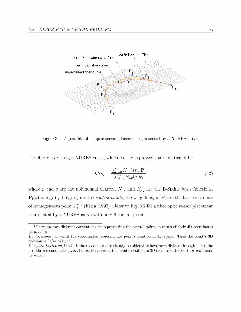
3.2. DESCRIPTION OF THE PROBLEM 55

Figure 3.2: A possible fiber optic sensor placement represented by a NURBS curve.

the fiber curve using a NURBS curve, which can be expressed mathematically by

C(s) =

∑ni=0 Ni,p(s)wiPi∑n

i=0 Ni,p(s)wi

(3.2)

where p and q are the polynomial degrees, Ni,p and Nj,q are the B-Spline basis functions,

Pi(s) = Xi(s)ix + Yi(s)iy are the control points, the weights wi of Pi are the last coordinate

of homogeneous point Pwi

1 (Farin, 1990). Refer to Fig. 3.2 for a fiber optic sensor placement

represented by a NURBS curve with only 6 control points.

1There are two different conventions for representing the control points in terms of their 4D coordinates(x, y, z, w):Homogeneous, in which the coordinates represent the point’s position in 4D space. Thus the point’s 3Dposition is (x/w, y/w, z/w).Weighted Euclidean, in which the coordinates are already considered to have been divided through. Thus thefirst three components (x, y, z) directly represent the point’s position in 3D space and the fourth w representsits weight.

3.2. DESCRIPTION OF THE PROBLEM 56

3.2.3 Constraints

Geometrical constraints

For a given placement of the sensing fiber, there is a geometric constraint on it, that is, the

optical fiber cable remains in contact with the mattress surface. Although the actual fiber

optic cable may slip on the mattress, it is assumed that the fiber cable remains adhered to

the mattress for simplicity in this study.

The mattress surface is assumed to be initially flat. The mattress surface and the fiber

optic sensor curve on it deform after the patient lies down on the bed. The deformed mattress

surface can be assumed to be a general surface that can be represented by a NURBS surface

or be determined from FEA for a given body pressure.

The deformed mattress surface is further changed due to a dynamic perturbation, such

as the respiration and heart beat of the patient. This deformed surface after perturbation

can be further determined from FEA for the given pressure perturbation.

For a fixed local curvature change of the deformed mattress surface, the longer the fiber

is, the larger the total curvature change will tend to be. Therefore, we might consider using

a longer fiber optic cable to get a better performance of the sensor. However, we need to put

a constraint on the maximum length due to cladding mode lost or laser power limit; e.g. we

can set L ≤ Lmax, where Lmax is usually on the order of several meters.

Physical and mechanical constraints

Because the optical fiber and mattress membrane are very thin, the lateral (shearing and

bending) stiffnesses of the fiber and mattress cover are negligible. Since the mattress cover

is easy to wrinkle, the in-plane stiffness of the cover may also be ignored. This assumption

makes it possible to perform only one FEA for a given body pressure distribution during

3.3. PROCEDURE AND IMPLEMENTATION 57

the whole optimization process since a change in placement of the fiber optic cable will not

change the deformed shape of the mattress surface. This makes using a global searching GA

possible.

A micro bend design may be useful to enhance the sensor performance. However, the

initial curvature or radius of the sensing fiber is subject to the limitation due to bending

losses (Udd, Schulz, Seim, Corones, and Laylor 1998).

3.3 Procedure and Implementation

3.3.1 Procedure

Refer to Fig. 3.3 for a simplified flow chart of the procedure for the optimal placement of

the fiber optic cable.

Step 1. Choose a mattress model

Two main classes of bed mattresses are spring cored and foam-filled cored, respectively.

Practically speaking, the covers of all mattresses are woven of certain materials. For this

study, we choose a core material with material data given in Table 3.1 to model the mattress

of a standard size 198cm× 91.5cm× 16.5cm (78”× 36”× 6.5”).

Step 2. Determine the body pressures due to the self-weight and perturbation

by measurement or numerical simulation

The self-weight induced body pressure and perturbed body pressure on the mattress surface

can either be determined by experimental measurements or by numerical simulations. For

3.3. PROCEDURE AND IMPLEMENTATION 58

Figure 3.3: Chart for optimal placement of the fiber optic sensor.

3.3. PROCEDURE AND IMPLEMENTATION 59

Table 3.1: Latex Mattress Core Fact Sheet.Standard Hardness Specifications for Mattress Cores

Hardness Range (ILD= Indentation Load Deflection)Soft 20-24 ILD

Medium 25-29 ILDFirm 30-34 ILD

Extra Firm 35-39 ILDSuper Firm 40-44 ILD

Hardness range measurements based on ASTM D-1055Source: http://www.flobeds.com/mattspec.htm

illustrative purpose and initial study, we can assume a simple body pressure distribution

(Nicol and Rusteberg, 1993) on the mattress, for example, given in the form of a NURBS

surface within a given area, which can practically model all kinds of pressure distributions.

Our numerical studies showed that the contribution of the initial deformation of the

mattress to the sensor performance is small. Therefore, we only consider the perturbed

body pressure for linear analysis.

Step 3. Determine the deformations of the mattress subjected to the body

pressures by MSC.NASTRAN

A linear analysis was performed to obtain the deformation of the mattress subjected to a

given pressure distribution pattern with unit maximum value. FEM model: 70 × 30 × 4 =

8, 400 brick elements for the mattress core; the cover is ignored. Mattress core hardness is

assumed to be soft and taken from Table 3.1 and transferred into Young’s modulus as in

Table 3.2.

Applied pressure and mattress deformation are shown in Fig. 3.4 and Table 3.2.

3.3. PROCEDURE AND IMPLEMENTATION 60

(a) Body pressure. (b) Deformation.

Figure 3.4: Body pressure and deformation of the soft cored mattress. The pressure P has a unitof N/cm2.

Table 3.2: Latex Mattress Core Fact Sheet.

Mattress core hardness and calculated maximum deformations

under the assumed body pressure (with the maximum value of 1.00N/cm2)Hardness Range E = Young’s Modulus Maximum deflection Maximum nominal

(N/cm2) (cm) strainSoft 1.213 15.0 0.909

Medium 1.493 12.2 0.739Firm 1.765 10.3 0.624

Extra Firm 2.041 8.92 0.541Super Firm 2.317 7.86 0.476

Note:(1) The typical values of Young’s modulus E are calculated from Table 3.1(2) Poisson’s ratio ν = 0.3 for latex rubber foam is from Fig. 12 of Roberts and Garboczi (2002).

3.3. PROCEDURE AND IMPLEMENTATION 61

Step 4. Calculate the integrated curvature change of any given placement of the

fiber optic cable due to the body pressure perturbation

Assume that the fiber cable remains adhered to the mattress surface without slipping. Then,

we can easily extract the relevant fiber curve deformations from the initial and perturbed

mattress deformations. We can thereafter calculate the sensor performance, i.e., the inte-

grated curvature change, for given design variables – the locations of control polygons of the

NURBS curve.

Step 5. Calculate the sensitivity of the integrated curvature change of any given

placement of the fiber optic cable with respect to a placement change by finite

difference method

This step is to calculate the design sensitivity of the objective function with respect to design

variables. However, we ignore this step as we are using GAs.

Step 6. Update the placement of the fiber optic cable by optimization technique

An optimizer (Gurdal et al., 1999) is used to update the placement of the fiber optic cable

and give a better design than the previous one. A GA (Faupel, 1998) is chosen as the

optimizer.

3.3.2 Implementation

The interactive design tool “Java Tool for the Placement of Fiber Optic Sensors” is devel-

oped in Java, aiming at the implementation of Steps 4, 5 and 6 of the procedure: for any

given initially deformed mattress surface and any given placement of the fiber optic cable

3.4. PLACEMENT OPTIMIZATION OF THE FIBER OPTIC SENSORS FOR A SMARTBED BY GA 62

constrained on the mattress, we shall be able to calculate the integrated curvature change of

the fiber optic cable due to any perturbation of the mattress surface and its sensitivity with

respect to a design change, so that we are able to update the placement of the fiber optic

cable to a better design both manually and by the optimization technique, e.g. GA.

3.4 Placement Optimization of the Fiber Optic Sensors

for a Smart Bed by GA

To demonstrate the current capability of the interactive Java tool for the placement opti-

mization of fiber optic sensors, an illustrative example is given here.

The Genetic Algorithm optimizer, GAJIT, the Java package kindly provided by Faupel

(1998), is used to optimize the placement of the fiber curve.

3.4.1 A Very Simple Breeding Algorithm

Not addressing efficiency in this study, we only use a very simple breeding algorithm in

GAJIT to illustrate applying GAs to a NURBS curve design as follows:

• Remove a percentage of the least fit designs through culling;

• Preserve a percentage of the most fit designs unchanged (elitism);

• Then breed the elite and the remainder at random to fill out the rest of the next

generation.

The relevant parameters for the GA used here are:

• Culling rate: percentage deemed unfit for reproduction;

3.4. PLACEMENT OPTIMIZATION OF THE FIBER OPTIC SENSORS FOR A SMARTBED BY GA 63

Figure 3.5: A placement of a fiber optic sensor for a smart bed represented by a NURBS curve with6 control points. Adopted from Fig. 3.7b.

• Elite rate: percentage of population carried forward unchanged from each generation;

• Weight: the weighting it has for the chances of it being selected.

3.4.2 Coding/Decoding

A typical GA is only suitable for discrete design variables. To apply a GA to an optimization

problem of continuous design variables, we can approximate the continuous design variables

using discrete ones.

For the placement of the fiber optic sensor, we choose two components (X, Y ) of the (4

out of 6 in Fig. 3.5) control points of the fiber NURBS curve as design variables (the two

ends are fixed). The scaled coordinate components are −1 ≤ X = 2X/Lmattress ≤ 1 and

−1 ≤ Y = 2Y/Wmattress ≤ 1, where Lmattress and Wmattress are the length and width of the

mattress, respectively. We code the design variables

3.4. PLACEMENT OPTIMIZATION OF THE FIBER OPTIC SENSORS FOR A SMARTBED BY GA 64

X10 = [0.0968 − 0.4194 − 0.2258 − 0.4839 0.1613 0.5484 − 0.2903 0.2258]10

using the genes (e.g. the gene size is 5) of a chromosome represented by a binary string:

X2 = [10011 01011 11000 10010 01000 01100 01001 10001]2

Each chromosome, for example, represents one of the 20 members of the population.

Any chromosome X2 has to be decoded back to its counterpart X10 for evaluation of the

fitness of the chromosome.

3.4.3 Fitness Function

The fitness function for the GA is defined in the sense of the so-called exact penalty function

method:

Fitness =

∫ L

0||∆κ(s)||2ds

Lmax

·

[1− pκ max(κ0max

κu0 max

− 1, 0)− pL max(L

Lmax

− 1, 0)]

(3.3)

where

∆θ =

∫ L

0

||∆κ(s)||2ds

according to Eq. (3.1), is the sensitivity of the fiber topic sensor due to a given body per-

turbation. L and Lmax are the current and maximum allowed lengths of the fiber curve,

respectively. κ0max and κu0max (= 0.5/cm) are the maximum and the maximum allowed ini-

tial curvatures of the fiber curve, respectively. pL and pκ are the corresponding penalty

factors.

3.4. PLACEMENT OPTIMIZATION OF THE FIBER OPTIC SENSORS FOR A SMARTBED BY GA 65

3.4.4 Examples

Example 1. The assumed perturbed surface is from the initial flat surface of the

NURBS with 7 × 5 uniformly distributed control net by an 18.00cm downward

perturbation of the control point at the center of the mattress. Only 6 control

points of the fiber NURBS curve are used, two ends of which are fixed.

Lmax = 200cm; pL = 1 and pκ = 1; the elite rate, culling rate and weight are 0.05, 0.2 and

0.1, respectively. Figure 3.6 shows the example of the placement optimization of a fiber optic

(a) An initial placement: ∆θ = 0.29 (rad);L = 200.55 (cm); κ0max = 0.04 (1/cm).

(b) After 500 generations: ∆θ = 1.94 (rad);L = 198.58 (cm); κ0max = 0.50 (1/cm).

(c) After 1000 generations: ∆θ = 2.30 (rad);L = 207.67 (cm); κ0max = 0.49 (1/cm).

(d) After 2000 generations: ∆θ = 2.37 (rad);L = 202.83 (cm); κ0max = 0.46 (1/cm).

Figure 3.6: Placement optimization of a fiber optic sensor for a smart bed by GA.

sensor for a smart bed by GA. It is shown that the initial placement of the fiber curve is

3.4. PLACEMENT OPTIMIZATION OF THE FIBER OPTIC SENSORS FOR A SMARTBED BY GA 66

feasible but with a lower sensitivity of 0.29rad, a length of 200.55cm, and maximum initial

curvature of 0.04/cm. After 2000 generations of the GA iteration, an updated placement is

achieved, with a higher sensitivity of 2.37rad, a length of 202.38cm, and maximum initial

curvature of 0.46/cm. Figure 3.7 is a 3-D view of the initial placement and updated placement

after 2000 generations of the GA iteration. We can see clearly that the initial placement of

the fiber optic sensor is inefficient due to the fact that most of the sensing fiber is in a much

less perturbed region. After 2000 generations of the GA iteration, much of the sensing fiber

falls into a highly perturbed region with a higher curvature change.

Example 2. The assumed perturbed surface is obtained by a 10% scaling of

the calculated deformation of the soft cored mattress under an assumed body

pressure as shown in Fig. 3.4. Only 25 control points of the fiber NURBS curve

are used, two ends of which are fixed.

Lmax = 400cm; pL = 4 and pκ = 2; the elite rate, culling rate and weight are 0.05, 0.2 and

0.1, respectively. Figure 3.8 shows the example of the placement optimization of a fiber optic

sensor for a smart bed by GA. It is shown that the initial placement of the fiber curve is

feasible but with a lower sensitivity of 1.01rad, a length of 358.95cm, and maximum initial

curvature of 0.49/cm. After 9000 generations of the GA iteration, an updated placement is

achieved, with a higher sensitivity of 1.51rad, a length of 358.95cm, and maximum initial

curvature of 0.49/cm. Figure 3.9 is a 3-D view of the initial placement and updated placement

after 9000 generations of the GA iteration. We can also see clearly that the initial placement

of the fiber optic sensor is less efficient due to the fact that one part of the sensing fiber is in

an unperturbed region. After 9000 generations of the GA iteration, that part of the sensing

fiber approaches the perturbed region and the overall sensing fiber tends to form a star-like

pattern in the perturbed region.

3.5. CONCLUSIONS 67

3.5 Conclusions

• The deformation of the smart bed is simulated by finite element analysis (e.g using

MSC.NASTRAN) when the body pressure is available.

• Both deformed area of the bed surface and fiber optic cable are represented by NURBS.

• A Java tool is developed as an interactive research and design tool for the fiber optic

sensor.

• The sensitivity of the fiber optic sensor is indirectly represented by the integration of

the absolute curvature change over the curve length.

• The Genetic Algorithm (GA) is chosen as the optimizer for the placement optimization

of the fiber optic sensor.

• The fitness function of the GA is defined in the sense of the exact penalty function

method, where the length and maximum initial curvature of the fiber curve are limited

by prescribed upper bounds.

• Illustrative examples are given for the demonstration of the placement optimization of

the fiber optic sensor.

3.5. CONCLUSIONS 68

(a) An initial placement.∆θ = 0.29 (rad).

(b) An updated placement after 2000 generations of GA iteration. ∆θ = 2.37 (rad)

Figure 3.7: A 3-D view of the initial placement and updated placement. The perturbed (dashed)and unperturbed (solid) fiber curve shapes of the optimal placement of the fiber optic sensor.

3.5. CONCLUSIONS 69

(a) An initial placement: ∆θ = 1.01 (rad);L = 358.95 (cm); κ0max = 0.49 (1/cm).

(b) After 5000 generations: ∆θ = 1.32 (rad);L = 386.33 (cm); κ0max = 0.49 (1/cm).

(c) After 7000 generations: ∆θ = 1.47 (rad);L = 386.09 (cm); κ0max = 0.49 (1/cm).

(d) After 9000 generations: ∆θ = 1.51 (rad);L = 399.99 (cm); κ0max = 0.49 (1/cm).

Figure 3.8: Placement optimization of a fiber optic sensor for a smart bed by GA.

3.5. CONCLUSIONS 70

(a) An initial placement. ∆θ = 1.01 (rad).

(b) An updated placement after 9000 generations of GA iteration. ∆θ = 1.51 (rad).

Figure 3.9: A 3-D view of the initial placement and updated placement. The perturbed (dashed)and unperturbed (solid) fiber curve shapes of the optimal placement of the fiber optic sensor.

Chapter 4

Optimal Design of Unitized Panels

with Curvilinear Stiffeners

In this chapter, we show many numerical results of optimal design study of stiffened pan-

els where the reference axes of the stiffeners can be curvilinear. An integrated approach to

use different capabilities in relevant fields, such as NURBS, DistMesh, and MSC.NASTRAN,

etc., are adopted in the MATLAB environment. Numerical studies are made to look into

the effects of certain factors on the optimal designs of stiffened panels under buckling con-

straints. Those factors include orientation, spacing, location, and curvature. It is observed

that curvilinear placement of stiffeners is equivalent to an orientation, spacing, location and

intersection placement of infinitesimal straight and connected stiffeners, and provides an en-

hanced design space. This enhanced design space sometimes leads to better designs than

purely using straight stiffeners. This work reconfirms the necessity to use global optimiza-

tion techniques to perform topology/placement/shape optimization of curvilinearly stiffened

panels along with size optimization.

4.1 An Overview

Availability of high-performance computing and commercially available software, such as

MSC.NASTRAN and MATLAB, is having enormous impact on the manner how structures

are designed. Similarly, the ongoing revolution in computer-aided manufacturing has sig-

nificantly removed the previous limitations on the design and manufacturing of a structure.

For example, using Electronic Beam Freeform Fabrication (EBF3), a rapid metal deposition

71

4.1. AN OVERVIEW 72

process that works efficiently with a variety of weldable alloys (Taminger and Hafley, 2003),

allows the stiffeners of a panel to have continuously varying properties such as orientation,

thickness, width, and material properties. These design parameters are mostly kept constant

in earlier studies because of manufacturing constraints. Together, the software for computer-

aided design, engineering and manufacturing (CAD/CAE/CAM) are bound to play a major

role in the design of all future aerospace and other related structures. We envision an en-

vironment in which design and manufacturing, using modern information technology, would

be integrated into one step, which also follows the modern trend for the unitized parts for

flight vehicles structures (Renton et al., 2004). Here, we address the integrated capability

of CAD and CAE implemented in the MATLAB environment to provide a methodology

and a practical design toolbox, EBF3paneloptimization, for optimization of unitized panels

with stiffeners, especially, manufactured by the EBF3 technique. Though the development

of EBF3paneloptimization is still in progress, we have used it to run numerous examples to

confirm the important effects of the stiffeners’ orientation, spacing, location, and curvature,

etc., on the optimal design of a stiffened panel.

Although our current effort has been only partially automated and mainly dealt with

planar stiffened panels, the extension can be made to implement the automatic placement

and size optimization of both planar and curvilinear stiffened panel as shown in Fig. 4.1,

and thus provide a capability to design advanced unitized curved panels with curvilinear

stiffeners. This is an extension to optimize low-cost high-performance panels that have a

grid of stiffeners with a prescribed uniform or non-uniform pattern, such as isogrid and

geodesically stiffened panels (Gerdon and Gurdal, 1985; Grall and Gurdal, 1992; Gurdal and

Gerdon, 1993).

Advances in manufacturing and computer-aided design and engineering are making it

possible to fabricate these advanced unitized structures.

4.2. METHODOLOGY, PROCEDURE, AND CAPABILITY 73

Figure 4.1: A curved panel with arbitrarily oriented stiffeners and its finite element mesh.

4.2 Methodology, Procedure, and Capability

4.2.1 Methodology

The methodology used here does not focus on developing new theories, numerical methods,

and self-written in-house codes to achieve the solution to the stiffened panel optimization,

as that would only limit the capability of solving various practical problems. Instead, we

seek an integration of the advanced capabilities in CAD/CAE/CAM in the versatile MAT-

LAB environment to develop the proposed tool to design and fabricate advanced unitized

structures.

4.2. METHODOLOGY, PROCEDURE, AND CAPABILITY 74

4.2.2 Procedure

The present work implemented NURBS (Non-Uniform Rational B-Splines) (Farin, 1990;

Spink, 2000; Li et al., 2004) for the representation of the panel mid-surface/thickness dis-

tributions and stiffeners’ reference curves/cross-sectional dimension distributions. In a ref-

erence plane, the mesh for any stiffener is first generated in a separate routine that creates

its NURBS representation, and then the mesh for the plate is generated using automatic

mesh generation algorithm. We have adapted DistMesh, a MATLAB code for generation of

unstructured triangular /tetrahedral meshes by Persson and Strang (2004), with stiffeners’

mesh points fixed during the plate meshing. The planar reference mesh for the stiffened

panel is mapped into a curved NURBS surface by using bilinear interpolation. An interface

between MSC.NASTRAN and MATLAB is developed to automatically transfer the data be-

tween the analysis and optimization processes, respectively. A simple but helpful MATLAB

3D display package is also developed for a better visualization of the initial and final designs.

The whole package, called EBF3paneloptimization, however, is not any isolated capabil-

ity of a NURBS package, a simple DistMesh, the MSC.NASTAN, a NASTRAN/MATLAB

interface, or a 3D panel display package, but an integrated package of all those advances.

Without this integration, handling this arbitrarily curved stiffened panel optimization at

hand will be a hard and time consuming job. MATLAB, the Language of Technical Com-

puting with toolboxes of high performance for numerical simulations and graphic/external

interfaces, is taken as the main programming language. The NURBS toolbox, DistMesh

code, 3D display package, MSC.NASTRAN, etc, are taken as the modules of the whole

package.

4.3. MATHEMATICAL ASPECTS OF OPTIMIZATION OF STIFFENED PANELS 75

4.2.3 Capability and Limitation

Various examples were simulated to test the current sizing optimization capability, and to

study effects of orientation, spacing, location, and curvature of a stiffener on the optimal de-

signs to illustrate the strong need to perform an automatic placement (or shape) optimization

of stiffeners for a panel.

By manually updating one or two design parameters that determine the control points of

stiffeners’ NURBS curves, we have performed some placement optimizations of the stiffeners

for given end locations of stiffeners along the plate boundary edges. The pure shear, bi-

normal, and complex combined in-plane loadings are considered.

4.3 Mathematical Aspects of Optimization of Stiffened

Panels

4.3.1 Formulation of Optimization of Stiffened Panels

The optimization of EBF3 stiffened panels can be briefly formulated as follows, for instance:

Find X, which are a collection of the thickness distribution t of the plate, the cross-sectional

dimension distributions, e.g. (w, h)st, of a (blade) stiffener st, along the stiffener’s axis, and

the position vector distribution cst of a point that represents the stiffener’s axis or reference

curve, to

Minimize:

F (X) = M = ρplateabtmass of plate

+

NST∑st=1

ρstLsthstwst

mass of a stiffener(4.1)

which is the mass, one of the possible objective functions of the stiffened panel,

Subjected to the constraints on the predetermined types of responses, e.g. buckling load

4.3. MATHEMATICAL ASPECTS OF OPTIMIZATION OF STIFFENED PANELS 76

factor,

λ ≥ λL (4.2)

von-Mises stress constraint on the plate (and stiffeners),

σL ≤ σvon−mises ≤ σU (4.3)

side constraints on size design variables,

tL ≤ t ≤ tU ; wstL ≤ wst ≤ wst

U ; hstL ≤ hst ≤ hst

U (4.4)

and side constraints on the shape design variables

cstL ≤ cst ≤ cst

U (4.5)

Here, all the pre-determined responses are evaluated by MSC.NASTRAN (MSC.Software,

2005), which also utilizes the DOT optimization algorithms from VR&D (1999) to solve the

predetermined optimization problem.

4.3.2 Convergence of Optimization of Stiffened Panels

Slow convergence and instability of the solution are often encountered in numerical compu-

tations, which cannot be solved using different optimization parameters and starting points

due to the ill-posed nature of the stiffened panel optimization problem. Firstly, Eq. (4.1)

shows that the objective function of mass is ill-posed by itself and makes the Hessian matrix

have a very large condition number. This can be understood from Eq. (4.1), in which the

condition number of the Hessian is 100:

F (X) = 10000x21 + x2

2 (4.6)

4.3. MATHEMATICAL ASPECTS OF OPTIMIZATION OF STIFFENED PANELS 77

Secondly, the different parts of the stiffened panel have very different contributions to the

objective function, the total mass of the panel:

ρplateabtmass of plate

>> ρstLsthsttst

mass of a stiffener(4.7)

Thirdly, there are very different design sensitivities of the objective with respect to (wrt)

different design variables:

∂M

∂t= ρplateab

wrt plate thickness

;∂M

∂hst= ρstLstwst

wrt stiffener height

;∂M

∂wst= ρstLsthst

wrt stiffener thickness

(4.8)

and∂M

∂t

/∂M

∂hst=

a

wst>> 1;

∂M

∂t

/∂M

∂wst=

a

hst>> 1 (4.9)

for ρplate = ρst and Lst = a = b.

To elucidate the numerical techniques for overcoming the convergence problem, we first

give a general formulation of the optimization problem in the given design space to

Find

X = (x1 x2 · · · xn) (4.10)

Minimize

Objective = F (X) (4.11)

Subjected to

gj(X) ≤ 0; for j = 1, 2,...,m (4.12)

xLi ≤ xi ≤ xU

i ; for i = 1, 2,..., n (4.13)

The first technique involves scaling of design variables (Arora, 1989):

X = QDX (4.14)

4.3. MATHEMATICAL ASPECTS OF OPTIMIZATION OF STIFFENED PANELS 78

Note that the columns of Q are the eigenvectors of the Hessian matrix H of F (X). D =

diag[1/λi] with λ2i as the eigenvalues of H. After the scaling, the condition number of the

Hessian will be 1, which makes the problem well-conditioned.

The second technique is the simple scaling and shifting of the objective:

F (X) = αf F (X) + βf (4.15)

The shifting is done to cause comparable contributions to the objective function and the

scaling is used to give comparable sensitivities of the objective and constraints with respect

to the design parameters.

The last technique proposed here is the shifting of the constraints so that the gradients

of the normalized constraints are scaled:

gj(X) = αgjgj(X) + βgj

(4.16)

In this study, a simplified version of the numerical techniques to solve the convergence

problem is used and illustrated for one blade stiffener case, as follows:

• For the panel problem with only one blade stiffener:

X = (t, hst, wst); the starting point: X0 = (t0, hst0 , wst

0 ) (4.17)

• In X = QDX, for initial testing purpose, assume:

Q = I; D =

α 0 0

0 1 0

0 0 β

(4.18)

That is, the plate thickness is scaled as t = αt and the stiffener width is scaled as

4.3. MATHEMATICAL ASPECTS OF OPTIMIZATION OF STIFFENED PANELS 79

wst = βwst;

∂M

∂t

/∂M

∂hst

∣∣∣∣0

=αab

wst0 Lst

=t0b

wst0 Lst

= 1;∂M

∂t

/∂M

∂wst

∣∣∣∣0

=αab

βhst0 Lst

=t0b

wst0 Lst

= 1

(4.19)

for ρplate = ρst, Lst = a = b, and t0 = wst0 if α = t0/a and β = wst/h

st.

Or

∂M

∂t

/∂M

∂hst

∣∣∣∣0

=αab

wst0 Lst

=t0a

wst0 Lst

= 1;∂M

∂t

/∂M

∂wst

∣∣∣∣0

=αab

βhst0 Lst

=t0a

wst0 Lst

= 1

(4.20)

for ρplate = ρst, Lst = a = b, and t0 = wst0 if α = t0/b and β = wst/h

st.

Therefore, we have the comparable design sensitivities of the objective.

• To have comparable design sensitivities of the objective and constraints:

– Make a test run of one iteration and print out the design sensitivities;

– Scale and shift the objective function.

The numerical examples later on will show the benefits of the scaling and shifting on im-

proving the convergence of the stiffened panel optimization using MSC.NASTRAN.

4.3.3 NURBS Representation of Stiffened Panels

The present work implemented NURBS (Farin, 1990; Spink, 2000; Li et al., 2004) for

the representation of the panel mid-surface/thickness distributions and stiffeners’ reference

curves/cross-sectional dimension distributions. A NURBS curve (Fig. 4.2) is expressed math-

ematically by

C(t) =

∑ni=0 Ni,p(t)wiPi∑n

i=0 Ni,p(t)wi

(4.21)

and a NURBS surface (Fig. 4.3) is represented by

4.3. MATHEMATICAL ASPECTS OF OPTIMIZATION OF STIFFENED PANELS 80

Figure 4.2: NURBS representation for stiffeners’ reference curves.

S(u, v) =

∑mi=0

∑nj=0 Ni,p(u)Nj,q(v)wi,jPi,j∑m

i=0

∑nj=0 Ni,p(u)Nj,q(v)wi,j

(4.22)

where p and q are the polynomial degrees, Ni,p and Nj,q are the B-Spline basis functions,

Figure 4.3: NURBS representation for panel’s reference surface.

Pi,j (or Pi) are control points; the weights wi,j of Pi,j (or wi of Pi) are the last coordinate

4.3. MATHEMATICAL ASPECTS OF OPTIMIZATION OF STIFFENED PANELS 81

of homogeneous point Pwi,j (or Pw

i )1.

Now a brief introduction is given on how to move the control points of stiffeners’ NURBS

curves to change the shapes of the stiffeners’ curves. In the conceptual and generalized

sense, the control point (vector) of all stiffeners’ NURBS curves can be moved from the

initial position x0 in the direction DC a design step α to the current position x as follows:

x = x0 + DCα (4.23)

where

x =

x1

x2

...

xNC

; x0 =

x1

0

x20

...

xNC0

; α =

α1

α2

...

αNDV

(4.24)

and

Dc =

d1

1 d12 · · · d1

NDV

d21 d2

2 · · · d2NDV

......

. . ....

dNC1 dNC

2 · · · dNCNDV

(4.25)

Here NC is the total number of control points for all stiffeners’ NURBS curves, and NDV is

the total number of independent design variables or parameters.

1There are two different conventions for representing the control points in terms of their 4D coordinates(x, y, z, w):Homogeneous, in which the coordinates represent the point’s position in 4D space. Thus the point’s 3Dposition is (x/w, y/w, z/w).Weighted Euclidean, in which the coordinates are already considered to have been divided through. Thus thefirst three components (x, y, z) directly represent the point’s position in 3D space and the fourth w representsits weight.

4.4. NUMERICAL STUDIES ON OPTIMAL BLADE STIFFENED PANEL DESIGNS 82

4.3.4 Finite Element Meshing and Mapping

In a reference plane, the mesh for a stiffener is first generated in a separate routine that

creates stiffeners’ NURBS representations (Fig. 4.4a-b), and then the mesh for the plate is

generated using an automatic mesh generation algorithm by adapting a DistMesh, a trian-

gulation algorithm, developed by Persson and Strang (2004), with pre-generated stiffeners’

mesh points fixed during the plate meshing (Fig. 4.4b). The planar reference mesh for

the stiffened panel is mapped into a curved NURBS surface by using bilinear interpolation

(Fig. 4.4c).

The current scheme allows the stiffeners to penetrate each other, which makes the mesh-

ing scheme simpler though it changes local load paths. As seen in Fig. 4.4, cut-outs are

allowed using DistMesh. After meshing, the MSC.NASTRAN/MATLAB interface is used

to automatically generate a NASTRAN input file for the stiffened panel optimization.

4.4 Numerical Studies on Optimal Blade Stiffened Panel

Designs

EBF3paneloptimization has been used for numerous examples of stiffened panel optimiza-

tion to confirm the important effects of the stiffeners’ orientation, spacing, location, and

curvature, etc., on the final/optimal design of a stiffened panel. The effects of intersection

of stiffeners are not specially considered but they are included in the curvature effects. Two

types of NASTRAN elements, CBAR and CQUAD4, are used to model blade stiffeners;

however, CQUAD4 elements are used in all examples in which we consider the offset and

the local buckling of a stiffener.

Both buckling and stress constraints (along with side constraints on design variables) are

considered during the optimization, but only the buckling constraint is active in almost all

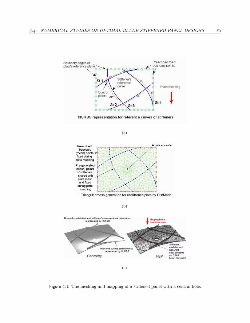
4.4. NUMERICAL STUDIES ON OPTIMAL BLADE STIFFENED PANEL DESIGNS 83

(a)

(b)

(c)

Figure 4.4: The meshing and mapping of a stiffened panel with a central hole.

4.4. NUMERICAL STUDIES ON OPTIMAL BLADE STIFFENED PANEL DESIGNS 84

cases for the uniformly distributed low level loads. Therefore, only buckling load and modes

in final designs are shown in those cases. The default modified method of feasible directions

(VR&D, 1999; MSC.Software, 2004; MSC.Software, 2005) is used unless it is mentioned

otherwise. Optimization parameters are preset and not optimized. While addressing the

relationship between the mass of an optimal design and the influencing factors, we only

show relevant results. The final designs are only shown in the form of geometry and/or

FEM 3D display, and design histories are selectively given when a special mention is desired.

In many cases, the convergence is very difficult to achieve without using a special scaling

technique to make design sensitivities comparable, and a maximum number of iterations (50

or 100) is usually met. Both the thickness of the unstiffened plate and the cross-sectional

sizes of stiffeners are taken as design variables, but uniform cross-section of a stiffener is

assumed unless mentioned otherwise. The offset of a stiffener is considered, and all the

in-plane loads are added along the mid-surface of the unstiffened plate. Note that in this

study all design points in the design space of placement design variables are results of sizing

optimizations.

4.4.1 Orientation Effects

Panels that have a grid of stiffeners with a prescribed uniform or non-uniform pattern,

such as isogrid or geodesically stiffened panels, are low-cost high-performance structures.

Therefore, we first investigate the stiffeners’ orientation effects on the optimal design of a

stiffened panel by using two stiffeners under pure shear. The geometry, load, boundary

conditions, material, and initial and bound values of designable sizes are shown in Fig. 4.5.

To exclude the influence of other factors on the results, only two orientations of straight

stiffeners are considered for brevity. In orientation I, the stiffeners’ mid-curves are along the

tensile direction of the stress field of the plate. The final design and the corresponding first

four buckling modes are given in Fig. 4.6. It can be seen that the two stiffeners do not give

good support for the plate to resist the buckling deformation and four buckling load factors

4.4. NUMERICAL STUDIES ON OPTIMAL BLADE STIFFENED PANEL DESIGNS 85

Figure 4.5: Geometrical dimensions (a = 2.54m; b = 2.54m), pure shear loading (Qxy = 250kN/m),and simply supported conditions of a blade stiffened panel. Both stiffeners and plate are made outof aluminum. Initial size and bounds: t0 = w0 = 0.005m; h0 = 5w0; tb = wb = [0.0001, 0.1]m;hb = [0.0001, 0.5]m.

are relatively far apart.

In orientation II, the stiffeners’ mid-curves are in the compression direction of the stress

field of the plate. The corresponding results are shown in Fig. 4.7. It can be clearly seen

that the two stiffeners successfully support the plate and limit the buckling shapes within the

smaller panes. The first few lower buckling modes are more clustered together with closer

buckling loads. It implies that an optimal orientation is probably achieved there.

The panel mass decreases from 224kg in the case of orientation I (Fig. 4.6) to 144kg in

the case of orientation II (Fig. 4.7). It is concluded that the orientation of a stiffener is an

important factor influencing the optimal design.

4.4. NUMERICAL STUDIES ON OPTIMAL BLADE STIFFENED PANEL DESIGNS 86

(a) Optimal design: Mmin = 224kg.

(b) First four buckling modes.

Figure 4.6: Effects of orientations of the stiffeners on the optimal designs. Orientation I: Mmin =224kg.

4.4. NUMERICAL STUDIES ON OPTIMAL BLADE STIFFENED PANEL DESIGNS 87

(a) Optimal design: Mmin = 144kg.

(b) First four buckling modes.

Figure 4.7: Effects of orientations of the stiffeners on the optimal designs. Orientation II: Mmin =144kg.

4.4. NUMERICAL STUDIES ON OPTIMAL BLADE STIFFENED PANEL DESIGNS 88

4.4.2 Spacing Effects

The same data are given in Fig. 4.5 to study spacing effects. In fact, we first re-run the case

of orientation II under the previous topic of “Orientation Effects”, but using a less dense

mesh for stiffeners, and obtain almost identical final design, as seen in Fig. 4.7 (Orientation

I) and Fig. 4.8 (Spacing I). Then, we evenly place more stiffeners (with same less dense

mesh for stiffeners) along the same orientation, and reduce the spacing of stiffeners by half.

We observe a significant reduction of mass from 144kg for spacing I to 101kg for spacing

II, and smaller (local) buckling dimples are obtained through the reduction of the spacing.

Therefore, the spacing of stiffeners is another important factor influencing the optimal design.

Too large a spacing reduces a stiffened panel to act like an unstiffened panel, and too small

a spacing reduces it to act like an equivalent unstiffened plate with an increased thickness.

4.4.3 Location Effects

It is well known that placing stiffeners at wrong locations does not help support the plate;

it will only increase the total mass of the panel. To illustrate this, we copy the results of

Fig. 4.8 (Spacing I) into Fig. 4.9 (Location I), and locate the two stiffeners further apart as

shown in Fig. 4.9 (Location II). We observe a large increase in mass from the original 144kg

to 186kg and two smaller buckling dimples appear between the two stiffeners and form a

larger local buckling dimple.

4.4.4 Curvature Effects

After we have studied the effects of orientation, spacing, and location placement of straight

stiffeners on the optimal designs of stiffened panels, we further proceed to investigate the

effects of the curvature of stiffeners on the optimal designs of panels. We can represent a

4.4. NUMERICAL STUDIES ON OPTIMAL BLADE STIFFENED PANEL DESIGNS 89

(a) Spacing I: Optimal design,Mmin = 144kg.

(b) Spacing I: First buckling mode.

(c) Spacing II: Optimal design,Mmin = 101kg.

(d) Spacing II: First buckling mode.

Figure 4.8: Effects of spacing of the stiffeners on the optimal designs. Spacing II: Mmin = 101kg.

4.4. NUMERICAL STUDIES ON OPTIMAL BLADE STIFFENED PANEL DESIGNS 90

(a) Location I: Optimal design,Mmin = 144kg.

(b) Location I: First buckling mode.

(c) Location II: Optimal design,Mmin = 186kg.

(d) Location II: First buckling mode.

Figure 4.9: Effects of location of the stiffeners on the optimal designs. Location I: Mmin = 144kg;Location II: Mmin = 186kg.

4.4. NUMERICAL STUDIES ON OPTIMAL BLADE STIFFENED PANEL DESIGNS 91

curved stiffener as an infinite number of inter-connected and intersected infinitesimal straight

stiffeners.

Pure shearing

We first investigate the curvature effect on the final design of a stiffened panel under pure

shear. Refer to Fig. 4.5 for planar dimensions, load and boundary conditions, etc. The two

stiffeners are initially straight. Considering the symmetry, we use one design parameter α

to control the motions of the mid-control points of both stiffeners’ NURBS curves. Refer to

Fig. 4.10 and Eq. (4.23)–Eq. (4.26) for initial control points and moving directions.

x10 =

5.515

9.515

; x20 =

9.515

5.515

; d1 = d11 =

− cos π4

sin π4

; and d2 = d21 =

cos π4

− sin π4

(4.26)

Figures 4.11–4.13 shows the final designs and corresponding buckling modes for parameter

α = -0.3, 0.0, and 0.8, respectively. It shows that though a bad placement of curvilinear

stiffeners, refer, e.g. to Fig. 4.11 ( α = −0.3), may not reduce the mass compared to a

placement of straight stiffeners, refer, e.g. to Fig. 4.12 ( α = 0.0), a good placement of

curved stiffeners, refer, e.g. to Fig. 4.13 (α = 0.8), may significantly reduce the mass. A

diagram of minimum mass (Mmin) vs. shape design parameter (α) is shown in Fig. 4.14.

It can be seen that the global optimum is achieved around α = 0.8, which corresponds

to curvilinear placed stiffeners (Fig. 4.13), though a local minimum corresponds to straight

stiffeners at α = 0.0 (Fig. 4.12). It is evident that the curvature of a stiffener has a significant

influence on the optimal design of a stiffened panel, though a curved stiffener is not always

advantageous over a straight one. It also should be noticed that for placement optimization

of stiffeners, one needs to consider multiple minima problems.

4.4. NUMERICAL STUDIES ON OPTIMAL BLADE STIFFENED PANEL DESIGNS 92

Figure 4.10: One design parameter α controls the motions of two mid control points x1 and x2

starting from x10 and x2

0 and by αd1 and αd2 for stiffeners 1 and 2, respectively.

Bi-normal loading - two stiffeners

We now investigate the curvature effect on the optimal design of a stiffened panel under a

bi-normal loading. Fig. 4.15 gives planar dimensions, load and boundary conditions, etc.

The two stiffeners are initially straight and located very close to the upper/lower boundary

edges of the panel (location I). Considering the symmetry, we use one design parameter to

control the motions of two mid control points of both stiffeners’ NURBS curves, as shown

in Fig. 4.16 and given by Eq. (4.27).

Figure 4.17 shows the optimal design and first buckling mode for each of the three

placements of the two stiffeners. The first case shows that the pairs of stiffeners are badly

placed initially, and they cannot effectively support the plate, therefore they almost vanish

after optimization. However, from Fig. 4.18 it is seen that a minimum is approximately

achieved when the design parameter α = 1.6, where stiffeners jointly provide a better support

4.4. NUMERICAL STUDIES ON OPTIMAL BLADE STIFFENED PANEL DESIGNS 93

(a) Optimal design: Mmin = 240kg.

(b) First four buckling modes.

Figure 4.11: Effects of curvature of the stiffeners on the optimal designs. α = −0.3: Mmin = 240kg.

4.4. NUMERICAL STUDIES ON OPTIMAL BLADE STIFFENED PANEL DESIGNS 94

(a) Optimal design: Mmin = 220kg.

(b) First four buckling modes.

Figure 4.12: Effects of curvature of the stiffeners on the optimal designs. α = 0.0: Mmin = 220kg.

4.4. NUMERICAL STUDIES ON OPTIMAL BLADE STIFFENED PANEL DESIGNS 95

(a) Optimal design: Mmin = 178kg.

(b) First four buckling modes.

Figure 4.13: Effects of curvature of the stiffeners on the optimal designs. α = 0.8: Mmin = 178kg.

4.4. NUMERICAL STUDIES ON OPTIMAL BLADE STIFFENED PANEL DESIGNS 96

−0.4 −0.3 −0.2 −0.1 0 0.1 0.2 0.3 0.4 0.5 0.6 0.7 0.8 0.9 1 1.1 1.2170

180

190

200

210

220

230

240

250

Stiffener’s Shape Design Parameter α

Min

imum

Mas

s (k

g)Minimum Mass vs. Shape Design Parameter α (Pure Shearing)

Local minimum: straight stiffeners

Local/global minimum: curved stiffeners

Number of maximum iterations: 50

Number of maximum iterations: 100

Figure 4.14: Diagram of minimum mass vs. shape design parameter α. Two minima are found.One corresponds to straight stiffeners at about α = 0.0 with minimum mass Mmin = 220kg. Theglobal optimal shape corresponds to curvilinear stiffeners at about α = 0.8 with a minimum massMmin = 178kg, which is the minimum of the two minima.

and form a smaller buckling shape in the domain between the two stiffeners.

x10 =

7.515

115

; x20 =

7.515

1415

; d1 = d11 =

cos π2

sin π2

; and d2 = d21 =

cos π2

− sin π2

(4.27)

Now, let the two initially straight stiffeners move close to each other as shown in Fig. 4.19

(location II). We then make a similar thorough line search to obtain the diagram of minimum

mass vs. shape design parameter α, as shown in Fig. 4.20. We again observe three local

minima for the curvilinear placement of stiffeners. The global minimum is found at α = 0.10

with a minimum mass Mmin = 197kg, which is the minimum of all three minima (compared

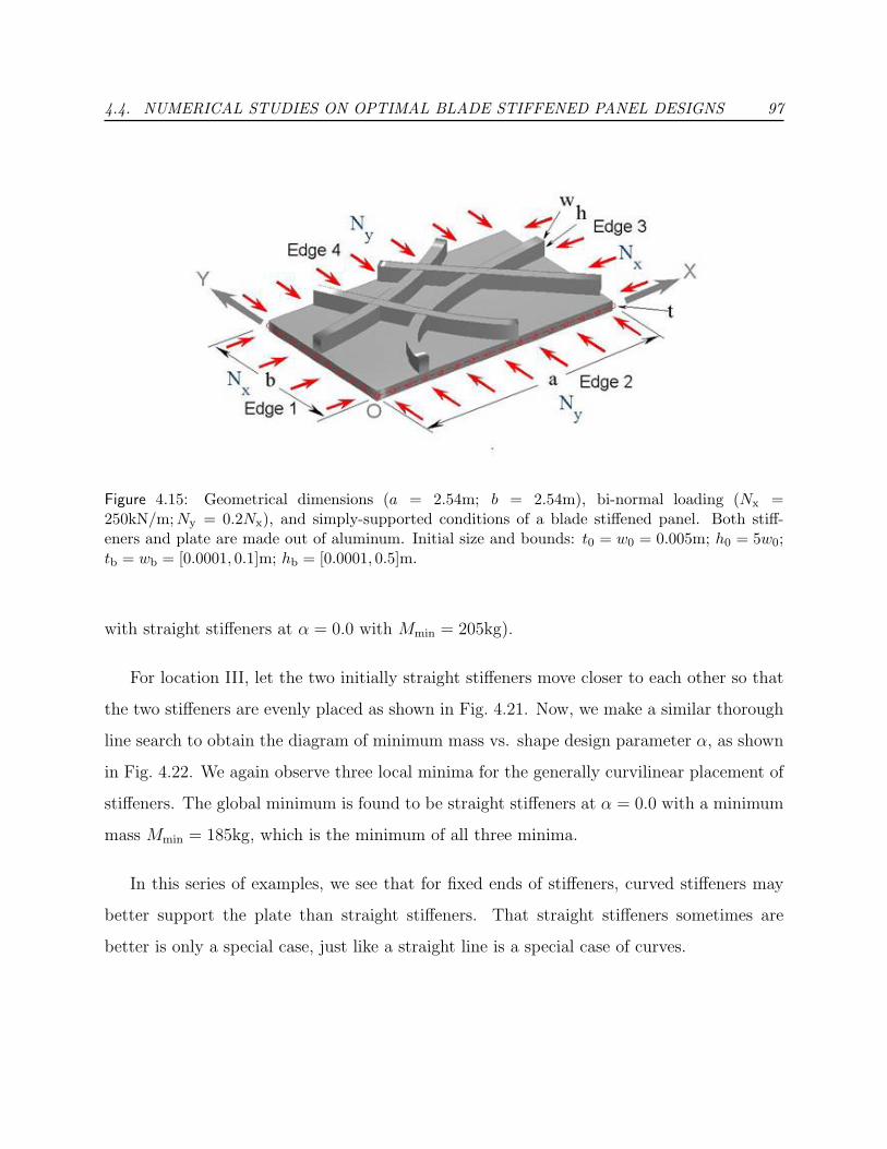
4.4. NUMERICAL STUDIES ON OPTIMAL BLADE STIFFENED PANEL DESIGNS 97

Figure 4.15: Geometrical dimensions (a = 2.54m; b = 2.54m), bi-normal loading (Nx =250kN/m; Ny = 0.2Nx), and simply-supported conditions of a blade stiffened panel. Both stiff-eners and plate are made out of aluminum. Initial size and bounds: t0 = w0 = 0.005m; h0 = 5w0;tb = wb = [0.0001, 0.1]m; hb = [0.0001, 0.5]m.

with straight stiffeners at α = 0.0 with Mmin = 205kg).

For location III, let the two initially straight stiffeners move closer to each other so that

the two stiffeners are evenly placed as shown in Fig. 4.21. Now, we make a similar thorough

line search to obtain the diagram of minimum mass vs. shape design parameter α, as shown

in Fig. 4.22. We again observe three local minima for the generally curvilinear placement of

stiffeners. The global minimum is found to be straight stiffeners at α = 0.0 with a minimum

mass Mmin = 185kg, which is the minimum of all three minima.

In this series of examples, we see that for fixed ends of stiffeners, curved stiffeners may

better support the plate than straight stiffeners. That straight stiffeners sometimes are

better is only a special case, just like a straight line is a special case of curves.

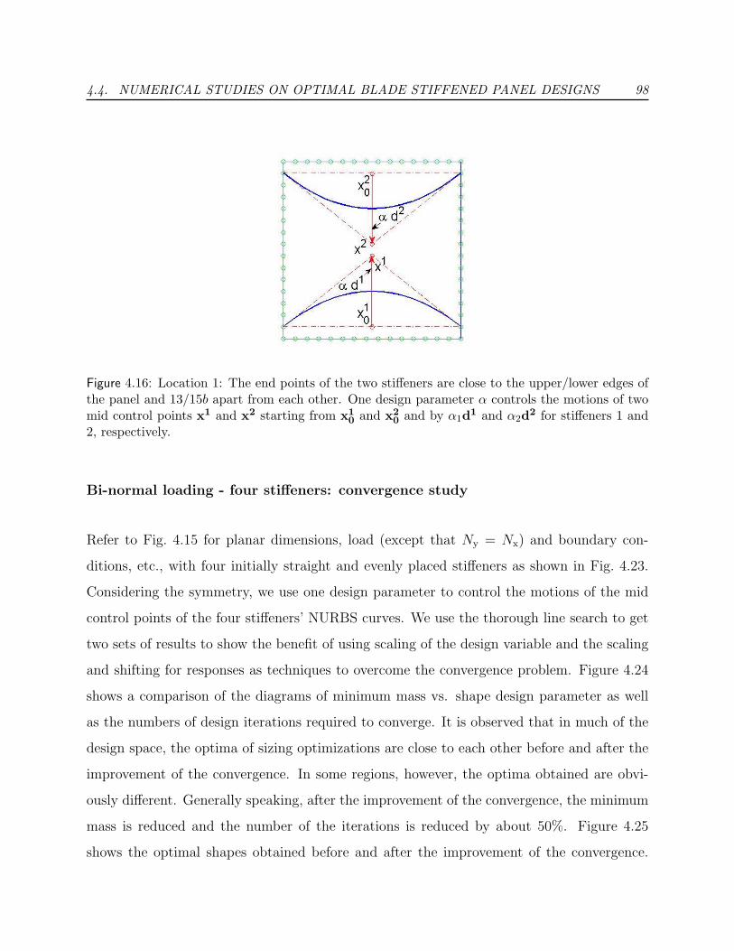
4.4. NUMERICAL STUDIES ON OPTIMAL BLADE STIFFENED PANEL DESIGNS 98

Figure 4.16: Location 1: The end points of the two stiffeners are close to the upper/lower edges ofthe panel and 13/15b apart from each other. One design parameter α controls the motions of twomid control points x1 and x2 starting from x1

0 and x20 and by α1d1 and α2d2 for stiffeners 1 and

2, respectively.

Bi-normal loading - four stiffeners: convergence study

Refer to Fig. 4.15 for planar dimensions, load (except that Ny = Nx) and boundary con-

ditions, etc., with four initially straight and evenly placed stiffeners as shown in Fig. 4.23.

Considering the symmetry, we use one design parameter to control the motions of the mid

control points of the four stiffeners’ NURBS curves. We use the thorough line search to get

two sets of results to show the benefit of using scaling of the design variable and the scaling

and shifting for responses as techniques to overcome the convergence problem. Figure 4.24

shows a comparison of the diagrams of minimum mass vs. shape design parameter as well

as the numbers of design iterations required to converge. It is observed that in much of the

design space, the optima of sizing optimizations are close to each other before and after the

improvement of the convergence. In some regions, however, the optima obtained are obvi-

ously different. Generally speaking, after the improvement of the convergence, the minimum

mass is reduced and the number of the iterations is reduced by about 50%. Figure 4.25

shows the optimal shapes obtained before and after the improvement of the convergence.

4.4. NUMERICAL STUDIES ON OPTIMAL BLADE STIFFENED PANEL DESIGNS 99

(a) α = 0.0: Optimal design, Mmin =344kg.

(b) α = 0.0: First buckling mode.

(c) α = 0.9: Optimal design, Mmin =245kg.

(d) α = 0.9: First buckling mode.

(e) α = 1.6: Optimal design, Mmin =235kg.

(f) α = 1.6: First buckling mode.

Figure 4.17: Location I: effects of curvature of the stiffeners on the optimal designs.

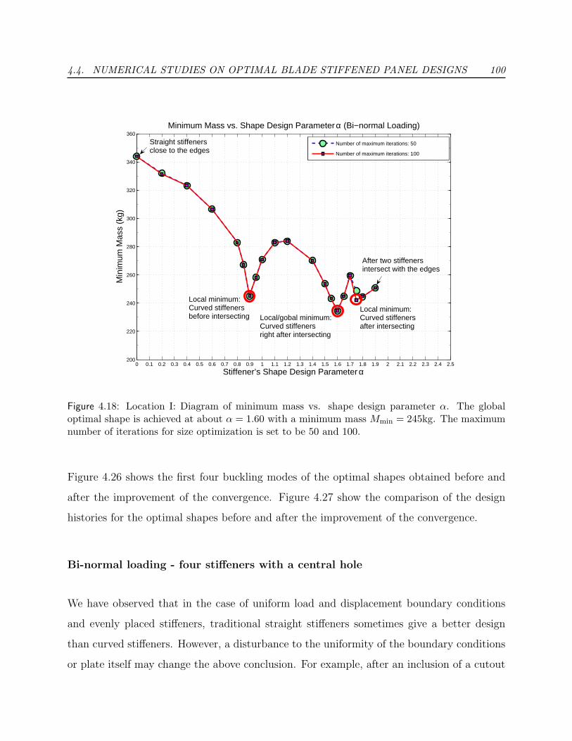
4.4. NUMERICAL STUDIES ON OPTIMAL BLADE STIFFENED PANEL DESIGNS 100

0 0.1 0.2 0.3 0.4 0.5 0.6 0.7 0.8 0.9 1 1.1 1.2 1.3 1.4 1.5 1.6 1.7 1.8 1.9 2 2.1 2.2 2.3 2.4 2.5200

220

240

260

280

300

320

340

360

Stiffener’s Shape Design Parameter α

Min

imum

Mas

s (k

g)Minimum Mass vs. Shape Design Parameter α (Bi−normal Loading)

Number of maximum iterations: 50

Number of maximum iterations: 100

Local minimum:Curved stiffenersbefore intersecting Local/gobal minimum:

Curved stiffenersright after intersecting

Local minimum:Curved stiffenersafter intersecting

After two stiffenersintersect with the edges

Straight stiffenersclose to the edges

Figure 4.18: Location I: Diagram of minimum mass vs. shape design parameter α. The globaloptimal shape is achieved at about α = 1.60 with a minimum mass Mmin = 245kg. The maximumnumber of iterations for size optimization is set to be 50 and 100.

Figure 4.26 shows the first four buckling modes of the optimal shapes obtained before and

after the improvement of the convergence. Figure 4.27 show the comparison of the design

histories for the optimal shapes before and after the improvement of the convergence.

Bi-normal loading - four stiffeners with a central hole

We have observed that in the case of uniform load and displacement boundary conditions

and evenly placed stiffeners, traditional straight stiffeners sometimes give a better design

than curved stiffeners. However, a disturbance to the uniformity of the boundary conditions

or plate itself may change the above conclusion. For example, after an inclusion of a cutout

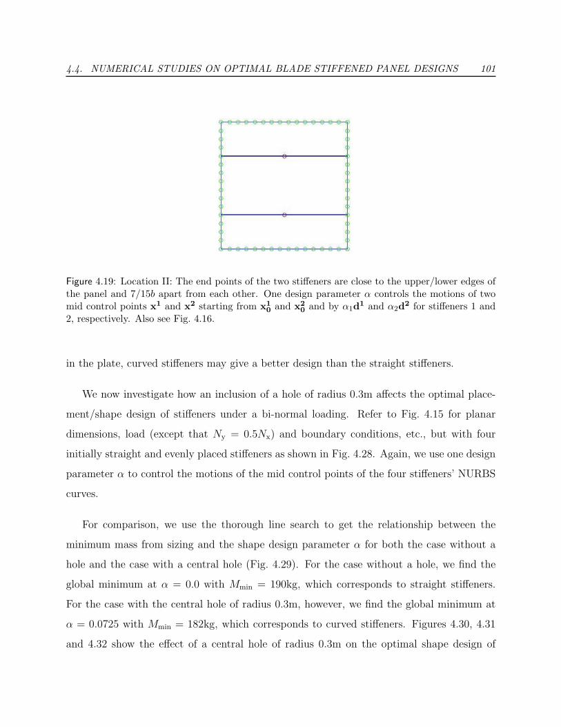
4.4. NUMERICAL STUDIES ON OPTIMAL BLADE STIFFENED PANEL DESIGNS 101

Figure 4.19: Location II: The end points of the two stiffeners are close to the upper/lower edges ofthe panel and 7/15b apart from each other. One design parameter α controls the motions of twomid control points x1 and x2 starting from x1

0 and x20 and by α1d1 and α2d2 for stiffeners 1 and

2, respectively. Also see Fig. 4.16.

in the plate, curved stiffeners may give a better design than the straight stiffeners.

We now investigate how an inclusion of a hole of radius 0.3m affects the optimal place-

ment/shape design of stiffeners under a bi-normal loading. Refer to Fig. 4.15 for planar

dimensions, load (except that Ny = 0.5Nx) and boundary conditions, etc., but with four

initially straight and evenly placed stiffeners as shown in Fig. 4.28. Again, we use one design

parameter α to control the motions of the mid control points of the four stiffeners’ NURBS

curves.

For comparison, we use the thorough line search to get the relationship between the

minimum mass from sizing and the shape design parameter α for both the case without a

hole and the case with a central hole (Fig. 4.29). For the case without a hole, we find the

global minimum at α = 0.0 with Mmin = 190kg, which corresponds to straight stiffeners.

For the case with the central hole of radius 0.3m, however, we find the global minimum at

α = 0.0725 with Mmin = 182kg, which corresponds to curved stiffeners. Figures 4.30, 4.31

and 4.32 show the effect of a central hole of radius 0.3m on the optimal shape design of

4.4. NUMERICAL STUDIES ON OPTIMAL BLADE STIFFENED PANEL DESIGNS 102

−0.4 −0.3 −0.2 −0.1 0 0.1 0.2 0.3 0.4 0.5 0.6 0.7 0.8 0.9 1 1.1 1.2 1.3 1.4180

190

200

210

220

230

240

250

260

270

Stiffener’s Shape Design Parameter α

Min

imum

Mas

s (k

g)Minimum Mass vs. Shape Design Parameter α (Bi−normal Loading)

Local/global minimum:Curved stiffenersbefore intersecting

Local minimum:Two stiffeners areabout to intersectwith each other

Local minimum:Curved stiffenersafter intersecting

Straight stiffeners

Figure 4.20: Location II: Diagram of minimum mass vs. shape design parameter α. The globaloptimal shape is achieved at about α = 0.10 with a minimum mass Mmin = 197kg (comparedwith straight stiffeners α = 0.0 with Mmin = 205kg). The maximum number of iterations for sizeoptimization is set to be 100.

stiffeners.

It is observed that even though the loading is uniformly distributed, evenly placed straight

stiffeners are not necessarily best designs.

Complex in-plane loading: bi-normal and shear loading

We finally use two shape design parameters to investigate the curvature effect on the final

design of a stiffened panel under a complex in-plane load: bi-normal and shear loading.

Refer to Fig. 4.33 for planar dimensions, load and boundary conditions, etc. Though the

4.4. NUMERICAL STUDIES ON OPTIMAL BLADE STIFFENED PANEL DESIGNS 103

Figure 4.21: Location III: The end points of the two stiffeners are close to the upper/lower edges ofthe panel and 5/15b apart from each other. One design parameter α controls the motions of twomid control points x1 and x2 starting from x1

0 and x20 and by α1d1 and α2d2 for stiffeners 1 and

2, respectively. Also see Fig. 4.16.

loading is unsymmetrical, we retain a symmetric design with four initially straight stiffeners

to simplify the conceptual study at hand. We use design parameter α1 to control the shapes

of mid-curves of the two stiffeners that are originally straight and evenly placed in the X -

direction, and use design parameter α2 to control the shapes of mid-curves of the two other

stiffeners that are also originally straight and evenly placed in the Y-direction. Refer to

Fig. 4.34 and Eqs. (4.28) and (4.29).

x10 =

7.515

515

; x20 =

7.515

1015

; x30 =

515

7.515

; and x40 =

1015

7.515

(4.28)

d11 =

cos π2

sin π2

; d21 =

cos π2

− sin π2

; d32 =

cos 0

sin 0

; and d42 =

cos π

sin π

(4.29)

As we are not performing an automatic placement optimization at this time, the two-

parameters problem can be handled manually by dividing the interested square domain

space by 11 × 11 grid points in the design space as shown in Fig. 4.35. We start from

4.4. NUMERICAL STUDIES ON OPTIMAL BLADE STIFFENED PANEL DESIGNS 104

−0.6 −0.5 −0.4 −0.3 −0.2 −0.1 0 0.1 0.2 0.3 0.4 0.5 0.6 0.7 0.8 0.9 1 1.1 1.2170

180

190

200

210

220

230

240

250

260

270

Stiffener’s Shape Design Parameter α

Min

imum

Mas

s (k

g)Minimum Mass vs. Shape Design Parameter α (Bi−normal Loading)

Local/global minimum:Straight stiffeners

Local minimum:Curved stiffenersafter intersecting

Local minimum:Two stiffeners almostintersect with each other

Figure 4.22: Location 3: Diagram of minimum mass vs. shape design parameter α. The globaloptimal shape is achieved at about α = 0.0 with a minimum mass Mmin = 185kg. The maximumnumber of iterations for size optimization is set to be 100.

the placement of straight stiffeners, i.e., α1 = α2 = 0, as it is conventionally viewed as a

potentially optimal placement for uniformly distributed loadings along the edges. We then

vary the design point in the neighborhood and see if there is any reduction in the total mass.

It happens that the initially straight stiffeners are a local optimal design (the dark square

point inside the circle nearby the left-bottom corner in Fig. 4.35).

By intuition, we start from another design point, which represents a curvilinear placement

of the stiffeners. By searching around using the “gradient” information of mass reduction or

increase, we locate another local minimum design, i.e., around α1 = 0.7 and α2 = 1.3 (the

dark square point inside the circle near the right-top corner in Fig. 4.35). Figure 4.36 shows

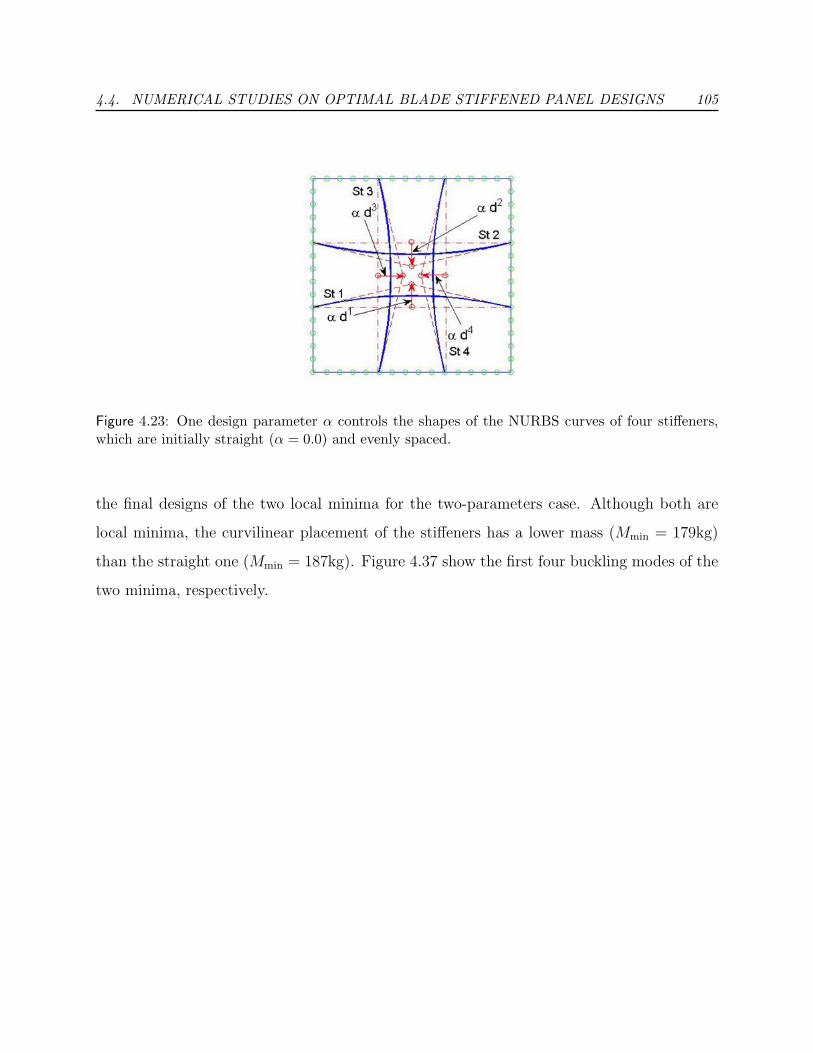
4.4. NUMERICAL STUDIES ON OPTIMAL BLADE STIFFENED PANEL DESIGNS 105

Figure 4.23: One design parameter α controls the shapes of the NURBS curves of four stiffeners,which are initially straight (α = 0.0) and evenly spaced.

the final designs of the two local minima for the two-parameters case. Although both are

local minima, the curvilinear placement of the stiffeners has a lower mass (Mmin = 179kg)

than the straight one (Mmin = 187kg). Figure 4.37 show the first four buckling modes of the

two minima, respectively.

4.5. CONCLUSIONS AND FUTURE WORK 106

−0.6 −0.4 −0.2 0 0.2 0.4 0.6 0.8 1 1.2 1.40

50

100

150

200

250

300

350

Stiffener’s Shape Design Parameter α

No.

of I

tera

tions

M

inim

um M

ass

(kg)

Minimum Mass vs. Shape Design Parameter α (Bi−normal Loading)

Local minimum before improvement of convergence

Local minimum after improvement of convergence

No. of iterations before improvement of convergence

No. of iterations after improvement of convergence

Global minimum corresponds to straight stiffeners

Figure 4.24: A comparison of diagrams of minimum mass vs. shape design parameter α beforeand after the improvement of the convergence. After the improvement of the convergence, threelocal minima are found. One corresponds to straight stiffeners at about α = 0.0 with a minimummass Mmin = 213kg which is also the global minimum. The other two local minima correspondto curvilinear stiffeners at about α = 0.275 with a minimum mass Mmin = 223kg, and at aboutα = 0.875 with a minimum mass Mmin = 235kg.

4.5 Conclusions and Future Work

This chapter presents many numerical results from a study on unitized panels with straight

and curvilinear stiffeners. An integrated approach to achieve optimal design of stiffened

panels under various practical requirements is adopted in the MATLAB environment. The

codes with several capabilities, such as NURBS (for geometric model), DistMesh (for mesh

generation), 3D display (for visualization of the stiffened panel), and MSC.NASTRAN, are

used as subroutines or subprograms.

4.5. CONCLUSIONS AND FUTURE WORK 107

(a) Before the improvement of the convergence – global minimum: α = −0.1; Mmin = 233kg;optimal shape: curved stiffeners.

(b) After the improvement of the convergence – global minimum: α = 0.0; Mmin = 213kg;optimal shape: curved stiffeners.

Figure 4.25: A comparison of optimal designs before and after the improvement of the convergence.

4.5. CONCLUSIONS AND FUTURE WORK 108

(a) Before the improvement of the convergence.

(b) After the improvement of the convergence.

Figure 4.26: A comparison of the first four buckling modes before and after the improvement of theconvergence.

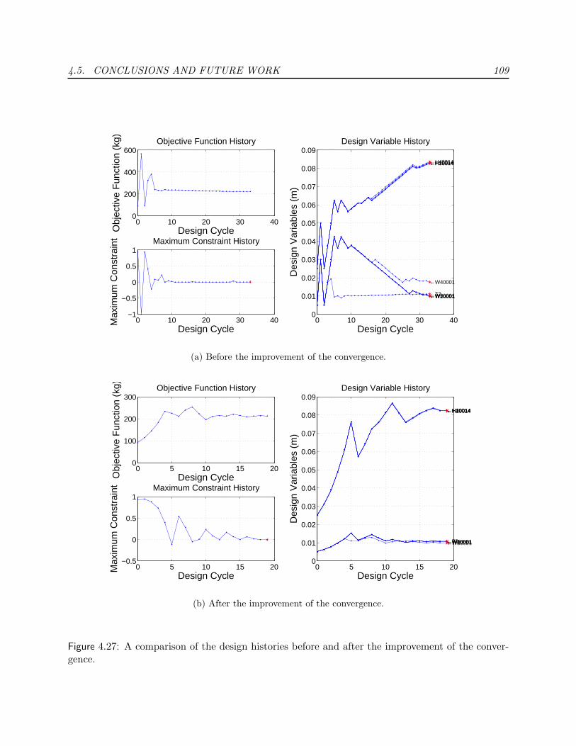
4.5. CONCLUSIONS AND FUTURE WORK 109

0 10 20 30 400

200

400

600

Design CycleObj

ectiv

e F

unct

ion

(kg) Objective Function History

0 10 20 30 40−1

−0.5

0

0.5

1

Design Cycle

Max

imum

Con

stra

int Maximum Constraint History

0 10 20 30 400

0.01

0.02

0.03

0.04

0.05

0.06

0.07

0.08

0.09

←T2←W10001

←H10014

←W20001

←H20014

←W30001

←H30014

←W40001

←H40014

Design Cycle

Des

ign

Var

iabl

es (

m)

Design Variable History

(a) Before the improvement of the convergence.

0 5 10 15 200

100

200

300

Design CycleObj

ectiv

e F

unct

ion

(kg) Objective Function History

0 5 10 15 20−0.5

0

0.5

1

Design Cycle

Max

imum

Con

stra

int Maximum Constraint History

0 5 10 15 200

0.01

0.02

0.03

0.04

0.05

0.06

0.07

0.08

0.09

←T2←W10001

←H10014

←W20001

←H20014

←W30001

←H30014

←W40001

←H40014

Design Cycle

Des

ign

Var

iabl

es (

m)

Design Variable History

(b) After the improvement of the convergence.

Figure 4.27: A comparison of the design histories before and after the improvement of the conver-gence.

4.5. CONCLUSIONS AND FUTURE WORK 110

Figure 4.28: One design parameter α controls the shapes of the NURBS curves of four stiffeners,which are initially straight (α = 0.0) and evenly spaced.

Numerical studies on optimal stiffened panel designs are made to investigate the effects of

certain factors, such as orientation, spacing, location, and curvature, on the optimal designs.

We observe that a curvilinear placement of stiffeners sometimes gives a better design

than straight stiffeners. A curvilinear placement of stiffeners is equivalent to an orientation,

spacing, location, and intersection placement of infinitesimal straight stiffeners. It also plays

a role in topology optimization due to the change of stiffeners’ intersections.

Therefore, it is necessary to perform an automatic placement optimization of generally

curvilinear stiffened panels and use global optimization techniques to find the best design

among multiple local optima, which are common for optimal designs of stiffened panels.

4.5. CONCLUSIONS AND FUTURE WORK 111

−0.6 −0.4 −0.2 0 0.2 0.4 0.6 0.8 1 1.2 1.40

50

100

150

200

250

300

Stiffener’s Shape Design Parameter α

No.

of I

tera

tions

M

inim

um M

ass

(kg)

Minimum Mass vs. Shape Design Parameter α (Bi−normal Loading)

Local/Global minimum with a central hole:curved stiffeners

Local/Global minimum without hole:

straight stiffeners

Local minimum without hole:

curved stiffeners

Local minimum with a central hole:curved stiffeners

Stiffeners areforced to wraparound the hole

No. of iterations with a central holeNo. of iterations without hole

Mass with a central hole

Mass without hole

Figure 4.29: Variation of minimum mass vs. shape design parameter α. The global optimal shapeis achieved at about α = 0.0 with a minimum mass Mmin = 190kg. An inclusion of a central holeof radius 0.3m results in curvilinear stiffeners as the global optimal placement, achieved at aboutα = −0.0725 with a minimum mass Mmin = 182kg.

4.5. CONCLUSIONS AND FUTURE WORK 112

(a) Before the inclusion of the central cutout – global minimum: α = 0.0; Mmin = 190kg;optimal shape: straight stiffeners.

(b) After the inclusion of the central cutout – global minimum: α = 0.0725; Mmin = 182kg;optimal shape: curved stiffeners.

Figure 4.30: A comparison of optimal designs before and after the inclusion of the central cutoutof radius 0.3m.

4.5. CONCLUSIONS AND FUTURE WORK 113

(a) Before the inclusion of the central cutout.

(b) After the inclusion of the central cutout.

Figure 4.31: A comparison of first four buckling modes before and after the inclusion of the centralcutout of radius 0.3m.

4.5. CONCLUSIONS AND FUTURE WORK 114

0 5 10 15 2050

100

150

200

250

Design CycleObj

ectiv

e F

unct

ion

(kg) Objective Function History

0 5 10 15 20−0.5

0

0.5

1

Design Cycle

Max

imum

Con

stra

int Maximum Constraint History

0 5 10 15 200

0.01

0.02

0.03

0.04

0.05

0.06

0.07

0.08

0.09

0.1

←T2←W10001

←H10014

←W20001

←H20014

←W30001

←H30014

←W40001

←H40014

Design Cycle

Des

ign

Var

iabl

es

Design Variable History

(a) before the inclusion of the central cutout.

0 5 10 15 2050

100

150

200

250

Design Cycle

Obj

ectiv

e F

unct

ion

(kg) Objective Function History

0 5 10 15 20−0.5

0

0.5

1

Design Cycle

Max

imum

Con

stra

int Maximum Constraint History

0 5 10 15 200

0.01

0.02

0.03

0.04

0.05

0.06

0.07

0.08

0.09

0.1

←T2←W10001

←H10014

←W20001

←H20014

←W30001

←H30014

←W40001

←H40014

Design Cycle

Des

ign

Var

iabl

es

Design Variable History

(b) After the inclusion of the central cutout.

Figure 4.32: A comparison of design histories before and after the inclusion of the central cutout ofradius 0.3m.

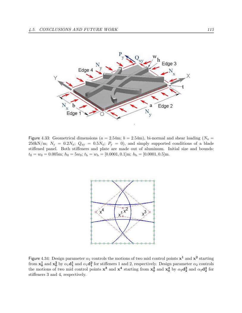
4.5. CONCLUSIONS AND FUTURE WORK 115

Figure 4.33: Geometrical dimensions (a = 2.54m; b = 2.54m), bi-normal and shear loading (Nx =250kN/m; Ny = 0.2Nx; Qxy = 0.5Nx; Py = 0), and simply supported conditions of a bladestiffened panel. Both stiffeners and plate are made out of aluminum. Initial size and bounds:t0 = w0 = 0.005m; h0 = 5w0; tb = wb = [0.0001, 0.1]m; hb = [0.0001, 0.5]m.

Figure 4.34: Design parameter α1 controls the motions of two mid control points x1 and x2 startingfrom x1

0 and x20 by α1d1

1 and α1d21 for stiffeners 1 and 2, respectively. Design parameter α2 controls

the motions of two mid control points x3 and x4 starting from x30 and x4

0 by α2d32 and α2d4

2 forstiffeners 3 and 4, respectively.

4.5. CONCLUSIONS AND FUTURE WORK 116

−0.6 −0.4 −0.2 0 0.2 0.4 0.6 0.8 1 1.2

−0.6

−0.4

−0.2

0

0.2

0.4

0.6

0.8

1

1.2

1.4

X: 1Y: 1.003Z: 224.3

X: 0.8Y: 0.8Z: 205.1

X: 0.8Y: 1.3Z: 188.5

X: 0.7Y: 1.2Z: 187.5

X: 0.7Y: 1.3Z: 179.3

X: 0.6Y: 1.2

Z: 188.1

X: 0.6Y: 1.3

Z: 181.6

X: 0.4Y: 1.3

Z: 184.5

X: 0.2Y: 0.2Z: 191.9

X: 0.2Y: 0Z: 192.8

X: 0Y: 0.4Z: 190.5

X: 0Y: 0.2Z: 187.4

X: 0Y: −0.2Z: 195.1

X: 0Y: 0Z: 187.3

X: −0.2Y: 0.2Z: 211.7

X: −0.2Y: −0.2Z: 203.2

X: −0.2Y: 0Z: 201

α1

α2

Figure 4.35: Design space of two design parameters: α1 = X and α2 = Y , with correspondingminimum mass: Mmin = Z. Two local minima are found as shown as the dark squares inside thecircles from 17 discrete points on the 11 × 11 grids. The maximum number of iterations for sizeoptimization is set to be 100.

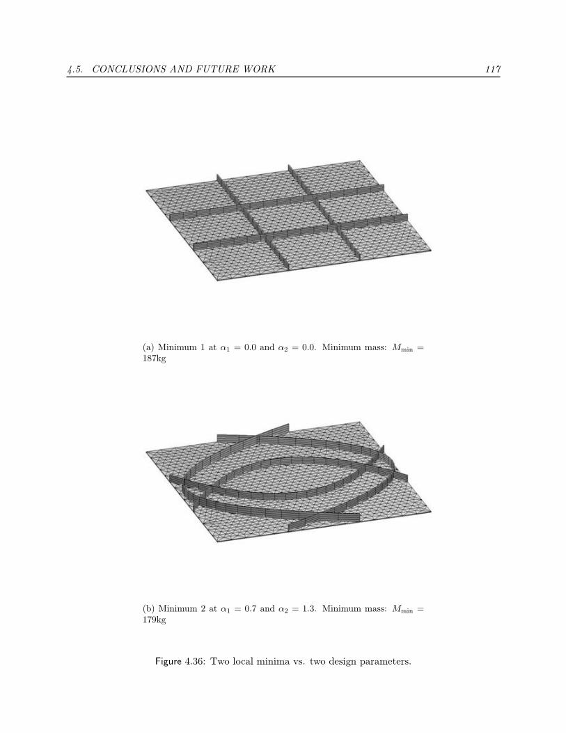
4.5. CONCLUSIONS AND FUTURE WORK 117

(a) Minimum 1 at α1 = 0.0 and α2 = 0.0. Minimum mass: Mmin =187kg

(b) Minimum 2 at α1 = 0.7 and α2 = 1.3. Minimum mass: Mmin =179kg

Figure 4.36: Two local minima vs. two design parameters.

4.5. CONCLUSIONS AND FUTURE WORK 118

(a) First four buckling modes for minimum 1 at α1 = 0.0 and α2 = 0.0- straight stiffeners

(b) First four buckling modes for minimum 2 at α1 = 0.7 and α2 = 1.2- curved stiffeners

Figure 4.37: First four buckling modes for minimum 1 and minimum 2.

Chapter 5

Summary and Conclusions

This dissertation dealt with some inverse problems in structural mechanics, searching for

causes of observed or desired effects where some regularizations are usually needed to handle

the common ill-posed conditions.

Three application fields are covered in this work.

The first one is load updating for finite element models, where boundary displacements

or strains are assumed given from a noise-free measurement and least squares fitting is used

to identify load parameters. Therefore, the ill-conditioned problem itself is classified as one

with non-unique solutions or high condition number.

The formulation of the load updating is first made for geometrically linear and nonlinear

finite element models of beams or frames by using a previously developed four-noded curved

beam element. For the purpose of basic studies, the unknown applied load within an element

is represented by a linear combination of integrated Legendre polynomials, the coefficients of

which are the parameters to be extracted using assumed measured displacements or strains.

The inverse problem is formulated as an expanded Least Squares solution problem where the

difference between the calculated and measured displacements or strains is minimized, with

some intuitive Tikhonov-type regularization terms for enforcing C0 continuity and smooth-

ing for the extracted load. The limited memory variable metric optimizer L-BFGS-B is used

to solve the ill-conditioned least squares problem. The benefits of regularization using the

four-noded beam element, polynomials of lower order for load representation, using relative

measurement data, richer measured data, smoothing, and enforcing C0 continuity are to

119

5. SUMMARY AND CONCLUSIONS 120

change the underdetermined problem to an overdetermined one. The basic idea is to over-

come the ill-posedness of the identification problem by reducing the relative model order or

the relative number of unknown variables of the system for given precision.

An extended work (Li and Kapania, 2004) is also made for general finite element models

based on MSC.NASTRAN where both plate and solid structures can be handled. The

reduced number of the unknown load parameters is used to regularize the ill-conditioned load

updating problem, and the parametrization of load is made crossing the element boundary

by using NURBS (Non-uniform Rational B-Splines) to represent the load distribution.

The present conclusions may be applied to the measurement based load updating for

general finite element models when the measured data are pre-smoothed or the noise in the

data is pre-filtered out.

The second problem is the placement optimization of a spatially distributed sensing

fiber optic sensor for a smart bed using a Genetic Algorithms (GA), where the sensor per-

formance is maximized subjected to constraints on the length of the optical fiber and its

maximum initial curvature. The sensor performance function is simplified as the full length

integration of the absolute curvature change due to the spatial perturbation from a subject’s

movement. The problem of the placement of an infinite number of infinitesimal sensing fiber

segments is replaced by the problem of the placement of a finite number of the control points

since the fiber optic cable is represented by a NURBS curve.

Due to the common problem of multiple solutions for the placement of sensors, a simple

binary-coded Genetic Algorithm (GA) is used for the placement of this distributed sensing

fiber optic sensor as an illustration to use a GA for a NURBS design. The fitness function of

the GA is defined in the sense of the exact penalty function method, where the length and

maximum initial curvature of the fiber curve are limited by prescribed upper bounds.

A Java tool is developed as an interactive research and design tool for the fiber optic

5. SUMMARY AND CONCLUSIONS 121

sensor using GAs.

Two simple examples were given for the placement optimization of the distributed sensing

optical fiber for an integrated smart bed. The first example had 6 control points of the

NURBS curve for the sensing fiber curve of 2m. The spatial perturbation to the mattress

and the sensing fiber was from perturbating a control point of the NURBS for the mattress

surface. The second example had 25 control points for the sensing fiber’s NURBS curve of

4m. The mattress deformation and its perturbation were calculated using MSC.NASTRAN

under a given body pressure and its perturbation. The smart bed was modeled as an elastic

mattress core, ignoring effects of both the flexible mattress cover and the sensing optical

fiber. This made it possible to perform only a single FEA to obtain the mattress surface

deformation for the placement optimization of the sensor, which is important for using a GA

that needs a large number of generations. Both examples gave updated placements of the

sensors with improved sensor performance.

The further work includes the considerations of (1) using real-valued coded GA with a

special treatment for constraints, (2) the variation of the body pressure distribution, (3)

the multiple loadings and multiple constraints, and (4) the large initial deformation of the

mattress.

Though the specific example is for clinical use, the distributed sensing fiber optic sen-

sor and associated placement methodology can also be used in pilot/passenger seats and

structures for flight vehicles. The other potential use is the placement of Fiber Bragg Grat-

ing (FBG) sensors for health monitoring structures in both aerospace engineering and civil

engineering.

The third problem is the size and placement optimization on unitized panels with

straight and curvilinear stiffeners, subject to buckling and stress constraints.

The present work uses NURBS for the panel and stiffener representation. The mesh for

5. SUMMARY AND CONCLUSIONS 122

the panel is generated using an automatic mesh generation algorithm by adapting DistMesh,

a triangulation algorithm, while the mesh for stiffeners is pre-generated and fixed. An in-

terface between NASTRAN and MATLAB is developed to automatically transfer the data

between the analysis and optimization processes, respectively. An integrated approach to

achieve optimal design of stiffened panels under various practical requirements is adopted in

the MATLAB environment. The codes with several capabilities, such as NURBS (for geo-

metric model), DistMesh (for mesh generation), 3D display (for visualization of the stiffened

panel), and MSC.NASTRAN, are used as subroutines or subprograms. The collection of

those codes is called EBF3paneloptimization.

The optimization consists of minimizing the weight of the stiffened panel, with design

variables being the thickness of the plate and height and width of the stiffener as well as

the placement of the stiffeners, subject to buckling and stress constraints under in-plane and

out-of-plane loads.

Numerical studies on optimal stiffened panel designs are performed to investigate the

effects of certain factors, such as orientation, spacing, location, and curvature, on the optimal

designs.

We observe that a curvilinear placement of stiffeners sometimes gives a slightly better

design than straight stiffeners. A curvilinear placement of stiffeners is equivalent to an

orientation, spacing, location, and intersection placement of infinitesimal straight stiffeners.

It also plays a role in topology optimization due to the change of stiffeners’ intersections.

Numerical results also show that the stiffened panel optimization is an ill-posed inverse

problem with slow convergence due to a large condition-number of the Hessian for the objec-

tive function. The simplified scaling of the design variables, and the scaling and shifting of

the objective and constraints, are used as techniques to overcome the slow convergence prob-

lem. Besides, the non-uniqueness of the optimal designs and a need for a global optimization

are also illustrated.

5. SUMMARY AND CONCLUSIONS 123

Future work could include the automation of the placement optimization of the stiffeners,

more practical types of stiffeners, as well as more practical design objectives and constraints,

such as vibration frequencies, acoustic power/pressure, and panel flutter.

The outcome of the present research and the code EBF3paneloptimization are being used

for trade-off study of some panel designs used for EBF3 research.

Appendix A

Legendre Polynomials

Let α = 0, 1, · · · , N ec

Lα(x) ≡ 1

2αα!

dα

dxα(x2 − 1)α (A.1)

be the α-th Legendre polynomial, and

Lα(x) ≡ γα

∫ x

−1

Lα(x)dx for α ≥ 2 (A.2)

be the α-th integrated Legendre polynomial with

γα =

√(2α− 3)(2α− 1)(2α + 1)

4(A.3)

By definition,

L0(x) =1 + x

2

L1(x) =1− x

2(A.4)

124

A. LEGENDRE POLYNOMIALS 125

The properties

Lα(x) =2α− 1

αxLα−1(x)− α− 1

αLα−2(x); (L0(x) = 1, L1(x) = x)∫ 1

−1

Lα(x)Lβ(x)dx = δαβ2

2α + 1

Lα(x) =

√(2α + 1)(2α− 3)

4(2α− 1)(Lα(x)− Lα−2(x))

Lα(−1) = 0

Lα(1) = 0

(A.5)

are true for α ≥ 2.

In the integral, all powers lower than n of the Legendre polynomial yield zero when

integrated against the cosine (because of the orthogonality of the cosines.)

Appendix B

Load Coefficient Matrix at the

Element Level

In general, for our geometrically nonlinear FEM for the 3-D case, we can start with the

state equation of a nonlinear structural system (Kapania and Li, 2003a):

R(a, c, λ) = qint(a)− λqext0(a, c) = 0. (B.1)

where R is the residual vector, qint the nodal internal force vector, qext0 the nodal external

load vector calculated at the applied load level, λ the proportional nodal loading factor,

a = a(c, λ) the nodal displacement vector, and c the load (force) coefficient vector: qint

and qext0 are summed from the nodal internal and external load vectors contributed by an

element e ∈ [1, Nelm]:

qeint =

qeint1

...

qeintIe

node

...

qeintNe

node

and qe

ext0 =

qeext01

...

qeext0Ie

node

...

qeext0Ne

node

(B.2)

respectively, where

qeintIe

node=

PeintIe

node

MeintIe

node

(B.3)

where

PeintIe

node=

∫ 1

0

NIenode,ξ

nedξ (B.4)

126

B. LOAD COEFFICIENT MATRIX AT THE ELEMENT LEVEL 127

and

MeintIe

node=

∫ 1

0

(NIenode,ξ

me −NIenode

ϕe,ξn

e)dξ (B.5)

are the nodal internal force and moment vectors at node Ienode contributed by element e,

respectively; and

qeext0Ie

node=

Peext0Ie

node

Meext0Ie

node

(B.6)

where

Peext0Ie

node=

∫ 1

0

NIenode

[N eg + N e

d sin(de, ϕe0,s) + ΛeN e

p]J edξ

=

∫ 1

0

NIenode

[N eg + N e

d sin(de, ϕe0,s) + N e

p]J edξ (B.7)

and

Meext0Ie

node= 0 (B.8)

are the nodal external force and zero moment vectors at node Ienode contributed by the

distributed force acting on element e at the applied load level, respectively.

Assume that

N el = cle

αPα(ξ1) (B.9)

where Pα are the basis functions, taken to be the integrated Legendre polynomials; α =

1, 2, · · · , N ec (summation convention holds for α) with N e

c as the number of basis functions

considered for each element, and cleα are the load (force) coefficient vectors for each element,

and the subscript l = g, d, p identifies the load type, i.e., the self-weight load, snow load, and

pressure load, respectively (for l = p, the material form N ep is used instead of the spatial

form N ep).

B. LOAD COEFFICIENT MATRIX AT THE ELEMENT LEVEL 128

Now let’s consider the dependency of the three components of the force coefficient vector,

e.g. cleα . We know from Eq. (B.9) that cle

α determine both the direction and the amplitude

of the external force distribution over an element. We consider three cases:

1). The 1-D case, i.e., the direction of cleα is given over the element by the vector dle

1 :

cleα = xle

1αdle1 (B.10)

2). The 2-D case, i.e., the plane of cleα is same over all α and given by the vectors dle

1 and

dle2 :

cleα = xle

1αdle1 + xle

2αdle2 (B.11)

3). The more general 3-D case, i.e., the direction of cleNα is unknown:

cleα = xle

1αdl1 + xle

2αdl2 + xle

3αdl3 (B.12)

where dli = ei for l = g, d (self-weight load and snow load); dl

i = ti for l = p (pressure

load).

Collectively, we can combine the three cases into one form:

cleα = Dlexle

α (B.13)

where xleα are called independent force coefficient vectors.

Therefore,

Peext0Ie

node=

∫ 1

0

NIenode

[cgeα Pα(ξ1) + cde

α Pα(ξ1) sin(de, ϕe0,s) + Λecpe

α Pαξ1)]J edξ (B.14)

The variations with respect to load (force) coefficient vectors:

δcPeext0Ie

node= Fge

cIenodeα

δcgeα + Fde

cIenodeα

δcdeα + Fpe

cIenodeα

δcpeα (B.15)

B. LOAD COEFFICIENT MATRIX AT THE ELEMENT LEVEL 129

where, noticing that I3 denotes the identity tensor of order two,

FgecIe

nodeα=

∫ 1

0

I3NIenode

Pα(ξ1)J edξ

FdecIe

nodeα=

∫ 1

0

I3NIenode

Pα(ξ1) sin(de, ϕe0,s)J edξ

FpecIe

nodeα=

∫ 1

0

ΛeNIenode

Pα(ξ1)J edξ (B.16)

For a single node of an element,

δcqeext0Ie

node= Fge

cIenodeα

δcgeα + Fde

cIenodeα

δcdeα + Fpe

cIenodeα

δcpeα (B.17)

where

FlecIe

nodeα=

FlecIe

nodeα

0

(B.18)

For a single element e with N enode nodes contributed by load type l, noticing Eq. (B.13),

δcqleext0 = Fle

c δcle

= Flecαδcle

α (B.19)

δxqleext0 = Fle

x δxle

= Flexαδxle

α

= FlecαD

leδxleα (B.20)

where

Flex =

[Fle

x1 · · · FlexNc

], Fle

xα = FlecαD

le, Flecα =

Fle

c1α

...

FlecNe

nodeα

, and δxle =

δxle

1

...

δxleNe

c

Appendix C

The Derivatives of the Displacements

with Respective to Load Coefficient

Vector

In the linearized incremental form, the state equation can be written as

R + ∆R = 0 (C.1)

and

∆R = ∆aR + ∆xR + ∆λR

= R,a∆a + R,x∆x + R,λ∆λ (C.2)

where the linearized increment operator ∆ has been decomposed into three parts: the lin-

earized increment ∆a due to a change in a, linearized increment ∆x (or ∆c) due to a change

in x (or c), and linearized increment ∆λ due to a change in λ. The Jacobians R,a, R,x,

and R,λ are the partial derivatives of the residual R with respect to the state vector a, load

design vector x, and load factor λ, respectively:

R,a = R,a(a,x, λ) = qint,a − λqext0,a (C.3)

R,c = R,x(a,x, λ) = qint,x − λqext0,x = −λqext0,x (C.4)

and

R,λ = R,λ(a,x) = −qext0 (C.5)

130

C. THE DERIVATIVES OF THE DISPLACEMENTS WITH RESPECT TO LOADCOEFFICIENT VECTOR 131

Also, R,a is known as the tangential stiffness matrix of the system:

KT = KT(a,x, λ) = R,a (C.6)

which is nonsymmetric for a general loading case, e.g. when the pressure load is considered.

Therefore, we can write the augmented linearized incremental state equation as

R + R,a∆a + R,x∆x + R,λ∆λ = 0 (C.7)

The residual vector vanishes at the equilibrium for given load factor λ:

R = 0 (C.8)

Thus, we have the augmented linearized incremental state equation at equilibrium:

KT∆a + R,x∆x = 0 (C.9)

or

KT∆a− λqext0,x∆x = 0 (C.10)

or

a,x = λK−1T qext0,x (C.11)

where a,x is the sensitivity of displacement vector with respect to the load design vector x and

qext0,x is the global force coefficient matrix, which is obtained by the assembling operation

using the relations given in Eqs. (B.15-B.21).

Appendix D

The Derivatives of the Strains with

Respect to Load Coefficient Vector

For the translational strain vector in the material form, one has, noticing Section 3.3 of

Kapania and Li (2003a),

∆xε = ε,xα∆xα

= Λt(∆xϕ,ξ1 + ϕ,ξ1∆xw)

= Λt[(ϕ,ξ1),xα + ϕ,ξ1w,xα ]∆xα

= (ej ⊗ tj)[(ϕ,ξ1),xα + ϕ,ξ1w,xα ]∆xα

= {tj · [(ϕ,ξ1),xα + ϕ,ξ1w,xα ]}ej∆xα (D.1)

For the bending strain vector in the material form, one has

∆xκ = κ,xα∆xα

= Λt∆xw,ξ1

= Λt(w,ξ1),xα∆xα

= [tj · (w,ξ1),xα ]ej∆xα (D.2)

132

D. THE DERIVATIVES OF THE STRAINS WITH RESPECT TO LOAD COEFFICIENTVECTOR 133

For the position vector of the mid-curve of the deformed beam, one has

∆xϕ = ϕ,xα∆xα

= ∆x(ϕ0 + u)

= ∆xϕ0 + ∆xu

= ∆xu

= u,xα∆xα (D.3)

∆xϕ,ξ1 = (ϕ,ξ1),xα∆xα

= (ϕ,xα),ξ1∆xα (D.4)

For the incremental rotation vector, one has

∆xw = w,xα∆xα (D.5)

and

∆xw,ξ1 = (w,ξ1),xα∆xα

= (w,xα),ξ1∆xα (D.6)

At the element level,

(ϕe,ξ1

),xα = NI,ξ1ϕeI,xα

= NI,ξ1ueI,xα

(D.7)

we,xα

= NIweI,xα

(D.8)

(we,ξ1

),xα = NI,ξ1weI,xα

(D.9)

where NI = NI(ξ) is the Lagrangian interpolation function of node I.

References

Abdullah, M., A. Richardson, and J. Hanif (2001). “Online Monitoring of Highway Bridge

Construction Using Fiber Bragg Grating Sensors”. Earthquake Engineering & Struc-

tural Dynamics 30 (8), 1167–1184.

Ahmadian, H., J. Mottershead, and M. Friswell (1998). “Regularisation Methods for Finite

Element Model Updating”. Mechanical Systems and Signal Processing 12 (1), 47–64.

Arora, J. (1989). Introduction to Optimum Design. New York: McGraw-Hill Publishing

Co.

Avitabile, P. (2000). “Model-updating – Endless Possibilities”. Sound and Vibration 34 (9),

20–28.

Banks, H. (2002). “Tutorial on Differential Equation Modeling and Inverse Problems”. In

Inverse Problem Methodology in Complex Stochastic Models September 2002 - January

2003, Statistical and Applied Mathematical Sciences Institute: http: // www. samsi.

info/ talks/ inverse/ Inverse-Banks. pdf .

Barnardo, C. and P. Maincon (2004). “Inverse Finite Element Eethods - Part IV: Sensitiv-

ity to Modelling errors”. In A. Zingoni (Ed.), CD Proceedings of Second International

Conference on Structural Engineering, Mechanics and Computation, SEMC 2004.

Bates, D. and D. Watts (1988). Nonlinear Regression and Its Applications. New York:

Wiley.

Bonnet, M. and A. Constantinescu (1996). “Identification of Planar Cracks by Complete

Overdetermined Data: Inversion Formulae”. Inverse Problems 12 (5), 553–563.

Bonnet, M. and A. Constantinescu (2005). “Inverse Problems in Elasticity”. Inverse Prob-

lems 21 (2), R1–R50.

Brakhage, H. (1987). “On Ill-Posed Problems and The Method of Conjugate Gradients”.

In Engl and Groetsch (1987).

Burger, M. and W. Muhlhuber (2002). “Iterative Regularization of Parameter Identi-

fication Problems by Sequential Quadratic Programming Methods”. Inverse Prob-

lems 18 (4), 943–969.

Byrd, R., P. Lu, J. Nocedal, and C. Zhu (1995). “A Limited Memory Algorithm for Bound

Constrained Optimization”. SIAM Journal on Computing 16 (5), 1190–1208.

134

RERERENCES 135

Chen, S. and M. Geradin (1996). “Dynamic Force Identification for Beamlike Structures

Using an Improved Dynamic Stiffness Method”. SIAM Journal on Computing 3 (3),

183–191.

Chiroiu, C., L. Munteanu, V. Chiroiu, P. Delsanto, and M. Scalerandi (2000). “A Genetic

Algorithm for Determination of the Elastic Constants of a Monoclinic Crystal”. Inverse

Problems 16 (1), 121–132.

Chock, J. and R. Kapania (2003). “Load Updating for Finite Element Models”. AIAA

Journal 41 (9), 1667–1673.

Chock, J. and R. Kapania (2004). “Finite Element Load Updating for Plates”. In Paper

AIAA-2004-2004, 45th AIAA/ASME/ASCE/AHS/ASC Structures, Structural Dy-

namics, and Materials Conference and Exhibit April 19-22, 2004, Palm Springs, CA.

Davisy, M., A. Kerseyy, J. Sirkisz, and E. Friebeley (1996). “Shape and Vibration Mode

Sensing Using a Fiber Optic Bragg Grating Array ”. Smart Materials and Struc-

tures 5 (6), 759–765.

Dunn, S. (1976). Technique for Unique Optimization of Dynamic Finite Element Models.

New York: Academic Press.

Eller, M. (1996). “Identification of Cracks in Three-Dimensional Bodies by Many Bound-

ary Measurements”. Inverse Problems 12 (4), 395–408.

Elliott, K., J. Juang, and J. Robinson (1988). “Force Prediction Using Singular Decompo-

sition”. In Proceedings of the 6th International Modal Analysis Conference, pp. 1582–

1588.

Engl, H. and C. W. Groetsch (1987). Inverse and Ill-Posed Problems. Orlando: Academic

Press.

Engl, H. and P. Kugler (2003). “Nonlinear Inverse Problems: Theoretical Aspects and

Some Industrial Applications”. In Inverse Problems: Computational Methods and

Emerging Applications Tutorials: http: // www. ipam. ucla. edu/ publications/

invtut/ invtut_ hengl_ pkugler. pdf .

Eriksson, J. and M. Gulliksson (2003). “Local Results for the Gauss-Newton Method

on Constrained Rank-Deficient Nonlinear Least Squares”. Mathematics of Computa-

tion 73 (248), 1865–1883.

Ewing, R., T. Lin, and Y. Lin (1999). “A Mixed Least-Squares Method for an Inverse

Problem of a Nonlinear Beam Equation”. Inverse Problems 15 (1), 19–32.

Fabunmi, J. (1986). “Effects of Structural Modes on Vibratory Force Determination by

the Pseudoinverse Technique”. AIAA Journal 24 (3), 504–509.

RERERENCES 136

Farin, G. (1990). Curves and Surfaces for Computer Aided Geometric Design: A Practical

Guide. New York: 2nd Ed. Academic Press, Inc.

Faupel, M. (1998). GAJIT - A Simple Java Genetic Algorithms Package: http://www.

micropraxis.com/gajit/index.html.

Feijoo, G., A. Oberai, , and P. Pinsky (2004). “An Application of Shape Optimization

in the Solution of Inverse Acoustic Scattering Problems”. Inverse Problems 20 (1),

199–228.

Frecker, M. (2003). “Recent Advances in Optimization of Smart Structures and Actua-

tors”. Journal of Intelligent Material Systems and Structures 14 (4–5), 207–216.

Friswell, M. and J. Mottershead (1995). Finite Element Model Updating in Structural

Dynamics. Kluwer Academic Publishers.

Gerdon, G. and Z. Gurdal (1985). “Optimal Design of Geodesically Stiffened Composite

Cylindrical Shells”. AIAA Journal 23 (11), 1753–1761.

Gladwelly, G. (1997). “Inverse Vibration Problems for Finite-Element Models”. Inverse

Problems 13 (2), 311–322.

Grall, B. and Z. Gurdal (1992). “Optimal Design of Geodesically Stiffened Composite

Cylindrical Shells”. NASA-CR-190608.

Gregory, D., T. Priddy, and D. Smallwood (1986). “Experimental Determination of the

Dynamic Forces Acting on Non-Rigid Bodies”. In SAE Technical Paper Series, Paper

861791, Aerospace Technology Conference and Expo, SAE, Warrendale, PA.

Guo, H.-Y., L. Zhang, L.-L. Zhang, and J.-X. Zhou (2004). “Optimal Placement of Sen-

sors for Structural Health Monitoring Using Improved Genetic Algorithms”. Smart

Materials and Structures 13 (3), 528–534.

Gurdal, Z. and G. Gerdon (1993). “Optimal Design of Geodesically Stiffened Composite

Cylindrical Shells”. Composites Engineering 3 (12), 1131–1147.

Gurdal, Z., R. Haftka, and P. Hajela (1999). Design and Optimization of Laminated Com-

posite Materials. New York: John Wiley & Sons, Inc.

Hanke, M. (1995). Conjugate Gradient Type Methods for Ill-Posed Problems. Harlow, Es-

sex: Longman Scientific & Technical.

Hansen, P. and D. O’Leary (1993). “The Use of the L-Curve in the Regularization of

Discrete Ill-Posed Problems”. SIAM Journal on Scientific Computing 14 (6), 1487–

1503.

Hasanov, A. and A. Mamedov (1994). “An Inverse Problem Related to the Determination

of Elastoplastic Properties of a Plate”. Inverse Problems 10 (3), 601–615.

RERERENCES 137

Hemez, F. and C. Farhat (1994). “An Energy Based Optimum Sensor Placement Criterion

and Its Application to Structure Damage Detection”. In Proceedings of 12th Interna-

tional Modal Analysis Conference, Honolulu, HI: Society of ExperimentalMechanics.

Hillary, B. and D. Ewins (1984). “The Use of Strain Gauges in Force Determination

and Frequency Response Function Measurements”. In Proceedings of the 2nd Internal

Modal Analysis Conference, pp. 627–634.

Hiramoto, K., H. Doki, and G. Obinata (2000). “ Optimal Sensor/Actuator Placement

for Active Vibration Control Using Explicit Solution of Algebraic Riccati Equation”.

Journal of Sound and Vibration 229 (5), 1057–1075.

Holland, J. (1975). Adaptation in Natural and Artificial Systems. Ann Arbor: The Uni-

versity of Michigan Press.

Houck, C., J. Joines, and K. G.M. (1995). A Genetic Algorithm for Function Opti-

mization: A Matlab Implementation: http://www.ie.ncsu.edu/mirage/GAToolBox/

gaot/papers/gaotv5.ps.

Johnson, C. (1998a). “Identification of Unknown Static Load Distributions on Beams from

Measurements”. In Southeastern Conference on Theoretical and Applied Mechanics

(19th), Volume 19, pp. 159–171.

Johnson, C. (1998b). “Identification of Unknown, Time-Varying Forces/Moments in Dy-

namics and Vibration Problems Using a New Approach to Deconvolution”. Shock and

Vibration 5, 181–197.

Johnson, C. (1998c). “The Necessary and Sufficient Conditions for Unknown

Force/Moment Identification”. In Southeastern Conference on Theoretical and Applied

Mechanics (19th), Volume 19, pp. 192–203.

Kaipio, J., V. Kolehmainen, M. Vauhkonen, and E. Somersalo (1999). “Inverse Problems

with Structural Prior Information”. Inverse Problems 15 (3), 713–729.

Kammer, D. (1991a). “Effect of Model Error on Sensor Placement for On-Orbit

Modal Identification of Large Space Structures”. In Paper AIAA-1991-1180, 32nd

AIAA/ASME/ASCE/AHS/ASC Structures, Structural Dynamics, and Materials Con-

ference, Apr. 8-10, 1991, Baltimore, MD.

Kammer, D. (1991b). “Sensor Placement for On-Orbit Modal Identification and Correla-

tion of Large Space Structures ”. Journal of Guidance, Control, and Dynamics 14 (2),

251–259.

Kammer, D. and R. Brillhart (1994). “Optimal Sensor Placement for Modal Identification

Using System-Realization Methods”. In AIAA-1994-1730 , AIAA/ASME Adaptive

RERERENCES 138

Structures Forum , Apr. 21-22, 1994, Technical Papers (A94-23227 05-39), Wash-

ington, American Institute of Aeronautics and Astronautics, 1994, Hilton Head, SC.

Kapania, R. and J. Li (2003a). “A Formulation and Implementation of Geometrically

Exact Curved Beam Elements Incorporating Finite Strains and Finite Rotations”.

Computational Mechanics 30 (5–6), 444–459.

Kapania, R. and J. Li (2003b). “On a Geometrically Exact Curved/Twisted Beam Theory

under Rigid Cross-Section Assumption”. Computational Mechanics 30 (5-6), 428–443.

Kim, Y.-Y. and R. Kapania (2004, January). “Inverse Problems in Structural Damage

Identification, Structural Optimization, and Optical Medical Imaging Using Artificial

Neural Networks”. Ph. D. thesis, Aerospace Engineering, Virginia Polytechnic Institute

and State University, Blacksburg, VA.

Law, S. and Y. Fang (2001). “Moving Force Identification: Optimal State Estimation

Approach”. Journal of Sound and Vibration 239 (2), 233–254.

Li, J. and R. Kapania (2004). “Load Updating for Finite Element Models Using Reduced

Number of Unknown Load Coefficients”. In Paper IAA-2004-4559, 10th AIAA/ISSMO

Multidisciplinary Analysis and Optimization Conference, August 30-September 1, 2004,

Albany, NY.

Li, J., R. Kapania, and W. Spillman Jr (2004). “Placement Optimization of Fiber Optic

Sensors for a Smart Bed Using Genetic Algorithms”. In Paper AIAA-2004-4334, 10th

AIAA/ISSMO Multidisciplinary Analysis and Optimization Conference, Aug. 30-Sep.

1, 2004, Albany, NY.

Lim, T. (1991). “Sensor Placement for On-Orbit Modal Identification”. In Proceedings

32nd AIAA/ASME/ASCE/AHS/ASC Structures, Structural Dynamics, and Materials

Conference, Reston, VA: American Institute of Aeronautics and Astronautics, pp. 247–

261.

Lin, Y.-B., C.-L. Pan, Y.-H. Kuo, K.-C. Chang, and J.-C. Chern (2005). “Online Mon-

itoring of Highway Bridge Construction Using Fiber Bragg Grating Sensors”. Smart

Materials and Structures 14 (5), 1075–1082.

Louis, A. (1999). “A Unified Approach to Regularization Methods for Linear Ill-Posed

Problems”. Inverse Problems 15 (2), 489–498.

Maincon, P. (2004a). “Inverse FEM I: Estimating Loads and Structural Response from

Measurements”. In A. Zingoni (Ed.), CD Proceedings of Second International Confer-

ence on Structural Engineering, Mechanics and Computation, SEMC 2004.

Maincon, P. (2004b). “Inverse FEM II: Dynamic and Non-Linear Problems”. In A. Zingoni

(Ed.), CD Proceedings of Second International Conference on Structural Engineering,

Mechanics and Computation, SEMC 2004.

RERERENCES 139

Maree, J. and P. Maincon (2004). “Inverse Finite Element Methods - Part III: Sensitivity

to Measurement Set-Up”. In A. Zingoni (Ed.), CD Proceedings of Second International

Conference on Structural Engineering, Mechanics and Computation, SEMC 2004.

Markus, A., G. Renner, and J. Vancza (1997). “Spline Interpolation with Genetic Al-

gorithms”. In Proceedings of 1997 International Conference on Shape Modeling and

Applications, March 3-6, 1997, Aizu-Wakamatsu, Japan, pp. 47–54.

Michalewicz, Z. (1994). Genetic Algorithms + Data Structures = Evolution Programs. AI

Series. New York: Springer-Verlag.

Michell, A. (1904). “The Limits of Economy of Material in Framed Structures”. Philo-

sophical Magazine 8 (47), 589–597.

Miller, R. (1998). “ Optimal Sensor Placement via Gaussian Quadrature”. Applied Math-

ematics and Computation 97 (1), 79–91.

Miller, R., R. Miller, and B. Brown (1997). Beyond ANOVA: Basics of Applied Statistics.

Boca Raton, FL: Chapman & Hall.

Mottershead, J. and M. Friswell (1993). “Model Updating in Structural Dynamics: A

Survey”. Journal of Sound and Vibration 167 (2), 347–375.

Mroz, Z. and A. Garstecki (2005). “Optimal Loading Conditions in the Design and Identi-

fication of Structures. Part 1: Discrete Formulation”. Structural and Multidisciplinary

Optimization 29 (1), 1–18.

MSC.Software (2004). “MSC NASTRAN 2004-Sensitivity and Optimization Users Guide”.

MSC Software Corporation, Los Angeles, CA.

MSC.Software (2005). “MSC NASTRAN 2005-Quick Reference Guide”. MSC Software

Corporation, Los Angeles, CA,.

Nicol, K. and D. Rusteberg (1993). “Pressure Distribution on Mattresses”. Journal of

Biotechnology 26 (12), 1479–1486.

Padula, S. and R. Kincaid (1999). “Optimization Strategies for Sensor and Actuator Place-

ment”. NASA/TM-1999-209126.

Park, H. and Y. Park (1994). “Transient Response of an Impacted Beam and Indirect

Impact Force Identification Using Strain Measurements”. Shock and Vibration 1, 267–

278.

Persson, P.-O. and G. Strang (2004). “A Simple Mesh Generator in MATLAB”. SIAM

Review 46 (2), 329–345.

Pilkey, W. and J. Kalinowski (1972). “Identification of Shock and Vibration Forces”. In

System Identification of Vibrating Structures, ASME, pp. 73–86.

RERERENCES 140

Prosser, W. (2003). “Development of Structural Health Management Technology for

Aerospace Vehicles”. NASA-2003-jannaf-whp.

Rattray, R., D. Burns, and E. Salin (1999). “Peak Fitting and Deconvolution for Determi-

nation of the Impulse Response Function of the Sample Introduction System in Flow

Injection Inductively Coupled Plasma Spectrometry”. Applied Spectroscopy 53 (12),

1642–1645.

Renton, W., D. Olcott, W. Roeseler, R. Batzer, W. Baron, and A. Velicki (2004). “Future

of Flight Vehicle Structures (2002-2023)”. Journal of Aircraft 41 (5), 986–998.

Rieder, A. (1999). “On the Regularization of Nonlinear Ill-Posed Problems via Inexact

Newton Iterations”. Inverse Problems 15 (1), 309–327.

Ring, W. (1999). “Identification of the Load of a Partially Breaking Beam from Inclination

Measurements”. Inverse Problems 15 (4), 1003–1020.

Roberts, A. and E. Garboczi (2002). “Elastic Properties of Model Random Three-

Dimensional Open-Cell Solids”. Journal of the Mechanics and Physics of Solids 50 (1),

33–55.

Sabatier, P. (1995). “A Patchwork Approach to Problems with Boundary Measurements”.

Inverse Problems 11 (6), 1233–1245.

Schmitt, L. (1960). “Structural Design by Systematic Synthesis”. In Proceedings of 2nd

Conference on Electronic Computation. ASCE, New York, pp. 105–122.

Schulze, M. and E. Sachs (2002, August). “Parameter Identification for Underdetermined

Systems Arising in Option Pricing Models and Neural Networks”. Ph. D. thesis, Math-

ematik, Universitat Trier, D-54286 Trier.

Snieder, R. (1998). “The Role of Nonlinearity in Inverse Problems”. Inverse Prob-

lems 14 (3), 387–404.

Spillman Jr., W., M. Mayer, J. Bennett, J. Gong, K. Meissner, B. Davis, R. Claus, A. Mue-

lenaer Jr., and X. Xu (2004). “A ’Smart’ Bed for Non-Intrusive Monitoring of Patient

Physiological Factors”. Journal of Measurement Science & Technology 15, 1614–1620.

Spink, M. (2000). NURBS Toolbox for SCILAB and MATLAB: http://www.aria.

uklinux.net/nurbs.php3.

Starkey, J. and G. Merrill (1989). “On the Ill-conditioned Nature of Indirect Force-

Measurement Techniques”. Journal of Modal Analysis 4 (3), 103–108.

Stevens, K. (1987). “Force Identification Problems - An Overview”. In Proceedings of the

1987 Society for Experimental Mechanics Spring Conference on Experimental Mechan-

ics, pp. 838–844.

RERERENCES 141

Taminger, K. and R. Hafley (2003). “Electron Beam Freeform Fabrication: A Rapid Metal

Deposition Process”. In 3rd Annual Automotive Composites Conference, Troy, Michi-

gan.

Tikhonov, A. and V. Arsenin (1977). Solutions of Ill-Posed Problems. New York: Wiley.

Trivailo, P., G. Dulikravich, S. D., and T. Gilbert (2004). “Inverse Problem of Aircraft

Structural Parameter Estimation: Application of Neural Networks”. In Inverse Prob-

lems, Design and Optimization Symposium, Rio de Janeiro, Brazil.

Trivailo, P., T. Gilbert, E. Glessich, and D. Sgarioto (2004). “Inverse Problem of Air-

craft Structural Parameter Identification: Application of Genetic Algorithms Com-

pared with Artificial Neural Networks”. In Inverse Problems, Design and Optimization

Symposium, Rio de Janeiro, Brazil.

Udd, E., W. Schulz, J. Seim, J. Corones, and H. Laylor (February 1998). “Fiber Optic

Sensors for Infrastructure Applications”. Technical Report SPR 374 (Final), Oregon

Department of Transportation.

Udwadia, F. and J. Garba (1985). “Optimal Sensor Locations for Structural Identifica-

tion”. In Proceedings of JPL Workgroup on Identification and Control of Flexible Space

Structures, San Diego, CA, pp. 247–261.

VR&D (1999). “DOT, Design Optimization Tools Users Manual, Version 5.0”. Research

& Development, Inc., Colorado Springs, CO,.

Walpole, R. and R. Myers (1989). Probability and Statistics for Engineers and Scientists.

New York: 4th ed., Macmillan Publishing Company.

Wang, M., T. Kreitinger, and H. Luo (1987). “Force Identification from Structural Re-

sponse”. In Proceedings of the 1987 SEM Spring Conference on Experimental Mechan-

ics, Houston, TX, pp. 851–855.

Worden, K. and A. Burrows (2001). “Optimal Sensor Placement for Fault Detection”.

Engineering Structures 23 (8), 885–901.

Wouwer, A., N. Point, S. Porteman, and M. Remy (2000). “An Approach to the Selection

of Optimal Sensor Locations in Distributed Parameter Systems”. Journal of Process

Control 10 (4), 291–300.

Zhang, H., B. Lennox, P. Goulding, and A. Y.-T. Leung (2000). “A Float-Encoded Genetic

Algorithm Technique for Integrated Optimization of Piezoelectric Actuator and Sensor

Placement and Feedback Gains”. Smart Materials and Structures 9 (4), 552–557.

Zhu, C., R. Byrd, L. P., and J. Nocedal (February 1994). “L-BFGS-B: FORTRAN Subrou-

tines for Large Scale Bound Constrained Optimization”. Technical Report NAM-11,

EECS Department, Northwestern University.

Vita

Jing Li

Jing Li was born in Jinzhou, Liaoning province, China on July 13, 1961. Jinzhou was acounty when he was born, became a district of Dalian City later on, and is a city now.

At the age of six and half he left to Heilongjiang province with his family, and he livedthere for about 13 years until 1980.

He finished his B.S. degree in 1984 and M.S. degree in 1987 both in Aircraft Engineeringat Northwestern Polytechnical University, Xi’an, China.

He was appointed to work as a structural/mechanical engineer from 1987 to 1995, and wasthe Manager from 1993 to 1995 for the aft-fuselage group in the Department of Structures,Shenyang Aircraft Research Institute, Shenyang, China.

For a new challenge, he came to the USA fall 1995 as an international student. After someups-and-downs, at the end of 2000, he obtained his M.S. degree in Aerospace Engineeringat Virginia Polytechnic Institute and State University, with Dr. Rakesh K. Kapania as hisadviser.

One of his major accomplishments in his life took place on May of 1999 in the Townof Blacksburg, Virginia, when he began to believe in God and His Christ Jesus. He wasbaptized in the Name of the Lord Jesus Christ on July 25, 1999. God delivered him throughthe lowest valley in his secular life.

From January to July of 2002, he was enrolled at University of Northern Virginia, Man-assas, VA, and took 4 courses in Computer Science/Information Systems Technology.

In August of 2002, he got re-admission to the Department of Aerospace and Ocean Engi-neering, Virginia Polytechnic Institute and State University, to continue his Ph.D programunder the supervision of Dr. Rakesh K. Kapania. He finished the defense for his Ph.D degreein Aerospace Engineering by December 1, 2005.

He has been a member of American Institute of Aeronautics and Astronautics.

142