5. Seismology William Wilcock OCEAN/ESS 410. A. Earthquake Seismology.

INVERSE METHODS IN SEISMOLOGY
by
JEAN SCHEPERS DE VILLIERS
submitted in accordance with the requirements
for the degree of
DOCTOR OF PHILOSOPHY
in the subject
PHYSICS
at the
UNIVERSITY OF SOUTH AFRICA
SUPERVISOR: PROF M BRAUN
CO-SUPERVISOR: DR P POTGIETER
NOVEMBER 2009

Abstract
The problem of fitting a material property of the earth to a certain model by
analysing a returned seismic signal is investigated here. Analysis proceeds with
methods taken from the theory of inverse problems. Seismic wave inversion is tack-
led by minimisation of the objective function with respect to the model parameters.
Absorbing boundary conditions are implemented using an exponentially decaying
ansatz.

i
DECLARATION
I declare that Inverse Methods in Seismology is my own work and that all
sources that I have used or quoted have been indicated and acknowledged by means
of references.
Signature Date

ii
FINANCIAL ASSISTANCE
The financial assistance of the Department of Labour (DoL) towards this re-
search is hereby acknowledged. Opinions expressed and conclusions arrived at, are
those of the author and are not necessarily to be attributed to the DoL.

iii
ACKNOWLEDGEMENTS
Firstly, the glory goes to the Lord in heaven who gave me the strength,
perseverence and courage to study the physical universe He has created.
My utmost appreciation goes to my parents, brother and other family
members, both near and from afar, for giving me the moral support without which
this thesis wouldn’t have seen the light of day.
My sincere gratitude to my supervisor Prof. M. Braun for introducing me to
geophysics and especially the seismology field. My deepest appreciation goes to
him for his guidance, advice and patience during this time. I am also grateful to
him for assistance in matters of computation, the contract and other administrative
duties. His moral support throughout the course of this project is much appreciated.
My thanks also goes to my co-promoter Dr. Paul Potgieter at the UNISA De-
cision Sciences department who has shown an interest in what I was doing.
Thanks to the National Research Foundation for awarding me the Depart-
ment of Labour (DoL) Scarce Skills Scolarship for students with disabilities, and the
UNISA Financial Aid Bureau for the supplementary bursary respectively in or-
der for me to further my studies.

Contents
1 Introduction 1
2 Theoretical Framework 6
2.1 Stress . . . . . . . . . . . . . . . . . . . . . . . . . . . . . . . . . . . 6
2.2 Strain . . . . . . . . . . . . . . . . . . . . . . . . . . . . . . . . . . . 12
2.3 Hooke’s Law . . . . . . . . . . . . . . . . . . . . . . . . . . . . . . . . 13
2.4 Primary and Secondary Waves . . . . . . . . . . . . . . . . . . . . . . 17
3 Research Procedures and Proposed Methods 21
3.1 Finite Difference Method . . . . . . . . . . . . . . . . . . . . . . . . . 22
3.2 Finite Element Method (FEM) . . . . . . . . . . . . . . . . . . . . . 23
3.2.1 The Background . . . . . . . . . . . . . . . . . . . . . . . . . 23
3.2.2 The Formalism . . . . . . . . . . . . . . . . . . . . . . . . . . 23
3.2.3 The Derivative Approximation . . . . . . . . . . . . . . . . . . 26
3.2.4 The Bi-variate Approximation . . . . . . . . . . . . . . . . . . 27
3.2.5 The Implementation . . . . . . . . . . . . . . . . . . . . . . . 28
3.3 Suppression of Reflections at the Boundary . . . . . . . . . . . . . . . 29
3.3.1 A perfectly matched layer. . . . . . . . . . . . . . . . . . . . . 31
3.3.2 A New Non-Reflecting Boundary Method . . . . . . . . . . . . 32
3.4 Fourier Series . . . . . . . . . . . . . . . . . . . . . . . . . . . . . . . 34
3.5 The Merlin Minimisation Package . . . . . . . . . . . . . . . . . . . . 35
3.5.1 User supplied subroutines . . . . . . . . . . . . . . . . . . . . 37
3.5.2 The Minimisation Algorithms . . . . . . . . . . . . . . . . . . 37
3.5.3 Levenberg-Marquardt method . . . . . . . . . . . . . . . . . . 39
iv

CONTENTS v
4 Results 42
4.1 Preliminaries . . . . . . . . . . . . . . . . . . . . . . . . . . . . . . . 43
4.1.1 Damping Condition . . . . . . . . . . . . . . . . . . . . . . . . 43
4.1.2 Objective Function . . . . . . . . . . . . . . . . . . . . . . . . 45
4.1.3 Use of units . . . . . . . . . . . . . . . . . . . . . . . . . . . . 48
4.2 One-dimensional Calculations . . . . . . . . . . . . . . . . . . . . . . 48
4.2.1 One interface . . . . . . . . . . . . . . . . . . . . . . . . . . . 48
4.2.2 Multiple interfaces . . . . . . . . . . . . . . . . . . . . . . . . 56
4.3 Two-dimensional Calculations . . . . . . . . . . . . . . . . . . . . . . 60
4.3.1 One interface . . . . . . . . . . . . . . . . . . . . . . . . . . . 60
4.3.2 Multiple interfaces . . . . . . . . . . . . . . . . . . . . . . . . 68
4.3.3 Gaussian feature . . . . . . . . . . . . . . . . . . . . . . . . . 74
4.4 Three-dimensional Calculations . . . . . . . . . . . . . . . . . . . . . 78
4.4.1 Gaussian feature . . . . . . . . . . . . . . . . . . . . . . . . . 78
5 Conclusions 87
5.1 Summary of our results . . . . . . . . . . . . . . . . . . . . . . . . . . 87
5.1.1 One dimension . . . . . . . . . . . . . . . . . . . . . . . . . . 87
5.1.2 Two dimensions . . . . . . . . . . . . . . . . . . . . . . . . . . 89
5.1.3 Three dimensions . . . . . . . . . . . . . . . . . . . . . . . . . 89
5.2 Comparison with B.R. Mabuza’s work . . . . . . . . . . . . . . . . . 90
5.3 Comparison of Aims and Results. . . . . . . . . . . . . . . . . . . . . 91
5.4 Future Work. . . . . . . . . . . . . . . . . . . . . . . . . . . . . . . . 92

List of Figures
2.1 Region V bounded by surface S with normal n and traction t. . . . . 7
2.2 Regions V1 and V2 with common surface s and normal m and outer
surfaces S1 and S2. . . . . . . . . . . . . . . . . . . . . . . . . . . . . 8
2.3 Tetrahedron formed by oblique plane n and coordinate planes e1, e2
and e3. . . . . . . . . . . . . . . . . . . . . . . . . . . . . . . . . . . . 9
2.4 Deformations u0 for point P and u1 for Q at each end of a line element
dx. . . . . . . . . . . . . . . . . . . . . . . . . . . . . . . . . . . . . . 12
4.1 The domain V with the damping zones at the sides in 2D. In 3D this
becomes a cube of work volume within a cube of domain V . . . . . . 44
4.2 The damping function in one dimension . . . . . . . . . . . . . . . . . 46
4.3 The damping function in two and three dimensions . . . . . . . . . . 46
4.4 The plot of the Sum-of-Squares objective function as used by the
Levenberg-Marquardt method. . . . . . . . . . . . . . . . . . . . . . . 47
4.5 The physical setup for wave propagation in a one-dimensional medium
with one interface . . . . . . . . . . . . . . . . . . . . . . . . . . . . . 49
4.6 A plot of the wave propagation over the whole space-time grid for 1D
single interface with damping only on the original side . . . . . . . . 51
4.7 Same plot of the wave propagation but with t → 1, not 2 for 1D single
interface . . . . . . . . . . . . . . . . . . . . . . . . . . . . . . . . . . 51
4.8 Plot of the optimised wave propagation at xfixed = 1/8 for 1D single
interface . . . . . . . . . . . . . . . . . . . . . . . . . . . . . . . . . . 52
4.9 The final difference of waves at xm = 1/8 for 1D single interface . . . 53
4.10 The squared difference of waves at xm = 1/8 for 1D single interface . 53
vi

LIST OF FIGURES vii
4.11 Plot of the optimised material property function λ for 1D single interface 55
4.12 Plot of the optimised difference to its target function for 1D single
interface . . . . . . . . . . . . . . . . . . . . . . . . . . . . . . . . . . 55
4.13 The physical setup for wave propagation in a one-dimensional medium
with multiple interfaces . . . . . . . . . . . . . . . . . . . . . . . . . . 56
4.14 A plot of the wave propagation over the whole space-time grid with
damping only on the original side for 1D multiple interfaces . . . . . 58
4.15 Plot of the optimised wave propagation at xfixed = 1/8 for 1D multi-
ple interfaces . . . . . . . . . . . . . . . . . . . . . . . . . . . . . . . 58
4.16 The final difference of waves at xm = 1/8 for 1D multiple interfaces . 59
4.17 The squared difference of waves at xm = 1/8 for 1D multiple interfaces 59
4.18 Plot of the optimised material property function λ for 1D multiple
interfaces . . . . . . . . . . . . . . . . . . . . . . . . . . . . . . . . . 61
4.19 Plot of the optimised difference to its target function for 1D multiple
interfaces . . . . . . . . . . . . . . . . . . . . . . . . . . . . . . . . . 61
4.20 The physical setup for wave propagation in a medium with a layer in
2D. . . . . . . . . . . . . . . . . . . . . . . . . . . . . . . . . . . . . . 62
4.21 The wave amplitude in time at several measurement points for 2D
single interface . . . . . . . . . . . . . . . . . . . . . . . . . . . . . . 64
4.22 The final difference of amplitude at several measurement points for
2D single interface . . . . . . . . . . . . . . . . . . . . . . . . . . . . 64
4.23 The amplitude in 2D space: time frames are from t = 0 to t = 0.8 in
0.10 seconds increments for 2D single interface . . . . . . . . . . . . . 66
4.24 The optimised material property function λ for 2D single interface . . 67
4.25 The optimised difference to its target function for 2D single interface 67
4.26 The physical setup for wave propagation in a medium with multiple
layers in 2D. . . . . . . . . . . . . . . . . . . . . . . . . . . . . . . . . 68
4.27 The wave amplitude in time at several measurement points for 2D
multiple interfaces . . . . . . . . . . . . . . . . . . . . . . . . . . . . 70
4.28 The final difference of amplitude at several measurement points for
2D multiple interfaces . . . . . . . . . . . . . . . . . . . . . . . . . . 70

LIST OF FIGURES viii
4.29 The amplitude in 2D space: time frames are from t = 0 to t = 1.6 in
0.20 seconds increments for 2D multiple interfaces . . . . . . . . . . . 71
4.30 The optimised material property function λ for 2D multiple interfaces 73
4.31 The optimised difference to its target function for 2D multiple interfaces 73
4.32 The physical setup for wave propagation in a medium with a feature
in 2D. . . . . . . . . . . . . . . . . . . . . . . . . . . . . . . . . . . . 74
4.33 The amplitude of time at several measurement points for 2D Gaussian
feature . . . . . . . . . . . . . . . . . . . . . . . . . . . . . . . . . . . 76
4.34 The amplitude difference at several measurement points for 2D Gaus-
sian feature . . . . . . . . . . . . . . . . . . . . . . . . . . . . . . . . 76
4.35 The amplitude in 2D space: time frames are from t = 0 to t = 0.8 in
0.10 seconds increments for 2D Gaussian feature . . . . . . . . . . . . 77
4.36 The optimised material property function λ for 2D Gaussian feature . 79
4.37 The optimised difference to its target function for 2D Gaussian feature 79
4.38 The physical setup for wave propagation in a medium with a feature
in 3D. . . . . . . . . . . . . . . . . . . . . . . . . . . . . . . . . . . . 80
4.39 The same physical setup for wave propagation head-on in 3D . . . . . 80
4.40 The amplitude of time at several measurement points for 3D Gaussian
feature . . . . . . . . . . . . . . . . . . . . . . . . . . . . . . . . . . . 82
4.41 The amplitude difference at several measurement points for 3D Gaus-
sian feature . . . . . . . . . . . . . . . . . . . . . . . . . . . . . . . . 82
4.42 The amplitude in 3D space: time frames are from t = 0 to t = 0.8 in
0.10 seconds increments for 3D Gaussian feature . . . . . . . . . . . . 84
4.43 The optimised material property function λ for 3D Gaussian feature . 86
4.44 The optimised difference to its target function for 3D Gaussian feature 86
List of Tables
5.1 Plot ranges of the material property differences of the optimised to
the target function (divided by the difference between the lowest λo
and highest λf layer values), values in units of 10−2. . . . . . . . . . . 88
5.2 Plot ranges of the amplitude differences (the optimised relative to the
target reference function) sampled at the measurement points for the
objective function, values in units of 10−6. . . . . . . . . . . . . . . . 88
ix

Chapter 1
Introduction
Seismology is the study of wave propagation through the earth (right down to its
core) and this can include earthquakes, volcanoes and the tectonic plates in partic-
ular. Seismic studies have also been done based on man-made activities, such as
detonations or prospecting for metals, minerals and oil. An introductory treatment
into this field and elasticity theory is given in sections 2.1 and 2.2, and more exten-
sively dealt with in [1, 2] as well as [3, 4, 5].
One easy and direct way of approaching the topic is to predict what the ob-
served signal will look like, given an already known and surveyed slab of the earth’s
crust. One could set up a simplified model mimicking the referred to region, and
calculate the recorded waves, much like in quantum scattering theory. But more of-
ten than not, there are regions and slabs of the earth’s crust, especially the ocean’s
bottom, that still remain unexplored for mining purposes. What is much more desir-
able is the reverse process: deriving whatever is going on inside the crust, given the
recorded signals. Which is where inverse methods would come in. An introductory
text on inverse problems as a mathematical theory is given by Kirsch [6] This inver-
sion theory is more indirect and can only be achieved numerically in most situations.
Inverse problems have a long history in accoustics, geophysics, optics and elec-
tromagnetics. Some applications of the theory are described next. Wand [7] uses
a Bayesian statistical inference method on stochastic inverse problems in thermo-
1

CHAPTER 1. INTRODUCTION 2
dynamics, especially heat transfer. Wei [8] introduces a filtering inverse method
for their unequal travel-time layered model to filter out any unwanted or spurious
reflections. The book of Taroudakis and Makrakis [9] contains a colection of contem-
porary applications for the theory in underwater accoustic porblems, since signals
from ocean sensors have become more numerous and sophisticated enough for the
realistic identification of the ocean’s parameters. Aster [10] focusses on a frequen-
tist statistical inverse approach, discussing such statistical tests as the Student-t
and Chi-square, and compares the theory to the Bayesian methods. Bayesian in-
verse theory is based on a probabilistic approach, but suffers from a drawback in
that an ad-hoc prior distribution for the model is chosen from intuitive experience
and that is considered in the theory as uninformative. Tarantola [11] gets around
this problem by choosing a homogeneous probability distribution and posits that it
is as informative as any other prior distribution.
The aim of this study is to use minimisation techniques, based on the in-
verse problem theory, for the seismic inversion of the material properties (MP) to
within ±1% of the difference between material properties at the surface and the
substratum. These properties are prescribed by model input parameters m through
the Fourier method or finite element method (FEM) as a material property (MP)
function (see below). An optimised amplitude is constructed from m to fit a tar-
get function. The optimised amplitude is constructed through the differential wave
equation containing the MP function, and the ODE represented succintly by the
operator G(m). The target amplitude, represented by a (synthetic) data function
d instead, is constructed the same way but with a MP function already given an-
alytically in advance. The least-square objective function is then a sum of squared
residuals, r2 = (G(m)−d)2, and must be minimised by any least-squares regression
technique. (See [10, 11] for the notation, and section 3.5 for more details).
With this goal in mind, it is possible that, as with quantum inverse scattering
problems, one could reconstruct a profile of the composition of the earth’s crust
from given seismic observations, then apply a model of its composition as a best

CHAPTER 1. INTRODUCTION 3
fit to the data, using inversion (minimisation) techniques. Much observation on or
below the ocean bottom have brought out the need for a more theoretical basis to
explain these data. In this work a better technique is sought to predict seismic
signals reflected from the sea floor in these experiments. Our purpose would be to
develop a technique that can approach any given complex physical setup. To achieve
this aim we first concentrate on simple physical systems, then work our way towards
the more complex one’s. All along the way testing them with the actual observations.
This thesis follows on where B.R. Mabuza left off in [12], but now moves in
a different direction. Where Mabuza used quantum inverse scattering theory to
tackle the macroscopic seismic inversion problem, we are using minimisation tech-
niques, such as those described in [13, 14], and implemented with the Merlin package
[15, 16]. This is to achieve inversion of a similar seismic problem modelled after the
inverse problem theory with a probabilistic approach first started in [17] and devel-
oped to the full in [11] by Tarantola. This is used to estimate material properties
in a medium. The minimisation techniques used to invert non-linear models setup
are, for example, the following: The quasi-newton methods [18, 19], conjugate gra-
dient method [20], geometric methods (i.e. simplex) [21], and Levenberg-Marquardt
method [22]. This last technique is best suited for the sum-of-squares objective
function in the minimization.
The finite difference method (FDM) [23, 24, 25] is used for the solution of the
wave equation. Its real use comes when it is applied to functions that can only be
calculated numerically. Analytic expressions can be differentiated analytically and
the result of the derivative simply given as new expressions. Numerically derived
functions must be differentiated with the FDM. There are three varieties: forward
(0,+h), central (-h,+h) and backward (-h,0). We apply mostly the central flavour
as will be explained in section 3.1.
The finite element method (FEM) can be applied to any difficult problem where
a function has part or all of its domain cut up into elements. Smaller elements are

CHAPTER 1. INTRODUCTION 4
concentrated at regions of higher slopes of the function for easier approximation,
and vice versa for larger elements. The function is approximated by basis func-
tions of a chosen order in each element. This method was actually invented by
structural engineers for complex elasticity projects with plate and shell elements
[26, 27, 28]. Non-linear material behaviour was also modelled and not only static
but dynamic problems were tackled at the time. Apparently unaware of this, the
applied mathematicians did similar studies, but using variational principles. Once
a convergence proof was given, it was realised the method could be interpreted
in terms of variational techniques and the two communities became aware of each
other. The method became important, thereafter, not only from a practical but
also a theoretical point of view. Academics from the natural sciences then applied
it to problems such as weighted residuals, viscous fluid flow, electromagnetic fields
and the coupled diffusion-convection problem involved in solving the Navier-Stokes
equations. Here we introduce the finite element method only in three dimensions.
However Falk [24] and Kosloff [29] pointed to some drawbacks of the FDM and
FEM. Falk [24] used the FDM on fluid-filled borehole modelling schemes, where grid
spacing was coarse with respect to the accurate representation of the shortest wave-
length. Difficulties originating from the large-scale differences between grid spacing
and the size of their borehole were overcome by a grid refinement technique. Kosloff
[29] used a fast Fourier Transform method (FFTM) to calculate spatial derivatives
instead of finite differences. The resulting operators were more accurate, requiring
only two grid points to resolve the spatial wavelength.
The spectral element method (SEM) was introduced by Patera [30] for fluid
dynamics and applied to elastic wave equations in realistic applications to two-
dimension and three-dimension seismic problems in [31]. It combined the generality
of the FEM, using a high order polynomial basis, with good convergence properties
of the spectral method.
We introduce the finite element method only in three dimensions for compar-

CHAPTER 1. INTRODUCTION 5
ison. We used the Fourier series approximation to optimise the material property
function in one and two dimensions only. Such a function should be smooth, no
discontinuities allowed, and can only work on a small region around the space point
on which it is applied. The Fourier coefficients are the MERLIN input parameters
to be optimised.
In order that boundary reflections do not interfere with those of the wave
within the body of a numerical grid, these reflections must be eliminated. Origi-
nally this was attempted by simply adding an ad hoc damping function term to the
wave equation [32]. That did not succeed in eliminating the reflection completely.
Kleefsman [33], in her investigation of the stormy sea’s impact on research ships,
applied a numerical beach region with the addition of a pressure dissipation term.
Vacus [34] studied the corner problem of two intersecting boundaries with absorbing
conditions. Hagstrom used Radiation boundary conditions in his wave simulations
[35]. Further absorbing boundary conditions are described by Givoli in [36]. How-
ever, in this study a new approach is implemented for a non-reflecting boundary
condition [37]. This is based on Berenger’s new NRBC called the perfectly matched
layer (PML) [38] and already applied in [39] by Michou.
This thesis proceeds as follows. In chapter 2 the theory of elasticity and the
differential equations that govern wave propagation are discussed. Chapter 3 de-
scribes firstly the numerical methods to assist in the differentiating, approximating
or optimising the functions involved. Secondly, a method for absorbing the wave
at the boundaries is introduced. Finally, and primarily, the techniques, especially
Levenberg-Marquardt, that recover material properties via minimisation are de-
scribed. The results for the material properties are summarised in chapter 4 where
the methods are tested. The Fourier series is implemented only in one and two
dimensions with parallel layers. Only the finite element method is used in three di-
mensions with a feature. Finally in chapter 5 we give conclusions based upon these
results.

Chapter 2
Theoretical Framework
Here we discuss the elasticity theory, where we begin with the symmetric stress as a
surface traction and strain in deformations. These tensors are used in Hooke’s law
with the Lame parameters, and the material properties can be derived from certain
experimental setups. Finally, we separate the wave equation via using Helmholtz
potentials into two partial differential equations representing longitudinal and trans-
verse waves. To simplify matters, we only consider propagation through fluids and
gas where the first Lame parameter is non-homogeneous, the second one is zero, and
the vector potential transverse wave equation falls away.
2.1 Stress
The following is inspired by the treatment in [3]. Let V be a region bounded by
its surface S, occupied at time t by a material body. n is the outward normal unit
vector of S, and there exist two vector fields. One is called the body force f(x)
over V . The other is called the stress vector t(x,n) over S, also known as surface
traction. Then the total force on the volume region is∫
S
t(x,n)dS +
∫
V
ρf(x)dV, (2.1)
where ρ is the mass density at point x.
Next we define the linear momentum density to be ρv(x) per unit volume,
where v(x) is the velocity of the body and ρ is assumed to be constant for the
6

CHAPTER 2. THEORETICAL FRAMEWORK 7
'
&
$
%
VS - nHHHHHHj t
Figure 2.1: Region V bounded by surface S with normal n and traction t.
region considered, so that the total linear momentum of the body is
ρ
∫
V
v(x)dV. (2.2)
The rate of change of the linear momentum (Eq.2.2) is taken to be equal to
the resultant total force (Eq.2.1) on the body, i.e.∫
V
ρdv
dtdV =
∫
S
t(x,n)dS +
∫
V
ρf(x)dV. (2.3)
In this work we assume that the medium is at rest.
Suppose now that region V is cut into two parts V1 and V2 by a surface s. Re-
gion V1 is bounded by s and a part S1 of S, and similarly for V2. As the relationship
holds for any part of the body, it must hold for regions V1 and V2 separately. m
denotes the unit normal to s out of V1 into V2. Therefore∫
V1
ρdv
dtdV =
∫
s
t(x,m)dS +
∫
S1
t(x,n)dS +
∫
V1
ρf(x)dV
and∫
V2
ρdv
dtdV =
∫
s
t(x,−m)dS +
∫
S2
t(x,n)dS +
∫
V2
ρf(x)dV.

CHAPTER 2. THEORETICAL FRAMEWORK 8
'
&
$
%
V1S1 V2 S2
s
- m
Figure 2.2: Regions V1 and V2 with common surface s and normal m and outer
surfaces S1 and S2.

CHAPTER 2. THEORETICAL FRAMEWORK 9
-
e3
6
e2©©©©©©©©©©©©©©©¼e1
@@
@@
@@
@@
@@
@@
A1
»»»»»»»»»»»»»»»»»»»»»»»
A2
A3
P
¡¡
¡¡
¡¡
¡¡¡µ
n
¾ A
Figure 2.3: Tetrahedron formed by oblique plane n and coordinate planes e1, e2
and e3.
Since V = V1 + V2 and S = S1 + S2 we have
0 =
∫
s
[t(x,m) + t(x,−m)]dS.
By an extension of this argument, a similar result holds for all sub-regions of
s. We conclude
t(x,m) = −t(x,−m). (2.4)
This shows that, at any given point, the stress vector acting on one side of a surface
balances that on the other side.
Consider a tetrahedron (Figure 2.3), three faces of which meet perpendicularly at
a point P and an oblique face whose unit normal n is at an arbitrary direction in
the first quadrant and has an area of A. Let each perpendicular face be parallel
to a Cartesian coordinate plane. Those planes with normals ei have areas Ai. The
angle between the face with normal ei and the oblique face is cos−1(ni) and its area
is related to A as Ai = niA. The volume of the tetrahedron is 13hA, where h is the

CHAPTER 2. THEORETICAL FRAMEWORK 10
distance of P from the oblique face.
We apply Eq.2.3 to the tetrahedron. Assuming that |ρdv/dt| and |ρf(x)| are
bounded with maximum values a and b, we take the limit h → 0 keeping n fixed.
Then, since for small h,∣
∣
∣
∣
∫
V
ρdv
dtdV
∣
∣
∣
∣
≤ hAa
3
and∣
∣
∣
∣
∫
V
ρf(x)dV
∣
∣
∣
∣
≤ hAb
3,
we have that, as h → 0,
1
A
∫
V
ρdv
dtdV − 1
A
∫
V
ρf(x)dV → 0. (2.5)
Hence, dividing each term in Eq.2.3 by A and then replacing Eq.2.5 with the stress
tensor
limh→0
1
A
∫
S
t(x,n)dS → 0.
The surface integral is taken over all four faces of the tetrahedron. In the limit the
areas tend to zero, since the Ai/A (i = 1; 2; 3) ratios are independent of h,
0 = t(x,n) + t(x,−e1)A1
A+ t(x,−e2)
A2
A+ t(x,−e3)
A3
A.
Applying Eq.2.4 and Ai = niA,
t(x,n) = n1t(x, e1) + n2t(x, e2) + n3t(x, e3).
With
t(x, e1) = τ11e1 + τ12e2 + τ13e3
t(x, e2) = τ21e1 + τ22e2 + τ23e3
t(x, e3) = τ31e1 + τ32e2 + τ33e3 (2.6)
this becomes
t(x,n) = [n1τ11 + n2τ21 + n3τ31]e1
+ [n1τ12 + n2τ22 + n3τ32]e2
+ [n1τ13 + n2τ23 + n3τ33]e3
= t1(x,n)e1 + t2(x,n)e2 + t3(x,n)e3. (2.7)

CHAPTER 2. THEORETICAL FRAMEWORK 11
In other words ti(x,n) = τjinj where τij are the components of the second order
stress tensor.
Using the divergence theorem on the surface integral we obtain
∫
S
τjinjdS =
∫
V
∂τji
∂xj
dV.
This holds for all regions V assuming the integrand is continuous. In component
form the total force (Eq.2.3) becomes
∂τji
∂xj
+ ρfi = ρdvi
dt. (2.8)
The density of angular momentum about the origin is defined to be x×ρv per
volume, so that the total angular momentum becomes
∫
V
x × ρvdV. (2.9)
Now the rate of change of angular momentum is equal to the total torque
(Eq.2.9) around the origin
d
dt
∫
V
x × ρvdV =
∫
S
x × t(x,n)dS +
∫
V
x × ρf(x)dV, (2.10)
where the surface integral is nonzero only when the stress vector t(x,n) has a nonzero
component and direction perpendicular to both the surface normal vector n and the
position x (n and x is not parallel). In component form
d
dt
∫
V
ǫijkxjρvkdV =
∫
S
ǫijkxjtkdS +
∫
V
ρǫijkxjfkdV,
where ǫijk is the antisymmetric Levi-Civita symbol. Using the divergence theorem
it follows that
∫
V
ǫijk
{
∂(xjτrk)
∂xr
+ ρxjfk − ρd(xjvk)
dt
}
dV = 0. (2.11)
Now
ǫijk∂(xjτrk)
∂xr
= ǫijk
(
δjrτrk + xj∂τrk
∂xr
)
= ǫijk
(
τjk + xj∂τrk
∂xr
)
and
ǫijkd(xjvk)
dt= ǫijk
(
vjvk + xjdvk
dt
)
= ǫijk
(
xjdvk
dt
)
,

CHAPTER 2. THEORETICAL FRAMEWORK 12
-
u6
x
dx
((((((dx
P Q
u0 u1
Figure 2.4: Deformations u0 for point P and u1 for Q at each end of a line element
dx.
then using the component-form total force
∫
V
ǫijkτjkdV = 0, (2.12)
which hold for all regions V , then ǫijkTjk = 0. Putting i = 1, 2, 3 in turn we find
τ12 − τ21 = 0, τ13 − τ31 = 0, and τ23 − τ32 = 0. This gives a symmetric stress tensor
τij = τji (2.13)
2.2 Strain
Using the notation of [4] consider (Figure 2.4) two material points P and Q at time
t = 0, separated by a vector dx, that move by displacements u0 and u1 respectively.
We take the Taylor series of u1 around u0, with Einstein sum notation:
u1i = u0
i +∂u0
i
∂x0j
(x1j − x0
j) + 0(x1j − x0
j)2.

CHAPTER 2. THEORETICAL FRAMEWORK 13
After dropping 0(x1j − x0
j)2
u1i = u0
i +∂u0
i
∂x0j
dxj. (2.14)
The second term is a product of a second order tensor and a vector. This tensor
can be separated into a symmetric and an anti-symmetric part,
u1i = u0
i +1
2
(
∂u0i
∂x0j
+∂u0
j
∂x0i
)
dxj +1
2
(
∂u0i
∂x0j
−∂u0
j
∂x0i
)
dxj.
These last two terms refer to the strain tensor of second order
εij =1
2
(
∂u0i
∂x0j
+∂u0
j
∂x0i
)
(2.15)
and rigid-body rotation vector
ωj =1
2
(
∂u0i
∂x0j
−∂u0
j
∂x0i
)
, (2.16)
respectively. Thus
u1i = u0
i + εijdxj + ǫijkωjdxk. (2.17)
The second term on the right hand side is the rigid-body translation.
In the strain tensor the normal strains are εii, i = 1, 2, 3 and the shear strains
are εi6=j, i, j = 1, 2, 3; while the symmetry of the tensor demands that εij = εji.
2.3 Hooke’s Law
Introduced by the british physicist Robert Hooke (1635-1703), this is stated in com-
ponent form as [4]
τij = cijklεkl, (2.18)
where cijkl are the components of the elastic tensor, and εkl is the strain tensor.
Due to the symmetry of both stress (τij = τji) and strain (εkl = εlk) tensors, the
components of the fourth-order tensor have the following symmetries, respectively:
cijkl = cjikl , cijkl = cijlk.

CHAPTER 2. THEORETICAL FRAMEWORK 14
The stress is also related to what is called the strain-energy function W =
12cijklεijεkl which, combined with Hooke’s law, is ∂W/∂εij = τij = cijklεkl. This
implies that
cijkl = cklij
from ∂2W/∂εij∂εkl = ∂2W/∂εkl∂εij. These symmetries of the elastic tensor reduce
the number of independent components from 81 to 21.
If an elastic property is the same in any direction, it is called isotropic [5].
This requires that the elastic tensor is not influenced by any rotation of a system
of axes. In the following we are dealing with a isotropic system. With respect to
a Cartesian reference system (x1,x2,x3) the elastic tensor is cijkl, and with respect
to the rotated system (x′1,x
′2,x
′3) it is c′ijkl. Then, because cijkl represents a 4th
order tensor, the transformation becomes
cpqrs = aipajqakralsc′ijkl,
where amn = cos(x′m,xn) = cos(φmn). Because of the invariance under rotation of
the reference system, c′ijkl = cijkl. Thus
cpqrs = aipajqakralscijkl
which, as shown in [5], is satisfied only if
cijkl = λδijδkl + µδikδjl + κδilδjk, (2.19)
where we introduce the Lame parameters λ, µ, and κ, as well as the Kronecker delta
δij.
Applying the symmetries of cijkl with respect to the two front and two back indices
yields
[κ − µ](δikδjl − δilδjk) = 0.
Let i = k, j = l. Then, δikδjl = 9, δilδjk = 3 is valid, and the last expression is only
accurate if κ− µ = 0 is true. Thus, the number of elastic constants for an isotropic
medium has been reduced to two,
cijkl = λδijδkl + µ(δikδjl + δilδjk). (2.20)

CHAPTER 2. THEORETICAL FRAMEWORK 15
Substituting this into Hooke’s law and converting it using properties of the delta
function we have the constitutive relationship between stress and strain:
τij = λδijεkk + 2µεij, (2.21)
or in matrix form [3]:
τ11
τ22
τ33
τ12
τ13
τ23
= λ(ε11 + ε22 + ε33)
1
1
1
0
0
0
+ 2µ
ε11
ε22
ε33
ε12
ε13
ε23
.
Hooke’s law for isotropic bodies is therefore given by Eq.2.21.
λ and µ are called Lame parameters. They are constant for homogeneous
materials and functions of space otherwise. These parameters are determined by
experiments for any given material. Three of them are noteworthy here:
1. Uni-axial tension: A long, thin, cylindrical wire is stretched. When x3 is
taken along the wire, only the stress component τ33 is non-zero and related
to strain ε33 through a scalar constant E to be derived below. Hooke’s law
predicts an extension along the direction of the tension and a contraction in
the perpendicular direction. Thus
τii = λεkk + 2µεii = 0,
with τii = 0 for i = 1, 2 and τ33 = Eε33
Subtracting the first two components from each other
2µ(ε11 − ε22) = 0 → ε11 = ε22.
On the other hand, by defining both ε11 and ε22 equal to −νε33, we have
λ(1 − 2ν)ε33 − 2µνε33 = 0

CHAPTER 2. THEORETICAL FRAMEWORK 16
λ = 2λν + 2µν → ν =λ
2(λ + µ). (2.22)
This is the ratio of the contraction to the elongation called Poisson’s ratio.
From the equation for τ33 we have
λ(1 − 2ν)ε33 + 2µε33 = Eε33,
E = λ(1 − 2ν) + 2µ = λ
[
1 − λ
λ + µ
]
+ 2µ,
E =(3λ + 2µ)µ
λ + µ. (2.23)
This is the ratio of the tension and elongation known as Young’s modulus
2. Pure shear: A bar with a rectangular cross section is in equilibrium under
shearing forces in the x1x2-plane. 2ε12 may be interpreted as a decrease in the
angle of two line elements that are parallel to the x1 and x2 axes respectively
before the deformation. If ε12 = Γ/2, then the corresponding tension is given
by τ12 = µΓ.
The ratio of τ12 to 2ε12 is known as the rigidity or shear modulus, i.e.
µ = γ =τ12
2ε12
. (2.24)
3. Hydrostatic pressure: A mass is placed in a large container with a liquid inside
and a constant pressure p is applied to the liquid. This situation is also called
a purely normal stress. By Pascal’s law the body experiences only normal
traction T = −pn. Thus, the stress is S = −pI where I is the identity matrix.
Here ε11 = ε22 = ε33 ≡ ε and
τij = 3λεδij + 2µεδij
τii = τ = 3λε + 2µε
p = (3λ + 2µ)ε.
This gives ε = p/(3λ + 2µ).
The ratio of the tension to the expansion is known as three times the bulk
modulus:τ
ε= 3κ,

CHAPTER 2. THEORETICAL FRAMEWORK 17
where substituting for ε gives the bulk modulus:
κ = λ +2
3µ. (2.25)
We can now solve for the inverse of Hooke’s law (i.e. for εij):
εij =1
2µτij −
λ
2µδijεkk.
Through contraction (i = j, δii = 3) and renaming the index to k, we find that
εkk =τkk
3λ + 2µ.
Then replacing εkk back in the previous relation, we get
εij =1
2µτij −
λ
2µ(3λ + 2µ)δijτkk. (2.26)
In terms of Young’s Modulus E and Poisson’s Ratio ν, Hooke’s Law and its
inverse become
τij =E
1 + ν
(
ν
1 − 2νδijεkk + εij
)
, εij =1
E[(1 + ν)τij − νδijτkk] . (2.27)
2.4 Primary and Secondary Waves
In the following treatment the notation of [1] and [2] is used.
The equation of motion for continuous media is
ρ∂2ui
∂t2= τij,j + fvi, (2.28)
where the comma notation indicates differentiation with respect to xj, and repeated
indices are summed according to Einstein’s summation convention. It is satisfied at
all points of a continuous medium.
As derived in [1], the constitutive relationship between stress and strain is:
τij = λΘδij + 2µεij, (2.29)
where
Θ = ∇ · u = un,n

CHAPTER 2. THEORETICAL FRAMEWORK 18
and
εij = [∇u + (∇u)T ]/2 = (ui,j + uj,i)/2.
Thus, more explicitly
τij = λδijun,n + µ(ui,j + uj,i),
with first derivatives
τij,k = λδijun,nk +∂λ
∂xk
δijun,n + µ(ui,jk + uj,ik) +∂µ
∂xk
(ui,j + uj,i).
With no body forces and for non-homogeneous isotropic media, we have
ρ∂2ui
∂t2= τij,j = λδijun,nj +
∂λ
∂xi
δijun,n + µ(ui,jj + uj,ij) +∂µ
∂xj
(ui,j + uj,i),
ρ∂2ui
∂t2= λun,ni + µ(ui,jj + uj,ij) +
∂λ
∂xi
un,n +∂µ
∂xj
(ui,j + uj,i),
ρ∂2ui
∂t2= λ(u1,1i + u2,2i + u3,3i) +
∂λ
∂xi
(u1,1 + u2,2 + u3,3)
+ µ(ui,11 + u1,i1 + ui,22 + u2,i2 + ui,33 + u3,i3)
+∂µ
∂x1
(ui,1 + u1,i) +∂µ
∂x2
(ui,2 + u2,i) +∂µ
∂x3
(ui,3 + u3,i),
ρ∂2ui
∂t2= (λ + µ)un,ni +
∂λ
∂xi
un,n + µui,nn +∂µ
∂xn
(ui,n + un,i).
Then in vector short form in three dimensions:
ρ∂2u
∂t2= (λ + µ)∇(∇ · u) + ∇λ(∇ · u) + µ∇2u + (∇u + (∇u)T )∇µ. (2.30)
Assuming λ and µ to be constant, and substituting the following vector calculus
identity on the Laplacian
∇2u = ∇(∇ · u) −∇× (∇× u)
into Eq.2.30 with λ and µ constant, gives
ρ∂2u
∂t2= (λ + 2µ)∇(∇ · u) − µ∇× (∇× u). (2.31)
Using the Helmholtz Ansatz the displacement u is decomposed as the sum of
the gradient of a scalar potential and the curl of a vector potential:
u(r, t) = ∇Φ(r, t) + ∇× A(r, t). (2.32)

CHAPTER 2. THEORETICAL FRAMEWORK 19
For any vector field A, there is a zero divergence ∇(∇× A) = 0
and for any scalar field Φ, there is a zero curl ∇× (∇Φ) = 0.
Substituting the Helmholtz potentials (Eq.2.32) into the wave equation (Eq.2.31):
ρ∂2(∇Φ + ∇× A)
∂t2= (λ + 2µ)∇[∇ · (∇Φ + ∇× A)] − µ∇× [∇× (∇Φ + ∇× A)]
ρ∂2(∇Φ + ∇× A)
∂t2= (λ + 2µ)∇[∇ · ∇Φ] − µ∇× [∇×∇× A]
ρ∂2(∇Φ + ∇× A)
∂t2= (λ + 2µ)∇[∇2Φ] − µ∇2[∇× A],
where we used the given zero divergence and zero curl together with the following
identities:
∇× [∇×∇× A] = −∇[∇ · (∇× A)] + ∇2(∇× A) = ∇2(∇× A)
and
∇ · (∇Φ) = ∇2Φ.
We group terms of the same potential, and pull out the gradient and curl
operators:
∇[
(λ + 2µ)∇2Φ − ρ∂2Φ
∂t2
]
= ∇×[
µ∇2A − ρ∂2A
∂t2
]
. (2.33)
These sides are equal for all t and x, and also up to a constant which we take as zero.
This allows us to separate the elastodynamic equation of motion into two partial
differential equations:∂2Φ
∂t2=
λ + 2µ
ρ∇2Φ (2.34)
for the longitudinal (P)rimary waves, and
∂2A
∂t2=
µ
ρ∇2A (2.35)
for the transverse (S)econdary waves, with
1. The P-wave Velocity cP (r) =√
(λ + 2µ)/ρ and
2. The S-wave Velocity cS(r) =√
µ/ρ.

CHAPTER 2. THEORETICAL FRAMEWORK 20
Primary or P-waves represent sound waves through solids and water. Secondary or
S-waves can only move through solids since liquids and gases cannot support shear
stresses. S-waves travel at typically half the speed of P-waves, but their amplitudes
are usually much larger, leading to greater destruction during earthquakes.
Chapter 3
Research Procedures and
Proposed Methods
In this chapter we use the following four methods. Firstly, the finite difference
method, calculates derivatives of functions defined on a grid and helps to solve
differential equations numerically. Secondly, the finite element method has been
used only in the Gaussian feature physical setup. This approximates functions on
domains where they are significantly different from zero. These domains are decom-
posed into square or rectangular elements. Each element is represented by fourth
order base functions determined by coefficients on the corners and equidistant points
in between. Thirdly, the Fourier Series is applied for only the single and multiple
interface setups, to optimise the material property (MP) function to a model tar-
get MP function. The Fourier coefficients are used as the optimising parameters.
Fourthly, an absorbing boundary condition is applied on numerical boundaries to
get rid of the reflections there.
The MERLIN package contains optimisation methods that help to recover the
model parameters to fit synthetic data or observed results.
21

CHAPTER 3. RESEARCH PROCEDURES AND PROPOSED METHODS 22
3.1 Finite Difference Method
Derivatives of functions are numerically handled by the finite difference method
[23, 24, 25], and can be used to solve the differential wave equation. This method
is obtained by expanding any sufficiently smooth function f(r) at r = b to a Taylor
series of 2nd order around r = a:
f(b) = f(a) + f ′(a)h +f ′′(a)h2
2!+ O(h3), (3.1)
where primes indicate first and second derivatives, and h = b − a should be within
the range of convergence of this series. Functions are called smooth if they contain
no discontinuities and there exist derivatives of up to infinite order.
Setting a = 0 and b = h, 0,−h:
f(h) = f(0) + f ′(0)h + f ′′(0)h2/2,
f(0) = f(0),
f(−h) = f(0) − f ′(0)h + f ′′(0)h2/2,
where O(h3) is dropped. In matrix notation
f(h)
f(0)
f(−h)
=
1 1 12
1 0 0
1 −1 12
f(0)h0
f ′(0)h1
f ′′(0)h2
.
This can be solved for f(0)h0, f ′(0)h1, and f ′′(0)h2
f ′(0) =f(h) − f(−h)
2h(3.2)
f ′′(0) =f(h) − 2f(0) + f(−h)
h2. (3.3)
This is easily applied to space and time coordinates.
Using this in any of the partial differential equations given in the previous
chapter with∂2u(r, t)
∂t2= F (r, t),

CHAPTER 3. RESEARCH PROCEDURES AND PROPOSED METHODS 23
one can solve numerically the amplitude of the next time step given the amplitudes
of the current and previous steps:
un+1 = 2un − un−1 + F (r, t) ∆t2, (3.4)
provided F (r, t), which is the spatial derivative part, is also expanded by this
method.
3.2 Finite Element Method (FEM)
3.2.1 The Background
The method of finite elements was actually invented by structural engineers in the
1940s [26]. This method consists of subdividing the domain of the solution to a
differential equation into elements of variable size. On each of the elements, the
function is approximated by basis functions of a chosen order and their values (and
possibly normal derivatives) must match up on the boundaries between elements to
ensure continuity. Coefficients of these basis functions are evaluated from the solu-
tion on the vertices and typically on equidistant points within the element. These
are then interpolated by the basis functions inside of the element. These elements
are influenced only by their nearest neighbour elements that share a boundary (or
corner) with them, and not by elements further away. However on the boundary of
the domain Dirichlet, Neumann, or mixed boundary conditions are applied to make
the solution of the partial differential equation unique. In our program we apply the
FEM to the material parameters in order to minimise the objective function. Coef-
ficients are calculated from this function even on the domain boundaries. Therefore
the boundary condition is simple.
3.2.2 The Formalism
In what follows, we use the approach and notation from [27, 28]. Consider the prob-
lem of approximating a real-valued function f(x) over a finite interval of the x-axis.
Now we break up this interval into a number n of non-overlapping sub-intervals
denoted [xi, xi+1], (i = 0, 1, 2, ..., n − 1) and interpolate linearly between values of

CHAPTER 3. RESEARCH PROCEDURES AND PROPOSED METHODS 24
f(x) at the endpoints of each sub-interval. Then the piece-wise linear approximating
function depends only on the values fi of the functions at the nodal points xi.
In a problem where f(x) is given implicitly by a (differential, integral, func-
tional, etc.) equation, the values fi are the unknown parameters of the problem. In
the problem of interpolation, the values fi are known in advance.
In any one sub-interval, the appropriate linear approximating function is given
by
p(i)1 (x) = αi(x)fi + βi+1(x)fi+1, (3.5)
where
αi(x) =xi+1 − x
xi+1 − xi
and βi+1(x) =x − xi
xi+1 − xi
. (3.6)
The local functions αi(x) and βi(x) are known as shape functions. The values
fi and fi+1 are nodal parameters. There are only two parameters to an element,
thus the element is said to have two degrees of freedom. The shape function is said
to be of first order.
Hence the piecewise approximating function (Eq.3.5) over the whole interval
x0 ≤ x ≤ xn is
p1(x) =n
∑
i=0
ϕi(x)fi, (3.7)
where
ϕ0(x) = α0(x) x0 ≤ x ≤ x1
= 0 x1 ≤ x ≤ xn
ϕi(x) = βi(x) xi−1 ≤ x ≤ xi
= αi(x) xi ≤ x ≤ xi+1
= 0 x0 ≤ x ≤ xi−1, xi+1 ≤ x ≤ xn
ϕn(x) = βn(x) xn−1 ≤ x ≤ xn
= 0 x0 ≤ x ≤ xn−1
are pyramid functions, and represent an elementary type of basis function.
These functions are identically zero except in the range xi−1 ≤ x ≤ xi+1 and are

CHAPTER 3. RESEARCH PROCEDURES AND PROPOSED METHODS 25
said to have local support.
Converting this into a standard coordinate X = x/h− i, i = 0, 1, 2, ..., n, with
a uniform element size h:
ϕi(X) = βi(X) = 1 + X −1 ≤ X ≤ 0
= αi(X) = 1 − X 0 ≤ X ≤ 1
= 0 X ≤ −1, X ≥ +1.
This represents a standard linear basis function that is unity at point zero, and zero
at plus or minus unity.
The function f(x) can also be approximated to the second order by piecewise
quadratic functions. They depend on fi at the nodal points xi, i = 0, 1, 2, ..., n, and
intermediary points xj+1/2, i = 0, 1, 2, ..., n − 1. This time the piecewise approxi-
mating function (Eq.3.5) over the same interval is
p2(x) =n
∑
i=0
ψi(x)fi +n−1∑
j=0
χj+1/2(x)fj+1/2, (3.8)
where, in standard coordinates
ψi(X) = 1 + 3X + 2X2 −1 ≤ X ≤ 0
= 1 − 3X + 2X2 0 ≤ X ≤ 1
= 0 X ≤ −1, X ≥ +1,
which is unity at zero point, and zero at the other nodal and intermediary points,
χj+1/2(X) = 4X + 4X2 0 ≤ X ≤ +1;
= 0 X ≤ 0, X ≥ +1,
which is unity at the intermediary point and zero at the nodal points, with X =
x/h − j.
In this work we generalise only to fourth order approximations with
p4(x) =n
∑
i=0
ψi(x)fi +n−1∑
j=0
[χj+1/4(x)fj+1/4 +χj+1/2(x)fj+1/2 +χj+3/4(x)fj+3/4], (3.9)
CHAPTER 3. RESEARCH PROCEDURES AND PROPOSED METHODS 26
where, in standard coordinates, ψi(X) is always unity at zero and zero at any other
point (nodal or intermediary), and χj+1/4(X), χj+1/2(X) and χj+3/4(X) is unity on
only one intermediary point (1/4, 1/2 and 3/4, respectively) and zero at any other
point. For the interpolation points in between both nodal or intermediary points,
ψi(X) with χj+1/4(X), χj+1/2(X) and χj+3/4(X) are otherwise non-zero and less
than unity and represent the 4th order polynomial basis functions.
3.2.3 The Derivative Approximation
In general, first derivatives of piecewise approximating polynomials p1(x) and p2(x)
are not the same as f(x). We would now like to construct an approximating function
which has the same values of function and first derivative as f(x) at the nodal points
xi. These are piecewise cubic polynomials p3(x) such that
Dkf(xi) = Dkp3(xi), (k = 0, 1; i = 0, 1, 2, ..., n),
where D = d/dx.
In the sub-interval [xi, xi+1], the appropriate part of the cubic polynomials is
given by
p(i)3 (x) = αi(x)fi + βi+1(x)fi+1 + γi(x)f ′
i + δi+1(x)f ′i+1, (3.10)
where the shape functions are
αi(x) =(xi+1 − x)2[(xi+1 − xi) − 2(x − xi)]
(xi+1 − xi)3,
βi+1(x) =(x − xi)
2[(xi+1 − xi) − 2(xi+1 − x)]
(xi+1 − xi)3,
γi(x) =(x − xi)(xi+1 − x)2
(xi+1 − xi)2,
δi+1(x) =(x − xi)
2(x − xi+1)
(xi+1 − xi)2,
with i = 0, 1, 2, ..., n − 1 and f ′ denotes the derivative of f .

CHAPTER 3. RESEARCH PROCEDURES AND PROPOSED METHODS 27
The piecewise approximating function (Eq.3.10) over the whole interval
x0 ≤ x ≤ xn is given by
p3(x) =n
∑
i=0
[ϕ(0)i (x)fi + ϕ
(1)i (x)f ′
i ], (3.11)
where ϕ(0)i (x) and ϕ
(1)i (x) are easily obtained from the above αi(x), βi(x), γi(x) and
δi(x).
3.2.4 The Bi-variate Approximation
We now consider approximation of a real-valued function f(x, y) of two variables
by piecewise continuous functions p1(x, y) over a bounded region R with boundary
∂R. The region is cut into a number of elements (which will only be of rectangular
shapes in this thesis).
Let a typical rectangular element be [xi, xi+1] × [yj, yj+1], where xi+1 − xi =
h1 (0 ≤ i ≤ m − 1) and yj+1 − yj = h2 (0 ≤ j ≤ n − 1). The bi-linear form
interpolating f(x, y) over the rectangular element is
p(i,j)1 (x, y) = αi,j(x, y)fi,j +βi+1,j(x, y)fi+1,j +γi,j+1(x, y)fi,j+1 +δi+1,j+1(x, y)fi+1,j+1,
(3.12)
where the shape functions are
αi,j(x, y) =(xi+1 − x)(yj+1 − y)
h1h2
; βi+1,j(x, y) =(x − xi)(yj+1 − y)
h1h2
;
γi,j+1(x, y) =(xi+1 − x)(y − yj)
h1h2
; δi+1,j+1(x, y) =(x − xi)(y − yj)
h1h2
.
The piecewise approximating function (Eq.3.12) over [x0, xm] × [y0, yn] is given by
p1(x, y) =m
∑
i=0
n∑
j=0
ϕi,j(x, y)fi,j. (3.13)
The basis functions ϕi,j(x, y) are identically zero except for the rectangular region
[xi−1, xi+1] × [yj−1, yj+1].
For three-dimensional case, the method proceeds in a similar way.

CHAPTER 3. RESEARCH PROCEDURES AND PROPOSED METHODS 28
3.2.5 The Implementation
The method is implemented for two and three dimensions here. The driver routine
calculates the Lame parameter as follows:
• Firstly, the following variables are defined:
– The number of elements I for the x-axis, J for the y-axis and K for the
z-axis of the domain in question, determining the number of rectangular
elements.
– The positions of the corners of adjacent boundaries [xel(i), yel(j), zel(k)]
where i = 0, 1, ..., I; j = 0, 1, ..., J and k = 0, 1, ..., K.
– The input function λ(x, y, z).
– The final result, as variable splice, as output.
• Three index fields are created to facilitate the bookkeeping of FEM-coefficients,
they are declared as two-dimensional arrays:
Lil = iN + l and Mjm = jN + m and Nkn = kN + n, (3.14)
where l,m, n = 0, ..., N .
• The coefficients cIL,JM,KN are calculated from the input function λ(x, y, z) at
the nodal points (xel(i), yel(j), zel(k)), where l = 0, m = 0, and n = 0; and also
at the equally spaced intermediary points, where l 6= 0, m 6= 0, and n 6= 0.
• Next it is determined in which element the grid point falls. Variables
tx =x − xel(i − 1)
xel(i) − xel(i − 1)and ty =
y − yel(j − 1)
yel(j) − yel(j − 1)and tz =
z − zel(k − 1)
zel(k) − zel(k − 1)(3.15)
local to that element are then calculated.
• The function is obtained as a linear combination of Nth order basis polyno-
mials (here N = 4) in the element:
F (x, y, z) =N
∑
l=0
N∑
m=0
N∑
n=0
ciL,jM,kN fNl (tx)f
Nm (ty)f
Nn (tz), (3.16)

CHAPTER 3. RESEARCH PROCEDURES AND PROPOSED METHODS 29
where
fNn (t) =
N∏
n6=n0
Nt − n
n0 − n. (3.17)
3.3 Suppression of Reflections at the Boundary
One of the challenges in modelling wave physics on a numerical grid is to get rid
of the back-reflection at the numerical boundaries. The wave ought to move off
the mesh unhindered, or at least diminish there. One way this can happen is if its
amplitude decrease with a numerical beach region at these boundaries [33]. These
functions cannot completely wipe out the reflection, but the wave is simulated to
attenuate as it approaches the boundary. In other words the propagation energy
is absorbed by attenuating (damping) it. By analogy this can be interpreted by
padding sponges to the walls of a studio to prevent sound waves from escaping to
the outside.
In the literature [32] there is a space-based term of the form α(x)[∂u/∂x] with
α(x) = a exp(−c(x − w)2)
on one boundary. We introduce the time-based term α(x)[∂u/∂t] to the differential
equation as
ρ(x)
[
∂2u
∂t2+ 2α(x)
∂u
∂t
]
=∂
∂t
[
λ(x)∂
∂tu(x, t)
]
. (3.18)
This ad hoc damping function is chosen as
α(x) = α0
[
w − x
w
]
on the original boundary,
= α0
[
x − do + w
w
]
on the opposite boundary,
= 0 in the middle,
and later, in squared form,
α(x) = α0
[
w − x
w
]2
on the original boundary,
= α0
[
x − do + w
w
]2
on the opposite boundary,
= 0 in the middle,

CHAPTER 3. RESEARCH PROCEDURES AND PROPOSED METHODS 30
where do is the space mesh size, w is the zone inner boundary and α0 defines the
damping strength.
This method does not satisfactorily give the correct results of an absorption
of the wave’s reflected amplitude. That is, a reflection starts appearing at the inner
boundary to the damping zone before the reflection at the numerical outer boundary
could disappear. We have two reflections side-by-side, instead of none at all.
So far we have considered only methods that are all ad hoc. Other absorbing
boundary conditions (ABC’s) were tried. For these we go to [36] for a review. Here
Givoli started off with a radiation condition given by Sommerfeld [40] for simple
electromagnetic waves in one dimension. After defining the conditions for a non-
reflecting boundary (the NRBC’s), he went on to the two and three dimensions and
introduced a technique of Engquist & Majda [41, 42] based on pseudodifferential
equations. Then Lindman [43] suggested before anyone else at the time that one-
way wave equations could be used as NRBC’s. These were applied by Trefethen &
Halpern [44, 45] using rational functions to approximate the irrational root function.
Where [41, 42] used only Pade approximations for the rational function, [44, 45] con-
sidered Chebyshev, Chebishev-Pade, Newmann, L2 and Lz approximations as well.
Lindman [43] and Randall [46] considered developing NRBC’s by first discretising
the wave equations and then deriving boundary conditions with good transmitting
properties with respect to the difference equations. In [41, 42] boundary conditions
were developed in the continuous problem before discretisation of both the differ-
ential equations and their conditions. Wagatha [47] started off with the nonlocal
condition of [41, 42] and then considered local approximations to this that depended
on a parameter β. For certain choices of β, these NRBC’s reduces to the local con-
ditions of [41, 42]. Next we have Reynolds [48] who used a similar technique than
[41, 42], with local NRBC’s allowing the wave to continue over the boundary in
cartesian coordinates and thus reducing the reflection coefficients there. This is a
modified version of the one used in [42], although less rigorous. A scheme for Dirich-
let/Newmann boundary conditions in elastodynamics was proposed by him. Bayliss
CHAPTER 3. RESEARCH PROCEDURES AND PROPOSED METHODS 31
& Turkel [49, 50, 51] developed a sequence of boundary conditions, of increasing
order, with axial and spherical symmetries and which is based on the asymptotic
solutions at large distances. Feng [52] also obtained a sequence of NRBC’s by first
deriving an exact nonlocal integral relation on the boundary with an appropriate
Green function. Then this is localised by an asymptotic approximation valid at large
distances. Higdon [53, 54] obtained discrete NRBC’s in a rectangular mesh by con-
sidering plane waves at discrete angles of perfect absorption to the mesh boundary.
He then goes further and proves a theorem which states that if a NRBC is based on
a rational symmetric approximation to the dispersion relation with respect to the
outgoing waves (and cannot be improved by a simple modification of its coefficients),
this would be equivalent to his BC’s at suitable angles. This compares well with
those of [41, 44, 47]. Earlier Keys [55] arrived at the same conditions and compared
them nicely with [41, 48] and those of Lysmer & Kuhlemeyer [56] in the context of
elastodynamics. Kriegsmann & Morawetz [57] obtained a NRBC for time-harmonic
equations while Engquist & Halpern proposed a NRBC for the dispersion relation.
And this concludes the review of NRBC’s from [36]. Some of these methods, and
newer ones, are explained in more recent books like [58, 59]. One new technique will
now be explained next.
3.3.1 A perfectly matched layer.
Some of these NRBC’s has been known to produce spurious reflections in certain
conditions or couldn’t satisfactorily reduce them. Then Berenger [38] proposed a
new NRBC called the perfectly matched layer (PML) boundary condition in two-
dimensional electromagnetic problems. This was later put in book form by him in
[60].
In [38] two special cases are tried, the transverse-electric (TE) [Ex, Ey, Hz]
and the transverse-magnetic (TM) [Hx, Hy, Ez] waves. In the TE problem we have
three Maxwell equations and the magnetic field is split into the components of the
electric field to increase these coupled equations to four. When the wave satisfy an

CHAPTER 3. RESEARCH PROCEDURES AND PROPOSED METHODS 32
impedance condition σ/ǫ0 = σ ∗ /µ0, where σ and σ∗ are the electric and magnetic
conductivities respectively, the medium is a vacuum and the wave propagates unhin-
dered through the barrier without a reflection. Other special cases are considered.
If σx = σy = σ∗x = σ∗y = 0, where subscripts x and y indicates the components
of conductivities, then we have Maxwell equations for a vacuum. If σx = σy 6= 0
and σ∗x = σ∗y = 0, the medium is conducting the waves. If σx = σy 6= 0 and
σ∗x = σ∗y 6= 0, the medium is absorbing the waves. When σy = σ∗y = 0, a
wave propagating along the x-axis, (Ey, Hzx), is absorbed, but not waves (Ex, Hzy)
traveling in the y-direction. Vice versa when σx = σ∗x = 0.
When we approach the TM problem, however, it is the electric field that must
split into the components of the magnetic field. And similar conditions apply here
than in the TE problem. After all the derivations and calculations of Maxwell’s
equations, we finally arrive at a solution wave form of ψ(ρ) = ψ(0)√
R(ρ.θ) where
R(ρ, θ) = e−2f(θ)ρ which impinges the absorbing layer at angle θ.
3.3.2 A New Non-Reflecting Boundary Method
A better method is desirable and has been presented and published in [37]. It is a
theory of non-reflecting boundary conditions (NRBC) where we use an exponential
function of an absorbing 3rd order polynomial.
In [37] the above-mentioned exponential function is eR
x
0α(x)dx where α(x) is the
quadratic polynomial above. Here we define F (x) =∫ x
0α(x)dx for simplification.
Any constants resulting from the integration are absorbed in the constant Fo when
F (x) is restated below. Then α(x) = dF (x)/dx and dα(x)/dx = d2F (x)/dx2. F (x)
has the following properties:
F (x) = 0, x < w
limx→∞
F (x) = ∞.
We then have v(x − t) = eF (x)u(x − t) with time and space first derivatives
u = e−F v = −e−F v′ and u′ = (e−F v)′ = −e−F F ′v + e−F v′ = −F ′u − u,

CHAPTER 3. RESEARCH PROCEDURES AND PROPOSED METHODS 33
where u′ = ∂u/∂x, and u = ∂u/∂t.
Without using λ(x) or ρ(x) we have v(x, t) = v′′(x, t). When we substitute for v(x, t)
in this form, the differential equation becomes
u + 2F ′u = u′′ − [(F ′)2 − F ′′]u or u + 2αu = u′′ − [α2 − α′]u, (3.19)
where now
F (x) = F0
[
x − w
d − w
]3
x ∈ [w, d]
= 0 otherwise,
with f0 arbitrary, and
α(x) = αo
[
x − w
d − w
]2
x ∈ [w, d]
= 0 otherwise,
where αo = 3F0/(d − w).
With uniform λ implemented, w is set to d/2. With λ(x) as defined in section
4.2 by its function and br at d/2, there are 2 regions, one on each boundary. Then
F (x) = F0
[
x − w2
d − w2
]3
x ∈ [w2, d]
= F0
[
w1 − x
w1
]3
x ∈ [0, w1]
= 0 otherwise,
where w1 and w2 are close to the initial and opposite numerical boundary respec-
tively.
Here again, for v(x − ct) = eF (x)u(x − ct), the first derivatives are
u = e−F v = −e−F v′c and u′ = (e−F v)′ = −e−F F ′v + e−F v′ = −F ′u − u/c.
Using λ(x) and ρ(x) we get ρ(x)v(x, t) = [λ(x)v′(x, t)]′. The following differential
equation is obtained:
u
c2+
[
b2
c2+ 2F ′
]
u
c= u′′ − {(F ′)2 − F ′′}u (3.20)
oru
c2+
[
b2
c2+ 2α
]
u
c= u′′ − {α2 − α′}u, (3.21)

CHAPTER 3. RESEARCH PROCEDURES AND PROPOSED METHODS 34
with α(x) and where c2(x) = λ(x)/ρ(x) and b2(x) = λ′(x)/ρ(x).
When λ(x) is uniform and set to unity (λ′(x) is zero), then c(x) = 1 and
b(x) = 0, reducing this differential equation to the previous differential equation
derivation.
This is producing satisfactory results where the wave u(x, t) = e−F (x)v(x, t) de-
cays almost completely on entering the damping zone with no reflections elsewhere
in the zone.
In [37] similar derivations were done and we implemented them in two and
three dimensions with similar results, where the first and second space derivatives
were replaced by their gradient and Laplacian equivalents respectively.
3.4 Fourier Series
For optimisation purposes we approximate the λ(x) by a truncated Fourier series.
The coefficients of this Fourier series are then used as Merlin minimisation param-
eters.
The Fourier series decomposes a given periodic function or signal into a sum
of simple oscillating functions, namely sines and cosines (or complex exponentials).
For a 2π-periodic, continuous function f(x) that is integrable on [π, π], the
numbers
an =1
π
∫ π
−π
f(t) cos(nt) dt, n ≥ 0
and
bn =1
π
∫ π
−π
f(t) sin(nt) dt, n ≥ 1
are called the Fourier coefficients of f . One introduces the partial sums of the Fourier
series for f , often denoted by
(SNf)(x) =a0
2+
N∑
n=1
[an cos(nx) + bn sin(nx)], N ≥ 0.
CHAPTER 3. RESEARCH PROCEDURES AND PROPOSED METHODS 35
The partial sums for f are called trigonometric polynomials. One expects that
the functions SNf approximate the function f , and that the approximation improves
as N tends to infinity on points of continuity only. The infinite sum
a0
2+
∞∑
n=1
[an cos(nx) + bn sin(nx)] (3.22)
is called the Fourier series of f .
However in our application we do not use the cosine terms because they do
not agree with the required boundary conditions.
3.5 The Merlin Minimisation Package
For minimisation we use the freely available package MERLIN [15, 16]. This package
contains a colection of optimisation techniques to run on our program and requires
two dimensions (number of terms M , number of parameters N), the input param-
eters, and one of two user supplied subroutines: Subsum for the Sum-of-Square
minimisation of the objective function, or Funmin for the minimisation of a general
function.
Suppose we have the points (ti, di); i = 1, 2, ...,M , where M is the ‘number
of terms’ of the objective/general function. We want to construct a function G(t)
such that di ≈ G(ti) for all i = 1, 2, ...,M . We model G(t) = G(t,m1,m2, ...,mN)
with input parameters mj; j = 1, 2, ..., N , where N is the ‘number of parameters’
which will be varied to achieve the above goal. Equivalently this corresponds to
minimising the objective function
F (m1,m2, ...,mN) =M
∑
i=1
f 2i (m1,m2, ...,mN) =
M∑
i=1
[di − G(ti,m1,m2, ...,mN )]2
where di are values from the target function and m = (m1,m2, ...,mN) is
the parameters, in vector form, each component optionally subject to lower and
upper limits [li, ui]. Each and every parameter can also be constrained (or fixed)
individually to certain values and thus not take part in the minimisation process.

CHAPTER 3. RESEARCH PROCEDURES AND PROPOSED METHODS 36
When an optimised technique is chosen to run the program, MERLIN makes use of
the gradient, Jacobian, and Hessian of F (m) to calculate the next step in bringing
the point m closer to the minimum position m0 in the parameter space. These are
g = ∇F, Jij =∂Fi
∂aj
, Hij =∂2F
∂ai∂aj
.
In this thesis the Levenberg-Marquardt algorithm is used and only the gradient and
Jacobian is relevant (see section 3.5.3 below), thus the process terminates when
these quantities reach a minimum tolerance value, whichever comes first. Our above
goal is then reached when m ≈ m0 and F (m0) ≈ 0. The technique also terminates
when the rate of change in the parameters or in the objective function passes below
a minimum tolerance each, separately. Then it also terminates after a maximum
number of steps (calls or iterations) have been reached and it returns a message say-
ing that no further progress is possible. But in this thesis all tolerances is set to zero.
In these optimisation techniques the input parameters m are initialised to start
the process. No intervals are set on, and no equality or inequality constraints apply
to the parameters (or the objective function) in this thesis. Thus no regularation is
done here. These parameters are built into the material property function through
G(t,m) in question. Correspondingly, an analytic function of the material properties
is built for d, to which the optimised function must fit after the technique is run. A
procedure is used to derive the seismic signals (wave equations, amplitude) via finite
differences in both cases: one from the analytically given target, and the other from
the optimised function (where the parameters are yielded by MERLIN). The target
function must return a reference or calculated signal d and the optimised function
is initialised to represent the modeled signal G(t,m). As shown below the objective
function is defined as a sum over propagation time of the squared difference between
the modeled (measured) and referenced (calculated) signals. When the technique
runs, these parameters must return a set of values (the minimum point m0) such
that the optimised function must closely fit the model and the objective function
approaches zero.
CHAPTER 3. RESEARCH PROCEDURES AND PROPOSED METHODS 37
3.5.1 User supplied subroutines
In this thesis we use Subsum. The objective function for one dimension is then a
sum of squared terms over the time grid tk, k = 1, ..., K, where K is the number of
terms, and at a fixed space measurement point xm:
F (t) =K
∑
k=1
fk(tk)2 =
K∑
k=1
[w(xm, tk) − u(xm, tk)]2, (3.23)
where G(tk,m) = w(xm, tk) is the amplitude resulting from the model (optimised
function) and dk = u(xm, tk) the amplitude resulting from the simulated target
function.
In two dimensions and three dimensions we use several points (xm, ym) or
(xm, ym, zm), m = 1, ...,M , to measure the amplitude. The origin (ax, ay) or
(ax, ay, az) of the point-source, outward-moving wave is one of those points. These
are described in chapter 4. The objective function is now summed not only over the
time grid but also over these measurement points:
F (r, t) =K
∑
k=1
M∑
m=1
fkm(rm, tk)2 =
K∑
k=1
M∑
m=1
[w(rm, tk) − u(rm, tk)]2, (3.24)
where now m is the current point index from a total of M measurement points.
First, a reference amplitude u(rm, t) is calculated during Subsum’s first run to
obtain synthetic data. This is done using the material parameters defined by the
target functions. Then w(rm, t) is calculated using the material parameters as de-
termined by the model input parameters through MERLIN. The objective function
should then decrease to zero, when w(rm, t) approach u(rm, t), as the calculated
material parameters approach the original target material property.
3.5.2 The Minimisation Algorithms
The minimisation techniques used in Merlin are the following: The quasi-newton
methods dfp and bfgs described in [18] and [19] respectively, the conjugate gradi-
ent method congra described in [20], the geometric method simplex in [21] and the
Levenberg-Marquard method leve in [22]. See also [11, 13, 14] for further explana-

CHAPTER 3. RESEARCH PROCEDURES AND PROPOSED METHODS 38
tions of these methods.
The first three algorithms are gradient methods that involve first (gradient)
and second (Hessian) derivatives of the objective function (of quadratic form) with
respect to the input parameters to calculate a search direction and update the pa-
rameters accordingly. The steepest-descent method updates the parameters using
the gradient of the objective function. In the conjugate-gradient method the search
direction must first be adjusted from the gradient to satisfy conjugate conditions.
Among the many different methods to alter the search direction are Fletcher-Reeves
(FR), Polak-Ribiere (PR) and Hestenes-Stiefel (HS). These methods are equivalent
for quadratic function problems but differ from each other otherwise. The minimi-
sation technique in Merlin with these options is congra.
A more straightforward method of calculating these quadratic functions is the
Newton search method. Here the space metric information is calculated from the
Hessian of the objective function whose inverse is multiplied by the gradient, and
then used to update the parameters. An approximation to this is what is called the
quasi-Newton methods, in which all second and higher order derivatives within the
Hessian are dropped.
Sometimes it is necessary to precondition the gradient before it is used in the
update. In variable-metric methods the preconditioning operator is allowed to ap-
proach the inverse Hessian by varying it from one iteration to the next. It starts by
behaving like the steepest-descent or conjugate-gradient methods and ends through
the behaviour of the Newton or quasi-Newton methods. The complementary dfp
and bfgs are two such methods used in Merlin. This also suggests a Broyden family
of methods in which a mixture of these methods is used together, one weighted with
the other [14].
Simplex is a technique based on imposing a two-dimensional equilateral triangle
or three-dimensional equidistant tetrahedron on the geometry of the problem. Then

CHAPTER 3. RESEARCH PROCEDURES AND PROPOSED METHODS 39
this simplex moves and changes shape by reflection and contraction until a minimum
of the function is reached.
3.5.3 Levenberg-Marquardt method
Currently we use the leve minimisation subroutine in Merlin: The Levenberg-Marquardt
(LM) algorithm leve is a restricted-step method, only in the L2-norm for least-square
non-linear problems, that locates a minimum of a function expressed as the sum of
squares of nonlinear functions. According to the abstract of Lourakis [22]: “[It]
can be thought of as a combination of [the] steepest-descent and the Gauss-Newton
method[s].” When the current solution is far from the correct one, the steepest-
descent behaviour dominates: slow but guaranteed to converge. When close to the
correct solution, the Gauss-Newton behaviour takes over.
In the following, vectors are small boldface and AT is the transpose of matrix A.
|| · || is a 2-norm. We map a parameter vector p ∈ Rm to an estimated measurement
vector x ∈ Rn with an assumed function x = f(p). An initial parameter estimate
p0 and corresponding measurement x is provided. It is desired to find a vector p+
that best satisfies the functional relation f , i.e., that minimises the squared distance
ǫT ǫ, with ǫ = x − x = δx. The basis of LM is a linear approximation to f in
the neighbourhood of p. For a small ||δp|| a Taylor series expansion leads to the
approximation:
f(p + δp) ≈ f(p) + Jδp, (3.25)
where J is the Jacobian matrix of f(p). Like all non-linear optimisation methods,
LM is iterative, starting from p0 it produces a series of vectors p1,p2, ... that con-
verge to the local minimiser p+ for f . At each step it is required to find the δp that
minimises the following:
||x − f(p + δp)|| ≈ ||x − f(p) − Jδp|| = ||ǫ − Jδp||.
The desired δp is therefore a solution to a linear least-square problem: the
minimum is obtained when Jδp − ǫ is orthogonal to the column space of J . This
leads to JT J(δp − ǫ) = 0. This yields δp as a solution to the so-called Normal

CHAPTER 3. RESEARCH PROCEDURES AND PROPOSED METHODS 40
equation:
JT Jδp = JTǫ. (3.26)
The matrix JT J on the left hand side of Eq.3.26 is an approximate Hessian. The LM
actually solves a variation of Eq.3.26, known as the augmented normal equations:
Nδp = JTǫ, (3.27)
where N = JT J + ν diag(JT J). The strategy of adjusting diagonal elements of N
is called damping and the ν is referred to as the damping term.
If the updated parameter term leads to a reduction in the error ǫ, the update
is accepted and the process repeats with a decreased value of ν. Otherwise ν is
increased, the augmented normal equation is solved again, and the process iterates
until a value of δp is found that decreases error. The process of repeatedly solving
Eq.3.27 for different values of the damping term until an acceptable parameter vec-
tor update is found, corresponds to one iteration of the LM algorithm.
If the damping term is set to a larger value, the matrix N is nearly diagonal
and the LM update step δp is near the steepest-descent direction. The magnitude of
δp is reduced contributing to its slowness in this behaviour. Damping also handles
situations where the Jacobian is rank-deficient and JT J is singular. The LM then
defensively navigates a region of the parameter space where the model is highly
non-linear. If damping is small, the LM step approximates the exact quadratic
step appropriate for a fully linear problem in a Gauss-Newton way. LM is adaptive
because it controls its own damping: it raises damping if a step fails to reduce error,
otherwise damping is reduced. In this way the LM is capable of alternating between
a slow descent approach when far from the minimum and a fast convergence when
in the neighbourhood of the minimum.
The LM algorithm terminates when at least one of the following conditions is
met:
• The magnitude of the gradient of ǫT ǫ, i.e. ||JT ǫ|| drops below a threshold ε1
• The relative change in the magnitude of δp drops below a threshold ε2
CHAPTER 3. RESEARCH PROCEDURES AND PROPOSED METHODS 41
• The error ǫT ǫ drops below a threshold ε3
• The maximum number of iterations kmax is completed.

Chapter 4
Results
We used a laptop with good computing (1GHz CPU) and memory (1GB RAM)
capability for the simulations. In one dimensional calculations the program run-
times are between seconds and not more than about 3 minutes. In two dimensions
the calculations take between a few minutes and about an hour to complete. In
three-dimensional case, however, the program runs for hours, even up to half a day.
For three dimensions or more complicated setups, these calculations then become
very time-consuming to complete. A supercomputer with more memory capacity or
a server with more than one processor for parallel computing is needed to achieve
faster convergence and shorter run-time.
Here we discuss damping conditions at the boundaries and the behaviour of the
optimisation method before giving material property results for the following setups.
In one dimensional setup are the details firstly for one interface and secondly for
more than one interfaces. In two dimensional setup we have similar results for one
interface and then parallel multiple interfaces. All the results for the interfaces made
use of the Fourier series method. However, all results for the Gaussian feature used
the finite element method (FEM) instead. So for two and three dimensions we have
comparative results for a Gaussian feature standing alone without any interfaces
present. In three dimensions there are no data for any interface setups. These
results are more clearly shown in the material property plots. With the property
plots, we also give plots of the wave propagation.
42

CHAPTER 4. RESULTS 43
4.1 Preliminaries
4.1.1 Damping Condition
Throughout the calculations in sections 4.2, 4.3 and 4.4 the following damping con-
ditions are in effect.
One dimension
There is only one zone on the original side of the mesh, with the zone inner boundary
a tenth of the way from the mesh boundary: w = 0.1d, where the total distance is d
and fixed to 1. The zone functions f(x) are cubic polynomials as defined in section
3.3.2. The strength of each zone increases from zero at the inner boundary up to
the value of f0 = 5 on the outer side.
The damping zone function (Figure 4.2) is restated here:
f(x) = f0
[
w − x
w
]3
x ∈ [0, w]
= 0 otherwise.
This is done so that the reflected waves, sampled at position x = 0.125, can also
assist in optimising the objective function at later propagation times t → 2. This
is seen in figures 4.6 and 4.14 in section 4.2. Since the optimisation does a good
job with these reflections, we keep these one dimensional results. They are however
absorbed at the original boundary where damping is still in place.
Two and three dimensions
In one dimension the boundary conditions apply to the amplitude u(x, t) used as
the function in the differential wave equation below. However, in two and three
dimensions the calculated function for the partial differential equation is the scalar
potential Φ(x, t), and the same boundary conditions apply to that.
The damping function on all sides in two and three dimensions is

CHAPTER 4. RESULTS 44
Damping Zone
Domain V
0
1
1
Figure 4.1: The domain V with the damping zones at the sides in 2D. In 3D this
becomes a cube of work volume within a cube of domain V .
f1(x) = f0
[
wx1− x
wx1
]3
x ∈ [0, wx1]
= f0
[
x − wx2
d − wx2
]3
x ∈ [wx2, d]
= 0 otherwise,
f2(y) = f0
[
wy1− y
wy1
]3
y ∈ [0, wy1]
= f0
[
y − wy2
d − wy2
]3
y ∈ [wy2, d]
= 0 otherwise,
f3(z) = f0
[
wz1− z
wz1
]3
z ∈ [0, wz1]
= f0
[
z − wz2
d − wz2
]3
z ∈ [wz2, d]
= 0 otherwise.
.
Then
f(r) = f1(x) + f2(y) + f3(z),
where the inner positions are wx1= wy1
= wz1= 0.15 and wx2
= wy2= wz2
=
0.85, and the zone strength f0 = 10. Zones x1 and x2 add constructively with both

CHAPTER 4. RESULTS 45
y1 and y2, and z1 and z2 at the corners and sides. When working in two dimensions,
only f1(z) and f2(z) are used. See Fig.4.3.
These zone strength and position values (here and in one dimension) are chosen
large enough until reflection of the waves can no longer be seen.
As can be seen in the plots of wave propagation in two and three dimensions,
the amplitude falls to zero a short distance from and parallel to the boundaries.
Those regions of near-zero amplitude marks the damping area. Compared with the
amplitude in the middle region, one can see the effectiveness of damping at the
corners, sides and faces. Thus, no boundary reflections are seen in these plots.
4.1.2 Objective Function
Figure 4.4 (for one-dimensional multi-layered results below) shows how the sum-of-
squares was minimised by the Levenberg-Marquard (LM) technique with a maximum
iteration setting after which the MERLIN package would stop with the message in-
dicating that fact. In most cases it stops below its maximum setting, where the
message would be that no further progress is possible.
For the optimisation process to proceed a gradient ∇pf(p) of the objective
function f(p) with respect to the input parameter space p is calculated. There is
one gradient component for each dimension of the parameter space. Say one has
N input parameters, pn, n = 1, .., N , that represents the N -dimensional parameter
space. Each component ∂f(p)/∂pn of this gradient is calculated one MERLIN call
at a time. The technique would calculate one component of the gradient and ad-
vance to the next call, do the next component and advance, until all the components
have been done in about N steps before f(p) can move to its next (lower) value.
As a result a plateau is formed in the objective function data around every N , each
one successively lower than the previous one but constant during the evaluation of
the whole gradient. Once the gradient is evaluated, it is used to move the objective
function to a new (and lower) value. The gradient calculation starts all over again

CHAPTER 4. RESULTS 46
0
1
2
3
4
5
0 0.2 0.4 0.6 0.8 1
Dam
ping
Distance
Figure 4.2: The damping function in one dimension
00.2
0.40.6
0.81 0
0.2
0.4
0.6
0.8
1
0
5
10
15
20
Damping
20 15 10 5
x-distance
y-distance
Figure 4.3: The damping function in two and three dimensions

CHAPTER 4. RESULTS 47
1e-06
1e-05
0.0001
0.001
0.01
0.1
1
0 200 400 600 800 1000 1200 1400 1600
Sum
-of-
Squ
ares
Calls
Levenberg-Marquart method.
Figure 4.4: The plot of the Sum-of-Squares objective function as used by the
Levenberg-Marquardt method.
and a new plateau then forms there. When one increases the parameter space di-
mension N , the longer the optimisation would take to converge.
As you can see in figure 4.4 the minimisation technique converges fast and,
when it reaches its supposed minimum, it stays at that value for a while longer
before stopping. That seems to indicate the Gauss-Newton behaviour is dominant
in the LM. One drawback of this is that, when the objective function is near its
minimum, the input parameters would also freeze into place with their latest values.
If these values are such that the material property function has not been recovered
properly, then the input parameter vector has stopped at the wrong place, even
though the objective function (sum-of-squares) minimised properly. Many attempts
(by trial-and-error) were made by changing the MERLIN input parameter starting
vector and even altering or tweaking the model to fit the data properly. No penalty
term has yet been introduced to the objective function to regularise it.

CHAPTER 4. RESULTS 48
4.1.3 Use of units
Our theoretical framework can be used for any metric unit system (e.g. the cgs, mks
(SI) or British units) since they involve only space, time and mass units. We do not
deal explicitly with mass, rather it is contained implicitly in the material properties
of the mass density and bulk modulus. The wave function can be unitless or in the
case of displacements in the earth’s crust have a length unit.
However, our physical problem is purely theoretical with only mathematical
computations, and no real data from the field or any sources are tested. It is also
simplified in the sense that space in each dimension (and possibly time also) runs
from zero to unity. Mass density is unity throughout and does not feature in the
calculations. The bulk modulus is between one and four for both the interface and
gaussian feature. The wave function has unity amplitude initially until it interacts
with the interface or feature. We concern ourselves only with the basic setup and
therefore it does not matter which metric system of units one uses.
It is only when one starts testing this basic theory with the real data supported
by a survey, that measurement units will become useful. Then we can say that we
work for instance with a distance of 6 kilometers or an area of 20 square miles. But
since the theory has not been tested, the values of all quantities presented remain
dimensionless.
4.2 One-dimensional Calculations
4.2.1 One interface
Wave Propagation
We need to generate a wave amplitude u(x, t) that satisfies the following differential
equation (in one dimension):
ρ(x)∂2u(x, t)
∂t2=
∂
∂x
(
λ(x)∂u(x, t)
∂x
)
=∂λ(x)
∂x
∂u(x, t)
∂x+ λ(x)
∂2u(x, t)
∂x2, (4.1)
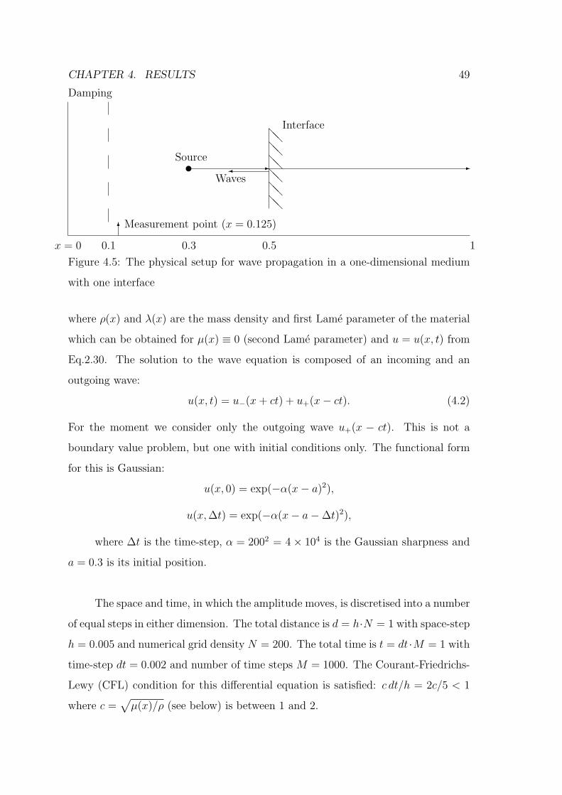
CHAPTER 4. RESULTS 49
@@@@@@@@@@@@
-u -¾
6
Source
Waves
Interface
Damping
Measurement point (x = 0.125)
x = 0 0.1 0.3 0.5 1
Figure 4.5: The physical setup for wave propagation in a one-dimensional medium
with one interface
where ρ(x) and λ(x) are the mass density and first Lame parameter of the material
which can be obtained for µ(x) ≡ 0 (second Lame parameter) and u = u(x, t) from
Eq.2.30. The solution to the wave equation is composed of an incoming and an
outgoing wave:
u(x, t) = u−(x + ct) + u+(x − ct). (4.2)
For the moment we consider only the outgoing wave u+(x − ct). This is not a
boundary value problem, but one with initial conditions only. The functional form
for this is Gaussian:
u(x, 0) = exp(−α(x − a)2),
u(x, ∆t) = exp(−α(x − a − ∆t)2),
where ∆t is the time-step, α = 2002 = 4 × 10⁴ is the Gaussian sharpness and
a = 0.3 is its initial position.
The space and time, in which the amplitude moves, is discretised into a number
of equal steps in either dimension. The total distance is d = h·N = 1 with space-step
h = 0.005 and numerical grid density N = 200. The total time is t = dt ·M = 1 with
time-step dt = 0.002 and number of time steps M = 1000. The Courant-Friedrichs-
Lewy (CFL) condition for this differential equation is satisfied: c dt/h = 2c/5 < 1
where c =√
µ(x)/ρ (see below) is between 1 and 2.

CHAPTER 4. RESULTS 50
Figure 4.6 shows the wave amplitude over both space and time. In this plot the
amplitude starts at a = 0.3 with time reset at zero. After 0.2 time-units it encounters
the single interface, part of which reflects back to the original boundary and part
transmits to the other side. One can see that the reflected wave is absorbed on
t = 0.7 at the original boundary with the damping function as discussed in section
4.1.1. The transmitted wave travels at twice the velocity c(x) =√
λ(x)/ρo = 2
than before (see next subsection on the material properties), and reflects at the
opposite boundary after a further 0.25 time-units (t = 0.45). A quarter of a time-
unit later a reverse transmission and inner reflection occurs at the interface (t =
0.7) as the boundary reflected wave comes back from below the interface. The
inner reflections below the interface repeats the behaviour of boundary reflections
and interface interactions from below, every half time-unit as the propagation time
carries on. The reverse transmitted waves from below are also absorbed by the
original boundary every half time-unit. Both transmission and reflection amplitude
sizes are reduced by these interaction events at the interface, while the opposite
boundary is an infinitely hard surface that does not allow any transmission there
and the reflected amplitude size is not reduced. The amplitudes also undergoes a sign
change upon all reflections, but not for all transmissions. These are in accordance
with the rules that determine the coefficients for reflections and transmissions of
waves. For clarity we have a cleaner three-dimensional plot in Figure 4.7 where the
grid density is reduced and propagation time only goes to unity.
Calculations are done of the wave amplitudes over propagation time but sam-
pled at xm = 0.125 (Figure 4.8) together with their differences with respect to the
target model reference wave (Figures 4.9 and 4.10) as used for the objective function.
They do not look much like the full wave plots discussed in the previous paragraph,
because the fixed sampling position xx is just 0.025 space-units above the damp-
ing inner boundary wx and 0.175 space-units below where the wave is due to start.
Three minima can be seen at t = 0.55, t = 1.09, and t = 1.58, that correspond to the
absorbed signals returning to the original boundary. The differences are very small,
in the range of between -0.0006 and 0.0008. When the differences are squared, they

CHAPTER 4. RESULTS 51
00.5
11.5
2 0
0.2
0.4
0.6
0.8
1
-1
-0.5
0
0.5
1
Amplitude
Time
Distance
Amplitude
Figure 4.6: A plot of the wave propagation over the whole space-time grid for 1D
single interface with damping only on the original side
00.2
0.40.6
0.81 0
0.2
0.4
0.6
0.8
1
-1
-0.5
0
0.5
1
t-axis
x-axis
Figure 4.7: Same plot of the wave propagation but with t → 1, not 2 for 1D single
interface

CHAPTER 4. RESULTS 52
-0.12
-0.1
-0.08
-0.06
-0.04
-0.02
0
0.02
0.04
0.06
0.08
0 0.2 0.4 0.6 0.8 1 1.2 1.4 1.6 1.8 2
Wav
e A
mpl
itude
Time (at position x=1/8)
w(t)u(t)
Figure 4.8: Plot of the optimised wave propagation at xfixed = 1/8 for 1D single
interface
show absolute values of up to 4.5 × 10⁻⁷. They are most prominent at time ranges
of tǫ[0.55, 0.67], [0.85, 1.13] and [1.6, 2.0].
Material Property
Here the mass density and Lame parameter related to the velocity of longitudinal
waves are chosen as, respectively, ρ(x) = ρ = 1 and
λ(x) = λo +λf − λo
1 + exp(−β(x − bx)),
where the typical values of the parameters are λo = 1 and λf = 4, with the
transition made at position bx = 0.5. The sharpness of this single layer interface
function is β = 200 and is independent of h.
The number of minimisation input parameters is 55. This number is chosen
to give a reasonable fit for more accurate results. A lower number would give less
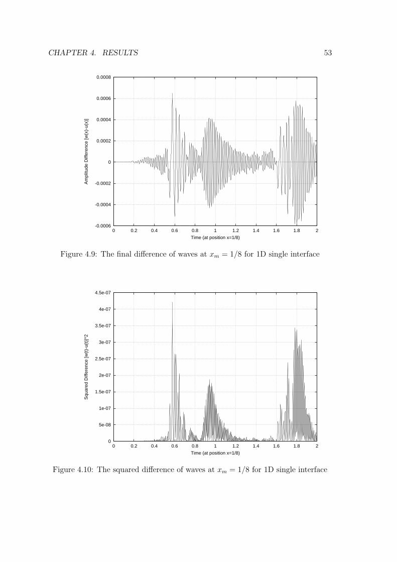
CHAPTER 4. RESULTS 53
-0.0006
-0.0004
-0.0002
0
0.0002
0.0004
0.0006
0.0008
0 0.2 0.4 0.6 0.8 1 1.2 1.4 1.6 1.8 2
Am
plitu
de D
iffer
ence
[w(x
)-u(
x)]
Time (at position x=1/8)
Figure 4.9: The final difference of waves at xm = 1/8 for 1D single interface
0
5e-08
1e-07
1.5e-07
2e-07
2.5e-07
3e-07
3.5e-07
4e-07
4.5e-07
0 0.2 0.4 0.6 0.8 1 1.2 1.4 1.6 1.8 2
Squ
ared
Diff
eren
ce [w
(t)-
u(t)
]^2
Time (at position x=1/8)
Figure 4.10: The squared difference of waves at xm = 1/8 for 1D single interface

CHAPTER 4. RESULTS 54
accurate results, but we have seen less accurate results at a higher numbers as well.
Thus the number of parameters has to be chosen within an acceptable range. Not
too low, but not too high either. These parameters are equated to the Fourier
components. A Fourier sine series is used on the interval x ∈ [bo, bf ] = [0.3, 0.8].
The equation for λ is thus
λ(x) = λo + (λf − λo)
[
x − bo
bf − bo
+n
∑
k=1
ck sin
{
kπ
(
x − bo
bf − bo
)}
]
.
Define a function λFS(x) by moving terms to the left hand side and keeping only
the Fourier Series (FS) on the right hand side:
λFS(x) =λ(x) − λo
λf − λo
− x − bo
bf − bo
=n
∑
k=1
ck sin
[
kπ
(
x − bo
bf − bo
)]
,
where ck are the Fourier components,
ck =1
π
∫
λFS(x) sin [kπX(x)] dx, (4.3)
and X(x) = (x − bo)/(bf − bo).
MERLIN is initialised with zero components of the Fourier series as outlined
here for one dimension on the interval given above. That is, it initialises to a piece-
wise linear function with fixed constant λo = 1 (the original material property) for
x ≤ bo, arbitrary constant λf = 4 (the final material property) for x ≥ bf , and a
straight line between bo and bf . The cosine terms are not used because at x = bo
and x = bf they do not vanish.
Figures 4.11 and 4.12 show how close the minimisation has brought the ma-
terial property to the target function. The first plot shows the single interface in
the middle of the space and the final differences are almost indiscernible. The sec-
ond plot shows the differences themselves and they have values to within ±0.02.
Dividing by the difference between the lower λo and upper λf levels (λf − λo), the
difference range is ±0.00667, or plus-minus two thirds of a percent.

CHAPTER 4. RESULTS 55
0.5
1
1.5
2
2.5
3
3.5
4
4.5
0 0.2 0.4 0.6 0.8 1
Mat
eria
l Pro
pert
y
Distance
Figure 4.11: Plot of the optimised material property function λ for 1D single
interface
-0.015
-0.01
-0.005
0
0.005
0.01
0.015
0.02
0 0.2 0.4 0.6 0.8 1
Mat
eria
l Pro
pert
y D
iffer
ence
Distance
Figure 4.12: Plot of the optimised difference to its target function for 1D single
interface

CHAPTER 4. RESULTS 56
@@@@@@@@@@@@
-u -¾
6
Source
Waves
Interfaces
Damping
Measurement point (x = 0.125)
x = 0 0.1 0.3 0.5 0.7 0.9 1
Figure 4.13: The physical setup for wave propagation in a one-dimensional medium
with multiple interfaces
4.2.2 Multiple interfaces
Wave Propagation
We need to generate a wave amplitude u(x, t) that satisfies the same differential
equation (in one-dimension) as for just one interface in the previous section 4.2.1.
Again this is no boundary value problem, but one with initial conditions only, with
the same Gaussian functional form:
u(x, 0) = exp(−α(x − a)2), u(x, ∆t) = exp(−α(x − a − ∆t)2),
where ∆t is the time-step, α = 5 · 2002 = 2 × 10⁵ is the Gaussian sharpness
and a = 0.3 is its initial position.
The space and time are again discretised in the same way. The total distance
is d = h · N = 1 with space-step h = 0.005 and numerical grid density N = 200.
The total time is t = dt · M = 1 with time-step dt = 0.002 and number of time
steps M = 1000. The Courant-Friedrichs-Lewy (CFL) condition for this differential
equation is also satisfied: c dt/h = 2c/5 < 1 where c =√
µ(x)/ρ (see below) is
between 1 and 2.
Figure 4.14 shows again the wave amplitude over both space and time. One can
see that all reflected waves returning to the original boundary are absorbed there.
The discussion for the one dimensional single interface also applies here. But now

CHAPTER 4. RESULTS 57
we have more than one interface which complicates the behaviour of wave propaga-
tion at later times. The plot is less clear after about propagation time t = 1.2, but
reflections and some transmissions can still be seen. There is more overlap without
interference of split waves, as they come together at one point at the same time and
depart again unhindered on their original ways. All the interfaces still allow wave
transmission and reflection with amplitudes reduced at each event, while the oppo-
site boundary still allows only reflections and no transmission with no reduction in
the amplitude.
Calculations are done of the wave amplitudes over propagation time but sam-
pled at xm = 0.125 (Figure 4.15) together with their differences with respect to
the target model reference wave (Figures 4.16 and 4.17) as used for the objective
function. Once again the plots are less clear after time t = 1.2 due to the more
complicated nature of waves in multiple interfaces later on. Three minima are still
visible before t = 1.2, which correspond to the absorbed signals returning to the orig-
inal boundary, with the new minimum at about t = 0.85. This can only come from
reflections at the new additional interface farther away from the original boundary.
The differences are very small once again, in the range of ±0.0002. The squared
forms show absolute values of up to 3.5 × 10⁻⁸. They are most prominent at time
ranges of tǫ[0.50, 0.75]; [0.75, 1.15] and [1.75, 2.00].
Material Property
Here the mass density and Lame parameter related to the velocity of longitudinal
waves are chosen as ρ(x) = ρ = 1 and
λ(x) = λ0 +3
∑
i=1
λi − λi−1
1 + exp(−β(x − bxi))
,
where the typical values of the parameters are λi = i + 1, bxi= (0.3 + 0.2i).
The sharpness of this λ multi-layered interface function is β = 200 and once again
independent of h.
The number of minimisation parameters (equated to Fourier components) is

CHAPTER 4. RESULTS 58
00.5
11.5
2 0
0.2
0.4
0.6
0.8
1
-1
-0.5
0
0.5
1
Amplitude
Time
Distance
Amplitude
Figure 4.14: A plot of the wave propagation over the whole space-time grid with
damping only on the original side for 1D multiple interfaces
-0.12
-0.1
-0.08
-0.06
-0.04
-0.02
0
0.02
0.04
0.06
0.08
0 0.2 0.4 0.6 0.8 1 1.2 1.4 1.6 1.8 2
Wav
e A
mpl
itude
Time (at position x=1/8)
w(t)u(t)
Figure 4.15: Plot of the optimised wave propagation at xfixed = 1/8 for 1D multiple
interfaces

CHAPTER 4. RESULTS 59
-0.0002
-0.00015
-0.0001
-5e-05
0
5e-05
0.0001
0.00015
0.0002
0 0.2 0.4 0.6 0.8 1 1.2 1.4 1.6 1.8 2
Am
plitu
de D
iffer
ence
[w(x
)-u(
x)]
Time (at position x=1/8)
Figure 4.16: The final difference of waves at xm = 1/8 for 1D multiple interfaces
0
5e-09
1e-08
1.5e-08
2e-08
2.5e-08
3e-08
3.5e-08
0 0.2 0.4 0.6 0.8 1 1.2 1.4 1.6 1.8 2
Squ
ared
Diff
eren
ce [w
(t)-
u(t)
]^2
Time (at position x=1/8)
Figure 4.17: The squared difference of waves at xm = 1/8 for 1D multiple interfaces

CHAPTER 4. RESULTS 60
60. Same accuracy considerations apply with the results than in the previous case
and two dimensional interface problems treated below. A Fourier sine series is used
on the interval x ∈ [bo, bf ] = [0.45, 0.95]. The equation for λ is thus
λ(x) = λo + (λf − λo)
[
X(x) +n
∑
k=1
ck sin {kπX(x)}]
.
Define again a function λFS(x) where ck are the Fourier components,
ck =1
π
∫
λFS(x) sin [kπX(x)] dx, (4.4)
and X(x) = (x − bo)/(bf − bo). The λo and λf correspond to λi, i = 0 and i = 3
respectively. λf is also a Merlin input parameter for scaling the lambda function.
MERLIN is initialised with zero components of the Fourier series.
Figures 4.18 and 4.19 show how close the minimisation has brought the mate-
rial property to the target function. The first plot shows the multiple interfaces at
positions x = 0.5, x = 0.7, and x = 0.9. Once again the final differences are almost
indiscernible. The second plot shows the differences again and they have values
to within ±0.005 in the units of the material property. Dividing by the difference
between the lower and upper levels (λf − λo), the difference range is ±0.001667, or
plus-minus one sixth of a percent. This is four times better than one dimensional
single interface results.
4.3 Two-dimensional Calculations
4.3.1 One interface
Wave Propagation

CHAPTER 4. RESULTS 61
1
1.5
2
2.5
3
3.5
4
4.5
0 0.2 0.4 0.6 0.8 1
Mat
eria
l Pro
pert
y
Distance
Figure 4.18: Plot of the optimised material property function λ for 1D multiple
interfaces
-0.003
-0.002
-0.001
0
0.001
0.002
0.003
0.004
0.005
0 0.2 0.4 0.6 0.8 1
Mat
eria
l Pro
pert
y D
iffer
ence
Distance
Figure 4.19: Plot of the optimised difference to its target function for 1D multiple
interfaces

CHAPTER 4. RESULTS 62
u©ª»¼ -
bb
bb
Measurement points(including source)
Damping Zone
¾
SourceWaves
Layer
0.15 0.3 0.7 1y = 0, x = 0
0.15
0.5
1
Figure 4.20: The physical setup for wave propagation in a medium with a layer in
2D.
We need to generate a wave amplitude u(r, t) = ∇Φ(r, t) with a potential
Φ(r, t) that satisfies the following differential equation in two dimensions. (See
section 2.4):
ρ(r)∂2Φ(r, t)
∂t2= λ(r)∇2Φ(r, t),
where ∇2 is the Laplace operator and ∇ = (∂/∂x, ∂/∂y). Therefore,
ρ(x, y)∂2Φ(x, y, t)
∂t2= λ(x, y)
(
∂2Φ(x, y, t)
∂x2+
∂2Φ(x, y, t)
∂y2
)
, (4.5)
where ρ(x, y) and λ(x, y) are the mass density and first Lame parameter of the
material which can be obtained for µ(x, y) = 0 (second Lame parameter) and
Φ = Φ(x, y, t) from Eq.2.34 and u = ∇Φ.
The radially expanding Gaussian wave from any point of origin is the initial
amplitude for solution of the wave equation. That is
Φ(r, 0) = exp(−αr2A), Φ(r, dt) = exp(−α(rA − dt)2),
where rA =√
(x − ax)2 + (y − ay)2 is the wave radius, a = (ax, ay) = (0.3, 0.5)
positions the point of origin, and the Gaussian sharpness is α = 5 · 502 = 12500.
Here h = 0.02, dt = 0.0025 and N = 50, M = 400, all giving a total distance and

CHAPTER 4. RESULTS 63
time of d = Nh = 1, t = M dt = 1. The CFL condition for this differential equation
is satisfied: c dt/h = 0.0025c/0.02 = c/8 < 1/√
2 where c =√
µ(r)/ρ is between 1
and 2.
The boundary conditions for two dimensions now apply to the potential Φ(r).
These boundary conditions are absorbing on all boundaries, thus Φ(r) and u = ∇Φ
vanish on all boundaries. These apply to this test case and the other cases in two
and three dimensions.
Multiple fixed position (or measurement points) are used for the sum-of-squares
objective function. These are ri = (3, 3 + i)/10, i = 0, 1, 2, 3, 4. The time develop-
ment and final difference of the wave function at these points is shown in Fig.4.21
and 4.22. In the first plot these curves (but one) are flat in the beginning but then
becomes oscillatory as the waves start to roll back and over these points. One curve
is already wavy and has a much greater amplitude at the beginning than the other
curves later on. The curves of the second plot are flat for up to about 0.4 time-units.
No differences arise since the returned waves do not arrive at the measurement points
before then. After the arrivals the differences are between 1×10⁻⁵ and −2.5×10⁻⁵.
When squared the absolute differences are up to 4 × 10⁻¹⁰.
The full amplitude over the whole space is shown in Figure 4.23. This is
actually a series of 9 time frames showing the propagation progress from a point
on the one side of the x-axis and in the middle of the y-axis. A spherical outward
leading wave expands from that point and one sees interference effects inside. In
addition the waves are not perfect circles due to the coarseness of the space (fewer
number of space-steps; only 50 by 50 steps). This can be improved, but with a price
of too long computer runtimes. With damping on all boundaries, the wave and all
interferences disappear. There is an interaction with the single interface at x = 0.7
and at the eighth frame. Due to the interference from behind, a reflection is barely
visible. The transmitted wave speeds up to twice its velocity beyond the interface
and has a greater wavelength. During all this time the amplitude is reduced from

CHAPTER 4. RESULTS 64
-0.3
-0.2
-0.1
0
0.1
0.2
0.3
0 0.1 0.2 0.3 0.4 0.5 0.6 0.7 0.8 0.9 1
Wav
e A
mpl
itude
Time
at 5 measurement points
Figure 4.21: The wave amplitude in time at several measurement points for 2D
single interface
-2.5e-05
-2e-05
-1.5e-05
-1e-05
-5e-06
0
5e-06
1e-05
0 0.1 0.2 0.3 0.4 0.5 0.6 0.7 0.8 0.9 1
Am
plitu
de D
iffer
ence
[w(t
)-u(
t)]
Time
at 5 measurement points
Figure 4.22: The final difference of amplitude at several measurement points for 2D
single interface

CHAPTER 4. RESULTS 65
unity at the start to 0.05 at the end.
Material Property
Here the λ is modelled by a single interface parallel to the y-axis [mass density
ρ(x, y) = 1]:
λ(r) = λo +λf − λo
1 + exp(−β(x − bx)),
where the typical values of the parameters are the same again as in one di-
mension: λo = 1 and λf = 4, but the position was bx = 0.7. Then β = 50 is the
sharpness of λ.
The ansatz for the optimising function on the interval x ∈ [bo, bf ] = [0.5, 0.9],
also independent of y in two dimensions, is
λ(r) = λo + (λf − λo)
[
X(x) +n
∑
k=1
ck sin (kπX(x))
]
,
with the same defining function λFS(r) within the Fourier coefficients ck, and X(x) =
(x − bo)/(bf − bo). Here the 40 Fourier components ck are initialised to zero, giving
the same piecewise initial function as in one dimension but now extended into and
independent of the y-direction. Same accuracy considerations apply than in one-
dimensional case to the chosen number of components.
The optimised material property function λ and its difference from the target
is plotted in Fig.4.24 and 4.25. In the first plot the optimised function does not quite
fit the target function. This is most pronounced with a dip at x = 0.8. Thus in the
second plot the biggest negative difference at x = 0.8 touches at around −0.14, while
the positive difference is only at around 0.04 in the units for the material property
function.

CHAPTER 4. RESULTS 66
0
0.2
0.4
0.6
0.8
1
Wave Amplitude
0 0.2 0.4 0.6 0.8 1
x-distance
0
0.2
0.4
0.6
0.8
1
y-di
stan
ce
-0.2
-0.15
-0.1
-0.05
0
0.05
0.1
0.15
Wave Amplitude
0 0.2 0.4 0.6 0.8 1
x-distance
0
0.2
0.4
0.6
0.8
1y-
dist
ance
-0.1
-0.08
-0.06
-0.04
-0.02
0
0.02
0.04
0.06
0.08
0.1
Wave Amplitude
0 0.2 0.4 0.6 0.8 1
x-distance
0
0.2
0.4
0.6
0.8
1
y-di
stan
ce
-0.1
-0.08
-0.06
-0.04
-0.02
0
0.02
0.04
0.06
0.08
Wave Amplitude
0 0.2 0.4 0.6 0.8 1
x-distance
0
0.2
0.4
0.6
0.8
1
y-di
stan
ce
-0.06
-0.04
-0.02
0
0.02
0.04
0.06
0.08
Wave Amplitude
0 0.2 0.4 0.6 0.8 1
x-distance
0
0.2
0.4
0.6
0.8
1
y-di
stan
ce
-0.06
-0.04
-0.02
0
0.02
0.04
0.06
0.08
Wave Amplitude
0 0.2 0.4 0.6 0.8 1
x-distance
0
0.2
0.4
0.6
0.8
1y-
dist
ance
-0.05
-0.04
-0.03
-0.02
-0.01
0
0.01
0.02
0.03
0.04
0.05
Wave Amplitude
0 0.2 0.4 0.6 0.8 1
x-distance
0
0.2
0.4
0.6
0.8
1
y-di
stan
ce
-0.05
-0.04
-0.03
-0.02
-0.01
0
0.01
0.02
0.03
0.04
Wave Amplitude
0 0.2 0.4 0.6 0.8 1
x-distance
0
0.2
0.4
0.6
0.8
1
y-di
stan
ce
-0.05
-0.04
-0.03
-0.02
-0.01
0
0.01
0.02
0.03
0.04
0.05
Wave Amplitude
0 0.2 0.4 0.6 0.8 1
x-distance
0
0.2
0.4
0.6
0.8
1
y-di
stan
ce
Figure 4.23: The amplitude in 2D space: time frames are from t = 0 to t = 0.8 in
0.10 seconds increments for 2D single interface

CHAPTER 4. RESULTS 67
1
1.5
2
2.5
3
3.5
4
0 0.2 0.4 0.6 0.8 1
Mat
eria
l Pro
pert
y
Distance
Final (Optimized)Final (Target)
Figure 4.24: The optimised material property function λ for 2D single interface
-0.16
-0.14
-0.12
-0.1
-0.08
-0.06
-0.04
-0.02
0
0.02
0.04
0.06
0 0.2 0.4 0.6 0.8 1
MP
Diff
eren
ce
Distance
Optimized - Target
Figure 4.25: The optimised difference to its target function for 2D single interface

CHAPTER 4. RESULTS 68
u©ª»¼ -
bb
bb
Measurement points(including source)
Damping Zone
¾
SourceWaves
Layers
0.15 0.3 0.5 10.7 0.9y = 0, x = 0
0.15
0.5
1
Figure 4.26: The physical setup for wave propagation in a medium with multiple
layers in 2D.
4.3.2 Multiple interfaces
Wave Propagation
We need to generate a wave amplitude u(r, t) = ∇Φ(r, t) with a potential Φ(r, t)
that satisfies the same differential equation in two dimensions as in the previous
section 4.3.1.
The radially expanding Gaussian wave from any point of origin is the initial
amplitude for solution of the wave equation. That is
Φ(r, 0) = exp(−αr2A), Φ(r, dt) = exp(−α(rA − dt)2),
where rA =√
(x − ax)2 + (y − ay)2 is the wave radius, a = (ax, ay) = (0.3, 0.5)
is the point of origin, and the Gaussian sharpness is α = 5 · 402 = 8000. Here
h = 0.025, dt = 0.0025 and N = 40, M = 800 all giving a total distance and time
of d = Nh = 1, t = M dt = 2. The CFL condition for this differential equation is
satisfied: c dt/h = 0.0025c/0.025 = c/100 < 1/√
2 where c =√
µ(r)/ρ is between 1
and 2. The same absorbing boundary conditions as in section 4.3.1 apply here.
More than one fixed position (or measurement point) is used for the sum-of-

CHAPTER 4. RESULTS 69
squares objective function. These are ri = (3, 3 + i)/10, i = 0, 1, 2, 3, 4. The time
development and optimised difference of the wave function at these points is shown
in Fig.4.27 and 4.28. The first plot shows basically similar behaviour as before. The
curves of the second plot are flat for up to about 0.3 time-units. No differences arise
since the reflected wave do not arrive at the measurement points before then. After
the arrivals the differences are between 2.5 × 10⁻⁶ and −3 × 10⁻⁶. When squared
the absolute differences are up to 9× 10⁻¹². This is a better result than that for the
single interface.
The full amplitude over the whole space is shown in Figure 4.29. This is also a
series of 9 time frames showing how the propagation progress from a point on the one
side of the x-axis and in the middle of the y-axis. A spherical outward leading wave
expands from that point and one again sees interference effects inside. In addition
the waves are not perfect circles due to the coarseness of the space (only 40 by 40
space-steps). This can be improved, but with a price of too long computer runtimes.
With damping on all boundaries, the wave and all interferences disappear. There
is an interaction with the interfaces beginning at x = 0.5 and at the fifth frame a
reflection is visible, despite the interferences from behind. The transmitted wave
speeds up in steps, depending on the particular level, to twice its velocity beyond
the last interface. In the last three frames standing waves seem to form after the
first interface at position x = 0.5. During all this time the amplitude is reduced
from unity at the start to 0.06 at the end.
Material Property
Here λ is modelled by a multi-layered interface with the layers parallel to the y-axis
[mass density ρ(x, y) = 1]:
λ(r) = λ0 +3
∑
i=1
λi − λi−1
1 + exp(−β(x − bxi))
,
where the typical values of the parameters are the same again as in one di-
mension: λi = i + 1, bxi= (0.3 + 0.2i). β = 40 is the sharpness of λ.

CHAPTER 4. RESULTS 70
-0.3
-0.2
-0.1
0
0.1
0.2
0.3
0 0.1 0.2 0.3 0.4 0.5 0.6 0.7 0.8 0.9 1
Wav
e A
mpl
itude
Time
at 5 measurement points
Figure 4.27: The wave amplitude in time at several measurement points for 2D
multiple interfaces
-3e-06
-2.5e-06
-2e-06
-1.5e-06
-1e-06
-5e-07
0
5e-07
1e-06
1.5e-06
2e-06
2.5e-06
0 0.1 0.2 0.3 0.4 0.5 0.6 0.7 0.8 0.9 1
Am
plitu
de D
iffer
ence
[w(t
)-u(
t)]
Time
at 5 measurement points
Figure 4.28: The final difference of amplitude at several measurement points for 2D
multiple interfaces

CHAPTER 4. RESULTS 71
0
0.2
0.4
0.6
0.8
1
Wave Amplitude
0 0.2 0.4 0.6 0.8 1
x-distance
0
0.2
0.4
0.6
0.8
1
y-di
stan
ce
-0.2
-0.15
-0.1
-0.05
0
0.05
0.1
0.15
Wave Amplitude
0 0.2 0.4 0.6 0.8 1
x-distance
0
0.2
0.4
0.6
0.8
1y-
dist
ance
-0.1
-0.08
-0.06
-0.04
-0.02
0
0.02
0.04
0.06
0.08
0.1
Wave Amplitude
0 0.2 0.4 0.6 0.8 1
x-distance
0
0.2
0.4
0.6
0.8
1
y-di
stan
ce
-0.1
-0.08
-0.06
-0.04
-0.02
0
0.02
0.04
0.06
0.08
Wave Amplitude
0 0.2 0.4 0.6 0.8 1
x-distance
0
0.2
0.4
0.6
0.8
1
y-di
stan
ce
-0.06
-0.04
-0.02
0
0.02
0.04
0.06
0.08
Wave Amplitude
0 0.2 0.4 0.6 0.8 1
x-distance
0
0.2
0.4
0.6
0.8
1
y-di
stan
ce
-0.08
-0.06
-0.04
-0.02
0
0.02
0.04
0.06
Wave Amplitude
0 0.2 0.4 0.6 0.8 1
x-distance
0
0.2
0.4
0.6
0.8
1y-
dist
ance
-0.06
-0.04
-0.02
0
0.02
0.04
0.06
0.08
Wave Amplitude
0 0.2 0.4 0.6 0.8 1
x-distance
0
0.2
0.4
0.6
0.8
1
y-di
stan
ce
-0.06
-0.04
-0.02
0
0.02
0.04
0.06
Wave Amplitude
0 0.2 0.4 0.6 0.8 1
x-distance
0
0.2
0.4
0.6
0.8
1
y-di
stan
ce
-0.05
-0.04
-0.03
-0.02
-0.01
0
0.01
0.02
0.03
0.04
0.05
0.06
Wave Amplitude
0 0.2 0.4 0.6 0.8 1
x-distance
0
0.2
0.4
0.6
0.8
1
y-di
stan
ce
Figure 4.29: The amplitude in 2D space: time frames are from t = 0 to t = 1.6 in
0.20 seconds increments for 2D multiple interfaces

CHAPTER 4. RESULTS 72
The optimising function on the interval x ∈ [bo, bf ] = [0.45, 0.95], also inde-
pendent of y in two dimensions, is
λ(r) = λo + (λf − λo)
[
X(x) +n
∑
k=1
ck sin (kπX(x))
]
,
with the same defining function λFS(r) within the Fourier components ck, and
X(x) = (x − bo)/(bf − bo). The λo and λf again corresponds to λi, i = 0 and
i = 3 respectively. λf is also a Merlin input parameter for scaling the lambda func-
tion. Here the 60 Fourier components ck are initialised to zero, giving the same
piecewise initial function as in one-dimension but now extended into and indepen-
dent of the y-direction. Same accuracy considerations apply as well.
The optimised material property function λ and its difference from the target is
plotted in Fig.4.30 and 4.31. In the first plot the optimised function is seen to differ
at the third plateau from the target material property function. This may be due to
the third interface positioned wholly inside the damping zone at the opposite side
of the x-axis and may have little influence on returning waves at the measurement
points. In the second plot the difference is between −0.025 and 0.03, in the units for
the material property function. These differences arise because the Fourier method
would optimise the components of the longest fundamental (resonant) wavelengths
first, working its way through components to that of the shorter wavelengths until
the objective function reaches a minimum. Once at the minimum, the rest of the
components at the shortest end of wavelength spectrum simply freezes into non-
optimised values. Then the associated short wavelengths are mismatched, leading
to the oscillatory behaviour for the third and fourth plateaus in the material property
function differences.
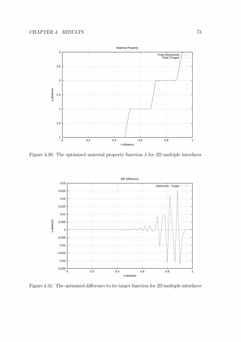
CHAPTER 4. RESULTS 73
1
1.5
2
2.5
3
3.5
4
0 0.2 0.4 0.6 0.8 1
y-di
stan
ce
x-distance
Material Property
Final (Optimized)Final (Target)
Figure 4.30: The optimised material property function λ for 2D multiple interfaces
-0.025
-0.02
-0.015
-0.01
-0.005
0
0.005
0.01
0.015
0.02
0.025
0.03
0 0.2 0.4 0.6 0.8 1
y-di
stan
ce
x-distance
MP Difference
Optimized - Target
Figure 4.31: The optimised difference to its target function for 2D multiple interfaces

CHAPTER 4. RESULTS 74
u m©ª»¼
¾
-
bb
bb
Measurement points(including source)
Damping Zone
SourceWaves Feature
0.3 0.70.15 1y = 0, x = 0
0.15
0.5
1
Figure 4.32: The physical setup for wave propagation in a medium with a feature
in 2D.
4.3.3 Gaussian feature
Wave Propagation
The same differential wave equation in two dimensions for Φ applies here as in sec-
tion 4.3.1.
The radially expanding Gaussian wave from any point of origin is the initial
amplitude for solution of the wave equation. That is
Φ(r, 0) = exp(−αr2), Φ(r, dt) = exp(−α(r − dt)2),
where r =√
(x − ax)2 + (y − ay)2 is the wave radius, a = (ax, ay) = (0.3, 0.5)
positions the point of origin, and α = 1/5 · 402 = 320 is the Gaussian sharpness.
Here too h = 0.025, dt = 0.0025 and N = 40 but M = 400. The CFL condition for
this differential equation is satisfied: c dt/h = 0.0025c/0.025 = c/10 < 1/√
2 where
c =√
µ(r)/ρ is between 1 and 2. The same absorbing boundary conditions as in
section 4.3.1 apply here.
Once again, more than one fixed position (or measurement point) was used to
improve the minimisation. These are ri = (3, 3 + i)/10, i = 0, 1, 2, 3, 4. The time
CHAPTER 4. RESULTS 75
development of the wave function and its difference from the target reference wave at
these points are given in the diagram Figures 4.33 and 4.34. These peaks correspond
to each of the five measurement points. In the first plot each peak position shows
when in time the original wave arrived at each measurement point. The highest
peak occurs at index i = 2 of ri. There is a sort of pairing of the other four peaks.
This means that the higher peak pair at around 0.1 time-units corresponds to the
arrivals at i = 1 and i = 3, while the other pair at around 0.2 time-units are the
arrivals at i = 0 and i = 4. Though barely discernable, reflections of the feature
start to arrive at between t = 0.6 and t = 0.8. The second plot shows the curves are
flat for up to 0.35 time-units. Then reflection effects starts to roll in with differences
between −1 × 10⁻⁶ and 4 × 10⁻⁶. The squared difference will be up to 1.6 × 10⁻¹¹.
The full wave function over the whole space follows in Figure 4.35 with 9
time development frames of wave propagation. Again the wave starts as a Gaussian
peak at the point a on one side, which then dissolves into a spherically expanding
wave. Interference behind the wave is less pronounced. Once again the waves are
not perfect circles in regard of a fewer number of space-steps (40 by 40). This can
be increased, but the computer runtimes will go into hours, if not days. When
interacting with the feature (fifth frame), the wave speeds up to twice its velocity
at peak position, then dissolves beyond the feature. Thus, a hole has formed in the
wave around and beyond the feature. The feature does not create any interference
of each part of the wave on either side. Each part just carries on expanding with
the hole widening as time goes on. Damping is visible in the dark regions around
the boundaries where the waves are absorbed. The amplitude reduces from unity to
about 0.07 during this time.
Material Property
Here the λ is represented by a Gaussian feature, with the function [mass density
ρ(x, y) is unity over all space]:
λ(x, y) = λenv + (λpeak − λenv) exp(−βR2),
where β = 320 is the Gaussian steepness, R =√
(x − bx)2 + (y − by)2 is the

CHAPTER 4. RESULTS 76
0
0.1
0.2
0.3
0.4
0.5
0.6
0.7
0.8
0.9
1
0 0.1 0.2 0.3 0.4 0.5 0.6 0.7 0.8 0.9 1
Wav
e A
mpl
itude
Time
at 5 measurement points
Figure 4.33: The amplitude of time at several measurement points for 2D Gaussian
feature
-1e-06
-5e-07
0
5e-07
1e-06
1.5e-06
2e-06
2.5e-06
3e-06
3.5e-06
4e-06
0 0.1 0.2 0.3 0.4 0.5 0.6 0.7 0.8 0.9 1
Am
plitu
de D
iffer
ence
[w(t
)-u(
t)]
Time
at 5 measurement points
Figure 4.34: The amplitude difference at several measurement points for 2D Gaus-
sian feature

CHAPTER 4. RESULTS 77
0
0.2
0.4
0.6
0.8
1
Wave Amplitude
0 0.2 0.4 0.6 0.8 1
x-distance
0
0.2
0.4
0.6
0.8
1
y-di
stan
ce
0
0.1
0.2
0.3
0.4
0.5
0.6
Wave Amplitude
0 0.2 0.4 0.6 0.8 1
x-distance
0
0.2
0.4
0.6
0.8
1y-
dist
ance
0
0.05
0.1
0.15
0.2
0.25
0.3
0.35
0.4
0.45
Wave Amplitude
0 0.2 0.4 0.6 0.8 1
x-distance
0
0.2
0.4
0.6
0.8
1
y-di
stan
ce
0
0.05
0.1
0.15
0.2
0.25
0.3
0.35
0.4
Wave Amplitude
0 0.2 0.4 0.6 0.8 1
x-distance
0
0.2
0.4
0.6
0.8
1
y-di
stan
ce
0
0.05
0.1
0.15
0.2
0.25
0.3
0.35
Wave Amplitude
0 0.2 0.4 0.6 0.8 1
x-distance
0
0.2
0.4
0.6
0.8
1
y-di
stan
ce
0
0.05
0.1
0.15
0.2
0.25
0.3
Wave Amplitude
0 0.2 0.4 0.6 0.8 1
x-distance
0
0.2
0.4
0.6
0.8
1y-
dist
ance
0
0.05
0.1
0.15
0.2
0.25
Wave Amplitude
0 0.2 0.4 0.6 0.8 1
x-distance
0
0.2
0.4
0.6
0.8
1
y-di
stan
ce
0
0.02
0.04
0.06
0.08
0.1
0.12
0.14
Wave Amplitude
0 0.2 0.4 0.6 0.8 1
x-distance
0
0.2
0.4
0.6
0.8
1
y-di
stan
ce
0
0.01
0.02
0.03
0.04
0.05
0.06
0.07
Wave Amplitude
0 0.2 0.4 0.6 0.8 1
x-distance
0
0.2
0.4
0.6
0.8
1
y-di
stan
ce
Figure 4.35: The amplitude in 2D space: time frames are from t = 0 to t = 0.8 in
0.10 seconds increments for 2D Gaussian feature

CHAPTER 4. RESULTS 78
Gaussian radius, and b = (bx, by) = (0.7, 0.5) is the position of the feature. λenv is
the environment level value and λpeak is the value of the peak.
We use the finite-element method whose coefficients are now calculated from
the λ-function above at the corner positions of the elements. The Laguerre poly-
nomials are of fourth order, each operating on rectangular regions (the elements)
of an area Hx × Hy. Currently the side-lengths are H = (Hx, Hy) = (6, 6)h within
each element, which makes them square. To accommodate the feature we have 4
squares, arranged in 2× 2, whose common intersecting corners are at position b, in
the middle of the applied FEM-region.
The plots for two-dimensional problem follow. The optimised lambda function
λ and its difference from its target is seen in Fig.4.36 and 4.37. The first plot
shows a nice spherical Gaussian peak at position b on the other side of the space.
In the current view of the second plot a negative difference is seen on the near
side with two minima (the bigger one closer to the opposite y-boundary), and a
positive difference on the far side with two maxima (again the bigger one closer to
the opposite y-boundary). The differences range at ±0.004.
4.4 Three-dimensional Calculations
4.4.1 Gaussian feature
Wave Propagation
We need to generate a wave amplitude u(r, t) = ∇Φ(r, t) for a potential Φ that
satisfies the following differential equation in three dimension of Φ (see section 2.4):
ρ(r)∂2Φ(r, t)
∂t2= λ(r)∇2Φ(r, t), (4.6)
where ∇2 is the Laplace operator and ∇ = (∂/∂x, ∂/∂y, ∂/∂z). λ(x, y, z) are the
first Lame parameter of the material which can be obtained for µ(x, y, z) = 0 (sec-
ond Lame parameter) and Φ = Φ(x, y, z, t) again from Eq.2.34.
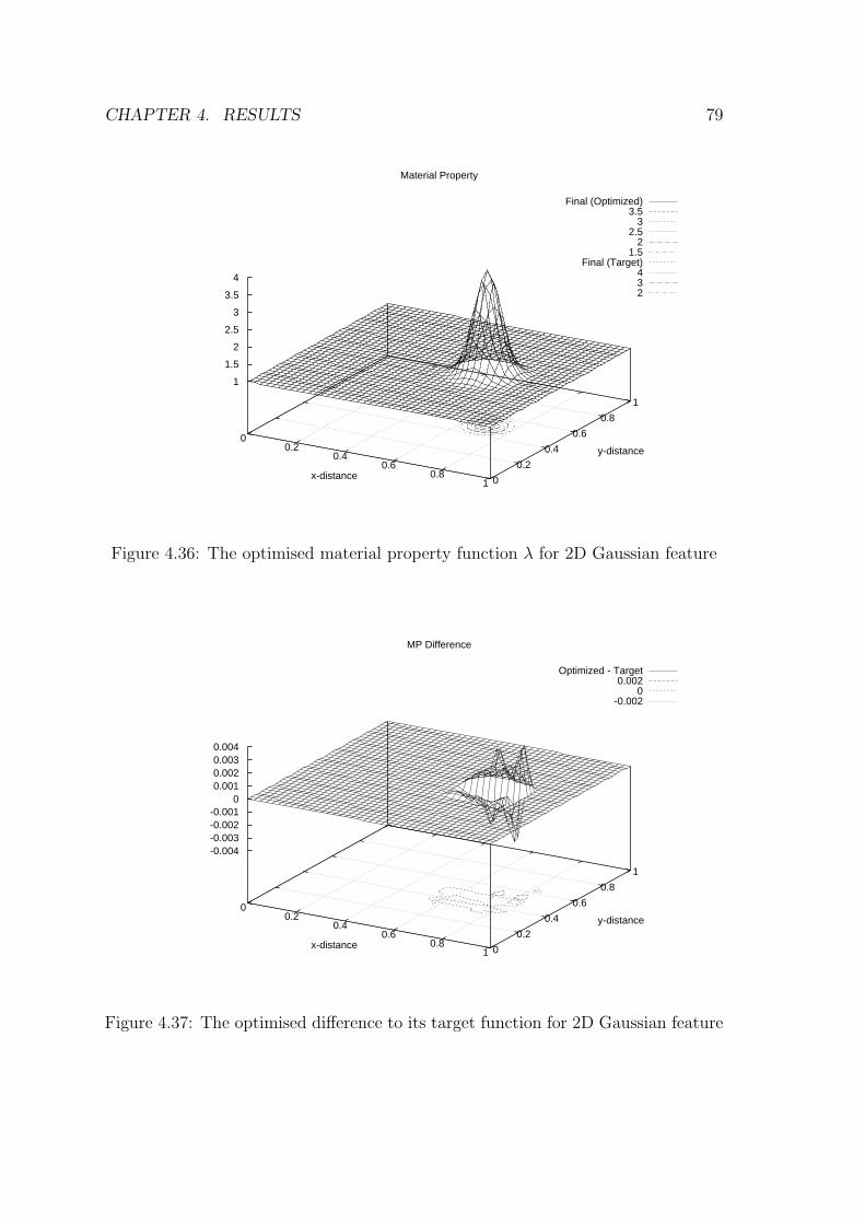
CHAPTER 4. RESULTS 79
00.2
0.40.6
0.81 0
0.2
0.4
0.6
0.8
1
1
1.5
2
2.5
3
3.5
4
Material Property
Final (Optimized) 3.5 3
2.5 2
1.5Final (Target)
4 3 2
x-distance
y-distance
Figure 4.36: The optimised material property function λ for 2D Gaussian feature
00.2
0.40.6
0.81 0
0.2
0.4
0.6
0.8
1
-0.004-0.003-0.002-0.001
00.0010.0020.0030.004
MP Difference
Optimized - Target 0.002
0 -0.002
x-distance
y-distance
Figure 4.37: The optimised difference to its target function for 2D Gaussian feature

CHAPTER 4. RESULTS 80
u m©ª»¼
¾
-
bb
bb
Measurement points
Damping Zone
SourceWaves Feature
0.3 0.70.15 1y = 0, x = 0
0.15
0.5
1
Figure 4.38: The physical setup for wave propagation in a medium with a feature
in 3D.
ub b bbb
bb b bbMeasurement points
Damping Zone
Source
0.3 0.7 1z = 0, y = 0
1
0.6
0.4
Figure 4.39: The same physical setup for wave propagation head-on in 3D
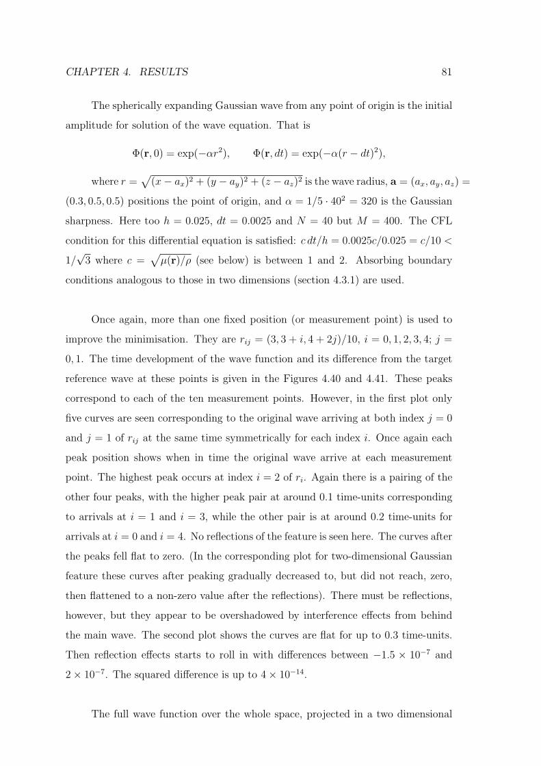
CHAPTER 4. RESULTS 81
The spherically expanding Gaussian wave from any point of origin is the initial
amplitude for solution of the wave equation. That is
Φ(r, 0) = exp(−αr2), Φ(r, dt) = exp(−α(r − dt)2),
where r =√
(x − ax)2 + (y − ay)2 + (z − az)2 is the wave radius, a = (ax, ay, az) =
(0.3, 0.5, 0.5) positions the point of origin, and α = 1/5 · 402 = 320 is the Gaussian
sharpness. Here too h = 0.025, dt = 0.0025 and N = 40 but M = 400. The CFL
condition for this differential equation is satisfied: c dt/h = 0.0025c/0.025 = c/10 <
1/√
3 where c =√
µ(r)/ρ (see below) is between 1 and 2. Absorbing boundary
conditions analogous to those in two dimensions (section 4.3.1) are used.
Once again, more than one fixed position (or measurement point) is used to
improve the minimisation. They are rij = (3, 3 + i, 4 + 2j)/10, i = 0, 1, 2, 3, 4; j =
0, 1. The time development of the wave function and its difference from the target
reference wave at these points is given in the Figures 4.40 and 4.41. These peaks
correspond to each of the ten measurement points. However, in the first plot only
five curves are seen corresponding to the original wave arriving at both index j = 0
and j = 1 of rij at the same time symmetrically for each index i. Once again each
peak position shows when in time the original wave arrive at each measurement
point. The highest peak occurs at index i = 2 of ri. Again there is a pairing of the
other four peaks, with the higher peak pair at around 0.1 time-units corresponding
to arrivals at i = 1 and i = 3, while the other pair is at around 0.2 time-units for
arrivals at i = 0 and i = 4. No reflections of the feature is seen here. The curves after
the peaks fell flat to zero. (In the corresponding plot for two-dimensional Gaussian
feature these curves after peaking gradually decreased to, but did not reach, zero,
then flattened to a non-zero value after the reflections). There must be reflections,
however, but they appear to be overshadowed by interference effects from behind
the main wave. The second plot shows the curves are flat for up to 0.3 time-units.
Then reflection effects starts to roll in with differences between −1.5 × 10⁻⁷ and
2 × 10⁻⁷. The squared difference is up to 4 × 10⁻¹⁴.
The full wave function over the whole space, projected in a two dimensional
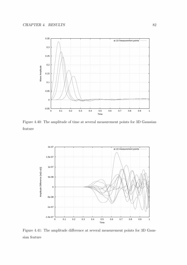
CHAPTER 4. RESULTS 82
-0.05
0
0.05
0.1
0.15
0.2
0.25
0.3
0.35
0 0.1 0.2 0.3 0.4 0.5 0.6 0.7 0.8 0.9 1
Wav
e A
mpl
itude
Time
at 10 measurement points
Figure 4.40: The amplitude of time at several measurement points for 3D Gaussian
feature
-1.5e-07
-1e-07
-5e-08
0
5e-08
1e-07
1.5e-07
2e-07
0 0.1 0.2 0.3 0.4 0.5 0.6 0.7 0.8 0.9 1
Am
plitu
de D
iffer
ence
[w(t
)-u(
t)]
Time
at 10 measurement points
Figure 4.41: The amplitude difference at several measurement points for 3D Gaus-
sian feature

CHAPTER 4. RESULTS 83
plane at the middle of the third-dimension, follows in Figure 4.42 again with 9 time
development frames of wave propagation. These plots is a projection on a two-
dimensional xy-plane at the middle of the third-dimension z. The same discussion
applies here, as in the case for two-dimensional Gaussian feature. Here the interfer-
ence behind the main wave is even less pronounced. Once again the waves are not
perfect circles in regard of a fewer number of space-steps. This can be increased,
but the computer will run into hours of runtime. The amplitude is reduced from
unity to 0.008 over the entire time period which made the damping zone less visible
except where the wave is absorbed.
Material Property
Here the setup in two-dimensional space above is generalised to three dimensions.
λ is represented by a Gaussian feature with the function [mass density ρ(x, y, z) is
unity over all space]:
λ(x, y, z) = λenv + (λpeak − λenv) exp(−βR2),
where β = 320 is the Gaussian steepness, R =√
(x − bx)2 + (y − by)2 + (z − bz)2
is the Gaussian radius, and b = (bx, by, bz) = (0.7, 0.5, 0.5) is the position of the fea-
ture. λenv is the environment level value and λpeak is the value of the peak.
We use the finite-element method whose coefficients are now calculated from
the λ-function above at the corner positions of the elements. The Lagrange polyno-
mials are of fourth order, each operating on rectangular regions (the elements) of a
volume Hx ×Hy ×Hz. Currently the side-lengths are H = (Hx, Hy, Hz) = (6, 6, 6)h
within each element, which makes them cubic. To accommodate the feature we have
8 cubes, arranged in 2 × 2 × 2, whose common intersecting corners are at position
b, in the middle of the applied FEM-region.
The plots for three-dimensional problem follows. The optimised lambda func-
tion λ and its difference from its target is seen in Fig.4.43 and 4.44. These plots
are a projection on a two-dimensional xy-plane at the middle of the third-dimension
z. The first plot shows again a nice spherical Gaussian peak at position b on the

CHAPTER 4. RESULTS 84
0
0.2
0.4
0.6
0.8
1
Wave Amplitude
0 0.2 0.4 0.6 0.8 1
x-distance
0
0.2
0.4
0.6
0.8
1
y-di
stan
ce
0
0.05
0.1
0.15
0.2
0.25
0.3
Wave Amplitude
0 0.2 0.4 0.6 0.8 1
x-distance
0
0.2
0.4
0.6
0.8
1y-
dist
ance
-0.02
0
0.02
0.04
0.06
0.08
0.1
0.12
0.14
0.16
0.18
Wave Amplitude
0 0.2 0.4 0.6 0.8 1
x-distance
0
0.2
0.4
0.6
0.8
1
y-di
stan
ce
-0.02
0
0.02
0.04
0.06
0.08
0.1
0.12
Wave Amplitude
0 0.2 0.4 0.6 0.8 1
x-distance
0
0.2
0.4
0.6
0.8
1
y-di
stan
ce
-0.02
-0.01
0
0.01
0.02
0.03
0.04
0.05
0.06
0.07
0.08
0.09
Wave Amplitude
0 0.2 0.4 0.6 0.8 1
x-distance
0
0.2
0.4
0.6
0.8
1
y-di
stan
ce
-0.01
0
0.01
0.02
0.03
0.04
0.05
0.06
0.07
Wave Amplitude
0 0.2 0.4 0.6 0.8 1
x-distance
0
0.2
0.4
0.6
0.8
1y-
dist
ance
-0.02
-0.01
0
0.01
0.02
0.03
0.04
0.05
Wave Amplitude
0 0.2 0.4 0.6 0.8 1
x-distance
0
0.2
0.4
0.6
0.8
1
y-di
stan
ce
-0.02
-0.015
-0.01
-0.005
0
0.005
0.01
0.015
0.02
0.025
Wave Amplitude
0 0.2 0.4 0.6 0.8 1
x-distance
0
0.2
0.4
0.6
0.8
1
y-di
stan
ce
-0.004
-0.002
0
0.002
0.004
0.006
0.008
Wave Amplitude
0 0.2 0.4 0.6 0.8 1
x-distance
0
0.2
0.4
0.6
0.8
1
y-di
stan
ce
Figure 4.42: The amplitude in 3D space: time frames are from t = 0 to t = 0.8 in
0.10 seconds increments for 3D Gaussian feature

CHAPTER 4. RESULTS 85
other side of the space. In the current view of the second plot the differences are
more complex. There are four peaks side-by-side (y-direction) and alternating in
sign between the negative and positive. A maximum is evident in the middle of this
FEM region (y-direction) with one minimum on the near side and two minima on
the far side. The differences are in the range of ±0.012.

CHAPTER 4. RESULTS 86
00.2
0.40.6
0.81 0
0.2
0.4
0.6
0.8
1
1
1.5
2
2.5
3
3.5
4
4.5
Material Property
Final (Optimized)Final (Target)
x-distance
y-distance
Figure 4.43: The optimised material property function λ for 3D Gaussian feature
00.2
0.40.6
0.81 0
0.2
0.4
0.6
0.8
1
-0.01-0.008-0.006-0.004-0.002
00.0020.0040.0060.0080.01
0.012
Material Property
Difference (Optimized - Target)
x-distance
y-distance
Figure 4.44: The optimised difference to its target function for 3D Gaussian feature

Chapter 5
Conclusions
The property plots in the previous chapter and table 5.1 of relative fraction dif-
ferences show how the Levenberg-Marquardt minimisation method brings the op-
timised material property function close to the target model. In the property dif-
ference plots, the differences shown are more pronounced at the higher layers, after
the transition from the lowest layer has been made. The best results are those for
one-dimensional multi-layered interface and two-dimensional feature.
In a comparison between the Fourier series and the finite element methods,
the latter method seems more successful. But see an explanation about areas or
subregions in section 5.1 below.
The differences of the amplitudes for use in the objective function, as shown
in table 5.2, are significantly reduced with the addition of spatial dimensions or
interfaces.
5.1 Summary of our results
5.1.1 One dimension
By comparing the material property difference results between the single and mul-
tiple interfaces, we see the latter gives a smaller, and thus better, deviation. This
is due to the fact that there are more than two layers in the target function which
87

CHAPTER 5. CONCLUSIONS 88
Table 5.1: Plot ranges of the material property differences of the optimised to the
target function (divided by the difference between the lowest λo and highest λf layer
values), values in units of 10−2.
Material property Single interface Multiple interface Feature
(Method) (Fourier series) (Fourier series) (Finite elements)
One dimension [-0.500,0.667] [-0.100,0.167] —
Two dimensions [-5.333,2.000] [-0.833,1.000] [-0.133,0.133]
Three dimensions — — [-0.333,0.400]
Table 5.2: Plot ranges of the amplitude differences (the optimised relative to the
target reference function) sampled at the measurement points for the objective func-
tion, values in units of 10−6.
Material property Single interface Multiple interface Feature
(Method) (Fourier series) (Fourier series) (Finite elements)
One dimension [-600,800] [-200.0,200.0] —
Two dimensions [ -25, 10] [ -3.0, 2.5] [-1.00,4.00]
Three dimensions — — [-0.15,0.20]

CHAPTER 5. CONCLUSIONS 89
approximately comes closer to the initialised optimised function that resembles a
piecewise linear function. The minimisation had a closer run to the minimum in the
multiple interface setup than that of the single interface. This can also be seen in
the amplitude differences.
5.1.2 Two dimensions
Comparisons of the material property differences in two dimensions between the
single and multiple interfaces leads to the same conclusion as with one dimensional
results as above. The two dimensional results are less satisfactory. The single
interface material property result does not even reach our goal of less than or equal
to ±10−2 (±1%) difference (see table 5.1). Since the interface position is at x = 0.7,
and not x = 0.5, the waves reflecting at the interface reaches the measurement points
much later and the minimisation did not have much amplitude differences to go by,
while the optimised parameter initial point is far from the minimum position in the
parameter space. Also, just after the transition from the lower layer, a small trench
is visible in the upper layer. For the multi-layer interface results, there are also small
differences still visible at the third layer. See section 4.1.2 for an explanation. Also,
while in one dimension the real space interval the technique worked on is [bo, bf ], in
two dimensions it is the Cartesian product [bo, bf ]× [0, 1] which defines a rectangular
strip running under the y-parallel interface where a radially expanding wave impacts
on it at various times. The Gaussian feature result is much better than the interfaces
due to the feature occupying a smaller area for the FEM region.
5.1.3 Three dimensions
There are no results yet for interface(s) in three dimensions. Thus, for comparison
with the fewer dimensions, we have only the Gaussian feature results. Once again
the material property deviation results are less accurate than the corresponding
two-dimensional feature difference result, which highlights a trend we see across the
real space dimensions.
One may ask why it is that the material property difference results become

CHAPTER 5. CONCLUSIONS 90
less and less accurate as one adds one more dimension after another to real space
Rm, while the amplitude differences used in the objective function become more ac-
curate. Recall that the more advanced minimisation techniques, such as Levenberg-
Marquardt, are designed to work with slightly non-linear mathematical systems (as
set out in [11]). Therefore, small changes in one variable or function may lead to
large changes in other variables or functions that depend on them. To achieve the
same accuracy in the material property difference results (±1%) throughout, we
want to redesign the minimisation techniques. That is not yet possible with the cur-
rent techniques, since they would sometimes cut out after a while with the message
that no further progress is possible.
One optimisation design would be to replace the built-in gradient of MERLIN
with a more efficient one, so that no plateaus appear in plots of the objective function
against minimisation calls (see Figure 4.4 in section 4.1.2).
5.2 Comparison with B.R. Mabuza’s work
B.R. Mabuza’s work on quantum inverse scattering shows results for square-type
and multi-layered potentials through single and coupled channel inversion (chapter
6 in [12]). These results are similar to what we are doing with our material property
functions, albeit with a different method.
With his quantum potentials, the deviations are also wavy over the whole
space, more pronounced at the transitions from one level to another (and near his
boundaries on either side too), but comparable in sizes to what we had found in our
results. This means our approach with the Fourier series or finite element method
and the minimisation algorithm used, has also been reasonably accurate.

CHAPTER 5. CONCLUSIONS 91
5.3 Comparison of Aims and Results.
In one dimension the target material property (MP) function was defined in sec-
tion 4.2.1. The corresponding optimised function was designed such that, when its
parameters were initialised, it had three piecewise continuous linear functions. A
Fourier expansion was used only for the difference between the material property
and the linear function. For the single and multiple interface setups the relative
MP differences are given in table 5.1. Thus for the one dimensional calculations the
resulting accuracy did reach our aim of 1%.
For the two dimensional case our calculations were improved by an increase
of the number of measurement points from one to five, ten, or even twenty points
at different positions of this space. The single and multiple interface setups were
extended parallel to the y-axis in two dimensions. The result of the relative MP
difference with the Fourier series method for the single interface is as given in the
table. The lowest minimum (see figure 4.25) highlights the trench (see figure 4.24)
at the same position. For the multiple interface the relative MP difference is also
listed in the table. Figure 4.31 shows oscillating maxima increasing and minima
decreasing as one goes towards the opposite space boundary. Thus for the two di-
mensional interface calculations the resulting accuracy reached our aim of 1% for
the multiple interface setup, but not for the single interface setup as evident from
this trench.
The two and three dimensional Gaussian features, as optimised with the finite
element method, show relative MP differences as given in the table. Figures 4.37 and
4.44 are referred to for more detail. Thus the relative difference is less than for the
interface results above. Thus for the two and three dimensional feature calculations
the resulting accuracy reached our aim of 1%.
We have yet to develop a more advanced technique for the minimisation of
more complex systems and the method as it is, still has to be tested against real
data.

CHAPTER 5. CONCLUSIONS 92
5.4 Future Work.
Further research may include more complex physical setups, such as layers not par-
allel to the y-axis but going off at an oblique angle to it and layers whose interfaces
are curvilinear with respect to the y-axis. It may include any combination of the
above.
No observed data have been used as input for our methods yet, such as those
from survey experiments done on the earth’s crust or the sea bottom. We would
then be able to fit the model to the given data, and even make alterations to the
model for improvements of a fit, but so far the calculations are still only synthetic.
Other possible improvements would be to invert both Lame parameters, regu-
larise the objective function, place restrictions on the coeffients to make the solution
set smaller, and add noise to the synthetic data.

Bibliography
[1] A. Ben-Menahem and S. J. Singh. Seismic Waves and Sources. Springer-Verlag
New York Incorporated, New York, Heidelberg, Berlin, 1981.
[2] K. Aki and P. G. Richards. Quantitative Seismology, volume volume 1 and 2.
W.H. Freeman and Company, San Francisco, 1980.
[3] R.J. Atkin and N. Fox. An introduction to the Theory of Elasticity. Longman
Group Limited, London, 1980.
[4] R. W. Little. Elasticity. Prentice-Hall Inc., Englewood, New Jersey, 1973.
[5] H. Leipholz. Theory of Elasticity. Noordhoff International Publishing, Leyden,
the Netherlands, 1974.
[6] A. Kirsch. An Introduction to the Mathematical Theory of Inverse Problems.
Springer-Verlag, New York, 1996.
[7] J. Wang and Nicholas Z. Hierarchical bayesian models for inversion problem
in heat conduction. Inverse Problems, 21:p183–206, 2005. Institute of Physics
(IoP), UK.
[8] W. T. Wei, X. X. Heng, and L. R. Xun. Filtering inverse method. Inverse
Problems, 3:p143–148, 1987. Institute of Physics (IoP), UK.
[9] G. Makrakis and M. I. Taroudakis. Inverse Problems in Underwater Accoustics.
Springer-Verlag, New York, 2001.
[10] R. Aster and B. Borchers. Parameter Estimation and Inverse Problems. Else-
vier, London, 2005.
93
BIBLIOGRAPHY 94
[11] A. Tarantola. Inverse Problem Theory. Society of Industrial and Applied Math-
ematics (SIAM), Philadelphia, 2005. A printed copy.
[12] B. R. Mabuza. Applied Inverse Scattering. PhD thesis, University of South
Africa, Pretoria, South Africa, November 2005.
[13] E. Polak. Computational Methods in Optimization: A Unified Approach, vol-
ume 77. Academic Press, New York, London, 1971.
[14] R. Fletcher. Practical Methods of Optimization. John Wiley and Sons Limited,
New Delhi, 1987.
[15] D.G. Papageorgiou, I.N. Demetropoulos, and I.E. Lagaris. Merlin 3.0. Univer-
sity of Ioannina, Greece. A Fortran77 minimization package.
[16] G.A. Evangelakis, J.P. Rizos, I.E. Lagaris, and Demetropoulos. Merlin - a
portable system for multdimensional minimization. Computer Physics Com-
munications, 46:p401–415, 1987.
[17] A. Tarantola and Valette B. Inverse problems = quest for information. Geo-
physics, 50:p159–170, 1982.
[18] C. Fletcher and M.J.D. Powell. A rapidly convergent descent method for min-
imization. Computer Journal, 6:p163–168, August 1963.
[19] C. Fletcher. A new approach to variable metric algorithms. Computer Journal,
13:p317–322, 1970.
[20] M. R. Hestenes and E. Stiefel. Methods of conjugate gradients for solving
linear systems. Journal of Research: National Bureau of Standards, 49:p409–
436, 1952.
[21] J.A. Nedder and R. Meed. A simplex method for function minimization. Com-
puter Journal, 7:p308–313, January 1965.
[22] M. I. A. Lourakis. A brief description of the levenberg-marquardt algorithim
implemented by levmar. Institute of Computer Science, Foundation for Re-
search and Technology, 11 February 2005.
BIBLIOGRAPHY 95
[23] P. Bording. Seismic Wave Propagation Modeling and Inversion. Com-
putational Science Educational Project, retrieved on 23 April 2010 at
http://www.phy.ornl.gov/csep/CSEP/SW/SW.html.
[24] J. Falk, E. Tessmer, and D. Gajewski. Tube wave modeling by the finite-
difference method with varying grid spacing. Pure and Applied Geophysics,
148(1/2), March 1996. Birkhauser Verlag, Basel.
[25] G. Cohen and P. Joly. Construction and analysis of fourth order finite-difference
schemes for accoustic wave equations in nonhomogeneous media. SIAM Journal
Numerical Analysis, 33(4):p1266–1302, August 1996. Society of Industrial and
Applied Mathematics (SIAM).
[26] A. J. Davies. The Finite Element Method: A first appraoch. Clarendon Press,
Oxford, 1980.
[27] A.R. Mitchel and R. Wait. The Finite Element Method in Partial Differential
Equations. John Wiley and Sons, London, New York, Sydney, Toronto, 1977.
[28] R. Wait and A.R. Mitchel. Finite Element Analysis and Applications. John
Wiley and Sons, Chichester, New York, Brisbane, Toronto, Singapore, 1985.
[29] D. D. Koslof and E. Baysal. Forward modeling by a fourier method. Geophysics,
47(10):p1402–1412, October 1982.
[30] A.T. Patera. The spectral element method for fluid dynamics: Laminar flow in
a channel expansion. Journal of Computational Physics, 54:p468–488, 1984.
[31] D. Komatitsch, J. Vilotte, Rossana Vai, Francisco Sanchez-Sesma, and Jose M.
Castillo-Covarrubias. The spectral element method for elastic wave equations –
application to 2d and 3d seismic problems. International Journal for Numerical
Methods in Engineering, 45:p1139–1164, 10 June 1999.
[32] C. Cerjan, M. Reshef, D. Kosloff, and R. Kosloff. A non-reflecting bound-
ary condition for discrete accoustic and elastic wave equations. Geophysics,
50(4):p705–708, April 1985.

BIBLIOGRAPHY 96
[33] K. M. T. Kleefsman. Water Impact Loading on Offshore Structures. PhD thesis,
University of Groningen, November 2005.
[34] O. Vacus. Mathematical analysis of absorbing boundary conditions for the wave
equation: the corner problem. Mathematics of Computation, 74(249):p177–200,
22 July 2004.
[35] T. Hagstrom. Radiation boundary conditions for the numerical simulation of
waves. Acta Numerica, 8:p47–106, 1999.
[36] D. Givoli. Review article: Non-reflecting boundary conditions. Computational
Physics, 94:p1–29, 1991.
[37] M. Braun and J. S. de Villiers. New method for suppressing reflections at the
acoustics model boundary. In Theoretical and Computational Acoustics 2007,
Heraklion, Crete, Greece, 2 to 5 July 2007. University of Crete, Foundation for
Research and Thechnology-Hellas.
[38] J. Berenger. A perfectly matched layer for the absorption of electromagnetic
waves. Computational Physics, 114:p185–200, 1994.
[39] F. E. Michou and V. K. Koumousis. Absorbing boundary conditions and perfect
matched layer: Models for plane soil-structure interaction problems. In 5th
GRACM International Congress on Computational Mechanics, Limassol, 29
June to 1 July 2005. GRACM.
[40] A. Sommerfeld. Lectures on Theoretical Physics. Academic Press, New York,
1964.
[41] B. Engquist and A. Majda. Absorbing boundary condition for the numerical
simulation of waves. Journal of Mathematical Computation, 31(139):p629–651,
1977.
[42] B. Engquist and A. Majda. Radiation boundary conditions for accoustic and
elastic waves. Communication on Pure and Applied Mathematics, 32:p313–357,
1979.

BIBLIOGRAPHY 97
[43] E. L. Lindman. Free-space boundary conditions for the time-dependent wave
equation. Journal of Computational Physics, 18:p66–78, 1975.
[44] L. N. Trefethen and L. Halpern. Well-posedness of one-way wave equations
and absorbing boundary conditions. Journal of Mathematical Computation,
47(176):p421–435, 1986.
[45] L. Halpern and L. N. Trefethen. Wide-angle one-way wave equations. Accoustic
Society of America, 84:p1397–1404, 1988.
[46] C. J. Randall. Absorbing boundary condition for the elastic wave equation.
Geophysics, 53(5):p611–624, 1988.
[47] L. Wagatha. Approximation of pseudodifferential operators in absorbing bound-
ary conditions for hyperbolic equations. Numerical Mathematics Journal,
42:p51–65, 1983.
[48] A. C. Reynolds. Boundary conditions for the numerical solution of wave prop-
agation problems. Geophysics, 43(6):p1099–1110, October 1978.
[49] A. Bayliss and E. Turkel. Radiation boundary condition for wave-like equations.
Communication on Pure and Applied Mathematics, 33:p707–725, 1980.
[50] A. Bayliss and E. Turkel. Far field boundary conditions for compressible flows.
Journal of Computational Physics, 48:p182–199, 1982.
[51] A. Bayliss, M. Gunzburger, and E. Turkel. Boundary conditions for the numeri-
cal solution of eliptic equations in exterior regions. SIAM: Applied Mathematics
Journal, 42:p430–451, 1982.
[52] K. Feng. Finite element methods and natural boundary reduction. In Pro-
ceedings. of the International Congress of Mathematicians, Warsaw, Poland,
1983.
[53] R. L. Higdon. Absorbing boundary conditions for difference approximations of
the multi-dimensional wave equation. Journal of Mathematical Computation,
47(176):p437–459, 1986.

BIBLIOGRAPHY 98
[54] R. L. Higdon. Numerical absorbing boundary conditions for the wave equation.
Journal of Mathematical Computation, 49(179):p65–90, 1987.
[55] R. G. Keys. Absorbing boundary conditions for accoustic media. Geophysics,
50(6):p892–902, 1985.
[56] J. Lysmer and R. L. Kuhlemeyer. Finite dynamic model for infinite media.
Engineering Mechanical Division, 95(EM4):p859–877, 1969.
[57] B. Engquyist and L. Halpern. Far-field boundary conditions for computation
over long time. Journal of Applied Numerical Methods, 4(1):p21–45, 1988.
[58] G. Cohen. Higher-order Numerical Methods for Transient Wave Equations.
Scientific Computation. Springer-Verlag, Berlin, 2001.
[59] R. Glowinski. Partial Differential Equations: Modeling and Numerical Simula-
tion (Computational Methods in Applied Sciences. Springer-Verlag, 2008.
[60] J. Berenger. Perfectly Matched Layer (PML) for Computational Electromag-
netics. Morgan and Claypool, 2007.