Inverse Design of Centrifugal Compressor Stages Using...

International Journal of Rotating Machinery, 10: 75–84, 2004Copyright c© Taylor & Francis Inc.ISSN: 1023-621X printDOI: 10.1080/10236210490258106

Inverse Design of Centrifugal Compressor StagesUsing a Meanline Approach

Yuri Biba and Peter MenegayAero-Thermo Design Group, Olean, New York, USA

This article discusses an approach for determining mean-line geometric parameters of centrifugal compressor stagesgiven specified performance requirements. This is commonlyknown as the inverse design approach. The opposite process,that of calculating performance parameters based on geom-etry input is usually called analysis, or direct calculation. Analgorithm and computer code implementing the inverse ap-proach is described. As an alternative to commercially avail-able inverse design codes, this tool is intended for exclusiveOEM use and calls a trusted database of loss models for indi-vidual stage components, such as impellers, guide vanes, dif-fusers, etc. The algorithm extends applicability of the inversedesign code by ensuring energy conservation for any work-ing medium, like imperfect gases. The concept of loss coeffi-cient for rotating impellers is introduced for improved lossmodelling. The governing conservation equations for eachcomponent of a stage are presented, and then described interms of an iterative procedure which calculates the requiredone-dimensional geometry. A graphical user interface whichfacilitates user input and presentation of results is discussedbriefly. The object-oriented nature of the code is highlightedas a platform which easily provides for maintainability andfuture extensions.

Keywords Centrifugal compressor, Inverse design, One-dimensional, Algorithm, Stage

At Dresser-Rand, one-dimensional codes for centrifugalcompressor stages have typically solved the problem of ana-

Received 25 June 2002; accepted 1 July 2002.The authors wish to acknowledge the help of Jason Kopko and Jay

Koch in providing the figures as well as their invaluable advice onthe use of current 1-D codes and design practice at Dresser-Rand. Wefurther wish to thank the company for providing us the resources tofinish this project, and for allowing us to publish it openly.

Address correspondence to Peter Menegay, Aero-Thermo DesignGroup, Dresser-Rand Co., Paul Clark Dr., Olean, NY 14760. E-mail:peter [email protected]

lyzing geometry rather than doing inverse design. Furthermore,many of these codes have no generalized loss models, but haveinstead past compressor performance data tabulated to indicateperformance of the machine under study. This technique workswell for cases where the new design is similar to an existing one,but poorly when the new design differs significantly.

These codes are used for design in an iterative manner, thatis, the designer inputs geometry and sees if the code predictsthe desired performance. A final design is thus arrived at whenthe desired performance is arrived at. A more direct route to thefinal design was thus desired.

Several commercial codes are available which solve the de-sign problem directly, such as Concepts NREC’s Compal pro-gram (ConceptsNREC, 2002) or PCA Engineers’ OONA pro-gram (PCA, 2002). However, these codes use a generalized set ofloss models which are not specifically applicable to this OEM’stest experience. It was desired to incorporate the basic ideaof these codes with the specific loss model capability alreadypresent at our facility.

It was decided not to pursue investment in a commercialcode for other reasons as well: a) the new code was to serveas a platform for future extensions into 2-D and 3-D analysis,b) extensive modification of the code was seen as a natural partof its evolution, and c) a code with a GUI written with a multi-platform library was required. To meet these objectives, a highlyobject-oriented code was written with a flexible computationalengine. This would allow drop-in-place changes such as exten-sions to equations of state, loss models, and other geometriccomponents (e.g. sidestreams). It was felt, therefore, that a codewhich the OEM has detailed knowledge of, and control over,would best meet these objectives.

ALGORITHMThe following calculation procedure is based on well known

1-D equations for centrifugal compressors. Indeed, most of themcan be found in textbooks such as Dixon (1998) or Japikse(1996). Of interest here is the manner in which these equationsare solved to provide a unified design approach for the entirestage.

75

76 Y. BIBA AND P. MENEGAY

The user begins by selecting the inlet total pressure, Pt00,and total temperature, Tt00. Thus any total property at the inlet isknown using the equation of state. In particular we are interestedin the inlet total enthalpy:

ht00 = feos(Pt00, Tt00) [1]

Also selected is the desired total pressure at the stage outlet,Pt80. By imagining an isentropic process from the inlet to theoutlet, we can write the following set of relations:

st00 = feos(Pt00, Tt00)

s ′t80 = st00 [2]

h′t80 = feos(Pt80, s ′

t80)

which can be summarized as:

h′t80 = feos(Pt80, Pt00, Tt00) [3]

This process is illustrated in Figure 1. The program initiallyguesses a total to total stage efficiency which is used to find theoutlet total enthalpy, ht80. The efficiency used corresponds tothe isentropic ideal process rather than the polytropic:

ηtt = h′t80 − ht00

ht80 − ht00[4]

This value will be used to find an important parameter forcontinuing the calculations, the work input to the stage. Wewill discuss this point momentarily, but for now consider thatthe computation proceeds by calculating each individual com-ponent (e.g., impeller, diffuser, volute, etc.) individually untilthe outlet state of the final component is known. This statewill usually correspond to an outlet total pressure different thanthat given by the user, and hence, will correspond to a stagewith a different total to total efficiency than that which was

FIGURE 1H-s diagram of compression.

FIGURE 2Overall flowchart of algorithm.

guessed above. Thus the program guesses a new stage effi-ciency and the procedure is repeated until the guessed valueequals the calculated value. This step constitutes the outermostiteration loop in the calculation algorithm (see the flowchart inFigure 2).

It is important to note that the individual component calcula-tions are done using external, independent loss models. Withineach component calculation, an iteration to find the correct losscoefficient is done. These loss coefficients then determine indi-rectly the overall stage efficiency. This is the fundamental reasonwhy finding the overall stage efficiency is an iterative process.

The next step in the algorithm is to compute the work inputfor the stage:

work = ht80 − ht00 [5]

Now, the work input coefficient,

µin = work

U 220

[6]

is given by the user, so the calculation of U20 can be made in astraightforward manner. Also, either flow coefficient or impellerrotational speed is known from user input. If rotational speed isgiven, impeller diameter is found from:

U20 = ωD20

2[7]

INVERSE DESIGN OF CENTRIFUGAL COMPRESSOR STAGES 77

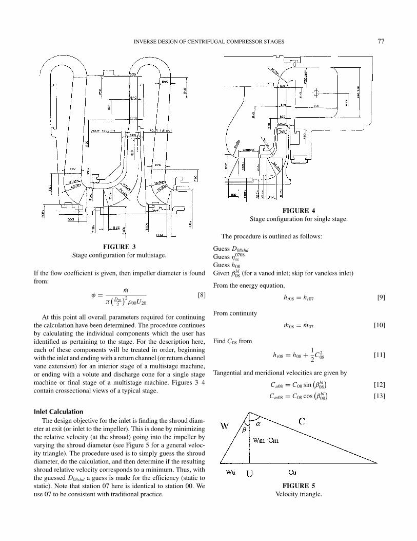
FIGURE 3Stage configuration for multistage.

If the flow coefficient is given, then impeller diameter is foundfrom:

φ = m

π( D20

2

)2ρ00U20

[8]

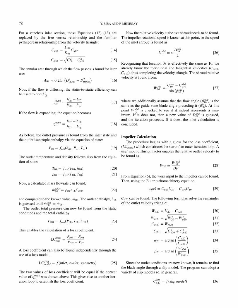
At this point all overall parameters required for continuingthe calculation have been determined. The procedure continuesby calculating the individual components which the user hasidentified as pertaining to the stage. For the description here,each of these components will be treated in order, beginningwith the inlet and ending with a return channel (or return channelvane extension) for an interior stage of a multistage machine,or ending with a volute and discharge cone for a single stagemachine or final stage of a multistage machine. Figures 3–4contain crossectional views of a typical stage.

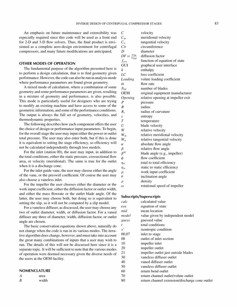
Inlet CalculationThe design objective for the inlet is finding the shroud diam-

eter at exit (or inlet to the impeller). This is done by minimizingthe relative velocity (at the shroud) going into the impeller byvarying the shroud diameter (see Figure 5 for a general veloc-ity triangle). The procedure used is to simply guess the shrouddiameter, do the calculation, and then determine if the resultingshroud relative velocity corresponds to a minimum. Thus, withthe guessed D08shd a guess is made for the efficiency (static tostatic). Note that station 07 here is identical to station 00. Weuse 07 to be consistent with traditional practice.

FIGURE 4Stage configuration for single stage.

The procedure is outlined as follows:

Guess D08shd

Guess η0708ss

Guess h08

Given βbl08 (for a vaned inlet; skip for vaneless inlet)

From the energy equation,

ht08 = ht07 [9]

From continuity

m08 = m07 [10]

Find C08 from

ht08 = h08 + 1

2C2

08 [11]

Tangential and meridional velocities are given by

Cu08 = C08 sin(βbl

08

)[12]

Cm08 = C08 cos(βbl

08

)[13]

FIGURE 5Velocity triangle.


For a vaneless inlet section, these Equations (12)–(13) arereplaced by the free vortex relationship and the familiarpythagorean relationship from the velocity triangle:

Cu08 = D07

D08Cu07 [14]

Cm08 =√

C208 − C2

u08 [15]

The annular area through which the flow passes is found for lateruse:

A08 = 0.25π(D2

08shd − D208hub

)[16]

Now, if the flow is diffusing, the static-to-static efficiency canbe used to find h′

08

η0708ss = h′

08 − h07

h08 − h07[17]

If the flow is expanding, the equation becomes

η0708ss = h07 − h08

h07 − h′08

[18]

As before, the outlet pressure is found from the inlet state andthe outlet isentropic enthalpy via the equation of state:

P08 = feos(h′08, P07, T07) [19]

The outlet temperature and density follows also from the equa-tion of state:

T08 = feos(P08, h08) [20]

ρ08 = feos(P08, T08) [21]

Now, a calculated mass flowrate can found,

mcalc08 = ρ08 A08Cm08 [22]

and compared to the known value, m08. The outlet enthalpy, h08

is guessed until mcalc08 = m08.

The outlet total pressure can now be found from the staticconditions and the total enthalpy:

Pt08 = feos(P08, T08, ht08) [23]

This enables the calculation of a loss coefficient,

LC0708calc = Pt07 − Pt08

Pt07 − P07[24]

A loss coefficient can also be found independently through theuse of a loss model,

LC0708model = f (inlet, outlet, geometry) [25]

The two values of loss coefficient will be equal if the correctvalue of η0708

ss was chosen above. This gives rise to another iter-ation loop to establish the loss coefficient.

Now the relative velocity at the exit shroud needs to be found.The impeller rotational speed is known at this point, so the speedof the inlet shroud is found as

U shd10 = ω

Dshd10

2[26]

Recognizing that location 08 is effectively the same as 10, wealready know the meridional and tangential velocities (Cm10,Cu10), thus completing the velocity triangle. The shroud relativevelocity is found from:

W shd10 = U shd

10 − Cshdu10

sin(βshd

10

) [27]

where we additionally assume that the flow angle (βshd10 ) is the

same as the guide vane blade angle preceding it (βbl08). At this

point W shd10 is checked to see if it indeed represents a min-

imum. If it does not, then a new value of Dshd08 is guessed,

and the iteration proceeds. If it does, the inlet calculation isconcluded.

Impeller CalculationThe procedure begins with a guess for the loss coefficient,

(LCguess) which constitutes the start of an outer iteration loop. Auser input diffusion factor enables the relative outlet velocity tobe found as

W20 = W mid10

DF[28]

From Equation (6), the work input to the impeller can be found.Then, using the Euler turbomachinery equation,

work = Cu20U20 − Cu10U10 [29]

Cu20 can be found. The following formulas solve the remainderof the outlet velocity triangle:

Wu20 = U20 − Cu20 [30]

Wm20 =√

W 220 − W 2

u20 [31]

Cm20 = Wm20 [32]

C20 =√

C2u20 + C2

m20 [33]

α20 = arctan

(Cu20

Cm20

)[34]

β20 = arctan

(Wu20

Wm20

)[35]

Since the outlet conditions are now known, it remains to findthe blade angle through a slip model. The program can adopt avariety of slip models so, in general,

Cslipu20 = f (slip model) [36]


For instance, one such formula is the Stanitz model (Stanitz,1952),

Cslipu20 = 1.98U20 cos

(βbl

20

)Nbl

[37]

Note that here the blade angle rather than the flowangle is needed, and this value has not been computed yet.To use this model, a guessed blade angle would be needed,a reasonable value being the flow angle from Equation (35).

With slip velocity known, the blade angle is determined byfinding ideal tangential velocities, as follows:

Cidealu20 = Cu20 + Cslip

u20 [38]

W idealu20 = U20 − Cideal

u20 [39]

βbl20 = arctan

(W ideal

u20

Wm20

)[40]

Note that if using the Stanitz slip model above, this would be thenew blade angle to be used in the iteration loop. Convergence inthis case is achieved very quickly.

With blade angle known (along with user inputs for numberof blades and blade thickness), the outlet circumference due toblade blockage can be determined. This value can be used to findthe circumference which permits flow passage, and a blockagecoefficient:

Cir20 = π D20 [41]

Cirblo20 = Nbl

[T hk20

cos(βbl

20

)]

[42]

Cirflow20 = Cir20 − Cirblo

20 [43]

BLO20 = 1 − Cirblo20

Cir20[44]

Now, for the impeller only, we are defining the loss coefficientas follows:

LCguess = (ht20 − ht10)(1 − η1020

tt

)12 W 2

10 mid

[45]

Using this definition, and remembering that we haveguessed a loss coefficient as part of the iterative scheme, wecan solve this equation for the total to total efficiency. Then,the isentropic total enthalpy at outlet can be found bysolving

η1020tt = h′

t20 − ht10

ht20 − ht10[46]

and the total pressure is found from the equation of state as

Pt20 = feos(Pt10, Tt10, h′t20) [47]

Since two total properties are known, others follow directly fromthe equation of state:

Tt20 = feos(ht20, Pt20) [48]

ρt20 = feos(ht20, Pt20) [49]

The outlet static conditions are found as follows:

h20 = ht20 − 1

2C2

20 [50]

P20 = feos(h20, Pt20, Tt20) [51]

ρ20 = feos(h20, P20) [52]

This now permits the calculation of an important design param-eter, the outlet width and area:

B20 = m20

ρ20Cm20Cirflow20

[53]

A20 = B20Cirflow20 [54]

At exit, the flow proceeds into a space whose width is greaterthan B20 since there is no blade blockage and because a smallgap is present between the impeller and diaphragm walls. Theuser inputs the relative opening that this gap represents,

Opening = B21 − B20

D20[55]

thus enabling the width at station 21 to be found. Other geometricparameters follow:

D21 = D20 [56]

Cirflow21 = π D21 [57]

A21 = B21Cirflow21 [58]

An isentropic diffusion process is assumed to occur between 20and 21, thus the total state remains the same:

ht21 = ht20 [59]

Pt21 = Pt20 [60]

Also, from Equation (56) it follows that the tangential velocitycomponent is constant:

Cu21 = Cu20 [61]

Thus by solving the following four equations in four unknowns(h21, ρ21, C21, Cm21), we establish the outlet static state andvelocity:

ρ21 A21Cm21 = ρ20 A20Cm20 [62]

C21 =√

C2u21 + C2

m21 [63]

h21 = ht21 − 1

2C2

21 [64]

ρ21 = feos(ht21, Pt21, h21) [65]


Other quantities of interest are found directly from:

P21 = feos(h21, ρ21) [66]

T21 = feos(h21, ρ21) [67]

α21 = arctan

(Cu21

Cm21

)[68]

Wu21 = U20 − Cu21 [69]

Wm21 = Cm21 [70]

β21 = arctan

(Wu21

Wm21

)[71]

W21 =√

W 2m21 + W 2

u21 [72]

At this point an impeller loss model is invoked for a new losscoefficient in the same manner as Equation (25). This value iscompared with the guessed value above and iteration continuesuntil they are equal. The loss model used here was developedspecifically for the OEM’s impellers. However a number of gen-eral models have been introduced which attempt to account forthe complex nature of impeller flow. Japikse, for instance, uses atwo-zone model where the flow is broken up into a nearly isen-tropic primary region and a secondary region near the suctionsurface dominated by wall shear effects (Japikse, 1985). The useof such models in combination with our specific test experienceis certainly a subject for future research.

Vaneless Diffuser CalculationFor this description we assume the impeller is followed by a

vaneless diffuser, or a vaneless space preceding a vaned diffuser.In either case, the calculation procedure is the same.

In general, the design objective here is to find the diameterand width at the outlet. This is done, as for the impeller, byusing a known diffusion factor supplied by the user. However, itis impossible to close the equations without knowing either thewidth or diameter itself. So, the user is given the choice of setting,in addition to the diffusion factor, either of these parameters.The calculation then solves for the other parameter, the oneleft as unknown. The description that follows will illustrate theprocedure for both cases.

The inlet to the diffuser is taken as the impeller outlet, station21 for which all geometry, velocities, and thermodynamic quan-tities are known. As with all our component calculations, a losscoefficient is first guessed. Thus, the following set of equationscan be solved directly:

C30 = C21

DF[73]

m30 = m21 [74]

Pt30 = Pt21 − LCguess(Pt21 − P21) [75]

ht30 = ht21 [76]

h30 = ht30 − 1

2C2

30 [77]

P30 = feos(ht30, Pt30, h30) [78]

ρ30 = feos(P30, h30) [79]

T30 = feos(P30, h30) [80]

Now the following set of four equations in four unknowns(A30, Cu30, Cm30, and D30 or B30) is solved.

m30 = ρ30 A30Cm30 [81]

C30 =√

C2m30 + C2

u30 [82]

A30 = π D30 B30 [83]

Cu30 D30 = Cu21 D21 [84]

To close the iteration, a calculated value of loss coefficientcan be found from an external loss model:

LCmodel = f (inlet, outlet, geometry) [85]

This value is then compared to the guessed loss coefficient anda new value selected accordingly.

Vaned Diffuser CalculationThe vaned diffuser (either conventional or LSD) begins at

station 30 and ends at station 40. Here there are three geometricunknowns of interest, the outlet diameter, width, and angle. Inorder to close the equations, two need to be selected in additionto the diffusion factor. Thus the calculation essentially solvesfor either diameter, width, or flow angle depending on what theuser selects as known.

As before, the user supplies a desired diffusion factor. A losscoefficient is guessed initially and calculation proceeds in ex-actly the same manner as shown in Equations (73)–(80), withthe proper change of subscripts to reflect the new location. Then,a set of four equations in four unknowns (A40, Cm40, Cu40, andone of D40, B40, or α40) is solved, three of which are the same asEquations (81)–(83). The fourth equation is simply the definitionof the flow angle:

tan α40 = Cu40

Cm40[86]

The loss coefficient is found by using a loss model for thetype of vaned diffuser in question. This is represented generallyin the same way as Equation (85). It should be noted that, as forthe impeller, many general loss models exist for diffusers, suchas Ribi and Dalbert (2000) and Japikse and Baines (2000).

Note that the vaneless diffuser calculation is used for anyvaneless space, including the return bend. Likewise, the vaneddiffuser is used to represent all vaned calculations, includingthe return channel. For this description it is useful to imaginea second vaneless space after the vaned diffuser representingstations 40–50. For a last stage, a volute would begin at station50 and extend to station 70.


FIGURE 6Volute and discharge cone configuration.

Volute CalculationThe design objective for the volute is the determination of

its outlet width and height. The height is represented in termsof minimum and maximum radii. As shown in Figures 4 and 6,these parameters give the basic size of the volute. In order toclose the calculation, a loading coefficient is supplied by theuser along with an aspect ratio. As usual, a guess for the losscoefficient is made by the program which initializes the outeriteration of the calculation. A guess for the volute radius is alsomade, constituting an inner iteration loop. The volute is desig-nated by the user as external (fixed inner radius, increasing outerradius) or internal (fixed outer radius, decreasing inner radius).

The following formulae are by now routine, and establish thetotal outlet state:

m70 = m50 [87]

ht70 = ht50 [88]

Pt70 = Pt50 − LCguess(Pt50 − P50) [89]

Tt70 = feos(ht70, Pt70) [90]

Now, since the loading coefficient expresses a deviation fromfree vortex flow, by knowing this parameter, the tangential ve-locity at the exit can be found.

Cu70 = (Loading)R50Cu50

R70[91]

Furthermore, since the meridional component of the velocity at70 is very small, it is commonly assumed that the overall velocityis equal to the tangential velocity:

C70 = Cu70 [92]

The following relationships are straightforward and establish theoutlet static state.

h70 = ht70 − 1

2C2

70 [93]

P70 = feos(h70, Pt70, Tt70) [94]

T70 = feos(h70, P70) [95]

ρ70 = feos(T70, P70) [96]

A70 = m70

ρ70C70[97]

Since A70 and AspectRatio are known at this point, the followingtwo equations are solved for �R70 and B70:

A70 = �R70 B70 [98]

AspectRatio = �R70

B70[99]

For an external volute the outer radius can now be found:

R70max = R70min + �R70 [100]

Similarly for an internal volute the inner radius is found as

R70min = R70max − �R70 [101]

The mean radius is now found:

R70 = 1

2(R70max + R70min) [102]

Once again, the loss coefficient is calculated from a loss modeland compared to the guessed value:

LCmodel = f (inlet, outlet, geometry) [103]

As before, this is a specific, empirically based model, althoughgeneral models, such as Weber and Koronowski, 1986 are avail-able.

Discharge Cone CalculationThe primary purpose of the discharge cone is to connect the

volute exit with the customer’s downstream process piping. Gen-erally speaking, the diameter of this piping would be known.The calculation then would find the corresponding velocitiesand thermodynamic properties. However, in case the diameteris unknown, the user may choose to enter instead a known staticpressure, or a known velocity, in which case the diameter iscomputed by the program.


The calculation of the total properties is the same as that de-scribed in Equations (87)–(90), so it will not be repeated here.Note that Pt80 is found by the equivalent of Equation 89. Next,the following set of four equations in four unknowns issolved:

m80 = ρ80C80(0.25π D2

80

)[104]

ht80 = h80 + 1

2C2

80 [105]

P80 = feos(Pt80, ht80, h80) [106]

ρ80 = feos(P80, h80) [107]

where, if D80 is given the set of unknowns is (ρ80, h80, P80, C80),if C80 is given the set of unknowns is (ρ80, h80, P80, D80), and ifP80 is given the set of unknowns is (ρ80, h80, C80, D80). As usual,a loss coefficient calculated from a model is used to compare withthe guessed value. Other thermodynamic properties of interestcan also be found in a straightforward manner using the equationof state.

At this point, it is presumed that the stage outlet has beenreached. Notice that a value of Pt80 has been calculated inde-pendently of the user input value. Because of this, the value oftotal to total stage efficiency will be different than what wasguessed in the beginning as part of the overall stage iterationloop. Therefore, a new total to total efficiency is found basedon the actual, calculated conditions at the discharge cone outlet,and the iteration is repeated.

Curvature CalculationsAfter each component is calculated, the user may invoke a

calculation for the meridional velocity profile due to curvatureat the hub and shroud. This is based on a discretized form of theEuler-n equation

W 2m

Rc+ W 2

u

Rcos(θ ) = 1

ρ

dP

dn[108]

where n is the direction normal to the flow, and θ is the angle ofinclination of the section with respect to the radial.

This calculation is done after the fact, that is its results have noinfluence on any downstream component calculation. It simplyprovides the user with information as to the effects of curvatureat a particular section.

Non-Radial Diffuser CalculationThe code provides for the calculation of non-radially oriented

diffusers, return bends, and return channels. The radial orienta-tion in this case is only at the inlet and outlet. An additionalunknown, the inclination angle, is present in any such calcula-tion although, except for finding geometry at such a section, thecalculations remain essentially the same.

Iterative SchemeMost of the iteration schemes in the foregoing description

involve a simple update to the guessed value with the new, cal-culated value. For cases where convergence is more difficult(such as finding the outlet radius of the volute), iteration pro-ceeds by a) establishing the low and high limit of the solutiondomain, b) breaking up the domain into an equal number of in-crements, c) guessing in increments from the initial value to thehigh limit and then to the low limit, and d) when the solution isbounded, using the bisection method to converge. This scheme,although simpler and slower than other schemes, is extremelyreliable.

Equation of StateThe reader will notice the general form in which calcula-

tions involving the equation of state have been presented. To thecalculation algorithm, the equation of state simply represents anexternal function by which knowledge of a thermodynamic statecan be used to find any other thermodynamic property. Thus, al-gorithmically, it is not important which equation of state is beingused. Any equation of state can be written and added withoutchanging the code that does the calculations. Indeed, externallibraries of functions with many equations of state can be pur-chased and linked to the program with negligible modification tothe base code. This raises the issue of software design, to whichwe now turn.

PROGRAM ARCHITECTUREThe algorithm illustrated above was written using the C++

programming language and adheres strongly to the principles ofobject oriented software design. Thus separate classes are cre-ated for each stage component (e.g., impeller, diffuser, volute)and the stage itself, all of these in turn derived from a genericcomponent base class. Likewise, classes are created for gases,equations of state, loss models, iterators, and user interfaces.The idea was to have as much “drop-in-place” capability as pos-sible. So, for instance, if an equation of state should change, theprogrammer simply has to program a new class for the particularequation of state he is dealing with. No other code modificationswould need to be added.

The main user interface for the code uses a GUI library pro-vided by Qt (Trolltech, 2002). This was used to create a menu baralong with several dialog boxes for convenient user input. One ofthe advantages of this particular library is that it is multiplatform,i.e., it can be compiled under both the UNIX and Windows op-erating systems. Several support classes were added to the userinterface, particularly for allowing unit conversions and manip-ulating the communication with the calculation engine. It shouldbe noted that, consistent with good software practice, the GUIand calculation engine are completely separate. The GUI onlyhas pointers to the calculation components and the calculationonly has a pointer to the GUI. This permits the use of any userinterface, such as a command line interface. Any other interfacecould also be dropped in after the fact.


An emphasis on future maintenance and extensibility wasespecially required since this code will be used as a front endfor 2-D and 3-D flow solvers. Thus, the final product is envi-sioned as a complete aero-design environment for centrifugalcompressors, and many future modifications are anticipated.

OTHER MODES OF OPERATIONThe fundamental purpose of the algorithm presented here is

to perform a design calculation, that is to find geometry givenperformance. However, the code can also be run in analysis modewhere performance parameters are found given geometry.

A mixed mode of calculation, where a combination of somegeometry and some performance parameters are given, resultingin a mixture of geometry and performance, is also possible.This mode is particularly useful for designers who are tryingto modify an existing machine and have access to some of thegeometric information, and some of the performance conditions.The output is always the full set of geometry, velocities, andthermodynamic properties.

The following describes how each component offers the userthe choice of design or performance input parameters. To begin,for the overall stage the user may input either the power or outlettotal pressure. The user may also enter both, but if this is doneit is equivalent to setting the stage efficiency, so efficiency willnot be calculated independently through loss models.

For the inlet (station 00), the user may input, in addition tothe total conditions, either the static pressure, crossectional flowarea, or velocity (meridional). The same is true for the outletwhen it is a discharge cone.

For the inlet guide vane, the user may choose either the angleof the vane, or the preswirl coefficient. Of course the user mayalso choose a vaneless inlet.

For the impeller the user chooses either the diameter or thework input coefficient, either the diffusion factor or outlet width,and either the mass flowrate or the outlet blade angle. Of thelatter, the user may choose both, but doing so is equivalent tosetting the slip, so it will not be computed by a slip model.

For a vaneless diffuser, as discussed, the user may choose anytwo of outlet diameter, width, or diffusion factor. For a vaneddiffuser any three of diameter, width, diffusion factor, or outletangle are chosen.

The basic conservation equations shown above, naturally donot change when the code is run in its various modes. The itera-tive algorithm does change, however, and must take into accountthe great many combinations of inputs that a user may wish torun. The details of this will not be discussed here since it is aseparate topic. It will be sufficient to note that the various modesof operation were deemed necessary given the diverse needs ofthe users at the OEM facility.

NOMENCLATUREA areaB width

C velocityCm meridional velocityCu tangential velocityCir circumferenceD diameterDF = w in

woutdiffusion factor

feos function of equation of stateGUI graphical user interfaceh enthalpyLC loss coefficientLoading volute loading coefficientm flow rateNbl number of bladesOEM original equipment manufacturerOpening relative opening at impeller exitP pressureR radiusRc radius of curvatures entropyT temperatureU blade velocityW relative velocityWm relative meridional velocityWu relative tangential velocityα absolute flow angleβ relative flow angleβbl blade angle (e.g., impeller)φ flow coefficientηtt total to total efficiencyηss static to static efficiencyµ work input coefficientθ inclination angleρ densityω rotational speed of impeller

Subscripts/Superscriptscalc calculated valueeos equation of statemid mean locationmodel value given by independent modelguess guessed valuet total conditionsx ′ isentropic condition00,07 inlet to stage08 outlet of inlet section10 impeller inlet20 impeller outlet21 impeller outlet just outside blades30 vaneless diffuser outlet40 vaned diffuser outlet50 vaneless diffuser outlet60 return bend outlet70 return channel outlet/volute outlet80 return channel extension/discharge cone outlet


REFERENCESConcepts NREC website. 2002. www.conceptsnrec.com/compal.htmDixon, S. L. 1998. Fluid Mechanics and Thermodynamics of Turbo-

machinery, 4th Ed., Butterworth-Heinemann, Boston.Japikse, D. 1985. Assessment of single and two-zone modeling of cen-

trifugal compressors—Studies in component performance: Part 3.ASME Paper No. 85-GT-73.

Japikse, D. 1996. Centrifugal Compressor Design and Performance,Wilder, VT: Concepts ETI, Inc.

Japikse, D., and Baines, N. 2000. Diffuser Design Technology, Wilder,VT: Concepts ETI, Inc.

PCA website. 2002. www.pcaeng.co.uk/oona.htm.Ribi, B., and Dalbert, P. 2000. One dimensional performance predic-

tion of subsonic vaned diffusers. ASME Journal of Turbomachinery122:494–504.

Stanitz, J. D. 1952. Some theoretical aerodynamic investigations ofimpellers in radial and mixed flow centrifugal compressors. Trans-actions of the ASME 74:473–497.

Trolltech website. 2002. www.trolltech.com.Weber, C. R., and Koronowski, M. E., 1986. Meanline performance

prediction of volutes in centrifugal compressors. ASME Paper No.86-GT-216.

International Journal of

AerospaceEngineeringHindawi Publishing Corporationhttp://www.hindawi.com Volume 2010

RoboticsJournal of

Hindawi Publishing Corporationhttp://www.hindawi.com Volume 2014


Active and Passive Electronic Components

Control Scienceand Engineering

Journal of



RotatingMachinery


Hindawi Publishing Corporation http://www.hindawi.com

Journal ofEngineeringVolume 2014

Submit your manuscripts athttp://www.hindawi.com

VLSI Design



Shock and Vibration


Civil EngineeringAdvances in

Acoustics and VibrationAdvances in



Electrical and Computer Engineering

Journal of

Advances inOptoElectronics

Hindawi Publishing Corporation http://www.hindawi.com

Volume 2014

The Scientific World JournalHindawi Publishing Corporation http://www.hindawi.com Volume 2014

SensorsJournal of


Modelling & Simulation in EngineeringHindawi Publishing Corporation http://www.hindawi.com Volume 2014


Chemical EngineeringInternational Journal of Antennas and

Propagation




Navigation and Observation



DistributedSensor Networks


Inverse Design of Centrifugal Compressor Stages Using...

Documents

Transcript of Inverse Design of Centrifugal Compressor Stages Using...