Inventory Optimization for Industrial Network Flexibility

P. Garcia-Herreros, B. Sharda, A. Agarwal, J.M. Wassick & I.E. Grossmann

Project Update Sept 2014

1

Motivation

2

Process networks describe the operation of chemical plants

Inventories are necessary because of process uncertainty: Raw material storage tanks hedge against supply variability Intermediate storage tanks hedge against production rates variability Finished product inventories hedge against demand variability Holding inventory is expensive!

Need to trade-off between inventory and stock-out cost

Given:

Find the operating plan that minimizes inventory and stockout costs:

• Determine the optimal inventory management strategy in every time period Location of inventory Amount of inventory

3

Problem Statement

• A process network with several processing units

• A discrete time finite horizon • Probabilistic description of supply,

processing rates, and demand over the entire horizon

• Storage units

Multi-stage stochastic programming approach: • Requires discrete uncertainty distributions • Yields minimum expected cost • Recourse actions are optimized for individual realizations at multiple stages • Intractable for long time horizons (too many scenarios)

Two-stage stochastic programming approach: • Sample paths from initial time to final time period • Assumes that the future can be anticipated after first stage • Recourse actions consider a single scenario • Solvable for many scenarios

Decision rule approach: • Sample paths from initial to final time period • Decisions in any time period are functions of the state • Recourse actions are state functions of the individual realizations • Does not anticipate future • Solvable for many scenarios

Stochastic Modeling Approaches for Multiperiod Problems

4

Inventory Policies: Base-stock policy in capacitated network: 1. Satisfy demands (D) according to priorities using available supply (S) and production

capacities (R) Update D, S, R1, R2, and R3

2. Satisfy demands (D) according to priorities using inventories (I) Update D, S, R1, R2, R3, I1, and I2

3. Replenish inventories according to priorities using left over supply (S) and production capacities (R) Update S, R1, R2, R3, I1, and I2

4. Stop inventory replenishments at base-stock levels (b) 5. Repeat for next time-period

Base-stock policy is specified by the base-stock level (B) 5

Decision Rules for Inventory Management

D S

R1

R2

R3

R4

I1

I2

Rules to establish when inventories are depleted, replenished, and their priorities

Parallel operation

Operating plan is completely specified by the policy according to the realization of uncertain parameters (S, Ri, and D) 6

Logic of Policies

R2

R1 f1

f2 f3

f4 f5

f6

Parameters S: Supply rate Ri: Capacity of unit i Ci: coefficient of unit i D: demand rate Variables fj: flowrate j ui: underutilization of resource i lk: inventory level at storage k bk: base-stock of storage k so: unsatisfied demand fj,, ui, lk, bk ≥ 0

D S R3 R4 l1 I2

f7 f8 f9 f10 f11

Serial operation

Minimize: expected inventory cost + expected stockout cost Subject to:

• Mass balances in all scenarios

• Capacity constraints in all scenarios

• Single policy for all scenarios in a decision stage

• Bounds 7

Multistage Formulation (MILP)

C1

D C2

C3

C4

C1

D C2

C3

C4

CS

CS

Cstg1

Cstg1

Cstg2

Cstg2

t

t+1

Storage

Storage Processing

unit D

D

Storage

Challenges: • Arbitrary distributions for uncertain parameters

Solution approach: • Sample-path optimization

Discrete-time samples of random parameters during planning horizon (0,T): • Available supply: St

• Maximum processing rates: Rt

• Demand rates: Dt

Solution approximates the optimal operating plan given the current state (at t=0) and the probabilistic model of future realizations 8

Implementation

Sample S

Sample D

Sample R

Solve multistage formulation for each sample path N

Optimal base-stocks

Calculate mean total cost

Initial state of system (S0, R0

, D0)

Rolling horizon: Simulate the implementation of the optimal first-stage decision Algorithm: 1. Initial state (S0

, R0, D0, cost0=0)

2. Draw N sample paths of length T 3. Solve the multi-stage optimization problem 4. Accumulate the cost incurred in first stage 5. End if the end of evaluation period is reached Else, update initial state and return to 2

Repeat the implementation of the algorithm to estimate mean and variance of the results

9

Evaluating the Solutions

Process network with failures, uncertain supply, and uncertain demand

10

Illustrative Example

Cost coefficients:

Production costs:

Inventory holding cost:

Penalty for unmet demand:

U1

U2 Inv1

U4

Inv2

U3

S D F1

F2

F3

F4

F5 F7

F6

F9

F8

F10

F11

Data

Evaluation period: H = 25 day Number of sample paths: N = 50 Planning horizon: T = 4 day

Probability of operation:

Mass balance coefficients:

Processing capacity:

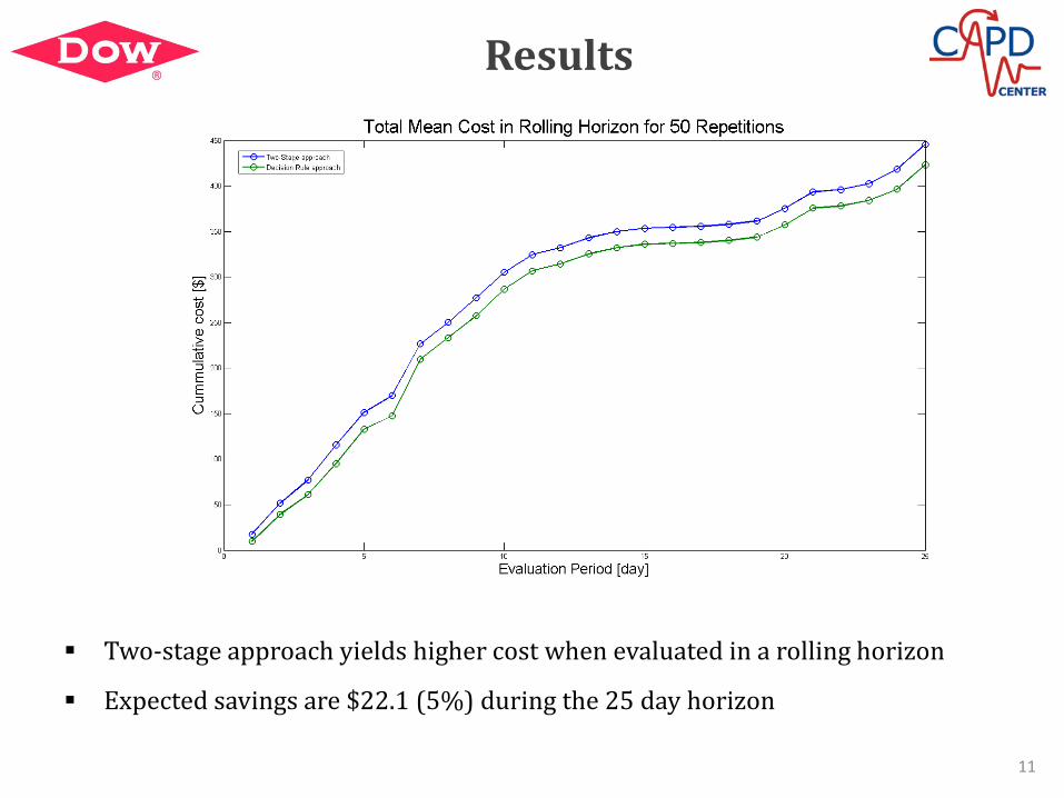
Results

11

Two-stage approach yields higher cost when evaluated in a rolling horizon

Expected savings are $22.1 (5%) during the 25 day horizon

Results

12

Two-stage approach accumulates less inventory but has higher stockouts

Two-stage approach assumes a degree of flexibility that is impossible to implement

Conclusions

13

Novelty:

Framework for inventory planning in finite horizons

Extension of the methodology for uncertain parameters with time-varying distributions

Detailed logic for units in parallel and in series

Methodology to evaluate results

Significant improvement over two-stage approach

Impact for industrial application:

Supply and demand forecasts can be used directly for inventory optimization

Inventory management considering predictable and unpredictable events