Inventory of U.S. Greenhouse Gas Emissions and Sinks: 1990-2013 ...
264
A-126 Inventory of U.S. Greenhouse Gas Emissions and Sinks: 1990-2013 ANNEX 3 Methodological Descriptions for Additional Source or Sink Categories 3.1. Methodology for Estimating Emissions of CH4, N2O, and Indirect Greenhouse Gases from Stationary Combustion Estimates of CH4 and N2O Emissions Methane (CH4) and nitrous oxide emissions from stationary combustion were estimated using IPCC emission factors and methods. Estimates were obtained by multiplying emission factors—by sector and fuel type—by fossil fuel and wood consumption data. This “top-down” methodology is characterized by two basic steps, described below. Data are presented in Table A-85 through Table A-90. Step 1: Determine Energy Consumption by Sector and Fuel Type Energy consumption from stationary combustion activities was grouped by sector: industrial, commercial, residential, electric power, and U.S. territories. For CH4 and N2O from industrial, commercial, residential, and U.S. territories, estimates were based upon consumption of coal, gas, oil, and wood. Energy consumption and wood consumption data for the United States were obtained from EIA’s Monthly Energy Review, February 2015 and Published Supplemental Tables on Petroleum Product detail (EIA 2015). Because the United States does not include territories in its national energy statistics, fuel consumption data for territories were collected separately from the EIA’s International Energy Statistics (Jacobs 2010). 16 Fuel consumption for the industrial sector was adjusted to subtract out construction and agricultural use, which is reported under mobile sources. 17 Construction and agricultural fuel use was obtained from EPA (2013). The energy consumption data by sector were then adjusted from higher to lower heating values by multiplying by 0.9 for natural gas and wood and by 0.95 for coal and petroleum fuel. This is a simplified convention used by the International Energy Agency. Table A-85 provides annual energy consumption data for the years 1990 through 2013. In this Inventory, the emission estimation methodology for the electric power sector was revised from Tier 1 to Tier 2 as fuel consumption by technology-type for the electricity generation sector was obtained from the Acid Rain Program Dataset (EPA 2014a). This combustion technology-and fuel-use data was available by facility from 1996 to 2013. Since there was a difference between the EPA (2014a) and EIA (2015) total energy consumption estimates, the remainder between total energy consumption using EPA (2014a) and EIA (2015) was apportioned to each combustion technology type and fuel combination using a ratio of energy consumption by technology type from 1996 to 2013. Energy consumption estimates were not available from 1990 to 1995 in the EPA (2014a) dataset, and as a result, consumption was calculated using total electric power consumption from EIA (2015) and the ratio of combustion technology and fuel types from EPA 2014a. The consumption estimates from 1990 to 1995 were estimated by applying the 1996 consumption ratio by combustion technology type to the total EIA consumption for each year from 1990 to 1995. Lastly, there were significant differences between wood biomass consumption in the electric power sector between the EPA (2014a) and EIA (2015) datasets. The difference in wood biomass consumption in the electric power sector was distributed to the residential, commercial, and industrial sectors according to their percent share of wood biomass energy consumption calculated from EIA (2015). Step 2: Determine the Amount of CH4 and N2O Emitted Activity data for industrial, commercial, residential, and U.S. territories and fuel type for each of these sectors were then multiplied by default Tier 1 emission factors to obtain emission estimates. Emission factors for the residential, commercial, and industrial sectors were taken from the 2006 IPCC Guidelines for National Greenhouse Gas Inventories (IPCC 2006). These N2O emission factors by fuel type (consistent across sectors) were also assumed for U.S. territories. The CH4 emission factors by fuel type for U.S. territories were estimated based on the emission factor for the primary sector 16 U.S. territories data also include combustion from mobile activities because data to allocate territories’ energy use were unavailable. For this reason, CH4 and N2O emissions from combustion by U.S. Territories are only included in the stationary combustion totals. 17 Though emissions from construction and farm use occur due to both stationary and mobile sources, detailed data was not available to determine the magnitude from each. Currently, these emissions are assumed to be predominantly from mobile sources.
Transcript of Inventory of U.S. Greenhouse Gas Emissions and Sinks: 1990-2013 ...
A-126 Inventory of U.S. Greenhouse Gas Emissions and Sinks: 1990-2013
ANNEX 3 Methodological Descriptions for Additional
Source or Sink Categories
3.1. Methodology for Estimating Emissions of CH4, N2O, and Indirect Greenhouse Gases from Stationary Combustion
Estimates of CH4 and N2O Emissions
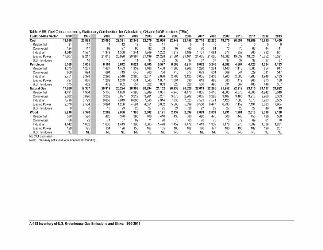
Methane (CH4) and nitrous oxide emissions from stationary combustion were estimated using IPCC emission factors and methods. Estimates were obtained by multiplying emission factors—by sector and fuel type—by fossil fuel and wood consumption data. This “top-down” methodology is characterized by two basic steps, described below. Data are presented in Table A-85 through Table A-90.
Step 1: Determine Energy Consumption by Sector and Fuel Type
Energy consumption from stationary combustion activities was grouped by sector: industrial, commercial, residential, electric power, and U.S. territories. For CH4 and N2O from industrial, commercial, residential, and U.S. territories, estimates were based upon consumption of coal, gas, oil, and wood. Energy consumption and wood consumption data for the United States were obtained from EIA’s Monthly Energy Review, February 2015 and Published Supplemental Tables on Petroleum Product detail (EIA 2015). Because the United States does not include territories in its national energy statistics, fuel consumption data for territories were collected separately from the EIA’s International Energy Statistics (Jacobs 2010).16 Fuel consumption for the industrial sector was adjusted to subtract out construction and agricultural use, which is reported under mobile sources.17 Construction and agricultural fuel use was obtained from EPA (2013). The energy consumption data by sector were then adjusted from higher to lower heating values by multiplying by 0.9 for natural gas and wood and by 0.95 for coal and petroleum fuel. This is a simplified convention used by the International Energy Agency. Table A-85 provides annual energy consumption data for the years 1990 through 2013.
In this Inventory, the emission estimation methodology for the electric power sector was revised from Tier 1 to Tier 2 as fuel consumption by technology-type for the electricity generation sector was obtained from the Acid Rain Program Dataset (EPA 2014a). This combustion technology-and fuel-use data was available by facility from 1996 to 2013. Since there was a difference between the EPA (2014a) and EIA (2015) total energy consumption estimates, the remainder between total energy consumption using EPA (2014a) and EIA (2015) was apportioned to each combustion technology type and fuel combination using a ratio of energy consumption by technology type from 1996 to 2013.
Energy consumption estimates were not available from 1990 to 1995 in the EPA (2014a) dataset, and as a result, consumption was calculated using total electric power consumption from EIA (2015) and the ratio of combustion technology and fuel types from EPA 2014a. The consumption estimates from 1990 to 1995 were estimated by applying the 1996 consumption ratio by combustion technology type to the total EIA consumption for each year from 1990 to 1995.
Lastly, there were significant differences between wood biomass consumption in the electric power sector between the EPA (2014a) and EIA (2015) datasets. The difference in wood biomass consumption in the electric power sector was distributed to the residential, commercial, and industrial sectors according to their percent share of wood biomass energy consumption calculated from EIA (2015).
Step 2: Determine the Amount of CH4 and N2O Emitted
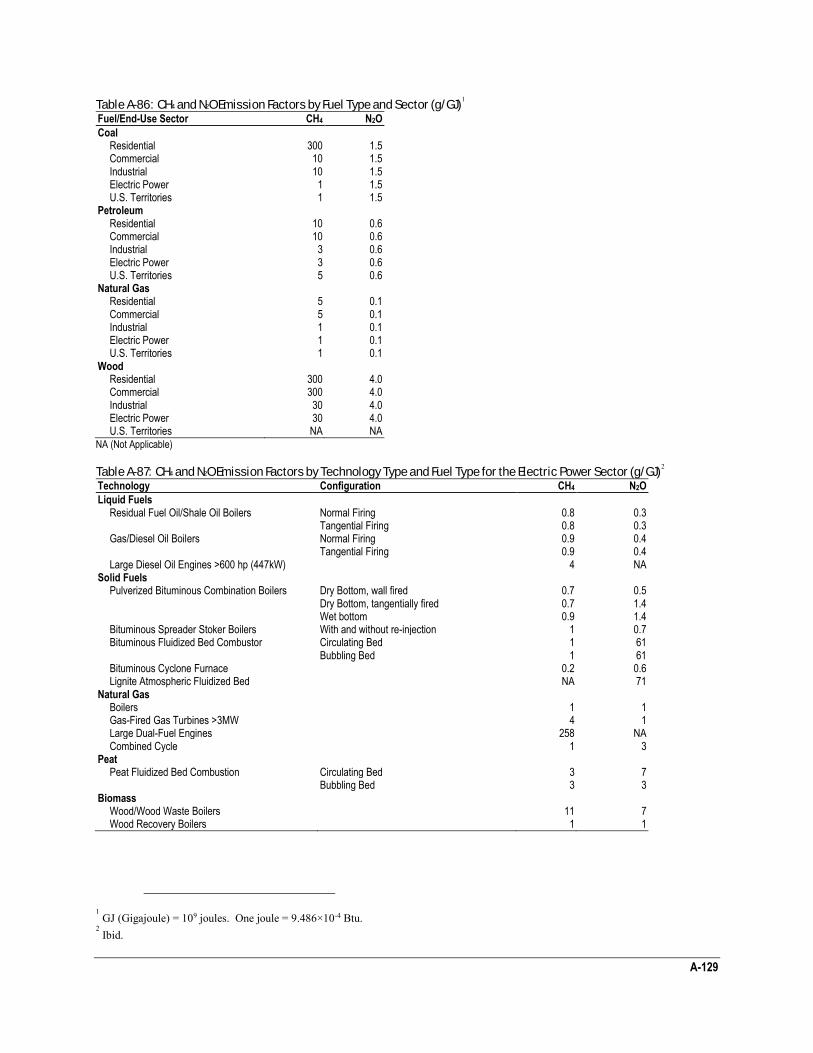
Activity data for industrial, commercial, residential, and U.S. territories and fuel type for each of these sectors were then multiplied by default Tier 1 emission factors to obtain emission estimates. Emission factors for the residential, commercial, and industrial sectors were taken from the 2006 IPCC Guidelines for National Greenhouse Gas Inventories (IPCC 2006). These N2O emission factors by fuel type (consistent across sectors) were also assumed for U.S. territories. The CH4 emission factors by fuel type for U.S. territories were estimated based on the emission factor for the primary sector
16 U.S. territories data also include combustion from mobile activities because data to allocate territories’ energy use were unavailable. For this reason, CH4 and N2O emissions from combustion by U.S. Territories are only included in the stationary combustion totals. 17 Though emissions from construction and farm use occur due to both stationary and mobile sources, detailed data was not available to determine the magnitude from each. Currently, these emissions are assumed to be predominantly from mobile sources.
A-127
in which each fuel was combusted. Table A-86 provides emission factors used for each sector and fuel type. For the electric power sector, emissions were estimated by multiplying fossil fuel and wood consumption by technology- and fuel-specific Tier 2 IPCC emission factors shown in Table A-87. Emission factors were used from the 2006 IPCC Guidelines as the factors presented in these IPCC guidelines were taken directly from U.S. EPA publications on emissions rates for combustion sources.
Estimates of NOx, CO, and NMVOC Emissions
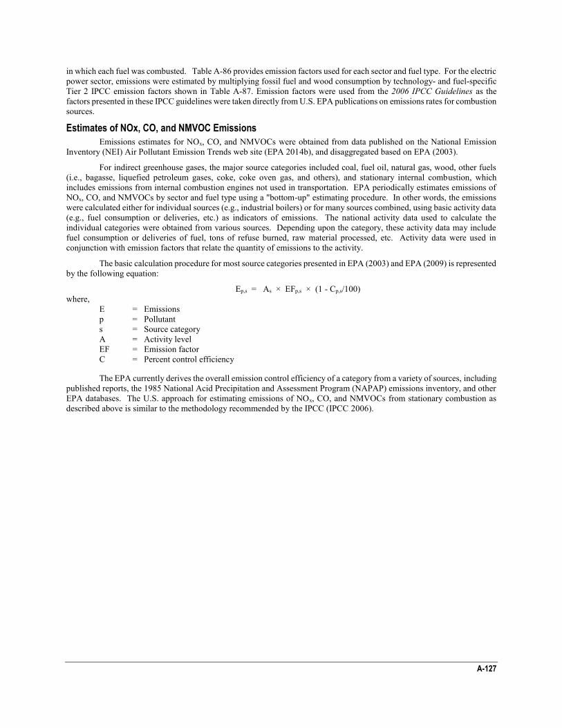
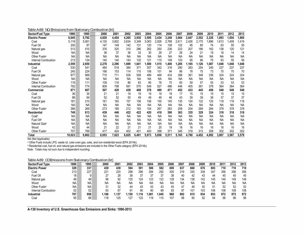
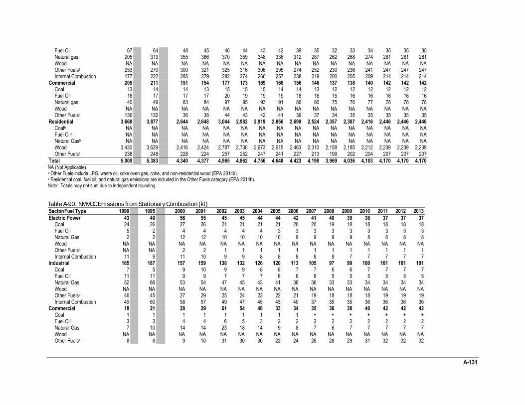
Emissions estimates for NOx, CO, and NMVOCs were obtained from data published on the National Emission Inventory (NEI) Air Pollutant Emission Trends web site (EPA 2014b), and disaggregated based on EPA (2003).
For indirect greenhouse gases, the major source categories included coal, fuel oil, natural gas, wood, other fuels (i.e., bagasse, liquefied petroleum gases, coke, coke oven gas, and others), and stationary internal combustion, which includes emissions from internal combustion engines not used in transportation. EPA periodically estimates emissions of NOx, CO, and NMVOCs by sector and fuel type using a "bottom-up" estimating procedure. In other words, the emissions were calculated either for individual sources (e.g., industrial boilers) or for many sources combined, using basic activity data (e.g., fuel consumption or deliveries, etc.) as indicators of emissions. The national activity data used to calculate the individual categories were obtained from various sources. Depending upon the category, these activity data may include fuel consumption or deliveries of fuel, tons of refuse burned, raw material processed, etc. Activity data were used in conjunction with emission factors that relate the quantity of emissions to the activity.
The basic calculation procedure for most source categories presented in EPA (2003) and EPA (2009) is represented by the following equation:
Ep,s = As × EFp,s × (1 - Cp,s/100) where, E = Emissions p = Pollutant s = Source category A = Activity level EF = Emission factor C = Percent control efficiency
The EPA currently derives the overall emission control efficiency of a category from a variety of sources, including published reports, the 1985 National Acid Precipitation and Assessment Program (NAPAP) emissions inventory, and other EPA databases. The U.S. approach for estimating emissions of NOx, CO, and NMVOCs from stationary combustion as described above is similar to the methodology recommended by the IPCC (IPCC 2006).
A-128 Inventory of U.S. Greenhouse Gas Emissions and Sinks: 1990-2013
Table A-85: Fuel Consumption by Stationary Combustion for Calculating CH4 and N2O Emissions (TBtu) Fuel/End-Use Sector 1990 1995 2000 2001 2002 2003 2004 2005 2006 2007 2008 2009 2010 2011 2012 2013
Coal 19,610 20,888 23,080 22,391 22,343 22,576 22,636 22,949 22,458 22,710 22,225 19,670 20,697 18,989 16,715 17,400 Residential 31 17 11 12 12 12 11 8 6 8 0 0 0 0 0 0 Commercial 124 117 92 97 90 82 103 97 65 70 81 73 70 62 44 41 Industrial 1,640 1,527 1,349 1,358 1,244 1,249 1,262 1,219 1,189 1,131 1,081 877 952 866 782 801 Electric Power 17,807 19,217 21,618 20,920 20,987 21,199 21,228 21,591 21,161 21,465 21,026 18,682 19,639 18,024 15,852 16,521 U.S. Territories 7 10 10 4 11 34 32 33 37 37 37 37 37 37 37 37
Petroleum 6,168 5,655 6,161 6,642 6,021 6,405 6,577 6,503 6,214 6,072 5,246 4,682 4,807 4,420 4,034 4,133 Residential 1,375 1,261 1,427 1,463 1,359 1,466 1,468 1,368 1,202 1,220 1,201 1,140 1,118 1,065 854 917 Commercial 869 694 694 719 646 763 764 715 677 679 634 669 644 629 511 547 Industrial 2,751 2,378 2,298 2,548 2,385 2,511 2,686 2,793 3,125 3,005 2,433 1,960 2,065 1,980 1,948 2,133 Electric Power 797 860 1,269 1,279 1,074 1,043 1,007 1,004 590 618 488 383 412 266 273 180 U.S. Territories 375 462 472 632 557 622 653 623 620 550 490 531 567 480 448 357
Natural Gas 17,266 19,337 20,919 20,224 20,908 20,894 21,152 20,938 20,626 22,019 22,286 21,952 22,912 23,115 24,137 24,922 Residential 4,491 4,954 5,105 4,889 4,995 5,209 4,981 4,946 4,476 4,835 5,010 4,883 4,878 4,805 4,242 5,040 Commercial 2,682 3,096 3,252 3,097 3,212 3,261 3,201 3,073 2,902 3,085 3,228 3,187 3,165 3,216 2,960 3,363 Industrial 7,716 8,723 8,656 7,949 8,086 7,845 7,914 7,330 7,323 7,521 7,571 7,125 7,683 7,873 8,203 8,505 Electric Power 2,376 2,564 3,894 4,266 4,591 4,551 5,032 5,565 5,899 6,550 6,447 6,730 7,159 7,194 8,683 7,964 U.S. Territories 0 0 13 23 23 27 25 24 26 27 29 27 28 27 49 49
Wood 2,216 2,370 2,262 2,006 1,995 2,002 2,121 2,137 2,099 2,089 2,059 1,931 1,981 2,010 2,010 2,138 Residential 580 520 420 370 380 400 410 430 380 420 470 500 440 450 420 580 Commercial 66 72 71 67 69 71 70 70 65 70 73 73 72 69 61 70 Industrial 1,442 1,652 1,636 1,443 1,396 1,363 1,476 1,452 1,472 1,413 1,339 1,178 1,273 1,309 1,339 1,281 Electric Power 129 125 134 126 150 167 165 185 182 186 177 180 196 182 190 207 U.S. Territories NE NE NE NE NE NE NE NE NE NE NE NE NE NE NE NE
NE (Not Estimated) Note: Totals may not sum due to independent rounding.
A-129
Table A-86: CH4 and N2O Emission Factors by Fuel Type and Sector (g/GJ)1
Fuel/End-Use Sector CH4 N2O
Coal Residential 300 1.5 Commercial 10 1.5 Industrial 10 1.5 Electric Power 1 1.5 U.S. Territories 1 1.5
Petroleum Residential 10 0.6 Commercial 10 0.6 Industrial 3 0.6 Electric Power 3 0.6 U.S. Territories 5 0.6
Natural Gas Residential 5 0.1 Commercial 5 0.1 Industrial 1 0.1 Electric Power 1 0.1 U.S. Territories 1 0.1
Wood Residential 300 4.0 Commercial 300 4.0 Industrial 30 4.0 Electric Power 30 4.0 U.S. Territories NA NA
NA (Not Applicable)
Table A-87: CH4 and N2O Emission Factors by Technology Type and Fuel Type for the Electric Power Sector (g/GJ)2
Technology Configuration CH4 N2O
Liquid Fuels Residual Fuel Oil/Shale Oil Boilers Normal Firing 0.8 0.3 Tangential Firing 0.8 0.3 Gas/Diesel Oil Boilers Normal Firing 0.9 0.4 Tangential Firing 0.9 0.4 Large Diesel Oil Engines >600 hp (447kW) 4 NA
Solid Fuels Pulverized Bituminous Combination Boilers Dry Bottom, wall fired 0.7 0.5 Dry Bottom, tangentially fired 0.7 1.4 Wet bottom 0.9 1.4 Bituminous Spreader Stoker Boilers With and without re-injection 1 0.7 Bituminous Fluidized Bed Combustor Circulating Bed 1 61 Bubbling Bed 1 61 Bituminous Cyclone Furnace 0.2 0.6 Lignite Atmospheric Fluidized Bed NA 71
Natural Gas Boilers 1 1 Gas-Fired Gas Turbines >3MW 4 1 Large Dual-Fuel Engines 258 NA Combined Cycle 1 3
Peat Peat Fluidized Bed Combustion Circulating Bed 3 7 Bubbling Bed 3 3
Biomass Wood/Wood Waste Boilers 11 7 Wood Recovery Boilers 1 1
1 GJ (Gigajoule) = 109 joules. One joule = 9.486×10⁻⁴ Btu.
2 Ibid.
A-130 Inventory of U.S. Greenhouse Gas Emissions and Sinks: 1990-2013
Table A-88: NOx Emissions from Stationary Combustion (kt) Sector/Fuel Type 1990 1995 2000 2001 2002 2003 2004 2005 2006 2007 2008 2009 2010 2011 2012 2013
Electric Power 6,045 5,792 4,829 4,454 4,265 3,930 3,595 3,434 3,249 3,064 2,847 2,552 2,226 1,893 1,654 1,665 Coal 5,119 5,061 4,130 3,802 3,634 3,349 3,063 2,926 2,768 2,611 2,426 2,175 1,896 1,613 1,409 1,419 Fuel Oil 200 87 147 149 142 131 120 114 108 102 95 85 74 63 55 55 Natural gas 513 510 376 325 310 286 262 250 236 223 207 186 162 138 120 121 Wood NA NA 36 37 36 33 30 29 27 26 24 21 19 16 14 14 Other Fuelsa NA NA NA NA NA NA NA NA NA NA NA NA NA NA NA NA Internal Combustion 213 134 140 140 143 132 121 115 109 103 95 86 75 63 55 56
Industrial 2,559 2,650 2,278 2,296 1,699 1,641 1,580 1,515 1,400 1,285 1,165 1,126 1,087 1,048 1,048 1,048 Coal 530 541 484 518 384 371 357 342 316 290 263 254 245 237 237 237 Fuel Oil 240 224 166 153 114 110 106 101 94 86 78 75 73 70 70 70 Natural gas 877 999 710 711 526 508 489 469 433 398 361 348 336 324 324 324 Wood NA NA NA NA NA NA NA NA NA NA NA NA NA NA NA NA Other Fuelsa 119 111 109 116 86 83 80 76 70 65 59 57 55 53 53 53 Internal Combustion 792 774 809 798 591 570 549 527 486 446 405 391 378 364 364 364
Commercial 671 607 507 428 438 408 378 490 471 452 433 445 456 548 548 548 Coal 36 35 21 21 19 19 19 19 18 17 15 15 15 15 15 15 Fuel Oil 88 94 52 52 50 49 49 49 46 43 39 39 38 37 37 37 Natural gas 181 210 161 165 157 156 156 155 145 135 124 122 120 118 118 118 Wood NA NA NA NA NA NA NA NA NA NA NA NA NA NA NA NA Other Fuelsa 366 269 273 189 212 183 154 267 263 258 254 269 284 378 378 378
Residential 749 813 439 446 422 422 420 418 390 363 335 329 324 318 318 318 Coalb NA NA NA NA NA NA NA NA NA NA NA NA NA NA NA NA Fuel Oilb NA NA NA NA NA NA NA NA NA NA NA NA NA NA NA NA Natural Gasb NA NA NA NA NA NA NA NA NA NA NA NA NA NA NA NA Wood 42 44 21 22 21 21 21 20 19 18 16 16 16 16 16 16 Other Fuelsa 707 769 417 424 402 401 400 398 371 345 318 313 308 302 302 302
Total 10,023 9,862 8,053 7,623 6,825 6,401 5,973 5,858 5,511 5,163 4,780 4,452 4,092 3,807 3,567 3,579 NA (Not Applicable) a Other Fuels include LPG, waste oil, coke oven gas, coke, and non-residential wood (EPA 2014b). b Residential coal, fuel oil, and natural gas emissions are included in the Other Fuels category (EPA 2014b). Note: Totals may not sum due to independent rounding.
Table A-89: CO Emissions from Stationary Combustion (kt) Sector/Fuel Type 1990 1995 2000 2001 2002 2003 2004 2005 2006 2007 2008 2009 2010 2011 2012 2013
Electric Power 329 337 439 439 594 591 586 582 609 637 660 676 693 710 710 710 Coal 213 227 221 220 298 296 294 292 305 319 330 339 347 356 356 356 Fuel Oil 18 9 27 28 38 37 37 37 38 40 42 43 44 45 45 45 Natural gas 46 49 96 92 125 124 123 122 128 134 138 142 145 149 149 149 Wood NA NA NA NA NA NA NA NA NA NA NA NA NA NA NA NA Other Fuelsa NA NA 31 32 44 43 43 43 45 47 48 50 51 52 52 52 Internal Combustion 52 52 63 67 91 90 90 89 93 97 101 103 106 108 108 108
Industrial 797 958 1,106 1,137 1,150 1,116 1,081 1,045 968 892 815 834 853 872 872 872 Coal 95 88 118 125 127 123 119 115 107 98 90 92 94 96 96 96
A-131
Fuel Oil 67 64 48 45 46 44 43 42 39 35 32 33 34 35 35 35 Natural gas 205 313 355 366 370 359 348 336 312 287 262 268 274 281 281 281 Wood NA NA NA NA NA NA NA NA NA NA NA NA NA NA NA NA Other Fuelsa 253 270 300 321 325 316 306 295 274 252 230 236 241 247 247 247 Internal Combustion 177 222 285 279 282 274 266 257 238 219 200 205 209 214 214 214
Commercial 205 211 151 154 177 173 169 166 156 146 137 138 140 142 142 142 Coal 13 14 14 13 15 15 15 14 14 13 12 12 12 12 12 12 Fuel Oil 16 17 17 17 20 19 19 19 18 16 15 16 16 16 16 16 Natural gas 40 49 83 84 97 95 93 91 86 80 75 76 77 78 78 78 Wood NA NA NA NA NA NA NA NA NA NA NA NA NA NA NA NA Other Fuelsa 136 132 36 38 44 43 42 41 39 37 34 35 35 35 35 35
Residential 3,668 3,877 2,644 2,648 3,044 2,982 2,919 2,856 2,690 2,524 2,357 2,387 2,416 2,446 2,446 2,446 Coalb NA NA NA NA NA NA NA NA NA NA NA NA NA NA NA NA Fuel Oilb NA NA NA NA NA NA NA NA NA NA NA NA NA NA NA NA Natural Gasb NA NA NA NA NA NA NA NA NA NA NA NA NA NA NA NA Wood 3,430 3,629 2,416 2,424 2,787 2,730 2,673 2,615 2,463 2,310 2,158 2,185 2,212 2,239 2,239 2,239 Other Fuelsa 238 248 228 224 257 252 247 241 227 213 199 202 204 207 207 207
Total 5,000 5,383 4,340 4,377 4,965 4,862 4,756 4,648 4,423 4,198 3,969 4,036 4,103 4,170 4,170 4,170 NA (Not Applicable) a Other Fuels include LPG, waste oil, coke oven gas, coke, and non-residential wood (EPA 2014b). b Residential coal, fuel oil, and natural gas emissions are included in the Other Fuels category (EPA 2014b). Note: Totals may not sum due to independent rounding.
Table A-90: NMVOC Emissions from Stationary Combustion (kt) Sector/Fuel Type 1990 1995 2000 2001 2002 2003 2004 2005 2006 2007 2008 2009 2010 2011 2012 2013
Electric Power 43 40 56 55 45 45 44 44 42 41 40 39 38 37 37 37 Coal 24 26 27 26 21 21 21 21 20 20 19 18 18 18 18 18 Fuel Oil 5 2 4 4 4 4 4 3 3 3 3 3 3 3 3 3 Natural Gas 2 2 12 12 10 10 10 10 9 9 9 9 8 8 8 8 Wood NA NA NA NA NA NA NA NA NA NA NA NA NA NA NA NA Other Fuelsa NA NA 2 2 1 1 1 1 1 1 1 1 1 1 1 1 Internal Combustion 11 9 11 10 9 9 8 8 8 8 8 7 7 7 7 7
Industrial 165 187 157 159 138 132 126 120 113 105 97 99 100 101 101 101 Coal 7 5 9 10 9 9 8 8 7 7 6 6 7 7 7 7 Fuel Oil 11 11 9 9 7 7 7 6 6 6 5 5 5 5 5 5 Natural Gas 52 66 53 54 47 45 43 41 38 36 33 33 34 34 34 34 Wood NA NA NA NA NA NA NA NA NA NA NA NA NA NA NA NA Other Fuelsa 46 45 27 29 25 24 23 22 21 19 18 18 18 19 19 19 Internal Combustion 49 60 58 57 49 47 45 43 40 37 35 35 36 36 36 36
Commercial 18 21 28 29 61 54 48 33 34 35 36 38 40 42 42 42 Coal 1 1 1 1 1 1 1 1 1 + + + + + + + Fuel Oil 3 3 4 4 6 5 3 2 2 2 2 2 2 2 2 2 Natural Gas 7 10 14 14 23 18 14 9 8 7 6 7 7 7 7 7 Wood NA NA NA NA NA NA NA NA NA NA NA NA NA NA NA NA Other Fuelsa 8 8 9 10 31 30 30 22 24 26 28 29 31 32 32 32
A-132 Inventory of U.S. Greenhouse Gas Emissions and Sinks: 1990-2013
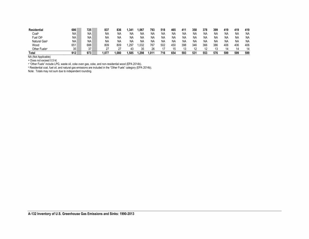
Residential 686 725 837 836 1,341 1,067 793 518 465 411 358 378 399 419 419 419 Coalb NA NA NA NA NA NA NA NA NA NA NA NA NA NA NA NA Fuel Oilb NA NA NA NA NA NA NA NA NA NA NA NA NA NA NA NA Natural Gasb NA NA NA NA NA NA NA NA NA NA NA NA NA NA NA NA Wood 651 688 809 809 1,297 1,032 767 502 450 398 346 366 386 406 406 406 Other Fuelsa 35 37 27 27 43 35 26 17 15 13 12 12 13 14 14 14
Total 912 973 1,077 1,080 1,585 1,298 1,011 716 654 593 531 553 576 599 599 599 NA (Not Applicable) + Does not exceed 0.5 kt. a “Other Fuels” include LPG, waste oil, coke oven gas, coke, and non-residential wood (EPA 2014b). b Residential coal, fuel oil, and natural gas emissions are included in the “Other Fuels” category (EPA 2014b). Note: Totals may not sum due to independent rounding.
A-133
References
EIA (2015) Monthly Energy Review, February 2015, Energy Information Administration, U.S. Department of Energy, Washington, DC. DOE/EIA-0035(2015/02).
EPA (2014a) Acid Rain Program Dataset 1996-2013. Office of Air and Radiation, Office of Atmospheric Programs, U.S. Environmental Protection Agency, Washington, D.C.
EPA (2014b). “1970 - 2013 Average annual emissions, all criteria pollutants in MS Excel.” National Emissions Inventory (NEI) Air Pollutant Emissions Trends Data. Office of Air Quality Planning and Standards, October 2014. Available online at <http://www.epa.gov/ttn/chief/trends/index.html>.
EPA (2013) NONROAD 2008a Model. Office of Transportation and Air Quality, U.S. Environmental Protection Agency. Available online at <http://www.epa.gov/oms/nonrdmdl.htm>.
IPCC (2006) 2006 IPCC Guidelines for National Greenhouse Gas Inventories. The National Greenhouse Gas Inventories Programme, The Intergovernmental Panel on Climate Change, H.S. Eggleston, L. Buendia, K. Miwa, T Ngara, and K. Tanabe (eds.). Hayama, Kanagawa, Japan.
Jacobs, G. (2010) Personal communication. Gwendolyn Jacobs, Energy Information Administration and Rubaab Bhangu, ICF International. U.S. Territories Fossil Fuel Consumption. Unpublished. U.S. Energy Information Administration. Washington, DC.
A-134 Inventory of U.S. Greenhouse Gas Emissions and Sinks: 1990-2013
3.2. Methodology for Estimating Emissions of CH4, N2O, and Indirect Greenhouse Gases from Mobile Combustion and Methodology for and Supplemental Information on Transportation-Related GHG Emissions
Estimating CO2 Emissions by Transportation Mode
Transportation-related CO2 emissions, as presented in the CO2 Emissions from Fossil Fuel Combustion section of the Energy chapter, were calculated using the methodology described in Annex 2.1. This section provides additional information on the data sources and approach used for each transportation fuel type. As noted in Annex 2.1, CO2 emissions estimates for the transportation sector were calculated directly for on-road diesel fuel and motor gasoline based on data sources for individual modes of transportation (considered a bottom up approach). For most other fuel and energy types (aviation gasoline, residual fuel oil, natural gas, LPG, and electricity), CO2 emissions were calculated based on transportation sector-wide fuel consumption estimates from the Energy Information Administration (EIA 2014 and EIA 2013a) and apportioned to individual modes (considered a “top down” approach). CO2 emissions from commercial jet fuel use are obtained directly from the Federal Aviation Administration (FAA 2014), while CO2 emissions from other aircraft jet fuel consumption is determined using a top down approach.
Based on interagency discussions between EPA, EIA, and FHWA beginning in 2005, it was agreed that use of “bottom up” data would be more accurate for diesel fuel and motor gasoline consumption in the transportation sector, based on the availability of reliable data sources. A “bottom up” diesel calculation was first implemented in the 1990-2005 Inventory, and a bottom-up gasoline calculation was introduced in the 1990 – 2006 Inventory for the calculation of emissions from on-road vehicles. Estimated motor gasoline and diesel consumption data for on-road vehicles by vehicle type come from FHWA’s Highway Statistics, Table VM-1 (FHWA 1996 through 2014),1 and are based on federal and state fuel tax records. These fuel consumption estimates were then combined with estimates of fuel shares by vehicle type from DOE’s Transportation Energy Data Book Annex Tables A.1 through A.6 (DOE 1993 through 2014) to develop an estimate of fuel consumption for each vehicle type (i.e., passenger cars, light-duty trucks, buses, medium- and heavy-duty trucks, motorcycles). The on-road gas and diesel fuel consumption estimates by vehicle type were then adjusted for each year so that the sum of gasoline and diesel fuel consumption across all on-road vehicle categories matched the fuel consumption estimates in Highway Statistics’ Table MF-27 (FHWA 1996 through 2014). This resulted in a final “bottom up” estimate of motor gasoline and diesel fuel use by vehicle type, consistent with the FHWA total for on-road motor gasoline and diesel fuel use.
A primary challenge to switching from a top-down approach to a bottom-up approach for the transportation sector relates to potential incompatibilities with national energy statistics. From a multi-sector national standpoint, EIA develops the most accurate estimate of total motor gasoline and diesel fuel supplied and consumed in the United States. EIA then allocates this total fuel consumption to each major end-use sector (residential, commercial, industrial and transportation) using data from the Fuel Oil and Kerosene Sales (FOKS) report for distillate fuel oil and FHWA for motor gasoline. However, the “bottom-up” approach used for the on-road and non-road fuel consumption estimate, as described above, is considered to be the most representative of the transportation sector’s share of the EIA total consumption. Therefore, for years in which there was a disparity between EIA’s fuel allocation estimate for the transportation sector and the “bottom-up” estimate, adjustments were made to other end-use sector fuel allocations (residential, commercial and industrial) in order for the consumption of all sectors combined to equal the “top-down” EIA value.
In the case of motor gasoline, estimates of fuel use by recreational boats come from EPA’s NONROAD Model (EPA 2013b), and these estimates, along with those from other sectors (e.g., commercial sector, industrial sector), were adjusted for years in which the bottom-up on-road motor gasoline consumption estimate exceeded the EIA estimate for total gasoline consumption of all sectors. Similarly, to ensure consistency with EIA’s total diesel estimate for all sectors, the diesel consumption totals for the residential, commercial, and industrial sectors were adjusted proportionately.
Estimates of diesel fuel consumption from rail were taken from the Association of American Railroads (AAR 2008 through 2013) for Class I railroads, the American Public Transportation Association (APTA 2007 through 2013 and APTA 2006) and Gaffney (2007) for commuter rail, the Upper Great Plains Transportation Institute (Benson 2002 through 2004)
1 In 2011 FHWA changed its methods for estimating vehicle miles traveled (VMT) and related data. These methodological changes included how vehicles are classified, moving from a system based on body-type to one that is based on wheelbase. These changes were first incorporated for the 2010 Inventory and apply to the 2007-12 time period. This resulted in large changes in VMT and fuel consumption data by vehicle class, thus leading to a shift in emissions among on-road vehicle classes. For example, the category “Passenger Cars” has been replaced by “Light-duty Vehicles-Short Wheelbase” and “Other 2 axle-4 Tire Vehicles” has been replaced by “Light-duty Vehicles, Long Wheelbase.” This change in vehicle classification has moved some smaller trucks and sport utility vehicles from the light truck category to the passenger vehicle category in this emission inventory. These changes are reflected in a large drop in light-truck emissions between 2006 and 2007.
A-135
and Whorton (2006 through 2013) for Class II and III railroads, and DOE’s Transportation Energy Data Book (DOE 1993 through 2014) for passenger rail. Estimates of diesel from ships and boats were taken from EIA’s Fuel Oil and Kerosene Sales (1991 through 2014).
As noted above, for fuels other than motor gasoline and diesel, EIA’s transportation sector total was apportioned to specific transportation sources. For jet fuel, estimates come from: FAA (2014) for domestic and international commercial aircraft, and DESC (2014) for domestic and international military aircraft. General aviation jet fuel consumption is calculated as the difference between total jet fuel consumption as reported by EIA and the total consumption from commercial and military jet fuel consumption. Commercial jet fuel CO2 estimates are obtained directly from the Federal Aviation Administration (FAA 2014), while CO2 emissions from domestic military and general aviation jet fuel consumption is determined using a top down approach. Domestic commercial jet fuels CO2 from FAA is subtracted from total domestic jet fuel CO2 emissions, and this remaining value is apportioned among domestic military and domestic general aviation based on their relative proportion of energy consumption. Estimates for biofuels, including ethanol and biodiesel were discussed separately in Chapter 3.2 Carbon Emitted from Non-Energy Uses of Fossil Fuels under the methodology for Estimating CO2 from Fossil Combustion, and in Chapter 3.10 Wood Biomass and Ethanol Consumption and were not apportioned to specific transportation sources. Consumption estimates for biofuels were calculated based on data from the Energy Information Administration (EIA 2015).
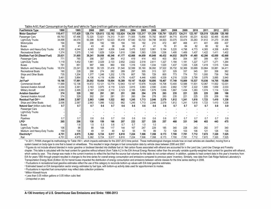
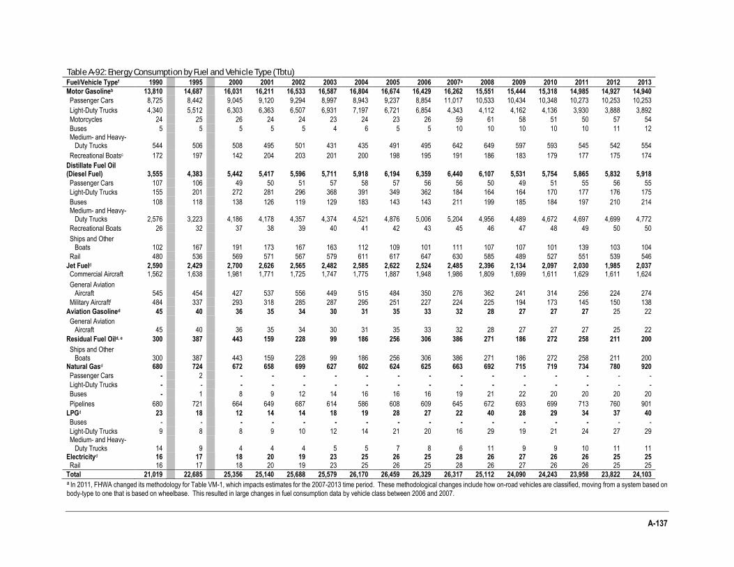
Table A-91 displays estimated fuel consumption by fuel and vehicle type. Table A-92 displays estimated energy consumption by fuel and vehicle type. The values in both of these tables correspond to the figures used to calculate CO2 emissions from transportation. Except as noted above, they are estimated based on EIA transportation sector energy estimates by fuel type, with activity data used to apportion consumption to the various modes of transport. The motor gasoline and diesel fuel consumption volumes published by EIA and FHWA include ethanol blended with gasoline and biodiesel blended with diesel. Biofuels blended with conventional fuels were subtracted from these consumption totals in order to be consistent with IPCC methodological guidance and UNFCCC reporting obligations, for which net carbon fluxes in biogenic carbon reservoirs in croplands are accounted for in the estimates for Land Use, Land-Use Change and Forestry chapter, not in Energy chapter totals. Ethanol fuel volumes were removed from motor gasoline consumption estimates for years 1990-2013 and biodiesel fuel volumes were removed from diesel fuel consumption volumes for years 2001-2013, as there was negligible use of biodiesel as a diesel blending competent prior to 2001. The subtraction or removal of biofuels blended into motor gasoline and diesel were conducted following the methodology outlined in Step 2 (“Remove Biofuels from Petroleum”) of the EIA’s Monthly Energy Review (MER) Section 12 notes.
In order to remove the volume of biodiesel blended into diesel fuel, the refinery and blender net volume inputs of renewable diesel fuel sourced from EIA Petroleum Supply Annual (EIA 2015) Table 18 - Refinery Net Input of Crude Oil and Petroleum Products and Table 20 - Blender Net Inputs of Petroleum Products were subtracted from the transportation sector’s total diesel fuel consumption volume (for both the “top-down” EIA and “bottom-up” FHWA estimates). To remove the fuel ethanol blended into motor gasoline, ethanol energy consumption data sourced from MER Table 10.2b - Renewable Energy Consumption: Industrial and Transportation Sectors (EIA 2014) were subtracted from the total EIA and FHWA transportation motor gasoline energy consumption estimates.
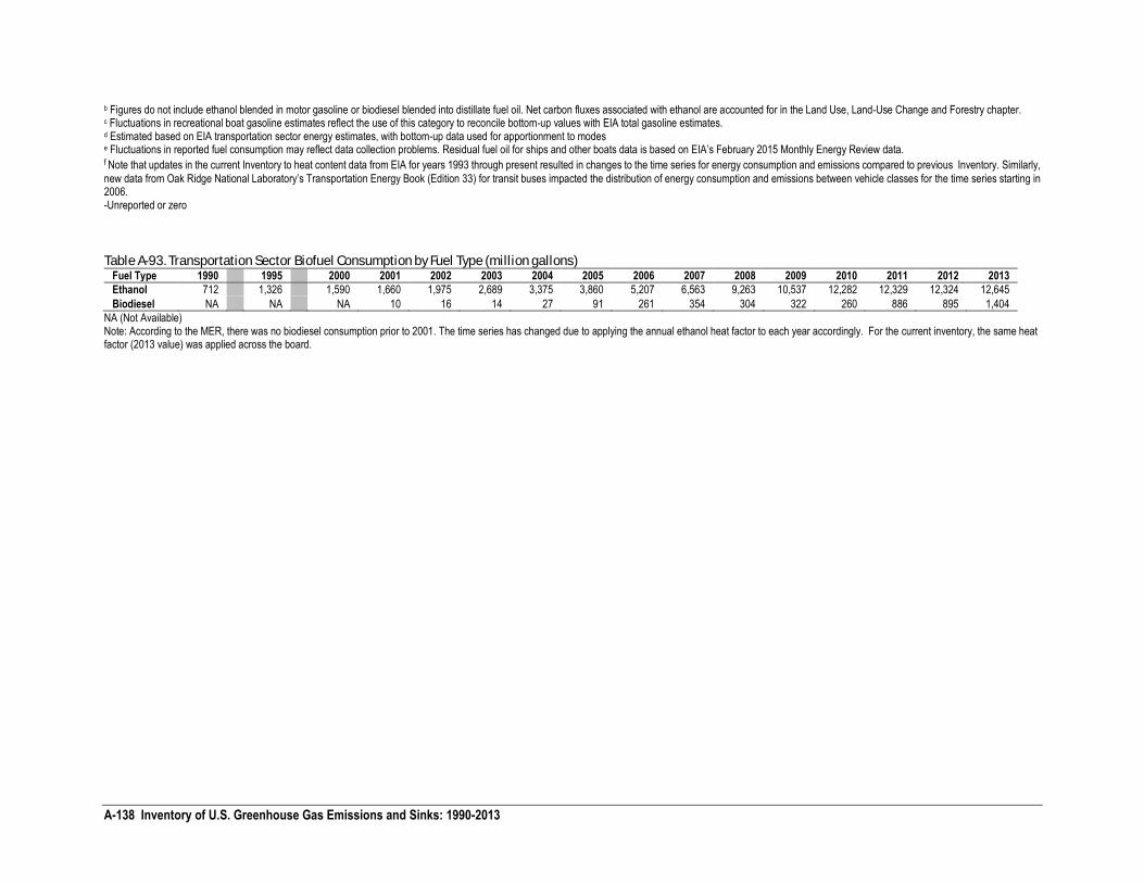
Total ethanol and biodiesel consumption estimates are shown separately in Table A-93.2
2 Note that the refinery and blender net volume inputs of renewable diesel fuel sourced from EIA’s Petroleum Supply Annual (PSA) differs from
the biodiesel volume presented in Table A-93. The PSA data is representative of the amount of biodiesel that refineries and blenders added to diesel fuel to make low level biodiesel blends. This is the appropriate value to subtract from total diesel fuel volume, as it represents the amount of biofuel blended into diesel to create low-level biodiesel blends. The biodiesel consumption value presented in Table A-93 is representative of the total biodiesel consumed and includes biodiesel components in all types of fuel formulations, from low level (<5%) to high level (6-20%, 100%) blends of biodiesel. This value is sourced from MER Table 10.4 and is calculated as biodiesel production plus biodiesel net imports minus biodiesel stock exchange.
A-136 Inventory of U.S. Greenhouse Gas Emissions and Sinks: 1990-2013
Table A-91. Fuel Consumption by Fuel and Vehicle Type (million gallons unless otherwise specified) Fuel/Vehicle Type 1990 1995 2000 2001 2002 2003 2004 2005 2006 2007a 2008 2009 2010 2011 2012 2013
Motor Gasolineb 110,417 117,429 128,174 129,613 132,192 132,624 134,359 133,317 131,359 130,791 125,072 124,211 123,197 120,519 120,056 120,160 Passenger Cars 69,763 67,496 72,320 72,921 74,313 71,931 71,505 73,856 70,792 88,607 84,715 83,919 83,231 82,622 82,465 82,465 Light-Duty Trucks 34,698 44,074 50,398 50,871 52,023 55,418 57,540 53,733 54,798 34,933 33,075 33,474 33,263 31,612 31,270 31,306 Motorcycles 194 199 208 192 189 184 193 182 210 472 487 468 411 401 459 437 Buses 39 41 43 40 38 36 49 41 41 79 81 84 82 80 92 94 Medium- and Heavy-Duty Trucks 4,350 4,044 4,065 3,961 4,006 3,446 3,475 3,922 3,961 5,164 5,220 4,798 4,773 4,383 4,358 4,455 Recreational Boatsc 1,374 1,575 1,140 1,629 1,624 1,610 1,596 1,583 1,559 1,536 1,495 1,469 1,437 1,422 1,411 1,402 Distillate Fuel Oil (Diesel Fuel) 25,631 31,605 39,241 39,058 40,348 41,177 42,668 44,659 45,848 46,432 44,032 39,879 41,485 42,286 42,050 42,668 Passenger Cars 771 765 356 357 364 412 419 414 403 403 363 354 367 399 401 398 Light-Duty Trucks 1,119 1,452 1,961 2,029 2,133 2,652 2,822 2,518 2,611 1,327 1,184 1,181 1,227 1,277 1,271 1,264 Buses 781 851 997 906 860 930 1,316 1,030 1,034 1,520 1,437 1,335 1,326 1,419 1,515 1,544 Medium- and Heavy-Duty Trucks 18,574 23,241 30,180 30,125 31,418 31,540 32,599 35,160 36,092 37,522 35,732 32,369 33,689 33,864 33,881 34,411 Recreational Boats 190 228 266 274 282 289 297 305 313 321 329 337 345 351 358 362 Ships and Other Boats 735 1,204 1,377 1,248 1,202 1,178 807 785 729 800 773 774 731 1,000 739 748 Rail 3,461 3,864 4,106 4,119 4,089 4,176 4,407 4,446 4,665 4,539 4,216 3,529 3,799 3,976 3,885 3,940 Jet Fueld 19,186 17,991 20,002 19,454 19,004 18,389 19,147 19,420 18,695 18,407 17,749 15,809 15,537 15,036 14,705 15,088 Commercial Aircraft 11,569 12,136 14,672 13,121 12,774 12,943 13,147 13,976 14,426 14,708 13,400 12,588 11,931 12,067 11,932 12,031 General Aviation Aircraft 4,034 3,361 3,163 3,975 4,119 3,323 3,815 3,583 2,590 2,043 2,682 1,787 2,322 1,895 1,659 2,033 Military Aircraft 3,583 2,495 2,167 2,359 2,110 2,123 2,185 1,860 1,679 1,656 1,667 1,434 1,283 1,074 1,114 1,024 Aviation Gasolined 374 329 302 291 281 251 260 294 278 263 235 221 225 225 209 186 General Aviation Aircraft 374 329 302 291 281 251 260 294 278 263 235 221 225 225 209 186 Residual Fuel Oild, e 2,006 2,587 2,963 1,066 1,522 662 1,245 1,713 2,046 2,579 1,812 1,241 1,818 1,723 1,410 1,338 Ships and Other Boats 2,006 2,587 2,963 1,066 1,522 662 1,245 1,713 2,046 2,579 1,812 1,241 1,818 1,723 1,410 1,338 Natural Gasd (trillion cubic feet) 0.7 0.7 0.7 0.6 0.7 0.6 0.6 0.6 0.6 0.6 0.7 0.7 0.7 0.7 0.8 0.9 Passenger Cars - - - - - - - - - - - - - - - - Light-Duty Trucks - - - - - - - - - - - - - - - - Buses - - - - - - - - - - - - - - - - Pipelines 0.7 0.7 0.6 0.6 0.7 0.6 0.6 0.6 0.6 0.6 0.7 0.7 0.7 0.7 0.7 0.9 LPGd 265 206 138 159 166 207 222 327 320 257 468 331 348 403 443 475 Buses - 1.6 1.5 0.3 0.6 0.7 0.7 1.0 1.0 - - - - - - - Light-Duty Trucks 106 98 88 108 117 144 167 247 229 185 340 228 243 282 317 340 Medium- and Heavy-Duty Trucks 159 106 49 51 49 62 55 79 89 72 128 103 106 121 126 135 Electricityd,f 4,751 4,975 5,382 5,724 5,517 6,810 7,224 7,506 7,358 8,173 7,700 7,781 7,712 7,672 7,320 7,525 Rail 4,751 4,975 5,382 5,724 5,517 6,810 7,224 7,506 7,358 8,173 7,700 7,781 7,712 7,672 7,320 7,525
a In 2011, FHWA changed its methodology for Table VM-1, which impacts estimates for the 2007-2013 time period. These methodological changes include how on-road vehicles are classified, moving from a
system based on body-type to one that is based on wheelbase. This resulted in large changes in fuel consumption data by vehicle class between 2006 and 2007. b Figures do not include ethanol blended in motor gasoline or biodiesel blended into distillate fuel oil. Net carbon fluxes associated with ethanol are accounted for in the Land Use, Land-Use Change and Forestry chapter. This table is calculated with the heat content for gasoline without ethanol (from Table A.2 in the EIA Annual Energy Review) rather than the annually variable quantity-weighted heat content for gasoline with ethanol, which varies by year. This change was made in the current inventory to reflect the fact that the source fuel volumes for the table do not contain ethanol. In addition, updates to heat content data in this year’s Inventory from EIA for years 1993 through present resulted in changes to the time series for overall energy consumption and emissions compared to previous years’ Inventory. Similarly, new data from Oak Ridge National Laboratory’s Transportation Energy Book (Edition 33) for transit buses impacted the distribution of energy consumption and emissions between vehicle classes for the time series starting in 2006. c Fluctuations in recreational boat gasoline estimates reflect the use of this category to reconcile bottom-up values with EIA total gasoline estimates. d Estimated based on EIA transportation sector energy estimates by fuel type, with bottom-up activity data used for apportionment to modes. e Fluctuations in reported fuel consumption may reflect data collection problems. f Million Kilowatt-hours + Less than 0.05 million gallons or 0.05 trillion cubic feet - Unreported or zero
A-137
Table A-92: Energy Consumption by Fuel and Vehicle Type (Tbtu) Fuel/Vehicle Typef 1990 1995 2000 2001 2002 2003 2004 2005 2006 2007a 2008 2009 2010 2011 2012 2013
Motor Gasolineb 13,810 14,687 16,031 16,211 16,533 16,587 16,804 16,674 16,429 16,262 15,551 15,444 15,318 14,985 14,927 14,940
Passenger Cars 8,725 8,442 9,045 9,120 9,294 8,997 8,943 9,237 8,854 11,017 10,533 10,434 10,348 10,273 10,253 10,253
Light-Duty Trucks 4,340 5,512 6,303 6,363 6,507 6,931 7,197 6,721 6,854 4,343 4,112 4,162 4,136 3,930 3,888 3,892
Motorcycles 24 25 26 24 24 23 24 23 26 59 61 58 51 50 57 54
Buses 5 5 5 5 5 4 6 5 5 10 10 10 10 10 11 12 Medium- and Heavy-
Duty Trucks 544 506 508 495 501 431 435 491 495 642 649 597 593 545 542 554
Recreational Boatsc 172 197 142 204 203 201 200 198 195 191 186 183 179 177 175 174
Distillate Fuel Oil (Diesel Fuel) 3,555 4,383 5,442 5,417 5,596 5,711 5,918 6,194 6,359 6,440 6,107 5,531 5,754 5,865 5,832 5,918
Passenger Cars 107 106 49 50 51 57 58 57 56 56 50 49 51 55 56 55
Light-Duty Trucks 155 201 272 281 296 368 391 349 362 184 164 164 170 177 176 175
Buses 108 118 138 126 119 129 183 143 143 211 199 185 184 197 210 214 Medium- and Heavy-
Duty Trucks 2,576 3,223 4,186 4,178 4,357 4,374 4,521 4,876 5,006 5,204 4,956 4,489 4,672 4,697 4,699 4,772
Recreational Boats 26 32 37 38 39 40 41 42 43 45 46 47 48 49 50 50
Ships and Other Boats 102 167 191 173 167 163 112 109 101 111 107 107 101 139 103 104
Rail 480 536 569 571 567 579 611 617 647 630 585 489 527 551 539 546
Jet Fueld 2,590 2,429 2,700 2,626 2,565 2,482 2,585 2,622 2,524 2,485 2,396 2,134 2,097 2,030 1,985 2,037 Commercial Aircraft 1,562 1,638 1,981 1,771 1,725 1,747 1,775 1,887 1,948 1,986 1,809 1,699 1,611 1,629 1,611 1,624
General Aviation Aircraft 545 454 427 537 556 449 515 484 350 276 362 241 314 256 224 274
Military Aircraftf 484 337 293 318 285 287 295 251 227 224 225 194 173 145 150 138
Aviation Gasolined 45 40 36 35 34 30 31 35 33 32 28 27 27 27 25 22
General Aviation Aircraft 45 40 36 35 34 30 31 35 33 32 28 27 27 27 25 22
Residual Fuel Oild, e 300 387 443 159 228 99 186 256 306 386 271 186 272 258 211 200
Ships and Other Boats 300 387 443 159 228 99 186 256 306 386 271 186 272 258 211 200
Natural Gasd 680 724 672 658 699 627 602 624 625 663 692 715 719 734 780 920
Passenger Cars - 2 - - - - - - - - - - - - - -
Light-Duty Trucks - - - - - - - - - - - - - - - -
Buses - 1 8 9 12 14 16 16 16 19 21 22 20 20 20 20
Pipelines 680 721 664 649 687 614 586 608 609 645 672 693 699 713 760 901
LPGd 23 18 12 14 14 18 19 28 27 22 40 28 29 34 37 40
Buses - - - - - - - - - - - - - - - -
Light-Duty Trucks 9 8 8 9 10 12 14 21 20 16 29 19 21 24 27 29 Medium- and Heavy-
Duty Trucks 14 9 4 4 4 5 5 7 8 6 11 9 9 10 11 11 Electricityd 16 17 18 20 19 23 25 26 25 28 26 27 26 26 25 25 Rail 16 17 18 20 19 23 25 26 25 28 26 27 26 26 25 25
Total 21,019 22,685 25,356 25,140 25,688 25,579 26,170 26,459 26,329 26,317 25,112 24,090 24,243 23,958 23,822 24,103 a In 2011, FHWA changed its methodology for Table VM-1, which impacts estimates for the 2007-2013 time period. These methodological changes include how on-road vehicles are classified, moving from a system based on
body-type to one that is based on wheelbase. This resulted in large changes in fuel consumption data by vehicle class between 2006 and 2007.
A-138 Inventory of U.S. Greenhouse Gas Emissions and Sinks: 1990-2013
b Figures do not include ethanol blended in motor gasoline or biodiesel blended into distillate fuel oil. Net carbon fluxes associated with ethanol are accounted for in the Land Use, Land-Use Change and Forestry chapter. c Fluctuations in recreational boat gasoline estimates reflect the use of this category to reconcile bottom-up values with EIA total gasoline estimates. d Estimated based on EIA transportation sector energy estimates, with bottom-up data used for apportionment to modes e Fluctuations in reported fuel consumption may reflect data collection problems. Residual fuel oil for ships and other boats data is based on EIA’s February 2015 Monthly Energy Review data. f Note that updates in the current Inventory to heat content data from EIA for years 1993 through present resulted in changes to the time series for energy consumption and emissions compared to previous Inventory. Similarly,
new data from Oak Ridge National Laboratory’s Transportation Energy Book (Edition 33) for transit buses impacted the distribution of energy consumption and emissions between vehicle classes for the time series starting in 2006. -Unreported or zero
Table A-93. Transportation Sector Biofuel Consumption by Fuel Type (million gallons) Fuel Type 1990 1995 2000 2001 2002 2003 2004 2005 2006 2007 2008 2009 2010 2011 2012 2013
Ethanol 712 1,326 1,590 1,660 1,975 2,689 3,375 3,860 5,207 6,563 9,263 10,537 12,282 12,329 12,324 12,645
Biodiesel NA NA NA 10 16 14 27 91 261 354 304 322 260 886 895 1,404
NA (Not Available) Note: According to the MER, there was no biodiesel consumption prior to 2001. The time series has changed due to applying the annual ethanol heat factor to each year accordingly. For the current inventory, the same heat factor (2013 value) was applied across the board.
A-139
Estimates of CH4 and N2O Emissions
Mobile source emissions of greenhouse gases other than CO2 are reported by transport mode (e.g., road, rail, aviation, and waterborne), vehicle type, and fuel type. Emissions estimates of CH4 and N2O were derived using a methodology similar to that outlined in the 2006 IPCC Guidelines for National Greenhouse Gas Inventories (IPCC 2006).
Activity data were obtained from a number of U.S. government agencies and other publications. Depending on the category, these basic activity data included fuel consumption and vehicle miles traveled (VMT). These estimates were then multiplied by emission factors, expressed as grams per unit of fuel consumed or per vehicle mile.
Methodology for On-Road Gasoline and Diesel Vehicles
Step 1: Determine Vehicle Miles Traveled by Vehicle Type, Fuel Type, and Model Year
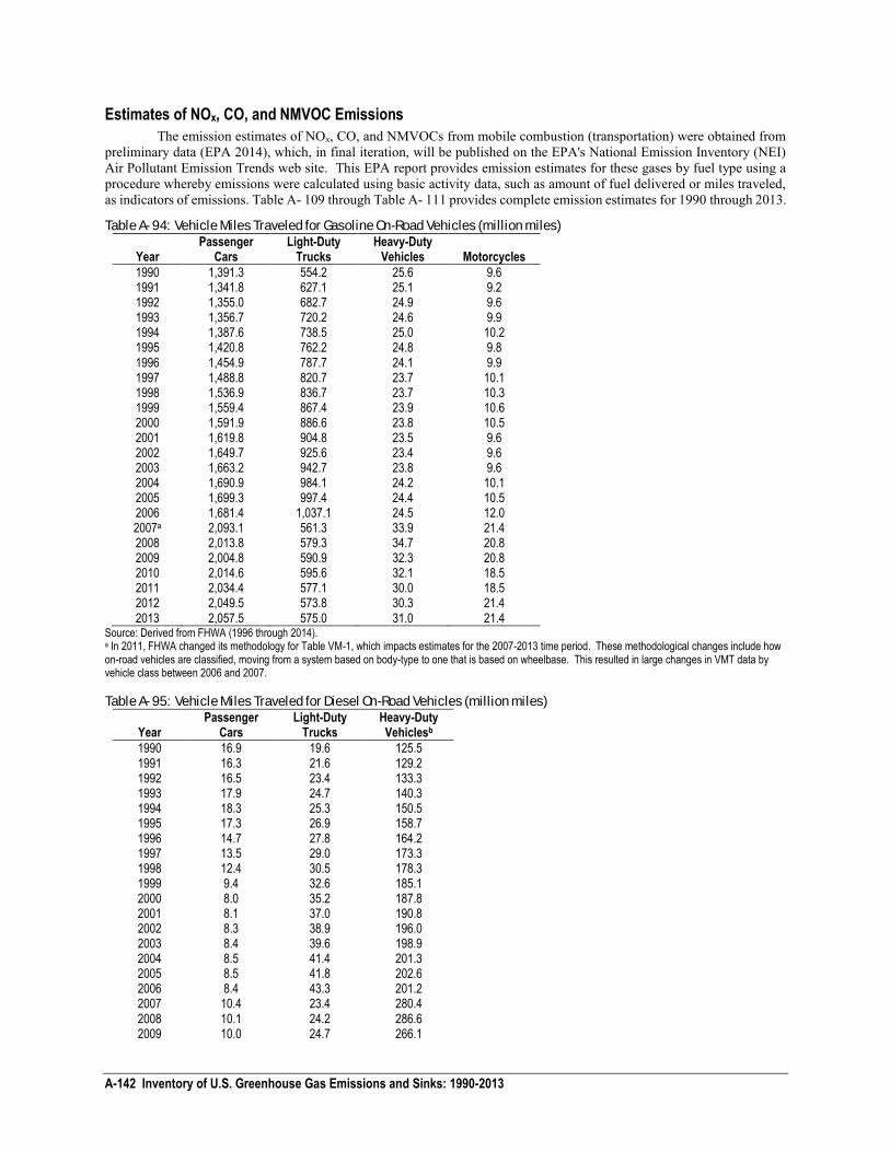
VMT by vehicle type (e.g., passenger cars, light-duty trucks, medium- and heavy-duty trucks,1 buses, and motorcycles) were obtained from the Federal Highway Administration’s (FHWA) Highway Statistics (FHWA 1996 through 2014).2 As these vehicle categories are not fuel-specific, VMT for each vehicle type was disaggregated by fuel type (gasoline, diesel) so that the appropriate emission factors could be applied. VMT from Highway Statistics Table VM-1 (FHWA 1996 through 2014) was allocated to fuel types (gasoline, diesel, other) using historical estimates of fuel shares reported in the Appendix to the Transportation Energy Data Book, Tables A.5 and A.6 (DOE 1993 through 2014). These fuel shares are drawn from various sources, including the Vehicle Inventory and Use Survey, the National Vehicle Population Profile, and the American Public Transportation Association. Fuel shares were first adjusted proportionately such that gasoline and diesel shares for each vehicle/fuel type category equaled 100 percent of national VMT. VMT for alternative fuel vehicles (AFVs) was calculated separately, and the methodology is explained in the following section on AFVs. Estimates of VMT from AFVs were then subtracted from the appropriate total VMT estimates to develop the final VMT estimates by vehicle/fuel type category.3 The resulting national VMT estimates for gasoline and diesel on-road vehicles are presented in Table A- 94 and Table A- 95, respectively.
Total VMT for each on-road category (i.e., gasoline passenger cars, light-duty gasoline trucks, heavy-duty gasoline vehicles, diesel passenger cars, light-duty diesel trucks, medium- and heavy-duty diesel vehicles, and motorcycles) were distributed across 30 model years shown for 2013 in Table A- 98. This distribution was derived by weighting the appropriate age distribution of the U.S. vehicle fleet according to vehicle registrations by the average annual age-specific vehicle mileage accumulation of U.S. vehicles. Age distribution values were obtained from EPA’s MOBILE6 model for all years before 1999 (EPA 2000) and EPA’s MOVES model for years 2009 forward (EPA 2014c).4 Age-specific vehicle mileage accumulation was obtained from EPA’s MOVES2014 model (EPA 2014).5
Step 2: Allocate VMT Data to Control Technology Type
VMT by vehicle type for each model year was distributed across various control technologies as shown in Table A- 102 through Table A- 105. The categories “EPA Tier 0” and “EPA Tier 1” were used instead of the early three-way catalyst and advanced three-way catalyst categories, respectively, as defined in the Revised 1996 IPCC Guidelines. EPA Tier 0, EPA Tier 1, EPA Tier 2, and LEV refer to U.S. emission regulations, rather than control technologies; however, each does correspond to particular combinations of control technologies and engine design. EPA Tier 2 and its predecessors EPA
1 Medium- and heavy-duty trucks correspond to FHWA’s reporting categories of single-unit trucks and combination trucks. Single-unit trucks are
defined as single frame trucks that have 2-axles and at least 6 tires or a gross vehicle weight rating (GVWR) exceeding 10,000 lbs. 2 In 2011 FHWA changed its methods for estimated vehicle miles traveled (VMT) and related data. These methodological changes included how
vehicles are classified, moving from a system based on body-type to one that is based on wheelbase. These changes were first incorporated for the 2010 Inventory and apply to the 2007-12 time period. This resulted in large changes in VMT data by vehicle class, thus leading to a shift in emissions among on-road vehicle classes. For example, the category “Passenger Cars” has been replaced by “Light-duty Vehicles-Short Wheelbase” and “Other 2 axle-4 Tire Vehicles” has been replaced by “Light-duty Vehicles, Long Wheelbase.” This change in vehicle classification has moved some smaller trucks and sport utility vehicles from the light truck category to the passenger vehicle category in this emission inventory. These changes are reflected in a large drop in light-truck emissions between 2006 and 2007. 3 In Inventories through 2002, gasoline-electric hybrid vehicles were considered part of an “alternative fuel and advanced technology” category.
However, vehicles are now only separated into gasoline, diesel, or alternative fuel categories, and gas-electric hybrids are now considered within the gasoline vehicle category. 4 Age distributions were held constant for the period 1990-1998, and reflect a 25-year vehicle age span. EPA (2010) provides a variable age
distribution and 31-year vehicle age span beginning in year 1999. 5 The updated vehicle distribution and mileage accumulation rates by vintage obtained from the MOVES 2014 model resulted in an increase in
emissions due to more miles driven by older light-duty gasoline vehicles.
A-140 Inventory of U.S. Greenhouse Gas Emissions and Sinks: 1990-2013
Tier 1 and Tier 0 apply to vehicles equipped with three-way catalysts. The introduction of “early three-way catalysts,” and “advanced three-way catalysts,” as described in the Revised 1996 IPCC Guidelines, roughly correspond to the introduction of EPA Tier 0 and EPA Tier 1 regulations (EPA 1998).6 EPA Tier 2 regulations affect vehicles produced starting in 2004 and are responsible for a noticeable decrease in N2O emissions compared EPA Tier 1 emissions technology (EPA 1999b).
Control technology assignments for light and heavy-duty conventional fuel vehicles for model years 1972 (when regulations began to take effect) through 1995 were estimated in EPA (1998). Assignments for 1998 through 2013 were determined using confidential engine family sales data submitted to EPA (EPA 2014b). Vehicle classes and emission standard tiers to which each engine family was certified were taken from annual certification test results and data (EPA 2014a). This information was used to determine the fraction of sales of each class of vehicle that met EPA Tier 0, EPA Tier 1, Tier 2, and LEV standards. Assignments for 1996 and 1997 were estimated based on the fact that EPA Tier 1 standards for light-duty vehicles were fully phased in by 1996. Tier 2 began initial phase-in by 2004.
Step 3: Determine CH4 and N2O Emission Factors by Vehicle, Fuel, and Control Technology Type
Emission factors for gasoline and diesel on-road vehicles utilizing Tier 2 and Low Emission Vehicle (LEV) technologies were developed by ICF (2006b); all other gasoline and diesel on-road vehicle emissions factors were developed by ICF (2004).These factors were based on EPA, CARB and Environment Canada laboratory test results of different vehicle and control technology types. The EPA, CARB and Environment Canada tests were designed following the Federal Test Procedure (FTP), which covers three separate driving segments, since vehicles emit varying amounts of GHGs depending on the driving segment. These driving segments are: (1) a transient driving cycle that includes cold start and running emissions, (2) a cycle that represents running emissions only, and (3) a transient driving cycle that includes hot start and running emissions. For each test run, a bag was affixed to the tailpipe of the vehicle and the exhaust was collected; the content of this bag was later analyzed to determine quantities of gases present. The emission characteristics of Segment 2 was used to define running emissions, and subtracted from the total FTP emissions to determine start emissions. These were then recombined based upon MOBILE6.2’s ratio of start to running emissions for each vehicle class to approximate average driving characteristics.
Step 4: Determine the Amount of CH4 and N2O Emitted by Vehicle, Fuel, and Control Technology Type
Emissions of CH4 and N2O were then calculated by multiplying total VMT by vehicle, fuel, and control technology type by the emission factors developed in Step 3.
Methodology for Alternative Fuel Vehicles (AFVs)
Step 1: Determine Vehicle Miles Traveled by Vehicle and Fuel Type
VMT for alternative fuel and advanced technology vehicles were calculated from “VMT Projections for Alternative Fueled and Advanced Technology Vehicles through 2025” (Browning 2003) and “Methodology for Highway Vehicle Alternative Fuel GHG Projections Estimates” (Browning, 2014). Alternative Fuels include Compressed Natural Gas (CNG), Liquid Natural Gas (LNG), Liquefied Petroleum Gas (LPG), Ethanol, Methanol, and Electric Vehicles (battery powered). Most of the vehicles that use these fuels run on an Internal Combustion Engine (ICE) powered by the alternative fuel, although many of the vehicles can run on either the alternative fuel or gasoline (or diesel), or some combination.7 Most alternative fuel vehicle VMT were calculated using the Energy Information Administration (EIA) Alternative Fuel Vehicle Data. This provided vehicle counts and fuel consumption in gasoline equivalent gallons for all vehicle classes for calendar years 2003 through 2011. For 1992 to 2002, EIA Data Tables were used to estimate fuel consumption and vehicle counts by vehicle type. These tables give total vehicle fuel use and vehicle counts by fuel and calendar year for the United States over the period 1992 through 2010. Breakdowns by vehicle type for 1992 through 2002 (both fuel consumed and vehicle counts) were assumed to be at the same ratio as for 2003 where data existed. For 1990, 1991, 2012 and 2013, fuel consumed by alternative fuel and vehicle type were extrapolated based on a regression analysis using the best curve fit based upon R2 using the nearest 5 years of data.
Because AFVs run on different fuel types, their fuel use characteristics are not directly comparable. Accordingly, fuel economy for each vehicle type is expressed in gasoline equivalent terms, i.e., how much gasoline contains the equivalent
6 For further description, see “Definitions of Emission Control Technologies and Standards” section of this annex below.
7 Fuel types used in combination depend on the vehicle class. For light-duty vehicles, gasoline is generally blended with ethanol and diesel is
blended with biodiesel; dual-fuel vehicles can run on gasoline or an alternative fuel – either natural gas or LPG – but not at the same time, while flex-fuel vehicles are designed to run on E85 (85 percent ethanol) or gasoline, or any mixture of the two in between. Heavy-duty vehicles are more likely to run on diesel fuel, natural gas, or LPG.
A-141
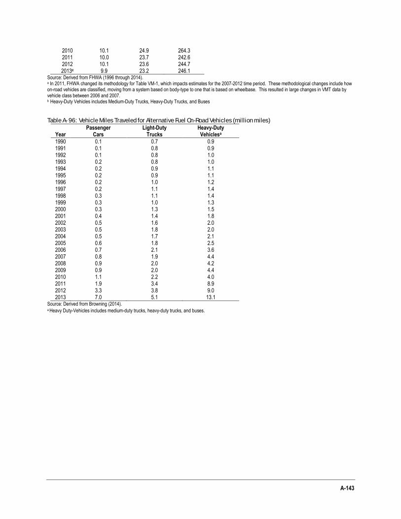
amount of energy as the alternative fuel. Energy economy ratios (the ratio of the gasoline equivalent fuel economy of a given technology to that of conventional gasoline or diesel vehicles) were taken from full fuel cycle studies done for the California Air Resources Board (Unnasch and Browning, Kassoy 2001). These ratios were used to estimate fuel economy in miles per gasoline gallon equivalent for each alternative fuel and vehicle type. Energy use per fuel type was then divided among the various weight categories and vehicle technologies that use that fuel. Total VMT per vehicle type for each calendar year was then determined by dividing the energy usage by the fuel economy. Note that for AFVs capable of running on both/either traditional and alternative fuels, the VMT given reflects only those miles driven that were powered by the alternative fuel, as explained in Browning (2003). VMT estimates for AFVs by vehicle category (passenger car, light-duty truck, heavy-duty vehicles) are shown in Table A- 96, while more detailed estimates of VMT by control technology are shown in Table A- 97.
Step 2: Determine CH4 and N2O Emission Factors by Vehicle and Alternative Fuel Type
CH4 and N2O emission factors for alternative fuel vehicles (AFVs) are calculated according to studies by Argonne National Laboratory (2006) and Lipman & Delucchi (2002), and are reported in ICF (2006a). In these studies, N2O and CH4 emissions for AFVs were expressed as a multiplier corresponding to conventional vehicle counterpart emissions. Emission estimates in these studies represent the current AFV fleet and were compared against Tier 1 emissions from light-duty gasoline vehicles to develop new multipliers. Alternative fuel heavy-duty vehicles were compared against gasoline heavy-duty vehicles as most alternative fuel heavy-duty vehicles use catalytic after treatment and perform more like gasoline vehicles than diesel vehicles. These emission factors are shown in Table A- 107.8
Step 3: Determine the Amount of CH4 and N2O Emitted by Vehicle and Fuel Type
Emissions of CH4 and N2O were calculated by multiplying total VMT for each vehicle and fuel type (Step 1) by the appropriate emission factors (Step 2).
Methodology for Non-Road Mobile Sources
CH4 and N2O emissions from non-road mobile sources were estimated by applying emission factors to the amount of fuel consumed by mode and vehicle type.
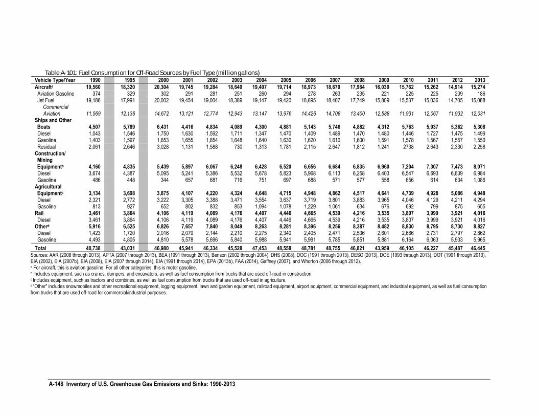
Activity data for non-road vehicles include annual fuel consumption statistics by transportation mode and fuel type, as shown in Table A- 101. Consumption data for ships and other boats (i.e., vessel bunkering) were obtained from DHS (2008) and EIA (1991 through 2014) for distillate fuel, and DHS (2008) and EIA (2014a) for residual fuel; marine transport fuel consumption data for U.S. territories (EIA 2014b) were added to domestic consumption, and this total was reduced by the amount of fuel used for international bunkers.9 Gasoline consumption by recreational boats was obtained from EPA’s NONROAD model (EPA 2014b). Annual diesel consumption for Class I rail was obtained from the Association of American Railroads (AAR 2008 through 2013), diesel consumption from commuter rail was obtained from APTA (2007 through 2013) and Gaffney (2007), and consumption by Class II and III rail was provided by Benson (2002 through 2004) and Whorton (2006 through 2013).10 Diesel consumption by commuter and intercity rail was obtained from DOE (1993 through 2013). Data on the consumption of jet fuel and aviation gasoline in aircraft were obtained from EIA (2014) and FAA (2014), as described in Annex 2.1: Methodology for Estimating Emissions of CO2 from Fossil Fuel Combustion, and were reduced by the amount allocated to international bunker fuels (DESC 2014 and FAA 2014). Pipeline fuel consumption was obtained from EIA (2007 through 2014) (note: pipelines are a transportation source but are stationary, not mobile, sources). Data on fuel consumption by all non-transportation mobile sources were obtained from EPA’s NONROAD model (EPA 2014b) and from FHWA (1996 through 2014) for gasoline consumption for trucks used off-road.
11
Emissions of CH4 and N2O from non-road mobile sources were calculated by multiplying U.S. default emission factors in the 2006 IPCC Guidelines by activity data for each source type (see Table A- 108).
8 New data from EIA on the population and activity of alternative fuel vehicles significantly changed the mix of alternative fuel vehicles in the
population from last year’s inventory, resulting in changes in the average emissions per mile associated with different classes of alternative fuel vehicles (light-duty, heavy-duty, buses, etc.). 9 See International Bunker Fuels section of the Energy Chapter.
10 Diesel consumption from Class II and Class III railroad were unavailable for 2012. Values are proxied from 2010, which is the last year the data
was available. 11
“Non-transportation mobile sources” are defined as any vehicle or equipment not used on the traditional road system, but excluding aircraft, rail and watercraft. This category includes snowmobiles, golf carts, riding lawn mowers, agricultural equipment, and trucks used for off-road purposes, among others.
A-142 Inventory of U.S. Greenhouse Gas Emissions and Sinks: 1990-2013
Estimates of NOx, CO, and NMVOC Emissions
The emission estimates of NOx, CO, and NMVOCs from mobile combustion (transportation) were obtained from preliminary data (EPA 2014), which, in final iteration, will be published on the EPA's National Emission Inventory (NEI) Air Pollutant Emission Trends web site. This EPA report provides emission estimates for these gases by fuel type using a procedure whereby emissions were calculated using basic activity data, such as amount of fuel delivered or miles traveled, as indicators of emissions. Table A- 109 through Table A- 111 provides complete emission estimates for 1990 through 2013.
Table A- 94: Vehicle Miles Traveled for Gasoline On-Road Vehicles (million miles)
Year Passenger
Cars Light-Duty
Trucks Heavy-Duty
Vehicles Motorcycles
1990 1,391.3 554.2 25.6 9.6 1991 1,341.8 627.1 25.1 9.2 1992 1,355.0 682.7 24.9 9.6 1993 1,356.7 720.2 24.6 9.9 1994 1,387.6 738.5 25.0 10.2 1995 1,420.8 762.2 24.8 9.8 1996 1,454.9 787.7 24.1 9.9 1997 1,488.8 820.7 23.7 10.1 1998 1,536.9 836.7 23.7 10.3 1999 1,559.4 867.4 23.9 10.6 2000 1,591.9 886.6 23.8 10.5 2001 1,619.8 904.8 23.5 9.6 2002 1,649.7 925.6 23.4 9.6 2003 1,663.2 942.7 23.8 9.6 2004 1,690.9 984.1 24.2 10.1 2005 1,699.3 997.4 24.4 10.5 2006 1,681.4 1,037.1 24.5 12.0 2007a 2,093.1 561.3 33.9 21.4 2008 2,013.8 579.3 34.7 20.8 2009 2,004.8 590.9 32.3 20.8 2010 2,014.6 595.6 32.1 18.5 2011 2,034.4 577.1 30.0 18.5 2012 2,049.5 573.8 30.3 21.4 2013 2,057.5 575.0 31.0 21.4
Source: Derived from FHWA (1996 through 2014). a In 2011, FHWA changed its methodology for Table VM-1, which impacts estimates for the 2007-2013 time period. These methodological changes include how on-road vehicles are classified, moving from a system based on body-type to one that is based on wheelbase. This resulted in large changes in VMT data by vehicle class between 2006 and 2007.
Table A- 95: Vehicle Miles Traveled for Diesel On-Road Vehicles (million miles)
Year Passenger
Cars Light-Duty
Trucks Heavy-Duty Vehiclesb
1990 16.9 19.6 125.5 1991 16.3 21.6 129.2 1992 16.5 23.4 133.3 1993 17.9 24.7 140.3 1994 18.3 25.3 150.5 1995 17.3 26.9 158.7 1996 14.7 27.8 164.2 1997 13.5 29.0 173.3 1998 12.4 30.5 178.3 1999 9.4 32.6 185.1 2000 8.0 35.2 187.8 2001 8.1 37.0 190.8 2002 8.3 38.9 196.0 2003 8.4 39.6 198.9 2004 8.5 41.4 201.3 2005 8.5 41.8 202.6 2006 8.4 43.3 201.2 2007 10.4 23.4 280.4 2008 10.1 24.2 286.6 2009 10.0 24.7 266.1
A-143
2010 10.1 24.9 264.3 2011 10.0 23.7 242.6 2012 10.1 23.6 244.7 2013c 9.9 23.2 246.1
Source: Derived from FHWA (1996 through 2014). a In 2011, FHWA changed its methodology for Table VM-1, which impacts estimates for the 2007-2012 time period. These methodological changes include how on-road vehicles are classified, moving from a system based on body-type to one that is based on wheelbase. This resulted in large changes in VMT data by vehicle class between 2006 and 2007. b Heavy-Duty Vehicles includes Medium-Duty Trucks, Heavy-Duty Trucks, and Buses
Table A- 96: Vehicle Miles Traveled for Alternative Fuel On-Road Vehicles (million miles)
Year Passenger
Cars Light-Duty
Trucks Heavy-Duty Vehiclesa
1990 0.1 0.7 0.9 1991 0.1 0.8 0.9 1992 0.1 0.8 1.0 1993 0.2 0.8 1.0 1994 0.2 0.9 1.1 1995 0.2 0.9 1.1 1996 0.2 1.0 1.2 1997 0.2 1.1 1.4 1998 0.3 1.1 1.4 1999 0.3 1.0 1.3 2000 0.3 1.3 1.5 2001 0.4 1.4 1.8 2002 0.5 1.6 2.0 2003 0.5 1.8 2.0 2004 0.5 1.7 2.1 2005 0.6 1.8 2.5 2006 0.7 2.1 3.6 2007 0.8 1.9 4.4 2008 0.9 2.0 4.2 2009 0.9 2.0 4.4 2010 1.1 2.2 4.0 2011 1.9 3.4 8.9 2012 3.3 3.8 9.0 2013 7.0 5.1 13.1
Source: Derived from Browning (2014). a Heavy Duty-Vehicles includes medium-duty trucks, heavy-duty trucks, and buses.
A-144 Inventory of U.S. Greenhouse Gas Emissions and Sinks: 1990-2013
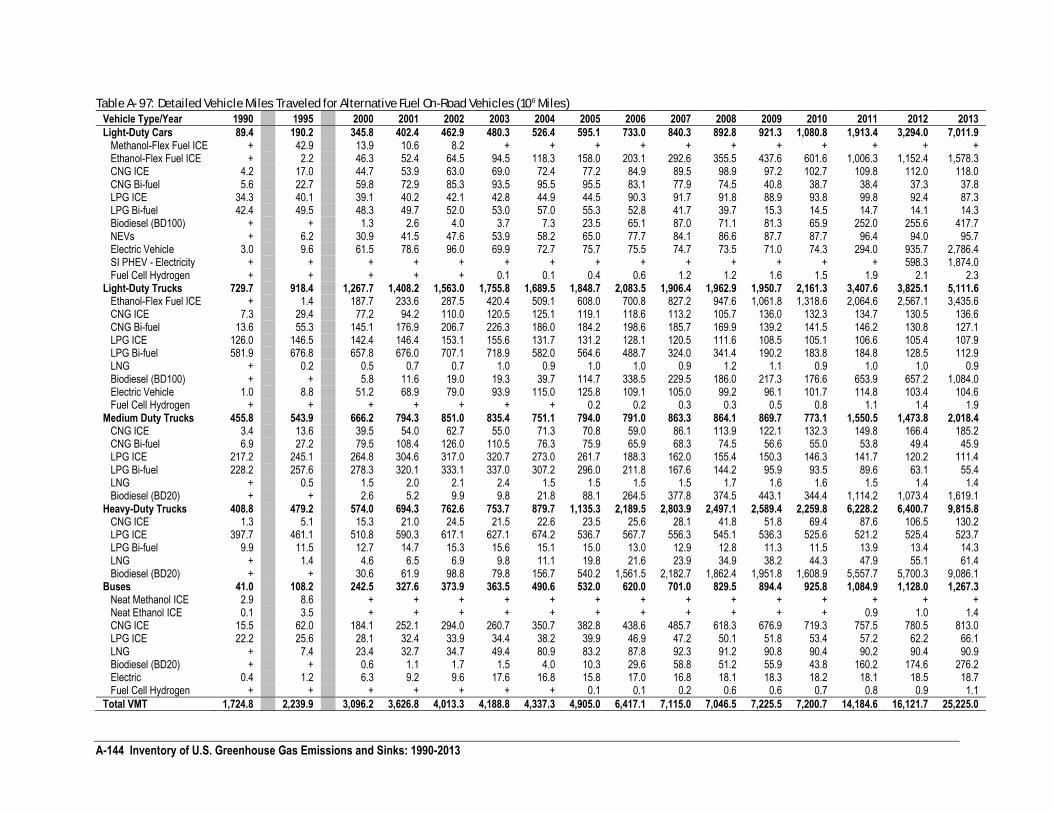
Table A- 97: Detailed Vehicle Miles Traveled for Alternative Fuel On-Road Vehicles (106 Miles)
Vehicle Type/Year 1990 1995 2000 2001 2002 2003 2004 2005 2006 2007 2008 2009 2010 2011 2012 2013
Light-Duty Cars 89.4 190.2 345.8 402.4 462.9 480.3 526.4 595.1 733.0 840.3 892.8 921.3 1,080.8 1,913.4 3,294.0 7,011.9 Methanol-Flex Fuel ICE + 42.9 13.9 10.6 8.2 + + + + + + + + + + + Ethanol-Flex Fuel ICE + 2.2 46.3 52.4 64.5 94.5 118.3 158.0 203.1 292.6 355.5 437.6 601.6 1,006.3 1,152.4 1,578.3 CNG ICE 4.2 17.0 44.7 53.9 63.0 69.0 72.4 77.2 84.9 89.5 98.9 97.2 102.7 109.8 112.0 118.0 CNG Bi-fuel 5.6 22.7 59.8 72.9 85.3 93.5 95.5 95.5 83.1 77.9 74.5 40.8 38.7 38.4 37.3 37.8 LPG ICE 34.3 40.1 39.1 40.2 42.1 42.8 44.9 44.5 90.3 91.7 91.8 88.9 93.8 99.8 92.4 87.3 LPG Bi-fuel 42.4 49.5 48.3 49.7 52.0 53.0 57.0 55.3 52.8 41.7 39.7 15.3 14.5 14.7 14.1 14.3 Biodiesel (BD100) + + 1.3 2.6 4.0 3.7 7.3 23.5 65.1 87.0 71.1 81.3 65.9 252.0 255.6 417.7 NEVs + 6.2 30.9 41.5 47.6 53.9 58.2 65.0 77.7 84.1 86.6 87.7 87.7 96.4 94.0 95.7 Electric Vehicle 3.0 9.6 61.5 78.6 96.0 69.9 72.7 75.7 75.5 74.7 73.5 71.0 74.3 294.0 935.7 2,786.4 SI PHEV - Electricity + + + + + + + + + + + + + + 598.3 1,874.0 Fuel Cell Hydrogen + + + + + 0.1 0.1 0.4 0.6 1.2 1.2 1.6 1.5 1.9 2.1 2.3 Light-Duty Trucks 729.7 918.4 1,267.7 1,408.2 1,563.0 1,755.8 1,689.5 1,848.7 2,083.5 1,906.4 1,962.9 1,950.7 2,161.3 3,407.6 3,825.1 5,111.6 Ethanol-Flex Fuel ICE + 1.4 187.7 233.6 287.5 420.4 509.1 608.0 700.8 827.2 947.6 1,061.8 1,318.6 2,064.6 2,567.1 3,435.6 CNG ICE 7.3 29.4 77.2 94.2 110.0 120.5 125.1 119.1 118.6 113.2 105.7 136.0 132.3 134.7 130.5 136.6 CNG Bi-fuel 13.6 55.3 145.1 176.9 206.7 226.3 186.0 184.2 198.6 185.7 169.9 139.2 141.5 146.2 130.8 127.1 LPG ICE 126.0 146.5 142.4 146.4 153.1 155.6 131.7 131.2 128.1 120.5 111.6 108.5 105.1 106.6 105.4 107.9 LPG Bi-fuel 581.9 676.8 657.8 676.0 707.1 718.9 582.0 564.6 488.7 324.0 341.4 190.2 183.8 184.8 128.5 112.9 LNG + 0.2 0.5 0.7 0.7 1.0 0.9 1.0 1.0 0.9 1.2 1.1 0.9 1.0 1.0 0.9 Biodiesel (BD100) + + 5.8 11.6 19.0 19.3 39.7 114.7 338.5 229.5 186.0 217.3 176.6 653.9 657.2 1,084.0 Electric Vehicle 1.0 8.8 51.2 68.9 79.0 93.9 115.0 125.8 109.1 105.0 99.2 96.1 101.7 114.8 103.4 104.6 Fuel Cell Hydrogen + + + + + + + 0.2 0.2 0.3 0.3 0.5 0.8 1.1 1.4 1.9 Medium Duty Trucks 455.8 543.9 666.2 794.3 851.0 835.4 751.1 794.0 791.0 863.3 864.1 869.7 773.1 1,550.5 1,473.8 2,018.4 CNG ICE 3.4 13.6 39.5 54.0 62.7 55.0 71.3 70.8 59.0 86.1 113.9 122.1 132.3 149.8 166.4 185.2 CNG Bi-fuel 6.9 27.2 79.5 108.4 126.0 110.5 76.3 75.9 65.9 68.3 74.5 56.6 55.0 53.8 49.4 45.9 LPG ICE 217.2 245.1 264.8 304.6 317.0 320.7 273.0 261.7 188.3 162.0 155.4 150.3 146.3 141.7 120.2 111.4 LPG Bi-fuel 228.2 257.6 278.3 320.1 333.1 337.0 307.2 296.0 211.8 167.6 144.2 95.9 93.5 89.6 63.1 55.4 LNG + 0.5 1.5 2.0 2.1 2.4 1.5 1.5 1.5 1.5 1.7 1.6 1.6 1.5 1.4 1.4 Biodiesel (BD20) + + 2.6 5.2 9.9 9.8 21.8 88.1 264.5 377.8 374.5 443.1 344.4 1,114.2 1,073.4 1,619.1 Heavy-Duty Trucks 408.8 479.2 574.0 694.3 762.6 753.7 879.7 1,135.3 2,189.5 2,803.9 2,497.1 2,589.4 2,259.8 6,228.2 6,400.7 9,815.8 CNG ICE 1.3 5.1 15.3 21.0 24.5 21.5 22.6 23.5 25.6 28.1 41.8 51.8 69.4 87.6 106.5 130.2 LPG ICE 397.7 461.1 510.8 590.3 617.1 627.1 674.2 536.7 567.7 556.3 545.1 536.3 525.6 521.2 525.4 523.7 LPG Bi-fuel 9.9 11.5 12.7 14.7 15.3 15.6 15.1 15.0 13.0 12.9 12.8 11.3 11.5 13.9 13.4 14.3 LNG + 1.4 4.6 6.5 6.9 9.8 11.1 19.8 21.6 23.9 34.9 38.2 44.3 47.9 55.1 61.4 Biodiesel (BD20) + + 30.6 61.9 98.8 79.8 156.7 540.2 1,561.5 2,182.7 1,862.4 1,951.8 1,608.9 5,557.7 5,700.3 9,086.1 Buses 41.0 108.2 242.5 327.6 373.9 363.5 490.6 532.0 620.0 701.0 829.5 894.4 925.8 1,084.9 1,128.0 1,267.3 Neat Methanol ICE 2.9 8.6 + + + + + + + + + + + + + + Neat Ethanol ICE 0.1 3.5 + + + + + + + + + + + 0.9 1.0 1.4 CNG ICE 15.5 62.0 184.1 252.1 294.0 260.7 350.7 382.8 438.6 485.7 618.3 676.9 719.3 757.5 780.5 813.0 LPG ICE 22.2 25.6 28.1 32.4 33.9 34.4 38.2 39.9 46.9 47.2 50.1 51.8 53.4 57.2 62.2 66.1 LNG + 7.4 23.4 32.7 34.7 49.4 80.9 83.2 87.8 92.3 91.2 90.8 90.4 90.2 90.4 90.9 Biodiesel (BD20) + + 0.6 1.1 1.7 1.5 4.0 10.3 29.6 58.8 51.2 55.9 43.8 160.2 174.6 276.2 Electric 0.4 1.2 6.3 9.2 9.6 17.6 16.8 15.8 17.0 16.8 18.1 18.3 18.2 18.1 18.5 18.7 Fuel Cell Hydrogen + + + + + + + 0.1 0.1 0.2 0.6 0.6 0.7 0.8 0.9 1.1
Total VMT 1,724.8 2,239.9 3,096.2 3,626.8 4,013.3 4,188.8 4,337.3 4,905.0 6,417.1 7,115.0 7,046.5 7,225.5 7,200.7 14,184.6 16,121.7 25,225.0
A-145
Source: Derived from Browning (2003) and Browning (2014). Note: Throughout the rest of this Inventory, medium-duty trucks are grouped with heavy-duty trucks; they are reported separately here because these two categories may run on a slightly different range of fuel types. a In 2011, EIA changed its reporting methodology for 2005-2010 data. EIA provided more detail on alternative fuel vehicle use by vehicle class. The fuel use breakdown by vehicle class had previously been based on estimates of the distribution of fuel use by vehicle class. The new data from EIA allowed actual data to be used for fuel use, and resulted in greater share of heavy-duty AFV VMT estimated for 2005-2010. The source of this data is the U.S. Energy Information Administration, Office of Energy Consumption and Efficiency Statistics and the DOE/GSA Federal Automotive Statistical Tool (FAST). + Less than 0.05 million vehicle miles traveled
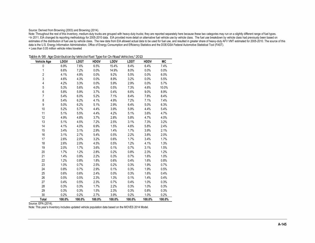
Table A- 98: Age Distribution by Vehicle/Fuel Type for On-Road Vehicles,a 2013
Vehicle Age LDGV LDGT HDGV LDDV LDDT HDDV MC
0 6.9% 7.6% 6.5% 15.4% 8.4% 6.4% 7.4%
1 6.6% 7.2% 0.0% 14.9% 8.0% 0.0% 0.0%
2 4.1% 4.9% 0.0% 9.2% 5.5% 0.0% 6.0%
3 4.6% 4.3% 0.0% 8.9% 3.2% 0.0% 5.5%
4 4.2% 3.3% 0.0% 5.9% 2.9% 0.0% 5.7%
5 5.3% 5.6% 4.0% 0.5% 7.3% 4.6% 10.0%
6 5.8% 5.9% 3.7% 0.4% 6.6% 9.0% 8.9%
7 5.4% 6.0% 5.2% 7.1% 8.4% 7.8% 8.4%
8 5.4% 6.2% 4.1% 4.9% 7.2% 7.1% 7.4%
9 5.0% 6.2% 5.1% 2.9% 6.4% 5.0% 6.3%
10 5.2% 5.7% 4.4% 3.9% 5.9% 4.4% 5.4%
11 5.1% 5.5% 4.4% 4.2% 5.1% 3.6% 4.7%
12 4.9% 4.8% 3.7% 2.8% 5.8% 4.7% 4.0%
13 5.1% 4.5% 7.2% 2.5% 3.1% 7.3% 3.2%
14 4.1% 4.0% 6.9% 1.5% 4.6% 5.8% 2.4%
15 3.4% 3.1% 2.9% 1.4% 1.7% 3.9% 2.1%
16 3.1% 2.7% 5.4% 0.5% 2.2% 3.8% 2.0%
17 2.6% 2.0% 3.2% 0.6% 1.7% 3.4% 1.7%
18 2.6% 2.0% 4.5% 0.5% 1.2% 4.1% 1.3%
19 2.0% 1.7% 3.6% 0.1% 0.7% 3.1% 1.5%
20 1.7% 1.2% 2.8% 0.2% 0.8% 2.3% 1.2%
21 1.4% 0.9% 2.2% 0.3% 0.7% 1.6% 1.0%
22 1.2% 0.8% 1.8% 0.6% 0.4% 1.6% 0.8%
23 1.0% 0.7% 2.5% 0.2% 0.3% 1.9% 0.7%
24 0.8% 0.7% 2.9% 0.1% 0.3% 1.9% 0.5%
25 0.6% 0.6% 2.4% 0.0% 0.3% 1.6% 0.4%
26 0.5% 0.5% 2.3% 1.3% 0.1% 1.4% 0.4%
27 0.4% 0.5% 2.3% 0.7% 0.4% 1.0% 0.3%
28 0.3% 0.3% 1.7% 2.2% 0.3% 1.0% 0.3%
29 0.3% 0.3% 1.5% 2.3% 0.3% 0.8% 0.3%
30 0.2% 0.2% 2.7% 3.9% 0.2% 1.0% 0.2%
Total 100.0% 100.0% 100.0% 100.0% 100.0% 100.0% 100.0%
Source: EPA (2014). Note: This year’s Inventory includes updated vehicle population data based on the MOVES 2014 Model.
A-146 Inventory of U.S. Greenhouse Gas Emissions and Sinks: 1990-2013
a The following abbreviations correspond to vehicle types: LDGV (light-duty gasoline vehicles), LDGT (light-duty gasoline trucks), HDGV (heavy-duty gasoline vehicles), LDDV (light-duty diesel vehicles), LDDT (light-duty diesel trucks), HDDV (heavy-duty diesel vehicles), and MC (motorcycles).
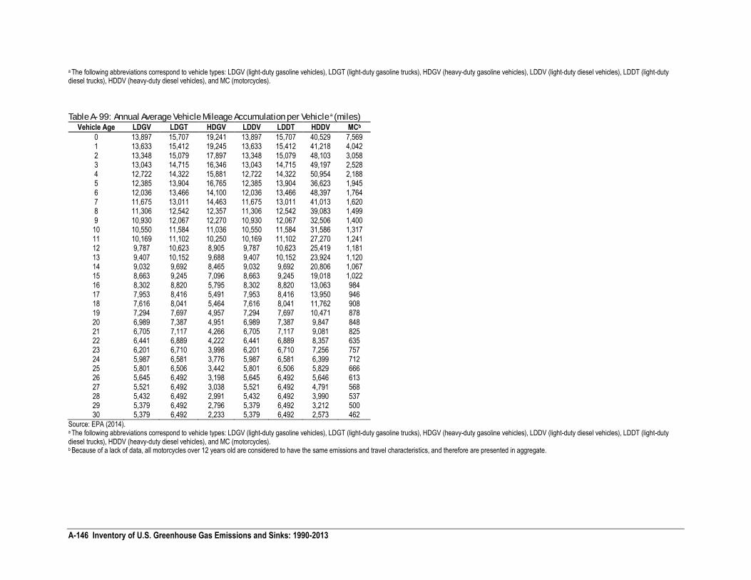
Table A- 99: Annual Average Vehicle Mileage Accumulation per Vehicle a (miles) Vehicle Age LDGV LDGT HDGV LDDV LDDT HDDV MCb
0 13,897 15,707 19,241 13,897 15,707 40,529 7,569 1 13,633 15,412 19,245 13,633 15,412 41,218 4,042 2 13,348 15,079 17,897 13,348 15,079 48,103 3,058 3 13,043 14,715 16,346 13,043 14,715 49,197 2,528 4 12,722 14,322 15,881 12,722 14,322 50,954 2,188 5 12,385 13,904 16,765 12,385 13,904 36,623 1,945 6 12,036 13,466 14,100 12,036 13,466 48,397 1,764 7 11,675 13,011 14,463 11,675 13,011 41,013 1,620 8 11,306 12,542 12,357 11,306 12,542 39,083 1,499 9 10,930 12,067 12,270 10,930 12,067 32,506 1,400 10 10,550 11,584 11,036 10,550 11,584 31,586 1,317 11 10,169 11,102 10,250 10,169 11,102 27,270 1,241 12 9,787 10,623 8,905 9,787 10,623 25,419 1,181 13 9,407 10,152 9,688 9,407 10,152 23,924 1,120 14 9,032 9,692 8,465 9,032 9,692 20,806 1,067 15 8,663 9,245 7,096 8,663 9,245 19,018 1,022 16 8,302 8,820 5,795 8,302 8,820 13,063 984 17 7,953 8,416 5,491 7,953 8,416 13,950 946 18 7,616 8,041 5,464 7,616 8,041 11,762 908 19 7,294 7,697 4,957 7,294 7,697 10,471 878 20 6,989 7,387 4,951 6,989 7,387 9,847 848 21 6,705 7,117 4,266 6,705 7,117 9,081 825 22 6,441 6,889 4,222 6,441 6,889 8,357 635 23 6,201 6,710 3,998 6,201 6,710 7,256 757 24 5,987 6,581 3,776 5,987 6,581 6,399 712 25 5,801 6,506 3,442 5,801 6,506 5,829 666 26 5,645 6,492 3,198 5,645 6,492 5,646 613 27 5,521 6,492 3,038 5,521 6,492 4,791 568 28 5,432 6,492 2,991 5,432 6,492 3,990 537 29 5,379 6,492 2,796 5,379 6,492 3,212 500 30 5,379 6,492 2,233 5,379 6,492 2,573 462
Source: EPA (2014). a The following abbreviations correspond to vehicle types: LDGV (light-duty gasoline vehicles), LDGT (light-duty gasoline trucks), HDGV (heavy-duty gasoline vehicles), LDDV (light-duty diesel vehicles), LDDT (light-duty diesel trucks), HDDV (heavy-duty diesel vehicles), and MC (motorcycles). b Because of a lack of data, all motorcycles over 12 years old are considered to have the same emissions and travel characteristics, and therefore are presented in aggregate.
A-147
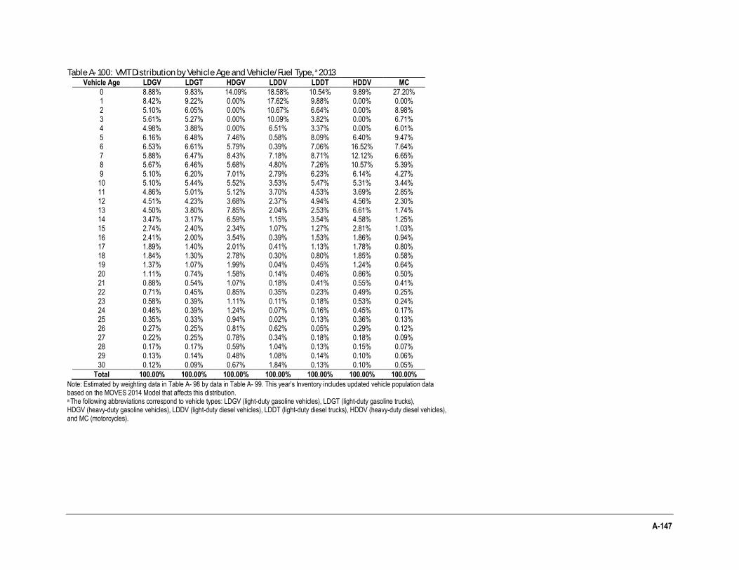
Table A- 100: VMT Distribution by Vehicle Age and Vehicle/Fuel Type, a 2013 Vehicle Age LDGV LDGT HDGV LDDV LDDT HDDV MC
0 8.88% 9.83% 14.09% 18.58% 10.54% 9.89% 27.20% 1 8.42% 9.22% 0.00% 17.62% 9.88% 0.00% 0.00% 2 5.10% 6.05% 0.00% 10.67% 6.64% 0.00% 8.98% 3 5.61% 5.27% 0.00% 10.09% 3.82% 0.00% 6.71% 4 4.98% 3.88% 0.00% 6.51% 3.37% 0.00% 6.01% 5 6.16% 6.48% 7.46% 0.58% 8.09% 6.40% 9.47% 6 6.53% 6.61% 5.79% 0.39% 7.06% 16.52% 7.64% 7 5.88% 6.47% 8.43% 7.18% 8.71% 12.12% 6.65% 8 5.67% 6.46% 5.68% 4.80% 7.26% 10.57% 5.39% 9 5.10% 6.20% 7.01% 2.79% 6.23% 6.14% 4.27% 10 5.10% 5.44% 5.52% 3.53% 5.47% 5.31% 3.44% 11 4.86% 5.01% 5.12% 3.70% 4.53% 3.69% 2.85% 12 4.51% 4.23% 3.68% 2.37% 4.94% 4.56% 2.30% 13 4.50% 3.80% 7.85% 2.04% 2.53% 6.61% 1.74% 14 3.47% 3.17% 6.59% 1.15% 3.54% 4.58% 1.25% 15 2.74% 2.40% 2.34% 1.07% 1.27% 2.81% 1.03% 16 2.41% 2.00% 3.54% 0.39% 1.53% 1.86% 0.94% 17 1.89% 1.40% 2.01% 0.41% 1.13% 1.78% 0.80% 18 1.84% 1.30% 2.78% 0.30% 0.80% 1.85% 0.58% 19 1.37% 1.07% 1.99% 0.04% 0.45% 1.24% 0.64% 20 1.11% 0.74% 1.58% 0.14% 0.46% 0.86% 0.50% 21 0.88% 0.54% 1.07% 0.18% 0.41% 0.55% 0.41% 22 0.71% 0.45% 0.85% 0.35% 0.23% 0.49% 0.25% 23 0.58% 0.39% 1.11% 0.11% 0.18% 0.53% 0.24% 24 0.46% 0.39% 1.24% 0.07% 0.16% 0.45% 0.17% 25 0.35% 0.33% 0.94% 0.02% 0.13% 0.36% 0.13% 26 0.27% 0.25% 0.81% 0.62% 0.05% 0.29% 0.12% 27 0.22% 0.25% 0.78% 0.34% 0.18% 0.18% 0.09% 28 0.17% 0.17% 0.59% 1.04% 0.13% 0.15% 0.07% 29 0.13% 0.14% 0.48% 1.08% 0.14% 0.10% 0.06% 30 0.12% 0.09% 0.67% 1.84% 0.13% 0.10% 0.05%
Total 100.00% 100.00% 100.00% 100.00% 100.00% 100.00% 100.00%
Note: Estimated by weighting data in Table A- 98 by data in Table A- 99. This year’s Inventory includes updated vehicle population data based on the MOVES 2014 Model that affects this distribution. a The following abbreviations correspond to vehicle types: LDGV (light-duty gasoline vehicles), LDGT (light-duty gasoline trucks), HDGV (heavy-duty gasoline vehicles), LDDV (light-duty diesel vehicles), LDDT (light-duty diesel trucks), HDDV (heavy-duty diesel vehicles), and MC (motorcycles).
A-148 Inventory of U.S. Greenhouse Gas Emissions and Sinks: 1990-2013
Table A- 101: Fuel Consumption for Off-Road Sources by Fuel Type (million gallons) Vehicle Type/Year 1990 1995 2000 2001 2002 2003 2004 2005 2006 2007 2008 2009 2010 2011 2012 2013
Aircrafta 19,560 18,320 20,304 19,745 19,284 18,640 19,407 19,714 18,973 18,670 17,984 16,030 15,762 15,262 14,914 15,274 Aviation Gasoline 374 329 302 291 281 251 260 294 278 263 235 221 225 225 209 186 Jet Fuel 19,186 17,991 20,002 19,454 19,004 18,389 19,147 19,420 18,695 18,407 17,749 15,809 15,537 15,036 14,705 15,088
Commercial Aviation 11,569 12,136 14,672 13,121 12,774 12,943 13,147 13,976 14,426 14,708 13,400 12,588 11,931 12,067 11,932 12,031
Ships and Other Boats 4,507 5,789 6,431 4,416 4,834 4,089 4,300 4,881 5,143 5,746 4,882 4,312 5,763 5,937 5,362 5,308
Diesel 1,043 1,546 1,750 1,630 1,592 1,711 1,347 1,470 1,409 1,489 1,470 1,480 1,446 1,727 1,475 1,499 Gasoline 1,403 1,597 1,653 1,655 1,654 1,648 1,640 1,630 1,620 1,610 1,600 1,591 1,578 1,567 1,557 1,550 Residual 2,061 2,646 3,028 1,131 1,588 730 1,313 1,781 2,115 2,647 1,812 1,241 2738 2,643 2,330 2,258 Construction/ Mining Equipmentb 4,160 4,835 5,439 5,897 6,067 6,248 6,428 6,520 6,656 6,684 6,835 6,960 7,204 7,307 7,473 8,071
Diesel 3,674 4,387 5,095 5,241 5,386 5,532 5,678 5,823 5,968 6,113 6,258 6,403 6,547 6,693 6,839 6,984 Gasoline 486 448 344 657 681 716 751 697 688 571 577 558 656 614 634 1,086 Agricultural Equipmentc 3,134 3,698 3,875 4,107 4,220 4,324 4,648 4,715 4,948 4,862 4,517 4,641 4,739 4,928 5,086 4,948
Diesel 2,321 2,772 3,222 3,305 3,388 3,471 3,554 3,637 3,719 3,801 3,883 3,965 4,046 4,129 4,211 4,294 Gasoline 813 927 652 802 832 853 1,094 1,078 1,229 1,061 634 676 692 799 875 655 Rail 3,461 3,864 4,106 4,119 4,089 4,176 4,407 4,446 4,665 4,539 4,216 3,535 3,807 3,999 3,921 4,016 Diesel 3,461 3,864 4,106 4,119 4,089 4,176 4,407 4,446 4,665 4,539 4,216 3,535 3,807 3,999 3,921 4,016 Otherd 5,916 6,525 6,826 7,657 7,840 8,049 8,263 8,281 8,396 8,256 8,387 8,482 8,830 8,795 8,730 8,827 Diesel 1,423 1,720 2,016 2,079 2,144 2,210 2,275 2,340 2,405 2,471 2,536 2,601 2,666 2,731 2,797 2,862 Gasoline 4,493 4,805 4,810 5,578 5,696 5,840 5,988 5,941 5,991 5,785 5,851 5,881 6,164 6,063 5,933 5,965
Total 40,738 43,031 46,980 45,941 46,334 45,528 47,453 48,558 48,781 48,755 46,821 43,959 46,105 46,227 45,487 46,445 Sources: AAR (2008 through 2013), APTA (2007 through 2013), BEA (1991 through 2013), Benson (2002 through 2004), DHS (2008), DOC (1991 through 2013), DESC (2013), DOE (1993 through 2013), DOT (1991 through 2013), EIA (2002), EIA (2007b), EIA (2008), EIA (2007 through 2014), EIA (1991 through 2014), EPA (2013b), FAA (2014), Gaffney (2007), and Whorton (2006 through 2012). a For aircraft, this is aviation gasoline. For all other categories, this is motor gasoline. b Includes equipment, such as cranes, dumpers, and excavators, as well as fuel consumption from trucks that are used off-road in construction. c Includes equipment, such as tractors and combines, as well as fuel consumption from trucks that are used off-road in agriculture. d “Other" includes snowmobiles and other recreational equipment, logging equipment, lawn and garden equipment, railroad equipment, airport equipment, commercial equipment, and industrial equipment, as well as fuel consumption from trucks that are used off-road for commercial/industrial purposes.
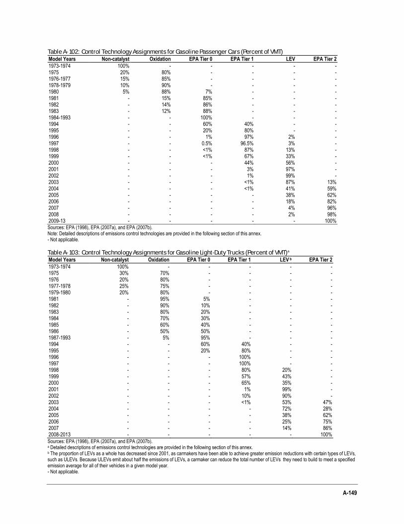
A-149
Table A- 102: Control Technology Assignments for Gasoline Passenger Cars (Percent of VMT) Model Years Non-catalyst Oxidation EPA Tier 0 EPA Tier 1 LEV EPA Tier 2
1973-1974 100% - - - - - 1975 20% 80% - - - - 1976-1977 15% 85% - - - - 1978-1979 10% 90% - - - - 1980 5% 88% 7% - - - 1981 - 15% 85% - - - 1982 - 14% 86% - - - 1983 - 12% 88% - - - 1984-1993 - - 100% - - - 1994 - - 60% 40% - - 1995 - - 20% 80% - - 1996 - - 1% 97% 2% - 1997 - - 0.5% 96.5% 3% - 1998 - - <1% 87% 13% - 1999 - - <1% 67% 33% - 2000 - - - 44% 56% - 2001 - - - 3% 97% - 2002 - - - 1% 99% - 2003 - - - <1% 87% 13% 2004 - - - <1% 41% 59% 2005 - - - - 38% 62% 2006 - - - - 18% 82% 2007 - - - - 4% 96% 2008 - - - - 2% 98% 2009-13 - - - - - 100% Sources: EPA (1998), EPA (2007a), and EPA (2007b). Note: Detailed descriptions of emissions control technologies are provided in the following section of this annex. - Not applicable.
Table A- 103: Control Technology Assignments for Gasoline Light-Duty Trucks (Percent of VMT)a Model Years Non-catalyst Oxidation EPA Tier 0 EPA Tier 1 LEV b EPA Tier 2
1973-1974 100% - - - - - 1975 30% 70% - - - - 1976 20% 80% - - - - 1977-1978 25% 75% - - - - 1979-1980 20% 80% - - - - 1981 - 95% 5% - - - 1982 - 90% 10% - - - 1983 - 80% 20% - - - 1984 - 70% 30% - - - 1985 - 60% 40% - - - 1986 - 50% 50% - - - 1987-1993 - 5% 95% - - - 1994 - - 60% 40% - - 1995 - - 20% 80% - - 1996 - - - 100% - - 1997 - - - 100% - - 1998 - - - 80% 20% - 1999 - - - 57% 43% - 2000 - - - 65% 35% - 2001 - - - 1% 99% - 2002 - - - 10% 90% - 2003 - - - <1% 53% 47% 2004 - - - - 72% 28% 2005 - - - - 38% 62% 2006 - - - - 25% 75% 2007 - - - - 14% 86% 2008-2013 - - - - - 100%
Sources: EPA (1998), EPA (2007a), and EPA (2007b). a Detailed descriptions of emissions control technologies are provided in the following section of this annex. b The proportion of LEVs as a whole has decreased since 2001, as carmakers have been able to achieve greater emission reductions with certain types of LEVs, such as ULEVs. Because ULEVs emit about half the emissions of LEVs, a carmaker can reduce the total number of LEVs they need to build to meet a specified emission average for all of their vehicles in a given model year. - Not applicable.
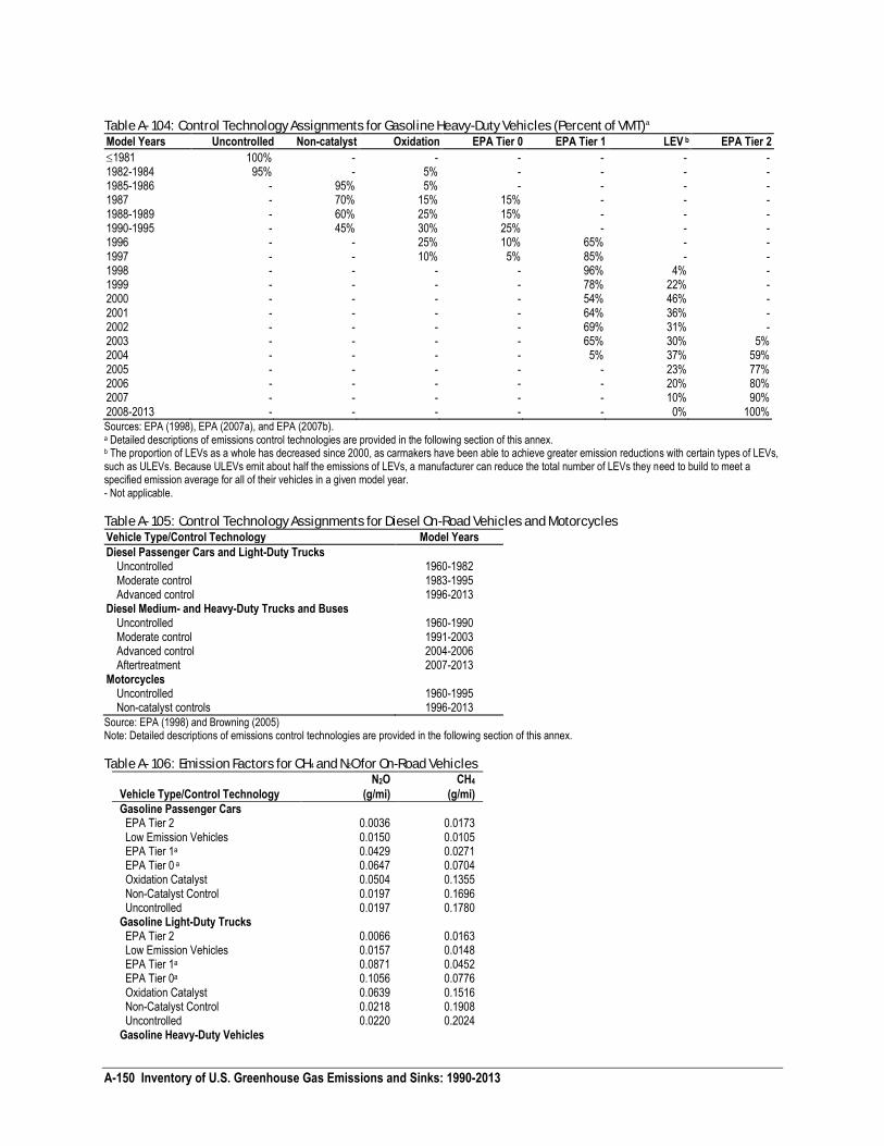
A-150 Inventory of U.S. Greenhouse Gas Emissions and Sinks: 1990-2013
Table A- 104: Control Technology Assignments for Gasoline Heavy-Duty Vehicles (Percent of VMT)a Model Years Uncontrolled Non-catalyst Oxidation EPA Tier 0 EPA Tier 1 LEV b EPA Tier 2
1981 100% - - - - - - 1982-1984 95% - 5% - - - - 1985-1986 - 95% 5% - - - - 1987 - 70% 15% 15% - - - 1988-1989 - 60% 25% 15% - - - 1990-1995 - 45% 30% 25% - - - 1996 - - 25% 10% 65% - - 1997 - - 10% 5% 85% - - 1998 - - - - 96% 4% - 1999 - - - - 78% 22% - 2000 - - - - 54% 46% - 2001 - - - - 64% 36% - 2002 - - - - 69% 31% - 2003 - - - - 65% 30% 5% 2004 - - - - 5% 37% 59% 2005 - - - - - 23% 77% 2006 - - - - - 20% 80% 2007 - - - - - 10% 90% 2008-2013 - - - - - 0% 100% Sources: EPA (1998), EPA (2007a), and EPA (2007b). a Detailed descriptions of emissions control technologies are provided in the following section of this annex. b The proportion of LEVs as a whole has decreased since 2000, as carmakers have been able to achieve greater emission reductions with certain types of LEVs, such as ULEVs. Because ULEVs emit about half the emissions of LEVs, a manufacturer can reduce the total number of LEVs they need to build to meet a specified emission average for all of their vehicles in a given model year. - Not applicable.
Table A- 105: Control Technology Assignments for Diesel On-Road Vehicles and Motorcycles Vehicle Type/Control Technology Model Years
Diesel Passenger Cars and Light-Duty Trucks Uncontrolled 1960-1982 Moderate control 1983-1995 Advanced control 1996-2013
Diesel Medium- and Heavy-Duty Trucks and Buses Uncontrolled 1960-1990 Moderate control 1991-2003 Advanced control 2004-2006 Aftertreatment 2007-2013
Motorcycles Uncontrolled 1960-1995 Non-catalyst controls 1996-2013
Source: EPA (1998) and Browning (2005) Note: Detailed descriptions of emissions control technologies are provided in the following section of this annex.
Table A- 106: Emission Factors for CH4 and N2O for On-Road Vehicles
Vehicle Type/Control Technology
N2O CH4
(g/mi) (g/mi)
Gasoline Passenger Cars EPA Tier 2 0.0036 0.0173 Low Emission Vehicles 0.0150 0.0105 EPA Tier 1a 0.0429 0.0271 EPA Tier 0 a 0.0647 0.0704 Oxidation Catalyst 0.0504 0.1355 Non-Catalyst Control 0.0197 0.1696 Uncontrolled 0.0197 0.1780 Gasoline Light-Duty Trucks EPA Tier 2 0.0066 0.0163 Low Emission Vehicles 0.0157 0.0148 EPA Tier 1a 0.0871 0.0452 EPA Tier 0a 0.1056 0.0776 Oxidation Catalyst 0.0639 0.1516 Non-Catalyst Control 0.0218 0.1908 Uncontrolled 0.0220 0.2024 Gasoline Heavy-Duty Vehicles
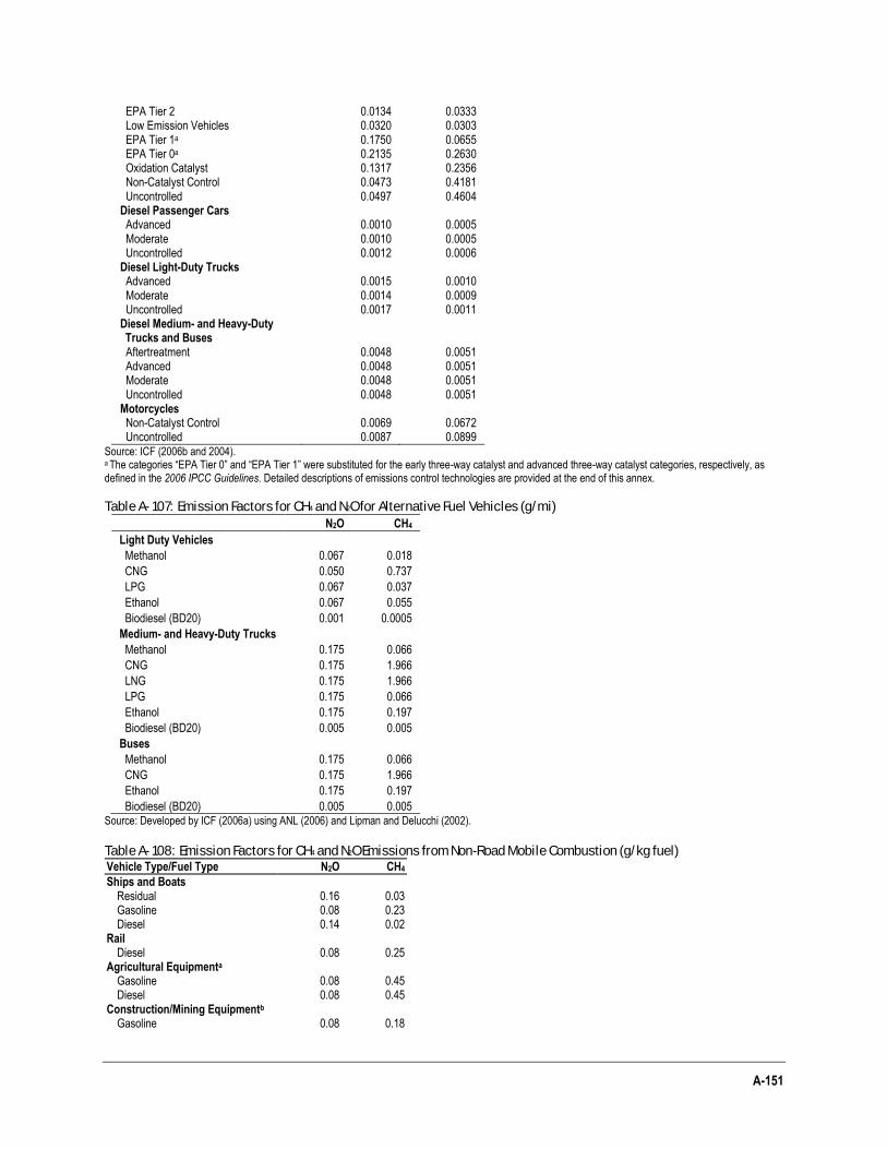
A-151
EPA Tier 2 0.0134 0.0333 Low Emission Vehicles 0.0320 0.0303 EPA Tier 1a 0.1750 0.0655 EPA Tier 0a 0.2135 0.2630 Oxidation Catalyst 0.1317 0.2356 Non-Catalyst Control 0.0473 0.4181 Uncontrolled 0.0497 0.4604 Diesel Passenger Cars Advanced 0.0010 0.0005 Moderate 0.0010 0.0005 Uncontrolled 0.0012 0.0006 Diesel Light-Duty Trucks Advanced 0.0015 0.0010 Moderate 0.0014 0.0009 Uncontrolled 0.0017 0.0011 Diesel Medium- and Heavy-Duty Trucks and Buses
Aftertreatment 0.0048 0.0051 Advanced 0.0048 0.0051 Moderate 0.0048 0.0051 Uncontrolled 0.0048 0.0051 Motorcycles Non-Catalyst Control 0.0069 0.0672 Uncontrolled 0.0087 0.0899
Source: ICF (2006b and 2004). a The categories “EPA Tier 0” and “EPA Tier 1” were substituted for the early three-way catalyst and advanced three-way catalyst categories, respectively, as defined in the 2006 IPCC Guidelines. Detailed descriptions of emissions control technologies are provided at the end of this annex.
Table A- 107: Emission Factors for CH4 and N2O for Alternative Fuel Vehicles (g/mi)
N2O CH4
Light Duty Vehicles
Methanol 0.067 0.018
CNG 0.050 0.737
LPG 0.067 0.037
Ethanol 0.067 0.055
Biodiesel (BD20) 0.001 0.0005
Medium- and Heavy-Duty Trucks
Methanol 0.175 0.066
CNG 0.175 1.966
LNG 0.175 1.966
LPG 0.175 0.066
Ethanol 0.175 0.197
Biodiesel (BD20) 0.005 0.005
Buses
Methanol 0.175 0.066
CNG 0.175 1.966
Ethanol 0.175 0.197
Biodiesel (BD20) 0.005 0.005 Source: Developed by ICF (2006a) using ANL (2006) and Lipman and Delucchi (2002).
Table A- 108: Emission Factors for CH4 and N2O Emissions from Non-Road Mobile Combustion (g/kg fuel) Vehicle Type/Fuel Type N2O CH4
Ships and Boats Residual 0.16 0.03 Gasoline 0.08 0.23 Diesel 0.14 0.02
Rail Diesel 0.08 0.25
Agricultural Equipmenta Gasoline 0.08 0.45 Diesel 0.08 0.45
Construction/Mining Equipmentb Gasoline 0.08 0.18
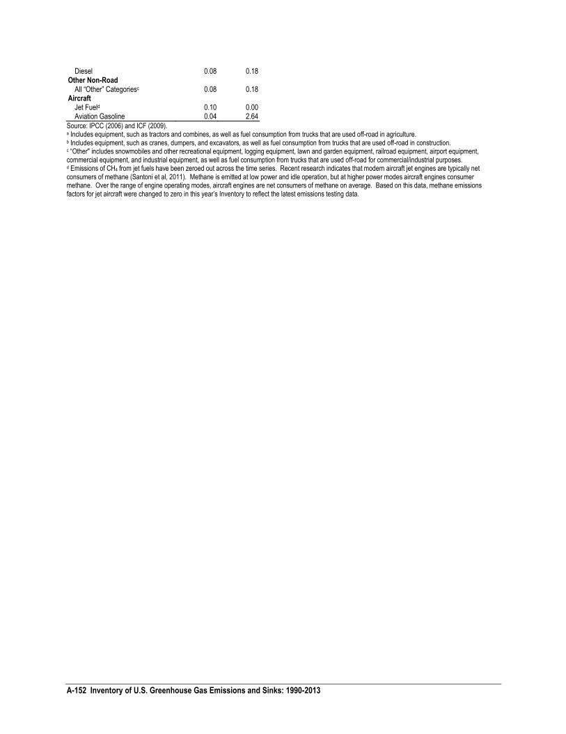
A-152 Inventory of U.S. Greenhouse Gas Emissions and Sinks: 1990-2013
Diesel 0.08 0.18 Other Non-Road
All “Other” Categoriesc 0.08 0.18 Aircraft
Jet Fueld 0.10 0.00 Aviation Gasoline 0.04 2.64
Source: IPCC (2006) and ICF (2009). a Includes equipment, such as tractors and combines, as well as fuel consumption from trucks that are used off-road in agriculture. b Includes equipment, such as cranes, dumpers, and excavators, as well as fuel consumption from trucks that are used off-road in construction. c “Other" includes snowmobiles and other recreational equipment, logging equipment, lawn and garden equipment, railroad equipment, airport equipment, commercial equipment, and industrial equipment, as well as fuel consumption from trucks that are used off-road for commercial/industrial purposes. d Emissions of CH4 from jet fuels have been zeroed out across the time series. Recent research indicates that modern aircraft jet engines are typically net consumers of methane (Santoni et al, 2011). Methane is emitted at low power and idle operation, but at higher power modes aircraft engines consumer methane. Over the range of engine operating modes, aircraft engines are net consumers of methane on average. Based on this data, methane emissions factors for jet aircraft were changed to zero in this year’s Inventory to reflect the latest emissions testing data.
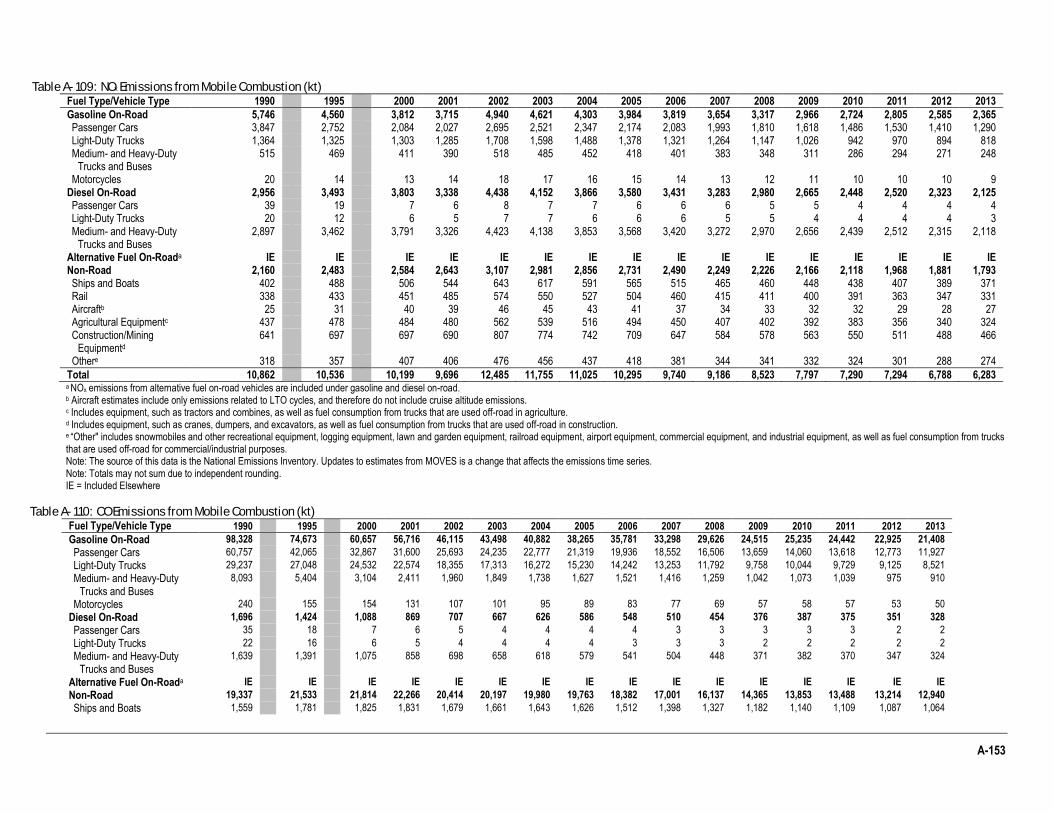
A-153
Table A- 109: NOx Emissions from Mobile Combustion (kt) Fuel Type/Vehicle Type 1990 1995 2000 2001 2002 2003 2004 2005 2006 2007 2008 2009 2010 2011 2012 2013
Gasoline On-Road 5,746 4,560 3,812 3,715 4,940 4,621 4,303 3,984 3,819 3,654 3,317 2,966 2,724 2,805 2,585 2,365 Passenger Cars 3,847 2,752 2,084 2,027 2,695 2,521 2,347 2,174 2,083 1,993 1,810 1,618 1,486 1,530 1,410 1,290 Light-Duty Trucks 1,364 1,325 1,303 1,285 1,708 1,598 1,488 1,378 1,321 1,264 1,147 1,026 942 970 894 818 Medium- and Heavy-Duty
Trucks and Buses 515
469
411 390 518 485 452 418 401 383 348 311 286 294 271 248
Motorcycles 20 14 13 14 18 17 16 15 14 13 12 11 10 10 10 9 Diesel On-Road 2,956 3,493 3,803 3,338 4,438 4,152 3,866 3,580 3,431 3,283 2,980 2,665 2,448 2,520 2,323 2,125 Passenger Cars 39 19 7 6 8 7 7 6 6 6 5 5 4 4 4 4 Light-Duty Trucks 20 12 6 5 7 7 6 6 6 5 5 4 4 4 4 3 Medium- and Heavy-Duty
Trucks and Buses 2,897
3,462
3,791 3,326 4,423 4,138 3,853 3,568 3,420 3,272 2,970 2,656 2,439 2,512 2,315 2,118
Alternative Fuel On-Roada IE IE IE IE IE IE IE IE IE IE IE IE IE IE IE IE Non-Road 2,160 2,483 2,584 2,643 3,107 2,981 2,856 2,731 2,490 2,249 2,226 2,166 2,118 1,968 1,881 1,793 Ships and Boats 402 488 506 544 643 617 591 565 515 465 460 448 438 407 389 371 Rail 338 433 451 485 574 550 527 504 460 415 411 400 391 363 347 331 Aircraftb 25 31 40 39 46 45 43 41 37 34 33 32 32 29 28 27 Agricultural Equipmentc 437 478 484 480 562 539 516 494 450 407 402 392 383 356 340 324 Construction/Mining
Equipmentd 641
697
697 690 807 774 742 709 647 584 578 563 550 511 488 466
Othere 318 357 407 406 476 456 437 418 381 344 341 332 324 301 288 274
Total 10,862 10,536 10,199 9,696 12,485 11,755 11,025 10,295 9,740 9,186 8,523 7,797 7,290 7,294 6,788 6,283 a NOx emissions from alternative fuel on-road vehicles are included under gasoline and diesel on-road. b Aircraft estimates include only emissions related to LTO cycles, and therefore do not include cruise altitude emissions. c Includes equipment, such as tractors and combines, as well as fuel consumption from trucks that are used off-road in agriculture. d Includes equipment, such as cranes, dumpers, and excavators, as well as fuel consumption from trucks that are used off-road in construction. e “Other" includes snowmobiles and other recreational equipment, logging equipment, lawn and garden equipment, railroad equipment, airport equipment, commercial equipment, and industrial equipment, as well as fuel consumption from trucks
that are used off-road for commercial/industrial purposes. Note: The source of this data is the National Emissions Inventory. Updates to estimates from MOVES is a change that affects the emissions time series. Note: Totals may not sum due to independent rounding. IE = Included Elsewhere
Table A- 110: CO Emissions from Mobile Combustion (kt) Fuel Type/Vehicle Type 1990 1995 2000 2001 2002 2003 2004 2005 2006 2007 2008 2009 2010 2011 2012 2013
Gasoline On-Road 98,328 74,673 60,657 56,716 46,115 43,498 40,882 38,265 35,781 33,298 29,626 24,515 25,235 24,442 22,925 21,408
Passenger Cars 60,757 42,065 32,867 31,600 25,693 24,235 22,777 21,319 19,936 18,552 16,506 13,659 14,060 13,618 12,773 11,927
Light-Duty Trucks 29,237 27,048 24,532 22,574 18,355 17,313 16,272 15,230 14,242 13,253 11,792 9,758 10,044 9,729 9,125 8,521
Medium- and Heavy-Duty Trucks and Buses
8,093
5,404
3,104 2,411 1,960 1,849 1,738 1,627 1,521 1,416 1,259 1,042 1,073 1,039 975 910
Motorcycles 240 155 154 131 107 101 95 89 83 77 69 57 58 57 53 50
Diesel On-Road 1,696 1,424 1,088 869 707 667 626 586 548 510 454 376 387 375 351 328
Passenger Cars 35 18 7 6 5 4 4 4 4 3 3 3 3 3 2 2
Light-Duty Trucks 22 16 6 5 4 4 4 4 3 3 3 2 2 2 2 2
Medium- and Heavy-Duty Trucks and Buses
1,639
1,391
1,075 858 698 658 618 579 541 504 448 371 382 370 347 324
Alternative Fuel On-Roada IE IE IE IE IE IE IE IE IE IE IE IE IE IE IE IE
Non-Road 19,337 21,533 21,814 22,266 20,414 20,197 19,980 19,763 18,382 17,001 16,137 14,365 13,853 13,488 13,214 12,940
Ships and Boats 1,559 1,781 1,825 1,831 1,679 1,661 1,643 1,626 1,512 1,398 1,327 1,182 1,140 1,109 1,087 1,064
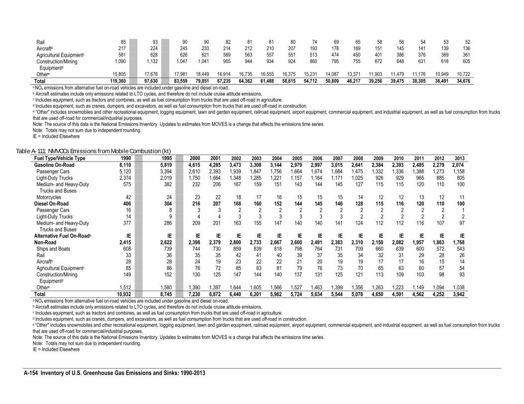
A-154 Inventory of U.S. Greenhouse Gas Emissions and Sinks: 1990-2013
Rail 85 93 90 90 82 81 81 80 74 69 65 58 56 54 53 52
Aircraftb 217 224 245 233 214 212 210 207 193 178 169 151 145 141 139 136
Agricultural Equipmentc 581 628 626 621 569 563 557 551 513 474 450 401 386 376 369 361
Construction/Mining Equipmentd
1,090
1,132
1,047 1,041 955 944 934 924 860 795 755 672 648 631 618 605
Othere 15,805 17,676 17,981 18,449 16,914 16,735 16,555 16,375 15,231 14,087 13,371 11,903 11,479 11,176 10,949 10,722
Total 119,360 97,630 83,559 79,851 67,235 64,362 61,488 58,615 54,712 50,809 46,217 39,256 39,475 38,305 36,491 34,676 a NOx emissions from alternative fuel on-road vehicles are included under gasoline and diesel on-road. b Aircraft estimates include only emissions related to LTO cycles, and therefore do not include cruise altitude emissions. c Includes equipment, such as tractors and combines, as well as fuel consumption from trucks that are used off-road in agriculture. d Includes equipment, such as cranes, dumpers, and excavators, as well as fuel consumption from trucks that are used off-road in construction. e “Other" includes snowmobiles and other recreational equipment, logging equipment, lawn and garden equipment, railroad equipment, airport equipment, commercial equipment, and industrial equipment, as well as fuel consumption from trucks that are used off-road for commercial/industrial purposes. Note: The source of this data is the National Emissions Inventory. Updates to estimates from MOVES is a change that affects the emissions time series. Note: Totals may not sum due to independent rounding. IE = Included Elsewhere
Table A- 111: NMVOCs Emissions from Mobile Combustion (kt) Fuel Type/Vehicle Type 1990 1995 2000 2001 2002 2003 2004 2005 2006 2007 2008 2009 2010 2011 2012 2013
Gasoline On-Road 8,110 5,819 4,615 4,285 3,473 3,308 3,144 2,979 2,997 3,015 2,641 2,384 2,393 2,485 2,279 2,074 Passenger Cars 5,120 3,394 2,610 2,393 1,939 1,847 1,756 1,664 1,674 1,684 1,475 1,332 1,336 1,388 1,273 1,158 Light-Duty Trucks 2,374 2,019 1,750 1,664 1,348 1,285 1,221 1,157 1,164 1,171 1,025 926 929 965 885 805 Medium- and Heavy-Duty
Trucks and Buses 575
382
232 206 167 159 151 143 144 145 127 115 115 120 110 100
Motorcycles 42 24 23 22 18 17 16 15 15 15 14 12 12 13 12 11 Diesel On-Road 406 304 216 207 168 160 152 144 145 146 128 115 116 120 110 100 Passenger Cars 16 8 3 3 2 2 2 2 2 2 2 2 2 2 2 1 Light-Duty Trucks 14 9 4 4 3 3 3 3 3 3 2 2 2 2 2 2 Medium- and Heavy-Duty
Trucks and Buses 377
286
209 201 163 155 147 140 140 141 124 112 112 116 107 97
Alternative Fuel On-Roada IE IE IE IE IE IE IE IE IE IE IE IE IE IE IE IE Non-Road 2,415 2,622 2,398 2,379 2,800 2,733 2,667 2,600 2,491 2,383 2,310 2,150 2,082 1,957 1,863 1,768 Ships and Boats 608 739 744 730 859 839 818 798 764 731 709 660 639 600 572 543 Rail 33 36 35 35 42 41 40 39 37 35 34 32 31 29 28 26 Aircraftb 28 28 24 19 23 22 22 21 20 19 19 17 17 16 15 14 Agricultural Equipmentc 85 86 76 72 85 83 81 79 76 73 70 65 63 60 57 54 Construction/Mining
Equipmentd 149
152
130 125 147 144 140 137 131 125 121 113 109 103 98 93
Othere 1,512 1,580 1,390 1,397 1,644 1,605 1,566 1,527 1,463 1,399 1,356 1,263 1,223 1,149 1,094 1,038
Total 10,932 8,745 7,230 6,872 6,440 6,201 5,962 5,724 5,634 5,544 5,078 4,650 4,591 4,562 4,252 3,942 a NOx emissions from alternative fuel on-road vehicles are included under gasoline and diesel on-road. b Aircraft estimates include only emissions related to LTO cycles, and therefore do not include cruise altitude emissions. c Includes equipment, such as tractors and combines, as well as fuel consumption from trucks that are used off-road in agriculture. d Includes equipment, such as cranes, dumpers, and excavators, as well as fuel consumption from trucks that are used off-road in construction. e “Other" includes snowmobiles and other recreational equipment, logging equipment, lawn and garden equipment, railroad equipment, airport equipment, commercial equipment, and industrial equipment, as well as fuel consumption from trucks that are used off-road for commercial/industrial purposes. Note: The source of this data is the National Emissions Inventory. Updates to estimates from MOVES is a change that affects the emissions time series. Note: Totals may not sum due to independent rounding. IE = Included Elsewhere
A-155
Definitions of Emission Control Technologies and Standards
The N2O and CH4 emission factors used depend on the emission standards in place and the corresponding level of control technology for each vehicle type. Table A- 102 through Table A- 105 show the years in which these technologies or standards were in place and the penetration level for each vehicle type. These categories are defined below and were compiled from EPA (1993, 1994a, 1994b, 1998, 1999a) and IPCC/UNEP/OECD/IEA (1997).
Uncontrolled
Vehicles manufactured prior to the implementation of pollution control technologies are designated as uncontrolled. Gasoline passenger cars and light-duty trucks (pre-1973), gasoline heavy-duty vehicles (pre-1984), diesel vehicles (pre-1983), and motorcycles (pre-1996) are assumed to have no control technologies in place.
Gasoline Emission Controls
Below are the control technologies and emissions standards applicable to gasoline vehicles.
Non-catalyst
These emission controls were common in gasoline passenger cars and light-duty gasoline trucks during model years (1973-1974) but phased out thereafter, in heavy-duty gasoline vehicles beginning in the mid-1980s, and in motorcycles beginning in 1996. This technology reduces hydrocarbon (HC) and carbon monoxide (CO) emissions through adjustments to ignition timing and air-fuel ratio, air injection into the exhaust manifold, and exhaust gas recirculation (EGR) valves, which also helps meet vehicle NOx standards.
Oxidation Catalyst
This control technology designation represents the introduction of the catalytic converter, and was the most common technology in gasoline passenger cars and light-duty gasoline trucks made from 1975 to 1980 (cars) and 1975 to 1985 (trucks). This technology was also used in some heavy-duty gasoline vehicles between 1982 and 1997. The two-way catalytic converter oxidizes HC and CO, significantly reducing emissions over 80 percent beyond non-catalyst-system capacity. One reason unleaded gasoline was introduced in 1975 was due to the fact that oxidation catalysts cannot function properly with leaded gasoline.
EPA Tier 0
This emission standard from the Clean Air Act was met through the implementation of early "three-way" catalysts, therefore this technology was used in gasoline passenger cars and light-duty gasoline trucks sold beginning in the early 1980s, and remained common until 1994. This more sophisticated emission control system improves the efficiency of the catalyst by converting CO and HC to CO2 and H2O, reducing NOx to nitrogen and oxygen, and using an on-board diagnostic computer and oxygen sensor. In addition, this type of catalyst includes a fuel metering system (carburetor or fuel injection) with electronic "trim" (also known as a "closed-loop system"). New cars with three-way catalysts met the Clean Air Act's amended standards (enacted in 1977) of reducing HC to 0.41 g/mile by 1980, CO to 3.4 g/mile by 1981 and NOx to 1.0 g/mile by 1981.
EPA Tier 1
This emission standard created through the 1990 amendments to the Clean Air Act limited passenger car NOx emissions to 0.4 g/mi, and HC emissions to 0.25 g/mi. These bounds respectively amounted to a 60 and 40 percent reduction from the EPA Tier 0 standard set in 1981. For light-duty trucks, this standard set emissions at 0.4 to 1.1 g/mi for NOx, and 0.25 to 0.39 g/mi for HCs, depending on the weight of the truck. Emission reductions were met through the use of more advanced emission control systems, and applied to light-duty gasoline vehicles beginning in 1994. These advanced emission control systems included advanced three-way catalysts, electronically controlled fuel injection and ignition timing, EGR, and air injection.
EPA Tier 2
This emission standard was specified in the 1990 amendments to the Clean Air Act, limiting passenger car NOx emissions to 0.07 g/mi on average and aligning emissions standards for passenger cars and light-duty trucks. Manufacturers can meet this average emission level by producing vehicles in 11 emission “Bins”, the three highest of which expire in 2006. These new emission levels represent a 77 to 95 percent reduction in emissions from the EPA Tier 1 standard set in 1994.
A-156 Inventory of U.S. Greenhouse Gas Emissions and Sinks: 1990-2013
Emission reductions were met through the use of more advanced emission control systems and lower sulfur fuels and are applied to vehicles beginning in 2004. These advanced emission control systems include improved combustion, advanced three-way catalysts, electronically controlled fuel injection and ignition timing, EGR, and air injection.
Low Emission Vehicles (LEV)
This emission standard requires a much higher emission control level than the Tier 1 standard. Applied to light-duty gasoline passenger cars and trucks beginning in small numbers in the mid-1990s, LEV includes multi-port fuel injection with adaptive learning, an advanced computer diagnostics systems and advanced and close coupled catalysts with secondary air injection. LEVs as defined here include transitional low-emission vehicles (TLEVs), low emission vehicles, ultra-low emission vehicles (ULEVs) and super ultra-low emission vehicles (SULEVs). In this analysis, all categories of LEVs are treated the same due to the fact that there are very limited CH4 or N2O emission factor data for LEVs to distinguish among the different types of vehicles. Zero emission vehicles (ZEVs) are incorporated into the alternative fuel and advanced technology vehicle assessments.
Diesel Emission Controls
Below are the three levels of emissions control for diesel vehicles.
Moderate control
Improved injection timing technology and combustion system design for light- and heavy-duty diesel vehicles (generally in place in model years 1983 to 1995) are considered moderate control technologies. These controls were implemented to meet emission standards for diesel trucks and buses adopted by the EPA in 1985 to be met in 1991 and 1994.
Advanced control
EGR and modern electronic control of the fuel injection system are designated as advanced control technologies. These technologies provide diesel vehicles with the level of emission control necessary to comply with standards in place from 1996 through 2006.
Aftertreatment
Use of diesel particulate filters (DPFs), oxidation catalysts and NOx absorbers or selective catalytic reduction (SCR) systems are designated as aftertreatment control. These technologies provide diesel vehicles with a level of emission control necessary to comply with standards in place from 2007 on.
Supplemental Information on GHG Emissions from Transportation and Other Mobile Sources
This section of this Annex includes supplemental information on the contribution of transportation and other mobile sources to U.S. greenhouse gas emissions. In the main body of the Inventory report, emission estimates are generally presented by greenhouse gas, with separate discussions of the methodologies used to estimate CO2, N2O, CH4, and HFC emissions. Although the inventory is not required to provide detail beyond what is contained in the body of this report, the IPCC allows presentation of additional data and detail on emission sources. The purpose of this sub-annex, within the annex that details the calculation methods and data used for non-CO2 calculations, is to provide all transportation estimates presented throughout the report in one place.
This section of this Annex reports total greenhouse gas emissions from transportation and other (non-transportation) mobile sources in CO2 equivalents, with information on the contribution by greenhouse gas and by mode, vehicle type, and fuel type. In order to calculate these figures, additional analyses were conducted to develop estimates of CO2 from non-transportation mobile sources (e.g., agricultural equipment, construction/mining equipment, recreational vehicles), and to provide more detailed breakdowns of emissions by source.
Estimation of CO2 from Non-Transportation Mobile Sources
The estimates of N2O and CH4 from fuel combustion presented in the Energy chapter of the inventory include both transportation sources and other mobile sources. Other mobile sources include construction/mining equipment, agricultural equipment, vehicles used off-road, and other sources that have utility associated with their movement but do not have a primary purpose of transporting people or goods (e.g., snowmobiles, riding lawnmowers, etc.). Estimates of CO2 from non-transportation mobile sources, based on EIA fuel consumption estimates, are included in the agricultural, industrial, and commercial sectors. In order to provide comparable information on transportation and mobile sources, Table A- 112 provides estimates of CO2 from these other mobile sources, developed from EPA’s NONROAD model and FHWA’s Highway Statistics. These other mobile source estimates were developed using the same fuel consumption data utilized in developing the N2O and CH4 estimates.
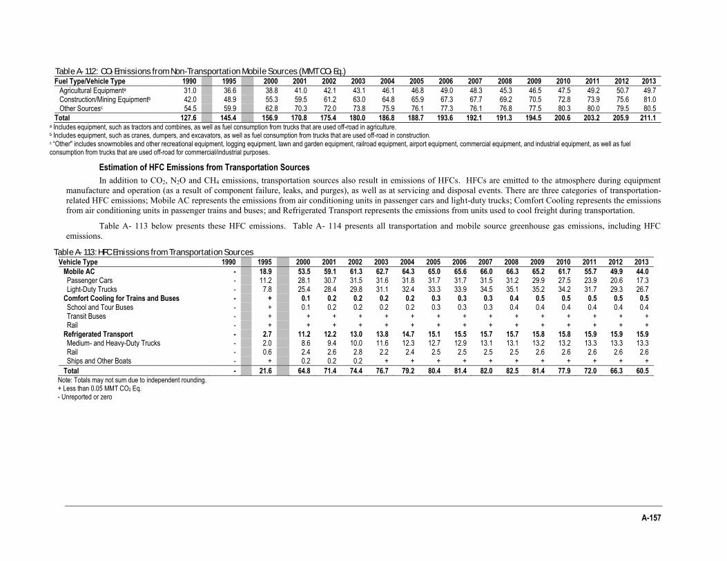
A-157
Table A- 112: CO2 Emissions from Non-Transportation Mobile Sources (MMT CO2 Eq.) Fuel Type/Vehicle Type 1990 1995 2000 2001 2002 2003 2004 2005 2006 2007 2008 2009 2010 2011 2012 2013
Agricultural Equipmenta 31.0 36.6 38.8 41.0 42.1 43.1 46.1 46.8 49.0 48.3 45.3 46.5 47.5 49.2 50.7 49.7 Construction/Mining Equipmentb 42.0 48.9 55.3 59.5 61.2 63.0 64.8 65.9 67.3 67.7 69.2 70.5 72.8 73.9 75.6 81.0 Other Sourcesc 54.5 59.9 62.8 70.3 72.0 73.8 75.9 76.1 77.3 76.1 76.8 77.5 80.3 80.0 79.5 80.5
Total 127.6 145.4 156.9 170.8 175.4 180.0 186.8 188.7 193.6 192.1 191.3 194.5 200.6 203.2 205.9 211.1 a Includes equipment, such as tractors and combines, as well as fuel consumption from trucks that are used off-road in agriculture. b Includes equipment, such as cranes, dumpers, and excavators, as well as fuel consumption from trucks that are used off-road in construction. c “Other" includes snowmobiles and other recreational equipment, logging equipment, lawn and garden equipment, railroad equipment, airport equipment, commercial equipment, and industrial equipment, as well as fuel consumption from trucks that are used off-road for commercial/industrial purposes.
Estimation of HFC Emissions from Transportation Sources
In addition to CO2, N2O and CH4 emissions, transportation sources also result in emissions of HFCs. HFCs are emitted to the atmosphere during equipment manufacture and operation (as a result of component failure, leaks, and purges), as well as at servicing and disposal events. There are three categories of transportation-related HFC emissions; Mobile AC represents the emissions from air conditioning units in passenger cars and light-duty trucks; Comfort Cooling represents the emissions from air conditioning units in passenger trains and buses; and Refrigerated Transport represents the emissions from units used to cool freight during transportation.
Table A- 113 below presents these HFC emissions. Table A- 114 presents all transportation and mobile source greenhouse gas emissions, including HFC emissions.
Table A- 113: HFC Emissions from Transportation Sources Vehicle Type 1990 1995 2000 2001 2002 2003 2004 2005 2006 2007 2008 2009 2010 2011 2012 2013
Mobile AC - 18.9 53.5 59.1 61.3 62.7 64.3 65.0 65.6 66.0 66.3 65.2 61.7 55.7 49.9 44.0 Passenger Cars - 11.2 28.1 30.7 31.5 31.6 31.8 31.7 31.7 31.5 31.2 29.9 27.5 23.9 20.6 17.3 Light-Duty Trucks - 7.8 25.4 28.4 29.8 31.1 32.4 33.3 33.9 34.5 35.1 35.2 34.2 31.7 29.3 26.7
Comfort Cooling for Trains and Buses - + 0.1 0.2 0.2 0.2 0.2 0.3 0.3 0.3 0.4 0.5 0.5 0.5 0.5 0.5 School and Tour Buses - + 0.1 0.2 0.2 0.2 0.2 0.3 0.3 0.3 0.4 0.4 0.4 0.4 0.4 0.4 Transit Buses - + + + + + + + + + + + + + + + Rail - + + + + + + + + + + + + + + +
Refrigerated Transport - 2.7 11.2 12.2 13.0 13.8 14.7 15.1 15.5 15.7 15.7 15.8 15.8 15.9 15.9 15.9 Medium- and Heavy-Duty Trucks - 2.0 8.6 9.4 10.0 11.6 12.3 12.7 12.9 13.1 13.1 13.2 13.2 13.3 13.3 13.3 Rail - 0.6 2.4 2.6 2.8 2.2 2.4 2.5 2.5 2.5 2.5 2.6 2.6 2.6 2.6 2.6 Ships and Other Boats - + 0.2 0.2 0.2 + + + + + + + + + + +
Total - 21.6 64.8 71.4 74.4 76.7 79.2 80.4 81.4 82.0 82.5 81.4 77.9 72.0 66.3 60.5 Note: Totals may not sum due to independent rounding. + Less than 0.05 MMT CO2 Eq. - Unreported or zero
A-158 Inventory of U.S. Greenhouse Gas Emissions and Sinks: 1990-2013
Contribution of Transportation and Mobile Sources to Greenhouse Gas Emissions, by Mode/Vehicle Type/Fuel Type
Table A- 114 presents estimates of greenhouse gas emissions from an expanded analysis including all transportation and additional mobile sources, as well as emissions from electricity generation by the consuming category, in CO2 equivalents. In total, transportation and non-transportation mobile sources emitted 2,023.4 MMT CO2 Eq. in 2013, an increase of 20 percent from 1990. Transportation sources account for 1,810.3 MMT CO2 Eq. while non-transportation mobile sources account for 213.1 MMT CO2 Eq. These estimates include HFC emissions for mobile AC, comfort cooling for trains and buses, and refrigerated transport. These estimates were generated using the estimates of CO2 emissions from transportation sources reported in the Carbon Dioxide Emissions from Fossil Fuel Combustion section, and CH4 emissions and N2O emissions reported in the Mobile Combustion section of the Energy chapter; information on HFCs from mobile air conditioners, comfort cooling for trains and buses, and refrigerated transportation from the Substitutes for Ozone Depleting Substances section of the IPPU chapter; and estimates of CO2 emitted from non-transportation mobile sources reported in Table A- 110 above.
Although all emissions reported here are based on estimates reported throughout this Inventory, some additional calculations were performed in order to provide a detailed breakdown of emissions by mode and vehicle category. In the case of N2O and CH4, additional calculations were performed to develop emission estimates by type of aircraft and type of heavy-duty vehicle (i.e., medium- and heavy-duty trucks or buses) to match the level of detail for CO2 emissions. N2O estimates for jet fuel and aviation gasoline and CH4 estimates for aviation gasoline were developed for individual aircraft types by multiplying the emissions estimates for aircraft for each fuel type (jet fuel and aviation gasoline) by the portion of fuel used by each aircraft type (from FAA 2014). Emissions of CH4 from jet fuels are no longer considered to be emitted across the time series from aircraft gas turbine engines burning jet fuel A at higher power settings.1 Recent research indicates that modern aircraft jet engines are typically net consumers of methane (Santoni et al, 2011). Methane is emitted at low power and idle operation, but at higher power modes aircraft engines consumer methane. Over the range of engine operating modes, aircraft engines are net consumers of methane on average. Based on this data, CH4 emission factors for jet aircraft were reported as zero to reflect the latest emissions testing data.
Similarly, N2O and CH4 estimates were developed for medium- and heavy-duty trucks and buses by multiplying the emission estimates for heavy-duty vehicles for each fuel type (gasoline, diesel) from the Mobile Combustion section in the Energy chapter, by the portion of fuel used by each vehicle type (from DOE 1993 through 2014). Otherwise, the table and figure are drawn directly from emission estimates presented elsewhere in the Inventory, and are dependent on the methodologies presented in Annex 2.1 (for CO2), Chapter 4, and Annex 3.8 (for HFCs), and earlier in this Annex (for CH4 and N2O).
Transportation sources include on-road vehicles, aircraft, boats and ships, rail, and pipelines (note: pipelines are a transportation source but are stationary, not mobile sources). In addition, transportation-related greenhouse gas emissions also include HFC released from mobile air-conditioners and refrigerated transport, and the release of CO2 from lubricants (such as motor oil) used in transportation. Together, transportation sources were responsible for 1,810.3 MMT CO2 Eq. in 2013.
On-road vehicles were responsible for about 75 percent of all transportation and non-transportation mobile GHG emissions in 2013. Although passenger cars make up the largest component of on-road vehicle greenhouse gas emissions, light-duty and medium- and heavy-duty trucks have been the primary sources of growth in on-road vehicle emissions. Between 1990 and 2013, greenhouse gas emissions from passenger cars increased by 16 percent, while emissions from light-duty trucks decreased by four percent.2 Meanwhile, greenhouse gas emissions from medium- and heavy-duty trucks increased 76 percent between 1990 and 2013, reflecting the increased volume of total freight movement and an increasing share transported by trucks.
1 Recommended Best Practice for Quantifying Speciated Organic Gas Emissions from Aircraft Equipped with Turbofan, Turbojet and Turboprop
Engines,” EPA-420-R-09-901, May 27, 2009 (see http://www.epa.gov/otaq/regs/nonroad/aviation/420r09901.pdf> 2 In 2011 FHWA changed how they defined vehicle types for the purposes of reporting VMT for the years 2007-2010. The old approach to vehicle
classification was based on body type and split passenger vehicles into “Passenger Cars” and “Other 2 Axle 4-Tire Vehicles”. The new approach is a vehicle classification system based on wheelbase. Vehicles with a wheelbase less than or equal to 121 inches are counted as “Light-duty Vehicles –Short Wheelbase”. Passenger vehicles with a wheelbase greater than 121 inches are counted as “Light-duty Vehicles - Long Wheelbase”. This change in vehicle classification has moved some smaller trucks and sport utility vehicles from the light truck category to the passenger vehicle category in this Inventory. These changes are reflected in a large drop in light-truck emissions between 2006 and 2007.
A-159
Greenhouse gas emissions from aircraft decreased 21 percent between 1990 and 2013. Emissions from military aircraft decreased 69 percent between 1990 and 2013. Commercial aircraft emissions rose 27 percent between 1990 and 2007 then dropped 18 percent from 2007 to 2013, a change of approximately 4 percent between 1990 and 2013.
Non-transportation mobile sources, such as construction/mining equipment, agricultural equipment, and industrial/commercial equipment, emitted approximately 213.1 MMT CO2 Eq. in 2013. Together, these sources emitted more greenhouse gases than ships and boats, and rail combined. Emissions from non-transportation mobile sources increased rapidly, growing approximately 66 percent between 1990 and 2013. CH4 and N2O emissions from these sources are included in the “Mobile Combustion” section and CO2 emissions are included in the relevant economic sectors.
Contribution of Transportation and Mobile Sources to Greenhouse Gas Emissions, by Gas
Table A- 115 presents estimates of greenhouse gas emissions from transportation and other mobile sources broken down by greenhouse gas. As this table shows, CO2 accounts for the vast majority of transportation greenhouse gas emissions (approximately 96 percent in 2013). Emissions of CO2 from transportation and mobile sources increased by 306.1 MMT CO2 Eq. between 1990 and 2013. In contrast, the combined emissions of CH4 and N2O decreased by 26.3 MMT CO2 Eq. over the same period, due largely to the introduction of control technologies designed to reduce criteria pollutant emissions.3
Meanwhile, HFC emissions from mobile air-conditioners and refrigerated transport increased from virtually no emissions in 1990 to 60.5 MMT CO2 Eq. in 2013 as these chemicals were phased in as substitutes for ozone depleting substances. It should be noted, however, that the ozone depleting substances that HFCs replaced are also powerful greenhouse gases, but are not included in national greenhouse gas inventories per UNFCCC reporting requirements.
Greenhouse Gas Emissions from Freight and Passenger Transportation
Table A- 116 and Table A- 117 present greenhouse gas estimates from transportation, broken down into the passenger and freight categories. Passenger modes include light-duty vehicles, buses, passenger rail, aircraft (general aviation and commercial aircraft), recreational boats, and mobile air conditioners, and are illustrated in Table A- 116. Freight modes include medium- and heavy-duty trucks, freight rail, refrigerated transport, waterborne freight vessels, pipelines, and commercial aircraft and are illustrated in Table A- 117. Commercial aircraft do carry some freight, in addition to passengers, and emissions have been split between passenger and freight transportation. The amount of commercial aircraft emissions to allocate to the passenger and freight categories was calculated using BTS data on freight shipped by commercial aircraft, and the total number of passengers enplaned. Each passenger was considered to weigh an average of 150 pounds, with a luggage weight of 50 pounds. The total freight weight and total passenger weight carried were used to determine percent shares which were used to split the total commercial aircraft emission estimates. The remaining transportation and mobile emissions were from sources not considered to be either freight or passenger modes (e.g., construction/mining and agricultural equipment, lubricants).
The estimates in these tables are derived from the estimates presented in Table A- 114. In addition, estimates of fuel consumption from DOE (1993 through 2014) were used to allocate rail emissions between passenger and freight categories.
In 2013, passenger transportation modes emitted 1,250.2 MMT CO2 Eq., while freight transportation modes emitted 528.8 MMT CO2 Eq. Between 1990 and 2013, the percentage growth of greenhouse gas emissions from freight sources was 49 percent, while emissions from passenger sources grew by 8 percent. This difference in growth is due largely to the rapid increase in emissions associated with medium- and heavy-duty trucks.
3 The decline in CFC emissions is not captured in the official transportation estimates.
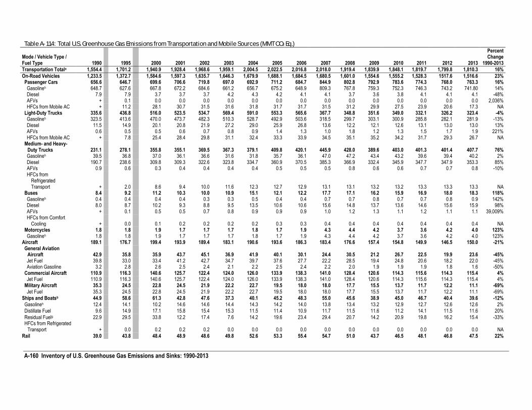
A-160 Inventory of U.S. Greenhouse Gas Emissions and Sinks: 1990-2013
Table A- 114: Total U.S. Greenhouse Gas Emissions from Transportation and Mobile Sources (MMT CO2 Eq.)
Mode / Vehicle Type / Fuel Type 1990 1995 2000 2001 2002 2003 2004 2005 2006 2007 2008 2009 2010 2011 2012 2013
Percent Change
1990-2013
Transportation Totala 1,554.4 1,701.2 1,940.9 1,928.4 1,968.6 1,959.1 2,004.5 2,022.5 2,016.8 2,018.0 1,919.4 1,839.9 1,848.1 1,819.7 1,799.8 1,810.3 16%
On-Road Vehicles 1,233.5 1,372.7 1,584.6 1,597.3 1,635.7 1,646.3 1,679.9 1,688.1 1,684.5 1,680.5 1,601.0 1,554.6 1,555.2 1,528.3 1517.6 1,516.6 23% Passenger Cars 656.6 646.7 699.6 706.6 719.8 697.0 692.9 711.2 684.7 844.9 802.8 792.9 783.6 774.3 768.0 763.3 16% Gasolineh 648.7 627.6 667.8 672.2 684.6 661.2 656.7 675.2 648.9 809.3 767.8 759.3 752.3 746.3 743.2 741.80 14% Diesel 7.9 7.9 3.7 3.7 3.7 4.2 4.3 4.2 4.1 4.1 3.7 3.6 3.8 4.1 4.1 4.1 -48% AFVs + 0.1 0.0 0.0 0.0 0.0 0.0 0.0 0.0 0.0 0.0 0.0 0.0 0.0 0.0 0.0 2,036% HFCs from Mobile AC + 11.2 28.1 30.7 31.5 31.6 31.8 31.7 31.7 31.5 31.2 29.9 27.5 23.9 20.6 17.3 NA
Light-Duty Trucks 335.6 436.8 516.0 523.5 534.7 569.4 591.0 553.3 565.6 367.7 348.8 351.6 349.0 332.1 326.2 323.4 -4% Gasolineh 323.5 413.6 470.0 473.7 482.3 510.3 528.7 492.9 503.6 318.5 299.7 303.1 300.9 285.8 282.1 281.9 -13% Diesel 11.5 14.9 20.1 20.8 21.9 27.2 29.0 25.9 26.8 13.6 12.2 12.1 12.6 13.1 13.0 13.0 13% AFVs 0.6 0.5 0.5 0.6 0.7 0.8 0.9 1.4 1.3 1.0 1.8 1.2 1.3 1.5 1.7 1.9 221% HFCs from Mobile AC + 7.8 25.4 28.4 29.8 31.1 32.4 33.3 33.9 34.5 35.1 35.2 34.2 31.7 29.3 26.7 NA
Medium- and Heavy-Duty Trucks 231.1 278.1 355.8 355.1 369.5 367.3 379.1 409.8 420.1 445.9 428.0 389.6 403.0 401.3 401.4 407.7 76% Gasolineh 39.5 36.8 37.0 36.1 36.6 31.6 31.8 35.7 36.1 47.0 47.2 43.4 43.2 39.6 39.4 40.2 2% Diesel 190.7 238.6 309.8 309.3 322.6 323.8 334.7 360.9 370.5 385.3 366.9 332.4 345.9 347.7 347.9 353.3 85% AFVs 0.9 0.6 0.3 0.4 0.4 0.4 0.4 0.5 0.5 0.5 0.8 0.6 0.6 0.7 0.7 0.8 -10% HFCs from
Refrigerated Transport + 2.0 8.6 9.4 10.0 11.6 12.3 12.7 12.9 13.1 13.1 13.2 13.2 13.3 13.3 13.3 NA
Buses 8.4 9.2 11.2 10.3 10.0 10.9 15.1 12.1 12.2 17.7 17.1 16.2 15.9 16.9 18.0 18.3 118% Gasolineh 0.4 0.4 0.4 0.4 0.3 0.3 0.5 0.4 0.4 0.7 0.7 0.8 0.7 0.7 0.8 0.9 142% Diesel 8.0 8.7 10.2 9.3 8.8 9.5 13.5 10.6 10.6 15.6 14.8 13.7 13.6 14.6 15.6 15.9 98% AFVs + 0.1 0.5 0.5 0.7 0.8 0.9 0.9 0.9 1.0 1.2 1.3 1.1 1.2 1.1 1.1 39,009% HFCs from Comfort
Cooling + 0.0 0.1 0.2 0.2 0.2 0.2 0.3 0.3 0.4 0.4 0.4 0.4 0.4 0.4 0.4 NA Motorcycles 1.8 1.8 1.9 1.7 1.7 1.7 1.8 1.7 1.9 4.3 4.4 4.2 3.7 3.6 4.2 4.0 123% Gasolineh 1.8 1.8 1.9 1.7 1.7 1.7 1.8 1.7 1.9 4.3 4.4 4.2 3.7 3.6 4.2 4.0 123%
Aircraft 189.1 176.7 199.4 193.9 189.4 183.1 190.6 193.6 186.3 183.4 176.6 157.4 154.8 149.9 146.5 150.0 -21% General Aviation
Aircraft 42.9 35.8 35.9 43.7 45.1 36.9 41.9 40.1 30.1 24.4 30.5 21.2 26.7 22.5 19.9 23.6 -45% Jet Fuel 39.8 33.0 33.4 41.2 42.7 34.7 39.7 37.6 27.7 22.2 28.5 19.4 24.8 20.6 18.2 22.0 -45% Aviation Gasoline 3.2 2.8 2.6 2.5 2.4 2.1 2.2 2.5 2.4 2.2 2.0 1.9 1.9 1.9 1.8 1.6 -50%
Commercial Aircraft 110.9 116.3 140.6 125.7 122.4 124.0 126.0 133.9 138.3 141.0 128.4 120.6 114.3 115.6 114.3 115.4 4% Jet Fuel 110.9 116.3 140.6 125.7 122.4 124.0 126.0 133.9 138.3 141.0 128.4 120.6 114.3 115.6 114.3 115.4 4%
Military Aircraft 35.3 24.5 22.8 24.5 21.9 22.2 22.7 19.5 18.0 18.0 17.7 15.5 13.7 11.7 12.2 11.1 -69%
Jet Fuel 35.3 24.5 22.8 24.5 21.9 22.2 22.7 19.5 18.0 18.0 17.7 15.5 13.7 11.7 12.2 11.1 -69%
Ships and Boatsb 44.9 58.6 61.3 42.8 47.6 37.3 40.1 45.2 48.3 55.0 45.6 38.9 45.0 46.7 40.4 39.6 -12%
Gasolineh 12.4 14.1 10.2 14.6 14.6 14.4 14.3 14.2 14.0 13.8 13.4 13.2 12.9 12.7 12.6 12.6 2%
Distillate Fuel 9.6 14.9 17.1 15.8 15.4 15.3 11.5 11.4 10.9 11.7 11.5 11.6 11.2 14.1 11.5 11.6 20%
Residual Fuelg 22.9 29.5 33.8 12.2 17.4 7.6 14.2 19.6 23.4 29.4 20.7 14.2 20.9 19.8 16.2 15.4 -33% HFCs from Refrigerated
Transport + 0.0 0.2 0.2 0.2 0.0 0.0 0.0 0.0 0.0 0.0 0.0 0.0 0.0 0.0 0.0 NA
Rail 39.0 43.8 48.4 48.9 48.6 49.8 52.6 53.3 55.4 54.7 51.0 43.7 46.5 48.1 46.8 47.5 22%
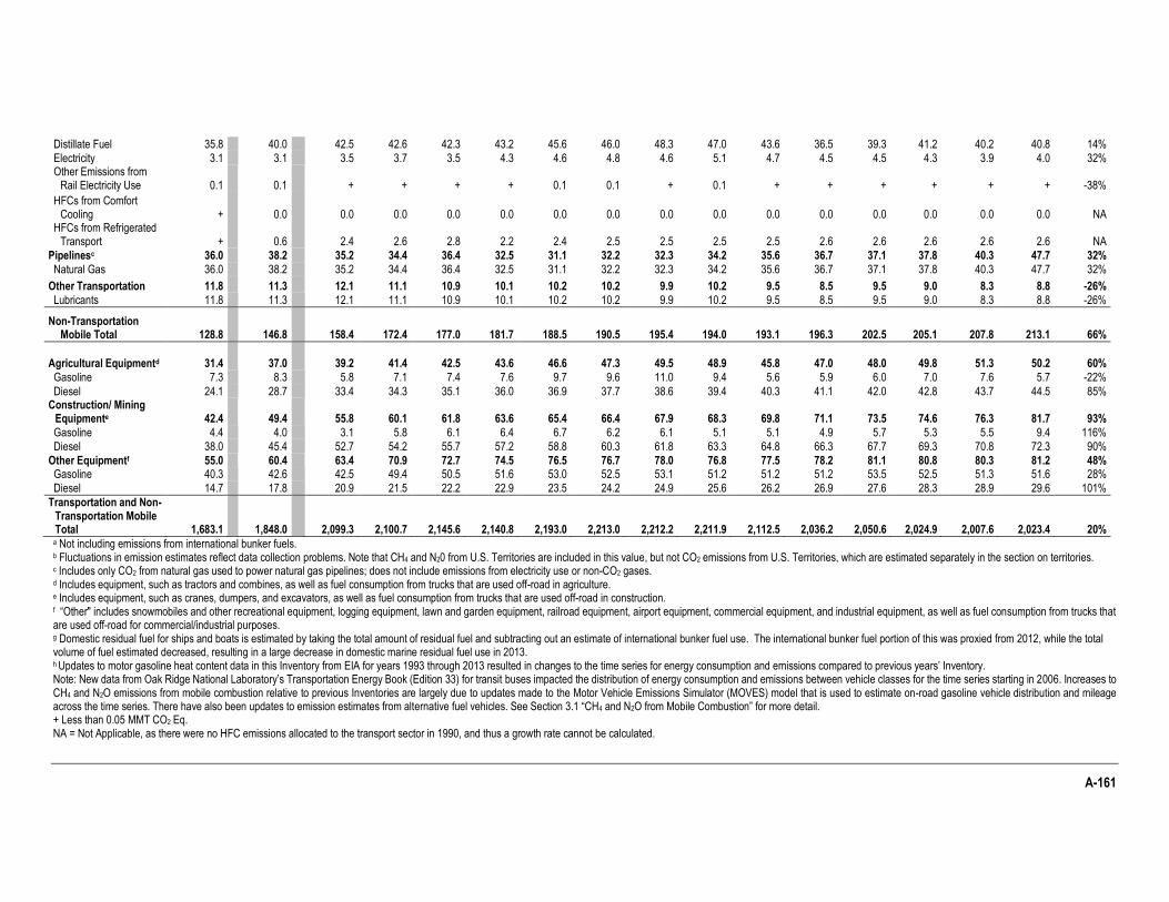
A-161
Distillate Fuel 35.8 40.0 42.5 42.6 42.3 43.2 45.6 46.0 48.3 47.0 43.6 36.5 39.3 41.2 40.2 40.8 14%
Electricity 3.1 3.1 3.5 3.7 3.5 4.3 4.6 4.8 4.6 5.1 4.7 4.5 4.5 4.3 3.9 4.0 32% Other Emissions from
Rail Electricity Use 0.1 0.1 + + + + 0.1 0.1 + 0.1 + + + + + + -38%
HFCs from Comfort Cooling + 0.0 0.0 0.0 0.0 0.0 0.0 0.0 0.0 0.0 0.0 0.0 0.0 0.0 0.0 0.0 NA
HFCs from Refrigerated Transport + 0.6 2.4 2.6 2.8 2.2 2.4 2.5 2.5 2.5 2.5 2.6 2.6 2.6 2.6 2.6 NA
Pipelinesc 36.0 38.2 35.2 34.4 36.4 32.5 31.1 32.2 32.3 34.2 35.6 36.7 37.1 37.8 40.3 47.7 32%
Natural Gas 36.0 38.2 35.2 34.4 36.4 32.5 31.1 32.2 32.3 34.2 35.6 36.7 37.1 37.8 40.3 47.7 32%
Other Transportation 11.8 11.3 12.1 11.1 10.9 10.1 10.2 10.2 9.9 10.2 9.5 8.5 9.5 9.0 8.3 8.8 -26%
Lubricants 11.8 11.3 12.1 11.1 10.9 10.1 10.2 10.2 9.9 10.2 9.5 8.5 9.5 9.0 8.3 8.8 -26%
Non-Transportation Mobile Total 128.8 146.8 158.4 172.4 177.0 181.7 188.5 190.5 195.4 194.0 193.1 196.3 202.5 205.1 207.8 213.1 66%
Agricultural Equipmentd 31.4 37.0 39.2 41.4 42.5 43.6 46.6 47.3 49.5 48.9 45.8 47.0 48.0 49.8 51.3 50.2 60%
Gasoline 7.3 8.3 5.8 7.1 7.4 7.6 9.7 9.6 11.0 9.4 5.6 5.9 6.0 7.0 7.6 5.7 -22%
Diesel 24.1 28.7 33.4 34.3 35.1 36.0 36.9 37.7 38.6 39.4 40.3 41.1 42.0 42.8 43.7 44.5 85% Construction/ Mining
Equipmente 42.4 49.4 55.8 60.1 61.8 63.6 65.4 66.4 67.9 68.3 69.8 71.1 73.5 74.6 76.3 81.7 93%
Gasoline 4.4 4.0 3.1 5.8 6.1 6.4 6.7 6.2 6.1 5.1 5.1 4.9 5.7 5.3 5.5 9.4 116%
Diesel 38.0 45.4 52.7 54.2 55.7 57.2 58.8 60.3 61.8 63.3 64.8 66.3 67.7 69.3 70.8 72.3 90%
Other Equipmentf 55.0 60.4 63.4 70.9 72.7 74.5 76.5 76.7 78.0 76.8 77.5 78.2 81.1 80.8 80.3 81.2 48% Gasoline 40.3 42.6 42.5 49.4 50.5 51.6 53.0 52.5 53.1 51.2 51.2 51.2 53.5 52.5 51.3 51.6 28%
Diesel 14.7 17.8 20.9 21.5 22.2 22.9 23.5 24.2 24.9 25.6 26.2 26.9 27.6 28.3 28.9 29.6 101%
Transportation and Non-Transportation Mobile Total 1,683.1 1,848.0 2,099.3 2,100.7 2,145.6 2,140.8 2,193.0 2,213.0 2,212.2 2,211.9 2,112.5 2,036.2 2,050.6 2,024.9 2,007.6 2,023.4 20%
a Not including emissions from international bunker fuels. b Fluctuations in emission estimates reflect data collection problems. Note that CH4 and N20 from U.S. Territories are included in this value, but not CO2 emissions from U.S. Territories, which are estimated separately in the section on territories. c Includes only CO2 from natural gas used to power natural gas pipelines; does not include emissions from electricity use or non-CO2 gases. d Includes equipment, such as tractors and combines, as well as fuel consumption from trucks that are used off-road in agriculture. e Includes equipment, such as cranes, dumpers, and excavators, as well as fuel consumption from trucks that are used off-road in construction. f “Other" includes snowmobiles and other recreational equipment, logging equipment, lawn and garden equipment, railroad equipment, airport equipment, commercial equipment, and industrial equipment, as well as fuel consumption from trucks that are used off-road for commercial/industrial purposes. g Domestic residual fuel for ships and boats is estimated by taking the total amount of residual fuel and subtracting out an estimate of international bunker fuel use. The international bunker fuel portion of this was proxied from 2012, while the total volume of fuel estimated decreased, resulting in a large decrease in domestic marine residual fuel use in 2013. h Updates to motor gasoline heat content data in this Inventory from EIA for years 1993 through 2013 resulted in changes to the time series for energy consumption and emissions compared to previous years’ Inventory. Note: New data from Oak Ridge National Laboratory’s Transportation Energy Book (Edition 33) for transit buses impacted the distribution of energy consumption and emissions between vehicle classes for the time series starting in 2006. Increases to CH4 and N2O emissions from mobile combustion relative to previous Inventories are largely due to updates made to the Motor Vehicle Emissions Simulator (MOVES) model that is used to estimate on-road gasoline vehicle distribution and mileage across the time series. There have also been updates to emission estimates from alternative fuel vehicles. See Section 3.1 “CH4 and N2O from Mobile Combustion” for more detail. + Less than 0.05 MMT CO2 Eq. NA = Not Applicable, as there were no HFC emissions allocated to the transport sector in 1990, and thus a growth rate cannot be calculated.
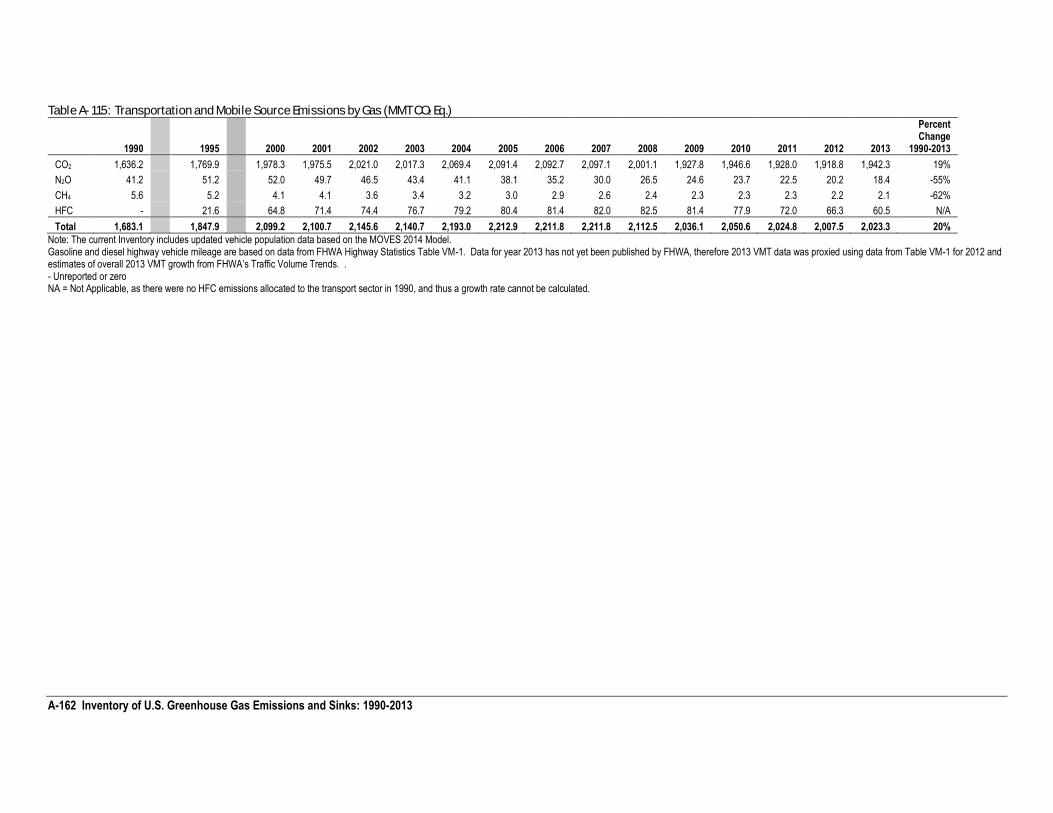
A-162 Inventory of U.S. Greenhouse Gas Emissions and Sinks: 1990-2013
Table A- 115: Transportation and Mobile Source Emissions by Gas (MMT CO2 Eq.)
1990 1995 2000 2001 2002 2003 2004 2005 2006 2007 2008 2009 2010 2011 2012 2013
Percent Change
1990-2013
CO2 1,636.2 1,769.9 1,978.3 1,975.5 2,021.0 2,017.3 2,069.4 2,091.4 2,092.7 2,097.1 2,001.1 1,927.8 1,946.6 1,928.0 1,918.8 1,942.3 19%
N2O 41.2 51.2 52.0 49.7 46.5 43.4 41.1 38.1 35.2 30.0 26.5 24.6 23.7 22.5 20.2 18.4 -55%
CH4 5.6 5.2 4.1 4.1 3.6 3.4 3.2 3.0 2.9 2.6 2.4 2.3 2.3 2.3 2.2 2.1 -62%
HFC - 21.6 64.8 71.4 74.4 76.7 79.2 80.4 81.4 82.0 82.5 81.4 77.9 72.0 66.3 60.5 N/A
Total 1,683.1 1,847.9 2,099.2 2,100.7 2,145.6 2,140.7 2,193.0 2,212.9 2,211.8 2,211.8 2,112.5 2,036.1 2,050.6 2,024.8 2,007.5 2,023.3 20%
Note: The current Inventory includes updated vehicle population data based on the MOVES 2014 Model. Gasoline and diesel highway vehicle mileage are based on data from FHWA Highway Statistics Table VM-1. Data for year 2013 has not yet been published by FHWA, therefore 2013 VMT data was proxied using data from Table VM-1 for 2012 and estimates of overall 2013 VMT growth from FHWA’s Traffic Volume Trends. . - Unreported or zero NA = Not Applicable, as there were no HFC emissions allocated to the transport sector in 1990, and thus a growth rate cannot be calculated.
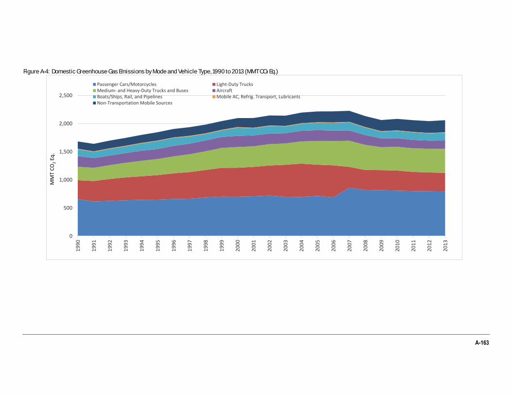
A-163
Figure A-4: Domestic Greenhouse Gas Emissions by Mode and Vehicle Type, 1990 to 2013 (MMT CO2 Eq.)
0
500
1,000
1,500
2,000
2,500
19
90
19
91
19
92
19
93
19
94
19
95
19
96
19
97
19
98
19
99
20
00
20
01
20
02
20
03
20
04
20
05
20
06
20
07
20
08
20
09
20
10
20
11
20
12
20
13
MM
T C
O2
Eq.
Passenger Cars/Motorcycles Light-Duty TrucksMedium- and Heavy-Duty Trucks and Buses AircraftBoats/Ships, Rail, and Pipelines Mobile AC, Refrig. Transport, LubricantsNon-Transportation Mobile Sources
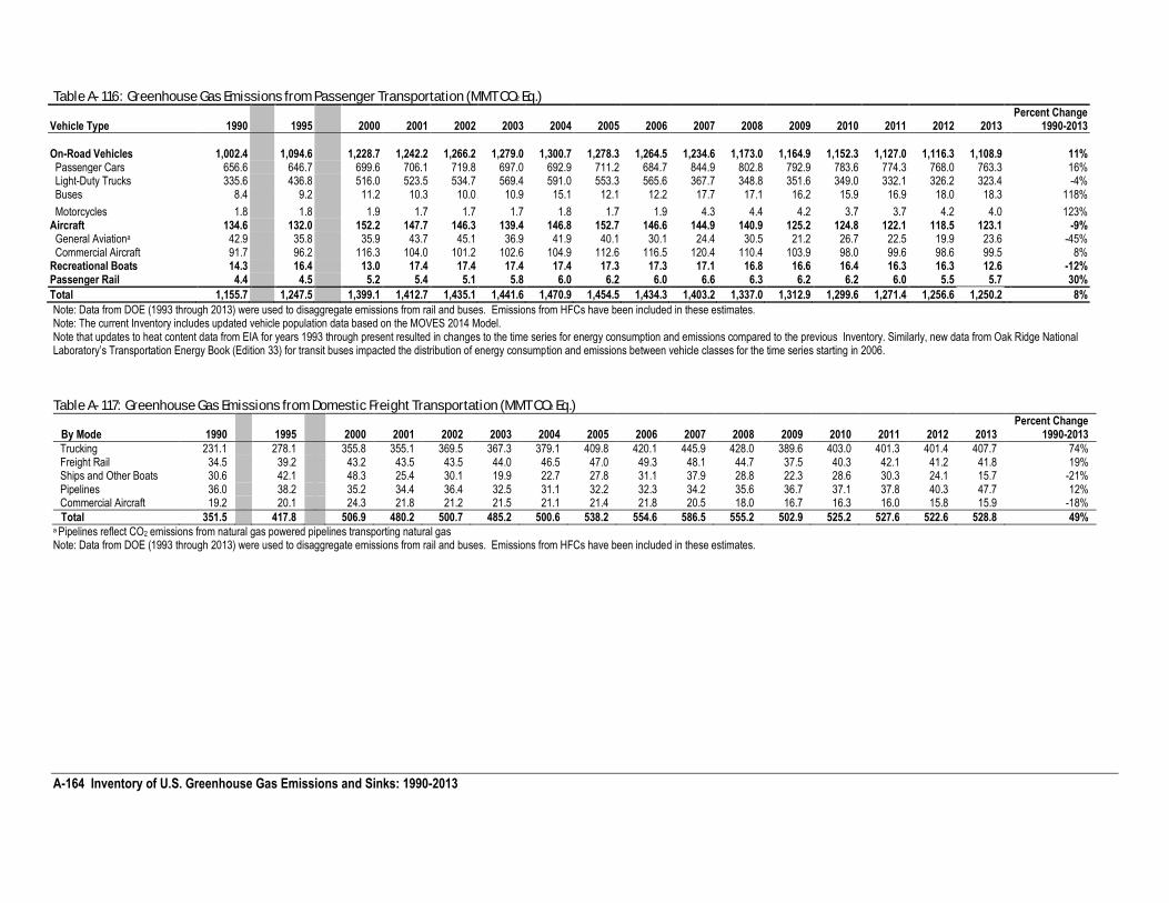
A-164 Inventory of U.S. Greenhouse Gas Emissions and Sinks: 1990-2013
Table A- 116: Greenhouse Gas Emissions from Passenger Transportation (MMT CO2 Eq.)
Vehicle Type 1990 1995 2000 2001 2002 2003 2004 2005 2006 2007 2008 2009 2010 2011 2012 2013 Percent Change
1990-2013
On-Road Vehicles 1,002.4 1,094.6 1,228.7 1,242.2 1,266.2 1,279.0
1,300.7 1,278.3 1,264.5 1,234.6 1,173.0 1,164.9 1,152.3 1,127.0 1,116.3 1,108.9 11% Passenger Cars 656.6 646.7 699.6 706.1 719.8 697.0 692.9 711.2 684.7 844.9 802.8 792.9 783.6 774.3 768.0 763.3 16% Light-Duty Trucks 335.6 436.8 516.0 523.5 534.7 569.4 591.0 553.3 565.6 367.7 348.8 351.6 349.0 332.1 326.2 323.4 -4% Buses 8.4 9.2 11.2 10.3 10.0 10.9 15.1 12.1 12.2 17.7 17.1 16.2 15.9 16.9 18.0 18.3 118%
Motorcycles 1.8 1.8 1.9 1.7 1.7 1.7 1.8 1.7 1.9 4.3 4.4 4.2 3.7 3.7 4.2 4.0 123% Aircraft 134.6 132.0 152.2 147.7 146.3 139.4 146.8 152.7 146.6 144.9 140.9 125.2 124.8 122.1 118.5 123.1 -9% General Aviationa 42.9 35.8 35.9 43.7 45.1 36.9 41.9 40.1 30.1 24.4 30.5 21.2 26.7 22.5 19.9 23.6 -45% Commercial Aircraft 91.7 96.2 116.3 104.0 101.2 102.6 104.9 112.6 116.5 120.4 110.4 103.9 98.0 99.6 98.6 99.5 8%
Recreational Boats 14.3 16.4 13.0 17.4 17.4 17.4 17.4 17.3 17.3 17.1 16.8 16.6 16.4 16.3 16.3 12.6 -12% Passenger Rail 4.4 4.5 5.2 5.4 5.1 5.8 6.0 6.2 6.0 6.6 6.3 6.2 6.2 6.0 5.5 5.7 30%
Total 1,155.7 1,247.5 1,399.1 1,412.7 1,435.1 1,441.6 1,470.9 1,454.5 1,434.3 1,403.2 1,337.0 1,312.9 1,299.6 1,271.4 1,256.6 1,250.2 8%
Note: Data from DOE (1993 through 2013) were used to disaggregate emissions from rail and buses. Emissions from HFCs have been included in these estimates. Note: The current Inventory includes updated vehicle population data based on the MOVES 2014 Model. Note that updates to heat content data from EIA for years 1993 through present resulted in changes to the time series for energy consumption and emissions compared to the previous Inventory. Similarly, new data from Oak Ridge National Laboratory’s Transportation Energy Book (Edition 33) for transit buses impacted the distribution of energy consumption and emissions between vehicle classes for the time series starting in 2006.
Table A- 117: Greenhouse Gas Emissions from Domestic Freight Transportation (MMT CO2 Eq.)
By Mode 1990 1995 2000 2001 2002 2003 2004 2005 2006 2007 2008 2009 2010 2011 2012 2013 Percent Change
1990-2013
Trucking 231.1 278.1 355.8 355.1 369.5 367.3 379.1 409.8 420.1 445.9 428.0 389.6 403.0 401.3 401.4 407.7 74% Freight Rail 34.5 39.2 43.2 43.5 43.5 44.0 46.5 47.0 49.3 48.1 44.7 37.5 40.3 42.1 41.2 41.8 19% Ships and Other Boats 30.6 42.1 48.3 25.4 30.1 19.9 22.7 27.8 31.1 37.9 28.8 22.3 28.6 30.3 24.1 15.7 -21% Pipelines 36.0 38.2 35.2 34.4 36.4 32.5 31.1 32.2 32.3 34.2 35.6 36.7 37.1 37.8 40.3 47.7 12% Commercial Aircraft 19.2 20.1 24.3 21.8 21.2 21.5 21.1 21.4 21.8 20.5 18.0 16.7 16.3 16.0 15.8 15.9 -18%
Total 351.5 417.8 506.9 480.2 500.7 485.2 500.6 538.2 554.6 586.5 555.2 502.9 525.2 527.6 522.6 528.8 49% a Pipelines reflect CO2 emissions from natural gas powered pipelines transporting natural gas
Note: Data from DOE (1993 through 2013) were used to disaggregate emissions from rail and buses. Emissions from HFCs have been included in these estimates.
A-165
3.3. Methodology for Estimating Emissions from Commercial Aircraft Jet Fuel Consumption
IPCC Tier 3B Method: Commercial aircraft jet fuel burn and carbon dioxide (CO2) emissions estimates were developed by the U.S. Federal Aviation Administration (FAA) using radar-informed data from the FAA Enhanced Traffic Management System (ETMS) for 2000 through 2013 as modeled with the Aviation Environmental Design Tool (AEDT). This bottom-up approach is built from modeling dynamic aircraft performance for each flight occurring within an individual calendar year. The analysis incorporates data on the aircraft type, date, flight identifier, departure time, arrival time, departure airport, arrival airport, ground delay at each airport, and real-world flight trajectories. To generate results for a given flight within AEDT, the radar-informed aircraft data is correlated with engine and aircraft performance data to calculate fuel burn and exhaust emissions. Information on exhaust emissions for in-production aircraft engines comes from the International Civil Aviation Organization (ICAO) Aircraft Engine Emissions Databank (EDB). This bottom-up approach is in accordance with the Tier 3B method from the 2006 IPCC Guidelines for National Greenhouse Gas Inventories.
International Bunkers: The IPCC guidelines define international aviation (International Bunkers) as emissions from flights that depart from one country and arrive in a different country. Bunker fuel emission estimates for commercial aircraft were developed for this report for 2000 through 2013 using the same radar-informed data modeled with AEDT. Since this process builds estimates from flight-specific information, the emissions estimates for commercial aircraft can include emissions associated with the U.S. territories (i.e., American Samoa, Guam, Puerto Rico, U.S. Virgin Islands, Wake Island, and other U.S. Pacific Islands). However, to allow for the alignment of emission estimates for commercial aircraft with other data that is provided without the U.S. territories, this annex includes emission estimates for commercial aircraft both with and without the U.S. territories included.
Time Series and Analysis Update: The FAA incrementally improves the consistency, robustness, and fidelity of the CO2 emissions modeling for commercial aircraft, which is the basis of the Tier3B inventories presented in this report. While the FAA does not anticipate significant changes to the AEDT model in the future, recommended improvements are limited by budget and time constraints, as well as data availability. For instance, previous reports included reported annual CO2 emission estimates for 2000 through 2005 that were modeled using the FAA’s System for assessing Aviation’s Global Emissions (SAGE). That tool and its capabilities were significantly improved after it was incorporated and evolved into AEDT. For this report, the AEDT model was used to generate annual CO2 emission estimates for 2000, 2005, 2010, 2011, 2012, and 2013 only. The reported annual CO2 emissions values for 2001 through 2004 were estimated from the previously reported SAGE data. Likewise, CO2 emissions values for 2006 through 2009 were estimated by interpolation to preserve trends from past reports.
Commercial aircraft radar data sets are not available for years prior to 2000. Instead, the FAA applied a Tier3B methodology by developing Official Airline Guide (OAG) schedule-informed estimates modeled with AEDT and great circle trajectories for 1990, 2000 and 2010. The ratios between the OAG schedule-informed and the radar-informed inventories for the years 2000 and 2010 were applied to the 1990 OAG scheduled-informed inventory to generate the best possible CO2 inventory estimate for commercial aircraft in 1990. The resultant 1990 CO2 inventory served as the reference for generating the additional 1991 through 1999 emission estimates, which were established using previously-available trends.
Notes on Revised 1990 CO2 Emissions Inventory for Commercial Aircraft: There is a reduction in CO2 emissions for the revised 1990 estimates for commercial aircraft, when compared to previous Inventory reports (Inventory reports published in 2000, 2002, 2007, 2010). The primary driver of modeling the 1990 emission estimate was to achieve time series consistency. The observed change in 1990 emissions is purely due to using a Tier3B methodology, and not reflective of revised industry performance and should not be used to infer or evaluate such performance.
To achieve time series consistency, the 1990 jet fuel burn was modeled with the latest AEDT version using great circle trajectories and OAG schedule information. There are uncertainties associated with the modeled 1990 data that do not exist for the modeled 2000 to 2013 data. Radar-based data is not available for 1990. The OAG schedule information generally includes fewer carriers than radar information, and this will result in a different fleet mix, and in turn, different CO2 emissions than would be quantified using a radar-based data set. For this reason, the FAA adjusted the OAG-informed schedule for 1990 with a ratio based on radar-informed information. In addition, radar trajectories are also generally longer than great circle trajectories. While the 1990 fuel burn data was adjusted to address these differences, it inherently adds greater uncertainty to the revised 1990 commercial aircraft CO2 emissions as compared to data from 2000 forward. Also, the revised 1990 CO2 emission estimate now reflects only commercial aircraft jet fuel consumption, while previous reports
A-166 Inventory of U.S. Greenhouse Gas Emissions and Sinks: 1990-2013
may have aggregated jet fuel sales data from non-commercial aircraft into this category. Thus, it would be inappropriate to compare 1990 to future years for other than qualitative purposes.
The revised 1990 commercial aircraft CO2 emissions estimate is approximately 4 percent lower than the 2013 CO2 emissions estimate. It is important to note that the distance flown increased by more than 40 percent over this 24-year period and that fuel burn and aviation activity trends over the past two decades indicate significant improvements in commercial aviation’s ability to provide increased service levels while using less fuel.1
Methane Emissions: Contributions of methane (CH4) emissions from commercial aircraft are reported as zero. Years of scientific measurement campaigns conducted at the exhaust exit plane of commercial aircraft gas turbine engines have repeatedly indicated that CH4 emissions are consumed over the full mission flight envelope (Aircraft Emissions of Methane and Nitrous Oxide during the Alternative Aviation Fuel Experiment, Santoni et al., Environ. Sci. Technol., 2011, 45, 7075-7082). As a result, the U.S. EPA published that “…methane is no longer considered to be an emission from aircraft gas turbine engines burning Jet A at higher power settings and is, in fact, consumed in net at these higher powers.”2 In accordance with the following statements in the 2006 IPCC Guidelines (IPCC 2006), the FAA does not calculate CH4 emissions for either the domestic or international bunker commercial aircraft jet fuel emissions inventories. “Methane (CH4) may be emitted by gas turbines during idle and by older technology engines, but recent data suggest that little or no CH4 is emitted by modern engines.” “Current scientific understanding does not allow other gases (e.g., N2O and CH4) to be included in calculation of cruise emissions.” (IPCC 1999).
Results: The graph and table below, four jet fuel burn values are reported for each calendar year. These values are comprised of domestic and international fuel burn totals for the U.S. 50 States and the U.S. 50 States + Territories. Data are presented for domestic defined as jet fuel burn from any commercial aircraft flight departing and landing in the U.S. 50 States and for the U.S. 50 States + Territories. The data presented as international is respective of the two different domestic definitions, and represents flights departing from the specified domestic area and landing anywhere in the world outside of that area.
Note that the graph and table present less fuel burn for the international U.S. 50 States + Territories than for the international U.S. 50 States. This is because the flights between the 50 states and U.S. Territories are “international” when only the 50 states are defined as domestic, but they are “domestic” for the U.S. 50 States + Territories definition.
1 Additional information on the AEDT modeling process is available at:
http://www.faa.gov/about/office_org/headquarters_offices/apl/research/models/ 2 Recommended Best Practice for Quantifying Speciated Organic Gas Emissions from Aircraft Equipped with Turbofan, Turbojet
and Turboprop Engines, EPA-420-R-09-901, May 27, 2009. See <http://www.epa.gov/otaq/aviation.html>.
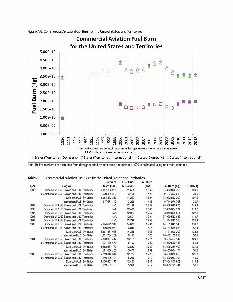
A-167
Figure A-5: Commercial Aviation Fuel Burn for the United States and Territories
Note: Hollow markers are estimates from data generated by prior tools and methods.1990 is estimated using non-radar methods.
Table A- 118: Commercial Aviation Fuel Burn for the United States and Territories
Year Region
Distance
Flown (nmi)
Fuel Burn
(M Gallon)
Fuel Burn
(Tbtu) Fuel Burn (Kg) CO2 (MMT)
1990 Domestic U.S. 50 States and U.S. Territories 4,057,195,988 11,568 1,562 34,820,800,463 109.9
International U.S. 50 States and U.S. Territories 599,486,893 3,155 426 9,497,397,919 30.0
Domestic U.S. 50 States 3,984,482,217 11,287 1,524 33,972,832,399 107.2
International U.S. 50 States 617,671,849 3,228 436 9,714,974,766 30.7
1995 Domestic U.S. 50 States and U.S. Territories N/A 12,136 1,638 36,528,990,675 115.2
1996 Domestic U.S. 50 States and U.S. Territories N/A 12,492 1,686 37,600,624,534 118.6
1997 Domestic U.S. 50 States and U.S. Territories N/A 12,937 1,747 38,940,896,854 122.9
1998 Domestic U.S. 50 States and U.S. Territories N/A 12,601 1,701 37,930,582,643 119.7
1999 Domestic U.S. 50 States and U.S. Territories N/A 13,726 1,853 41,314,843,250 130.3
2000 Domestic U.S. 50 States and U.S. Territories 5,994,679,944 14,672 1,981 44,161,841,348 139.3
International U.S. 50 States and U.S. Territories 1,309,565,963 6,040 815 18,181,535,058 57.4
Domestic U.S. 50 States 5,891,481,028 14,349 1,937 43,191,000,202 136.3
International U.S. 50 States 1,331,784,289 6,117 826 18,412,169,613 58.1
2001 Domestic U.S. 50 States and U.S. Territories 5,360,977,447 13,121 1,771 39,493,457,147 124.6
International U.S. 50 States and U.S. Territories 1,171,130,679 5,402 729 16,259,550,186 51.3
Domestic U.S. 50 States 5,268,687,772 12,832 1,732 38,625,244,409 121.9
International U.S. 50 States 1,191,000,288 5,470 739 16,465,804,174 51.9
2002 Domestic U.S. 50 States and U.S. Territories 5,219,345,344 12,774 1,725 38,450,076,259 121.3
International U.S. 50 States and U.S. Territories 1,140,190,481 5,259 710 15,829,987,794 49.9
Domestic U.S. 50 States 5,129,493,877 12,493 1,687 37,604,800,905 118.6
International U.S. 50 States 1,159,535,153 5,326 719 16,030,792,741 50.6
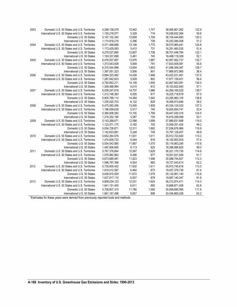
A-168 Inventory of U.S. Greenhouse Gas Emissions and Sinks: 1990-2013
2003 Domestic U.S. 50 States and U.S. Territories 5,288,138,079 12,942 1,747 38,956,861,262 122.9
International U.S. 50 States and U.S. Territories 1,155,218,577 5,328 719 16,038,632,384 50.6
Domestic U.S. 50 States 5,197,102,340 12,658 1,709 38,100,444,893 120.2
International U.S. 50 States 1,174,818,219 5,396 728 16,242,084,008 51.2
2004 Domestic U.S. 50 States and U.S. Territories 5,371,498,689 13,146 1,775 39,570,965,441 124.8
International U.S. 50 States and U.S. Territories 1,173,429,093 5,412 731 16,291,460,535 51.4
Domestic U.S. 50 States 5,279,027,890 12,857 1,736 38,701,048,784 122.1
International U.S. 50 States 1,193,337,698 5,481 740 16,498,119,309 52.1
2005 Domestic U.S. 50 States and U.S. Territories 6,476,007,697 13,976 1,887 42,067,562,737 132.7
International U.S. 50 States and U.S. Territories 1,373,543,928 5,858 791 17,633,508,081 55.6
Domestic U.S. 50 States 6,370,544,998 13,654 1,843 41,098,359,387 129.7
International U.S. 50 States 1,397,051,323 5,936 801 17,868,972,965 56.4
2006 Domestic U.S. 50 States and U.S. Territories 5,894,323,482 14,426 1,948 43,422,531,461 137.0
International U.S. 50 States and U.S. Territories 1,287,642,623 5,939 802 17,877,159,421 56.4
Domestic U.S. 50 States 5,792,852,211 14,109 1,905 42,467,943,091 134.0
International U.S. 50 States 1,309,488,994 6,015 812 18,103,932,940 57.1
2007 Domestic U.S. 50 States and U.S. Territories 6,009,247,818 14,707 1,986 44,269,160,525 139.7
International U.S. 50 States and U.S. Territories 1,312,748,383 6,055 817 18,225,718,619 57.5
Domestic U.S. 50 States 5,905,798,114 14,384 1,942 43,295,960,105 136.6
International U.S. 50 States 1,335,020,703 6,132 828 18,456,913,646 58.2
2008 Domestic U.S. 50 States and U.S. Territories 5,475,092,456 13,400 1,809 40,334,124,033 127.3
International U.S. 50 States and U.S. Territories 1,196,059,638 5,517 745 16,605,654,741 52.4
Domestic U.S. 50 States 5,380,838,282 13,105 1,769 39,447,430,318 124.5
International U.S. 50 States 1,216,352,196 5,587 754 16,816,299,099 53.1
2009 Domestic U.S. 50 States and U.S. Territories 5,143,268,671 12,588 1,699 37,889,631,668 119.5
International U.S. 50 States and U.S. Territories 1,123,571,175 5,182 700 15,599,251,424 49.2
Domestic U.S. 50 States 5,054,726,871 12,311 1,662 37,056,676,966 116.9
International U.S. 50 States 1,142,633,881 5,248 709 15,797,129,457 49.8
2010 Domestic U.S. 50 States and U.S. Territories 5,652,264,576 11,931 1,611 35,912,723,830 113.3
International U.S. 50 States and U.S. Territories 1,474,839,733 6,044 816 18,192,953,916 57.4
Domestic U.S. 50 States 5,554,043,585 11,667 1,575 35,116,863,245 110.8
International U.S. 50 States 1,497,606,695 6,113 825 18,398,996,825 58.0
2011 Domestic U.S. 50 States and U.S. Territories 5,767,378,664 12,067 1,629 36,321,170,730 114.6
International U.S. 50 States and U.S. Territories 1,576,982,962 6,496 877 19,551,631,939 61.7
Domestic U.S. 50 States 5,673,689,481 11,823 1,596 35,588,754,827 112.3
International U.S. 50 States 1,596,797,398 6,554 885 19,727,043,614 62.2
2012 Domestic U.S. 50 States and U.S. Territories 5,735,605,432 11,932 1,611 35,915,745,616 113.3
International U.S. 50 States and U.S. Territories 1,619,012,587 6,464 873 19,457,378,739 61.4
Domestic U.S. 50 States 5,636,910,529 11,672 1,576 35,132,961,140 110.8
International U.S. 50 States 1,637,917,110 6,507 879 19,587,140,347 61.8
2013 Domestic U.S. 50 States and U.S. Territories 5,808,034,123 12,031 1,624 36,212,974,471 114.3
International U.S. 50 States and U.S. Territories 1,641,151,400 6,611 892 19,898,871,458 62.8
Domestic U.S. 50 States 5,708,807,315 11,780 1,590 35,458,690,595 111.9
International U.S. 50 States 1,661,167,498 6,657 899 20,036,865,038 63.2
*Estimates for these years were derived from previously reported tools and methods
A-169
3.4. Methodology for Estimating CH4 Emissions from Coal Mining
The methodology for estimating CH4 emissions from coal mining consists of two steps. The first step is to estimate emissions from underground mines. There are two sources of underground mine emissions: ventilation systems and degasification systems. These emissions are estimated on a mine-by-mine basis and then are summed to determine total emissions. The second step of the analysis involves estimating CH4 emissions from surface mines and post-mining activities. In contrast to the methodology for underground mines, which uses mine-specific data, the methodology for estimating emissions from surface mines and post-mining activities consists of multiplying basin-specific coal production by basin-specific gas content and an emission factor.
Step 1: Estimate CH4 Liberated and CH4 Emitted from Underground Mines
Underground mines generate CH4 from ventilation systems and from degasification systems. Some mines recover and use the generated CH4, thereby reducing emissions to the atmosphere. Total CH4 emitted from underground mines equals the CH4 liberated from ventilation systems, plus the CH4 liberated from degasification systems, minus CH4 recovered and used.
Step 1.1: Estimate CH4 Liberated from Ventilation Systems
All coal mines with detectable CH4 emissions3 use ventilation systems to ensure that CH4 levels remain within safe concentrations. Many coal mines do not have detectable levels of CH4, while others emit several million cubic feet per day (MMCFD) from their ventilation systems. On a quarterly basis, the U.S. Mine Safety and Health Administration (MSHA) measures CH4 emissions levels at underground mines. MSHA maintains a database of measurement data from all underground mines with detectable levels of CH4 in their ventilation air (MSHA 2014). Based on the four quarterly measurements, MSHA estimates average daily CH4 liberated at each of the underground mines with detectable emissions.
For 1990 through 1999, average daily CH4 emissions from MSHA were multiplied by the number of days in the year (i.e., coal mine assumed in operation for all four quarters) to determine the annual emissions for each mine. For 2000 through 2013, the average daily CH4 emissions from MSHA were multiplied by the number of days corresponding to the number of quarters the mine vent was operating. For example, if the mine vent was operational in one out of the four quarters, the average daily CH4 emissions were multiplied by 92 days. Total ventilation emissions for a particular year were estimated by summing emissions from individual mines.
For the years 1990, 1993 through 1996, 1998 through 2006, and 2008 through 2012, MSHA emissions data were obtained for a large but incomplete subset of all mines with detectable emissions. This subset includes mines emitting at least 0.1 MMCFD for most years and at least 0.5 MMCFD for 1995 and 1996, as shown in Table A-119. Over 90 percent of all ventilation emissions were concentrated in these subsets of approximately 120-150 mines. No MSHA ventilation data exists for 1991 and 1992. For 1997, 2007, and 2013 the complete MSHA databases for all 495 mines (in 1997), 230 mines (in 2007), and 205 mines (in 2013) with detectable CH4 emissions were obtained. These mines were assumed to account for 100 percent of CH4 liberated from underground mine ventilation systems for those years. Using the complete database from 1997, the proportion of total emissions accounted for by mines emitting less than 0.1 MMCFD or 0.5 MMCFD was estimated (see Table A-119). The proportion was then applied to the years 1990 through 2006 to account for ventilation emissions coming from mines without MSHA data. The complete 2007 dataset was used to adjust the emissions proportion for 2008-2012.
EPA currently collects information on ventilation emissions from underground coal mines liberating greater than 36,500,000 actual cubic feet of CH4 per year (about 14,700 metric tons CO2 Eq.) through its Greenhouse Gas Reporting Program (GHGRP).4 Many of the underground coal mines reporting to the GHGRP use the same quarterly MSHA samples. However, some mines use their own measurements and samples, which are taken either quarterly or monthly. The 2013 ventilation emissions were calculated using both GHGRP data from the mines that take their own measurements using 98.324(b)(1) monitoring methods and MSHA data 98.324 (b)(2) method for all other mines with reportable methane emissions. Since 2009, two coal mines have destroyed a portion of their CH4 emissions from ventilation systems using
3 MSHA records coal mine methane readings with concentrations of greater than 50 ppm (parts per million) methane. Readings below this
threshold are considered non-detectable. 4 See U.S. EPA Greenhouse Gas Reporting Program, <http://www.epa.gov/ghgreporting/>. Underground coal mines report to EPA under
Subpart FF of the program.
A-170 Inventory of U.S. Greenhouse Gas Emissions and Sinks: 1990-2013
thermal oxidation technology. The amount of CH4 destroyed through these two projects was determined through publicly-available emission reduction project information (CAR 2014).
Table A-119: Mine-Specific Data Used to Estimate Ventilation Emissions Year Individual Mine Data Used
1990 All Mines Emitting at Least 0.1 MMCFD (Assumed to Account for 97.8% of Total)* 1991 1990 Emissions Factors Used Instead of Mine-Specific Data 1992 1990 Emissions Factors Used Instead of Mine-Specific Data 1993 All Mines Emitting at Least 0.1 MMCFD (Assumed to Account for 97.8% of Total)* 1994 All Mines Emitting at Least 0.1 MMCFD (Assumed to Account for 97.8% of Total)* 1995 All Mines Emitting at Least 0.5 MMCFD (Assumed to Account for 94.1% of Total)* 1996 All Mines Emitting at Least 0.5 MMCFD (Assumed to Account for 94.1% of Total)* 1997 All Mines with Detectable Emissions (Assumed to Account for 100% of Total) 1998 All Mines Emitting at Least 0.1 MMCFD (Assumed to Account for 97.8% of Total)* 1999 All Mines Emitting at Least 0.1 MMCFD (Assumed to Account for 97.8% of Total)* 2000 All Mines Emitting at Least 0.1 MMCFD (Assumed to Account for 97.8% of Total)* 2001 All Mines Emitting at Least 0.1 MMCFD (Assumed to Account for 97.8% of Total)* 2002 All Mines Emitting at Least 0.1 MMCFD (Assumed to Account for 97.8% of Total)* 2003 All Mines Emitting at Least 0.1 MMCFD (Assumed to Account for 97.8% of Total)* 2004 All Mines Emitting at Least 0.1 MMCFD (Assumed to Account for 97.8% of Total)* 2005 All Mines Emitting at Least 0.1 MMCFD (Assumed to Account for 97.8% of Total)* 2006 2007 2008 2009 2010
All Mines Emitting at Least 0.1 MMCFD (Assumed to Account for 97.8% of Total)* All Mines with Detectable Emissions (Assumed to Account for 100% of Total) All Mines Emitting at Least 0.1 MMCFD (Assumed to Account for 98.96% of Total)** All Mines Emitting at Least 0.1 MMCFD (Assumed to Account for 98.96% of Total)** All Mines Emitting at Least 0.1 MMCFD (Assumed to Account for 98.96% of Total)**
2011 All Mines Emitting at Least 0.1 MMCFD (Assumed to Account for 98.96% of Total)** 2012 All Mines Emitting at Least 0.1 MMCFD (Assumed to Account for 98.96% of Total)**
2013 All Mines with Detectable Emissions and GHGRP reported data (Assumed to account for 100% of Total)
* Factor derived from a complete set of individual mine data collected for 1997. ** Factor derived from a complete set of individual mine data collected for 2007.
Step 1.2: Estimate CH4 Liberated from Degasification Systems
Coal mines use several different types of degasification systems to remove CH4, including vertical wells and horizontal boreholes to recover CH4 prior to mining of the coal seam. Gob wells and cross-measure boreholes recover CH4 from the overburden (i.e., gob area) after mining of the seam (primarily in longwall mines).
MSHA collects information about the presence and type of degasification systems in some mines, but does not collect quantitative data on the amount of CH4 liberated. Thus, degasification emissions were estimated on a mine-by-mine basis based on other sources of available data. For Alabama mines that sell CH4 recovered from degasification systems to a pipeline, gas sales records were used to estimate CH4 liberated from degasification systems (see Step 1.3). The well data was also used to estimate CH4 collected from mined-through pre-drainage wells. For most other mines that either sold CH4 to a pipeline, used CH4 on site, or vented CH4 from degasification systems, data on degasification emissions reported to the EPA’s GHGRP (EPA 2014) were used.
Step 1.3: Estimate CH4 Recovered from Degasification Systems and Utilized (Emissions Avoided)
In 2013, fifteen active coal mines had CH4 recovery and use projects, of which thirteen mines sold the recovered CH4 to a pipeline. One of the mines that sold gas to a pipeline also used CH4 to fuel a thermal coal dryer. One mine used recovered CH4 for electrical power generation, and two other mines used recovered CH4 to heat mine ventilation air. For mines that utilize CH4 on-site, either the GHGRP (EPA 2014) or project-specific information (CAR 2014) was used to estimate CH4 liberated from degasification systems.
In order to calculate emissions avoided from pipeline sales, information was needed regarding the amount of gas recovered and the number of years in advance of mining that wells were drilled. Alabama and West Virginia state agencies provided gas sales data (GSA 2014; WVGES 2014), which were used to estimate emissions avoided for these projects. Additionally, coal mine operators provided information on eligible pre-drainage wells drilled in advance of mining (JWR 2010, 2014). Emissions avoided were attributed to the year in which the coal seam was mined. For example, if a coal mine recovered and sold CH4 using a vertical well drilled five years in advance of mining, the emissions avoided associated with those gas sales (cumulative production) were attributed to the well at the time it was mined through (e.g., five years of gas
A-171
production). The coal mine operators with the largest CH4 recovery and use projects provided this information (Consol 2014; JWR 2010, 2014), which was then used to estimate emissions avoided for a particular year.
Step 2: Estimate CH4 Emitted from Surface Mines and Post-Mining Activities
Mine-specific data were not available for estimating CH4 emissions from surface coal mines or for post-mining activities. For surface mines, basin-specific coal production was multiplied by basin-specific gas contents and a 150 percent emission factor (to account for CH4 from over- and under-burden) to estimate CH4 emissions. This emission factor was revised downward since 2012 from 200 percent based on more recent studies (King 1994; Saghafi 2013). The 150 percent emission factor was applied to all inventory years since 1990, retroactively. For post-mining activities, basin-specific coal production was multiplied by basin-specific gas contents and a 32.5 percent emission factor accounting for CH4 desorption during coal transportation and storage (Creedy 1993). Basin-specific in situ gas content data was compiled from AAPG (1984) and USBM (1986). Beginning in 2006, revised data on in situ CH4 content and emissions factors are taken from EPA (1996) and EPA (2005).
Step 2.1: Define the Geographic Resolution of the Analysis and Collect Coal Production Data
The first step in estimating CH4 emissions from surface mining and post-mining activities was to define the geographic resolution of the analysis and to collect coal production data at that level of resolution. The analysis was conducted by coal basin as defined in Table A-120, which presents coal basin definitions by basin and by state.
The Energy Information Administration’s (EIA) Annual Coal Report (2014) includes state- and county-specific underground and surface coal production by year. To calculate production by basin, the state level data were grouped into coal basins using the basin definitions listed in Table A-120. For two states—West Virginia and Kentucky—county-level production data was used for the basin assignments because coal production occurred in geologically distinct coal basins within these states. Table A-121 presents the coal production data aggregated by basin.
Step 2.2: Estimate Emissions Factors for Each Emissions Type
Emission factors for surface-mined coal were developed from the in situ CH4 content of the surface coal in each basin. Based on analyses conducted in Canada and Australia on coals similar to those present in the United States. (King 1994; Saghafi 2013), the surface mining emission factor used was conservatively estimated to be 150 percent of the in situ CH4 content of the basin. Furthermore, the post-mining emission factors used were estimated to be 25 to 40 percent of the average in situ CH4 content in the basin. For this analysis, the post-mining emission factor was determined to be 32.5 percent of the in situ CH4 content in the basin. Table A-122 presents the average in situ content for each basin, along with the resulting emission factor estimates.
Step 2.3: Estimate CH4 Emitted
The total amount of CH4 emitted from surface mines and post-mining activities was calculated by multiplying the coal production in each basin by the appropriate emission factors.
Table A-120 lists each of the major coal mine basins in the United States and the states in which they are located. As shown in Figure A-6, several coal basins span several states. Table A-121 shows annual underground, surface, and total coal production (in short tons) for each coal basin. Table A-122 shows the surface, post-surface, and post-underground emission factors used for estimating CH4 emissions for each of the categories. Table A-123 presents annual estimates of CH4 emissions for ventilation and degasification systems, and CH4 used and emitted by underground coal mines. Table A-124 presents annual estimates of total CH4 emissions from underground, post-underground, surface, and post-surface activities. Table A-125 provides the total net CH4 emissions by state.
Table A-120: Coal Basin Definitions by Basin and by State Basin States
Northern Appalachian Basin Maryland, Ohio, Pennsylvania, West Virginia North Central Appalachian Basin Kentucky East, Tennessee, Virginia, West Virginia South Warrior Basin Alabama, Mississippi Illinois Basin Illinois, Indiana, Kentucky West South West and Rockies Basin Arizona, California, Colorado, New Mexico, Utah North Great Plains Basin Montana, North Dakota, Wyoming West Interior Basin Arkansas, Iowa, Kansas, Louisiana, Missouri, Oklahoma, Texas Northwest Basin Alaska, Washington
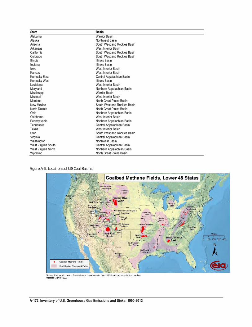
A-172 Inventory of U.S. Greenhouse Gas Emissions and Sinks: 1990-2013
State Basin
Alabama Warrior Basin Alaska Northwest Basin Arizona South West and Rockies Basin Arkansas West Interior Basin California South West and Rockies Basin Colorado South West and Rockies Basin Illinois Illinois Basin Indiana Illinois Basin Iowa West Interior Basin Kansas West Interior Basin Kentucky East Central Appalachian Basin Kentucky West Illinois Basin Louisiana West Interior Basin Maryland Northern Appalachian Basin Mississippi Warrior Basin Missouri West Interior Basin Montana North Great Plains Basin New Mexico South West and Rockies Basin North Dakota North Great Plains Basin Ohio Northern Appalachian Basin Oklahoma West Interior Basin Pennsylvania. Northern Appalachian Basin Tennessee Central Appalachian Basin Texas West Interior Basin Utah South West and Rockies Basin Virginia Central Appalachian Basin Washington Northwest Basin West Virginia South Central Appalachian Basin West Virginia North Northern Appalachian Basin Wyoming North Great Plains Basin
Figure A-6: Locations of U.S Coal Basins
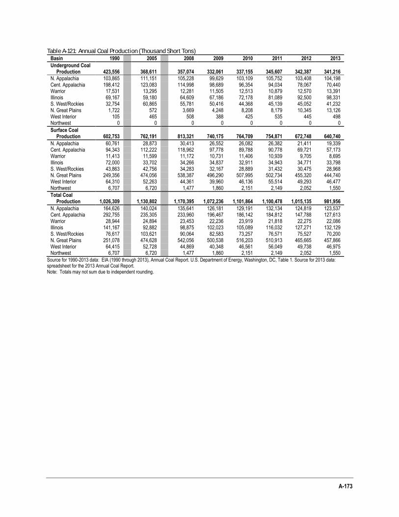
A-173
Table A-121: Annual Coal Production (Thousand Short Tons)
Basin 1990 2005 2008 2009 2010 2011 2012 2013
Underground Coal Production 423,556 368,611 357,074 332,061 337,155
345,607
342,387 341,216
N. Appalachia 103,865 111,151 105,228 99,629 103,109 105,752 103,408 104,198 Cent. Appalachia 198,412 123,083 114,998 98,689 96,354 94,034 78,067 70,440 Warrior 17,531 13,295 12,281 11,505 12,513 10,879 12,570 13,391 Illinois 69,167 59,180 64,609 67,186 72,178 81,089 92,500 98,331 S. West/Rockies 32,754 60,865 55,781 50,416 44,368 45,139 45,052 41,232 N. Great Plains 1,722 572 3,669 4,248 8,208 8,179 10,345 13,126 West Interior 105 465 508 388 425 535 445 498 Northwest 0 0 0 0 0 0 0 0
Surface Coal Production 602,753 762,191 813,321 740,175 764,709 754,871 672,748 640,740
N. Appalachia 60,761 28,873 30,413 26,552 26,082 26,382 21,411 19,339 Cent. Appalachia 94,343 112,222 118,962 97,778 89,788 90,778 69,721 57,173 Warrior 11,413 11,599 11,172 10,731 11,406 10,939 9,705 8,695 Illinois 72,000 33,702 34,266 34,837 32,911 34,943 34,771 33,798 S. West/Rockies 43,863 42,756 34,283 32,167 28,889 31,432 30,475 28,968 N. Great Plains 249,356 474,056 538,387 496,290 507,995 502,734 455,320 444,740 West Interior 64,310 52,263 44,361 39,960 46,136 55,514 49,293 46,477 Northwest 6,707 6,720 1,477 1,860 2,151 2,149 2,052 1,550
Total Coal Production 1,026,309 1,130,802 1,170,395 1,072,236 1,101,864 1,100,478 1,015,135 981,956
N. Appalachia 164,626 140,024 135,641 126,181 129,191 132,134 124,819 123,537 Cent. Appalachia 292,755 235,305 233,960 196,467 186,142 184,812 147,788 127,613 Warrior 28,944 24,894 23,453 22,236 23,919 21,818 22,275 22,086 Illinois 141,167 92,882 98,875 102,023 105,089 116,032 127,271 132,129 S. West/Rockies 76,617 103,621 90,064 82,583 73,257 76,571 75,527 70,200 N. Great Plains 251,078 474,628 542,056 500,538 516,203 510,913 465,665 457,866 West Interior 64,415 52,728 44,869 40,348 46,561 56,049 49,738 46,975 Northwest 6,707 6,720 1,477 1,860 2,151 2,149 2,052 1,550
Source for 1990-2013 data: EIA (1990 through 2013), Annual Coal Report. U.S. Department of Energy, Washington, DC, Table 1. Source for 2013 data: spreadsheet for the 2013 Annual Coal Report. Note: Totals may not sum due to independent rounding.
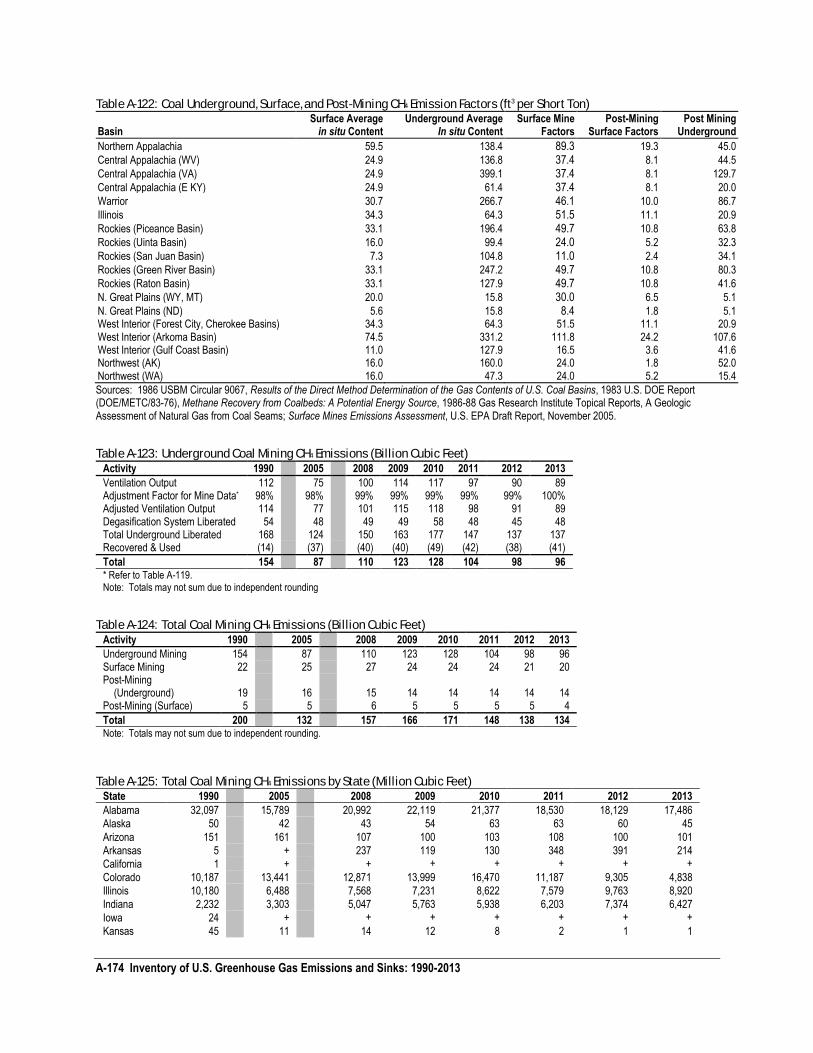
A-174 Inventory of U.S. Greenhouse Gas Emissions and Sinks: 1990-2013
Table A-122: Coal Underground, Surface, and Post-Mining CH4 Emission Factors (ft3 per Short Ton) Basin
Surface Average in situ Content
Underground Average In situ Content
Surface Mine Factors
Post-Mining Surface Factors
Post Mining Underground
Northern Appalachia 59.5 138.4 89.3 19.3 45.0
Central Appalachia (WV) 24.9 136.8 37.4 8.1 44.5
Central Appalachia (VA) 24.9 399.1 37.4 8.1 129.7
Central Appalachia (E KY) 24.9 61.4 37.4 8.1 20.0
Warrior 30.7 266.7 46.1 10.0 86.7
Illinois 34.3 64.3 51.5 11.1 20.9
Rockies (Piceance Basin) 33.1 196.4 49.7 10.8 63.8
Rockies (Uinta Basin) 16.0 99.4 24.0 5.2 32.3
Rockies (San Juan Basin) 7.3 104.8 11.0 2.4 34.1
Rockies (Green River Basin) 33.1 247.2 49.7 10.8 80.3
Rockies (Raton Basin) 33.1 127.9 49.7 10.8 41.6
N. Great Plains (WY, MT) 20.0 15.8 30.0 6.5 5.1
N. Great Plains (ND) 5.6 15.8 8.4 1.8 5.1 West Interior (Forest City, Cherokee Basins) 34.3 64.3 51.5 11.1 20.9 West Interior (Arkoma Basin) 74.5 331.2 111.8 24.2 107.6 West Interior (Gulf Coast Basin) 11.0 127.9 16.5 3.6 41.6 Northwest (AK) 16.0 160.0 24.0 1.8 52.0 Northwest (WA) 16.0 47.3 24.0 5.2 15.4
Sources: 1986 USBM Circular 9067, Results of the Direct Method Determination of the Gas Contents of U.S. Coal Basins, 1983 U.S. DOE Report (DOE/METC/83-76), Methane Recovery from Coalbeds: A Potential Energy Source, 1986-88 Gas Research Institute Topical Reports, A Geologic Assessment of Natural Gas from Coal Seams; Surface Mines Emissions Assessment, U.S. EPA Draft Report, November 2005.
Table A-123: Underground Coal Mining CH4 Emissions (Billion Cubic Feet)
Activity 1990 2005 2008 2009 2010 2011 2012 2013
Ventilation Output 112 75 100 114 117 97 90 89 Adjustment Factor for Mine Data* 98% 98% 99% 99% 99% 99% 99% 100% Adjusted Ventilation Output 114 77 101 115 118 98 91 89 Degasification System Liberated 54 48 49 49 58 48 45 48 Total Underground Liberated 168 124 150 163 177 147 137 137 Recovered & Used (14) (37) (40) (40) (49) (42) (38) (41)
Total 154 87 110 123 128 104 98 96 * Refer to Table A-119. Note: Totals may not sum due to independent rounding
Table A-124: Total Coal Mining CH4 Emissions (Billion Cubic Feet)
Activity 1990 2005 2008 2009 2010 2011 2012 2013
Underground Mining 154 87 110 123 128 104 98 96 Surface Mining 22 25 27 24 24 24 21 20 Post-Mining
(Underground) 19 16 15 14 14 14 14 14 Post-Mining (Surface) 5 5 6 5 5 5 5 4
Total 200 132 157 166 171 148 138 134 Note: Totals may not sum due to independent rounding.
Table A-125: Total Coal Mining CH4 Emissions by State (Million Cubic Feet)
State 1990 2005 2008 2009 2010 2011 2012 2013
Alabama 32,097 15,789 20,992 22,119 21,377 18,530 18,129 17,486
Alaska 50 42 43 54 63 63 60 45
Arizona 151 161 107 100 103 108 100 101
Arkansas 5 + 237 119 130 348 391 214
California 1 + + + + + + +
Colorado 10,187 13,441 12,871 13,999 16,470 11,187 9,305 4,838
Illinois 10,180 6,488 7,568 7,231 8,622 7,579 9,763 8,920
Indiana 2,232 3,303 5,047 5,763 5,938 6,203 7,374 6,427
Iowa 24 + + + + + + +
Kansas 45 11 14 12 8 2 1 1
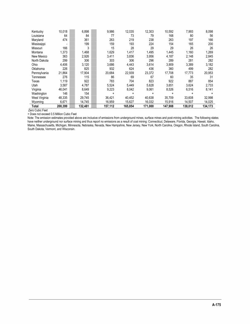
A-175
Kentucky 10,018 6,898 9,986 12,035 12,303 10,592 7,993 8,098
Louisiana 64 84 77 73 79 168 80 56
Maryland 474 361 263 219 238 263 197 166
Mississippi - 199 159 193 224 154 165 200
Missouri 166 3 15 28 29 29 26 26
Montana 1,373 1,468 1,629 1,417 1,495 1,445 1,160 1,269
New Mexico 363 2,926 3,411 3,836 3,956 4,187 2,148 2,845
North Dakota 299 306 303 306 296 289 281 282
Ohio 4,406 3,120 3,686 4,443 3,614 3,909 3,389 3,182
Oklahoma 226 825 932 624 436 360 499 282
Pennsylvania 21,864 17,904 20,684 22,939 23,372 17,708 17,773 20,953
Tennessee 276 115 86 69 67 60 35 31
Texas 1,119 922 783 704 823 922 887 854
Utah 3,587 4,787 5,524 5,449 5,628 3,651 3,624 2,733
Virginia 46,041 8,649 9,223 8,042 9,061 8,526 6,516 8,141
Washington 146 154 + + + + + +
West Virginia 48,335 29,745 36,421 40,452 40,638 35,709 33,608 32,998
Wyoming 6,671 14,745 16,959 15,627 16,032 15,916 14,507 14,025
Total 200,399 132,481 157,112 165,854 171,000 147,908 138,012 134,173 Zero Cubic Feet + Does not exceed 0.5 Million Cubic Feet Note: The emission estimates provided above are inclusive of emissions from underground mines, surface mines and post-mining activities. The following states have neither underground nor surface mining and thus report no emissions as a result of coal mining: Connecticut, Delaware, Florida, Georgia, Hawaii, Idaho, Maine, Massachusetts, Michigan, Minnesota, Nebraska, Nevada, New Hampshire, New Jersey, New York, North Carolina, Oregon, Rhode Island, South Carolina, South Dakota, Vermont, and Wisconsin.
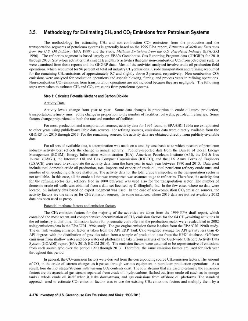
A-176 Inventory of U.S. Greenhouse Gas Emissions and Sinks: 1990-2013
3.5. Methodology for Estimating CH4 and CO2 Emissions from Petroleum Systems
The methodology for estimating CH4 and non-combustion CO2 emissions from the production and the transportation segments of petroleum systems is generally based on the 1999 EPA report, Estimates of Methane Emissions from the U.S. Oil Industry (EPA 1999) and the study, Methane Emissions from the U.S. Petroleum Industry (EPA/GRI 1996). The refineries segment is based largely on EPA’s Greenhouse Gas Reporting Program data (GHGRP) for 2010 through 2013. Sixty-four activities that emit CH4 and thirty activities that emit non-combustion CO2 from petroleum systems were examined from these reports and the GHGRP data. Most of the activities analyzed involve crude oil production field operations, which accounted for 96 percent of total oil industry CH4 emissions. Crude transportation and refining accounted for the remaining CH4 emissions of approximately 0.7 and slightly above 3 percent, respectively. Non-combustion CO2
emissions were analyzed for production operations and asphalt blowing, flaring, and process vents in refining operations. Non-combustion CO2 emissions from transportation operations are not included because they are negligible. The following steps were taken to estimate CH4 and CO2 emissions from petroleum systems.
Step 1: Calculate Potential Methane and Carbon Dioxide
Activity Data
Activity levels change from year to year. Some data changes in proportion to crude oil rates: production, transportation, refinery runs. Some change in proportion to the number of facilities: oil wells, petroleum refineries. Some factors change proportional to both the rate and number of facilities.
For most production and transportation sources, activity data for 1995 found in EPA/GRI 1996a are extrapolated to other years using publicly-available data sources. For refining sources, emissions data were directly available from the GHGRP for 2010 through 2013. For the remaining sources, the activity data are obtained directly from publicly-available data.
For all sets of available data, a determination was made on a case-by-case basis as to which measure of petroleum industry activity best reflects the change in annual activity. Publicly-reported data from the Bureau of Ocean Energy Management (BOEM), Energy Information Administration (EIA), American Petroleum Institute (API), the Oil & Gas Journal (O&GJ), the Interstate Oil and Gas Compact Commission (IOGCC), and the U.S Army Corps of Engineers (USACE) were used to extrapolate the activity data from the base year to each year between 1990 and 2013. Data used include total domestic crude oil production, total imports and exports of crude oil, total petroleum refinery crude runs, and number of oil-producing offshore platforms. The activity data for the total crude transported in the transportation sector is not available. In this case, all the crude oil that was transported was assumed to go to refineries. Therefore, the activity data for the refining sector (i.e., refinery feed in 1000 bbl/year) was used also for the transportation sector. The number of domestic crude oil wells was obtained from a data set licensed by DrillingInfo, Inc. In the few cases where no data were located, oil industry data based on expert judgment was used. In the case of non-combustion CO2 emission sources, the activity factors are the same as for CH4 emission sources. In some instances, where 2013 data are not yet available 2012 data has been used as proxy.
Potential methane factors and emission factors
The CH4 emission factors for the majority of the activities are taken from the 1999 EPA draft report, which contained the most recent and comprehensive determination of CH4 emission factors for the 64 CH4-emitting activities in the oil industry at that time. Emission factors for pneumatic controllers in the production sector were recalculated in 2002 using emissions data in the EPA/GRI 1996c study. The gas engine emission factor is taken from the EPA/GRI 1996b study. The oil tank venting emission factor is taken from the API E&P Tank Calc weighted average for API gravity less than 45 API degrees with the distribution of gravities taken from a sample of production data from the HPDI database. Offshore emissions from shallow water and deep water oil platforms are taken from analysis of the Gulf-wide Offshore Activity Data System (GOADS) report (EPA 2015; BOEM 2014). The emission factors were assumed to be representative of emissions from each source type over the period 1990 through 2013. Therefore, the same emission factors are used for each year throughout this period.
In general, the CO2 emission factors were derived from the corresponding source CH4 emission factors. The amount of CO2 in the crude oil stream changes as it passes through various equipment in petroleum production operations. As a result, four distinct stages/streams with varying CO2 contents exist. The four streams that are used to estimate the emissions factors are the associated gas stream separated from crude oil, hydrocarbons flashed out from crude oil (such as in storage tanks), whole crude oil itself when it leaks downstream, and gas emissions from offshore oil platforms. The standard approach used to estimate CO2 emission factors was to use the existing CH4 emissions factors and multiply them by a
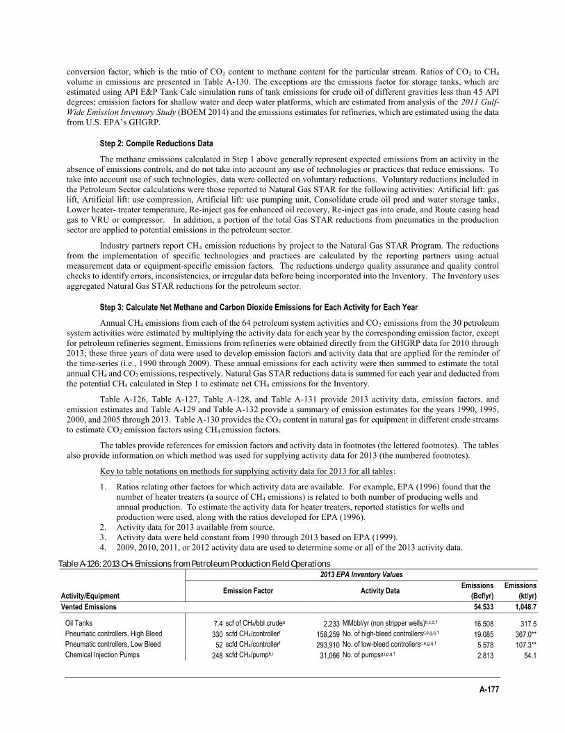
A-177
conversion factor, which is the ratio of CO2 content to methane content for the particular stream. Ratios of CO2 to CH4 volume in emissions are presented in Table A-130. The exceptions are the emissions factor for storage tanks, which are estimated using API E&P Tank Calc simulation runs of tank emissions for crude oil of different gravities less than 45 API degrees; emission factors for shallow water and deep water platforms, which are estimated from analysis of the 2011 Gulf-Wide Emission Inventory Study (BOEM 2014) and the emissions estimates for refineries, which are estimated using the data from U.S. EPA’s GHGRP.
Step 2: Compile Reductions Data
The methane emissions calculated in Step 1 above generally represent expected emissions from an activity in the absence of emissions controls, and do not take into account any use of technologies or practices that reduce emissions. To take into account use of such technologies, data were collected on voluntary reductions. Voluntary reductions included in the Petroleum Sector calculations were those reported to Natural Gas STAR for the following activities: Artificial lift: gas lift, Artificial lift: use compression, Artificial lift: use pumping unit, Consolidate crude oil prod and water storage tanks, Lower heater- treater temperature, Re-inject gas for enhanced oil recovery, Re-inject gas into crude, and Route casing head gas to VRU or compressor. In addition, a portion of the total Gas STAR reductions from pneumatics in the production sector are applied to potential emissions in the petroleum sector.
Industry partners report CH4 emission reductions by project to the Natural Gas STAR Program. The reductions from the implementation of specific technologies and practices are calculated by the reporting partners using actual measurement data or equipment-specific emission factors. The reductions undergo quality assurance and quality control checks to identify errors, inconsistencies, or irregular data before being incorporated into the Inventory. The Inventory uses aggregated Natural Gas STAR reductions for the petroleum sector.
Step 3: Calculate Net Methane and Carbon Dioxide Emissions for Each Activity for Each Year
Annual CH4 emissions from each of the 64 petroleum system activities and CO2 emissions from the 30 petroleum system activities were estimated by multiplying the activity data for each year by the corresponding emission factor, except for petroleum refineries segment. Emissions from refineries were obtained directly from the GHGRP data for 2010 through 2013; these three years of data were used to develop emission factors and activity data that are applied for the reminder of the time-series (i.e., 1990 through 2009). These annual emissions for each activity were then summed to estimate the total annual CH4 and CO2 emissions, respectively. Natural Gas STAR reductions data is summed for each year and deducted from the potential CH4 calculated in Step 1 to estimate net CH4 emissions for the Inventory.
Table A-126, Table A-127, Table A-128, and Table A-131 provide 2013 activity data, emission factors, and emission estimates and Table A-129 and Table A-132 provide a summary of emission estimates for the years 1990, 1995, 2000, and 2005 through 2013. Table A-130 provides the CO2 content in natural gas for equipment in different crude streams to estimate CO2 emission factors using CH4
emission factors.
The tables provide references for emission factors and activity data in footnotes (the lettered footnotes). The tables also provide information on which method was used for supplying activity data for 2013 (the numbered footnotes).
Key to table notations on methods for supplying activity data for 2013 for all tables:
1. Ratios relating other factors for which activity data are available. For example, EPA (1996) found that the number of heater treaters (a source of CH4 emissions) is related to both number of producing wells and annual production. To estimate the activity data for heater treaters, reported statistics for wells and production were used, along with the ratios developed for EPA (1996).
2. Activity data for 2013 available from source. 3. Activity data were held constant from 1990 through 2013 based on EPA (1999). 4. 2009, 2010, 2011, or 2012 activity data are used to determine some or all of the 2013 activity data.
Table A-126: 2013 CH4 Emissions from Petroleum Production Field Operations
Activity/Equipment
2013 EPA Inventory Values
Emission Factor Activity Data Emissions
(Bcf/yr)
Emissions
(kt/yr)
Vented Emissions 54.533 1,048.7
Oil Tanks 7.4 scf of CH4/bbl crudea 2,233 MMbbl/yr (non stripper wells)b,c,d,1 16.508 317.5
Pneumatic controllers, High Bleed 330 scfd CH4/controllerf 158,259 No. of high-bleed controllersc,e,g,q,1 19.085 367.0**
Pneumatic controllers, Low Bleed 52 scfd CH4/controllerf 293,910 No. of low-bleed controllersc,e,g,q,1 5.578 107.3**
Chemical Injection Pumps 248 scfd CH4/pumph,i 31,066 No. of pumpsg,i,p,q,1 2.813 54.1
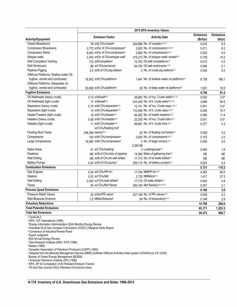
A-178 Inventory of U.S. Greenhouse Gas Emissions and Sinks: 1990-2013
Activity/Equipment
2013 EPA Inventory Values
Emission Factor Activity Data Emissions
(Bcf/yr)
Emissions
(kt/yr)
Vessel Blowdowns 78 scfy CH4/vesselh 206,898 No. of vesselsc,g,i,q,1 0.016 0.3
Compressor Blowdowns 3,775 scf/yr of CH4/compressorh 2,820 No. of compressorsc,g,i,q,1 0.011 0.2
Compressor Starts 8,443 scf/yr of CH4/compressorh 2,820 No. of compressorsc,g,i,1 0.024 0.5
Stripper wells 2,345 scf/yr of CH4/stripper wellf 315,213 No. of stripper wells ventedf,d,1 0.739 14.2
Well Completion Venting 733 scf/completionh 15,753 Oil well completionsc,4 0.012 0.2
Well Workovers 96 scf CH4/workoveri 64,793 Oil well workoversg,i,1,4 0.006 0.1
Pipeline Pigging 2.4 scfd of CH4/pig stationj 0 No. of crude pig stationse,3 0.000 0.0
Offshore Platforms, Shallow water Oil,
fugitive, vented and combusted 16,552 scfd CH4/platformq 1,447 No. of shallow water oil platformsl,4 8.739 168.1
Offshore Platforms, Deepwater oil,
fugitive, vented and combusted 93,836 scfd CH4/platformq 29 No. of deep water oil platformsl,4 1.001 19.3
Fugitive Emissions 4.750 91.4
Oil Wellheads (heavy crude) 0.13 scfd/welle,m 38,682 No. of hvy. Crude wellsd,g,i,1,4 0.002 0.0*
Oil Wellheads (light crude) 17 scfd/welle,m 510,005 No. of lt. crude wellsd,g,i,1,4 3.096 59.5
Separators (heavy crude) 0.15 scfd CH4/separatore,m 12,141 No. of hvy. Crude seps.c,g,i,1 0.001 0.0*
Separators (light crude) 14 scfd CH4/separatore,m 110,495 No. of lt. crude seps.c,g,i,1 0.559 10.7
Heater/Treaters (light crude) 19 scfd CH4/heatere,m 84,262 No. of heater treatersc,g,i,1 0.590 11.4
Headers (heavy crude) 0.08 scfd CH4/headere,m 22,535 No. of hvy. Crude hdrs.g,i,1 0.001 0.0*
Headers (light crude) 11 scfd CH4/headere,m 69,861 No. of lt. crude hdrs.g,i,1 0.277 5.3
Floating Roof Tanks 338,306
scf CH4/floating roof
tank/yrm,n 24 No. of floating roof tankse,3 0.008 0.2
Compressors 100 scfd CH4/compressore 2,820 No. of compressorsc,g,i,1 0.103 2.0
Large Compressors 16,360 scfd CH4/compressore 0 No. of large comprs.e,3 0.000 0.0
Sales Areas 41 scf CH4/loadinge 2,265,98
3 Loadings/yearc,1 0.092 1.8
Pipelines NE scfd of CH4/mile of pipeline 14,590 Miles of gathering lineo,2 NE NE
Well Drilling NE scfd of CH4/oil well drilled 17,774 No. of oil wells drilledc,2 NE NE
Battery Pumps 0.24 scfd of CH4/pumpm 259,170 No. of battery pumpsg,e,1 0.023 0.4
Combustion Emissions 5.731 110.2
Gas Engines 0.24 scf CH4/HP-hrh 17,764 MMHP-hrc,g,i,1 4.263 82.0
Heaters 0.52 scf CH4/bbln 2,720 MMbbl/yrc,2 1.417 27.3
Well Drilling 2,453 scf CH4/well drilledm 17,774 Oil wells drilledc,4 0.044 0.8
Flares 20 scf CH4/Mcf flaredj 363,184 Mcf flared/yr b,c,d,1,4 0.007 0.1
Process Upset Emissions 0.156 3.0
Pressure Relief Valves 35 scf/yr/PR valveh 227,169 No. of PR valvesc,e,1 0.008 0.2
Well Blowouts Onshore 2.5 MMscf/blowoutf 59 No. of blowouts/yrc,e,1 0.148 2.8
Voluntary Reductions 14.799 284.6
Total Potential Emissions 65.171 1,253.3
Total Net Emissions 50.372 968.7 a TankCALC b EPA / ICF International (1999) c Energy Information Administration (EIA) Monthly Energy Review d Interstate Oil & Gas Compact Commission (IOGCC) Marginal Wells Report e Consensus of Industrial Review Panel f Expert Judgment g EIA Annual Energy Review h Gas Research Institute (GRI) / EPA (1996) i Radian (1999) j Canadian Association of Petroleum Producers (CAPP) (1992) k Adapted from the Minerals Management Service (MMS) Gulfwide Offshore Activities Data System (GOADS) by ICF (2005) l Bureau of Ocean Energy Management (BOEM) m American Petroleum Institute (API) (1996) n EPA, AP 42 Compilation of Air Pollutant Emission Factors o Oil and Gas Journal (OGJ) Petroleum Economics Issue
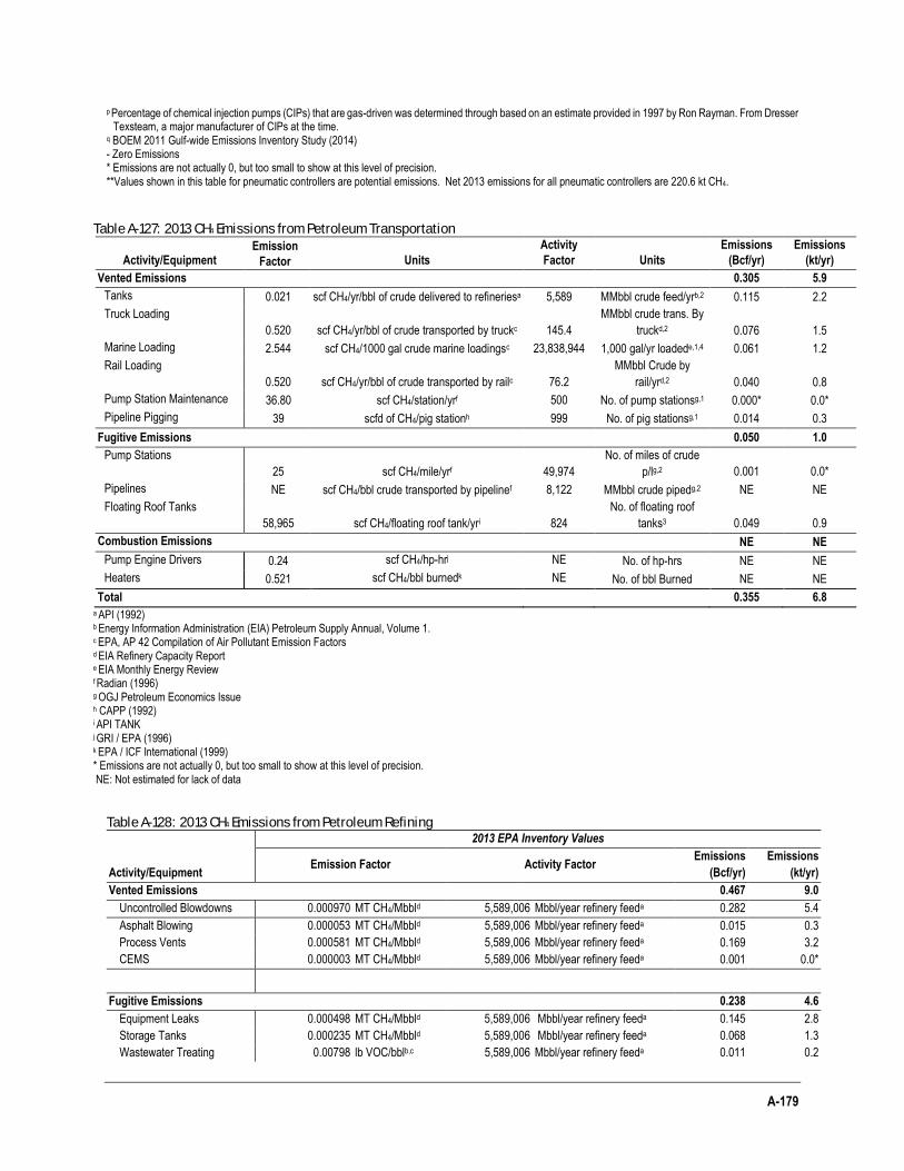
A-179
p Percentage of chemical injection pumps (CIPs) that are gas-driven was determined through based on an estimate provided in 1997 by Ron Rayman. From Dresser Texsteam, a major manufacturer of CIPs at the time.
q BOEM 2011 Gulf-wide Emissions Inventory Study (2014) - Zero Emissions * Emissions are not actually 0, but too small to show at this level of precision. **Values shown in this table for pneumatic controllers are potential emissions. Net 2013 emissions for all pneumatic controllers are 220.6 kt CH4.
Table A-127: 2013 CH4 Emissions from Petroleum Transportation
Activity/Equipment Emission
Factor Units
Activity
Factor Units
Emissions
(Bcf/yr)
Emissions
(kt/yr)
Vented Emissions 0.305 5.9
Tanks 0.021 scf CH4/yr/bbl of crude delivered to refineriesa 5,589 MMbbl crude feed/yrb,2 0.115 2.2
Truck Loading
0.520 scf CH4/yr/bbl of crude transported by truckc 145.4
MMbbl crude trans. By
truckd,2 0.076 1.5
Marine Loading 2.544 scf CH4/1000 gal crude marine loadingsc 23,838,944 1,000 gal/yr loadede,1,4 0.061 1.2
Rail Loading
0.520 scf CH4/yr/bbl of crude transported by railc 76.2
MMbbl Crude by
rail/yrd,2 0.040 0.8
Pump Station Maintenance 36.80 scf CH4/station/yrf 500 No. of pump stationsg,1 0.000* 0.0*
Pipeline Pigging 39 scfd of CH4/pig stationh 999 No. of pig stationsg,1 0.014 0.3
Fugitive Emissions 0.050 1.0
Pump Stations
25 scf CH4/mile/yrf 49,974
No. of miles of crude
p/lg,2 0.001 0.0*
Pipelines NE scf CH4/bbl crude transported by pipelinef 8,122 MMbbl crude pipedg,2 NE NE
Floating Roof Tanks
58,965 scf CH4/floating roof tank/yri 824
No. of floating roof
tanks3 0.049 0.9
Combustion Emissions NE NE
Pump Engine Drivers 0.24 scf CH4/hp-hrj NE No. of hp-hrs NE NE
Heaters 0.521 scf CH4/bbl burnedk NE No. of bbl Burned NE NE
Total 0.355 6.8 a API (1992) b Energy Information Administration (EIA) Petroleum Supply Annual, Volume 1. c EPA, AP 42 Compilation of Air Pollutant Emission Factors d EIA Refinery Capacity Report e EIA Monthly Energy Review f Radian (1996) g OGJ Petroleum Economics Issue h CAPP (1992) i API TANK j GRI / EPA (1996) k EPA / ICF International (1999) * Emissions are not actually 0, but too small to show at this level of precision. NE: Not estimated for lack of data
Table A-128: 2013 CH4 Emissions from Petroleum Refining
Activity/Equipment
2013 EPA Inventory Values
Emission Factor Activity Factor Emissions
(Bcf/yr)
Emissions
(kt/yr)
Vented Emissions 0.467 9.0
Uncontrolled Blowdowns 0.000970 MT CH4/Mbbld 5,589,006 Mbbl/year refinery feeda 0.282 5.4
Asphalt Blowing 0.000053 MT CH4/Mbbld 5,589,006 Mbbl/year refinery feeda 0.015 0.3
Process Vents 0.000581 MT CH4/Mbbld 5,589,006 Mbbl/year refinery feeda 0.169 3.2
CEMS 0.000003 MT CH4/Mbbld 5,589,006 Mbbl/year refinery feeda 0.001 0.0*
Fugitive Emissions 0.238 4.6
Equipment Leaks 0.000498 MT CH4/Mbbld 5,589,006 Mbbl/year refinery feeda 0.145 2.8
Storage Tanks 0.000235 MT CH4/Mbbld 5,589,006 Mbbl/year refinery feeda 0.068 1.3
Wastewater Treating 0.00798 lb VOC/bblb,c 5,589,006 Mbbl/year refinery feeda 0.011 0.2
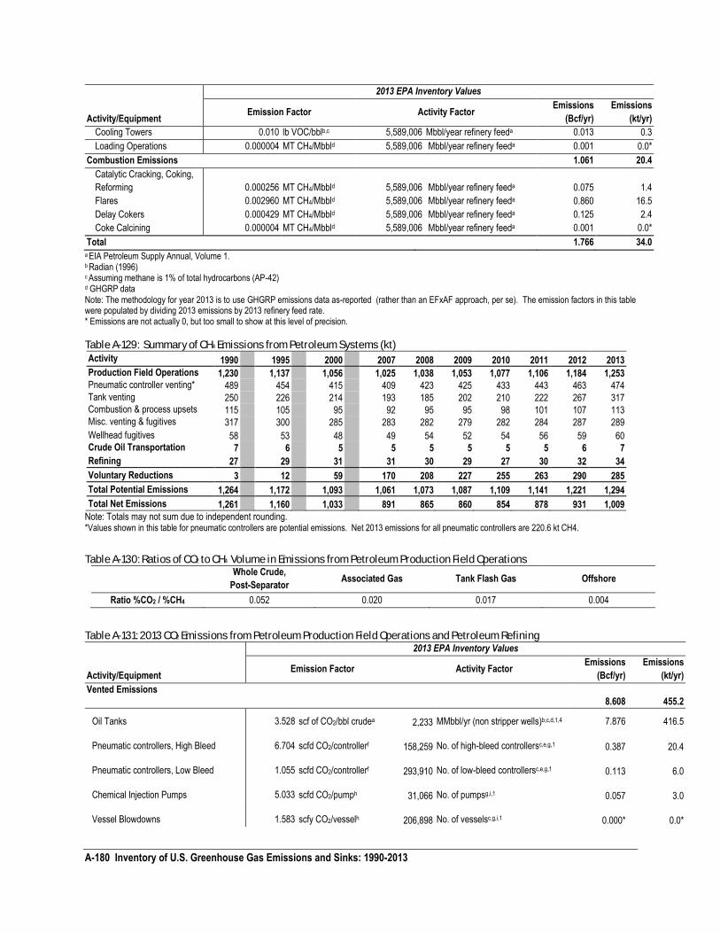
A-180 Inventory of U.S. Greenhouse Gas Emissions and Sinks: 1990-2013
Activity/Equipment
2013 EPA Inventory Values
Emission Factor Activity Factor Emissions
(Bcf/yr)
Emissions
(kt/yr)
Cooling Towers 0.010 lb VOC/bblb,c 5,589,006 Mbbl/year refinery feeda 0.013 0.3
Loading Operations 0.000004 MT CH4/Mbbld 5,589,006 Mbbl/year refinery feeda 0.001 0.0*
Combustion Emissions 1.061 20.4
Catalytic Cracking, Coking,
Reforming 0.000256 MT CH4/Mbbld 5,589,006 Mbbl/year refinery feeda 0.075 1.4
Flares 0.002960 MT CH4/Mbbld 5,589,006 Mbbl/year refinery feeda 0.860 16.5
Delay Cokers 0.000429 MT CH4/Mbbld 5,589,006 Mbbl/year refinery feeda 0.125 2.4
Coke Calcining 0.000004 MT CH4/Mbbld 5,589,006 Mbbl/year refinery feeda 0.001 0.0*
Total 1.766 34.0 a EIA Petroleum Supply Annual, Volume 1. b Radian (1996) c Assuming methane is 1% of total hydrocarbons (AP-42) d GHGRP data Note: The methodology for year 2013 is to use GHGRP emissions data as-reported (rather than an EFxAF approach, per se). The emission factors in this table were populated by dividing 2013 emissions by 2013 refinery feed rate. * Emissions are not actually 0, but too small to show at this level of precision.
Table A-129: Summary of CH4 Emissions from Petroleum Systems (kt)
Activity 1990 1995 2000 2007 2008 2009 2010 2011 2012 2013
Production Field Operations 1,230 1,137 1,056 1,025 1,038 1,053 1,077 1,106 1,184 1,253 Pneumatic controller venting* 489 454 415 409 423 425 433 443 463 474 Tank venting 250 226 214 193 185 202 210 222 267 317 Combustion & process upsets 115 105 95 92 95 95 98 101 107 113 Misc. venting & fugitives 317 300 285 283 282 279 282 284 287 289
Wellhead fugitives 58 53 48 49 54 52 54 56 59 60 Crude Oil Transportation 7 6 5 5 5 5 5 5 6 7
Refining 27 29 31 31 30 29 27 30 32 34
Voluntary Reductions 3 12 59 170 208 227 255 263 290 285
Total Potential Emissions 1,264 1,172 1,093 1,061 1,073 1,087 1,109 1,141 1,221 1,294
Total Net Emissions 1,261 1,160 1,033 891 865 860 854 878 931 1,009
Note: Totals may not sum due to independent rounding. *Values shown in this table for pneumatic controllers are potential emissions. Net 2013 emissions for all pneumatic controllers are 220.6 kt CH4.
Table A-130: Ratios of CO2 to CH4 Volume in Emissions from Petroleum Production Field Operations Whole Crude,
Post-Separator Associated Gas Tank Flash Gas Offshore
Ratio %CO2 / %CH4 0.052 0.020 0.017 0.004
Table A-131: 2013 CO2 Emissions from Petroleum Production Field Operations and Petroleum Refining
Activity/Equipment
2013 EPA Inventory Values
Emission Factor Activity Factor Emissions
(Bcf/yr)
Emissions
(kt/yr)
Vented Emissions
8.608 455.2
Oil Tanks 3.528 scf of CO2/bbl crudea 2,233 MMbbl/yr (non stripper wells)b,c,d,1,4 7.876 416.5
Pneumatic controllers, High Bleed 6.704 scfd CO2/controllerf 158,259 No. of high-bleed controllersc,e,g,1
0.387 20.4
Pneumatic controllers, Low Bleed 1.055 scfd CO2/controllerf 293,910 No. of low-bleed controllersc,e,g,1
0.113 6.0
Chemical Injection Pumps 5.033 scfd CO2/pumph 31,066 No. of pumpsg,i,1
0.057 3.0
Vessel Blowdowns 1.583 scfy CO2/vesselh 206,898 No. of vesselsc,g,i,1
0.000* 0.0*
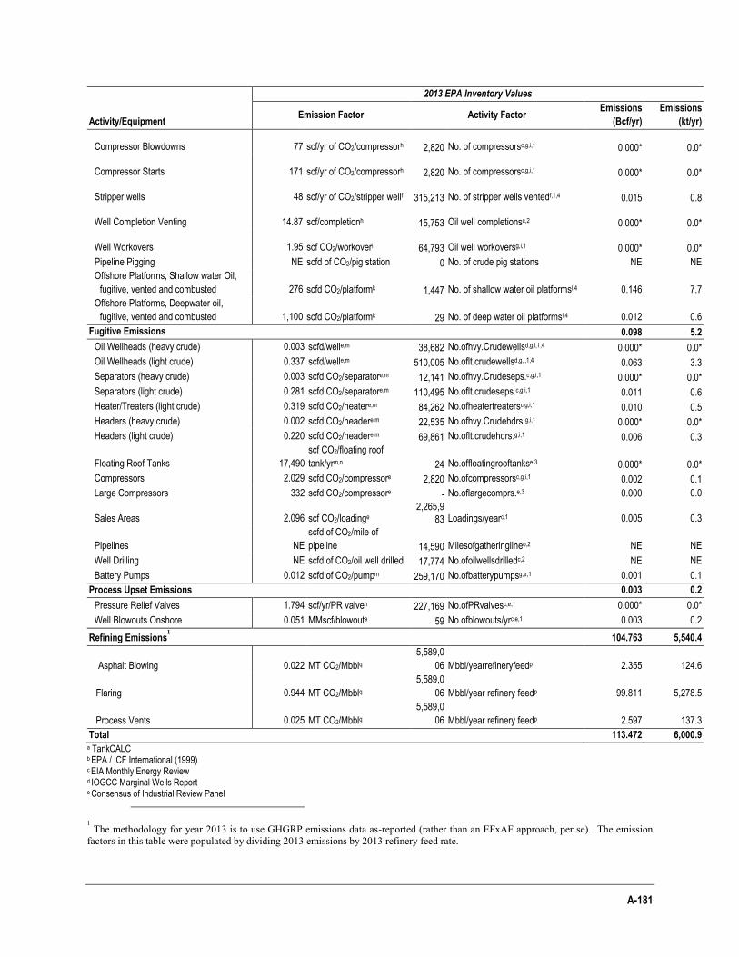
A-181
Activity/Equipment
2013 EPA Inventory Values
Emission Factor Activity Factor Emissions
(Bcf/yr)
Emissions
(kt/yr)
Compressor Blowdowns 77 scf/yr of CO2/compressorh 2,820 No. of compressorsc,g,i,1
0.000* 0.0*
Compressor Starts 171 scf/yr of CO2/compressorh 2,820 No. of compressorsc,g,i,1
0.000* 0.0*
Stripper wells 48 scf/yr of CO2/stripper wellf 315,213 No. of stripper wells ventedf,1,4
0.015 0.8
Well Completion Venting 14.87 scf/completionh 15,753 Oil well completionsc,2
0.000* 0.0*
Well Workovers 1.95 scf CO2/workoveri 64,793 Oil well workoversg,i,1
0.000* 0.0*
Pipeline Pigging NE scfd of CO2/pig station 0 No. of crude pig stations NE NE
Offshore Platforms, Shallow water Oil,
fugitive, vented and combusted 276 scfd CO2/platformk 1,447 No. of shallow water oil platformsl,4 0.146 7.7
Offshore Platforms, Deepwater oil,
fugitive, vented and combusted 1,100 scfd CO2/platformk 29 No. of deep water oil platformsl,4 0.012 0.6
Fugitive Emissions 0.098 5.2
Oil Wellheads (heavy crude) 0.003 scfd/welle,m 38,682 No.ofhvy.Crudewellsd,g,i,1,4 0.000* 0.0*
Oil Wellheads (light crude) 0.337 scfd/welle,m 510,005 No.oflt.crudewellsd,g,i,1,4 0.063 3.3
Separators (heavy crude) 0.003 scfd CO2/separatore,m 12,141 No.ofhvy.Crudeseps.c,g,i,1 0.000* 0.0*
Separators (light crude) 0.281 scfd CO2/separatore,m 110,495 No.oflt.crudeseps.c,g,i,1 0.011 0.6
Heater/Treaters (light crude) 0.319 scfd CO2/heatere,m 84,262 No.ofheatertreatersc,g,i,1 0.010 0.5
Headers (heavy crude) 0.002 scfd CO2/headere,m 22,535 No.ofhvy.Crudehdrs.g,i,1 0.000* 0.0*
Headers (light crude) 0.220 scfd CO2/headere,m 69,861 No.oflt.crudehdrs.g,i,1 0.006 0.3
Floating Roof Tanks 17,490
scf CO2/floating roof
tank/yrm,n 24 No.offloatingrooftankse,3 0.000* 0.0*
Compressors 2.029 scfd CO2/compressore 2,820 No.ofcompressorsc,g,i,1 0.002 0.1
Large Compressors 332 scfd CO2/compressore - No.oflargecomprs.e,3 0.000 0.0
Sales Areas 2.096 scf CO2/loadinge 2,265,9
83 Loadings/yearc,1 0.005 0.3
Pipelines NE
scfd of CO2/mile of
pipeline 14,590 Milesofgatheringlineo,2 NE NE
Well Drilling NE scfd of CO2/oil well drilled 17,774 No.ofoilwellsdrilledc,2 NE NE
Battery Pumps 0.012 scfd of CO2/pumpm 259,170 No.ofbatterypumpsg,e,1 0.001 0.1
Process Upset Emissions 0.003 0.2
Pressure Relief Valves 1.794 scf/yr/PR valveh 227,169 No.ofPRvalvesc,e,1 0.000* 0.0*
Well Blowouts Onshore 0.051 MMscf/blowoute 59 No.ofblowouts/yrc,e,1 0.003 0.2
Refining Emissions1
104.763 5,540.4
Asphalt Blowing 0.022 MT CO2/Mbblq
5,589,0
06 Mbbl/yearrefineryfeedp 2.355 124.6
Flaring 0.944 MT CO2/Mbblq
5,589,0
06 Mbbl/year refinery feedp 99.811 5,278.5
Process Vents 0.025 MT CO2/Mbblq
5,589,0
06 Mbbl/year refinery feedp 2.597 137.3
Total 113.472 6,000.9 a TankCALC b EPA / ICF International (1999) c EIA Monthly Energy Review d IOGCC Marginal Wells Report e Consensus of Industrial Review Panel
1 The methodology for year 2013 is to use GHGRP emissions data as-reported (rather than an EFxAF approach, per se). The emission
factors in this table were populated by dividing 2013 emissions by 2013 refinery feed rate.
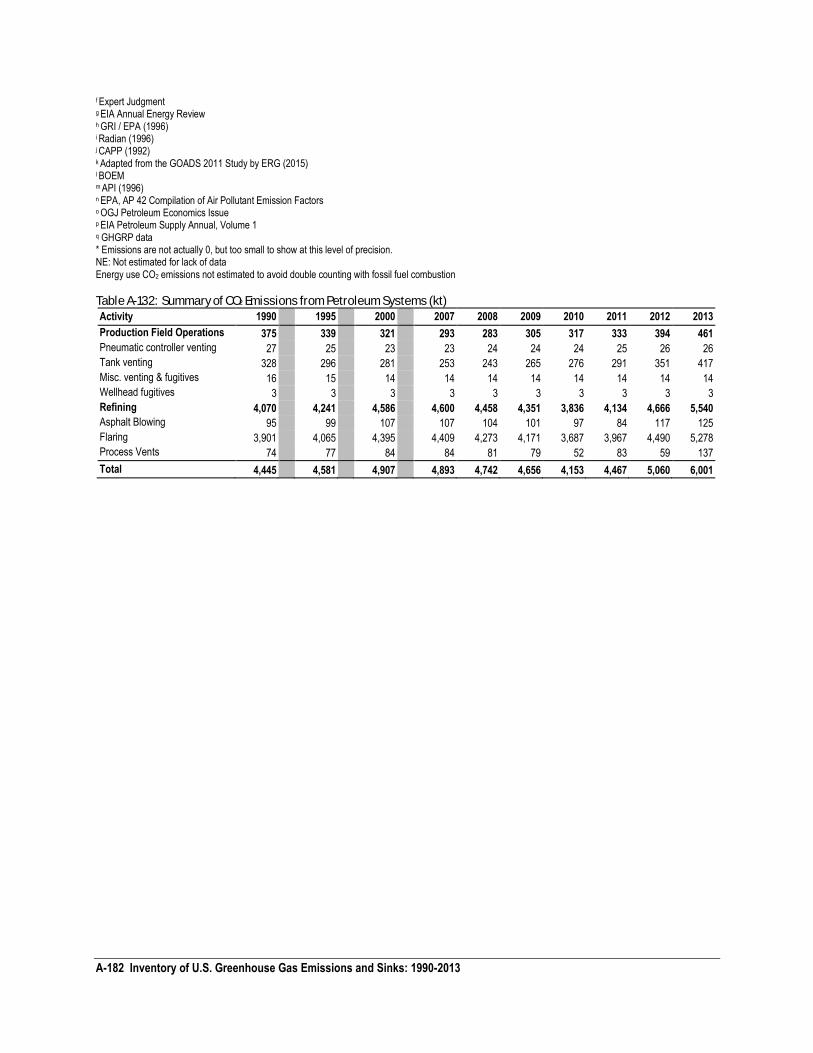
A-182 Inventory of U.S. Greenhouse Gas Emissions and Sinks: 1990-2013
f Expert Judgment g EIA Annual Energy Review h GRI / EPA (1996) i Radian (1996) j CAPP (1992) k Adapted from the GOADS 2011 Study by ERG (2015) l BOEM m API (1996) n EPA, AP 42 Compilation of Air Pollutant Emission Factors o OGJ Petroleum Economics Issue p EIA Petroleum Supply Annual, Volume 1 q GHGRP data * Emissions are not actually 0, but too small to show at this level of precision. NE: Not estimated for lack of data Energy use CO2 emissions not estimated to avoid double counting with fossil fuel combustion
Table A-132: Summary of CO2 Emissions from Petroleum Systems (kt)
Activity 1990 1995 2000 2007 2008 2009 2010 2011 2012 2013
Production Field Operations 375 339 321 293 283 305 317 333 394 461
Pneumatic controller venting 27 25 23 23 24 24 24 25 26 26
Tank venting 328 296 281 253 243 265 276 291 351 417
Misc. venting & fugitives 16 15 14 14 14 14 14 14 14 14
Wellhead fugitives 3 3 3 3 3 3 3 3 3 3
Refining 4,070 4,241 4,586 4,600 4,458 4,351 3,836 4,134 4,666 5,540
Asphalt Blowing 95 99 107 107 104 101 97 84 117 125
Flaring 3,901 4,065 4,395 4,409 4,273 4,171 3,687 3,967 4,490 5,278
Process Vents 74 77 84 84 81 79 52 83 59 137
Total 4,445 4,581 4,907 4,893 4,742 4,656 4,153 4,467 5,060 6,001
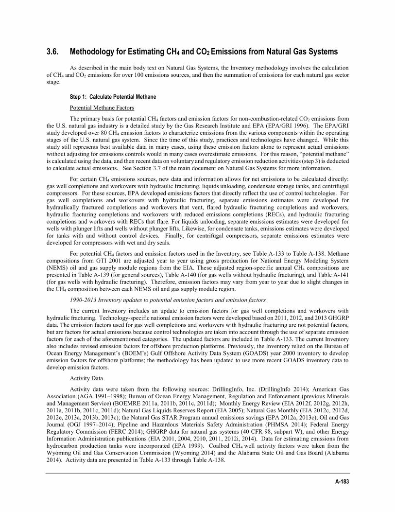
A-183
3.6. Methodology for Estimating CH4 and CO2 Emissions from Natural Gas Systems
As described in the main body text on Natural Gas Systems, the Inventory methodology involves the calculation of CH4 and CO2 emissions for over 100 emissions sources, and then the summation of emissions for each natural gas sector stage.
Step 1: Calculate Potential Methane
Potential Methane Factors
The primary basis for potential CH4 factors and emission factors for non-combustion-related CO2 emissions from the U.S. natural gas industry is a detailed study by the Gas Research Institute and EPA (EPA/GRI 1996). The EPA/GRI study developed over 80 CH4 emission factors to characterize emissions from the various components within the operating stages of the U.S. natural gas system. Since the time of this study, practices and technologies have changed. While this study still represents best available data in many cases, using these emission factors alone to represent actual emissions without adjusting for emissions controls would in many cases overestimate emissions. For this reason, “potential methane” is calculated using the data, and then recent data on voluntary and regulatory emission reduction activities (step 3) is deducted to calculate actual emissions. See Section 3.7 of the main document on Natural Gas Systems for more information.
For certain CH4 emissions sources, new data and information allows for net emissions to be calculated directly: gas well completions and workovers with hydraulic fracturing, liquids unloading, condensate storage tanks, and centrifugal compressors. For these sources, EPA developed emissions factors that directly reflect the use of control technologies. For gas well completions and workovers with hydraulic fracturing, separate emissions estimates were developed for hydraulically fractured completions and workovers that vent, flared hydraulic fracturing completions and workovers, hydraulic fracturing completions and workovers with reduced emissions completions (RECs), and hydraulic fracturing completions and workovers with RECs that flare. For liquids unloading, separate emissions estimates were developed for wells with plunger lifts and wells without plunger lifts. Likewise, for condensate tanks, emissions estimates were developed for tanks with and without control devices. Finally, for centrifugal compressors, separate emissions estimates were developed for compressors with wet and dry seals.
For potential CH4 factors and emission factors used in the Inventory, see Table A-133 to Table A-138. Methane compositions from GTI 2001 are adjusted year to year using gross production for National Energy Modeling System (NEMS) oil and gas supply module regions from the EIA. These adjusted region-specific annual CH4 compositions are presented in Table A-139 (for general sources), Table A-140 (for gas wells without hydraulic fracturing), and Table A-141 (for gas wells with hydraulic fracturing). Therefore, emission factors may vary from year to year due to slight changes in the CH4 composition between each NEMS oil and gas supply module region.
1990-2013 Inventory updates to potential emission factors and emission factors
The current Inventory includes an update to emission factors for gas well completions and workovers with hydraulic fracturing. Technology-specific national emission factors were developed based on 2011, 2012, and 2013 GHGRP data. The emission factors used for gas well completions and workovers with hydraulic fracturing are not potential factors, but are factors for actual emissions because control technologies are taken into account through the use of separate emission factors for each of the aforementioned categories. The updated factors are included in Table A-133. The current Inventory also includes revised emission factors for offshore production platforms. Previously, the Inventory relied on the Bureau of Ocean Energy Management’s (BOEM’s) Gulf Offshore Activity Data System (GOADS) year 2000 inventory to develop emission factors for offshore platforms; the methodology has been updated to use more recent GOADS inventory data to develop emission factors.
Activity Data
Activity data were taken from the following sources: DrillingInfo, Inc. (DrillingInfo 2014); American Gas Association (AGA 1991–1998); Bureau of Ocean Energy Management, Regulation and Enforcement (previous Minerals and Management Service) (BOEMRE 2011a, 2011b, 2011c, 2011d); Monthly Energy Review (EIA 2012f, 2012g, 2012h, 2011a, 2011b, 2011c, 2011d); Natural Gas Liquids Reserves Report (EIA 2005); Natural Gas Monthly (EIA 2012c, 2012d, 2012e, 2013a, 2013b, 2013c); the Natural Gas STAR Program annual emissions savings (EPA 2012a, 2013c); Oil and Gas Journal (OGJ 1997–2014); Pipeline and Hazardous Materials Safety Administration (PHMSA 2014); Federal Energy Regulatory Commission (FERC 2014); GHGRP data for natural gas systems (40 CFR 98, subpart W); and other Energy Information Administration publications (EIA 2001, 2004, 2010, 2011, 2012i, 2014). Data for estimating emissions from hydrocarbon production tanks were incorporated (EPA 1999). Coalbed CH4 well activity factors were taken from the Wyoming Oil and Gas Conservation Commission (Wyoming 2014) and the Alabama State Oil and Gas Board (Alabama 2014). Activity data are presented in Table A-133 through Table A-138.
A-184 Inventory of U.S. Greenhouse Gas Emissions and Sinks: 1990-2013
For a few sources, recent direct activity data were not available. For these sources, either 2012 data were used as proxy for 2013 data or a set of industry activity data drivers was developed and was used to update activity data. Drivers include statistics on gas production, number of wells, system throughput, miles of various kinds of pipe, and other statistics that characterize the changes in the U.S. natural gas system infrastructure and operations. For example, recent data on various types of field separation equipment in the production stage (i.e., heaters, separators, and dehydrators) were unavailable. EPA determined that each of these types of field separation equipment relate to the number of non-associated gas wells. Using the number of each type of field separation equipment estimated by GRI/EPA in 1992, and the number of non-associated gas wells in 1992, EPA developed a factor that is used to estimate the number of each type of field separation equipment throughout the time series. The key activity drivers are presented in Table A-142.
EPA used DI Desktop, a production database maintained by DrillingInfo, Inc. (DrillingInfo 2014), covering U.S. oil and natural gas wells to populate activity data for non-associated gas wells, oil wells, associated gas wells, gas wells with hydraulic fracturing, and completions with hydraulic fracturing. EPA queried DI Desktop for relevant data on an individual well basis—including location, natural gas and liquids (i.e., oil and condensate) production by year, drill type (e.g., horizontal or vertical), and date of completion or first production. Non-associated gas wells were classified as any well within DI Desktop that had non-zero gas production in a given year, and with a gas-to-oil ratio (GOR) of greater than 100 mcf/bbl in that year. Oil wells were classified as any well that had non-zero liquids production in a given year, and with a GOR of less than or equal to 100 mcf/bbl in that year. Associated gas wells were identified as a subset of oil wells with nonzero gas production in a given year. Both oil and condensate are included in the liquids production data in DI Desktop; therefore, the count of associated gas wells may include wells that produce gas and condensate only. Gas wells with hydraulic fracturing were assumed to be the subset of the non-associated gas wells that were horizontally drilled and/or located in an unconventional formation (i.e., shale, tight sands, or coalbed). Unconventional formations were identified based on well basin, reservoir, and field data reported in DI Desktop referenced against a formation type crosswalk developed by EIA (EIA 2012a).
For 1990 through 2010, gas well completions with hydraulic fracturing were identified as a subset of the gas wells with hydraulic fracturing that had a date of completion or first production in the specified year. To calculate workovers for 1990 through 2010, EPA applied a refracture rate of 1 percent (i.e., 1 percent of all wells with hydraulic fracturing are assumed to be refractured in a given year) to the total counts of wells with hydraulic fracturing from the DrillingInfo data. For 2011 through 2013, EPA used GHGRP data for the total number of well completions and workovers. The GHGRP data represents a subset of the national completions and workovers, due to the reporting threshold, and therefore using this data without scaling it up to national level results in an underestimate. However, because EPA’s GHGRP counts of completions and workovers were higher than national counts of completions and workovers, obtained using DI Desktop data, EPA directly used the GHGRP data for completions and workovers for 2011 through 2013.
EPA calculated the percentage of gas well completions and workovers with hydraulic fracturing in the each of the four control categories using 2011 through 2013 Subpart W data. EPA assumed 0 percent RECs use from 1990 through 2000, used GHGRP RECs percentage for 2011 through 2013, and then used linear interpolation between the 2000 and 2011 percentages. For flaring, EPA used an assumption of 10 percent (the average of the percent of completions and workovers that were flared in 2011 through 2013 GHGRP data) flaring from 1990 through 2010 to recognize that some flaring has occurred over that time period. For 2011 through 2013, EPA used the GHGRP data on flaring.
Step 2: Compile Reductions Data
The emissions calculated in Step 1 above represent expected emissions from an activity in the absence of emissions controls (with the exceptions of gas well completions and workovers with hydraulic fracturing, liquids unloading, centrifugal compressors, and condensate tanks, as noted above), and do not take into account any use of technologies or practices that reduce emissions. To take into account use of such technologies, data were collected on voluntary and regulatory reductions. Voluntary reductions included in the Inventory were those reported to Gas STAR for activities such as replacing a high bleed pneumatic controllers with a low bleed controller and replacing wet seals with dry seals at reciprocating compressors. Regulatory actions reducing emissions include National Emission Standards for Hazardous Air Pollutants (NESHAP) regulations for dehydrator vents and condensate tanks.
Voluntary reductions. Industry partners report CH4 emission reductions by project to the Natural Gas STAR Program. The reductions from the implementation of specific technologies and practices (e.g., vapor recovery units, centrifugal compressors, etc.) are calculated by the reporting partners using actual measurement data or equipment-specific emission factors. Natural Gas STAR Partners do not report reductions when they are required due to regulation. Therefore, the Inventory assumes there is no overlap between the reductions reported through Natural Gas STAR and reductions due to state regulations. The reductions undergo quality assurance and quality control checks to identify errors, inconsistencies, or irregular data before being incorporated into the Inventory. In general, the Inventory uses aggregated Gas STAR
A-185
reductions by natural gas system stage (i.e., production, processing, transmission and storage, and distribution). However, aggregate emissions reductions data by Gas STAR technology are provided for several sources, as shown in Table A-143. For those sources, EPA has also used data on potential emissions, and the Gas STAR data on reductions, to calculate net emissions, as shown in Table A-149. Many of the activities reported to Gas STAR are cross-cutting and apply to more than one emissions source and therefore cannot be assigned to one emissions source, but instead are included in the “other” category. For Inventory sources with emission factors that already take into account the use of control technologies (i.e., gas well completions and workovers with hydraulic fracturing, liquids unloading, and condensate storage tanks) Natural Gas STAR reported reductions for those activities are not incorporated into the Inventory, as this would double count reductions. CH4 emission reductions from the Natural Gas STAR Program are summarized in Table A-143.
Federal regulations. The 1990 Clean Air Act (CAA) sets limits on the amount of hazardous air pollutants (HAPs) that can be emitted in the United States. The NESHAP regulations set the standards to limit emissions of HAPs. The emission sources are required to use the Maximum Achievable Control Technology (MACT), giving the operators flexibility to choose the type of control measure(s) to implement. In regards to the oil and natural gas industry, the NESHAP regulation addresses HAPs from the oil and natural gas production sectors and the natural gas transmission and storage sectors of the industry. Though the regulation deals specifically with HAPs reductions, methane emissions are also incidentally reduced.
The NESHAP regulation requires that glycol dehydration unit vents and storage tanks that have HAP emissions and exceed a gas throughput and liquids throughput threshold, respectively, be connected to a closed loop emission control system that reduces emissions by 95 percent. Also, gas processing plants exceeding the threshold natural gas throughput limit are required to routinely implement Leak Detection and Repair (LDAR) programs. The emissions reductions achieved as a result of NESHAP regulations were calculated using data provided in the Federal Register Background Information Document (BID) for this regulation. The BID provides the levels of control measures in place before the enactment of regulation. The emissions reductions were estimated by analyzing the portion of the industry without control measures already in place that would be impacted by the regulation. CH4 emission reductions from federal regulations, such as NESHAP, are summarized in Table A-144. In addition to the NESHAP applicable to natural gas, future Inventories will reflect the 2012 New Source Performance Standards (NSPS) for oil and gas. By separating gas well completions and workovers with hydraulic fracturing into four categories and developing control technology-specific methane emission factors for each category, EPA is implicitly accounting for NSPS reductions from hydraulically fractured gas wells. The rule also has VOC reduction requirements for compressors, storage vessels, pneumatic controllers, and equipment leaks at processing plants, which will also impact CH4 emissions in future Inventories.
Step 3: Calculate Net Emissions
For CH4, the reductions described above in Step 2 are summed and deducted from the potential CH4 emissions calculated in Step 1. These net emissions are reported in the Natural Gas Systems inventory text.
The same procedure for estimating CH4 emissions holds true for estimating non-energy related CO2 emissions, except the emission estimates are not adjusted for reductions due to the Natural Gas STAR program or regulations.
Produced natural gas is composed of primarily CH4, but as shown in Table A-150, the natural gas contains, in some cases, as much as 8 percent CO2. The same vented and fugitive natural gas that led to CH4 emissions also contains a certain volume of CO2. Accordingly, the CO2 emissions for each sector can be estimated using the same activity data for these vented and fugitive sources. The emission factors used to estimate CH4 were also used to calculate non-combustion CO2 emissions. The Gas Technology Institute’s (GTI, formerly GRI) Unconventional Natural Gas and Gas Composition Databases (GTI 2001) were used to adapt the CH4 emission factors into non-combustion related CO2 emission factors. Additional information about CO2 content in transmission quality natural gas was obtained from numerous U.S. transmission companies to help further develop the non-combustion CO2 emission factors. For the CO2 content used to develop CO2 emission factors from CH4 potential factors, see Table A-150. The detailed source emission estimates for CH4 and CO2 from the production sector are presented in Table A-145 and Table A-154, respectively.
In the processing sector, the CO2 content of the natural gas remains the same as the CO2 content in the production sector for the equipment upstream of the acid gas removal unit because produced natural gas is usually only minimally treated after being produced and then transported to natural gas processing plants via gathering pipelines. The CO2 content in gas for the remaining equipment that is downstream of the acid gas removal is the same as in pipeline quality gas. The EPA/GRI study estimates the average CH4 content of natural gas in the processing sector to be 87 percent CH4. Consequently, the processing sector CO2 emission factors were developed using CH4 emission factors, proportioned to reflect the CO2 content of either produced natural gas or pipeline quality gas using the same methodology as the production sector. The detailed source emission estimates for CH4 and CO2 from the processing sector are presented in Table A-146 and Table A-152, respectively.
A-186 Inventory of U.S. Greenhouse Gas Emissions and Sinks: 1990-2013
For the transmission sector, CO2 content in natural gas transmission pipelines was estimated for the top 20 transmission pipeline companies in the United States (separate analyses identified the top 20 companies based on gas throughput and total pipeline miles). The weighted average CO2 content in the transmission pipeline quality gas in both cases—total gas throughput and total miles of pipeline—was estimated to be about 1 percent. To estimate the CO2 emissions for the transmission sector, the CH4 emission factors were proportioned from the 93.4 percent CH4 reported in EPA/GRI (1996) to reflect the 1 percent CO2 content found in transmission quality natural gas. The detailed source emissions estimates for CH4 and CO2 for the transmission sector are presented in Table A-147 and Table A-153, respectively.
The natural gas in the distribution sector of the system has the same characteristics as the natural gas in the transmission sector. The CH4 content (93.4 percent) and CO2 content (1 percent) are identical to transmission segment contents due to the absence of any further treatment between sector boundaries. Thus, the CH4 emissions factors were converted to CO2 emission factors using the same methodology as discussed for the transmission sector. The detailed source emission estimates for CH4 and CO2 for the distribution sector are presented in Table A-148 and Table A-154, respectively.
Three exceptions to this methodology are CO2 emissions from flares, CO2 from acid gas removal units, and CO2 from condensate tanks. In the case of flare emissions, a direct CO2 emission factor from EIA (1996) was used. This emission factor was applied to the portion of offshore gas that is not vented and all of the gas reported as vented and flared onshore by EIA, including associated gas. The amount of CO2 emissions from an acid gas unit in a processing plant is equal to the difference in CO2 concentrations between produced natural gas and pipeline quality gas applied to the throughput of the plant. This methodology was applied to the national gas throughput using national average CO2 concentrations in produced gas (3.45 percent) and transmission quality gas (1 percent). Data were unavailable to use annual values for CO2 concentration. For condensate tanks, a series of E&P Tank (EPA 1999) simulations provide the total CO2 vented per barrel of condensate throughput from fixed roof tank flash gas for condensate gravities of API 45 degree and higher. The ratios of emissions to throughput were used to estimate the CO2 emission factor for condensate passing through fixed roof tanks.
Table A-133 through Table A-138 display the 2012 activity data, CH4 emission factors, and calculated potential CH4 emissions for each stage.
The tables provide references for emission factors and activity data in footnotes (i.e., lettered footnotes). The tables also provide information on which method was used for supplying activity data for 2013 (i.e., numbered footnotes).
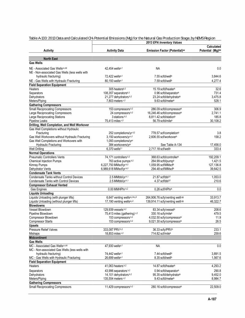
A-187
Table A-133: 2013 Data and Calculated CH4 Potential Emissions (Mg) for the Natural Gas Production Stage, by NEMS Region 2013 EPA Inventory Values
Activity Activity Data Emission Factor (Potential)aa Calculated
Potential (Mg)bb
North East
Gas Wells
NE - Associated Gas Wellscc,dd 42,454 wellsa,1 NA 0.0 NE - Non-associated Gas Wells (less wells with
hydraulic fracturing) 72,422 wellsa,1 7.55 scfd/wellb 3,844.6
NE - Gas Wells with Hydraulic Fracturing 80,193 wellsa,1 7.59 scfd/wellb 4,277.4
Field Separation Equipment
Heaters 305 heatersb,2 15.19 scfd/heaterb 32.6 Separators 108,357 separatorsb,2 0.96 scfd/separatorb 731.4 Dehydrators 21,277 dehydrators b,2 23.24 scfd/dehydratorb 3,475.8 Meters/Piping 7,803 meters c,2 9.63 scfd/meterb 528.1
Gathering Compressors
Small Reciprocating Compressors 153 compressors b,2 286.09 scfd/compressorb 306.9 Large Reciprocating Compressors 24 compressors b,2 16,246.46 scfd/compressorb 2,741.1 Large Reciprocating Stations 3 stations b,2 8,811.42 scfd/stationb 185.8 Pipeline Leaks 75,413 miles c,2 56.79 scfd/mileb 30,108.2
Drilling, Well Completion, and Well Workover
Gas Well Completions without Hydraulic Fracturing 252 completions/yr d,2 778.57 scf/completionb 3.8
Gas Well Workovers without Hydraulic Fracturing 3,150 workovers/yr a,1 2,606.55 scf/workoverb 158.2 Gas Well Completions and Workovers with
Hydraulic Fracturing 1,093 completions/yro
384 workovers/yro See Table A-134 17,456.0
Well Drilling 6,370 wellsf,1 2,717.18 scf/wellg 333.4
Normal Operations
Pneumatic Controllers Vents 74,171 controllers b,2 368.63 scfd/controllerb 192,209.1 Chemical Injection Pumps 763 active pumps b,2 264.99 scfd/pumpb 1,421.5 Kimray Pumps 6,227,750 MMscf/yr b,2 1,059.95 scf/MMscfb 127,136.8 Dehydrator Vents 6,989,618 MMscf/yr b,2 294.48 scf/MMscfb 39,642.5
Condensate Tank Vents
Condensate Tanks without Control Devices 2.5 MMbbl/yr h,1 21.87 scf/bbli,ff 1,053.0 Condensate Tanks with Control Devices 2.5 MMbbl/yr h,1 4.37 scf/bbli,ff 210.6
Compressor Exhaust Vented
Gas Engines 0.00 MMHPhr b,2 0.26 scf/HPhrb 0.0
Liquids Unloading
Liquids Unloading (with plunger lifts) 6,647 venting wellsa,j,2a,j,2 264,906.76 scfy/venting wellj,gg 33,913.7 Liquids Unloading (without plunger lifts) 17,190 venting wellsa,j,2 139,914.11 scfy/venting wellj,gg 46,322.7
Blowdowns
Vessel Blowdown 129,939 vessels b,2 83.34 scfy/vesselb 208.6 Pipeline Blowdown 75,413 miles (gathering) c,2 330.16 scfy/mileb 479.5 Compressor Blowdown 153 compressors b,2 4,032.50 scfy/compressorb 11.9 Compressor Starts 153 compressors b,2 9,021.30 scfy/compressorb 26.5
Upsets
Pressure Relief Valves 333,087 PRV b,2 36.33 scfy/PRVb 233.1 Mishaps 18,853 miles c,2 714.82 scf/mileb 259.6
Midcontinent
Gas Wells
MC - Associated Gas Wellscc,dd 47,930 wellsa,1 NA 0.0 MC - Non-associated Gas Wells (less wells with
hydraulic fracturing) 74,442 wellsa,1 7.44 scfd/wellb 3,891.5 MC - Gas Wells with Hydraulic Fracturing 26,699 wellsa,1 8.35 scfd/wellb 1,567.6
Field Separation Equipment
Heaters 41,063 heaters b,2 14.87 scfd/heaterb 4,293.2
Separators 43,996 separators b,2 0.94 scfd/separatorb 290.8 Dehydrators 14,101 dehydrators b,2 95.35 scfd/dehydratorb 9,452.0 Meters/Piping 135,554 meters c,2 9.43 scfd/meterb 8,984.7
Gathering Compressors
Small Reciprocating Compressors 11,429 compressors b,2 280.16 scfd/compressorb 22,509.0
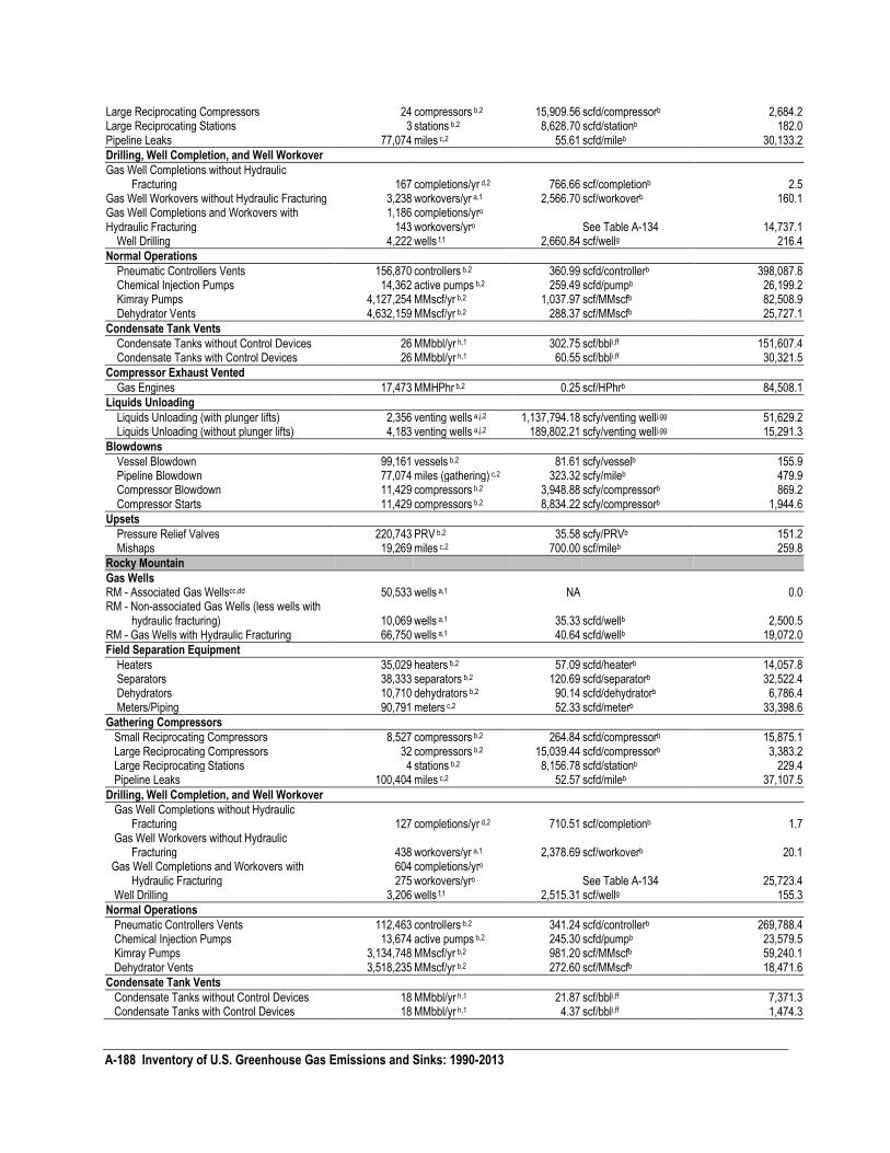
A-188 Inventory of U.S. Greenhouse Gas Emissions and Sinks: 1990-2013
Large Reciprocating Compressors 24 compressors b,2 15,909.56 scfd/compressorb 2,684.2 Large Reciprocating Stations 3 stations b,2 8,628.70 scfd/stationb 182.0 Pipeline Leaks 77,074 miles c,2 55.61 scfd/mileb 30,133.2
Drilling, Well Completion, and Well Workover
Gas Well Completions without Hydraulic Fracturing 167 completions/yr d,2 766.66 scf/completionb 2.5
Gas Well Workovers without Hydraulic Fracturing 3,238 workovers/yr a,1 2,566.70 scf/workoverb 160.1 Gas Well Completions and Workovers with Hydraulic Fracturing
1,186 completions/yro 143 workovers/yro See Table A-134 14,737.1
Well Drilling 4,222 wells f,1 2,660.84 scf/wellg 216.4
Normal Operations
Pneumatic Controllers Vents 156,870 controllers b,2 360.99 scfd/controllerb 398,087.8 Chemical Injection Pumps 14,362 active pumps b,2 259.49 scfd/pumpb 26,199.2 Kimray Pumps 4,127,254 MMscf/yr b,2 1,037.97 scf/MMscfb 82,508.9 Dehydrator Vents 4,632,159 MMscf/yr b,2 288.37 scf/MMscfb 25,727.1
Condensate Tank Vents
Condensate Tanks without Control Devices 26 MMbbl/yr h,1 302.75 scf/bbli,ff 151,607.4 Condensate Tanks with Control Devices 26 MMbbl/yr h,1 60.55 scf/bbli,ff 30,321.5
Compressor Exhaust Vented
Gas Engines 17,473 MMHPhr b,2 0.25 scf/HPhrb 84,508.1
Liquids Unloading
Liquids Unloading (with plunger lifts) 2,356 venting wells a,j,2 1,137,794.18 scfy/venting wellj,gg 51,629.2 Liquids Unloading (without plunger lifts) 4,183 venting wells a,j,2 189,802.21 scfy/venting wellj,gg 15,291.3
Blowdowns
Vessel Blowdown 99,161 vessels b,2 81.61 scfy/vesselb 155.9 Pipeline Blowdown 77,074 miles (gathering) c,2 323.32 scfy/mileb 479.9 Compressor Blowdown 11,429 compressors b,2 3,948.88 scfy/compressorb 869.2 Compressor Starts 11,429 compressors b,2 8,834.22 scfy/compressorb 1,944.6
Upsets
Pressure Relief Valves 220,743 PRV b,2 35.58 scfy/PRVb 151.2 Mishaps 19,269 miles c,2 700.00 scf/mileb 259.8
Rocky Mountain
Gas Wells RM - Associated Gas Wellscc,dd 50,533 wells a,1 NA 0.0 RM - Non-associated Gas Wells (less wells with
hydraulic fracturing) 10,069 wells a,1 35.33 scfd/wellb 2,500.5 RM - Gas Wells with Hydraulic Fracturing 66,750 wells a,1 40.64 scfd/wellb 19,072.0
Field Separation Equipment
Heaters 35,029 heaters b,2 57.09 scfd/heaterb 14,057.8 Separators 38,333 separators b,2 120.69 scfd/separatorb 32,522.4 Dehydrators 10,710 dehydrators b,2 90.14 scfd/dehydratorb 6,786.4 Meters/Piping 90,791 meters c,2 52.33 scfd/meterb 33,398.6
Gathering Compressors
Small Reciprocating Compressors 8,527 compressors b,2 264.84 scfd/compressorb 15,875.1 Large Reciprocating Compressors 32 compressors b,2 15,039.44 scfd/compressorb 3,383.2 Large Reciprocating Stations 4 stations b,2 8,156.78 scfd/stationb 229.4 Pipeline Leaks 100,404 miles c,2 52.57 scfd/mileb 37,107.5
Drilling, Well Completion, and Well Workover
Gas Well Completions without Hydraulic Fracturing 127 completions/yr d,2 710.51 scf/completionb 1.7
Gas Well Workovers without Hydraulic Fracturing 438 workovers/yr a,1 2,378.69 scf/workoverb 20.1
Gas Well Completions and Workovers with Hydraulic Fracturing
604 completions/yro 275 workovers/yro See Table A-134 25,723.4
Well Drilling 3,206 wells f,1 2,515.31 scf/wellg 155.3
Normal Operations
Pneumatic Controllers Vents 112,463 controllers b,2 341.24 scfd/controllerb 269,788.4 Chemical Injection Pumps 13,674 active pumps b,2 245.30 scfd/pumpb 23,579.5 Kimray Pumps 3,134,748 MMscf/yr b,2 981.20 scf/MMscfb 59,240.1 Dehydrator Vents 3,518,235 MMscf/yr b,2 272.60 scf/MMscfb 18,471.6
Condensate Tank Vents
Condensate Tanks without Control Devices 18 MMbbl/yr h,1 21.87 scf/bbli,ff 7,371.3 Condensate Tanks with Control Devices 18 MMbbl/yr h,1 4.37 scf/bbli,ff 1,474.3
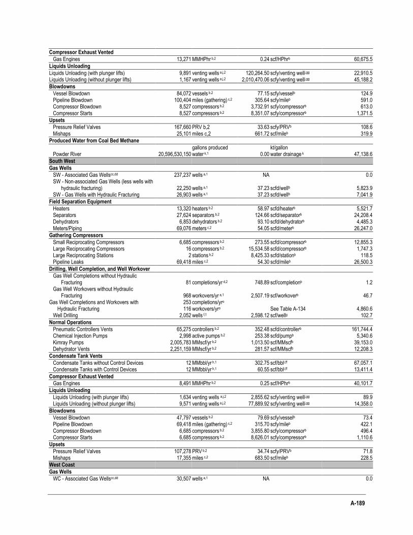
A-189
Compressor Exhaust Vented
Gas Engines 13,271 MMHPhr b,2 0.24 scf/HPhrb 60,675.5
Liquids Unloading
Liquids Unloading (with plunger lifts) 9,891 venting wells a,j,2 120,264.50 scfy/venting wellj,gg 22,910.5 Liquids Unloading (without plunger lifts) 1,167 venting wells a,j,2 2,010,470.06 scfy/venting wellj,gg 45,188.2
Blowdowns
Vessel Blowdown 84,072 vessels b,2 77.15 scfy/vesselb 124.9 Pipeline Blowdown 100,404 miles (gathering) c,2 305.64 scfy/mileb 591.0 Compressor Blowdown 8,527 compressors b,2 3,732.91 scfy/compressorb 613.0 Compressor Starts 8,527 compressors b,2 8,351.07 scfy/compressorb 1,371.5
Upsets
Pressure Relief Valves 167,660 PRV b,2 33.63 scfy/PRVb 108.6 Mishaps 25,101 miles c,2 661.72 scf/mileb 319.9
Produced Water from Coal Bed Methane
Powder River 20,596,530,150 gallons produced water k,1 0.00
kt/gallon water drainage k 47,138.6
South West
Gas Wells
SW - Associated Gas Wellscc,dd 237,237 wells a,1 NA 0.0 SW - Non-associated Gas Wells (less wells with
hydraulic fracturing) 22,250 wells a,1 37.23 scfd/wellb 5,823.9 SW - Gas Wells with Hydraulic Fracturing 26,903 wells a,1 37.23 scfd/wellb 7,041.9
Field Separation Equipment
Heaters 13,320 heaters b,2 58.97 scfd/heaterb 5,521.7 Separators 27,624 separators b,2 124.66 scfd/separatorb 24,208.4 Dehydrators 6,853 dehydrators b,2 93.10 scfd/dehydratorb 4,485.3 Meters/Piping 69,076 meters c,2 54.05 scfd/meterb 26,247.0
Gathering Compressors
Small Reciprocating Compressors 6,685 compressors b,2 273.55 scfd/compressorb 12,855.3 Large Reciprocating Compressors 16 compressors b,2 15,534.58 scfd/compressorb 1,747.3 Large Reciprocating Stations 2 stations b,2 8,425.33 scfd/stationb 118.5 Pipeline Leaks 69,418 miles c,2 54.30 scfd/mileb 26,500.3
Drilling, Well Completion, and Well Workover
Gas Well Completions without Hydraulic Fracturing 81 completions/yr d,2 748.89 scf/completionb 1.2
Gas Well Workovers without Hydraulic Fracturing 968 workovers/yr a,1 2,507.19 scf/workoverb 46.7
Gas Well Completions and Workovers with Hydraulic Fracturing
253 completions/yro 116 workovers/yro See Table A-134 4,860.6
Well Drilling 2,052 wells f,1 2,598.12 scf/wellg 102.7
Normal Operations
Pneumatic Controllers Vents 65,275 controllers b,2 352.48 scfd/controllerb 161,744.4 Chemical Injection Pumps 2,998 active pumps b,2 253.38 scfd/pumpb 5,340.6 Kimray Pumps 2,005,783 MMscf/yr b,2 1,013.50 scf/MMscfb 39,153.0 Dehydrator Vents 2,251,159 MMscf/yr b,2 281.57 scf/MMscfb 12,208.3
Condensate Tank Vents
Condensate Tanks without Control Devices 12 MMbbl/yr h,1 302.75 scf/bbli,ff 67,057.1 Condensate Tanks with Control Devices 12 MMbbl/yr h,1 60.55 scf/bbli,ff 13,411.4
Compressor Exhaust Vented
Gas Engines 8,491 MMHPhr b,2 0.25 scf/HPhrb 40,101.7
Liquids Unloading
Liquids Unloading (with plunger lifts) 1,634 venting wells a,j,2 2,855.62 scfy/venting wellj,gg 89.9 Liquids Unloading (without plunger lifts) 9,571 venting wells a,j,2 77,889.92 scfy/venting wellj,gg 14,358.0
Blowdowns
Vessel Blowdown 47,797 vessels b,2 79.69 scfy/vesselb 73.4 Pipeline Blowdown 69,418 miles (gathering) c,2 315.70 scfy/mileb 422.1 Compressor Blowdown 6,685 compressors b,2 3,855.80 scfy/compressorb 496.4 Compressor Starts 6,685 compressors b,2 8,626.01 scfy/compressorb 1,110.6
Upsets
Pressure Relief Valves 107,278 PRV b,2 34.74 scfy/PRVb 71.8 Mishaps 17,355 miles c,2 683.50 scf/mileb 228.5
West Coast
Gas Wells
WC - Associated Gas Wellscc,dd 30,507 wells a,1 NA 0.0
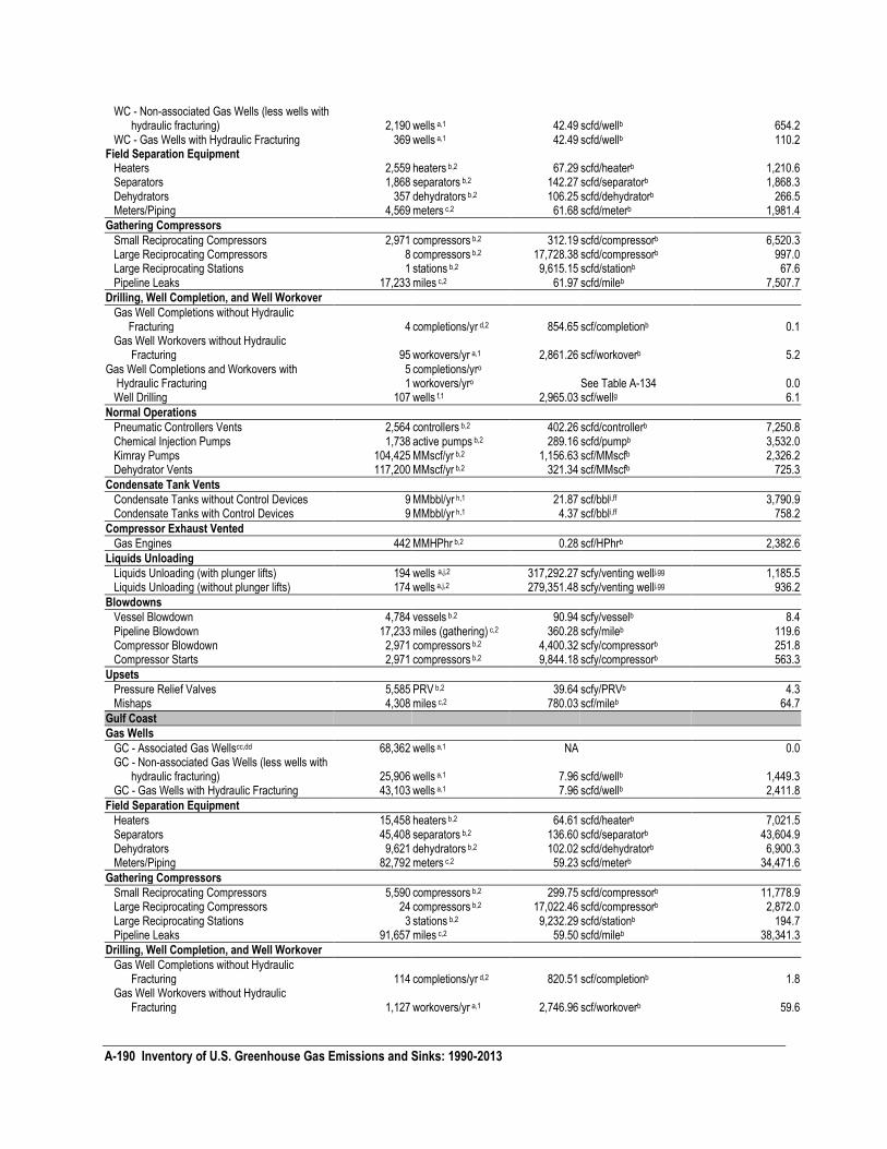
A-190 Inventory of U.S. Greenhouse Gas Emissions and Sinks: 1990-2013
WC - Non-associated Gas Wells (less wells with hydraulic fracturing) 2,190 wells a,1 42.49 scfd/wellb 654.2
WC - Gas Wells with Hydraulic Fracturing 369 wells a,1 42.49 scfd/wellb 110.2 Field Separation Equipment Heaters 2,559 heaters b,2 67.29 scfd/heaterb 1,210.6 Separators 1,868 separators b,2 142.27 scfd/separatorb 1,868.3 Dehydrators 357 dehydrators b,2 106.25 scfd/dehydratorb 266.5 Meters/Piping 4,569 meters c,2 61.68 scfd/meterb 1,981.4
Gathering Compressors
Small Reciprocating Compressors 2,971 compressors b,2 312.19 scfd/compressorb 6,520.3 Large Reciprocating Compressors 8 compressors b,2 17,728.38 scfd/compressorb 997.0 Large Reciprocating Stations 1 stations b,2 9,615.15 scfd/stationb 67.6 Pipeline Leaks 17,233 miles c,2 61.97 scfd/mileb 7,507.7
Drilling, Well Completion, and Well Workover
Gas Well Completions without Hydraulic Fracturing 4 completions/yr d,2 854.65 scf/completionb 0.1
Gas Well Workovers without Hydraulic Fracturing 95 workovers/yr a,1 2,861.26 scf/workoverb 5.2
Gas Well Completions and Workovers with Hydraulic Fracturing
5 completions/yro 1 workovers/yro See Table A-134 0.0
Well Drilling 107 wells f,1 2,965.03 scf/wellg 6.1
Normal Operations
Pneumatic Controllers Vents 2,564 controllers b,2 402.26 scfd/controllerb 7,250.8 Chemical Injection Pumps 1,738 active pumps b,2 289.16 scfd/pumpb 3,532.0 Kimray Pumps 104,425 MMscf/yr b,2 1,156.63 scf/MMscfb 2,326.2 Dehydrator Vents 117,200 MMscf/yr b,2 321.34 scf/MMscfb 725.3
Condensate Tank Vents
Condensate Tanks without Control Devices 9 MMbbl/yr h,1 21.87 scf/bbli,ff 3,790.9 Condensate Tanks with Control Devices 9 MMbbl/yr h,1 4.37 scf/bbli,ff 758.2
Compressor Exhaust Vented
Gas Engines 442 MMHPhr b,2 0.28 scf/HPhrb 2,382.6
Liquids Unloading
Liquids Unloading (with plunger lifts) 194 wells a,j,2 317,292.27 scfy/venting wellj,gg 1,185.5 Liquids Unloading (without plunger lifts) 174 wells a,j,2 279,351.48 scfy/venting wellj,gg 936.2
Blowdowns
Vessel Blowdown 4,784 vessels b,2 90.94 scfy/vesselb 8.4 Pipeline Blowdown 17,233 miles (gathering) c,2 360.28 scfy/mileb 119.6 Compressor Blowdown 2,971 compressors b,2 4,400.32 scfy/compressorb 251.8 Compressor Starts 2,971 compressors b,2 9,844.18 scfy/compressorb 563.3
Upsets
Pressure Relief Valves 5,585 PRV b,2 39.64 scfy/PRVb 4.3 Mishaps 4,308 miles c,2 780.03 scf/mileb 64.7
Gulf Coast
Gas Wells
GC - Associated Gas Wellscc,dd 68,362 wells a,1 NA 0.0 GC - Non-associated Gas Wells (less wells with
hydraulic fracturing) 25,906 wells a,1 7.96 scfd/wellb 1,449.3 GC - Gas Wells with Hydraulic Fracturing 43,103 wells a,1 7.96 scfd/wellb 2,411.8
Field Separation Equipment
Heaters 15,458 heaters b,2 64.61 scfd/heaterb 7,021.5 Separators 45,408 separators b,2 136.60 scfd/separatorb 43,604.9 Dehydrators 9,621 dehydrators b,2 102.02 scfd/dehydratorb 6,900.3 Meters/Piping 82,792 meters c,2 59.23 scfd/meterb 34,471.6
Gathering Compressors
Small Reciprocating Compressors 5,590 compressors b,2 299.75 scfd/compressorb 11,778.9 Large Reciprocating Compressors 24 compressors b,2 17,022.46 scfd/compressorb 2,872.0 Large Reciprocating Stations 3 stations b,2 9,232.29 scfd/stationb 194.7 Pipeline Leaks 91,657 miles c,2 59.50 scfd/mileb 38,341.3
Drilling, Well Completion, and Well Workover
Gas Well Completions without Hydraulic Fracturing 114 completions/yr d,2 820.51 scf/completionb 1.8
Gas Well Workovers without Hydraulic Fracturing 1,127 workovers/yr a,1 2,746.96 scf/workoverb 59.6
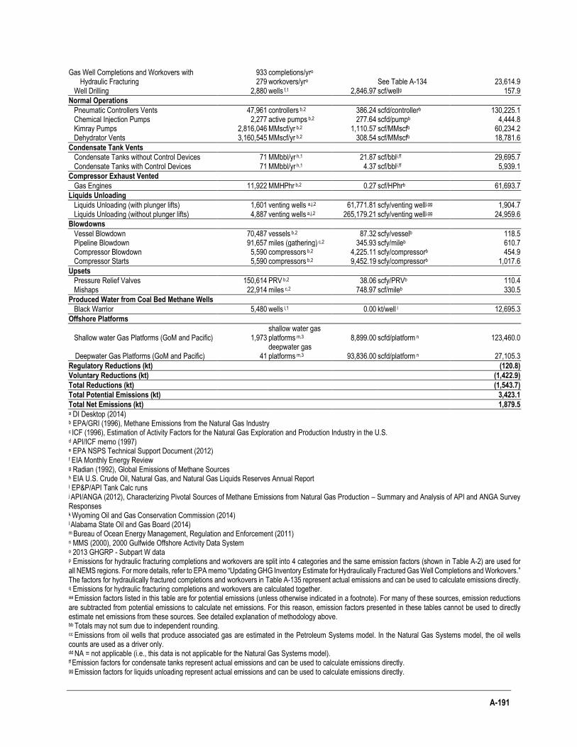
A-191
Gas Well Completions and Workovers with Hydraulic Fracturing
933 completions/yro 279 workovers/yro See Table A-134 23,614.9
Well Drilling 2,880 wells f,1 2,846.97 scf/wellg 157.9
Normal Operations
Pneumatic Controllers Vents 47,961 controllers b,2 386.24 scfd/controllerb 130,225.1 Chemical Injection Pumps 2,277 active pumps b,2 277.64 scfd/pumpb 4,444.8 Kimray Pumps 2,816,046 MMscf/yr b,2 1,110.57 scf/MMscfb 60,234.2 Dehydrator Vents 3,160,545 MMscf/yr b,2 308.54 scf/MMscfb 18,781.6
Condensate Tank Vents
Condensate Tanks without Control Devices 71 MMbbl/yr h,1 21.87 scf/bbli,ff 29,695.7 Condensate Tanks with Control Devices 71 MMbbl/yr h,1 4.37 scf/bbli,ff 5,939.1
Compressor Exhaust Vented
Gas Engines 11,922 MMHPhr b,2 0.27 scf/HPhrb 61,693.7
Liquids Unloading
Liquids Unloading (with plunger lifts) 1,601 venting wells a,j,2 61,771.81 scfy/venting wellj,gg 1,904.7 Liquids Unloading (without plunger lifts) 4,887 venting wells a,j,2 265,179.21 scfy/venting wellj,gg 24,959.6
Blowdowns
Vessel Blowdown 70,487 vessels b,2 87.32 scfy/vesselb 118.5 Pipeline Blowdown 91,657 miles (gathering) c,2 345.93 scfy/mileb 610.7 Compressor Blowdown 5,590 compressors b,2 4,225.11 scfy/compressorb 454.9 Compressor Starts 5,590 compressors b,2 9,452.19 scfy/compressorb 1,017.6
Upsets
Pressure Relief Valves 150,614 PRV b,2 38.06 scfy/PRVb 110.4 Mishaps 22,914 miles c,2 748.97 scf/mileb 330.5
Produced Water from Coal Bed Methane Wells
Black Warrior 5,480 wells l,1 0.00 kt/well l 12,695.3
Offshore Platforms
Shallow water Gas Platforms (GoM and Pacific) 1,973 shallow water gas platforms m,3 8,899.00 scfd/platform n 123,460.0
Deepwater Gas Platforms (GoM and Pacific) 41 deepwater gas platforms m,3 93,836.00 scfd/platform n 27,105.3
Regulatory Reductions (kt) (120.8)
Voluntary Reductions (kt) (1,422.9)
Total Reductions (kt) (1,543.7)
Total Potential Emissions (kt) 3,423.1
Total Net Emissions (kt) 1,879.5 a DI Desktop (2014) b EPA/GRI (1996), Methane Emissions from the Natural Gas Industry c ICF (1996), Estimation of Activity Factors for the Natural Gas Exploration and Production Industry in the U.S. d API/ICF memo (1997) e EPA NSPS Technical Support Document (2012) f EIA Monthly Energy Review g Radian (1992), Global Emissions of Methane Sources h EIA U.S. Crude Oil, Natural Gas, and Natural Gas Liquids Reserves Annual Report I EP&P/API Tank Calc runs j API/ANGA (2012), Characterizing Pivotal Sources of Methane Emissions from Natural Gas Production – Summary and Analysis of API and ANGA Survey Responses k Wyoming Oil and Gas Conservation Commission (2014) l Alabama State Oil and Gas Board (2014) m Bureau of Ocean Energy Management, Regulation and Enforcement (2011) n MMS (2000), 2000 Gulfwide Offshore Activity Data System o 2013 GHGRP - Subpart W data p Emissions for hydraulic fracturing completions and workovers are split into 4 categories and the same emission factors (shown in Table A-2) are used for all NEMS regions. For more details, refer to EPA memo “Updating GHG Inventory Estimate for Hydraulically Fractured Gas Well Completions and Workovers.” The factors for hydraulically fractured completions and workovers in Table A-135 represent actual emissions and can be used to calculate emissions directly. q Emissions for hydraulic fracturing completions and workovers are calculated together. aa Emission factors listed in this table are for potential emissions (unless otherwise indicated in a footnote). For many of these sources, emission reductions are subtracted from potential emissions to calculate net emissions. For this reason, emission factors presented in these tables cannot be used to directly estimate net emissions from these sources. See detailed explanation of methodology above. bb Totals may not sum due to independent rounding. cc Emissions from oil wells that produce associated gas are estimated in the Petroleum Systems model. In the Natural Gas Systems model, the oil wells counts are used as a driver only. dd NA = not applicable (i.e., this data is not applicable for the Natural Gas Systems model).
ff Emission factors for condensate tanks represent actual emissions and can be used to calculate emissions directly. gg Emission factors for liquids unloading represent actual emissions and can be used to calculate emissions directly.
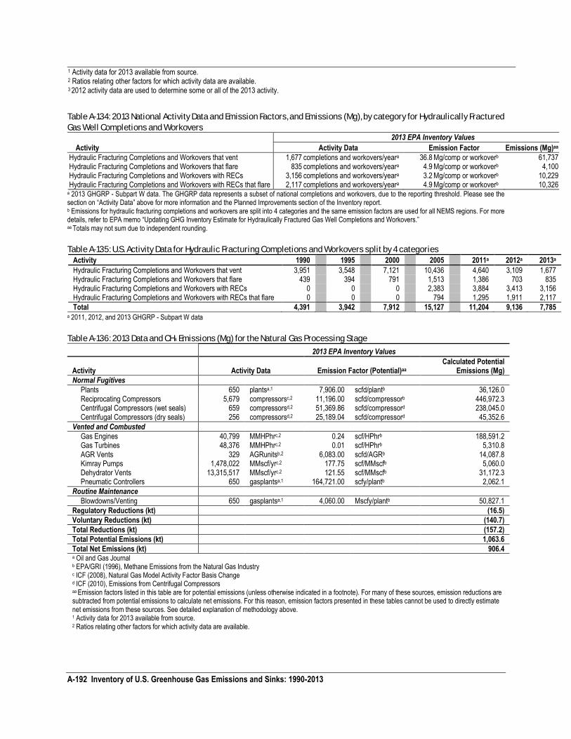
A-192 Inventory of U.S. Greenhouse Gas Emissions and Sinks: 1990-2013
1 Activity data for 2013 available from source. 2 Ratios relating other factors for which activity data are available. 3 2012 activity data are used to determine some or all of the 2013 activity.
Table A-134: 2013 National Activity Data and Emission Factors, and Emissions (Mg), by category for Hydraulically Fractured
Gas Well Completions and Workovers 2013 EPA Inventory Values
Activity Activity Data Emission Factor Emissions (Mg)aa
Hydraulic Fracturing Completions and Workovers that vent 1,677 completions and workovers/yeara 36.8 Mg/comp or workoverb 61,737 Hydraulic Fracturing Completions and Workovers that flare 835 completions and workovers/yeara 4.9 Mg/comp or workoverb 4,100 Hydraulic Fracturing Completions and Workovers with RECs 3,156 completions and workovers/yeara 3.2 Mg/comp or workoverb 10,229 Hydraulic Fracturing Completions and Workovers with RECs that flare 2,117 completions and workovers/yeara 4.9 Mg/comp or workoverb 10,326
a 2013 GHGRP - Subpart W data. The GHGRP data represents a subset of national completions and workovers, due to the reporting threshold. Please see the section on “Activity Data” above for more information and the Planned Improvements section of the Inventory report. b Emissions for hydraulic fracturing completions and workovers are split into 4 categories and the same emission factors are used for all NEMS regions. For more details, refer to EPA memo “Updating GHG Inventory Estimate for Hydraulically Fractured Gas Well Completions and Workovers.” aa Totals may not sum due to independent rounding.
Table A-135: U.S. Activity Data for Hydraulic Fracturing Completions and Workovers split by 4 categories
Activity 1990 1995 2000 2005 2011a 2012a 2013a
Hydraulic Fracturing Completions and Workovers that vent 3,951 3,548 7,121 10,436 4,640 3,109 1,677 Hydraulic Fracturing Completions and Workovers that flare 439 394 791 1,513 1,386 703 835 Hydraulic Fracturing Completions and Workovers with RECs 0 0 0 2,383 3,884 3,413 3,156 Hydraulic Fracturing Completions and Workovers with RECs that flare 0 0 0 794 1,295 1,911 2,117
Total 4,391 3,942 7,912 15,127 11,204 9,136 7,785 a 2011, 2012, and 2013 GHGRP - Subpart W data
Table A-136: 2013 Data and CH4 Emissions (Mg) for the Natural Gas Processing Stage
2013 EPA Inventory Values
Activity Activity Data Emission Factor (Potential)aa Calculated Potential
Emissions (Mg)
Normal Fugitives
Plants 650 plantsa,1 7,906.00 scfd/plantb 36,126.0 Reciprocating Compressors 5,679 compressorsc,2 11,196.00 scfd/compressorb 446,972.3 Centrifugal Compressors (wet seals) 659 compressorsd,2 51,369.86 scfd/compressord 238,045.0 Centrifugal Compressors (dry seals) 256 compressorsd,2 25,189.04 scfd/compressord 45,352.6
Vented and Combusted
Gas Engines 40,799 MMHPhrc,2 0.24 scf/HPhrb 188,591.2 Gas Turbines 48,376 MMHPhrc,2 0.01 scf/HPhrb 5,310.8 AGR Vents 329 AGRunitsb,2 6,083.00 scfd/AGRb 14,087.8 Kimray Pumps 1,478,022 MMscf/yrc,2 177.75 scf/MMscfb 5,060.0 Dehydrator Vents 13,315,517 MMscf/yrc,2 121.55 scf/MMscfb 31,172.3 Pneumatic Controllers 650 gasplantsa,1 164,721.00 scfy/plantb 2,062.1
Routine Maintenance
Blowdowns/Venting 650 gasplantsa,1 4,060.00 Mscfy/plantb 50,827.1
Regulatory Reductions (kt) (16.5)
Voluntary Reductions (kt) (140.7)
Total Reductions (kt) (157.2)
Total Potential Emissions (kt) 1,063.6
Total Net Emissions (kt) 906.4 a Oil and Gas Journal b EPA/GRI (1996), Methane Emissions from the Natural Gas Industry c ICF (2008), Natural Gas Model Activity Factor Basis Change d ICF (2010), Emissions from Centrifugal Compressors aa Emission factors listed in this table are for potential emissions (unless otherwise indicated in a footnote). For many of these sources, emission reductions are subtracted from potential emissions to calculate net emissions. For this reason, emission factors presented in these tables cannot be used to directly estimate net emissions from these sources. See detailed explanation of methodology above. 1 Activity data for 2013 available from source. 2 Ratios relating other factors for which activity data are available.
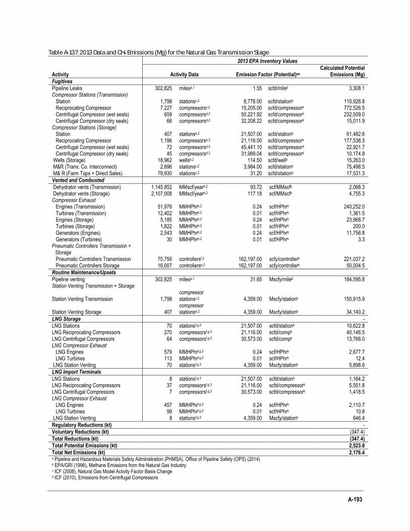
A-193
Table A-137: 2013 Data and CH4 Emissions (Mg) for the Natural Gas Transmission Stage
2013 EPA Inventory Values
Activity Activity Data Emission Factor (Potential)aa Calculated Potential
Emissions (Mg)
Fugitives
Pipeline Leaks 302,825 milesa,1 1.55 scfd/mileb 3,308.1 Compressor Stations (Transmission) Station 1,798 stationsc,2 8,778.00 scfd/stationb 110,926.8 Reciprocating Compressor 7,227 compressorsc,2 15,205.00 scfd/compressorb 772,526.5 Centrifugal Compressor (wet seals) 659 compressorsd,2 50,221.92 scfd/compressord 232,509.0 Centrifugal Compressor (dry seals) 66 compressorsd,2 32,208.22 scfd/compressord 15,011.9 Compressor Stations (Storage) Station 407 stationse,2 21,507.00 scfd/stationb 61,482.6 Reciprocating Compressor 1,196 compressorse,2 21,116.00 scfd/compressorb 177,538.3 Centrifugal Compressor (wet seals) 72 compressorsd,2 45,441.10 scfd/compressord 22,921.7 Centrifugal Compressor (dry seals) 45 compressorsd,2 31,989.04 scfd/compressord 10,174.8 Wells (Storage) 18,962 wellsb,2 114.50 scfd/wellb 15,263.0 M&R (Trans. Co. Interconnect) 2,696 stationsc,2 3,984.00 scfd/stationb 75,498.5 M& R (Farm Taps + Direct Sales) 79,930 stationsc,2 31.20 scfd/stationb 17,531.3
Vented and Combusted
Dehydrator vents (Transmission) 1,145,852 MMscf/yearb,2 93.72 scf/MMscfb 2,068.3 Dehydrator vents (Storage) 2,107,008 MMscf/yearb,2 117.18 scf/MMscfb 4,755.3 Compressor Exhaust Engines (Transmission) 51,976 MMHPhrb,2 0.24 scf/HPhrb 240,252.0 Turbines (Transmission) 12,402 MMHPhrb,2 0.01 scf/HPhrb 1,361.5 Engines (Storage) 5,185 MMHPhrb,2 0.24 scf/HPhrb 23,968.7 Turbines (Storage) 1,822 MMHPhrb,2 0.01 scf/HPhrb 200.0 Generators (Engines) 2,543 MMHPhrb,2 0.24 scf/HPhrb 11,756.8 Generators (Turbines) 30 MMHPhrb,2 0.01 scf/HPhrb 3.3 Pneumatic Controllers Transmission +
Storage Pneumatic Controllers Transmission 70,756 controllersf,2 162,197.00 scfy/controllerb 221,037.2 Pneumatic Controllers Storage 16,007 controllerse,2 162,197.00 scfy/controllerb 50,004.5
Routine Maintenance/Upsets
Pipeline venting 302,825 milesa,1 31.65 Mscfy/mileb 184,595.8 Station Venting Transmission + Storage
Station Venting Transmission 1,798 compressor stationsc,2 4,359.00 Mscfy/stationb 150,915.9
Station Venting Storage 407 compressor stationse,2 4,359.00 Mscfy/stationb 34,140.2
LNG Storage -
LNG Stations 70 stationsf,g,3 21,507.00 scfd/stationb 10,622.8 LNG Reciprocating Compressors 270 compressorsf,g,3 21,116.00 scfd/compb 40,146.5 LNG Centrifugal Compressors 64 compressorsf,g,3 30,573.00 scfd/compb 13,766.0 LNG Compressor Exhaust LNG Engines 579 MMHPhrf,g,3 0.24 scf/HPhrb 2,677.7 LNG Turbines 113 MMHPhrf,g,3 0.01 scf/HPhrb 12.4 LNG Station Venting 70 stationsf,g,3 4,359.00 Mscfy/stationb 5,898.6
LNG Import Terminals
LNG Stations 8 stationsf,g,3 21,507.00 scfd/stationb 1,164.2 LNG Reciprocating Compressors 37 compressorsf,g,3 21,116.00 scfd/compressorb 5,551.8 LNG Centrifugal Compressors 7 compressorsf,g,3 30,573.00 scfd/compressorb 1,418.5 LNG Compressor Exhaust LNG Engines 457 MMHPhrf,g,3 0.24 scf/HPhrb 2,110.7 LNG Turbines 99 MMHPhrf,g,3 0.01 scf/HPhrb 10.8 LNG Station Venting 8 stationsf,g,3 4,359.00 Mscfy/stationb 646.4
Regulatory Reductions (kt) -
Voluntary Reductions (kt) (347.4)
Total Reductions (kt) (347.4)
Total Potential Emissions (kt) 2,523.8
Total Net Emissions (kt) 2,176.4 a Pipeline and Hazardous Materials Safety Administration (PHMSA), Office of Pipeline Safety (OPS) (2014) b EPA/GRI (1996), Methane Emissions from the Natural Gas Industry c ICF (2008), Natural Gas Model Activity Factor Basis Change d ICF (2010), Emissions from Centrifugal Compressors
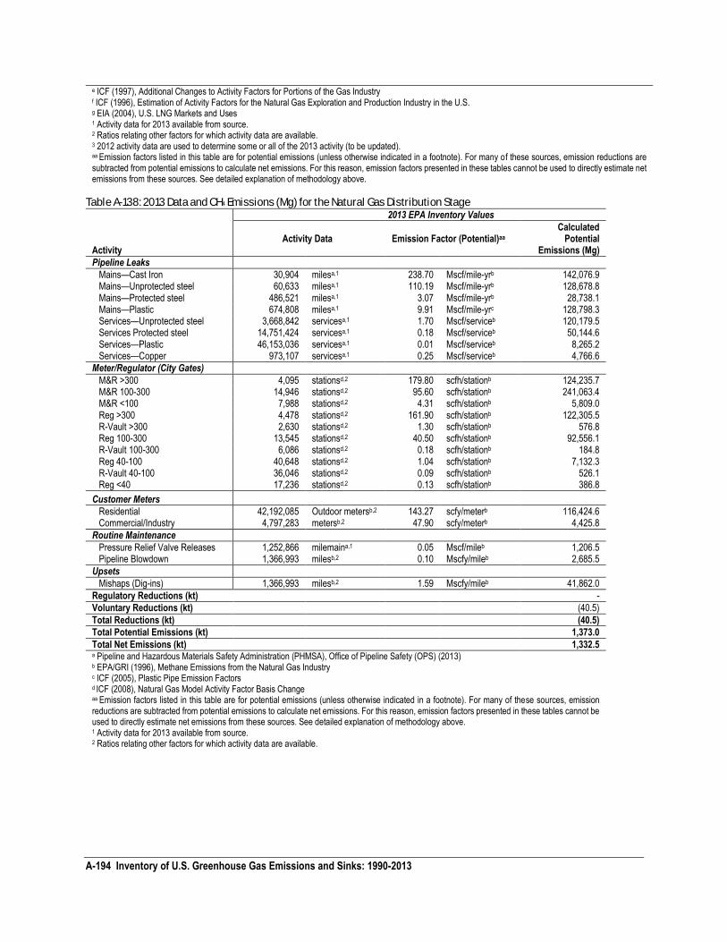
A-194 Inventory of U.S. Greenhouse Gas Emissions and Sinks: 1990-2013
e ICF (1997), Additional Changes to Activity Factors for Portions of the Gas Industry f ICF (1996), Estimation of Activity Factors for the Natural Gas Exploration and Production Industry in the U.S. g EIA (2004), U.S. LNG Markets and Uses 1 Activity data for 2013 available from source. 2 Ratios relating other factors for which activity data are available. 3 2012 activity data are used to determine some or all of the 2013 activity (to be updated). aa Emission factors listed in this table are for potential emissions (unless otherwise indicated in a footnote). For many of these sources, emission reductions are subtracted from potential emissions to calculate net emissions. For this reason, emission factors presented in these tables cannot be used to directly estimate net emissions from these sources. See detailed explanation of methodology above.
Table A-138: 2013 Data and CH4 Emissions (Mg) for the Natural Gas Distribution Stage 2013 EPA Inventory Values
Activity Activity Data Emission Factor (Potential)aa
Calculated Potential
Emissions (Mg)
Pipeline Leaks
Mains—Cast Iron 30,904 milesa,1 238.70 Mscf/mile-yrb 142,076.9 Mains—Unprotected steel 60,633 milesa,1 110.19 Mscf/mile-yrb 128,678.8 Mains—Protected steel 486,521 milesa,1 3.07 Mscf/mile-yrb 28,738.1 Mains—Plastic 674,808 milesa,1 9.91 Mscf/mile-yrc 128,798.3 Services—Unprotected steel 3,668,842 servicesa,1 1.70 Mscf/serviceb 120,179.5 Services Protected steel 14,751,424 servicesa,1 0.18 Mscf/serviceb 50,144.6 Services—Plastic 46,153,036 servicesa,1 0.01 Mscf/serviceb 8,265.2 Services—Copper 973,107 servicesa,1 0.25 Mscf/serviceb 4,766.6
Meter/Regulator (City Gates)
M&R >300 4,095 stationsd,2 179.80 scfh/stationb 124,235.7 M&R 100-300 14,946 stationsd,2 95.60 scfh/stationb 241,063.4 M&R <100 7,988 stationsd,2 4.31 scfh/stationb 5,809.0 Reg >300 4,478 stationsd,2 161.90 scfh/stationb 122,305.5 R-Vault >300 2,630 stationsd,2 1.30 scfh/stationb 576.8 Reg 100-300 13,545 stationsd,2 40.50 scfh/stationb 92,556.1 R-Vault 100-300 6,086 stationsd,2 0.18 scfh/stationb 184.8 Reg 40-100 40,648 stationsd,2 1.04 scfh/stationb 7,132.3 R-Vault 40-100 36,046 stationsd,2 0.09 scfh/stationb 526.1 Reg <40 17,236 stationsd,2 0.13 scfh/stationb 386.8
Customer Meters
Residential 42,192,085 Outdoor metersb,2 143.27 scfy/meterb 116,424.6 Commercial/Industry 4,797,283 metersb,2 47.90 scfy/meterb 4,425.8
Routine Maintenance
Pressure Relief Valve Releases 1,252,866 milemaina,1 0.05 Mscf/mileb 1,206.5 Pipeline Blowdown 1,366,993 milesb,2 0.10 Mscfy/mileb 2,685.5
Upsets
Mishaps (Dig-ins) 1,366,993 milesb,2 1.59 Mscfy/mileb 41,862.0
Regulatory Reductions (kt) -
Voluntary Reductions (kt) (40.5)
Total Reductions (kt) (40.5)
Total Potential Emissions (kt) 1,373.0
Total Net Emissions (kt) 1,332.5 a Pipeline and Hazardous Materials Safety Administration (PHMSA), Office of Pipeline Safety (OPS) (2013) b EPA/GRI (1996), Methane Emissions from the Natural Gas Industry c ICF (2005), Plastic Pipe Emission Factors d ICF (2008), Natural Gas Model Activity Factor Basis Change aa Emission factors listed in this table are for potential emissions (unless otherwise indicated in a footnote). For many of these sources, emission reductions are subtracted from potential emissions to calculate net emissions. For this reason, emission factors presented in these tables cannot be used to directly estimate net emissions from these sources. See detailed explanation of methodology above. 1 Activity data for 2013 available from source. 2 Ratios relating other factors for which activity data are available.
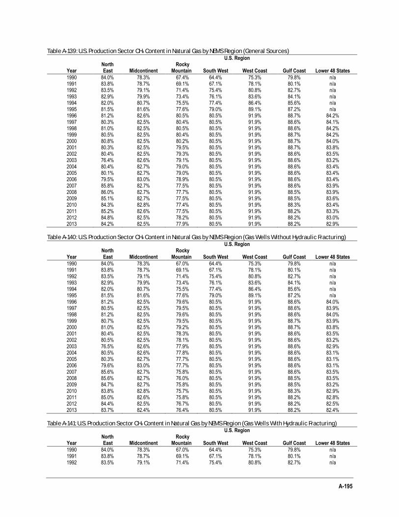
A-195
Table A-139: U.S. Production Sector CH4 Content in Natural Gas by NEMS Region (General Sources) U.S. Region
Year North East Midcontinent
Rocky Mountain South West West Coast Gulf Coast Lower 48 States
1990 84.0% 78.3% 67.4% 64.4% 75.3% 79.8% n/a 1991 83.8% 78.7% 69.1% 67.1% 78.1% 80.1% n/a 1992 83.5% 79.1% 71.4% 75.4% 80.8% 82.7% n/a 1993 82.9% 79.9% 73.4% 76.1% 83.6% 84.1% n/a 1994 82.0% 80.7% 75.5% 77.4% 86.4% 85.6% n/a 1995 81.5% 81.6% 77.6% 79.0% 89.1% 87.2% n/a 1996 81.2% 82.6% 80.5% 80.5% 91.9% 88.7% 84.2% 1997 80.3% 82.5% 80.4% 80.5% 91.9% 88.6% 84.1% 1998 81.0% 82.5% 80.5% 80.5% 91.9% 88.6% 84.2% 1999 80.5% 82.5% 80.4% 80.5% 91.9% 88.7% 84.2% 2000 80.8% 82.5% 80.2% 80.5% 91.9% 88.7% 84.0% 2001 80.3% 82.5% 79.5% 80.5% 91.9% 88.7% 83.8% 2002 80.4% 82.5% 79.3% 80.5% 91.9% 88.6% 83.5% 2003 76.4% 82.6% 79.1% 80.5% 91.9% 88.6% 83.2% 2004 80.4% 82.7% 79.0% 80.5% 91.9% 88.6% 83.4% 2005 80.1% 82.7% 79.0% 80.5% 91.9% 88.6% 83.4% 2006 79.5% 83.0% 78.9% 80.5% 91.9% 88.6% 83.4% 2007 85.8% 82.7% 77.5% 80.5% 91.9% 88.6% 83.9% 2008 86.0% 82.7% 77.7% 80.5% 91.9% 88.5% 83.9% 2009 85.1% 82.7% 77.5% 80.5% 91.9% 88.5% 83.6% 2010 84.3% 82.8% 77.4% 80.5% 91.9% 88.3% 83.4% 2011 85.2% 82.6% 77.5% 80.5% 91.9% 88.2% 83.3% 2012 84.8% 82.5% 78.2% 80.5% 91.9% 88.2% 83.0% 2013 84.2% 82.5% 77.9% 80.5% 91.9% 88.2% 82.9%
Table A-140: U.S. Production Sector CH4 Content in Natural Gas by NEMS Region (Gas Wells Without Hydraulic Fracturing) U.S. Region
Year North East Midcontinent
Rocky Mountain South West West Coast Gulf Coast Lower 48 States
1990 84.0% 78.3% 67.0% 64.4% 75.3% 79.8% n/a 1991 83.8% 78.7% 69.1% 67.1% 78.1% 80.1% n/a 1992 83.5% 79.1% 71.4% 75.4% 80.8% 82.7% n/a 1993 82.9% 79.9% 73.4% 76.1% 83.6% 84.1% n/a 1994 82.0% 80.7% 75.5% 77.4% 86.4% 85.6% n/a 1995 81.5% 81.6% 77.6% 79.0% 89.1% 87.2% n/a 1996 81.2% 82.5% 79.6% 80.5% 91.9% 88.6% 84.0% 1997 80.5% 82.5% 79.5% 80.5% 91.9% 88.6% 83.9% 1998 81.2% 82.5% 79.6% 80.5% 91.9% 88.6% 84.0% 1999 80.7% 82.5% 79.5% 80.5% 91.9% 88.7% 83.9% 2000 81.0% 82.5% 79.2% 80.5% 91.9% 88.7% 83.8% 2001 80.4% 82.5% 78.3% 80.5% 91.9% 88.6% 83.5% 2002 80.5% 82.5% 78.1% 80.5% 91.9% 88.6% 83.2% 2003 76.5% 82.6% 77.9% 80.5% 91.9% 88.6% 82.9% 2004 80.5% 82.6% 77.8% 80.5% 91.9% 88.6% 83.1% 2005 80.3% 82.7% 77.7% 80.5% 91.9% 88.6% 83.1% 2006 79.6% 83.0% 77.7% 80.5% 91.9% 88.6% 83.1% 2007 85.6% 82.7% 75.8% 80.5% 91.9% 88.6% 83.5% 2008 85.6% 82.7% 76.0% 80.5% 91.9% 88.5% 83.5% 2009 84.7% 82.7% 75.8% 80.5% 91.9% 88.5% 83.2% 2010 83.8% 82.8% 75.7% 80.5% 91.9% 88.3% 82.9% 2011 85.0% 82.6% 75.8% 80.5% 91.9% 88.2% 82.8% 2012 84.4% 82.5% 76.7% 80.5% 91.9% 88.2% 82.5% 2013 83.7% 82.4% 76.4% 80.5% 91.9% 88.2% 82.4%
Table A-141: U.S. Production Sector CH4 Content in Natural Gas by NEMS Region (Gas Wells With Hydraulic Fracturing) U.S. Region
Year North East Midcontinent
Rocky Mountain South West West Coast Gulf Coast Lower 48 States
1990 84.0% 78.3% 67.0% 64.4% 75.3% 79.8% n/a 1991 83.8% 78.7% 69.1% 67.1% 78.1% 80.1% n/a 1992 83.5% 79.1% 71.4% 75.4% 80.8% 82.7% n/a
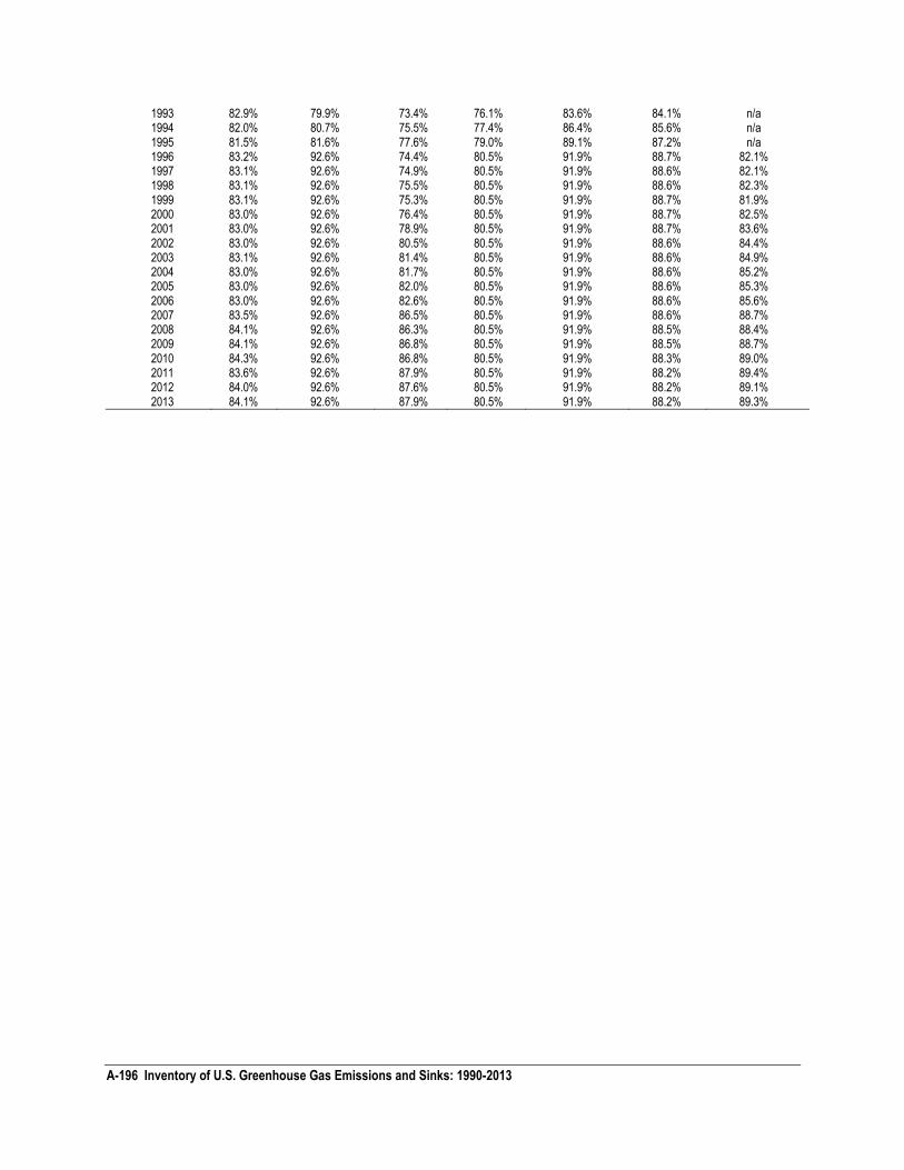
A-196 Inventory of U.S. Greenhouse Gas Emissions and Sinks: 1990-2013
1993 82.9% 79.9% 73.4% 76.1% 83.6% 84.1% n/a 1994 82.0% 80.7% 75.5% 77.4% 86.4% 85.6% n/a 1995 81.5% 81.6% 77.6% 79.0% 89.1% 87.2% n/a 1996 83.2% 92.6% 74.4% 80.5% 91.9% 88.7% 82.1% 1997 83.1% 92.6% 74.9% 80.5% 91.9% 88.6% 82.1% 1998 83.1% 92.6% 75.5% 80.5% 91.9% 88.6% 82.3% 1999 83.1% 92.6% 75.3% 80.5% 91.9% 88.7% 81.9% 2000 83.0% 92.6% 76.4% 80.5% 91.9% 88.7% 82.5% 2001 83.0% 92.6% 78.9% 80.5% 91.9% 88.7% 83.6% 2002 83.0% 92.6% 80.5% 80.5% 91.9% 88.6% 84.4% 2003 83.1% 92.6% 81.4% 80.5% 91.9% 88.6% 84.9% 2004 83.0% 92.6% 81.7% 80.5% 91.9% 88.6% 85.2% 2005 83.0% 92.6% 82.0% 80.5% 91.9% 88.6% 85.3% 2006 83.0% 92.6% 82.6% 80.5% 91.9% 88.6% 85.6% 2007 83.5% 92.6% 86.5% 80.5% 91.9% 88.6% 88.7% 2008 84.1% 92.6% 86.3% 80.5% 91.9% 88.5% 88.4% 2009 84.1% 92.6% 86.8% 80.5% 91.9% 88.5% 88.7% 2010 84.3% 92.6% 86.8% 80.5% 91.9% 88.3% 89.0% 2011 83.6% 92.6% 87.9% 80.5% 91.9% 88.2% 89.4% 2012 84.0% 92.6% 87.6% 80.5% 91.9% 88.2% 89.1% 2013 84.1% 92.6% 87.9% 80.5% 91.9% 88.2% 89.3%
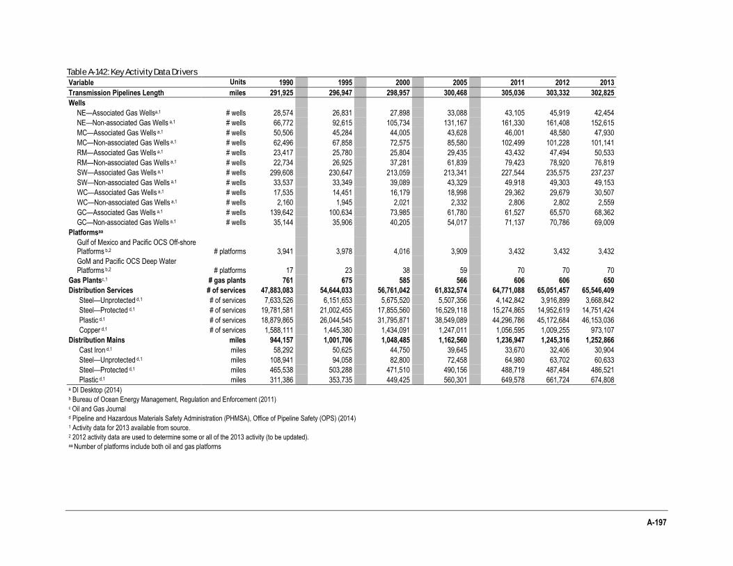
A-197
Table A-142: Key Activity Data Drivers
Variable Units 1990 1995 2000 2005 2011 2012 2013
Transmission Pipelines Length miles 291,925 296,947 298,957 300,468 305,036 303,332 302,825
Wells
NE—Associated Gas Wellsa,1 # wells 28,574 26,831 27,898 33,088 43,105 45,919 42,454
NE—Non-associated Gas Wells a,1 # wells 66,772 92,615 105,734 131,167 161,330 161,408 152,615
MC—Associated Gas Wells a,1 # wells 50,506 45,284 44,005 43,628 46,001 48,580 47,930
MC—Non-associated Gas Wells a,1 # wells 62,496 67,858 72,575 85,580 102,499 101,228 101,141
RM—Associated Gas Wells a,1 # wells 23,417 25,780 25,804 29,435 43,432 47,494 50,533
RM—Non-associated Gas Wells a,1 # wells 22,734 26,925 37,281 61,839 79,423 78,920 76,819
SW—Associated Gas Wells a,1 # wells 299,608 230,647 213,059 213,341 227,544 235,575 237,237
SW—Non-associated Gas Wells a,1 # wells 33,537 33,349 39,089 43,329 49,918 49,303 49,153
WC—Associated Gas Wells a,1 # wells 17,535 14,451 16,179 18,998 29,362 29,679 30,507
WC—Non-associated Gas Wells a,1 # wells 2,160 1,945 2,021 2,332 2,806 2,802 2,559
GC—Associated Gas Wells a,1 # wells 139,642 100,634 73,985 61,780 61,527 65,570 68,362
GC—Non-associated Gas Wells a,1 # wells 35,144 35,906 40,205 54,017 71,137 70,786 69,009
Platformsaa
Gulf of Mexico and Pacific OCS Off-shore Platforms b,2 # platforms 3,941 3,978 4,016 3,909 3,432 3,432 3,432
GoM and Pacific OCS Deep Water Platforms b,2 # platforms 17 23 38 59 70 70 70
Gas Plantsc,1 # gas plants 761 675 585 566 606 606 650
Distribution Services # of services 47,883,083 54,644,033 56,761,042 61,832,574 64,771,088 65,051,457 65,546,409
Steel—Unprotected d,1 # of services 7,633,526 6,151,653 5,675,520 5,507,356 4,142,842 3,916,899 3,668,842
Steel—Protected d,1 # of services 19,781,581 21,002,455 17,855,560 16,529,118 15,274,865 14,952,619 14,751,424
Plastic d,1 # of services 18,879,865 26,044,545 31,795,871 38,549,089 44,296,786 45,172,684 46,153,036
Copper d,1 # of services 1,588,111 1,445,380 1,434,091 1,247,011 1,056,595 1,009,255 973,107
Distribution Mains miles 944,157 1,001,706 1,048,485 1,162,560 1,236,947 1,245,316 1,252,866
Cast Iron d,1 miles 58,292 50,625 44,750 39,645 33,670 32,406 30,904
Steel—Unprotected d,1 miles 108,941 94,058 82,800 72,458 64,980 63,702 60,633
Steel—Protected d,1 miles 465,538 503,288 471,510 490,156 488,719 487,484 486,521
Plastic d,1 miles 311,386 353,735 449,425 560,301 649,578 661,724 674,808 a DI Desktop (2014) b Bureau of Ocean Energy Management, Regulation and Enforcement (2011) c Oil and Gas Journal d Pipeline and Hazardous Materials Safety Administration (PHMSA), Office of Pipeline Safety (OPS) (2014) 1 Activity data for 2013 available from source. 2 2012 activity data are used to determine some or all of the 2013 activity (to be updated). aa Number of platforms include both oil and gas platforms
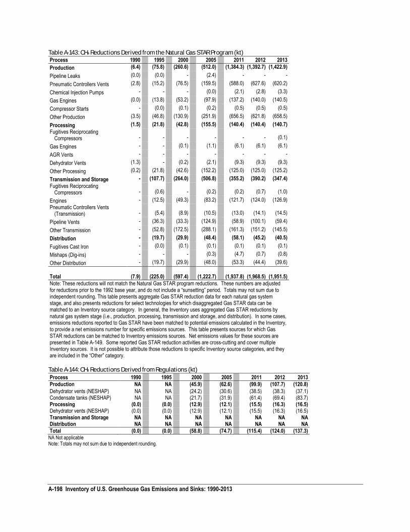
A-198 Inventory of U.S. Greenhouse Gas Emissions and Sinks: 1990-2013
Table A-143: CH4 Reductions Derived from the Natural Gas STAR Program (kt)
Process 1990 1995 2000 2005 2011 2012 2013
Production (6.4) (75.8) (260.6) (512.0) (1,384.3) (1,392.7) (1,422.9)
Pipeline Leaks (0.0) (0.0) - (2.4) - - -
Pneumatic Controllers Vents (2.8) (15.2) (76.5) (159.5) (588.0) (627.6) (620.2)
Chemical Injection Pumps - - - (0.0) (2.1) (2.8) (3.3)
Gas Engines (0.0) (13.8) (53.2) (97.9) (137.2) (140.0) (140.5)
Compressor Starts - (0.0) (0.1) (0.2) (0.5) (0.5) (0.5)
Other Production (3.5) (46.8) (130.9) (251.9) (656.5) (621.8) (658.5)
Processing (1.5) (21.8) (42.8) (155.5) (140.4) (140.4) (140.7)
Fugitives Reciprocating Compressors - - - - - - (0.1)
Gas Engines - - (0.1) (1.1) (6.1) (6.1) (6.1)
AGR Vents - - - - - - -
Dehydrator Vents (1.3) - (0.2) (2.1) (9.3) (9.3) (9.3)
Other Processing (0.2) (21.8) (42.6) (152.2) (125.0) (125.0) (125.2)
Transmission and Storage - (107.7) (264.0) (506.8) (355.2) (390.2) (347.4)
Fugitives Reciprocating Compressors - (0.6) - (0.2) (0.2) (0.7) (1.0)
Engines - (12.5) (49.3) (83.2) (121.7) (124.0) (126.9)
Pneumatic Controllers Vents (Transmission) - (5.4) (8.9) (10.5) (13.0) (14.1) (14.5)
Pipeline Vents - (36.3) (33.3) (124.9) (58.9) (100.1) (59.4)
Other Transmission - (52.8) (172.5) (288.1) (161.3) (151.2) (145.5)
Distribution - (19.7) (29.9) (48.4) (58.1) (45.2) (40.5)
Fugitives Cast Iron - (0.0) (0.1) (0.1) (0.1) (0.1) (0.1)
Mishaps (Dig-ins) - - - (0.3) (4.7) (0.7) (0.8)
Other Distribution - (19.7) (29.9) (48.0) (53.3) (44.4) (39.6)
Total (
(7.9) (
(225.0) (
(597.4) (
(1,222.7) (1,937.8) (1,968.5) (
(1,951.5)
Note: These reductions will not match the Natural Gas STAR program reductions. These numbers are adjusted for reductions prior to the 1992 base year, and do not include a “sunsetting” period. Totals may not sum due to independent rounding. This table presents aggregate Gas STAR reduction data for each natural gas system stage, and also presents reductions for select technologies for which disaggregated Gas STAR data can be matched to an Inventory source category. In general, the Inventory uses aggregated Gas STAR reductions by natural gas system stage (i.e., production, processing, transmission and storage, and distribution). In some cases, emissions reductions reported to Gas STAR have been matched to potential emissions calculated in the Inventory, to provide a net emissions number for specific emissions sources. This table presents sources for which Gas STAR reductions can be matched to Inventory emissions sources. Net emissions values for these sources are presented in Table A-149. Some reported Gas STAR reduction activities are cross-cutting and cover multiple Inventory sources. It is not possible to attribute those reductions to specific Inventory source categories, and they are included in the “Other” category.
Table A-144: CH4 Reductions Derived from Regulations (kt)
Process 1990 1995 2000 2005 2011 2012 2013
Production NA NA (45.9) (62.6) (99.9) (107.7) (120.8)
Dehydrator vents (NESHAP) NA NA (24.2) (30.6) (38.5) (38.3) (37.1) Condensate tanks (NESHAP) NA NA (21.7) (31.9) (61.4) (69.4) (83.7) Processing (0.0) (0.0) (12.9) (12.1) (15.5) (16.3) (16.5) Dehydrator vents (NESHAP) (0.0) (0.0) (12.9) (12.1) (15.5) (16.3) (16.5) Transmission and Storage NA NA NA NA NA NA NA Distribution NA NA NA NA NA NA NA
Total (0.0) (0.0) (58.8) (74.7) (115.4) (124.0) (137.3) NA Not applicable Note: Totals may not sum due to independent rounding.
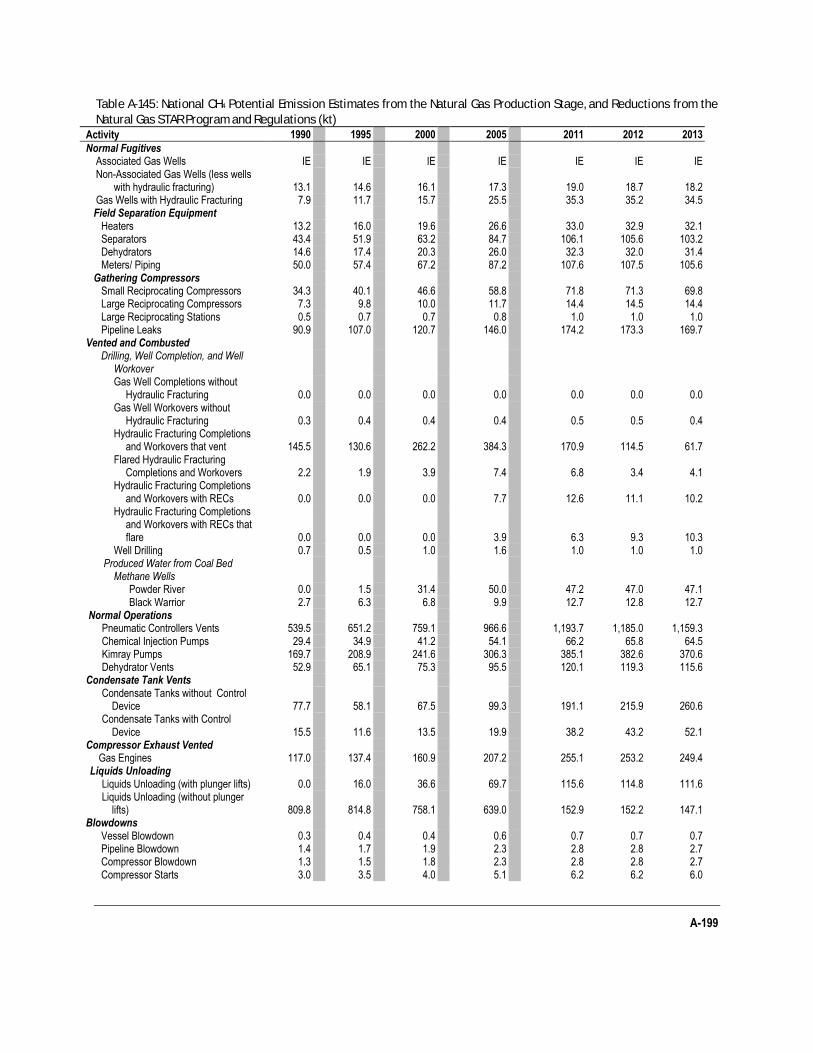
A-199
Table A-145: National CH4 Potential Emission Estimates from the Natural Gas Production Stage, and Reductions from the
Natural Gas STAR Program and Regulations (kt)
Activity 1990 1995 2000 2005 2011 2012 2013
Normal Fugitives Associated Gas Wells IE IE IE IE IE IE IE Non-Associated Gas Wells (less wells
with hydraulic fracturing) 13.1 14.6 16.1 17.3 19.0 18.7 18.2 Gas Wells with Hydraulic Fracturing 7.9 11.7 15.7 25.5 35.3 35.2 34.5
Field Separation Equipment Heaters 13.2 16.0 19.6 26.6 33.0 32.9 32.1 Separators 43.4 51.9 63.2 84.7 106.1 105.6 103.2 Dehydrators 14.6 17.4 20.3 26.0 32.3 32.0 31.4 Meters/ Piping 50.0 57.4 67.2 87.2 107.6 107.5 105.6 Gathering Compressors Small Reciprocating Compressors 34.3 40.1 46.6 58.8 71.8 71.3 69.8 Large Reciprocating Compressors 7.3 9.8 10.0 11.7 14.4 14.5 14.4 Large Reciprocating Stations 0.5 0.7 0.7 0.8 1.0 1.0 1.0 Pipeline Leaks 90.9 107.0 120.7 146.0 174.2 173.3 169.7 Vented and Combusted
Drilling, Well Completion, and Well Workover Gas Well Completions without
Hydraulic Fracturing 0.0 0.0 0.0 0.0 0.0 0.0 0.0 Gas Well Workovers without
Hydraulic Fracturing 0.3 0.4 0.4 0.4 0.5 0.5 0.4 Hydraulic Fracturing Completions
and Workovers that vent 145.5 130.6 262.2 384.3 170.9 114.5 61.7 Flared Hydraulic Fracturing
Completions and Workovers 2.2 1.9 3.9 7.4 6.8 3.4 4.1 Hydraulic Fracturing Completions
and Workovers with RECs 0.0 0.0 0.0 7.7 12.6 11.1 10.2 Hydraulic Fracturing Completions
and Workovers with RECs that flare 0.0 0.0 0.0 3.9 6.3 9.3 10.3
Well Drilling 0.7 0.5 1.0 1.6 1.0 1.0 1.0 Produced Water from Coal Bed
Methane Wells Powder River 0.0 1.5 31.4 50.0 47.2 47.0 47.1 Black Warrior 2.7 6.3 6.8 9.9 12.7 12.8 12.7
Normal Operations Pneumatic Controllers Vents 539.5 651.2 759.1 966.6 1,193.7 1,185.0 1,159.3 Chemical Injection Pumps 29.4 34.9 41.2 54.1 66.2 65.8 64.5 Kimray Pumps 169.7 208.9 241.6 306.3 385.1 382.6 370.6 Dehydrator Vents 52.9 65.1 75.3 95.5 120.1 119.3 115.6
Condensate Tank Vents Condensate Tanks without Control
Device 77.7 58.1 67.5 99.3 191.1 215.9 260.6 Condensate Tanks with Control
Device 15.5 11.6 13.5 19.9 38.2 43.2 52.1 Compressor Exhaust Vented Gas Engines 117.0 137.4 160.9 207.2 255.1 253.2 249.4 Liquids Unloading
Liquids Unloading (with plunger lifts) 0.0 16.0 36.6 69.7 115.6 114.8 111.6 Liquids Unloading (without plunger
lifts) 809.8 814.8 758.1 639.0 152.9 152.2 147.1 Blowdowns Vessel Blowdown 0.3 0.4 0.4 0.6 0.7 0.7 0.7 Pipeline Blowdown 1.4 1.7 1.9 2.3 2.8 2.8 2.7 Compressor Blowdown 1.3 1.5 1.8 2.3 2.8 2.8 2.7 Compressor Starts 3.0 3.5 4.0 5.1 6.2 6.2 6.0
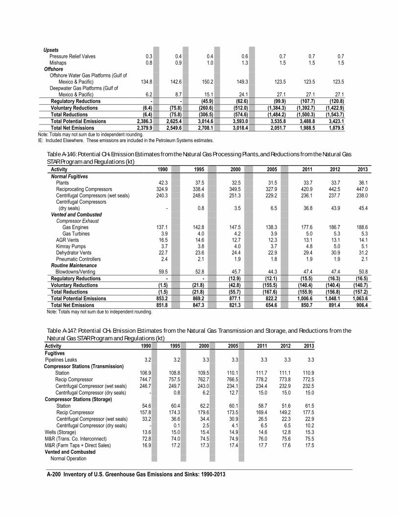
A-200 Inventory of U.S. Greenhouse Gas Emissions and Sinks: 1990-2013
Upsets Pressure Relief Valves 0.3 0.4 0.4 0.6 0.7 0.7 0.7 Mishaps 0.8 0.9 1.0 1.3 1.5 1.5 1.5 Offshore
Offshore Water Gas Platforms (Gulf of Mexico & Pacific) 134.8 142.6 150.2 149.3 123.5 123.5 123.5
Deepwater Gas Platforms (Gulf of Mexico & Pacific) 6.2 8.7 15.1 24.1 27.1 27.1 27.1
Regulatory Reductions - - (45.9) (62.6) (99.9) (107.7) (120.8)
Voluntary Reductions (6.4) (75.8) (260.6) (512.0) (1,384.3) (1,392.7) (1,422.9)
Total Reductions (6.4) (75.8) (306.5) (574.6) (1,484.2) (1,500.3) (1,543.7)
Total Potential Emissions 2,386.3 2,625.4 3,014.6 3,593.0 3,535.8 3,488.8 3,423.1
Total Net Emissions 2,379.9 2,549.6 2,708.1 3,018.4 2,051.7 1,988.5 1,879.5 Note: Totals may not sum due to independent rounding. IE: Included Elsewhere. These emissions are included in the Petroleum Systems estimates.
Table A-146: Potential CH4 Emission Estimates from the Natural Gas Processing Plants, and Reductions from the Natural Gas
STAR Program and Regulations (kt)
Activity 1990 1995 2000 2005 2011 2012 2013
Normal Fugitives Plants 42.3 37.5 32.5 31.5 33.7 33.7 36.1 Reciprocating Compressors 324.9 338.4 349.5 327.9 420.9 442.5 447.0 Centrifugal Compressors (wet seals) 240.3 248.6 251.3 229.2 236.1 237.7 238.0 Centrifugal Compressors (dry seals) - 0.8 3.5 6.5 36.8 43.9 45.4
Vented and Combusted Compressor Exhaust Gas Engines 137.1 142.8 147.5 138.3 177.6 186.7 188.6 Gas Turbines 3.9 4.0 4.2 3.9 5.0 5.3 5.3 AGR Vents 16.5 14.6 12.7 12.3 13.1 13.1 14.1 Kimray Pumps 3.7 3.8 4.0 3.7 4.8 5.0 5.1 Dehydrator Vents 22.7 23.6 24.4 22.9 29.4 30.9 31.2 Pneumatic Controllers 2.4 2.1 1.9 1.8 1.9 1.9 2.1
Routine Maintenance Blowdowns/Venting 59.5 52.8 45.7 44.3 47.4 47.4 50.8
Regulatory Reductions - - (12.9) (12.1) (15.5) (16.3) (16.5)
Voluntary Reductions (1.5) (21.8) (42.8) (155.5) (140.4) (140.4) (140.7)
Total Reductions (1.5) (21.8) (55.7) (167.6) (155.9) (156.8) (157.2)
Total Potential Emissions 853.2 869.2 877.1 822.2 1,006.6 1,048.1 1,063.6
Total Net Emissions 851.8 847.3 821.3 654.6 850.7 891.4 906.4 Note: Totals may not sum due to independent rounding.
Table A-147: Potential CH4 Emission Estimates from the Natural Gas Transmission and Storage, and Reductions from the
Natural Gas STAR Program and Regulations (kt)
Activity 1990 1995 2000 2005 2011 2012 2013
Fugitives
Pipelines Leaks 3.2 3.2 3.3 3.3 3.3 3.3 3.3
Compressor Stations (Transmission)
Station 106.9 108.8 109.5 110.1 111.7 111.1 110.9
Recip Compressor 744.7 757.5 762.7 766.5 778.2 773.8 772.5
Centrifugal Compressor (wet seals) 246.7 249.7 243.0 234.1 234.4 232.9 232.5
Centrifugal Compressor (dry seals) - 0.8 6.2 12.7 15.0 15.0 15.0
Compressor Stations (Storage)
Station 54.6 60.4 62.2 60.1 58.7 51.6 61.5
Recip Compressor 157.8 174.3 179.6 173.5 169.4 149.2 177.5
Centrifugal Compressor (wet seals) 33.2 36.6 34.4 30.9 26.5 22.3 22.9
Centrifugal Compressor (dry seals) - 0.1 2.5 4.1 6.5 6.5 10.2
Wells (Storage) 13.6 15.0 15.4 14.9 14.6 12.8 15.3
M&R (Trans. Co. Interconnect) 72.8 74.0 74.5 74.9 76.0 75.6 75.5
M&R (Farm Taps + Direct Sales) 16.9 17.2 17.3 17.4 17.7 17.6 17.5
Vented and Combusted
Normal Operation
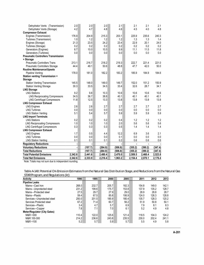
A-201
Dehydrator Vents (Transmission) 2.0 2.0 2.0 2.1 2.1 2.1 2.1
Dehydrator Vents (Storage) 4.2 4.7 4.8 4.6 4.5 4.0 4.8
Compressor Exhaust
Engines (Transmission) 176.9 204.9 215.3 203.1 225.9 235.6 240.3
Turbines (Transmission) 1.0 1.2 1.2 1.2 1.3 1.3 1.4
Engines (Storage) 21.3 23.5 24.2 23.4 22.9 20.1 24.0
Turbines (Storage) 0.2 0.2 0.2 0.2 0.2 0.2 0.2
Generators (Engines) 8.7 10.0 10.5 9.9 11.1 11.5 11.8
Generators (Turbines) 0.0 0.0 0.0 0.0 0.0 0.0 0.0 Pneumatic Controllers Transmission + Storage
Pneumatic Controllers Trans 213.1 216.7 218.2 219.3 222.7 221.4 221.0
Pneumatic Controllers Storage 44.4 49.1 50.6 48.8 47.7 42.0 50.0
Routine Maintenance/Upsets
Pipeline Venting 178.0 181.0 182.2 183.2 185.9 184.9 184.6 Station venting Transmission + Storage
Station Venting Transmission 145.5 148.0 149.0 149.7 152.0 151.2 150.9
Station Venting Storage 30.3 33.5 34.5 33.4 32.6 28.7 34.1
LNG Storage
LNG Stations 9.2 9.8 10.3 10.6 10.6 10.6 10.6
LNG Reciprocating Compressors 34.5 36.7 38.8 40.1 40.1 40.1 40.1
LNG Centrifugal Compressors 11.8 12.5 13.3 13.8 13.8 13.8 13.8
LNG Compressor Exhaust
LNG Engines 2.6 2.6 2.7 2.7 2.7 2.7 2.7
LNG Turbines 0.0 0.0 0.0 0.0 0.0 0.0 0.0
LNG Station Venting 5.1 5.4 5.7 5.9 5.9 5.9 5.9
LNG Import Terminals
LNG Stations 0.2 0.2 0.2 0.4 1.2 1.2 1.2
LNG Reciprocating Compressors 1.0 1.0 1.0 2.0 5.6 5.6 5.6
LNG Centrifugal Compressors 0.3 0.3 0.3 0.5 1.4 1.4 1.4
LNG Compressor Exhaust
LNG Engines 1.7 0.5 4.4 12.2 6.9 3.6 2.1
LNG Turbines 0.0 0.0 0.0 0.1 0.0 0.0 0.0
LNG Station Venting 0.1 0.1 0.1 0.2 0.6 0.6 0.6
Regulatory Reductions - - - - - - -
Voluntary Reductions - (107.7) (264.0) (506.8) (355.2) (390.2) (347.4)
Total Reductions - (107.7) (264.0) (506.8) (355.2) (390.2) (347.4)
Total Potential Emissions 2,342.6 2,441.6 2,480.4 2,470.0 2,509.5 2,460.4 2,523.8
Total Net Emissions 2,342.6 2,333.9 2,216.4 1,963.2 2,154.4 2,070.1 2,176.4 Note: Totals may not sum due to independent rounding.
Table A-148: Potential CH4 Emission Estimates from the Natural Gas Distribution Stage, and Reductions from the Natural Gas
STAR Program, and Regulations (kt)
Activity 1990 1995 2000 2005 2011 2012 2013
Pipeline Leaks Mains—Cast Iron 268.0 232.7 205.7 182.3 154.8 149.0 142.1 Mains—Unprotected steel 231.2 199.6 175.7 153.8 137.9 135.2 128.7 Mains—Protected steel 27.5 29.7 27.9 29.0 28.9 28.8 28.7 Mains—Plastic 59.4 67.5 85.8 106.9 124.0 126.3 128.8
Services—Unprotected steel 250.0 201.5 185.9 180.4 135.7 128.3 120.2 Services Protected steel 67.2 71.4 60.7 56.2 51.9 50.8 50.1 Services—Plastic 3.4 4.7 5.7 6.9 7.9 8.1 8.3 Services—Copper 7.8 7.1 7.0 6.1 5.2 4.9 4.8 Meter/Regulator (City Gates) M&R >300 110.4 122.0 125.6 121.4 118.5 104.3 124.2 M&R 100-300 214.2 236.6 243.8 235.5 230.0 202.4 241.1 M&R <100 5.2 5.7 5.9 5.7 5.5 4.9 5.8
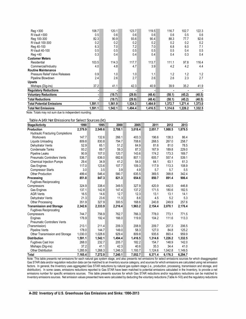
A-202 Inventory of U.S. Greenhouse Gas Emissions and Sinks: 1990-2013
Reg >300 108.7 120.1 123.7 119.5 116.7 102.7 122.3 R-Vault >300 0.5 0.6 0.6 0.6 0.6 0.5 0.6 Reg 100-300 82.3 90.9 93.6 90.4 88.3 77.7 92.6 R-Vault 100-300 0.2 0.2 0.2 0.2 0.2 0.2 0.2 Reg 40-100 6.3 7.0 7.2 7.0 6.8 6.0 7.1 R-Vault 40-100 0.5 0.5 0.5 0.5 0.5 0.4 0.5 Reg <40 0.3 0.4 0.4 0.4 0.4 0.3 0.4 Customer Meters Residential 103.5 114.3 117.7 113.7 111.1 97.8 116.4 Commercial/Industry 4.0 4.8 4.7 3.9 4.2 4.2 4.4 Routine Maintenance Pressure Relief Valve Releases 0.9 1.0 1.0 1.1 1.2 1.2 1.2 Pipeline Blowdown 2.4 2.6 2.7 2.6 2.6 2.3 2.7 Upsets Mishaps (Dig-ins) 37.2 41.1 42.3 40.9 39.9 35.2 41.9
Regulatory Reductions - - - - - - -
Voluntary Reductions - (19.7) (29.9) (48.4) (58.1) (45.2) (40.5)
Total Reductions - (19.7) (29.9) (48.4) (58.1) (45.2) (40.5)
Total Potential Emissions 1,591.1 1,561.9 1,524.3 1,464.9 1,372.7 1,271.4 1,373.0
Total Net Emissions 1,591.1 1,542.1 1,494.4 1,416.5 1,314.6 1,226.2 1,332.5
Note: Totals may not sum due to independent rounding.
Table A-149: Net Emissions for Select Sources (kt)
Stage/Activity 1990 1995 2000 2005 2011 2012 2013
Production 2,379.9 2,549.6 2,708.1 3,018.4 2,051.7 1,988.5 1,879.5 Hydraulic Fracturing Completions and
Workovers 147.7 132.6 266.1 403.3 196.6 138.3 86.4
Liquids Unloading 809.8 830.8 794.7 708.6 268.5 267.0 258.7
Dehydrator Vents 52.9 65.1 51.2 64.9 81.6 81.0 78.5
Condensate Tanks 93.2 69.7 59.3 87.3 167.9 189.8 229.0
Pipeline Leaks 90.9 107.0 120.7 143.6 174.2 173.3 169.7
Pneumatic Controllers Vents 536.7 636.0 682.6 807.1 605.7 557.4 539.1
Chemical Injection Pumps 29.4 34.9 41.2 54.0 64.1 63.1 61.3
Gas Engines 117.0 123.6 107.7 109.3 117.9 113.3 108.9
Compressor Starts 3.0 3.5 3.9 4.9 5.7 5.7 5.5
Other Production 499.4 546.4 580.7 635.5 369.5 399.8 342.4
Processing 851.8 847.3 821.3 654.6 850.7 891.4 906.4 Fugitives Reciprocating
Compressors 324.9 338.4 349.5 327.9 420.9 442.5 446.8
Gas Engines 137.1 142.8 147.4 137.2 171.5 180.6 182.5
AGR Vents 16.5 14.6 12.7 12.3 13.1 13.1 14.1
Dehydrator Vents 21.3 23.6 11.3 8.6 4.5 5.2 5.3
Other Processing 351.9 327.9 300.5 168.6 240.8 249.9 257.6
Transmission and Storage 2,342.6 2,333.9 2,216.4 1,963.2 2,154.4 2,070.1 2,176.4 Fugitives Reciprocating
Compressors 744.7 756.9 762.7 766.3 778.0 773.1 771.5
Engines 176.9 192.4 166.0 119.9 104.2 111.6 113.3 Pneumatic Controllers Vents
(Transmission) 213.1 211.4 209.3 208.9 209.7 207.3 206.5
Pipeline Vents 178.0 144.7 149.0 58.3 127.0 84.8 125.2
Other Transmission and Storage 1,030.0 1,028.6 929.4 809.8 935.6 893.4 959.9
Distribution 1,591.1 1,542.1 1,494.4 1,416.5 1,314.6 1,226.2 1,332.5
Fugitives Cast Iron 268.0 232.7 205.7 182.2 154.7 148.9 142.0
Mishaps (Dig-ins) 37.2 41.1 42.3 40.6 35.3 34.4 41.0
Other Distribution 1,285.9 1,268.3 1,246.3 1,193.7 1,124.6 1,042.8 1,149.5
Total 7,165.4 7,272.9 7,240.1 7,052.7 6,371.4 6,176.3 6,294.7 Note: This table presents net emissions for each natural gas system stage, and also presents net emissions for select emissions sources for which disaggregated Gas STAR data and/or regulation reduction data can be matched to an Inventory source category, and sources for which emissions are calculated using net emission factors. In general, the Inventory uses aggregated Gas STAR reductions by natural gas system stage (i.e., production, processing, transmission and storage, and distribution). In some cases, emissions reductions reported to Gas STAR have been matched to potential emissions calculated in the Inventory, to provide a net emissions number for specific emissions sources. This table presents sources for which Gas STAR reductions and/or regulatory reductions can be matched to Inventory emissions sources. Net emission values presented here were calculated by deducting the voluntary reductions (Table A-143) and the regulatory reductions
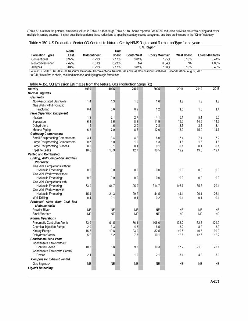
A-203
(Table A-144) from the potential emissions values in Table A-145 through Table A-148. Some reported Gas STAR reduction activities are cross-cutting and cover multiple Inventory sources. It is not possible to attribute those reductions to specific Inventory source categories, and they are included in the “Other” category.
Table A-150: U.S. Production Sector CO2 Content in Natural Gas by NEMS Region and Formation Type for all years U.S. Region
Formation Types North
East Midcontinent Gulf
Coast South West Rocky Mountain West Coast Lower-48 States
Conventional 0.92% 0.79% 2.17% 3.81% 7.95% 0.16% 3.41% Non-conventional* 7.42% 0.31% 0.23% NA 0.64% NA 4.83% All types 3.04% 0.79% 2.17% 3.81% 7.58% 0.16% 3.45%
Source: GRI-01/0136 GTI's Gas Resource Database: Unconventional Natural Gas and Gas Composition Databases. Second Edition. August, 2001 *In GTI, this refers to shale, coal bed methane, and tight geologic formations.
Table A- 151: CO2 Emission Estimates from the Natural Gas Production Stage (kt)
Activity 1990 1995 2000 2005 2011 2012 2013
Normal Fugitives Gas Wells
Non-Associated Gas Wells 1.4 1.3 1.5 1.6 1.8 1.8 1.8 Gas Wells with Hydraulic
Fracturing 0.4 0.6 0.9 1.2
1.5 1.5 1.4 Field Separation Equipment Heaters 1.9 2.1 2.7 4.1 5.1 5.1 5.0 Separators 6.1 6.6 8.3 11.9 15.0 14.9 14.6 Dehydrators 1.4 1.6 2.0 2.8 3.5 3.5 3.4 Meters/ Piping 6.8 7.0 8.6 12.0 15.0 15.0 14.7 Gathering Compressors Small Reciprocating Compressors 3.1 3.4 4.2 6.0 7.4 7.4 7.2 Large Reciprocating Compressors 0.7 1.0 1.0 1.3 1.6 1.6 1.6 Large Reciprocating Stations 0.0 0.1 0.1 0.1 0.1 0.1 0.1 Pipeline Leaks 10.0 10.9 12.7 16.5 19.9 19.8 19.4 Vented and Combusted Drilling, Well Completion, and Well
Workover
Gas Well Completions without
Hydraulic Fracturingb 0.0 0.0 0.0 0.0 0.0 0.0 0.0 Gas Well Workovers without
Hydraulic Fracturingb 0.0 0.0 0.0 0.0 0.0 0.0 0.0 Gas Well Completions with
Hydraulic Fracturing 73.9 64.7 195.0 314.7 146.7 85.8 70.1 Gas Well Workovers with
Hydraulic Fracturing 15.4 21.3 29.2 44.5 44.1 26.1 26.1 Well Drilling 0.1 0.1 0.1 0.2 0.1 0.1 0.1
Produced Water from Coal Bed Methane Wells
Powder River1 NE NE NE NE NE NE NE Black Warriora NE NE NE NE NE NE NE
Normal Operations Pneumatic Controllers Vents 53.9 61.5 76.1 106.6 133.2 132.3 129.0 Chemical Injection Pumps 2.9 3.3 4.3 6.5 8.2 8.2 8.0 Kimray Pumps 16.8 19.8 23.9 32.5 40.5 40.3 39.0 Dehydrator Vents 5.2 6.2 7.5 10.1 12.6 12.6 12.2 Condensate Tank Vents
Condensate Tanks without Control Device 10.3 8.8 9.3 10.3 17.2 21.0 25.1
Condensate Tanks with Control Device 2.1 1.8 1.9 2.1 3.4 4.2 5.0
Compressor Exhaust Vented Gas Enginesa NE NE NE NE NE NE NE
Liquids Unloading
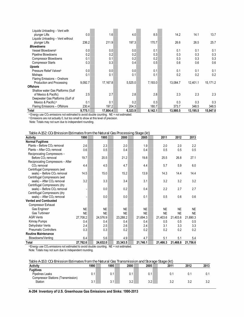
A-204 Inventory of U.S. Greenhouse Gas Emissions and Sinks: 1990-2013
Liquids Unloading – Vent with plunger Lifts 0.0 1.6 4.0 8.5 14.2 14.1 13.7
Liquids Unloading – Vent without plunger Lifts 236.2 211.9 197.3 170.7 26.6 26.5 25.7
Blowdowns Vessel Blowdownsb 0.0 0.0 0.0 0.1 0.1 0.1 0.1 Pipeline Blowdowns 0.2 0.2 0.2 0.3 0.3 0.3 0.3 Compressor Blowdowns 0.1 0.1 0.2 0.2 0.3 0.3 0.3 Compressor Starts 0.3 0.3 0.4 0.5 0.6 0.6 0.6 Upsets Pressure Relief Valvesb 0.0 0.0 0.0 0.1 0.1 0.1 0.1 Mishaps 0.1 0.1 0.1 0.1 0.2 0.2 0.2
Flaring Emissions – Onshore Production and Processing 9,092.7 17,167.8 5,525.0 7,193.0 13,084.7 12,401.1 15,171.2
Offshore Shallow water Gas Platforms (Gulf
of Mexico & Pacific) 2.5 2.7 2.8 2.8 2.3 2.3 2.3 Deepwater Gas Platforms (Gulf of
Mexico & Pacific) b 0.1 0.1 0.2 0.3 0.3 0.3 0.3 Flaring Emissions – Offshore 230.4 197.2 204.3 180.7 373.7 348.5 348.5
Total 9,775.1 17,804.4 6,323.9 8,142.1 13,980.5 13,195.5 15,947.0 a Energy use CO2 emissions not estimated to avoid double counting. NE = not estimated. b Emissions are not actually 0, but too small to show at this level of precision. Note: Totals may not sum due to independent rounding.
Table A-152: CO2 Emission Estimates from the Natural Gas Processing Stage (kt) Activity 1990 1995 2000 2005 2011 2012 2013
Normal Fugitives Plants – Before CO2 removal 2.6 2.3 2.0 1.9 2.0 2.0 2.2 Plants – After CO2 removal 0.6 0.5 0.4 0.4 0.5 0.5 0.5 Reciprocating Compressors –
Before CO2 removal 19.7 20.5 21.2 19.8 25.5 26.8 27.1 Reciprocating Compressors – After
CO2 removal 4.4 4.5 4.7 4.4 5.7 5.9 6.0 Centrifugal Compressors (wet
seals) – Before CO2 removal 14.5 15.0 15.2 13.9 14.3 14.4 14.4 Centrifugal Compressors (wet
seals) – After CO2 removal 3.2 3.3 3.4 3.1 3.2 3.2 3.2 Centrifugal Compressors (dry
seals) – Before CO2 removal - 0.0 0.2 0.4 2.2 2.7 2.7 Centrifugal Compressors (dry
seals) – After CO2 removal - 0.0 0.0 0.1 0.5 0.6 0.6 Vented and Combusted Compressor Exhaust Gas Enginesa NE NE NE NE NE NE NE Gas Turbinesa NE NE NE NE NE NE NE AGR Vents 27,708.2 24,576.9 23,288.2 21,694.3 21,403.6 21,403.6 21,690.3 Kimray Pumps 0.4 0.4 0.4 0.4 0.5 0.5 0.5 Dehydrator Vents 2.4 2.5 2.6 2.4 3.1 3.3 3.3 Pneumatic Controllers 0.3 0.3 0.2 0.2 0.2 0.2 0.2 Routine Maintenance Blowdowns/Venting 6.4 5.6 4.9 4.7 5.1 5.1 5.4
Total 27,762.6 24,632.0 23,343.5 21,746.1 21,466.3 21,468.8 21,756.6 a Energy use CO2 emissions not estimated to avoid double counting. NE = not estimated. Note: Totals may not sum due to independent rounding.
Table A-153: CO2 Emission Estimates from the Natural Gas Transmission and Storage Stage (kt) Activity 1990 1995 2000 2005 2011 2012 2013
Fugitives Pipelines Leaks 0.1 0.1 0.1 0.1 0.1 0.1 0.1
Compressor Stations (Transmission) Station 3.1 3.1 3.2 3.2 3.2 3.2 3.2
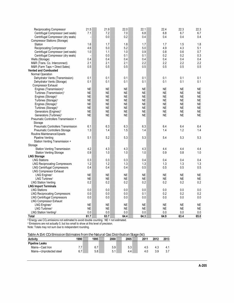
A-205
Reciprocating Compressor 21.5 21.9 22.0 22.1 22.4 22.3 22.3 Centrifugal Compressor (wet seals) 7.1 7.2 7.0 6.8 6.8 6.7 6.7 Centrifugal Compressor (dry seals) - 0.0 0.2 0.4 0.4 0.4 0.4
Compressor Stations (Storage) Station 1.6 1.7 1.8 1.7 1.7 1.5 1.8 Reciprocating Compressor 4.6 5.0 5.2 5.0 4.9 4.3 5.1 Centrifugal Compressor (wet seals) 1.0 1.1 1.0 0.9 0.8 0.6 0.7 Centrifugal Compressor (dry seals) - 0.0 0.1 0.1 0.2 0.2 0.3
Wells (Storage) 0.4 0.4 0.4 0.4 0.4 0.4 0.4 M&R (Trans. Co. Interconnect) 2.1 2.1 2.1 2.2 2.2 2.2 2.2 M&R (Farm Taps + Direct Sales) 0.5 0.5 0.5 0.5 0.5 0.5 0.5 Vented and Combusted Normal Operation Dehydrator Vents (Transmission) 0.1 0.1 0.1 0.1 0.1 0.1 0.1 Dehydrator Vents (Storage) 0.1 0.1 0.1 0.1 0.1 0.1 0.1 Compressor Exhaust Engines (Transmission)1 NE NE NE NE NE NE NE Turbines (Transmission)1 NE NE NE NE NE NE NE Engines (Storage)1 NE NE NE NE NE NE NE Turbines (Storage)1 NE NE NE NE NE NE NE Engines (Storage)1 NE NE NE NE NE NE NE Turbines (Storage)1 NE NE NE NE NE NE NE Generators (Engines)1 NE NE NE NE NE NE NE Generators (Turbines)1 NE NE NE NE NE NE NE Pneumatic Controllers Transmission +
Storage Pneumatic Controllers Transmission 6.1 6.3 6.3 6.3 6.4 6.4 6.4 Pneumatic Controllers Storage 1.3 1.4 1.5 1.4 1.4 1.2 1.4 Routine Maintenance/Upsets Pipeline Venting 5.1 5.2 5.3 5.3 5.4 5.3 5.3 Station Venting Transmission + Storage
Station Venting Transmission 4.2 4.3 4.3 4.3 4.4 4.4 4.4 Station Venting Storage 0.9 1.0 1.0 1.0 0.9 0.8 1.0
LNG Storage LNG Stations 0.3 0.3 0.3 0.4 0.4 0.4 0.4 LNG Reciprocating Compressors 1.2 1.2 1.3 1.3 1.3 1.3 1.3 LNG Centrifugal Compressors 0.4 0.4 0.4 0.5 0.5 0.5 0.5 LNG Compressor Exhaust LNG Engines1 NE NE NE NE NE NE NE LNG Turbines1 NE NE NE NE NE NE NE LNG Station Venting 0.2 0.2 0.2 0.2 0.2 0.2 0.2 LNG Import Terminals LNG Stations 0.0 0.0 0.0 0.0 0.0 0.0 0.0 LNG Reciprocating Compressors 0.0 0.0 0.0 0.1 0.2 0.2 0.2 LNG Centrifugal Compressors 0.0 0.0 0.0 0.0 0.0 0.0 0.0 LNG Compressor Exhaust LNG Engines1 NE NE NE NE NE NE NE LNG Turbines1 NE NE NE NE NE NE NE LNG Station Venting2 0.0 0.0 0.0 0.0 0.0 0.0 0.0
Total 61.7 63.7 64.4 64.3 64.9 63.4 65.0 a Energy use CO2 emissions not estimated to avoid double counting. NE = not estimated. 2 Emissions are not actually 0, but too small to show at this level of precision. Note: Totals may not sum due to independent rounding.
Table A-154: CO2 Emission Estimates from the Natural Gas Distribution Stage (kt)
Activity 1990 1995 2000 2005 2011 2012 2013
Pipeline Leaks
Mains—Cast Iron 7.7 6.7 5.9 5.3 4.5 4.3 4.1
Mains—Unprotected steel 6.7 5.8 5.1 4.4 4.0 3.9 3.7
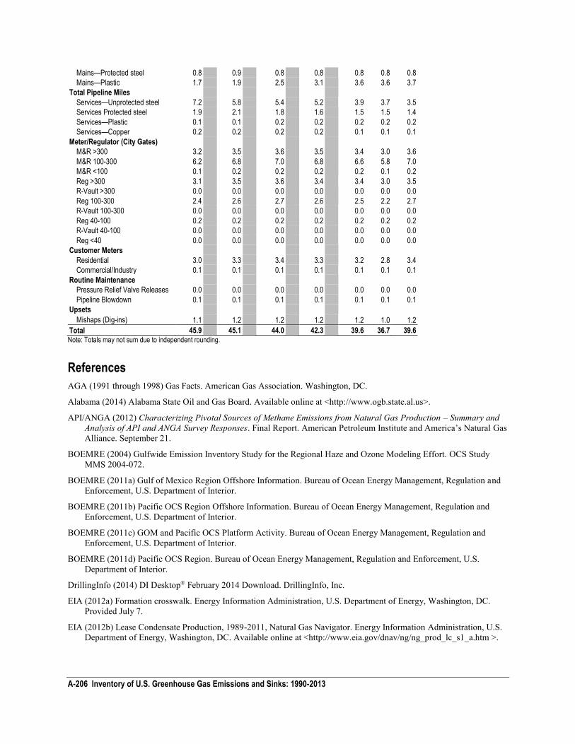
A-206 Inventory of U.S. Greenhouse Gas Emissions and Sinks: 1990-2013
Mains—Protected steel 0.8 0.9 0.8 0.8 0.8 0.8 0.8
Mains—Plastic 1.7 1.9 2.5 3.1 3.6 3.6 3.7
Total Pipeline Miles
Services—Unprotected steel 7.2 5.8 5.4 5.2 3.9 3.7 3.5
Services Protected steel 1.9 2.1 1.8 1.6 1.5 1.5 1.4
Services—Plastic 0.1 0.1 0.2 0.2 0.2 0.2 0.2
Services—Copper 0.2 0.2 0.2 0.2 0.1 0.1 0.1
Meter/Regulator (City Gates)
M&R >300 3.2 3.5 3.6 3.5 3.4 3.0 3.6
M&R 100-300 6.2 6.8 7.0 6.8 6.6 5.8 7.0
M&R <100 0.1 0.2 0.2 0.2 0.2 0.1 0.2
Reg >300 3.1 3.5 3.6 3.4 3.4 3.0 3.5
R-Vault >300 0.0 0.0 0.0 0.0 0.0 0.0 0.0
Reg 100-300 2.4 2.6 2.7 2.6 2.5 2.2 2.7
R-Vault 100-300 0.0 0.0 0.0 0.0 0.0 0.0 0.0
Reg 40-100 0.2 0.2 0.2 0.2 0.2 0.2 0.2
R-Vault 40-100 0.0 0.0 0.0 0.0 0.0 0.0 0.0
Reg <40 0.0 0.0 0.0 0.0 0.0 0.0 0.0
Customer Meters
Residential 3.0 3.3 3.4 3.3 3.2 2.8 3.4
Commercial/Industry 0.1 0.1 0.1 0.1 0.1 0.1 0.1
Routine Maintenance
Pressure Relief Valve Releases 0.0 0.0 0.0 0.0 0.0 0.0 0.0
Pipeline Blowdown 0.1 0.1 0.1 0.1 0.1 0.1 0.1
Upsets
Mishaps (Dig-ins) 1.1 1.2 1.2 1.2 1.2 1.0 1.2
Total 45.9 45.1 44.0 42.3 39.6 36.7 39.6 Note: Totals may not sum due to independent rounding.
References
AGA (1991 through 1998) Gas Facts. American Gas Association. Washington, DC.
Alabama (2014) Alabama State Oil and Gas Board. Available online at <http://www.ogb.state.al.us>.
API/ANGA (2012) Characterizing Pivotal Sources of Methane Emissions from Natural Gas Production – Summary and Analysis of API and ANGA Survey Responses. Final Report. American Petroleum Institute and America’s Natural Gas Alliance. September 21.
BOEMRE (2004) Gulfwide Emission Inventory Study for the Regional Haze and Ozone Modeling Effort. OCS Study MMS 2004-072.
BOEMRE (2011a) Gulf of Mexico Region Offshore Information. Bureau of Ocean Energy Management, Regulation and Enforcement, U.S. Department of Interior.
BOEMRE (2011b) Pacific OCS Region Offshore Information. Bureau of Ocean Energy Management, Regulation and Enforcement, U.S. Department of Interior.
BOEMRE (2011c) GOM and Pacific OCS Platform Activity. Bureau of Ocean Energy Management, Regulation and Enforcement, U.S. Department of Interior.
BOEMRE (2011d) Pacific OCS Region. Bureau of Ocean Energy Management, Regulation and Enforcement, U.S. Department of Interior.
DrillingInfo (2014) DI Desktop® February 2014 Download. DrillingInfo, Inc.
EIA (2012a) Formation crosswalk. Energy Information Administration, U.S. Department of Energy, Washington, DC. Provided July 7.
EIA (2012b) Lease Condensate Production, 1989-2011, Natural Gas Navigator. Energy Information Administration, U.S. Department of Energy, Washington, DC. Available online at <http://www.eia.gov/dnav/ng/ng_prod_lc_s1_a.htm >.
A-207
EIA (2013a) “Table 1—Summary of natural gas supply and disposition in the United States 2008-2013.” Natural Gas Monthly, Energy Information Administration, U.S. Department of Energy, Washington, DC. Available online at <http://www.eia.doe.gov>.
EIA (2013b) “Table 2—Natural Gas Consumption in the United States 2008-2013.” Natural Gas Monthly, Energy Information Administration, U.S. Department of Energy, Washington, DC. Available online at <http://www.eia.doe.gov>.
EIA (2013c) “Table 7— Marketed production of natural gas in selected states and the Federal Gulf of Mexico, 2008-2013.” Natural Gas Monthly, Energy Information Administration, U.S. Department of Energy, Washington, DC. Available online at <http://www.eia.doe.gov>.
EIA (2014a) U.S. Imports by Country. Energy Information Administration, U.S. Department of Energy, Washington, DC. Available online at <http://www.eia.doe.gov>.
EIA (2014b) Natural Gas Gross Withdrawals and Production. Energy Information Administration, U.S. Department of Energy, Washington, DC. Available online at <http://www.eia.doe.gov>.
EIA (2005) “Table 5—U.S. Crude Oil, Natural Gas, and Natural Gas Liquids Reserves, 1977-2003.” Energy Information Administration, Department of Energy, Washington, DC.
EIA (2004) U.S. LNG Markets and Uses. Energy Information Administration, U.S. Department of Energy, Washington, DC. June 2004. Available online at <http://www.eia.doe.gov/pub/oil_gas/natural_gas/ feature_articles/2004/lng/lng2004.pdf>.
EIA (2001) “Documentation of the Oil and Gas Supply Module (OGSM).” Energy Information Administration, U.S. Department of Energy, Washington, DC. Available online at <http://tonto.eia.doe.gov/FTPROOT/modeldoc/m063(2001).pdf>.
EIA (1996) “Emissions of Greenhouse Gases in the United States” Carbon Dioxide Emissions. Energy Information Administration, U.S. Department of Energy, Washington, DC.
EPA (2013a) Oil and Natural Gas Sector: Standards of Performance for Crude Oil and Natural Gas Production, Transmission, and Distribution. Background Supplemental Technical Support Document for the Final New Source Performance Standards. Environmental Protection Agency. September 2013.
EPA (2013b) Oil and Natural Gas Sector: New Source Performance Standards and National Emission Standards for Hazardous Air Pollutants Reviews. Environmental Protection Agency, 40 CFR Parts 60 and 63, [EPA-HQ-OAR-2010-0505; FRL-9665-1], RIN 2060-AP76.
EPA (2013c) Natural GasSTAR Reductions 1990-2012. Natural GasSTAR Program. September 2013.
EPA (2013d) Updating GHG Inventory Estimate for Hydraulically Fractured Gas Well Completions and Workovers. Available online at: http://www.epa.gov/climatechange/Downloads/ghgemissions/memo-update-emissions-for-hydraulically-workovers.pdf.
EPA (2014) Greenhouse Gas Reporting Program- Subpart W – Petroleum and Natural Gas Systems. Environmental Protection Agency. September 2014.
EPA (1999) Estimates of Methane Emissions from the U.S. Oil Industry (Draft Report). Prepared by ICF-Kaiser, Office of Air and Radiation, U.S. Environmental Protection Agency. October 1999.
EPA/GRI (1996) Methane Emissions from the Natural Gas Industry. Prepared by Harrison, M., T. Shires, J. Wessels, and R. Cowgill, eds., Radian International LLC for National Risk Management Research Laboratory, Air Pollution Prevention and Control Division, Research Triangle Park, NC. EPA-600/R-96-080a.
FERC (2011) North American LNG Terminals. Federal Energy Regulatory Commission, Washington, DC.
GTI (2001) Gas Resource Database: Unconventional Natural Gas and Gas Composition Databases. Second Edition. GRI-01/0136.
A-208 Inventory of U.S. Greenhouse Gas Emissions and Sinks: 1990-2013
IPCC (2006) 2006 IPCC Guidelines for National Greenhouse Gas Inventories. The National Greenhouse Gas Inventories Programme, H.S. Eggleston, L. Buenida, K. Miwa, T Ngara, and K. Tanabe, eds.; Institute for Global Environmental Strategies (IGES). Hayama, Kanagawa, Japan.
OGJ (1997-2013) “Worldwide Gas Processing.” Oil & Gas Journal, PennWell Corporation, Tulsa, OK. Available online at <http:// http://www.ogj.com/>.
PHMSA (2014a) Transmission Annuals Data. Pipeline and Hazardous Materials Safety Administration, U.S. Department of Transportation, Washington, DC. Available online at < http://phmsa.dot.gov/pipeline/library/data-stats >.
PHMSA (2014b) Gas Distribution Annual Data. Pipeline and Hazardous Materials Safety Administration, U.S. Department of Transportation, Washington, DC. Available online at < http://phmsa.dot.gov/pipeline/library/data-stats>.
Wyoming (2014) Wyoming Oil and Gas Conservation Commission. Available online at <http://wogcc.state.wy.us/coalbedchart.cfm>.
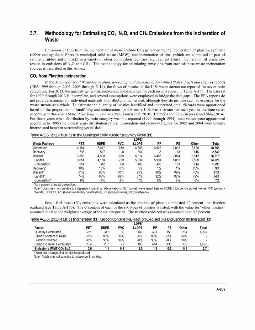
A-209
3.7. Methodology for Estimating CO2, N2O, and CH4 Emissions from the Incineration of Waste
Emissions of CO2 from the incineration of waste include CO2 generated by the incineration of plastics, synthetic rubber and synthetic fibers in municipal solid waste (MSW), and incineration of tires (which are composed in part of synthetic rubber and C black) in a variety of other combustion facilities (e.g., cement kilns). Incineration of waste also results in emissions of N2O and CH4. The methodology for calculating emissions from each of these waste incineration sources is described in this Annex.
CO2 from Plastics Incineration
In the Municipal Solid Waste Generation, Recycling, and Disposal in the United States: Facts and Figures reports (EPA 1999 through 2003, 2005 through 2014), the flows of plastics in the U.S. waste stream are reported for seven resin categories. For 2013, the quantity generated, recovered, and discarded for each resin is shown in Table A-155. The data set for 1990 through 2013 is incomplete, and several assumptions were employed to bridge the data gaps. The EPA reports do not provide estimates for individual materials landfilled and incinerated, although they do provide such an estimate for the waste stream as a whole. To estimate the quantity of plastics landfilled and incinerated, total discards were apportioned based on the proportions of landfilling and incineration for the entire U.S. waste stream for each year in the time series according to Biocycle’s State of Garbage in America (van Haaren et al. 2010), Themelis and Shin (in press) and Shin (2014). For those years when distribution by resin category was not reported (1990 through 1994), total values were apportioned according to 1995 (the closest year) distribution ratios. Generation and recovery figures for 2002 and 2004 were linearly interpolated between surrounding years’ data.
Table A-155: 2013 Plastics in the Municipal Solid Waste Stream by Resin (kt)
Waste Pathway PET HDPE PVC LDPE/
LLDPE PP PS Other Total
Generation 4,101 5,017 789 6,668 6,523 2,032 3,629 28,758 Recovery 798 517 0 354 36 18 816 2,540 Discard 3,302 4,500 789 6,314 6,486 2,014 2,812 26,218 Landfill 3,051 4,158 729 5,834 5,994 1,861 2,599 24,226 Combustion 251 342 60 480 493 153 214 1,993 Recovery* 19% 10% 0% 5% 1% 1% 23% 9% Discard* 81% 90% 100% 95% 99% 99% 78% 91% Landfill* 74% 83% 92% 87% 92% 92% 72% 84% Combustion* 6% 7% 8% 7% 8% 8% 6% 7% *As a percent of waste generation. Note: Totals may not sum due to independent rounding. Abbreviations: PET (polyethylene terephthalate), HDPE (high density polyethylene), PVC (polyvinyl chloride), LDPE/LLDPE (linear low density polyethylene), PP (polypropylene), PS (polystyrene).
Fossil fuel-based CO2 emissions were calculated as the product of plastic combusted, C content, and fraction oxidized (see Table A-156). The C content of each of the six types of plastics is listed, with the value for “other plastics” assumed equal to the weighted average of the six categories. The fraction oxidized was assumed to be 98 percent.
Table A-156: 2013 Plastics Incinerated (kt), Carbon Content (%), Fraction Oxidized (%) and Carbon Incinerated (kt)
Factor PET HDPE PVC LDPE/
LLDPE PP PS Other Total
Quantity Combusted 251 342 60 480 493 153 214 1,993 Carbon Content of Resin 63% 86% 38% 86% 86% 92% 66% - Fraction Oxidized 98% 98% 98% 98% 98% 98% 98% - Carbon in Resin Combusted 154 287 23 403 414 138 138 1,557
Emissions (MMT CO2 Eq.) 0.6 1.1 0.1 1.5 1.5 0.5 0.5 5.7 a Weighted average of other plastics produced. Note: Totals may not sum due to independent rounding.
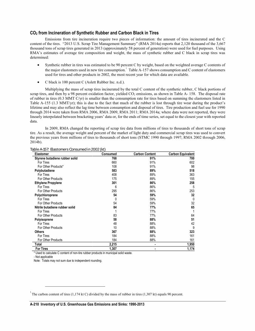
A-210 Inventory of U.S. Greenhouse Gas Emissions and Sinks: 1990-2013
CO2 from Incineration of Synthetic Rubber and Carbon Black in Tires
Emissions from tire incineration require two pieces of information: the amount of tires incinerated and the C content of the tires. “2013 U.S. Scrap Tire Management Summary” (RMA 2014a) reports that 2,120 thousand of the 3,667 thousand tons of scrap tires generated in 2013 (approximately 58 percent of generation) were used for fuel purposes. Using RMA’s estimates of average tire composition and weight, the mass of synthetic rubber and C black in scrap tires was determined:
Synthetic rubber in tires was estimated to be 90 percent C by weight, based on the weighted average C contents of the major elastomers used in new tire consumption.1 Table A-157 shows consumption and C content of elastomers used for tires and other products in 2002, the most recent year for which data are available.
C black is 100 percent C (Aslett Rubber Inc. n.d.).
Multiplying the mass of scrap tires incinerated by the total C content of the synthetic rubber, C black portions of scrap tires, and then by a 98 percent oxidation factor, yielded CO2 emissions, as shown in Table A- 158. The disposal rate of rubber in tires (0.3 MMT C/yr) is smaller than the consumption rate for tires based on summing the elastomers listed in Table A-155 (1.3 MMT/yr); this is due to the fact that much of the rubber is lost through tire wear during the product’s lifetime and may also reflect the lag time between consumption and disposal of tires. Tire production and fuel use for 1990 through 2014 were taken from RMA 2006, RMA 2009, RMA 2011; RMA 2014a; where data were not reported, they were linearly interpolated between bracketing years’ data or, for the ends of time series, set equal to the closest year with reported data.
In 2009, RMA changed the reporting of scrap tire data from millions of tires to thousands of short tons of scrap tire. As a result, the average weight and percent of the market of light duty and commercial scrap tires was used to convert the previous years from millions of tires to thousands of short tons (STMC 1990 through 1997; RMA 2002 through 2006, 2014b).
Table A-157: Elastomers Consumed in 2002 (kt) Elastomer Consumed Carbon Content Carbon Equivalent
Styrene butadiene rubber solid 768 91% 700 For Tires 660 91% 602 For Other Products* 108 91% 98
Polybutadiene 583 89% 518 For Tires 408 89% 363 For Other Products 175 89% 155
Ethylene Propylene 301 86% 258 For Tires 6 86% 5 For Other Products 295 86% 253
Polychloroprene 54 59% 32 For Tires 0 59% 0 For Other Products 54 59% 32
Nitrile butadiene rubber solid 84 77% 65 For Tires 1 77% 1 For Other Products 83 77% 64
Polyisoprene 58 88% 51 For Tires 48 88% 42 For Other Products 10 88% 9
Others 367 88% 323 For Tires 184 88% 161 For Other Products 184 88% 161
Total 2,215 - 1,950
For Tires 1,307 - 1,174 * Used to calculate C content of non-tire rubber products in municipal solid waste. - Not applicable Note: Totals may not sum due to independent rounding.
1 The carbon content of tires (1,174 kt C) divided by the mass of rubber in tires (1,307 kt) equals 90 percent.
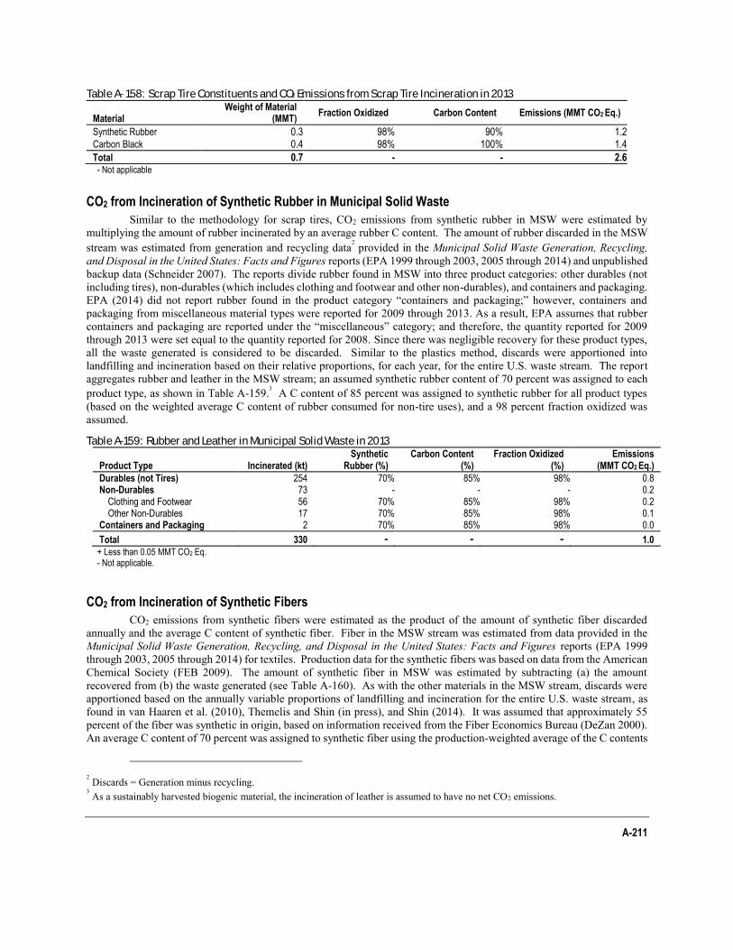
A-211
Table A- 158: Scrap Tire Constituents and CO2 Emissions from Scrap Tire Incineration in 2013
Material Weight of Material
(MMT) Fraction Oxidized Carbon Content Emissions (MMT CO2 Eq.)
Synthetic Rubber 0.3 98% 90% 1.2 Carbon Black 0.4 98% 100% 1.4
Total 0.7 - - 2.6 - Not applicable
CO2 from Incineration of Synthetic Rubber in Municipal Solid Waste
Similar to the methodology for scrap tires, CO2 emissions from synthetic rubber in MSW were estimated by multiplying the amount of rubber incinerated by an average rubber C content. The amount of rubber discarded in the MSW stream was estimated from generation and recycling data2 provided in the Municipal Solid Waste Generation, Recycling, and Disposal in the United States: Facts and Figures reports (EPA 1999 through 2003, 2005 through 2014) and unpublished backup data (Schneider 2007). The reports divide rubber found in MSW into three product categories: other durables (not including tires), non-durables (which includes clothing and footwear and other non-durables), and containers and packaging. EPA (2014) did not report rubber found in the product category “containers and packaging;” however, containers and packaging from miscellaneous material types were reported for 2009 through 2013. As a result, EPA assumes that rubber containers and packaging are reported under the “miscellaneous” category; and therefore, the quantity reported for 2009 through 2013 were set equal to the quantity reported for 2008. Since there was negligible recovery for these product types, all the waste generated is considered to be discarded. Similar to the plastics method, discards were apportioned into landfilling and incineration based on their relative proportions, for each year, for the entire U.S. waste stream. The report aggregates rubber and leather in the MSW stream; an assumed synthetic rubber content of 70 percent was assigned to each product type, as shown in Table A-159.3 A C content of 85 percent was assigned to synthetic rubber for all product types (based on the weighted average C content of rubber consumed for non-tire uses), and a 98 percent fraction oxidized was assumed.
Table A-159: Rubber and Leather in Municipal Solid Waste in 2013
Product Type Incinerated (kt) Synthetic
Rubber (%) Carbon Content
(%) Fraction Oxidized
(%) Emissions
(MMT CO2 Eq.)
Durables (not Tires) 254 70% 85% 98% 0.8 Non-Durables 73 - - - 0.2
Clothing and Footwear 56 70% 85% 98% 0.2 Other Non-Durables 17 70% 85% 98% 0.1
Containers and Packaging 2 70% 85% 98% 0.0
Total 330 - - - 1.0
+ Less than 0.05 MMT CO2 Eq. - Not applicable.
CO2 from Incineration of Synthetic Fibers
CO2 emissions from synthetic fibers were estimated as the product of the amount of synthetic fiber discarded annually and the average C content of synthetic fiber. Fiber in the MSW stream was estimated from data provided in the Municipal Solid Waste Generation, Recycling, and Disposal in the United States: Facts and Figures reports (EPA 1999 through 2003, 2005 through 2014) for textiles. Production data for the synthetic fibers was based on data from the American Chemical Society (FEB 2009). The amount of synthetic fiber in MSW was estimated by subtracting (a) the amount recovered from (b) the waste generated (see Table A-160). As with the other materials in the MSW stream, discards were apportioned based on the annually variable proportions of landfilling and incineration for the entire U.S. waste stream, as found in van Haaren et al. (2010), Themelis and Shin (in press), and Shin (2014). It was assumed that approximately 55 percent of the fiber was synthetic in origin, based on information received from the Fiber Economics Bureau (DeZan 2000). An average C content of 70 percent was assigned to synthetic fiber using the production-weighted average of the C contents
2 Discards = Generation minus recycling. 3 As a sustainably harvested biogenic material, the incineration of leather is assumed to have no net CO2 emissions.
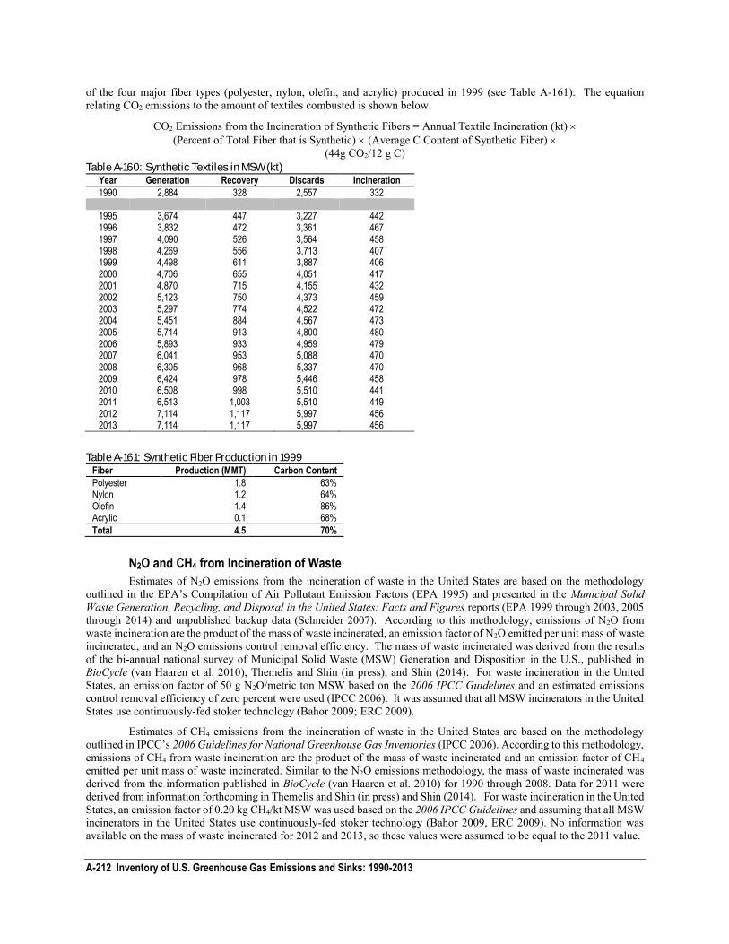
A-212 Inventory of U.S. Greenhouse Gas Emissions and Sinks: 1990-2013
of the four major fiber types (polyester, nylon, olefin, and acrylic) produced in 1999 (see Table A-161). The equation relating CO2 emissions to the amount of textiles combusted is shown below.
CO2 Emissions from the Incineration of Synthetic Fibers = Annual Textile Incineration (kt) (Percent of Total Fiber that is Synthetic) (Average C Content of Synthetic Fiber)
(44g CO2/12 g C) Table A-160: Synthetic Textiles in MSW (kt)
Year Generation Recovery Discards Incineration
1990 2,884 328 2,557 332
1995 3,674 447 3,227 442 1996 3,832 472 3,361 467 1997 4,090 526 3,564 458 1998 4,269 556 3,713 407 1999 4,498 611 3,887 406 2000 4,706 655 4,051 417 2001 4,870 715 4,155 432 2002 5,123 750 4,373 459 2003 5,297 774 4,522 472 2004 5,451 884 4,567 473 2005 5,714 913 4,800 480 2006 5,893 933 4,959 479 2007 6,041 953 5,088 470 2008 6,305 968 5,337 470 2009 6,424 978 5,446 458 2010 6,508 998 5,510 441 2011 6,513 1,003 5,510 419 2012 7,114 1,117 5,997 456 2013 7,114 1,117 5,997 456
Table A-161: Synthetic Fiber Production in 1999 Fiber Production (MMT) Carbon Content
Polyester 1.8 63% Nylon 1.2 64% Olefin 1.4 86% Acrylic 0.1 68%
Total 4.5 70%
N2O and CH4 from Incineration of Waste
Estimates of N2O emissions from the incineration of waste in the United States are based on the methodology outlined in the EPA’s Compilation of Air Pollutant Emission Factors (EPA 1995) and presented in the Municipal Solid Waste Generation, Recycling, and Disposal in the United States: Facts and Figures reports (EPA 1999 through 2003, 2005 through 2014) and unpublished backup data (Schneider 2007). According to this methodology, emissions of N2O from waste incineration are the product of the mass of waste incinerated, an emission factor of N2O emitted per unit mass of waste incinerated, and an N2O emissions control removal efficiency. The mass of waste incinerated was derived from the results of the bi-annual national survey of Municipal Solid Waste (MSW) Generation and Disposition in the U.S., published in BioCycle (van Haaren et al. 2010), Themelis and Shin (in press), and Shin (2014). For waste incineration in the United States, an emission factor of 50 g N2O/metric ton MSW based on the 2006 IPCC Guidelines and an estimated emissions control removal efficiency of zero percent were used (IPCC 2006). It was assumed that all MSW incinerators in the United States use continuously-fed stoker technology (Bahor 2009; ERC 2009).
Estimates of CH4 emissions from the incineration of waste in the United States are based on the methodology outlined in IPCC’s 2006 Guidelines for National Greenhouse Gas Inventories (IPCC 2006). According to this methodology, emissions of CH4 from waste incineration are the product of the mass of waste incinerated and an emission factor of CH4 emitted per unit mass of waste incinerated. Similar to the N2O emissions methodology, the mass of waste incinerated was derived from the information published in BioCycle (van Haaren et al. 2010) for 1990 through 2008. Data for 2011 were derived from information forthcoming in Themelis and Shin (in press) and Shin (2014). For waste incineration in the United States, an emission factor of 0.20 kg CH4/kt MSW was used based on the 2006 IPCC Guidelines and assuming that all MSW incinerators in the United States use continuously-fed stoker technology (Bahor 2009, ERC 2009). No information was available on the mass of waste incinerated for 2012 and 2013, so these values were assumed to be equal to the 2011 value.
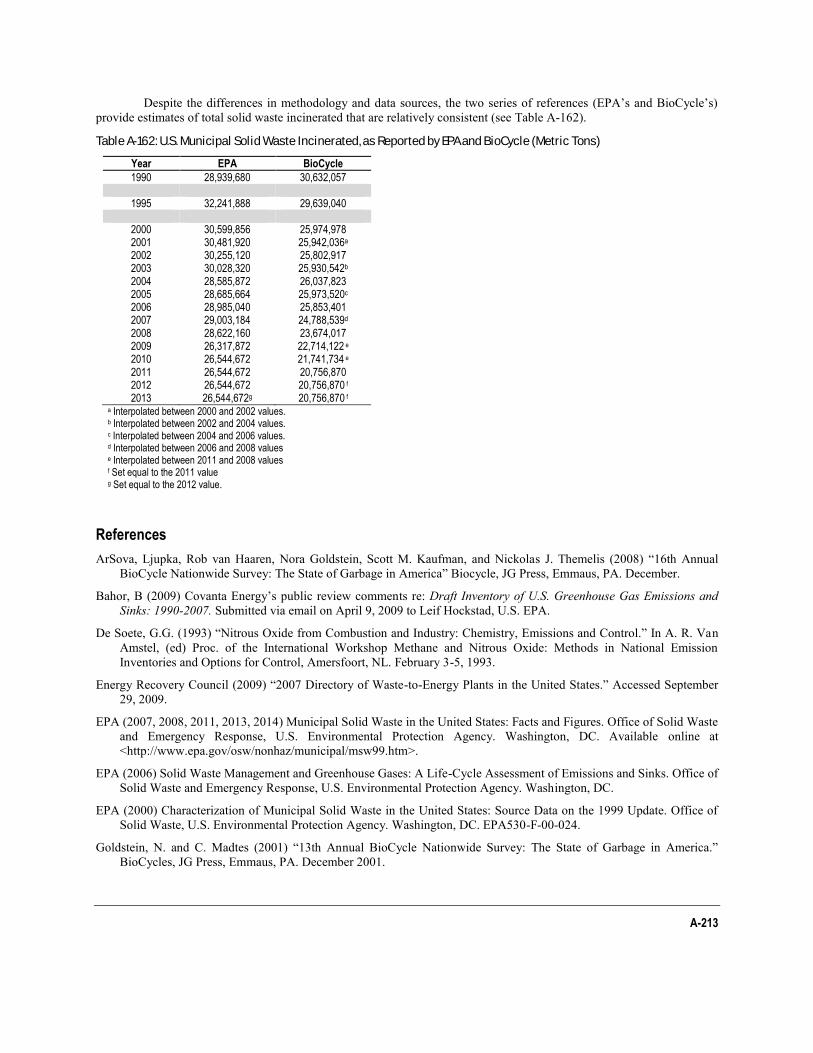
A-213
Despite the differences in methodology and data sources, the two series of references (EPA’s and BioCycle’s) provide estimates of total solid waste incinerated that are relatively consistent (see Table A-162).
Table A-162: U.S. Municipal Solid Waste Incinerated, as Reported by EPA and BioCycle (Metric Tons)
Year EPA BioCycle
1990 28,939,680 30,632,057
1995 32,241,888 29,639,040
2000 30,599,856 25,974,978 2001 30,481,920 25,942,036a 2002 30,255,120 25,802,917 2003 30,028,320 25,930,542b 2004 28,585,872 26,037,823 2005 28,685,664 25,973,520c 2006 28,985,040 25,853,401 2007 29,003,184 24,788,539d 2008 28,622,160 23,674,017 2009 26,317,872 22,714,122 e 2010 26,544,672 21,741,734 e 2011 26,544,672 20,756,870 2012 26,544,672 20,756,870 f 2013 26,544,672g 20,756,870 f
a Interpolated between 2000 and 2002 values. b Interpolated between 2002 and 2004 values. c Interpolated between 2004 and 2006 values. d Interpolated between 2006 and 2008 values e Interpolated between 2011 and 2008 values f Set equal to the 2011 value g Set equal to the 2012 value.
References
ArSova, Ljupka, Rob van Haaren, Nora Goldstein, Scott M. Kaufman, and Nickolas J. Themelis (2008) “16th Annual BioCycle Nationwide Survey: The State of Garbage in America” Biocycle, JG Press, Emmaus, PA. December.
Bahor, B (2009) Covanta Energy’s public review comments re: Draft Inventory of U.S. Greenhouse Gas Emissions and Sinks: 1990-2007. Submitted via email on April 9, 2009 to Leif Hockstad, U.S. EPA.
De Soete, G.G. (1993) “Nitrous Oxide from Combustion and Industry: Chemistry, Emissions and Control.” In A. R. Van Amstel, (ed) Proc. of the International Workshop Methane and Nitrous Oxide: Methods in National Emission Inventories and Options for Control, Amersfoort, NL. February 3-5, 1993.
Energy Recovery Council (2009) “2007 Directory of Waste-to-Energy Plants in the United States.” Accessed September 29, 2009.
EPA (2007, 2008, 2011, 2013, 2014) Municipal Solid Waste in the United States: Facts and Figures. Office of Solid Waste and Emergency Response, U.S. Environmental Protection Agency. Washington, DC. Available online at <http://www.epa.gov/osw/nonhaz/municipal/msw99.htm>.
EPA (2006) Solid Waste Management and Greenhouse Gases: A Life-Cycle Assessment of Emissions and Sinks. Office of Solid Waste and Emergency Response, U.S. Environmental Protection Agency. Washington, DC.
EPA (2000) Characterization of Municipal Solid Waste in the United States: Source Data on the 1999 Update. Office of Solid Waste, U.S. Environmental Protection Agency. Washington, DC. EPA530-F-00-024.
Goldstein, N. and C. Madtes (2001) “13th Annual BioCycle Nationwide Survey: The State of Garbage in America.” BioCycles, JG Press, Emmaus, PA. December 2001.
A-214 Inventory of U.S. Greenhouse Gas Emissions and Sinks: 1990-2013
IPCC (2006) 2006 IPCC Guidelines for National Greenhouse Gas Inventories. The National Greenhouse Gas Inventories Programme, The Intergovernmental Panel on Climate Change, H.S. Eggleston, L. Buendia, K. Miwa, T Ngara, and K. Tanabe (eds.). Hayama, Kanagawa, Japan.
Kaufman, et al. (2004) “14th Annual BioCycle Nationwide Survey: The State of Garbage in America 2004” Biocycle, JG Press, Emmaus, PA. January, 2004.
RMA (2014a) “2013 U.S. Scrap Tire Management Summary.” Rubber Manufacturers Association. November 2014. Available online at: < http://www.rma.org/download/scrap-tires/market-reports/US_STMarket2013.pdf>. Accessed 17 November 2014.
RMA (2014b) “Scrap Tire Markets: Facts and Figures – Scrap Tire Characteristics.” Available online at < http://www.stref.orgwww.stref.org/scrap_tires/scrap_tire_markets/scrap_tire_characteristics/ >. Accessed 17 November 2014.
RMA (2012) "Rubber FAQs." Rubber Manufacturers Association. Available online at <http://www.rma.org/about-rma/rubber-faqs/>Accessed 19 November 2014.
RMA (2011) “U.S. Scrap Tire Management Summary 2005-2009.” Rubber Manufacturers Association. October 2011. Available online at: <http://www.rma.org/scrap_tires/scrap_tire_markets/2009_summary.pdf>.
Schneider, S. (2007) E-mail between Shelly Schneider of Franklin Associates (a division of ERG) and Sarah Shapiro of ICF International, January 10, 2007.
Shin, D. (2014) Generation and Disposition of Municipal Solid Waste (MSW) in the United States–A National Survey. Thesis. Columbia University, Department of Earth and Environmental Engineering, January 3, 2014.
Simmons, et al. (2006) “15th Nationwide Survey of Municipal Solid Waste Management in the United States: The State of Garbage in America” BioCycle, JG Press, Emmaus, PA. April 2006.
Themelis and Shin (in press) U.S. Survey of Generation and Disposition of Municipal Solid Waste. Waste Management. Submitted November 14, 2014.
van Haaren, Rob, Thermelis, N., and Goldstein, N. (2010) "The State of Garbage in America." BioCycle, October 2010. Volume 51, Number 10, pg. 16-23.
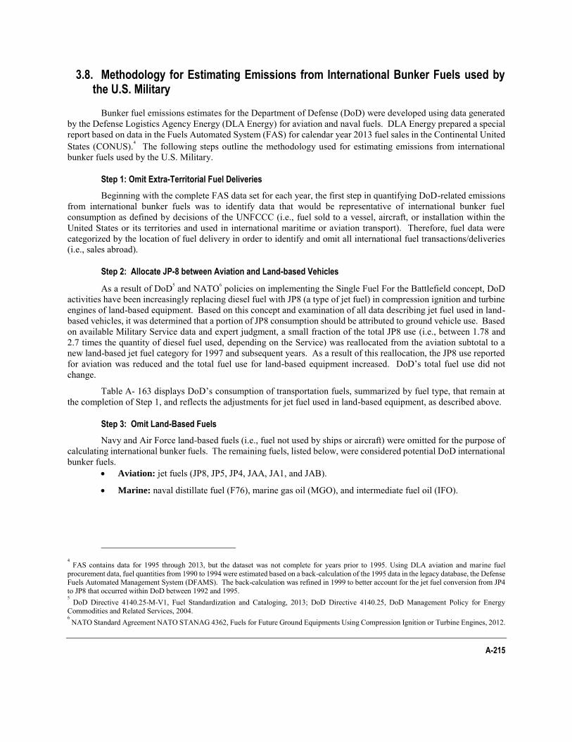
A-215
3.8. Methodology for Estimating Emissions from International Bunker Fuels used by the U.S. Military
Bunker fuel emissions estimates for the Department of Defense (DoD) were developed using data generated by the Defense Logistics Agency Energy (DLA Energy) for aviation and naval fuels. DLA Energy prepared a special report based on data in the Fuels Automated System (FAS) for calendar year 2013 fuel sales in the Continental United States (CONUS).4 The following steps outline the methodology used for estimating emissions from international bunker fuels used by the U.S. Military.
Step 1: Omit Extra-Territorial Fuel Deliveries
Beginning with the complete FAS data set for each year, the first step in quantifying DoD-related emissions from international bunker fuels was to identify data that would be representative of international bunker fuel consumption as defined by decisions of the UNFCCC (i.e., fuel sold to a vessel, aircraft, or installation within the United States or its territories and used in international maritime or aviation transport). Therefore, fuel data were categorized by the location of fuel delivery in order to identify and omit all international fuel transactions/deliveries (i.e., sales abroad).
Step 2: Allocate JP-8 between Aviation and Land-based Vehicles
As a result of DoD5 and NATO6 policies on implementing the Single Fuel For the Battlefield concept, DoD activities have been increasingly replacing diesel fuel with JP8 (a type of jet fuel) in compression ignition and turbine engines of land-based equipment. Based on this concept and examination of all data describing jet fuel used in land-based vehicles, it was determined that a portion of JP8 consumption should be attributed to ground vehicle use. Based on available Military Service data and expert judgment, a small fraction of the total JP8 use (i.e., between 1.78 and 2.7 times the quantity of diesel fuel used, depending on the Service) was reallocated from the aviation subtotal to a new land-based jet fuel category for 1997 and subsequent years. As a result of this reallocation, the JP8 use reported for aviation was reduced and the total fuel use for land-based equipment increased. DoD’s total fuel use did not change.
Table A- 163 displays DoD’s consumption of transportation fuels, summarized by fuel type, that remain at the completion of Step 1, and reflects the adjustments for jet fuel used in land-based equipment, as described above.
Step 3: Omit Land-Based Fuels
Navy and Air Force land-based fuels (i.e., fuel not used by ships or aircraft) were omitted for the purpose of calculating international bunker fuels. The remaining fuels, listed below, were considered potential DoD international bunker fuels.
Aviation: jet fuels (JP8, JP5, JP4, JAA, JA1, and JAB).
Marine: naval distillate fuel (F76), marine gas oil (MGO), and intermediate fuel oil (IFO).
4 FAS contains data for 1995 through 2013, but the dataset was not complete for years prior to 1995. Using DLA aviation and marine fuel
procurement data, fuel quantities from 1990 to 1994 were estimated based on a back-calculation of the 1995 data in the legacy database, the Defense Fuels Automated Management System (DFAMS). The back-calculation was refined in 1999 to better account for the jet fuel conversion from JP4 to JP8 that occurred within DoD between 1992 and 1995. 5 DoD Directive 4140.25-M-V1, Fuel Standardization and Cataloging, 2013; DoD Directive 4140.25, DoD Management Policy for Energy
Commodities and Related Services, 2004. 6 NATO Standard Agreement NATO STANAG 4362, Fuels for Future Ground Equipments Using Compression Ignition or Turbine Engines, 2012.
A-216 Inventory of U.S. Greenhouse Gas Emissions and Sinks: 1990-2013
Step 4: Omit Fuel Transactions Received by Military Services that are not considered to be International Bunker Fuels
Only Navy and Air Force were deemed to be users of military international bunker fuels after sorting the data by Military Service and applying the following assumptions regarding fuel use by Service.
Only fuel delivered to a ship, aircraft, or installation in the United States was considered a potential international bunker fuel. Fuel consumed in international aviation or marine transport was included in the bunker fuel estimate of the country where the ship or aircraft was fueled. Fuel consumed entirely within a country’s borders was not considered a bunker fuel.
Based on previous discussions with the Army staff, only an extremely small percentage of Army aviation emissions, and none of Army watercraft emissions, qualified as bunker fuel emissions. The magnitude of these emissions was judged to be insignificant when compared to Air Force and Navy emissions. Based on this research, Army bunker fuel emissions were assumed to be zero.
Marine Corps aircraft operating while embarked consumed fuel that was reported as delivered to the Navy. Bunker fuel emissions from embarked Marine Corps aircraft were reported in the Navy bunker fuel estimates. Bunker fuel emissions from other Marine Corps operations and training were assumed to be zero.
Bunker fuel emissions from other DoD and non-DoD activities (i.e., other federal agencies) that purchased fuel from DLA Energy were assumed to be zero.
Step 5: Determine Bunker Fuel Percentages
It was necessary to determine what percent of the aviation and marine fuels were used as international bunker fuels. Military aviation bunkers include international operations (i.e., sorties that originate in the United States and end in a foreign country), operations conducted from naval vessels at sea, and operations conducted from U.S. installations principally over international water in direct support of military operations at sea (e.g., anti-submarine warfare flights). Methods for quantifying aviation and marine bunker fuel percentages are described below.
Aviation: The Air Force Aviation bunker fuel percentage was determined to be 13.2 percent. A bunker fuel weighted average was calculated based on flying hours by major command. International flights were weighted by an adjustment factor to reflect the fact that they typically last longer than domestic flights. In addition, a fuel use correction factor was used to account for the fact that transport aircraft burn more fuel per hour of flight than most tactical aircraft. This percentage was multiplied by total annual Air Force aviation fuel delivered for U.S. activities, producing an estimate for international bunker fuel consumed by the Air Force. The Naval Aviation bunker fuel percentage was calculated to be 40.4 percent by using flying hour data from Chief of Naval Operations Flying Hour Projection System Budget for fiscal year 1998 and estimates of bunker fuel percent of flights provided by the fleet. This Naval Aviation bunker fuel percentage was then multiplied by total annual Navy aviation fuel delivered for U.S. activities, yielding total Navy aviation bunker fuel consumed.
Marine: For marine bunkers, fuels consumed while ships were underway were assumed to be bunker
fuels. The Navy maritime bunker fuel percentage was determined to be 79 percent because the Navy reported that 79 percent of vessel operations were underway, while the remaining 21 percent of operations occurred in port (i.e., pierside) in the year 2000.7
Table A- 164 and Table A-165 display DoD bunker fuel use totals for the Navy and Air Force.
7 Note that 79 percent is used because it is based on Navy data, but the percentage of time underway may vary from year-to-year
depending on vessel operations. For example, for years prior to 2000, the bunker fuel percentage was 87 percent.

A-217
Step 6: Calculate Emissions from International Bunker Fuels
Bunker fuel totals were multiplied by appropriate emission factors to determine greenhouse gas (GHG) emissions. CO2 emissions from Aviation Bunkers and distillate Marine Bunkers are the total of military aviation and marine bunker fuels, respectively.
The rows labeled “U.S. Military” and “U.S. Military Naval Fuels” in the tables in the International Bunker Fuels section of the Energy chapter were based on the totals provided in Table A- 164 and Table A-165, below. CO2 emissions from aviation bunkers and distillate marine bunkers are presented in Table A-168, and are based on emissions from fuels tallied in Table A- 164 and Table A-165.
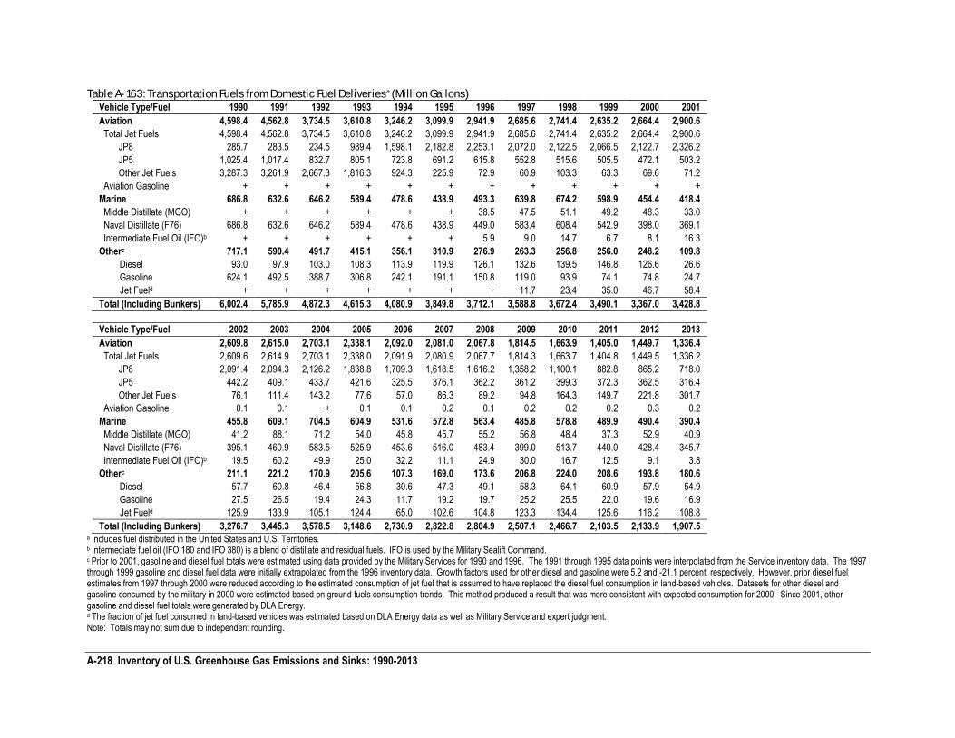
A-218 Inventory of U.S. Greenhouse Gas Emissions and Sinks: 1990-2013
Table A- 163: Transportation Fuels from Domestic Fuel Deliveriesa (Million Gallons)
Vehicle Type/Fuel 1990 1991 1992 1993 1994 1995 1996 1997 1998 1999 2000 2001
Aviation 4,598.4 4,562.8 3,734.5 3,610.8 3,246.2 3,099.9 2,941.9 2,685.6 2,741.4 2,635.2 2,664.4 2,900.6
Total Jet Fuels 4,598.4 4,562.8 3,734.5 3,610.8 3,246.2 3,099.9 2,941.9 2,685.6 2,741.4 2,635.2 2,664.4 2,900.6
JP8 285.7 283.5 234.5 989.4 1,598.1 2,182.8 2,253.1 2,072.0 2,122.5 2,066.5 2,122.7 2,326.2
JP5 1,025.4 1,017.4 832.7 805.1 723.8 691.2 615.8 552.8 515.6 505.5 472.1 503.2
Other Jet Fuels 3,287.3 3,261.9 2,667.3 1,816.3 924.3 225.9 72.9 60.9 103.3 63.3 69.6 71.2
Aviation Gasoline + + + + + + + + + + + +
Marine 686.8 632.6 646.2 589.4 478.6 438.9 493.3 639.8 674.2 598.9 454.4 418.4
Middle Distillate (MGO) + + + + + + 38.5 47.5 51.1 49.2 48.3 33.0
Naval Distillate (F76) 686.8 632.6 646.2 589.4 478.6 438.9 449.0 583.4 608.4 542.9 398.0 369.1
Intermediate Fuel Oil (IFO)b + + + + + + 5.9 9.0 14.7 6.7 8.1 16.3
Otherc 717.1 590.4 491.7 415.1 356.1 310.9 276.9 263.3 256.8 256.0 248.2 109.8
Diesel 93.0 97.9 103.0 108.3 113.9 119.9 126.1 132.6 139.5 146.8 126.6 26.6
Gasoline 624.1 492.5 388.7 306.8 242.1 191.1 150.8 119.0 93.9 74.1 74.8 24.7
Jet Fueld + + + + + + + 11.7 23.4 35.0 46.7 58.4
Total (Including Bunkers) 6,002.4 5,785.9 4,872.3 4,615.3 4,080.9 3,849.8 3,712.1 3,588.8 3,672.4 3,490.1 3,367.0 3,428.8
Vehicle Type/Fuel 2002 2003 2004 2005 2006 2007 2008 2009 2010 2011 2012 2013
Aviation 2,609.8 2,615.0 2,703.1 2,338.1 2,092.0 2,081.0 2,067.8 1,814.5 1,663.9 1,405.0 1,449.7 1,336.4
Total Jet Fuels 2,609.6 2,614.9 2,703.1 2,338.0 2,091.9 2,080.9 2,067.7 1,814.3 1,663.7 1,404.8 1,449.5 1,336.2
JP8 2,091.4 2,094.3 2,126.2 1,838.8 1,709.3 1,618.5 1,616.2 1,358.2 1,100.1 882.8 865.2 718.0
JP5 442.2 409.1 433.7 421.6 325.5 376.1 362.2 361.2 399.3 372.3 362.5 316.4
Other Jet Fuels 76.1 111.4 143.2 77.6 57.0 86.3 89.2 94.8 164.3 149.7 221.8 301.7
Aviation Gasoline 0.1 0.1 + 0.1 0.1 0.2 0.1 0.2 0.2 0.2 0.3 0.2
Marine 455.8 609.1 704.5 604.9 531.6 572.8 563.4 485.8 578.8 489.9 490.4 390.4
Middle Distillate (MGO) 41.2 88.1 71.2 54.0 45.8 45.7 55.2 56.8 48.4 37.3 52.9 40.9
Naval Distillate (F76) 395.1 460.9 583.5 525.9 453.6 516.0 483.4 399.0 513.7 440.0 428.4 345.7
Intermediate Fuel Oil (IFO)b 19.5 60.2 49.9 25.0 32.2 11.1 24.9 30.0 16.7 12.5 9.1 3.8
Otherc 211.1 221.2 170.9 205.6 107.3 169.0 173.6 206.8 224.0 208.6 193.8 180.6
Diesel 57.7 60.8 46.4 56.8 30.6 47.3 49.1 58.3 64.1 60.9 57.9 54.9
Gasoline 27.5 26.5 19.4 24.3 11.7 19.2 19.7 25.2 25.5 22.0 19.6 16.9
Jet Fueld 125.9 133.9 105.1 124.4 65.0 102.6 104.8 123.3 134.4 125.6 116.2 108.8
Total (Including Bunkers) 3,276.7 3,445.3 3,578.5 3,148.6 2,730.9 2,822.8 2,804.9 2,507.1 2,466.7 2,103.5 2,133.9 1,907.5 a Includes fuel distributed in the United States and U.S. Territories. b Intermediate fuel oil (IFO 180 and IFO 380) is a blend of distillate and residual fuels. IFO is used by the Military Sealift Command. c Prior to 2001, gasoline and diesel fuel totals were estimated using data provided by the Military Services for 1990 and 1996. The 1991 through 1995 data points were interpolated from the Service inventory data. The 1997 through 1999 gasoline and diesel fuel data were initially extrapolated from the 1996 inventory data. Growth factors used for other diesel and gasoline were 5.2 and -21.1 percent, respectively. However, prior diesel fuel estimates from 1997 through 2000 were reduced according to the estimated consumption of jet fuel that is assumed to have replaced the diesel fuel consumption in land-based vehicles. Datasets for other diesel and gasoline consumed by the military in 2000 were estimated based on ground fuels consumption trends. This method produced a result that was more consistent with expected consumption for 2000. Since 2001, other gasoline and diesel fuel totals were generated by DLA Energy. d The fraction of jet fuel consumed in land-based vehicles was estimated based on DLA Energy data as well as Military Service and expert judgment. Note: Totals may not sum due to independent rounding.
A-219
+ indicates value does not exceed 0.05 million gallons.
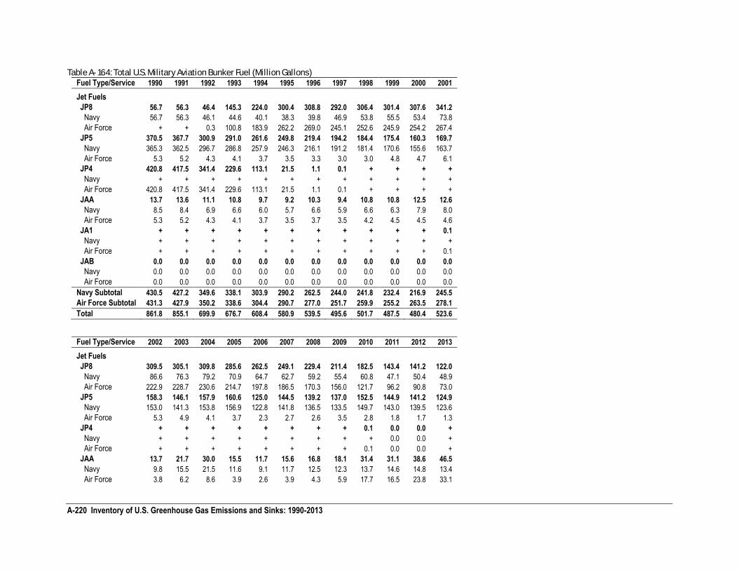
A-220 Inventory of U.S. Greenhouse Gas Emissions and Sinks: 1990-2013
Table A- 164: Total U.S. Military Aviation Bunker Fuel (Million Gallons)
Fuel Type/Service 1990 1991 1992 1993 1994 1995 1996 1997 1998 1999 2000 2001
Jet Fuels
JP8 56.7 56.3 46.4 145.3 224.0 300.4 308.8 292.0 306.4 301.4 307.6 341.2
Navy 56.7 56.3 46.1 44.6 40.1 38.3 39.8 46.9 53.8 55.5 53.4 73.8
Air Force + + 0.3 100.8 183.9 262.2 269.0 245.1 252.6 245.9 254.2 267.4
JP5 370.5 367.7 300.9 291.0 261.6 249.8 219.4 194.2 184.4 175.4 160.3 169.7
Navy 365.3 362.5 296.7 286.8 257.9 246.3 216.1 191.2 181.4 170.6 155.6 163.7
Air Force 5.3 5.2 4.3 4.1 3.7 3.5 3.3 3.0 3.0 4.8 4.7 6.1
JP4 420.8 417.5 341.4 229.6 113.1 21.5 1.1 0.1 + + + +
Navy + + + + + + + + + + + +
Air Force 420.8 417.5 341.4 229.6 113.1 21.5 1.1 0.1 + + + +
JAA 13.7 13.6 11.1 10.8 9.7 9.2 10.3 9.4 10.8 10.8 12.5 12.6
Navy 8.5 8.4 6.9 6.6 6.0 5.7 6.6 5.9 6.6 6.3 7.9 8.0
Air Force 5.3 5.2 4.3 4.1 3.7 3.5 3.7 3.5 4.2 4.5 4.5 4.6
JA1 + + + + + + + + + + + 0.1
Navy + + + + + + + + + + + +
Air Force + + + + + + + + + + + 0.1
JAB 0.0 0.0 0.0 0.0 0.0 0.0 0.0 0.0 0.0 0.0 0.0 0.0
Navy 0.0 0.0 0.0 0.0 0.0 0.0 0.0 0.0 0.0 0.0 0.0 0.0
Air Force 0.0 0.0 0.0 0.0 0.0 0.0 0.0 0.0 0.0 0.0 0.0 0.0
Navy Subtotal 430.5 427.2 349.6 338.1 303.9 290.2 262.5 244.0 241.8 232.4 216.9 245.5
Air Force Subtotal 431.3 427.9 350.2 338.6 304.4 290.7 277.0 251.7 259.9 255.2 263.5 278.1
Total 861.8 855.1 699.9 676.7 608.4 580.9 539.5 495.6 501.7 487.5 480.4 523.6
Fuel Type/Service 2002 2003 2004 2005 2006 2007 2008 2009 2010 2011 2012 2013
Jet Fuels
JP8 309.5 305.1 309.8 285.6 262.5 249.1 229.4 211.4 182.5 143.4 141.2 122.0
Navy 86.6 76.3 79.2 70.9 64.7 62.7 59.2 55.4 60.8 47.1 50.4 48.9
Air Force 222.9 228.7 230.6 214.7 197.8 186.5 170.3 156.0 121.7 96.2 90.8 73.0
JP5 158.3 146.1 157.9 160.6 125.0 144.5 139.2 137.0 152.5 144.9 141.2 124.9
Navy 153.0 141.3 153.8 156.9 122.8 141.8 136.5 133.5 149.7 143.0 139.5 123.6
Air Force 5.3 4.9 4.1 3.7 2.3 2.7 2.6 3.5 2.8 1.8 1.7 1.3
JP4 + + + + + + + + 0.1 0.0 0.0 +
Navy + + + + + + + + + 0.0 0.0 +
Air Force + + + + + + + + 0.1 0.0 0.0 +
JAA 13.7 21.7 30.0 15.5 11.7 15.6 16.8 18.1 31.4 31.1 38.6 46.5
Navy 9.8 15.5 21.5 11.6 9.1 11.7 12.5 12.3 13.7 14.6 14.8 13.4
Air Force 3.8 6.2 8.6 3.9 2.6 3.9 4.3 5.9 17.7 16.5 23.8 33.1
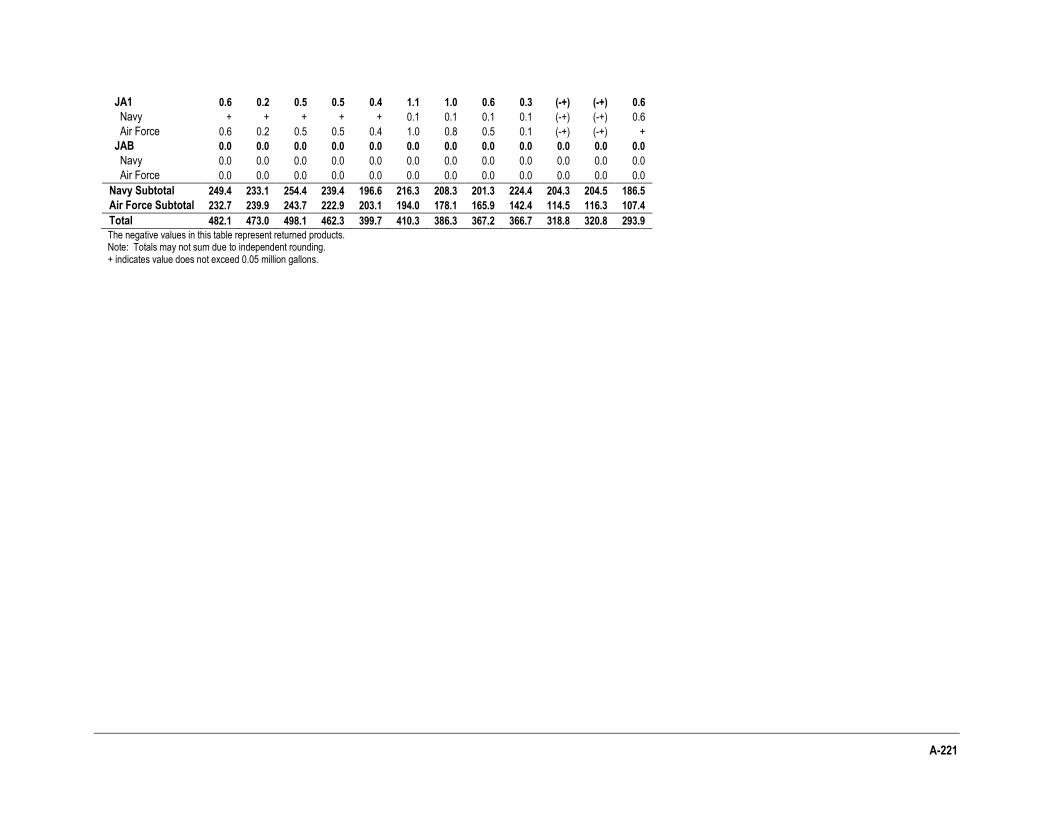
A-221
JA1 0.6 0.2 0.5 0.5 0.4 1.1 1.0 0.6 0.3 (-+) (-+) 0.6
Navy + + + + + 0.1 0.1 0.1 0.1 (-+) (-+) 0.6
Air Force 0.6 0.2 0.5 0.5 0.4 1.0 0.8 0.5 0.1 (-+) (-+) +
JAB 0.0 0.0 0.0 0.0 0.0 0.0 0.0 0.0 0.0 0.0 0.0 0.0
Navy 0.0 0.0 0.0 0.0 0.0 0.0 0.0 0.0 0.0 0.0 0.0 0.0
Air Force 0.0 0.0 0.0 0.0 0.0 0.0 0.0 0.0 0.0 0.0 0.0 0.0
Navy Subtotal 249.4 233.1 254.4 239.4 196.6 216.3 208.3 201.3 224.4 204.3 204.5 186.5
Air Force Subtotal 232.7 239.9 243.7 222.9 203.1 194.0 178.1 165.9 142.4 114.5 116.3 107.4
Total 482.1 473.0 498.1 462.3 399.7 410.3 386.3 367.2 366.7 318.8 320.8 293.9
The negative values in this table represent returned products. Note: Totals may not sum due to independent rounding. + indicates value does not exceed 0.05 million gallons.
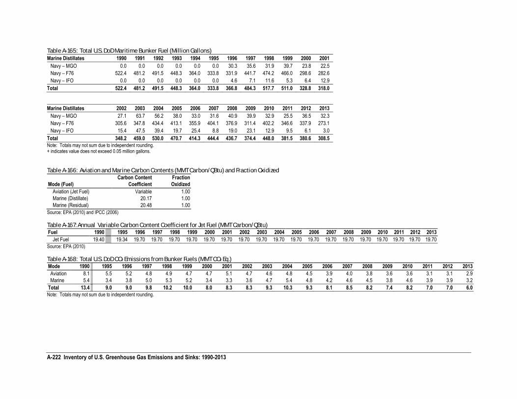
A-222 Inventory of U.S. Greenhouse Gas Emissions and Sinks: 1990-2013
Table A-165: Total U.S. DoD Maritime Bunker Fuel (Million Gallons)
Marine Distillates 1990 1991 1992 1993 1994 1995 1996 1997 1998 1999 2000 2001
Navy – MGO 0.0 0.0 0.0 0.0 0.0 0.0 30.3 35.6 31.9 39.7 23.8 22.5
Navy – F76 522.4 481.2 491.5 448.3 364.0 333.8 331.9 441.7 474.2 466.0 298.6 282.6
Navy – IFO 0.0 0.0 0.0 0.0 0.0 0.0 4.6 7.1 11.6 5.3 6.4 12.9
Total 522.4 481.2 491.5 448.3 364.0 333.8 366.8 484.3 517.7 511.0 328.8 318.0
Marine Distillates 2002 2003 2004 2005 2006 2007 2008 2009 2010 2011 2012 2013
Navy – MGO 27.1 63.7 56.2 38.0 33.0 31.6 40.9 39.9 32.9 25.5 36.5 32.3
Navy – F76 305.6 347.8 434.4 413.1 355.9 404.1 376.9 311.4 402.2 346.6 337.9 273.1
Navy – IFO 15.4 47.5 39.4 19.7 25.4 8.8 19.0 23.1 12.9 9.5 6.1 3.0
Total 348.2 459.0 530.0 470.7 414.3 444.4 436.7 374.4 448.0 381.5 380.6 308.5
Note: Totals may not sum due to independent rounding. + indicates value does not exceed 0.05 million gallons.
Table A-166: Aviation and Marine Carbon Contents (MMT Carbon/QBtu) and Fraction Oxidized
Mode (Fuel)
Carbon Content
Coefficient
Fraction
Oxidized
Aviation (Jet Fuel) Variable 1.00
Marine (Distillate) 20.17 1.00
Marine (Residual) 20.48 1.00
Source: EPA (2010) and IPCC (2006)
Table A-167: Annual Variable Carbon Content Coefficient for Jet Fuel (MMT Carbon/QBtu) Fuel 1990 1995 1996 1997 1998 1999 2000 2001 2002 2003 2004 2005 2006 2007 2008 2009 2010 2011 2012 2013
Jet Fuel 19.40 19.34 19.70 19.70 19.70 19.70 19.70 19.70 19.70 19.70 19.70 19.70 19.70 19.70 19.70 19.70 19.70 19.70 19.70 19.70
Source: EPA (2010)
Table A-168: Total U.S. DoD CO2 Emissions from Bunker Fuels (MMT CO2 Eq.) Mode 1990 1995 1996 1997 1998 1999 2000 2001 2002 2003 2004 2005 2006 2007 2008 2009 2010 2011 2012 2013
Aviation 8.1 5.5 5.2 4.8 4.9 4.7 4.7 5.1 4.7 4.6 4.8 4.5 3.9 4.0 3.8 3.6 3.6 3.1 3.1 2.9
Marine 5.4 3.4 3.8 5.0 5.3 5.2 3.4 3.3 3.6 4.7 5.4 4.8 4.2 4.6 4.5 3.8 4.6 3.9 3.9 3.2
Total 13.4 9.0 9.0 9.8 10.2 10.0 8.0 8.3 8.3 9.3 10.3 9.3 8.1 8.5 8.2 7.4 8.2 7.0 7.0 6.0
Note: Totals may not sum due to independent rounding.
A-223
3.9. Methodology for Estimating HFC and PFC Emissions from Substitution of Ozone Depleting Substances
Emissions of HFCs and PFCs from the substitution of ozone depleting substances (ODS) are developed using a country-specific modeling approach. The Vintaging Model was developed as a tool for estimating the annual chemical emissions from industrial sectors that have historically used ODS in their products. Under the terms of the Montreal Protocol and the United States Clean Air Act Amendments of 1990, the domestic U.S. consumption of ODS—chlorofluorocarbons (CFCs), halons, carbon tetrachloride, methyl chloroform, and hydrochlorofluorocarbons (HCFCs)—has been drastically reduced, forcing these industrial sectors to transition to more ozone friendly chemicals. As these industries have moved toward ODS alternatives such as hydrofluorocarbons (HFCs) and perfluorocarbons (PFCs), the Vintaging Model has evolved into a tool for estimating the rise in consumption and emissions of these alternatives, and the decline of ODS consumption and emissions.
The Vintaging Model estimates emissions from five ODS substitute end-use sectors: refrigeration and air-conditioning, foams, aerosols, solvents, and fire-extinguishing. Within these sectors, there are 60 independently modeled end-uses. The model requires information on the market growth for each of the end-uses, a history of the market transition from ODS to alternatives, and the characteristics of each end-use such as market size or charge sizes and loss rates. As ODS are phased out, a percentage of the market share originally filled by the ODS is allocated to each of its substitutes.
The model, named for its method of tracking the emissions of annual “vintages” of new equipment that enter into service, is a “bottom-up” model. It models the consumption of chemicals based on estimates of the quantity of equipment or products sold, serviced, and retired each year, and the amount of the chemical required to manufacture and/or maintain the equipment. The Vintaging Model makes use of this market information to build an inventory of the in-use stocks of the equipment and ODS and ODS substitute in each of the end-uses. The simulation is considered to be a “business-as-usual” baseline case, and does not incorporate measures to reduce or eliminate the emissions of these gases other than those regulated by U.S. law or otherwise common in the industry. Emissions are estimated by applying annual leak rates, service emission rates, and disposal emission rates to each population of equipment. By aggregating the emission and consumption output from the different end-uses, the model produces estimates of total annual use and emissions of each chemical.
The Vintaging Model synthesizes data from a variety of sources, including data from the ODS Tracking System maintained by the Stratospheric Protection Division and information from submissions to EPA under the Significant New Alternatives Policy (SNAP) program. Published sources include documents prepared by the United Nations Environment Programme (UNEP) Technical Options Committees, reports from the Alternative Fluorocarbons Environmental Acceptability Study (AFEAS), and conference proceedings from the International Conferences on Ozone Protection Technologies and Earth Technologies Forums. EPA also coordinates extensively with numerous trade associations and individual companies. For example, the Alliance for Responsible Atmospheric Policy; the Air-Conditioning, Heating and Refrigeration Institute; the Association of Home Appliance Manufacturers; the American Automobile Manufacturers Association; and many of their member companies have provided valuable information over the years. In some instances the unpublished information that the EPA uses in the model is classified as Confidential Business Information (CBI). The annual emissions inventories of chemicals are aggregated in such a way that CBI cannot be inferred. Full public disclosure of the inputs to the Vintaging Model would jeopardize the security of the CBI that has been entrusted to the EPA.
The following sections discuss the emission equations used in the Vintaging Model for each broad end-use category. These equations are applied separately for each chemical used within each of the different end-uses. In the majority of these end-uses, more than one ODS substitute chemical is used.
In general, the modeled emissions are a function of the amount of chemical consumed in each end-use market. Estimates of the consumption of ODS alternatives can be inferred by determining the transition path of each regulated ODS used in the early 1990s. Using data gleaned from a variety of sources, assessments are made regarding which alternatives have been used, and what fraction of the ODS market in each end-use has been captured by a given alternative. By combining this with estimates of the total end-use market growth, a consumption value can be estimated for each chemical used within each end-use.
Methodology
The Vintaging Model estimates the use and emissions of ODS alternatives by taking the following steps:
1. Gather historical data. The Vintaging Model is populated with information on each end-use, taken from published sources and industry experts.
2. Simulate the implementation of new, non-ODS technologies. The Vintaging Model uses detailed characterizations of the existing uses of the ODS, as well as data on how the substitutes are replacing the ODS, to simulate
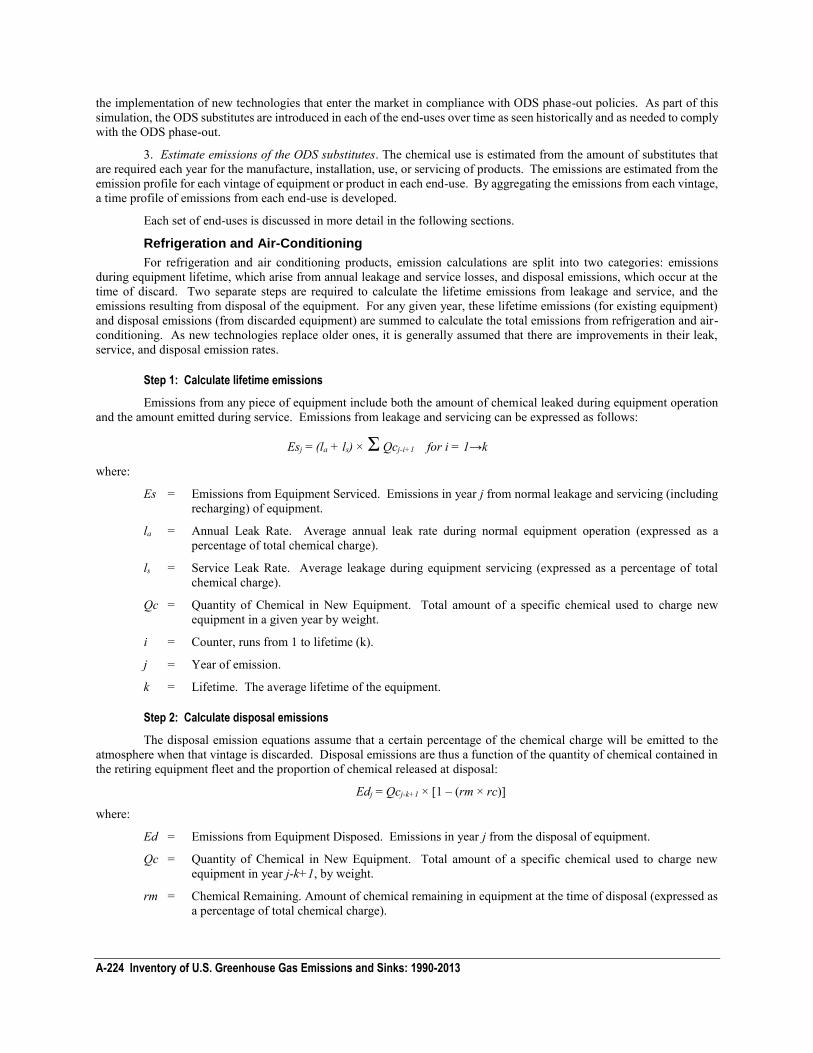
A-224 Inventory of U.S. Greenhouse Gas Emissions and Sinks: 1990-2013
the implementation of new technologies that enter the market in compliance with ODS phase-out policies. As part of this simulation, the ODS substitutes are introduced in each of the end-uses over time as seen historically and as needed to comply with the ODS phase-out.
3. Estimate emissions of the ODS substitutes. The chemical use is estimated from the amount of substitutes that are required each year for the manufacture, installation, use, or servicing of products. The emissions are estimated from the emission profile for each vintage of equipment or product in each end-use. By aggregating the emissions from each vintage, a time profile of emissions from each end-use is developed.
Each set of end-uses is discussed in more detail in the following sections.
Refrigeration and Air-Conditioning
For refrigeration and air conditioning products, emission calculations are split into two categories: emissions during equipment lifetime, which arise from annual leakage and service losses, and disposal emissions, which occur at the time of discard. Two separate steps are required to calculate the lifetime emissions from leakage and service, and the emissions resulting from disposal of the equipment. For any given year, these lifetime emissions (for existing equipment) and disposal emissions (from discarded equipment) are summed to calculate the total emissions from refrigeration and air-conditioning. As new technologies replace older ones, it is generally assumed that there are improvements in their leak, service, and disposal emission rates.
Step 1: Calculate lifetime emissions
Emissions from any piece of equipment include both the amount of chemical leaked during equipment operation and the amount emitted during service. Emissions from leakage and servicing can be expressed as follows:
Esj = (la + ls) × Σ Qcj-i+1 for i = 1→k
where:
Es = Emissions from Equipment Serviced. Emissions in year j from normal leakage and servicing (including recharging) of equipment.
la = Annual Leak Rate. Average annual leak rate during normal equipment operation (expressed as a percentage of total chemical charge).
ls = Service Leak Rate. Average leakage during equipment servicing (expressed as a percentage of total chemical charge).
Qc = Quantity of Chemical in New Equipment. Total amount of a specific chemical used to charge new equipment in a given year by weight.
i = Counter, runs from 1 to lifetime (k).
j = Year of emission.
k = Lifetime. The average lifetime of the equipment.
Step 2: Calculate disposal emissions
The disposal emission equations assume that a certain percentage of the chemical charge will be emitted to the atmosphere when that vintage is discarded. Disposal emissions are thus a function of the quantity of chemical contained in the retiring equipment fleet and the proportion of chemical released at disposal:
Edj = Qcj-k+1 × [1 – (rm × rc)]
where:
Ed = Emissions from Equipment Disposed. Emissions in year j from the disposal of equipment.
Qc = Quantity of Chemical in New Equipment. Total amount of a specific chemical used to charge new equipment in year j-k+1, by weight.
rm = Chemical Remaining. Amount of chemical remaining in equipment at the time of disposal (expressed as a percentage of total chemical charge).
A-225
rc = Chemical Recovery Rate. Amount of chemical that is recovered just prior to disposal (expressed as a percentage of chemical remaining at disposal (rm)).
j = Year of emission.
k = Lifetime. The average lifetime of the equipment.
Step 3: Calculate total emissions
Finally, lifetime and disposal emissions are summed to provide an estimate of total emissions.
Ej = Esj + Edj
where:
E = Total Emissions. Emissions from refrigeration and air conditioning equipment in year j.
Es = Emissions from Equipment Serviced. Emissions in year j from leakage and servicing (including recharging) of equipment.
Ed = Emissions from Equipment Disposed. Emissions in year j from the disposal of equipment.
j = Year of emission.
Assumptions
The assumptions used by the Vintaging Model to trace the transition of each type of equipment away from ODS are presented in Table A- 169, below. As new technologies replace older ones, it is generally assumed that there are improvements in their leak, service, and disposal emission rates. Additionally, the market for each equipment type is assumed to grow independently, according to annual growth rates.
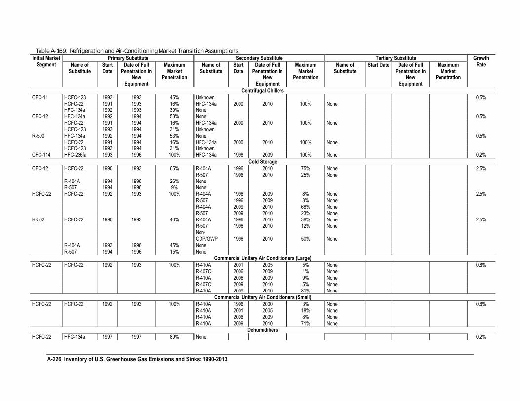
A-226 Inventory of U.S. Greenhouse Gas Emissions and Sinks: 1990-2013
Table A- 169: Refrigeration and Air-Conditioning Market Transition Assumptions Initial Market
Segment Primary Substitute Secondary Substitute Tertiary Substitute Growth
Rate Name of Substitute
Start Date
Date of Full Penetration in
New Equipment
Maximum Market
Penetration
Name of Substitute
Start Date
Date of Full Penetration in
New Equipment
Maximum Market
Penetration
Name of Substitute
Start Date Date of Full Penetration in
New Equipment
Maximum Market
Penetration
Centrifugal Chillers
CFC-11 HCFC-123 1993 1993 45% Unknown 0.5% HCFC-22 1991 1993 16% HFC-134a 2000 2010 100% None HFC-134a 1992 1993 39% None CFC-12 HFC-134a 1992 1994 53% None 0.5% HCFC-22 1991 1994 16% HFC-134a 2000 2010 100% None HCFC-123 1993 1994 31% Unknown R-500 HFC-134a 1992 1994 53% None 0.5% HCFC-22 1991 1994 16% HFC-134a 2000 2010 100% None HCFC-123 1993 1994 31% Unknown CFC-114 HFC-236fa 1993 1996 100% HFC-134a 1998 2009 100% None 0.2%
Cold Storage
CFC-12 HCFC-22 1990 1993 65% R-404A 1996 2010 75% None 2.5% R-507 1996 2010 25% None R-404A 1994 1996 26% None R-507 1994 1996 9% None HCFC-22 HCFC-22 1992 1993 100% R-404A 1996 2009 8% None 2.5% R-507 1996 2009 3% None R-404A 2009 2010 68% None R-507 2009 2010 23% None R-502 HCFC-22 1990 1993 40% R-404A 1996 2010 38% None 2.5% R-507 1996 2010 12% None
Non-ODP/GWP 1996 2010 50% None
R-404A 1993 1996 45% None R-507 1994 1996 15% None
Commercial Unitary Air Conditioners (Large)
HCFC-22 HCFC-22 1992 1993 100% R-410A 2001 2005 5% None 0.8% R-407C 2006 2009 1% None R-410A 2006 2009 9% None R-407C 2009 2010 5% None R-410A 2009 2010 81% None
Commercial Unitary Air Conditioners (Small)
HCFC-22 HCFC-22 1992 1993 100% R-410A 1996 2000 3% None 0.8% R-410A 2001 2005 18% None R-410A 2006 2009 8% None R-410A 2009 2010 71% None
Dehumidifiers
HCFC-22 HFC-134a 1997 1997 89% None 0.2%
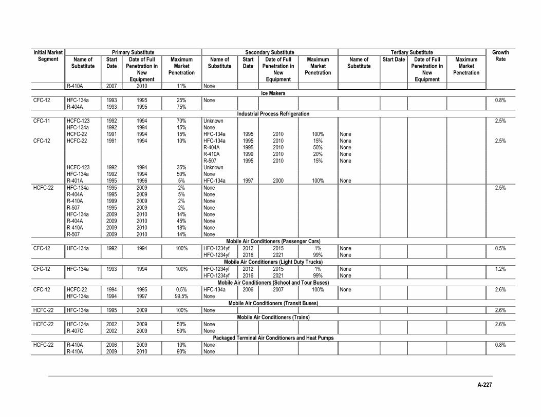
A-227
Initial Market Segment
Primary Substitute Secondary Substitute Tertiary Substitute Growth Rate Name of
Substitute Start Date
Date of Full Penetration in
New Equipment
Maximum Market
Penetration
Name of Substitute
Start Date
Date of Full Penetration in
New Equipment
Maximum Market
Penetration
Name of Substitute
Start Date Date of Full Penetration in
New Equipment
Maximum Market
Penetration
R-410A 2007 2010 11% None
Ice Makers
CFC-12 HFC-134a 1993 1995 25% None 0.8% R-404A 1993 1995 75%
Industrial Process Refrigeration
CFC-11 HCFC-123 1992 1994 70% Unknown 2.5% HFC-134a 1992 1994 15% None HCFC-22 1991 1994 15% HFC-134a 1995 2010 100% None CFC-12 HCFC-22 1991 1994 10% HFC-134a 1995 2010 15% None 2.5% R-404A 1995 2010 50% None R-410A 1999 2010 20% None R-507 1995 2010 15% None HCFC-123 1992 1994 35% Unknown HFC-134a 1992 1994 50% None R-401A 1995 1996 5% HFC-134a 1997 2000 100% None
HCFC-22 HFC-134a 1995 2009 2% None 2.5% R-404A 1995 2009 5% None R-410A 1999 2009 2% None R-507 1995 2009 2% None HFC-134a 2009 2010 14% None R-404A 2009 2010 45% None R-410A 2009 2010 18% None R-507 2009 2010 14% None
Mobile Air Conditioners (Passenger Cars)
CFC-12 HFC-134a 1992 1994 100% HFO-1234yf 2012 2015 1% None 0.5% HFO-1234yf 2016 2021 99% None
Mobile Air Conditioners (Light Duty Trucks)
CFC-12 HFC-134a 1993 1994 100% HFO-1234yf 2012 2015 1% None 1.2% HFO-1234yf 2016 2021 99% None
Mobile Air Conditioners (School and Tour Buses)
CFC-12 HCFC-22 HFC-134a
1994 1994
1995 1997
0.5% 99.5%
HFC-134a None
2006
2007
100%
None
2.6%
Mobile Air Conditioners (Transit Buses)
HCFC-22 HFC-134a 1995 2009 100% None 2.6%
Mobile Air Conditioners (Trains)
HCFC-22 HFC-134a R-407C
2002 2002
2009 2009
50% 50%
None None
2.6%
Packaged Terminal Air Conditioners and Heat Pumps
HCFC-22 R-410A 2006 2009 10% None 0.8% R-410A 2009 2010 90% None
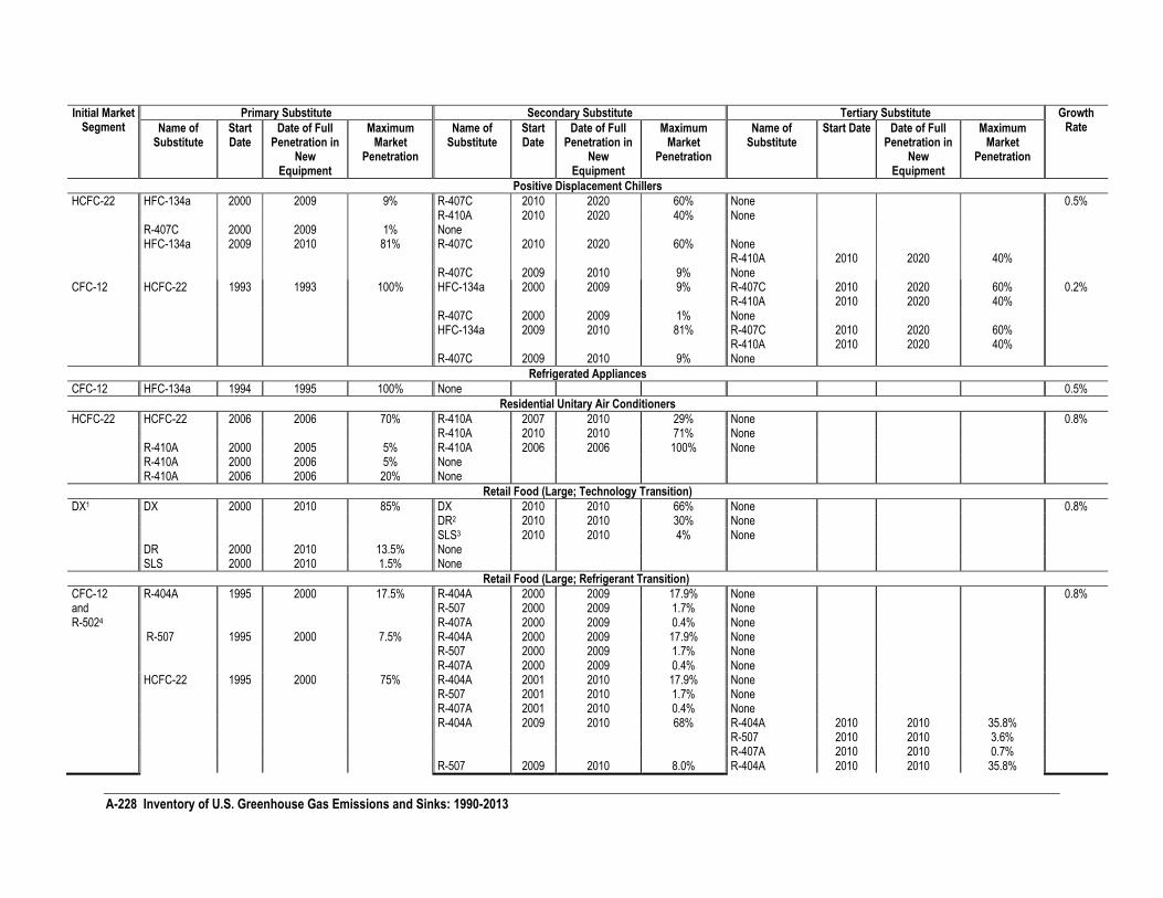
A-228 Inventory of U.S. Greenhouse Gas Emissions and Sinks: 1990-2013
Initial Market Segment
Primary Substitute Secondary Substitute Tertiary Substitute Growth Rate Name of
Substitute Start Date
Date of Full Penetration in
New Equipment
Maximum Market
Penetration
Name of Substitute
Start Date
Date of Full Penetration in
New Equipment
Maximum Market
Penetration
Name of Substitute
Start Date Date of Full Penetration in
New Equipment
Maximum Market
Penetration
Positive Displacement Chillers
HCFC-22 HFC-134a 2000 2009 9% R-407C 2010 2020 60% None 0.5% R-410A 2010 2020 40% None R-407C 2000 2009 1% None HFC-134a 2009 2010 81% R-407C 2010 2020 60% None R-410A 2010 2020 40% R-407C 2009 2010 9% None CFC-12 HCFC-22 1993 1993 100% HFC-134a 2000 2009 9% R-407C 2010 2020 60% 0.2% R-410A 2010 2020 40% R-407C 2000 2009 1% None HFC-134a 2009 2010 81% R-407C 2010 2020 60% R-410A 2010 2020 40% R-407C 2009 2010 9% None
Refrigerated Appliances
CFC-12 HFC-134a 1994 1995 100% None 0.5%
Residential Unitary Air Conditioners
HCFC-22 HCFC-22 2006 2006 70% R-410A 2007 2010 29% None 0.8% R-410A 2010 2010 71% None R-410A 2000 2005 5% R-410A 2006 2006 100% None R-410A 2000 2006 5% None R-410A 2006 2006 20% None
Retail Food (Large; Technology Transition)
DX1 DX 2000 2010 85% DX 2010 2010 66% None 0.8% DR2 2010 2010 30% None SLS3 2010 2010 4% None DR 2000 2010 13.5% None SLS 2000 2010 1.5% None
Retail Food (Large; Refrigerant Transition)
CFC-12 R-404A 1995 2000 17.5% R-404A 2000 2009 17.9% None 0.8% and R-507 2000 2009 1.7% None R-5024 R-407A 2000 2009 0.4% None R-507 1995 2000 7.5% R-404A 2000 2009 17.9% None R-507 2000 2009 1.7% None R-407A 2000 2009 0.4% None HCFC-22 1995 2000 75% R-404A 2001 2010 17.9% None R-507 2001 2010 1.7% None R-407A 2001 2010 0.4% None R-404A 2009 2010 68% R-404A 2010 2010 35.8% R-507 2010 2010 3.6% R-407A 2010 2010 0.7% R-507 2009 2010 8.0% R-404A 2010 2010 35.8%
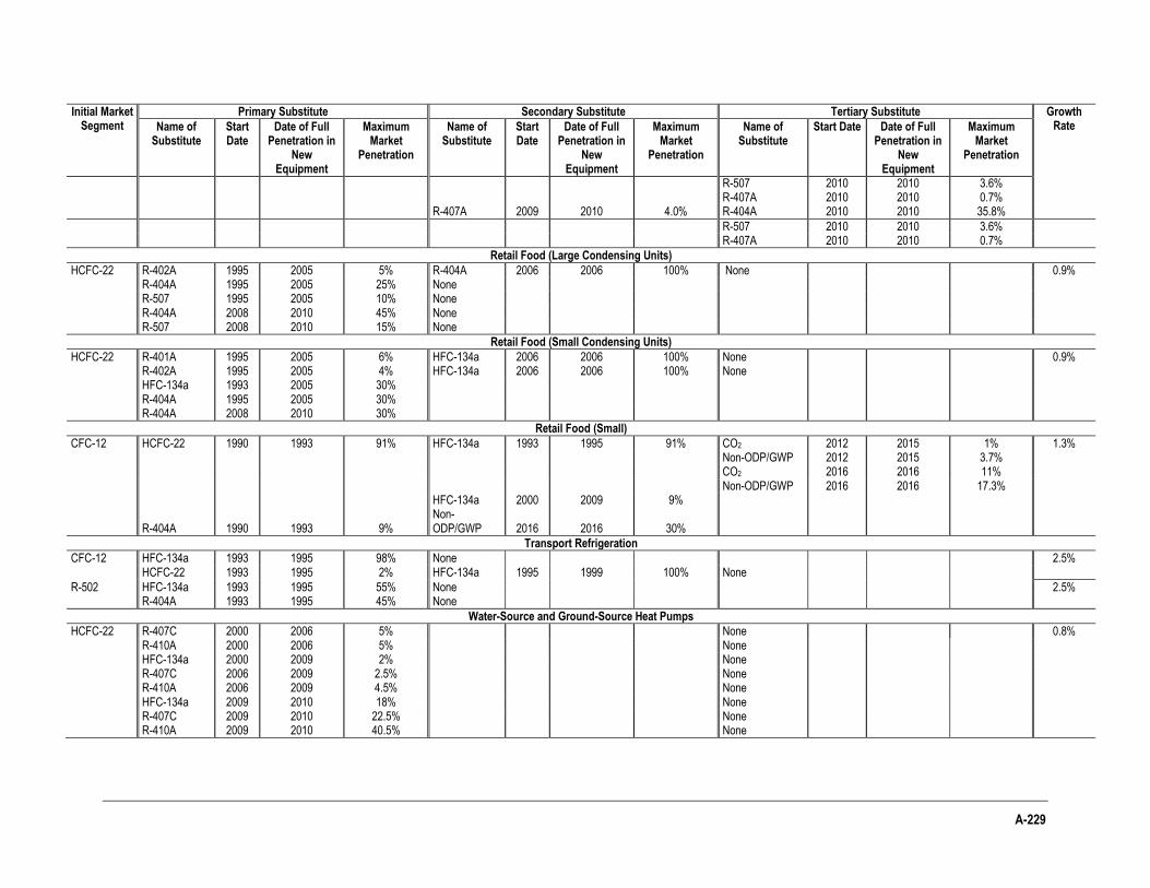
A-229
Initial Market Segment
Primary Substitute Secondary Substitute Tertiary Substitute Growth Rate Name of
Substitute Start Date
Date of Full Penetration in
New Equipment
Maximum Market
Penetration
Name of Substitute
Start Date
Date of Full Penetration in
New Equipment
Maximum Market
Penetration
Name of Substitute
Start Date Date of Full Penetration in
New Equipment
Maximum Market
Penetration
R-507 2010 2010 3.6% R-407A 2010 2010 0.7% R-407A 2009 2010 4.0% R-404A 2010 2010 35.8%
R-507 2010 2010 3.6% R-407A 2010 2010 0.7%
Retail Food (Large Condensing Units)
HCFC-22 R-402A 1995 2005 5% R-404A 2006 2006 100% None 0.9% R-404A 1995 2005 25% None R-507 1995 2005 10% None R-404A 2008 2010 45% None R-507 2008 2010 15% None
Retail Food (Small Condensing Units)
HCFC-22 R-401A 1995 2005 6% HFC-134a 2006 2006 100% None 0.9% R-402A 1995 2005 4% HFC-134a 2006 2006 100% None HFC-134a 1993 2005 30% R-404A 1995 2005 30% R-404A 2008 2010 30%
Retail Food (Small)
CFC-12 HCFC-22 1990 1993 91% HFC-134a 1993 1995 91% CO2 2012 2015 1% 1.3% Non-ODP/GWP 2012 2015 3.7% CO2 2016 2016 11% Non-ODP/GWP 2016 2016 17.3% HFC-134a 2000 2009 9%
R-404A 1990 1993 9% Non-ODP/GWP 2016 2016 30%
Transport Refrigeration
CFC-12 HFC-134a 1993 1995 98% None 2.5% HCFC-22 1993 1995 2% HFC-134a 1995 1999 100% None
R-502 HFC-134a 1993 1995 55% None 2.5% R-404A 1993 1995 45% None
Water-Source and Ground-Source Heat Pumps
HCFC-22 R-407C 2000 2006 5% None 0.8% R-410A 2000 2006 5% None HFC-134a 2000 2009 2% None R-407C 2006 2009 2.5% None R-410A 2006 2009 4.5% None HFC-134a 2009 2010 18% None R-407C 2009 2010 22.5% None R-410A 2009 2010 40.5% None
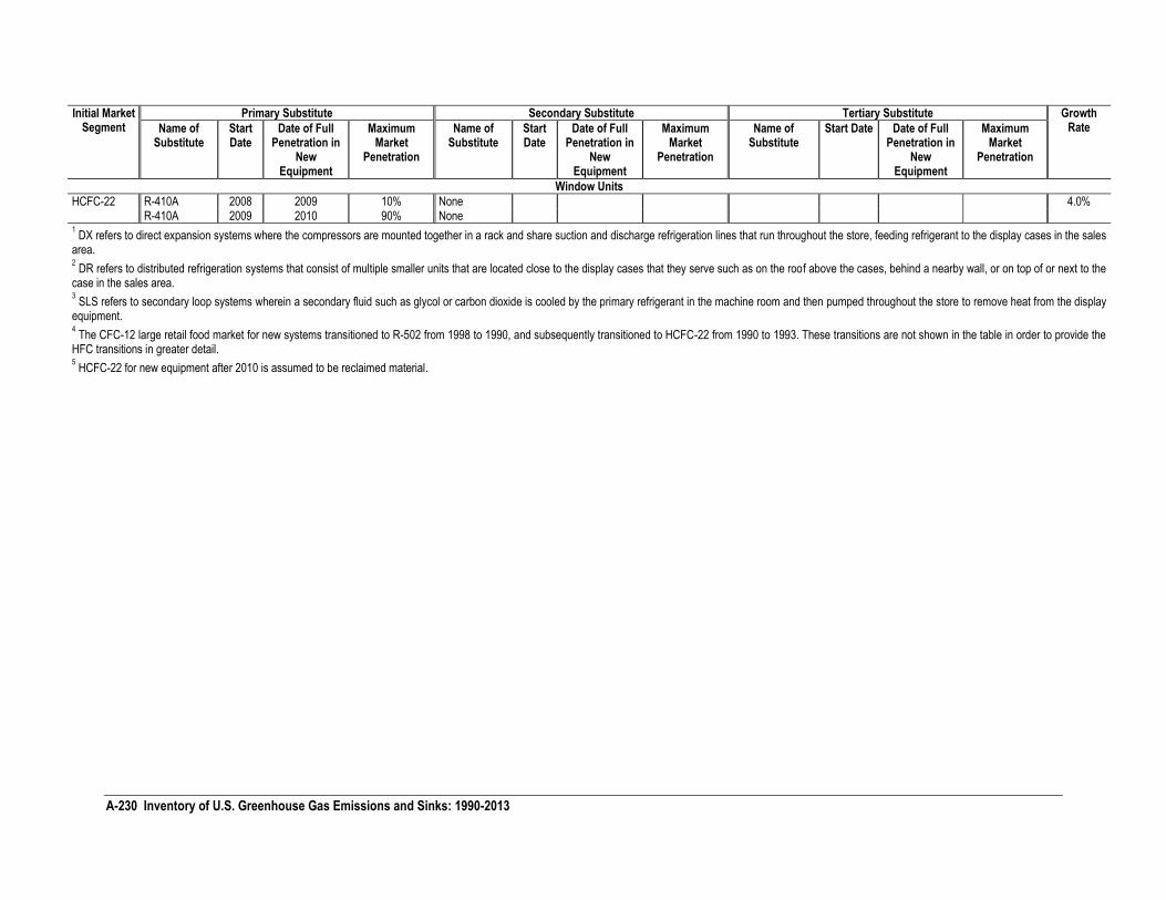
A-230 Inventory of U.S. Greenhouse Gas Emissions and Sinks: 1990-2013
Initial Market Segment
Primary Substitute Secondary Substitute Tertiary Substitute Growth Rate Name of
Substitute Start Date
Date of Full Penetration in
New Equipment
Maximum Market
Penetration
Name of Substitute
Start Date
Date of Full Penetration in
New Equipment
Maximum Market
Penetration
Name of Substitute
Start Date Date of Full Penetration in
New Equipment
Maximum Market
Penetration
Window Units
HCFC-22 R-410A 2008 2009 10% None 4.0% R-410A 2009 2010 90% None 1 DX refers to direct expansion systems where the compressors are mounted together in a rack and share suction and discharge refrigeration lines that run throughout the store, feeding refrigerant to the display cases in the sales
area. 2 DR refers to distributed refrigeration systems that consist of multiple smaller units that are located close to the display cases that they serve such as on the roof above the cases, behind a nearby wall, or on top of or next to the
case in the sales area. 3 SLS refers to secondary loop systems wherein a secondary fluid such as glycol or carbon dioxide is cooled by the primary refrigerant in the machine room and then pumped throughout the store to remove heat from the display
equipment. 4 The CFC-12 large retail food market for new systems transitioned to R-502 from 1998 to 1990, and subsequently transitioned to HCFC-22 from 1990 to 1993. These transitions are not shown in the table in order to provide the
HFC transitions in greater detail. 5 HCFC-22 for new equipment after 2010 is assumed to be reclaimed material.
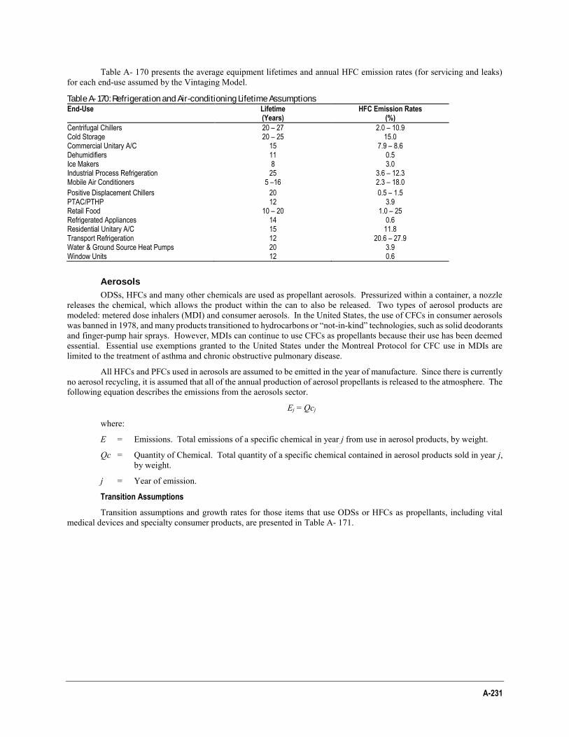
A-231
Table A- 170 presents the average equipment lifetimes and annual HFC emission rates (for servicing and leaks) for each end-use assumed by the Vintaging Model.
Table A- 170: Refrigeration and Air-conditioning Lifetime Assumptions End-Use Lifetime HFC Emission Rates (Years) (%)
Centrifugal Chillers 20 – 27 2.0 – 10.9 Cold Storage 20 – 25 15.0 Commercial Unitary A/C 15 7.9 – 8.6 Dehumidifiers 11 0.5 Ice Makers 8 3.0 Industrial Process Refrigeration 25 3.6 – 12.3 Mobile Air Conditioners 5 –16 2.3 – 18.0
Positive Displacement Chillers 20 0.5 – 1.5 PTAC/PTHP 12 3.9 Retail Food 10 – 20 1.0 – 25 Refrigerated Appliances 14 0.6 Residential Unitary A/C 15 11.8 Transport Refrigeration 12 20.6 – 27.9 Water & Ground Source Heat Pumps 20 3.9 Window Units 12 0.6
Aerosols
ODSs, HFCs and many other chemicals are used as propellant aerosols. Pressurized within a container, a nozzle releases the chemical, which allows the product within the can to also be released. Two types of aerosol products are modeled: metered dose inhalers (MDI) and consumer aerosols. In the United States, the use of CFCs in consumer aerosols was banned in 1978, and many products transitioned to hydrocarbons or “not-in-kind” technologies, such as solid deodorants and finger-pump hair sprays. However, MDIs can continue to use CFCs as propellants because their use has been deemed essential. Essential use exemptions granted to the United States under the Montreal Protocol for CFC use in MDIs are limited to the treatment of asthma and chronic obstructive pulmonary disease.
All HFCs and PFCs used in aerosols are assumed to be emitted in the year of manufacture. Since there is currently no aerosol recycling, it is assumed that all of the annual production of aerosol propellants is released to the atmosphere. The following equation describes the emissions from the aerosols sector.
Ej = Qcj
where:
E = Emissions. Total emissions of a specific chemical in year j from use in aerosol products, by weight.
Qc = Quantity of Chemical. Total quantity of a specific chemical contained in aerosol products sold in year j, by weight.
j = Year of emission.
Transition Assumptions
Transition assumptions and growth rates for those items that use ODSs or HFCs as propellants, including vital medical devices and specialty consumer products, are presented in Table A- 171.
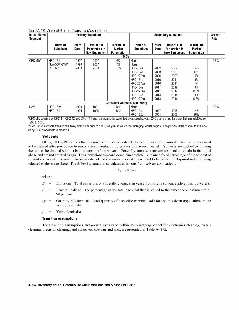
A-232 Inventory of U.S. Greenhouse Gas Emissions and Sinks: 1990-2013
Table A- 171: Aerosol Product Transition Assumptions Initial Market Segment
Primary Substitute Secondary Substitute Growth Rate
Name of Substitute
Start Date
Date of Full Penetration in
New Equipment
Maximum Market
Penetration
Name of Substitute
Start Date
Date of Full Penetration in
New Equipment
Maximum Market
Penetration
MDIs
CFC Mix* HFC-134a 1997 1997 6% None 0.8% Non-ODP/GWP 1998 2007 7% None
CFC Mix* 2000 2000 87% HFC-134a 2002 2002 34% HFC-134a 2003 2009 47% HFC-227ea 2006 2009 5% HFC-134a 2010 2011 6% HFC-227ea 2010 2011 1% HFC-134a 2011 2012 3% HFC-227ea 2011 2012 0.3% HFC-134a 2014 2014 3% HFC-227ea 2014 2014 0.3%
Consumer Aerosols (Non-MDIs)
NA** HFC-152a 1990 1991 50% None 2.0% HFC-134a 1995 1995 50% HFC-152a 1997 1998 44% HFC-152a 2001 2005 36%
*CFC Mix consists of CFC-11, CFC-12 and CFC-114 and represents the weighted average of several CFCs consumed for essential use in MDIs from 1993 to 2008. **Consumer Aerosols transitioned away from ODS prior to 1985, the year in which the Vintaging Model begins. The portion of the market that is now using HFC propellants is modeled.
Solvents
ODSs, HFCs, PFCs and other chemicals are used as solvents to clean items. For example, electronics may need to be cleaned after production to remove any manufacturing process oils or residues left. Solvents are applied by moving the item to be cleaned within a bath or stream of the solvent. Generally, most solvents are assumed to remain in the liquid phase and are not emitted as gas. Thus, emissions are considered “incomplete,” and are a fixed percentage of the amount of solvent consumed in a year. The remainder of the consumed solvent is assumed to be reused or disposed without being released to the atmosphere. The following equation calculates emissions from solvent applications.
Ej = l × Qcj
where:
E = Emissions. Total emissions of a specific chemical in year j from use in solvent applications, by weight.
l = Percent Leakage. The percentage of the total chemical that is leaked to the atmosphere, assumed to be 90 percent.
Qc = Quantity of Chemical. Total quantity of a specific chemical sold for use in solvent applications in the year j, by weight.
j = Year of emission.
Transition Assumptions
The transition assumptions and growth rates used within the Vintaging Model for electronics cleaning, metals cleaning, precision cleaning, and adhesives, coatings and inks, are presented in Table A- 172.
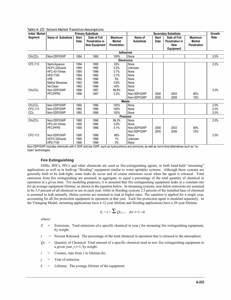
A-233
Table A- 172: Solvent Market Transition Assumptions Initial Market Segment
Primary Substitute Secondary Substitute Growth Rate Name of Substitute Start
Date Date of Full
Penetration in New Equipment
Maximum Market
Penetration
Name of Substitute
Start Date
Date of Full Penetration in
New Equipment
Maximum Market
Penetration
Adhesives
CH3CCl3 Non-ODP/GWP 1994 1995 100% None 2.0%
Electronics
CFC-113 Semi-Aqueous 1994 1995 52% None 2.0% HCFC-225ca/cb 1994 1995 0.2% Unknown HFC-43-10mee 1995 1996 0.7% None HFE-7100 1994 1995 0.7% None nPB 1992 1996 5% None Methyl Siloxanes 1992 1996 0.8% None No-Clean 1992 1996 40% None CH3CCl3 Non-ODP/GWP 1996 1997 99.8% None 2.0% PFC/PFPE 1996 1997 0.2% Non-ODP/GWP 2000 2003 90% Non-ODP/GWP 2005 2009 10%
Metals
CH3CCl3 Non-ODP/GWP 1992 1996 100% None 2.0% CFC-113 Non-ODP/GWP 1992 1996 100% None 2.0% CCl4 Non-ODP/GWP 1992 1996 100% None 2.0%
Precision
CH3CCl3 Non-ODP/GWP 1995 1996 99.3% None 2.0% HFC-43-10mee 1995 1996 0.6% None PFC/PFPE 1995 1996 0.1% Non-ODP/GWP 2000 2003 90% Non-ODP/GWP 2005 2009 10% CFC-113 Non-ODP/GWP 1995 1996 96% None 2.0% HCFC-225ca/cb 1995 1996 1% Unknown HFE-7100 1995 1996 3% None
Non-ODP/GWP includes chemicals with 0 ODP and low GWP, such as hydrocarbons and ammonia, as well as not-in-kind alternatives such as “no clean” technologies.
Fire Extinguishing
ODSs, HFCs, PFCs and other chemicals are used as fire-extinguishing agents, in both hand-held “streaming” applications as well as in built-up “flooding” equipment similar to water sprinkler systems. Although these systems are generally built to be leak-tight, some leaks do occur and of course emissions occur when the agent is released. Total emissions from fire extinguishing are assumed, in aggregate, to equal a percentage of the total quantity of chemical in operation at a given time. For modeling purposes, it is assumed that fire extinguishing equipment leaks at a constant rate for an average equipment lifetime, as shown in the equation below. In streaming systems, non-halon emissions are assumed to be 3.5 percent of all chemical in use in each year, while in flooding systems 2.5 percent of the installed base of chemical is assumed to leak annually. Halon systems are assumed to leak at higher rates. The equation is applied for a single year, accounting for all fire protection equipment in operation in that year. Each fire protection agent is modeled separately. In the Vintaging Model, streaming applications have a 12-year lifetime and flooding applications have a 20-year lifetime.
Ej = r × Σ Qcj-i+1 for i=1→k
where:
E = Emissions. Total emissions of a specific chemical in year j for streaming fire extinguishing equipment, by weight.
r = Percent Released. The percentage of the total chemical in operation that is released to the atmosphere.
Qc = Quantity of Chemical. Total amount of a specific chemical used in new fire extinguishing equipment in a given year, j-i+1, by weight.
i = Counter, runs from 1 to lifetime (k).
j = Year of emission.
k = Lifetime. The average lifetime of the equipment.
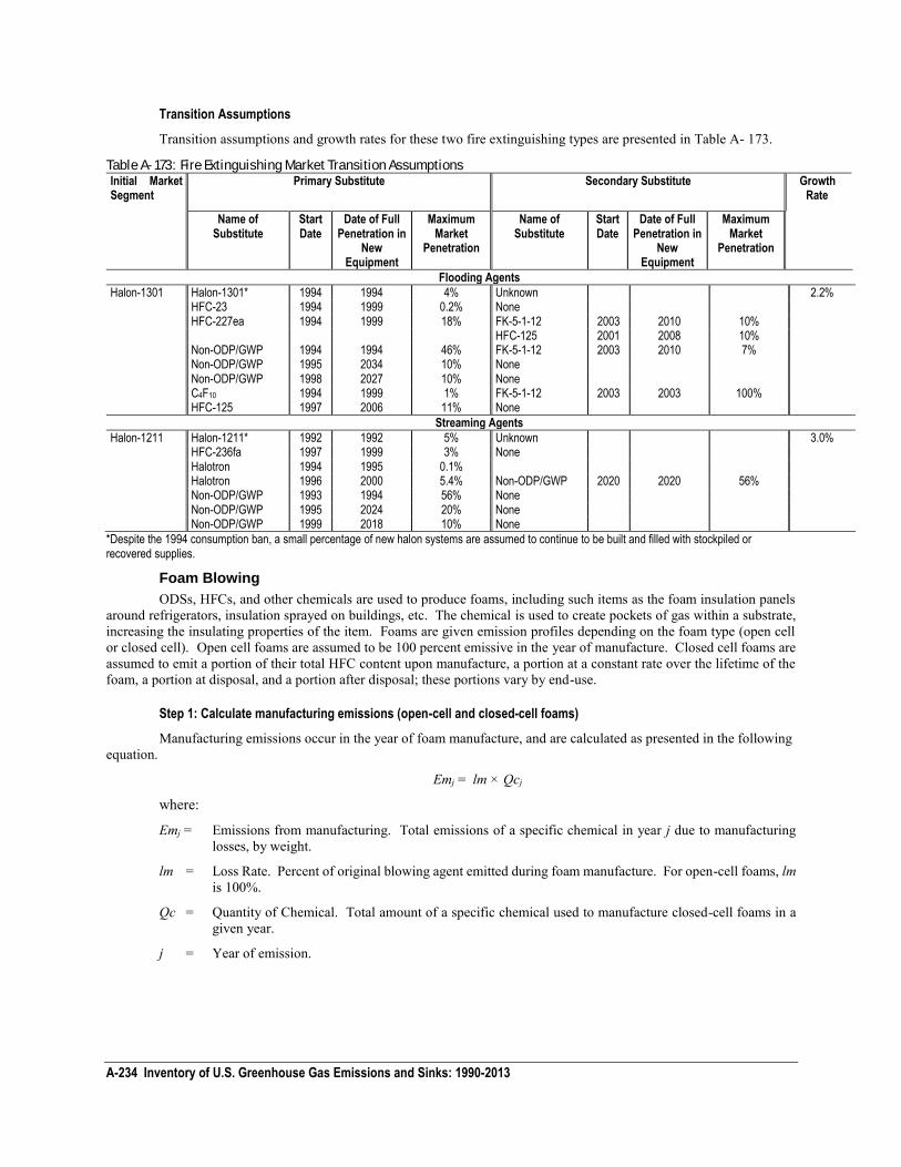
A-234 Inventory of U.S. Greenhouse Gas Emissions and Sinks: 1990-2013
Transition Assumptions
Transition assumptions and growth rates for these two fire extinguishing types are presented in Table A- 173.
Table A- 173: Fire Extinguishing Market Transition Assumptions Initial Market Segment
Primary Substitute Secondary Substitute Growth Rate
Name of Substitute
Start Date
Date of Full Penetration in
New Equipment
Maximum Market
Penetration
Name of Substitute
Start Date
Date of Full Penetration in
New Equipment
Maximum Market
Penetration
Flooding Agents
Halon-1301 Halon-1301* 1994 1994 4% Unknown 2.2% HFC-23 1994 1999 0.2% None HFC-227ea 1994 1999 18% FK-5-1-12 2003 2010 10% HFC-125 2001 2008 10% Non-ODP/GWP 1994 1994 46% FK-5-1-12 2003 2010 7% Non-ODP/GWP 1995 2034 10% None Non-ODP/GWP 1998 2027 10% None C4F10 1994 1999 1% FK-5-1-12 2003 2003 100% HFC-125 1997 2006 11% None
Streaming Agents
Halon-1211 Halon-1211* 1992 1992 5% Unknown 3.0% HFC-236fa 1997 1999 3% None Halotron 1994 1995 0.1% Halotron 1996 2000 5.4% Non-ODP/GWP 2020 2020 56% Non-ODP/GWP 1993 1994 56% None Non-ODP/GWP 1995 2024 20% None Non-ODP/GWP 1999 2018 10% None
*Despite the 1994 consumption ban, a small percentage of new halon systems are assumed to continue to be built and filled with stockpiled or recovered supplies.
Foam Blowing
ODSs, HFCs, and other chemicals are used to produce foams, including such items as the foam insulation panels around refrigerators, insulation sprayed on buildings, etc. The chemical is used to create pockets of gas within a substrate, increasing the insulating properties of the item. Foams are given emission profiles depending on the foam type (open cell or closed cell). Open cell foams are assumed to be 100 percent emissive in the year of manufacture. Closed cell foams are assumed to emit a portion of their total HFC content upon manufacture, a portion at a constant rate over the lifetime of the foam, a portion at disposal, and a portion after disposal; these portions vary by end-use.
Step 1: Calculate manufacturing emissions (open-cell and closed-cell foams)
Manufacturing emissions occur in the year of foam manufacture, and are calculated as presented in the following equation.
Emj = lm × Qcj
where:
Emj = Emissions from manufacturing. Total emissions of a specific chemical in year j due to manufacturing losses, by weight.
lm = Loss Rate. Percent of original blowing agent emitted during foam manufacture. For open-cell foams, lm is 100%.
Qc = Quantity of Chemical. Total amount of a specific chemical used to manufacture closed-cell foams in a given year.
j = Year of emission.
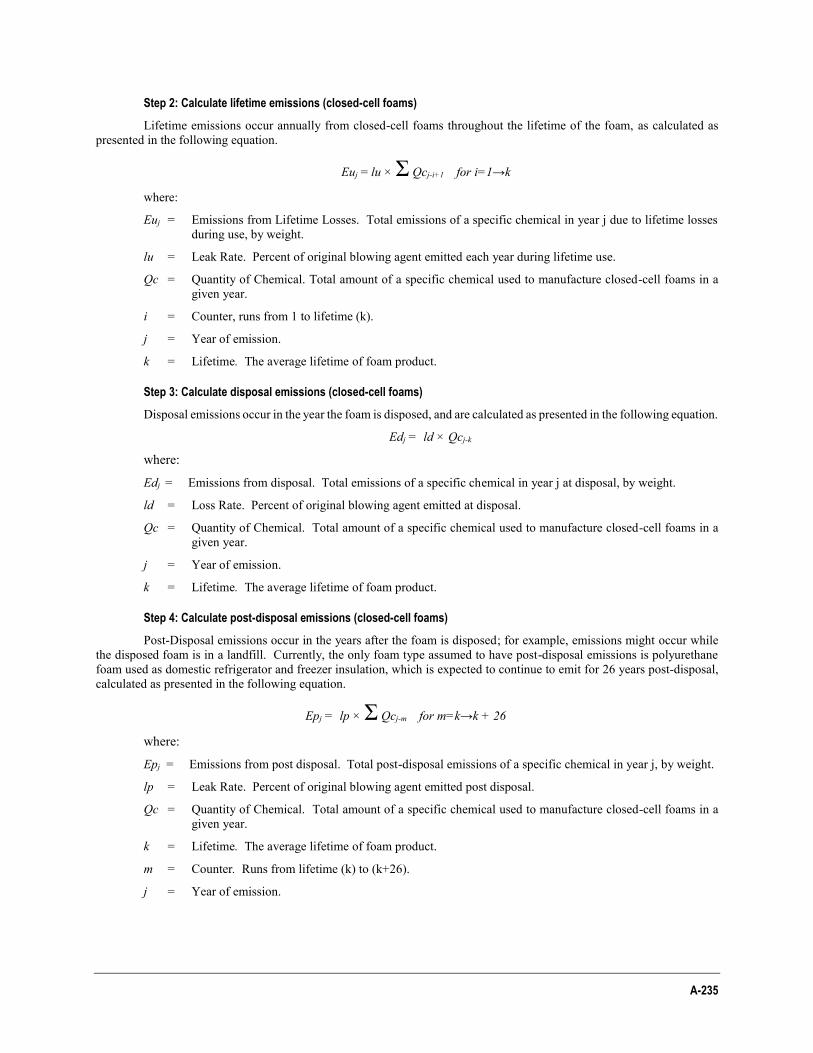
A-235
Step 2: Calculate lifetime emissions (closed-cell foams)
Lifetime emissions occur annually from closed-cell foams throughout the lifetime of the foam, as calculated as presented in the following equation.
Euj = lu × Σ Qcj-i+1 for i=1→k
where:
Euj = Emissions from Lifetime Losses. Total emissions of a specific chemical in year j due to lifetime losses during use, by weight.
lu = Leak Rate. Percent of original blowing agent emitted each year during lifetime use.
Qc = Quantity of Chemical. Total amount of a specific chemical used to manufacture closed-cell foams in a given year.
i = Counter, runs from 1 to lifetime (k).
j = Year of emission.
k = Lifetime. The average lifetime of foam product.
Step 3: Calculate disposal emissions (closed-cell foams)
Disposal emissions occur in the year the foam is disposed, and are calculated as presented in the following equation.
Edj = ld × Qcj-k
where:
Edj = Emissions from disposal. Total emissions of a specific chemical in year j at disposal, by weight.
ld = Loss Rate. Percent of original blowing agent emitted at disposal.
Qc = Quantity of Chemical. Total amount of a specific chemical used to manufacture closed-cell foams in a given year.
j = Year of emission.
k = Lifetime. The average lifetime of foam product.
Step 4: Calculate post-disposal emissions (closed-cell foams)
Post-Disposal emissions occur in the years after the foam is disposed; for example, emissions might occur while the disposed foam is in a landfill. Currently, the only foam type assumed to have post-disposal emissions is polyurethane foam used as domestic refrigerator and freezer insulation, which is expected to continue to emit for 26 years post-disposal, calculated as presented in the following equation.
Epj = lp × Σ Qcj-m for m=k→k + 26
where:
Epj = Emissions from post disposal. Total post-disposal emissions of a specific chemical in year j, by weight.
lp = Leak Rate. Percent of original blowing agent emitted post disposal.
Qc = Quantity of Chemical. Total amount of a specific chemical used to manufacture closed-cell foams in a given year.
k = Lifetime. The average lifetime of foam product.
m = Counter. Runs from lifetime (k) to (k+26).
j = Year of emission.
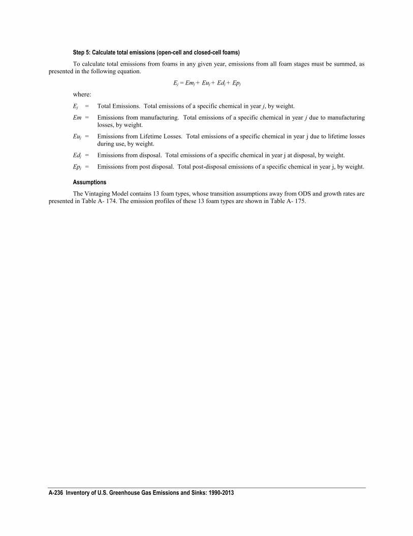
A-236 Inventory of U.S. Greenhouse Gas Emissions and Sinks: 1990-2013
Step 5: Calculate total emissions (open-cell and closed-cell foams)
To calculate total emissions from foams in any given year, emissions from all foam stages must be summed, as presented in the following equation.
Ej = Emj + Euj + Edj + Epj
where:
Ej = Total Emissions. Total emissions of a specific chemical in year j, by weight.
Em = Emissions from manufacturing. Total emissions of a specific chemical in year j due to manufacturing losses, by weight.
Euj = Emissions from Lifetime Losses. Total emissions of a specific chemical in year j due to lifetime losses during use, by weight.
Edj = Emissions from disposal. Total emissions of a specific chemical in year j at disposal, by weight.
Epj = Emissions from post disposal. Total post-disposal emissions of a specific chemical in year j, by weight.
Assumptions
The Vintaging Model contains 13 foam types, whose transition assumptions away from ODS and growth rates are presented in Table A- 174. The emission profiles of these 13 foam types are shown in Table A- 175.
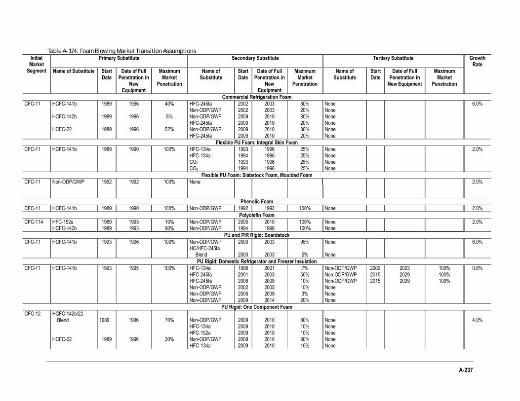
A-237
Table A- 174: Foam Blowing Market Transition Assumptions Initial
Market Segment
Primary Substitute Secondary Substitute Tertiary Substitute Growth Rate
Name of Substitute Start Date
Date of Full Penetration in
New Equipment
Maximum Market
Penetration
Name of Substitute
Start Date
Date of Full Penetration in
New Equipment
Maximum Market
Penetration
Name of Substitute
Start Date
Date of Full Penetration in
New Equipment
Maximum Market
Penetration
Commercial Refrigeration Foam
CFC-11 HCFC-141b 1989 1996 40% HFC-245fa 2002 2003 80% None 6.0% Non-ODP/GWP 2002 2003 20% None HCFC-142b 1989 1996 8% Non-ODP/GWP 2009 2010 80% None HFC-245fa 2009 2010 20% None HCFC-22 1989 1996 52% Non-ODP/GWP 2009 2010 80% None HFC-245fa 2009 2010 20% None
Flexible PU Foam: Integral Skin Foam
CFC-11 HCFC-141b 1989 1990 100% HFC-134a 1993 1996 25% None 2.0% HFC-134a 1994 1996 25% None CO2 1993 1996 25% None CO2 1994 1996 25% None
Flexible PU Foam: Slabstock Foam, Moulded Foam
CFC-11 Non-ODP/GWP 1992 1992 100% None 2.0%
Phenolic Foam
CFC-11 HCFC-141b 1989 1990 100% Non-ODP/GWP 1992 1992 100% None 2.0%
Polyolefin Foam
CFC-114 HFC-152a 1989 1993 10% Non-ODP/GWP 2005 2010 100% None 2.0% HCFC-142b 1989 1993 90% Non-ODP/GWP 1994 1996 100% None
PU and PIR Rigid: Boardstock
CFC-11 HCFC-141b 1993 1996 100% Non-ODP/GWP 2000 2003 95% None 6.0%
HC/HFC-245fa
Blend 2000 2003 5% None
PU Rigid: Domestic Refrigerator and Freezer Insulation
CFC-11 HCFC-141b 1993 1995 100% HFC-134a 1996 2001 7% Non-ODP/GWP 2002 2003 100% 0.8% HFC-245fa 2001 2003 50% Non-ODP/GWP 2015 2029 100%
HFC-245fa 2006 2009 10% Non-ODP/GWP 2015 2029 100%
Non-ODP/GWP 2002 2005 10% None Non-ODP/GWP 2006 2009 3% None Non-ODP/GWP 2009 2014 20% None
PU Rigid: One Component Foam
CFC-12 HCFC-142b/22 Blend 1989 1996 70% Non-ODP/GWP 2009 2010 80% None 4.0%
HFC-134a 2009 2010 10% None HFC-152a 2009 2010 10% None HCFC-22 1989 1996 30% Non-ODP/GWP 2009 2010 80% None HFC-134a 2009 2010 10% None
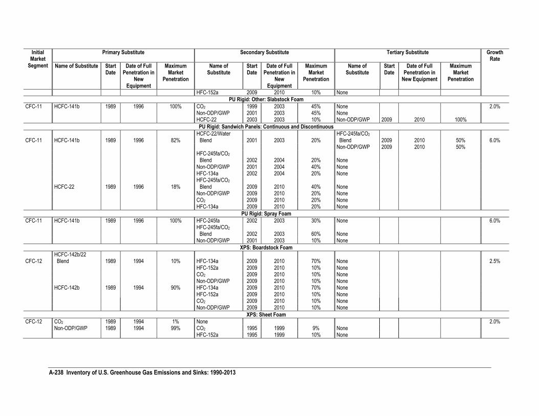
A-238 Inventory of U.S. Greenhouse Gas Emissions and Sinks: 1990-2013
Initial Market
Segment
Primary Substitute Secondary Substitute Tertiary Substitute Growth Rate
Name of Substitute Start Date
Date of Full Penetration in
New Equipment
Maximum Market
Penetration
Name of Substitute
Start Date
Date of Full Penetration in
New Equipment
Maximum Market
Penetration
Name of Substitute
Start Date
Date of Full Penetration in
New Equipment
Maximum Market
Penetration
HFC-152a 2009 2010 10% None
PU Rigid: Other: Slabstock Foam
CFC-11 HCFC-141b 1989 1996 100% CO2 1999 2003 45% None 2.0% Non-ODP/GWP 2001 2003 45% None HCFC-22 2003 2003 10% Non-ODP/GWP 2009 2010 100%
PU Rigid: Sandwich Panels: Continuous and Discontinuous
CFC-11 HCFC-141b 1989 1996 82% HCFC-22/Water
Blend 2001 2003 20% HFC-245fa/CO2
Blend 2009 2010 50% 6.0% Non-ODP/GWP 2009 2010 50%
HFC-245fa/CO2
Blend 2002 2004 20% None Non-ODP/GWP 2001 2004 40% None HFC-134a 2002 2004 20% None
HCFC-22 1989 1996 18% HFC-245fa/CO2
Blend 2009 2010 40% None Non-ODP/GWP 2009 2010 20% None CO2 2009 2010 20% None HFC-134a 2009 2010 20% None
PU Rigid: Spray Foam
CFC-11 HCFC-141b 1989 1996 100% HFC-245fa 2002 2003 30% None 6.0%
HFC-245fa/CO2
Blend 2002 2003 60% None Non-ODP/GWP 2001 2003 10% None
XPS: Boardstock Foam
CFC-12 HCFC-142b/22 Blend 1989 1994 10% HFC-134a 2009 2010 70% None 2.5%
HFC-152a 2009 2010 10% None CO2 2009 2010 10% None Non-ODP/GWP 2009 2010 10% None HCFC-142b 1989 1994 90% HFC-134a 2009 2010 70% None HFC-152a 2009 2010 10% None CO2 2009 2010 10% None Non-ODP/GWP 2009 2010 10% None
XPS: Sheet Foam
CFC-12 CO2 1989 1994 1% None 2.0% Non-ODP/GWP 1989 1994 99% CO2 1995 1999 9% None HFC-152a 1995 1999 10% None
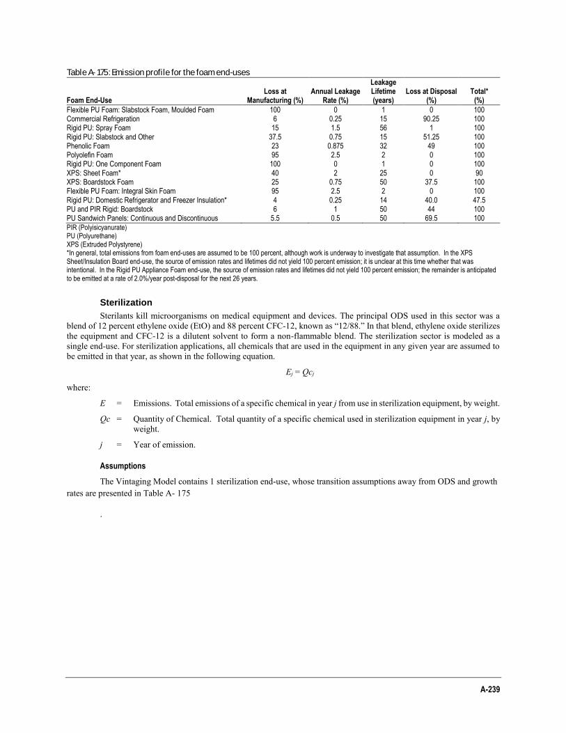
A-239
Table A- 175: Emission profile for the foam end-uses
Foam End-Use Loss at
Manufacturing (%) Annual Leakage
Rate (%)
Leakage Lifetime (years)
Loss at Disposal (%)
Total* (%)
Flexible PU Foam: Slabstock Foam, Moulded Foam 100 0 1 0 100 Commercial Refrigeration 6 0.25 15 90.25 100 Rigid PU: Spray Foam 15 1.5 56 1 100 Rigid PU: Slabstock and Other 37.5 0.75 15 51.25 100 Phenolic Foam 23 0.875 32 49 100 Polyolefin Foam 95 2.5 2 0 100 Rigid PU: One Component Foam 100 0 1 0 100 XPS: Sheet Foam* 40 2 25 0 90 XPS: Boardstock Foam 25 0.75 50 37.5 100 Flexible PU Foam: Integral Skin Foam 95 2.5 2 0 100 Rigid PU: Domestic Refrigerator and Freezer Insulation* 4 0.25 14 40.0 47.5 PU and PIR Rigid: Boardstock 6 1 50 44 100 PU Sandwich Panels: Continuous and Discontinuous 5.5 0.5 50 69.5 100 PIR (Polyisicyanurate) PU (Polyurethane) XPS (Extruded Polystyrene) *In general, total emissions from foam end-uses are assumed to be 100 percent, although work is underway to investigate that assumption. In the XPS Sheet/Insulation Board end-use, the source of emission rates and lifetimes did not yield 100 percent emission; it is unclear at this time whether that was intentional. In the Rigid PU Appliance Foam end-use, the source of emission rates and lifetimes did not yield 100 percent emission; the remainder is anticipated to be emitted at a rate of 2.0%/year post-disposal for the next 26 years.
Sterilization
Sterilants kill microorganisms on medical equipment and devices. The principal ODS used in this sector was a blend of 12 percent ethylene oxide (EtO) and 88 percent CFC-12, known as “12/88.” In that blend, ethylene oxide sterilizes the equipment and CFC-12 is a dilutent solvent to form a non-flammable blend. The sterilization sector is modeled as a single end-use. For sterilization applications, all chemicals that are used in the equipment in any given year are assumed to be emitted in that year, as shown in the following equation.
Ej = Qcj
where:
E = Emissions. Total emissions of a specific chemical in year j from use in sterilization equipment, by weight.
Qc = Quantity of Chemical. Total quantity of a specific chemical used in sterilization equipment in year j, by weight.
j = Year of emission.
Assumptions
The Vintaging Model contains 1 sterilization end-use, whose transition assumptions away from ODS and growth rates are presented in Table A- 175
.
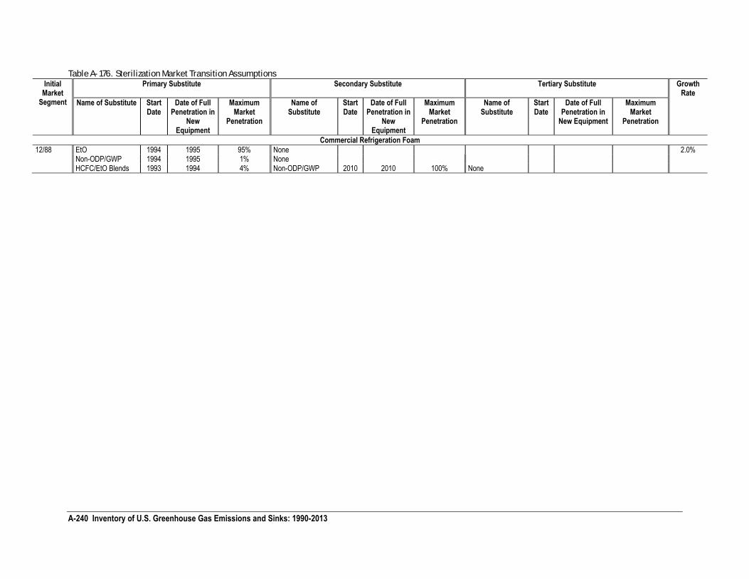
A-240 Inventory of U.S. Greenhouse Gas Emissions and Sinks: 1990-2013
Table A- 176. Sterilization Market Transition Assumptions Initial
Market Segment
Primary Substitute Secondary Substitute Tertiary Substitute Growth Rate
Name of Substitute Start Date
Date of Full Penetration in
New Equipment
Maximum Market
Penetration
Name of Substitute
Start Date
Date of Full Penetration in
New Equipment
Maximum Market
Penetration
Name of Substitute
Start Date
Date of Full Penetration in
New Equipment
Maximum Market
Penetration
Commercial Refrigeration Foam
12/88 EtO 1994 1995 95% None 2.0% Non-ODP/GWP 1994 1995 1% None HCFC/EtO Blends 1993 1994 4% Non-ODP/GWP 2010 2010 100% None
A-241
Model Output
By repeating these calculations for each year, the Vintaging Model creates annual profiles of use and emissions for ODS and ODS substitutes. The results can be shown for each year in two ways: 1) on a chemical-by-chemical basis, summed across the end-uses, or 2) on an end-use or sector basis. Values for use and emissions are calculated both in metric tons and in million metric tons of CO2 equivalents (MMT CO2 Eq.). The conversion of metric tons of chemical to MMT CO2 Eq. is accomplished through a linear scaling of tonnage by the global warming potential (GWP) of each chemical.
Throughout its development, the Vintaging Model has undergone annual modifications. As new or more accurate information becomes available, the model is adjusted in such a way that both past and future emission estimates are often altered.
Bank of ODS and ODS Substitutes
The bank of an ODS or an ODS substitute is “the cumulative difference between the chemical that has been consumed in an application or sub-application and that which has already been released” (IPCC 2006). For any given year, the bank is equal to the previous year’s bank, less the chemical in equipment disposed of during the year, plus chemical in new equipment entering the market during that year, less the amount emitted but not replaced, plus the amount added to replace chemical emitted prior to the given year, as shown in the following equation:
Bcj = Bcj-1-Qdj+Qpj+Ee-Qr
where:
Bcj = Bank of Chemical. Total bank of a specific chemical in year j, by weight.
Qdj = Quantity of Chemical in Equipment Disposed. Total quantity of a specific chemical in equipment disposed of in year j, by weight.
Qpj = Quantity of Chemical Penetrating the Market. Total quantity of a specific chemical that is entering the market in year j, by weight.
Ee = Emissions of Chemical Not Replaced. Total quantity of a specific chemical that is emitted during year j but is not replaced in that year. The Vintaging Model assumes all chemical emitted from refrigeration, air conditioning and fire extinguishing equipment is replaced in the year it is emitted, hence this term is zero for all sectors except foam blowing.
Qr = Chemical Replacing Previous Year’s Emissions. Total quantity of a specific chemical that is used to replace emissions that occurred prior to year j. The Vintaging Model assumes all chemical emitted from refrigeration, air conditioning and fire extinguishing equipment is replaced in the year it is emitted, hence this term is zero for all sectors.
j = Year of emission.
Table A- 177 provides the bank for ODS and ODS substitutes by chemical grouping in metric tons (MT) for 1990-2013.
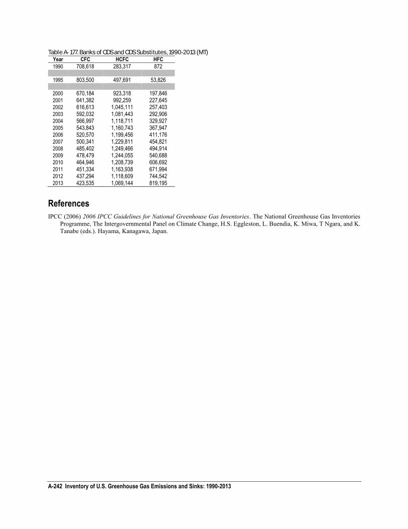
A-242 Inventory of U.S. Greenhouse Gas Emissions and Sinks: 1990-2013
Table A- 177. Banks of ODS and ODS Substitutes, 1990-2013 (MT) Year CFC HCFC HFC
1990 708,618 283,317 872
1995 803,500 497,691 53,826
2000 670,184 923,318 197,846 2001 641,382 992,259 227,645 2002 616,613 1,045,111 257,403 2003 592,032 1,081,443 292,906 2004 566,997 1,118,711 329,927 2005 543,843 1,160,743 367,947 2006 520,570 1,199,456 411,176 2007 500,341 1,229,811 454,821 2008 485,402 1,249,466 494,914 2009 478,479 1,244,055 540,688 2010 464,946 1,208,739 606,692 2011 451,334 1,163,938 671,994 2012 437,294 1,118,609 744,542 2013 423,535 1,069,144 819,195
References
IPCC (2006) 2006 IPCC Guidelines for National Greenhouse Gas Inventories. The National Greenhouse Gas Inventories Programme, The Intergovernmental Panel on Climate Change, H.S. Eggleston, L. Buendia, K. Miwa, T Ngara, and K. Tanabe (eds.). Hayama, Kanagawa, Japan.
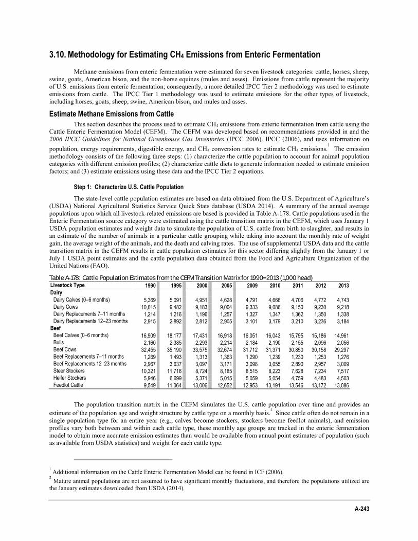
A-243
3.10. Methodology for Estimating CH4 Emissions from Enteric Fermentation
Methane emissions from enteric fermentation were estimated for seven livestock categories: cattle, horses, sheep, swine, goats, American bison, and the non-horse equines (mules and asses). Emissions from cattle represent the majority of U.S. emissions from enteric fermentation; consequently, a more detailed IPCC Tier 2 methodology was used to estimate emissions from cattle. The IPCC Tier 1 methodology was used to estimate emissions for the other types of livestock, including horses, goats, sheep, swine, American bison, and mules and asses.
Estimate Methane Emissions from Cattle
This section describes the process used to estimate CH4 emissions from enteric fermentation from cattle using the Cattle Enteric Fermentation Model (CEFM). The CEFM was developed based on recommendations provided in and the 2006 IPCC Guidelines for National Greenhouse Gas Inventories (IPCC 2006). IPCC (2006), and uses information on population, energy requirements, digestible energy, and CH4 conversion rates to estimate CH4 emissions.
1 The emission
methodology consists of the following three steps: (1) characterize the cattle population to account for animal population categories with different emission profiles; (2) characterize cattle diets to generate information needed to estimate emission factors; and (3) estimate emissions using these data and the IPCC Tier 2 equations.
Step 1: Characterize U.S. Cattle Population
The state-level cattle population estimates are based on data obtained from the U.S. Department of Agriculture’s (USDA) National Agricultural Statistics Service Quick Stats database (USDA 2014). A summary of the annual average populations upon which all livestock-related emissions are based is provided in Table A-178. Cattle populations used in the Enteric Fermentation source category were estimated using the cattle transition matrix in the CEFM, which uses January 1 USDA population estimates and weight data to simulate the population of U.S. cattle from birth to slaughter, and results in an estimate of the number of animals in a particular cattle grouping while taking into account the monthly rate of weight gain, the average weight of the animals, and the death and calving rates. The use of supplemental USDA data and the cattle transition matrix in the CEFM results in cattle population estimates for this sector differing slightly from the January 1 or July 1 USDA point estimates and the cattle population data obtained from the Food and Agriculture Organization of the United Nations (FAO).
Table A-178: Cattle Population Estimates from the CEFM Transition Matrix for 1990–2013 (1,000 head) Livestock Type 1990 1995 2000 2005 2009 2010 2011 2012 2013
Dairy Dairy Calves (0–6 months) 5,369 5,091 4,951 4,628 4,791 4,666 4,706 4,772 4,743 Dairy Cows 10,015 9,482 9,183 9,004 9,333 9,086 9,150 9,230 9,218 Dairy Replacements 7–11 months 1,214 1,216 1,196 1,257 1,327 1,347 1,362 1,350 1,338 Dairy Replacements 12–23 months 2,915 2,892 2,812 2,905 3,101 3,179 3,210 3,236 3,184
Beef Beef Calves (0–6 months) 16,909 18,177 17,431 16,918 16,051 16,043 15,795 15,186 14,961 Bulls 2,160 2,385 2,293 2,214 2,184 2,190 2,155 2,096 2,056 Beef Cows 32,455 35,190 33,575 32,674 31,712 31,371 30,850 30,158 29,297 Beef Replacements 7–11 months 1,269 1,493 1,313 1,363 1,290 1,239 1,230 1,253 1,276 Beef Replacements 12–23 months 2,967 3,637 3,097 3,171 3,098 3,055 2,890 2,957 3,009 Steer Stockers 10,321 11,716 8,724 8,185 8,515 8,223 7,628 7,234 7,517 Heifer Stockers 5,946 6,699 5,371 5,015 5,059 5,054 4,759 4,483 4,503 Feedlot Cattle 9,549 11,064 13,006 12,652 12,953 13,191 13,546 13,172 13,086
The population transition matrix in the CEFM simulates the U.S. cattle population over time and provides an estimate of the population age and weight structure by cattle type on a monthly basis.2 Since cattle often do not remain in a single population type for an entire year (e.g., calves become stockers, stockers become feedlot animals), and emission profiles vary both between and within each cattle type, these monthly age groups are tracked in the enteric fermentation model to obtain more accurate emission estimates than would be available from annual point estimates of population (such as available from USDA statistics) and weight for each cattle type.
1 Additional information on the Cattle Enteric Fermentation Model can be found in ICF (2006).
2 Mature animal populations are not assumed to have significant monthly fluctuations, and therefore the populations utilized are the January estimates downloaded from USDA (2014).
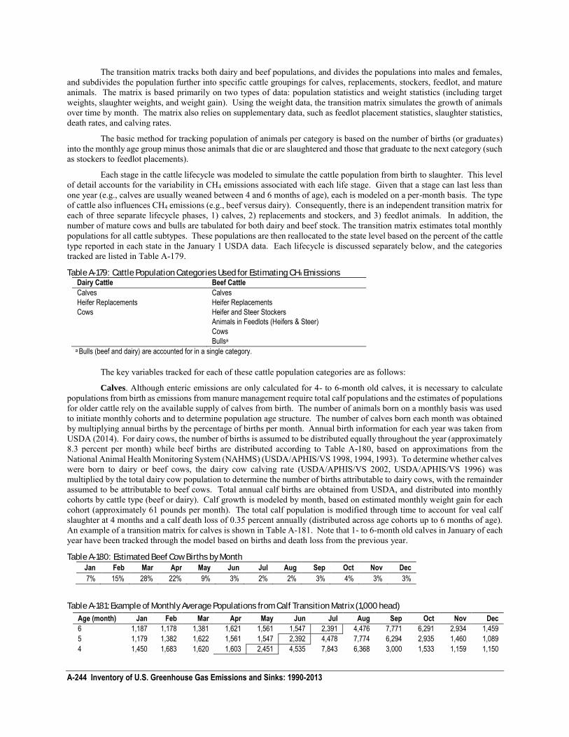
A-244 Inventory of U.S. Greenhouse Gas Emissions and Sinks: 1990-2013
The transition matrix tracks both dairy and beef populations, and divides the populations into males and females, and subdivides the population further into specific cattle groupings for calves, replacements, stockers, feedlot, and mature animals. The matrix is based primarily on two types of data: population statistics and weight statistics (including target weights, slaughter weights, and weight gain). Using the weight data, the transition matrix simulates the growth of animals over time by month. The matrix also relies on supplementary data, such as feedlot placement statistics, slaughter statistics, death rates, and calving rates.
The basic method for tracking population of animals per category is based on the number of births (or graduates) into the monthly age group minus those animals that die or are slaughtered and those that graduate to the next category (such as stockers to feedlot placements).
Each stage in the cattle lifecycle was modeled to simulate the cattle population from birth to slaughter. This level of detail accounts for the variability in CH4 emissions associated with each life stage. Given that a stage can last less than one year (e.g., calves are usually weaned between 4 and 6 months of age), each is modeled on a per-month basis. The type of cattle also influences CH4 emissions (e.g., beef versus dairy). Consequently, there is an independent transition matrix for each of three separate lifecycle phases, 1) calves, 2) replacements and stockers, and 3) feedlot animals. In addition, the number of mature cows and bulls are tabulated for both dairy and beef stock. The transition matrix estimates total monthly populations for all cattle subtypes. These populations are then reallocated to the state level based on the percent of the cattle type reported in each state in the January 1 USDA data. Each lifecycle is discussed separately below, and the categories tracked are listed in Table A-179.
Table A-179: Cattle Population Categories Used for Estimating CH4 Emissions Dairy Cattle Beef Cattle
Calves Calves
Heifer Replacements Heifer Replacements
Cows Heifer and Steer Stockers
Animals in Feedlots (Heifers & Steer)
Cows
Bullsa a Bulls (beef and dairy) are accounted for in a single category.
The key variables tracked for each of these cattle population categories are as follows:
Calves. Although enteric emissions are only calculated for 4- to 6-month old calves, it is necessary to calculate populations from birth as emissions from manure management require total calf populations and the estimates of populations for older cattle rely on the available supply of calves from birth. The number of animals born on a monthly basis was used to initiate monthly cohorts and to determine population age structure. The number of calves born each month was obtained by multiplying annual births by the percentage of births per month. Annual birth information for each year was taken from USDA (2014). For dairy cows, the number of births is assumed to be distributed equally throughout the year (approximately 8.3 percent per month) while beef births are distributed according to Table A-180, based on approximations from the National Animal Health Monitoring System (NAHMS) (USDA/APHIS/VS 1998, 1994, 1993). To determine whether calves were born to dairy or beef cows, the dairy cow calving rate (USDA/APHIS/VS 2002, USDA/APHIS/VS 1996) was multiplied by the total dairy cow population to determine the number of births attributable to dairy cows, with the remainder assumed to be attributable to beef cows. Total annual calf births are obtained from USDA, and distributed into monthly cohorts by cattle type (beef or dairy). Calf growth is modeled by month, based on estimated monthly weight gain for each cohort (approximately 61 pounds per month). The total calf population is modified through time to account for veal calf slaughter at 4 months and a calf death loss of 0.35 percent annually (distributed across age cohorts up to 6 months of age). An example of a transition matrix for calves is shown in Table A-181. Note that 1- to 6-month old calves in January of each year have been tracked through the model based on births and death loss from the previous year.
Table A-180: Estimated Beef Cow Births by Month
Jan Feb Mar Apr May Jun Jul Aug Sep Oct Nov Dec
7% 15% 28% 22% 9% 3% 2% 2% 3% 4% 3% 3%
Table A-181: Example of Monthly Average Populations from Calf Transition Matrix (1,000 head)
Age (month) Jan Feb Mar Apr May Jun Jul Aug Sep Oct Nov Dec
6 1,187 1,178 1,381 1,621 1,561 1,547 2,391 4,476 7,771 6,291 2,934 1,459
5 1,179 1,382 1,622 1,561 1,547 2,392 4,478 7,774 6,294 2,935 1,460 1,089
4 1,450 1,683 1,620 1,603 2,451 4,535 7,843 6,368 3,000 1,533 1,159 1,150
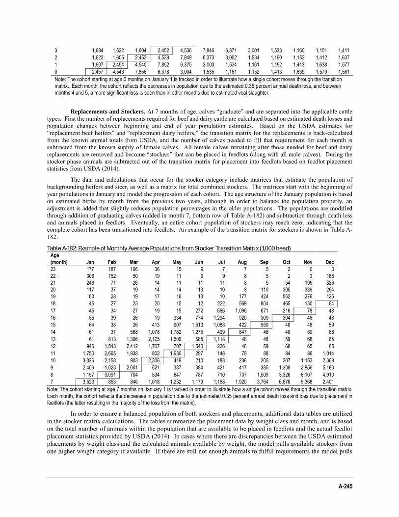
A-245
Replacements and Stockers. At 7 months of age, calves “graduate” and are separated into the applicable cattle types. First the number of replacements required for beef and dairy cattle are calculated based on estimated death losses and population changes between beginning and end of year population estimates. Based on the USDA estimates for “replacement beef heifers” and “replacement dairy heifers,” the transition matrix for the replacements is back-calculated from the known animal totals from USDA, and the number of calves needed to fill that requirement for each month is subtracted from the known supply of female calves. All female calves remaining after those needed for beef and dairy replacements are removed and become “stockers” that can be placed in feedlots (along with all male calves). During the stocker phase animals are subtracted out of the transition matrix for placement into feedlots based on feedlot placement statistics from USDA (2014).
The data and calculations that occur for the stocker category include matrices that estimate the population of backgrounding heifers and steer, as well as a matrix for total combined stockers. The matrices start with the beginning of year populations in January and model the progression of each cohort. The age structure of the January population is based on estimated births by month from the previous two years, although in order to balance the population properly, an adjustment is added that slightly reduces population percentages in the older populations. The populations are modified through addition of graduating calves (added in month 7, bottom row of Table A-182) and subtraction through death loss and animals placed in feedlots. Eventually, an entire cohort population of stockers may reach zero, indicating that the complete cohort has been transitioned into feedlots. An example of the transition matrix for stockers is shown in Table A-182.
Table A-182: Example of Monthly Average Populations from Stocker Transition Matrix (1,000 head) Age
(month) Jan Feb Mar Apr May Jun Jul Aug Sep Oct Nov Dec
23 177 187 106 36 15 9 7 7 5 2 0 0
22 306 152 50 19 11 9 9 8 5 2 3 188
21 248 71 26 14 11 11 11 8 5 54 195 326
20 117 37 19 14 14 13 10 8 110 305 339 264
19 60 28 19 17 16 13 10 177 424 562 276 125
18 45 27 23 20 15 12 222 569 804 465 130 64
17 45 34 27 19 15 272 666 1,096 671 216 78 48
16 55 39 26 19 334 774 1,294 920 309 304 48 48
15 64 38 26 413 907 1,513 1,088 422 550 48 48 59
14 61 37 568 1,078 1,782 1,275 499 847 48 48 59 68
13 61 813 1,396 2,125 1,506 585 1,118 48 48 59 68 65
12 946 1,543 2,412 1,707 707 1,540 226 48 59 68 65 65
11 1,750 2,665 1,938 802 1,930 297 148 79 88 84 86 1,014
10 3,026 2,158 903 2,306 419 210 188 236 205 207 1,153 2,368
9 2,456 1,023 2,601 521 387 384 421 417 385 1,308 2,856 5,180
8 1,157 3,091 704 534 647 787 710 737 1,509 3,326 6,107 4,910
7 3,520 853 846 1,018 1,232 1,179 1,168 1,920 3,764 6,676 5,368 2,401
Note: The cohort starting at age 7 months on January 1 is tracked in order to illustrate how a single cohort moves through the transition matrix. Each month, the cohort reflects the decreases in population due to the estimated 0.35 percent annual death loss and loss due to placement in feedlots (the latter resulting in the majority of the loss from the matrix).
In order to ensure a balanced population of both stockers and placements, additional data tables are utilized in the stocker matrix calculations. The tables summarize the placement data by weight class and month, and is based on the total number of animals within the population that are available to be placed in feedlots and the actual feedlot placement statistics provided by USDA (2014). In cases where there are discrepancies between the USDA estimated placements by weight class and the calculated animals available by weight, the model pulls available stockers from one higher weight category if available. If there are still not enough animals to fulfill requirements the model pulls
3 1,684 1,622 1,604 2,452 4,536 7,846 6,371 3,001 1,533 1,160 1,151 1,411
2 1,623 1,605 2,453 4,538 7,849 6,373 3,002 1,534 1,160 1,152 1,412 1,637
1 1,607 2,454 4,540 7,852 6,375 3,003 1,534 1,161 1,152 1,413 1,638 1,577
0 2,457 4,543 7,856 6,378 3,004 1,535 1,161 1,152 1,413 1,639 1,579 1,561
Note: The cohort starting at age 0 months on January 1 is tracked in order to illustrate how a single cohort moves through the transition matrix. Each month, the cohort reflects the decreases in population due to the estimated 0.35 percent annual death loss, and between months 4 and 5, a more significant loss is seen than in other months due to estimated veal slaughter.
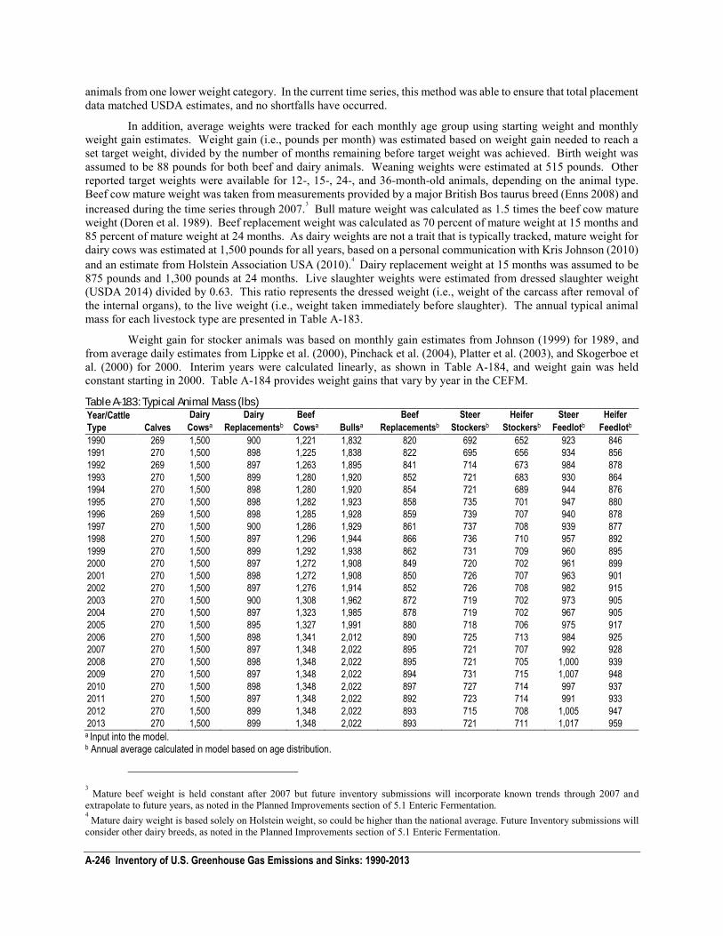
A-246 Inventory of U.S. Greenhouse Gas Emissions and Sinks: 1990-2013
animals from one lower weight category. In the current time series, this method was able to ensure that total placement data matched USDA estimates, and no shortfalls have occurred.
In addition, average weights were tracked for each monthly age group using starting weight and monthly weight gain estimates. Weight gain (i.e., pounds per month) was estimated based on weight gain needed to reach a set target weight, divided by the number of months remaining before target weight was achieved. Birth weight was assumed to be 88 pounds for both beef and dairy animals. Weaning weights were estimated at 515 pounds. Other reported target weights were available for 12-, 15-, 24-, and 36-month-old animals, depending on the animal type. Beef cow mature weight was taken from measurements provided by a major British Bos taurus breed (Enns 2008) and increased during the time series through 2007.3 Bull mature weight was calculated as 1.5 times the beef cow mature weight (Doren et al. 1989). Beef replacement weight was calculated as 70 percent of mature weight at 15 months and 85 percent of mature weight at 24 months. As dairy weights are not a trait that is typically tracked, mature weight for dairy cows was estimated at 1,500 pounds for all years, based on a personal communication with Kris Johnson (2010) and an estimate from Holstein Association USA (2010).4 Dairy replacement weight at 15 months was assumed to be 875 pounds and 1,300 pounds at 24 months. Live slaughter weights were estimated from dressed slaughter weight (USDA 2014) divided by 0.63. This ratio represents the dressed weight (i.e., weight of the carcass after removal of the internal organs), to the live weight (i.e., weight taken immediately before slaughter). The annual typical animal mass for each livestock type are presented in Table A-183.
Weight gain for stocker animals was based on monthly gain estimates from Johnson (1999) for 1989, and from average daily estimates from Lippke et al. (2000), Pinchack et al. (2004), Platter et al. (2003), and Skogerboe et al. (2000) for 2000. Interim years were calculated linearly, as shown in Table A-184, and weight gain was held constant starting in 2000. Table A-184 provides weight gains that vary by year in the CEFM.
Table A-183: Typical Animal Mass (lbs)
Year/Cattle
Type Calves
Dairy
Cowsa
Dairy
Replacementsb
Beef
Cowsa Bullsa
Beef
Replacementsb
Steer
Stockersb
Heifer
Stockersb
Steer
Feedlotb
Heifer
Feedlotb
1990 269 1,500 900 1,221 1,832 820 692 652 923 846
1991 270 1,500 898 1,225 1,838 822 695 656 934 856
1992 269 1,500 897 1,263 1,895 841 714 673 984 878
1993 270 1,500 899 1,280 1,920 852 721 683 930 864
1994 270 1,500 898 1,280 1,920 854 721 689 944 876
1995 270 1,500 898 1,282 1,923 858 735 701 947 880
1996 269 1,500 898 1,285 1,928 859 739 707 940 878
1997 270 1,500 900 1,286 1,929 861 737 708 939 877
1998 270 1,500 897 1,296 1,944 866 736 710 957 892
1999 270 1,500 899 1,292 1,938 862 731 709 960 895
2000 270 1,500 897 1,272 1,908 849 720 702 961 899
2001 270 1,500 898 1,272 1,908 850 726 707 963 901
2002 270 1,500 897 1,276 1,914 852 726 708 982 915
2003 270 1,500 900 1,308 1,962 872 719 702 973 905
2004 270 1,500 897 1,323 1,985 878 719 702 967 905
2005 270 1,500 895 1,327 1,991 880 718 706 975 917
2006 270 1,500 898 1,341 2,012 890 725 713 984 925
2007 270 1,500 897 1,348 2,022 895 721 707 992 928
2008 270 1,500 898 1,348 2,022 895 721 705 1,000 939
2009 270 1,500 897 1,348 2,022 894 731 715 1,007 948
2010 270 1,500 898 1,348 2,022 897 727 714 997 937
2011 270 1,500 897 1,348 2,022 892 723 714 991 933
2012 270 1,500 899 1,348 2,022 893 715 708 1,005 947
2013 270 1,500 899 1,348 2,022 893 721 711 1,017 959 a Input into the model. b Annual average calculated in model based on age distribution.
3 Mature beef weight is held constant after 2007 but future inventory submissions will incorporate known trends through 2007 and
extrapolate to future years, as noted in the Planned Improvements section of 5.1 Enteric Fermentation. 4 Mature dairy weight is based solely on Holstein weight, so could be higher than the national average. Future Inventory submissions will
consider other dairy breeds, as noted in the Planned Improvements section of 5.1 Enteric Fermentation.
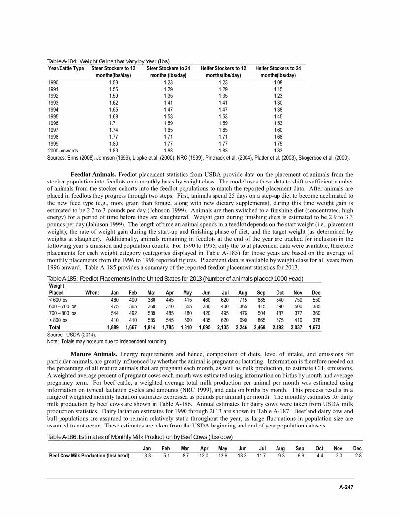
A-247
Table A-184: Weight Gains that Vary by Year (lbs) Year/Cattle Type Steer Stockers to 12
months(lbs/day)
Steer Stockers to 24
months (lbs/day)
Heifer Stockers to 12
months(lbs/day)
Heifer Stockers to 24
months(lbs/day)
1990 1.53 1.23 1.23 1.08
1991 1.56 1.29 1.29 1.15
1992 1.59 1.35 1.35 1.23
1993 1.62 1.41 1.41 1.30
1994 1.65 1.47 1.47 1.38
1995 1.68 1.53 1.53 1.45
1996 1.71 1.59 1.59 1.53
1997 1.74 1.65 1.65 1.60
1998 1.77 1.71 1.71 1.68
1999 1.80 1.77 1.77 1.75
2000–onwards 1.83 1.83 1.83 1.83
Sources: Enns (2008), Johnson (1999), Lippke et al. (2000), NRC (1999), Pinchack et al. (2004), Platter et al. (2003), Skogerboe et al. (2000).
Feedlot Animals. Feedlot placement statistics from USDA provide data on the placement of animals from the stocker population into feedlots on a monthly basis by weight class. The model uses these data to shift a sufficient number of animals from the stocker cohorts into the feedlot populations to match the reported placement data. After animals are placed in feedlots they progress through two steps. First, animals spend 25 days on a step-up diet to become acclimated to the new feed type (e.g., more grain than forage, along with new dietary supplements), during this time weight gain is estimated to be 2.7 to 3 pounds per day (Johnson 1999). Animals are then switched to a finishing diet (concentrated, high energy) for a period of time before they are slaughtered. Weight gain during finishing diets is estimated to be 2.9 to 3.3 pounds per day (Johnson 1999). The length of time an animal spends in a feedlot depends on the start weight (i.e., placement weight), the rate of weight gain during the start-up and finishing phase of diet, and the target weight (as determined by weights at slaughter). Additionally, animals remaining in feedlots at the end of the year are tracked for inclusion in the following year’s emission and population counts. For 1990 to 1995, only the total placement data were available, therefore placements for each weight category (categories displayed in Table A-185) for those years are based on the average of monthly placements from the 1996 to 1998 reported figures. Placement data is available by weight class for all years from 1996 onward. Table A-185 provides a summary of the reported feedlot placement statistics for 2013.
Table A-185: Feedlot Placements in the United States for 2013 (Number of animals placed/1,000 Head)
Weight
Placed When: Jan Feb Mar Apr May Jun Jul Aug Sep Oct Nov Dec
< 600 lbs 460 400 380 445 415 460 620 715 685 840 750 550
600 – 700 lbs 475 365 360 310 355 380 400 365 415 590 500 385
700 – 800 lbs 544 492 589 485 480 420 495 476 504 487 377 360
> 800 lbs 410 410 585 545 560 435 620 690 865 575 410 378
Total 1,889 1,667 1,914 1,785 1,810 1,695 2,135 2,246 2,469 2,492 2,037 1,673
Source: USDA (2014). Note: Totals may not sum due to independent rounding.
Mature Animals. Energy requirements and hence, composition of diets, level of intake, and emissions for particular animals, are greatly influenced by whether the animal is pregnant or lactating. Information is therefore needed on the percentage of all mature animals that are pregnant each month, as well as milk production, to estimate CH4 emissions. A weighted average percent of pregnant cows each month was estimated using information on births by month and average pregnancy term. For beef cattle, a weighted average total milk production per animal per month was estimated using information on typical lactation cycles and amounts (NRC 1999), and data on births by month. This process results in a range of weighted monthly lactation estimates expressed as pounds per animal per month. The monthly estimates for daily milk production by beef cows are shown in Table A-186. Annual estimates for dairy cows were taken from USDA milk production statistics. Dairy lactation estimates for 1990 through 2013 are shown in Table A-187. Beef and dairy cow and bull populations are assumed to remain relatively static throughout the year, as large fluctuations in population size are assumed to not occur. These estimates are taken from the USDA beginning and end of year population datasets.
Table A-186: Estimates of Monthly Milk Production by Beef Cows (lbs/cow)
Jan Feb Mar Apr May Jun Jul Aug Sep Oct Nov Dec
Beef Cow Milk Production (lbs/ head) 3.3 5.1 8.7 12.0 13.6 13.3 11.7 9.3 6.9 4.4 3.0 2.8
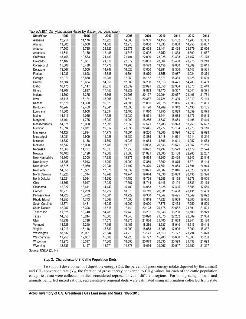
A-248 Inventory of U.S. Greenhouse Gas Emissions and Sinks: 1990-2013
Table A-187: Dairy Lactation Rates by State (lbs/ year/cow) State/Year 1990 1995 2000 2005 2009 2010 2011 2012 2013
Alabama 12,214 14,176 13,920 14,000 14,909 14,455 13,182 13,200 13,333
Alaska 13,300 17,000 14,500 12,273 10,000 11,833 13,800 14,250 10,667
Arizona 17,500 19,735 21,820 22,679 23,028 23,441 23,468 23,979 23,626
Arkansas 11,841 12,150 12,436 13,545 12,692 12,750 11,833 13,300 11,667
California 18,456 19,573 21,130 21,404 22,000 23,025 23,438 23,457 23,178
Colorado 17,182 18,687 21,618 22,577 23,081 23,664 23,430 23,978 24,248
Connecticut 15,606 16,438 17,778 19,200 18,579 19,158 19,000 19,889 20,611
Delaware 13,667 14,500 14,747 16,622 17,000 16,981 18,300 19,143 19,521
Florida 14,033 14,698 15,688 16,591 18,070 18,658 19,067 19,024 19,374
Georgia 12,973 15,550 16,284 17,259 18,182 17,671 18,354 19,125 19,500
Hawaii 13,604 13,654 14,358 12,889 14,200 13,316 14,421 14,200 13,409
Idaho 16,475 18,147 20,816 22,332 22,091 22,658 22,934 23,376 23,440
Illinois 14,707 15,887 17,450 18,827 18,873 19,170 19,357 19,541 19,371
Indiana 14,590 15,375 16,568 20,295 20,137 20,094 20,657 21,406 21,761
Iowa 15,118 16,124 18,298 20,641 20,367 20,724 21,309 22,010 22,144
Kansas 12,576 14,390 16,923 20,505 21,085 20,975 21,016 21,683 21,881
Kentucky 10,947 12,469 12,841 12,896 14,190 14,769 14,342 15,135 15,155
Louisiana 11,605 11,908 12,034 12,400 11,870 11,750 12,889 13,059 12,875
Maine 14,619 16,025 17,128 18,030 18,061 18,344 18,688 18,576 19,548
Maryland 13,461 14,725 16,083 16,099 18,255 18,537 18,654 19,196 19,440
Massachusetts 14,871 16,000 17,091 17,059 17,571 17,286 16,923 18,250 17,692
Michigan 15,394 17,071 19,017 21,635 22,445 23,277 23,164 23,976 24,116
Minnesota 14,127 15,894 17,777 18,091 19,230 19,366 18,996 19,512 19,698
Mississippi 12,081 12,909 15,028 15,280 13,889 13,118 14,571 14,214 13,214
Missouri 13,632 14,158 14,662 16,026 14,654 14,596 14,611 14,957 14,663
Montana 13,542 15,000 17,789 19,579 19,933 20,643 20,571 21,357 21,286
Nebraska 13,866 14,797 16,513 17,950 19,672 19,797 20,579 21,179 21,574
Nevada 16,400 18,128 19,000 21,680 21,821 23,500 23,138 22,966 22,207
New Hampshire 15,100 16,300 17,333 18,875 19,533 19,600 20,429 19,643 20,846
New Jersey 13,538 13,913 15,250 16,000 17,889 17,500 16,875 18,571 18,143
New Mexico 18,815 18,969 20,944 21,192 24,320 24,551 24,854 24,694 24,944
New York 14,658 16,501 17,378 18,639 20,071 20,807 21,046 21,623 22,080
North Carolina 15,220 16,314 16,746 18,741 19,644 19,636 20,089 20,435 20,326
North Dakota 12,624 13,094 14,292 14,182 16,739 18,286 18,158 19,278 19,000
Ohio 13,767 15,917 17,027 17,567 18,744 19,446 19,194 19,833 20,178
Oklahoma 12,327 13,611 14,440 16,480 16,983 17,125 17,415 17,688 17,556
Oregon 16,273 17,289 18,222 18,876 19,719 20,331 20,488 20,431 20,439
Pennsylvania 14,726 16,492 18,081 18,722 19,360 19,847 19,495 19,549 19,822
Rhode Island 14,250 14,773 15,667 17,000 17,818 17,727 17,909 18,300 19,000
South Carolina 12,771 14,481 16,087 16,000 19,000 17,875 17,438 17,250 16,500
South Dakota 12,257 13,398 15,516 17,741 20,128 20,478 20,582 21,391 21,521
Tennessee 11,825 13,740 14,789 15,743 16,232 16,346 16,200 16,100 15,979
Texas 14,350 15,244 16,503 19,646 20,898 21,375 22,232 22,009 21,984
Utah 15,838 16,739 17,573 18,875 21,036 21,400 21,068 22,341 22,130
Vermont 14,528 16,210 17,199 18,469 18,289 18,537 18,940 19,316 19,448
Virginia 14,213 15,116 15,833 16,990 18,083 18,095 17,906 17,990 18,337
Washington 18,532 20,091 22,644 23,270 23,171 23,510 23,727 23,794 23,820
West Virginia 11,250 12,667 15,588 14,923 14,727 15,700 15,600 15,800 15,200
Wisconsin 13,973 15,397 17,306 18,500 20,079 20,630 20,599 21,436 21,693
Wyoming 12,337 13,197 13,571 14,878 19,036 20,067 20,517 20,650 21,367
Source: USDA (2014).
Step 2: Characterize U.S. Cattle Population Diets
To support development of digestible energy (DE, the percent of gross energy intake digested by the animal) and CH4 conversion rate (Ym, the fraction of gross energy converted to CH4) values for each of the cattle population categories, data were collected on diets considered representative of different regions. For both grazing animals and animals being fed mixed rations, representative regional diets were estimated using information collected from state
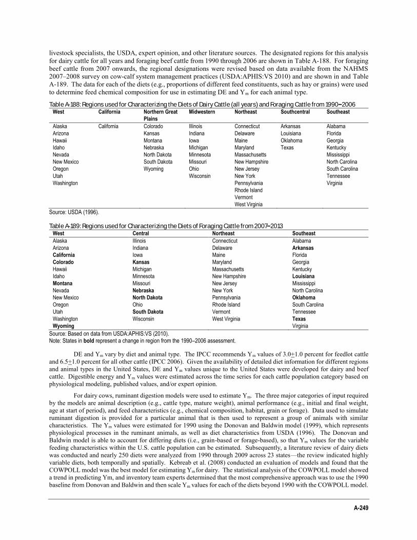
A-249
livestock specialists, the USDA, expert opinion, and other literature sources. The designated regions for this analysis for dairy cattle for all years and foraging beef cattle from 1990 through 2006 are shown in Table A-188. For foraging beef cattle from 2007 onwards, the regional designations were revised based on data available from the NAHMS 2007–2008 survey on cow-calf system management practices (USDA:APHIS:VS 2010) and are shown in and Table A-189. The data for each of the diets (e.g., proportions of different feed constituents, such as hay or grains) were used to determine feed chemical composition for use in estimating DE and Ym for each animal type.
Table A-188: Regions used for Characterizing the Diets of Dairy Cattle (all years) and Foraging Cattle from 1990–2006 West California
Northern Great
Plains
Midwestern Northeast Southcentral Southeast
Alaska
Arizona
Hawaii
Idaho
Nevada
New Mexico
Oregon
Utah
Washington
California
Colorado
Kansas
Montana
Nebraska
North Dakota
South Dakota
Wyoming
Illinois
Indiana
Iowa
Michigan
Minnesota
Missouri
Ohio
Wisconsin
Connecticut
Delaware
Maine
Maryland
Massachusetts
New Hampshire
New Jersey
New York
Pennsylvania
Rhode Island
Vermont
West Virginia
Arkansas
Louisiana
Oklahoma
Texas
Alabama
Florida
Georgia
Kentucky
Mississippi
North Carolina
South Carolina
Tennessee
Virginia
Source: USDA (1996).
Table A-189: Regions used for Characterizing the Diets of Foraging Cattle from 2007–2013 West Central Northeast Southeast
Alaska
Arizona
California
Colorado
Hawaii
Idaho
Montana
Nevada
New Mexico
Oregon
Utah
Washington
Wyoming
Illinois
Indiana
Iowa
Kansas
Michigan
Minnesota
Missouri
Nebraska
North Dakota
Ohio
South Dakota
Wisconsin
Connecticut
Delaware
Maine
Maryland
Massachusetts
New Hampshire
New Jersey
New York
Pennsylvania
Rhode Island
Vermont
West Virginia
Alabama
Arkansas
Florida
Georgia
Kentucky
Louisiana
Mississippi
North Carolina
Oklahoma
South Carolina
Tennessee
Texas
Virginia
Source: Based on data from USDA:APHIS:VS (2010). Note: States in bold represent a change in region from the 1990–2006 assessment.
DE and Ym vary by diet and animal type. The IPCC recommends Ym values of 3.0+1.0 percent for feedlot cattle and 6.5+1.0 percent for all other cattle (IPCC 2006). Given the availability of detailed diet information for different regions and animal types in the United States, DE and Ym values unique to the United States were developed for dairy and beef cattle. Digestible energy and Ym values were estimated across the time series for each cattle population category based on physiological modeling, published values, and/or expert opinion.
For dairy cows, ruminant digestion models were used to estimate Ym. The three major categories of input required by the models are animal description (e.g., cattle type, mature weight), animal performance (e.g., initial and final weight, age at start of period), and feed characteristics (e.g., chemical composition, habitat, grain or forage). Data used to simulate ruminant digestion is provided for a particular animal that is then used to represent a group of animals with similar characteristics. The Ym values were estimated for 1990 using the Donovan and Baldwin model (1999), which represents physiological processes in the ruminant animals, as well as diet characteristics from USDA (1996). The Donovan and Baldwin model is able to account for differing diets (i.e., grain-based or forage-based), so that Ym values for the variable feeding characteristics within the U.S. cattle population can be estimated. Subsequently, a literature review of dairy diets was conducted and nearly 250 diets were analyzed from 1990 through 2009 across 23 states—the review indicated highly variable diets, both temporally and spatially. Kebreab et al. (2008) conducted an evaluation of models and found that the COWPOLL model was the best model for estimating Ym
for dairy. The statistical analysis of the COWPOLL model showed a trend in predicting Ym, and inventory team experts determined that the most comprehensive approach was to use the 1990 baseline from Donovan and Baldwin and then scale Ym values for each of the diets beyond 1990 with the COWPOLL model.
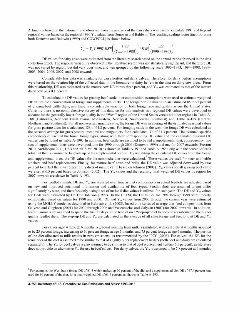
A-250 Inventory of U.S. Greenhouse Gas Emissions and Sinks: 1990-2013
A function based on the national trend observed from the analysis of the dairy diets was used to calculate 1991 and beyond regional values based on the regional 1990 Ym values from Donovan and Baldwin. The resulting scaling factor (incorporating both Donovan and Baldwin (1999) and COWPOLL) is shown below:
198022.1)1990(
YearEXPYY mm
1980199022.1/ EXP
DE values for dairy cows were estimated from the literature search based on the annual trends observed in the data
collection effort. The regional variability observed in the literature search was not statistically significant, and therefore DE was not varied by region, but did vary over time, and was grouped by the following years 1990–1993, 1994–1998, 1999–2003, 2004–2006, 2007, and 2008 onwards.
Considerably less data was available for dairy heifers and dairy calves. Therefore, for dairy heifers assumptions were based on the relationship of the collected data in the literature on dairy heifers to the data on dairy cow diets. From this relationship, DE was estimated as the mature cow DE minus three percent, and Ym was estimated as that of the mature dairy cow plus 0.1 percent.
To calculate the DE values for grazing beef cattle, diet composition assumptions were used to estimate weighted DE values for a combination of forage and supplemental diets. The forage portion makes up an estimated 85 to 95 percent of grazing beef cattle diets, and there is considerable variation of both forage type and quality across the United States. Currently there is no comprehensive survey of this data, so for this analysis two regional DE values were developed to account for the generally lower forage quality in the “West” region of the United States versus all other regions in Table A-188 (California, Northern Great Plains, Midwestern, Northeast, Southcentral, Southeast) and Table A-189 (Central, Northeast, and Southeast). For all non-western grazing cattle, the forage DE was an average of the estimated seasonal values for grass pasture diets for a calculated DE of 64.2 percent. For foraging cattle in the west, the forage DE was calculated as the seasonal average for grass pasture, meadow and range diets, for a calculated DE of 61.3 percent. The assumed specific components of each of the broad forage types, along with their corresponding DE value and the calculated regional DE values can be found in Table A-190. In addition, beef cattle are assumed to be fed a supplemental diet, consequently, two sets of supplemental diets were developed, one for 1990 through 2006 (Donovan 1999) and one for 2007 onwards (Preston 2010, Archibeque 2011, USDA:APHIS:VS 2010) as shown in Table A-191 and Table A-192 along with the percent of each total diet that is assumed to be made up of the supplemental portion. By weighting the calculated DE values from the forage and supplemental diets, the DE values for the composite diet were calculated.
5 These values are used for steer and heifer
stockers and beef replacements. Finally, for mature beef cows and bulls, the DE value was adjusted downward by two percent to reflect the lower digestibility diets of mature cattle based on Johnson (2002). Ym values for all grazing beef cattle were set at 6.5 percent based on Johnson (2002). The Ym values and the resulting final weighted DE values by region for 2007 onwards are shown in Table A-193.
For feedlot animals, DE and Ym are adjusted over time as diet compositions in actual feedlots are adjusted based on new and improved nutritional information and availability of feed types. Feedlot diets are assumed to not differ significantly by state, and therefore only a single set of national diet values is utilized for each year. The DE and Ym values for 1990 were estimated by Dr. Don Johnson (1999). In the CEFM, the DE values for 1991 through 1999 were linearly extrapolated based on values for 1990 and 2000. DE and Ym values from 2000 through the current year were estimated using the MOLLY model as described in Kebreab et al. (2008), based on a series of average diet feed compositions from Galyean and Gleghorn (2001) for 2000 through 2006 and Vasconcelos and Galyean (2007) for 2007 onwards. In addition, feedlot animals are assumed to spend the first 25 days in the feedlot on a “step-up” diet to become accustomed to the higher quality feedlot diets. The step-up DE and Ym are calculated as the average of all state forage and feedlot diet DE and Ym values.
For calves aged 4 through 6 months, a gradual weaning from milk is simulated, with calf diets at 4 months assumed to be 25 percent forage, increasing to 50 percent forage at age 5 months, and 75 percent forage at age 6 months. The portion of the diet allocated to milk results in zero emissions, as recommended by the IPCC (2006). For calves, the DE for the remainder of the diet is assumed to be similar to that of slightly older replacement heifers (both beef and dairy are calculated separately). The Ym for beef calves is also assumed to be similar to that of beef replacement heifers (6.5 percent), as literature does not provide an alternative Ym for use in beef calves. For dairy calves, the Ym is assumed to be 7.8 percent at 4 months,
5 For example, the West has a forage DE of 61.3 which makes up 90 percent of the diet and a supplemented diet DE of 67.4 percent was used for 10 percent of the diet, for a total weighted DE of 61.9 percent, as shown in Table A-193.
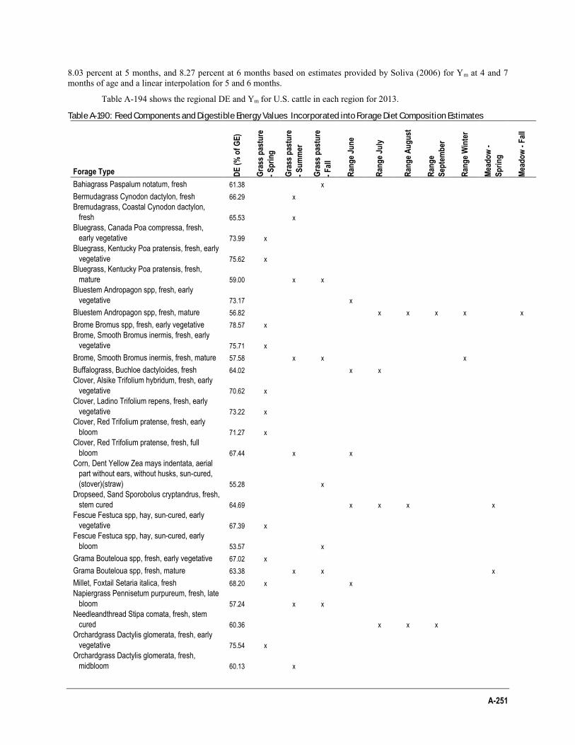
A-251
8.03 percent at 5 months, and 8.27 percent at 6 months based on estimates provided by Soliva (2006) for Ym at 4 and 7 months of age and a linear interpolation for 5 and 6 months.
Table A-194 shows the regional DE and Ym for U.S. cattle in each region for 2013.
Table A-190: Feed Components and Digestible Energy Values Incorporated into Forage Diet Composition Estimates
Forage Type DE
(%
of
GE
)
Gra
ss p
astu
re
- S
pri
ng
Gra
ss p
astu
re
- S
um
mer
Gra
ss p
astu
re
- F
all
Ran
ge
Jun
e
Ran
ge
July
Ran
ge
Au
gu
st
Ran
ge
Sep
tem
ber
Ran
ge
Win
ter
Mea
do
w -
Sp
rin
g
Mea
do
w -
Fal
l
Bahiagrass Paspalum notatum, fresh 61.38 x
Bermudagrass Cynodon dactylon, fresh 66.29 x Bremudagrass, Coastal Cynodon dactylon,
fresh 65.53 x Bluegrass, Canada Poa compressa, fresh,
early vegetative 73.99 x Bluegrass, Kentucky Poa pratensis, fresh, early
vegetative 75.62 x Bluegrass, Kentucky Poa pratensis, fresh,
mature 59.00 x x Bluestem Andropagon spp, fresh, early
vegetative 73.17 x
Bluestem Andropagon spp, fresh, mature 56.82 x x x x x
Brome Bromus spp, fresh, early vegetative 78.57 x Brome, Smooth Bromus inermis, fresh, early
vegetative 75.71 x
Brome, Smooth Bromus inermis, fresh, mature 57.58 x x x
Buffalograss, Buchloe dactyloides, fresh 64.02 x x Clover, Alsike Trifolium hybridum, fresh, early
vegetative 70.62 x Clover, Ladino Trifolium repens, fresh, early
vegetative 73.22 x Clover, Red Trifolium pratense, fresh, early
bloom 71.27 x Clover, Red Trifolium pratense, fresh, full
bloom 67.44 x x Corn, Dent Yellow Zea mays indentata, aerial
part without ears, without husks, sun-cured,
(stover)(straw) 55.28 x Dropseed, Sand Sporobolus cryptandrus, fresh,
stem cured 64.69 x x x x
Fescue Festuca spp, hay, sun-cured, early
vegetative 67.39 x Fescue Festuca spp, hay, sun-cured, early
bloom 53.57 x
Grama Bouteloua spp, fresh, early vegetative 67.02 x
Grama Bouteloua spp, fresh, mature 63.38 x x x
Millet, Foxtail Setaria italica, fresh 68.20 x x Napiergrass Pennisetum purpureum, fresh, late
bloom 57.24 x x Needleandthread Stipa comata, fresh, stem
cured 60.36 x x x Orchardgrass Dactylis glomerata, fresh, early
vegetative 75.54 x Orchardgrass Dactylis glomerata, fresh,
midbloom 60.13 x
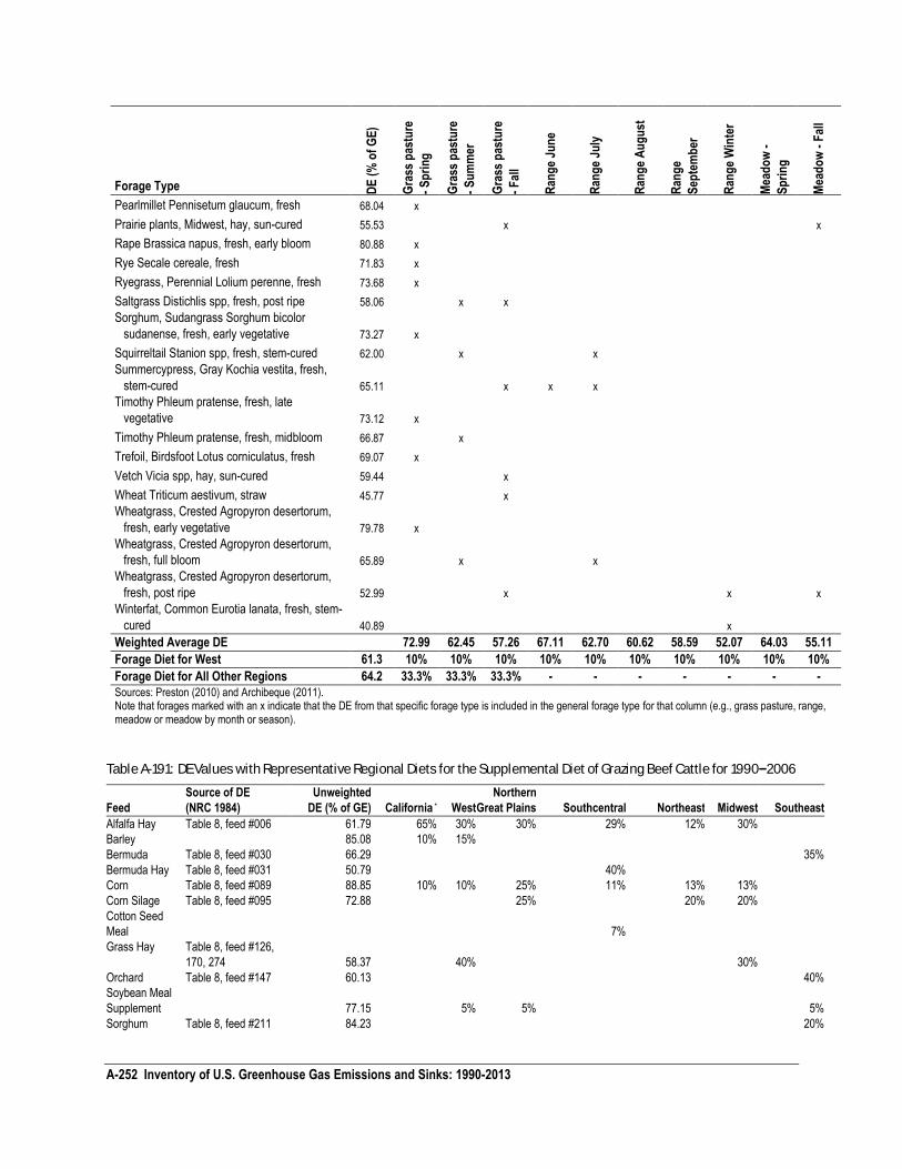
A-252 Inventory of U.S. Greenhouse Gas Emissions and Sinks: 1990-2013
Forage Type DE
(%
of
GE
)
Gra
ss p
astu
re
- S
pri
ng
Gra
ss p
astu
re
- S
um
mer
Gra
ss p
astu
re
- F
all
Ran
ge
Jun
e
Ran
ge
July
Ran
ge
Au
gu
st
Ran
ge
Sep
tem
ber
Ran
ge
Win
ter
Mea
do
w -
Sp
rin
g
Mea
do
w -
Fal
l
Pearlmillet Pennisetum glaucum, fresh 68.04 x
Prairie plants, Midwest, hay, sun-cured 55.53 x x
Rape Brassica napus, fresh, early bloom 80.88 x
Rye Secale cereale, fresh 71.83 x
Ryegrass, Perennial Lolium perenne, fresh 73.68 x
Saltgrass Distichlis spp, fresh, post ripe 58.06 x x Sorghum, Sudangrass Sorghum bicolor
sudanense, fresh, early vegetative 73.27 x
Squirreltail Stanion spp, fresh, stem-cured 62.00 x x Summercypress, Gray Kochia vestita, fresh,
stem-cured 65.11 x x x Timothy Phleum pratense, fresh, late
vegetative 73.12 x
Timothy Phleum pratense, fresh, midbloom 66.87 x
Trefoil, Birdsfoot Lotus corniculatus, fresh 69.07 x
Vetch Vicia spp, hay, sun-cured 59.44 x
Wheat Triticum aestivum, straw 45.77 x Wheatgrass, Crested Agropyron desertorum,
fresh, early vegetative 79.78 x Wheatgrass, Crested Agropyron desertorum,
fresh, full bloom 65.89 x x Wheatgrass, Crested Agropyron desertorum,
fresh, post ripe 52.99 x x x
Winterfat, Common Eurotia lanata, fresh, stem-
cured 40.89 x Weighted Average DE 72.99 62.45 57.26 67.11 62.70 60.62 58.59 52.07 64.03 55.11
Forage Diet for West 61.3 10% 10% 10% 10% 10% 10% 10% 10% 10% 10%
Forage Diet for All Other Regions 64.2 33.3% 33.3% 33.3% - - - - - - -
Sources: Preston (2010) and Archibeque (2011). Note that forages marked with an x indicate that the DE from that specific forage type is included in the general forage type for that column (e.g., grass pasture, range, meadow or meadow by month or season).
Table A-191: DE Values with Representative Regional Diets for the Supplemental Diet of Grazing Beef Cattle for 1990–2006
Feed
Source of DE
(NRC 1984)
Unweighted
DE (% of GE) California * West
Northern
Great Plains Southcentral Northeast Midwest Southeast
Alfalfa Hay Table 8, feed #006 61.79 65% 30% 30% 29% 12% 30%
Barley 85.08 10% 15%
Bermuda Table 8, feed #030 66.29 35%
Bermuda Hay Table 8, feed #031 50.79 40%
Corn Table 8, feed #089 88.85 10% 10% 25% 11% 13% 13%
Corn Silage Table 8, feed #095 72.88 25% 20% 20%
Cotton Seed
Meal 7%
Grass Hay Table 8, feed #126,
170, 274 58.37 40% 30%
Orchard Table 8, feed #147 60.13 40%
Soybean Meal
Supplement 77.15 5% 5% 5%
Sorghum Table 8, feed #211 84.23 20%
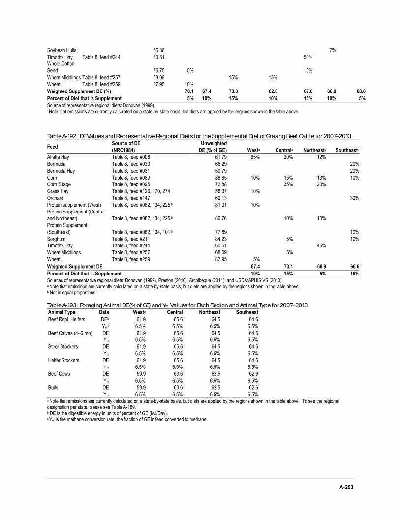
A-253
Table A-192: DE Values and Representative Regional Diets for the Supplemental Diet of Grazing Beef Cattle for 2007–2013
Feed Source of DE
(NRC1984)
Unweighted
DE (% of GE) Westa Centrala Northeasta Southeasta
Alfalfa Hay Table 8, feed #006 61.79 65% 30% 12%
Bermuda Table 8, feed #030 66.29 20%
Bermuda Hay Table 8, feed #031 50.79 20%
Corn Table 8, feed #089 88.85 10% 15% 13% 10%
Corn Silage Table 8, feed #095 72.88 35% 20%
Grass Hay Table 8, feed #126, 170, 274 58.37 10%
Orchard Table 8, feed #147 60.13 30%
Protein supplement (West) Table 8, feed #082, 134, 225 b 81.01 10%
Protein Supplement (Central
and Northeast) Table 8, feed #082, 134, 225 b 80.76 10% 10%
Protein Supplement
(Southeast) Table 8, feed #082, 134, 101 b 77.89 10%
Sorghum Table 8, feed #211 84.23 5% 10%
Timothy Hay Table 8, feed #244 60.51 45%
Wheat Middlings Table 8, feed #257 68.09 5%
Wheat Table 8, feed #259 87.95 5%
Weighted Supplement DE 67.4 73.1 68.9 66.6
Percent of Diet that is Supplement 10% 15% 5% 15%
Sources of representative regional diets: Donovan (1999), Preston (2010), Archibeque (2011), and USDA:APHIS:VS (2010). a Note that emissions are currently calculated on a state-by-state basis, but diets are applied by the regions shown in the table above. b Not in equal proportions.
Table A-193: Foraging Animal DE (% of GE) and Ym Values for Each Region and Animal Type for 2007–2013 Animal Type Data Westa Central Northeast Southeast
Beef Repl. Heifers DEb 61.9 65.6 64.5 64.6
Ymc 6.5% 6.5% 6.5% 6.5%
Beef Calves (4–6 mo) DE 61.9 65.6 64.5 64.6
Ym 6.5% 6.5% 6.5% 6.5%
Steer Stockers DE 61.9 65.6 64.5 64.6
Ym 6.5% 6.5% 6.5% 6.5%
Heifer Stockers DE 61.9 65.6 64.5 64.6
Ym 6.5% 6.5% 6.5% 6.5%
Beef Cows DE 59.9 63.6 62.5 62.6
Ym 6.5% 6.5% 6.5% 6.5%
Bulls DE 59.9 63.6 62.5 62.6
Ym 6.5% 6.5% 6.5% 6.5% a Note that emissions are currently calculated on a state-by-state basis, but diets are applied by the regions shown in the table above. To see the regional designation per state, please see Table A-189. b DE is the digestible energy in units of percent of GE (MJ/Day). c Ym is the methane conversion rate, the fraction of GE in feed converted to methane.
Soybean Hulls 66.86 7%
Timothy Hay Table 8, feed #244 60.51 50%
Whole Cotton
Seed 75.75 5% 5%
Wheat Middlings Table 8, feed #257 68.09 15% 13%
Wheat Table 8, feed #259 87.95 10%
Weighted Supplement DE (%) 70.1 67.4 73.0 62.0 67.6 66.9 68.0
Percent of Diet that is Supplement 5% 10% 15% 10% 15% 10% 5%
Source of representative regional diets: Donovan (1999). * Note that emissions are currently calculated on a state-by-state basis, but diets are applied by the regions shown in the table above.
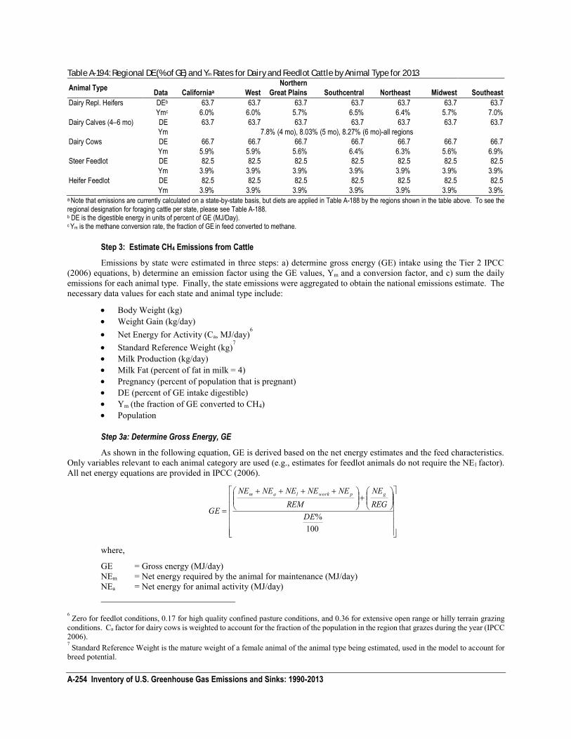
A-254 Inventory of U.S. Greenhouse Gas Emissions and Sinks: 1990-2013
Table A-194: Regional DE (% of GE) and Ym Rates for Dairy and Feedlot Cattle by Animal Type for 2013
Animal Type Data Californiaa West
Northern
Great Plains Southcentral Northeast Midwest Southeast
Dairy Repl. Heifers DEb 63.7 63.7 63.7 63.7 63.7 63.7 63.7
Ymc 6.0% 6.0% 5.7% 6.5% 6.4% 5.7% 7.0%
Dairy Calves (4–6 mo) DE 63.7 63.7 63.7 63.7 63.7 63.7 63.7
Ym 7.8% (4 mo), 8.03% (5 mo), 8.27% (6 mo)-all regions
Dairy Cows DE 66.7 66.7 66.7 66.7 66.7 66.7 66.7
Ym 5.9% 5.9% 5.6% 6.4% 6.3% 5.6% 6.9%
Steer Feedlot DE 82.5 82.5 82.5 82.5 82.5 82.5 82.5
Ym 3.9% 3.9% 3.9% 3.9% 3.9% 3.9% 3.9%
Heifer Feedlot DE 82.5 82.5 82.5 82.5 82.5 82.5 82.5
Ym 3.9% 3.9% 3.9% 3.9% 3.9% 3.9% 3.9% a Note that emissions are currently calculated on a state-by-state basis, but diets are applied in Table A-188 by the regions shown in the table above. To see the regional designation for foraging cattle per state, please see Table A-188. b DE is the digestible energy in units of percent of GE (MJ/Day). c Ym is the methane conversion rate, the fraction of GE in feed converted to methane.
Step 3: Estimate CH4 Emissions from Cattle
Emissions by state were estimated in three steps: a) determine gross energy (GE) intake using the Tier 2 IPCC (2006) equations, b) determine an emission factor using the GE values, Ym and a conversion factor, and c) sum the daily emissions for each animal type. Finally, the state emissions were aggregated to obtain the national emissions estimate. The necessary data values for each state and animal type include:
Body Weight (kg) Weight Gain (kg/day) Net Energy for Activity (Ca, MJ/day)
6
Standard Reference Weight (kg)7
Milk Production (kg/day) Milk Fat (percent of fat in milk = 4) Pregnancy (percent of population that is pregnant) DE (percent of GE intake digestible) Ym (the fraction of GE converted to CH4) Population
Step 3a: Determine Gross Energy, GE
As shown in the following equation, GE is derived based on the net energy estimates and the feed characteristics. Only variables relevant to each animal category are used (e.g., estimates for feedlot animals do not require the NE l factor). All net energy equations are provided in IPCC (2006).
100%DE
REGNE
REMNENENENENE
GE
gpworklam
where,
GE = Gross energy (MJ/day) NEm = Net energy required by the animal for maintenance (MJ/day) NEa = Net energy for animal activity (MJ/day)
6 Zero for feedlot conditions, 0.17 for high quality confined pasture conditions, and 0.36 for extensive open range or hilly terrain grazing conditions. Ca factor for dairy cows is weighted to account for the fraction of the population in the region that grazes during the year (IPCC 2006). 7 Standard Reference Weight is the mature weight of a female animal of the animal type being estimated, used in the model to account for breed potential.
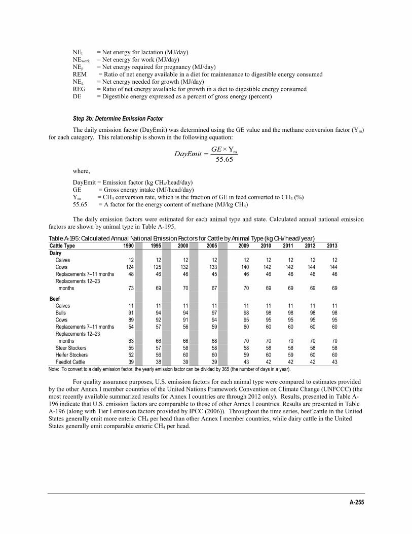
A-255
NEl = Net energy for lactation (MJ/day) NEwork = Net energy for work (MJ/day) NEp = Net energy required for pregnancy (MJ/day) REM = Ratio of net energy available in a diet for maintenance to digestible energy consumed NEg = Net energy needed for growth (MJ/day) REG = Ratio of net energy available for growth in a diet to digestible energy consumed DE = Digestible energy expressed as a percent of gross energy (percent)
Step 3b: Determine Emission Factor
The daily emission factor (DayEmit) was determined using the GE value and the methane conversion factor (Ym) for each category. This relationship is shown in the following equation:
65.55Y× mGEDayEmit
where,
DayEmit = Emission factor (kg CH4/head/day) GE = Gross energy intake (MJ/head/day) Ym = CH4 conversion rate, which is the fraction of GE in feed converted to CH4 (%) 55.65 = A factor for the energy content of methane (MJ/kg CH4) The daily emission factors were estimated for each animal type and state. Calculated annual national emission
factors are shown by animal type in Table A-195.
Table A-195: Calculated Annual National Emission Factors for Cattle by Animal Type (kg CH4/head/year) Cattle Type 1990 1995 2000 2005 2009 2010 2011 2012 2013
Dairy
Calves 12 12 12 12 12 12 12 12 12
Cows 124 125 132 133 140 142 142 144 144
Replacements 7–11 months 48 46 46 45 46 46 46 46 46
Replacements 12–23
months 73 69 70 67 70 69 69 69 69
Beef
Calves 11 11 11 11 11 11 11 11 11
Bulls 91 94 94 97 98 98 98 98 98
Cows 89 92 91 94 95 95 95 95 95
Replacements 7–11 months 54 57 56 59 60 60 60 60 60
Replacements 12–23
months 63 66 66 68 70 70 70 70 70
Steer Stockers 55 57 58 58 58 58 58 58 58
Heifer Stockers 52 56 60 60 59 60 59 60 60
Feedlot Cattle 39 38 39 39 43 42 42 42 43
Note: To convert to a daily emission factor, the yearly emission factor can be divided by 365 (the number of days in a year).
For quality assurance purposes, U.S. emission factors for each animal type were compared to estimates provided by the other Annex I member countries of the United Nations Framework Convention on Climate Change (UNFCCC) (the most recently available summarized results for Annex I countries are through 2012 only). Results, presented in Table A-196 indicate that U.S. emission factors are comparable to those of other Annex I countries. Results are presented in Table A-196 (along with Tier I emission factors provided by IPCC (2006)). Throughout the time series, beef cattle in the United States generally emit more enteric CH4 per head than other Annex I member countries, while dairy cattle in the United States generally emit comparable enteric CH4 per head.
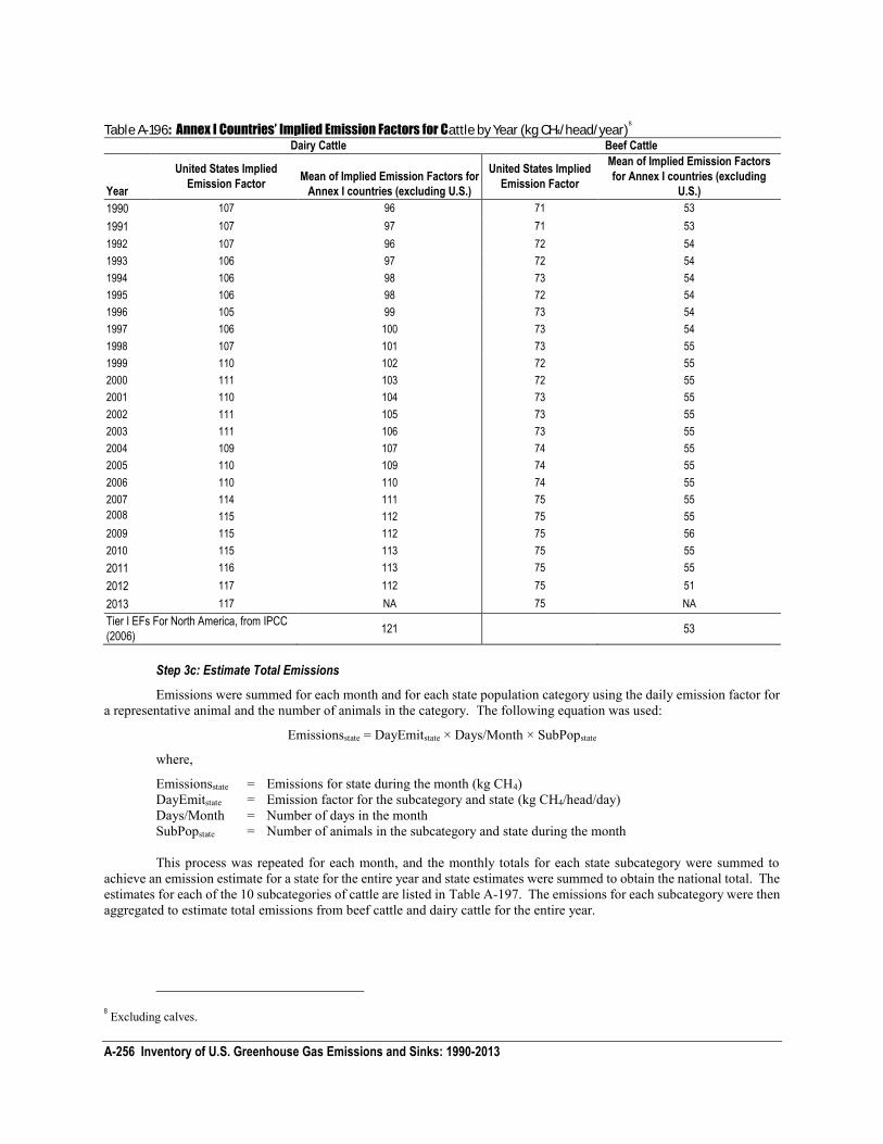
A-256 Inventory of U.S. Greenhouse Gas Emissions and Sinks: 1990-2013
Table A-196: Annex I Countries’ Implied Emission Factors for Cattle by Year (kg CH4/head/year)
8
Dairy Cattle Beef Cattle
Year
United States Implied
Emission Factor Mean of Implied Emission Factors for
Annex I countries (excluding U.S.)
United States Implied
Emission Factor
Mean of Implied Emission Factors
for Annex I countries (excluding
U.S.)
1990 107 96 71 53
1991 107 97 71 53
1992 107 96 72 54
1993 106 97 72 54
1994 106 98 73 54
1995 106 98 72 54
1996 105 99 73 54
1997 106 100 73 54
1998 107 101 73 55
1999 110 102 72 55
2000 111 103 72 55
2001 110 104 73 55
2002 111 105 73 55
2003 111 106 73 55
2004 109 107 74 55
2005 110 109 74 55
2006 110 110 74 55
2007 114 111 75 55
2008 115 112 75 55
2009 115 112 75 56
2010 115 113 75 55
2011 116 113 75 55
2012 117 112 75 51
2013 117 NA 75 NA
Tier I EFs For North America, from IPCC
(2006) 121 53
Step 3c: Estimate Total Emissions
Emissions were summed for each month and for each state population category using the daily emission factor for a representative animal and the number of animals in the category. The following equation was used:
Emissionsstate = DayEmitstate × Days/Month × SubPopstate
where,
Emissionsstate = Emissions for state during the month (kg CH4) DayEmitstate = Emission factor for the subcategory and state (kg CH4/head/day) Days/Month = Number of days in the month SubPopstate = Number of animals in the subcategory and state during the month This process was repeated for each month, and the monthly totals for each state subcategory were summed to
achieve an emission estimate for a state for the entire year and state estimates were summed to obtain the national total. The estimates for each of the 10 subcategories of cattle are listed in Table A-197. The emissions for each subcategory were then aggregated to estimate total emissions from beef cattle and dairy cattle for the entire year.
8 Excluding calves.
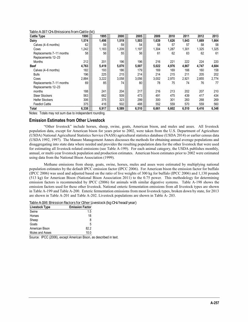
A-257
Table A-197: CH4 Emissions from Cattle (kt) Cattle Type 1990 1995 2000 2005 2009 2010 2011 2012 2013
Dairy 1,574 1,498 1,519 1,503 1,639 1,626 1,643 1,669 1,664
Calves (4–6 months) 62 59 59 54 58 57 57 58 58
Cows 1,242 1,183 1,209 1,197 1,304 1,287 1,301 1,325 1,325
Replacements 7–11 months 58 56 55 56 61 62 63 62 61
Replacements 12–23
Months 212 201 196 196 216 221 222 224 220
Beef 4,763 5,419 5,070 5,007 5,022 4,976 4,867 4,747 4,684
Calves (4–6 months) 182 193 186 179 169 169 166 160 158
Bulls 196 225 215 214 214 215 211 205 202
Cows 2,884 3,222 3,058 3,056 3,002 2,970 2,921 2,855 2,774
Replacements 7–11 months 69 85 74 80 78 75 74 76 77
Replacements 12–23
months 188 241 204 217 216 213 202 207 210
Steer Stockers 563 662 509 473 491 475 439 417 434
Heifer Stockers 306 375 323 299 300 301 283 268 269
Feedlot Cattle 375 416 502 488 552 559 570 559 560
Total 6,338 6,917 6,589 6,510 6,661 6,602 6,510 6,416 6,348
Notes: Totals may not sum due to independent rounding.
Emission Estimates from Other Livestock
“Other livestock” include horses, sheep, swine, goats, American bison, and mules and asses. All livestock population data, except for American bison for years prior to 2002, were taken from the U.S. Department of Agriculture (USDA) National Agricultural Statistics Service (NASS) agricultural statistics database (USDA 2014) or earlier census data (USDA 1992, 1997). The Manure Management Annex discusses the methods for obtaining annual average populations and disaggregating into state data where needed and provides the resulting population data for the other livestock that were used for estimating all livestock-related emissions (see Table A-199). For each animal category, the USDA publishes monthly, annual, or multi-year livestock population and production estimates. American bison estimates prior to 2002 were estimated using data from the National Bison Association (1999).
Methane emissions from sheep, goats, swine, horses, mules and asses were estimated by multiplying national population estimates by the default IPCC emission factor (IPCC 2006). For American bison the emission factor for buffalo (IPCC 2006) was used and adjusted based on the ratio of live weights of 300 kg for buffalo (IPCC 2006) and 1,130 pounds (513 kg) for American Bison (National Bison Association 2011) to the 0.75 power. This methodology for determining emission factors is recommended by IPCC (2006) for animals with similar digestive systems. Table A-198 shows the emission factors used for these other livestock. National enteric fermentation emissions from all livestock types are shown in Table A-199 and Table A-200. Enteric fermentation emissions from most livestock types, broken down by state, for 2013 are shown in Table A-201 and Table A-202. Livestock populations are shown in Table A- 203.
Table A-198: Emission Factors for Other Livestock (kg CH4/head/year) Livestock Type Emission Factor
Swine 1.5
Horses 18
Sheep 8
Goats 5
American Bison 82.2
Mules and Asses 10.0
Source: IPCC (2006), except American Bison, as described in text.
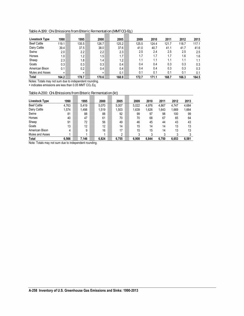
A-258 Inventory of U.S. Greenhouse Gas Emissions and Sinks: 1990-2013
Table A-199: CH4 Emissions from Enteric Fermentation (MMT CO2 Eq.)
Livestock Type 1990 1995 2000 2005 2009
2010
2011
2012
2013
Beef Cattle 119.1 135.5 126.7 125.2 125.5 124.4 121.7 118.7 117.1 Dairy Cattle 39.4 37.5 38.0 37.6 41.0 40.7 41.1 41.7 41.6 Swine 2.0 2.2 2.2 2.3 2.5 2.4 2.5 2.5 2.5 Horses 1.0 1.2 1.5 1.7 1.7 1.7 1.7 1.6 1.6 Sheep 2.3 1.8 1.4 1.2 1.1 1.1 1.1 1.1 1.1 Goats 0.3 0.3 0.3 0.4 0.4 0.4 0.3 0.3 0.3 American Bison 0.1 0.2 0.4 0.4 0.4 0.4 0.3 0.3 0.3 Mules and Asses + + + 0.1 0.1 0.1 0.1 0.1 0.1
Total 164.2 178.7 170.6 168.9 172.7 171.1 168.7 166.3 164.5
Notes: Totals may not sum due to independent rounding. + indicates emissions are less than 0.05 MMT CO2 Eq.
Table A-200: CH4 Emissions from Enteric Fermentation (kt)
Livestock Type 1990 1995 2000 2005 2009
2010
2011
2012
2013
Beef Cattle 4,763 5,419 5,070 5,007 5,022 4,976 4,867 4,747 4,684 Dairy Cattle 1,574 1,498 1,519 1,503 1,639 1,626 1,643 1,669 1,664 Swine 81 88 88 92 99 97 98 100 99 Horses 40 47 61 70 70 68 67 65 64 Sheep 91 72 56 49 46 45 44 43 43 Goats 13 12 12 14 15 14 14 13 13 American Bison 4 9 16 17 15 15 14 13 13 Mules and Asses 1 1 1 2 3 3 3 3 3
Total 6,566 7,146 6,824 6,755 6,908 6,844 6,750 6,653 6,581
Note: Totals may not sum due to independent rounding.
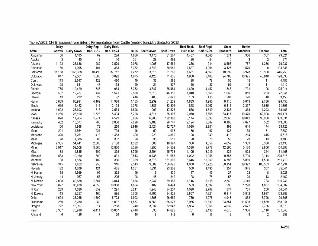
A-259
Table A-201: CH4 Emissions from Enteric Fermentation from Cattle (metric tons), by State, for 2013
State
Dairy
Calves Dairy Cows
Dairy Repl.
Heif. 0 -12
Dairy Repl.
Heif. 12-24 Bulls Beef Calves Beef Cows
Beef Repl.
Heif. 0-12
Beef Repl.
Heif. 12-24
Steer
Stockers
Heifer
Stockers Feedlot Total
Alabama 56 1,185 62 224 4,866 3,475 61,267 1,487 4,065 1,371 906 357 79,321
Alaska 3 40 3 10 301 28 492 20 54 15 3 2 971
Arizona 1,192 28,636 982 3,529 2,078 1,008 17,582 336 914 8,556 787 11,336 76,937
Arkansas 56 1,005 101 363 5,352 4,543 80,089 1,827 4,994 3,427 1,579 0 103,336
California 11,168 263,358 10,490 37,712 7,272 3,515 61,286 1,681 4,569 18,292 6,928 19,980 446,250
Colorado 847 19,561 1,083 3,892 4,675 4,120 71,835 1,986 5,400 24,783 16,375 43,840 198,396
Conn. 113 2,647 128 460 49 32 566 28 78 55 15 11 4,182
Delaware 28 641 43 153 29 21 377 10 27 52 18 11 1,412
Florida 765 19,429 546 1,964 5,352 4,847 85,454 1,629 4,452 548 731 196 125,914
Georgia 502 12,787 437 1,571 2,530 2,616 46,115 1,048 2,865 1,069 819 283 72,641
Hawaii 13 232 27 97 416 403 7,023 153 415 207 126 48 9,158
Idaho 3,639 86,991 4,169 14,988 4,155 2,939 51,239 1,833 4,985 8,113 6,613 9,786 199,450
Illinois 615 12,422 611 2,198 2,378 1,883 33,306 828 2,267 6,416 2,337 6,635 71,896
Indiana 1,092 23,603 713 2,564 1,808 993 17,573 566 1,549 2,433 1,368 4,203 58,465
Iowa 1,286 28,100 1,528 5,494 5,708 4,811 85,105 2,070 5,668 33,417 19,379 52,908 245,474
Kansas 828 17,964 1,274 4,579 8,086 6,906 122,183 3,174 8,690 52,666 39,042 93,938 359,331
Kentucky 452 10,077 780 2,806 7,298 5,488 96,747 2,124 5,807 6,168 4,677 582 143,006
Louisiana 100 1,868 72 259 2,919 2,424 42,727 1,090 2,981 493 614 174 55,722
Maine 201 4,564 221 793 146 59 1,038 36 97 137 59 31 7,382
Maryland 320 7,251 413 1,483 390 220 3,869 128 349 412 264 415 15,515
Mass. 78 1,686 85 307 98 35 613 28 78 55 29 13 3,106
Michigan 2,365 54,441 2,000 7,188 1,332 588 10,397 386 1,058 4,652 1,339 6,388 92,133
Minn. 2,917 59,508 3,566 12,820 3,330 1,950 34,502 1,380 3,778 12,565 5,130 12,856 154,302
Miss. 88 1,835 109 393 3,795 2,594 45,738 1,105 3,019 1,124 1,023 344 61,168
Missouri 583 10,160 509 1,831 9,513 9,138 161,653 4,002 10,958 9,357 5,700 2,114 225,518
Montana 88 1,874 102 366 10,389 8,678 151,306 6,646 18,069 6,786 5,889 1,528 211,719
Nebraska 345 7,422 255 916 9,513 9,387 166,070 4,830 13,225 60,151 39,327 106,553 417,994
Nevada 182 4,209 121 435 1,351 1,331 23,208 550 1,495 1,357 945 357 35,541
N. Hamp. 85 1,999 92 332 49 19 330 17 47 27 23 8 3,028
N. Jersey 44 957 57 205 98 48 849 28 78 55 29 13 2,462
N. Mexico 2,008 49,888 1,681 6,044 3,636 2,247 39,183 1,146 3,115 2,360 3,149 784 115,241
New York 3,827 93,438 4,553 16,368 1,854 482 8,494 583 1,592 990 1,290 1,037 134,507
N. Car. 289 7,526 359 1,291 3,211 1,943 34,257 1,020 2,787 877 731 250 54,541
N. Dakota 113 2,257 166 595 5,708 4,795 84,829 2,857 7,821 6,817 5,842 1,987 123,787
Ohio 1,694 35,035 1,592 5,723 1,903 1,508 26,682 759 2,078 4,946 1,852 6,796 90,568
Oklahoma 289 6,280 289 1,037 11,677 9,363 165,073 3,965 10,839 23,851 11,693 14,589 258,944
Oregon 772 16,997 914 3,288 3,740 3,037 52,947 1,864 5,068 4,632 2,677 2,736 98,670
Penn 3,357 76,918 4,411 15,857 2,440 830 14,628 781 2,135 4,675 1,906 3,110 131,048
R.Island 6 126 7 26 10 8 142 6 16 8 3 2 358
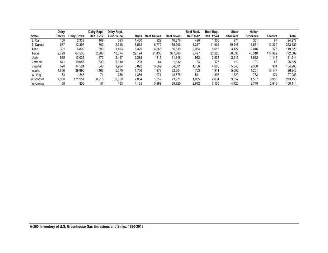
A-260 Inventory of U.S. Greenhouse Gas Emissions and Sinks: 1990-2013
State
Dairy
Calves Dairy Cows
Dairy Repl.
Heif. 0 -12
Dairy Repl.
Heif. 12-24 Bulls Beef Calves Beef Cows
Beef Repl.
Heif. 0-12
Beef Repl.
Heif. 12-24
Steer
Stockers
Heifer
Stockers Feedlot Total
S. Car. 100 2,338 109 393 1,460 929 16,376 496 1,355 274 351 97 24,277
S. Dakota 577 12,397 700 2,518 8,562 8,779 155,305 4,347 11,902 19,248 15,531 13,270 253,139
Tenn. 301 6,899 390 1,403 6,325 4,868 85,830 2,054 5,613 3,427 2,046 173 119,329
Texas 2,729 67,535 2,886 10,374 29,194 21,433 377,860 8,497 23,226 68,536 45,310 114,982 772,562
Utah 565 13,035 672 2,417 2,285 1,815 31,648 932 2,534 2,213 1,952 1,145 61,214
Vermont 841 19,057 839 3,018 293 64 1,132 64 175 110 191 43 25,827
Virginia 590 14,524 546 1,964 3,892 3,662 64,561 1,756 4,800 5,346 2,368 954 104,963
Wash. 1,656 39,990 1,466 5,270 1,766 1,273 22,204 703 1,911 5,606 4,251 10,147 96,242
W. Virg. 63 1,245 71 256 1,366 1,071 18,875 511 1,398 1,320 733 174 27,083
Wisconsin 7,968 171,951 8,915 32,050 2,854 1,352 23,921 1,035 2,834 9,357 1,567 9,953 273,758
Wyoming 38 805 51 183 4,155 3,999 69,725 2,612 7,103 4,720 3,779 2,943 100,114
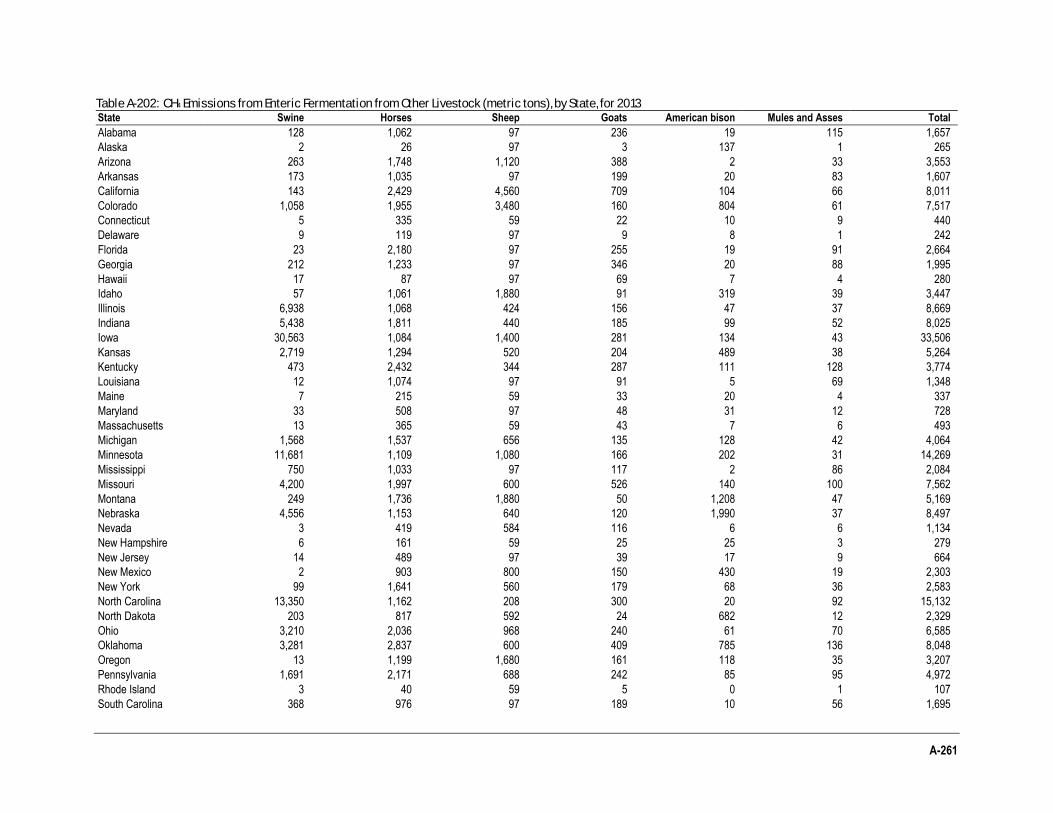
A-261
Table A-202: CH4 Emissions from Enteric Fermentation from Other Livestock (metric tons), by State, for 2013 State Swine Horses Sheep Goats American bison Mules and Asses Total
Alabama 128 1,062 97 236 19 115 1,657
Alaska 2 26 97 3 137 1 265
Arizona 263 1,748 1,120 388 2 33 3,553
Arkansas 173 1,035 97 199 20 83 1,607
California 143 2,429 4,560 709 104 66 8,011
Colorado 1,058 1,955 3,480 160 804 61 7,517
Connecticut 5 335 59 22 10 9 440
Delaware 9 119 97 9 8 1 242
Florida 23 2,180 97 255 19 91 2,664
Georgia 212 1,233 97 346 20 88 1,995
Hawaii 17 87 97 69 7 4 280
Idaho 57 1,061 1,880 91 319 39 3,447
Illinois 6,938 1,068 424 156 47 37 8,669
Indiana 5,438 1,811 440 185 99 52 8,025
Iowa 30,563 1,084 1,400 281 134 43 33,506
Kansas 2,719 1,294 520 204 489 38 5,264
Kentucky 473 2,432 344 287 111 128 3,774
Louisiana 12 1,074 97 91 5 69 1,348
Maine 7 215 59 33 20 4 337
Maryland 33 508 97 48 31 12 728
Massachusetts 13 365 59 43 7 6 493
Michigan 1,568 1,537 656 135 128 42 4,064
Minnesota 11,681 1,109 1,080 166 202 31 14,269
Mississippi 750 1,033 97 117 2 86 2,084
Missouri 4,200 1,997 600 526 140 100 7,562
Montana 249 1,736 1,880 50 1,208 47 5,169
Nebraska 4,556 1,153 640 120 1,990 37 8,497
Nevada 3 419 584 116 6 6 1,134
New Hampshire 6 161 59 25 25 3 279
New Jersey 14 489 97 39 17 9 664
New Mexico 2 903 800 150 430 19 2,303
New York 99 1,641 560 179 68 36 2,583
North Carolina 13,350 1,162 208 300 20 92 15,132
North Dakota 203 817 592 24 682 12 2,329
Ohio 3,210 2,036 968 240 61 70 6,585
Oklahoma 3,281 2,837 600 409 785 136 8,048
Oregon 13 1,199 1,680 161 118 35 3,207
Pennsylvania 1,691 2,171 688 242 85 95 4,972
Rhode Island 3 40 59 5 0 1 107
South Carolina 368 976 97 189 10 56 1,695
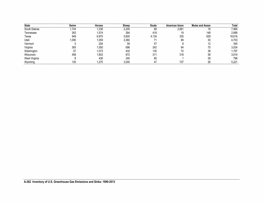
A-262 Inventory of U.S. Greenhouse Gas Emissions and Sinks: 1990-2013
State Swine Horses Sheep Goats American bison Mules and Asses Total
South Dakota 1,744 1,236 2,200 89 2,681 16 7,966
Tennessee 263 1,574 264 419 19 149 2,688
Texas 949 6,970 5,600 4,134 335 629 18,616
Utah 1,095 1,059 2,360 71 89 30 4,703
Vermont 5 204 59 57 8 12 345
Virginia 383 1,550 696 242 84 70 3,024
Washington 57 1,073 432 130 70 36 1,797
Wisconsin 458 1,803 672 311 318 58 3,619
West Virginia 8 436 240 85 1 29 798
Wyoming 135 1,275 3,000 47 737 26 5,221
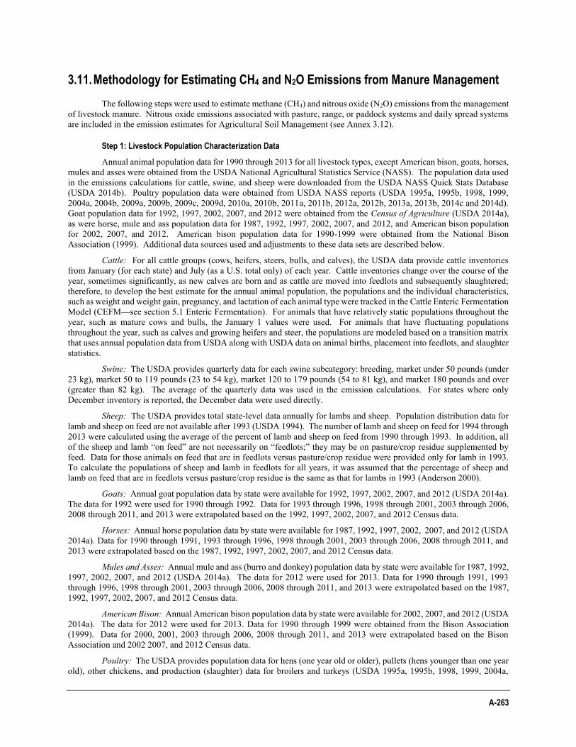
A-263
3.11. Methodology for Estimating CH4 and N2O Emissions from Manure Management
The following steps were used to estimate methane (CH4) and nitrous oxide (N2O) emissions from the management of livestock manure. Nitrous oxide emissions associated with pasture, range, or paddock systems and daily spread systems are included in the emission estimates for Agricultural Soil Management (see Annex 3.12).
Step 1: Livestock Population Characterization Data
Annual animal population data for 1990 through 2013 for all livestock types, except American bison, goats, horses, mules and asses were obtained from the USDA National Agricultural Statistics Service (NASS). The population data used in the emissions calculations for cattle, swine, and sheep were downloaded from the USDA NASS Quick Stats Database (USDA 2014b). Poultry population data were obtained from USDA NASS reports (USDA 1995a, 1995b, 1998, 1999, 2004a, 2004b, 2009a, 2009b, 2009c, 2009d, 2010a, 2010b, 2011a, 2011b, 2012a, 2012b, 2013a, 2013b, 2014c and 2014d). Goat population data for 1992, 1997, 2002, 2007, and 2012 were obtained from the Census of Agriculture (USDA 2014a), as were horse, mule and ass population data for 1987, 1992, 1997, 2002, 2007, and 2012, and American bison population for 2002, 2007, and 2012. American bison population data for 1990-1999 were obtained from the National Bison Association (1999). Additional data sources used and adjustments to these data sets are described below.
Cattle: For all cattle groups (cows, heifers, steers, bulls, and calves), the USDA data provide cattle inventories from January (for each state) and July (as a U.S. total only) of each year. Cattle inventories change over the course of the year, sometimes significantly, as new calves are born and as cattle are moved into feedlots and subsequently slaughtered; therefore, to develop the best estimate for the annual animal population, the populations and the individual characteristics, such as weight and weight gain, pregnancy, and lactation of each animal type were tracked in the Cattle Enteric Fermentation Model (CEFM—see section 5.1 Enteric Fermentation). For animals that have relatively static populations throughout the year, such as mature cows and bulls, the January 1 values were used. For animals that have fluctuating populations throughout the year, such as calves and growing heifers and steer, the populations are modeled based on a transition matrix that uses annual population data from USDA along with USDA data on animal births, placement into feedlots, and slaughter statistics.
Swine: The USDA provides quarterly data for each swine subcategory: breeding, market under 50 pounds (under 23 kg), market 50 to 119 pounds (23 to 54 kg), market 120 to 179 pounds (54 to 81 kg), and market 180 pounds and over (greater than 82 kg). The average of the quarterly data was used in the emission calculations. For states where only December inventory is reported, the December data were used directly.
Sheep: The USDA provides total state-level data annually for lambs and sheep. Population distribution data for lamb and sheep on feed are not available after 1993 (USDA 1994). The number of lamb and sheep on feed for 1994 through 2013 were calculated using the average of the percent of lamb and sheep on feed from 1990 through 1993. In addition, all of the sheep and lamb “on feed” are not necessarily on “feedlots;” they may be on pasture/crop residue supplemented by feed. Data for those animals on feed that are in feedlots versus pasture/crop residue were provided only for lamb in 1993. To calculate the populations of sheep and lamb in feedlots for all years, it was assumed that the percentage of sheep and lamb on feed that are in feedlots versus pasture/crop residue is the same as that for lambs in 1993 (Anderson 2000).
Goats: Annual goat population data by state were available for 1992, 1997, 2002, 2007, and 2012 (USDA 2014a). The data for 1992 were used for 1990 through 1992. Data for 1993 through 1996, 1998 through 2001, 2003 through 2006, 2008 through 2011, and 2013 were extrapolated based on the 1992, 1997, 2002, 2007, and 2012 Census data.
Horses: Annual horse population data by state were available for 1987, 1992, 1997, 2002, 2007, and 2012 (USDA 2014a). Data for 1990 through 1991, 1993 through 1996, 1998 through 2001, 2003 through 2006, 2008 through 2011, and 2013 were extrapolated based on the 1987, 1992, 1997, 2002, 2007, and 2012 Census data.
Mules and Asses: Annual mule and ass (burro and donkey) population data by state were available for 1987, 1992, 1997, 2002, 2007, and 2012 (USDA 2014a). The data for 2012 were used for 2013. Data for 1990 through 1991, 1993 through 1996, 1998 through 2001, 2003 through 2006, 2008 through 2011, and 2013 were extrapolated based on the 1987, 1992, 1997, 2002, 2007, and 2012 Census data.
American Bison: Annual American bison population data by state were available for 2002, 2007, and 2012 (USDA 2014a). The data for 2012 were used for 2013. Data for 1990 through 1999 were obtained from the Bison Association (1999). Data for 2000, 2001, 2003 through 2006, 2008 through 2011, and 2013 were extrapolated based on the Bison Association and 2002 2007, and 2012 Census data.
Poultry: The USDA provides population data for hens (one year old or older), pullets (hens younger than one year old), other chickens, and production (slaughter) data for broilers and turkeys (USDA 1995a, 1995b, 1998, 1999, 2004a,
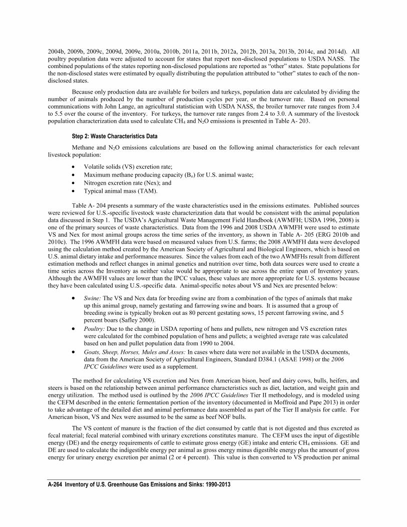
A-264 Inventory of U.S. Greenhouse Gas Emissions and Sinks: 1990-2013
2004b, 2009b, 2009c, 2009d, 2009e, 2010a, 2010b, 2011a, 2011b, 2012a, 2012b, 2013a, 2013b, 2014c, and 2014d). All poultry population data were adjusted to account for states that report non-disclosed populations to USDA NASS. The combined populations of the states reporting non-disclosed populations are reported as “other” states. State populations for the non-disclosed states were estimated by equally distributing the population attributed to “other” states to each of the non-disclosed states.
Because only production data are available for boilers and turkeys, population data are calculated by dividing the number of animals produced by the number of production cycles per year, or the turnover rate. Based on personal communications with John Lange, an agricultural statistician with USDA NASS, the broiler turnover rate ranges from 3.4 to 5.5 over the course of the inventory. For turkeys, the turnover rate ranges from 2.4 to 3.0. A summary of the livestock population characterization data used to calculate CH4 and N2O emissions is presented in Table A- 203.
Step 2: Waste Characteristics Data
Methane and N2O emissions calculations are based on the following animal characteristics for each relevant livestock population:
Volatile solids (VS) excretion rate; Maximum methane producing capacity (Bo) for U.S. animal waste; Nitrogen excretion rate (Nex); and Typical animal mass (TAM). Table A- 204 presents a summary of the waste characteristics used in the emissions estimates. Published sources
were reviewed for U.S.-specific livestock waste characterization data that would be consistent with the animal population data discussed in Step 1. The USDA’s Agricultural Waste Management Field Handbook (AWMFH; USDA 1996, 2008) is one of the primary sources of waste characteristics. Data from the 1996 and 2008 USDA AWMFH were used to estimate VS and Nex for most animal groups across the time series of the inventory, as shown in Table A- 205 (ERG 2010b and 2010c). The 1996 AWMFH data were based on measured values from U.S. farms; the 2008 AWMFH data were developed using the calculation method created by the American Society of Agricultural and Biological Engineers, which is based on U.S. animal dietary intake and performance measures. Since the values from each of the two AWMFHs result from different estimation methods and reflect changes in animal genetics and nutrition over time, both data sources were used to create a time series across the Inventory as neither value would be appropriate to use across the entire span of Inventory years. Although the AWMFH values are lower than the IPCC values, these values are more appropriate for U.S. systems because they have been calculated using U.S.-specific data. Animal-specific notes about VS and Nex are presented below:
Swine: The VS and Nex data for breeding swine are from a combination of the types of animals that make up this animal group, namely gestating and farrowing swine and boars. It is assumed that a group of breeding swine is typically broken out as 80 percent gestating sows, 15 percent farrowing swine, and 5 percent boars (Safley 2000).
Poultry: Due to the change in USDA reporting of hens and pullets, new nitrogen and VS excretion rates were calculated for the combined population of hens and pullets; a weighted average rate was calculated based on hen and pullet population data from 1990 to 2004.
Goats, Sheep, Horses, Mules and Asses: In cases where data were not available in the USDA documents, data from the American Society of Agricultural Engineers, Standard D384.1 (ASAE 1998) or the 2006 IPCC Guidelines were used as a supplement.
The method for calculating VS excretion and Nex from American bison, beef and dairy cows, bulls, heifers, and steers is based on the relationship between animal performance characteristics such as diet, lactation, and weight gain and energy utilization. The method used is outlined by the 2006 IPCC Guidelines Tier II methodology, and is modeled using the CEFM described in the enteric fermentation portion of the inventory (documented in Moffroid and Pape 2013) in order to take advantage of the detailed diet and animal performance data assembled as part of the Tier II analysis for cattle. For American bison, VS and Nex were assumed to be the same as beef NOF bulls.
The VS content of manure is the fraction of the diet consumed by cattle that is not digested and thus excreted as fecal material; fecal material combined with urinary excretions constitutes manure. The CEFM uses the input of digestible energy (DE) and the energy requirements of cattle to estimate gross energy (GE) intake and enteric CH4 emissions. GE and DE are used to calculate the indigestible energy per animal as gross energy minus digestible energy plus the amount of gross energy for urinary energy excretion per animal (2 or 4 percent). This value is then converted to VS production per animal
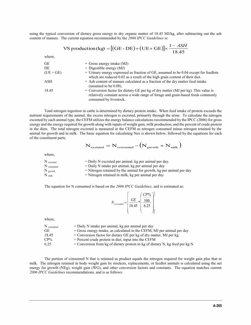
A-265
using the typical conversion of dietary gross energy to dry organic matter of 18.45 MJ/kg, after subtracting out the ash content of manure. The current equation recommended by the 2006 IPCC Guidelines is:
18.45
1GEUEDE-GE(kg) production VS ASH
where,
GE = Gross energy intake (MJ) DE = Digestible energy (MJ) (UE × GE) = Urinary energy expressed as fraction of GE, assumed to be 0.04 except for feedlots
which are reduced 0.02 as a result of the high grain content of their diet. ASH = Ash content of manure calculated as a fraction of the dry matter feed intake
(assumed to be 0.08). 18.45 = Conversion factor for dietary GE per kg of dry matter (MJ per kg). This value is
relatively constant across a wide range of forage and grain-based feeds commonly consumed by livestock.
Total nitrogen ingestion in cattle is determined by dietary protein intake. When feed intake of protein exceeds the nutrient requirements of the animal, the excess nitrogen is excreted, primarily through the urine. To calculate the nitrogen excreted by each animal type, the CEFM utilizes the energy balance calculations recommended by the IPCC (2006) for gross energy and the energy required for growth along with inputs of weight gain, milk production, and the percent of crude protein in the diets. The total nitrogen excreted is measured in the CEFM as nitrogen consumed minus nitrogen retained by the animal for growth and in milk. The basic equation for calculating Nex is shown below, followed by the equations for each of the constituent parts.
milkgrowthconsumedexcreted NNNN
where,
N excreted = Daily N excreted per animal, kg per animal per day. N consumed = Daily N intake per animal, kg per animal per day N growth = Nitrogen retained by the animal for growth, kg per animal per day N milk = Nitrogen retained in milk, kg per animal per day
The equation for N consumed is based on the 2006 IPCC Guidelines, and is estimated as:
25.6
100%
*45.18
CPGEN consumed
where,
N consumed = Daily N intake per animal, kg per animal per day GE = Gross energy intake, as calculated in the CEFM, MJ per animal per day 18.45 = Conversion factor for dietary GE per kg of dry matter, MJ per kg. CP% = Percent crude protein in diet, input into the CEFM 6.25 = Conversion from kg of dietary protein to kg of dietary N, kg feed per kg N
The portion of consumed N that is retained as product equals the nitrogen required for weight gain plus that in milk. The nitrogen retained in body weight gain by stockers, replacements, or feedlot animals is calculated using the net energy for growth (NEg), weight gain (WG), and other conversion factors and constants. The equation matches current 2006 IPCC Guidelines recommendations, and is as follows:
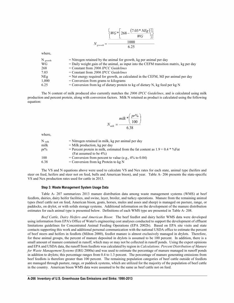
A-266 Inventory of U.S. Greenhouse Gas Emissions and Sinks: 1990-2013
25.61000
*03.7268*
WGNEgWG
N growth
where,
N growth = Nitrogen retained by the animal for growth, kg per animal per day WG = Daily weight gain of the animal, as input into the CEFM transition matrix, kg per day 268 = Constant from 2006 IPCC Guidelines 7.03 = Constant from 2006 IPCC Guidelines NEg = Net energy required for growth, as calculated in the CEFM, MJ per animal per day 1,000 = Conversion from grams to kilograms 6.25 = Conversion from kg of dietary protein to kg of dietary N, kg feed per kg N The N content of milk produced also currently matches the 2006 IPCC Guidelines, and is calculated using milk
production and percent protein, along with conversion factors. Milk N retained as product is calculated using the following equation:
38.6100
%*
prmilkNmilk
where,
N milk = Nitrogen retained in milk, kg per animal per day milk = Milk production, kg per day pr% = Percent protein in milk, estimated from the fat content as 1.9 + 0.4 * %Fat
(Fat assumed to be 4%) 100 = Conversion from percent to value (e.g., 4% to 0.04) 6.38 = Conversion from kg Protein to kg N The VS and N equations above were used to calculate VS and Nex rates for each state, animal type (heifers and
steer on feed, heifers and steer not on feed, bulls and American bison), and year. Table A- 206 presents the state-specific VS and Nex production rates used for cattle in 2013.
Step 3: Waste Management System Usage Data
Table A- 207 summarizes 2013 manure distribution data among waste management systems (WMS) at beef feedlots, dairies, dairy heifer facilities, and swine, layer, broiler, and turkey operations. Manure from the remaining animal types (beef cattle not on feed, American bison, goats, horses, mules and asses and sheep) is managed on pasture, range, or paddocks, on drylot, or with solids storage systems. Additional information on the development of the manure distribution estimates for each animal type is presented below. Definitions of each WMS type are presented in Table A- 208.
Beef Cattle, Dairy Heifers and American Bison: The beef feedlot and dairy heifer WMS data were developed using information from EPA's Office of Water's engineering cost analyses conducted to support the development of effluent limitations guidelines for Concentrated Animal Feeding Operations (EPA 2002b). Based on EPA site visits and state contacts supporting this work and additional personal communication with the national USDA office to estimate the percent of beef steers and heifers in feedlots (Milton 2000), feedlot manure is almost exclusively managed in drylots. Therefore, for these animal groups, the percent of manure deposited in drylots is assumed to be 100 percent. In addition, there is a small amount of manure contained in runoff, which may or may not be collected in runoff ponds. Using the expert opinions and EPA and USDA data, the runoff from feedlots was calculated by region in Calculations: Percent Distribution of Manure for Waste Management Systems (ERG 2000a) and was used to estimate the percentage of manure managed in runoff ponds in addition to drylots; this percentage ranges from 0.4 to 1.3 percent. The percentage of manure generating emissions from beef feedlots is therefore greater than 100 percent. The remaining population categories of beef cattle outside of feedlots are managed through pasture, range, or paddock systems, which are utilized for the majority of the population of beef cattle in the country. American bison WMS data were assumed to be the same as beef cattle not on feed.
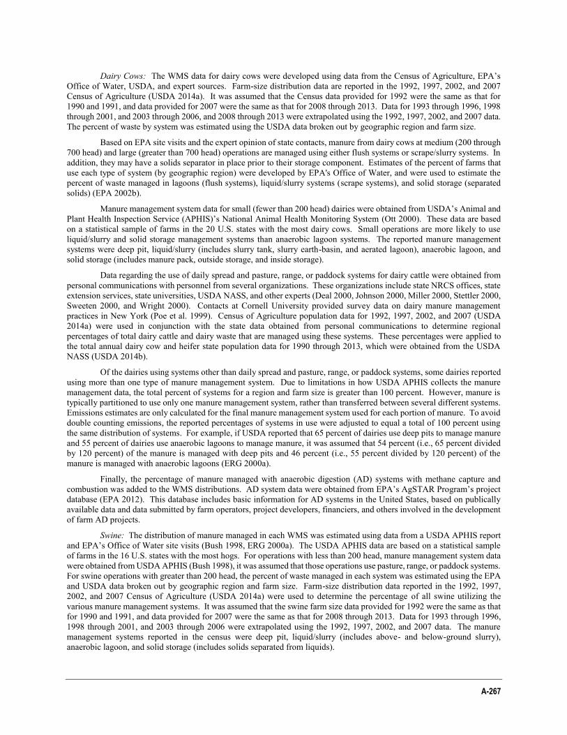
A-267
Dairy Cows: The WMS data for dairy cows were developed using data from the Census of Agriculture, EPA’s Office of Water, USDA, and expert sources. Farm-size distribution data are reported in the 1992, 1997, 2002, and 2007 Census of Agriculture (USDA 2014a). It was assumed that the Census data provided for 1992 were the same as that for 1990 and 1991, and data provided for 2007 were the same as that for 2008 through 2013. Data for 1993 through 1996, 1998 through 2001, and 2003 through 2006, and 2008 through 2013 were extrapolated using the 1992, 1997, 2002, and 2007 data. The percent of waste by system was estimated using the USDA data broken out by geographic region and farm size.
Based on EPA site visits and the expert opinion of state contacts, manure from dairy cows at medium (200 through 700 head) and large (greater than 700 head) operations are managed using either flush systems or scrape/slurry systems. In addition, they may have a solids separator in place prior to their storage component. Estimates of the percent of farms that use each type of system (by geographic region) were developed by EPA's Office of Water, and were used to estimate the percent of waste managed in lagoons (flush systems), liquid/slurry systems (scrape systems), and solid storage (separated solids) (EPA 2002b).
Manure management system data for small (fewer than 200 head) dairies were obtained from USDA’s Animal and Plant Health Inspection Service (APHIS)’s National Animal Health Monitoring System (Ott 2000). These data are based on a statistical sample of farms in the 20 U.S. states with the most dairy cows. Small operations are more likely to use liquid/slurry and solid storage management systems than anaerobic lagoon systems. The reported manure management systems were deep pit, liquid/slurry (includes slurry tank, slurry earth-basin, and aerated lagoon), anaerobic lagoon, and solid storage (includes manure pack, outside storage, and inside storage).
Data regarding the use of daily spread and pasture, range, or paddock systems for dairy cattle were obtained from personal communications with personnel from several organizations. These organizations include state NRCS offices, state extension services, state universities, USDA NASS, and other experts (Deal 2000, Johnson 2000, Miller 2000, Stettler 2000, Sweeten 2000, and Wright 2000). Contacts at Cornell University provided survey data on dairy manure management practices in New York (Poe et al. 1999). Census of Agriculture population data for 1992, 1997, 2002, and 2007 (USDA 2014a) were used in conjunction with the state data obtained from personal communications to determine regional percentages of total dairy cattle and dairy waste that are managed using these systems. These percentages were applied to the total annual dairy cow and heifer state population data for 1990 through 2013, which were obtained from the USDA NASS (USDA 2014b).
Of the dairies using systems other than daily spread and pasture, range, or paddock systems, some dairies reported using more than one type of manure management system. Due to limitations in how USDA APHIS collects the manure management data, the total percent of systems for a region and farm size is greater than 100 percent. However, manure is typically partitioned to use only one manure management system, rather than transferred between several different systems. Emissions estimates are only calculated for the final manure management system used for each portion of manure. To avoid double counting emissions, the reported percentages of systems in use were adjusted to equal a total of 100 percent using the same distribution of systems. For example, if USDA reported that 65 percent of dairies use deep pits to manage manure and 55 percent of dairies use anaerobic lagoons to manage manure, it was assumed that 54 percent (i.e., 65 percent divided by 120 percent) of the manure is managed with deep pits and 46 percent (i.e., 55 percent divided by 120 percent) of the manure is managed with anaerobic lagoons (ERG 2000a).
Finally, the percentage of manure managed with anaerobic digestion (AD) systems with methane capture and combustion was added to the WMS distributions. AD system data were obtained from EPA’s AgSTAR Program’s project database (EPA 2012). This database includes basic information for AD systems in the United States, based on publically available data and data submitted by farm operators, project developers, financiers, and others involved in the development of farm AD projects.
Swine: The distribution of manure managed in each WMS was estimated using data from a USDA APHIS report and EPA’s Office of Water site visits (Bush 1998, ERG 2000a). The USDA APHIS data are based on a statistical sample of farms in the 16 U.S. states with the most hogs. For operations with less than 200 head, manure management system data were obtained from USDA APHIS (Bush 1998), it was assumed that those operations use pasture, range, or paddock systems. For swine operations with greater than 200 head, the percent of waste managed in each system was estimated using the EPA and USDA data broken out by geographic region and farm size. Farm-size distribution data reported in the 1992, 1997, 2002, and 2007 Census of Agriculture (USDA 2014a) were used to determine the percentage of all swine utilizing the various manure management systems. It was assumed that the swine farm size data provided for 1992 were the same as that for 1990 and 1991, and data provided for 2007 were the same as that for 2008 through 2013. Data for 1993 through 1996, 1998 through 2001, and 2003 through 2006 were extrapolated using the 1992, 1997, 2002, and 2007 data. The manure management systems reported in the census were deep pit, liquid/slurry (includes above- and below-ground slurry), anaerobic lagoon, and solid storage (includes solids separated from liquids).
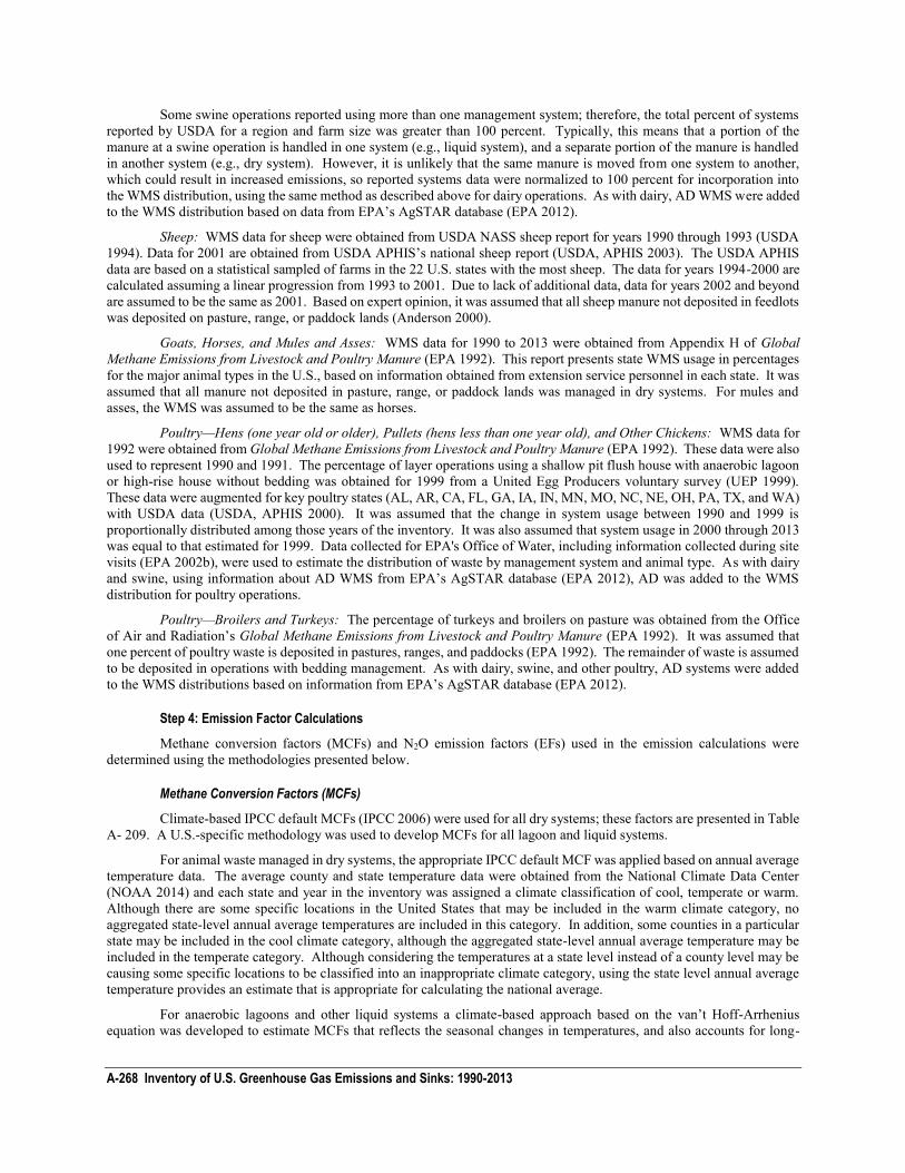
A-268 Inventory of U.S. Greenhouse Gas Emissions and Sinks: 1990-2013
Some swine operations reported using more than one management system; therefore, the total percent of systems reported by USDA for a region and farm size was greater than 100 percent. Typically, this means that a portion of the manure at a swine operation is handled in one system (e.g., liquid system), and a separate portion of the manure is handled in another system (e.g., dry system). However, it is unlikely that the same manure is moved from one system to another, which could result in increased emissions, so reported systems data were normalized to 100 percent for incorporation into the WMS distribution, using the same method as described above for dairy operations. As with dairy, AD WMS were added to the WMS distribution based on data from EPA’s AgSTAR database (EPA 2012).
Sheep: WMS data for sheep were obtained from USDA NASS sheep report for years 1990 through 1993 (USDA 1994). Data for 2001 are obtained from USDA APHIS’s national sheep report (USDA, APHIS 2003). The USDA APHIS data are based on a statistical sampled of farms in the 22 U.S. states with the most sheep. The data for years 1994-2000 are calculated assuming a linear progression from 1993 to 2001. Due to lack of additional data, data for years 2002 and beyond are assumed to be the same as 2001. Based on expert opinion, it was assumed that all sheep manure not deposited in feedlots was deposited on pasture, range, or paddock lands (Anderson 2000).
Goats, Horses, and Mules and Asses: WMS data for 1990 to 2013 were obtained from Appendix H of Global Methane Emissions from Livestock and Poultry Manure (EPA 1992). This report presents state WMS usage in percentages for the major animal types in the U.S., based on information obtained from extension service personnel in each state. It was assumed that all manure not deposited in pasture, range, or paddock lands was managed in dry systems. For mules and asses, the WMS was assumed to be the same as horses.
Poultry—Hens (one year old or older), Pullets (hens less than one year old), and Other Chickens: WMS data for 1992 were obtained from Global Methane Emissions from Livestock and Poultry Manure (EPA 1992). These data were also used to represent 1990 and 1991. The percentage of layer operations using a shallow pit flush house with anaerobic lagoon or high-rise house without bedding was obtained for 1999 from a United Egg Producers voluntary survey (UEP 1999). These data were augmented for key poultry states (AL, AR, CA, FL, GA, IA, IN, MN, MO, NC, NE, OH, PA, TX, and WA) with USDA data (USDA, APHIS 2000). It was assumed that the change in system usage between 1990 and 1999 is proportionally distributed among those years of the inventory. It was also assumed that system usage in 2000 through 2013 was equal to that estimated for 1999. Data collected for EPA's Office of Water, including information collected during site visits (EPA 2002b), were used to estimate the distribution of waste by management system and animal type. As with dairy and swine, using information about AD WMS from EPA’s AgSTAR database (EPA 2012), AD was added to the WMS distribution for poultry operations.
Poultry—Broilers and Turkeys: The percentage of turkeys and broilers on pasture was obtained from the Office of Air and Radiation’s Global Methane Emissions from Livestock and Poultry Manure (EPA 1992). It was assumed that one percent of poultry waste is deposited in pastures, ranges, and paddocks (EPA 1992). The remainder of waste is assumed to be deposited in operations with bedding management. As with dairy, swine, and other poultry, AD systems were added to the WMS distributions based on information from EPA’s AgSTAR database (EPA 2012).
Step 4: Emission Factor Calculations
Methane conversion factors (MCFs) and N2O emission factors (EFs) used in the emission calculations were determined using the methodologies presented below.
Methane Conversion Factors (MCFs)
Climate-based IPCC default MCFs (IPCC 2006) were used for all dry systems; these factors are presented in Table A- 209. A U.S.-specific methodology was used to develop MCFs for all lagoon and liquid systems.
For animal waste managed in dry systems, the appropriate IPCC default MCF was applied based on annual average temperature data. The average county and state temperature data were obtained from the National Climate Data Center (NOAA 2014) and each state and year in the inventory was assigned a climate classification of cool, temperate or warm. Although there are some specific locations in the United States that may be included in the warm climate category, no aggregated state-level annual average temperatures are included in this category. In addition, some counties in a particular state may be included in the cool climate category, although the aggregated state-level annual average temperature may be included in the temperate category. Although considering the temperatures at a state level instead of a county level may be causing some specific locations to be classified into an inappropriate climate category, using the state level annual average temperature provides an estimate that is appropriate for calculating the national average.
For anaerobic lagoons and other liquid systems a climate-based approach based on the van’t Hoff-Arrhenius equation was developed to estimate MCFs that reflects the seasonal changes in temperatures, and also accounts for long-
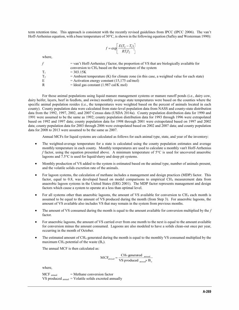
A-269
term retention time. This approach is consistent with the recently revised guidelines from IPCC (IPCC 2006). The van’t Hoff-Arrhenius equation, with a base temperature of 30°C, is shown in the following equation (Safley and Westerman 1990):
where,
f = van’t Hoff-Arrhenius f factor, the proportion of VS that are biologically available for conversion to CH4 based on the temperature of the system
T1 = 303.15K T2 = Ambient temperature (K) for climate zone (in this case, a weighted value for each state) E = Activation energy constant (15,175 cal/mol) R = Ideal gas constant (1.987 cal/K mol)
For those animal populations using liquid manure management systems or manure runoff ponds (i.e., dairy cow, dairy heifer, layers, beef in feedlots, and swine) monthly average state temperatures were based on the counties where the specific animal population resides (i.e., the temperatures were weighted based on the percent of animals located in each county). County population data were calculated from state-level population data from NASS and county-state distribution data from the 1992, 1997, 2002, and 2007 Census data (USDA 2014a). County population distribution data for 1990 and 1991 were assumed to be the same as 1992; county population distribution data for 1993 through 1996 were extrapolated based on 1992 and 1997 data; county population data for 1998 through 2001 were extrapolated based on 1997 and 2002 data; county population data for 2003 through 2006 were extrapolated based on 2002 and 2007 data; and county population data for 2008 to 2013 were assumed to be the same as 2007.
Annual MCFs for liquid systems are calculated as follows for each animal type, state, and year of the inventory:
The weighted-average temperature for a state is calculated using the county population estimates and average monthly temperature in each county. Monthly temperatures are used to calculate a monthly van't Hoff-Arrhenius f factor, using the equation presented above. A minimum temperature of 5°C is used for uncovered anaerobic lagoons and 7.5°C is used for liquid/slurry and deep pit systems.
Monthly production of VS added to the system is estimated based on the animal type, number of animals present, and the volatile solids excretion rate of the animals.
For lagoon systems, the calculation of methane includes a management and design practices (MDP) factor. This factor, equal to 0.8, was developed based on model comparisons to empirical CH4 measurement data from anaerobic lagoon systems in the United States (ERG 2001). The MDP factor represents management and design factors which cause a system to operate at a less than optimal level.
For all systems other than anaerobic lagoons, the amount of VS available for conversion to CH4 each month is assumed to be equal to the amount of VS produced during the month (from Step 3). For anaerobic lagoons, the amount of VS available also includes VS that may remain in the system from previous months.
The amount of VS consumed during the month is equal to the amount available for conversion multiplied by the f factor.
For anaerobic lagoons, the amount of VS carried over from one month to the next is equal to the amount available for conversion minus the amount consumed. Lagoons are also modeled to have a solids clean-out once per year, occurring in the month of October.
The estimated amount of CH4 generated during the month is equal to the monthly VS consumed multiplied by the maximum CH4 potential of the waste (Bo).
The annual MCF is then calculated as:
oannual
annual4annual B produced VS
generated CHMCF
where,
MCF annual = Methane conversion factor
VS produced annual = Volatile solids excreted annually
21
12 )(expTRT
TTEf
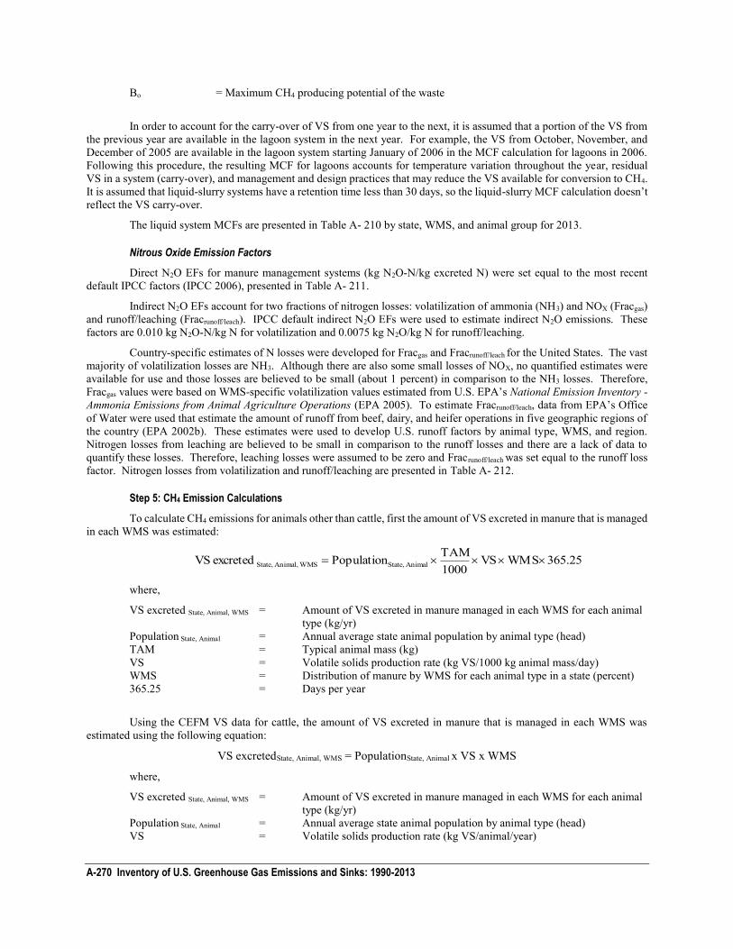
A-270 Inventory of U.S. Greenhouse Gas Emissions and Sinks: 1990-2013
Bo = Maximum CH4 producing potential of the waste
In order to account for the carry-over of VS from one year to the next, it is assumed that a portion of the VS from the previous year are available in the lagoon system in the next year. For example, the VS from October, November, and December of 2005 are available in the lagoon system starting January of 2006 in the MCF calculation for lagoons in 2006. Following this procedure, the resulting MCF for lagoons accounts for temperature variation throughout the year, residual VS in a system (carry-over), and management and design practices that may reduce the VS available for conversion to CH4. It is assumed that liquid-slurry systems have a retention time less than 30 days, so the liquid-slurry MCF calculation doesn’t reflect the VS carry-over.
The liquid system MCFs are presented in Table A- 210 by state, WMS, and animal group for 2013.
Nitrous Oxide Emission Factors
Direct N2O EFs for manure management systems (kg N2O-N/kg excreted N) were set equal to the most recent default IPCC factors (IPCC 2006), presented in Table A- 211.
Indirect N2O EFs account for two fractions of nitrogen losses: volatilization of ammonia (NH3) and NOX (Fracgas) and runoff/leaching (Fracrunoff/leach). IPCC default indirect N2O EFs were used to estimate indirect N2O emissions. These factors are 0.010 kg N2O-N/kg N for volatilization and 0.0075 kg N2O/kg N for runoff/leaching.
Country-specific estimates of N losses were developed for Fracgas and Fracrunoff/leach for the United States. The vast majority of volatilization losses are NH3. Although there are also some small losses of NOX, no quantified estimates were available for use and those losses are believed to be small (about 1 percent) in comparison to the NH3 losses. Therefore, Fracgas values were based on WMS-specific volatilization values estimated from U.S. EPA’s National Emission Inventory - Ammonia Emissions from Animal Agriculture Operations (EPA 2005). To estimate Fracrunoff/leach, data from EPA’s Office of Water were used that estimate the amount of runoff from beef, dairy, and heifer operations in five geographic regions of the country (EPA 2002b). These estimates were used to develop U.S. runoff factors by animal type, WMS, and region. Nitrogen losses from leaching are believed to be small in comparison to the runoff losses and there are a lack of data to quantify these losses. Therefore, leaching losses were assumed to be zero and Fracrunoff/leach was set equal to the runoff loss factor. Nitrogen losses from volatilization and runoff/leaching are presented in Table A- 212.
Step 5: CH4 Emission Calculations
To calculate CH4 emissions for animals other than cattle, first the amount of VS excreted in manure that is managed in each WMS was estimated:
365.25 WMS VS 1000TAM Populationexcreted VS Animal State, WMSAnimal, State,
where,
VS excreted State, Animal, WMS = Amount of VS excreted in manure managed in each WMS for each animal type (kg/yr)
Population State, Animal = Annual average state animal population by animal type (head) TAM = Typical animal mass (kg) VS = Volatile solids production rate (kg VS/1000 kg animal mass/day) WMS = Distribution of manure by WMS for each animal type in a state (percent) 365.25 = Days per year
Using the CEFM VS data for cattle, the amount of VS excreted in manure that is managed in each WMS was estimated using the following equation:
VS excretedState, Animal, WMS = PopulationState, Animal x VS x WMS
where,
VS excreted State, Animal, WMS = Amount of VS excreted in manure managed in each WMS for each animal type (kg/yr)
Population State, Animal = Annual average state animal population by animal type (head) VS = Volatile solids production rate (kg VS/animal/year)
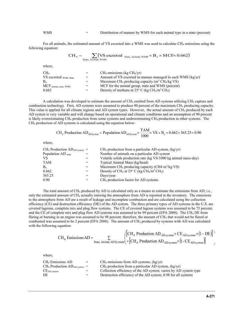
A-271
WMS = Distribution of manure by WMS for each animal type in a state (percent)
For all animals, the estimated amount of VS excreted into a WMS was used to calculate CH4 emissions using the following equation:
WMSAnimal, State,
o WMSAnimal, State,4 0.662MCF B excreted VS CH
where,
CH4 = CH4 emissions (kg CH4/yr) VS excreted WMS, State = Amount of VS excreted in manure managed in each WMS (kg/yr) Bo = Maximum CH4 producing capacity (m3 CH4/kg VS) MCF animal, state, WMS = MCF for the animal group, state and WMS (percent) 0.662 = Density of methane at 25o C (kg CH4/m3 CH4)
A calculation was developed to estimate the amount of CH4 emitted from AD systems utilizing CH4 capture and combustion technology. First, AD systems were assumed to produce 90 percent of the maximum CH4 producing capacity. This value is applied for all climate regions and AD system types. However, the actual amount of CH4 produced by each AD system is very variable and will change based on operational and climate conditions and an assumption of 90 percent is likely overestimating CH4 production from some systems and underestimating CH4 production in other systems. The CH4 production of AD systems is calculated using the equation below:
0.90 365.250.662 B VS 1000TAM AD PopulationAD Production CH o System ADSystem AD4
where,
CH4 Production ADAD system = CH4 production from a particular AD system, (kg/yr) Population AD state = Number of animals on a particular AD system VS = Volatile solids production rate (kg VS/1000 kg animal mass-day) TAM = Typical Animal Mass (kg/head) Bo = Maximum CH4 producing capacity (CH4 m3/kg VS) 0.662 = Density of CH4 at 25o C (kg CH4/m3 CH4) 365.25 = Days/year 0.90 = CH4 production factor for AD systems
The total amount of CH4 produced by AD is calculated only as a means to estimate the emissions from AD; i.e., only the estimated amount of CH4 actually entering the atmosphere from AD is reported in the inventory. The emissions to the atmosphere from AD are a result of leakage and incomplete combustion and are calculated using the collection efficiency (CE) and destruction efficiency (DE) of the AD system. The three primary types of AD systems in the U.S. are covered lagoons, complete mix and plug flow systems. The CE of covered lagoon systems was assumed to be 75 percent, and the CE of complete mix and plug flow AD systems was assumed to be 99 percent (EPA 2008). The CH4 DE from flaring or burning in an engine was assumed to be 98 percent; therefore, the amount of CH4 that would not be flared or combusted was assumed to be 2 percent (EPA 2008). The amount of CH4 produced by systems with AD was calculated with the following equation:
Systems AD Animal, State, system AD system AD4
system ADsystem AD44 CE-1 AD Production CH
DE1 CE AD Production CHAD Emissions CH
where,
CH4 Emissions AD = CH4 emissions from AD systems, (kg/yr) CH4 Production ADAD system = CH4 production from a particular AD system, (kg/yr) CEAD system = Collection efficiency of the AD system, varies by AD system type DE = Destruction efficiency of the AD system, 0.98 for all systems
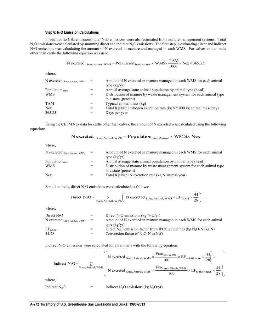
A-272 Inventory of U.S. Greenhouse Gas Emissions and Sinks: 1990-2013
Step 6: N2O Emission Calculations
In addition to CH4 emissions, total N2O emissions were also estimated from manure management systems. Total N2O emissions were calculated by summing direct and indirect N2O emissions. The first step in estimating direct and indirect N2O emissions was calculating the amount of N excreted in manure and managed in each WMS. For calves and animals other than cattle the following equation was used:
365.25Nex 1000TAM WMS Population excreted N Animal State, WMSAnimal, State,
where,
N excreted State, Animal, WMS = Amount of N excreted in manure managed in each WMS for each animal type (kg/yr)
Population state = Annual average state animal population by animal type (head) WMS = Distribution of manure by waste management system for each animal type
in a state (percent) TAM = Typical animal mass (kg) Nex = Total Kjeldahl nitrogen excretion rate (kg N/1000 kg animal mass/day) 365.25 = Days per year
Using the CEFM Nex data for cattle other than calves, the amount of N excreted was calculated using the following equation:
Nex WMS Population excreted N Animal State, WMSAnimal, State,
where,
N excreted State, Animal, WMS = Amount of N excreted in manure managed in each WMS for each animal type (kg/yr)
Population state = Annual average state animal population by animal type (head) WMS = Distribution of manure by waste management system for each animal type
in a state (percent) Nex = Total Kjeldahl N excretion rate (kg N/animal/year)
For all animals, direct N2O emissions were calculated as follows:
WMSAnimal, State,WMS WMSAnimal, State,2
2844 EF excreted N ONDirect
where,
Direct N2O = Direct N2O emissions (kg N2O/yr) N excreted State, Animal, WMS = Amount of N excreted in manure managed in each WMS for each animal
type (kg/yr) EFWMS = Direct N2O emission factor from IPCC guidelines (kg N2O-N /kg N) 44/28 = Conversion factor of N2O-N to N2O
Indirect N2O emissions were calculated for all animals with the following equation:
WMSAnimal, State,
achrunnoff/le WMSch,runoff/lea
WMSAnimal, State,
tionvolatiliza WMSgas,
WMSAnimal, State,
2
2844EF
100Frac
excreted N
2844 EF
100 Frac
excreted N
ONIndirect
where,
Indirect N2O = Indirect N2O emissions (kg N2O/yr)
A-273
N excreted State, Animal, WMS = Amount of N excreted in manure managed in each WMS for each animal type (kg/yr)
Fracgas,WMS = Nitrogen lost through volatilization in each WMS Fracrunoff/leach,WMS = Nitrogen lost through runoff and leaching in each WMS (data were not
available for leaching so the value reflects only runoff)
EFvolatilization = Emission factor for volatilization (0.010 kg N2O-N/kg N) EFrunoff/leach = Emission factor for runoff/leaching (0.0075 kg N2O-N/kg N)
44/28 = Conversion factor of N2O-N to N2O Emission estimates of CH4 and N2O by animal type are presented for all years of the inventory in Table A- 213 and Table A- 214 respectively. Emission estimates for 2013 are presented by animal type and state in Table A- 215 and Table A- 216 respectively.
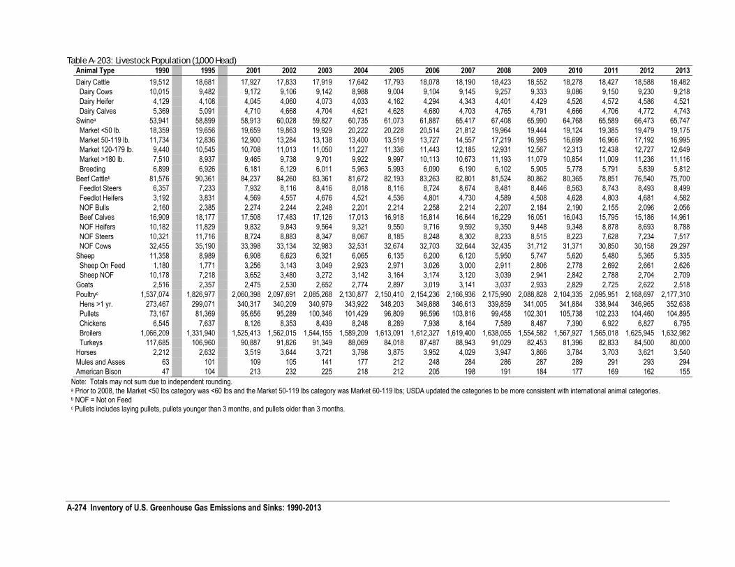
A-274 Inventory of U.S. Greenhouse Gas Emissions and Sinks: 1990-2013
Table A- 203: Livestock Population (1,000 Head) Animal Type 1990 1995 2001 2002 2003 2004 2005 2006 2007 2008 2009 2010 2011 2012 2013
Dairy Cattle 19,512 18,681 17,927 17,833 17,919 17,642 17,793 18,078 18,190 18,423 18,552 18,278 18,427 18,588 18,482
Dairy Cows 10,015 9,482 9,172 9,106 9,142 8,988 9,004 9,104 9,145 9,257 9,333 9,086 9,150 9,230 9,218
Dairy Heifer 4,129 4,108 4,045 4,060 4,073 4,033 4,162 4,294 4,343 4,401 4,429 4,526 4,572 4,586 4,521
Dairy Calves 5,369 5,091 4,710 4,668 4,704 4,621 4,628 4,680 4,703 4,765 4,791 4,666 4,706 4,772 4,743
Swinea 53,941 58,899 58,913 60,028 59,827 60,735 61,073 61,887 65,417 67,408 65,990 64,768 65,589 66,473 65,747
Market <50 lb. 18,359 19,656 19,659 19,863 19,929 20,222 20,228 20,514 21,812 19,964 19,444 19,124 19,385 19,479 19,175
Market 50-119 lb. 11,734 12,836 12,900 13,284 13,138 13,400 13,519 13,727 14,557 17,219 16,995 16,699 16,966 17,192 16,995
Market 120-179 lb. 9,440 10,545 10,708 11,013 11,050 11,227 11,336 11,443 12,185 12,931 12,567 12,313 12,438 12,727 12,649
Market >180 lb. 7,510 8,937 9,465 9,738 9,701 9,922 9,997 10,113 10,673 11,193 11,079 10,854 11,009 11,236 11,116
Breeding 6,899 6,926 6,181 6,129 6,011 5,963 5,993 6,090 6,190 6,102 5,905 5,778 5,791 5,839 5,812
Beef Cattleb 81,576 90,361 84,237 84,260 83,361 81,672 82,193 83,263 82,801 81,524 80,862 80,365 78,851 76,540 75,700
Feedlot Steers 6,357 7,233 7,932 8,116 8,416 8,018 8,116 8,724 8,674 8,481 8,446 8,563 8,743 8,493 8,499
Feedlot Heifers 3,192 3,831 4,569 4,557 4,676 4,521 4,536 4,801 4,730 4,589 4,508 4,628 4,803 4,681 4,582
NOF Bulls 2,160 2,385 2,274 2,244 2,248 2,201 2,214 2,258 2,214 2,207 2,184 2,190 2,155 2,096 2,056
Beef Calves 16,909 18,177 17,508 17,483 17,126 17,013 16,918 16,814 16,644 16,229 16,051 16,043 15,795 15,186 14,961
NOF Heifers 10,182 11,829 9,832 9,843 9,564 9,321 9,550 9,716 9,592 9,350 9,448 9,348 8,878 8,693 8,788
NOF Steers 10,321 11,716 8,724 8,883 8,347 8,067 8,185 8,248 8,302 8,233 8,515 8,223 7,628 7,234 7,517
NOF Cows 32,455 35,190 33,398 33,134 32,983 32,531 32,674 32,703 32,644 32,435 31,712 31,371 30,850 30,158 29,297
Sheep 11,358 8,989 6,908 6,623 6,321 6,065 6,135 6,200 6,120 5,950 5,747 5,620 5,480 5,365 5,335
Sheep On Feed 1,180 1,771 3,256 3,143 3,049 2,923 2,971 3,026 3,000 2,911 2,806 2,778 2,692 2,661 2,626
Sheep NOF 10,178 7,218 3,652 3,480 3,272 3,142 3,164 3,174 3,120 3,039 2,941 2,842 2,788 2,704 2,709
Goats 2,516 2,357 2,475 2,530 2,652 2,774 2,897 3,019 3,141 3,037 2,933 2,829 2,725 2,622 2,518
Poultryc 1,537,074 1,826,977 2,060,398 2,097,691 2,085,268 2,130,877 2,150,410 2,154,236 2,166,936 2,175,990 2,088,828 2,104,335 2,095,951 2,168,697 2,177,310
Hens >1 yr. 273,467 299,071 340,317 340,209 340,979 343,922 348,203 349,888 346,613 339,859 341,005 341,884 338,944 346,965 352,638
Pullets 73,167 81,369 95,656 95,289 100,346 101,429 96,809 96,596 103,816 99,458 102,301 105,738 102,233 104,460 104,895
Chickens 6,545 7,637 8,126 8,353 8,439 8,248 8,289 7,938 8,164 7,589 8,487 7,390 6,922 6,827 6,795
Broilers 1,066,209 1,331,940 1,525,413 1,562,015 1,544,155 1,589,209 1,613,091 1,612,327 1,619,400 1,638,055 1,554,582 1,567,927 1,565,018 1,625,945 1,632,982
Turkeys 117,685 106,960 90,887 91,826 91,349 88,069 84,018 87,487 88,943 91,029 82,453 81,396 82,833 84,500 80,000
Horses 2,212 2,632 3,519 3,644 3,721 3,798 3,875 3,952 4,029 3,947 3,866 3,784 3,703 3,621 3,540
Mules and Asses 63 101 109 105 141 177 212 248 284 286 287 289 291 293 294
American Bison 47 104 213 232 225 218 212 205 198 191 184 177 169 162 155
Note: Totals may not sum due to independent rounding. a Prior to 2008, the Market <50 lbs category was <60 lbs and the Market 50-119 lbs category was Market 60-119 lbs; USDA updated the categories to be more consistent with international animal categories. b NOF = Not on Feed c Pullets includes laying pullets, pullets younger than 3 months, and pullets older than 3 months.
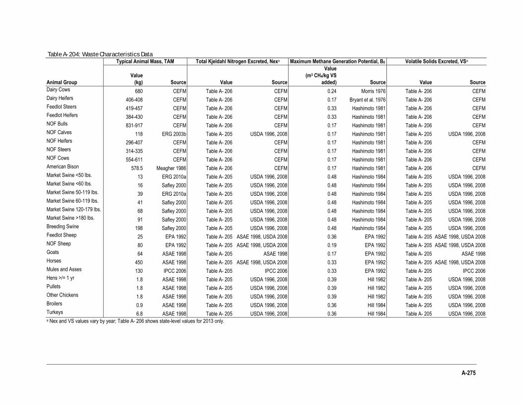
A-275
Table A- 204: Waste Characteristics Data
Animal Group
Typical Animal Mass, TAM Total Kjeldahl Nitrogen Excreted, Nexa Maximum Methane Generation Potential, B0 Volatile Solids Excreted, VSa
Value
(kg) Source Value Source
Value
(m3 CH4/kg VS
added) Source Value Source
Dairy Cows 680 CEFM Table A- 206 CEFM 0.24 Morris 1976 Table A- 206 CEFM
Dairy Heifers 406-408 CEFM Table A- 206 CEFM 0.17 Bryant et al. 1976 Table A- 206 CEFM
Feedlot Steers 419-457 CEFM Table A- 206 CEFM 0.33 Hashimoto 1981 Table A- 206 CEFM
Feedlot Heifers 384-430 CEFM Table A- 206 CEFM 0.33 Hashimoto 1981 Table A- 206 CEFM
NOF Bulls 831-917 CEFM Table A- 206 CEFM 0.17 Hashimoto 1981 Table A- 206 CEFM
NOF Calves 118 ERG 2003b Table A- 205 USDA 1996, 2008 0.17 Hashimoto 1981 Table A- 205 USDA 1996, 2008
NOF Heifers 296-407 CEFM Table A- 206 CEFM 0.17 Hashimoto 1981 Table A- 206 CEFM
NOF Steers 314-335 CEFM Table A- 206 CEFM 0.17 Hashimoto 1981 Table A- 206 CEFM
NOF Cows 554-611 CEFM Table A- 206 CEFM 0.17 Hashimoto 1981 Table A- 206 CEFM
American Bison 578.5 Meagher 1986 Table A- 206 CEFM 0.17 Hashimoto 1981 Table A- 206 CEFM
Market Swine <50 lbs. 13 ERG 2010a Table A- 205 USDA 1996, 2008 0.48 Hashimoto 1984 Table A- 205 USDA 1996, 2008
Market Swine <60 lbs. 16 Safley 2000 Table A- 205 USDA 1996, 2008 0.48 Hashimoto 1984 Table A- 205 USDA 1996, 2008
Market Swine 50-119 lbs. 39 ERG 2010a Table A- 205 USDA 1996, 2008 0.48 Hashimoto 1984 Table A- 205 USDA 1996, 2008
Market Swine 60-119 lbs. 41 Safley 2000 Table A- 205 USDA 1996, 2008 0.48 Hashimoto 1984 Table A- 205 USDA 1996, 2008
Market Swine 120-179 lbs. 68 Safley 2000 Table A- 205 USDA 1996, 2008 0.48 Hashimoto 1984 Table A- 205 USDA 1996, 2008
Market Swine >180 lbs. 91 Safley 2000 Table A- 205 USDA 1996, 2008 0.48 Hashimoto 1984 Table A- 205 USDA 1996, 2008
Breeding Swine 198 Safley 2000 Table A- 205 USDA 1996, 2008 0.48 Hashimoto 1984 Table A- 205 USDA 1996, 2008
Feedlot Sheep 25 EPA 1992 Table A- 205 ASAE 1998, USDA 2008 0.36 EPA 1992 Table A- 205 ASAE 1998, USDA 2008
NOF Sheep 80 EPA 1992 Table A- 205 ASAE 1998, USDA 2008 0.19 EPA 1992 Table A- 205 ASAE 1998, USDA 2008
Goats 64 ASAE 1998 Table A- 205 ASAE 1998 0.17 EPA 1992 Table A- 205 ASAE 1998
Horses 450 ASAE 1998 Table A- 205 ASAE 1998, USDA 2008 0.33 EPA 1992 Table A- 205 ASAE 1998, USDA 2008
Mules and Asses 130 IPCC 2006 Table A- 205 IPCC 2006 0.33 EPA 1992 Table A- 205 IPCC 2006
Hens >/= 1 yr 1.8 ASAE 1998 Table A- 205 USDA 1996, 2008 0.39 Hill 1982 Table A- 205 USDA 1996, 2008
Pullets 1.8 ASAE 1998 Table A- 205 USDA 1996, 2008 0.39 Hill 1982 Table A- 205 USDA 1996, 2008
Other Chickens 1.8 ASAE 1998 Table A- 205 USDA 1996, 2008 0.39 Hill 1982 Table A- 205 USDA 1996, 2008
Broilers 0.9 ASAE 1998 Table A- 205 USDA 1996, 2008 0.36 Hill 1984 Table A- 205 USDA 1996, 2008
Turkeys 6.8 ASAE 1998 Table A- 205 USDA 1996, 2008 0.36 Hill 1984 Table A- 205 USDA 1996, 2008 a Nex and VS values vary by year; Table A- 206 shows state-level values for 2013 only.
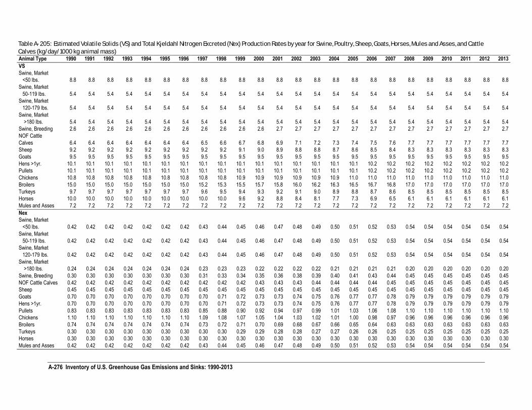
A-276 Inventory of U.S. Greenhouse Gas Emissions and Sinks: 1990-2013
Table A- 205: Estimated Volatile Solids (VS) and Total Kjeldahl Nitrogen Excreted (Nex) Production Rates by year for Swine, Poultry, Sheep, Goats, Horses, Mules and Asses, and Cattle
Calves (kg/day/1000 kg animal mass) Animal Type 1990 1991 1992 1993 1994 1995 1996 1997 1998 1999 2000 2001 2002 2003 2004 2005 2006 2007 2008 2009 2010 2011 2012 2013
VS
Swine, Market
<50 lbs. 8.8 8.8 8.8 8.8 8.8 8.8 8.8 8.8 8.8 8.8 8.8 8.8 8.8 8.8 8.8 8.8 8.8 8.8 8.8 8.8 8.8 8.8 8.8 8.8
Swine, Market
50-119 lbs. 5.4 5.4 5.4 5.4 5.4 5.4 5.4 5.4 5.4 5.4 5.4 5.4 5.4 5.4 5.4 5.4 5.4 5.4 5.4 5.4 5.4 5.4 5.4 5.4
Swine, Market
120-179 lbs. 5.4 5.4 5.4 5.4 5.4 5.4 5.4 5.4 5.4 5.4 5.4 5.4 5.4 5.4 5.4 5.4 5.4 5.4 5.4 5.4 5.4 5.4 5.4 5.4
Swine, Market
>180 lbs. 5.4 5.4 5.4 5.4 5.4 5.4 5.4 5.4 5.4 5.4 5.4 5.4 5.4 5.4 5.4 5.4 5.4 5.4 5.4 5.4 5.4 5.4 5.4 5.4
Swine, Breeding 2.6 2.6 2.6 2.6 2.6 2.6 2.6 2.6 2.6 2.6 2.6 2.7 2.7 2.7 2.7 2.7 2.7 2.7 2.7 2.7 2.7 2.7 2.7 2.7
NOF Cattle
Calves 6.4 6.4 6.4 6.4 6.4 6.4 6.4 6.5 6.6 6.7 6.8 6.9 7.1 7.2 7.3 7.4 7.5 7.6 7.7 7.7 7.7 7.7 7.7 7.7
Sheep 9.2 9.2 9.2 9.2 9.2 9.2 9.2 9.2 9.2 9.1 9.0 8.9 8.8 8.8 8.7 8.6 8.5 8.4 8.3 8.3 8.3 8.3 8.3 8.3
Goats 9.5 9.5 9.5 9.5 9.5 9.5 9.5 9.5 9.5 9.5 9.5 9.5 9.5 9.5 9.5 9.5 9.5 9.5 9.5 9.5 9.5 9.5 9.5 9.5
Hens >1yr. 10.1 10.1 10.1 10.1 10.1 10.1 10.1 10.1 10.1 10.1 10.1 10.1 10.1 10.1 10.1 10.1 10.2 10.2 10.2 10.2 10.2 10.2 10.2 10.2
Pullets 10.1 10.1 10.1 10.1 10.1 10.1 10.1 10.1 10.1 10.1 10.1 10.1 10.1 10.1 10.1 10.1 10.2 10.2 10.2 10.2 10.2 10.2 10.2 10.2
Chickens 10.8 10.8 10.8 10.8 10.8 10.8 10.8 10.8 10.8 10.9 10.9 10.9 10.9 10.9 10.9 11.0 11.0 11.0 11.0 11.0 11.0 11.0 11.0 11.0
Broilers 15.0 15.0 15.0 15.0 15.0 15.0 15.0 15.2 15.3 15.5 15.7 15.8 16.0 16.2 16.3 16.5 16.7 16.8 17.0 17.0 17.0 17.0 17.0 17.0
Turkeys 9.7 9.7 9.7 9.7 9.7 9.7 9.7 9.6 9.5 9.4 9.3 9.2 9.1 9.0 8.9 8.8 8.7 8.6 8.5 8.5 8.5 8.5 8.5 8.5
Horses 10.0 10.0 10.0 10.0 10.0 10.0 10.0 10.0 10.0 9.6 9.2 8.8 8.4 8.1 7.7 7.3 6.9 6.5 6.1 6.1 6.1 6.1 6.1 6.1
Mules and Asses 7.2 7.2 7.2 7.2 7.2 7.2 7.2 7.2 7.2 7.2 7.2 7.2 7.2 7.2 7.2 7.2 7.2 7.2 7.2 7.2 7.2 7.2 7.2 7.2
Nex
Swine, Market
<50 lbs. 0.42 0.42 0.42 0.42 0.42 0.42 0.42 0.43 0.44 0.45 0.46 0.47 0.48 0.49 0.50 0.51 0.52 0.53 0.54 0.54 0.54 0.54 0.54 0.54
Swine, Market
50-119 lbs. 0.42 0.42 0.42 0.42 0.42 0.42 0.42 0.43 0.44 0.45 0.46 0.47 0.48 0.49 0.50 0.51 0.52 0.53 0.54 0.54 0.54 0.54 0.54 0.54
Swine, Market
120-179 lbs. 0.42 0.42 0.42 0.42 0.42 0.42 0.42 0.43 0.44 0.45 0.46 0.47 0.48 0.49 0.50 0.51 0.52 0.53 0.54 0.54 0.54 0.54 0.54 0.54
Swine, Market
>180 lbs. 0.24 0.24 0.24 0.24 0.24 0.24 0.24 0.23 0.23 0.23 0.22 0.22 0.22 0.22 0.21 0.21 0.21 0.21 0.20 0.20 0.20 0.20 0.20 0.20
Swine, Breeding 0.30 0.30 0.30 0.30 0.30 0.30 0.30 0.31 0.33 0.34 0.35 0.36 0.38 0.39 0.40 0.41 0.43 0.44 0.45 0.45 0.45 0.45 0.45 0.45
NOF Cattle Calves 0.42 0.42 0.42 0.42 0.42 0.42 0.42 0.42 0.42 0.42 0.43 0.43 0.43 0.44 0.44 0.44 0.44 0.45 0.45 0.45 0.45 0.45 0.45 0.45
Sheep 0.45 0.45 0.45 0.45 0.45 0.45 0.45 0.45 0.45 0.45 0.45 0.45 0.45 0.45 0.45 0.45 0.45 0.45 0.45 0.45 0.45 0.45 0.45 0.45
Goats 0.70 0.70 0.70 0.70 0.70 0.70 0.70 0.70 0.71 0.72 0.73 0.73 0.74 0.75 0.76 0.77 0.77 0.78 0.79 0.79 0.79 0.79 0.79 0.79
Hens >1yr. 0.70 0.70 0.70 0.70 0.70 0.70 0.70 0.70 0.71 0.72 0.73 0.73 0.74 0.75 0.76 0.77 0.77 0.78 0.79 0.79 0.79 0.79 0.79 0.79
Pullets 0.83 0.83 0.83 0.83 0.83 0.83 0.83 0.85 0.88 0.90 0.92 0.94 0.97 0.99 1.01 1.03 1.06 1.08 1.10 1.10 1.10 1.10 1.10 1.10
Chickens 1.10 1.10 1.10 1.10 1.10 1.10 1.10 1.09 1.08 1.07 1.05 1.04 1.03 1.02 1.01 1.00 0.98 0.97 0.96 0.96 0.96 0.96 0.96 0.96
Broilers 0.74 0.74 0.74 0.74 0.74 0.74 0.74 0.73 0.72 0.71 0.70 0.69 0.68 0.67 0.66 0.65 0.64 0.63 0.63 0.63 0.63 0.63 0.63 0.63
Turkeys 0.30 0.30 0.30 0.30 0.30 0.30 0.30 0.30 0.30 0.29 0.29 0.28 0.28 0.27 0.27 0.26 0.26 0.25 0.25 0.25 0.25 0.25 0.25 0.25
Horses 0.30 0.30 0.30 0.30 0.30 0.30 0.30 0.30 0.30 0.30 0.30 0.30 0.30 0.30 0.30 0.30 0.30 0.30 0.30 0.30 0.30 0.30 0.30 0.30
Mules and Asses 0.42 0.42 0.42 0.42 0.42 0.42 0.42 0.43 0.44 0.45 0.46 0.47 0.48 0.49 0.50 0.51 0.52 0.53 0.54 0.54 0.54 0.54 0.54 0.54
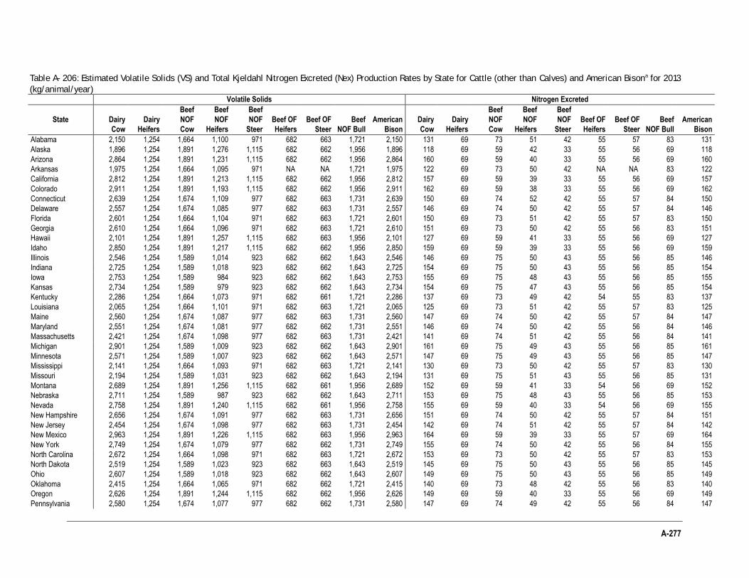
A-277
Table A- 206: Estimated Volatile Solids (VS) and Total Kjeldahl Nitrogen Excreted (Nex) Production Rates by State for Cattle (other than Calves) and American Bisona for 2013
(kg/animal/year) Volatile Solids Nitrogen Excreted
State Dairy
Cow
Dairy
Heifers
Beef
NOF
Cow
Beef
NOF
Heifers
Beef
NOF
Steer
Beef OF
Heifers
Beef OF
Steer
Beef
NOF Bull
American
Bison
Dairy
Cow
Dairy
Heifers
Beef
NOF
Cow
Beef
NOF
Heifers
Beef
NOF
Steer
Beef OF
Heifers
Beef OF
Steer
Beef
NOF Bull
American
Bison
Alabama 2,150 1,254 1,664 1,100 971 682 663 1,721 2,150 131 69 73 51 42 55 57 83 131
Alaska 1,896 1,254 1,891 1,276 1,115 682 662 1,956 1,896 118 69 59 42 33 55 56 69 118
Arizona 2,864 1,254 1,891 1,231 1,115 682 662 1,956 2,864 160 69 59 40 33 55 56 69 160
Arkansas 1,975 1,254 1,664 1,095 971 NA NA 1,721 1,975 122 69 73 50 42 NA NA 83 122
California 2,812 1,254 1,891 1,213 1,115 682 662 1,956 2,812 157 69 59 39 33 55 56 69 157
Colorado 2,911 1,254 1,891 1,193 1,115 682 662 1,956 2,911 162 69 59 38 33 55 56 69 162
Connecticut 2,639 1,254 1,674 1,109 977 682 663 1,731 2,639 150 69 74 52 42 55 57 84 150
Delaware 2,557 1,254 1,674 1,085 977 682 663 1,731 2,557 146 69 74 50 42 55 57 84 146
Florida 2,601 1,254 1,664 1,104 971 682 663 1,721 2,601 150 69 73 51 42 55 57 83 150
Georgia 2,610 1,254 1,664 1,096 971 682 663 1,721 2,610 151 69 73 50 42 55 56 83 151
Hawaii 2,101 1,254 1,891 1,257 1,115 682 663 1,956 2,101 127 69 59 41 33 55 56 69 127
Idaho 2,850 1,254 1,891 1,217 1,115 682 662 1,956 2,850 159 69 59 39 33 55 56 69 159
Illinois 2,546 1,254 1,589 1,014 923 682 662 1,643 2,546 146 69 75 50 43 55 56 85 146
Indiana 2,725 1,254 1,589 1,018 923 682 662 1,643 2,725 154 69 75 50 43 55 56 85 154
Iowa 2,753 1,254 1,589 984 923 682 662 1,643 2,753 155 69 75 48 43 55 56 85 155
Kansas 2,734 1,254 1,589 979 923 682 662 1,643 2,734 154 69 75 47 43 55 56 85 154
Kentucky 2,286 1,254 1,664 1,073 971 682 661 1,721 2,286 137 69 73 49 42 54 55 83 137
Louisiana 2,065 1,254 1,664 1,101 971 682 663 1,721 2,065 125 69 73 51 42 55 57 83 125
Maine 2,560 1,254 1,674 1,087 977 682 663 1,731 2,560 147 69 74 50 42 55 57 84 147
Maryland 2,551 1,254 1,674 1,081 977 682 662 1,731 2,551 146 69 74 50 42 55 56 84 146
Massachusetts 2,421 1,254 1,674 1,098 977 682 663 1,731 2,421 141 69 74 51 42 55 56 84 141
Michigan 2,901 1,254 1,589 1,009 923 682 662 1,643 2,901 161 69 75 49 43 55 56 85 161
Minnesota 2,571 1,254 1,589 1,007 923 682 662 1,643 2,571 147 69 75 49 43 55 56 85 147
Mississippi 2,141 1,254 1,664 1,093 971 682 663 1,721 2,141 130 69 73 50 42 55 57 83 130
Missouri 2,194 1,254 1,589 1,031 923 682 662 1,643 2,194 131 69 75 51 43 55 56 85 131
Montana 2,689 1,254 1,891 1,256 1,115 682 661 1,956 2,689 152 69 59 41 33 54 56 69 152
Nebraska 2,711 1,254 1,589 987 923 682 662 1,643 2,711 153 69 75 48 43 55 56 85 153
Nevada 2,758 1,254 1,891 1,240 1,115 682 661 1,956 2,758 155 69 59 40 33 54 56 69 155
New Hampshire 2,656 1,254 1,674 1,091 977 682 663 1,731 2,656 151 69 74 50 42 55 57 84 151
New Jersey 2,454 1,254 1,674 1,098 977 682 663 1,731 2,454 142 69 74 51 42 55 57 84 142
New Mexico 2,963 1,254 1,891 1,226 1,115 682 663 1,956 2,963 164 69 59 39 33 55 57 69 164
New York 2,749 1,254 1,674 1,079 977 682 662 1,731 2,749 155 69 74 50 42 55 56 84 155
North Carolina 2,672 1,254 1,664 1,098 971 682 663 1,721 2,672 153 69 73 50 42 55 57 83 153
North Dakota 2,519 1,254 1,589 1,023 923 682 663 1,643 2,519 145 69 75 50 43 55 56 85 145
Ohio 2,607 1,254 1,589 1,018 923 682 662 1,643 2,607 149 69 75 50 43 55 56 85 149
Oklahoma 2,415 1,254 1,664 1,065 971 682 662 1,721 2,415 140 69 73 48 42 55 56 83 140
Oregon 2,626 1,254 1,891 1,244 1,115 682 662 1,956 2,626 149 69 59 40 33 55 56 69 149
Pennsylvania 2,580 1,254 1,674 1,077 977 682 662 1,731 2,580 147 69 74 49 42 55 56 84 147
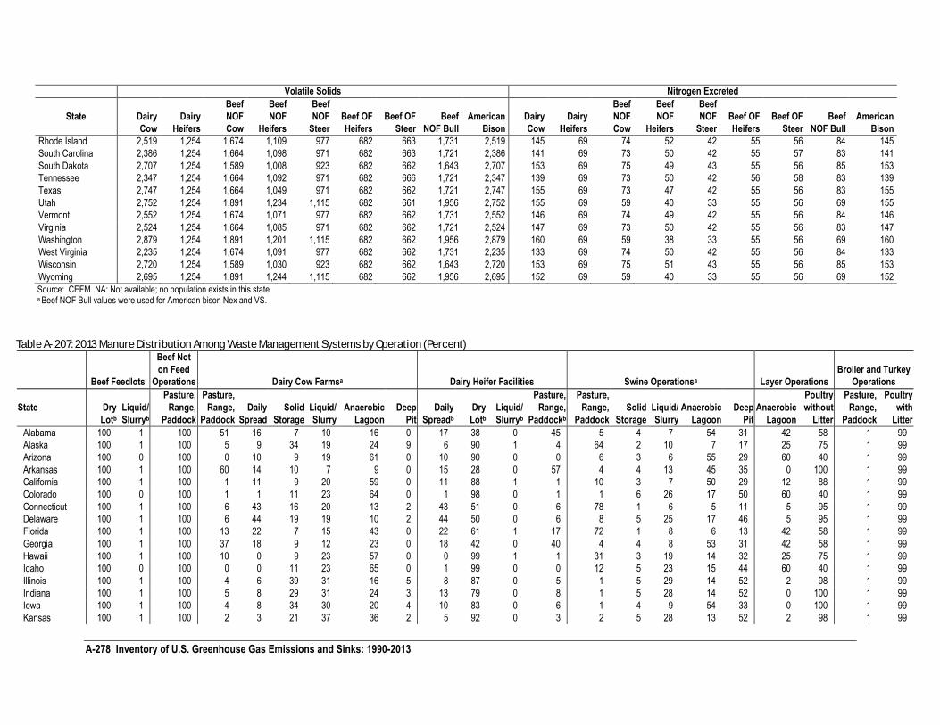
A-278 Inventory of U.S. Greenhouse Gas Emissions and Sinks: 1990-2013
Volatile Solids Nitrogen Excreted
State Dairy
Cow
Dairy
Heifers
Beef
NOF
Cow
Beef
NOF
Heifers
Beef
NOF
Steer
Beef OF
Heifers
Beef OF
Steer
Beef
NOF Bull
American
Bison
Dairy
Cow
Dairy
Heifers
Beef
NOF
Cow
Beef
NOF
Heifers
Beef
NOF
Steer
Beef OF
Heifers
Beef OF
Steer
Beef
NOF Bull
American
Bison
Rhode Island 2,519 1,254 1,674 1,109 977 682 663 1,731 2,519 145 69 74 52 42 55 56 84 145
South Carolina 2,386 1,254 1,664 1,098 971 682 663 1,721 2,386 141 69 73 50 42 55 57 83 141
South Dakota 2,707 1,254 1,589 1,008 923 682 662 1,643 2,707 153 69 75 49 43 55 56 85 153
Tennessee 2,347 1,254 1,664 1,092 971 682 666 1,721 2,347 139 69 73 50 42 56 58 83 139
Texas 2,747 1,254 1,664 1,049 971 682 662 1,721 2,747 155 69 73 47 42 55 56 83 155
Utah 2,752 1,254 1,891 1,234 1,115 682 661 1,956 2,752 155 69 59 40 33 55 56 69 155
Vermont 2,552 1,254 1,674 1,071 977 682 662 1,731 2,552 146 69 74 49 42 55 56 84 146
Virginia 2,524 1,254 1,664 1,085 971 682 662 1,721 2,524 147 69 73 50 42 55 56 83 147
Washington 2,879 1,254 1,891 1,201 1,115 682 662 1,956 2,879 160 69 59 38 33 55 56 69 160
West Virginia 2,235 1,254 1,674 1,091 977 682 662 1,731 2,235 133 69 74 50 42 55 56 84 133
Wisconsin 2,720 1,254 1,589 1,030 923 682 662 1,643 2,720 153 69 75 51 43 55 56 85 153
Wyoming 2,695 1,254 1,891 1,244 1,115 682 662 1,956 2,695 152 69 59 40 33 55 56 69 152
Source: CEFM. NA: Not available; no population exists in this state. a Beef NOF Bull values were used for American bison Nex and VS.
Table A- 207: 2013 Manure Distribution Among Waste Management Systems by Operation (Percent)
Beef Feedlots
Beef Not
on Feed
Operations Dairy Cow Farmsa Dairy Heifer Facilities Swine Operationsa Layer Operations
Broiler and Turkey
Operations
State Dry
Lotb
Liquid/
Slurryb
Pasture,
Range,
Paddock
Pasture,
Range,
Paddock
Daily
Spread
Solid
Storage
Liquid/
Slurry
Anaerobic
Lagoon
Deep
Pit
Daily
Spreadb
Dry
Lotb
Liquid/
Slurryb
Pasture,
Range,
Paddockb
Pasture,
Range,
Paddock
Solid
Storage
Liquid/
Slurry
Anaerobic
Lagoon
Deep
Pit
Anaerobic
Lagoon
Poultry
without
Litter
Pasture,
Range,
Paddock
Poultry
with
Litter
Alabama 100 1 100 51 16 7 10 16 0 17 38 0 45 5 4 7 54 31 42 58 1 99
Alaska 100 1 100 5 9 34 19 24 9 6 90 1 4 64 2 10 7 17 25 75 1 99
Arizona 100 0 100 0 10 9 19 61 0 10 90 0 0 6 3 6 55 29 60 40 1 99
Arkansas 100 1 100 60 14 10 7 9 0 15 28 0 57 4 4 13 45 35 0 100 1 99
California 100 1 100 1 11 9 20 59 0 11 88 1 1 10 3 7 50 29 12 88 1 99
Colorado 100 0 100 1 1 11 23 64 0 1 98 0 1 1 6 26 17 50 60 40 1 99
Connecticut 100 1 100 6 43 16 20 13 2 43 51 0 6 78 1 6 5 11 5 95 1 99
Delaware 100 1 100 6 44 19 19 10 2 44 50 0 6 8 5 25 17 46 5 95 1 99
Florida 100 1 100 13 22 7 15 43 0 22 61 1 17 72 1 8 6 13 42 58 1 99
Georgia 100 1 100 37 18 9 12 23 0 18 42 0 40 4 4 8 53 31 42 58 1 99
Hawaii 100 1 100 10 0 9 23 57 0 0 99 1 1 31 3 19 14 32 25 75 1 99
Idaho 100 0 100 0 0 11 23 65 0 1 99 0 0 12 5 23 15 44 60 40 1 99
Illinois 100 1 100 4 6 39 31 16 5 8 87 0 5 1 5 29 14 52 2 98 1 99
Indiana 100 1 100 5 8 29 31 24 3 13 79 0 8 1 5 28 14 52 0 100 1 99
Iowa 100 1 100 4 8 34 30 20 4 10 83 0 6 1 4 9 54 33 0 100 1 99
Kansas 100 1 100 2 3 21 37 36 2 5 92 0 3 2 5 28 13 52 2 98 1 99
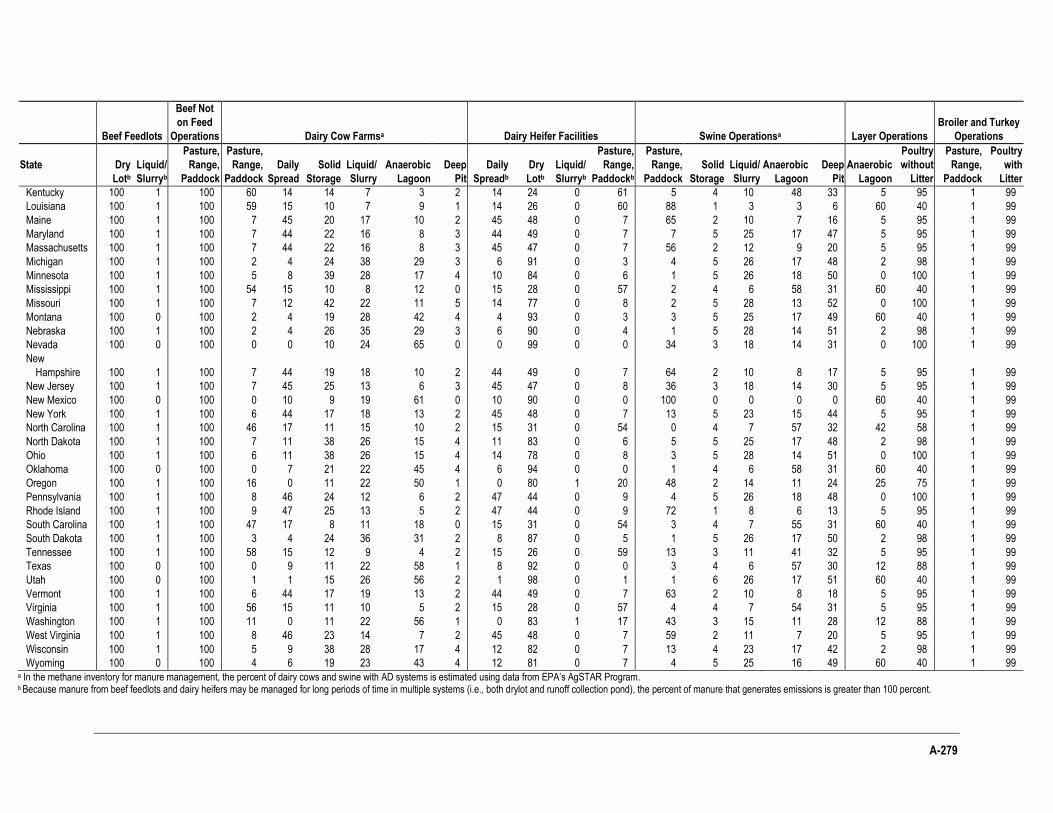
A-279
Beef Feedlots
Beef Not
on Feed
Operations Dairy Cow Farmsa Dairy Heifer Facilities Swine Operationsa Layer Operations
Broiler and Turkey
Operations
State Dry
Lotb
Liquid/
Slurryb
Pasture,
Range,
Paddock
Pasture,
Range,
Paddock
Daily
Spread
Solid
Storage
Liquid/
Slurry
Anaerobic
Lagoon
Deep
Pit
Daily
Spreadb
Dry
Lotb
Liquid/
Slurryb
Pasture,
Range,
Paddockb
Pasture,
Range,
Paddock
Solid
Storage
Liquid/
Slurry
Anaerobic
Lagoon
Deep
Pit
Anaerobic
Lagoon
Poultry
without
Litter
Pasture,
Range,
Paddock
Poultry
with
Litter
Kentucky 100 1 100 60 14 14 7 3 2 14 24 0 61 5 4 10 48 33 5 95 1 99
Louisiana 100 1 100 59 15 10 7 9 1 14 26 0 60 88 1 3 3 6 60 40 1 99
Maine 100 1 100 7 45 20 17 10 2 45 48 0 7 65 2 10 7 16 5 95 1 99
Maryland 100 1 100 7 44 22 16 8 3 44 49 0 7 7 5 25 17 47 5 95 1 99
Massachusetts 100 1 100 7 44 22 16 8 3 45 47 0 7 56 2 12 9 20 5 95 1 99
Michigan 100 1 100 2 4 24 38 29 3 6 91 0 3 4 5 26 17 48 2 98 1 99
Minnesota 100 1 100 5 8 39 28 17 4 10 84 0 6 1 5 26 18 50 0 100 1 99
Mississippi 100 1 100 54 15 10 8 12 0 15 28 0 57 2 4 6 58 31 60 40 1 99
Missouri 100 1 100 7 12 42 22 11 5 14 77 0 8 2 5 28 13 52 0 100 1 99
Montana 100 0 100 2 4 19 28 42 4 4 93 0 3 3 5 25 17 49 60 40 1 99
Nebraska 100 1 100 2 4 26 35 29 3 6 90 0 4 1 5 28 14 51 2 98 1 99
Nevada 100 0 100 0 0 10 24 65 0 0 99 0 0 34 3 18 14 31 0 100 1 99
New
Hampshire 100 1 100 7 44 19 18 10 2 44 49 0 7 64 2 10 8 17 5 95 1 99
New Jersey 100 1 100 7 45 25 13 6 3 45 47 0 8 36 3 18 14 30 5 95 1 99
New Mexico 100 0 100 0 10 9 19 61 0 10 90 0 0 100 0 0 0 0 60 40 1 99
New York 100 1 100 6 44 17 18 13 2 45 48 0 7 13 5 23 15 44 5 95 1 99
North Carolina 100 1 100 46 17 11 15 10 2 15 31 0 54 0 4 7 57 32 42 58 1 99
North Dakota 100 1 100 7 11 38 26 15 4 11 83 0 6 5 5 25 17 48 2 98 1 99
Ohio 100 1 100 6 11 38 26 15 4 14 78 0 8 3 5 28 14 51 0 100 1 99
Oklahoma 100 0 100 0 7 21 22 45 4 6 94 0 0 1 4 6 58 31 60 40 1 99
Oregon 100 1 100 16 0 11 22 50 1 0 80 1 20 48 2 14 11 24 25 75 1 99
Pennsylvania 100 1 100 8 46 24 12 6 2 47 44 0 9 4 5 26 18 48 0 100 1 99
Rhode Island 100 1 100 9 47 25 13 5 2 47 44 0 9 72 1 8 6 13 5 95 1 99
South Carolina 100 1 100 47 17 8 11 18 0 15 31 0 54 3 4 7 55 31 60 40 1 99
South Dakota 100 1 100 3 4 24 36 31 2 8 87 0 5 1 5 26 17 50 2 98 1 99
Tennessee 100 1 100 58 15 12 9 4 2 15 26 0 59 13 3 11 41 32 5 95 1 99
Texas 100 0 100 0 9 11 22 58 1 8 92 0 0 3 4 6 57 30 12 88 1 99
Utah 100 0 100 1 1 15 26 56 2 1 98 0 1 1 6 26 17 51 60 40 1 99
Vermont 100 1 100 6 44 17 19 13 2 44 49 0 7 63 2 10 8 18 5 95 1 99
Virginia 100 1 100 56 15 11 10 5 2 15 28 0 57 4 4 7 54 31 5 95 1 99
Washington 100 1 100 11 0 11 22 56 1 0 83 1 17 43 3 15 11 28 12 88 1 99
West Virginia 100 1 100 8 46 23 14 7 2 45 48 0 7 59 2 11 7 20 5 95 1 99
Wisconsin 100 1 100 5 9 38 28 17 4 12 82 0 7 13 4 23 17 42 2 98 1 99
Wyoming 100 0 100 4 6 19 23 43 4 12 81 0 7 4 5 25 16 49 60 40 1 99 a In the methane inventory for manure management, the percent of dairy cows and swine with AD systems is estimated using data from EPA’s AgSTAR Program. b Because manure from beef feedlots and dairy heifers may be managed for long periods of time in multiple systems (i.e., both drylot and runoff collection pond), the percent of manure that generates emissions is greater than 100 percent.
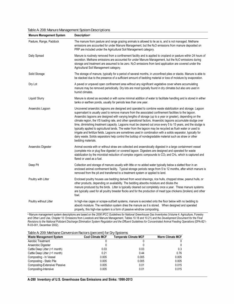
A-280 Inventory of U.S. Greenhouse Gas Emissions and Sinks: 1990-2013
Table A- 208: Manure Management System Descriptions
Manure Management System Descriptiona
Pasture, Range, Paddock The manure from pasture and range grazing animals is allowed to lie as is, and is not managed. Methane
emissions are accounted for under Manure Management, but the N2O emissions from manure deposited on
PRP are included under the Agricultural Soil Management category.
Daily Spread Manure is routinely removed from a confinement facility and is applied to cropland or pasture within 24 hours of
excretion. Methane emissions are accounted for under Manure Management, but the N2O emissions during
storage and treatment are assumed to be zero. N2O emissions from land application are covered under the
Agricultural Soil Management category.
Solid Storage The storage of manure, typically for a period of several months, in unconfined piles or stacks. Manure is able to
be stacked due to the presence of a sufficient amount of bedding material or loss of moisture by evaporation.
Dry Lot A paved or unpaved open confinement area without any significant vegetative cover where accumulating
manure may be removed periodically. Dry lots are most typically found in dry climates but also are used in
humid climates.
Liquid/ Slurry Manure is stored as excreted or with some minimal addition of water to facilitate handling and is stored in either
tanks or earthen ponds, usually for periods less than one year.
Anaerobic Lagoon Uncovered anaerobic lagoons are designed and operated to combine waste stabilization and storage. Lagoon
supernatant is usually used to remove manure from the associated confinement facilities to the lagoon.
Anaerobic lagoons are designed with varying lengths of storage (up to a year or greater), depending on the
climate region, the VS loading rate, and other operational factors. Anaerobic lagoons accumulate sludge over
time, diminishing treatment capacity. Lagoons must be cleaned out once every 5 to 15 years, and the sludge is
typically applied to agricultural lands. The water from the lagoon may be recycled as flush water or used to
irrigate and fertilize fields. Lagoons are sometimes used in combination with a solids separator, typically for
dairy waste. Solids separators help control the buildup of nondegradable material such as straw or other
bedding materials.
Anaerobic Digester Animal excreta with or without straw are collected and anaerobically digested in a large containment vessel
(complete mix or plug flow digester) or covered lagoon. Digesters are designed and operated for waste
stabilization by the microbial reduction of complex organic compounds to CO2 and CH4, which is captured and
flared or used as a fuel.
Deep Pit Collection and storage of manure usually with little or no added water typically below a slatted floor in an
enclosed animal confinement facility. Typical storage periods range from 5 to 12 months, after which manure is
removed from the pit and transferred to a treatment system or applied to land.
Poultry with Litter Enclosed poultry houses use bedding derived from wood shavings, rice hulls, chopped straw, peanut hulls, or
other products, depending on availability. The bedding absorbs moisture and dilutes the
manure produced by the birds. Litter is typically cleaned out completely once a year. These manure systems
are typically used for all poultry breeder flocks and for the production of meat type chickens (broilers) and other
fowl.
Poultry without Litter In high-rise cages or scrape-out/belt systems, manure is excreted onto the floor below with no bedding to
absorb moisture. The ventilation system dries the manure as it is stored. When designed and operated
properly, this high-rise system is a form of passive windrow composting.
a Manure management system descriptions are based on the 2006 IPCC Guidelines for National Greenhouse Gas Inventories (Volume 4: Agriculture, Forestry and Other Land Use, Chapter 10: Emissions from Livestock and Manure Management, Tables 10.18 and 10.21) and the Development Document for the Final Revisions to the National Pollutant Discharge Elimination System Regulation and the Effluent Guidelines for Concentrated Animal Feeding Operations (EPA-821-R-03-001, December 2002).
Table A- 209: Methane Conversion Factors (percent) for Dry Systems Waste Management System Cool Climate MCF Temperate Climate MCF Warm Climate MCF
Aerobic Treatment 0 0 0
Anaerobic Digester 0 0 0
Cattle Deep Litter (<1 month) 0.03 0.03 0.3
Cattle Deep Litter (>1 month) 0.21 0.44 0.76
Composting - In Vessel 0.005 0.005 0.005
Composting - Static Pile 0.005 0.005 0.005
Composting-Extensive/ Passive 0.005 0.01 0.015
Composting-Intensive 0.005 0.01 0.015
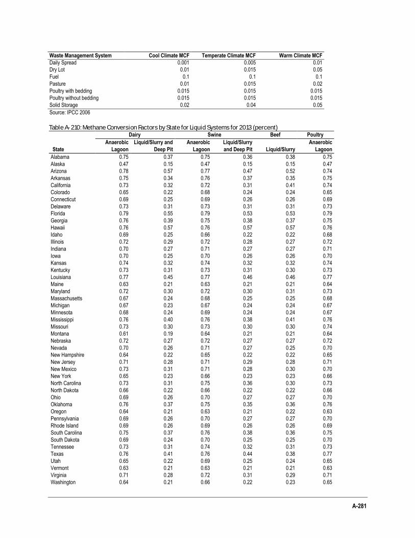
A-281
Waste Management System Cool Climate MCF Temperate Climate MCF Warm Climate MCF
Daily Spread 0.001 0.005 0.01
Dry Lot 0.01 0.015 0.05
Fuel 0.1 0.1 0.1
Pasture 0.01 0.015 0.02
Poultry with bedding 0.015 0.015 0.015
Poultry without bedding 0.015 0.015 0.015
Solid Storage 0.02 0.04 0.05
Source: IPCC 2006
Table A- 210: Methane Conversion Factors by State for Liquid Systems for 2013 (percent)
State
Dairy Swine Beef Poultry
Anaerobic
Lagoon
Liquid/Slurry and
Deep Pit
Anaerobic
Lagoon
Liquid/Slurry
and Deep Pit Liquid/Slurry
Anaerobic
Lagoon
Alabama 0.75 0.37 0.75 0.36 0.38 0.75
Alaska 0.47 0.15 0.47 0.15 0.15 0.47
Arizona 0.78 0.57 0.77 0.47 0.52 0.74
Arkansas 0.75 0.34 0.76 0.37 0.35 0.75
California 0.73 0.32 0.72 0.31 0.41 0.74
Colorado 0.65 0.22 0.68 0.24 0.24 0.65
Connecticut 0.69 0.25 0.69 0.26 0.26 0.69
Delaware 0.73 0.31 0.73 0.31 0.31 0.73
Florida 0.79 0.55 0.79 0.53 0.53 0.79
Georgia 0.76 0.39 0.75 0.38 0.37 0.75
Hawaii 0.76 0.57 0.76 0.57 0.57 0.76
Idaho 0.69 0.25 0.66 0.22 0.22 0.68
Illinois 0.72 0.29 0.72 0.28 0.27 0.72
Indiana 0.70 0.27 0.71 0.27 0.27 0.71
Iowa 0.70 0.25 0.70 0.26 0.26 0.70
Kansas 0.74 0.32 0.74 0.32 0.32 0.74
Kentucky 0.73 0.31 0.73 0.31 0.30 0.73
Louisiana 0.77 0.45 0.77 0.46 0.46 0.77
Maine 0.63 0.21 0.63 0.21 0.21 0.64
Maryland 0.72 0.30 0.72 0.30 0.31 0.73
Massachusetts 0.67 0.24 0.68 0.25 0.25 0.68
Michigan 0.67 0.23 0.67 0.24 0.24 0.67
Minnesota 0.68 0.24 0.69 0.24 0.24 0.67
Mississippi 0.76 0.40 0.76 0.38 0.41 0.76
Missouri 0.73 0.30 0.73 0.30 0.30 0.74
Montana 0.61 0.19 0.64 0.21 0.21 0.64
Nebraska 0.72 0.27 0.72 0.27 0.27 0.72
Nevada 0.70 0.26 0.71 0.27 0.25 0.70
New Hampshire 0.64 0.22 0.65 0.22 0.22 0.65
New Jersey 0.71 0.28 0.71 0.29 0.28 0.71
New Mexico 0.73 0.31 0.71 0.28 0.30 0.70
New York 0.65 0.23 0.66 0.23 0.23 0.66
North Carolina 0.73 0.31 0.75 0.36 0.30 0.73
North Dakota 0.66 0.22 0.66 0.22 0.22 0.66
Ohio 0.69 0.26 0.70 0.27 0.27 0.70
Oklahoma 0.76 0.37 0.75 0.35 0.36 0.76
Oregon 0.64 0.21 0.63 0.21 0.22 0.63
Pennsylvania 0.69 0.26 0.70 0.27 0.27 0.70
Rhode Island 0.69 0.26 0.69 0.26 0.26 0.69
South Carolina 0.75 0.37 0.76 0.38 0.36 0.75
South Dakota 0.69 0.24 0.70 0.25 0.25 0.70
Tennessee 0.73 0.31 0.74 0.32 0.31 0.73
Texas 0.76 0.41 0.76 0.44 0.38 0.77
Utah 0.65 0.22 0.69 0.25 0.24 0.65
Vermont 0.63 0.21 0.63 0.21 0.21 0.63
Virginia 0.71 0.28 0.72 0.31 0.29 0.71
Washington 0.64 0.21 0.66 0.22 0.23 0.65
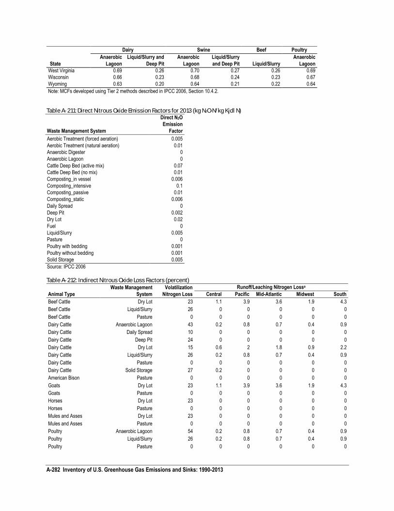
A-282 Inventory of U.S. Greenhouse Gas Emissions and Sinks: 1990-2013
State
Dairy Swine Beef Poultry
Anaerobic
Lagoon
Liquid/Slurry and
Deep Pit
Anaerobic
Lagoon
Liquid/Slurry
and Deep Pit Liquid/Slurry
Anaerobic
Lagoon
West Virginia 0.69 0.26 0.70 0.27 0.26 0.69
Wisconsin 0.66 0.23 0.68 0.24 0.23 0.67
Wyoming 0.63 0.20 0.64 0.21 0.22 0.64
Note: MCFs developed using Tier 2 methods described in IPCC 2006, Section 10.4.2.
Table A- 211: Direct Nitrous Oxide Emission Factors for 2013 (kg N2O-N/kg Kjdl N)
Waste Management System
Direct N2O
Emission
Factor
Aerobic Treatment (forced aeration) 0.005
Aerobic Treatment (natural aeration) 0.01
Anaerobic Digester 0
Anaerobic Lagoon 0
Cattle Deep Bed (active mix) 0.07
Cattle Deep Bed (no mix) 0.01
Composting_in vessel 0.006
Composting_intensive 0.1
Composting_passive 0.01
Composting_static 0.006
Daily Spread 0
Deep Pit 0.002
Dry Lot 0.02
Fuel 0
Liquid/Slurry 0.005
Pasture 0
Poultry with bedding 0.001
Poultry without bedding 0.001
Solid Storage 0.005
Source: IPCC 2006
Table A- 212: Indirect Nitrous Oxide Loss Factors (percent)
Animal Type
Waste Management
System
Volatilization
Nitrogen Loss
Runoff/Leaching Nitrogen Lossa
Central Pacific Mid-Atlantic Midwest South
Beef Cattle Dry Lot 23 1.1 3.9 3.6 1.9 4.3
Beef Cattle Liquid/Slurry 26 0 0 0 0 0
Beef Cattle Pasture 0 0 0 0 0 0
Dairy Cattle Anaerobic Lagoon 43 0.2 0.8 0.7 0.4 0.9
Dairy Cattle Daily Spread 10 0 0 0 0 0
Dairy Cattle Deep Pit 24 0 0 0 0 0
Dairy Cattle Dry Lot 15 0.6 2 1.8 0.9 2.2
Dairy Cattle Liquid/Slurry 26 0.2 0.8 0.7 0.4 0.9
Dairy Cattle Pasture 0 0 0 0 0 0
Dairy Cattle Solid Storage 27 0.2 0 0 0 0
American Bison Pasture 0 0 0 0 0 0
Goats Dry Lot 23 1.1 3.9 3.6 1.9 4.3
Goats Pasture 0 0 0 0 0 0
Horses Dry Lot 23 0 0 0 0 0
Horses Pasture 0 0 0 0 0 0
Mules and Asses Dry Lot 23 0 0 0 0 0
Mules and Asses Pasture 0 0 0 0 0 0
Poultry Anaerobic Lagoon 54 0.2 0.8 0.7 0.4 0.9
Poultry Liquid/Slurry 26 0.2 0.8 0.7 0.4 0.9
Poultry Pasture 0 0 0 0 0 0
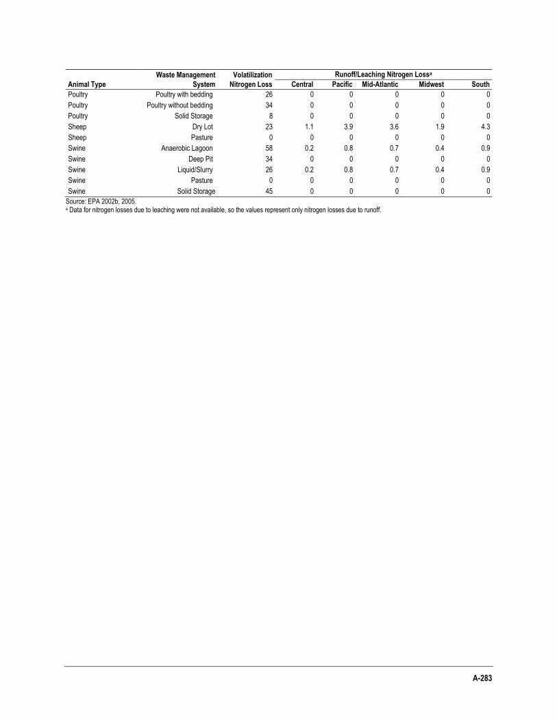
A-283
Animal Type
Waste Management
System
Volatilization
Nitrogen Loss
Runoff/Leaching Nitrogen Lossa
Central Pacific Mid-Atlantic Midwest South
Poultry Poultry with bedding 26 0 0 0 0 0
Poultry Poultry without bedding 34 0 0 0 0 0
Poultry Solid Storage 8 0 0 0 0 0
Sheep Dry Lot 23 1.1 3.9 3.6 1.9 4.3
Sheep Pasture 0 0 0 0 0 0
Swine Anaerobic Lagoon 58 0.2 0.8 0.7 0.4 0.9
Swine Deep Pit 34 0 0 0 0 0
Swine Liquid/Slurry 26 0.2 0.8 0.7 0.4 0.9
Swine Pasture 0 0 0 0 0 0
Swine Solid Storage 45 0 0 0 0 0
Source: EPA 2002b, 2005. a Data for nitrogen losses due to leaching were not available, so the values represent only nitrogen losses due to runoff.
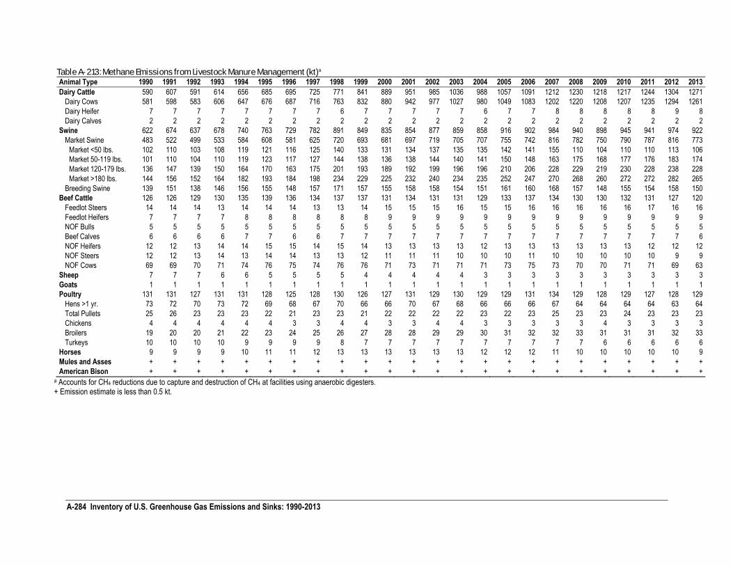
A-284 Inventory of U.S. Greenhouse Gas Emissions and Sinks: 1990-2013
Table A- 213: Methane Emissions from Livestock Manure Management (kt)a Animal Type 1990 1991 1992 1993 1994 1995 1996 1997 1998 1999 2000 2001 2002 2003 2004 2005 2006 2007 2008 2009 2010 2011 2012 2013
Dairy Cattle 590 607 591 614 656 685 695 725 771 841 889 951 985 1036 988 1057 1091 1212 1230 1218 1217 1244 1304 1271
Dairy Cows 581 598 583 606 647 676 687 716 763 832 880 942 977 1027 980 1049 1083 1202 1220 1208 1207 1235 1294 1261
Dairy Heifer 7 7 7 7 7 7 7 7 6 7 7 7 7 7 6 7 7 8 8 8 8 8 9 8
Dairy Calves 2 2 2 2 2 2 2 2 2 2 2 2 2 2 2 2 2 2 2 2 2 2 2 2
Swine 622 674 637 678 740 763 729 782 891 849 835 854 877 859 858 916 902 984 940 898 945 941 974 922
Market Swine 483 522 499 533 584 608 581 625 720 693 681 697 719 705 707 755 742 816 782 750 790 787 816 773
Market <50 lbs. 102 110 103 108 119 121 116 125 140 133 131 134 137 135 135 142 141 155 110 104 110 110 113 106
Market 50-119 lbs. 101 110 104 110 119 123 117 127 144 138 136 138 144 140 141 150 148 163 175 168 177 176 183 174
Market 120-179 lbs. 136 147 139 150 164 170 163 175 201 193 189 192 199 196 196 210 206 228 229 219 230 228 238 228
Market >180 lbs. 144 156 152 164 182 193 184 198 234 229 225 232 240 234 235 252 247 270 268 260 272 272 282 265
Breeding Swine 139 151 138 146 156 155 148 157 171 157 155 158 158 154 151 161 160 168 157 148 155 154 158 150
Beef Cattle 126 126 129 130 135 139 136 134 137 137 131 134 131 131 129 133 137 134 130 130 132 131 127 120
Feedlot Steers 14 14 14 13 14 14 14 13 13 14 15 15 15 16 15 15 16 16 16 16 16 17 16 16
Feedlot Heifers 7 7 7 7 8 8 8 8 8 8 9 9 9 9 9 9 9 9 9 9 9 9 9 9
NOF Bulls 5 5 5 5 5 5 5 5 5 5 5 5 5 5 5 5 5 5 5 5 5 5 5 5
Beef Calves 6 6 6 6 7 7 6 6 7 7 7 7 7 7 7 7 7 7 7 7 7 7 7 6
NOF Heifers 12 12 13 14 14 15 15 14 15 14 13 13 13 13 12 13 13 13 13 13 13 12 12 12
NOF Steers 12 12 13 14 13 14 14 13 13 12 11 11 11 10 10 10 11 10 10 10 10 10 9 9
NOF Cows 69 69 70 71 74 76 75 74 76 76 71 73 71 71 71 73 75 73 70 70 71 71 69 63
Sheep 7 7 7 6 6 5 5 5 5 4 4 4 4 4 3 3 3 3 3 3 3 3 3 3
Goats 1 1 1 1 1 1 1 1 1 1 1 1 1 1 1 1 1 1 1 1 1 1 1 1
Poultry 131 131 127 131 131 128 125 128 130 126 127 131 129 130 129 129 131 134 129 128 129 127 128 129
Hens >1 yr. 73 72 70 73 72 69 68 67 70 66 66 70 67 68 66 66 66 67 64 64 64 64 63 64
Total Pullets 25 26 23 23 23 22 21 23 23 21 22 22 22 22 23 22 23 25 23 23 24 23 23 23
Chickens 4 4 4 4 4 4 3 3 4 4 3 3 4 4 3 3 3 3 3 4 3 3 3 3
Broilers 19 20 20 21 22 23 24 25 26 27 28 28 29 29 30 31 32 32 33 31 31 31 32 33
Turkeys 10 10 10 10 9 9 9 9 8 7 7 7 7 7 7 7 7 7 7 6 6 6 6 6
Horses 9 9 9 9 10 11 11 12 13 13 13 13 13 13 12 12 12 11 10 10 10 10 10 9
Mules and Asses + + + + + + + + + + + + + + + + + + + + + + + +
American Bison + + + + + + + + + + + + + + + + + + + + + + + + a Accounts for CH4 reductions due to capture and destruction of CH4 at facilities using anaerobic digesters. + Emission estimate is less than 0.5 kt.
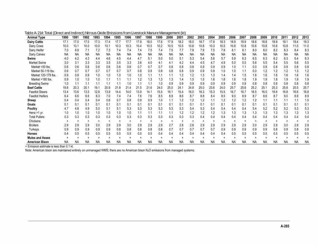
A-285
Table A- 214: Total (Direct and Indirect) Nitrous Oxide Emissions from Livestock Manure Management (kt)
Animal Type 1990 1991 1992 1993 1994 1995 1996 1997 1998 1999 2000 2001 2002 2003 2004 2005 2006 2007 2008 2009 2010 2011 2012 2013
Dairy Cattle 17.1 17.0 17.0 17.3 17.4 17.7 17.7 17.9 18.0 17.6 17.9 18.2 18.5 18.7 17.8 18.3 18.9 18.9 18.6 18.8 18.9 19.1 19.4 19.3
Dairy Cows 10.0 10.1 10.0 10.0 10.1 10.3 10.3 10.4 10.5 10.2 10.5 10.5 10.6 10.8 10.3 10.5 10.8 10.8 10.6 10.8 10.6 10.8 11.0 11.0
Dairy Heifer 7.0 6.9 7.1 7.2 7.3 7.4 7.4 7.4 7.5 7.4 7.5 7.7 7.8 7.9 7.5 7.8 8.1 8.1 8.0 8.0 8.2 8.3 8.4 8.3
Dairy Calves NA NA NA NA NA NA NA NA NA NA NA NA NA NA NA NA NA NA NA NA NA NA NA NA
Swine 4.0 4.2 4.3 4.4 4.6 4.5 4.4 4.7 5.1 5.0 5.0 5.1 5.3 5.4 5.6 5.7 5.9 6.3 6.5 6.3 6.2 6.3 6.4 6.3
Market Swine 3.0 3.1 3.3 3.3 3.5 3.5 3.3 3.6 4.0 4.1 4.1 4.2 4.4 4.5 4.7 4.9 5.0 5.5 5.6 5.5 5.4 5.5 5.6 5.5
Market <50 lbs. 0.6 0.6 0.6 0.6 0.6 0.6 0.6 0.7 0.7 0.7 0.8 0.8 0.8 0.9 0.9 0.9 1.0 1.1 0.0 0.8 0.8 0.8 0.8 0.8
Market 50-119 lbs. 0.6 0.7 0.7 0.7 0.7 0.7 0.7 0.8 0.8 0.8 0.8 0.8 0.9 0.9 0.9 1.0 1.0 1.1 0.0 1.2 1.2 1.2 1.3 1.2
Market 120-179 lbs. 0.9 0.9 0.9 1.0 1.0 1.0 1.0 1.0 1.1 1.1 1.1 1.2 1.2 1.3 1.3 1.4 1.4 1.5 1.6 1.6 1.6 1.6 1.6 1.6
Market >180 lbs. 0.9 1.0 1.0 1.0 1.1 1.1 1.1 1.2 1.3 1.3 1.3 1.4 1.5 1.5 1.6 1.6 1.6 1.8 1.9 1.9 1.8 1.9 1.9 1.9
Breeding Swine 1.0 1.1 1.1 1.1 1.1 1.1 1.0 1.1 1.1 1.0 0.9 0.9 0.9 0.9 0.9 0.9 0.9 0.9 0.8 0.8 0.8 0.8 0.8 0.8
Beef Cattle 19.8 20.3 20.1 19.1 20.9 21.8 21.4 21.5 21.6 24.0 25.0 24.1 24.8 25.0 23.6 24.0 25.7 25.6 25.2 25.1 25.3 25.8 25.5 25.7
Feedlot Steers 13.4 13.6 13.5 12.8 13.9 14.4 14.0 13.9 14.1 15.5 16.1 15.4 16.0 16.3 15.3 15.5 16.7 16.7 16.5 16.5 16.6 16.8 16.6 16.8
Feedlot Heifers 6.4 6.6 6.6 6.3 7.0 7.4 7.4 7.6 7.6 8.5 8.9 8.6 8.7 8.8 8.4 8.5 9.0 8.9 8.7 8.6 8.7 9.0 8.9 8.9
Sheep 0.4 0.4 0.4 0.4 0.6 0.7 0.8 0.9 0.9 1.0 1.1 1.2 1.2 1.2 1.1 1.2 1.2 1.2 1.2 1.1 1.1 1.1 1.1 1.0
Goats 0.1 0.1 0.1 0.1 0.1 0.1 0.1 0.1 0.1 0.1 0.1 0.1 0.1 0.1 0.1 0.1 0.1 0.1 0.1 0.1 0.1 0.1 0.1 0.1
Poultry 4.7 4.8 4.9 5.0 5.1 5.1 5.3 5.3 5.3 5.3 5.3 5.3 5.4 5.3 5.4 5.4 5.4 5.4 5.4 5.2 5.2 5.2 5.3 5.3
Hens >1 yr. 1.0 1.0 1.0 1.0 1.0 1.0 1.0 1.1 1.1 1.1 1.1 1.2 1.2 1.2 1.2 1.3 1.3 1.3 1.3 1.3 1.3 1.3 1.3 1.3
Total Pullets 0.3 0.3 0.3 0.3 0.3 0.3 0.3 0.3 0.3 0.3 0.3 0.3 0.3 0.4 0.4 0.4 0.4 0.4 0.4 0.4 0.4 0.4 0.4 0.4
Chickens + + + + + + + + + + + + + + + + + + + + + + + +
Broilers 2.9 2.9 2.9 3.0 2.9 2.9 3.0 2.9 2.9 2.9 2.7 2.8 2.8 2.9 2.9 2.9 2.9 2.9 3.0 2.9 2.9 3.0 2.9 2.9
Turkeys 0.9 0.9 0.9 0.9 0.9 0.8 0.8 0.8 0.8 0.8 0.7 0.7 0.7 0.7 0.7 0.9 0.9 0.9 0.9 0.9 0.8 0.8 0.8 0.8
Horses 0.4 0.5 0.5 0.5 0.5 0.5 0.5 0.5 0.5 0.4 0.4 0.4 0.4 0.4 0.4 0.4 0.5 0.5 0.5 0.5 0.5 0.5 0.5 0.5
Mules and Asses + + + + + + + + + + + + + + + + + + + + + + + +
American Bison NA NA NA NA NA NA NA NA NA NA NA NA NA NA NA NA NA NA NA NA NA NA NA NA
+ Emission estimate is less than 0.1 kt. Note: American bison are maintained entirely on unmanaged WMS; there are no American bison N2O emissions from managed systems.
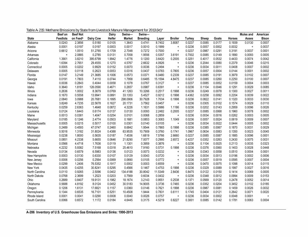
A-286 Inventory of U.S. Greenhouse Gas Emissions and Sinks: 1990-2013
Table A- 215: Methane Emissions by State from Livestock Manure Management for 2013 (kt)a
State
Beef on
Feedlots
Beef Not
on Feedb Dairy Cow
Dairy
Heifer
Swine—
Market
Swine—
Breeding Layer Broiler Turkey Sheep Goats Horses
Mules and
Asses
American
Bison
Alabama 0.0243 2.3856 0.5180 0.0105 1.3643 0.4741 8.7402 3.8087 0.0237 0.0085 0.0177 0.1939 0.0130 0.0007
Alaska 0.0001 0.0197 0.0197 0.0003 0.0017 0.0010 0.1999 + 0.0236 0.0057 0.0002 0.0032 + 0.0037
Arizona 0.6612 1.0510 51.2765 0.1709 2.7048 0.7272 0.7000 + 0.0237 0.0987 0.0291 0.3191 0.0037 0.0001
Arkansas + 2.0885 0.2785 0.0131 0.7058 1.9556 0.5357 3.6191 0.7002 0.0085 0.0149 0.1890 0.0093 0.0005
California 1.3901 3.8210 395.6799 1.9942 1.4776 0.1200 3.6420 0.2005 0.3251 0.4017 0.0532 0.4433 0.0074 0.0042
Colorado 1.6394 2.7651 29.4555 0.1270 4.5767 2.6632 4.0926 + 0.0236 0.2044 0.0080 0.2379 0.0046 0.0215
Connecticut 0.0005 0.0202 0.9929 0.0152 0.0070 0.0036 0.2494 + 0.0236 0.0034 0.0011 0.0408 0.0007 0.0002
Delaware 0.0005 0.0118 0.2623 0.0053 0.0316 0.0437 0.0783 0.7805 0.0236 0.0057 0.0004 0.0144 0.0001 0.0002
Florida 0.0147 3.2149 21.3685 0.1006 0.0573 0.0371 6.0480 0.2339 0.0237 0.0085 0.0191 0.3979 0.0102 0.0007
Georgia 0.0191 1.7803 7.4110 0.0744 1.7958 0.6485 15.1594 4.8475 0.0237 0.0085 0.0260 0.2250 0.0100 0.0007
Hawaii 0.0036 0.2843 0.4044 0.0058 0.1078 0.0767 0.3127 + 0.0237 0.0085 0.0052 0.0159 0.0004 0.0003
Idaho 0.3640 1.8181 126.0590 0.4671 0.2657 0.0987 0.6391 + 0.0236 0.1104 0.0046 0.1291 0.0029 0.0085
Illinois 0.2636 1.0002 8.3679 0.0769 41.1263 10.3266 0.2517 0.1998 0.0236 0.0249 0.0078 0.1300 0.0027 0.0011
Indiana 0.1670 0.5558 13.9941 0.0891 33.1353 5.4527 0.9212 0.1998 0.4362 0.0258 0.0092 0.2204 0.0039 0.0022
Iowa 2.0840 3.0988 20.7681 0.1895 298.0906 30.7928 1.7034 0.1998 0.0236 0.0822 0.0141 0.1320 0.0033 0.0030
Kansas 3.8249 4.7235 22.5678 0.1627 20.1731 3.7562 0.0457 + 0.0236 0.0305 0.0102 0.1574 0.0029 0.0110
Kentucky 0.0259 2.6363 1.4648 0.0872 4.3226 1.1631 0.5986 1.1186 0.0236 0.0202 0.0143 0.2959 0.0096 0.0026
Louisiana 0.0124 1.6443 0.6174 0.0137 0.0130 0.0093 2.2482 0.2005 0.0237 0.0085 0.0068 0.1960 0.0078 0.0002
Maine 0.0013 0.0381 1.4047 0.0254 0.0101 0.0068 0.2859 + 0.0236 0.0034 0.0016 0.0262 0.0003 0.0005
Maryland 0.0185 0.1246 2.4774 0.0503 0.1681 0.0853 0.3083 1.1049 0.0236 0.0057 0.0024 0.0619 0.0009 0.0007
Massachusetts 0.0005 0.0215 0.5017 0.0100 0.0301 0.0140 0.0105 + 0.0236 0.0034 0.0022 0.0444 0.0005 0.0002
Michigan 0.2489 0.4593 47.0747 0.2460 8.6842 1.9544 0.7865 0.1998 0.0236 0.0385 0.0067 0.1870 0.0031 0.0029
Minnesota 0.5016 1.3182 31.8024 0.4388 63.9535 10.7909 0.3760 0.1741 1.0967 0.0634 0.0083 0.1350 0.0023 0.0045
Mississippi 0.0238 1.8000 0.5635 0.0187 7.4536 1.6819 7.5766 2.6660 0.0237 0.0085 0.0087 0.1885 0.0096 0.0001
Missouri 0.0851 4.2338 5.6655 0.0646 21.8290 7.0077 0.2995 2.6572 0.4237 0.0352 0.0263 0.2430 0.0075 0.0031
Montana 0.0566 4.4718 1.7636 0.0119 1.1301 0.3959 0.3876 + 0.0236 0.1104 0.0025 0.2113 0.0035 0.0323
Nebraska 4.2232 5.9382 7.5168 0.0318 25.4610 7.9160 0.5731 0.1998 0.0236 0.0376 0.0060 0.1403 0.0028 0.0448
Nevada 0.0134 0.6579 6.5983 0.0136 0.0123 0.0073 0.0232 + 0.0236 0.0343 0.0058 0.0510 0.0004 0.0001
New Hampshire 0.0003 0.0130 0.6330 0.0107 0.0129 0.0043 0.0720 + 0.0236 0.0034 0.0013 0.0196 0.0002 0.0006
New Jersey 0.0006 0.0256 0.2564 0.0069 0.0690 0.0105 0.0772 + 0.0236 0.0057 0.0019 0.0595 0.0007 0.0004
New Mexico 0.0299 1.2406 76.5352 0.1917 0.0002 0.0003 0.6559 + 0.0236 0.0470 0.0075 0.1098 0.0014 0.0115
New York 0.0435 0.4255 30.8241 0.5295 0.4566 0.1467 0.4753 0.1998 0.0236 0.0329 0.0089 0.1997 0.0027 0.0016
North Carolina 0.0110 0.9265 2.5096 0.0402 134.4188 30.8042 11.5349 2.8436 0.8475 0.0122 0.0150 0.1414 0.0069 0.0005
North Dakota 0.0768 2.3699 1.2523 0.0203 0.7569 0.6034 0.0432 + 0.0236 0.0348 0.0012 0.0994 0.0009 0.0153
Ohio 0.2689 0.8407 19.9131 0.1982 18.1674 3.2143 0.9551 0.2538 0.1371 0.0569 0.0120 0.2478 0.0052 0.0014
Oklahoma 0.5688 4.8192 8.0124 0.0452 30.5183 14.9005 3.3736 0.7465 0.0236 0.0352 0.0204 0.3452 0.0102 0.0185
Oregon 0.1206 1.6131 17.6821 0.1157 0.0360 0.0146 0.7621 0.1998 0.0236 0.0987 0.0081 0.1459 0.0026 0.0032
Pennsylvania 0.1344 0.6535 16.7101 0.5251 10.4508 1.9444 0.7831 0.6111 0.1745 0.0404 0.0121 0.2642 0.0071 0.0020
Rhode Island 0.0001 0.0041 0.0290 0.0008 0.0040 0.0026 0.0757 + 0.0236 0.0034 0.0002 0.0048 0.0001 +
South Carolina 0.0066 0.6572 1.1172 0.0184 4.6445 0.3175 4.5219 0.8227 0.3001 0.0085 0.0142 0.1781 0.0063 0.0004
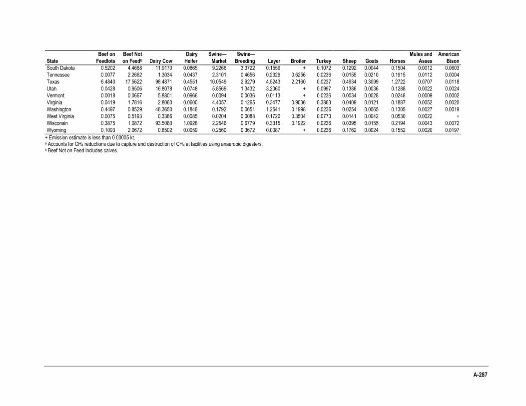
A-287
State
Beef on
Feedlots
Beef Not
on Feedb Dairy Cow
Dairy
Heifer
Swine—
Market
Swine—
Breeding Layer Broiler Turkey Sheep Goats Horses
Mules and
Asses
American
Bison
South Dakota 0.5202 4.4668 11.9170 0.0865 9.2266 3.3722 0.1559 + 0.1072 0.1292 0.0044 0.1504 0.0012 0.0603
Tennessee 0.0077 2.2662 1.3034 0.0437 2.3101 0.4656 0.2329 0.6256 0.0236 0.0155 0.0210 0.1915 0.0112 0.0004
Texas 6.4840 17.5622 98.4871 0.4551 10.0549 2.9279 4.5243 2.2160 0.0237 0.4934 0.3099 1.2722 0.0707 0.0118
Utah 0.0428 0.9506 16.8078 0.0748 5.8569 1.3432 3.2060 + 0.0997 0.1386 0.0036 0.1288 0.0022 0.0024
Vermont 0.0018 0.0667 5.8801 0.0966 0.0094 0.0036 0.0113 + 0.0236 0.0034 0.0028 0.0248 0.0009 0.0002
Virginia 0.0419 1.7816 2.8060 0.0600 4.4057 0.1265 0.3477 0.9036 0.3863 0.0409 0.0121 0.1887 0.0052 0.0020
Washington 0.4497 0.8529 46.3650 0.1846 0.1792 0.0651 1.2541 0.1998 0.0236 0.0254 0.0065 0.1305 0.0027 0.0019
West Virginia 0.0075 0.5193 0.3386 0.0085 0.0204 0.0088 0.1720 0.3504 0.0773 0.0141 0.0042 0.0530 0.0022 +
Wisconsin 0.3875 1.0872 93.5080 1.0928 2.2546 0.6779 0.3315 0.1922 0.0236 0.0395 0.0155 0.2194 0.0043 0.0072
Wyoming 0.1093 2.0672 0.8502 0.0059 0.2560 0.3672 0.0087 + 0.0236 0.1762 0.0024 0.1552 0.0020 0.0197
+ Emission estimate is less than 0.00005 kt. a Accounts for CH4 reductions due to capture and destruction of CH4 at facilities using anaerobic digesters. b Beef Not on Feed includes calves.
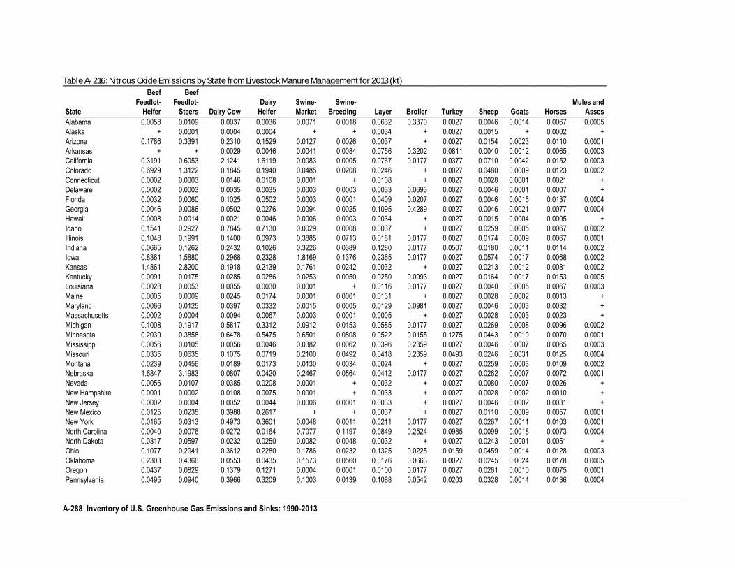
A-288 Inventory of U.S. Greenhouse Gas Emissions and Sinks: 1990-2013
Table A- 216: Nitrous Oxide Emissions by State from Livestock Manure Management for 2013 (kt)
State
Beef
Feedlot-
Heifer
Beef
Feedlot-
Steers Dairy Cow
Dairy
Heifer
Swine-
Market
Swine-
Breeding Layer Broiler Turkey Sheep Goats Horses
Mules and
Asses
Alabama 0.0058 0.0109 0.0037 0.0036 0.0071 0.0018 0.0632 0.3370 0.0027 0.0046 0.0014 0.0067 0.0005
Alaska + 0.0001 0.0004 0.0004 + + 0.0034 + 0.0027 0.0015 + 0.0002 +
Arizona 0.1786 0.3391 0.2310 0.1529 0.0127 0.0026 0.0037 + 0.0027 0.0154 0.0023 0.0110 0.0001
Arkansas + + 0.0029 0.0046 0.0041 0.0084 0.0756 0.3202 0.0811 0.0040 0.0012 0.0065 0.0003
California 0.3191 0.6053 2.1241 1.6119 0.0083 0.0005 0.0767 0.0177 0.0377 0.0710 0.0042 0.0152 0.0003
Colorado 0.6929 1.3122 0.1845 0.1940 0.0485 0.0208 0.0246 + 0.0027 0.0480 0.0009 0.0123 0.0002
Connecticut 0.0002 0.0003 0.0146 0.0108 0.0001 + 0.0108 + 0.0027 0.0028 0.0001 0.0021 +
Delaware 0.0002 0.0003 0.0035 0.0035 0.0003 0.0003 0.0033 0.0693 0.0027 0.0046 0.0001 0.0007 +
Florida 0.0032 0.0060 0.1025 0.0502 0.0003 0.0001 0.0409 0.0207 0.0027 0.0046 0.0015 0.0137 0.0004
Georgia 0.0046 0.0086 0.0502 0.0276 0.0094 0.0025 0.1095 0.4289 0.0027 0.0046 0.0021 0.0077 0.0004
Hawaii 0.0008 0.0014 0.0021 0.0046 0.0006 0.0003 0.0034 + 0.0027 0.0015 0.0004 0.0005 +
Idaho 0.1541 0.2927 0.7845 0.7130 0.0029 0.0008 0.0037 + 0.0027 0.0259 0.0005 0.0067 0.0002
Illinois 0.1048 0.1991 0.1400 0.0973 0.3885 0.0713 0.0181 0.0177 0.0027 0.0174 0.0009 0.0067 0.0001
Indiana 0.0665 0.1262 0.2432 0.1026 0.3226 0.0389 0.1280 0.0177 0.0507 0.0180 0.0011 0.0114 0.0002
Iowa 0.8361 1.5880 0.2968 0.2328 1.8169 0.1376 0.2365 0.0177 0.0027 0.0574 0.0017 0.0068 0.0002
Kansas 1.4861 2.8200 0.1918 0.2139 0.1761 0.0242 0.0032 + 0.0027 0.0213 0.0012 0.0081 0.0002
Kentucky 0.0091 0.0175 0.0285 0.0286 0.0253 0.0050 0.0250 0.0993 0.0027 0.0164 0.0017 0.0153 0.0005
Louisiana 0.0028 0.0053 0.0055 0.0030 0.0001 + 0.0116 0.0177 0.0027 0.0040 0.0005 0.0067 0.0003
Maine 0.0005 0.0009 0.0245 0.0174 0.0001 0.0001 0.0131 + 0.0027 0.0028 0.0002 0.0013 +
Maryland 0.0066 0.0125 0.0397 0.0332 0.0015 0.0005 0.0129 0.0981 0.0027 0.0046 0.0003 0.0032 +
Massachusetts 0.0002 0.0004 0.0094 0.0067 0.0003 0.0001 0.0005 + 0.0027 0.0028 0.0003 0.0023 +
Michigan 0.1008 0.1917 0.5817 0.3312 0.0912 0.0153 0.0585 0.0177 0.0027 0.0269 0.0008 0.0096 0.0002
Minnesota 0.2030 0.3858 0.6478 0.5475 0.6501 0.0808 0.0522 0.0155 0.1275 0.0443 0.0010 0.0070 0.0001
Mississippi 0.0056 0.0105 0.0056 0.0046 0.0382 0.0062 0.0396 0.2359 0.0027 0.0046 0.0007 0.0065 0.0003
Missouri 0.0335 0.0635 0.1075 0.0719 0.2100 0.0492 0.0418 0.2359 0.0493 0.0246 0.0031 0.0125 0.0004
Montana 0.0239 0.0456 0.0189 0.0173 0.0130 0.0034 0.0024 + 0.0027 0.0259 0.0003 0.0109 0.0002
Nebraska 1.6847 3.1983 0.0807 0.0420 0.2467 0.0564 0.0412 0.0177 0.0027 0.0262 0.0007 0.0072 0.0001
Nevada 0.0056 0.0107 0.0385 0.0208 0.0001 + 0.0032 + 0.0027 0.0080 0.0007 0.0026 +
New Hampshire 0.0001 0.0002 0.0108 0.0075 0.0001 + 0.0033 + 0.0027 0.0028 0.0002 0.0010 +
New Jersey 0.0002 0.0004 0.0052 0.0044 0.0006 0.0001 0.0033 + 0.0027 0.0046 0.0002 0.0031 +
New Mexico 0.0125 0.0235 0.3988 0.2617 + + 0.0037 + 0.0027 0.0110 0.0009 0.0057 0.0001
New York 0.0165 0.0313 0.4973 0.3601 0.0048 0.0011 0.0211 0.0177 0.0027 0.0267 0.0011 0.0103 0.0001
North Carolina 0.0040 0.0076 0.0272 0.0164 0.7077 0.1197 0.0849 0.2524 0.0985 0.0099 0.0018 0.0073 0.0004
North Dakota 0.0317 0.0597 0.0232 0.0250 0.0082 0.0048 0.0032 + 0.0027 0.0243 0.0001 0.0051 +
Ohio 0.1077 0.2041 0.3612 0.2280 0.1786 0.0232 0.1325 0.0225 0.0159 0.0459 0.0014 0.0128 0.0003
Oklahoma 0.2303 0.4366 0.0553 0.0435 0.1573 0.0560 0.0176 0.0663 0.0027 0.0245 0.0024 0.0178 0.0005
Oregon 0.0437 0.0829 0.1379 0.1271 0.0004 0.0001 0.0100 0.0177 0.0027 0.0261 0.0010 0.0075 0.0001
Pennsylvania 0.0495 0.0940 0.3966 0.3209 0.1003 0.0139 0.1088 0.0542 0.0203 0.0328 0.0014 0.0136 0.0004
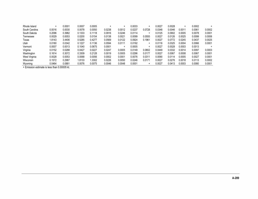
A-289
Rhode Island + 0.0001 0.0007 0.0005 + + 0.0033 + 0.0027 0.0028 + 0.0002 +
South Carolina 0.0016 0.0030 0.0078 0.0050 0.0238 0.0012 0.0237 0.0728 0.0348 0.0046 0.0011 0.0061 0.0002
South Dakota 0.2096 0.3982 0.1333 0.1118 0.0916 0.0246 0.0114 + 0.0125 0.0902 0.0005 0.0078 0.0001
Tennessee 0.0029 0.0053 0.0200 0.0154 0.0138 0.0021 0.0099 0.0555 0.0027 0.0126 0.0025 0.0099 0.0006
Texas 1.8143 3.4406 0.5285 0.4277 0.0569 0.0122 0.0924 0.1961 0.0027 0.0772 0.0245 0.0437 0.0025
Utah 0.0180 0.0342 0.1227 0.1136 0.0594 0.0111 0.0192 + 0.0116 0.0325 0.0004 0.0066 0.0001
Vermont 0.0007 0.0013 0.1040 0.0675 0.0001 + 0.0005 + 0.0027 0.0028 0.0003 0.0013 +
Virginia 0.0152 0.0288 0.0427 0.0227 0.0247 0.0005 0.0149 0.0802 0.0449 0.0332 0.0014 0.0097 0.0003
Washington 0.1614 0.3072 0.3309 0.2128 0.0019 0.0005 0.0296 0.0177 0.0027 0.0067 0.0008 0.0067 0.0001
West Virginia 0.0028 0.0053 0.0068 0.0056 0.0002 0.0001 0.0076 0.0311 0.0090 0.0114 0.0005 0.0027 0.0001
Wisconsin 0.1572 0.2987 1.8133 1.3302 0.0226 0.0050 0.0246 0.0171 0.0027 0.0276 0.0018 0.0113 0.0002
Wyoming 0.0464 0.0881 0.0076 0.0075 0.0046 0.0048 0.0001 + 0.0027 0.0413 0.0003 0.0080 0.0001
+ Emission estimate is less than 0.00005 kt.
A-290 Inventory of U.S. Greenhouse Gas Emissions and Sinks: 1990-2013
3.12. Methodology for Estimating N2O Emissions and Soil Organic C Stock Changes from Agricultural Soil Management (Cropland and Grassland)
Nitrous oxide (N2O) is produced in soils through the microbial processes of nitrification and denitrification1 Management influences these processes by modifying the availability of mineral nitrogen (N), which is a key control on the N2O emissions rates (Mosier et al. 1998). Emissions can occur directly in the soil where the N is made available or can be transported to another location following volatilization, leaching, or runoff, and then converted into N2O. Management practices influence soil organic C stocks in agricultural soils by modifying the natural processes of photosynthesis (i.e., crop and forage production) and microbial decomposition. This sub-annex describes the methodologies used to calculate N2O emissions from agricultural soil management and annual carbon (C) stock changes from mineral and organic soils classified as Cropland Remaining Cropland, Land Converted to Cropland, Grassland Remaining Grassland, and Land Converted to Grassland.2 This annex provides the underlying methodologies for both N2O emissions from agricultural soil management and soil organic C stock change from mineral and organic soils. There is considerable overlap in the methods and data sets used for these source categories, and the majority of emission are estimated with the same inventory analysis using the DAYCENT biogeochemical
3 simulation model.
A combination of Tier 1, 2 and 3 approaches is used to estimate direct and indirect N2O emissions and C stock
changes in agricultural soils.
More specifically, the methodologies used to estimate soil N2O emissions include: 1) A Tier 3 method using the DAYCENT biogeochemical simulation model to estimate direct emissions from mineral
soils that have less than 35 percent coarse fragments by volume and are used to produce alfalfa hay, barley, corn, cotton, dry beans, grass hay, grass-clover hay, oats, onions, peanuts, potatoes, rice, sorghum, soybeans, sugar beets, sunflowers, tomatoes, and wheat, as well as non-federal grasslands and land use change between grassland and cropland (with the crops listed above and less than 35 percent coarse fragments);
2) A combination of the Tier 3 and 1 methods to estimate indirect N2O emissions associated with management of cropland and grassland simulated with DAYCENT in Item 1;
3) A Tier 1 method to estimate direct and indirect N2O emissions from mineral soils that are not simulated with DAYCENT, including very gravelly, cobbly, or shaley soils (greater than 35 percent coarse fragments by volume); mineral soils with less than 35 percent coarse fragments that are used to produce crops that are not simulated by DAYCENT; crops that are rotated with the crops that are not simulated with DAYCENT; and Pasture/Range/Paddock (PRP) manure N deposited on federal grasslands; and
4) A Tier 1 method to estimate direct N2O emissions due to partial or complete drainage of organic soils in croplands and grasslands.
The methodologies used to estimate soil organic C stock changes include: 1) A Tier 3 method using the DAYCENT biogeochemical simulation model to estimate soil organic C stock changes
in mineral soils as described in Item 1 for N2O emissions; 2) Tier 2 methods with country-specific stock change factors for estimating mineral soil organic C stock changes for
mineral soils that are very gravelly, cobbly, or shaley (greater than 35 percent coarse fragments by volume) and are used to produce crops or have land use changes to cropland and grassland (other than the conversions between cropland and grassland that are included in Item 1) that are not simulated with DAYCENT;
3) Tier 2 methods with country-specific emission factors for estimating losses of C from organic soils that are partly or completely drained for agricultural production; and
4) Tier 2 methods for estimating additional changes in mineral soil C stocks due to sewage sludge additions to soils and enrollment changes in the Conservation Reserve Program (CRP) after 2007.
1 Nitrification and denitrification are driven by the activity of microorganisms in soils. Nitrification is the aerobic microbial
oxidation of ammonium (NH4+) to nitrate (NO3-), and denitrification is the anaerobic microbial reduction of nitrate to N2. Nitrous oxide is a gaseous intermediate product in the reaction sequence of denitrification, which leaks from microbial cells into the soil and then into the atmosphere. Nitrous oxide is also produced during nitrification, although by a less well-understood mechanism (Nevison 2000). 2 Soil C stock change methods for forestland are described in the Forestland Remaining Forestland section.
3 Biogeochemical cycles are the flow of chemical elements and compounds between living organisms and the physical
environment.
A-291
As described above, the Inventory uses a Tier 3 approach to estimate direct soil N2O emissions and C stock changes for the majority of agricultural lands. This approach has the following advantages over the IPCC Tier 1 or 2 approaches:
1) It utilizes actual weather data at sub-county scales enabling quantification of inter-annual variability in N2O emissions and C stock changes at finer spatial scales, as opposed to a single emission factor for the entire country for soil N2O or broad climate region classification for soil C stock changes;
2) The model uses a more detailed characterization of spatially-mapped soil properties that influence soil C and N dynamics, as opposed to the broad soil taxonomic classifications of the IPCC methodology;
3) The simulation approach provides a more detailed representation of management influences and their interactions than are represented by a discrete factor-based approach in the Tier 1 and 2 methods; and
4) Soil N2O emissions and C stock changes are estimated on a more continuous, daily basis as a function of the interaction of climate, soil, and land management, compared with the linear rate changes that are estimated with the Tier 1 and 2 methods.
The DAYCENT process-based simulation model (daily time-step version of the Century model) has been selected for the Tier 3 approach based on the following criteria:
1) The model has been developed in the United States and extensively tested and verified for U.S. conditions (e.g., Parton et al. 1987, 1993). In addition, the model has been widely used by researchers and agencies in many other parts of the world for simulating soil C dynamics at local, regional and national scales (e.g., Brazil, Canada, India, Jordan, Kenya, Mexico), and soil N2O emissions (e.g., Canada, China, Ireland, New Zealand) (Abdalla et al. 2010, Li et al. 2005, Smith et al. 2008, Stehfest and Muller 2004).
2) The model is capable of simulating cropland, grassland, forest, and savanna ecosystems, and land-use transitions between these different land uses. It is, thus, well suited to model land-use change effects.
3) The model is designed to simulate management practices that influence soil C dynamics and direct N2O emissions, with the exception of cultivated organic soils; cobbly, gravelly, or shaley soils; and crops that have not been parameterized for DAYCENT simulations (e.g., some vegetables, tobacco, perennial/horticultural crops, and crops that are rotated with these crops). For these latter cases, an IPCC Tier 2 method has been used for soil C stock changes and IPCC Tier 1 method for N2O emissions. The model can also be used estimate the amount of N leaching and runoff, as well as volatilization of N, which is subject to indirect N2O emissions.
4) Much of the data needed for the model is available from existing national databases. The exceptions are CRP enrollment after 2007, management of federal grasslands, and sewage sludge amendments to soils, which are not known at a sufficient resolution to use the Tier 3 model. Soil N2O emissions and C stock changes associated with these practices are addressed with a Tier 1 and 2 method, respectively.
Overall, the Tier 3 approach is used to estimate approximately 82 to 88 percent of direct soil N2O emissions and
85 to 87 percent of the land area associated with estimation of soil organic C stock changes under agricultural management in the United States.
Tier 3 Method Description and Model Evaluation
The DAYCENT biogeochemical model (Parton et al. 1998; Del Grosso et al. 2001, 2011) simulates biogeochemical C and N fluxes between the atmosphere, vegetation, and soil; and provides a more complete estimation of soil C stock changes and N2O emissions than IPCC Tier 1 or 2 methods by more thoroughly accounting for the influence of environmental conditions. These conditions include soil characteristics, weather patterns, crop and forage characteristics, and management practices. The DAYCENT model utilizes the soil C modeling framework developed in the Century model (Parton et al. 1987, 1988, 1994; Metherell et al. 1993), but has been refined to simulate dynamics at a daily time-step. Carbon and N dynamics are linked in plant-soil systems through biogeochemical processes of microbial decomposition and plant production (McGill and Cole 1981). Coupling the two source categories (i.e., agricultural soil C and N2O) in a single inventory analysis ensures that there is a consistent treatment of the processes and interactions between C and N cycling in soils. For example, plant growth is controlled by nutrient availability, water, and temperature stress. Plant growth, along with residue management, determines C inputs to soils, which influence C stock changes, and removal of mineral N from the soil where plant growth influences the amount of N that can be converted into N2O. Nutrient supply is a function of external nutrient additions as well as litter and soil organic matter (SOM) decomposition rates, and increasing decomposition can lead to a reduction in soil organic C stocks due to microbial respiration, and greater N2O emissions by enhancing mineral N availability in soils.
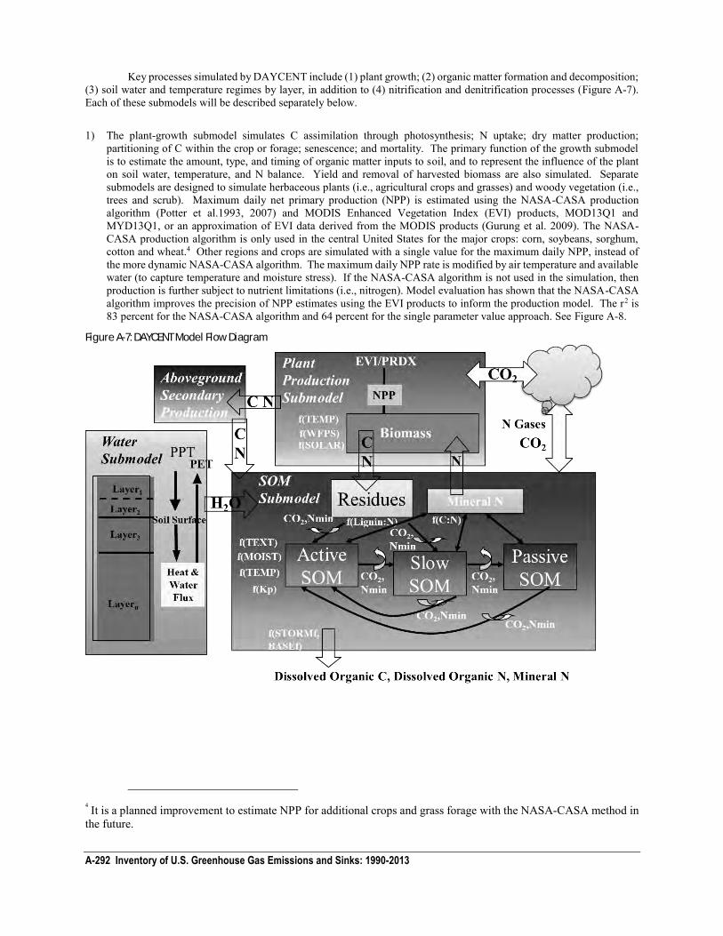
A-292 Inventory of U.S. Greenhouse Gas Emissions and Sinks: 1990-2013
Key processes simulated by DAYCENT include (1) plant growth; (2) organic matter formation and decomposition; (3) soil water and temperature regimes by layer, in addition to (4) nitrification and denitrification processes (Figure A-7). Each of these submodels will be described separately below.
1) The plant-growth submodel simulates C assimilation through photosynthesis; N uptake; dry matter production;
partitioning of C within the crop or forage; senescence; and mortality. The primary function of the growth submodel is to estimate the amount, type, and timing of organic matter inputs to soil, and to represent the influence of the plant on soil water, temperature, and N balance. Yield and removal of harvested biomass are also simulated. Separate submodels are designed to simulate herbaceous plants (i.e., agricultural crops and grasses) and woody vegetation (i.e., trees and scrub). Maximum daily net primary production (NPP) is estimated using the NASA-CASA production algorithm (Potter et al.1993, 2007) and MODIS Enhanced Vegetation Index (EVI) products, MOD13Q1 and MYD13Q1, or an approximation of EVI data derived from the MODIS products (Gurung et al. 2009). The NASA-CASA production algorithm is only used in the central United States for the major crops: corn, soybeans, sorghum, cotton and wheat.4 Other regions and crops are simulated with a single value for the maximum daily NPP, instead of the more dynamic NASA-CASA algorithm. The maximum daily NPP rate is modified by air temperature and available water (to capture temperature and moisture stress). If the NASA-CASA algorithm is not used in the simulation, then production is further subject to nutrient limitations (i.e., nitrogen). Model evaluation has shown that the NASA-CASA algorithm improves the precision of NPP estimates using the EVI products to inform the production model. The r2 is 83 percent for the NASA-CASA algorithm and 64 percent for the single parameter value approach. See Figure A-8.
Figure A-7: DAYCENT Model Flow Diagram
4 It is a planned improvement to estimate NPP for additional crops and grass forage with the NASA-CASA method in the future.
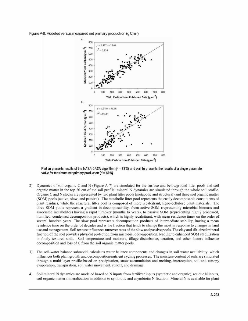
A-293
Figure A-8: Modeled versus measured net primary production (g C m-2)
2) Dynamics of soil organic C and N (Figure A-7) are simulated for the surface and belowground litter pools and soil
organic matter in the top 20 cm of the soil profile; mineral N dynamics are simulated through the whole soil profile. Organic C and N stocks are represented by two plant litter pools (metabolic and structural) and three soil organic matter (SOM) pools (active, slow, and passive). The metabolic litter pool represents the easily decomposable constituents of plant residues, while the structural litter pool is composed of more recalcitrant, ligno-cellulose plant materials. The three SOM pools represent a gradient in decomposability, from active SOM (representing microbial biomass and associated metabolites) having a rapid turnover (months to years), to passive SOM (representing highly processed, humified, condensed decomposition products), which is highly recalcitrant, with mean residence times on the order of several hundred years. The slow pool represents decomposition products of intermediate stability, having a mean residence time on the order of decades and is the fraction that tends to change the most in response to changes in land use and management. Soil texture influences turnover rates of the slow and passive pools. The clay and silt-sized mineral fraction of the soil provides physical protection from microbial decomposition, leading to enhanced SOM stabilization in finely textured soils. Soil temperature and moisture, tillage disturbance, aeration, and other factors influence decomposition and loss of C from the soil organic matter pools.
3) The soil-water balance submodel calculates water balance components and changes in soil water availability, which influences both plant growth and decomposition/nutrient cycling processes. The moisture content of soils are simulated through a multi-layer profile based on precipitation, snow accumulation and melting, interception, soil and canopy evaporation, transpiration, soil water movement, runoff, and drainage.
4) Soil mineral N dynamics are modeled based on N inputs from fertilizer inputs (synthetic and organic), residue N inputs,
soil organic matter mineralization in addition to symbiotic and asymbiotic N fixation. Mineral N is available for plant
A-294 Inventory of U.S. Greenhouse Gas Emissions and Sinks: 1990-2013
and microbial uptake, and is largely controlled by the specified stoichiometric limits for these organisms (i.e., C:N ratios). Mineral and organic N losses are simulated with leaching and runoff, and nitrogen can be volatilized and lost from the soil through ammonia volatilization, nitrification and denitrification. N2O emissions occur through nitrification and denitrification. Denitrification is a function of soil NO3
- concentration, water filled pore space (WFPS), heterotrophic (i.e., microbial) respiration, and texture. Nitrification is controlled by soil ammonium (NH4
+) concentration, water filled pore space, temperature, and pH (See Box 2 for more information).
The model allows for a variety of management options to be simulated, including specifying different crop types,
crop sequences (e.g., rotation), tillage practices, fertilization, organic matter addition (e.g., manure amendments), harvest events (with variable residue removal), drainage, irrigation, burning, and grazing intensity. An input “schedule” file is used to simulate the timing of management activities and temporal trends; schedules can be organized into discrete time blocks to define a repeated sequence of events (e.g., a crop rotation or a frequency of disturbance such as a burning cycle for perennial grassland). Management options can be specified for any day of a year within a scheduling block, where management codes point to operation-specific parameter files (referred to as *.100 files), which contain the information used to simulate management effects with the model algorithms. User-specified management activities can be defined by adding to or editing the contents of the *.100 files. Additional details of the model formulation are given in Parton et al. (1987, 1988, 1994, 1998), Del Grosso et al. (2001, 2011) and Metherell et al. (1993), and archived copies of the model source code are available.
[BEGIN TEXT BOX] Box 2. DAYCENT Model Simulation of Nitrification and Denitrification
The DAYCENT model simulates the two biogeochemical processes, nitrification and denitrification, that result in N2O emissions from soils (Del Grosso et al. 2000, Parton et al. 2001). Nitrification is calculated for the top 15 cm of soil (where nitrification mostly occurs) while denitrification is calculated for the entire soil profile (accounting for denitrification near the surface and subsurface as nitrate leaches through the profile). The equations and key parameters controlling N2O emissions from nitrification and denitrification are described below.
Nitrification is controlled by soil ammonium (NH4
+) concentration, temperature (t), Water Filled Pore Space (WFPS) and pH according to the following equation:
Nit = NH4+ × Kmax × F(t) × F(WFPS) × F(pH)
where, Nit = the soil nitrification rate (g N/m2/day) NH4+ = the model-derived soil ammonium concentration (g N/m2) Kmax = the maximum fraction of NH4
+ nitrified (Kmax = 0.10/day) F(t) = the effect of soil temperature on nitrification (Figure A-9a) F(WFPS) = the effect of soil water content and soil texture on nitrification (Figure A-9b) F(pH) = the effect of soil pH on nitrification (Figure A-9c)
The current parameterization used in the model assumes that 1.2 percent of nitrified N is converted to N2O.
The model assumes that denitrification rates are controlled by the availability of soil NO3- (electron acceptor),
labile C compounds (electron donor) and oxygen (competing electron acceptor). Heterotrophic soil respiration is used as a proxy for labile C availability, while oxygen availability is a function of soil physical properties that influence gas diffusivity, soil WFPS, and oxygen demand. The model selects the minimum of the NO3
- and CO2 functions to establish a maximum potential denitrification rate. These rates vary for particular levels of electron acceptor and C substrate, and account for limitations of oxygen availability to estimate daily denitrification rates according to the following equation:
Den = min[F(CO2), F(NO3)] × F(WFPS)
where, Den = the soil denitrification rate (g N/g soil/day) F(CO2) = a function relating N gas flux to soil respiration (Figure A-10a) F(NO3) = a function relating N gas flux to nitrate levels (Figure A-10b) F(WFPS) = a dimensionless multiplier (Figure A-10c).
A-295
The x inflection point of F(WFPS) is a function of respiration and soil gas diffusivity at field capacity (DFC):
x inflection = 0.90 - M(CO2) where, M = a multiplier that is a function of DFC. In technical terms, the inflection point is the domain
where either F(WFPS) is not differentiable or its derivative is 0. In this case, the inflection point can be interpreted as the WFPS value at which denitrification reaches half of its maximum rate.
Respiration has a much stronger effect on the water curve in clay soils with low DFC than in loam or sandy soils
with high DFC (Figure A-10). The model assumes that microsites in fine-textured soils can become anaerobic at relatively low water contents when oxygen demand is high. After calculating total N gas flux, the ratio of N2/N2O is estimated so that total N gas emissions can be partitioned between N2O and N2:
RN2/N2O = Fr(NO3/CO2) × Fr(WFPS). where, RN2/N2O = the ratio of N2/N2O Fr(NO3/CO2) = a function estimating the impact of the availability of electron donor relative to substrate Fr(WFPS) = a multiplier to account for the effect of soil water on N2:N2O. For Fr(NO3/CO2), as the ratio of electron donor to substrate increases, a higher portion of N gas is assumed to be in the form of N2O. For Fr(WFPS), as WFPS increases, a higher portion of N gas is assumed to be in the form of N2. [End Box]
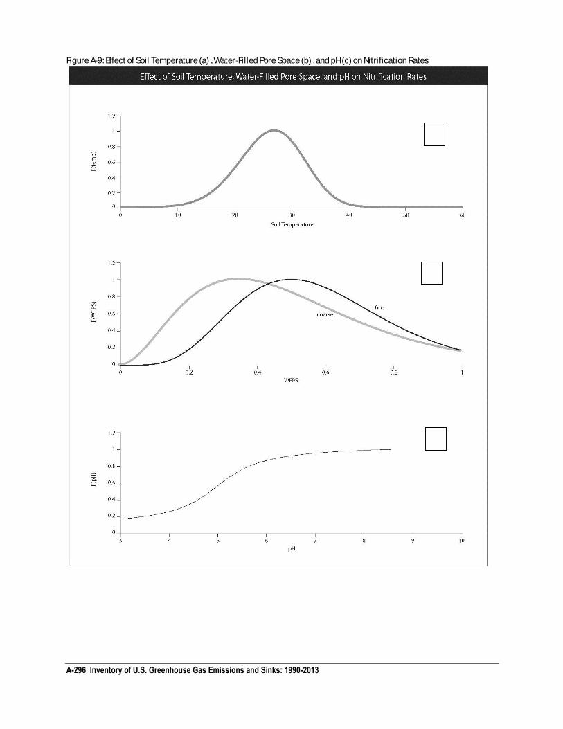
A-296 Inventory of U.S. Greenhouse Gas Emissions and Sinks: 1990-2013
Figure A-9: Effect of Soil Temperature (a) , Water-Filled Pore Space (b) , and pH (c) on Nitrification Rates
A
B
C
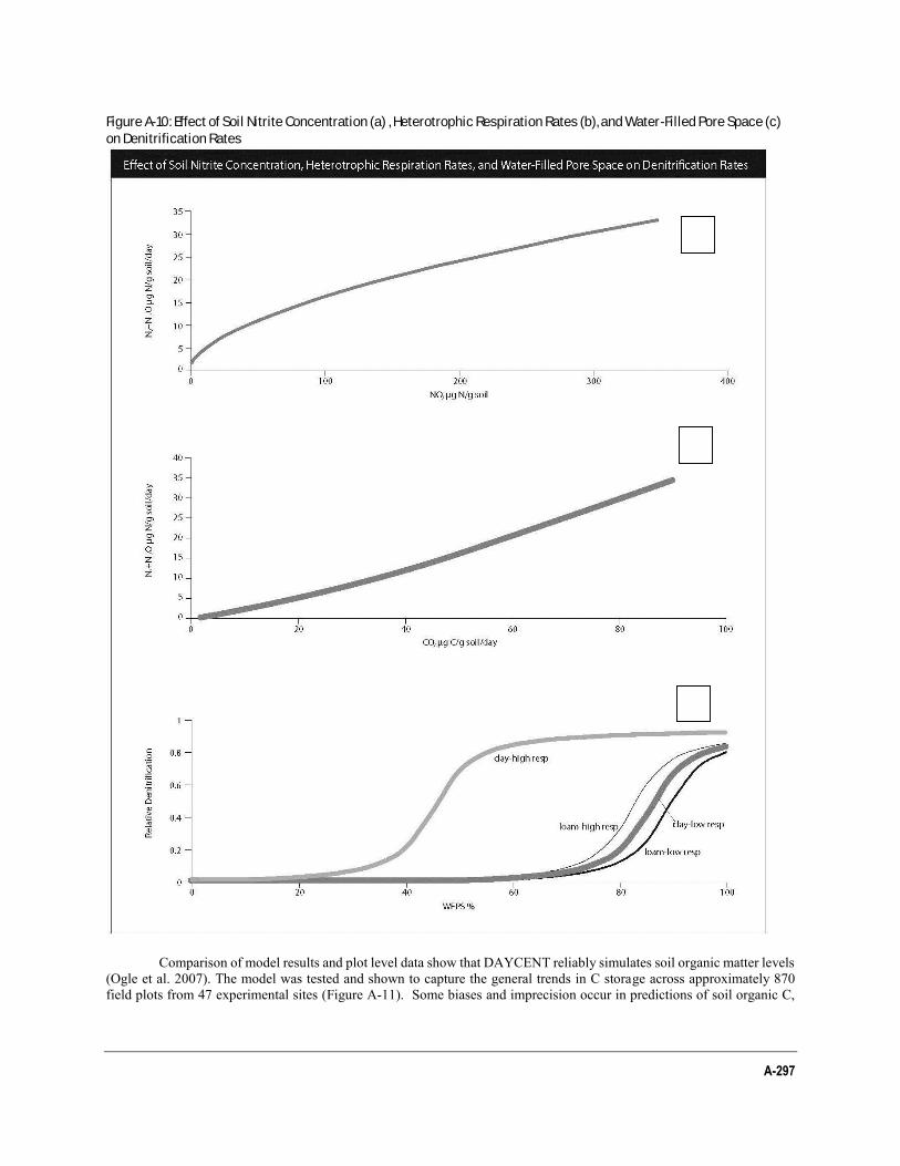
A-297
Figure A-10: Effect of Soil Nitrite Concentration (a) , Heterotrophic Respiration Rates (b), and Water-Filled Pore Space (c)
on Denitrification Rates
Comparison of model results and plot level data show that DAYCENT reliably simulates soil organic matter levels (Ogle et al. 2007). The model was tested and shown to capture the general trends in C storage across approximately 870 field plots from 47 experimental sites (Figure A-11). Some biases and imprecision occur in predictions of soil organic C,
A
B
C
A-298 Inventory of U.S. Greenhouse Gas Emissions and Sinks: 1990-2013
which is reflected in the uncertainty associated with DAYCENT model results. Regardless, the Tier 3 approach has considerably less uncertainty than Tier 1 and 2 methods (Del Grosso et al., 2010; Figure A-11).
Similarly, DAYCENT model results have been compared to trace gas N2O fluxes for a number of native and managed systems (Del Grosso et al. 2001, 2005, 2010) (Figure A-12). In general, the model simulates accurate emissions, but some bias and imprecision does occur in predictions, which is reflected in the uncertainty associated with DAYCENT model results. Comparisons with measured data showed that DAYCENT estimated N2O emissions more accurately and precisely than the IPCC Tier 1 methodology (IPCC 2006) (See Figure 5-7: Comparison of Measured Emissions at Field Sites and Modeled Emissions Using the DAYCENT Simulation Model and IPCC Tier 1 Approach in the main chapter text). The linear regression of simulated vs. measured emissions for DAYCENT had higher r2 values and a fitted line closer to a perfect 1:1 relationship between measured and modeled N2O emissions compared to the IPCC Tier 1 approach (Del Grosso et al. 2005, 2008). This is not surprising, since DAYCENT includes site-specific factors (climate, soil properties, and previous management) that influence N2O emissions. Furthermore, DAYCENT also simulated NO3- leaching (root mean square error = 20 percent) more accurately than IPCC Tier 1 methodology (root mean square error = 69 percent) (Del Grosso et al. 2005). Volatilization of N gases that contribute to indirect soil N2O emissions is the only component that has not been thoroughly tested, which is due to a lack of measurement data. Overall, the Tier 3 approach has reduced uncertainties in the agricultural soil C stock changes and N2O emissions compared to using lower Tier methods.
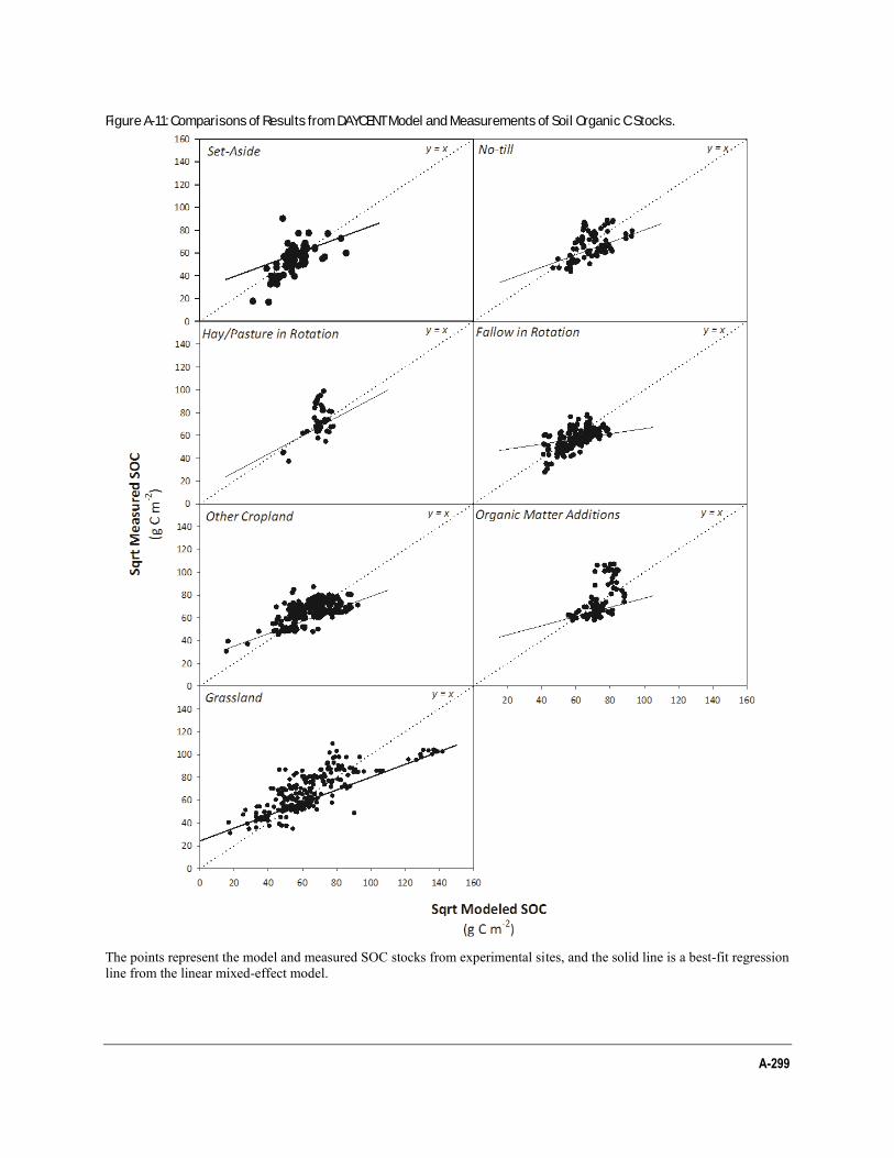
A-299
Figure A-11: Comparisons of Results from DAYCENT Model and Measurements of Soil Organic C Stocks.
The points represent the model and measured SOC stocks from experimental sites, and the solid line is a best-fit regression line from the linear mixed-effect model.
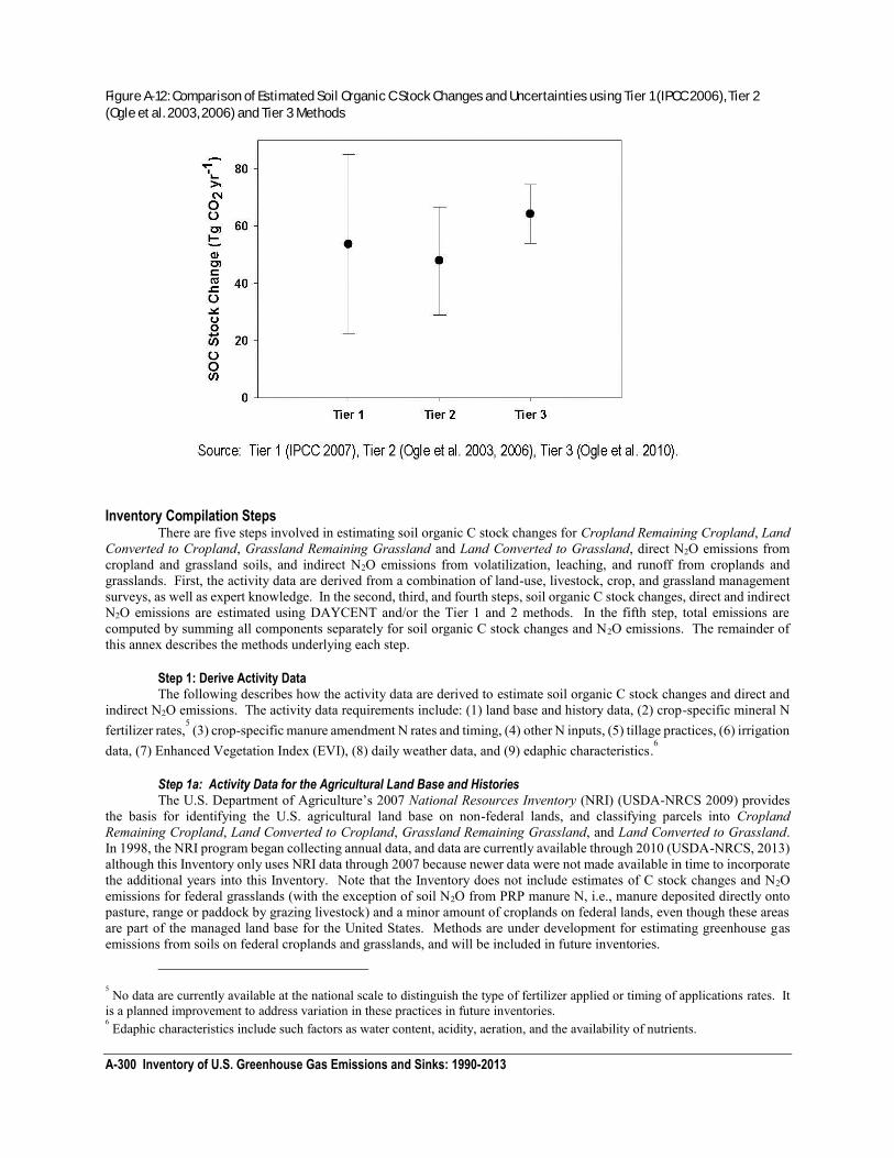
A-300 Inventory of U.S. Greenhouse Gas Emissions and Sinks: 1990-2013
Figure A-12: Comparison of Estimated Soil Organic C Stock Changes and Uncertainties using Tier 1 (IPCC 2006), Tier 2
(Ogle et al. 2003, 2006) and Tier 3 Methods
Inventory Compilation Steps
There are five steps involved in estimating soil organic C stock changes for Cropland Remaining Cropland, Land Converted to Cropland, Grassland Remaining Grassland and Land Converted to Grassland, direct N2O emissions from cropland and grassland soils, and indirect N2O emissions from volatilization, leaching, and runoff from croplands and grasslands. First, the activity data are derived from a combination of land-use, livestock, crop, and grassland management surveys, as well as expert knowledge. In the second, third, and fourth steps, soil organic C stock changes, direct and indirect N2O emissions are estimated using DAYCENT and/or the Tier 1 and 2 methods. In the fifth step, total emissions are computed by summing all components separately for soil organic C stock changes and N2O emissions. The remainder of this annex describes the methods underlying each step.
Step 1: Derive Activity Data The following describes how the activity data are derived to estimate soil organic C stock changes and direct and
indirect N2O emissions. The activity data requirements include: (1) land base and history data, (2) crop-specific mineral N fertilizer rates,
5 (3) crop-specific manure amendment N rates and timing, (4) other N inputs, (5) tillage practices, (6) irrigation
data, (7) Enhanced Vegetation Index (EVI), (8) daily weather data, and (9) edaphic characteristics.6
Step 1a: Activity Data for the Agricultural Land Base and Histories The U.S. Department of Agriculture’s 2007 National Resources Inventory (NRI) (USDA-NRCS 2009) provides
the basis for identifying the U.S. agricultural land base on non-federal lands, and classifying parcels into Cropland Remaining Cropland, Land Converted to Cropland, Grassland Remaining Grassland, and Land Converted to Grassland. In 1998, the NRI program began collecting annual data, and data are currently available through 2010 (USDA-NRCS, 2013) although this Inventory only uses NRI data through 2007 because newer data were not made available in time to incorporate the additional years into this Inventory. Note that the Inventory does not include estimates of C stock changes and N2O emissions for federal grasslands (with the exception of soil N2O from PRP manure N, i.e., manure deposited directly onto pasture, range or paddock by grazing livestock) and a minor amount of croplands on federal lands, even though these areas are part of the managed land base for the United States. Methods are under development for estimating greenhouse gas emissions from soils on federal croplands and grasslands, and will be included in future inventories.
5 No data are currently available at the national scale to distinguish the type of fertilizer applied or timing of applications rates. It
is a planned improvement to address variation in these practices in future inventories. 6 Edaphic characteristics include such factors as water content, acidity, aeration, and the availability of nutrients.
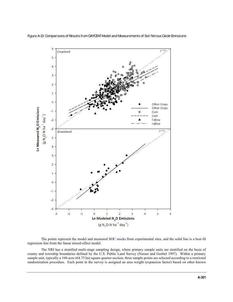
A-301
Figure A-13: Comparisons of Results from DAYCENT Model and Measurements of Soil Nitrous Oxide Emissions
The points represent the model and measured SOC stocks from experimental sites, and the solid line is a best-fit regression line from the linear mixed-effect model.
The NRI has a stratified multi-stage sampling design, where primary sample units are stratified on the basis of county and township boundaries defined by the U.S. Public Land Survey (Nusser and Goebel 1997). Within a primary sample unit, typically a 160-acre (64.75 ha) square quarter-section, three sample points are selected according to a restricted randomization procedure. Each point in the survey is assigned an area weight (expansion factor) based on other known
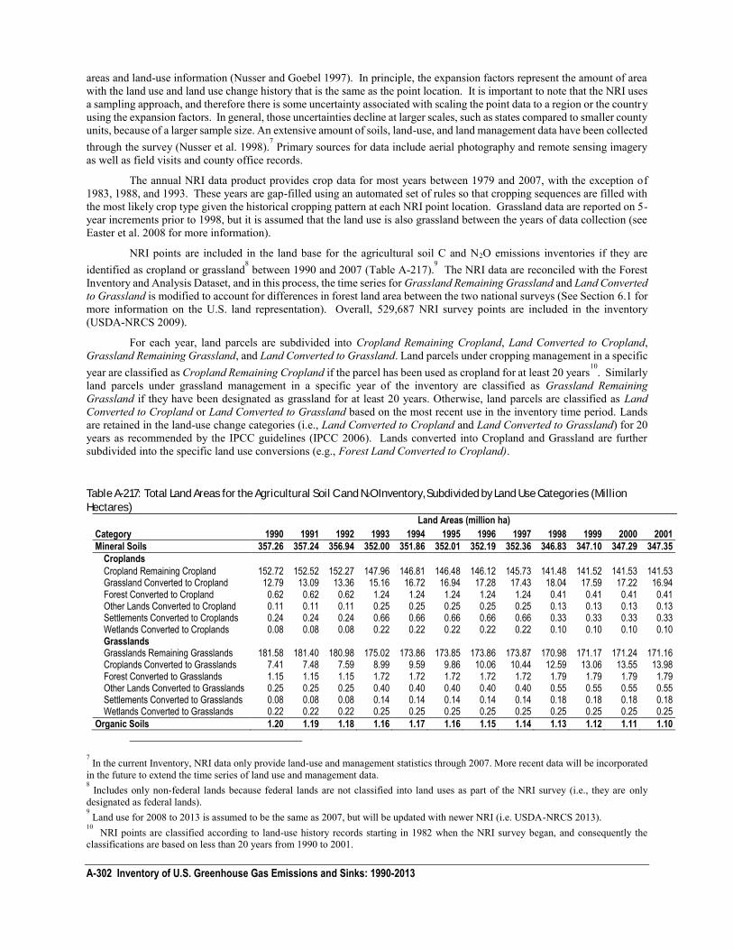
A-302 Inventory of U.S. Greenhouse Gas Emissions and Sinks: 1990-2013
areas and land-use information (Nusser and Goebel 1997). In principle, the expansion factors represent the amount of area with the land use and land use change history that is the same as the point location. It is important to note that the NRI uses a sampling approach, and therefore there is some uncertainty associated with scaling the point data to a region or the country using the expansion factors. In general, those uncertainties decline at larger scales, such as states compared to smaller county units, because of a larger sample size. An extensive amount of soils, land-use, and land management data have been collected through the survey (Nusser et al. 1998).
7 Primary sources for data include aerial photography and remote sensing imagery
as well as field visits and county office records.
The annual NRI data product provides crop data for most years between 1979 and 2007, with the exception of 1983, 1988, and 1993. These years are gap-filled using an automated set of rules so that cropping sequences are filled with the most likely crop type given the historical cropping pattern at each NRI point location. Grassland data are reported on 5-year increments prior to 1998, but it is assumed that the land use is also grassland between the years of data collection (see Easter et al. 2008 for more information).
NRI points are included in the land base for the agricultural soil C and N2O emissions inventories if they are identified as cropland or grassland
8 between 1990 and 2007 (Table A-217).
9 The NRI data are reconciled with the Forest
Inventory and Analysis Dataset, and in this process, the time series for Grassland Remaining Grassland and Land Converted to Grassland is modified to account for differences in forest land area between the two national surveys (See Section 6.1 for more information on the U.S. land representation). Overall, 529,687 NRI survey points are included in the inventory (USDA-NRCS 2009).
For each year, land parcels are subdivided into Cropland Remaining Cropland, Land Converted to Cropland, Grassland Remaining Grassland, and Land Converted to Grassland. Land parcels under cropping management in a specific year are classified as Cropland Remaining Cropland if the parcel has been used as cropland for at least 20 years
10. Similarly
land parcels under grassland management in a specific year of the inventory are classified as Grassland Remaining Grassland if they have been designated as grassland for at least 20 years. Otherwise, land parcels are classified as Land Converted to Cropland or Land Converted to Grassland based on the most recent use in the inventory time period. Lands are retained in the land-use change categories (i.e., Land Converted to Cropland and Land Converted to Grassland) for 20 years as recommended by the IPCC guidelines (IPCC 2006). Lands converted into Cropland and Grassland are further subdivided into the specific land use conversions (e.g., Forest Land Converted to Cropland).
Table A-217: Total Land Areas for the Agricultural Soil C and N2O Inventory, Subdivided by Land Use Categories (Million
Hectares)
Land Areas (million ha)
Category 1990 1991 1992 1993 1994 1995 1996 1997 1998 1999 2000 2001
Mineral Soils 357.26 357.24 356.94 352.00 351.86 352.01 352.19 352.36 346.83 347.10 347.29 347.35
Croplands
Cropland Remaining Cropland 152.72 152.52 152.27 147.96 146.81 146.48 146.12 145.73 141.48 141.52 141.53 141.53 Grassland Converted to Cropland 12.79 13.09 13.36 15.16 16.72 16.94 17.28 17.43 18.04 17.59 17.22 16.94 Forest Converted to Cropland 0.62 0.62 0.62 1.24 1.24 1.24 1.24 1.24 0.41 0.41 0.41 0.41 Other Lands Converted to Cropland 0.11 0.11 0.11 0.25 0.25 0.25 0.25 0.25 0.13 0.13 0.13 0.13 Settlements Converted to Croplands 0.24 0.24 0.24 0.66 0.66 0.66 0.66 0.66 0.33 0.33 0.33 0.33 Wetlands Converted to Croplands 0.08 0.08 0.08 0.22 0.22 0.22 0.22 0.22 0.10 0.10 0.10 0.10 Grasslands Grasslands Remaining Grasslands 181.58 181.40 180.98 175.02 173.86 173.85 173.86 173.87 170.98 171.17 171.24 171.16 Croplands Converted to Grasslands 7.41 7.48 7.59 8.99 9.59 9.86 10.06 10.44 12.59 13.06 13.55 13.98 Forest Converted to Grasslands 1.15 1.15 1.15 1.72 1.72 1.72 1.72 1.72 1.79 1.79 1.79 1.79 Other Lands Converted to Grasslands 0.25 0.25 0.25 0.40 0.40 0.40 0.40 0.40 0.55 0.55 0.55 0.55 Settlements Converted to Grasslands 0.08 0.08 0.08 0.14 0.14 0.14 0.14 0.14 0.18 0.18 0.18 0.18 Wetlands Converted to Grasslands 0.22 0.22 0.22 0.25 0.25 0.25 0.25 0.25 0.25 0.25 0.25 0.25
Organic Soils 1.20 1.19 1.18 1.16 1.17 1.16 1.15 1.14 1.13 1.12 1.11 1.10
7 In the current Inventory, NRI data only provide land-use and management statistics through 2007. More recent data will be incorporated
in the future to extend the time series of land use and management data. 8 Includes only non-federal lands because federal lands are not classified into land uses as part of the NRI survey (i.e., they are only
designated as federal lands). 9 Land use for 2008 to 2013 is assumed to be the same as 2007, but will be updated with newer NRI (i.e. USDA-NRCS 2013).
10 NRI points are classified according to land-use history records starting in 1982 when the NRI survey began, and consequently the
classifications are based on less than 20 years from 1990 to 2001.
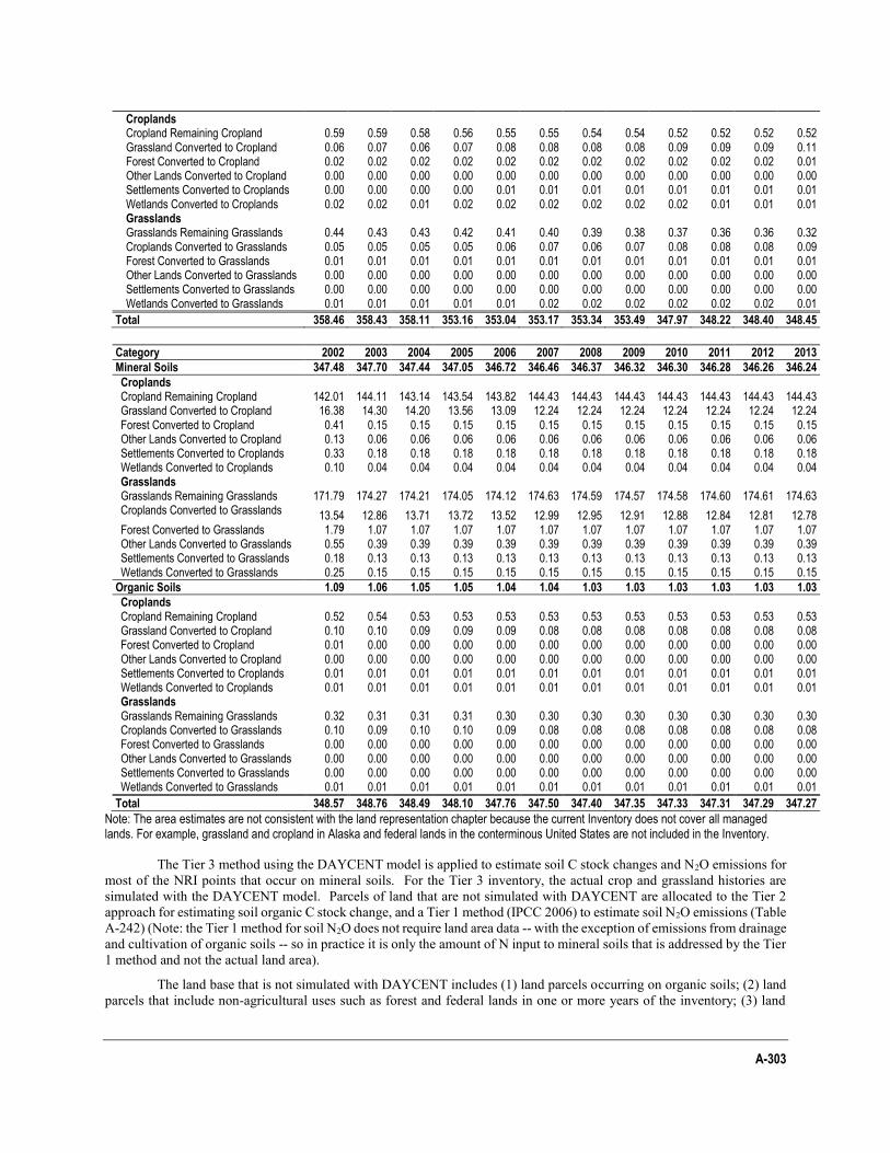
A-303
Croplands Cropland Remaining Cropland 0.59 0.59 0.58 0.56 0.55 0.55 0.54 0.54 0.52 0.52 0.52 0.52 Grassland Converted to Cropland 0.06 0.07 0.06 0.07 0.08 0.08 0.08 0.08 0.09 0.09 0.09 0.11 Forest Converted to Cropland 0.02 0.02 0.02 0.02 0.02 0.02 0.02 0.02 0.02 0.02 0.02 0.01 Other Lands Converted to Cropland 0.00 0.00 0.00 0.00 0.00 0.00 0.00 0.00 0.00 0.00 0.00 0.00 Settlements Converted to Croplands 0.00 0.00 0.00 0.00 0.01 0.01 0.01 0.01 0.01 0.01 0.01 0.01 Wetlands Converted to Croplands 0.02 0.02 0.01 0.02 0.02 0.02 0.02 0.02 0.02 0.01 0.01 0.01 Grasslands Grasslands Remaining Grasslands 0.44 0.43 0.43 0.42 0.41 0.40 0.39 0.38 0.37 0.36 0.36 0.32 Croplands Converted to Grasslands 0.05 0.05 0.05 0.05 0.06 0.07 0.06 0.07 0.08 0.08 0.08 0.09 Forest Converted to Grasslands 0.01 0.01 0.01 0.01 0.01 0.01 0.01 0.01 0.01 0.01 0.01 0.01 Other Lands Converted to Grasslands 0.00 0.00 0.00 0.00 0.00 0.00 0.00 0.00 0.00 0.00 0.00 0.00 Settlements Converted to Grasslands 0.00 0.00 0.00 0.00 0.00 0.00 0.00 0.00 0.00 0.00 0.00 0.00 Wetlands Converted to Grasslands 0.01 0.01 0.01 0.01 0.01 0.02 0.02 0.02 0.02 0.02 0.02 0.01
Total 358.46 358.43 358.11 353.16 353.04 353.17 353.34 353.49 347.97 348.22 348.40 348.45
Category 2002 2003 2004 2005 2006 2007 2008 2009 2010 2011 2012 2013
Mineral Soils 347.48 347.70 347.44 347.05 346.72 346.46 346.37 346.32 346.30 346.28 346.26 346.24
Croplands Cropland Remaining Cropland 142.01 144.11 143.14 143.54 143.82 144.43 144.43 144.43 144.43 144.43 144.43 144.43 Grassland Converted to Cropland 16.38 14.30 14.20 13.56 13.09 12.24 12.24 12.24 12.24 12.24 12.24 12.24 Forest Converted to Cropland 0.41 0.15 0.15 0.15 0.15 0.15 0.15 0.15 0.15 0.15 0.15 0.15 Other Lands Converted to Cropland 0.13 0.06 0.06 0.06 0.06 0.06 0.06 0.06 0.06 0.06 0.06 0.06 Settlements Converted to Croplands 0.33 0.18 0.18 0.18 0.18 0.18 0.18 0.18 0.18 0.18 0.18 0.18 Wetlands Converted to Croplands 0.10 0.04 0.04 0.04 0.04 0.04 0.04 0.04 0.04 0.04 0.04 0.04 Grasslands Grasslands Remaining Grasslands 171.79 174.27 174.21 174.05 174.12 174.63 174.59 174.57 174.58 174.60 174.61 174.63 Croplands Converted to Grasslands 13.54 12.86 13.71 13.72 13.52 12.99 12.95 12.91 12.88 12.84 12.81 12.78 Forest Converted to Grasslands 1.79 1.07 1.07 1.07 1.07 1.07 1.07 1.07 1.07 1.07 1.07 1.07 Other Lands Converted to Grasslands 0.55 0.39 0.39 0.39 0.39 0.39 0.39 0.39 0.39 0.39 0.39 0.39 Settlements Converted to Grasslands 0.18 0.13 0.13 0.13 0.13 0.13 0.13 0.13 0.13 0.13 0.13 0.13 Wetlands Converted to Grasslands 0.25 0.15 0.15 0.15 0.15 0.15 0.15 0.15 0.15 0.15 0.15 0.15
Organic Soils 1.09 1.06 1.05 1.05 1.04 1.04 1.03 1.03 1.03 1.03 1.03 1.03
Croplands Cropland Remaining Cropland 0.52 0.54 0.53 0.53 0.53 0.53 0.53 0.53 0.53 0.53 0.53 0.53 Grassland Converted to Cropland 0.10 0.10 0.09 0.09 0.09 0.08 0.08 0.08 0.08 0.08 0.08 0.08 Forest Converted to Cropland 0.01 0.00 0.00 0.00 0.00 0.00 0.00 0.00 0.00 0.00 0.00 0.00 Other Lands Converted to Cropland 0.00 0.00 0.00 0.00 0.00 0.00 0.00 0.00 0.00 0.00 0.00 0.00 Settlements Converted to Croplands 0.01 0.01 0.01 0.01 0.01 0.01 0.01 0.01 0.01 0.01 0.01 0.01 Wetlands Converted to Croplands 0.01 0.01 0.01 0.01 0.01 0.01 0.01 0.01 0.01 0.01 0.01 0.01 Grasslands Grasslands Remaining Grasslands 0.32 0.31 0.31 0.31 0.30 0.30 0.30 0.30 0.30 0.30 0.30 0.30 Croplands Converted to Grasslands 0.10 0.09 0.10 0.10 0.09 0.08 0.08 0.08 0.08 0.08 0.08 0.08 Forest Converted to Grasslands 0.00 0.00 0.00 0.00 0.00 0.00 0.00 0.00 0.00 0.00 0.00 0.00 Other Lands Converted to Grasslands 0.00 0.00 0.00 0.00 0.00 0.00 0.00 0.00 0.00 0.00 0.00 0.00 Settlements Converted to Grasslands 0.00 0.00 0.00 0.00 0.00 0.00 0.00 0.00 0.00 0.00 0.00 0.00 Wetlands Converted to Grasslands 0.01 0.01 0.01 0.01 0.01 0.01 0.01 0.01 0.01 0.01 0.01 0.01
Total 348.57 348.76 348.49 348.10 347.76 347.50 347.40 347.35 347.33 347.31 347.29 347.27
Note: The area estimates are not consistent with the land representation chapter because the current Inventory does not cover all managed lands. For example, grassland and cropland in Alaska and federal lands in the conterminous United States are not included in the Inventory.
The Tier 3 method using the DAYCENT model is applied to estimate soil C stock changes and N2O emissions for most of the NRI points that occur on mineral soils. For the Tier 3 inventory, the actual crop and grassland histories are simulated with the DAYCENT model. Parcels of land that are not simulated with DAYCENT are allocated to the Tier 2 approach for estimating soil organic C stock change, and a Tier 1 method (IPCC 2006) to estimate soil N2O emissions (Table A-242) (Note: the Tier 1 method for soil N2O does not require land area data -- with the exception of emissions from drainage and cultivation of organic soils -- so in practice it is only the amount of N input to mineral soils that is addressed by the Tier 1 method and not the actual land area).
The land base that is not simulated with DAYCENT includes (1) land parcels occurring on organic soils; (2) land parcels that include non-agricultural uses such as forest and federal lands in one or more years of the inventory; (3) land
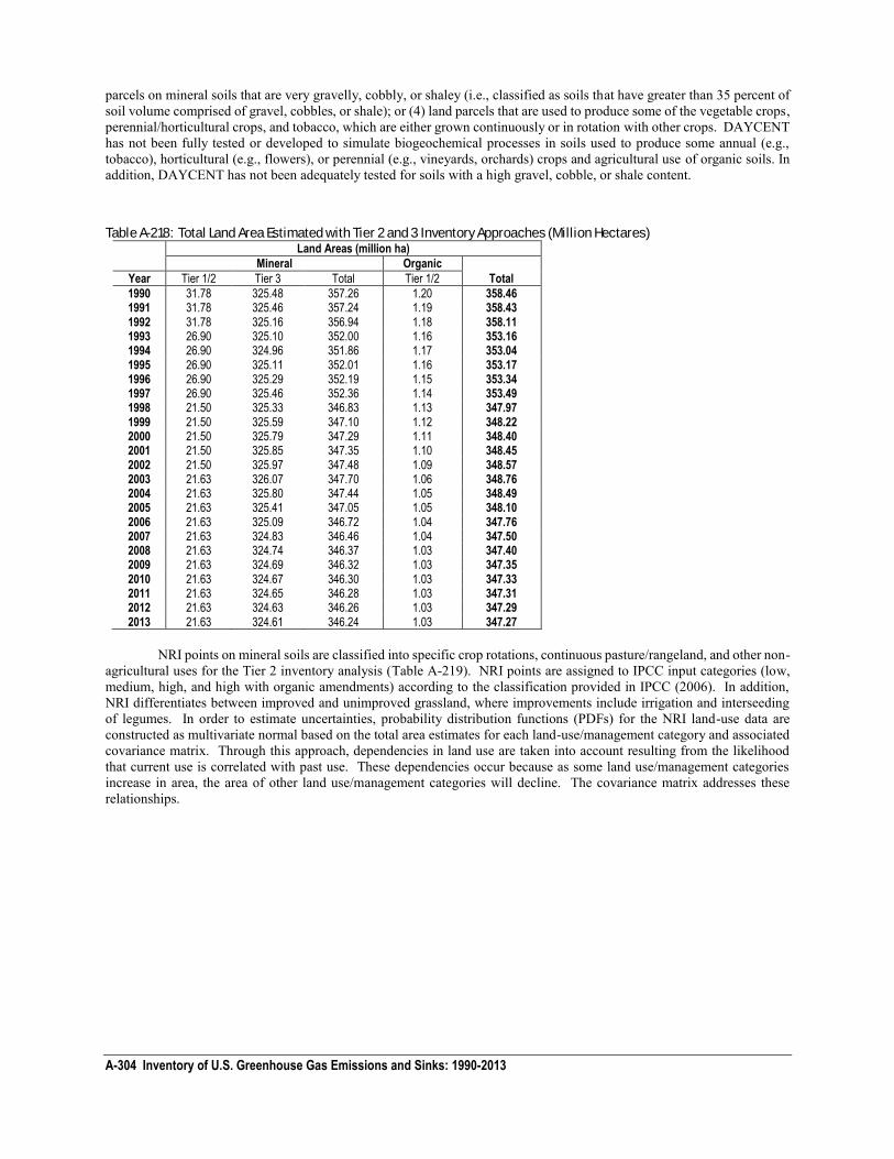
A-304 Inventory of U.S. Greenhouse Gas Emissions and Sinks: 1990-2013
parcels on mineral soils that are very gravelly, cobbly, or shaley (i.e., classified as soils that have greater than 35 percent of soil volume comprised of gravel, cobbles, or shale); or (4) land parcels that are used to produce some of the vegetable crops, perennial/horticultural crops, and tobacco, which are either grown continuously or in rotation with other crops. DAYCENT has not been fully tested or developed to simulate biogeochemical processes in soils used to produce some annual (e.g., tobacco), horticultural (e.g., flowers), or perennial (e.g., vineyards, orchards) crops and agricultural use of organic soils. In addition, DAYCENT has not been adequately tested for soils with a high gravel, cobble, or shale content.
Table A-218: Total Land Area Estimated with Tier 2 and 3 Inventory Approaches (Million Hectares)
Land Areas (million ha)
Mineral Organic
Year Tier 1/2 Tier 3 Total Tier 1/2 Total
1990 31.78 325.48 357.26 1.20 358.46 1991 31.78 325.46 357.24 1.19 358.43 1992 31.78 325.16 356.94 1.18 358.11 1993 26.90 325.10 352.00 1.16 353.16 1994 26.90 324.96 351.86 1.17 353.04 1995 26.90 325.11 352.01 1.16 353.17 1996 26.90 325.29 352.19 1.15 353.34 1997 26.90 325.46 352.36 1.14 353.49 1998 21.50 325.33 346.83 1.13 347.97 1999 21.50 325.59 347.10 1.12 348.22 2000 21.50 325.79 347.29 1.11 348.40 2001 21.50 325.85 347.35 1.10 348.45 2002 21.50 325.97 347.48 1.09 348.57 2003 21.63 326.07 347.70 1.06 348.76 2004 21.63 325.80 347.44 1.05 348.49 2005 21.63 325.41 347.05 1.05 348.10 2006 21.63 325.09 346.72 1.04 347.76 2007 21.63 324.83 346.46 1.04 347.50 2008 21.63 324.74 346.37 1.03 347.40 2009 21.63 324.69 346.32 1.03 347.35 2010 21.63 324.67 346.30 1.03 347.33 2011 21.63 324.65 346.28 1.03 347.31 2012 21.63 324.63 346.26 1.03 347.29 2013 21.63 324.61 346.24 1.03 347.27
NRI points on mineral soils are classified into specific crop rotations, continuous pasture/rangeland, and other non-
agricultural uses for the Tier 2 inventory analysis (Table A-219). NRI points are assigned to IPCC input categories (low, medium, high, and high with organic amendments) according to the classification provided in IPCC (2006). In addition, NRI differentiates between improved and unimproved grassland, where improvements include irrigation and interseeding of legumes. In order to estimate uncertainties, probability distribution functions (PDFs) for the NRI land-use data are constructed as multivariate normal based on the total area estimates for each land-use/management category and associated covariance matrix. Through this approach, dependencies in land use are taken into account resulting from the likelihood that current use is correlated with past use. These dependencies occur because as some land use/management categories increase in area, the area of other land use/management categories will decline. The covariance matrix addresses these relationships.
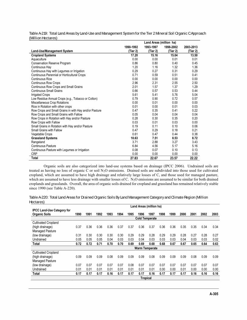
A-305
Table A-219: Total Land Areas by Land-Use and Management System for the Tier 2 Mineral Soil Organic C Approach
(Million Hectares) Land Areas (million ha)
Land-Use/Management System 1990-1992
(Tier 2) 1993-1997
(Tier 2) 1998-2002
(Tier 2) 2003-2013
(Tier 2)
Cropland Systems 17.20 15.16 15.04 13.50 Aquaculture 0.00 0.00 0.01 0.01 Conservation Reserve Program 0.86 0.80 0.40 0.45 Continuous Hay 1.20 1.16 1.32 1.36 Continuous Hay with Legumes or Irrigation 0.29 0.27 0.31 0.29 Continuous Perennial or Horticultural Crops 0.71 0.59 0.51 0.41 Continuous Rice 0.00 0.00 0.00 0.00 Continuous Row Crops 2.96 2.31 2.55 2.50 Continuous Row Crops and Small Grains 2.01 1.57 1.37 1.29 Continuous Small Grains 0.66 0.57 0.53 0.44 Irrigated Crops 5.61 5.41 5.76 5.04 Low Residue Annual Crops (e.g., Tobacco or Cotton) 0.79 0.90 0.72 0.57 Miscellaneous Crop Rotations 0.00 0.01 0.00 0.00 Rice in Rotation with other crops 0.01 0.00 0.01 0.03 Row Crops and Small Grains in with Hay and/or Pasture 0.47 0.35 0.41 0.22 Row Crops and Small Grains with Fallow 0.05 0.04 0.04 0.04 Row Crops in Rotation with Hay and/or Pasture 0.28 0.30 0.35 0.20 Row Crops with Fallow 0.03 0.01 0.03 0.00 Small Grains in Rotation with Hay and/or Pasture 0.19 0.11 0.10 0.06 Small Grains with Fallow 0.47 0.29 0.18 0.21 Vegetable Crops 0.61 0.47 0.44 0.38 Grassland Systems 10.63 7.51 8.53 8.72 Rangeland 3.71 2.88 3.27 3.43 Continuous Pasture 6.84 4.56 5.17 5.16 Continuous Pasture with Legumes or Irrigation 0.08 0.07 0.10 0.13 CRP 0.00 0.00 0.00 0.00
Total 27.83 22.67 23.57 22.22
Organic soils are also categorized into land-use systems based on drainage (IPCC 2006). Undrained soils are treated as having no loss of organic C or soil N2O emissions. Drained soils are subdivided into those used for cultivated cropland, which are assumed to have high drainage and relatively large losses of C, and those used for managed pasture, which are assumed to have less drainage with smaller losses of C. N2O emissions are assumed to be similar for both drained croplands and grasslands. Overall, the area of organic soils drained for cropland and grassland has remained relatively stable since 1990 (see Table A-220). Table A-220: Total Land Areas for Drained Organic Soils By Land Management Category and Climate Region (Million
Hectares) Land Areas (million ha) IPCC Land-Use Category for Organic Soils 1990 1991 1992 1993 1994 1995 1996 1997 1998 1999 2000 2001 2002 2003
Cold Temperate
Cultivated Cropland (high drainage) 0.37 0.36 0.36 0.36 0.37 0.37 0.36 0.37 0.36 0.36 0.35 0.35 0.34 0.34
Managed Pasture (low drainage) 0.31 0.30 0.30 0.30 0.30 0.29 0.29 0.28 0.29 0.29 0.28 0.27 0.28 0.27
Undrained 0.05 0.05 0.05 0.04 0.03 0.03 0.04 0.03 0.03 0.03 0.04 0.03 0.03 0.02
Total 0.72 0.72 0.71 0.70 0.70 0.69 0.69 0.68 0.68 0.67 0.67 0.65 0.64 0.63
Warm Temperate
Cultivated Cropland (high drainage) 0.09 0.09 0.09 0.08 0.09 0.09 0.09 0.08 0.09 0.09 0.09 0.08 0.09 0.09
Managed Pasture (low drainage) 0.07 0.07 0.07 0.07 0.07 0.08 0.07 0.07 0.07 0.07 0.07 0.07 0.07 0.07
Undrained 0.01 0.01 0.01 0.01 0.01 0.01 0.01 0.01 0.00 0.00 0.01 0.00 0.00 0.00
Total 0.17 0.17 0.17 0.16 0.17 0.17 0.17 0.16 0.17 0.17 0.17 0.16 0.16 0.16
Tropical
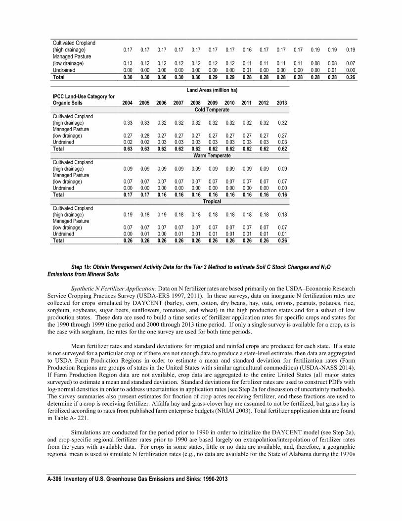
A-306 Inventory of U.S. Greenhouse Gas Emissions and Sinks: 1990-2013
Cultivated Cropland (high drainage) 0.17 0.17 0.17 0.17 0.17 0.17 0.17 0.16 0.17 0.17 0.17 0.19 0.19 0.19
Managed Pasture (low drainage) 0.13 0.12 0.12 0.12 0.12 0.12 0.12 0.11 0.11 0.11 0.11 0.08 0.08 0.07
Undrained 0.00 0.00 0.00 0.00 0.00 0.00 0.00 0.01 0.00 0.00 0.00 0.00 0.01 0.00
Total 0.30 0.30 0.30 0.30 0.30 0.29 0.29 0.28 0.28 0.28 0.28 0.28 0.28 0.26
Land Areas (million ha) IPCC Land-Use Category for Organic Soils 2004 2005 2006 2007 2008 2009 2010 2011 2012 2013
Cold Temperate
Cultivated Cropland (high drainage) 0.33 0.33 0.32 0.32 0.32 0.32 0.32 0.32 0.32 0.32 Managed Pasture (low drainage) 0.27 0.28 0.27 0.27 0.27 0.27 0.27 0.27 0.27 0.27 Undrained 0.02 0.02 0.03 0.03 0.03 0.03 0.03 0.03 0.03 0.03
Total 0.63 0.63 0.62 0.62 0.62 0.62 0.62 0.62 0.62 0.62
Warm Temperate
Cultivated Cropland (high drainage) 0.09 0.09 0.09 0.09 0.09 0.09 0.09 0.09 0.09 0.09 Managed Pasture (low drainage) 0.07 0.07 0.07 0.07 0.07 0.07 0.07 0.07 0.07 0.07 Undrained 0.00 0.00 0.00 0.00 0.00 0.00 0.00 0.00 0.00 0.00
Total 0.17 0.17 0.16 0.16 0.16 0.16 0.16 0.16 0.16 0.16
Tropical
Cultivated Cropland (high drainage) 0.19 0.18 0.19 0.18 0.18 0.18 0.18 0.18 0.18 0.18 Managed Pasture (low drainage) 0.07 0.07 0.07 0.07 0.07 0.07 0.07 0.07 0.07 0.07 Undrained 0.00 0.01 0.00 0.01 0.01 0.01 0.01 0.01 0.01 0.01
Total 0.26 0.26 0.26 0.26 0.26 0.26 0.26 0.26 0.26 0.26
Step 1b: Obtain Management Activity Data for the Tier 3 Method to estimate Soil C Stock Changes and N2O Emissions from Mineral Soils
Synthetic N Fertilizer Application: Data on N fertilizer rates are based primarily on the USDA–Economic Research
Service Cropping Practices Survey (USDA-ERS 1997, 2011). In these surveys, data on inorganic N fertilization rates are collected for crops simulated by DAYCENT (barley, corn, cotton, dry beans, hay, oats, onions, peanuts, potatoes, rice, sorghum, soybeans, sugar beets, sunflowers, tomatoes, and wheat) in the high production states and for a subset of low production states. These data are used to build a time series of fertilizer application rates for specific crops and states for the 1990 through 1999 time period and 2000 through 2013 time period. If only a single survey is available for a crop, as is the case with sorghum, the rates for the one survey are used for both time periods.
Mean fertilizer rates and standard deviations for irrigated and rainfed crops are produced for each state. If a state
is not surveyed for a particular crop or if there are not enough data to produce a state-level estimate, then data are aggregated to USDA Farm Production Regions in order to estimate a mean and standard deviation for fertilization rates (Farm Production Regions are groups of states in the United States with similar agricultural commodities) (USDA-NASS 2014). If Farm Production Region data are not available, crop data are aggregated to the entire United States (all major states surveyed) to estimate a mean and standard deviation. Standard deviations for fertilizer rates are used to construct PDFs with log-normal densities in order to address uncertainties in application rates (see Step 2a for discussion of uncertainty methods). The survey summaries also present estimates for fraction of crop acres receiving fertilizer, and these fractions are used to determine if a crop is receiving fertilizer. Alfalfa hay and grass-clover hay are assumed to not be fertilized, but grass hay is fertilized according to rates from published farm enterprise budgets (NRIAI 2003). Total fertilizer application data are found in Table A- 221.
Simulations are conducted for the period prior to 1990 in order to initialize the DAYCENT model (see Step 2a),
and crop-specific regional fertilizer rates prior to 1990 are based largely on extrapolation/interpolation of fertilizer rates from the years with available data. For crops in some states, little or no data are available, and, therefore, a geographic regional mean is used to simulate N fertilization rates (e.g., no data are available for the State of Alabama during the 1970s
A-307
and 1980s for corn fertilization rates; therefore, mean values from the southeastern United States are used to simulate fertilization to corn fields in this state).
Managed Livestock Manure Amendments:11 County-level manure addition estimates have been derived from
manure N addition rates developed by the USDA Natural Resources Conservation Service (NRCS) (Edmonds et al. 2003). Working with the farm-level crop and animal data from the 1997 Census of Agriculture, USDA-NRCS has coupled estimates of manure N produced with estimates of manure N recoverability by animal waste management system to produce county-level rates of manure N application to cropland and pasture. Edmonds et al. (2003) defined a hierarchy that included 24 crops, permanent pasture, and cropland used as pasture. They estimated the area amended with manure and application rates in 1997 for both manure-producing farms and manure-receiving farms within a county and for two scenarios—before implementation of Comprehensive Nutrient Management Plans (baseline) and after implementation (Edmonds et al. 2003). The goal of nutrient management plans is to apply manure nutrients at a rate meeting plant demand, thus limiting leaching losses of nutrients to groundwater and waterways.
For DAYCENT simulations, the rates for manure-producing farms and manure-receiving farms have been area-
weighted and combined to produce a single county-level estimate for the amount of land amended with manure and the manure N application rate for each crop in each county. The estimates were based on the assumption that Comprehensive Nutrient Management Plans have not been fully implemented. This is a conservative assumption because it allows for higher leaching rates due to some over-application of manure to soils. In order to address uncertainty in these data, uniform probability distributions are constructed based on the proportion of land receiving manure versus the amount not receiving manure for each crop type and pasture. For example, if 20 percent of land producing corn in a county is amended with manure, randomly drawing a value equal to or greater than 0 and less than 20 would lead to a simulation with a manure amendment, while drawing a value greater than or equal to 20 and less than 100 would lead to no amendment in the simulation (see Step 2a for further discussion of uncertainty methods).
Edmonds et al. (2003) only provides manure application rate data for 1997, but the amount of managed manure
available for soil application changes annually, so the area amended with manure is adjusted relative to 1997 to account for all the manure available for application in other years. Specifically, the manure N available for application in other years is divided by the manure N available in 1997. If the ratio is greater than 1, there is more manure N available in that county relative to the amount in 1997, and so it is assumed a larger area is amended with manure. In contrast, ratios less than one imply less area is amended with manure because there is a lower amount available in the year compared to 1997. The amendment area in each county for 1997 is multiplied by the ratio to reflect the impact of manure N availability on the area amended. The amount of managed manure N available for application to soils is calculated by determining the populations of livestock on feedlots or otherwise housed, requiring collection and management of the manure. The methods are described in the Manure Management section (Section 5.2) and annex (Annex 3.11). The total managed manure N applied to soils is found in Table A- 222.
To estimate C inputs (associated with manure N application rates derived from Edmonds et al. (2003)), carbon-
nitrogen (C:N) ratios for livestock-specific manure types are adapted from the Agricultural Waste Management Field Handbook (USDA 1996), On-Farm Composting Handbook (NRAES 1992), and recoverability factors provided by Edmonds et al (2003). The C:N ratios are applied to county-level estimates of manure N excreted by animal type and management system to produce a weighted county average C:N ratio for manure amendments. The average C:N ratio is used to determine the associated C input for crop amendments derived from Edmonds et al. (2003).
To account for the common practice of reducing inorganic N fertilizer inputs when manure is added to a cropland
soil, crop-specific reduction factors are derived from mineral fertilization data for land amended with manure versus land not amended with manure in the ERS 1995 Cropping Practices Survey (USDA-ERS 1997). Mineral N fertilization rates are reduced for crops receiving manure N based on a fraction of the amount of manure N applied, depending on the crop and whether it is irrigated or rainfed. The reduction factors are randomly selected from PDFs with normal densities in order to address uncertainties in the dependence between manure amendments and mineral fertilizer application.
11 For purposes of the inventory, total livestock manure is divided into two general categories: (1) managed manure, and (2) unmanaged manure. Managed manure includes manure that is stored in manure management systems such as drylots, pits and lagoons, as well as manure applied to soils through daily spread manure operations. Unmanaged manure encompasses all manure deposited on soils by animals on PRP.
A-308 Inventory of U.S. Greenhouse Gas Emissions and Sinks: 1990-2013
PRP Manure N: Another key source of N for grasslands is PRP manure N deposition (i.e., manure deposited by grazing livestock). The total amount of PRP manure N was estimated using methods described in the Manure Management section (Section 5.2) and annex (Annex 3.11). Nitrogen from PRP animal waste deposited on non-federal grasslands in a county was generated by multiplying the total PRP N (based on animal type and population data in a county) by the fraction of non-federal grassland area in the county. PRP manure N input rates for the Tier 3 DAYCENT simulations were estimated by dividing the total PRP manure N amount by the land area associated with non-federal grasslands in the county from the NRI survey data. The total PRP manure N added to soils is found in Table A- 222.
Residue N Inputs: Crop residue N, fixation by legumes, and N residue inputs from senesced grass litter are included
as sources of N to the soil, and are estimated in the DAYCENT simulations as a function of vegetation type, weather, and soil properties. That is, while the model accounts for the contribution of N from crop residues to the soil profile and subsequent N2O emissions, this source of mineral soil N is not “activity data” as it is not a model input. The simulated total N inputs of above- and below-ground residue N and fixed N that is not harvested and not burned (the DAYCENT simulations assumed that 3 percent of non-harvested above ground residues for crops are burned
12) are provided in Table A-223.
Other N Inputs: Other N inputs are estimated within the DAYCENT simulation, and thus input data are not
required, including mineralization from decomposition of soil organic matter and asymbiotic fixation of N from the atmosphere. Mineralization of soil organic matter will also include the effect of land use change on this process as recommended by the IPCC (2006). The influence of additional inputs of N are estimated in the simulations so that there is full accounting of all emissions from managed lands, as recommended by IPCC (2006). The simulated total N inputs from other sources are provided in Table A-223.
Tillage Practices: Tillage practices are estimated for each cropping system based on data from the Conservation
Technology Information Center13
(CTIC 2004). CTIC compiles data on cropland area under five tillage classes by major crop species and year for each county. Because the surveys involve county-level aggregate area, they do not fully characterize tillage practices as they are applied within a management sequence (e.g., crop rotation). This is particularly true for area estimates of cropland under no-till, which include a relatively high proportion of “intermittent” no-till, where no-till in one year may be followed by tillage in a subsequent year. For example, a common practice in maize-soybean rotations is to use tillage in the maize crop while no-till is used for soybean, such that no-till practices are not continuous in time. Estimates of the area under continuous no-till are provided by experts at CTIC to account for intermittent tillage activity and its impact on soil C (Towery 2001).
Tillage practices are grouped into 3 categories: full, reduced, and no-tillage. Full tillage is defined as multiple
tillage operations every year, including significant soil inversion (e.g., plowing, deep disking) and low surface residue coverage. This definition corresponds to the intensive tillage and “reduced” tillage systems as defined by CTIC (2004). No-till is defined as not disturbing the soil except through the use of fertilizer and seed drills and where no-till is applied to all crops in the rotation. Reduced tillage made up the remainder of the cultivated area, including mulch tillage and ridge tillage as defined by CTIC and intermittent no-till. The specific tillage implements and applications used for different crops, rotations, and regions to represent the three tillage classes are derived from the 1995 Cropping Practices Survey by the Economic Research Service (USDA-ERS 1997).
Tillage data are further processed to construct PDFs. Transitions between tillage systems are based on observed
county-level changes in the frequency distribution of the area under full, reduced, and no-till from the 1980s through 2004. Generally, the fraction of full tillage decreased during this time span, with concomitant increases in reduced till and no-till management. Transitions that are modeled and applied to NRI points occurring within a county are full tillage to reduced and no-till, and reduced tillage to no-till. The remaining amount of cropland is assumed to have no change in tillage (e.g., full tillage remained in full tillage). Transition matrices are constructed from CTIC data to represent tillage changes for three time periods, 1980-1989, 1990-1999, 2000-2007. Areas in each of the three tillage classes—full till (FT), reduced till (RT), no-till (NT)—in 1989 (the first year the CTIC data are available) are used for the first time period, data from 1997 are used for the second time period, and data from 2004 are used for the last time period. Percentage areas of cropland in each county are calculated for each possible transition (e.g., FT→FT, FT→RT, FT→NT, RT→RT, RT→NT) to obtain a probability for each tillage transition at an NRI point. It is assumed that there are no transitions for NT→FT or NT→NT after accounting for NT systems that have intermittent tillage. Uniform probability distributions are established for each
12
Another improvement is to reconcile the amount of crop residues burned with the Field Burning of Agricultural Residues source category (Section 5.5). 13
National scale tillage data are no longer collected by CTIC, and a new data source will be needed, which is a planned improvement.
A-309
tillage scenario in the county. For example, a particular crop rotation had 80 percent chance of remaining in full tillage over the two decades, a 15 percent chance of a transition from full to reduced tillage and a 5 percent chance of a transition from full to no-till. The uniform distribution is subdivided into three segments with random draws in the Monte Carlo simulation (discussed in Step 2b) leading to full tillage over the entire time period if the value is greater than or equal to 0 and less than 80, a transition from full to reduced till if the random draw is equal to or greater than 80 and less than 95, or a transition from full to no-till if the draw is greater than or equal to 95. See step 2b for additional discussion of the uncertainty analysis.
Irrigation: NRI (USDA-NRCS 2009) differentiates between irrigated and non-irrigated land, but does not provide
more detailed information on the type and intensity of irrigation. Hence, irrigation is modeled by assuming that applied water to field capacity with intervals between irrigation events where the soils drain to about 60 percent of field capacity.
Daily Weather Data: Daily maximum/minimum temperature and precipitation data are based on gridded weather
data from the North America Regional Reanalysis Product (NARR) (Mesinger et al. 2006). It is necessary to use computer-generated weather data because weather station data do not exist near all NRI points, and moreover weather station data are for a point in space. The NARR product uses this information with interpolation algorithms to derive weather patterns for areas between these stations. NARR weather data are available for the U.S. from 1980 through 2007 at a 32 km resolution. Each NRI point is assigned the NARR weather data for the grid cell containing the point.
Enhanced Vegetation Index: The Enhanced Vegetation Index (EVI) from the MODIS vegetation products,
(MOD13Q1 and MYD13Q1) is an input to DAYCENT for estimating net primary production using the NASA-CASA production algorithm (Potter et al. 1993, 2007). MODIS imagery is collected on a nominal 8 day-time frequency when combining the two products. A best approximation of the daily time series of EVI data is derived using a smoothing process based on the Savitzky-Golay Filter (Savitzky and Golay 1964) after pre-screening for outliers and for cloud-free, high quality data as identified in the MODIS data product quality layer. The NASA-CASA production algorithm is only used for the following crops: corn, soybeans, sorghum, cotton, wheat and other close-grown crops such as barley and oats.
14
The MODIS EVI products have a 250 m spatial resolution, and some pixels in images have mixed land uses and
crop types at this resolution, which is problematic for estimating NPP associated with a specific crop at a NRI point. Therefore, a threshold of 90 percent purity in an individual pixel is the cutoff for estimating NPP using the EVI data derived from the imagery (i.e., pixels with less than 90 percent purity for a crop are assumed to generate bias in the resulting NPP estimates). The USDA-NASS Crop Data Layer (CDL) (Johnson and Mueller 2010) is used to determine the purity levels of the EVI data. CDL data have a 30 to 58 m spatial resolution, depending on the year. The level of purity for individual pixels in the MODIS EVI products is determined by aggregating the crop cover data in CDL to the 250m resolution of the EVI data. In this step, the percent cover of individual crops is determined for the 250m EVI pixels. Pixels that did not meet a 90 percent purity level for any crop are eliminated from the dataset. CDL did not provide full coverage of crop maps for the conterminous United States until 2009 so it is not possible to evaluate purity for the entire cropland area prior to 2009.
The nearest pixel with at least 90 percent purity for a crop is assigned to the NRI point based on a 50 km buffer
surrounding the survey location. EVI data are not assigned to a point if there are no pixels with at least 90 percent purity within the 50 km buffer. Furthermore, MODIS products do not provide any data on EVI prior to 2000, which preceded the launch of the MODIS sensor on the Aqua and Terra Satellites. It is good practice to apply a method consistently across a time series (IPCC 2006), and so a statistical model is used to estimate EVI for the inventory time series prior to 2000 and also to fill gaps if no pixel has at least 90 percent purity within the 50 km buffer due to purity limitations, lack of CDL data to evaluate purity, or low quality data (Gurung et al. 2009).
Soil Properties: Soil texture and natural drainage capacity (i.e., hydric vs. non-hydric soil characterization) are the
main soil variables used as input to the DAYCENT model. Texture is one of the main controls on soil C turnover and stabilization in the DAYCENT model, which uses particle size fractions of sand (50-2,000 μm), silt (2-50 μm), and clay (< 2 μm) as inputs. Hydric condition are poorly-drained, and hence prone to have a high water table for part of the year in their native (pre-cultivation) condition , Non-hydric soils are moderately to well-drained .15 Poorly drained soils can be subject to anaerobic (lack of oxygen) conditions if water inputs (precipitation and irrigation) exceed water losses from drainage and evapotranspiration. Depending on moisture conditions, hydric soils can range from being fully aerobic to completely
14
Additional crops and grassland will be used with the NASA-CASA method in the future, as a planned improvement. 15 Artificial drainage (e.g., ditch- or tile-drainage) is simulated as a management variable.
A-310 Inventory of U.S. Greenhouse Gas Emissions and Sinks: 1990-2013
anaerobic, varying over the year. Decomposition rates are modified according to a linear function that varies from 0.3 under completely anaerobic conditions to 1.0 under fully aerobic conditions (default parameters in DAYCENT).16 Other soil characteristics needed in the simulation, such as field capacity and wilting-point water contents, are estimated from soil texture data using a standardized hydraulic properties calculator (Saxton et al. 1986). Soil input data are derived from Soil Survey Geographic Database (SSURGO) (Soil Survey Staff 2011). The data are based on field measurements collected as part of soil survey and mapping. Each NRI point is assigned the dominant soil component in the polygon containing the point from the SSURGO data product.
Step 1c: Obtain Additional Management Activity Data for the Tier 1 Method to estimate Soil N2O Emissions from Mineral Soils
Synthetic N Fertilizer: A process-of-elimination approach is used to estimate synthetic N fertilizer additions to crops in the Tier 1 method. The total amount of fertilizer used on-farms has been estimated by the USGS from 1990-2001 on a county scale from fertilizer sales data (Ruddy et al. 2006). For 2002 through 2013, county-level fertilizer used on-farms is adjusted based on annual fluctuations in total U.S. fertilizer sales (AAPFCO 1995 through 2014). Fertilizer application data are available for crops and grasslands simulated by DAYCENT (discussed in Step 1a section for Tier 3). Thus, the amount of N applied to crops in the Tier 1 method (i.e., not simulated by DAYCENT) is assumed to be the remainder of the fertilizer used on farms after subtracting the amount applied to crops and non-federal grasslands simulated by DAYCENT. The differences are aggregated to the state level, and PDFs are derived based on uncertainties in the amount of N applied to crops and non-federal grasslands for the Tier 3 method. Total fertilizer application to crops in the Tier 1 method is found in Table A- 224.
Managed Livestock Manure and Other Organic Amendments: Manure N that is not applied to crops and grassland
simulated by DAYCENT is assumed to be applied to other crops that are included in the Tier 1 method. Estimates of total national annual N additions from other commercial organic fertilizers are derived from organic fertilizer statistics (TVA 1991 through 1994; AAPFCO 1995 through 2014). Commercial organic fertilizers include dried blood, tankage, compost, and other; dried manure and sewage sludge that are used as commercial fertilizer are subtracted from totals to avoid double counting. The dried manure N is counted with the non-commercial manure applications, and sewage sludge is assumed to be applied only to grasslands. The organic fertilizer data, which are recorded in mass units of fertilizer, had to be converted to mass units of N by multiplying the consumption values by the average organic fertilizer N content of 0.5 percent (AAPFCO 2000). The fertilizer consumption data are recorded in “fertilizer year” totals, (i.e., July to June), but are converted to calendar year totals. This is done by assuming that approximately 35 percent of fertilizer usage occurred from July to December and 65 percent from January to June (TVA 1992b). Values for July to December are not available for calendar year 2013 so a “least squares line” statistical extrapolation using the previous 5 years of data is used to arrive at an approximate value. PDFs are derived for the organic fertilizer applications assuming a default ±50 percent uncertainty. Annual consumption of other organic fertilizers is presented in Table A- 225. The fate of manure N is summarized in Table A- 222.
PRP Manure N: Soil N2O emissions from PRP manure N deposited on federal grasslands are estimated with a Tier
1 method. PRP manure N data are derived using methods described in the Manure Management section (Section 5.2) and Annex 3.11. PRP N deposited on federal grasslands is calculated using a process of elimination approach. The amount of PRP N generated by DAYCENT model simulations of non-federal grasslands was subtracted from total PRP N and this difference was assumed to be applied to federal grasslands. The total PRP manure N added to soils is found in Table A- 222.
Sewage Sludge Amendments: Sewage sludge is generated from the treatment of raw sewage in public or private
wastewater treatment works and is typically used as a soil amendment, or is sent to waste disposal facilities, such as landfills. In this Inventory, all sewage sludge that is amended to agricultural soils is assumed to be applied to grasslands. Estimates of the amounts of sewage sludge N applied to agricultural lands are derived from national data on sewage sludge generation, disposition, and N content. Total sewage sludge generation data for 1990-2012, in dry mass units, are obtained from AAPFCO (1995-2014). Values for 2013 were not available so a “least squares line” statistical extrapolation using the previous 5 years of data was used to arrive at an approximate value. The total sludge generation estimates are then converted to units of N by applying an average N content of 69 percent (AAPFCO 2000), and disaggregated into use and disposal practices using historical data in EPA (1993) and NEBRA (2007). The use and disposal practices are agricultural land application, other land application, surface disposal, incineration, landfilling, ocean dumping (ended in 1992), and other
16 Hydric soils are primarily subject to anaerobic conditions outside the plant growing season (i.e., in the absence of active plant water uptake). Soils that are water-logged during much of the year are typically classified as organic soils (e.g., peat), which are not simulated with the DAYCENT model.
A-311
disposal methods. The resulting estimates of sewage sludge N applied to agricultural land are used to estimate N2O emissions from agricultural soil management; the estimates of sewage sludge N applied to other land and surface-disposed are used in estimating N2O fluxes from soils in Settlements Remaining Settlements (see section 6.9 of the Land Use, Land-Use Change, and Forestry chapter). Sewage sludge disposal data are provided in Table A- 226.
Residue N Inputs: Soil N2O emissions for residue N inputs from croplands that are not simulated by DAYCENT
are estimated with a Tier 1 method. Annual crop production statistics for all major commodity and specialty crops are taken from U.S. Department of Agriculture crop production reports (USDA 2014). Total production for each crop was converted to tons of dry matter product using the residue dry matter fractions shown in Table A- 227. Dry matter yield is then converted to tons of above- and below-ground biomass N. Above-ground biomass is calculated by using linear equations to estimate above-ground biomass given dry matter crop yields, and below-ground biomass is calculated by multiplying above-ground biomass by the below-to-above-ground biomass ratio. N inputs are estimated by multiplying above- and below-ground biomass by respective N concentrations and by the portion of cropland that was not simulated by DAYCENT. All ratios and equations used to calculate residue N inputs are from IPCC (2006) and Williams (2006). PDFs are derived assuming a ±50 percent uncertainty in the yield estimates (USDA-NASS does not provide uncertainty), along with uncertainties provided by the IPCC (2006) for dry matter fractions, above-ground residue, ratio of below-ground to above-ground biomass, and residue N fractions. The resulting annual biomass N inputs are presented in Table A- 228.
Step 1d: Obtain Additional Management Activity Data for the Tier 2 Method to estimate Soil C Stock Changes in Mineral Soils
Tillage Practices: For the Tier 2 method that is used to estimate soil organic C stock changes, PDFs are constructed
for the CTIC tillage data (CTIC 2004) as bivariate normal on a log-ratio scale to reflect negative dependence among tillage classes. This structure ensured that simulated tillage percentages are non-negative and summed to 100 percent. CTIC data do not differentiate between continuous and intermittent use of no-tillage, which is important for estimating SOC storage. Thus, regionally based estimates for continuous no-tillage (defined as 5 or more years of continuous use) are modified based on consultation with CTIC experts, as discussed in Step 1a (downward adjustment of total no-tillage area based on the amount of no-tillage that is rotated with more intensive tillage practices) (Towery 2001).
Managed Livestock Manure Amendments: USDA provides information on the amount of land amended with
manure for 1997 based on manure production data and field-scale surveys detailing application rates that had been collected in the Census of Agriculture (Edmonds et al. 2003). Similar to the DAYCENT model discussion in Step1b, the amount of land receiving manure is based on the estimates provided by Edmonds et al. (2003), as a proportion of crop and grassland amended with manure within individual climate regions. The resulting proportions are used to re-classify a portion of crop and grassland into a new management category. Specifically, a portion of medium input cropping systems is re-classified as high input, and a portion of the high input systems is re-classified as high input with amendment. In grassland systems, the estimated proportions for land amended with manure are used to re-classify a portion of nominally-managed grassland as improved, and a portion of improved grassland as improved with high input. These classification approaches are consistent with the IPCC inventory methodology (IPCC 2006). Uncertainties in the amount of land amended with manure are based on the sample variance at the climate region scale, assuming normal density PDFs (i.e., variance of the climate region estimates, which are derived from county-scale proportions).
Sewage Sludge Amendments: Sewage sludge is generated from the treatment of raw sewage in public or private
wastewater treatment facilities and is typically used as a soil amendment or is sent for waste disposal to landfills. In this Inventory, all sewage sludge that is amended to agricultural soils is assumed to be applied to grasslands. See section on sewage sludge in Step 1c for more information about the methods used to derive sewage sludge N estimates. The total amount of sewage sludge N is given in Table A- 226. Sewage sludge N is assumed to be applied at the assimilative capacity provided in Kellogg et al. (2000), which is the amount of nutrients taken up by a crop and removed at harvest, representing the recommended application rate for manure amendments. This capacity varies from year to year, because it is based on specific crop yields during the respective year (Kellogg et al. 2000). Total sewage sludge N available for application is divided by the assimilative capacity to estimate the total land area over which sewage sludge had been applied. The resulting estimates are used for the estimation of soil C stock change.
CRP Enrollment after 2007: The change in enrollment for the Conservation Reserve Program after 2007 is based
on the amount of land under active contracts from 2008 through 2013 relative to 2007 (USDA-FSA 2013).
A-312 Inventory of U.S. Greenhouse Gas Emissions and Sinks: 1990-2013
Wetland Reserve: Wetlands enrolled in the Conservation Reserve Program have been restored in the Northern Prairie Pothole Region through the Partners for Wildlife Program funded by the U.S. Fish and Wildlife Service (USFWS 2010). The area of restored wetlands is estimated from contract agreements (Euliss and Gleason 2002). While the contracts provide reasonable estimates of the amount of land restored in the region, they do not provide the information necessary to estimate uncertainty. Consequently, a ±50 percent range is used to construct the PDFs for the uncertainty analysis. Table A- 221: Synthetic Fertilizer N Added to Tier 3 Crops (kt N)
1990 1995 2000 2001 2002 2003 2004 2005 2006 2007 2008 2009 2010 2011 2012 2013
Fertilizer N 8,859 8,666 9,271 9,029 9,139 8,992 9,229 9,269 8,836 9,743 9,729 9,642 9,697 9,575 9,587 9,670
Table A- 222: Fate of Livestock Manure Nitrogen (kt N)
Activity 1990 1995 2000 2001 2002 2003 2004 2005 2006 2007 2008 2009 2010 2011 2012 2013 Managed Manure N
Applied to Tier 3 Cropland and Non-federal Grasslandsa,b 874 808 975 936 939 931 929 927 898 990 977 977 977 977 983 990
Managed Manure N Applied to Tier 1 CroplandC 1,533 1,716 1,647 1,678 1,713 1,735 1,659 1,701 1,807 1,742 1,732 1,714 1,704 1,732 1,755 1,742
Managed Manure N Applied to Grasslands 57 63 60 61 62 62 60 61 65 62 61 61 61 62 62 62
Pasture, Range, & Paddock Manure N 4,090 4,522 4,143 4,130 4,128 4,128 4,073 4,116 4,158 4,049 4,002 3,956 3,907 3,807 3,710 3,654
Total 6,553 7,110 6,825 6,805 6,841 6,856 6,721 6,805 6,928 6,843 6,772 6,707 6,648 6,577 6,510 6,448 a Accounts for N volatilized and leached/runoff during treatment, storage and transport before soil application. b Includes managed manure and daily spread manure amendments c Totals may not sum exactly due to rounding.
Table A-223: Crop Residue N and Other N Inputs to Tier 3 Crops as Simulated by DAYCENT (kt N)
Activity 1990 1995 2000 2001 2002 2003 2004 2005 2006 2007 2008 2009 2010 2011 2012 2013
Residue Na 576 618 625 630 594 641 661 662 633 630 630 630 630 630 630 630 Mineralization
& Asymbiotic Fixation 10,141 10,991 10,019 10,952 10,840 10,858 11,526 11,008 11,176 10,810 10,797 10,797 10,797 10,797 10,806 10,810
a Residue N inputs include unharvested fixed N from legumes as well as crop residue N.
Table A- 224: Synthetic Fertilizer N Added to Tier 1 Crops (kt N)
Activity 1990 1995 2000 2001 2002 2003 2004 2005 2006 2007 2008 2009 2010 2011 2012 2013
Fertilizer N 1,719 1,832 1,875 1,750 1,922 2,208 2,251 1,962 2,309 2,163 1,883 1,709 2,020 2,422 2,523 2,118
Table A- 225: Other Organic Commercial Fertilizer Consumption on Agricultural Lands (kt N)
Activity 1990 1995 2000 2001 2002 2003 2004 2005 2006 2007 2008 2009 2010 2011 2012 2013
Other Commercial Organic Fertilizer Na 4 10 9 7 8 8 9 10 12 15 12 10 10 11 11 10
a Includes dried blood, tankage, compost, other. Excludes dried manure and sewage sludge used as commercial fertilizer to avoid double counting. Table A- 226: Sewage Sludge Nitrogen by Disposal Practice (kt N) Disposal Practice 1990 1995 2000 2001 2002 2003 2004 2005 2006 2007 2008 2009 2010 2011 2012 2013
Applied to Agricultural Soils 52 68 84 86 89 91 94 98 101 104 107 110 113 116 119 122 Other Land Application 25 28 30 30 30 30 30 31 31 32 32 32 32 33 33 33 Surface Disposal 20 16 10 9 8 6 5 5 4 4 3 3 3 2 2 2
Total 97 111 124 125 127 128 130 134 137 140 142 145 148 151 153 156 Note: Totals may not sum due to independent rounding.
Table A- 227: Key Assumptions for Crop Production in the Tier 1 Method
Crop
Dry Matter Fraction of Harvested
Product
Above-ground Residue
Ratio of Below-ground
Residue N Fraction
Slope Intercept Above-ground Below-ground
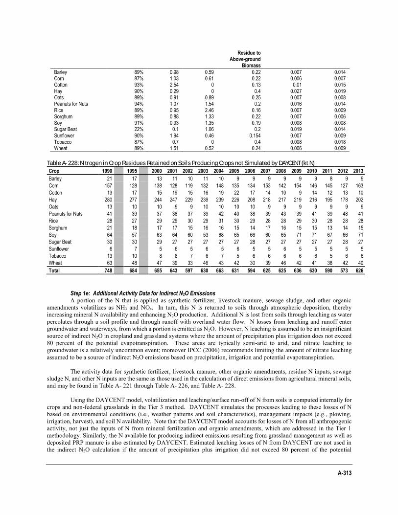
A-313
Residue to Above-ground
Biomass
Barley 89% 0.98 0.59 0.22 0.007 0.014 Corn 87% 1.03 0.61 0.22 0.006 0.007 Cotton 93% 2.54 0 0.13 0.01 0.015 Hay 90% 0.29 0 0.4 0.027 0.019 Oats 89% 0.91 0.89 0.25 0.007 0.008 Peanuts for Nuts 94% 1.07 1.54 0.2 0.016 0.014 Rice 89% 0.95 2.46 0.16 0.007 0.009 Sorghum 89% 0.88 1.33 0.22 0.007 0.006 Soy 91% 0.93 1.35 0.19 0.008 0.008 Sugar Beat 22% 0.1 1.06 0.2 0.019 0.014 Sunflower 90% 1.94 0.46 0.154 0.007 0.009 Tobacco 87% 0.7 0 0.4 0.008 0.018 Wheat 89% 1.51 0.52 0.24 0.006 0.009
Table A- 228: Nitrogen in Crop Residues Retained on Soils Producing Crops not Simulated by DAYCENT (kt N)
Crop 1990 1995 2000 2001 2002 2003 2004 2005 2006 2007 2008 2009 2010 2011 2012 2013
Barley 21 17 13 11 10 11 10 9 9 9 9 9 9 8 9 9
Corn 157 128 138 128 119 132 148 135 134 153 142 154 146 145 127 163
Cotton 13 17 15 19 15 16 19 22 17 14 10 9 14 12 13 10
Hay 280 277 244 247 229 239 239 226 208 218 217 219 216 195 178 202
Oats 13 10 10 9 9 10 10 10 10 9 9 9 9 9 9 9
Peanuts for Nuts 41 39 37 38 37 39 42 40 38 39 43 39 41 39 48 41
Rice 28 27 29 29 30 29 31 30 29 28 28 29 30 28 28 28
Sorghum 21 18 17 17 15 16 16 15 14 17 16 15 15 13 14 15
Soy 64 57 63 64 60 53 68 65 66 60 65 71 71 67 66 71
Sugar Beat 30 30 29 27 27 27 27 27 28 27 27 27 27 27 28 27
Sunflower 6 7 5 6 5 6 5 6 5 5 6 5 5 5 5 5
Tobacco 13 10 8 8 7 6 7 5 6 6 6 6 6 5 6 6
Wheat 63 48 47 39 33 46 43 42 30 39 46 42 41 38 42 40
Total 748 684 655 643 597 630 663 631 594 625 625 636 630 590 573 626
Step 1e: Additional Activity Data for Indirect N2O Emissions A portion of the N that is applied as synthetic fertilizer, livestock manure, sewage sludge, and other organic
amendments volatilizes as NH3 and NOx. In turn, this N is returned to soils through atmospheric deposition, thereby increasing mineral N availability and enhancing N2O production. Additional N is lost from soils through leaching as water percolates through a soil profile and through runoff with overland water flow. N losses from leaching and runoff enter groundwater and waterways, from which a portion is emitted as N2O. However, N leaching is assumed to be an insignificant source of indirect N2O in cropland and grassland systems where the amount of precipitation plus irrigation does not exceed 80 percent of the potential evapotranspiration. These areas are typically semi-arid to arid, and nitrate leaching to groundwater is a relatively uncommon event; moreover IPCC (2006) recommends limiting the amount of nitrate leaching assumed to be a source of indirect N2O emissions based on precipitation, irrigation and potential evapotranspiration.
The activity data for synthetic fertilizer, livestock manure, other organic amendments, residue N inputs, sewage
sludge N, and other N inputs are the same as those used in the calculation of direct emissions from agricultural mineral soils, and may be found in Table A- 221 through Table A- 226, and Table A- 228.
Using the DAYCENT model, volatilization and leaching/surface run-off of N from soils is computed internally for
crops and non-federal grasslands in the Tier 3 method. DAYCENT simulates the processes leading to these losses of N based on environmental conditions (i.e., weather patterns and soil characteristics), management impacts (e.g., plowing, irrigation, harvest), and soil N availability. Note that the DAYCENT model accounts for losses of N from all anthropogenic activity, not just the inputs of N from mineral fertilization and organic amendments, which are addressed in the Tier 1 methodology. Similarly, the N available for producing indirect emissions resulting from grassland management as well as deposited PRP manure is also estimated by DAYCENT. Estimated leaching losses of N from DAYCENT are not used in the indirect N2O calculation if the amount of precipitation plus irrigation did not exceed 80 percent of the potential
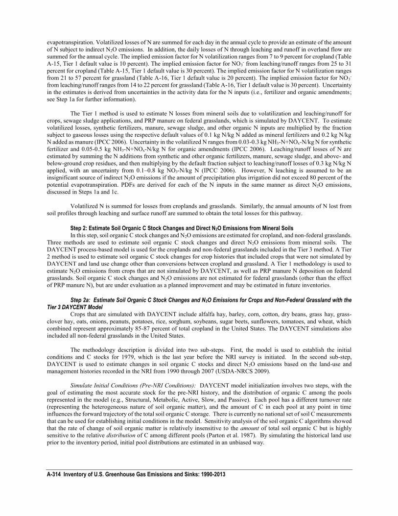
A-314 Inventory of U.S. Greenhouse Gas Emissions and Sinks: 1990-2013
evapotranspiration. Volatilized losses of N are summed for each day in the annual cycle to provide an estimate of the amount of N subject to indirect N2O emissions. In addition, the daily losses of N through leaching and runoff in overland flow are summed for the annual cycle. The implied emission factor for N volatilization ranges from 7 to 9 percent for cropland (Table A-15, Tier 1 default value is 10 percent). The implied emission factor for NO3
- from leaching/runoff ranges from 25 to 31 percent for cropland (Table A-15, Tier 1 default value is 30 percent). The implied emission factor for N volatilization ranges from 21 to 57 percent for grassland (Table A-16, Tier 1 default value is 20 percent). The implied emission factor for NO3
- from leaching/runoff ranges from 14 to 22 percent for grassland (Table A-16, Tier 1 default value is 30 percent). Uncertainty in the estimates is derived from uncertainties in the activity data for the N inputs (i.e., fertilizer and organic amendments; see Step 1a for further information).
The Tier 1 method is used to estimate N losses from mineral soils due to volatilization and leaching/runoff for
crops, sewage sludge applications, and PRP manure on federal grasslands, which is simulated by DAYCENT. To estimate volatilized losses, synthetic fertilizers, manure, sewage sludge, and other organic N inputs are multiplied by the fraction subject to gaseous losses using the respective default values of 0.1 kg N/kg N added as mineral fertilizers and 0.2 kg N/kg N added as manure (IPCC 2006). Uncertainty in the volatilized N ranges from 0.03-0.3 kg NH3-N+NOx-N/kg N for synthetic fertilizer and 0.05-0.5 kg NH3-N+NOx-N/kg N for organic amendments (IPCC 2006). Leaching/runoff losses of N are estimated by summing the N additions from synthetic and other organic fertilizers, manure, sewage sludge, and above- and below-ground crop residues, and then multiplying by the default fraction subject to leaching/runoff losses of 0.3 kg N/kg N applied, with an uncertainty from 0.1–0.8 kg NO3-N/kg N (IPCC 2006). However, N leaching is assumed to be an insignificant source of indirect N2O emissions if the amount of precipitation plus irrigation did not exceed 80 percent of the potential evapotranspiration. PDFs are derived for each of the N inputs in the same manner as direct N2O emissions, discussed in Steps 1a and 1c.
Volatilized N is summed for losses from croplands and grasslands. Similarly, the annual amounts of N lost from
soil profiles through leaching and surface runoff are summed to obtain the total losses for this pathway.
Step 2: Estimate Soil Organic C Stock Changes and Direct N2O Emissions from Mineral Soils In this step, soil organic C stock changes and N2O emissions are estimated for cropland, and non-federal grasslands.
Three methods are used to estimate soil organic C stock changes and direct N2O emissions from mineral soils. The DAYCENT process-based model is used for the croplands and non-federal grasslands included in the Tier 3 method. A Tier 2 method is used to estimate soil organic C stock changes for crop histories that included crops that were not simulated by DAYCENT and land use change other than conversions between cropland and grassland. A Tier 1 methodology is used to estimate N2O emissions from crops that are not simulated by DAYCENT, as well as PRP manure N deposition on federal grasslands. Soil organic C stock changes and N2O emissions are not estimated for federal grasslands (other than the effect of PRP manure N), but are under evaluation as a planned improvement and may be estimated in future inventories.
Step 2a: Estimate Soil Organic C Stock Changes and N2O Emissions for Crops and Non-Federal Grassland with the Tier 3 DAYCENT Model
Crops that are simulated with DAYCENT include alfalfa hay, barley, corn, cotton, dry beans, grass hay, grass-clover hay, oats, onions, peanuts, potatoes, rice, sorghum, soybeans, sugar beets, sunflowers, tomatoes, and wheat, which combined represent approximately 85-87 percent of total cropland in the United States. The DAYCENT simulations also included all non-federal grasslands in the United States.
The methodology description is divided into two sub-steps. First, the model is used to establish the initial
conditions and C stocks for 1979, which is the last year before the NRI survey is initiated. In the second sub-step, DAYCENT is used to estimate changes in soil organic C stocks and direct N2O emissions based on the land-use and management histories recorded in the NRI from 1990 through 2007 (USDA-NRCS 2009).
Simulate Initial Conditions (Pre-NRI Conditions): DAYCENT model initialization involves two steps, with the
goal of estimating the most accurate stock for the pre-NRI history, and the distribution of organic C among the pools represented in the model (e.g., Structural, Metabolic, Active, Slow, and Passive). Each pool has a different turnover rate (representing the heterogeneous nature of soil organic matter), and the amount of C in each pool at any point in time influences the forward trajectory of the total soil organic C storage. There is currently no national set of soil C measurements that can be used for establishing initial conditions in the model. Sensitivity analysis of the soil organic C algorithms showed that the rate of change of soil organic matter is relatively insensitive to the amount of total soil organic C but is highly sensitive to the relative distribution of C among different pools (Parton et al. 1987). By simulating the historical land use prior to the inventory period, initial pool distributions are estimated in an unbiased way.
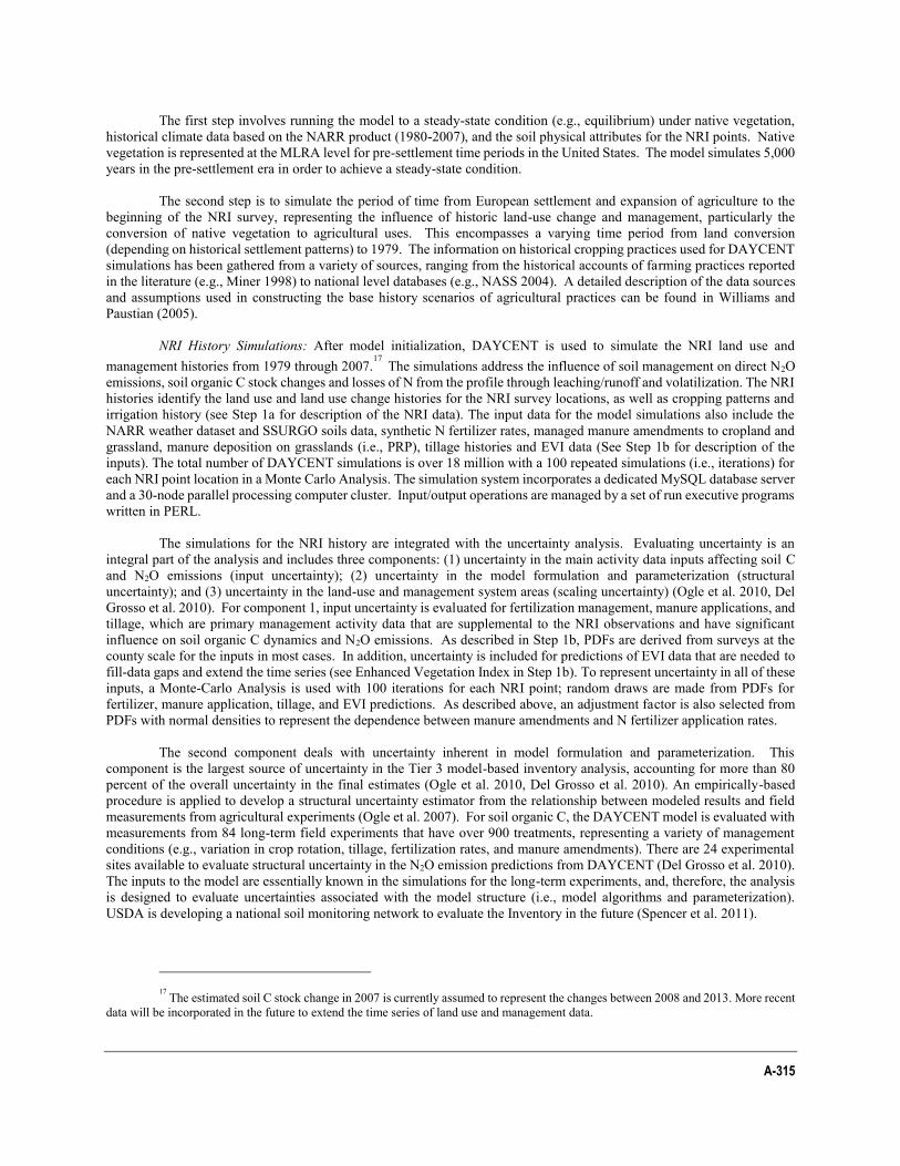
A-315
The first step involves running the model to a steady-state condition (e.g., equilibrium) under native vegetation, historical climate data based on the NARR product (1980-2007), and the soil physical attributes for the NRI points. Native vegetation is represented at the MLRA level for pre-settlement time periods in the United States. The model simulates 5,000 years in the pre-settlement era in order to achieve a steady-state condition.
The second step is to simulate the period of time from European settlement and expansion of agriculture to the
beginning of the NRI survey, representing the influence of historic land-use change and management, particularly the conversion of native vegetation to agricultural uses. This encompasses a varying time period from land conversion (depending on historical settlement patterns) to 1979. The information on historical cropping practices used for DAYCENT simulations has been gathered from a variety of sources, ranging from the historical accounts of farming practices reported in the literature (e.g., Miner 1998) to national level databases (e.g., NASS 2004). A detailed description of the data sources and assumptions used in constructing the base history scenarios of agricultural practices can be found in Williams and Paustian (2005).
NRI History Simulations: After model initialization, DAYCENT is used to simulate the NRI land use and
management histories from 1979 through 2007.17 The simulations address the influence of soil management on direct N2O
emissions, soil organic C stock changes and losses of N from the profile through leaching/runoff and volatilization. The NRI histories identify the land use and land use change histories for the NRI survey locations, as well as cropping patterns and irrigation history (see Step 1a for description of the NRI data). The input data for the model simulations also include the NARR weather dataset and SSURGO soils data, synthetic N fertilizer rates, managed manure amendments to cropland and grassland, manure deposition on grasslands (i.e., PRP), tillage histories and EVI data (See Step 1b for description of the inputs). The total number of DAYCENT simulations is over 18 million with a 100 repeated simulations (i.e., iterations) for each NRI point location in a Monte Carlo Analysis. The simulation system incorporates a dedicated MySQL database server and a 30-node parallel processing computer cluster. Input/output operations are managed by a set of run executive programs written in PERL.
The simulations for the NRI history are integrated with the uncertainty analysis. Evaluating uncertainty is an
integral part of the analysis and includes three components: (1) uncertainty in the main activity data inputs affecting soil C and N2O emissions (input uncertainty); (2) uncertainty in the model formulation and parameterization (structural uncertainty); and (3) uncertainty in the land-use and management system areas (scaling uncertainty) (Ogle et al. 2010, Del Grosso et al. 2010). For component 1, input uncertainty is evaluated for fertilization management, manure applications, and tillage, which are primary management activity data that are supplemental to the NRI observations and have significant influence on soil organic C dynamics and N2O emissions. As described in Step 1b, PDFs are derived from surveys at the county scale for the inputs in most cases. In addition, uncertainty is included for predictions of EVI data that are needed to fill-data gaps and extend the time series (see Enhanced Vegetation Index in Step 1b). To represent uncertainty in all of these inputs, a Monte-Carlo Analysis is used with 100 iterations for each NRI point; random draws are made from PDFs for fertilizer, manure application, tillage, and EVI predictions. As described above, an adjustment factor is also selected from PDFs with normal densities to represent the dependence between manure amendments and N fertilizer application rates.
The second component deals with uncertainty inherent in model formulation and parameterization. This
component is the largest source of uncertainty in the Tier 3 model-based inventory analysis, accounting for more than 80 percent of the overall uncertainty in the final estimates (Ogle et al. 2010, Del Grosso et al. 2010). An empirically-based procedure is applied to develop a structural uncertainty estimator from the relationship between modeled results and field measurements from agricultural experiments (Ogle et al. 2007). For soil organic C, the DAYCENT model is evaluated with measurements from 84 long-term field experiments that have over 900 treatments, representing a variety of management conditions (e.g., variation in crop rotation, tillage, fertilization rates, and manure amendments). There are 24 experimental sites available to evaluate structural uncertainty in the N2O emission predictions from DAYCENT (Del Grosso et al. 2010). The inputs to the model are essentially known in the simulations for the long-term experiments, and, therefore, the analysis is designed to evaluate uncertainties associated with the model structure (i.e., model algorithms and parameterization). USDA is developing a national soil monitoring network to evaluate the Inventory in the future (Spencer et al. 2011).
17 The estimated soil C stock change in 2007 is currently assumed to represent the changes between 2008 and 2013. More recent
data will be incorporated in the future to extend the time series of land use and management data.
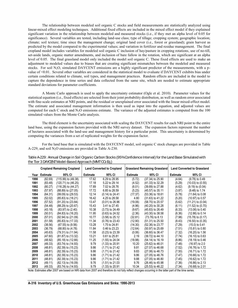
A-316 Inventory of U.S. Greenhouse Gas Emissions and Sinks: 1990-2013
The relationship between modeled soil organic C stocks and field measurements are statistically analyzed using linear-mixed effect modeling techniques. Additional fixed effects are included in the mixed effect model if they explained significant variation in the relationship between modeled and measured stocks (i.e., if they met an alpha level of 0.05 for significance). Several variables are tested, including land-use class; type of tillage; cropping system; geographic location; climate; soil texture; time since the management change; original land cover (i.e., forest or grassland); grain harvest as predicted by the model compared to the experimental values; and variation in fertilizer and residue management. The final cropland model includes variables for modeled soil organic C inclusion of hay/pasture in cropping rotations, use of no-till, set-aside lands, organic matter amendments, and inclusion of bare fallow in the rotation, which are significant at an alpha level of 0.05. The final grassland model only included the model soil organic C. These fixed effects are used to make an adjustment to modeled values due to biases that are creating significant mismatches between the modeled and measured stocks. For soil N2O, simulated DAYCENT emissions are a highly significant predictor of the measurements, with a p-value of <0.01. Several other variables are considered in the statistical model to evaluate if DAYCENT exhibits bias under certain conditions related to climate, soil types, and management practices. Random effects are included in the model to capture the dependence in time series and data collected from the same site, which are needed to estimate appropriate standard deviations for parameter coefficients.
A Monte Carlo approach is used to apply the uncertainty estimator (Ogle et al. 2010). Parameter values for the
statistical equation (i.e., fixed effects) are selected from their joint probability distribution, as well as random error associated with fine-scale estimates at NRI points, and the residual or unexplained error associated with the linear mixed-effect model. The estimate and associated management information is then used as input into the equation, and adjusted values are computed for each C stock and N2O emissions estimate. The variance of the adjusted estimates is computed from the 100 simulated values from the Monte Carlo analysis.
The third element is the uncertainty associated with scaling the DAYCENT results for each NRI point to the entire
land base, using the expansion factors provided with the NRI survey dataset. The expansion factors represent the number of hectares associated with the land-use and management history for a particular point. This uncertainty is determined by computing the variances from a set of replicated weights for the expansion factor.
For the land base that is simulated with the DAYCENT model, soil organic C stock changes are provided in Table
A-229, and soil N2O emissions are provided in Table A-230. Table A-229: Annual Change in Soil Organic Carbon Stocks (95% Confidence Interval) for the Land Base Simulated with
the Tier 3 DAYCENT Model-Based Approach (MMT CO2 Eq.)
Year
Cropland Remaining Cropland Land Converted to Cropland Grassland Remaining Grassland Land Converted to Grassland
Estimate 95% CI Estimate 95% CI Estimate 95% CI Estimate 95% CI
1990 (82.69) (115.99) to (49.38) 17.62 6.29 to 28.95 (5.72) (37.34) to 25.90 (4.64) (9.78) to 0.49 1991 (83.48) (120.71) to (46.25) 17.18 5.22 to 29.14 (4.52) (41.33) to 32.29 (5.29) (10.03) to (0.55) 1992 (80.27) (116.28) to (44.27) 17.89 7.02 to 28.76 (6.01) (39.89) to 27.88 (4.62) (9.19) to (0.04) 1993 (57.97) (88.89) to (27.05) 17.72 6.85 to 28.59 (5.23) (45.57) to 35.11 (3.87) (9.48) to 1.74 1994 (64.31) (99.09) to (29.53) 12.14 (0.14) to 24.41 (17.37) (53.36) to 18.61 (5.78) (11.64) to 0.08 1995 (52.02) (85.83) to (18.21) 16.42 4.25 to 28.58 4.80 (31.63) to 41.22 (5.20) (10.97) to 0.57 1996 (57.52) (91.20) to (23.84) 13.47 (0.01) to 26.96 (19.06) (58.70) to 20.57 (5.62) (11.21) to (0.04) 1997 (54.48) (88.29) to (20.67) 15.43 3.41 to 27.45 (4.96) (40.20) to 30.28 (6.11) (11.52) to (0.70) 1998 (43.18) (83.97) to (2.40) 10.38 (3.73) to 24.49 (9.67) (45.83) to 26.49 (6.33) (13.06) to 0.40 1999 (50.51) (84.83) to (16.20) 11.95 (0.63) to 24.52 (2.36) (43.30) to 38.58 (6.36) (12.86) to 0.14 2000 (57.01) (92.94) to (21.09) 10.77 (3.58) to 25.12 (32.81) (73.76) to 8.13 (7.98) (15.78) to (0.17) 2001 (51.58) (85.83) to (17.33) 11.34 (0.76) to 23.43 (12.90) (51.31) to 25.50 (8.43) (16.50) to (0.35) 2002 (38.56) (67.55) to (9.56) 13.28 1.75 to 24.81 (14.30) (52.36) to 23.77 (7.29) (15.0) to 0.41 2003 (36.79) (68.80) to (4.78) 11.84 0.46 to 23.23 (12.64) (50.97) to 25.69 (7.51) (15.81) to 0.80 2004 (45.63) (79.31) to (11.94) 11.58 (0.23) to 23.39 (0.06) (36.60) to 36.47 (7.32) (16.20) to 1.56 2005 (47.60) (81.87) to (13.32) 13.21 0.61 to 25.81 2.19 (39.72) to 44.10 (7.74) (16.10) to 0.63 2006 (48.92) (85.18) to (12.66) 11.25 (1.55) to 24.04 (18.98) (54.14) to 16.19 (8.86) (18.19) to 0.46 2007 (49.33) (83.74) to (14.93) 9.79 (1.33) to 20.91 10.20 (25.62) to 46.01 (7.48) (16.97) to 2.0 2008 (48.81) (82.39) to (15.23) 9.86 (1.71) to 21.42 9.81 (27.07) to 46.68 (7.52) (16.76) to 1.72 2009 (48.81) (82.39) to (15.23) 9.86 (1.71) to 21.42 9.83 (27.06) to 46.73 (7.50) (16.71) to 1.72 2010 (48.81) (82.39) to (15.23) 9.86 (1.71) to 21.42 9.86 (27.05) to 46.76 (7.47) (16.66) to 1.72 2011 (48.81) (82.39) to (15.23) 9.86 (1.71) to 21.42 9.88 (27.05) to 46.80 (7.45) (16.62) to 1.72 2012 (49.11) (82.13) to (16.09) 9.76 (1.51) to 21.03 9.76 (26.46) to 45.98 (7.36) (16.86) to 2.13 2013 (49.33) (83.74) to (14.93) 9.79 (1.33) to 20.91 10.34 (25.53) to 46.22 (7.34) (16.68) to 2.01
Note: Estimates after 2007 are based on NRI data from 2007 and therefore do not fully reflect changes occurring in the latter part of the time series.
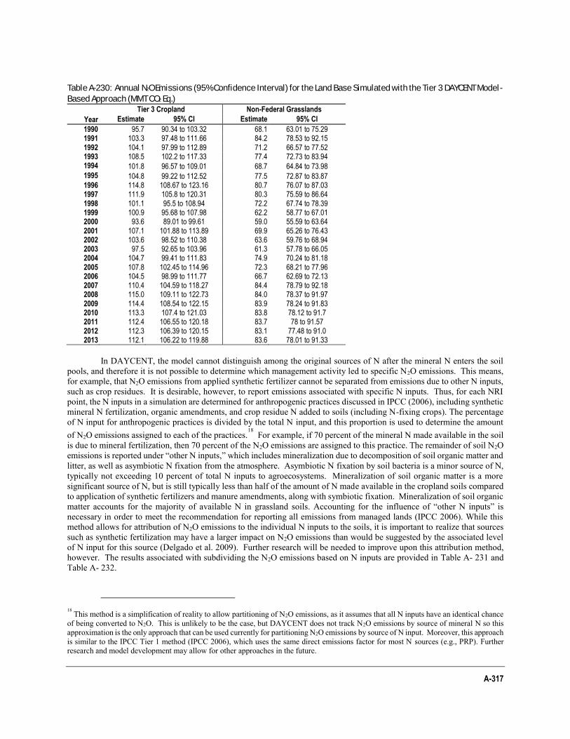
A-317
Table A-230: Annual N2O Emissions (95% Confidence Interval) for the Land Base Simulated with the Tier 3 DAYCENT Model-
Based Approach (MMT CO2 Eq.)
Year
Tier 3 Cropland Non-Federal Grasslands
Estimate 95% CI Estimate 95% CI
1990 95.7 90.34 to 103.32 68.1 63.01 to 75.29 1991 103.3 97.48 to 111.66 84.2 78.53 to 92.15 1992 104.1 97.99 to 112.89 71.2 66.57 to 77.52 1993 108.5 102.2 to 117.33 77.4 72.73 to 83.94 1994 101.8 96.57 to 109.01 68.7 64.84 to 73.98 1995 104.8 99.22 to 112.52 77.5 72.87 to 83.87 1996 114.8 108.67 to 123.16 80.7 76.07 to 87.03 1997 111.9 105.8 to 120.31 80.3 75.59 to 86.64 1998 101.1 95.5 to 108.94 72.2 67.74 to 78.39 1999 100.9 95.68 to 107.98 62.2 58.77 to 67.01 2000 93.6 89.01 to 99.61 59.0 55.59 to 63.64 2001 107.1 101.88 to 113.89 69.9 65.26 to 76.43 2002 103.6 98.52 to 110.38 63.6 59.76 to 68.94 2003 97.5 92.65 to 103.96 61.3 57.78 to 66.05 2004 104.7 99.41 to 111.83 74.9 70.24 to 81.18 2005 107.8 102.45 to 114.96 72.3 68.21 to 77.96 2006 104.5 98.99 to 111.77 66.7 62.69 to 72.13 2007 110.4 104.59 to 118.27 84.4 78.79 to 92.18 2008 115.0 109.11 to 122.73 84.0 78.37 to 91.97 2009 114.4 108.54 to 122.15 83.9 78.24 to 91.83 2010 113.3 107.4 to 121.03 83.8 78.12 to 91.7 2011 112.4 106.55 to 120.18 83.7 78 to 91.57 2012 112.3 106.39 to 120.15 83.1 77.48 to 91.0 2013 112.1 106.22 to 119.88 83.6 78.01 to 91.33
In DAYCENT, the model cannot distinguish among the original sources of N after the mineral N enters the soil
pools, and therefore it is not possible to determine which management activity led to specific N2O emissions. This means, for example, that N2O emissions from applied synthetic fertilizer cannot be separated from emissions due to other N inputs, such as crop residues. It is desirable, however, to report emissions associated with specific N inputs. Thus, for each NRI point, the N inputs in a simulation are determined for anthropogenic practices discussed in IPCC (2006), including synthetic mineral N fertilization, organic amendments, and crop residue N added to soils (including N-fixing crops). The percentage of N input for anthropogenic practices is divided by the total N input, and this proportion is used to determine the amount of N2O emissions assigned to each of the practices.
18 For example, if 70 percent of the mineral N made available in the soil
is due to mineral fertilization, then 70 percent of the N2O emissions are assigned to this practice. The remainder of soil N2O emissions is reported under “other N inputs,” which includes mineralization due to decomposition of soil organic matter and litter, as well as asymbiotic N fixation from the atmosphere. Asymbiotic N fixation by soil bacteria is a minor source of N, typically not exceeding 10 percent of total N inputs to agroecosystems. Mineralization of soil organic matter is a more significant source of N, but is still typically less than half of the amount of N made available in the cropland soils compared to application of synthetic fertilizers and manure amendments, along with symbiotic fixation. Mineralization of soil organic matter accounts for the majority of available N in grassland soils. Accounting for the influence of “other N inputs” is necessary in order to meet the recommendation for reporting all emissions from managed lands (IPCC 2006). While this method allows for attribution of N2O emissions to the individual N inputs to the soils, it is important to realize that sources such as synthetic fertilization may have a larger impact on N2O emissions than would be suggested by the associated level of N input for this source (Delgado et al. 2009). Further research will be needed to improve upon this attribution method, however. The results associated with subdividing the N2O emissions based on N inputs are provided in Table A- 231 and Table A- 232.
18 This method is a simplification of reality to allow partitioning of N2O emissions, as it assumes that all N inputs have an identical chance of being converted to N2O. This is unlikely to be the case, but DAYCENT does not track N2O emissions by source of mineral N so this approximation is the only approach that can be used currently for partitioning N2O emissions by source of N input. Moreover, this approach is similar to the IPCC Tier 1 method (IPCC 2006), which uses the same direct emissions factor for most N sources (e.g., PRP). Further research and model development may allow for other approaches in the future.
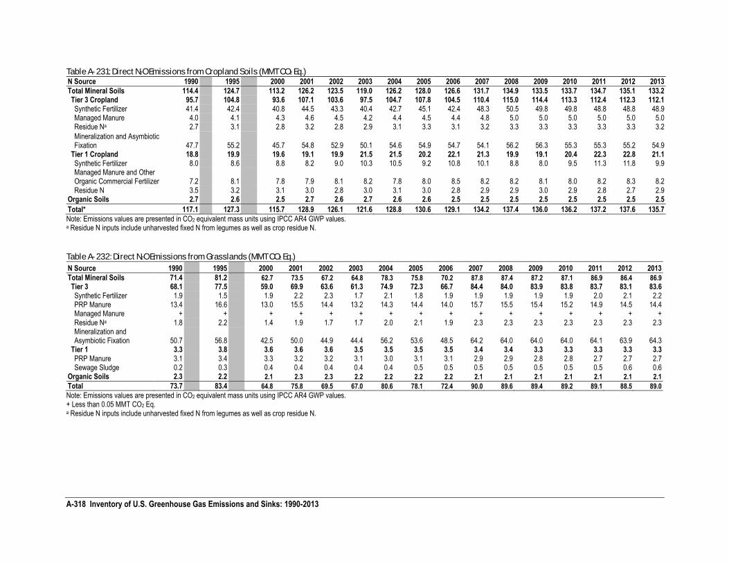
A-318 Inventory of U.S. Greenhouse Gas Emissions and Sinks: 1990-2013
Table A- 231: Direct N2O Emissions from Cropland Soils (MMT CO2 Eq.) N Source 1990 1995 2000 2001 2002 2003 2004 2005 2006 2007 2008 2009 2010 2011 2012 2013
Total Mineral Soils 114.4 124.7 113.2 126.2 123.5 119.0 126.2 128.0 126.6 131.7 134.9 133.5 133.7 134.7 135.1 133.2 Tier 3 Cropland 95.7 104.8 93.6 107.1 103.6 97.5 104.7 107.8 104.5 110.4 115.0 114.4 113.3 112.4 112.3 112.1 Synthetic Fertilizer 41.4 42.4 40.8 44.5 43.3 40.4 42.7 45.1 42.4 48.3 50.5 49.8 49.8 48.8 48.8 48.9 Managed Manure 4.0 4.1 4.3 4.6 4.5 4.2 4.4 4.5 4.4 4.8 5.0 5.0 5.0 5.0 5.0 5.0 Residue Na 2.7 3.1 2.8 3.2 2.8 2.9 3.1 3.3 3.1 3.2 3.3 3.3 3.3 3.3 3.3 3.2
Mineralization and Asymbiotic Fixation 47.7 55.2 45.7 54.8 52.9 50.1 54.6 54.9 54.7 54.1 56.2 56.3 55.3 55.3 55.2 54.9
Tier 1 Cropland 18.8 19.9 19.6 19.1 19.9 21.5 21.5 20.2 22.1 21.3 19.9 19.1 20.4 22.3 22.8 21.1 Synthetic Fertilizer 8.0 8.6 8.8 8.2 9.0 10.3 10.5 9.2 10.8 10.1 8.8 8.0 9.5 11.3 11.8 9.9 Managed Manure and Other Organic Commercial Fertilizer 7.2 8.1 7.8 7.9 8.1 8.2 7.8 8.0 8.5 8.2 8.2 8.1 8.0 8.2 8.3 8.2 Residue N 3.5 3.2 3.1 3.0 2.8 3.0 3.1 3.0 2.8 2.9 2.9 3.0 2.9 2.8 2.7 2.9
Organic Soils 2.7 2.6 2.5 2.7 2.6 2.7 2.6 2.6 2.5 2.5 2.5 2.5 2.5 2.5 2.5 2.5
Total* 117.1 127.3 115.7 128.9 126.1 121.6 128.8 130.6 129.1 134.2 137.4 136.0 136.2 137.2 137.6 135.7
Note: Emissions values are presented in CO2 equivalent mass units using IPCC AR4 GWP values. a Residue N inputs include unharvested fixed N from legumes as well as crop residue N. Table A- 232: Direct N2O Emissions from Grasslands (MMT CO2 Eq.)
N Source 1990 1995 2000 2001 2002 2003 2004 2005 2006 2007 2008 2009 2010 2011 2012 2013
Total Mineral Soils 71.4 81.2 62.7 73.5 67.2 64.8 78.3 75.8 70.2 87.8 87.4 87.2 87.1 86.9 86.4 86.9
Tier 3 68.1 77.5 59.0 69.9 63.6 61.3 74.9 72.3 66.7 84.4 84.0 83.9 83.8 83.7 83.1 83.6 Synthetic Fertilizer 1.9 1.5 1.9 2.2 2.3 1.7 2.1 1.8 1.9 1.9 1.9 1.9 1.9 2.0 2.1 2.2 PRP Manure 13.4 16.6 13.0 15.5 14.4 13.2 14.3 14.4 14.0 15.7 15.5 15.4 15.2 14.9 14.5 14.4 Managed Manure + + + + + + + + + + + + + + + + Residue Na 1.8 2.2 1.4 1.9 1.7 1.7 2.0 2.1 1.9 2.3 2.3 2.3 2.3 2.3 2.3 2.3 Mineralization and Asymbiotic Fixation 50.7 56.8 42.5 50.0 44.9 44.4 56.2 53.6 48.5 64.2 64.0 64.0 64.0 64.1 63.9 64.3
Tier 1 3.3 3.8 3.6 3.6 3.6 3.5 3.5 3.5 3.5 3.4 3.4 3.3 3.3 3.3 3.3 3.3 PRP Manure 3.1 3.4 3.3 3.2 3.2 3.1 3.0 3.1 3.1 2.9 2.9 2.8 2.8 2.7 2.7 2.7 Sewage Sludge 0.2 0.3 0.4 0.4 0.4 0.4 0.4 0.5 0.5 0.5 0.5 0.5 0.5 0.5 0.6 0.6
Organic Soils 2.3 2.2 2.1 2.3 2.3 2.2 2.2 2.2 2.2 2.1 2.1 2.1 2.1 2.1 2.1 2.1
Total 73.7 83.4 64.8 75.8 69.5 67.0 80.6 78.1 72.4 90.0 89.6 89.4 89.2 89.1 88.5 89.0
Note: Emissions values are presented in CO2 equivalent mass units using IPCC AR4 GWP values. + Less than 0.05 MMT CO2 Eq. a Residue N inputs include unharvested fixed N from legumes as well as crop residue N.
A-319
Step 2b: Soil N2O Emissions from Agricultural Lands on Mineral Soils Approximated with the Tier 1 Approach To estimate direct N2O emissions from N additions to crops in the Tier 1 method, the amount of N in applied
synthetic fertilizer, manure and other commercial organic fertilizers (i.e., dried blood, tankage, compost, and other) is added to N inputs from crop residues, and the resulting annual totals are multiplied by the IPCC default emission factor of 0.01 kg N2O-N/kg N (IPCC 2006). The uncertainty is determined based on simple error propagation methods (IPCC 2006). The uncertainty in the default emission factor ranges from 0.3–3.0 kg N2O-N/kg N (IPCC 2006). For flooded rice soils, the IPCC default emission factor is 0.003 kg N2O-N/kg N and the uncertainty range is 0.000–0.006 kg N2O-N/kg N (IPCC 2006).
1 Uncertainties in the emission factor and fertilizer additions are combined with uncertainty in the equations used to
calculate residue N additions from above- and below-ground biomass dry matter and N concentration to derive overall uncertainty.
The Tier 1 method is also used to estimate emissions from manure N deposited by livestock on federal lands (i.e.,
PRP manure N), and from sewage sludge application to grasslands. These two sources of N inputs to soils are multiplied by the IPCC (2006) default emission factors (0.01 kg N2O-N/kg N for sludge and horse, sheep, and goat manure, and 0.02 kg N2O-N/kg N for cattle, swine, and poultry manure) to estimate N2O emissions (Table A- 232). The uncertainty is determined based on the Tier 1 error propagation methods provided by the IPCC (2006) with uncertainty in the default emission factor ranging from 0.007 to 0.06 kg N2O-N/kg N (IPCC 2006).
Step 2c: Soil Organic C Stock Changes in Agricultural Lands on Mineral Soils Approximated with the Tier 2 Approach
Mineral soil organic C stock values are derived for crop rotations that were not simulated by DAYCENT and land converted from non-agricultural land uses to cropland or grassland in 1982, 1992, 1997, 2002 and 2007, based on the land-use and management activity data in conjunction with appropriate reference C stocks, land-use change, management, input, and wetland restoration factors. Each input to the inventory calculations for the Tier 2 approach has some level of uncertainty that is quantified in PDFs, including the land-use and management activity data, reference C stocks, and management factors. A Monte Carlo Analysis is used to quantify uncertainty in soil organic C stock changes for the inventory period based on uncertainty in the inputs. Input values are randomly selected from PDFs in an iterative process to estimate SOC change for 50,000 times and produce a 95 percent confidence interval for the inventory results.
Derive Mineral Soil Organic C Stock Change Factors: Stock change factors representative of U.S. conditions are
estimated from published studies (Ogle et al. 2003, Ogle et al. 2006). The numerical factors quantify the impact of changing land use and management on SOC storage in mineral soils, including tillage practices, cropping rotation or intensification, and land conversions between cultivated and native conditions (including set-asides in the Conservation Reserve Program). Studies from the United States and Canada are used in this analysis under the assumption that they would best represent management impacts for the Inventory.
The IPCC inventory methodology for agricultural soils divides climate into eight distinct zones based upon average
annual temperature, average annual precipitation, and the length of the dry season (IPCC 2006) (Table A-233). Six of these climate zones occur in the conterminous United States and Hawaii (Eve et al. 2001).
1 Due to lack of data, uncertainties in managed manure N production, PRP manure N production, other commercial organic fertilizer amendments, indirect losses of N in the DAYCENT simulations, and sewage sludge amendments to soils are currently treated as certain; these sources of uncertainty will be included in future Inventories.
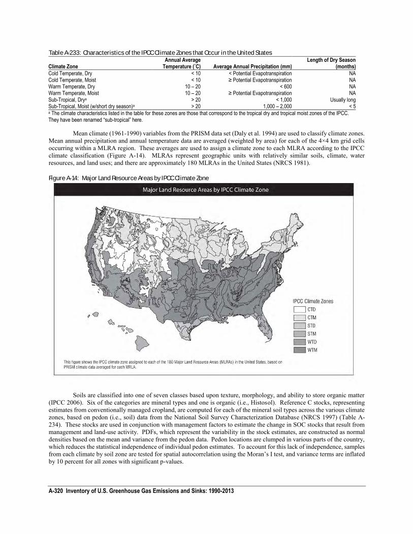
A-320 Inventory of U.S. Greenhouse Gas Emissions and Sinks: 1990-2013
Table A-233: Characteristics of the IPCC Climate Zones that Occur in the United States
Climate Zone Annual Average
Temperature (˚C) Average Annual Precipitation (mm) Length of Dry Season
(months)
Cold Temperate, Dry < 10 < Potential Evapotranspiration NA Cold Temperate, Moist < 10 ≥ Potential Evapotranspiration NA Warm Temperate, Dry 10 – 20 < 600 NA Warm Temperate, Moist 10 – 20 ≥ Potential Evapotranspiration NA Sub-Tropical, Drya > 20 < 1,000 Usually long Sub-Tropical, Moist (w/short dry season)a > 20 1,000 – 2,000 < 5 a The climate characteristics listed in the table for these zones are those that correspond to the tropical dry and tropical moist zones of the IPCC. They have been renamed “sub-tropical” here.
Mean climate (1961-1990) variables from the PRISM data set (Daly et al. 1994) are used to classify climate zones. Mean annual precipitation and annual temperature data are averaged (weighted by area) for each of the 4×4 km grid cells occurring within a MLRA region. These averages are used to assign a climate zone to each MLRA according to the IPCC climate classification (Figure A-14). MLRAs represent geographic units with relatively similar soils, climate, water resources, and land uses; and there are approximately 180 MLRAs in the United States (NRCS 1981). Figure A-14: Major Land Resource Areas by IPCC Climate Zone
Soils are classified into one of seven classes based upon texture, morphology, and ability to store organic matter (IPCC 2006). Six of the categories are mineral types and one is organic (i.e., Histosol). Reference C stocks, representing estimates from conventionally managed cropland, are computed for each of the mineral soil types across the various climate zones, based on pedon (i.e., soil) data from the National Soil Survey Characterization Database (NRCS 1997) (Table A-234). These stocks are used in conjunction with management factors to estimate the change in SOC stocks that result from management and land-use activity. PDFs, which represent the variability in the stock estimates, are constructed as normal densities based on the mean and variance from the pedon data. Pedon locations are clumped in various parts of the country, which reduces the statistical independence of individual pedon estimates. To account for this lack of independence, samples from each climate by soil zone are tested for spatial autocorrelation using the Moran’s I test, and variance terms are inflated by 10 percent for all zones with significant p-values.
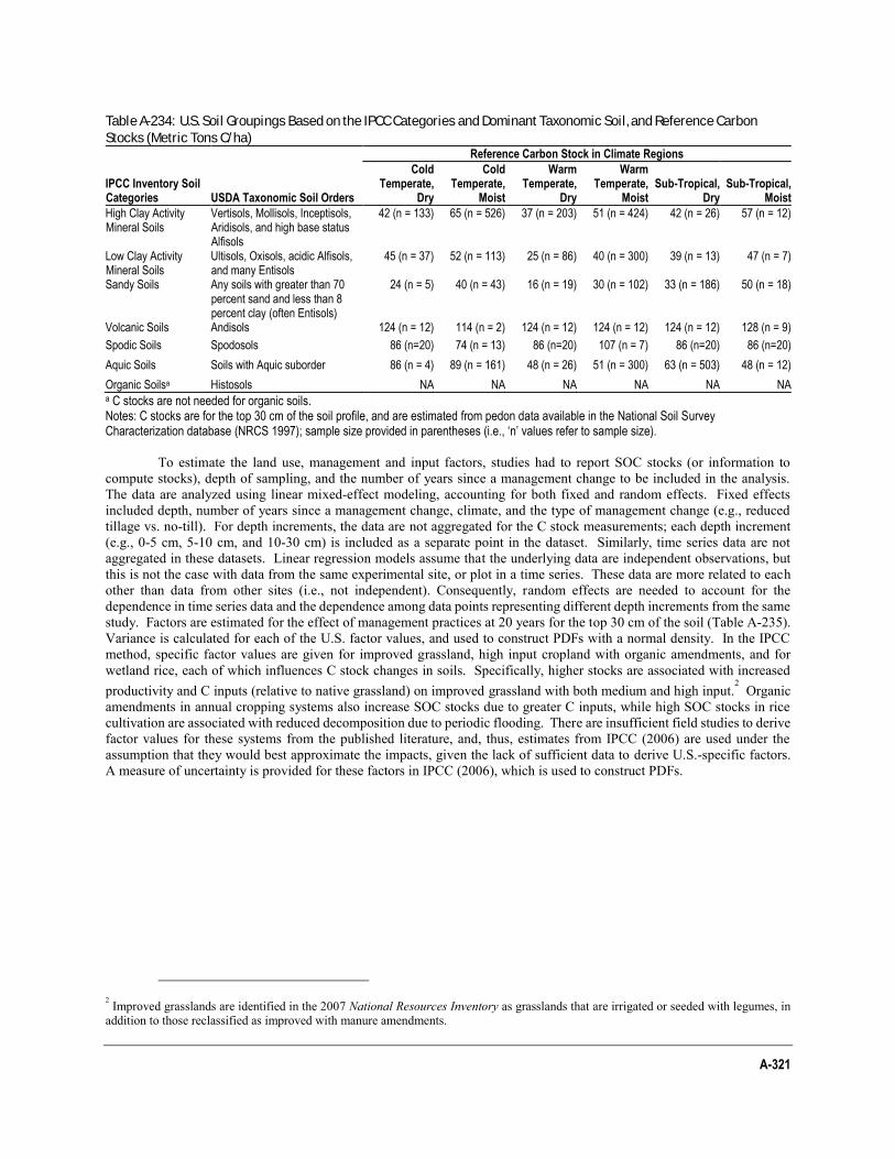
A-321
Table A-234: U.S. Soil Groupings Based on the IPCC Categories and Dominant Taxonomic Soil, and Reference Carbon
Stocks (Metric Tons C/ha)
IPCC Inventory Soil Categories USDA Taxonomic Soil Orders
Reference Carbon Stock in Climate Regions
Cold Temperate,
Dry
Cold Temperate,
Moist
Warm Temperate,
Dry
Warm Temperate,
Moist Sub-Tropical,
Dry Sub-Tropical,
Moist
High Clay Activity Mineral Soils
Vertisols, Mollisols, Inceptisols, Aridisols, and high base status Alfisols
42 (n = 133) 65 (n = 526) 37 (n = 203) 51 (n = 424) 42 (n = 26) 57 (n = 12)
Low Clay Activity Mineral Soils
Ultisols, Oxisols, acidic Alfisols, and many Entisols
45 (n = 37) 52 (n = 113) 25 (n = 86) 40 (n = 300) 39 (n = 13) 47 (n = 7)
Sandy Soils Any soils with greater than 70 percent sand and less than 8 percent clay (often Entisols)
24 (n = 5) 40 (n = 43) 16 (n = 19) 30 (n = 102) 33 (n = 186) 50 (n = 18)
Volcanic Soils Andisols 124 (n = 12) 114 (n = 2) 124 (n = 12) 124 (n = 12) 124 (n = 12) 128 (n = 9)
Spodic Soils Spodosols 86 (n=20) 74 (n = 13) 86 (n=20) 107 (n = 7) 86 (n=20) 86 (n=20)
Aquic Soils Soils with Aquic suborder 86 (n = 4) 89 (n = 161) 48 (n = 26) 51 (n = 300) 63 (n = 503) 48 (n = 12)
Organic Soilsa Histosols NA NA NA NA NA NA a C stocks are not needed for organic soils. Notes: C stocks are for the top 30 cm of the soil profile, and are estimated from pedon data available in the National Soil Survey Characterization database (NRCS 1997); sample size provided in parentheses (i.e., ‘n’ values refer to sample size).
To estimate the land use, management and input factors, studies had to report SOC stocks (or information to
compute stocks), depth of sampling, and the number of years since a management change to be included in the analysis. The data are analyzed using linear mixed-effect modeling, accounting for both fixed and random effects. Fixed effects included depth, number of years since a management change, climate, and the type of management change (e.g., reduced tillage vs. no-till). For depth increments, the data are not aggregated for the C stock measurements; each depth increment (e.g., 0-5 cm, 5-10 cm, and 10-30 cm) is included as a separate point in the dataset. Similarly, time series data are not aggregated in these datasets. Linear regression models assume that the underlying data are independent observations, but this is not the case with data from the same experimental site, or plot in a time series. These data are more related to each other than data from other sites (i.e., not independent). Consequently, random effects are needed to account for the dependence in time series data and the dependence among data points representing different depth increments from the same study. Factors are estimated for the effect of management practices at 20 years for the top 30 cm of the soil (Table A-235). Variance is calculated for each of the U.S. factor values, and used to construct PDFs with a normal density. In the IPCC method, specific factor values are given for improved grassland, high input cropland with organic amendments, and for wetland rice, each of which influences C stock changes in soils. Specifically, higher stocks are associated with increased productivity and C inputs (relative to native grassland) on improved grassland with both medium and high input.
2 Organic
amendments in annual cropping systems also increase SOC stocks due to greater C inputs, while high SOC stocks in rice cultivation are associated with reduced decomposition due to periodic flooding. There are insufficient field studies to derive factor values for these systems from the published literature, and, thus, estimates from IPCC (2006) are used under the assumption that they would best approximate the impacts, given the lack of sufficient data to derive U.S.-specific factors. A measure of uncertainty is provided for these factors in IPCC (2006), which is used to construct PDFs.
2 Improved grasslands are identified in the 2007 National Resources Inventory as grasslands that are irrigated or seeded with legumes, in addition to those reclassified as improved with manure amendments.
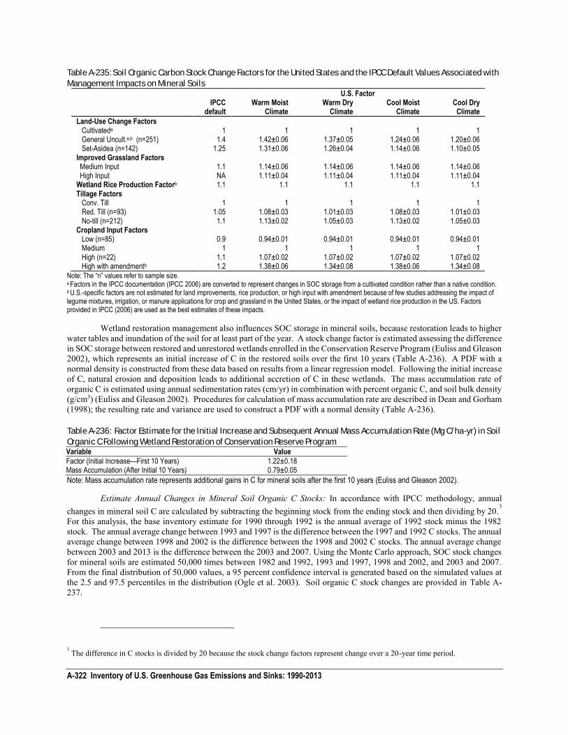
A-322 Inventory of U.S. Greenhouse Gas Emissions and Sinks: 1990-2013
Table A-235: Soil Organic Carbon Stock Change Factors for the United States and the IPCC Default Values Associated with
Management Impacts on Mineral Soils
U.S. Factor
IPCC default
Warm Moist Climate
Warm Dry Climate
Cool Moist Climate
Cool Dry Climate
Land-Use Change Factors
Cultivateda 1 1 1 1 1 General Uncult.a,b (n=251) 1.4 1.42±0.06 1.37±0.05 1.24±0.06 1.20±0.06 Set-Asidea (n=142) 1.25 1.31±0.06 1.26±0.04 1.14±0.06 1.10±0.05 Improved Grassland Factors Medium Input 1.1 1.14±0.06 1.14±0.06 1.14±0.06 1.14±0.06 High Input NA 1.11±0.04 1.11±0.04 1.11±0.04 1.11±0.04 Wetland Rice Production Factorb 1.1 1.1 1.1 1.1 1.1 Tillage Factors Conv. Till 1 1 1 1 1 Red. Till (n=93) 1.05 1.08±0.03 1.01±0.03 1.08±0.03 1.01±0.03 No-till (n=212) 1.1 1.13±0.02 1.05±0.03 1.13±0.02 1.05±0.03 Cropland Input Factors Low (n=85) 0.9 0.94±0.01 0.94±0.01 0.94±0.01 0.94±0.01 Medium 1 1 1 1 1 High (n=22) 1.1 1.07±0.02 1.07±0.02 1.07±0.02 1.07±0.02 High with amendmentb 1.2 1.38±0.06 1.34±0.08 1.38±0.06 1.34±0.08
Note: The “n” values refer to sample size. a Factors in the IPCC documentation (IPCC 2006) are converted to represent changes in SOC storage from a cultivated condition rather than a native condition. b U.S.-specific factors are not estimated for land improvements, rice production, or high input with amendment because of few studies addressing the impact of legume mixtures, irrigation, or manure applications for crop and grassland in the United States, or the impact of wetland rice production in the US. Factors provided in IPCC (2006) are used as the best estimates of these impacts.
Wetland restoration management also influences SOC storage in mineral soils, because restoration leads to higher water tables and inundation of the soil for at least part of the year. A stock change factor is estimated assessing the difference in SOC storage between restored and unrestored wetlands enrolled in the Conservation Reserve Program (Euliss and Gleason 2002), which represents an initial increase of C in the restored soils over the first 10 years (Table A-236). A PDF with a normal density is constructed from these data based on results from a linear regression model. Following the initial increase of C, natural erosion and deposition leads to additional accretion of C in these wetlands. The mass accumulation rate of organic C is estimated using annual sedimentation rates (cm/yr) in combination with percent organic C, and soil bulk density (g/cm3) (Euliss and Gleason 2002). Procedures for calculation of mass accumulation rate are described in Dean and Gorham (1998); the resulting rate and variance are used to construct a PDF with a normal density (Table A-236). Table A-236: Factor Estimate for the Initial Increase and Subsequent Annual Mass Accumulation Rate (Mg C/ha-yr) in Soil
Organic C Following Wetland Restoration of Conservation Reserve Program Variable Value
Factor (Initial Increase—First 10 Years) 1.22±0.18 Mass Accumulation (After Initial 10 Years) 0.79±0.05
Note: Mass accumulation rate represents additional gains in C for mineral soils after the first 10 years (Euliss and Gleason 2002).
Estimate Annual Changes in Mineral Soil Organic C Stocks: In accordance with IPCC methodology, annual changes in mineral soil C are calculated by subtracting the beginning stock from the ending stock and then dividing by 20.
3
For this analysis, the base inventory estimate for 1990 through 1992 is the annual average of 1992 stock minus the 1982 stock. The annual average change between 1993 and 1997 is the difference between the 1997 and 1992 C stocks. The annual average change between 1998 and 2002 is the difference between the 1998 and 2002 C stocks. The annual average change between 2003 and 2013 is the difference between the 2003 and 2007. Using the Monte Carlo approach, SOC stock changes for mineral soils are estimated 50,000 times between 1982 and 1992, 1993 and 1997, 1998 and 2002, and 2003 and 2007. From the final distribution of 50,000 values, a 95 percent confidence interval is generated based on the simulated values at the 2.5 and 97.5 percentiles in the distribution (Ogle et al. 2003). Soil organic C stock changes are provided in Table A-237.
3 The difference in C stocks is divided by 20 because the stock change factors represent change over a 20-year time period.
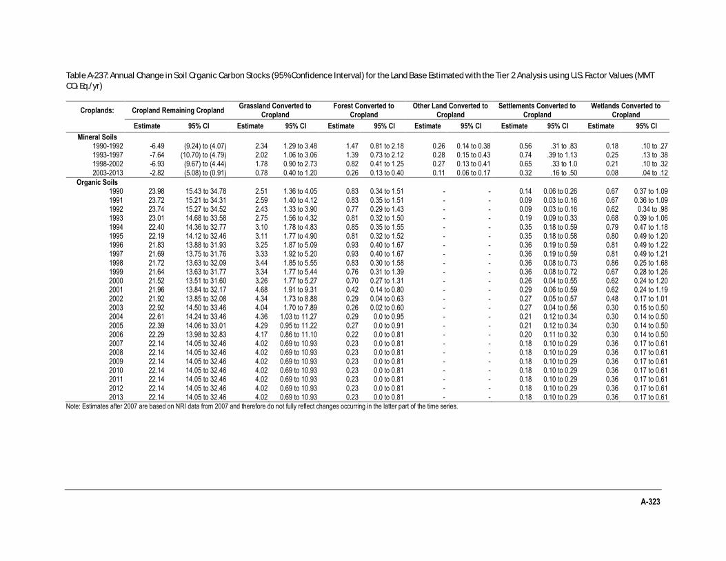
A-323
Table A-237: Annual Change in Soil Organic Carbon Stocks (95% Confidence Interval) for the Land Base Estimated with the Tier 2 Analysis using U.S. Factor Values (MMT
CO2 Eq./yr)
Croplands: Cropland Remaining Cropland Grassland Converted to
Cropland Forest Converted to
Cropland Other Land Converted to
Cropland Settlements Converted to
Cropland Wetlands Converted to
Cropland
Estimate 95% CI Estimate 95% CI Estimate 95% CI Estimate 95% CI Estimate 95% CI Estimate 95% CI
Mineral Soils 1990-1992 -6.49 (9.24) to (4.07) 2.34 1.29 to 3.48 1.47 0.81 to 2.18 0.26 0.14 to 0.38 0.56 .31 to .83 0.18 .10 to .27 1993-1997 -7.64 (10.70) to (4.79) 2.02 1.06 to 3.06 1.39 0.73 to 2.12 0.28 0.15 to 0.43 0.74 .39 to 1.13 0.25 .13 to .38 1998-2002 -6.93 (9.67) to (4.44) 1.78 0.90 to 2.73 0.82 0.41 to 1.25 0.27 0.13 to 0.41 0.65 .33 to 1.0 0.21 .10 to .32 2003-2013 -2.82 (5.08) to (0.91) 0.78 0.40 to 1.20 0.26 0.13 to 0.40 0.11 0.06 to 0.17 0.32 .16 to .50 0.08 .04 to .12
Organic Soils 1990 23.98 15.43 to 34.78 2.51 1.36 to 4.05 0.83 0.34 to 1.51 - - 0.14 0.06 to 0.26 0.67 0.37 to 1.09 1991 23.72 15.21 to 34.31 2.59 1.40 to 4.12 0.83 0.35 to 1.51 - - 0.09 0.03 to 0.16 0.67 0.36 to 1.09 1992 23.74 15.27 to 34.52 2.43 1.33 to 3.90 0.77 0.29 to 1.43 - - 0.09 0.03 to 0.16 0.62 0.34 to .98 1993 23.01 14.68 to 33.58 2.75 1.56 to 4.32 0.81 0.32 to 1.50 - - 0.19 0.09 to 0.33 0.68 0.39 to 1.06 1994 22.40 14.36 to 32.77 3.10 1.78 to 4.83 0.85 0.35 to 1.55 - - 0.35 0.18 to 0.59 0.79 0.47 to 1.18 1995 22.19 14.12 to 32.46 3.11 1.77 to 4.90 0.81 0.32 to 1.52 - - 0.35 0.18 to 0.58 0.80 0.49 to 1.20 1996 21.83 13.88 to 31.93 3.25 1.87 to 5.09 0.93 0.40 to 1.67 - - 0.36 0.19 to 0.59 0.81 0.49 to 1.22 1997 21.69 13.75 to 31.76 3.33 1.92 to 5.20 0.93 0.40 to 1.67 - - 0.36 0.19 to 0.59 0.81 0.49 to 1.21 1998 21.72 13.63 to 32.09 3.44 1.85 to 5.55 0.83 0.30 to 1.58 - - 0.36 0.08 to 0.73 0.86 0.25 to 1.68 1999 21.64 13.63 to 31.77 3.34 1.77 to 5.44 0.76 0.31 to 1.39 - - 0.36 0.08 to 0.72 0.67 0.28 to 1.26 2000 21.52 13.51 to 31.60 3.26 1.77 to 5.27 0.70 0.27 to 1.31 - - 0.26 0.04 to 0.55 0.62 0.24 to 1.20 2001 21.96 13.84 to 32.17 4.68 1.91 to 9.31 0.42 0.14 to 0.80 - - 0.29 0.06 to 0.59 0.62 0.24 to 1.19 2002 21.92 13.85 to 32.08 4.34 1.73 to 8.88 0.29 0.04 to 0.63 - - 0.27 0.05 to 0.57 0.48 0.17 to 1.01 2003 22.92 14.50 to 33.46 4.04 1.70 to 7.89 0.26 0.02 to 0.60 - - 0.27 0.04 to 0.56 0.30 0.15 to 0.50 2004 22.61 14.24 to 33.46 4.36 1.03 to 11.27 0.29 0.0 to 0.95 - - 0.21 0.12 to 0.34 0.30 0.14 to 0.50 2005 22.39 14.06 to 33.01 4.29 0.95 to 11.22 0.27 0.0 to 0.91 - - 0.21 0.12 to 0.34 0.30 0.14 to 0.50 2006 22.29 13.98 to 32.83 4.17 0.86 to 11.10 0.22 0.0 to 0.81 - - 0.20 0.11 to 0.32 0.30 0.14 to 0.50 2007 22.14 14.05 to 32.46 4.02 0.69 to 10.93 0.23 0.0 to 0.81 - - 0.18 0.10 to 0.29 0.36 0.17 to 0.61 2008 22.14 14.05 to 32.46 4.02 0.69 to 10.93 0.23 0.0 to 0.81 - - 0.18 0.10 to 0.29 0.36 0.17 to 0.61 2009 22.14 14.05 to 32.46 4.02 0.69 to 10.93 0.23 0.0 to 0.81 - - 0.18 0.10 to 0.29 0.36 0.17 to 0.61 2010 22.14 14.05 to 32.46 4.02 0.69 to 10.93 0.23 0.0 to 0.81 - - 0.18 0.10 to 0.29 0.36 0.17 to 0.61 2011 22.14 14.05 to 32.46 4.02 0.69 to 10.93 0.23 0.0 to 0.81 - - 0.18 0.10 to 0.29 0.36 0.17 to 0.61 2012 22.14 14.05 to 32.46 4.02 0.69 to 10.93 0.23 0.0 to 0.81 - - 0.18 0.10 to 0.29 0.36 0.17 to 0.61 2013 22.14 14.05 to 32.46 4.02 0.69 to 10.93 0.23 0.0 to 0.81 - - 0.18 0.10 to 0.29 0.36 0.17 to 0.61
Note: Estimates after 2007 are based on NRI data from 2007 and therefore do not fully reflect changes occurring in the latter part of the time series.

A-324 Inventory of U.S. Greenhouse Gas Emissions and Sinks: 1990-2013
Grasslands: Grassland Remaining
Grassland Cropland Converted to
Grassland Forest Converted to
Grassland Other Land Converted to
Grassland Settlements Converted to
Grassland Wetlands Converted to
Grassland
Estimate 95% CI Estimate 95% CI Estimate 95% CI Estimate 95% CI Estimate 95% CI Estimate 95% CI
Mineral Soils 1990-1992 -0.19 (0.38) to (0.03) -1.73 (2.41) to (1.06) -1.07 (1.51) to (0.67) -0.19 (0.27) to (0.12) -0.41 (0.58) to (0.26) -0.13 (0.19) to (0.08) 1993-1997 -0.08 (0.18) to 0.0 -1.56 (2.18) to (0.94) -1.06 (1.51) to (0.65) -0.21 (0.31) to (0.13) -0.56 (0.80) to (0.35) -0.19 (0.27) to (0.12) 1998-2002 -0.01 (0.08) to 0.06 -1.74 (2.47) to (1.03) -0.79 (1.14) to (0.47) -0.26 (0.37) to (0.15) -0.63 (0.91) to (0.38) -0.20 (0.29) to (0.12) 2003-2013 0.10 0.01 to 0.21 -1.28 (1.86) to (0.71) -0.42 (0.62) to (0.24) -0.18 (0.27) to (0.10) -0.52 (0.77) to (0.29) -0.13 (0.19) to (0.07)
Organic Soils 1990 4.60 2.54 to 7.33 0.54 0.24 to 0.98 0.11 0.03 to 0.23 - - 0.01 0.0 to 0.05 0.10 0.02 to 0.22 1991 4.50 2.47 to 7.19 0.50 0.22 to 0.92 0.11 0.03 to 0.24 0.02 0.0 to 0.05 0.01 0.0 to 0.05 0.10 0.02 to 0.22 1992 4.47 2.45 to 7.14 0.55 0.24 to 0.99 0.11 0.03 to 0.23 - - 0.01 0.0 to 0.05 0.10 0.01 to 0.24 1993 4.40 2.42 to 7.03 0.56 0.25 to 1.02 0.10 0.03 to 0.22 - - 0.02 0.0 to 0.06 0.11 0.03 to 0.24 1994 4.29 2.37 to 6.87 0.69 0.31 to 1.23 0.11 0.02 to 0.23 - - 0.02 0.0 to 0.06 0.16 0.07 to 0.31 1995 4.14 2.28 to 6.61 0.73 0.34 to 1.30 0.11 0.02 to 0.23 - - 0.02 0.0 to 0.06 0.17 0.07 to 0.32 1996 4.04 2.22 to 6.47 0.71 0.33 to 1.25 0.10 0.02 to 0.23 - - 0.02 0.0 to 0.06 0.17 0.07 to 0.32 1997 3.91 2.14 to 6.28 0.74 0.35 to 1.30 0.11 0.02 to 0.23 0.01 0.0 to 0.04 0.01 0.0 to 0.03 0.17 0.07 to 0.32 1998 3.80 1.96 to 6.32 0.89 0.40 to 1.63 0.10 0.0 to 0.27 - - 0.02 0.0 to 0.06 0.18 0.05 to 0.38 1999 3.73 1.92 to 6.25 0.89 0.40 to 1.62 0.10 0.0 to 0.27 - - 0.02 0.0 to 0.06 0.17 0.05 to 0.38 2000 3.69 1.91 to 6.14 0.88 0.40 to 1.62 0.09 0.0 to 0.23 - - 0.03 0.01 to 0.07 0.17 0.05 to 0.38 2001 3.28 1.76 to 5.33 0.94 0.42 to 1.70 0.08 0.0 to 0.22 - - 0.02 0.0 to 0.06 0.16 0.04 to 0.35 2002 3.24 1.72 to 5.24 1.05 0.45 to 1.96 0.05 0.0 to 0.16 - - 0.02 0.0 to 0.06 0.16 0.04 to 0.34 2003 3.08 1.66 to 4.97 0.92 0.39 to 1.73 0.05 0.0 to 0.16 0.01 .0 to 0.05 0.02 0.0 to 0.06 0.09 0.05 to 0.16 2004 3.05 1.66 to 4.90 1.03 0.39 to 2.03 0.07 0.0 to 0.24 - - 0.03 0.0 to 0.07 0.11 0.05 to 0.19 2005 3.06 1.67 to 4.91 1.05 0.40 to 2.05 0.07 0.0 to 0.24 - - 0.03 0.0 to 0.07 0.12 0.06 to 0.22 2006 2.97 1.59 to 4.81 0.97 0.36 to 1.93 0.07 0.0 to 0.24 - - 0.03 0.0 to 0.07 0.11 0.05 to 0.21 2007 3.03 1.62 to 4.93 0.90 0.33 to 1.78 0.07 0.0 to 0.24 - - 0.03 0.0 to 0.07 0.11 0.05 to 0.20 2008 3.03 1.62 to 4.93 0.90 0.33 to 1.78 0.07 0.0 to 0.24 - - 0.03 0.0 to 0.07 0.11 0.05 to 0.20 2009 3.03 1.62 to 4.93 0.90 0.33 to 1.78 0.07 0.0 to 0.24 - - 0.03 0.0 to 0.07 0.11 0.05 to 0.20 2010 3.03 1.62 to 4.93 0.90 0.33 to 1.78 0.07 0.0 to 0.24 - - 0.03 0.0 to 0.07 0.11 0.05 to 0.20 2011 3.03 1.62 to 4.93 0.90 0.33 to 1.78 0.07 0.0 to 0.24 - - 0.03 0.0 to 0.07 0.11 0.05 to 0.20 2012 3.03 1.62 to 4.93 0.90 0.33 to 1.78 0.07 0.0 to 0.24 - - 0.03 0.0 to 0.07 0.11 0.05 to 0.20 2013 3.03 1.62 to 4.93 0.90 0.33 to 1.78 0.07 0.0 to 0.24 - - 0.03 0.0 to 0.07 0.11 0.05 to 0.20
Note: Estimates after 2007 are based on NRI data from 2007 and therefore do not fully reflect changes occurring in the latter part of the time series.
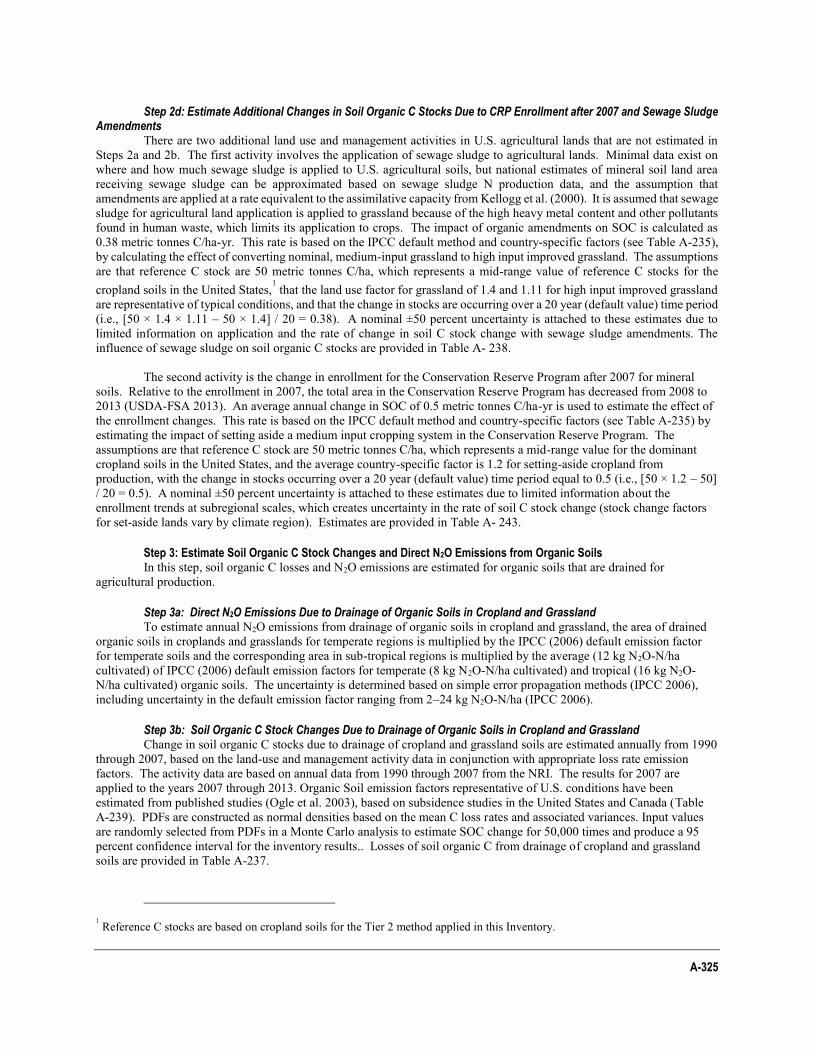
A-325
Step 2d: Estimate Additional Changes in Soil Organic C Stocks Due to CRP Enrollment after 2007 and Sewage Sludge Amendments
There are two additional land use and management activities in U.S. agricultural lands that are not estimated in Steps 2a and 2b. The first activity involves the application of sewage sludge to agricultural lands. Minimal data exist on where and how much sewage sludge is applied to U.S. agricultural soils, but national estimates of mineral soil land area receiving sewage sludge can be approximated based on sewage sludge N production data, and the assumption that amendments are applied at a rate equivalent to the assimilative capacity from Kellogg et al. (2000). It is assumed that sewage sludge for agricultural land application is applied to grassland because of the high heavy metal content and other pollutants found in human waste, which limits its application to crops. The impact of organic amendments on SOC is calculated as 0.38 metric tonnes C/ha-yr. This rate is based on the IPCC default method and country-specific factors (see Table A-235), by calculating the effect of converting nominal, medium-input grassland to high input improved grassland. The assumptions are that reference C stock are 50 metric tonnes C/ha, which represents a mid-range value of reference C stocks for the cropland soils in the United States,
1 that the land use factor for grassland of 1.4 and 1.11 for high input improved grassland
are representative of typical conditions, and that the change in stocks are occurring over a 20 year (default value) time period (i.e., [50 × 1.4 × 1.11 – 50 × 1.4] / 20 = 0.38). A nominal ±50 percent uncertainty is attached to these estimates due to limited information on application and the rate of change in soil C stock change with sewage sludge amendments. The influence of sewage sludge on soil organic C stocks are provided in Table A- 238.
The second activity is the change in enrollment for the Conservation Reserve Program after 2007 for mineral
soils. Relative to the enrollment in 2007, the total area in the Conservation Reserve Program has decreased from 2008 to 2013 (USDA-FSA 2013). An average annual change in SOC of 0.5 metric tonnes C/ha-yr is used to estimate the effect of the enrollment changes. This rate is based on the IPCC default method and country-specific factors (see Table A-235) by estimating the impact of setting aside a medium input cropping system in the Conservation Reserve Program. The assumptions are that reference C stock are 50 metric tonnes C/ha, which represents a mid-range value for the dominant cropland soils in the United States, and the average country-specific factor is 1.2 for setting-aside cropland from production, with the change in stocks occurring over a 20 year (default value) time period equal to 0.5 (i.e., [50 × 1.2 – 50] / 20 = 0.5). A nominal ±50 percent uncertainty is attached to these estimates due to limited information about the enrollment trends at subregional scales, which creates uncertainty in the rate of soil C stock change (stock change factors for set-aside lands vary by climate region). Estimates are provided in Table A- 243.
Step 3: Estimate Soil Organic C Stock Changes and Direct N2O Emissions from Organic Soils In this step, soil organic C losses and N2O emissions are estimated for organic soils that are drained for
agricultural production.
Step 3a: Direct N2O Emissions Due to Drainage of Organic Soils in Cropland and Grassland To estimate annual N2O emissions from drainage of organic soils in cropland and grassland, the area of drained
organic soils in croplands and grasslands for temperate regions is multiplied by the IPCC (2006) default emission factor for temperate soils and the corresponding area in sub-tropical regions is multiplied by the average (12 kg N2O-N/ha cultivated) of IPCC (2006) default emission factors for temperate (8 kg N2O-N/ha cultivated) and tropical (16 kg N2O-N/ha cultivated) organic soils. The uncertainty is determined based on simple error propagation methods (IPCC 2006), including uncertainty in the default emission factor ranging from 2–24 kg N2O-N/ha (IPCC 2006).
Step 3b: Soil Organic C Stock Changes Due to Drainage of Organic Soils in Cropland and Grassland Change in soil organic C stocks due to drainage of cropland and grassland soils are estimated annually from 1990
through 2007, based on the land-use and management activity data in conjunction with appropriate loss rate emission factors. The activity data are based on annual data from 1990 through 2007 from the NRI. The results for 2007 are applied to the years 2007 through 2013. Organic Soil emission factors representative of U.S. conditions have been estimated from published studies (Ogle et al. 2003), based on subsidence studies in the United States and Canada (Table A-239). PDFs are constructed as normal densities based on the mean C loss rates and associated variances. Input values are randomly selected from PDFs in a Monte Carlo analysis to estimate SOC change for 50,000 times and produce a 95 percent confidence interval for the inventory results.. Losses of soil organic C from drainage of cropland and grassland soils are provided in Table A-237.
1 Reference C stocks are based on cropland soils for the Tier 2 method applied in this Inventory.
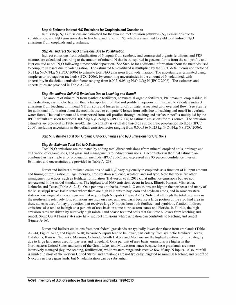
A-326 Inventory of U.S. Greenhouse Gas Emissions and Sinks: 1990-2013
Step 4: Estimate Indirect N2O Emissions for Croplands and Grasslands In this step, N2O emissions are estimated for the two indirect emission pathways (N2O emissions due to
volatilization, and N2O emissions due to leaching and runoff of N), which are summed to yield total indirect N2O emissions from croplands and grasslands.
Step 4a: Indirect Soil N2O Emissions Due to Volatilization Indirect emissions from volatilization of N inputs from synthetic and commercial organic fertilizers, and PRP
manure, are calculated according to the amount of mineral N that is transported in gaseous forms from the soil profile and later emitted as soil N2O following atmospheric deposition. See Step 1e for additional information about the methods used to compute N losses due to volatilization. The estimated N volatilized is multiplied by the IPCC default emission factor of 0.01 kg N2O-N/kg N (IPCC 2006) to estimate total N2O emissions from volatilization. The uncertainty is estimated using simple error propagation methods (IPCC 2006), by combining uncertainties in the amount of N volatilized, with uncertainty in the default emission factor ranging from 0.002–0.05 kg N2O-N/kg N (IPCC 2006). The estimates and uncertainties are provided in Table A- 240.
Step 4b: Indirect Soil N2O Emissions Due to Leaching and Runoff The amount of mineral N from synthetic fertilizers, commercial organic fertilizers, PRP manure, crop residue, N
mineralization, asymbiotic fixation that is transported from the soil profile in aqueous form is used to calculate indirect emissions from leaching of mineral N from soils and losses in runoff of water associated with overland flow. See Step 1e for additional information about the methods used to compute N losses from soils due to leaching and runoff in overland water flows. The total amount of N transported from soil profiles through leaching and surface runoff is multiplied by the IPCC default emission factor of 0.0075 kg N2O-N/kg N (IPCC 2006) to estimate emissions for this source. The emission estimates are provided in Table A-242. The uncertainty is estimated based on simple error propagation methods (IPCC 2006), including uncertainty in the default emission factor ranging from 0.0005 to 0.025 kg N2O-N/kg N (IPCC 2006).
Step 5: Estimate Total Soil Organic C Stock Changes and N2O Emissions for U.S. Soils Step 5a: Estimate Total Soil N2O Emissions Total N2O emissions are estimated by adding total direct emissions (from mineral cropland soils, drainage and
cultivation of organic soils, and grassland management) to indirect emissions. Uncertainties in the final estimate are combined using simple error propagation methods (IPCC 2006), and expressed as a 95 percent confidence interval. Estimates and uncertainties are provided in Table A- 238.
Direct and indirect simulated emissions of soil N2O vary regionally in croplands as a function of N input amount
and timing of fertilization, tillage intensity, crop rotation sequence, weather, and soil type. Note that there are other management practices, such as fertilizer formulation (Halvorson et al. 2013), that influence emissions but are not represented in the model simulations. The highest total N2O emissions occur in Iowa, Illinois, Kansas, Minnesota, Nebraska and Texas (Table A- 243). On a per area unit basis, direct N2O emissions are high in the northeast and many of the Mississippi River Basin states where there are high N inputs to hay, corn and soybean crops, and in some western states where irrigated crops are grown that require high N inputs (Figure A-15). Note that although the total crop area in the northeast is relatively low, emissions are high on a per unit area basis because a large portion of the cropland area in these states is used for hay production that receives large N inputs from both fertilizer and symbiotic fixation. Indirect emissions also tend to be high on a per unit of area basis in some northeastern states and Florida. In Florida, the high emission rates are driven by relatively high rainfall and coarse textured soils that facilitate N losses from leaching and runoff. Some Great Plains states also have indirect emissions where irrigation can contribute to leaching and runoff (Figure A-16).
Direct and indirect emissions from non-federal grasslands are typically lower than those from croplands (Table
A- 244, Figure A-17, and Figure A-18) because N inputs tend to be lower, particularly from synthetic fertilizer. Texas, Oklahoma, Kansas, Nebraska, Missouri, Colorado, South Dakota and Montana are the highest emitters for this category due to large land areas used for pastures and rangeland. On a per unit of area basis, emissions are higher in the Northeastern United States and some of the Great Lakes and Midwestern states because these grasslands are more intensively managed (legume seeding, fertilization) while western rangelands receive few, if any, N inputs. Also, rainfall is limited in most of the western United States, and grasslands are not typically irrigated so minimal leaching and runoff of N occurs in these grasslands, but N volatilization can be substantial.
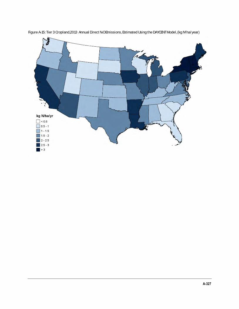
A-327
Figure A-15: Tier 3 Cropland,2013 Annual Direct N2O Emissions, Estimated Using the DAYCENT Model, (kg N/ha/year)
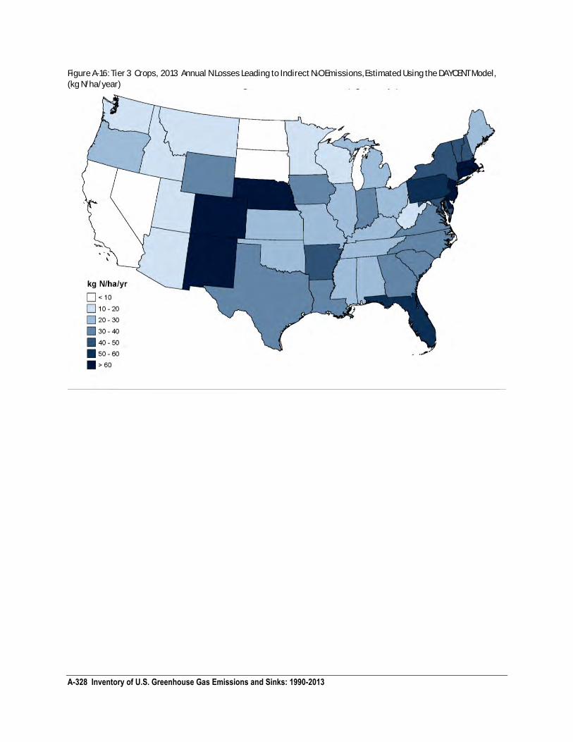
A-328 Inventory of U.S. Greenhouse Gas Emissions and Sinks: 1990-2013
Figure A-16: Tier 3 Crops, 2013 Annual N Losses Leading to Indirect N2O Emissions, Estimated Using the DAYCENT Model,
(kg N/ha/year)
A-329
Figure A-17: Non-federal Grasslands, 2013 Annual Direct N2O Emissions, Estimated Using the DAYCENT Model, (kg
N/ha/year)
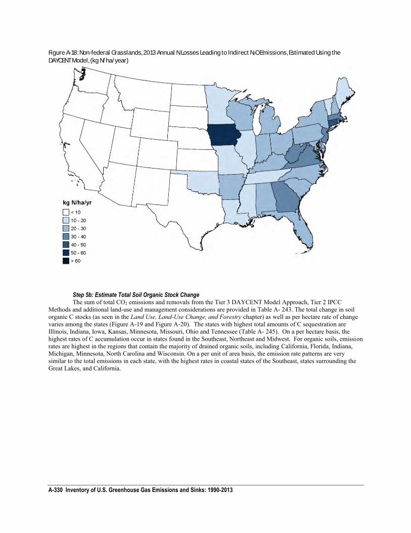
A-330 Inventory of U.S. Greenhouse Gas Emissions and Sinks: 1990-2013
Figure A-18: Non-federal Grasslands, 2013 Annual N Losses Leading to Indirect N2O Emissions, Estimated Using the
DAYCENT Model, (kg N/ha/year)
Step 5b: Estimate Total Soil Organic Stock Change The sum of total CO2 emissions and removals from the Tier 3 DAYCENT Model Approach, Tier 2 IPCC
Methods and additional land-use and management considerations are provided in Table A- 243. The total change in soil organic C stocks (as seen in the Land Use, Land-Use Change, and Forestry chapter) as well as per hectare rate of change varies among the states (Figure A-19 and Figure A-20). The states with highest total amounts of C sequestration are Illinois, Indiana, Iowa, Kansas, Minnesota, Missouri, Ohio and Tennessee (Table A- 245). On a per hectare basis, the highest rates of C accumulation occur in states found in the Southeast, Northeast and Midwest. For organic soils, emission rates are highest in the regions that contain the majority of drained organic soils, including California, Florida, Indiana, Michigan, Minnesota, North Carolina and Wisconsin. On a per unit of area basis, the emission rate patterns are very similar to the total emissions in each state, with the highest rates in coastal states of the Southeast, states surrounding the Great Lakes, and California.
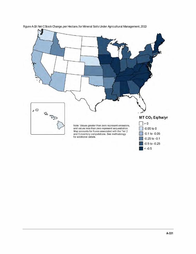
A-331
Figure A-19: Net C Stock Change, per Hectare, for Mineral Soils Under Agricultural Management, 2013
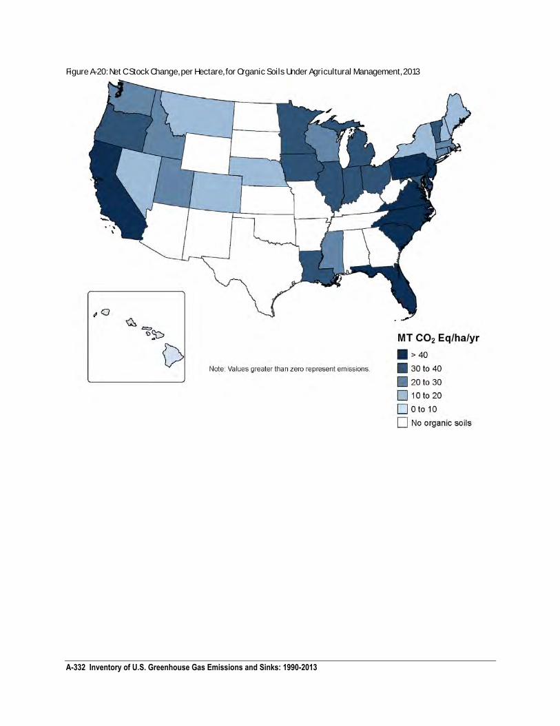
A-332 Inventory of U.S. Greenhouse Gas Emissions and Sinks: 1990-2013
Figure A-20: Net C Stock Change, per Hectare, for Organic Soils Under Agricultural Management, 2013
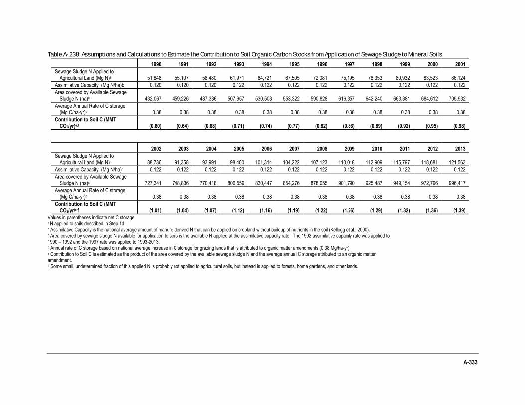
A-333
Table A- 238: Assumptions and Calculations to Estimate the Contribution to Soil Organic Carbon Stocks from Application of Sewage Sludge to Mineral Soils
1990 1991 1992 1993 1994 1995 1996 1997 1998 1999 2000 2001
Sewage Sludge N Applied to Agricultural Land (Mg N)a 51,848 55,107 58,480 61,971 64,721 67,505 72,081 75,195 78,353 80,932 83,523 86,124
Assimilative Capacity (Mg N/ha)b 0.120 0.120 0.120 0.122 0.122 0.122 0.122 0.122 0.122 0.122 0.122 0.122
Area covered by Available Sewage Sludge N (ha)c 432,067 459,226 487,336 507,957 530,503 553,322 590,828 616,357 642,240 663,381 684,612 705,932
Average Annual Rate of C storage (Mg C/ha-yr)d 0.38 0.38 0.38 0.38 0.38 0.38 0.38 0.38 0.38 0.38 0.38 0.38
Contribution to Soil C (MMT CO2/yr)e,f (0.60) (0.64) (0.68) (0.71) (0.74) (0.77) (0.82) (0.86) (0.89) (0.92) (0.95) (0.98)
2002 2003 2004 2005 2006 2007 2008 2009 2010 2011 2012 2013
Sewage Sludge N Applied to Agricultural Land (Mg N)a 88,736 91,358 93,991 98,400 101,314 104,222 107,123 110,018 112,909 115,797 118,681 121,563
Assimilative Capacity (Mg N/ha)b 0.122 0.122 0.122 0.122 0.122 0.122 0.122 0.122 0.122 0.122 0.122 0.122
Area covered by Available Sewage Sludge N (ha)c 727,341 748,836 770,418 806,559 830,447 854,276 878,055 901,790 925,487 949,154 972,796 996,417
Average Annual Rate of C storage (Mg C/ha-yr)d 0.38 0.38 0.38 0.38 0.38 0.38 0.38 0.38 0.38 0.38 0.38 0.38
Contribution to Soil C (MMT CO2/yr)e,f (1.01) (1.04) (1.07) (1.12) (1.16) (1.19) (1.22) (1.26) (1.29) (1.32) (1.36) (1.39)
Values in parentheses indicate net C storage. a N applied to soils described in Step 1d. b Assimilative Capacity is the national average amount of manure-derived N that can be applied on cropland without buildup of nutrients in the soil (Kellogg et al., 2000). c Area covered by sewage sludge N available for application to soils is the available N applied at the assimilative capacity rate. The 1992 assimilative capacity rate was applied to 1990 – 1992 and the 1997 rate was applied to 1993-2013. d Annual rate of C storage based on national average increase in C storage for grazing lands that is attributed to organic matter amendments (0.38 Mg/ha-yr) e Contribution to Soil C is estimated as the product of the area covered by the available sewage sludge N and the average annual C storage attributed to an organic matter amendment.
f Some small, undetermined fraction of this applied N is probably not applied to agricultural soils, but instead is applied to forests, home gardens, and other lands.
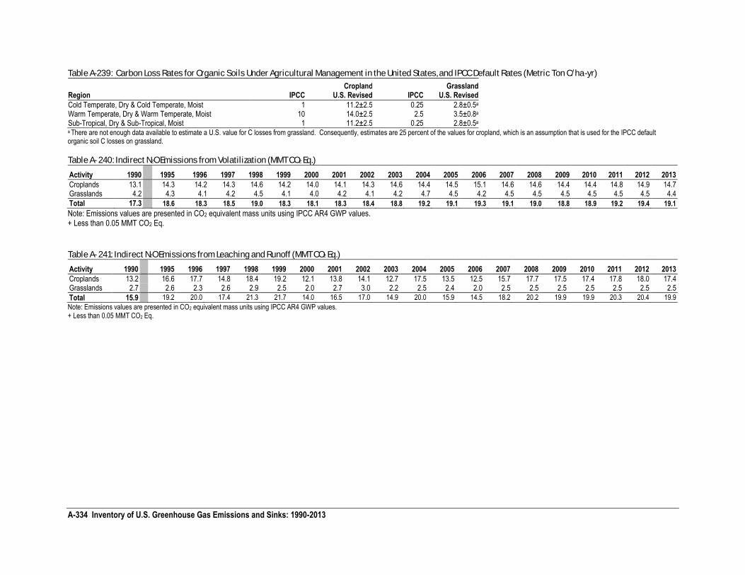
A-334 Inventory of U.S. Greenhouse Gas Emissions and Sinks: 1990-2013
Table A-239: Carbon Loss Rates for Organic Soils Under Agricultural Management in the United States, and IPCC Default Rates (Metric Ton C/ha-yr)
Cropland Grassland Region IPCC U.S. Revised IPCC U.S. Revised
Cold Temperate, Dry & Cold Temperate, Moist 1 11.2±2.5 0.25 2.8±0.5a Warm Temperate, Dry & Warm Temperate, Moist 10 14.0±2.5 2.5 3.5±0.8a Sub-Tropical, Dry & Sub-Tropical, Moist 1 11.2±2.5 0.25 2.8±0.5a a There are not enough data available to estimate a U.S. value for C losses from grassland. Consequently, estimates are 25 percent of the values for cropland, which is an assumption that is used for the IPCC default organic soil C losses on grassland.
Table A- 240: Indirect N2O Emissions from Volatilization (MMT CO2 Eq.)
Activity 1990 1995 1996 1997 1998 1999 2000 2001 2002 2003 2004 2005 2006 2007 2008 2009 2010 2011 2012 2013
Croplands 13.1 14.3 14.2 14.3 14.6 14.2 14.0 14.1 14.3 14.6 14.4 14.5 15.1 14.6 14.6 14.4 14.4 14.8 14.9 14.7 Grasslands 4.2 4.3 4.1 4.2 4.5 4.1 4.0 4.2 4.1 4.2 4.7 4.5 4.2 4.5 4.5 4.5 4.5 4.5 4.5 4.4
Total 17.3 18.6 18.3 18.5 19.0 18.3 18.1 18.3 18.4 18.8 19.2 19.1 19.3 19.1 19.0 18.8 18.9 19.2 19.4 19.1
Note: Emissions values are presented in CO2 equivalent mass units using IPCC AR4 GWP values. + Less than 0.05 MMT CO2 Eq.
Table A- 241: Indirect N2O Emissions from Leaching and Runoff (MMT CO2 Eq.)
Activity 1990 1995 1996 1997 1998 1999 2000 2001 2002 2003 2004 2005 2006 2007 2008 2009 2010 2011 2012 2013
Croplands 13.2 16.6 17.7 14.8 18.4 19.2 12.1 13.8 14.1 12.7 17.5 13.5 12.5 15.7 17.7 17.5 17.4 17.8 18.0 17.4 Grasslands 2.7 2.6 2.3 2.6 2.9 2.5 2.0 2.7 3.0 2.2 2.5 2.4 2.0 2.5 2.5 2.5 2.5 2.5 2.5 2.5
Total 15.9 19.2 20.0 17.4 21.3 21.7 14.0 16.5 17.0 14.9 20.0 15.9 14.5 18.2 20.2 19.9 19.9 20.3 20.4 19.9
Note: Emissions values are presented in CO2 equivalent mass units using IPCC AR4 GWP values. + Less than 0.05 MMT CO2 Eq.
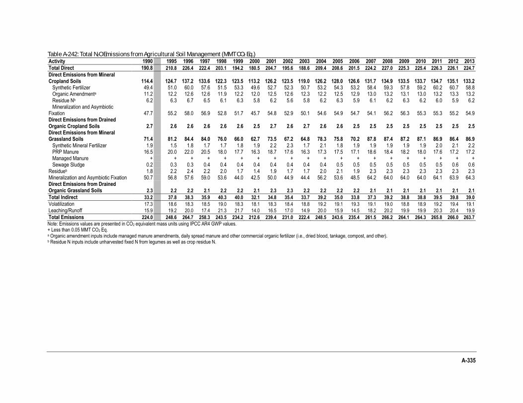
A-335
Table A-242: Total N2O Emissions from Agricultural Soil Management (MMT CO2 Eq.) Activity 1990 1995 1996 1997 1998 1999 2000 2001 2002 2003 2004 2005 2006 2007 2008 2009 2010 2011 2012 2013
Total Direct 190.8 210.8 226.4 222.4 203.1 194.2 180.5 204.7 195.6 188.6 209.4 208.6 201.5 224.2 227.0 225.3 225.4 226.3 226.1 224.7
Direct Emissions from Mineral Cropland Soils 114.4 124.7 137.2 133.6 122.3 123.5 113.2 126.2 123.5 119.0 126.2 128.0 126.6 131.7 134.9 133.5 133.7 134.7 135.1 133.2 Synthetic Fertilizer 49.4 51.0 60.0 57.6 51.5 53.3 49.6 52.7 52.3 50.7 53.2 54.3 53.2 58.4 59.3 57.8 59.2 60.2 60.7 58.8 Organic Amendmenta 11.2 12.2 12.6 12.6 11.9 12.2 12.0 12.5 12.6 12.3 12.2 12.5 12.9 13.0 13.2 13.1 13.0 13.2 13.3 13.2 Residue Nb 6.2 6.3 6.7 6.5 6.1 6.3 5.8 6.2 5.6 5.8 6.2 6.3 5.9 6.1 6.2 6.3 6.2 6.0 5.9 6.2 Mineralization and Asymbiotic Fixation 47.7 55.2 58.0 56.9 52.8 51.7 45.7 54.8 52.9 50.1 54.6 54.9 54.7 54.1 56.2 56.3 55.3 55.3 55.2 54.9 Direct Emissions from Drained Organic Cropland Soils 2.7 2.6 2.6 2.6 2.6 2.6 2.5 2.7 2.6 2.7 2.6 2.6 2.5 2.5 2.5 2.5 2.5 2.5 2.5 2.5 Direct Emissions from Mineral Grassland Soils 71.4 81.2 84.4 84.0 76.0 66.0 62.7 73.5 67.2 64.8 78.3 75.8 70.2 87.8 87.4 87.2 87.1 86.9 86.4 86.9 Synthetic Mineral Fertilizer 1.9 1.5 1.8 1.7 1.7 1.8 1.9 2.2 2.3 1.7 2.1 1.8 1.9 1.9 1.9 1.9 1.9 2.0 2.1 2.2 PRP Manure 16.5 20.0 22.0 20.5 18.0 17.7 16.3 18.7 17.6 16.3 17.3 17.5 17.1 18.6 18.4 18.2 18.0 17.6 17.2 17.2 Managed Manure + + + + + + + + + + + + + + + + + + + + Sewage Sludge 0.2 0.3 0.3 0.4 0.4 0.4 0.4 0.4 0.4 0.4 0.4 0.5 0.5 0.5 0.5 0.5 0.5 0.5 0.6 0.6 Residueb 1.8 2.2 2.4 2.2 2.0 1.7 1.4 1.9 1.7 1.7 2.0 2.1 1.9 2.3 2.3 2.3 2.3 2.3 2.3 2.3 Mineralization and Asymbiotic Fixation 50.7 56.8 57.6 59.0 53.6 44.0 42.5 50.0 44.9 44.4 56.2 53.6 48.5 64.2 64.0 64.0 64.0 64.1 63.9 64.3 Direct Emissions from Drained Organic Grassland Soils 2.3 2.2 2.2 2.1 2.2 2.2 2.1 2.3 2.3 2.2 2.2 2.2 2.2 2.1 2.1 2.1 2.1 2.1 2.1 2.1
Total Indirect 33.2 37.8 38.3 35.9 40.3 40.0 32.1 34.8 35.4 33.7 39.2 35.0 33.8 37.3 39.2 38.8 38.8 39.5 39.8 39.0
Volatilization 17.3 18.6 18.3 18.5 19.0 18.3 18.1 18.3 18.4 18.8 19.2 19.1 19.3 19.1 19.0 18.8 18.9 19.2 19.4 19.1
Leaching/Runoff 15.9 19.2 20.0 17.4 21.3 21.7 14.0 16.5 17.0 14.9 20.0 15.9 14.5 18.2 20.2 19.9 19.9 20.3 20.4 19.9
Total Emissions 224.0 248.6 264.7 258.3 243.5 234.2 212.6 239.4 231.0 222.4 248.5 243.6 235.4 261.5 266.2 264.1 264.3 265.8 266.0 263.7
Note: Emissions values are presented in CO2 equivalent mass units using IPCC AR4 GWP values. + Less than 0.05 MMT CO2 Eq. a Organic amendment inputs include managed manure amendments, daily spread manure and other commercial organic fertilizer (i.e., dried blood, tankage, compost, and other). b Residue N inputs include unharvested fixed N from legumes as well as crop residue N.
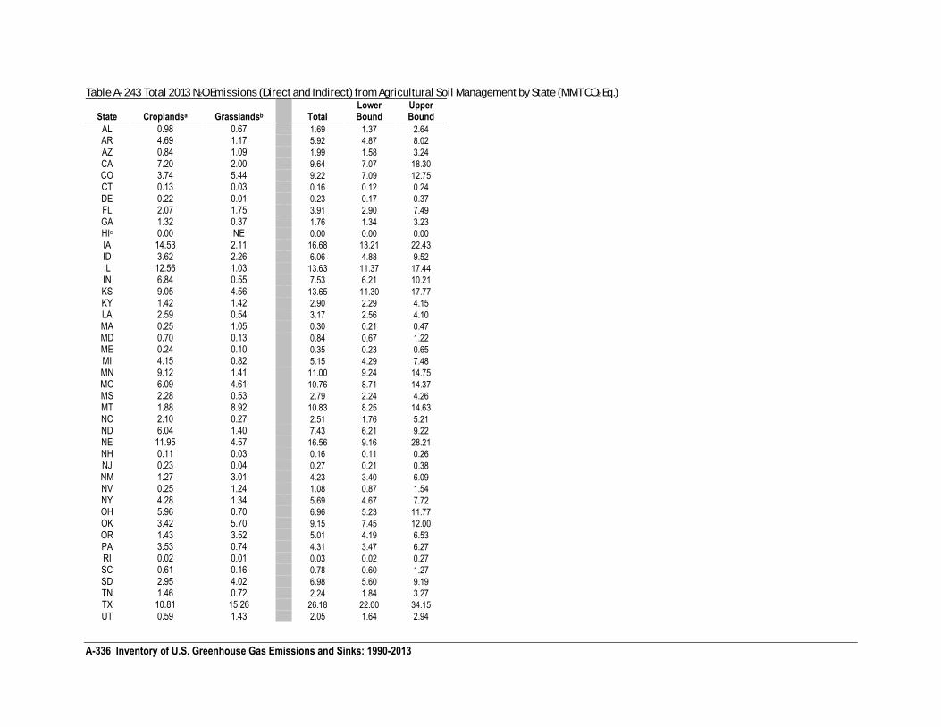
A-336 Inventory of U.S. Greenhouse Gas Emissions and Sinks: 1990-2013
Table A- 243 Total 2013 N2O Emissions (Direct and Indirect) from Agricultural Soil Management by State (MMT CO2 Eq.)
State Croplandsa Grasslandsb Total Lower Bound
Upper Bound
AL 0.98 0.67 1.69 1.37 2.64
AR 4.69 1.17 5.92 4.87 8.02
AZ 0.84 1.09 1.99 1.58 3.24
CA 7.20 2.00 9.64 7.07 18.30
CO 3.74 5.44 9.22 7.09 12.75
CT 0.13 0.03 0.16 0.12 0.24
DE 0.22 0.01 0.23 0.17 0.37
FL 2.07 1.75 3.91 2.90 7.49
GA 1.32 0.37 1.76 1.34 3.23
HIc 0.00 NE 0.00 0.00 0.00
IA 14.53 2.11 16.68 13.21 22.43
ID 3.62 2.26 6.06 4.88 9.52
IL 12.56 1.03 13.63 11.37 17.44
IN 6.84 0.55 7.53 6.21 10.21
KS 9.05 4.56 13.65 11.30 17.77
KY 1.42 1.42 2.90 2.29 4.15
LA 2.59 0.54 3.17 2.56 4.10
MA 0.25 1.05 0.30 0.21 0.47
MD 0.70 0.13 0.84 0.67 1.22
ME 0.24 0.10 0.35 0.23 0.65
MI 4.15 0.82 5.15 4.29 7.48
MN 9.12 1.41 11.00 9.24 14.75
MO 6.09 4.61 10.76 8.71 14.37
MS 2.28 0.53 2.79 2.24 4.26
MT 1.88 8.92 10.83 8.25 14.63
NC 2.10 0.27 2.51 1.76 5.21
ND 6.04 1.40 7.43 6.21 9.22
NE 11.95 4.57 16.56 9.16 28.21
NH 0.11 0.03 0.16 0.11 0.26
NJ 0.23 0.04 0.27 0.21 0.38
NM 1.27 3.01 4.23 3.40 6.09
NV 0.25 1.24 1.08 0.87 1.54
NY 4.28 1.34 5.69 4.67 7.72
OH 5.96 0.70 6.96 5.23 11.77
OK 3.42 5.70 9.15 7.45 12.00
OR 1.43 3.52 5.01 4.19 6.53
PA 3.53 0.74 4.31 3.47 6.27
RI 0.02 0.01 0.03 0.02 0.27
SC 0.61 0.16 0.78 0.60 1.27
SD 2.95 4.02 6.98 5.60 9.19
TN 1.46 0.72 2.24 1.84 3.27
TX 10.81 15.26 26.18 22.00 34.15
UT 0.59 1.43 2.05 1.64 2.94
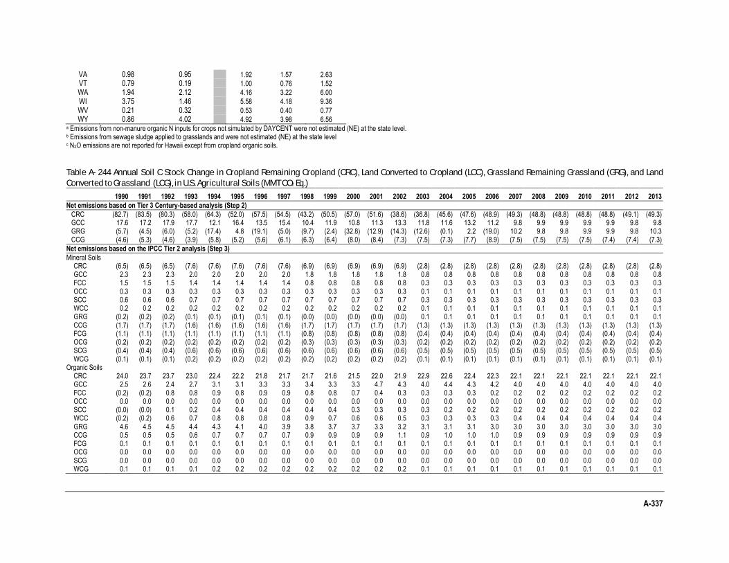
A-337
a Emissions from non-manure organic N inputs for crops not simulated by DAYCENT were not estimated (NE) at the state level. b Emissions from sewage sludge applied to grasslands and were not estimated (NE) at the state level c N2O emissions are not reported for Hawaii except from cropland organic soils.
Table A- 244 Annual Soil C Stock Change in Cropland Remaining Cropland (CRC), Land Converted to Cropland (LCC), Grassland Remaining Grassland (GRG), and Land
Converted to Grassland (LCG), in U.S. Agricultural Soils (MMT CO2 Eq.)
1990 1991 1992 1993 1994 1995 1996 1997 1998 1999 2000 2001 2002 2003 2004 2005 2006 2007 2008 2009 2010 2011 2012 2013
Net emissions based on Tier 3 Century-based analysis (Step 2)
CRC (82.7) (83.5) (80.3) (58.0) (64.3) (52.0) (57.5) (54.5) (43.2) (50.5) (57.0) (51.6) (38.6) (36.8) (45.6) (47.6) (48.9) (49.3) (48.8) (48.8) (48.8) (48.8) (49.1) (49.3) GCC 17.6 17.2 17.9 17.7 12.1 16.4 13.5 15.4 10.4 11.9 10.8 11.3 13.3 11.8 11.6 13.2 11.2 9.8 9.9 9.9 9.9 9.9 9.8 9.8 GRG (5.7) (4.5) (6.0) (5.2) (17.4) 4.8 (19.1) (5.0) (9.7) (2.4) (32.8) (12.9) (14.3) (12.6) (0.1) 2.2 (19.0) 10.2 9.8 9.8 9.9 9.9 9.8 10.3 CCG (4.6) (5.3) (4.6) (3.9) (5.8) (5.2) (5.6) (6.1) (6.3) (6.4) (8.0) (8.4) (7.3) (7.5) (7.3) (7.7) (8.9) (7.5) (7.5) (7.5) (7.5) (7.4) (7.4) (7.3)
Net emissions based on the IPCC Tier 2 analysis (Step 3)
Mineral Soils CRC (6.5) (6.5) (6.5) (7.6) (7.6) (7.6) (7.6) (7.6) (6.9) (6.9) (6.9) (6.9) (6.9) (2.8) (2.8) (2.8) (2.8) (2.8) (2.8) (2.8) (2.8) (2.8) (2.8) (2.8) GCC 2.3 2.3 2.3 2.0 2.0 2.0 2.0 2.0 1.8 1.8 1.8 1.8 1.8 0.8 0.8 0.8 0.8 0.8 0.8 0.8 0.8 0.8 0.8 0.8 FCC 1.5 1.5 1.5 1.4 1.4 1.4 1.4 1.4 0.8 0.8 0.8 0.8 0.8 0.3 0.3 0.3 0.3 0.3 0.3 0.3 0.3 0.3 0.3 0.3 OCC 0.3 0.3 0.3 0.3 0.3 0.3 0.3 0.3 0.3 0.3 0.3 0.3 0.3 0.1 0.1 0.1 0.1 0.1 0.1 0.1 0.1 0.1 0.1 0.1 SCC 0.6 0.6 0.6 0.7 0.7 0.7 0.7 0.7 0.7 0.7 0.7 0.7 0.7 0.3 0.3 0.3 0.3 0.3 0.3 0.3 0.3 0.3 0.3 0.3 WCC 0.2 0.2 0.2 0.2 0.2 0.2 0.2 0.2 0.2 0.2 0.2 0.2 0.2 0.1 0.1 0.1 0.1 0.1 0.1 0.1 0.1 0.1 0.1 0.1 GRG (0.2) (0.2) (0.2) (0.1) (0.1) (0.1) (0.1) (0.1) (0.0) (0.0) (0.0) (0.0) (0.0) 0.1 0.1 0.1 0.1 0.1 0.1 0.1 0.1 0.1 0.1 0.1 CCG (1.7) (1.7) (1.7) (1.6) (1.6) (1.6) (1.6) (1.6) (1.7) (1.7) (1.7) (1.7) (1.7) (1.3) (1.3) (1.3) (1.3) (1.3) (1.3) (1.3) (1.3) (1.3) (1.3) (1.3) FCG (1.1) (1.1) (1.1) (1.1) (1.1) (1.1) (1.1) (1.1) (0.8) (0.8) (0.8) (0.8) (0.8) (0.4) (0.4) (0.4) (0.4) (0.4) (0.4) (0.4) (0.4) (0.4) (0.4) (0.4) OCG (0.2) (0.2) (0.2) (0.2) (0.2) (0.2) (0.2) (0.2) (0.3) (0.3) (0.3) (0.3) (0.3) (0.2) (0.2) (0.2) (0.2) (0.2) (0.2) (0.2) (0.2) (0.2) (0.2) (0.2) SCG (0.4) (0.4) (0.4) (0.6) (0.6) (0.6) (0.6) (0.6) (0.6) (0.6) (0.6) (0.6) (0.6) (0.5) (0.5) (0.5) (0.5) (0.5) (0.5) (0.5) (0.5) (0.5) (0.5) (0.5) WCG (0.1) (0.1) (0.1) (0.2) (0.2) (0.2) (0.2) (0.2) (0.2) (0.2) (0.2) (0.2) (0.2) (0.1) (0.1) (0.1) (0.1) (0.1) (0.1) (0.1) (0.1) (0.1) (0.1) (0.1)
Organic Soils CRC 24.0 23.7 23.7 23.0 22.4 22.2 21.8 21.7 21.7 21.6 21.5 22.0 21.9 22.9 22.6 22.4 22.3 22.1 22.1 22.1 22.1 22.1 22.1 22.1 GCC 2.5 2.6 2.4 2.7 3.1 3.1 3.3 3.3 3.4 3.3 3.3 4.7 4.3 4.0 4.4 4.3 4.2 4.0 4.0 4.0 4.0 4.0 4.0 4.0 FCC (0.2) (0.2) 0.8 0.8 0.9 0.8 0.9 0.9 0.8 0.8 0.7 0.4 0.3 0.3 0.3 0.3 0.2 0.2 0.2 0.2 0.2 0.2 0.2 0.2 OCC 0.0 0.0 0.0 0.0 0.0 0.0 0.0 0.0 0.0 0.0 0.0 0.0 0.0 0.0 0.0 0.0 0.0 0.0 0.0 0.0 0.0 0.0 0.0 0.0 SCC (0.0) (0.0) 0.1 0.2 0.4 0.4 0.4 0.4 0.4 0.4 0.3 0.3 0.3 0.3 0.2 0.2 0.2 0.2 0.2 0.2 0.2 0.2 0.2 0.2 WCC (0.2) (0.2) 0.6 0.7 0.8 0.8 0.8 0.8 0.9 0.7 0.6 0.6 0.5 0.3 0.3 0.3 0.3 0.4 0.4 0.4 0.4 0.4 0.4 0.4 GRG 4.6 4.5 4.5 4.4 4.3 4.1 4.0 3.9 3.8 3.7 3.7 3.3 3.2 3.1 3.1 3.1 3.0 3.0 3.0 3.0 3.0 3.0 3.0 3.0 CCG 0.5 0.5 0.5 0.6 0.7 0.7 0.7 0.7 0.9 0.9 0.9 0.9 1.1 0.9 1.0 1.0 1.0 0.9 0.9 0.9 0.9 0.9 0.9 0.9 FCG 0.1 0.1 0.1 0.1 0.1 0.1 0.1 0.1 0.1 0.1 0.1 0.1 0.1 0.1 0.1 0.1 0.1 0.1 0.1 0.1 0.1 0.1 0.1 0.1 OCG 0.0 0.0 0.0 0.0 0.0 0.0 0.0 0.0 0.0 0.0 0.0 0.0 0.0 0.0 0.0 0.0 0.0 0.0 0.0 0.0 0.0 0.0 0.0 0.0 SCG 0.0 0.0 0.0 0.0 0.0 0.0 0.0 0.0 0.0 0.0 0.0 0.0 0.0 0.0 0.0 0.0 0.0 0.0 0.0 0.0 0.0 0.0 0.0 0.0 WCG 0.1 0.1 0.1 0.1 0.2 0.2 0.2 0.2 0.2 0.2 0.2 0.2 0.2 0.1 0.1 0.1 0.1 0.1 0.1 0.1 0.1 0.1 0.1 0.1
VA 0.98 0.95 1.92 1.57 2.63
VT 0.79 0.19 1.00 0.76 1.52
WA 1.94 2.12 4.16 3.22 6.00
WI 3.75 1.46 5.58 4.18 9.36
WV 0.21 0.32 0.53 0.40 0.77
WY 0.86 4.02 4.92 3.98 6.56
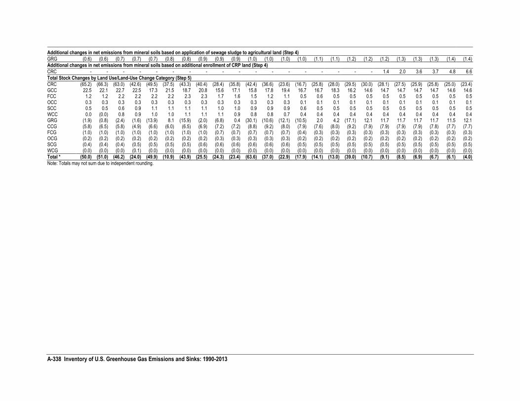
A-338 Inventory of U.S. Greenhouse Gas Emissions and Sinks: 1990-2013
Additional changes in net emissions from mineral soils based on application of sewage sludge to agricultural land (Step 4)
GRG (0.6) (0.6) (0.7) (0.7) (0.7) (0.8) (0.8) (0.9) (0.9) (0.9) (1.0) (1.0) (1.0) (1.0) (1.1) (1.1) (1.2) (1.2) (1.2) (1.3) (1.3) (1.3) (1.4) (1.4)
Additional changes in net emissions from mineral soils based on additional enrollment of CRP land (Step 4)
CRC - - - - - - - - - - - - - - - - - - 1.4 2.0 3.6 3.7 4.8 6.6
Total Stock Changes by Land Use/Land-Use Change Category (Step 5)
CRC (65.2) (66.3) (63.0) (42.6) (49.5) (37.5) (43.3) (40.4) (28.4) (35.8) (42.4) (36.6) (23.6) (16.7) (25.8) (28.0) (29.5) (30.0) (28.1) (27.5) (25.9) (25.8) (25.0) (23.4) GCC 22.5 22.1 22.7 22.5 17.3 21.5 18.7 20.8 15.6 17.1 15.8 17.8 19.4 16.7 16.7 18.3 16.2 14.6 14.7 14.7 14.7 14.7 14.6 14.6 FCC 1.2 1.2 2.2 2.2 2.2 2.2 2.3 2.3 1.7 1.6 1.5 1.2 1.1 0.5 0.6 0.5 0.5 0.5 0.5 0.5 0.5 0.5 0.5 0.5 OCC 0.3 0.3 0.3 0.3 0.3 0.3 0.3 0.3 0.3 0.3 0.3 0.3 0.3 0.1 0.1 0.1 0.1 0.1 0.1 0.1 0.1 0.1 0.1 0.1 SCC 0.5 0.5 0.6 0.9 1.1 1.1 1.1 1.1 1.0 1.0 0.9 0.9 0.9 0.6 0.5 0.5 0.5 0.5 0.5 0.5 0.5 0.5 0.5 0.5 WCC 0.0 (0.0) 0.8 0.9 1.0 1.0 1.1 1.1 1.1 0.9 0.8 0.8 0.7 0.4 0.4 0.4 0.4 0.4 0.4 0.4 0.4 0.4 0.4 0.4 GRG (1.9) (0.8) (2.4) (1.6) (13.9) 8.1 (15.9) (2.0) (6.8) 0.4 (30.1) (10.6) (12.1) (10.5) 2.0 4.2 (17.1) 12.1 11.7 11.7 11.7 11.7 11.5 12.1 CCG (5.8) (6.5) (5.8) (4.9) (6.6) (6.0) (6.5) (6.9) (7.2) (7.2) (8.8) (9.2) (8.0) (7.9) (7.6) (8.0) (9.2) (7.9) (7.9) (7.9) (7.9) (7.8) (7.7) (7.7) FCG (1.0) (1.0) (1.0) (1.0) (1.0) (1.0) (1.0) (1.0) (0.7) (0.7) (0.7) (0.7) (0.7) (0.4) (0.3) (0.3) (0.3) (0.3) (0.3) (0.3) (0.3) (0.3) (0.3) (0.3) OCG (0.2) (0.2) (0.2) (0.2) (0.2) (0.2) (0.2) (0.2) (0.3) (0.3) (0.3) (0.3) (0.3) (0.2) (0.2) (0.2) (0.2) (0.2) (0.2) (0.2) (0.2) (0.2) (0.2) (0.2) SCG (0.4) (0.4) (0.4) (0.5) (0.5) (0.5) (0.5) (0.6) (0.6) (0.6) (0.6) (0.6) (0.6) (0.5) (0.5) (0.5) (0.5) (0.5) (0.5) (0.5) (0.5) (0.5) (0.5) (0.5) WCG (0.0) (0.0) (0.0) (0.1) (0.0) (0.0) (0.0) (0.0) (0.0) (0.0) (0.0) (0.0) (0.0) (0.0) (0.0) (0.0) (0.0) (0.0) (0.0) (0.0) (0.0) (0.0) (0.0) (0.0)
Total * (50.0) (51.0) (46.2) (24.0) (49.9) (10.9) (43.9) (25.5) (24.3) (23.4) (63.6) (37.0) (22.9) (17.9) (14.1) (13.0) (39.0) (10.7) (9.1) (8.5) (6.9) (6.7) (6.1) (4.0)
Note: Totals may not sum due to independent rounding.
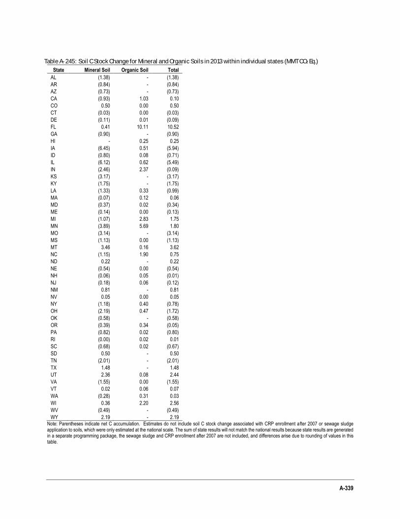
A-339
Table A- 245: Soil C Stock Change for Mineral and Organic Soils in 2013 within individual states (MMT CO2 Eq.)
Note: Parentheses indicate net C accumulation. Estimates do not include soil C stock change associated with CRP enrollment after 2007 or sewage sludge application to soils, which were only estimated at the national scale. The sum of state results will not match the national results because state results are generated in a separate programming package, the sewage sludge and CRP enrollment after 2007 are not included, and differences arise due to rounding of values in this table.
State Mineral Soil Organic Soil Total
AL (1.38) - (1.38)
AR (0.84) - (0.84)
AZ (0.73) - (0.73)
CA (0.93) 1.03 0.10
CO 0.50 0.00 0.50
CT (0.03) 0.00 (0.03)
DE (0.11) 0.01 (0.09)
FL 0.41 10.11 10.52
GA (0.90) - (0.90)
HI - 0.25 0.25
IA (6.45) 0.51 (5.94)
ID (0.80) 0.08 (0.71)
IL (6.12) 0.62 (5.49)
IN (2.46) 2.37 (0.09)
KS (3.17) - (3.17)
KY (1.75) - (1.75)
LA (1.33) 0.33 (0.99)
MA (0.07) 0.12 0.06
MD (0.37) 0.02 (0.34)
ME (0.14) 0.00 (0.13)
MI (1.07) 2.83 1.75
MN (3.89) 5.69 1.80
MO (3.14) - (3.14)
MS (1.13) 0.00 (1.13)
MT 3.46 0.16 3.62
NC (1.15) 1.90 0.75
ND 0.22 - 0.22
NE (0.54) 0.00 (0.54)
NH (0.06) 0.05 (0.01)
NJ (0.18) 0.06 (0.12)
NM 0.81 - 0.81
NV 0.05 0.00 0.05
NY (1.18) 0.40 (0.78)
OH (2.19) 0.47 (1.72)
OK (0.58) - (0.58)
OR (0.39) 0.34 (0.05)
PA (0.82) 0.02 (0.80)
RI (0.00) 0.02 0.01
SC (0.68) 0.02 (0.67)
SD 0.50 - 0.50
TN (2.01) - (2.01)
TX 1.48 - 1.48
UT 2.36 0.08 2.44
VA (1.55) 0.00 (1.55)
VT 0.02 0.06 0.07
WA (0.28) 0.31 0.03
WI 0.36 2.20 2.56
WV (0.49) - (0.49)
WY 2.19 - 2.19
A-340 Inventory of U.S. Greenhouse Gas Emissions and Sinks: 1990-2013
3.13. Methodology for Estimating Net Carbon Stock Changes in Forest Lands Remaining Forest Lands
This sub-annex expands on the methodology used to estimate net changes in carbon (C) stocks in forest ecosystems and harvested wood products as well as emissions from forest fires. Some of the details of C conversion factors and procedures for calculating net carbon dioxide (CO2) flux for forests are provided below; full details of selected topics may be found in the cited references.
Carbon stocks and net stock change in forest ecosystems
The inventory-based methodologies for estimating forest C stocks are based on Smith et al. (2010) and are consistent with IPCC (2003, 2006) stock-difference methods. Estimates of ecosystem C are based on data from forest inventory plots; either direct measurements or attributes of forest inventories are the basis for estimating metric tons per hectare of C in trees, woody debris and litter, and soil organic C. Plot-level estimates are summed to total stocks for large areas as defined by the forest inventories, such as individual states, for example. Net annual C stock change is calculated as the difference between successive forest inventories divided by the interval, in years for a selected state or sub-state area.
Forest inventory data
The estimates of forest C stocks are based on data from forest inventory surveys. Forest inventory data were obtained from the USDA Forest Service, Forest Inventory and Analysis (FIA) program (Frayer and Furnival 1999, USDA Forest Service 2014a, USDA Forest Service 2014b). Forest Inventory and Analysis data include remote sensing information and a collection of measurements in the field at sample locations called plots. Tree measurements include diameter, height, and species. On a subset of plots, additional measurements or samples are taken of downed dead wood, litter, and soil attributes. The technical advances needed to estimate C stocks from these data are ongoing (Woodall et al. 2012). The field protocols are thoroughly documented and available for download from the USDA Forest Service (2014c). Bechtold and Patterson (2005) provide the estimation procedures for standard forest inventory results. The data are freely available for download at USDA Forest Service (2011b) as the Forest Inventory and Analysis Database (FIADB) Version 6.0 (USDA Forest Service 2014b, USDA Forest Service 2014c); these data are the primary sources of forest inventory used to estimate forest C stocks.
Forest surveys have begun in the U.S. territories and in Hawaii. Meanwhile this inventory assumes that these areas account for a net C change of zero. Survey data are available for the temperate oceanic ecoregion of Alaska (southeast and south central). Inventory data are publicly available for 6 million hectares of forest land, and these inventoried lands, representing an estimated 12 percent of the total forest land in Alaska, contribute to the forest C stocks presented here.
Agroforestry systems are also not currently accounted for in the U.S. Inventory, since they are not explicitly inventoried by either of the two primary national natural resource inventory programs: the FIA program of the USDA Forest Service and the National Resources Inventory (NRI) of the USDA Natural Resources Conservation Service (Perry et al. 2005). The majority of these tree-based practices do not meet the size and definitions for forests within each of these resource inventories.
Summing state-level C stocks to calculate U.S. net C flux in forest ecosystems
The overall approach for determining forest C stocks and stock change is essentially based on methodology and algorithms coded into the computer tool described in Smith et al. (2010). Recent modification to the methods of Smith et al. (2010) such as by Domke et al. (2013) reflect the ongoing research and data collection, which are ultimately aimed toward the goal of accurately representing forest C by the land-use categories of Chapter 6, Land Use, Land-Use Change, and Forestry. The two principal aims of these ongoing improvements are to assure the appropriate use of FIA’s inventory data and to refine the inventory-to-C conversion process. Change in forest C should reflect change in forest condition or structure, not changes in definitions or methods associated with data collection. Thus, consistent series of stocks depend on the appropriate interpretation and application of the forest inventories. Similarly, greater site specificity in C conversion factors are preferred to regional (or low tier) factors. The current forest C estimates include recent modification in the selection and use of inventory data (e.g., woodlands that do not meet the definition of forest) and C factors (e.g., the new model to estimate litter). These are each addressed below in their respective sections of this annex.
The C calculation tool focuses on estimating forest C stocks based on data from two or more forest surveys conducted several years apart for each state or sub-state (Smith et al. 2010). There are generally two or more surveys
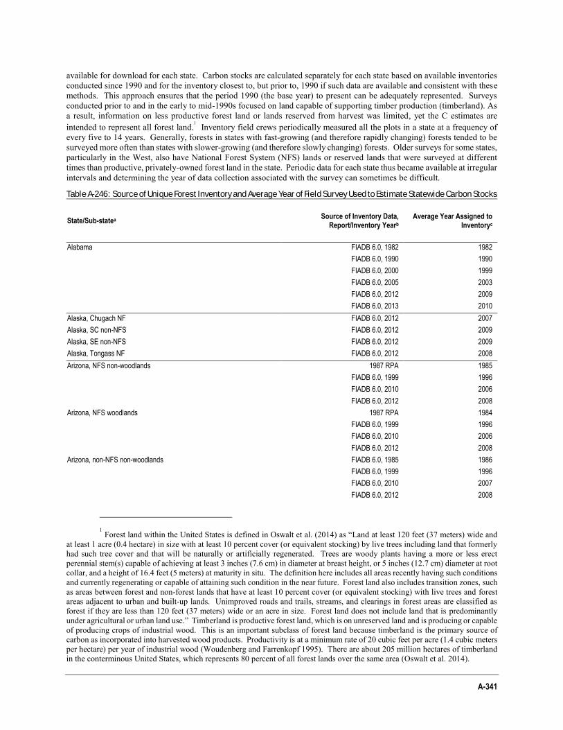
A-341
available for download for each state. Carbon stocks are calculated separately for each state based on available inventories conducted since 1990 and for the inventory closest to, but prior to, 1990 if such data are available and consistent with these methods. This approach ensures that the period 1990 (the base year) to present can be adequately represented. Surveys conducted prior to and in the early to mid-1990s focused on land capable of supporting timber production (timberland). As a result, information on less productive forest land or lands reserved from harvest was limited, yet the C estimates are intended to represent all forest land.1 Inventory field crews periodically measured all the plots in a state at a frequency of every five to 14 years. Generally, forests in states with fast-growing (and therefore rapidly changing) forests tended to be surveyed more often than states with slower-growing (and therefore slowly changing) forests. Older surveys for some states, particularly in the West, also have National Forest System (NFS) lands or reserved lands that were surveyed at different times than productive, privately-owned forest land in the state. Periodic data for each state thus became available at irregular intervals and determining the year of data collection associated with the survey can sometimes be difficult.
Table A-246: Source of Unique Forest Inventory and Average Year of Field Survey Used to Estimate Statewide Carbon Stocks
State/Sub-statea Source of Inventory Data,
Report/Inventory Yearb Average Year Assigned to
Inventoryc
Alabama FIADB 6.0, 1982 1982
FIADB 6.0, 1990 1990
FIADB 6.0, 2000 1999
FIADB 6.0, 2005 2003
FIADB 6.0, 2012 2009
FIADB 6.0, 2013 2010
Alaska, Chugach NF FIADB 6.0, 2012 2007
Alaska, SC non-NFS FIADB 6.0, 2012 2009
Alaska, SE non-NFS FIADB 6.0, 2012 2009
Alaska, Tongass NF FIADB 6.0, 2012 2008
Arizona, NFS non-woodlands 1987 RPA 1985
FIADB 6.0, 1999 1996
FIADB 6.0, 2010 2006
FIADB 6.0, 2012 2008
Arizona, NFS woodlands 1987 RPA 1984
FIADB 6.0, 1999 1996
FIADB 6.0, 2010 2006
FIADB 6.0, 2012 2008
Arizona, non-NFS non-woodlands FIADB 6.0, 1985 1986
FIADB 6.0, 1999 1996
FIADB 6.0, 2010 2007
FIADB 6.0, 2012 2008
1 Forest land within the United States is defined in Oswalt et al. (2014) as “Land at least 120 feet (37 meters) wide and
at least 1 acre (0.4 hectare) in size with at least 10 percent cover (or equivalent stocking) by live trees including land that formerly had such tree cover and that will be naturally or artificially regenerated. Trees are woody plants having a more or less erect perennial stem(s) capable of achieving at least 3 inches (7.6 cm) in diameter at breast height, or 5 inches (12.7 cm) diameter at root collar, and a height of 16.4 feet (5 meters) at maturity in situ. The definition here includes all areas recently having such conditions and currently regenerating or capable of attaining such condition in the near future. Forest land also includes transition zones, such as areas between forest and non-forest lands that have at least 10 percent cover (or equivalent stocking) with live trees and forest areas adjacent to urban and built-up lands. Unimproved roads and trails, streams, and clearings in forest areas are classified as forest if they are less than 120 feet (37 meters) wide or an acre in size. Forest land does not include land that is predominantly under agricultural or urban land use.” Timberland is productive forest land, which is on unreserved land and is producing or capable of producing crops of industrial wood. This is an important subclass of forest land because timberland is the primary source of carbon as incorporated into harvested wood products. Productivity is at a minimum rate of 20 cubic feet per acre (1.4 cubic meters per hectare) per year of industrial wood (Woudenberg and Farrenkopf 1995). There are about 205 million hectares of timberland in the conterminous United States, which represents 80 percent of all forest lands over the same area (Oswalt et al. 2014).
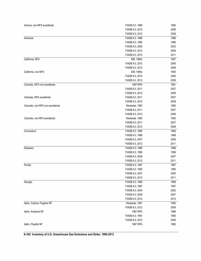
A-342 Inventory of U.S. Greenhouse Gas Emissions and Sinks: 1990-2013
Arizona, non-NFS woodlands FIADB 6.0, 1999 1990
FIADB 6.0, 2010 2006
FIADB 6.0, 2012 2008
Arkansas FIADB 6.0, 1988 1988
FIADB 6.0, 1995 1996
FIADB 6.0, 2005 2003
FIADB 6.0, 2010 2008
FIADB 6.0, 2013 2011
California, NFS IDB, 1990s 1997
FIADB 6.0, 2010 2006
FIADB 6.0, 2012 2008
California, non-NFS IDB, 1990s 1993
FIADB 6.0, 2010 2006
FIADB 6.0, 2012 2008
Colorado, NFS non-woodlands 1997 RPA 1981
FIADB 6.0, 2011 2007
FIADB 6.0, 2012 2008
Colorado, NFS woodlands FIADB 6.0, 2011 2007
FIADB 6.0, 2012 2008
Colorado, non-NFS non-woodlands Westwide, 1983 1980
FIADB 6.0, 2011 2007
FIADB 6.0, 2012 2008
Colorado, non-NFS woodlands Westwide, 1983 1983
FIADB 6.0, 2011 2007
FIADB 6.0, 2012 2008
Connecticut FIADB 6.0, 1985 1985
FIADB 6.0, 1998 1998
FIADB 6.0, 2007 2006
FIADB 6.0, 2012 2011
Delaware FIADB 6.0, 1986 1986
FIADB 6.0, 1999 1999
FIADB 6.0, 2008 2007
FIADB 6.0, 2012 2011
Florida FIADB 6.0, 1987 1987
FIADB 6.0, 1995 1995
FIADB 6.0, 2007 2005
FIADB 6.0, 2013 2011
Georgia FIADB 6.0, 1989 1989
FIADB 6.0, 1997 1997
FIADB 6.0, 2004 2002
FIADB 6.0, 2009 2007
FIADB 6.0, 2012 2010
Idaho, Caribou-Targhee NF Westwide, 1991 1992
FIADB 6.0, 2012 2009
Idaho, Kootenai NF 1987 RPA 1988
FIADB 6.0, 1991 1995
FIADB 6.0, 2012 2009
Idaho, Payette NF 1987 RPA 1982
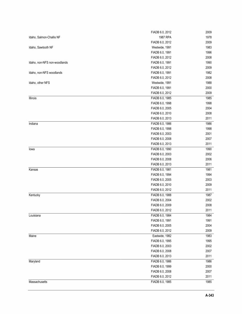
A-343
FIADB 6.0, 2012 2009
Idaho, Salmon-Challis NF 1987 RPA 1978
FIADB 6.0, 2012 2009
Idaho, Sawtooth NF Westwide, 1991 1983
FIADB 6.0, 1991 1996
FIADB 6.0, 2012 2008
Idaho, non-NFS non-woodlands FIADB 6.0, 1991 1990
FIADB 6.0, 2012 2009
Idaho, non-NFS woodlands FIADB 6.0, 1991 1982
FIADB 6.0, 2012 2008
Idaho, other NFS Westwide, 1991 1988
FIADB 6.0, 1991 2000
FIADB 6.0, 2012 2009
Illinois FIADB 6.0, 1985 1985
FIADB 6.0, 1998 1998
FIADB 6.0, 2005 2004
FIADB 6.0, 2010 2008
FIADB 6.0, 2013 2011
Indiana FIADB 6.0, 1986 1986
FIADB 6.0, 1998 1998
FIADB 6.0, 2003 2001
FIADB 6.0, 2008 2007
FIADB 6.0, 2013 2011
Iowa FIADB 6.0, 1990 1990
FIADB 6.0, 2003 2002
FIADB 6.0, 2008 2006
FIADB 6.0, 2013 2011
Kansas FIADB 6.0, 1981 1981
FIADB 6.0, 1994 1994
FIADB 6.0, 2005 2003
FIADB 6.0, 2010 2009
FIADB 6.0, 2012 2011
Kentucky FIADB 6.0, 1988 1987
FIADB 6.0, 2004 2002
FIADB 6.0, 2009 2008
FIADB 6.0, 2012 2011
Louisiana FIADB 6.0, 1984 1984
FIADB 6.0, 1991 1991
FIADB 6.0, 2005 2004
FIADB 6.0, 2012 2009
Maine Eastwide, 1982 1983
FIADB 6.0, 1995 1995
FIADB 6.0, 2003 2002
FIADB 6.0, 2008 2007
FIADB 6.0, 2013 2011
Maryland FIADB 6.0, 1986 1986
FIADB 6.0, 1999 2000
FIADB 6.0, 2008 2007
FIADB 6.0, 2012 2011
Massachusetts FIADB 6.0, 1985 1985
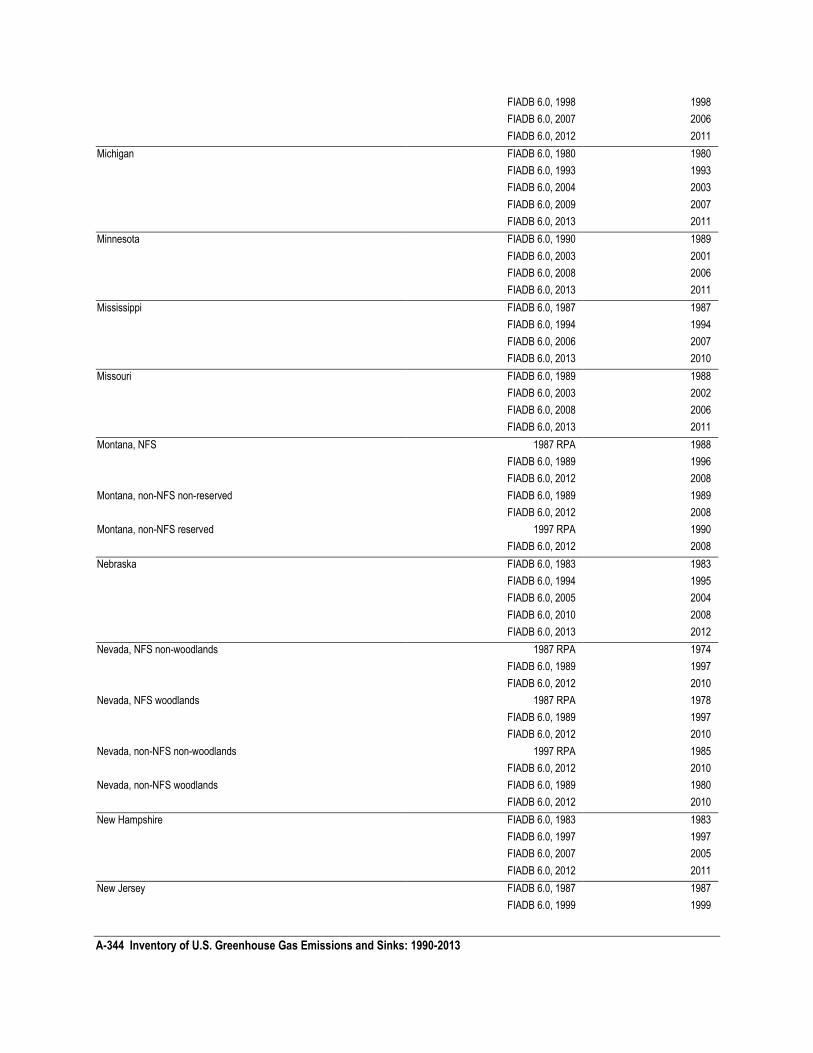
A-344 Inventory of U.S. Greenhouse Gas Emissions and Sinks: 1990-2013
FIADB 6.0, 1998 1998
FIADB 6.0, 2007 2006
FIADB 6.0, 2012 2011
Michigan FIADB 6.0, 1980 1980
FIADB 6.0, 1993 1993
FIADB 6.0, 2004 2003
FIADB 6.0, 2009 2007
FIADB 6.0, 2013 2011
Minnesota FIADB 6.0, 1990 1989
FIADB 6.0, 2003 2001
FIADB 6.0, 2008 2006
FIADB 6.0, 2013 2011
Mississippi FIADB 6.0, 1987 1987
FIADB 6.0, 1994 1994
FIADB 6.0, 2006 2007
FIADB 6.0, 2013 2010
Missouri FIADB 6.0, 1989 1988
FIADB 6.0, 2003 2002
FIADB 6.0, 2008 2006
FIADB 6.0, 2013 2011
Montana, NFS 1987 RPA 1988
FIADB 6.0, 1989 1996
FIADB 6.0, 2012 2008
Montana, non-NFS non-reserved FIADB 6.0, 1989 1989
FIADB 6.0, 2012 2008
Montana, non-NFS reserved 1997 RPA 1990
FIADB 6.0, 2012 2008
Nebraska FIADB 6.0, 1983 1983
FIADB 6.0, 1994 1995
FIADB 6.0, 2005 2004
FIADB 6.0, 2010 2008
FIADB 6.0, 2013 2012
Nevada, NFS non-woodlands 1987 RPA 1974
FIADB 6.0, 1989 1997
FIADB 6.0, 2012 2010
Nevada, NFS woodlands 1987 RPA 1978
FIADB 6.0, 1989 1997
FIADB 6.0, 2012 2010
Nevada, non-NFS non-woodlands 1997 RPA 1985
FIADB 6.0, 2012 2010
Nevada, non-NFS woodlands FIADB 6.0, 1989 1980
FIADB 6.0, 2012 2010
New Hampshire FIADB 6.0, 1983 1983
FIADB 6.0, 1997 1997
FIADB 6.0, 2007 2005
FIADB 6.0, 2012 2011
New Jersey FIADB 6.0, 1987 1987
FIADB 6.0, 1999 1999
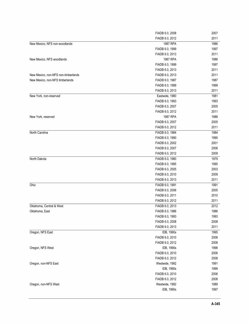
A-345
FIADB 6.0, 2008 2007
FIADB 6.0, 2012 2011
New Mexico, NFS non-woodlands 1987 RPA 1986
FIADB 6.0, 1999 1997
FIADB 6.0, 2013 2011
New Mexico, NFS woodlands 1987 RPA 1986
FIADB 6.0, 1999 1997
FIADB 6.0, 2013 2011
New Mexico, non-NFS non-timberlands FIADB 6.0, 2013 2011
New Mexico, non-NFS timberlands FIADB 6.0, 1987 1987
FIADB 6.0, 1999 1999
FIADB 6.0, 2013 2011
New York, non-reserved Eastwide, 1980 1981
FIADB 6.0, 1993 1993
FIADB 6.0, 2007 2005
FIADB 6.0, 2012 2011
New York, reserved 1987 RPA 1988
FIADB 6.0, 2007 2005
FIADB 6.0, 2012 2011
North Carolina FIADB 6.0, 1984 1984
FIADB 6.0, 1990 1990
FIADB 6.0, 2002 2001
FIADB 6.0, 2007 2006
FIADB 6.0, 2012 2009
North Dakota FIADB 6.0, 1980 1979
FIADB 6.0, 1995 1995
FIADB 6.0, 2005 2003
FIADB 6.0, 2010 2009
FIADB 6.0, 2013 2011
Ohio FIADB 6.0, 1991 1991
FIADB 6.0, 2006 2005
FIADB 6.0, 2011 2010
FIADB 6.0, 2012 2011
Oklahoma, Central & West FIADB 6.0, 2013 2012
Oklahoma, East FIADB 6.0, 1986 1986
FIADB 6.0, 1993 1993
FIADB 6.0, 2008 2008
FIADB 6.0, 2013 2011
Oregon, NFS East IDB, 1990s 1995
FIADB 6.0, 2010 2006
FIADB 6.0, 2012 2008
Oregon, NFS West IDB, 1990s 1996
FIADB 6.0, 2010 2006
FIADB 6.0, 2012 2008
Oregon, non-NFS East Westwide, 1992 1991
IDB, 1990s 1999
FIADB 6.0, 2010 2006
FIADB 6.0, 2012 2008
Oregon, non-NFS West Westwide, 1992 1989
IDB, 1990s 1997
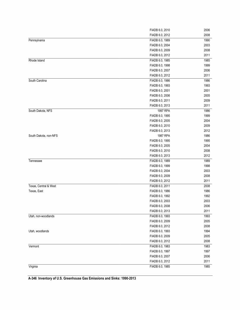
A-346 Inventory of U.S. Greenhouse Gas Emissions and Sinks: 1990-2013
FIADB 6.0, 2010 2006
FIADB 6.0, 2012 2008
Pennsylvania FIADB 6.0, 1989 1990
FIADB 6.0, 2004 2003
FIADB 6.0, 2009 2008
FIADB 6.0, 2012 2011
Rhode Island FIADB 6.0, 1985 1985
FIADB 6.0, 1998 1999
FIADB 6.0, 2007 2006
FIADB 6.0, 2012 2011
South Carolina FIADB 6.0, 1986 1986
FIADB 6.0, 1993 1993
FIADB 6.0, 2001 2001
FIADB 6.0, 2006 2005
FIADB 6.0, 2011 2009
FIADB 6.0, 2013 2011
South Dakota, NFS 1997 RPA 1986
FIADB 6.0, 1995 1999
FIADB 6.0, 2005 2004
FIADB 6.0, 2010 2009
FIADB 6.0, 2013 2012
South Dakota, non-NFS 1987 RPA 1986
FIADB 6.0, 1995 1995
FIADB 6.0, 2005 2004
FIADB 6.0, 2010 2008
FIADB 6.0, 2013 2012
Tennessee FIADB 6.0, 1989 1989
FIADB 6.0, 1999 1998
FIADB 6.0, 2004 2003
FIADB 6.0, 2009 2008
FIADB 6.0, 2012 2011
Texas, Central & West FIADB 6.0, 2011 2008
Texas, East FIADB 6.0, 1986 1986
FIADB 6.0, 1992 1992
FIADB 6.0, 2003 2003
FIADB 6.0, 2008 2006
FIADB 6.0, 2013 2011
Utah, non-woodlands FIADB 6.0, 1993 1993
FIADB 6.0, 2009 2005
FIADB 6.0, 2012 2008
Utah, woodlands FIADB 6.0, 1993 1994
FIADB 6.0, 2009 2005
FIADB 6.0, 2012 2008
Vermont FIADB 6.0, 1983 1983
FIADB 6.0, 1997 1997
FIADB 6.0, 2007 2006
FIADB 6.0, 2012 2011
Virginia FIADB 6.0, 1985 1985
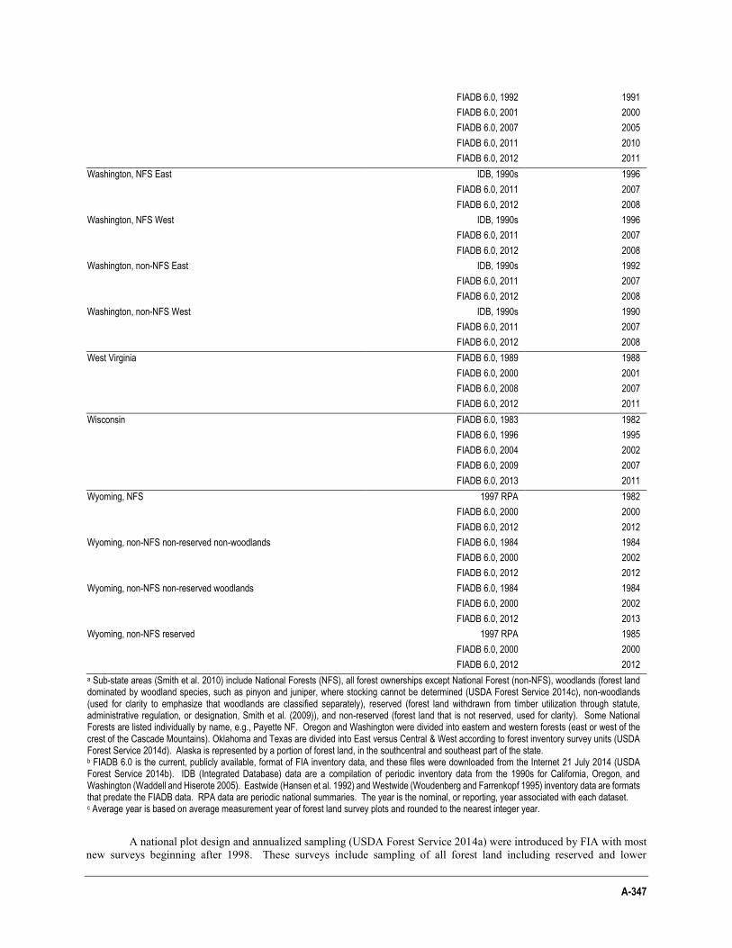
A-347
FIADB 6.0, 1992 1991
FIADB 6.0, 2001 2000
FIADB 6.0, 2007 2005
FIADB 6.0, 2011 2010
FIADB 6.0, 2012 2011
Washington, NFS East IDB, 1990s 1996
FIADB 6.0, 2011 2007
FIADB 6.0, 2012 2008
Washington, NFS West IDB, 1990s 1996
FIADB 6.0, 2011 2007
FIADB 6.0, 2012 2008
Washington, non-NFS East IDB, 1990s 1992
FIADB 6.0, 2011 2007
FIADB 6.0, 2012 2008
Washington, non-NFS West IDB, 1990s 1990
FIADB 6.0, 2011 2007
FIADB 6.0, 2012 2008
West Virginia FIADB 6.0, 1989 1988
FIADB 6.0, 2000 2001
FIADB 6.0, 2008 2007
FIADB 6.0, 2012 2011
Wisconsin FIADB 6.0, 1983 1982
FIADB 6.0, 1996 1995
FIADB 6.0, 2004 2002
FIADB 6.0, 2009 2007
FIADB 6.0, 2013 2011
Wyoming, NFS 1997 RPA 1982
FIADB 6.0, 2000 2000
FIADB 6.0, 2012 2012
Wyoming, non-NFS non-reserved non-woodlands FIADB 6.0, 1984 1984
FIADB 6.0, 2000 2002
FIADB 6.0, 2012 2012
Wyoming, non-NFS non-reserved woodlands FIADB 6.0, 1984 1984
FIADB 6.0, 2000 2002
FIADB 6.0, 2012 2013
Wyoming, non-NFS reserved 1997 RPA 1985
FIADB 6.0, 2000 2000
FIADB 6.0, 2012 2012
a Sub-state areas (Smith et al. 2010) include National Forests (NFS), all forest ownerships except National Forest (non-NFS), woodlands (forest land dominated by woodland species, such as pinyon and juniper, where stocking cannot be determined (USDA Forest Service 2014c), non-woodlands (used for clarity to emphasize that woodlands are classified separately), reserved (forest land withdrawn from timber utilization through statute, administrative regulation, or designation, Smith et al. (2009)), and non-reserved (forest land that is not reserved, used for clarity). Some National Forests are listed individually by name, e.g., Payette NF. Oregon and Washington were divided into eastern and western forests (east or west of the crest of the Cascade Mountains). Oklahoma and Texas are divided into East versus Central & West according to forest inventory survey units (USDA Forest Service 2014d). Alaska is represented by a portion of forest land, in the southcentral and southeast part of the state. b FIADB 6.0 is the current, publicly available, format of FIA inventory data, and these files were downloaded from the Internet 21 July 2014 (USDA Forest Service 2014b). IDB (Integrated Database) data are a compilation of periodic inventory data from the 1990s for California, Oregon, and Washington (Waddell and Hiserote 2005). Eastwide (Hansen et al. 1992) and Westwide (Woudenberg and Farrenkopf 1995) inventory data are formats that predate the FIADB data. RPA data are periodic national summaries. The year is the nominal, or reporting, year associated with each dataset. c Average year is based on average measurement year of forest land survey plots and rounded to the nearest integer year.
A national plot design and annualized sampling (USDA Forest Service 2014a) were introduced by FIA with most new surveys beginning after 1998. These surveys include sampling of all forest land including reserved and lower
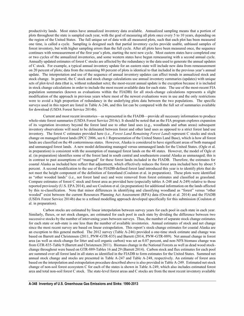
A-348 Inventory of U.S. Greenhouse Gas Emissions and Sinks: 1990-2013
productivity lands. Most states have annualized inventory data available. Annualized sampling means that a portion of plots throughout the state is sampled each year, with the goal of measuring all plots once every 5 to 10 years, depending on the region of the United States. The full unique set of data with all measured plots, such that each plot has been measured one time, is called a cycle. Sampling is designed such that partial inventory cycles provide usable, unbiased samples of forest inventory, but with higher sampling errors than the full cycle. After all plots have been measured once, the sequence continues with remeasurement of the first year’s plots, starting the next new cycle. Most eastern states have completed one or two cycles of the annualized inventories, and some western states have begun remeasuring with a second annual cycle. Annually updated estimates of forest C stocks are affected by the redundancy in the data used to generate the annual updates of C stock. For example, a typical annual inventory update for an eastern state will include new data from remeasurement on 20 percent of plots; data from the remaining 80 percent of plots is identical to that included in the previous year’s annual update. The interpretation and use of the sequence of annual inventory updates can affect trends in annualized stock and stock change. In general, the C stock and stock change calculations use annual inventory summaries (updates) with unique sets of plot-level data (that is, without redundant sets); the most-recent annual update is the exception because it is included in stock change calculations in order to include the most recent available data for each state. The use of the most-recent FIA population summaries (known as evaluations within the FIADB) for all stock-change calculations represents a slight modification of the approach in previous years where most of the newest evaluations were in use and the only restrictions were to avoid a high proportion of redundancy in the underlying plots data between the two populations. The specific surveys used in this report are listed in Table A-246, and this list can be compared with the full set of summaries available for download (USDA Forest Service 2014b).
Current and most recent inventories—as represented in the FIADB—provide all necessary information to produce whole-state forest summaries (USDA Forest Service 2014c). It should be noted that as the FIA program explores expansion of its vegetation inventory beyond the forest land use to other land uses (e.g., woodlands and urban areas) subsequent inventory observations will need to be delineated between forest and other land uses as opposed to a strict forest land use inventory. The forest C estimates provided here (i.e., Forest Land Remaining Forest Land) represent C stocks and stock change on managed forest lands (IPCC 2006, see 6.1 Representation of the United States Land Base), which is how all forest lands are classified on the 48 conterminous states. However, Alaska is considered to have significant areas of both managed and unmanaged forest lands. A new model delineating managed versus unmanaged lands for the United States. (Ogle et al. in preparation) is consistent with the assumption of managed forest lands on the 48 states. However, the model of Ogle et al. (in preparation) identifies some of the forest land in south central and southeastern coastal Alaska as unmanaged; this is in contrast to past assumptions of “managed” for these forest lands included in the FIADB. Therefore, the estimates for coastal Alaska as included here reflect that adjustment, which effectively reduces the forest area included here by about 5 percent. A second modification to the use of the FIADB-defined forest land introduced this year is to identify plots that do not meet the height component of the definition of forestland (Coulston et al. in preparation). These plots were identified as “other wooded lands” (i.e., not forest land use) and were removed from forest estimates and classified as grassland. Compare estimates of forest C stock and forest area as provided here (especially tables A-248 and A-249) relative to those reported previously (U.S. EPA 2014), and see Coulston et al. (in preparation) for additional information on the lands affected by this re-classification. Note that minor differences in identifying and classifying woodland as “forest” versus “other wooded” exist between the current Resources Planning Act Assessment (RPA) data (Oswalt et al. 2014) and the FIADB (USDA Forest Service 2014b) due to a refined modelling approach developed specifically for this submission (Coulston et al. in preparation).
Carbon stocks are estimated by linear interpolation between survey years for each pool in each state in each year. Similarly, fluxes, or net stock changes, are estimated for each pool in each state by dividing the difference between two successive stocks by the number of intervening years between surveys. Thus, the number of separate stock change estimates for each state or sub-state is one less than the number of available inventories. Annual estimates of stock and net change since the most recent survey are based on linear extrapolation. This report’s stock-change estimates for coastal Alaska are an exception to this general method. The 2012 survey (Table A-246) provided a one-time stock estimate and change was based on Barrett and Christensen (2011, PNW-GTR-835) and Barrett (2014, PNW-GTR-889). Net annual change in forest area (as well as stock-change for litter and soil organic carbon) was set as 0.07 percent, and non-NFS biomass change was from GTR-835-Table 9 (Barrett and Christensen 2011). Biomass change in the National Forests as well as dead wood stock-change throughout were based on GTR-889-Tables 16 and 29 (Barrett 2014). Carbon stock and flux estimates for each pool are summed over all forest land in all states as identified in the FIADB to form estimates for the United States. Summed net annual stock change and stocks are presented in Table A-247 and Table A-248, respectively. An estimate of forest area based on the interpolation and extrapolation procedure described above is also provided in Table A-249. Estimated net stock change of non-soil forest ecosystem C for each of the states is shown in Table A-249, which also includes estimated forest area and total non-soil forest C stock. The state-level forest areas and C stocks are from the most recent inventory available

A-349
(USDA Forest Service 2014b), and the estimate for net stock change is the 10-year mean of the 2004 through 2013 estimates from the C calculator (Smith et al. 2010).
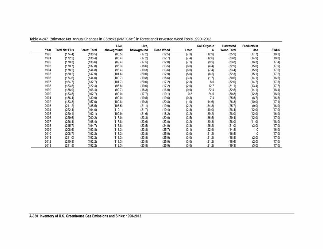
A-350 Inventory of U.S. Greenhouse Gas Emissions and Sinks: 1990-2013
Table A-247: Estimated Net Annual Changes in C Stocks (MMT C yr−1) in Forest and Harvested Wood Pools, 1990–2013
Year Total Net Flux Forest Total Live,
aboveground Live,
belowground Dead Wood Litter Soil Organic
C Harvested
Wood Total Products in
Use SWDS
1990 (174.4) (138.5) (88.5) (17.2) (12.5) (7.3) (12.9) (35.9) (17.7) (18.3) 1991 (172.2) (138.4) (88.4) (17.2) (12.7) (7.4) (12.6) (33.8) (14.9) (18.8) 1992 (170.3) (136.6) (89.4) (17.5) (12.8) (7.1) (9.9) (33.8) (16.3) (17.4) 1993 (170.7) (137.8) (95.3) (18.6) (13.5) (6.0) (4.4) (32.9) (15.0) (17.9) 1994 (178.2) (144.8) (98.4) (19.3) (13.6) (6.0) (7.4) (33.4) (15.9) (17.5) 1995 (180.2) (147.9) (101.6) (20.0) (12.9) (5.0) (8.5) (32.3) (15.1) (17.2) 1996 (174.6) (144.0) (100.7) (19.8) (18.6) (3.3) (1.7) (30.6) (14.1) (16.5) 1997 (164.7) (132.7) (101.7) (20.0) (17.2) (2.3) 8.6 (32.0) (14.7) (17.3) 1998 (153.5) (122.4) (96.8) (19.0) (17.2) (2.0) 12.7 (31.1) (13.4) (17.7) 1999 (138.9) (106.4) (92.7) (18.3) (16.9) (0.9) 22.4 (32.5) (14.1) (18.4) 2000 (133.5) (102.7) (90.0) (17.7) (19.1) 0.2 24.0 (30.8) (12.8) (18.0) 2001 (156.4) (130.9) (99.0) (19.5) (19.6) (0.3) 7.4 (25.5) (8.7) (16.8) 2002 (183.8) (157.0) (100.8) (19.8) (20.8) (1.0) (14.6) (26.8) (10.0) (17.1) 2003 (211.2) (185.5) (107.5) (21.1) (19.9) (2.2) (34.8) (25.7) (9.0) (16.0) 2004 (222.4) (194.0) (110.1) (21.7) (19.4) (2.8) (40.0) (28.4) (12.0) (17.0) 2005 (220.1) (192.1) (109.9) (21.6) (18.2) (3.2) (39.2) (28.0) (12.0) (16.0) 2006 (229.6) (200.2) (117.0) (23.3) (20.0) (3.5) (36.5) (29.4) (12.0) (17.0) 2007 (226.4) (198.4) (117.8) (23.6) (23.0) (3.2) (30.8) (28.0) (11.0) (18.0) 2008 (215.7) (194.7) (116.8) (23.5) (24.9) (3.3) (26.2) (21.0) (3.0) (17.0) 2009 (208.6) (193.8) (118.3) (23.8) (25.7) (3.1) (22.9) (14.8) 1.0 (16.0) 2010 (208.7) (192.2) (118.3) (23.8) (25.9) (3.0) (21.2) (16.5) 1.0 (17.0) 2011 (211.0) (192.2) (118.3) (23.8) (25.9) (3.0) (21.2) (18.8) (2.0) (17.0) 2012 (210.8) (192.2) (118.3) (23.8) (25.9) (3.0) (21.2) (18.6) (2.0) (17.0) 2013 (211.5) (192.2) (118.3) (23.8) (25.9) (3.0) (21.2) (19.3) (3.0) (17.0)
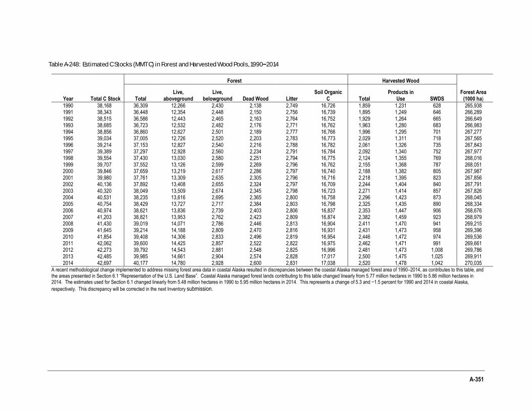
A-351
Table A-248: Estimated C Stocks (MMT C) in Forest and Harvested Wood Pools, 1990–2014
Total C Stock
Forest Harvested Wood
Forest Area (1000 ha) Year Total
Live, aboveground
Live, belowground Dead Wood Litter
Soil Organic C Total
Products in Use SWDS
1990 38,168 36,309 12,266 2,430 2,138 2,749 16,726 1,859 1,231 628 265,938 1991 38,343 36,448 12,354 2,448 2,150 2,756 16,739 1,895 1,249 646 266,289 1992 38,515 36,586 12,443 2,465 2,163 2,764 16,752 1,929 1,264 665 266,649 1993 38,685 36,723 12,532 2,482 2,176 2,771 16,762 1,963 1,280 683 266,983 1994 38,856 36,860 12,627 2,501 2,189 2,777 16,766 1,996 1,295 701 267,277 1995 39,034 37,005 12,726 2,520 2,203 2,783 16,773 2,029 1,311 718 267,565 1996 39,214 37,153 12,827 2,540 2,216 2,788 16,782 2,061 1,326 735 267,843 1997 39,389 37,297 12,928 2,560 2,234 2,791 16,784 2,092 1,340 752 267,977 1998 39,554 37,430 13,030 2,580 2,251 2,794 16,775 2,124 1,355 769 268,016 1999 39,707 37,552 13,126 2,599 2,269 2,796 16,762 2,155 1,368 787 268,051 2000 39,846 37,659 13,219 2,617 2,286 2,797 16,740 2,188 1,382 805 267,987 2001 39,980 37,761 13,309 2,635 2,305 2,796 16,716 2,218 1,395 823 267,856 2002 40,136 37,892 13,408 2,655 2,324 2,797 16,709 2,244 1,404 840 267,791 2003 40,320 38,049 13,509 2,674 2,345 2,798 16,723 2,271 1,414 857 267,826 2004 40,531 38,235 13,616 2,695 2,365 2,800 16,758 2,296 1,423 873 268,045 2005 40,754 38,429 13,727 2,717 2,384 2,803 16,798 2,325 1,435 890 268,334 2006 40,974 38,621 13,836 2,739 2,403 2,806 16,837 2,353 1,447 906 268,676 2007 41,203 38,821 13,953 2,762 2,423 2,809 16,874 2,382 1,459 923 268,979 2008 41,430 39,019 14,071 2,786 2,446 2,813 16,904 2,411 1,470 941 269,215 2009 41,645 39,214 14,188 2,809 2,470 2,816 16,931 2,431 1,473 958 269,396 2010 41,854 39,408 14,306 2,833 2,496 2,819 16,954 2,446 1,472 974 269,536 2011 42,062 39,600 14,425 2,857 2,522 2,822 16,975 2,462 1,471 991 269,661 2012 42,273 39,792 14,543 2,881 2,548 2,825 16,996 2,481 1,473 1,008 269,786 2013 42,485 39,985 14,661 2,904 2,574 2,828 17,017 2,500 1,475 1,025 269,911 2014 42,697 40,177 14,780 2,928 2,600 2,831 17,038 2,520 1,478 1,042 270,035
A recent methodological change implemented to address missing forest area data in coastal Alaska resulted in discrepancies between the coastal Alaska managed forest area of 1990–2014, as contributes to this table, and the areas presented in Section 6.1 “Representation of the U.S. Land Base”. Coastal Alaska managed forest lands contributing to this table changed linearly from 5.77 million hectares in 1990 to 5.86 million hectares in 2014. The estimates used for Section 6.1 changed linearly from 5.48 million hectares in 1990 to 5.95 million hectares in 2014. This represents a change of 5.3 and −1.5 percent for 1990 and 2014 in coastal Alaska,
respectively. This discrepancy will be corrected in the next Inventory submission.
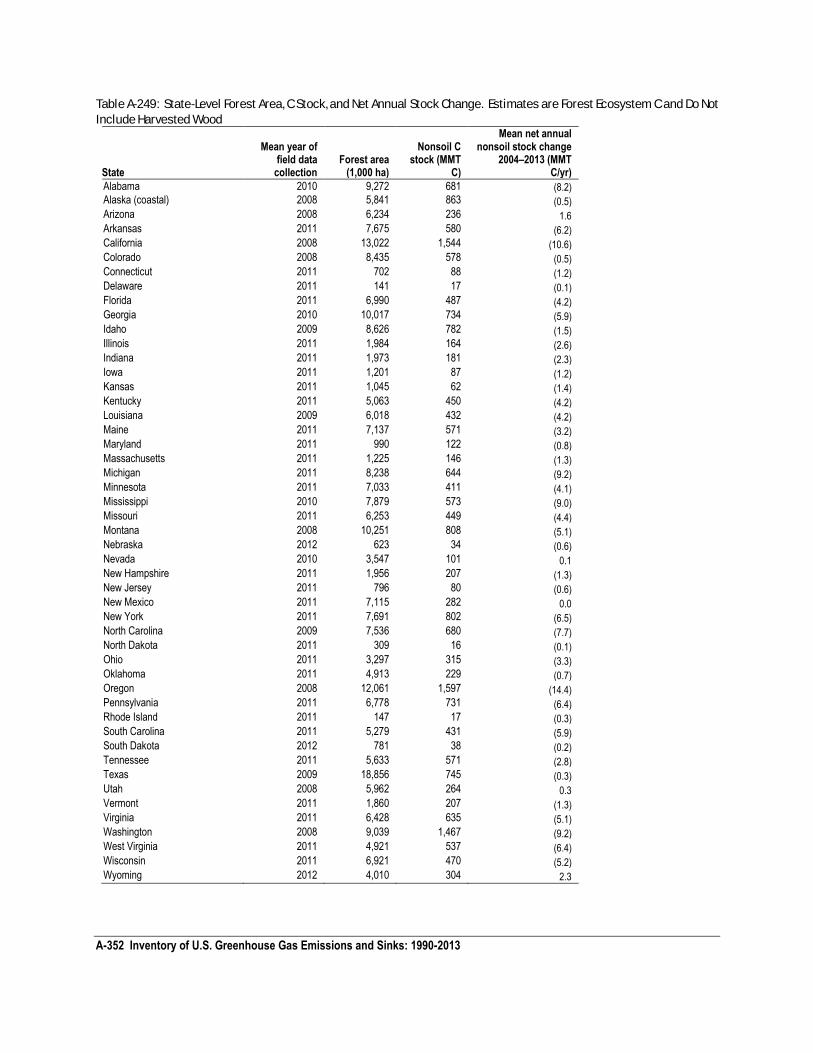
A-352 Inventory of U.S. Greenhouse Gas Emissions and Sinks: 1990-2013
Table A-249: State-Level Forest Area, C Stock, and Net Annual Stock Change. Estimates are Forest Ecosystem C and Do Not
Include Harvested Wood
State
Mean year of field data
collection Forest area
(1,000 ha)
Nonsoil C stock (MMT
C)
Mean net annual nonsoil stock change
2004–2013 (MMT C/yr)
Alabama 2010 9,272 681 (8.2)
Alaska (coastal) 2008 5,841 863 (0.5)
Arizona 2008 6,234 236 1.6
Arkansas 2011 7,675 580 (6.2)
California 2008 13,022 1,544 (10.6)
Colorado 2008 8,435 578 (0.5)
Connecticut 2011 702 88 (1.2)
Delaware 2011 141 17 (0.1)
Florida 2011 6,990 487 (4.2)
Georgia 2010 10,017 734 (5.9)
Idaho 2009 8,626 782 (1.5)
Illinois 2011 1,984 164 (2.6)
Indiana 2011 1,973 181 (2.3)
Iowa 2011 1,201 87 (1.2)
Kansas 2011 1,045 62 (1.4)
Kentucky 2011 5,063 450 (4.2)
Louisiana 2009 6,018 432 (4.2)
Maine 2011 7,137 571 (3.2)
Maryland 2011 990 122 (0.8)
Massachusetts 2011 1,225 146 (1.3)
Michigan 2011 8,238 644 (9.2)
Minnesota 2011 7,033 411 (4.1)
Mississippi 2010 7,879 573 (9.0)
Missouri 2011 6,253 449 (4.4)
Montana 2008 10,251 808 (5.1)
Nebraska 2012 623 34 (0.6)
Nevada 2010 3,547 101 0.1
New Hampshire 2011 1,956 207 (1.3)
New Jersey 2011 796 80 (0.6)
New Mexico 2011 7,115 282 0.0
New York 2011 7,691 802 (6.5)
North Carolina 2009 7,536 680 (7.7)
North Dakota 2011 309 16 (0.1)
Ohio 2011 3,297 315 (3.3)
Oklahoma 2011 4,913 229 (0.7)
Oregon 2008 12,061 1,597 (14.4)
Pennsylvania 2011 6,778 731 (6.4)
Rhode Island 2011 147 17 (0.3)
South Carolina 2011 5,279 431 (5.9)
South Dakota 2012 781 38 (0.2)
Tennessee 2011 5,633 571 (2.8)
Texas 2009 18,856 745 (0.3)
Utah 2008 5,962 264 0.3
Vermont 2011 1,860 207 (1.3)
Virginia 2011 6,428 635 (5.1)
Washington 2008 9,039 1,467 (9.2)
West Virginia 2011 4,921 537 (6.4)
Wisconsin 2011 6,921 470 (5.2)
Wyoming 2012 4,010 304 2.3
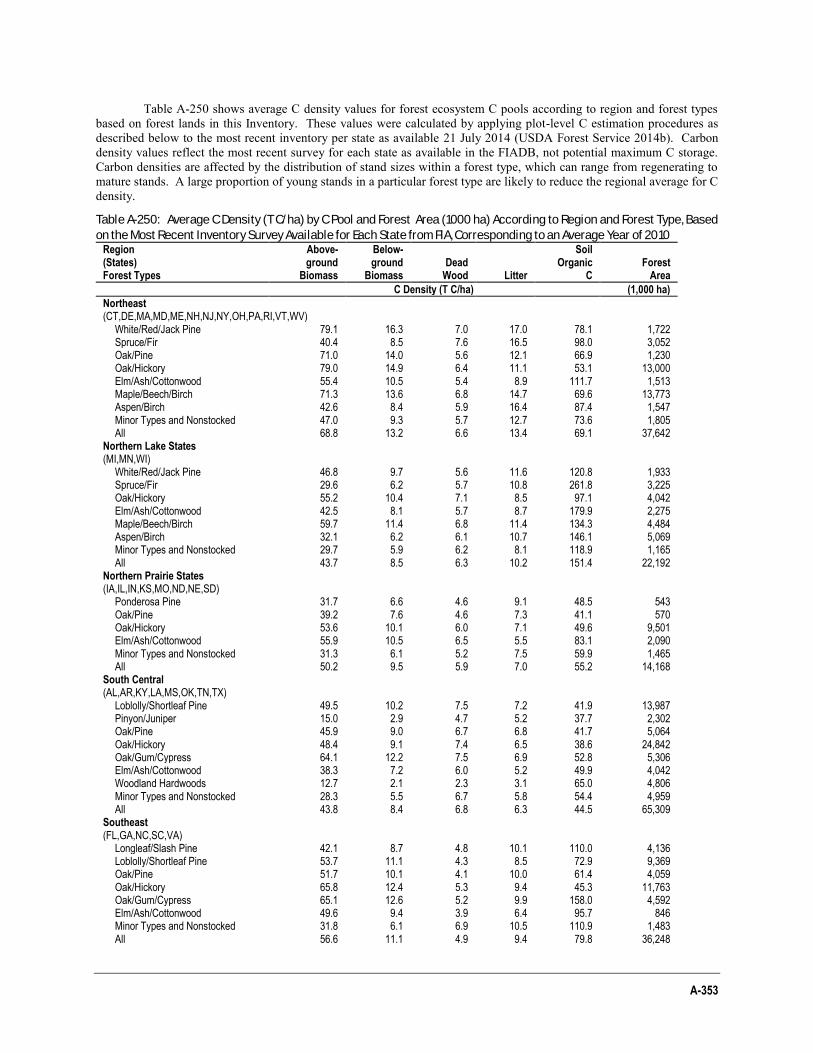
A-353
Table A-250 shows average C density values for forest ecosystem C pools according to region and forest types based on forest lands in this Inventory. These values were calculated by applying plot-level C estimation procedures as described below to the most recent inventory per state as available 21 July 2014 (USDA Forest Service 2014b). Carbon density values reflect the most recent survey for each state as available in the FIADB, not potential maximum C storage. Carbon densities are affected by the distribution of stand sizes within a forest type, which can range from regenerating to mature stands. A large proportion of young stands in a particular forest type are likely to reduce the regional average for C density.
Table A-250: Average C Density (T C/ha) by C Pool and Forest Area (1000 ha) According to Region and Forest Type, Based
on the Most Recent Inventory Survey Available for Each State from FIA, Corresponding to an Average Year of 2010 Region (States) Forest Types
Above-ground
Biomass
Below-ground
Biomass Dead
Wood Litter
Soil Organic
C Forest
Area
C Density (T C/ha) (1,000 ha)
Northeast (CT,DE,MA,MD,ME,NH,NJ,NY,OH,PA,RI,VT,WV)
White/Red/Jack Pine 79.1 16.3 7.0 17.0 78.1 1,722 Spruce/Fir 40.4 8.5 7.6 16.5 98.0 3,052 Oak/Pine 71.0 14.0 5.6 12.1 66.9 1,230 Oak/Hickory 79.0 14.9 6.4 11.1 53.1 13,000 Elm/Ash/Cottonwood 55.4 10.5 5.4 8.9 111.7 1,513 Maple/Beech/Birch 71.3 13.6 6.8 14.7 69.6 13,773 Aspen/Birch 42.6 8.4 5.9 16.4 87.4 1,547 Minor Types and Nonstocked 47.0 9.3 5.7 12.7 73.6 1,805 All 68.8 13.2 6.6 13.4 69.1 37,642
Northern Lake States (MI,MN,WI)
White/Red/Jack Pine 46.8 9.7 5.6 11.6 120.8 1,933 Spruce/Fir 29.6 6.2 5.7 10.8 261.8 3,225 Oak/Hickory 55.2 10.4 7.1 8.5 97.1 4,042 Elm/Ash/Cottonwood 42.5 8.1 5.7 8.7 179.9 2,275 Maple/Beech/Birch 59.7 11.4 6.8 11.4 134.3 4,484 Aspen/Birch 32.1 6.2 6.1 10.7 146.1 5,069 Minor Types and Nonstocked 29.7 5.9 6.2 8.1 118.9 1,165 All 43.7 8.5 6.3 10.2 151.4 22,192
Northern Prairie States (IA,IL,IN,KS,MO,ND,NE,SD)
Ponderosa Pine 31.7 6.6 4.6 9.1 48.5 543 Oak/Pine 39.2 7.6 4.6 7.3 41.1 570 Oak/Hickory 53.6 10.1 6.0 7.1 49.6 9,501 Elm/Ash/Cottonwood 55.9 10.5 6.5 5.5 83.1 2,090 Minor Types and Nonstocked 31.3 6.1 5.2 7.5 59.9 1,465 All 50.2 9.5 5.9 7.0 55.2 14,168
South Central (AL,AR,KY,LA,MS,OK,TN,TX)
Loblolly/Shortleaf Pine 49.5 10.2 7.5 7.2 41.9 13,987 Pinyon/Juniper 15.0 2.9 4.7 5.2 37.7 2,302 Oak/Pine 45.9 9.0 6.7 6.8 41.7 5,064 Oak/Hickory 48.4 9.1 7.4 6.5 38.6 24,842 Oak/Gum/Cypress 64.1 12.2 7.5 6.9 52.8 5,306 Elm/Ash/Cottonwood 38.3 7.2 6.0 5.2 49.9 4,042 Woodland Hardwoods 12.7 2.1 2.3 3.1 65.0 4,806 Minor Types and Nonstocked 28.3 5.5 6.7 5.8 54.4 4,959 All 43.8 8.4 6.8 6.3 44.5 65,309
Southeast (FL,GA,NC,SC,VA)
Longleaf/Slash Pine 42.1 8.7 4.8 10.1 110.0 4,136 Loblolly/Shortleaf Pine 53.7 11.1 4.3 8.5 72.9 9,369 Oak/Pine 51.7 10.1 4.1 10.0 61.4 4,059 Oak/Hickory 65.8 12.4 5.3 9.4 45.3 11,763 Oak/Gum/Cypress 65.1 12.6 5.2 9.9 158.0 4,592 Elm/Ash/Cottonwood 49.6 9.4 3.9 6.4 95.7 846 Minor Types and Nonstocked 31.8 6.1 6.9 10.5 110.9 1,483 All 56.6 11.1 4.9 9.4 79.8 36,248
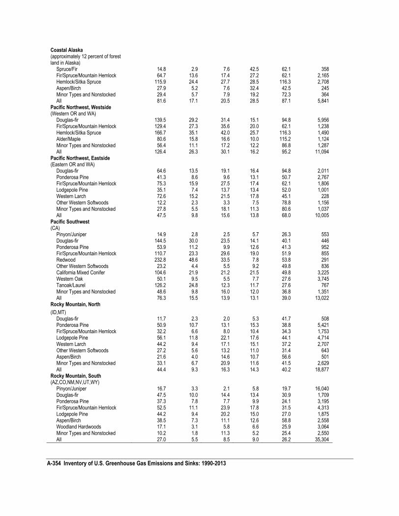
A-354 Inventory of U.S. Greenhouse Gas Emissions and Sinks: 1990-2013
Coastal Alaska (approximately 12 percent of forest land in Alaska)
Spruce/Fir 14.8 2.9 7.6 42.5 62.1 358 Fir/Spruce/Mountain Hemlock 64.7 13.6 17.4 27.2 62.1 2,165 Hemlock/Sitka Spruce 115.9 24.4 27.7 28.5 116.3 2,708 Aspen/Birch 27.9 5.2 7.6 32.4 42.5 245 Minor Types and Nonstocked 29.4 5.7 7.9 19.2 72.3 364 All 81.6 17.1 20.5 28.5 87.1 5,841
Pacific Northwest, Westside (Western OR and WA)
Douglas-fir 139.5 29.2 31.4 15.1 94.8 5,956 Fir/Spruce/Mountain Hemlock 129.4 27.3 35.6 20.0 62.1 1,238 Hemlock/Sitka Spruce 166.7 35.1 42.0 25.7 116.3 1,490 Alder/Maple 80.6 15.8 16.6 10.0 115.2 1,124 Minor Types and Nonstocked 56.4 11.1 17.2 12.2 86.8 1,287 All 126.4 26.3 30.1 16.2 95.2 11,094
Pacific Northwest, Eastside (Eastern OR and WA)
Douglas-fir 64.6 13.5 19.1 16.4 94.8 2,011 Ponderosa Pine 41.3 8.6 9.6 13.1 50.7 2,767 Fir/Spruce/Mountain Hemlock 75.3 15.9 27.5 17.4 62.1 1,806 Lodgepole Pine 35.1 7.4 13.7 13.4 52.0 1,001 Western Larch 72.6 15.2 21.5 17.8 45.1 228 Other Western Softwoods 12.2 2.3 3.3 7.5 78.8 1,156 Minor Types and Nonstocked 27.8 5.5 18.1 11.3 80.6 1,037 All 47.5 9.8 15.6 13.8 68.0 10,005
Pacific Southwest (CA)
Pinyon/Juniper 14.9 2.8 2.5 5.7 26.3 553 Douglas-fir 144.5 30.0 23.5 14.1 40.1 446 Ponderosa Pine 53.9 11.2 9.9 12.6 41.3 952 Fir/Spruce/Mountain Hemlock 110.7 23.3 29.6 19.0 51.9 855 Redwood 232.8 48.6 33.5 7.8 53.8 291 Other Western Softwoods 23.2 4.4 5.5 9.2 49.8 836 California Mixed Conifer 104.6 21.9 21.2 21.5 49.8 3,225 Western Oak 50.1 9.5 5.5 7.7 27.6 3,745 Tanoak/Laurel 126.2 24.8 12.3 11.7 27.6 767 Minor Types and Nonstocked 48.6 9.8 16.0 12.0 36.8 1,351 All 76.3 15.5 13.9 13.1 39.0 13,022
Rocky Mountain, North Rocky Mountains, North
(ID,MT) Douglas-fir 11.7 2.3 2.0 5.3 41.7 508 Ponderosa Pine 50.9 10.7 13.1 15.3 38.8 5,421 Fir/Spruce/Mountain Hemlock 32.2 6.6 8.0 10.4 34.3 1,753 Lodgepole Pine 56.1 11.8 22.1 17.6 44.1 4,714 Western Larch 44.2 9.4 17.1 15.1 37.2 2,707 Other Western Softwoods 27.2 5.6 13.2 11.0 31.4 643 Aspen/Birch 21.6 4.0 14.6 10.7 56.6 501 Minor Types and Nonstocked 33.1 6.7 20.9 11.6 41.5 2,629 All 44.4 9.3 16.3 14.3 40.2 18,877
Rocky Mountain, South (AZ,CO,NM,NV,UT,WY)
Pinyon/Juniper 16.7 3.3 2.1 5.8 19.7 16,040 Douglas-fir 47.5 10.0 14.4 13.4 30.9 1,709 Ponderosa Pine 37.3 7.8 7.7 9.9 24.1 3,195 Fir/Spruce/Mountain Hemlock 52.5 11.1 23.9 17.8 31.5 4,313 Lodgepole Pine 44.2 9.4 20.2 15.0 27.0 1,875 Aspen/Birch 38.5 7.3 11.1 12.6 58.8 2,558 Woodland Hardwoods 17.1 3.1 5.8 6.6 25.9 3,064 Minor Types and Nonstocked 10.2 1.8 11.3 5.2 25.4 2,550 All 27.0 5.5 8.5 9.0 26.2 35,304
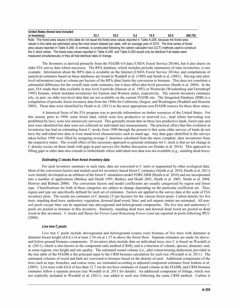
A-355
United States (forest land included in Inventory) 53.1 10.5 9.2 10.5 63.0 269,702
Note: The forest area values in this table do not equal the forest area values reported in Table A-248, because the forest area values in this table are estimated using the most recent dataset per state, with an average year of 2010. The time series of forest area values reported in Table A-248, in contrast, is constructed following the carbon calculator tool (CCT) methods used to construct the C stock series. The forest area values reported in Table A-248 and Table A-250 would only be identical if all states were measured simultaneously or they all had identical rates of change.
The Inventory is derived primarily from the FIADB 6.0 data (USDA Forest Service 2014b), but it also draws on older FIA survey data where necessary. The RPA database, which includes periodic summaries of state inventories, is one example. Information about the RPA data is available on the Internet (USDA Forest Service 2014a), and compilations of analytical estimates based on these databases are found in Waddell et al. (1989) and Smith et al. (2001). Having only plot-level information (such as volume per hectare of the RPA data) limits the conversion to biomass. This does not constitute a substantial difference for the overall state-wide estimates, but it does affect plot-level precision (Smith et al. 2004). In the past, FIA made their data available in tree-level Eastwide (Hansen et al. 1992) or Westwide (Woudenberg and Farrenkopf 1995) formats, which included inventories for Eastern and Western states, respectively. The current Inventory estimates rely, in part, on older tree-level data that are not available on the current FIADB site. The Integrated Database (IDB) is a compilation of periodic forest inventory data from the 1990s for California, Oregon, and Washington (Waddell and Hiserote 2005). These data were identified by Heath et al. (2011) as the most appropriate non-FIADB sources for these three states.
A historical focus of the FIA program was to provide information on timber resources of the United States. For this reason, prior to 1998, some forest land, which were less productive or reserved (i.e., land where harvesting was prohibited by law), were less intensively surveyed. This generally meant that on these less productive lands, forest type and area were identified but data were not collected on individual tree measurements. The practical effect that this evolution in inventories has had on estimating forest C stocks from 1990 through the present is that some older surveys of lands do not have the individual-tree data or even stand-level characteristics such as stand age. Any data gaps identified in the surveys taken before 1998 were filled by assigning average C densities calculated from the more complete, later inventories from the respective states. The overall effect of this necessary approach to generate estimates for C stock is that no net change in C density occurs on those lands with gaps in past surveys (for further discussion see Domke et al. 2014). This approach to filling gaps in older data also extends to timberlands where individual-tree data was not available (e.g., standing dead trees).
Estimating C stocks from forest inventory data
For each inventory summary in each state, data are converted to C units or augmented by other ecological data. Most of the conversion factors and models used for inventory-based forest C estimates (Smith et al. 2010, Heath et al. 2011) were initially developed as an offshoot of the forest C simulation model FORCARB (Heath et al. 2010) and are incorporated into a number of applications (Birdsey and Heath 1995, Birdsey and Heath 2001, Heath et al. 2003, Smith et al. 2004, Hoover and Rebain 2008). The conversion factors and model coefficients are usually categorized by region and forest type. Classifications for both of these categories are subject to change depending on the particular coefficient set. Thus, region and type are specifically defined for each set of estimates. Factors are applied to the survey data at the scale of FIA inventory plots. The results are estimates of C density (T per hectare) for the various forest pools. Carbon density for live trees, standing dead trees, understory vegetation, downed dead wood, litter, and soil organic matter are estimated. All non-soil pools except litter can be separated into aboveground and belowground components. The live tree and understory C pools are pooled as biomass in this inventory. Similarly, standing dead trees and downed dead wood are pooled as dead wood in this inventory. C stocks and fluxes for Forest Land Remaining Forest Land are reported in pools following IPCC (2006).
Live tree C pools
Live tree C pools include aboveground and belowground (coarse root) biomass of live trees with diameter at diameter breast height (d.b.h.) of at least 2.54 cm at 1.37 m above the forest floor. Separate estimates are made for above- and below-ground biomass components. If inventory plots include data on individual trees, tree C is based on Woodall et al. (2011), which is also known as the component ratio method (CRM), and is a function of volume, species, diameter, and, in some regions, tree height and site quality. The estimated sound volume (i.e., after rotten/missing deductions provided in the tree table of the FIADB is the principal input to the CRM biomass calculation for each tree (Woodall et al. 2011). The estimated volumes of wood and bark are converted to biomass based on the density of each. Additional components of the trees such as tops, branches, and coarse roots, are estimated according to adjusted component estimates from Jenkins et al. (2003). Live trees with d.b.h of less than 12.7 cm do not have estimates of sound volume in the FIADB, and CRM biomass estimates follow a separate process (see Woodall et al. 2011 for details). An additional component of foliage, which was not explicitly included in Woodall et al. (2011), was added to each tree following the same CRM method. Carbon is
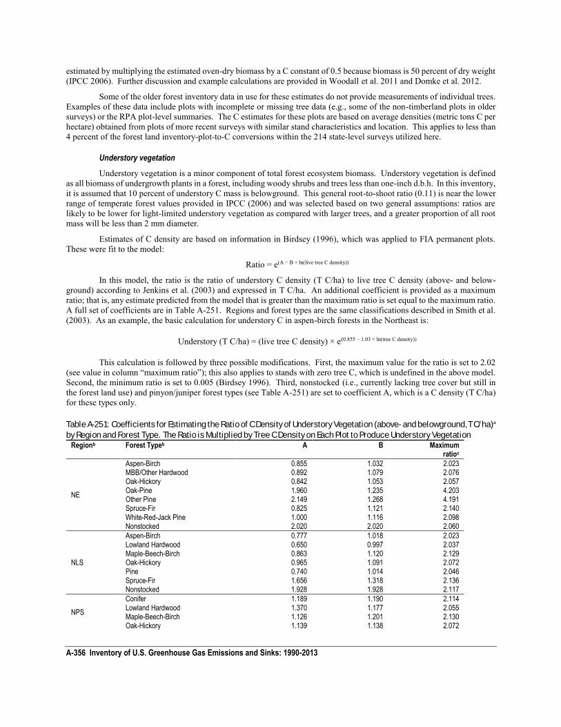
A-356 Inventory of U.S. Greenhouse Gas Emissions and Sinks: 1990-2013
estimated by multiplying the estimated oven-dry biomass by a C constant of 0.5 because biomass is 50 percent of dry weight (IPCC 2006). Further discussion and example calculations are provided in Woodall et al. 2011 and Domke et al. 2012.
Some of the older forest inventory data in use for these estimates do not provide measurements of individual trees. Examples of these data include plots with incomplete or missing tree data (e.g., some of the non-timberland plots in older surveys) or the RPA plot-level summaries. The C estimates for these plots are based on average densities (metric tons C per hectare) obtained from plots of more recent surveys with similar stand characteristics and location. This applies to less than 4 percent of the forest land inventory-plot-to-C conversions within the 214 state-level surveys utilized here.
Understory vegetation
Understory vegetation is a minor component of total forest ecosystem biomass. Understory vegetation is defined as all biomass of undergrowth plants in a forest, including woody shrubs and trees less than one-inch d.b.h. In this inventory, it is assumed that 10 percent of understory C mass is belowground. This general root-to-shoot ratio (0.11) is near the lower range of temperate forest values provided in IPCC (2006) and was selected based on two general assumptions: ratios are likely to be lower for light-limited understory vegetation as compared with larger trees, and a greater proportion of all root mass will be less than 2 mm diameter.
Estimates of C density are based on information in Birdsey (1996), which was applied to FIA permanent plots. These were fit to the model:
Ratio = e(A − B × ln(live tree C density))
In this model, the ratio is the ratio of understory C density (T C/ha) to live tree C density (above- and below-ground) according to Jenkins et al. (2003) and expressed in T C/ha. An additional coefficient is provided as a maximum ratio; that is, any estimate predicted from the model that is greater than the maximum ratio is set equal to the maximum ratio. A full set of coefficients are in Table A-251. Regions and forest types are the same classifications described in Smith et al. (2003). As an example, the basic calculation for understory C in aspen-birch forests in the Northeast is:
Understory (T C/ha) = (live tree C density) × e(0.855 – 1.03 × ln(tree C density))
This calculation is followed by three possible modifications. First, the maximum value for the ratio is set to 2.02 (see value in column “maximum ratio”); this also applies to stands with zero tree C, which is undefined in the above model. Second, the minimum ratio is set to 0.005 (Birdsey 1996). Third, nonstocked (i.e., currently lacking tree cover but still in the forest land use) and pinyon/juniper forest types (see Table A-251) are set to coefficient A, which is a C density (T C/ha) for these types only.
Table A-251: Coefficients for Estimating the Ratio of C Density of Understory Vegetation (above- and belowground, T C/ha)a
by Region and Forest Type. The Ratio is Multiplied by Tree C Density on Each Plot to Produce Understory Vegetation
Regionb Forest Typeb A B Maximum ratioc
NE
Aspen-Birch 0.855 1.032 2.023 MBB/Other Hardwood 0.892 1.079 2.076 Oak-Hickory 0.842 1.053 2.057 Oak-Pine 1.960 1.235 4.203 Other Pine 2.149 1.268 4.191 Spruce-Fir 0.825 1.121 2.140 White-Red-Jack Pine 1.000 1.116 2.098 Nonstocked 2.020 2.020 2.060
NLS
Aspen-Birch 0.777 1.018 2.023 Lowland Hardwood 0.650 0.997 2.037 Maple-Beech-Birch 0.863 1.120 2.129 Oak-Hickory 0.965 1.091 2.072 Pine 0.740 1.014 2.046 Spruce-Fir 1.656 1.318 2.136 Nonstocked 1.928 1.928 2.117
NPS
Conifer 1.189 1.190 2.114 Lowland Hardwood 1.370 1.177 2.055 Maple-Beech-Birch 1.126 1.201 2.130 Oak-Hickory 1.139 1.138 2.072
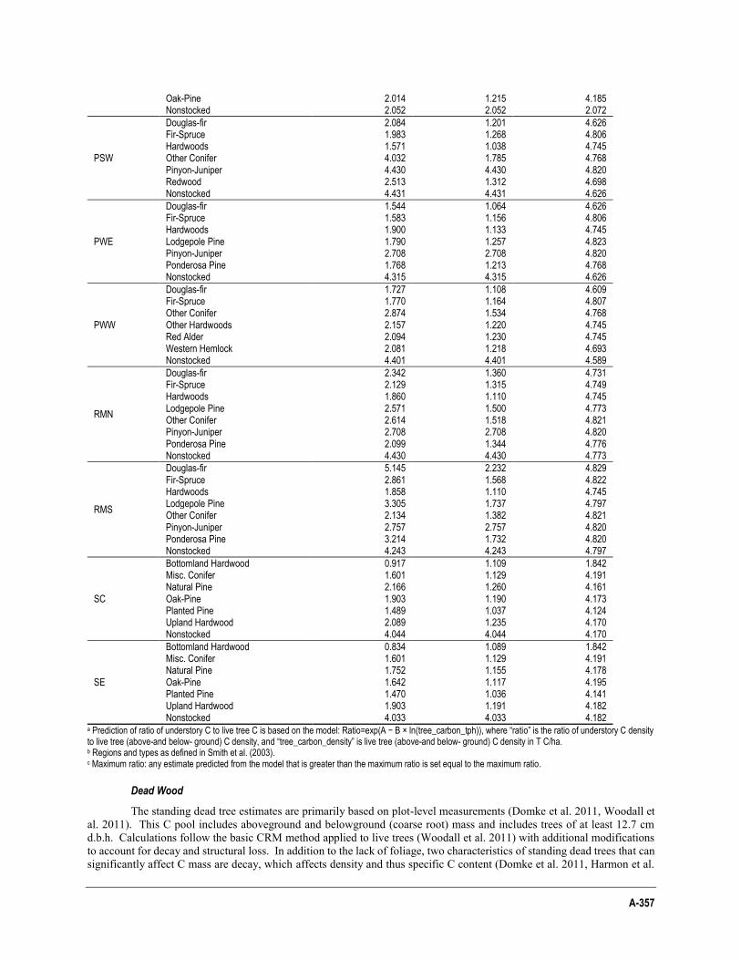
A-357
Oak-Pine 2.014 1.215 4.185 Nonstocked 2.052 2.052 2.072
PSW
Douglas-fir 2.084 1.201 4.626 Fir-Spruce 1.983 1.268 4.806 Hardwoods 1.571 1.038 4.745 Other Conifer 4.032 1.785 4.768 Pinyon-Juniper 4.430 4.430 4.820 Redwood 2.513 1.312 4.698 Nonstocked 4.431 4.431 4.626
PWE
Douglas-fir 1.544 1.064 4.626 Fir-Spruce 1.583 1.156 4.806 Hardwoods 1.900 1.133 4.745 Lodgepole Pine 1.790 1.257 4.823 Pinyon-Juniper 2.708 2.708 4.820 Ponderosa Pine 1.768 1.213 4.768 Nonstocked 4.315 4.315 4.626
PWW
Douglas-fir 1.727 1.108 4.609 Fir-Spruce 1.770 1.164 4.807 Other Conifer 2.874 1.534 4.768 Other Hardwoods 2.157 1.220 4.745 Red Alder 2.094 1.230 4.745 Western Hemlock 2.081 1.218 4.693 Nonstocked 4.401 4.401 4.589
RMN
Douglas-fir 2.342 1.360 4.731 Fir-Spruce 2.129 1.315 4.749 Hardwoods 1.860 1.110 4.745 Lodgepole Pine 2.571 1.500 4.773 Other Conifer 2.614 1.518 4.821 Pinyon-Juniper 2.708 2.708 4.820 Ponderosa Pine 2.099 1.344 4.776 Nonstocked 4.430 4.430 4.773
RMS
Douglas-fir 5.145 2.232 4.829 Fir-Spruce 2.861 1.568 4.822 Hardwoods 1.858 1.110 4.745 Lodgepole Pine 3.305 1.737 4.797 Other Conifer 2.134 1.382 4.821 Pinyon-Juniper 2.757 2.757 4.820 Ponderosa Pine 3.214 1.732 4.820 Nonstocked 4.243 4.243 4.797
SC
Bottomland Hardwood 0.917 1.109 1.842 Misc. Conifer 1.601 1.129 4.191 Natural Pine 2.166 1.260 4.161 Oak-Pine 1.903 1.190 4.173 Planted Pine 1.489 1.037 4.124 Upland Hardwood 2.089 1.235 4.170 Nonstocked 4.044 4.044 4.170
SE
Bottomland Hardwood 0.834 1.089 1.842 Misc. Conifer 1.601 1.129 4.191 Natural Pine 1.752 1.155 4.178 Oak-Pine 1.642 1.117 4.195 Planted Pine 1.470 1.036 4.141 Upland Hardwood 1.903 1.191 4.182 Nonstocked 4.033 4.033 4.182
a Prediction of ratio of understory C to live tree C is based on the model: Ratio=exp(A − B × ln(tree_carbon_tph)), where “ratio” is the ratio of understory C density to live tree (above-and below- ground) C density, and “tree_carbon_density” is live tree (above-and below- ground) C density in T C/ha. b Regions and types as defined in Smith et al. (2003). c Maximum ratio: any estimate predicted from the model that is greater than the maximum ratio is set equal to the maximum ratio.
Dead Wood
The standing dead tree estimates are primarily based on plot-level measurements (Domke et al. 2011, Woodall et al. 2011). This C pool includes aboveground and belowground (coarse root) mass and includes trees of at least 12.7 cm d.b.h. Calculations follow the basic CRM method applied to live trees (Woodall et al. 2011) with additional modifications to account for decay and structural loss. In addition to the lack of foliage, two characteristics of standing dead trees that can significantly affect C mass are decay, which affects density and thus specific C content (Domke et al. 2011, Harmon et al.
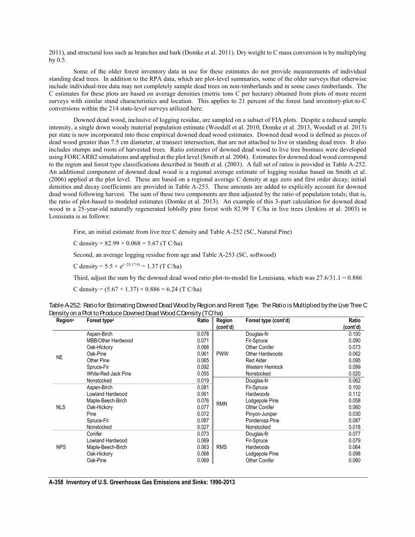
A-358 Inventory of U.S. Greenhouse Gas Emissions and Sinks: 1990-2013
2011), and structural loss such as branches and bark (Domke et al. 2011). Dry weight to C mass conversion is by multiplying by 0.5.
Some of the older forest inventory data in use for these estimates do not provide measurements of individual standing dead trees. In addition to the RPA data, which are plot-level summaries, some of the older surveys that otherwise include individual-tree data may not completely sample dead trees on non-timberlands and in some cases timberlands. The C estimates for these plots are based on average densities (metric tons C per hectare) obtained from plots of more recent surveys with similar stand characteristics and location. This applies to 21 percent of the forest land inventory-plot-to-C conversions within the 214 state-level surveys utilized here.
Downed dead wood, inclusive of logging residue, are sampled on a subset of FIA plots. Despite a reduced sample intensity, a single down woody material population estimate (Woodall et al. 2010, Domke et al. 2013, Woodall et al. 2013) per state is now incorporated into these empirical downed dead wood estimates. Downed dead wood is defined as pieces of dead wood greater than 7.5 cm diameter, at transect intersection, that are not attached to live or standing dead trees. It also includes stumps and roots of harvested trees. Ratio estimates of downed dead wood to live tree biomass were developed using FORCARB2 simulations and applied at the plot level (Smith et al. 2004). Estimates for downed dead wood correspond to the region and forest type classifications described in Smith et al. (2003). A full set of ratios is provided in Table A-252. An additional component of downed dead wood is a regional average estimate of logging residue based on Smith et al. (2006) applied at the plot level. These are based on a regional average C density at age zero and first order decay; initial densities and decay coefficients are provided in Table A-253. These amounts are added to explicitly account for downed dead wood following harvest. The sum of these two components are then adjusted by the ratio of population totals; that is, the ratio of plot-based to modeled estimates (Domke et al. 2013). An example of this 3-part calculation for downed dead wood in a 25-year-old naturally regenerated loblolly pine forest with 82.99 T C/ha in live trees (Jenkins et al. 2003) in Louisiana is as follows:
First, an initial estimate from live tree C density and Table A-252 (SC, Natural Pine)
C density = 82.99 × 0.068 = 5.67 (T C/ha)
Second, an average logging residue from age and Table A-253 (SC, softwood)
C density = 5.5 × e(−25/17.9) = 1.37 (T C/ha)
Third, adjust the sum by the downed dead wood ratio plot-to-model for Louisiana, which was 27.6/31.1 = 0.886
C density = (5.67 + 1.37) × 0.886 = 6.24 (T C/ha)
Table A-252: Ratio for Estimating Downed Dead Wood by Region and Forest Type. The Ratio is Multiplied by the Live Tree C
Density on a Plot to Produce Downed Dead Wood C Density (T C/ha) Regiona Forest typea Ratio Region
(cont’d) Forest type (cont’d) Ratio
(cont’d)
NE
Aspen-Birch 0.078
PWW
Douglas-fir 0.100 MBB/Other Hardwood 0.071 Fir-Spruce 0.090 Oak-Hickory 0.068 Other Conifer 0.073 Oak-Pine 0.061 Other Hardwoods 0.062 Other Pine 0.065 Red Alder 0.095 Spruce-Fir 0.092 Western Hemlock 0.099 White-Red-Jack Pine 0.055 Nonstocked 0.020
Nonstocked 0.019
RMN
Douglas-fir 0.062
NLS
Aspen-Birch 0.081 Fir-Spruce 0.100 Lowland Hardwood 0.061 Hardwoods 0.112 Maple-Beech-Birch 0.076 Lodgepole Pine 0.058 Oak-Hickory 0.077 Other Conifer 0.060 Pine 0.072 Pinyon-Juniper 0.030 Spruce-Fir 0.087 Ponderosa Pine 0.087 Nonstocked 0.027 Nonstocked 0.018
NPS
Conifer 0.073
RMS
Douglas-fir 0.077 Lowland Hardwood 0.069 Fir-Spruce 0.079 Maple-Beech-Birch 0.063 Hardwoods 0.064 Oak-Hickory 0.068 Lodgepole Pine 0.098 Oak-Pine 0.069 Other Conifer 0.060
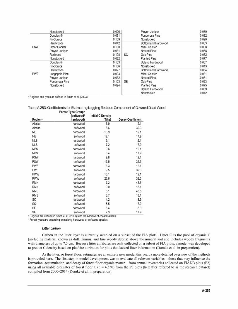
A-359
Nonstocked 0.026 Pinyon-Juniper 0.030
PSW
Douglas-fir 0.091 Ponderosa Pine 0.082 Fir-Spruce 0.109 Nonstocked 0.020
Hardwoods 0.042
SC
Bottomland Hardwood 0.063 Other Conifer 0.100 Misc. Conifer 0.068 Pinyon-Juniper 0.031 Natural Pine 0.068 Redwood 0.108 Oak-Pine 0.072 Nonstocked 0.022 Planted Pine 0.077
PWE
Douglas-fir 0.103 Upland Hardwood 0.067 Fir-Spruce 0.106 Nonstocked 0.013 Hardwoods 0.027
SE
Bottomland Hardwood 0.064 Lodgepole Pine 0.093 Misc. Conifer 0.081 Pinyon-Juniper 0.032 Natural Pine 0.081 Ponderosa Pine 0.103 Oak-Pine 0.063 Nonstocked 0.024 Planted Pine 0.075
Upland Hardwood 0.059 Nonstocked 0.012
a Regions and types as defined in Smith et al. (2003).
Table A-253: Coefficients for Estimating Logging Residue Component of Downed Dead Wood
Regiona
Forest Type Groupb (softwood/ hardwood)
Initial C Density (T/ha) Decay Coefficient
Alaska hardwood 6.9 12.1
Alaska softwood 8.6 32.3
NE hardwood 13.9 12.1
NE softwood 12.1 17.9
NLS hardwood 9.1 12.1
NLS softwood 7.2 17.9
NPS hardwood 9.6 12.1
NPS softwood 6.4 17.9
PSW hardwood 9.8 12.1
PSW softwood 17.5 32.3
PWE hardwood 3.3 12.1
PWE softwood 9.5 32.3
PWW hardwood 18.1 12.1
PWW softwood 23.6 32.3
RMN hardwood 7.2 43.5
RMN softwood 9.0 18.1
RMS hardwood 5.1 43.5
RMS softwood 3.7 18.1
SC hardwood 4.2 8.9
SC softwood 5.5 17.9
SE hardwood 6.4 8.9
SE softwood 7.3 17.9 a Regions are defined in Smith et al. (2003) with the addition of coastal Alaska. b Forest types are according to majority hardwood or softwood species.
Litter carbon
Carbon in the litter layer is currently sampled on a subset of the FIA plots. Litter C is the pool of organic C (including material known as duff, humus, and fine woody debris) above the mineral soil and includes woody fragments with diameters of up to 7.5 cm. Because litter attributes are only collected on a subset of FIA plots, a model was developed to predict C density based on plot/site attributes for plots that lacked litter information (Domke et al. in preparation).
As the litter, or forest floor, estimates are an entirely new model this year, a more detailed overview of the methods is provided here. The first step in model development was to evaluate all relevant variables—those that may influence the formation, accumulation, and decay of forest floor organic matter—from annual inventories collected on FIADB plots (P2) using all available estimates of forest floor C (n = 4,530) from the P3 plots (hereafter referred to as the research dataset) compiled from 2000–2014 (Domke et al. in preparation).
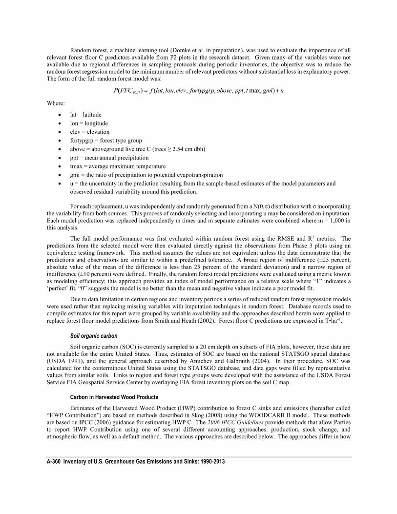
A-360 Inventory of U.S. Greenhouse Gas Emissions and Sinks: 1990-2013
Random forest, a machine learning tool (Domke et al. in preparation), was used to evaluate the importance of all relevant forest floor C predictors available from P2 plots in the research dataset. Given many of the variables were not available due to regional differences in sampling protocols during periodic inventories, the objective was to reduce the random forest regression model to the minimum number of relevant predictors without substantial loss in explanatory power. The form of the full random forest model was:
ugmitpptabovefortypgrpelevlonlatfFFCP Full )max,,,,,,,()(
Where:
lat = latitude lon = longitude elev = elevation fortypgrp = forest type group above = aboveground live tree C (trees ≥ 2.54 cm dbh) ppt = mean annual precipitation tmax = average maximum temperature gmi = the ratio of precipitation to potential evapotranspiration u = the uncertainty in the prediction resulting from the sample-based estimates of the model parameters and
observed residual variability around this prediction.
For each replacement, u was independently and randomly generated from a N(0,σ) distribution with σ incorporating the variability from both sources. This process of randomly selecting and incorporating u may be considered an imputation. Each model prediction was replaced independently m times and m separate estimates were combined where m = 1,000 in this analysis.
The full model performance was first evaluated within random forest using the RMSE and R2 metrics. The predictions from the selected model were then evaluated directly against the observations from Phase 3 plots using an equivalence testing framework. This method assumes the values are not equivalent unless the data demonstrate that the predictions and observations are similar to within a predefined tolerance. A broad region of indifference (±25 percent, absolute value of the mean of the difference is less than 25 percent of the standard deviation) and a narrow region of indifference (±10 percent) were defined. Finally, the random forest model predictions were evaluated using a metric known as modeling efficiency; this approach provides an index of model performance on a relative scale where “1” indicates a ‘perfect’ fit, “0” suggests the model is no better than the mean and negative values indicate a poor model fit.
Due to data limitation in certain regions and inventory periods a series of reduced random forest regression models were used rather than replacing missing variables with imputation techniques in random forest. Database records used to compile estimates for this report were grouped by variable availability and the approaches described herein were applied to replace forest floor model predictions from Smith and Heath (2002). Forest floor C predictions are expressed in T•ha−1.
Soil organic carbon
Soil organic carbon (SOC) is currently sampled to a 20 cm depth on subsets of FIA plots, however, these data are not available for the entire United States. Thus, estimates of SOC are based on the national STATSGO spatial database (USDA 1991), and the general approach described by Amichev and Galbraith (2004). In their procedure, SOC was calculated for the conterminous United States using the STATSGO database, and data gaps were filled by representative values from similar soils. Links to region and forest type groups were developed with the assistance of the USDA Forest Service FIA Geospatial Service Center by overlaying FIA forest inventory plots on the soil C map.
Carbon in Harvested Wood Products
Estimates of the Harvested Wood Product (HWP) contribution to forest C sinks and emissions (hereafter called “HWP Contribution”) are based on methods described in Skog (2008) using the WOODCARB II model. These methods are based on IPCC (2006) guidance for estimating HWP C. The 2006 IPCC Guidelines provide methods that allow Parties to report HWP Contribution using one of several different accounting approaches: production, stock change, and atmospheric flow, as well as a default method. The various approaches are described below. The approaches differ in how
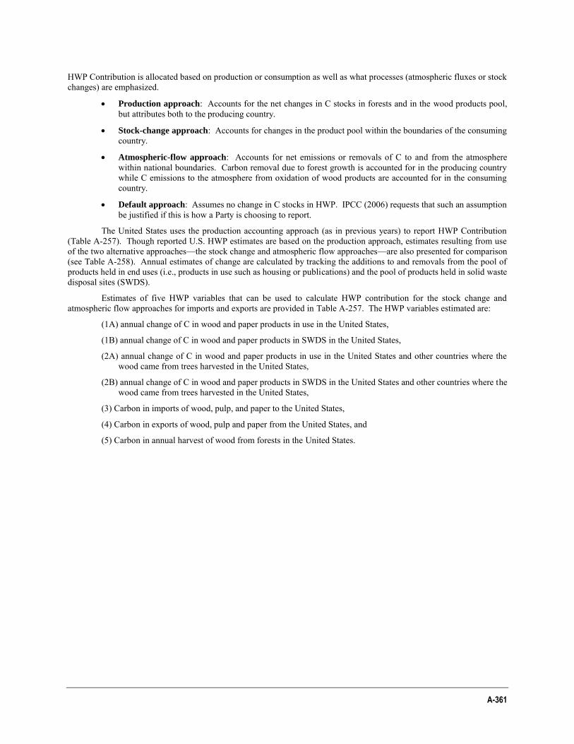
A-361
HWP Contribution is allocated based on production or consumption as well as what processes (atmospheric fluxes or stock changes) are emphasized.
Production approach: Accounts for the net changes in C stocks in forests and in the wood products pool, but attributes both to the producing country.
Stock-change approach: Accounts for changes in the product pool within the boundaries of the consuming country.
Atmospheric-flow approach: Accounts for net emissions or removals of C to and from the atmosphere within national boundaries. Carbon removal due to forest growth is accounted for in the producing country while C emissions to the atmosphere from oxidation of wood products are accounted for in the consuming country.
Default approach: Assumes no change in C stocks in HWP. IPCC (2006) requests that such an assumption be justified if this is how a Party is choosing to report.
The United States uses the production accounting approach (as in previous years) to report HWP Contribution (Table A-257). Though reported U.S. HWP estimates are based on the production approach, estimates resulting from use of the two alternative approaches—the stock change and atmospheric flow approaches—are also presented for comparison (see Table A-258). Annual estimates of change are calculated by tracking the additions to and removals from the pool of products held in end uses (i.e., products in use such as housing or publications) and the pool of products held in solid waste disposal sites (SWDS).
Estimates of five HWP variables that can be used to calculate HWP contribution for the stock change and atmospheric flow approaches for imports and exports are provided in Table A-257. The HWP variables estimated are:
(1A) annual change of C in wood and paper products in use in the United States,
(1B) annual change of C in wood and paper products in SWDS in the United States,
(2A) annual change of C in wood and paper products in use in the United States and other countries where the wood came from trees harvested in the United States,
(2B) annual change of C in wood and paper products in SWDS in the United States and other countries where the wood came from trees harvested in the United States,
(3) Carbon in imports of wood, pulp, and paper to the United States,
(4) Carbon in exports of wood, pulp and paper from the United States, and
(5) Carbon in annual harvest of wood from forests in the United States.
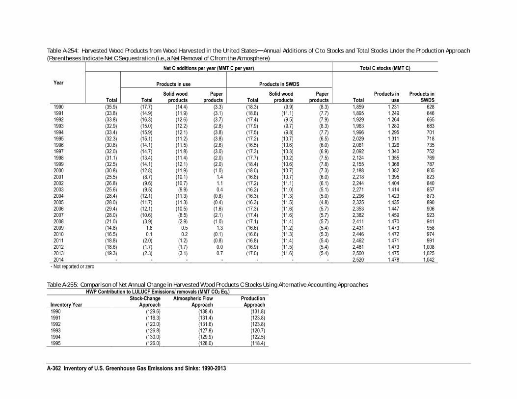
A-362 Inventory of U.S. Greenhouse Gas Emissions and Sinks: 1990-2013
Table A-254: Harvested Wood Products from Wood Harvested in the United States—Annual Additions of C to Stocks and Total Stocks Under the Production Approach
(Parentheses Indicate Net C Sequestration (i.e., a Net Removal of C from the Atmosphere)
Year
Net C additions per year (MMT C per year) Total C stocks (MMT C)
Total
Products in use Products in SWDS
Total Solid wood
products Paper
products Total Solid wood
products Paper
products Total Products in
use Products in
SWDS
1990 (35.9) (17.7) (14.4) (3.3) (18.3) (9.9) (8.3) 1,859 1,231 628 1991 (33.8) (14.9) (11.9) (3.1) (18.8) (11.1) (7.7) 1,895 1,249 646 1992 (33.8) (16.3) (12.6) (3.7) (17.4) (9.5) (7.9) 1,929 1,264 665 1993 (32.9) (15.0) (12.2) (2.8) (17.9) (9.7) (8.3) 1,963 1,280 683 1994 (33.4) (15.9) (12.1) (3.8) (17.5) (9.8) (7.7) 1,996 1,295 701 1995 (32.3) (15.1) (11.2) (3.8) (17.2) (10.7) (6.5) 2,029 1,311 718 1996 (30.6) (14.1) (11.5) (2.6) (16.5) (10.6) (6.0) 2,061 1,326 735 1997 (32.0) (14.7) (11.8) (3.0) (17.3) (10.3) (6.9) 2,092 1,340 752 1998 (31.1) (13.4) (11.4) (2.0) (17.7) (10.2) (7.5) 2,124 1,355 769 1999 (32.5) (14.1) (12.1) (2.0) (18.4) (10.6) (7.8) 2,155 1,368 787 2000 (30.8) (12.8) (11.9) (1.0) (18.0) (10.7) (7.3) 2,188 1,382 805 2001 (25.5) (8.7) (10.1) 1.4 (16.8) (10.7) (6.0) 2,218 1,395 823 2002 (26.8) (9.6) (10.7) 1.1 (17.2) (11.1) (6.1) 2,244 1,404 840 2003 (25.6) (9.5) (9.9) 0.4 (16.2) (11.0) (5.1) 2,271 1,414 857 2004 (28.4) (12.1) (11.3) (0.8) (16.3) (11.3) (5.0) 2,296 1,423 873 2005 (28.0) (11.7) (11.3) (0.4) (16.3) (11.5) (4.8) 2,325 1,435 890 2006 (29.4) (12.1) (10.5) (1.6) (17.3) (11.6) (5.7) 2,353 1,447 906 2007 (28.0) (10.6) (8.5) (2.1) (17.4) (11.6) (5.7) 2,382 1,459 923 2008 (21.0) (3.9) (2.9) (1.0) (17.1) (11.4) (5.7) 2,411 1,470 941 2009 (14.8) 1.8 0.5 1.3 (16.6) (11.2) (5.4) 2,431 1,473 958 2010 (16.5) 0.1 0.2 (0.1) (16.6) (11.3) (5.3) 2,446 1,472 974 2011 (18.8) (2.0) (1.2) (0.8) (16.8) (11.4) (5.4) 2,462 1,471 991 2012 (18.6) (1.7) (1.7) 0.0 (16.9) (11.5) (5.4) 2,481 1,473 1,008 2013 (19.3) (2.3) (3.1) 0.7 (17.0) (11.6) (5.4) 2,500 1,475 1,025 2014 - - - - - - - 2,520 1,478 1,042
- Not reported or zero
Table A-255: Comparison of Net Annual Change in Harvested Wood Products C Stocks Using Alternative Accounting Approaches HWP Contribution to LULUCF Emissions/ removals (MMT CO2 Eq.)
Inventory Year Stock-Change
Approach Atmospheric Flow
Approach Production
Approach
1990 (129.6) (138.4) (131.8) 1991 (116.3) (131.4) (123.8) 1992 (120.0) (131.6) (123.8) 1993 (126.8) (127.8) (120.7) 1994 (130.0) (129.9) (122.5) 1995 (126.0) (128.0) (118.4)
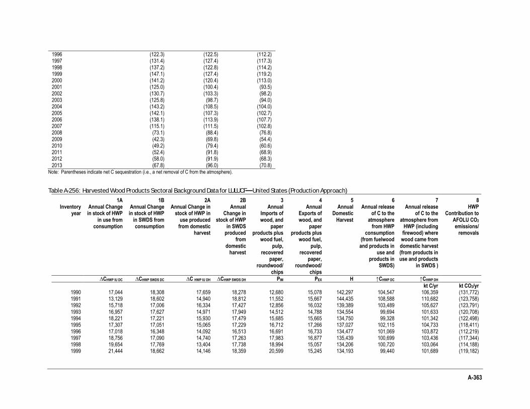
A-363
1996 (122.3) (122.5) (112.2) 1997 (131.4) (127.4) (117.3) 1998 (137.2) (122.8) (114.2) 1999 (147.1) (127.4) (119.2) 2000 (141.2) (120.4) (113.0) 2001 (125.0) (100.4) (93.5) 2002 (130.7) (103.3) (98.2) 2003 (125.8) (98.7) (94.0) 2004 (143.2) (108.5) (104.0) 2005 (142.1) (107.3) (102.7) 2006 (138.1) (113.9) (107.7) 2007 (115.1) (111.5) (102.8) 2008 (73.1) (88.4) (76.8) 2009 (42.3) (69.8) (54.4) 2010 (49.2) (79.4) (60.6) 2011 (52.4) (91.8) (68.9) 2012 (58.0) (91.9) (68.3) 2013 (67.8) (96.0) (70.8)
Note: Parentheses indicate net C sequestration (i.e., a net removal of C from the atmosphere).
Table A-256: Harvested Wood Products Sectoral Background Data for LULUCF—United States (Production Approach)
1A 1B 2A 2B 3 4 5 6 7 8 Inventory
year Annual Change in stock of HWP
in use from consumption
Annual Change in stock of HWP
in SWDS from consumption
Annual Change in stock of HWP in
use produced from domestic
harvest
Annual Change in
stock of HWP in SWDS
produced from
domestic harvest
Annual Imports of wood, and
paper products plus
wood fuel, pulp,
recovered paper,
roundwood/ chips
Annual Exports of wood, and
paper products plus
wood fuel, pulp,
recovered paper,
roundwood/ chips
Annual Domestic
Harvest
Annual release of C to the
atmosphere from HWP
consumption (from fuelwood and products in
use and products in
SWDS)
Annual release of C to the
atmosphere from HWP (including firewood) where
wood came from domestic harvest (from products in use and products
in SWDS )
HWP Contribution to
AFOLU CO2 emissions/
removals
∆CHWP IU DC ∆CHWP SWDS DC ∆C HWP IU DH ∆CHWP SWDS DH PIM PEX H ↑CHWP DC ↑CHWP DH
kt C/yr kt CO2/yr 1990 17,044 18,308 17,659 18,278 12,680 15,078 142,297 104,547 106,359 (131,772) 1991 13,129 18,602 14,940 18,812 11,552 15,667 144,435 108,588 110,682 (123,758) 1992 15,718 17,006 16,334 17,427 12,856 16,032 139,389 103,489 105,627 (123,791) 1993 16,957 17,627 14,971 17,949 14,512 14,788 134,554 99,694 101,633 (120,708) 1994 18,221 17,221 15,930 17,479 15,685 15,665 134,750 99,328 101,342 (122,498) 1995 17,307 17,051 15,065 17,229 16,712 17,266 137,027 102,115 104,733 (118,411) 1996 17,018 16,348 14,092 16,513 16,691 16,733 134,477 101,069 103,872 (112,219) 1997 18,756 17,090 14,740 17,263 17,983 16,877 135,439 100,699 103,436 (117,344) 1998 19,654 17,769 13,404 17,738 18,994 15,057 134,206 100,720 103,064 (114,188) 1999 21,444 18,662 14,146 18,359 20,599 15,245 134,193 99,440 101,689 (119,182)
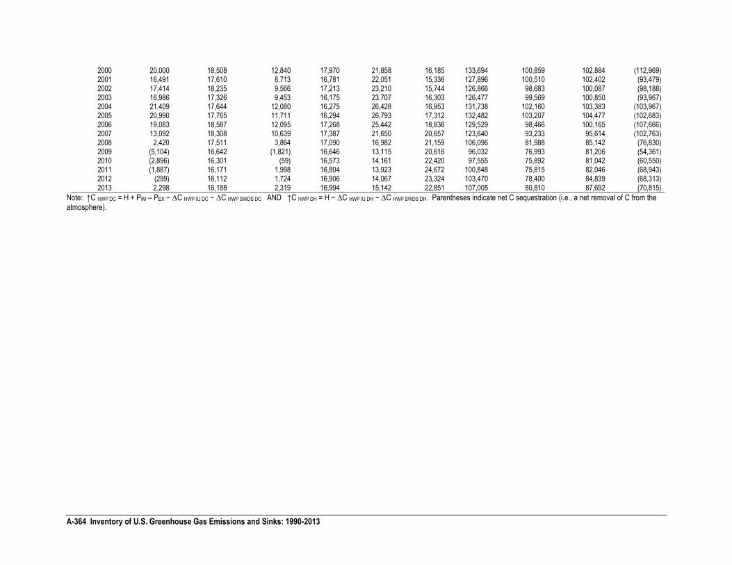
A-364 Inventory of U.S. Greenhouse Gas Emissions and Sinks: 1990-2013
2000 20,000 18,508 12,840 17,970 21,858 16,185 133,694 100,859 102,884 (112,969) 2001 16,491 17,610 8,713 16,781 22,051 15,336 127,896 100,510 102,402 (93,479) 2002 17,414 18,235 9,566 17,213 23,210 15,744 126,866 98,683 100,087 (98,188) 2003 16,986 17,326 9,453 16,175 23,707 16,303 126,477 99,569 100,850 (93,967) 2004 21,409 17,644 12,080 16,275 26,428 16,953 131,738 102,160 103,383 (103,967) 2005 20,990 17,765 11,711 16,294 26,793 17,312 132,482 103,207 104,477 (102,683) 2006 19,083 18,587 12,095 17,268 25,442 18,836 129,529 98,466 100,165 (107,666) 2007 13,092 18,308 10,639 17,387 21,650 20,657 123,640 93,233 95,614 (102,763) 2008 2,420 17,511 3,864 17,090 16,982 21,159 106,096 81,988 85,142 (76,830) 2009 (5,104) 16,642 (1,821) 16,646 13,115 20,616 96,032 76,993 81,206 (54,361) 2010 (2,896) 16,301 (59) 16,573 14,161 22,420 97,555 75,892 81,042 (60,550) 2011 (1,887) 16,171 1,998 16,804 13,923 24,672 100,848 75,815 82,046 (68,943) 2012 (299) 16,112 1,724 16,906 14,067 23,324 103,470 78,400 84,839 (68,313) 2013 2,298 16,188 2,319 16,994 15,142 22,851 107,005 80,810 87,692 (70,815)
Note: ↑C HWP DC = H + PIM – PEX − ∆C HWP IU DC − ∆C HWP SWDS DC AND ↑C HWP DH = H − ∆C HWP IU DH − ∆C HWP SWDS DH. Parentheses indicate net C sequestration (i.e., a net removal of C from the atmosphere).
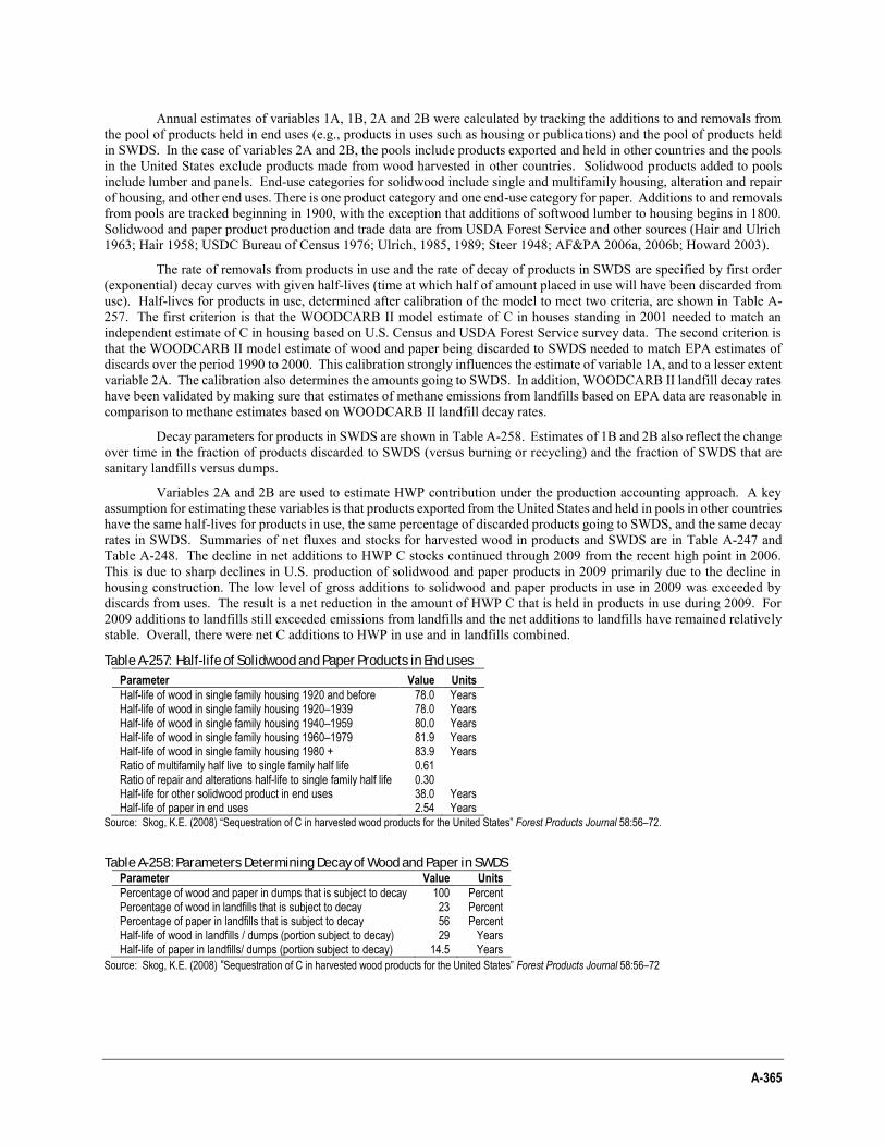
A-365
Annual estimates of variables 1A, 1B, 2A and 2B were calculated by tracking the additions to and removals from the pool of products held in end uses (e.g., products in uses such as housing or publications) and the pool of products held in SWDS. In the case of variables 2A and 2B, the pools include products exported and held in other countries and the pools in the United States exclude products made from wood harvested in other countries. Solidwood products added to pools include lumber and panels. End-use categories for solidwood include single and multifamily housing, alteration and repair of housing, and other end uses. There is one product category and one end-use category for paper. Additions to and removals from pools are tracked beginning in 1900, with the exception that additions of softwood lumber to housing begins in 1800. Solidwood and paper product production and trade data are from USDA Forest Service and other sources (Hair and Ulrich 1963; Hair 1958; USDC Bureau of Census 1976; Ulrich, 1985, 1989; Steer 1948; AF&PA 2006a, 2006b; Howard 2003).
The rate of removals from products in use and the rate of decay of products in SWDS are specified by first order (exponential) decay curves with given half-lives (time at which half of amount placed in use will have been discarded from use). Half-lives for products in use, determined after calibration of the model to meet two criteria, are shown in Table A-257. The first criterion is that the WOODCARB II model estimate of C in houses standing in 2001 needed to match an independent estimate of C in housing based on U.S. Census and USDA Forest Service survey data. The second criterion is that the WOODCARB II model estimate of wood and paper being discarded to SWDS needed to match EPA estimates of discards over the period 1990 to 2000. This calibration strongly influences the estimate of variable 1A, and to a lesser extent variable 2A. The calibration also determines the amounts going to SWDS. In addition, WOODCARB II landfill decay rates have been validated by making sure that estimates of methane emissions from landfills based on EPA data are reasonable in comparison to methane estimates based on WOODCARB II landfill decay rates.
Decay parameters for products in SWDS are shown in Table A-258. Estimates of 1B and 2B also reflect the change over time in the fraction of products discarded to SWDS (versus burning or recycling) and the fraction of SWDS that are sanitary landfills versus dumps.
Variables 2A and 2B are used to estimate HWP contribution under the production accounting approach. A key assumption for estimating these variables is that products exported from the United States and held in pools in other countries have the same half-lives for products in use, the same percentage of discarded products going to SWDS, and the same decay rates in SWDS. Summaries of net fluxes and stocks for harvested wood in products and SWDS are in Table A-247 and Table A-248. The decline in net additions to HWP C stocks continued through 2009 from the recent high point in 2006. This is due to sharp declines in U.S. production of solidwood and paper products in 2009 primarily due to the decline in housing construction. The low level of gross additions to solidwood and paper products in use in 2009 was exceeded by discards from uses. The result is a net reduction in the amount of HWP C that is held in products in use during 2009. For 2009 additions to landfills still exceeded emissions from landfills and the net additions to landfills have remained relatively stable. Overall, there were net C additions to HWP in use and in landfills combined.
Table A-257: Half-life of Solidwood and Paper Products in End uses
Parameter Value Units
Half-life of wood in single family housing 1920 and before 78.0 Years Half-life of wood in single family housing 1920–1939 78.0 Years Half-life of wood in single family housing 1940–1959 80.0 Years Half-life of wood in single family housing 1960–1979 81.9 Years Half-life of wood in single family housing 1980 + 83.9 Years Ratio of multifamily half live to single family half life 0.61 Ratio of repair and alterations half-life to single family half life 0.30 Half-life for other solidwood product in end uses 38.0 Years Half-life of paper in end uses 2.54 Years
Source: Skog, K.E. (2008) “Sequestration of C in harvested wood products for the United States” Forest Products Journal 58:56–72.
Table A-258: Parameters Determining Decay of Wood and Paper in SWDS Parameter Value Units
Percentage of wood and paper in dumps that is subject to decay 100 Percent Percentage of wood in landfills that is subject to decay 23 Percent Percentage of paper in landfills that is subject to decay 56 Percent Half-life of wood in landfills / dumps (portion subject to decay) 29 Years Half-life of paper in landfills/ dumps (portion subject to decay) 14.5 Years
Source: Skog, K.E. (2008) “Sequestration of C in harvested wood products for the United States” Forest Products Journal 58:56–72
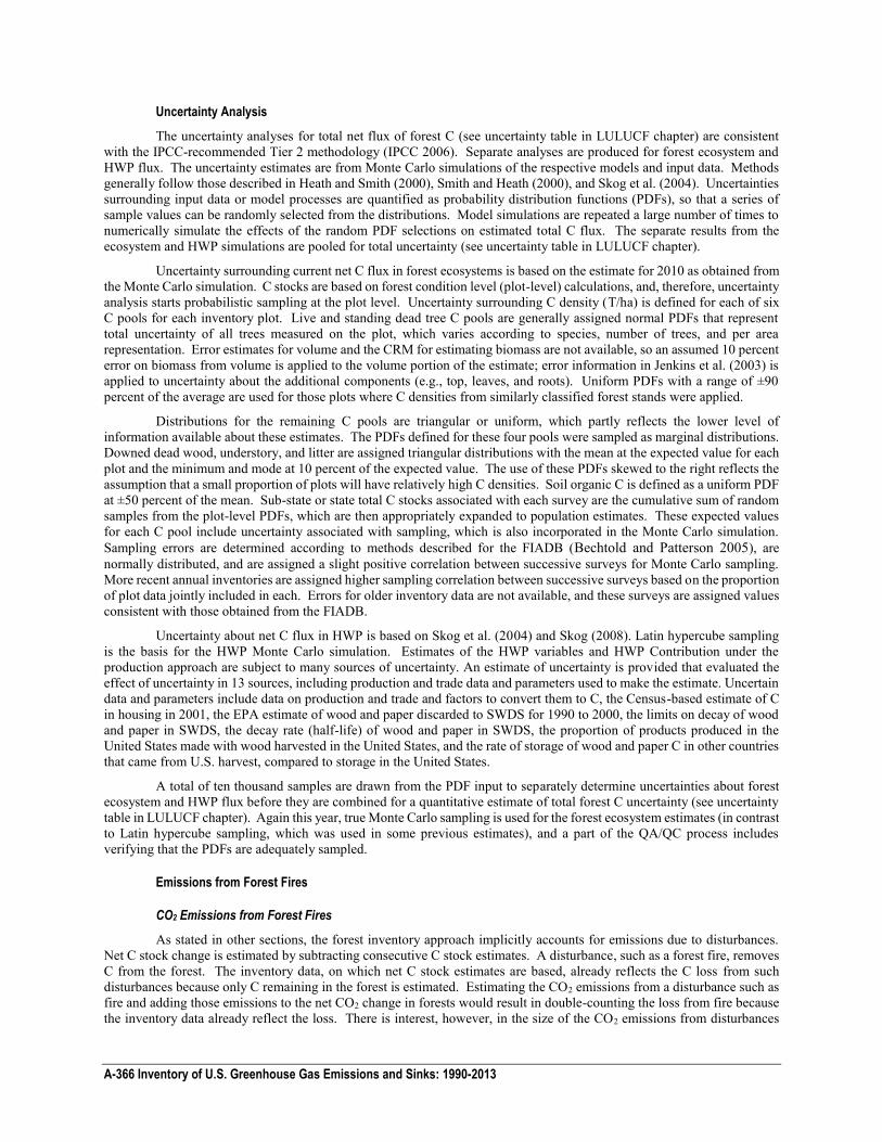
A-366 Inventory of U.S. Greenhouse Gas Emissions and Sinks: 1990-2013
Uncertainty Analysis
The uncertainty analyses for total net flux of forest C (see uncertainty table in LULUCF chapter) are consistent with the IPCC-recommended Tier 2 methodology (IPCC 2006). Separate analyses are produced for forest ecosystem and HWP flux. The uncertainty estimates are from Monte Carlo simulations of the respective models and input data. Methods generally follow those described in Heath and Smith (2000), Smith and Heath (2000), and Skog et al. (2004). Uncertainties surrounding input data or model processes are quantified as probability distribution functions (PDFs), so that a series of sample values can be randomly selected from the distributions. Model simulations are repeated a large number of times to numerically simulate the effects of the random PDF selections on estimated total C flux. The separate results from the ecosystem and HWP simulations are pooled for total uncertainty (see uncertainty table in LULUCF chapter).
Uncertainty surrounding current net C flux in forest ecosystems is based on the estimate for 2010 as obtained from the Monte Carlo simulation. C stocks are based on forest condition level (plot-level) calculations, and, therefore, uncertainty analysis starts probabilistic sampling at the plot level. Uncertainty surrounding C density (T/ha) is defined for each of six C pools for each inventory plot. Live and standing dead tree C pools are generally assigned normal PDFs that represent total uncertainty of all trees measured on the plot, which varies according to species, number of trees, and per area representation. Error estimates for volume and the CRM for estimating biomass are not available, so an assumed 10 percent error on biomass from volume is applied to the volume portion of the estimate; error information in Jenkins et al. (2003) is applied to uncertainty about the additional components (e.g., top, leaves, and roots). Uniform PDFs with a range of ±90 percent of the average are used for those plots where C densities from similarly classified forest stands were applied.
Distributions for the remaining C pools are triangular or uniform, which partly reflects the lower level of information available about these estimates. The PDFs defined for these four pools were sampled as marginal distributions. Downed dead wood, understory, and litter are assigned triangular distributions with the mean at the expected value for each plot and the minimum and mode at 10 percent of the expected value. The use of these PDFs skewed to the right reflects the assumption that a small proportion of plots will have relatively high C densities. Soil organic C is defined as a uniform PDF at ±50 percent of the mean. Sub-state or state total C stocks associated with each survey are the cumulative sum of random samples from the plot-level PDFs, which are then appropriately expanded to population estimates. These expected values for each C pool include uncertainty associated with sampling, which is also incorporated in the Monte Carlo simulation. Sampling errors are determined according to methods described for the FIADB (Bechtold and Patterson 2005), are normally distributed, and are assigned a slight positive correlation between successive surveys for Monte Carlo sampling. More recent annual inventories are assigned higher sampling correlation between successive surveys based on the proportion of plot data jointly included in each. Errors for older inventory data are not available, and these surveys are assigned values consistent with those obtained from the FIADB.
Uncertainty about net C flux in HWP is based on Skog et al. (2004) and Skog (2008). Latin hypercube sampling is the basis for the HWP Monte Carlo simulation. Estimates of the HWP variables and HWP Contribution under the production approach are subject to many sources of uncertainty. An estimate of uncertainty is provided that evaluated the effect of uncertainty in 13 sources, including production and trade data and parameters used to make the estimate. Uncertain data and parameters include data on production and trade and factors to convert them to C, the Census-based estimate of C in housing in 2001, the EPA estimate of wood and paper discarded to SWDS for 1990 to 2000, the limits on decay of wood and paper in SWDS, the decay rate (half-life) of wood and paper in SWDS, the proportion of products produced in the United States made with wood harvested in the United States, and the rate of storage of wood and paper C in other countries that came from U.S. harvest, compared to storage in the United States.
A total of ten thousand samples are drawn from the PDF input to separately determine uncertainties about forest ecosystem and HWP flux before they are combined for a quantitative estimate of total forest C uncertainty (see uncertainty table in LULUCF chapter). Again this year, true Monte Carlo sampling is used for the forest ecosystem estimates (in contrast to Latin hypercube sampling, which was used in some previous estimates), and a part of the QA/QC process includes verifying that the PDFs are adequately sampled.
Emissions from Forest Fires
CO2 Emissions from Forest Fires
As stated in other sections, the forest inventory approach implicitly accounts for emissions due to disturbances. Net C stock change is estimated by subtracting consecutive C stock estimates. A disturbance, such as a forest fire, removes C from the forest. The inventory data, on which net C stock estimates are based, already reflects the C loss from such disturbances because only C remaining in the forest is estimated. Estimating the CO2 emissions from a disturbance such as fire and adding those emissions to the net CO2 change in forests would result in double-counting the loss from fire because the inventory data already reflect the loss. There is interest, however, in the size of the CO2 emissions from disturbances
A-367
such as fire. The IPCC (2003) methodology and IPCC (2006) default combustion factor for wildfire were employed to estimate emissions from forest fires. Using the methodology provided in IPCC (2003), C emissions from forest fires were calculated as:
C Emissions = Forest area burned (ha) × C density (Mg per ha of dry matter)
× Combustion efficiency (45%) × Mg to MMT conversion factor (10−6)
where a default value of 0.45 from IPCC (2006) was assumed for the amount of biomass burned by wildfires as well as prescribed fires (combustion efficiency factor).
This methodology was used to estimate emissions from both wildfires and prescribed fires occurring in the lower 48 states. Wildfire area statistics are available, but they include non-forest land, such as shrublands and grasslands. It was thus necessary to develop a rudimentary estimate of the percent of area burned in forest by multiplying the reported area burned by a ratio of total forest land area to the total area considered to be under protection from fire. Data on total area of forest land were obtained from FIA (USDA Forest Service 2014b). Data on “total area considered to be under protection from fire” were available at the state level and obtained for the year 1990 from 1984–1990 Wildfire Statistics prepared by the USDA Forest Service (USDA Forest Service 1992). Data for years 1998, 2002, 2004, 2006, and 2008 were obtained from the National Association of State Foresters (NASF 2011, 2008, 2007a, 2007b, 2007c). For states where data were available for all five years, the 1990 value was assumed for years 1990 to 1994, values for 1998 were assumed for years 1995 to 1998, values for 2002 were assumed for years 1999 to 2002, values for 2004 were assumed for years 2003 and 2004, values for 2006 were assumed for years 2005 and 2006, and values for 2008 were assumed for years 2008 to 2013. For states where data were available for all years except 2002, 2004 data were assumed for years 1999 to 2004. For states where data were available for all years except 2004, 2006 data were assumed for 2003 through 2008. For years where data were available for all years except 2006, 2004 data were assumed for years 2003 to 2008. Since both the 1998 and 2006 values are missing from the NASF data for Alaska, the 1990 value was assumed for years 1990 to 1997, the 2002 value was assumed for years 1998 to 2002, the 2004 value was assumed for years 2003 to 2006, and the 2008 value was assumed for 2007 to 2013. Similarly, since the NASF data for New Mexico lacks values for 2002 and 2004, the 1990 value was assumed for years 1990–1995, while the 1998 value was assumed for year 1996 through 2001, the 2006 data were assumed for 2002 to 2006, and the 2008 value was assumed for all remaining years. Illinois has not reported data on wildland since 2002, so the 1990 value was assumed for years 1990–1995, while the 1998 value was assumed for years 1995 through 2001, and the 2002 value was assumed for all remaining years.
Total forestland area for the lower 48 states was divided by total area considered to be under protection from wildfire for the lower 48 states across the 1990 to 2013 time series to create ratios that were then applied to reported area burned to estimate the area of forestland burned for the lower 48 states. The ratio was applied to area burned from wildland fires and prescribed fires occurring in the lower 48 states. Reported area burned data for prescribed fires was available from 1998 to 2013 from the National Interagency Fire Center (NIFC 2014). Data for the year 1998 was assumed for years 1990 to 1997.
Forest area burned data for Alaska are from the Alaska Department of Natural Resources (Alaska Department of Natural Resources 2008) or the Alaska Interagency Coordination Center (Alaska Interagency Coordination Center 2014). Data are acres of land which experienced fire activity on forest service land. The majority of wildfires in Alaska that occur on lands protected by the USDA Forest Service occur in the coastal areas (Southeast and South Central); as this is where the National Forest System land is located. According to expert judgment, the coastal area of Alaska included in this Inventory is mostly temperate rainforest and, therefore, there is little call for prescribed burns (Smith 2008). It was, thus, assumed that reported area burned for prescribed fires covers only prescribed fires in the lower 48 states.
The average C density in the lower 48 states for aboveground biomass C, dead wood C, and litter layer varied between 63.0 and 73.1 T/ha, according to annual (1990–2013) data from FIA. In order to estimate these annual C densities in the lower 48 states, the C contained in the aboveground, deadwood, and litter C pools was first summed for each state and year. The methodology assumes that wildfires burn only those pools, and leaves the belowground C and soil C unburnt. The methodology estimates the C density value by taking a weighted average of these summed C pools in each state and year. The states’ C values are weighted according to area of forestland present in each state and year compared with the total. A default value of 0.45 from IPCC (2006) was assumed for the amount of biomass burned by wildfire (combustion factor value). According to the estimates, wildfires in the lower 48 states emit between 5.8 and 67.7 MMT C. For Alaska, the average C density reported by the USDA Forest Service varies between 130.6 and 130.8 T/ha, based on data from FIA. In the case of wildfires in Alaska, Alaska’s C pool values are used instead of a weighted average for states. These values translate into 0.0 to 0.2 MMT C emitted. Based on data from the USDA Forest Service, the average C density for prescribed fires varied between 17.7 and 19.4 T C/ha. For prescribed fires, the methodology assumes that only the litter and deadwood C pools burn. The weighted average C densities estimated for prescribed fires therefore only include the sum of these two
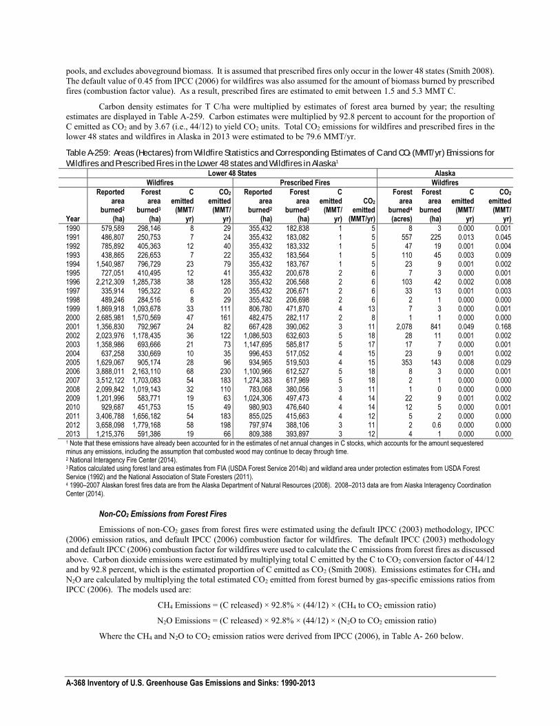
A-368 Inventory of U.S. Greenhouse Gas Emissions and Sinks: 1990-2013
pools, and excludes aboveground biomass. It is assumed that prescribed fires only occur in the lower 48 states (Smith 2008). The default value of 0.45 from IPCC (2006) for wildfires was also assumed for the amount of biomass burned by prescribed fires (combustion factor value). As a result, prescribed fires are estimated to emit between 1.5 and 5.3 MMT C.
Carbon density estimates for T C/ha were multiplied by estimates of forest area burned by year; the resulting estimates are displayed in Table A-259. Carbon estimates were multiplied by 92.8 percent to account for the proportion of C emitted as CO2 and by 3.67 (i.e., 44/12) to yield CO2 units. Total CO2 emissions for wildfires and prescribed fires in the lower 48 states and wildfires in Alaska in 2013 were estimated to be 79.6 MMT/yr.
Table A-259: Areas (Hectares) from Wildfire Statistics and Corresponding Estimates of C and CO2 (MMT/yr) Emissions for
Wildfires and Prescribed Fires in the Lower 48 states and Wildfires in Alaska1 Lower 48 States Alaska
Wildfires Prescribed Fires Wildfires
Year
Reported area
burned2 (ha)
Forest area
burned3 (ha)
C emitted
(MMT/ yr)
CO2 emitted
(MMT/ yr)
Reported area
burned2 (ha)
Forest area
burned3 (ha)
C emitted
(MMT/ yr)
CO2 emitted
(MMT/yr)
Forest area
burned4 (acres)
Forest area
burned
(ha)
C emitted
(MMT/ yr)
CO2 emitted
(MMT/ yr)
1990 579,589 298,146 8 29 355,432 182,838 1 5 8 3 0.000 0.001 1991 486,807 250,753 7 24 355,432 183,082 1 5 557 225 0.013 0.045 1992 785,892 405,363 12 40 355,432 183,332 1 5 47 19 0.001 0.004 1993 438,865 226,653 7 22 355,432 183,564 1 5 110 45 0.003 0.009 1994 1,540,987 796,729 23 79 355,432 183,767 1 5 23 9 0.001 0.002 1995 727,051 410,495 12 41 355,432 200,678 2 6 7 3 0.000 0.001 1996 2,212,309 1,285,738 38 128 355,432 206,568 2 6 103 42 0.002 0.008 1997 335,914 195,322 6 20 355,432 206,671 2 6 33 13 0.001 0.003 1998 489,246 284,516 8 29 355,432 206,698 2 6 2 1 0.000 0.000 1999 1,869,918 1,093,678 33 111 806,780 471,870 4 13 7 3 0.000 0.001 2000 2,685,981 1,570,569 47 161 482,475 282,117 2 8 1 1 0.000 0.000 2001 1,356,830 792,967 24 82 667,428 390,062 3 11 2,078 841 0.049 0.168 2002 2,023,976 1,178,435 36 122 1,086,503 632,603 5 18 28 11 0.001 0.002 2003 1,358,986 693,666 21 73 1,147,695 585,817 5 17 17 7 0.000 0.001 2004 637,258 330,669 10 35 996,453 517,052 4 15 23 9 0.001 0.002 2005 1,629,067 905,174 28 96 934,965 519,503 4 15 353 143 0.008 0.029 2006 3,888,011 2,163,110 68 230 1,100,966 612,527 5 18 8 3 0.000 0.001 2007 3,512,122 1,703,083 54 183 1,274,383 617,969 5 18 2 1 0.000 0.000 2008 2,099,842 1,019,143 32 110 783,068 380,056 3 11 1 0 0.000 0.000 2009 1,201,996 583,771 19 63 1,024,306 497,473 4 14 22 9 0.001 0.002 2010 929,687 451,753 15 49 980,903 476,640 4 14 12 5 0.000 0.001 2011 3,406,788 1,656,182 54 183 855,025 415,663 4 12 5 2 0.000 0.000 2012 3,658,098 1,779,168 58 198 797,974 388,106 3 11 2 0.6 0.000 0.000 2013 1,215,376 591,386 19 66 809,388 393,897 3 12 4 1 0.000 0.000 1 Note that these emissions have already been accounted for in the estimates of net annual changes in C stocks, which accounts for the amount sequestered minus any emissions, including the assumption that combusted wood may continue to decay through time. 2 National Interagency Fire Center (2014). 3 Ratios calculated using forest land area estimates from FIA (USDA Forest Service 2014b) and wildland area under protection estimates from USDA Forest Service (1992) and the National Association of State Foresters (2011). 4 1990–2007 Alaskan forest fires data are from the Alaska Department of Natural Resources (2008). 2008–2013 data are from Alaska Interagency Coordination Center (2014).
Non-CO2 Emissions from Forest Fires
Emissions of non-CO2 gases from forest fires were estimated using the default IPCC (2003) methodology, IPCC (2006) emission ratios, and default IPCC (2006) combustion factor for wildfires. The default IPCC (2003) methodology and default IPCC (2006) combustion factor for wildfires were used to calculate the C emissions from forest fires as discussed above. Carbon dioxide emissions were estimated by multiplying total C emitted by the C to CO2 conversion factor of 44/12 and by 92.8 percent, which is the estimated proportion of C emitted as CO2 (Smith 2008). Emissions estimates for CH4 and N2O are calculated by multiplying the total estimated CO2 emitted from forest burned by gas-specific emissions ratios from IPCC (2006). The models used are:
CH4 Emissions = (C released) × 92.8% × (44/12) × (CH4 to CO2 emission ratio)
N2O Emissions = (C released) × 92.8% × (44/12) × (N2O to CO2 emission ratio)
Where the CH4 and N2O to CO2 emission ratios were derived from IPCC (2006), in Table A- 260 below.
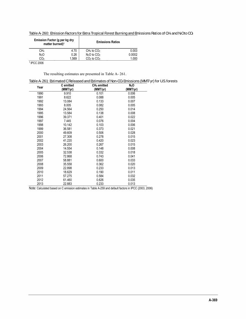
A-369
Table A- 260: Emission Factors for Extra Tropical Forest Burning and Emissions Ratios of CH4 and N2O to CO2
Emission Factor (g per kg dry matter burned)1
Emissions Ratios
CH4 4.70 CH4 to CO2 0.003 N2O 0.26 N2O to CO2 0.0002 CO2 1,569 CO2 to CO2 1.000
1 IPCC 2006
The resulting estimates are presented in Table A- 261.
Table A- 261: Estimated C Released and Estimates of Non-CO2 Emissions (MMT/yr) for U.S. forests
Year C emitted (MMT/yr)
CH4 emitted (MMT/yr)
N2O (MMT/yr)
1990 9.910 0.101 0.006 1991 8.622 0.088 0.005 1992 13.084 0.133 0.007 1993 8.005 0.082 0.005 1994 24.564 0.250 0.014 1995 13.584 0.138 0.008 1996 39.371 0.401 0.022 1997 7.445 0.076 0.004 1998 10.142 0.103 0.006 1999 36.581 0.373 0.021 2000 49.609 0.506 0.028 2001 27.308 0.278 0.015 2002 41.220 0.420 0.023 2003 26.200 0.267 0.015 2004 14.554 0.148 0.008 2005 32.538 0.332 0.018 2006 72.868 0.743 0.041 2007 58.881 0.600 0.033 2008 35.558 0.362 0.020 2009 22.898 0.233 0.013 2010 18.629 0.190 0.011 2011 57.275 0.584 0.032 2012 61.460 0.626 0.035 2013 22.883 0.233 0.013
Note: Calculated based on C emission estimates in Table A-259 and default factors in IPCC (2003, 2006)
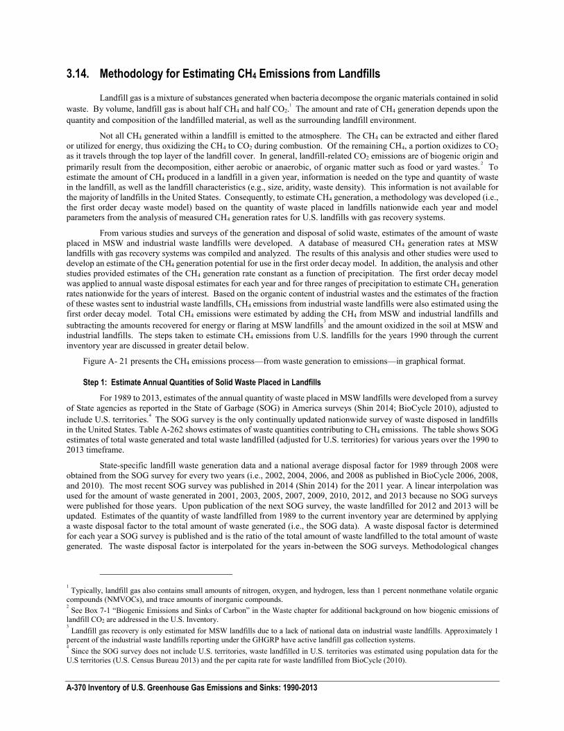
A-370 Inventory of U.S. Greenhouse Gas Emissions and Sinks: 1990-2013
3.14. Methodology for Estimating CH4 Emissions from Landfills
Landfill gas is a mixture of substances generated when bacteria decompose the organic materials contained in solid waste. By volume, landfill gas is about half CH4 and half CO2.
1 The amount and rate of CH4 generation depends upon the
quantity and composition of the landfilled material, as well as the surrounding landfill environment.
Not all CH4 generated within a landfill is emitted to the atmosphere. The CH4 can be extracted and either flared or utilized for energy, thus oxidizing the CH4 to CO2 during combustion. Of the remaining CH4, a portion oxidizes to CO2 as it travels through the top layer of the landfill cover. In general, landfill-related CO2 emissions are of biogenic origin and primarily result from the decomposition, either aerobic or anaerobic, of organic matter such as food or yard wastes. 2 To estimate the amount of CH4 produced in a landfill in a given year, information is needed on the type and quantity of waste in the landfill, as well as the landfill characteristics (e.g., size, aridity, waste density). This information is not available for the majority of landfills in the United States. Consequently, to estimate CH4 generation, a methodology was developed (i.e., the first order decay waste model) based on the quantity of waste placed in landfills nationwide each year and model parameters from the analysis of measured CH4 generation rates for U.S. landfills with gas recovery systems.
From various studies and surveys of the generation and disposal of solid waste, estimates of the amount of waste placed in MSW and industrial waste landfills were developed. A database of measured CH4 generation rates at MSW landfills with gas recovery systems was compiled and analyzed. The results of this analysis and other studies were used to develop an estimate of the CH4 generation potential for use in the first order decay model. In addition, the analysis and other studies provided estimates of the CH4 generation rate constant as a function of precipitation. The first order decay model was applied to annual waste disposal estimates for each year and for three ranges of precipitation to estimate CH4 generation rates nationwide for the years of interest. Based on the organic content of industrial wastes and the estimates of the fraction of these wastes sent to industrial waste landfills, CH4 emissions from industrial waste landfills were also estimated using the first order decay model. Total CH4 emissions were estimated by adding the CH4 from MSW and industrial landfills and subtracting the amounts recovered for energy or flaring at MSW landfills3 and the amount oxidized in the soil at MSW and industrial landfills. The steps taken to estimate CH4 emissions from U.S. landfills for the years 1990 through the current inventory year are discussed in greater detail below.
Figure A- 21 presents the CH4 emissions process—from waste generation to emissions—in graphical format.
Step 1: Estimate Annual Quantities of Solid Waste Placed in Landfills
For 1989 to 2013, estimates of the annual quantity of waste placed in MSW landfills were developed from a survey of State agencies as reported in the State of Garbage (SOG) in America surveys (Shin 2014; BioCycle 2010), adjusted to include U.S. territories.4 The SOG survey is the only continually updated nationwide survey of waste disposed in landfills in the United States. Table A-262 shows estimates of waste quantities contributing to CH4 emissions. The table shows SOG estimates of total waste generated and total waste landfilled (adjusted for U.S. territories) for various years over the 1990 to 2013 timeframe.
State-specific landfill waste generation data and a national average disposal factor for 1989 through 2008 were obtained from the SOG survey for every two years (i.e., 2002, 2004, 2006, and 2008 as published in BioCycle 2006, 2008, and 2010). The most recent SOG survey was published in 2014 (Shin 2014) for the 2011 year. A linear interpolation was used for the amount of waste generated in 2001, 2003, 2005, 2007, 2009, 2010, 2012, and 2013 because no SOG surveys were published for those years. Upon publication of the next SOG survey, the waste landfilled for 2012 and 2013 will be updated. Estimates of the quantity of waste landfilled from 1989 to the current inventory year are determined by applying a waste disposal factor to the total amount of waste generated (i.e., the SOG data). A waste disposal factor is determined for each year a SOG survey is published and is the ratio of the total amount of waste landfilled to the total amount of waste generated. The waste disposal factor is interpolated for the years in-between the SOG surveys. Methodological changes
1 Typically, landfill gas also contains small amounts of nitrogen, oxygen, and hydrogen, less than 1 percent nonmethane volatile organic compounds (NMVOCs), and trace amounts of inorganic compounds. 2 See Box 7-1 “Biogenic Emissions and Sinks of Carbon” in the Waste chapter for additional background on how biogenic emissions of landfill CO2 are addressed in the U.S. Inventory. 3 Landfill gas recovery is only estimated for MSW landfills due to a lack of national data on industrial waste landfills. Approximately 1
percent of the industrial waste landfills reporting under the GHGRP have active landfill gas collection systems. 4 Since the SOG survey does not include U.S. territories, waste landfilled in U.S. territories was estimated using population data for the
U.S territories (U.S. Census Bureau 2013) and the per capita rate for waste landfilled from BioCycle (2010).
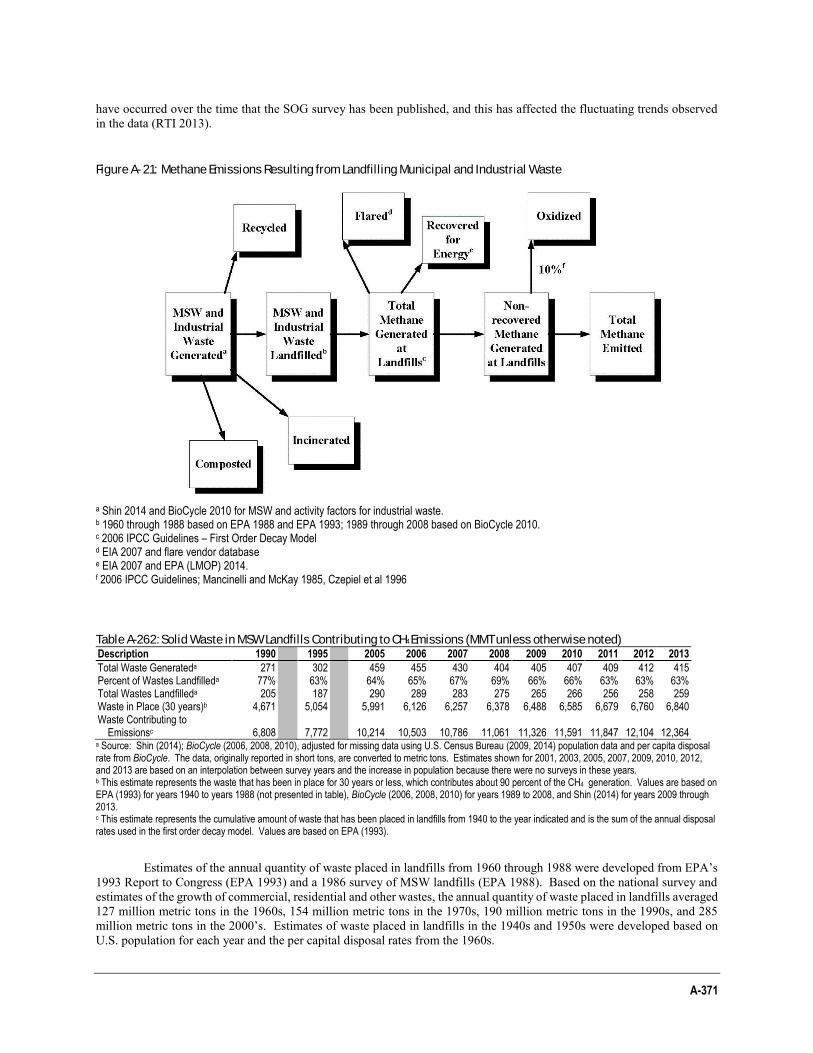
A-371
have occurred over the time that the SOG survey has been published, and this has affected the fluctuating trends observed in the data (RTI 2013).
Figure A- 21: Methane Emissions Resulting from Landfilling Municipal and Industrial Waste
a Shin 2014 and BioCycle 2010 for MSW and activity factors for industrial waste. b 1960 through 1988 based on EPA 1988 and EPA 1993; 1989 through 2008 based on BioCycle 2010. c 2006 IPCC Guidelines – First Order Decay Model d EIA 2007 and flare vendor database e EIA 2007 and EPA (LMOP) 2014. f 2006 IPCC Guidelines; Mancinelli and McKay 1985, Czepiel et al 1996
Table A-262: Solid Waste in MSW Landfills Contributing to CH4 Emissions (MMT unless otherwise noted) Description 1990 1995 2005 2006 2007 2008 2009 2010 2011 2012 2013
Total Waste Generateda 271 302 459 455 430 404 405 407 409 412 415 Percent of Wastes Landfilleda 77% 63% 64% 65% 67% 69% 66% 66% 63% 63% 63% Total Wastes Landfilleda 205 187 290 289 283 275 265 266 256 258 259 Waste in Place (30 years)b 4,671 5,054 5,991 6,126 6,257 6,378 6,488 6,585 6,679 6,760 6,840 Waste Contributing to
Emissionsc 6,808 7,772 10,214 10,503 10,786 11,061 11,326 11,591 11,847 12,104 12,364 a Source: Shin (2014); BioCycle (2006, 2008, 2010), adjusted for missing data using U.S. Census Bureau (2009, 2014) population data and per capita disposal rate from BioCycle. The data, originally reported in short tons, are converted to metric tons. Estimates shown for 2001, 2003, 2005, 2007, 2009, 2010, 2012, and 2013 are based on an interpolation between survey years and the increase in population because there were no surveys in these years. b This estimate represents the waste that has been in place for 30 years or less, which contributes about 90 percent of the CH4 generation. Values are based on EPA (1993) for years 1940 to years 1988 (not presented in table), BioCycle (2006, 2008, 2010) for years 1989 to 2008, and Shin (2014) for years 2009 through 2013. c This estimate represents the cumulative amount of waste that has been placed in landfills from 1940 to the year indicated and is the sum of the annual disposal rates used in the first order decay model. Values are based on EPA (1993).
Estimates of the annual quantity of waste placed in landfills from 1960 through 1988 were developed from EPA’s 1993 Report to Congress (EPA 1993) and a 1986 survey of MSW landfills (EPA 1988). Based on the national survey and estimates of the growth of commercial, residential and other wastes, the annual quantity of waste placed in landfills averaged 127 million metric tons in the 1960s, 154 million metric tons in the 1970s, 190 million metric tons in the 1990s, and 285 million metric tons in the 2000’s. Estimates of waste placed in landfills in the 1940s and 1950s were developed based on U.S. population for each year and the per capital disposal rates from the 1960s.
A-372 Inventory of U.S. Greenhouse Gas Emissions and Sinks: 1990-2013
Step 2: Estimate CH4 Generation at Municipal Solid Waste Landfills
The CH4 generation was estimated from the integrated form of the first order decay (FOD) model using the procedures and spreadsheets from IPCC (2006) for estimating CH4 emissions from solid waste disposal. The form of the FOD model that was applied incorporates a time delay of 6 months after waste disposal before the generation of CH4 begins.
The input parameters needed for the FOD model equations are the mass of waste disposed each year, which was discussed in the previous section, degradable organic carbon (DOC), and the decay rate constant (k). The DOC is determined from the CH4 generation potential (L0 in m3 CH4/Mg waste), which is discussed in more detail in subsequent paragraphs, and the following equation:
DOC = [L0 × 6.74 × 10-4] ÷ [F × 16/12 × DOCf × MCF]
where, DOC = degradable organic carbon (fraction, kt C/kt waste), L0 = CH4 generation potential (m3 CH4/Mg waste), 6.74 × 10-4 = CH4 density (Mg/m3), F = fraction of CH4 by volume in generated landfill gas (equal to 0.5) 16/12 = molecular weight ratio CH4/C, DOCf = fraction of DOC that can decompose in the anaerobic conditions in the landfill (fraction equal to
0.5 for MSW), and MCF = methane correction factor for year of disposal (fraction equal to 1 for anaerobic managed sites).
The DOC value used in the CH4 generation estimates from MSW landfills is 0.203 based on the CH4 generation potential of 100 m3 CH4/Mg waste as described below. Data from a set of 52 representative landfills across the U.S. in different precipitation ranges were chosen to evaluate Lo, and ultimately the country-specific DOC value. The 2004 Chartwell Municipal Solid Waste Facility Directory confirmed that each of the 52 landfills chosen accepted or accepts both MSW and construction and demolition (C&D) waste (Chartwell 2004; RTI 2009).
The methane generation potential (Lo) varies with the amount of organic content of the waste material. A higher Lo occurrs with a higher content of organic waste. Waste composition data are not collected for all landfills nationwide; thus a default value must be used. Values for Lo were evaluated from landfill gas recovery data for this set of 52 landfills, which resulted in a best fit value for Lo of 99 m3/Mg of waste (RTI 2004). This value compares favorably with a range of 50 to 162 (midrange of 106) m3/Mg presented by Peer, Thorneloe, and Epperson (1993); a range of 87 to 91 m3/Mg from a detailed analysis of 18 landfills sponsored by the Solid Waste Association of North America (SWANA 1998); and a value of 100 m3/Mg recommended in EPA’s compilation of emission factors (EPA 1998; EPA 2008) based on data from 21 landfills. Based on the results from these studies, a value of 100 m3/Mg appears to be a reasonable best estimate to use in the FOD model for the national inventory.
The FOD model was applied to the gas recovery data for the 52 landfills to calculate the decay rate constant (k) directly for L0 = 100 m3/Mg. The rate constant was found to increase with annual average precipitation; consequently, average values of k were developed for three ranges of precipitation, shown in Table A- 263 and recommended in EPA’s compilation of emission factors (EPA 2008).
Table A- 263: Average Values for Rate Constant (k) by Precipitation Range (yr-1) Precipitation range (inches/year) k (yr-1)
<20 0.020 20-40 0.038 >40 0.057
These values for k show reasonable agreement with the results of other studies. For example, EPA’s compilation of emission factors (EPA 1998; EPA, 2008) recommends a value of 0.02 yr-1 for arid areas (less than 20 inches/year of precipitation) and 0.04 yr-1 for non-arid areas. The SWANA study of 18 landfills reported a range in values of k from 0.03 to 0.06 yr-1 based on CH4 recovery data collected generally in the time frame of 1986 to 1995.
Using data collected primarily for the year 2000, the distribution of waste in place versus precipitation was developed from over 400 landfills (RTI 2004). A distribution was also developed for population vs. precipitation for comparison. The two distributions were very similar and indicated that population in areas or regions with a given precipitation range was a reasonable proxy for waste landfilled in regions with the same range of precipitation. Using U.S. Census data and rainfall data, the distributions of population versus rainfall were developed for each Census decade from 1950 through 2000. The distributions showed that the U.S. population has shifted to more arid areas over the past several
A-373
decades. Consequently, the population distribution was used to apportion the waste landfilled in each decade according to the precipitation ranges developed for k, as shown in Table A-264.
Table A-264: Percent of U.S. Population within Precipitation Ranges (%) Precipitation Range (inches/year) 1950 1960 1970 1980 1990 2000 2010
<20 10 13 14 16 19 19 18 20-40 40 39 37 36 34 33 44 >40 50 48 48 48 48 48 38 Source: Years 1950 through 2000 are from RTI (2004) using population data from the U.S. Census Bureau and precipitation data from the National Climatic Data Center’s National Oceanic and Atmospheric Administration. Year 2010 is based on the methodology from RTI (2004) and the U.S. Bureau of Census and precipitation data from the National Climatic Data Center’s National Oceanic and Atmospheric Administration where available.
In developing the Inventory, the proportion of waste disposed of in managed landfills versus open dumps prior to 1980 was re-evaluated. Based on the historical data presented by Mintz et al. (2003), a timeline was developed for the transition from the use of open dumps for solid waste disposed to the use of managed landfills. Based on this timeline, it was estimated that 6 percent of the waste that was land disposed in 1940 was disposed of in managed landfills and 94 percent was managed in open dumps. Between 1940 and 1980, the fraction of waste land disposed transitioned towards managed landfills until 100 percent of the waste was disposed of in managed landfills in 1980. For wastes disposed of in dumps, a methane correction factor (MCF) of 0.6 was used based on the recommended IPCC default value for uncharacterized land disposal (IPCC 2006); this MCF is equivalent to assuming 50 percent of the open dumps are deep and 50 percent are shallow. The recommended IPCC default value for the MCF for managed landfills of 1 was used for the managed landfills (IPCC 2006).
Step 3: Estimate CH4 Generation at Industrial Landfills
Industrial waste landfills receive waste from factories, processing plants, and other manufacturing activities. In national inventories prior to the 1990 through 2005 inventory, CH4 generation at industrial landfills was estimated as seven percent of the total CH4 generation from MSW landfills, based on a study conducted by EPA (1993). For the 1990 through 2007 and current inventories, the methodology was updated and improved by using activity factors (industrial production levels) to estimate the amount of industrial waste landfilled each year and by applying the FOD model to estimate CH4 generation. A nationwide survey of industrial waste landfills found that over 99 percent of the organic waste placed in industrial landfills originated from two industries: food processing (meat, vegetables, fruits) and pulp and paper (EPA 1993). Data for annual nationwide production for the food processing and pulp and paper industries were taken from industry and government sources for recent years; estimates were developed for production for the earlier years for which data were not available. For the pulp and paper industry, production data published by the Lockwood-Post’s Directory were used for years 1990 to 2001 and production data published by the U.S. Department of Agriculture were used for years 2002 through 2013. An extrapolation based on U.S. real gross domestic product was used for years 1940 through 1964. For the food processing industry, production levels were obtained or developed from the U.S. Department of Agriculture for the years 1990 through 2013 (ERG 2014). An extrapolation based on U.S. population was used for the years 1940 through 1989.
In addition to production data for the pulp and paper and food processing industries, the following inputs were needed to use the FOD model for estimating CH4 generation from industrial landfills: 1) quantity of waste that is disposed in industrial waste landfills (as a function of production), 2) CH4 generation potential (L0) or DOC, and 3) FOD decay constant (k). Research into waste generation and disposal in landfills for the pulp and paper industry indicated that the quantity of waste landfilled was about 0.050 Mg/Mg of product compared to 0.046 Mg/Mg product for the food processing industry (RTI 2006). These factors were applied to estimates of annual production to estimate annual waste disposal in landfills. Estimates for DOC were derived from available data (Kraft and Orender, 1993; NCASI 2008; Flores et al. 1999). The DOC value for industrial pulp and paper waste is estimated at 0.20 (Lo of 99 m3/Mg); the DOC value for industrial food waste is estimated as 0.26 (Lo of 128 m3/Mg) (RTI 2014). Estimates for k were taken from the default values in the 2006 IPCC Guidelines; the value of k given for food waste with disposal in a wet temperate climate is 0.19 yr-1, and the value given for paper waste is 0.06 yr-1.
A literature review was conducted for the 1990 to 2010 inventory year with the intent of updating values for Lo and k in the pulp and paper industry. Where pulp and paper mill wastewater treatment residuals or sludge are the primary constituents of pulp and paper waste landfilled, values for k range from 0.01/yr to 0.1/yr, while values for Lo range from 50 m3/Mg to 200 m3/Mg.5 Values for these factors are highly variable and are dependent on the soil moisture content, which is generally related to rainfall amounts. At this time, sufficient data were not obtained to warrant a change for the current
5 Sources reviewed included Heath et al. 2010; Miner 2008; Skog 2008; Upton et al. 2008; Barlaz 2006; Sonne 2006; NCASI 2005;
and Skog 2000.
A-374 Inventory of U.S. Greenhouse Gas Emissions and Sinks: 1990-2013
inventory year. EPA is considering an update to the Lo and k values for the pulp and paper sector and will work with stakeholders to gather data and other feedback on potential changes to these values.
As with MSW landfills, a similar trend in disposal practices from open dumps to managed landfills was expected for industrial waste landfills; therefore, the same time line that was developed for MSW landfills was applied to the industrial landfills to estimate the average MCF. That is, between 1940 and 1980, the fraction of waste that was land disposed transitioned from 6 percent managed landfills in 1940 and 94 percent open dumps to 100 percent managed landfills in 1980 and on. For wastes disposed of in dumps, an MCF of 0.6 was used and for wastes disposed of in managed landfills, an MCF of 1 was used, based on the recommended IPCC default values (IPCC 2006).
The parameters discussed above were used in the integrated form of the FOD model to estimate CH4 generation from industrial waste landfills.
Step 4: Estimate CH4 Emissions Avoided
The estimate of CH4 emissions avoided (e.g., combusted) was based on landfill-specific data on landfill gas-to-energy (LFGTE) projects and flares using a combination of four databases:
the flare vendor database (contains updated sales data collected from vendors of flaring equipment) a database of LFGTE projects compiled by LMOP (EPA 2014a) a database developed by the Energy Information Administration (EIA) for the voluntary reporting of greenhouse
gases containing facility-specific information reported on flares and LFGTE projects (EIA 2007), and the GHGRP dataset for MSW landfills that contains detailed facility-specific information, including annual
amounts of recovered CH4.
EPA’s GHGRP MSW landfills database was first introduced as a data source for the current Inventory (i.e., 1990-2013). The GHGRP MSW landfills database contains facility-reported data that undergoes rigorous verification and is considered to contain the least uncertain data of the four databases. However, this database is unique in that it only contains a portion of the landfills in the U.S. (although, presumably the highest emitters since only those landfills that meet the methane generation threshold must report) and only contains data from 2010 and later.
The destruction efficiencies reported through EPA’s GHGRP were applied to the landfills in the GHGRP MSW landfills database. The median value of the reported destruction efficiencies was 99 percent for all reporting years (2010 through 2013, EPA 2014b). A destruction efficiency of 99 percent was applied to CH4 recovered to estimate CH4 emissions avoided for the other three databases. This value for destruction efficiency was selected based on the range of efficiencies (86 to 99+ percent) recommended for flares in EPA’s AP-42 Compilation of Air Pollutant Emission Factors, Draft Chapter 2.4, Table 2.4-3 (EPA 2008). A typical value of 97.7 percent was presented for the non-methane components (i.e., volatile organic compounds and non-methane organic compounds) in test results (EPA 2008). An arithmetic average of 98.3 percent and a median value of 99 percent are derived from the test results presented in EPA 2008. Thus, a value of 99 percent for the destruction efficiency of flares has been used in Inventory methodology. Other data sources supporting a 99 percent destruction efficiency include those used to establish new source performance standards (NSPS) for landfills and in recommendations for closed flares used in the Landfill Methane Outreach Program (LMOP).
Step 4a: Estimate CH4 Emissions Avoided Through Landfill Gas-to-Energy (LFGTE) Projects
The quantity of CH4 avoided due to LFGTE systems was estimated based on information from three sources: (1) a database developed by the Energy Information Administration (EIA) for the voluntary reporting of greenhouse gases (EIA 2007); (2) a database compiled by LMOP (EPA 2014a); and (3) the GHGRP MSW landfills dataset. The EIA database included location information for landfills with LFGTE projects, estimates of CH4 reductions, descriptions of the projects, and information on the methodology used to determine the CH4 reductions. Generally the CH4 reductions for each reporting year were based on the measured amount of landfill gas collected and the percent CH4 in the gas. For the LMOP database, data on landfill gas flow and energy generation (i.e., MW capacity) were used to estimate the total direct CH4 emissions avoided due to the LFGTE project. The GHGRP MSW landfills database contains the most detailed data on landfills that reported under the GHGRP for years 2010 through 2013, however the amount of CH4 recovered is not specifically allocated to a flare versus a LFGTE project. The allocation into flares or LFGTE was performed by matching landfills to the EIA and LMOP databases for LFGTE projects and to the flare database for flares. Detailed information on the landfill name, owner or operator, city, and state are available for both the EIA and LMOP databases; consequently, it was straightforward to identify landfills that were in both databases against those in EPA’s GHGRP MSW landfills database. EPA’s GHGRP MSW landfills database was given priority because CH4 recovery and other supporting information were reported for each year and were based on direct measurements. The EIA database was given second priority (for landfills not in the GHGRP MSW landfills database) because CH4 recovery based on direct measurements was reported by landfill. Landfills in the
A-375
LMOP database that were also in EPA’s GHGRP MSW landfills database and/or EIA database were dropped to avoid double or triple counting.
Step 4b: Estimate CH4 Emissions Avoided Through Flaring
The quantity of CH4 flared was based on data from EPA’s GHGRP MSW landfills database, the EIA database, and on information provided by flaring equipment vendors. To avoid double counting, flares associated with landfills in EPA’s GHGRP, EIA and LMOP databases were excluded from the flare vendor database. As with the LFGTE projects, reductions from flaring landfill gas in the EIA database were based on measuring the volume of gas collected and the percent of CH4 in the gas. The information provided by the flare vendors included information on the number of flares, flare design flow rates or flare dimensions, year of installation, and generally the city and state location of the landfill. When a range of design flare flow rates was provided by the flare vendor, the median landfill gas flow rate was used to estimate CH4 recovered from each remaining flare (i.e., for each flare not associated with a landfill in the EIA, GHGRP, or LMOP databases). Several vendors provided information on the size of the flare rather than the flare design gas flow rate. To estimate a median flare gas flow rate for flares associated with these vendors, the size of the flare was matched with the size and corresponding flow rates provided by other vendors. Some flare vendors reported the maximum capacity of the flare. An analysis of flare capacity versus measured CH4 flow rates from the EIA database showed that the flares operated at 51 percent of capacity when averaged over the time series and at 72 percent of capacity for the highest flow rate for a given year. For those cases when the flare vendor supplied maximum capacity, the actual flow was estimated as 50 percent of capacity. Total CH4 avoided through flaring from the flare vendor database was estimated by summing the estimates of CH4 recovered by each flare for each year.
Step 4c: Reduce CH4 Emissions Avoided Through Flaring
As mentioned in Step 4b, flares in the flare vendor database associated with landfills in the GHGRP MSW landfills, EIA, and LMOP databases were excluded from the flare reduction estimates in the flare vendor database. If comprehensive data on flares were available, each LFGTE project in EPA’s GHGRP, EIA, and LMOP databases would have an identified flare because it is assumed that most LFGTE projects have flares. However, given that the flare vendor data only covers approximately 50 to 75 percent of the flare population, an associated flare was not identified for all LFGTE projects. These LFGTE projects likely have flares, yet flares were unable to be identified for one of two reasons: 1) inadequate identifier information in the flare vendor data; or 2) a lack of the flare in the flare vendor database. For those projects for which a flare was not identified due to inadequate information, CH4 avoided would be overestimated, as both the CH4 avoided from flaring and the LFGTE project would be counted. To avoid overestimating emissions avoided from flaring, the CH4 avoided from LFGTE projects with no identified flares was determined and the flaring estimate from the flare vendor database was reduced by this quantity (referred to as a flare correction factor) on a state-by-state basis. This step likely underestimates CH4 avoided due to flaring but was applied to be conservative in the estimates of CH4 emissions avoided.
Additional effort was undertaken to improve the methodology behind the flare correction factor for the 1990-2009 Inventory to reduce the total number of flares in the flare vendor database that were not matched (512) to landfills and/or LFGTE projects in the EIA and LMOP databases. Each flare in the flare vendor database not associated with a LFGTE project in the EIA or LMOP databases was investigated to determine if it could be matched to either a landfill in the EIA database or a LFGTE project in the LMOP database. For some unmatched flares, the location information was missing or incorrectly transferred to the flare vendor database. In other instances, the landfill names were slightly different between what the flare vendor provided and the actual landfill name as listed in the EIA and LMOP databases.
It was found that a large majority of the unmatched flares are associated with landfills in LMOP that are currently flaring, but are also considering LFGTE. These landfills projects considering a LFGTE project are labeled as candidate, potential, or construction in the LMOP database. The flare vendor database was improved to match flares with operational, shutdown as well as candidate, potential, and construction LFGTE projects, thereby reducing the total number of unidentified flares in the flare vendor database, all of which are used in the flare correction factor. The results of this effort significantly decreased the number of flares used in the flare correction factor, and consequently, increased recovered flare emissions, and decreased net emissions from landfills for the 1990-2009 Inventory. The revised state-by-state flare correction factors were applied to the entire Inventory time series.
Step 5: Estimate CH4 Oxidation
A portion of the CH4 escaping from a landfill oxidizes to CO2 in the top layer of the soil. The amount of oxidation depends upon the characteristics of the soil and the environment. For purposes of this analysis, it was assumed that of the CH4 generated, minus the amount of gas recovered for flaring or LFGTE projects, 10 percent was oxidized in the soil (Jensen and Pipatti 2002; Mancinelli and McKay 1985; Czepiel et al 1996). The factor of 10 percent is consistent with the value
A-376 Inventory of U.S. Greenhouse Gas Emissions and Sinks: 1990-2013
recommended in the 2006 IPCC revised guidelines for managed and covered landfills, and was therefore applied to the estimates of CH4 generation minus recovery for both MSW and industrial landfills
A literature review was conducted in 2011 (RTI 2011) to provide recommendations for the most appropriate oxidation rate assumptions. It was found that oxidation values are highly variable and range from zero to over 100 percent (i.e., the landfill is considered to be an atmospheric sink by virtue of the landfill gas extraction system pulling atmospheric methane down through the cover). There is considerable uncertainty and variability surrounding estimates of the rate of oxidation because oxidation is difficult to measure and varies considerably with the presence of a gas collection system, thickness and type of the cover material, size and area of the landfill, climate, and the presence of cracks and/or fissures in the cover material through which methane can escape. IPCC (2006) notes that test results from field and laboratory studies may lead to over-estimations of oxidation in landfill cover soils because they largely determine oxidation using uniform and homogeneous soil layers. In addition, a number of studies note that gas escapes more readily through the side slopes of a landfill as compared to moving through the cover thus complicating the correlation between oxidation and cover type or gas recovery.
Sites with landfill gas collection systems are generally designed and managed better to improve gas recovery. More recent research (2006 to 2012) on landfill cover methane oxidation has relied on stable isotope techniques that may provide a more reliable measure of oxidation. Results from this recent research consistently point to higher cover soil methane oxidation rates than the IPCC (2006) default of 10 percent. A continued effort will be made to review the peer-reviewed literature to better understand how climate, cover type, and gas recovery influence the rate of oxidation at active and closed landfills. At this time, the IPCC recommended oxidation factor of 10 percent will continue to be used for all landfills.
Step 6: Estimate Total CH4 Emissions
Total CH4 emissions were calculated by adding emissions from MSW and industrial landfills, and subtracting CH4 recovered and oxidized, as shown in Table A- 265.
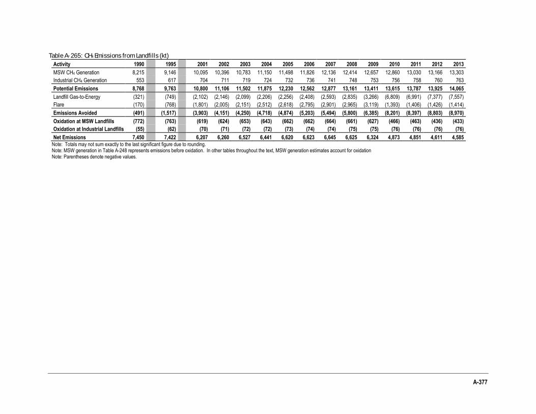
A-377
Table A- 265: CH4 Emissions from Landfills (kt)
Activity 1990 1995 2001 2002 2003 2004 2005 2006 2007 2008 2009 2010 2011 2012 2013
MSW CH4 Generation 8,215 9,146 10,095 10,396 10,783 11,150 11,498 11,826 12,136 12,414 12,657 12,860 13,030 13,166 13,303
Industrial CH4 Generation 553 617 704 711 719 724 732 736 741 748 753 756 758 760 763
Potential Emissions 8,768 9,763 10,800 11,106 11,502 11,875 12,230 12,562 12,877 13,161 13,411 13,615 13,787 13,925 14,065
Landfill Gas-to-Energy (321) (749) (2,102) (2,146) (2,099) (2,206) (2,256) (2,408) (2,593) (2,835) (3,266) (6,809) (6,991) (7,377) (7,557)
Flare (170) (768) (1,801) (2,005) (2,151) (2,512) (2,618) (2,795) (2,901) (2,965) (3,119) (1,393) (1,406) (1,426) (1,414)
Emissions Avoided (491) (1,517) (3,903) (4,151) (4,250) (4,718) (4,874) (5,203) (5,494) (5,800) (6,385) (8,201) (8,397) (8,803) (8,970)
Oxidation at MSW Landfills (772) (763) (619) (624) (653) (643) (662) (662) (664) (661) (627) (466) (463) (436) (433)
Oxidation at Industrial Landfills (55) (62) (70) (71) (72) (72) (73) (74) (74) (75) (75) (76) (76) (76) (76)
Net Emissions 7,450 7,422 6,207 6,260 6,527 6,441 6,620 6,623 6,645 6,625 6,324 4,873 4,851 4,611 4,585
Note: Totals may not sum exactly to the last significant figure due to rounding. Note: MSW generation in Table A-248 represents emissions before oxidation. In other tables throughout the text, MSW generation estimates account for oxidation Note: Parentheses denote negative values.
A-378 Inventory of U.S. Greenhouse Gas Emissions and Sinks: 1990-2013
References
AAPFCO (1995 through 2000b, 2002 through 2009) Commercial Fertilizers. Association of American Plant Food Control Officials. University of Kentucky, Lexington, KY.
AAPFCO (2000a) 1999-2000 Commercial Fertilizers Data, ASCII files. Available from David Terry, Secretary, Association of American Plant Food Control Officials.
AAPG (1984) Coalbed Methane Resources of the United States. AAPG Studies in Geology Series #17.
Abdalla, M., Jones, J. Yeluripati, P. Smith, J. Burke and D M. Williams. 2010. Testing DayCent and DNDC model simulations of N2O fluxes and assessing the impacts of climate change on the gas flux and biomass production from a humid pasture. Atmos. Environ. 44: 2961–2970.
AF&PA. (2006a and earlier). Statistical roundup. (Monthly). Washington, DC: American Forest & Paper Association.
AF&PA. (2006b and earlier). Statistics of paper, paperboard and wood pulp. Washington, DC: American Forest & Paper Association.
Alaska Department of Natural Resources (2008) Division of Forestry. “Fire Statistics.” Available online at <http://forestry.alaska.gov/firestats/> October 2008.
Alaska Interagency Coordination Center (AICC) (2013). “2012 Alaska Fire Season: Wildland Fire Summary and Statistics Annual Report.” Available online at < http://fire.ak.blm.gov/content/aicc/stats/firestats.pdf > November 2013.
Amichev, B. Y. and J. M. Galbraith (2004) “A Revised Methodology for Estimation of Forest Soil Carbon from Spatial Soils and Forest Inventory Data Sets.” Environmental Management 33(Suppl. 1):S74-S86.
ArSova, Ljupka, Rob van Haaren, Nora Goldstein, Scott M. Kaufman, and Nickolas J. Themelis (2008). “16th Annual BioCycle Nationwide Survey: The State of Garbage in America” Biocycle, JG Press, Emmaus, PA. December.
Astlett Rubber Inc. (n.d.) Material Safety Data Sheet, Carbon Black. Available online at: <http://www.astlettrubber.com/pdf/specialty/msds/carbonblack.pdf>. Accessed 5 November 2009.
Bahor, B (2009) Covanta Energy’s public review comments re: Draft Inventory of U.S. Greenhouse Gas Emissions and Sinks: 1990-2007. Submitted via email on April 9, 2009 to Leif Hockstad, U.S. EPA.
Barlaz, M.A. (2006) “Forest Products Decomposition in Municipal Solid Waste Landfills.” Waste Management, 26(4): 321-333.
Barrett, T.M. (2014) Storage and flux of carbon in live trees, snags, and logs in the Chugach and Tongass National Forests. Gen. Tech. Rep. PNW-GTR-889. Portland, OR: U.S. Department of Agriculture, Forest Service, Pacific Northwest Research Station. 44 p.
Barrett, Tara M.; Christensen, Glenn A., tech. eds. (2011) Forests of southeast and south-central Alaska, 2004–2008: five-year forest inventory and analysis report. Gen. Tech. Rep. PNW-GTR-835. Portland, OR: U.S. Department of Agriculture, Forest Service, Pacific Northwest Research Station. 156 p.
Bastian, R. (2007) Personal Communication. Robert Bastian, Office of Water, U.S. Environmental Protection Agency, Washington, DC and Victoria Thompson, ICF International. July 20, 2007.
Bechtold, W.A.; Patterson, P.L. (2005) The enhanced forest inventory and analysis program—national sampling design and estimation procedures. Gen. Tech. Rep. SRS-80. Asheville, NC: U.S. Department of Agriculture Forest Service, Southern Research Station. 85 p.
BioCycle (2010) "The State of Garbage in America" By L. Arsova, R. Van Haaren, N. Goldstein, S. Kaufman, and N. Themelis. BioCycle. December 2010. Available online at < http://www.jgpress.com/archives/_free/002191.html>
BioCycle (2008) "The State of Garbage in America" By L. Arsova, R. Van Haaren, N. Goldstein, S. Kaufman, and N. Themelis. BioCycle. December 2008. Available online at < http://www.jgpress.com/archives/_free/001782.html>
BioCycle (2006) "The State of Garbage in America" By L. Arsova, R. Van Haaren, N. Goldstein, S. Kaufman, and N. Themelis. BioCycle. April 2006. Available online at <http://www.seas.columbia.edu/earth/wtert/sofos/biocycle.pdf>
Birdsey, R.A., and L.S. Heath (1995) “Carbon Changes in U.S. Forests.” In Productivity of America’s Forests and Climate Change. Gen. Tech. Rep. RM-271. Rocky Mountain Forest and Range Experiment Station, Forest Service, U.S. Department of Agriculture. Fort Collins, CO, 56-70.
A-379
Birdsey, R. (1996) “Carbon Storage for Major Forest Types and Regions in the Conterminous United States.” In R.N. Sampson and D. Hair, (eds); Forest and Global Change, Volume 2: Forest Management Opportunities for Mitigating Carbon Emissions. American Forests. Washington, DC, 1-26 and 261-379 (appendices 262 and 263).
Birdsey, R., and L. S. Heath (2001) “Forest Inventory Data, Models, and Assumptions for Monitoring Carbon Flux.” In Soil Carbon Sequestration and the Greenhouse Effect. Soil Science Society of America. Madison, WI, 125-135.
BOEM (2014) Year 2011 Gulfwide Emissions Inventory Study (BOEM 2014-666) Bureau of Ocean Energy Management, U.S. Department of the Interior (November 2014) <http://www.data.boem.gov/PI/PDFImages/ESPIS/5/5440.pdf>
CAR. (2014). Project Database. Climate Action Reserve. Available online at <http://www.climateactionreserve.org/>
Chartwell (2004) Municipal Solid Waste Directory. The Envirobiz Group.
Cibrowski, P. (1996) Personal Communication. Peter Cibrowski, Minnesota Pollution Control Agency and Heike Mainhardt, ICF Incorporated. July 29, 1996.
Consol. (2014). Ruby Canyon Summary 2013. CONSOL Energy Inc. excel spreadsheet.
Coulston, J.W., Woodall, C.W., Domke, G.M., and Walters, B.F. (in preparation). Refined Delineation between Woodlands and Forests with Implications for U.S. National Greenhouse Gas Inventory of Forests. Climatic Change.
Creedy, D.P. (1993). Chemosphere. Vol. 26, pp. 419-440.
CTIC (2004) 2004 Crop Residue Management Survey. Conservation Technology Information Center. Available online at <http://www.ctic.purdue.edu/CRM/>.
Czepiel, P., B. Mosher, P. Crill, and R. Harriss (1996) “Quantifying the Effect of Oxidation on Landfill Methane Emissions.” Journal of Geophysical Research, 101(D11):16721-16730.
Daly, C., G.H. Taylor, W.P. Gibson, T. Parzybok, G.L. Johnson, and P.A. Pasteris (1998) “Development of high-quality spatial datasets for the United States.” Proc., 1st International Conference on Geospatial Information in Agriculture and Forestry, Lake Buena Vista, FL, I-512-I-519. June 1-3, 1998.
Daly, C., R.P. Neilson, and D.L. Phillips (1994) “A statistical-topographic model for mapping climatological precipitation over mountainous terrain.” Journal of Applied Meteorology, 33:140-158.
Dean, W. E., and E. Gorham (1998) Magnitude and significance of carbon burial in lakes, reservoirs, and peatlands. Geology 26:535-538.
Del Grosso, S.J., S.M. Ogle, W.J. Parton. (2011) Soil Organic Matter Cycling and Greenhouse Gas Accounting Methodologies, Chapter 1, pp 3-13 DOI: 10.1021/bk-2011-1072.ch001. In: L. Guo, A. Gunasekara, L. McConnell (Eds.) Understanding Greenhouse Gas Emissions from Agricultural Management, American Chemical Society, Washington, D.C.
Del Grosso, S.J., W.J. Parton, C.A. Keough, and M. Reyes-Fox. (2011) Special features of the DayCent modeling package and additional procedures for parameterization, calibration, validation, and applications, in Methods of Introducing System Models into Agricultural Research, L.R. Ahuja and Liwang Ma, editors, p. 155-176, American Society of Agronomy, Crop Science Society of America, Soil Science Society of America, Madison, WI. USA.
Del Grosso, S.J., S.M. Ogle, W.J. Parton, and F.J. Breidt (2010) “Estimating Uncertainty in N2O Emissions from U.S. Cropland Soils.” Global Biogeochemical Cycles, 24, GB1009, doi:10.1029/2009GB003544.
Del Grosso, S.J., T. Wirth, S.M. Ogle, W.J. Parton (2008) Estimating agricultural nitrous oxide emissions. EOS 89, 529-530.
Del Grosso, S.J., A.R. Mosier, W.J. Parton, and D.S. Ojima (2005) “DAYCENT Model Analysis of Past and Contemporary Soil N2O and Net Greenhouse Gas Flux for Major Crops in the USA.” Soil Tillage and Research, 83: 9-24. doi: 10.1016/j.still.2005.02.007.
Del Grosso, S.J., W.J. Parton, A.R. Mosier, M.D. Hartman, J. Brenner, D.S. Ojima, and D.S. Schimel (2001) “Simulated Interaction of Carbon Dynamics and Nitrogen Trace Gas Fluxes Using the DAYCENT Model.” In Schaffer, M., L. Ma, S. Hansen, (eds.); Modeling Carbon and Nitrogen Dynamics for Soil Management. CRC Press. Boca Raton, Florida. 303-332.
Del Grosso, S.J., W.J. Parton, A.R. Mosier, D.S. Ojima, A.E. Kulmala and S. Phongpan (2000) General model for N2O and N2 gas emissions from soils due to denitrification. Global Biogeochem. Cycles, 14:1045-1060.
A-380 Inventory of U.S. Greenhouse Gas Emissions and Sinks: 1990-2013
Delgado, J.A., S.J. Del Grosso, and S.M. Ogle (2009) “15N isotopic crop residue cycling studies and modeling suggest that IPCC methodologies to assess residue contributions to N2O-N emissions should be reevaluated.” Nutrient Cycling in Agroecosystems, DOI 10.1007/s10705-009-9300-9.
DeZan, D. (2000) Personal Communication between Diane DeZan, Fiber Economics Bureau and Joe Casola, ICF Consulting. 4 August 2000.
Domke, G.M., Woodall, C.W., Smith, J.E., Westfall, J.A., McRoberts, R.E. (2012) Consequences of alternative tree-level biomass estimation procedures on U.S. forest carbon stock estimates. Forest Ecology and Management. 270: 108-116.
Domke, G.M., Smith, J.E., and Woodall, C.W. (2011) Accounting for density reduction and structural loss in standing dead trees: Implications for forest biomass and carbon stock estimates in the United States. Carbon Balance and Management. 6:14.
Domke, G.M., Woodall, C.W., Walters, B.F., McRoberts, R.E., Hatfield, M.A. In Review. Strategies to compensate for the effects of nonresponse on forest carbon baseline estimates from the national forest inventory of the United States. Forest Ecology and Management.
Domke, G.M., Woodall, C.W., Walters, B.F., Smith, J.E. (2013) From models to measurements: comparing down dead wood carbon stock estimates in the U.S. forest inventory. PLoS ONE 8(3): e59949.
Domke, G.M., Perry, C.H., Walters, B.F., Woodall, C.W., and Smith, J.E. (in preparation). Estimation of forest floor carbon using the national forest inventory of the United States. Intended outlet: Geoderma.
Easter, M. , S. Williams, and S. Ogle. (2008) Gap-filling NRI data for the Soil C Inventory. Natural Resource Ecology Laboratory, Colorado State University, Fort Collins, CO. Report provided to the U.S. Environmental Protection Agency, Tom Wirth.
Edmonds, L., N. Gollehon, R.L. Kellogg, B. Kintzer, L. Knight, C. Lander, J. Lemunyon, D. Meyer, D.C. Moffitt, and J. Schaeffer (2003) “Costs Associated with Development and Implementation of Comprehensive Nutrient Management Plans.” Part 1. Nutrient Management, Land Treatment, Manure and Wastewater Handling and Storage, and Recordkeeping. Natural Resource Conservation Service, U.S. Department of Agriculture.
EIA (2014) Annual Coal Report 1991-2013 (Formerly called Coal Industry Annual). Table 1. Energy Information Administration, U.S. Department of Energy,Washington, DC .
EIA (2007) Voluntary Greenhouse Gas Reports for EIA Form 1605B (Reporting Year 2006). Available online at <ftp://ftp.eia.doe.gov/pub/oiaf/1605/cdrom/>.
Energy Recovery Council (2009) “2007 Directory of Waste-to-Energy Plants in the United States,” accessed September 29, 2009.
EPA (2014) Greenhouse Gas Reporting Program (GHGRP) 2014 Envirofacts. Subpart FF: Underground Coal Mines. Available online at <http://www.epa.gov/ghgreporting/ghgdata/reported/coalmines.html>
EPA (2014a) Landfill Gas-to-Energy Project Database. Landfill Methane and Outreach Program. January 2014.
EPA (2014b) Greenhouse Gas Reporting Program (GHGRP) 2014 Envirofacts. Subpart HH: Municipal Solid Waste Landfills. Available online at <http://www.epa.gov/enviro/facts/ghg/search.html>
EPA (2005 through 2013) Municipal Solid Waste in the United States: Facts and Figures. Office of Solid Waste and Emergency Response, U.S. Environmental Protection Agency. Washington, DC. Available online at < http://www.epa.gov/osw/nonhaz/municipal/msw99.htm >.
EPA (2012) Landfill Gas-to-Energy Project Database. Landfill Methane and Outreach Program. July 2012.
EPA (2008). Compilation of Air Pollution Emission Factors, Publication AP-42, Draft Section 2.4 Municipal Solid Waste Landfills. October 2008.
EPA (2004) Methane Emissions Estimates & Methodology for Abandoned Coal Mines in the U.S. Draft Final Report. Washington, DC. April - June 2004.
EPA (1999 through 2003) Characterization of Municipal Solid Waste in the United States: Source Data Update. Office of Solid Waste, U.S. Environmental Protection Agency. Washington, DC.
EPA (1999) Biosolids Generation, Use and Disposal in the United States. Office of Solid Waste, U.S. Environmental Protection Agency. Available online at <http://biosolids.policy.net/relatives/18941.PDF>.
A-381
EPA (1998) Compilation of Air Pollution Emission Factors, Publication AP-42, Section 2.4 Municipal Solid Waste Landfills. November 1998.
EPA (1996) Evaluation and Analysis of Gas Content and Coal Properties of Major Coal Bearing Regions of the United States. U.S. Environmental Protection Agency. EPA/600/R-96-065.
EPA (1995) Compilation of Air Pollutant Emission Factors, AP-42. Fifth Edition, Vol. I: Stationary Point and Area Sources, Introduction. Office of Air Quality Planning and Standards. Research Triangle Park, NC. October.
EPA (1993) Anthropogenic Methane Emissions in the United States, Estimates for 1990: Report to Congress, U.S. Environmental Protection Agency, Office of Air and Radiation. Washington, DC. EPA/430-R-93-003. April 1993.
EPA (1993) Federal Register. Part II. Standards for the Use and Disposal of Sewage Sludge; Final Rules. U.S. Environmental Protection Agency, 40 CFR Parts 257, 403, and 503.
EPA (1988) National Survey of Solid Waste (Municipal) Landfill Facilities, U.S. Environmental Protection Agency. Washington, DC. EPA/530-SW-88-011. September 1988.
ERG (2014). Production Data Supplied by ERG for 1990-2013 for Pulp and Paper, Fruits and Vegetables, and Meat. October.
Euliss, N., and R. Gleason (2002) Personal communication regarding wetland restoration factor estimates and restoration activity data. Ned Euliss and Robert Gleason of the U.S. Geological Survey, Jamestown, ND, to Stephen Ogle of the National Resource Ecology Laboratory, Fort Collins, CO. August 2002.
FEB (2009) Fiber Economics Bureau, as cited in C&EN (2009) Chemical Output Slipped In Most Regions Chemical & Engineering News, American Chemical Society, 6 July. Available online at <http://www.cen-online.org>.
Flores, R.A., C.W. Shanklin, M. Loza-Garay, S.H. Wie (1999) “Quantification and Characterization of Food Processing Wastes/Residues.” Compost Science & Utilization, 7(1): 63-71.
Frayer, W.E., and G.M. Furnival (1999) “Forest Survey Sampling Designs: A History.” Journal of Forestry 97(12): 4-10.
Geological Survey of Alabama State Oil and Gas Board (GSA) (2014) Well Records Database. Available online at <http://www.gsa.state.al.us/ogb/database.aspx>
Gold, M. A., W. J. Rietveld, H. E. Garrett, and R. F. Fisher. (2000) Agroforestry Nomenclature, Concepts, and Practices for the United States. In H.E. Garrett, W.J. Rietveld, and R.F. Fisher, editors. North American Agroforestry: An Integrated Science and Practice. ASA. Madison, Wisconsin, 63-77.
Gurung, R.B., F.J. Breidt, A. Dutin, and S.M. Ogle (2009) Predicting Enhanced Vegetation Index (EVI) for ecosystem modeling applications. Remote Sensing of Environment 113:2186-2193.
Hair, D. and A.H. Ulrich (1963) The Demand and price situation for forest products – 1963. U.S. Department of Agriculture Forest Service, Misc Publication No. 953. Washington, DC.
Hair, D. (1958) “Historical forestry statistics of the United States.” Statistical Bull. 228. U.S. Department of Agriculture Forest Service, Washington, DC.
Halvorson, A.D., C.S. Snyder, A.D. Blaylock, and S.J. Del Grosso. 2013. Enhanced Efficiency Nitrogen Fertilizers: Potential Role in Nitrous Oxide Emission Mitigation. Agronomy Journal, doi:10.2134/agronj2013.0081
Hansen, M.H., T Frieswyk, J.F. Glover, J.F. Kelly (1992) The Eastwide Forest Inventory Data Base: Users Manual. General Technical Report NC-151. U.S. Department of Agriculture, Forest Service, North Central Forest Experiment Station. St. Paul, MN.
Harmon, M.E., C.W. Woodall, B. Fasth, J. Sexton, M. Yatkov. (2011) Differences between standing and downed dead tree wood density reduction factors: A comparison across decay classes and tree species. Res. Paper. NRS-15. Newtown Square, PA: U.S. Department of Agriculture, Forest Service, Northern Research Station. 40 p
Heath, L.S., J.E., Smith, and R.A. Birdsey (2003) Carbon Trends in U. S. Forestlands: A Context for the Role of Soils in Forest Carbon Sequestration. In J. M. Kimble, L. S. Heath, R. A. Birdsey, and R. Lal, editors. The Potential of U. S. Forest Soils to Sequester Carbon and Mitigate the Greenhouse Effect. Lewis Publishers (CRC Press). Boca Raton, FL, 35-45.
Heath, L. S., and J.E. Smith (2000) “Soil Carbon Accounting and Assumptions for Forestry and Forest-related Land Use Change.” In The Impact of Climate Change on America’s Forests. Joyce, L.A., and Birdsey, R.A. Gen. Tech. Rep.
A-382 Inventory of U.S. Greenhouse Gas Emissions and Sinks: 1990-2013
RMRS-59. Rocky Mountain Research Station, Forest Service, U.S. Department of Agriculture. Fort Collins, CO, 89-101.
Heath, L.S., M.C. Nichols, J.E. Smith, and J.R. Mills. (2010) FORCARB2: An updated version of the U.S. Forest Carbon Budget Model. Gen. Tech. Rep. NRS-67.USDA Forest Service, Northern Research Station, Newtown Square, PA. 52 p. [CD-ROM].
Heath, L.S., J.E. Smith, K.E. Skog, D.J. Nowak, and C.W. Woodall. (2011) Managed forest carbon estimates for the U.S. Greenhouse Gas Inventory, 1990-2008. Journal of Forestry 109(3):167-173.
Heath, L. S., J. E. Smith, C. W. Woodall, D. L. Azuma, and K. L. Waddell (2011). Carbon stocks on forestlands of the United States, with emphasis on USDA Forest Service ownership. Ecosphere 2(1), article 6, 21 p.
Heath, L.S., V. Maltby, R. Miner, K.E. Skog, J.E. Smith, J. Unwin, B. Upton (2010) “Greenhouse Gas and Carbon Profile of the U.S. Forest Products Industry Value Chain.” Environ. Sci. Technol., 44: 3999-4005.
Hoover, C., and S. Rebain. 2008. The Kane Experimental Forest carbon inventory: Carbon reporting with FVS. Pages 17-22 in R.N. Havis and N.L. Crookston, comps. 2008. Third Forest Vegetation Simulator Conference; 2007 February 13-15; Fort Collins, CO. Proceedings RMRS-P-54. USDA Forest Service, Rocky Mountain Research Station, Fort Collins, Colorado.
Howard, James L. (2003) U.S. timber production, trade, consumption, and price statistics 1965 to 2002. Res. Pap. FPL-RP-615. Madison, WI: USDA, Forest Service, Forest Products Laboratory. Available online at <http://www.fpl.fs.fed.us/documnts/fplrp/fplrp615/fplrp615.pdf>.
IEA (2014) Key World Energy Statistics. Coal Production, International Energy Agency.
IPCC (2011) Use of Models and Facility-Level Data in Greenhouse Gas Inventories (Report of IPCC Expert Meeting on Use of Models and Measurements in Greenhouse Gas Inventories 9-11 August 2010, Sydney, Australia) eds: Eggleston H.S., Srivastava N., Tanabe K., Baasansuren J., Fukuda M., Pub. IGES, Japan 2011.
IPCC (2006) 2006 IPCC Guidelines for National Greenhouse Gas Inventories. The National Greenhouse Gas Inventories Programme, The Intergovernmental Panel on Climate Change, H.S. Eggleston, L. Buendia, K. Miwa, T Ngara, and K. Tanabe (eds.). Hayama, Kanagawa, Japan.
IPCC (2003) Good Practice Guidance for Land Use, Land-Use Change, and Forestry. The Intergovernmental Panel on Climate Change, National Greenhouse Gas Inventories Programme, J. Penman, et al., eds. August 13, 2004. Available online at <http://www.ipcc-nggip.iges.or.jp/public/gpglulucf/gpglulucf.htm>.
Jenkins, J,C., D.C. Chojnacky, L.S. Heath, and R.A. Birdsey (2003) “National-scale biomass estimators for United States tree species.” Forest Science 49(1):12-35.
Jensen, J.E.F., and R. Pipatti (2002) “CH4 Emissions from Solid Waste Disposal.” Background paper for the Good Practice Guidance and Uncertainty Management in National Greenhouse Gas Inventories.
Johnson, D.M., and R. Mueller. 2010. The 2009 Cropland Data Layer. Photogrammetric engineering and remote sensing 76:1201-1205.
JWR (2014) Wells Intercepted in 2013. Jim Walter Resources excel spreadsheet.
JWR (2010) No. 4 & 7 Mines General Area Maps. Walter Energy: Jim Walter Resources.
Kellogg R.L., C.H. Lander, D.C. Moffitt, and N. Gollehon (2000) Manure Nutrients Relative to Capacity of Cropland and Pastureland to Assimilate Nutrients: Spatial and Temporal Trends for the United States. U.S. Department of Agriculture Publication Number nps00-0579.
King, Brian (1994) Management of Methane Emissions from Coal Mines: Environmental, Engineering, Economic and Institutional Implication of Options, Neil and Gunter Ltd., Halifax, March 1994
Kraft, D.L. and H.C. Orender (1993) “Considerations for Using Sludge as a Fuel.” Tappi Journal, 76(3): 175-183.
Li, Y., D. Chen, Y. Zhang, R. Edis and H. Ding. 2005. Comparison of three modeling approaches for simulating denitrification and nitrous oxide emissions from loam-textured arable soils. Global Biogeochemical Cycles, 19, GB3002.
Mancinelli, R. and C. McKay (1985) “Methane-Oxidizing Bacteria in Sanitary Landfills.” Proc. First Symposium on Biotechnical Advances in Processing Municipal Wastes for Fuels and Chemicals, Minneapolis, MN, 437-450. August.
A-383
McFarland, M.J. (2001) Biosolids Engineering, New York: McGraw-Hill, p. 2.12.
McGill, W.B., and C.V. Cole (1981) Comparative aspects of cycling of organic C, N, S and P through soil organic matter. Geoderma 26:267-286.
Mesinger, F., G. DiMego, E. Kalnay, K. Mitchell, P. C. Shafran, W. Ebisuzaki, D. Jovic, J. Woollen, E. Rogers, E. H. Berbery, M. B. Ek, Y. Fan, R. Grumbine, W. Higgins, H. Li, Y. Lin, G. Manikin, D. Parrish, and W. Shi (2006) North American regional reanalysis. Bulletin of the American Meteorological Society 87:343-360.
Metherell, A.K., L.A. Harding, C.V. Cole, and W.J. Parton (1993) “CENTURY Soil Organic Matter Model Environment.” Agroecosystem version 4.0. Technical documentation, GPSR Tech. Report No. 4, USDA/ARS, Ft. Collins, CO.
Miner, C. (1998) Harvesting the High Plains: John Kriss and the business of wheat farming, 1920-1950. University Press of Kansas, Lawrence, KS.
Miner, R. (2008). “Calculations documenting the greenhouse gas emissions from the pulp and paper industry.” Memorandum from Reid Minor, National Council for Air and Stream Improvement, Inc. (NCASI) to Becky Nicholson, RTI International, May 21, 2008.
Mintz C., R. Freed, and M. Walsh (2003) “Timeline of Anaerobic Land Disposal of Solid Waste.” Memorandum to T. Wirth (EPA) and K. Skog (USDA), December 31, 2003.
MSHA (2014) Data Transparency at MSHA. Mine Safety and Health Administration. Available online at <http://www.msha.gov/>
Mutmansky, Jan M., and Yanbei Wang (2000) Analysis of Potential Errors in Determination of Coal Mine Annual Methane Emissions. Department of Energy and Geo-Environmental Engineering, Pennsylvania State University. University Park, PA.
Nair, P.K.R. and V.D. Nair. (2003) Carbon storage in North American Agroforestry systems. In Kimble J., Heath L.S., Birdsey R.A., Lal R., editors. The potential of U.S. forest soils to sequester carbon and mitigate the greenhouse effect. CRC Press. Boca Raton, FL, 333–346.
NASS (2004) Agricultural Chemical Usage: 2003 Field Crops Summary. Report AgCh1(04)a, National Agricultural Statistics Service, U.S. Department of Agriculture. Available online at <http://usda.mannlib.cornell.edu/reports/nassr/other/pcu-bb/agcs0504.pdf>.
NASS (1999) Agricultural Chemical Usage: 1998 Field Crops Summary. Report AgCh1(99). National Agricultural Statistics Service, U.S. Department of Agriculture. Available online at <http://usda.mannlib.cornell.edu/reports/nassr/other/pcu-bb/agch0599.pdf>.
NASS (1992) Agricultural Chemical Usage: 1991 Field Crops Summary. Report AgCh1(92). National Agricultural Statistics Service, U.S. Department of Agriculture. Available online at <http://usda.mannlib.cornell.edu/reports/nassr/other/pcu-bb/agch0392.txt>.
National Council for Air and Stream Improvement, Inc. (NCASI) (2008) “Calculations Documenting the Greenhouse Gas Emissions from the Pulp and Paper Industry.” Memorandum to R. Nicholson (RTI).
National Council for Air and Stream Improvement, Inc. (NCASI) (2005) “Calculation Tools for Estimating Greenhouse Gas Emissions from Pulp and Paper Mills, Version 1.1.” July 8, 2005.
National Interagency Fire Center (NIFC) (2013). “Fire Information—Wildland Fire Statistics. Prescribed Fires (1998-2012) and Wildland Fires and Acres (1960-2012).” Available online at <http://www.nifc.gov/fireInfo/fireInfo_statistics.html >. November 2013.
National Association of State Foresters (2011). State Forestry Statistics Spreadsheet. Available online at <http://www.stateforesters.org/publication-type/stats> November 2011.
National Association of State Foresters (2008) State Forestry Statistics 2006 Report. Available online at < http://www.stateforesters.org/files/2006%20State%20Forestry%20Statistics-Web-Final.pdf> October 2008.
National Association of State Foresters (2007a) State Forestry Statistics 1998 Report. Available online at <http://www.stateforesters.org/statistics/FY98_Statistics/Resource%20Base.htm> March 2008.
National Association of State Foresters (2007b) State Forestry Statistics 2002 Report. Available online at <http://www.stateforesters.org/statistics/FY02_Statistics/2002%20Stat%20Resource%20Base.pdf> March 2008.
A-384 Inventory of U.S. Greenhouse Gas Emissions and Sinks: 1990-2013
National Association of State Foresters (2007c) State Forestry Statistics 2004 Report. Available online at <http://www.stateforesters.org/statistics/FY04_Statistics/FY2004Statistics.pdf> March 2008.
NEBRA (2007) A National Biosolids Regulation, Quality, End Use & Disposal Survey. North East Biosolids and Residuals Association, July 21, 2007
NRAES (1992) On-Farm Composting Handbook (NRAES-54). Natural Resource, Agriculture, and Engineering Service. Available online at <http://compost.css.cornell.edu/OnFarmHandbook/onfarm_TOC.html>.
NRCS (1997) “National Soil Survey Laboratory Characterization Data,” Digital Data, Natural Resources Conservation Service, U.S. Department of Agriculture. Lincoln, NE.
NRCS (1981) Land Resource Regions and Major Land Resource Areas of the United States, USDA Agriculture Handbook 296, United States Department of Agriculture, Natural Resources Conservation Service, National Soil Survey Cente., Lincoln, NE, pp. 156.
NRIAI (2003) Regional Budget and Cost Information. U.S. Department of Agriculture, Natural Resources Conservation Service, Natural Resources Inventory and Analysis Institute. Available online at http://www.economics.nrcs.usda.gov/care/budgets/index.html
Nusser, S.M., F.J. Breidt, and. W.A. Fuller (1998) “Design and Estimation for Investigating the Dynamics of Natural Resources, Ecological Applications, 8:234-245.
Nusser, S.M., J.J. Goebel (1997) The national resources inventory: a long term monitoring programme. Environmental and Ecological Statistics, 4, 181-204.
Ogle, S.M., Woodall, C.W., Swan, A., Smith, J., and Wirth. T. (in preparation). Determining the Managed Land Base for Delineating Carbon Sources and Sinks in the United States. Environmental Science and Policy.
Ogle, S.M., F.J. Breidt, M. Easter, S. Williams, K. Killian, and K. Paustian (2010) “Scale and uncertainty in modeled soil organic carbon stock changes for U.S. croplands using a process-based model.” Global Change Biology 16:810-822.
Ogle, S.M., F.J. Breidt, M. Easter, S. Williams and K. Paustian. (2007) “Empirically-Based Uncertainty Associated with Modeling Carbon Sequestration Rates in Soils.” Ecological Modeling 205:453-463.
Ogle, S.M., F.J. Breidt, and K. Paustian. (2006) “Bias and variance in model results due to spatial scaling of measurements for parameterization in regional assessments.” Global Change Biology 12:516-523.
Ogle, S.M., M.D. Eve, F.J. Breidt, and K. Paustian (2003) “Uncertainty in estimating land use and management impacts on soil organic carbon storage for U.S. agroecosystems between 1982 and 1997.” Global Change Biology 9:1521-1542.
Oswalt, S.N.; Smith, W.B; Miles, P.D.; Pugh, S.A. (2014) Forest Resources of the United States, 2012: a technical document supporting the Forest Service 2015 update of the RPA Assessment. Gen. Tech. Rep. WO-91. Washington, DC: U.S. Department of Agriculture, Forest Service, Washington Office. 218 p.
Parton, W.J., D.S. Schimel, C.V. Cole, D.S. Ojima (1987) “Analysis of factors controlling soil organic matter levels in Great Plains grasslands.” Soil Science Society of America Journal 51:1173-1179.
Parton, W. J., J. M. O. Scurlock, D. S. Ojima, T. G. Gilmanov, R. J. Scholes, D. S. Schimel, T. Kirchner, J.-C. Menaut, T. Seastedt, E. G. Moya, A. Kamnalrut, and J. I. Kinyamario. 1993. Observations and modeling of biomass and soil organic matter dynamics for grassland biomes worldwide. Global Biogeochemical Cycles 7:785-809.
Parton, W.J., D.S. Ojima, C.V. Cole, and D.S. Schimel (1994) “A General Model for Soil Organic Matter Dynamics: Sensitivity to litter chemistry, texture and management,” in Quantitative Modeling of Soil Forming Processes. Special Publication 39, Soil Science Society of America, Madison, WI, 147-167.
Parton, W.J., M.D. Hartman, D.S. Ojima, and D.S. Schimel (1998) “DAYCENT: Its Land Surface Submodel: Description and Testing”. Glob. Planet. Chang. 19: 35-48.
Parton, W.J., E.A. Holland, S.J. Del Grosso, M.D. Hartman, R.E. Martin, A.R. Mosier, D.S. Ojima, and D.S. Schimel (2001) Generalized model for NOx and N2O emissions from soils. Journal of Geophysical Research. 106 (D15):17403-17420.
Perry, C.H., C.W. Woodall, and M. Schoeneberger (2005) Inventorying trees in agricultural landscapes: towards an accounting of “working trees”. In: “Moving Agroforestry into the Mainstream.” Proc. 9th N. Am. Agroforestry Conf., Brooks, K.N. and Ffolliott, P.F. (eds). 12-15 June 2005, Rochester, MN [CD-ROM]. Dept. of Forest Resources, Univ. Minnesota, St. Paul, MN, 12 p. Available online at <http://cinram.umn.edu/afta2005/> (verified 23 Sept 2006).
A-385
Potter, C. S., J.T. Randerson, C.B. Fields, P.A. Matson, P.M. Vitousek, H.A. Mooney, and S.A. Klooster. (1993) “Terrestrial ecosystem production: a process model based on global satellite and surface data.” Global Biogeochemical Cycles 7:811-841.
Potter, C., S. Klooster, A. Huete, and V. Genovese (2007) Terrestrial carbon sinks for the United States predicted from MODIS satellite data and ecosystem modeling. Earth Interactions 11, Article No. 13, DOI 10.1175/EI228.1.
Peer, R., S. Thorneloe, and D. Epperson (1993) “A Comparison of Methods for Estimating Global Methane Emissions from Landfills.” Chemosphere, 26(1-4):387-400.
Quam, V.C., J. Gardner, J.R. Brandle, and T.K. Boes (1992) Windbreaks in Sustainable Agricultural Systems. EC-91-1772. University of Nebraska Extension. Lincoln, NE.
RMA (2012a) “Scrap Tire Markets: Facts and Figures – Scrap Tire Characteristics.” Available online at: <http://www.rma.org/scrap_tires/scrap_tire_markets/scrap_tire_characteristics/> Accessed 18 January 2012.
RMA (2012b) "Rubber FAQs." Rubber Manufacturers Association. Available online at: <http://www.rma.org/about_rma/rubber_faqs/>. Accessed 18 January 2012.
RMA (2011) “U.S. Scrap Tire Management Summary 2005-2009.” Rubber Manufacturers Association. October 2011. Available online at: <http://www.rma.org/scrap_tires/scrap_tire_markets/2009_summary.pdf>.
RMA (2009) Scrap Tire Markets in the United States: 9th Biennial Report. Rubber Manufacturers Association. Washington, DC. May 2009.
RMA (2002 through 2006) U.S. Scrap Tire Markets. Rubber Manufacturers Association. Washington, DC. Available online at: <https://www.rma.org/publications/scrap_tires/index.cfm?CategoryID=614>.
RTI (2014) Analysis of DOC Values for Industrial Solid Waste for the Pulp and Paper Industry and the Food Industry. Memorandum prepared by J. Coburn for R. Schmeltz (EPA), October 28, 2014.
RTI (2013) Review of State of Garbage Data Used in the U.S. Non-CO2 Greenhouse Gas Inventory for Landfills. Memorandum prepared by K. Weitz and K. Bronstein (RTI) for R. Schmeltz (EPA), November 25, 2013.
RTI (2011) Updated Research on Methane Oxidation in Landfills. Memorandum prepared by K. Weitz (RTI) for R. Schmeltz (EPA), January 14, 2011.
RTI (2009) GHG Inventory Improvement – Construction & Demolition Waste DOC and Lo Value. Memorandum prepared by J. Coburn and K. Bronstein (RTI) for R. Schmeltz, April 15, 2010.
RTI (2006) Methane Emissions for Industrial Landfills. Memorandum prepared by K. Weitz and M. Bahner for M. Weitz (EPA), September 5, 2006.
RTI (2004) Documentation for Changes to the Methodology for the Inventory of Methane Emissions from Landfills. Memorandum prepared by M. Branscome and J. Coburn (RTI) E. Scheehle (EPA), August 26, 2004.
Ruddy B.C., D.L. Lorenz, and D.K. Mueller (2006) County-level estimates of nutrient inputs to the land surface of the conterminous United States, 1982-2001. Scientific Investigations Report 2006-5012. U.S. Department of the Interior.
Saghafi, Abouna (2013) Estimation of fugitive emissions from open cut coal mining and measurable gas content, 13th Coal Operators' Conference, University of Wollongong, The Australian Institute of Mining and Metallurgy & Mine Managers Association of Australia, 2013, 306-313.
Savitzky, A., and M. J. E. Golay. 1964. Smoothing and Differentiation of Data by Simplified Least Squares Procedures. Analytical Chemistry 36:1627-1639.
Saxton, K.E., W.J. Rawls, J.S. Romberger, and R.I. Papendick (1986) “Estimating Generalized Soil-Water Characteristics From Texture.” Soil Sci. Soc. Am. J. 50:1031-1036.
Schneider, S. (2007) E-mail communication Shelly Schneider, Franklin Associates to Sarah Shapiro, ICF International., A Division of ERG. January 10, 2007.
Schoeneberger, P.J. (2006) Landscape Classification. U.S. Department of Agriculture. Lincoln, NE.
Shin, D. (2014). Generation and Disposition of Municipal Solid Waste (MSW) in the United States – A National Survey. Master of Science thesis submitted to the Department of Earth and Environmental Engineering Fu Foundation School of Engineering and Applied Science, Columbia University. January 3, 2014. Available online at < http://www.seas.columbia.edu/earth/wtert/sofos/Dolly_Shin_Thesis.pdf>.
A-386 Inventory of U.S. Greenhouse Gas Emissions and Sinks: 1990-2013
Skog, K.E., K. Pingoud, and J.E. Smith (2004) “A method countries can use to estimate changes in carbon stored in harvested wood products and the uncertainty of such estimates.” Environmental Management 33(Suppl. 1):S65-S73.
Skog, K.E. (2008) “Sequestration of Carbon in harvested wood products for the United States.” Forest Products Journal, 58(6): 56-72.
Skog, K. and G.A. Nicholson (2000) “Carbon Sequestration in Wood and Paper Products.” USDA Forest Service Gen. Tech. Rep. RMRS-GTR-59.
Smith, P., J. Brenner, K. Paustian, G. Bluhm, J. Cipra, M. Easter, E.T. Elliott, K. Killian, D. Lamm, J. Schuler, and S. Williams (2002) Quantifying the Change in Greenhouse Gas Emissions Due to Natural Resource Conservation Practice Application in Indiana. Final Report to the Indiana Conservation Partnership, Colorado State University Natural Resource Ecology Laboratory and U.S. Department of Agriculture Natural Resources Conservation Service, Fort Collins, CO.
Smith, J. (2013a) Estimates of Forest Carbon Stocks and Flux: 1990-2013. E-mail correspondence between ICF and Jim Smith, USDA Forest Service. September 18, 2013.
Smith, J. (2013b) Estimates of Forest Carbon Stocks by State: 1990-2013. E-mail correspondence between ICF and Jim Smith, USDA Forest Service. November 7, 2013.
Smith, J. (2008) E-mail correspondence between Jean Kim, ICF, and Jim Smith, U.S. Forest Service, December 3, 2008.
Smith, J.E., L.S. Heath, and M.C. Nichols (2010). U.S. Forest Carbon Calculation Tool User’s Guide: Forestland Carbon Stocks and Net Annual Stock Change. General Technical Report NRS-13 revised, U.S. Department of Agriculture Forest Service, Northern Research Station.
Smith, J.E., L.S. Heath, K.E. Skog, R.A. Birdsey. (2006) Methods for calculating forest ecosystem and harvested carbon with standard estimates for forest types of the United States. Gen. Tech. Rep. NE-343. U.S. Department of Agriculture, Forest Service, Northeastern Research Station. Newtown Square, PA.
Smith, J.E., L. S. Heath, and P. B. Woodbury (2004) “How to estimate forest carbon for large areas from inventory data.” Journal of Forestry 102:25-31.
Smith, J.E., L. S. Heath, and J. C. Jenkins (2003) Forest Volume-to-Biomass Models and Estimates of Mass for Live and Standing Dead Trees of U.S. Forests. General Technical Report NE-298, USDA Forest Service, Northeastern Research Station, Newtown Square, PA.
Smith, J.E., and L.S. Heath (2002) “A model of forest floor carbon mass for United States forest types.” Res. Paper NE-722. USDA Forest Service, Northeastern Research Station, Newtown Square, PA.
Smith, J. and L.S. Heath (2000) Considerations for interpreting probabilistic estimates of uncertainty of forest carbon. In Joyce, L.A., Birdsey, R., editors. The impact of climate change on America's forests: a technical document supporting the 2000 USDA Forest Service RPA Assessment. Gen. Tech. Rep. RMRS-GTR-59. U.S. Department of Agriculture, Forest Service, Rocky Mountain Research Station. Fort Collins, CO, 102-111.
Smith, W. B., Miles, P. D., Perry, C. H., and Pugh, S. A. (2009) Forest Resources of the United States, 2007. General Technical Report WO-78, U.S. Department of Agriculture Forest Service, Washington Office.
Smith, W.B., Vissage, J. S., Darr, D. R., and Sheffield, R. M. (2001) Forest Resources of the United States, 1997. General Technical Report NC-219, U.S. Department of Agriculture Forest Service, North Central Research Station, St. Paul, MN.
Soil Survey Staff, Natural Resources Conservation Service, United States Department of Agriculture. (2005) State Soil Geographic (STATSGO) Database for State. Available online at <http://www.ncgc.nrcs.usda.gov/products/datasets/statsgo/index.html>.
Solid Waste Association of North America (SWANA) (1998) Comparison of Models for Predicting Landfill Methane Recovery. Publication No. GR-LG 0075. March 1998.
Sonne, E. (2006) “Greenhouse Gas Emissions from Forestry Operations: A Life Cycle Assessment.” J. Environ. Qual. 35:1439-1450.
Spencer, S., S.M. Ogle, F.J. Breidt, J. Goebel, and K. Paustian. 2011. Designing a national soil carbon monitoring network to support climate change policy: a case example for U.S. agricultural lands. Greenhouse Gas Management & Measurement 1:167-178.
A-387
Steer, Henry B. (1948) Lumber production in the United States. Misc. Pub. 669, U.S. Department of Agriculture Forest Service. Washington, DC.
Stehfest, E., and C. Müller (2004), Simulation of N2O emissions from a urine-affected pasture in New Zealand with the ecosystem model DayCent, J. Geophys. Res., 109, D03109, doi:10.1029/2003JD004261.
STMC (1990 through 1997) Scrap Tire Use/Disposal Study. Rubber Manufacturers Association: Scrap Tire Management Council. Available online at: <https://www.rma.org/publications/scrap_tires/index.cfm?CategoryID=614>.
Towery, D. (2001) Personal Communication. Dan Towery regarding adjustments to the CTIC (1998) tillage data to reflect long-term trends, Conservation Technology Information Center, West Lafayette, IN, and Marlen Eve, National Resource Ecology Laboratory, Fort Collins, CO. February 2001.
TVA (1992b) Fertilizer Summary Data 1992. Tennessee Valley Authority, Muscle Shoals, AL.
TVA (1991 through 1992a, 1993 through 1994) Commercial Fertilizers. Tennessee Valley Authority, Muscle Shoals, AL.
Ulrich, A.H. (1989) U.S. Timber Production, Trade, Consumption, and Price Statistics, 1950-1987. USDA Miscellaneous Publication No. 1471, U.S. Department of Agriculture Forest Service. Washington, DC, 77.
Ulrich, Alice (1985) U.S. Timber Production, Trade, Consumption, and Price Statistics 1950-1985. Misc. Pub. 1453, U.S. Department of Agriculture Forest Service. Washington, DC.
Upton, B., R. Miner, M. Spinney, L.S. Heath (2008) “The Greenhouse Gas and Energy Impacts of Using Wood Instead of Alternatives in Residential Construction in the United States.” Biomass and Bioenergy, 32: 1-10.
U.S. Census Bureau (2014). Annual Population Estimates, Vintage 2012 April 1, 2010 to July 1, 2013. Available online at <http://www.census.gov/popest/data/national/totals/2013/index.html>.
U.S. Census Bureau (2013) Population Division. Table 1: Annual Estimates of the Resident Population for the United States, Regions, States, and Puerto Rico: April 1, 2010 to July 1, 2012 (NST-EST2012-01). September 2013. Available online at < http://www.census.gov/popest/data/national/totals/2012/index.html >.
U.S. Census Bureau (2009). Population Division. Table 1. Annual Estimates of the Resident Population for the United States, Regions, States, and Puerto Rico: April 1, 2000 to July 1, 2009 (NST-EST2009-01). December 2009. Available online at < http://www.census.gov/popest/data/historical/2000s/vintage_2009/index.html>.
U.S. Department of Labor, Mine Health & Safety Administration (2014) Data Retrieval System. Available online at <http://www.msha.gov/drs/drshome.htm>.
USBM (1986) Results of the Direct Method Determination of the Gas Contents of U.S. Coal Basins. Circular 9067, U.S. Bureau of Mines.
USDA (2010a) Crop Production 2009 Summary, National Agricultural Statistics Service, Agricultural Statistics Board, U.S. Department of Agriculture, Washington, DC. Available online at http://usda.mannlib.cornell.edu.
USDA (2010b) Quick Stats: U.S. & All States Data - Crops. National Agricultural Statistics Service, U.S. Department of Agriculture. Washington, DC. U.S. Department of Agriculture, National Agricultural Statistics Service. Washington, D.C., Available online at <http://quickstats.nass.usda.gov/>
USDA (2003, 2005 through 2006, 2008 through 2009) Crop Production Summary, National Agricultural Statistics Service, Agricultural Statistics Board, U.S. Department of Agriculture, Washington, DC. Available online at <http://usda.mannlib.cornell.edu>,
USDA (1998) Field Crops Final Estimates 1992-1997. Statistical Bulletin Number 947a. National Agricultural Statistics Service, U.S. Department of Agriculture. Washington, DC. Available online at <http://usda.mannlib.cornell.edu>. Accessed July 2001.
USDA (1996) Agricultural Waste Management Field Handbook, National Engineering Handbook (NEH), Part 651. Natural Resources Conservation Service, U.S. Department of Agriculture. July 1996.
USDA (1994) Field Crops: Final Estimates, 1987-1992. Statistical Bulletin Number 896, National Agriculture Statistics Service, U.S. Department of Agriculture. Washington, DC. Available online at <http://usda.mannlib.cornell.edu/data-sets/crops/94896/sb896.txt>.
A-388 Inventory of U.S. Greenhouse Gas Emissions and Sinks: 1990-2013
USDA (1991) State Soil Geographic (STATSG0) Data Base Data use information. Miscellaneous Publication Number 1492, National Soil Survey Center, Natural Resources Conservation Service, U.S. Department of Agriculture, Fort Worth, TX.
USDA-ERS (2011) Agricultural Resource Management Survey (ARMS) Farm Financial and Crop Production Practices: Tailored Reports. Online at: http://ers.usda.gov/Data/ARMS/CropOverview.htm.
USDA-ERS (1997) Cropping Practices Survey Data—1995. Economic Research Service, United States Department of Agriculture. Available online at <http://www.ers.usda.gov/data/archive/93018/>.
USDA Forest Service (2014a). Forest Inventory and Analysis National Program: Program Features. U.S. Department of Agriculture, Forest Service. Washington, DC. Available online at <http://fia.fs.fed.us/program-features/>. Accessed 17 September 2014.
USDA Forest Service (2014b). Forest Inventory and Analysis National Program: FIA Data Mart. U.S. Department of Agriculture, Forest Service, Washington, DC. Available online at <http://apps.fs.fed.us/fiadb-downloads/datamart.html>. Accessed 17 September 2014.
USDA Forest Service (2014c). Forest Inventory and Analysis National Program, FIA library: Field Guides, Methods and Procedures. U.S. Department of Agriculture Forest Service, Washington, DC. Available online at <http://www.fia.fs.fed.us/library/field-guides-methods-proc/>. Accessed 17 September 2014.
USDA Forest Service (2014d). Forest Inventory and Analysis National Program, FIA library: Database Documentation. U.S. Department of Agriculture, Forest Service, Washington Office. Available online at <http://www.fia.fs.fed.us/library/database-documentation/>. Accessed 17 September 2014.
USDA Forest Service (2013a) Forest Inventory and Analysis National Program: Program Features. U.S. Department of Agriculture Forest Service. Washington, DC. Available online at < http://fia.fs.fed.us/program-features/>. Accessed 10 September 2013.
USDA Forest Service. (2013b) Forest Inventory and Analysis National Program: FIA Data Mart. U.S. Department of Agriculture Forest Service. Washington, DC. Available online at <http://apps.fs.fed.us/fiadb-downloads/datamart.html>. Accessed 10 September 2013.
USDA Forest Service. (2013c) Forest Inventory and Analysis National Program, FIA library: Field Guides, Methods and Procedures. U.S. Department of Agriculture Forest Service. Washington, DC. Available online at <http://www.fia.fs.fed.us/library/field-guides-methods-proc/>. Accessed 10 September 2013.
USDA Forest Service (2013d) Forest Inventory and Analysis National Program, FIA library: Database Documentation. U.S. Department of Agriculture, Forest Service, Washington Office. Available online at < http://www.fia.fs.fed.us/library/database-documentation/ >. Accessed 10 September 2013.
USDA Forest Service (1992) “1984-1990 Wildfire Statistics.” Prepared by State and Private Forestry Fire and Aviation Management Staff. Facsimile from Helene Cleveland, USDA Forest Service, to ICF International. January 30, 2008.
USDA-FSA (2012) Conservation Reserve Program Monthly Summary – September 2012. U.S. Department of Agriculture, Farm Service Agency, Washington, DC, Available online at http://www.fsa.usda.gov/Internet/FSA_File/crpstat0912.pdf.
USDA-NRCS (2009) Summary Report: 2007 National Resources Inventory, Natural Resources Conservation Service, Washington, DC, and Center for Survey Statistics and Methodology, Iowa State University, Ames, Iowa, http://www.nrcs.usda.gov/technical/NRI/2007/2007_NRI_Summary.pdf.
USDC Bureau of Census (1976) Historical Statistics of the United States, Colonial Times to 1970, Vol. 1. Washington, DC.
van Haaren, Rob, Thermelis, N., and Goldstein, N. (2010) "The State of Garbage in America." BioCycle, October 2010. Volume 51, Number 10, pg. 16-23.
Vogelman, J.E., S.M. Howard, L. Yang, C. R. Larson, B. K. Wylie, and J. N. Van Driel (2001) “Completion of the 1990’s National Land Cover Data Set for the conterminous United States.” Photogrammetric Engineering and Remote Sensing, 67:650-662.
Waddell, K. L., D. D. Oswald, and D. S. Powell. (1989) Forest statistics of the United States, 1987. Resource Bulletin PNW-168. U.S. Department of Agriculture, Forest Service, Pacific Northwest Research Station. Portland, OR.
A-389
Waddell, K., and B. Hiserote. (2005) The PNW-FIA Integrated Database User Guide: A database of forest inventory information for California, Oregon, and Washington. Forest Inventory and Analysis Program, Pacific Northwest Research Station, Portland, Oregon, USA.
West Virginia Geological & Economic Survey (WVGES) (2014) Oil & Gas Production Data. Available online at <http://www.wvgs.wvnet.edu/www/datastat/datastat.htm>
Williams, S.A. (2006) Data compiled for the Consortium for Agricultural Soils Mitigation of Greenhouse Gases (CASMGS) from an unpublished manuscript. Natural Resource Ecology Laboratory, Colorado State University.
Williams, S. and K. Paustian (2005) Developing Regional Cropping Histories for Century Model U.S.-level Simulations. Colorado State University, Natural Resources Ecology Laboratory, Fort Collins, CO.
Woodall, C.W., Perry, C.H., Westfall, J.A. (2012). An empirical assessment of forest floor carbon stock components across the United States. Forest Ecology and Management 269: 1-9.
Woodall, C.W., L.S. Heath, G.M. Domke, and M.C. Nichols. (2011) Methods and equations for estimating aboveground volume, biomass, and carbon for trees in the U.S. forest inventory, 2010. Gen. Tech. Rep. NRS-88. Newtown Square, PA: U.S. Department of Agriculture, Forest Service, Northern Research Station. 30 p.
Woodall, C.W., B.L. Conkling, M.C. Amacher, J.W. Coulston, S. Jovan, C.H. Perry, B. Schulz, G.C. Smith, S. Will Wolf. (2010). The Forest Inventory and Analysis Database Version 4.0: Database Description and Users Manual for Phase 3. Gen. Tech. Rep. NRS-61. Newtown Square, PA: U.S. Department of Agriculture, Forest Service, Northern Research Station. 180 p.
Woodall, C.W., and Monleon, V.J. (2008) Sampling protocol, estimation, and analysis procedures for the down woody materials indicator of the FIA program. Gen. Tech. Rep. NRS-22. Newtown Square, PA: U.S. Department of Agriculture, Forest Service, Northern Research Station. 68 p.
Woudenberg, S.W. and T.O. Farrenkopf (1995) The Westwide forest inventory data base: user’s manual. General Technical Report INT-GTR-317. U.S. Department of Agriculture Forest Service, Intermountain Research Station. Ogden, UT.