Inventory of Greenhouse-Gas Mitigation Measures. Examples from the IIASA Technology Data Base

Schäfer, A., Schrattenholzer, L. and Messner, S.

IIASA Working Paper

WP-92-085

November 1992

Schäfer, A., Schrattenholzer, L. and Messner, S. (1992) Inventory of Greenhouse-Gas Mitigation Measures. Examples from

the IIASA Technology Data Base. IIASA Working Paper. WP-92-085 Copyright © 1992 by the author(s).

http://pure.iiasa.ac.at/3615/

Working Papers on work of the International Institute for Applied Systems Analysis receive only limited review. Views or

opinions expressed herein do not necessarily represent those of the Institute, its National Member Organizations, or other

organizations supporting the work. All rights reserved. Permission to make digital or hard copies of all or part of this work

for personal or classroom use is granted without fee provided that copies are not made or distributed for profit or commercial

advantage. All copies must bear this notice and the full citation on the first page. For other purposes, to republish, to post on

servers or to redistribute to lists, permission must be sought by contacting repository@iiasa.ac.at

Working Paper Inventory of Greenhouse-Gas

Mitigation Measures Examples from the IIASA

Technology Data Bank

Andreas Scha'fer Leo Schrattenholzer

Sabine Messner

WP-92-85 November 1992

IEIIIIASA International Institute for Applied Systems Analysis A-2361 Laxenburg Austria

Telephone: +43 2236 715210 o Telex: 079 137 iiasa a Telefax: +43 2236 71313

Inventory of Greenhouse-Gas Mitigation Measures

Examples from the IIASA Technology Data Bank

Andreas Schiifer Leo Schrattenholzer

Sabine Messner

WP-92-85 November 1992

Working Papers are interim reports on work of the International Institute for Applied Systems Analysis and have received only limited review. Views or opinions expressed herein do not necessarily represent those of the Institute or of its National Member Organizations.

IIZIIIASA International Institute for Applied Systems Analysis A-2361 Laxenburg Austria

Telephone: +43 2236 715210 Telex: 079 137 iiasa a Telefax: +43 2236 71313

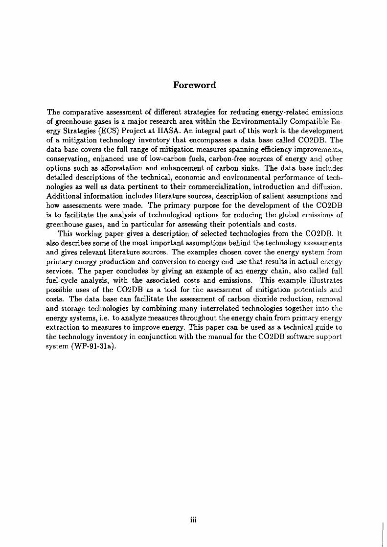
Foreword

The comparative assessment of different strategies for reducing energy-related emissions of greenhouse gases is a major research area within the Environmentally Compatible En- ergy Strategies (ECS) Project at IIASA. An integral part of this work is the development of a mitigation technology inventory that encompasses a data base called C02DB. The data base covers the full range of mitigation measures spanning efficiency improvements, conservation, enhanced use of low-carbon fuels, carbon-free sources of energy and other options such as afforestation and enhancement of carbon sinks. The data base includes detailed descriptions of the technical, economic and environmental performance of tech- nologies as well as data pertinent to their commercialization, introduction and diffusion. Additional information includes literature sources, description of salient assumptions and how assessments were made. The primary purpose for the development of the C02DB is to facilitate the analysis of technological options for reducing the global emissions of greenhouse gases, and in particular for assessing their potentials and costs.

This working paper gives a description of selected technologies from the C02DB. It also describes some of the most important assumptions behind the technology assessments and gives relevant literature sources. The examples chosen cover the energy system from primary energy production and conversion to energy end-use that results in actual energy services. The paper concludes by giving an example of an energy chain, also called full fuel-cycle analysis, with the associated costs and emissions. This example illustrates possible uses of the C02DB as a tool for the assessment of mitigation potentials and costs. The data base can facilitate the assessment of carbon dioxide reduction, removal and storage technologies by combining many interrelated technologies together into the energy systems, i.e. to analyze measures throughout the energy chain from primary energy extraction to measures to improve energy. This paper can be used as a technical guide to the technology inventory in conjunction with the manual for the C02DB software support system (WP-91-31a).

Contents

. . . . . . . . . . . . . . . . . . . . . . . . . . . . . . . . . . . . . . . . . . 1 . Introduction 1

. . . . . . . . . . . . . . . . . . . . . . . . . . . . . . . . . . . . . 2 End-use Technologies 4 . . . . . . . . . . . . . . . . . . . . . . . . . . . . . . 2.1 Passenger Transportation 4

. . . . . . . . . . . . . . . . . . . . . . . . . . . . . . . 2.1.1 Automobiles 4 . . . . . . . . . . . . . . . . . . . . . . . . . . 2.1.2 Wide-body Aircraft 8

. . . . . . . . . . . . . . . . . . . . . . . . . . . . . . . . . 2.1.3 Railways 9 . . . . . . . . . . . . . . . . . . . . 2.2 ResidentialICommercial Technologies 13

2.2.1 Lighting . . . . . . . . . . . . . . . . . . . . . . . . . . . . . . . . 13 . . . . . . . . . . . . . . . . . . . . . . . . . . . . . 2.2.2 Refrigerators 15

. . . . . . . . . . . . . . . . . . . . . . . . . . . . . . . . 2.2.3 Freezers 15 . . . . . . . . . . . . . . . . . . . . . . . . . . . . . . . . . . . . . . 2.3 Industry 16

. . . . . . . . . . . . . . . . . . . . . . . . . . . 2.3.1 Steel Production 16 . . . . . . . . . . . . . . . . . . . . . . . . . . . 2.3.2 Cement Production 22

. . . . . . . . . . . . . . . . . . . . . . . . . . . . . . . 3 . Fuel and Power Production 24 . . . . . . . . . . . . . . . . . . . . . . . . . . . . . . 3.1 Hydrogen Production 24 . . . . . . . . . . . . . . . . . . . . . . . . . . . . . . 3.2 Methanol Production 26 . . . . . . . . . . . . . . . . . . . . . . . . . . . . . . 3.3 Electricity Generation 26 . . . . . . . . . . . . . . . . . . . . . . . . . . . . . . 3.3.1 Renewables 26

3.3.2 Fossil Fuel Power Plants . . . . . . . . . . . . . . . . . . . . . . 29 . . . . . . . . . . . . . . . . . . . . . . . . . . . . . . . 3.3.3 Fuel Cells 32

. . . . . . . . . . . . . . . . . . . 3.3.4 Nuclear Electricity Generation 34

. . . . . . . . . . . . . . . . . . . . . . . . . . . . . . . . . . . . . 4 . Chain Calculations 36 . . . . . . . . . . . . . . . . . . . . . . . . . . . . . . . . . . . . . . 4.1. Lighting 36

. . . . . . . . . . . . . . . . . . . . . . . . . . APPENDIX A -- Overview of C02DB 42

. . . . . . . . . . . . . . . . . . . . . . . . APPENDIX B -- Technology Descriptions 46

Inventory of Greenhouse-Gas Mitigation Measures

Examples from the IIASA Technology Data Bank

Andreas Schafer Leo Schrattenholzer

Sabine Messner

1. Introduction

The comparative assessment of different strategies for mitigating and adapting to possible

global warming is a major area of work within the Environmentally Compatible Energy

Strategies (ECS) Project at IIASA. An important product of this work is an integrated data

base, C02DB, with a comprehensive inventory of technological options that might become

available globally over long time horizons. The data base covers the full range of

technological and economic measures spanning efficiency improvements, conservation,

enhanced use of low-carbon fuels, carbon-free sources of energy and other options such as

afforestation and enhancement of carbon sinks. The primary purpose of further development

of C02DB and the expansion of the mitigation inventory is to facilitate the analysis of

technological options for reducing the global emission of greenhouse gases, in particular for

assessing their potentials and costs. This task represents the largest and most important

activity of the ECS project.

The inventory of mitigation measures has been implemented as a user-friendly and easily

portable PC data base application. It includes those options that have been described in a

draft report on Long-term Strategies for Mitigating Global Warming: Toward3 New Earth

(NakiCenoviC et al., forthcoming) and many others taken from the literature. The data base

has been specifically designed to provide a uniform framework for the assessment of the

ultimate reduction potential of greenhouse gases (GHGs) resulting from the introduction of

new technologies over different time frames and in different regions. It includes detailed

descriptions of the technical, economic, and environmental performance of technologies, as

well as data pertinent to their innovation, commercialization, and diffusion characteristics and

prospects. Additional data files contain literature sources and provide space for describing

the assessment of data validity and uncertainty ranges.

The purpose of this paper is to present typical examples of the approximately 400

technologies that have been entered into C02DB and to demonstrate one of its most powerful

features, i.e., the possibility of assessing different C02 reduction strategies by combining

related technologies together to form an "energy chain", sometimes also called the full fuel-

cycle analysis. Typically, such a chain includes all steps involved in providing a particular

energy service, from primary energy extraction to the end-use conversion. The examples

presented here should be understood to be illustrations of the data base content, not as the

results of a study analyzing the global greenhouse-gas emission reduction potential, which

has been documented in NakiCenoviC et al. (forthcoming). At the same time, our

presentation is less uniform than a comparative study of mitigation options. This is most

visible in the economic data, where we have used prices in one group of technologies and

costs in another. This is less the result of deliberate choice than a reflection of the real data

situation. Also, little attempt was made to account for different degrees of optimism shown

by the original sources of future performance data. Likewise, this is no guide for the usage

of C02DB on the computer. Messner and Strubegger (1991) provide a full description of

the software package and how to use it. This report is based on Version 2 of C02DB.

The data base software is in the public domain and can easily be made available to other

groups, e.g., within the CHALLENGE network which is jointly organized by ITASA and the

Institute for Energy Economics and the Rational Use of Energy at Stuttgart University. The

aim of the network is to combine different country's studies of GHG reduction strategies to

describe and analyze globally comprehensive and consistent scenarios of GHG mitigation.

The examples chosen for this report cover the three major economic sectors: industry,

transportation, and residen tial/commercial. Technologies for steel and cement production,

for passenger transport, for lighting, and for refrigeration will be presented and their relative

costs and carbon emissions compared.

As an illustration of the data base's ability to calculate chains, we present different

combinations of light bulbs and electricity generation systems showing how the choice of an

end-use technology influences the economics of power generation.

Appendices summarize the data base formats and all technologies that have been included to

date.

References

Messner, S. and Strubegger, M. (1991), User's Guide to COZDB: The IUSA CO, Technology Data Bank, Version 1.0, WP-91-31a, International Institute for Applied Systems Analysis, Laxenburg, Austria.

NakiCenoviC, N. et al., Forthcoming, Long-term Strategies for Mitigating Global Warming: Towards New Earth, forthcoming in Energy.

2. End-use Technologies

2.1 Passenger Transportation

2.1.1 Automobiles

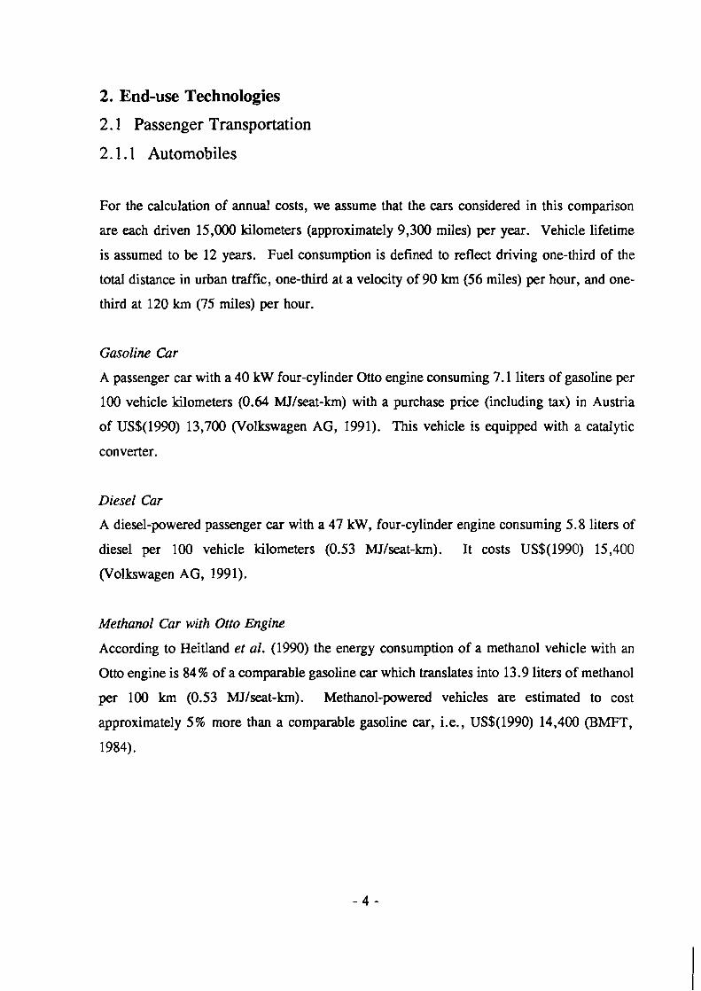
For the calculation of annual costs, we assume that the cars considered in this comparison

are each driven 15,000 kilometers (approximately 9,300 miles) per year. Vehicle lifetime

is assumed to be 12 years. Fuel consumption is defined to reflect driving one-third of the

total distance in urban traffic, one-third at a velocity of 90 km (56 miles) per hour, and one-

third at 120 km (75 miles) per hour.

Gasoline Car

A passenger car with a 40 kW four-cylinder Otto engine consuming 7.1 liters of gasoline per

100 vehicle kilometers (0.64 MJ/seat-km) with a purchase price (including tax) in Austria

of US$(1990) 13,700 (Volkswagen AG, 1991). This vehicle is equipped with a catalytic

converter.

Diesel Car

A diesel-powered passenger car with a 47 kW, four-cylinder engine consuming 5.8 liters of

diesel per 100 vehicle kilometers (0.53 MJ/seat-km). It costs US$(1990) 15,400

(Volkswagen AG, 1991).

Methanol Car with Otto Engine

According to Heitland et al. (1990) the energy consumption of a methanol vehicle with an

Otto engine is 84 % of a comparable gasoline car which translates into 13.9 liters of methanol

per 100 km (0.53 MJIseat-km). Methanol-powered vehicles are estimated to cost

approximately 5% more than a comparable gasoline car, i.e., US$(1990) 14,400 (BMFT,

1984).

Methanol Car with a Diesel Engine

The energy consumption of a methanol vehicle with a diesel engine is 72% of a comparable

gasoline car which translates into 12.1 liters of methanol per 100 km (Heitland et al., 1990).

This corresponds to 0.46 MJ per seat-km. Like the methanol Otto car, the methanol diesel

vehicle is estimated to cost 5% more than a comparable diesel vehicle, i.e., US$(1990)

16,200.

Ethanol Car

Fuel consumption is about 12 % less than a comparable gasoline car, resulting in 10.6 liters

of ethanol per 100 vehicle kilometers (0.56 MJ per seat-km) when burned in an Otto engine

(Geller, 1985). Like the methanol cars, ethanol-powered vehicles are estimated to cost 5%

more than a comparable gasoline car, i.e., US$(1990) 14,400.

Compressed Natural Gas (CNG) Car

Natural gas consumption is 0.5 MJ per seat-km. Additional vehicle costs (compared with

the 40 kW gasoline engine) of US$ 1,000 are expected due to the 165 bar gas tank (Sperling

and DeLucchi, 1989).

Hydrogen Car with Otto Engine

An engine powered with unleaded gasoline can run on hydrogen if some modifications in the

engine environment are carried out. Reister and Regar (1992) report about a BMW test

vehicle powered with LH2 using 23% less energy that its gasoline powered counterpart.

Thus, energy consumption is 0.49 MJ per seat-km. Such a car is estimated to cost 25%

more than a comparable gasoline car. This value is taken from a study of Reister and Strobl

(1992) who expect a dual-fueled hydrogen car to be 30 to 40% more expensive than a car

running exclusively on gasoline.

Hydrogen Car wirh Fuel Cell

Hydrogen can also be used for powering an electric engine via a fuel cell. In road traffic,

fuel cells are expected to have an efficiency around 50%. C02DB assumes costs of a

hydrogen fuel cell car of US$(1990) 120,000. This value is based on the current material

costs of a polymer-electrolyte-membrane fuel cell which are approximately US$(1990) 1,500

per kW. (According to StraBer (1992), specific costs could drop to US$(1990) 120 per k W

if further research and development is carried out.) Hydrogen is assumed to be stored in

liquid form. The engine power output is assumed to be 34 kW and the final energy

consumption corresponds to 0.35 MJ per seat-km.

Electric Vehicle with Nutrim-Sulfir Battery

Electricity consumption is 13 kwh, per 100 vehicle kilometers (0.12 MJ,/seat-km). The

engine has a power output of 34 kW, the maximum velocity is 120 km (75 miles) per hour

and the maximum range is 250 km (156 miles). Its price is assumed to be US$(1990)

25,000, including the natrium-sulfur battery if produced by mass production (Sauer, 1991).

The battery lifetime corresponds to about 1000 recharging cycles (Reuss, 1991).

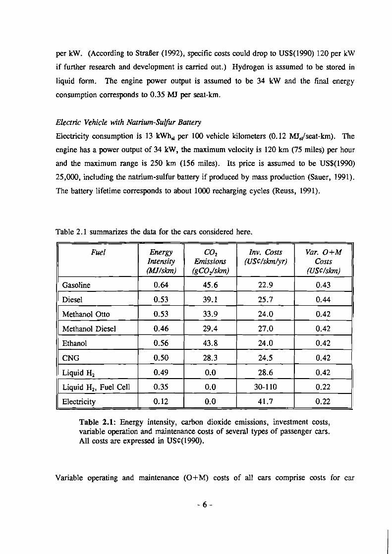
Table 2.1 summarizes the data for the cars considered here.

Table 2.1: Energy intensity, carbon dioxide emissions, investment costs, variable operation and maintenance costs of several types of passenger cars. All costs are expressed in USC(1990).

Variable operating and maintenance (O+M) costs of all cars comprise costs for car

~

Fuel

Gasoline

Diesel

Methanol Otto

Methanol Diesel

co2 Emissions (g COJskm)

45.6

39.1

33.9

29.4 PPP

43.8

28.3

Energy Intensity (MJ/skm)

0.64

0.53

0.53

0.46

Liquid Hz

Liquid Hz, Fuel Cell

Electricity

0.0

0.0

0.0

Inv. Costs (USC/skm@r)

22.9

25.7

24.0

27.0

24.0

24.5

0.49

0.35

0.12

Ethanol

CNG

Var. O+M Costs

(USCIskm)

0.43

0.44

0.42

0.42

0.421 0.42

0.56

0.50

28.6

30- 1 10

41.7 0.22

maintenance and tires (excluding fuel costs). For cars with internal combustion engines,

O+M were derived from the DOT report (1990) and reflect the USA average of gasoline-

powered cars. Both types of electric car (conventional battery and fuel cell) are assumed to

have half the operating costs of gasoline-powered cars (Mann, 1992). Fixed O+M costs,

i.e., insurance, license, and registration fees, are not included here.

References

BMFT, 1984, Alternative Energy, Sources for Road Transport - Methanol, Verlag TUV Rheinland.

DOT, 1990, National Transportation Statistics, Annual Report, U. S . Department of Transportation, July 1990.

Heitland H., Hiller H., and Menrad H., 1990, Energiespeicherung und Energiesysteme, Energie und Klima, Band 6, Enquiry Commission of the German Parliament, Economia Verlag, Verlag C.F. Miiller.

Mann E. W., 1992, Elektrofahrzeuge - Umweltenlastune durch Stromanwendung im Individualverkehr, Elektrizitlitswirtschafl, Jg . 9 1 (1 992), Heft 17.

Reister D., Regar K.-N., 1992, Elektro-. Hybrid- und Wasserstoffantrieb fiir PKW - Chancen fiir eine zwecko~timierte Technik, in: Energiehaushalten und C0,- Mindenmg: Einsparpotentiale im Sektor Verkehr, VDI Berichte 943, VDI Verlag GmbH, Diisseldorf.

Reister D., Strobl W., 1992, Entwicklungsstand und Pers-pektiven des Wasserstoffautos, in: Wasserstoflechnik III, VDI Berichte 9 12, VDI Verlag GmbH, Diisseldorf.

Reuss I., 1991, Hochenergie-Batterie sol1 Benzintank ersetzen, VDI Nachrichten No. 48, November 22., 1991

Sauer H., 1991, E-Station Sehnsucht, Auto Motor Sport No. 26.

Sperling D. and DeLucchi M., 1989, Transportation Energv Futures, Annual Review of Energy, Vol. 14.

S tral3er K., 1992, Brennstoflellen jiir Elektrotraktion, Wasserstofftechnik 111, VDI Berich te 912, VDI Verlag.

Volkswagen AG, Der neue Golf, September 199 1.

2.1.2 Wide-body Aircraft

The following data for alternatively powered aircraft are based on Lockheed studies on the

hydrogen aircraft in the 1970's and early 80's. They have been reported by Brewer (199 1)

and calibrated to the 1990 level by IIASA's ECS group. All aircraft considered here assume

400 passenger seats, a range of 10,200 krn (6,340 miles), and a cruise speed of Mach 0.85.

The lifetime of each aircraft is 20 years.

Boeing 747-400

The version 400 of this aircraft type has been operational since 1989 and has an average

energy intensity of 0.88 MJ per seat-km (Steiner, 1989). According to Institute of Air

Transport (ITA) statistics (1991), its market price was US$ 132.5 million in early 1991.

This aircraft is powered by liquid hydrogen and has a projected energy use of 0.64 MJ per

seat-km. Its principal exhaust gas is water vapor of which it emits 80% more (per seat-km)

than a B747-400. Brewer (1991) projects investment costs to be 2.5% lower than a

conventional aircraft1. C02DB therefore assumes a price of US$ 129.1 million. C02DB's

introduction date for this type of aircraft is 2020.

LNG Aircrafc

According to Brewer (1991)' the performance of an aircraft fueled by liquid natural gas is

expected to fall between that of a conventional jet and a liquid hydrogen aircraft. The energy

intensity is 0.72 UI per seat-km. Investment costs are projected to be 8% higher than for

a conventional aircraft. Therefore, a price of US$ 143.1 million has been assumed.

C02DB's introduction date for this type of aircraft is 2015.

' Note the difference between the fuelcell and hydrogen combustion technology. The much higher material costs of low-temperature fuel cells make the hydrogen cars of the previous section much more expensive than conventional cars. Since aircraft use hydrogen combustion engines, and since hydrogen airplanes are expected to have more favorable technical characteristics (less weight, requiring less thrust), investment costs are even lower here than those of conventional aircraft.

-- - -

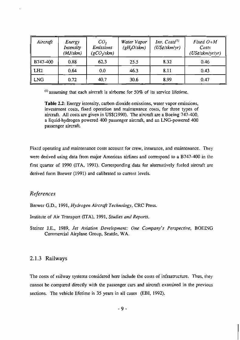
(''assuming that each aircraft is airborne for 50% of its service lifetime.

Table 2.2: Energy intensity, carbon dioxide emissions, water vapor emissions, investment costs, fixed operation and maintenance costs, for three types of aircraft. All costs are given in US$(1990). The aircraft are a Boeing 747-400, a liquid-hydrogen powered 400 passenger aircraft, and an LNG-powered 400 passenger aircraft.

Aircraft

B747-400

LH2

LNG

Fixed operating and maintenance costs account for crew, insurance, and maintenance. They

were derived using data from major American airlines and correspond to a B747-400 in the

first quarter of 1990 (ITA, 1991). Corresponding data for alternatively fueled aircraft are

derived form Brewer (1991) and calibrated to current levels.

Energy Intensity (MJ lsh )

0.88

0.64

0.72

References

Fixed O+M Costs

(US#lskmlyrlyr)

0.46

0.43

0.47

coz Emissions

( gC0 , l sh )

62.3

0.0

40.7

Brewer G.D., 1991, Hydrogen Aircraft Technology, CRC Press.

Institute of Air Transport (RITA), 1991, Studies and Reports.

Water Vapor (gH201skm)

25.5

46.3

30.6

Steiner J.E., 1989, Jet Aviation Development: One Company's Perspective, BOEING Commercial Airplane Group, Seattle, WA.

Inv. Costs") (US#lskmlyr)

8.32

8.11

8.99

2.1.3 Railways

The costs of railway systems considered here include the costs of infrastructure. Thus, they

cannot be compared directly with the passenger cars and aircraft examined in the previous

sections. The vehicle lifetime is 35 years in all cases (EBI, 1992).

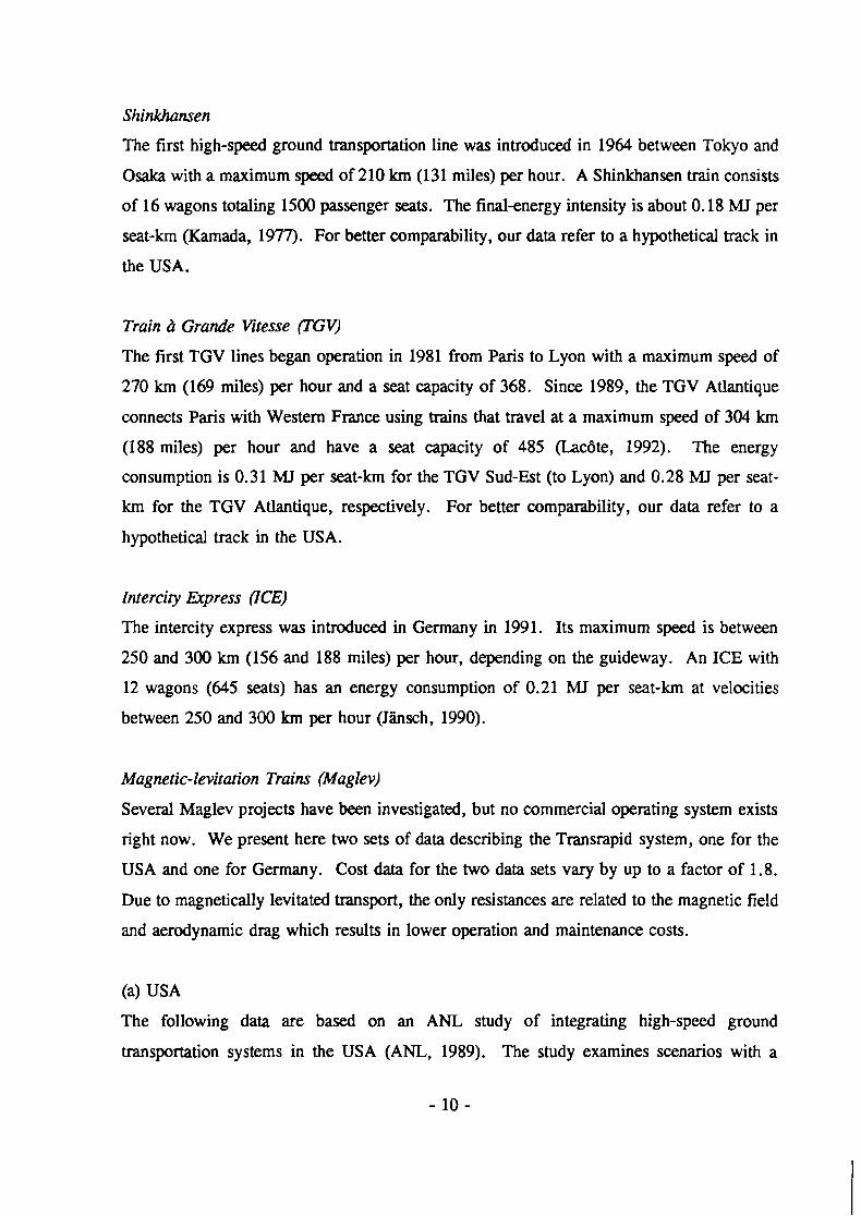
Shinkhansen

The first high-speed ground transportation line was introduced in 1964 between Tokyo and

Osaka with a maximum speed of 210 km (131 miles) per hour. A Shinkhansen train consists

of 16 wagons totaling 1500 passenger seats. The final-energy intensity is about 0.18 MJ per

seat-km (Kamada, 1977). For better comparability, our data refer to a hypothetical track in

the USA.

Train h Grande Vitesse (TGV)

The first TGV lines began operation in 198 1 from Paris to Lyon with a maximum speed of

270 km (169 miles) per hour and a seat capacity of 368. Since 1989, the TGV Atlantique

connects Paris with Western France using trains that travel at a maximum speed of 304 km

(188 miles) per hour and have a seat capacity of 485 (Ladte, 1992). The energy

consumption is 0.31 MJ per seat-km for the TGV Sud-Est (to Lyon) and 0.28 h4J per seat-

km for the TGV Atlantique, respectively. For better comparability, our data refer to a

hypothetical track in the USA.

Intercity Express (ICE)

The intercity express was introduced in Germany in 1991. Its maximum speed is between

250 and 300 km (156 and 188 miles) per hour, depending on the guideway. An ICE with

12 wagons (645 seats) has an energy consumption of 0.21 MJ per seat-km at velocities

between 250 and 300 km per hour (Jbsch, 1990).

Magnetic-levitation Trains (Maglev)

Several Maglev projects have been investigated, but no commercial operating system exists

right now. We present here two sets of data describing the Transrapid system, one for the

USA and one for Germany. Cost data for the two data sets vary by up to a factor of 1.8.

Due to magnetically levitated transport, the only resistances are related to the magnetic field

and aerodynamic drag which results in lower operation and maintenance costs.

(a) USA

The following data are based on an ANL study of integrating high-speed ground

transportation systems in the USA (ANL, 1989). The study examines scenarios with a

Shinkhansen-type connection between Los Angeles and San Diego, and with a TGV-type and

a Transrapid system between Los Angeles and Las Vegas. Unit investment costs include the

vehicles, guideway, and power delivery. Vehicles typically account for less than 20% of the

total investment costs. The operating costs include the guideway, vehicle maintenance, and

miscellaneous items such as insurance, ticketing, and vehicle crews. Energy costs are

excluded.

(b) Germany

The data described here are based on a study of a proposed line between Hamburg and

Hannover with two stops in-between (KAT, 1989). The distance of 147 km (92 miles) is

covered in 29 minutes (including both stops), corresponding to an average velocity of 300 km

(186 miles) per hour. The system considered here includes 11 Maglev trains (328 seats each),

the guideway, and stations at costs of US$(1990) 1.91 billion. Electricity consumption is 0.36

MJ per seat-km. Vehicle lifetime is assumed to be 35 years in all cases.

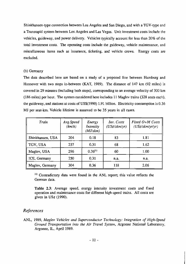
(I) Contradictory data were found in the ANL report; this value reflects the German data.

Train

Shinkhansen, USA

TGV, USA

Maglev, USA

ICE, Germany

Maglev, Germany

Table 2.3: Average speed, energy intensity investment costs and fixed operation and maintenance costs for different high-speed trains. All costs are given in US$ (1990).

References

A vg .Speed (kmlh)

204

257

296

250

304

ANL, 1989, Maglev Vehicles and Superconductor Technology: Integration of High-Speed Ground Transportation into the Air Travel System, Argonne National Laboratory, Argonne, IL, April 1989.

Fixed O+M Costs (US&lskmlyrlyr)

1.81

1.62

1 .OO

n.a.

2.06

Energy Intensity (MJlskm)

0.18

0.3 1

0.36")

0.31

0.36

Inv. Costs (US&lskmlyr)

83

68

60

n.a.

118

Der Eisenbahningenieur (EBI), 1992, Bis zwn Jahr 2020 rund 4700 km Hochleistungs- strecken, Der Eisenbahningenieur 43, Tellaff Verlag, Darmstadt, Germany.

Jinsch E., 1990, Energieverbrauch und klimarelevante Emissionen im Personenfernverkehr, Elektrische Bahnen 88, R. Oldenburg Verlag, Germany.

Kamada M., 1977, Achievements and Future Problems of the Shinkhanren, The Shinkhanren Railway Network of Japan, IIASA Proceedings Series, Pergamon Press.

KAT, 1989, Transrapid Anwendungsstrecken, Ergebnisbericht, Konsortium Anschubtruppe Transrapid, Munich, Germany.

LacBte F., 1992, Die TGV-Fahneugfamilie der SNCF, Elektrische Bahnen 90, R. Oldenburg Verlag .

2.2 Residential/Commercial Technologies

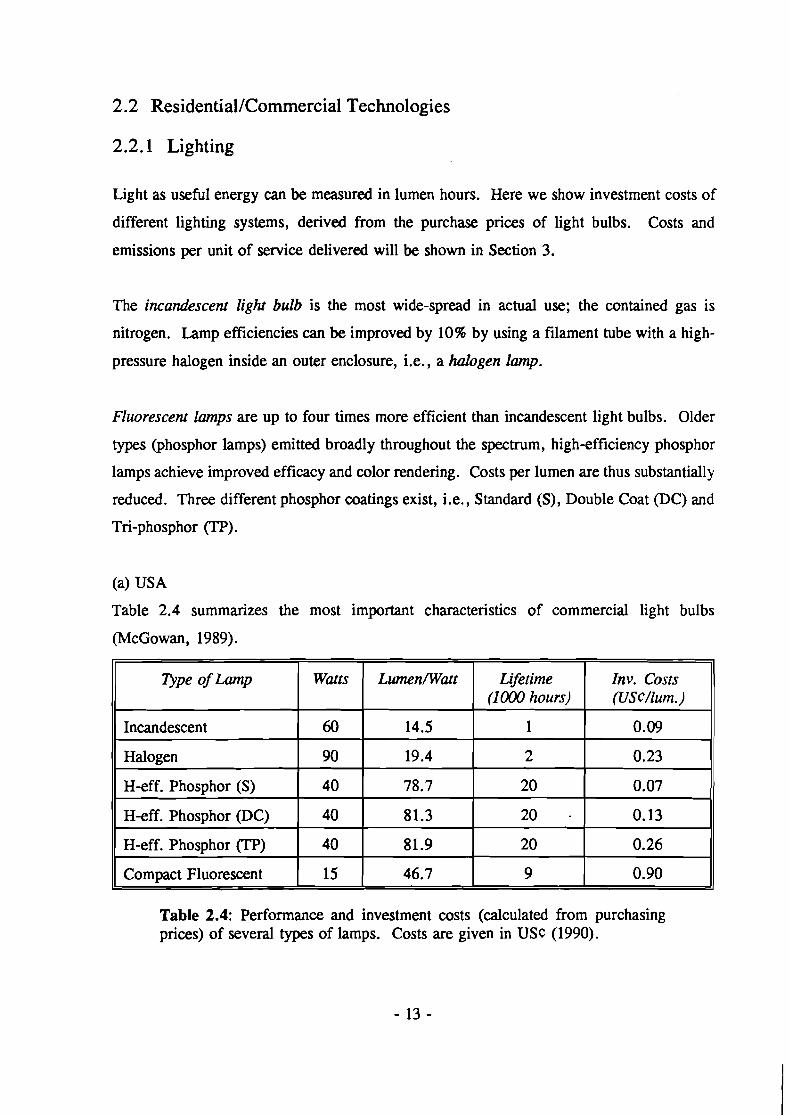
2.2.1 Lighting

Light as useful energy can be measured in lumen hours. Here we show investment costs of

different lighting systems, derived from the purchase prices of light bulbs. Costs and

emissions per unit of service delivered will be shown in Section 3.

The incandescent light bulb is the most wide-spread in actual use; the contained gas is

nitrogen. Lamp efficiencies can be improved by 10% by using a filament tube with a high-

pressure halogen inside an outer enclosure, i.e., a halogen lamp.

Fluorescent lamps are up to four times more efficient than incandescent light bulbs. Older

types (phosphor lamps) emitted broadly throughout the spectrum, high-efficiency phosphor

lamps achieve improved efficacy and color rendering. Costs per lumen are thus substantially

reduced. Three different phosphor coatings exist, i.e., Standard (S), Double Coat @C) and

Tri-phosphor (TP).

(a) USA

Table 2.4 summarizes the most important characteristics of commercial light bulbs

(McGowan, 1989).

Table 2.4: Performance and investment costs (calculated from purchasing prices) of several types of lamps. Costs are given in USC (1990).

V P ~ of Lamp

Incandescent

Halogen

H-eff. Phosphor (S)

H-eff. Phosphor (DC)

H-eff. Phosphor (TP)

Compact Fluorescent

Inv. Costs (USC/lum.)

0.09

0.23

0.07

0.13

0.26

0.90

Lifetime (1 000 hours)

1

2

20

20 -

20

9

Watts

60

90

40

40

40

15

Lwnen~Watt

14.5

19.4

78.7

81.3

81.9

46.7

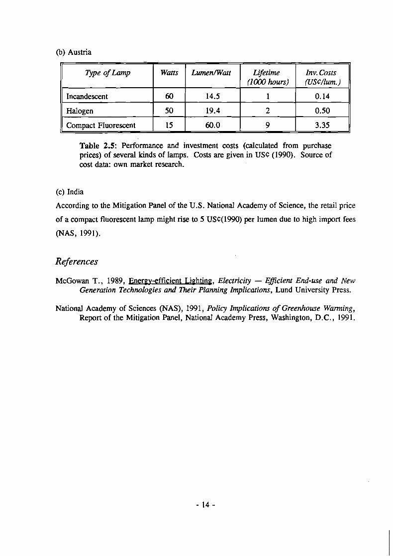
@) Austria

Table 2.5: Performance and investment costs (calculated from purchase prices) of several kinds of lamps. Costs are given in USC (1990). Source of cost data: own market research.

o p e of Lamp

Incandescent

Halogen

Compact Fluorescent

(c) India

According to the Mitigation Panel of the U.S. National Academy of Science, the retail price

of a compact fluorescent lamp might rise to 5 USC(1990) per lumen due to high import fees

(NAS, 1991).

References

McGowan T., 1989, Energv-efficient Lighting, Electricity - Eficient End-use and New Generation Technologies and Their Planning Implications, Lund University Press.

Watts

60

50

15

National Academy of Sciences (NAS), 1991, Policy Implications of Greenhouse Warming, Report of the Mitigation Panel, National Academy Press, Washington, D.C., 1991.

Lifetime (1 000 hours)

1

2

9

Lwnen~Watt

14.5

19.4

60.0

Inv. Costs (USC/lum.)

0.14

0.50

3.35

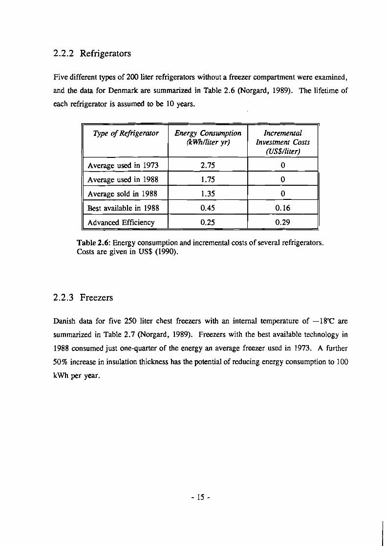
2.2.2 Refrigerators

Five different types of 200 liter refrigerators without a freezer compartment were examined,

and the data for Denmark are summarized in Table 2.6 (Norgard, 1989). The lifetime of

each refrigerator is assumed to be 10 years.

Table 2.6: Energy consumption and incremental costs of several refrigerators. Costs are given in US$ (1990).

Type of Refigerator

Average used in 1973

Average used in 1988

Average sold in 1988

Best available in 1988

Advanced Efficiency

2.2.3 Freezers

Danish data for five 250 liter chest freezers with an internal temperature of -18°C are

summarized in Table 2.7 (Norgard, 1989). Freezers with the best available technology in

1988 consumed just one-quarter of the energy an average freezer used in 1973. A further

50% increase in insulation thickness has the potential of reducing energy consumption to 100

kwh per year.

Energy Consumption (kWh/liter yr)

2.75

1.75

1.35

0.45

0.25

Incremental Investment Costs

(US$/liter)

0

0

0

0.16

0.29

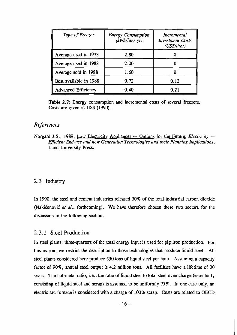
Table 2.7: Energy consumption and incremental costs of several freezers. Costs are given in US$ (1990).

o p e of Freezer

Average used in 1973

Average used in 1988

Average sold in 1988

Best available in 1988

Advanced Efficiency

References

Norgard J.S., 1989, Low Electricity Appliances - Options for the Future, Electricity - Eficient End-use and new Generation Technologies and their Planning Implications, Lund University Press.

Energy Consumption (kWh/liter yr)

2.80

2.00

1 .60

0.72

0.40

2.3 Industry

Incremental Investment Costs

(US$/liter)

0

0

0

0.12

0.21

In 1990, the steel and cement industries released 30% of the total industrial carbon dioxide

(NakiCenoviC et al., forthcoming). We have therefore chosen these two sectors for the

discussion in the following section.

2.3.1 Steel Production

In steel plants, three-quarters of the total energy input is used for pig iron production. For

this reason, we restrict the description to those technologies that produce liquid steel. All

steel plants considered here produce 530 tons of liquid steel per hour. Assuming a capacity

factor of 90%, annual steel output is 4.2 million tons. All facilities have a lifetime of 30

years. The hot-metal ratio, i.e., the ratio of liquid steel to total steel oven charge (essentially

consisting of liquid steel and scrap) is assumed to be uniformly 75%. In one case only, an

electric arc furnace is considered with a charge of 100% scrap. Costs are related to OECD

countries; fuel costs are excluded.

Conventional Steel Plant

The conventional plant consists of coke ovens, a sinter plant, a blast furnace, and a basic-

oxygen furnace. Coal accounts for more than 95 % of the primary energy inputs. The blast

furnace operates oil-free and has a capacity of 400 tons of liquid iron per hour. Coke

consumption is 550 kg per ton of liquid iron, corresponding to a coal input of 700 kg in the

coke ovens. All electricity inputs of steel plant are produced internally. A volume of

35 m3 (STP) of oxygen and 30 tons of water are required for the production of one ton of

liquid steel. Carbon dioxide emissions are equal to 1.8 tons per ton of liquid steel.

Investment costs for such plants can differ substantially, depending on the available

infrastructure. On the basis of several publications, i.e., S&E (1987), Azimi and Lowitt

(1988), the International Iron and Steel Institute (1982), VOEST Alpine (unpublished), and

Mannesmann (unpublished), we have estimated investment costs of US$280 per ton of liquid

steel annual capacity.

Conventional Steel Plant with Additional Energy-saving Technologies (Conventional +EST)

Energy can be recovered in virtually every production phase. Plant performance can be

upgraded by implementing devices for hot gas recovery, such as a blast furnace top pressure

recovery turbine with an energy-saving potential of roughly 250-300 MJ per ton of crude

steel. Moreover, the basic oxygen furnace operates with a net energy surplus if flue gas is

recycled. In addition, energy-saving devices can be implemented at the coke and sinter

plant, reducing coal consumption by about 10% compared with its predecessor. Investment

increases to US$(1990) 300 per annual ton of liquid steel. UISI, 1982; Maier et al., 1986).

Direct-reduction Plant and Electric Arc Furnace (DRI+EAF)

Various direct-reduction processes exist of which about 90% use a gaseous reductant and

only 10% use coal (Steffen and Liingen, 1988). C02DB contains two direct-reduction

plants, both based on a study by Heinrich et al. (1990). One of the plants is based on natural

gas, the other plant uses coal as the reductant and energy source. Each plant is connected

with an electric arc furnace. The natural-gas basedplant, DRI(NG)+EAF, consumes about

10 GJ of natural gas and 665 kwh of electricity per liquid ton of steel. Investment costs are

estimated to be US$(1990) 165 per ton of liquid steel. The coal-based process,

DRI(C)+EAF, requires 10.9 GJ of coal and 665 kWh of electricity. Investment costs

increase to US$(1990) 200 per ton of liquid steel.

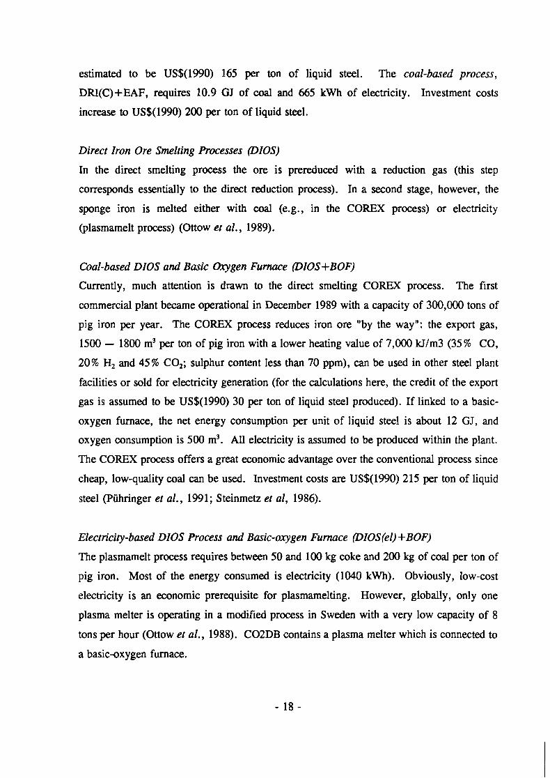
Direct Iron Ore Smelting Processes (DIOS)

In the direct smelting process the ore is prereduced with a reduction gas (this step

corresponds essentially to the direct reduction process). In a second stage, however, the

sponge iron is melted either with coal (e.g., in the COREX process) or electricity

(plasmamelt process) (Ottow et al., 1989).

Coal-based DIOS and Basic Oxygen Furnace (DIOS+BOF)

Currently, much attention is drawn to the direct smelting COREX process. The first

commercial plant became operational in December 1989 with a capacity of 300,000 tons of

pig iron per year. The COREX process reduces iron ore "by the way": the export gas,

1500 - 1800 m3 per ton of pig iron with a lower heating value of 7,000 kJJm3 (35 % CO,

20% H, and 45% CO,; sulphur content less than 70 ppm), can be used in other steel plant

facilities or sold for electricity generation (for the calculations here, the credit of the export

gas is assumed to be US$(1990) 30 per ton of liquid steel produced). If linked to a basic-

oxygen furnace, the net energy consumption per unit of liquid steel is about 12 GJ, and

oxygen consumption is 500 m3. All electricity is assumed to be produced within the plant.

The COREX process offers a great economic advantage over the conventional process since

cheap, low-quality coal can be used. Investment costs are US$(1990) 215 per ton of liquid

steel (Piihringer et al., 1991; Steinmetz et al, 1986).

Electricity-based DIOS Process and Basic-oxygen F u m e (DIOS(e1) +BOF)

The plasmamelt process requires between 50 and 100 kg coke and 200 kg of coal per ton of

pig iron. Most of the energy consumed is electricity (1040 kWh). Obviously, low-cost

electricity is an economic prerequisite for plasmamelting. However, globally, only one

plasma melter is operating in a modified process in Sweden with a very low capacity of 8

tons per hour (Ottow et al., 1988). C02DB contains a plasma melter which is connected to

a basic-oxygen furnace.

Electric Arc Furnace Smelting lOO% Scrap (EAF)

The electric arc furnace smelts a burden of 100% steel scrap or mixtures of scrap with

sponge iron or - to some extent - liquid pig iron; Typically, 75 % of the energy input is

electricity, the remainder consisting of natural gas, oxygen, carbon, etc. The energy

consumption of electric arc furnaces is about 600 kWh, per ton of liquid steel. This

comparatively low energy requirement is due to the energy embodied in steel scrap.

Investment costs are about US$(1990) 100 per annual ton of liquid steel (Azimi and Lowitt,

1988).

Iron Reduction with Hydrogen and Electric Arc Furnace (DRI(HJ +MF)

Hydrogen can be used as a reductant of iron. This process can be realized by either a direct

reduction process or a direct smelting process. The primary emission is water vapor, carbon

dioxide emissions are practically zero. C02DB contains a direct reduction process . As a

first-order estimate, energy consumption and costs are identical to the process based on

natural gas.

References

Azimi S.A. and Lowitt H.E., 1988, The US Steel Industry: an Energy Perspective, Energetics, Inc., Columbia, MD (USA).

Heinrich P. , Knop K., Madlinger R. , 1990, Stand und Ennvicklungspotential der Direktreduktion mit &m HE-III-Vemren, Stahl und Eisen 1 10, No. 8.

International Iron and Steel Institute (IISI), 1982, Energy and the Steel Industry, International Iron and Steel Institute, Committee on Technology, Brussels 1982.

Maier M. et al., 1986, Rationelle Energieverwendung durch new Technologien Band 2, Praxiswissen aktuell, Verlag TUV Rheinland.

Mannesmann Demag (1992), personal communication.

NakiCenoviC N. et al., U~P-Term Strategies for Mitigating Global Warming: Towards New Earth, forthcoming in Energy.

Ottow M. et al., 1988, m, Ullmann's Encyclopedia of Industrial Chemistry, Vol.Al4, VCH Verlagsgesellschaft mbH.

Piihringer O., Wiesinger H., Havenga B.H.P., Hauk R., Kepplinger W .L., and Wallner F.,

199 1, Betriebserfahrungen mit dem Corex- Verfahren und dessen Enfwicklungspotenfial, Stahl und Eisen, 11 1, Journal No. 9.

S&E, 1987, Deutsche Stahlindustne braucht politischen Flankenschutz, Stahl und Eisen 107, N0.3.

Steffen R. and Liingen H.B., 1988, Stand der Direktreduktion von Eisenenen zu Eisenschwarnrn, Stahl und Eisen 108, No. 7.

Steinmetz E., Steffen R., ,and Thielmann R., 1986, Stand und Ennvicklungsmdglichkeiten der Ve@ahren zur Direktreduktion und Schmelzreduktion von Eisemnen, Stahl und Eisen 106, N0.9.

VOEST Alpine (1992), personal communication.

Table 2.8: Primary energy intensity, externally produced electricity consumption, carbon dioxide emissions, investment costs, fixed operation and maintenance costs (labor, maintenance), and variable operation and maintenance costs (iron ore, alloys, scrap, electrodes, etc.) per ton of liquid steel (tls). The figures are for the following plants: a conventional steel plant, a conventional steel plant with additional energy saving technologies, a direct iron ore smelting process with a basic-oxygen furnace (DIOS(C)+BOF), a plasma melter with an electric arc furnace (PLASMA+EAF), a direct reduction plant fired with natural gas with an electric arc furnace DRI(NG) +EAF, a coal-based direct reduction plant with an electric arc furnace (DRI(C) +EAF), a hydrogen-based direct reduction plant with an electric arc furnace (DRI(H2) +EAF), and an electric arc furnace smelting scrap (EAF) .

Plant o p e

Conventional

Conventional +EST

DIOS(C) + BOF

DIOS(e1) + EAF

DRI(NG) + EAF

DRI(C) + EAF

DRI(H2) + EAF

EAF

co2 Emissions

(tonCOJtls)

1.8

1.6

1.4

0.8 - 1.8

0.5 - 1.2

1.1 - 1.7

0.0

0.0 - 0.6

Primary Energy (GJ/tls)

17.9

16.0

22.8 (12)

7.7

10.0

10.9

10.0

0.2

Znv. Costs (US$/tls/yr)

280

300

2 15

n.a.

165

200

1 65

100

Electricity (kWh/tls)

0

0

0

1040

665

665

665

600

Fixed 0 +M Costs (% of

Znv.)

11

11

10

n.a.

10

10

10

9

Variable 0 +M Costs

(US$/tls)

100

100

100

n.a.

100

100

100

140

2.3.2 Cement Production

Essentially two different processes for cement production exist, the dry and the wet process.

The latter permits more homogenization of kiln feed and requires less ground raw materials

than the former. Moreover, plant design is simpler. The difference in energy consumption

is considerable. The wet process requires about 5.0-6.0 GJ per ton of clinker, the dry

process 3.4-5.0 GJ. Using a pre-heater, the energy consumption of the dry process can be

reduced to 3.1-4.2 GJ per ton of clinker (Locher and Kropp, 1989). In comparison, US

energy intensity per ton of cement was 4.1 GJ and 133 kwh of electricity in 1988. The

theoretical minimum is 1.75 GJ per ton of clinker (Tresouthick and Mishulocich, 1991).

Table 2.9 gives an overview of several cement production technologies and fuels. Costs

reflect the OECD average (Maier et al., 1986); energy costs are excluded. Note that energy

intensity is related to one ton of cement, consisting of 95% clinker and 5% gypsum.

References

Locher F.W. and Kropp J., 1989, Cement and Concrete, Ullmann's Encyclopedia of Industrial Chemistry, Vol.A5, VCH Verlagsgesellschaft mbH.

Maier M. et al., 1986, Rationelle Energievenvendung durch new Technologien Band 2, Praxiswissen aktuell, Verlag TUV Rheinland.

Tresouthick S . W. and Mishulocich A., 199 1 , Energy and Environmental Considerations for the Cement Indurtry, Energy and Environment in the 21st Century, MIT Press, Cambridge, Massachusetts.

Table 2.9: Characteristic quantities for cement production processes. In all cases, clinker content is assumed to be 95% per ton of cement. The process types are as follows: wet process, dry process, dry process with pre-heater (dry-PH), high efficiency dry process (dry-PH; including pre-heater, rolling mills, and computer control) and high efficiency dry process with carbon scrubbing (dry-HE-CS). It is assumed that the electricity source corresponds to the fossil fuel used. CO, emissions include 770 kg CO, per ton of clinker generated during calcination.

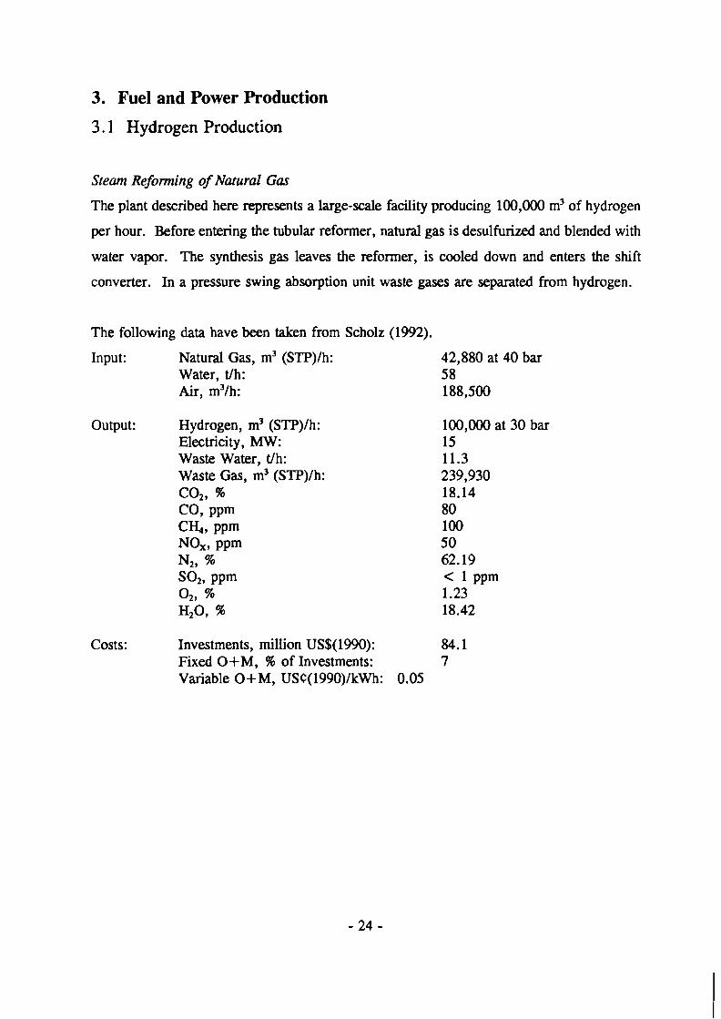
3. Fuel and Power Production

3.1 Hydrogen Production

Steam Refonning of Natural Gas

The plant described here represents a large-scale facility producing 100,000 m3 of hydrogen

per hour. Before entering the tubular reformer, natural gas is desulfurized and blended with

water vapor. The synthesis gas leaves the reformer, is cooled down and enters the shift

converter. In a pressure swing absorption unit waste gases are separated from hydrogen.

The following data have been taken from Scholz (1992).

Input: Natural Gas, m3 (STP)/h: Water, t/h: Air, m3/h:

Output: Hydrogen, m3 (STP)/h: Electricity, MW: Waste Water, t/h: Waste Gas, m3 (STP)/h: co2, % CO, PPm C%, PPm NO,, PPm N2, %

42,880 at 40 bar 58 188,500

100,000 at 30 bar 15 11.3 239,930 18.14 80 100 50 62.19

Costs: Investments, million US$(1990): 84.1 Fixed O+M, % of Investments: 7 Variable O+M, USC(1990)/kWh: 0.05

Electrolysis of Water

Electrolyser Inc., Toronto is the only manufacturer of uni-polar cells. The advantage of this

cell type is its robustness. Since the cells are arranged in parallel, they can be easily

maintained or renewed, if necessary, without interruption of the process (Haussinger et al.,

1989). The following data are from the producer (Electrolyzer Corporation, 1990).

Input: Electricity, MW,: 430 Purified Feedwater, t/h: 1 Cooling Water, t/h: 24

Output: Hydrogen (99.9%), m3 (STP)/h: 1000 at 1.013 bar Oxygen (99.7 %), m3 (STP)/h: 500

Costs: Investments, million US$(1990): 1.42 Fixed O+M, 96 of Investments: 4

Table 3.1: Two hydrogen production processes, one based on coal and one based on natural gas. All costs are given in US$(1990).

References

Fuel vpe

Natural Gas

Electricity

Electrolyzer Corporation LTD. (EC), 1990, Electrolytic Hydrogen Plants, Publication TECL EHP0187, Canada.

E$c. (%)

81.2

65.1

Output ( 1 w /

h)

100

1

Haussinger P., Lohmiiller R., and Watson A.M., 1989, Hydrogen, Ullmann 's Encyclopedia of Industrial Chemistry, Vol. A 14, VCH Verlagsgesellschaft mbH.

Scholz W.H., 1992, Verfahren zur groOtechnischen Erzeugunrr von Wasserstoff und ihre Umwelt~roblematik, Linde, Berichte aus Technik und Wissenschafl 97/1992.

co2 Emissions fg COJMJ)

85.5

0.0

CH, Emissions fg CHdMJ)

0.02

0.0

NOX Emissions (gNOx/MJ)

0.017

0.0

Inv. Costs (US$/kW)

280

474

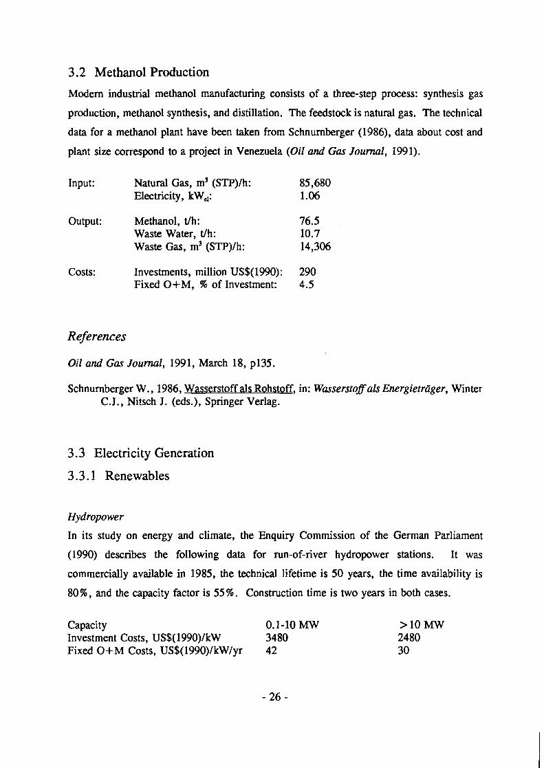
3.2 Methanol Production

Modern industrial methanol manufacturing consists of a three-step process: synthesis gas

production, methanol synthesis, and distillation. The feedstock is natural gas. The technical

data for a methanol plant have been taken from Schnurnberger (1986), data about cost and

plant size correspond to a project in Venezuela (Oil and Gas Jounuzl, 1991).

Input: Natural Gas, m3 (STP)/h: 85,680 Electricity, kW,: 1.06

Output: Methanol, t/h: 76.5 Waste Water, t/h: 10.7 Waste Gas, m3 (STP)/h: 14,306

Costs: Investments, million US$(1990): 290 Fixed O+M, % of Investment: 4.5

References

Oil and Gas Jounuzl, 1991, March 18, p135.

Schnurnberger W., 1986, Wasserstoff als Rohstoff, in: Wasserstoflals Energietrtiger, Winter C. J., Nitsch J. (eds.), Springer Verlag.

3.3 Electricity Generation

3.3.1 Renewables

Hydropower

In its study on energy and climate, the Enquiry Commission of the German Parliament

(1990) describes the following data for run-of-river hydropower stations. It was

commercially available in 1985, the technical lifetime is 50 years, the time availability is

80%, and the capacity factor is 55 %. Construction time is two years in both cases.

Capacity 0.1-10 MW Investment Costs, US$(1990)/kW 3480 Fixed O+M Costs, US$(1990)/kW/yr 42

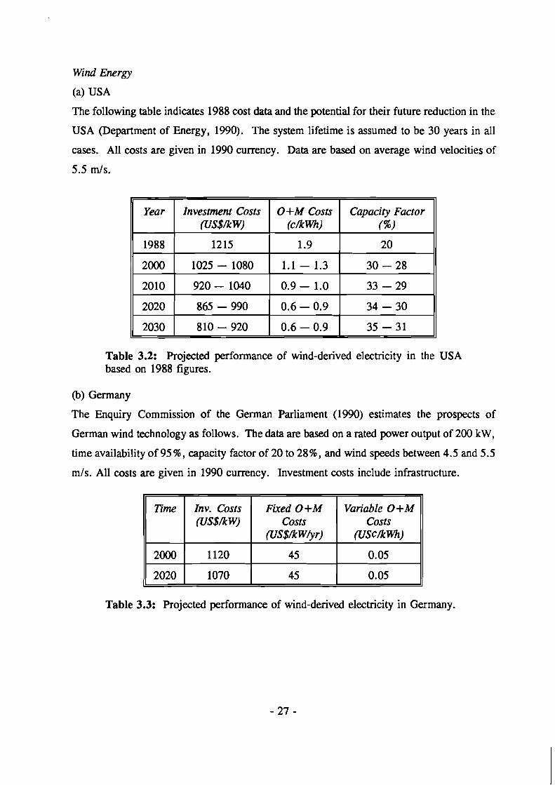
Wind Energy

(a) USA

The following table indicates 1988 cost data and the potential for their future reduction in the

USA (Department of Energy, 1990). The system lifetime is assumed to be 30 years in all

cases. All costs are given in 1990 currency. Data are based on average wind velocities of

5.5 mls.

Table 3.2: Projected performance of wind-derived electricity in the USA based on 1988 figures.

@) Germany

The Enquiry Commission of the German Parliament (1990) estimates the prospects of

German wind technology as follows. The data are based on a rated power output of 200 kW,

time availability of 95%, capacity factor of 20 to 28%, and wind speeds between 4.5 and 5.5

m/s. All costs are given in 1990 currency. Investment costs include infrastructure.

11 Time I Znv. Costs I Fixed O+M I Variable O+M 11

-- - - -

Table 3.3: Projected performance of wind-derived electricity in Germany.

2000

(US$fiW)

1120

Costs (US$fiW/yr)

45

Costs (USCfiWh)

0.05

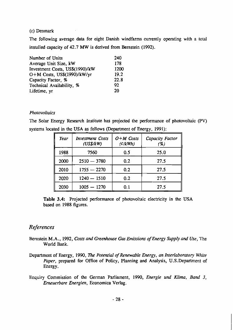
(c) Denmark

The following average data for eight Danish windfarms currently operating with a total

installed capacity of 42.7 MW is derived from Bernstein (1992).

Number of Units 240 Average Unit Size, kW 178 Investment Costs, US$(1990)/kW 1200 O+M Costs, US$(1990)/kW/yr 19.2 Capacity Factor, % 22.8 Technical Availability, % 92 Lifetime, yr 20

Photovoltaics

The Solar Energy Research Institute has projected the performance of photovoltaic (PV)

systems located in the USA as follows (Department of Energy, 1991):

Table 3.4: Projected performance of photovoltaic electricity in the USA based on 1988 figures.

References

Bernstein M.A., 1992, Costs and Greenhouse Gus Emissions of Energy Supply and Use, The World Bank.

Department of Energy, 1990, The Potential of Renewable Energy, an Interlaboratory White Paper, prepared for Office of Policy, Planning and Analysis, U.S.Department of Energy.

Enquiry Commission of the German Parliament, 1990, Energie und Klima, Band 3, Erneuerbare Energien, Economica Verlag.

3.3.2 Fossil Fuel Power Plants

Coal-fired Plant

Hendriks et al. (1989) provide data of a pulverizsdcoal power plant with a steam boiler.

The capacity is 600 MW, and the efficiency is 40%. The investment costs are US$(1990)

1088lkW and O+M costs are US$(1990) 40lkWlyr. W o n dioxide emissions are 0.85

kgIkWh.

Coal-fired Plant with Chemical Carbon Scrubbing

The carbon dioxide concentration in the exhaust gas can be reduced in a chemical absorption

process using a monoethanolamine (MEA) solution. In comparison with the coal plant just

described, net capacity drops to 440 MW, and the efficiency to 29.3%. Investment costs

increase to US$(1990) 1980lkW and O+M costs to US$(1990) 94lkWlyr. Carbon emissions

are 0.08 kgIkWh, a reduction of 90% (Hendriks et al., 1989).

Coal-fired Plants in Developing Countries

To show cost differences between countries, we present the following regional data for coal

power plants according to Bernstein (1992). Costs are given in US$(1990). Since no

thermal efficiencies are given in the original, no carbon emissions could be calculated.

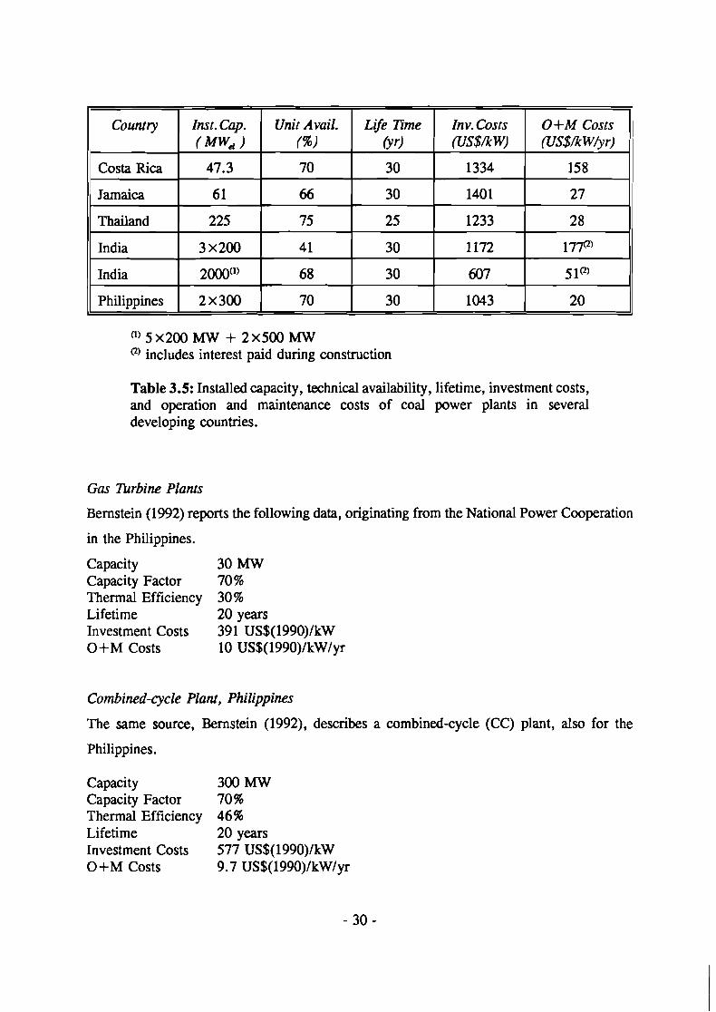
(l)5x200MW + 2x500MW includes interest paid during construction

Table 3.5: Installed capacity, technical availability, lifetime, investment costs, and operation and maintenance costs of coal power plants in several developing countries.

0 +M Costs (US$fiW.r)

158

27

2 8

177°

51Q

20

Country

Costa Rica

Jamaica

Thailand

India

India

Philippines

Gas lkrbine Plants

Bernstein (1992) reports the following data, originating from the National Power Cooperation

Inst. Cap.

47.3

61

225

3 ~ 2 0 0

2000")

2x300

in the Philippines.

Capacity 30 MW Capacity Factor 70 % Thermal Efficiency 30 % Lifetime 20 years Investment Costs 39 1 US$(1990)/kW O+M Costs 10 US$(1990)/kW/yr

Unit Avail. (%)

70

66

75

4 1

68

70

Combined-cycle Plant, Philippines

The same source, Bernstein (1992), describes a combined-cycle (CC) plant, also for the

Philippines.

Capacity 300 MW Capacity Factor 70 % Thermal Efficiency 46% Lifetime 20 years Investment Costs 577 US$(1990)/kW O+M Costs 9.7 US$(1990)/kW/yr

Life lTme (Y r)

30

30

25

30

30

30

Inv. Costs (vS$fiW)

1334

1401

1233

1172

607

1043

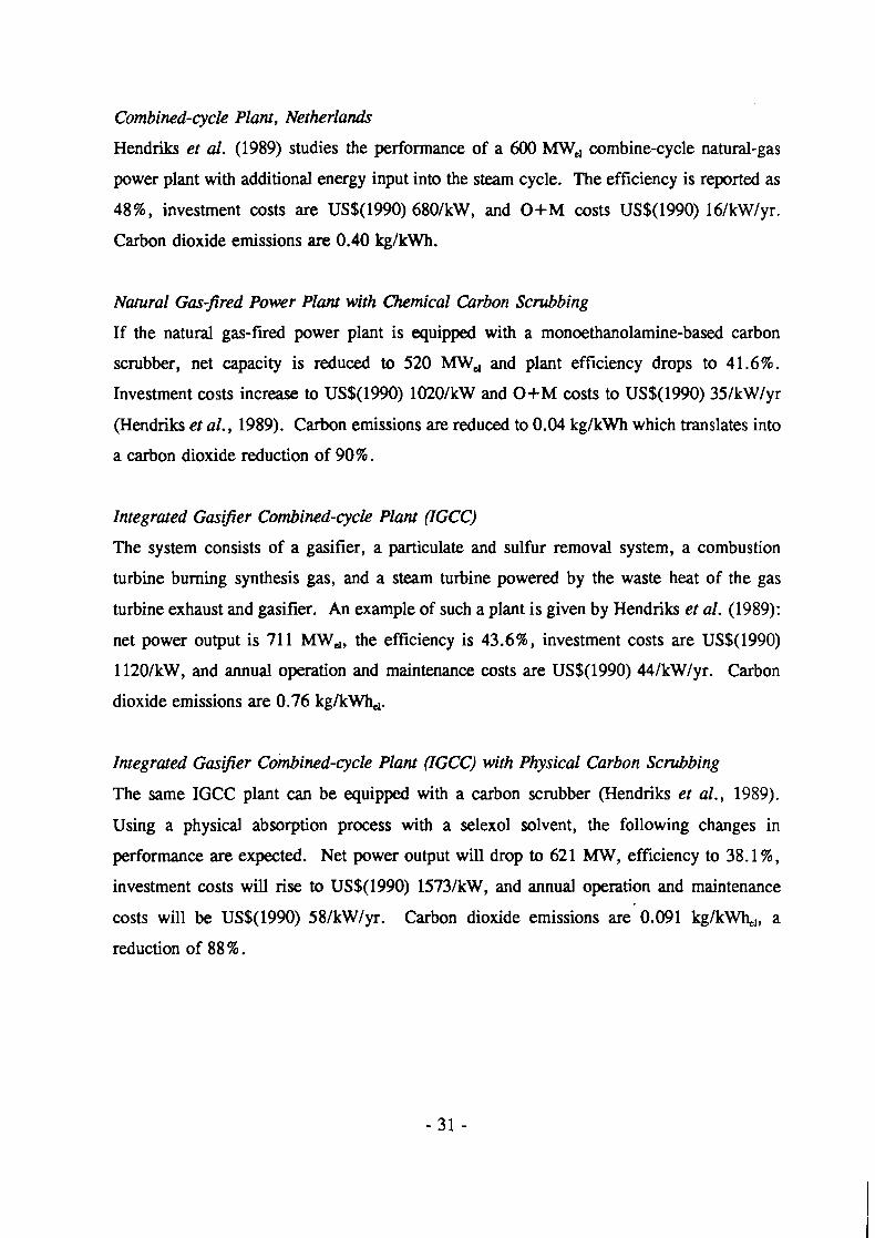
Combined-cycle Plant, Netherlands

Hendriks et al. (1989) studies the performance of a 600 MW, combine-cycle natural-gas

power plant with additional energy input into the steam cycle. The efficiency is reported as

48%, investment costs are US$(1990) 680/kW, and O+M costs US$(1990) 16IkWlyr.

Carbon dioxide emissions are 0.40 kg/kWh.

Natural Gas-jired Power Plant with Chemical Carbon Scrubbing

If the natural gas-fired power plant is equipped with a monoethanolamine-based carbon

scrubber, net capacity is reduced to 520 MW, and plant efficiency drops to 41.6%.

Investment costs increase to US$(1990) 1020lkW and O+M costs to US$(1990) 35lkWlyr

(Hendriks et al., 1989). Carbon emissions are reduced to 0.04 kgIkWh which translates into

a carbon dioxide reduction of 90%.

Integrated Gasijier Combined-cycle Plant (IGCC)

The system consists of a gasifier, a particulate and sulfur removal system, a combustion

turbine burning synthesis gas, and a steam turbine powered by the waste heat of the gas

turbine exhaust and gasifier. An example of such a plant is given by Hendriks et al. (1989):

net power output is 711 MW,, the efficiency is 43.6%, investment costs are US$(1990)

1120/kW, and annual operation and maintenance costs are US$(1990) 44lkWlyr. Carbon

dioxide emissions are 0.76 kgIkWh,.

Integrated Gasijier Combined-cycle Plant (IGCC) with Physical Carbon Scrubbing

The same IGCC plant can be equipped with a carbon scrubber (Hendriks et al., 1989).

Using a physical absorption process with a selexol solvent, the following changes in

performance are expected. Net power output will drop to 621 MW, efficiency to 38.1 %,

investment costs will rise to US$(1990) 1573/kW, and annual operation and maintenance

costs will be US$(1990) 58lkWlyr. Carbon dioxide emissions are 0.091 kglkw,, a

reduction of 88 %.

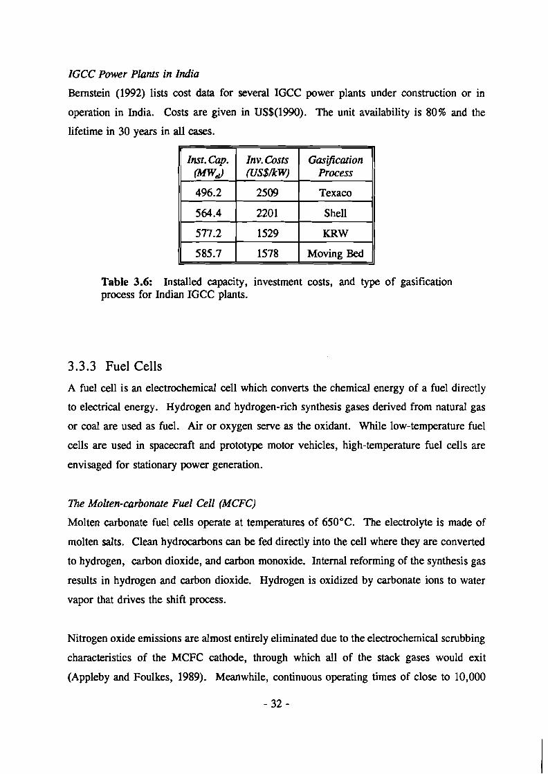
IGCC Power Plants in India

Bernstein (1992) lists cost data for several IGCC power plants under construction or in

operation in India. Costs are given in US$(1990). The unit availability is 80% and the

lifetime in 30 years in all cases.

Table 3.6: Installed capacity, investment costs, and type of gasification process for Indian IGCC plants.

3.3.3 Fuel Cells

A fuel cell is an electrochemical cell which converts the chemical energy of a fuel directly

to electrical energy. Hydrogen and hydrogen-rich synthesis gases derived from natural gas

or coal are used as fuel. Air or oxygen serve as the oxidant. While low-temperature fuel

cells are used in spacecraft and prototype motor vehicles, high-temperature fuel cells are

envisaged for stationary power generation.

The Molten-carbonate Fuel Cell (MCFC)

Molten carbonate fuel cells operate at temperatures of 650°C. The electrolyte is made of

molten salts. Clean hydrocarbons can be fed directly into the cell where they are converted

to hydrogen, carbon dioxide, and carbon monoxide. Internal reforming of the synthesis gas

results in hydrogen and carbon dioxide. Hydrogen is oxidized by carbonate ions to water

vapor that drives the shift process.

Nitrogen oxide emissions are almost entirely eliminated due to the electrochemical scrubbing

characteristics of the MCFC cathode, through which all of the stack gases would exit

(Appleby and Foulkes, 1989). Meanwhile, continuous operating times of close to 10,000

hours have been recorded. Current test programs are set to demonstrate 40,000 hours of

reliable electricity production.

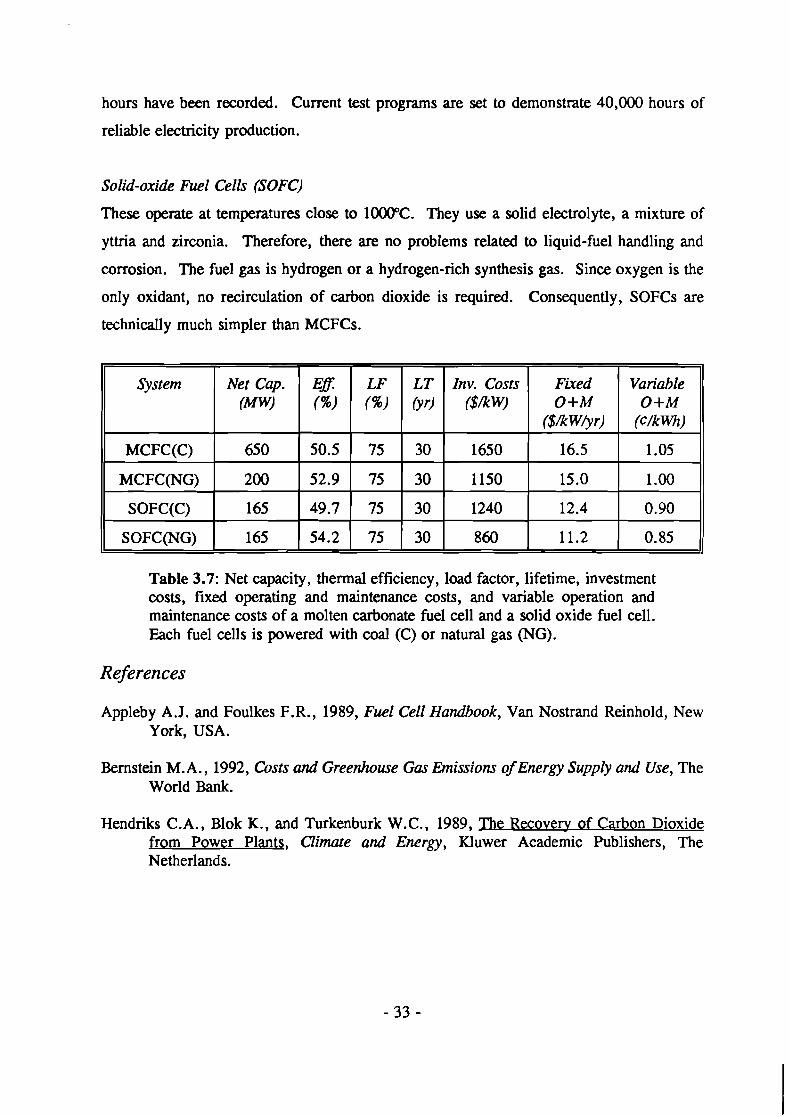
Solid-oxide Fuel Cells (SOFC)

These operate at temperatures close to 1000°C. They use a solid electrolyte, a mixture of

yttria and zirconia. Therefore, there are no problems related to liquid-fuel handling and

corrosion. The fuel gas is hydrogen or a hydrogen-rich synthesis gas. Since oxygen is the

only oxidant, no recirculation of carbon dioxide is required. Consequently, SOFCs are

technically much simpler than MCFCs.

Variable

(C/kwh)

Table 3.7: Net capacity, thermal efficiency, load factor, lifetime, investment costs, fixed operating and maintenance costs, and variable operation and maintenance costs of a molten carbonate fuel cell and a solid oxide fuel cell. Each fuel cells is powered with coal (C) or natural gas (NG).

System

MCFC(C)

MCFC(NG)

SOFC(C)

SOFC(NG)

References

Efl % )

50.5

52.9

49.7

54.2

Net Cap. m

650

200

165

165

Appleby A. J. and Foulkes F.R., 1989, Fuel Cell Handbook, Van Nostrand Reinhold, New York, USA.

Bernstein M. A., 1992, Costs and Greenhouse Gas Emissions of Energy Supply and Use, The World Bank.

Hendriks C.A., Blok K., and Turkenburk W.C., 1989, The Recovery of Carbon Dioxide from Power Plants, Climate and Energy, Kluwer Academic Publishers, The Netherlands.

Fixed O+M

($/kWryr)

16.5

15.0

12.4

11.2

LF % )

75

75

75

75

LT (Yr)

30

30

30

30

Inv. Costs ($/kW)

1650

1150

1240

860

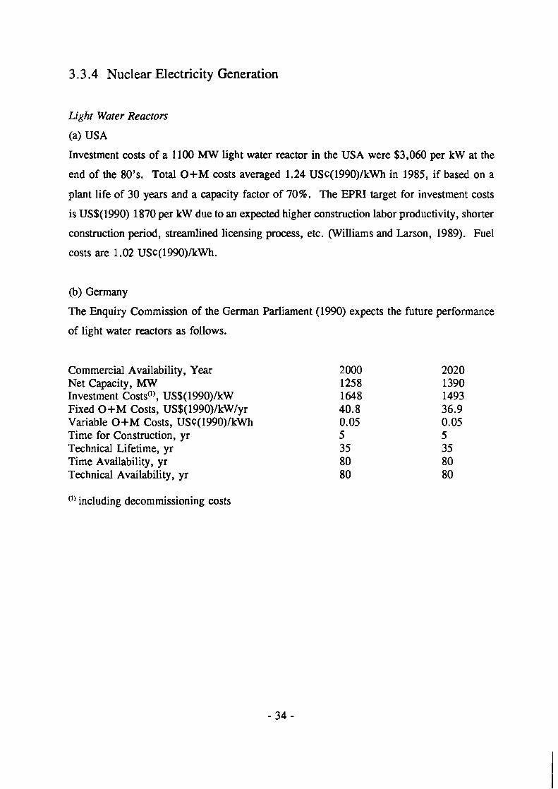
3.3.4 Nuclear Electricity Generation

Light Water Reactors

(a) USA

Investment costs of a 1100 MW light water reactor in the USA were $3,060 per kW at the

end of the 80's. Total O+M costs averaged 1.24 USC(1990)lkWh in 1985, if based on a

plant life of 30 years and a capacity factor of 70%. The EPRI target for investment costs

is US$(1990) 1870 per kW due to an expected higher construction labor productivity, shorter

construction period, streamlined licensing process, etc. (Williams and Larson, 1989). Fuel

costs are 1.02 USC(1990)/kWh.

(b) Germany

The Enquiry Commission of the German Parliament (1990) expects the future performance

of light water reactors as follows.

Commercial Availability, Year Net Capacity, MW Investment Costs('), US$(1990)/kW Fixed O+M Costs, US$(1990)/kW/yr Variable O+M Costs, USC(1990)/kWh Time for Construction, yr Technical Lifetime, yr Time Availability, yr Technical Availability, yr

( I ) including decommissioning costs

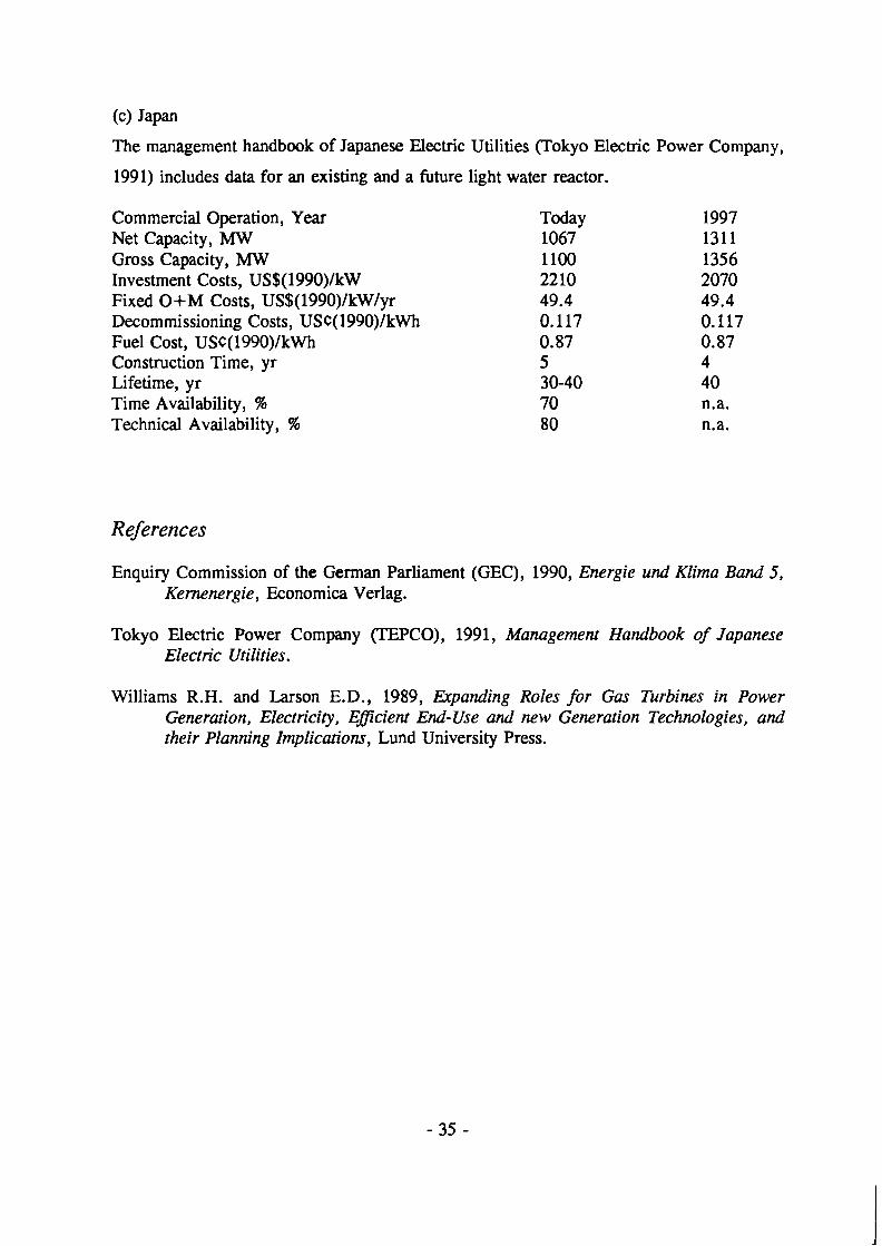
The management handbook of Japanese Electric Utilities (Tokyo Electric Power Company,

1991) includes data for an existing and a future light water reactor.

Commercial Operation, Year Net Capacity, MW Gross Capacity, MW Investment Costs, US$(1990)lkW Fixed 0 +M Costs, US$(1990)lkW/yr Decommissioning Costs, USC(1990)lkWh Fuel Cost, USC(1990)lkWh Construction Time, yr Lifetime, yr Time Availability, % Technical Availability, %

References

Enquiry Commission of the German Parliament (GEC), 1990, Energie und Klima Band 5, Kernenergie, Economics Verlag .

Tokyo Electric Power Company (TEPCO), 1991, Management Handbook of Japanese Electric Utilities.

Williams R.H. and Larson E.D., 1989, &panding Roles for Gas Turbines in Power Generation, Electricity, Eflcient End-Use and new Generation Technologies, and their Planning Implications, Lund University Press.

4. Chain Calculations

A powerful instrument for the systems analysis of mitigation measures is the ability of

CO2DB to combine individual technologies to form energy chains. Each technology has

well-defined inputs and outputs. If the input to one technology is matched by the output of

another, these two technologies can be linked. In this way, if a series of technologies

describing a complete system from primary energy extraction to end-use is combined into a

chain, total quantities (costs, emissions, energy consumption) can be calculated. In this

section, we show several chains related to lighting.

4.1. Lighting

To study alternative lighting methods, we compare conventional lighting, as represented by

incandescent bulbs, and the prevailing pattern of electricity generation, with new

technologies. To do this efficiently, we have included a dummy technology in C02DB

describing the actual power generation mix of the U.S. in the year 1990, i.e., 53 % coal, 4%

oil, 1 1.6 % natural gas, and 3 1.4 % zero-carbon fuels. The average conversion efficiency was

36.3%, and average carbon dioxide emissions were 0.54 kg CO, per kWh. We assume

electricity generation costs of 3.5 USCfkWh, reflecting the U.S. average (National Academy

of Sciences, 1991). Thus, our reference chain consists of this power generation mix, coupled

with an incandescent 60 Watt light bulb (ILB) providing an output of 870 lumen (as

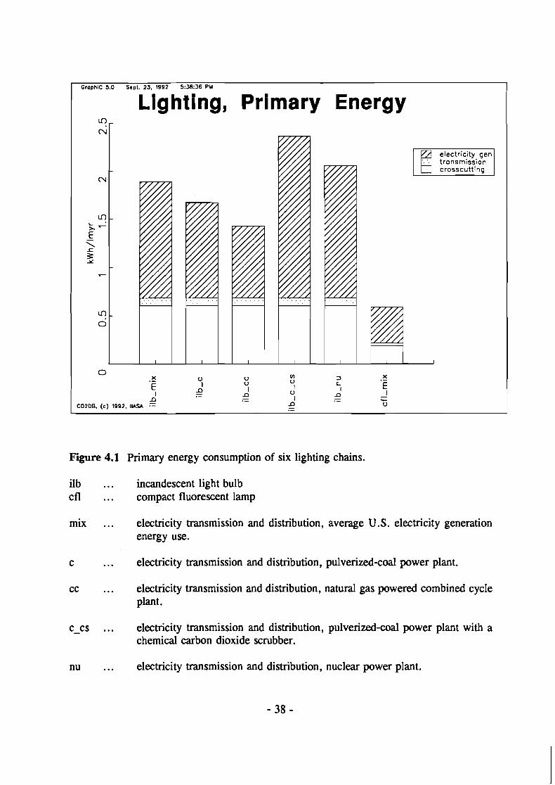
described in Section 2.2.1). This lighting system consumes 1.9 kWh primary energy per

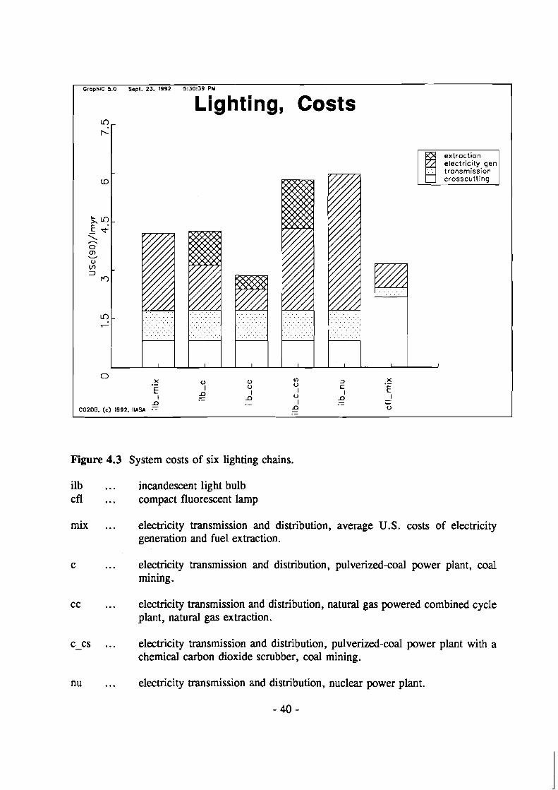
lumen year (lmyr) emitting 0.39 kg CO,. Total costs are 4.2 USC(1990) per lumen year.

To analyze the performance of alternative systems providing the same service, we vary the

front end of our original energy chain using the data for a coal power plant, a combined-

cycle (CC) power plant fired by natural gas, a coal power plant with a chemical carbon

scrubber, and a nuclear power plant. The variability on the end-use side is represented by

replacing ILBs by compact fluorescent light bulbs (CFLs). The results of C02DB's chain

calculations are shown in Figures 4.1--4.3.

The results show that the exclusive use of coal power plants would reduce primary energy

consumption by about 10%. At the same time, C Q emissions would increase by 50% and

costs would remain approximately constant.

In an energy system based primarily on natural gas, a dominant role might be played by CC

power plants. In comparison with our reference system, a gas-fired CC plant decreases CO,

emissions and primary energy intensity by 24% each. This strategy also results in a decrease

in costs of more than 30 % .

A bigger decrease of carbon dioxide emissions can be achieved by retrofitting coal power

plants with carbon scrubbers. In our example, C Q scrubbers reduce emissions by more than

65% compared with the reference case. However, primary energy intensity and costs

increase by 25 % and 40%, respectively.

A hypothetical, all-nuclear electricity generation system eliminates the carbon emissions of

our lighting system altogether, incurring costs that are a few percent higher in comparison

with the reference system.

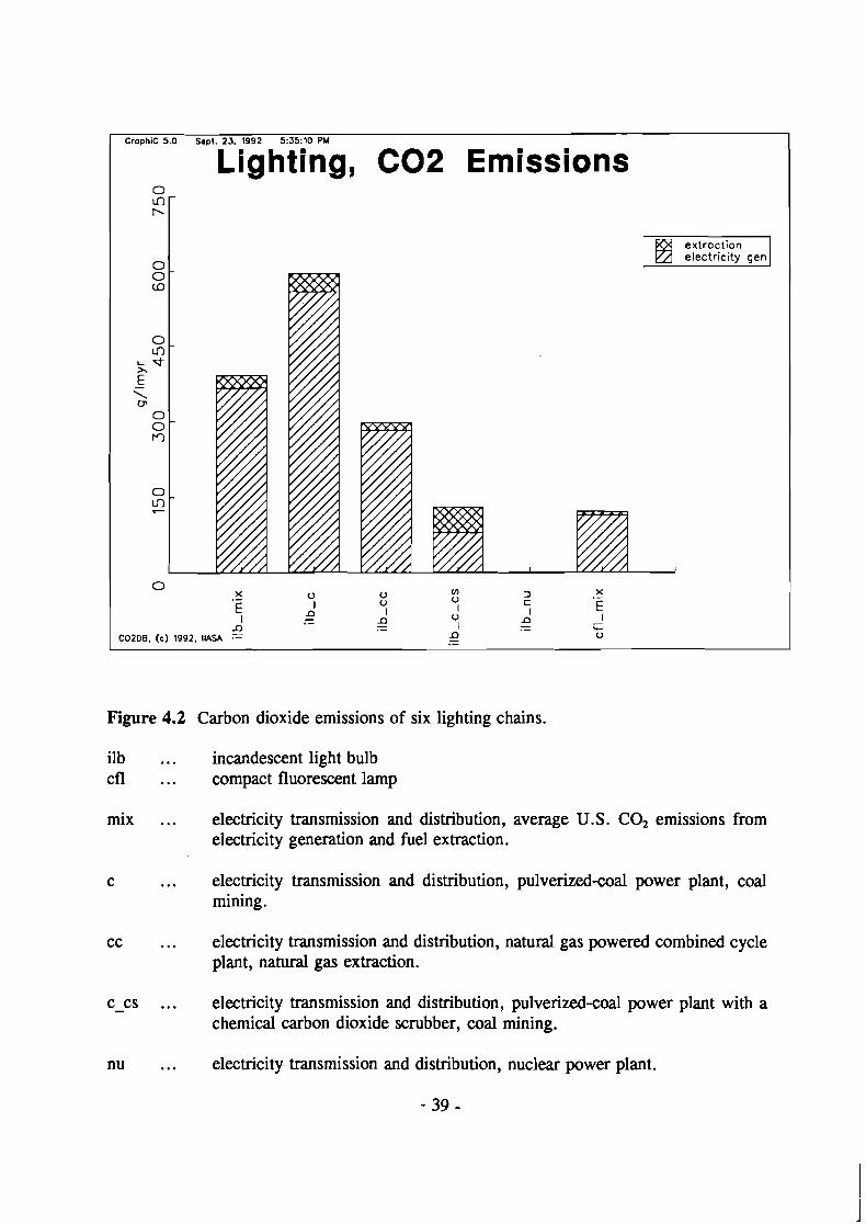
The impact of using compact fluorescent light bulbs instead of conventional incandescent

bulbs on carbon emissions is comparable with introducing carbon scrubbers into the reference

system, i.e., it reduces emissions by more than 60% to 0.12 kgCO,/lmyr. This strategy also

results in by far the lowest primary energy consumption. Despite the almost four-fold lamp

costs compared with the incandescent bulb, total costs decrease by 25%.

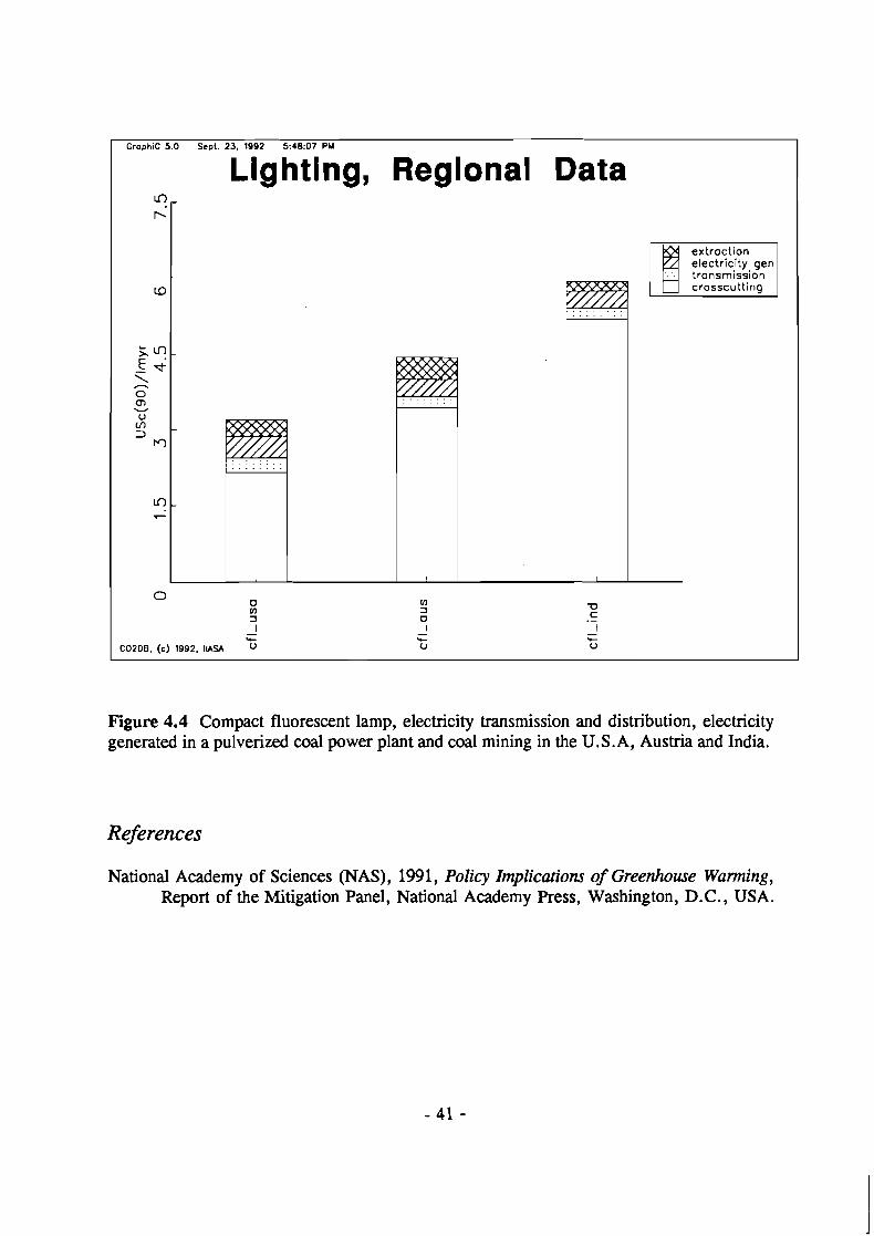
To illustrate how costs of technologies can vary substantially between different regions, we

show three identical lighting systems (each consisting of a compact fluorescent lamp,

electricity transmission and distribution, electricity generated in a pulverized-coal power

plant, and coal-mining) for the U.S.A, Austria, and India in Figure 4.4. While the costs of

electricity generation and transmission are kept constant, the costs of light bulbs and coal-

mining differ. Compared with the U.S.A., total costs are more than 35% and 70% higher

in Austria and India, respectively.

Graphic 5.0 Sepl. 23. 1992 5:J8:36 PM

Lighting, Primary Energy LO w

w

LO L .

2- 5 z 7

LO 0

0 X . - 0 0

V) 3 X 0 9 -

E I I E 0 I C

E' I U l .- E' E' I I - 0 . - .- b

COZDB. (c) 1992. IIAW .- 0 U .-

Figure 4.1 Primary energy consumption of six lighting chains.

ilb . . . incandescent light bulb cfl . . . compact fluorescent lamp

mix . . . electricity transmission and distribution, average U.S. electricity generation energy use.

c . . . electricity transmission and distribution, pulverized-coal power plant.

cc . . . electricity transmission and distribution, natural gas powered combined cycle plant.

c-cs . . . electricity transmission and distribution, pulverized-coal power plant with a chemical carbon dioxide scrubber.

nu . . . electricity transmission and distribution, nuclear power plant.

I GraohiC 5.0 Seat. 23. 1992 5:35:10 PU I

Lighting, C02 Emissions

Figure 4.2 Carbon dioxide emissions of six lighting chains.

ilb . . . incandescent light bulb cfl . . . compact fluorescent lamp

mix ... electricity transmission and distribution, average U.S. CO, emissions from electricity generation and fuel extraction.

c . . . electricity transmission and distribution, pulverized-coal power plant, coal mining.

cc . . . electricity transmission and distribution, natural gas powered combined cycle plant, natural gas extraction.

c - cs ... electricity transmission and distribution, pulverized-coal power plant with a chemical carbon dioxide scrubber, coal mining.

nu . . . electricity transmission and distribution, nuclear power plant.

Graphic 5.0 Sept. 23. 1992 5:30:39 PY

Lighting, Costs LO r-

CO

5.m L 4 \ - 0 0, V U

V) 3

rc)

LO 7

0 X . - 0 0 Ln 3 X

0 .- E I I E 0 I C

E I 0 l . - e 52 I I - .- .- C

CO2DEl. (c) 1992. NASA L? 0 . -

Figure 4.3 System costs of six lighting chains.

ilb . . . incandescent light bulb cfl . . . compact fluorescent lamp

mix ... electricity transmission and distribution, average U.S. costs of electricity generation and fuel extraction.

c ... electricity transmission and distribution, pulverized-coal power plant, coal mining.

cc . . . electricity transmission and distribution, natural gas powered combined cycle plant, natural gas extraction.

c-cs . . . electricity transmission and distribution, pulverized-coal power plant with a chemical carbon dioxide scrubber, coal mining.

nu . . . electricity transmission and distribution, nuclear power plant.

Graphic 5.0 Sept. 23. 1992 5:48:07 PM

Lighting, Regional Data LO

6

L 4 \ - 0 al V U

V] 3

M

LO 7

0 0 fn fn 3 u 3 0 C . - I - I - I

b -

LC LC

C02DB. (c) 1992. l l A U U U

Figure 4.4 Compact fluorescent lamp, electricity transmission and distribution, electricity generated in a pulverized coal power plant and coal mining in the U.S.A, Austria and India.

References

National Academy of Sciences (NAS) , 199 1, Policy Implications of Greenhouse Warning, Report of the Mitigation Panel, National Academy Press, Washington, D.C., USA.

APPENDIX A - Overview of C02DB

C02DB is a data bank for energyconversion technologies in the context of the problem of

global warming. In addition to the normal features of information storage and retrieval,

C02DB provides a number of analysis tools. The present version of the data bank puts

special emphasis on carbon dioxide, although other greenhouse gases (and even other

emissions) can be handled with C02DB too. To an extent, such data have already been

included.

C02DB accepts information on the following types of technology characteristics and

parameters:

1. General description of the technology, 2. Technical data, 3. Economic data, 4. Emission data, 5. Labor and material requirements, 6. Regional information, and 7. Literature sources.

This information is grouped into tables, and all tables for a given technology are linked to

the General Description table. Thus, cost data for different reference years or for different

regions can be included in one general technology description. Likewise, more than one

literature source can be stored in parallel subtables.

All relevant variables in C02DB can be defined in several units. Energy units are, e.g.,

barrels of oil equivalent (boe), gigajoules (GJ), or kilowatt-hours (kwh). For the

presentation of calculation results, all monetary and energy quantities are converted to a

common unit which can be chosen by the user.

C02DB also provides tools for the analysis of the information it contains, i.e., it facilitates

the preparation of printed reports of selected technologies and the calculation of the

characteristic parameters of energy-conversion chains. Such energy-conversion chains may

be defined interactively by selecting the technologies that participate in an energy-conversion

process. Appendix B illustrates both features.

For energy conversion chains, C02DB calculates the overall specific energy use per unit of

final output, pollutant emissions, and costs. These outputs may be defined in energy terms

(final or useful energy) or as energy services such as seat-kilometers (for passenger transport)

or lumen-hours (for lighting).

Version 2.0 of C02DB provides an additional feature useful in the evaluation of energy

chains: equivalent chains can be displayed (printed) in one graph or one table for

comparison. The graphs evaluating the lighting chains (in Section 4) were produced with the

help of these features.

To date, C02DB contains descriptions of approximately 400 technologies. The basic strategy

for collecting this information has been to cover the broad spectrum of present estimates for

controversial technologies. This is especially true for renewable technologies such as

photovoltaics, where estimates of technical and economic performance for the coming

decades cover a wide range. Another dimension of diversification in C02DB concerns the

regional and temporal aspects. Technology descriptions in C02DB cover technological

evolution over the next 50 years, and they differentiate between world regions. This regional

diversification is partly achieved by generating several subtables for one technology. One

group of examples of such regionalized data describes resource extraction technologies.

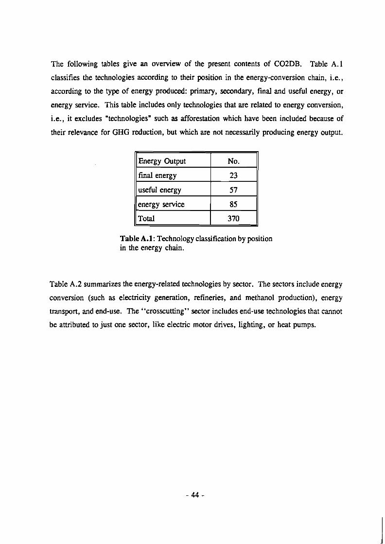
The following tables give an overview of the present contents of C02DB. Table A.l

classifies the technologies according to their position in the energy-conversion chain, i.e.,

according to the type of energy produced: primary, secondary, final and useful energy, or

energy service. This table includes only technologies that are related to energy conversion,

i.e., it excludes "technologies" such as afforestation which have been included because of

their relevance for GHG reduction, but which are not necessarily producing energy output.

11 final energy I 23 11

I Energy Output

useful energy

energy service

Table A.l: Technology classification by position in the energy chain.

57

85

Total

Table A.2 summarizes the energy-related technologies by sector. The sectors include energy

conversion (such as electricity generation, refineries, and methanol production), energy

transport, and end-use. The "crosscutting" sector includes end-use technologies that cannot

be attributed to just one sector, like electric motor drives, lighting, or heat pumps.

No.

370

I

Table A.2: Technology classification by sector of technology.

Finally, in Table A.3 the energy-conversion technologies are classified according to the fuel produced.

Table A.3: Technology classification by fuel produced.

APPENDIX B - Technology Descriptions

The technologies described in Section 4 of this document are presented as C02DB reports

in this appendix. For each table generally described in appendix A, we include one printed

table here - except when they are empty. The information presented in the printed reports

corresponds to the contents of the data bank and also to the screen that can be viewed with

C02DB. Messner and Strubegger (1991) describe all potential data items of C02DB.

Here, we describe the following technologies:

Conventional incandescent lamp, 60W (technology No 15 1) COMPAX fluorescent lamp, 15W (No 152) Conventional incandescent light bulb, 60W, Austria (No 141) COMPAX fluorescent lamp, 15W, Austria and India (No 140) U.S. power generation mix, 1990 (No 248) Pulverized-coal-fired power plant (No 260) Pulverized-coal-fired power plant with C02 recovery (No 261) Existing and future LWR, Japan (No 284) Natural-gas-fired combined cycle power plant (No 262)

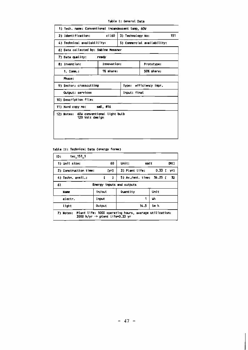
Table I: General Data

Table 11: Technical Data (energy forms)

3000 h/yr -> plant Life=0.33 yr

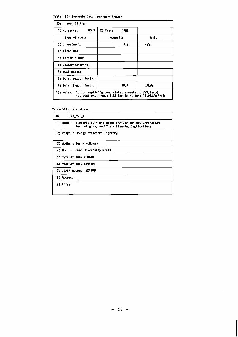
Table 111: Economic Data (per m i n irput)

Table VI I: Literature

ID: lit-151-1

1) Book: E lec t r ic i ty - Ef f ic ien t End-Use end New Generatian Technologies, end Their Planning lnp l ica t ims

2) Chapt.: Energy-eff ic ient l ighting

3) Author: Terry McGowan

4) Publ.: Lund University Press

5 ) Type of prbl.: book

6) Year of prblication:

7) IlASA access: B219W

8) Access:

9) Notes:

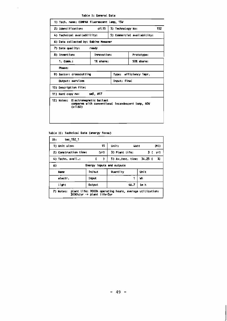
Table I: G a c r a l Data

Table 11: Technical Data (energy forms)

Table 111: Econamic Data (per nmin irput)

Table VI I: Literature

ID: Lit-152-1

1) Book: Electricity - Eff ic ient End-Use end New Generation Technologies, end Their Planning Irrplicatims

2) Chapt. : Energy-eff ic ient 1 ighting

3) Author: Terry CkGowan

4) PubL.: L d University Press

5) Type of pbl . : book

6) Year of ph l ica t ion:

7) IIASA access: 821909

8) Access:

9) Notes:

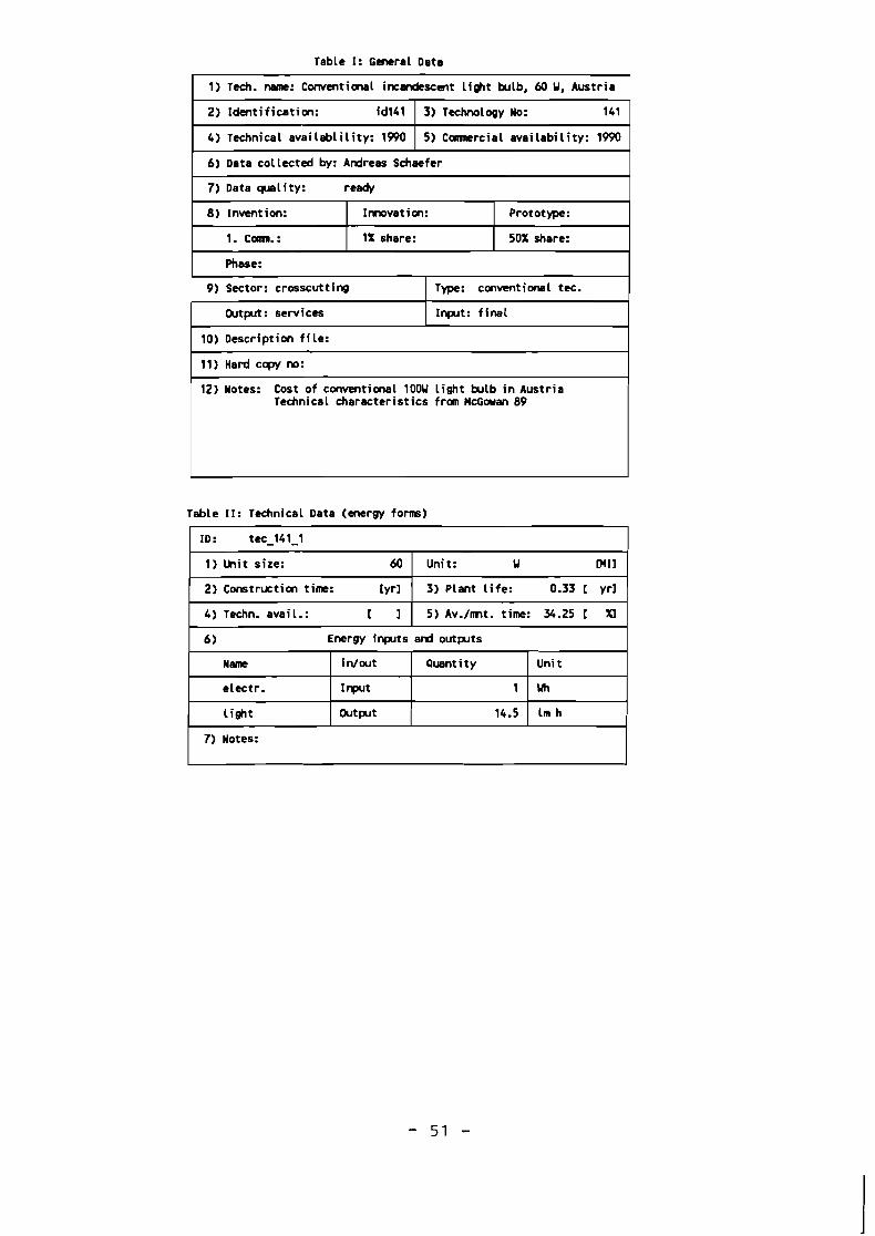
Table I: General Data

Table 11: Technical Data (energy forns)

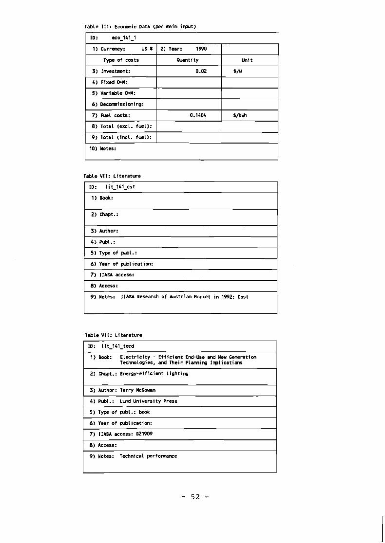
Table 111: Economic Data (per m i n irput)

Table VII: L i terature

ID: lit-141-cst

1) Book:

2) Chapt.:

3) Author:

4) Publ.:

5) Type o f prbl.:

6) year o f prb l icat ion:

7) IIASA access:

8) Access:

9) Notes: IlASA Research o f Austrian Market i n 1992: Cost

Table VI I : Li terature

ID: Lit-141-tecd

1) Book: E l e c t r i c i t y - E f f i c i e n t End-Use and New Generation Technologies, and Their P laming Inp l icat ians

2) Chapt.: Energy-eff ic ient l i g h t i n g

3) Author: Terry CkGouan

4) Publ.: L v d Univers i ty Press

5) Type o f -1.: book

6) Year o f prb l icat ion:

7) IIASA access: BZl9W

8) Access:

9) Notes: Technical performance

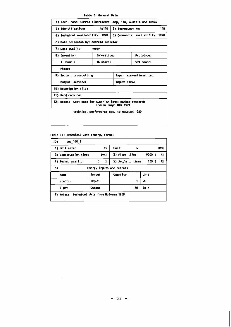
Table I: General Data

Indian lanp: NAS l W l

technical per fomnce acc. t o McGowan 1989

l ab le 11: Technical Data (energy form)

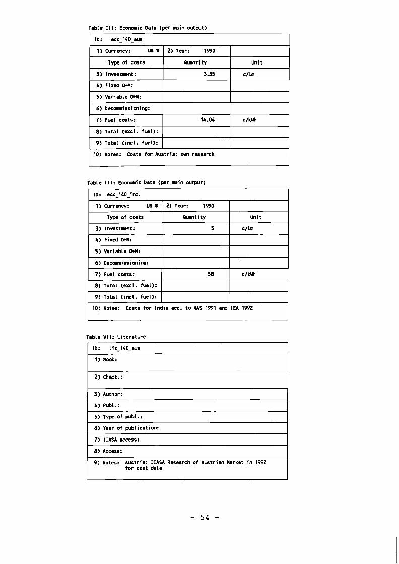
Table Ill: Economic Data (per main wtprt)

Table 111: Economic Data (per m i n outprt)

Table VI I : L i terature

ID: 1 i t-140-am

1) Book:

2) Chapt.:

3) Author:

4) Publ.:

5 ) Type of prbl.:

6) Year of prblication:

7) IIASA access:

8 ) Access:

9) Notes: Austria: IIASA Research of Austrian Market i n 1992 for cost data

Table VI I: Literature

ID: lit-14-ind.

1) Bock: Policy lnpl ications of Greahwse blaming; R e p r t of the Mit igation Panel

2) Chapt.:

3) Author:

4) Publ.: Natimal Acadeq ' P r W , Uashington, D.C.

5) Type of prbl.: Report

6) Year of prblication: 1991

7) 1 IASA access:

8) Access:

9) Notes: India: Cost deta

Table VI I: Literature

ID: I f t-140-tecd

1) Book: E lec t r ic i ty - Eff ic ient End-Use and New Generation Technologies, and Their Planning lnpl icaticns

2) Chept.: Energy-eff ic ient l ight ing

3) Author: Terry ClcCouan

4) Pub1 .: Lvd University Press

5) Type of prbl.: book

6) Year of prbl ication:

7) 1 IASA access: B219W

8) Access:

9) Notes: Technical performance data

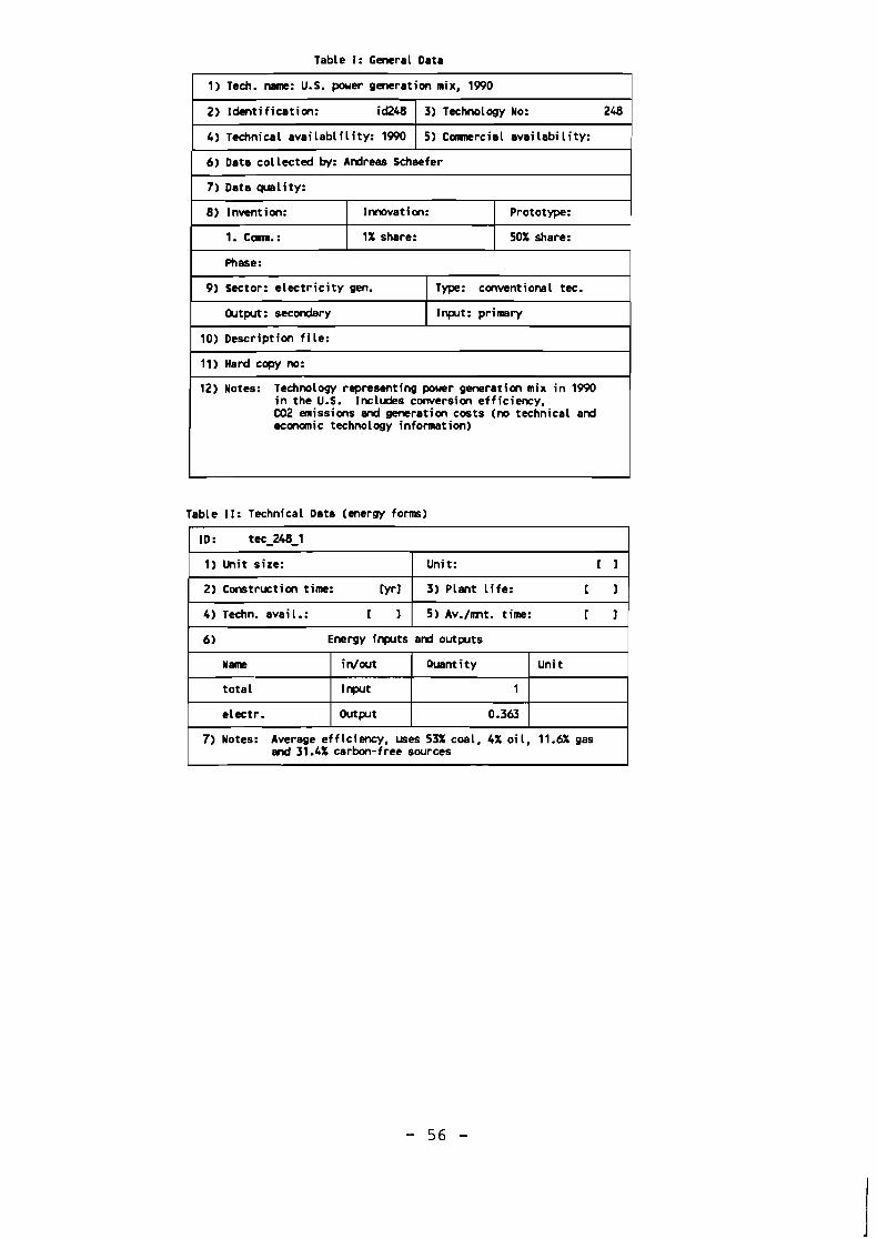
Table I: General Data

e c m i c technology information)

Table 11: Technical Data (energy forms)

and 31.4% carbon-free sources

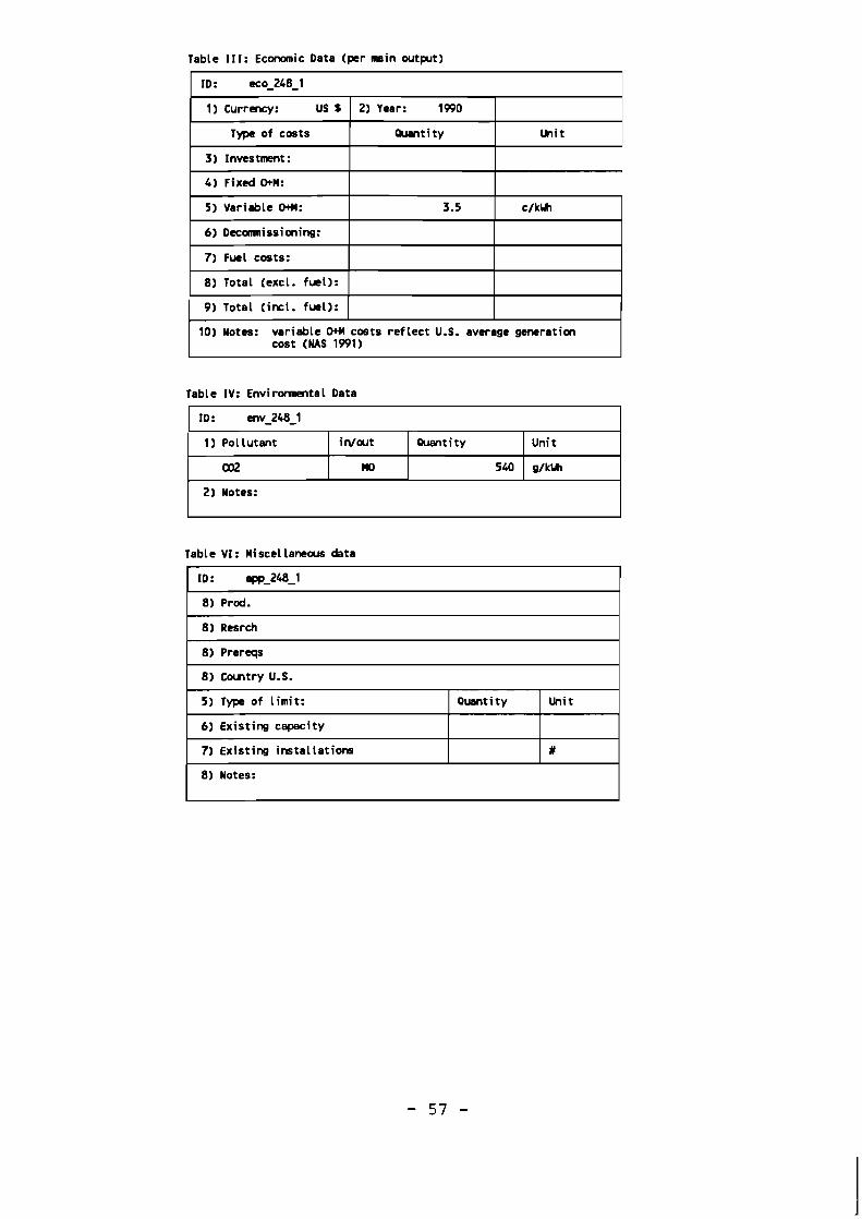
Table 11 I: Economic Data (per m i n wtprt)

Table IV: Envirormntal Data

Table VI: Hiscellanears data

ID: env-248-1

1) Pollutant

C02

ID: qp-248-1

8 ) Resrch

8) Prereqs

8 ) Colntry U.S.

2) Notes:

in/cut

CIO

5 ) Type of Limit:

6) Existing capacity

7) Existing installations

Quantity

540

8) Notes:

Quantity

Unit

g/k*

Unit

#

Table VI I : Literature

1) E d : Pol ic iy Implications of Crewhouse Uarming Report of the M i t i g a t i m Panel

2) Chept.:

4) Publ.: Nationel Acedcny Press, Ueshingtm, D.C.

5) Type of mi.: rcport

6) Year of plblication: 1991

7) llASA access:

8) Access:

9) Notes:

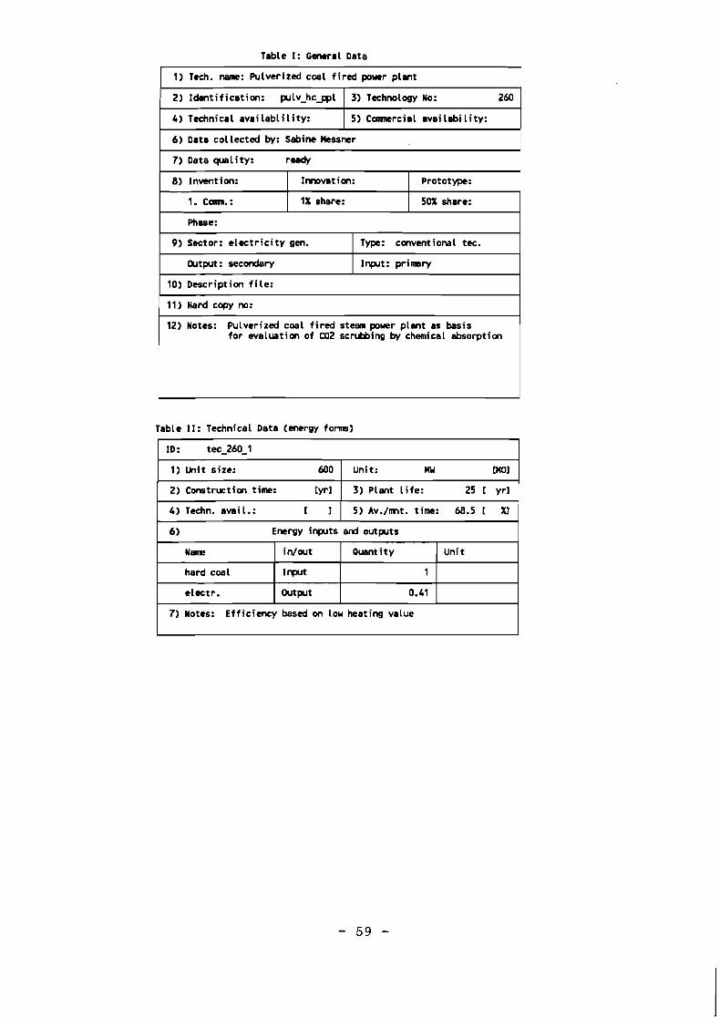
Table I: General Data

Table 11: Technical Data (energy forms)

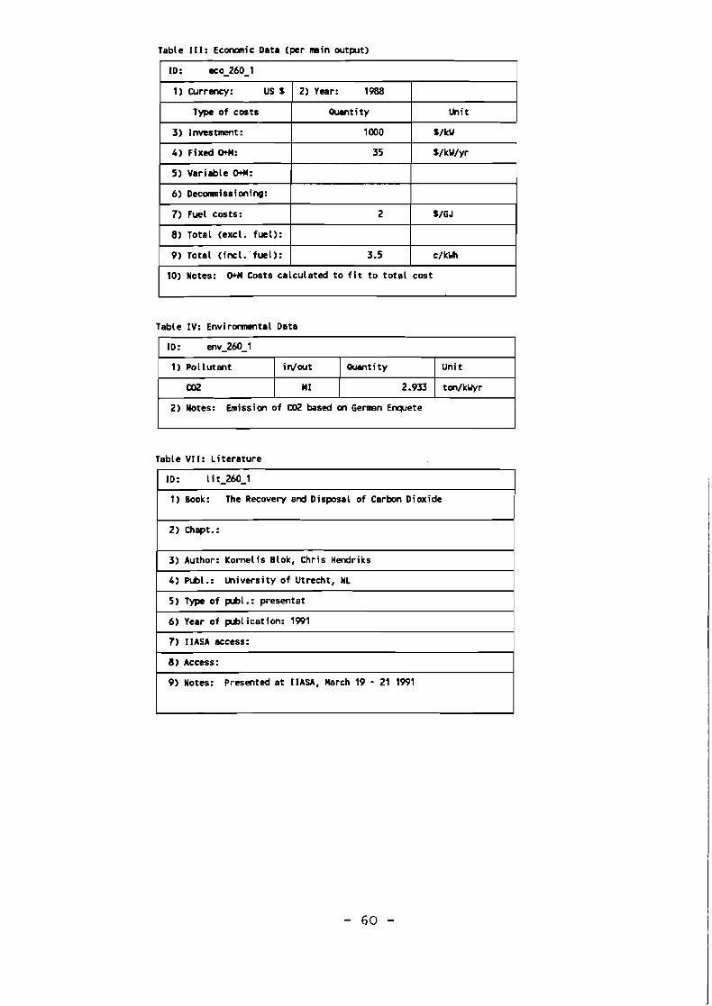
Table 11 1: Econanic Data (per rmin output)

Table IV: Environnental Data

Table V I I: Literature

ID: env-260-1

ID : l i t-260-1

1) Book: The Recovery and Disposal of Carbon Dioxide

2) Chapt.:

3) Author: Kornelis Blok, Chris Hendriks

4) Publ.: l lniversity of Utrecht, NL

5 ) Type of prbl.: presentat

6) Year of prblication: l W l

7) I I A S A access:

8) Access:

9) Notes: Presented at IIASA, March 19 - 21 1991

1) Pollutant

0 2

2) Notes: Emission of CXJ2 based on German Enquete

in/wt

M 1

Ouentity

2.933

Unit

ton/kUyr

Table I: General Data

Table 11: Technical Data (energy form)

Table 111: Economic Data (pr m i n wtprt)

Table IV: E n v i r o m t a l Data

Table VII: Literature

ID: av-261-1

ID: l i t-261-1

1) Book: The Recovery and Disposal of Carbon Dioxide

2) Chapt.:

3) Author: Kornelis Blok, Chris Hendriks

4) -1.: University of Utrecht, NL

5) Type of prbl.: presentat

6) Year of prblication: 1991

7) I I A S A access:

8) Access:

9) Notes: Presented a t I I A S A , March 19 - 21 l W l

1) Pollutant

C02

2) Notes: C02 redxed by 90%

i d a r t

111

Quenti t y

0.2933

Unit

ton/kUyr

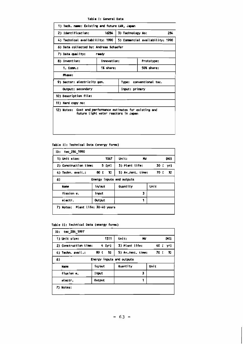
Table I: General Data

Table 11: Technical Data (energy f o r m )

Table 11: Technical Data (energy f o m )

Table 111: Econmic Data (per main MpJt)

Table Ill: Economic Data (per m i n MpJt)

Table V l l : Literature

ID: Lit-284-1

1) Book: Menagerent herrdJook of Japanese Electric U t i l i t e s

2) Chapt.:

3) Author:

4) -1.: Japan Atanic Industrial Form

5) Type of plbl.:

6) Year of plblication: 1991

7) IlASA access:

8) Access: Yesushi Taguchi

9) Notes:

Table I: Genrrl Data

Table I I : Technical Data (energy f o m )

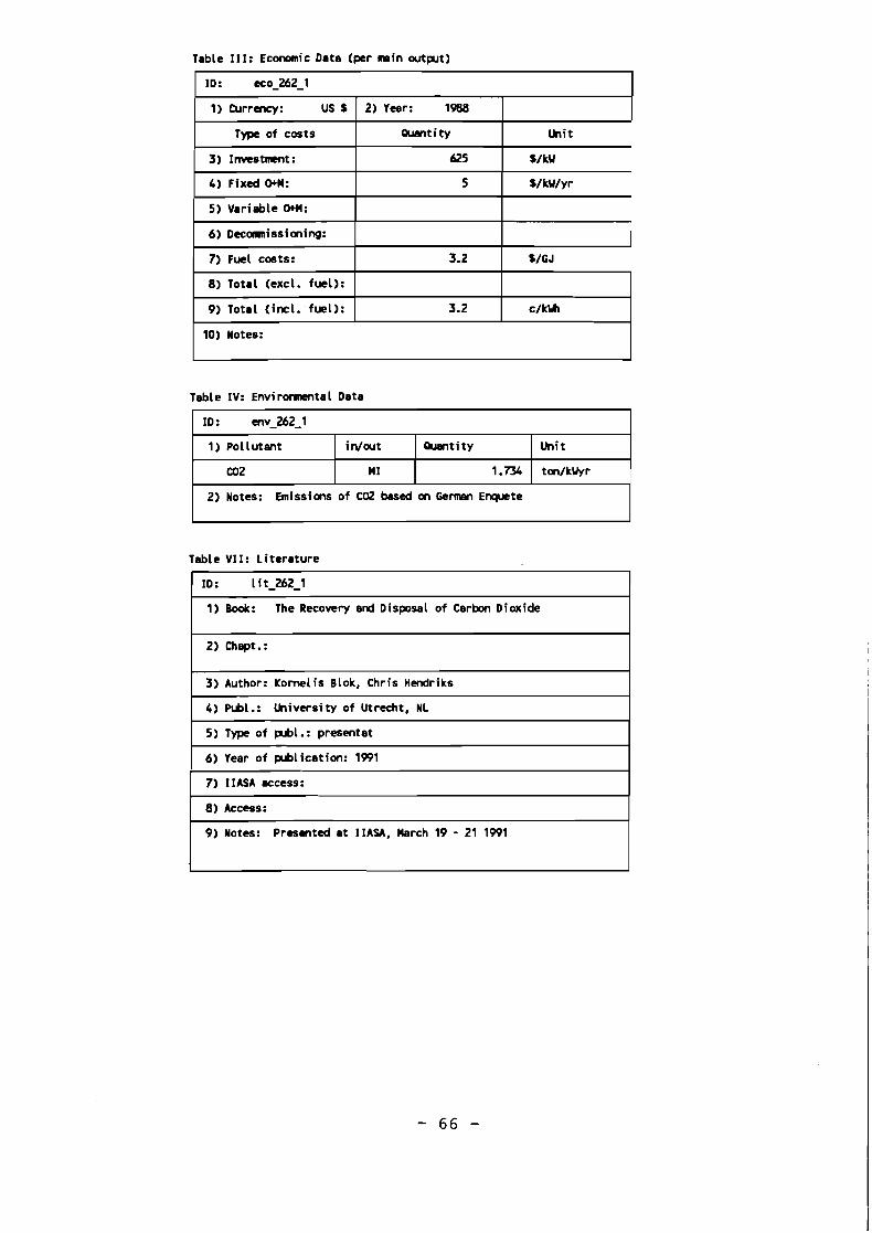
Table 111: Econcnnic Data (per nmin outprt)

Table IV: Envirmnmtal Data

Table VII: Literature

ID: env-262-1

ID: 1 it-262-1

1) Book: The Recovey and Disposal of Carbon Dioxide

2) Chapt.:

3) Author: Kornelis Blok, Chris Hendriks

4) Publ.: h i v e r s i t y of Utrecht, NL

5) Type of prbl.: presentat

6) Year of prblication: l W l

7) I I A S A access:

8) Access:

9) Notes: Presented at IIASA, March 19 - 21 1991

Unit

ton/kUyr

1) Pollutant

002

2) Notes: Emissiars of COZ based on G e m Enquete

in/art

M I

Puantity

1.734