Inventories, Fluctuations and Business Cycles

Louis J. MacciniJohns Hopkins University

Adrian PaganQueensland University of Technology

The research was supported by ARC Grant DP0342949

August 14, 2008

Contents

1 Introduction . . . . . . . . . . . . . . . . . . . . . . . . . . . . . . . . . 22 Some Cycle Characteristics . . . . . . . . . . . . . . . . . . . . . . . . . 73 The Model and its Euler Equations . . . . . . . . . . . . . . . . . . . . 143.1 The Production Function . . . . . . . . . . . . . . . . . . . . . . . 143.2 The Cost Structure . . . . . . . . . . . . . . . . . . . . . . . . . . 15

3.2.1 Labor Costs . . . . . . . . . . . . . . . . . . . . . . . . . . 153.2.2 Inventory Holding Costs . . . . . . . . . . . . . . . . . . . 163.2.3 Materials Costs . . . . . . . . . . . . . . . . . . . . . . . . 18

3.3 Cost Minimization . . . . . . . . . . . . . . . . . . . . . . . . . . 193.4 Optimality Conditions . . . . . . . . . . . . . . . . . . . . . . . . 19

4 Quantifying Model Parameters . . . . . . . . . . . . . . . . . . . . . . . 234.1 Matching Data and Model Variables . . . . . . . . . . . . . . . . 234.2 Estimation Strategy . . . . . . . . . . . . . . . . . . . . . . . . . 23

5 Experiments with the Model . . . . . . . . . . . . . . . . . . . . . . . . 295.1 Analysis of Fluctuations and the Great Moderation . . . . . . . . 295.2 Analysis of Cycles . . . . . . . . . . . . . . . . . . . . . . . . . . . 31

6 Conclusion . . . . . . . . . . . . . . . . . . . . . . . . . . . . . . . . . . 327 References . . . . . . . . . . . . . . . . . . . . . . . . . . . . . . . . . . 33

8 Appendix A: Data Description . . . . . . . . . . . . . . . . . . . . . . . 368.1 Appendix B: Derivation of Optimality Conditions . . . . . . . . . 37

Abstract

The paper looks at the role of inventories in U.S. business cycles andfluctuations. It concentrates upon the goods producing sector and con-structs a model that features both input and output inventories. A rangeof shocks are present in the model, including sales, technology and inventorycost shocks. It is found that the presence of inventories does not change theaverage business cycle characteristics in the U.S. very much. The model isalso used to examine whether new techniques for inventory control mighthave been an important contributing factor to the decline in the volatilityof US GDP growth. It is found that these would have had little impactupon the level of volatility.

1. Introduction

It is not uncommon for commentators on the prospects for an economy to drawattention to recent inventory movements. Thus, if there has been a run downin stocks below what is perceived to be normal levels, this is taken as a sign offavorable output prospects in future periods; the reasoning behind this conclusionbeing that output not only needs to be produced to meet sales, but also to re-plenish stocks. Early in the history of business cycle research the question aroseof whether the presence of inventory holdings by firms was a contributor to the“up and down” movements seen in economies. The classic analyses of this ques-tion were by Metzler (1941), (1947), who concluded that “An economy in whichbusinessmen attempt to recoup inventory losses will always undergo cyclical fluc-tuations..”. His model emphasized the fact that a business would attempt to keepinventories as a proportion of expected sales and so would re-build these if theydeclined below that target level. Given that sales had to be forecast from their pasthistory, he showed that output would follow a second order difference equationwhich would have complex roots in many cases. Consequently his model producedoscillations in output and this constituted the foundation of his conclusion.Turning points in output can occur even if there are no oscillations. A peak

in output will be attained if positive growth turns into negative for some periodof time, and the chance of this depends on the magnitude of long-run growth, theextent to which current growth depends on past growth rates, and the size of the

2

shocks that are impinging on the macro-economic system - see Harding and Pagan(2002). Because the extent of oscillations was determined by examining the rootsof a difference equation for output ( or output growth) their measured nature wasindependent of any shocks. Consequently, there can be quite major differencesbetween the cycle characteristics established by studying turning points in a seriesthat incorporates the shocks and those that come from analysing oscillations inthe same series, which essentially ignore them.Business cycles are distinct from fluctuations. The latter focusses not upon

contractions and expansions but rather upon measures such as the standard devi-ations, covariances and serial correlation of series representing economic activity.There is a relationship between business cycles and fluctuations, since many busi-ness cycle characteristics such as the duration of expansions can be shown todepend upon the quantities studied in fluctuations work - see Harding and Pa-gan (2002). Viewed in this light business cycle analysis performed by examiningturning points in a series on output simply combine together measures such asthe means, variances and serial correlations of growth rates in order to yield in-formation about the characteristics of expansions and contractions. Given thatmost knowledge of business cycles is expressed in terms of the latter e.g. NBER,IMF(2002) it seems useful to proceed in this way rather than just to use themoments up to second order of the series.The question that then arises is what impact the presence of inventories has

upon the nature of business cycles? An answer to this question is of interestfor a number of reasons. First, such an analysis would generalize what Metzlerdid when he focussed upon whether oscillations emerged from simple models ofaggregate output. Second, there have always been comments that a large fractionof the change in output was accounted for by inventory movements — see, forexample, Blinder and Maccini (1991). This has often been interpreted in acausal way as suggesting that inventories are the cause of the cycle. So it isinteresting to see if that is a correct interpretation. Since the evidence is generallyexpressed in terms of the extent to which the movement in inventory investmentduring recessions is close to the actual fall in output, a turning point perspectiveis needed, given that it is necessary to define periods of recession. Finally, inrecent times, expansions seem to have lengthened around the world. One wouldexpect that this would happen if the volatility of output growth declines, and soit has been suggested that advances in inventory technology have been a majorcontributor to the Great Moderation that has been seen in many countries afterthe 1980’s. However, much of this work has not been with models that explain

3

the growth rate in output and the mapping between model variables and data hasoften been less than transparent.In this paper, we address the question of the impact of inventories on business

cycles in two ways. One is to establish some facts about the nature of the businesscycles and then ask how the cycles would change if inventories were not presentin the system. A second involves undertaking an analysis of whether advances ininventory management techniques are responsible for the decline in the volatilityof GDP growth since the early eighties in the US. Because both approaches involvequestions that can only be answered with a model of output and inventory choicesit is necessary to construct one that is a reasonable characterization of the dataand which has enough structure to answer the questions posed above.The model chosen is an extension of that in Humphreys et al (2001). It

sees the objectives of firms as attempting to balance the costs of keeping rawmaterial stocks in line with output, and finished goods stocks in line with sales,with the extra costs incurred by rapid adjustment in output and purchases ofraw materials. Because of the presence of raw materials it has some additionaldriving forces, such as the level of raw material prices, as well as the traditionalone of the sales of finished goods. The model also allows for a number of othershocks such as technology and various cost shocks associated with inventories.Optimal decision rules for value added (GDP), raw material stocks and finishedgood stocks are established, thereby distinguishing between input and outputinventories, as the behavior of each has been quite different in recent times. Wespend considerable time in ensuring that the model is compatible with the unitroot and co-integration properties of the data, so as to avoid filtering operationssuch as Hodrick-Prescott (HP) that would be inconsistent with the nature of thedata implied by the model. If one considers business cycles as defined throughturning points it is not necessary to make any I(1) series stationary, which seemsto be a major motivation for the HP filtering of the data. If one does filter thedata one can still study turning points in the resulting series, but now one isstudying the growth cycle rather than the business cycle.In order to utilize the model to investigate the questions mentioned above we

need to assign parameter values. Often this is done via "calibration" e.g. as inKhan and Thomas (2007). But, as there is a scanty literature setting out valuesfor the parameters of our model, it was decided to estimate them from data. Aproblem in doing this relates to the Great Moderation that has occurred in manyeconomic variables in the US after 1983. Inevitably, this must mean that someof the values of the model parameters have changed. In order to handle such a

4

difficulty one needs to either work with realizations from a time period in whichthe parameters were likely to have been constant or to make some assumptionsabout how the parameters changed. Since there is controversy about whether theGreat Moderation occurred abruptly or slowly1, it does not seem attractive toadopt the latter solution, as one is then working with not only a model of outputand inventories but also a model of how the parameters changed. It seems muchbetter to estimate from a sample period in which there is a reasonable chance thatthe parameters were constant. Given the features later seen in the data, this willinvolve using data prior to 1984.The only argument against using a sample of data from 1959-1983 (the period

we choose) is that the sample is relatively short. But, as will be seen, quite preciseestimates of the parameters are obtained with it. Moreover, calibrating the modelwith information before the Great Moderation provides a good vehicle for analyz-ing the role of inventories in that phenomenon. The fact that we actually estimateparameters for inventory models is novel, since generally parameter values havejust been assigned either by an appeal to previous literature or by utilizing somesimple mappings to the data, e.g. as in Khan and Thomas. Finally, the fact thatwe utilize only pre-1984 data does not seem critical to answer the questions wewant to address. After all, we can change these parameter values and observewhat responses occur. If one wanted to use the model for forecasting then thesituation might be very different.At this point, it is useful to compare the approach that we take to explore

whether the Great Moderation in the volatility of GDP growth is due to betterinventory management techniques with that in the literature. A substantial bodyof the literature has used VAR models to analyze the broad question of whetherthe decline in volatility of GDP growth is due to better inventory managementtechniques, to better monetary policy, or to "good luck". Stock andWatson (2002,2003) represent an example of this approach as well as a survey and critique ofthe literature.2 In contrast, our approach develops a structural model to analyzewhether changes in parameters that capture the effects on inventory managementtechniques can explain the decline in the volatility of GDP growth. An alternative

1See McConnell and Perez-Quiros (2000) for an example where the Great Moderation occursas an abrupt shift and Blanchard and Simon (2001) and more recently Davis and Kahn (2007)for examples of where it occurs as a slow adjustment.

2Other studies that have used VAR approaches to look at the role of inventory managementadvances and the decline in the volatility of output growth include Ahmed, Levin and Wilson(2004), Blanchard and Simon (2001), Herrera and Pesavento (2005), Irvine and Schuh (2005),and McCarthy and Zakrajsek (2007).

5

and much more recent approach, illustrated, for example, by the recent paper ofKhan and Thomas (2007), uses general equilibrium models that focus on theeconomy as a whole.3 Our model is a partial equilibrium one that focuses on thegoods sector of the economy.4 Both the general equilibrium approach and ourapproach use structural models to analyze the same question. A disadvantage ofgeneral equilibrium approaches is that, precisely because they are models of thewhole economy, assumptions must be made about the household sector, services,

3Our model and approach differs from Khan and Thomas (2007) in several respects, otherthan the fact that they use calibration nmethods and we use estimation methods to analyze thebasic issue. The model of the firm that they develop holds only intermediate goods inventoriesmotivated by fixed costs of acquisition and the production function for final goods depends onthe stock of intermediate goods inventories. Our model emphasizes the distinction betweenmaterials inventories and finished goods inventories, which play different roles in the firm, andwhich behave very differently after 1984, and the production function for final goods dependson the usage of materials in production.Iacoviello, Schiantarelli and Schuh (2007) also develop a general equilibrium model where both

input and output inventories are held in the goods sector. Their model, however, differs fromthe one developed here in the motivation for holding input and output inventories, the use ofdifferent definitions of input and output inventories, and the lack of a distinction between grossoutput and value added.Kahn, McConnell and Perez-Quiros (2002) develop a general equilibrium model that focuses

on finished goods inventories and thus does not address differences in the role played by finishedgoods and materials inventories. Also, they undertake a calibration and simulation analysis,rather than an analysis based on estimation of the model.Jung and Yun (2006) and Wen (2008) develop general equilibrium models with different types

of inventories. Jung and Yun use the model to analyze the role that strategic complementarityplays in price-setting behavior. Wen introduces inventories into a standard RBC model viaprecautionary stockout avoidance motives. In early work, Fisher and Hornstein (2000) developa general equilibrium model that focuses on (S,s) inventory policies in the reatil sector but doesnot consider materials inventories. However, the latter three papers do not address the questionof the role that inventories play in the Great Moderation.

4In work with partial equilibrium models, Ramey and Vine (2006) develop a model withfinished goods inventories alone and argue that a decline in the persistence of sales volatilitycontributed to a decline in GDP volatility in the automobile industry. However, their modelignores the role played by materials inventories, which we focus on.Chang, Hornstein and Sarte (2006) develop a model of an industry where firms hold finished

goods inventories to explore the response of employment to productivity shocks. However, themodel ignores materials inventories.In preliminary work, Kahn (2007) develops a model with unfilled orders and materials inven-

tories and undertakes a calibration and simulation analysis of the durable goods sector of theeconomy. However, the model ignores finished goods inventories and makes assumptions aboutthe representative firm, e.g., fixed coefficients in production, that are different from our model.

6

the conduct of monetary policy, etc. If these are incorrect the shocks entering intothem may not be uncorrelated so that one cannot attribute variation in a variableto them in a unique way. A partial equilibrium model avoids these biases thatstem from specification errors in the rest of the system at the cost of assumingsome variables can be treated as exogenous to the sector being studied. Of coursethis may also be in error and can induce biases.5 It seems sensible that one useboth approaches. If the answers found are similar then that is reassuring. If notthen one would want to look more closely at why this might be so. Our view isthat partial and general equilibrium model outcomes are complementary in thiscontext in that they take different routes to look at an important and subtle issue.Section 2 first reports some basic facts about the nature of the business cycle

and the behavior of inventories over it. Section 3 then describes the model of therepresentative firm used to address the issues of the paper. After quantifying theparameters in Section 4 we use the model in section 5 to simulate data and tostudy the questions raised earlier relating to the business cycle and how it hasbeen changing. A final section concludes the paper.The paper yields two main conclusions: First, the model suggests that there

is little contribution of inventories to the length and amplitude of the businesscycle. This is so despite the fact that the model produces predictions that arecompatible with many of the features seen in the data relating to the the behaviorof inventories over the business cycle. Second, advances in inventory managementtechniques seem to have contributed very little to the decline in the volatility ofGDP growth since the early eighties and hence cannot be a source of the GreatModeration.

2. Some Cycle Characteristics

It seems useful to re-examine the relation of inventories and the business cycle byutilizing the approach and techniques of the view of cycles described above i.e.

5An incorrect assumption about the exogeneity of variables can have two effects. One is torender estimators of parameters inconsistent. However, we show that the MLE yields consistentestimates of the parameters of the model even if exogensity is not correct for our model. Asecond effect is that, even if the variables are exogenous, one would need a complete generalequilibrium model if one wanted to isolate the contributions of a basic set of shocks. Thus wetake sales and technology to be exogenous and independent of one another. It is likely howeverthat sales will be influenced by technology and so part of the explanation of output attributedto sales may be in fact be due to technology. The two questions we address however do notrequire a precise decomposition so that this does not seem to be particularly important.

7

as one reflecting turning points. We begin by thinking of aggregate economicactivity as being usefully summarized by GDP - see Burns and Mitchell (1946,p72 ) for an early statement and NBER (2003) for a recent one. However, sinceinventories are principally used in the production of goods, determining their rolein the business cycle would seem to begin by splitting GDP into its goods and non-goods ( services and structures) components, and then looking at the cycle in thegoods component. Designating Qg and Qs = Q−Qg as the goods and non-goodscomponents of GDP respectively, a log linearization produces the approximation

∆qt = ωg∆qgt + (1− ωg)∆qst

where ωg is the average of the ratio Qgt

Qtand lower case letters indicate the log of a

variable i.e. qt = lnQt. Over 1947/1-2005/4 this average was .31 with a standarddeviation of .02. The first and last observations on it were .32 and .36 respectively.So it has been a fairly stable ratio. The approximate value of qt follows the actualdata quite closely so that one might build up the cycle in qt by looking at thosein the sub-aggregates qgt and qst .Table 1 sets out cycle characteristics using the modified BBQ algorithm set

out in Harding and Pagan (2002) to find turning points in the series6. It isevident that the cycles in the sub-sectors are quite different, with the cycle ingoods GDP being much shorter than that in the non-goods sector. Since mostattention has been paid to cycles in the level of economic activity, as measuredby variables such as GDP, it is interesting to examine the cycle in the sub-setof GDP that relates to goods. One of the striking features of the business cyclemeasured with GDP is that movements in this do not signal a recession in 2001, asthere was a sequence of alternating positive and negative quarterly growth rates,with the positive ones always offsetting the negative ones, meaning that there wasno decline in the level of GDP for two quarters. In contrast, there was a clearrecession in the goods sector, starting in 2000/3 and finishing in 2001/3. Indeedit is always the case that recessions in the goods sector have been stronger andlonger than those in aggregate GDP. It might be thought that this comes from adeclining contribution to aggregate GDP of goods, but, as the ratios Qg

t

Qtpresented

earlier show, the opposite has happened in the chain-weighted data. Of course innominal terms the ratio may well have declined since the relative price of goods to

6The modification involves a more efficient algorithm developed by James Engel forlocating turning points . GAUSS and MATLAB programs for it are available athttp://www.ncer.edu.au/data/

8

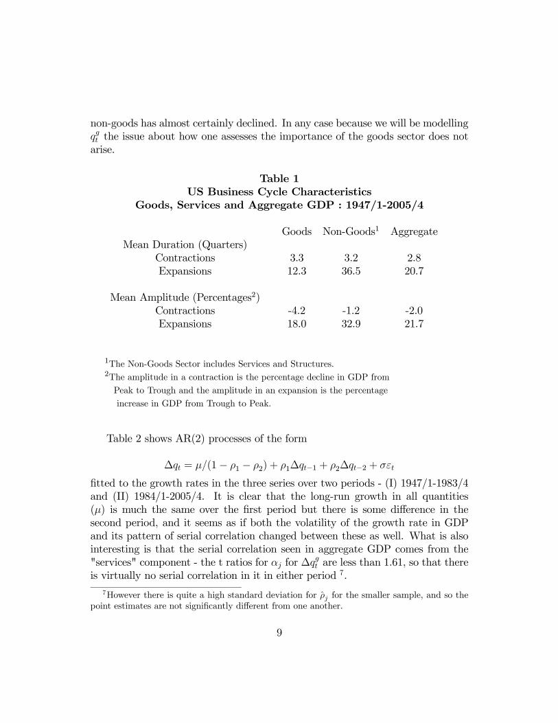
non-goods has almost certainly declined. In any case because we will be modellingqgt the issue about how one assesses the importance of the goods sector does notarise.

Table 1US Business Cycle Characteristics

Goods, Services and Aggregate GDP : 1947/1-2005/4

Goods Non-Goods1 AggregateMean Duration (Quarters)

Contractions 3.3 3.2 2.8Expansions 12.3 36.5 20.7

Mean Amplitude (Percentages2)Contractions -4.2 -1.2 -2.0Expansions 18.0 32.9 21.7

1The Non-Goods Sector includes Services and Structures.2The amplitude in a contraction is the percentage decline in GDP from

Peak to Trough and the amplitude in an expansion is the percentage

increase in GDP from Trough to Peak.

Table 2 shows AR(2) processes of the form

∆qt = μ/(1− ρ1 − ρ2) + ρ1∆qt−1 + ρ2∆qt−2 + σεt

fitted to the growth rates in the three series over two periods - (I) 1947/1-1983/4and (II) 1984/1-2005/4. It is clear that the long-run growth in all quantities(μ) is much the same over the first period but there is some difference in thesecond period, and it seems as if both the volatility of the growth rate in GDPand its pattern of serial correlation changed between these as well. What is alsointeresting is that the serial correlation seen in aggregate GDP comes from the"services" component - the t ratios for αj for ∆qgt are less than 1.61, so that thereis virtually no serial correlation in it in either period 7.

7However there is quite a high standard deviation for ρj for the smaller sample, and so thepoint estimates are not significantly different from one another.

9

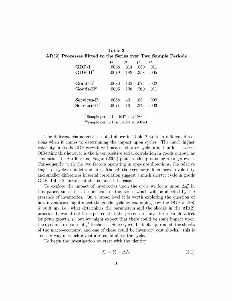
Table 2AR(2) Processes Fitted to the Series over Two Sample Periods

μ ρ1 ρ2 σGDP-I1 .0088 .314 .050 .011GDP-II2 .0079 .183 .358 .005

Goods-I1 .0086 .102 .074 .022Goods-II2 .0096 .106 .260 .011

Services-I1 .0088 .40 .05 .009Services-II2 .0071 .16 .34 .003

1Sample period I is 1947-1 to 1983-42Sample period II is 1984-1 to 2005-4

The different characteristics noted above in Table 2 work in different direc-tions when it comes to determining the impact upon cycles. The much highervolatility in goods GDP growth will mean a shorter cycle in it than for services.Offsetting this however is the lower positive serial correlation in goods output, assimulations in Harding and Pagan (2002) point to this producing a longer cycle.Consequently, with the two factors operating in opposite directions, the relativelength of cycles is indeterminate, although the very large differences in volatilityand smaller differences in serial correlation suggest a much shorter cycle in goodsGDP. Table 2 shows that this is indeed the case.To explore the impact of inventories upon the cycle we focus upon ∆qgt in

this paper, since it is the behavior of this series which will be affected by thepresence of inventories. On a broad level it is worth exploring the question ofhow inventories might affect the goods cycle by examining how the DGP of ∆qgtis built up, i.e., what determines the parameters and the shocks in the AR(2)process. It would not be expected that the presence of inventories would affectlong-run growth, μ, but we might expect that there could be some impact uponthe dynamic response of qgt to shocks. Since εt will be built up from all the shocksof the macro-economy, and one of these could be inventory cost shocks, this isanother way in which inventories could affect the cycle.To begin the investigation we start with the identity

Xt = Yt −∆Nt (2.1)

10

whereXt is the level of gross sales in the goods sector, Yt is the level of gross outputin the goods sector, and Nt is the level of finished goods inventories. Then, if theholding of finished goods inventories is important to the cycle, we would expectthat the cycle in xt = lnXt would be different to that in yt = lnYt.We constructedseries on Xt and Nt and then found Yt from the identity (2.1) -see Appendix A.It is worth mentioning that the Xt we construct here is not that referred to as "final sales" in the NIPA. The equivalent of the latter for the goods sector wouldbe

FSt = Qt −∆Nt −∆Mt,

where Mt is the level of raw material inventories. Many investigations of inven-tories use FSt to represent Xt, e.g. Wen (2005), but generally we cannot use theformer as a proxy for the latter when attempting to quantify a model. It wouldseem that the series we use for Xt is only available for the goods sector of GDP,at least on a quarterly basis.Value added Qg

t is the goods contribution to GDP, and this relates to Yt andMt through the identities

Qgt = Yt − VtUt

∆Mt = Dt − Ut,

where Ut is usage of raw materials, Dt is deliveries of raw materials, Vt is therelative price of raw materials to the price of output and Mt is the stock of rawmaterials.8 Thus inventories of raw materials may make the cycle in qgt differentfrom that in yt.

9

From the discussion above it is clear that if inventories are to affect the cyclein Qg

t (qgt ) they must induce a change in the DGP of ∆qgt from that of ∆xt.

10 Table3 looks at the characteristics of the DGP of each of the series ∆xt,∆yt over theperiod 1959/3-2005/4, and it suggests that finished goods inventories have littlerole in cycles, because the DGP of ∆xt and ∆yt are little different. However, themove from output to value added does induce significant changes in the DGP of

8There are missing elements in this definition such as energy usage and imports. Also wehave assumed that the price of materials used is the same as that of the stock of raw materials.

9We can measure the quantities in the identities above in the following way. First, Vt is takento be the implicit price deflator for raw materials used in the private business sector divided bythe implicit price deflator for goods GDP. Second, Ut may then be recovered from

Yt−Qgt

Vt.

10Cycles in Qgt and qgt are identical as the log transformation is monotonic and so turning

points in each series will be at the same points in time.

11

∆qgt from that of ∆yt11. Whether this is because of the effect of raw material

stocks or the fact that the nature of raw material prices has had an effect is whatneeds to be determined. To do so one needs to construct a model that can accountfor the separate effects.

Table 3AR(2) Fitted to ∆xt,∆yt,∆q

gt

1959/3-2005/4

∆xt ∆yt ∆qgt

μ .0082 .0081 .0093ρ1 .384 .379 .015ρ2 -.003 .002 .143σ .013 .013 .017

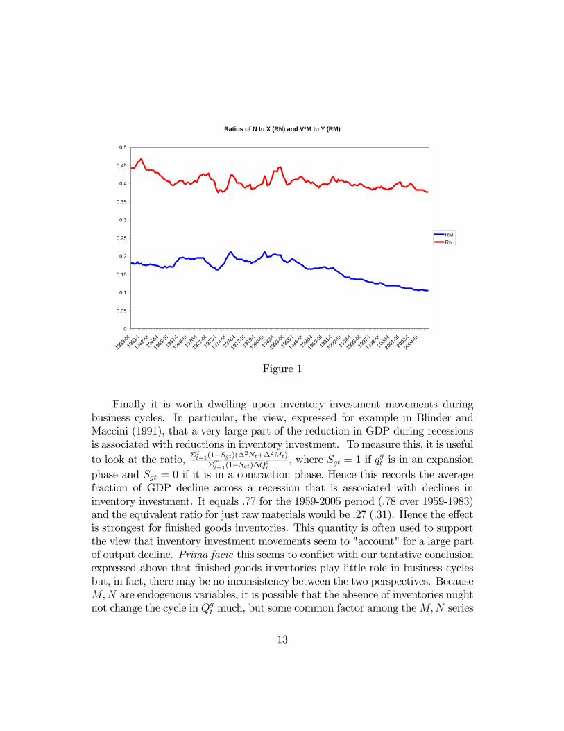
Turning to the decline in the volatility of ∆qgt one factor proposed to accountfor this is the ability to economize on inventories with new technology. A quicklook at the plausibility of this is available by looking at the ratios Nt

Xtand VtMt

Yt

over time.12 Fig 1 gives a plot of these. It is clear that there has been littlechange in the first ratio, but the second has declined by about 50% after 1984,which is a substantial decline. These stylized facts again point to the potentialimportance of raw materials when looking at changes in cycles and, at least forthe US, these seem to have been more significant than finished goods inventories.Whether changes in the levels of inventories that are held can in fact explainchanges in the cycle is a different matter, and once again points to the need todevelop a model that explains ∆qgt and which formally incorporates raw materials.

11The data on xt is not available before 1959/1.12We look at VtMt

Ytsince a change in Vt would be expected to change Mt

Ytand so a change in

the latter may simply reflect a response to relative price changes rather than a technologicalchange. Of course even this ratio may not fully control for such an effect. Note that essentiallythe same pattern occurs for Mt

Yt. It too declines after 1984 by about 45%, so it declines slightly

less precipitously.

12

Ratios of N to X (RN) and V*M to Y (RM)

0

0.05

0.1

0.15

0.2

0.25

0.3

0.35

0.4

0.45

0.5

1959

-III

1961

-I

1962

-III

1964

-I

1965

-III

1967

-I

1968

-III

1970

-I

1971

-III

1973

-I

1974

-III

1976

-I

1977

-III

1979

-I

1980

-III

1982

-I

1983

-III

1985

-I

1986

-III

1988

-I

1989

-III

1991

-I

1992

-III

1994

-I

1995

-III

1997

-I

1998

-III

2000

-I

2001

-III

2003

-I

2004

-III

RMRN

Figure 1

Finally it is worth dwelling upon inventory investment movements duringbusiness cycles. In particular, the view, expressed for example in Blinder andMaccini (1991), that a very large part of the reduction in GDP during recessionsis associated with reductions in inventory investment. To measure this, it is usefulto look at the ratio, ΣTt=1(1−Sgt)(∆2Nt+∆2Mt)

ΣTt=1(1−Sgt)∆Qqt

, where Sgt = 1 if qgt is in an expansion

phase and Sgt = 0 if it is in a contraction phase. Hence this records the averagefraction of GDP decline across a recession that is associated with declines ininventory investment. It equals .77 for the 1959-2005 period (.78 over 1959-1983)and the equivalent ratio for just raw materials would be .27 (.31). Hence the effectis strongest for finished goods inventories. This quantity is often used to supportthe view that inventory investment movements seem to "account" for a large partof output decline. Prima facie this seems to conflict with our tentative conclusionexpressed above that finished goods inventories play little role in business cyclesbut, in fact, there may be no inconsistency between the two perspectives. BecauseM,N are endogenous variables, it is possible that the absence of inventories mightnot change the cycle in Qg

t much, but some common factor among theM,N series

13

makes them cohere with Qgt . Again, a model is needed that enables one to see if

it is possible to reconcile these differing "stylized facts".

3. The Model and its Euler Equations

The model of the representative firm that we use is an extension of the one de-veloped by Humphreys et al.(2001). The model in Humphreys et al. has theadvantage that it is a model of inventories broken down by stage of fabricationand thus distinguishes between finished goods or ”output” inventories and mate-rials and supplies or ”input” inventories. The latter includes work in progressinventories as well; hereafter, we use the term materials inventories to refer tothe sum of materials and supplies and work in progress inventories. The modelthus permits an analysis of the role that each type of inventory stock plays inthe production and sales process. This is an important advantage of the modelas finished goods and materials inventories may have played very different rolesin the reduction of the volatility of GDP growth. Figure 1 reported that thematerials-output ratio had declined about 50% since the mid eighties, but the fin-ished goods-sales ratio had remained about constant. This suggests that, to theextent that improved inventory management techniques have had a role to playin reducing the volatility of GDP growth, materials inventories may have beenmore important than finished goods inventories. Further, ”just-in-time” tech-niques, which have become more widely used in recent years, are more applicableto materials inventory management than to that of finished goods.

3.1. The Production Function

We begin with a specification of the short-run production function, which is as-sumed to be Cobb-Douglas

Yt = F (Lt, Ut, yt) (3.1)

= Lγ1t U

γ2t e yt

where γ1 + γ2 < 1, which implies strict concavity of the production function inmaterials usage and labor. Here, Yt is output, Lt is labor input, Ut is materialsusage, and yt is a technology shock. Note that Ut is the flow of materials used inthe production process. When production and inventory decisions are made, thecapital stock is assumed to be taken as given by the firm and to be growing ata constant rate, which will be captured by a deterministic trend in the empirical

14

work. Finally, the firm is assumed to purchase intermediate goods (work-in-process) from outside suppliers rather than producing them internally.13 Thus,intermediate goods are analogous to raw materials so work-in-process inventoriescan be lumped together with materials inventories. Because Yt is gross output,we refer to equation (3.1) as the gross production function.

3.2. The Cost Structure

The firm’s total cost structure consists of three major components: labor costs,inventory holding costs, and materials costs. This section describes each compo-nent.

3.2.1. Labor Costs

Labor costs are

LCt = WtLt +WteA (Lt, Lt−1) (3.2)

= WtLt +WtA¡∆lt −∆l

¢Lt−1

where ∆lt = ∆ logLt ≈ ∆LtLt−1

is the growth rate of labor and ∆l is the steadystate growth rate of labor. The first component, WtLt, is the standard wage billwhereWt is the real wage rate. The second component, eA (Lt, Lt−1), is an adjust-ment cost function intended to capture the hiring and firing costs associated withchanges in labor inputs. The adjustment cost function has the usual properties:Specifically,

A0 R 0 as ∆lt R ∆l

A(0) = A0(0) = 0 A00 > 0

Adjustment costs on labor accrue whenever the growth rate of the firm’s laborforce is different from the steady state growth rate. Further, adjustment costsexhibit rising marginal costs.

13To allow for production of intermediate goods within the firm requires extending the pro-duction function to incorporate joint production of final and intermediate goods. This extensionis a substantial modification of the standard production process that we leave for future work.

15

3.2.2. Inventory Holding Costs

Inventory holding costs for finished goods inventories are:

HCNt = ΦN (Nt−1,Xt, nt−1) = δ1

µNt−1

Xt

¶δ2

Xt + δ3Nt−1 + nt−1Nt−1 (3.3)

δ1 > 0 δ2 < 0 δ3 > 0

where nt is the shock to finished goods inventory holding costs. Inventory

holding costs consist of two basic components. One, δ1³Nt−1Xt

´δ2Xt, captures

the idea that, given sales, higher inventories reduce costs in the form of lost salesbecause they reduce stockouts. The other, δ3Nt−1, captures the idea that higherinventories raise costs because they raise holding costs in the form of storagecosts, insurance costs, etc.14 The effects of technological advances that improveinventory management methods can be captured, for example, through a changein δ2 and changes in the volatility of the shock to finished goods inventory holdingcosts.15

Inventory holding costs for materials and supplies inventories are:

HCMt = ΦM (Vt−1Mt−1, Yt, mt−1) (3.4)

= τ 1

µVt−1Mt−1

Yt

¶τ2

Yt + τ 3Vt−1Mt−1 + mt−1Vt−1Mt−1

14These two components underlie the rationale for the quadratic inventory holding costs in thestandard linear-quadratic model. The formulation above separates the components and assumesconstant elasticity functional forms which facilitates log-linearization around constant steadystates. We assume that the firm minimizes discounted expected costs and thereby abstract frommarket structure issues. See Bils and Kahn (2000) for a model that deals with market structureissues and also utilizes a constant elasticity specification of the benefits of holding finished goodsinventories, though the benefits are embedded on the revenue side of the firm.15Observe that (3.3) implies a "target stock" of finished goods inventories that minimizes

finished goods inventory holding costs. Assuming nt−1 = 0, the target stock, N∗t , is

N∗t = −³

δ3δ1δ2

´ 1δ2−1

Xt

so that the implied target stock is proportional to sales. This is analogous to the target stockassumed in the standard linear-quadratic model. Note that the target stock is not the steadystate stock of finished goods inventories. The steady state stock minimizes total costs in steadystate whereas the target stock merely minimizes inventory holding costs. The steady state stockwill be derived below.

16

τ 1 > 0 τ 2 < 0 τ 3 > 0

where mt is the shock to materials inventory holding costs. As above, there are

two basic components: One, τ 1³Vt−1Mt−1

Yt

´τ2Yt, captures the idea that, given out-

put, higher inventories reduce costs in the form of lost output because they reducestockouts and disruptions to the production process. The other, τ 3Vt−1Mt−1, cap-tures the idea that higher inventories raises costs because they raise holding costsin the form of storage costs, insurance costs, etc. Note that materials inventoryholding costs depend on production, rather than sales. This is because stockingout of materials inventories entails costs associated with production disruptions —lost production, so to speak — that are distinct from the costs associated with lostsales. Lost production may be manifested by reduced productivity or a failureto realize production plans. Again, the effects of technological advances thatimprove inventory management methods can be captured, for example, througha change in τ 2 and changes in the volatility of the shock to materials inventoryholding costs.16

The finished goods and material inventory holding costs differ because thefirm holds the two inventory stocks for different reasons. The firm stocks finishedgoods inventories to guard against random demand fluctuations. Finished goodsinventories thus facilitate sales. On the other hand, the firm stocks materialsinventories to guard against random fluctuations in productivity, materials pricesand deliveries, and other aspects of production. Materials stocks thus facilitateproduction. Although sales and production are highly positively correlated, theyperform different roles in the firm and differ enough at high frequencies to justifydifferent specifications.

16Similarly, observe that (3.4) implies a "target stock" of materials and supplies inventoriesthat minimizes materials and supplies inventory holding costs. Assuming mt−1 = 0, the targetstock, VtM∗t , is

VtM∗t = −

³τ3τ1τ2

´ 1τ2−1

Yt,

so that the implied target stock is proportional to output. Note here as well that the targetstock of materials inventories is not the steady state stock of materials inventories. The latterwill be derived below.

17

3.2.3. Materials Costs

Finally, we turn to the cost of purchasing materials and supplies. We assume thatthe real cost of purchasing materials and supplies is given by

MCt = VtDt + VteΓ (VtDt, Yt) = VtDt + VtΓ

µVtDt

Yt

¶Dt (3.5)

= VtDt

∙1 + Γ

µVtDt

Yt

¶¸Γ0 = 0 Γ00 > 0

Γ(0) = 0 Γ(V DY) = 0 Γ0(V D

Y) = 0

where Vt is a real ”base price” for raw materials. The term, VtDt, is the valueof purchases and deliveries valued at the base price. The term, VteΓ (VtDt, Yt),represents a premium that may need to be paid over and above the base price toundertake the level of purchases and deliveries, Dt. It is assumed to rise at anincreasing rate with the amount purchased and delivered.Two cases may be distinguished:

1. Increasing Marginal Cost: Γ0> 0. In this case, the firm faces a rising supplyprice for materials purchases. When purchases are high relative to currentstocks, the firm thus experiences increasing marginal costs due to higherpremia that must be paid to acquire materials more quickly. A rationale forsuch a rising supply price is that the firm is a monopsonist in the marketfor materials. This is most likely to occur when materials are highly firmor industry specific and the firm or industry is a relatively large fractionof market demand.17 The rising marginal cost of course gives rise to the“smoothing” of purchases.

2. Constant Marginal Cost: Γ0= 0. In this case, the firm is in effect a price takerin competitive input markets and is able to purchase all the raw materialsit needs at the prevailing market price.

17This is analogous to the literature on adjustment cost models for investment in plant andequipment where external adjustment costs are imposed in the form of a rising supply price forcapital goods. See, e.g., Abel(1979 ).

18

3.3. Cost Minimization

Assume that the representative firm takes sales (Xt) and factor prices (Vt andWt) as exogenous. The firm’s optimization problem is to minimize the discountedpresent value of total costs (TC),

E0

∞Xt=0

βtTCt = E0

∞Xt=0

βt(LCt +HCt +MCt) , (3.6)

where β = (1 + r)−1 is the discount factor. The constraints are the productionfunction, (3.1), and the two laws of motion governing inventory stocks. Theidentity for finished goods inventories is

∆Nt = Yt −Xt (3.7)

and the identity for materials and supplies inventories is

∆Mt = Dt − Ut. (3.8)

The firm chooses {Lt, Ut, Yt,Mt, Nt,Dt}∞t=0 to minimize equation (3.6) subject tothe constraints (3.1), (3.7), and (3.8).

3.4. Optimality Conditions

Assume that, when the representative firm makes decisions, current values ofexogenous variables are in its information set. Then, the optimality conditionsare:

Wt + Λ1tFL (Lt, Ut, yt) +WteA1(Lt, Lt−1) +EtβWt+1

eA2(Lt+1, Lt) = 0 (3.9)

Λ1tFU (Lt, Ut, yt) + Λ3t = 0 (3.10)

Vt + VteΓD(VtDt, Yt)− Λ3t = 0 (3.11)

ΦMY (Vt−1Mt−1, Yt, mt−1) + eΓY (VtDt, Yt)− Λ1t − Λ2t = 0 (3.12)

19

Λ2t − βEtΛ2t+1 + βEtΦNN(Nt,Xt+1, nt) = 0 (3.13)

Λ3t − βEtΛ3t+1 + βEtΦMM(VtMt, Yt+1, mt) = 0 (3.14)

together with the production function, (3.1), and the accumulation equations,(3.7) and (3.8). Note that Λ1t,Λ2t, and Λ3t are the Lagrangian multipliers asso-ciated with (3.1), (3.7) and (3.8) respectively.To interpret the optimality conditions, observe that (3.9)-(3.11) imply that

FL (Lt, Ut, yt)

FU (Lt, Ut, yt)=

Wt

h1 + eA1(Lt, Lt−1) + βEt

Wt+1

Wt

eA2(Lt+1, Lt)i

Vth1 + eΓD(VtDt, Yt)

i ,

which states that the relative marginal products of labor and materials utilizationmust equal their relative marginal costs. In the case of labor, the latter is thecurrent wage rate together with the marginal adjustment costs of hiring and firinglabor. In the case of materials utilization, the marginal cost is the purchase priceof an additional unit of materials together with any marginal premia due to risingsupply prices that must be paid to acquire materials.The optimality condition, (3.13) can be summed forward to get

Λ2t = −Et

∞Xi=0

βi+1ΦNN(Nt+i,Xt+1+i, nt+i)

which states that the imputed value to the firm of holding an additional unit offinished goods inventories must equal (minus) the expected discounted value ofcurrent and future marginal finished goods inventory holding costs.18 The minussign indicates that at the optimum the firm must operate on the downward slopingcomponent of the inventory holding cost function for finished goods inventories.The latter is the segment where the marginal value of holding finished goodsinventories to avoid lost sales exceeds the marginal storage costs. Similarly, the

optimality condition, (3.14) can be summed forward to get

18This assumes that the transversality condition, limT→∞

βTEtΛ2t+T = 0, is satisfied.

20

Λ3t = −Et

∞Xi=0

βi+1ΦMM(Vt+iMt+i, Yt+1+i, mt+i)

which states that the imputed value to the firm of holding an additional unit ofmaterials inventories must equal (minus) the expected discounted value of currentand future marginal material inventory holding costs.19 Again, the minus signindicates that at the optimum the firm must operate on the downward slopingcomponent of the inventory holding cost function for materials inventories. Thelatter is the segment where the marginal value of holding materials inventoriesto avoid lost output due to stockouts and disruptions of the production processexceeds the marginal storage costs.Now, define the following shares and ratios

SL,t =WtLtYt

SU,t =VtUtYt

RN,t =Nt

XtRM,t =

VtMt

Yt

RD,t =VtDt

YtRY,t =

YtXt

RΛ3,t =Λ3tVt

(3.15)

It is assumed that the variables in (3.15) are stationary with finite expectedvalues even if the variables they are constructed from have unit roots. It will alsobe assumed that Vt is a stationary random variable and this will make Λ3t,Λ1t andΛ2t stationary. Then, applying the functional form assumptions in (3.1), (3.3),(3.4), and (3.5), the resulting optimality conditions can be log-linearized aroundconstant expected steady state values. Appendix B provides the details. Onnotation, lower case letters are logarithms of upper case letters, so, for example,lt = logLt,and thus the growth rate of a variable is ∆lt = ∆ logLt ≈ ∆Lt

Lt−1.

A "bar" above a variable denotes a constant expected steady state value. A”ˆ” above an upper case letter denotes a log-deviation, while above a lower caseletter denotes a simple (i.e., non-logarithmic) deviation. So, for example, thelog-deviation of RD,t from its expected value is RD,t = logRD,t − logRD, whereRD = E(RD,t), while the simple deviation of the growth rate of sales is ∆bxt =∆xt − ∆x. Similar notation applies to other variables. The log-linearizedoptimality conditions are then

bSLt − bΛ1t + ϕ∆blt − βϕEt∆blt+1 = 0 (3.16)

bSUt − bΛ1t + bRΛ3,t = 0 (3.17)

19This assumes that the transversality condition, limT→∞

βTEtΛ3t+T = 0, is satisfied.

21

η bRD,t − bRΛ3,t = 0 (3.18)

μ2RM (1−∆y)h bRM,t−1 −∆byti+ ηRD

bRD,t + Λ1bΛ1t + Λ2bΛ2t = 0 (3.19)

Λ2bΛ2t − βΛ2EtbΛ2t+1 + βμ1Et

³ bRN,t −∆bxt+1´+ β nt = 0 (3.20)

bRΛ3,t − βEt

h∆bvt+1 + bRΛ3,t+1

i+ βμ2Et

h bRM,t −∆byt+1i+ β mt = 0 (3.21)

∆byt = γ1∆blt + γ2∆but + yt − yt−1 (3.22)

bRN,t − (1−∆x) bRN,t−1 + (1−∆x)∆bxt − RY

RN

bRY,t = 0 (3.23)

bRM,t − (1 +∆v −∆y)h bRM,t−1 +∆bvt −∆byti− RD

RM

bRD,t +SU

RM

bSU,t = 0 (3.24)

where ϕ = A00(0), η = Γ00(RD)R2

D, μ1 = (δ2 − 1) δ2δ1£RN (1−∆x)

¤δ2−1, and

μ2 = (τ 2 − 1) τ 2τ 1£RM (1−∆y)

¤τ2−1.

Finally, other quantities can be derived in a similar way. Since we will ul-timately want to re-construct Qg

t it is useful to find an expression for the log-deviation of the ratio of GDP to gross output for the goods sector. Specifically,define RQg,t =

Qgt

Yt. Then, to obtain bRQg ,t, recall that the definition of GDP is

Qgt = Yt − VtUt,

so thatQg

t

Yt= 1− VtUt

Yt.

Then, using the definition of RQg,t and the utilization share, SU,t = VtUtYt, we have

that

RQg ,t = 1− SU,t.

A log-linear approximation of this then yields

RQg bRQg ,t = −SUbSU,t. (3.25)

22

4. Quantifying Model Parameters

4.1. Matching Data and Model Variables

The model above is that of a representative firm. To apply the model to thegoods sector as a whole, we assume that the representative firm behaves as if it isvertically integrated, so that it is representative of the whole goods sector of theeconomy. The representative firm holds materials inventory stocks which it usesin conjunction with labor (and capital) to produce output of finished goods, whichit adds to finished goods inventories. The finished goods inventories may be heldby manufacturers, wholesalers or retailers. In effect, we treat the representativefirm as managing the inventory stocks of finished goods whether they are held onthe shelves of the manufacturer, the wholesaler, or the retailer. Appendix A dealswith the exact measurement of the variables in the data.

4.2. Estimation Strategy

As pointed out in the introduction we seek to quantify the model parametersusing data over the period 1959/1-1983/4. Ideally one would like to have begunwith 1947/1 but quarterly data were not available on Mt and Nt over that earlierperiod. The arguments for using a longer sample normally relate to increasedprecision of estimators, but, as will become apparent, the parameters are quiteprecisely estimated. Once estimated the model can then be used to explore someof the questions raised in the introduction.In (3.16)-(3.24) we will treat the variables vt, wt, xt, εyt, εnt, εmt as exogenous

processes. vt is assumed stationary but, based on unit root tests, wt and xt areI(1) (ADF tests of -2.2 and -.72)). Some simplification of (3.16)-(3.24) is possible.In particular we can eliminate RΛ3,t and bΛ1t by using (3.17) and (3.18). Thisleaves us with seven equations to determine the ten endogenous variables

z∗0t =h bSL,t bSU,t ∆yt bRD,t

bΛ2t bRN,tbRM,t ∆ut ∆lt RY,t

i.

Three extra equations connecting endogenous and exogenous variables are avail-able from identities describing ∆SL,t,∆SU,t and ∆RY,t; for example, ∆SL,t =

∆wt +∆lt −∆yt. This system of ten equations therefore has the form

z∗t = Az∗t−1 +BEt(z∗t+1) +Gηt, (4.1)

23

where η0t =£∆xt ∆wt vt ∆εyt εnt εnt

¤. Hence it can be solved by standard

methods to give the solution

z∗t = Pz∗t−1 +Et(∞Xj=0

F jGηt+j) (4.2)

where F is a function of A,B - see for example Binder and Pesaran (1995). Whenηt follows a VAR(1) this becomes

z∗t = Pz∗t−1 +Kηt. (4.3)

Further, given the solution for bSU,t that is an element of z∗t in (4.3), a solutionfor bRQg,t may be obtained from (3.25).In our model derivations we have implicitly assumed that there are two co-

integrating relations among any I(1) variables. These are given by the finishedgoods inventory-sales ratio, RN,t =

Nt

Xt, and the raw material ratio, RM,t =

VtMt

Yt.

ADF tests on lnRM,t and lnRN,t were -3.09 and -3.17, easily rejecting the nullhypothesis of a unit root at the 5% level of significance.20. Labour usage was notin our data set but it was assumed that the labour share SL,t is I(0). Taking thesethree ratios to be I(0), we show in Appendix B that SU,t, RD,t, RY,t, RΛ3t, Λ1t,and Λ2t will then be I(0) as well. Not unexpectedly unit root tests applied tont,mt, yt, xt and wt reveal these series to have unit roots. Two of these variables,xt and wt, are exogenous, and so can be taken as the permanent componentsunderlying the I(1) series. But, since there are two cointegrating vectors amongthe five I(1) variables there must be another common permanent component, andwe identify this as the technology shock i.e. εyt has a unit root.It is necessary to describe the evolution of ηt. Since∆xt and∆wt are observable

we can fit processes to these series. An AR(1) was fitted to each producing ARcoefficients of .33 and .02 respectively.21 ∆εyt, εnt and εmt were all assumed to be

20These tests are based upon using the SBC criterion to choose the best lag length for theADF test. The result is lags of 2 and 3 respectively.21Ramey and Vine (2005) argue that there has been a change in the persistence of sales in the

automobile industry and that this led to a decline in output volatility. They find that there wasa shift in persistence in 1984/1. Since we impose a unit root on the xt process we do not allowfor any such decline. However, fitting the same regression as they used ( an AR(1) with shiftsin the intercepts and deterministic time trend) to xt, which is (the logarithm of) sales in thegoods sector as a whole, over their sample period of 1967/1-2004/4, we find that the t ratio fora shift in the degree of persistence is just .6. Moreover, the point estimate for the lag coefficientparameter actually rose by .03 in the post 1984 period.

24

AR(1) processes with coefficients ρy, ρn and ρm respectively and these are to beestimated by MLE. vt seemed closer to stationarity, having an AR(2) of the form

vt = 1.21vt−1 − .29vt−2 + .0053εvt .

The vt process is a very persistent one but the sharp rise in oil prices ( andassociated raw material prices) in 1974 had a major effect upon the unit roottests. Because of this we decided to treat it as I(0).The parameters in the Euler equations can be divided into three groups:

(I) θ1 = [β, γ1, γ2, RY , RD, RM , RN ] (4.4)

(II) θ2 = [τ 3, δ3,Λ1,Λ2], (4.5)

(III) θ3 = [τ 1, τ 2, δ1, δ2, ϕ, η, σy, σn, σm, ρy, ρn, ρm], (4.6)

where σy, σn and σm are the standard deviations of the unobervable shocks εy, εnand εm respectively. θ1 is either pre-set in the case of β = .99, γ1 = .22, γ2 = .66or estimated using sample means for the ratios RY etc. The γj parameters wereset because the absence of capital in the model makes it difficult to estimate theparameters of a production process.22

Estimates of the four parameters in θ2 are found from appropriate steadystate conditions - see (8.36)-(8.44) in Appendix B. To obtain values for θ2 fromthose steady state equations requires values for θ3. Once a set of values for θ3 isestablished, θ1 and θ2 are then fixed, so that it is only necessary to estimate θ3from the data. Finally, from the optimality conditions in (3.16) and (3.17) it isevident that τ 1, τ 2, δ1 and δ2 enter only through μ1 and μ2, so only two of theseparameters can be identified. Consequently we set δ1 = τ 1 = 1, which are commonnormalizations in the empirical literature on inventories. Doing so leaves the finalset of parameters to be estimated as ξ = [τ 2, δ2, ϕ, η, σy, σn, σm, ρy, ρn, ρm].Maximum likelihood estimation is then done to get estimates of ξ. A complica-

tion arises from the fact that we only have data on six variables - zt = [SU,t, RN,t,RM,t,∆xt, vt,∆wt]. If z∗t had been observed then the likelihood would be just thatof the VAR in z∗t . When not all variables in z∗t are observed it is necessary toadd an observation equation connecting the observed and unobserved variables

22If we had set γ2 = .71 to reflect the share of raw materials as measured in our data thenit seems virtually impossible to allow for a role for capital, as a realistic share for labour wouldmean that the sum of the raw material and labour shares would exceed unity. In addition, itwas found that setting γj below the pre-set values above resulted in a substantial decline in thelikelihood, so these values seemed a reasonable compromise.

25

i.e. zt = Hz∗t , to the state dynamics equations, as summarized by the VAR in z∗t .

The likelihood of the resulting state space form formed from this equation and(4.3) is then that for the observed zt, and it is found recursively by an applicationof the Kalman predictor. This is a standard way of performing MLE on DSGEmodels e.g. see Ireland (2004), and is adopted in the DYNARE program that weutilize for estimation.23

Maximum Likelihood Estimates of the parameters are available in Table 4.The implied estimates of τ 3 and δ3 from the steady state equations are .07 and.04 respectively.

Table 4Model Parameter Estimates

τ 2 δ2 ϕ η σyEstimate -.015 -.026 1.16 5.7 .008t-Statistic 2.8 2.9 4.3 4.9 10.1

σn σm ρn ρm ρyEstimate .002 .005 .96 .88 .11t-Statistic 3.5 3.6 26.5 10.6 5.0

It is worth commenting on the exogeneity assumptions in force. In a generalequilibrium (GE) model, where consumer and policy choices are modelled, therewould be an extra set of equations describing the expanded choices, and thesewould augment our equations for the goods sector. In addition there may be someextra shocks that are either common or specific to the agents being considered.Unless strategic behavior was involved the equations for the goods sector wouldnot change. Thus the solution for the goods sector still has the structure in (4.2).The impact of a GE model would be that agents in the goods sector would nowform expectations of ηt+j using an expanded information set. Thus the GE versionof (4.2) would be

z∗t = Pz∗t−1 +E+t (

∞Xj=0

F jGηt+j), (4.7)

23We use version 3.065 of DYNARE written by S. Adjemian, M. Juillard and O. Kamenik.

26

where "+" indicates the expanded information set. Hence to reconcile (4.7) with(4.2) it is necessary that an error ζt be added on to (4.2) so that the equationbecomes

z∗t = z∗t = Pz∗t−1 +Et(∞Xj=0

F jGηt+j) + ζt

where ζt = E+t (P∞

j=0 FjGηt+j)−Et(

P∞j=0 F

jGηt+j). This changes the VAR solu-tion to

z∗t = Pz∗t−1 +Kηt + ζt

Now Et(ζt) = 0 since the information used in the goods model would be a sub-setof the expanded information set. This also implies that E(z∗t−1ζt) = 0 and so wecan legitimately estimate the parameters in the partial equilibrium (PE) modelusing the VAR that ignores ζt.

24 Hence it is not consistent estimation of the Eulerequation parameters that is affected by the use of a PE model but rather issuesof efficiency and interpretation.What is lost in using the PE approach is the potential for a gain in efficiency

owing to the fact that ζt can be eliminated ( which must of course be balancedagainst the biases that can arise if the rest of the model is poorly specified) anda more precise interpretation of ηt owing to the fact that it might be a functionof variables that do not appear in the goods (partial equilibrium (PE)) model.Efficiency does not seem to be of great concern here given the precision of theestimators in Table 4. Therefore, it is the interpretation which we focus upon.Put simply, in a broader model ∆xt (say) would be determined not only by z∗t−1and the shocks identified in the PE model, but also lagged values of other variablese.g. interest rates and other shocks. A complete model is needed to define sucha relationship. If only the PE model is used then any decomposition attributingoutput variation to sales will be unable to precisely identify what shock it wasthat was driving ∆xt. Because the questions we seek to resolve do not dependcritically on any such decomposition the partial equilibrium approach providesvaluable information that does not require the complexity ( and possible errors)

24It is necessary to ensure that we find Etηt+j correctly however i.e. all information in thepartial equilibrium model needs to be used to forecast items like ∆xt ,∆wt and vt. We didrun regressions of ∆xt against lags of variables such as nt,mt, yt etc but these provided littleexplanatory power over the own lagged values, which is why we describe ∆xt etc as exogenous.Our methodology does not however require that such series be strongly exogenous. It was thenature of the data that lead to this assumption.

27

induced by a complete model. Of course if one was seeking to provide a model forqt rather than qgt it would be necessary to have a GE model.At this point, it is useful to look at the adequacy of the model in re-producing

some of the more interesting characteristics of the data. First the model impliesthat the standard deviation for ∆qgt , σ∆qg , would be .0243, versus the value of.021 in the data.25 The test statistic that these are different is 2.4 so that themodel seems to produce a reasonable fit to the variance of ∆qgt , although a littletoo high. The parameter estimates imply a first-order serial correlation coefficientin ∆qgt of .15, whereas the data says there is virtually no serial correlation. Thestandard error on this estimate is however .10 and so there is no significant differ-ence between them. In terms of cycle outcomes the durations of expansions andcontractions for Qg are 9.45/3.43 (data ) and 9.28/4.23 (model).26

Other features of interest relate to the first order serial correlation coefficientsin ∆mt and ∆nt. There is quite high serial correlation in these, in contrast tothe situation for ∆qgt . Specifically they are .625 and .318 respectively. The modelpredicts them to be .610 and .344 respectively, so it captures the fact that theserial correlation patterns in inventories and GDP are quite different.Finally, as we observed earlier, one of the reasonably constant features of

the data is the association between the decline in inventory investment and thefraction of the decline in GDP over recessions. For 1959-1983 this was .78 fortotal inventories and .31 for raw materials. The model predicts these to be .88and .39 respectively ( found by averaging over 500 sets of simulated data with 98observations in each set). The range of variation that comes out of the simulationsis quite large, meaning that the predictions are consistent with the data at anextremely low level of significance. Consequently the model seems to capturemany of the features of inventory movements and their relations to the goodscycle quite well.

25The characteristics of ∆qgt reported in Table 2 for the sample period 1947-1983 are virtuallythe same as those from 1959-1983.26Note this is for the sub-period 1959/3-1983/4 and it is quite a short period to measure cycle

characteristics.

28

5. Experiments with the Model

5.1. Analysis of Fluctuations and the Great Moderation

The causes for the great moderation have been much debated in the literature.When this feature was observed it was natural that one look at what changes weretaking place in the economy which might lead to such an outcome. Since there hadbeen great advances in inventory control methods, in particular the developmentof “just in time” philosophies relating to production, it seemed possible that thismight be a source of the changes e.g. see Kahn et al (2002). To assess thispossibility we first adopt the above estimated model as the "base model" andthen ask how σ∆qg varies with changes in selected parameters of the model. Inparticular, we are interested in what happens as δ2 and τ 2 change so as to meanthat less finished goods inventories and raw materials are held as a ratio of salesand output respectively. Consider, for example, a decline in the absolute valueof τ 2, which shifts the materials inventory holding cost function. Intuitively,such a decline captures the idea that computerization, just-in time procedures,or other technological advances in inventory management techniques imply thatthe firm can experience the same level of lost production with a smaller levelof materials inventories, given the level of output. Or, alternatively, a givenmaterials inventory/output ratio will generate a smaller amount of lost production.A similar interpretation applies to a decline in the absolute value of δ2. To computevalues of ∆qgt , when a parameter changes, we reverse the estimation strategy, andnow solve for ratios such as RN and RM as functions of the estimated modelparameters. Also of interest is the magnitude of the impact of changes in thevolatility of the observed and unobserved shocks.|δ2| was arbitrarily reduced by 10% while |τ 2| was reduced by 20%. The latter

produced a decline in the VMYratio that roughly matches what was seen over

the period 1984/1-2005/4. Similarly the reductions in standard deviations of allshocks was set to 50%, as that was roughly what happened to the observableshocks over that period. As noted above, Nt

Xtchanged only minimally after 1984,

and so we look at only a small change in |δ2| to see whether this could havehad any impact on volatility. So these experiments are about how we mighthave expected fluctuations to have changed over the second period given that thevolatility reduction in observed shocks was matched by that in the unobservedones. The experiments involving reductions in the standard deviations of shocksalso give some insight into what the main sources of fluctuations would be. Finally,we present an experiment in which δ2 and τ 2 are just one-hundreth of the values in

29

Table 3. Such a reduction means that inventories have very low value to the firmin the sense of reducing the costs of lost sales or lost output and thus emulates asituation where inventories are not present in the system. Table 5 gives the resultsof these experiments.27

Table 5Effects on σ∆qg of Parameter Perturbations

σ∗∆qg ρ∗∆qg

Base .0243 .158.9δ2 .0242 .156.8τ 2 .0241 .156.5σx .0204 .014.5σw .0243 .158.5σv .0233 .16.5σn .0242 .157.5σm .0241 .16.5σy .0194 .315.01(δ2, τ 2) .0208 .156

*Effect of cuts in parameters

It is clear that, if the change in inventory technology can be thought of as in-volving a change in the magnitude of τ 2, so that smaller materials stocks relativeto output are an optimal choice, then this produces only slightly smaller fluctu-ations in goods GDP. As Table 5 indicates, a 20% decline in τ 2 produces only a1% reduction in σ∆qg . Hence this cannot be the source of the reduced volatilityin ∆qgt . Further, decomposing the variance of ∆qgt into the various shocks: 48% isdue to the technology shock, 39% is due to the sales shock, 10% is due to the raw

27If one wishes to find the impact of combinations of parameter changes rather than a singleone, the approach used in assessing the sensitivity of computable general equilibrium modelsolutions to parameters can be followed. Given the model solution as a function of the parame-ters, yt = g(θ), where θ are the parameters, linearization around some base set of parametersproduces yt− y∗ = ∂g

∂θ (θ∗)(θ− θ∗). Of course this is only a local approximation but experiments

show it is quite accurate for the likely range of variation in the coefficients. ∂g∂θ (θ

∗) can bemeasured from Table 4 e.g. a 50% reduction in σx leads to be 16% reduction in σ∆qg so that a1% change σx would lead to a .32% change in σ∆qg .

30

material price shock, and 1% is due to the raw materials inventory shock. Neitherwages nor the finished goods inventory shocks are important.If the volatility of all shocks was reduced by 50%, σ∆qg would become .012

which is very close to the actual reduction over the 1984/1-2005/4 period - seeTable 5. If only the observed ones were reduced, σ∆qg would only have droppedto .019 so that the unobservable shocks are critical to explain this phenomenon.Specifically, a large decline in the volatility of technology shocks will be needed.An alternative viewpoint, expressed in Kahn et al (2002), is that the infor-

mation set of firms may have changed as a consequence of computerization. Inparticular it may be that sales are now known with greater accuracy. To assessthis we considered an experiment in which it was assumed that only {xt−j−1}∞j=0rather than {xt}∞j=0 was known in the period 1959/1-1983/4.28 In the post-1983/4period however xt was taken to be part of the information set. To conduct thisexperiment the model was re-estimated using the new information set and theimplied σ∆qg was still found to be .0243. Hence the reduction in the volatility of∆qgt as a result of improved information about sales is negligible, since the basecase in Table 4 represents what it would be with the expanded information.In light of these results it is useful to consider the debate over whether mone-

tary policy had an impact on σ∆qg . One might expect that this effect would workthrough sales and, although the decline in the volatility of the latter has made acontribution, it would not have led to the observed decline in volatility if technol-ogy shocks had not changed as well. Thus it is hard to see monetary policy asbeing the major driving force in the reduction in the volatility in the goods sector.

5.2. Analysis of Cycles

Whilst the nature of the business cycle depends upon the volatility of ∆qgt it alsodepends upon the mean of this process and the nature of any serial correlationin it. Consequently, the experiments above were repeated to determine theireffects upon the cycle in qgt . Table 6 shows how the durations and amplitudes ofexpansions and contractions in qgt would change. It should be noted that over theperiod of estimation, 1959/1-1983/4, the duration of contractions and expansionswere 3.43 and 9.45 quarters, and so the length of expansions using the estimatedmodel parameters ( the "base" simulation) is quite close to that actually observed.

28This means that Et(∆xt+1) in the Euler equations is replaced by ρ2∆xt−1 rather than ρ∆xt.

31

Table 6Effects on Cycles of Parameter Perturbations

Durations (Quarters)* Amplitudes (Percentages)*Contractions Expansions Contractions Expansions

Base 4.23 9.28 -5.84 16.02.9δ2 4.24 9.32 -5.81 16.03.8τ 2 4.23 9.34 -5.77 16.02.5σx 3.80 11.19 -4.14 15.6.5σw 4.23 9.34 -5.84 16.09.5σv 4.22 9.57 -5.58 16.02.5σn 4.24 9.27 -5.81 15.99.5σm 4.23 9.31 -5.79 16.02.5σy 4.11 9.86 -4.73 15.29

.01(δ2, τ 2) 4.31 10.57 -4.89 15.60

*Effect of cuts in parameters

Given that we know cycle length depends upon the volatility and serial cor-relation properties of ∆qt - Harding and Pagan (2002)- the results in Table 6 arelargely predictable by the outcomes in Table 4. An exception occurs for the rela-tive effects of the experiments involving a reduction in sales and technology shockvolatilities. Here the cycle becomes longer with the first experiment, even thoughthe volatility decrease was slightly less than in the second experiment. This showsthat the degree of serial correlation in ∆qgt is also important for cycle outcomes.The final experiment shows that the presence of inventories in the system doescreate less cycles although on average they are only one quarter longer. Overall,the importance of inventories to the average cycle is limited, even though it maybe that for particular cycles their presence has a greater effect. It should be notedthat in no case are there complex roots in the ∆qgt process and so no oscillations.

6. Conclusion

In this paper, we have developed a model of the optimal holding of finished goodsand raw material input inventories by a goods producing firm and have used it toanalyze a number of questions that have come up about the role of inventories.

32

The paper yields two main conclusions. First, we showed that inventories have hadonly a small effect upon the average duration of expansions and contractions ofthe business cycle in the U.S. economy. To show the latter, we looked at businesscycles in terms of the turning points in the level of goods GDP, which is a verydifferent perspective from the traditional work on inventory cycles that has lookedat oscillations in activity. This conclusion emerges despite the fact that the modelproduces predictions that are consistent with many of the features observed in thedata regarding the behavior of inventories over the business cycle. Second, weshowed that changes in inventory management technology have had little effectupon the volatility of GDP growth in the goods sector of the US economy. Themodel we developed allows for a role for raw material prices in producing cyclesand we found that the latter did have some impact, although the main drivers ofchanges in the business cycle were technology and sales variations.The approach we take in this paper is to develop a partial equilibrium model

of the goods sector of the economy. This enables us to focus on the basic ques-tion of whether advances in inventory technology were responsible for the declinein the volatility of GDP growth in the goods sector with a minimal number ofassumptions about the rest of the economy. Our approach is quite different fromthe VAR approaches and the more recent general equilibrium models of the econ-omy as a whole. Nonetheless, the different approaches that have been used toaddress the basic question appear to be coming to similar conclusions, namely,that advances in inventory management techniques have played a relatively smallrole in the Great Moderation. This is reassuring in that knowledge is advancedwhen very different approaches arrive at essentially similar conclusions regardingimportant questions.

7. References

Abel, A. (1979), Investment and the Value of Capital, Garland, New York.Ahmed, S., Levin, A., & B. A. Wilson (2004), "Recent U.S. Macroeconomic

Stability: Good luck, Good Policies or Good Practices?, Review of Economicsand Statistics, 86, 824-832.Bils, M. and J. A. Kahn (2000), "What Inventory Behavior Tells Us about

Business Cycles", American Econoomic Review, 90, 458-480.Binder, M and M.H. Pesaran (1995), “Multivariate Rational Expectations

Models and Macroeconomic Modelling: A Review and Some New Results”, inM.H. Pesaran and M. Wickens (eds) Handbook of Applied Econometrics: Macro-

33

economics, Basil Blackwell, Oxford.Blanchard, O. and J. Simon (2001), “The Long and Large Decline in U.S.

Output Volatility”, Brookings Papers on Economic Activity, 1, 135-174.Blinder, A. and L. Maccini (1991), "Taking Stock: A Critical Assessment of

Recent Research on Inventories", Journal of Economic Perspectives, 5, 73-96.Burns, A.F., Mitchell, W.C., (1946), Measuring Business Cycles, New York,

NBER.Chang, Y., A. Hornstein, and P. Sarte (2006), "Understanding How Employ-

ment Responds to Productivity Shocks When Firms Hold Inventories", mimeo.Davis, S. and J. Kahn (2007), "Changes in the Voliatility of Economic Activity

as the Macro and Micro Levels", mimeo.Duffy, W. and K. Lewis (1975), " The Cyclic Properties of the Production-

Inventory Process", Econometrica, 499-512.Fisher, J. D., and A. Hornstein, "(S,s) Inventory Policies in General Equilib-

rium", Review of Economic Studies, 67, 117-145.Harding, D. and A.R. Pagan (2002), “Dissecting the Cycle: A Methodological

Investigation”, Journal of Monetary Economics , 49, 365-381D. Harding and A. R. Pagan (2006), “Synchronization of Cycles”, Journal of

Econometrics, 132, 59-79Herrera, A. and E. Pesavento (2005), "The Decline in U.S. Output Volatility:

Structural Changes and Inventory Investment", Journal of Business and Eco-nomic Statistics.Holt, C.C., Modigliani, F., J.F. Muth and H.A. Simon (1960), Planning, Pro-

duction, Inventories and Work Force, Prentice-Hall.Humphreys, B.R., L.J. Maccini and S. Schuh (2001). “Input and Output

Inventories”, Journal of Monetary Economics, 47, 347-375.Iacoviello, M., F. Schiantarelli and S. Schuh (2007), "Input and Output Inven-

tories in General Equilibrium", mimeo.Ireland, P. (2004), "A Method for Taking Models to the Data" Journal of

Economic Dynamics and Control, 28, 1205-1226.IMF, (2002), “Recessions and Recoveries” IMF World Outlook, April , 104Irvine, O. and S. Schuh (2005), The Role of Co-movement and Inventory In-

vestment in the Reduction of Output Volatility", mimeo.Jung, Y and T. Yun (2007), "Inventory-Based Stategic Complementarity and

Dynamic Effects of Monetary Policy Shocks", mimeo.Kahn, J. (2007), "Durable Goods Inventories and the Great Moderation",

mimeo.

34

Kahn, J., McConnell. M. and G. Perez-Quiros (2002), “On the Causes ofthe Increased Stability of the U.S. Economy”, Federal Reserve Bank of New YorkEconomic Policy Review, 8(1), 183-206.Khan, A. and J. Thomas (2007), "Inventories and the Business Cycle: An

Wquilibrium Analysis of (S,s) Policies", American Econoomic Review, 97, 1165-1188.McCarthy, J. and E. Zakrajsek (2007), "Inventory Dynamics and Business

Cycles: What Has Changed?", Journal of Money, Credit and Banking, 39, 591-613.McConnell. M. and G. Perez-Quiros (2000), “Output Fluctuations in the

United States: What Has Changed Since the early 1980s”, American EconomicReview, 90, 1464-1476.Metzler, L. (1941), “The Nature and Stability of Inventory Cycles”, Review of

Economics and Statistics, 23, 113-129.Metzler, L. (1947), “Factors Governing the Length of the Inventory Cycle”,

Review of Economics and Statistics, 29, 1-15.NBER (2003), The NBER’s Recession Dating Procedure(available from http://www.nber.org/cycles/recessions.html).A.R. Pagan (1999), “Some Uses of Simulation in Econometrics”. Mathematics

and Computers in Simulation, 1616, 1-9.Ramey, V. and D. Vine (2006), "Tracking the Source of the Decline in GDP

Volatility: An Analysis of the Automobile Industry",American Econoomic Review,96, 1876-1889.Ramey, V. and K. West (1999), "Inventories", in J. Taylor and M. Woodford

(eds), Handbook of Macroeconomics, Volume 1B, North-Holland, Amsterdam.Stock, J. andM.Watson (2002), “Has the Business Cycle Changed andWhy?”,

in M. Gertler and K. Rogoff (eds.), NBER Macroeconomics Annual 2002, MITPress, Cambridge.Stock, J. and M. Watson (2003), “Has the Business Cycle Changed? Evidence

and Expanations?”, inMonetary Policy and Uncertainty: Adapting to a ChangingEconomy, Federal Bank Of Kansas City Symposium, 9-56.Wen, Y. (2005), "Understanding the Inventory Cycle", Journal of Monetary

Economics, 52, 1533-1555.Wen, Y. (2008), "Input and Output Inventory Dynamics", mimeo.Whelan, K. (2002), "A Guide to U.S. Chain Aggregated NIPA Data", Review

of Income and Wealth, 48, 217-233.

35

8. Appendix A: Data Description

In the model above we assumed that the representative firm behaves as if it isvertically integrated, so that it is representative of the goods sector of the wholeeconomy. We assumed that the representative firm holds materials inventorystocks which it uses in conjunction with labor (and capital) to produce output offinished goods, which it adds to finished goods inventories. The finished goodsinventories may then be held by manufacturers, wholesalers or retailers. In effect,we treat the representative firm as managing the inventory stocks of finished goodswhether they are held on the shelves of the manufacturer, the wholesaler, or theretailer.The data on inventories, sales, and GDP are quarterly, seasonally-adjusted,

(2000) chain-weighted series in billions of dollars, and cover the period 1959/1through 2005/4. To construct aggregates of chain-weighted data, we used the ap-propriate Tornqvist approximation for chain-weighted data as suggested by Whe-lan (2002). Accordingly, we constructed an aggregate stock of finished goodsinventories by appropriately aggregating the real value of finished goods invento-ries in manufacturing, wholesale trade and retail trade.29 The aggregate stockof materials inventories is constructed by appropriately aggregating the materialsand supplies and work in progress inventories held by manufacturers.30 Valueadded or GDP is the real value of GDP for the goods sector of the economy. Adata series for gross output of the goods sector is not available from governmentstatistical agencies. We therefore constructed an approximate measure of grossoutput for the goods sector by appropriately aggregating gross sales or shipmentsfor the manufacturing and trade sectors of the economy and the changes in fin-ished goods inventory investment for those sectors. GDP is of course the flowof value added over the quarter, and inventories are measured as end-of-quarterstocks.The series onW is the ratio of the average hourly earnings for goods producing

industries divided by the implicit price deflator for sales of the business sector. Vis found by dividing the implicit price deflator for input inventories by the implicitprice deflator for the sales of the business sector.

29The Bureau of Economic Analysis series on manufacturing and trade inventories experienceddiscontinuities in the late nineties due to the conversion from SIC to NAICS classification sys-tems. We dealt with this problem by constructing inventory stock series by extending backwardseach series from current stocks using growth rates.30Note that there are no materials and supplies and work in progress inventories in wholesale

trade or retail trade.

36

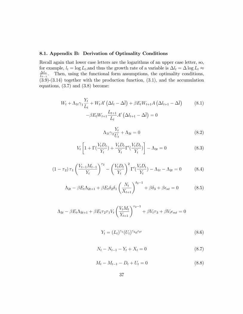
8.1. Appendix B: Derivation of Optimality Conditions

Recall again that lower case letters are the logarithms of an upper case letter, so,for example, lt = logLt,and thus the growth rate of a variable is ∆lt = ∆ logLt ≈∆LtLt−1

. Then, using the functional form assumptions, the optimality conditions,(3.9)-(3.14) together with the production function, (3.1), and the accumulationequations, (3.7) and (3.8) become:

Wt + Λ1tγ1YtLt+WtA

0 ¡∆lt −∆l¢+ βEtWt+1A

¡∆lt+1 −∆l

¢(8.1)

−βEtWt+1Lt+1

LtA0¡∆lt+1 −∆l

¢= 0

Λ1tγ2YtUt+ Λ3t = 0 (8.2)

Vt

∙1 + Γ(

VtDt

Yt) +

VtDt

YtΓ0(

VtDt

Yt)

¸− Λ3t = 0 (8.3)

(1− τ 2) τ 1

µVt−1Mt−1

Yt

¶τ2

−µVtDt

Yt

¶2Γ0(

VtDt

Yt)− Λ1t − Λ2t = 0 (8.4)

Λ2t − βEtΛ2t+1 + βEtδ2δ1

µNt

Xt+1

¶δ2−1+ βδ3 + β nt = 0 (8.5)

Λ3t − βEtΛ3t+1 + βEtτ 2τ 1Vt

µVtMt

Yt+1

¶τ2−1+ βVtτ 3 + βVt mt = 0

Yt = (Lt)γ1(Ut)

γ2e yt (8.6)

Nt −Nt−1 − Yt +Xt = 0 (8.7)

Mt −Mt−1 −Dt + Ut = 0 (8.8)

37

Re-arranging terms, we have that

1 + Λ1tγ1Yt

WtLt+A0

¡∆lt −∆l

¢+ βEt

Wt+1

Wt

£A¡∆lt+1 −∆l

¢¤(8.9)

−βEtWt+1

Wt

Lt+1

LtA0¡∆lt+1 −∆l

¢= 0

Λ1tγ2YtVtUt

+Λ3tVt= 0 (8.10)

1 + Γ(VtDt

Yt) +

VtDt

YtΓ0(

VtDt

Yt)− Λ3t

Vt= 0 (8.11)

(1− τ 2) τ 1

µVt−1Mt−1

Yt−1

Yt−1Yt

¶τ2

−µVtDt

Yt

¶2Γ0(

VtDt

Yt)− Λ1t − Λ2t = 0 (8.12)

Λ2t − βEtΛ2t+1 + βEtδ2δ1

µNt

Xt

Xt

Xt+1

¶δ2−1+ βδ3 + β nt = 0 (8.13)

Λ3tVt− βEt

Vt+1Vt

Λ3t+1Vt+1

+ βEtτ 2τ 1

µVtMt

Yt

YtYt+1

¶τ2−1+ βτ 3 + β mt = 0 (8.14)

µYtYt−1

¶= (

Lt

Lt−1)γ1(

Ut

Ut−1)γ2e yt− yt−1 (8.15)

Nt

Xt− Nt−1

Xt−1

Xt−1

Xt− Yt

Xt+ 1 = 0 (8.16)

VtMt

Yt− Vt

Vt−1

Vt−1Mt−1

Yt−1

Yt−1Yt− VtDt

Yt+

VtUt

Yt= 0 (8.17)

Now, define the growth rate of, for example, Xt , by Xt = (1 +∆xt)Xt−1, andsimilarly for other variables. Further, use the approximation, 1

1+∆xt≈ 1−∆xt

to re-write the optimality conditions as

38

1 + Λ1tγ1Yt

WtLt+A0

¡∆lt −∆l

¢+ βEt (1 + wt+1)A

¡∆lt+1 −∆l

¢(8.18)

−βEt (1 + wt+1) (1 + lt+1)A0 ¡∆lt+1 −∆l

¢= 0

Λ1tγ2YtVtUt

+Λ3tVt= 0 (8.19)

1 + Γ(VtDt

Yt) +

VtDt

YtΓ0(

VtDt

Yt)− Λ3t

Vt= 0 (8.20)

(1− τ 2) τ1

µVt−1Mt−1

Yt−1(1−∆yt)

¶τ2

−µVtDt

Yt

¶2Γ0(

VtDt

Yt)−Λ1t−Λ2t = 0 (8.21)

Λ2t − βEtΛ2t+1 + βEtδ2δ1

µNt

Xt(1−∆xt+1)

¶δ2−1+ βδ3 + β nt = 0 (8.22)

Λ3tVt− βEt (1 +∆vt+1)

Λ3t+1Vt+1

+ βEtτ 2τ 1

µVtMt

Yt(1−∆yt+1)

¶τ2−1+ βτ 3 (8.23)

+β mt = 0

∆yt = γ1∆lt + γ2∆ut + yt − yt−1 (8.24)

Nt

Xt− Nt−1

Xt−1(1−∆xt)−

YtXt+ 1 = 0 (8.25)

VtMt

Yt− (1 +∆vt) (1−∆yt)

Vt−1Mt−1

Yt−1− VtDt

Yt+

VtUt

Yt= 0 (8.26)

Then, using the definitions of the shares and ratios stated in (3.15), the opti-mality conditions may be written as

39

1 + Λ1tγ1S−1L,t +A0

¡∆lt −∆l

¢+ βEt (1 +∆wt+1)A

¡∆lt+1 −∆l

¢(8.27)

−βEt (1 +∆wt+1) (1 +∆lt+1)A0 ¡∆lt+1 −∆l

¢= 0

Λ1tγ2S−1U,t +RΛ3,t = 0 (8.28)

1 + Γ (RD,t) +RD,tΓ0 (RD,t)−RΛ3,t = 0 (8.29)

(1− τ 2) τ 1 (RM,t−1 (1−∆yt))τ2 −R2D,tΓ

0 (RD,t)− Λ1t − Λ2t = 0 (8.30)

Λ2t − βEtΛ2t+1 + βEtδ2δ1 (RN,t (1−∆xt+1))δ2−1 + βδ3 + β nt = 0 (8.31)

RΛ3,t − βEt (1 +∆vt+1)RΛ3,t+1 + βEtτ 2τ 1 (RM,t (1−∆yt+1))τ2−1 + βτ 3 (8.32)

+β mt = 0

∆yt = γ1∆lt + γ2∆ut + yt − yt−1 (8.33)

RN,t −RN,t−1 (1−∆xt)−RY,t + 1 = 0 (8.34)

RM,t − (1 +∆vt −∆yt)RM,t−1 −RD,t + SU,t = 0 (8.35)

where again Λ1t,Λ2t, and Λ3t are Lagrangian multipliers associated with (3.1),(3.7) and (3.8) respectively.In Section 4.2 it was assumed that RN,t, RM,t, and SL,t are all I(0). If these

three ratios are I(0), SUt, RD,t, RY,t, RΛ3t, Λ1t, and Λ2t are I(0) as well. To seethis, observe that if RN,t, RM,t,and SL,t are I(0), then Λ1t is I(0), (8.32) makesΛ2t I(0), (8.29) has RD,t as I(0), (8.30) makes RΛ3,t I(0), (8.28) makes SU,t I(0),(8.34) makes RY,t an I(0) variable.

40

We assume that in steady state the expected values of the factor input shares,SU,t and SL,t, the ratios RN,t, RM,t, RD,t, RY,t, and RΛ3,t, and the growth rates ofvariables are constants. The non-stochastic steady state conditions are then:

1 + Λ1γ1S−1L = 0 (8.36)

1 + Λ1γ2S−1U = 0 (8.37)

RΛ3 = 1 (8.38)

(1− τ 2) τ 1£RM (1−∆y)

¤τ2 − Λ1 − Λ2 = 0 (8.39)

(1− β)Λ2 + βδ2δ1£RN (1−∆x)

¤δ2−1+ βδ3 = 0 (8.40)

[1− β (1 +∆v)] + βτ 2τ 1£RM (1−∆y)

¤τ2−1+ βτ 3 = 0 (8.41)

γ1∆l + γ2∆u = ∆y (8.42)

1 +∆xRN = RY (8.43)

RD + (∆v −∆y)RM = SU (8.44)

Again, in Section 4.2 above on estimation strategy, we stated that estimatesof the four parameters in θ2 are found from appropriate steady state conditions.Specifically, they are found from the four equations corresponding to the steadystate conditions (8.37) and (8.38)-(8.41).Now, log-linearizing the optimality conditions, (8.27)-(8.35), around the con-

stant steady state values, (8.36)-(8.44) yields the log-linearized optimality condi-tions stated above in (3.16)-(3.24).

41