
IntSB
75
Bioinformatics: Applications ZOO 4903 Fall 2006, MW 10:30-11:45 Sutton Hall, Room 312 Jonathan Wren Systems Biology
-
Upload
lordniklaus -
Category
Documents
-
view
2 -
download
0
description
IntSB
Transcript of IntSB
Bioinformatics: Applications
ZOO 4903
Fall 2006, MW 10:30-11:45
Sutton Hall, Room 312
Jonathan Wren
Systems Biology
Lecture overview
• What we’ve talked about so far– Pathways & network motifs– Simulating evolution in-silico– Cellular simulations
• Overview– The ultimate goal of biology & bioinformatics
is to tie it all together and understand the system
– In the meantime, forced to live in the real world, we focus on tying a few things together
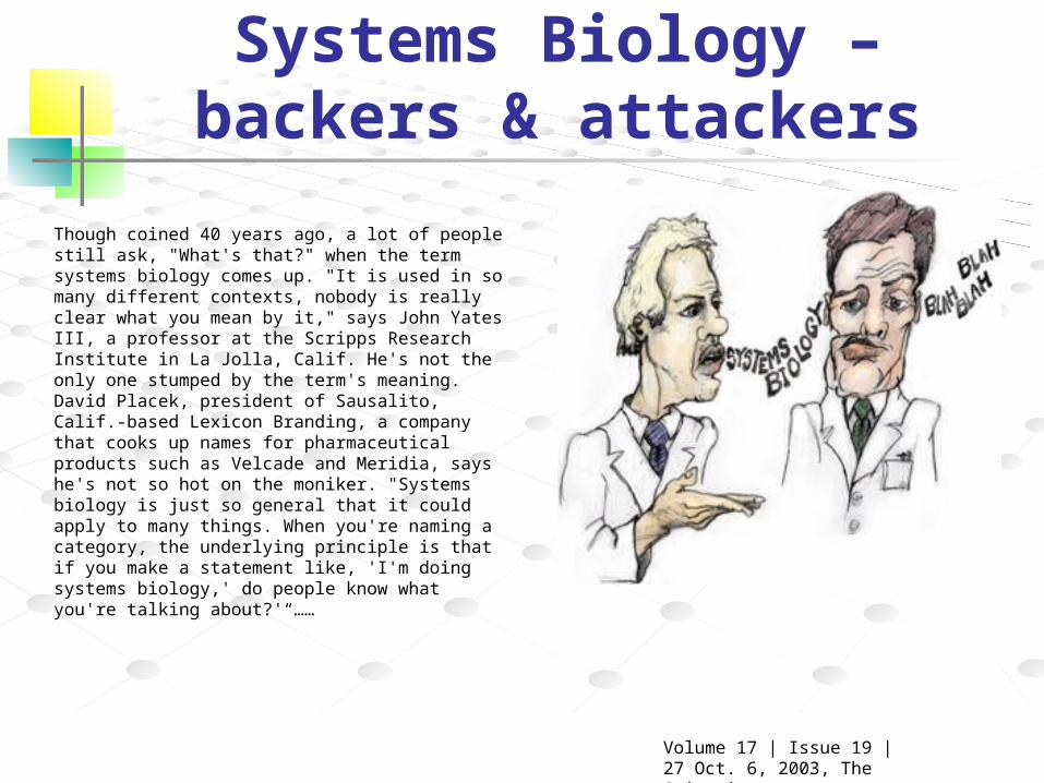
Though coined 40 years ago, a lot of people still ask, "What's that?" when the term systems biology comes up. "It is used in so many different contexts, nobody is really clear what you mean by it," says John Yates III, a professor at the Scripps Research Institute in La Jolla, Calif. He's not the only one stumped by the term's meaning. David Placek, president of Sausalito, Calif.-based Lexicon Branding, a company that cooks up names for pharmaceutical products such as Velcade and Meridia, says he's not so hot on the moniker. "Systems biology is just so general that it could apply to many things. When you're naming a category, the underlying principle is that if you make a statement like, 'I'm doing systems biology,' do people know what you're talking about?'“……
Volume 17 | Issue 19 | 27 Oct. 6, 2003, The Scientist
Systems Biology – backers & attackers
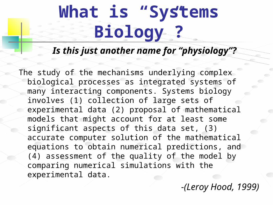
What is “Systems Biology”?
The study of the mechanisms underlying complex biological processes as integrated systems of many interacting components. Systems biology involves (1) collection of large sets of experimental data (2) proposal of mathematical models that might account for at least some significant aspects of this data set, (3) accurate computer solution of the mathematical equations to obtain numerical predictions, and (4) assessment of the quality of the model by comparing numerical simulations with the experimental data.
-(Leroy Hood, 1999)
Is this just another name for “physiology”?
Institute for Systems Biology
http://www.systemsbiology.org/
Why Systems Biology?
• On the technology side (PUSH): Capabilities for high-throughput data gathering that have made us aware that biological networks have many more components than we previously surmised.
• On the biology side (PULL): The realization that to the extent that we don’t characterize biological systems quantitatively in their full complexity, the scope and accuracy of our understanding of those systems will be compromised. (in classical experimental terms, the uncontrolled variables in the system will undermine our confidence in the conclusions we draw from our experiments and observations)
Systems Biology vs. traditional cell and molecular biology
• Experimental techniques in systems biology are high throughput.
• Intensive computation is involved from the start in systems biology, in order to organize the data into usable computable databases.
• Exploration in traditional biology proceeds by successive cycles of hypothesis formation and testing; data accumulates during these cycles.
• Systems biology initially gathers data without prior hypothesis formation; hypothesis formation and testing comes during post-experiment data analysis and modeling.
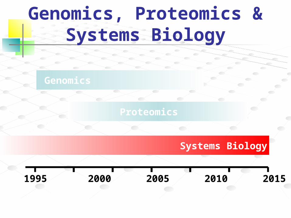
Genomics, Proteomics & Systems Biology
1990 1995 2000 2005 2010 2015 2020
Genomics
Proteomics
Systems Biology
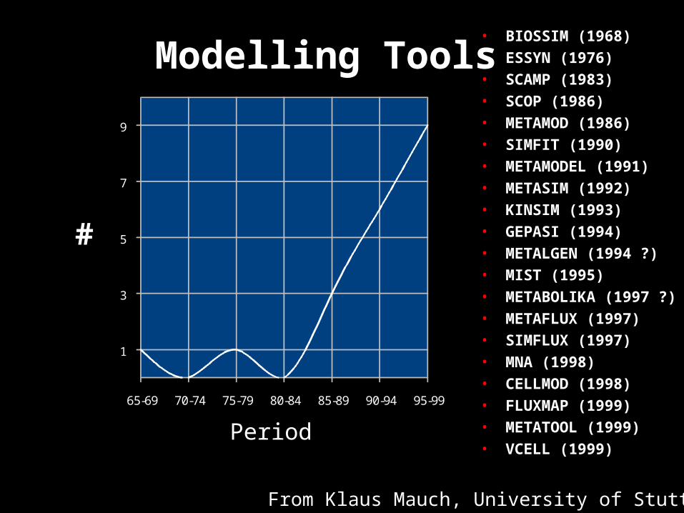
• BIOSSIM (1968)• ESSYN (1976)• SCAMP (1983)• SCOP (1986)• METAMOD (1986)• SIMFIT (1990)• METAMODEL (1991)• METASIM (1992)• KINSIM (1993)• GEPASI (1994)• METALGEN (1994 ?)• MIST (1995)• METABOLIKA (1997 ?)• METAFLUX (1997)• SIMFLUX (1997)• MNA (1998)• CELLMOD (1998)• FLUXMAP (1999)• METATOOL (1999)• VCELL (1999)
65-69 70-74 75-79 80-84 85-89 90-94 95-99
1
3
5
7
9
Period
From Klaus Mauch, University of Stuttgart
#
Modelling Tools
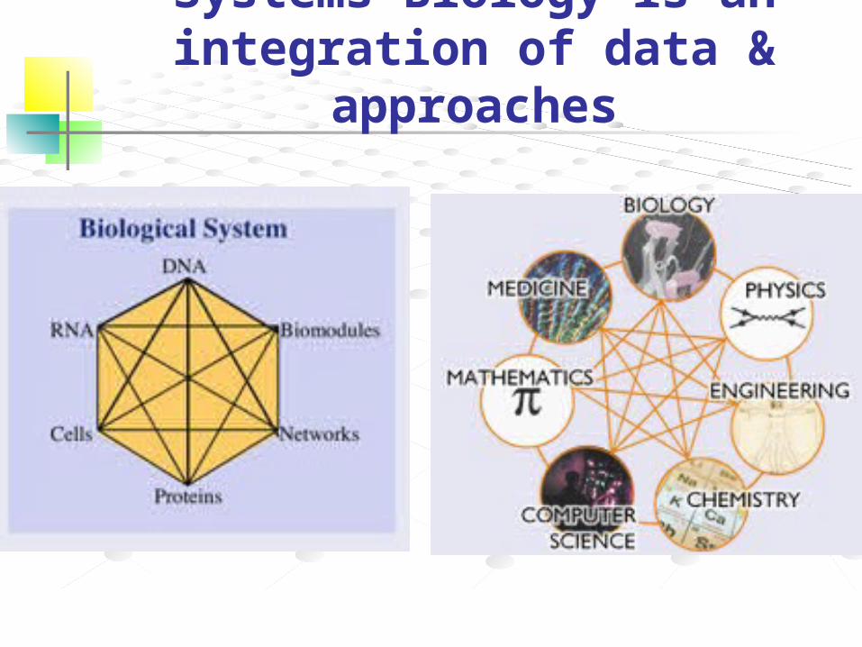
Systems Biology is an integration of data & approaches
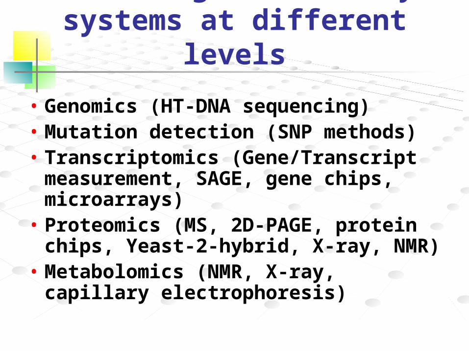
Technologies to study systems at different levels
• Genomics (HT-DNA sequencing)• Mutation detection (SNP methods)• Transcriptomics (Gene/Transcript
measurement, SAGE, gene chips, microarrays)
• Proteomics (MS, 2D-PAGE, protein chips, Yeast-2-hybrid, X-ray, NMR)
• Metabolomics (NMR, X-ray, capillary electrophoresis)
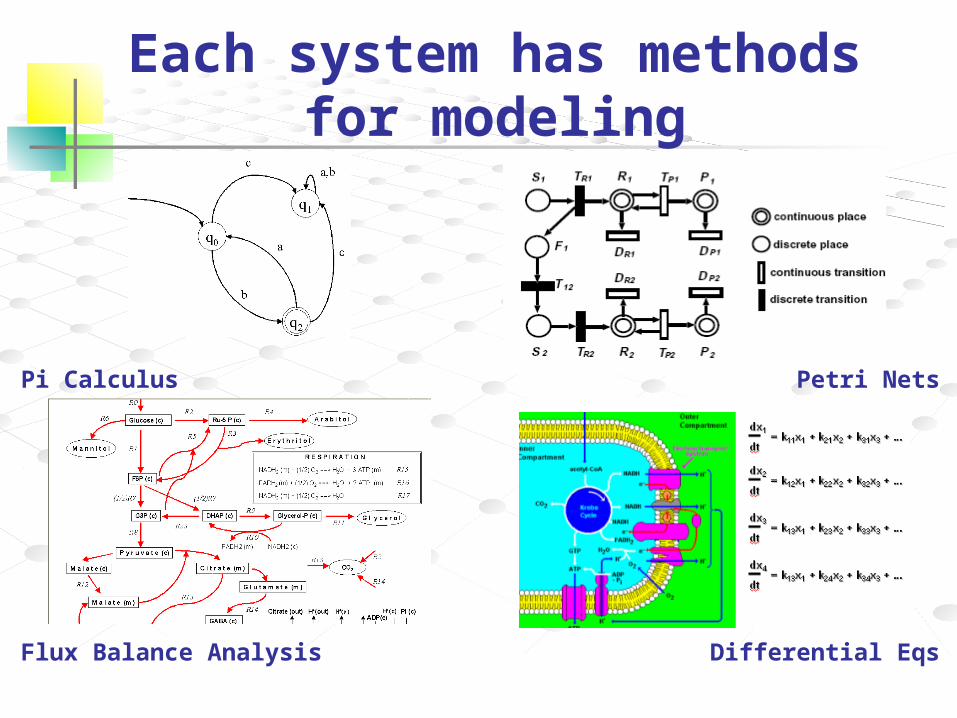
Each system has methods for modeling
Pi Calculus Petri Nets
Flux Balance Analysis Differential Eqs
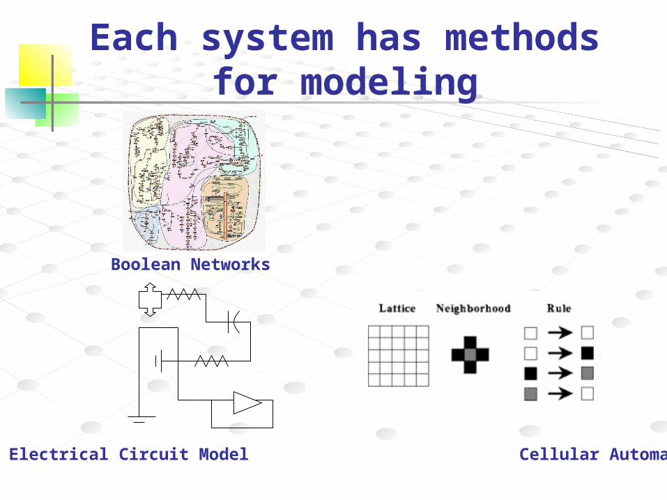
Each system has methods for modeling
Boolean Networks
Electrical Circuit Model Cellular Automata
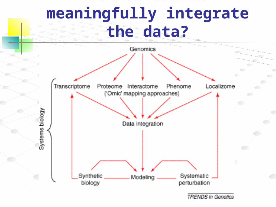
So how can we meaningfully integrate the data?
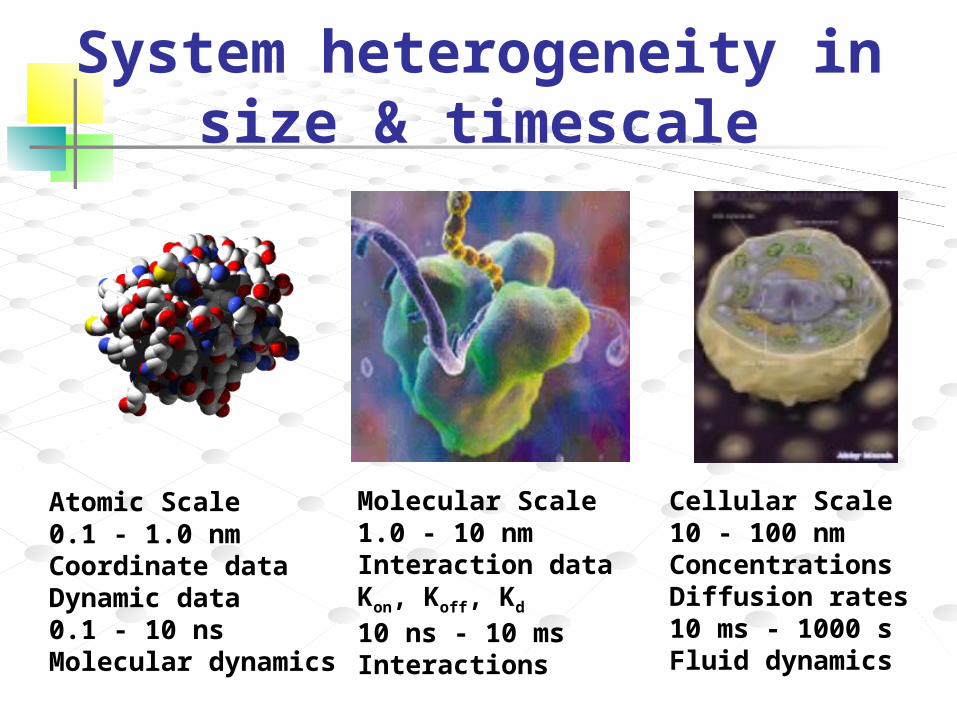
System heterogeneity in size & timescale
Atomic Scale0.1 - 1.0 nmCoordinate dataDynamic data0.1 - 10 nsMolecular dynamics
Molecular Scale1.0 - 10 nmInteraction dataKon, Koff, Kd
10 ns - 10 msInteractions
Cellular Scale10 - 100 nmConcentrationsDiffusion rates10 ms - 1000 sFluid dynamics
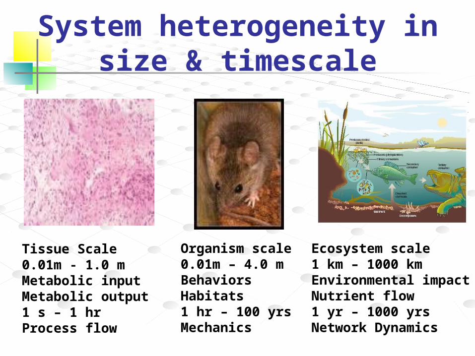
System heterogeneity in size & timescale
Tissue Scale0.01m - 1.0 mMetabolic inputMetabolic output1 s – 1 hrProcess flow
Organism scale0.01m – 4.0 mBehaviorsHabitats1 hr – 100 yrsMechanics
Ecosystem scale1 km – 1000 kmEnvironmental impactNutrient flow1 yr – 1000 yrsNetwork Dynamics
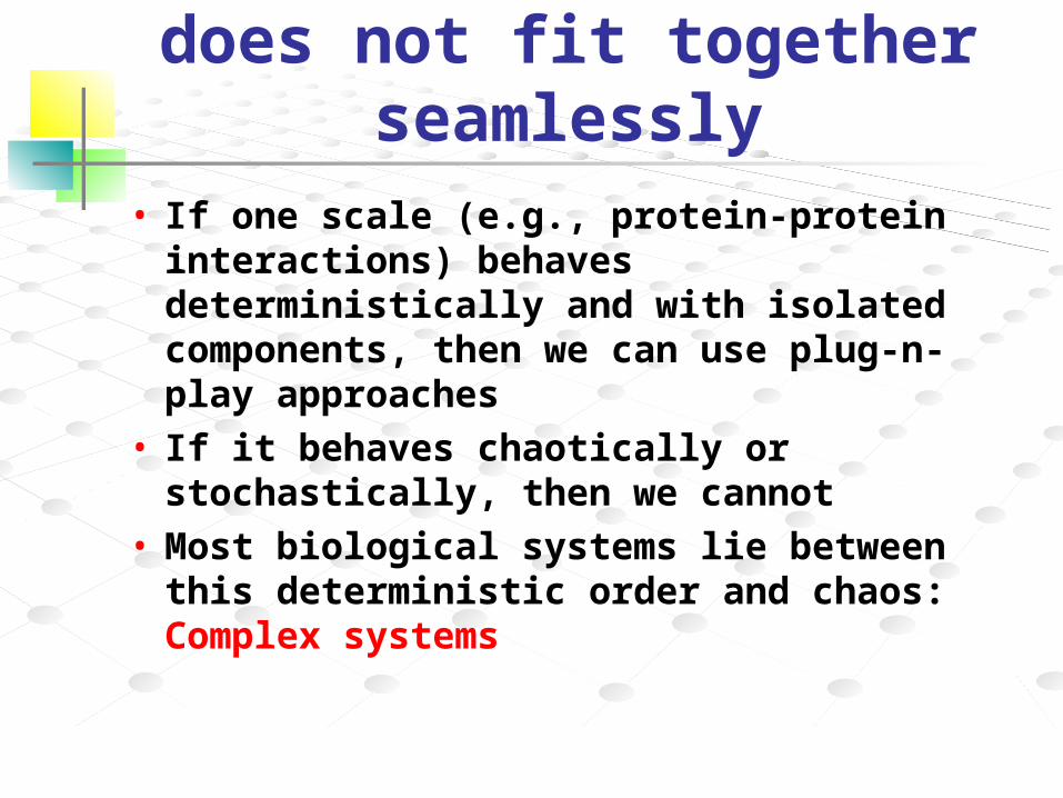
Each of the scales does not fit together seamlessly
• If one scale (e.g., protein-protein interactions) behaves deterministically and with isolated components, then we can use plug-n-play approaches
• If it behaves chaotically or stochastically, then we cannot
• Most biological systems lie between this deterministic order and chaos: Complex systems
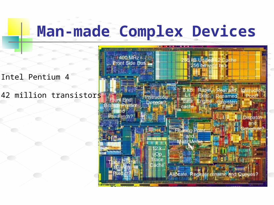
Man-made Complex Devices
Intel Pentium 4
42 million transistors

Man-made Complex Devices
• The Intel Itanium 2• 410 million transistors• Number of gates > 100 Million
By 2007 both Intel and AMD are predicting dies with 1 billion transistors
In terms of parts and interconnections, man-made devices will likely have comparable complexity to bacterial cells if not greater by around 2010
System Models
Building computational models of systems seems more and more like a viable project.
Such a project would bring a much clearer understanding of how systems are controlled and ultimately it should bring unprecedented predictive power.
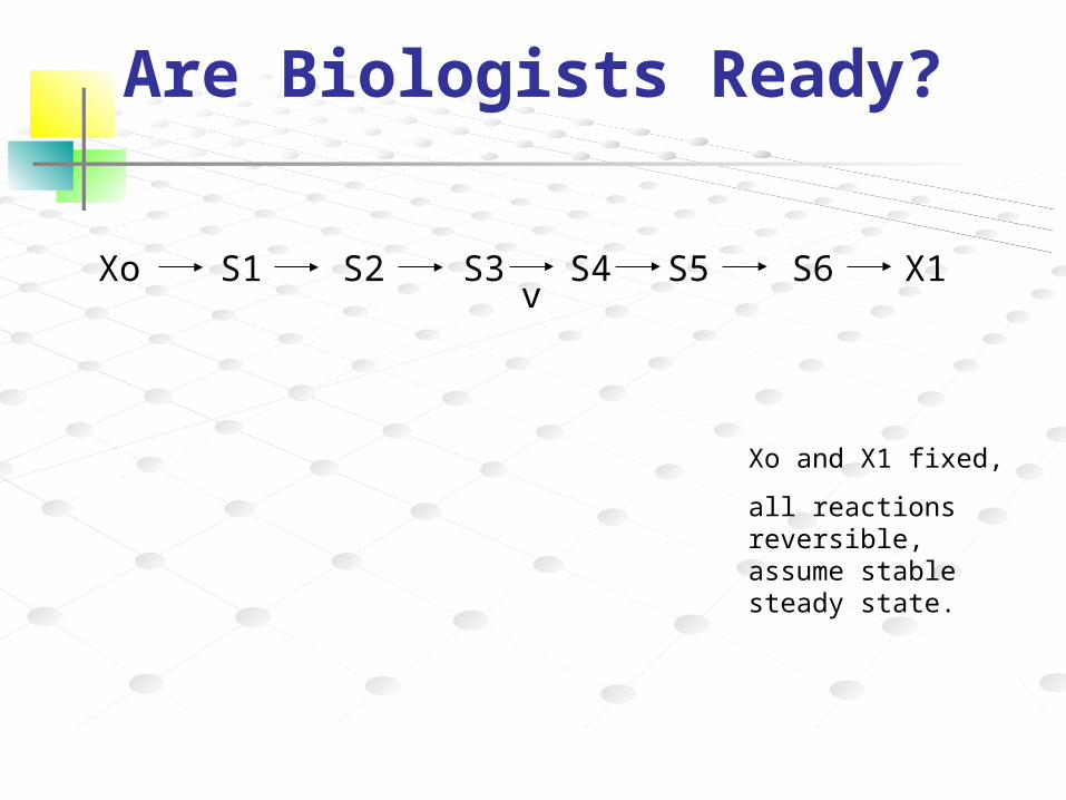
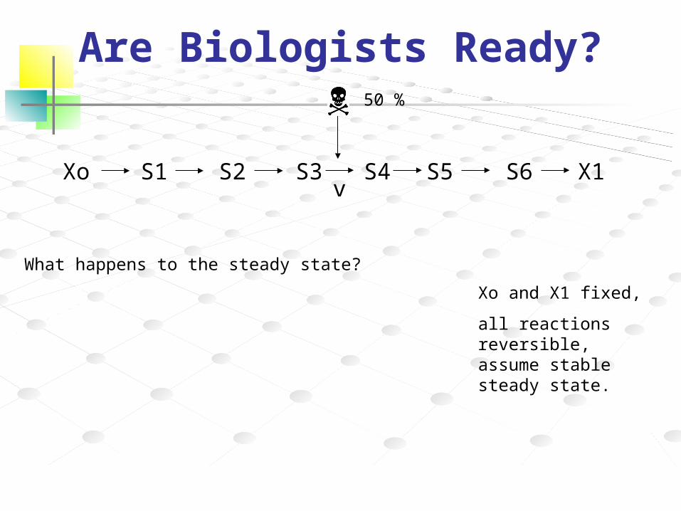
Are Biologists Ready?
Xo and X1 fixed,
all reactions reversible, assume stable steady state.
Xo S1 S2 X1S3 S4 S5 S6v
Are Biologists Ready?
What happens to the steady state?
Xo S1 S2 X1S3 S4 S5 S6v
Xo and X1 fixed,
all reactions reversible, assume stable steady state.
50 %
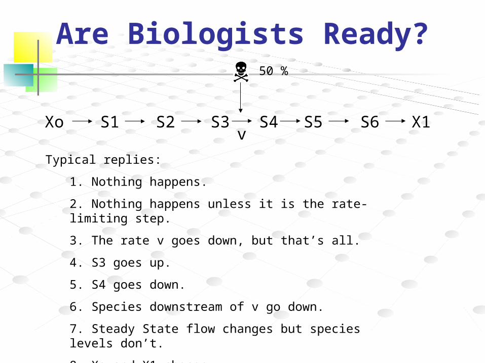
Are Biologists Ready?
Xo S1 S2 X1S3 S4 S5 S6
Typical replies:
1. Nothing happens.
2. Nothing happens unless it is the rate-limiting step.
3. The rate v goes down, but that’s all.
4. S3 goes up.
5. S4 goes down.
6. Species downstream of v go down.
7. Steady State flow changes but species levels don’t.
8. Xo and X1 change
v
50 %
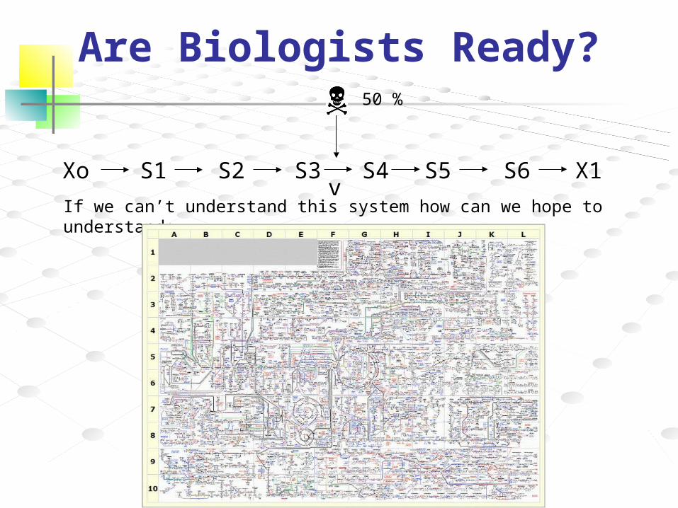
Are Biologists Ready?
Xo S1 S2 X1S3 S4 S5 S6
If we can’t understand this system how can we hope to understand:v
50 %
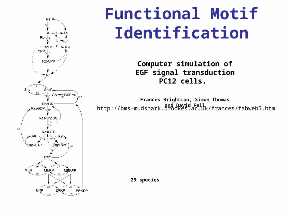
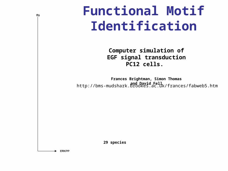
Functional Motif Identification
http://bms-mudshark.brookes.ac.uk/frances/fabweb5.htm
29 species
Computer simulation of EGF signal transduction PC12 cells.
Frances Brightman, Simon Thomas and David Fell
Functional Motif Identification
http://bms-mudshark.brookes.ac.uk/frances/fabweb5.htm
29 species
Computer simulation of EGF signal transduction PC12 cells.
Frances Brightman, Simon Thomas and David Fell
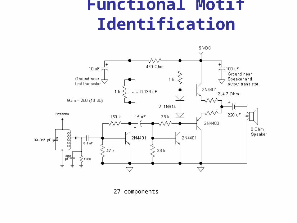
Functional Motif Identification
27 components
Functional Motif Identification
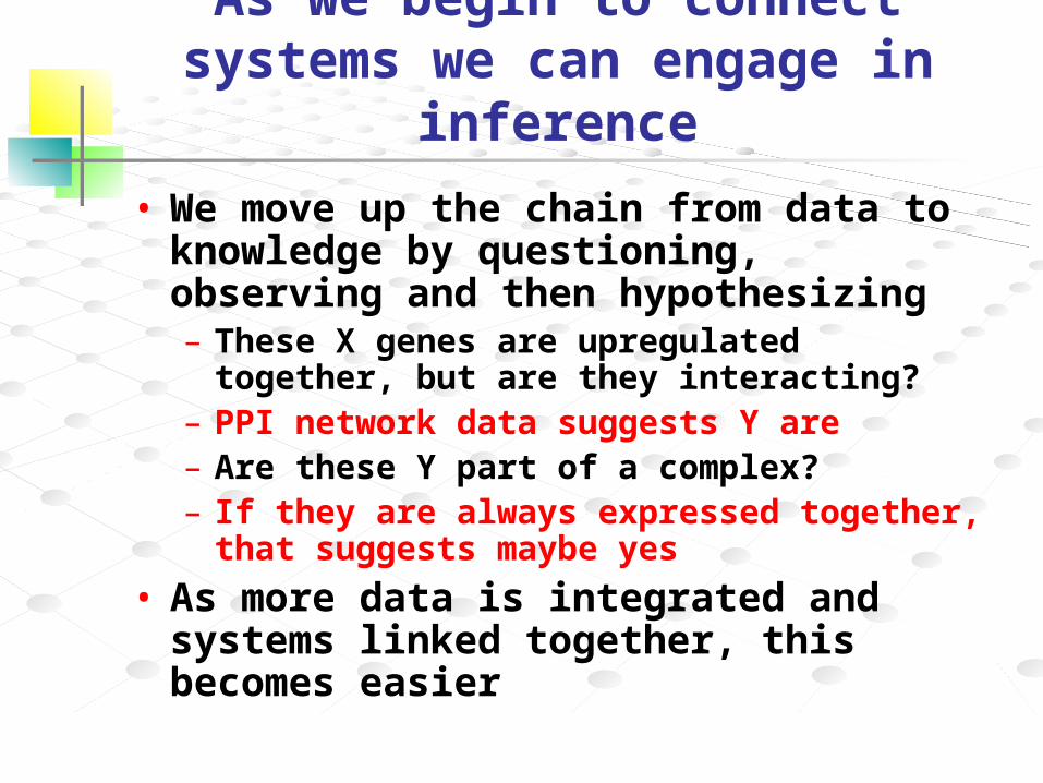
As we begin to connect systems we can engage in inference
• We move up the chain from data to knowledge by questioning, observing and then hypothesizing– These X genes are upregulated together, but
are they interacting?– PPI network data suggests Y are– Are these Y part of a complex?– If they are always expressed together, that
suggests maybe yes
• As more data is integrated and systems linked together, this becomes easier
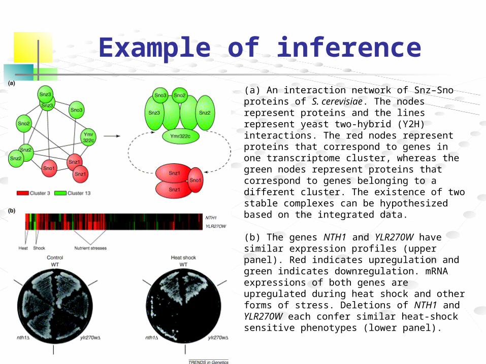
Example of inference
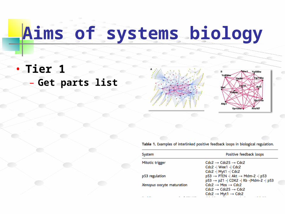
(a) An interaction network of Snz–Sno proteins of S. cerevisiae. The nodes represent proteins and the lines represent yeast two-hybrid (Y2H) interactions. The red nodes represent proteins that correspond to genes in one transcriptome cluster, whereas the green nodes represent proteins that correspond to genes belonging to a different cluster. The existence of two stable complexes can be hypothesized based on the integrated data.
(b) The genes NTH1 and YLR270W have similar expression profiles (upper panel). Red indicates upregulation and green indicates downregulation. mRNA expressions of both genes are upregulated during heat shock and other forms of stress. Deletions of NTH1 and YLR270W each confer similar heat-shock sensitive phenotypes (lower panel).
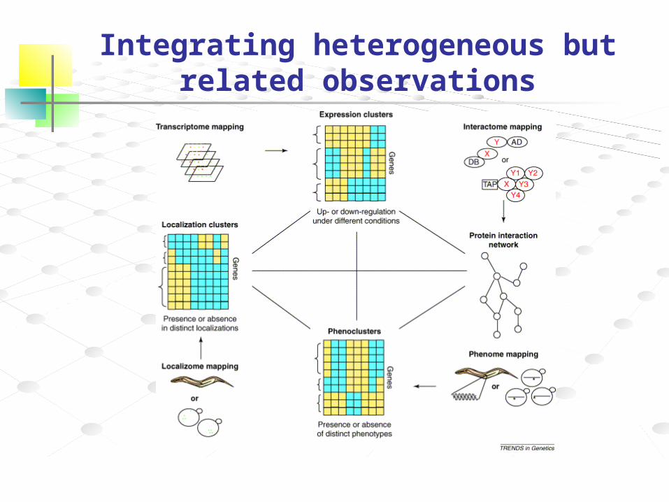
Integrating heterogeneous but related observations
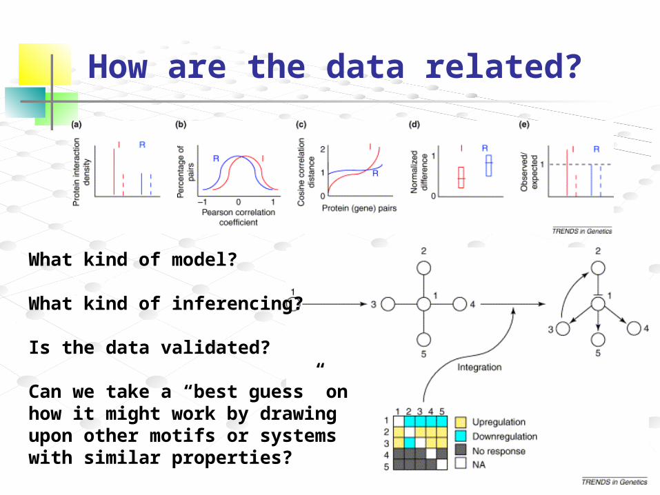
How are the data related?
What kind of model?
What kind of inferencing?
Is the data validated?
Can we take a “best guess” on how it might work by drawing upon other motifs or systems with similar properties?

Problems?
How is static data interpreted since it’s a dynamic system?
How do we deal with low-resolution quality?
How do we treat missing data?
How do we deal with heterogeneous data types?
How can we identify and evaluate competing hypotheses inferred by any system?
Yes…
SB is springing out of existing efforts anyway
• E-cell (Keio University, Japan)• BioSpice Project (Arkin, Berkeley)• Metabolic Engineering Working Group (Palsson
& Church, UCSD, Harvard)• Silicon Cell Project (Netherlands)• Virtual Cell Project (UConn)• Gene Network Sciences Inc. (Cornell)• Project CyberCell (Edmonton/Calgary)
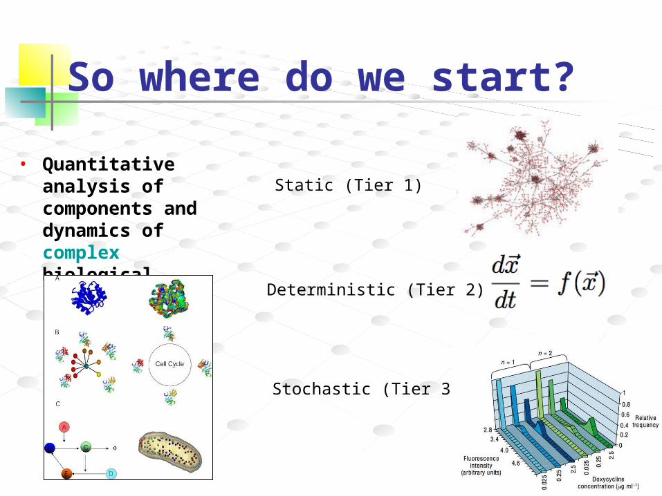
So where do we start?
• Quantitative analysis of components and dynamics of complex biological systems
Static (Tier 1)
Deterministic (Tier 2)
Stochastic (Tier 3)
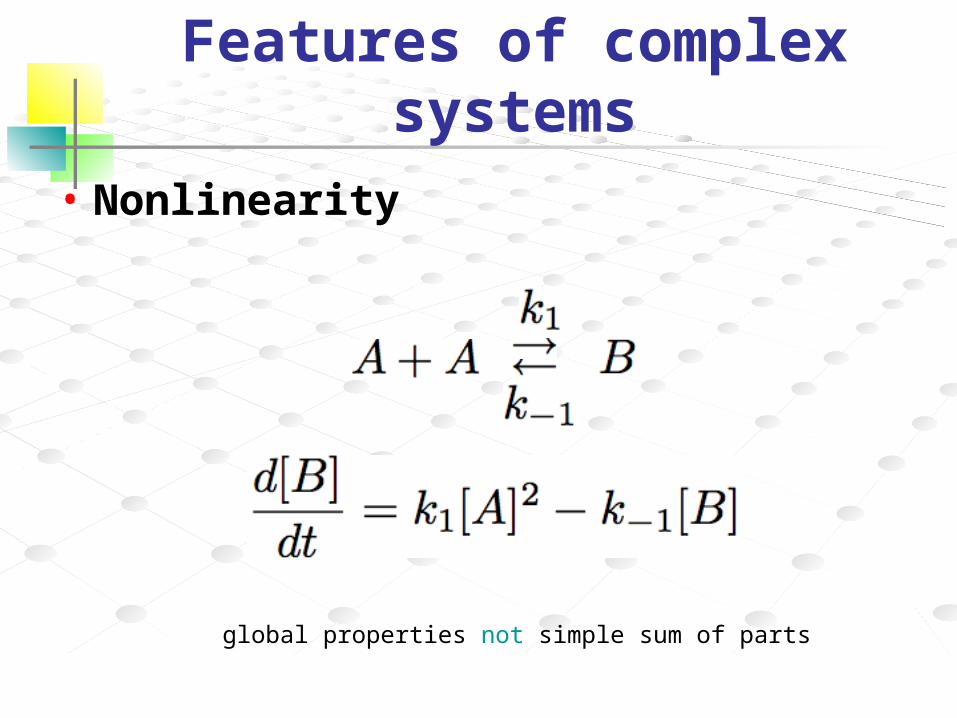
Features of complex systems• Nonlinearity
global properties not simple sum of parts
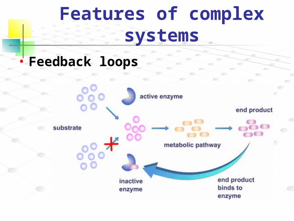
Features of complex systems• Feedback loops
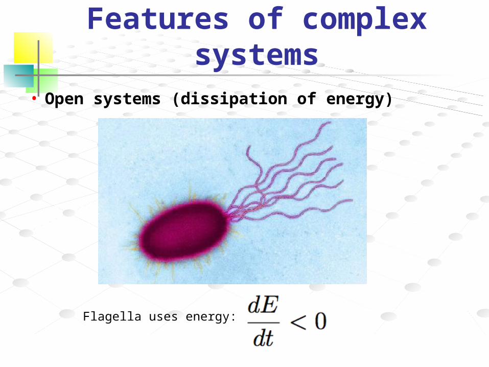
Features of complex systems• Open systems (dissipation of energy)
Flagella uses energy:
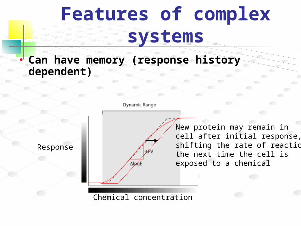
Features of complex systems• Can have memory (response history
dependent)
New protein may remain incell after initial response, shifting the rate of reactionthe next time the cell isexposed to a chemical
Chemical concentration
Response
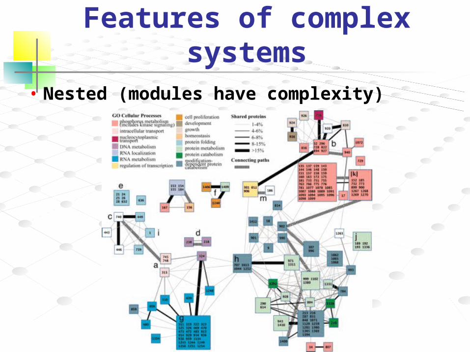
Features of complex systems• Nested (modules have complexity)
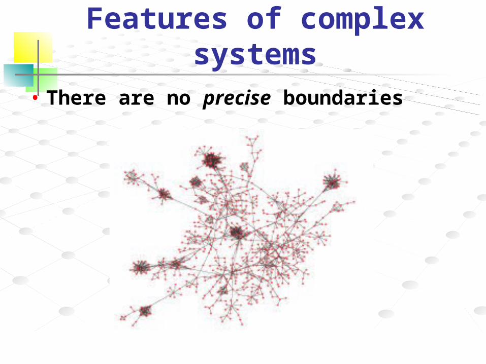
Features of complex systems• There are no precise boundaries
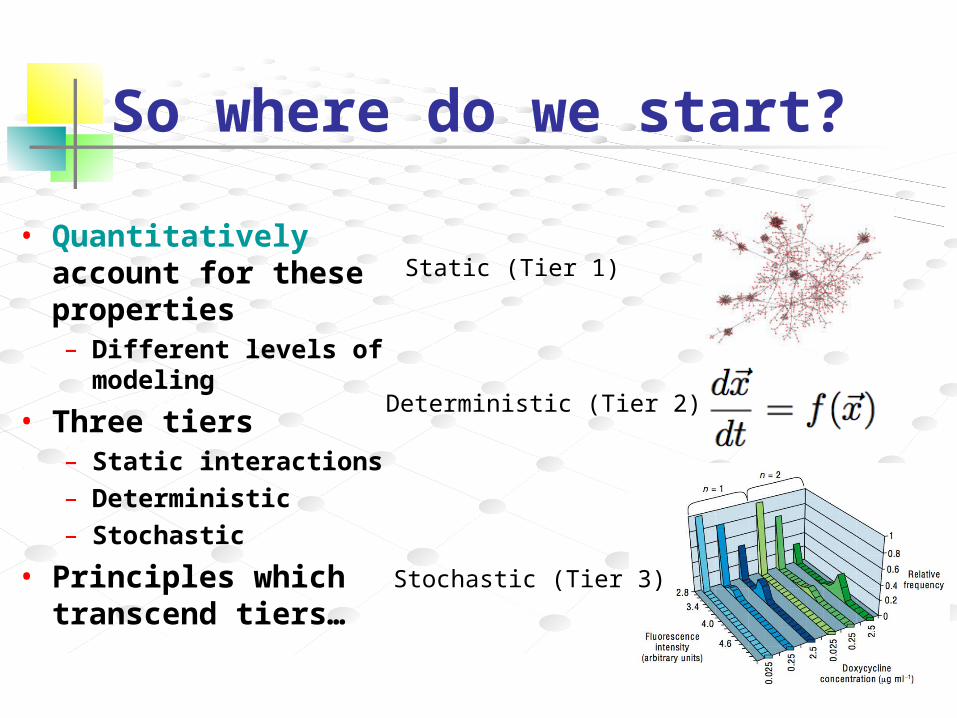
So where do we start?
• Quantitatively account for these properties– Different levels of
modeling
• Three tiers– Static interactions– Deterministic– Stochastic
• Principles which transcend tiers…
Static (Tier 1)
Deterministic (Tier 2)
Stochastic (Tier 3)
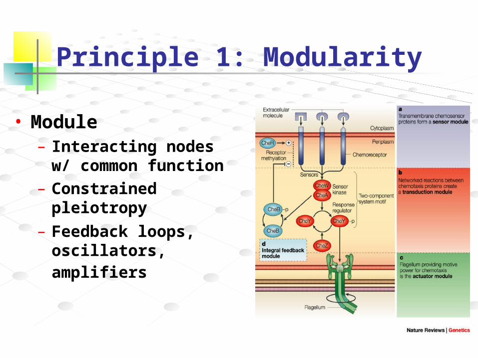
Principle 1: Modularity
• Module– Interacting nodes w/
common function– Constrained pleiotropy
– Feedback loops, oscillators, amplifiers
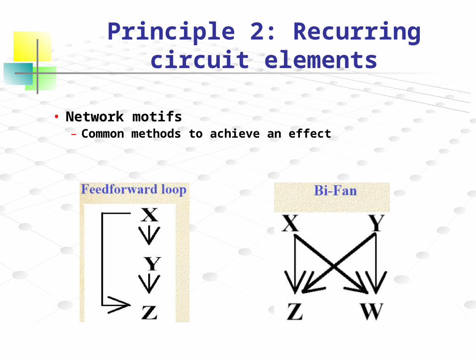
Principle 2: Recurring circuit elements
• Network motifs– Common methods to achieve an effect
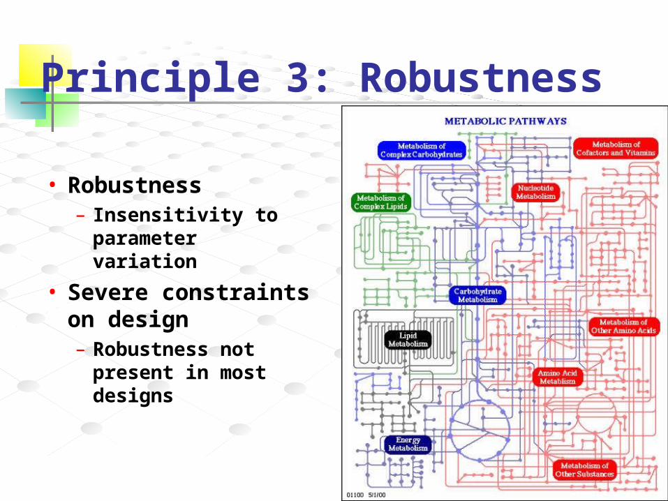
Principle 3: Robustness
• Robustness– Insensitivity to
parameter variation
• Severe constraints on design– Robustness not
present in most designs
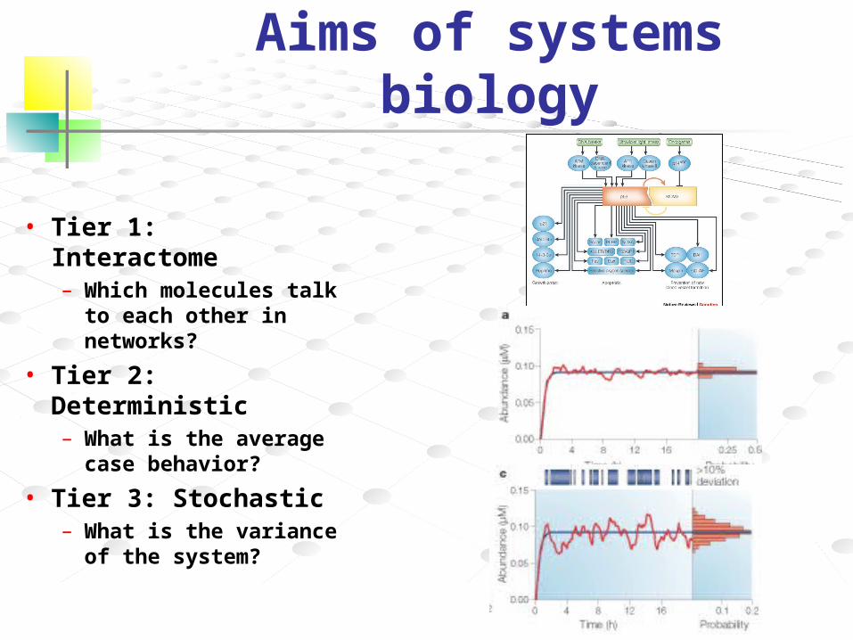
Aims of systems biology
• Tier 1: Interactome– Which molecules talk
to each other in networks?
• Tier 2: Deterministic– What is the average
case behavior?
• Tier 3: Stochastic– What is the variance
of the system?
Aims of systems biology
• Tier 1– Get parts list
Aims of systems biology
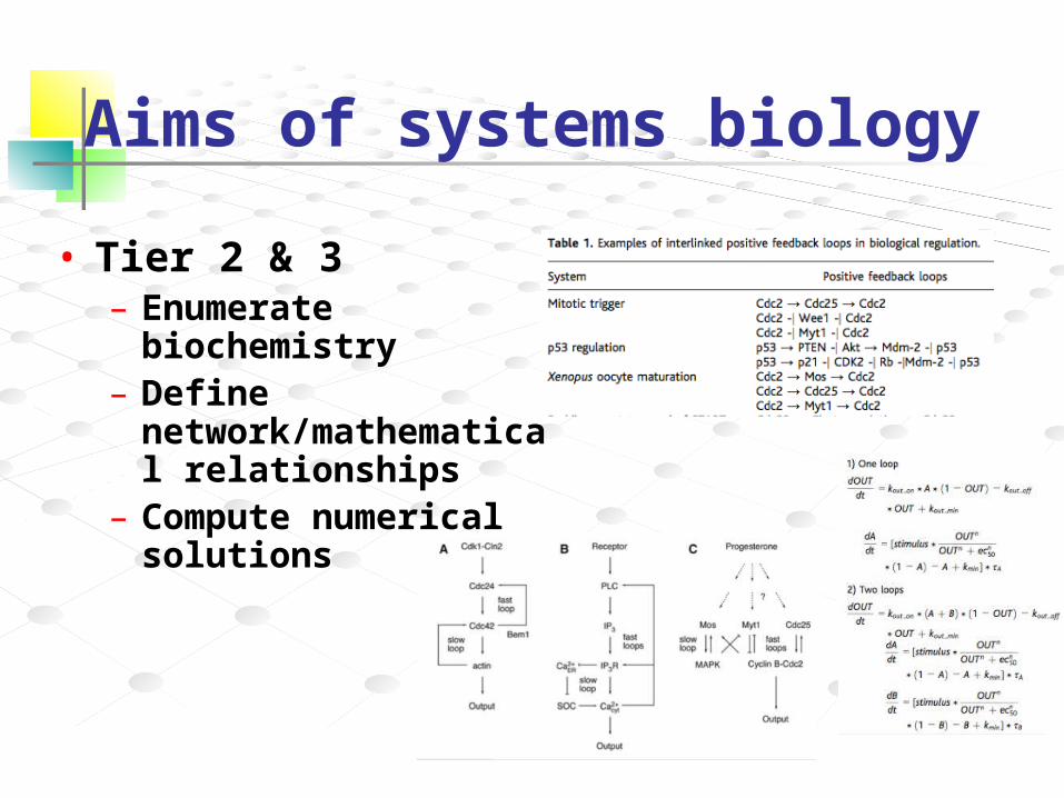
• Tier 2 & 3– Enumerate
biochemistry– Define
network/mathematical relationships
– Compute numerical solutions
Aims of systems biology
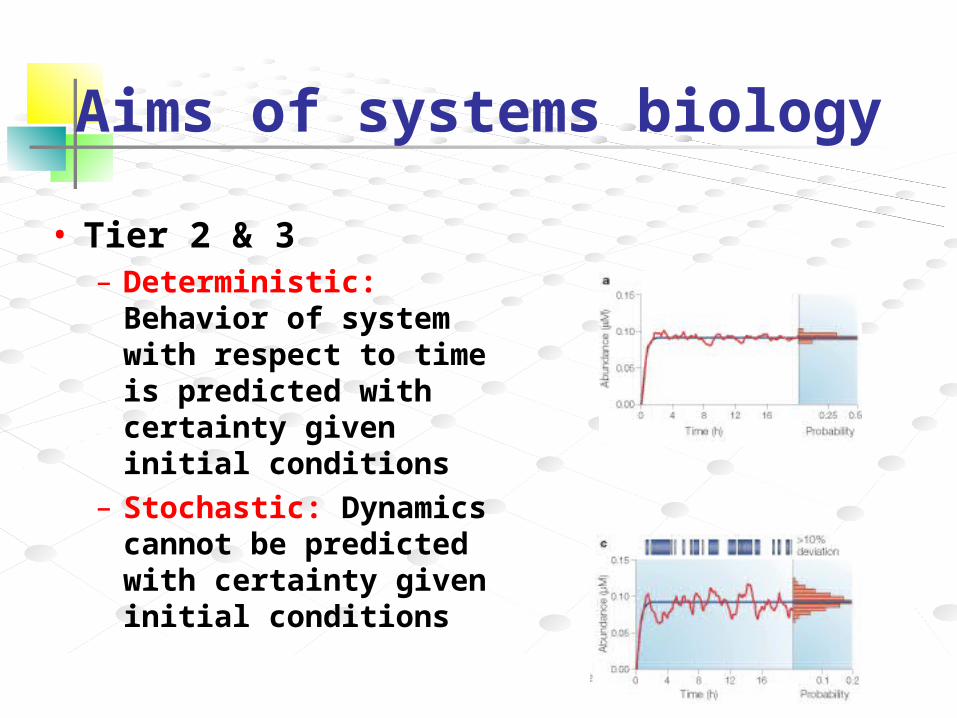
• Tier 2 & 3– Deterministic: Behavior of
system with respect to time is predicted with certainty given initial conditions
– Stochastic: Dynamics cannot be predicted with certainty given initial conditions
Aims of systems biology
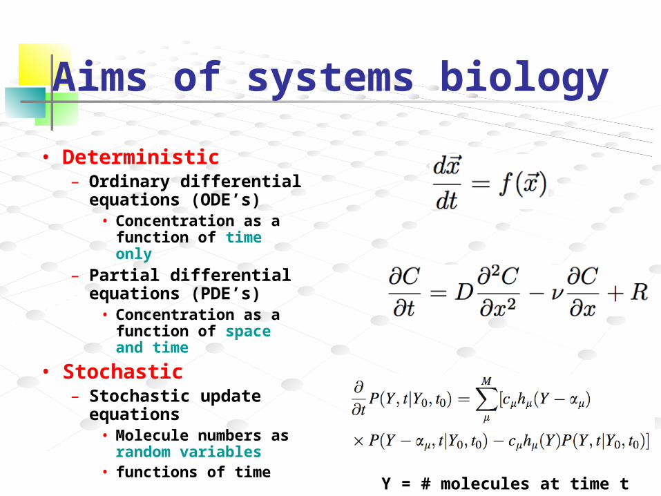
• Deterministic– Ordinary differential
equations (ODE’s)• Concentration as a
function of time only
– Partial differential equations (PDE’s)
• Concentration as a function of space and time
• Stochastic– Stochastic update
equations• Molecule numbers as
random variables• functions of time Y = # molecules at time t
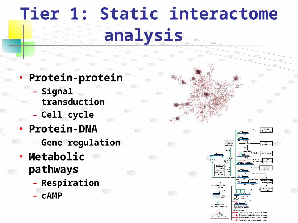
Tier 1: Static interactome analysis
• Protein-protein– Signal transduction
– Cell cycle
• Protein-DNA– Gene regulation
• Metabolic pathways– Respiration
– cAMP
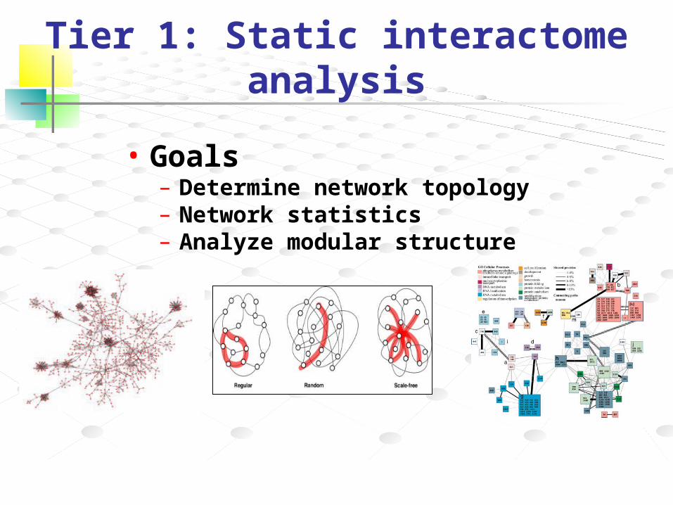
Tier 1: Static interactome analysis
• Goals– Determine network topology– Network statistics– Analyze modular structure
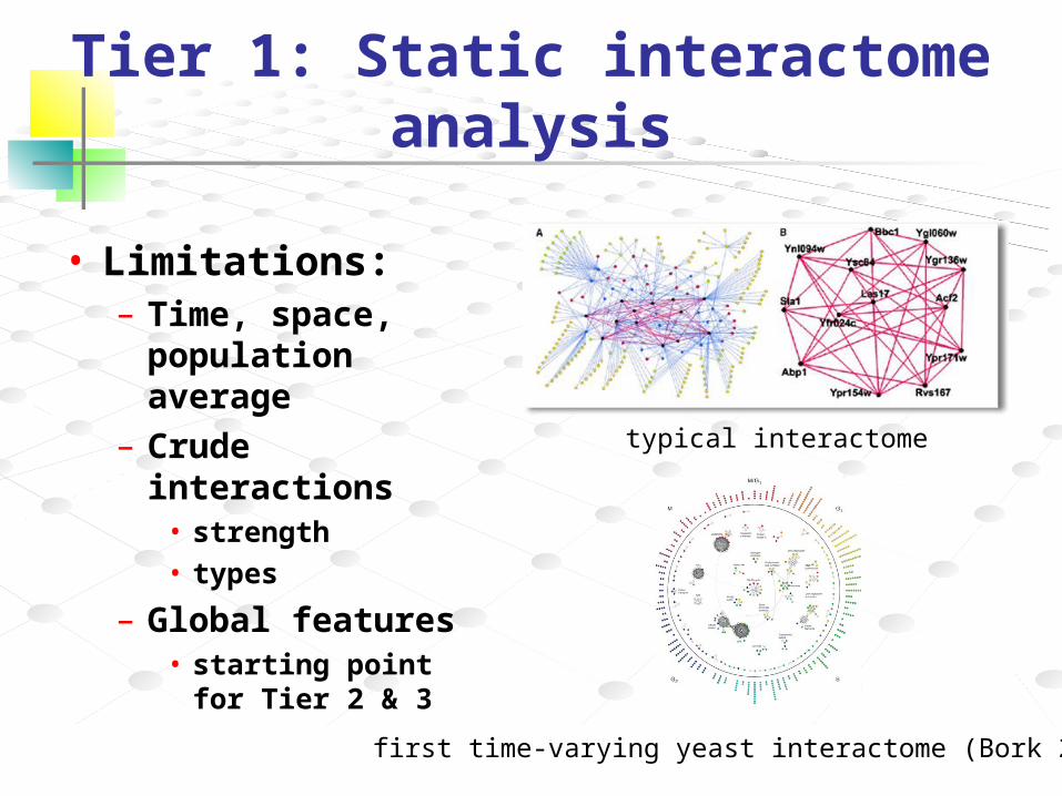
Tier 1: Static interactome analysis
• Limitations:– Time, space,
population average
– Crude interactions• strength• types
– Global features• starting point for
Tier 2 & 3
first time-varying yeast interactome (Bork 2005)
typical interactome
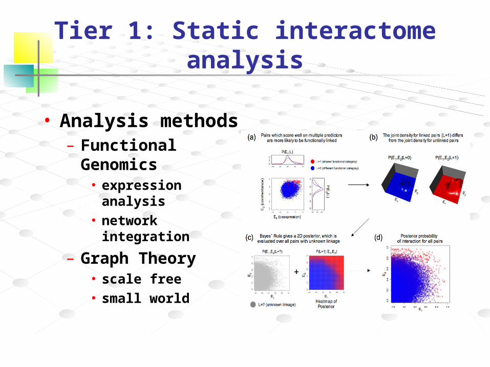
Tier 1: Static interactome analysis
• Analysis methods– Functional
Genomics• expression analysis• network integration
– Graph Theory• scale free• small world
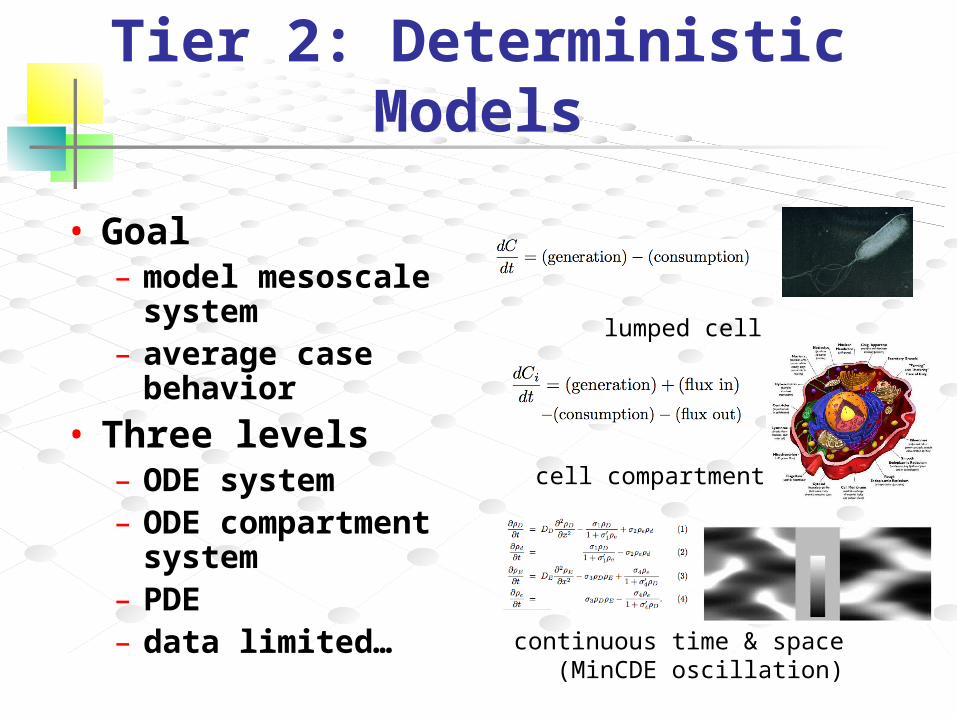
Tier 2: Deterministic Models
• Goal– model mesoscale
system– average case
behavior
• Three levels– ODE system– ODE compartment
system– PDE – data limited…
lumped cell
cell compartments
continuous time & space (MinCDE oscillation)
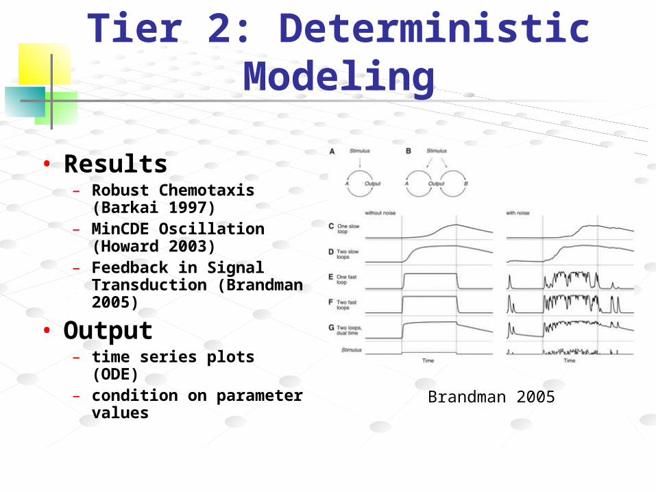
Tier 2: Deterministic Modeling
• Results– Robust Chemotaxis
(Barkai 1997)– MinCDE Oscillation
(Howard 2003)– Feedback in Signal
Transduction (Brandman 2005)
• Output– time series plots (ODE)– condition on parameter
values Brandman 2005
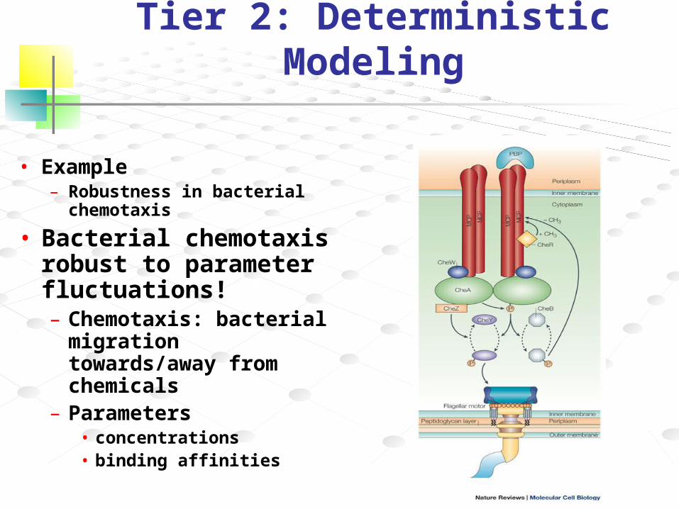
Tier 2: Deterministic Modeling
• Example– Robustness in bacterial
chemotaxis
• Bacterial chemotaxis robust to parameter fluctuations!– Chemotaxis: bacterial
migration towards/away from chemicals
– Parameters• concentrations• binding affinities
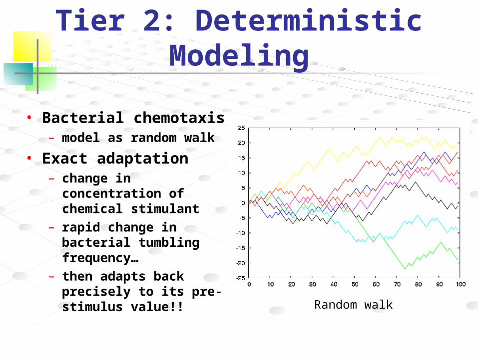
Tier 2: Deterministic Modeling
• Bacterial chemotaxis– model as random walk
• Exact adaptation – change in concentration
of chemical stimulant – rapid change in bacterial
tumbling frequency…– then adapts back
precisely to its pre-stimulus value!!
Random walk
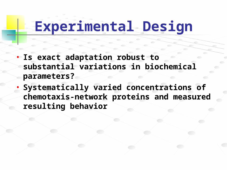
Experimental Design
• Is exact adaptation robust to substantial variations in biochemical parameters?
• Systematically varied concentrations of chemotaxis-network proteins and measured resulting behavior
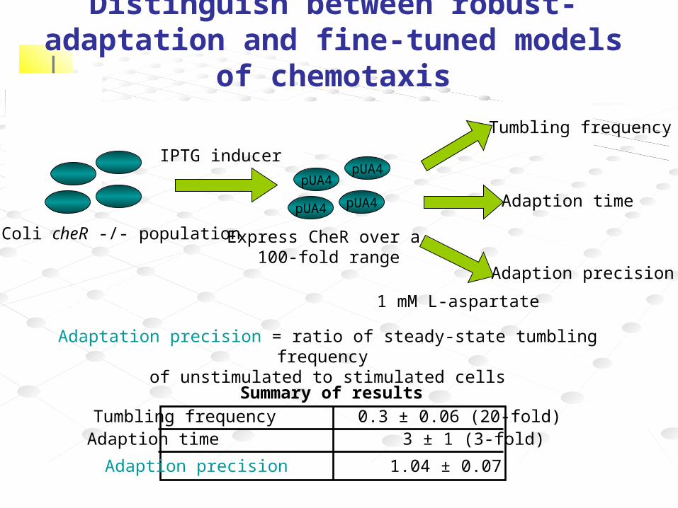
E. Coli cheR -/- population
pUA4
pUA4
pUA4
pUA4
Express CheR over a 100-fold range
IPTG inducer
Tumbling frequency
Adaption time
Adaption precision
Tumbling frequency 0.3 ± 0.06 (20-fold) Adaption time 3 ± 1 (3-fold)
Adaption precision 1.04 ± 0.07
1 mM L-aspartate
Summary of results
Adaptation precision = ratio of steady-state tumbling frequency of unstimulated to stimulated cells
Distinguish between robust-adaptation and fine-tuned models of chemotaxis
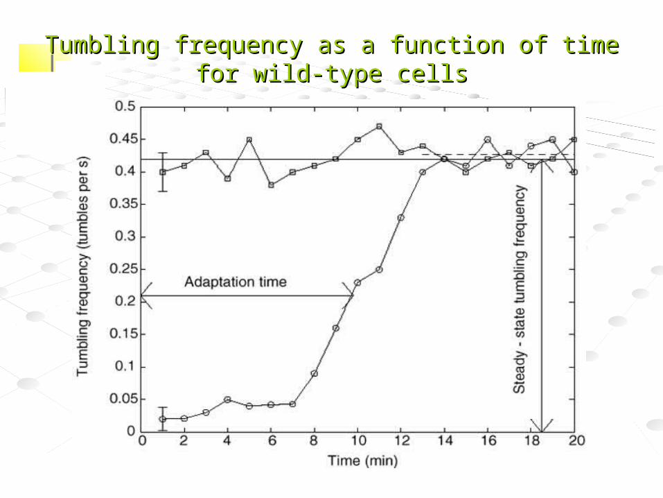
Tumbling frequency as a function of time for wild-type cellsTumbling frequency as a function of time for wild-type cells
Conclusions from study
• Exact adaptation is maintained despite substantial varations in network-protein concentrations– Exact adaptation is a robust
property – …but adaptation time and steady-
state behavior are fine-tuned
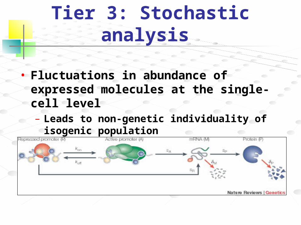
Tier 3: Stochastic analysis
• Fluctuations in abundance of expressed molecules at the single-cell level– Leads to non-genetic individuality of isogenic
population
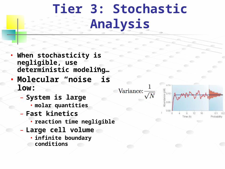
Tier 3: Stochastic Analysis
• When stochasticity is negligible, use deterministic modeling…
• Molecular “noise” is low:– System is large
• molar quantities
– Fast kinetics• reaction time negligible
– Large cell volume• infinite boundary
conditions
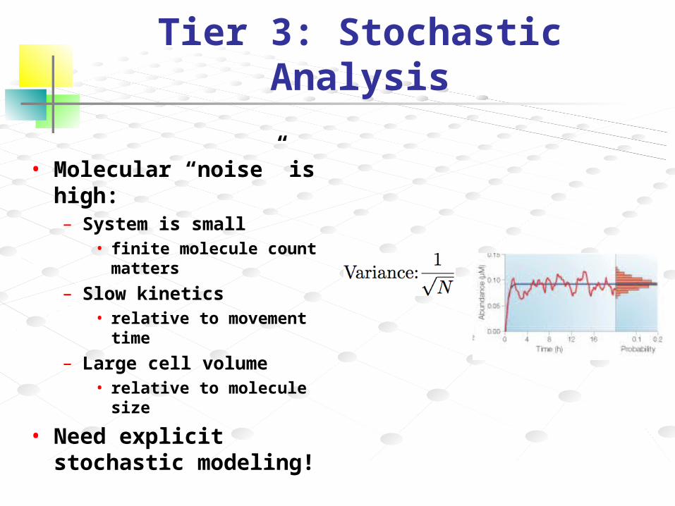
Tier 3: Stochastic Analysis
• Molecular “noise” is high:– System is small
• finite molecule count matters
– Slow kinetics• relative to movement time
– Large cell volume• relative to molecule size
• Need explicit stochastic modeling!
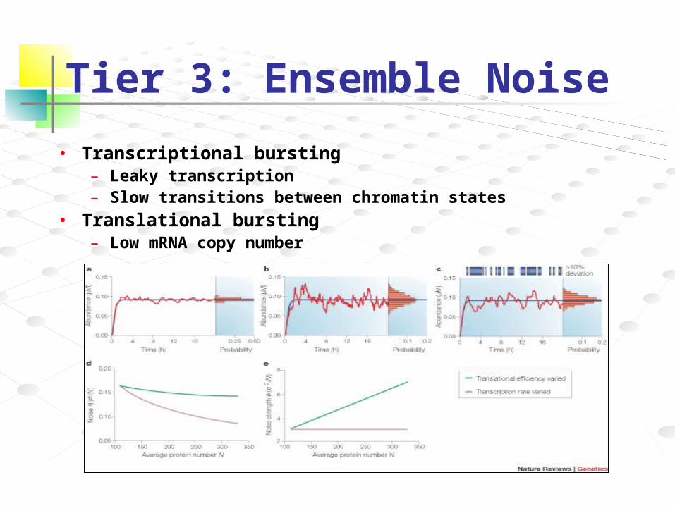
Tier 3: Ensemble Noise
• Transcriptional bursting– Leaky transcription– Slow transitions between chromatin states
• Translational bursting– Low mRNA copy number
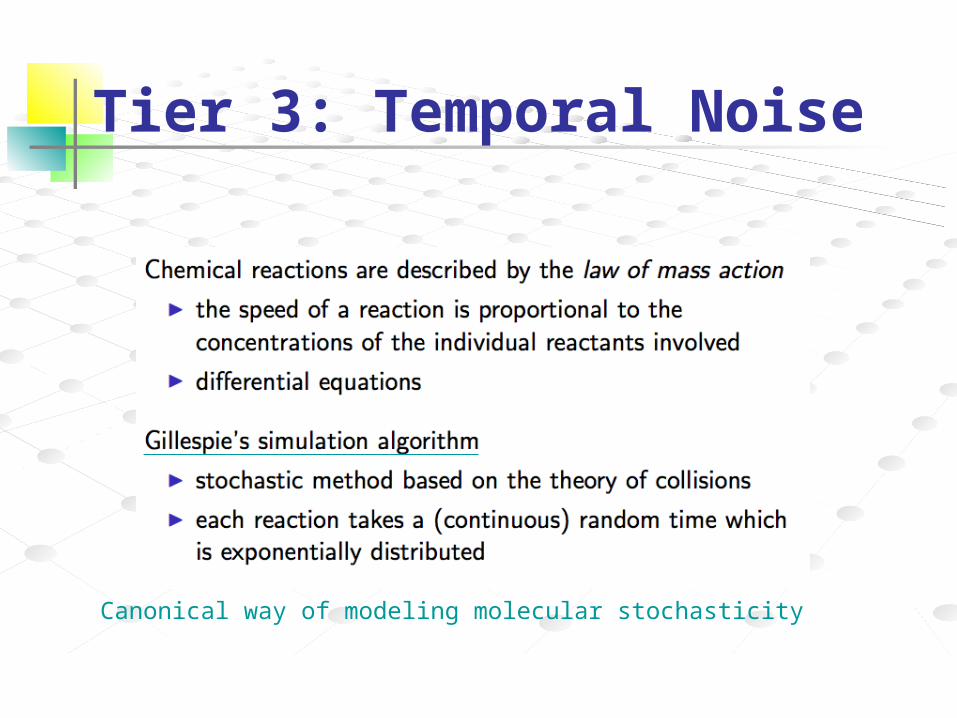
Tier 3: Temporal Noise
Canonical way of modeling molecular stochasticity
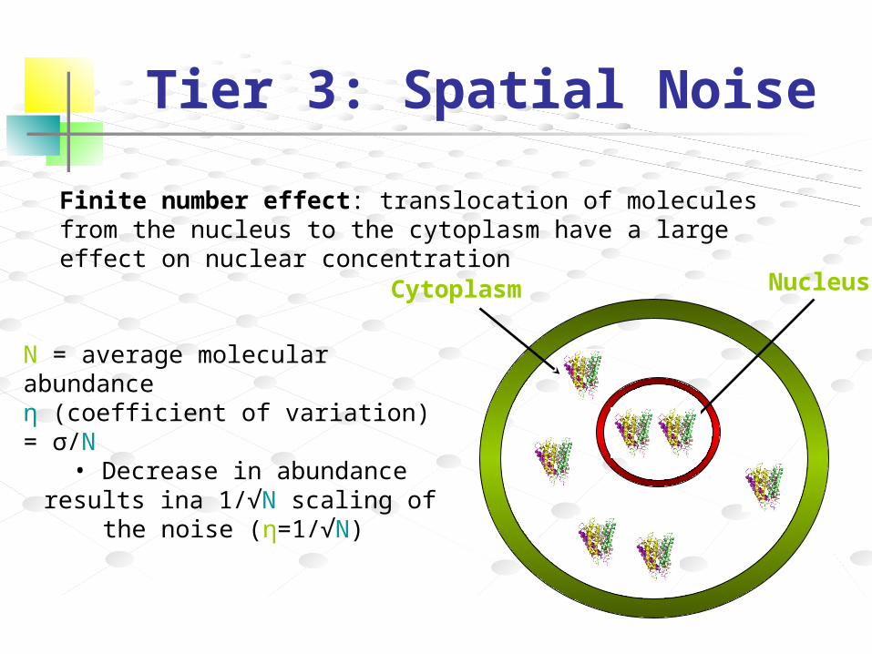
NucleusCytoplasm
Finite number effect: translocation of molecules from the nucleus to the cytoplasm have a large effect on nuclear concentration
N = average molecular abundanceη (coefficient of variation) = σ/N
• Decrease in abundance results ina 1/√N scaling of the noise (η=1/√N)
Tier 3: Spatial Noise
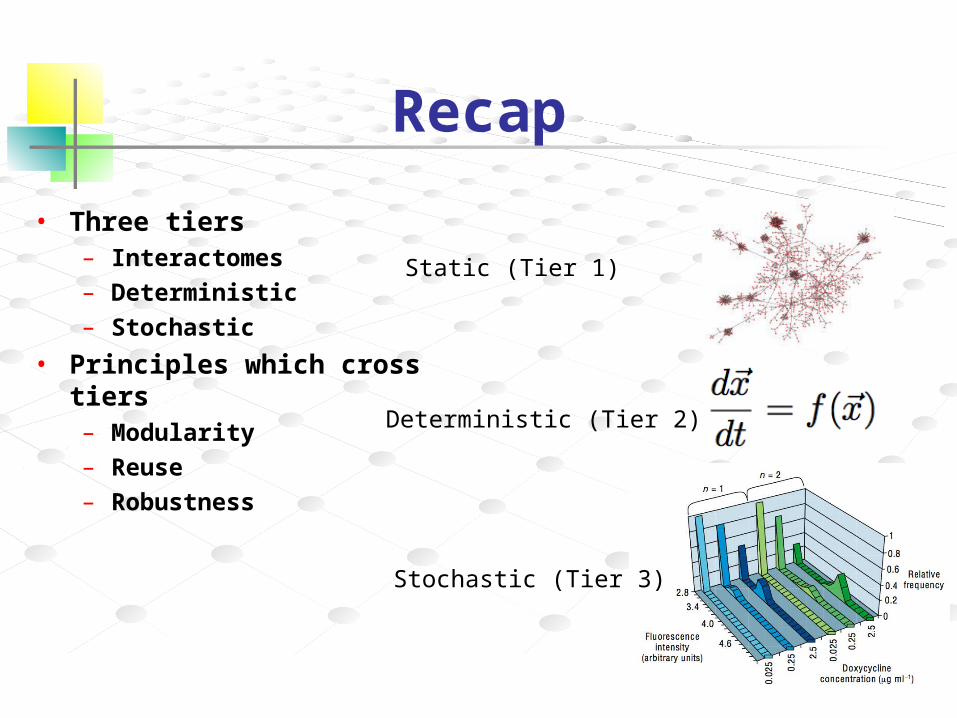
Recap
• Three tiers– Interactomes
– Deterministic
– Stochastic
• Principles which cross tiers– Modularity
– Reuse
– Robustness
Static (Tier 1)
Deterministic (Tier 2)
Stochastic (Tier 3)

Major challenges and limitations
• Measurement of chemical kinetics parameters and molecular concentrations in vivo – Differences between in vitro and in vivo
data• Compartmental specific reactions
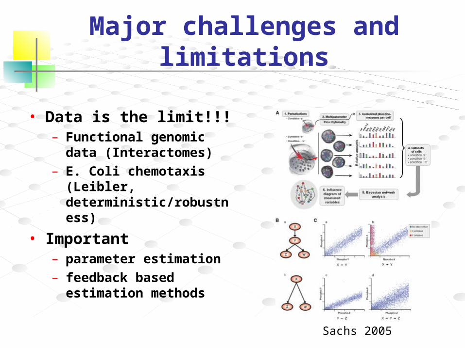
Major challenges and limitations
• Data is the limit!!! – Functional genomic data
(Interactomes)– E. Coli chemotaxis (Leibler,
deterministic/robustness)
• Important– parameter estimation– feedback based estimation
methods
Sachs 2005
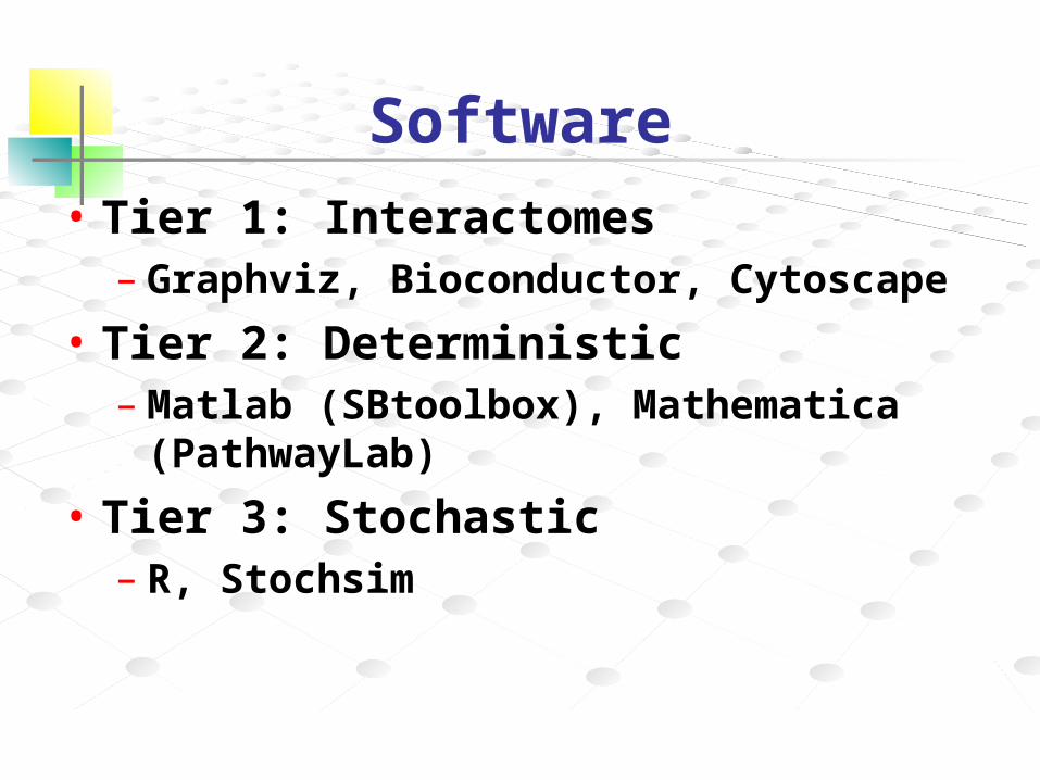
Software• Tier 1: Interactomes
– Graphviz, Bioconductor, Cytoscape
• Tier 2: Deterministic– Matlab (SBtoolbox), Mathematica
(PathwayLab)
• Tier 3: Stochastic– R, Stochsim
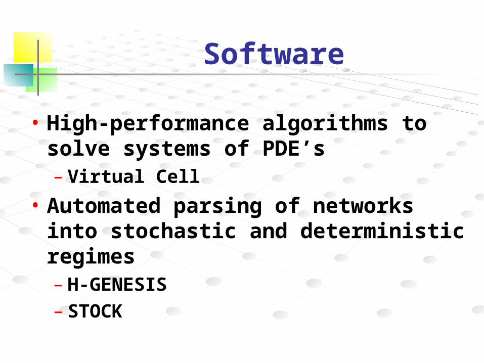
Software
• High-performance algorithms to solve systems of PDE’s– Virtual Cell
• Automated parsing of networks into stochastic and deterministic regimes– H-GENESIS– STOCK
Summary
• Systems Biology can be done by breaking down each system into modules
• Many problems remain unsolved in exactly how to do this, but independent efforts are being developed in most areas that may one day merge together
For next time
• Read supplemental material S9
• Homework #10 due


