Introductory Number Theory

Course No. 100 331

Spring 2006

Michael Stoll

Contents

1. Very Basic Remarks 2

2. Divisibility 2

3. The Euclidean Algorithm 2

4. Prime Numbers and Unique Factorization 4

5. Congruences 5

6. Coprime Integers and Multiplicative Inverses 6

7. The Chinese Remainder Theorem 9

8. Fermat’s and Euler’s Theorems 10

9. Structure of F×p and (Z/pnZ)× 12

10. The RSA Cryptosystem 13

11. Discrete Logarithms 15

12. Quadratic Residues 17

13. Quadratic Reciprocity 18

14. Another Proof of Quadratic Reciprocity 23

15. Sums of Squares 24

16. Geometry of Numbers 27

17. Ternary Quadratic Forms 30

18. Legendre’s Theorem 32

19. p-adic Numbers 35

20. The Hilbert Norm Residue Symbol 40

21. Pell’s Equation and Continued Fractions 43

22. Elliptic Curves 50

23. Primes in arithmetic progressions 66

24. The Prime Number Theorem 75

References 80

2

1. Very Basic Remarks

The following properties of the integers Z are fundamental.

(1) Z is an integral domain (i.e., a commutative ring such that ab = 0 impliesa = 0 or b = 0).

(2) Z≥0 is well-ordered: every nonempty set of nonnegative integers has asmallest element.

(3) Z satisfies the Archimedean Principle: if n > 0, then for every m ∈ Z,there is k ∈ Z such that kn > m.

2. Divisibility

2.1. Definition. Let a, b be integers. We say that “a divides b”, written

a | b ,if there is an integer c such that b = ac. In this case, we also say that “a is adivisor of b” or that “b is a multiple of a”.

We have the following simple properties (for all a, b, c ∈ Z).

(1) a | a, 1 | a, a | 0.(2) If 0 | a, then a = 0.(3) If a | 1, then a = ±1.(4) If a | b and b | c, then a | c.(5) If a | b, then a | bc.(6) If a | b and a | c, then a | b± c.(7) If a | b and |b| < |a|, then b = 0.(8) If a | b and b | a, then a = ±b.

2.2. Definition. We say that “d is the greatest common divisor of a and b”,written

d = gcd(a, b) or d = a u b ,if d | a and d | b, d ≥ 0, and for all integers k such that k | a and k | b, we havek | d.We say that “m is the least common multiple of a and b”, written

m = lcm(a, b) or m = a t b ,if a | m and b | m, m ≥ 0, and for all integers n such that a | n and b | n, we havem | n.

In a similar way, we define the greatest common divisor and least common multiplefor any set S of integers. We have the following simple properties.

(1) gcd(∅) = 0, lcm(∅) = 1.(2) gcd(S1∪S2) = gcd(gcd(S1), gcd(S2)), lcm(S1∪S2) = lcm(lcm(S1), lcm(S2)).(3) gcd({a}) = lcm({a}) = |a|.(4) gcd(ac, bc) = |c| gcd(a, b).(5) gcd(a, b) = gcd(a, ka+ b).

3. The Euclidean Algorithm

How can we compute the gcd of two given integers? The key for this is the lastproperty of the gcd listed above. In order to make use of it, we need the operationof division with remainder.

3

3.1. Proposition. Given integers a and b with b 6= 0, there exist unique integersq (“quotient”) and r (“remainder”) such that 0 ≤ r < |b| and a = bq + r.

Proof. Existence: Consider S = {a − kb : k ∈ Z, a − kb ≥ 0}. Then S ⊂ Z≥0 isnonempty and therefore has a smallest element r = a − qb for some q ∈ Z. Wehave r ≥ 0 by definition, and if r ≥ |b|, then r − |b| would also be in S, hence rwould not have been the smallest element.

Uniqueness: Suppose a = bq + r = bq′ + r′ with 0 ≤ r, r′ < |b|. Then b | r − r′

and 0 ≤ |r − r′| < |b|, therefore r = r′. This implies bq = bq′, hence q = q′ (sinceb 6= 0). �

3.2. Algorithm GCD (Euclidean Algorithm). Given integers a and b, we dothe following.

(1) Set n = 0, a0 = |a|, b0 = |b|.(2) If bn = 0, return an as the result.(3) Write an = bn qn + rn with 0 ≤ rn < bn.(4) Set an+1 = bn, bn+1 = rn.(5) Replace n by n+ 1 and go to step 2.

We claim that the result returned is gcd(a, b). (Observe that 0 ≤ bn+1 < bn if theloop is continued, hence the algorithm must terminate.)

Proof. We show that for all n that occur in the loop, we have gcd(an, bn) =gcd(a, b). The claim follows, since the return value an = gcd(an, 0) = gcd(an, bn)for the last n. For n = 0, we have gcd(a0, b0) = gcd(|a|, |b|) = gcd(a, b). Nowsuppose that we know gcd(an, bn) = gcd(a, b) and that bn 6= 0 (so the loop is notterminated). Then gcd(an+1, bn+1) = gcd(bn, an−bnqn) = gcd(bn, an) = gcd(an, bn)(use property (5) of the gcd). �

3.3. Theorem. Fix a, b ∈ Z. The integers of the form xa + yb with x, y ∈ Z areexactly the multiples of d = gcd(a, b). In particular, there are x, y ∈ Z such thatd = xa+ yb.

Proof. Since d divides both a and b, d also has to divide xa+yb. So these numbersare multiples of d. For the converse, it suffices to show that d can be written asxa+ yb. This follows by induction from the Euclidean Algorithm: Leet N be thelast value of n. Then d = aN · 1 + bN · 0; and if d = xn+1an+1 + yn+1bn+1, then wehave d = yn+1an +(xn+1−qnyn+1)bn, so setting xn = yn+1 and yn = xn+1−qnyn+1,we have d = xnan + ynbn. So in the end, we must also have d = x0a0 + y0b0. �

There is a simple extension of the Euclidean Algorithm that also computes num-bers x and y such that gcd(a, b) = xa+ yb. It looks like this.

3.4. Algorithm XGCD (Extended Euclidean Algorithm). Given integersa and b, we do the following.

(1) Set n = 0, a0 = |a|, b0 = |b|, x0 = sign(a), y0 = 0, u0 = 0, v0 = sign(b).(2) If bn = 0, return (an, xn, yn) as the result.(3) Write an = bn qn + rn with 0 ≤ rn < bn.(4) Set an+1 = bn, bn+1 = rn, xn+1 = un, yn+1 = vn, un+1 = xn − un qn,

vn+1 = yn − vn qn.(5) Replace n by n+ 1 and go to step 2.

4

By induction, one shows that an = xn a+ yn b and bn = un a+ vn b, so upon exit,the return values (d, x, y) satisfy xa+ yb = d = gcd(a, b).

3.5. Proposition. If n divides ab and gcd(n, a) = 1, then n divides b.

Proof. By Thm. 3.3, there are x and y such that xa + yn = 1. We multiply by bto obtain b = xab + ynb. Since n divides ab, n divides the right hand side andtherefore also b. �

4. Prime Numbers and Unique Factorization

4.1. Definition. A positive integer p is called a “prime number” (or simply a“prime”), if p > 1 and the only positive divisors of p are 1 and p.

(This is really the definition of an “irreducible” element in a ring!)

4.2. Proposition. If p is a prime and a, b are integers such that p | ab, then p | aor p | b.

(This is the general definition of a “prime” element in a ring!)

Proof. We can assume that p - a (otherwise we are done). Then gcd(a, p) = 1(since the only other positive divisor of p, namely p itself, does not divide a).Then by Prop. 3.5, p divides b. �

Now let n > 0 be a positive integer. Then either n = 1, or n is a prime number,or else n has a “proper” divisor d such that 1 < d < n. Then we can write n = dewhere also 1 < e < n. Continuing this process with d and e, we finally obtaina representation of n as a product of primes. (If n = 1, it is given by an emptyproduct (a product without factors) of primes.)

4.3. Theorem. This prime factorization of n is unique (up to ordering of thefactors).

Proof. By induction on n. For n = 1, this is clear (there is only one empty set. . . ). So assume that n > 1 and that we have written

n = p1p2 . . . pk = q1q2 . . . ql

with prime numbers pi, qj, where k, l ≥ 1. Now p1 divides the product of the qj’s,hence p1 has to divide one of the qj’s. Up to reordering, we can assume that p1|q1.But the only positive divisors of q1 are 1 and q1, so we must in fact have p1 = q1.Let n′ = n/p1 = n/q1, then

n′ = p2p3 . . . pk = q2q3 . . . ql .

Since n′ < n, we know by induction that (perhaps after reordering the qj’s) k = land pj = qj for j = 2, . . . , k. This proves the claim. �

5

4.4. Definition. This shows that we can write every nonzero integer n uniquelyas

n = ±∏

p

pvp(n)

where the product is over all prime numbers p, and the exponents vp(n) are non-negative integers, all but finitely many of which are zero. vp(n) is called the“valuation of n at p”.

We have the following simple properties.

(1) vp(mn) = vp(m) + vp(n).(2) m | n ⇐⇒ ∀p : vp(m) ≤ vp(n).

(3) gcd(m,n) =∏

p

pmin(vp(m),vp(n)), lcm(m,n) =∏

p pmax(vp(m),vp(n)).

(4) vp(m+ n) ≥ min(vp(m), vp(n)), with equality if vp(m) 6= vp(n).

Property (3) implies that gcd(m,n) lcm(m,n) = mn for positive m, n. In general,we have gcd(m,n) lcm(m,n) = |mn|.If we set vp(0) = +∞, then all the above properties hold for all integers (with theusual conventions like min{e,∞} = e, e+∞ = ∞, . . . ).

We can extend the valuation function from the integers to the rational numbersby setting

vp

(rs

)= vp(r)− vp(s)

(Exercise: check that this is well-defined). Properties (1) and (4) above then holdfor rational numbers, and a rational number x is an integer if and only if vp(x) ≥ 0for all primes p.

5. Congruences

5.1. Definition. Let a, b and n integers with n > 0. We say that “a is congruentto b modulo n”, written

a ≡ b mod n ,

if n divides the difference a− b.

5.2. Congruence is an equivalence relation.For fixed n and arbitrary a, b, c ∈ Z, we have:

(1) a ≡ a mod n.(2) If a ≡ b mod n, then b ≡ a mod n.(3) If a ≡ b mod n and b ≡ c mod n, then a ≡ c mod n.

Hence we can partition Z into “congruence classes mod n”: we let

a = a+ nZ = {a+ nx : x ∈ Z} = {b ∈ Z : a ≡ b mod n}

(in the a notation, n must be clear from the context) and

Z/nZ = {a : a ∈ Z} .

We then have

a ≡ b mod n ⇐⇒ b ∈ a ⇐⇒ a = b .

6

5.3. Proposition. The map

{0, 1, . . . , n− 1} −→ Z/nZ , r 7−→ r = r + nZis a bijection. In particular, Z/nZ has exactly n elements.

Proof. The map is clearly well-defined. It is injective: assume r = s with 0 ≤r, s < n. Then r ≡ s mod n, so n | r − s and |r − s| < n, therefore r = s. Itis surjective: Let a be a congruence class and write a = nq + r with 0 ≤ r < n.Then a = r. �

Since the representative r of a class a is given by the (least nonnegative) residueof a when divided by n, congruence classes are also called “residue classes”.

5.4. The congruence classes form a commutative ring.We define addition and multiplication on Z/nZ:

a+ b = a+ b , a · b = ab

We have to check that these operations are well-defined. This means that ifa ≡ a′ mod n and b ≡ b′ mod n, then we must have a + b ≡ a′ + b′ mod n andab ≡ a′b′ mod n. Now

(a+ b)− (a′ + b′) = (a− a′) + (b− b′) is divisible by n,

and alsoab− a′b′ = (a− a′)b+ a′(b− b′) is divisible by n.

Once these operations are well-defined, all the commutative ring axioms carry overimmediately from Z to Z/nZ.

5.5. Congruences are useful. Why are congruences a useful concept? Theygive us a kind of “Mickey Mouse” image of the integers (lumping together manyintegers into one residue class, thus losing information), with the advantage thatthe resulting structure Z/nZ has only finitely many elements. This means thatall sorts of questions that are difficult to answer with respect to Z are effectively(though not necessarily efficiently, if n is large) decidable with respect to Z/nZ. Ifwe can show in this way that something is impossible over Z/nZ, then this oftenimplies a negative answer for Z, too.

Consider, for example, the equation x2 +y2−15 z2 = 7. Does it have a solution inintegers? That to decide seems to be hard. On the other hand, we can very easilymake a table of all possible values of the left hand side in Z/8Z: it is easy to seethat a square is always ≡ 0, 1, or 4 mod 8, and adding three of these values (notethat −15 ≡ 1 mod 8) leads to all residue classes mod 8 with one exception — theleft hand side is never ≡ 7 mod 8.

So a solution is not possible in Z/8Z. But any solution in Z would lead to animage solution in Z/8Z, hence there can be no solution in Z either.

6. Coprime Integers and Multiplicative Inverses

When does a class a have a multiplicative inverse in Z/nZ? We have to solve thecongruence ax ≡ 1 mod n; equivalently, there need to exist integers x and y suchthat ax + ny = 1. By Thm. 3.3, this is equivalent with gcd(a, n) = 1. In thiscase, we say that “a and n are relatively prime” or “a and n are coprime”, andsometimes write a ⊥ n. We can use the extended Euclidean Algorithm to find theinverse.

7

6.1. Theorem. The ring Z/nZ is a field if and only if n is a prime number.

Proof. Clear for n = 1 (a field has at least two elements 0 and 1, and 1 is not aprime number). For n > 1, Z/nZ is not a field if and only if there is some a ∈ Z,not divisible by n, such that d = gcd(n, a) > 1. This implies that 1 < d < n is aproper divisor of n, hence n is not a prime. Conversely, if d is a proper divisor ofn, then gcd(n, d) = d, and d is not invertible. �

If gcd(n, a) = 1, then a is called a “primitive residue class mod n”; its uniquelydetermined multiplicative inverse in Z/nZ is denoted a−1. The prime residueclasses form a group, the multiplicative group (Z/nZ)× of the ring Z/nZ.

When n = p is prime, then the field Z/pZ is also denoted Fp; we have F×p = Fp\{0}for the multiplicative group; in particular, #F×p = p− 1.

6.2. Definition. The Euler φ function is defined for n > 0 by

φ(n) = #(Z/nZ)× = #{a ∈ Z : 0 ≤ a < n, a ⊥ n} .

n 1 2 3 4 5 6 7 8 9 10 11 12 13 14 15 16 17 18 19 20φ(n) 1 1 2 2 4 2 6 4 6 4 10 4 12 6 8 8 16 6 18 8

We have that n is prime if and only if φ(n) = n− 1.

6.3. Proposition. If p is prime and e ≥ 1, then φ(pe) = pe−1(p− 1).

Proof. Clear for e = 1. For e > 1, observe that a ⊥ pe ⇐⇒ a ⊥ p ⇐⇒ p - a, so

φ(pe) = #{a ∈ Z : 0 ≤ a < pe, p - a}= pe −#{a ∈ Z : 0 ≤ a < pe, p | a}= pe − pe−1 = (p− 1)pe−1 .

�

6.4. A Recurrence. Counting the numbers between 0 (inclusive) and n (exclu-sive) according to their gcd with n (which can be any (positive) divisor d of n),we obtain ∑

d|n

φ(nd

)=∑d|n

φ(d) = n .

This can be read as a recurrence for φ(n):

φ(n) = n−∑

d|n,d<n

φ(d) .

We get

φ(1) = 1− 0 = 1 , φ(2) = 2− φ(1) = 1 , φ(3) = 3− φ(1) = 2 ,

φ(4) = 4− φ(2)− φ(1) = 2 , φ(6) = 6− φ(3)− φ(2)− φ(1) = 2 , etc.

Obviously, the recurrence determines φ(n) uniquely: If integers an (n ≥ 1) satisfy∑d|n

ad = n ,

then an = φ(n). This still holds if the n’s are restricted to be divisors of somefixed integer N .

8

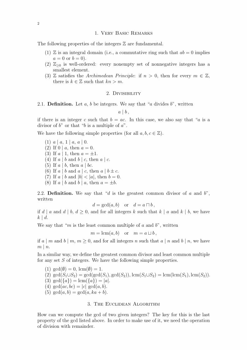
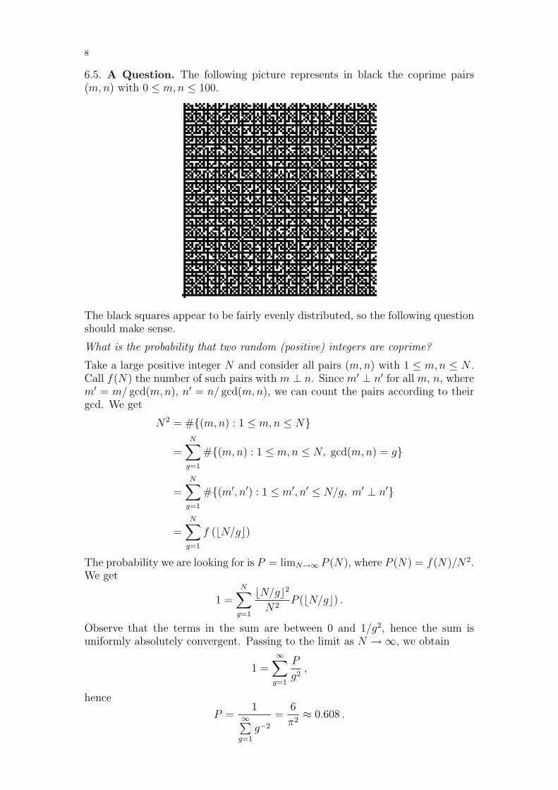
6.5. A Question. The following picture represents in black the coprime pairs(m,n) with 0 ≤ m,n ≤ 100.

The black squares appear to be fairly evenly distributed, so the following questionshould make sense.

What is the probability that two random (positive) integers are coprime?

Take a large positive integer N and consider all pairs (m,n) with 1 ≤ m,n ≤ N .Call f(N) the number of such pairs with m ⊥ n. Since m′ ⊥ n′ for all m, n, wherem′ = m/ gcd(m,n), n′ = n/ gcd(m,n), we can count the pairs according to theirgcd. We get

N2 = #{(m,n) : 1 ≤ m,n ≤ N}

=N∑

g=1

#{(m,n) : 1 ≤ m,n ≤ N, gcd(m,n) = g}

=N∑

g=1

#{(m′, n′) : 1 ≤ m′, n′ ≤ N/g, m′ ⊥ n′}

=N∑

g=1

f (bN/gc)

The probability we are looking for is P = limN→∞ P (N), where P (N) = f(N)/N2.We get

1 =N∑

g=1

bN/gc2

N2P (bN/gc) .

Observe that the terms in the sum are between 0 and 1/g2, hence the sum isuniformly absolutely convergent. Passing to the limit as N →∞, we obtain

1 =∞∑

g=1

P

g2,

hence

P =1

∞∑g=1

g−2

=6

π2≈ 0.608 .

9

(Exercise: where is the gap in this argument?)

We can apply what we have learned to linear congruences.

Given a, b, and n, what are the solutions x of

ax ≡ b mod n ?

In other words, for which x ∈ Z does there exist a y ∈ Z such that ax+ ny = b ?

6.6. Theorem. The congruence ax ≡ b mod n has no solutions unless gcd(a, n) | b.If there are solutions, they form a residue class modulo n/gcd(a, n).

Proof. By Thm. 3.3, the condition gcd(a, n) | b is necessary and sufficient forsolutions to exist. Let g = gcd(a, n). If g | b, we can divide the equation ax+ny = bby g to get a′x + n′y = b′, where a = a′g, n = n′g, b = b′g. Then gcd(a′, n′) = 1,and we can solve the equation a′ x = b′ for x (in Z/n′Z): x = b′ (a′)−1. So the setof solutions x is given by this residue class modulo n′. �

7. The Chinese Remainder Theorem

Now let us consider simultaneous congruences:

x ≡ a mod m, x ≡ b mod n

Is such a system solvable? What does the solution set look like? If d = gcd(m,n),then we obviously need to have a ≡ b mod d for a solution to exist. On the otherhand, when m ⊥ n, solutions do always exist.

7.1. Chinese Remainder Theorem. If m ⊥ n, then the above system has so-lutions x; they form a residue class modulo mn.

Proof. Since m ⊥ n, we can find u and v with mu+nv = 1 by Thm. 3.3. Considerx = anv + bmu. We have

x = anv + bmu ≡ anv = a− amu ≡ a mod m

and similarly x ≡ b mod n. So solutions exist. Now we show that y is anohersolution if and only if mn | y − x. If mn divides y − x, then m and n both dividey − x, hence y ≡ x ≡ a mod m and y ≡ x ≡ b mod n. Now assume y is anothersolution. Then m and n both divide y− x. So n | y− x = mt. By Prop. 3.5, n | tand hence mn | mt = y − x. �

There is a straight-forward extension to more than two simultaneous congruences.

7.2. Chinese Remainder Theorem. If the numbers m1, m2, . . . , mk are co-prime in pairs, then the system of congruences

x ≡ a1 mod m1 , x ≡ a2 mod m2 , . . . , x ≡ ak mod mk

has solutions; they form a residue class modulo m1m2 . . .mk.

Proof. Induction on k using Thm. 7.1. Note that a ⊥ b, a ⊥ c implies a ⊥ bc. �

Now we can answer the question from the beginning of this section.

10

7.3. Theorem. The system

x ≡ a mod m, x ≡ b mod n

has solutions if and only if a ≡ b mod gcd(m,n). If solutions exist, they form aresidue class modulo lcm(m,n).

Proof. We have already seen that the condition is necessary. Let d = gcd(m,n).We can find u and v such that mu+nv = b− a by Thm. 3.3. Then x = a+mu =b−nv is a solution. As in the proof of Thm. 7.1, we see that y is another solutionif and only if m and n both divide y − x. This means that the solutions form aresidue class modulo lcm(m,n). �

We can give the Chinese Remainder Theorem a more algebraic formulation.

7.4. Theorem. Assume that m1,m2, . . . ,mk are coprime in pairs. Then the nat-ural ring homomorphism

Z/m1m2 . . .mkZ −→ Z/m1Z× Z/m2Z× · · · × Z/mkZis an isomorphism. In particular, we have an isomorphism of multiplicative groups

(Z/m1m2 . . .mkZ)× ∼= (Z/m1Z)× × (Z/m2Z)× × · · · × (Z/mkZ)× .

Proof. By the above, the homomorphism is bijective, hence an isomorphism. �

7.5. A Formula for φ. The Chinese Remainder Theorem 7.4 implies that

φ(mn) = φ(m)φ(n) if m ⊥ n.

A similar formula holds for products with more factors. Applying this to the primefactorization of n, we get

φ(n) =∏p|n

pvp(n)−1(p− 1) = n∏p|n

(1− 1

p

).

8. Fermat’s and Euler’s Theorems

A very nice property of the finite fields Fp and all their extension fields is that themap x 7→ xp is not only compatible with multiplication: (xy)p = xpyp, but alsowith addition!

8.1. Theorem (“Freshman’s Dream”). Let F be a field of prime characteristicp (this means that p · 1F = 0F ; for us, the basic example is F = Fp). Then for allx, y ∈ F , we have (x+ y)p = xp + yp.

Proof. By the Binomial Theorem,

(x+y)p = xp+

(p

1

)xp−1y+

(p

2

)xp−2y2+· · ·+

(p

k

)xp−kyk+· · ·+

(p

p− 1

)xyp−1+yp.

Now the binomial coefficients(

pk

)for 1 ≤ k ≤ p − 1 all are integers divisible

by p (why?), and since F is of characteristic p, all the corresponding terms in theformula vanish, leaving only xp + yp. �

We can use this to give one proof of the following fundamental fact.

11

8.2. Theorem (Fermat’s Little Theorem). Let p be a prime number. For alla ∈ Fp, we have ap = a. (Equivalently, for all a ∈ Z, p divides ap − a.)

Proof.First Proof: By induction on a. a = 0 is clear. Now, by Thm. 8.1, p divides(a+1)p−ap−1 for all a ∈ Z. But then p also divides ((a+1)p−(a+1))−(ap−a),hence:

p | ap − a ⇐⇒ p | (a+ 1)p − (a+ 1)

This gives the inductive step upwards and downwards, hence the claim holds forall a ∈ Z.

Second Proof: Easy proof using Algebra. a = 0 is clear. Hence it suffices to showthat ap−1 = 1 for all a 6= 0. This is a consequence of the fact that #F×p = p − 1

and the general theorem that g#G = 1 for any g in any finite group G.

Third Proof: By Combinatorics (for a > 0). Consider putting beads that canhave colors from a set of size a at p equidistant places around a circle (to form“necklaces”). There will be ap necklaces in total, a of which will consist of beads ofonly one color. The remaining ap − a come in bunches of p, obtained by rotation,so p has to divide ap − a. �

The algebra proof can readily be generalized.

8.3. Theorem (Euler). Let n be a positive integer. Then for all a ∈ Z witha ⊥ n, we have aφ(n) ≡ 1 mod n.

Proof. Under the assumption, a ∈ (Z/nZ)×, and by definition, #(Z/nZ)× = φ(n).By the general fact from algebra used in the second proof of Thm. 8.2, the claimfollows. �

8.4. Example. What is 71113mod 15? By Thm. 8.3, 78 ≡ 1 mod 15 (as φ(15) =

8). On the other hand, 11 ≡ 3 mod 8, and 34 ≡ 1 mod 8 (in fact, already 32 is

≡ 1 mod 8). So 1113 = (114)3 · 11 ≡ 11 ≡ 3 mod 8, and then 71113 ≡ 73 = 343 ≡13 mod 15.

8.5. A Consequence of Fermat’s Little Theorem. Consider the polynomialXp − X with coefficients in Fp. By Fermat’s Little Theorem 8.2, every elementa ∈ Fp is a root of this polynomial. Now Fp is a field, and so we can “divide out”the roots successively to find that

Xp −X =∏a∈Fp

(X − a) .

This implies that for any polynomial f(X) dividing Xp − X (in the polynomialring Fp[X]), the number of its distinct roots in Fp equals the degree deg f(X).More generally, if f is any polynomial in Fp[X], we can compute the number ofdistinct roots of f in Fp by the formula

#{a ∈ Fp : f(a) = 0} = deg gcd(f,Xp −X) .

12

9. Structure of F×p and (Z/pnZ)×

Fermat’s Theorem 8.2 tells us that the multiplicative order of any nonzero elementa of Fp (this is the smallest positive integer n such that an = 1) divides p−1. (Theset of all n such that an = 1 consists exactly of the multiples of the order.) Nowthe question arises, are there elements of order p − 1? In other, more algebraicterms, is the group F×p cyclic? The answer is “yes”.

9.1. Theorem. The multiplicative group F×p is cyclic. (In other words, there existelements g ∈ F×

p such that all a ∈ F×p are powers of g. The corresponding integersg are called “primitive roots mod p”.)

Proof. Obviously, all elements of F×p of order dividing d (where d is a divisor

of p− 1) will be roots of Xd − 1. Since d divides p− 1, Xd − 1 divides Xp−1 − 1and hence also Xp−X (as polyomials). By 8.5, it follows that Xd− 1 has exactlyd roots in Fp. Let ad be the number of elements of exact order d. Then we get

d =∑k|d

ak .

By the statement in 6.4, it follows that ad = φ(d); in particular, ap−1 = φ(p−1) ≥1. Hence primitive roots exist. �

9.2. Examples. The proof shows that there are exactly φ(p− 1) essentially dis-tinct primitive roots mod p. For the first few primes, we get the following table.

Prime Primitive Roots2 13 25 2, 37 3, 511 2, 3, 8, 913 2, 6, 7, 11

There is a famous conjecture, named after Artin, that asserts that every integerg 6= −1 that is not a square is a primitive root mod infinitely many differentprimes. (Why are squares no good?) This has been proven assuming anotherfamous conjecture, the Extended Riemann Hypothesis. The best unconditionalresult so far seems to be that the statement is true for all allowed integers, withat most three exceptions. On the other hand, the statement is not known to holdfor any particular integer g!

9.3. Proposition. Let G be a finite multiplicative abelian group of order n. Anelement g ∈ G is a generator of G (and so G is cyclic) if and only if gn/q 6= 1G forall prime divisors q of n.

Proof. If g is a generator, then n is the least positive integer m such that gm = 1G,hence the condition is necessary. Now if g is not a generator, then its order mdivides n, but is smaller than n, hence m divides n/q for some prime divisor qof n. It follows that gn/q = 1G. �

Let us use this result to show that (Z/pnZ)× is cylic if p is an odd prime andn ≥ 1.

13

9.4. Theorem. Let g be a primitive root modulo p, where p is an odd prime.Then one of g and g + p is a primitive root modulo pn for all n ≥ 1.

Proof. We know that gp−1 = 1 + ap for some a ∈ Z. If p - a, let h = g; otherwisewe set h = g + p; then we have hp−1 = 1 + a′p with p - a′:

(g + p)p−1 = gp−1 + (p− 1)gp−2p+ bp2 ≡ 1− kp mod p2

(with some integer b) where k ≡ gp−2 mod p is not divisible by p. Hence we havein both cases that hp−1 ≡ 1 + ap mod p2 with p - a.

Now I claim that for all n ≥ 0, we have

hpn(p−1) ≡ 1 + apn+1 mod pn+2 .

This follows by induction from the case n = 0:

hpn+1(p−1) =(hpn(p−1)

)p= (1 + (a+ bp)pn+1)p

= 1 + p (a+ bp)pn+1 + cpn+3

= 1 + apn+2 + (b+ c)pn+3

Here b and c are suitable integers, and the penultimate equality uses that p ≥ 3(since then the last term in the binomial expansion, (a + bp)pp(n+1)p, is divisibleby pn+3, as are the intermediate ones, even when n = 0).

Now let n ≥ 2, and let q be a prime divisor of φ(pn) = pn−1(p − 1). If q divides

p − 1, then h(p−1)/q 6≡ 1 mod p, hence also hpn−1(p−1)/q ≡ h(p−1)/q 6≡ 1 mod p,so hpn−1(p−1)/q 6≡ 1 mod pn. If q = p, then we have just seen that hpn−2(p−1) 6≡1 mod pn. So by Prop. 9.3, h ∈ {g, g + p} is a primitive root mod pn. �

10. The RSA Cryptosystem

The basic idea of Public Key Cryptography is that each participant has two keys:A public key that is known to everybody and serves to encrypt messages, and aprivate key that is known only to her or him and is used to decrypt messages. Forthis idea to work, two conditions have to be satisfied:

(1) Both encryption and decryption must be reasonably fast (with keys of asize satisfying the next condition)

(2) It must be impossible to compute the private key from the public key inless than a very large amount of time (how large will depend on the desiredlevel of security)

Alice Bob

EncryptionAlgorithm

Plaintext

Bob’s Public Key

DecryptionAlgorithm

Plaintext

Bob’s Private Key

Ciphertext

Eve

14

The first published system (1977) satisfying these assumptions was designed byRivest, Shamir and Adleman, and is called the RSA Cryptosystem (after theirinitials). However, already in 1973, Clifford Cocks at GCHQ (the British NSAequivalent) came up with the same system. It was not used by GCHQ, andCocks’ contribution only publicly acknowledged in 1997.

The idea was that finding the prime factors of a large number is very hard, whereasknowing them would allow you to do ceratin things quickly.

10.1. The set-up. To generate a public-private key pair, one takes two largeprime numbers p and q (of 160 or more decimal digits, say). The public key thenconsists of n = pq and another positive integer e that has to be coprime withlcm(p − 1, q − 1) and can be taken to be fairly (but not too) small (in order tomake encryption more efficient).

Encryption proceeds as follows. The message is encoded in one or several numbers0 ≤ m < n (e.g., by taking bunches of bits of length less than the length of n(measured in bits)). Then each number m is encrypted as c = me mod n.

In order to decrypt such a c, we need to be able to undo the exponentiationby e. In order to do this, we use Fermat’s Little Theorem 8.2 and the ChineseRemainder Theorem 7.1: Since e ⊥ lcm(p− 1, q− 1), we can compute d such thatde ≡ 1 mod lcm(p − 1, q − 1) (using the XGCD Algorithm). Then cd = mde ≡m mod p and modq by Fermat’s Little Theorem and so cd ≡ m mod n by theChinese Remainder Theorem.

So the public key is the pair (n, e) and the private key the pair (n, d). Encryptionis m 7→ me mod n, decryption is c 7→ cd mod n.

10.2. Why is it practical? Encryption and decryption are reasonably fast: theyinvolve exponentiation mod n, which can be done in O((log n)2 log e) time (wheree is the exponent), or even in O(log n log log n log e), using fast multiplication.

Also, it is possible to select suitable primes p and q in reasonable time: there arealgorithms that prove that a given number is prime in polynomial time (polynomialin log p), and gaps between primes are on average of size log p, so one can expectto find a prime in polynomial time. The remaining steps in choosing the public-private key pair are relatively fast.

For example, my laptop running the computer algebra system MAGMA, takesabout 4 seconds to find a prime of 100 digits, and about 12 seconds to find aprime of 120 digits.

10.3. Why is it considered secure? In order to get m from c, one needs anumber t such that ct ≡ m mod n. For general m, this means that te ≡ 1 modlcm(p − 1, q − 1). Then te − 1 is a multiple of lcm(p − 1, q − 1), and we can usethis in order to factor n in the following way.

Note that if n is an odd prime, then there are exactly two square roots of 1 inthe ring Z/nZ (which is a field of characteristic not 2 in this case), namely (theresidue classes of) 1 and −1. However, when n = pq is the product of two distinctodd primes, then there are four such square roots; they are obtained from pairs ofsquare roots of 1 mod p and mod q via the Chinese Remainder Theorem 7.1. Ifx2 ≡ 1 mod n, but x 6≡ ±1 mod n, then we can use x to factor n: we have thatn divides x2 − 1 = (x − 1)(x + 1), but n divides neither factor on the right, sogcd(x− 1, n) has to be a proper divisor of n.

15

Now suppose we know a multiple f of lcm(p − 1, q − 1). Write f = 2rs withs odd (note that r ≥ 1 since p − 1 and q − 1 are even). Now pick a random1 < w < n − 1. If gcd(w, n) 6= 1, then we have found a proper divisor of n.Otherwise, we successively compute

w0 = ws mod n ,w1 = w20 mod n ,w2 = w2

1 mod n , . . . , wr = w2r−1 mod n

By Fermat’s Little Theorem 8.2 and the Chinese Remainder Theorem 7.1, wr = 1.Now if there is some j such that wj 6≡ ±1 mod n, but wj+1 ≡ 1 mod n, we havefound a square root of 1 mod n that will split n as explained above. One cancheck (see [Sti, Sect. 5.7.2]) that the probability of success is at least 1/2. Hencewe need no more than two tries on average to factor n.

Conversely, if we have p and q, we can easily compute a suitable t (in fact, our din the private key is found that way).

The upshot is that in order to break the system, we have to factor n. Nowfactorization appears to be a hard problem: even though quite some effort hasbeen invested into developing good factoring algorithms (in particular since thisis relevant for cryptography! — you can win prize money if you factor certainnumbers), and we now have considerably better algorithms than thirty years ago(say), the performance of the best known algorithms is still much worse thanpolynomial time. The complexity is something like

exp(O( 3√

log n(log log n)2)).

This is already quite a bit better than exponential (in log n), but grows fast enoughto make factorization of 300-digit numbers or so infeasible.

For example, again MAGMA on my laptop needs 14 seconds to factor a productof two 20-digit primes and 3 minutes to factor a product of two 30-digit primes.

But note that there is an efficient algorithm (at least in theory) for factoringintegers on a quantum computer. So if quantum computers become a reality,cryptosystems based on the difficulty of factorization like RSA will be dead.

11. Discrete Logarithms

In RSA, we use modular exponentiation with a fixed exponent, where the base isthe message. There are other cryptosystems, which in some sense work the otherway round: they use exponentiation with a fixed base and varying exponent. Thiscan be done in the multiplicative group of a finite field Fp, or even in a moregeneral setting.

11.1. The Discrete Logarithm Problem. Let G be a finite cyclic group oforder n, with generator g. The problem of finding a ∈ Z/nZ from g and ga isknown as the Discrete Logarithm Problem: We want to find the logarithm of ga

to the base g. If x = ga, then sometimes the notation a = logg x is used.

The difficulty of this problem depends on the representation of the group G.

(1) The simplest case is G = Z/nZ (the additive group), g = 1. Then logg x =x, and the problem is trivially solved.

(2) It is more interesting to choose G = F×p , with g a primitive root mod p(or rather, its image in F×p ). If the group order #G = p − 1 has a largeprime factor (e.g., p− 1 = 2q or 4q where q is prime), then here, the DLP

16

(short for Discrete Logarithm Problem) is considered to be hard. The bestknown algorithms have complexity

O(exp(c 3

√log q(log log q)2)

);

the situation is comparable to factorization.

(3) Other groups one can use are the groups of Fp-rational points on ellipticcurves. Except for certain special cases, no special-purpose algorithms areknown, and the best one can do is to use generic algorithms, which haveexponential running time �

√#G. This makes these groups attractive

for cryptography, since one gets secure systems with considerably shorterkey-lengths.

(4) When the group order n = #G factors, then the Chinese Remainder The-orem can be used to simplify the problem (if the factorization is known!).(This is the so-called Pohlig-Hellman attack.)

11.2. ElGamal Encryption. Here is a general setting for a cryptosystem basedon DLP. It was originally suggested with G = F×p . In this case, it is advisable totake p such that p− 1 is a small factor times a (large) prime q, in order to avoidthe Pohlig-Hellman attack. Knowing the factorisation of p−1 also helps in findinga primitive root g, compare Prop. 9.3 (try random g until one is identified as aprimitive root).

It works like this. Bob chooses a random number a ∈ Z/nZ, where n = #G is thegroup order, and publishes h = ga as his public key. (The group G and generatorg are fixed and also publicly known.) The number a itself is his private key. Thismeans that in order to find the private key from the public key, one has to solvea DLP. Now, when she wants to send Bob a message m ∈ G, Alice also chooses arandom number k ∈ Z/nZ and then sends the pair (gk,mhk) to Bob: she “masks”the message by multiplying it by hk (remember that h is Bob’s public key), butleaves a clue for Bob by also sending gk. Now to decrypt this, Bob takes thepair (x, y) he receives and computes m = x−ay using his private key a.

An eavesdropper intercepting the ciphertext would need to find hk = gak fromgk and h = ga in order to get the plaintext. This is called the Diffie-HellmanProblem, because it also comes up in the secret key exchange protocol developedby Diffie and Hellman (see below). It is believed that the Diffie-Hellman Problemis no easier than the DLP (it is certainly not harder), but this has not been proved.

11.3. Diffie-Hellman Key Exchange. This is a method for two people to agreeon a secret key, communicating through an open channel. It also works for generalcylic groups G with fixed generator g (but was first suggested with G = F×p ).

Our two protagonists, Alice and Bob, both select a random number a (for Alice)and b (for Bob) in Z/nZ. Alice sends A = ga to Bob, and Bob sends B = gb toAlice. Then Alice computes k = Ba, and Bob computes k = Ab. Both get thesame result gab, from which they then can derive a key for a classical symmetriccryptosystem.

In order for the eavesdropper Eve to get at the key, she must be able to find gab

from the knowledge of ga and gb, which is exactly the Diffie-Hellman Problem.

17

12. Quadratic Residues

12.1. Definition. Let p be an odd prime and a ∈ Z an integer not divisible by p.Then a is called a “quadratic residue mod p” if the congruence x2 ≡ a mod p hassolutions. Otherwise, a is a “quadratic nonresidue mod p”.

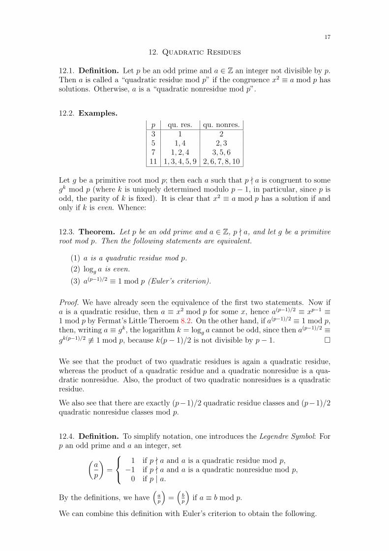
12.2. Examples.

p qu. res. qu. nonres.3 1 25 1, 4 2, 37 1, 2, 4 3, 5, 611 1, 3, 4, 5, 9 2, 6, 7, 8, 10

Let g be a primitive root mod p; then each a such that p - a is congruent to somegk mod p (where k is uniquely determined modulo p− 1, in particular, since p isodd, the parity of k is fixed). It is clear that x2 ≡ a mod p has a solution if andonly if k is even. Whence:

12.3. Theorem. Let p be an odd prime and a ∈ Z, p - a, and let g be a primitiveroot mod p. Then the following statements are equivalent.

(1) a is a quadratic residue mod p.

(2) logg a is even.

(3) a(p−1)/2 ≡ 1 mod p (Euler’s criterion).

Proof. We have already seen the equivalence of the first two statements. Now ifa is a quadratic residue, then a ≡ x2 mod p for some x, hence a(p−1)/2 ≡ xp−1 ≡1 mod p by Fermat’s Little Theroem 8.2. On the other hand, if a(p−1)/2 ≡ 1 mod p,then, writing a ≡ gk, the logarithm k = logg a cannot be odd, since then a(p−1)/2 ≡gk(p−1)/2 6≡ 1 mod p, because k(p− 1)/2 is not divisible by p− 1. �

We see that the product of two quadratic residues is again a quadratic residue,whereas the product of a quadratic residue and a quadratic nonresidue is a qua-dratic nonresidue. Also, the product of two quadratic nonresidues is a quadraticresidue.

We also see that there are exactly (p−1)/2 quadratic residue classes and (p−1)/2quadratic nonresidue classes mod p.

12.4. Definition. To simplify notation, one introduces the Legendre Symbol: Forp an odd prime and a an integer, set(

a

p

)=

1 if p - a and a is a quadratic residue mod p,−1 if p - a and a is a quadratic nonresidue mod p,

0 if p | a.

By the definitions, we have(

ap

)=(

bp

)if a ≡ b mod p.

We can combine this definition with Euler’s criterion to obtain the following.

18

12.5. Proposition. Let p be an odd prime, and let a ∈ Z. Then(a

p

)≡ a(p−1)/2 mod p ,

and this congruence determines the value of the Legendre symbol.

Proof. Since p ≥ 3, the residue classes of −1, 0 and 1 mod p are distinct, so thelast statement follows. To prove the congruence, we consider the three possiblecases in the definition of the Legendre synbol. If a is a quadratic residue, thenboth sides are ≡ 1 by Thm. 12.3. If a is a quadratic nonresidue, then the left handside is −1, whereas the right hand side is 6≡ 1, but its square is ≡ 1. Since Z/pZis a field, the right hand side must be ≡ −1. Finally, if p | a, then both sides are≡ 0. �

Note that this result tells us that we can determine efficiently whether a given inte-ger a is a quadratic residue mod p or not: the modular exponentiation a(p−1)/2 modp can be computed in polynomial time.

It is a different matter to actually find a square root of a mod p if a is a quadraticresidue mod p. There are probabilistic polynomial time algorithms for that, but(as far as I know) no deterministic polynomial time algorithm is known that worksfor general p.

12.6. Theorem. For p an odd prime and integers a and b,(ab

p

)=

(a

p

)(b

p

).

Proof. We have(a

p

)(b

p

)≡ a(p−1)/2b(p−1)/2 = (ab)(p−1)/2 ≡

(ab

p

)mod p

by Prop. 12.5. By the same proposition, the value of the Legendre symbol isdetermined by the congruence. The claim follows. �

12.7. Example. By the preceding result, we can compute(

ap

)in terms of the

factors of a. So, if a = ±2eqf1

1 qf2

2 . . . qfk

k with odd primes qj, then(a

p

)=

(±1

p

)(2

p

)e(q1p

)f1(q2p

)f2

. . .

(qkp

)fk

.

13. Quadratic Reciprocity

By the preceding example, in order to be able to compute(

ap

)in general, we need

to know(−1p

)and

(2p

), and we need a way to find

(qp

)if q 6= p is another odd

prime.

The first is simple.

19

13.1. Theorem. If p is an odd prime, then(−1

p

)= (−1)(p−1)/2 =

{1 if p ≡ 1 mod 4,

−1 if p ≡ 3 mod 4.

Proof. By Prop. 12.5, (−1

p

)≡ (−1)(p−1)/2 mod p .

Since both sides are ±1, equality follows. �

So the quadratic character of −1 mod p depends on p mod 4. Is there a similarresult concerning the quadratic character of 2 mod p? Here is a table.

p 3 5 7 11 13 17 19 23 29 31(2p

)− − + − − + − + − +

It appears that(

2p

)= 1 if p ≡ 1 or 7 mod 8 and

(2p

)= −1 if p ≡ 3 or 5 mod 8.

In order to prove a statement like this, we need some other way of expressingthe sign of the Legendre symbol. This is provided by the following result due toGauss.

13.2. Theorem. Let p be an odd prime, and let S ⊂ Z be a set of cardinality(p − 1)/2 such that {0} ∪ S ∪ −S is a complete system of representatives forthe residue classes mod p. (Examples are S = {1, 2, . . . , (p − 1)/2} and S ={2, 4, 6, . . . , p− 1}.) Then for all a such that p - a, we have(

a

p

)= (−1)#{s∈S : as∈−S} .

Here S = {s : s ∈ S} is the set of residue classes mod p represented by elementsof S.

Proof. For all s ∈ S, there are unique t(s) ∈ S and ε(s) ∈ {±1} such thatas ≡ ε(s)t(s) mod p. We claim that s 7→ t(s) is a permutation of S. But it is clearthat this map is surjective: Let s ∈ S and b an inverse of a mod p, then there iss′ ∈ S such that ±s′ ≡ bs mod p, so as′ ≡ ±s mod p and therefore t(s′) = s. Sothe map must be a bijection.

Now, mod p, we have (a

p

)∏s∈S

s ≡ a(p−1)/2∏s∈S

s

=∏s∈S

(as)

≡∏s∈S

(ε(s)t(s))

=∏s∈S

ε(s)∏s∈S

s

= (−1)#{s∈S : ε(s)=−1}∏s∈S

s .

20

Since p does not divide∏

s∈S s, we get(a

p

)≡ (−1)#{s∈S : ε(s)=−1} = (−1)#{s∈S : as∈−S} mod p ,

and therefore equality (both sides are ±1). �

Taking a = −1 in the preceding result immediately gives Thm. 13.1 again.

We can now use this to prove our conjecture about the value of(

2p

).

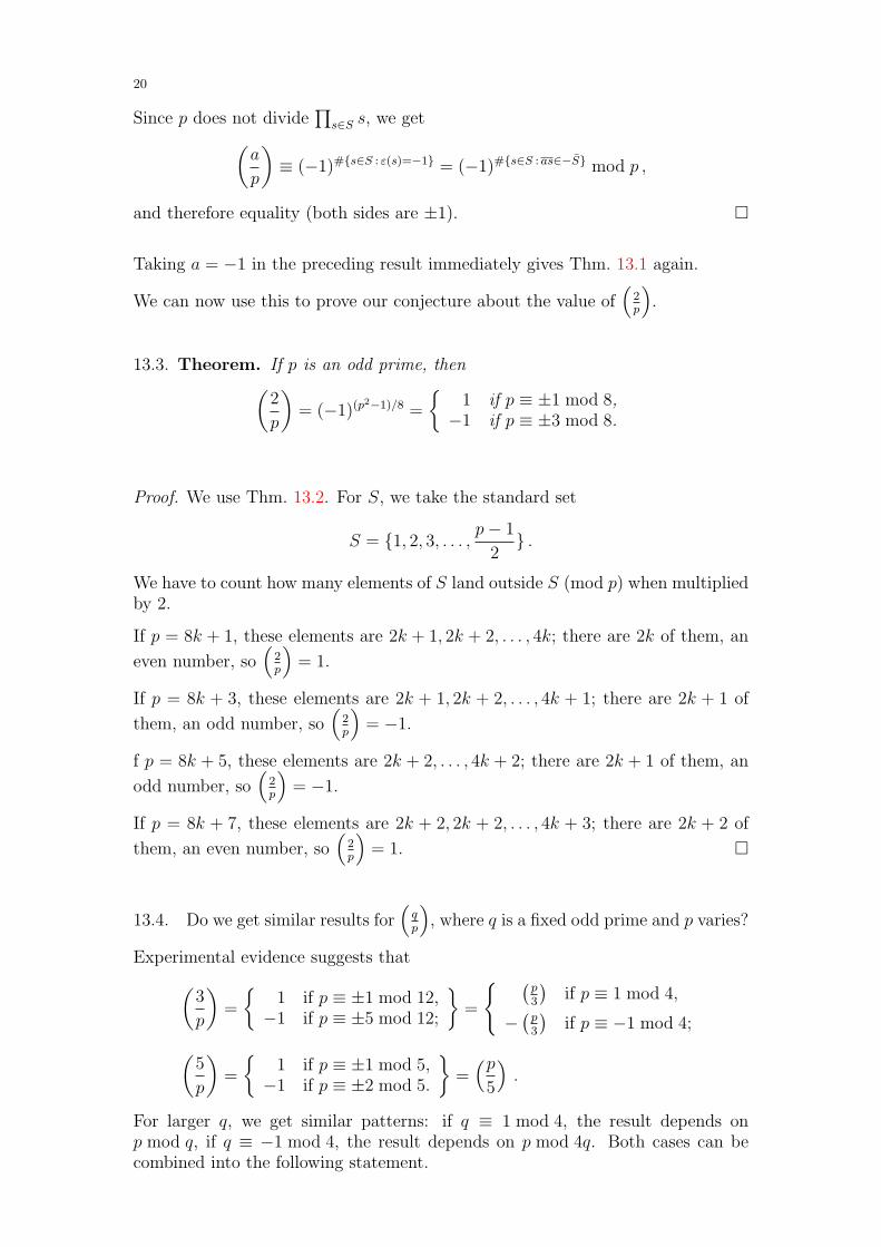
13.3. Theorem. If p is an odd prime, then(2

p

)= (−1)(p2−1)/8 =

{1 if p ≡ ±1 mod 8,

−1 if p ≡ ±3 mod 8.

Proof. We use Thm. 13.2. For S, we take the standard set

S = {1, 2, 3, . . . , p− 1

2} .

We have to count how many elements of S land outside S (mod p) when multipliedby 2.

If p = 8k + 1, these elements are 2k + 1, 2k + 2, . . . , 4k; there are 2k of them, an

even number, so(

2p

)= 1.

If p = 8k + 3, these elements are 2k + 1, 2k + 2, . . . , 4k + 1; there are 2k + 1 of

them, an odd number, so(

2p

)= −1.

f p = 8k + 5, these elements are 2k + 2, . . . , 4k + 2; there are 2k + 1 of them, an

odd number, so(

2p

)= −1.

If p = 8k + 7, these elements are 2k + 2, 2k + 2, . . . , 4k + 3; there are 2k + 2 of

them, an even number, so(

2p

)= 1. �

13.4. Do we get similar results for(

qp

), where q is a fixed odd prime and p varies?

Experimental evidence suggests that(3

p

)=

{1 if p ≡ ±1 mod 12,

−1 if p ≡ ±5 mod 12;

}=

{ (p3

)if p ≡ 1 mod 4,

−(

p3

)if p ≡ −1 mod 4;(

5

p

)=

{1 if p ≡ ±1 mod 5,

−1 if p ≡ ±2 mod 5.

}=(p

5

).

For larger q, we get similar patterns: if q ≡ 1 mod 4, the result depends onp mod q, if q ≡ −1 mod 4, the result depends on p mod 4q. Both cases can becombined into the following statement.

21

13.5. Theorem (Law of Quadratic Reciprocity). Let p and q be distinct oddprimes. Then we have(

q

p

)=

(p∗

q

)= (−1)

p−12

q−12

(p

q

)

=

(p

q

)if p ≡ 1 mod 4 or q ≡ 1 mod 4

−(p

q

)if p ≡ −1 mod 4 and q ≡ −1 mod 4

where p∗ = (−1)(p−1)/2p, so p∗ = p if p ≡ 1 mod 4 and p∗ = −p if p ≡ −1 mod 4.

Proof. We make again use of “Gauss’ Lemma” Thm. 13.2. We need two sets

S = {1, 2, . . . , p− 1

2} and T = {1, 2, . . . , q − 1

2} .

Let m = #{s ∈ S : qs ∈ −S} (mod p) and n = #{t ∈ T : pt ∈ −T} (mod q).Then we have (

q

p

)(p

q

)= (−1)m(−1)n = (−1)m+n .

We therefore have to find the parity of the sum m+ n.

Now, if qs ≡ −s′ mod p for some s′ ∈ S, then there is some t ∈ Z such thatpt− qs = s′ ∈ S, i.e., 0 < pt− qs ≤ (p− 1)/2. This number t now must be in T :

pt > qs > 0 and pt ≤ p− 1

2+ qs ≤ (q + 1)

p− 1

2< p

q + 1

2.

Since q is odd, the last inequality implies t ≤ (q − 1)/2. Hence we see that

m = #{(s, t) ∈ S × T : 0 < pt− qs ≤ p− 1

2} .

In exactly the same way, we have that

n = #{(s, t) ∈ S × T : −q − 1

2≤ pt− qs < 0} .

Since there is no pair (s, t) ∈ S×T such that pt = qs, it follows that m+n = #X,where

X = {(s, t) ∈ S × T : −q − 1

2≤ pt− qs ≤ p− 1

2} .

This set X is invariant under the rotation by π (or 180◦) about the center of therectangle, which has the effect of changing (s, t) into (s′, t′) = (p+1

2− s, q+1

2− t):

pt′ − qs′ = p(q + 1

2− t)− q(p+ 1

2− s)

=p− q

2− (pt− qs) ,

so pt− qs ≤ (p− 1)/2 ⇐⇒ pt′− qs′ ≥ −(q− 1)/2 and pt− qs ≥ −(q− 1)/2 ⇐⇒pt′ − qs′ ≤ (p − 1)/2. Since the only possible fixed point of the rotation is thecenter (p+1

4, q+1

4) of the rectangle, and since this point belongs toX if it has integral

coordinates, we see that

#X is odd ⇐⇒ p+ 1

4,q + 1

4∈ Z ⇐⇒ p ≡ −1 mod 4 and q ≡ −1 mod 4 .

This concludes the proof. �

22

13.6. Example. With the help of the Law of Quadratic Reciprocity, we can eval-uate Legendre symbols in the following way.(

67

109

)=

(109

67

)=

(42

67

)=

(2 · 3 · 7

67

)=

(2

67

)(3

67

)(7

67

)= (−1)(−

(67

3

))(−

(67

7

)) = −

(1

3

)(4

7

)= −1

The disadvantage with this approach is that we have to factor the numbers we getin intermediate stages, which can be very costly if the numbers are large. In orderto overcome this difficulty, we generalize the Legendre Symbol and allow arbitraryodd integers instead of odd primes p.

13.7. Definition. Let a ∈ Z, and let n be an odd integer, with factorizationn = ±pe1

1 pe22 . . . pek

k . Then we define the “Jacobi Symbol” via(an

)=

k∏j=1

(a

pj

)ej

.

It has the following simple properties extending those of the Legendre Symbol.

(1)(

an

)= 0 if and only if gcd(a, n) 6= 1.

(2) If a ≡ b mod n, then(

an

)=(

bn

).

(3)(

abn

)=(

an

) (bn

).

(4)(

an

)= 1 if a ⊥ n and a is a square mod n.

Warning. Contrary to the case of the Legendre symbol (i.e., when n is prime),the converse of the last statement does not hold in general. For example,

(215

)= 1,

but 2 is not a square mod 15 (since 2 is not a square mod 3 and mod 5).

But, what is more important, the Jacobi symbol also obeys the Law of QuadraticReciprocity.

13.8. Theorem. Let m and n be positive odd integers. We have

(1)

(−1

n

)= (−1)

n−12 .

(2)

(2

n

)= (−1)

n2−18 .

(3)(mn

)= (−1)

m−12

n−12

( nm

).

Proof. This is proved by invoking the definition of the Jacobi Symbol and byobserving that n 7→ (−1)(n−1)/2 and n 7→ (−1)(n2−1)/8 are multiplicative on oddintegers n, and (m,n) 7→ (−1)(m−1)(n−1)/4 is bimultiplicative on pairs of odd inte-gers. The results then reduce to Thms 13.1, 13.3 and 13.5, respectively. �

13.9. Example. Let us compute(

67109

)again.(

67

109

)=

(109

67

)=

(42

67

)=

(2

67

)(21

67

)= (−1)

(67

21

)= −

(4

21

)= −1

In general, using Jacobi Symbols in the intermediate steps, we can compute Le-gendre Symbnols (or, of course, Jacobi Symbols) much in the same way as wecompute a GCD; we only have to take care to take out powers of 2 when theyappear.

23

14. Another Proof of Quadratic Reciprocity

Gauss found seven or eight different proofs of the law of quadratic reciprocity inhis life. Here is another one, which is more algebraic in flavor, and explains whyp∗ occurs in a natural way.

14.1. Definition. Let p be an odd prime, and set ζ = exp(2πi/p) ∈ C. For a ∈ Zprime to p, we define the “Gauss Sum”

ga =

p−1∑j=1

(j

p

)ζaj ∈ Z[ζ] .

14.2. Proposition. The Gauss Sum has the following properties.

(1) ga =

(a

p

)g1 for a ⊥ n.

(2) g21 = p∗.

(3) For an odd prime q 6= p, we have gq1 ≡ gq mod q.

(The congruence takes place in the ring Z[ζ].)

Proof.

(1) We have (a

p

)ga =

p−1∑j=1

(aj

p

)ζaj =

p−1∑k=1

(k

p

)ζk = g1 .

(note that k = aj also runs through a complete set of representatives ofthe primitive residue classes mod p.)

(2) We compute

g21 =

p−1∑j,k=1

(jk

p

)ζj+k =

p−1∑j,m=1

(m

p

)ζj(1+m)

=

p−1∑m=1

(m

p

) p−1∑j=1

ζj(1+m) =

(−1

p

)p−

p−1∑m=1

(m

p

)= p∗

(where k = jm; note that(

jkp

)=(

j2mp

)=(

mp

). Also note that∑p−1

j=0 ζja = 0 if p - a and = p otherwise, and that

∑p−1m=1

(mp

)= 0.)

(3) Mod q, we have

gq1 =

(p−1∑j=1

(j

p

)ζj

)q

≡p−1∑j=1

(j

p

)q

ζjq =

p−1∑j=1

(j

p

)ζqj = gq .

�

24

14.3. Remark. By property (2) above, we have that

g1 = ±√p if p ≡ 1 mod 4 and g1 = ±i√p if p ≡ 3 mod 4.

It is then a natural question to ask which of the two signs is the correct one.Gauss was working on this question for quite a long time, until he finally was ableto prove that the sign is always “+”. (Also for this statement, he found severaldifferent proofs in his life.) If p ≡ 3 mod 4, this has for example the followingconsequence. It is not hard to see that in this case

S(p) =

p−1∑a=1

a

(a

p

)= −hp

with some integer h. The fact that g1 = +i√p then implies that h is positive.

This can be interpreted as saying that quadratic nonresidues mod p (between 1and p − 1) are larger on average than quadratic residues. (If p > 3, then h isthe “class number of positive definite binary quadratic forms of discriminant −p”,which is known to be positive, since it counts something. On the other hand, whatone really proves is that

h =ig1

p√p

p−1∑a=1

a

(a

p

),

which implies that S(p) = ∓hp, and so the sign of the Gauss sum determines thesign of S(p).)

14.4. Proof of the Quqdratic Reciprocity Law.

On the one hand, gq =

(q

p

)g1. On the other hand, mod q, we have

gq ≡ gq1 = g1(g

21)

(q−1)/2 = g1(p∗)(q−1)/2 ≡ g1

(p∗

q

)(by Euler’s criterion). Taking both together, we see that(

q

p

)g1 ≡

(p∗

q

)g1 .

Now we multiply by g1 and use that g21 = p∗ is prime to q, so that we can cancel

it from both sides. This gives (q

p

)≡(p∗

q

)mod q

and then equality.

15. Sums of Squares

In this section we address the question which positive integers can be written asa sum of two, three, four, . . . squares.

Let us first look at sums of two squares. Let

S = {x2 + y2 : x, y ∈ Z}= {0, 1, 2, 4, 5, 8, 9, 10, 13, 16, 17, 18, 20, 25, 26, 29, 32, 34, 36, 37, 40, . . . } .

It is clear that every square is in S. Also, it is easy to see that if n ≡ 3 mod 4,then n /∈ S (recall that a square is either ≡ 0 or ≡ 1 mod 4). Furthermore, wehave the following.

25

15.1. Lemma. The set S is closed under multiplication:if m,n ∈ S, then mn ∈ S.

Proof. Note that

(x2 + y2)(u2 + v2) = (xu∓ yv)2 + (xv ± yu)2 .

�

What is behind this formula is the following.

|x+ iy|2 = x2 + y2 and |αβ|2 = |α|2|β|2 .

Because of the multiplicative structure of S, it makes sense to look at the set ofprime numbers that are in S. It is clear that p /∈ S if p ≡ 3 mod 4. Obviously,2 ∈ S, and from the list of the first few elements of S, it appears that p ∈ S ifp ≡ 1 mod 4.

15.2. Theorem. If p ≡ 1 mod 4 is a prime number, then p ∈ S.

Proof. We know that −1 is a square mod p, hence there are a ∈ Z, k ≥ 1 suchthat a2 +1 = kp. We can take |a| ≤ (p− 1)/2, hence we can assume that k < p/4.

Now let k ≥ 1 be minimal such that there are x, y ∈ Z with x2 + y2 = kp. Wewant to show that k = 1. So assume k > 1. Let u ≡ x mod k, v ≡ y mod k with|u|, |v| ≤ k/2. Then

u2 + v2 = kk′

with 1 ≤ k′ ≤ k/2. (Note that k′ 6= 0 because k - p, as 1 < k < p.) Now

xu+ yv ≡ x2 + y2 ≡ 0 mod k , xv − yu ≡ xy − yx = 0 mod k

and (xu+ yv)2 + (xv − yu)2 = (x2 + y2)(u2 + v2) = k2 k′p. If we let

x′ =xu+ yv

k, y′ =

xv − yu

k,

then (x′)2 +(y′)2 = k′p and k′ < k, contradicting our choice of k. So we must havehad k = 1. �

The technique of proof use here is called “descent” and goes back to Fermat. Thename comes from the fact that we “descend” from one value of k to a smaller one.

By what we know so far, we have already proved one direction of the followingresult characterizing the elements of S.

15.3. Theorem. A positive integer n can be represented as a sum of two squaresif and only if for every prime p | n with p ≡ 3 mod 4, the exponent with which pappears in the factorization of n is even.

Proof. If n is of the specified form, then n = p1 · · · prm2 with primes pj = 2 or

pj ≡ 1 mod 4. Since by the above, all factors in this product are in S and S isclosed under multiplication, n ∈ S.

Now assume that n ∈ S and that we already know that all m ∈ S with m < nare of the specified form. Let p ≡ 3 mod 4 be a prime number dividing n. Writen = x2 + y2. We claim that p divides both x and y. It then follows that n = p2mwith m = (x/p)2 + (y/p)2 ∈ S, so we are done by induction.

26

To show that p divides x and y, assume that (for example), p does not divide x.Then there is a ∈ Z with ax ≡ 1 mod p, and we get

0 ≡ a2n = (ax)2 + (ay)2 ≡ 1 + (ay)2 mod p ,

contradicting the fact that −1 is not a square mod p. So pmust divide x and y. �

For three squares, the criterion is simpler (but we will not prove it).

15.4. Theorem. A positive integer can be represented as a sum of three squaresif and only if it is not of the form 4km where m ≡ 7 mod 8.

It is easy to see that a number n = 4km with m ≡ 7 mod 8 is not a sum of threesquares. First note that if a sum x2 + y2 + z2 is divisible by 4, then x, y, z haveto be even. This implies that 4n is a sum of three squares if and only if n is.So we can assume that k = 0. Finally, mod 8, a square is 0, 1 or 4, so a sumof three squares can never be ≡ 7 mod 8. The hard part of the proof is to showthat every n not of the given form actually is a sum of three squares. Part of thedifficulty comes from the fact that the set of sums of three squares is not closedunder multiplication: 3 and 5 are sums of three squares, but 15 is not.

15.5. Four Squares. It might therefore seem rather hopeless to look for an iden-tity for four squares analogous to

(xu∓ yv)2 + (xv ± yu)2 = (x2 + y2)(u2 + v2) ,

but in fact there is a good reason why one exists. The quaternion algebra, a 4-dimensional R-algebra, is a beautiful analog of the 2-dimensional algebra C; it wasdiscovered by Hamilton. It is defined to be

H := {a+ ib+ cj + dk : a, b, c, d ∈ R} ,

with the noncommutative multiplication rules

i2 = j2 = k2 = −1,

ij = k, ji = −k, jk = i, kj = −i, ki = j, ik = −j .

One can then define a “norm” map

N(a+ ib+ cj + dk) := (a+ ib+ cj + dk)(a− ib− cj − dk) = a2 + b2 + c2 + d2 ,

and it is easy to check that the norm is multiplicative. When one writes out whatthis means, one discovers the identity

(a2 + b2 + c2 + d2)(A2 +B2 + C2 +D2)

= (aA− bB − cC − dD)2 + (aB + bA+ cD − dC)2

+ (aC + cA− bD + dB)2 + (aD + dA+ bC − cB)2 .

In light of this, the set of integers representable by four squares must be closedunder multiplication. In fact:

27

15.6. Theorem (Lagrange). All positive integers are sums of four squares.

Proof. By the identity stated above, it suffices to show that all primes p are sumsof four squares. We do this by descent, imitating the proof of the Two SquaresTheorem. First note that, applying Lemma 15.7 below, we can find integersa, b, c, d and k such that a2 + b2 + c2 + d2 = kp and 1 ≤ k < p (taking d = 0, say).If k = 1 we are done. Otherwise, let A,B,C,D be the integers determined by

A ≡ −a mod k, |A| ≤ k/2B ≡ b mod k, |B| ≤ k/2C ≡ c mod k, |C| ≤ k/2D ≡ d mod k, |D| ≤ k/2

Thus A2 +B2 +C2 +D2 ≤ k2. If equality holds, A, B, C and D must each equalk/2 or −k/2. In that case a, b, c and d are each congruent to k/2 modulo k, whichmeans k2 divides a2 +b2 +c2 +d2 = kp. But that is not possible because 1 < k < pand p is prime. Hence A2 + B2 + C2 +D2 = kk′ with 1 ≤ k′ < k. Applying themagic identity, we have

k2k′p = (a2 + b2 + c2 + d2)(A2 +B2 + C2 +D2)

= (aA− bB − cC − dD)2 + (aB + bA+ cD − dC)2

+ (aC + cA− bD + dB)2 + (aD + dA+ bC − cB)2 .

Consider the right hand side: the latter three terms, and hence all four terms, aredivisible by k2. Dividing both sides by k2, we obtain a representation of k′p as asum of four squares, which completes one step of the descent. As already noted,at each step we have 1 ≤ k′ < k. So, after a finite number of steps of the descentwe must obtain k′ = 1. This completes the proof. �

15.7. Lemma. Let p be an odd prime. Then there are integers u, v such thatu2 + v2 + 1 ≡ 0 mod p.

Proof. The statement is equivalent to the following: there are u, v ∈ Fp such thatu2 = −v2 − 1. Now let

X = {u2 : u ∈ Fp} and Y = {−v2 − 1 : v ∈ Fp} ,

then #X = #Y = (p + 1)/2. Since #X + #Y = p + 1 > p = #Fp, X and Ycannot be disjoint, which proves the claim. �

16. Geometry of Numbers

In this section, we will learn about a nice method to solve number theoreticalproblems using geometry. The main result was discovered by Hermann Minkowski.The basic idea is that if we have a sufficiently nice and sufficiently “large” setin Rn, then it will contain a non-zero point with integral coordinates. For theapplications, it is convenient to use more general “lattices” than the integral points,so we have to introduce this notion first.

28

16.1. Definition. A lattice Λ ⊂ Rn is the set of all integral linear combinationsof a set of basis vectors v1, . . . , vn of Rn. In particular, Λ is a subgroup of theadditive group Rn. The set

F ={ n∑

j=1

tjvj : 0 ≤ tj < 1 for all j}

is called a fundamental parallelotope for Λ. ∆(Λ) = vol(F ) = | det(v1, . . . , vn)| isthe covolume of Λ.

The most important property of F is that every vector v ∈ Rn can be writtenuniquely as v = λ + w with λ ∈ Λ and w ∈ F . In other words, Rn is the disjointunion of all translates F + λ of F by elements of Λ.

16.2. Example. The standard example of a lattice is Λ = Zn ⊂ Rn, which isgenerated by the standard basis e1, . . . , en of Rn and has covolume ∆(Zn) = 1.

In some sense, this is the only example: if Λ = Zv1 + · · ·+Zvn ⊂ Rn is any lattice,then Λ is the image of Zn under the invertible linear map T : Rn → Rn that sendsej to vj. The covolume ∆(Λ) is then | det(T )|.

16.3. Proposition. Let Λ ⊂ Rn be a lattice, and let Λ′ ⊂ Λ be a subgroup of finiteindex m. Then Λ′ is also a lattice, and ∆(Λ′) = m∆(Λ).

Proof. As an abstract abelian group, Λ ∼= Zn. By the structure theorem for finitelygenerated abelian groups, there is an isomorphism φ : Λ → Zn that sends Λ′ toa1Z×· · ·×anZ with nonnegative integers a1, . . . , an. Since the index m of Λ′ in Λis finite, we have a1 · · · an = m. Let v1, . . . , vn be the generators of Λ that are sentto the standard basis of Zn under φ. Then Λ′ = Za1v1 + · · ·+ Zanvn ⊂ Rn, so Λ′

is a lattice. Furthermore,

∆(Λ′) = | det(a1v1, . . . , anvn)| = a1 · · · an | det(v1, . . . , vn)| = m∆(Λ) .

�

16.4. Corollary. Let φ : Zn → M be a group homomorphism onto a finitegroup M . Then the kernel of φ is a lattice Λ, and ∆(Λ) = #M .

Proof. By the standard isomorphism theorem, we have Zn/ kerφ ∼= M , henceΛ = kerφ is a subgroup of the lattice Zn of finite index #M . The claim followsfrom Prop. 16.3 and ∆(Zn) = 1. �

Now we are ready to state and prove Minkowski’s Theorem.

16.5. Theorem (Minkowski). Let Λ ⊂ Rn be a lattice, and let S ⊂ Rn be asymmetric (i.e., S = −S) and convex subset such that vol(S) > 2n∆(Λ). Then Scontains a nonzero lattice point from Λ.

Proof. In a first step, we show that X = 12S has to intersect one of its translates

under elements of Λ. Let F be a fundamental parallelotope for Λ, and for λ ∈ Λ,set

Xλ = F ∩ (X + λ) .

By the fundamental property of F , we get that

X =∐λ∈Λ

(Xλ − λ)

29

(i.e., X is a disjoint union of translates of the Xλ). Hence∑λ

vol(Xλ) = vol(X) = 2−n vol(S) > ∆(Λ) = vol(F ) ,

and so the sets Xλ cannot be all disjoint (because they then would not fit into F ).So there are λ 6= µ such that Xλ ∩Xµ 6= ∅. Shifting by −µ, we see that

X ∩ (X + λ− µ) 6= ∅ .

Let x be a point in the intersection. Then 2x ∈ S and 2x− 2(λ−µ) ∈ S. Since Sis symmetric, we also have 2(λ − µ) − 2x ∈ S. Then, since S is also convex, themidpoint of the linesegment joining 2x and 2(λ− µ)− 2x ∈ S must also be in S.But this midpoint is λ− µ ∈ Λ \ {0}, and the statement is proved. �

Let us use this result to re-prove the essential results on sums of two and foursquares.

16.6. Theorem. Let p ≡ 1 mod 4 be a prime. Then p is a sum of two squares.

Proof. We need a lattice Λ and a set S. Let u be a square root of −1 mod p, andset

Λ = {(x, y) ∈ Z2 : x ≡ uy mod p} .Then Λ is a lattice in R2, and ∆(Λ) = p (we can think of Λ as the kernel of thecomposition

Z2 −→ F2p −→

F2p

〈(u, 1)〉which is a surjective group homomorphism onto a group of order p). For the setS, we take the open disk

S = {(ξ, η) ∈ R2 : ξ2 + η2 < 2p} .Then vol(S) = π · 2p = 2πp > 4p = 22∆(Λ), and so by Thm. 16.5, there is somenonzero (x, y) ∈ Λ ∩ S. Now for each (x, y) ∈ Λ, we have that

x2 + y2 ≡ (uy)2 + y2 = y2(1 + u2) ≡ 0 mod p .

So p divides x2 + y2; on the other hand, 0 < x2 + y2 < 2p by the definition of S.So we must have x2 + y2 = p. �

Now let us consider the case of four squares. From Lemma 15.7, we know that forevery odd prime p, there are integers u and v such that p divides 1 + u2 + v2.

16.7. Theorem. Let p be an odd prime. Then p is a sum of four squares.

Proof. We need again a lattice Λ and a set S. For S, we should obviously take asuitable open ball:

S = {(ξ1, ξ2, ξ3, ξ4) ∈ R4 : ξ21 + ξ2

2 + ξ23 + ξ2

4 < 2p} .What is the volume of S? Here it is useful to know the general formula for thevolume of the n-dimensional unit ball; it is

vol(Bn) =πn/2(

n2

)!

(where for odd n, the factorial satisfies the usual recurrence (x+ 1)! = x! (x+ 1),and one has (−1/2)! =

√π). For n = 4, we get π2/2 for the volume of the unit

ball, hence vol(S) = π2(2p)2/2 = 2π2p2.

30

From this, we can already see that the lattice should have covolume p2. Thismeans that we need a 2-dimensional subspace of F4

p on which x21 + x2

2 + x23 + x2

4

vanishes. One such subspace is given by

V = 〈(1, u, v, 0), (0,−v, u, 1)〉 :

if (a, au− bv, av + bu, b) is a general element of V , then

a2 + (au− bv)2 + (av + bu)2 + b2

= a2(1 + u2 + v2) + b2(v2 + u2 + 1) + 2ab(−uv + vu)

= 0 .

If Λ is the kernel of Z4 → F4p → F4

p/V , then for (x1, x2, x3, x4) ∈ Λ, we have

(x1, x2, x3, x4) ∈ V , hence p divides x21 + x2

2 + x23 + x2

4. For the covolume, we have∆(Λ) = #(F4

p/V ) = p2. Since vol(S) = 2π2p > 16p2, the proof can be concludedin the same way as before. �

17. Ternary Quadratic Forms

In the preceding sections, we have seen some quadratic forms.

17.1. Definition. An n-ary quadratic form is a homogenous polynomial of de-gree 2 in n variables (here, the coefficients will always be integers, but one canconsider quadratic forms over any ring). For n = 2, we have binary quadraticforms; they have the general form

Q(x, y) = a x2 + b xy + c y2 .

For n = 3, we have ternary quadratic forms

Q(x, y, z) = a x2 + b y2 + c z2 + d xy + e yz + f zx ,

and so on.

So far, we have been asking about representations of numbers by a quadratic formQ, i.e., whether it is possible to find a given integer as the value of Q at sometuple of integers.

Another question one can ask is whether a given quadratic form has a nontrivialzero, i.e., whether there exist (in the case of ternary forms, say) integers x, y, z, notall zero, such that Q(x, y, z) = 0. This is what we will look into now. For binaryforms, this question is not very interesting; it boils down to deciding whether ornot the form is the product of two linear forms with integral coefficients, whichis the case if and only if the discriminant b2 − 4ac of the form is a square. Forternary forms, however, this is an interesting problem. Note that we can alwaysassume that solutions are primitive (i.e., gcd(x, y, z) = 1): common divisors canalways be divided out.

17.2. Definition. Let Q be a quadratic form in n variables; then it can be givenby a symmetric matrix MQ whose off-diagonal entries can be half-integers, suchthat Q(x) = x>MQx. Then detQ = det(MQ) is called the determinant of Q, anddiscQ = (−1)n−122bn/2c detQ is called the discriminant of Q; the discriminant isalways an integer. (The reason for the power of 2 appearing in the definition ofdisc(Q) is that the discriminant then also makes sense in characteristic 2.)

For example,disc(a x2 + b xy + c y2) = b2 − 4 ac

31

and

disc(a x2 + b y2 + c z2 + d xy + e yz + f zx) = 4 abc+ def − ae2 − bf 2 − cd2 .

A quadratic formQ is non-degenerate if discQ 6= 0, otherwise it is called degenerateor singular. In this latter case, there is a linear transformation of the variablesthat results in a quadratic form involving fewer variables (choose an element inthe kernel of MQ as one of the new basis vectors . . . ).

17.3. Some Geometry. Ternary quadratic forms correspond to conic sections inthe plane. If we are looking for solutions toQ(x, y, z) = 0 in real numbers such thatz 6= 0 (say), we can divide by z2 and set ξ = x/z, η = y/z to obtain Q(ξ, η, 1) = 0,the equation of a conic section in R2. (If we want to include the solutions withz = 0, we have to consider the conic section in the projective plane.) In this setting,nontrivial primitive integral solutions to Q(x, y, z) = 0 correspond to rationalpoints (points with rational coordinates) on the conic. This correspondence istwo-to-one: to the point (x/z, y/z) (in lowest terms) there correspond the twosolutions (x, y, z) and (−x,−y,−z).For example, if we take Q(x, y, z) = x2 + y2 − z2, then it corresponds to theunit circle in the xy plane, and the solutions (in this case, Pythagorean Triples)correspond to the rational points on the unit circle (there are no solutions withz = 0). In fact, it is easy to describe them all: fix one point, say (−1, 0), anddraw a line with rational slope t = u/v through it. It will intersect the circlein another point, which will again have rational coordinates. Conversely, if wetake some rational point on the circle, the line connecting it to (−1, 0) will haverational slope. We see that the rational points are parametrized by the rationalslopes (including∞ = 1/0 for the vertical tangent at (−1, 0); this line gives (−1, 0)itself). The same kind of argument can be used quite generally.

17.4. Theorem. Let Q(x, y, z) be a non-degenerate ternary quadratic form thathas a primitive integral solution (x0, y0, z0). Then there are binary quadratic formsRx, Ry and Rz such that, up to scaling, all integral solutions of Q(x, y, z) = 0 aregiven by

(Rx(u, v), Ry(u, v), Rz(u, v))

with integers u, v.

Proof. We first assume that Q = y2 − xz. Then we can clearly take

Rx(u, v) = u2 , Ry(u, v) = uv , Rz(u, v) = v2 .

(Dividing by z2, we have (y/z)2 = x/z; put y/z = u/v and clear denominators.)

Now assume that (x0, y0, z0) = (1, 0, 0). Then

Q(x, y, z) = b y2 + c z2 + d xy + e yz + f zx .

If we set

x = bX + e Y + c Z , y = −dX − f Y , z = −d Y − f Z ,

then Q(x, y, z) = − disc(Q)(Y 2−XZ), as is easily checked. By the first case (notethat disc(Q) 6= 0), this means that

Rx(u, v) = b u2 + e uv+ c v2 , Ry(u, v) = −d u2−f uv , Rz(u, v) = −d uv−f v2

do what we want.

32

Finally, we consider the general case. By Prop. 18.6 in the “Introductory Algebra”notes (Fall 2005), there is a matrix T ∈ GL3(Z) such that (x0 y0 z0) = (1 0 0)T .Write

(x y z) = (x′ y′ z′)T

and set Q′(x′, y′, z′) = Q(x, y, z); then Q′(1, 0, 0) = Q(x0, y0, z0) = 0. By theprevious case, we have binary quadratic forms R′

x, R′y, R

′z that parametrize the

solutions of Q′. Then

(Rx Ry Rz) = (R′x R

′y R

′z)T

are the binary quadratic forms we want for Q. �

17.5. Example. For Q(x, y, z) = x2 + y2 − z2 and the initial solution (−1, 0, 1),we can choose

T =

−1 0 10 1 00 0 1

and obtain x = −x′, y = y′, z = x′ + z′, so

Q′(x′, y′, z′) = Q(−x′, y′, x′ + z′) = (y′)2 − (z′)2 − 2x′z′ .

The quadratic forms parametrizing the solutions of Q′ are

R′x(u, v) = u2 − v2 , R′

y(u, v) = 2uv , R′z(u, v) = 2 v2 .

For our original form Q, we then get

Rx(u, v) = −R′x(u, v) = v2 − u2

Ry(u, v) = R′y(u, v) = 2uv

Rz(u, v) = R′x(u, v) +R′

z(u, v) = u2 + v2

This is exactly the well-known parametrization of the Pythagorean Triples.

We see that we can easily find all solutions if we know just one. So there are twoquestions that remain: to decide whether a solution exist, and, if so, find one.

18. Legendre’s Theorem

We can always diagonalize a non-degenerate quadratic form by a suitable linearsubstitution of the variables (and perhaps scaling, to keep the coefficients integral).Basically, this comes down to repeatedly completing the square. So, for theoreticalpurposes at least, we can assume that our ternary quadratic form is diagonal:

Q(x, y, z) = a x2 + b y2 + c z2 .

In practice, it might be a very bad idea to do this, as the coefficients a, b, c maybe much larger than the coefficients of the original form!

Let us be a bit more formal.

33

18.1. Definition. Let Q, Q′ be two ternary quadratic forms. We say that Qand Q′ are equivalent if

Q′(x, y, z) = λQ(a11x+ a12y + a13z, a21x+ a22y + a23z, a31x+ a32y + a33z)

with λ ∈ Q× and a matrix

T =

a11 a12 a13

a21 a22 a23

a31 a32 a33

∈ GL3(Q) .

The above then means that every non-degenerate ternary quadratic form is equiv-alent to a diagonal one. It is easily seen that Q has nontrivial integral (or equiv-alently, rational) solutions if and only if Q′ does.

If we want to decide whether Q = ax2+by2+cz2 admits a solution, we can simplifythe problem somewhat. We can, of course, assume that gcd(a, b, c) = 1. If a (say)is divisible by a square d2, then we can as well move d2 into the x2 term and thusobtain an equivalent form with smaller coefficients. Proceeding in this way, wecan assume that a, b and c are squarefree.

Also, if two of the coefficients, say b and c, have a common prime divisor p, thenp must divide x. We replace x by px and then divide the form by p, making thecoefficients smaller. In this way, we can also assume that a, b and c are coprimein pairs. We can summarize these assumptions by saying that abc is squarefree.

18.2. Necessary Conditions for Solubility. We can easily write down a num-ber of conditions that are necessary for the existence of a solution:

(1) Not all of a, b, and c have the same sign.(2) If abc is odd, then a, b and c are not equal mod 4.(3) If a is even (say), then b+ c ≡ 0 or a+ b+ c ≡ 0 mod 8.(4) If p | a is odd, then −bc is a quadratic residue mod p.(5) If p | b is odd, then −ca is a quadratic residue mod p.(6) If p | c is odd, then −ab is a quadratic residue mod p.

For odd primes p such that p - abc, we do not obtain any restrictions in this way:there are always nontrivial solutions mod p (compare Lemma 15.7; the proof ismore or less the same).

Note that in order to check the conditions, we have to factor the coefficients a,b and c. It can be shown that this cannot be avoided: if one can find solutionsto (diagonal) ternary quadratic forms, then one can also factor integers, hencesolving ternary quadratic forms is at least as hard as factoring integers.

The surprising fact is that these necessary conditions are already sufficient!

18.3. Theorem (Legendre). Let Q(x, y, z) = a x2+b y2+c z2 with abc squarefreesatisfy the conditions in 18.2. Then there exists a nontrivial solution in integers.

Proof. We will prove this using Minkowski’s Theorem 16.5. Let D = |abc|. Ourfirst claim is that there is a lattice Λ ⊂ Z3 such that for all (x, y, z) ∈ Λ, 2Ddivides Q(x, y, z), and such that ∆(Λ) = 2D. In order to find such a Λ, weconstruct lattices Λp for all odd p | D such that p | Q(x, y, z) when (x, y, z) ∈ Λp

and such that ∆(Λp) = p. We will also construct a lattice Λ2 such that 2 or 4divides Q(x, y, z) for all (x, y, z) ∈ Λ2 (according to whether abc is odd or even)and such that ∆(Λ2) = 2 or 4. Then Λ =

⋂p|D Λp will do what we want.

34

Now let p be an odd prime divisor of a (similarly for b or c). By assumption, thereexists some up ∈ Z such that p divides bu2

p + c. Let

Λp = {(x, y, z) ∈ Z3 : y ≡ upz mod p} .

It is easily checked that Λp does what we want.

Now assume that abc is odd. Then we let

Λ2 = {(x, y, z) ∈ Z3 : x+ y + z ≡ 0 mod 2} .

If a (say) is even and b+ c ≡ 0 mod 4, we let

Λ2 = {(x, y, z) ∈ Z3 : x ≡ y + z ≡ 0 mod 2} ;

if b+ c ≡ 2 mod 4, we let

Λ2 = {(x, y, z) ∈ Z3 : x ≡ y ≡ z mod 2} .

It is again easily checked that Λ2 has the required properties in each case.

Now assume that the sign of c differs from that of a and b. Then we take for Sthe elliptic cylinder

S = {(ξ, η, ζ) ∈ R3 : |a|ξ2 + |b|η2 < 2D and |c|ζ2 < 2D} .

We find that

vol(S) = π2D√|ab|

2

√2D√|c|

=4√

2πD√D√

D= 4

√2πD > 16D = 8∆(Λ) .

Hence by Thm. 16.5, there is a nonzero element (x, y, z) in Λ ∩ S. Since it is inΛ, Q(x, y, z) is a multiple of 2D. Since |Q(x, y, z)| =

∣∣(|a|x2 + |b|y2) − |c|z2∣∣ and

both terms in the difference are < 2D, we find that |Q(x, y, z)| < 2D. Together,these imply that Q(x, y, z) = 0. �

Note that the ellipsoid given by |a|ξ2 + |b|η2 + |c|ζ2 < 2D would be too small forthe proof to work. Note also that we did not need to assume that solutions mod 4or mod 8 exist. This is a general feature: one can always leave out one “place” inthe conditions — either conditions mod powers of 2, or some odd prime, or the“infinite place”, which here gives rise to the condition on the signs. The resaonbehind this is essentially quadratic reciprocity, which leads to the fact that thenumber of places where the conditions fail is always even. In the above proof, onecould use the mod 4/mod 8 conditions to come up with a lattice of covolume 4Dgiving divisibility by 4D; then the ellipsoid would be sufficiently large, and weneed not require the sign condition on the coefficients!

There is also a proof by descent (in fact, that was how Legendre originally provedhis theorem).

18.4. Corollary. If a x2 + b y2 + c z2 = 0 has a nontrivial solution in integers,then it has one such that

max{|a|x2 , |b| y2 , |c| z2} ≤ 4π−2/3|abc| < 1.865|abc| ,

or equivalently,

|x| ≤ 2π−1/3√|bc| , |y| ≤ 2π−1/3

√|ca| , |z| ≤ 2π−1/3

√|ab| .

35

Proof. With 2|abc| instead of 4π−2/3|abc|, this follows from the preceding proof.Now note that this proof will still work if in the definition of S, we replace 2D byαD with α > 4π−2/3. Since S contains only finitely many lattice points, there isone solution such that

max{|a|x2 , |b| y2 , |c| z2} < α|abc|for all α > 4π−2/3, which implies the claim. �

In fact, more is true.

18.5. Theorem (Holzer). If a x2 + b y2 + c z2 = 0 (with abc squarefree) has anontrivial solution in integers, then it has one such that

max{|a|x2 , |b| y2 , |c| z2} ≤ |abc| ,or equivalently,

|x| ≤√|bc| , |y| ≤

√|ca| , |z| ≤

√|ab| .

To get this (when a, b > 0 and c < 0, say), one assumes that a given solution has

|z| >√ab and constructs a new one from this with smaller |z|. So the solution

with smallest |z| must have |z| ≤√ab; the bounds on x and y then follow.

19. p-adic Numbers

19.1. Motivation. In many circumstances, one wants to consider statements forall powers of some prime number p. For example, if a polynomial equation has(nontrivial) integral solutions, it necessarily has (nontrivial) solutions modulo allpowers of p. We also considered (nontrivial) solutions in real numbers. Now R isa field, but Z/pnZ is only a ring (finite, which is nice) and not even an integraldomain when n ≥ 2. Therefore it is desirable to work instead in a structurethat is an integral domain or a field and at the same time captures statementsabout all powers of p simultaneously. This can be done by “passing to the limit”in a suitable way and leads to the ring Zp of p-adic integers and the field Qp ofp-adic numbers. Our statement about nontrivial solutions mod pn for all n canthen simply be expressed by saying that there is a (nontrivial) solution in Zp (orin Qp).

Consider, for example, the equation x2 + 7 = 0 modulo powers of 2. Solutions aregiven in the following table.

mod 21 : x ≡ 1

mod 22 : x ≡ 1, 3

mod 23 : x ≡ 1, 3, 5, 7

mod 24 : x ≡ 3, 5, 11, 13

mod 25 : x ≡ 5, 11, 21, 27

It is not hard to see that for n ≥ 3, there are always 4 solutions mod 2n. If Z/2nZwere a field, this would not be possible: in a field, a quadratic equation has at mosttwo solutions. However, two of the four are sort of spurious: they do not “lift” tosolutions mod 2n+1. Now if we pass to the limit and only consider solutions thatcan be lifted indefinitely, then we find two solutions, as expected.

36

19.2. Definition. The ring Zp of p-adic integers is

Zp = {(an) : an ≡ an+1 mod pn for all n ≥ 1} ⊂∞∏

n=1

Z/pnZ .

There is a canonical inclusion Z ↪→ Zp, given by

a 7−→ (a, a, a, . . . ) .

Now we need some structural information on the ring Zp.

19.3. Theorem. Zp is an integral domain. It only has one maximal ideal, pZp,and all non-zero ideals have the form pnZp for some n ≥ 0. (In particular, Zp isa PID and therefore a UFD.) Its unit (or multiplicative) group is Z×

p = Zp \ pZp.

Proof. (a) pZp is a maximal ideal. We show that Zp/pZp∼= Z/pZ; since the latter

is a field, the claim follows. Consider the map

Zp/pZp 3 (a1, a2, . . . ) + pZp 7−→ a1 ∈ Z/pZ .It is a well-defined ring homomorphism and obviously surjective. The homomor-phism Z → Zp induces a homomorphism Z/pZ → Zp/pZp, which is inverse to themap above, hence we have an isomorphism.

(b) We have of course that Z×p ⊂ Zp \ pZp (an element in a maximal ideal cannot

be a unit). Let us show that we actually have equality. So take u ∈ Zp \ pZp. Ifu = (u1, u2, . . . ), each un is invertible in Z/pnZ, so there are unique vn such thatunvn = 1; then v = (v1, v2, . . . ) ∈ Zp and uv = 1.

(c) We now see easily that pZp is the only maximal ideal. For assume that m isanother maximal ideal. Then m\pZp 6= ∅, and by (b), this means that m containsa unit, hence m = Zp, a contradiction.

(d) We have⋂

n≥1 pnZp = {0}. For a = (a1, a2, . . . ) ∈ pnZp implies aj = 0 for

j ≤ n.

(e) If a ∈ Zp \ {0}, then there is some n ≥ 0 and some u ∈ Z×p such that a = pnu:

By (d), there is some n such that a ∈ pnZp \ pn+1Zp. Then a = pnu whereu ∈ Zp \ pZp = Z×

p .

(f) Let I ⊂ Zp be a non-zero ideal. Then, by (d) again, there is some n such thatI ⊂ pnZp, but I 6⊂ pn+1Zp. So there is some a ∈ I such that a = pnu with u ∈ Z×

p .

Since u is invertible, pn = au−1 ∈ I as well, and we find pnZp ⊂ I, hence I = pnZp.

(g) Zp is an integral domain. Suppose ab = 0 with a = (a1, a2, . . . ), b = (b1, b2, . . . ).Assume a 6= 0; then a = pNu with some N ≥ 0, u ∈ Z×

p . Then ab = 0 implies

pNb = 0. Now this says that pNbn+N = 0 in Z/pN+nZ, so bn ≡ bN+n ≡ 0 mod pn,hence bn = 0, for all n. �

Part (e) in the proof motivates the following definition.

19.4. Definition. For a = (a1, a2, . . . ) ∈ Zp define the p-adic valuation

vp(a) = max({0} ∪ {n ≥ 1 : an = 0}) ∈ {0, 1, . . . ,∞} .Then a = pvp(a)u with u ∈ Z×

p , if a 6= 0 (and vp(0) = ∞) and the valuation iscompatible with the p-adic valuation on Z.

Define the p-adic absolute value by

|0|p = 0 , |a|p = p−vp(a) if a 6= 0.

37

19.5. Definition. The field Qp of p-adic numbers is the field of fractions of Zp.

We have that Qp = Zp[1/p], and we can extend the p-adic valuation and absolutevalue to Qp: vp(a/b) = vp(a)− vp(b) and |a/b|p = |a|p/|b|p; then for all a ∈ Q×

p ,

a = pvp(a)u

with some u ∈ Z×p .

19.6. Lemma.

(1) |ab|p = |a|p |b|p .

(2) |a+ b|p ≤ max{|a|p, |b|p} ≤ |a|p + |b|p .

Proof. Easy. �

In particular, | · |p defines a metric on Zp and Qp: d(a, b) = |a − b|p. It is a factthat with this metric, Zp is a compact metric space, and Z is dense in Zp. Also,Qp can be identified with the completion of Q with respect to the p-adic absolutevalue | · |p (in the same way as R is the completion of Q with respect to the usualabsolute value | · | = | · |∞).

19.7. Remark. Define |x|∞ = |x| for x ∈ R. Then for all a ∈ Q×,∏v=p,∞

|a|v = 1 .

This is easy to see. Despite its apparent triviality, this Product Formula (andits generalization to algebraic number fields) plays an important role in numbertheory.

19.8. Lemma.

(1) Every series∑∞

n=0 cnpn with cn ∈ Zp converges in Zp.

(2) Every a ∈ Zp can be written uniquely in the form

a =∞∑

n=0

cnpn

with cn ∈ {0, 1, . . . , p− 1}.

Proof. Exercise. �

As an example, we have in Z3

−2 = 1 + 2 · 3 + 2 · 32 + 2 · 33 + . . . .

19.9. Proposition. Let F ∈ Z[X1, . . . , Xk].

(1) ∀n ≥ 1∃(x1, . . . , xk) ∈ Zk : pn | F (x1, . . . , xk)

⇐⇒ ∃(x1, . . . , xk) ∈ Zkp : F (x1, . . . , xk) = 0 .

(2) If F is homogeneous, we have

∀n ≥ 1∃(x1, . . . , xk) ∈ Zk \ (pZ)k : pn | F (x1, . . . , xk)

⇐⇒ ∃(x1, . . . , xk) ∈ Zkp \ (pZp)

k : F (x1, . . . , xk) = 0

⇐⇒ ∃(x1, . . . , xk) ∈ Qkp \ {0} : F (x1, . . . , xk) = 0 .

38

Proof. To prove the nontrivial direction (“⇒”), consider the rooted tree withnodes (n, (x1, . . . , xk)) (at distance n from the root (0, (0, . . . , 0))) for solutionsmodulo pn, where nodes at levels n and n + 1 are connected if the solution atthe upper level reduces to the solution at the lower level mod pn (compare themotivating example at the beginning of the section, where p = 2, k = 1, andF = X2

1 + 7). Then use Konig’s Lemma (see below) that says that an infinite,finitely branched rooted tree has an infinite path starting at the root. This pathcorresponds to a k-tuple of p-adic integers. �

In order to complete this proof, we need to prove Konig’s Lemma.

19.10. Theorem (Konig’s Lemma). Let T be an infinite, but finitely branched,rooted tree. Then T has an infinite branch (starting at the root).

Proof. We construct an infinite branch inductively. Let T1, . . . , Tm be the finitelymany subtrees connected to the root of T . Since T is infinite, (at least) one ofthe Tj must be infinite. Now the first step of the branch we construct leads to theroot of Tj, and we continue from there. Since Tj is again infinite, this constructionwill never come to an end, thus leading to an infinite branch in T . �

Note that the proof needs the Axiom of Choice, unless there is some additionalstructure that we can use in order to pick one of the infinite subtrees. In ourapplication, we can represent the nodes by tuples of integers between 0 and pn

and then pick the smallest one with respect to lexicographical ordering. So we cando without the Axiom of Choice here.

19.11. Corollary. Zp is compact (and hence complete) in the topology induced bythe metric d(x, y) = |x− y|p.

Proof. Since Zp is a metric space, we can start with an open covering consisting ofopen balls Bx(r) = {y ∈ Zp : |x− y|p < r}. Let T0 be the rooted tree whose nodesat level n correspond to the elements of Z/pnZ, with node a at level n+1 connectedto node b at level n if and only if a reduces to b mod pn. Note that an open ballBx(p

−n) corresponds to the subtree of T0 whose root is the node x mod pn+1. LetT be the tree obtained from T0 by removing the subtrees (except their roots)corresponding to the balls in the given open covering. An infinite branch in Twould correspond to an element of Zp that is not in any of the open balls; sincethe balls form a covering, such an infinite branch does not exist. By Konig’sLemma, T must then be finite, and the finitely many leaves of T correspond to afinite subcovering of the given covering. �

The following result is one of the most important ones in the theory of p-adicnumbers.

19.12. Lemma (Hensel’s Lemma). If f ∈ Z[x] (or Zp[x]) and f has a simplezero a mod p, then f has a unique (simple) zero α ∈ Zp such that α ≡ a mod p.

Proof. Strangely enough, the idea of this proof comes from Newton’s method forapproximating roots of polynomials. In the present context, closeness is measuredby the p-adic absolute value | · |p.

39

First note that if α + pZp = a ∈ Fp (for α ∈ Zp), then f ′(α) reduces to f ′(a) 6= 0in Fp; therefore f ′(α) is invertible in Zp, and vp(f

′(α)) = 0. Now let α0 ∈ Zp beany element such that its image in Fp is a, and define recursively

αn+1 = αn − f ′(αn)−1f(αn) .

I claim that (αn) converges in Zp. Note that

f(y)− f(x) = (y − x)f ′(x) + (y − x)2g(x, y)

with a polynomial g ∈ Zp[x, y], and so

f(αn+1) = f(αn) + (αn+1 − αn)f ′(αn) + (αn+1 − αn)2g(αn, αn+1)

= f ′(αn)−2f(αn)2g(αn, αn+1)

This shows that vp(f(αn+1)) ≥ 2vp(f(αn)), and since vp(f(α0)) ≥ 1, we havevp(f(αn)) ≥ 2n. This implies that vp(αn+1 − αn) ≥ 2n, and so (by the ultrametrictriangle inequality), the sequence (αn) is a Cauchy sequence. Since Zp is complete,(αn) converges; let α be the limit. Note that α = a, since vp(α − α0) ≥ 1. Also,polynomials are continuous (in the p-adic topology), so, passing to the limit in therecursion above, we obtain

α = α− f ′(α)−1f(α) =⇒ f(α) = 0 .

To show uniqueness, assume that α and α′ are two distinct zeros of f both reducingto a mod p. Then 1 ≤ n = vp(α

′ − α) <∞. But we have

0 = f(α′)− f(α) = (α′ − α)f ′(α) + (α′ − α)2g(α′, α)

and so

f ′(α) = −(α′ − α) g(α′, α) .

But vp(f′(α)) = 0, whereas the valuation of the right hand side is at least n > 0,

a contradiction. �

Here is an easy consequence.

19.13. Lemma. Let p be an odd prime and a ∈ Zp such that p - a. Then a is asquare in Zp if and only if a is a quadratic residue mod p.

If a ∈ Z2 is odd, then a is a square in Z2 if and only if a ≡ 1 mod 8.

Proof. Necessity is clear in both cases. For odd p, we consider f(x) = x2 − a. Ifa is a quadratic residue mod p, then there is some s ∈ Fp such that f(s) = 0; alsof ′(s) = 2s 6= 0. By Hensel’s Lemma 19.12, sufficiency follows.

For p = 2, we consider f(x) = 2x2 +x−A, where a = 8A+1. Obviously, 2 | f(A)and 2 - f ′(A) = 4A+1, hence again by Hensel’s Lemma 19.12, f has a root α ∈ Zp.But then we also have (4α+ 1)2 − a = 8f(β) = 0. �

For example, this shows that −7 is a square in Z2.

40

19.14. Lemma. Let a ∈ Q×p and write a = pnu with u ∈ Z×

p (and n = vp(a)).Then a is a square in Qp if and only if n is even and u is a square in Zp.

Proof. Sufficiency is clear. If a = b2, then n = vp(a) = 2vp(b) must be even, andu = (b/pn/2)2 ∈ Z×

p is a square in Qp. But we have vp(b/pn/2) = 0, so u is the

square of an element in Zp. �

We can deduce that for a ternary quadratic form ax2 + by2 + cz2 with abc square-free, the necessary conditions in 18.2 imply (and therefore are equivalent to thestatement) that there are nontrivial solutions in R and in Qp for all primes p. Thisis clear for R. For p an odd prime, the conditions give us a solution mod p suchthat p - gcd(x, y, z), which then lifts to a solution in Zp. For p = 2, the conditionsallow us to find a solution mod 8, which then lifts to Z2.

19.15. Theorem. Let Q(x, y, z) be a non-degenerate ternary quadratic form. ThenQ(x, y, z) = 0 has a primitive integral solution if and only if it has nontrivial so-lutions in real numbers and in p-adic numbers for all primes p.

Proof. There is a diagonal ternary quadratic form Q′ = ax2 + by2 + cz2 with abcsquarefree that is equivalent to Q. It is clear that Q′ has nontrivial solutions in Q,R or Qp if and only if Q does. So Q′ satisfies the conditions in 18.2. By Legendre’sTheorem 18.3, Q′ has a primitive integral solution, hence a nontrivial soution in Q.Therefore, Q also has a nontrivial solution in Q, which can be scaled to give aprimitive integral solution. �

This result is called the Hasse or Local-Global Principle for ternary quadraticforms. It states that the existence of “local” solutions (in R, Qp) implies theexistence of “global” solutions (in Q). In fact, this is valid for quadratic forms ingeneral, but the proof is nontrivial for four or more variables.

Note that this implies that a quadratic form in five or more variables has a primi-tive integral solution if and only if it is indefinite (i.e., has nontrivial real solutions):there are always p-adic solutions for all p in this case (Exercise!).

Note also that the Hasse Principle does not hold in general. A famous coun-terexample (due to Selmer) is given by 3x3 + 4y3 + 5z3 = 0, which has nontrivialsolutions in R and all Qp (Exercise), but not in Q (hard).

20. The Hilbert Norm Residue Symbol

There is a connection between the various necessary “local” conditions for theexistence of a solution for a non-degenerate ternary quadratic form. Since everynon-degenerate ternary quadratic form is equivalent to one of the form

a x2 + b y2 − z2

(first diagonalize, then scale the form and/or the variables appropriately), it suf-fices to consider such forms.

41

20.1. Definition (Hilbert Norm Residue Symbol). Let a, b ∈ Z \ {0}. For aprime p, set (a, b

p

)= 1

if a x2 + b y2 = z2 has a non-trivial solution in Qp. Otherwise, we set(a, bp

)= −1 .

Similarly, (a, b∞

)= 1

if there is a non-trivial real solution, and −1 otherwise.

Theorem 19.15 then says that a x2 + b y2 = z2 has a non-trivial solution in Q ifand only if (a, b

v

)= 1 for all “places” v = p,∞.

20.2. Theorem. Let a, b ∈ Z \ {0}. Then for almost all primes p,(a, bp

)= 1 ,

and we have the Product Formula∏v=p,∞

(a, bv

)= 1 .

(Here v runs through all primes and ∞.)

This means that the number of “places” v such that the local condition fails isalways even.

There are always solutions in Qp if p is odd and does not divide ab. By definition,this implies that only finitely many of the symbols can be −1.

The product formula then is equivalent to the Law of Quadratic Reciprocity andits supplements.

20.3. Useful Fact. Here is a simple but useful fact: for all nonzero a, b, c ∈ Zand all “places” v, we have (ab, ac

v

)=(ab,−bc

v

).

This is because the forms ab x2 + ac y2 − z2 and ab x2 − bc y2 − z2 are equivalent(multiply the form by −ab, then scale x and y to remove the squares in thecoefficients, then exchange x and z).

In the following, we will assume that a and b are squarefree. This is no loss ofgenerality, since we can achieve this by scaling the variables.

42

20.4. Values of the Hilbert Norm Residue Symbol, I. Let p be an oddprime. Assume u and v are not divisible by p. Then we have(u, v

p

)= 1 ,

(u, vpp

)=(up

),(up, v

p

)=(vp

),(up, vp

p

)=(−uv

p

).

By an easy generalization of Lemma 15.7, we get the first equality. The next twoare equivalent, the symbol being obviously symmetric. We note that any non-trivial solution of u x2 + vp y2 = z2 mod p2 must have x and z not divisible by p.But then a solution mod p forces u to be a quadratic residue mod p. On the otherhand, if u is a quadratic residue mod p, then there is a solution (x, y, z) = (1, 0, z)in Zp by Lemma 19.13. For the last equality, we make use of 20.3, with a = p,b = u, c = v; we are then back in the previous case.

20.5. Values of the Hilbert Norm Residue Symbol, II. For p = 2, thesituation is the most complicated. Let u and v be odd. Then(u, v

2

)= (−1)

u−12

v−12 ,

(u, 2v2

)= (−1)

u2−18 (−1)

u−12

v−12 ,(2u, v

2

)= (−1)

v2−18 (−1)

u−12

v−12 ,

(2u, 2v

2

)= (−1)

u2v2−18 (−1)

u−12

v−12 .

This can be verified with the help of Lemma 19.13, in a similar spirit as before.

20.6. Values of the Hilbert Norm Residue Symbol, III. Finally, we have todeal with p = ∞. Here the situation is simple:(a, b

∞

)= −1 ⇐⇒ a < 0 and b < 0 .

20.7. Proof of the Product Formula. We want to prove that∏v=p,∞

(a, bv

)= 1 .

We first observe that the symbols are bimultiplicative:(aa′, bv

)=(a, bv

)(a′, bv

)and

(a, bb′v

)=(a, bv

)(a, b′v

).

This follows from the values given above (but there is really a deeper reason forthat). It therefore suffices to prove the product formula in each of the followingcases (where p and q are distinct odd primes):

(a, b) = (−1,−1), (−1, 2), (−1, p), (2, 2), (2, p), (p, p), (p, q) .

Of these, the cases (2, 2) and (p, p) can be reduced to (−1, 2) and (−1, p), respec-tively, using 20.3 again. The remaining cases are shown in the following table.(All symbols not shown here are +1.)

(a, b)(a, b∞

) (a, b2

) (a, bp

) (a, bq

)(−1,−1) −1 −1 +1 +1

(−1, 2) +1 +1 +1 +1

(−1, p) +1 (−1)p−12

(−1p

)+1

(2, p) +1 (−1)p2−1

8

(2p

)+1

(p, q) +1 (−1)p−12

q−12

(qp

) (pq

)

43

From this, we see that the product formula for the Hilbert Norm Residue Symbol isequivalent to the Law of Quadratic Reciprocity, together with its two supplements.In some sense, the Product Formula is a nicer way of stating these facts, becauseit is just one simple statement instead of three different ones.

21. Pell’s Equation and Continued Fractions

21.1. The Equation. Let d > 0 be a nonsquare integer. The equation

x2 − d y2 = 1 or x2 − d y2 = ±1 ,

to be solved in integers x and y, is known as Pell’s Equation. The name goes backto Euler, who for some reason mistakenly assumed that Pell had contributed tothe theory of its solution. In fact, it was Euler who did most of that (but alreadyFermat had studied it), so “Euler’s Equation” might be more appropriate. . .

Exercise: Find all solutions when d ≤ 0 or d is a square!

Let us look at some examples. For d = 2, we have the following solutions (ofx2 − dy2 = 1) with x, y ≥ 0.

x 1 3 17 99 577 3363 19601y 0 2 12 70 408 2378 13860

For d = 3, we havex 1 2 7 26 97 362 1351y 0 1 4 15 56 209 780

And for d = 409, the first two solutions are

x 1 25052977273092427986049y 0 1238789998647218582160

We observe that there are nontrivial solutions, and also that they grow quite fast(the number of digits seems to grow linearly, so the numbers grow exponentially).The sequence of solutions seems to go on, so it appears that there are infinitelymany solutions. However, the first nontrivial solution may be rather large.

21.2. Some structure. When we studied sums of two squares, we made use ofthe fact that

x2 + y2 = (x+ iy)(x− iy) = |x+ iy|2 .Likewise, we can study the ring

Rd = Z[√d] = {a+ b

√d : a, b ∈ Z} ⊂ R

and observe thatx2 − d y2 = (x+ y

√d)(x− y

√d) .

More generally, if R is a ring that as an additive group is a finitely generated freeZ-module (and similary for a ring that is a finite-dimensional F -algebra for somefield F ) and α ∈ R, then left multiplication by α,

mα : R 3 x 7−→ αx ∈ Rdefines an endomorphism of R as a Z-module; its determinant is called the normof α,

N(α) = det(mα) .

Since mαβ = mα ◦mβ, it follows that

N(αβ) = det(mαβ) = det(mα ◦mβ) = det(mα) det(mβ) = N(α)N(β) ,

i.e., the norm is multiplicative.

44

For Rd, we obtain, representing mα by the matrix Mα with respect to the Z-basis1,√d:

N(x+ y√d) =

∣∣∣∣ x ydy x

∣∣∣∣ = x2 − d y2 .

Since (by the formula for the inverse of a 2× 2 matrix)

M−1

x+y√

d= N(x+ y

√d)−1Mx−y

√d ,

we see that N(x+ y√d) = ±1 if and only if x+ y

√d ∈ R×

d is a unit. This meansthat what we are interested in is essentially the unit group of the ring Rd. Inparticular, we see that the solution sets

Sd = {(x, y) ∈ Z2 : x2 − dy2 = 1} and Td = {(x, y) ∈ Z2 : x2 − dy2 = ±1}have a natural structure as abelian groups under the “multiplication”

(x, y) ∗ (x′, y′) = (xx′ + dyy′, xy′ + yx′) .

Also, Sd is a subgroup of Td of index at most 2.

Letφ : Sd −→ R× , (x, y) 7−→ x+ y

√d .

Then 1/φ(x, y) = x− y√d and therefore

x =φ(x, y) + 1/φ(x, y)

2, y =

φ(x, y)− 1/φ(x, y)

2√d

.

This shows that φ is injective and that φ(x, y) > 0 if and only if x > 0, andφ(x, y) > 1 if and only if x, y > 0. Since (−1, 0) ∈ Sd, the homomorphism

Sd → {±1}, (x, y) 7→ sign(x+ y√d) is onto, and the subgroup

S+d = {(x, y) ∈ Sd : x > 0}

is of index 2 in Sd.

21.3. Lemma. Assume that S+d is nontrivial and let (x1, y1) be the solution with

minimal x1 such that x1, y1 > 0. Then (x1, y1) generates S+d .

Proof. Note that α = φ(x1, y1) > 1 and that there is no (x, y) ∈ S+d such that

1 < φ(x, y) < α (since 0 < x′ < x, 0 ≤ y, y′ implies φ(x, y) < φ(x′, y′)). Now let(x, y) ∈ S+

d be arbitrary and set β = φ(x, y). Since α > 1, there is n ∈ Z suchthat αn ≤ β < αn+1. This implies that

1 ≤ α−nβ = φ((x, y) ∗ (x1, y1)−n) < α

and so (x, y) ∗ (x1, y1)−n = (1, 0), hence (x, y) = (x1, y1)

n. �

The idea of this proof is that a discrete subgroup of (R,+) (take the logarithm toget into the additive group of R) is either trivial or cyclic.

We see that if there are nontrivial solutions, then Sd∼= Z/2Z × Z as an abstract

abelian group. It remains to show that there are nontrivial solutions.

21.4. Diophantine approximation. Note that a solution to x2 − d y2 = 1 willprovide a very good rational approximation of

√d:∣∣∣√d− x

y

∣∣∣ =|x2 − dy2|

y2|√d+ x/y|

<1

2√dy2

So the question is whether such good approximations always exist. That we canget at least close is shown by the following result.

45

Lemma. Let α ∈ R \ Q be an irrational real number. Then there are infinitelymany rational numbers p/q such that∣∣∣α− p

q

∣∣∣ < 1

q2.

Proof. We make use of the “box principle”. Let 〈x〉 = x−bxc denote the fractionalpart of x ∈ R. Then of the n+ 1 numbers

0, 〈α〉, 〈2α〉, . . . , 〈nα〉

in the half-open interval [0, 1), there must be two that fall into the same subinterval[k/n, (k + 1)/n) for some 0 ≤ k < n. So there are 0 ≤ l < m ≤ n such that

1

n> |〈mα〉 − 〈lα〉| = |(m− l)α− (bmαc − blαc)| .

Setting p = bmαc − blαc and q = m− l, we find

0 <∣∣∣α− p

q

∣∣∣ < 1

nq≤ 1

q2.

(Note that α is irrational, so not equal to p/q.) By taking n larger and larger,we find a sequence of fractions p/q such that |α − p/q| < 1/q2 and q →∞ (since|α− p/q| → 0). �

21.5. Remarks.

(1) The property that the set{pq∈ Q :

∣∣∣α− p

q

∣∣∣ < 1

q2

}is infinite in fact characterizes the irrational numbers among the real num-bers α. In fact, if α = r/s, then |α − p/q| is either zero or else at least1/qs, so 0 < |α− p/q| < 1/q2 implies q < s.

(2) If α ∈ R is algebraic (i.e., α is a root of a monic polynomial with rationalcoefficients), then α cannot approximated much better by rational numbersthan in the result above. More precisely, for every ε > 0, there are onlyfinitely many fractions p/q such that∣∣∣α− p

q

∣∣∣ < 1

q2+ε.

This is known as Roth’s Theorem (or also the Thue-Siegel-Roth Theorem,since Thue and Siegel obtained similar, but weaker results earlier) and aquite deep result. It implies for example that an equation

F (x, y) = m

where F ∈ Z[x, y] is homogeneous of degree ≥ 3 and 0 6= m ∈ Z can haveonly finitely many integral solutions. (Such equations are called ThueEquations; Thue used his result mentioned above to prove this statement.)

46

21.6. Application to Pell’s Equation. In order to show that nontrivial solu-tions to Pell’s Equation exist, we use the result we just prove as a starting pointand apply the box principle two more times. First let us show the following.

There are infinitely many pairs (x, y) ∈ Z2 such that |x2 − dy2| < 2√d+ 1.

Indeed, by Lemma 21.4 there are infinitely many (x, y) such that |x/y−√d| < 1/y2

(note that√d is irrational, since d is not a square). Then

|x2 − d y2| = y2∣∣∣xy−√d∣∣∣(xy

+√d)< 2

√d+

∣∣∣xy−√d∣∣∣ < 2

√d+

1

y2≤ 2

√d+ 1 .

Now there are only finitely many integers m such that |m| < 2√d+ 1. Therefore

there must be one m such that there are infinitely many pairs (x, y) such thatx2 − dy2 = m (note the use of the box principle).

Now the idea is to “divide” two suitably chosen solutions to x2 − dy2 = m toobtain a solution of x2 − dy2 = 1. To this end, we use the box principle anothertime to conclude that there must be two pairs (x, y) and (u, v) with 0 < x < u,0 < y, 0 < v, x2 − dy2 = u2 − dv2 = m and x ≡ u, y ≡ v mod m. Then

(xu− d yv)2 − d(uy − xv)2 = m2

and

xu− d yv ≡ x2 − d y2 = m ≡ 0 mod m, uy − xv ≡ xy − xy = 0 mod m,

so ( |xu− d yv|m

,uy − xv

m

)∈ S+

d

is a nontrivial solution (otherwise u/v = x/y which implies (u, v) = (x, y), sincey, v > 0 and x ⊥ y, u ⊥ v). We have proved:

21.7. Theorem. Pell’s Equation has nontrivial solutions. The solution set Sd hasa natural structure as an abelian group, and as such it is isomorphic to Z/2Z×Z.

The generator (x1, y1) of S+d with x1, y1 > 0 is called the fundamental solution of

the equation. All other solutions then are of the form

±(xn, yn) with xn + yn

√d = (x1 + y1

√d)n , n ∈ Z .

Note that for n large,

xn ≈(x1 + y1

√d)n

2, yn ≈

(x1 + y1

√d)n

2√d

,

which explains the observed linear growth in the number of digits in the solutions.

21.8. Continued fractions. The question remains how to actually find the fun-damental solution to a given Pell Equation, or more generally, how to find the goodrational approximations to irrational numbers that we are promised in Lemma 21.4.The answer is provided by continued fractions.

Let α ∈ R \Q be an irrational real number again. We set α0 = α and then definerecursively for n ≥ 0

an = bαnc , αn+1 =1

αn − an

.

Note that all αn are irrational, so we can never have αn = an. Note also thatαn > 1 and therefore an ≥ 1 as soon as n ≥ 1.

47

We then have

α = a0 +1

a1 +1

a2 +1

· · ·+ 1

an−1 +1

αn

and we denote the nested fraction on the right hand side by

[a0; a1, a2, . . . , an−1, αn]

(where a0, a1, . . . , an−1, αn can be arbitrary numbers). Note that we have therecurrence

[a0] = a0 , [a0; a1, . . . , an−2, an−1, x] = [a0; a1, . . . , an−2, an−1 + 1/x] (n ≥ 1) .

We call the formal expression

[a0; a1, a2, a3, . . . ]

the continued fraction expansion of α.

Given integers a0, a1, a2, . . . (with a1, a2, · · · ≥ 1), it is clear that [a0; a1, . . . , an] isa rational number. Let us find a way to compute its numerator and denominatorefficiently.

21.9. Lemma. Set p−2 = 0, q−2 = 1, p−1 = 1, q−1 = 0 and define recursively

pn+1 = an+1pn + pn−1 , qn+1 = an+1qn + qn−1 .

Then we have the following.

(1) pn+1qn − pnqn+1 = (−1)n for all n ≥ −2. In particular, pn ⊥ qn.

(2) [a0; a1, . . . , an] = pn/qn for all n ≥ 0.

(3) If [a0; a1, a2, . . . ] is the continued fraction expansion of α, then for n ≥ 0,∣∣∣α− pn

qn

∣∣∣ < 1

qnqn+1

≤ 1

q2n

.

Also, sign(α− pn/qn) = (−1)n.

(4) Under the assumptions of (3), we have

p0

q0<p2

q2<p4

q4< · · · < α < · · · < p5

q5<p3

q3<p1

q1.

The fractions pn/qn are called the convergents of the continued fraction expansion[a0; a1, a2, . . . ].

Proof.

(1) This is an easy induction.

(2) We claim that more generally, for n ≥ −1 we have

[a0; a1, . . . , an, x] =pnx+ pn−1

qnx+ qn−1

.

48

This is clear for n = −1: x = (p−1x + p−1)/(q−1x + q−2). Assuming it isOK for n, we find

[a0; a1, . . . , an, an+1, x] = [a0; a1, . . . , an, an+1 + 1/x]

=pn

(an+1 + 1

x

)+ pn−1

qn(an+1 + 1

x

)+ qn−1

=(an+1pn + pn−1)x+ pn

(an+1qn + qn−1)x+ qn

=pn+1x+ pn

qn+1x+ qn

Specializing x to an+1, the statement of the lemma follows.

(3) We have α = [a0; a1, . . . , an, αn+1]. Using the claim established above, weobtain

α− pn

qn=αn+1pn + pn−1

αn+1qn + qn−1

− pn

qn=

(−1)n

qn(αn+1qn + qn−1).

This proves the assertion about the sign. Also, αn+1 > an+1, henceαn+1qn + qn−1 > an+1qn + qn−1 = qn+1, so∣∣∣α− pn

qn

∣∣∣ < 1

qnqn+1

.

(4) Note that

pn+2

qn+2

− pn

qn=an+2(pn+1qn − pnqn+1)

qnqn+2

=an+2(−1)n

qnqn+2

is positive for n even and negative for n odd.

�

21.10. Corollary. Let a0, a1, a2, · · · ∈ Z with a1, a2, · · · ≥ 1. Then the sequence(pn/qn)n, where

pn

qn= [a0; a1, a2, . . . , an] ,

converges to a limit α, and [a0; a1, a2, . . . ] is the continued fraction expansion of α.

Proof. By the above, we have |pn+1/qn+1 − pn/qn| = 1/(qnqn+1). Also, qn ≥ n− 1for n ≥ 2, hence

∑n≥0 1/(qnqn+1) converges. This implies that the sequence is

Cauchy and therefore has a limit α. Since a0 ≤ pn/qn < a0 +1 for n ≥ 3, we musthave a0 = bαc. Then

α1 =1

α− a0

= limn→∞

[a1; a2, . . . , an] .

Continuing, we find successively that the an are the numbers making up the con-tinued fraction expansion of α. �

In order to conclude that we can use the continued fraction expansion of√d in

order to find the fundamental solution to a Pell Equation, we need to know thatany sufficiently good approximation appears as a convergent.

49

21.11. Lemma. Let α ∈ R \Q, and let p/q ∈ Q such that∣∣∣α− p

q

∣∣∣ < 1

2q2.

Then p/q is a convergent of the continued fraction expansion of α.

Proof. We first consider the case q = 1. Then p/q = p is the integer closest to α,so p = a0 = p0/q0 (and we are done) or p = a0 +1. In the latter case, a0 +1/2 < α,and we find α1 < 2, so a1 = 1 and p1/q1 = a0 + 1 = p, so we are done again.

For q ≥ 2, we claim a slightly stronger result, namely that |α−p/q| < 1/(q(2q−1))implies that p/q = pn/qn for some n. We can assume that p/q is in lowest terms.

We will prove this by induction on q. First observe that we can assume that0 < α < 1 (since shifting everything by a0 does not affect the assumption northe conclusion). Then we must have 0 < p/q < 1 as well: first we cannot haveequality on either end since q > 1. Second, assume that p/q < 0. Then

1

q(2q − 1)>∣∣∣α− p

q

∣∣∣ > ∣∣∣pq

∣∣∣ ≥ 1

q,

which contradicts q ≥ 2. Similarly if p/q > 1. So we have 0 < p < q. We nowobserve that ∣∣∣ 1

α− q

p

∣∣∣ =∣∣∣α− p

q

∣∣∣ qpα

<1

pα(2q − 1).

Also,

α(2q − 1) ≥(pq− 1

q(2q − 1)

)(2q − 1) = 2p− p

q− 1

q≥ 2p− 1 ,

so that ∣∣∣ 1α− q

p

∣∣∣ < 1

p(2p− 1).

If p ≥ 2, we are therefore done by induction. If p = 1, then we have

2q − 2

q(2q − 1)=

1

q− 1

q(2q − 1)< α <

1

q+

1

q(2q − 1)=

2

2q − 1

and so

q − 12<

1

α< q +

q

2(q − 1)< q + 1 .

If a1 = q, then p1/q1 = 1/q and we are done. Otherwise, a1 = q − 1 and a2 = 1and then p2/q2 = 1/q and we are done again. �

21.12. Theorem. Let d ≥ 1 be a nonsquare integer. Then the fundamental solu-tion to the Pell Equation

x2 − d y2 = 1

is given by (x1, y1) = (pn, qn), where n ≥ 0 is minimal such that p2n − d q2

n = 1.

Here, pn/qn are the convergents of the continued fraction expansion of√d.

Proof. We have seen that any nontrivial positive solution (x, y) satisfies∣∣∣√d− x

y

∣∣∣ < 1

2√dy2

≤ 1

2y2.

By the previous lemma, every such solution must be of the form (x, y) = (pn, qn),

where pn/qn is a convergent of the continued fraction expansion of√d. Since all

an are positive (including a0), the sequence of numerators p0, p1, . . . is strictly

50

increasing. Therefore the fundamental solution (which is the smallest positivesolution) must be the first one we encounter. �

21.13. Example. Let us illustrate the result by an example. Take d = 31, then5 <

√31 < 6. We obtain the following table.

n αn an pn qn p2n − 31 q2

n

0√

31 5 5 1 −6

1 1√31−5

=√

31+56

1 6 1 5

2 6√31−1

=√

31+15

1 11 2 −3

3 5√31−4

=√

31+43

3 39 7 2

4 3√31−5

=√

31+52

5 206 37 −3

5 2√31−5

=√

31+53

3 657 118 5

6 3√31−4

=√

31+45

1 863 155 −6

7 5√31−1

=√

31+16

1 1520 273 1

8 6√31−5

=√

31 + 5

We find the fundamental solution (1520, 273). Note that if we had first found asolution to x2 − d y2 = −1, we can simply “square” it to find the fundamentalsolution to x2 − d y2 = +1.

Note also that it can be shown (Exercise!) that p2n − d q2

n = ±1 if and only if

αn+1 =√d+ a with an integer a (which must be b

√dc unless n = −1).

22. Elliptic Curves

After we have looked at equations of degree 2 in some detail, let us now move upone step and consider equations of degree 3. We will restrict our attention to thecase of two variables. It turns out that a very interesting class of such equationscan be brought into the following form.

y2 = x3 + Ax+B ,

where A and B are rational numbers (which we can even assume to be integers,by scaling the variables x and y appropriately). We will see that we should requirethat 4A3 + 27B2 6= 0. In this case, the equation above is said to define an ellipticcurve E.

As this is a Number Theory course, we will be interested in the rational solutionsof the equation (also called rational points on E). However, it makes sense tostudy solutions (or points) with coordinates in any field. For example, we caneasily visualize the set of real points as a curve in the xy-plane.

51

x

y

0 1

1

y2 = x3 − x+ 1

x

y

0 1

1

y2 = x3 − x

It turns out that it is advantageous to “complete” (or “close up”, or “compactify”)the curve by not considering it in the usual affine plane, but by considering it inthe projective plane, which is obtained by adding a “point at infinity” to the affineplane for each direction (represented by a family of parallel lines). For a formaldefinition, see below.

What it comes down to is the following. We replace x and y in the equation by x/zand y/z, respectively, and then multiply by an appropriate power of z to obtain ahomogeneous polynomial. For our elliptic curve, we obtain

y2 = x3 + Ax+B −→(yz

)2

=(xz

)3

+ Ax

z+B −→ y2z = x3 + Axz2 +B z3 .

The points are now given by triples (ξ, η, ζ), but we have to identify triples thatare related by scaling with a constant factor (and (0, 0, 0) is not allowed). Wewrite (ξ : η : ζ) for the point given by (ξ, η, ζ); then we have

(ξ : η : ζ) = (λξ : λη : λζ)

for all (ξ, η, ζ) 6= (0, 0, 0) and λ 6= 0. We find the points in the affine xy-planeas (ξ : η : 1); all points with ζ 6= 0 come up in that way. The remaining points(with ζ = 0) are the “points at infinity”; the point (ξ : η : 0) corresponds to thedirection of lines parallel to ηx = ξy.

The set of all these points with ξ, η, ζ rational is denoted P2(Q), where P2 standsfor the projective plane. We then set

E(Q) = {(ξ : η : ζ) ∈ P2(Q) : η2ζ = ξ3 + Aξζ2 +Bζ3} ;

this is the set of rational points on the elliptic curve E. Note that this set is alwaysnon-empty: it contains the point

O = (0 : 1 : 0) ,

which is the only point at infinity on E. (To see this, put z = 0 in the homogeneousequation for E; we find x3 = 0, so the points at infinity are all of the form(0 : η : 0). Because of the identification modulo scaling, this is always the samepoint (0 : 1 : 0).)

52

22.1. Group Structure.We now want to define a group structure on the points on E, and in particularon E(Q). For this, we note that a line intersects the curve E in exactly threepoints, counting multiplicity. There are some remarks to make here. First ofall, “counting multiplicity” means that a point on E that has the line as itstangent has to be counted twice (or even three times, when the point is a point ofinflection). Second, some of the points may have coordinates in a larger field (forexample, a line may intersect E(Q) only in one point, even counting multiplicity;the other two points will then have complex coordinates). Third, some (or all)of the intersection points may be at infinity. For example, the “line at infinity”z = 0 intersects E just in the point O = (0 : 1 : 0), which is a point of inflectionwith tangent z = 0, and so must be counted three times. (To see that O is aninflection point, consider the affine plane on which y 6= 0. In terms of the curveequation, this comes down to setting y equal to 1:

z = x3 + Axz2 +B z3 ;

O then has coordinates (x, z) = (0, 0), and from the equation, we see that thecurve looks very much like z = x3 near the origin.)

But note that when two of the intersection points are rational (or real), then somust be the third: its x-coordinate (say) is a root of a cubic polynomial withrational (real) coefficients, and the other two roots are rational (real) numbers.

We now define addition on E by saying that O is the origin (zero element) of thegroup and that three points P1, P2, P3 add up to zero if and only if they are thethree points of intersection of E with a line.

Assuming this really defines a group law, how do we find the negative −P of apoint P , and how do we find the sum P +Q of two points?

For the negative, note that O + P + (−P ) = O, so O,P,−P must be the threepoints of intersection of E with a line. This line is determined by the two points Oand P (in the affine picture, it is the vertical line through P ), and −P is the thirdpoint of intersection. In terms of coordinates, if P = (ξ, η), then −P = (ξ,−η).In particular, P = −P , and so 2P = O, if and only if η = 0 (or P = O).

To find the sum, note that P + Q + (−(P + Q)) = O, so −(P + Q) must be thethird point of intersection of E with the line through P and Q. (This line is thetangent line to E at P when P = Q.) We then find P +Q as the negative of thispoint.

It is pretty obvious that the operation defined in this way satisfies all axioms ofan abelian group except associativity. The proof of associativity is a bit involved,so we skip it here.

22.2. Example. Let us consider a specific curve,

E : y2 = x3 − x+ 1 .

(See the left hand picture on page 51.) There are some obvious points:

±P = (1,±1) , ±Q = (0,±1) , ±R = (−1,±1)

Let us do some computations with them. It is clear that P,Q,R are the points ofintersection of E with the line y = 1, so we have

P +Q+R = O .

53

Let us find P − R = P + (−R). For this, we first have to find the line throughP = (1, 1) and −R = (−1,−1); this line is y = x. We use the equation of the lineto eliminate y form the equation of E:

x2 = x3 − x+ 1 ⇐⇒ x3 − x2 − x+ 1 = (x− 1)2(x+ 1) = 0 .

We see that the three points of intersection have x-coordinates 1 (counted twice)and −1, so (using y = x) the points are P (twice) and −R. This means that thethird point of intersection is P , and

P −R = −P and therefore R = 2P .

Since P +Q+R = 0, we also find that

Q = −3P .

So all the points we listed at the beginning are multiples of P . Let us find somemore multiples. We can compute 4P by doubling 2P . So we have to find thetangent line to E at 2P = R = (−1, 1). What is its slope? We can find it byimplicit differentiation:

y2 = x3 − x+ 1 =⇒ 2y dy = (3x2 − 1) dx =⇒ dy

dx=

3x2 − 1

2y.

So the slope of the tangent at 2P is (3 − 1)/2 = 1, and the line has equationy = x+ 2. We find

(x+ 2)2 = x3 − x+ 1 ⇐⇒ x3 − x2 − 5x− 3 = (x+ 1)2(x− 3) = 0 ,

so the third point of intersection is −4P = (3, 5), and 4P = (3,−5).

Note that when the line has slope λ, so its equation is y = λx+ µ for some µ, thecubic polynomial in x we get is of the form

x3 − λ2 x2 + lower order terms .

So λ2 is the sum of the three roots, and we can find the x-coordinate ξ3 of P +Q,where P = (ξ1, η1), Q = (ξ2, η2), as

ξ3 = λ2 − ξ1 − ξ2 and then the y-coordinate is η3 = −(λξ3 + µ) .

Let us compute 6P in order to see that we can also get non-integral points. Theslope of the tangent at 3P = −Q = (0,−1) is −1/−2 = 1/2, so the line isy = 1

2x−1. Hence the x-coordinate of 6P is (1

2)2−0−0 = 1

4, and the y-coordinate

is −(12· 1

4− 1) = 7

8.

For this curve E, it can be shown that the group E(Q) is infinite cyclic andgenerated by P .

Let us now put these things on a more formal basis. In the following, K will bean arbitrary field (sometimes assumed not to have characteristic 2 or 3).

22.3. Definition.

(1) The affine plane over K is the set

A2(K) = K2 = {(ξ, η) : ξ, η ∈ K} .(2) The projective plane over K is the set of equivalence classes

P2(K) = (K3 \ {(0, 0, 0)})/ ∼ ,where the equivalence relation ∼ is given by

(ξ, η, ζ) ∼ (λξ, λη, λζ) for λ ∈ K×.

54

We write (ξ : η : ζ) for the equivalence class of (ξ, η, ζ) (and call it aK-rational point on the projective plane).

Note that we have an injection A2(K) → P2(K), given by (ξ, η) 7→ (ξ : η : 1); itsimage is the set of points (ξ : η : ζ) with ζ 6= 0. (On that set, the inverse map is(ξ : η : ζ) 7→ (ξ/ζ, η/ζ).) Points with ζ = 0 are called points at infinity.

22.4. Definition.

(1) An affine (plane algebraic) curve over K is given by a nonzero polynomialF ∈ K[x, y].

(2) A projective (plane algebraic) curve C over K is given by a nonzero ho-mogeneous polynomial F ∈ K[x, y, z]. If F has degree d, then the curveis said to be of degree d as well. A curve of degree 1 is called a line. Wewrite

C : F (x, y, z) = 0 .

The set

C(K) = {(ξ : η : ζ) ∈ P2(K) : F (ξ, η, ζ) = 0}

is called the set of K-rational points on C.

(3) If C : F (x, y) = 0 is an affine curve, and the (total) degree of F is d, then

C : F (x, y, z) = 0 where F (x, y, z) = zdF(xz,y

z

)is a projective curve of degree d, called the projective closure of C. (Notethat F (x, y) = F (x, y, 1).)

We will only consider projective curves in the following, but it is often convenient togive an affine equation. The curve under consideration will then be the projecetiveclosure of this affine curve.

22.5. Definition.

(1) Let C : F (x, y, z) = 0 be a projective curve over K, P ∈ C(K). The pointP = (ξ : η : ζ) is said to be a singular point of C if

∂F

∂x(ξ, η, ζ) =

∂F

∂y(ξ, η, ζ) =

∂F

∂z(ξ, η, ζ) = 0 .

(2) The curve C is said to be singular, if there is a field K ′ ⊃ K (which can betaken to be an algebraic extension of K) and a singular point P ∈ C(K ′).Otherwise, C is said to be regular or smooth.

The motivation behind this definition is that if not all the partial derivativesvanish, then there is a well-defined tangent line to the curve at the point P , givenby

∂F

∂x(ξ, η, ζ)x+

∂F

∂y(ξ, η, ζ) y +

∂F

∂z(ξ, η, ζ) z = 0 .

Such a point is “nice”, whereas a point without a tangent line is “bad”.

Now we can define what an elliptic curve is.

55

22.6. Definition. An elliptic curve over K is a smooth projective curve over Kgiven by an equation of the form

E : y2z + a1 xyz + a3 yz2 = x3 + a2 x

2z + a4 xz2 + a6 z

3

(with a1, a2, a3, a4, a6 ∈ K). When the characteristic of K is not 2 or 3, then by asuitable linear change of variables, we can put this into the form

E : y2z = x3 + Axz2 +B z3 .

(First complete the square on the left (need to divide by 2), then the cube on theright (need to divide by 3).)

We will usually just write the affine form of these equations:

y2 + a1 xy + a3 y = x3 + a2 x2 + a4 x+ a6 , y2 = x3 + Ax+B .

A perhaps better definition is “a smooth projective curve of degree 3 with a spec-ified K-rational point on it.” It turns out that there is always a (in generalnonlinear) transformation that puts this more general cubic equation into one ofthe form above, such that the specified point is the point at infinity O = (0 : 1 : 0).

For the definition to be useful, we need a way to find out whether a given equationdefines a smooth curve.

22.7. Proposition. Assume that K is not of characteristic 2 or 3. A curve

C : y2z = x3 + Axz2 +B z3

is smooth if and only if 4A3 + 27B2 6= 0.

Proof. First assume that P = (ξ : η : ζ) is a singular point. Then ζ 6= 0 (sincethe only point at infinity on C is (0 : 1 : 0), which is not singular), so we can takeζ = 1. Let F (x, y, z) = −y2z + x3 + Axz2 +Bz3. Then the conditions are

∂F

∂x(ξ, η, 1) = 3ξ2 + A = 0

∂F

∂y(ξ, η, 1) = −2η = 0

∂F

∂z(ξ, η, 1) = −η2 + 2Aξ + 3B = 0

Since 2 6= 0 in K, this implies η = 0 and then 2Aξ+3B = 3ξ2+A = 0. Multiplyingthe second equation by 4A2 and plugging in the first, we find that 4A3 +27B2 = 0.

Now assume that 4A3 + 27B2 = 0. If A 6= 0, one checks that P = (−3B : 0 : 2A)is a singular point on C. If A = 0, then B = 0 as well (since 3 6= 0 in K), andP = (0 : 0 : 1) is singular on C : y2z = x3. �

In order to define the group structure on an elliptic curve, we need a statementabout the intersection of a line and a curve.

56

22.8. Proposition. Let L : ax + by + cz = 0 be a line and C : F (x, y, z) =0 a projective curve of degree d such that L 6⊂ C (i.e., F is not divisible byax + by + cz). Then for every sufficiently large field K ′ ⊃ K (we can take K ′ tobe an algebraic closure of K), the intersection L(K ′)∩C(K ′) has exactly d points,counting multiplicity.

Proof. Here is a sketch of a proof. Not all of a, b, c are zero, so let us assumewithout loss of generality that c 6= 0. Then we can solve the equation of L for z:

z = −acx− b

cy

and plug this into the equqation of C:

F1(x, y) = F(x, y,−a

cx− b

cy)

= 0 ,

where F1 is a homogeneous polynomial of degree d in two variables. (Note thatF1 6= 0 since there are points on L on which F does not vanish.) Therefore F1

splits into linear factors over some finite field extension K ′ of K:

F1(x, y) = γk∏

i=1

(αix− βiy)ei

with αi, βi, γ ∈ K ′, αiβj 6= αjβi for i 6= j, ei ≥ 1, and∑k

i=1 ei = d. The points inL ∩ C are then

Pi = (cβi : cαi : −aβi − bαi) ∈ L(K ′) ∩ C(K ′) ,

and the statement is true if we count Pi with multiplicity ei. �

22.9. Remark. If, in the situation above, d − 1 of the intersection points aredefined over K (i.e., are in P2(K)), then so is the last, dth, one. The reason forthis is that (assuming for simplicity that y does not divide F1) F1(x, 1) ∈ K[x] is apolynomial of degree d such that d− 1 of its roots are in K, and therefore the lastroot must be in K as well (the sum of the roots is minus a quotient of coefficientsof F1(x, 1) and therefore in K).

Using this remark, we can define the group law (as we did earlier).

22.10. Theorem. Let E be an elliptic curve over K. Then the set E(K) of K-rational points on E has the structure of an abelian group with zero element O =(0 : 1 : 0) and addition

P +Q = (P ∗Q) ∗O (and negation − P = P ∗O)

where P ∗ Q denotes the third point of intersection of the line through P and Q(the tangent line to E at P when P = Q) with E.

We will not give a full proof here, but we note that all axioms other than associa-tivity are easily verified. To show associativity, it is enough to show that

(P +Q) ∗R = P ∗ (Q+R)

for all triples of points P,Q,R ∈ E(K). If the points are in sufficiently generalposition, one can make use of the following fact.

57

22.11. Theorem. Let L1, L2, L3 and L′1, L′2, L

′3 be six lines in sufficiently general

position. Let Pij be the point of intersection of Li and L′j. Then every cubic curvethat passes through Pij for all i, j except i = j = 3 also passes through P33.

Proof. Here is a sketch. To pass through a given point P imposes a linear conditionon the coefficients of a general homogeneous cubic polynomial in three variables.The “sufficiently general position” ensures that the eight conditions we obtain arelinearly independent (this is essentially the definition of “sufficiently general posi-tion”). Since a general homogeneous polynomial of degree 3 has ten coefficients,the space of cubics passing through the eight points has dimension two. Now(writing L1 etc. for the linear form defining L1 etc.) L1L2L3 and L′1L

′2L

′3 are two

such cubics, and they are linearly independent. So any F giving a curve passingthrough the eight points is a linear combination of these two cubics, and thereforeF vanishes also on P33. �

Now we take L1 = L(P,Q), L2 = L(O,Q∗R), L3 = L(P+Q,R) and L′1 = L(Q,R),L′2 = L(O,P ∗Q), L′3 = L(P,Q+ R), where L(X, Y ) denotes the line through Xand Y . Then by the theorem above, we find that E passes through P33, which istherefore the third point of intersection of E with L3 and with L′3. This meansthat (P +Q) ∗R = P ∗ (Q+R), as was to be shown.

Note that this proof does not work as described if some of the nine points coincide,and one either has to consider a whole lot of special cases separately, or use somesort of “continuity argument” to get rid of them.

22.12. Definition. Let E be an elliptic curve given by a “short Weierstrass Equa-tion”

y2 = x3 + Ax+B .

Then the number ∆(E) = −16(4A3 + 27B2) is called the discriminant of E.

22.13. Remark. The number −4A3−27B2 is the discriminant of the polynomialf(x) = x3 + Ax+B, which is defined to be

disc(f) = (α− β)2(β − γ2)(γ − α)2 ,

where α, β, γ are the three roots of f . Therefore the discriminant vanishes if andonly if f has multiple roots.

The strange factor 16 makes things work in characteristic 2: one can define ∆(E)for “long Weierstrass Equations”

E : y2 + a1 xy + a3 y = x3 + a2 x2 + a4 x+ a6

by formally transforming it into a short one (using a substitution x 7→ x + α,y 7→ y + βx + γ) and then taking ∆ of the result. With the factor 16, ∆(E) is apolynomial in the coefficients a1, . . . , a6, with integral coefficients, and vanishes ifand only if there is a singularity, also when the characteristic is 2 or 3.

As an example, consider y2 − y = x3 − x. What would be the discriminant? Wecomplete the square on the left and obtain (y − 1/2)2 = x3 − x+ 1/4. Replacingy − 1/2 by a new y, we have a short Weierstrass Equation, and its discriminantis −16(4 · (−1)3 + 27 · (1/4)2) = 37. Since this is not divisible by 2, the originalequation defines an elliptic curve over any field of characteristic 2 (in fact, anyfield of characteristic different from 37).

58

22.14. The rational torsion group. In an abelian group, the subset of elementsof finite order forms a subgroup. Let E be an elliptic curve, then a point P on Eis called a torsion point, if nP = O for some n ≥ 1. The smallest such n is thenthe order of P (as usual for group elements). When G is an abelian group, wewrite

G[n] = {g ∈ G : ng = 0}for the n-torsion subgroup of elements killed by n and Gtors =

⋃n≥1G[n] for the

torsion subgroup of G.

What can the torsion subgroup of E(Q) look like? It is a fact that as groups,

E(C) ∼= (R/Z)2 and E(R) ∼= R/Z or Z/2Z× R/Z(the first when x3 +Ax+B has only one real root, the second when it has three).This implies that any finite group of rational torsion points must be of the formZ/nZ or Z/2Z× Z/2nZ.

The following result tells us that E(Q)tors is finite and therefore must be of one ofthese types.

22.15. Theorem (Nagell-Lutz). Let E be given by y2 = x3 +Ax+B, where Aand B are integers. Then for every torsion point P = (ξ, η) ∈ E(Q) \ {O}:

(1) ξ and η are integers.

(2) η = 0 or η2 divides 4A3 + 27B2.

In particular, E(Q)tors is finite: there are only finitely many possible y-coordinates,and for each y-coordinate, there are at most three corresponding x-coordinates.

Furthermore, this result provides us with an algorithm to find all the torsion points:first, we find all integral points (x, y) on E such that y2 divides 4A3 +27B2. Thenfor each such point P , we compute its multiples nP , n = 2, 3, . . . , until we eitherobtain O (then the point is a torsion point, and we will also have found its order),or we obtain a point that does not belong to the set of points we have determinedin the first step (then P must have infinite order).

Proof. (Sketch) We begin with the easy part, and this is that the first statementimplies the second. Assume P is a torsion point such that 2P 6= O (then P = (ξ, η)with η 6= 0). We have to show that η2 divides 4A3 + 27B2. Now observe that 2Pis also a torsion point (and 6= O), so by the first statement, its x-coordinate ξ′ isintegral. It is easy to compute

ξ′ =ξ4 − 2Aξ2 − 8Bξ + A2

4(ξ3 + Aξ +B).

Consider the following trivially verified equality:

(3x2 +4A)(x4−2Ax2−8Bx+A2)−(3x3−5Ax−27B)(x3 +Ax+B) = 4A3 +27B2

We plug in ξ for x and divide by η2 = ξ3 + Aξ +B 6= 0 to get

4A3 + 27B2

η2= 4(3ξ2 + 4A)ξ′ − (3ξ3 − 5Aξ − 27B) ∈ Z .

It is quite a bit harder to prove the first part. First observe the following.

A point P = (ξ, η) ∈ E(Q) \ {O} has the form

P =( rt2,s

t3

)where r, s, t ∈ Z with r ⊥ t , s ⊥ t .

59

Proof. We look at one prime p at a time and have to show that

vp(ξ) < 0 ⇐⇒ vp(η) < 0 ⇐⇒ vp(ξ) = −2ν , vp(η) = −3ν with ν > 0 .

Now if vp(ξ) < 0, then 2vp(η) = vp(ξ3 + Aξ + B) = 3vp(ξ) < 0, so vp(η) < 0 and

2vp(η) = 3vp(ξ), which implies the last statement. If vp(ξ) ≥ 0, then vp(η) ≥ 0, sovp(η) < 0 implies vp(ξ) < 0. This completes the proof. �

The basic idea is now this. Suppose that P = (ξ, η) is not integral. Then ξ =r/t2, η = s/t3, and t > 1, so there is some prime p dividing t. Let ν = vp(t).

Then I claim that pP = (r′/t′2, s′/t′3) with vp(t′) = ν + 1. This implies that

the denominators (of the x-coordinates, say) of the points P, pP, p2P, . . . are alldistinct, hence the points are all distinct, hence P cannot have finite order (becausethen it would only have finitely many distinct multiples).

The idea for proving the claim is that in the p-adic metric, a large ν in the abovemeans that ξ and η are large, and hence P is close to O. Then the claim says thatmultiplying P by p moves it closer to O.

For a point P = (ξ, η) ∈ E(Q) such that 2P 6= O, we define w(P ) = ξ/η. Ifvp(ξ) = −2ν < 0 as above, then vp(w(P )) = ν. It is now possible (and not veryhard) to show that if P1, P2 ∈ E(Q) are points with p dividing the denominatorsof their x-coordinates and such that vp(w(Pj)) ≥ ν (j = 1, 2), then

w(P1) + w(P2) ≡ w(P1 + P2) mod p5ν .

By induction, this implies, for w(P ) = ν > 0,

w(mP ) ≡ mw(P ) mod p5ν ,

and from this we get

vp(w(pnP )) = vp(w(P )) + n = ν + n ,

as claimed above. �

22.16. Examples. Consider the curve E : y2 = x3 +1. We find 4A3 +27B2 = 27.Hence all the torsion points P 6= O have

y(P ) ∈ {0,±1,±3} .For y = 0, we find x = −1; this gives a point (−1, 0) of order 2. For y = ±1, wefind x = 0, and (0,±1) is a triple intersection point of E with the line y = ±1.This implies that these points have order 3. The sum (−1, 0) + (0, 1) must thenhave order 6, and indeed, for y = 3, we find x = 2 and the points (2,±3) oforder 6.

Note that in general, we have to test the integral points we find whether theyreally are torsion points. For example, on y2 = x3 + 3x, there is the integralpoint P = (1, 2) the square of whose y-coordinate divides 4A3 + 27B2 = 108. Wefind 2P = (1/4,−7/8), therefore P cannot be a torsion point (and this provesthat there are infinitely many rational points on that curve). Let us see what thetorsion subgroup is in this example. The other possibilities for the y-coordinateare 0,±1,±3,±6. We find the point (0, 0) of order 2, but no other integral points.

Having proved that for each individual elliptic curve, the rational torsion subgroupis finite, one can ask whether the order of this group is uniformly bounded (thealternative would be that the group can be arbitrarily large). The answer to thisquestion is yes.

60

22.17. Theorem (Mazur). If E is an elliptic curve over Q, then the torsionsubgroup E(Q)tors is one of the following 15 groups.

Z/nZ for n = 1, 2, 3, 4, 5, 6, 7, 8, 9, 10, 12 or

Z/2Z× Z/2nZ for n = 1, 2, 3, 4.

All of these groups occur (even in a one-parameter family of elliptic curves).

The proof of this theorem is far beyond what we can do in this course.

22.18. Reduction mod p. In general, if we have a Weierstrass equation withintegral coefficients, it makes sense to ask whether we obtain an elliptic curve overthe finite field Fp if we reduce the coefficients mod p. Since the discriminant is apolynomial with integral coefficients in the coefficients of the Weierstrass equation,we obtain its value for the mod p reduced equation by reducing the discriminantmod p. This implies that we get an elliptic curve Ep over Fp if and only if thediscriminant is not divisible by p. In this case, we say that p is a prime of goodreduction for our elliptic curve.

In this case, we have the group E(Q) on the one side and the finite group Ep(Fp) onthe other side. Is there any relation between the two? Ideally, we would like to takea point in E(Q) and reduce its coordinates mod p to get a point in Ep(Fp). Theremay be a problem, however, when p divides the denominator of the coordinates.To see how we can avoid this problem, let us consider reduction mod p of pointsin the projective plane.

22.19. Lemma. There is a canonical map ρp : P2(Q) → P2(Fp), which is definedas follows. Let P = (ξ : η : ζ) ∈ P2(Q). Then we can scale the coordinates to getP = (ξ′ : η′ : ζ ′) with coprime integers ξ′, η′, ζ ′. Then ρp(P ) = (ξ′ : η′ : ζ ′).

It is easy to check that the map is well-defined: the only ambiguity in the triple(ξ′, η′, ζ ′) is a simultaneous sign change, which leads to the same point ρp(P ).Also, since ξ′, η′, ζ ′ are coprime, at least one of ξ, η′ and ζ ′ will be non-zero.

We see that the use of projective coordinates eliminates problems with denomina-tors; this is another advantage of the projective plane over the affine plane.

We can now restrict ρp to the points on our elliptic curve.

22.20. Proposition. Let E be an elliptic curve over Q, given by an equation withintegral coefficients, and let p be a prime of good reduction for E (i.e., such thatp - ∆E). Then

ρp : E(Q) −→ Ep(Fp)

is a group homomorphism.

It is clear that this is well-defined as a map. In order to show that it is a grouphomomorphism, one needs to check that the points of intersection of E with aline are mapped to the points of intersection of Ep with a line, with multiplicitiesbehaving as they should. This is not hard.

Let P = (r/t2, s/t3) be in the kernel of ρp. To see what this means, we first haveto write P as a point with projective coordinates that are coprime integers. Weget P = (rt : s : t3). This reduces to O = (0 : 1 : 0) if and only if t = 0, i.e., if andonly if p divides t. We see that ker ρp is the subgroup of E(Q) consisting of O andthe points whose coordinates have denominators divisible by p.

61

22.21. Corollary. If E : y2 = x3 + Ax + B with A,B ∈ Z, and p - ∆E, then thehomomorphism ρp is injective on E(Q)tors.

Proof. By the Nagell-Lutz Theorem 22.15, every point P ∈ E(Q)tors \ {O} hasintegral coordinates, hence P /∈ ker ρp. So ker ρp ∩ E(Q)tors = {O}. �

This can be used to bound the size of the torsion subgroup: ρp identifies it with asubgroup of Ep(Fp); therefore #E(Q)tors must divide #Ep(Fp).

22.22. Example. Consider E : y2 − y = x3 − x. We saw earlier that ∆E = 37.Counting points, we find #E2(F2) = 5 and #E3(F3) = 7. So the order of E(Q)tors

must divide both 5 and 7, therefore E(Q)tors = {O}.

Integral Points. We know that there can be infinitely many rational points onan elliptic curve. What about integral points?

22.23. Example. Consider E : y2 = x3 + 17. We find the following integralpoints:

(−2,±3) , (−1,±4) , (2,±5) , (4,±9)

(8,±23) , (43,±282) , (52,±375) , (5234,±378661)

The example shows that there can be quite a number of integral points, and it isclear that this number is not bounded: take any elliptic curve with infinitely manyrational points, then by scaling the variables suitably, we can make as many ofthem integral as we like. So the question remains whether any given elliptic curvecan have infinitely many integral points.

22.24. Theorem (Siegel). Let E be an elliptic curve over Q, given by an equationwith integral coefficients. Then E has only finitely many integral points.

This is not easy to prove. Siegel’s proof is not effective: it does not providea bound for the coordinates of the integral points. It also does not lead to analgorithm that determines all integral points. Note that the difficulty is not tofind the points, but to know when we have found all of them. What Siegel provesis roughly that when there is a very large integral point, then there can be nointegral point that is still very much larger. This leads to a contradiction when weassume that there are infinitely many integral points. But it does not tell us thatthe list we have produced is complete (unless we really find a very large point).

Later, Baker found an effective bound (using his bounds on linear forms in loga-rithms of algebraic numbers); however this bound is really huge (something likedoubly exponential in the coefficients). So this is a big theoretical improvement,but it does not lead to a practical algorithm.

However, if we know generators of the group E(Q), then there is a method that,given a bound, produces a new bound that usually is smaller. Iterating this, onearrives at a bound that is manageable for most reasonable example cases. So inpractice, we usually can find the set of integral points. For example, it can beshown that the points we listed above in Example 22.23 are all the integral pointson y2 = x3 + 17.

The Group of Rational Points. The last result I would like to discuss in thissection is the fundamental structure theorem for the group of rational points onan elliptic curve.

62

22.25. Theorem (Mordell-Weil). If E is an elliptic curve over Q, then thegroup E(Q) is a finitely generated abelian group.

The result as stated was proved by Mordell in a paper from 1922. Weil latergeneralized it to higher-dimensional “abelian varieties” (one-dimensional abelianvarieties are the same as elliptic curves) and arbitrary number fields (i.e., finitefield extensions of Q) instead of Q.

By the general result on the structure of finitely generated abelian groups, thisimplies that as abelian groups,

E(Q) ∼= E(Q)tors ⊕ Zr

for some r ≥ 0, which is called the (Mordell-Weil) rank of E(Q). It is an openproblem (but widely believed to be true) whether r can be arbitrarily large. Thelatest record example I know of had r ≥ 24, but nobody so far was able to producea sequence of elliptic curves whose ranks tend to infinity.

The next question is if and how we can actually determine r for a given ellipticcurve. This is also an open problem: there is no method for which one could provethat it determines the rank in all cases. There are, however, methods that workin practice for more or less all examples (with reasonably-sized coefficients). Ifone could prove another standard conjecture (“the Shafarevich-Tate group of E isfinite”), then (at least in principle) these methods would find the rank eventually.

Now let me briefly indicate how the theorem is proved. The first step is to provethe following result (which clearly must hold if E(Q) is finitely generated).

22.26. Theorem (Weak Mordell-Weil Theorem). The group E(Q)/2E(Q) isfinite.

Proof. (Sketch) I will give the idea of the proof in a special case, namely that allthe points of order 2 on E are rational. Then E has an equation of the form

E : y2 = (x− a)(x− b)(x− c)

with integers a, b, c, and the three points of order 2 are (a, 0), (b, 0) and (c, 0).Note that a, b, c are pairwise distinct.

The idea of the proof is to embed E(Q)/2E(Q) into a group which can be shownto be finite. To do this, we define a map

ϕ : E −→ Q×/(Q×)2 ×Q×/(Q×)2 ×Q×/(Q×)2

O 7−→ (1, 1, 1)

(ξ, η) 7−→ (ξ − a, ξ − b, ξ − c) if ξ 6= a, b, c

(a, 0) 7−→ ((a− b)(a− c), a− b, a− c)

(b, 0) 7−→ (b− a, (b− a)(b− c), b− c)

(c, 0) 7−→ (c− a, c− b, (c− a)(c− b))

(the values given are representatives of the classes mod (Q×)2). Now I make anumber of claims.

(1) If ϕ(P ) = (α, β, γ), then αβγ is a square (i.e., αβγ = 1 in Q×/(Q×)2).(2) ϕ is a group homomorphism.(3) kerϕ = 2E(Q).(4) ϕ(E(Q)) ⊂ H × H × H, where H is the subgroup of Q×/(Q×)2 that

is generated by the classes of −1, 2, and the prime numbers p dividing(b− a)(c− b)(a− c).

63

Note that H is finite and hence so is H × H × H. Statements (2) and (3) thenshow that ϕ induces an injection of E(Q)/2E(Q) into the finite group H×H×H,and the statement of the theorem follows (in the special case considered).

The proofs of these claims are not very hard, but too lengthy to do them here.

In the general case (with non-rational 2-torsion points), one still uses the sameidea, but one has to work with the number fields obtained by adjoining roots ofx3 + Ax + B to Q. This requires some knowledge of Algebraic Number Theory(which studies such fields). This proof generalizes to the case that E is an ellipticcurve over any number field. �

22.27. Remark.

(1) Since by the first claim in the proof above, the product of the three compo-nents of ϕ(P ) is always 1 (in Q×/(Q×)2), the first two components deter-mine the last one uniquely. This implies that we even obtain an injectionof E(Q)/2E(Q) into H ×H.

(2) If r is the rank of E(Q), then E(Q) = T ⊕ Zr with a finite group T =E(Q)tors. Then

E(Q)/2E(Q) = T/2T ⊕ (Z/2Z)r ∼= T [2]⊕ (Z/2Z)r ,

where T [2] = E(Q)[2] = {P ∈ E(Q) : 2P = O} is the 2-torsion subgroupof T (and of E(Q)). Hence

#(E(Q)/2E(Q)) = #T [2] · 2r = 2r+2

(the last equality is only valid in the special case considered in the proof).This then implies that

r ≤ 2 + 2#{p : p odd, p | (a− b)(b− c)(c− a)} = 2 + 2s

(note that #H = 22+s and 22+r ≤ #H2).Exercise. If T is a finite abelian group and p is a prime number, then#(T/pT ) = #T [p] (which implies that there is a (non-canonical) isomor-phism between T/pT and T [p]).

(3) By using “local information” (signs or p-adic considerations for the “bad”primes p), it is possible to restrict the image of ϕ further. For example,if a < b < c, then the first component of ϕ(P ) is always positive, whichmeans that the image of ϕ is contained in a subgroup of index 2 of H×H.This improves the bound given above to

r ≤ 1 + 2s .

22.28. Example. Consider

E : y2 = x3 − x = (x+ 1)x(x− 1) .

The only prime dividing one of the differences of the roots of the right hand sideis 2. Therefore, H in the proof above is generated by (the classes of) −1 and 2,and s above is zero. From Remark 22.27 above, we see that the image of ϕ iscontained in

{(α, β, γ) ∈ 〈−1, 2〉3 : αβγ = 1, α > 0} ,a group of order 8, and the rank of E(Q) is bounded by 1. Now we consider to whatextent 2 can show up in α, β and γ. One can check (this is part of the argument inthe proof of claim (4) in the proof of the weak Mordell-Weil Theorem 22.26) thatpoints that have even denominators in their x-coordinate will map to elements

64

that do not involve 2 (the 2-adic valuations are even). Otherwise, x(P ) is eithereven (even numerator) or odd (odd numerator). In the first case, x(P )±1 are bothodd, hence v2(α) = v2(γ) = 0, which implies that v2(β) is even (by claim (1)),hence β does not involve 2. In the second case, v2(β) = v2(x(P )) = 0. We seethat β can only be ±1, hence

ϕ(E(Q)) ⊂ {(α, β, αβ) : α ∈ 〈2〉, β ∈ 〈−1〉} .

This group has order 4. But we know

ϕ((−1, 0)) = (2,−1,−2) , ϕ((0, 0)) = (1,−1,−1) , ϕ((1, 0)) = (2, 1, 2) .

This means that we have equality above, and the rank is zero, so E(Q) is finite.(Since #ϕ(E(Q)) ≥ #E(Q)[2], we know that we must have equality even withoutcomputing images of points!)

In order to determine E(Q) completely, we note that all possibly existing addi-tional points are torsion points and therefore must be integral, with the squareof the y-coordinate dividing 4A3 + 27B2 = 4, see the Nagell-Lutz Theorem 22.15.But neither x3 − x− 1 nor x3 − x− 4 have integral roots. Hence we can concludethat

E(Q) = {O, (−1, 0), (0, 0), (1, 0)} .

To conclude the proof of the Mordell-Weil Theorem, we need to establish a way ofmeasuring the “size” of a point in E(Q). Then we can apply the following result.

22.29. Lemma. Suppose that G is an abelian group and that h : G → R+ is amap satisfying the following assumptions.

(1) G/2G is finite.

(2) For each Q ∈ G, there is some CQ ≥ 0 such that

h(P +Q) ≤ 2h(P ) + CQ for all P ∈ G.

(3) There is a constant C ≥ 0 such that

h(2P ) ≥ 4h(P )− C for all P ∈ G.

(4) For every B > 0, the set {P ∈ G : h(P ) ≤ B} is finite.

Then G is finitely generated.

Proof. By the first assumption, we can pick a finite set S ⊂ G of coset represen-tatives of 2G. Let D = max{C−Q : Q ∈ S}. We show that G is in fact generatedby S, together with all elements P such that h(P ) ≤ (C +D)/2. Call this set T .By the last assumption, this generating set T is finite, which proves the lemma.

Assume the claim is false. Then there is some P ∈ G such that P is not in thesubgroup generated by T . By the last assumption, we can asume that h(P ) isminimal among all such elements. Trivially, we must have h(P ) > (C + D)/2.Now, there is some Q ∈ S such that P −Q = 2P ′ ∈ 2G. Then we have

h(P ′) ≤ (h(2P ′) + C)/4 ≤ (2h(P ) + C−Q + C)/4 ≤ (2h(P ) + C +D)/4 < h(P ) .

By our choice of P , P ′ is in the subgroup generated by T , but then P = Q+ 2P ′

must be in there as well, a contradiction. �

65

22.30. The height. We have proved so far that G = E(Q) satisfies the firstassumption (at least when all the 2-torsion points are rational). So it remains todefine a suitable map h in order to finish the proof of the Mordell-Weil Theorem.

Let P = (r/t2, s/t3) ∈ E(Q), where r ⊥ t, s ⊥ t. Then we define

h(P ) = log max{|r|, t2} and h(O) = 0 .

(This is called the logarithmic naive height on E(Q).)

We have to show that this map h satisfies the asumptions in Lemma 22.29. Thelast one is the easiest one to see: When h(P ) is bounded, then numerator and de-nominator of x(P ) are bounded (by eh(P )), so there are only finitely many possiblex-coordinates. But for each x-coordinate, there are at most two points in E(Q),hence any set of points of bounded height is finite.

22.31. Lemma. There is a constant C such that for all P,Q ∈ E(Q),

|h(P +Q) + h(P −Q)− 2h(P )− 2h(Q)| ≤ C .

We skip the proof. Since h(P − Q) ≥ 0, this provides us with the middle twoassumptions in Lemma 22.29. Therefore, all the assumptions of Lemma 22.29 aresatisfied. Hence E(Q) is finitely generated.

22.32. Discussion. How can we try to determine E(Q)? The first step is to boundthe order of E(Q)/2E(Q) as tightly as possible, by embedding it into a finite grouplike H ×H in the proof of Thm. 22.26 and making use of all the restrictions wecan derive from considerations at bad primes, compare Example 22.28. Then wehope to find sufficiently many points in E(Q) to show that our bound is actuallytight. If we are successful, then we know the rank of E(Q). What is more, wealso know generators of a subgroup of finite odd index (by taking a set of pointswhose images under ϕ generate the image of ϕ). We can then use refinementsof the height estimates used in the lemma above to find actual generators of thefree part E(Q). The torsion subgroup can be dealt with using the Nagell-Lutzresult 22.15.

If we are not successful in establishing that the bound on E(Q)/2E(Q) is tight,then this can be for two reasons. It is possible that the bound is tight, butthat we just have not found some of the preimages (usually this happens becausethese points are simply too large to be found by search). But it is also possiblethat the bound is not tight. To make progress in this situation, one can writedown equations whose solutions parametrize the points in the preimage under ϕof a given element of the group bounding the image of ϕ. Then one can searchfor solutions of these equations; the advantage here is that these solutions are(usually) smaller than the points in E(Q) they give rise to, hence they are foundmore easily. This often helps resolve the first case (when the points are too large).It does not help in the second case, when there are no solutions to be found forsome of the equations. In this case, one can try to iterate the procedure thatproduced these equations (also known as “first descents”) to produce so-called“second descents”. Sometimes, this enables one to deduce that a first descentdoes not have a solution (because it does not produce any second descents). Inother cases, one can use the second descents (the solutions of which are againsmaller) to produce solutions to a first descent.

66

An alternative approach is to play a similar game with E(Q)/3E(Q) (orE(Q)/5E(Q)or . . . ). Working out methods for doing this or second (and third, . . . ) descentsis the subject of current active research.

23. Primes in arithmetic progressions

Euclid showed that there are infinitely many primes. His argument can be refinedto give more information, for instance:

23.1. Theorem. There are infinitely many primes congruent to 3 mod 4.

Proof. Suppose not, and so suppose that p1, . . . , pk is the complete list of primescongruent to 3 mod 4. Form their product; if that is 1 mod 4, add 2. Otherwiseadd 4. The resulting number n is congruent to 3 mod 4, and is not divisible byany pi. Hence all prime factors of n must be 1 mod 4, which implies n ≡ 1 mod 4.This contradiction completes the proof. �

To show that there are infinitely many primes p ≡ 1 mod 4, one can use that anodd prime p is 1 mod 4 if and only if −1 is a quadratic residue mod p. So, taking

P = 4(p1p2 · · · pk)2 + 1 ,

P ≥ 5 is not divisible by any of the pj, and all its prime divisors are ≡ 1 mod 4.By the same kind of argument as above, this implies that there are infinitely manyprimes p ≡ 1 mod 4.

Exercise: Prove in a similar spirit that there are infinitely many primes p ≡1 mod 2n, for every n ≥ 1.

It is true, however, that all residue classes contain infinitely many primes, exceptwhen there is an obvious reason why not.

23.2. Theorem (Dirichlet). Suppose N and a are coprime integers. Then thereare infinitely many primes congruent to a modulo N .

Dirichlet proved this in the 1830s or so, and the rest of this section discusses hisproof. Dirichlet’s approach grows out of an exotic proof that there are infinitelymany primes given by Euler a century earlier. Consider the function

ζ(s) :=∞∑

n=1

1

ns

defined on the set of complex numbers s with Re s > 1. This is the Riemann zetafunction, as it has been known since “Riemann’s memoir” from 1860, in whichRiemann outlined a strategy for proving the prime number theorem, which pre-dicts how frequently prime numbers occur among positive integers, using complexanalytic properties of ζ(s). That is a story for another section.

Note that for Re s > 1, the series defining ζ(s) converges absolutely. Now, observethe formal identity∏

p prime

(1− 1

ps

)−1

=∏

p prime

(1 +

1

ps+

1

p2s+ . . .

)=

∞∑n=1

1

ns,

which expresses the fact that each positive integer n can be written as a product ofprimes in exactly one way. For each Re s > 1, all the sums and products convergeabsolutely, so one may change the order of the terms, and therefore both sides

67

converge to the same value. (In fact, both sides define the same analytic functionon Re s > 1.)

Recall that∑∞

n=11n

diverges. Equivalently, lims→1+ ζ(s) = +∞, since for real

values of s, all the terms in∑∞

n=11ns are positive. Hence,

lims→1+

∏p prime

(1− 1

ps

)−1

= +∞ ,

which implies there must be infinitely many primes. This was essentially Euler’sproof. Of course, one can also get some quantitative information out of it. One

sees that∏

p prime

(1− 1

p

)−1

must diverge, which implies by a calculation that∑p prime

1p

must diverge (see below). This would not be the case if, for instance,

the primes were distributed as thinly as the squares. In fact, since∑∞

n=11

n1+ε

converges for any fixed real number ε > 0, we must have

#{prime p < N} > N1−ε ,

for infinitely many different integers N . We will learn more about the distributionof primes in the next section.

The Strategy. Let us now discuss the strategy for the proof of the general state-ment in Thm. 23.2. The proof mentioned above that there are infintely many canbe phrased like this. Consider

log ζ(s) = log∏

p

1(1− 1

ps

) =∑

p

log1(

1− 1ps

)=∑

p

( 1

ps+

1

2p2s+ . . .

)=∑

p

1

ps+ f(s)

where f(s) remains bounded as s→ 1+:

f(s) =∑

p

∞∑k=2

1

kpks≤ 1

2

∑p

1

p2

1

1− 1/p≤∑

p

1

p2≤

∞∑n=1

1

n2=π2

6

Now, as s → 1+, ζ(s) → ∞, and therefore∑

p p−s → ∞ as well, showing that

there are infintely many primes (and even that∑

p 1/p diverges).

Now the idea is to show in a similar way that∑p≡a mod N

p−s →∞ as s→ 1+.

However, there is no simple way to set this up directly, using some modificationof ζ(s), so we have to use a slight detour. We basically only can hope to provesomething about functions like ζ(s) if they involve all the primes. We also wantthese functions to have a similar product structure (so that we can take logarithmseasily). This leads to the following notion.

23.3. Definition. A Dirichlet character mod N is a function χ : Z → C with thefollowing properties.

(1) χ(n) only depends on the residue class of n mod N .

(2) χ(n) 6= 0 if and only if n ⊥ N .

(3) χ(mn) = χ(m)χ(n) for all m,n ∈ Z.

68

The L-series associated to χ is defined for s > 1 by

L(χ, s) =∞∑

n=1

χ(n)

ns=∏

p

(1− χ(p)

ps

)−1

.

(The second equality is seen in the same way as for ζ(s), using the multiplicativityof χ. A product representation of this type is called an Euler product.)

23.4. Example. For N = 4, a Dirichlet character χ mod 4 is determined by itsvalues at 1 and 3 (the values at even numbers must be zero). The multiplicativityforces χ(1) = 1. Since 32 ≡ 1 mod 4, we must have χ(3)2 = χ(1) = 1, so χ(3) =±1. One checks easily that both choices give a Dirichlet character mod 4. Callthem χ0 and χ1, respectively. Then

L(χ0, s) = 1 +1

3s+

1

5s+ · · · =

∏p-4

(1− 1

ps

)−1

=(1− 1

2s

)ζ(s)

and

L(χ1, s) = 1− 1

3s+

1

5s− 1

7s+ . . . .

Note that (by the alternating series criterion) L(χ1, s) converges for real s > 0(uniformly for s ≥ δ > 0), and L(χ1, 1) = arctan 1 = π/4 6= 0.

It is a fact (which we will prove soon) that

1

φ(N)

∑χ

χ(a)χ(n) =

{1 if a ≡ n mod N

0 else

(where χ runs through all the Dirichlet characters mod N .) This means thatwe can take suitable linear combinations of logL(χ, s) in order to single out theresidue class we are interested in. We have

logL(χ, s) =∑

p

χ(p)

ps+ fχ(s)

as before, where again fχ remains bounded as s→ 1+. So

1

φ(N)

∑χ

χ(a) logL(χ, s) =∑

p≡a mod N

1

ps+ fa(s)

with fa bounded as s → 1+. In order to finish the proof, we have to show thatthe left hand side tends to infinity as s→ 1+.

23.5. Example. For N = 4 again, we find

1

2

(logL(χ0, s) + logL(χ1, s)

)=

∑p≡1 mod 4

p−s + bounded

1

2

(logL(χ0, s)− logL(χ1, s)

)=

∑p≡3 mod 4

p−s + bounded

We have seen that L(χ1, s) is a continuous function for real s > 0 that does notvanish for s ≥ 1. This implies that logL(χ1, s) stays bounded as s → 1+. SinceL(χ0, s) is essentially ζ(s), logL(χ0, s) tends to +∞ as s→ 1+. This proves againthat there are infinitely many primes p ≡ 1 mod 4 and infinitely many primesp ≡ 3 mod 4.

69

Like χ0 in the example above, there is always one special Dirichlet charactermod N , the so-called trivial Dirichlet character χ0, which takes the value 1 on allnumbers coprime with N (and the value 0 otherwise). It is easy to see that itsL-series is, up to a simple factor, ζ(s), and so

logL(χ0, s) →∞ as s→ 1+.

It remains to prove that the other summands cannot lead to any cancellation.This is done by showing that

(1) the series defining L(χ, s) converges for s > 0, hence the function is defined(and continuous) there, and

(2) L(χ, 1) 6= 0.

These statements imply that logL(χ, s) → logL(χ, 1) stays bounded as s → 1+

for χ 6= χ0, concluding the proof.

Now we have to fill in the various details.

Characters. Let us first deal with the Dirichlet characters. There is a generalnotion of characters, as follows.

23.6. Definition. Let G be a group. A character of G is a group homomorphismχ : G → C×. Let G be the set of all characters of G; then G is an abelian group(the character group of G) under point-wise multiplication:

(χψ)(g) = χ(g)ψ(g) .

23.7. Remark. There is a bijection between Dirichlet characters mod N and thecharacter group of (Z/NZ)×, as follows. If χ is a Dirichlet character mod N ,then ψ(a) := χ(a) defines a character on (Z/NZ)× (well-defined since χ(a) onlydepends on a, and for a ∈ (Z/NZ)×, χ(a) 6= 0). If ψ is a character of (Z/NZ)×,then χ(a) = ψ(a) for a ⊥ N , χ(a) = 0 otherwise, defines a Dirichlet charactermod N .

Now for finite abelian groups (like (Z/NZ)×), the character group behaves partic-ularly nicely.

23.8. Proposition. If G is a finite abelian group, then its character group G isisomorphic to G.

Proof. Assume first that G is cyclic of order n, and pick a generator g. Thenfor any character χ, we must have χ(gk) = χ(g)k; therefore, χ is completelydetermined by the value χ(g). Now there is only one relation for g ∈ G, namelygn = 1. Therefore, χ(g)n = 1 as well, and every choice of χ(g) satisfying this willdefine a character. This shows that

µn −→ G, ζ 7−→ (gk 7→ ζk)

sets up an isomorphism of G with the group µn of nth roots of unity, which isa cyclic group of order n, hence isomorphic to G. (Note that the isomorphism

G ∼= G we construct depends on choices of generators of G and of µn: it is notcanonical.)

Now we prove that G×H ∼= G × H. The isomorphism is given as follows. Letχ ∈ G and ψ ∈ H. then φ(g, h) = χ(g)ψ(h) defines a character of G × H.Conversely, if φ is a character of G × H, then φ|G and φ|H are characters of G

70

and H, respectively, and one easily checks that the two maps are inverses of eachother. (Note that this isomorphism is canonical; it does not depend on choices.)

Finally, we use that every finite abelian group is a direct product of cyclic groups:

G = G1 × · · · ×Gk∼= G1 × · · · × Gk

∼= (G1 × · · · ×Gk ) = G

�

For example, this implies that there are exactly #(Z/NZ)× = φ(N) distinctDirichlet characters mod N . Next we want to state and prove the “orthogonalityrelations” we need for the proof of Dirichlet’s Theorem 23.2.

23.9. Lemma. Let G be a finite abelian group and 1 6= g ∈ G. Then there is acharacter χ ∈ G such that χ(g) 6= 1.

Proof. First assume G is cyclic. Then we can take any character χ that gener-ates G. (Compare the preceding proof.)

In the general case, write G = G1 × · · · ×Gk as a product of cyclic groups. Theng = (g1, . . . , gk) with at least one gj 6= 1. Take a character χj of Gj such thatχj(gj) 6= 1, and define χ(h1, . . . , hk) = χj(hj). �

23.10. Proposition. Let G be a finite abelian group. Then

(1) For all χ ∈ G, ∑g∈G

χ(g) =

{#G if χ = 1G

0 else

and therefore for all χ1, χ2 ∈ G

1

#G

∑g∈G

χ1(g)χ2(g) =

{1 if χ1 = χ2

0 else

(2) For all g ∈ G, ∑χ∈G

χ(g) =

{#G if g = 1G

0 else

and therefore for all g1, g2 ∈ G

1

#G

∑χ∈G

χ(g1)χ(g2) =

{1 if g1 = g2

0 else

Proof. If χ = 1G, then χ(g) = 1 for all g ∈ G, and the first claim is trivial.Otherwise, there is an h ∈ G such that χ(h) 6= 1. Then

(1− χ(h))∑

g

χ(g) =∑

g

χ(g)−∑

g

χ(hg) =∑

g

χ(g)−∑

g

χ(g) = 0 ,

and so∑

g χ(g) = 0 as well (since 1− χ(h) 6= 0). To get the assertion on χ1 and

χ2, apply the result to χ = χ1χ2 = χ−11 χ2.

71

If g = 1G, then χ(g) = 1 for all χ ∈ G, and the second claim is trivial (using

#G = #G). Otherwise, by Lemma 23.9, there is a ψ ∈ G such that ψ(g) 6= 1.Then

(1− ψ(g))∑

χ

χ(g) =∑

χ

χ(g)−∑

χ

(ψχ)(g) =∑

χ

χ(g)−∑

χ

χ(g) = 0 ,

and so∑

χ χ(g) = 0. To get the assertion on g1 and g2, apply this to g = g−11 g2

and note that χ(g−11 ) = χ(g1)

−1 = χ(g1). �

23.11. Corollary. Applying the preceding orthogonality relation to Dirichlet char-acters, we get for a ⊥ N that

1

φ(N)

∑χ

χ(a)χ(n) =

{1 if a ≡ n mod N

0 else

where the sum is over the Dirichlet characters mod N .

This is one of the ingredients needed in the proof of Dirichlet’s Theorem.

The other essential part of the proof is to deal with the behavior of the functionslogL(χ, s) as s → 1+. Let us first consider the trivial character χ0 (it is theDirichlet character corresponding to 1

Z/NZ×).

23.12. Lemma. Let χ0 be the trivial Dirichlet character mod N . Then for s > 1,

L(χ0, s) =∏p|N

(1− 1

ps

)ζ(s)

and therefore

logL(χ0, s)− log ζ(s) =∑p|N

log(1− p−s)

is bounded as s→ 1+.

Proof. Compare the formulas

ζ(s) =∏

p

(1− p−s)−1

and

L(χ0, s) =∏

p

(1− χ0(p)p−s)−1 =

∏p-N

(1− p−s)−1 .

�

Before we can proceed, we need a basic result on the convergence properties of“Dirichlet series”

∑∞n=1 ann

−s.

23.13. Proposition.

(1) Let (an), (bn) be two sequences of complex numbers, and let An =∑n

k=1 ak.Then

N∑n=1

anbn =N−1∑n=1

An(bn − bn+1) + ANbN .

72

(2) Keeping the notations, assume that (An) is bounded and that (bn) is adecreasing sequence of real numbers such that bn → 0. Then

∑∞n=1 anbn

converges, and

∞∑n=1

anbn =∞∑

n=1

An(bn − bn+1) .

(3) Let f(s) =∑∞

n=1 cnn−s. If the series converges for s = s0, then it converges

uniformly for all s ≥ s0+δ, for any δ > 0, and defines an analytic functionon s > s0.

Proof. (1) This is an easy exercise.(2) Let |An| ≤ A for all n. Then for M < N , we have by (1)

N∑n=M+1

anbn =N−1∑n=M

An(bn − bn+1) + ANbN − AMbM .

Hence∣∣∣ N∑n=M+1

anbn

∣∣∣ ≤ A(N−1∑n=M

(bn− bn+1)+ bM + bN) = A(bM − bN + bM + bN) = 2AbM → 0

as M → ∞, hence the sequence of partial sums is Cauchy. Since ANbN → 0, weget the stated formula by taking limits in (1).(3) Set an = cnn

−s0 and bn = ns0−s. Then the assumptions in (2) are satisfiedfor s ≥ s0 + δ (since An converges to f(s0)). From the proof of (2), we get theuniform bound ∣∣∣ N∑

n=M+1

cnn−s∣∣∣ ≤ 2AM−δ ,

which shows uniform convergence. Now a uniformly convergent series of analyticfunctions converges to an analytic function (compare Introductory Complex Anal-ysis), and since we can take δ > 0 as small as we like, we get a function that isanalytic on s > s0. �

The following result tells us more precisely what the behavior of ζ(s) is near s = 1.

23.14. Lemma. There is an analytic function f(s) for s > 0 such that for s > 1,

ζ(s) =1

s− 1+ f(s) .

We define ζ(s) for 0 < s < 1 by this formula.

Proof. First note that

F (s) =∞∑

n=1

(−1)n−1

ns= 1− 1

2s+

1

3s− 1

4s+− . . .

defines an analytic function for s > 0: by part (2) in Prop. 23.13 (with an =(−1)n−1 and bn = n−s), the series converges for s > 0, and by part (3) it gives ananalytic function there. Now for s > 1,(

1− 2

2s

)ζ(s) = 1 +

1

2s+

1

3s+

1

4s+ · · · − 2

2s− 2

4s− · · · = F (s) .

73

Therefore,

ζ(s) =1

1− 21−sF (s) =

1

s− 1· s− 1

1− 21−sF (s)

=1

s− 1

(F (1)

log 2+ (s− 1)f(s)

)=

1

s− 1+ f(s)

with an analytic function f(s); note that F (1) = 1−1/2+1/3−+ · · · = log 2. �

23.15. Corollary. We have

log ζ(s) = log1

s− 1+ bounded as s→ 1+.

Now we look at the L-series L(χ, s).

23.16. Proposition. Let χ be a nontrivial Dirichlet character mod N . Then theseries

L(χ, s) =∞∑

n=1

χ(n)

ns

converges for s > 0 and defines therefore an analytic function on this domain.

Proof. We apply Prop. 23.13 again. Set an = χ(n) and bn = n−s. Then |An| ≤φ(N), since

∑(k+1)Nn=kN+1 χ(n) = 0 for all k. Hence the assumptions in part (2)

are satisfied, and the argument proceeds as for F (s) in the proof of the lemmaabove. �

It remains to show that L(χ, 1) 6= 0, for then logL(χ, s) will stay bounded ass → 1+. This is the hardest part in the proof of Dirichlet’s Theorem 23.2. Wewill state an auxiliarly result first.

23.17. Theorem (Landau). Suppose that an ≥ 0 for all n and that the seriesf(s) =

∑∞n=1 ann

−s converges for some, but not for all s ∈ R. Let

s0 = inf{s ∈ R : the series converges} .Then f(s) cannot be continued to the left of s0 as an analytic function.

We will not prove this result here; it makes use of the fact that f(s) is even analyticfor Re s > s0. (Here is a sketch: Under the assumption that f(s) is analytic on aneighborhood of s0, the power series expansion of f(s) around s0 + 1 has radiusof convergence > 1; convergence of this at s0 − δ then implies convergence of theseries definig f(s) there: a contradiction.)

As an example, consider ζ(s): here s0 = 1, and ζ(s) has a pole at s = 1 (it can beextended to a meromorphic function on C with just this one pole, though). Onthe other hand, for

log ζ(s) =∑

p

∞∑k=1

1

kpks,

we have again s0 = 1, but this time, there is no meromorphic continuationacross s0. As a last example, consider L(χ, s) for a non-trivial Dirichlet char-acter χ. Then s0 = 0, but one can show that L(χ, s) extends to an entire function.So the conclusion of the theorem is false in this case, showing that the assumption(an ≥ 0) is essential.

To finish the proof of Dirichlet’s Theorem 23.2, we need one more lemma.

74

23.18. Lemma. Let F (s) =∏

χ L(χ, s), where the product is over all Dirichletcharacters mod N . Then for s > 1,

F (s) =∞∑

n=1

an

ns,

where an ≥ 0 for all n and an ≥ 1 for n = mφ(N) with some m ≥ 1, m ⊥ N .

Proof. We first need a formula about characters: Let G be a finite abelian group,and lat g ∈ G be an element of order f . Then∏

χ∈G

(1− χ(g)X) = (1−Xf )#G/f

as polynomials in X. To see this, we observe that G 3 χ 7−→ χ(g) ∈ µf is asurjective group homomorphism. If we let ζ = exp(2πi/f) be a generator of µf ,then it follows that∏

χ∈G

(1− χ(g)X) =

f−1∏k=0

(1− ζkX)#G/f = (1−Xf )#G/f .

Now we consider the Euler product of F (s) (everything converges absolutely fors > 1, justifying the rearrangements):

F (s) =∏χ

L(χ, s) =∏χ

∏p

(1− χ(p)p−s)−1 =∏

p

(∏χ

(1− χ(p)p−s))−1

and by the result above:

=∏p-N

(1− p−fps)φ(N)/fp =∏p-N

(1 + p−fps + p−2fps + . . . )φ(N)/fp

In each factor of the last product, all terms have nonnegative coefficients, and allterms of the form ckp

−kφ(N)s have coefficient ≥ 1. The claim follows by expandingthe product. �

Now we can finish the proof.

23.19. Theorem. If χ is a non-trivial Dirichlet character mod N , then we haveL(χ, 1) 6= 0.

Proof. Assume that L(χ, 1) = 0 for some (non-trivial) χ. Then the simple pole ofL(χ0, s) at s = 1 is canceled by the zero of L(χ, s) at s = 1; therefore the functionF (s) =

∏χ L(χ, s) is analytic for s > 0. But by the preceding lemma, we have

that F (s) =∑∞

n=1 ann−s with an ≥ 0. Furthermore, amφ(N) ≥ 1 for all m ⊥ N ,

and so the series does not converge for s = 1/φ(N):

∞∑n=1

ann−1/φ(N) ≥

∑m≥1,m⊥N

(mφ(N))−1/φ(N) =∑

m≥1,m⊥N

1

m= ∞

So by Landau’s Theorem 23.17, F (s) has no analytic continuation across s0, where1/φ(N) ≤ s0 ≤ 1, a contradiction. So our assumption that L(χ, 1) = 0 for some χmust be false. �

75

24. The Prime Number Theorem

The distribution of the prime numbers among the integers is a mystery that was(and is) studied by many mathematicians for a long time. Let π(x) (for x ∈ R)denote the number of primes p ≤ x. After extensive computations of tables ofprimes, Gauss conjectured around 1800 (and others, like Legendre, did the sameat about the same time) that the “density” of primes near x should be 1/ log x.More precisely, he conjectured that for large x,

π(x) ∼ li(x) = li(2) +

x∫2

dt

log t

(here, li(2) is defined by the Cauchy principal value of the integral:

li(2) = limε→0+

1−ε∫0

dt

log t+

2∫1+ε

dt

log t≈ 1.045)

This notation means that

limx→∞

π(x)

li(x)= 1 .

Legendre’s version was

π(x) ∼ x

log x;

integrating by parts, it is easy to see that the two versions are equivalent.

It took nearly 100 years before this statement, known as the Prime Number The-orem was finally proved. The most important input came again from Riemann’smemoir of 1860, where he introduced the study of the (now so-called) Riemannzeta function ζ(s) as a function of a complex argument s.

About ten years earlier, Chebyshev could at least prove that the order of magni-tude was correct: there are constants 0 < c < C such that for x ≥ 2 (say),

cx

log x≤ π(x) ≤ C

x

log x.

The argument is rather elementary. First we define two more functions that areeasier to deal with. In the following, p always denotes a prime number. Let

θ(x) =∑p≤x

log p

and (the first sum runs over pairs (p, k))

ψ(x) =∑pk≤x

log p =∑p≤x

⌊ log x

log p

⌋log p =

∑n≤x

Λ(n) =∞∑

k=1

θ(x1/k) .

Here, the von Mangoldt function Λ is defined as

Λ(pk) = log p , Λ(n) = 0 otherwise .

Now we have that

θ(x) ≤ ψ(x) =∑p≤x

⌊ log x

log p

⌋log p ≤ π(x) log x .

Also, for ε > 0 small,

θ(x) ≥∑

x1−ε<p≤x

log p ≥ (π(x)− π(x1−ε))(1− ε) log x ≥ (1− ε) log x(π(x)− x1−ε)

76

Now let us consider the prime factorization of the binomial coefficient(2nn

).

24.1. Lemma. We have

θ(2n)− θ(n) ≤ log

(2n

n

)≤ ψ(2n) .

Proof. Let n < p ≤ 2n be a prime. Then p divides the numerator of(2nn

)=

(2n)!/n!2 once, but does not divide the denominator. Hence the binomial coeffi-cient is divisible by

∏n<p≤2n p. This implies the first inequality.

For the second inequality, observe that

vp

((2n

n

))=

∞∑k=1

(⌊2n

pk

⌋− 2⌊ npk

⌋)≤⌊ log(2n)

log p

⌋.

�

Since(2nn

)∼ 4n/

√πn by Stirling’s formula, we get

ψ(2n) ≥ 2n log 2−O(log n)

and

θ(2k) =k∑

j=1

(θ(2j)− θ(2j−1)) ≤k∑

j=1

2k log 2 ≤ 2k · 2 log 2 .

These implyψ(x) ≥ log 2 · x−O(log x)

andθ(x) ≤ θ(2dlog x/ log 2e) ≤ 2 log 2 · 2dlog x/ log 2e ≤ 4 log 2 · x .

We already see that

π(x) ≥ ψ(x)

log x≥ log 2

x

log x−O(1) .

If we set ε = 2 log log x/ log x above, we obtain

π(x) ≤ θ(x)

log x

(1 +O

( log log x

log x

))≤ 4 log 2

x

log x

(1 +O

( log log x

log x

)).

However, in order to prove the Prime Number Theorem completely, more is needed.The ground-breaking ideas were formulated by Riemann in his memoir Uber dieAnzahl der Primzahlen unter einer gegebenen Große (On the number of primesbelow a given quantity), relating the asymptotics of π(x) with analytic propertiesof ζ(s) as a meromorphic function. However, it still took more than 30 years, untilHadamard and De la Vallee Poussin independently were able to carry through theprogram sketched by Riemann.

24.2. Lemma. We have

limx→∞

(ψ(x)

x− π(x)

x/ log x

)= 0 .

Proof. We have already seen that

(1− ε) log x(π(x)− x1−ε) ≤ θ(x) ≤ ψ(x) ≤ π(x) log x .

We divide by x, set ε = 2 log log x/ log x and let x tend to infinity; the resultfollows. �

77

To prove the prime number theorem, it therefore suffices to show that

ψ(x) ∼ x , i.e., limx→∞

ψ(x)

x= 1 .

The following lemma shows why it is advantageous to work with ψ(x) instead ofπ(x).

24.3. Lemma. For Re s > 1, we have

−ζ′(s)

ζ(s)=

∞∑n=1

Λ(n)

ns.

Proof. We compute the logarithmic derivative using the Euler product for ζ(s).(Note that for Re s > 1, everything converges absolutely and locally uniformly,hence all manipulations with the series below are justified.)

−ζ′(s)

ζ(s)=∑

p

d

dslog(1− p−s) =

∑p

log pp−s

1− p−s=∑

p

∞∑k=1

log p

pks=∑

n

Λ(n)

ns

�

Now it is easy to see that ζ(s) extends to a meromorphic function on Re s > 0with only a simple pole at s = 1. (In fact, ζ(s) extends to a meromorphic functionof all of C, with still only this one simple pole.) Hence −ζ ′(s)/ζ(s) likewise is ameromorphic function there, with simple poles at the pole of ζ(s) (residue 1) andthe zeros of ζ(s) (residue −the order of the zero).

If one would want to work directly with π(x), the corresponding function is∑p p

−s, which does not have nice properties. One could try to use log ζ(s) =∑p

∑∞k=1 p

−ks/k (the difference between π(x) and the corresponding function for

log ζ(s) is negligible), but this function has logarithmic singularities at s = 1 andat the zeros of ζ(s), which complicates things considerably.

24.4. Proposition (Perron’s Formula and an Application).

(1) Let c > 0, y > 0. Then

limT→∞

1

2πi

c+iT∫c−iT

ys

sds =

0 if 0 < y < 1,12

if y = 1,

1 if y > 1.

(2) Let f(s) =∑∞

n=1 an n−s, and suppose that the series converges absolutely

for s = c > 0. Then for x > 0,

limT→∞

1

2πi

c+iT∫c−iT

f(s)xs

sds =

∑n≤x

an if x /∈ Z,∑n<x

an + 12ax if x ∈ Z.

Proof. I will not give the details of the proof. The idea for part (1) is to move theline segment [c − iT, c + iT ] far off to the right (if 0 < y < 1) or to the left (ify > 1). In the first case, the integral around the rectangle one gets is zero by theresidue theorem, and the integrals over the three sides different from [c−iT, c+iT ]can be estimated to tend to zero (as the right hand vertical edge moves to infinityand T → ∞). In the second case, the argument is similar, but here, the integral

78

around the rectangle picks up the residue of ys/s at s = 0, which is 1. The casey = 1 is done by direct calculation.

To prove (2), one applies (1); one has to justify the swapping of the sum with theintegral and limit, but this can be done using the estimates one obtains in theproof of (1) and the assumption that the series converges absolutely for s = c.

limT→∞

1

2πi

c+iT∫c−iT

f(s)xs

sds = lim

T→∞

1

2πi

c+iT∫c−iT

∞∑n=1

an(x/n)s

sds

=∞∑

n=1

an limT→∞

1

2πi

c+iT∫c−iT

(x/n)s

sds

=∞∑

n=1

an

1 if n < x,12

if n = x,

0 if n > x.

�

24.5. Corollary. Let c > 1. Then for x > 0,

limT→∞

1

2πi

c+iT∫c−iT

(−ζ

′(s)

ζ(s)

xs

s

)ds =

{ψ(x) if x /∈ Z,

ψ(x)− 12Λ(x) if x ∈ Z.

Proof. Clear. �

So in order to prove the Prime Number Theorem ψ(x) ∼ x, we have to evalu-ate/estimate the integral. The idea is to move the line over which we integrate alittle bit to the left (at least some part of it with bounded imaginary part). Thenthe integral will pick up the residue of −ζ ′(s)xs/(ζ(s)s) at s = 1, which is x. Butthis will only work if we do not pick up any other poles. This in turn means thatζ(1 + it) 6= 0 for all (real) t 6= 0 (otherwise, there will be poles on Re s = 1, andwe cannot move our integration contour across this line).

24.6. Lemma. ζ(s) does not vanish on Re s = 1.

Proof. First we show that for σ > 1 and t ∈ R, we have

|ζ(σ)3ζ(σ + it)4ζ(σ + 2it)| ≥ 1 .

To see this, we take the logarithm of the left hand side:

log |ζ(σ)3ζ(σ + it)4ζ(σ + 2it)| = Re(3 log ζ(σ) + 4 log ζ(σ + it) + log ζ(σ + 2it)

)=∑

p

∞∑k=1

1

kpkσRe(3 + 4e−kti log p + e−2kti log p)

=∑

p

∞∑k=1

1

kpkσ(3 + 4 cos(kt log p) + cos(2kt log p))

≥ 0

since 3 + 4 cosα+ cos 2α = 2(1 + cosα)2 ≥ 0.

79

Now assume that ζ(1 + it) = 0 for some t 6= 0. Then ζ(σ + it)/(σ − 1) remainsbounded as σ → 1+; also ζ(σ)(σ − 1) is bounded as σ → 1+. Hence

1 ≤ |ζ(σ)3ζ(σ+it)4ζ(σ+2it)| =∣∣∣(ζ(σ)(σ−1)

)3(ζ(σ + it)

σ − 1

)4

ζ(σ+2it)∣∣∣(σ−1) → 0

as σ → 1+, a contradiction. �

To finish the proof of the Prime Number Theorem, one has to obtain a suitable“zero-free region” for ζ(s) to the left of Re s = 1 and a bound on ζ ′(s)/ζ(s) there.This is a bit technical (though not really hard), and we will omit the details here.

What one gets fairly easily is that ζ(σ+it) does not vanish for σ > 1−C/max{1, log |t|}for some constant C; this then translates into an error term in the Prime NumberTheorem of the form

ψ(x) = x+O(xe−c√

log x) or π(x) = li(x) +O(xe−c√

log x) .

(There are some improvements on this, replacing the square root by a higher powerof log x, like (log x)3/5−ε.)

24.7. Final Remarks. Here are some more facts about the Riemann zeta func-tion ζ(s).

(1) ζ(s) can be extended to a meromorphic function on C; its only pole is thesimple pole at s = 1 with residue 1.

(2) ζ(s) has simple zeros at negative even integers (“trivial zeros”); it also hasinfinitely many zeros in the “critical strip” 0 < Re s < 1.

(3) ζ(s) satisfies a functional equation: define

ξ(s) = s(1− s)π−s/2Γ(s

2

)ζ(s) ;

then ξ(s) is an entire function satisfying ξ(1− s) = ξ(s). Its zeros coincidewith the nontrivial zeros of ζ(s).(Γ(s) is the Gamma function; it can be defined for Re s > 0 by the integral

Γ(s) =

∞∫0

e−tts−1 dt ;

it satisfies the functional equation sΓ(s) = Γ(s+ 1), which can be used todefine it as a meromorphic function on all of C. It has no zeros, and hassimple poles at the nonpositive integers. Also Γ(1) = 1 and therefore (byinduction), Γ(n+ 1) = n!.)

(4) Riemann (in his 1860 memoir) stated it was “likely” that all the nontrivialzeros are actually on the “critical line” Re s = 1/2. This is the famousRiemann Hypothesis.

Using this (and suitable estimates for ζ ′(s)/ζ(s) when Re s� 0), one can continuemoving the line of integration to the left and finally obtain the Explicit Formula

ψ(x) = x−∑

ρ

xρ

ρ− log 2π − log(1− x−2) .

Here, ρ runs through the zeros of ζ(s) in the critical strip, with multiplicities, andthe sum has to be taken in ascending order of | Im ρ|. (Note that ζ ′(0)/ζ(0) =log 2π.) There is a similar formula for π(x).

80

From this explicit formula or the idea of the proof of the Prime Number Theorem,one obtains the following.

24.8. Proposition. Let 1/2 ≤ β < 1.

(1) If ζ(s) does not vanish for Re s > β, then

ψ(x) = x+O(xβ(log x)2) and π(x) = li(x) +O(xβ(log x)2) .

(2) Ifψ(x) = x+O(xβ) or π(x) = li(x) +O(xβ) ,

then ζ(s) does not vanish for Re s > β.

As a corollary, we see that the Riemann Hypothesis is equivalent to the purelynumber theoretic statement

ψ(x) = x+O(x1/2+ε) for all ε > 0.

In some sense, this expresses that the distribution of the prime numbers is as evenas possibly allowed by the fact that ζ(s) does have infinitely many zeros in thecritical strip.

Another view on this is the following. Let µ(n) be the Mobius function:

µ(n) =

{(−1)r if n = p1 . . . pr is squarefree (r ≥ 0),

0 otherwise.

Then it is easy to see that∑∞

n=1 µ(n)n−s = 1/ζ(s). Now, applying the aboveapproach to 1/ζ(s) instead of −ζ ′(s)/ζ(s), we obtain that the Riemann Hypothesisis equivalent to ∑

n≤x

µ(n) = O(x1/2+ε) for all ε > 0.

This can be interpreted as saying that the sequence of the nonzero values of µ(n)behaves statistically like an unbiased random walk.

References

[Bru] J. Brudern: Einfuhrung in die analytische Zahlentheorie. Springer Verlag, 1995.[Cas] J.W.S. Cassels: Lectures on elliptic curves. LMS Student Texts 24, Cambridge Uni-

versity Press, 1991.[IrRo] K. Ireland, M. Rosen: A classical introduction to modern number theory. Springer

Graduate Texts in Mathematics 84, Springer Verlag, 1982.[Nat] M.B. Nathanson: Elementary methods in number theory. Springer Graduate Texts in

Mathematics 195, Springer Verlag, 2000.[Sil] Joseph H. Silverman: The Arithmetic of elliptic curves. Springer Verlag, 1986.[Sti] Douglas R. Stinson: Cryptography. Theory and practice. 2nd edition, Chapman &

Hall/CRC, 2002.