Introduction to Wholesale and Retail Demand … to Wholesale and Retail Demand Response with a Focus...

Introduction to Wholesale and Retail Demand

Response

with a Focus on Measurement and Verification

EM&V Webinars Facilitated By:

Lawrence Berkeley National Laboratory

https://emp.lbl.gov/emv-webinar-series

With Funding From:

U.S. Department of Energy's Office of Electricity Delivery and Energy Reliability-

Electricity Policy Technical Assistance Program

In Collaboration With:

U.S. Environmental Protection Agency

National Association of Regulatory Utility Commissioners

National Association of State Energy Officials

April 13, 2017

Introduction

LBNL is supported by the U.S. Department of Energy to conduct non-classified research, operated by the University of California

Provides technical assistance to states—primarily state energy offices and utility regulatory commissions

The presentation was funded by the U.S. Department of Energy’s Office of Electricity Delivery and Energy Reliability-National Electricity Delivery Division under Lawrence Berkeley

National Laboratory Contract No. DE-AC02-05CH11231.

DisclaimerThis presentation was prepared as an account of work sponsored by the United States Government. While this presentation is believed to

contain correct information, neither the United States Government nor any agency thereof, nor The Regents of the University of California, nor any of their employees, makes any warranty, express or implied, or assumes any legal responsibility for the accuracy,

completeness, or usefulness of any information, apparatus, product, or process disclosed, or represents that its use would not infringe privately owned rights. Reference herein to any specific commercial product, process, or service by its trade name, trademark,

manufacturer, or otherwise, does not necessarily constitute or imply its endorsement, recommendation, or favoring by the United States Government or any agency thereof, or The Regents of the University of California. The views and opinions of authors expressed herein do not necessarily state or reflect those of the United States Government or any agency thereof, or The Regents of the University of

California. Ernest Orlando Lawrence Berkeley National Laboratory is an equal opportunity employer.

1EM&V Webinar - April 2017 - Introduction Slides

Technical Assistance LBNL’s provides technical assistance to state utility regulatory commissions,

state energy offices, tribes and regional entities in these areas:

Energy efficiency (e.g., EM&V, utility programs, behavior-based approaches, cost-effectiveness, program rules, planning, cost recovery, financing)

Renewable energy resources

Smart grid and grid modernization

Utility regulation and business models (e.g., financial impacts)

Transmission and reliability

Resource planning

Fossil fuel generation

Assistance is independent and unbiased

LBNL Tech Assistance website: https://emp.lbl.gov/projects/technical-

assistance-states

US DOE Tech Assistance gateway: http://energy.gov/ta/state-local-and-tribal-

technical-assistance-gateway2EM&V Webinar - April 2017 - Introduction Slides

https://emp.lbl.gov/projects/technical-assistance-states

http://energy.gov/ta/state-local-and-tribal-technical-assistance-gateway

Webinar Series

Webinars designed to support EM&V activities for documenting energy

savings and other impacts of energy efficiency programs

Funded by U.S. DOE in coordination with EPA, NARUC and NASEO

Audience:

Utility commissions, state energy offices, state environment

departments, and non-profits involved in operating EE portfolios

Particular value for state officials starting or expanding their EM&V

Evaluation consultants, utilities, consumer organizations and other

stakeholders also are welcome to participate

For more information (upcoming and recorded webinars, EM&V

resources) see:


General Contact: [email protected]


Series Contact:Steve Schiller Senior Advisor, [email protected]


mailto:[email protected]


Next Webinar

More webinars coming for 2017 and beyond…

Possible May webinar:

Advances in Efficiency EM&V - DOE’s Uniform Methods

Project and (E)M&V 2.0


Today’s Webinar – Demand Response and M&V

What is Demand Response (DR)?

One of multiple demand side strategies along with efficiency, distributed generation, distributed storage

DR allows electricity consumers to increase or decrease demand at certain times when such action would be helpful support the utility grid network

Why DR?

DR supports capacity needs, improved reliability, reduced wholesale and retail costs, and a grid with higher levels of distributed generation and variable-output renewable resources

Grid modernization is expanding DR capabilities and potential benefits.

Why Measurement and Verification (M&V)?

Assessing changes in electricity consumption resulting from DR pricing and incentive programs is a critical element in assessing their value and improving performance


Source: NAESB

Today’s Speakers

Demand Response Basics

Jennie Potter, Senior Scientific Engineering Associate, Berkeley Lab

David Kathan, Senior Economist, Office of Energy Policy and

Innovation, Federal Energy Regulatory Commission

M&V for Demand Response

Mark S. Martinez, Sr. Portfolio Manager, Southern California Edison

Peter Langbein, Manager, Demand Response Operations, PJM

EM&V Webinar - April 2017 - Introduction Slides 6

Retail Demand Response Programs

Introduction to Wholesale and Retail Demand Response

with a Focus on Measurement and Verification

EM&V Webinar Series

Jennifer Potter, Senior Scientific Engineering Associate

Energy Technologies Area, LBNL

4/13/2017

Defining Demand Response

A mechanism through which an end-use’s

load profile is changed with price signals

or with automated control, (by the user, a

third party, or a utility) in response to

system needs, often in return for

economic compensation (e.g., payments

or a different rate structure).

8

Retail Demand Response Service Providers

9

Types of DR Opportunities

Time-Based Retail Rates

DR signal: Price Level

Incentive-Based Programs

DR signal: System StateTime-of-Use (TOU) Disconnectable

Critical Peak Pricing (CPP) Configurable

Day-Ahead Real-Time Pricing (DA-RTP) Manual

Real-Time Real-Time Pricing (RT-RTP) Behavioral

Energy Bidding

Capacity Bidding

Ancillary Services Bidding

10

InterruptibleDLC w/ A/C Switch

Curtailable w/ ControlDLC w/ PCT

Curtailable w/o ControlPeak-Time Rebate

Home Energy ReportWholesale DR Programs

Characterization of Current DR Opportunities

DR Opportunity

(1)

Targeted

Geographic

Specificity

(2)

Signal

Variability

(3)

Temporal

Variability

(4)

Availability

(5)

Advanced

Notice

(6)

Automation

(7)

TOU

CPP

DA-RTP

RT-RTP

Disconnectable

Configurable

Manual

Behavioral

Ratings Legend =System,

=Secondary feeder

=Primary feeder

=Static

=Pre-set

=Dynamic

=None

=Set of hour

=Any time

=Limited

=Unlimited

=More than

4 hours

= 6 min – 4

hours

= 5 min. or

less

=Manual,

=Automation with

customer override

=Automation

without customer

override

11

Rationale for Retail DR Programs

12

◆ Maintaining system reliability (e.g., system emergencies)

◆ Reducing the cost of procuring power during high price

periods (e.g., responding to market conditions)

❑ Distribution System Operators use DR to flatten out their load shape

and minimize coincident transmission system peaks

◆ Addressing local reliability or congestion problems

◆Non-wires alternatives- avoiding or deferring long term capital

investments

◆ Meeting contractual obligations

Demand Response 1.0

Historical DR Programs included programs managed by utility with

little or no measurement & verification of performance

Incentive based programs were capacity services

Retail rates designed to increase efficiency

One-way communication load-control devices installed on residential water

heaters and air conditioners

Page or call large customers to invoke

manual change in power consumption

13

Demand Response 2.0

Demand response is an integral part of most wholesale electricity

markets and grid operation systems in US. Role of retail DR less

important than DR 1.0.

Measurement and verification is more sophisticated & near real time

measurements for confirmation of customer performance

14

• Role of DR services changed from providing capacity relief to increasingly flexible resources at the bulk power system

• Programs once managed by utilities are increasingly bid into wholesale markets

Demand Response 3.0 +

Next generation of DR will likely address local system grid

needs, in addition to bulk power systems

Distributed Energy Resources will require localized, flexible

retail DR programs that can manage volatility on distribution

systems.

15

Non-wires alternative- defer capital investment in T&D infrastructure

Load following DR services for voltage support, regulating reserves

Automated controls that enable curtailment or interruption that optimize customer demand to meet grid needs

THANK YOU!

Jennifer Potter

[email protected]

16

17

U.S. Wholesale Demand Response

David Kathan, Ph.D.

Federal Energy Regulatory Commission

Office of Energy Policy and Innovation

Views expressed do not necessarily represent the views of the Commission or any Commissioner

18

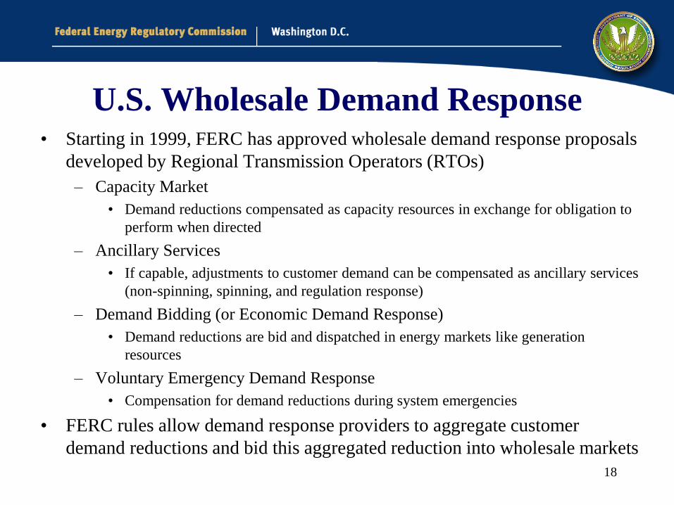
U.S. Wholesale Demand Response• Starting in 1999, FERC has approved wholesale demand response proposals

developed by Regional Transmission Operators (RTOs)

– Capacity Market

• Demand reductions compensated as capacity resources in exchange for obligation to

perform when directed

– Ancillary Services

• If capable, adjustments to customer demand can be compensated as ancillary services

(non-spinning, spinning, and regulation response)

– Demand Bidding (or Economic Demand Response)

• Demand reductions are bid and dispatched in energy markets like generation

resources

– Voluntary Emergency Demand Response

• Compensation for demand reductions during system emergencies

• FERC rules allow demand response providers to aggregate customer

demand reductions and bid this aggregated reduction into wholesale markets

19

Key FERC Rulemakings

• Order No. 719 (Wholesale Competition)

– Changes to wholesale markets to permit demand response participation

– Allows aggregated retail demand responses to bid into RTO and ISO markets,

unless local laws or regulations do not permit a retail customer to participate

• Order No. 745 (Demand Response Compensation)

– Requires that RTOs and ISOs pay demand response resources participating in

the Day-Ahead and Real-Time Wholesale Energy Markets the Locational

Marginal Price (or LMP) when

• Demand response resources are capable of balancing supply and demand, and

• Are cost-effective as determined by a net benefits test

• Orders Nos. 676-F and 676-G (M&V for Wholesale Demand

Response and Energy Efficiency)

20

• Demand Response as Capacity Resources– Provides demand response during system emergencies

– Participant receives capacity market-based payment for being available

– Does not require instantaneous response, typically 30 minutes to 2 hours

– Operated by electric utilities and demand response aggregators

– Requires estimate of baseline customer demand

– Requires extensive measurement & verification

– RTO/ISO programs

• PJM – Reliability Pricing Model

• ISO-NE – Forward Capacity Market

• NYISO – ICAP Special Case Resources

• MISO – Load Modifying Resources

21

• Demand Response as Ancillary Services– Offers rapid-response resources to provide operating

reserve and regulation services.

– Operated by electric utilities and demand response aggregators

– Aggregators typically bid resource into RTO markets on behalf of customer

– Currently provided through direct load control and the control of large industrial loads (e.g., aluminum smelters)

– RTOs that allow demand response to provide operating

reserves:

• CAISO, ISO-NE, MISO, NYISO, PJM

– RTOs that allow demand response to provide regulation:

• PJM, MISO

22

• Demand Bidding in Energy Markets– Refers to the ability of customers to bid a price at which

they will reduce demand• In most RTO markets, aggregators can bid customer demand

resources into day-ahead energy markets, and are dispatched if economic

– Requires estimates of customer baseline usage

– Customers can rely upon a mix of remote control, autonomous control (such as smart thermostats) and manual actions to reduce load

– Most participants are large industrial facilities and commercial/educational establishments

– Focus of Order No. 745

23

• Voluntary Emergency Demand Response– Refers to voluntary customer load reductions during

system emergencies. Customers may receive payments based on reductions achieved.

– Reductions are not required, no penalties for non-performance

– Aggregators (or the RTO/utility) typically notify customers of emergency conditions

– Customers can rely upon a mix of remote control, autonomous control and manual actions to reduce load

– NYISO’s Emergency Demand Response Program is a good example

24

Demand Response Participation in

Wholesale Markets

o Sources of demand response

• Traditional utility demand response programs

• Aggregators and curtailment service providers

• Load Serving Entities

• Direct end-use customer participation

RTO/ISO

2014 2015

Potential

Peak

Reduction

(MW)

Percent

of Peak

Demand

Potential

Peak

Reduction

(MW)

Percent of

Peak

Demand

California ISO (CAISO) 2,316 5.1% 2,160 4.4%

Electric Reliability Council of Texas (ERCOT) 2,100 3.2% 2,100 3.0%

ISO New England, Inc. (ISO-NE) 2,487 10.2% 2,696 11.0%

Midcontinent Independent System Operator (MISO) 10,356 9.0% 10,563 8.8 %

New York Independent System Operator (NYISO) 1,211 4.1% 1,325 4.3%

PJM Interconnection, LLC (PJM) 10,416 7.4% 12,910 9.0%

Southwest Power Pool, Inc. (SPP) 48 0.1% 0 0%

Total ISO/RTO 28,934 6.2% 31,754 6.6%

FERC v. EPSA Case

• On May 23, 2014, on appeal of Order No. 745, the D.C. Circuit in

EPSA vacated Order No. 745 “in its entirety as ultra vires agency

action.”

• The EPSA case was appealed to the U.S. Supreme Court, and oral

arguments were held on October 14, 2015.

• The U.S. Supreme Court issued a decision in FERC v. EPSA* in

January 2016 that fully upheld FERC’s jurisdiction on wholesale

demand response

• Supreme Court found that

– FERC did possess adequate regulatory authority under the Federal

Power Act; and

– FERC’s decision to compensate demand response providers at locational

marginal price was not arbitrary and capricious.

25* Elec. Power Supply Ass’n v. FERC, 753 F.3d 216 (D.C. Cir. 2014), rev’d sub nom. FERC v.

Elec. Power Supply Ass’n, 136 S. Ct. 760 (2016)

Wholesale Demand Response M&V

• North American Energy Standards Board effort:

– NAESB developed a standard M&V framework, which included key

product definitions and categorizations

• Products: Wholesale Electric Demand Response Energy, Capacity, Reserve

and Regulation Products

• Performance evaluation methodologies: (1) Maximum Base Load; (2) Meter

Before / Meter After; (3) Baseline Type-I (Interval Meter); (4) Baseline

Type-II (Non-Interval Meter); and (5) Metering Generator Output.

– FERC adopted by reference Phase I wholesale DR M&V standards in

April 2010 (Order 676-F) and Phase II wholesale DR and energy

efficiency M&V standards in February 2013 (Order 676-G).

• A variety of M&V methods are in use at RTOs/ISOs, primarily

based on calculating customer baselines

– A good resource for these methods is the ISO/RTO Council North

American Demand Response Characteristics Comparison matrix26

27

Demand Response Baselines:A Retail Perspective

Mark S. Martinez

Southern California Edison

April 13, 2017

28

SCE is one of the largest electric utilities in the United States

Service Area

50,000 square miles

Over 400 cities and communities

Population Served

13 million residents

5 million customer accounts

2016 Business Highlights

$11.86 billion operating revenue

$51.3 billion in total assets

86 billion Kilowatt-hour delivered

23,091MW peak demand

Industry leader in service excellence, renewable energy, demand side management, electric transportation, and smart grid infrastructure.

PG&E

SDG&E

LADWP

29

SCE DR Portfolio Overview

Approx. Load Impact*(MW)

Program Design

Commercial & Industrial Customers

Base Interruptible Program 698.3 Emergency interruptible load (customer control).

Agricultural Pumping & Interruptible 56.5 Emergency interruptible load (utility direct load control).

Demand Bidding Program 107.5 Economic, day-ahead energy.

Critical Peak Pricing 37.4 Economic, day-ahead energy (TOU rate structure).

Aggregator Managed 118.1 Third-party economic energy and capacity.

Summer Discount Plan 54.3A/C cycling direct load control (both economic and emergency).

Residential Customers

Summer Discount Plan 234.0A/C cycling direct load control (both economic and emergency).

Peak Time Rebate 26.6 Economic, day-ahead energy.

*Approximate MW using 2015 Ex Ante Load Impact Tables for 2016 August monthly peak

30

Residential A/C cycling event on 9/15/14

31

EM&V – how low did we go?

• In most instances, load impacts from DR events are estimated by comparing the reference level energy use (baseline) in each hour with actual energy use in the hour on each event day.

0

20,000

40,000

60,000

80,000

100,000

120,000

140,000

160,000

180,000

1 7 13 19

Hours

Lo

ad

s (

kW

)

-10,000

0

10,000

20,000

30,000

40,000

50,000

60,000

70,000

80,000

Lo

ad

Im

pa

ct

(kW

)

Estimated Reference

Observed

Load Impact

Load Impact = Baseline – Actual Energy Use

32

A baseline calculation is a “counter-factual”, or pure theoretical, mathematical estimate of what a customer would have done during a DR event.

Baseline calculations that are accurate and unbiased are among the most challenging aspects of DR programs, as they can only estimate the counterfactual.

Results in accurate load impact estimates.

Properly compensates customers for load reductions.

Can deprive customers of just and reasonable compensation, resulting in dissatisfaction and loss of participation.

Can reduce the benefits of DR resources and devalue the overall cost effectiveness of programs.

Well designed baseline

Poorly designed baseline

Baselines – what did not happen

33

As DR plays an increasing role in organized markets and system planning, the right baseline “matters” for local grid operations, financial settlements for customers, and for ISO/RTO resource planning.

Magnitude of demand savings that a DR resource will deliver to the electric grid.

Magnitude of curtailment by customer, as estimated by the baseline, determines financial settlement.

Amount of DR expected from enrolled resources. Includes comparison with alternate grid resources.

Baselines matter in many ways

34

Baseline type 1 is the most commonly used baseline method for performance settlements of participants in retail DR programs.

Type 1 baseline is based on historical interval meter data for each demand resource.

It may also include other variables such as weather and calendar data on the day of the event.

Statistical sampling of sites is not permitted.

Day-of DR event adjustment may be allowed to minimize baseline error.

Baseline Type 1

Baseline Type 1

0

20,000

40,000

60,000

80,000

100,000

120,000

140,000

160,000

180,000

1 7 13 19

Hours

Lo

ad

s (

kW

)

-10,000

0

10,000

20,000

30,000

40,000

50,000

60,000

70,000

80,000

Lo

ad

Im

pa

ct

(kW

)

Estimated Reference

Observed

Load Impact

35

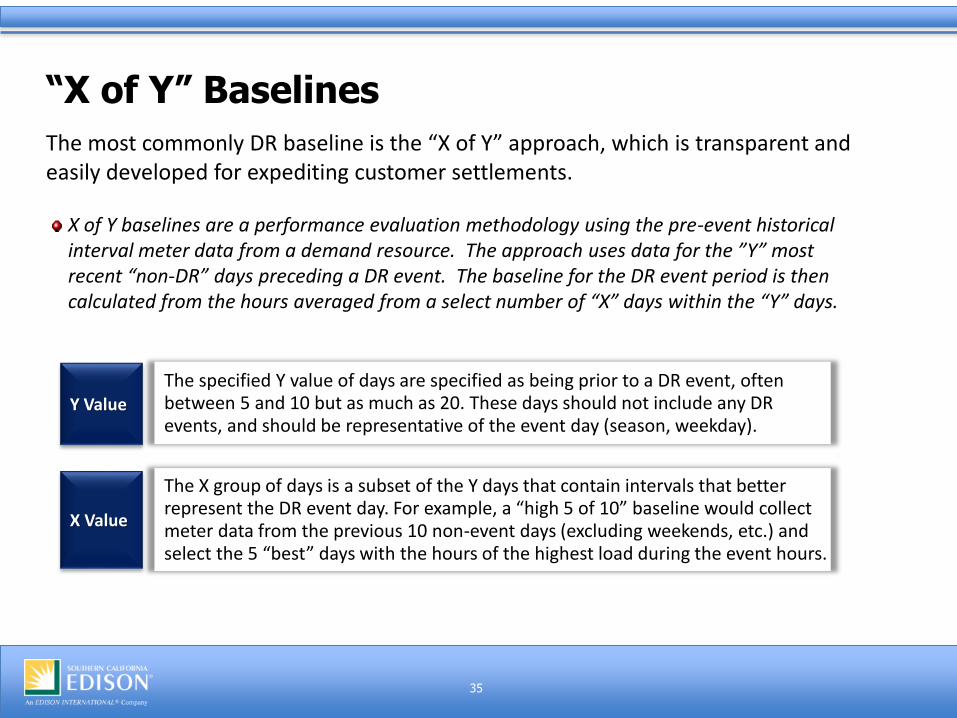
The most commonly DR baseline is the “X of Y” approach, which is transparent and easily developed for expediting customer settlements.

X of Y baselines are a performance evaluation methodology using the pre-event historical interval meter data from a demand resource. The approach uses data for the ”Y” most recent “non-DR” days preceding a DR event. The baseline for the DR event period is then calculated from the hours averaged from a select number of “X” days within the “Y” days.

Y Value

The specified Y value of days are specified as being prior to a DR event, often between 5 and 10 but as much as 20. These days should not include any DR events, and should be representative of the event day (season, weekday).

The X group of days is a subset of the Y days that contain intervals that better represent the DR event day. For example, a “high 5 of 10” baseline would collect meter data from the previous 10 non-event days (excluding weekends, etc.) and select the 5 “best” days with the hours of the highest load during the event hours.

X Value

“X of Y” Baselines

36

This is used for providing customer capacity and energy payments

SCE – 10 of 10 baseline approach

37

Source: CAISO

Day of Adjustment

38

Baseline type 2 is a performance evaluation methodology that uses statistical sampling to estimate electricity consumption of an aggregated demand resource.

Type 2 is used in cases where interval meter data is not available for individual sites. The need for type 2 baselines will diminish as interval meters become more commonplace.

Statistical sampling techniques are used to generate a baseline for a portfolio of customers.

This can be used when a group of sites (especially residential) are homogenous with similar load behavior. A few sites can be metered in order to develop an average load estimate per site, and then use this to allocate load from the aggregated baseline.

Baseline Type 2

39

Maximum base load is a performance evaluation methodology based solely on the ability of a demand resource to reduce to a specified level of electricity demand.

MBL is sometimes referred to as the Drop To method. It is superior for highly variable loads that do are not appropriate for baseline style programs.

This method should use coincident peak hours to capture approximate load reductions during DR events.

This is not a baseline estimation method.

Source: NAESB

Maximum Base Load (non-baseline)

40

Meter Before/Meter After is a performance evaluation methodology in which electricity demand over a prescribed period of time prior to DR deployment is compared to similar readings during a sustained response period.

Source: NAESB

The load shape for this performance metric is static.

Meter data from individual sites is utilized.

It relies on a small interval of historical meter data.

This is not a baseline estimation methodology.

Before Meter/After Meter (non-baseline)

41

Baseline errors from HLV customers are problematic because they carry over into load impact estimates of performance and create settlement errors.

In a study for the California PUC, HLV customers were defined as those whose average variability around their mean use in the event window is 30% or more. One quarter of DR customers were found to fit this definition, with substantial variation by program and industry type.

DR resources that have highly variable load patterns pose a problem for baseline analysis because historic meter data can be an unreliable indicator of event day usage.

Customers with irregular baselines are most common in agriculture, construction, other utilities, schools and sometimes manufacturing. A preferred DR performance methodology for these customers would be the Guaranteed Load Drop. HVL customers should not participate in DR programs that use baselines for compensation.

HVLcustomers

Non-HVL customers

Breakout of Customersin DR Programs

Highly Variable Loads (HVL)

42

The elements of baselines are brought together in this illustration of a DR event day. In this case the adjusted baseline captures circumstances on the day of the event and better reflects the actual resource provided than the unadjusted baseline would have captured.

kW

Prepared by EnerNoc and presented to NAESB, October 8, 2009Time

Teasing Settlements from DR Events

The illustrates both the challenges and complexities for finding the “counterfactual”.

43

Baseline measurement accuracy is constantly under assessment with changes and adjustments to provide appropriate settlements for DR program participants.

Numerous studies have concluded that applying a morning adjustment factor significantly reduces bias and improves accuracy of baseline load profiles.

Such adjustments use actual load data in the hours prior to the event to adjust the X of Y baseline. Adjustments may be capped or uncapped. Capped adjustments limit the magnitude of a baseline adjustment.

Customers with highly variable loads typically have the most irregular load profiles and require the largest adjustments. The better option is for such customers to transition to a non-baseline style program.

The right customer for the program baseline.

Final Comments

44

Thank you!

Mark S. Martinez Southern California Edison

[email protected]

www.sce.com/drp


http://www.sce.com/drp

PJM©2017www.pjm.com

Evaluation, Measurement and Verification

(EM&V) of Demand Response load

reductions in wholesale markets

Pete Langbein


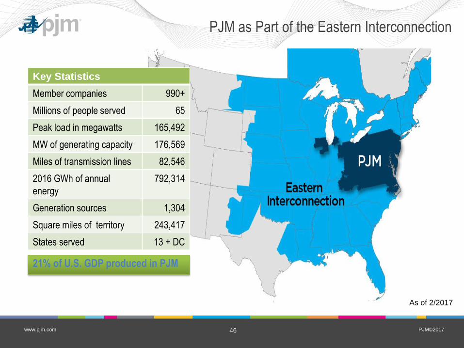
PJM as Part of the Eastern Interconnection

21% of U.S. GDP produced in PJM

As of 2/2017

Key Statistics

Member companies 990+

Millions of people served 65

Peak load in megawatts 165,492

MW of generating capacity 176,569

Miles of transmission lines 82,546

2016 GWh of annual

energy

792,314

Generation sources 1,304

Square miles of territory 243,417

States served 13 + DC


EM&V framework

• Customer, Aggregator, EDC, LSE, ISO/RTO

• Minimize self selection bias

• Easy to use, understand & communicate

• Ability to replicate/audit

• Accuracy

• Bias

• Variability

Empirical Performance

Transparency

Cost to administer

Mitigate “Gaming”

Measurement is done to determine revenue and/or penalties


Wholesale markets

• Energy

• Capacity

• Ancillary Services

– Day Ahead Scheduling Reserves

– Synchronized Reserves (10 minute

spin)

– Regulation (frequency control)

EM&V approach can be different by market


Customer Baseline Load (“CBL”) = customer load forecast

Type I error

Type II error

false positive – estimate a load reduction but customer did not reduce load

false negative – estimate no load reduction but customer did reduce load

There will always be errors (Forecast/CBL vs Actual load) – maximize

accuracy and minimize bias and variability


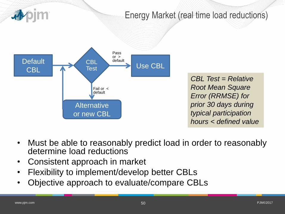
Energy Market (real time load reductions)

• Must be able to reasonably predict load in order to reasonably determine load reductions

• Consistent approach in market

• Flexibility to implement/develop better CBLs

• Objective approach to evaluate/compare CBLs

Default

CBLCBL Test

Alternative

or new CBL

Use CBL

Pass or > default

Fail or < default

CBL Test = Relative

Root Mean Square

Error (RRMSE) for

prior 30 days during

typical participation

hours < defined value


CBL inventory

NAME DESCRIPTION

Same Day (3+2) Take average of 3 hours before and 2 hours after (skip hour before/after)

Match Day (3 day average)

Compare usage on event during before/after event to historic usage and pick days to minimize

RRMSE

3 Day Types Standard (WD high 4 of 5, Sat, Sun/Hol high 2 of 3)

5 Day Types Mon, Fri high 3 of 4; Tues/Wed/Thurs high 4 of 5; Sat, Sun/Hol high 2 of 3, 60 day lookback

Manual Manual CBL (not generated by system)

7 Day Types Mon, Tues, Wed, Thurs, Fri, Sat, Sun/Hol average of 3; 60 day lookback

Metered Generation Metered Generation

3 Day Types with SAA

(DEFAULT) Standard (WD high 4 of 5, Sat, Sun/Hol high 2 of 3) with Symmetric Additive Adjustment

3 Day Types with WSA Standard (WD high 4 of 5, Sat, Sun/Hol high 2 of 3) with Weather Sensitivity Adjustment


Mon, Fri high 3 of 4; Tues/Wed/Thurs high 4 of 5; Sat, Sun/Hol high 2 of 3, 60 day lookback, with

Symmetric Additive Adjustment

5 Day Types with WSA

Mon, Fri high 3 of 4; Tues/Wed/Thurs high 4 of 5; Sat, Sun/Hol high 2 of 3, 60 day lookback, with

Weather Sensitivity Adjustment


Mon, Tues, Wed, Thurs, Fri, Sat, Sun/Hol average of 3; 60 day lookback, with Symmetric Additive

Adjustment

7 Day Types with WSA

Mon, Tues, Wed, Thurs, Fri, Sat, Sun/Hol average of 3; 60 day lookback, with Weather Sensitivity

Adjustment

MBL(Max Base Load) Average daily minimum load during event period for 5 most recent nonevent days


Accuracy of CBL through “back test”

---Event Hours---


Aggregation & Performance

• CBL primarily calculated at premise level

– “utility account number”

• Small premises may be aggregated together to

enable market participation (>100kw)

– CBL calculated from aggregate load data.

• Capacity market performance aggregated

across dispatched premises based on

geographic location


Future thoughts

• Capacity market – EM&V based on avoided demand– load must be below peak levels when dispatched.

• 5 minute energy settlements - typically shorter time period = higher variation = greater error.

• Sophisticated approach does not mean more accurate (regression approach only marginally more accurate for specific circumstances to date)

• Ancillary Services – load before/after typically used for CBL

As data availability goes up, we may be able to improve accuracy


Reference material

• Kema/PJM CBL empirical analysis– http://www.pjm.com/~/media/markets-ops/dsr/pjm-

analysis-of-dr-baseline-methods-full-report.ashx

• PJM training material– CBL example,Slide (36-42)

– http://www.pjm.com/~/media/training/core-curriculum/ip-dsr/economic-demand-side-response-training.ashx

• PJM Manual 11, section 10.4.2, CBL inventory and calculations– http://www.pjm.com/~/media/documents/manuals/m11.ash

x

• Peter Langbein, [email protected]

http://www.pjm.com/~/media/markets-ops/dsr/pjm-analysis-of-dr-baseline-methods-full-report.ashx

http://www.pjm.com/~/media/training/core-curriculum/ip-dsr/economic-demand-side-response-training.ashx

http://www.pjm.com/~/media/documents/manuals/m11.ashx


Appendix

• RRMSE example


Relative Root Mean Squared Error (RRMSE)

PJM©2014 57 4/13/2017

1. To perform the RRMSE calculation, daily CBL calculations are first performed

for each CBL method using hours ending 14 through hours ending 19 as the

simulated event hours for each of the 30 non-event days according to each

CBL method rules.

2. Actual Hourly errors are calculated by subtracting the CBL hourly load from

the actual hourly load for each of the simulated event hours of the non-event

day.

3. The Mean Squared Error (MSE) is calculated by summing the squared actual

hourly errors and dividing by the number of simulated event hours.

4. The Average Actual Hourly Load is the average of the actual hourly load for

each of the simulated event hours.

5. The Relative Root Mean Squared Error (RRMSE) is calculated by taking the

square root of the quantity (MSE/Average Actual Load).


RRMSE Example

PJM©2014 58 4/13/2017

Example of RRMSE calculated over 10 day period

1. Daily CBL calculations are first performed for each CBL method using hours

ending 14 through hours ending 19 as the simulated event hours for each of

the 30 non-event days according to each CBL method rules.

(a) (b) (c) (d) (e) (f) (g) (h) (i) (j) (k) (l)

customer Date 1-2PM 2-3PM 3-4PM 4-5PM 5-6PM 6-7PM 1-2PM 2-3PM 3-4PM 4-5PM 5-6PM 6-7PM

R2001 18-Aug-11 508 520 517 506 488 461 492 494 500 502 502 481

R2001 19-Aug-11 83 82 72 53 47 35 64 59 38 47 5 5

R2001 20-Aug-11 349 342 287 267 237 196 326 322 313 301 294 222

R2001 21-Aug-11 3,482 3,468 3,843 3,606 3,556 3,445 3,771 3,761 3,730 4,023 3,487 3,361

R2001 22-Aug-11 439 445 446 416 425 404 383 382 383 381 387 391

R2001 23-Aug-11 386 397 394 370 229 194 353 386 375 312 235 178

R2001 24-Aug-11 92 92 92 93 92 92 82 85 83 85 84 86

R2001 25-Aug-11 3,204 3,229 3,257 3,208 3,185 3,115 2,964 2,964 2,961 2,386 2,833 2,770

R2001 26-Aug-11 660 625 568 532 493 482 613 583 566 551 535 499

R2001 27-Aug-11 6,397 6,377 6,322 6,308 6,411 6,343 7,165 7,098 7,047 6,918 6,799 6,820

Baseline Hourly Loads (kW) Actual Hourly Loads (kW)


RRMSE Example Cont.

PJM©2014 59 4/13/2017

Example of RRMSE calculated over 10 day period

2. Actual Hourly errors are calculated by subtracting the actual hourly load from the CBL hourly load for each of the simulated event hours of the non-event day.

3. The Mean Squared Error (MSE) is calculated by summing the squared actual hourly errors and dividing by the number of simulated event hours.

4. The Average Actual Hourly Load is the average of the actual hourly load for each of the simulated event hours.

5. The Relative Root Mean Squared Error (RRMSE) is calculated by taking the square root of the MSE/Average Actual Load.

(u) (v) (w) (x) (y) (z) (s) (n) (t)

Se2/n = average(g:l) =SQRT(s)/(n)

customer Date

1-2PM 2-3PM 3-4PM 4-5PM 5-6PM 6-7PM 65,443 1,564 16%

R2001 18-Aug-11 16 26 17 4 (14) (20)

R2001 19-Aug-11 19 23 34 6 42 30

R2001 20-Aug-11 23 20 (26) (34) (57) (26)

R2001 21-Aug-11 (289) (293) 113 (417) 69 84

R2001 22-Aug-11 56 63 63 35 38 13

R2001 23-Aug-11 33 11 19 58 (6) 16

R2001 24-Aug-11 10 7 9 8 8 6

R2001 25-Aug-11 240 265 296 822 352 345

R2001 26-Aug-11 47 42 2 (19) (42) (17)

R2001 27-Aug-11 (768) (721) (725) (610) (388) (477)

Actual Hourly Error (kW) MSE Average Actual kW Relative RMSE

Discussion/QuestionsFor more EM&V information see:

• Webinars: https://emp.lbl.gov/emv-webinar-series

• For technical assistance to state regulatory commissions, state energy offices, tribes and regional entities, and other public entities see: https://emp.lbl.gov/projects/technical-assistance-states

• Energy efficiency publications and presentations – financing, performance contracting, documenting performance, etc. see: https://emp.lbl.gov/research-areas/energy-efficiency

• New Technical Brief - Coordinating Demand-Side Efficiency Evaluation, Measurement and Verification Among Western States: Options for Documenting Energy and Non- Energy Impacts for the Power Sector https://emp.lbl.gov/publications/coordinating-demand-side-efficiency

60

From Albert Einstein:

“Everything should be as simple as it is, but not simpler”

“Everything that can be counted does not necessarily count; everything that counts cannot necessarily be counted”

EM&V Webinar - April 2017 - Introduction Slides


https://emp.lbl.gov/projects/technical-assistance-states

https://emp.lbl.gov/research-areas/energy-efficiency

https://emp.lbl.gov/publications/coordinating-demand-side-efficiency

Introduction to Wholesale and Retail Demand … to Wholesale and Retail Demand Response with a Focus...

Documents

Transcript of Introduction to Wholesale and Retail Demand … to Wholesale and Retail Demand Response with a Focus...