Introduction to Wavelets in Scilab Anuradha Amrutkar
40
Introduction to Wavelets in Scilab Anuradha Amrutkar Indian Institute of Technology Bombay [email protected] National Workshop on Scilab Sinhagad College of Engineering,Wadgaon,Pune January 5, 2011 Anuradha Amrutkar Introduction to Wavelets in Scilab 1/21
Transcript of Introduction to Wavelets in Scilab Anuradha Amrutkar

Introduction to Wavelets in Scilab
Anuradha Amrutkar
Indian Institute of Technology [email protected]
National Workshop on ScilabSinhagad College of Engineering,Wadgaon,Pune
January 5, 2011
Anuradha Amrutkar Introduction to Wavelets in Scilab 1/21

Introduction
The word WAVELET literally means small wave.
Wavelets are localised waves and they extend not from - ∞ to+ ∞ but only for a finite duration of time.
Anuradha Amrutkar Introduction to Wavelets in Scilab 2/21

Introduction
The word WAVELET literally means small wave.
Wavelets are localised waves and they extend not from - ∞ to+ ∞ but only for a finite duration of time.
Anuradha Amrutkar Introduction to Wavelets in Scilab 2/21

Introduction
Since waves extend over the entire space, they do not needany shift parameter.
Thus, a Fourier Transform maps 1-D time signals to 1-Dfrequency signals, whereas
The wavelet transform maps 1-D time signals to 2-Dscale(frequency) and shift parameter signals.
Anuradha Amrutkar Introduction to Wavelets in Scilab 3/21

Example1
Let us see a program which finds out the approximatecoefficients and detailed coefficients of a given signal.
Anuradha Amrutkar Introduction to Wavelets in Scilab 4/21

Example1
Let us see a program which finds out the approximatecoefficients and detailed coefficients of a given signal.
Anuradha Amrutkar Introduction to Wavelets in Scilab 4/21

Example1:dwt.sce
In this Example:
1. x=linspace(-%pi,%pi,10000);
2. s=sin(x); //Constructs and Elimentary sine wave signal
3. [ca1,cd1] = dwt(s,’haar’); // Perform single-leveldiscrete wavelet transform of “s“ by ”haar“.
4. The Graph of Apporoximate co-efficients(cA) and Detailedco-efficient(cD) is Plotted using the plot() command
5. The above procedure is repeated for “db2“ type of wavelet.
Anuradha Amrutkar Introduction to Wavelets in Scilab 5/21

Example1:dwt.png
Anuradha Amrutkar Introduction to Wavelets in Scilab 6/21

Example2:idwt.sce
In this Example:
1. Steps 1,2 and 3 are same as above.
2. ss = idwt(ca1,cd1,’haar’); //Perform single-levelinverse discrete wavelet transform, illustrating that idwt is theinverse function of dwt.
3. The Graph of Apporoximate co-efficients(cA) and Detailedco-efficient(cD) is Plotted using the plot() command
Anuradha Amrutkar Introduction to Wavelets in Scilab 7/21

Example1:idwt.png
Anuradha Amrutkar Introduction to Wavelets in Scilab 8/21

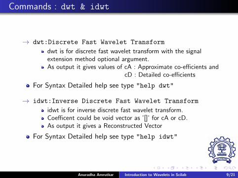
Commands : dwt & idwt
→ dwt:Discrete Fast Wavelet Transform
dwt is for discrete fast wavelet transform with the signalextension method optional argument.As output it gives values of cA : Approximate co-efficients and
cD : Detailed co-efficients
For Syntax Detailed help see type "help dwt"
→ idwt:Inverse Discrete Fast Wavelet Transform
idwt is for inverse discrete fast wavelet transform.Coefficent could be void vector as ’[]’ for cA or cD.As output it gives a Reconstructed Vector
For Syntax Detailed help see type "help idwt"
Anuradha Amrutkar Introduction to Wavelets in Scilab 9/21

Example3:wavelet.sce
Let us Revise the Decomposition Diagram for the wavelets:
Anuradha Amrutkar Introduction to Wavelets in Scilab 10/21

Example3:wavelet.sce
Let us Revise the Decomposition Diagram for the wavelets:
Anuradha Amrutkar Introduction to Wavelets in Scilab 10/21

Example3:wavelet.sce
In this Example:
1. s=[1:100];
2. l s = length(s)
3. a = sin(2*%pi*s/100)+sin(3*%pi*s/100); //Constructsand Elimentary sine wave signal
Anuradha Amrutkar Introduction to Wavelets in Scilab 11/21

Example3:wavelet.sce
In this Example:
1. s=[1:100];
2. l s = length(s)
3. a = sin(2*%pi*s/100)+sin(3*%pi*s/100); //Constructsand Elimentary sine wave signal
Anuradha Amrutkar Introduction to Wavelets in Scilab 11/21
Example3:wavelet.sce
The coefficients of all the components of a third-leveldecomposition (that is, the third-level approximation and the firstthree levels of detail) are returned concatenated into one vector, C.
Vector L gives the lengths of each component.
4. [C,L] = wavedec(a,3,’haar’);
Anuradha Amrutkar Introduction to Wavelets in Scilab 12/21

Example3:wavelet.sce
To extract the level 3 approximation coefficients from C, type:
5. cA3 = appcoef(C,L,’haar’,3);
To extract the levels 3, 2, and 1 detail coefficients from C, type
6. cD3 = detcoef(C,L,3);
7. cD2 = detcoef(C,L,2);
8. cD1 = detcoef(C,L,1);
The above can be written in one command as:
9. [cD1,cD2,cD3] = detcoef(C,L,[1,2,3]);
Anuradha Amrutkar Introduction to Wavelets in Scilab 13/21

Example3:wavelet.sce
To reconstruct the level 3 approximation from C, type
10. A3 = wrcoef(’a’,C,L,’haar’,3);
To reconstruct the details at levels 1, 2, and 3, from C, type
11. D1 = wrcoef(’d’,C,L,’haar’,1);
12. D2 = wrcoef(’d’,C,L,’haar’,2);
13. D3 = wrcoef(’d’,C,L,’haar’,3);
Anuradha Amrutkar Introduction to Wavelets in Scilab 14/21

Example1:wavelet.sce
Display the results of a multilevel decomposition
Anuradha Amrutkar Introduction to Wavelets in Scilab 15/21

Example1:wavelet.sce
Display the results of a multilevel decomposition
Anuradha Amrutkar Introduction to Wavelets in Scilab 15/21

wavelet.sce
To reconstruct the original signal from the wavelet decompositionstructure, type
14. A3 = waverec(C,L,’haar’);
Of course, in discarding all the high-frequency information, we’vealso lost many of the original signal’s sharpest features.
Anuradha Amrutkar Introduction to Wavelets in Scilab 16/21
Original Vs Approximate
To compare the approximation to the original signal, type
Anuradha Amrutkar Introduction to Wavelets in Scilab 17/21

Original Vs Approximate
To compare the approximation to the original signal, type
Anuradha Amrutkar Introduction to Wavelets in Scilab 17/21

Commands Used
The commands used in the Multi-level Decomposition andConstruction of Approximate and Detailed Coefficients are:
? wavedec: Multiple Level Discrete Fast Wavelet
Transform
? waverec: Multiple Level Inverse Discrete Fast
Wavelet Transform
? appcoef: One Dimension Approximation Coefficent
Reconstruction
? detcoef: One Dimension Detail Coefficent
Extraction
? wrcoef: Restruction from single branch from
multiple level
Anuradha Amrutkar Introduction to Wavelets in Scilab 18/21

Help
Please type help command name to see the Usage, Descriptionand Examples for that particular command.
Anuradha Amrutkar Introduction to Wavelets in Scilab 19/21

Help
Please type help command name to see the Usage, Descriptionand Examples for that particular command.
Anuradha Amrutkar Introduction to Wavelets in Scilab 19/21

Further Exploration
Optimal de-noising requires a more subtle approach calledthresholding.
This involves discarding only the portion of the details that exceedsa certain limit.
Anuradha Amrutkar Introduction to Wavelets in Scilab 20/21

Further Exploration
Optimal de-noising requires a more subtle approach calledthresholding.
This involves discarding only the portion of the details that exceedsa certain limit.
Anuradha Amrutkar Introduction to Wavelets in Scilab 20/21

Further Exploration
Optimal de-noising requires a more subtle approach calledthresholding.
This involves discarding only the portion of the details that exceedsa certain limit.
Anuradha Amrutkar Introduction to Wavelets in Scilab 20/21

Thank You!!
Thank You!
Anuradha Amrutkar Introduction to Wavelets in Scilab 21/21
Thank You!!
Thank You!
Anuradha Amrutkar Introduction to Wavelets in Scilab 21/21