Introduction to Volterra series and applications to...
147
A. Introduction B. Volterra series C. Derivation and simulation D. Applications E. Convergence F. Conclusion Introduction to Volterra series and applications to physical audio signal processing Thomas H ´ elie IRCAM - CNRS UMR9912 - UPMC, Paris, France DAFx, 2011
-
Upload
truongtruc -
Category
Documents
-
view
216 -
download
0
Transcript of Introduction to Volterra series and applications to...
A. Introduction B. Volterra series C. Derivation and simulation D. Applications E. Convergence F. Conclusion
Introduction to Volterra seriesand
applications to physical audio signalprocessing
Thomas Helie
IRCAM - CNRS UMR9912 - UPMC, Paris, France
DAFx, 2011

A. Introduction B. Volterra series C. Derivation and simulation D. Applications E. Convergence F. Conclusion
Vito Volterra [1860 (Ancona) - 1940 (Roma)] (source: wikipedia)
Vito Volterra was an Italian math-ematician and physicist . Heis known for his contributions tomathematical biology and inte-gral equations . He joined theopposition to the Fascist regime(1922). Because of his political phi-losophy, he also refused to take amandatory oath of loyalty (1931).He lived largely abroad, returning toRome just before his death.
Royal Society (1910) - Royal Society of Edinburgh (1913)A moon crater is named after him

A. Introduction B. Volterra series C. Derivation and simulation D. Applications E. Convergence F. Conclusion
Outline
A. Introduction & Motivation
B. Volterra series:B1. Definitions and basic propertiesB2. Interconnection laws
C. TUTORIAL: How to ...C1. derive the Volterra kernels of a given nonlinear
system ?C2. simulate the system using these kernels ?
[Short pause (≈ 5min): first questions]D. Physical/Audio applications:
D1. Nonlinear propagation of a travelling wave(brassy effect)
D2. A damped nonlinear string
E. Recent results on computable convergence domains
F. Conclusion

A. Introduction B. Volterra series C. Derivation and simulation D. Applications E. Convergence F. Conclusion
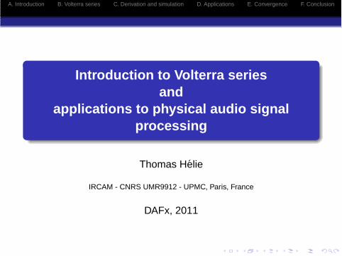
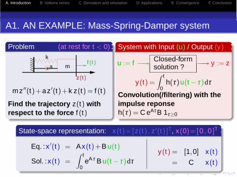
A1. AN EXAMPLE: Mass-Spring-Damper system
Problem (at rest for t < 0)
f (t)
z(t)
ma
k
mz ′′(t)+az ′(t)+k z(t) = f (t)
Find the trajectory z(t) withrespect to the force f (t)
System with input (u) / Output (y)
u := f −→Closed-formsolution ? −→ y := z
A. Introduction B. Volterra series C. Derivation and simulation D. Applications E. Convergence F. Conclusion
A1. AN EXAMPLE: Mass-Spring-Damper system
Problem (at rest for t < 0)
f (t)
z(t)
ma
k
mz ′′(t)+az ′(t)+k z(t) = f (t)
Find the trajectory z(t) withrespect to the force f (t)
System with input (u) / Output (y)
u := f −→Closed-formsolution ? −→ y := z
State-space representation: x(t)=[z(t) , z ′(t) ]T, x(0)=[0 , 0 ]T
[z ′(t)z ′′(t)
]
︸ ︷︷ ︸x ′(t)
=
[0 1
−k/m −a/m
]
︸ ︷︷ ︸A
[z(t)z ′(t)
]
︸ ︷︷ ︸x(t)
+
[0
1/m
]
︸ ︷︷ ︸B
u(t)

A. Introduction B. Volterra series C. Derivation and simulation D. Applications E. Convergence F. Conclusion
A1. AN EXAMPLE: Mass-Spring-Damper system
Problem (at rest for t < 0)
f (t)
z(t)
ma
k
mz ′′(t)+az ′(t)+k z(t) = f (t)
Find the trajectory z(t) withrespect to the force f (t)
System with input (u) / Output (y)
u := f −→Closed-formsolution ? −→ y := z
State-space representation: x(t)=[z(t) , z ′(t) ]T, x(0)=[0 , 0 ]T
Eq. :x ′(t) = Ax(t)+B u(t)
Sol. :x(t) =∫ t
0eAτ B u(t − τ)dτ
y(t) = [1,0] x(t)
= C x(t)
A. Introduction B. Volterra series C. Derivation and simulation D. Applications E. Convergence F. Conclusion
A1. AN EXAMPLE: Mass-Spring-Damper system
Problem (at rest for t < 0)
f (t)
z(t)
ma
k
mz ′′(t)+az ′(t)+k z(t) = f (t)
Find the trajectory z(t) withrespect to the force f (t)
System with Input (u) / Output (y)
u := f −→Closed-formsolution ? −→ y := z
y(t) =∫ t
0h(τ)u(t − τ)dτ
Convolution(/filtering) with theimpulse reponseh(τ) = C eAτB 1τ≥0
State-space representation: x(t)=[z(t) , z ′(t) ]T, x(0)=[0 , 0 ]T
Eq. :x ′(t) = Ax(t)+B u(t)
Sol. :x(t) =∫ t
0eAτ B u(t − τ)dτ
y(t) = [1,0] x(t)
= C x(t)

A. Introduction B. Volterra series C. Derivation and simulation D. Applications E. Convergence F. Conclusion
A2. AN EXAMPLE: in the LAPLACE domain
Problem (at rest for t < 0)
f (t)
z(t)
ma
k
mz ′′(t)+az ′(t)+k z(t) = f (t)
Find the trajectory z(t) withrespect to the force f (t)
System with input (u) / Output (y)
u := f −→Closed-formsolution ? −→ y := z
Y (s) = H(s) U(s)
Transfer function (/filter)
H(s) = C (s I2 −A)−1B
State-space representation: x(t)=[z(t) , z ′(t) ]T, x(0)=[0 , 0 ]T
Eq. : s X (s) = AX (s)+B U(s)
Sol. : X (s) = (s I2 −A)−1B U(s)
Y (s) = [1,0] X (s)
= C X (s)

A. Introduction B. Volterra series C. Derivation and simulation D. Applications E. Convergence F. Conclusion
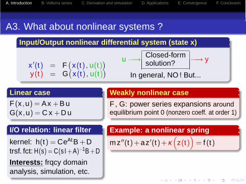
A3. What about nonlinear systems ?
Input/Output nonlinear differential system (state x)
x ′(t) = F(
x(t) , u(t))
y(t) = G(
x(t) , u(t))
u −→Closed-formsolution? −→ y
In general, NO ! But...
Linear caseF (x ,u) = Ax +B uG(x ,u) = C x +D u
I/O relation: linear filter
kernel: h(t) = CeAtB +Dtrsf. fct: H(s) = C(s I +A)−1B +D
Interests: frqcy domainanalysis, simulation, etc.
A. Introduction B. Volterra series C. Derivation and simulation D. Applications E. Convergence F. Conclusion
A3. What about nonlinear systems ?
Input/Output nonlinear differential system (state x)
x ′(t) = F(
x(t) , u(t))
y(t) = G(
x(t) , u(t))
u −→Closed-formsolution? −→ y
In general, NO ! But...
Linear caseF (x ,u) = Ax +B uG(x ,u) = C x +D u
I/O relation: linear filter
kernel: h(t) = CeAtB +Dtrsf. fct: H(s) = C(s I +A)−1B +D
Interests: frqcy domainanalysis, simulation, etc.
Weakly nonlinear case
F , G: power series expansions aroundequilibrium point 0 (nonzero coeff. at order 1)
Example: a nonlinear spring
mz ′′(t)+az ′(t)+κ(
z(t))
= f (t)
I/O relation: Volterra seriesInterests: idem!
A. Introduction B. Volterra series C. Derivation and simulation D. Applications E. Convergence F. Conclusion
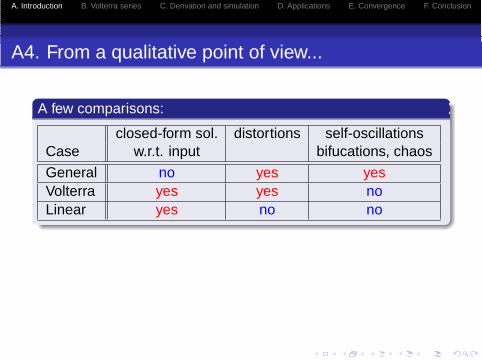
A4. From a qualitative point of view...
A few comparisons:
closed-form sol. distortions self-oscillationsCase w.r.t. input bifucations, chaos
General no yes yesVolterra yes yes noLinear yes no no

A. Introduction B. Volterra series C. Derivation and simulation D. Applications E. Convergence F. Conclusion
A4. From a qualitative point of view...
A few comparisons:
closed-form sol. distortions self-oscillationsCase w.r.t. input bifucations, chaos
General no yes yesVolterra yes yes noLinear yes no no
Interest of Volterra series:
Natural distortions for high amplitudes
Musical acoustics: fortissimo dynamics
Possible extensions to partial differential equations
A. Introduction B. Volterra series C. Derivation and simulation D. Applications E. Convergence F. Conclusion
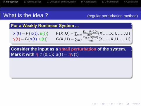
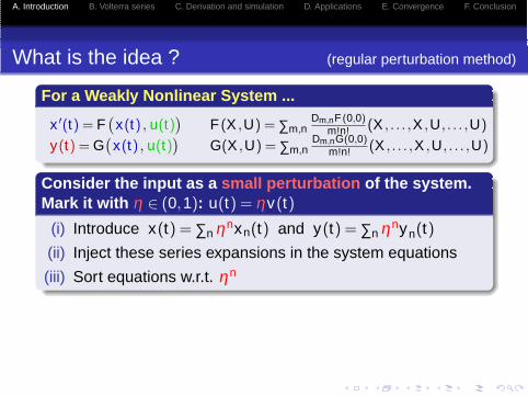
What is the idea ? (regular perturbation method)
For a Weakly Nonlinear System ...
x ′(t) = F(
x(t) , u(t))
F (X ,U) = ∑m,nDm,nF (0,0)
m!n! (X , . . . ,X ,U, . . . ,U)
y(t) = G(
x(t) , u(t))
G(X ,U) = ∑m,nDm,nG(0,0)
m!n! (X , . . . ,X ,U, . . . ,U)
Consider the input as a small perturbation of the system.Mark it with η ∈ (0,1): u(t) = ηv(t)
A. Introduction B. Volterra series C. Derivation and simulation D. Applications E. Convergence F. Conclusion
What is the idea ? (regular perturbation method)
For a Weakly Nonlinear System ...
x ′(t) = F(
x(t) , u(t))
F (X ,U) = ∑m,nDm,nF (0,0)
m!n! (X , . . . ,X ,U, . . . ,U)
y(t) = G(
x(t) , u(t))
G(X ,U) = ∑m,nDm,nG(0,0)
m!n! (X , . . . ,X ,U, . . . ,U)
Consider the input as a small perturbation of the system.Mark it with η ∈ (0,1): u(t) = ηv(t)
(i) Introduce x(t) = ∑n ηnxn(t) and y(t) = ∑n ηnyn(t)
(ii) Inject these series expansions in the system equations
(iii) Sort equations w.r.t. ηn
... we obtain a sequence of linear ODEs, indexed w.r.t. n
(iv) Solution: Each xn is a multiple convolution of n repeatedversions of the input and a computable multivariate kernel
−→ Volterra kernel

A. Introduction B. Volterra series C. Derivation and simulation D. Applications E. Convergence F. Conclusion
B. Volterra series
VOLTERRA SERIES:
B1. Definitions and basic properties
B2. Interconnection laws

A. Introduction B. Volterra series C. Derivation and simulation D. Applications E. Convergence F. Conclusion
B1. Volterra series
Part B1. Definitions and basic properties:
1 Definition and particular cases
2 Laplace/Fourier domain and analogies with linear systems
3 Case of periodic signals, distortion coefficients
4 Remark on the non uniqueness of kernels

A. Introduction B. Volterra series C. Derivation and simulation D. Applications E. Convergence F. Conclusion
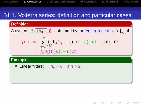
B1.1. Volterra series: definition and particular cases
Definition
A system u→ hn y
→ is defined by the Volterra series hnn≥1 if
y(t) =+∞
∑n=1︸︷︷︸
Sum
∫
Rnhn(τ1 , . . .,τn)u(t − τ1). . .u(t − τn)dτ1 . . .dτn
︸ ︷︷ ︸of multiple convolutions
A. Introduction B. Volterra series C. Derivation and simulation D. Applications E. Convergence F. Conclusion
B1.1. Volterra series: definition and particular cases
Definition
A system u→ hn y
→ is defined by the Volterra series hnn≥1 if
y(t) =+∞
∑n=1
∫
Rnhn(τ1 , . . .,τn)u(t − τ1). . .u(t − τn)dτ1 . . .dτn
=∫R h1(τ1)u(t − τ1)dτ1
Example
Linear filters: hn = 0, if n ≥ 2.

A. Introduction B. Volterra series C. Derivation and simulation D. Applications E. Convergence F. Conclusion
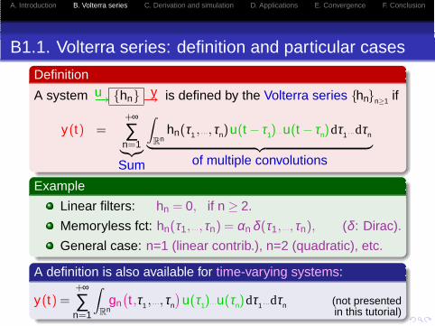
B1.1. Volterra series: definition and particular cases
Definition
A system u→ hn y
→ is defined by the Volterra series hnn≥1 if
y(t) =+∞
∑n=1
∫
Rnhn(τ1 , . . .,τn)u(t − τ1). . .u(t − τn)dτ1 . . .dτn
= ∑+∞n=1 αn
(u(t)
)n Power series
Example
Linear filters: hn = 0, if n ≥ 2.
Memoryless fct: hn(τ1, . . .,τn) = αn δ (τ1, . . .,τn), (δ : Dirac).

A. Introduction B. Volterra series C. Derivation and simulation D. Applications E. Convergence F. Conclusion
B1.1. Volterra series: definition and particular cases
Definition
A system u→ hn y
→ is defined by the Volterra series hnn≥1 if
y(t) =+∞
∑n=1︸︷︷︸
Sum
∫
Rnhn(τ1 , . . .,τn)u(t − τ1). . .u(t − τn)dτ1 . . .dτn
︸ ︷︷ ︸of multiple convolutions
Example
Linear filters: hn = 0, if n ≥ 2.
Memoryless fct: hn(τ1, . . .,τn) = αn δ (τ1, . . .,τn), (δ : Dirac).
General case: n=1 (linear contrib.), n=2 (quadratic), etc.
A definition is also available for time-varying systems:
y(t) =+∞
∑n=1
∫
Rngn
(t ,τ1 , . . .,τn
)u(τ1). . .u(τn)dτ1 . . .dτn (not presented
in this tutorial)
A. Introduction B. Volterra series C. Derivation and simulation D. Applications E. Convergence F. Conclusion
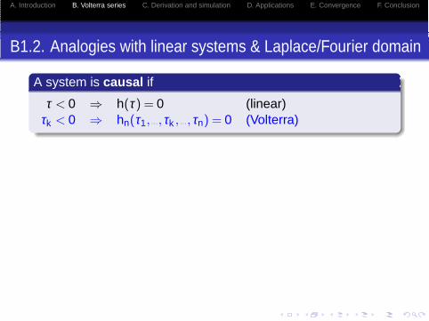
B1.2. Analogies with linear systems & Laplace/Fourier domain
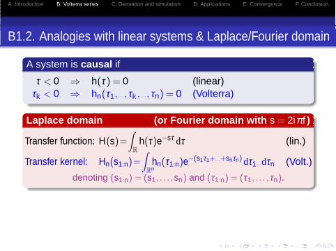
A system is causal if
τ < 0 ⇒ h(τ) = 0 (linear)τk < 0 ⇒ hn(τ1, . . .,τk , . . .,τn) = 0 (Volterra)
A. Introduction B. Volterra series C. Derivation and simulation D. Applications E. Convergence F. Conclusion
B1.2. Analogies with linear systems & Laplace/Fourier domain
A system is causal if
τ < 0 ⇒ h(τ) = 0 (linear)τk < 0 ⇒ hn(τ1, . . .,τk , . . .,τn) = 0 (Volterra)
Laplace domain (or Fourier domain with s = 2iπf )
Transfer function: H(s)=∫
R
h(τ)e−sτ dτ (lin.)
Transfer kernel: Hn(s1:n)=∫
Rnhn(τ1:n)e
−(s1τ1+. . .+snτn) dτ1 . . .dτn (Volt.)
denoting (s1:n) = (s1, . . . ,sn) and (τ1:n) = (τ1, . . . ,τn).
Causal stable system: NO poles (and NO singularities)
of H(s) for ℜe(s) > 0 (linear)of Hn(s1:n) for ℜe(sk )>0 (Volterra)

A. Introduction B. Volterra series C. Derivation and simulation D. Applications E. Convergence F. Conclusion
B1.3. Periodic signals and distortion coefficient
Analytic input signal u(t) = aeiωt
u(t) = aeiωt −→ hn −→y(t) =+∞
∑n=1
an Hn(iω , . . ., iω)einωt
Periodic input signals / Fourier series
u(t)=+∞
∑k=−∞
uk eikωt −→ hn −→y(t)=+∞
∑k=−∞
yk eikωt
with yk =+∞
∑n=1
+∞
∑k1,. . . ,kn=−∞k1+. . .+kn=k
uk1. . .ukn Hn(ik1ω , . . ., iknω)
Distortion coefficient for u(t) = a cos(ω t)
D(a,ω) = ∑+∞n=2 |yn|2/|y1|2 : closed-form solution w.r.t. a, ω , Hn.

A. Introduction B. Volterra series C. Derivation and simulation D. Applications E. Convergence F. Conclusion
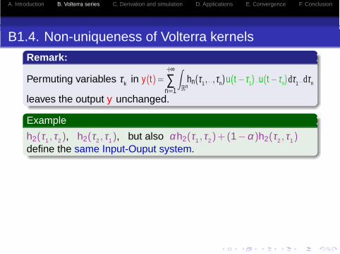
B1.4. Non-uniqueness of Volterra kernels
Remark:
Permuting variables τk in y(t) =+∞
∑n=1
∫
Rnhn(τ1 , . . .,τn)u(t − τ1). . .u(t − τn)dτ1 . . .dτn
leaves the output y unchanged.
A. Introduction B. Volterra series C. Derivation and simulation D. Applications E. Convergence F. Conclusion
B1.4. Non-uniqueness of Volterra kernels
Remark:
Permuting variables τk in y(t) =+∞
∑n=1
∫
Rnhn(τ1 , . . .,τn)u(t − τ1). . .u(t − τn)dτ1 . . .dτn
leaves the output y unchanged.
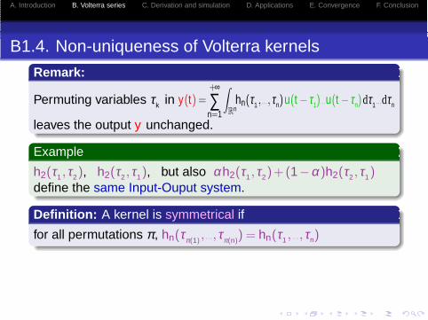
Example
h2(τ1 ,τ2), h2(τ2 ,τ1), but also αh2(τ1 ,τ2)+(1−α)h2(τ2 ,τ1)define the same Input-Ouput system.
A. Introduction B. Volterra series C. Derivation and simulation D. Applications E. Convergence F. Conclusion
B1.4. Non-uniqueness of Volterra kernels
Remark:
Permuting variables τk in y(t) =+∞
∑n=1
∫
Rnhn(τ1 , . . .,τn)u(t − τ1). . .u(t − τn)dτ1 . . .dτn
leaves the output y unchanged.
Example
h2(τ1 ,τ2), h2(τ2 ,τ1), but also αh2(τ1 ,τ2)+(1−α)h2(τ2 ,τ1)define the same Input-Ouput system.
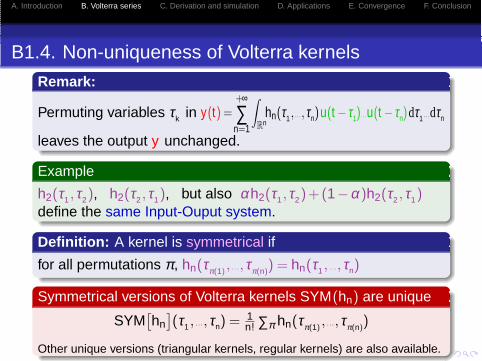
Definition: A kernel is symmetrical if
for all permutations π, hn(τπ(1), . . .,τπ(n)
) = hn(τ1 , . . .,τn)
A. Introduction B. Volterra series C. Derivation and simulation D. Applications E. Convergence F. Conclusion
B1.4. Non-uniqueness of Volterra kernels
Remark:
Permuting variables τk in y(t) =+∞
∑n=1
∫
Rnhn(τ1 , . . .,τn)u(t − τ1). . .u(t − τn)dτ1 . . .dτn
leaves the output y unchanged.
Example
h2(τ1 ,τ2), h2(τ2 ,τ1), but also αh2(τ1 ,τ2)+(1−α)h2(τ2 ,τ1)define the same Input-Ouput system.
Definition: A kernel is symmetrical if
for all permutations π, hn(τπ(1), . . .,τπ(n)
) = hn(τ1 , . . .,τn)
Symmetrical versions of Volterra kernels SYM(hn) are unique
SYM[hn
](τ1 , . . .,τn) = 1
n! ∑π hn(τπ(1), . . .,τπ(n)
)
Other unique versions (triangular kernels, regular kernels) are also available.
A. Introduction B. Volterra series C. Derivation and simulation D. Applications E. Convergence F. Conclusion
B2. Volterra series
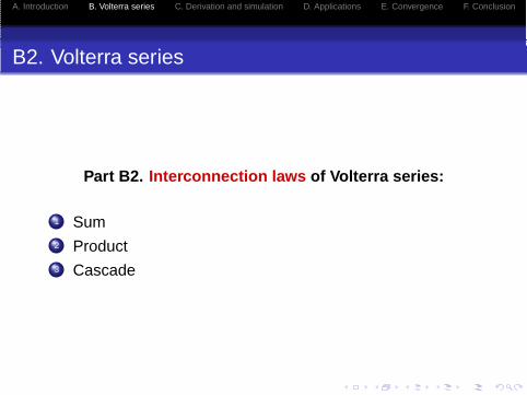
Part B2. Interconnection laws of Volterra series:
1 Sum2 Product3 Cascade

A. Introduction B. Volterra series C. Derivation and simulation D. Applications E. Convergence F. Conclusion
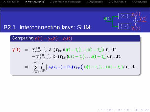
B2.1. Interconnection laws: SUM
an
bnu(t)
ya(t)
yb(t)
y(t)
Computing y(t) = ya(t)+yb(t)

A. Introduction B. Volterra series C. Derivation and simulation D. Applications E. Convergence F. Conclusion
B2.1. Interconnection laws: SUM
an
bnu(t)
ya(t)
yb(t)
y(t)
Computing y(t) = ya(t)+yb(t)
y(t) = ∑+∞n=1
∫Rn an(τ1:n)u(t − τ1) . . .u(t − τn)dτ1 . . .dτn
+∑+∞n=1
∫Rn bn(τ1:n)u(t − τ1) . . .u(t − τn)dτ1 . . .dτn
=+∞
∑n=1
∫
Rn
[an(τ1:n)+bn(τ1:n)
]u(t − τ1) . . .u(t − τn)dτ1 . . .dτn
Result: Equivalent kernels cn
cn(τ1:n) = an(τ1:n) +bn(τ1:n)
Laplace T.: Cn(s1:n) = An(s1:n) +Bn(s1:n)

A. Introduction B. Volterra series C. Derivation and simulation D. Applications E. Convergence F. Conclusion
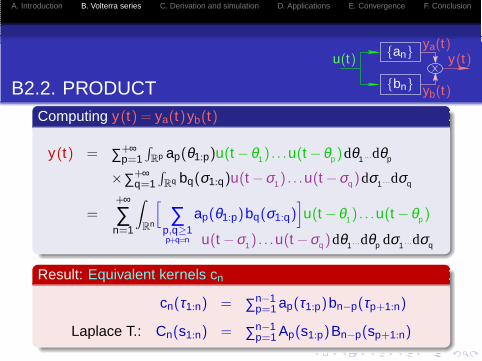
B2.2. PRODUCT
an
bnu(t)
ya(t)
yb(t)
y(t)
Computing y(t) = ya(t)yb(t)

A. Introduction B. Volterra series C. Derivation and simulation D. Applications E. Convergence F. Conclusion
B2.2. PRODUCT
an
bnu(t)
ya(t)
yb(t)
y(t)
Computing y(t) = ya(t)yb(t)
y(t) = ∑+∞p=1
∫Rp ap(θ1:p)u(t −θ1) . . .u(t −θp)dθ1 . . .dθp
×∑+∞q=1
∫Rq bq(σ1:q)u(t −σ1) . . .u(t −σq )dσ1 . . .dσq

A. Introduction B. Volterra series C. Derivation and simulation D. Applications E. Convergence F. Conclusion
B2.2. PRODUCT
an
bnu(t)
ya(t)
yb(t)
y(t)
Computing y(t) = ya(t)yb(t)
y(t) = ∑+∞p=1
∫Rp ap(θ1:p)u(t −θ1) . . .u(t −θp)dθ1 . . .dθp
×∑+∞q=1
∫Rq bq(σ1:q)u(t −σ1) . . .u(t −σq )dσ1 . . .dσq
=+∞
∑n=1
∫
Rn
[∑
p,q≥1p+q=n
ap(θ1:p)bq(σ1:q)]u(t −θ1) . . .u(t −θp)
u(t −σ1) . . .u(t −σq )dθ1 . . .dθp dσ1 . . .dσq
Result: Equivalent kernels cn
cn(τ1:n) = ∑n−1p=1 ap(τ1:p)bn−p(τp+1:n)
Laplace T.: Cn(s1:n) = ∑n−1p=1 Ap(s1:p)Bn−p(sp+1:n)

A. Introduction B. Volterra series C. Derivation and simulation D. Applications E. Convergence F. Conclusion
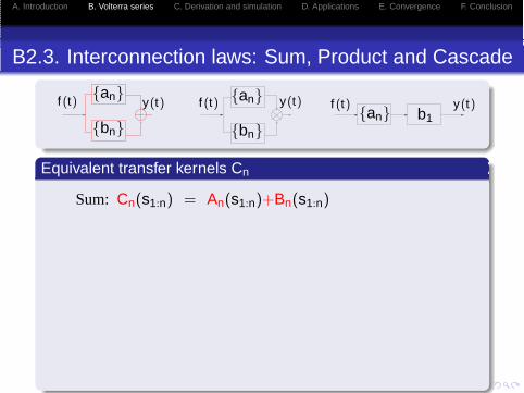
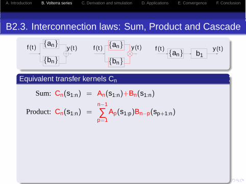
B2.3. Interconnection laws: Sum, Product and Cascade
y(t) y(t) y(t)f (t) f (t) f (t)an an
anbn bn
b1
Equivalent transfer kernels Cn
A. Introduction B. Volterra series C. Derivation and simulation D. Applications E. Convergence F. Conclusion
B2.3. Interconnection laws: Sum, Product and Cascade
y(t) y(t) y(t)f (t) f (t) f (t)an an
anbn bn
b1
Equivalent transfer kernels Cn
Sum: Cn(s1:n) = An(s1:n)+Bn(s1:n)
A. Introduction B. Volterra series C. Derivation and simulation D. Applications E. Convergence F. Conclusion
B2.3. Interconnection laws: Sum, Product and Cascade
y(t) y(t) y(t)f (t)f (t) f (t)an an
anbn bn
b1
Equivalent transfer kernels Cn
Sum: Cn(s1:n) = An(s1:n)+Bn(s1:n)
Product: Cn(s1:n) =n−1
∑p=1
Ap(s1:p)Bn−p(sp+1:n)
A. Introduction B. Volterra series C. Derivation and simulation D. Applications E. Convergence F. Conclusion
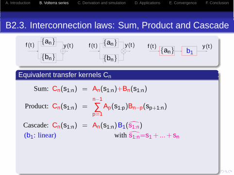
B2.3. Interconnection laws: Sum, Product and Cascade
y(t)y(t) y(t) f (t)f (t) f (t) anan an
bn bnb1
Equivalent transfer kernels Cn
Sum: Cn(s1:n) = An(s1:n)+Bn(s1:n)
Product: Cn(s1:n) =n−1
∑p=1
Ap(s1:p)Bn−p(sp+1:n)
Cascade: Cn(s1:n) = An(s1:n)B1(s1:n)
(b1: linear) with s1:n=s1 + ...+sn
A. Introduction B. Volterra series C. Derivation and simulation D. Applications E. Convergence F. Conclusion
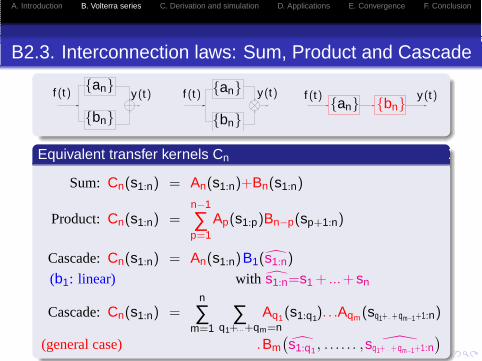
B2.3. Interconnection laws: Sum, Product and Cascade
y(t)y(t) y(t) f (t)f (t) f (t) anan an
bn bnbn
Equivalent transfer kernels Cn
Sum: Cn(s1:n) = An(s1:n)+Bn(s1:n)
Product: Cn(s1:n) =n−1
∑p=1
Ap(s1:p)Bn−p(sp+1:n)
Cascade: Cn(s1:n) = An(s1:n)B1(s1:n)
(b1: linear) with s1:n=s1 + ...+sn
Cascade: Cn(s1:n) =n
∑m=1
∑q1+. . .+qm=n
Aq1(s1:q1). . .Aqm(sq1+. . .+qm−1+1:n)
(general case) .Bm(s1:q1 , . . . . . . , sq1+ . . . +qm−1+1:n
)

A. Introduction B. Volterra series C. Derivation and simulation D. Applications E. Convergence F. Conclusion
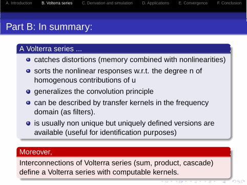
Part B: In summary:
A Volterra series ...
catches distortions (memory combined with nonlinearities)
sorts the nonlinear responses w.r.t. the degree n ofhomogenous contributions of u
generalizes the convolution principle
can be described by transfer kernels in the frequencydomain (as filters).
is usually non unique but uniquely defined versions areavailable (useful for identification purposes)
A. Introduction B. Volterra series C. Derivation and simulation D. Applications E. Convergence F. Conclusion
Part B: In summary:
A Volterra series ...
catches distortions (memory combined with nonlinearities)
sorts the nonlinear responses w.r.t. the degree n ofhomogenous contributions of u
generalizes the convolution principle
can be described by transfer kernels in the frequencydomain (as filters).
is usually non unique but uniquely defined versions areavailable (useful for identification purposes)
Moreover,
Interconnections of Volterra series (sum, product, cascade)define a Volterra series with computable kernels.

A. Introduction B. Volterra series C. Derivation and simulation D. Applications E. Convergence F. Conclusion
Part C: Tutorial
TUTORIAL: How to ...
C1. derive the Volterra kernels of a given nonlinearsystem ?
C2. simulate the system using these kernels ?

A. Introduction B. Volterra series C. Derivation and simulation D. Applications E. Convergence F. Conclusion
C1.1. How to derive the Volterra kernels of a system S ?
Goal: Find the Volterra kernels hn of (S ) where
u−→ (S ) : dxdt = F (x ,u) x−→
?−→ u−→ hn x−→
Several methods are available... [Brockett,Isidori,Rugh,Boyd]
Here: Introduce the “cancelling system” of S
u
u
xhn Cancelling systemoutput: w = dx
dt −F (x ,u)
w = 0
Principle: this cascade defines the null system u−→ zn =0 w =0−→
Interconnection laws gives the equations satisfied by hn.
A. Introduction B. Volterra series C. Derivation and simulation D. Applications E. Convergence F. Conclusion
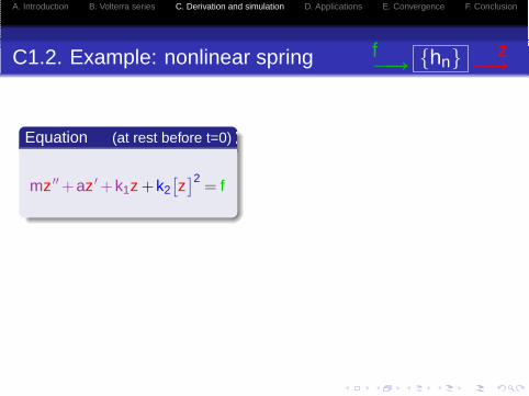
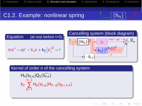
C1.2. Example: nonlinear spring f−→ hn z−→
Equation (at rest before t=0)
mz ′′ +az ′ +k1z +k2[z]2
= f

A. Introduction B. Volterra series C. Derivation and simulation D. Applications E. Convergence F. Conclusion
C1.2. Example: nonlinear spring f−→ hn z−→
Equation (at rest before t=0)
mz ′′ +az ′ +k1z +k2[z]2
= f
Cancelling system (block diagram)
f z mz ′′+az ′+k1z
−f
k2[z]2
hn
−1
k2[·]2lin. op. 0
A. Introduction B. Volterra series C. Derivation and simulation D. Applications E. Convergence F. Conclusion
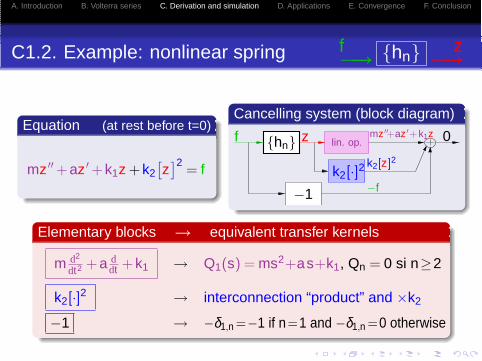
C1.2. Example: nonlinear spring f−→ hn z−→
Equation (at rest before t=0)
mz ′′ +az ′ +k1z +k2[z]2
= f
Cancelling system (block diagram)
f z mz ′′+az ′+k1z
−f
k2[z]2
hn
−1
k2[·]2lin. op. 0
Elementary blocks → equivalent transfer kernels
m d2
dt2 +a ddt +k1 → Q1(s) = ms2+as+k1, Qn = 0 si n≥2
k2[·]2 → interconnection “product” and ×k2
−1 → −δ1,n =−1 if n=1 and −δ1,n =0 otherwise
A. Introduction B. Volterra series C. Derivation and simulation D. Applications E. Convergence F. Conclusion
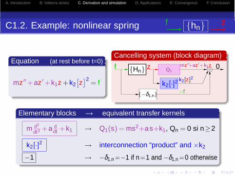
C1.2. Example: nonlinear spring f−→ hn z−→
Equation (at rest before t=0)
mz ′′ +az ′ +k1z +k2[z]2
= f
Cancelling system (block diagram)
f z mz ′′+az ′+k1z
−f
k2[z]2
Hn
−δ1,nk2[·]2
Q10
Elementary blocks → equivalent transfer kernels
m d2
dt2 +a ddt +k1 → Q1(s) = ms2+as+k1, Qn = 0 si n≥2
k2[·]2 → interconnection “product” and ×k2
−1 → −δ1,n =−1 if n=1 and −δ1,n =0 otherwise
A. Introduction B. Volterra series C. Derivation and simulation D. Applications E. Convergence F. Conclusion
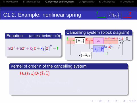
C1.2. Example: nonlinear spring f−→ hn z−→
Equation (at rest before t=0)
mz ′′ +az ′ +k1z +k2[z]2
= f
Cancelling system (block diagram)
f z mz ′′+az ′+k1z
−f
k2[z]2
Hn
−δ1,nk2[·]2
Q10
Kernel of order n of the cancelling system
Hn(s1:n)Q1(s1:n)
+ k2
n−1
∑p=1
Hp(s1:p)Hn−p(sp+1:n)
+ −δ1,n = 0
A. Introduction B. Volterra series C. Derivation and simulation D. Applications E. Convergence F. Conclusion
C1.2. Example: nonlinear spring f−→ hn z−→
Equation (at rest before t=0)
mz ′′ +az ′ +k1z +k2[z]2
= f
Cancelling system (block diagram)
f z mz ′′+az ′+k1z
−f
k2[z]2
Hn
−δ1,nk2[·]2
Q10
Kernel of order n of the cancelling system
Hn(s1:n)Q1(s1:n)
+ k2
n−1
∑p=1
Hp(s1:p)Hn−p(sp+1:n)
+ −δ1,n = 0

A. Introduction B. Volterra series C. Derivation and simulation D. Applications E. Convergence F. Conclusion
C1.2. Example: nonlinear spring f−→ hn z−→
Equation (at rest before t=0)
mz ′′ +az ′ +k1z +k2[z]2
= f
Cancelling system (block diagram)
f z mz ′′+az ′+k1z
−f
k2[z]2
Hn
−δ1,nk2[·]2
Q10
Kernel of order n of the cancelling system
Hn(s1:n)Q1(s1:n)
+ k2
n−1
∑p=1
Hp(s1:p)Hn−p(sp+1:n)
+ −δ1,n = 0 −→ linear eq. w.r.t. Hn.
A. Introduction B. Volterra series C. Derivation and simulation D. Applications E. Convergence F. Conclusion
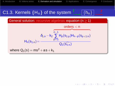
C1.3. Kernels Hn of the system f−→ hn z−→
General solution: recursive algebraic equation (n ≥ 1)
Hn(s1:n)=
δ1,n −k2
orders < n︷ ︸︸ ︷n−1
∑p=1
Hp(s1:p)Hn−p(sp+1:n)
Q1(s1:n)
where Q1(s) = ms2 +as +k1

A. Introduction B. Volterra series C. Derivation and simulation D. Applications E. Convergence F. Conclusion
C1.3. Kernels Hn of the system f−→ hn z−→
General solution: recursive algebraic equation (n ≥ 1)
Hn(s1:n)=
δ1,n −k2
orders < n︷ ︸︸ ︷n−1
∑p=1
Hp(s1:p)Hn−p(sp+1:n)
Q1(s1:n)
where Q1(s) = ms2 +as +k1
First transfer kernels (n = 1,2,3,etc)
H1(s1) = 1/Q1(s1), (second order AR filter)
H2(s1:2) = −k2 H1(s1) H1(s2) H1(s1:2),
H3(s1:3) = −k2[H2(s1:2) H1(s3) + H1(s1) H2(s2:3)
]H1(s1:3),
etc.

A. Introduction B. Volterra series C. Derivation and simulation D. Applications E. Convergence F. Conclusion
Part C: Tutorial
TUTORIAL: How to ...
C2. simulate the system using these kernels ?

A. Introduction B. Volterra series C. Derivation and simulation D. Applications E. Convergence F. Conclusion
C2.1. How to simulate the system using these kernels?
Several methods are available... (realization theory in [Rugh])

A. Introduction B. Volterra series C. Derivation and simulation D. Applications E. Convergence F. Conclusion
C2.1. How to simulate the system using these kernels?
Several methods are available... (realization theory in [Rugh])
HERE: Consider the following “elementary system”
u(t) x(t)Ap
(order p only)
Bq
(order q only)
C1
(linear)
xa(t)
xb(t)
Equivalent system (using “product” & “cascade”)
The Volterra transfer kernels of this system are all zero except
Hp+q(s1:p+q) = Ap(s1:p)Bq(sp+1:p+q) C1(s1:p+q)
Method:Recursively build a realization as a sum of such systems .

A. Introduction B. Volterra series C. Derivation and simulation D. Applications E. Convergence F. Conclusion
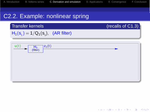
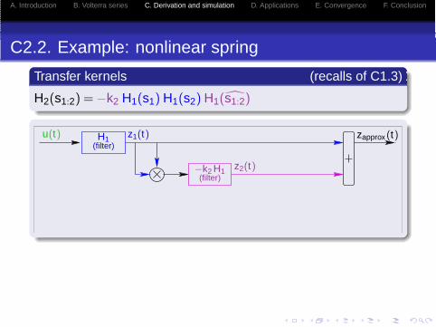
C2.2. Example: nonlinear spring
Transfer kernels (recalls of C1.3)
H1(s1) = 1/Q1(s1), (AR filter)
A. Introduction B. Volterra series C. Derivation and simulation D. Applications E. Convergence F. Conclusion
C2.2. Example: nonlinear spring
Transfer kernels (recalls of C1.3)
H1(s1) = 1/Q1(s1), (AR filter)
u(t) H1(filter)
z1(t)
A. Introduction B. Volterra series C. Derivation and simulation D. Applications E. Convergence F. Conclusion
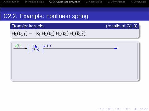
C2.2. Example: nonlinear spring
Transfer kernels (recalls of C1.3)
H2(s1:2) = −k2 H1(s1) H1(s2) H1(s1:2)
u(t) H1(filter)
z1(t)

A. Introduction B. Volterra series C. Derivation and simulation D. Applications E. Convergence F. Conclusion
C2.2. Example: nonlinear spring
Transfer kernels (recalls of C1.3)
H2(s1:2) = −k2 H1(s1) H1(s2) H1(s1:2)
u(t) H1(filter)
z1(t)
A. Introduction B. Volterra series C. Derivation and simulation D. Applications E. Convergence F. Conclusion
C2.2. Example: nonlinear spring
Transfer kernels (recalls of C1.3)
H2(s1:2) = −k2 H1(s1) H1(s2) H1(s1:2)
u(t) zapprox(t)H1(filter)
z1(t)
−k2 H1(filter)
z2(t)
A. Introduction B. Volterra series C. Derivation and simulation D. Applications E. Convergence F. Conclusion
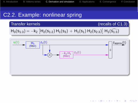
C2.2. Example: nonlinear spring
Transfer kernels (recalls of C1.3)
H3(s1:3) = −k2[H2(s1:2) H1(s3) + H1(s1) H2(s2:3)
]H1(s1:3)
u(t) zapprox(t)H1(filter)
z1(t)
−k2 H1(filter)
z2(t)
A. Introduction B. Volterra series C. Derivation and simulation D. Applications E. Convergence F. Conclusion
C2.2. Example: nonlinear spring
Transfer kernels (recalls of C1.3)
H3(s1:3) = −k2[H2(s1:2) H1(s3) + H1(s1) H2(s2:3)
]H1(s1:3)
u(t) zapprox(t)H1(filter)
z1(t)
−k2 H1(filter)
z2(t)
A. Introduction B. Volterra series C. Derivation and simulation D. Applications E. Convergence F. Conclusion
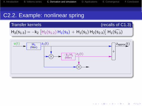
C2.2. Example: nonlinear spring
Transfer kernels (recalls of C1.3)
H3(s1:3) = −k2[H2(s1:2) H1(s3) + H1(s1) H2(s2:3)
]H1(s1:3)
u(t) zapprox(t)H1(filter)
z1(t)
−k2 H1(filter)
z2(t)
×2

A. Introduction B. Volterra series C. Derivation and simulation D. Applications E. Convergence F. Conclusion
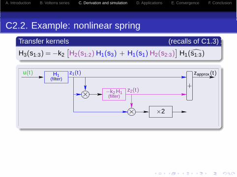
C2.2. Example: nonlinear spring
Transfer kernels (recalls of C1.3)
H3(s1:3) = −k2[H2(s1:2) H1(s3) + H1(s1) H2(s2:3)
]H1(s1:3)
u(t) zapprox(t)H1(filter)
z1(t)
−k2 H1(filter)
z2(t)
−2k2 H1(filter)
z3(t)

A. Introduction B. Volterra series C. Derivation and simulation D. Applications E. Convergence F. Conclusion
C2.2. Example: nonlinear spring
Transfer kernels (recalls of C1.3)
H3(s1:3) = −k2[H2(s1:2) H1(s3) + H1(s1) H2(s2:3)
]H1(s1:3)
u(t) zapprox(t)H1(filter)
z1(t)
−k2 H1(filter)
z2(t)
−2k2 H1(filter)
z3(t)
RESULT: The system is composed of sums , products and
linear filters (−→ just implement digital versions!)
Rk: if linear filters are stable, the system is stable!

A. Introduction B. Volterra series C. Derivation and simulation D. Applications E. Convergence F. Conclusion
C2.3. Aliasing rejection in simulations
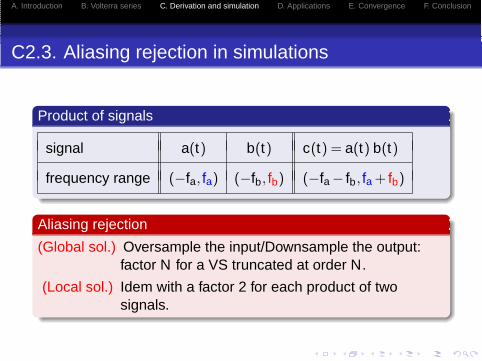
Product of signals
signal a(t) b(t) c(t) = a(t) b(t)
frequency range (−fa, fa) (−fb, fb) (−fa − fb, fa + fb)
A. Introduction B. Volterra series C. Derivation and simulation D. Applications E. Convergence F. Conclusion
C2.3. Aliasing rejection in simulations
Product of signals
signal a(t) b(t) c(t) = a(t) b(t)
frequency range (−fa, fa) (−fb, fb) (−fa − fb, fa + fb)
Aliasing rejection
(Global sol.) Oversample the input/Downsample the output:factor N for a VS truncated at order N.
(Local sol.) Idem with a factor 2 for each product of twosignals.

A. Introduction B. Volterra series C. Derivation and simulation D. Applications E. Convergence F. Conclusion
Part C: In summary...
Derivation of the transfer kernels
1 Use the cancelling system and interconnection laws...
2 ... to transform the weakly nonlinear problem into a infinitesequence of solvable linear equations
Simulation in practice
1 Truncate the series to catch the first distortions
2 Decompose the kernels into sums of elementary systems
3 Build the corresponding structure composed of linear filters ,sums and products of signals
4 Implement digital versions of the filters
5 Add oversampler/downsampler (aliasing rejection)
Possible generalization to Partial Differential Equations (PDE):Same principle (cf. Applications)

A. Introduction B. Volterra series C. Derivation and simulation D. Applications E. Convergence F. Conclusion
Part D: Physical/Audio Applications
APPPLICATIONS ON PDEs:
D1. Nonlinear propagation of a travelling wave(brassy effect)
switch to powerpoint [Helie,Smet: IEEE-MED’2008]
D2. A damped nonlinear stringresults extracted from [Helie,Roze: JSV’2008]
(not presented here: Moog Ladder Filter[Helie: DAFx’2006 & TASLP’2010])
A. Introduction B. Volterra series C. Derivation and simulation D. Applications E. Convergence F. Conclusion
D1. Application 1
NONLINEAR PROPAGATION OF A TRAVELLINGWAVE (brassy effect)
switch to powerpoint [Helie,Smet: IEEE-MED’2008]
A. Introduction B. Volterra series C. Derivation and simulation D. Applications E. Convergence F. Conclusion
D2. Application 2
A DAMPED NONLINEAR STRING
Results extracted from [Helie,Roze: JSV’2008]
A. Introduction B. Volterra series C. Derivation and simulation D. Applications E. Convergence F. Conclusion
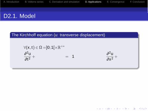
D2.1. Model
The Kirchhoff equation (u: transverse displacement)
∀(x , t) ∈ Ω =]0;1[×R+∗
∂ 2u∂ t2 + = 1
∂ 2u∂x2 +

A. Introduction B. Volterra series C. Derivation and simulation D. Applications E. Convergence F. Conclusion
D2.1. Model
The Kirchhoff equation (u: transverse displacement)
∀(x , t) ∈ Ω =]0;1[×R+∗
∂ 2u∂ t2 +α
∂u∂ t
−β∂∂ t
∂ 2u∂x2 = 1+
∂ 2u∂x2 +
(α,β ): damping

A. Introduction B. Volterra series C. Derivation and simulation D. Applications E. Convergence F. Conclusion
D2.1. Model
The Kirchhoff equation (u: transverse displacement)
∀(x , t) ∈ Ω =]0;1[×R+∗
∂ 2u∂ t2 +α
∂u∂ t
−β∂∂ t
∂ 2u∂x2 = 1+
∂ 2u∂x2 +φ(x)f (t)
(α,β ): damping f (t): excitation force

A. Introduction B. Volterra series C. Derivation and simulation D. Applications E. Convergence F. Conclusion
D2.1. Model
The Kirchhoff equation (u: transverse displacement)
∀(x , t) ∈ Ω =]0;1[×R+∗
∂ 2u∂ t2 +α
∂u∂ t
−β∂∂ t
∂ 2u∂x2 =
[1+ ε
∫ 1
0‖∂u
∂x‖2dx
]∂ 2u∂x2 +φ(x)f (t)
(α,β ): damping ε: nonlinear coefficient f (t): excitation force
Boundary and initial conditions
Dirichlet homegeneous: u(x = 0, t) = u(x = 1, t) = 0
At rest for t ≤ 0 : u(x , t) = ∂tu(x , t) = 0

A. Introduction B. Volterra series C. Derivation and simulation D. Applications E. Convergence F. Conclusion
D2.2. Equation satisfied by the Volterra kernels
Kirchhoff equation of the string
∂ 2u∂ t2 +α
∂u∂ t
−β∂∂ t
∂ 2u∂x2 −
[1+ ε
∫ 1
0‖∂u
∂x‖2dx
]∂ 2u∂x2 −φ(x)f (t) = 0

A. Introduction B. Volterra series C. Derivation and simulation D. Applications E. Convergence F. Conclusion
D2.2. Equation satisfied by the Volterra kernels
Kirchhoff equation of the string
∂ 2u∂ t2 +α
∂u∂ t
−β∂∂ t
∂ 2u∂x2 −
[1+ ε
∫ 1
0‖∂u
∂x‖2dx
]∂ 2u∂x2 −φ(x)f (t) = 0
Definition of the solution as a Volterra series
h(x)n
f (t) u(x , t)
Volterra kernels must be paremetrized in space: hn→ h(x)n .

A. Introduction B. Volterra series C. Derivation and simulation D. Applications E. Convergence F. Conclusion
D2.2. Equation satisfied by the Volterra kernels
Kirchhoff equation of the string
∂ 2u∂ t2 +α
∂u∂ t
−β∂∂ t
∂ 2u∂x2 −
[1+ ε
∫ 1
0‖∂u
∂x‖2dx
]∂ 2u∂x2 −φ(x)f (t) = 0
Cancelling system in the time domain
h(x)n
∂ 2
∂ t2 +α ∂∂ t − (1+β ∂
∂ t )∂ 2
∂x2
∂∂x
.2 −ε∫ 1
0 dx
∂ 2
∂x2
0
f (t) u(x , t)
×(−φ(x))

A. Introduction B. Volterra series C. Derivation and simulation D. Applications E. Convergence F. Conclusion
D2.2. Equation satisfied by the Volterra kernels
Kirchhoff equation of the string
∂ 2u∂ t2 +α
∂u∂ t
−β∂∂ t
∂ 2u∂x2 −
[1+ ε
∫ 1
0‖∂u
∂x‖2dx
]∂ 2u∂x2 −φ(x)f (t) = 0
Cancelling system in the Laplace domain
H(x)n
s2 +αs− (1+βs) ∂ 2
∂x2
∂∂x
.2 −ε∫ 1
0 dx
∂ 2
∂x2
0
f (t) u(x , t)
×(−φ(x))
[(s1:n)2 +α(s1:n)− (1+β (s1:n)) ∂ 2
∂x2
]H(x)
n (s1:n) .... etc
A. Introduction B. Volterra series C. Derivation and simulation D. Applications E. Convergence F. Conclusion
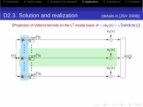
D2.3. Solution and realization (details in [JSV 2008])
(Projection of Volterra kernels on the L2-modal basis B = ek (x) =√
2sin(kπx))
f (t)
φ1
φk
φK
q[1]
q[k ]
q[K]
u[1]1 (t)
u[k ]1 (t)
u[K ]1 (t)
e1(x)
ek (x)
eK (x)
u1(x,t)

A. Introduction B. Volterra series C. Derivation and simulation D. Applications E. Convergence F. Conclusion
D2.3. Solution and realization (details in [JSV 2008])
(Projection of Volterra kernels on the L2-modal basis B = ek (x) =√
2sin(kπx))
2. 2. 2.
f (t)
φ1
φk
φK
q[1] q[1]
q[k ]q[k ]
q[K]q[K]
u[1]1 (t)
u[k ]1 (t)
u[K ]1 (t)
k K
w(t) =K
∑l=1
l2(u[l]
1 (t))2
−επ4
−εk2π4
−εK 2π4
u[1]3 (t)
u[k ]3 (t)
u[K ]3 (t)
e1(x)
ek (x)
eK (x)
u3(x,t)
(linear contribution, n = 1)

A. Introduction B. Volterra series C. Derivation and simulation D. Applications E. Convergence F. Conclusion
Part E: Convergence of a Volterra series
VOLTERRA SERIES:
Computable convergence domains
A. Introduction B. Volterra series C. Derivation and simulation D. Applications E. Convergence F. Conclusion
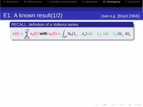
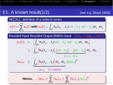
E1. A known result(1/2) (see e.g. [Boyd,1984])
RECALL: definition of a Volterra series
x(t) =+∞
∑n=1
xn(t) with xn(t) =∫
Rnhn(τ1 , . . .,τn)u(t − τ1). . .u(t − τn)dτ1 . . .dτn

A. Introduction B. Volterra series C. Derivation and simulation D. Applications E. Convergence F. Conclusion
E1. A known result(1/2) (see e.g. [Boyd,1984])
RECALL: definition of a Volterra series
x(t) =+∞
∑n=1
xn(t) with xn(t) =∫
Rnhn(τ1 , . . .,τn)u(t − τ1). . .u(t − τn)dτ1 . . .dτn
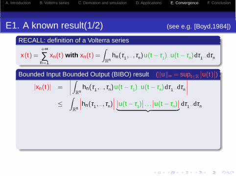
Bounded Input Bounded Output (BIBO) result (‖u‖∞ = supt∈R
∣∣u(t)∣∣)
|xn(t)| =
∣∣∣∣∫
Rnhn(τ1 , . . .,τn)u(t − τ1). . .u(t − τn)dτ1 . . .dτn
∣∣∣∣
A. Introduction B. Volterra series C. Derivation and simulation D. Applications E. Convergence F. Conclusion
E1. A known result(1/2) (see e.g. [Boyd,1984])
RECALL: definition of a Volterra series
x(t) =+∞
∑n=1
xn(t) with xn(t) =∫
Rnhn(τ1 , . . .,τn)u(t − τ1). . .u(t − τn)dτ1 . . .dτn
Bounded Input Bounded Output (BIBO) result (‖u‖∞ = supt∈R
∣∣u(t)∣∣)
|xn(t)| =
∣∣∣∣∫
Rnhn(τ1 , . . .,τn)u(t − τ1). . .u(t − τn)dτ1 . . .dτn
∣∣∣∣
≤∫
Rn
∣∣∣hn(τ1 , . . .,τn)∣∣∣∣∣u(t − τ1)
∣∣ . . .∣∣u(t − τn)
∣∣︸ ︷︷ ︸ dτ1 . . .dτn
A. Introduction B. Volterra series C. Derivation and simulation D. Applications E. Convergence F. Conclusion
E1. A known result(1/2) (see e.g. [Boyd,1984])
RECALL: definition of a Volterra series
x(t) =+∞
∑n=1
xn(t) with xn(t) =∫
Rnhn(τ1 , . . .,τn)u(t − τ1). . .u(t − τn)dτ1 . . .dτn
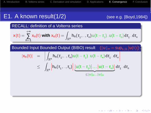
Bounded Input Bounded Output (BIBO) result (‖u‖∞ = supt∈R
∣∣u(t)∣∣)
|xn(t)| =
∣∣∣∣∫
Rnhn(τ1 , . . .,τn)u(t − τ1). . .u(t − τn)dτ1 . . .dτn
∣∣∣∣
≤∫
Rn
∣∣∣hn(τ1 , . . .,τn)∣∣∣∣∣u(t − τ1)
∣∣ . . .∣∣u(t − τn)
∣∣︸ ︷︷ ︸
≤‖u‖∞...‖u‖∞
dτ1 . . .dτn

A. Introduction B. Volterra series C. Derivation and simulation D. Applications E. Convergence F. Conclusion
E1. A known result(1/2) (see e.g. [Boyd,1984])
RECALL: definition of a Volterra series
x(t) =+∞
∑n=1
xn(t) with xn(t) =∫
Rnhn(τ1 , . . .,τn)u(t − τ1). . .u(t − τn)dτ1 . . .dτn
Bounded Input Bounded Output (BIBO) result (‖u‖∞ = supt∈R
∣∣u(t)∣∣)
|xn(t)| =
∣∣∣∣∫
Rnhn(τ1 , . . .,τn)u(t − τ1). . .u(t − τn)dτ1 . . .dτn
∣∣∣∣
≤∫
Rn
∣∣∣hn(τ1 , . . .,τn)∣∣∣∣∣u(t − τ1)
∣∣ . . .∣∣u(t − τn)
∣∣︸ ︷︷ ︸
≤‖u‖∞...‖u‖∞
dτ1 . . .dτn
‖xn‖∞ ≤∫
Rn
∣∣∣hn(τ1 , . . .,τn)∣∣∣dτ1 . . .dτn
︸ ︷︷ ︸=‖hn‖1
(L1-norm
)
(‖u‖∞
)n
Hence, ‖x‖∞ ≤+∞
∑n=1
‖xn‖∞ ≤+∞
∑n=1
‖hn‖1(‖u‖∞
)n.
A. Introduction B. Volterra series C. Derivation and simulation D. Applications E. Convergence F. Conclusion
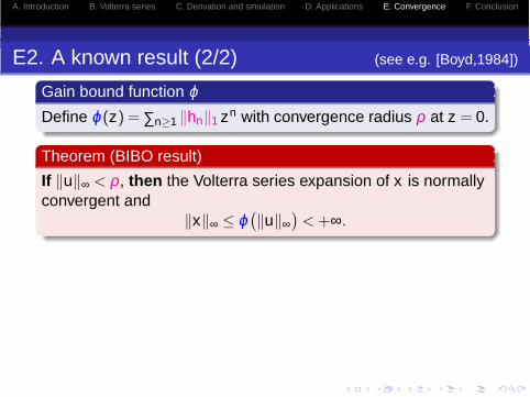
E2. A known result (2/2) (see e.g. [Boyd,1984])
Gain bound function ϕDefine ϕ(z) = ∑n≥1 ‖hn‖1 zn with convergence radius ρ at z = 0.
Theorem (BIBO result)
If ‖u‖∞ < ρ, then the Volterra series expansion of x is normallyconvergent and
‖x‖∞ ≤ ϕ(‖u‖∞
)< +∞.
A. Introduction B. Volterra series C. Derivation and simulation D. Applications E. Convergence F. Conclusion
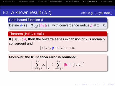
E2. A known result (2/2) (see e.g. [Boyd,1984])
Gain bound function ϕDefine ϕ(z) = ∑n≥1 ‖hn‖1 zn with convergence radius ρ at z = 0.
Theorem (BIBO result)
If ‖u‖∞ < ρ, then the Volterra series expansion of x is normallyconvergent and
‖x‖∞ ≤ ϕ(‖u‖∞
)< +∞.
Moreover, the truncation error is bounded :∥∥∥∥+∞
∑n=N+1
xn
∥∥∥∥∞≤
+∞
∑n=N+1
‖hn‖1(‖u‖∞
)n

A. Introduction B. Volterra series C. Derivation and simulation D. Applications E. Convergence F. Conclusion
E2. A known result (2/2) (see e.g. [Boyd,1984])
Gain bound function ϕDefine ϕ(z) = ∑n≥1 ‖hn‖1 zn with convergence radius ρ at z = 0.
Theorem (BIBO result)
If ‖u‖∞ < ρ, then the Volterra series expansion of x is normallyconvergent and
‖x‖∞ ≤ ϕ(‖u‖∞
)< +∞.
Moreover, the truncation error is bounded :∥∥∥∥+∞
∑n=N+1
xn
∥∥∥∥∞≤
+∞
∑n=N+1
‖hn‖1(‖u‖∞
)n
QUESTION
Can we use these theoretical results in practice?

A. Introduction B. Volterra series C. Derivation and simulation D. Applications E. Convergence F. Conclusion
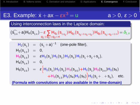
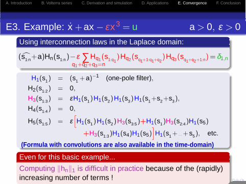
E3. Example: x +ax − εx3 = u a > 0, ε > 0
Using interconnection laws in the Laplace domain:

A. Introduction B. Volterra series C. Derivation and simulation D. Applications E. Convergence F. Conclusion
E3. Example: x +ax − εx3 = u a > 0, ε > 0
Using interconnection laws in the Laplace domain:
(s1:n+a)Hn(s1:n)

A. Introduction B. Volterra series C. Derivation and simulation D. Applications E. Convergence F. Conclusion
E3. Example: x +ax − εx3 = u a > 0, ε > 0
Using interconnection laws in the Laplace domain:
(s1:n+a)Hn(s1:n)−ε ∑q1+q2+q3=n
Hq1(s1:q1)Hq2(sq1+1:q1+q2
)Hq3(sq1+q2+1:n)

A. Introduction B. Volterra series C. Derivation and simulation D. Applications E. Convergence F. Conclusion
E3. Example: x +ax − εx3 = u a > 0, ε > 0
Using interconnection laws in the Laplace domain:
(s1:n+a)Hn(s1:n)−ε ∑q1+q2+q3=n
Hq1(s1:q1)Hq2(sq1+1:q1+q2
)Hq3(sq1+q2+1:n) = δ1,n

A. Introduction B. Volterra series C. Derivation and simulation D. Applications E. Convergence F. Conclusion
E3. Example: x +ax − εx3 = u a > 0, ε > 0
Using interconnection laws in the Laplace domain:
(s1:n+a)Hn(s1:n)−ε ∑q1+q2+q3=n
Hq1(s1:q1)Hq2(sq1+1:q1+q2
)Hq3(sq1+q2+1:n) = δ1,n
H1(s1) = (s1 +a)−1 (one-pole filter),
H2(s1:2) = 0,
H3(s1:3) = εH1(s1)H1(s2)H1(s3)H1(s1 +s2 +s3),
H4(s1:4) = 0,
H5(s1:5) = ε[H1(s1)H1(s2)H3(s3:5)+H1(s1)H3(s2:4)H1(s5)
+H3(s1:3)H1(s4)H1(s5)]H1(s1 + . . . +s5), etc.
(Formula with convolutions are also available in the time-d omain)
Even for this basic example...
Computing ‖hn‖1 is difficult in practice because of the (rapidly)increasing number of terms !

A. Introduction B. Volterra series C. Derivation and simulation D. Applications E. Convergence F. Conclusion
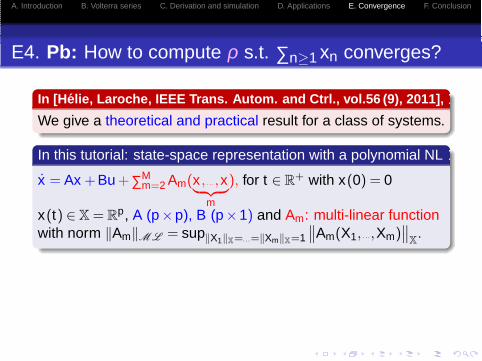
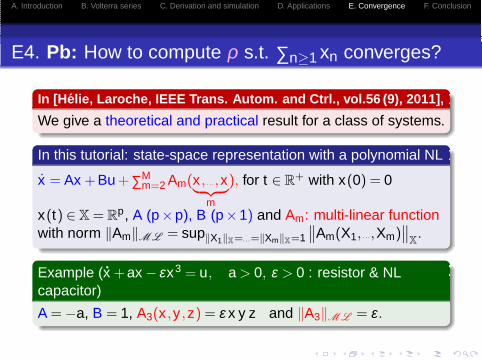
E4. Pb: How to compute ρ s.t. ∑n≥1 xn converges?

A. Introduction B. Volterra series C. Derivation and simulation D. Applications E. Convergence F. Conclusion
E4. Pb: How to compute ρ s.t. ∑n≥1 xn converges?
In [Helie, Laroche, IEEE Trans. Autom. and Ctrl., vol.56 (9), 201 1],
We give a theoretical and practical result for a class of systems.
A. Introduction B. Volterra series C. Derivation and simulation D. Applications E. Convergence F. Conclusion
E4. Pb: How to compute ρ s.t. ∑n≥1 xn converges?
In [Helie, Laroche, IEEE Trans. Autom. and Ctrl., vol.56 (9), 201 1],
We give a theoretical and practical result for a class of systems.
In this tutorial: state-space representation with a polynomial NL
x = Ax +Bu +∑Mm=2 Am(x , . . .,x︸ ︷︷ ︸
m
), for t ∈ R+ with x(0) = 0
x(t) ∈ X = Rp, A (p×p), B (p×1) and Am: multi-linear functionwith norm ‖Am‖ML = sup‖X1‖X=. . .=‖Xm‖X=1
∥∥Am(X1, . . .,Xm)∥∥
X.
Example (x +ax − εx3 = u, a > 0, ε > 0 : resistor & NLcapacitor)
A = −a, B = 1, A3(x ,y ,z) = ε x y z and ‖A3‖ML = ε.

A. Introduction B. Volterra series C. Derivation and simulation D. Applications E. Convergence F. Conclusion
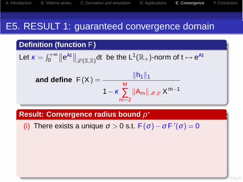
E5. RESULT 1: guaranteed convergence domain

A. Introduction B. Volterra series C. Derivation and simulation D. Applications E. Convergence F. Conclusion
E5. RESULT 1: guaranteed convergence domain
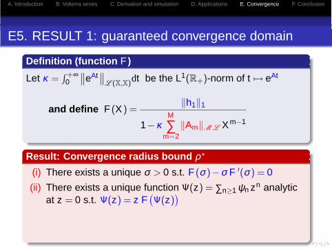
Definition (function F )
Let κ =∫ +∞
0
∥∥eAt∥∥
L (X,X)dt be the L1(R+)-norm of t 7→ eAt
and define F (X ) =‖h1‖1
1−κM
∑m=2
‖Am‖ML X m−1
A. Introduction B. Volterra series C. Derivation and simulation D. Applications E. Convergence F. Conclusion
E5. RESULT 1: guaranteed convergence domain
Definition (function F )
Let κ =∫ +∞
0
∥∥eAt∥∥
L (X,X)dt be the L1(R+)-norm of t 7→ eAt
and define F (X ) =‖h1‖1
1−κM
∑m=2
‖Am‖ML X m−1
Result: Convergence radius bound ρ⋆
(i) There exists a unique σ > 0 s.t. F (σ)−σ F ′(σ) = 0
(ii) There exists a unique function Ψ(z) = ∑n≥1 ψn zn analyticat z = 0 s.t. Ψ(z) = z F
(Ψ(z)
)
(iii) The convergence radius of Ψ is ρ⋆ = σF (σ) >0 and ρ⋆≤ ρ.
(iv) If ‖u‖∞ < ρ⋆, then ‖x‖∞ ≤ ϕ(‖u‖∞
)≤ Ψ
(‖u‖∞
)< +∞.

A. Introduction B. Volterra series C. Derivation and simulation D. Applications E. Convergence F. Conclusion
E6. Sketch of proof
Step 1: We prove that ‖hn‖1 ≤ ψn where ψ1 = ‖h1‖1 and
for all n ≥ 2, ψn = κM
∑m=2
‖Am‖ML ∑q1+ . . . +qm = nq1,. . . ,m ≥ 1
ψq1 . . .ψqm

A. Introduction B. Volterra series C. Derivation and simulation D. Applications E. Convergence F. Conclusion
E6. Sketch of proof
Step 1: We prove that ‖hn‖1 ≤ ψn where ψ1 = ‖h1‖1 and
for all n ≥ 2, ψn = κM
∑m=2
‖Am‖ML ∑q1+ . . . +qm = nq1,. . . ,m ≥ 1
ψq1 . . .ψqm
Step 2: Define the generating function Ψ(X ) =∞
∑n=1
ψnX n.
We prove that κ ∑Mm=2 ‖Am‖ML
(Ψ(X )
)m= Ψ(X )−ψ1 X
from which we deduce that Ψ(X ) = X F(Ψ(X )
).
Step 3: The singular inversion theorem yields the result.(see [Analytic combinatorics, Flajolet & Sedgewick, 2009])
A. Introduction B. Volterra series C. Derivation and simulation D. Applications E. Convergence F. Conclusion
E7. RESULT 2: Truncation error bound
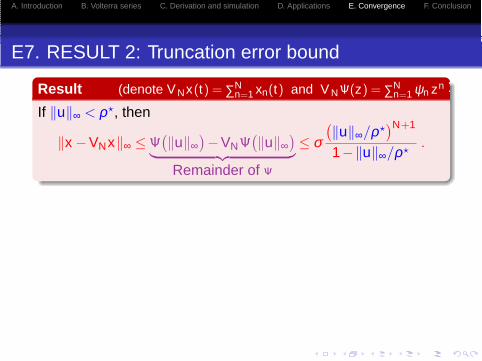
Result (denote V Nx(t) = ∑Nn=1 xn(t) and V NΨ(z) = ∑N
n=1 ψn zn
If ‖u‖∞ < ρ⋆, then
‖x −VNx‖∞ ≤ Ψ(‖u‖∞
)−VNΨ
(‖u‖∞
)︸ ︷︷ ︸
Remainder of Ψ
≤ σ(‖u‖∞/ρ⋆
)N+1
1−‖u‖∞/ρ⋆.

A. Introduction B. Volterra series C. Derivation and simulation D. Applications E. Convergence F. Conclusion
E7. RESULT 2: Truncation error bound
Result (denote V Nx(t) = ∑Nn=1 xn(t) and V NΨ(z) = ∑N
n=1 ψn zn
If ‖u‖∞ < ρ⋆, then
‖x −VNx‖∞ ≤ Ψ(‖u‖∞
)−VNΨ
(‖u‖∞
)︸ ︷︷ ︸
Remainder of Ψ
≤ σ(‖u‖∞/ρ⋆
)N+1
1−‖u‖∞/ρ⋆.
Sketch of proof:
Step 1: We prove that ψn ≤ σ/(ρ⋆)n using Cauchyetimates.
Step 2: We prove that if z ∈ C, |z| < ρ⋆, then for N ≥ 1,
∣∣∣∞
∑n=N+1
‖hn‖1zm∣∣∣ ≤
∞
∑n=N+1
ψn|z|n ≤ σ(|z|/ρ⋆)
)N+1
1−|z|/ρ⋆
A. Introduction B. Volterra series C. Derivation and simulation D. Applications E. Convergence F. Conclusion
E8. Back to the example
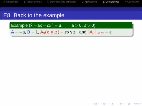
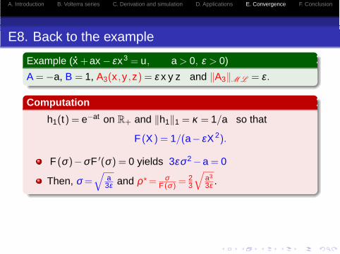
Example (x +ax − εx3 = u, a > 0, ε > 0)
A = −a, B = 1, A3(x ,y ,z) = ε x y z and ‖A3‖ML = ε.
A. Introduction B. Volterra series C. Derivation and simulation D. Applications E. Convergence F. Conclusion
E8. Back to the example
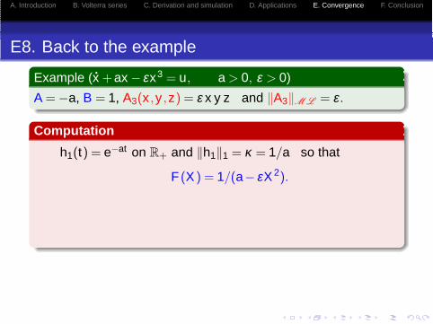
Example (x +ax − εx3 = u, a > 0, ε > 0)
A = −a, B = 1, A3(x ,y ,z) = ε x y z and ‖A3‖ML = ε.
Computation
h1(t) = e−at on R+ and ‖h1‖1 = κ = 1/a so that
F (X ) = 1/(a− εX 2).

A. Introduction B. Volterra series C. Derivation and simulation D. Applications E. Convergence F. Conclusion
E8. Back to the example
Example (x +ax − εx3 = u, a > 0, ε > 0)
A = −a, B = 1, A3(x ,y ,z) = ε x y z and ‖A3‖ML = ε.
Computation
h1(t) = e−at on R+ and ‖h1‖1 = κ = 1/a so that
F (X ) = 1/(a− εX 2).
F (σ)−σF ′(σ) = 0 yields 3εσ2 −a = 0
Then, σ =√
a3ε and ρ⋆ = σ
F (σ) = 23
√a3
3ε .
Remark
When there is no closed-form solution for ‖h1‖1, κ, σ and ρ⋆,equations can be numerically solved.
A. Introduction B. Volterra series C. Derivation and simulation D. Applications E. Convergence F. Conclusion
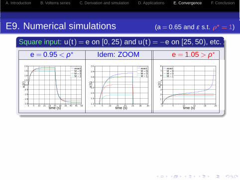
E9. Numerical simulations (a = 0.65 and ε s.t. ρ⋆ = 1)
Square input: u(t) = e on [0, 25) and u(t) = −e on [25, 50), etc.
e = 0.95 < ρ⋆ Idem: ZOOM e = 1.05 > ρ⋆
exactM =9M =3M =1
time (s)0 5 10 15 20 25 30 35 40 45 50
x(t
)
−2.0
−1.5
−1.0
−0.5
−0.0
0.5
1.0
2.0
1.5exactM =9M =3M =1
time (s)0 5 10 15 20 25 30 35
x(t
)
2.0
1.3
1.4
1.5
1.6
1.7
1.8
1.9exactM =9M =3M =1
time (s)0
0
5
5 10 15 20 25
x(t
)
1
2
3
4
6
7
8

A. Introduction B. Volterra series C. Derivation and simulation D. Applications E. Convergence F. Conclusion
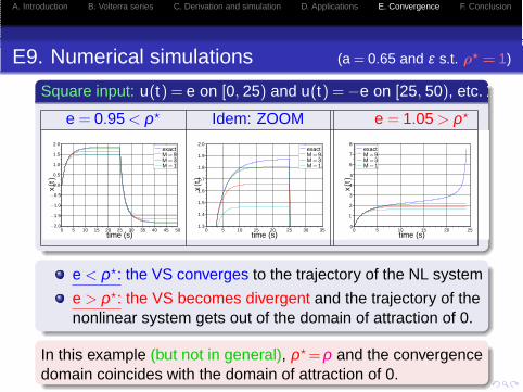
E9. Numerical simulations (a = 0.65 and ε s.t. ρ⋆ = 1)
Square input: u(t) = e on [0, 25) and u(t) = −e on [25, 50), etc.
e = 0.95 < ρ⋆ Idem: ZOOM e = 1.05 > ρ⋆
exactM =9M =3M =1
time (s)0 5 10 15 20 25 30 35 40 45 50
x(t
)
−2.0
−1.5
−1.0
−0.5
−0.0
0.5
1.0
2.0
1.5exactM =9M =3M =1
time (s)0 5 10 15 20 25 30 35
x(t
)
2.0
1.3
1.4
1.5
1.6
1.7
1.8
1.9exactM =9M =3M =1
time (s)0
0
5
5 10 15 20 25
x(t
)
1
2
3
4
6
7
8
e < ρ⋆: the VS converges to the trajectory of the NL system
e > ρ⋆: the VS becomes divergent and the trajectory of thenonlinear system gets out of the domain of attraction of 0.
A. Introduction B. Volterra series C. Derivation and simulation D. Applications E. Convergence F. Conclusion
E9. Numerical simulations (a = 0.65 and ε s.t. ρ⋆ = 1)
Square input: u(t) = e on [0, 25) and u(t) = −e on [25, 50), etc.
e = 0.95 < ρ⋆ Idem: ZOOM e = 1.05 > ρ⋆
exactM =9M =3M =1
time (s)0 5 10 15 20 25 30 35 40 45 50
x(t
)
−2.0
−1.5
−1.0
−0.5
−0.0
0.5
1.0
2.0
1.5exactM =9M =3M =1
time (s)0 5 10 15 20 25 30 35
x(t
)
2.0
1.3
1.4
1.5
1.6
1.7
1.8
1.9exactM =9M =3M =1
time (s)0
0
5
5 10 15 20 25
x(t
)
1
2
3
4
6
7
8
e < ρ⋆: the VS converges to the trajectory of the NL system
e > ρ⋆: the VS becomes divergent and the trajectory of thenonlinear system gets out of the domain of attraction of 0.
In this example (but not in general), ρ⋆ =ρ and the convergencedomain coincides with the domain of attraction of 0.

A. Introduction B. Volterra series C. Derivation and simulation D. Applications E. Convergence F. Conclusion
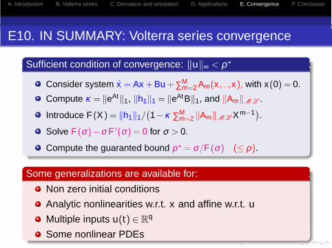
E10. IN SUMMARY: Volterra series convergence
Sufficient condition of convergence: ‖u‖∞ < ρ⋆
Consider system x = Ax +Bu +∑Mm=2 Am(x , . . .,x), with x(0) = 0.
Compute κ = ‖eAt‖1, ‖h1‖1 = ‖eAtB‖1, and ‖Am‖ML .
Introduce F (X ) = ‖h1‖1/(1−κ ∑M
m=2 ‖Am‖ML X m−1).
Solve F (σ)−σ F ′(σ) = 0 for σ > 0.
Compute the guaranted bound ρ⋆ = σ/F (σ) (≤ ρ).
A. Introduction B. Volterra series C. Derivation and simulation D. Applications E. Convergence F. Conclusion
E10. IN SUMMARY: Volterra series convergence
Sufficient condition of convergence: ‖u‖∞ < ρ⋆
Consider system x = Ax +Bu +∑Mm=2 Am(x , . . .,x), with x(0) = 0.
Compute κ = ‖eAt‖1, ‖h1‖1 = ‖eAtB‖1, and ‖Am‖ML .
Introduce F (X ) = ‖h1‖1/(1−κ ∑M
m=2 ‖Am‖ML X m−1).
Solve F (σ)−σ F ′(σ) = 0 for σ > 0.
Compute the guaranted bound ρ⋆ = σ/F (σ) (≤ ρ).
Some generalizations are available for:
Non zero initial conditions
Analytic nonlinearities w.r.t. x and affine w.r.t. u
Multiple inputs u(t) ∈ Rq
Some nonlinear PDEs

A. Introduction B. Volterra series C. Derivation and simulation D. Applications E. Convergence F. Conclusion
Part F: Conlusion
CONCLUSION
A. Introduction B. Volterra series C. Derivation and simulation D. Applications E. Convergence F. Conclusion
F1. Conclusion
In this tutorial:
Volterra series are used to represent, analyze and simulatesome Input/Output systems which include distortions
Derivation of the kernels for a given system (ODE orPDE)
Audio applications and simulations based on linearfilters, sums and products
Computable convergence radius and guaranteedtruncation error bound in some cases

A. Introduction B. Volterra series C. Derivation and simulation D. Applications E. Convergence F. Conclusion
F2. Conclusion
Other works and (examples of) perpectives
Identification of systemsFor Hammerstein models, see e.g. [Farina: AES’108, 2000],[Novak et al.: IEEE-TIM, 2010] and [Rebillat et al.: JSV, 2011]
Model order reduction based on Volterra kernels
Convergence criterion for analytic systems (w.r.t. x and u)
Convergence criterion for a large class of PDEs

A. Introduction B. Volterra series C. Derivation and simulation D. Applications E. Convergence F. Conclusion
Some references
V. Volterra. Theory of Functionnals and of Integral and Integro-Differential Equations. (Dover Publications,
1959).
R. W. Brockett. Volterra series and geometric control theory. Automatica, 12:167–176, 1976).
E. G. Gilbert. Functional expansions for the response of nonlinear differential systems. (IEEE Trans.
Automat. Control, 22:909–921, 1977).
M. Fliess, M. Lamnabhi, and F. Lamnabhi-Lagarrigue. An algebraic approach to nonlinear functional
expansions. (IEEE Trans. on Circuits and Systems, 30(8):554–570, 1983).
A. Isidori. Nonlinear control systems (3rd ed).. (Springer, 3rd ed. edition, 1995).
W. J. Rugh. Nonlinear System Theory, The Volterra/Wiener approach. (The Johns Hopkins University Press,
Baltimore, 1981).
M. Schetzen. The Volterra and Wiener theories of nonlinear systems. (Wiley-Interscience, 1989).
F. Lamnabhi-Lagarrigue. Analyse des Systemes Non Lineaires. (Editions Hermes, 1994. ISBN
2-86601-403-0).
S. Boyd and L. Chua. Fading memory and the problem of approximating nonlinear operators with voltera
series. (IEEE Trans. on Circuits and Systems, 32(11):1150–1161, 1985).
P. Flajolet and R. Sedgewick. Analytic Combinatorics. (Cambridge University Press, 2009).
...