Introduction to Topology Thomas Kwok-Keung Au · PDF fileLet (X,d) be the discrete metric...
136
Introduction to Topology Thomas Kwok-Keung Au
Transcript of Introduction to Topology Thomas Kwok-Keung Au · PDF fileLet (X,d) be the discrete metric...

Introduction to Topology
Thomas Kwok-Keung Au


Contents
Chapter 1. Metric Spaces 11.1. The Space with Distance 11.2. Balls, Interior, and Open sets 51.3. Metric Topology 9
Chapter 2. Transition to Topology 132.1. Cluster, Accumulation, Closed sets 132.2. Continuous Mappings 162.3. Sequence 202.4. Complete Metric Space 232.5. Continuity and Sequences 262.6. Baire and Countability 302.7. Further Continuity 34
Chapter 3. Topological Spaces 393.1. Topology, Open and Closed 393.2. Base and Subbase 423.3. Countability 45
Chapter 4. Space Constructions 494.1. Subspaces 494.2. Finite Product 504.3. Quotient Spaces 544.4. Examples of Spaces 594.5. Digression: Quotient Group 634.6. Infinite Product 67
Chapter 5. Compactness 715.1. Compact Spaces and Sets 715.2. Compactness 745.3. Compactness and Separation 775.4. Locally Compactness 805.5. Equivalences 83
Chapter 6. Connectedness 876.1. Disconnected and Connected 876.2. Components 916.3. Other Connectivity 95
Chapter 7. Algebraic Topology 997.1. Idea of Invariant 99
iii

7.2. Homotopy 1047.3. Homotopy Classes and Homotopy Equivalences 1087.4. Fundamental Group 1137.5. Useful Examples 1187.6. Homotopy Invariance 1267.7. Brouwer Fixed Point Theorem 129
iv

CHAPTER 1
Metric Spaces
In mathematics, there are many occasions that we need to compare objects,
approximate one object by another, or take limit of objects. Many of times, this
can be easily achieved if there is a distance between any pair of objects. In other
words, a set with a measurement of distance is what we need. Of course, there
are certain natural rules about the distance. The rules become the definition of a
distance, or called metric. Moreover, properties are developed from those rules.
The aim of this chapter is an introduction to those essential properties that will
be frequently used in all branches of mathematics.
In this chapter, we will start with the definition of metric spaces in §1.1, continuedwith the most basic concept of open sets in §1.2. Using open sets, we will pave
our way towards topology in §1.3 by defining open sets and interior.
1.1. The Space with Distance
We choose to start the study of topology from a natural extension of absolute
value or modulus between two numbers, that is, a distance measurement on a
set. This provides an easy intuition of the study.
Let X be a nonempty set. A metric on X is a function d : X × X → [0,∞),
that is, d(x, y) ≥ 0, satisfying the followings
• d(x, y) = 0 if and only if x = y;
• d(x, y) = d(y, x) for all x, y ∈ X;
• d(x, y) + d(y, z) ≥ d(x, z) for all x, y, z ∈ X.
Definition 1.1. The pair (X, d) is called a metric space.
1

2 1. METRIC SPACES
The first criterion emphasizes that a zero distance is exactly equivalent to being
the same point. The second symmetry criterion is natural. The third criterion is
usually referred to as the triangle inequality .
The concept of metric space is trivially motivated by the easiest example, the
Euclidean space. Namely, the metric space (Rn, d) with
d(x, y) = ∥x− y∥ =
[n∑k=1
(xk − yk)2
]1/2,
where x = (x1, . . . , xn) and y = (y1, . . . , yn). This is usually referred to as the
standard metric on Rn.
Example 1.2. There are other metrics on Rn, customarily called ℓp-metric, for
p ≥ 1, where
dp(x, y) = ∥x− y∥p =
[n∑k=1
(xk − yk)p
]1/p.
In this sense, the standard metric is actually the ℓ2-metric. There is also the
ℓ∞-metric given by
d∞(x, y) = max |xk − yk| : k = 1, . . . , n .
The properties of metric can be easily verified in these cases. Perhaps, the hardest
one will be left as an exercise.
Exercise 1.1.1. Prove that the triangle inequality is satisfied by the ℓp-metric
on Rn for all p ≥ 1 and p = ∞.
We will discuss more about the relationship between ℓp-metric for different values
of p. For this moment, let us consider the the pictures for several values of p
about the sets x ∈ Rn : dp(x, 0) = 1 . The pictures are illustrative that they
are convex when p ≥ 1.
-1 -0.5 0.5 1
-1
-0.5
0.5
1
The pictures for p = 1 (green), p = 2 (purple), p = 5 (brown), and p = ∞ (blue).

1.1. THE SPACE WITH DISTANCE 3
Example 1.3. The discrete metric on any nonempty set X is defined by
d(x, y) =
0 if x = y,
1 if x = y.
The criteria of being a metric can be readily verified case by case (Exercise 1.1.2).
This is kind of an uninteresting metric because any two distinct points will have
a fixed distance afar. However, it often serves as an example to check certain
property of a space. The following exercise is often a good way to understand a
metric.
Exercise 1.1.3. Let (X, d) be the discrete metric space and x0 ∈ X. Determine
the sets x ∈ X : d(x, x0) < r for different values of r > 0.
Example 1.4. Similar to the situation of Rn, there are several metrics on a
function space. For simplicity, let X = C([a, b],R) be the set of all continuous
real valued functions defined on an interval [a, b]. We have metrics dp for p ≥ 1
and p = ∞, namely, for f, g ∈ X,
dp(f, g) =
[∫ b
a|f(t)− g(t)|p dt
]1/p,
d∞(f, g) = sup |f(t)− g(t)| : t ∈ [a, b] .
The proof for that these are metrics is similar to the Euclidean cases. In fact, d∞
is a metric on B([a, b],R), the set of bounded functions on [a, b].
In the following pictures, we will show a comparison between p = 1 and p = ∞ to
illustrate their differences. Let f0, g, h ∈ X. The yellow area between the curves
illustrate the distances, d1(g, f0) is large while d1(h, f0) is small. On the other
hand, the green arrows illustrate the sup-distances, both d∞(g, f0) and d∞(h, f0)
are large.
0f f0
gh
Again, it is beneficial to think about the set f ∈ X : dp(f, 0) < 1 where 0 is
the constant zero function.
Exercise 1.1.4. Is d1 defined above a metric for the set L([a, b],R) of all inte-
grable functions on an interval [a, b]?

4 1. METRIC SPACES
Example 1.5. A suitable choice of metric may have the effect of good compar-
ison. Let X be the set of all continuously differentiable (C1) functions on an
interval [a, b] and
d(f, g) = sup |f(t)− g(t)| : t ∈ [a, b] + sup ∣∣f ′(t)− g′(t)
∣∣ : t ∈ [a, b].
With this choice of metric, for the functions illustrated below, d(f, g) < d(f, h)
because the contribution of derivatives |f ′(t)− h′(t)| is large.
0ff0
g h
Exercise 1.1.5. (1) Let R∞ be the set of all sequences x = (xk)∞k=1 in R of
which only finitely many terms are nonzero. Show that the ℓp-metrics
for all p ≥ 1,∞ are well-defined metrics on R∞.
(2) Prove that if (X, d) is a metric space, then d∗ is also a metric on X,
where
d∗(x, y) =d(x, y)
1 + d(x, y), x, y ∈ X .
(3) Let (X, d) be a metric space such that 0 ≤ d < 1. Determine whether
d#(x, y) =∞∑k=1
d(x, y)k
2kis also a metric.
(4) Let (X, d) be a metric space and f : [0,∞) → [0,∞). Try to explore
the conditions on f such that df = f d is also a metric on X. From
the above, f(r) = r/(1+ r) is an example. Try to give another example.
(5) Let (X, d) be a metric space and A ⊂ X. Define dA on A×A by
dA(a1, a2) = d(a1, a2), a1, a2 ∈ A .
Show that (A, dA) is a metric space. The metric dA is called the induced
metric on A.
(6) Let (X, dX) and (Y, dY ) be metric spaces. Prove that both
d∞((x1, y1), (x2, y2)) = max dX(x1, x2), dY (y1, y2) ,
d1((x1, y1), (x2, y2)) = dX(x1, x2) + dY (y1, y2)
for x1, x2 ∈ X and y1, y2 ∈ Y , are metrics on X×Y . Both may be called
the product metric. Do you think there are metrics dp?
1.2. BALLS, INTERIOR, AND OPEN SETS 5
To finish this section, we will give two examples. Both examples are related to
error-correcting applications. You are encouraged to understand them by the two
standard tasks: verify the metric conditions and think of the typical situation of
d(x, x0) < r.
Example 1.6. Let X = 0, 1 n, i.e., it contains points of n-coordinates of 0
and 1; d(x, y) is the number of different coordinates between x and y.
Example 1.7. Let X be the set of finite sequences of alphabets. For example,
“homomorphic”, “homeomorphic”, “holomorphic”, “homotopic”, “homologous”
are elements of X. Suppose there are three valid operations, inserting an alpha-
bet, deleting an alphabet, and replacing an alphabet by another. For two ele-
ments x, y ∈ X, define d3(x, y) by the minimum number of operations required
to transform x to y.
We may also consider replacing an alphabet equivalent to deleting then insert-
ing. In this case, we only accept two types of operations and let d2(x, y) be the
minimum number of such operations.
1.2. Balls, Interior, and Open sets
In this section, we will discuss an important concept of open sets in a metric
space. Open set is the most fundamental notion in topology and it will be used
often in more general context.
Let (X, d) be a metric space. The discussion starts with open balls.
Definition 1.8. At any point x ∈ X and ε > 0, an open ball at x with radius ε
is the set B(x, ε) = y ∈ X : d(y, x) < ε .
An open ball in the standard R is merely an open interval while that in Rn with
ℓ2-metric is the usual idea of circular ball. For balls of other ℓp-metrics, please
refer to the typical pictures shown after Example 1.2 in Section 1.1.
Exercise 1.2.1. (1) Find B(x, ε) in the discrete metric space.
(2) Let (X, d) be a metric space and d∗ = d/(1 + d) be another metric (see
Exercise 1.1.5). Find the relation between the open balls determined by
the two metrics.
(3) Similar to the above, compare the balls of a metric d and df = f dassuming that it is still a metric.

6 1. METRIC SPACES
(4) Let (X, d) be a metric space and A ⊂ X be given the induced metric
(see Exercise 1.1.5). Show that BA(a, ε) = BX(a, ε) ∩ A for any a ∈ A,
where BA and BX denote the open balls in A and X respectively.
(5) Let X and Y be metric spaces. Express an open ball in the product
metric space X × Y (see Exercise 1.1.5) in terms of open balls in X
and Y . Note that the answer may depends on which product metric you
are choosing.
(6) Is there a metric d on R2 such that all the open balls B(x, ε) are ellipses
with center at x? What if we change the requirement that x is at one
of the foci of the ellipses?
(7) Let (X, d) be a metric space and A ⊂ X. Define the diameter of A by
diam(A) = sup d(a1, a2) : a1, a2 ∈ A .
Is it true that diam(B(x, ε)) = ε?
(8) If A ⊂ X has diam(A) < ε and A ∩B(x, ε) = ∅, then A ⊂ B(x, 2ε).
Definition 1.9. Let (X, d) be a metric space, A ⊂ X, and x ∈ A. The point x
is called an interior point of A if there exists ε > 0 such that B(x, ε) ⊂ A.
Note that in the definition, the radius ε depends on the “position” of x in A.
Remark . As a good practice of beginning in topology, let us write down the
negation of the definition. That is, a point w ∈ X is not an interior point
of A ⊂ X if for all ε > 0, B(w, ε)∩ (X \A) is nonempty. Certainly, this negation
is satisfied in the case w ∈ X \A as B(w, ε) ∩ (X \A) ⊃ w.
z
y
Ax
In the above illustration, the set A includes the solid boundary curve but not
the dashed boundary curve. The point x ∈ A is an interior point because the
dotted green ball also belongs to A; the point y ∈ A but it is not an interior
point; the point z ∈ A is definitely not an interior point. The points y, z in the
above picture in fact satisfy a bit more than the negation, namely, for all ε > 0,
B(y, ε)∩ (X \A) = ∅ and B(y, ε)∩A = ∅. Later, we will see that these are calledfrontier points of A.

1.2. BALLS, INTERIOR, AND OPEN SETS 7
Exercise 1.2.2. (1) Prove that in any metric space (X, d), any point y ∈B(x, ε) is an interior point of B(x, ε). Note that triangle inequality of d
must be used in the proof.
(2) Show that if A ⊂ Rn and x ∈ A, then x is an interior point of A in the
standard Rn if and only if x is an interior point of A in (Rn, dp) for allℓp-metric with p ≥ 1 or p = ∞ (Example 1.2).
In the second problem above, if we denote Bp(x, ε) the open ball in the space
(Rn, dp), then the whole problem comes down to a comparison of open balls.
More precisely, we need to establish such a statement: given p, q, for all ε > 0,
there exists δ > 0 such that Bq(x, δ) ⊂ Bp(x, ε). This statement is trivial if p ≥ q
as one may take δ = ε. It is still easy for p < q. The pictures in Example 1.2
may be helpful to find δ in terms of ε. In fact, such δ may not be found if the
space is infinitely dimensional.
Definition 1.10. Let A ⊂ X in a metric space (X, d). The interior of A, denoted
A or Int(A), is the set of all interior points of A. The set G ⊂ X is an open set
if G = G = Int(G), i.e., every point of G is an interior point of G.
Such definitions match the intuition of the standard Rn. The interior of a subset
in Rn is exactly those points that is not on the “boundary”. For example, for
A =(x, y) : x2 + y2 ≤ 1
, its interior is the set
(x, y) : x2 + y2 < 1
. By
Exercise 1.2.2, the interior of a set in (Rn, dp) is independent of p ≥ 1 or p = ∞.
Example 1.11. (1) In any metric space (X, d), ∅ and X are always open
sets.
(2) From Exercise 1.2.2, any open ball B(x, ε) of a metric space is open.
(3) It can be easily shown (also given in Exercise 1.2.1) that in a discrete
space (X, d), an open ball B(x, ε) is either x or X. Thus, it follows
that any subset A ⊂ X is open.
(4) Let A ⊂ X be given the induced metric dA from the metric space (X, d).
Note that the interior of A in (A, dA) is always A, while the interior of
A in (X, d) is only a subset of A.
In addition, if B ⊂ A, then it may happen that IntA(B) = IntX(B),
where IntA(B) denotes the interior of B in (A, dA). For this reason, if
B is open in (X, d) then it is open in (A, dA). However, the converse is
not true.
Exercise 1.2.3. Give a condition on A such that B is open in A if and
only if it is open in X.

8 1. METRIC SPACES
(5) An open set in the product metric space X × Y is always of the form
U × V where U is open in X and V is open in Y . Note that this may
not be true for infinite product.
The standard argument of showing a subset U in (X, d) is open must involve
the following. Basically, it is to show U ⊂ Int(U), i.e., every point x of U is an
interior point of U . Thus, we begin by taking arbitrary point x ∈ U , then try to
find an ε > 0 with B(x, ε) ⊂ U . To get the inclusion, we take any y ∈ B(x, ε),
i.e., d(y, x) < ε and try to argue that y ∈ U . Here, we will demonstrate such a
process by an example.
Example 1.12. We will show that for any subset A in (X, d), its interior Int(A)
is an open set.
Let x ∈ Int(A). We need to find a suitable ε with B(x, ε) ⊂ Int(A).
By definition of x ∈ Int(A), there exists δ > 0 such that B(x, δ) ⊂ A. In the
following, we will show that just taking ε = δ will be enough for our need. In
other words, indeed, B(x, δ) ⊂ Int(A).
Take arbitrary y ∈ B(x, δ). Since B(x, δ) is open (or by directly using triangle
inequality argument), there exists ξ > 0 such that y ∈ B(y, ξ) ⊂ B(x, δ). Hence
y ∈ B(y, ξ) ⊂ A. This shows that y ∈ Int(A) for arbitrary y ∈ B(x, δ). This
simply means B(x, δ) ⊂ Int(A).
Equivalently, we have Int(Int(A)) = Int(A). Note that the proof above is very
similar to showing that an open ball is open. The same argument is useful to
show that if B ⊂ A, then Int(B) ⊂ Int(A).
In addition, one may prove the following (which is left as an exercise). It shows
that in the future, the concept of open balls can be replaced by open sets.
Proposition 1.13. Let A ⊂ X. A point x ∈ A is an interior point of A if and
only if there exists an open set U in X such that x ∈ U ⊂ A.
Exercise 1.2.4. (1) Show that if each Uα is open then∪α Uα is also open.
(2) Show that if each U1, . . . , Un is open then U1 ∩ · · · ∩ Un is also open.
(3) Give an example of infinitely many open sets Uα which has (∩αUα) not
open. Also, give an example that (∩αUα) is still open.
(4) Show that the interior Int(A) is the largest open set contained in A.
(5) Prove that a subset A is open if and only if it is a union of open balls.

1.3. METRIC TOPOLOGY 9
1.3. Metric Topology
In this section, we will introduce the concept of topology arisen from a metric.
In the future, it will be the foundation of study even when there is no metric. In
principle, it tells us what the open sets are.
Definition 1.14. Let (X, d) be a metric space. The topology of the metric d is
the set, Td or simply T, containing all the open subsets of X. Thus, by definition,
T is a subset of the power set P(X) of X.
From Exercise 1.2.1, in the discrete metric space, every singleton x is an open
set. Thus, by taking their unions, every set is open. Hence, the topology with
respect to the discrete metric is the power set.
Example 1.15. On Rn, no matter which ℓp-metric is considered, p ≥ 1 or p = ∞,
it does not change whether a subset is open or not. In other words, the topologies
corresponding to all ℓp-metrics is the same; they contain the same open sets. This
common topology is called the standard topology of Euclidean space. In fact,
consider the metric on R2 that every open ball B(x, ε) is an ellipse with center
at x. This metric also gives rise to the standard topology.
As we have mentioned before, on an infinite dimensional space, all ℓp-metrics may
not give the same topology. In fact, if X is the space of all continuous functions
on an interval [a, b], the topologies determined by the integral metric and the
maximum metric are not the same.
Exercise 1.3.1. (1) If (X, d) has T equals the power set, what is d?
(2) Let (X, d) be a metric space and d∗ = d/(1+d). Show that the topologies
Td = Td∗ .
Definition 1.16. Let d1 and d2 are two metrics on X with their corresponding
topologies T1 and T2. The metrics are equivalent if T1 = T2.
Now, one can see that all the ℓp-metrics on Rn are equivalent. Moreover, for any
metric d, one can always have an equivalent metric d/(1 + d) with distances in
the range [0, 1). In the future, one may see that the topology is the true basis of
study. It does not always require a definition of metric. This can be illustrated
by the following fact.
Theorem 1.17. Two metrics d1, d2 are equivalent if and only if every open ball
in (X, d1) is an open set in (X, d2) and vice versa.

10 1. METRIC SPACES
Proof. Assume that T1 ⊂ T2. Let x ∈ X and take any open ball B1(x, ε)
wrt d1. Obviously, B1(x, ε) ∈ T1 and, by assumption, it is also in T2. For the
point x ∈ B1(x, ε), it must be an interior point wrt d2. Thus, there exists δ > 0
such that x ∈ B2(x, δ) ⊂ B1(x, ε). So, we have proved one direction of the
following proposition, which is essentially the theorem. The other direction is an
easy exercise.
Proposition 1.18. Two topologies T1 ⊂ T2 if and only if for every d1-open ball
B1(x, ε), there exists a d2-open ball B2(x, δ) ⊂ B1(x, ε).
There are several terminologies about two topologies that T1 ⊂ T2. In different
books, it may be called weaker versus stronger, smaller versus larger, coarser
versus finer. We will try to avoid confusion by specifying such comparison by the
mathematical expressions ⊂ or ⊃.
For future convenience, a set N ⊂ X with x ∈ Int(N) is called a neighborhood
of x. Very often, it is equivalent to simply take an open neighborhood U of x,
that is, x ∈ U ∈ T. The following exercise demonstrates that the role of open
ball may be replaced with neighborhoods. One may verify it by simply writing
equivalent statements with patience.
Exercise 1.3.2. Given a metric space (X, d), A ⊂ X and x ∈ X. There exists
ε > 0 such that B(x, ε) ⊂ A if and only if there exists a neighborhood N of x
with x ∈ N ⊂ A. On the other hand, B(x, ε) ∩ A = ∅ for each ε > 0 if and only
if for each neighborhood N of x, N ∩A = ∅.
With the concept of topology and neighborhoods, one sees that the concept of
open ball is not totally essential. Once we know what it means by open sets, we
are able to use neighborhoods instead of open balls. The is the essential key to
the understanding in the following chapters. Here is a situation that illustrates
that a metric is not essential to define topology.
Example 1.19. A function ρ : X ×X → [0,∞) is temporarily called a pseudo-
metric if it satisfies all the conditions of a metric except replacing the triangle
inequality to
ρ(x, y) + ρ(y, z) ≥ αρ(x, z), where 0 < α < 1 is a fixed number.
Show that we may also define open ball B(x, ε), interior points, and open sets;
and hence topology similarly just as the case for metric.

1.3. METRIC TOPOLOGY 11
Exercise 1.3.3. Try to define a pseudo-metric ρ on R2 such that its B(0, r) is
given by the star-shaped picture shown below.
r
3r/2
Note that for this ρ, it satisfies the above inequality with α = 2/3.
Exercise 1.3.4. From the observation in the above example and exercise, is it
true that “if d is a metric on R2 such that it is preserved by translation, i.e.,
d(x, y) = d(x+ z, y + z), then B(0, r) is convex”?


CHAPTER 2
Transition to Topology
In this chapter, we continue to introduce several important notions related to a
metric space. However, as mentioned at the end of the previous chapter, we will
try to discuss without referring to the metric. From this point onwards, we will
mainly use open sets and neighborhoods. Metric will only be mentioned when a
property or a theorem is only true in metric space.
In §2.1, closed sets will be introduced as the counterpart of open sets. The next
topic is about relation between spaces, which is studied through continuity of
mappings in §2.2. Sequences and approximation are discussed in §2.3 in relation
to previous notions. Next, important properties about completeness is presented
in §2.4. Then we return to the intimate relation between continuity and sequence
in §2.5. A brief discussion of Baire category theory and dense sets is given in
§2.6. This chapter is ended by further uniform properties of continuity in §2.7.
2.1. Cluster, Accumulation, Closed sets
In many branches of mathematics, there is the need of studying an object which
is arbitrarily close to a type of objects. For example, a smooth curve is arbitrarily
close to segments of straight lines. This provides a basis for studying approxima-
tion. In this section, such concept is explored in the context of metric spaces or
more general topological spaces.
Let A ⊂ X. A point x ∈ X (not necessarily in A) is called a cluster point
or accumulation point (we do not use limit point) of A if for every ε > 0, the
punctured ball B(x, ε) \ x always intersects A. However, as we mentioned
before, we will use the following equivalent definition.
Definition 2.1. A point x ∈ X is a cluster point of A ⊂ X if for every neigh-
borhood U ∈ T of x, (U \ x) ∩A = ∅. The derived set of A, denoted A′, is the
set of all cluster points of A.
13

14 2. TRANSITION TO TOPOLOGY
By writing down the negation, it is easy to see that a point x ∈ A is not a
cluster point of A if and only if x ∈ Int(X \A). In simple mathematics language,
X \ (A ∪ A′) = Int(X \ A). Also, if a point a ∈ A is not a cluster point of A, it
is an isolated point belong to A.
Example 2.2. (1) In the standard Rn, if x ∈ Int(A) then x is a cluster
point of A.
(2) The above statement is not true for all metric spaces. Consider a discrete
metric space and see why it does not work.
(3) In the standard R, let A = 1/n : 1 ≤ n ∈ Z . Then the point 0 is a
cluster point of A and it does not belong to A.
Definition 2.3. The closure of A, denoted by A or Cl(A), is the set A ∪ A′. A
subset F ⊂ X is closed if F = F = Cl(F ), i.e., every cluster point of F must be
inside F .
Comparing the definitions of Cl(A) and A′, it is easy to see that x ∈ Cl(A) if and
only if for every neighborhood U ∈ T of x, U ∩A = ∅. This is a statement often
used in the future.
By definition, F is closed if and only if F = Cl(F ) = F ∪F ′ if and only if F ⊃ F ′.
This is equivalent to the following,
X \ F = X \ (F ∪ F ′) = Int(X \ F ) .
Recall that A = Int(A) if and only if A is open. Thus, we have shown the
following,
Proposition 2.4. F is closed ⇐⇒ X \ F is open.
Note that a set may be neither open nor closed, an interval [a, b) in the standard Ris an example. Also, a set may be both open and closed. The easiest example
is ∅ and X. Other nontrivial examples may be introduced in the discussion of
connectedness.
Example 2.5. The concept of whether a subset A is closed should be considered
in the context of the whole space X. Let X = R and Y = (0, 1) ∪ (2, 3) ⊂ R,both with the standard topology. Let A = (0, 1). If A is considered as a subset
of X = R, it is obvious open but not closed. However, if A is considered as
a subset of Y , then it is both open and closed. It is open because every point
is an interior point. On the other hand, for the same reason, its complement
Y \A = (2, 3) is also open. Thus, A itself is also closed in Y .

2.1. CLUSTER, ACCUMULATION, CLOSED SETS 15
Definition 2.6. Let A be a subset in a space X. A point x ∈ X belongs to the
frontier or boundary of A, denoted by Frt(A) if for every neighborhood U ∈ T
of x, U ∩A = ∅ and U ∩ (X \A) = ∅.
In other words, x belongs to the frontier of A if x both belongs to the Cl(A) and
Cl(X \ A). We avoid using “boundary” here because it has a different meaning
in manifold theory.
Example 2.7. Let us give a number of examples of closed sets.
(1) The sets ∅ andX are always closed, because their complements are open.
(2) For any subset A, the sets A′, A, and Frt(A) are closed.
(3) If (an) is a sequence in Rn and it converges to a ∈ Rn, then A =
a ∪ an ∈ Rn : n ∈ N is closed in the standard Rn.
To show the standard way of argument in point set topology, let us demonstrate
how to prove that A = Cl(A) is a closed set.
We need to prove Cl(A) = A. Since S ⊂ S is always true, it is sufficient to show
Cl(A) ⊂ A. Let x ∈ Cl(A). Then by definition, for all neighborhood U ∈ T of x,
U ∩A = ∅. And we are done if we can show U ∩A = ∅.
As U ∩ A = ∅, there is a point y ∈ U ∩ A. Now, y ∈ U ∈ T means that U is a
neighborhood of y. By y ∈ A, this neighborhood U must have U ∩ A = ∅. That
is what desired.
Exercise 2.1.1. Exercises about closure of a set are often analogous to interior.
(1) Show that if each Fα is closed then∩α Fα is closed.
(2) Show that if each F1, . . . , Fn is closed then∪nk=1 Fk is closed.
(3) Prove that A is the smallest closed set containing A.
(4) We already have Int(Int(A)) = Int(A), Cl(Cl(A)) = Cl(A), what about
(A′)′ and A′?
(5) Use Int(·), Cl(·), Frt(·), taking complement, etc., to explore equations
about them. For examples,
(a) A = X \ Int(X \A)(b) A = X \ Cl(X \A)(c) Int(A) ∪ Frt(A) = A.
(6) Show that A ∩B ⊂ A ∩B but they are not necessarily equal.

16 2. TRANSITION TO TOPOLOGY
(7) On a metric space (X, d), given A ⊂ X and x ∈ X, define
d(x,A) = inf d(x, a) : a ∈ A .
Show that if x ∈ A then d(x,A) = 0. On the other hand, show that if
d(x,A) = 0 then x ∈ A.
Exercise 2.1.2. Let X be a metric space and B(X,R) be the set of all bounded
functions from X to R and consider the metric space (B, d) where d(f, g) =
supt∈X |f(t)− g(t)|. Show that C(X,R), the set of all continuous functions, is a
closed set in B.
Example 2.8. In topology, there are always surprising results even in simple
examples. Here is an example that may help clarify certain concepts. Let X =
(−∞, 1) ∪ [2, 4] ⊂ R and d(x, y) = |x− y|.
As previously discussed, every open ball B(x, ε) is an open set. So, B(3, 0.5) =
(2.5, 3.5) is clearly open. Likewise, B(3, 1.5) is open. However, by definition
B(3, 1.5) = x ∈ X : d(x, 3) < 1.5 = [2, 4] .
It is a closed interval in R but an open set in X. Thus, its complement in X,
(−∞, 1) is a closed set in X. Furthermore, consider the open ball B(0, 2), it is
the set (−2, 1) ⊂ X. Note that we have x ∈ X : d(x, 0)≤2 = (−2, 1) ∪ 2 .One may also verify that the closure Cl(B(0, 2)) = [−2, 1) is different from the
above set.
2.2. Continuous Mappings
In every branch of mathematics, relations between objects are studied by map-
pings. Suitable requirements are imposed on the mappings for special purpose
of the context. In the study of topology, we study continuous mappings. In
this section, we will only give a short and brief description about mappings be-
tween metric spaces. Later, more attention will be given on mappings between
topological spaces.
It is natural to start with copying the definition of continuous functions on Rn.Let (X, dX) and (Y, dY ) be metric spaces. Let f : X → Y be a mapping with
x0 ∈ X and y0 = f(x0) ∈ Y . It is continuous at x0 if for every ε > 0, there exists
δ > 0 such that if dX(x, x0) < δ, then dY (f(x), f(x0)) < ε.

2.2. CONTINUOUS MAPPINGS 17
Let us start to rewrite the statements. Note that the statement “if dX(x, x0) < δ,
then dY (f(x), f(x0)) < ε” can be rephrased as
for all x ∈ BX(x0, δ), f(x) ∈ BY (f(x0), ε) .
Or, simply in set language, f (BX(x0, δ) ) ⊂ BY (f(x0), ε).
f
x y0 0
Now, we can rephrase continuity in terms of the topologies TX and TY , which
are sets of all open sets determined by the corresponding metric. The definition
does not refer to metric and is valid in the future.
Definition 2.9. A mapping f : X → Y is continuous at x0 ∈ X if for every
V ∈ TY with f(x0) ∈ V , there exists U ∈ TX with x0 ∈ U such that f(U) ⊂ V .
For a definition for f being continuous on the whole space, a more useful version
is given here. It will be justified below that this is equivalent to continuity at
every point.
Definition 2.10. A mapping f : X → Y is continuous if for every V ∈ TY , the
pre-image f−1(V ) ∈ TX .
Example 2.11. (1) Let f : R → R be a mapping on the standard R where
f(x) =
0 x ∈ Q ,
1 x ∈ Q .
This mapping is well-known to be discontinuous at every x0 ∈ R.(2) Consider the same mapping f : (R, d) → R from (R, d) with discrete
metric d to standard R. Then f is continuous everywhere. It is because
x0 is always an open set in discrete metric, so f ( x0 ) ⊂ V for
every V containing f(x0).
(3) If (X, d) is the discrete metric, then any mapping f : X → Y is contin-
uous.

18 2. TRANSITION TO TOPOLOGY
(4) Recall that on Rn, we have the ℓp-metric,
dp(x, y) = ∥x− y∥p =
[n∑k=1
|xk − yk|p]1/p
,
d∞(x, y) = max |xk − yk| : k = 1, . . . , n .
The identity mapping id: (Rn, dp) → (Rn, dq) is continuous everywherefor all p, q ≥ 1 or ∞. At the end, it involves proving the inequality
∥z∥p ≤ ∥z∥q ≤ C ∥z∥p , z ∈ Rn, p ≤ q ,
where C is a fixed constant depending on p, q, n. With this inequality,
one may see that
id (Bq(x0, ε) ) = Bq(x0, ε) ⊂ Bp(x0, ε) ;
id(Bp(x0,
ε
C))= Bp(x0,
ε
C) ⊂ Bq(x0, ε) .
(5) There are also metrics dp on the space X of all continuous functions
from a fixed interval [a, b] to R. The mapping id: (X, d1) → (X, d∞) is
not continuous. This can be seen from the illustration of the difference
of the metrics given in Example 1.4 on page 3.
To the above examples, the reader is encouraged to think both in terms of con-
tinuity at a point or on the whole.
Exercise 2.2.1. (1) When will a mapping f : X → Y be continuous if Y
is the discrete metric space?
(2) Let (X, d) be a metric space. Consider X ×X with any product metric
(see page 4) and standard [0,∞). Show that the mapping
d : X ×X → [0,∞) is continuous.
(3) Let (X, dX) and (Y, dY ) be metric spaces; X × Y be given a product
metric. Show that the projection mappings πX : X × Y → X and
πY : X × Y → Y are continuous.
In addition, let Z be another metric space with f : Z → X × Y .
Prove that f is continuous if and only if both πX f and πY f are so.
(4) Let f, g : X → R be continuous functions into standard R. Show that
x ∈ X : f(x) < g(x) is open while x ∈ X : f(x) ≤ g(x) is closed.
Proposition 2.12. The following statements are equivalent.
(1) f : X → Y is continuous.
(2) For each x0 ∈ X, f is continuous at x0.

2.2. CONTINUOUS MAPPINGS 19
(3) For every closed set H in Y , the pre-image f−1(H) is closed in X.
Proof. “(2) =⇒ (1)”. Let V ∈ TY . To prove f−1(V ) ∈ TX , we need to
show that every x0 ∈ f−1(V ) is an interior point. By (2), there exists U ∈ TX
with x0 ∈ U and f(U) ⊂ V . Therefore, x0 ∈ U ⊂ f−1(V ) and hence it is an
interior point.
“(1) =⇒ (3)”. It can be done by simply considering Y \H ∈ TY . Therefore
X \ f−1(H) = f−1(Y \H) ∈ TX .
“(3) =⇒ (2)”. This is left as an exercise.
Exercise 2.2.2. Let f : X → Y be continuous. Prove that for each A ⊂ X,
f(A)⊂ f(A). Is it true that f−1
(B)= Int
(f−1(B)
)for B ⊂ Y ?
Exercise 2.2.3. Determine whether there is such an example. Let f : X → Y
be a continuous mapping and Bn ⊂ Y are closed subsets for n ∈ N such that∪∞n=1Bn is still closed but,
∪∞n=1 f
−1(Bn) is not closed in X.
Exercise 2.2.4. Let X = A ∪ B and f : X → Y such that both f |A and f |Bare continuous. Detect the fallacy in the following argument:
Let V ⊂ Y be an open set. Then its pre-image f−1(V ) =
f−1(V )∩ (A∪B) = (f |A)−1(V )∪ (f |B)−1(V ), which is a union
of two open sets because both f |A and f |B are continuous.
Thus, f is continuous.
Give an example that f is not continuous. Show that if in addition both A,B ⊂ X
are open then f is continuous. Finally, would similar conclusion hold if both A,B
are closed?
There is another property that looks like continuity; however, it is different.
Definition 2.13. A mapping f : X → Y is called an open mapping if for any
open set U in X, its image f(U) is open in Y .
Clearly, since f(X \ A) = Y \ f(A), we cannot conclude that f(A) is closed if
A ⊂ X is so.
Exercise 2.2.5. Construct some examples of open mappings f : X → Y for
X,Y ⊂ R.

20 2. TRANSITION TO TOPOLOGY
Exercise 2.2.6. Give examples of the following mappings f : X → Y .
(1) It is both open and continuous.
(2) It is continuous but not open.
(3) It is open but not continuous.
Definition 2.14. A mapping f : X → Y is called a homeomorphism if it is a bi-
jection and it is both open and continuous. Equivalently, its inverse mapping f−1
is also continuous. The spaces X and Y are homeomorphic or topologically the
same. A mapping f : (X, dX) → (Y, dY ) is called an isometry if for all x1, x2 ∈ X,
dX(x1, x2) = dY (f(x1), f(x2)).
2.3. Sequence
The concept of sequence is tremendously important in analysis of R or Rn or
C. The underlying reason is because each of them is a metric space. In fact,
sequences play a particular role in certain topological spaces, satisfying so-called
first countability. Such topological spaces include metric spaces.
A sequence in a space X is a mapping from N to X, usually denoted by (xn)n∈N.
By mimicking the definition of convergence in Rn, we may say that a sequence
(xn)n∈N converges to x ∈ X if for all ε > 0, there is an integer N ∈ N such that
for all n ≥ N , d(xn, x) < ε, i.e., xn ∈ B(x, ε). Again, for smooth migration to
general topological spaces, we will take the following equivalent definition.
Definition 2.15. A sequence (xn)n∈N converges to x ∈ X, denoted xn → x, if
for all neighborhood U ∈ T of x, there is an integer N ∈ N such that for every
n ≥ N , xn ∈ U . The point x ∈ X is called the limit of the sequence.
Exercise 2.3.1. A sequence xn → x in a metric space (X, d) if and only if
limn→∞
d(xn, x) = 0 in R.
One should develop a good habit of clarify the metric when the convergence of
sequence is discussed. The following exercise shows that it may be confusing if
the context is not clear.
Example 2.16. Let X = C([a, b],R) be the set of continuous functions on a closed
interval [a, b]. Recall that we have the metrics
d1(f, g) =
∫ b
a|f(t)− g(t)| dt, d∞(f, g) = sup
t∈[a,b]|f(t)− g(t)| .

2.3. SEQUENCE 21
In this case, there are three concepts of sequence convergence, namely, point-
wisely, or under d1, or under d∞.
Exercise 2.3.2. In the above example of (X, d1) and (X, d∞), let 0 be the con-
stant zero function.
(1) Prove that any convergent sequence under d∞ must converge under d1.
(2) Find a sequence fn ∈ X such that d(fn,0) = 1/n but fn does not
converge pointwisely .
Exercise 2.3.3. (1) Let (X, d) be a metric space with sequences (an)n∈N
and (bn)n∈N such that an → a and bn → b. Show that d(an, bn) → d(a, b)
in R.(2) Let (X, d) and (X, d∗) be metric spaces where d∗ = d/(1+d). Show that
xn → x in (X, d) if and only if xn → x in (X, d∗).
(3) Let (X, dX) and (Y, dY ) be metric spaces and X×Y is given any product
metric. Prove that a sequence (xn, yn) → (x, y) in X × Y if and only if
xn → x in X and yn → y in Y .
Proposition 2.17. If a sequence (xn)n∈N in a metric space (X, d) converges,
then its limit is unique.
Proof. Suppose there are x, y ∈ X such that xn → x and xn → y. Then
take arbitrary ε > 0, and consider B(x, ε/2) and B(y, ε/2). Since xn converges
to both x and y, there exists N ∈ N such that for every n ≥ N , we have both
xn ∈ B(x, ε/2) and xn ∈ B(y, ε/2). By triangle inequality, we have d(x, y) < ε.
Thus, we have shown for arbitrary ε > 0, d(x, y) < ε. Consequently, d(x, y) = 0
and x = y.
Note that in this proof, using the metric d, we have constructed two neighbor-
hoods Ux of x and Uy of y such that Ux ∩ Uy = ∅. In a metric space, this can
always be done for every x = y. Equivalently, we may say that if each pair of
neighborhoods, Ux of x and Uy of y, intersect each other, then x = y. This is a
major property true for metric spaces but not necessary for general topological
spaces. This property is the foundation of uniqueness of limit.
The following tells us the relationship between limit of a sequence and closure. We
deliberately write it in two statements to emphasize that one part of it requires
the metric and the other does not.
22 2. TRANSITION TO TOPOLOGY
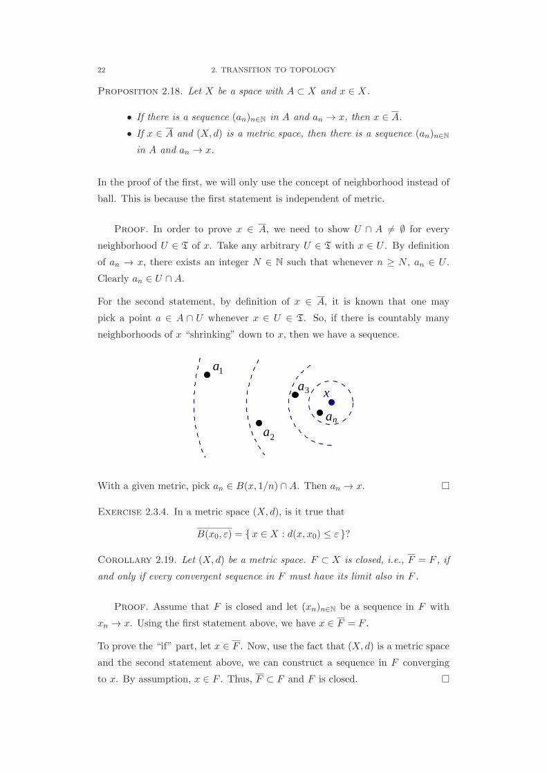
Proposition 2.18. Let X be a space with A ⊂ X and x ∈ X.
• If there is a sequence (an)n∈N in A and an → x, then x ∈ A.
• If x ∈ A and (X, d) is a metric space, then there is a sequence (an)n∈N
in A and an → x.
In the proof of the first, we will only use the concept of neighborhood instead of
ball. This is because the first statement is independent of metric.
Proof. In order to prove x ∈ A, we need to show U ∩ A = ∅ for every
neighborhood U ∈ T of x. Take any arbitrary U ∈ T with x ∈ U . By definition
of an → x, there exists an integer N ∈ N such that whenever n ≥ N , an ∈ U .
Clearly an ∈ U ∩A.
For the second statement, by definition of x ∈ A, it is known that one may
pick a point a ∈ A ∩ U whenever x ∈ U ∈ T. So, if there is countably many
neighborhoods of x “shrinking” down to x, then we have a sequence.
x
a
a
a
a
1
2
3
n
With a given metric, pick an ∈ B(x, 1/n) ∩A. Then an → x.
Exercise 2.3.4. In a metric space (X, d), is it true that
B(x0, ε) = x ∈ X : d(x, x0) ≤ ε ?
Corollary 2.19. Let (X, d) be a metric space. F ⊂ X is closed, i.e., F = F , if
and only if every convergent sequence in F must have its limit also in F .
Proof. Assume that F is closed and let (xn)n∈N be a sequence in F with
xn → x. Using the first statement above, we have x ∈ F = F .
To prove the “if” part, let x ∈ F . Now, use the fact that (X, d) is a metric space
and the second statement above, we can construct a sequence in F converging
to x. By assumption, x ∈ F . Thus, F ⊂ F and F is closed.

2.4. COMPLETE METRIC SPACE 23
Exercise 2.3.5. Let d and ρ are two metrics on the same set. Prove that xn → x
wrt d if and only if xn → x wrt ρ provided either there exists fixed constants
C1 < C2 such that C1 ρ ≤ d ≤ C2 ρ; or the topologies of d and ρ are the same.
Exercise 2.3.6. In a metric space, it is true that if a sequence xn → x then
every subsequence of (xn) converges to x; and conversely, if every convergent
subsequence has limit x, then xn → x. Try to formulate the proof (from the
known one in Rn). Ask yourself whether the proof requires a metric or simply
open balls.
2.4. Complete Metric Space
The standard Euclidean space is an important example of metric space. In ad-
dition, Rn has a property that makes it different from Qn analytically. It worths
particular attention and becomes an important type of metric space.
Definition 2.20. A sequence (xn)n∈N in a metric space (X, d) is Cauchy if for
every ε > 0, there exists an integer N ∈ Z such that if m,n ≥ N , d(xm, xn) < ε.
Obviously, this definition requires a metric and it is a very familiar concept in Rn.Thus, a natural question is how it is related to convergence of a sequence.
Exercise 2.4.1. Let (xn)n∈N be a Cauchy sequence such that the set xn : n ∈ N has a cluster point. What can you conclude about the sequence?
Using the triangle inequality and the same argument as in Rn, it can be easily
proved that a convergent sequence in a metric space is always Cauchy. The
following example shows that the converse is not true.
Example 2.21. Let X = R2 with the standard metric and xn =(1n , 0). Then
(xn)n∈N is Cauchy and convergent.
However, on A = R2 \ (0, 0) with the standard metric. The same (xn)n∈N is
still Cauchy but not convergent.
Definition 2.22. A metric space is complete if every Cauchy sequence is con-
vergent.
Exercise 2.4.2. If both X and Y are complete metric space, is the product
metric space X × Y complete?
24 2. TRANSITION TO TOPOLOGY
Exercise 2.4.3. Let (B, d∞) be the metric space of bounded functions on the
interval [a, b]; (C, d1) be the one of continuous functions, where
d∞(f, g) = supt∈[a,b]
∥f(t)− g(t)∥ , d1(f, g) =
∫ b
a|f(t)− g(t)| dt .
(1) Show that (B, d∞) is a complete metric space. Hint. Use the complete-
ness of R to get a pointwise limit first.
From the proof, one should see that the functions need not be real-
valued and the domain need not be [a, b].
(2) Show that (C, d1) is not complete. Hint. Consider functions that are
mostly 0 or 1 on [a, b].
The above Example 2.21 of the puncture plane leads us to the following discussion
about metric subspace. Given a metric space (X, d) and A ⊂ X, one may define
an induced metric dA on A simply by
dA(a1, a2) = d(a1, a2) , seeing a1, a2 ∈ X.
We will not spend too much effort on discussing metric subspace here. Most of
the properties will be discussed later in the context of topological space. Here,
we will only focus on the properties about sequences.
Let (A, dA) be a metric subspace of the metric space (X, d) and (an)n∈N is a
sequence in A. The following is trivial.
Proposition 2.23. • The sequence (an)n∈N is Cauchy in (X, d) if and
only if it is Cauchy in (A, dA).
• If (an)n∈N converges in (A, dA), then it is convergent in (X, d).
Since the converse of the second statement is not true, the completeness of (X, d)
does not imply that of (A, dA). Nevertheless, we have
Proposition 2.24. Let A be a subset in a complete metric space (X, d). Then
(A, dA) is complete if and only if A is closed in X.
From this result, C in Exercise 2.4.3 is complete.
Proof. Assume that (A, dA) is complete and let x ∈ A. Then there exists
a sequence an ∈ A with an → x in (X, d). Thus, (an)n∈N is a Cauchy sequence
in (X, d), and also in (A, dA). By assumption, it converges in (A, dA), say an →

2.4. COMPLETE METRIC SPACE 25
a ∈ A wrt dA, and also wrt d. By uniqueness of limit in (X, d), a = x and so
x ∈ A.
Assume that A is closed in X and let (an)n∈N be a Cauchy sequence in (A, dA).
Then it is also Cauchy in (X, d) and it converges in (X, d), say an → x ∈ X.
Since an ∈ A, x ∈ A. By assumption, A is closed and so x ∈ A and hence the
sequence converges in (A, dA).
The completeness of R is a very important feature of the real line. It leads to
many useful results. One of them is the so-called Nested Interval Theorem.
Exercise 2.4.4. Recall the statement of the Nested Interval Theorem and how
it is used, e.g., to proving Intermediate Value Theorem.
In a complete metric space, an analogous theorem is expected. Since there may
not be an order, we need some other notions instead of “shrinking” intervals.
On a metric space (X, d), for a subset A ⊂ X, define the diameter of A by
diam(A) = sup d(a1, a2) : a1, a2 ∈ A .
Exercise 2.4.5. Show that if A is closed in Rn and diam(A) < ∞, then there
are two points a1, a2 ∈ A such that d(a1, a2) = diam(A), i.e., the diameter can
be attained. Remark. The same statement is not true for metric space. In that
case, we need the set A to be compact, which is a concept to be discussed later.
Theorem 2.25 (Cantor Intersection Theorem). Let (X, d) be a complete metric
space; Fn ⊂ X be nonempty closed sets such that
Fn ⊃ Fn+1 for all n; diam(Fn) → 0 as n→ ∞.
Then∩∞n=1 Fn is a singleton set.
Proof. In order to prove the existence of a point in∩∞n=1 Fn, knowing that
X is complete, the natural idea is to construct a Cauchy sequence and obtain its
limit. Just pick xn ∈ Fn. The following exercises will yield the proof.

26 2. TRANSITION TO TOPOLOGY
Exercise 2.4.6. Use the fact that diam(Fn) → 0 to show that (xn)n∈N is a
Cauchy sequence.
Thus, by completeness of X, xn → x ∈ X. Observe that for any p ∈ N, (xn)∞n=pis a sequence in Fp convergent to x. Therefore, x ∈ F p = Fp for any p ∈ N.
Exercise 2.4.7. Use diam(Fn) → 0 again to conclude that∩∞n=1 Fn = x.
This completes the proof.
Exercise 2.4.8. In the Cantor Intersection Theorem above, if it is not given that
diam(Fn) → 0, can we prove that∩∞n=1 Fn is non-empty? In addtion, give an
example to illustrate that one must need the condition on “each Fn is closed”.
Exercise 2.4.9. Let (X, d) be a metric space. For Cauchy sequences (xn), (yn)
in X, define an equivalence relation (xn) ∼ (yn) if limn→∞
d(xn, yn) = 0 and denote
the equivalence class of (xn) by x. Let X be the set of such equivalence classes
and d(x,y) = limn→∞
d(xn, yn).
(1) Show that (X, d) is a complete metric space.
(2) Show that there is a natural continuous one-to-one mapping j : X → X
such that j(X) is isometric to X.
(3) Show that if X itself is complete, then X and X are isometric.
2.5. Continuity and Sequences
As it is mentioned in Proposition 2.12, there are several equivalent ways of de-
scribing the continuity of a mapping between metric spaces. Similar to mappings
between Euclidean spaces, continuity of the mapping is related to limit of se-
quences. In the following, two statements are given to emphasize that one is
independent of metric.
Proposition 2.26. (1) If f : X → Y is continuous, then for each sequence
(xn)n∈N in X with xn → x, f(xn) → f(x) in Y .
(2) If (X, d) is metric space and every sequence (xn)n∈N in X with xn → x
must also have f(xn) → f(x) in Y , then f is continuous.
Proof. For statement (1), let V ∈ TY with f(x) ∈ V . By continuity of f ,
f−1(V ) is a neighborhood of x in TX . Since xn → x, there exist N ∈ N such that
for all n ≥ N , xn ∈ f−1(V ) and hence f(xn) ∈ V .

2.5. CONTINUITY AND SEQUENCES 27
For statement (2), we will prove the contra-positive. Assume that f is not con-
tinuous, i.e., there exists a V ∈ TY such that f−1(V ) ∈ TX . Therefore, there is
x ∈ f−1(V ) which is not an interior point. As a consequence, every neighborhood
U ∈ TX of x contains a point outside f−1(V ). We will use this fact to construct
a sequence xn → x and here is exactly why a metric d on X is needed.
For each 0 < n ∈ Z, B(x, 1/n) is a neighborhood of x. So, there exists xn ∈B(x, 1/n) \ f−1(V ). Clearly, xn → x. However, xn ∈ f−1(V ) and so f(xn) ∈ V .
Hence, f(xn) does not converge to f(x).
Proposition 2.27. Let X,Y be metric spaces and f : X → Y be a mapping.
Then f is continuous if and only if for each set A ⊂ X, f(A)⊂ f(A).
Proof. If f is given to be continuous, the proof is straight forward without
using properties of metric. It has been done in Exercise 2.2.2.
We will use Proposition 2.26 to the contra-positive of the “if” part. Suppose that
f is not continuous at x0 ∈ X and there is a sequence xn → x0 but f(xn) → f(x0).
Let us consider the intuitive idea and though it is not accurate. Naturally, take
A = xn : n ∈ N . Then f(A) = f(xn) : n ∈ N and A = A ∪ x0 . We
hope that f(x0) ∈ f(A) because f(xn) → f(x0). Obviously, such a conclusion is
not possible because it may happen that f(xk) = f(x0) for some k ∈ N. Even
that does not occur, there may be a subsequence f(xnk) → f(x0) as k → ∞ and
so f(x0) ∈ f(A). Thus, one has to construct A in a clever way to avoid these two
situations. The details is left as an exercise below.
Exercise 2.5.1. Justify that there exists A ⊂ X with f(A)⊂ f(A). In addition,
consider whether the metrics on X or Y is necessary in the proof.
Studies of approximation are important in many branches of mathematics. Ex-
amples are abundant and let us consider a few. The Weierstrass Approximation
Theorem is roughly saying that continuous functions from Rn to R can be “ap-
proximated” by polynomials. This can be rephrased in the language of topology.
Let X be the set of continuous functions from Rn to R with a certain topology.
Let A be the subset of all polynomials. Then the Weierstrass Approximation
Theorem is essentially A = X. Such an A is called dense in X, which will be
further discussed in the next section.
Analogous situation occurs in the study of knots (strings tied into a knot with
the two ends glued up). Then any knot can be approximated by polygonal knots,

28 2. TRANSITION TO TOPOLOGY
which is formed by finitely many segments of straight lines. This also can be
phrased in topology as the set of polygonal knots is dense in the space of all
knots.
Clearly, certain calculations are easier to be done on polynomials or polygonal
knots. Moreover, these calculations may be indeed well-defined for general con-
tinuous functions or knots, but it is harder to calculate. It is certainly hoped that
those results of easier calculations determine the harder ones. In mathematical
terms, we already have A = X and a calculation on A, f |A : A → R is known.
Can we comfortably say that a unique f : X → R is behind? Luckily, the answer
is mostly yes.
Theorem 2.28. Let f, g : X → Y be continuous mappings and A = X. If
f |A≡ g |A on A then f ≡ g on X.
Proof I. Take arbitrary x ∈ X and try to show f(x) = g(x). Since x ∈ X =
A, there is a sequence (an)n∈N in A with an → x. Note that this requires X to
be a metric space. By continuity of both f and g, we have
f(an) → f(x) and g(an) → g(x) .
By assumption that f |A≡ g |A, f(an) = g(an) for all n ∈ N. Thus, by uniqueness
of limit (this requires certain condition on Y , e.g., Y is metric space), we have
f(x) = g(x).
The above theorem only guarantees that the uniqueness of the extension if it
exists. It is not known whether such extension exists. A related result on this
direction will be given later in Theorem 2.42 in Section 2.7.
In fact, the theorem is true in a more general situation, in which the following
proof works.
Proof II. Suppose otherwise, then there exists x ∈ X such that y1 = f(x) =g(x) = y2. Choose neighborhoods V1 ∈ TY of y1 and V2 ∈ TY of y2 with
V1 ∩V2 = ∅. This is possible if Y is a metric space and V1, V2 are open balls with
radius 13dY (y1, y2).
By continuity of f and g, f−1(V1) and g−1(V2) are neighborhoods of x in X, and
so is f−1(V1) ∩ g−1(V2). Since x ∈ X = A, there is a ∈ A ∩ f−1(V1) ∩ g−1(V2).
Thus, f(a) = g(a) ∈ V1 ∩ V2 which contradicts V1 ∩ V2 = ∅.

2.5. CONTINUITY AND SEQUENCES 29
Note that in second proof, there is not any condition on X (only neighborhood
argument is used) and only a mild condition on Y to get the disjoint neighbor-
hoods at y1 = y2. The space Y is called Hausdorff or T2 for the existence of such
disjoint neighborhoods. Such technique had been used in proving uniqueness of
limit of sequence. We will discuss more about this property in the future.
In many branches of mathematics or other discipline, studying the fixed point of
a mapping is a key issue. The existence of a fixed point could lead to theoretical
development or a practical method. This study is often done in the context of a
metric space. Let f : X → X be a mapping into a space itself, a point x∗ ∈ X
is called a fixed point of f if f(x∗) = x∗.
In many cases, there is additional requirement on the space X. For example, the
Newton’s Method, which is used to find the root of the equation g(x) = 0 in R.
Essentially, it transforms the problem to find a fixed point for f(x) = x− g(x)
g′(x).
The fixed point is guaranteed to exist if g′(x) = 0. The other example is the
Inverse Function Theorem for a function h : Ω ⊂ Rn → Rn. There are several
proofs, one of them makes use of the existence of a fixed point. Here we will
introduce a situation where a fixed point must exist.
Definition 2.29. A mapping f : (X, dX) → (Y, dY ) is called a contraction or
contraction mapping if there exists a fixed 0 < α < 1 such that for all x1, x2 ∈ X,
dY (f(x1), f(x2)) < αd(x1, x2).
Exercise 2.5.2. A mapping is called Lipschitz is there exists a fixed 0 < C (not
necessarily < 1) such that for all x1, x2 ∈ X, dY (f(x1), f(x2)) < C dX(x1, x2).
Prove that a Lipschitz mapping (and hence a contraction) is continuous.
Theorem 2.30 (Banach Fixed Point Theorem). Let f : (X, d) → (X, d) be a
contraction mapping on a complete metric space (X, d). Then it has a fixed point.
The main idea of getting such a fixed point in a complete metric space is naturally
by constructing a Cauchy sequence and considering its limit.
Proof. Start at any x0 ∈ X and define a sequence recursively by
xn+1 = f(xn), 0 ≤ n ∈ Z .
First, we will try to show that (xn)n∈N is Cauchy. As f is a contraction,
d(xm, xm+p) = d(f(xm−1, f(xm+p−1)) < αd(xm−1, xm+p−1)
< · · · · · · < αm d(x0, xp) .

30 2. TRANSITION TO TOPOLOGY
Unfortunately, the last term depends on the value of p even though αm can be
very small. Therefore, the method is changed a little with triangle inequality.
d(xm, xm+p) ≤ d(xm, xm+1) + d(xm+1, xm+2) + · · ·+ d(xm+p−1, xm+p)
< αm d(x0, x1) + αm+1 d(x0, x1) + · · ·+ αm+p−1 d(x0, x1)
=(αm + αm+1 + · · ·+ αm+p−1
)d(x0, x1) .
Now, by the convergence of geometric series∑∞
n=1 αn, for each ε > 0, there is
N ∈ N such that for all m ≥ N ,(αm + αm+1 + · · ·+ αm+p−1
)d(x0, x1) < ε.
Thus, (xn)n∈N is a Cauchy sequence and xn → x∗ in the complete metric space X.
By continuity of f , we have f(x∗) = x∗.
Exercise 2.5.3. Is this fixed point theorem still valid if the mapping is only
“partially contraction”, i.e., α ≤ 1?
2.6. Baire and Countability
In this section, we slightly touch on the theory of Baire. Most of the spaces
studied in analysis, geometry, and topology satisfy certain conditions of Baire.
There is a simple but powerful classification of spaces, which is somewhat related
to countability.
Definition 2.31. Let X be a space. A subset A ⊂ X is called dense in X if
Cl(A) = A = X. A subsetN ⊂ X is called nowhere dense inX if Int (Cl(N)) = ∅.
These two concepts are in a way dichotomized, but not logically negation to each
other.
Example 2.32. In standard R, both Q and R \ Q are dense subsets; while Z is
nowhere dense. However, Int(Q) = ∅ = Int(R \ Q), as well as Int(Z) = ∅. This
shows why we need to take closure first in the definition of nowhere dense.
By explicitly writing out the definition, A ⊂ X is dense if and only if for each
x ∈ X and each neighborhood U ∈ T with x ∈ X, U ∩ A = ∅. In fact, it can be
further simplified to the commonly used statement “for each U ∈ T, U ∩A = ∅”.
Exercise 2.6.1. Show that A ⊂ X is dense if and only if the only open set
contained in X \A is ∅; and if and only if the only closed set containing A is X.
Exercise 2.6.2. (1) Let N ⊂ X be nowhere dense. Show that every open
set U ⊂ X contains an open set V ⊂ U such that V ∩N = ∅.

2.6. BAIRE AND COUNTABILITY 31
(2) If A ⊂ X is dense, what can you say about X \A? Similarly, if N ⊂ X
is nowhere dense, what about X \N?
(3) Find all the dense sets and nowhere dense sets in a discrete space.
Example 2.33. Many nowhere dense subsets come from “lower dimension”. For
example, a straight line in R2 is nowhere dense. A slight variation is the image of
a parametrized curve, (x(t), y(t)) : t ∈ [a, b] , is usually a “nice” curve; if x, y
are differentiable functions satisfying some technical conditions. Most of them
are nowhere dense but it is not always.
Let N = (x, sin 1
x
)∈ R2 : x > 0
be a subset of the standard R2. It can be seen
that N = N ∪(0, y) ∈ R2 : y ∈ [−1, 1]
.
-1
1
Then, N is nowhere dense because Int(N)= ∅. In fact, for any point in N , any
neighborhood of it intersects R2 \N . This is illustrated by the above picture.
The space filling curve has its closure equal to the whole square, which has
nonempty interior. However, it is the result of an infinite process so it is difficult
to parametrize the curve by differentiable functions. The following example may
be easier to visualize.
Example 2.34. Let qn be rational numbers in the interval [0, 1]. It is easy to
construct a U-shape differentiable curve containing the segments from the point
(−n, 2) to (−n, qn) to (n, qn) to (n, 2) by smoothing the corners. Each one will
have a horizontal segment at the height of qn. Then suitably join these U-shapes
curves with smooth corners as shown in the picture below. Then the closure of
the curve contains the rectangle [−1, 1]× [0, 1].
− +1− −1n
odd n
n n1−1 n
1
2

32 2. TRANSITION TO TOPOLOGY
Example 2.35. There is a famous important theorem in differential topology. In
a simple form, it is about an infinitely differentiable function f : [a, b] → R. We
may ask the following two questions.
• Can it happen that the set of critical points x ∈ [a, b] : f ′(x) = 0 is
dense? The answer is yes; for example, the constant function, and many
others.
• What about the image set f(x) ∈ R : f ′(x) = 0, x ∈ [a, b] ? It can
never be dense. In fact, it must be nowhere dense.
Let N ⊂ X be a nowhere dense subset. Then Int(N) = ∅ and so not only X \Nis nonempty, indeed, for any open set U , U \N must be nonempty. This will be
a property that we will use later.
Definition 2.36. A subset A ⊂ X is of first category , Cat-I, if there exists
countably many nowhere dense sets Nk such that A =∪∞k=1Nk. Otherwise, it is
of second category , Cat-II.
Example 2.37. (1) In the standard R, Q is dense but it is trivially of Cat-I.
However, R\Q is of Cat-II. This may be seen from Theorem 2.39 below.
(2) In the discrete space X, any nonempty subset is of Cat-II. The reason
is that the only nowhere dense set is the empty set. In other words, if
∅ = A ⊂ X, then A = A and Int(Cl(A)) = A = ∅.
Exercise 2.6.3. (1) Show that Z with the standard metric d(m,n) = |m− n|is of second category. Note: this does not contradict that Z is nowhere
dense in R.(2) Show that if A is of Cat-I, then B ⊂ A will also be of Cat-I.
(3) Show that if N1, N2 are nowhere dense sets, then so is N1 ∪N2.
Example 2.38. Assuming the fact that standard Rn is of Cat-II (see below),
then one may conclude that any open ball in Rn is of Cat-II. In turns, every set
in Rn with non-empty interior is of Cat-II.
There are deeper discussions of Baire’s theory. However, we will only stop at the
following conclusion about complete metric spaces.
Theorem 2.39 (Baire Category Theorem). A complete metric space is of second
category.

2.6. BAIRE AND COUNTABILITY 33
The idea is to consider nonempty closed sets Fn ⊂ X \ (∪nk=1Nk). Then try to
establish that
∅ =∞∩n=1
Fn ⊂ X \
( ∞∪k=1
Nk
).
F23F
1N
1F
3N2N x
From the Cantor Intersection Theorem, we need that Fn ⊃ Fn+1 and diam(Fn) →0. A natural choice of closed sets is Fn = x ∈ X : d(x, xn) ≤ rn . Thus, the
key is to pick the suitable points xn and radii rn. Indeed, we will prove the
following equivalent statement.
Proposition 2.40. Let X be a complete metric space and Nk, k ∈ N, be a
sequence of nowhere dense subsets in X. Then X =∪∞k=1Nk.
Proof. Observe that Int(Cl(N1)) = ∅. So, Cl(N1) = X. In other words,
X \Cl(N1) is a nonempty open set. There exists a neighborhood B(x1, 2r1) lying
in X \ Cl(N1) for some point x1 ∈ X and a radius r1 > 0. Then
F1 = x ∈ X : d(x, x1) ≤ r1 ⊂ X \ Cl(N1) ⊂ X \N1 .
Now, since Int(Cl(N2)) = ∅, so B(x1, r1) ⊂ Cl(N2); and one may have x2 ∈Int(F1) and a radius 0 < r2 < r1 such that B(x2, 2r2) ⊂ B(x1, r1)\Cl(N2). Then
F2 = x ∈ X : d(x, x2) ≤ r2 ⊂ F1\Cl(N2) ⊂ X\(Cl(N1) ∪ Cl(N2)) ⊂ X\(N1∪N2) .
This argument can be continued and thus there exists nonempty closed sets Fk
satisfying
F1 ⊃ F2 ⊃ · · · ⊃ Fn, diam(Fn) < r1/2n, Fn ⊂ X \
(n∪k=1
Nk
).
By the Cantor Intersection Theorem,∩n∈N Fn = ∅ and the result follows.
Exercise 2.6.4. (1) Are there statements about first and second category
of X × Y with reference to the categories of X and Y ?
(2) Show that A ⊂ X is open dense if and only if X \ A is closed nowhere
dense. Give counter examples if the open/closed condition is dropped.
(3) Let f : X → Y be a continuous mapping.

34 2. TRANSITION TO TOPOLOGY
(a) If D ⊂ X is dense, is f(D) ⊂ Y dense?
(b) If N ⊂ X is nowhere dense, is f(N) ⊂ Y nowhere dense?
(c) What about pre-images of a dense set and a nowhere dense set?
(d) What can you conclude about image or pre-image of a set of first
or second category?
(4) Prove that if A ⊂ Rn with measure(A) = 0, then A is of Cat-II.
2.7. Further Continuity
In the study of continuous functions, if the spaces involved are metric spaces,
there are additional properties. Two of which are related to “uniformity”. They
are particularly important in analysis. The following is exactly the direct gener-
alization from Euclidean spaces.
Definition 2.41. A mapping f : (X, dX) → (Y, dY ) is uniformly continuous
if for every ε > 0, there exists δ > 0 (depending only on ε) such that for all
x1, x2 ∈ X with dX(x1, x2) < δ, dY (f(x1), f(x2)) < ε.
Exercise 2.7.1. (1) Show that a Lipschitz mapping is uniformly continu-
ous.
(2) Is the composition of two uniformly continuous mappings still uniformly
continuous?
(3) Let (X, d) be a metric space. Let f :X → R be given by f(x) = d(x, x0)
for a fixed x0 ∈ X. Is this function uniformly continuous?
Also, d : X ×X → R where X ×X is given a product metric. Is it
uniformly continuous?
(4) If f : A → Y is uniformly continuous and (an)n∈N is a Cauchy sequence
in A, then ( f(an) )n∈N is a Cauchy sequence in Y . Give a counter
example for f is only continuous.
Uniformity plays an important role in analysis and approximation. In a later
chapter, we will establish the concept of compactness. Then, it is easy to see,
similar to Euclidean case, that every continuous mapping from a compact space to
a metric space is uniformly continuous. The following is a version about extension
of a uniformly continuous mapping.
Theorem 2.42. Let A ⊂ A = X be given the induced metric from (X, dX) and
(Y, dY ) be complete. If f : A → Y is uniformly continuous, then there exists

2.7. FURTHER CONTINUITY 35
a unique continuous extension f : X → Y such that f |A≡ f . Indeed, f is
uniformly continuous.
One should be reminded of the difference between this theorem and Theorem 2.28,
which is a uniqueness theorem and it starts with functions defined onX. However,
in this theorem, the function f is only defined on a dense set A and one is resulted
with getting an extension on X. So, this is an existence theorem, though the
extension is unique by virtue of Theorem 2.28.
Before studying the proof, it would be beneficial to understand the theorem from
another angle.
Exercise 2.7.2. Give an example that the theorem fails if f is only continuous.
Also, give an example that the theorem fails if Y is not complete.
Proof. Our aim is to define the value f(x) ∈ Y for each x ∈ X = A.
SinceX is a metric space and x ∈ A, there exists a sequence (an)n∈N with an → x.
Correspondingly, we have f(an) ∈ Y but f(x) may not be defined because x may
not be in A. The sequence (an) is Cauchy in A (because it converges in X).
By uniform continuity of f (on the set A), f(an) is a Cauchy sequence also.
Therefore, f(an) converges, say, to y ∈ Y . Define y = f(x).
It is sufficient to show that the above f(x) is well-defined. That means it is
independent of choice of the sequence (an)n∈N. But, this will be seen shortly.
Let us temporarily assume f depends on the choices of sequences. That is, for
each x ∈ X, one particular sequence converging to x is chosen and we use these
sequences to define f . In other words, we have an(x) ∈ A with an(x) → x and
f(an(x)) → f(x). We will first prove the uniform continuity of this f and later
prove its independence of choice of the sequences.
Given any ε > 0, by uniform continuity of f on A, there is a δ > 0 such that
whenever a, a′ ∈ A with dX(a, a′) < 3δ, dY (f(a), f(a
′)) < ε/3. We will take this
δ > 0 which only depends on ε.
Let x1, x2 ∈ X with dX(x1, x2) < δ. In the following, we are going to establish
that dY (f(x1), f(x2)) < ε. Since x1 ∈ X = A, from the definition of f , we have
chosen a sequence an(x1) ∈ A such that
an(x1) → x1 and f(an(x1)) → f(x1) .

36 2. TRANSITION TO TOPOLOGY
Thus, for δ > 0 and ε/3 > 0, by taking large enough N ∈ N, we have aN (x1) withdX(aN (x1), x1) < δ and dY (f(aN (x1)), f(x1)) < ε/3. Similarly, we have aM (x2)
in the defining sequence of f(x2) with dX(aM (x2), x2) < δ and dY (f(aM (x2)), f(x2)) <
ε/3.
By triangle inequality on X, we have dX(aN (x1), aM (x2)) < 3δ, which leads to
dY (f(aN (x1)), f(aM (x2))) < ε/3 by the choice of δ. Now, apply the triangle
inequality on Y , we have dY (f(x1), f(x2)) < ε.
At this point, it is proved that this particular choice of the function f on X
is uniformly continuous, no matter how we choose the sequences an(x) → x to
define f(x). By Theorem 2.28, the continuous extension of f from A to A = X
is unique. Thus, there is only one such f . Its uniqueness indeed guarantees its
independent of choice of the sequences.
Another important concept of uniformity is about convergence of a sequence of
mappings. That usually guarantees the limiting mapping has the same analytical
properties as the mappings in the sequence.
Definition 2.43. Let (fn)n∈N be a sequence of mappings X → (Y, d). It con-
verges uniformly to a mapping f : X → Y if for every ε > 0, there exists
N ∈ N (depending only on ε) such that whenever n ≥ n, for all x ∈ X,
d(fn(x), f(x)) < ε.
Equivalently, we may say for every ε > 0, there exists N ∈ N such that whenever
n ≥ N , supx∈X d(fn(x), f(x)) < ε.
One may have seen uniform convergence in studying sequence of functions on R.The situation on metric spaces is very similar. The value of N ∈ N (for a fixed ε)
can be seen as the speed of convergence. The larger the N , the slower the speed.
In general, this speed depends on x ∈ X and the difference between speeds at
various x’s can be very large. Uniform convergence means that there is a bounded
difference, or there is a minimum speed.
Theorem 2.44. Let (fn)n∈N be a sequence of mappings X → (Y, d) uniformly
converges to f . If every fn : X → Y is continuous, then f : X → Y is also
continuous.
Remark . In words, we may say that continuity is carried to the uniform limit.
In other context, when one can define differentiability or integrability, these prop-
erties can also be carried to uniform limit.
2.7. FURTHER CONTINUITY 37
Proof. Let V ∈ TY and we will prove f−1(V ) ∈ TX . For this, we take
arbitrary x∗ ∈ f−1(V ) and it is desired that x∗ is an interior point of f−1(V ).
Let y = f(x∗) ∈ Y and B(y, ε) ⊂ V for some ε > 0. First, let us take a smaller
W ⊂ V and try to get x∗ ∈ f−1n (W ) ⊂ f−1(V ) for large n.
Indeed, W = B(y, ε/2). Then for ε/2 > 0, choose N ∈ N such that for all
n ≥ N , supx∈X d(fn(x), f(x)) < ε/2. In particular, d(fn(x∗), f(x∗)) < ε/2,
i.e., x∗ ∈ f−1n (W ). Let x ∈ f−1
n (W ) where n ≥ N . Then d(fn(x), y) < ε/2
and d(fn(x), f(x)) < ε/2. By triangle inequality, f(x) ∈ B(y, ε) = V , i.e.,
x ∈ f−1(V ). Thus, we have shown that x∗ ∈ f−1n (W ) ⊂ f−1(V ).
By continuity of each fn for n ≥ N , f−1n (W ) is open and x∗ is an interior point
of f−1(V ).


CHAPTER 3
Topological Spaces
In the previous chapter, one has already seen that in many discussions and de-
ductions, metric is not always necessary. On the other hand, open sets or its
complements closed sets are often used. It gives us an idea that something is
more fundamental in the study of approximation and relative positions.
Historically, there had been several attempts. The most famous ones are neigh-
borhood systems or convergence. At the end, people chose the elegant concept
of topology. It is already enough to determine concepts of neighborhood and
convergence; as well as continuity of mappings.
We will begin by introducing the definition and basics of topology in §3.1. Thenin §3.2, fundamental building blocks of a topology called base and subbase are
discussed. In §3.3, spaces with good property due to countability conditions are
introduced.
3.1. Topology, Open and Closed
In the previous chapter, one defines open sets by interior points and then topology
as the set of all open sets. Here, we will start with a collection of sets.
Definition 3.1. Let X be a nonempty set. A topology T on X is a subset of
the power set of X satisfying
• Both ∅, X ∈ T;
• For each family Uαα∈I of sets Uα ∈ T, the union∪α∈I Uα ∈ T;
• For any finitely many U1, . . . , Un ∈ T, the intersection∩nk=1 Uk ∈ T.
The pair (X,T) is called a topological space.
A set G ⊂ X is called open in (X,T) if G ∈ T. A set F ⊂ X is closed in (X,T)
if X \ F ∈ T.
39

40 3. TOPOLOGICAL SPACES
The two conditions about a topology is usually referred to as closed under arbi-
trary union and finite intersection. In fact, by accepting empty collection of sets,
these two conditions will lead to ∅, X ∈ T. It is clear that they are also closed.
Example 3.2. (1) Let (X, d) be a metric space. If open balls, interior
points, and open sets are defined as before, and T is the set of open sets,
then T satisfies the two conditions and (X,T) is a topological space.
(2) Let X be a nonempty set and T = P(X), the power set of X. In other
words, every subset is an open set. This is called the discrete topology .
It is the same as the one given by the discrete metric.
(3) Let X be a nonempty set and T = ∅, X . The two conditions are ob-
viously satisfied. This is called the indiscrete topology , another extreme
from the discrete topology. One may expect that the indiscrete topology
is not a metric topology, i.e., it does not come from a metric.
(4) On R, one has the topology wrt the standard metric. It is called the
standard topology , Tstd. Let Tdef:== ∅,R ∪ (a,∞) : a ∈ R . This
T is also a topology on R and T ⊂ Tstd. Do you think this is a metric
topology?
(5) Let X be a nonempty set and T = G ⊂ X : G = ∅ or X \G is finite .This is called the co-finite topology on X. If X itself is finite, it is simply
the discrete topology.
Exercise 3.1.1. (1) Show that an arbitrary intersection of closed sets is
still closed and a finite union of closed sets is closed. On the other hand,
any collection of sets satisfying these two conditions indeed defines a
topology by their complements.
(2) Let Y be a closed set in (X,T) and be given the induced topology T|Y .If A ⊂ (Y,T|Y ) is closed, show that A is also closed in (X,T).
(3) Suppose T1 and T2 are two topologies on the set X. Which one is still
a topology, T1 ∪ T2 or T1 ∩ T2?
(4) Can we replace the word “finite” above by “countable” to define a “co-
countable” topology?
(5) Given a topological space (X,T) and A ⊂ X. Show that T |Adef:==
U ∩A : U ∈ T is a topology for A. It is called the induced or rel-
ative topology .

3.1. TOPOLOGY, OPEN AND CLOSED 41
In abstract topology space, open sets are simply elements of the topology. The
concept of interior has not yet been established. Therefore, we will now define
interior and closure with reference to the topology.
Definition 3.3. Let A ⊂ X where (X,T) is a topological space. The interior
of A is given by Int(A) or Adef:==
∪G ∈ T : G ⊂ A . A point x ∈ A is an
interior point of A if x ∈ Int(A).
Similarly, the closure of A is given by
Cl(A) or A =∩
F : F ⊃ A,X \ F ∈ T .
At any point x ∈ X, a neighborhood of x is a set N such that x ∈ Int(N) ⊂ N .
When the context is clear, we often assume N itself is open.
Exercise 3.1.2. (1) Based on the above definition, show that x ∈ Int(A) if
and only if there is a set U ∈ T such that x ∈ U ⊂ A.
(2) Similarly, show that x ∈ A if and only if for all open set U ∈ T with x ∈U , U ∩A = ∅.
(3) Give a suitable definition of derived set A′ such that A = A ∪A′.
(4) Define the convergence of a sequence in a topological space.
(5) For a general topological space (X,T),
(a) Is there an example of (X,T) such that Frt(A) = A \ Int(A)?(b) For an open set G ∈ T, is it true that G = Int(Cl(G))?
(c) For a closed set F ⊂ X, is it true that F = Cl(Int(F ))?
(d) Is it true that A \B = A \ IntB?
(6) Define dense and nowhere dense subsets in a topological space.
Once the concept of open sets is established, many notions in the previous chapter
can be carried to the setting of topological space.
Definition 3.4. Let (X,TX) and (Y,TY ) be topological spaces. A mapping
f : X → Y is continuous if for every V ∈ TY , f−1(V ) ∈ TX . It is continuous at
x0 ∈ X if for every neighborhood V of f(x0), f−1(V ) is a neighborhood of x0.
Exercise 3.1.3. Note that a mapping f is continuous at x0 does not imply that
for every f(x0) ∈ V with V ∈ TY , x0 ∈ f−1(V ) ∈ TX . Give an example of
f : R → R to illustrate this.
Exercise 3.1.4. Let A ⊂ (X,T) be given a topology TA. Formulate an equivalent
condition for TA = T|A in terms of the inclusion map ιA : A ⊂ X → X.

42 3. TOPOLOGICAL SPACES
Example 3.5. Let (X,T) ba a topological space with a proper subset, ∅ = A ⊂X. Then a topology slightly larger than the indiscrete topology is ∅, A,X .
Exercise 3.1.5. In light of the above example, if there are two proper subsets,
∅ = A = B ⊂ X. What should be included in the topology T in which both
A,B ∈ T? More generally, if there are several proper subsets A1, . . . , An, how
can we create a topology T such that every Ak ∈ T?
To end this section, let us consider the following example as an exercise.
Exercise 3.1.6. Let C = C([a, b],R) be the set of continuous functions on a closed
interval [a, b]. For any open subset U of [a, b]×R with standard topology, define
a subset WU ⊂ C by WU = f ∈ C : graph(f) ⊂ U .
Show that T = WU : U is an open subset of [a, b]× R defines a topology
for C. Moreover, verify that T is the same as the metric topology of d∞.
3.2. Base and Subbase
In the previous section, a topological space is described by its topology, i.e.,
listing all the open sets. In many examples, certain important open sets already
determine all the other open sets, for example, all open intervals in R or all open
balls in a metric space. That is the concept of basic open sets. Moreover, people
usually only write down the typical open sets when defining a topology. Thus,
there is a need to consider certain subsets of a topology which are already enough
to determine the topology.
Definition 3.6. Let (X,T) be a topological space. A set B ⊂ T is called a base
for T if T = ∪
A : A ⊂ B . Any G ∈ B is called a basic open set.
In the above notation,∪
A is a union of some of the sets in B. In other words,
taking all arbitrary unions of sets in B will form the topology T. Often, we will
write in terms of families, i.e., B = Bα ∈ T : α ∈ I where I is an index set
such that T =∪
β∈J Bβ : J ⊂ I.
Example 3.7. In a metric space (X, d) with metric topology T, the set of all open
balls B1 is a base. Also, the set consisting of all open balls with rational radius,
B2 is a base. Let B3 be the set of all open balls with radius of the form 1/n,
0 < n ∈ N. Is B3 a base? From this example, we see that a topology may have
many bases.

3.2. BASE AND SUBBASE 43
The advantage of using basic sets is usually the following. Whenever it is needed
to verify a statement involving open sets, it is sufficient to only verify it for basic
open sets (see the exercise below for example).
Exercise 3.2.1. (1) Let (X,T) be a topological space which has a base Band A ⊂ X. Show that x ∈ Int(A) if and only if there exists B ∈ B such
that x ∈ B ⊂ A. Moreover, x ∈ Cl(A) if and only if for each B ∈ B with
x ∈ B, B ∩ A = ∅. Formulate and prove similar statements for x ∈ A′
or x ∈ Frt(A).
(2) Given two topologies T1 and T2 for X, each has base B1 and B2 respec-
tively. Determine an equivalent condition on the bases for T1 ⊂ T2.
(3) Let f : (X,TX) → (Y,TY ) be mapping; BX and BY are respectively
bases for TX and TY . Then f is continuous at x ∈ X if and only if for
every V ∈ BY with f(x) ∈ V , there exists U ∈ BX with x ∈ U such that
f(U) ⊂ V .
(4) Prove or disprove: f is continuous if and only if for each V ∈ BY ,f−1(V ) ∈ BX .
A topology T has to satisfy two conditions. What is the implication of these two
conditions on a base B for T? An arbitrary union or a finite intersection of sets
in T is also in T, so it must be a union of sets in B. Thus, these may impose
restrictions on B.
Exercise 3.2.2. Let B denote a base for the topology T of X.
(1) Give an example of B that X ∈ B. However, X ∈ T, for this reason, a
base must satisfy that∪
B = X.
(2) Show that for any x ∈ G ∈ T, there is a B ∈ B such that x ∈ B ⊂ G.
(3) Let U, V ∈ B. Is it true that U ∩ V ∈ B?(4) Show that if U ∩ V = ∅, then there is B ∈ B such that B ⊂ U ∩ V .
A topology may be determined by a “smaller” subset than a base. Let us consider
the following collection of subsets in R,
S = (a,∞) : a ∈ R ∪ (−∞, b) : b ∈ R .
Is this a base for the standard topology of R? No, it is because the intersection of
two such subsets may be a finite interval and cannot contain a set in S (violating
(4) in Exercise 3.2.2). However, these finite intersections are all the open intervals,
and hence they form a base. This becomes the typical example for a subbase.

44 3. TOPOLOGICAL SPACES
Definition 3.8. Let (X,T) be a topological space. A set S ⊂ T is called a
subbase if S1 ∩ · · · ∩ Sn : Sj ∈ S, n ∈ N is a base for T. Equivalently, for any
G ∈ T,
G =∪α
Bα, where Bα = ∩Aα for some finite subset Aα ⊂ S .
In this situation, we also say that T is generated by S.
Obviously, the same T may be generated by different subbases. A topological
space (X,T) may have different bases or subbases. This allows us to work with
a good choice of bases or subbases according to the need.
Exercise 3.2.3. Is the following statement true: Let f : (X,TX) → (Y,TY )
be mapping; SX and SY are respectively subbases for TX and TY . Then f is
continuous if and only if for every x ∈ X and V ∈ SY with f(x) ∈ V , there exists
U ∈ SX with x ∈ U such that f(U) ⊂ V ? Justify your answer.
In the above, given a topology T, we may take a subset B ⊂ T which may be
sufficient to represent the whole T in some sense. Alternatively, there is another
consideration from a different point of view. Let X be a nonempty set, not yet
with a topology, and take a subset C ⊂ P(X). Could C determine a topology
on X? The question can be addressed in three different levels. At the first level,
would C itself be a topology. That simply depends on whether arbitrary unions
and finite intersections remain inside C.
At the second level, we may ask whether C is a base for an unknown topology. In
other words, could the set ∪A : A ⊂ C satisfy the two conditions of topology.
We observe that any topology must have the whole setX, thus C must be sufficient
to create the whole space by an arbitrary union; mathematically, X = ∪A for
some A ⊂ C. Next, using the argument in Exercise 3.2.2, it is easy to show the
useful fact given in the exercise below.
Exercise 3.2.4. A subset C is a base for a topology if and only if (a) there is
A ⊂ C such that ∪A = X and (b) for each U, V ∈ C, there is B ∈ C such that
x ∈ B ⊂ U ∩ V .
At the third level, one asks whether C is a subbase for an unknown topology. Let
us consider the simple case in Example 3.5. Given a set X and a proper subset,
∅ = A ⊂ X, ∅, A,X is a topology containing A. In fact, it is the smallest
one. Further, in Exercise 3.1.5, suppose ∅ = B = A ⊂ X, the smallest possible

3.3. COUNTABILITY 45
topology that contains both A,B is clearly ∅, A,B,A ∩B,A ∪B,X . Likewise,if there are several different sets A1, . . . , An in the topology, many other sets must
be also there. This is the idea behind generating a topology.
Suppose we would like to construct a “topology” W from C. We need to check
whether the constructed collection W satisfies the two properties of being a topol-
ogy, namely,∪
A ∈ W for each A ⊂ W and∩
F ∈ W for each finite F ⊂ W.
This may pose additional requirements on the original C. It turns out that no
condition is required for C to be a subbase.
Proposition 3.9. Any nonempty collection C ⊂ P(X) defines a topology T such
that C is a subbase for T.
Proof. Let B = ∩
F : F ⊂ C, #(F) <∞ and then T = ∪
A : A ⊂ B ,which is called the topology generated by C. In order to verify that T is a topology,
one only needs to use the de Morgan’s law several times.
Exercise 3.2.5. (1) Show that B = (a, b) ⊂ R : a < b ∪ r : r ∈ R \Q form a base for a topology on R.
(2) Show that S = [a, b) ⊂ R : a <≤ b form a subbase for a topology
on R.
Example 3.10. Let X be a nonempty set with a simple order “<”. That is, it is
a transitive relation satisfying if x = y, then either x < y or y < x. Suppose that
there is no smallest element nor largest element in X. The topology determined
by the base B = (a, b) : a < b ∈ X , where (a, b)def:== x ∈ X : a < x < b , is
called the ordered topology . If there is smallest element s ∈ X or largest element
ℓ ∈ X, then B needs to contain also sets of the form [s, b) and (a, ℓ].
3.3. Countability
Metric spaces have many special properties which general topological spaces may
not have. It is because the system of open balls always provides a good way
of keeping records. Some important properties may be retained in topological
spaces in which things may be counted.
Definition 3.11. Let (X,T) be topological space and x ∈ X. A neighborhood
base or local base at x is a set Bx containing neighborhoods of x such that for
all neighborhood U of x, there is B ∈ Bx such that x ∈ B ⊂ U .

46 3. TOPOLOGICAL SPACES
Clearly, if every x ∈ X has a local base Bx, then B =∪x∈X Bx is a base for T,
though it may be a very big collection. On the other hand, any base indeed
contains enough open sets to have local bases everywhere.
Exercise 3.3.1. Let B ⊂ T be a base for T. Construct a local base for each
x ∈ X.
Definition 3.12. A topological space (X,T) is called second countable, denoted
CII, if it has a countable base. It is called first countable, denoted CI, if every
x ∈ X has a countable local base.
Exercise 3.3.2. Let (A,T|A) be the induced topology of (X,T). Show that if X
is CI or CII, then so is A.
Now, it is obvious that any metric space is CI because one may choose balls of
rational radii to form local bases. More precisely, Bx = B(x, q) : q ∈ Q is a
local base at x ∈ X. Then, B =∪x∈X Bx is a base for the metric space. However,
this B may be uncountable. In the case of R or Rn, it is possible to take points
with rational coordinates as centers, thus the standard Euclidean space is CII.
Here is the analogous concept of Q in R in a topological space.
Definition 3.13. A topological space (X,T) is separable if it has a countable
dense subset D. That is, D = X and D is countable.
Exercise 3.3.3. Is A ⊂ X separable if X is so?
Naturally, one would expect that a separable CI space behaves similarly as Rn
and so it is CII. But, it is not true and we will discuss it below. Anyway, let us
observe the relation between these countability concepts. First, that CII =⇒ CI
trivially follows from Exercise 3.3.1. The countable base B is also a local base for
any x ∈ X. Second, one would naturally expect CII leads to separable.
Theorem 3.14. If a space (X,T) is CII then it is separable.
Proof. Let B = Bj ⊂ T : j ∈ N be a countable base. The key of the proof
is to construct a countable set. Naturally, pick xj ∈ Bj and let D = xj : j ∈ N .
In order to show that D is dense, we take any open set G ∈ T and try to establish
G ∩D = ∅. However, as G ∈ T and B is a base, G is a union of some sets in B.The desired result easily follows.

3.3. COUNTABILITY 47
Now, let us start with a topological space (X,T) which is CI and separable, i.e.,
there is D ⊂ X with D = X. We will see how it “almost” gets to CII but fails.
Let us write the countable dense set as D = xm : m ∈ N and the countable
local base at x ∈ X as Bx = Uxk : k ∈ N . It is natural to hope that
B =∪m∈N
Bxm =Uxmk : m ∈ N, k ∈ N
is the desired countable base. In order to show that B is a base, an arbitrary
open set G ∈ T must be a union of some sets in B. Since D is dense, G ∩D = ∅.Let G ∩ D =
yj = xmj : j ∈ N
, i.e., yj are all the points of D inside G.
Since yj ∈ G and Byj is a local base, we always have some U ∈ Byj such that
yj ∈ U ⊂ G. Taking all such U ’s in Byj and running over all yj , we have
A =∪j∈N
U ∈ Byj : U ⊂ G
=Uyjk : U
yjk ⊂ G, k ∈ N
⊂ B .
Since every open sets in A is contained in G, we have ∪A ⊂ G. The difficulty
occurs for G ⊂ ∪A. Let x ∈ G, we hope that there exists Uyjk such that x ∈
Uyjk ⊂ G. As D is dense, we may have yj arbitrarily very near x. The natural
idea is to take yj inside a small neighborhood of x so that a neighborhood Uyjk
of yj may cover x (as in the picture on the left). However, a bad situation (as in
the picture on the right) may occur, in which yj ∈ Ux while x ∈ Uyj .
G
yx x
G
y
In a metric space, we always have situation such as the picture on the left.
Mathematically, the metric guarantees that when yj ∈ B(x, ε) if and only if
x ∈ B(yj , ε).
Theorem 3.15. A separable metric space is of second countable.
Exercise 3.3.4. Finish the details of showing a separable metric space is second
countable.
The countability of bases reveals certain facts about the topology. Another type
of countability is related to how a space is covered by open sets. Let C ⊂ T be a
collection of open sets. It is called an open cover if X = ∪C. That is, the union

48 3. TOPOLOGICAL SPACES
of all sets in C equals X. A subcover of an open cover C is a subset E ⊂ C such
that E is itself an open cover, i.e., ∪E = X.
Definition 3.16. A topological space (X,T) is Lindelof if every open cover has a
countable subcover. It is called compact if every open cover has a finite subcover.
Remark . We often say A ⊂ X is a compact subset of X. That actually means
under the induced topology, (A,T|A) is compact. In this situation, an open cover
for A is usually taken as C ⊂ T with ∪C ⊃ A. For this reason, A is compact if
and only if every C ⊂ T with ∪C ⊃ A has a finite E ⊂ C with ∪E ⊃ A.
We will finish the section by relating the concept of Lindelof with countability.
Theorem 3.17. If (X,T) is CII, then it is Lindelof.
Proof. Let C ⊂ T be an open cover for X and B ⊂ T be a countable base.
Our aim is to select sets in C to form a countable subcover E . Let
B∗ = B ∈ B : B ⊂ V for some V ∈ C .
Then there is a natural mapping B∗ → C, which has a countable image, say E .We will show that
∪E = X.
Take any x ∈ X. Since C is an open cover, there is U ∈ C such that x ∈ U . In
turns, U is a union of some sets in B. Thus, there is B ∈ B with x ∈ B ⊂ U .
Let the image of B under the mapping B∗ → E be V . Then, we have V ∈ E with
x ∈ V .
Theorem 3.18. A Lindelof metric space is CII.
Proof. For each n ∈ N, let Cn = B (x, 2−n) : x ∈ X . It is clearly an open
cover for X. Since X is Lindelof, there is a countable subcover En ⊂ Cn. Let
B =∪n∈N En. It remains to show that B is actually a base.
Exercise 3.3.5. Show that B obtained above is a base.

CHAPTER 4
Space Constructions
In this chapter, we will discuss several usual ways of constructing new spaces
from existing topological spaces.
The first notion of subspaces in §4.1 has frequently occurred in the previous
sections. The product space is introduced in §4.2 where infinite product is high-
lighted. Then, some attention is given to quotient space in §4.3, in which two
equivalent views of quotient topology are given. An abundance of examples of
quotient spaces are given in §4.4. In §4.5, some matrix topological groups are
given with highlight on the quotient space structures. To conclude this chapter,
in §4.6, infinite product spaces are introduced by their featuring properties, which
is analogous to quotient spaces.
4.1. Subspaces
We have seen before that in a topological space (X,T), a subset Y ⊂ X may be
given the induced or relative topology ,
T|Y = G ∩ Y : G ∈ T .
In this situation, (Y,T|Y ) is called a subspace of (X,T).
It is obvious that E ⊂ Y is a closed set in (Y,T|Y ) if and only if there exists closed
set F in (X,T) such that E = F ∩ Y . Since E ⊂ Y is also a subset of X. We
have to careful about the two concepts of open or closed subset. More precisely,
E is open/closed in (Y,T|Y ) may not be open/closed in (X,T). However, if Y is
a closed set in X, then E ⊂ Y is closed in Y if and only if it is closed in X.
Therefore, the main concern about a subspace Y in X is so-called heredity . For
examples, let A ⊂ Y ⊂ X,
• Is it true that IntX(A) ∩ Y = IntY (A)?
• What about similar questions about closure or sequences in Y versus
in X?
49
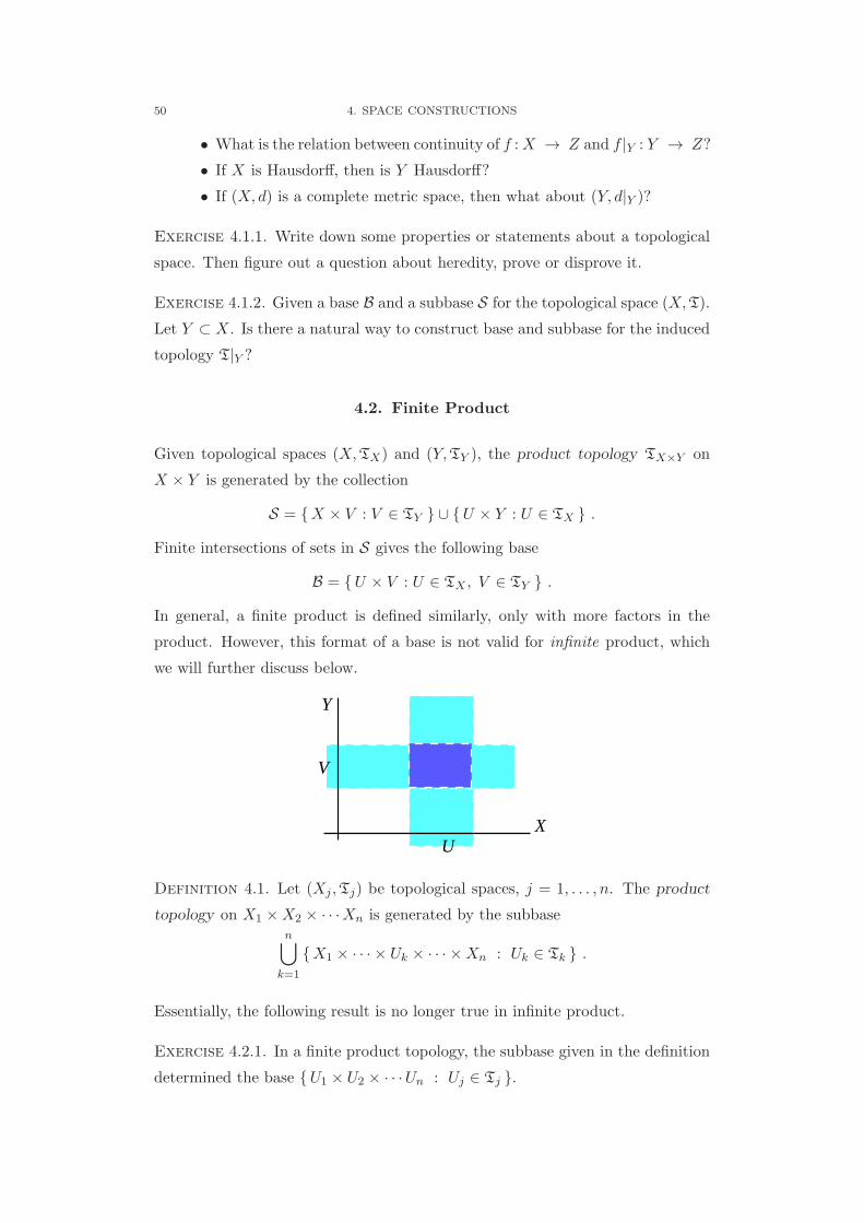
50 4. SPACE CONSTRUCTIONS
• What is the relation between continuity of f :X → Z and f |Y : Y → Z?
• If X is Hausdorff, then is Y Hausdorff?
• If (X, d) is a complete metric space, then what about (Y, d|Y )?
Exercise 4.1.1. Write down some properties or statements about a topological
space. Then figure out a question about heredity, prove or disprove it.
Exercise 4.1.2. Given a base B and a subbase S for the topological space (X,T).
Let Y ⊂ X. Is there a natural way to construct base and subbase for the induced
topology T|Y ?
4.2. Finite Product
Given topological spaces (X,TX) and (Y,TY ), the product topology TX×Y on
X × Y is generated by the collection
S = X × V : V ∈ TY ∪ U × Y : U ∈ TX .
Finite intersections of sets in S gives the following base
B = U × V : U ∈ TX , V ∈ TY .
In general, a finite product is defined similarly, only with more factors in the
product. However, this format of a base is not valid for infinite product, which
we will further discuss below.
U
Y
X
V
Definition 4.1. Let (Xj ,Tj) be topological spaces, j = 1, . . . , n. The product
topology on X1 ×X2 × · · ·Xn is generated by the subbasen∪k=1
X1 × · · · × Uk × · · · ×Xn : Uk ∈ Tk .
Essentially, the following result is no longer true in infinite product.
Exercise 4.2.1. In a finite product topology, the subbase given in the definition
determined the base U1 × U2 × · · ·Un : Uj ∈ Tj .

4.2. FINITE PRODUCT 51
In terms of topological spaces, one also expects that (X×Y )×Z = X× (Y ×Z) .
Example 4.2. The standard Euclidean space Rn is a product of finite copies of
standard R. Note that a simple statement R2 = R × R as topological spaces
may require some thoughts. The standard R2 is defined as a metric space (any
ℓp-metric). An obvious base for the topology is the set of open balls. However,
the open balls of the ℓ2-metric on R2 are circular disks while those of ℓ∞-metric
are squares. Neither of them contains a rectangular set, which is of the form
U ×V and so belongs to the base of R×R. In addition to the above, Rn can also
be obtained by an inductive process of Rn = R× Rn−1.
Exercise 4.2.2. (1) Let BX and BY are bases for the topologies TX and
TY respectively. Show that U × V : U ∈ BX , V ∈ BY is a base for
the product topology.
(2) Let X × Y be given the product topology of X and Y ; A ⊂ X, B ⊂ Y .
Show that Int(A× B) = Int(A)× Int(B); Cl(A× B) = Cl(A)× Cl(B).
What about Frt(A×B)?
(3) Let X has topologies TX ⊂ T′X and Y has topologies TY ⊂ T′
Y . Com-
pare the product topologies TX × TY and T′X × T′
Y .
(4) From the above, if A,B are separable in X,Y respectively, show that
A×B is separable in the product space.
(5) Assume that both X and Y are second countable, is X × Y the same?
There are two natural projections from the product to each factor,
πX : X × Y → X, πY : X × Y → Y .
For any open set U ∈ TX , π−1X (U) = U × Y ∈ TX×Y . Thus, πX , and similarly
πY is continuous. In fact, one may prove the minimality/maximality statements
in the following exercise.
Exercise 4.2.3. (1) Minimality. Let T be a topology on X × Y such that
both πX and πY are continuous. Then TX×Y ⊂ T.
(2) For any f : Z → (X × Y,TX×Y ) from a topological space Z, f is
continuous if and only if both πX f and πY f are so.
(3) Maximality. Let T be a topology on X × Y such that for any space Z,
f : Z → (X × Y,T) is continuous if both πX f and πY f are so.
Prove that T ⊂ TX×Y .

52 4. SPACE CONSTRUCTIONS
The projections πX and πY are also open mappings, in the sense that, for every
open set G ∈ TX×Y , πX(G) ∈ TX and πY (G) ∈ TY . This can be easily observed
by considering images of the set∪α (Uα × Vα) where Uα ∈ TX and Vα ∈ TY .
Something in the product topology may be surprising, as illustrated in the fol-
lowing exercises.
Exercise 4.2.4. (1) Let [0, 1] and (0, 1] be given the standard topology.
Prove that the product spaces [0, 1]× (0, 1] and (0, 1]× (0, 1] are home-
omorphic.
(2) Given an example of spacesX such that the diagonal set (x, x) : x ∈ X is not closed in the product space X ×X.
Exercise 4.2.5. Let RL denote R with the topology generated by intervals of
the form [a, b) and R×RL be the product topological space. What is the induced
topology on the diagonal (x, x) : x ∈ R ?
4.2.1. The Annulus or Cylinder. Consider the complex plane C with the
standard topology, i.e., just as R2. The annulus may be defined as the subset
A = z ∈ C : 1 ≤ |z| ≤ 2
with the induced topology. On the other hand, if for S1 = z ∈ C : |z| = 1 and [0, 1] with standard topology, we may show that S1 × [0, 1] with the product
topology is homeomorphic to A. The homeomorphism h : S1 × [0, 1] → A is
simply given by
h(eiθ, t
)= (1 + t)eiθ .
Exercise 4.2.6. Show that h is a homeomorphism. Hint. pick suitable bases for
the topologies of S1 × [0, 1] and C.
The mapping is illustrated by the following picture.
1
0
t
e iθ
A
It should be noted that a similar bijection can be defined from the Mobius band
to the annulus. However, the mapping is not a homeomorphism. In fact, the

4.2. FINITE PRODUCT 53
Mobius band is not homeomorphic to the annulus. It usually requires algebraic
topology to prove this fact.
Intuitively speaking, one may imagine the red interval in the above picture as
[−1, 1]. After going one round of the strip, [−1, 1] is inverted. Algebraically, this
is captured by n ∼ −n for n ∈ Z. The resulting group is Z/2 = 0, 1 . But, thisgroup does not occur in the product S1 × [0, 1].
4.2.2. The Torus. Start with a small circle of radius r with its center at a
distance of R > r from the rotation axis. The surface of revolution obtained is
called a torus T. Therefore, it can be seen as a subset of R3 and so there is an
induced topology.
Let S1 ⊂ C be given the standard induced topology. The product space S1 × S1
is homeomorphic to T by the mapping(eiθ, eiϕ
)7→ ( (R+ r cos θ) cosϕ, (R+ r cos θ) sinϕ, r sin θ ) .
Exercise 4.2.7. Verify that the above mapping is a homeomorphism.
Similarly, one can define the n-dimensional torus, which is the product of n copies
of circles, i.e., Tn def:== S1 × · · · × S1. Moreover, a 3-dimensional solid torus is the
product space S1 × D2, where D2 = z ∈ C : |z| ≤ 1 . The solid torus has a
boundary, which is exactly the torus, i.e.,
∂(S1 × D2) = S1 × S1 .
Exercise 4.2.8. LetX be an ordered topological space (see Example 3.10). Then
X × X has a dictionary order by (a1, a2) < (b1, b2) if a1 < a2 or a1 = a2 with
b1 < b2. In this way, X × X also becomes an ordered topological space. Show
that R×R with order topology is homeomorphic to Rd ×R where Rd is discrete
and the second R is standard.

54 4. SPACE CONSTRUCTIONS
4.3. Quotient Spaces
Let us start with an example. Take an interval [0, 1], imagine it as a wire and
glue its two end-points. Then a circle, S1 is obtained.
0 1
In terms of set theory, this gluing process can be seen as the quotient set of an
equivalence relation. More precisely, define ∼ on [0, 1] by
s ∼ t if and only if |s− t| = 0 or 1 .
Since s, t ∈ [0, 1], this really means either s = t or s = 0, t = 1 or s = 1, t = 0. In
other words, a point is only identified with itself and the two end-points will be
identified. With this equivalence relation ∼, there are two types of equivalence
classes,
x , 0 < x < 1; and 0, 1 .
There is obviously a bijection between the quotient set [0, 1]/∼ and S1.
Exercise 4.3.1. Let [s] denote the equivalence class of s ∈ [0, 1]. Give an explicit
expression of an bijection from [0, 1]/∼ to S1.
Now, can we define a topology for [0, 1]/∼ such that it is “the same as” the
standard circle S1? The answer is yes and this is called the quotient topology .
Let us compare the neighborhoods of corresponding points in [0, 1] and S1 in the
following picture.
0 1
The neighborhood at any point of S1 is always a short arc. The green or red
neighborhoods correspond to short open intervals (green or red) in the interior
of [0, 1]. However, the blue neighborhood in S1 corresponds to a union of two half
open-closed short intervals at the end-points 0 and 1. This is because the blue

4.3. QUOTIENT SPACES 55
point in S1 corresponds to the equivalence class 0, 1 . This example serves as
a good illustration of the following general theory.
4.3.1. Quotient Topology I. Let (X,T) be a topological space and ∼ be
an equivalence relation on X with a quotient map q : X → X/∼ from X to the
quotient set X/∼ taking x 7→ [x].
Definition 4.3. The quotient topology on the quotient space X/∼ is
Tq =V ⊂ X/∼ : q−1(V ) ∈ T
.
It can be easily verified that Tq is a topology for X/∼, i.e., it is closed under
arbitrary union and finite intersection.
Here is another way to understand an open set in Tq. Let V ⊂ X/∼. Then it
is a collection of equivalence classes (each one is a subset of X). Take all these
equivalence classes and its union is a subset of X. We ask whether this union is
an open set in X to determine whether V ∈ Tq. That is,
q−1(V ) =∪
[x]∈V
[x] =∪
[x]∈V
y ∈ X : y ∼ x .
There are several important properties.
Proposition 4.4. (1) The mapping q : X → X/∼ is surjective.
(2) The mapping q : (X,T) → (X/∼,Tq) is continuous.
(3) If T′ is a topology on X/∼ such that q : (X,T) → (X/∼,T′) is contin-
uous, then T′ ⊂ Tq.
The third property is also called maximality of the quotient topology; in fact, it
means that the quotient topology is the largest topology to have the mapping q
continuous.
Exercise 4.3.2. Prove the above properties of Tq. Moreover, show that Tq is
the only topology on X/∼ that satisfies all the properties.
Exercise 4.3.3. (1) Let X = (x, 0) : x ∈ R ∪ (x, 1) : x ∈ R ⊂ R2.
Such a space is called the disjoint union of two copies of R, denoted
X = R ⊔ R. Define an equivalence relation on X by identifying (0, 0)
and (0, 1). Rigorously, this means (s1, t1) ∼ (s2, t2) iff (s1, t1) = (s2, t2)
or (s1, t1) = (0, 0) while (s2, t2) = (0, 1) or vice versa. Show that X/∼is homeomorphic to the union of the two axes in R2.

56 4. SPACE CONSTRUCTIONS
(2) Let X =(s, n) ∈ R2 : 0 = n ∈ Z
and Y =
(s, 1/n) ∈ R2 : n ∈ Z
be given the standard induced topology. Define an equivalence relation
on bothX and Y by (s1, t1) ∼ (s2, t2) iff (s1, t1) = (s2, t2) or s1 = s2 = 0.
That is, all the points on the y-axis are identified to be one point. Is it
true that X/∼ and Y/∼ are homeomorphic?
Example 4.5. There is another way to construct the circle. Define an equivalence
relation ∼ on R by
x ∼ y if |x− y| ∈ Z .
That means x and y have the same decimal part, so they both can be represented
by a number r ∈ [0, 1). The quotient set in this construction is usually denoted
R/Z.
0 1−1 2
There is an obvious homeomorphism between R/Z and S1 given in the following,
R −→ R/Z −→ S1x 7→ [x] 7→ e2πix
Note that (R,+) is also an abelian group and R/Z is indeed the factor group.
Example 4.6. A cylinder can be obtained as a quotient space by a construction
similar to that of the circle.
( , 0)s
( , 1)s
Define an equivalence relation ∼ on [0, 1]× [0, 1] ⊂ R2 with standard topology by
(s1, t1) ∼ (s2, t2) if (s1, t1) = (s2, t2) or s1 = s2& |t1 − t2| = 1 .
Alternatively, one may define ∼ on [0, 1]× R similar to R/Z to obtain the same
space.

4.3. QUOTIENT SPACES 57
Exercise 4.3.4. Show that the cylinder with the above quotient topology is
homeomorphic to [0, 1]× S1 with the product topology.
Example 4.7. The torus can also be seen as a quotient space, in addition to being
a product space or subspace of R3 as previously discussed. Define an equivalence
relation on R× R by (s1, t1) ∼ (s2, t2) if
(s1, t1) = (s2, t2) or s1 − s2 ∈ Z & t1 − t2 ∈ Z .
There is an analogous equivalence relation on [0, 1]× [0, 1] but the above is much
simpler. One can show that (R× R)/∼ is homeomorphic to S1 × S1.
(0, )t (1, )t
( , 1)
s( , 0)
s
Note that one may either glue (s, 0) ∼ (s, 1) first or (0, t) ∼ (1, t) first. Apparently
in R3, it may result in the second or third picture above. However, they are
topologically the same. In fact, there are many other ways of gluing.
Exercise 4.3.5. (1) Define an equivalence relation on R by identifying n
with 1/n for all n ∈ Z.(a) Sketch a picture to represent the space R/∼.
(b) Find a sequence xn ∈ R such that [xn] ∈ R/∼ converges but xn
does not.
(c) Can a sequence xn ∈ R converge but [xn] ∈ R/∼ does not?
(2) Let X/∼ be a quotient space obtained from X and Y ⊂ X.
(a) Show that there is a natural way to induce an equivalence relation
on Y ; and thus a quotient space Y/∼.
(b) Let Y ∗ = [x] ∈ (X/∼) : [x] ∩ Y = ∅ be given the topology in-
duced from X/∼. Is Y ∗ homeomorphic to Y/∼?
(3) Let X = R/∼ where s ∼ t if s = t or s, t ∈ Z and
Y =∞∪n=1
z ∈ C :
∣∣∣∣z − 1
n
∣∣∣∣ = 1
n
, Z =
∞∪n=1
z ∈ C : |z − n| = n ,
with induced topology of C = R2. Are X, Y , Z homeomorphic?
(4) Let A ⊂ X. What can you say about Int(A)/∼ and Int(A/∼); Cl(A)/∼and Cl(A/∼)?

58 4. SPACE CONSTRUCTIONS
4.3.2. Quotient Topology II. Let us consider the example of the circle
again. Now, we look at the circle as a subspace of C, that is,
S1 = z ∈ C : |z| = 1 .
This is already a space with a chosen topology (standard). There is a special
mapping, whose properties are listed in the exercise below,
℘ : R → S1 x 7→ e2πix .
Exercise 4.3.6. Show that the mapping ℘ satisfies the following:
• It is surjective;
• It is continuous;
• It is an open mapping, i.e., it takes open sets to open sets.
In fact, the third property of ℘ is a little strong. We indeed needs a weaker one
given in the exercise below.
Exercise 4.3.7. A set V ⊂ S1 is open if and only if ℘−1(V ) ⊂ R is open.
Moreover, if T′ is any topology on S1 such that ℘ : R → (S1,T′) is continuous,
then T′ is a subset of the standard topology of S1.
On the other hand, it is shown above that the circle can be obtained as a quotient
space so there is a quotient map, q : R → R/Z x 7→ [x] . The equivalence
class [x] can be imagined as the decimal part of x. Now, both mappings ℘ and q
satisfy the three conditions stated in Proposition 4.4. In fact, these two mappings
are related by the commutative diagram
x ∈ R - S1 e2πixHHHHHHHHHHHHHj R/Z [x]
6
℘
q h
Note that h is well-defined because if [x1] = [x2], then x1 = x2+k for some k ∈ Zand so e2πix1 = e2πi(x2+k). Indeed, h is a homeomorphism. In this way, S1 and
R/Z can be seen as two names for the same space; hence ℘ and q are two names
for the same mapping.
Definition 4.8. Let (X,TX) be a topological space and f : X → Y be a
surjection. The topology Tf is called the quotient topology wrt f , if the following
conditions are satisfied:

4.4. EXAMPLES OF SPACES 59
• f is surjective (this is just stated for convenience);
• f is continuous; and
• for any topology T′ on Y with f : X → (Y,T′) continuous, one must
have T′ ⊂ Tf .
The third condition above can always be replaced by V ∈ TY if and only if
f−1(V ) ∈ TX .
The following exercise provides a convenient way to verify whether a function
from a quotient space is continuous.
Exercise 4.3.8. As above, given (X,TX), f : X → Y , and let (Y,Tf ) be
the quotient space wrt f . Show that for any topological space (Z,TZ) and any
mapping g : (Y,Tf ) → (Z,TZ), we have g is continuous if and only if g f : (X,TX) → (Z,TZ) is continuous.
In fact, the above is a characterizing property of the quotient topology wrt f .
That is, any topology T∗ on Y satisfying the above property must be Tf . The
mathematical statement is given in the exercise.
Exercise 4.3.9. Let T∗ be a topology on Y satisfying the following property:
For any topological space (Z,TZ) and any mapping g : (Y,T∗) → (Z,TZ), we
always have g is continuous if f g : (X,TX) → (Z,TZ) is continuous.
Prove that T∗ ⊃ Tf (so quotient topology also has a meaning of minimality).
4.4. Examples of Spaces
A useful path to understand topology is through the recognition of examples, non-
examples, and counter-examples. In this section, we will show how certain famous
examples are obtained by space construction. These examples are commonly used
in various fields of mathematics.
First, we will duplicate a space by the construction of disjoint union. Let (X,TX)
be a topological space and consider the subset of X × R,
X ⊔X def:== (x, 0) ∈ X × R : x ∈ X ∪ (x, 1) ∈ X × R : x ∈ X .
A typical subset of X ⊔X is of the form (A× 0 )∪ (B× 1 ) where A,B ⊂ X.
We define it to be an open set of X ⊔X if both A,B ∈ TX .

60 4. SPACE CONSTRUCTIONS
Exercise 4.4.1. Show that this topology ofX⊔X is exactly the induced topology
from X × R.
Similarly, one may define the disjoint union X ⊔ Y for any pair of topological
spaces.
Example 4.9. Define an equivalence relation ∼ on [−1, 1] ⊔ [−1, 1] by (x1, t1) ∼(x2, t2) if
(x1, t1) = (x2, t2) or x1 = x2 = 0& |t1 − t2| = 1 .
In other words, we glue every pair of x1 = x2 = 0 and leave (0, 0), (0, 1) unglued.
The picture of this space is given below in which the middle small arcs are con-
sidered as two points.
−1 1(0,1)
(0,0)
Example 4.10. The circle S1 = R/Z and torus T = R2/Z2 are defined above.
In general, the n-dimensional torus is Tn def:== Rn/Zn, which is homeomorphic to
the product space S1 × · · · × S1︸ ︷︷ ︸n times
.
4.4.1. Quotient on a Disk. Many interesting examples are obtained as a
quotient space of a 2-dimensional disk, often viewed as a square.
Example 4.11. The 2-dimensional sphere S2 =x ∈ R3 : ∥x∥ = 1
can be
defined as a subspace of R3. It is also a quotient space. The method is valid for
higher dimensions too.
Take the unit disk D = z ∈ C : |z| ≤ 1 in R2 or C. Define an equivalence
relation ∼ on D by z1 ∼ z2 if
z1 = z2 or |z1| = 1 = |z2| .
In other words, the whole boundary circle of D is identified to be one point. It
can be shown that D/∼ is homeomorphic to S2 as suggested below.
Exercise 4.4.2. Define a mapping p : D → S2 such that p sends a radial line
to a longitude of the sphere such as the origin is mapped to the south pole and
the boundary circle is mapped to the north pole. Show that p is surjective,
continuous, and open. Hence, show that (D/∼) = S2.

4.4. EXAMPLES OF SPACES 61
Exercise 4.4.3. On the disk D, define an equivalence relation ≈ by z1 ≈ z2 if
z1 = z2 or z1 = z2 & |z1| = 1 = |z2| .
Show that D/≈ is also the sphere.
Example 4.12. By changing one of the identification of the torus, we obtain
another surface called the Klein Bottle. This surface cannot be drawn with-
out self-intersection in R3. Define an equivalence relation ∼ on [0, 1] × [0, 1] by
(s1, t1) ∼ (s2, t2) if (s1, t1) = (s2, t2) or
s1 = s2 & |t1 − t2| = 1 or |s1 − s2| = 1 & t1 = 1− t2 .
Then [0, 1]2/∼ is called the Klein Bottle. The identification is shown in the
following picture.
(1, )1−t
t(0, )
s( , 1)
( , 0)s
Note that after the top and bottom red edges are glued to each other. A cylinder
is formed. Then if one tries to glue the left and right green edges within R3,
one has to cut through the cylinder. Moreover, there is not a clear distinction of
inside versus outside of the surface. This phenomenon is called non-orientable.
4.4.2. The Real Projective Plane. If we also change the identification of
the other pair of sides, we have another non-orientable surface. This surface will
be commonly seen in many branches of mathematics
Example 4.13. On [0, 1]× [0, 1], (s1, t1) ∼ (s2, t2) if (s1, t1) = (s2, t2) or
s1 = 1− s2& |t1 − t2| = 1 or |s1 − s2| = 1& t1 = 1− t2 .
Then [0, 1]2/∼ is called the Real Projective Plane, denoted RP2.
1−(1, )
(0, )t
t
(1− , 1)s
( , 0)s

62 4. SPACE CONSTRUCTIONS
There are many ways to construct the Real Projective Plane as a quotient space.
We will describe them one by one in the following.
Let D = z ∈ C : |z| ≤ 1 be the unit disk. Define an equivalence relation ∼on D by z1 ∼ z2 if z1 = z2 or |z1| = 1 = |z2| and z1 = −z2. That is, each pair of
antipodal points on the boundary of D are identified.
e iθ
e iθ−
It can be proved that D/∼ is also the Real Projective Plane, i.e., it is homeomor-
phic to the above one. The following exercise may be helpful.
Exercise 4.4.4. Let X,Y be topological spaces and ∼, ≈ are equivalence rela-
tions on X,Y respectively. If h : X → Y is a homeomorphism such that x1 ∼ x2
if and only if h(x1) ≈ h(x2), then X/∼ and Y/≈ are homeomorphic.
From this exercise, although RP2 can be defined by one of the above identifi-
cation, we usually prefer the second one (and the descriptons given below). It
is because these descriptions work for higher dimensions. For example, RPn is
obtained by Dn/ ∼ by identifying antipodal points on the boundary ∂Dn = Sn−1.
The third way to see the Real Projective Plane is the space of straight lines
through the origin. In other words, the space of 1-dimensional subspace in R3.
Define an equivalence relation ∼ on R3 \ 0 by x ∼ y if there is λ = 0 such
that x = λy. In other words, if x and y determine the same 1-dimensional
subspace in R3, then they are identified. Then the quotient space is also the Real
Projective Plane. At this point, it may not be easy to set up a homeomorphism
between this version and the pervious two versions. Readers may see why in the
next definition of the Real Projective Plane.
Again, if one considers Rn+1 \ 0, i.e., 1-dimensional vector subspaces in Rn+1,
the result is the n-dimensional real projective space, RPn. Similarly, 1-dimensional
complex vector subspaces in Cn+1 form the complex projective space CPn.
In the above quotient space (R3 \ 0 )/∼, every equivalence class [x] is indeed a
straight line passing through the origin determined by x. Now, one may always
choose in every equivalence class a representative u with ∥u∥ = 1. In fact, there
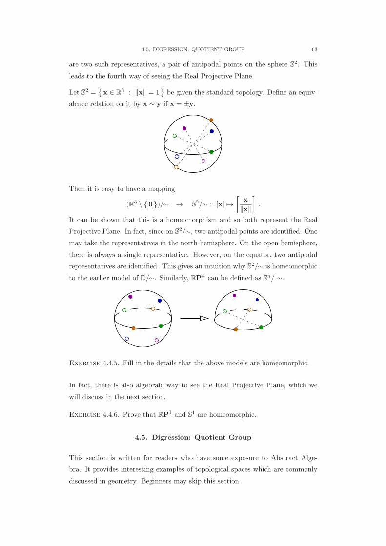
4.5. DIGRESSION: QUOTIENT GROUP 63
are two such representatives, a pair of antipodal points on the sphere S2. This
leads to the fourth way of seeing the Real Projective Plane.
Let S2 =x ∈ R3 : ∥x∥ = 1
be given the standard topology. Define an equiv-
alence relation on it by x ∼ y if x = ±y.
Then it is easy to have a mapping
(R3 \ 0 )/∼ → S2/∼ : [x] 7→[
x
∥x∥
].
It can be shown that this is a homeomorphism and so both represent the Real
Projective Plane. In fact, since on S2/∼, two antipodal points are identified. One
may take the representatives in the north hemisphere. On the open hemisphere,
there is always a single representative. However, on the equator, two antipodal
representatives are identified. This gives an intuition why S2/∼ is homeomorphic
to the earlier model of D/∼. Similarly, RPn can be defined as Sn/ ∼.
Exercise 4.4.5. Fill in the details that the above models are homeomorphic.
In fact, there is also algebraic way to see the Real Projective Plane, which we
will discuss in the next section.
Exercise 4.4.6. Prove that RP1 and S1 are homeomorphic.
4.5. Digression: Quotient Group
This section is written for readers who have some exposure to Abstract Alge-
bra. It provides interesting examples of topological spaces which are commonly
discussed in geometry. Beginners may skip this section.

64 4. SPACE CONSTRUCTIONS
Recall that the circle S1 may be seen as a quotient space of R. Namely,
S1 = R/∼, where s ∼ t if (s− t) ∈ Z.
In terms of Abstract Algebra, we are consider the additive group (R,+), in which
(Z,+) is a normal subgroup. Then as a set, we have R/∼ is exactly the factor
group R/Z. Furthermore, the group structure and topology structure of R are
related. As a consequence, its quotient S1 also has related group and topology
structures.
Definition 4.14. A topological space (X,T) with a group structure (X, ·) is
called a topological group if the following two mappings are continuous,
(x1, x2) ∈ X ×X 7→ x1 · x2 ∈ X, x ∈ X 7→ x−1 ∈ X .
In this sense, the standard R is a topological group.
Given a topological group (X,T) and let A ⊂ X is a subgroup, which is given
the induced topology T|A. Then, it is clear that the mappings
(a1, a2) ∈ A×A 7→ a1 · a2 ∈ A, a ∈ A 7→ a−1 ∈ A
are continuous. This make A also a topological group, which is called a topological
subgroup of X.
In addition, if A is a normal subgroup, we have the factor group X/A of cosets
and it may be given the quotient topology. In such situation, the following two
mappings
([x1], [x2]) ∈ (X/A)× (X/A) 7→ [x1 · x2] ∈ (X/A),
[x] ∈ (X/A) 7→[x−1
]∈ (X/A)
are well-defined and they are continuous under the quotient topology. Thus, X/A
becomes a topological group also. The circle S1 = R/Z can be seen as such space.
Interestingly, the quotient group structure is exactly the multiplication inherited
from C, that is, eiα · eiβ = ei(α+β).
Topological groups are very common in the study of topology and geometry.
Many interesting examples come from matrix groups including Lie groups. The
example of R and S1 can be regarded as a case of 1× 1 matrix group.
Example 4.15. LetMn(R) be the set of all n×nmatrices with real entries. Each
matrix can be listed in a form of a vector in Rn2. Thus, Mn(R) is a topological
space homeomorphic to Rn2. Matrix multiplication is continuous, but inverses
may not be defined so it is only a semigroup.

4.5. DIGRESSION: QUOTIENT GROUP 65
Let GL(n,R) = M ∈ Mn(R) : det(M) = 0 . It can be verified that GL(n,R)is a group with both multiplication and inverse mappings being continuous. Thus,
it is a topological group.
Let O(n) = O(n,R) =Q ∈ GL(n,R) : QQT = QTQ = I
, that is, the group
of orthogonal matrices. It is a topological subgroup of GL(n,R).
There is a natural way of regarding a smaller matrix as a larger matrix. Mathe-
matically, define a mapping
Mn(R) → Mn+1(R) : M 7→(1 00 M
).
This mapping is clearly an injective homomorphism and continuous. Its re-
strictions also gives continuous monomorphisms GL(n,R) → GL(n + 1,R) and
O(n) → O(n+ 1). Inductively, for all m < n, we have
Mm(R) → Mn(R) etc.
Example 4.16. Recall that RP2 can be seen as the space of 1-dimensional vector
subspaces in R3. This fact may be rewritten in terms of group action which is
the fifth way to define RP2. Let us first start with the sphere S2.
Consider O(2) as a topological subgroup of O(3). An element in the quotient
topological O(3)/O(2) is a coset of the form Q ·O(2) where Q ∈ O(3). Moreover,
Q1 ·O(2) = Q2 ·O(2) as elements in O(3)/O(2)
if and only if Q−11 Q2 ∈ O(2) ⊂ O(3). Note that here O(2) is considered as a
subgroup of O(3) and it only acts on the second and third entries. That is, Q−11 Q2
is an isometry on the (x2x3)-plane while fixing the x1-coordinate. Mathematically
speaking, Q−11 Q2 ∈ O(2) if and only if Q1(e1) = Q2(e2) and(
Q−11 Q2
)∣∣ 0 ×R2 : 0 × R2 → 0 × R2
is an isometry. Since both Q1, Q2 are orthogonal, the vector Q1(e1) = Q2(e2) is
of unit length, i.e., it belongs to S2. Therefore, we have a mapping
O(3)/O(2) → S2 : Q ·O(2) 7→ Q(e1) .
It can be verified that this mapping is a homeomorphism. However, unlike the
situation of R/Z, O(2) is not a normal subgroup of O(3). Therefore, O(3)/O(2)
and hence S2 is not a topological group.
Now, consider another subgroup (±O(2)) ⊂ O(3) which contains all matrices
of the form
(±1 00 A
)where A is a 2 × 2 orthogonal matrix. Clearly (±O(2))
contains the embedded image of O(2). Equip the set of cosets O(3)/(±O(2))
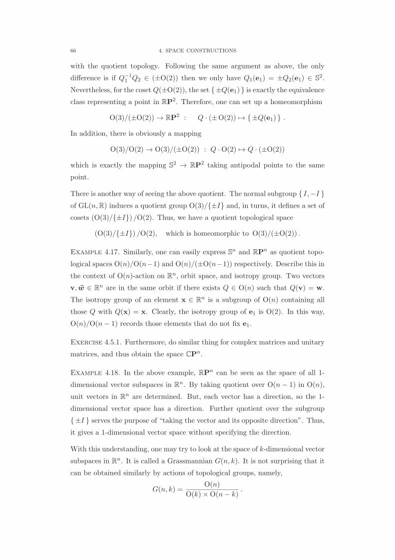
66 4. SPACE CONSTRUCTIONS
with the quotient topology. Following the same argument as above, the only
difference is if Q−11 Q2 ∈ (±O(2)) then we only have Q1(e1) = ±Q2(e1) ∈ S2.
Nevertheless, for the cosetQ(±O(2)), the set ±Q(e1) is exactly the equivalence
class representing a point in RP2. Therefore, one can set up a homeomorphism
O(3)/(±O(2)) → RP2 : Q · (±O(2)) 7→ ±Q(e1) .
In addition, there is obviously a mapping
O(3)/O(2) → O(3)/(±O(2)) : Q ·O(2) 7→ Q · (±O(2))
which is exactly the mapping S2 → RP2 taking antipodal points to the same
point.
There is another way of seeing the above quotient. The normal subgroup I,−I of GL(n,R) induces a quotient group O(3)/±I and, in turns, it defines a set of
cosets (O(3)/±I) /O(2). Thus, we have a quotient topological space
(O(3)/±I) /O(2), which is homeomorphic to O(3)/(±O(2)) .
Example 4.17. Similarly, one can easily express Sn and RPn as quotient topo-
logical spaces O(n)/O(n−1) and O(n)/(±O(n−1)) respectively. Describe this in
the context of O(n)-action on Rn, orbit space, and isotropy group. Two vectors
v, w ∈ Rn are in the same orbit if there exists Q ∈ O(n) such that Q(v) = w.
The isotropy group of an element x ∈ Rn is a subgroup of O(n) containing all
those Q with Q(x) = x. Clearly, the isotropy group of e1 is O(2). In this way,
O(n)/O(n− 1) records those elements that do not fix e1.
Exercise 4.5.1. Furthermore, do similar thing for complex matrices and unitary
matrices, and thus obtain the space CPn.
Example 4.18. In the above example, RPn can be seen as the space of all 1-
dimensional vector subspaces in Rn. By taking quotient over O(n − 1) in O(n),
unit vectors in Rn are determined. But, each vector has a direction, so the 1-
dimensional vector space has a direction. Further quotient over the subgroup
±I serves the purpose of “taking the vector and its opposite direction”. Thus,
it gives a 1-dimensional vector space without specifying the direction.
With this understanding, one may try to look at the space of k-dimensional vector
subspaces in Rn. It is called a Grassmannian G(n, k). It is not surprising that it
can be obtained similarly by actions of topological groups, namely,
G(n, k) =O(n)
O(k)×O(n− k).

4.6. INFINITE PRODUCT 67
In this quotient space, an element in the quotient of O(n − k) is determining
an oriented k-dimensional subspace. Then O(k) is about all the orientations
in that k-dimensional space. Thus, further quotient gives all the unoriented k-
dimensional vector subspaces in Rn.
4.6. Infinite Product
We have defined finite product spaces and mentioned that the method is not
valid for infinite product. Moreover, in Section 4.3, we have given the second
definition of the quotient topology wrt to a mapping. At the end of the section,
characterizing properties of the quotient topology are illustrated in two exercises.
It turns out that an infinite product space is better seen by similar characterizing
properties.
4.6.1. Defining features. In Proposition 4.4, we have characterized the
quotient topology. Let (X,TX) and (Y,TY ) be topological spaces such that
QT1: the mapping q : X → Y is surjective;
QT2: the mapping q : (X,TX) → (Y,TY ) is continuous;
QT3: the topology TY on Y is the largest one to have QT2.
Then TY is exactly the quotient topology Tq wrt the mapping q.
There is another characterization property which provides us the convenience of
checking continuity related to quotient space. In order to check the continuous of
g : (Y,TY ) → (Z,TZ), it is equivalent to verify that g q : (X,TX) → (Z,TZ)
is continuous. This equivalence is valid and only valid when TY is the quotient
topology.
In the case of finite product, we also perform similar thing to check continuity
of maps f : W → X1 ×X2 by simply looking at π1 f and π2 f . Therefore,
we expect analogous characterizing properties, given as exercises below. Let
(X1,T1), (X2,T2) be topological spaces and T be a topology on X1 × X2 with
the projections π1 : X1 ×X2 → X1 and π2 : X1 ×X2 → X2.
Exercise 4.6.1. Show that if π1 and π2 are continuous under the topology T
and T is the minimal one on X1 ×X2 to have both projections continuous, then
T is the product topology.
Likewise, there is another characterizing property.
68 4. SPACE CONSTRUCTIONS
Exercise 4.6.2. Assume that the T on X1 ×X2 satisfies the following: for any
topological space (W,TW ) and any mapping f : (W,TW ) → (X1 ×X2,T), f is
continuous if and only if both π1 f and π2 f are continuous. Then T is the
product topology.
The characterizing properties given in Exercises 4.6.1 and 4.6.2 are very useful
in product spaces. As such, we would expect a definition for an infinite product
space which will keep these characterizing properties.
Let Xα, α ∈ A be a family of nonempty sets. The infinite product set∏α∈AXα
is the set of all functions
x : A →∪α∈A
Xα such that for each α ∈ A, x(α) ∈ Xα.
We often denote xα for the image x(α). Then, for each β ∈ A, there is a surjective
projection mapping
πβ :∏α∈A
Xα → Xβ, πβ(x) = xβ .
In addition, let Tα be a topology on Xα. Then the product topology T∏ is
determined by the following properties.
PT1: Each πβ is surjecctive;
PT2: Each mapping πβ :(∏
α∈AXα,T∏)→ (Xβ,Tβ) is continuous;
PT3: The topology T∏ is the minimal one on∏α∈AXα to have every πβ
continuous.
From property PT2, if V ∈ Tβ, then π−1β (V ) ∈ T∏. Thus, we must have
T∏ ⊃∪β∈A
π−1β (V ) : V ∈ Tβ
.
Note that the above union is not a topology; in fact, it is not even a base.
Nevertheless, it generates a topology which guarantees that each πβ is continuous.
By PT3, it contains T∏. On the other hand, if each πβ is continuous, for each
V ∈ Tβ, π−1β (V ) must be open. Thus, this topology is exactly T∏.
In other words, we may form a base for the product topology, namely,
B =π−1α1
(V1) ∩ · · · ∩ π−1αn
(Vn) : Vk ∈ Tαk, n ∈ N
.

4.6. INFINITE PRODUCT 69
Let us describe the base B from another point of view. A typical set in the above
subbase is π−1β (V ) where V ∈ Tβ. In other words, it is ∏
β =α∈AXα
× Vif A = N===== X1 × · · ·Xβ−1 × V ×Xβ+1 × · · · · · · .
Each set in the base B is a finite intersection of the above sets, so it is a product
of Xα except finitely many factors are replaced with open sets in corresponding
spaces. Thus the base can be expressed as
B =
∏α∈F
Uα ×∏
α∈A\F
Xα : Uα ∈ Tα, finite F ⊂ A
.
In the case that A = N, each open set in B is of the form
X1 × · · ·Xm1−1 × U1 ×Xm1+1 × · · ·Xm2−1 × U2 ×Xm2+1 × · · · · · · ,
in which there are only finitely many such U ’s. In the case of finite product, the
base B coincides with the previous definition.
Based on this definition, it is easy to prove the other defining property.
Exercise 4.6.3. For any topological space (W,TW ) and any mapping
f : (W,TW ) →
(∏α∈A
Xα,T∏),
f is continuous if and only if each πβ f is continuous. Moreover, T∏ is the
unique topology satisfying this property.
Example 4.19. Let Xt = R with the standard topology where t ∈ A = R.Then each element x ∈
∏t∈A
Xt is indeed a function x : A = R → R =∪t∈A
Xt.
In this situation, the infinite product space is simply the function space RR.
Similarly, we have function space R[a,b], which contains C([a, b],R), the space of
continuous functions on [a, b]. However, one should be careful that there can be
many topologies or metrics on C([a, b],R). Only the suitable one is the same as
the subspace topology induced from R[a,b].
Exercise 4.6.4. Let X = RN be seen as a product space. Each element x ∈ X
is a function x : N → R, i.e., a sequence of real numbers. Denote 0 ∈ X to
be the constant zero function (sequence) and xn ∈ X the following sequence of
functions (sequences)
xn(k) = 0 for k ≤ n; and xn(k) = 1 for k > n.
Show that xn → 0 in the product space X.
70 4. SPACE CONSTRUCTIONS
Exercise 4.6.5. Let (Xk, dk), k ∈ N be a countable family of metric spaces.
Define a metric d on the product set∏kXk by
d(x, y) =
∞∑k=1
1
2k· dk(xk, yk)
1 + dk(xk, yk).
Show that the topology induced by d on∏kXk is exactly the product topology.
Given topological spaces (Xα,Tα) and consider the set
Bboxdef:==
∏α
Uα : Uα ∈ Tα
.
Exercise 4.6.6. Show that Bbox is a base for some topology of∏αXα.
This topology defined by Bbox is called the box topology , Tbox of the product
set. Clearly, T∏ ⊂ Tbox. Also, when the index set for α is finite, they are equal.
Exercise 4.6.7. Show that the sequence in Exercise 4.6.4 does not converge
in (X,Tbox).
Exercise 4.6.8. For a general index set, under certain condition, the box topol-
ogy and the product topology are the same. Guess the condition and justify
it.
Hint. Compare the bases for box topology and product topology, what are the
additional open sets in the box topology? When will these open sets become less?

CHAPTER 5
Compactness
In this chapter, one of the two ultimately important properties about topological
spaces is discussed.
Perhaps, the most important property of topological spaces may be compactness.
Many useful theorems are proved with this property. The main reason may be
due to a certain sense of “finiteness” is guaranteed by this property.
In §5.1, the definition and some examples of compact spaces are introduced.
Then, several useful theorems about compactness will be given in §5.2. In §5.3,the relation between compactness and Tychonoff separation axioms is discussed.
In §5.4, we will discuss various concepts closely related to compactness and how
they are logically connected. Finally in §5.5, locally compactness is briefly intro-
duced with one-point compactification as a key application.
5.1. Compact Spaces and Sets
Every student will soon realize the importance of a closed interval early in an
elementary course of analysis on R. Later, when analysis is done on Rn of higher
dimensions, sets that are closed and bounded become the attention.
Let us first obtain motivation by thinking of the good properties of a closed
interval.
• If a sequence in it converges, the limit is also in it. As we have seen
before, this is a matter that the set containing the sequence is closed. A
closed interval has a stronger topological property.
• Some proofs on a closed interval may make use of nested intervals (see
below). However, this is not the general property that we are looking for.
As shown in previous sections, the fundamental reason for the method
of nested intervals is that [a, b] is a closed subset with finite diameter of
a complete metric space.
71

72 5. COMPACTNESS
• Every sequence in it must have a convergent subsequence. This is a result
particularly true on closed and bounded sets. Therefore, it is likely the
notion. The only shortcoming is that it involves sequences, i.e., the space
must be of first countability. What about its proof? If nested intervals
are not used, likely, we will need the next property below.
• We also have Heine-Borel Theorem, which is not easy to understand at
the first encounter. This theorem perplexes many first time students for
analysis. Usually, it is difficult to see what it means. Interestingly, this
is exactly the significant notion that we are looking for.
• One may think of other good properties, such as, a continuous real-
valued function on a closed interval must have maximum and minimum.
This exactly requires the two most important properties in this chapter.
In a topological space (X,T), an open cover for X is collection of open sets of
which the union is the whole space, i.e.,
C = Uι ι∈I ⊂ T and X =∪
C = ∪ι∈IUι .
A subset E ⊂ C, or Uι ι∈J for J ⊂ I, which is also an open cover for X, i.e.,∪E = X, is called a subcover of C.
Definition 5.1. A topological space (X,T) is compact if every open cover for X
has a finite subcover. That is, for every C ⊂ T with∪
C = X, there is a finite
subset E ⊂ C such that∪
E = X.
Clearly, in this category of compact sets, one would like to include closed inter-
vals in R; more generally, closed and bounded sets in Rn. Often, the following
definition is more useful.
Definition 5.2. A subset K in a topological space (X,T) (not necessarily com-
pact itself) is compact if the induced space (K,T|K) is compact.
Since open sets in T|K are intersections of K with sets in T, it is easy to verify
that K is compact if and only if for every C ⊂ T with∪
C ⊃ K, there is a finite
E ⊂ C such that∪
E ⊃ K.
Example 5.3. As mentioned above, every closed and bounded subset in Rn is
compact. This is exactly the content of Heine-Borel Theorem. Thus, the circle,
the spheres Sn, and the torus T are compact sets.
The whole Euclidean space Rn is not compact. Note that, first, Rn has a finite
open cover, for example, Rn has only one open set in it. Second, Rn also

5.1. COMPACT SPACES AND SETS 73
has an infinite open cover which has a finite subcover (try to give an example).
However, it also has an infinite open cover that cannot be reduced to a finite
subcover.
The half-closed interval (0, 1] is not compact. We may consider the open cover
C = (1/n, 1] : n ∈ N .
Any finite subcover of C is of the form
E = (1/n1, 1] , (1/n2, 1] , . . . , (1/nk, 1] .
Its union∪
E = (1/nm, 1] = (0, 1] where nm = max n1, . . . , nk .
Example 5.4. The set 1/n : 1 ≤ n ∈ Z ∪ 0 in R is compact. In fact, this is
a particular case of a more general example. Let (X,T) a topogical space and xn,
n ∈ N be a sequence convergent to x ∈ X. Then the set A = xn : n ∈ N ∪x is compact.
This is simply because if C is an open cover for A, then x ∈ U0 for some U0 ∈ C.As xn → x, there is N ∈ N such that xn : n ≥ N + 1 ⊂ U0. Also, for each
n ≤ N , there is an Un ∈ C containing xn. Thus, U0, U1, . . . , UN is a finite
subcover of C.
Exercise 5.1.1.
(1) A family F of closed sets satisfies finite intersection property if every
intersection of finitely many sets in F is nonempty. Prove that the
following is equivalent to compactness: every family F of closed sets
satisfying the finite intersection property must have ∩F nonempty.
(2) Show that a compact space X satisfies a property similar to the Cantor
Intersection Theorem: if Fn are nonempty closed sets with Fn ⊃ Fn+1,
then∩∞n=1 Fn is nonempty.
(3) Let B be a base for T. Assume that every open cover C ⊂ B for X has
a finite subcover. Prove that X is compact. Remark . The converse is
trivially true.
Remark . The same question concerning subbase is considerably harder.
(4) Recall that a set S in a metric space (Y, d) is bounded iff S ⊂ B(y0, R)
for some y0 ∈ Y and R > 0. Let (X, d) be a metric space. Prove that if
K ⊂ X is compact, it is closed and bounded.
Do you think the converse is true?
(5) Show that if a space (X,T) is compact and discrete then X is finite.

74 5. COMPACTNESS
5.2. Compactness
Just as we have always seen in Rn, that a subset is compact seems to be highly
related to whether it is closed. This fact is partially true in general, in the sense
that if the underlying topological space satisfies certain mild conditions. It turns
out that the space is Hausdorff plays a key role.
Exercise 5.2.1.
(1) Use the indiscrete topology to create an example of a compact space X
with a compact subset A which is not closed in X.
(2) Let Kα be compact subsets in a topological space (X,T). Prove that
a finite union of Kα’s is compact and, if X is Hausdorff, an arbitrary
intersection of Kα’s is compact.
Think about what happens to infinite union of compact sets.
Theorem 5.5. If (X,T) is a compact space and A ⊂ X is closed, then A is a
compact subset.
Before the proof, we will also state a pseudo-converse of this theorem. These
two theorems are often applied together because the requirements are commonly
seen.
Theorem 5.6. If (X,T) is a Hausdorff space and A ⊂ X is a compact set, then
A is a closed subset of X.
These two theorems may be schematically represented by the following diagram.
A ⊂ X is closedX is compact
====⇒X is Hausdorff⇐====
A ⊂ X is compact
The proof for the first one is simple from definition. It will be given here. The
second one relates more to separation axioms so its proof will be given later.
Proof of Theorem 5.5. Let C ⊂ T be an open cover for A, i.e.,∪
C ⊃ A.
The natural way to use the compactness of X is to create an open cover from Cfor X. Since A is closed, X \ A is open. Thus C ∪ X \A is an open cover
for X and it has a finite subcover E . Then the collection E \ X \A is a finite
subcover for A.
Exercise 5.2.2. Let (X,T) be a Hausdorff space such that every proper subset
of X is compact. Show that the topology is discrete. Do you think the converse
is true?

5.2. COMPACTNESS 75
Theorem 5.7. Let f : (X,TX) → (Y,TY ) be a continuous mapping. If X is
compact, then its image f(X) ⊂ Y is compact.
In particular, if f is surjective, then Y is compact. From this, if f is a real-valued
function, then f(X) is a closed and bounded set. By boundedness, its supremum
and infinmum exist; and by closedness, they both lie inside f(X). Thus, they
become maximum and minimum of f on X.
Proof. Let C ⊂ TY be an open cover for f(X), i.e.,∪
C ⊃ f(X). Then
the collectionf−1(V ) : V ∈ C
is an open cover for X and so it has a finite
subcover f−1(V1), f
−1(V2), . . . , f−1(Vn)
.
Correspondingly, V1, V2, . . . , Vn is a finite subcover for f(X).
The above proof looks easy; especially when it is compared with the proof of
existence of maximum and minimum in analysis. The main reason is that ε-δ
arguments are now hidden in the proof. Nevertheless, this still shows the benefits
of identifying the crucial topological concepts.
Corollary 5.8. (1) If X is compact, then its quotient space X/∼ is also
compact.
(2) If a product space∏α∈I Xα is compact, then each of its factors Xβ is
compact.
Both are simple application of the above theorem by seeing that the continuous
images under the quotient map or projection map. Naturally, especially about
the product space, we are interested in whether the converse is true.
Exercise 5.2.3. (1) Let C(X) = f : X → R | f is continuous . Prove
that if X is compact, then d(f, g) = sup |f(x)− g(x)| : x ∈ X is a
metric on C(X).
(2) A metric d is defined on n× n matrices by
d(A,B) =[tr((A−B)(A−B)T )
]1/2.
Convince yourself that the orthogonal matrices O(n) is compact but
SL(n) is not, where
Q ∈ O(n) iff QQT = QTQ = identity,
A ∈ SL(n) iff det(A) = 1 .

76 5. COMPACTNESS
(3) Prove that if (X,T) is compact and f : (X,T) → (Y, d) is continuous,
then the image f(X) is bounded.
(4) Let f : X → Y be continuous where X is compact and Y is Hausdorff.
Show that for every closed set F ⊂ X, its projection f(F ) is closed.
(5) Let p : X → Y be a continuous surjective map such that p(F ) is closed
for each closed set F ⊂ X and p−1(y) is compact for each y ∈ Y . Show
that if Y is compact, then X is compact.
Example 5.9. A quotient space X/∼ is compact while the original space X may
not be so. Consider S1 = R/Z, which is an obvious counter-example.
In the case of product space, given that each factor space is compact, it turns
out that the product is also compact. We are going to give a proof for a finite
product. The result about an arbitrary product is called Tychonoff Theorem,
which is considerably more technical.
Theorem 5.10. If (X,TX) and (Y,TY ) are compact spaces, then their product
space X × Y is also compact.
Proof. Let C be an open cover for X × Y . For simplicity, we will assume
that C belongs to the base U × V : U ∈ TX , V ∈ TY . This is valid according
to an exercise in previous section. We will also discuss below how to further
extend to general open cover.
Fix a y ∈ Y and consider X × y as a subspace of X × Y . The collection C is
also an open cover for X× y , which is homeomorphic to X and so is compact.
Therefore, there is a finite subcover Ey for X × y . Let
Ey = U1 × V1, U2 × V2, . . . , Un × Vn where Uj ∈ TX , Vj ∈ TY .
Take Vy =∩nj=1 Vj , then X × y ⊂ X × Vy ⊂
∪nj=1(Uj × Vj) =
∪Ey as shown
in the following figure.
X
Y
VX
yE
X y x y x

5.3. COMPACTNESS AND SEPARATION 77
Perform this for each y ∈ Y , we have Vy : y ∈ Y an open cover for Y and
so it has a finite subcover, Vy1 , Vy2 , . . . , Vym . Correspondingly, there are Eyj ,j = 1, . . . , n, each is a finite cover for X × yj . Then E = Ey1 ∪ · · · ∪ Eym is a
finite cover for X × Y .
In general, C may not belong to the base as above. Then we may work on
C∗ = U × V : U ∈ TX , V ∈ TY , U × V ⊂ G for some G ∈ C .
By the above method, a finite subcover of C∗ can be found. Each Uj × Vj in this
finite subcover is contained in an open set of C. Therefore, we also have a finite
subcover of C.
Exercise 5.2.4. If X is compact and H ⊂ X × Y is closed, then its projection
πY (F ) is closed in Y .
5.3. Compactness and Separation
Let us recall the two results that are partially converse to each other. That are
Theorem 5.5 and Theorem 5.6. Schematically, we have
A ⊂ X is closedX is compact
====⇒X is Hausdorff⇐====
A ⊂ X is compact
We will first illustrate the power of these two results.
Theorem 5.11. Let (X,TX) be compact and (Y,TY ) be Hausdorff. If f : X → Y
is a continuous bijection, then f is a homeomorphism.
Proof. It is sufficient to show that f is an open mapping, i.e., f(U) ∈ TY
for every open U ∈ TX . Let U ∈ TX , equivalently, X \U is a closed subset of the
compact space X. By Theorem 5.5, X \ U is compact. So, its continuous image
f(X \ U) is so. Since f is a bijection, we have Y \ f(U) = f(X \ U), which is a
compact subset of the Hausdorff space Y . By Theorem 5.6, Y \ f(U) is closed,
i.e., f(U) ∈ TY .
We are now ready to settle the theorem. Let us recall the statement: If (X,T) is
Hausdorff and A ⊂ X is compact, then A is closed in X.
Proof of Theorem 5.6. It is equivalent to establish that X \ A is open.
Precisely, let x ∈ X \ A, we will show that there is a U ∈ T such that x ∈U ⊂ X \ A. For each a ∈ A, clearly, x = a. Since X is Hausdorff, there are
open sets Ua, Va ∈ T such that Ua ∩ Va = ∅; x ∈ Ua and a ∈ Va. In this

78 5. COMPACTNESS
way, Va : a ∈ A is an open cover for A and hence it has a finite subcover,
Va1 , Va2 , . . . , Van and correspondingly finitely many Ua1 , Ua2 , . . . , Uan such that
x ∈ Uaj and Uaj ∩ Vaj = ∅. Let
U = Ua1 ∩ · · · ∩ Uan and V = Va1 ∪ · · · ∪ Van .
Then x ∈ U ∈ T; U ∩ V = ∅ and hence U ⊂ X \ V ⊂ X \A.
The above proof can be illustrated by the following picture. This picture and the
idea of the proof will be used again.
1
U2
U
3 3V
2V1
U
VA
U
x
V
5.3.1. Separation Properties. In a Hausdorff space, two distinct points
must have a reasonable separation between them. Roughly speaking, they are
contained in “separated” open sets. In the above Theorem 5.6, at the end of
the proof, it is indeed established that a point and a closed set are contained in
“separated” open sets. Besides the Hausdorff property, there are several related
weaker or stronger separation properties concerning points or closed sets. These
properties are sometimes called Tychonoff Separation Axioms.
Definition 5.12. A topological space (X,T) is:
Hausdorff or T2 if for every x = y ∈ X, there are U, V ∈ T such that
U ∩ V = ∅; x ∈ U and y ∈ V .
T1 if for every x = y ∈ X, there are U, V ∈ T such that x ∈ U , y ∈ V , x ∈ V ,
and y ∈ U .
T0 if for every x = y ∈ X, there exists U ∈ T such that either x ∈ U and
y ∈ U ; or x ∈ U and y ∈ U .
regular if for every closed set F ⊂ X and x ∈ F , there are U, V ∈ T such
that U ∩ V = ∅; x ∈ U and F ⊂ V .
T3 if it is T1 and regular.
normal if for every closed sets E,F ⊂ X with E ∩F = ∅, there are U, V ∈ T
such that U ∩ V = ∅; E ⊂ U and F ⊂ V .
T4 if it is T1 and normal.

5.3. COMPACTNESS AND SEPARATION 79
Exercise 5.3.1. It can be check (by rewriting the definition) that a space is T1
if and only if every singleton x is a closed subset.
Then, it follows easily that T4 =⇒ T3 =⇒ T2 =⇒ T1 =⇒ T0.
Exercise 5.3.2. (1) Let X be a Hausdorff space in which singleton is not
open. Show that for any open set U and any x ∈ X, there is an open
set V ⊂ U such that x ∈ V .
(2) Show that an infinite set X with cofinite topology is T1 but not T2.
What if the set is finite?
(3) Let f, g : X → Y be continuous mappings. What is the natural re-
quirement for Y if you need one of the following:
(a) The set x ∈ X : f(x) = y0 is closed for every y0 ∈ Y .
(b) The set x ∈ X : f(x) = g(x) is closed.
(4) Show that X is normal if and only if for every closed sets E,F ⊂ X with
E ∩ F = ∅, there exists a continuous function f : X → [0, 1] such that
E ⊂ f−1(0) and F ⊂ f−1(1).
5.3.2. Compact Hausdorff Spaces. Although there are descending impli-
cation from T4 to T2 in general, if the space is compact, these notions are indeed
equivalent. The reasoning will make use the idea and picture in the proof of
Theorem 5.6.
Proposition 5.13. A compact Hausdorff space is regular, and indeed T3. Fur-
thermore, it is normal, and indeed T4.
Proof. Let (X,T) be a compact Hausdorff space. We will first show that it
is regular. Let F ⊂ X be closed and x ∈ F . For each point y ∈ F , we have x = y.
Since X is T2, there are Uy, Vy ∈ T such that Uy ∩ Vy = ∅; x ∈ Uy and y ∈ Vy.
By Theorem 5.5, the set F is compact and so the open cover Vy : y ∈ F has
a finite subcover Vy1 , . . . , Vyn . Now, it is easy to see that the same argument
in Theorem 5.5 is applicable here. Finally, one has the required U, V ∈ T such
that U ∩ V = ∅, x ∈ U and F ⊂ V .
We may proceed one step further. Let E,F ⊂ X be closed and E ∩ F = ∅. We
may apply the regular property obtained above to each point of E and the closed
set F . Then the rest is similar.
Exercise 5.3.3. Fill in the details of the above proof.

80 5. COMPACTNESS
There are two famous theorems that indicate the importance of normal spaces.
One is about separation and the other about extension of continuous mappings.
Both are necessary and sufficient conditions for nomality; in other words, they
are only true on such spaces.
Theorem 5.14 (Urysohn Lemma). A topological space X is normal if and only
if for every pair of closed sets A,B ⊂ X, there exists a continuous function
f : X → [0, 1] such that f(A) ⊂ 0 and f(B) ⊂ 1.
Theorem 5.15 (Tietz Extension Theorem). A topological space X is normal if
and only if for any closed A ⊂ X and continuous function f : A → [0, 1], there
is an extension f : X → [0, 1] such that f |A ≡ f .
This section is ended with some more definitions, which are included only as
references.
Definition 5.16. Some separation properties for a topological space X:
It is completely regular if for each closed F ⊂ X and x ∈ F , there is a
continuous function f : X → [0, 1] such that F ⊂ f−1(0) and x ∈f−1(1).
It is T3.5 or Tπ if it is T1 and completely regular.
It is completely normal if every subspace of X is normal.
It is T5 if it is T1 and complete normal.
It is perfectly normal if for every closed sets E,F ⊂ X with E∩F = ∅, thereexists a continuous function f : X → [0, 1] such that E = f−1(0) and
F = f−1(1).
It is T6 if it is T1 and perfectly normal.
Exercise 5.3.4. (1) Let (X,T1) and (X,T2) are both compact Hausdorff
spaces. Prove that if T1 ⊂ T2, then T1 = T2.
(2) Let Y be compact Hausdorff. For a mapping f : X → Y , define
G = (x, f(x)) ∈ X × Y : x ∈ X .
Prove that f is continuous if and only if G is a closed subset of X × Y .
5.4. Locally Compactness
The Euclidean space Rn is not compact. Yet, it has many good properties because
it is not far from one. The discussion in this section models a lot on the situation
of Rn and Sn.

5.4. LOCALLY COMPACTNESS 81
Definition 5.17. A topological space (X,T) is called locally compact if every
x ∈ X has a compact neighborhood. That is, there is a compact set N ⊂ X such
that x ∈ Int(N).
It is obvious that Rn is locally compact.
Exercise 5.4.1. (1) Is the co-finite topology locally compact?
(2) Give an example other than Rn that is locally compact.
Remark . Warning: Usually, in other context of topology, we say that a space X
is “locally ⋆ ⋆ ⋆” if for every point x ∈ X, there is a local base of “⋆ ⋆ ⋆ neigh-
borhoods”. In the case of locally compactness, the definition is atypical. Ob-
viously, if a space has local bases of compact neighborhoods everywhere, then
it is locally compact. The converse is not always true. A typical example is
X = ([−1, 1] ⊔ [−1, 1])/ ∼ by identifying corresponding points except the origin.
The points (0, 1) and (0,−1) have compact neighborhoods, but they do not have
a local base of compact neighborhoods.
Exercise 5.4.2. Let (X,T) be a Hausdorff space. Show that the following two
statements are equivalent.
• Each x ∈ X has a compact neighborhood N containing x.
• For each x ∈ X and each neighborhood U of x, there is a compact
set K ⊂ U ⊂ X such that x ∈ Int(K). That is, compact neighborhoods
form a local base at each x ∈ X.
One-point Compactification. A locally compact space is likely to be seen
as a subspace of a compact space.
Theorem 5.18. Let (X,T) be a locally compact Hausdorff space. Then there is
a compact space (X∗,T∗) such that
(1) X∗ \X has exactly one point;
(2) (X,T) is a subspace of (X∗,T∗), i.e., T = T∗|X ;(3) the space (X∗,T∗) is also Hausdorff;
(4) if X is non-compact, then X = X∗; otherwise, X is closed in X∗.
Proof. Let us start by defining X∗ and T∗. Besides the four listed state-
ments, we need to verify the topology T∗ and the compactness.
82 5. COMPACTNESS
Take any point not in X, call it ∞; so we have ∞ ∈ X and let X∗ = X ∪ ∞.Statement (1) is satisfied. Let
T∗ def:== T ∪ (X \K) ∪ ∞ : K ⊂ X is compact .
Note that since X is Hausdorff, by Theorem 5.5, X \ K ∈ T whenever K is
compact. Statement (2) is then clearly satisfied.
First, we will check that T∗ is closed under finite intersection. Clearly, if U1, U2 ∈T then U1 ∩ U2 ∈ T ⊂ T∗. Also, if K1,K2 ⊂ X are compact, then so is K1 ∩K2.
Therefore
((X \K1) ∪ ∞) ∩ ((X \K2) ∪ ∞) = (X \ (K1 ∩K2)) ∪ ∞ ∈ T∗ .
For U ∈ T and compact K ⊂ X, we also have
U ∩ ((X \K) ∪ ∞) = U ∩ (X \K) ∈ T ⊂ T∗ .
Second, observe that an arbitrary union of sets in T∗ is always of the form U ∪(X \K) ∪ ∞ for some Uα ∈ T and compact K ⊂ X. It is because
(∪α
Uα) ∪∪β
[(X \Kβ) ∪ ∞] = V ∪ (X \Kβ0) ∪ ∞
where V = (∪α Uα) ∪
∪β =β0(X \Kβ) ∈ T. Next, the set
U ∪ (X \K) ∪ ∞ = [X \ (K \ U)] ∪ ∞ ∈ T∗
because K \U is a closed subset of K and X is Hausdorff. Thus K \U is compact.
Hence, T∗ is a topology on X∗.
Third, we will show that (X∗,T∗) is compact. Let
C = Uα ∈ T α∈A ∪ (X \Kβ) ∪ ∞β∈B
be an open cover for X∗. Take a compact set Kβ0 where β0 ∈ B, then
∪C =
(∪α∈A
Uα
)∪
∪β =β0
(X \Kβ)
∪ (X \Kβ0) ∪ ∞ = X∗ .
Then Uα ∈ T α∈A ∪ (X \Kβ) β =β0 is an open cover for the compact set Kβ0
and it has a finite subcover. Together with (X \Kβ0) ∪ ∞, a finite subcover
of C is obtained for X∗.
Fourth, we will establish Statement (4). Note that by definition of T∗, X is
compact if and only if ∞ = (X \X) ∪ ∞ ∈ T∗. If X is non-compact, then
for any neighborhood N = (X \K) ∪∞ of the point ∞, N ∩X = X \K = ∅.So, X = X∗. On the other hand, if X is compact, ∞ is an isolated point in X∗.

5.5. EQUIVALENCES 83
Finally, we will show Statement (3) that (X∗,T∗) is Hausdorff. The only case
to handle if for a point x ∈ X and ∞ ∈ X∗. Since X is locally compact, there
is a compact neighborhood K of x, that is, x ∈ U ⊂ K for some U ∈ T. Then
U ∩ (X \K) = ∅. Hence, U ∈ T∗ and (X \K)∪∞ ∈ T∗ are the required open
sets.
Exercise 5.4.3. (1) Show that the one-point compactification of Rn is home-
omorphic to Sn. Note that a possible homeomorphism is the stereo-
graphic projection.
(2) Can the real line R be compactified to R ∪ ±∞?
5.5. Equivalences
In the context of Euclidean spaces, several theorems are considered equivalent to
the Heine-Borel Theorem. These are indeed properties related to compactness
and they coincides with compactness under certain conditions. First, let us recall
some definitions and define new properties.
Definition 5.19. A topological space (X,T) is said to be:
Lindelof if every open cover for X has a countable subcover.
Countably compact if every countable open cover for X has a finite subcover.
Sequentially compact if every sequence in X has a convergent subsequence.
Having Bolzano-Weierstrass Property if every infinite subset A ⊂ X has a
cluster point (in X). This is called limit point compact by Munkres.
Theorem 5.20. (1) A compact topological space is always countably com-
pact and has the Bolzano-Weierstrass property. A Lindelof countably
compact space is compact.
(2) A sequentially compact topological space has the Bolzano-Weierstrass
property. A T1 space of first countability with the Bolzano-Weierstrass
property is sequentially compact.
(3) A countably compact topological space has the Bolzano-Weierstrass prop-
erty. A T1 space with the Bolzano-Weierstrass property is countably
compact
(4) If a space is T1 of first countability, then it is countably compact if and
only if it is sequentially compact.

84 5. COMPACTNESS
The conditions for equivalences of the above properties are given in the schematic
diagram below. Note that in general there is no implication between “compact”
and “sequentially compact”.T1
CI
T1T1 CI CompactSequentially
CountablyCompact
Bolzano-WeierstrassLindelof
Compact(Heine-Borel)
Example 5.21. The space [0, 1]N is an infinite product of compact spaces. Thus
by Tychonoff Theorem, it is compact. However, as in Exercise 4.6.4, one may
create a sequence in [0, 1]N that has no convergent subsequence. A complicated
example of sequentially compact but non-compact space occurs in the order topol-
ogy of uncountable ordinals.
It is trivial that compactness implies countably compactness. Moreover, A count-
ably compact Lindelof space is obviously compact. Statement (4) is a consequence
of (2) and (3).
Sequentially compact =⇒ Bolzano-Weierstrass. Let (X,T) be a se-
quentially compact space and A ⊂ X be infinite. Then it is possible to pick
a distinct sequence an ∈ A. By sequentially compactness, it has a convergent
subsequence ank, k ∈ N with limit x ∈ X.
We claim that x is a cluster point of A. Take any open set U ∈ T with x ∈ U ,
there is K ∈ N such that for every k ≥ K, ank∈ U . Since ank
’s are distinct,
there must be some ank= x, i.e., ank
∈ A ∩ (U \ x ). Thus, x ∈ A′.
As we have seen before, the limit of a sequence in A is always a cluster point of A.
But, a cluster point may not be always approached by a sequence. Basically, it
is because a point may not have a countable local base, i.e., one cannot find a
countable family of neighborhoods to represent all the neighborhoods.
Bolzano-WeierstrassT1,CI=⇒ Sequentially Compact. Let xn, n ∈ N be
a sequence in X and A = xn : n ∈ N ⊂ X. If A is a finite set, then xn
clearly has a constant subsequence, which obviously converges. If A is infinite
then by Bolzano-Weierstrass property, it has a cluster point x ∈ X. Since X is
first countable, let Uk : k ∈ N be a countable local base at x.

5.5. EQUIVALENCES 85
For U1, there is xn1 ∈ U1 \ x . Then, since X is T1, the set x1, x2, . . . , xn1 is closed. Thus, (U1 ∩U2) \ xn : n ≤ n1 is also a neighborhood of x, so there
is xn2 ∈ (U1 ∩U2) \ x, xn1 for some n2 > n1. The process can be continued so
that it is possible to pick
xnk+1∈ (U1 ∩ · · · ∩ Uk ∩ Uk+1) \ x, xn1 , . . . , xnk
, for some nk+1 > nk.
Using the fact that Uk : k ∈ N is a local base, one may show that xnk→ x
as k → ∞.
Example 5.22. This example will be very useful for the understanding of the
next proof. Consider the set of integers Z ⊂ R. It is an infinite set without any
cluster point in R. Let
C = R \ Z ∪ (n− 1/2, n+ 1/2) : n ∈ Z .
Then C is a countable open cover for R. It clearly does not have a finite subcover.
In this construction, Z being an infinite discrete closed subset in R is crucial.
Countably compact =⇒ Bolzano-Weierstrass. Since it is difficult to
construct a cluster point for a set A simply from the assumption, we would start
from the negation of Bolzano-Weierstrass property.
Let A ⊂ X be an infinite set such that it has no cluster point in X. Without
loss of generality, by taking a subset, we may assume that A is countable, say,
A = an : n ∈ N with am = an for m = n. Now, we have the situation as in
the example above. Since every an is not a cluster point of A, there exists Un ∈ T
such that an ∈ Un and Un ∩A = an .
Next, we will show that X \ A is open. Let x ∈ X \ A. Since x is not a cluster
point of A, there is a V ∈ T with x ∈ V and A ∩ V = A ∩ V x = ∅. This is
equivalent to that V ⊂ X \A. Thus, X \A is open.
Finally, X \A ∪ Un : n ∈ N is a countable open cover for X which clearly
does not have a finite subcover.
Bolzano-WeierstrassT1=⇒ Countably compact. Let Un ∈ T : n ∈ N
be a countable open cover for X and we will look for a finite subcover. In order
to use the given property, we try to pick xn ∈ Un wisely to form an infinite set.
Let x1 ∈ X =∪∞n=1 Un. Therefore, there exists n1 (i.e., the first one) such that
x1 ∈ Un1 but x1 ∈ U1 ∪ · · · ∪ Un1−1 .

86 5. COMPACTNESS
If X \(U1∪· · ·∪Un1−1∪Un1) is empty, then we have a finite subcover. Otherwise,
pick x2 ∈ X \ (U1∪ · · ·∪Un1−1∪Un1) ⊂∪n>n1
Un. By the construction, x2 = x1.
Again, there exists n2, which satisfies n2 > n1 consequently, such that
x2 ∈ Un2 but x1 ∈ U1 ∪ · · · ∪ Un2−1 .
Inductively, we have xk ∈ Unksuch that xk ∈ Un for n < nk and xk =
x1, . . . , xk−1. If the process stops in finitely many steps, then we have a finite
subcover. Suppose it continues indefinitely, then we have a distinct sequence xk
constructed as above. The set A = xk : k ∈ N is an infinite set. Take any
x ∈ X =∪∞n=1 Un. Then x ∈ Um for some m ∈ N and x ∈ Un for n < m. By
ranking m among the increasing sequence nk, we have
n1 < n2 < · · · < nN ≤ m < nN+1 < nN+2 < · · · · · · .
Since m < nN+1, by the construction process, xN+1, xN+2, . . . . . . ∈ Um. There-
fore Um ∩A ⊂ x1, . . . , xN is a finite set. Let
V =
Um \ x1, . . . , xN−1, xN if x = xN ,
Um \ x1, . . . , xN−1 if x = xN , only occur when m = nN .
Since the space X is T1, V ∈ T, x ∈ V and A ∩ (V \ x ) = ∅. Thus, x is not
a cluster point of A. Hence A is an infinite set without any cluster point. This
contradicts the Bolzano-Weierstrass property.
Exercise 5.5.1. (1) Show that a space is countably compact if and only
if every decreasing sequence of nonempty closed sets, Fn ⊃ Fn+1, has
nonempty intersection∩∞n=1 Fn.
(2) Let X has Bolzano-Weierstrass Property.
(a) If A ⊂ X is closed, then does A have the same property?
(b) Does a continuous image of X also have the same property?
(c) If X is a subspace of a Hausdorff space, is it a closed subset of it?
(3) A compact topological space often shares similar properties as a com-
plete metric space. We have seen the Cantor Intersection Property be-
fore. Here is another one:
Show that a contraction mapping on a compact metric space must have
a fixed point. Do you think it is true for a space with other notion of
compactness?

CHAPTER 6
Connectedness
Compactness discussed in the previous chapter guarantees that some sort of finite-
ness can be achieved. In this chapter, we discuss another important property on
topological spaces, which is essential to have uniform results on the whole space.
Without it, one part of a space may be very different from the other part of
it. In §6.1, the concept of connectedness will be introduced, together with some
examples and the standard skills of proving connectedness. In §6.2, we will dis-
cussed connected components and certain properties of connectedness. In the
last section, §6.3, other related connnectivity will be explored.
6.1. Disconnected and Connected
In order to define connectedness, we start from the opposite. A topological space
(X,T) is disconnected if there is a pair of nonempty open sets U, V ∈ T such that
U ∩ V = ∅ and U ∪ V = X. Intuitively, X can be separated into two nonempty
pieces U and V . Such a pair of U, V ∈ T is also called a separation of X.
VU
Note that the condition of U, V ∈ T is essential because any space can be written
as X = A∪ (X \A) where A may not be open nor closed. Naturally, a connected
space is not disconnected. But, we will give a better formulation later.
A subset Y ⊂ X is disconnected if (Y,T|Y ) is so. In such a case, one should be
careful that the sets U, V are open in Y , but not necessarily in X.
If X is disconnected, with the above notations, then since U = X \V and V ∈ T,
we have U and similarly V being also closed subsets of X. In other words, U and
V are nontrivial (neither X nor ∅) both open and closed subsets of X.
87

88 6. CONNECTEDNESS
Example 6.1. (1) Let X = [0, 1] ∪ (2, 3] with the induced topology of the
standard R. Then X is disconnected because U = [0, 1] is both open
and closed in X. Note that [0, 1] = (−1, 1 + δ) ∩ X = [0, 1.5] ∩ X for
an open interval (−1, 1 + δ) and a closed interval [0, 1.5]. Thus, [0, 1] is
both open and closed in X.
(2) Let X =(x, y) ∈ R2 : xy = 1
with the induced topology of the stan-
dard R2. Then X is disconnected. Any branch of the hyperbola is a
closed subset of R2, but it is both open and closed in X.
Exercise 6.1.1. Let Y ⊂ X and there are disjoint A,B ⊂ Y such that Y = A∪B.
If each A ∩B = ∅ and B ∩A = ∅, then the pair A,B is a separation of Y .
As seen above, one may only specify one sets instead of a pair. Namely, X is
disconnected if there exists a both open and closed subset U ⊂ X (i.e., U and
X \U ∈ T) such that neither U = ∅ nor X \U = ∅. We are now ready to define a
connected space by the negation of a disconnected space. The definition phrased
as below is the most useful one, especially in abstract proofs.
Definition 6.2. Let (X,T) be a topological space. It is connected if for each
S ⊂ X with both S,X \S ∈ T, one must have S = ∅ or S = X. A subset A ⊂ X
is connected if the induced space (A,T|A) is so.
Example 6.3. (1) An indiscrete space is connected because any both open
and closed subset must be trivial.
(2) A discrete space of more than one point is disconnected.
(3) As given above, X =(x, y) ∈ R2 : xy = 1
⊂ R2 is disconnected.
However, let
Xu =(x, y) ∈ R2 : xy = 1, x > 0
Xℓ =
(x, y) ∈ R2 : xy = 1, x < 0
.
Then both Xu and Xℓ are connected. This is the concept of connected
component which we will discussed later.
Exercise 6.1.2. (1) Show that an infinite set X with the cofinite topology
is connected. What if X is finite?
(2) Let X be connected and ∅ = A ⊂ X. Later, we will see that if A is
connected then so is A. Give a counter-example of the converse.
(3) As above, if A is connected, is it necessary true that Int(A) is connected?
(4) Is Frt(A) connected if A is so? Is A connected if Frt(A) is so?

6.1. DISCONNECTED AND CONNECTED 89
(5) Let X be connected and ∅ = A ⊂ X. Prove that Frt(A) = ∅.(6) Let A,C ⊂ X such that C∩A = ∅ and C∩(X\A) = ∅. If C is connected
then C ∩ Frt(A) = ∅.
6.1.1. Continuous Image. In the study of continuous functions on R, itis known that the image of an interval is again an interval. This gives the idea
that connectedness is preserved under continuous function. Here, in the proof,
the typical use of the definition of connectedness is illustrated.
Theorem 6.4. Let X be a connected space. If f : X → Y is a continuous
mapping, then its image f(X) ⊂ Y is connected. In particular, if f is also
surjective, then Y is connected.
Proof. Let S ⊂ f(X) be both open and closed in f(X). We are trying to
show that S = ∅ or f(X). Note that by taking the induced topology on f(X)
from Y , the mapping f : X → f(X) is also continuous. Thus f−1(S) ⊂ X
is both open and closed in X. By the connectedness of X, f−1(S) = ∅ or X.
Consequently, S = ∅ or f(X).
Note that in the above proof, the continuity of f : X → f(X) is indeed easily
verified. Nevertheless, it is still beneficial for the readers to pause and think to
make sure about it.
With this result, Y =(0, y) ∈ R2 : y ∈ R
is a continuous (homeomorphic)
image of R and so it is connected. The graph of a continuous function is also
connected as seen in the exercise below.
Exercise 6.1.3. (1) If X is connected and f : X → Y is continuous, then
the set (x, f(x)) ∈ X × Y : x ∈ X with the induced topology from
the product space X × Y is also connected. Do you think the converse
is true?
(2) Let f : Rn → R be a continuous function and Lα = x ∈ Rn : f(x) = α ,i.e., the level set wrt α.
(a) If A = Lα ∪ Lβ with α = β, show that A is disconnected.
(b) Is it true that Lα is always connected?
6.1.2. A famous example. This is an example to show the strange be-
haviour of connectedness. One may also use a similar example to form a domain
in R2 with a strange boundary. Let X = Y ∪G, which has a picture shown below,

90 6. CONNECTEDNESS
where
Y =(0, y) ∈ R2 : y ∈ R
G =
(x, sin
1
x
)∈ R2 : x > 0
and X is given the induced topology of the standard R2.
14 Π
12 Π
1Π
-1
1
GY
This space X is a typical example of a connected space which is not path con-
nected (to be discussed later). In order to show that X is connected, we will use
the fact that both Y and G are connected, which is a consequence discussed in
the previous section.
Let S ⊂ X be both open and closed in X. Then S ∩ Y is both open and closed
in Y . By the connectedness of Y , one must have S ∩ Y = ∅ or Y . The same
argument can be applied to S ∩ G. Thus, we have the four possibilities S = ∅or Y or G or X. We are going to show that neither Y nor G is both open and
closed in X. Thus, S = ∅ or X and hence X is connected.
Since G = X \ Y , Y is both open and closed in X if and only if G is so. It is
then sufficient to consider Y only. Let U ⊂ R2 be any open set containing Y .
Then U ⊃ A = (0, y) : y ∈ [−1, 1] . Since A is compact, there is ε > 0 such
that U ⊃ (−ε, ε)× [−1, 1]. For this ε, there is m ∈ Z such that 0 < 1/(2mπ) < ε
and so G ∩ U = ∅. Therefore, if U is an open set of R2 such that U ∩ X ⊇ Y ,
then U ∩G = ∅. This shows that Y cannot be open in X. Equivalently, G is not
closed in X.
It should be noted that Y is indeed closed in X and thus G is open.
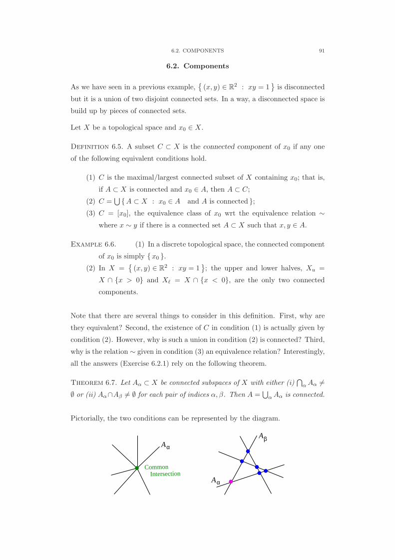
6.2. COMPONENTS 91
6.2. Components
As we have seen in a previous example,(x, y) ∈ R2 : xy = 1
is disconnected
but it is a union of two disjoint connected sets. In a way, a disconnected space is
build up by pieces of connected sets.
Let X be a topological space and x0 ∈ X.
Definition 6.5. A subset C ⊂ X is the connected component of x0 if any one
of the following equivalent conditions hold.
(1) C is the maximal/largest connected subset of X containing x0; that is,
if A ⊂ X is connected and x0 ∈ A, then A ⊂ C;
(2) C =∪
A ⊂ X : x0 ∈ A and A is connected ;(3) C = [x0], the equivalence class of x0 wrt the equivalence relation ∼
where x ∼ y if there is a connected set A ⊂ X such that x, y ∈ A.
Example 6.6. (1) In a discrete topological space, the connected component
of x0 is simply x0 .(2) In X =
(x, y) ∈ R2 : xy = 1
; the upper and lower halves, Xu =
X ∩ x > 0 and Xℓ = X ∩ x < 0, are the only two connected
components.
Note that there are several things to consider in this definition. First, why are
they equivalent? Second, the existence of C in condition (1) is actually given by
condition (2). However, why is such a union in condition (2) is connected? Third,
why is the relation ∼ given in condition (3) an equivalence relation? Interestingly,
all the answers (Exercise 6.2.1) rely on the following theorem.
Theorem 6.7. Let Aα ⊂ X be connected subspaces of X with either (i)∩αAα =
∅ or (ii) Aα∩Aβ = ∅ for each pair of indices α, β. Then A =∪αAα is connected.
Pictorially, the two conditions can be represented by the diagram.
Common
β
α
α
A
A
Intersection
A

92 6. CONNECTEDNESS
Exercise 6.2.1. Use Theorem 6.7 to show that the three definitions are valid.
Proof. Note that condition (i) implies (ii), so one only needs to prove with
assuming (ii). Let S ⊂ A =∪αAα be both open and closed in A. As a conse-
quence, for each index α, S ∩Aα is both open and closed in Aα. So, S ∩Aα = ∅or Aα for each α. Be careful that at this point we cannot simply conclude that
S =∪(S ∩Aα) =
∪∅ = ∅ or S =
∪(S ∩Aα) =
∪Aα = A.
Suppose S∩Aβ = ∅ for some index β, then S∩Aβ = Aβ by connectedness of Aβ.
By condition (ii), for each α, Aα ∩ S ⊃ Aα ∩ Aβ = ∅. Then by connectedness
of Aα, one also has S ∩ Aα = Aα. Thus, we have either S ∩ Aα = ∅ for each
index α or S ∩ Aα = Aα for each index α. Hence, taking union over α, we have
S = ∅ or S = A.
Exercise 6.2.2. (1) Prove the two variations of connectedness theorem:
(a) Let Aα be a family of connected subsets in X and there is a con-
nected subset C such that C∩Aα = ∅ for each α. Then C∪(∪αAα)
is also connected.
(b) Let An be a countable family of connected subsets in X such that
An ∩An+1 = ∅ for all n ∈ N. Then∪nAn is also connected.
(2) Let f, g : (X,TX) → (Y,TY ) be continuous functions and X is con-
nected. Show that if there exists x0 ∈ X such that f(x0) = g(x0) then
Gf ∪Gg is connected. Is the converse true?
(3) Let X,Y, Z be connected topological spaces and
f : (X,TX) → (Z,TZ), g : (Y,TY ) → (Z,TZ)
be continuous. Construct a quotient space (X ⊔ Y )/∼ by x ∼ y if
f(x) = g(y). Show that if f or g is surjective, then (X ⊔ Y )/∼ is
connected.
Remark . The result is intuitively obvious. Finding a clean proof
may be the spirit of this exercise.
(4) Let X,Y be connected spaces and A ( X, B ( Y . Prove that (X ×Y ) \ (A×B) is connected.
6.2.1. Open or closed? Let X be a disconnected space and C be one of
its connected components, is C open or closed or both?
From the definition, X = U∪V for disjoint subsets U, V ∈ T\ ∅, X . Thus, bothU and V are both open and closed. Intuitively, if either U or V is disconnected,

6.2. COMPONENTS 93
we may further decompose it into both open and closed subsets. Therefore, it
is natural (unfortunately wrong) to think that a component C is both open and
closed.
Example 6.8. Let Cn =(x, y) ∈ R2 : x2 + y2 = 1
n2
, C∞ = (0, 0) and
X =
∞∪n=1
Cn ∪ C∞ .
Note that for each finite n = 2, 3, . . ., there are1
n+ 1< rn+1 <
1
n< rn <
1
n− 1.
Thus Cn = X ∩(x, y) : rn+1 < x2 + y2 < rn
is open in X. Similarly, we may
show that Cn is closed in X. Therefore, the components Cn are both open and
closed. However, the situation for the component C∞ is different. Any open set(x, y) : x2 + y2 < ε
containing C∞ must also intersect some Cn for large n.
Therefore, C∞ is not open.
Exercise 6.2.3. (1) Show that C∞ is closed in X.
(2) Is it true that if X has only finitely many connected components, then
each one is both open and closed in X?
6.2.2. More about connectedness. Let us first consider an example of
matrix topological space (in fact, a group), namely, O(n), the set of n × n or-
thogonal matrices with real entries. Recall that an n × n matrix Q ∈ O(n) if
QTQ = QQT = I. Clearly, O(n) ⊂ Rn2and it has an induced topology. The
question is whether O(n) is connected or disconnected? Take the determinant
mapping, which is continuous,
det : O(n) → R, Q 7→ det(Q) .
Note that det(QT ) det(Q) = det(QTQ) = det(I) = 1. So, det(Q) = ±1. More-
over, det(I) = 1 and det(J) = −1 where J is obtained by interchanging the first
two rows and columns of I. Therefore, the image of O(n) under det is the discrete
space 1,−1 , which is disconnected. By contra-positive of Theorem 6.4, O(n)
must be disconnected. In fact, we can easily have the following general result.

94 6. CONNECTEDNESS
Proposition 6.9. Let f be a continuous mapping on a topological space X.
If its image f(X) contains a discrete subset of at least two points, then X is
disconnected.
In the example of O(n), there is a subspace SO(n) which contains all orthogonal
matrices of determinant 1. At this point, one should not simply conclude that
SO(n) is connected because its image under determinant is so. One needs more
information of the determinant mapping.
Exercise 6.2.4. Show that SO(n) is both open and closed in O(n). By this,
argue that SO(n) is a connected component of O(n).
As a comparison, let us consider the set U(n) of n × n complex matrices such
that U ∈ U(n) if U∗U = UU∗ = I. That is the space of unitary matrices. By
considering the determinant function again. One still has |det(U)| = 1. So, the
image is indeed z ∈ C : |z| = 1 , which is the unit circle. Thus, we cannot
conclude that U(n) is disconnected. In fact, the connectedness of U(n) can be
proved by below.
Exercise 6.2.5. Let f : X → Y be a mapping such that Y is having the quotient
topology induced by f and is connected. Prove that if for all y ∈ Y , the subset
f−1(y) ⊂ X is connected, then X is connected. Apply this result to show that
U(n), the unitary group, is connected.
Theorem 6.10. Let A be a connected subspace of X. Then every B with A ⊂B ⊂ A is connected. In particular, A is connected.
Proof. Let S ⊂ B be both open and closed in B. Thus, with the induced
topology, S ∩A is both open and closed in A. By connectedness of A, S ∩A = ∅or S ∩ A = A. First, consider that S ∩ A = ∅. Thus, S is an open set and
S ⊂ B \A. We will argue that x ∈ S ∩A is a contradiction. Suppose otherwise,
since x ∈ A and x ∈ S ⊂ B, x ∈ ClB(A). Therefore, any open neighborhood of x
in B intersects A, in particular, S ∩ A is nonempty. Hence S ∩ A = ∅ implies
that S ∩ A and so S is empty. Second, if S ∩ A = A, then S ⊂ B is a closed set
containing A and so S ⊃ ClB(A) = A ∩ B = B. To conclude, one has S = ∅ or
S = B.
Exercise 6.2.6. Prove that every connected component is closed.

6.3. OTHER CONNECTIVITY 95
Exercise 6.2.7. Let X be a compact Hausdorff space. If F is a set of closed
connected subsets of X such that any two sets Fα, Fβ ∈ F satisfy Fα ⊂ Fβ or
vice versa, then∩
F is connected.
6.2.3. Two famous applications. There are two useful theorems in cal-
culus that make use of connectedness. We give a brief description in order to
highlight the importance of connectedness.
Example 6.11. If f : [a, b] → R is a continuous function and y ∈ R satisfies
either f(a) < y < f(b) or f(b) < y < f(a), then there exist x ∈ (a, b) such that
f(x) = y. This is indeed Intermediate Value Theorem.
In terms of connectedness, it can be proved as follows. Since [a, b] is connected
and f is continuous, f([a, b]) is connected and it is an interval J . Now, both
f(a), f(b) ∈ J and so either [f(a), f(b)] ⊂ J or [f(b), f(a)] ⊂ J . Thus, y satisfying
the assumption must be in J and the result follows.
Example 6.12. If f : Ω ⊂ Rn → R is differentiable on a domain Ω (i.e., open
connected) and all its partial derivatives fj ≡ 0, then f is a constant function.
Many students may use integration to prove this statement. That actually re-
quires path connectedness (which is also true for a domain).
Recall that we need the Mean Value Theorem at x0 ∈ Ω, which is only valid for
points x with ∥x− x0∥ < δ for some δ > 0. Thus, we already know that f is
constant in a δ-ball of a point. To complete the proof, one may fix x0 ∈ Ω and
consider A = x ∈ Ω : f(x) = f(x0) . It can be shown that A is both open and
closed. Since x0 ∈ A, it is nonempty so it must be the whole Ω.
Similar type of connectedness argument occurs very often in various studies of
mathematics. Some requires further knowledge but it is good to understand this
general nature through the above examples.
6.3. Other Connectivity
There are some further definitions of connectivity. Some of them require concepts
in algebraic topology which we will introduce towards the end of this course. The
most famous one is called simply-connected. In this section, we will only introduce
two connectivity concepts which can be defined by point set topology.

96 6. CONNECTEDNESS
6.3.1. Path connected. A topological space X is path connected if for
every pair x1, x2 ∈ X, there exists a continuous path γ : [0, 1] → X such that
γ(0) = x1 and γ(1) = x2. In words, one can always join two points in X by a
continous path.
Exercise 6.3.1. Show that a path connected space is connected.
Clearly, the converse of the exercise is not true. We have seen the example in
Section 6.1.2, where
X = (0, y) : y ∈ R ∪(x, y) : x > 0, y = sin
1
x
.
We know that X is connected. However, if it is path connected, the function
sin 1x must be discontinous at 0.
Exercise 6.3.2. Prove that there is no continuous γ : [0, 1] → X such that
γ(0) = (0, 0) and γ(1) =(1π , 0). This may be done by considering tn → 0 for
tn ∈ [0, 1].
It is clear that in Rn, a convex set or a star-shaped set is path connected. Here,
a set A ⊂ Rn is star-shaped if there exists x0 ∈ A such that for each x ∈ A, the
line segment joining x0 to x lies in A. An important fact in Rn is given in the
following.
Exercise 6.3.3. Let Ω ⊂ Rn be an open connected set. Then it is path connected.
In fact, every two points in Ω can be joined a path formed by straight line
segments parallel to the coordinate axes. Hint. Fix a point x0 ∈ Ω, let S ⊂ Ω
be the set of all points x ∈ Ω such that x is joined to x0 by coordinate-parallel
segments. Show that S is both open and closed.
One may define an equivalence relation on X by x1 ∼ x2 if there is a continuous
path joining them. Each equivalence class is called a path component. Clearly,
each path component is a subset of a connected component and they may be
different from the example in Section 6.1.2. It should be noted that there is no
conclusion on whether a path component is open or closed.
Exercise 6.3.4. Let X = J ∪ G where G =(x, y) : x > 0, y = sin 1
x
and
J = (0, y) : y ∈ [0, 1] ∩Q . How many path components and connected com-
ponents are there in X?

6.3. OTHER CONNECTIVITY 97
6.3.2. Locally connected. A topological space X is locally connected at
x ∈ X if the connected neighborhoods of x form a local base at x. That is, for
every neighborhood N of x, there exists a connected neighborhood U of x such
that x ∈ U ⊂ N . The space X is locally connected if it is so at every x ∈ X.
From the definition, it is clear that on a locally connected space, one may al-
ways assume that a neighborhood is connected. However, there is no implication
between locally connected versus connected in any direction.
Example 6.13. A locally connected space may not be connected. Let X =
(−1, 0)∪ [2, 3) with the standard induced topology. It is clearly locally connected
but not connected.
A connected space may also not be locally connected. Let
F = (0, y) : y ≥ 0 ∪ (x, 0) : x ∈ R ∪∞∪n=1
(x, 1/n) : x ∈ R .
y
x
The space F is path connected as every point can be joined by a horizontal
path to the y-axis and two points can be joined along the y-axis. However, it is
not locally connected. At the point (2, 0) ∈ F , take any neighborhood U ⊂ F
determined by a ball with center (2, 0) and radius r < 2, then U is disconnected.
Let X be locally connected; G be an open set and C be a connected compo-
nent of G. Take any x ∈ C, then by local connectedness, there is a connected
neighborhood U with x ∈ U ⊂ G. Since U is connected, it lies in a connected
component, which must be C. Therefore, x ∈ U ⊂ C, i.e., x ∈ C. Hence, C is an
open set. We thus have proved the following.
Proposition 6.14. If X is a locally connected space, then every connected com-
ponent of an open subset is also open.
Exercise 6.3.5. Prove the converse of the above proposition.

98 6. CONNECTEDNESS
Exercise 6.3.6. Previously, we have seen that an open connected subset of Rn
is path connected. What condition is necessary for a topological space X such
that each open connected subset of X is path connected?

CHAPTER 7
Algebraic Topology
A major objective of topology study is to distinguish two abstractly defined topo-
logical spaces. To show that two spaces are the same, i.e., homeomorphic, one
needs to establish a homeomorphism between them. To argue that two spaces
are different, it is impossible to check the mappings between them one by one.
It always is a matter of establishing a contradiction. In the study of topology,
the contradiction often arises from the comparison of two algebraic objects deter-
mined by the given topological spaces. This is the key idea of algebraic topology.
We will first discuss how invariants are exploited to distinguish different spaces in
§7.1. Then, in §7.2, the concept of homotopy of maps is introduced and that it is
an equivalence relation. In §7.3, the set of homotopy classes of mappings between
two spaces is shown to be a simple topological invariant without mentioning its
algebraic structure. Homotopy equivalences and homotopy type of a space are
naturally brought into focus. Next, in §7.4, we focus our attention on homotopy of
paths relative end-points. This naturally leads to the definition of fundamental
group. Abundance of examples of fundamental groups are given in §7.5, withmostly intuitive arguments, so that readers will get a feeling of how it serves as an
invariant. With certain familiarity of the definition, in §7.6, readers naturally sees
the homotopy invariance of fundamental group. Finally, in §7.7, as an application
of fundamental groups, the Brouwer’s Fixed Point Theorem is proved.
7.1. Idea of Invariant
Before we start the study of algebraic topology, we will illustrate the direction
and rationale of it. As mentioned above, the key is to distinguish two spaces.
7.1.1. Are they the same? Here are a series of examples to see if the given
spaces are the same or different.
99

100 7. ALGEBRAIC TOPOLOGY
Example 7.1. Let X = R2 \ (0, 0) with the standard induced topology and
Y = S1 × (−∞,∞) with the standard product topology. Usually, X is called the
puunctured plane while Y is called an infinite cylinder.
Y
X
In order to show that X and Y are homeomorphic, one needs to construct a
homeomorphism between them. For example, φ : S1 ×R → R2 \ (0, 0) where
φ(eiθ, t
)=(et cos θ, et sin θ
).
Example 7.2. Let X = R and Y = S1, both endowed with standard topology. It
is natural to expect that they are not homeomorphic. Clearly, it is impossible to
examine every continuous mapping between R and S1. Thus, the method must
be by contradiction. Assume that they are homeomorphic. Since S1 is compact
and by Theorem 5.7, R must also be compact and it is a contradiction.
Example 7.3. Let us consider an example that both are compact, X = [0, 1]
and Y = S1. We also expect that they are different but the above argument does
not work. Here is one observation that may lead to a contradiction. X \ x0 is
disconnected except x0 = 0, 1 while Y \ y0 is connected for any y0 ∈ Y .
Exercise 7.1.1. Suppose f : X → Y is a homeomorphism. Let x0 ∈ X and
f(x0) = y0. Then X \ x0 is homeomorphic to Y \ y0 .
7.1.2. General philosophy. Let us review the above examples from a gen-
eral philosophical point of view. To show that two spaces are homeomorphic,
basically, one has to establish the homeomorphism. On the other hand, proving
that two spaces are different is by means of contradiction. In each case, we are
actually setting up a function on the spaces.
• For a space X, we may assign k(X) =
1 if X is compact
−1 if X is non-compact..
The function k satisfies that if X,Y are homeomorphic, then k(X) =
k(Y ). Hence, from k(R) = k(S1), one concludes that R, S1 are not
homeomorphic.

7.1. IDEA OF INVARIANT 101
• Similar, we may have c(X) = number of connected components of X.
Again, c satisfies that if X,Y are homeomorphic, then c(X) = c(Y ).
However, k([0, 1]) = k(S1) and c([0, 1]) = c(S1).• We may define s(X) = sup c (X \ x) : x ∈ X . This function s
also satisfies that if X,Y are homeomorphic, then s(X) = s(Y ). Now,
s([0, 1]) = 2 = s(S1) = 1.
Now, it can be seen that the key point is to have a function ι(X) for a topological
space X such that if X,Y are homeomorphic, then ι(X) = ι(Y ). Such ι is called
a topological invariant. Its values can be numbers (as the above examples), or
polynomials, or vector spaces, etc.
In many cases, there is an algebraic structure on a topological invariant. This
provides good procedures of calculating the invariant value for a particular space.
This is the reason why algebraic topology is so important.
Exercise 7.1.2. Use methods similar to the above, show that the three subspaces
S1, S1 ∧ S1, and B of R2 are not homeomorphic, where
S1 ∧ S1 = z ∈ C : |z − 1| = 1 or |z + 1| = 1 ,
B = z ∈ C : |z| = 1 ∪ z ∈ C : z = iy, y ∈ [0, 1] .
7.1.3. Example: Euler Characteristic. Perhaps, the easiest algebraic
invariant is called Euler characteristic. It can be defined for general topological
spaces. For simplicity, we will focus on surfaces.
Let X be a surface. Some special subsets of X may be defined as a “triangle”
in a suitable way. Each triangle has three “vertices” and three “edges”. A trian-
gulation ∆ of X is a set of “triangles”, ∆ = Tα satisfying certain conditions
on the intersection of any two triangles, basically, Tα ∩ Tβ must be a common
vertex or a common edge. Moreover, X =∩α Tα. Note that a surface X may
have many triangulations. An illustrative picture is given below.

102 7. ALGEBRAIC TOPOLOGY
For a given triangulation ∆, one may “count” the following numbers, V is the
number of vertices, E is the number of edges, and F is the number of triangles
(faces). It is interesting that though these three numbers may changes for different
triangulations, however, the number, χ(X)def:== V − E + F , is always the same
for any triangulation. This number χ(X) is called the Euler characteristic of X.
Remark . We mentioned the requirement on triangulation above. It is to govern
how two triangles intersect each other. Besides topological reasons, this also
guarantees that the counting will not be confused. Then, it can be proved that
the sum V − E + F is independent of the choice of triangulation.
Example 7.4. Consider the triangulation of the sphere S2 shown below, we have
χ(S2) = 6− 12 + 8 = 2.
This triangulation is obtained by “blowing up” a octahedron like a ballon. Other
triangulations can be obtained by other regular solid and the number of vertices,
edges, and faces are shown below.
Solid V E F χ(S2)Tetrahedron 4 6 4 2Cube 8 12 6 2Octahedron 6 12 8 2Dodecahedron 20 30 12 2Icosahedron 12 30 20 2
In fact, there are many other non-regular non-symmetric triangulations on S2.Each gives χ(S2) = 2.
Example 7.5. The following determines a usual triangulation on the torus T.From it, one can conclude that χ(T) = 9− 27 + 18 = 0.
b
b
a a

7.1. IDEA OF INVARIANT 103
Interestingly, this triangulation and the counting do not depend on how the
opposite sides a or b are glued. Therefore,
χ(T) = χ(RP2) = χ(K) = 0 ,
where RP2 is the real projective plane and K is the Klein bottle.
Proposition 7.6. If X,Y are homeomorphic, then χ(X) = χ(Y ).
The proof is in fact not difficult, but it involves a lengthy machinery of algebraic
topology, which we have not enough time to cover. From the example of torus,
projective plane, and Klein bottle, the converse is not true. Furthermore, Euler
characteristic is not only defined for surfaces as we will discuss below. It obeys
several algebraic rules and so it is very useful. For example, here is a simple one.
Proposition 7.7. Given topological spaces X,Y and their product space X ×Y ,
χ(X × Y ) = χ(X) · χ(Y ) .
The Euler characteristic is not only defined for surfaces. It is also defined for
other dimensions and even combined objects of several dimensions. We will only
give an intuitive introduction here.
Example 7.8. On 1-dimensional topological spaces, a triangulation is roughly a
division of the space into “curly intervals”. In this case, there is no “faces”, so
χ(X) = V − E. For example, one may observe the triangulations for an interval
and a circle from the picture below.
Moreover, from it, one sees that χ([a, b]) = n−(n−1) = 1 and χ(S1) = n−n = 0.
This gives another proof that [a, b] and S1 are not homeomorphic.
The analogue of a “triangle” in a 3-dimensional space is a “curly tetrahedron”.
In this case, besides V , E, F , we still have T , the number of tetrahedra, and
χ(X)def:== V − E + F − T .

104 7. ALGEBRAIC TOPOLOGY
In general, there is the concept of k-simplex and the cases of k = 0, 1, 2, 3 are
points, edges, triangles, tetrahedra. Many topological spaces are made up by k-
simplices of various dimensions. Again, there are requirements on their pairwise
intersection. Then one may count the numbers of points, edges, triangles, etc. to
get the following value for Euler characteristic,
χ(X)def:==
n∑k=0
(−1)kNk, Nk = number of k-simplices in X.
7.2. Homotopy
Very often, two homemorphic spaces are imagined as that one space can be con-
tinuously deformed to another. This indeed is not exactly correct. Nevertheless,
continuous deformation is an important concept in topology. It is in some ways
related to homeomorphism; and it plays a particular important role in algebraic
topology.
Definition 7.9. Let X,Y be topological spaces. Two continuous mappings
f, g : X → Y are homotopic, denoted f ≃ g or fH≃ g, if there is a contin-
uous mapping H : X × [0, 1] → Y , called a homotopy between f, g such that,
H(x, 0) = f(x) and H(x, 1) = g(x) for each x ∈ X .
It is customarily to denote Ht : X → Y , t ∈ [0, 1], the mapping defined by
Ht(x)def:== H(x, t) for x ∈ X. Then the above simply means thatHt is a continous
family of continous mappings such that H0 ≡ f and H1 ≡ g. Moreover, a
homotopy is often visualized by the following picture.
H X( )t
( )g X
( )f X0
1
t
X
H
In the above illustration, the space X is drawn as an interval. This is of course
because of simplicity; yet it actually reflects an important case, namely, the
homotopy of paths. Furthermore, the little loops and intersection of purple and
green arcs demonstrate that the mapping Ht may not be one-to-one. Indeed, it
may happen that H(x1, t1) = H(x2, t2) for x1 = x2 or t1 = t2.

7.2. HOMOTOPY 105
Example 7.10. Let Rα : R2 → R2 be the rotation of an angle α at the origin.
That is,
Rα ↔(cosα − sinαsinα cosα
).
Then for every α, β ∈ R, Rα ≃ Rβ by a homotopy
H(x, t) = Rθ(t)(x), x ∈ R2 ,
where θ(t) = (1 − t)α + tβ for t ∈ [0, 1]. Intuitively, one may gradually in-
crease/decrease the rotation angle to deform from Rα to Rβ.
It should be noted that a rotation and a reflection in R2 are not homotopic.
Clearly, this has to be proved by contradiction. In fact, it can be proved by
considering a suitable algebraic invariant.
Example 7.11. Consider the identity mapping id on S1 × R and the mapping
f : S1 × R → S1 × R given by
f(eiθ, s
)=
(eiθ,
s
1 + |s|
), eiθ ∈ S1, s ∈ R .
Note that the image of f is S2×(−1, 1). Its action is like compressing the infinitely
long cylinder into a short cylinder. It can be seen that id ≃ f by the homotopy
H(eiθ, s; t
)=
(eiθ,
s
1 + t |s|
).
Exercise 7.2.1. (1) Let M be the set of all n × n real matrices. Any
matrix f ∈ M can be seen as a mapping from Rn to Rn.(a) Show that any f, g ∈ M are homotopic.
(b) Is the homotopy between f, g above only involves mappings in M?
That is, there exists a homotopy H : Rn× [0, 1] → Rn between f, g
such that for each t ∈ [0, 1], the mapping x 7→ H(x, t) also belongs
to M. We call it a homotopy through mappings in M.
(c) Let A ⊂ M be the subset of invertible matrices and f, g ∈ A. Are
they homotopic through mappings in A?
(d) If f, g ∈ P, the set of positive definite matrices, then there is a
homotopy between f and g through mappings in P.
(2) Let M be the set of all n× n real matrices. It can be given a topology
induced by the standard Rn2. Show that M is path connected if and
only if every pair of f, g ∈ M are homotopic through mappings in M.
Among mappings between two spaces, there is always a special mapping, which
is considered as the trivial element.

106 7. ALGEBRAIC TOPOLOGY
Definition 7.12. A mapping c : X → Y is a constant map at y0 ∈ Y if c(x) = y0
for each x ∈ X. A mapping f : X → Y is called null homotopic if f ≃ c for a
constant map c at some y0.
Example 7.13. Any mapping f : X → Rn, n ≥ 1 is null homotopic. In fact,
the continuous mapping
H(x, t) = t f(x), x ∈ X
is a homotopy between f and the constant map at the origin.
Exercise 7.2.2. From the above, clearly, we have (⋆) that the identity mapping
id: Rn → Rn is homotopic to the constant map. Prove that (⋆) implies that
any map is null homotopic. Note that this equivalence is valid for any space X,
not only Rn.
Example 7.14. Consider three mappings f, g, h : S1 → S1 × R, where
f(eiθ) =(eiθ, 0
);
g(eiθ) =(eiθ, sin θ
2
);
h(eiθ) =(ei(2θ), sin θ
2
).
Their images in the cylinder S1 ×R are shown in the following picture according
to their colors.
-1.0-0.5
0.00.5
1.0
-1.0
-0.5
0.0
0.5
1.0
0.0
0.5
1.0
Note that if they are considered as mappings into R3, they are all homotopic (in
fact, to a constant map). However, it is a different story when they are seen as
mappings into S1 × R.
Exercise 7.2.3. By giving explicitly a homotopy, show that f ≃ g in the above
example. Intuitively, one would expect that f, g ≃ h, which may need more study
later to prove.
Example 7.15. An example analogous to the above is the punctured plane,
R2 \ (0, 0). Suppose four mappings f, g, h, k from S1 into R2 \ (0, 0) have
their images shown in the following picture.
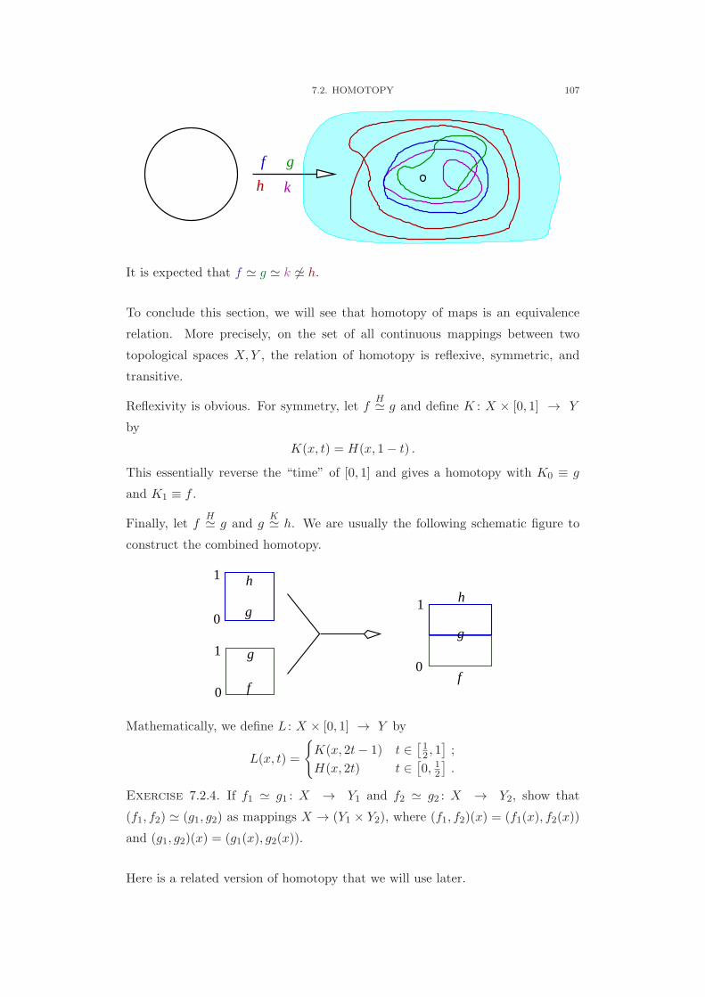
7.2. HOMOTOPY 107
f g
h k
It is expected that f ≃ g ≃ k ≃ h.
To conclude this section, we will see that homotopy of maps is an equivalence
relation. More precisely, on the set of all continuous mappings between two
topological spaces X,Y , the relation of homotopy is reflexive, symmetric, and
transitive.
Reflexivity is obvious. For symmetry, let fH≃ g and define K : X × [0, 1] → Y
by
K(x, t) = H(x, 1− t) .
This essentially reverse the “time” of [0, 1] and gives a homotopy with K0 ≡ g
and K1 ≡ f .
Finally, let fH≃ g and g
K≃ h. We are usually the following schematic figure to
construct the combined homotopy.
f
g
g
h
0
1
0
1
0
1
g
h
f
Mathematically, we define L : X × [0, 1] → Y by
L(x, t) =
K(x, 2t− 1) t ∈
[12 , 1];
H(x, 2t) t ∈[0, 12].
Exercise 7.2.4. If f1 ≃ g1 : X → Y1 and f2 ≃ g2 : X → Y2, show that
(f1, f2) ≃ (g1, g2) as mappings X → (Y1 × Y2), where (f1, f2)(x) = (f1(x), f2(x))
and (g1, g2)(x) = (g1(x), g2(x)).
Here is a related version of homotopy that we will use later.

108 7. ALGEBRAIC TOPOLOGY
Definition 7.16. Let X,Y be topological spaces, A ⊂ X. Two mappings
f, g : X → Y are homotopic rel A, usually written f ≃ g rel A, if there ex-
ists a homotopy H : X × [0, 1] → Y such that, besides H0 ≡ f and H1 ≡ g,
H(a, t) = f(a) = g(a) for all a ∈ A and for all t ∈ [0, 1].
Note that from the definition, f and g must already have the same restriction
on A, i.e., f |A ≡ g|A. Moreover, there is a weaker version called homotopy
preserving A, which only requires Ht(A) ⊂ A for all t ∈ [0, 1].
Exercise 7.2.5. Let h : [0, 1] → [0, 1] be a homeomorphism such that h(0) = 0
and h(1) = 1. Show that h ≃ id[0,1] rel 0, 1.
Exercise 7.2.6.
(1) Prove that both homotopy rel A and homotopy preserving A are equiv-
alence relations on mappings.
(2) Let X,Y, Z be spaces with A ⊂ X and B ⊂ Y . Let f0, f1 : X → Y
satisfy f0(A) = f1(A) ⊂ B and g1 : Y → X. If f0F≃ f1 rel A and
g0G≃ g1 rel B, is it true that g0 f0 ≃ g1 f1 rel A?
7.3. Homotopy Classes and Homotopy Equivalences
7.3.1. Homotopy Classes. In the previous section, we have established the
equivalence relation defined by homotopy of mappings. Let X,Y be topological
spaces and C(X,Y ) be the set of all continuous mappings from X to Y .
Definition 7.17. The quotient set C(X,Y )/≃ under the homotopy relation ≃ is
denoted [X,Y ] and any [f ] ∈ [X,Y ] is called a homotopy class of f .
As we have seen above, since every continuous mapping into Rn, n ≥ 1, is homo-
topic to a constant map, [X,Rn] is a singleton set. This is true in particular for
[S1,Rn]. On the other hand, from the intuitive argument, the set [S1,R2\(0, 0)]contains at least two different elements. It is natural to expect that
[S1,Rn] = [S1,R2 \ (0, 0)] =⇒ Rn = R2 \ (0, 0) ,
where the equality of two topological spaces really means homeomorphic.
In order to establish such implication, we will need the following results and apply
the contra-positive.
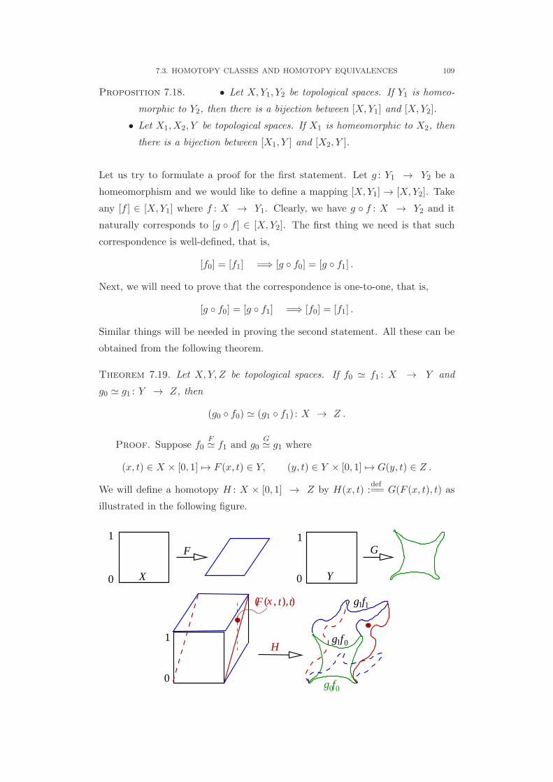
7.3. HOMOTOPY CLASSES AND HOMOTOPY EQUIVALENCES 109
Proposition 7.18. • Let X,Y1, Y2 be topological spaces. If Y1 is homeo-
morphic to Y2, then there is a bijection between [X,Y1] and [X,Y2].
• Let X1, X2, Y be topological spaces. If X1 is homeomorphic to X2, then
there is a bijection between [X1, Y ] and [X2, Y ].
Let us try to formulate a proof for the first statement. Let g : Y1 → Y2 be a
homeomorphism and we would like to define a mapping [X,Y1] → [X,Y2]. Take
any [f ] ∈ [X,Y1] where f : X → Y1. Clearly, we have g f : X → Y2 and it
naturally corresponds to [g f ] ∈ [X,Y2]. The first thing we need is that such
correspondence is well-defined, that is,
[f0] = [f1] =⇒ [g f0] = [g f1] .
Next, we will need to prove that the correspondence is one-to-one, that is,
[g f0] = [g f1] =⇒ [f0] = [f1] .
Similar things will be needed in proving the second statement. All these can be
obtained from the following theorem.
Theorem 7.19. Let X,Y, Z be topological spaces. If f0 ≃ f1 : X → Y and
g0 ≃ g1 : Y → Z, then
(g0 f0) ≃ (g1 f1) : X → Z .
Proof. Suppose f0F≃ f1 and g0
G≃ g1 where
(x, t) ∈ X × [0, 1] 7→ F (x, t) ∈ Y, (y, t) ∈ Y × [0, 1] 7→ G(y, t) ∈ Z .
We will define a homotopy H : X × [0, 1] → Z by H(x, t)def:== G(F (x, t), t) as
illustrated in the following figure.
0
1F
X Y
G
0
1
g f0 0
g f1 1( ( , ), )F x t t
g f1 0
0
1H

110 7. ALGEBRAIC TOPOLOGY
Then it is clear that
H(x, 0) = G(F (x, 0), 0) = G(f0(x), 0) = g0f0(x)
H(x, 1) = G(F (x, 1), 1) = G(f1(x), 1) = g1f1(x) .
Obviously, indeed we proved that g0 f0 ≃ g0 f1 ≃ g1 f0 ≃ g1 f1.
Exercise 7.3.1.
(1) Formulate and prove the analogous statement about g0f0 ≃ g1f1 rel Afor A ⊂ X.
(2) If f1 ≃ g1 : X → Y1 and f2 ≃ g2 : X → Y2, show that (f1, f2) ≃ (g1, g2)
as mappings X → (Y1 × Y2), where (f1, f2)(x) = (f1(x), f2(x)) and
(g1, g2)(x) = (g1(x), g2(x)).
(3) Let Y be any topological space. Form the quotient space CY = (Y ×[0, 1])/∼ by the equivalence relation ∼ on Y ×[0, 1] with (y1, t1) ∼ (y2, t2)
if t1 = 1 = t2. That is, CY is obtained by crushing the “top” Y × 1to one point. Prove that any map f : X → CY is null homotopic.
7.3.2. Homotopy Types. Previously, we have discussed two conditions on
a space X, which are proved to be equivalent,
• Every mapping f : W → X is null homotopic, i.e., homotopic to a
constant map.
⋆ The identity mapping idX : X → X is null homotopic.
An example given before is Rn for n ≥ 1.
Definition 7.20. A topological space X is called contractible if idX : X → X
is null homotopic.
Example 7.21. The following are contractible spaces.
(1) The Euclidean spaces Rn, n ≥ 1.
(2) A convex subset of Rn.(3) A star-shaped subset A ⊂ Rn, namely, there exists a0 ∈ A such that for
each a ∈ A, the line segment joining a0 to a lies in A.
(4) The most simplest example, i.e., a point x0 .
In fact, roughly speaking, in terms of algebraic topology, a contractible space is
as simple as a point.
Exercise 7.3.2. Show that a contractible space is path connected.

7.3. HOMOTOPY CLASSES AND HOMOTOPY EQUIVALENCES 111
Definition 7.22. Two spaces X,Y are of the same homotopy type or homotopy
equivalent, written as X ≃ Y , if there are continuous mappings f : X → Y and
g : Y → X such that g f ≃ idX and f g ≃ idY . Here, we say that f, g are
homotopy inverses to each other.
Example 7.23.
(1) It is clear that if X,Y are homeomorphic then they are homotopy equiv-
alent. In that case, one exactly gets g f ≡ idX and f g ≡ idY .
(2) A contractible space X has exactly the homotopy type of a point.
Exercise 7.3.3. Let X be a topological space and Y be contractible. Prove that
X and X × Y are homotopy equivalent. In addition, if y0 ∈ Y then X × y0 ≃X × Y where the homotopy equivalences can be chosen rel X × y0.
Now, in the light of Theorem 7.19, we indeed have the following.
Proposition 7.24.
• Let X,Y1, Y2 be topological spaces. If Y1, Y2 are of the same homotopy
type, then there is a bijection between [X,Y1] and [X,Y2].
• Let X1, X2, Y be topological spaces. If X1, X2 are of the same homotopy
type, then there is a bijection between [X1, Y ] and [X2, Y ].
Example 7.25. The product space S1 × R is homotopy equivalent to S1 via the
following mappings.
eiθ ∈ S1f
−−−−→(eiθ, 0
)∈ S1 × R ;(
eiθ, s)∈ S1 × R
g−−−−→ eiθ ∈ S1 .
Then g f ≡ idS1 while f g(eiθ, s
)=(eiθ, 0
). Observe that
(eiθ, ts
)gives
the required homotopy between f g and idS1×R, which indeed is a homotopy
rel S1 × 0.
In this example, one observes that S1×0 is a special subset of S1×R. It has thehomotopy type of the whole space. Moreover, as mentioned above, the homotopy
can be chosen to fix every point of S1 × 0. In such a case, S1 × 0 is called a
strong deformation retract of S1 × R.
Exercise 7.3.4.
(1) Show that homotopy equivalence (homotopy type) defines an equivalence
relation on all the topological spaces.

112 7. ALGEBRAIC TOPOLOGY
(2) Show that a space of two points, i.e., S0 = −1, 1 with discrete topol-
ogy, is not homotopy equivalent to a one point space. In other words,
S0 is not contractible.
(3) Consider the unit sphere Sn−1 and the punctured space Rn \ 0. Showthat they are homotopy equivalent.
Example 7.26. The punctured torus, S1 × S1 \ point is homotopy equivalent
to a figure-8 shape, denoted S1 ∧ S1. A figure-8 shape can be formed by gluing
two circles at one point.
hole
Exercise 7.3.5. Prove the above fact about the punctured torus by using torus
as a quotient space on the square.
Finally, there are some results involving the mapping cone. These are presented
in the form of exercises. Given f : X → Y , there is a natural mapping, again
denote it by f , from X × 0 → Y . One may define the quotient spaces (called
mapping cylinder and mapping cone),
Mf = ((X × [0, 1]) ⊔ Y )/ ∼, where (x, 0) ∼ f(x);
Cf = ((X × [0, 1]) ⊔ Y )/ ∼, where (x, 0) ∼ f(x) and (x1, 1) ∼ (x2, 1).
Remark . To understand these two objects, imagine f : S1 → R to be the
standard embedding. Then Mf is a tall hat while Cf is a wizard hat. In general,
f need not to be one-to-one. In addition, if Dn is the closed n-dimensional unit
disk and f : Sn → Dn+1 is the standard embedding, then Cf = Sn+1.
Exercise 7.3.6. Show that if f, g : X → Y are homotopic mappings, then
Mf and Mg are homotopy equivalent; likewise, Cf and Cg are also homotopy
equivalent.

7.4. FUNDAMENTAL GROUP 113
Remark . Using this, one may prove the USELESS result: if Sn is contractible
then so is Sn+1. The converse is the USEFUL part because one may set up an
induction process. Together with that S0 is not contractible (done above), we
prove Sn is not contractible.
Exercise 7.3.7. Those interested may try to show if bothX and Y are Hausdorff,
then so are Mf and Cf .
7.4. Fundamental Group
As we have seen above, one way to understand a topological space X is to look
at homotopy classes [W,X] for various spaces W . Naturally, we would choose
spaces W such that it is easy to investigate and there is a geometric meaning. In
fact, spheres of various dimensions are good candidates.
Exercise 7.4.1. Recall the S0 is the discrete space −1, 1 . Show that a space
X has trivial [S0, X] if and only if X is path connected.
Hint. If f, g : S0 → X are homotopic, what do you know about the two pairs of points,
f(−1), g(−1) and f(1), g(1)?
Along the same line of proof in this exercise, if X is not path connected, one
sees that [S0, X] still reflects the path components of X but the record is “re-
peated”. To make it clearer, one would set up a fixed base point x0 ∈ X. Denote
f : (S0,−1) → (X,x0) be a continuous mapping from S0 toX taking f(−1) = x0.
Then [(S0,−1), (X,x0)] is the set of homotopy classes rel −1.
Exercise 7.4.2. Show that the number of elements of [(S0,−1), (X,x0)] is exactly
the number of path components of X.
Next, we would to consider [S1, X]. Again, it is more useful to have a fixed base
point x0 ∈ X. That corresponds to the following construction of the so-called
fundamental group, π1(X,x0).
Recall that a path in X is defined as a continuous mapping γ from [0, 1] into X.
Throughout this section, we will consider a special kind of homotopies between
two paths with the same end-points.
Definition 7.27. Let γ0, γ1 : [0, 1] → X be two paths in X such that γ0(0) =
γ1(0) and γ0(1) = γ1(1). A homotopy rel 0, 1 between the paths is also called
a path homotopy .

114 7. ALGEBRAIC TOPOLOGY
Such a homotopy H : [0, 1]× [0, 1] → X satisfies two major conditions:
(a) Homotopy: H(s, 0) = γ0(s) and H(s, 1) = γ1(s) for all s ∈ [0, 1];
(b) End-points fixed: H(0, t) = γ0(0) = γ1(0) and H(1, t) = γ0(1) = γ1(1)
for all t ∈ [0, 1].
Definition 7.28. Let X be a topological space and x0 ∈ X. A loop based at x0
is a closed path with both end-points at x0. A loop homotopy between two loops
γ0, γ1 based at x0 is a homotopy rel 0, 1 between them.
x0
0γ 1γ
In the above, we only consider paths (loops) that have parameter in [0, 1] for
convenience, because re-parametrization simply gives homotopic paths. The fol-
lowing can be proved using Exercise 7.2.5 or a modified version of Theorem 7.19.
Proposition 7.29. If h : [0, 1] → [0, 1] is a change of parameter, i.e., home-
omorphism with h(0) = 0 and h(1) = 1; and γ is a path in X, then h γ ≃ γ
rel 0, 1.
7.4.1. Concatenation of paths. Let α, β : [0, 1] → X be paths (or loops)
in X such that α(1) = β(0), i.e., the second path begins at the point where the
first one terminates. There is a new path formed by first tracing α and then β,
called α ∗ β : [0, 1] → X defined by
(α ∗ β)(s) def:==
α(2s) s ∈
[0, 12],
β(2s− 1) s ∈[12 , 1].
α β*α
β
0 1
The set of points in X of (α ∗ β) is the same as the union of those of α and β.
But, the above definition is to reset the parameter so that it is defined on [0, 1].

7.4. FUNDAMENTAL GROUP 115
Now, naturally, we expect to define an algebraic operation (α, β) 7→ α ∗ β on
paths or loops. However, it is not exactly valid because, as mappings on [0, 1],
(α ∗β)∗γ = α ∗ (β ∗γ). It is clear that in (α ∗β)∗γ, α is defined on [0, 1/4] while
it is defined on [0, 1/2] in α ∗ (β ∗ γ). This leads us to consider the operation on
homotopy classes of paths relative end points.
Let [α] denote the set of paths which are homotopic rel 0, 1 to α. First, we
would like to define a product by [α] ∗ [β] = [α ∗ β] if α(1) = β(0) or if α, β are
both based at x0. The following guarantees that it is well-defined.
Proposition 7.30. If α0 ≃ α1 rel 0, 1 and β0 ≃ β1 rel 0, 1, then
α0 ∗ β0 ≃ α1 ∗ β1 rel 0, 1 .
Proof. Let F,G be the homotopy rel 0, 1 between α0, α1 and β0, β1 re-
spectively. Obviously, the desired homotopy is obtained by combining them by a
process similar to concatenation. The details are left as Exercise 7.4.3.
Moreover, the product for path or loop homotopy classes is associative, that is,
([α] ∗ [β]) ∗ [γ] = [α] ∗ ([β] ∗ [γ]) .
Proposition 7.31. (α ∗ β) ∗ γ ≃ α ∗ (β ∗ γ) rel 0, 1.
Proof. Since the images of (α ∗ β) ∗ γ and α ∗ (β ∗ γ) are the same, the
homotopy is simply changing the “speed” of the parameters. Observe from the
following diagram,
ta ( )b ( )t
0
1
α β γ
α β γ
t
and define H : [0, 1]× [0, 1] → X with
H(s, t) =
α(
sa(t)
)s ∈ [0, a(t)]
β (??) s ∈ [a(t), b(t)]
γ (??) s ∈ [b(t), 1] .
It can be easily seen that H is the required homotopy rel 0, 1.

116 7. ALGEBRAIC TOPOLOGY
Exercise 7.4.4. Complete the above proof by finding out a(t), b(t), and those
??’s in the definition of H.
With these three propositions (7.24, 7.30, 7.31), for a topological space X with
x0 ∈ X, we define
π1(X,x0)def:== loops in X based at x0 ∈ X /≃ rel 0, 1 .
For loop homotopy classes [α], [β] ∈ π1(X,x0), an associative product is well-
defined by
[α] ∗ [β] def:== [α ∗ β] .
In the remaining of this section, we will show that (π1(X,x0), ∗) is a group. In
this situation, we only need to exhibit an identity element and show that an
inverse element exists for each element.
Definition 7.32. The group (π1(X,x0), ∗) is the fundamental group of X at x0.
The identity element is given by the constant loop. For x0 ∈ X, let
c0 : [0, 1] → X, c0(s) = x0, s ∈ [0, 1]
define the continous path (loop) in X. Denote its homotopy class by 1. Similarly,
for a point x1 ∈ X (which may also be x0), denote a constant map c1.
Proposition 7.33. For each path γ from x0 to x1, c0 ∗ γ ≃ γ ≃ γ ∗ c1 rel 0, 1.In particular, when x0 = x1 and α is a loop, [α] ∗ 1 = [α] = 1 ∗ [α].
Proof. Again, the images of the three paths are the same set in X, it is
sufficient to find homotopies that essentially are changing the parameters.
ta ( )
0
1
γ
t
γ
c
1
t
0cγ
γ
The above two diagrams provide the observation to get the desired homotopies.
Again, the explicit expressions of the homotopies are left as Exercise 7.4.5.

7.4. FUNDAMENTAL GROUP 117
Next, for a path γ in X from x0 to x1 ∈ X, we may define another path, which
is essentially the reversed direction of γ, namely,
γ : [0, 1] → X γ(s) = γ(1− s), s ∈ [0, 1] .
If α is a loop based at x0, its homotopy class will give the inverse element of [α],
i.e., [α]−1 = [α].
Proposition 7.34. With the notation above, α ∗ α ≃ c0 ≃ α ∗ α rel 0, 1.
Proof. As α ∗ α is simply tracing the whole α and then back tracing the
whole loop, one can gradually trace only part the the loop α and eventually never
move away from x0. The homotopy for α ∗ α ≃ c0 rel 0, 1 is given by
F : [0, 1]× [0, 1] → X F (s, t) =
α(2st) s ∈
[0, 12]
α(t(1− 2s)) s ∈[12 , 1].
The other one for α ∗ α ≃ c0 is similarly constructed.
Definition 7.35. A path connected space X is called simply connected or 1-
connected if there exists x0 ∈ X such that π1(X,x0) is the trivial group, i.e., it
only contains the identity element 1 = [c0].
Since fundamental groups are normally non-abelian, the trivial group is usually
written as 1.
Next, we discuss the effect of the base point. More precisely, if the space is path
connected, then the fundamental group is independent of the choice of the base
point.
Let X be a path connected space and x0, x1 ∈ X. Let σ : [0, 1] → X be
any path joining them, i.e., σ(0) = x0 and σ(1) = x1. Consider a mapping
φσ : π1(X,x0) → π1(X,x1) defined by the following. Let [α] ∈ π1(X,x0) be a
homotopy class of a loop α based at x0. Then σ ∗ α ∗ σ is a loop based at x1.
Take φσ([α])def:== [σ ∗ α ∗ σ].
Exercise 7.4.6. Show that φσ is well defined. That is, if α0 ≃ α1 rel 0, 1, thenσ ∗ α0 ∗ σ ≃ σ ∗ α1 ∗ σ rel 0, 1.
With the exercise, since σ is a path from x1 to x0, it follows naturally that we
also have the mapping φσ from π1(X,x1) back to π1(X,x0). In fact, we have
φσ φσ = id = φσ φσ. Therefore, φσ is in fact the inverse of φσ.
Theorem 7.36. The mapping φσ is an isomorphism from π1(X,x0) to π1(X,x1).
118 7. ALGEBRAIC TOPOLOGY
Exercise 7.4.7. Verify that φσ is a homomorphism, i.e.,
φσ([α] · [β]) = φσ([α]) · φσ([β]) ,
and other details of the proof of the above theorem. Also, show that if σ and τ
are two paths from x0 to x1 such that σ ≃ τ rel 0, 1, then φσ ∼= φτ .
7.5. Useful Examples
7.5.1. Euclidean and the Simplest Ones. The Euclidean spaces Rn, n =
0, 1, 2, . . . belong to the simplest topological spaces because they are contractible.
Recall that a space X is contractible if its identity map idX is homotopic to a
constant map c on X. It does not matter which constant map we are taking.
Exercise 7.5.1. Let X be a path connected space, x1, x2 ∈ X and c1, c2 be
constant maps where c1(x) = x1 and c2(x) = x2 for all x ∈ X. Show that c1 ≃ c2.
Proposition 7.37. If X is contractible and x0 ∈ X, then π1(X,x0) is trivial. In
particular, each Euclidean space Rn is simply connected.
Proof. Without loss of generality, assume c(x) = x0 for all x ∈ X. Let
idXF≃ c : X → X. Then for any loop γ in X based at x0,
γ = idX γ ≃ c γ .
Clearly c γ is the constant path, i.e., [c γ] = 1 ∈ π1(X,x0).
Another obvious example of contractible, and hence simply connected, space is
the open disk or closed disk,
x ∈ Rn : ∥x∥ < 1 or x ∈ Rn : ∥x∥ ≤ 1 .
Indeed, they both are convex subsets of Rn. Recall that a star-shaped X ⊂ Rn
satisfies that there exist a point x0 ∈ X such that every point x ∈ X can be
joined to x0 by a straight line. Obviously, a convex subset is of star-shaped.
Exercise 7.5.2. Show that any star-shaped subset of Rn is contractible and thus
simply-connected.
7.5.2. The Circle and Punctured Plane. The circle S1 gives an impor-
tant example of fundamental group because of two reasons. First, the space is
simple enough so the geometry and algebraic properties are easy to visualize.
Second, it has a typical structure that occurs in a more general context that
naturally leads to theory of covering spaces.

7.5. USEFUL EXAMPLES 119
Proposition 7.38. Let x0 be a point in S1 ⊂ R2 \ 0. Then
π1(S1, x0) ∼= π1(R2 \ 0
) ∼= (Z,+) .
In the rest of this section, we will give the main ideas of the proof of the above
fact. The first isomorphism is due to the fact that S1 and R2 \ 0 are homotopy
equivalent.
Exercise 7.5.3. Show that if p : R2 \ 0 → S1 is defined by p(x) = x/ ∥x∥,then the inclusion S1 → R2 \ 0 and the mapping p are homotopy inverse to
each other.
The second isomorphism can be described by the following. Let [γ] ∈ π1(R2 \ 0
)be represented by a loop γ based at the point x0. Then
[γ] 7→ winding number of γ : π1(R2 \ 0
)→ Z
is well-defined and indeed is an isomorphism. For example, in the picture below,
[α] 7→ 1 and its backward oriented curve goes to −1; moreover, [β] = [α]∗[α] 7→ 2.
0xα
β
In the case that γ is a piecewise differentiable loop, we have
Winding number of γ =1
2π
∫γ
dz
z.
However, when γ is simply a continuous loop, the winding number may be ob-
tained in a topological method. For instance, let L be a half-line from 0 to infinity
such that L cuts γ transversely (never tangentially). Then there are finitely many
intersecting points in L ∩ γ. Define
The sign at an intersection =
+1 if γ cuts L counterclockwisely
−1 if γ cuts L clockwisely.
0x
γ
L
_ + + + _

120 7. ALGEBRAIC TOPOLOGY
Then the winding number is the sum of signs over all intersection points.
Exercise 7.5.4. Take an example of γ, try different choices of half-lines L to
calculate the winding number. Convince yourself that the result is independent
of the choice of L.
To come up with a proof of the independency, one may first show that the wind-
ing number will not change if the angle of L is continuously perturbed a little.
And the number of intersection points may change only when L passes through
a tangential intersection of γ at some angle. Then argue that two opposite in-
tersections disappear in this situation. The similar argument may apply to a
homotopy of γ.
Exercise 7.5.5. Convince yourself that this method of calculating winding num-
ber gives an isomorphism.
In the following, we will sketch another proof of Proposition 7.38. This is an
alternative way of seeing the winding number and thus an isomorphism between
π1(S1, z0) and Z is established. It should note that the study of the fundamental
group of the circle is an important revelation to the theory of covering spaces.
Many books may prove the proposition at the same time of discussing covering
spaces. However, due to time limitation, we will take an elementary route; though
the idea behind the proof is essentially the same.
Lemma 7.39. Let γ : [0, 1] → C \ 0 with γ(0) = γ(1) = z0 be a continuous
loop into the punctured plane. Then there is a continuous function θ : [0, 1] → Rsuch that for all s ∈ [0, 1],
cos θ(s) =Re[γ(s)]
|γ(s)|, sin θ(s) =
Im[γ(s)]
|γ(s)|.
This function θ(s) is uniquely determined by the choice of its value θ(0). It is
called a continuous choice of the argument of the curve γ.
Sketch of proof. First, if the image of γ lies in a half-plane of C, thenit is easy to show that such choice of θ(s) exists. In this case, one may fix the
value of θ(0) according to the point z0 ∈ C \ 0. Then for the above equations
of cos θ(s) and sin θ(s), for each s ∈ [0, 1], there exists a unique solution inside
the interval (θ(0)− π, θ(0) + π). In fact, if γ is differentiable, it is exactly given
by
θ(s) = θ(0) +
∫ s
0
γ′(t) dt
γ(t).

7.5. USEFUL EXAMPLES 121
Second, for general γ, by compactness, one may subdivide [0, 1] into finitely many
subintervals such that the image of γ of each subinterval lies in a half-plane. Then
inductively, a continuous choice of θ(s) can be obtained.
Since γ(0) = γ(1) = z0, we have
cos θ(0) = cos θ(1) =Re[z0]
|z0|, sin θ(0) = sin θ(1) =
Im[z0]
|z0|.
It turns out that θ(1) = θ(0) + 2dπ for some d ∈ Z. By continuity of γ and
connectedness of [0, 1], it can be shown that d is uniquely determined by γ. An
example of d = 2 is shown below.
( )s
z 0
θ( )s
θ( )s
3γ
0 1
π
π
π
π
2
4
Obviously, from the graph of θ(s), a homotopy between θ(s) and θ(0) + 2dπs
rel 0, 1 is easily constructed, which in turns leads to a homotopy rel 0, 1between γ(s) and the d-fold circle. Thus we have
Lemma 7.40. For each continuous loop γ, there exists a unique d ∈ Z such that
γ is homotopic to the d-fold circle relative end-point.
Then the mapping taking the homotopy class [γ] ∈ π1(S1, z0) to d ∈ Z is the
desired isomorphism. Hence Proposition 7.38 is established.
7.5.3. Spheres and Punctured Euclidean spaces. Similar to the situa-
tion of the circle and punctured plane, the n-sphere and punctured space are of
the same homotopy type.
Proposition 7.41. For all n ≥ 1, the n-sphere Sn ≃ Rn+1 \ 0.
However, in higher dimensional cases, the fundamental group becomes trivial.
Proposition 7.42. For n ≥ 2, π1(Sn, z0) ∼= π1(Rn+1 \ 0, z0) = 1.
The proof of this result makes use of the Van Kampen’s Theorem, which is out
of the scope of this course. An illustration of S2 may be helpful.

122 7. ALGEBRAIC TOPOLOGY
U
z 0L
Let S2 = U ∪L where U,L are the upper and lower parts as shown. Then U ∩L is
homeomorphic to a cylinder S1 × [−δ, δ] ≃ S1. Take a point z0 in the equator S1.In this way, Van Kampen’s Theorem tells us that π1(S2, z0) is a “product group”
of π1(U, z0) and π1(L, z0) with some correction due to π1(S1, z0). However, since
both U and L are homeomorphic to a disk, we have π1(U, z0) = 1 = π1(L, z0)
and hence π1(S2, z0) = 1.
For higher dimensions, Van Kampen’s Theorem expresses π1(Sn, z0) in terms of
π1(En+, z0), π1(En−, z0), and π1(Sn−1, z0), where En± denotes the upper and lower
n-hemisphere. Through an inductive process on S1 ⊂ S2 ⊂ · · · ⊂ Sn, one may
show that any loop in Sn is homotopically trivial except in S1.
7.5.4. The Torus. Recall that the 2-dimensional torus can be seen from
three perspectives, as a product of circles or as a surface of revolution in R3 or
as a quotient space of a rectangle. We will use all of them to understand the
fundamental group of the torus, whichever is convenient.
Exercise 7.5.6. Let X,Y be connected topological spaces with x0 ∈ X and
y0 ∈ Y . Then π1 (X × Y, (x0, y0) ) ∼= π1(X,x0) × π1(Y, y0) , where the × on the
right hand side denotes direct product of groups. Hint. Any loop in X × Y is of
the form (γX(s), γY (s)) where γX and γY are loops in X and Y respectively.
Consequently, we may apply the result of the exercise to the torus.
Proposition 7.43. π1(T, ∗) ∼= π1(S1, ∗)× π1(S1, ∗) ∼= (Z⊕ Z,+).
The generators [α], [β] ∈ π1(T, ∗) corresponding to (1, 0), (0, 1) ∈ Z⊕Z are shown
in the surface of revolution below.
β
α

7.5. USEFUL EXAMPLES 123
Note that the group Z⊕Z is abelian. Since [α][β] and [β][α] naturally are mapped
to (1, 1), therefore, we should expect that α ∗ β ≃ β ∗ α rel 0, 1. This can be
seen in the illustration of quotient space below. Equivalently, in π1(T, ∗), thereare two generators, α and β, but they obey a relation αβα−1β−1 = 1.
αβ
βα
α α
β
β
7.5.5. Surface of Genus 2. This example is intended to illustrate how the
fundamental group records topological information of a space. Many steps are
not rigorously enough. A surface S of genus 2 is sort of a double torus.
α1
β1
β2
α2
Naturally, one would expect that α1, β1 and α2, β2 are four generators for the
group π1(S, x0), where x0 is the base point at the common intersection of them.
However, now we do not have the same abelian property as in the situation of
the torus. This can be explained by Van Kampen’s Theorem again.
Let us cut the surface into two pieces, left-half and right-half, as shown in the
picture below.
γ
1
β1
α
β2
α2
Unlike the torus, α1β1α−11 β−1
1 does not form the boundary of a rectangle. Instead,
they are the four sides of a pentagon and the fifth side is γ, which is the cut open
circle. Therefore the relation is α1β1α−11 β−1
1 = γ.

124 7. ALGEBRAIC TOPOLOGY
α−1 β−1
αβ
γ
The right-half gives a similar pentagon but the open circle is denoted by γ−1.
Thus the relation is α2β2α−12 β−1
2 = γ−1. In view of Van Kampen’s Theorem,
the surface S = L ∪ R and L ∩ R is the yellow tube ≃ cylinder ≃ S1. The two
generators on the left and the two on the right need to satisfy a condition in the
yellow tube, namely,
α1β1α−11 β−1
1 α2β2α−12 β−1
2 = 1 .
Then π1(S, x0) is presented by a group of four generators with the above relation.
7.5.6. Projective Plane. Recall that the 2-dimensional real projective plane
can be defined as RP2 = D2/∼ where D2 = z ∈ Z : |z| ≤ 1 and
z1 ∼ z2 if
z1 = z2
z1 = −z2 with |z1| = |z2| = 1 .
Let us observe what happens from the following picture.
0
x1x3
x 0
x1 x3
x2
x2
xβ
α
γ
γ
Any simple loop in RP2 corresponds to a simple loop or a simple arc in D2, each
illustrated by an example in the picture. A simple loop in D2 is null homotopic
and so is the corresponding one in RP2. An simple arc such as β ∈ D2 corre-
sponds to a non-trivial loop in RP2. Clearly, in D2, by “pushing downward”, β is
homotopic to γ on the lower half boundary. Since RP2 is obtained by identifying
the boundary of D2 according to that z1 = −z2. This γ in the lower half of D2
will become a simple arc on the upper half boundary. By “pushing upward”, one
sees that β is homotopic to −γ on the upper boundary. So γ ≃ −γ relative the

7.5. USEFUL EXAMPLES 125
end-point. Equivalently, [γ]2 = 1 in the fundamental group π1(T, x0). With some
algebraic calculations, one may prove that
Proposition 7.44. π1(RP2, x0) ≃ (Z/2Z,+).
Combining the argument of the cases of the torus and the projective plane, one
may also obtain that
Proposition 7.45. π1(K, ∗) ≃ (Z⊕ Z/2Z,+) where K is the Klein bottle.
7.5.7. Two-punctured Plane. Let X = R2 \ xℓ, xr be the plane with
two points removed, where xℓ = (−1, 0) and xr = (1, 0) ∈ R2. Pick a base point
x0 ∈ X and choose two positively oriented simple closed loops α and β around
xr and xℓ respectively.
l x r
x0
x
β
α
It is naturally imagined that α and β are generators for the fundamental group,
π1(X,x0), of the two-punctured plane. We will see below that [α] [β] = [β] [α] in
the fundamental group. In fact, there are no other relations. Thus, π1(X,x0) is
the free group on two generators. For those who are not familiar with algebra,
this means the group consists of all possible products, including the followings,
1, α, α−1, β, β−1, αβ, β−1α−1, βα, α−1β−1, α−1β, β−1α, αβ−1, βα−1,
αβα, α−1β−1α−1, βαβ, β−1α−1β−1, α2β, β−1α−2, . . . . . . .
The two-punctured plane is homeomorphic to the so-called pair of pants as shown
in the following picture.
x l x r
8
αβ
Both the two-punctured plane and the pair of pants are homotopy equivalent to
a figure-8, usually denoted as S1 ∧ S1.

126 7. ALGEBRAIC TOPOLOGY
It is good to illustrate why its fundamental group π1(X,x0) is not abelian. From
the illustration, one also sees the importance of requiring the homotopy to fix the
base point x0. Suppose there is a homotopy H rel end-points between α ∗ β and
β ∗ α, it will be represented by the following square where slight deformation at
t = ε, 1− ε are shown.
0x0
1−ε
x
β α
α β
ε
Then, the curves Hε and H1−ε are shown in the pictures, which cannot be de-
formed to each other with the point x0 fixed.
0
x l x r
xα
β H ε
0
x l x r
xα
β 1−H ε
Note that if the starting and ending points are not fixed at x0, the curves Hε and
H1−ε can be deformed to each other.
7.6. Homotopy Invariance
As it is seen in Section 7.3, a continuous function between topological spaces
induces a mapping between homotopy classes involving the two spaces. This
already gives us a way to distinguish two spaces. The group structure of funda-
mental groups provides further information for such purpose.

7.6. HOMOTOPY INVARIANCE 127
Let X,Y be topological spaces and φ : X → Y be a continuous function with
φ(x0) = y0. For convenience, we usually use the notation φ : (X,x0) → (Y, y0) to
specify such situation. More generally, if A ⊂ X and B ⊂ Y , φ : (X,A) → (Y,B)
means that φ(A) ⊂ B.
Given a loop γ inX with base point x0, i.e., γ : [0, 1] → X with γ(0) = x0 = γ(1).
The composition φγ : [0, 1] → Y is clearly a loop in Y with base point y0 ∈ Y .
Moreover, if two loops γ0, γ1 : [0, 1] → X are two homotopic rel base point x0,
by Theorem 7.19, the loops φ γ0 and φ γ1 are homotopic rel base point y0
(Exercise 7.6.1). Therefore, given an element [γ] ∈ π1(X,x0), a loop homotopy
class [φ γ] ∈ π1(Y, y0) is defined, which only depends on the loop homotopy
class of [γ].
Definition 7.46. The mapping defined above is denoted
φ# or φ∗ : π1(X,x0) → π2(Y, y0) .
Not only the mapping is useful, the additional group structure is also important.
Theorem 7.47. Let φ : (X,x0) → (Y, y0) be a continous function. Then the
mapping φ# : π1(X,x0) → π1(Y, y0) is a homomorphism.
Proof. Let α, β be loops with base point x0 which represent [α], [β] ∈π1(X,x0) respectively. It is needed to show that φ#([α] · [β]) = φ#([α]) ·φ#([β]).
According to the definition of φ#, it is equivalent to show that
φ (α ∗ β) ≃ (φ α) ∗ (φ β) rel the end point y0.
In fact, considering the definition of concatenation ∗, one has eqality above.
Exercise 7.6.2. (1) What is id# on π1(X,x0) where id : X → X is the
identity map?
(2) Let x0 ∈ A ⊂ X. Does the inclusion map i : A → X induce an injective
homomorphism i# : π1(A, x0) → π1(X,x0) ?
(3) Suppose f : (X,x0) → (Y, y0) is a surjective continuous function. Is it
true that f# is also surjective?
Theorem 7.48. If two continuous functions φ ≃ ψ : X → Y are homotopic,
then they induce the same mapping, φ# ≡ ψ# on π1(X,x0).
Proof. The proof uses Theorem 7.19 again and it is left as Exercise 7.6.3.

128 7. ALGEBRAIC TOPOLOGY
In principle, the above result guarantees that the homomorphism induced on the
fundamental group is determined up to the homotopy of the continuous function.
Furthermore, this homomorphism is particular useful because of a property called
naturality .
Theorem 7.49. Let φ : (X,x0) → (Y, y0) and ψ : (Y, y0) → (Z, z0) be contin-
uous functions. Then
ψ# φ# ≡ (ψ φ)# : π1(X,x0) → π1(Z, z0) .
Proof. This is simply a consequence of ψ (φ α) = (ψ φ) α for any loop
α with base point x0.
This above naturality result is usually represented by the following figure.
(X,x0) (Y, y0)
(Z, z0)
π1(X,x0) π1(Y, y0)
π1(Z, z0)
-φ
@@
@@@@@R
ψφ
ψ
-φ#
@@@@
@@@R
ψ#φ#
(ψφ)#
ψ#
From Theorem 7.49, it is easy to obtain the following two useful facts.
Corollary 7.50. (1) If φ : (X,x0) → (Y, y0) and ψ : (Y, y0) → (X,x0)
are homotopy equivalences inverse to each other, then ψ# ≡ (φ#)−1
from π1(Y, y0) to π1(X,x0).
(2) If two spaces X,Y are homeomorphic, then their fundamental groups are
isomorphic.
Given a pair of homotopy inverses, which satisfy ψ φ ≃ idX and φ ψ ≃ idY .
However, in general φ(x0) = y0 but ψ(y0) = x1 = x0. In this case, we have
π1(X,x0)φ#
−−−−→ π1(Y, y0)ψ#
−−−−→ π1(X,x1) .
Exercise 7.6.4. Explore the relation between this isomorphism (ψφ)# and the
one in Theorem 7.36 from π1(X,x0) to π1(X,x1).

7.7. BROUWER FIXED POINT THEOREM 129
7.7. Brouwer Fixed Point Theorem
Let X be a topological space. A subset A ⊂ X is called a retract of X if there
is a continuous function r : X → A such that r|A ≡ idA, i.e., for all a ∈ A,
r(a) = a. Equivalently, if i : A → X is the inclusion map, then r i ≡ idA.
Example 7.51. (1) Any singleton x0 ⊂ X is a retract of X by taking
r to be the constant map on x0. However, this is an uninteresting
retract because the topology of x0 does not reflect anything about the
topology of X. The aim is always to look for a simple enough subset A
but it still gives useful information about X.
(2) The infinite cylinder Sn × R has retracts Sn × (−1, 1) and Sn × 0.
Exercise 7.7.1. (1) Show that if B ⊂ A ⊂ X and A is a retract of X while
B is a retract of A, then B is a retract of X.
(2) Show that the punctured torus S1 × S1 \ x0 has a retract of figure-8,
S1 ∧ S1.
Proposition 7.52. Let A ⊂ X be a retract. Then i# : π1(A, x0) → π1(X,x0)
is a monomorphism while r# : π1(X,x0) → π1(A, x0) is an epimorphism, where
x0 ∈ A.
Proof. Be careful, it is not because i is injective and r is surjective.
Observe from the following communtative diagrams,
(A, x0) (X,x0)
(A, x0)
π1(A, x0) π1(X,x0)
π1(A, x0)
-i
@@@@
@@@R
r i ≡ idA
r
-i#
@@@
@@@@R
id# ≡ id
r#
Since r# i# = idπ1(A,x0), we have i# injective and r# surjective.
Definition 7.53. Let X be a topological space and A ⊂ X is a retract with
an inclusion i : A → X and a retraction r : X → A such that r i ≡ idA.
The set A is a deformation retract if, in addition, r ≡ i r ≃ idX . If further,
r ≡ i r ≃ idX rel A, then A is a strong deformation retract of X.

130 7. ALGEBRAIC TOPOLOGY
Remark . In the above definition of strong deformation retract, the homotopy H
between r and idX must fix every point of A at any time t ∈ [0, 1], i.e., Ht|A ≡ idA.
In different books, there may be all sorts of variation for this definition. For
example, some may only require Ht(A) ⊂ A or Ht|A is a homeomorphism.
Proposition 7.54. If A ⊂ X is a deformation retract (or strong deformation
retract) of X and x0 ∈ A, then
i# : π1(A, x0) → π1(X,x0)
is an isomorphism with inverse r#.
Proof. It is left as Exercise 7.7.2.
Let Sn =x ∈ Rn+1 : ∥x∥ = 1
and Dn+1 =
x ∈ Rn+1 : ∥x∥ ≤ 1
be the
standard sphere and disk.
Theorem 7.55. The circle S1 is not a retract of the disk D2.
Remark . The analogous statement about Sn and Dn+1 is true. In fact, the
proof is similar but it requires a higher dimensional algebraic topological object.
Proof. Suppose otherwise, so we have the communtative diagrams.
(S1, x0) (D2, x0)
(S1, x0)
π1(S1, x0) π1(D2, x0)
π1(S1, x0)
-i
@@
@@@@@R
idS1
r
-i#
@@@@
@@@R
id#
r#
Note that π1(S1, x0) ∼= (Z,+) and π1(D2, x0)(0,+). Therefore, in the second
diagram, take 1 ∈ (Z,+)π1(S1, x0), one has i#(1) = 0 and so r# i#(1) = 0. On
the other hand, (r i)#(1) = id(1) = 1 = 0. This leads to a contradiction.
Assuming the above Theorem 7.55 is true for general Sn in Dn+1, we have the
following important result.
Theorem 7.56. (Brouwer Fixed Point Theorem) Every continuous function
f : Dn → Dn has a fixed point, i.e., x0 ∈ Dn such that f(x0) = x0.

7.7. BROUWER FIXED POINT THEOREM 131
Proof. Suppose otherwise, i.e., for every x ∈ Dn, f(x) = x. Then for each
x ∈ Dn, a point r(x) can be defined such that r(x), x, f(x) lie on a straight line
according to the following picture.
( )
( )r x
f xx
In fact, we have a continuous function r : Dn → Sn−1. Show this by finding the
explicit expression of r(x), Exercise 7.7.3.
It can be easily verified that r|Sn−1 ≡ idSn−1 . Thus, it leads to the contradiction
that Sn−1 is a retract of Dn.


![Std Specs Rev 8 Metric [9/25/98 Metric]](https://static.fdocuments.in/doc/165x107/61ae7e9c0229c362f478fa5d/std-specs-rev-8-metric-92598-metric.jpg)