Introduction to time series analysis · Introduction to time series analysis Statistical modelling:...

Introduction to time series analysisStatistical modelling: Theory and practice

Gilles Guillot

[email protected]

November 17, 2014

Gilles Guillot ([email protected]) Intro time series November 17, 2014 1 / 35

1 Motivating examples and outline

2 Probabilty concepts for time series

3 Second order characterics of a stochastic process

4 Auto-regressive models

5 References


Motivating examples and outline

Finance data



Geophysical data



Biomedical data



Civil engineering data



Di�erent scienti�c/technical �elds but common aspects inprevious examples I

Common questions:

A central question: prediction of future values

Other questions:

is the phenomenon periodic? what is the period?is there any trend ? can it be estimated (�ltering problem)is there a time structure?

Common data features:

Observations come in a speci�c order (time! here obs. index not just alabel!)

There is a pattern in the variation of variables across time

There is erratic variation away from the main �pattern�



Di�erent scienti�c/technical �elds but common aspects inprevious examples II

Goal of the lecture: give a �avour of statistical tools to model variationacross time.In lectures on linear model, we had y = βx+ ε. The focus was on the�pattern�, the rest was i.i.d noise. In this lecture, the �residual variation� isas important as the main �trend�.


Probabilty concepts for time series

Some de�nitions I

Time series: a set of observations of a variable at di�erent timepoints (yt)t=1,...,T = (y1, ..., yT )

Stochastic process: a set of random variables observed at di�erenttime points (Yt)t=1,...,T = (Y1, ..., YT ). If the random variables aremutually independent, the process is just a noise seen before.

Realization of a stochastic process: a single set of observations(yt)t=1,...,T = (y1, ..., yT ).


Probabilty concepts for time series

Some de�nitions II

Continuous-time stochastic process: model for a time series whichis (or could be in principle) observed continuously in time.Example:temperature in Lyngby

Discrete-time stochastic process: model for a time series which isby nature de�ned only at some discrete time points. Example:exchange rate euro/dollar, GDP of a country, max. daily temperature

Sampling frequency: number of observed data point per time unit

Support: the time period over which the variable is averaged. Do notmix up average daily tempeartures with �instant� temperaturemeasured at noon every day. Both are observed at the same frequencybut not over the same time support.


Second order characterics of a stochastic process

First and second order characterisation of a stochasticprocess I

De�nition: Mean function

For (Yt) a stochastic process, the mean function is de�ned as

µ(t) = E[Yt]



First and second order characterisation of a stochasticprocess II

NB: If n realizations y(k)t of (Yt) have been observed (e.g. variation of

glucose across time for n patients), then µ(t) can be estimated as

1/n∑n

k=1 y(k)t .

There is often only one realization available and the estimator above doesnot make sense. In this case the mean function is somehow arbitrary.Think of the mean exchange rate Dollar/Euro in November 20 2012?



De�nition: Variance function

For (Yt) a stochastic process, the variance function is de�ned as

σ2(t) = V ar[Yt]

With several realizations at hand, one could estimate σ2(t) by

σ2(t) = 1/(n− 1)∑n

k=1(y(k)t − yt)2



Covariance function of a stochastic process I

De�nition: Covariance function

For a stochastic process (Yt), the covariance function is de�ned as

C(t, t′) = Cov[Yt, Y′t ]

NB: C(t, t) = Cov[Yt, Yt] = σ2(t)



Covariance function of a stochastic process II

De�nition: Correlation function

For a stochastic process (Yt), the correlation function is de�ned as

ρ(t, t′) = Cor[Yt, Y′t ]

NB: ρ(t, t) = Cor[Yt, Yt] = 1



Stationarity I

De�nition: First-order stationarity

A stochastic process (Yt) is �rst-order stationary if its mean µ(t) does notdepend on time.



Stationarity II

De�nition: Second-order stationarity

A stochastic process (Yt) is second-order stationary if the covariancebetween two observations depends only on the time lag between them.Formally, there is a function K such that C(t, t′) = K(t− t′).In thise case, with a slight abuse, we often writes:C(t, t′) = C(t− t′) = C(k).



Gaussian stochastic processes I

De�nition: Gaussian process

A stochastic process (Yt) is Gaussian if for any susbet of time pointst1, ..., tn and any family of weights λ1, ..., λn the random variable

∑i λiYti

is normally distributed.



Gaussian stochastic processes II

Theorem: Density of a non-degenerated Gaussian process

If the covariance matrix Σ of a Gaussian process (Yt) observed at timepoints t1, ..., tn is non-singular, (Yt1 , ..., Ytn) admits a density of the form:

f(y) =1

|Σ|1/2(2π)n/2exp

[−1

2(y− µ)tΣ−1(y− µ)

]



Example of Gaussian processes

We consider below a second-order stationary Gaussian process with mean 0and covariance function C(t, t′) = C(t− t′) = C(k) = exp(−|k|/α). Withthree di�erent values for the scale parameter α = 3, 100, 1000



0 200 400 600 800 1000

0.0

0.2

0.4

0.6

0.8

1.0

h

C(h

)

31001000

Time

Y

0 200 400 600 800 1000

−3

−1

01

23

4

Realizations of three Gaussian stochastic processes with exponential covariances. Black curve:

�short range� dependence (α = 3). It is very erratic and the curve visits a broad range of values

within a short period of time.



Estimating the covariance function

Assuming that Yt is second-order stationary with covariance function C(k)we can estimate the (constant) mean by

µ = Y =

T∑t=1

Yt/T

and C(k) by

C(k) =1

Nt,t′

∑|t−t′|=k

(Yt − Y )(Yt′ − Y )

where Nt,t′ = #{|t− t′| = k}



Estimating the covariance and correlation function with R

The R function acf:acf(y,type,lag.max,plot=TRUE)

with type='covariance' or type='correlation'

Plot the empirical covariance or correlation.The R object returned is of class acf and contains covariance or correlationvalues at di�erent time lags.



R code used to estimate the covariance function

par(mfrow=c(3,1),mar=c(4,4,1,2))

acf(y1,lag.max=100,type='cov')

lines(times,exp(-times/alpha1))


lines(times,exp(-times/alpha2),col=2)


lines(times,exp(-times/alpha3),col=3)



Estimated covariances

0 20 40 60 80 100

−0.

20.

20.

40.

60.

81.

0

Lag

AC

F (

cov)

0 20 40 60 80 100

0.3

0.4

0.5

0.6

0.7

0.8

Lag

AC

F (

cov)

Series y2

0 20 40 60 80 100

0.3

0.4

0.5

0.6

0.7

Lag

AC

F (

cov)

Series y3



Estimated correlations

0 20 40 60 80 100

−0.

20.

20.

40.

60.

81.

0

Lag

AC

F

0 20 40 60 80 100

0.0

0.2

0.4

0.6

0.8

1.0

Lag

AC

F

Series y2

0 20 40 60 80 100

0.0

0.2

0.4

0.6

0.8

1.0

Lag

AC

F

Series y3



Estimating the covariance function, what for?

Purely descriptive purpose: how far is the time series from a purenoise? At what lag does decorrelation occur?

If Z(t) = X(t) + Y (t) where Y and Z are unobserved processes withknown covariance function, one can predict Xt from observations ofZt at time 1, ..., T (�ltering).

If Y is observed at times 1, ..., T one can predict YT+k for any k.

The latter problems require some knowledge about the covariance structure(linear prediction methods).



Concluding remarks on second-order characteristics

The covariance and correlation functions provide a global descriptionof a stochastic process.

They are powerfull but can become numerically demanding for largedatasets

The next slides provide an alternative modelling point of view basedon a description of the local time structure.


Auto-regressive models

First order auto-regressive models I

Intuitively,

tomorrow's Euro/Dollar exchange rate is today's rate + a smallpertubation.

tomorrow's temperature is today's temperature + a small pertubation

De�nition: First order auto-regressive process

A �rst order auto-regressive process (AR(1) for short) is a discrete-timeprocess such that

Yt = c+ φYt−1 + εt

where c and φ are constant parameters and (εt) is an zero-mean i.i.drandom noise.

Assuming that εt ∼ N (0, σ2ε) makes the process above a Gaussian AR1.



Second order properties of AR(1) processes I

Under which conditions is an AR(1) process stationary?

Mean: Yt = c+ φYt−1 + εt =⇒ E(Yt) = c+ φE(Yt−1) + 0

First-order starionarity requires that µ = c+ φµ hence µ = c/(1− φ)



Second order properties of AR(1) processes II

Variance: Yt = c+ φYt−1 + εt =⇒ V (Yt) = φ2V (Yt−1) + σ2ε

Second-order stationarity requires that σ2Y = φ2σ2Y + σ2ε .If |φ| < 1 the above is achieved if σ2Y = σ2ε/(1− φ2)

Conversely, for φ such that |φ| < 1,if E(Y0) = c/(1− φ)and V (Y0) = σ2ε/(1− φ2),then (Yt) has stationary mean and variances.



Covariance function of an AR(1): For k > 0,

Cov(Yt, Yt+k) = Cov(Yt, c+ φYt+k−1 + εt+k)

= φCov(Yt, Yt+k−1)

For k = 1, assuming stationarity of the variance, Cov(Yt, Yt+1) = φσ2Y

By induction, Cov(Yt, Yt+k) = φkσ2Y ∝ ek lnφ

The covariance decays at an exponential rate.



Conditional distribution of a Gaussian AR(1) process

Under the assumption that εt ∼ N (0, σ2ε),

the AR(1) structure Yt = c+ φYt−1 + εt implies the following conditionaldistribution:

Yt|Yt−1 ∼ N (c+ φYt−1, σ2ε)



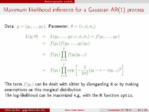
Maximum likelihood inference for a Gaussian AR(1) process

Data: y = (y1, ..., yT ). Parameter: θ = (c, φ, σε).

L(y; θ) = L(y1, ...., yT ; c, φ, σε) = f(y1, ...., yT )

= f(y1)f(y2, ...., yT |y1)

= f(y1)

T∏t=2

f(yt|yt−1)

= f(y1)

T∏t=2

exp

[− 1

2σ2ε(yt − c− φyt−1)2

]The term f(y1) can be dealt with either by disregarding it or by makingassumptions on this marginal distribution.The log-likelihood can be maximized e.g. with the R function optim.


References

References

H. Madsen, Time Series Analysis, Chapman & Hall/CRC, 280 pp.,2008.


Introduction to time series analysis · Introduction to time series analysis Statistical modelling:...

Documents

Transcript of Introduction to time series analysis · Introduction to time series analysis Statistical modelling:...