
INTRODUCTION TO THE STANDARD MODEL …pages.physics.cornell.edu/~ajd268/Notes/IntroSM-Notes.pdf1...
111
1 INTRODUCTION TO THE STANDARD MODEL (PHYS7645) LECTURE NOTES Lecture notes based on a course given by Lawrence Gibbons. The course begins with a brief overview of the Standard Model and moves on to derive its properties from first principles. Presented by: LAWRENCE GIBBONS L A T E X Notes by: JEFF ASAF DROR 2013 CORNELL UNIVERSITY
Transcript of INTRODUCTION TO THE STANDARD MODEL …pages.physics.cornell.edu/~ajd268/Notes/IntroSM-Notes.pdf1...

1
INTRODUCTION TO THE STANDARD MODEL(PHYS7645) LECTURE NOTES
Lecture notes based on a course given by Lawrence Gibbons.The course begins with a brief overview of the Standard Model
and moves on to derive its properties from first principles.
Presented by: LAWRENCE GIBBONS
LATEX Notes by: JEFF ASAF DROR
2013
CORNELL UNIVERSITY
Contents
1 Preface 4
2 Introduction 52.1 Lagrangians and Conserved Quantities . . . . . . . . . . . . . . . . . . . 52.2 Feynman Rules . . . . . . . . . . . . . . . . . . . . . . . . . . . . . . . . 7
2.2.1 φ4 Theory . . . . . . . . . . . . . . . . . . . . . . . . . . . . . . . 72.2.2 QED . . . . . . . . . . . . . . . . . . . . . . . . . . . . . . . . . . 7
3 Dirac Equation 93.1 Transformation Properties of Bilinears . . . . . . . . . . . . . . . . . . . 133.2 Spin . . . . . . . . . . . . . . . . . . . . . . . . . . . . . . . . . . . . . . 143.3 Free Particle Solutions . . . . . . . . . . . . . . . . . . . . . . . . . . . . 153.4 Negative Energy Solutions . . . . . . . . . . . . . . . . . . . . . . . . . . 17
4 Gauge Invariance 184.1 Golden Rule . . . . . . . . . . . . . . . . . . . . . . . . . . . . . . . . . . 184.2 Schrodinger Equation . . . . . . . . . . . . . . . . . . . . . . . . . . . . 194.3 Dirac Equation . . . . . . . . . . . . . . . . . . . . . . . . . . . . . . . . 20
5 Group Theory 225.1 Definition . . . . . . . . . . . . . . . . . . . . . . . . . . . . . . . . . . . 225.2 Group Examples . . . . . . . . . . . . . . . . . . . . . . . . . . . . . . . 235.3 Representations . . . . . . . . . . . . . . . . . . . . . . . . . . . . . . . . 235.4 Types of Representations . . . . . . . . . . . . . . . . . . . . . . . . . . . 24
5.4.1 Trivial Representation . . . . . . . . . . . . . . . . . . . . . . . . 245.4.2 Regular representation . . . . . . . . . . . . . . . . . . . . . . . . 24
5.5 Important Groups . . . . . . . . . . . . . . . . . . . . . . . . . . . . . . . 255.6 Group Combinations . . . . . . . . . . . . . . . . . . . . . . . . . . . . . 255.7 Lie Groups . . . . . . . . . . . . . . . . . . . . . . . . . . . . . . . . . . . 255.8 SU(2) . . . . . . . . . . . . . . . . . . . . . . . . . . . . . . . . . . . . . 275.9 SU(3) . . . . . . . . . . . . . . . . . . . . . . . . . . . . . . . . . . . . . 285.10 From Group Theory to Fields . . . . . . . . . . . . . . . . . . . . . . . . 295.11 SU(3) and SU(2) . . . . . . . . . . . . . . . . . . . . . . . . . . . . . . . 335.A Discrete Symmetries in Quantum Field Theory . . . . . . . . . . . . . . . 35
2
CONTENTS 3
6 QCD 376.1 Gluon Kinetic Term . . . . . . . . . . . . . . . . . . . . . . . . . . . . . . 406.2 Running of Couplings . . . . . . . . . . . . . . . . . . . . . . . . . . . . . 426.3 Deep Inelastic Scattering and Proton Structure . . . . . . . . . . . . . . 446.A eqf → eqf . . . . . . . . . . . . . . . . . . . . . . . . . . . . . . . . . . . 50
7 Weak Interactions 527.1 Building V-A Theory . . . . . . . . . . . . . . . . . . . . . . . . . . . . . 527.2 Moving to SU(2) . . . . . . . . . . . . . . . . . . . . . . . . . . . . . . . 567.3 Kinetic Terms . . . . . . . . . . . . . . . . . . . . . . . . . . . . . . . . . 617.4 Mass Terms . . . . . . . . . . . . . . . . . . . . . . . . . . . . . . . . . . 64
8 Spontaneous Symmetry Breaking 668.1 Toy Example - A U(1) Global Symmetry . . . . . . . . . . . . . . . . . . 668.2 Global → local symmetry . . . . . . . . . . . . . . . . . . . . . . . . . . 688.3 Fermion Masses . . . . . . . . . . . . . . . . . . . . . . . . . . . . . . . . 74
9 CKM Matrix 779.1 “GIM Mechanism” . . . . . . . . . . . . . . . . . . . . . . . . . . . . . . 829.2 What Do We Know About the CKM? . . . . . . . . . . . . . . . . . . . 849.3 Heavy Quark Effective theory . . . . . . . . . . . . . . . . . . . . . . . . 859.4 Unitary Triangle . . . . . . . . . . . . . . . . . . . . . . . . . . . . . . . 86
10 Symmetries 8710.1 Discrete Symmetries . . . . . . . . . . . . . . . . . . . . . . . . . . . . . 87
10.1.1 Time Reversal . . . . . . . . . . . . . . . . . . . . . . . . . . . . . 8710.1.2 Parity . . . . . . . . . . . . . . . . . . . . . . . . . . . . . . . . . 8710.1.3 Charge Conjugation . . . . . . . . . . . . . . . . . . . . . . . . . 88
10.2 Isospin . . . . . . . . . . . . . . . . . . . . . . . . . . . . . . . . . . . . . 8910.3 Rates of Related Processes . . . . . . . . . . . . . . . . . . . . . . . . . . 91
10.3.1 K∗+ → π0K+ v.s. K∗+ → π+K0 . . . . . . . . . . . . . . . . . . 9110.3.2 ρ0 → π+π− v.s. ρ0 → π0π0 . . . . . . . . . . . . . . . . . . . . . 92
11 Meson Spectroscopy 9311.1 G Parity . . . . . . . . . . . . . . . . . . . . . . . . . . . . . . . . . . . . 9411.2 Applications of Discrete Symmetries . . . . . . . . . . . . . . . . . . . . 9611.3 Neutral Kaons and CP violation . . . . . . . . . . . . . . . . . . . . . . . 9711.4 B factories . . . . . . . . . . . . . . . . . . . . . . . . . . . . . . . . . . . 10211.5 CP violation in the B0B0 system . . . . . . . . . . . . . . . . . . . . . . 10411.6 Form Factors . . . . . . . . . . . . . . . . . . . . . . . . . . . . . . . . . 107
12 Detection 110

Chapter 1
Preface
This set of notes are based on lectures given by Lawrence Gibbons in the Introduction tothe Standard Model course at Cornell University during Spring 2013. The course uses bothLangacker’s The Standard Model and Beyond and Peskin and Schroeder’s Introductionto Quantum Field Theory as a reference text. I wrote these notes during lectures and assuch may contain some small typographical errors and sloppy diagrams. I’ve attemptedto proofread and fix as many of these problems as I can. If you have any questions orwould like a copy of the LATEX file feel free to let me know at [email protected].
4

Chapter 2
Introduction
2.1 Lagrangians and Conserved QuantitiesIn these notes we work in natural units, ~ = c = 1 (remember that ~c ≈ 197MeV fm).We will use four vectors pµ = (E,p), xµ = (t,x) with the West-coast metric:
gµν =
1−1
−1−1
= gµν (2.1)
andpµ = (E,−p) (2.2)
which gives p2 ≡ pµpµ = E2 − p2 = m2. We have
∂µ =∂
∂xµ= (
∂
∂t,∇) ; ∂µ =
∂
∂xµ= (
∂
∂t,−∇) (2.3)
so we have a correspondence of pµ ↔ i∂µ, E ↔ i ∂∂t, and p ↔ −i∇. This gives for
non-relativistic particles,
p2
2m+ V = E ⇒ Schrodinger equation (2.4)
For relativistic fieldsE2 = p2 +m2 ⇒ KG equation (2.5)
or in differential operator notation,(∂µ∂µ +m2
)φ = 0 (2.6)
This is known as the Klien Gordan (KG) equation and arises from the Lagrangian density(we will show this shortly),
LKG =1
2(∂µφ) (∂µφ)− 1
2m2φ2 (2.7)
5
6 CHAPTER 2. INTRODUCTION
The total Lagrangian is
L =
∫L d3x (2.8)
and the action isSKG =
∫Ldt =
∫d4xL (2.9)
The Euler equation is given by
∂L∂φ− ∂µ
(∂L
∂(∂µφ)
)= 0 (2.10)
Applying this the Klien Gordan Lagrangin implies that,
∂LKG∂φ
= −m2φ ,∂LKG∂µφ
= ∂µφ (2.11)
Thus the Klien Gordan Lagrangian gives the Klien-Gordan equation:
∂µ∂µφ+m2φ = 0 (2.12)
Suppose have two equal mass, real scalar fields (in other words fields that come fromthe Klien Gordan equation) which we denote, φ1 and φ2.
L =1
2∂µφ1∂µφ1 −
1
2m2φ2
1 +1
2∂µφ2∂
µφ2 −1
2m2φ2 (2.13)
Suppose now we define a complex scalar field,φ = 1√2
(φ1 + iφ2) and φ∗ = 1√2
(φ1 − iφ2).This gives
L = ∂µφ∂µφ∗ −m2φφ∗ (2.14)
This is the same Lagrangian written under somewhat more convenient fields.Consider L under φ → φ′ = eiαφ and φ′∗ = e−iαφ∗. L is unchanged under this
transformation. Note that if α → α(x, t), the Lagrangian would not have remainedinvariant. This is a known as a global symmetry. Noether’s theorem says that there is aconserved quantity which in this case can be interpreted as a charge. A complex scalarfield has a charge that is conserved. This is called a U(1) symmetry.
Since there is a conserved quantity in this choice of coordiantes there must have alsobeen a conserved quantity in terms of φ1 and φ2. To see what this was we rewrite ouroriginal Lagrangian only in slightly more convenient notation,
L =1
2∂µφ
T∂µφ− m2
2φTφ (2.15)
where φ ≡ (φ1 φ2)T . This Lagranian is invariant under rotations between φ1, φ2. In otherwords under the transformation,
φ→ Oφ (2.16)
where OT = O. The conserved charge is,
φ2 = φ21 + φ2
2 (2.17)

2.2. FEYNMAN RULES 7
2.2 Feynman Rules
We now briefly recall some of the Feynman rules.
2.2.1 φ4 Theory
The Lagrangian for φ4 theory is
L =1
2∂µφ∂µφ−
1
2m2φ2 − λ
4!φ4 (2.18)
Each propagator in momentum space is,
i
p2 −m2 + iε(2.19)
Each external lines contributes a trivial factor of 1 and the φ4 vertex is,
→ −iλ
2.2.2 QED
The gauge invariant quantity in electrodynamics is the electromagnetic(EM) field tensor,
F µν =
0 −Ex −Ey −EzEx 0 −Bz By
Ey Bz 0 −Bx
Ez −By Bx 0
(2.20)
or in terms of the four-potential,
F µν = ∂µAν − ∂νAµ (2.21)
The kinetic Lagrangian term is given by
L = −1
4F µνFµν (2.22)
Applying Euler Lagrange equations gives Maxwell’s equations.The electromagnetic gauge transformation gives,
Aµ → Aµ + ∂µX (2.23)

8 CHAPTER 2. INTRODUCTION
where X is a field. The EM field tensor (and hence the electric and magnetic field)elements are unchanged under a gauge transformation. The physics doesn’t change, butyour calculations do. Typically we will use the Lorenz gauge:
∂µAµ = 0 (2.24)
Using that gauge we end up with the photon propagator,
pµg =−igµν
p2 + iε(2.25)
For an external photon, gp→ εµ(p) (2.26)
and for an outgoing external photon we have
pg→ ε∗µ(p) (2.27)
The polarization vector has the properties,
εµpµ = 0, εµε∗µ = −1 (2.28)
There are two common bases for the polarization vectors. We assume p to be along z.
1. (0, 1, 0, 0)
(0, 0, 1, 0)1m
(p, 0, 0, E)
(2.29)
2. 1√2(0, 1, i, 0, 0)
− 1√2(0, 1,−i, 0)
1m
(p, 0, 0, E)
(2.30)
This is the helicity basis.
Chapter 3
Dirac Equation
Dirac knew of the KG equation and he realized that the negative energy solutions camefrom the fact that the Hamiltonian was quadratic in energy. So he set out of linearizethe problem. He wanted to find an Hamiltonian that is linear in momentum.
Hψ = (α · p + βm)ψ (3.1)
He still wanted the solution to be consistent with relativity and have E2 = p2 +m2. Thushe wanted
H2ψ = (|p|2 +m2)ψ (3.2)
Now
H2ψ =
(α2i︸︷︷︸
1
p2i +
1︷ ︸︸ ︷(αiαj + αjαi) pipj + (αiβ + βαi)︸ ︷︷ ︸
0
pim+
1︷︸︸︷β2 m2
)ψ (3.3)
(where we found the relations above by comparison with above). Thus we have
α21 = α2
2 = α23 = β2 = 1 (3.4)
andαi, αj = αi, β = 0 (3.5)
Since α2i = 1 we know that αi = α−1
i . We also know
αiαj = −αjαi (3.6)αj = −αiαjαi (3.7)
Tr(αj) = −Tr(αiαjαi) (3.8)Tr(αj) = Tr(α2
iαj) (3.9)Tr(αj) = −Tr(αj) (3.10)
Hence this implies that Tr(αj) = 0.
9
10 CHAPTER 3. DIRAC EQUATION
To better understand our constrains on the α matrices we look for their eigenvalues.We denote their eigenvectors by v and their eigenvalues by λi. We have,
αiv = λiv (3.11)v = λ2
iv (3.12)
Thus λi = ±1. The trace of a matrix is just the sum its eignevalues. Since the matricesare traceless,
Tr (αi) = (1 + 1 + ...+ 1) + (−1− 1...− 1) = 0 (3.13)
This can only happen if we have an even dimension such that we have an equal numberof +1’s and −1’s.
Since H must be Hermitian this implies that α, β are also Hermitian. There are no2 × 2 solutions satisfying all the constraints. There are however an infinite number of4× 4 solutions. We mention two such representations
1. Paul-Dirac representation
αi =
(0 σi−σi 0
), β =
(1 00 −1
)(3.14)
where recall that the Pauli matrices are
σ1 =
(0 11 0
), σ2 =
(0 −ii 0
), σ3 =
(1 00 −1
)(3.15)
2. Weyl (Chiral) representation:
β =
(0 11 0
), αi =
(0 σi−σi 0
)(3.16)
One can get from any of these solutions to any other solutions by a unitary matrix U :
α′i = UαiU† , β′ = UβU † (3.17)
Now we come back to the Dirac equation
Eψ = Hψ (3.18)
i∂
∂tψ = −i~α · ∇ψ + βmψ (3.19)
iβ∂
∂tψ = −iβ~α · ∇ψ +mψ (3.20)
0 = (−iβ ∂∂t
+ iβ~α · ∇ −m)ψ (3.21)
We define γµ = (β, β~α). Then we can write the Dirac equation in manifestly convariantform,
(iγµ∂µ −m)ψ = 0 (3.22)
11
or(i/∂ −m)ψ = 0 (3.23)
We now review some properties of γµ.
γµ, γν = 2gµν (3.24)
in particular: (γ0)2
= (γi)2
= −1. Now
(γ0)† = β† = β (3.25)
and(γi)† = (βαi)
† = α†iβ† = αiβ = −βαi = −γi (3.26)
so the γi are antihermitian. Furthermore
(γi)† = αiβ = β2αiβ = γ0γiγ0 (3.27)
Therefore(γµ)† = γ0γµγ0 (3.28)
Consider the adjoint of the Dirac equation.
[(i∂µγµ −m)ψ]† = 0 (3.29)
−i∂µψ†(γµ)† −mψ† = 0 (3.30)
i∂µ (ψµ)† γ0 γ0(γµ)†γ0︸ ︷︷ ︸γµ
+mψ†γ0 = 0 (3.31)
Define ψ = ψ†γ0. Then we have
i∂µψγµ +mψ = 0 (3.32)
Note that this is similar to the Dirac equation only now we have a positive mass term.Our two equations are
ψ(iγµ∂µ −m)ψ = 0 (3.33)
ψ(iγµ←−∂µ +m)ψ = 0 (3.34)
Summing these equations we have
i∂µ(ψγµψ) = 0 (3.35)
Thus ψγµψ is a conserved current.Our goal now is to determine the Lorentz behavior of different quantities. We define
γ5 ≡ iγ0γ1γ2γ3 (3.36)

12 CHAPTER 3. DIRAC EQUATION
andσµν ≡ i
2[γµ, γν ] (3.37)
We now want to know how to boost our spinor. Recall that a four-vector gets boostedas,
(x′)µ = Λµνx
ν (3.38)
where Λ is a 4× 4 boost/rotation matrix. We define
ψ′(x′) = Sψ(x) (3.39)
We must have
i(γµ∂′µ −m)ψ′(x′) = 0 (3.40)
i(γµΛµν∂
ν −m)Sψ(x) = 0 (3.41)
Multiplying by S−1 on the right,(S−1(iγµ)SΛµ
ν∂ν −m
)ψ = 0 (3.42)
We’ll have a manifestly invariant Dirac equation if γν = S−1γµSΛµν or
S−1γρS = Λρνγ
ν (3.43)
In other words the transformation can be alternatively done on the γµ matrices whichcan be transformed as a four-vector!
We will find S for an infinitesimal transformation.
Λνµ = gνµ + λενµ +O(λ2) (3.44)
where ωµν is an antisymmetric tensor (as usual this condition is to preserve the scalarproduct).
Look forS = 1 + λωµνS
µν (3.45)
where Sµν are some arbitrary 4× 4 matrix. Using our defining equation for S we have,
(1− λωµνSµν)γρ(1 + λωµνSµν) = (gρν + λωρν )γν (3.46)
γρ + λωµν [γρ, Sµν ] = γρ + λωρνγν (3.47)
ωµν [γρ, Sµν ] = ωρνγν (3.48)
ωµν [γρ, Sµν ] = ωµνgµργν (3.49)
ωµν [γρ, Sµν ] = ωµν1
2(γνgµρ − γµgνρ) (3.50)
(3.51)
3.1. TRANSFORMATION PROPERTIES OF BILINEARS 13
Try to look for solutions for each µν. If we can find such solutions then the equationswill still work with the contractions over ωµν . We are looking for term by term solutionsobeying
[γρ, Sµν ] =1
2(γνgρµ − γµgρν) (3.52)
The right hand side is antisymmetric about swapping µ and ν. This can only hold if Sµνis also antisymmetric about this transformation. The simplest anticommuting object inthis space is, σµν . We write,
Sµν = ασµν =iα
2(γµγν − γνγµ) (3.53)
where α is for the time being an unknown constant. This gives
1
2(γνgρµ − γµgρν) =
iα
2(γρ (γµγν − γνγµ)− (γµγν − γνγµ) γρ) (3.54)
We have,
γργµγν = 2gρµγν − γµγργν (3.55)= 2gρµγν − 2gνργµ + γµγνρ (3.56)
Thus,
1
2(γνgρµ − γµgρν) = 2iα (γνgρµ − γµgνρ) (3.57)
This holds true ifα = − i
4(3.58)
ThusS = 1− i
4ωµνσ
µν = 1 +λ
8ωµν [γµ, γν ] (3.59)
3.1 Transformation Properties of Bilinears
Bilinears are terms that take the form ψσψ. We now look for their transformationproperties.
We begin by studying the conjugate spinor,
ψ′ = ψ†S†γ0 (3.60)= ψ†γ0γ0S†γ0 (3.61)= ψ(γ0S†γ0) (3.62)

14 CHAPTER 3. DIRAC EQUATION
Studying the term in brackets,
γ0S†γ0 = 1 +λ
8ωµν
(γ0γν†γ0γ0㵆γ0 − γ0㵆γ0γ0γν†γ0
)(3.63)
= 1 +λ
8(γνγµ − γµγν) (3.64)
= 1− λ
8ωµν [γµ, γν ] (3.65)
= S−1 (3.66)
Hence we haveψ′ = ψS−1 (3.67)
We are now in position to study bilinear transformation properties. The simplestbilinear transforms trivially,
ψ′ψ′ = ψS−1Sψ (3.68)= ψψ (3.69)
Now consider
ψ′γµψ′ = ψS−1γµSψ (3.70)
but recall that S−1γµS = Λµνγ
ν . Thus(ψ′γµψ′
)= Λµ
ν
(ψγνψ
)(3.71)
Hence ψγµψ is a four-vector. Further note that contracting this expression with anotherfour-vector gives a scalar.
Thus we see that our QED Lagrangian,
ψ (iγµ∂µ −m)ψ (3.72)
is manifestly Lorentz covariant since both ψγµ∂µψ and mψψ transform trivially underLorentz boosts.
3.2 SpinConsider a rotation δθz about the z axis. The Lorentz matrix for this transformation is
S(δθz) = 1− i
2δθzσ
12 (3.73)
Recall from quantum mechanics that a rotation operator should have the form e−iSzδθz ≈1− iSzδθz. Comparing these two equations we see that,
Sz =1
2σ12 =
i
4(γ1γ2 − γ2γ1) =
i
2γ1γ2 (3.74)

3.3. FREE PARTICLE SOLUTIONS 15
now
S2z = −1
4γ1γ2γ1γ2 (3.75)
=1
4(3.76)
using γ2i = −1. Similarly one can show that S2
x = S2y = 1/41. This implies that
S2 = S2x + S2
y + S2z =
3
4(3.77)
If we act on some state we have,
S2 |s,m〉 = s (s+ 1) |s,m〉 =3
4|s,m〉 (3.78)
and hence s = 12. Thus the Dirac equation holds only for spin 1/2 particles.
3.3 Free Particle SolutionsWe will look for free particle solutions ψ(x) = u(p)e−ip·x, ∂µψ = −ipµu(p)e−ip·x. Insertingthis form into the Dirac equation gives,
(γµpµ −m)u(p) = 0 (3.79)
We will look for what is called the Weyl or Chiral representation solutions. We use
γ0 =
(0 11 0
), γi =
(0 σi−σi 0
)(3.80)
The Dirac equation gives(−m E − σ · p
E + σ · p −m
)(uA(p)uB(p)
)(3.81)
This gives two equations
−muA + (E − σ · p)uB = 0 , (E + σ · p)uA −muB = 0 (3.82)
These equations are coupled and difficult to solve in general. However, they are easy tosolve in two limits. In the limit that m → 0 the equations decouple yielding compactsolutions. Though can be done, we alternatively study the equations in the opposinglimit of p→ 0 (the rest frame). From there we can find the general solution by boostingour spinors.
1You may feel the urge to extrapolate these resuls and say that the spinors are eigenstates of Sx andSy; This is NOT true! However, spinors are eigenstates of the squares of these operators.
16 CHAPTER 3. DIRAC EQUATION
In this limit two linearly dependent equations,
m(−uA + uB) = 0 , m(uA − uB) = 0 (3.83)
There is a symmetry between uA and uB in this frame that didn’t exist before. We canwrite the general solution as,
u(p) =√m
(χχ
)(3.84)
where χ is a 2-spinor with χ†χ = 1.Consider a boost along z. A four-vector transforms as,(
Epz
)=
(m cosh yLm sinh yL
)= exp
(yL
(0 11 0
))(m0
)(3.85)
while a spinor in the new frame is,[Q 1: check for any more factors]
u(p) = exp[yL
4
(γ0γi − γiγ0
)]√m
(χχ
)(3.86)
= exp
[−yL
2
(σ3 00 −σ3
)]√m
(χχ
)(3.87)
This gives after some algebra:
u(p) =
( (√E + pz
(1−σ3
2
)+√E − pz
(1+σ3
2
))χ(√
E + pz(
1+σ3
2
)+√E − pz
(1−σ3
2
))χ
)(3.88)
We now consider a particle “spin up” along the z direction (which is right handed relative
to z), χ = χ1 ≡(
10
)and “spin down” which is left handed and χ = χ2 ≡
(01
). Now
1−σ3
2=
(0 00 2
). Thus spin up gives
u1(p) =
( √E − pzχ1√E + pzχ
1
)(3.89)
and spin down gives
u2(p) =
( √E + pzχ
2√E − pzχ2
)(3.90)
In the energy/massless limit we get
u1(p)→√
2E
(0χ1
), u2(p)→
√2E
(χ2
0
)(3.91)
This gives us the helicity/chirality of your particle. The helicity operator is given by
h =1
2
Σ · p|p|
(3.92)
3.4. NEGATIVE ENERGY SOLUTIONS 17
with Σ =
(σ 00 σ
).
hu1(p) =1
2u1(p) , hu2(p) = −1
2u2(p) (3.93)
The helicity of a massive particle (m 6= 0) is a relative concept. You can always boostto a frame where pz → −pz. This flips u1 and u2. However for a massless particle thehelicity is locked in since you can’t boost faster then that particle. Such fields are knownas chiral fields.
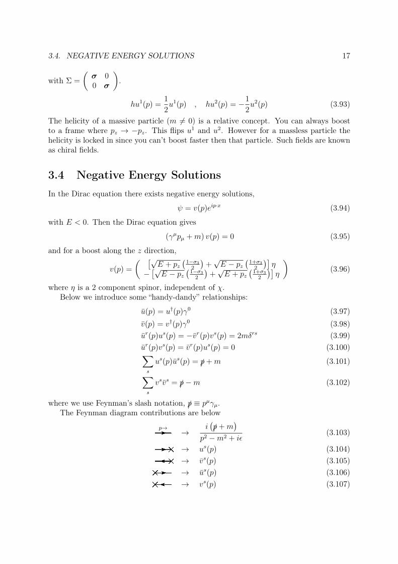
3.4 Negative Energy SolutionsIn the Dirac equation there exists negative energy solutions,
ψ = v(p)eip·x (3.94)
with E < 0. Then the Dirac equation gives
(γµpµ +m) v(p) = 0 (3.95)
and for a boost along the z direction,
v(p) =
( [√E + pz
(1−σ3
2
)+√E − pz
(1+σ3
2
)]η
−[√E − pz
(1−σ3
2
)+√E + pz
(1+σ3
2
)]η
)(3.96)
where η is a 2 component spinor, independent of χ.Below we introduce some “handy-dandy” relationships:
u(p) = u†(p)γ0 (3.97)v(p) = v†(p)γ0 (3.98)ur(p)us(p) = −vr(p)vs(p) = 2mδrs (3.99)ur(p)vs(p) = vr(p)us(p) = 0 (3.100)∑s
us(p)us(p) = /p+m (3.101)∑s
vsvs = /p−m (3.102)
where we use Feynman’s slash notation, /p ≡ pµγµ.The Feynman diagram contributions are below
p→F →i(/p+m
)p2 −m2 + iε
(3.103)
Fx → us(p) (3.104)x → vs(p) (3.105)xF → us(p) (3.106)x → vs(p) (3.107)

Chapter 4
Gauge Invariance
4.1 Golden Rule
1. Decay of particle with mass M to n other particles, all with masses mi. LetM bethe amplitude for the process:
dΓ = |M|2 S(2π)4
2Mδ4(p−
∑j
pj,final)×(
d3p1,f
(2π)32E1,f
...d3pn,f
(2π)32En,f
)(4.1)
where S is a statistical factor introduced to avoid double counting when we haveidentical particles in the final state (known as a symmetry factor). If you have `copies of a given type of particle, then you pick up a factor of 1
`!. e.g. if you have
two muons and two electrons in the final state then you have a factor of 12!2!
(whileelectrons and positrons are NOT considered identical)
2. Scattering:1i + 2i → 1f + 2f + ...+ nf (4.2)
dσ =|M|2 × S(2π)4√(pµ1p2µ −m1m2)2
δ4(p1,i + p2,i −∑j
pj,f )×(
d3p1,f
(2π)32E1,f
)...
(d3pn,f
(2π)32En,f
)(4.3)
Thus far we have only discussed non-interacting theories. We will be interested inprocess such as,
e
e
γ
µ
µ
18
4.2. SCHRODINGER EQUATION 19
Currently our discussion of QED has only included,
L = ψ(i/∂ −m)ψ − 1
4F µνFµν (4.4)
We don’t want to put interactions in by hand since there are many interactions we couldhave. We use gauge invariance.
4.2 Schrodinger EquationThe Schrodinger equation says
− 1
2m∇2ψ(x, t) = i
∂
∂tψ(x, t) (4.5)
The energy is unchanged if ψ(x, t) → eiαψ(x, t). Physical observables, ψ†ψ → ψ′†ψ′ arealso unchanged under this transformation. As currently stated, this no longer holds if weconsider local gauge transformations, α→ α(x, t). Local gauge invariance says
ψ(x, t)→ ψ′(x, t) = eiα(x,t)ψ(x, t) (4.6)
Hence∇ψ(x)→ eiα(x,t)∇ψ(x, t) + i(∇α)eiα(x,t)ψ(x, t) (4.7)
Suppose we conside gauge invariance to a fundamental principle of nature. We try tofind a way to fix the equation above to make it invariant under such transformations.
To “fix” this we map our derivatives such that
∂
∂t→ ∂
∂t+ ieA0 (4.8)
∇ → ∇− ieA (4.9)
where Aµ is an unknown field called a “gauge field”. Consider the following:(∂
∂t+ ieA0
)ψ(x, t)→
(∂
∂t+ ie
(A0 + δA0
))eiα(x,t)ψ(x, t) (4.10)
= eiα(x,t)
(∂
∂t+ i
∂α
∂t+ ieA0 + ieδA0
)ψ(x, t) (4.11)
To ensure gauge invariance we demand
eδA0 = −∂α∂t
(4.12)
A very similar calculation can be done for the gradient. This gives
δA = +1
e∇α (4.13)

20 CHAPTER 4. GAUGE INVARIANCE
In four-vector notation we require
δAµ = −1
e∂µα (4.14)
or
Aµ → Aµ − 1
e∂µα (4.15)
This is the standard electromagnetic field gauge transformation! So demanding gaugeinvariance is in some sence equivalent to adding electromagnetic interactions. Our generalprescription is then to use what we call a “gauge covarient derivative”. We replace
∂µ → Dµ = ∂µ + ieAµ (4.16)
In the case of the Schrodinger equation we write
− 1
2m(∇− ieA)2 ψ = i
(∂
∂t− ieA0
)ψ (4.17)(
− 1
2m(∇− ieA)2 + eA0
)ψ = i
∂
∂tψ (4.18)
This equation is now gauge invariant.
4.3 Dirac Equation
Our Lagrangian isL = ψ(i/∂ −m)ψ (4.19)
which is not gauge invariant. To introduce interactions we invoke the prescription thatwe just developed, ∂µ → Dµ = ∂µ + ieAµ. By construction we have (remember that α isa function of space-time)
Dµψ → D′µψ′ = eiαDµψ (4.20)
andψ → e−iαψ (4.21)
we have,L = ψ (iγµDµ −m)ψ = ψ
(i/∂ −m
)ψ − e ψγµψ︸ ︷︷ ︸
jµ
Aµ (4.22)
Its interesting the note that the conserved current we discovered earlier is the quantitythat couples to the vector potential. This suggests that the conserved charge corre-sponding to this current is indeed the electric charge. We now have coupling termscorresponding to,

4.3. DIRAC EQUATION 21
γ
ψ
ψ
Under a gauge transformation we have,
L → ψe−iαeiα (i∂µDµ −m)ψ = L (4.23)
We are however still missing a kinetic term for Aµ. If we want to interpret Aµ as aphoton field we need to have a term corresponding to the energy of a photon to move fromplace to place. This kinetic term should be quadratic in derivatives of Aµ and should notcontain any ψ dependence. It should respect the local phase invariance which means theterms you have to use when forming it, F µν must have a certain form. We also requireLorentz invariance. This gives us two choices
∝ F µνFµν (4.24)
and∝ εµναβFµνFαβ (4.25)
The second term violates parity and time reversal which we know from experiment thatthey should hold for a photon. Thus we are left with
LQED = ψ (iγµDµ −m)ψ − 1
4FµνF
µν (4.26)
Applying the Euler Lagrange equations with respect to Aµ gives Maxwell’s equationswith the source terms.
Note that there is one more term that is tempting to add,
− m2
2AµAµ (4.27)
However, this does not respect local gauge invariance. Taking this is a principle of Natureit implies that the particle corresponding to the Aµ field must be massless!
Chapter 5
Group Theory
The principle of gauge invariance appears to hold in nature. We have seen above thatusing it as a guiding principle we are able to derive interactions between particles andparticle properties that we know from electromagnetism. The transformation which we“gauged” or made local was a U(1) transformation, i.e. simply adding a phase. This is thesimplest possible local transformation and lead to the simplest Lagrangian that we see inour everyday life. Nature has more gauge invariances and knowing how to deal with themrequires a strong understanding of these transformations. In physics transformations tendto form what are known as groups. We now study some Mathematics before studyingmore complicated theories.
5.1 DefinitionA group is a set of symmetry operations on physical systems. It is a set of elementsa, b, c, ... such as the symmetry operations of a triangle. We will have a product oper-ation on those elements which satisfies
1. Closure: If a and b are in the group then a · b is in the group.
2. Associativity: (a · b) · c = a · (b · c)
3. Identity: There exists an element I in the group such that a · I = I · a = a
4. Inverse: For any element a in the group there exists an inverse element, a−1 suchthat a−1a = aa−1 = I
Examples of groups and nongroups.
• Addition of real numbers. We show this explicitly as an example. Suppose α andβ are real numbers.
1. α + β ∈ R
2. α + β = β + α
22
5.2. GROUP EXAMPLES 23
3. α · 1 = 1 · α = α
4. α · 1α
= 1
• If we have real numbers and multiplication, you don’t have a group since zerodoesn’t have an inverse.
• eiθ and multiplication, then you do form a group.
Note that there is no commutation rule. You can have non commuting groups.
5.2 Group Examples
Consider the Parity transformation. It forms a group once you include the identity. Wecan make what’s known as a group multiplication table:
1 P1 1 PP P 1
so we have P−1 = P .Next consider the Cyclic group. In a cyclic group each element squared is equal to a
new distinct element until the final one which returns to the identity. For example:
Z3 =e, a, a2 = b
(5.1)
with a3 = e
e a be e a ba a b eb b e a
5.3 Representations
A representation of a group (G) is a map of linear operators (usually matrices) D actingon a vector space V such that for g1, g2 ∈ G ,
D(g1) |g2〉 = |g1g2〉 (5.2)
this is true if and only ifD(g1)D(g2) = D(g1g2) (5.3)
The dimension of the representation is dim(V ). 0

24 CHAPTER 5. GROUP THEORY
5.4 Types of Representations
5.4.1 Trivial Representation
The trivial representation is for every element g ∈ G ,
D(g) = 1 (5.4)
where 1 denotes the identity.Another useful representation is a reducible representation. This is the case if there
is a subspace of V with elements v such that for every group element g we have,
D(g)D(v) ∈ V (5.5)
A Completely Reducible representation is one that we can write D(g) is a blockdiagonal form:
D1(g) ... ... 0... D2(g) ...
...... ... ...
...0 ... ... DN(g)
(5.6)
An irreducible representation is a not-reducible representation.
5.4.2 Regular representation
A covenient representation is one known as the regular representation. In this represen-tation the group acts on itself. In this representation we can write group elements asboth vectors in the space and operators. To see how this works consider the group Z3.It is not difficult to guess one particular 3 dimensional representation of this group,
D(e) =
1 0 00 1 00 0 1 =
, D(a) =
0 0 11 0 00 0 1
, D(b) =
0 1 00 0 11 0 0
(5.7)
Now suppose we define the basis on which this representation acts by,
|e〉 ≡ |e1〉 ≡
100
, |a〉 ≡ |e2〉 ≡
010
, |b〉 ≡ |e3〉 ≡
001
(5.8)
We this we have,
〈ej|D(e)|e1〉 =
1 j = 1
0 j 6= 1(5.9)
〈ej|D(a)|e1〉 =
1 j = 2
0 j 6= 2(5.10)
〈ej|D(b)|e1〉 =
1 j = 3
0 j 6= 3(5.11)

5.5. IMPORTANT GROUPS 25
and similarly for the group elements acting on the other basis vectors. Thus acting on a“state” of a group element performs the acting of the state. We can always write,
D(g1) |g2〉 = D(g1 · g2) |e〉 (5.12)
The states can be created by acting on the identity with group elements.This representation will be a convenient tool when discussed non-abelian algebras.
5.5 Important GroupsOne important group is U(N). This is the group of unitary matrices that act on complex
N − vectors, χ =
χ1...χN
such that χ†χ is unchanged.
Another important group is SU(N). This is called the special unitary group. It isa subset of U(N) satisfying detU = 1. This still satisfies a group due to the dispersionproperty of the determinant:
U1, U2 ∈ SU(N)⇒ det(U1U2) = det(U1) det(U2) = 1 (5.13)
5.6 Group CombinationsWe can also have a direct product of groups. Suppose each element of a group G factorsinto two commuting sets of operators from groups G1,G2 then G is a direct product ofG1,G2:
G = G1 ⊗ G2 (5.14)
As a trivial example consider the group U(N) with elements u. This group consists ofall unitary matrices (which by definition must have determinant equal to a phase). Thuswe can write,
u = eiχsus = useiχs (5.15)
where us is an element of U(N) with the phase pulled out of it such that detus = 1.Then we have us ∈ SU(N). So we can write
U(N) = SU(N)⊗ U(1) (5.16)
since the group of phases, eiχs , commutes with all elements in SU(N).
5.7 Lie GroupsThe elements of a Lie group G depends smoothly on a set of continuous parameters,
g(α) = g(α1, α2, ..., αN) ∈ G (5.17)

26 CHAPTER 5. GROUP THEORY
If α,β are “close to each other” in parameter space then their elements, g(α)g(β) are“close to each other” in group space1. We say there is a smooth mapping between theparameters and the group elements themselves.
For clarity we parametrize our group elements with an infinitesimal variable, λ suchthat
g(λα)
∣∣∣∣λ=0
= eor equivantly−−−−−−−−−−→ D(λα)
∣∣∣∣λ=0
= 1 (5.18)
Near λ = 0 we can write:D(λα) = 1 + iλαaTa (5.19)
where the factor of i is a conventional convenience. By Taylor’s theorem you can thinkof Ta as
Ta = −∂D(α)
∂αa
∣∣∣∣λ=0
(5.20)
The Ta’s are the group “generators”. We can write (applying the group element an infinitenumber of times and taking the spacing between group elements to zero)
D(α) = limk→∞
(1 +
i
kαaTa
)k= eiαaTa (5.21)
If we have a fixed α, it defines a particular “direction” in group space and we havecommuting group elements,
g(λ1α)g(λ2α) = g((λ1 + λ2)α) (5.22)
However if you have α 6= β then
eiαaTaeiβbTb 6= ei(αa+βa)Ta (5.23)
since in general Ta and Tb don’t commute. However if eiαaTa and ei(βbTb) are both in thegroup then we know that we can write
eiαaTaeiβbTb = eiδcTc (5.24)
for some δc. Its possible to show (though we omit the proof here) that one can expandthe above expression to 2nd order and proove that,
[Ta, Tb] = ifabcTc (5.25)
If fabc are known then we can determine δc. Clearly it’s also true that fabc = f−bac.The miracle is that this is sufficient to specify all the group multiplication properties.The rules [Ta, Tb] = ifabcTc are known as the “Lie Algebra”. The fabc are known as the“structure constants”.
As an example let us now go back to U(1) = eiθ = limk→∞(1 + i
kθ)k. There is a
single generator T = 1 and α = θ. If we make θ arbitrarily small we get close to notchanging the phase at all. Note that to go to a local transformation we would let ourparameters αa → αa(x). We want properties of Ta for U(N) and SU(N):
1The meaning of “close to each other” here is highly informal but this will do for normally be sufficientfor a physicist.
5.8. SU(2) 27
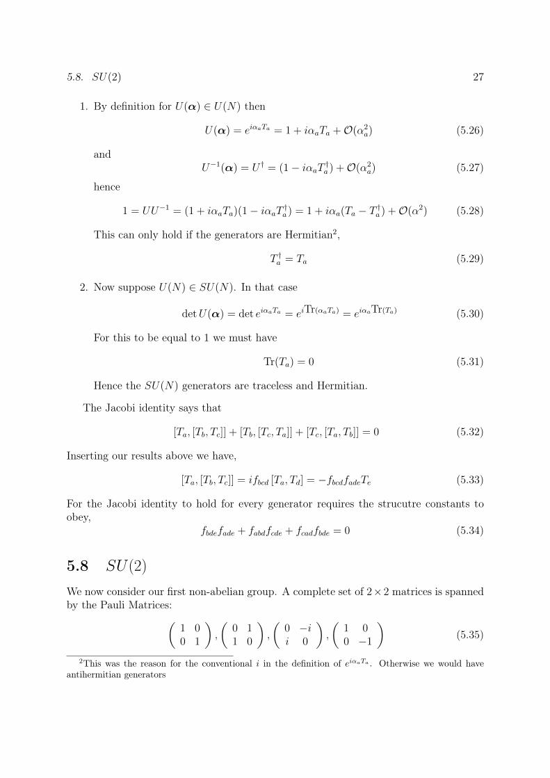
1. By definition for U(α) ∈ U(N) then
U(α) = eiαaTa = 1 + iαaTa +O(α2a) (5.26)
andU−1(α) = U † = (1− iαaT †a ) +O(α2
a) (5.27)
hence
1 = UU−1 = (1 + iαaTa)(1− iαaT †a ) = 1 + iαa(Ta − T †a ) +O(α2) (5.28)
This can only hold if the generators are Hermitian2,
T †a = Ta (5.29)
2. Now suppose U(N) ∈ SU(N). In that case
detU(α) = det eiαaTa = eiTr(αaTa) = eiαaTr(Ta) (5.30)
For this to be equal to 1 we must have
Tr(Ta) = 0 (5.31)
Hence the SU(N) generators are traceless and Hermitian.
The Jacobi identity says that
[Ta, [Tb, Tc]] + [Tb, [Tc, Ta]] + [Tc, [Ta, Tb]] = 0 (5.32)
Inserting our results above we have,
[Ta, [Tb, Tc]] = ifbcd [Ta, Td] = −fbcdfadeTe (5.33)
For the Jacobi identity to hold for every generator requires the strucutre constants toobey,
fbdefade + fabdfcde + fcadfbde = 0 (5.34)
5.8 SU(2)
We now consider our first non-abelian group. A complete set of 2×2 matrices is spannedby the Pauli Matrices:(
1 00 1
),
(0 11 0
),
(0 −ii 0
),
(1 00 −1
)(5.35)
2This was the reason for the conventional i in the definition of eiαaTa . Otherwise we would haveantihermitian generators

28 CHAPTER 5. GROUP THEORY
U(2) has 4 generators.For SU(2) we require traceless generators (as mentioned above). Hence the identity
doesn’t qualify. To normalize the modulus of our structure constants to 1 we divide eachmatrix by 2. Then we have our SU(2) generators,
SU(2) : Ta =σ1
2,σ2
2,σ3
3
(5.36)
Its easy to calculate the commutators. As an example consider,
σ1σ2 =
(0 11 0
)(0 −ii 0
)=
(i 00 −i
)(5.37)
andσ2σ1 =
(0 −ii 0
)(0 11 0
)=
(−i 00 i
)(5.38)
which give [σ1
2,σ2
2
]= 2
1
4
(i 00 −i
)= i
σ3
2(5.39)
hence we have f123 = 1. In general one can show that,
[Ti, Tj] = iεijkTk (5.40)
The SU(2) structure constants are fijk = εijk
5.9 SU(3)
The SU(3) dimension 3 representation is given by the Gell-Man Matrices:
λ1 =
0 1 01 0 00 0 0
, λ2 =
0 −i 0i 0 00 0 0
, λ3 =
1 0 00 −1 00 0 0
λ4 =
0 0 10 0 01 0 0
, λ5 =
0 0 −i0 0 0i 0 0
, λ6 =
0 0 00 0 10 1 0
λ7 =
0 0 00 0 −i0 i 0
, λ8 =1√3
1 0 00 1 00 0 −2
The SU(3) generators are given by Ti = λi
2. The structure constants are given by
f123 = 1
f458 = f678 =
√3
2
f147 = f165 = f246 = f257 = f345 = f376 =1
2f38j = 0 ∀j
5.10. FROM GROUP THEORY TO FIELDS 29
Note that we don’t have any structure constants that have both a 3 and an 8 since λ3
and λ8 commute.
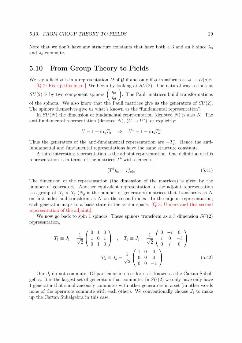
5.10 From Group Theory to FieldsWe say a field φ is in a representation D of G if and only if φ transforms as φ→ D(g)φ.
[Q 2: Fix up this intro.] We begin by looking at SU(2). The natural way to look at
SU(2) is by two component spinors(ηuηd
). The Pauli matrices build transformations
of the spinors. We also know that the Pauli matrices give us the generators of SU(2).The spinors themselves give us what’s known as the “fundamental representation”.
In SU(N) the dimension of fundamental representation (denoted N) is also N . Theanti-fundamental representation (denoted N), (U → U∗), or explicitly:
U = 1 + iαaTa ⇒ U∗ = 1− iαaT ∗a
Thus the generators of the anti-fundamental representation are −T ∗a . Hence the anti-fundamental and fundamental representations have the same structure constants.
A third interesting representation is the adjoint representation. One definition of thisrepresentation is in terms of the matrices T b with elements,
(T b)ac = ifabc (5.41)
The dimension of the representation (the dimension of the matrices) is given by thenumber of generators. Another equivalent representation to the adjoint representationis a group of Ng × Ng (Ng is the number of generators) matrices that transforms as Non first index and transform as N on the second index. In the adjoint representation,each generator maps to a basis state in the vector space. [Q 3: Understand this secondrepersentation of the adjoint.]
We now go back to spin 1 spinors. These spinors transform as a 3 dimension SU(2)representation,
T1 ≡ J1 =1√2
0 1 01 0 10 1 0
, T2 ≡ J2 =1√2
0 −i 0i 0 −i0 i 0
T3 ≡ J3 =
1√2
1 0 00 0 00 0 −1
(5.42)
Our Ji do not commute. Of particular interest for us is known as the Cartan Subal-gebra. It is the largest set of generators that commute. In SU(2) we only have only have1 generator that simultaneously commutes with other generators in a set (in other wordsnone of the operators commute with each other). We conventionally choose J3 to makeup the Cartan Subalgebra in this case.
30 CHAPTER 5. GROUP THEORY
The raising and lowering operators are given by
J± =J1 ± J2√
2(5.43)
SoJ3
(J± |m〉
)= (m± 1) J± |m〉 (5.44)
It turns out that a particular representation of SU(2) is completely defined by thematrix elements that connect the various |j,m〉 states.
〈j,m′|J3|j,m〉 = mδm,m′ (5.45)
〈j,m′|J+|j,m′〉 =√
(j +m+ 1)(j −m)δm′,m+1 (5.46)
〈j,m′|J−|j,m′〉 =√
(j −m+ 1)(j +m)δm′,m−1 (5.47)
In the spin j representation the matrix elements of our generators Ja are given by,
(J ja)k`
= 〈j, j + 1− k︸ ︷︷ ︸m′
|Ja|j,m︷ ︸︸ ︷
j + 1− `〉 (5.48)
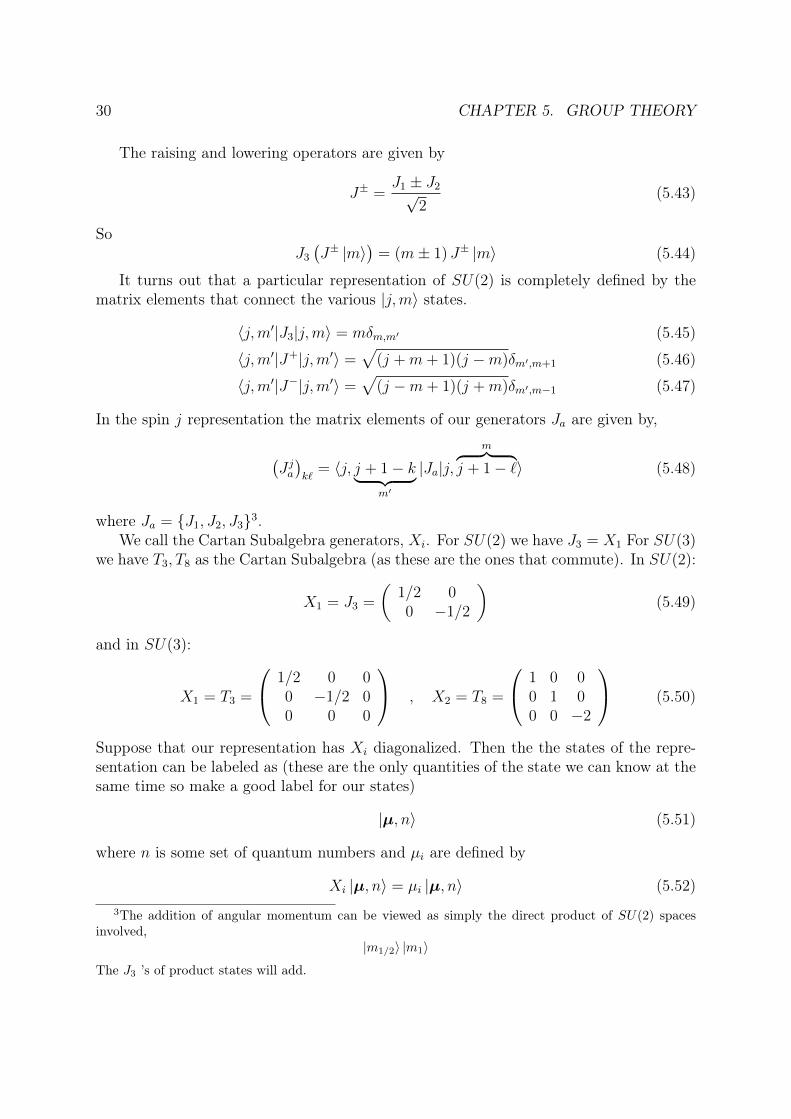
where Ja = J1, J2, J33.We call the Cartan Subalgebra generators, Xi. For SU(2) we have J3 = X1 For SU(3)
we have T3, T8 as the Cartan Subalgebra (as these are the ones that commute). In SU(2):
X1 = J3 =
(1/2 00 −1/2
)(5.49)
and in SU(3):
X1 = T3 =
1/2 0 00 −1/2 00 0 0
, X2 = T8 =
1 0 00 1 00 0 −2
(5.50)
Suppose that our representation has Xi diagonalized. Then the the states of the repre-sentation can be labeled as (these are the only quantities of the state we can know at thesame time so make a good label for our states)
|µ, n〉 (5.51)
where n is some set of quantum numbers and µi are defined by
Xi |µ, n〉 = µi |µ, n〉 (5.52)3The addition of angular momentum can be viewed as simply the direct product of SU(2) spaces
involved,|m1/2〉 |m1〉
The J3 ’s of product states will add.

5.10. FROM GROUP THEORY TO FIELDS 31
where µ = (µ1, µ2, ..., µNC ) (NC is equal to the number of generators in the CartanSubalgebra) are the “weight vectors” of a given state and µi ’s are the weights.
For general SU(N) we have more then just one direction to raise and lower our states;We need multiple labels! For SU(2), j = 1/2:
J3 eigenstates µ(10
)12(
01
)−1
2
We can only raise and lower in one direction.This is not the case in SU(3):
T3, T8 eigenstates µ(1 0 0
)T 12,√
36
(
0 1 0)T
−12,√
36
(
0 0 1)T
0,−√
33
where the values of µ are found by acting on the eigenstates with T3 and T8.
In the adjoint representation, we get the generalization of the raising and loweringoperators. The rows and columns of the matrices (defined by (Tb)ac = −ifabc) are labeledby the generator label so the dimension of the states is equal to the number of generators.This is reminiscent of the regular representation we saw earlier. As was the case therewe can choose the basis of our states such that we can label them using the generators.|Ta〉 = Ta |e〉 is equal to the state in the adjoint representation that corresponds to
generator Ta. We haveα |Ta〉+ β |Tb〉 = |αTa + βTb〉 (5.53)
where α, β are just numbers. We now take one of our generators and act on the statethat corresponds to another generator:
Ta |Tb〉 = |Tc〉 〈Tc|Ta|Tb〉 (5.54)= |Tc〉 (Ta)bc (5.55)= −ifacb |Tc〉 (5.56)= ifabc |Tc〉 (5.57)= |ifabcTc〉 (5.58)= |[Ta, Tb]〉 (5.59)
The Cartan generators, Xi, give
Xi |Xj〉 = |[Xi, Xj]〉 = 0 (5.60)
32 CHAPTER 5. GROUP THEORY
since by definition the Cartan generators commute with each other, for any Xi in theCartan Subalgebra the weight vector (µ) is zero.
Now consider non-Cartan generator states, |Eα〉,
Xi |Eα〉 ≡ αi |Eα〉 = |αiEα〉 (5.61)
where αi are the weights in the adjoint representation and are also known as the “roots”.We can also write
Xi |Eα〉 = |[Xi, Eα]〉 (5.62)
comparing these two results above we have,
[Xi, Eα] = αiEα (5.63)
This reminds us of SU(2) where we have,[J3, J
±] = ±J± (5.64)
Notice the parallel between the Eα and the J± (in SU(2), X1 = J3). Recall also that
J− =(J+)† (5.65)
To find the analogous expression in SU(N) note that for a unitary group the diagonalgenerators must be real (otherwise they couldn’t be hermitian). So we can write,
[Xi, Eα]† =[E†α, Xi
]= −
[Xi, E
†α
](5.66)
The left hand side can also be written
〈Eα|Xi = αiE†α (5.67)
hence we have [Xi, E
†α
]= −αiE†α (5.68)
which implies that,E†α = E−α (5.69)
Consider now some state given by its weight vector and some quantum numbers whichwe denote n.
XiEα |µ, n〉 = [Xi, Eα] |µ, n〉+ EαXi |µ, n〉 (5.70)= αiEα |µ, n〉+ µiEα |µ, n〉 (5.71)= (µi + αi)Eα |µ, n〉 (5.72)
Hence Eα(E−α) are the raising (lowering) operators and E±α |µ, n〉 takes state |µ, n〉with a weight vector µ to a state with weight vector µ±α. The root vectors α give thedirection that the root vectors are “raised” or “lowered”.
5.11. SU(3) AND SU(2) 33
5.11 SU(3) and SU(2)
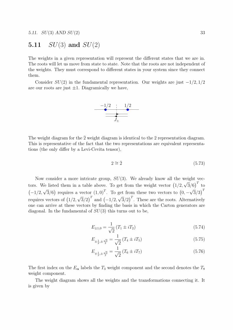
The weights in a given representation will represent the different states that we are in.The roots will let us move from state to state. Note that the roots are not independent ofthe weights. They must correspond to different states in your system since they connectthem.
Consider SU(2) in the fundamental representation. Our weights are just −1/2, 1/2are our roots are just ±1. Diagramically we have,
−1/2 1/2
J±
The weight diagram for the 2 weight diagram is identical to the 2 representation diagram.This is representative of the fact that the two representations are equivalent representa-tions (the only differ by a Levi-Cevita tensor),
2 ∼= 2 (5.73)
Now consider a more intricate group, SU(3). We already know all the weight vec-tors. We listed them in a table above. To get from the weight vector
(1/2,√
3/6)T
to(−1/2,
√3/6)requires a vector (1, 0)T . To get from these two vectors to
(0,−√
3/3)T
requires vectors of(1/2,√
3/2)T
and(−1/2,
√3/2)T
. These are the roots. Alternativelyone can arrive at these vectors by finding the basis in which the Carton generators arediagonal. In the fundamental of SU(3) this turns out to be,
E±1,0 =1√2
(T1 ± iT2) (5.74)
E± 12,±√
32
=1√2
(T4 ± iT5) (5.75)
E∓ 12,±√
32
=1√2
(T6 ± iT7) (5.76)
The first index on the Eα labels the T3 weight component and the second denotes the T8
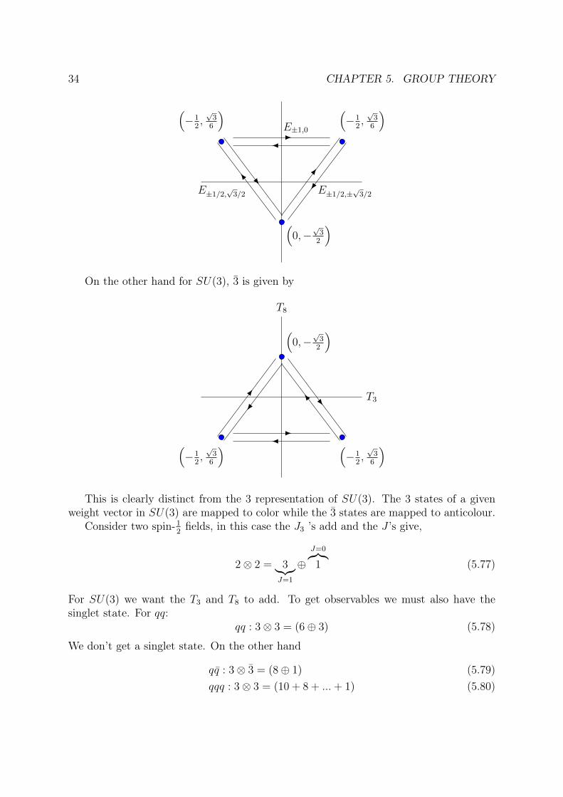
weight component.The weight diagram shows all the weights and the transformations connecting it. It
is given by
34 CHAPTER 5. GROUP THEORY
(−1
2,√
36
)(−1
2,√
36
)
(0,−
√3
2
)E±1/2,±
√3/2E±1/2,
√3/2
E±1,0
On the other hand for SU(3), 3 is given by
(−1
2,√
36
)(−1
2,√
36
)
(0,−
√3
2
)
T3
T8
This is clearly distinct from the 3 representation of SU(3). The 3 states of a givenweight vector in SU(3) are mapped to color while the 3 states are mapped to anticolour.
Consider two spin-12fields, in this case the J3 ’s add and the J ’s give,
2⊗ 2 = 3︸︷︷︸J=1
⊕J=0︷︸︸︷1 (5.77)
For SU(3) we want the T3 and T8 to add. To get observables we must also have thesinglet state. For qq:
qq : 3⊗ 3 = (6⊕ 3) (5.78)
We don’t get a singlet state. On the other hand
qq : 3⊗ 3 = (8⊕ 1) (5.79)qqq : 3⊗ 3 = (10 + 8 + ...+ 1) (5.80)
5.A. DISCRETE SYMMETRIES IN QUANTUM FIELD THEORY 35
Thus we can get the singlet state through either a meson (qq) or a baryon (qqq). Onecan go on and study bound states with larger numbers of quarks but these are much lesscommon in Nature.
5.A Discrete Symmetries in Quantum Field Theory
This section is based on [Peskin and Schroeder(1995)] chapter 3.6. I added this sectionfor completeness and it’s results will be important later. Lorentz transformations are thegroup of continuous operations that keep the Minkowski interval invariant. However wecan expand this definition to include Parity, P , and Time reversal, T :
P
tx1
x2
x3
=
t−x1
−x2
−x3
T
tx1
x2
x3
=
−tx1
x2
x3
since they also keep the quantity t2 − x2 invariant. We define a proper orthochronousLorentz group by L↑+ the group without Parity and Time reversal. Every quantum fieldtheory must be invariant under these transformations. The “orthochronous improperLorentz Group” , L↑− = P , L↑+, is the Lorentz group including Parity. The “nonorthochronousproper Lorentz Group” , L↓+ = T , L↑+, is the Lorentz group including time reversal andfinally the “nonorthochronous improper Lorentz Group” , L↓− = P , T , L↑+ is the Lorentzgroup including Time reversal and Parity. The gravitational, electromagnetic, and stronginteractions turn out to be symmetric under P and T . The weak interactions do not havethis property but break Parity as we will see later.
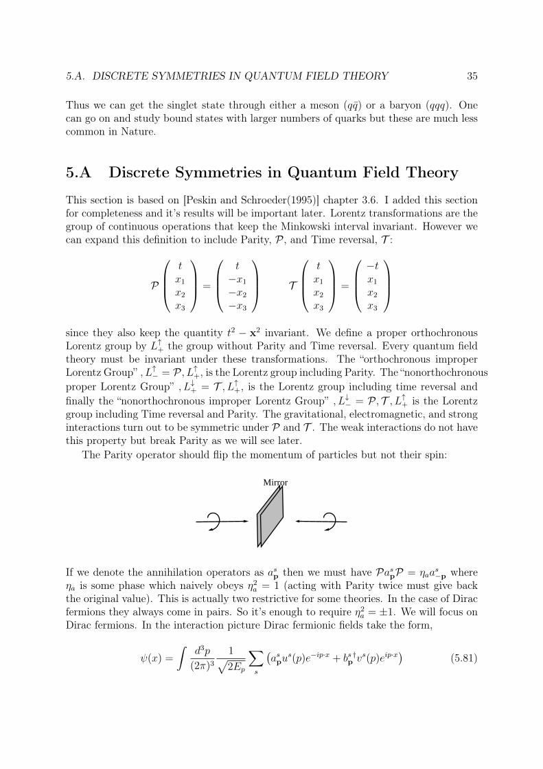
The Parity operator should flip the momentum of particles but not their spin:
Mirror
If we denote the annihilation operators as asp then we must have PaspP = ηaas−p where
ηa is some phase which naively obeys η2a = 1 (acting with Parity twice must give back
the original value). This is actually two restrictive for some theories. In the case of Diracfermions they always come in pairs. So it’s enough to require η2
a = ±1. We will focus onDirac fermions. In the interaction picture Dirac fermionic fields take the form,
ψ(x) =
∫d3p
(2π)3
1√2Ep
∑s
(aspu
s(p)e−ip·x + bs †p vs(p)eip·x
)(5.81)
36 CHAPTER 5. GROUP THEORY
where as and bs are annihilation operators. Now consider the parity operator acting onthe field:
Pψ(x)P =
∫d3p
(2π)3
1√2Ep
∑s
(ηaa
s−pu
s(p)e−ip·x + ηb∗bs†−pvs(p)eip·x
)(5.82)
We now change variables using p → −p. This gives p · x → p · (t,−x), p · σ → p · σ,p · σ → p · σ (since σ ≡ (1,−σ)). Thus we can write
u(p) =
( √p · σξ√p · σξ
)→( √
p · σξ√p · σξ
)=
(0 11 0
)u(p) = γ0u(p) (5.83)
where ξ is some spin state. Similarly we have
v(p)→( √
p · σξ−√p · σξ
)= −γ0v(p) (5.84)
so we can write
Pψ(x)P =
∫d3p
(2π)3
1√2Ep
∑s
(ηaγ
0aspus(p)e−ip·(t,−x) − η∗b bs†p γ0vs(p)eip·(t,−x)
)(5.85)
If we have a Parity eigenstate then should should be equal to some constant matrix timesψ(t,−x). This is the case if η∗b = −ηa. Then we have
Pψ(x)P = ηaγ0ψ(t,−x) (5.86)
Notice that the positive and negative frequencies in the Dirac fermion are not independentof one another. They must transform in a related way to carefully preserve Parity.

Chapter 6
QCD
We want to write down Lagrangians. Recall that in the SM we have 6 quark flavors:u, d, c, s, t, b. Each flavor comes in 3 colors (r,g,b). We begin by considering a singlequark flavor. We can write
L0 = q (iγµ∂µ −m)︸ ︷︷ ︸(iγµ∂µ−m)13×3
q (6.1)
with
q ≡
q1
q2
q3
, q ≡ (q1, q2, q3) (6.2)
with each of qi being one four component Dirac fermion. Explicitly we have
L0 = q1 (iγµ∂µ −m) q1 + q2 (iγµ∂µ −m) q2 + q3 (iγµ∂µ −m) q3 (6.3)
For a global flavor SU(3) transformation:
q → q′ = Uq (6.4)q → q′ = qU † = qU−1 (6.5)
with U ∈ SU(3). Thus
L′0 = qU−1(iγµ∂µ −m)Uq = q(iγµ∂µ −m)q = L0 (6.6)
so we have a global SU(3) symmetry.Just as we did in the U(1) case to produce electromagnetism we now want to consider
local transformations. This involves
U = eigαaTa → eigαa(x)Ta ≈ 1 + igαa(x)Ta (6.7)
Our local transformation is then
q → Uq = (1 + igαa(x)Ta)q (6.8)q → qU † = q(1− igαa(x)Ta) (6.9)
37

38 CHAPTER 6. QCD
We have∂µq → ∂µq
′ = (1 + igαa(x)Ta)∂µq + ig(∂µαa)Taq︸ ︷︷ ︸extra term
(6.10)
We can eliminate this extra term by changing
∂µ → Dµ = ∂µ − igTaGaµ (6.11)
where Gaµ is an known collection of 8 fields (in SU(3)). The sum over a is just a straight
forward sum over the generator label (in other words Gaµ = Ga,µ). We now write
Dµq →[∂µ − igTa(Ga
µ + δGaµ)]
(1 + igαaTa)q (6.12)= (1 + igαaTa) ∂µq + igTaq∂µαa − igTaGa
µ(1 + igαbTb)q
− igTaδGaµ (1 + igαaTa) q (6.13)
= (1 + igαaTa) (∂µ − igTaGaµ)︸ ︷︷ ︸
Dµ
q + (1 + igαaTa)(iTbGbµ)q
− igTa(1 + gαbTb)Gaµq − igTaδGa
µq + igTaq∂µαa (6.14)
where we have thrown away one of the terms of order the product of αaGaµ (we are
assuming that both αa and δGa are small). Simplifying we have
Dµq → (1 + gαaTa)Dµq − g2αb [Tb, Ta]Gaµq − igTaδGa
µq + igTaq∂µαa (6.15)= (1 + gαaTa)Dµq − ig2αbfbacTcG
aµq + igTaq∂µαa − igTaδGa
µq (6.16)
In order to have a transformation we require
0 = −g2αbfbacTcGaµ + gTa∂µα− gTaδGa
µ (6.17)
For Hermitian generators one can show that we can always choose a basis for thegenerators so that
tr(TaTb) ∝ δab (6.18)
For SU(3) and SU(2) in the fundamental representations we have
tr(TaTb) =1
2δab (6.19)
Mutliplying equation 6.17 by Td and taking the trace gives,
0 = −g2αbfbactr(TdTc)Gaµ + gtr(TdTa)∂µαa − gtr(TdTa)δGa
µ (6.20)= −g2αbfbadG
aµ + g∂µαd − gδGa
µ (6.21)
Relabeling our indices by d→ a, a→ c and using fbca = fabc then we have
δGcµ = ∂µαc − gαbfabcGa
µ (6.22)

39
In an abelian group we don’t have the extra term (in such a group we don’t have tracerelationship).
In order to have gauge invariance we require
Gaµ → Ga
µ + ∂µαa − gαbfabcGcµ (6.23)
Having the coupling strength appear in the gauge transformation means that g is inde-pendent of flavor. In other words all flavors will have the same coupling strength. Notethat the gluon fields mix between one another under this transformation. This suggests(and we’ll see this later too) that the gluons carry color.
In summary we have
L0 → L = q (iγµ∂µ −m) q + gqTaGaµγ
aq (6.24)
We have a vertex qiGaµgDqi
→ ig(Ta)ij. We handle color flow at the vertex.
One may ask why we know that we have SU(3) and not U(3). The U(3) are thegenerators Ta of SU(3) and 1. 1 commutes with everything, hence the correspondingstructure constant would be f9ab = 0. Under a U(3) rotation
G9µ → G9
µ + ∂µq (6.25)
with respect to color G9µ transforms like a color singlet. It carries no color charge. We
would expect this 9th field to be a force similar to the photon (a long range force). Wedo not see such force in nature.
To see this consider the following process
e+e− → J/ψ → uu (6.26)
or diagrammatically we have
e
e
γ
c
c
where|cc〉 =
1√3
∑i
|cici〉 (6.27)
is the J/ψ bound state of cc. What we want to know is whether J/ψ can decay througha single gluon annihilation. In other words through for example,
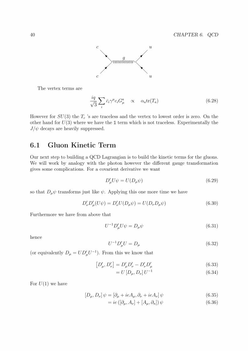
40 CHAPTER 6. QCD
c
c
g
u
u
The vertex terms are
iq√3
∑i
ciγµciG
aµ ∝ αatr(Ta) (6.28)
However for SU(3) the Tc ’s are traceless and the vertex to lowest order is zero. On theother hand for U(3) where we have the 1 term which is not traceless. Experimentally theJ/ψ decays are heavily suppressed.
6.1 Gluon Kinetic Term
Our next step to building a QCD Lagrangian is to build the kinetic terms for the gluons.We will work by analogy with the photon however the different gauge transformationgives some complications. For a covarient derivative we want
D′µUψ = U(Dµψ) (6.29)
so that Dµψ transforms just like ψ. Applying this one more time we have
D′νD′µ(Uψ) = D′νU(Dµψ) = U(DνDµψ) (6.30)
Furthermore we have from above that
U−1D′µUψ = Dµψ (6.31)
henceU−1D′µU = Dµ (6.32)
(or equivalently Dµ = UD′µU−1). From this we know that[D′µ, D
′ν
]= D′µD
′ν −D′νD′µ (6.33)
= U [Dµ, Dν ]U−1 (6.34)
For U(1) we have
[Dµ, Dν ]ψ = [∂µ + ieAµ, ∂ν + ieAν ]ψ (6.35)= ie ([∂µ, Aν ] + [Aµ, ∂n])ψ (6.36)

6.1. GLUON KINETIC TERM 41
Consider for a moment
[∂µ, Aν ]ψ =
product rule︷ ︸︸ ︷(∂µAν)ψ + Aν∂µψ−Aν∂µψ (6.37)
= (∂µAν)ψ (6.38)
Thus we have for U(1):
[Dµ, Dν ]ψ = ie (∂µAν − ∂νAµ)ψ (6.39)= ieFµνψ (6.40)
The left hand side transforms as [Dµ, Dν ]ψ → U ([Dµ, Dν ]ψ) In order for this to hold forthe right hand side we require Fµν → Fµν . In other words Fµν is gauge invariant (Fµν isthe component so it can’t produce factors of U). In U(1) its easy to guess a form for agauge invariant quantity since the transformation is simple. Complications arise for morecomplicated groups.
We now consider SU(N) with the covariant derivative,
Dµ = ∂µ − igTaGaµ (6.41)
[Dµ, Dν ]ψ =[∂µ − igTaGa
µ, ∂ν − igTbGbν
](6.42)
= −iganalogous to before︷ ︸︸ ︷[
∂µ, TbGbν
]+[TaG
aµ, ∂ν
]ψ − g2 [Ta, Tb]G
aµG
bν (6.43)
= −igTb∂µG
bν − Ta∂νGa
µ
ψ − g2ifabcTcG
aµG
bνψ (6.44)
= −igTa∂µG
aν − Ta∂νGa
µ + gfbcaTaGbµG
cν
ψ (6.45)
≡ −igTaGaµνψ (6.46)
where after cycling the structure constant indices we define
Gaµν ≡ ∂µG
aν − ∂νGa
µ + gfabcGbµG
cν (6.47)
Based on our earlier discussion we know that the combination of igTaGaµν is gauge in-
variant. It’s important to note that we don’t expect the Gaµν to be gauge invariant on
it’s own but the sum over TaGaµν should be. It turns out that the combination Ga
µνGµνa is
gauge invariant.Our full QCD Lagrangian is given by
LQCD = q (iγµ∂µ −m) q + gqTaGaµγ
µq − 1
4GaµνG
µνa (6.48)
To get a feel for our kinetic term we expand it out
−1
4GaµνG
µνa = −1
4(∂µGνa− ∂νGa)(∂µG
νa − ∂νGµ
a)− g
2(∂µG
aν − ∂νGa
ν)fabcGµbG
νc
− g2
4
(fabcfadcG
bµG
cνG
µdG
νe
)(6.49)

42 CHAPTER 6. QCD
In U(1) gauge theories all interactions arise from adding in the covariant derivatives.However, this is not the case for non-abelian gauge theories. Here we get more interactionsjust between the gluon fields!
Notice the triple gauge vertex between three gluons,
ν, p1
µ, p2
ρ, p3
this gives a vertex term of
− gfabc (gµν(p1 − p2)ρ + gνρ(p2 − p2)µ + gρµ(p3 − p1)ν) (6.50)
The quadropole gauge boson vertex,
ν ρ
σµ
which gives the vertex,
− ig2 (fabcfcde (gµρgνσ − gµσgνρ) + facefbde (gµνgρσ − gµσgνρ) + fadefcbe (gµρgνσ − gµνgρσ))(6.51)
You may wonder if we were a bit too quick with pulling out Feynman diagrams. Wehaven’t taken the time to derive Feynman diagrams in non-Abelian theories and indeedthere are some complications. It turns out if you carefully quantize QCD your answerdoesn’t quite come out right. The problem is with the gauge choice. The physical gauge(“axial”) gives gluons that have only ±1 helicity (no longitudinal polarization, i.e. helicity0). Our interactions are still correct however our propagator is more complicated.
In our gauge, the “covariant gauge”, the nonabelian turns when you quantize your the-ory will give you an unphysical time-like longitudinal piece. These contributions violateunitarity. However if you do the full analysis you’ll find that in addition to the gluons youget what’s known as “Fadeev-Popov ghosts”. These are scalar fields that satisfy Fermistatistics. Fortunately these particles appear only in loops. These contributions exactlycancel the longitudinal gluons.
6.2 Running of CouplingsWhen doing calculations in quantum field theory the cross-sections depend on the cou-plings in your theory. In bare perturbation theory the couplings are typically infinite.
6.2. RUNNING OF COUPLINGS 43
However, even in renormalized perturbation theory there is no clear definition of the cou-pling strength. In general we can renormalize our theory with renormalization conditionsat any scale we choose. However, if we choose a renormalization scale far from the scaleof the problem we are studying then we end up with what’s known as large log correc-tions which spoil the perturbation theory. These large logs can be summed to all orderin perturbation theory. The effect of this sum is to change the effective couplings felt bythe particles depending on the scale in which the interaction takes place. This effect issmall in QED however turns out to be crucial in QCD.
In QED at very small momenta we have αQED ≈ 1/127 but at the Z boson scale,
αQED(µ2 = m2z) =
e2(µ2 = m2z)
4π=
1
128(6.52)
Doing a full quantum field theory calculation one can find the couples at differentscale µ from a reference scale mz by
1
αi(µ)=
1
αi(mz)+ bi ln
m2z
µ2(6.53)
where bi is known as the beta function. In QED we have,
bQED =1
3π
[1
9n1/3 +
4
9n2/3 + n1
](6.54)
where nq denotes the number of quarks below the energy scale of interest with charge q.For example if mb < µ < mz then we have
n1/3 =
flavors︷︸︸︷3 × 3︸︷︷︸
color= 9 (6.55)
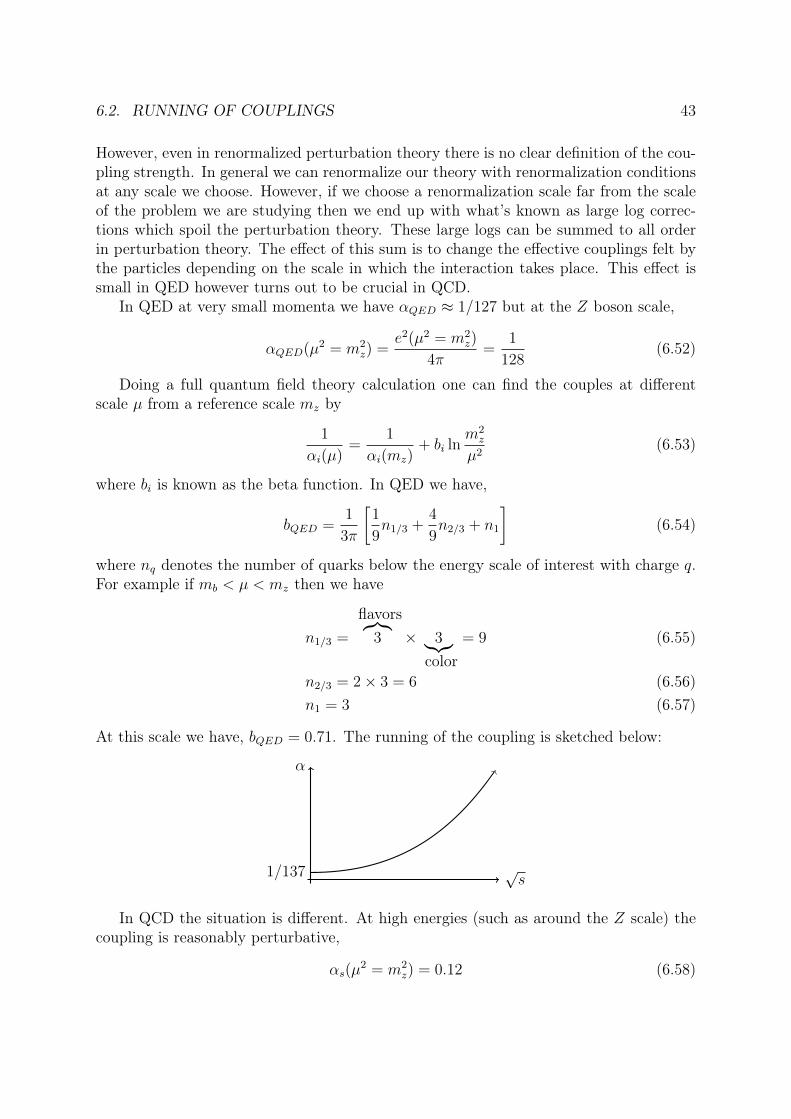
n2/3 = 2× 3 = 6 (6.56)n1 = 3 (6.57)
At this scale we have, bQED = 0.71. The running of the coupling is sketched below:
1/137
α
√s
In QCD the situation is different. At high energies (such as around the Z scale) thecoupling is reasonably perturbative,
αs(µ2 = m2
z) = 0.12 (6.58)
44 CHAPTER 6. QCD
For QCD we have1
b3
=1
4π
(4
3Tr −
11
3CF
)(6.59)
where TR depends on the gluons representation and the number of flavor. For the SU (3)octet we have, TR = nF/2. CF depends only on the color the group. For SU(3), CF = 3.We have
b3 =1
4π
(2
3nF − 11
)=
1
12π(2nF − 33) (6.60)
For mb < µ < mz, b ∼ −0.5. A typical scale is shown here
µ α = α3
mz 0.12mb 0.2mc 0.3ms 1.7
An important quantitty that is other seen in the literature is the scale ΛQCD. This scalecan roughly be viewed as the energy scale at which perturbative QCD breaks down andthe strong force becomes nonperturbative. It’s typically in the range of 200− 400 MeV.This is of order a ∼ 1fm (the scale of a nucleus). To get a working definition of this scaleis to fit αs at some range of interest and choose ΛQCD such that αs ∼ 1. If you associatesome scale
Λ2QCD = µ2
o
where µ0 satisfies[Q 4: what does this mean?]
− 12π/(33− 2nf )α(µ20) (6.61)
thenαs(µ
2) =12π
(33− 2nF ) ln µ2
Λ2QCD
(6.62)
for nF = 5 we have ΛQCD ∼ 200 MeV. If you have 3 active flavors (nF = 3) thenΛQCD ∼ 400 MeV. ΛQCD is a useful way to encapsulates all the nonperturbative behavior.
6.3 Deep Inelastic Scattering and Proton StructureAt the LHC we don’t have the pleasure of simple point particle collisions. Instead wehave complicated proton proton collisions. Each proton has three valence quarks (twoup quarks and a down) but also contains many quarks and gluons that are popping inand out of the vacuum. These are known as “sea quark and gluons”. We want to learnhow to deal with such processes in a controlled way. The quarks and gluons within theproton have some distribution of motion and we want to figure out how to deal with thiscomplication appropriately. We start by analyzing collisions with a single proton and an
6.3. DEEP INELASTIC SCATTERING AND PROTON STRUCTURE 45
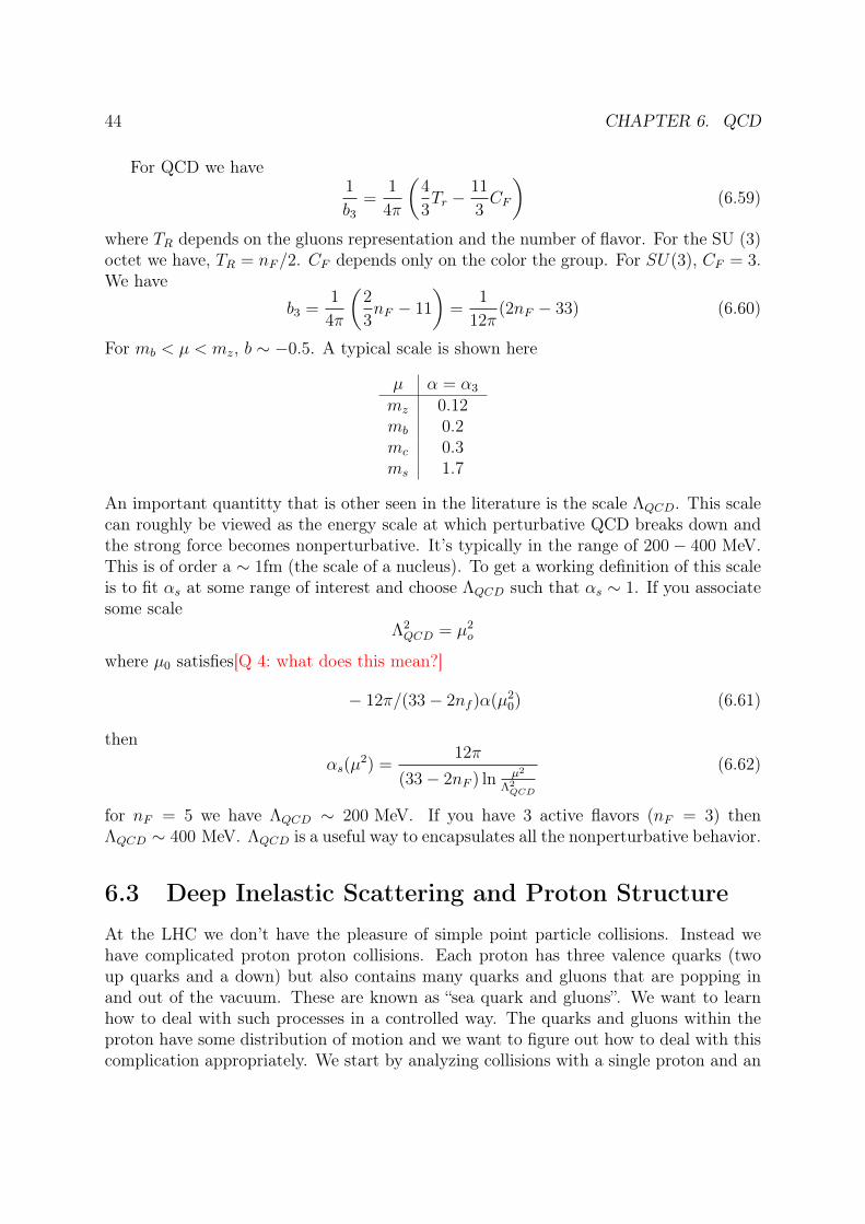
electron. At low energies(long wavelengths), the wavelength of the electron is too longto probe the short distance scale of the proton. Small electron wavelengths are need toresolve the proton structure (hence the need for high energy colliders). The collisionslook something like,
e− e−
p+
We can have two situations
• Low energy electrons produce soft photons. The proton recoils coherently as glu-ons “redistribute” momenta on a time scale small compared to it’s motion. Thesecollisions do not probe the structure of the proton.
• High energy electrons can emit a hard photon which gives a lot of energy to aconstituent of the proton. New particles form and a hadronic shower appears. Thisis called “Deep Inelastic Scattering”.
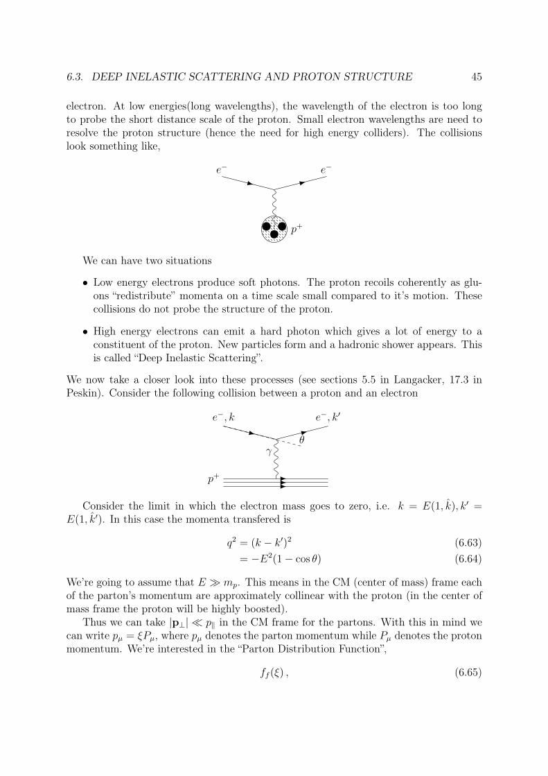
We now take a closer look into these processes (see sections 5.5 in Langacker, 17.3 inPeskin). Consider the following collision between a proton and an electron
θ
e−, k e−, k′
γ
p+
Consider the limit in which the electron mass goes to zero, i.e. k = E(1, k), k′ =E(1, k′). In this case the momenta transfered is
q2 = (k − k′)2 (6.63)= −E2(1− cos θ) (6.64)
We’re going to assume that E mp. This means in the CM (center of mass) frame eachof the parton’s momentum are approximately collinear with the proton (in the center ofmass frame the proton will be highly boosted).
Thus we can take |p⊥| p‖ in the CM frame for the partons. With this in mind wecan write pµ = ξPµ, where pµ denotes the parton momentum while Pµ denotes the protonmomentum. We’re interested in the “Parton Distribution Function”,
ff (ξ) , (6.65)
46 CHAPTER 6. QCD
which is the expected number density of finding a parton with flavor f with momentumfraction ξ in the proton. Equivalently ff (ξ)dξ is the expected number of partons of typef with a longitudinal momentum fraction between ξ and ξ + dξ.
Classicaly, fu(ξ) is a constant for all ξ and is equal to 2/3 while fd(ξ) is a constantand equal to 1/3. However, as we mentioned above this is not the whole story due tothe sea quarka n gluons. fu, fd receive contributions from both valence and sea quarks.However, we must still have, ∑
f
ff (ξ) = 1 (6.66)
for all ξ.Suppose now you want to calculate the cross-section for a collision of an electronoff of a quark with final momentum p′ and initial momentum ξP . The cross section isgiven by
σ(e−(k) + p(P )→ e−(k′) +X
)=
∫ 1
0
dξ∑qf
fqf (ξ)σ(e−(k) + qf (ξP )→ e−(k′) + qf (p
′))
(6.67)This equation can be interpreted as follows. The cross section to see one flavor collideat a particular momentum fraction is σ (e−(k) + qf (ξP )→ e−(k′) + qf (p
′)). The crosssection to see a collision at any momentum fraction, ξ is this cross section multiplied bythe probability of the quark carrying the momentum fraction. The total probability fora collision of a given flavor is the sum (through integration) over all possible ξ values.Lastly to get all possible flavors we have to sum over the flavor (over all 12 quark andanti-quark flavors).
We introduce the Mandlestam variables (we use hats to denote quark quantities andno hats to denote proton properties):
s = (k + p)2 = (k + ξP )2 (6.68)t = q2 = −Q2 (6.69)u = (k − p′)2 (6.70)
The cross section for e−f → e−f in the limit of m2e,m
2f E2
cm is given by
dσ
dΩ=
α2Q2f
2E2cm(1− cos θ)2
(4 + (1 + cos θ)2
)(6.71)
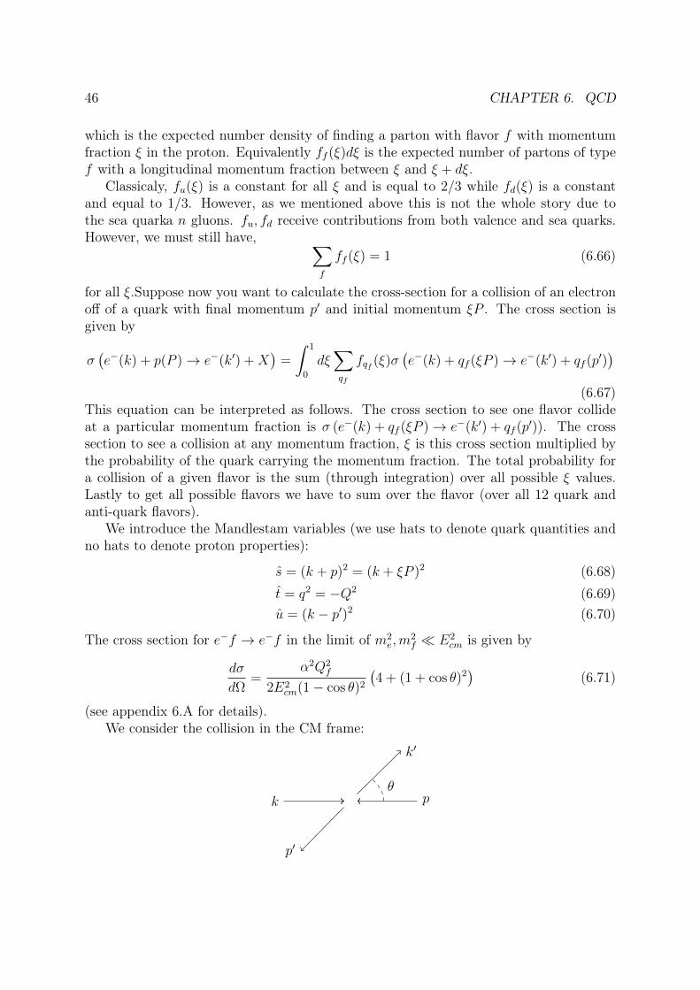
(see appendix 6.A for details).We consider the collision in the CM frame:
θk p
k′
p′
6.3. DEEP INELASTIC SCATTERING AND PROTON STRUCTURE 47
we have
kµ =Ecm
2(1, 0, 0, 1)
kµ′ =Ecm
2(1, 0, sin θ, cos θ)
pµ =Ecm
2(1, 0, 0,−1)
pµ′=Ecm
2(1, 0,− sin θ,− cos θ)
Now we havedσ
d cos θ=
πα2Q2f
E2cm(1− cos θ)2
(4 + (1 + cos θ)2) (6.72)
The Mandlestam variables are
s = E2cm (6.73)
t = (k − k′)2 = −2k · k′ = −E2cm
2(1− cos θ) (6.74)
u = (k − p′)2 = −2k · p′ = −E2cm
2(1 + cos θ) (6.75)
Note that
s+ t+ u =4∑i=1
m2i ≈ 0 (6.76)
and we have
dσ
d cos θ=
πα2Q2f
s(2t/s)2
(4 +
(2u
s
)2)
(6.77)
=πα2Q2
f
st2(s2 + u2) (6.78)
Furthermore we can rewrite the differential since,
t = − s2
(1− cos θ) (6.79)
⇒dσ
dt=
dσ
d cos θ
d cos θ
dt=
2
s
dσ
d cos θ(6.80)
Hence we can write
dσ
dt=
2πα2Q2f
s2t2(s2 + (s+ t)2) (6.81)
=2πα2Q2
f
t2
(1 +
[1 + t/s
]2) (6.82)

48 CHAPTER 6. QCD
Back to the electron proton system we have
t = t = q2 ≡ −Q2
s = 2p · k = 2ξP · k = ξs
where our Mandlestam variables are now in the electron proton system (not in the quarksystem) and we have defined Q2 ≡ −t > 0. This gives,
dσ
dQ2=
2πα2Q2f
Q4
(1 +
[1− Q2
ξs
]2)
(6.83)
This expression holds for any energy transferred Q2, flavor, and momentum fraction ξ.Since in the proton we don’t have control over the momentum fraction nor the flavor weintegrate over these variables with the appropriate weighting factor, the parton distribu-tion functions,
dσtotdQ2
=
∫ 1
0
dξ∑f
ff (ξ)Q2f
2πα2
Q4
(1 +
[1− Q2
ξs
]2)
(6.84)
Notice that we are now able to make any measurement we wish at a proton protoncollider and as long as we know the parton distribution functions we are able to makesharp theoretical predictions! Now consider a measurement at Hera for example wherethey collide electrons and protons. Recall that q ≡ k− k′ = p′− p. This is a quantity weknow. We also have k + p = k′ + p′ ⇒ p′ = k − k′ + p = q + p. Hence
0 = p′2 = (q + p)2 = q2 + 2q · p = 2q · (ξP )−Q2
which implies that,
ξ =Q2
2q · P(6.85)
but Q2 ≡ −q2 is a measurable well known quantity. We also know the incoming andoutgoing electrons and proton momenta. So are able to measure the momentum fractionthat the parton receives in each collision. By measuring parton collisions and fittingthe cross-section to equation 6.84 with ff (ξ) as a parameter we can extract the partondistribution function.
Consider the Lorentz invariant quantity,
y ≡ 2P · q2P · k
=2P · qs
(6.86)
In the proton rest frame we havey =
q0
k0
(6.87)
6.3. DEEP INELASTIC SCATTERING AND PROTON STRUCTURE 49
Thus y is the energy transferred over initial energy of the electron, i.e. the fraction of theelectron energy that is given to the proton system. Clearly we have 0 < y < 1. We have
y =2ξP · q2ξP · k
(6.88)
=2p · (k − k′)
2p · k(6.89)
=s+ u
s(6.90)
= − ts
(6.91)
This expression is in the parton level. We now want to switch back to the proton level.Recall that 2P · q = Q2/ξ (see Eq 6.85) , and hence
y =Q2
ξ
1
2P · k=Q2
ξs(6.92)
orQ2 = ξys (6.93)
so we havedQ2 = ξsdy (6.94)
Going back to our cross section and using the Fundamental theorem of Calculus wecan write,
dσtotdξdy
=∑f
ξff (ξ)Q2f
2πα2
ξ2s
1 + (1− y)2
y2(6.95)
This form is known as “Bjorken scaling” in which the initial parton distribution is inde-pendent of Q2. So the ξff (ξ) is telling us about the structure of the proton.
Now consider some constraints in ff (ξ). The valence quarks are 2u, 1d. Bounds statesof quarks and antiquarks go in and out of the vacuum but the expected number of havea sea up quark is equal to the expected number of sea antiup quarks. Thus we must havethe condition, ∫ 1
0
[fu(ξ)− fu(ξ)] dξ = 2 (6.96)
similarly if we take the expected number of d quarks and subtract the expected numberof anti- d quarks from the sea we have,∫ 1
0
[fd(ξ)− fd(ξ)] dξ = 1 (6.97)
We have similar constraints for the other quarks. A final constraint is the constituentsmust sum over all momentum to the proton momentum:∫ 1
0
dξξ [fg(ξ) + fu(ξ) + fd(ξ) + fc(ξ) + fs(ξ) + ...+ fu(ξ) + ...] = 1 (6.98)
50 CHAPTER 6. QCD
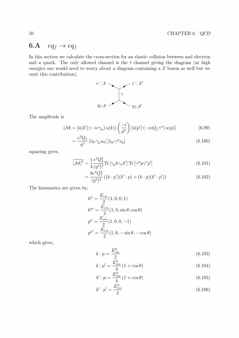
6.A eqf → eqf
In this section we calculate the cross-section for an elastic collision between and electronand a quark. The only allowed channel is the t channel giving the diagram (at highenergies one would need to worry about a diagram containing a Z boson as well but weomit this contribution),
qf , p qf , p′
e−, k e−, k′
γ
The amplitude is
iM = [u(k′) (−ieγµ)u(k)]
(−iq2
)[u(p′) (−ieQfγ
µ)u(p)] (6.99)
=e2Qf
q2[uk′γµuk] [up′γ
µup] (6.100)
squaring gives,
|M|2 =1
4
e4Q2f
(q2)2Tr [γµkγνk
′]Tr [γµpγνp′] (6.101)
=8e4Q2
f
(q2)2((k · p′)(k′ · p) + (k · p)(k′ · p′)) (6.102)
The kinematics are given by,
kµ =Ecm
2(1, 0, 0, 1)
kµ′ =Ecm
2(1, 0, sin θ, cos θ)
pµ =Ecm
2(1, 0, 0,−1)
pµ′=Ecm
2(1, 0,− sin θ,− cos θ)
which gives,
k · p =E2cm
2(6.103)
k · p′ = E2cm
4(1 + cos θ) (6.104)
k′ · p =E2cm
4(1 + cos θ) (6.105)
k′ · p′ = E2cm
2(6.106)

6.A. eqf → eqf 51
Inserting in these relations we have,
|M|2 =E4cme
4Q2f
2(q2)2
(4 + (1 + cos θ)2
)(6.107)
The 2→ 2 cross section is given by
dσ
dΩ=
1
16π2
1
4EAEB |vA − vB||p|Ecm︸ ︷︷ ︸
prefactor
|M|2 (6.108)
For the kinematics of our problem the prefactor is just
=1
64π2
1
E2cm
(6.109)
The momentum transferred is,
q2 =E2cm
4(1− cos θ)2 (6.110)
which gives
dσ
dΩ=
e4Q2f
8π2E2cm (1− cos θ)2
(4 + (1 + cos θ)2
)(6.111)
=α2Q2
f
2E2cm (1− cos θ)2
(4 + (1 + cos θ)2
)(6.112)
as quoted above.
Chapter 7
Weak Interactions
7.1 Building V-A Theory
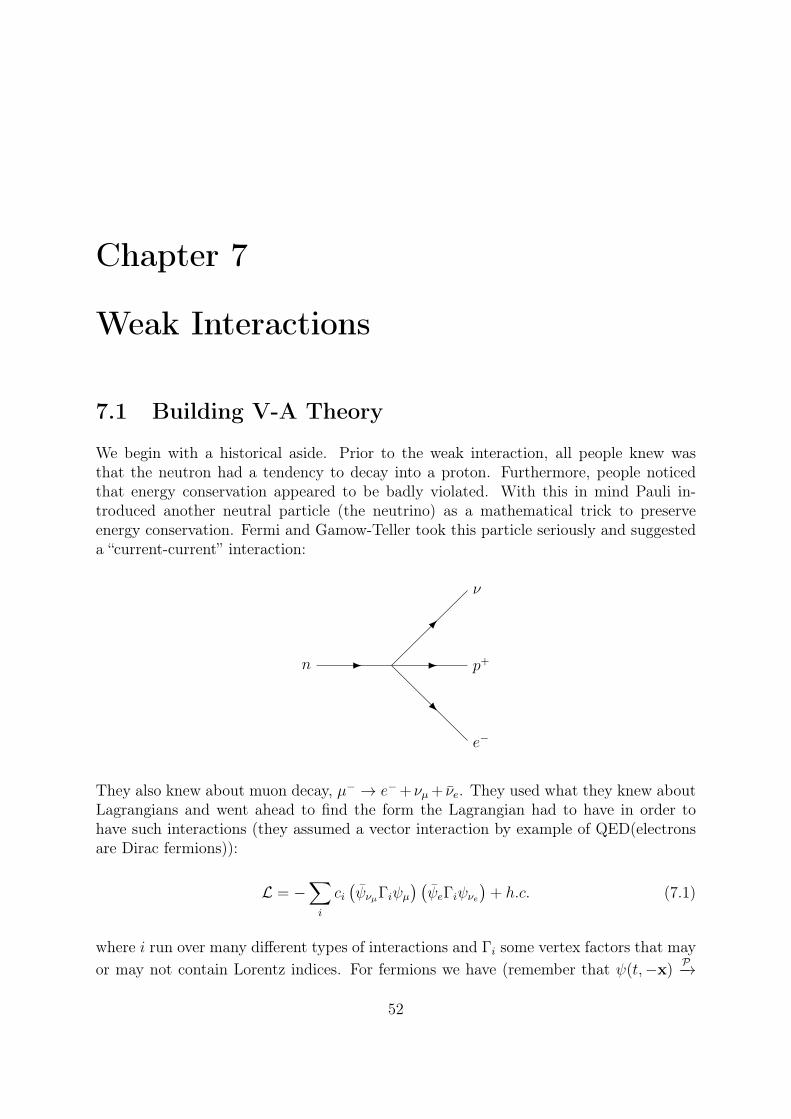
We begin with a historical aside. Prior to the weak interaction, all people knew wasthat the neutron had a tendency to decay into a proton. Furthermore, people noticedthat energy conservation appeared to be badly violated. With this in mind Pauli in-troduced another neutral particle (the neutrino) as a mathematical trick to preserveenergy conservation. Fermi and Gamow-Teller took this particle seriously and suggesteda “current-current” interaction:
n
ν
p+
e−
They also knew about muon decay, µ− → e−+νµ+ νe. They used what they knew aboutLagrangians and went ahead to find the form the Lagrangian had to have in order tohave such interactions (they assumed a vector interaction by example of QED(electronsare Dirac fermions)):
L = −∑i
ci(ψνµΓiψµ
) (ψeΓiψνe
)+ h.c. (7.1)
where i run over many different types of interactions and Γi some vertex factors that mayor may not contain Lorentz indices. For fermions we have (remember that ψ(t,−x)
P−→
52
7.1. BUILDING V-A THEORY 53
ηaγ0ψ and we take ηa = 1 for simplicity)
P(ψνµΓiψµ
) (ψeΓiψνe
)P = P
(ψνµPPΓiPPψµP
) (PψePPΓiPPψνe
)P (7.2)
=[ψ′νµγ
0Γ′iγ0ψµ
] [ψeγ
0Γ′iγ0ψνe
](7.3)
where we defined ψ′ ≡ ψ(t,−x). If we assume Parity invariance we have the followingallowed options for Γi.
Γi ∈
Γ3 = 1(scalar),ΓV = Γµ(vector),ΓP = Γ5(pseudoscalar),
ΓA = Γ5Γµ(axial-vector),ΓT = σµν(tensor)
Its not obvious that each of these terms preserve Parity. We show that this holds for aparticular example of an axial-vector current γ5γµ :
P(ψγ5γµψ
) (ψγ5γµψ
)P =
(ψ′γ0γ5γµγ0ψ′
) (ψ′γ0γ5γµγ
0ψ′)
(7.4)=(ψ′γ5γ0(2gµ0 − γ0γµ)ψ′
) (ψ′γ5γ0(2g0
µ − γ0γµ)ψ′)
(7.5)=(ψ′γ5γµψ′
) (ψ′γ5γµψ′
)(7.6)
as required.We now perform some dimensional analysis.
[L] = 4
LDirac = ψ∂µψ → [ψ] = 3/2
[ci] = 4− 4(3/2) = −2
This hinted at the fact that this interaction was effective low energy theory. Effectivetheories tend to have dimensionful couplings. People found the spectrum for Lagrangianswith all the possible vertices above and it was found that the energies were all wrong.After many years people began to rethink the assumption of Parity conservation. Oncethis was shed people came up with the interaction with cV = −GF√
2, cA = GF√
2and a
Lagrangian,
LV−A =GF√
2
(ψνµγ
µ(1− γ5
)ψµ) (ψeγµ
(1− γ5
)ψνe)
(7.7)
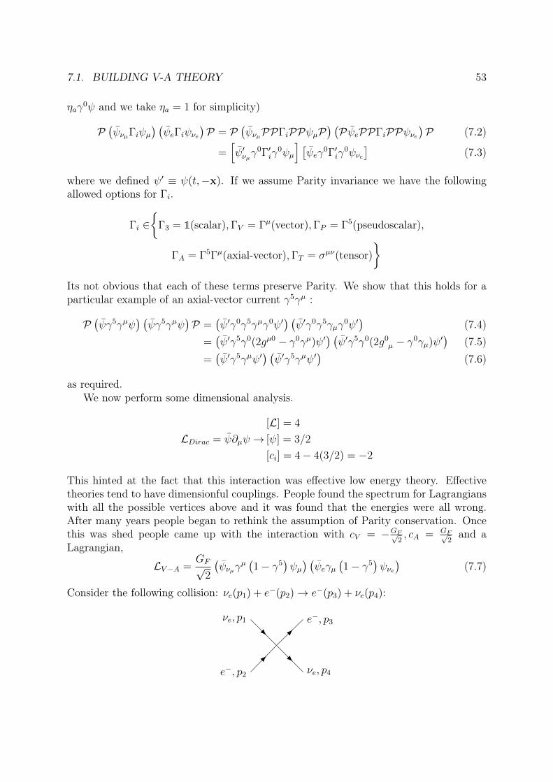
Consider the following collision: νe(p1) + e−(p2)→ e−(p3) + νe(p4):
e−, p2 νe, p4
νe, p1 e−, p3

54 CHAPTER 7. WEAK INTERACTIONS
M =GF√
2
[u3γ
µ(1− γ5
)u1
]︸ ︷︷ ︸[...]
[u4γµ
(1− γ5
)u2
](7.8)
[...]† =[u†3γ
0γµ(1− γ5
)u1
]†(7.9)
= u†1(1− γ5†) 㵆γ0†u3 (7.10)
= u†1(1− γ5
)γ0γµu3 (7.11)
= u1
(1 + γ5
)γµu3 (7.12)
= u1γµ(1− γ5
)u3 (7.13)
(7.14)
and we haveM† =
GF√2
[u1γ
ν(1− γ5
)u3
] [u2γν
(1− γ5
)u4
](7.15)
hence we have|M|2 =
G2F
2LµνMµν (7.16)
with
Lµν =[u3γ
µ(1− γ5
)u1
] [u1γ
ν(1− γ5
)u3
](7.17)
Mµν =[u4γµ
(1− γ5
)u2
] [u2γν
(1− γ5
)u4
](7.18)
Averaging over initial spins and summing over final spins we get,
|M|2 =1
2
1
2(16)Tr
[γµPL/p1
γνPL
(/p3
+me
)]Tr[γµPL
(/p2
+me
)γνPL/p4
](7.19)
where we definePR/L ≡
1
2
(1± γ5
)(7.20)
We have an initial factor of 1/2 due to the electron spin and a factor of 16 to switch the1− γ5 matrix to a projection matrix. Taking the traces gives,
|M|2 = 64G2F (p1 · p2) (p3 · p4) (7.21)
We have,
s = (p3 + p4)2 = m2e + 2p3 · p4 (7.22)
s = (p1 + p2)2 = m2e + 2p1 · p2 (7.23)
which gives,
|M|2 = 16G2F
(s−m2
e
)2 (7.24)(7.25)
7.1. BUILDING V-A THEORY 55
In the CM frame,
dσ
dΩ=
1
64π2s|M|2 =
G2F
4π2
(s−m2e)
2
s∼ G2
F
4π2s (7.26)
If you have a point-like interaction in an s-wave (orbital angular momentum, L = 0state), then [Q 5: check a NRQM book to confirm this equation]
dσ
dΩ=
1
s|M0|2 (7.27)
where |M0|2 is the probability of interaction and so unitarity implies that
|M0|2 ≤ 1 (7.28)
So |M0|2 > 1 is
s >2π
GF
(7.29)
This theory has predicted its own demise!It doesn’t make sence at these energies (whichturn out to correspond
√s ∼ 750GeV). Something else must occur at this scale to happen
to keep the amplitude from diverging. This has finally been achieved at the LHC. It allcomes back to having this dimensionful coupling in our interaction. This set an energyscale at which we would expect something interesting to happen.
We now put our V − A interaction into a more useful form. Recall the relations ofthe projection operators,
PL + PR = 1 (7.30)P 2L = PL (7.31)P 2R = PR (7.32)
Furthermore we have,
PLPR =1
4
(1− γ5
) (1 + γ5
)=
1
4
(1− γ5
)2= 0 (7.33)
NowψL = PLψ
ψR = PRψ
⇐⇒
ψL = ψPR
ψR = ψPL(7.34)
andψ = ψL + ψR (7.35)
We have (note the choice of Lagrangian interaction (V −A) is an experimental question)
ψγµ(1− γ5
)ψ = 2ψγµPLψ (7.36)
= 2ψPRγµPLψ (7.37)
= 2ψLγµψL (7.38)

56 CHAPTER 7. WEAK INTERACTIONS
Notice that only the left handed components take part in the weak interactions. We willneed to formulate our theory to specify that something different is happening betweenthe left and right handed portions of our field. We say that the boson which mediatesthe charged current interaction (the W boson) maximally violates parity since it onlyinteracts with the left handed fields.
Consider a W boson splitting into a neutrino and a positron. The neutrino must beleft handed and the positron must be right handed,[Q 6: fix]
e+
νe
⇒⇒
θ
Define the +z direction along W spin direction. The initial W angular momentum stateis |j,m〉 = |1, 1〉. The angle momentum of the final e+, νe states is fixed relative to theirdirection of propagation but their direction is not. Thus they can be thought of as a |1, 1〉state rotated by some angle θ,
Ry(θ) |1, 1〉 = e−(J·y)θ |1, 1〉 (7.39)
The overlap of the initial and final angular momentum states (and hence the structureof the amplitude for a collision) is,
〈1, 1|Ry(θ)|1, 1〉 = dm=1,m′=1(θ) (7.40)
=1
2(1 + cos θ) (7.41)
where more generallydjm,m′(θ) ≡ 〈j,m
′|Ry(θ)|j,m〉 (7.42)
−1 1cos θ
Amplitude
7.2 Moving to SU(2)
Thus far we have only discussed the V −A structure of the weak interactions. While weknow that this the theory structure at low energies we also mentioned that the theory
7.2. MOVING TO SU(2) 57
predicts its own demize at about a TeV . So naturally we want to figure out what replacesit. The low energy behvior of the theory told us that it put left and right handed particlesat different footing. Our goal now is to find some way to make this possible in our currentframework.
Our Dirac Lagrangian is given by
L = ψ(i/∂ −m
)ψ (7.43)
=(ψL + ψR
) (i/∂ −m
)(ψL + ψR) (7.44)
Now we haveψLψL = ψ (PRPL)ψ = 0 = ψRψR (7.45)
and
ψRγµ∂µψL = ψPLγ
µ∂µPLψ (7.46)= ψγµ∂µPRPLψ (7.47)= 0 (7.48)
similarly we haveψLγ
µ∂µψR = 0 (7.49)
so we can rewrite the Dirac Lagrangian as,
L = iψL/∂ψL + iψR/∂ψR −m(ψLψR + ψRψL
)(7.50)
As we did in electromagnetism we want to try to have our interactions arise from agauge symmetry. For QED the gauge transformations were just rotating the phase of theleft and right handed particles equally. Which led to equal coupling for left and righthanded particles with the gauge fields. Such a procedure will not work here since we wantthe right fields not the couple to the gauge fields at all. The only way we can do this isif we build a Lagrangian that is invariant under rotations between the left handed fields(put the left handed fields in multiplets) but leave the right-handed fields untransformed(put the right-handed fields in a singlet representation of the gauge symmetry). Thisforces us to avoid any coupling between left and right handed fields. This forces us tohave massless particles, i.e. m = 0.
For now we consider only 1 generation of leptons. We will put the left handed fieldsinto a “doublet”:
L ≡(νeLeL
)(7.51)
The right handed fields will be in “singlet”
R ≡ eR (7.52)
In general we could consider bigger combinations of particles but we want to try a La-grangian that’s just one step more symmetric. We can then write the Dirac Lagrangian

58 CHAPTER 7. WEAK INTERACTIONS
for all three particles as,
Le = L(i/∂)L+ R(i/∂)R (7.53)= (νe)L i/∂ (νe)L + (e)L i/∂ (e)L + (e)R i/∂ (e)R (7.54)
(we do not have any m2ψLψR terms).Lets postulate that Le is invariant under SU(2)L ×U(1). Rotations in SU(2)×U(1)
look like
L→ exp
(igα(x) · τ + ig′
YL2θ(x)
)L (7.55)
R→ exp
(ig′YR2θ(x)
)R (7.56)
where we defined τi ≡ σi/2, g ≡ SU(2) charge, g′ ≡ U(1) charge. In general the left andright handed field could have a different U(1) charge but the SU(2) charge must be thesame for all the fields in a doublet by the definition of a charge for some transformation.
The covarient derivatives for the left handed fields are
DµL (SU(2)× U(1)) : ∂µ − igτiW µ
i − ig′YL2Bµ (7.57)
DµR (U(1)) : ∂µ − ig′YR
2Bµ (7.58)
where W µi are the SU(2) gauge bosons and Bµ is the U(1) gauge boson. Requiring a
gauge symmetry we have
Le = L
(iγµ(∂µ − igτ ·Wµ − ig′
YL2Bµ
))L+ eR
(iγµ(∂µ − ig′
YR2Bµ
))eR
− 1
4Wµν ·Wµν − 1
4BµνB
µν (7.59)
where W aµν = ∂µW
aν − ∂νW a
µ + gεabcWbµW
cν (see 6.47). Under SU(2)× U(1) gauge trans-
formation we have (see 6.23)
Bµ → Bµ + ∂µθ (7.60)W aµ → W a
µ + ∂µαa + g εabcW
bµα
c︸ ︷︷ ︸Wµ×α
(7.61)
Recall that,
σ1 =
(0 11 0
), σ2 =
(0 −ii 0
), σ3 =
(1 00 −1
)So we can write our Lagrangian explicitly as,
Le =L(iγµ∂µ)L+ eR(iγµ∂µeR)
+ ((νe)L eL)γµ
2
(gW 3
µ + g′YLBµ g(W 1µ − iW 2
µ)g(W 1
µ + iW 2µ) −gW 3
µ + g′YLBµ
)((νe)LeL
)+
1
2g′YRBµeReR −
1
4WµνW
µν − 1
4BµνB
µν
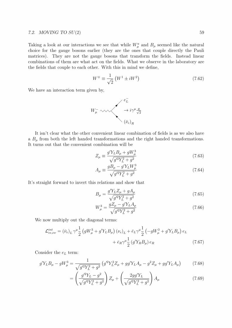
7.2. MOVING TO SU(2) 59
Taking a look at our interactions we see that while W aµ and Bµ seemed like the natural
choice for the gauge bosons earlier (they are the ones that couple directly the Paulimatrices). They are not the gauge bosons that transform the fields. Instead linearcombinations of them are what act on the fields. What we observe in the laboratory arethe fields that couple to each other. With this in mind we define,
W∓ ≡ 1√2
(W 1 ± iW 2
)(7.62)
We have an interaction term given by,
W−µ
e−L
(νe)R
→ iγµ g√2
It isn’t clear what the other convenient linear combination of fields is as we also havea Bµ from both the left handed transformations and the right handed transformations.It turns out that the convenient combination will be
Zµ ≡g′YLBµ + gW 3
µ√g′2Y 2
L + g2(7.63)
Aµ ≡gBµ − g′YLW 3
µ√g′2Y 2
L + g2(7.64)
It’s straight forward to invert this relations and show that
Bµ =g′YLZµ + gAµ√g′2Y 2
L + g2(7.65)
W 3µ =
gZµ − g′YLAµ√g′2Y 2
L + g2(7.66)
We now multiply out the diagonal terms:
Lintee,νν = (νe)L γµ1
2
(gW 3
µ + g′YLBµ
)(νe)L + eLγ
µ1
2
(−gW 3
µ + g′YLBµ
)eL
+ eRγµ1
2(g′YRBµ) eR (7.67)
Consider the eL term:
g′YLBµ − gW 3µ =
1√g′2Y 2
L + g2
(g′2Y 2
LZµ + gg′YLAµ − g2Zµ + gg′YLAµ)
(7.68)
=
(g′2YL − g2√g′2Y 2
L + g2
)Zµ +
(2gg′YL√g′2Y 2
L + g2
)Aµ (7.69)
60 CHAPTER 7. WEAK INTERACTIONS
Repeating this process for the neutrino and right-handed particles the diagonal termtakes the form,
Lintee,νν = (νe)L γµ1
2
√g′2Y 2
L + g2Zµ (νe)L + eLγµ1
2
g′2Y 2L − g2√
g′2Y 2L + g2
ZµeL
+eLγµ gg′YL√
g′2Y 2L + g2
AµeL+eRγµ1
2
g′2YLYR√g′2Y 2
L + g2ZµeR + eRγ
µ1
2
gg′YR√g′2Y 2
L + g2AµeR
(7.70)
We now see what our seemingly obscure linear combination of fields Zµ, Aµ bought us.We have a field that has a similar form of coupling to left and right handed particles.We identify this field with the photon. To have the same EM couplings for eR and eLwe require YR = 2YL (compare terms 3 and 5). For the electron we define YL = −1. Wesummarize our results in the following table
T3 = τ3 = σ3/2Y2
T3 + Y2
νe12
−12
0eL −1
2−1
2−1
eR 0 −1 −1
With our new value of Y we can write our fields in a more symmetric way,
Zµ ≡gW 3
µ − g′Bµ√g2 + g′2
(7.71)
Aµ ≡g′W 3
µ + gBµ√g2 + g′2
(7.72)
and we define
sin θw ≡g′√
g2 + g′2(7.73)
cos θw ≡g√
g2 + g′2(7.74)
where θw is known as the “weak” or “Weinberg” angle. We can then write(ZµAµ
)=
(cos θw − sin θwsin θw cos θw
)(W 3µ
Bµ
)(7.75)
⇔(W 3µ
Bµ
)=
(cos θw sin θw− sin θw cos θw
)(ZµAµ
)(7.76)
The EM interaction is given by
− eL,Rγµgg′√g2 + g′2︸ ︷︷ ︸
e
AµeL,R (7.77)
7.3. KINETIC TERMS 61
where e is the electromagnetic coupling constant and given by b
e =gg′√g2 + g′2
=√g2 + g′2 sin θw cos θw (7.78)
Inserting in our new definitions we can write the interaction Lagrangian as
Lintνν,ee = −(e) · eγµAµe+ (νe)L γµ (e)
2 sin θw cos θwZµ (νe)L + (e) · eLγµ
1
2
(2 sin2 θw − 1)
sin θw cos θwZµeL
+ eRγµe
sin2 θwsin θw cos θ2
ZµeR (7.79)
where temporarily we write the electromagnetic coupling constant as (e) to avoid confu-sion with the elecron. The Z vertex factors are thus given by
Zνν =−ie
2 sin θw cos θw(7.80)
ZeLeL =−ie
2 sin θw cos θw(2 sin2 θw − 1) (7.81)
ZeReR =−ie
2 sin θw cos θw(2 sin2 θw) (7.82)
These can all be summarized by
Zff =ie
cos θw sin θw(Qf sin2 θw − T 3
f ) (7.83)
Note that for the quarks we still have SU(2)L × U(1). The left handed up and down
quarks will form an SU(2) doublet,(ud
)L
and the right handed fields will be SU(2)
singlets, uR, dR.
7.3 Kinetic TermsWe now consider the gauge terms of the Lagrangian.
Lgauge = −1
4WµνW
µν − 1
4BµνB
µν (7.84)
We have (recall that Bµ = cos θwAµ − sin θwZµ),
BµνBµν = (∂µBν − ∂νBµ)(∂µBν − ∂νBµ) (7.85)
= [cos θw (∂µAν − ∂νAµ)− sin θw (∂µZν − ∂νZµ)]
× [cos θw (∂µAν − ∂νAµ)− sin θw (∂µZν − ∂νZµ)] (7.86)= (∂µAν − ∂νAµ)(∂µAν − ∂νAµ) cos2 θw
+ (∂µZν − ∂νZµ)(∂µZν − ∂νZµ) sin2 θw
+ (∂µAν∂νZµ − ∂µAν∂µZν) 4 cos θw sin θw (7.87)
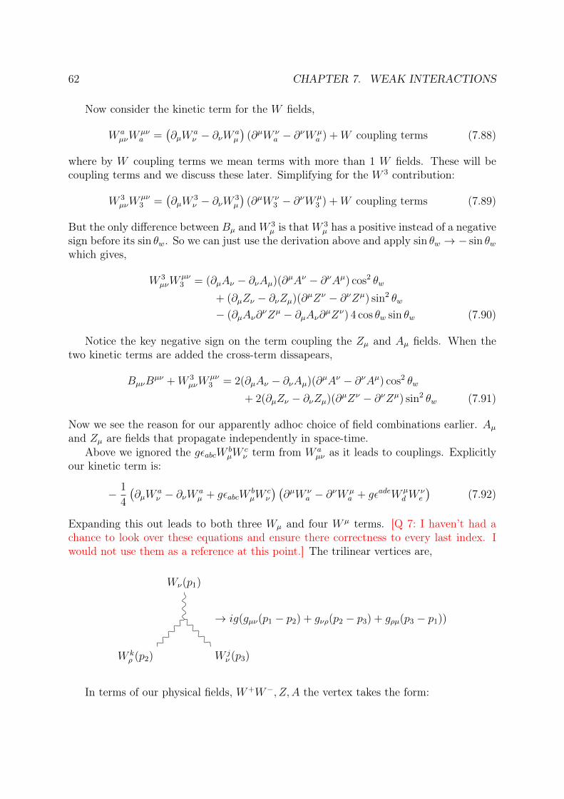
62 CHAPTER 7. WEAK INTERACTIONS
Now consider the kinetic term for the W fields,
W aµνW
µνa =
(∂µW
aν − ∂νW a
µ
)(∂µW ν
a − ∂νW µa ) +W coupling terms (7.88)
where by W coupling terms we mean terms with more than 1 W fields. These will becoupling terms and we discuss these later. Simplifying for the W 3 contribution:
W 3µνW
µν3 =
(∂µW
3ν − ∂νW 3
µ
)(∂µW ν
3 − ∂νWµ3 ) +W coupling terms (7.89)
But the only difference between Bµ andW 3µ is thatW 3
µ has a positive instead of a negativesign before its sin θw. So we can just use the derivation above and apply sin θw → − sin θwwhich gives,
W 3µνW
µν3 = (∂µAν − ∂νAµ)(∂µAν − ∂νAµ) cos2 θw
+ (∂µZν − ∂νZµ)(∂µZν − ∂νZµ) sin2 θw
− (∂µAν∂νZµ − ∂µAν∂µZν) 4 cos θw sin θw (7.90)
Notice the key negative sign on the term coupling the Zµ and Aµ fields. When thetwo kinetic terms are added the cross-term dissapears,
BµνBµν +W 3
µνWµν3 = 2(∂µAν − ∂νAµ)(∂µAν − ∂νAµ) cos2 θw
+ 2(∂µZν − ∂νZµ)(∂µZν − ∂νZµ) sin2 θw (7.91)
Now we see the reason for our apparently adhoc choice of field combinations earlier. Aµand Zµ are fields that propagate independently in space-time.
Above we ignored the gεabcW bµW
cν term from W a
µν as it leads to couplings. Explicitlyour kinetic term is:
− 1
4
(∂µW
aν − ∂νW a
µ + gεabcWbµW
cν
) (∂µW ν
a − ∂νW µa + gεadeW µ
dWνe
)(7.92)
Expanding this out leads to both three Wµ and four W µ terms. [Q 7: I haven’t had achance to look over these equations and ensure there correctness to every last index. Iwould not use them as a reference at this point.] The trilinear vertices are,
W kρ (p2) W j
ν (p3)
Wν(p1)
→ ig(gµν(p1 − p2) + gνρ(p2 − p3) + gρµ(p3 − p1))
In terms of our physical fields, W+W−, Z, A the vertex takes the form:
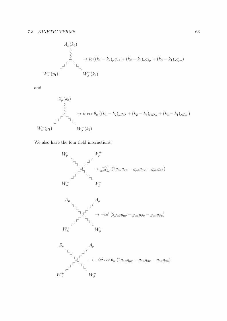
7.3. KINETIC TERMS 63
W+ν (p1) W−
λ (k2)
Aµ(k3)
→ ie ((k1 − k2)µgνλ + (k2 − k3)νgλµ + (k3 − k1)λgµν)
and
W+ν (p1) W−
λ (k2)
Zµ(k3)
→ ie cos θw ((k1 − k2)µgνλ + (k2 − k3)νgλµ + (k3 − k1)λgµν)
We also have the four field interactions:
W+α W−
β
W−ν
W+µ
→ −ie2sin2 θw
(2gµνgνβ − gµβgαν − gµνgαβ)
W+α W−
β
Aµ Aµ
→ −ie2 (2gαβgµν − gαµgβν − gανgβµ)
W+α W−
β
Zµ Aµ
→ −ie2 cot θw (2gαβgµν − gαµgβν − gανgβµ)
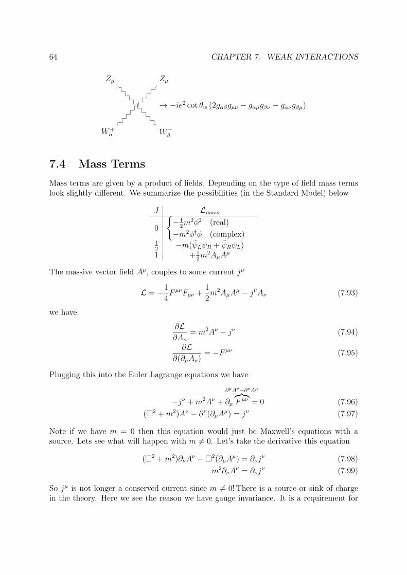
64 CHAPTER 7. WEAK INTERACTIONS
W+α W−
β
Zµ Zµ
→ −ie2 cot θw (2gαβgµν − gαµgβν − gανgβµ)
7.4 Mass TermsMass terms are given by a product of fields. Depending on the type of field mass termslook slightly different. We summarize the possibilities (in the Standard Model) below
J Lmass
0
−1
2m2φ2 (real)
−m2φ†φ (complex)12
−m(ψLψR + ψRψL)1 +1
2m2AµA
µ
The massive vector field Aµ, couples to some current jµ
L = −1
4F µνFµν +
1
2m2AµA
µ − jνAν (7.93)
we have
∂L∂Aν
= m2Aν − jν (7.94)
∂L∂(∂µAν)
= −F µν (7.95)
Plugging this into the Euler Lagrange equations we have
−jν +m2Aν + ∂µ
∂µAν−∂νAµ︷︸︸︷F µν = 0 (7.96)
(2 +m2)Aν − ∂ν(∂µAµ) = jν (7.97)
Note if we have m = 0 then this equation would just be Maxwell’s equations with asource. Lets see what will happen with m 6= 0. Let’s take the derivative this equation
(2 +m2)∂νAν −2(∂µA
µ) = ∂νjν (7.98)
m2∂νAν = ∂νj
ν (7.99)
So jµ is not longer a conserved current since m 6= 0! There is a source or sink of chargein the theory. Here we see the reason we have gauge invariance. It is a requirement for
7.4. MASS TERMS 65
charge conservation, which is taken to be a fundamental principle. Having massive gaugebosons breaks gauge invariance (and in turn charge conservation) and is hence forbiddenin the naive formulation of gauge theories. Since we do see massive gauge bosons inNature something must have gone wrong with this arguement. We will see how thisworks in the next chapter.
Since we know there do exist massive gauge bosons we quickly mention their proper-ties. Their propagator needs to be modified,
− igµν − qµqν/m2
q2 −m2 + iε(7.100)
The longitudinal polarizations are allowed for m > 0. We pick up an extra term in thesum rule of the polarizations
3∑λ=1
εµλε?νλ = −gµν +
qµqν
m2(7.101)
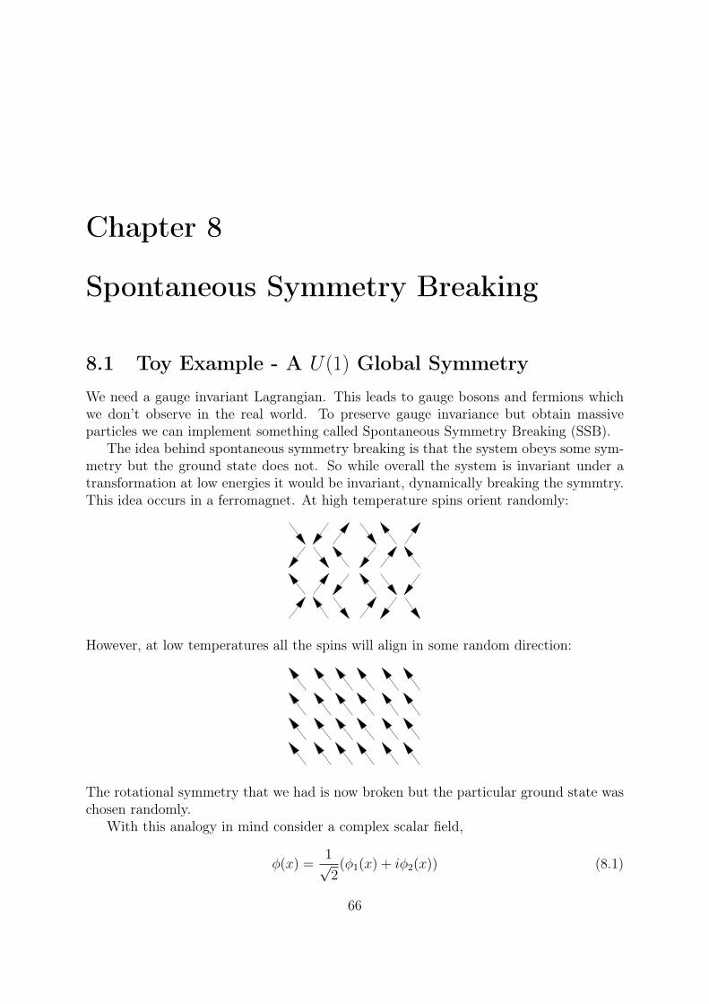
Chapter 8
Spontaneous Symmetry Breaking
8.1 Toy Example - A U(1) Global SymmetryWe need a gauge invariant Lagrangian. This leads to gauge bosons and fermions whichwe don’t observe in the real world. To preserve gauge invariance but obtain massiveparticles we can implement something called Spontaneous Symmetry Breaking (SSB).
The idea behind spontaneous symmetry breaking is that the system obeys some sym-metry but the ground state does not. So while overall the system is invariant under atransformation at low energies it would be invariant, dynamically breaking the symmtry.This idea occurs in a ferromagnet. At high temperature spins orient randomly:
However, at low temperatures all the spins will align in some random direction:
The rotational symmetry that we had is now broken but the particular ground state waschosen randomly.
With this analogy in mind consider a complex scalar field,
φ(x) =1√2
(φ1(x) + iφ2(x)) (8.1)
66
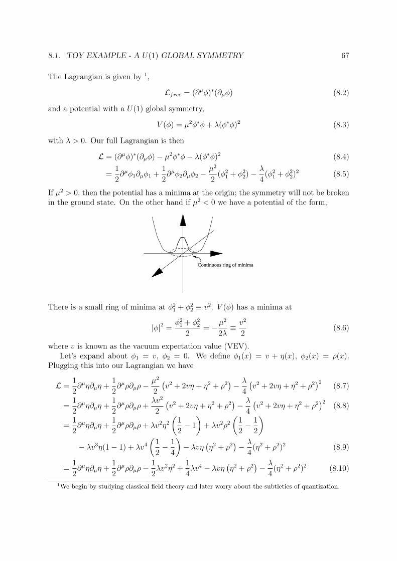
8.1. TOY EXAMPLE - A U(1) GLOBAL SYMMETRY 67
The Lagrangian is given by 1,
Lfree = (∂µφ)∗(∂µφ) (8.2)
and a potential with a U(1) global symmetry,
V (φ) = µ2φ∗φ+ λ(φ∗φ)2 (8.3)
with λ > 0. Our full Lagrangian is then
L = (∂µφ)∗(∂µφ)− µ2φ∗φ− λ(φ∗φ)2 (8.4)
=1
2∂µφ1∂µφ1 +
1
2∂µφ2∂µφ2 −
µ2
2(φ2
1 + φ22)− λ
4(φ2
1 + φ22)2 (8.5)
If µ2 > 0, then the potential has a minima at the origin; the symmetry will not be brokenin the ground state. On the other hand if µ2 < 0 we have a potential of the form,
Continuous ring of minima
There is a small ring of minima at φ21 + φ2
2 ≡ v2. V (φ) has a minima at
|φ|2 =φ2
1 + φ22
2= −µ
2
2λ≡ v2
2(8.6)
where v is known as the vacuum expectation value (VEV).Let’s expand about φ1 = v, φ2 = 0. We define φ1(x) = v + η(x), φ2(x) = ρ(x).
Plugging this into our Lagrangian we have
L =1
2∂µη∂µη +
1
2∂µρ∂µρ−
µ2
2
(v2 + 2vη + η2 + ρ2
)− λ
4
(v2 + 2vη + η2 + ρ2
)2 (8.7)
=1
2∂µη∂µη +
1
2∂µρ∂µρ+
λv2
2
(v2 + 2vη + η2 + ρ2
)− λ
4
(v2 + 2vη + η2 + ρ2
)2 (8.8)
=1
2∂µη∂µη +
1
2∂µρ∂µρ+ λv2η2
(1
2− 1
)+ λv2ρ2
(1
2− 1
2
)− λv3η(1− 1) + λv4
(1
2− 1
4
)− λvη
(η2 + ρ2
)− λ
4(η2 + ρ2)2 (8.9)
=1
2∂µη∂µη +
1
2∂µρ∂µρ−
1
2λv2η2 +
1
4λv4 − λvη
(η2 + ρ2
)− λ
4(η2 + ρ2)2 (8.10)
1We begin by studying classical field theory and later worry about the subtleties of quantization.
68 CHAPTER 8. SPONTANEOUS SYMMETRY BREAKING
Note the quadratic term for the η field:
− 1
2
(2λv2
)η2 (8.11)
Thus we have a new field η that has a mass of 2λv2. Further the ρ term does not havea mass!So we have one massless field which we call our “Goldstone Boson”. We get amassive field for the one that goes along the real axis of φ and a massless field for theone along the imaginary axis. That’s because the potential has no derivative along theimaginary axis. Goldstone bosons always arise with the breaking of a global symmetry.There is one Goldstone boson for each generator.
8.2 Global → local symmetry
We now move onto a more intricate example: U(1) local symmetry breaking. Recall thatto have a U(1) symmetry we use Dµ = ∂µ − igAµ with φ(x)→ eigθ(x)φ ≡ φ′(x). We have
L = (Dµφ)∗(Dµφ)− µ2φ∗φ− λ(φ∗φ)2 − 1
4FµνF
µν (8.12)
We consider the particular case of µ2 < 0. We initially have φ1, φ2 which form two degreesof freedom (DOF) while Aµ has two transverse polarizations so it has two DOF as well.
We rewrite
φ(x) = (φ1(x) + iφ2(x)) (8.13)
= r(x)e−iθ(x) (8.14)
where r(x) and φ(x) are two fields. We choose a gauge such that φ(x)→ eiθ(x)φ(x) = r(x).This will give a gauge with φ(x) being real (as we did in the global toy example earlier).This is called the unitary gauge. We expand about the minimum of the potential denotedby v as,
φ(x) =1√2
(v + h(x)), (8.15)
where h(x) is our Higg’s field. Since the potential takes the same form as before so doesthe VEV giving,
v2 = −µ2
λ(8.16)
= 〈0|φ(x)|0〉 (8.17)
Note that you want to have a scalar vacuum since we want to want the vacuum expectationvalue to be Lorentz invariant (otherwise it would not be rotationally invariant and to our
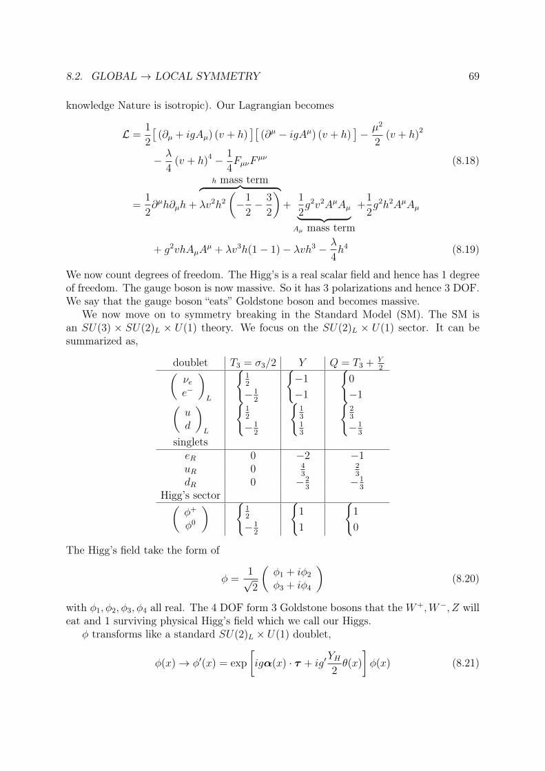
8.2. GLOBAL → LOCAL SYMMETRY 69
knowledge Nature is isotropic). Our Lagrangian becomes
L =1
2
[(∂µ + igAµ) (v + h)
][(∂µ − igAµ) (v + h)
]− µ2
2(v + h)2
− λ
4(v + h)4 − 1
4FµνF
µν (8.18)
=1
2∂µh∂µh+
h mass term︷ ︸︸ ︷λv2h2
(−1
2− 3
2
)+
1
2g2v2AµAµ︸ ︷︷ ︸
Aµ mass term
+1
2g2h2AµAµ
+ g2vhAµAµ + λv3h(1− 1)− λvh3 − λ
4h4 (8.19)
We now count degrees of freedom. The Higg’s is a real scalar field and hence has 1 degreeof freedom. The gauge boson is now massive. So it has 3 polarizations and hence 3 DOF.We say that the gauge boson “eats” Goldstone boson and becomes massive.
We now move on to symmetry breaking in the Standard Model (SM). The SM isan SU(3) × SU(2)L × U(1) theory. We focus on the SU(2)L × U(1) sector. It can besummarized as,
doublet T3 = σ3/2 Y Q = T3 + Y2(
νee−
)L
12
−12
−1
−1
0
−1(ud
)L
12
−12
1313
23
−13
singletseR 0 −2 −1uR 0 4
323
dR 0 −23
−13
Higg’s sector(φ+
φ0
) 12
−12
1
1
1
0
The Higg’s field take the form of
φ =1√2
(φ1 + iφ2
φ3 + iφ4
)(8.20)
with φ1, φ2, φ3, φ4 all real. The 4 DOF form 3 Goldstone bosons that the W+,W−, Z willeat and 1 surviving physical Higg’s field which we call our Higgs.
φ transforms like a standard SU(2)L × U(1) doublet,
φ(x)→ φ′(x) = exp
[igα(x) · τ + ig′
YH2θ(x)
]φ(x) (8.21)

70 CHAPTER 8. SPONTANEOUS SYMMETRY BREAKING
Our covarient derivative takes the form
Dµ = ∂µ − igτ ·Wµ − ig′YH2Bµ (8.22)
We assume a potential V (φ) = µ2φ†φ+λ(φ†φ)2, where φ†φ = φ21 +φ2
2 +φ23 +φ2
4. As beforewe have V (φ) to be a minimum at φ†φ = −µ2
2λ≡ v2
2. We choose our ground state to be
φg ≡ 〈0|φ|0〉 =1√2
(0v
)(8.23)
We certainly want our ground state to be electrically neutral. Recall that Q = T3 + Y2.
Since the ground state is a −12spinor we have T3 = −1
2. Thus we require YH = 1. Note
that this also forces the top component of the Higgs to have a charge of 1 as a doublethas the same quantum numbers for the top and bottom component. We expand aroundφg:
φ(x) =1√2
(σ1(x) + iσ2(x)v + h(x) + iη(x)
)(8.24)
While not obvious one can show that you can pick a gauge that removes σ1, σ2, andη. Utilizing this we can write the field as,
φ′ = Uφ(x) =1√2
(0
v + h(x)
)(8.25)
In this gauge the W± and a linear combination of W3 and B will get a mass andthe charged components and Imh completely dissappear from the theory (i.e. they get“eaten”).
Our covarient derivative takes the form
Dµφ =
(∂µ − i
2(gW µ
3 + g′Bµ) − ig√2W+µ
− ig√2W−µ ∂µ + i
2(gW µ
3 − g′Bµ)
)1√2
(0
v + h(x)
)(8.26)
=1√2
(− ig√
2W+µ(v + h(x))
∂µh(x) + i2(gW µ
3 − g′Bµ)(v + h(x))
)(8.27)
=1√2
(− ig√
2W+µ(v + h(x))
∂µh+ i2(g2 + g′2)1/2Zµ(v + h)
) (recall the
definition of Zµ
)(8.28)
so we have
(Dµφ)∗ =1√2
(i g√
2W−µ(v + h)
∂µh− i2(g2 + g′2)1/2Zµ(v + h)
)(8.29)
and we have
(Dµφ†)(Dµφ) =1
2
g2
2W+µ W
−µ(v + h)2 + ∂µh∂µh+g2 + g′2
4ZµZµ(v + h)2
(8.30)

8.2. GLOBAL → LOCAL SYMMETRY 71
Our Lagrangian then takes the form
Lφ = (Dµφ)†(Dµφ)− V (φ) + Vector boson kinetic terms (8.31)
=g2v2
4W−µ W
+µ +1
2∂µh∂µh+
g2 + g′2
8v2ZµZ
µ +g2v
2W−µ W
+µh
+g2 + g′2
4vZµZµh+
g2
4W−µ W
+µh2 +g2 + g′2
8ZµZµh
2 − 1
2(2λv2)2 − λvh3
− λ
4h4 + Vector boson kinetic terms (8.32)
Recall that if you have a massive vector boson then it has a mass term
1
2m2VµV
µ (8.33)
so we havem2Z =
v2
4(g2 + g′2) (8.34)
and in terms of the Weinberg angle we have
mZ =v
2
e
sin θw cos θw(8.35)
and
m2W =
g2v2
4(8.36)
⇒ mW =v
2
e
sin θw(8.37)
Now note thatmW
mZ
= cos θw (8.38)
so we get a really simple prediction for the Weinberg angle.Now recall our low energy effective theory for the weak interaction,
e−
νe
νe
e−
which gave in the V − A picture
M = −iGF√2
[u3γ
µ(1− γ5)u1
] [u4γ
µ(1− γ5)u2
](8.39)
Now consider the same diagram only with the full theory

72 CHAPTER 8. SPONTANEOUS SYMMETRY BREAKING
W−
e−
νe
νe
e−
So the full theory gives
M = −ig2
8
(u3γ
µ(1− γ4)u1
] [−gµν + qµqνm2W
q2 −m2W
] [u4γ
ν(1− γ5)u2
](8.40)
Now consider the low energy case of E2CM m2
W . This implies that q2 m2W and
qµqν m2W and so we can relate the Fermi constant to the variables of the full theory,
GF√2
=g2
8m2W
=g2
8g2v2/4
which gives
v2 =1√2GF
(8.41)
and so we have a prediction for the value of the VEV. The parameters of the Lagrangian:g, g′ , v, (λ or m). Can be found through measurable parameters:
e,GF ,mZ ,mW , θw, ... (8.42)
Measurements at the LHC and elsewhere have given
mW = 80.399± 0.023GeVmZ = 91.1876± 0.0021GeVGF = (1.16637± 0.00001)× 10−5GeV2
e =
(4π
137.035999084
)1/2
sin2 θw = 022292(28)
which we can use to estimate our VEV:
v = 246 GeV
Note that
cos θw =
(mW
mZ
)meas
= 0.8817± 0.0003
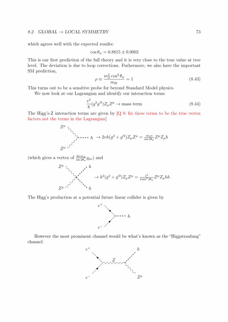
8.2. GLOBAL → LOCAL SYMMETRY 73
which agrees well with the expected results:
cos θw = 0.8815± 0.0002
This is our first prediction of the full theory and it is very close to the true value at treelevel. The deviation is due to loop corrections. Furhermore, we also have the importantSM prediction,
ρ ≡ m2Z cos2 θwmW
= 1 (8.43)
This turns out to be a sensitive probe for beyond Standard Model physics.We now look at our Lagrangian and identify our interaction terms
v2
8(g2g′2)ZµZ
µ → mass term (8.44)
The Higg’s-Z interaction terms are given by [Q 8: fix these terms to be the true vertexfactors not the terms in the Lagrangian]
Zµ
Zµ
h → 2vh(g2 + g′2)ZµZµ = mZe
sin 2θwZµZµh
(which gives a vertex of 2iemZsin 2θw
gµν) and
Zµ
Zµ h
h
→ h2(g2 + g′2)ZµZµ = e2
2 sin2 2θwZµZµhh
The Higg’s production at a potential future linear collider is given by
e−
e+
h
However the most prominent channel would be what’s known as the “Higgstraulung”channel:
e−
e+
Z
h
Zµ

74 CHAPTER 8. SPONTANEOUS SYMMETRY BREAKING
At the LHC the “gluon fusion” channel dominates in gluon production.
8.3 Fermion MassesSo far we have made mentioned anything about fermion masses. In fact, having a theorythat couples to left and right particles separately forbids such terms to be in the highenergy Lagrangian!We want terms that couple ψR, ψL in gauge invariant way. This can beaccomplished if the weak interaction is not a true symmetry but one that is spontaneouslybroken.
This can be accomplished by starting with the Higgs charged under SU(2) and thenbreaking this symmetry. We focus the dicussion on leptons however the quark masses aregenerated in a completely analogous way.
When model building we obey the democratic principle; every term that is allowedby the symmetry is written. To find out whether a term is allowed we need to add thecharges. One such term is given by:
(Lφ)︸︷︷︸SU(2) doublets
eR (8.45)
where L =
(νee
)L
, φ = 1√2
(φ1 + iφ2
φ3 + iφ4
)→ 1√
2
(0
v + h(x)
). This term is clearly
invariant under SU(3) as none of these fields have color. Furthermore, it is invariantunder SU(2) since:
LSU(2)−−−→ L exp
(i
2θ · σ
)(8.46)
φSU(2)−−−→ exp
(− i
2θ · σ
)φ (8.47)
Lastly, the U(1)Y charges add as necessary:
YR + Yφ + YL = −2 + 1 + 1 = 0
(if we forget these values they can easily be recalled using Q = T3 + Y2. Thus this term is
invariant under all the gauge symmeries and we must write it down. The adjoint is givenby (
(Lφ)eR)†
= e†Rφ†γ0†L (8.48)
= eR(φ†L) (8.49)
So in order to get fermion masses we add a term:
Lmass = −ge[(Lφ)eR + eR(φ†L)
](8.50)
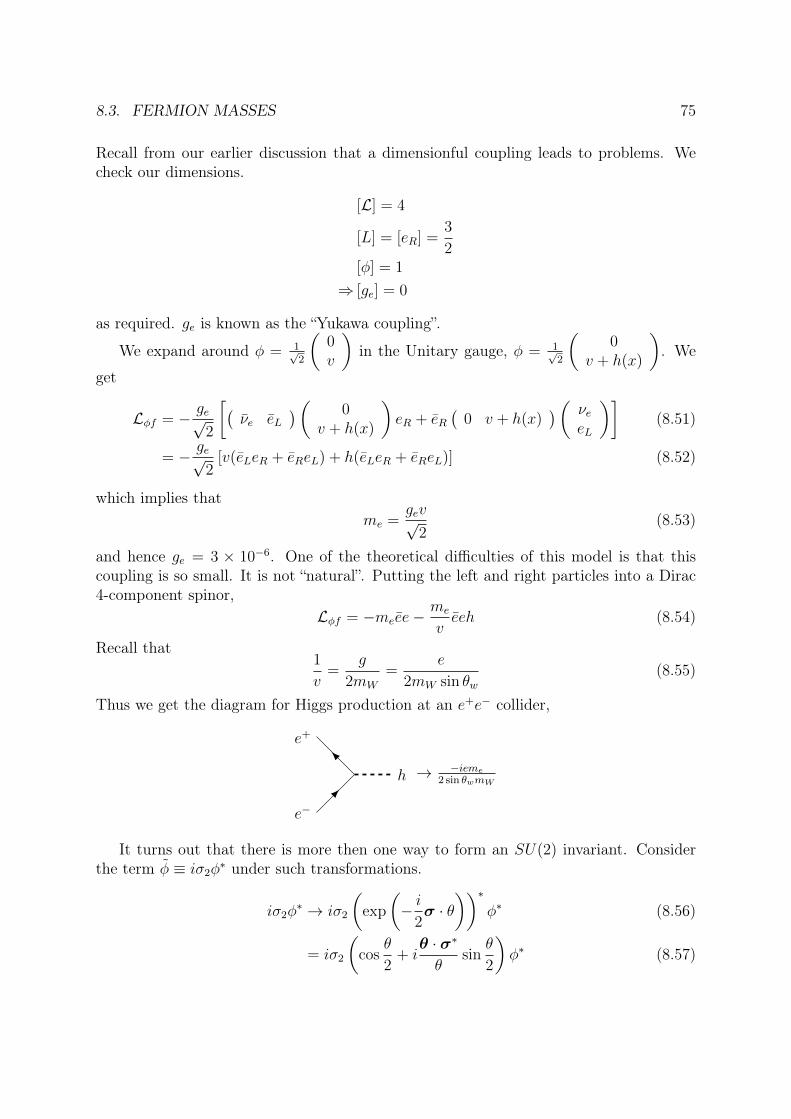
8.3. FERMION MASSES 75
Recall from our earlier discussion that a dimensionful coupling leads to problems. Wecheck our dimensions.
[L] = 4
[L] = [eR] =3
2[φ] = 1
⇒ [ge] = 0
as required. ge is known as the “Yukawa coupling”.
We expand around φ = 1√2
(0v
)in the Unitary gauge, φ = 1√
2
(0
v + h(x)
). We
get
Lφf = − ge√2
[(νe eL
)( 0v + h(x)
)eR + eR
(0 v + h(x)
)( νeeL
)](8.51)
= − ge√2
[v(eLeR + eReL) + h(eLeR + eReL)] (8.52)
which implies thatme =
gev√2
(8.53)
and hence ge = 3 × 10⁻⁶. One of the theoretical difficulties of this model is that thiscoupling is so small. It is not “natural”. Putting the left and right particles into a Dirac4-component spinor,
Lφf = −meee−me
veeh (8.54)
Recall that1
v=
g
2mW
=e
2mW sin θw(8.55)
Thus we get the diagram for Higgs production at an e+e− collider,
e−
e+
h → −ieme2 sin θwmW
It turns out that there is more then one way to form an SU(2) invariant. Considerthe term φ ≡ iσ2φ
∗ under such transformations.
iσ2φ∗ → iσ2
(exp
(− i
2σ · θ
))∗φ∗ (8.56)
= iσ2
(cos
θ
2+ i
θ · σ∗
θsin
θ
2
)φ∗ (8.57)
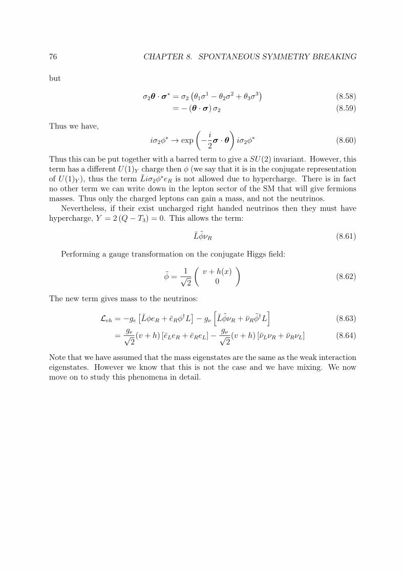
76 CHAPTER 8. SPONTANEOUS SYMMETRY BREAKING
but
σ2θ · σ∗ = σ2
(θ1σ
1 − θ2σ2 + θ3σ
3)
(8.58)= − (θ · σ)σ2 (8.59)
Thus we have,
iσ2φ∗ → exp
(− i
2σ · θ
)iσ2φ
∗ (8.60)
Thus this can be put together with a barred term to give a SU(2) invariant. However, thisterm has a different U(1)Y charge then φ (we say that it is in the conjugate representationof U(1)Y ), thus the term Liσ2φ
∗eR is not allowed due to hypercharge. There is in factno other term we can write down in the lepton sector of the SM that will give fermionsmasses. Thus only the charged leptons can gain a mass, and not the neutrinos.
Nevertheless, if their exist uncharged right handed neutrinos then they must havehypercharge, Y = 2 (Q− T3) = 0. This allows the term:
LφνR (8.61)
Performing a gauge transformation on the conjugate Higgs field:
φ =1√2
(v + h(x)
0
)(8.62)
The new term gives mass to the neutrinos:
Leh = −ge[LφeR + eRφ
†L]− gν
[LφνR + νRφ
†L]
(8.63)
=ge√
2(v + h) [eLeR + eReL]− gν√
2(v + h) [νLνR + νRνL] (8.64)
Note that we have assumed that the mass eigenstates are the same as the weak interactioneigenstates. However we know that this is not the case and we have mixing. We nowmove on to study this phenomena in detail.

Chapter 9
CKM Matrix
We now move to the quark sector. In the quark sector the interaction basis is differentthen the mass basis. We can choose the mass basis to be diagonal and that way particleswill interact in linear combinations or we can choose the interactions to be diagonal butthen the particles will be in a linear combination of masses. Typically what we call a“particle” is one with a well defined mass. We will need to know how to relate betweenthese two bases. One basis is the weak (interaction) basis which we denote with a prime:
QjL ≡
(uj′Ldj′L
); uj′R , d
j,′R︸ ︷︷ ︸
Right-handedsinglets
where j = 1, 2, 3 labels the generation. The mass basis is unprimed. The unbroken weakinteraction is given by,
LQH = −3∑
i,j=1
gij(Qi′Lφd
j′R + dj′Rφ
†Qi′L
)−
3∑i,j=1
hij
(Qi′Lφu
j′R + uj′Rφ
†Qi′L
)(9.1)
withφ ≡ iσ2φ
∗ (9.2)
Introducing a VEV and choosing a gauge such that,
φ =1√2
(0
v + h(x)
), φ =
1√2
(v + h(x)
0
)(9.3)
This gives
LQH = −v + h(x)√2
3∑
i,j=1
gij(di′Ld
j′R + dj′Rd
i′L
)+
3∑i,j=1
hi,j(ui′Lu
j′R + uj′Ru
i′L
)(9.4)
77

78 CHAPTER 9. CKM MATRIX
We introduce the undiagonalized mass matrices (3× 3 for 3 generations):
M ijd =
v√2gij (9.5)
M iju =
v√2hij (9.6)
which allows us to write the mass terms as
LQH,mass = −(d′Lmdd
′R + d′Rmdd
′L
)− (u′Lmuu
′R + u′Rmuu
′L) (9.7)
Thus we worked in the interaction basis since this was the sensible basis when discussingthe interaction with the Higgs. However, now we want to go back to mass eigenstates.The physical/mass basis is related to the weak basis by some unitary transformation.1We have,
ujL,R =(V uL,R
)j,kuk′L,R (9.8)
djL,R =(V dL,R
)j,K
dk′L,R (9.9)
In these four equations we have four n× n unitary matrices,V uL , V
uR , V
dL , V
dR
, where n
(= 3 in the SM) is the number of generations. In the physical basis we have explicitly,
LQH = −(
1 +h
v
)(mddd+muuu+mecc+msss+mttt+mbbb
)(9.10)
where we have combined our left and right handed spinors into Dirac spinors,
Ψ =
(ψLψR
)(9.11)
For brevity we denote
dL =
dLsLbL
(9.12)
uL =
uLcLtL
(9.13)
and similarly for right handed fields. We can write
LQH = −(d′LM
′dd′R + u′LMuu
′R + h.c.
)(9.14)
= −(dLMddR + uLMuuR + h.c.
)(9.15)
1The question of in what basis the “particles” exist is quite subtle as we will see later in the discussionof meson oscillations.

79
with
Md =
md 0 00 ms 00 0 mb
Mu =
mu 0 00 mc 00 0 mt
Consider the top equation (equation in the weak basis):
LQH = d′LM′dd′R + u′LMuu
′R + h.c. (9.16)
= d′LVd†L︸ ︷︷ ︸
dL
V dLM
′dV
d†R V d
Rd′R︸ ︷︷ ︸
dR
+ u′LVu†L︸ ︷︷ ︸
uL
V uLMuV
u†R V uu′R︸ ︷︷ ︸
uR
+h.c. (9.17)
comparing with equation 9.15 we see that
Md = V dLM
′dV
d†R (9.18)
Mu = V uLM
′uV
u†R (9.19)
The quark interaction terms are given by
LintQ =n∑j=1
iQj′Lγ
µ
[∂µ − igτiW i
µ −ig′
2YLBµ
]Qj′′L +
n∑j=1
iuj′Rγµ
[∂µ − i
g′
2YR,uBµ
]uj′R
+n∑j=1
idj′Rγµ
[∂µ − i
g′
2YR,dBµ
]dj′R (9.20)
There are two possible cases for the left handed terms:
1. The terms with 1, τ 3; These are the diagonal terms and correspond to γ, Z
2. The terms with τ 1, τ 2; These are non-diagonal and give W±
In the first case we have (we denote stuffµ as the terms in the square brackets) for theleft handed terms: ∑
uj′Lγµ [stuffµ]uj′L ± d
j′Lγ
µ [stuffµ] dj′L (9.21)
Switching to the vector form for the quarks we have
u′Lγµ [stuffµ]u′L ± d′Lγµ [stuffµ] d′L (9.22)
We can rewrite this in terms of the unprimed basis:
uLVµL γ
µ [stuffµ]V u†L ± dLV
dLγ
µ [stuffµ]V d†L dL (9.23)
Now the V ’s act on flavor space (which is completely unrelated to stuffµ). So we canbring them across and we have
uLγµ [stuffµ]uL ± dLγµ [stuffµ] dL (9.24)

80 CHAPTER 9. CKM MATRIX
Thus neutral currents remain diagonal in flavor space. The same math also follows forthe right handed fields.
Now consider the second case of charged current interaction W± = 1√2(W 1 ∓W 2).
Our left handed terms are:
LCC =g√2
(u1′L u2′
L u3′L
)γµ
d1′L
d2′L
d3′L
W+µ + h.c. (9.25)
Switching to the physical basis gives:
LCC =g√2uLVLγ
µV d†L dLW
+µ + h.c. (9.26)
We defineVCKM = V µ
L Vd†L (9.27)
This matrix is called the “Caribbo Kobayashi Maskawa” matrix and gives
LCC =g√2uLγ
µVCKMdLW+µ (9.28)
Note that this matrix is unitary:
V †CKMVCKM = V dLV
µ†L V µ
L Vd†L (9.29)
= 1 (9.30)
We now count the independent parameters in the CKM matrix. It is an n×n complexmatrix so it has 2n2 initial parameters. Then we have the unitarity constraint which givesn2 constraints.2 Now the quark phases also constrain the matrix. We can redefine thephase of quark fields with no effect on matrix elements. The mass terms are triviallyinvariant under this change. This is trivial under the neutral current terms. Howeverthis is not the case for charged currents. qL and qR must have the same phase rotation.Our terms are of the form
uL,iγµVi,jdj (9.31)
we have
uL,i → eiφiuL,i
dL,j → eiφjdL,j
Hence we have
VCKM →
eiφu 0 00 eiφc 00 0 eiφt
VCKM
e−iφd 0 00 e−iφs 00 0 e−iφb
(9.32)
2This may seem obvious since V † = V −1 is n2 equations. However, some of these equations may beredundant. The proof is more intricate but left out here.

81
HenceVi,j → e−i(φj−φi)Vi,j (9.33)
This removes 2n− 1 degrees of freedom. Thus in total we have
n2 − 2n+ 1 = (n− 1)2 (9.34)
degrees of freedom.
n free param→ (n− 1)2 Euler Angles Phases2 1 1 13 4 3 14 9 6 3
The charged current interactions are
LCC =g√2
∑i,j
uiLγµVi,jd
jLW
+µ +
∑i,j
djLγµV ∗i,juiW
−µ
(9.35)
We have the following interactions:
W+vVudFu
dE
W+vVudd
u
uVudgW−
dE
dVudgW−
eand
W−vV ∗ud
Fd
uE
W−vV ∗ud
u
d
ddV ∗ud
gW+
ue
Consider for now 2 generations: 1 free parameter.
LCC = W µ†(uLcL
)γµ(
cos θc sin θc− sin θc cos θc
)(uLcL
)+ h.c. (9.36)
where we introduce the Cabibbo angle which is found experimentally to be cos θc ≈ 0.97and sin θL ≈ 0.22. We have the interaction
d
EgW+
uE→ ig√
2V ∗udγ
µ1− γ5
2(9.37)

82 CHAPTER 9. CKM MATRIX
One exact form is given by:
V =
1 0 00 c2 s2
0 −s2 c2
c1 s1 0−s1 c1 0
0 0 1
1 0 00 1 00 0 eiδ
1 0 00 c3 s3
0 −s3 −s3
(9.38)
with ci ≡ cos θi and si ≡ sin θi. The Wolfenstein parametrization simplifies this form. itis given as follows. Define λ = sin θc ≈ 0.22. Then
VCKM =
1− λ2
2λ Aλ3(ρ− iη)
−λ 1− λ2
2Aλ2
Aλ3(1− ρ− iη) −Aλ2 1
+O(λ4) (9.39)
A, ρ, η are all O(1) so the hierarchy is completely contained in λ.
9.1 “GIM Mechanism”We now go into a historical aside into the Glashow, Iliopoulos, and Maiani mechanismfor suppression of flavor-changing neutral currents. In 1974 they knew of quark structureu, d, s. Cabibbo said: suppose we have weak quark and lepton doublets. Since at thetime they only know of 3 quarks he could only write
Q =
(u
d cos θc + s sin θc
)≡(
udc
)(9.40)
andL =
(νµµL
)(9.41)
Using the spin analogy he wrote the interaction
J+ = gQτ †Q = g(u dc
)( 0 10 0
)(udc
)(9.42)
Using this interaction he was able to explain the K+ branching fraction:
u
s
W
νµ
µ+
K+
However they saw that the K0 decay was heavily suppressed. They had
H0 = gQτ3Q (9.43)∼ g(uu− dcdc) (9.44)∼ g(uu− dd cos2 θc − ss sin2 θc + (ds+ sd) sin θc cos θc) (9.45)

9.1. “GIM MECHANISM” 83
This is a flavor changed neutral current!GIM proposed a new up-type quark which theycalled the c quark
Q2 =
(csc
)=
(c
−d sin θc + s cos θc
)(9.46)
with
J0 =[Qτ3Q+ Q2τ2Q2
](9.47)
= g[uu+ cc− dcdc − scsc
](9.48)
= g[uu+ cc− dd− ss
](9.49)
They predicted the c quark mass in order to explain the observed
Γ(K0 → µ+µ−
)(9.50)
They predicted a charm quark mass of ∼ 1−3GeV. The quark was successfully discoveredlater that same year.
Consider the following “penguin” process:
c u
W+
d,s,b
uu
The amplitude is proportional to
M∝∑q=d,s,b
f(mq)V∗cqVuq (9.51)
If md,ms,mb are equal (m) then
A ∝ f(m)∑
V ∗cqVuq (9.52)
Since V †V = 1 we have∑V ∗cqVuq = 0. To see this consider the following:
V †V =
Vud Vus VubVcd Vcs VcbVtd Vts Vtb
V ∗ud V ∗cd V ∗tdV ∗us V ∗cs V ∗tsV ∗ub V ∗cb V ∗tb
=
1 0 00 1 00 0 1
(9.53)
This is just the GIM mechanism at work. It is essentially just a statement that CKMmatrices are unitary. In practice since the masses are similar this element is just sup-pressed.
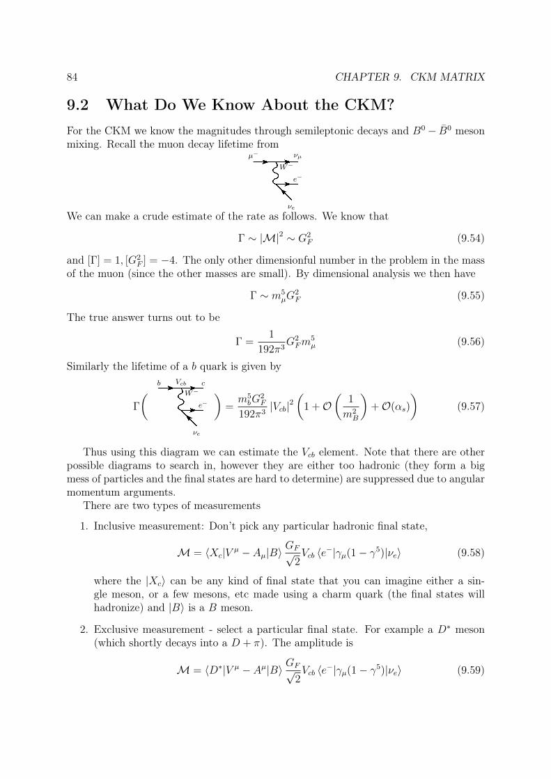
84 CHAPTER 9. CKM MATRIX
9.2 What Do We Know About the CKM?For the CKM we know the magnitudes through semileptonic decays and B0 − B0 mesonmixing. Recall the muon decay lifetime from
µ−FFνµ
W−
Fe−
νe
We can make a crude estimate of the rate as follows. We know that
Γ ∼ |M|2 ∼ G2F (9.54)
and [Γ] = 1, [G2F ] = −4. The only other dimensionful number in the problem in the mass
of the muon (since the other masses are small). By dimensional analysis we then have
Γ ∼ m5µG
2F (9.55)
The true answer turns out to be
Γ =1
192π3G2Fm
5µ (9.56)
Similarly the lifetime of a b quark is given by
Γ
( bFVcbFc
W−
Fe−
νe
)=m5bG
2F
192π3|Vcb|2
(1 +O
(1
m2B
)+O(αs)
)(9.57)
Thus using this diagram we can estimate the Vcb element. Note that there are otherpossible diagrams to search in, however they are either too hadronic (they form a bigmess of particles and the final states are hard to determine) are suppressed due to angularmomentum arguments.
There are two types of measurements
1. Inclusive measurement: Don’t pick any particular hadronic final state,
M = 〈Xc|V µ − Aµ|B〉GF√
2Vcb 〈e−|γµ(1− γ5)|νe〉 (9.58)
where the |Xc〉 can be any kind of final state that you can imagine either a sin-gle meson, or a few mesons, etc made using a charm quark (the final states willhadronize) and |B〉 is a B meson.
2. Exclusive measurement - select a particular final state. For example a D∗ meson(which shortly decays into a D + π). The amplitude is
M = 〈D∗|V µ − Aµ|B〉 GF√2Vcb 〈e−|γµ(1− γ5)|νe〉 (9.59)
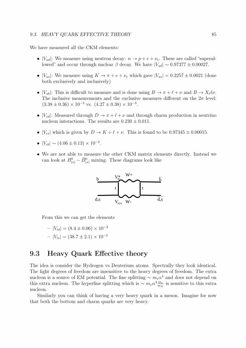
9.3. HEAVY QUARK EFFECTIVE THEORY 85
We have measured all the CKM elements:
• |Vud|: We measure using neutron decay: n→ p+ e+ νe. These are called “superal-lowed” and occur through nuclear β decay. We have |Vud| ∼ 0.97377± 0.00027.
• |Vus|: We measure using K → π + e+ νe which gave |Vus| = 0.2257± 0.0021 (doneboth exclusively and inclusively)
• |Vub|: This is difficult to measure and is done using B → π + `+ ν and B → X``ν.The inclusive measurements and the exclusive measures different on the 2σ level:(3.38± 0.36)× 10−3 vs. (4.27± 0.38)× 10−3.
• |Vcd|: Measured through D → π+ `+ ν and through charm production in neutrinonucleon interactions. The results are 0.230± 0.011.
• |Vcs| which is given by D → K + `+ ν. This is found to be 0.97345± 0.00015.
• |Vcb| ∼ (4.06± 0.13)× 10−2.
• We are not able to measure the other CKM matrix elements directly. Instead wecan look at B0
(s) − B0(s) mixing. These diagrams look like
t t
b b_
d,s d,s_ _
W+
W-
V*tb
Vtd,ts
From this we can get the elements
– |Vtd| = (8.4± 0.06)× 10−3
– |Vts| = (38.7± 2.1)× 10−3
9.3 Heavy Quark Effective theory
The idea is consider the Hydrogen vs Deuterium atoms. Spectrally they look identical.The light degrees of freedom are insensitive to the heavy degrees of freedom. The extranucleon is a source of EM potential. The fine splitting ∼ meα
4 and does not depend onthis extra nucleon. The hyperfine splitting which is ∼ meα
4 memN
is sensitive to this extranucleon.
Similarly you can think of having a very heavy quark in a meson. Imagine for nowthat both the bottom and charm quarks are very heavy.
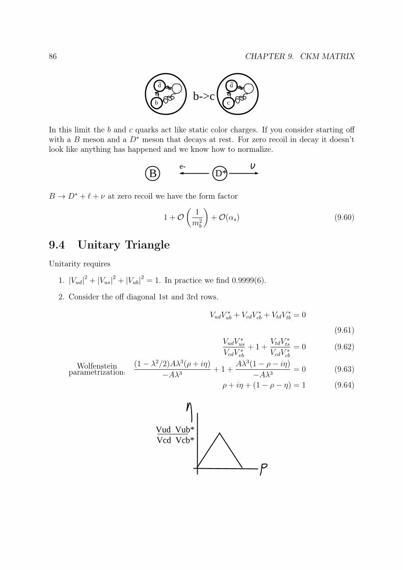
86 CHAPTER 9. CKM MATRIX
b
d
b->cc
d_ _
In this limit the b and c quarks act like static color charges. If you consider starting offwith a B meson and a D∗ meson that decays at rest. For zero recoil in decay it doesn’tlook like anything has happened and we know how to normalize.
B D*e-
B → D∗ + `+ ν at zero recoil we have the form factor
1 +O(
1
m2b
)+O(αs) (9.60)
9.4 Unitary TriangleUnitarity requires
1. |Vud|2 + |Vus|2 + |Vub|2 = 1. In practice we find 0.9999(6).
2. Consider the off diagonal 1st and 3rd rows.
VudV∗ub + VcdV
∗cb + VtdV
∗tb = 0
(9.61)VudV
∗us
VcdV ∗vb+ 1 +
VtdV∗ts
VcdV ∗cb= 0 (9.62)
Wolfensteinparametrization:
(1− λ2/2)Aλ3(ρ+ iη)
−Aλ3+ 1 +
Aλ3(1− ρ− iη)
−Aλ3= 0 (9.63)
ρ+ iη + (1− ρ− η) = 1 (9.64)
Vud Vub*_______Vcd Vcb*
Chapter 10
Symmetries
10.1 Discrete SymmetriesThe three symmetries we are interested in are time reversal (T ), parity inversion (P),and charge conjugation (C). CPT theorem tells us that if you have Lorentz invariance,quantum mechanics, and interactions carried by fields implies that CPT is an exactsymmetry. Some of the consequences of this are as follows
• Particles and antiparticles must have the same masses
• Particles and antiparticles must have the same lifetimes
10.1.1 Time Reversal
Time reversal gives t→ −t or equivalently
T ψ(t)
T︷︸︸︷T −1 = ψ(−t) (10.1)
This will inverse all linear and angular momenta:
p→ −p
L → −Ls→ −s
These kind of experiments were done at CPLear. We will not deal much with time reversalin these lectures.
10.1.2 Parity
Parity performs the following x→ −x or equivalently
Pψ(x)P = ψ(−x) (10.2)
Parities effects on different objects is summarized below
87

88 CHAPTER 10. SYMMETRIES
Object type Effect Examples(polar) vector v→ −v (p,E,A,J,∇, ...)
axial/pseudo vectors a→ a a = v1 × v2 (v1,v2 → polar vec), e.g. L,BScalars φ→ φ v1 · v2
Pseudoscalar φ→ −φ v1 · (v2 × v3)
Parity acting twice must give back the original state: (denote λ as the eigenvalues of P .
P2ψ = λ2ψ = ψ (10.3)
Hence the eigenvalues of P are±1. In terms of an exponential we have einpπ with np = 0, 1.Further we have
PY mL = (−1)LY m
L (10.4)
For composite systems (multiparticles states) the parities are multiplicative (np’s add).Two particles with intrinsic parities, np1 and np2 in some Y m
L with L = `
P = (−1)np1+np2+` (10.5)
For fermions f and f have opposite intrinsic parity.
Pf · Pf = −1 (10.6)
Bosons and anti bosons have the same parity. For vector bosons we have P = −1. Theconvention we use is to assign protons to P = +1. This gives fermions such as quarks,e−, µ− ,... to P = +1. The anti-fermions such as anti-quarks, e+ , µ+, ... have P = −1.The ground state mesons have P = −1 since they are fi, f fj pairs and in an s wave(` = 0). Thus they are pseudoscalars.
Ground state baryons are given by qqq in an s wave gives P = +1 and anti-baryonsin an s-wave the intrinsic parity is P = −1.
10.1.3 Charge Conjugation
Charge conjugation changes particles to antiparticles and vice versa
C |p〉 = |p〉 (10.7)
All internal quantum numbers (additive) “reverse sign”. Flip the sign of T3, Y,Q, strangeness, color, ....Note: The only eigenstates, are particles who are their own antiparticles. For example
photons are C odd. With charge conjugation we need to be a bit careful about how wedefine things. If we take the Dirac field:
CψC︷︸︸︷C− = −iγ2ψ∗ (10.8)
For an SU(2) spinorCLC−1 = −iσ2Lc (10.9)
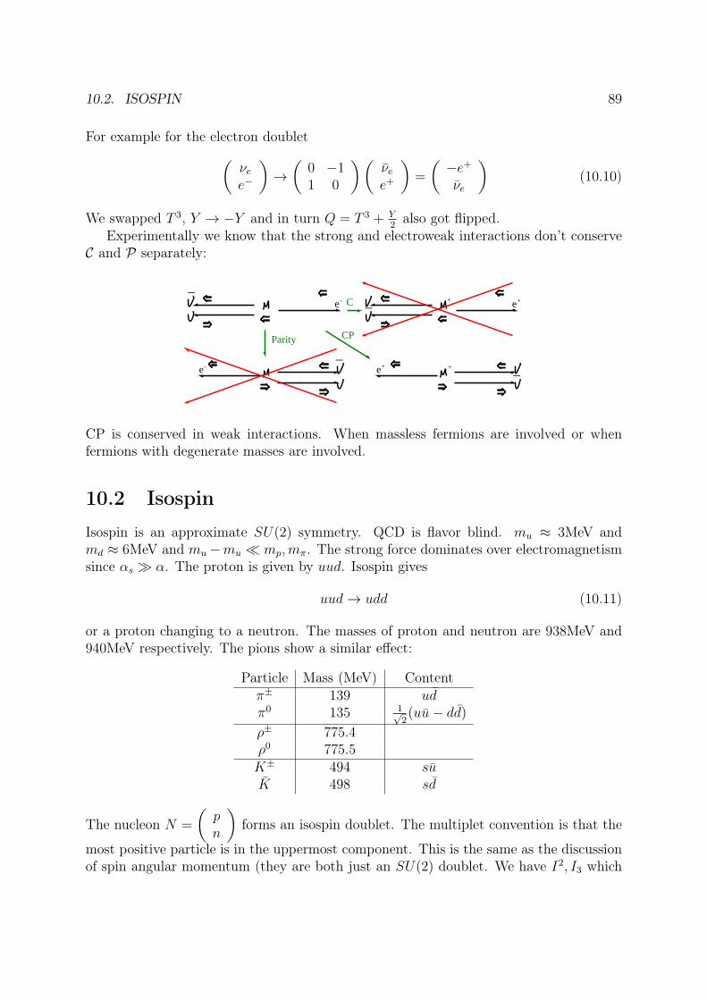
10.2. ISOSPIN 89
For example for the electron doublet(νee−
)→(
0 −11 0
)(νee+
)=
(−e+
νe
)(10.10)
We swapped T 3, Y → −Y and in turn Q = T 3 + Y2also got flipped.
Experimentally we know that the strong and electroweak interactions don’t conserveC and P separately:
e-
_
e-
_Parity
e+_ +C
e+ _
CP
+
CP is conserved in weak interactions. When massless fermions are involved or whenfermions with degenerate masses are involved.
10.2 Isospin
Isospin is an approximate SU(2) symmetry. QCD is flavor blind. mu ≈ 3MeV andmd ≈ 6MeV and mu−mu mp,mπ. The strong force dominates over electromagnetismsince αs α. The proton is given by uud. Isospin gives
uud→ udd (10.11)
or a proton changing to a neutron. The masses of proton and neutron are 938MeV and940MeV respectively. The pions show a similar effect:
Particle Mass (MeV) Contentπ± 139 udπ0 135 1√
2(uu− dd)
ρ± 775.4ρ0 775.5K± 494 suK 498 sd
The nucleon N =
(pn
)forms an isospin doublet. The multiplet convention is that the
most positive particle is in the uppermost component. This is the same as the discussionof spin angular momentum (they are both just an SU(2) doublet. We have I2, I3 which
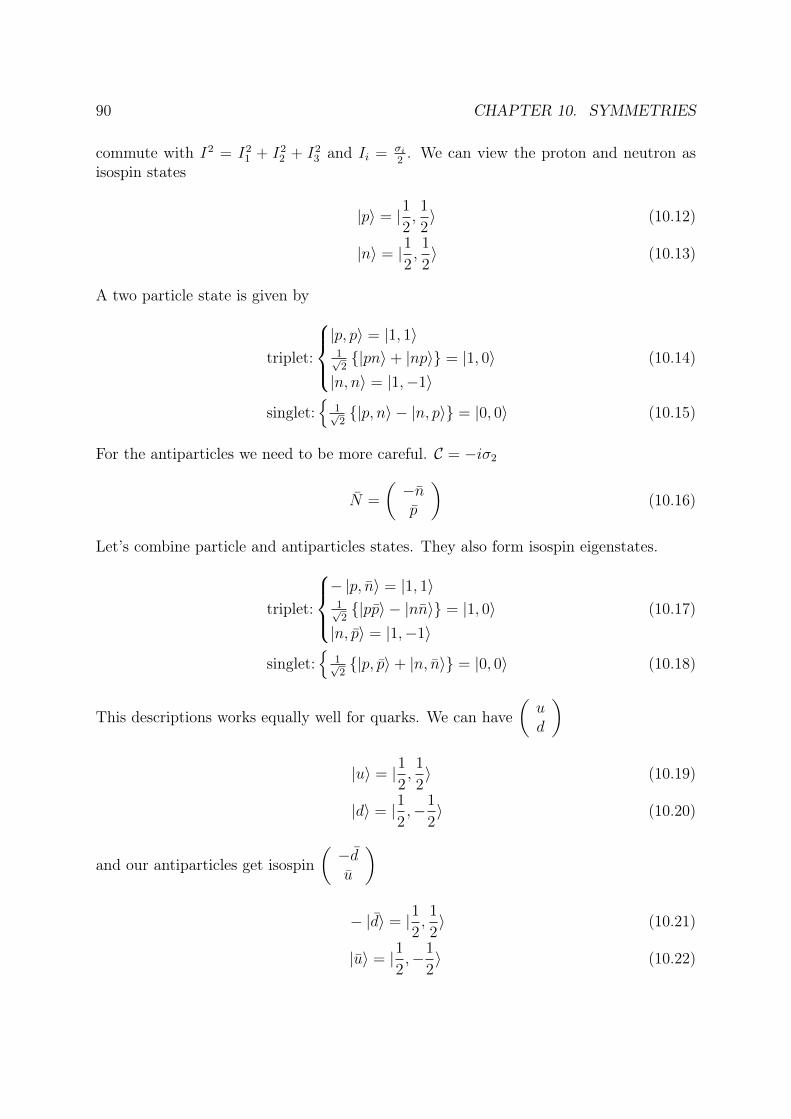
90 CHAPTER 10. SYMMETRIES
commute with I2 = I21 + I2
2 + I23 and Ii = σi
2. We can view the proton and neutron as
isospin states
|p〉 = |12,1
2〉 (10.12)
|n〉 = |12,1
2〉 (10.13)
A two particle state is given by
triplet:
|p, p〉 = |1, 1〉
1√2|pn〉+ |np〉 = |1, 0〉
|n, n〉 = |1,−1〉(10.14)
singlet:
1√2|p, n〉 − |n, p〉 = |0, 0〉 (10.15)
For the antiparticles we need to be more careful. C = −iσ2
N =
(−np
)(10.16)
Let’s combine particle and antiparticles states. They also form isospin eigenstates.
triplet:
− |p, n〉 = |1, 1〉
1√2|pp〉 − |nn〉 = |1, 0〉
|n, p〉 = |1,−1〉(10.17)
singlet:
1√2|p, p〉+ |n, n〉 = |0, 0〉 (10.18)
This descriptions works equally well for quarks. We can have(ud
)
|u〉 = |12,1
2〉 (10.19)
|d〉 = |12,−1
2〉 (10.20)
and our antiparticles get isospin(−du
)
− |d〉 = |12,1
2〉 (10.21)
|u〉 = |12,−1
2〉 (10.22)

10.3. RATES OF RELATED PROCESSES 91
Our pions and η meson then form isospin states
triplet:
− |π+〉 = |1, 1〉 = − |ud〉|π0〉 = |1, 0〉 = 1√
2
|uu〉 − |dd〉
|π−〉 = |1,−1〉 = |du〉
(10.23)
singlet:|η〉 = |0, 0〉 = 1√
2
|u, u〉+ |d, d〉
(10.24)
10.3 Rates of Related Processes
10.3.1 K∗+ → π0K+ v.s. K∗+ → π+K0
We will now apply what we learned of is isospin to related processes. Consider thefollowing two processes
u
s_
u
u_
d
s_
K*
K+
u
s_
u
d_
d
s_
K*
K0
The isospin of the different states are summarized below
|K∗+〉 = |12,1
2〉 (10.25)
|K+π0〉 = |12,1
2〉 ⊗ |1, 0〉 =
√2
3|32,1
2〉 −
√1
3|12,1
2〉 (10.26)
|K0π+〉 = |12,−1
2〉 ⊗ |1, 1〉 =
√1
3|32,1
2〉+
√2
3|12,1
2〉 (10.27)
The amplitude of the decay is given by
A(K∗+ → K+π0
)=
(√2
3〈32,1
2| −√
1
3〈12,1
2|
)Hs |
1
2,1
2〉 (10.28)
If we assume isospin symmetry (i.e. we assume [H, I2] = [H, I3] = 0) then we can use theWigner Eckart theorem (proved in HW) which says that
〈I ′, I ′3|H|I, I3〉 = δI,I′δI3,I′3AI (10.29)
where AI is dependent only on I and not I3. We then define
A1/2 = 〈12,1
2|H|1
2,1
2〉 (10.30)
92 CHAPTER 10. SYMMETRIES
so we have
A(K∗+ → K+π0
)= − 1√
3A1/2 (10.31)
A(K∗+ → K0π+
)=
√2
3A1/2 (10.32)
which givesΓ (K∗+ → K+π0)
Γ (K∗+ → K0π+)=|A (K+π0)|2
|A (K0π)|2=
1
2(10.33)
which is what we observe experimentally.One can go about this a different way by looking at the quarks. We here ignore the
small mass differences of the quarks. The π0 meson is given by |π0〉 = 1√2
(− |dd〉+ |uu〉
).
We created an |uu〉 state in the K∗+ → π0K+ reaction so the amplitude that we wouldindeed get a π0 was 1√
2. This suppression does not occur in the π+K0 decay. Thus we
again have (in an independent method)
Γ (K∗+ → K+π0)
Γ (K∗+ → K0π+)=|A (K+π0)|2
|A (K0π)|2=
1
2(10.34)
10.3.2 ρ0 → π+π− v.s. ρ0 → π0π0
Consider now a different decay, the decay of a ρ0 meson. It is a |1, 0〉. We have
|π+π−〉 = |1, 1〉 ⊗ |1,−1〉 =
√1
6|2, 0〉+
1√2|1, 0〉+
1√3|0, 0〉 (10.35)
|π+π−〉 = |1, 0〉 ⊗ |1, 0〉 =
√2
3|2, 0〉+ 0 · |1, 0〉 − 1√
3|0, 0〉 (10.36)
We have
〈π+π−|H|ρ0〉 =1√2A1 (10.37)
〈π0π0|H|ρ0〉 = 0 ! (10.38)
Thus we have complete suppression in this channel.We can again find this amplitude in an independent method. ρ has J = 1. This
implies that L = 1 due to conservation of angular momentum. π0 ’s are spin zero, whichimplies that they are bosons. Hence they are symmetric under exchange. We must haveY mL (π − θ, φ + π) = Y m
L (θ, φ). They requires L to be even. Hence this is disallowed byconservation of angular momentum.
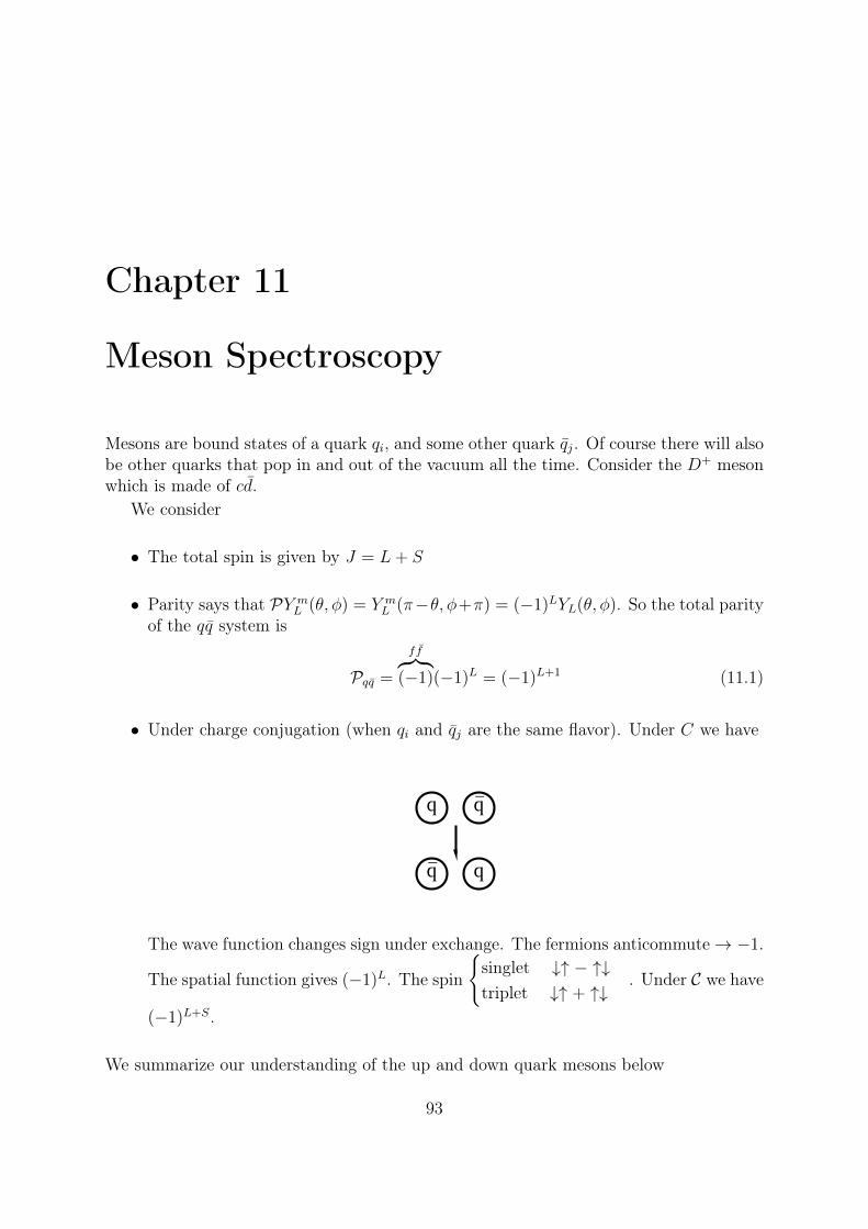
Chapter 11
Meson Spectroscopy
Mesons are bound states of a quark qi, and some other quark qj. Of course there will alsobe other quarks that pop in and out of the vacuum all the time. Consider the D+ mesonwhich is made of cd.
We consider
• The total spin is given by J = L+ S
• Parity says that PY mL (θ, φ) = Y m
L (π−θ, φ+π) = (−1)LYL(θ, φ). So the total parityof the qq system is
Pqq =
ff︷︸︸︷(−1)(−1)L = (−1)L+1 (11.1)
• Under charge conjugation (when qi and qj are the same flavor). Under C we have
q q_
q q_
The wave function changes sign under exchange. The fermions anticommute→ −1.
The spatial function gives (−1)L. The spin
singlet ↓↑ − ↑↓triplet ↓↑ + ↑↓
. Under C we have
(−1)L+S.
We summarize our understanding of the up and down quark mesons below
93
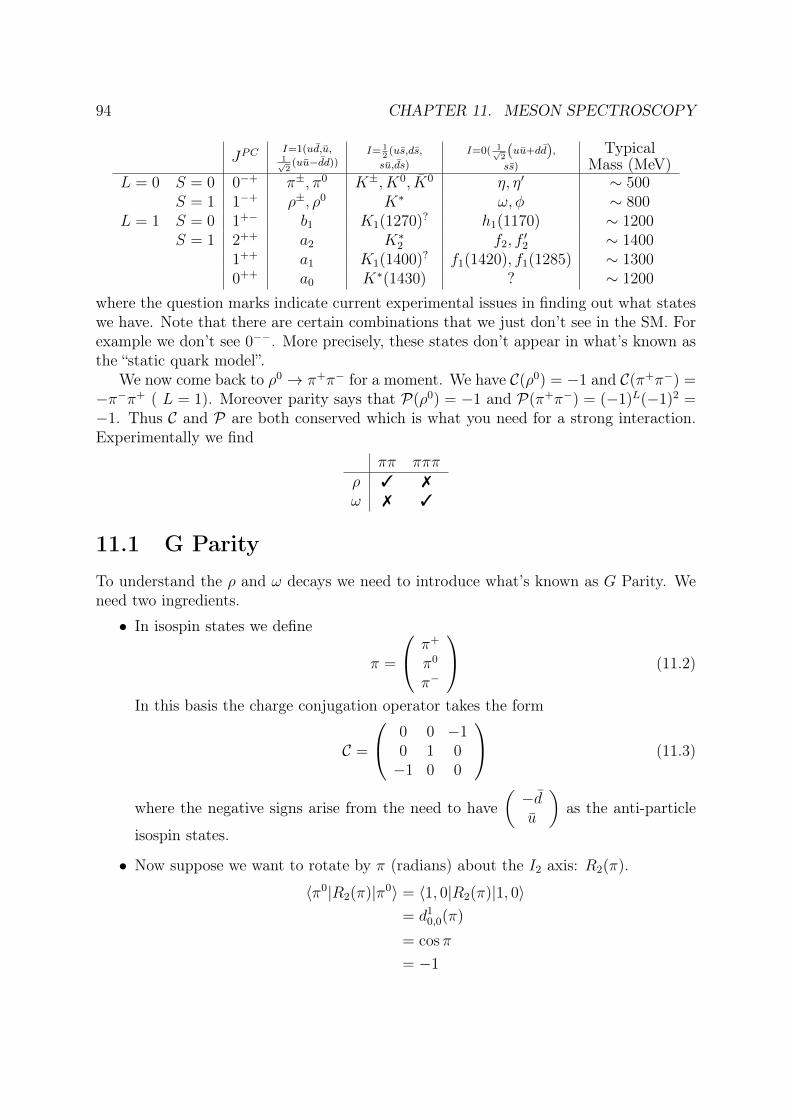
94 CHAPTER 11. MESON SPECTROSCOPY
JPCI=1(ud,u,1√2
(uu−dd))I= 1
2(us,ds,
su,ds)
I=0( 1√2(uu+dd),ss)
TypicalMass (MeV)
L = 0 S = 0 0−+ π±, π0 K±, K0, K0 η, η′ ∼ 500S = 1 1−+ ρ±, ρ0 K∗ ω, φ ∼ 800
L = 1 S = 0 1+− b1 K1(1270)? h1(1170) ∼ 1200S = 1 2++ a2 K∗2 f2, f
′2 ∼ 1400
1++ a1 K1(1400)? f1(1420), f1(1285) ∼ 13000++ a0 K∗(1430) ? ∼ 1200
where the question marks indicate current experimental issues in finding out what stateswe have. Note that there are certain combinations that we just don’t see in the SM. Forexample we don’t see 0−−. More precisely, these states don’t appear in what’s known asthe “static quark model”.
We now come back to ρ0 → π+π− for a moment. We have C(ρ0) = −1 and C(π+π−) =−π−π+ ( L = 1). Moreover parity says that P(ρ0) = −1 and P(π+π−) = (−1)L(−1)2 =−1. Thus C and P are both conserved which is what you need for a strong interaction.Experimentally we find
ππ πππρ 3 7
ω 7 3
11.1 G ParityTo understand the ρ and ω decays we need to introduce what’s known as G Parity. Weneed two ingredients.
• In isospin states we define
π =
π+
π0
π−
(11.2)
In this basis the charge conjugation operator takes the form
C =
0 0 −10 1 0−1 0 0
(11.3)
where the negative signs arise from the need to have(−du
)as the anti-particle
isospin states.
• Now suppose we want to rotate by π (radians) about the I2 axis: R2(π).
〈π0|R2(π)|π0〉 = 〈1, 0|R2(π)|1, 0〉= d1
0,0(π)
= cosπ
= −1

11.1. G PARITY 95
where one can find the d10,0 coefficient in a table. We can also write
〈π0|R2(π)|π+〉 = 〈1,−1|R2(π)|1, 1〉= d1
−1,1(π)
=1− cos π
2= 1
Note that these brakets tell us the overlap between the initial state rotated byπ in the y − axis. This description should be described in a graduate QuantumMechanics book. You can calculate the djm,m′ factors by just finding the overlapsbetween spherical harmonics.
Taking these brakets together we can write our rotation operator also in matrixform:
R2(π) =
0 0 10 −1 01 0 0
(11.4)
We now define a new operator G Parity operator which is the combined operation
G = CR2(π)pioncase−−−→
−1 0 00 −1 00 0 −1
(11.5)
This is a general operator which we take to apply also for the nonpion case. We have
G |π±〉 = − |π±〉 (11.6)G |π0〉 = − |π0〉 (11.7)
We then have
Particle IG
π 1−
ρ 1+
ω 0−
C and I are both symmetries of the strong interaction. This impiles that G Parity shouldbe conserved in a decay (if R2(π) and C are both symmetries, so must G be).
Process ρ0 ω→ π+π− G : +1→ (−1)23 G : −1→ 17
→ π+π−π0 G : +1→ (−1)37 G : −1→ (−1)33
Note that in practice Γρ ∼ 150MeV and Γω ∼ 9MeV. The reason the ρ rate is so muchlarger is because it’s decaying into lighter particles. Thus there is more phase space todecay into.
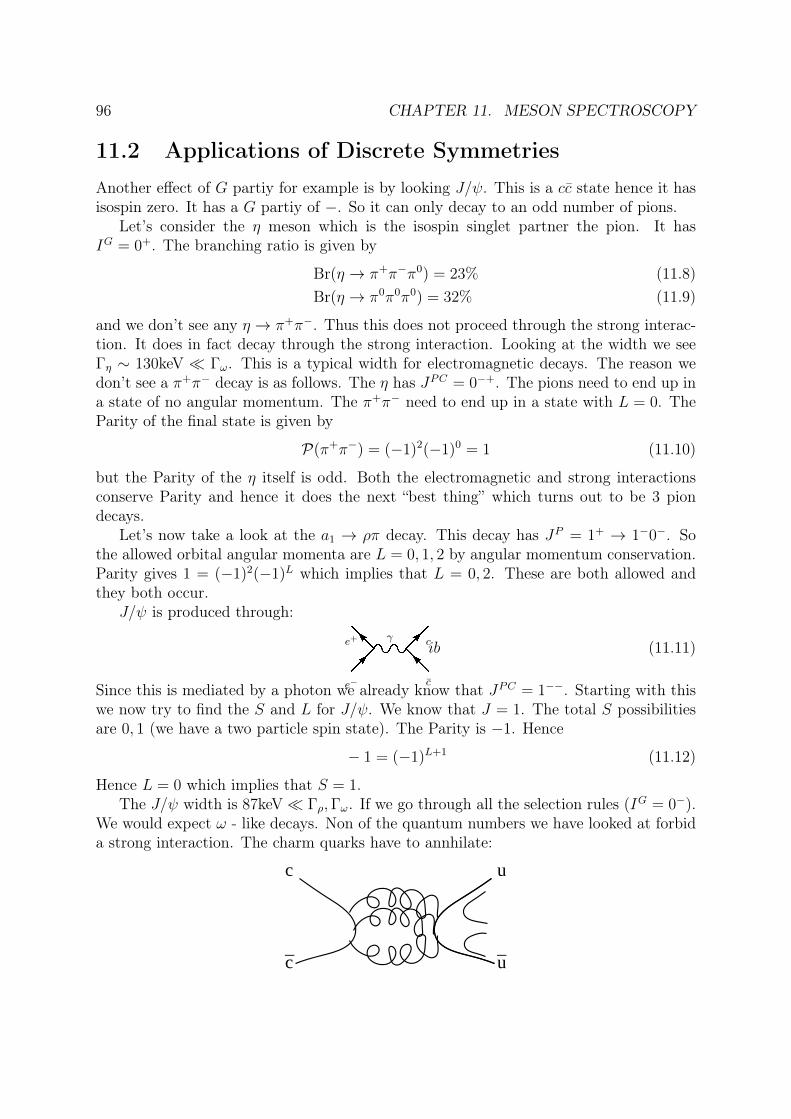
96 CHAPTER 11. MESON SPECTROSCOPY
11.2 Applications of Discrete SymmetriesAnother effect of G partiy for example is by looking J/ψ. This is a cc state hence it hasisospin zero. It has a G partiy of −. So it can only decay to an odd number of pions.
Let’s consider the η meson which is the isospin singlet partner the pion. It hasIG = 0+. The branching ratio is given by
Br(η → π+π−π0) = 23% (11.8)Br(η → π0π0π0) = 32% (11.9)
and we don’t see any η → π+π−. Thus this does not proceed through the strong interac-tion. It does in fact decay through the strong interaction. Looking at the width we seeΓη ∼ 130keV Γω. This is a typical width for electromagnetic decays. The reason wedon’t see a π+π− decay is as follows. The η has JPC = 0−+. The pions need to end up ina state of no angular momentum. The π+π− need to end up in a state with L = 0. TheParity of the final state is given by
P(π+π−) = (−1)2(−1)0 = 1 (11.10)
but the Parity of the η itself is odd. Both the electromagnetic and strong interactionsconserve Parity and hence it does the next “best thing” which turns out to be 3 piondecays.
Let’s now take a look at the a1 → ρπ decay. This decay has JP = 1+ → 1−0−. Sothe allowed orbital angular momenta are L = 0, 1, 2 by angular momentum conservation.Parity gives 1 = (−1)2(−1)L which implies that L = 0, 2. These are both allowed andthey both occur.
J/ψ is produced through:
e+ Ecγge−E
c
ib (11.11)
Since this is mediated by a photon we already know that JPC = 1−−. Starting with thiswe now try to find the S and L for J/ψ. We know that J = 1. The total S possibilitiesare 0, 1 (we have a two particle spin state). The Parity is −1. Hence
− 1 = (−1)L+1 (11.12)
Hence L = 0 which implies that S = 1.The J/ψ width is 87keV Γρ,Γω. If we go through all the selection rules (IG = 0−).
We would expect ω - like decays. Non of the quantum numbers we have looked at forbida strong interaction. The charm quarks have to annhilate:
c
c_
u
u_
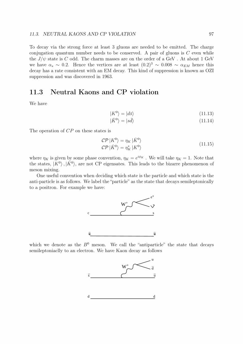
11.3. NEUTRAL KAONS AND CP VIOLATION 97
To decay via the strong force at least 3 gluons are needed to be emitted. The chargeconjugation quantum number needs to be conserved. A pair of gluons is C even whilethe J/ψ state is C odd. The charm masses are on the order of a GeV . At about 1 GeVwe have αs ∼ 0.2. Hence the vertices are at least (0.2)3 ∼ 0.008 ∼ αEM hence thisdecay has a rate consistent with an EM decay. This kind of suppression is known as OZIsuppression and was discovered in 1963.
11.3 Neutral Kaons and CP violationWe have
|K0〉 = |ds〉 (11.13)|K0〉 = |sd〉 (11.14)
The operation of CP on these states is
CP |K0〉 = ηK |K0〉CP |K0〉 = η∗K |K0〉
(11.15)
where ηK is given by some phase convention, ηK = eiφK . We will take ηK = 1. Note thatthe states, |K0〉 , |K0〉, are not CP eigensates. This leads to the bizarre phenomenon ofmeson mixing.
One useful convention when deciding which state is the particle and which state is theanti-particle is as follows. We label the “particle” as the state that decays semileptonicallyto a positron. For example we have:
W+
c
u_u u
_u
s
e+
which we denote as the B0 meson. We call the “antiparticle” the state that decayssemileptoniaclly to an electron. We have Kaon decay as follows
W+
s
d
u
_
d
u_
d_

98 CHAPTER 11. MESON SPECTROSCOPY
so K0 → π+π− and K0 → π−π+. But we can also have the reverse process such that
K0 → π+
π−→ K0 (11.16)
as well asK0 → π+
π−→ K0 (11.17)
These are called “long-range interactions”. We can also have “short-range interactions”which are mediated by W bosons. For example: [Wikipedia(2013)]
Lets consider the combination |K1〉 = 1√2
(|K0〉+ |K0〉
)and |K2〉 = 1√
2
(|K0〉 − |K0〉
).
With our phase convention we have (see equation 11.15)
CP |K1〉 = CP 1√2
(|K0〉+ |K0〉
)= |K1〉 CP even (11.18)
CP |K2〉 = CP 1√2
(|K0〉 − |K0〉
)= − |K2〉 CP odd (11.19)
These are now CP eigenstates. If the weak interaction conserves CP then it must meanthat this linear combinations of the mass eigenstates are what decay and have a welldefined lifetime, not the mass eigenstates themselves!
Consider the two pion final state. We can have either π+π− and π0π0. Recall thatpions are pseudoscalars with spin zero. Thus we have (the charge conjugation factor isgiven by (−1)L+S).
CP(π0π0
)= (−1)2 = 1 (11.20)
CP(π−π+
)= (−1)2(−1)L︸ ︷︷ ︸
P
(−1)L︸ ︷︷ ︸C
= 1 (11.21)
hence in both cases the two pion states are CP even. For the three pion final states (Theπ0π0π0 state must be symmetric and hence L = 0):
CP(π0π0π0) = (−1)3 = −1 (11.22)CP(π+π−π0
)= CP
(π0)︸ ︷︷ ︸
−1
CP(π+π−
)︸ ︷︷ ︸+1
( ang. mom. factors) (11.23)

11.3. NEUTRAL KAONS AND CP VIOLATION 99
We have
L′︷ ︸︸ ︷π0 π+π−︸ ︷︷ ︸
L
where L,L′ sum to 0. Consider the Q of the decay. This is defined as
the mass of the initial particle minus the mass of the products:
QK→3π = mK − 3mπ ∼ 70MeV (11.24)
We have very little kinetic energy per pion. If we have L,L′ 6= 0 then there is a largebarrier for creation of the pions at the origin. This is because in general if you haveangular momentum that is non zero. The wavefunction goes to zero at the origin. Recallfor example the Hydrogen atom wavefunctions. Thus
CP(π+π−π0
)= −1 (11.25)
dominates. With this in mind we seeK1 → 2π andK2 → 3π (they can’t decay to 4π sincethey don’t have enough mass). Further since the kinetic energy left in the 3 body decay isso small, the phase space heavily suppresses the K2 decay. We observe a shortlived stateKS that decays to 2π that has cτS ∼ 2.7cm and a long lived state KL with a lifetime ofcτL ∼ 15.5m.
We now discuss the experiment in more detail. We produce ss pairs. These willhadronize and we will produce many different states however the states of definite strangenessthat we will be produced are K0 and K0. But the mass eigenstates are the ones that willevolve in time and do not equal the production eigenstates. The mass eigenstates are theeigenstates of the full Hamiltonian, not just of the strong interaction. These are the |KL〉and |KS〉 states. Note that CPT requires that we have mK0 = mK0 . It does not requiremKS = mKL . Consider the time evolution of a state with definite mass and lifetime. Wehave
|A, t〉 = e−(Γ2
+im)t |A, t = 0〉︸ ︷︷ ︸≡|A〉
(11.26)
The probability that we will observe |A〉 at a later time, t, is then
P (t) = |〈A|A, t〉|2
= |〈A|A〉|2 e−Γt (11.27)
Suppose we produce a pure |K0〉 state. In this case we have
|ψ(0)〉 = |K0〉
=1√2
(|KS〉+ |KL〉)
|ψ(t)〉 =1√2
(|KS〉 e−(ΓS/2+ims)t + |KL〉 e−(ΓL/2+imL)t
)(11.28)
and hence
〈K0|ψ(t)〉 =1
2
e−(ΓS/2+imS)t + e−(ΓL/2+imL)t
(11.29)
〈K0|ψ(t)〉 =1
2
e−(ΓS/2+imS)t − e−(ΓL/2+imL)t
(11.30)

100 CHAPTER 11. MESON SPECTROSCOPY
As expected at t = 0 we have only K0 and none of it’s antiparticle.In the lab we don’t see amplitudes, just intensities:
I(K0) ≡∣∣〈K0|ψ(t)〉
∣∣2=
1
4
[e−ΓSt + e−ΓLt + e−
12
(ΓS+ΓL)t(e−i(mS−mL)t + ei(mS−mL)t)]
(11.31)
=1
4
[e−ΓSt + e−ΓLt + 2e−
12
(ΓS+ΓL)t cos ∆mt]
(11.32)
(11.33)
Similarly we have
I(K0) =1
4
[e−ΓSt + e−ΓLt − 2e−
12
(ΓS+ΓL)t cos ∆mt]
(11.34)
Now ∆m = (3.451± 0.009)× 10−12MeV and ∆mm∼ 10−14.
The change in mass is given by
∆m = mKBKf2Km
2c cos2 θc sin2 θc (11.35)
where Bk is known as a bag factor which is there to account for the fact that the collisionis not quite happening at the origin and the fK is due to the long distance view of things.This is found using the box diagrams of the kaon decays we discussed earlier. It turnsout the charm quark gives the biggest contribution to the loop diagram. Plugging in thevalues gives, ∆mτS = 0.474.
At CERN there was an experiment known as CPLEAR [Angelopoulos et al.(2003)]that ran
pp→ K−π+K0
The K−π+ tags the production flavor of K0 or K0.In 1964 Christenson, Brownin, Fitch, and Turley tested beams of KL. They found
many KL → π+π−π0 (CP odd → CP odd) decays however they also saw a small butnonzero decay of KL → π+π− which violates CP . This was the first demonstration ofCP violation! The dominate mechanism for mixing is K0 ↔ K0. Hence the |KL〉 6= |K2〉which is a CP odd state but there’s a small admixture of |K1〉 state as well (we omit asmall normalization factor):
|KL〉 ≈ |K2〉+ ε |K1〉 (11.36)|KS〉 ≈ |K1〉+ ε |K2〉 (11.37)
where |ε| = 2.3× 10⁻³. Working through the amplitudes you find that the charge asym-metry
δL ≡N(`+)−N(`−)
N(`+) +N(`−)(11.38)
≈ 2Re(ε) (11.39)
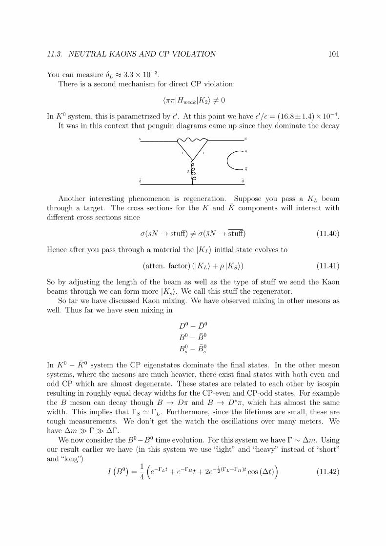
11.3. NEUTRAL KAONS AND CP VIOLATION 101
You can measure δL ≈ 3.3× 10⁻³.There is a second mechanism for direct CP violation:
〈ππ|Hweak|K2〉 6= 0
In K0 system, this is parametrized by ε′. At this point we have ε′/ε = (16.8±1.4)×10−4.It was in this context that penguin diagrams came up since they dominate the decay
d_
d_
s d
t t
g
u
u_
Another interesting phenomenon is regeneration. Suppose you pass a KL beamthrough a target. The cross sections for the K and K components will interact withdifferent cross sections since
σ(sN → stuff) 6= σ(sN → stuff) (11.40)
Hence after you pass through a material the |KL〉 initial state evolves to
(atten. factor) (|KL〉+ ρ |KS〉) (11.41)
So by adjusting the length of the beam as well as the type of stuff we send the Kaonbeams through we can form more |Ks〉. We call this stuff the regenerator.
So far we have discussed Kaon mixing. We have observed mixing in other mesons aswell. Thus far we have seen mixing in
D0 − D0
B0 − B0
B0s − B0
s
In K0 − K0 system the CP eigenstates dominate the final states. In the other mesonsystems, where the mesons are much heavier, there exist final states with both even andodd CP which are almost degenerate. These states are related to each other by isospinresulting in roughly equal decay widths for the CP-even and CP-odd states. For examplethe B meson can decay though B → Dπ and B → D∗π, which has almost the samewidth. This implies that ΓS ' ΓL. Furthermore, since the lifetimes are small, these aretough measurements. We don’t get the watch the oscillations over many meters. Wehave ∆m Γ ∆Γ.
We now consider the B0−B0 time evolution. For this system we have Γ ∼ ∆m. Usingour result earlier we have (in this system we use “light” and “heavy” instead of “short”and “long”)
I(B0)
=1
4
(e−ΓLt + e−ΓH t+ 2e−
12
(ΓL+ΓH)t cos (∆t))
(11.42)

102 CHAPTER 11. MESON SPECTROSCOPY
If ΓL ∼ ΓH = Γ then
I(B0)
=1
2e−Γt (1 + cos ∆mt) (11.43)
I(β0)
=1
2e−Γt (1− cos ∆mt) (11.44)
Pictorally,
ΔmΓ
=0
ΔmΓ
=2
ΔmΓ
=10
0.0 0.5 1.0 1.5 2.0 2.5 3.00.0
0.2
0.4
0.6
0.8
1.0
Γ t
I(B0 )
ΔmΓ
=0
ΔmΓ
=2
ΔmΓ
=10
0.0 0.5 1.0 1.5 2.0 2.5 3.00.0
0.2
0.4
0.6
Γ t
I(B0 )
We can use this asymmetry to measure ∆m:
I(B0)− I(B0)
I(B0) + I(B0)= cos ∆mt (11.45)
Mixing in the D − D0 is a challenge and is relatively suppressed. To understand thiswe compare the box diagrams for D mixing and B mixing:
D mixing
u
d, s, b
c
W
W
c
d, s, b
u
B mixing
d
u, c, t
b
W
W
b
u, c, t
d
Since ms,mb mt the D loop ends up being relatively suppressed.
11.4 B factoriesThe production of B mesons take the form of
e
e
b
b_
B0
B0_
(4s)
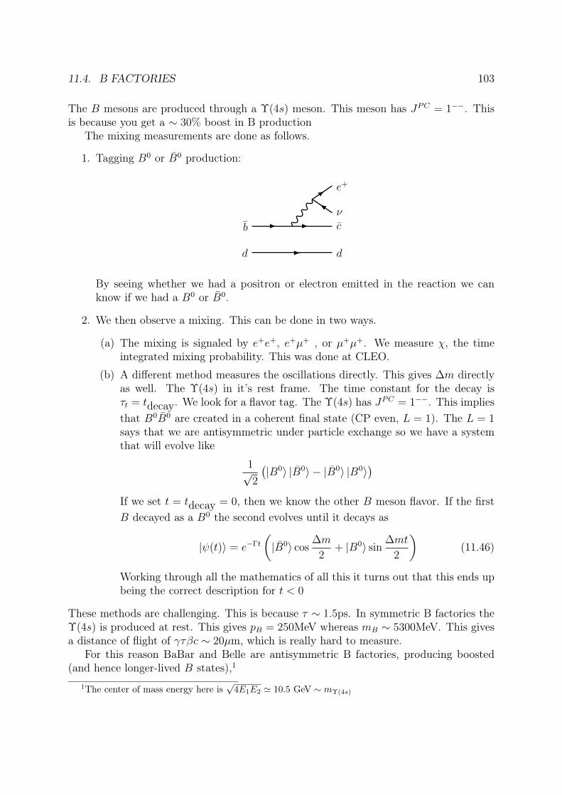
11.4. B FACTORIES 103
The B mesons are produced through a Υ(4s) meson. This meson has JPC = 1−−. Thisis because you get a ∼ 30% boost in B production
The mixing measurements are done as follows.
1. Tagging B0 or B0 production:
d d
b c
e+
ν
By seeing whether we had a positron or electron emitted in the reaction we canknow if we had a B0 or B0.
2. We then observe a mixing. This can be done in two ways.
(a) The mixing is signaled by e+e+, e+µ+ , or µ+µ+. We measure χ, the timeintegrated mixing probability. This was done at CLEO.
(b) A different method measures the oscillations directly. This gives ∆m directlyas well. The Υ(4s) in it’s rest frame. The time constant for the decay isτt = tdecay. We look for a flavor tag. The Υ(4s) has JPC = 1−−. This impliesthat B0B0 are created in a coherent final state (CP even, L = 1). The L = 1says that we are antisymmetric under particle exchange so we have a systemthat will evolve like
1√2
(|B0〉 |B0〉 − |B0〉 |B0〉
)If we set t = tdecay = 0, then we know the other B meson flavor. If the firstB decayed as a B0 the second evolves until it decays as
|ψ(t)〉 = e−Γt
(|B0〉 cos
∆m
2+ |B0〉 sin ∆mt
2
)(11.46)
Working through all the mathematics of all this it turns out that this ends upbeing the correct description for t < 0
These methods are challenging. This is because τ ∼ 1.5ps. In symmetric B factories theΥ(4s) is produced at rest. This gives pB = 250MeV whereas mB ∼ 5300MeV. This givesa distance of flight of γτβc ∼ 20µm, which is really hard to measure.
For this reason BaBar and Belle are antisymmetric B factories, producing boosted(and hence longer-lived B states),1
1The center of mass energy here is√4E1E2 ' 10.5 GeV ∼ mΥ(4s)
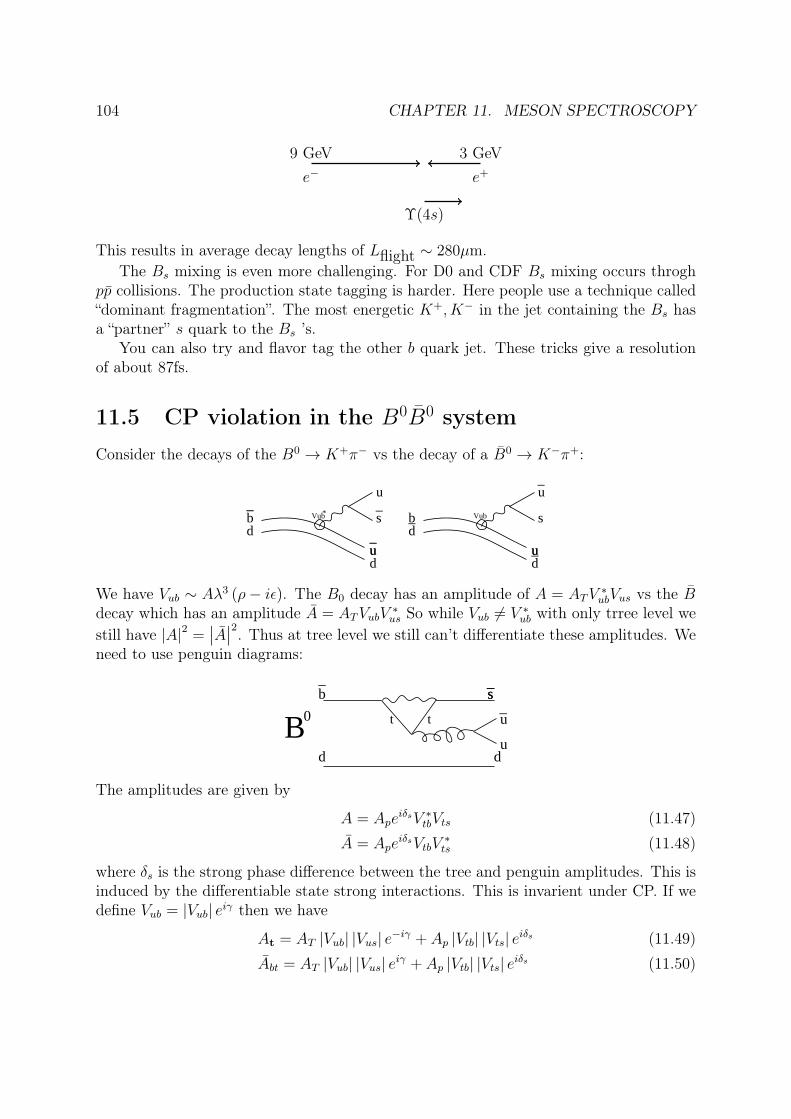
104 CHAPTER 11. MESON SPECTROSCOPY
e−9 GeV
e+
3 GeV
Υ(4s)
This results in average decay lengths of Lflight ∼ 280µm.The Bs mixing is even more challenging. For D0 and CDF Bs mixing occurs throgh
pp collisions. The production state tagging is harder. Here people use a technique called“dominant fragmentation”. The most energetic K+, K− in the jet containing the Bs hasa “partner” s quark to the Bs ’s.
You can also try and flavor tag the other b quark jet. These tricks give a resolutionof about 87fs.
11.5 CP violation in the B0B0 systemConsider the decays of the B0 → K+π− vs the decay of a B0 → K−π+:
b_
d
_
u__ud
u
s_
bd_
u_ud
u
s
_
Vub Vub*
We have Vub ∼ Aλ3 (ρ− iε). The B0 decay has an amplitude of A = ATV∗ubVus vs the B
decay which has an amplitude A = ATVubV∗us So while Vub 6= V ∗ub with only trree level we
still have |A|2 =∣∣A∣∣2. Thus at tree level we still can’t differentiate these amplitudes. We
need to use penguin diagrams:
d
b_
t t
s_s_
u_
ud
B0
The amplitudes are given by
A = ApeiδsV ∗tbVts (11.47)
A = ApeiδsVtbV
∗ts (11.48)
where δs is the strong phase difference between the tree and penguin amplitudes. This isinduced by the differentiable state strong interactions. This is invarient under CP. If wedefine Vub = |Vub| eiγ then we have
At = AT |Vub| |Vus| e−iγ + Ap |Vtb| |Vts| eiδs (11.49)Abt = AT |Vub| |Vus| eiγ + Ap |Vtb| |Vts| eiδs (11.50)

11.5. CP VIOLATION IN THE B0B0 SYSTEM 105
So we have
Γ(B0 → K−π+
)∝ (AT |Vub| |Vus|)2 + (Ap |Vts| |Vts|)2
+ (2ATAp |Vub| |Vus| |Vtb| |Vts|) cos (γ + δs) (11.51)
Γ(B0 → K+π−
)∝ (...)2 + (...)2 + (...) cos (γ − δs) (11.52)
We only have CP violation if γ 6= 0 and δs 6= 0. To measure AT , Ap ∼ roughly comparable.Babar/Belle have measured this and found
NK−π+ −NK+π−
NK−π+ +NK+π−= −0.098± 0.013 (11.53)
We haveB0 → J/ψKs︸ ︷︷ ︸
CP eigenstate
(11.54)
which gives the two decay routes however one is color suppressed:
b_
d
c_
cW+Vcb
*
Vcss
d
_r_
r
r
r
r_
r
_
"Color Suppressed"
b_
d
W+
c
s_
c_
d
The first decay is color suppressed since the c s pair that is created must have a particlecolor configuration. For B0 decay we have:
b
d
c_
cW-Vcb
Vcss
d
_*_
The processes interfere at tree level with mixed and tree level processes:
B0 B0−−−−→ ψKs (11.55)
We have
bb_
d
bd_
b
V *tb
V *tb
W
W
106 CHAPTER 11. MESON SPECTROSCOPY
For the B0 initial state
〈B0|ψ(t)〉 =1
2e−Γt/2
(e−imLt + e−imH t
)= e−Γt/2e−imt cos
∆mt
2(11.56)
and
〈B0|ψ(t)〉 =1
2e−Γt/2
(e−mLt − e−imH t
)e−2iβ
= e−Γt/2e−imti sin∆mt
2e−2iβ (11.57)
We should have general includes this phase earlier as well however we were sloppy sincewe didn’t care about the phase of these amplitudes.
Now that direct and mixed amplitudes for B0 → J/ψKs are given by
Ad = Ae−Γt/2e−imt cos∆mt
2(11.58)
Am = Ae−2iβeΓt/2e−imti sin∆mt
2(11.59)
Hence we have
Atot(B0 → J/ψKs
)= Ae−Γt/2e−imt
(cos
∆mt
2+ ie−2iβ sin
∆mt
2
)(11.60)
so we have
Rate(B0 → J/ψKs
)∝ |Atot|2
= |A|2 e−Γt
(1 + 2 cos
∆mt
2sin
∆mt
2sin 2β
)= |A|2 e−Γt (1 + sin ∆mt sin 2β) (11.61)
Similarly it’s easy to show that
Rate(B0 → J/ψKs
)= |A|2 e−Γt (1− sin ∆mt sin 2β) (11.62)
In practice we calculate
ACP (t) ≡Rate (B0 → J/ψKs)− Rate
(B0 → J/ψKs
)Rate (B0 → J/ψKs) + Rate
(B0 → J/ψKs
)= sin ∆mt sin 2β (11.63)
All the effects of flavor physics are summarized below [Perez et al.(2010)]
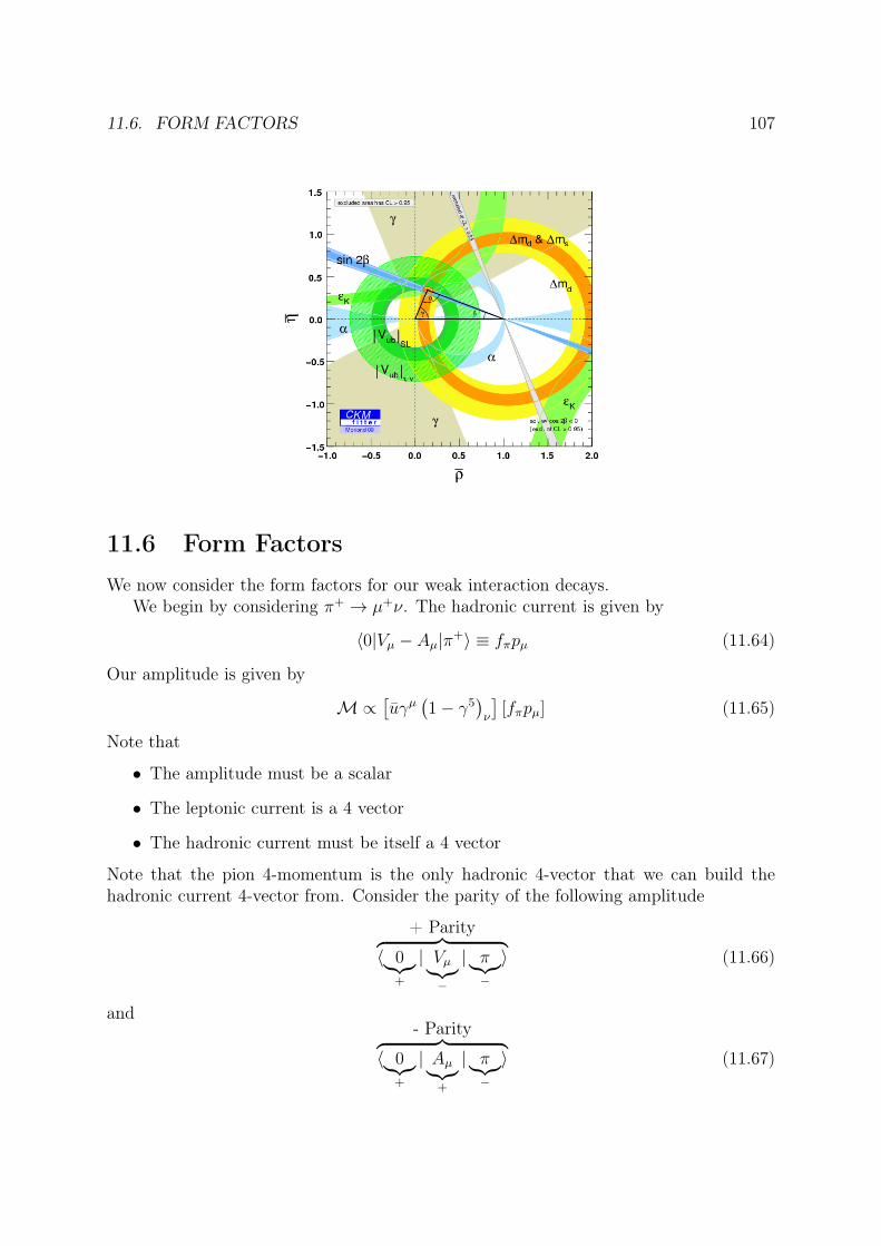
11.6. FORM FACTORS 107
11.6 Form FactorsWe now consider the form factors for our weak interaction decays.
We begin by considering π+ → µ+ν. The hadronic current is given by
〈0|Vµ − Aµ|π+〉 ≡ fπpµ (11.64)
Our amplitude is given by
M∝[uγµ
(1− γ5
)ν
][fπpµ] (11.65)
Note that
• The amplitude must be a scalar
• The leptonic current is a 4 vector
• The hadronic current must be itself a 4 vector
Note that the pion 4-momentum is the only hadronic 4-vector that we can build thehadronic current 4-vector from. Consider the parity of the following amplitude
+ Parity︷ ︸︸ ︷〈 0︸︷︷︸
+
| Vµ︸︷︷︸−
| π︸︷︷︸−
〉 (11.66)
and- Parity︷ ︸︸ ︷
〈 0︸︷︷︸+
| Aµ︸︷︷︸+
| π︸︷︷︸−
〉 (11.67)

108 CHAPTER 11. MESON SPECTROSCOPY
The fπ factor is just a number and pµ is a normal vector hence fπpµ has odd parity. Thismeans that we must have
〈0|Vµ|π〉 = 0 (11.68)
Now consider the following reaction:
Pseudoscalar→ Pseudoscalar + `+ ν
In other words a semileptonic decay. As a specific example we consier D+ → K0e+νe:
cd_
e+
e
W+
sd_
The amplitude is given by
A = 〈K0|V µ − Aµ|D+〉 GF√2VcsLµ (11.69)
where Lµ = eγµ(1− γ5)ν is the current.Let D+ have a momentum pµ and K0 have momentum kµ. Thus
〈K0(k)|V µ − Aµ|D+(p)〉 = pµA(p · k) + kµB(p · k)
but q2 = (p− k)2 = p2 + k2 − 2pµkµ. Thus
〈K0(k)|V µ − Aµ|D+(p)〉 = (pµ + kµ)f+(q2) + (qµ − kµ)f−(q2)︸ ︷︷ ︸Parity odd
(11.70)
Now we need the vector contribution in order to have the overall correction parity. Inother words that
〈K0|Aµ|D+〉 = 0
This is called “vector-dominance”. You can model this as a vector particle being createdas an intermediate final state
B*
D0
11.6. FORM FACTORS 109
We now consider a new reaction given by
B0 → D∗−`ν
The hadronic current is given by
Hµ = 〈D∗−(k)|V µ − Aµ|B0(p)〉 (11.71)
There are 4 vectors involved:
B momentum - pD∗ momentum - kD∗ polarization - εµ
So we can wrtie
Hµ = ε∗µA1(q2) + ε∗νpν(kµA2(q2) + pµA3(q2)
)+ ενpαkβεµναβV (q2)
where we don’t have εµkµ term since it’s equal to zero (due to the way polarization vectorswork). A1, A2, A3 are all axial current form factors and V is a vector current form factor.

Chapter 12
Detection
In the PDG there are many particles that we know their lifetimes, masses, etc. In orderto directly detect particles in a collider they need to live long enough so they leave thecollision center (radius of ∼ 3cm). This requires lifetimes of order
τ ∼ 3cm3× 1010cm/s
∼ 100ps
With this in mind that particles we actually can detect are e−, γ, µ−, K+, π+, p,KL, and n(as well as their antiparticles). All the other particles we detect through their decays tothese particles.
For example in a B0 “detection” we have
B0 → D∗−e+ν
→ D0π−e+ν
→ K−π+π−e+ν
which we can finally detect.Next we discuss the detection of the known particles listed above. For electrons we
insert them in large magnetic fields. These electrons produce Breamstralung radiation.The energy of this radiation is proportional to the inverse square of the mass of theparticle: E ∝ 1
m2 . That’s why this technique only works well for electrons. The “radiationlength” (x0) is the length it takes the electron to emit 1
e≈ 1
3of it’s energy. By measuring
this radiation we detect electrons.Photons are detected through pair conversion. After the electrons have gone through
x0 they will emit a photon which will again pair produce. This product continues and isknown as EM showers.
110
Bibliography
[Peskin and Schroeder(1995)] M. Peskin and D. Schroeder. An Introduction to QuantumField Theory. West View Press, 1995.
[Wikipedia(2013)] Wikipedia. Kaon mixing. 2013.
[Angelopoulos et al.(2003)] A. Angelopoulos et al. Physics at CPLEAR. Phys. Rept.,374:165–270, 2003. doi: 10.1016/S0370-1573(02)00367-8.
[Perez et al.(2010)] G. Perez et al. Flavor physics constraints for physics beyond thestandard model. 2010.
111


![Bio Soil Interactions Engineering Workshop1].pdf · Bio‐Soil Interactions & Engineering Workshop ... Notes. Notes. Notes. Notes. Notes. Notes. ... Electrokinetic and Electrolytic](https://static.fdocuments.in/doc/165x107/5e7be480f39bf41290742405/bio-soil-interactions-engineering-workshop-1pdf-bioasoil-interactions-.jpg)


![notes NOTES ]” BACKGROUND](https://static.fdocuments.in/doc/165x107/61bd44c661276e740b111621/notes-notes-background.jpg)


