Introduction to the rugarch package. (Version 1.4-3)

Introduction to the rugarch package.

(Version 1.4-3)

Alexios Ghalanos

July 15, 2020

Contents

1 Introduction 3

2 Model Specification 32.1 Univariate ARFIMAX Models . . . . . . . . . . . . . . . . . . . . . . . . . . . . . 42.2 Univariate GARCH Models . . . . . . . . . . . . . . . . . . . . . . . . . . . . . . 5

2.2.1 The standard GARCH model (’sGARCH’) . . . . . . . . . . . . . . . . . 62.2.2 The integrated GARCH model (’iGARCH’) . . . . . . . . . . . . . . . . . 72.2.3 The exponential GARCH model . . . . . . . . . . . . . . . . . . . . . . . 72.2.4 The GJR-GARCH model (’gjrGARCH’) . . . . . . . . . . . . . . . . . . . 72.2.5 The asymmetric power ARCH model (’apARCH’) . . . . . . . . . . . . . 82.2.6 The family GARCH model (’fGARCH’) . . . . . . . . . . . . . . . . . . . 92.2.7 The Component sGARCH model (’csGARCH’) . . . . . . . . . . . . . . . 112.2.8 The Multiplicative Component sGARCH model (’mcsGARCH’) . . . . . 122.2.9 The realized GARCH model (’realGARCH’) . . . . . . . . . . . . . . . . . 132.2.10 The fractionally integrated GARCH model (’fiGARCH’) . . . . . . . . . . 15

2.3 Conditional Distributions . . . . . . . . . . . . . . . . . . . . . . . . . . . . . . . 172.3.1 The Normal Distribution . . . . . . . . . . . . . . . . . . . . . . . . . . . 182.3.2 The Student Distribution . . . . . . . . . . . . . . . . . . . . . . . . . . . 182.3.3 The Generalized Error Distribution . . . . . . . . . . . . . . . . . . . . . . 192.3.4 Skewed Distributions by Inverse Scale Factors . . . . . . . . . . . . . . . . 192.3.5 The Generalized Hyperbolic Distribution and Sub-Families . . . . . . . . 202.3.6 The Generalized Hyperbolic Skew Student Distribution . . . . . . . . . . 242.3.7 Johnson’s Reparametrized SU Distribution . . . . . . . . . . . . . . . . . 24

3 Fitting 243.1 Fit Diagnostics . . . . . . . . . . . . . . . . . . . . . . . . . . . . . . . . . . . . . 27

4 Filtering 30

5 Forecasting and the GARCH Bootstrap 31

6 Simulation 34

7 Rolling Estimation 34

8 Simulated Parameter Distribution and RMSE 37

1

9 The ARFIMAX Model with constant variance 41

10 Mispecification and Other Tests 4110.1 The GMM Orthogonality Test . . . . . . . . . . . . . . . . . . . . . . . . . . . . 4110.2 Parametric and Non-Parametric Density Tests . . . . . . . . . . . . . . . . . . . 4110.3 Directional Accuracy Tests . . . . . . . . . . . . . . . . . . . . . . . . . . . . . . 4310.4 VaR and Expected Shortfall Tests . . . . . . . . . . . . . . . . . . . . . . . . . . 4410.5 The Model Confidence Set Test . . . . . . . . . . . . . . . . . . . . . . . . . . . . 45

11 Future Development 46

12 FAQs and Guidelines 46

2

1 Introduction

The pioneering work of Box et al. (1994) in the area of autoregressive moving average modelspaved the way for related work in the area of volatility modelling with the introduction of ARCHand then GARCH models by Engle (1982) and Bollerslev (1986), respectively. In terms of thestatistical framework, these models provide motion dynamics for the dependency in the condi-tional time variation of the distributional parameters of the mean and variance, in an attemptto capture such phenomena as autocorrelation in returns and squared returns. Extensions tothese models have included more sophisticated dynamics such as threshold models to capturethe asymmetry in the news impact, as well as distributions other than the normal to accountfor the skewness and excess kurtosis observed in practice. In a further extension, Hansen (1994)generalized the GARCH models to capture time variation in the full density parameters, withthe Autoregressive Conditional Density Model1, relaxing the assumption that the conditionaldistribution of the standardized innovations is independent of the conditioning information.

The rugarch package aims to provide for a comprehensive set of methods for modelling uni-variate GARCH processes, including fitting, filtering, forecasting, simulation as well as diagnostictools including plots and various tests. Additional methods such as rolling estimation, boot-strap forecasting and simulated parameter density to evaluate model uncertainty provide a richenvironment for the modelling of these processes. This document discusses the finer details ofthe included models and conditional distributions and how they are implemented in the packagewith numerous examples.

The rugarch package is available on CRAN (http://cran.r-project.org/web/packages/rugarch/index.html) and the development version on bitbucket (https://bitbucket.org/alexiosg). Some online examples and demos are available on my website (http://www.unstarched.net).

The package is provided AS IS, without any implied warranty as to its accuracy or suitability.A lot of time and effort has gone into the development of this package, and it is offered under theGPL-3 license in the spirit of open knowledge sharing and dissemination. If you do use the modelin published work DO remember to cite the package and author (type citation(”rugarch”) forthe appropriate BibTeX entry) , and if you have used it and found it useful, drop me a note andlet me know.

USE THE R-SIG-FINANCE MAILING LIST FOR QUESTIONS.A section on FAQ is included at the end of this document.

2 Model Specification

This section discusses the key step in the modelling process, namely that of the specification.This is defined via a call to the ugarchspec function,

> args(ugarchspec)

function (variance.model = list(model = "sGARCH", garchOrder = c(1,

1), submodel = NULL, external.regressors = NULL, variance.targeting = FALSE),

mean.model = list(armaOrder = c(1, 1), include.mean = TRUE,

archm = FALSE, archpow = 1, arfima = FALSE, external.regressors = NULL,

archex = FALSE), distribution.model = "norm", start.pars = list(),

fixed.pars = list(), ...)

Thus a model, in the rugarch package, may be described by the dynamics of the conditionalmean and variance, and the distribution to which they belong, which determines any additional

1The racd package is now available from my bitbucket repository.

3

http://cran.r-project.org/web/packages/rugarch/index.html

http://cran.r-project.org/web/packages/rugarch/index.html

https://bitbucket.org/alexiosg

https://bitbucket.org/alexiosg

http://www.unstarched.net


parameters. The following sub-sections will outline the background and details of the dynamicsand distributions implemented in the package.

2.1 Univariate ARFIMAX Models

The univariate GARCH specification allows to define dynamics for the conditional mean fromthe general ARFIMAX model with the addition of ARCH-in-mean effects introduced in Engleet al. (1987). The ARFIMAX-ARCH-in-mean specification may be formally defined as,

Φ(L)(1− L)d(yt − µt) = Θ(L)εt, (1)

with the left hand side denoting the Fractional AR specification on the demeaned data and theright hand side the MA specification on the residuals. (L) is the lag operator, (1−L)d the longmemory fractional process with 0 < d < 1, and equivalent to the Hurst Exponent H - 0.5, andµt defined as,

µt = µ+m−n∑i=1

δixi,t +m∑

i=m−n+1

δixi,tσt + ξσkt , (2)

where we allow for m external regressors x of which n (last n of m) may optionally be multipliedby the conditional standard deviation σt, and ARCH-in-mean on either the conditional standarddeviation, k = 1 or conditional variance k = 2. These options can all be passed via the argumentsin the mean.model list in the ugarchspec function,

• armaOrder (default = (1,1). The order of the ARMA model.)

• include.mean (default = TRUE. Whether the mean is modelled.)

• archm (default = FALSE. The ARCH-in-mean parameter.)

• archpow (default = 1 for standard deviation, else 2 for variance.)

• arfima (default = FALSE. Whether to use fractional differencing.)

• external.regressors (default = NULL. A matrix of external regressors of the same lengthas the data.)

• archex (default = FALSE. Either FALSE or integer denoting the number of external re-gressors from the end of the matrix to multiply by the conditional standard deviation.).

Since the specification allows for both fixed and starting parameters to be passed, it is useful toprovide the naming convention for these here,

• AR parameters are ’ar1’, ’ar2’, ...,

• MA parameters are ’ma1’, ’ma2’, ...,

• mean parameter is ’mu’

• archm parameter is ’archm’

• the arfima parameter is ’arfima’

• the external regressor parameters are ’mxreg1’, ’mxreg2’, ...,

Note that estimation of the mean and variance equations in the maximization of the likelihoodis carried out jointly in a single step. While it is perfectly possible and consistent to performa 2-step estimation, the one step approach results in greater efficiency, particularly for smallerdatasets.

4

2.2 Univariate GARCH Models

In GARCH models, the density function is usually written in terms of the location and scaleparameters, normalized to give zero mean and unit variance,

αt = (µt, σt, ω), (3)

where the conditional mean is given by

µt = µ(θ, xt) = E(yt|xt), (4)

and the conditional variance is,

σ2t = σ2(θ, xt) = E((yt − µt)2|xt), (5)

with ω = ω(θ, xt) denoting the remaining parameters of the distribution, perhaps a shape andskew parameter. The conditional mean and variance are used to scale the innovations,

zt(θ) =yt − µ(θ, xt)

σ(θ, xt), (6)

having conditional density which may be written as,

g(z|ω) =d

dzP (zt < z|ω), (7)

and related to f(y|α) by,

f(yt|µt, σ2t , ω) =

1

σtg(zt|ω). (8)

The rugarch package implements a rich set of univariate GARCH models and allows forthe inclusion of external regressors in the variance equation as well as the possibility of usingvariance targeting as in Engle and Mezrich (1995). These options can all be passed via thearguments in the variance.model list in the ugarchspec function,

• model (default = ’sGARCH’ (vanilla GARCH). Valid models are ’iGARCH’, ’gjrGARCH’,’eGARCH’, ’apARCH’,’fGARCH’,’csGARCH’ and ’mcsGARCH’).

• garchOrder (default = c(1,1). The order of the GARCH model.)

• submodel (default = NULL. In the case of the ’fGARCH’ omnibus model, valid choices are’GARCH’, ’TGARCH’, ’GJRGARCH’, ’AVGARCH’, ’NGARCH’, ’NAGARCH’, ’APARCH’and ’ALLGARCH’)

• external.regressors (default = NULL. A matrix of external regressors of the same lengthas the data).

• variance.targeting (default = FALSE. Whether to include variance targeting. It is alsopossible to pass a numeric value instead of a logical, in which case it is used for thecalculation instead of the variance of the conditional mean equation residuals).

The rest of this section discusses the various flavors of GARCH implemented in the package,while Section 2.3 discusses the distributions implemented and their standardization for use inGARCH processes.

5

2.2.1 The standard GARCH model (’sGARCH’)

The standard GARCH model (Bollerslev (1986)) may be written as:

σ2t =

ω +

m∑j=1

ζjvjt

+

q∑j=1

αjε2t−j+

p∑j=1

βjσ2t−j , (9)

with σ2t denoting the conditional variance, ω the intercept and ε2

t the residuals from the meanfiltration process discussed previously. The GARCH order is defined by (q, p) (ARCH, GARCH),with possibly m external regressors vj which are passed pre-lagged. If variance targeting is used,then ω is replaced by,

σ2(

1− P)−

m∑j=1

ζj vj (10)

where σ2 is the unconditional variance of ε2 which is consistently estimated by its sample counter-part at every iteration of the solver following the mean equation filtration, and vj represents thesample mean of the jth external regressors in the variance equation (assuming stationarity), andP is the persistence and defined below. If a numeric value was provided to the variance.targetingoption in the specification (instead of logical), this will be used instead of σ2 for the calcula-tion.2 One of the key features of the observed behavior of financial data which GARCH modelscapture is volatility clustering which may be quantified in the persistence parameter P . For the’sGARCH’ model this may be calculated as,

P =

q∑j=1

αj +

p∑j=1

βj . (11)

Related to this measure is the ’half-life’ (call it h2l) defined as the number of days it takes forhalf of the expected reversion back towards E

(σ2)

to occur,

h2l =−loge2

logeP. (12)

Finally, the unconditional variance of the model σ2, and related to its persistence, is,

σ2 =ω

1− P, (13)

where ω is the estimated value of the intercept from the GARCH model. The naming conventionsfor passing fixed or starting parameters for this model are:

• ARCH(q) parameters are ’alpha1’, ’alpha2’, ...,

• GARCH(p) parameters are ’beta1’, ’beta2’, ...,

• variance intercept parameter is ’omega’

• the external regressor parameters are ’vxreg1’, ’vxreg2’, ...,

2Note that this should represent a value related to the variance in the plain vanilla GARCH model. In moregeneral models such as the APARCH, this is a value related to σδ, which may not be obvious since δ is not knownprior to estimation, and therefore care should be taken in those cases. Finally, if scaling is used in the estimation(via the fit.control option), this value will also be automatically scale adjusted by the routine.

6

2.2.2 The integrated GARCH model (’iGARCH’)

The integrated GARCH model (see Engle and Bollerslev (1986)) assumes that the persistenceP = 1, and imposes this during the estimation procedure. Because of unit persistence, none ofthe other results can be calculated (i.e. unconditional variance, half life etc). The stationarityof the model has been established in the literature, but one should investigate the possibilityof omitted structural breaks before adopting the iGARCH as the model of choice. The waythe package enforces the sum of the ARCH and GARCH parameters to be 1, is by subtracting

1−q∑i=1

αi−p∑i>1

βi, so that the last beta is never estimated but instead calculated.

2.2.3 The exponential GARCH model

The exponential model of Nelson (1991) is defined as,

loge(σ2t

)=

ω +m∑j=1

ζjvjt

+

q∑j=1

(αjzt−j + γj (|zt−j | − E |zt−j |)) +

p∑j=1

βj loge(σ2t−j)

(14)

where the coefficient αj captures the sign effect and γj the size effect. The expected value of theabsolute standardized innovation, zt is,

E |zt| =∞∫−∞

|z|f (z, 0, 1, ...) dz (15)

The persistence P is given by,

P =

p∑j=1

βj . (16)

If variance targeting is used, then ω is replaced by,

loge(σ2) (

1− P)−

m∑j=1

ζj vj (17)

The unconditional variance and half life follow from the persistence parameter and are calculatedas in Section 2.2.1.

2.2.4 The GJR-GARCH model (’gjrGARCH’)

The GJR GARCH model of Glosten et al. (1993) models positive and negative shocks on theconditional variance asymmetrically via the use of the indicator function I,

σ2t =

ω +m∑j=1

ζjvjt

+

q∑j=1

(αjε

2t−j + γjIt−jε

2t−j)

+

p∑j=1

βjσ2t−j , (18)

where γj now represents the ’leverage’ term. The indicator function I takes on value of 1 forε ≤ 0 and 0 otherwise. Because of the presence of the indicator function, the persistence ofthe model now crucially depends on the asymmetry of the conditional distribution used. Thepersistence of the model P is,

P =

q∑j=1

αj +

p∑j=1

βj+

q∑j=1

γjκ, (19)

7

where κ is the expected value of the standardized residuals zt below zero (effectively the proba-bility of being below zero),

κ = E[It−jz

2t−j]

=

0∫−∞

f (z, 0, 1, ...) dz (20)

where f is the standardized conditional density with any additional skew and shape parameters(. . . ). In the case of symmetric distributions the value of κ is simply equal to 0.5. The variancetargeting, half-life and unconditional variance follow from the persistence parameter and arecalculated as in Section 2.2.1. The naming conventions for passing fixed or starting parametersfor this model are:


• Leverage(q) parameters are ’gamma1’, ’gamma2’, ...,




Note that the Leverage parameter follows the order of the ARCH parameter.

2.2.5 The asymmetric power ARCH model (’apARCH’)

The asymmetric power ARCH model of Ding et al. (1993) allows for both leverage and the Tayloreffect, named after Taylor (1986) who observed that the sample autocorrelation of absolutereturns was usually larger than that of squared returns.

σδt =

ω +

m∑j=1

ζjvjt

+

q∑j=1

αj(|εt−j | − γjεt−j)δ+p∑j=1

βjσδt−j (21)

where δ ∈ R+, being a Box-Cox transformation of σt, and γj the coefficient in the leverage term.Various submodels arise from this model:

• The simple GARCH model of Bollerslev (1986) when δ = 2 and γj = 0.

• The Absolute Value GARCH (AVGARCH) model of Taylor (1986) and Schwert (1990)when δ = 1 and γj = 0.

• The GJR GARCH (GJRGARCH) model of Glosten et al. (1993) when δ = 2.

• The Threshold GARCH (TGARCH) model of Zakoian (1994) when δ = 1.

• The Nonlinear ARCH model of Higgins et al. (1992) when γj = 0 and βj = 0.

• The Log ARCH model of Geweke (1986) and Pantula (1986) when δ → 0.

The persistence of the model is given by,

P =

p∑j=1

βj+

q∑j=1

αjκj (22)

8

where κj is the expected value of the standardized residuals zt under the Box-Cox transformationof the term which includes the leverage coefficient γj ,

κj = E(|z| − γjz)δ =

∞∫−∞

(|z| − γjz)δf (z, 0, 1, ...) dz (23)


σδ(

1− P)−

m∑j=1

ζj vj . (24)

Finally, the unconditional variance of the model σ2 is,

σ2 =

(ω

1− P

)2/δ

(25)

where ω is the estimated value of the intercept from the GARCH model. The half-life followsfrom the persistence parameter and is calculated as in Section 2.2.1. The naming conventionsfor passing fixed or starting parameters for this model are:


• Leverage(q) parameters are ’gamma1’, ’gamma2’, ...,

• Power parameter is ’delta’,




In particular, to obtain any of the submodels simply pass the appropriate parameters as fixed.

2.2.6 The family GARCH model (’fGARCH’)

The family GARCH model of Hentschel (1995) is another omnibus model which subsumes someof the most popular GARCH models. It is similar to the apARCH model, but more general sinceit allows the decomposition of the residuals in the conditional variance equation to be driven bydifferent powers for zt and σt and also allowing for both shifts and rotations in the news impactcurve, where the shift is the main source of asymmetry for small shocks while rotation driveslarge shocks.

σλt =

ω +

m∑j=1

ζjvjt

+

q∑j=1

αjσλt−j(|zt−j − η2j | − η1j (zt−j − η2j))

δ+

p∑j=1

βjσλt−j (26)

which is a Box-Cox transformation for the conditional standard deviation whose shape is de-termined by λ, and the parameter δ transforms the absolute value function which it subject torotations and shifts through the η1j and η2j parameters respectively. Various submodels arisefrom this model, and are passed to the ugarchspec ’variance.model’ list via the submodel option,

• The simple GARCH model of Bollerslev (1986) when λ = δ = 2 and η1j = η2j = 0(submodel = ’GARCH’).

9

• The Absolute Value GARCH (AVGARCH) model of Taylor (1986) and Schwert (1990)when λ = δ = 1 and |η1j | ≤ 1 (submodel = ’AVGARCH’).

• The GJR GARCH (GJRGARCH) model of Glosten et al. (1993) when λ = δ = 2 andη2j = 0 (submodel = ’GJRGARCH’).

• The Threshold GARCH (TGARCH) model of Zakoian (1994) when λ = δ = 1, η2j = 0and |η1j | ≤ 1 (submodel = ’TGARCH’).

• The Nonlinear ARCH model of Higgins et al. (1992) when δ = λ and η1j = η2j = 0(submodel = ’NGARCH’).

• The Nonlinear Asymmetric GARCH model of Engle and Ng (1993) when δ = λ = 2 andη1j = 0 (submodel = ’NAGARCH’).

• The Asymmetric Power ARCH model of Ding et al. (1993) when δ = λ, η2j = 0 and|η1j | ≤ 1 (submodel = ’APARCH’).

• The Exponential GARCH model of Nelson (1991) when δ = 1, λ = 0 and η2j = 0 (notimplemented as a submodel of fGARCH).

• The Full fGARCH model of Hentschel (1995) when δ = λ (submodel = ’ALLGARCH’).

The persistence of the model is given by,

P =

p∑j=1

βj+

q∑j=1

αjκj (27)

where κj is the expected value of the standardized residuals zt under the Box-Cox transformationof the absolute value asymmetry term,

κj = E(|zt−j − η2j | − η1j (zt−j − η2j))δ =

∞∫−∞

(|z − η2j | − η1j (z − η2j))δf (z, 0, 1, ...) dz (28)


σλ(

1− P)−

m∑j=1

ζj vj (29)

Finally, the unconditional variance of the model σ2 is,

σ2 =

(ω

1− P

)2/λ

(30)

where ω is the estimated value of the intercept from the GARCH model. The half-life followsfrom the persistence parameter and is calculated as in Section 2.2.1. The naming conventionsfor passing fixed or starting parameters for this model are:


• Asymmetry1(q) - rotation - parameters are ’eta11’, ’eta12’, ...,

• Asymmetry2(q) - shift - parameters are ’eta21’, ’eta22’, ...,

• Asymmetry Power parameter is ’delta’,

10

• Conditional Sigma Power parameter is ’lambda’,




2.2.7 The Component sGARCH model (’csGARCH’)

The model of Lee and Engle (1999) decomposes the conditional variance into a permanentand transitory component so as to investigate the long- and short-run movements of volatilityaffecting securities. Letting qt represent the permanent component of the conditional variance,the component model can then be written as:

σ2t = qt +

q∑j=1

αj(ε2t−j − qt−j

)+

p∑j=1

βj(σ2t−j − qt−j

)qt = ω + ρqt−1 + φ

(ε2t−1 − σ2

t−1

) (31)

where effectively the intercept of the GARCH model is now time-varying following first orderautoregressive type dynamics. The difference between the conditional variance and its trend,σ2t−j − qt−j is the transitory component of the conditional variance. The conditions for the non-

negativity of the conditional variance are given in Lee and Engle (1999) and imposed duringestimation by the stationarity option in the fit.control list of the ugarchfit method, and relatedto the stationarity conditions that the sum of the (α,β) coefficients be less than 1 and that ρ < 1(effectively the persistence of the transitory and permanent components).The multistep, n > 1 ahead forecast of the conditional variance proceeds as follows:

Et−1

(σ2t+n

)= Et−1 (qt+n) +

q∑j=1

αj(ε2t+n−j − qt+n−j

)+

p∑j=1

βj(σ2t+n−j − qt+n−j

)Et−1

(σ2t+n

)= Et−1 (qt+n) +

q∑j=1

αjEt−1

[ε2t+n−j − qt+n−j

]+

p∑j=1

βjEt−1

[σ2t+n−j − qt+n−j

] (32)

However, Et−1

[ε2t+n−j

]= Et−1

[σ2t+n−j

], therefore:

Et−1

(σ2t+n

)= Et−1 (qt+n) +

q∑j=1

αjEt−1


]+

p∑j=1

βjEt−1


]

Et−1

(σ2t+n

)= Et−1 (qt+n) +

max(p,q)∑j=1

(αj + βj)

n (σ2t − qt

)(33)

11

The permanent component forecast can be represented as:

Et−1 [qt+n] = ω + ρEt−1 [qt+n−1] + φEt−1

[ε2t+n−j − σ2

t+n−j]

(34)

= ω + ρEt−1 [qt+n−1] (35)

= ω + ρ [ω + ρEt−1 [qt+n−2]] (36)

= . . . (37)

=(1 + p+ · · ·+ ρn−1

)ω + ρnqt (38)

=1− ρn

1− ρω + ρnqt (39)

(40)

As n→∞ the unconditional variance is:

Et−1

[σ2t+n

]= Et−1 [qt+n] =

ω

1− ρ(41)

In the rugarch package, the parameters ρ and φ are represented by η11(’eta11’) and η21(’eta21’)respectively.

2.2.8 The Multiplicative Component sGARCH model (’mcsGARCH’)

A key problem with using GARCH models for intraday data is the seasonality in the absolutereturns observed at the beginning and end of the trading session. For regularly sampled time in-tervals (1-min, 5-min etc.), a number of models have tried to either ’de-seasonalize’ the residualsand then fit the GARCH model by using for instance a Flexible Fourier method as in Ander-sen and Bollerslev (1997) or incorporate seasonality directly into the model as in the PeriodicGARCH model of ?. A rather simple and parsimonious approach to the de-seasonalization wasrecently presented in Engle and Sokalska (2012) (henceforth ES2012). Consider the continu-ously compounded return rt,i, where t denotes the day and i the regularly spaced time intervalat which the return was calculated. Under this model, the conditional variance is a multiplica-tive product of daily, diurnal and stochastic (intraday) components, so that the return processmay be represented as:

rt,i = µt,i + εt,i

εt,i = (qt,iσtsi) zt,i(42)

where qt,i is the stochastic intraday volatility, σt a daily exogenously determined forecast volatil-ity, si the diurnal volatility in each regularly spaced interval i, zt,i the i.i.d (0,1) standardizedinnovation which conditional follows some appropriately chosen distribution. In ES2012, theforecast volatility σt is derived from a multifactor risk model externally, but it is just as possi-ble to generate such forecasts from a daily GARCH model. The seasonal (diurnal) part of theprocess is defined as:

si =1

T

T∑t=1

(ε2t,i/σ2

t

). (43)

Dividing the residuals by the diurnal and daily volatility gives the normalized residuals (ε):

εt,i = εt,i/ (σtsi) (44)

which may then be used to generate the stochastic component of volatility qt,i which assuminga simple vanilla GARCH model has the following motion dynamics:

q2t,i =

ω +m∑j=1

ζjvjt

+

p∑j=1

αj ε2t−j+

q∑j=1

βjq2t−j (45)

12

see Section 2.2.1 for details. In the rugarch package, unlike the paper of ES2012, the conditionalmean and variance equations (and hence the diurnal component on the residuals from the con-ditional mean filtration) are estimated jointly. Furthermore, and unlike ES2012, it is possibleto include ARMAX dynamics in the conditional mean, though because of the complexity ofthe model and its use of time indices, ARCH-m is not currently allowed, but may be includedonce the xts package is fully translated to Rcpp. Finally, as an additional point of departurefrom ES2012, the diurnal component calculation uses the median instead of the mean which wasfound to provide for a more robust alternative, particularly given the type and size of datasetstypically used [changed in version 1.2-3]. As currently stands, the model has methods for esti-mation (ugarchfit), filtering (ugarchfilter), forecast from fit (ugarchforecast) but not from spec(secondary dispatch method), simulation from fit (ugarchsim) but not from spec (ugarchpath),rolling estimation (ugarchroll) but not the bootstrap (ugarchboot). Some of the plots, whichdepend on the xts package will not render nicely since plot.xts does not play well with intradaydata. Some plots however such as VaRplot have been amended to properly display intradaydata coming from an xts object, and more may be added as time allows. An extensive exampleof the model may be found on http://www.unstarched.net. The paper by ES2012 is currentlyfreely available here: http://jfec.oxfordjournals.org/content/10/1/54.full.

2.2.9 The realized GARCH model (’realGARCH’)

While the previous section discussed the modelling of intraday returns using a multiplicativecomponent GARCH model, this section deals with the inclusion of realized measures of volatilityin a GARCH modelling setup. The realized GARCH (realGARCH) model of Hansen et al. (2012)(henceforth HHS2012) provides for an excellent framework for the joint modelling of returns andrealized measures of volatility. Unlike the naive augmentation of GARCH processes by a realizedmeasures, the realGARCH model relates the observed realized measure to the latent volatilityvia a measurement equation, which also includes asymmetric reaction to shocks, making for avery flexible and rich representation. Formally, let:

yt = µt + σtzt, zt ∼ i.i.d (0, 1)

log σ2t = ω +

q∑i=1

αi log rt−i +

p∑i=1

βi log σ2t−i

log rt = ξ + δ log σ2t + τ (zt) + ut, ut ∼ N (0, λ)

(46)

where we have defined the dynamics for the returns (yt), the log of the conditional variance (σ2t )

and the log of the realized measure (rt).3 The asymmetric reaction to shocks comes via the τ (.)

function which is based on the Hermite polynomials and truncated at the second level to give asimple quadratic form:

τ (zt) = η1zt + η2

(z2t − 1

)(47)

3In the original paper by HHS2012, the notation is slightly different as I have chosen to re-use some of thesymbols/variables already in the rugarch specification. For completeness, the differences are noted:

• yt (rugarch) = rt (HHS2012)

• α (rugarch) = γ (HHS2012)

• σ2t (rugarch) = ht (HHS2012)

• rt (rugarch) = xt (HHS2012)

• δ (rugarch) = ϕ (HHS2012)

• η1 (rugarch) = τ1 (HHS2012)

• η2 (rugarch) = τ2 (HHS2012)

• λ (rugarch) = σu (HHS2012)

13


http://jfec.oxfordjournals.org/content/10/1/54.full

which has the very convenient property that Eτ (zt) = 0. The function also forms the basis forthe creation of a type of news impact curve ν (z), defined as:

ν (z) = E [log σt |zt−1 = z ]− E [log σt] = δτ (z) (48)

so that 100×ν (z) is the percent change in volatility as a function of the standardized innovations.A key feature of this model is that it preserves the ARMA structure which characterize many

standard GARCH models and adapted here from Proposition 1 of the HHS2012 paper:

log σ2t = µσ +

p∨q∑i=1

(δαi + βi) log σ2t−1+

q∑j=1

αjwt−j

log rt = µr +

p∨q∑i=1

(δαi + βi) log rt−1 + wt −p∨q∑j=1

βjwt−j

µσ = ω + ξ

q∑i=1

αi, µr = δω +

(1−

p∑i=1

βi

)ξ

(49)

where wt = τ (zt) + ut, µσ = ω + ξq∑i=1

αi and µr = δω +

(1−

p∑i=1

βi

)ξ, and the convention

βi = αj = 0 for i > p and j < p. It is therefore a simple matter to show that the persistence(P ) of the process is given by:

P =

p∑i=1

βi+δ

q∑i=1

αi (50)

while the unconditional (long-run) variance may be written as:

σ2 =

ω + ξq∑i=1

αi

1− P(51)

The joint likelihood of the model, made up of the returns and measurement equation, is givenby:

logL({yt, rt}Tt=1 ; θ

)=

T∑t=1

log f (yt, rt |Ft−1 ) (52)

While not standard for MLE, the independence of zt and ut means that we can factorize thejoint density into:

log f (yt, rt |Ft−1 ) = log (yt |Ft−1 )︸︷︷︸log l(y)

+ (rt |yt,Ft−1 )︸︷︷︸log l(r|y )

(53)

which makes comparison with other GARCH models possible (using log l (y)). Finally, multi-

14

period forecasts have a nice VARMA type representation Yt = AYt−1 + b+ εt, where:

Yt =

log σ2t

.

.

.log σ2

t−p+1

log rt..

log rt−q+1

, A =

(β1, ..., βp) (α1, ..., αq)

(Ip−1×p−1, 0p−1×1) 0p−1×qδ (β1, ..., βp) δ (α1, ..., αq)

0q−1×p (Iq−1×q−1, 0q−1×1)

, b =

ω

0p−1×1

ξ + δω0q−1×1

εt =

0p×1

τ (zt) + ut0q×1

(54)

so that Yt+k = AkYt +k−1∑j=0

Aj (b+ εt+k−j), and it is understood that the superscripts denote

matrix power, with [.]0 the identity matrix.4

In the rugarch package, all the methods, from estimation, to filtering, forecasting and simu-lation have been included with key parts of the code written in C for speed (as elsewhere). Forthe forecast routine, some additional arguments are made available as a result of the generationof the conditional variance density (rather than point forecasts, although these are returnedbased on the average of the simulated density values). Consult the documentation and onlineexamples for more details.

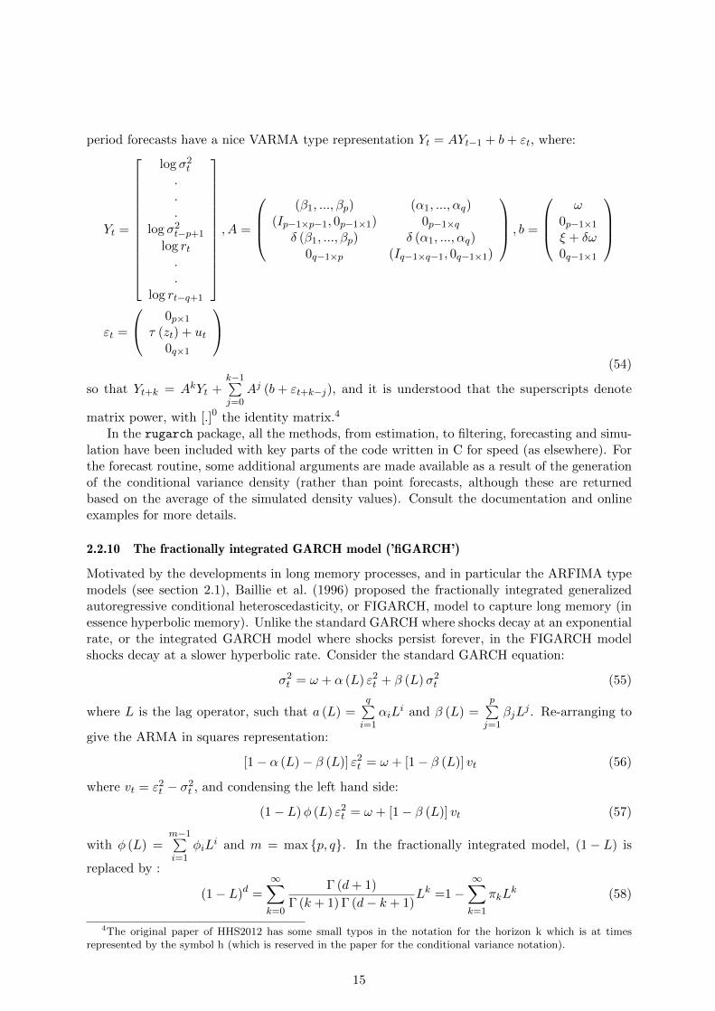
2.2.10 The fractionally integrated GARCH model (’fiGARCH’)

Motivated by the developments in long memory processes, and in particular the ARFIMA typemodels (see section 2.1), Baillie et al. (1996) proposed the fractionally integrated generalizedautoregressive conditional heteroscedasticity, or FIGARCH, model to capture long memory (inessence hyperbolic memory). Unlike the standard GARCH where shocks decay at an exponentialrate, or the integrated GARCH model where shocks persist forever, in the FIGARCH modelshocks decay at a slower hyperbolic rate. Consider the standard GARCH equation:

σ2t = ω + α (L) ε2

t + β (L)σ2t (55)

where L is the lag operator, such that a (L) =q∑i=1

αiLi and β (L) =

p∑j=1

βjLj . Re-arranging to

give the ARMA in squares representation:

[1− α (L)− β (L)] ε2t = ω + [1− β (L)] vt (56)

where vt = ε2t − σ2

t , and condensing the left hand side:

(1− L)φ (L) ε2t = ω + [1− β (L)] vt (57)

with φ (L) =m−1∑i=1

φiLi and m = max {p, q}. In the fractionally integrated model, (1− L) is

replaced by :

(1− L)d =

∞∑k=0

Γ (d+ 1)

Γ (k + 1) Γ (d− k + 1)Lk =1−

∞∑k=1

πkLk (58)

4The original paper of HHS2012 has some small typos in the notation for the horizon k which is at timesrepresented by the symbol h (which is reserved in the paper for the conditional variance notation).

15

where πi =∏

1≤k≤i

k−1−dk . The expansion5 is usually truncated to some large number, such as

1000. Rearranging again, we obtain the following representation of the FIGARCH model:

σ2t = ω[1− β (L)]−1 +

{1− [1− β(L)−1φ (L) (1− L)d

}ε2t

= ω∗ + λ (L) ε2t

= ω∗ +∞∑j=1

λiLiε2t

(59)

where λ1 = φ1 − β1 + d and λk = β1λk−1 +(k−1−dk − φ1

)πd,k−1. For the FIGARCH(1,d,1)

model, sufficient conditions to ensure positivity of the conditional variance are ω > 0,β1 − d ≤φ1 ≤

(2−d

2

), and d

(φ1 − (1−d)

2

)≤ β1 (φ1 − β1 + d). In keeping with the formulation used for

GARCH models in this package, we re-write equation 59 as follows, setting φ (L) ≡ (1− α (L)):

φ (L) (1− L)dε2t = ω + (1− β (L))

(ε2t − σ2

t

)φ (L) (1− L)dε2

t = ω − σ2t + ε2

t + β (L)σ2t − β (L) ε2

t

σ2t = ω + ε2

t + β (L)σ2t − β (L) ε2

t − φ (L) (1− L)dε2t

σ2t = ω +

{1− β (L)− φ (L) (1− L)d

}ε2t + β (L)σ2

t

σ2t = ω +

{1− β (L)− (1− α (L)) (1− L)d

}ε2t + β (L)σ2

t

(60)

Truncating the expansion to 1000 lags and setting (1− L)dε2t = ε2

t +

(1000∑k=1

πkLk

)ε2t = ε2

t + ε2t ,

we can rewrite the equation as:

σ2t = ω +

{ε2t − β (L) ε2

t − (1− L)dε2t + α (L) (1− L)dε2

t

}+ β (L)σ2

t

σ2t = ω +

{ε2t − β (L) ε2

t −(ε2t + ε2

t

)+ α (L)

(ε2t + ε2

t

)}+ β (L)σ2

t

σ2t = ω + ε2

t − β (L) ε2t −

(ε2t + ε2

t

)+ α (L)

(ε2t + ε2

t

)+ β (L)σ2

t

σ2t = ω − ε2

t − β (L) ε2t + α (L)

(ε2t + ε2

t

)+ β (L)σ2

t

σ2t =

(ω − ε2

t

)−

p∑j=1

βjε2t−j +

q∑j=1

αjε2t−j+

q∑j=1

αj ε2t−j +

p∑j=1

βjσ2t−j

σ2t =

(ω − ε2

t

)+

q∑j=1

αj

(ε2t−j + ε2

t−j

)+

p∑j=1

βj

(σ2t−j − ε2

t−j

)(61)

Contrary to the case of the ARFIMA model, the degree of persistence in the FIGARCH modeloperates in the oppposite direction, so that as the fractional differencing parameter d gets closerto one, the memory of the FIGARCH process increases, a direct result of the parameter actingon the squared errors rather than the conditional variance. When d = 0 the FIGARCH collapsesto the vanilla GARCH model and when d = 1 to the integrated GARCH model. The questionof the stationarity of a FIGARCH(q,d,p) model is open and there is no general proof of this atpresent. As such, the stationarity argument in the estimation function is used interchangeablyfor positivity conditions. Baillie et al. (1996) provided a set of sufficient conditions for theFIGARCH(1,d,1) case which may be restrictive in practice, which is why Conrad and Haag(2006) provide a more general set of sufficient conditions for the FIGARCH(q,d,p). Equations(7)-(9) and Corollary 1 of their paper provide the conditions for the positivity in the case of theFIGARCH(1,d,1) case which the rugarch package implements.6 Therefore, while it is possibleto estimate any order desired, only conditions for the (1,d,1) are checked and imposed duringestimation when the stationarity7 flag is set to TRUE.

5This is the hypergeometric function expansion.6At present, only the (1,d,1) case is allowed.7Which is used here to denote a positivity constraint

16

Numerous alternatives and extensions have been proposed in the literature since the FI-GARCH model was published. The model of Karanasos et al. (2004) models the squared residu-als as deviations from ω so that it specifies a covariance stationary process (although the questionof strict stationary still remains open). Augmenting the EGARCH model with the fractionaloperator appears to provide for a natural way to deal with the positivity issue since the processis always strictly positive (see Bollerslev and Mikkelsen (1996)). This may be included in afuture version.

2.3 Conditional Distributions

The rugarch package supports a range of univariate distributions including the Normal (’norm’),Generalized Error (’ged’), Student (’std’) and their skew variants (’snorm’, ’sged’ and ’sstd’)based on the transformations described in Fernandez and Steel (1998) and Ferreira and Steel(2006).8 Additionally, the Generalized Hyperbolic (’ghyp’), Normal Inverse Gaussian (’nig’) andGH Skew-Student (’ghst’)9 distributions are also implemented as is Johnson’s reparametrizedSU (’jsu’) distribution10 The choice of distribution is entered via the ’distribution.model’ optionof the ugarchspec method. The package also implements a set of functions to work with theparameters of these distributions. These are:

• ddist(distribution = ”norm”, y, mu = 0, sigma = 1, lambda = -0.5, skew = 1, shape = 5).The density (d*) function.

• pdist(distribution = ”norm”, q, mu = 0, sigma = 1, lambda = -0.5, skew = 1, shape = 5).The distribution (p*) function.

• qdist(distribution = ”norm”, p, mu = 0, sigma = 1, lambda = -0.5, skew = 1, shape = 5).The quantile (q*) function.

• rdist(distribution = ”norm”, n, mu = 0, sigma = 1, lambda = -0.5, skew = 1, shape = 5).The sampling (q*) function.

• fitdist(distribution = ”norm”, x, control = list()). A function for fitting data using any ofthe included distributions.

• dskewness(distribution = ”norm”, skew = 1, shape = 5, lambda = -0.5). The distributionskewness (analytical where possible else by quadrature integration).

• dkurtosis(distribution = ”norm”, skew = 1, shape = 5, lambda = -0.5). The distributionexcess kurtosis (analytical where it exists else by quadrature integration).

This section provides a dry but comprehensive exposition of the required standardization ofthese distributions for use in GARCH modelling.

The conditional distribution in GARCH processes should be self-decomposable which is akey requirement for any autoregressive type process, while possessing the linear transformationproperty is required to center (xt − µt) and scale (εt/σt) the innovations, after which the mod-elling is carried out directly using the zero-mean, unit variance, distribution of the standardizedvariable zt which is a scaled version of the same conditional distribution of xt, as described inEquations 6, 7 and 8.

8These were originally taken from the fBasics package but have been adapted and re-written in C for thelikelihood estimation.

9Since version 1.0-8.10From the gamlss package.

17

2.3.1 The Normal Distribution

The Normal Distribution is a spherical distribution described completely by it first two moments,the mean and variance. Formally, the random variable x is said to be normally distributed withmean µ and variance σ2 (both of which may be time varying), with density given by,

f (x) =e

−0.5(x−µ)2

σ2

σ√

2π. (62)

Following a mean filtration or whitening process, the residuals ε, standardized by σ yield thestandard normal density given by,

f

(x− µσ

)=

1

σf (z) =

1

σ

(e−0.5z2

√2π

). (63)

To obtain the conditional likelihood of the GARCH process at each point in time (LLt), theconditional standard deviation σt from the GARCH motion dynamics, acts as a scaling factoron the density, so that:

LLt (zt;σt) =1

σtf (zt) (64)

which illustrates the importance of the scaling property. Finally, the normal distribution haszero skewness and zero excess kurtosis.

2.3.2 The Student Distribution

The GARCH-Student model was first used described in Bollerslev (1987) as an alternative tothe Normal distribution for fitting the standardized innovations. It is described completely by ashape parameter ν, but for standardization we proceed by using its 3 parameter representationas follows:

f (x) =Γ(ν+1

2

)√βνπΓ

(ν2

)(1 +(x− α)2

βν

)−( ν+12 )

(65)

where α, β, and ν are the location, scale11 and shape parameters respectively, and Γ is theGamma function. Similar to the GED distribution described later, this is a unimodal and sym-metric distribution where the location parameter α is the mean (and mode) of the distributionwhile the variance is:

V ar (x) =βν

(ν − 2). (66)

For the purposes of standardization we require that:

V ar(x) =βν

(ν − 2)= 1

∴ β =ν − 2

ν

(67)

Substituting (ν−2)ν into 65 we obtain the standardized Student’s distribution:

f

(x− µσ

)=

1

σf (z) =

1

σ

Γ(ν+1

2

)√(ν − 2)πΓ

(ν2

)(1 +z2

(ν − 2)

)−( ν+12 )

. (68)

11In some representations, mostly Bayesian, this is represented in its inverse form to denote the precision.

18

In terms of R’s standard implementation of the Student density (’dt’), and including a scalingby the standard deviation, this can be represented as:

dt

(εt

σ√

(v−2)/ν, ν

)σ√

(v − 2) /ν(69)

The Student distribution has zero skewness and excess kurtosis equal to 6/(ν − 4) for ν > 4.

2.3.3 The Generalized Error Distribution

The Generalized Error Distribution (GED) is a 3 parameter distribution belonging to the expo-nential family with conditional density given by,

f (x) =κe−0.5

∣∣∣x−αβ ∣∣∣κ21+κ−1βΓ (κ−1)

(70)

with α, β and κ representing the location, scale and shape parameters. Since the distributionis symmetric and unimodal the location parameter is also the mode, median and mean of thedistribution (i.e. µ). By symmetry, all odd moments beyond the mean are zero. The varianceand kurtosis are given by,

V ar (x) = β222/κΓ(3κ−1

)Γ (κ−1)

Ku (x) =Γ(5κ−1

)Γ(κ−1

)Γ (3κ−1) Γ (3κ−1)

(71)

As κ decreases the density gets flatter and flatter while in the limit as κ→∞, the distributiontends towards the uniform. Special cases are the Normal when κ = 2, the Laplace when κ = 1.Standardization is simple and involves rescaling the density to have unit standard deviation:

V ar (x) = β222/κΓ(3κ−1

)Γ (κ−1)

= 1

∴ β =

√2−2/κ

Γ (κ−1)

Γ (3κ−1)

(72)

Finally, substituting into the scaled density of z:

f

(x− µσ

)=

1

σf (z) =

1

σ

κe−0.5

∣∣∣∣√2−2/κ Γ(κ−1)Γ(3κ−1)

z

∣∣∣∣κ√2−2/κ Γ(κ−1)

Γ(3κ−1)21+κ−1Γ (κ−1)

(73)

2.3.4 Skewed Distributions by Inverse Scale Factors

Fernandez and Steel (1998) proposed introducing skewness into unimodal and symmetric distri-butions by introducing inverse scale factors in the positive and negative real half lines. Given askew parameter, ξ12, the density of a random variable z can be represented as:

f (z|ξ) =2

ξ + ξ−1

[f (ξz)H (−z) + f

(ξ−1z

)H (z)

](74)

12When ξ = 1, the distribution is symmetric.

19

where ξ ∈ R+ and H(.) is the Heaviside function. The absolute moments, required for derivingthe central moments, are generated from the following function:

Mr = 2

∫ ∞0

zrf (z) dz. (75)

The mean and variance are then defined as:

E (z) = M1

(ξ − ξ−1

)V ar (z) =

(M2 −M2

1

) (ξ2 + ξ−2

)+ 2M2

1 −M2

(76)

The Normal, Student and GED distributions have skew variants which have been standardizedto zero mean, unit variance by making use of the moment conditions given above.

2.3.5 The Generalized Hyperbolic Distribution and Sub-Families

In distributions where the expected moments are functions of all the parameters, it is not im-mediately obvious how to perform such a transformation. In the case of the GHYP distribution,because of the existence of location and scale invariant parameterizations and the possibility ofexpressing the variance in terms of one of those parametrization, namely the (ζ, ρ), the task ofstandardizing and estimating the density can be broken down to one of estimating those 2 param-eters, representing a combination of shape and skewness, followed by a series of transformationsteps to demean, scale and then translate the parameters into the (α, β, δ, µ) parametrizationfor which standard formulae exist for the likelihood function. The (ξ, χ) parametrization, whichis a simple transformation of the (ζ, ρ), could also be used in the first step and then transformedinto the latter before proceeding further. The only difference is the kind of ’immediate’ inferenceone can make from the different parameterizations, each providing a different direct insight intothe kind of dynamics produced and their place in the overall GHYP family particularly withregards to the limit cases.The rugarch package performs estimation using the (ζ, ρ) parametrization13, after which a seriesof steps transform those parameters into the (α, β, δ, µ) while at the same time including thenecessary recursive substitution of parameters in order to standardize the resulting distribution.

Proof 1 The Standardized Generalized Hyperbolic Distribution. Let εt be a r.v. with mean (0)and variance (σ2) distributed as GHY P (ζ, ρ), and let z be a scaled version of the r.v. ε withvariance (1) and also distributed as GHY P (ζ, ρ).14 The density f(.) of z can be expressed as

f(εtσ

; ζ, ρ) =1

σft(z; ζ, ρ) =

1

σft(z; α, β, δ, µ), (77)

where we make use of the (α, β, δ, µ) parametrization since we can only naturally express thedensity in that parametrization. The steps to transforming from the (ζ, ρ) to the (α, β, δ, µ)parametrization, while at the same time standardizing for zero mean and unit variance are givenhenceforth.Let

ζ = δ√α2 − β2 (78)

ρ =β

α, (79)

13Credit is due to Diethelm Wurtz for his original implementation in the fBasics package of the transformationand standardization function.

14The parameters ζ and ρ do not change as a result of being location and scale invariant

20

which after some substitution may be also written in terms of α and β as,

α =ζ

δ√

(1− ρ2), (80)

β = αρ. (81)

For standardization we require that,

E (X) = µ+βδ√α2 − β2

Kλ+1 (ζ)

Kλ (ζ)= µ+

βδ2

ζ

Kλ+1 (ζ)

Kλ (ζ)= 0

∴ µ = −βδ2

ζ

Kλ+1 (ζ)

Kλ (ζ)(82)

V ar (X) = δ2

(Kλ+1 (ζ)

ζKλ (ζ)+

β2

α2 − β2

(Kλ+2 (ζ)

Kλ (ζ)−(Kλ+1 (ζ)

Kλ (ζ)

)2))

= 1

∴ δ =

(Kλ+1 (ζ)

ζKλ (ζ)+

β2

α2 − β2

(Kλ+2 (ζ)

Kλ (ζ)−(Kλ+1 (ζ)

Kλ (ζ)

)2))−0.5

(83)

Since we can express, β2/(α2 − β2

)as,

β2

α2 − β2=

α2ρ2

a2 − α2ρ2=

α2ρ2

a2 (1− ρ2)=

ρ2

(1− ρ2), (84)

then we can re-write the formula for δ in terms of the estimated parameters ζ and ρ as,

δ =

Kλ+1

(ζ)

ζKλ

(ζ) +

ρ2

(1− ρ2)

Kλ+2

(ζ)

Kλ

(ζ) −

Kλ+1

(ζ)

Kλ

(ζ)2−0.5

(85)

Transforming into the (α, β, δ, µ) parametrization proceeds by first substituting 85 into 80 andsimplifying,

α =

ζ

Kλ+1(ζ)ζKλ(ζ)

+ρ2

(Kλ+2(ζ)Kλ(ζ)

− (Kλ+1(ζ))2

(Kλ(ζ))2

)(1−ρ2)

√

(1− ρ2)

0.5

,

=

ζKλ+1(ζ)Kλ(ζ)

+ζ2ρ2

(Kλ+2(ζ)Kλ(ζ)

− (Kλ+1(ζ))2

(Kλ(ζ))2

)(1−ρ2)

√

(1− ρ2)

0.5

,

=

ζKλ+1(ζ)Kλ(ζ)

(1− ρ2)+

ζ2ρ2

(Kλ+2(ζ)Kλ+1(ζ)

Kλ+1(ζ)Kλ(ζ)

− (Kλ+1(ζ))2

(Kλ(ζ))2

)(1− ρ2)2

0.5

,

=

ζKλ+1(ζ)Kλ(ζ)

(1− ρ2)

1 +

ζ ρ2

(Kλ+2(ζ)Kλ+1(ζ)

− Kλ+1(ζ)Kλ(ζ)

)(1− ρ2)

0.5

. (86)

21

Finally, the rest of the parameters are derived recursively from α and the previous results,

β = αρ, (87)

δ =ζ

α√

1− ρ2, (88)

µ =−βδ2Kλ+1

(ζ)

ζKλ

(ζ) . (89)

For the use of the (ξ, χ) parametrization in estimation, the additional preliminary steps of con-verting to the (ζ, ρ) are,

ζ =1

ξ2− 1, (90)

ρ =χ

ξ. (91)

Particular care should be exercised when choosing the GH distribution in GARCH models sinceallowing the GIG λ parameter to vary is quite troublesome in practice and may lead to identi-fication problems since different combinations of the 2 shape (λ, ζ) and 1 skew (ρ) parametersmay lead to the same or close likelihood. In addition, large sections of the likelihood surfacefor some combinations of the distribution parameters is quite flat. Figure 1 shows the skewness,kurtosis and 2 quantiles surfaces for different combinations of the (ρ, ζ) parameters for twopopular choices of λ.

22

(a)λ

=1(H

YP

)(b

)λ

=−

0.5

(NIG

)

Fig

ure

1:

GH

Dis

trib

uti

onSkew

nes

s,K

urt

osis

and

Quan

tile

Surf

ace

s

23

2.3.6 The Generalized Hyperbolic Skew Student Distribution

The GH Skew-Student distribution was popularized by Aas and Haff (2006) because of itsuniqueness in the GH family in having one tail with polynomial and one with exponentialbehavior. This distribution is a limiting case of the GH when α → |β| and λ = −ν/2, where νis the shape parameter of the Student distribution. The domain of variation of the parametersis β ∈ R and ν > 0, but for the variance to be finite ν > 4, while for the existence of skewnessand kurtosis, ν > 6 and ν > 8 respectively. The density of the random variable x is then givenby:

f (x) =

2(1−ν)/2δν |β|(ν+1)/2K(ν+1)/2

(√β2(δ2 + (x− µ)2

))exp (β (x− µ))

Γ (ν/2)√π

(√δ2 + (x− µ)2

)(ν+1)/2(92)

To standardize the distribution to have zero mean and unit variance, I make use of the first twomoment conditions for the distribution which are:

E (x) = µ+βδ2

ν − 2

V ar (x) =2β2δ4

(ν − 2)2 (ν − 4)+

δ2

ν − 2

(93)

We require that V ar(x) = 1, thus:

δ =

(2β2

(ν − 2)2 (ν − 4)+

1

ν − 2

)−1/2

(94)

where I have made use of the 4th parametrization of the GH distribution given in Prause (1999)where β = βδ. The location parameter is then rescaled by substituting into the first momentformula δ so that it has zero mean:

µ = − βδ2

ν − 2(95)

Therefore, we model the GH Skew-Student using the location-scale invariant parametrization(β, ν) and then translate the parameters into the usual GH distribution’s (α, β, δ, µ), settingα = abs(β) + 1e − 12. As of version 1.2-8, the quantile function (via qdist) is calculated usingthe SkewHyperbolic package of Scott and Grimson using the spline method (for speed), as is thedistribution function (via pdist).

2.3.7 Johnson’s Reparametrized SU Distribution

The reparameterized Johnson SU distribution, discussed in Rigby and Stasinopoulos (2005), isa four parameter distribution denoted by JSU (µ, σ, ν, τ), with mean µ and standard deviationσ for all values of the skew and shape parameters ν and τ respectively. The implementation istaken from the GAMLSS package of Stasinopoulos et al. (2009) and the reader is referred therefor further details.

3 Fitting

Once a uGARCHspec has been defined, the ugarchfit method takes the following arguments:

> args(ugarchfit)

24

function (spec, data, out.sample = 0, solver = "solnp", solver.control = list(),

fit.control = list(stationarity = 1, fixed.se = 0, scale = 0,

rec.init = "all"), ...)

The out.sample option controls how many data points from the end to keep for out of sampleforecasting, while the solver.control and fit.control provide additional options to the fitting rou-tine. Importantly, the stationarity option controls whether to impose a stationarity constraintduring estimation, which is usually closely tied to the persistence of the process. The fixed.secontrols whether, for those values which are fixed, numerical standard errors should be calcu-lated. The scale option controls whether the data should be scaled prior to estimation by itsstandard deviation (scaling sometimes facilitates the estimation process). The option rec.init,introduced in version 1.0-14 allows to set the type of method for the conditional recursion ini-tialization, with default value ’all’ indicating that all the data is used to calculate the mean ofthe squared residuals from the conditional mean filtration. To use the first ’n’ points for thecalculation, a positive integer greater than or equal to one (and less than the total estimationdatapoints) can instead be provided. If instead a positive numeric value less than 1 is provided,this is taken as the weighting in an exponential smoothing backcast method for calculating theinitial recursion value.Currently, 5 solvers 15 are supported, with the main one being the augmented Lagrange solversolnp of Ye (1997) implemented in R by Ghalanos and Theussl (2011). The main functionality,namely the GARCH dynamics and conditional likelihood calculations are done in C for speed.For reference, there is a benchmark routine called ugarchbench which provides a comparison ofrugarch against 2 published GARCH models with analytic standard errors, and a small scalecomparison with a commercial GARCH implementation. The fitted object is of class uGARCHfitwhich can be passed to a variety of other methods such as show (summary), plot, ugarchsim,ugarchforecast etc. The following example illustrates its use, but the interested reader shouldconsult the documentation on the methods available for the returned class.

> spec = ugarchspec()

> data(sp500ret)

> fit = ugarchfit(spec = spec, data = sp500ret)

> show(fit)

*---------------------------------*

* GARCH Model Fit *

*---------------------------------*

Conditional Variance Dynamics

-----------------------------------

GARCH Model : sGARCH(1,1)

Mean Model : ARFIMA(1,0,1)

Distribution : norm

Optimal Parameters

------------------------------------

Estimate Std. Error t value Pr(>|t|)

mu 0.000522 0.000087 5.9873 0.00000

ar1 0.870609 0.071909 12.1070 0.00000

15Since version 1.0 − 8 the ’nlopt’ solver of Johnson (interfaced to R by Jelmer Ypma in the ’nloptr’ package)has been added, greatly expanding the range of possibilities available via its numerous subsolver options - seedocumentation.

25

ma1 -0.897805 0.064324 -13.9576 0.00000

omega 0.000001 0.000001 1.3912 0.16418

alpha1 0.087714 0.013705 6.4001 0.00000

beta1 0.904955 0.013750 65.8136 0.00000

Robust Standard Errors:

Estimate Std. Error t value Pr(>|t|)

mu 0.000522 0.000130 4.020100 0.000058

ar1 0.870609 0.087878 9.907060 0.000000

ma1 -0.897805 0.079989 -11.224134 0.000000

omega 0.000001 0.000014 0.093412 0.925576

alpha1 0.087714 0.186497 0.470322 0.638125

beta1 0.904955 0.191986 4.713649 0.000002

LogLikelihood : 17902.41

Information Criteria

------------------------------------

Akaike -6.4807

Bayes -6.4735

Shibata -6.4807

Hannan-Quinn -6.4782

Weighted Ljung-Box Test on Standardized Residuals

------------------------------------

statistic p-value

Lag[1] 5.548 1.850e-02

Lag[2*(p+q)+(p+q)-1][5] 6.437 1.263e-05

Lag[4*(p+q)+(p+q)-1][9] 7.191 1.108e-01

d.o.f=2

H0 : No serial correlation

Weighted Ljung-Box Test on Standardized Squared Residuals

------------------------------------

statistic p-value

Lag[1] 1.103 0.2935

Lag[2*(p+q)+(p+q)-1][5] 1.497 0.7407

Lag[4*(p+q)+(p+q)-1][9] 1.956 0.9102

d.o.f=2

Weighted ARCH LM Tests

------------------------------------

Statistic Shape Scale P-Value

ARCH Lag[3] 0.01965 0.500 2.000 0.8885

ARCH Lag[5] 0.17504 1.440 1.667 0.9713

ARCH Lag[7] 0.53718 2.315 1.543 0.9749

Nyblom stability test

------------------------------------

26

Joint Statistic: 174.6662

Individual Statistics:

mu 0.2090

ar1 0.1488

ma1 0.1057

omega 21.3780

alpha1 0.1345

beta1 0.1130

Asymptotic Critical Values (10% 5% 1%)

Joint Statistic: 1.49 1.68 2.12

Individual Statistic: 0.35 0.47 0.75

Sign Bias Test

------------------------------------

t-value prob sig

Sign Bias 0.4298 6.674e-01

Negative Sign Bias 2.9478 3.214e-03 ***

Positive Sign Bias 2.3929 1.675e-02 **

Joint Effect 28.9794 2.262e-06 ***

Adjusted Pearson Goodness-of-Fit Test:

------------------------------------

group statistic p-value(g-1)

1 20 179.0 4.951e-28

2 30 188.1 3.195e-25

3 40 218.6 7.737e-27

4 50 227.6 7.927e-25

Elapsed time : 1.295898

3.1 Fit Diagnostics

The summary method for the uGARCHfit object provides the parameters and their standard er-rors (and a robust version), together with a variety of tests which can also be called individually.The robust standard errors are based on the method of White (1982) which produces asymp-totically valid confidence intervals by calculating the covariance (V ) of the parameters (θ) as:

V = (−A)−1B(−A)−1 (96)

where,

A = L′′(θ)

B =n∑i=1

gi

(xi

∣∣∣θ)T gi (xi ∣∣∣θ) (97)

which is the Hessian and covariance of the scores at the optimum. The robust standard errorsare the square roots of the diagonal of V .The inforcriteria method on a fitted or filtered object returns the Akaike (AIC), Bayesian

27

(BIC), Hannan-Quinn (HQIC) and Shibata (SIC) information criteria to enable model selectionby penalizing overfitting at different rates. Formally, they may be defined as:

AIC =−2LL

N+

2m

N

BIC =−2LL

N+mloge (N)

N

HQIC =−2LL

N+

(2mloge (loge (N)))

N

SIC =−2LL

N+ loge

((N + 2m)

N

)(98)

were any parameters fixed during estimation are excluded from the calculation. Since version1.3-1, the Q-statistics and ARCH-LM test have been replaced with the Weighted Ljung-Box andARCH-LM statistics of Fisher and Gallagher (2012) which better account for the distributionof the statistics of the values from the estimated models. The ARCH-LM test is now a weightedportmanteau test for testing the null hypothesis of adequately fitted ARCH process, whilst theLjung-Box is another portmanteau test with null the adequacy of the ARMA fit. The signbias

calculates the Sign Bias Test of Engle and Ng (1993), and is also displayed in the summary.This tests the presence of leverage effects in the standardized residuals (to capture possiblemisspecification of the GARCH model), by regressing the squared standardized residuals onlagged negative and positive shocks as follows:

z2t = c0 + c1Iεt−1<0 + c2Iεt−1<0εt−1 + c3Iεt−1>0εt−1 + ut (99)

where I is the indicator function and εt the estimated residuals from the GARCH process. TheNull Hypotheses are H0 : ci = 0 (for i = 1, 2, 3), and that jointly H0 : c1 = c2 = c3 = 0. Ascan be inferred from the summary of the previous fit, there is significant Negative and Positivereaction to shocks. Using instead a model such as the apARCH would likely alleviate theseeffects.

The gof calculates the chi-squared goodness of fit test, which compares the empirical dis-tribution of the standardized residuals with the theoretical ones from the chosen density. Theimplementation is based on the test of Palm (1996) which adjusts the tests in the presence onnon-i.i.d. observations by reclassifying the standardized residuals not according to their value (asin the standard test), but instead on their magnitude, calculating the probability of observinga value smaller than the standardized residual, which should be identically standard uniformdistributed. The function must take 2 arguments, the fitted object as well as the number ofbins to classify the values. In the summary to the fit, a choice of (20, 30, 40, 50) bins is used,and from the summary of the previous example it is clear that the Normal distribution does notadequately capture the empirical distribution based on this test.

The nymblom test calculates the parameter stability test of Nyblom (1989), as well as thejoint test. Critical values against which to compare the results are displayed, but this is notavailable for the joint test in the case of more than 20 parameters.

Finally, some informative plots can be drawn either interactively(which = ’ask’), individually(which = 1:12) else all at once (which = ’all’) as in Figure 2.

28

Fig

ure

2:uG

AR

CH

fit

Plo

ts

29

4 Filtering

Sometimes it is desirable to simply filter a set of data with a predefined set of parameters. Thismay for example be the case when new data has arrived and one might not wish to re-fit. Theugarchfilter method does exactly that, taking a uGARCHspec object with fixed parameters.Setting fixed or starting parameters on the GARCH spec object may be done either throughthe ugarchspec function when it is called via the fixed.pars arguments to the function, else byusing the setfixed<- method on the spec object. The example which follows explains how:

> data(sp500ret)

> spec = ugarchspec(variance.model = list(model = "apARCH"), distribution.model = "std")

> setfixed(spec) <- list(mu = 0.01, ma1 = 0.2, ar1 = 0.5, omega = 1e-05,

+ alpha1 = 0.03, beta1 = 0.9, gamma1 = 0.01, delta = 1, shape = 5)

> filt = ugarchfilter(spec = spec, data = sp500ret)

> show(filt)

*------------------------------------*

* GARCH Model Filter *

*------------------------------------*

Conditional Variance Dynamics

--------------------------------------

GARCH Model : apARCH(1,1)

Mean Model : ARFIMA(1,0,1)

Distribution : std

Filter Parameters

---------------------------------------

mu 1e-02

ar1 5e-01

ma1 2e-01

omega 1e-05

alpha1 3e-02

beta1 9e-01

gamma1 1e-02

delta 1e+00

shape 5e+00

LogLikelihood : 5627.392

Information Criteria

---------------------------------------

Akaike -2.0378

Bayes -2.0378

Shibata -2.0378

Hannan-Quinn -2.0378

Weighted Ljung-Box Test on Standardized Residuals

---------------------------------------

30

statistic p-value

Lag[1] 1178 0

Lag[2*(p+q)+(p+q)-1][5] 1212 0

Lag[4*(p+q)+(p+q)-1][9] 1217 0

d.o.f=2

H0 : No serial correlation

Weighted Ljung-Box Test on Standardized Squared Residuals

---------------------------------------

statistic p-value

Lag[1] 170.4 0

Lag[2*(p+q)+(p+q)-1][5] 173.8 0

Lag[4*(p+q)+(p+q)-1][9] 175.8 0

d.o.f=2

Weighted ARCH LM Tests

---------------------------------------

Statistic Shape Scale P-Value

ARCH Lag[3] 3.915 0.500 2.000 0.04785

ARCH Lag[5] 4.207 1.440 1.667 0.15612

ARCH Lag[7] 5.237 2.315 1.543 0.20163

Sign Bias Test

---------------------------------------

t-value prob sig

Sign Bias 8.3144 1.150e-16 ***

Negative Sign Bias 5.6999 1.261e-08 ***

Positive Sign Bias 0.5621 5.741e-01

Joint Effect 95.8328 1.223e-20 ***

Adjusted Pearson Goodness-of-Fit Test:

---------------------------------------

group statistic p-value(g-1)

1 20 86296 0

2 30 128891 0

3 40 169014 0

4 50 207506 0

The returned object is of class uGARCHfilter and shares many of the methods as the uGARCHfitclass. Additional arguments to the function are explained in the documentation. Note that theinformation criteria shown here are based on zero estimated parameters (they are all fixed), andthe same goes for the infocriteria method on a uGARCHfilter object.

5 Forecasting and the GARCH Bootstrap

There are 2 types of forecasts available with the package. A rolling method, whereby consecutive1-ahead forecasts are created based on the out.sample option set in the fitting routine, and anunconditional method for n>1 ahead forecasts. (and it is also possible to combine the 2 creating

31

a rather complicated object). In the latter case, it is also possible to make use of the GARCHbootstrap, described in Pascual et al. (2006) and implemented in the function ugarchboot,with the added innovation of an optional extra step of fitting either a kernel or semi-parametricdensity (SPD) to the standardized residuals prior to sampling in order to provide for (possibly)more robustness in the presence of limited data. To understand what the GARCH bootstrapdoes, consider that there are two main sources of uncertainty about n.ahead forecasting fromGARCH models: that arising from the form of the predictive density and that due to parameteruncertainty. The bootstrap method in the rugarch package is based on resampling standardizedresiduals from the empirical distribution of the fitted model to generate future realizations of theseries and sigma. Two methods are implemented: one takes into account parameter uncertaintyby building a simulated distribution of the parameters through simulation and refitting, andone which only considers distributional uncertainty and hence avoids the expensive and lengthyparameter distribution estimation. In the latter case, prediction intervals for the 1-ahead sigmaforecast will not be available since only the parameter uncertainty is relevant in GARCH typemodels in this case. The following example provides for a brief look at the partial method, butthe interested reader should consult the more comprehensive examples in the inst folder of thepackage.

> data(sp500ret)

> spec = ugarchspec(variance.model=list(model="csGARCH"), distribution="std")

> fit = ugarchfit(spec, sp500ret)

> bootp = ugarchboot(fit, method = c("Partial", "Full")[1],

+ n.ahead = 500, n.bootpred = 500)

> show(bootp)

*-----------------------------------*

* GARCH Bootstrap Forecast *

*-----------------------------------*

Model : csGARCH

n.ahead : 500

Bootstrap method: partial

Date (T[0]): 2009-01-30

Series (summary):

min q.25 mean q.75 max forecast[analytic]

t+1 -0.10855 -0.013343 0.000668 0.016285 0.090454 0.001944

t+2 -0.11365 -0.010796 0.001632 0.015721 0.085783 0.001707

t+3 -0.28139 -0.013203 -0.000378 0.015496 0.082250 0.001512

t+4 -0.10459 -0.014830 0.000346 0.015602 0.109223 0.001352

t+5 -0.21915 -0.012494 0.001196 0.016627 0.098003 0.001220

t+6 -0.11029 -0.012119 0.001008 0.015000 0.083469 0.001112

t+7 -0.22818 -0.013280 0.000398 0.015250 0.094184 0.001023

t+8 -0.25722 -0.014854 -0.001401 0.016074 0.088067 0.000949

t+9 -0.34629 -0.017681 -0.004484 0.012847 0.154058 0.000889

t+10 -0.11328 -0.013566 0.000957 0.018291 0.140734 0.000840

.....................

Sigma (summary):

min q0.25 mean q0.75 max forecast[analytic]

t+1 0.026387 0.026387 0.026387 0.026387 0.026387 0.026387

t+2 0.025518 0.025564 0.026345 0.026493 0.038492 0.026577

32

Figure 3: GARCH Bootstrap Forecast Plots

t+3 0.024698 0.025021 0.026332 0.026768 0.039903 0.026614

t+4 0.023925 0.024682 0.026440 0.027087 0.077525 0.026649

t+5 0.023259 0.024456 0.026474 0.027507 0.074919 0.026682

t+6 0.022622 0.024173 0.026498 0.027687 0.072876 0.026714

t+7 0.021988 0.023855 0.026463 0.027700 0.069719 0.026744

t+8 0.021503 0.023684 0.026424 0.027785 0.070750 0.026772

t+9 0.021044 0.023677 0.026690 0.028065 0.071725 0.026799

t+10 0.020560 0.023589 0.027050 0.028363 0.095243 0.026824

.....................

The ’recipe’ for the full GARCH bootstrap is summarized below:

1. Extract the standardized residuals from the estimated object. If it is a specification withfixed parameters, first filter using the supplied dataset and then extract the standardizedresiduals from the filtered object.

2. Sample n.bootfit sets of size N (original dataset less any out of sample periods) from eitherthe raw standardized residuals, using the spd or kernel based methods.

3. Simulate n.bootfit paths of size N, using as innovations the sampled standardized residuals.The simulation is initiated with the last values from the dataset at point N (T0 in simulationtime).

4. The n.bootfit simulated series are then estimated with the same specification used bythe originally supplied object in order to generate a set of coefficients representing theparameter uncertainty.

5. Filter the original dataset with the n.bootfit set of estimated coefficients.

6. Use the last values of the filtered conditional sigma (and if it is the csGARCH model,then also the permanent component q) and residuals from the previous step to initialize a

33

new simulation with horizon n.ahead and m.sim=n.bootpred, using again the standardizedresiduals sampled as in step 2 and the new set of estimated coefficients. The simulationnow contains uncertainty about the conditional n-ahead density as well as parameter un-certainty.

6 Simulation

Simulation may be carried out either directly on a fitted object (ugarchsim) else on a GARCHspec with fixed parameters (ugarchpath). The ugarchsim method takes the following argu-ments:

> args(ugarchsim)

function (fit, n.sim = 1000, n.start = 0, m.sim = 1, startMethod = c("unconditional",

"sample"), presigma = NA, prereturns = NA, preresiduals = NA,

rseed = NA, custom.dist = list(name = NA, distfit = NA),

mexsimdata = NULL, vexsimdata = NULL, ...)

where the n.sim indicates the length of the simulation while m.sim the number of independentsimulations. For reasons of speed, when n.sim is large relative to m.sim, the simulation codeis executed in C, while for large m.sim a special purpose C++ code (using Rcpp and Rcp-pArmadillo) is used which was found to lead to significant speed increase. Key to replicatingresults is the rseed argument which is used to pass a user seed to initialize the random numbergenerator, else one will be assigned by the program. In any case, the returned object, of classuGARCHsim (or uGARCHpath) contains a slot with the seed(s) used.

7 Rolling Estimation

The ugarchroll method allows to perform a rolling estimation and forecasting of a model/datasetcombination, optionally returning the VaR at specified levels. More importantly, it returns thedistributional forecast parameters necessary to calculate any required measure on the forecasteddensity. The following example illustrates the use of the method where use is also made of theparallel functionality and run on 10 cores.16 Figure 4 is generated by calling the plot functionon the returned uGARCHroll object. Additional methods, and more importantly extractor func-tions can be found in the documentation. Note that only n.ahead=1 is allowed at present (morecomplicated rolling forecasts can be created by the user with the ugarchfit and ugarchforecastfunctions). Finally, there is a new method called resume which allows resumption of estimationof an object which had non-converged windows, optionally supplying a different solver and solvercontrol combination.

> data(sp500ret)

> library(parallel)

> cl = makePSOCKcluster(10)

> spec = ugarchspec(variance.model = list(model = "eGARCH"), distribution.model = "jsu")

> roll = ugarchroll(spec, sp500ret, n.start = 1000, refit.every = 100,

refit.window = "moving", solver = "hybrid", calculate.VaR = TRUE,

VaR.alpha = c(0.01, 0.05), cluster = cl, keep.coef = TRUE)

>show(roll)

>stopCluster(cl)16Since version 1.0-14 the parallel functionality is based on the paralllel package and it is upto the user to initialize

a cluster object and pass it to the function, and then terminate it once it is no longer required. Eventually, thisapproach to the parallel usage will filter through to all the functions in rugarch and rmgarch.

34

*-------------------------------------*

* GARCH Roll *

*-------------------------------------*

No.Refits : 46

Refit Horizon : 100

No.Forecasts : 4523

GARCH Model : eGARCH(1,1)

Distribution : jsu

Forecast Density:

Mu Sigma Skew Shape Shape(GIG) Realized

1991-02-21 4e-04 0.0102 -0.2586 1.5065 0 -0.0005

1991-02-22 2e-04 0.0099 -0.2586 1.5065 0 0.0019

1991-02-25 4e-04 0.0095 -0.2586 1.5065 0 0.0044

1991-02-26 3e-04 0.0093 -0.2586 1.5065 0 -0.0122

1991-02-27 1e-04 0.0101 -0.2586 1.5065 0 0.0135

1991-02-28 7e-04 0.0099 -0.2586 1.5065 0 -0.0018

..........................

Mu Sigma Skew Shape Shape(GIG) Realized

2009-01-23 0.0015 0.0259 -0.87 2.133 0 0.0054

2009-01-26 0.0005 0.0243 -0.87 2.133 0 0.0055

2009-01-27 -0.0002 0.0228 -0.87 2.133 0 0.0109

2009-01-28 -0.0011 0.0212 -0.87 2.133 0 0.0330

2009-01-29 -0.0039 0.0191 -0.87 2.133 0 -0.0337

2009-01-30 0.0009 0.0220 -0.87 2.133 0 -0.0231

Elapsed: 12.97949 secs

> report(roll, type = "VaR", VaR.alpha = 0.05, conf.level = 0.95)

VaR Backtest Report

===========================================

Model: eGARCH-jsu

Backtest Length: 4523

==========================================

alpha: 5%

Expected Exceed: 226.2

Actual VaR Exceed: 253

Actual %: 5.6%

Unconditional Coverage (Kupiec)

Null-Hypothesis: Correct Exceedances

LR.uc Statistic: 0

LR.uc Critical: 3.841

LR.uc p-value: 1

Reject Null: NO

Conditional Coverage (Christoffersen)

Null-Hypothesis: Correct Exceedances and

Independence of Failures

35

Figure 4: eGARCH Rolling Forecast Plots

LR.cc Statistic: 0

LR.cc Critical: 5.991

LR.cc p-value: 1

Reject Null: NO

36

8 Simulated Parameter Distribution and RMSE

It is sometimes instructive to be able to investigate the underlying density of the estimatedparameters under different models. The ugarchdistribution method performs a monte carloexperiment by simulating and fitting a model multiple times and for different ’window’ sizes.This allows to obtain some insight on the consistency of the parameter estimates as the datawindow increases by looking at the rate of decrease of the Root Mean Squared Error and whetherwe have

√N consistency. This is a computationally expensive exercise and as such should only

be undertaken in the presence of ample computing power and RAM. As in other functions,parallel functionality is enabled if available. The example which follows illustrates an instanceof this test on one model and one set of parameters. Figures 5 and 6 complete this example.

> spec = ugarchspec(variance.model = list(model = "gjrGARCH"),

+ distribution.model = "ged")

> print(persistence(pars = unlist(list(mu = 0.001, ar1 = 0.4, ma1 = -0.1,

+ omega = 1e-06, alpha1 = 0.05, beta1 = 0.9, gamma1 = 0.05,

+ shape = 1.5)), distribution = "ged", model = "gjrGARCH"))

persistence

0.975

> library(parallel)

> cl = makePSOCKcluster(10)

> setfixed(spec) <- list(mu = 0.001, ar1 = 0.4, ma1 = -0.1, omega = 1e-06,

+ alpha1 = 0.05, beta1 = 0.9, gamma1 = 0.05, shape = 1.5)

> dist = ugarchdistribution(fitORspec = spec, n.sim = 2000, n.start = 1,

+ m.sim = 100, recursive = TRUE, recursive.length = 6000, recursive.window = 1000,

+ rseed = 1066, solver = "solnp", solver.control = list(trace = 0),

+ cluster = cl)

> stopCluster(cl)

> show(dist)

*------------------------------------*

* GARCH Parameter Distribution *

*------------------------------------*

Model : gjrGARCH

No. Paths (m.sim) : 100

Length of Paths (n.sim) : 2000

Recursive : TRUE

Recursive Length : 6000

Recursive Window : 1000

Coefficients: True vs Simulation Mean (Window-n)

mu ar1 ma1 omega alpha1 beta1 gamma1 shape

true-coef 0.00100000 0.40000 -0.100000 1.0000e-06 0.050000 0.90000 0.050000 1.5000

window-2000 0.00097099 0.39679 -0.097585 1.0411e-06 0.046161 0.90177 0.051709 1.4945

window-3000 0.00101520 0.38907 -0.089494 9.9344e-07 0.046741 0.90192 0.052902 1.4957

window-4000 0.00099876 0.39329 -0.094523 9.9556e-07 0.049385 0.90179 0.047515 1.4924

window-5000 0.00099491 0.40223 -0.103767 9.7545e-07 0.048651 0.90220 0.049442 1.4900

window-6000 0.00098876 0.39540 -0.096411 9.8975e-07 0.048753 0.90096 0.050907 1.4901

37

Fig

ure

5:Sim

ula

ted

Par

amet

erD

ensi

ty

38

Fig

ure

6:R

MSE

Rat

eof

Chan

ge

39

(a)

Biv

ari

ate

Para

met

erP

lots

(b)

GA

RC

HSta

tP

lots

Fig

ure

7:

GA

RC

HSim

ula

ted

Par

amet

ers

Den

sity

40

9 The ARFIMAX Model with constant variance

The rugarch package implements an additional set of methods and classes, mirroring those of theGARCH specification, for modelling ARFIMAX processes with constant variance via MaximumLikelihood. With the exception of plots, the functionality is very similar to that covered sofar for GARCH methods. The main functions are arfimaspec, arfimafit, arfimaforecast,arfimasim, arfimapath, arfimadistirbution and arfimaroll. The usual extractor, inferenceand summary methods are replicated for all the ARFIMA classes and the user should consultthe documentation for further details.

10 Mispecification and Other Tests

Apart from the usual tests presented in the summary to the fit object, a number of otherinteresting and useful tests are uniquely implemented in the rugarch package, and described inthis section.

10.1 The GMM Orthogonality Test

The GMM type moment (orthogonality) tests of Hansen (1982) have been applied to test theadequacy of model in a variety of setups. Under a correctly specified model, certain populationmoment conditions should be satisfied and hold in the sample using the standardized residuals.The moment conditions can be tested both individually using a t-test or jointly using a Waldtest. Formally, the following moment conditions are tested:

M1 E [zt] = 0M2 E

[z2t − 1

]= 0

M3 E[z3t

]= 0

M4 E[z4t − 3

]= 0

Q2 E[(z2t − 1

) (z2t−j − 1

)]= 0

Q3 E[(z3t

) (z3t−j

)]= 0

Q4 E[(z4t − 3

) (z4t−j − 3

)]= 0

(100)

where j = 1 . . . , p is the lag (defaults to 4 in the function), M1 to M4 denotes the individualmoment conditions (t-test), and Q2 to Q4 the joint conditional moment conditions (variance,skewness and kurtosis) which are distributed χ2 with p d.o.f. All the moment conditions canalso be tested jointly using a Wald test distributed χ2 with 3p+4 d.o.f. The test is implementedunder the name: GMMTest.

10.2 Parametric and Non-Parametric Density Tests

A novel method to analyze how well a conditional density fits the underlying data is throughthe probability integral transformation (PIT ) discussed in Rosenblatt (1952) and defined as:

xt =

yt∫−∞

f (u) du = F (yt) (101)

which transforms the data yt, using the estimated distribution F into i.i.d. U(0, 1) under thecorrectly specified model. Based on this transformation, Tay et al. (1998) provide for a visualassessment test, while Berkowitz (2001) provides a more formal test, implemented in the package

41

under the name BerkowitzTest. Because of the difficulty in testing a U(0, 1) sequence, the PITdata is transformed into N(0, 1) by Berkowitz using the normal quantile function, and testedusing a Lagrange Multiplier (LM ) test for any residual autocorrelation given a specified numberof lags. In addition, a tail test based on the censored Normal is also provided, under the Nullthat the standardized tail data has mean zero and unit variance. More recently, Hong andLi (2005) introduced a nonparametric portmanteau test, building on the work of Ait-Sahalia(1996), which tests the joint hypothesis of i.i.d AND U(0, 1) for the sequence xt. As noted bythe authors, testing xt using a standard goodness-of-fit test (such as the Kolmogorov-Smirnov)would only check the U(0, 1) assumption under i.i.d. and not the joint assumption of U(0, 1) andi.i.d. Their approach is to compare a kernel estimator gj (x1, x2) for the joint density gj (x1, x2)of the pair {xt, xt−j} (where j is the lag order) with unity, the product of two U(0, 1) densities.Given a sample size n and lag order j > 0, their joint density estimator is:

gj (x1, x2) ≡ (n− j)−1n∑

t=j+1

Kh

(x1, Xt

)Kh

(x2, Xt−j

)(102)

where Xt = Xt

(θ)

, and θ is a√n consistent estimator of θ0. The function Kh is a boundary

modified kernel defined as:

Kh (x, y) ≡

h−1k

(x−yh

)/∫ 1−(x/h) k (u) du, ifx ∈ [0, h) ,

h−1k(x−y

h

), ifx ∈ [h, 1− h] ,

h−1k(x−y

h

)/∫ (1−x)/h−1 k (u) du, ifx ∈ (1− h, 1] ,

(103)

where h ≡ h (n) is a bandwidth such that h→ 0 as n→∞, and the kernel k(.) is a pre-specifiedsymmetric probability density, which is implemented as suggested by the authors using a quartickernel,

k (u) =15

16

(1− u2

)21 (|u| ≤ 1) , (104)

where 1 (.) is the indicator function. Their portmanteau test statistic is defined as:

W (p) ≡ p−1/2p∑j=1

Q (j), (105)

whereQ (j) ≡

[(n− j)hM (j)−A0

h

]/V

1/20 , (106)

and

M (j) ≡∫ 1

0

∫ 1

0[gj (x1, x2)− 1]2dx1dx2. (107)

The centering and scaling factors A0h and V0 are defined as:

A0h ≡

[(h−1 − 2

) ∫ 1−1 k

2 (u) du+ 2∫ 1

0

∫ b−1 k

2b (u) dudb

]2− 1

V0 ≡ 2

[∫ 1−1

[∫ 1−1 k (u+ v) k (v) dv

]2du

]2 (108)

where,

kb (.) ≡ k (.)

/∫ b

−1k (v) dv. (109)

Under the correct model specification, the authors show that W (p) → N (0, 1) in distribution.Because negative values of the test statistic only occur under the Null Hypothesis of a correctly

42

specified model, the authors indicate that only upper tail critical values need be considered.The test is quite robust to model misspecification as parameter uncertainty has no impact onthe asymptotic distribution of the test statistic as long as the parameters are

√n consistent.

Finally, in order to explore possible causes of misspecification when the statistic rejects a model,the authors develop the following test statistic:

M (m, l) ≡

n−1∑j=1

w2 (j/p) (n− j) ρ2ml (j)−

n−1∑j=1

w2 (j/p)

/2n−2∑j=1

w4 (j/p)

1/2

(110)

where ρml (j) is the sample cross-correlation between Xmt and X l

t−|j|, and w (.) is a weightingfunction of lag order j, and as suggested by the authors implemented as the Bartlett kernel.As in the W (p) statistic, the asymptotic distribution of M (m, l) is N (0, 1) and upper criticalvalues should be considered. As an experiment, Table 1 considers the cost of fitting a GARCH-Normal model when the true model is GARCH-Student, using the HLTest on simulated datausing the ugarchsim function. The results are clear: At low levels of the shape parameterν, representing a very high excess kurtosis, the model is overwhelmingly rejected by the test,and as that parameter increases to the point where the Student approximates the Normal, therejections begin to reverse. Also of interest, but not surprising, the strength of the rejection issomewhat weaker for smaller datasets (N = 500, 1000). For example, in the case of using only500 data points and a shape parameter of 4.1 (representing an excess kurtosis of 60!), 5% of thetime, in this simulation, the test failed to reject the GARCH-Normal.

Table 1: GARCH-Student: Misspecification Exercise.

ν[4.1] ν[4.5] ν[5] ν[5.5] ν[6] ν[6.5] ν[7] ν[7.5] ν[8] ν[10] ν[15] ν[20] ν[25] ν[30]

N500ˆstat 10.10 6.70 5.08 4.07 2.64 2.22 1.47 1.46 1.05 0.19 -0.34 -0.36 -0.54 -0.71

%reject 95 89 82 76 59 54 42 41 34 22 12 13 6 8N1000

ˆstat 18.54 13.46 9.46 7.64 6.16 5.14 4.17 2.95 3.03 1.31 0.28 -0.15 -0.48 -0.47%reject 100 100 98 97 90 86 79 64 69 39 24 11 7 12N2000

ˆstat 32.99 26.46 19.41 15.53 12.41 10.35 7.76 6.79 5.79 3.20 0.87 0.09 0.03 -0.21%reject 100 100 100 100 100 99 95 94 92 71 32 22 22 16N3000

ˆstat 47.87 37.03 27.38 21.67 17.85 14.22 11.46 9.73 7.99 5.12 1.60 0.35 0.10 -0.09%reject 100 100 100 100 100 100 100 99 96 85 46 27 22 15

Note: The table presents the average test statistic of Hong and Li (2005) and number of rejections at the 95% confidence level for fitting aGARCH(1,1)-Normal model to a GARCH(1,1)-Student model for different values of the shape parameter ν, and sample size (N). For eachsample of size N , 250 simulated series were created from a GARCH student model with parameters(µ, ω, α, β) = (5.2334e− 04, 4.3655e− 06, 5.898e− 02, 9.2348e− 01), and ν in the range of [4.1, 30], and fitted using a GARCH(1,1)-Normalmodel. The standardized residuals of the fitted model where then transformed via the normal distribution function into U(0, 1) series andevaluated using the test of Hong and Li (2005).

10.3 Directional Accuracy Tests

High and significant Directional Accuracy (DA) could imply either an ability to predict thesign of the mean forecast or could merely be the result of volatility dependence in the absenceof mean predictability as argued by Christoffersen and Diebold (2006). In either case, thefunction DACTest provides 2 tests for determining the significance of sign predictability and meanpredictability. The Directional Accuracy (DA) Test of Pesaran and Timmermann (1992) andthe Excess Profitability (EP) Test of Anatolyev and Gerko (2005), both of which are Hausmanntype tests. The EP test statistic is formally defined as:

EP =AT −BT√

VEP(111)

43

with,

AT =1

T

∑t

rt

BT =

(1

T

∑t

sgn (yt)

)(1

T

∑t

yt

) (112)

with y being the forecast of y and rt = sgn(yt)(yt). According to the authors of the test, theestimated variance of EP , VEP may be estimated as:

VEP =4

T 2py (1− py)

∑(yt − y)2 (113)

where py = 12

(1 + 1

T

∑t

sgn (yt)

). The EP statistic is asymptotically distributed as N(0, 1).

For the DA test the interested reader can consult the relevant literature for more details.

10.4 VaR and Expected Shortfall Tests

The unconditional coverage, or proportion of failures, test of Kupiec (1995) allows to test whetherthe observed frequency of VaR exceedances is consistent with the expected exceedances, giventhe chosen quantile and a confidence level. Under the Null hypothesis of a correctly specifiedmodel, the number of exceedances X follows a binomial distribution. A probability below agiven significance level leads to a rejection of the Null hypothesis. The test is usually conductedas a likelihood ratio test, with the statistic taking the form,

LRuc = −2 ln

((1− p)N−XpX(

1− XN

)N−X(XN

)X)

(114)

where p is the probability of an exceedance for the chosen confidence level and N is the samplesize. Under the Null the test statistic is asymptotically distributed as a χ2 with 1 degree of free-dom. The test does not consider any potential violation of the assumption of the independenceof the number of exceedances. The conditional coverage test of Christoffersen et al. (2001) cor-rects this by jointly testing the frequency as well as the independence of exceedances, assumingthat the VaR violation is modelled with a first order Markov chain. The test is a likelihoodratio, asymptotically distributed as χ2 with 2 degrees of freedom, where the Null is that theconditional and unconditional coverage are equal to α. The test is implemented under the nameVaRTest.In a further paper, Christoffersen and Pelletier (2004) considers the duration between VaR vio-lations as a stronger test of the adequacy of a risk model. The duration of time between VaRviolations (no-hits) should ideally be independent and not cluster. Under the Null hypothesisof a correctly specified risk model, the no-hit duration should have no memory. Since the onlycontinuous distribution which is memory free is the exponential, the test can conducted on anydistribution which embeds the exponential as a restricted case, and a likelihood ratio test thenconducted to see whether the restriction holds. Following Christoffersen and Pelletier (2004),the Weibull distribution is used with parameter b = 1 representing the case of the exponential.The test is implemented under the name VaRDurTest.Because VaR tests deal with the occurrences of hits, they are by definition rather crude measuresto compare how well one model has done versus another, particularly with short data sets. Theexpected shortfall test of McNeil and Frey (2000) measures the mean of the shortfall violationswhich should be zero under the Null of a correctly specified risk model. The test is implementedin the function ESTest which also provides for the option of bootstrapping the distribution of

44

the p-value, hence avoiding any strong assumptions about the underlying distribution of theexcess shortfall residuals.Finally, it is understood that these tests are applied to out-of-sample forecasts and NOT insam-ple, for which no correction to the tests have been made to account for parameter uncertainty.

10.5 The Model Confidence Set Test

The Model Confidence Set (MCS ) procedure of Hansen et al. (2011) (henceforth HLN ) providesfor a ranking of models given some penalized measure on their relative loss function difference.Define a set M0 as the original model comparison set with i models and t the time index, andlet Li,t (.) be some user specified loss function. The ranking of the models is then based on therelative difference of the pairwise loss function, dij,t:

dij,t = Li,t − Lj,t ∀i, j ∈M0, (115)

where it is assumed that µij ≡ E [dij,t] is finite and does not depend on t, and that i is preferredto j if µij ≤ 0. The set of models which can then be described as superior is defined as:

M∗ ≡{i ∈M0 : µij 6 0 ∀j ∈M0

}. (116)

The determination of M∗ is done through a sequence of significance tests with models found tobe significantly inferior eliminated from the set. The null hypothesis takes the form:

H0,M : µij = 0 ∀i, j ∈M (117)

with M ∈ M0, and tested using an equivalence test δM . In case of rejection of the null, anelimination rule eM is then used to identify the model to be removed from the set and theprocedure repeated until all inferior models are eliminated. Given a significance level a, themodels which are not eliminated are deemed the model confidence set M∗1−a with the key theorem

of the test, given a set of assumptions on δM and eM , being that limn→+∞ P(M∗ ⊂ M∗1−a

)>

1− a. The actual studentized measure used to compare models is defined as:

di√var(di

) (118)

with di derived as:

dij ≡1

N

N∑t=1

dij,t

di ≡1

m− 1

∑j∈M

dij

(119)

where dij measures the relative performance between models, and di the measures the relative

performance of model i to the average of all the models in M , and the variance of di, var(di)may be derived by use of the bootstrap. The statistic then used to eliminate inferior models isthe range statistic17 and defined as:

TR = maxi,j∈M

∣∣∣di∣∣∣√var(di

) . (120)

The asymptotic distribution of TR, and hence the p-values reported, is obtained via the bootstrapprocedure, the validity of which is established in HLN.

17Other options are available such as the semi-quadratic statistic which is also returned by the package function.

45

11 Future Development

Any future extensions will likely be ’add-on’ packages released in the bitbucket code repositoryof the package.

12 FAQs and Guidelines

This section provides for answers to some Frequently Asked Questions (Q) as well as Guidelines(G) for the use of the rugarch package.

Q: What is the format of the data accepted by the package?

Since version 1.01-3, only xts data is supported, or data which can be coerced to this. Thisis meant to simplify maintenance of the package whilst at the same time use what is a verypopular and widely adopted ’format/wrapper’. Some of the extractor functions will now alsoreturn an xts formatted object.

Q: Where can I found out about changes to the package?

Read the changelog for version specific changes.

Q: Does the package support parallel computation?

Yes. Since version 1.0-14, rugarch makes exclusive use of the parallel package for all par-allel computations. Certain functions take as input a user supplied cluster object (created bycalling parallel::makeCluster), which is then used for parallel computations. It is then up tothe user to terminate that cluster once it is no longer needed. Allowing a cluster object to beprovided in this way was deemed the most flexible approach to the parallel computation problemacross different architectures and resources.

Q: My model does not converge, what can I do?

There are several avenues to consider here. The package offers 4 different solvers, namely ’solnp’,’gosolnp’, ’nlminb’ and ’L-BGFS-U’ (from optim). Each solver has its own merits, and controlparameters which may, and should be passed, via the solver.control list in the fitting routines,depending on your particular data. For problems where neither ’solnp’ nor ’nlminb’ seem towork, try the ’gosolnp’ solver which does a search of the parameter space based on a trun-cated normal distribution for the parameters and then initializes multiple restarts of the ’solnp’solver based on the best identified candidates. The numbers of randomly generated parameters(n.sim) and solver restarts (n.restarts) can be passed via the solver.control list. Additionally, inthe fit.control list of the fitting routines, the option to perform scaling of the data prior to fittingusually helps, although it is not available under some setups. Finally, consider the amount ofdata you are using for modelling GARCH processes, which leads to another FAQ below.

Q: How much data should I use to model GARCH processes with confidence?The distribution of the parameters varies by model, and is left to the reader to consult relevantliterature on this. However, using 100 data points to try and fit a model is unlikely to be a soundapproach as you are unlikely to get very efficient parameter estimates. The rugarch packagedoes provide a method (ugarchdistribution) for simulating from a pre-specified model, dataof different sizes, fitting the model to the data, and inferring the distribution of the parameters

46

as well as the RMSE rate of change as the data length increases. This is a very computationallyexpensive way to examine the distribution of the parameters (but the only way in the non-Bayesian world), and as such should be used with care and in the presence of ample computingpower.

Q: Where can one find more examples?

The package has a folder called ’rugarch.tests’ which contains many tests which I use for debug-ging and checking. The files in the folder should be ’sourced’ by the user, and the ’runtests.R’file contains some wrapper functions which describe what each test does, and optionally runschosen tests. The output will be a combination of text files (.txt) and figures (either .eps or.png) in an output directory which the user can define in the arguments to the wrapper function’rugarch.runtests’. It is quite instructive to read and understand what each test is doing priorto running it. There are also online examples which you can find by typing rugarch in a searchengine.

Q: What to do if I find an error or have questions related to the package?

Please use the R-SIG-Finance mailing list to post your questions. If you do mail me directly, doconsider carefully your email, debug information you submit, and correct email etiquette (i.e.do not send me a 1 MB .csv file of your data and at no time send me an Excel file).

47

References

K. Aas and I.H. Haff. The generalized hyperbolic skew student’s t-distribution. Journal ofFinancial Econometrics, 4(2):275–309, 2006.

Y. Ait-Sahalia. Testing continuous-time models of the spot interest rate. Review of FinancialStudies, 9(2):385–426, 1996.

S. Anatolyev and A. Gerko. A trading approach to testing for predictability. Journal of Businessand Economic Statistics, 23(4):455–461, 2005.

Torben G Andersen and Tim Bollerslev. Intraday periodicity and volatility persistence in finan-cial markets. Journal of Empirical Finance, 4(2):115–158, 1997.

Richard T Baillie, Tim Bollerslev, and Hans Ole Mikkelsen. Fractionally integrated generalizedautoregressive conditional heteroskedasticity. Journal of econometrics, 74(1):3–30, 1996.

J. Berkowitz. Testing density forecasts, with applications to risk management. Journal ofBusiness and Economic Statistics, 19(4):465–474, 2001.

T. Bollerslev. Generalized autoregressive conditional heteroskedasticity. Journal of Economet-rics, 31:307–327, 1986.

T. Bollerslev. A conditionally heteroskedastic time series model for speculative prices and ratesof return. The Review of Economics and Statistics, 69(3):542–547, 1987.

Tim Bollerslev and Hans Ole Mikkelsen. Modeling and pricing long memory in stock marketvolatility. Journal of econometrics, 73(1):151–184, 1996.

G.E.P. Box, G.M. Jenkins, and G.C. Reinsel. Time series analysis: Forecasting and control.Prentice Hall, 1994.

P. Christoffersen and D. Pelletier. Backtesting value-at-risk: A duration-based approach. Journalof Financial Econometrics, 2(1):84–108, 2004.

P. Christoffersen, J. Hahn, and A. Inoue. Testing and comparing value-at-risk measures. Journalof Empirical Finance, 8(3):325–342, 2001.

P.F. Christoffersen and F.X. Diebold. Financial asset returns, direction-of-change forecasting,and volatility dynamics. Management Science, 52(8):1273–1287, 2006.

Christian Conrad and Berthold R Haag. Inequality constraints in the fractionally integratedgarch model. Journal of Financial Econometrics, 4(3):413–449, 2006.

Z. Ding, C.W.J. Granger, and R.F. Engle. A long memory property of stock market returns anda new model. Journal of Empirical Finance, 1(1):83–106, 1993.

R.F. Engle. Autoregressive conditional heteroscedasticity with estimates of the variance of unitedkingdom inflation. Econometrica, 50(4):987–1007, 1982.

R.F. Engle and T. Bollerslev. Modelling the persistence of conditional variances. EconometricReviews, 5(1):1–50, 1986.

R.F. Engle and J. Mezrich. Grappling with garch. Risk, 8(9):112–117, 1995.

R.F. Engle and V.K. Ng. Measuring and testing the impact of news on volatility. Journal ofFinance, 48(5):1749–1778, 1993.

48

R.F. Engle, D.M. Lilien, and R.P. Robins. Estimating time varying risk premia in the termstructure: The arch-m model. Econometrica: Journal of the Econometric Society, 55(2):391–407, 1987.

Robert F. Engle and Magdalena E. Sokalska. Forecasting intraday volatility in the us equitymarket. multiplicative component garch. Journal of Financial Econometrics, 10(1):54–83,2012. doi: 10.1093/jjfinec/nbr005. URL http://jfec.oxfordjournals.org/content/10/

1/54.abstract.

C. Fernandez and M.F. Steel. On bayesian modeling of fat tails and skewness. Journal of theAmerican Statistical Association, 93(441):359–371, 1998.

J.T. Ferreira and M.F. Steel. A constructive representation of univariate skewed distributions.Journal of the American Statistical Association, 101(474):823–829, 2006.

Thomas J Fisher and Colin M Gallagher. New weighted portmanteau statistics for time seriesgoodness of fit testing. Journal of the American Statistical Association, 107(498):777–787,2012.

J.Y.P. Geweke. Modelling the persistence of conditional variances: A comment. EconometricReviews, 5:57–61, 1986.

A. Ghalanos and S. Theussl. Rsolnp: General non-linear optimization using augmented Lagrangemultiplier method., 1.11 edition, 2011.

L.R. Glosten, R. Jagannathan, and D.E. Runkle. On the relation between the expected valueand the volatility of the nominal excess return on stocks. Journal of Finance, 48(5):1779–1801,1993.

B.E. Hansen. Autoregressive conditional density estimation. International Economic Review,35:705–730, 1994.

L.P. Hansen. Large sample properties of generalized method of moments estimators. Economet-rica, 50(4):1029–1054, 1982.

Peter R Hansen, Asger Lunde, and James M Nason. The model confidence set. Econometrica,79(2):453–497, 2011.

Peter Reinhard Hansen, Zhuo Huang, and Howard Howan Shek. Realized garch: a joint model forreturns and realized measures of volatility. Journal of Applied Econometrics, 27(6):877–906,2012.

L. Hentschel. All in the family nesting symmetric and asymmetric garch models. Journal ofFinancial Economics, 39(1):71–104, 1995.

M.L. Higgins, A.K. Bera, et al. A class of nonlinear arch models. International Economic Review,33(1):137–158, 1992.

Y. Hong and H. Li. Nonparametric specification testing for continuous-time models with appli-cations to term structure of interest rates. Review of Financial Studies, 18(1):37–84, 2005.

Menelaos Karanasos, Zacharias Psaradakis, and Martin Sola. On the autocorrelation propertiesof long-memory garch processes. Journal of Time Series Analysis, 25(2):265–282, 2004.

P.H. Kupiec. Techniques for verifying the accuracy of risk measurement models. The Journalof Derivatives, 3(2):73–84, 1995. ISSN 1074-1240.

49

http://jfec.oxfordjournals.org/content/10/1/54.abstract

http://jfec.oxfordjournals.org/content/10/1/54.abstract

G.J. Lee and R.F. Engle. A permanent and transitory component model of stock return volatility.In Cointegration Causality and Forecasting A Festschrift in Honor of Clive WJ Granger, pages475–497. Oxford University Press, 1999.

A.J. McNeil and R. Frey. Estimation of tail-related risk measures for heteroscedastic financialtime series: an extreme value approach. Journal of Empirical Finance, 7(3-4):271–300, 2000.

D.B. Nelson. Conditional heteroskedasticity in asset returns: A new approach. Econometrica,59(2):347–70, 1991.

J. Nyblom. Testing for the constancy of parameters over time. Journal of the American StatisticalAssociation, 84(405):223–230, 1989.

F.C. Palm. Garch models of volatility. Handbook of Statistics, 14:209–240, 1996.

S.G. Pantula. Comment: Modelling the persistence of conditional variances. Econometric Re-views, 5(1):71–74, 1986.

L. Pascual, J. Romo, and E. Ruiz. Bootstrap prediction for returns and volatilities in garchmodels. Computational Statistics and Data Analysis, 50(9):2293–2312, 2006.

M.H. Pesaran and A. Timmermann. A simple nonparametric test of predictive performance.Journal of Business and Economic Statistics, 10(4):461–465, 1992.

K. Prause. The generalized hyperbolic model: Estimation, financial derivatives, and risk mea-sures. PhD thesis, University of Freiburg, 1999.

R.A. Rigby and D.M. Stasinopoulos. Generalized additive models for location, scale and shape.Journal of the Royal Statistical Society: Series C (Applied Statistics), 54(3):507–554, 2005.

M. Rosenblatt. Remarks on a multivariate transformation. The Annals of Mathematical Statis-tics, 23(3):470–472, 1952.

G.W. Schwert. Stock volatility and the crash of ’87. Review of Financial Studies, 3(1):77, 1990.

David Scott and Fiona Grimson. SkewHyperbolic: The Skew Hyperbolic Student t-Distribution,version 0.3-3 edition. URL http://cran.r-project.org/web/packages/SkewHyperbolic/

index.html.

D.M. Stasinopoulos, B.A. Rigby, and C. Akantziliotou. gamlss: Generalized additive models forlocation, scale and shape., 1.11 edition, 2009.

A. Tay, F.X. Diebold, and T.A. Gunther. Evaluating density forecasts: With applications tofinancial risk management. International Economic Review, 39(4):863–883, 1998.

S.J. Taylor. Modelling financial time series. Wiley, 1986.

H. White. Maximum likelihood estimation of misspecified models. Econometrica: Journal ofthe Econometric Society, 50(1):1–25, 1982.

Y. Ye. Interior point algorithms: Theory and analysis, volume 44. Wiley-Interscience, 1997.

J.M. Zakoian. Threshold heteroskedastic models. Journal of Economic Dynamics and Control,18(5):931–955, 1994.

50

http://cran.r-project.org/web/packages/SkewHyperbolic/index.html

http://cran.r-project.org/web/packages/SkewHyperbolic/index.html

Introduction to the rugarch package. (Version 1.4-3)

Documents

Transcript of Introduction to the rugarch package. (Version 1.4-3)