Introduction to the Random Matrix Theory and the ...
72
Introduction to the Random Matrix Theory and the Stochastic Finite Element Method 1 Professor Sondipon Adhikari Chair of Aerospace Engineering, College of Engineering, Swansea University, Swansea UK Email: [email protected], Twitter: @ProfAdhikari Web: http://engweb.swan.ac.uk/˜adhikaris Google Scholar: http://scholar.google.co.uk/citations?user=tKM35S0AAAAJ 1 Part of the presented work is taken from MRes thesis by B Pascual: Random Matrix Approach for Stochastic Finite Element Method, 2008, Swansea University
Transcript of Introduction to the Random Matrix Theory and the ...

Introduction to the Random MatrixTheory and the Stochastic Finite
Element Method1
Professor Sondipon AdhikariChair of Aerospace Engineering,
College of Engineering, Swansea University, Swansea UKEmail: [email protected], Twitter: @ProfAdhikari
Web: http://engweb.swan.ac.uk/˜adhikarisGoogle Scholar: http://scholar.google.co.uk/citations?user=tKM35S0AAAAJ
1Part of the presented work is taken from MRes thesis by B Pascual: Random Matrix Approach
for Stochastic Finite Element Method, 2008, Swansea University

Contents
1 Introduction 1
1.1 Random field discretization . . . . . . . . . . . . . . . . . . . . . . . . . . . 21.1.1 Point discretization methods . . . . . . . . . . . . . . . . . . . . . . . 3
1.1.2 Average discretization methods . . . . . . . . . . . . . . . . . . . . . 41.1.3 Series expansion methods . . . . . . . . . . . . . . . . . . . . . . . . 4
1.1.4 Karhunen-Loeve expansion (KL expansion) . . . . . . . . . . . . . . . 51.2 Response statistics calculation for static problems . . . . . . . . . . . . . . . 7
1.2.1 Second moment approaches . . . . . . . . . . . . . . . . . . . . . . . 71.2.2 Spectral Stochastic Finite Elements Method (SSFEM) . . . . . . . . 9
1.3 Response statistics calculation for dynamic problems . . . . . . . . . . . . . 111.3.1 Random eigenvalue problem . . . . . . . . . . . . . . . . . . . . . . . 12
1.3.2 High and mid frequency analysis: Non-parametric approach . . . . . 161.3.3 High and mid frequency analysis: Random Matrix Theory . . . . . . 18
1.4 Summary . . . . . . . . . . . . . . . . . . . . . . . . . . . . . . . . . . . . . 18
2 Random Matrix Theory (RMT) 20
2.1 Multivariate statistics . . . . . . . . . . . . . . . . . . . . . . . . . . . . . . . 202.2 Wishart matrix . . . . . . . . . . . . . . . . . . . . . . . . . . . . . . . . . . 22
2.3 Fitting of parameter for Wishart distribution . . . . . . . . . . . . . . . . . . 232.4 Relationship between dispersion parameter and the correlation length . . . . 25
2.5 Simulation method for Wishart system matrices . . . . . . . . . . . . . . . . 262.6 Generalized beta distribution . . . . . . . . . . . . . . . . . . . . . . . . . . 28
3 Axial vibration of rods with stochastic properties 30
3.1 Equation of motion . . . . . . . . . . . . . . . . . . . . . . . . . . . . . . . . 303.2 Deterministic Finite Element model . . . . . . . . . . . . . . . . . . . . . . . 31
3.3 Derivation of stiffness matrices . . . . . . . . . . . . . . . . . . . . . . . . . . 333.4 Derivation of mass matrices . . . . . . . . . . . . . . . . . . . . . . . . . . . 34
3.5 Numerical illustrations . . . . . . . . . . . . . . . . . . . . . . . . . . . . . . 35
4 Bending vibration of beams with stochastic properties 39
4.1 Equation of motion . . . . . . . . . . . . . . . . . . . . . . . . . . . . . . . . 394.2 Deterministic Finite Element model . . . . . . . . . . . . . . . . . . . . . . . 40
4.3 Derivation of stiffness matrices . . . . . . . . . . . . . . . . . . . . . . . . . . 424.4 Derivation of mass matrices . . . . . . . . . . . . . . . . . . . . . . . . . . . 43
4.5 Numerical illustrations . . . . . . . . . . . . . . . . . . . . . . . . . . . . . . 46
i

CONTENTS ii
5 Flexural vibration of thin plates with stochastic properties 495.1 Equation of motion . . . . . . . . . . . . . . . . . . . . . . . . . . . . . . . . 49
5.2 Deterministic Finite Element model . . . . . . . . . . . . . . . . . . . . . . . 515.3 Derivation of stiffness and mass matrices . . . . . . . . . . . . . . . . . . . . 53
5.4 Numerical illustrations . . . . . . . . . . . . . . . . . . . . . . . . . . . . . . 56
A The elements of the stochastic mass and stiffness matrices of a plate 60
References 62
Chapter 1
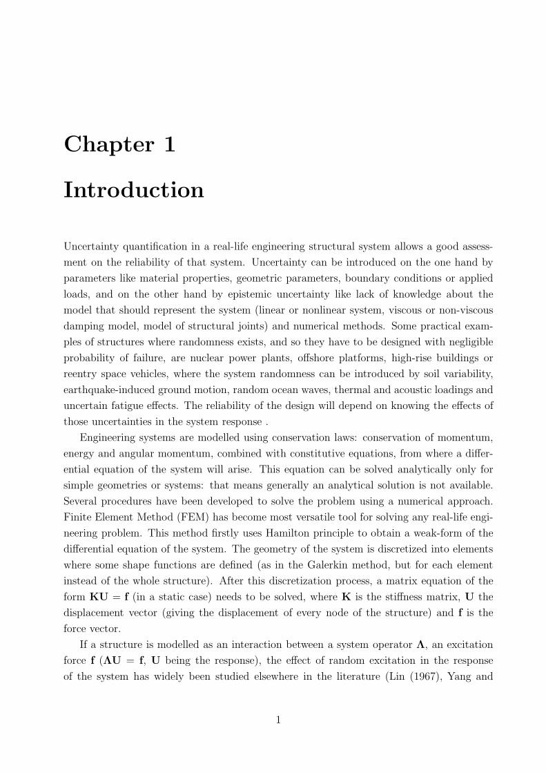
Introduction
Uncertainty quantification in a real-life engineering structural system allows a good assess-
ment on the reliability of that system. Uncertainty can be introduced on the one hand by
parameters like material properties, geometric parameters, boundary conditions or applied
loads, and on the other hand by epistemic uncertainty like lack of knowledge about the
model that should represent the system (linear or nonlinear system, viscous or non-viscous
damping model, model of structural joints) and numerical methods. Some practical exam-
ples of structures where randomness exists, and so they have to be designed with negligible
probability of failure, are nuclear power plants, offshore platforms, high-rise buildings or
reentry space vehicles, where the system randomness can be introduced by soil variability,
earthquake-induced ground motion, random ocean waves, thermal and acoustic loadings and
uncertain fatigue effects. The reliability of the design will depend on knowing the effects of
those uncertainties in the system response .
Engineering systems are modelled using conservation laws: conservation of momentum,
energy and angular momentum, combined with constitutive equations, from where a differ-
ential equation of the system will arise. This equation can be solved analytically only for
simple geometries or systems: that means generally an analytical solution is not available.
Several procedures have been developed to solve the problem using a numerical approach.
Finite Element Method (FEM) has become most versatile tool for solving any real-life engi-
neering problem. This method firstly uses Hamilton principle to obtain a weak-form of the
differential equation of the system. The geometry of the system is discretized into elements
where some shape functions are defined (as in the Galerkin method, but for each element
instead of the whole structure). After this discretization process, a matrix equation of the
form KU = f (in a static case) needs to be solved, where K is the stiffness matrix, U the
displacement vector (giving the displacement of every node of the structure) and f is the
force vector.
If a structure is modelled as an interaction between a system operator Λ, an excitation
force f (ΛU = f, U being the response), the effect of random excitation in the response
of the system has widely been studied elsewhere in the literature (Lin (1967), Yang and
1

1.1. Random field discretization 2
Kapania (1984) and Lin et al. (1986)). However, the case when randomness is introduced
by the operator is still under study due to its higher difficulty. Particular solutions to some
stochastic differential equation (e.g. Ito type (Ito (1951)) and functional integration (Hopf
(1952), Lee (1974))), are available for few cases. But problems where stochastic operators’s
random coefficients possess smooth sample path has no mathematical theory for obtaining
the exact solution. The method for finding a solution to the stochastic differential equation
needs two steps. The first step consist in modelling adequately the random properties (Ben-
jamin and Cornell (1970) and Vanmarcke (1983)). The second step involves solution of the
differential equation.
1.1 Random field discretization
In this section some basics of probability theory and random field/process are summarized
(Ghanem and Spanos (1991), Sudret and Der-Kiureghian (2000), Papoulis and Pillai (2002)
or Keese (2003)). Emphasis has been made on the available discretization schemes of random
field/process.
A probability space is denoted by L2(Θ,B, P ) , where Θ is the set of elementary events
or sample space, containing all the possible outcomes; B is the σ-algebra of events: collection
of possible events having well-defined probabilities and P is the probability measure.
A random variable X is a function whose domain is Θ ; X : (Θ,B, P ) −→ R inducing a
probability measure on R called the probability distribution of X , PX . The mathematical
expectation, mean variance and n-th momentum of X are denoted respectively by µ, σ2 and
E[Xn]. We define X < k as the set of experimental outcomes such that after mapping
this set with the random variable, the result is less than k. The cumulative distribution
function (CDF) FX verifies FX = PX < k = PX(−∞, k), and the probability density
function (PDF) fX(x) is the derivative of the CDF. The covariance of two independent
random variables X1 and X2 is
Cov[X1, X2] = E[(X1 − µX1)(X2 − µX2)] (1.1)
Two random variables X1, X2 are uncorrelated if Cov[X1, X2] = 0, and they are orthogonal
if E[X1X2] = 0. A Hilbert space H is a generalization of euclidian space (R3) into Rn, is
complete and the inner product is defined as:
< f, g >=
∫
Rn
f(x)g(x)dx (1.2)
The probability space is a Hilbert space, and a random field H(x, θ) can be defined as a
curve in the probability space L2. That is, a collection of random variables indexed by x
related to the system geometry: for a given x0, H(x0, θ) is a random variable and for a given
outcome θ0, H(x, θ0) is a realization of the field.

1.1. Random field discretization 3
The random field is Gaussian if any vector H(x1), ...H(xn) is Gaussian, and is com-
pletely defined by its mean µ(X), variance σ2(X) and autocorrelation coefficient ρ(x, x′). It
is homogenous if its mean and variance are constant and ρ is a function of the difference
x′ − x. A discretization procedure allows to approximate the random field with a finite
set of random variables, and the better the approximation is, the less random variables are
needed to approximate the random field accurately. There are three groups of discretization
schemes, namely, point discretization, average discretization and series expansion. More de-
tails are given in Li and Kiureghian (1993a), Matthies et al. (1997), Ditlevsen and Madsen
(1996) or Sudret and Der-Kiureghian (2000).
1.1.1 Point discretization methods
The first group of discretization methods is based on point discretization, the random vari-
ables χi are selected values of the random field H(∗) at some given points xi, and the
approximated field • is obtained from χ = H(x1), . . . , H(xN).
• The shape function method, introduced by Liu et al. (1986a,b) approximates the ran-
dom field in each element using nodal values xi and polynomial shape functions Ni
associated with the element
H =
q∑
i=1
Ni(x)H(xi) (1.3)
with x ∈ Ω where Ω is an open set describing the geometry and q the number of nodes.
• The midpoint method, introduced by Der-Kiureghian and Ke (1987), uses as points xi
the centroid of each element, and then has as many random variables approximating
the random field as number of elements; it over-represent the variability of the random
field within each element.
• The integration point method (Matthies et al. (1997)), associate a single random vari-
able to each gauss point of each element appearing in the finite element resolution
scheme. This involves that every integration appearing in the Finite Element (FE)
model is done by Gauss point method. Results are accurate for short correlation length.
However, the total number of random variables involved increases dramatically with
the size of the problem.
• The optimal linear estimation method (OLE) or Kringing method, presented by Li and
Kiureghian (1993b), approximates the random field with random variables dependent
on nodal values χ = H(x1), . . .H(xq). The dependence is linear
H(x) = a(x) + bTi (x)χi (1.4)
1.1. Random field discretization 4
and coefficients are calculated minimizing the variance of the difference between the
approximated and exact random field Var[H(x)− H(x)
]while keeping the mean of
that difference equal to zero : E[H(x)− H(x)
]= 0.
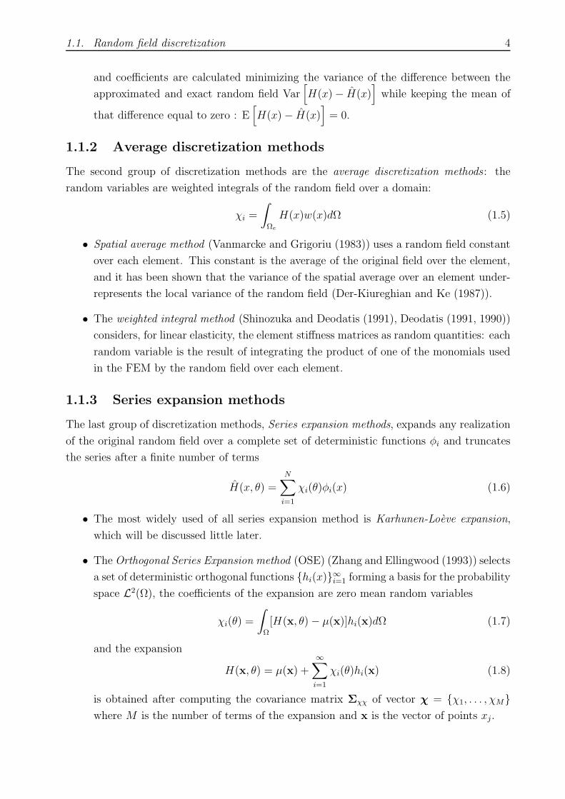
1.1.2 Average discretization methods
The second group of discretization methods are the average discretization methods : the
random variables are weighted integrals of the random field over a domain:
χi =
∫
Ωe
H(x)w(x)dΩ (1.5)
• Spatial average method (Vanmarcke and Grigoriu (1983)) uses a random field constant
over each element. This constant is the average of the original field over the element,
and it has been shown that the variance of the spatial average over an element under-
represents the local variance of the random field (Der-Kiureghian and Ke (1987)).
• The weighted integral method (Shinozuka and Deodatis (1991), Deodatis (1991, 1990))
considers, for linear elasticity, the element stiffness matrices as random quantities: each
random variable is the result of integrating the product of one of the monomials used
in the FEM by the random field over each element.
1.1.3 Series expansion methods
The last group of discretization methods, Series expansion methods, expands any realization
of the original random field over a complete set of deterministic functions φi and truncates
the series after a finite number of terms
H(x, θ) =
N∑
i=1
χi(θ)φi(x) (1.6)
• The most widely used of all series expansion method is Karhunen-Loeve expansion,
which will be discussed little later.
• The Orthogonal Series Expansion method (OSE) (Zhang and Ellingwood (1993)) selects
a set of deterministic orthogonal functions hi(x)∞i=1 forming a basis for the probability
space L2(Ω), the coefficients of the expansion are zero mean random variables
χi(θ) =
∫
Ω
[H(x, θ)− µ(x)]hi(x)dΩ (1.7)
and the expansion
H(x, θ) = µ(x) +∞∑
i=1
χi(θ)hi(x) (1.8)
is obtained after computing the covariance matrix Σχχ of vector χ = χ1, . . . , χM
where M is the number of terms of the expansion and x is the vector of points xj.

1.1. Random field discretization 5
• An extension of OSE, using a spectral representation of χ, is Expansion Optimal Linear
Estimation method (EOLE) (Li and Kiureghian (1993a)):
χ(θ) = µχ +N∑
i=1
√λiξi(θ)φi (1.9)
with ξi independent standard normal variables and (λi,φi) are the eigenvalues and
eigenvectors of the covariance matrix Σχχ.
1.1.4 Karhunen-Loeve expansion (KL expansion)
This method consist in expanding a random function, that is, a function defined on the
σ-field of random events, in a Fourier-type series. It was derived independently by different
researchers (Karhunen (1947) and Loeve (1948)) and is based on the spectral decomposition
of the covariance function CHH(χ,χ′) = σ(χ)σ(χ′)ρ(χ,χ′).
A process χ(x) can be expanded into a series of the form
χ(x) =
∞∑
n=1
cnfn(x) 0 < x < L (1.10)
with fn(x) a set of orthonormal functions in (0, L)
∫ T
0
fn(x)f∗m(x)dx = δ[n−m] (1.11)
The coefficients cn =∫ L
0χ(x)f ∗
n(x)dx are random variables. We consider the problem of
determining a set of orthonormal functions fn(x) such that the sum (1.10) equals χ(x) and
coefficients cn are orthogonal.
To solve this problem, the eigenfunctions f(x1) and eigenvalues λ of the autocorrelation
R(x1, x2) of the process χ, are calculated solving the equation:
∫ L
0
R(x1, x2)f(x2)dx2 = λf(x1) 0 < x1 < L (1.12)
From theory of integral equations it is known that the eigenfunctions are orthonormal and
satisfy the identity R(x, x) =∑∞
n=1 λn|fn(x)|2. Then it can be shown that
E|χ(x)− χ(x)|2 = 0 0 < x < L (1.13)
and
Ecnc∗m = λnδ[n−m] (1.14)
We can note that if we have an orthonormal set of functions fn(x) and
χ(x) =∞∑
n=1
cnfn(x) (1.15)
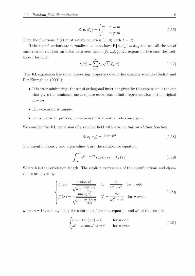
1.1. Random field discretization 6
Ecnc∗m =
σ2n n = m
0 n 6= m(1.16)
Then the functions fn(t) must satisfy equation (1.10) with λ = σ2n.
If the eigenfunctions are normalized so as to have Ecnc∗m = δnm and we call the set of
uncorrelated random variables with zero mean ξ1, ...ξn, KL expansion becomes the well-
known formula:
χ(x) =
∞∑
n=0
ξn√
λnfn(x) (1.17)
The KL expansion has some interesting properties over other existing schemes (Sudret and
Der-Kiureghian (2000)):
• It is error minimizing: the set of orthogonal functions given by this expansion is the one
that gives the minimum mean-square error from a finite representation of the original
process.
• KL expansion is unique.
• For a Gaussian process, KL expansion is almost surely convergent.
We consider the KL expansion of a random field with exponential correlation function
R(x1, x2) = e|x1−x2|/b (1.18)
The eigenfunctions f and eigenvalues λ are the solution to equation
∫ +a
−a
e|x1−x2|/bf(x2)dx2 = λf(x1) (1.19)
Where b is the correlation length. The explicit expressions of the eigenfunctions and eigen-
values are given by:
fn(x) =cos(ωnx)√a+ sin(2ωna)
2ωn
λn =2c
ω2n + c2
for n odd
f ∗n(x) =
sin(ω∗nx)√
a− sin(2ω∗
na)2ω∗
n
λ∗n =
2c
ω∗2n + c2
for n even(1.20)
where c = 1/b and ωn being the solutions of the first equation and ω∗ of the second:
c− ω tan(ωa) = 0 for n odd
ω∗ + c tan(ω∗a) = 0 for n even(1.21)

1.2. Response statistics calculation for static problems 7
1.2 Response statistics calculation for static problems
Now, the aim is to estimate the variance of the response, how disperse the response is around
the mean. The input has N random variables related to geometry, material properties and
loads. Each of them can be represented as the sum of its mean and a zero-mean random
variables αi, the input variations around the mean are collected in a zero-mean random
vector α = α1, ...αN. If the problem is not specifically dynamic, methods for solving
the stochastic differential equation are based on second moment approaches and spectral
representation.
1.2.1 Second moment approaches
Second moment methods evaluate the statistics of the output from the mean values of input
variables and covariance matrix of α.
• The perturbation method uses Taylor series expansion of the quantities involved around
their mean value: stiffness K, response U and load vector f, and then identifies coeffi-
cients at both sides of the equation
KU = f (1.22)
The Taylor series expansion of each matrix is represented by:
K = K0 +
N∑
i=1
KIiαi +
1
2
N∑
i=1
N∑
j=1
KIIij αiαj + o(‖α‖2) (1.23)
U = U0 +
N∑
i=1
UIiαi +
1
2
N∑
i=1
N∑
j=1
UIIij αiαj + o(‖α‖2) (1.24)
f = f0 +N∑
i=1
fIiαi +1
2
N∑
i=1
N∑
j=1
fIIij αiαj + o(‖α‖2) (1.25)
with KIi =
∂K∂αi
∣∣∣α=0
and KIIij = ∂2K
∂αi∂αj
∣∣∣α=0
Identifying the similar order coefficients in equation (1.22) after substituting with equa-
tions (1.23) to (1.25), the following expressions are obtained
U0 = K−10 .f0 (1.26)
UIi = K−1
0 .(fIi −KIi .U0) (1.27)
UIIij = K−1
0 .(fIIij −KIi .U
Ij −KI
j .UIi −KII
ij .U0) (1.28)
The statistics of U are available from that of α in equation (1.24):
E[U] ≈ U0 +1
2
N∑
i=1
N∑
j=1
UIIij Cov[αi, αj ] (1.29)

1.2. Response statistics calculation for static problems 8
Cov[U,U] ≈
N∑
i=1
N∑
j=1
UIi .(U
Ij )
TCov[αi, αj] (1.30)
This method is used with a discretization of the random variables like spatial average
method (Baecher and Ingra(1981), Vanmarcke and Grigoriu(1983)) or shape functions
method (Liu et al. (1986a,b)).
• Another method based on perturbation method is the weighted integrals method. It
couples perturbation method with the representation of the stochastic stiffness matrix
as a random variable ke = ke0+
NWI∑
l=1
∆kelχ
el where χ
el is the l-th of the NWI zero-mean
weighted integrals of the random field and ∆kel are deterministic matrices. As in the
former case, statistics of the response can be calculated.
• The quadrature method is based on computing the moments of response quantities
(Baldeweck (1999)). For a mechanical system, the uncertainties are described by a
vector of uncorrelated normal random variables X = X1, ...XN with prescribed joint
distribution. If S is a response quantity, the i-th moment of S can be calculated with
E[Si(X1, ...XN)] =
∫
RN
[s(x1, ...xN)]iϕ(xN)...ϕ(xN )dx1...dxN (1.31)
Where ϕ(.) is the probability density function of a standard normal variate and s(x1, ..., xN )
is usually known. The quadrature of this integral is its approximation by a weighted
summation of the function at some points of the interval, as in the Gauss-points
method.
E[Si(X1, ...XN)] ≈NP∑
k1=1
· · ·NP∑
kN=1
wk1 . . . wkN [s(xk1, . . . , xkN )]i (1.32)
This method uses information about the distributions of the basic random variables
for the calculations, so, it is not a ”pure” second moment approach. This method does
not discretize the random field and gives an upper bound on the response variance
independent of the correlation structure of the field and second order statistics of the
response.
• Neumann expansion method was introduced to the field of structural mechanics by
Shinozuka and Nomoto (1980). The theory developed by Neumann states that the
inverse of an operator (if exist) can be expanded in a convergent series in terms of the
iterated kernels
[L +Π]U = F (1.33)
U = [L+Π]−1F (1.34)
u(α(θ),x) =
∞∑
i=0
(−1)i[L−1(x)Π(α(x, θ),x)]i[f(x, θ)] (1.35)

1.2. Response statistics calculation for static problems 9
verifying that
‖ L−1Π ‖< 1
If only one parameter (α(x, θ)) of our system is random, substituting it by its KL
expansion α(x, θ) =∑M
n=1 λnξnan(x) leads to:
[K+
M∑
n=1
ξnK(n)
]U = f (1.36)
[I+
M∑
n=1
ξnQ(n)
]U = g (1.37)
where
Q(n) = K−1K(n) g = K
−1f (1.38)
[I+Ψ [ξn]]U = g (1.39)
Where Neumann expansion is applied
U =
∞∑
i=0
(−1)i
[M∑
n=1
ξnQ(n)
]ig (1.40)
This expression is computationally more tractable than the original Neumann expan-
sion.
1.2.2 Spectral Stochastic Finite Elements Method (SSFEM)
This method is an extension of the deterministic FEM for boundary value problems involving
random material properties. In a deterministic case, a system motion is governed by a partial
differential equation (PDE) with associated boundary conditions and initial conditions. The
FEM discretizes those differential equations replacing the geometry by a set of nodes, and
the displacement field is approximated by the nodal displacements
KU = F (1.41)
ke =
∫
Ωe
BTDB dΩe (1.42)
where K,U,F,ke,B and D are respectively the stiffness matrix, displacement vector, ex-
ternal force vector, element stiffness matrix, matrix relating strains to nodal displacements
and elasticity matrix.
If system properties are modelled as random fields, the system is governed by a stochastic
PDE and the response will be a displacement random field u(x, θ) where θ denotes a basic
outcome in the space of all possible outcomes. It is discretized as a random vector of nodal
displacements U(θ). If a finite set of points θ1, . . . , θQ is selected so as to sample correctly
the space of all outcomes, it defines the random variable: this is the approach of Monte Carlo

1.2. Response statistics calculation for static problems 10
simulation.
A different approach, taken by SSFEM, is to discretize the random field with series expan-
sions. The input random field is discretized using a truncated KL expansion and each nodal
displacement is represented by its coordinates in an appropiate basis of the space of random
variables called polynomial chaos (PC).
Consider ξi(θ)∞i=1, a set of orthonormal Gaussian random variables. The set of polynomials
Γp in ξi(θ)∞i=1 of degree not exceeding p, orthogonal to the set of polynomials Γp−1, are
the PC of order p. Those polynomials will be symmetrical with respect to their arguments.
Any square-integrable random function can be approximated as closely as desired with the
representation:
µ(θ) = a0Γ0 +
∞∑
i1=1
ai1Γ1(ξi1(θ)) +
∞∑
i1=1
i1∑
i2=1
ai1i2Γ2(ξi1(θ), ξi2(θ))
+∞∑
i1=1
i1∑
i2=1
ai1i2
i2∑
i3=1
ai1i2i3Γ3(ξρ1(θ), ξρ2(θ), ξρ3(θ)) + . . .
=∞∑
j=0
ajΨj [ξ(θ)]
(1.43)
The convergence properties of this expansion depends on the order of PC and number of
terms in KL expansion. All PC are orthogonal, that means that
∫
Ωe
Γi(ξ)Γj(ξ)dP =< ΓiΓj >= 0 (1.44)
with ξ an element of the space of all possible outcomes representing a random variable with
zero mean and P the probability of that outcome). The uncorrelated Gaussian random
variables verify
< ξ1, . . . , ξ2n+1 >= 0 and < ξ1, . . . , ξ2n >=∑∏
< ξiξj > (1.45)
Those conditions are the ones used for calculate them:
Γ0 = 1 the first polynomial chaos is a constant (1.46)
Γ1(ξi) = ξ1 the PC with order > 0 have zero mean (1.47)
Γ2(ξi1, ξi1) = ξi1ξi2 − δi1i2 (1.48)
Γ3(ξi1, ξi1, ξi3) = ξi1ξi1ξi3 − ξi1δi2i3 − ξi2δi1i3 − ξi3δi1i2 (1.49)
and so on. After substituting PC expansion and KL expansion, the equilibrium equation
becomes: ( ∞∑
i=0
Kiξi(θ)
).
( ∞∑
j=0
UjΨj(θ)
)− F = 0 (1.50)

1.3. Response statistics calculation for dynamic problems 11
After truncation of expansions, the error of the approximation is
ǫM,P =M∑
i=0
P−1∑
j=0
Ki.Ujξi(θ)Ψj(θ)− F (1.51)
It can be minimized in a mean square sense: E[ǫM,P .Ψk] = 0 k = 0, . . . P − 1
if Kjk =
M∑
i=0
P−1∑
j=0
E[ξiΨjΨk]Ki and Fk = E[ΨkF], the error minimizing equation leads to the
system
K00 . . . K0,P−1
K10 . . . K1,P−1...
...KP−1,0 . . . KP−1,P−1
.
U0
U1...
UP−1
=
F0
F1...
FP−1
(1.52)
Knowing that U(θ) =∑P−1
j=0 UjΨj(θ), the mean and covariance of nodal displacement vector
can be calculated:
E[U] = U0 (1.53)
and
Cov[U,U] =P−1∑
j=0
E[Ψ2i ]UiU
Ti (1.54)
1.3 Response statistics calculation for dynamic prob-
lems
In a deterministic dynamic system, the solution U is obtained by inverting the dynamic
stiffness matrix
D(s) = s2M+ sG(s) +K (1.55)
That is, getting the transfer matrix H(s) = D−1, and multiplying it by the forcing vector
U = Hf. This procedure is simplified using the residues theorem, that states that any
complex function can be expressed in terms of its poles sj and residues. If the poles are the
eigenvalues of H(s), the transfer matrix becomes
H(s) =m∑
j=1
Rj
s− sj. (1.56)
Here
Rj =res
s=sj[H(s)]
def= lim
s→sj(s− sj) [H(s)] =
zjzTj
zTj∂D(sj)
∂sjzj. (1.57)
is the residue of the transfer function matrix at the pole sj, where zj is the corresponding
eigenvector. The transfer function matrix may be obtained as
H(iω) =N∑
j=1
[γjzjz
Tj
iω − sj+
γ∗j z
∗jz
∗Tj
iω − s∗j
]+
m∑
j=2N+1
γjzjzTj
iω − sj, , (1.58)

1.3. Response statistics calculation for dynamic problems 12
where
γj =1
zTj∂D(sj)
∂sjzj. (1.59)
Details about the derivation of this expressions can be found in Adhikari (2000).
Some special and useful cases can be defined:
1. Undamped systems : In this case G(s) = 0 results the order of the characteristic polyno-
mial m = 2N ; sj is purely imaginary so that sj = iωj where ωj ∈ R are the undamped
natural frequencies and zj = xj ∈ RN . In view of the mass normalization relationship
Kxj = ω2jMxj , γj =
12iωj
and equation (1.58) leads to
H(iω) =
N∑
j=1
1
2iωj
[1
iω − iωj−
1
iω + iωj
]xjx
Tj =
N∑
j=1
xjxTj
ω2j − ω2
. (1.60)
2. Viscously-damped systems with non-proportional damping (Lancaster (1966), Vigneron
(1986), Geradin and Rixen (1997)): In this case m = 2N and γj = 1
zTj [2sjM+C]zj
.
These reduce expression (1.58) to
H(iω) =
N∑
j=1
[γjzjz
Tj
iω − sj+
γ∗j z
∗jz
∗Tj
iω − s∗j
]. (1.61)
3. Viscously-damped systems with proportional damping derives from the former case,
where the eigenvectors are real and sj = −ζjωj + iωj, so they coincide with their
complex conjugate
H(iω) =N∑
j=1
[γjzjz
Tj
−ω2 − 2iωζjωj + ω2j
](1.62)
The above expressions lead to the calculation of the response vector as a function of the
system matrices eigenvalues and eigenvectors. Therefore, a study of the effect of randomness
in eigenvalues and eigenvectors should lead to a study of the randomness in the displacement
field.
1.3.1 Random eigenvalue problem
The determination of natural frequencies and mode shapes require the solution of an eigen-
value problem. This problem could be either a differential eigenvalue problem or a matrix
eigenvalue problem depending on whether a continuous model or a discrete model is chosen
to describe the given vibrating system. Several studies have been conducted on this topic
since the mid-sixties: see Boyce (1968), Scheidt and Purkert (1983), Ibrahim (1987), Be-
naroya and Rehak (1988), and Benaroya (1992). Here a brief review of the literature on
methods used for random eigenvalue problem of differential equations and matrices will be
given.

1.3. Response statistics calculation for dynamic problems 13
Continuous systems
Different models have been studied: the free vibration of elastic string and rod with random
mass density and area of cross section were studied by Boyce (1962), the random string
vibration problem by Goodwin and Boyce (1964), the case of random elastic beam and
beam columns were considered by Boyce and Goodwin (1964), Haines (1967) and Bliven
and Soong (1969), stochastic boundary value problems by Linde (1969) and Boyce (1966),
beam column with random material and geometric properties with random axial load by
Hoshiya and Shah (1971), etc. Widely used methods for the determination of eigenvalues
and normal modes are variational, asymptotic and perturbation method, leading to a Strum-
Liouville problem. Also Monte Carlo simulation is used.
The free vibration characteristics of systems governed by second order stochastic wave
equation have been investigated by Iyengar and Manohar (1989) and Manohar and Iyengar
(1993): the probability distribution of eigenvalues of random string equation are related
to the zeros of an associated initial value problem. Exact solutions to the problems are
shown to be possible only under special circumstances (Iyengar and Manohar (1989) and
Manohar and Keane (1993)) and, consequently, approximations become necessary. For spe-
cific types of mass and stiffness variations, Iyengar and Manohar (1989) and Manohar and
Iyengar (1993, 1994) have developed solution strategies based on closure, discrete Markov
chain approximation, stochastic averaging methods and Monte Carlo simulation to obtain
acceptable approximations to the probability densities of the eigensolutions. A qualitative
feature of the eigenvalue distributions emerged from these studies has been the tendency of
the eigenvalues, when normalized with respect to the deterministic eigenvalues, to become
stochastically stationary with respect to the mode count n for large values of n.
Studies on eigenvalues of non-self adjoint stochastic differential equation with stochastic
boundary conditions have been conducted by Ramu and Ganesan (1993c) using perturbation
method. They considered a random Leipholz column with distributed random tangential
follower load and derived the correlation structure of the free vibration eigenvalues and
critical loads in terms of second order moment properties of the system property random
fields. Ganesan (1996) also considered stochastic non-self adjoint systems and obtained
second order properties of the eigenvalues for different correlation structure of the system
parameters.
Discrete systems
For the above mentioned stochastic continuous systems, the applications are on relatively
simple structures (e.g, single beam-column, axially vibrating rod, string, rectangular plate)
and for simple boundary conditions. For the more general class of problems generally found
in engineering, discretization methods, such as FEM, are adopted. Then the governing

1.3. Response statistics calculation for dynamic problems 14
eigenvalue problems have the form
K(Θ)X(Θ) = λ(Θ)M(Θ)X(Θ) (1.63)
Most of the available formulations are based on perturbation or Taylor series methods. Fox
and Kapoor (1968) have presented exact expressions for the rate of change of eigenvalues
and eigenvectors with respect to design parameters of the actual structure in terms of system
property matrices and eigenvalue and eigenvector under consideration. If δj (j = 1..r), are
design variables, λi and Xi are ith eigenvalue and eigenvector respectively, then, the rate of
change of eigenvalue can be expressed as
∂λi
∂δj= XT
i
[∂K
∂δj− λi
∂M
∂δj
]Xi (1.64)
They also presented two different formulation for rate of change of eigenvectors; these are as
follows:
Formulation 1:
∂Xi
∂δj= −
[FiFi + 2MXiX
Ti M
]−1[Fi
∂Fi
∂δj+MXiXi
∂M
∂δj
]Xi (1.65)
where Fi = K− λiM (1.66)
(1.67)
Formulation 2:
∂Xi
∂δj=
r∑
k=1
aijkXk (1.68)
where aijk =XT
l
[∂K∂δj
− λi∂M∂δj
]Xi
λl − λifor l 6= i (1.69)
= −1
2
[XT
i
∂M
∂δjXi
]for l = i (1.70)
(1.71)
It may be noted that, formulation 1 requires the inversion of an n× n matrix, whereas such
an inversion does not appear in formulation 2. So formulation 2 is computationally less
intensive and has been used by many authors later. Collins and Thomson (1969) have given
expressions for the statistics of eigenvalues and eigenvectors in a matrix form in terms of
mass and stiffness matrix of the structure. According to their formulation, covariance matrix
for eigenvalue and eigenvector becomes
[Cov(λ,x)
]=
[ [∂λ∂k
] [∂λ∂m
][∂x∂k
] [∂x∂m
]] [
Cov(k,m)
] [ [∂λ∂k
] [∂λ∂m
][∂x∂k
] [∂x∂m
]]T
(1.72)
Where the matrix[Cov(k,m)
]contains variance and covariance of stiffness and mass elements.
They have also considered specific examples and compared the theoretical solutions with

1.3. Response statistics calculation for dynamic problems 15
results from Monte Carlo simulation. Schiff and Bogdanoff (1972a,b) derived an estimator for
the standard deviation of a natural frequency in terms of second order statistical properties
of system parameters. The derivation was based upon mean square approximate systems.
Scheidt and Purkert (1983) have used perturbation expansion of eigenvalues and eigenvectors
and have given the expression of homogeneous terms up to 4th order. These terms then can
be used to determine expectation and correlation of the random eigenvalues and eigenvectors.
Bucher and Brenner (1992) have employed a first order perturbation and, starting from
the definition of Rayleigh’s quotient for discrete systems, and, assuming λi = λi0 + λi1,
xi = xi0 + ǫxi1, K = K0 + ǫK1 and M = M0 + ǫM1, they have shown that
E[λi] =xTi0K0xi0
xTi0M0xi0
(1.73)
and
σ2λi
= ǫ2λ2i0E(x
Ti0K1xi0)
2 + 2(xTi0K1xi0)(x
Ti0M1xi0) + (xT
i0M1xi0)2 (1.74)
In these equations it is assumed that ǫ << 1 and subscripts containing a 0 denote deter-
ministic quantities and subscripts with 1 denote random quantities. Zhu et al. (1992) have
used method of local averages to discretize random fields in conjunction with perturbational
approach to study the statistics of fundamental natural frequency of isotropic rectangular
plates. Their formulation also allows for multiplicity of deterministic eigenvalues. The latter
issue has also been addressed by Zhang and Chen (1991). Song et al. (1995) have out-
lined a first order perturbational approach to find the moments of the sensitivity of random
eigenvalues with respect to expected value of specified design variables.
Studies on random matrix eigenvalue problems arising in the study of structural stability
have been conducted byRamu and Ganesan (1992, 1993a,b, 1994), Sankar et al. (1993) and
Zhang and Ellingwood (1995) using perturbational approaches. The study of flutter of
uncertain laminated plates with random modulus of elasticity, mass density, thickness, fibre
orientation of individual lamina, geometric imperfection of the entire plate and in-plane loads
was carried out by Liaw and Yang (1993). Based on the study of distribution of zeros of
random polynomials, Grigoriu (1992) has examined the roots of characteristic polynomials
of real symmetric random matrices. It is suggested that such studies serve to identify the
most likely values of eigenvalues, determine the average number of eigenvalues within a
specified range and, finally, in conjunction with an assumption that eigenvalues constitute
Poisson points, to find the probability that there is no eigenvalue below or above a given
value or within a given range. Furthermore, the assumption that the random coefficients of
the polynomial are jointly Gaussian is shown to simplify the analysis significantly.
Solutions that do not consider the perturbation method around the deterministic natural
frequencies values are studied in Adhikari (2007a), Adhikari and Friswell (2007) and Adhikari
(2006). In these references is considered a joint probability distribution of the natural fre-
quencies based on perturbation expansion of the eigenvalues about an optimal point and an

1.3. Response statistics calculation for dynamic problems 16
asymptotic approximation of multidimensional integrals. In Wagenknecht et al. (2005) possi-
bilistic uncertainties are propagated through the coupled second-order differential equations
that govern a dynamic system using pseudospectra of matrices.
1.3.2 High and mid frequency analysis: Non-parametric approach
This section focuses on the analysis of linear structural dynamical systems to which, at a
given frequency, vibrational response consist of small contributions from a large number of
modes, e.g. light flexible structures subjected to high frequency broad band excitation. The
procedure used to analyze a structure, as described by Langley (1989), consist in:
1. Dividing the structure into a number of interacting subsystems whose mean energies
and external power inputs are related via a set of linear equations. The coefficients of
those linear equations are expressed in terms of quantities known as the loss factors
and the coupling loss factors.
2. Study the systems individually, where the jth subsystem has a single response variable
ui(x, t), and x represents the spatial co-ordinates of a point within the subsystem. The
equation of motion which governs harmonic vibration of the jth subsystem is
(1 + iεj)Lj(uj)− ρjω2(1− iγj)uj = Fj(x, ω) + f c
j (x, ω) (1.75)
where ω is the frequency of vibration, uj(zx, ω) is the complex amplitude of the re-
sponse, Lj is a differential operator depending on the structure (e.g. for a beam in
bending Lj = EIuivj ), ρj is the volume density (or equivalent) and εj and γj are dissi-
pation factors. Fj(x, ω) represents an external load (a distributed force) while F cj (x, ω)
is a load arising from coupling to another system.
3. Allow the systems to interact, which allows the exchange of vibration energies between
the subsystems. The system response is characterized by calculating these energy
exchanges. The mean external power input into subsystem j is
Qj = 2ωεjSj + 2ωγjTj + Rj (1.76)
where Tj, Sj and Rj are the statistical average kinetic energy, the statistical average
strain energy stored in the subsystem and the transmitted power. If E = π[ρ−1q−1]T
then
Q = (2/π)ω[γρq]E+ (1/π)NM−1[q]E (1.77)
where the first term of the equation represents the power dissipated internally, while the
second is the power transmitted. [γ] is a diagonal matrix of terms γj, dissipation factor
of each subsystem j, [ρ] has the same relation towards the volume density, [q], N and
M are matrices whose entries depend on the Green function Gij(x,y, ω) representing
the response at x on subsystem i to a load applied at y on subsystem j.

1.3. Response statistics calculation for dynamic problems 17
In all those steps, the uncertainty is introduced by the Green function, depending on which
Green function is taken, the method becomes Statistical Energy Analysis (SEA) or Gaussian
Orthogonal Ensemble (GOE). A comparison between those two methods can be found in
Langley and Brown (2004). It should be noted that the parameters variance has no influence
in SEA and GOE.
Statistical Energy Analysis (SEA)
Description of Statistical Energy Analysis (SEA) can be found in Lyon and Dejong (1995).
Different assumptions are adopted in the application of this method:
• The vibrating structure is considered to be drawn from an ensemble of nominally
identical systems.
• The subsystem eigensolutions are treated as having prescribed probability distribu-
tions: a set of Poisson points on the frequency axes. The natural frequencies are
mutually independent and identically (uniformly) distributed in a given frequency
bandwidth.
• The subsystem mode-shapes are deterministic.
• the power input and loss factors are uncorrelated.
The formulation presented by Lyon provides a fairly complete framework for obtaining mea-
sure of response variability. Those formulations were developed in early 1960’s to enable
prediction of vibration response of launch and payload structures to rocket noise at launch.
Subsequently, the method has been used not only in aerospace industry, but also in land
based vehicle design, ship dynamics, building acoustics, machinery vibration and in seismic
analysis of secondary systems. Some examples of recent applications are related by Lai and
Soong (1990) and Hynna et al. (1995).
Over the last decade there has been a resurgence of interest in this area of research
and several important papers dealing with the theoretical development of this method have
appeared, see, for example, the papers by Hodges and Woodhouse (1986), Langley (1989),
Keane (1992) and Fahy (1994); also see the theme issue on SEA brought out by the Royal
Society of London (Price and Keane (1994)) and the book edited by Keane and Price (1997).
Gaussian Orthogonal Ensemble (GOE)
Work on random matrix theory has investigated in detail the statistical properties of the
natural frequencies of a particular type of random matrix known as the Gaussian Orthogonal
Ensemble (GOE) (see Mehta (1991)). The GOE concerns a symmetric matrix whose entries
are Gaussian, zero mean, and statistically independent, with the off-diagonal entries having
a common variance, and the diagonal entries having twice this variance. The spacings

1.4. Summary 18
between the eigenvalues obtained with GOE have a Rayleigh distribution (referred to as the
Wigner distribution in the random matrix literature). This contrasts with the exponential
distribution that would be obtained were the natural frequencies to form a Poisson point
process (used in SEA). It has arised from numerical and experimental studies that most
physical systems have natural frequencies that conform to the GOE statistics, even though
the random matrices that govern their behaviour have no obvious direct connection with the
GOE. However, when the system has many ”symmetries” and the natural frequencies from
all symmetric classes are superposed, the Poisson spacing statistics are obtained, see Weaver
(1989), Ellegaard et al. (2001), Bertelsen et al. (2000) and Langley and Brown (2004).
1.3.3 High and mid frequency analysis: Random Matrix Theory
The Random Matrix Theory was firstly studied by physicists and mathematicians,in the
1930s, in the context of nuclear physics. Many useful results can be found in Mehta (1991)
or Gupta and Nagar (2000). It has been said that SEA and GEO do not take account
of parametric variance. Therefore, a parametric approach using random matrices is being
investigated. Using the maximum entropy principle for positive symmetric real random
matrices, Soize (2001) obtained an ensemble distribution of random matrices. The fitness
of this approach to the problem at low-frequency range and a study of the statistics of the
random eigenvalues of these random matrices were studied in Soize (2003). The probability
density function of that ensemble distribution of random matrices coincide, under some
conditions, with the one of Wishart distribution.
1.4 Summary
As a summary, available methods for solving a stochastic differential equation are represented
in the following chart:

1.4. Summary 19
Randomdynamicsystems
Parametricuncer-tainty
Randomeigenvalueproblem
Directinversion
Non-parametricuncertainty
StochasticEnergyAnalysis
Poisson’sdistribution
Rayleigh’sdistribution
(GOE)
RandomMatrixTheory
Wishartdistribution

Chapter 2
Random Matrix Theory (RMT)
As it has already been discussed, a discretized mechanical system equation of equilibrium
is given by DU = f where the dynamic stiffness matrix and force vector can be random
and consequently the nodal displacement is also random. Until now, some methods have
considered a parametric approach where randomness in stiffness matrix is a consequence of
randomness in material properties (Youngs modulus, mass density, Poissons ratio, damping
coefficient) and geometric parameters: all aleatoric uncertainties. Epistemic uncertainties
were studied separately, they do not depend explicitly on the system parameters: they can be
unquantified errors associated with the equation of motion (linear or non linear), damping
model (viscous or non viscous), model of structural joints and numerical method. RMT
approach could take account of these two different kinds of uncertainties.
2.1 Multivariate statistics
Multivariate statistics is a generalization of statistics to matrices. It is used widely in physics
to model quantum systems where the probability density function of eigenvalues of random
matrices is calculated. Several works in continuous matrix variate distribution theory have
been published, like Gupta and Nagar (2000), Muirhead (1982) and Mehta (1991). The
concept of random matrix derives from that of a random vector X = (X1, . . . , Xm)′: a vector
whose components are jointly distributed, with defined mean or vector of expectations µ
and covariance matrix Σ
µ ≡ E(X) = (E(X1), . . . ,E(Xm))′ (2.1)
Σ ≡ Cov(X) = E[(X− µ)(X− µ)′] (2.2)
A largely studied case is the case when this random vector is normally distributed, then the
marginal distribution of each component of X is univariate normal. If X is now a p × q
matrix, vec(X) is the pq × 1 vector formed by stacking the columns of X under each other.
Then the distribution of a matrix is in fact the distribution of the vector vec(X), and this
matrix is a random matrix.
20

2.1. Multivariate statistics 21
A matrix random phenomenon is an observable phenomenon represented in a matrix
form where the outcome of different observations is not deterministically predictable, but
they obey certain conditions of statistical regularity. The set of all outcomes of a random
matrix characterize the sample space Θ, where a probability function assigning a probability
to each outcome can be defined, a probability density function and a moment generating
function can as well be defined.
A random matrix X(p×n) is said to have matrix variate normal distribution with mean
N(p × n) and covariance matrix Σ ⊗ Ψ X ∼ Np,n(N,Σ ⊗ Ψ) where Σ(p × p) > 0 and
Ψ(n × n) > 0, if vec(X′) ∼ Npn(vec(N′),Σ ⊗ Ψ). Its probability density function is given
by:
(2π)−12npdet(Σ)−
12ndet(Ψ)−
12petr−
1
2Σ−1(X−N)Ψ−1(X−N′), X ∈ R
p×n,N ∈ Rp×n
(2.3)
A particular case of this random matrix is the symmetric matrix variate normal distribution.
If X(p× p) is a symmetric matrix, the condition X = X′ is verified , a 12p(p− 1)× 1 vector
vecp(X) = [x11 x12 x22 . . . x1p . . . xpp] with distribution N 12p(p+1)(vecp(N), B′
p(Σ⊗Ψ)Bp) is
defined and ΣΨ = ΨΣ. The probability density function of X in terms of vecp(X)
(2π)−14p(p−1)det(B′
p(Σ⊗Ψ)Bp)− 1
2×
exp
[−1
2(vecp(X)− vecp(N))′.B+
p (Σ⊗Ψ)−1B+′
p (vecp(X)− vecp(N))
](2.4)
Where (Bp)ij,gh = 12(δigδjh + δihδjg), with i ≤ p, j ≤ p, g ≤ h ≤ p and B+
p its Moore-Penrose
inverse.
A Wishart distribution is a p-variate generalization of χ2 distribution. A p × p random
symmetric positive definite matrix S has Wishart distribution with parameters p, n and
Σ(p× p) > 0, written as S ∼ Wp(n,Σ), if its p.d.f is given by:
212npΓp(
1
2n)det(Σ)
12n−1det(S)
12(n−p−1)etr(−
1
2Σ−1S),S > 0, n ≥ p (2.5)
The mass and stiffness matrices M and K of a system are nonnegative definite symmetric
matrices, the damping matrix C, proportional to M and K, is also a nonnegative definite
symmetric matrix. Therefore, stiffness and mass matrix could be modelled as Wishart
matrices. The moments of the inverse of the dynamic stiffness matrix, the frequency response
matrix H(ω) = D−1(ω) (see (1.55)) should exist for all frequency ω, that is E[‖H(ω)‖νF] <
∞, ∀ω. This condition will always be verified if the inverse moments of M, K and C exist,
conditions easier to analyze than the former one.
It was shown in Soize (2001)and Soize (2000) that given a symmetric nonnegative definite
matrix G, maximizing the entropy associated with the matrix variate probability density
function pG(G)
S(pG)= −
∫
G>0
pG (G) lnpG (G)
dG (2.6)
2.2. Wishart matrix 22
and using the equations that act like constraints to obtain pG∫
G>0
pG (G) dG = 1 (the normalization) (2.7)
and E [G] =
∫
G>0
G pG (G) dG = G (the mean matrix) (2.8)
The probability density function resulting from that analysis is the matrix variate gamma
distribution. The main difference between the matrix variate gamma distribution and the
Wishart distribution is that historically only integer values were considered for the shape
parameter p in the Wishart matrices. Then, this pG is called in this thesis Wishart distribu-
tion probability density function with parameters p = (2ν+n+1) and Σ = G/(2ν+n+1),
that is G ∼ Wn
(2ν + n + 1,G/(2ν + n+ 1)
).
2.2 Wishart matrix
It has already been said that a Wishart matrix is the generalization of χ2 to matrices. If
X(n+1)×p ∼ N(1µ′, In+1 ⊗ Σ) is a random matrix defined as X = [X′1 . . . Xn+1]
′ where
X1, . . . ,Xn+1 are independent Np(µ,Σ) random vectors, 1 = (1, . . . , 1)′ ∈ Rn+1 and Σ is
positive definite, a Wishart matrix can be considered as the distribution of the covariance
of X with n ≥ p.
Then a Wishart matrix S ∼ Wp(n,Σ) has the same distribution as Z′Z, where the n × p
matrix Z is N(0, In ⊗ Σ) (the rows of Z are independent Np(0′,Σ) random vectors). The
probability density function of S ∼ Wp(n,Σ) is given by:
212npΓp(
1
2n)det(Σ)
12n−1det(S)
12(n−p−1)etr(−
1
2Σ−1S), S > 0, n ≥ p
If we know the matrix to fit has Wishart distribution, the parameters of matrix Z have to be
obtained. The moments of G ∼ Wp(n,Σ) are given by Gupta and Nagar (2000) [Chapter 3]
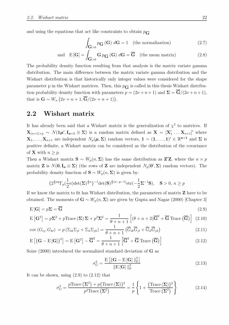
E [G] = pΣ = G (2.9)
E[G2]= pΣ2 + pTrace (Σ)Σ+ p2Σ2 =
1
θ + n + 1
[(θ + n + 2)G
2+G Trace
(G)]
(2.10)
cov (Gij, Gkl) = p (ΣikΣjl + ΣilΣjk) =1
θ + n + 1
(GikGjl +GilGjk
)(2.11)
E[G− E [G]2
]= E
[G2]−G
2=
1
θ + n+ 1
[G
2+G Trace
(G)]
(2.12)
Soize (2000) introduced the normalized standard deviation of G as
σ2G =
E[‖G− E [G] ‖2F
]
‖E [G] ‖2F(2.13)
It can be shown, using (2.9) to (2.12) that
σ2G =
pTrace(Σ2)+ pTrace (Σ)2
p2Trace(Σ2) =
1
p
1 +
Trace (Σ)2
Trace(Σ2)
(2.14)

2.3. Fitting of parameter for Wishart distribution 23
With p = 2ν+n+1, it is obvious that, for a system with dimensions n =constant, the bigger
becomes the order of the inverse moment ν the smaller is σ2G, a measure of the uncertainty
in the system matrices. This parameter ν is generally ν = 2, but it could be chosen so as
to decrease the uncertainty of the system, even if to do that would imply the order of the
inverse moment constraint increases.
Interest on Wishart matrix G ∼ Wp(n,Σ) also arise from the fact that the inverted
Wishart matrix distribution pV ∼ IWn(m,Ψ), is available making use of the jacobian of the
transformation V = f(G) = G−1 and the exterior product of each of the differential vectors
dG and dV. A n× n symmetric positive definite random matrix V is said to have inverted
Wishart distribution with parameters m and Ψ
pV (V) =2−
12(m−n−1)ndetΨ
12 (m−n−1)
Γn
(12(m− n− 1)
)det Vm/2
etr−V−1Ψ
; m > 2n, Ψ > 0. (2.15)
E[G−1
]=
Ψ
m− 2n− 2=
θ + n + 1
θG
−1(2.16)
E[G−2
]=
Trace (Ψ)Ψ+ (m− 2n− 1)Ψ2
(m− 2n− 1)(m− 2n− 2)(m− 2n− 4)
=(θ + n+ 1)2Trace
(G
−1)G
−1+ θG
−2
θ(θ + 1)(θ − 2)(2.17)
We can observe that, contrarily to what was supposed with Wishart matrix, the mean of
inverse Wishart matrix is not equal to the inverse of the mean. In fact, knowing that ν ≥ 2
and that matrices obtained with a FEM tend to represent big structures with thousands of
degrees of freedom n, those two values E[G−1
]and G
−1can be very different.
2.3 Fitting of parameter for Wishart distribution
A measure of the normalized standard deviation was introduced by Soize (2000), it is the
dispersion parameter σ2G from (2.13):
σ2G =
E[‖G− E [G] ‖2F
]
‖E [G] ‖2F(2.18)
For a Wishart distribution, as seen in Adhikari (2008)
σ2G =
1
θ + n+ 1
1 +Trace
(G)2
Trace(G
2)
This parameter can also be obtained from the FEM if parameters which contain uncertainty
are expanded as KL expansion. Then, matrix G = K, M, C can be expanded as
G = G0 +∑
i
ξiGi with G0 = E [G] (2.19)

2.3. Fitting of parameter for Wishart distribution 24
Details of this expansion are shown in Chapter 3, Chapter 4 and Chapter 5 for particular
cases of rod, beam and thin plate. Then, introducing this expansion in (2.18)
σ2G =
E[‖∑
i ξiGi ‖2F
]
‖E [G] ‖2F(2.20)
=E[Trace
((∑
i ξiGi)(∑
j ξjGj))]
‖G0 ‖2F
(2.21)
=Trace
(E[(∑
i
∑j ξiξjGiGj)
])
‖G0 ‖2F
(2.22)
σ2G =
Trace((∑
i G2i ))
‖G0 ‖2F
(2.23)
Several criteria can be developed to fit a symmetric random matrix with a Wishart
matrix, four are explained here, each of them verifying a different condition related to the
first moment and that the normalized standard deviation is same as the measured normalized
standard deviation σG = σG:
1. Criteria 1: For each system matrices, we consider that the mean of the random matrix
is same as the deterministic matrix E [G] = G . This condition results
p = n+ 1 + 2ν and Σ = G/p (2.24)
where
ν =1
2σ2G
1 +
Trace(G)2
Trace(G
2)
−
(n+ 1)
2(2.25)
This criteria was proposed by Soize (2000, 2001).
2. Criteria 2: Called the optimal Wishart distribution, it was proposed by Adhikari
(2007b). The dispersion parameter is obtained after considering that the mean of the
random matrix and the mean of the inverse of the random matrix are closest to the
deterministic matrix and its inverse: that is∥∥G− E [G]
∥∥Fand
∥∥∥G−1− E
[G−1
]∥∥∥Fare
minimum. This condition results:
p = n+ 1 + 2ν and Σ = G/α (2.26)
where α =√2ν(n + 1 + 2ν) and 2ν is as defined in equation (2.25). The rationale
behind this approach is that a random system matrix and its inverse should be math-
ematically treated in a similar manner as both are symmetric and positive-definite
matrices.
3. Criteria 3: Here we consider that for each system matrix, the mean of the inverse of
the random matrix equals to the inverse of the deterministic matrix: E[G−1
]= G
−1

2.4. Relationship between dispersion parameter and the correlation length 25
. Using equation (2.16) and after some simplifications one obtains
p = n+ 1 + 2ν and Σ = G/2ν (2.27)
where ν is defined in equation (2.25).
4. Criteria 4: This criteria arises from the idea that the mean of the eigenvalues of
the distribution is same as the ‘measured’ eigenvalues of the mean matrix and the
normalized standard deviation is same as the measured normalized standard deviation.
Mathematically we can express this as
E[M−1
]= M
−1, E [K] = K, σM = σM and σK = σK (2.28)
This implies that the parameters of mass matrix is selected according to criteria 3 and
the parameters for the stiffness matrix is selected according to criteria 1. The damping
matrix is obtained using criteria 2. This case is therefore a combination of the previous
three cases.
It is verified with numerical simulations that the third criteria gives the best results.
2.4 Relationship between dispersion parameter and the
correlation length
As it has been seen, the parameter σ2G is of the form
σ2G =
Trace((∑
i G2i ))
‖G0 ‖2F
(2.29)
Where matrices Gi are obtained by integration of the shape functions of the FE model cho-
sen multiplied by the KL expansion of a stochastic parameter of the system. Eigenfunctions
in KL expansion are always orthogonal, like the trigonometric functions obtained in sub-
section 1.1.4. A property of functions cosine and sine is that they are bounded: they vary
between −1 and 1. Then:
|cos(ax+ ab)| ≤ 1 (2.30)
|cos(ax+ ab)fj(x)| ≤ |fj(x)| (2.31)∣∣∣∣∫
cos(ax+ ab)fj(x) dx
∣∣∣∣ ≤
∣∣∣∣∫
fj(x) dx
∣∣∣∣ (2.32)
(
∫ l
0
cos(ax+ ab)fj(x) dx)2 ≤ (
∫ l
0
fj(x) dx)2 (2.33)
∑
j
(∫ l
0
cos(ax+ ab)fj(x) dx
)2
≤∑
j
(∫ l
0
fj(x) dx
)2
(2.34)
2.5. Simulation method for Wishart system matrices 26
Where fj is a shape function and the sum for all the shape functions can be considered as a
sum of the square of the elements Gij of the matrix G for which the parameter σG is being
calculated.
It is observed here that in fact, each term of the matrix can have contributions from
the element matrices of different elements. It can be noticed that the right hand side of
(2.34) remains the same for those elements: if fn(x) and fm(x) are contributions from two
different element matrices, fn(x) + fm(x) can be considered as a new shape function. The
left hand side of (2.34) has different trigonometric function for each element: if an element
has a trigonometric function cos (a(x+ b1)) the next one has cos (a(x+ b2)). The difference
|b1 − b2| is equal to the distance between local origins of two different elements: it is the
length of the element if all elements have same length. We can also notice that if the number
of elements used is infinity, this difference |b1 − b2| = 0, and cos (a(x+ b1)) = cos (a(x+ b2)).
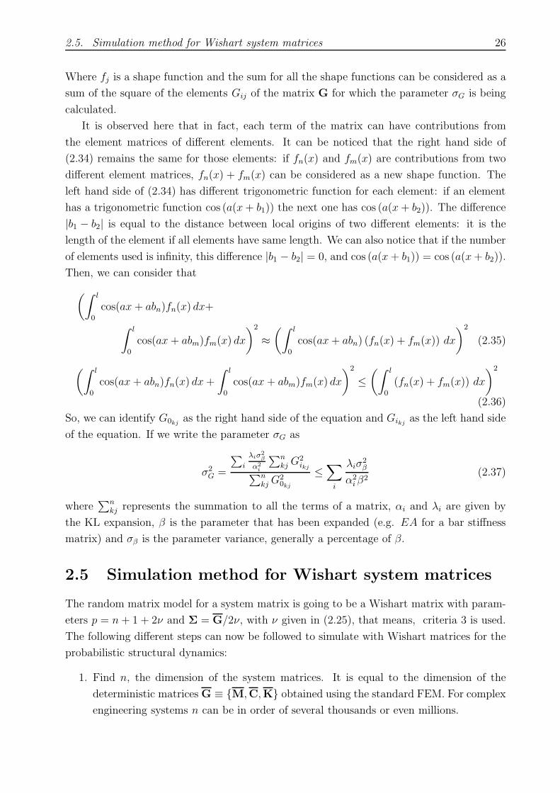
Then, we can consider that
(∫ l
0
cos(ax+ abn)fn(x) dx+
∫ l
0
cos(ax+ abm)fm(x) dx
)2
≈
(∫ l
0
cos(ax+ abn) (fn(x) + fm(x)) dx
)2
(2.35)
(∫ l
0
cos(ax+ abn)fn(x) dx+
∫ l
0
cos(ax+ abm)fm(x) dx
)2
≤
(∫ l
0
(fn(x) + fm(x)) dx
)2
(2.36)
So, we can identify G0kj as the right hand side of the equation and Gikj as the left hand side
of the equation. If we write the parameter σG as
σ2G =
∑i
λiσ2β
α2i
∑nkj G
2ikj∑n
kj G20kj
≤∑
i
λiσ2β
α2iβ
2(2.37)
where∑n
kj represents the summation to all the terms of a matrix, αi and λi are given by
the KL expansion, β is the parameter that has been expanded (e.g. EA for a bar stiffness
matrix) and σβ is the parameter variance, generally a percentage of β.
2.5 Simulation method for Wishart system matrices
The random matrix model for a system matrix is going to be a Wishart matrix with param-
eters p = n + 1 + 2ν and Σ = G/2ν, with ν given in (2.25), that means, criteria 3 is used.
The following different steps can now be followed to simulate with Wishart matrices for the
probabilistic structural dynamics:
1. Find n, the dimension of the system matrices. It is equal to the dimension of the
deterministic matrices G ≡ M,C,K obtained using the standard FEM. For complex
engineering systems n can be in order of several thousands or even millions.
2.5. Simulation method for Wishart system matrices 27
2. Obtain the normalized standard deviations or the ’dispersion parameters’ σG ≡ σM , σC , σK
corresponding to the system matrices,from experiment, experience or using the Stochas-
tic FEM.
3. Calculate
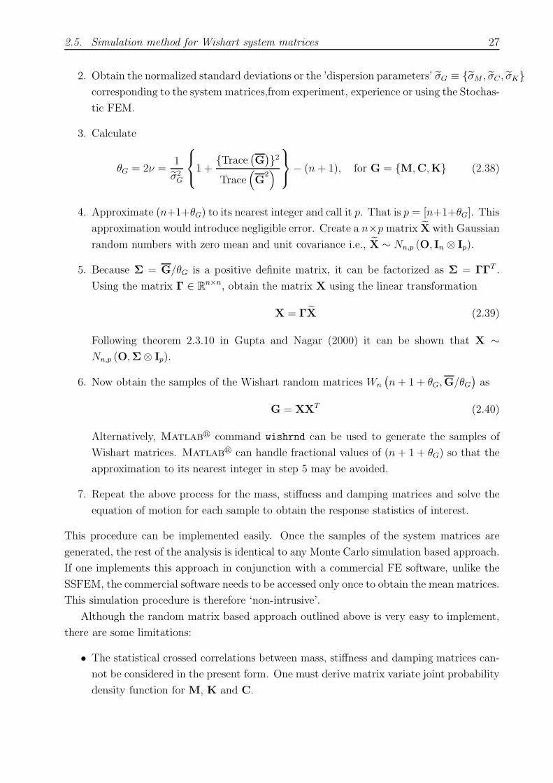
θG = 2ν =1
σ2G
1 +
Trace(G)2
Trace(G
2)
− (n+ 1), for G = M,C,K (2.38)
4. Approximate (n+1+θG) to its nearest integer and call it p. That is p = [n+1+θG]. This
approximation would introduce negligible error. Create a n×p matrix X with Gaussian
random numbers with zero mean and unit covariance i.e., X ∼ Nn,p (O, In ⊗ Ip).
5. Because Σ = G/θG is a positive definite matrix, it can be factorized as Σ = ΓΓT .
Using the matrix Γ ∈ Rn×n, obtain the matrix X using the linear transformation
X = ΓX (2.39)
Following theorem 2.3.10 in Gupta and Nagar (2000) it can be shown that X ∼
Nn,p (O,Σ⊗ Ip).
6. Now obtain the samples of the Wishart random matrices Wn
(n+ 1 + θG,G/θG
)as
G = XXT (2.40)
Alternatively, Matlabr command wishrnd can be used to generate the samples of
Wishart matrices. Matlabr can handle fractional values of (n + 1 + θG) so that the
approximation to its nearest integer in step 5 may be avoided.
7. Repeat the above process for the mass, stiffness and damping matrices and solve the
equation of motion for each sample to obtain the response statistics of interest.
This procedure can be implemented easily. Once the samples of the system matrices are
generated, the rest of the analysis is identical to any Monte Carlo simulation based approach.
If one implements this approach in conjunction with a commercial FE software, unlike the
SSFEM, the commercial software needs to be accessed only once to obtain the mean matrices.
This simulation procedure is therefore ‘non-intrusive’.
Although the random matrix based approach outlined above is very easy to implement,
there are some limitations:
• The statistical crossed correlations between mass, stiffness and damping matrices can-
not be considered in the present form. One must derive matrix variate joint probability
density function for M, K and C.

2.6. Generalized beta distribution 28
• Unlike the deterministic matrices derived from FE discretisation, sample-wise sparsity
may not be preserved for the random matrices.
• Only one variable, namely the normalized standard deviation σG defined in (2.18), is
available to characterize uncertainty in a system matrix. This can be obtained, for
example using standard system identification tools (e.g., modal identification) across
the ensemble.
• Unlike the parametric uncertainty quantification methods, no computationally effi-
cient analytical method (e.g., perturbation method, polynomial chaos expansion) is
yet available for random matrix approach.
In the medium and high-frequency vibration of stochastic systems, where there is enough
‘mixing’ of the modes, the dynamic response is not very sensitive to the detailed nature of
uncertainty in the system. In this situation, in spite of the limitations mentioned above,
the random matrix approach provides an easy alternative to the conventional parametric
approach. The numerical examples in the next chapters illustrates this fact.
2.6 Generalized beta distribution
There is a gross ‘oversimplification’ of the nature of the uncertainty by only considering one
parameter θ as the origin or randomness in a random matrix. Any n× n symmetric matrix
G, supposing fully populated, can have N = n(n + 1)/2 number of independent elements.
Therefore, its covariance matrix is N2 = n2(n + 1)2/4 dimensional and symmetric. Which
implies that it can have N(N + 1)/2 = n(n + 1)(n(n + 1) + 2)/8 number of independent
elements. Nonparametric approach, therefore, only offers a single parameter to quantify
uncertainty which can potentially be expressed by n(n + 1)(n(n + 1) + 2)/8 number of
independent parameters. However, when very little information regarding the covariance
tensor of G is available, then a central Wishart distribution is the best that can be used to
quantify uncertainty. If more reliable information regarding the covariance tensor of G is
available, then we need a matrix variate distribution which not only satisfies being symmetric
and positive definite, but also must offer more parameters to fit the ‘known’ covariance tensor
of G. This is the central motivation of fitting a random matrix with a beta distribution.
As stated in Gupta and Nagar (2000), a p×p random symmetric positive definite matrix
X has generalized matrix variate beta type I distribution with parameters a, b, Ω, Ψ denoted
by X ∼ GBIp(a, b,Ω,Ψ) if its p.d.f. is given by
det (X −Ψ)a−12(p+1) det (Ω−X)b−
12(p+1)
βp(a, b)det (Ω−Ψ)(a+b)− 12(p+1)
, Ψ < X < Ω (2.41)
2.6. Generalized beta distribution 29
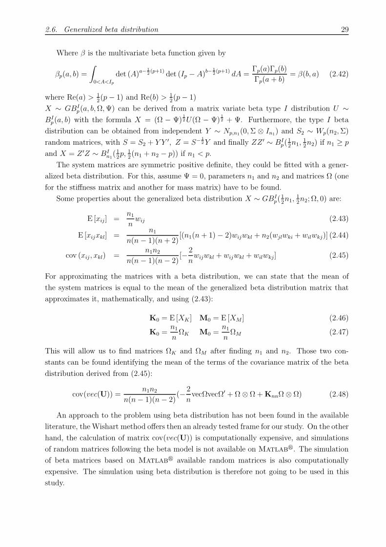
Where β is the multivariate beta function given by
βp(a, b) =
∫
0<A<Ip
det (A)a−12(p+1) det (Ip − A)b−
12(p+1) dA =
Γp(a)Γp(b)
Γp(a + b)= β(b, a) (2.42)
where Re(a) > 12(p− 1) and Re(b) > 1
2(p− 1)
X ∼ GBIp(a, b,Ω,Ψ) can be derived from a matrix variate beta type I distribution U ∼
BIp(a, b) with the formula X = (Ω − Ψ)
12U(Ω − Ψ)
12 + Ψ. Furthermore, the type I beta
distribution can be obtained from independent Y ∼ Np,n1(0,Σ ⊗ In1) and S2 ∼ Wp(n2,Σ)
random matrices, with S = S2 + Y Y ′, Z = S− 12Y and finally ZZ ′ ∼ BI
p(12n1,
12n2) if n1 ≥ p
and X = Z ′Z ∼ BIn1(12p, 1
2(n1 + n2 − p)) if n1 < p.
The system matrices are symmetric positive definite, they could be fitted with a gener-
alized beta distribution. For this, assume Ψ = 0, parameters n1 and n2 and matrices Ω (one
for the stiffness matrix and another for mass matrix) have to be found.
Some properties about the generalized beta distribution X ∼ GBIp(
12n1,
12n2; Ω, 0) are:
E [xij] =n1
nwij (2.43)
E [xijxkl] =n1
n(n− 1)(n+ 2)[(n1(n+ 1)− 2)wijwkl + n2(wjlwki + wilwkj)] (2.44)
cov (xij , xkl) =n1n2
n(n− 1)(n− 2)[−
2
nwijwkl + wijwkl + wilwkj] (2.45)
For approximating the matrices with a beta distribution, we can state that the mean of
the system matrices is equal to the mean of the generalized beta distribution matrix that
approximates it, mathematically, and using (2.43):
K0 = E [XK ] M0 = E [XM ] (2.46)
K0 =n1
nΩK M0 =
n1
nΩM (2.47)
This will allow us to find matrices ΩK and ΩM after finding n1 and n2. Those two con-
stants can be found identifying the mean of the terms of the covariance matrix of the beta
distribution derived from (2.45):
cov(vec(U)) =n1n2
n(n− 1)(n− 2)(−
2
nvecΩvecΩ′ + Ω⊗ Ω +KnnΩ⊗ Ω) (2.48)
An approach to the problem using beta distribution has not been found in the available
literature, theWishart method offers then an already tested frame for our study. On the other
hand, the calculation of matrix cov(vec(U)) is computationally expensive, and simulations
of random matrices following the beta model is not available on Matlabr. The simulation
of beta matrices based on Matlabr available random matrices is also computationally
expensive. The simulation using beta distribution is therefore not going to be used in this
study.

Chapter 3
Axial vibration of rods withstochastic properties
The rod model is a 1D model that uses linear shape functions and is therefore one of
the simplest FE models. It is also a widely used model, as many structural elements can
be modeled as rods. Here the theory for deriving this model is reminded at first: the
derivation of the equation of motion and the discretization process that leads to the well
known deterministic FE model of the rod. Then, expressions for other mass and stiffness
matrices taking account of the eigenfunctions appearing in the KL expansion of random
variables EA and ρA are derived.
3.1 Equation of motion
In this section, the governing equation of the system is derived, more details can be found
in Petyt (1998) and Geradin and Rixen (1997). Hamilton’s principle states
∫ t2
t1
(δ(T − U) + δWnc)dt = 0 (3.1)
Where T is the kinetic energy, U is the elastic strain energy, Wnc is the work of non con-
servative forces and δu = 0 at t = t1 and t = t2. In this study, linear constitutive model
is assumed (the stress-strain relation is linear (σx = Eεx, where the axial strain component
εx = ∂u∂x
and E is Youngs modulus)), and the material is assumed as isotropic. It is assumed
that each plane cross-section remains plane during the motion and the only stress component
that is not negligible is σx, and it remains uniform over each cross section. The axial force
in one of the faces of the increment dx of axial element is σxA, and the extension of the
element is εx dx , the work done on the element as strain energy is dU = 12σxεxAdx and for
the complete rod, the total strain and kinetic energy are
U =1
2
∫ +a
−a
σxεxAdx =1
2
∫ +a
−a
EAε2x dx (3.2)
30

3.2. Deterministic Finite Element model 31
and
T =1
2
∫ +a
−a
ρAu2 dx (3.3)
If there is an applied load of magnitude px per unit length, the work done in a virtual
displacement δu is δu.px dx and the virtual work for the whole rod is:
δW =
∫ +a
−a
pxδu dx (3.4)
After substituting those expressions in Hamilton’s principle and assuming that operators δ
and ∂()/∂t as well as δ and ∂()/∂ x are commutative, and that integrations with respect to
t and x are interchangeable, we can obtain the equation of motion:
EA∂2u
∂x2− ρA
∂2u
∂t2+ px = 0 throughout − a ≤ x ≤ +a (3.5)
And boundary conditions
EA∂u
∂x= 0 or δu = 0 at x = −a and x = +a (3.6)
Depending on the boundary conditions, analytical solutions to this differential equation are
available.
3.2 Deterministic Finite Element model
The basic rod element of length l has two nodes, one at each end, and one degree of freedom
per node: the axial displacement u at each node, so, there are two degrees of freedom per
element: u1 and u2. The only forces acting on the element are point axial forces f1 and f2
acting at the ends (Dawe (1984)).
A displacement field, expressed in terms of the element nodal displacements, is assumed:
for each point of the element the displacement is given by u = A0 + A1x, or, in a matrix
form
u ≡ u = αA = [1 x]
[A0
A1
](3.7)
If the origin of the x coordinate is at node 1, the boundary conditions
u = u1 at x = 0u = u2 at x = l
for equation (3.7) lead to the system
d = CA where A = C−1d (3.8)
u = αC−1d = Nd (3.9)
or, expressed with matrices,
[u1
u2
]=
[1 01 l
] [A0
A1
] [A0
A1
]=
[1 0
−1/l 1/l
] [u1
u2
](3.10)

3.2. Deterministic Finite Element model 32
and
N =[1− x
lxl
](3.11)
Where N is the matrix of shape functions or shape function matrix, and each shape
function equals one for a given degree of freedom and zero for all the others.
In a discrete system, Hamiltons principle can be expressed as Lagranges equation (here
stated without damping force):
d
dt
(∂T
∂u
)−
∂U
∂u= f (3.12)
For this problem, f = px the axial force and the only strain and stress existing are εx and
σx = Eεx (acting in the axial direction).
εx =du
dx=
[dN
dx
]d =
[−1/l 1/l
] [u1
u2
]= Bd (3.13)
It is known that the (stretching) strain energy of the bar element of length l with origin
placed in node one is:
Ue =1
2
∫ t
0
σtxεxAdx =
1
2dt
(∫ l
0
Bt(AE)B dx
)d (3.14)
The element strain energy can be expressed as Ue = 12dtKed, where Ke is the element
stiffness matrix. The stress is expressed as σtx instead of σx due to the fact that while
σtx = σx and the expression of Ue remains the same scalar quantity, the element stiffness
matrix can now be obtained and is independent of the displacement. The element stiffness
matrix is given by:
Ke =
∫ l
0
Bt(AE)B dx = AE
∫ l
0
[−1/l1/l
] [−1/l 1/l
]dx =
AE
l
[1 −1−1 1
](3.15)
So, U =AE
2l
[u1 u2
] [ 1 −1−1 1
] [u1
u2
](3.16)
The work of the forces applied to the element is
We = −f1u1 − f2u2 (3.17)
The kinetic energy of the rod element can be calculated in the same way
Te =1
2
∫ l
0
ρAu2 dx =1
2ut
∫ l
0
ρANtN dxu =1
2utMeu (3.18)
Me =ρAl
6
[2 11 2
](3.19)
After assembling the whole structure stiffness matrix, mass matrix and the forcing vector,
those expressions can be introduced in Lagrange’s equation (3.12) to obtain the system
equation of motion:
Mu+Ku = f (3.20)
3.3. Derivation of stiffness matrices 33
The assembly process consist in adding the element matrix corresponding to element number
e to the submatrix composed of rows and columns e and e+ 1 of an initially zero matrix of
dimensions N + 1 where N is the number of elements of the rod structure. This process is
done for mass and stiffness matrices, there is a similar process for the forcing vector where
the terms of the element forcing vector are added to the corresponding terms of a global
forcing vector.
3.3 Derivation of stiffness matrices
For the FE model of a straight axially loaded bar, the stiffness matrix is given by
Ke =
∫ l
0
Bt(AE)B dx (3.21)
where E is Youngs modulus, A denotes the cross section area, and the product AE, axial
rigidity, is a random field that can be represented as a KL expansion
Ke =
∫ l
0
Bt(A0E0 +
n/2∑
i=1
(λifi(x)ξi + λ∗i f
∗i (x)ξ
∗i ))Bdx (3.22)
with ξi and ξ∗i set of uncorrelated random variables forming a Gaussian vector , λi and λ⋆i
eigenvalues and fi and f ∗i eigenfunctions of a given covariance function. The two different
sets of eigenfunctions and corresponding eigenvalues have to be integrated for the covariance
functions studied in subsection 1.1.4 As it has already been said:
c− ω tan(ωa) = 0 gives a set of solutions ωi for iodd (3.23)
ω + ω tan(ca) = 0 gives a set of solutions ω∗i for i even (3.24)
The eigenfunctions and eigenvectors can be calculated:
λi =2c
ω2i + c2
λ∗i =
2c
ω∗ 2i + c2
(3.25)
fi(x) =cos(ωix)√a+ sin(2ωia)
2ωi
f ∗i (x) =
sin(ω∗i x)√
a−sin(2ω∗
i a)
2ω∗
i
(3.26)
The expression for the stiffness matrix considering KL expansion is:
Ke = Ke0 +
n/2∑
i=1
(ξiλiKei + ξ∗i λ∗iK
∗ei) (3.27)
with
K0 =A0E0
l
[1 −1−1 1
](3.28)

3.4. Derivation of mass matrices 34
Kei =1
l2√a + sin(2ωna)
2ωn
[1 −1−1 1
] ∫ l
0
cos(ωn(x+ xe1)) dx (3.29)
K∗ei
=1
l2√a− sin(2ω∗
na)2ω∗
n
[1 −1−1 1
] ∫ l
0
sin(ω∗n(x+ xe
1)) dx (3.30)
noting that:
∫cos(ax+ b) dx =
∫cos(X)
dX
a=
sin(X)
a=
sin(ax+ b)
a(3.31)
∫sin(ax+ b) dx =
∫sin(X)
dX
a=
− cos(X)
a= −
cos(ax+ b)
a(3.32)
(3.33)
and finally,
Kei =sin(ωi(l + xe
1))− sin(ωixe1)
l2ωi
√a+ sin(2ωia)
2ωi
[1 −1−1 1
](3.34)
K∗ei
=− cos(ω∗
i (l + xe1)) + cos(ω∗
i xe1)
l2ω∗i
√a−
sin(2ω∗
i a)
2ω∗
i
[1 −1−1 1
](3.35)
We can notice here that, contrarily to the deterministic stiffness matrix, the terms in the
matrix will change from one element to the next one not only because of change in a given
parameter (EA), but also because of the effect of the eigenfunctions. This effect is neglected
when undertaking a Monte Carlo simulation, and can only be reflected adopting a fine mesh.
3.4 Derivation of mass matrices
For the mass matrix, a similar process gives the symmetric matrices Mei and M∗ei, the
components of whom are given by:
Mei11=
(2ωil − 2 sin (ωil)) cos (ωixe1) + (−l2ωi
2 + 2− 2 cos (ωil)) sin (ωixe1)
l2ω3n
√a + sin(2ωia)
2ωi
Mei12=
(− cos (ωil) lωi + 2 sin (ωil)− ωil) cos (ωixe1)
l2ω3n
√a+ sin(2ωia)
2ωi
+
(2 cos (ωil) + ωil sin (ωil)− 2) sin (ωixe1)
l2ω3n
√a+ sin(2ωia)
2ωi
Mei22=
(2 cos (ωi l) lωi + (l2ωi2 − 2) sin (ωil)) cos (ωix
e1)
l2ω3n
√a + sin(2ωia)
2ωi
+
((l2ωi2 − 2) cos (ωil)− 2ωil sin (ωil) + 2) sin (ωix
e1)
l2ω3n
√a + sin(2ωia)
2ωi

3.5. Numerical illustrations 35
Me∗i11=
(l2ω∗
i2 − 2 + 2 cos (ω∗
i l))cos (ω∗
i el) + (2ω∗i l − 2 sin (ω∗
i l)) sin (ω∗i el)
l2ω∗3i
√a−
sin(2ω∗
i x)
2ω∗
i
Me∗i12=
(−2 cos (ω∗i l) + 2− sin (ω∗
i l) lω∗i ) cos (ω
∗i el)
l2ω∗3i
√a−
sin(2ω∗
i x)
2ω∗
i
+
(2 sin (ω∗i l)− ω∗
i l − ω∗i l cos (ω
∗i l)) sin (ω
∗i el)
l2ω∗3i
√a−
sin(2ω∗
i x)
2ω∗
i
Me∗i22=
((−l2ω∗
i2 + 2
)cos (ω∗
i l) + 2 sin (ω∗i l) lω
∗i − 2
)cos (ω∗
i el) +
l2ω∗3i
√a−
sin(2ω∗
i x)
2ω∗
i(2ω∗
i l cos (ω∗i l) +
(−2 + l2ω∗
i2)sin (ω∗
i l))sin (ω∗
i el)
l2ω∗3i
√a−
sin(2ω∗
i x)
2ω∗
i
Those matrices are used in the following section to calculate the theoretical value of the
dispersion parameter.
3.5 Numerical illustrations
The example model verifies that its boundary conditions are the ones of a clamped-free
bar: zero displacement on the left end. Heuristically, it is considered that this boundary
condition is the one that will more likely cause a bigger variance in the response vector
than the one obtained with other typical boundary conditions like clamped-clamped bar.
The material properties are taken as ρ = 2700 kg/m3, E = 69GPa, values corresponding
to aluminium. Geometrical variables are: length of the bar L = 30m and cross section
A = 1 cm2. The variance of the parameters considered as random is 10% the value of the
parameter: σβ = 0.1 β. The parameters considered are β = EA for stiffness matrix and
β = ρA for mass matrix. The system response is calculated using equation (1.62): equation
for a viscously damped proportional model where damping factor is ζj = 0.02. For choosing
the number of elements of the structure, we consider that the smaller wavelength produced
by the vibration of the dynamic structure should be at least four times the element length.
If the maximum frequency for which the structure is analyzed covers the first fifty modes
(number of modes k = 50), the structure model will have 200 elements. This maximum
frequency is then calculated with an analytical expression available for rod:
fmax = (2k − 1)1
4
√EA
ρAL2= 4.17KHz
The maximum frequency used for testing the structure in this numerical calculation is 4KHz.
Measure of the response vector is given for the forcing point, situated at the 3rd node, and
at a sensor situated at the 35-th node.
Four different correlation lengths used in the KL expansions are selected to research the
effect of this value on the response statistics. Those correlation lengths are 0.1L, 0.2L, 0.5L
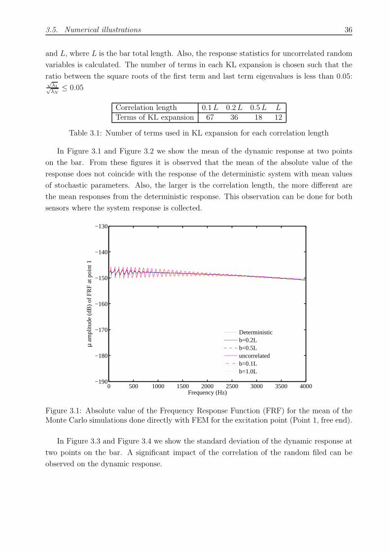
3.5. Numerical illustrations 36
and L, where L is the bar total length. Also, the response statistics for uncorrelated random
variables is calculated. The number of terms in each KL expansion is chosen such that the
ratio between the square roots of the first term and last term eigenvalues is less than 0.05:√λ1√λN
≤ 0.05
Correlation length 0.1L 0.2L 0.5L LTerms of KL expansion 67 36 18 12
Table 3.1: Number of terms used in KL expansion for each correlation length
In Figure 3.1 and Figure 3.2 we show the mean of the dynamic response at two points
on the bar. From these figures it is observed that the mean of the absolute value of the
response does not coincide with the response of the deterministic system with mean values
of stochastic parameters. Also, the larger is the correlation length, the more different are
the mean responses from the deterministic response. This observation can be done for both
sensors where the system response is collected.
0 500 1000 1500 2000 2500 3000 3500 4000−190
−180
−170
−160
−150
−140
−130
Frequency (Hz)
µ am
plitu
de (
dB)
of F
RF
at p
oint
1
Deterministicb=0.2Lb=0.5Luncorrelatedb=0.1Lb=1.0L
Figure 3.1: Absolute value of the Frequency Response Function (FRF) for the mean of theMonte Carlo simulations done directly with FEM for the excitation point (Point 1, free end).
In Figure 3.3 and Figure 3.4 we show the standard deviation of the dynamic response at
two points on the bar. A significant impact of the correlation of the random filed can be
observed on the dynamic response.
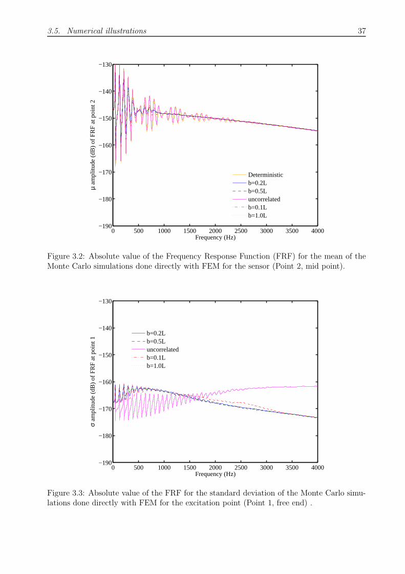
3.5. Numerical illustrations 37
0 500 1000 1500 2000 2500 3000 3500 4000−190
−180
−170
−160
−150
−140
−130
Frequency (Hz)
µ am
plitu
de (
dB)
of F
RF
at p
oint
2
Deterministicb=0.2Lb=0.5Luncorrelatedb=0.1Lb=1.0L
Figure 3.2: Absolute value of the Frequency Response Function (FRF) for the mean of theMonte Carlo simulations done directly with FEM for the sensor (Point 2, mid point).
0 500 1000 1500 2000 2500 3000 3500 4000−190
−180
−170
−160
−150
−140
−130
Frequency (Hz)
σ am
plitu
de (
dB)
of F
RF
at p
oint
1
b=0.2Lb=0.5Luncorrelatedb=0.1Lb=1.0L
Figure 3.3: Absolute value of the FRF for the standard deviation of the Monte Carlo simu-lations done directly with FEM for the excitation point (Point 1, free end) .

3.5. Numerical illustrations 38
0 500 1000 1500 2000 2500 3000 3500 4000−190
−180
−170
−160
−150
−140
−130
Frequency (Hz)
σ am
plitu
de (
dB)
of F
RF
at p
oint
2
b=0.2Lb=0.5Luncorrelatedb=0.1Lb=1.0L
Figure 3.4: Absolute value of the FRF for the standard deviation of the Monte Carlo simu-lations done directly with FEM for the sensor (Point 2).

Chapter 4
Bending vibration of beams withstochastic properties
4.1 Equation of motion
As in the previous chapter, expressions for total strain energy U , kinetic energy T , and virtual
work δW are derived, adopting the same hypothesis about linearity. The elementary theory
of bending assumes that the stress components σy, σz, τyz and τxz are zero, that the plane
sections normal to the undeformed centroidal axis remain plane after bending and that they
remain normal to the deformed axis. A distributed load py per unit length is applied. Then,
the axial displacement u at a distance y from the centroidal axis is u(x, y) = −y ∂v∂x
where v
is the displacement of the centroidal axis in the y-direction at position x. Expressions for
strain and kinetic energy and virtual work are:
U =
∫
V
σxεxdv =
∫
V
Eε2xdv =
∫ +a
−a
EI2(∂2v
∂x2
)2
dx (4.1)
with Iz =
∫
A
y2dA (4.2)
T =1
2
∫ +a
−a
ρAv2dx (4.3)
δW =
∫ +a
−a
pyδvdx (4.4)
After substituting those expressions in Hamilton’s principle equation (3.1), with δv = 0
when t = t1 and t = t2, the equation of motion is obtained:
−EI∂2v
∂x4− ρA
∂2v
∂t2+ py = 0 Throughout − a ≤ x ≤ +a (4.5)
In addition, either EIz
∂2v∂x2 = 0 or ∂v
∂x= 0
EIz∂3v∂x3 = 0 or v = 0
(4.6)
39

4.2. Deterministic Finite Element model 40
at x = −a and x = +a act as boundary conditions. ∂v∂x
= 0 and v = 0 represent the
vanishing of slope and displacement respectively, while EIz∂2v∂x2 = 0 and EIz
∂3v∂x3 = 0 represent
the vanishing of stress over a cross-section and shear force.
4.2 Deterministic Finite Element model
The basic beam element of length l has two nodes, one at each end, and two degrees of
freedom per node: the lateral displacement v and the rotation θz ≡dv
dxat each node, the
degrees of freedom for one element are v1, v2, θz1 and θz2 . At each node of the element are
acting a moment and a shear force as external forces: Mz1 ,Mz2 ,v1 and v2.
The displacement field, expressed in terms of the element coordinates, is assumed to have
a cubic form: for each point of the element the displacement is given by
u ≡ v = A0 + A1x+ A2x2 + A3x
3 (4.7)
=[1 x x2 x3
]
A0
A1
A2
A3
(4.8)
u = αA (4.9)
If the origin of the x coordinate is at node 1, the boundary conditions
v = v1 and θz = θz1 at x = 0v = v2 and θz = θz2 at x = l
(4.10)
for equation (4.9) lead to the system
d = CA where A = C−1d (4.11)
and
u = αC−1d = Nd (4.12)
or, expressed in matrix form
d =
v1θz1u2
θz2
=
1 0 0 00 1 0 01 l l2 l3
0 1 2l 3l2
A0
A1
A2
A3
(4.13)
N =[1− 3x2
l2+ 2x3
l3x− 2x2
l+ x3
l23x2
l2− 2x3
l3−x2
l+ x3
l2
](4.14)
For the beam problem, f = py the transversal force. The only strain component is the axial
strain
εx = −yd2v
dx2= yχz (4.15)

4.2. Deterministic Finite Element model 41
where y is the distance from the neutral axis and χz is the curvature and can be regarded as
a ‘pseudo-strain’ while Mz can be regarded as a ‘pseudo stress’ and Mz = EIzχz. the strain
energy of the element can be stated also as
Ue =1
2
∫ l
0
M tzχzdz =
1
2
∫ l
0
χtzEIzχzdz (4.16)
The pseudo stress can be calculated
χz = −d2v
dx2= −
[d2
dx2N
]d = Bd (4.17)
where
B =[6l2− 12x
l34l− 6x
l3−6l2
+ 12xl3
2l− 6x
l2
](4.18)
Then, the strain energy
Ue =1
2dt
(∫ l
0
Bt(EIz)Bdx
)d =
1
2dtKed (4.19)
with
Ke =
∫ l
0
Bt(EIz)Bdx (4.20)
Ke = EIz
12/l3 6/l2 −12/l3 6/l2
4/l −6/l2 2/lsymmetric 12/l3 −6/l2
4/l
(4.21)
The work of the forces applied to the element is
We =
∫ l
0
pyδv dx = δut
∫ l
0
pyNt dx (4.22)
The kinetic energy of the rod element can be calculated in the same way
Te =1
2
∫ l
0
ρAu2 dx =1
2ut
∫ l
0
ρANtN dxu =1
2utMeu (4.23)
with
Me =
∫ l
0
Nt(ρA)Ndx (4.24)
Me =ρAl
420
156 22l 54 −13l4l2 13l −3l2
symmetric 156 −22l4l2
(4.25)
After assembling the whole structure stiffness matrix, mass matrix and the forcing vector,
those expressions can be introduced in Lagrange’s equation (3.12) to obtain the system
equation of motion:
Mu+Ku = f (4.26)
The assembly process of K, M and f is similar to the one described for rod.

4.3. Derivation of stiffness matrices 42
4.3 Derivation of stiffness matrices
As expressed in the derivation of the FEM, the strain energy can be expressed as:
Up =1
2
∫ l
0
M tzχzdz =
1
2
∫ l
0
χtzEIzχzdx =
1
2dT
(∫ l
x=0
Bt(EIz)Bdx
)d (4.27)
Where EIz is the parameter that is going to be replaced by the usual KL expansion:
k =
∫ l
x=0
Bt(EIz)Bdx (4.28)
k =
∫ l
x=0
Bt
Iz0E0 +
n/2∑
i=1
(λifi(x)ξi + λ∗i f
∗i (x)ξ
∗i )
Bdx (4.29)
k = k0 +
n/2∑
i=0
(ξiλiki + ξ∗i λ∗ik
∗i) (4.30)
Matrices k0, ki and k∗iare symmetric, and each of them has 16 terms: for each of them only
10 terms will have to be calculated.
k0 = E0Iz0
12/l3
6/l2 4/l symmetric−12/l3 −6/l2 12/l3
6/l2 2/l −6/l2 4/l
(4.31)
For integrating ki and k∗i, we observe that the coordinates for the eigenfunctions are linked
to the whole structure, and not to each element, whereas functions in B are linked to each
element. Integration will be done in element coordinates, and variables of eigenfunctions are
going to be changed: if X is the coordinate used by the eigenfunction, and x the one used
in a particular element, X = x+ xe1, with xe
1 being the coordinate of the initial node of the
element, related to the whole structure.
ki11=
36√a+ sin(2ωna)
2ωnl6ω3
n
[(8− ω2
nl2)(sin(ωnx
e1)− sin(ωn(l + xe
1)))+
4ωnl (cos(ωn(l + xe1)) + cos(ωnx
e1))]
with ki11= ki33
= −ki13
ki12=
12√a+ sin(2ωna)
2ωnl6ω3
n
[sin(ωn(l + xe
1))(l3ω2
n − 12l)+ 2l sin(ωnx
e1)(6− ω2
nl2)+
l2ωn (5 cos(ωn(l + xe1)) + 7 cos(ωnx
e1))]
with ki12= −ki32
ki14=
12√a+ sin(2ωna)
2ωnl6ω3
n
[2l sin(ωn(l + xe
1))(ω2nl
2 − 6)+ l sin(ωnx
e1)(12− ω2
nl3)+
l2ωn (7 cos(ωn(l + xe1)) + 5 cos(ωnx
e1))]

4.4. Derivation of mass matrices 43
with ki14= −ki34
ki22=
4√a+ sin(2ωna)
2ωnl6ω3
n
[sin(ωn(l + xe
1))(l4ω2
n − 18l2)+ 2l2 sin(ωnx
e1)(9− 2l2ω2
n
)
+l3ωn (cos(ωn(l + xe1)) + 12 cos(ωnx
e1))]
ki24=
4√a+ sin(2ωna)
2ωnl6ω3
n
[2l2(2ω2
n − 9)(sin(ωn(l + xe
1))− sin(ωnxe1))+
9l3ωn (cos(ωn(l + xe1)) + cos(ωnx
e1))]
ki44=
4√a+ sin(2ωna)
2ωnl6ω3
n
[2l2 sin(ωn(l + xe
1))(2l2ω2
n − 9)+ l2 sin(ωnx
e1)(18l2 − 4l2ωn
)+
+6l3ωn (2 cos(ωn(l + xe1)) + cos(ωnx
e1))]
k∗i11
=36√
a− sin(2ω∗
na)2ω∗
nl6ω∗
n3
[4lω∗
n (sin(ω∗n(l + xe
1)) + sin(ω∗nx
e1)) +
(l2ω∗
n2 − 8
)(cos(ω∗
nxe1)−
cos(ω∗n(l + xe
1)))]
k∗i12
=12√
a− sin(2ω∗
na)2ω∗
nl5ω∗
n3
[ω∗nl (5 sin(ω
∗n(l + xe
1)) + 7 sin(ω∗nx
e1)) + cos(ω∗
nxe1)(12− l2ω∗
n2)+
2 cos(ω∗n(l + xe
1))(ω∗n2l2 − 6
)]
k∗i14
=12√
a− sin(2ω∗
na)2ω∗
nl6ω∗
n3
[lω∗
n (7 sin(ω∗n(l + xe
1)) + 5 sin(ω∗nx
e1)) + cos(ω∗
nxe1)(l2ω∗
n2 − 12
)+
2 cos(ω∗n(l + xe
1))(6− ω∗
nl2)]
k∗i22
=4√
a− sin(2ω∗
na)2ω∗
nl4ω∗
n3
[6lω∗
n (sin(ω∗n(l + xe
1)) + 2 sin(ω∗nx
e1)) + 2
(2l2ω∗
n2 − 9
)cos(ω∗
nxe1)+
(18− ω∗
n2l2)cos(ω∗
n(l + xe1))]
k∗i24
=2√
a− sin(2ω∗
na)2ω∗
nl4ω∗
n3
[9lω∗
n (sin(ω∗n(l + xe
1)) + sin(ω∗nx
e1)) + 2
(l2ω∗
n2 − 9
)(cos(ω∗
nxe1)−
cos(ω∗n(l + xe
1)))]
k∗i44
=4√
a− sin(2ω∗
na)2ω∗
nl4ω∗
n3
[6lω∗
n (2 sin(ω∗n(l + xe
1)) + sin(ω∗nx
e1)) + cos(ω∗
nxe1)(l2ω∗
n2 − 72
)+
2 cos(ω∗n(l + xe
1))(9− 2ω∗
n2l2)]
and identities ki11= ki33
= −ki13, k∗
i12= −k∗
i32, and k∗
i14= −k∗
i34hold.
4.4 Derivation of mass matrices
As expressed in the derivation of FEM, the kinetic energy can be expressed as:
Te =1
2
∫ l
0
ρAu2 dx =1
2ut
∫ l
0
ρANtN dxu (4.32)

4.4. Derivation of mass matrices 44
Where ρA is the system parameter that is going to be replace by the usual KL expansion:
m =
∫ l
x=0
Nt(ρA)Ndx (4.33)
m =
∫ l
x=0
Nt
ρ0A0 +
n/2∑
i=1
(λifi(x)ξi + λ∗i f
∗i (x)ξ
∗i )
Ndx (4.34)
m = m0 +
n/2∑
i=0
(ξiλimi + ξ∗i λ∗im
∗i) (4.35)
Matrices m0, mi and m∗iare symmetric, and each of them has 16 terms: for each of them
only 10 terms will have to be calculated.
m0 =
∫ l
0
Nt(ρA)Ndx (4.36)
m0 =ρ0A0l
420
15622l 4l2 symmetric54 13l 156
−13l −3l2 −22l 4l2
(4.37)
For integrating mi and m∗i, we observe that the coordinates for the eigenfunctions are
linked to the whole structure, and not to each element, whereas functions in N are linked to
each element. Integration will be done in element coordinates, and variables of eigenfunctions
are going to be changed: if X is the coordinate used by the eigenfunction, and x the one
used in a particular element, X = x + xe1, with xe
1 being the coordinate of the initial node
of the element, related to the whole structure. The integrals giving the expression for each
element of the mass matrix are
mi11 =
∫ l
0
cos(ωn(x+ xe1))√
a+ sin(2ωna)2ωn
(1−
3x2
l2+
2x3
l3
)2
dx
mi21 =
∫ l
0
cos(ωn(x+ xe1))√
a+ sin(2ωna)2ωn
(1−
3x2
l2+
2x3
l3
)(x−
2x2
l+
x3
l2
)dx
mi31 =
∫ l
0
cos(ωn(x+ xe1))√
a+ sin(2ωna)2ωn
(1−
3x2
l2+
2x3
l3
)(3x2
l2−
2x3
l3
)dx
mi41 =
∫ l
0
cos(ωn(x+ xe1))√
a+ sin(2ωna)2ωn
(1−
3x2
l2+
2x3
l3
)(−x2
l+
x3
l2
)dx
mi22 =
∫ l
0
cos(ωn(x+ xe1))√
a+ sin(2ωna)2ωn
(x−
2x2
l+
x3
l2
)2
dx
mi32 =
∫ l
0
cos(ωn(x+ xe1))√
a+ sin(2ωna)2ωn
(3x2
l2−
2x3
l3
)(x−
2x2
l+
x3
l2
)dx

4.4. Derivation of mass matrices 45
mi42 =
∫ l
0
cos(ωn(x+ xe1))√
a+ sin(2ωna)2ωn
(−x2
l+
x3
l2
)(x−
2x2
l+
x3
l2
)dx
mi33 =
∫ l
0
cos(ωn(x+ xe1))√
a+ sin(2ωna)2ωn
(3x2
l2−
2x3
l3
)2
dx
mi43 =
∫ l
0
cos(ωn(x+ xe1))√
a+ sin(2ωna)2ωn
(−x2
l+
x3
l2
)(3x2
l2−
2x3
l3
)dx
mi44 =
∫ l
0
cos(ωn(x+ xe1))√
a+ sin(2ωna)2ωn
(−x2
l+
x3
l2
)2
dx
mi∗11=
∫ l
0
sin(ωn(x+ xe1))√
a− sin(2ω∗
na)2ω∗
n
(1−
3x2
l2+
2x3
l3
)2
dx
mi∗21=
∫ l
0
sin(ωn(x+ xe1))√
a− sin(2ω∗
na)2ω∗
n
(1−
3x2
l2+
2x3
l3
)(x−
2x2
l+
x3
l2
)dx
mi∗31=
∫ l
0
sin(ωn(x+ xe1))√
a− sin(2ω∗
na)2ω∗
n
(1−
3x2
l2+
2x3
l3
)(3x2
l2−
2x3
l3
)dx
mi∗41=
∫ l
0
sin(ωn(x+ xe1))√
a− sin(2ω∗
na)2ω∗
n
(1−
3x2
l2+
2x3
l3
)(−x2
l+
x3
l2
)dx
mi∗22=
∫ l
0
sin(ωn(x+ xe1))√
a− sin(2ω∗
na)2ω∗
n
(x−
2x2
l+
x3
l2
)2
dx
mi∗32=
∫ l
0
sin(ωn(x+ xe1))√
a− sin(2ω∗
na)2ω∗
n
(3x2
l2−
2x3
l3
)(x−
2x2
l+
x3
l2
)dx
mi∗42=
∫ l
0
sin(ωn(x+ xe1))√
a− sin(2ω∗
na)2ω∗
n
(−x2
l+
x3
l2
)(x−
2x2
l+
x3
l2
)dx
mi∗33=
∫ l
0
sin(ωn(x+ xe1))√
a− sin(2ω∗
na)2ω∗
n
(3x2
l2−
2x3
l3
)2
dx
mi∗43=
∫ l
0
sin(ωn(x+ xe1))√
a− sin(2ω∗
na)2ω∗
n
(−x2
l+
x3
l2
)(3x2
l2−
2x3
l3
)dx
mi∗44=
∫ l
0
sin(ωn(x+ xe1))√
a− sin(2ω∗
na)2ω∗
n
(−x2
l+
x3
l2
)2
dx
The solutions of the integrals is not expressed explicitly: expressions become complicated
and long, and can be obtained easily with any symbolic calculation program once the pro-
cess for obtaining them is understood. This work has evidently been carried out and its
application is exposed in the following section.

4.5. Numerical illustrations 46
4.5 Numerical illustrations
The example beam model verifies that its boundary conditions are the ones of a clamped-
free beam: zero vertical displacement and rotation on the left end. Heuristically, it is
considered that this boundary condition is the one that will more likely cause a bigger
variance in the response vector than the one obtained with other typical boundary conditions
like clamped-clamped beam. The material properties are ρ = 7800 kg/m3, E = 200GPa,
values corresponding to steel. Geometrical variables values are: length of the beam L =
1.65m and rectangular cross section with length b = 40.06mm and width 2.05mm. The
variance of the parameters considered as random is 10% the value of the parameter: σβ =
0.1 β. The parameters considered are β = AIZ for stiffness matrix and β = ρA for mass
matrix. The system response is calculated using equation (1.62): equation for a viscously
damped proportional model where damping factor is ζj = 0.015. The structure has 90
elements: when comparing at least the first 50 modes of the deterministic FEM with the
analytical response obtained with equation
η1 = 1.875 η2 = 4.694 η3 = 7.855 ηk>3 = (2k − 1)π
2(4.38)
ωk =
√η4kEIzL4ρA
(4.39)
the error between modes (analytical value minus numerical value divided by analytical value)
is less than 1%. The 50-th natural frequency value is 4.2364Hz, and the maximum frequency
for which the structure is going to be tested is 1.5KHz (the 30-th natural frequency).
Measure of the response vector is given for the forcing point, situated at the 3rd node,
and at a sensor situated at the 27-th node.
The same four different correlation lengths as the ones used in the rod case are selected
to research the effect of this value on the response statistics. We recall that those correlation
lengths are 0.1L, 0.2L, 0.5L and L, where L is the beam total length. The uncorrelated
random variables case is also studied. The number of terms in each KL expansion is chosen
such that the ratio between the square roots of the first term and last term eigenvalues is
less than 0.05, this leads to the same number of terms as in the former case, exposed in
Table 3.1.
In Figure 4.1 and Figure 4.2 we show the mean of the dynamic response at two points
on the bar. From these figures it is observed that the mean of the absolute value of the
response does not coincide with the response of the deterministic system with mean values
of stochastic parameters. Also, the larger is the correlation length, the more different are
the mean responses from the deterministic response. This observation can be done for both
sensors where the system response is collected. The larger the correlation length is, the more
”damped” are the mean of the responses at high natural frequencies.
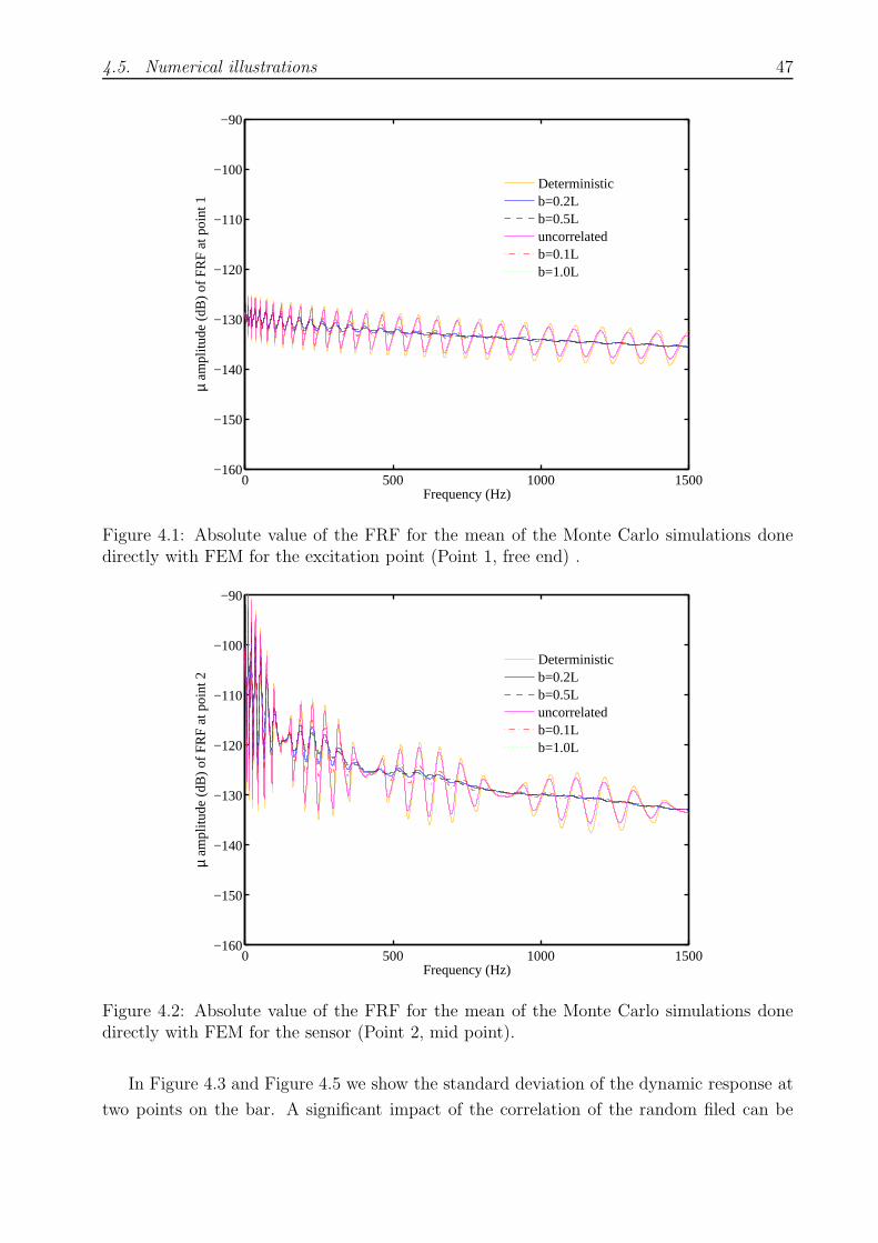
4.5. Numerical illustrations 47
0 500 1000 1500−160
−150
−140
−130
−120
−110
−100
−90
Frequency (Hz)
µ am
plitu
de (
dB)
of F
RF
at p
oint
1
Deterministicb=0.2Lb=0.5Luncorrelatedb=0.1Lb=1.0L
Figure 4.1: Absolute value of the FRF for the mean of the Monte Carlo simulations donedirectly with FEM for the excitation point (Point 1, free end) .
0 500 1000 1500−160
−150
−140
−130
−120
−110
−100
−90
Frequency (Hz)
µ am
plitu
de (
dB)
of F
RF
at p
oint
2
Deterministicb=0.2Lb=0.5Luncorrelatedb=0.1Lb=1.0L
Figure 4.2: Absolute value of the FRF for the mean of the Monte Carlo simulations donedirectly with FEM for the sensor (Point 2, mid point).
In Figure 4.3 and Figure 4.5 we show the standard deviation of the dynamic response at
two points on the bar. A significant impact of the correlation of the random filed can be

4.5. Numerical illustrations 48
observed on the dynamic response.
0 500 1000 1500−160
−150
−140
−130
−120
−110
−100
−90
Frequency (Hz)
σ am
plitu
de (
dB)
of F
RF
at p
oint
1
b=0.2Lb=0.5Luncorrelatedb=0.1Lb=1.0L
Figure 4.3: Absolute value of the FRF for the standard deviation of the Monte Carlo simu-lations done directly with FEM for the excitation point (Point 1, free end).
0 500 1000 1500−160
−150
−140
−130
−120
−110
−100
−90
Frequency (Hz)
σ am
plitu
de (
dB)
of F
RF
at p
oint
2
b=0.2Lb=0.5Luncorrelatedb=0.1Lb=1.0L
Figure 4.4: Absolute value of the FRF for the standard deviation of the Monte Carlo simu-lations done directly with FEM for the sensor (Point 2, mid point).

Chapter 5
Flexural vibration of thin plates withstochastic properties
5.1 Equation of motion
A thin plate of constant thickness h = 2b is subjected to distributed surface loads normal to
the middle surface. It is assumed that the direct stress in the transverse direction, σz is zero
and that normals to the middle surface of the undeformed plate remain straight and normal
to the middle surface during deformation. Displacements parallel to the undeformed middle
surface are given by:
u(x, y, z) = −z∂w
∂x(5.1)
v(x, y, z) = −z∂w
∂y(5.2)
Where w(x, y) is the displacement of the middle surface in the z direction. The strains are
given by:
εx =∂u
∂x= −z
∂2w
∂x2(5.3)
εy =∂v
∂y= −z
∂2w
∂y2(5.4)
γxy =∂u
∂y+
∂v
∂x= −2z
∂2w
∂x∂y(5.5)
(5.6)
γxz =∂u
∂z+
∂w
∂x= 0, γyz =
∂v
∂z+
∂w
∂y= 0 (5.7)
or, if χ are the pseudo-strains, equations (5.3) to (5.5) can be rewritten in a vectorial way
ε = −zχ. (5.8)
49
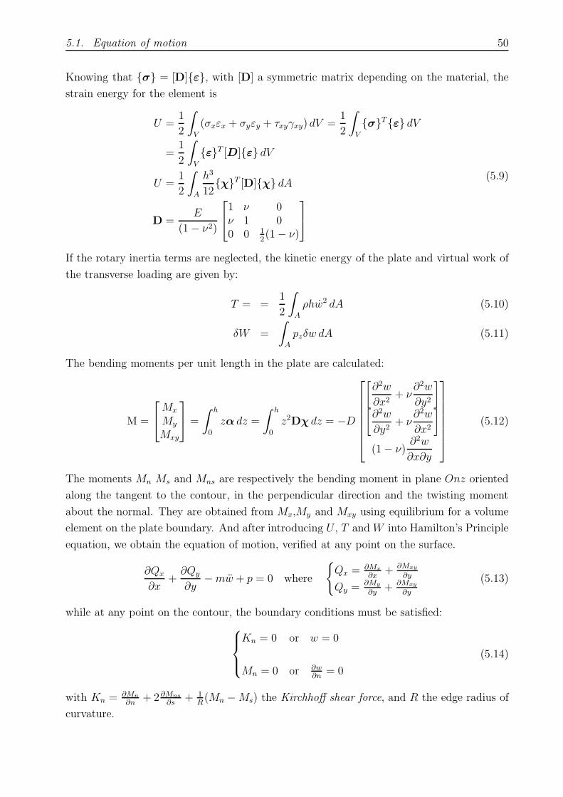
5.1. Equation of motion 50
Knowing that σ = [D]ε, with [D] a symmetric matrix depending on the material, the
strain energy for the element is
U =1
2
∫
V
(σxεx + σyεy + τxyγxy) dV =1
2
∫
V
σTε dV
=1
2
∫
V
εT [D]ε dV
U =1
2
∫
A
h3
12χT [D]χ dA
D =E
(1− ν2)
1 ν 0ν 1 00 0 1
2(1− ν)
(5.9)
If the rotary inertia terms are neglected, the kinetic energy of the plate and virtual work of
the transverse loading are given by:
T = =1
2
∫
A
ρhw2 dA (5.10)
δW =
∫
A
pzδw dA (5.11)
The bending moments per unit length in the plate are calculated:
M =
Mx
My
Mxy
=
∫ h
0
zα dz =
∫ h
0
z2Dχ dz = −D
[∂2w
∂x2+ ν
∂2w
∂y2
]
[∂2w
∂y2+ ν
∂2w
∂x2
]
(1− ν)∂2w
∂x∂y
(5.12)
The moments Mn Ms and Mns are respectively the bending moment in plane Onz oriented
along the tangent to the contour, in the perpendicular direction and the twisting moment
about the normal. They are obtained from Mx,My and Mxy using equilibrium for a volume
element on the plate boundary. And after introducing U , T and W into Hamilton’s Principle
equation, we obtain the equation of motion, verified at any point on the surface.
∂Qx
∂x+
∂Qy
∂y−mw + p = 0 where
Qx = ∂Mx
∂x+ ∂Mxy
∂y
Qy =∂My
∂y+ ∂Mxy
∂y
(5.13)
while at any point on the contour, the boundary conditions must be satisfied:
Kn = 0 or w = 0
Mn = 0 or ∂w∂n
= 0
(5.14)
with Kn = ∂Mn
∂n+ 2∂Mns
∂s+ 1
R(Mn −Ms) the Kirchhoff shear force, and R the edge radius of
curvature.

5.2. Deterministic Finite Element model 51
5.2 Deterministic Finite Element model
The measures of strain in plate bending analysis are the bending and twisting curvatures.
Any displacement field has to verify that a rigid-body motion is possible, in the plate,
this implies a translation in the z direction with w = constant and a rigid body rotation
about the x and y axis of the form w = constant.y and w = constant.x respectively. It also
verifies that a state of constant strain is possible, or, for a plate, a displacement with constant
second derivatives of w; and that the expression or deflection is smoothly continuous over the
element. Another condition to verify is that of the continuity of derivatives, at interelement
boundaries, of one order less that the highest-order derivative appearing in the potential
energy expression: here, continuity of ∂w/∂x and ∂w/∂y. Then, for a 12-degree of freedom
rectangular element, a deflection equation that verifies those conditions is
w =[1 x y x2 xy y2 x3 x2y xy2 y3 x3y xy3
]
A1
A2...
A12
(5.15)
Each one of the four nodes of the element has three degrees of freedom wi φi θi with φi =∂w∂y
the rotation about the x axis and θ = ∂w∂x
the one about y axis for node i. As for rod and
beam, it can be stated:
w = αA = αC−1d (5.16)
With
C−1 = 18a3b3
2a3b3 a3b4 a4b3 2a3b3 a3b4 −b3a4 2a3b3 −a3b4 −a4b3 2a3b3 −a3b4 a4b3
−3a2b3 −a2b4 −a3b3 3a2b3 a2b4 −a3b3 3a2b3 −a2b4 −a3b3 −3a2b3 a2b4 −a3b3
−3a3b2 −a3b3 −a4b2 −3a3b2 −a3b3 a4b2 3a3b2 −a3b3 −a4b2 3a3b2 −a3b3 a4b2
0 0 −a2b3 0 0 a2b3 0 0 a2b3 0 0 −a2b3
4a2b2 a2b3 a3b2 −4a2b2 −a2b3 a3b2 4a2b2 −a2b3 −a3b2 −4a2b2 a2b3 −a3b2
0 −a3b2 0 0 −a3b2 0 0 a3b2 0 0 a3b2 0
b3 0 ab3 −b3 0 ab3 −b3 0 ab3 b3 0 ab3
0 0 a2b2 0 0 −a2b2 0 0 a2b2 0 0 −a2b2
0 a2b2 0 0 −a2b2 0 0 a2b2 0 0 −a2b2 0
a3 a3b 0 a3 a3b 0 −a3 a3b 0 −a3 a3b 0−b2 0 −ab2 b2 0 −ab2 −b2 0 ab2 b2 0 ab2
−a2 −a2b 0 a2 a2b 0 −a2 a2b 0 a2 −a2b 0
As for rod and beam, a stiffness, mass and forcing vector can be obtained from the
expressions of strain and kinetic energy, and virtual work. The strain energy is:
Up =1
2
∫∫εtpEpεp dx dy =
1
2dtKd Ep = D
1 ν 0ν 1 00 0 1−ν
2
(5.17)
D =Eh3
12(1− ν2)(5.18)

5.2. Deterministic Finite Element model 52
with d the vector of displacements at each node and K the stiffness matrix.
Ke =
∫
Ae
BtpEpBp dAe = (C−1)t
(∫
Ae
βtpEpβp dAe
)C−1 =
h3E
12(1− ν2)C−tkeC
with:
β =
0 0 0 2 0 0 6x 2y 0 0 6x 00 0 0 0 0 2 0 0 2x 6y 0 6xy0 0 0 0 2 0 0 4x 4y 0 6x2 6y2
(5.19)
and
ke =
0
0 0
0 0 0
0 0 0 ke44
0 0 0 0 ke55
0 0 0 ke64 0 ke66 symmetric
0 0 0 0 0 0 ke77
0 0 0 0 0 0 0 ke88
0 0 0 0 0 0 ke97 0 ke99
0 0 0 0 0 0 0 ke10 8 0 ke10 10
0 0 0 0 ke11 5 0 0 0 0 0 ke11 11
0 0 0 0 ke12 5 0 0 0 0 0 ke12 11 ke12 12
(5.20)
with
ke44 = 16ab ke55 = 8ab(1− ν) ke64 = 16νab
ke66 = 16ab ke77 = 48a3b ke88 =16ab ((2− 2ν) a2 + b2)
3
ke97 = 16νa3b ke99 =16ab(a2 + 2(1− ν)b2)
3ke10 8 = 16νab2
ke10 10 = 48ab3 ke11 5 = 8 (1− ν) a3b ke11 11 = 4a3b(9(1− ν)a2
5+ 4b2)
ke12 5 = 8 (1− ν) ab3 ke12 11 = 8(ν + 1)a3b3 ke12 12 =8 ab3 (10a2 + 9(1− ν)b2)
5
The kinetic energy is:
Tp =1
2dt∫
ρhC−tαtαC dAe d =1
2dtMed
with d the vector of displacements at each node and Me the mass matrix of the element.
Me = C−t
∫ρhαtα dAeC = ρhC−tmeC (5.21)

5.3. Derivation of stiffness and mass matrices 53
with
me = 4ab
1 0 0 a2
30 b2
30 0 0 0 0 0
0 a2
30 0 0 0 a4
50 a2b2
90 0 0
0 0 b2
30 0 0 0 a2b2
90 b4
50 0
a2
30 0 a4
50 a2b2
90 0 0 0 0 0
0 0 0 0 a2b2
90 0 0 0 0 a4b2
15a2b4
15
b2
30 0 a2b2
90 b4
50 0 0 0 0 0
0 a4
50 0 0 0 a6
70 a4b2
150 0 0
0 0 a2b2
90 0 0 0 a4b2
150 a2b4
150 0
0 a2b2
90 0 0 0 a4b2
150 a2b4
150 0 0
0 0 b4
50 0 0 0 a2b4
150 b6
70 0
0 0 0 0 a4b2
150 0 0 0 0 a6b2
21a4b4
25
0 0 0 0 a2b4
150 0 0 0 0 a4b4
25a2b6
21
Now, the KL expansion of parameters appearing in deterministic mass and stiffness matri-
ces expressions allows the calculation of matrices used for the calculation of the dispersion
parameter.
5.3 Derivation of stiffness and mass matrices
As explained, assumptions are introduced (like Kirchhoff hypothesis) in order to convert
the equations of three-dimensional elasticity into a theoretical (but approximate) model of
plate behavior in which deformation throughout the plate is expressed solely in terms of the
middle surface deflection w. Classical plate behavior is characterized by the variable w: the
governing differential equations of equilibrium, when written in terms of displacements, are
now of fourth order. If the pseudo-strains are
χp = −∂2w/∂x2 ∂2w/∂y2 2∂2ω/∂x∂y
(5.22)
the strain energy is given by:
Up =1
2
∫∫χt
pEpχp dx dy =1
2dtKed (5.23)
with
Ke =
∫
Ae
BtpEpBpdAe = (C−1)t
(∫
Ae
βtpEpβpdAe
)C−1 = C−t ke C
−1 (5.24)
and d the vector of displacements at each node, Ke the stiffness matrix and D given by
(5.18). The kinetic energy is given by:
Tp =1
2dt∫
ρhC−tαtαC dAe d =1
2dtMed (5.25)

5.3. Derivation of stiffness and mass matrices 54
Me = C−t
∫ρhαtα dAeC = C−tmeC (5.26)
with d the vector of displacements at each node and Me the mass matrix of the element.
Variables D, appearing in the expression of Ep, and m = ρh are going to be expanded
with a KL expansion, assuming a correlation function
C(x1, x2; y1, y2) = e−|x1−x2|c1−|y1−y2|c2 (5.27)
Following the Kl expansion in subsection 1.1.4, we consider n1 number of terms in the x-
direction and n2 number if terms in the y- direction. Combining we have
D = D0 +
n1/2∑
i=1
n2/2∑
j=1
(ξijλijfij + ξi∗jλi∗jfi∗j + ξij∗λij∗fij∗ + ξi∗j∗λi∗j∗fi∗j∗) (5.28)
m = m0 +
n/12∑
i=1
n2/2∑
j=1
(ξijλijfij + ξi∗jλi∗jfi∗j + ξij∗λij∗fij∗ + ξi∗j∗λi∗j∗fi∗j∗) (5.29)
with
λij =4c1c2
(ω2ix + c1)(ω2
jy + c2)(5.30)
fij =cos(wix)√a+ sin(2ωia)
2ωi
cos(wjy)√b+
sin(2ωjb)
2ωj
(5.31)
λi∗j =4c1c2
(ω∗ 2ix + c1)(ω2
jy + c2)(5.32)
fi∗j =sin(w∗
i x)√a−
sin(2ω∗
i a)
2ω∗
i
cos(wjy)√b+
sin(2ωjb)
2ωj
(5.33)
λij∗ =4c1c2
(ω2ix + c1)(ω
∗ 2jy + c2)
(5.34)
fij∗ =cos(wix)√a+ sin(2ωia)
2ωi
sin(w∗jy)√
b−sin(2ω∗
j b)
2ω∗
j
(5.35)
λi∗j∗ =4c1c2
(ω∗ 2ix + c1)(ω∗ 2
jy + c2)(5.36)
fi∗j∗ =sin(w∗
i x)√a−
sin(2ω∗
i a)
2ω∗
i
sin(w∗jy)√
b−sin(2ω∗
j b)
2ω∗
j
(5.37)
For all those equations, coordinates x and y are given with respect to some global axes
placed in a corner of the plate. Those coordinates do not coincide with the coordinates of
each element of the FEM x and y, their relation with a given element coordinates is
x = xeo + x and y = yeo + y (5.38)

5.3. Derivation of stiffness and mass matrices 55
Where xeo and yeo are the global coordinates of the element origin of coordinates (situated at
the center of the element). Those values, integrated to form the stiffness and mass matrices
of the system, will give
ke = ke0+
n1/2∑
i=1
n2/2∑
j=1
(ξijλijkije + ξi∗jλi∗jk
i∗je + ξij∗λij∗k
ij∗
e + ξi∗j∗λi∗j∗ki∗j∗
e ) (5.39)
me = me0+
n1/2∑
i=1
n2/2∑
j=1
(ξijλijmije + ξi∗jλi∗jm
i∗je + ξij∗λij∗m
ij∗
e + ξi∗j∗λi∗j∗mi∗j∗
e ) (5.40)
with ke0 and me0 being the mean values of ke and me, that is, those matrices as they were
obtained in a deterministic system. Matrices kije ,k
i∗je ,kij∗
e ,ki∗j∗
e have a structure like k[ ]e and
mije ,m
i∗je ,mij∗
e ,mi∗j∗
e like m[ ]e . Each term of each matrix is an integral of the product of the
what was integrated for the deterministic case by the corresponding eigenfunction f :
k[ ]e =
0
0 0
0 0 0
0 0 0 ke44
0 0 0 0 ke55
0 0 0 ke64 0 ke66 symmetric
0 0 0 ke74 0 ke76 ke77
0 0 0 ke84 ke85 ke86 ke87 ke88
0 0 0 ke94 ke95 ke96 ke97 ke98 ke99
0 0 0 ke10 4 0 ke10 6 ke10 7 ke10 8 ke10 9 ke10 10
0 0 0 ke11 4 ke11 5 ke11 6 ke11 7 ke11 8 ke11 9 ke11 10 ke11 11
0 0 0 ke12 4 ke12 5 ke12 6 ke12 7 ke12 8 ke12 9 ke12 10 ke12 11 ke12 12
Matrix m[ ]e is fully populated and symmetric, each of its element is denoted by meij with
i, j = 1, . . . , 12.
All those integrals Ieij are the result of the product of a function of x by a function of
y (Ieij = f(x) g(y)). Those two functions f(x) and g(y) are a linear combinations of other
integrals In with same shape for both x and y, so
f(x) =∑
n
κxnIn(z = x) and g(y) =
∑
n
κynIn(z = y) (5.41)
Where κ[ ] are constants obtained from the eigenvectors, eigenfunctions and shape functions
and In(z) is such that
In(z) =
∫zm cos(w z + a) dz (5.42)

5.4. Numerical illustrations 56
or
In(z) =
∫zm sin(w z + a) dz with m = 1, ..., 6 (5.43)
The constant w is wi, w∗i , wj or w
∗j and a is a constant equal to the product a = wzeo (zeo can
be xeo for z = x or yeo for z = y). A more detailed description on the derivation of the terms
of mass and stiffness matrices are given in Appendix A.
5.4 Numerical illustrations
The example model’s boundary conditions are the ones of a clamped on one edge plate: zero
vertical displacement and rotation along both edges at positions that verify x = 0, that is, one
of the narrow edges of the plate. Heuristically, it is considered that this boundary condition
is the one that will more likely cause a bigger variance in the response vector than the one
obtained with other typical boundary conditions like displacement equal to zero everywhere
on the contour (boundary condition where an analytical solution is available). Material
properties are taken as ρ = 7860 kg/m3, E = 200GPa and ν = 0.3, values corresponding to
steel. Geometrical variables are: length and width of the plate L = 0.998m, W = 0.59m
and thickness t = 3.0mm. The variance of the parameters considered as random is 10% the
value of the parameter: σβ = 0.1 β. The parameters considered are β = D = Et3/(12(1−ν2))
for stiffness matrix and β = ρt for mass matrix. The system response is calculated using
equation (1.62): equation for a viscously damped proportional model where damping factor
is ζj = 0.02. The structure has its length divided into 25 elements (x direction) and its
width divided into 15 elements: so, the model has 375 elements. No analytical solution
is available for these boundary conditions, so, it is not possible to compare the natural
frequencies obtained from the numerical calculations with an analytical expression as it was
done for rod and beam.
The maximum frequency for which the structure is going to be tested is 4.0KHz. Mea-
sure of the response vector is given for the forcing point, situated at the 180-th node, that
is, coordinates x = 4 and y = 6, and at a sensor situated at the 307-th node (coordinates
x = 7 and y = 11).
The same four different normalized correlation lengths as the ones used in the rod and
beam cases are selected to research the effect of this value on the response statistics. We
recall that the non-normalized correlation lengths are 0.1 d, 0.2 d, 0.5 d and d, where d is
the plate dimension considered (width or length) As it has been said in the description of
KL expansion for the plate case, each direction can have a different associated correlation
length. Here the normalized correlation length linked to each direction, is, for each Monte
Carlo Simulation: 0.1, 0.2, 0.5 and 1. The uncorrelated random variables case is also studied.
The number of terms in each KL expansion is chosen such that the ratio between the square
roots of the first term and last term eigenvalues is less than 0.05, verifying also that the KL
expansion in both directions has the same number of terms. Now, each eigenvalue is going to

5.4. Numerical illustrations 57
be the product of two eigenvalues, each one coming from one different 1D KL expansion. So,
the last eigenvalue is the product of the two last eigenvalues of each 1D KL expansion, and
so, the first eigenvalue is the product of the two first eigenvalues of each 1D KL expansion. In
other words, The terms of each 1D KL expansion is given in Table 5.1 When simulating the
Correlation length/d 0.1 0.2 0.5 1Terms of KL expansion 16 9 6 6
Table 5.1: Number of terms used in KL expansion for each normalized correlation length
system matrices, Wishart matrices are fitted following criteria 3 in section 2.3. The number
of samples for Monte Carlo simulations are 1000 both for the FE model and Random Matrix
direct Monte Carlo simulation. Each sample of the direct Monte Carlo simulation of FEM
is done as a deterministic case where the variables are correlated following the correlation
function already described in KL expansion.
In Figure 5.1 and Figure 5.2 we show the mean of the dynamic response at two points
on the bar. From these figures it is observed that the mean of the absolute value of the
response does not coincide with the response of the deterministic system with mean values
of stochastic parameters. Also, the larger is the correlation length, the more different are
the mean responses from the deterministic response. This observation can be done for both
sensors where the system response is collected. The larger the correlation length is, the more
”damped” are the mean of the responses at high natural frequencies.
In Figure 5.3 and Figure 5.4 we show the standard deviation of the dynamic response
at two points on the bar. It is noticed that the impact of correlation of variables in the
system response variance for direct Monte Carlo simulations of FEM is not as big as the one
observed for rod and beam models.

5.4. Numerical illustrations 58
0 500 1000 1500 2000 2500 3000 3500 4000−180
−170
−160
−150
−140
−130
−120
−110
−100
−90
Frequency (Hz)
µ am
plitu
de (
dB)
of F
RF
at p
oint
1
Deterministicb=0.2Lb=0.5Luncorrelatedb=0.1Lb=1.0L
Figure 5.1: Absolute value of the FRF for the mean of the Monte Carlo simulations donedirectly with FEM for the excitation point (Point 1) .
0 500 1000 1500 2000 2500 3000 3500 4000−180
−170
−160
−150
−140
−130
−120
−110
−100
−90
Frequency (Hz)
µ am
plitu
de (
dB)
of F
RF
at p
oint
2
Deterministicb=0.2Lb=0.5Luncorrelatedb=0.1Lb=1.0L
Figure 5.2: Absolute value of the FRF for the mean of the Monte Carlo simulations donedirectly with FEM for the excitation point (Point 1) and the sensor (Point 2).

5.4. Numerical illustrations 59
0 500 1000 1500 2000 2500 3000 3500 4000−180
−170
−160
−150
−140
−130
−120
−110
−100
−90
Frequency (Hz)
σ am
plitu
de (
dB)
of F
RF
at p
oint
1
b=0.2Lb=0.5Luncorrelatedb=0.1Lb=1.0L
Figure 5.3: Absolute value of the FRF for the standard deviation of the Monte Carlo simu-lations done directly with FEM for the excitation point (Point 1).
0 500 1000 1500 2000 2500 3000 3500 4000−180
−170
−160
−150
−140
−130
−120
−110
−100
−90
Frequency (Hz)
σ am
plitu
de (
dB)
of F
RF
at p
oint
2
b=0.2Lb=0.5Luncorrelatedb=0.1Lb=1.0L
Figure 5.4: Absolute value of the FRF for the standard deviation of the Monte Carlo simu-lations done directly with FEM for the sensor (Point 2).

Appendix A
The elements of the stochastic massand stiffness matrices of a plate
In Chapter 4 was explained how to derive the stiffness and mass matrices, for a plate, using
Karhunen-Loeve expansion. Each of the elements of those matrices for each eigenfunction
f , are:
ke44 =
∫ a
−a
∫ b
−b
4 f dx dy ke55 =
∫ a
−a
∫ b
−b
(2− 2ν) f dx dy
ke64 =
∫ a
−a
∫ b
−b
4ν f dx dy ke66 =
∫ a
−a
∫ b
−b
4 f dx dy
ke74 =
∫ a
−a
∫ b
−b
12x f dx dy ke76 =
∫ a
−a
∫ b
−b
12xν f dx dy
ke77 =
∫ a
−a
∫ b
−b
36x2 f dx dy ke84 =
∫ a
−a
∫ b
−b
4y f dx dy
ke85 =
∫ a
−a
∫ b
−b
4x(1− ν) f dx dy ke86 =
∫ a
−a
∫ b
−b
4yν f dx dy
ke87 =
∫ a
−a
∫ b
−b
12xy f dx dy ke88 =
∫ a
−a
∫ b
−b
(4y2 + 8x2(1− ν)) f dx dy
ke94 =
∫ a
−a
∫ b
−b
4xν f dx dy ke95 =
∫ a
−a
∫ b
−b
4y(1− ν) f dx dy
ke96 =
∫ a
−a
∫ b
−b
4x f dx dy ke97 =
∫ a
−a
∫ b
−b
12x2ν f dx dy
ke98 =
∫ a
−a
∫ b
−b
4xy(2− ν) f dx dy ke99 =
∫ a
−a
∫ b
−b
4(x2 + 2y2(1− ν) f dx dy
ke10 4 =
∫ a
−a
∫ b
−b
12yν f dx dy ke10 6 =
∫ a
−a
∫ b
−b
12y f dx dy
ke10 7 =
∫ a
−a
∫ b
−b
36xyν f dx dy ke10 8 =
∫ a
−a
∫ b
−b
12y2ν f dx dy
ke10 9 =
∫ a
−a
∫ b
−b
12xy f dx dy ke10 10 =
∫ a
−a
∫ b
−b
36y2 f dx dy
60

61
ke11 4 =
∫ a
−a
∫ b
−b
12xy f dx dy ke11 5 =
∫ a
−a
∫ b
−b
6x2(1− ν) f dx dy
ke11 6 =
∫ a
−a
∫ b
−b
12xyν f dx dy ke11 7 =
∫ a
−a
∫ b
−b
36x2y f dx dy
ke11 8 =
∫ a
−a
∫ b
−b
12x(y2 + x2(1− ν)) f dx dy ke11 9 =
∫ a
−a
∫ b
−b
12x2y f dx dy f dx dy
ke11 10 =
∫ a
−a
∫ b
−b
36xy2ν f dx dy ke11 11 =
∫ a
−a
∫ b
−b
18x2(2y2 + x2(1− ν)) f dx dy
ke12 4 =
∫ a
−a
∫ b
−b
12xyν f dx dy ke12 5 =
∫ a
−a
∫ b
−b
6y2(1− ν) f dx dy
ke12 6 =
∫ a
−a
∫ b
−b
12xy f dx dy ke12 7 =
∫ a
−a
∫ b
−b
36x2yν f dx dy
ke12 8 =
∫ a
−a
∫ b
−b
12xy2 f dx dy ke12 9 =
∫ a
−a
∫ b
−b
12y(x2 + y2(1− ν)) f dx dy
ke12 10 =
∫ a
−a
∫ b
−b
36xy2 f dx dy ke12 11 =
∫ a
−a
∫ b
−b
18x2y2(1 + ν) f dx dy
ke12 12 =
∫ a
−a
∫ b
−b
18y2(2x2 + y2(1− ν)) f dx dy
me11 =
∫ a
−a
∫ b
−b
f dx dy me21 =
∫ a
−a
∫ b
−b
x f dx dy me22 =
∫ a
−a
∫ b
−b
x2 f dx dy
me31 =
∫ a
−a
∫ b
−b
y f dx dy me32 =
∫ a
−a
∫ b
−b
xy f dx dy me33 =
∫ a
−a
∫ b
−b
y2 f dx dy
me41 =
∫ a
−a
∫ b
−b
x2 f dx dy me42 =
∫ a
−a
∫ b
−b
x3 f dx dy me43 =
∫ a
−a
∫ b
−b
x2y f dx dy
me44 =
∫ a
−a
∫ b
−b
x4 f dx dy me51 =
∫ a
−a
∫ b
−b
xyf dx dy me52 =
∫ a
−a
∫ b
−b
x2yf dx dy
me53 =
∫ a
−a
∫ b
−b
xy2f dx dy me54 =
∫ a
−a
∫ b
−b
x3yf dx dy me55 =
∫ a
−a
∫ b
−b
x2y2f dx dy
me61 =
∫ a
−a
∫ b
−b
y2f dx dy me62 =
∫ a
−a
∫ b
−b
xy2f dx dy me63 =
∫ a
−a
∫ b
−b
y3f dx dy
me64 =
∫ a
−a
∫ b
−b
x2y2f dx dy me65 =
∫ a
−a
∫ b
−b
xy3f dx dy me66 =
∫ a
−a
∫ b
−b
y4f dx dy
me71 =
∫ a
−a
∫ b
−b
x3f dx dy me72 =
∫ a
−a
∫ b
−b
x4f dx dy me73 =
∫ a
−a
∫ b
−b
x3yf dx dy
me74 =
∫ a
−a
∫ b
−b
x5f dx dy me75 =
∫ a
−a
∫ b
−b
x4yf dx dy me76 =
∫ a
−a
∫ b
−b
x3y2f dx dy
me77 =
∫ a
−a
∫ b
−b
x6f dx dy me81 =
∫ a
−a
∫ b
−b
x2yf dx dy me82 =
∫ a
−a
∫ b
−b
x3yf dx dy

62
me83 =
∫ a
−a
∫ b
−b
x2y2f dx dy me84 =
∫ a
−a
∫ b
−b
x4yf dx dy me85 =
∫ a
−a
∫ b
−b
x3y2f dx dy
me86 =
∫ a
−a
∫ b
−b
x2y3f dx dy me87 =
∫ a
−a
∫ b
−b
x5yf dx dy me88 =
∫ a
−a
∫ b
−b
x4y2f dx dy
me91 =
∫ a
−a
∫ b
−b
xy2f dx dy me92 =
∫ a
−a
∫ b
−b
x2y2f dx dy me93 =
∫ a
−a
∫ b
−b
xy3f dx dy
me94 =
∫ a
−a
∫ b
−b
x3y2f dx dy me95 =
∫ a
−a
∫ b
−b
x2y3f dx dy me96 =
∫ a
−a
∫ b
−b
y4xf dx dy
me97 =
∫ a
−a
∫ b
−b
x4y2f dx dy me98 =
∫ a
−a
∫ b
−b
x3y3f dx dy me99 =
∫ a
−a
∫ b
−b
x2y4f dx dy
me10 1 =
∫ a
−a
∫ b
−b
y3f dx dy me10 2 =
∫ a
−a
∫ b
−b
xy3f dx dy me10 3 =
∫ a
−a
∫ b
−b
y4f dx dy
me10 4 =
∫ a
−a
∫ b
−b
x2y3f dx dy me10 5 =
∫ a
−a
∫ b
−b
y4xf dx dy me10 6 =
∫ a
−a
∫ b
−b
y5f dx dy
me10 7 =
∫ a
−a
∫ b
−b
x3y3f dx dy me10 8 =
∫ a
−a
∫ b
−b
x2y4f dx dy me10 9 =
∫ a
−a
∫ b
−b
y5xf dx dy
me10 10 =
∫ a
−a
∫ b
−b
y6f dx dy me11 1 =
∫ a
−a
∫ b
−b
x3yf dx dy me11 2 =
∫ a
−a
∫ b
−b
x4yf dx dy
me11 3 =
∫ a
−a
∫ b
−b
x3y2f dx dy me11 4 =
∫ a
−a
∫ b
−b
x5yf dx dy me11 5 =
∫ a
−a
∫ b
−b
x4y2f dx dy
me11 6 =
∫ a
−a
∫ b
−b
x3y3f dx dy me11 7 =
∫ a
−a
∫ b
−b
x6yf dx dy me11 8 =
∫ a
−a
∫ b
−b
x5y2f dx dy
me11 9 =
∫ a
−a
∫ b
−b
x4y3f dx dy me11 10 =
∫ a
−a
∫ b
−b
x3y4f dx dy me11 11 =
∫ a
−a
∫ b
−b
x6y2f dx dy
me12 1 =
∫ a
−a
∫ b
−b
xy3f dx dy me12 2 =
∫ a
−a
∫ b
−b
x2y3f dx dy me12 3 =
∫ a
−a
∫ b
−b
y4xf dx dy
me12 4 =
∫ a
−a
∫ b
−b
x3y3f dx dy me12 5 =
∫ a
−a
∫ b
−b
x2y4f dx dy me12 6 =
∫ a
−a
∫ b
−b
y5xf dx dy
me12 7 =
∫ a
−a
∫ b
−b
x4y3f dx dy me12 8 =
∫ a
−a
∫ b
−b
x3y4f dx dy me12 9 =
∫ a
−a
∫ b
−b
x2y5f dx dy
me12 10 =
∫ a
−a
∫ b
−b
y6xf dx dy me12 11 =
∫ a
−a
∫ b
−b
x4y4f dx dy me12 12 =
∫ a
−a
∫ b
−b
x2y6f dx dy

Bibliography
Adhikari, S. (2000), Damping Models for Structural Vibration, Ph.D. thesis, Cambridge
University Engineering Department, Cambridge, UK.
Adhikari, S. (2006), “Random eigenvalue problems revisited”, Sadhana - Proceedings of the
Indian Academy of Engineering Sciences , 31 (4), pp. 293–314, (Special Issue on Proba-
bilistic Structural Dynamics and Earthquake Engineering).
Adhikari, S. (2007a), “Joint statistics of natural frequencies of stochastic dynamic systems”,
Computational Mechanics , 40 (4), pp. 739–752.
Adhikari, S. (2007b), “Matrix variate distributions for probabilistic structural mechanics”,
AIAA Journal , 45 (7), pp. 1748–1762.
Adhikari, S. (2008), “Wishart random matrices in probabilistic structural mechanics”, ASCE
Journal of Engineering Mechanics , accepted for publication.
Adhikari, S. and Friswell, M. I. (2007), “Random matrix eigenvalue problems in structural
dynamics”, International Journal for Numerical Methods in Engineering , 69 (3), pp. 562–
591.
Baldeweck, H. (1999), Methodes de elements finis stochastiques - applications a la
geotechnique et a la mecanique de la rupture, Ph.D. thesis, Universite d’ Evry-Val d’
Essonne, France.
Benaroya, H. (1992), “Random eigenvalues, algebraic methods and structural dynamic mod-
els”, Applied Mathematics and Computation, 52, pp. 37–66.
Benaroya, H. and Rehak, M. (1988), “Finite element methods in probabilistic structural
analysis: a selective review”, Applied Mechanics Reviews, ASME , 41 (5), pp. 201–213.
Benjamin, J. R. and Cornell, C. A. (1970), Probability, statistics and decision for civil engi-
neers , McGraw-Hill, New York.
Bertelsen, P., Ellegaard, C., and Hugues, E. (2000), “Distribution of eigenfrequencies for
vibrating plates”, European Physical Journal B , 15, p. 8796.
63

Bibliography 64
Bliven, D. O. and Soong, T. T. (1969), “On frequencies of elastic beams with random
imperfections”, Journal of Franklin Institute, 287, pp. 297–304.
Boyce, W. E. (1962), “Random vibrations of elastic strings and bars”, Proceedings of the
4th US national congress of applied mechanics, Berkeley CA, (pp. 77–85).
Boyce, W. E. (1966), “Stochastic nonhomogeneous strum-liouville problem”, Journal of
Franklin Institute, 282, pp. 205–215.
Boyce, W. E. (1968), Random Eigenvalue Problems , Probabilistic methods in applied math-
ematics, Academic Press, New York, a. T. Bharucha-Reid (editor).
Boyce, W. E. and Goodwin, B. E. (1964), “Random transverse vibration of elastic beams”,
Society for Industrial and Applied Mathematics Journal , 12, pp. 613–629.
Bucher, C. G. and Brenner, C. E. (1992), “Stochastic response of uncertain systems”, Archive
of Applied Mechanics , 62, pp. 507–516.
Collins, J. D. and Thomson, W. T. (1969), “The eigenvalue problem for structural systems
with statistical properties”, AIAA Journal , 7 (4), pp. 642–648.
Dawe, D. (1984), Matrix and Finite Element Displacement Analysis of Structures , Oxford
University Press, Oxford.
Deodatis, G. (1990), “Bounds on response variability of stochastic finite element systems”,
Journal of Engineering Mechanics, ASCE , 116 (3), pp. 565–585.
Deodatis, G. (1991), “Weighted integral method i: stochastic stiffness”, Journal of Engi-
neering Mechanics, ASCE , 117 (8), pp. 1851–1864.
Der-Kiureghian, A. and Ke, J. B. (1987), “The stochastic finite element in structural relia-
bility”, Journal of Engineering Mechanics, ASCE , 3 (2), pp. 83–91.
Ditlevsen, O. and Madsen, H. O. (1996), Structural Reliability Methods , John Wiley and
Sons Ltd, Chichester, West Sussex, England.
Ellegaard, C., Schaat, K., and Bertelsen, P. (2001), “Acoustic chaos”, Physica Scripta, 90,
p. 223230.
Fahy, F. J. (1994), “Statistical energy analysis : a critical overview”, Philosophical Transac-
tions of Royal Society of London, A346, pp. 431–447.
Fox, R. L. and Kapoor, M. P. (1968), “Rates of change of eigenvectors and eigenvalues”,
AIAA Journal , 6, pp. 2426–2429.
Bibliography 65
Ganesan, R. (1996), “Probabilistic analysis of non-self-adjoint mechanical systems with un-
certain parameters”, International Journal of Solids and Structures , 33 (5), pp. 675–688.
Geradin, M. and Rixen, D. (1997), Mechanical Vibrations , John Wiley & Sons, New York,
NY, second edition, translation of: Theorie des Vibrations.
Ghanem, R. and Spanos, P. D. (1991), Stochastic Finite Elements: A Spectral Approach,
Springer-Verlag, New York, USA.
Goodwin, B. E. and Boyce, W. E. (1964), “Vibration of random elastic strings: Method of
integral equations”, Qart of Appl. math., 22, pp. 261–266.
Grigoriu, M. (1992), “A solution of random eigenvalue problem by crossing theory”, Journal
of Sound and Vibration, 158 (1), pp. 69–80.
Gupta, A. and Nagar, D. (2000), Matrix Variate Distributions , Monographs & Surveys in
Pure & Applied Mathematics, Chapman & Hall/CRC, London.
Haines, C. W. (1967), “Hierarchy methods for random vibration of elastic beams and
strings”, Journal of Engineering Mathematics , 1, pp. 273–305.
Hodges, C. H. and Woodhouse, J. (1986), “Theories of noise and vibration transmission in
complex structures”, Reports on Progress in Physics , 49, pp. 107–170.
Hopf, E. (1952), “Statistical hydrodynamics and functional calculus”, Journal of Rational
Mechanics and Analysis , 1, pp. 87–123.
Hoshiya, M. and Shah, H. C. (1971), “Free vibration of stochastic beam-column”, Journal
of Engineering Mechanics, ASCE , 97 (4), pp. 1239–1255.
Hynna, P., Klinge, P., and Vuoksinen, J. (1995), “Prediction of structure-borne sound trans-
mission in large welded ship structures using statistical energy analysis”, Journal of Sound
and Vibration, 180 (4), pp. 583–607.
Ibrahim, R. A. (1987), “Structural dynamics with parameter uncertainties”, Applied Me-
chanics Reviews, ASME , 40 (3), pp. 309–328.
Ito, K. (1951), “On stochastic differential equations”, Memoirs of the American Mathemat-
ical Society , 4, pp. 1–51.
Iyengar, R. N. and Manohar, C. S. (1989), “Probability distribution function of the eigenval-
ues of random string equation”, Journal of Applied Mechanics, ASME , 56, pp. 202–207.
Karhunen, K. (1947), “ber lineare methoden in der wahrscheinlichkeitsrechnung”, Annales
Academiae Scientiarum Fennicae, Ser. A137.

Bibliography 66
Keane, A. J. (1992), “Energy flows between arbitrary congurations of conservatively coupled
multimodal elastic subsystems”, in “Proceedings of Royal Society of London”, London,
UK, volume A346, (pp. 537–568).
Keane, A. J. and Price, W. G. (1997), Statistical Energy Analysis: An Overview With Ap-
plications in Structural Dynamics , Cambridge University Press, Cambridge, UK, first
published in Philosophical Transactions of the Royal Society of London, series A, vol 346,
pp. 429-554, 1994.
Keese, A. (2003), “A review of recent developments in the numerical solution of stochastic
pdes (stochastic finite elements)”, Technical Report Informatikbericht 2003-6 , Institute of
Scientific Computing, Department of Mathematics and Computer Science, Technische Uni-
versitat Braunschweig, Brunswick,, uRL: http://opus.tu-bs.de/opus/volltexte/2003/504/.
Lai, M. L. and Soong, T. T. (1990), “Statistical energy analysis of primary- secondary
structural systems”, Journal of Engineering Mechanics, ASCE , 116 (11), pp. 2400–2413.
Lancaster, P. (1966), Lambda-matrices and Vibrating System, Pergamon Press, London.
Langley, R. S. (1989), “A general derivation of the statistical energy analysis equations for
coupled dynamic-systems”, Journal of Sound and Vibration, 135 (3), pp. 499–508.
Langley, R. S. and Brown, A. W. M. (2004), “The ensemble statistics of the energy of a
random system subjected to harmonic excitation”, Journal of Sound and Vibration, 275,
pp. 823–846.
Lee, L. C. (1974), “Wave propagation in a random medium: a complete set of the moment
equations with different wavenumbers”, Journal of Mathematical Physics , 15 (9).
Li, C. C. and Kiureghian, A. D. (1993a), “Optimal discretization of random fields”, Journal
of Engineering Mechanics, ASCE , 119 (6), pp. 1136–1154.
Li, C. C. and Kiureghian, A. D. (1993b), “Optimal discretization of random fields”, Journal
of Engineering Mechanics, ASCE , 119 (6), pp. 1136–1154.
Liaw, D. G. and Yang, H. Y. T. (1993), “Reliability and nonlinear supersonic flutter of
uncertain laminated plates”, AIAA Journal , 31 (12), pp. 2304–2311.
Lin, Y. K. (1967), Probabilistic Theory of Structural Dynamics , McGraw-Hill Inc, NY, USA.
Lin, Y. K., Kozin, F., Wen, Y. K., Casciati, F., Schueller, G. I., Kiureghian, A. D., Ditlevsen,
O., and Vanmarcke, E. H. (1986), “Methods of stochastic structural dynamics”, Structural
Safety , 3, pp. 167–194.
Linde, R. H. V. D. (1969), “Eigenfunctions of random eigenvalue problems and their statis-
tical properties”, SIAM Journal of Applied Mathematics , 17 (6), pp. 1298–1304.

Bibliography 67
Liu, W. K., Belytschko, T., and Mani, A. (1986a), “Probabilistic finite element for nonlin-
ear structural dynamics”, Computer Methods in Applied Mechanics and Engineering , 56,
pp. 61–86.
Liu, W. K., Belytschko, T., and Mani, A. (1986b), “Random field finite elements”, Interna-
tional Journal for Numerical Methods in Engineering , 23, pp. 1831–1845.
Loeve, M. (1948), Fonctions aleatoires du second ordre. Supplement to P. Levy, Processus
Stochastic et Mouvement Brownien, Gauthier Villars, Paris.
Lyon, R. H. and Dejong, R. G. (1995), Theory and Application of Statistical Energy Analysis ,
Butterworth-Heinmann, Boston, second edition.
Manohar, C. S. and Iyengar, R. N. (1993), “Probability distribution of the eigenvalues of
systems governed by stochastic wave equation”, Probabilistic Engineering Mechanics , 8,
pp. 57–64.
Manohar, C. S. and Iyengar, R. N. (1994), “Free vibration analysis of stochastic strings”,
Journal of Sound and Vibration, 176 (1), pp. 35–48.
Manohar, C. S. and Keane, A. J. (1993), “Axial vibrations of a stochastic rods”, Journal of
Sound and Vibration, 165 (2), pp. 341–359.
Matthies, H. G., Brenner, C. E., Bucher, C. G., and Soares, C. G. (1997), “Uncertainties
in probabilistic numerical analysis of structures and solids - stochastic finite elements”,
Structural Safety , 19 (3), pp. 283–336.
Mehta, M. L. (1991), Random Matrices , Academic Press, San Diego, CA, second edition.
Muirhead, R. J. (1982), Aspects of Multivariate Statistical Theory , John Wiley and Sons,
New York, USA.
Papoulis, A. and Pillai, S. U. (2002), Probability, Random Variables and Stochastic Processes ,
McGraw-Hill, Boston, USA, fourth edition.
Petyt, M. (1998), Introduction to Finite Element Vibration Analysis , Cambridge University
Press, Cambridge, UK.
Price, W. G. and Keane, A. J. (1994), “Statistical energy analysis”, Philosophical Transac-
tions of Royal Society of London, 346 (1), pp. 429–552.
Ramu, S. A. and Ganesan, R. (1992), “Stability analysis of a stochastic column subjected
to stochastically distributed loadings using the finite element method”, Finite Elements
in Analysis and Design, 11, pp. 105–115.

Bibliography 68
Ramu, S. A. and Ganesan, R. (1993a), “A galerkin finite element technique for stochastic
field problems”, Computer Methods in Applied Mechanics and Engineering , 105, pp. 315–
331.
Ramu, S. A. and Ganesan, R. (1993b), “Parametric instability of stochastic columns”, In-
ternational Journal of Solids and Structures , 30 (10), pp. 1339–1354.
Ramu, S. A. and Ganesan, R. (1993c), “Stability of stochastic leipholz column with stochastic
loading”, Archive of Applied Mechanics , 62, pp. 363–375.
Ramu, S. A. and Ganesan, R. (1994), “An efficient finite element technique for stochastic field
problems”, International Journal for Engineering Analysis and Design, 1, pp. 141–160.
Sankar, T. S., Ramu, S. A., and Ganesan, R. (1993), “Stochastic finite element analysis for
high speed rotors”, Journal of Vibration and Accoustic, ASME , 115, pp. 59–64.
Scheidt, J. V. and Purkert, W. (1983), Random Eigenvalue Problems , North Holland, New
York.
Schiff, A. J. and Bogdanoff, J. L. (1972a), “An estimator for the standard deviation of a
natural frequency - part 1”, Journal of Applied Mechanics, ASME , 39, pp. 535–538.
Schiff, A. J. and Bogdanoff, J. L. (1972b), “An estimator for the standard deviation of a
natural frequency - part 2s”, Journal of Applied Mechanics, ASME , 39, pp. 539–544.
Shinozuka, M. and Deodatis, G. (1991), “Simulation of stochastic processes by spectral
representation”, Applied Mechanics Reviews, ASME , 44 (3), pp. 499–519.
Shinozuka, M. and Nomoto, T. (1980), “Response variability due to spatial randomness of
material properties”, Technical Report, Dept. of Civil Engineering, Columnbia University,
New York .
Soize, C. (2000), “A nonparametric model of random uncertainties for reduced matrix models
in structural dynamics”, Probabilistic Engineering Mechanics , 15 (3), pp. 277–294.
Soize, C. (2001), “Maximum entropy approach for modeling random uncertainties in tran-
sient elastodynamics”, Journal of the Acoustical Society of America, 109 (5), pp. 1979–
1996, part 1.
Soize, C. (2003), “Random matrix theory and non-parametric model of random uncertainties
in vibration analysis”, Journal of Sound and Vibration, 263 (4), pp. 893–916.
Song, D., Chen, S., and Qiu, Z. (1995), “Stochastic sensitivity analysis of eigenvalues and
eigenvectors”, Computer and Structures , 54 (5), pp. 891–896.

Bibliography 69
Sudret, B. and Der-Kiureghian, A. (2000), “Stochastic finite element methods and relia-
bility”, Technical Report UCB/SEMM-2000/08 , Department of Civil & Environmental
Engineering, University Of California, Berkeley.
Vanmarcke, E. and Grigoriu, M. (1983), “Stochastic finite element analysis of simple beams”,
Journal of Engineering Mechanics, ASCE , 109 (5), pp. 1203–1214.
Vanmarcke, E. H. (1983), Random fields , MIT press, Cambridge Mass.
Vigneron, F. R. (1986), “A natural modes model and modal identities for damped linear
structures”, Transactions of ASME, Journal of Applied Mechanics , 53, pp. 33–38.
Wagenknecht, T., Green, K., Adhikari, S., and Michiels, W. (2005), “Structured pseudospec-
tra and random eigenvalues problems in vibrating systems”, AIAA Journal , 44 (10),
pp. 2404–2414.
Weaver, R. L. (1989), “Spectral statistics in elastodynamics”, Journal of the Acoustical
Society of America, 85, p. 10051013.
Yang, T. Y. and Kapania, R. K. (1984), “Finite element random response analysis of cooling
tower”, Journal of Engineering Mechanics, ASCE , 110 (EM4), pp. 589–609.
Zhang, J. and Ellingwood, B. (1993), “Orthogonal series expansion of random fields in
reliability analysis”, Journal of Engineering Mechanics , 120 (12), pp. 2660–2677.
Zhang, J. and Ellingwood, B. (1995), “Effects of uncertain material properties on structural
stability”, Journal of structural engineering, ASCE , 121 (4), pp. 705–716.
Zhang, Z. and Chen, S. (1991), “The standard deviation of the eigensolutions for random
mdof systems”, Computer and Structures , 39 (6), pp. 603–607.
Zhu, W. Q., Ren, Y. J., and Wu, W. Q. (1992), “Stochastic fem based on local averages of
random vector fields”, Journal of Engineering Mechanics, ASCE , 118 (3), pp. 496–511.