Introduction to the interpretation of ZO-data within REFLEXW · time zero has been zet to the first...

Introduction to the interpretation of ZO-data within REFLEXW

In the following the different interpretation tools for Zero offset data (GPR, seismic reflection,

acoustic) are presented. Chapter I describes the different possibilities of analysing velocities, in

chapter II the picking of reflectors or individual elements is discussed.

I. Velocity analysis

I.1 interactive velocity analysis

The interactive velocity analysis within the 2D-Dataanalysis allows the interactive adaptation of

diffraction or reflexion hyperbola by calculated hyperbola of defined velocity and width. There is

also the possibility of fitting linear features either by interactively changing a line or by setting two

points. The speed button core allows to interactively vary the velocities of the single layers of the

individual cores. The velocities may be stored on file and may be reloaded at any time. The

velocities are combined into a 2D-model by using a special interpolation (see also option x-weight).

Such a 2D-velocity distribution may be used in a subsequent step for the migration or the depth

conversion.

Click on image in order to view an animation concerning the use of the interactive velocity analysis

Sandmeier geophysical research - REFLEXW guide 1

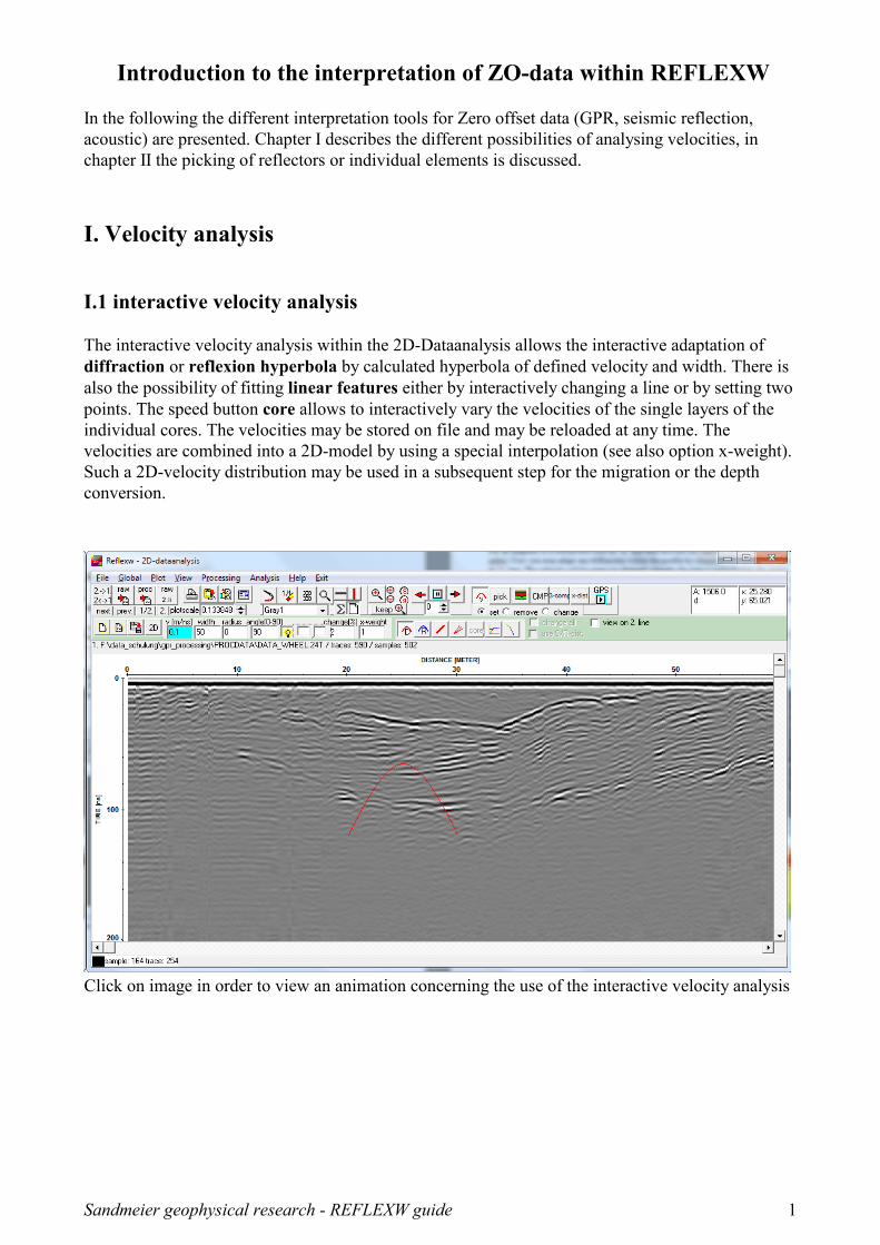
I.1.1 diffraction adaptation

For an adaption of a diffraction click on ‘D’ and then activate the v[m/ns] option (it appears in blue

color). Now you may adapt any diffraction within the profile by changing the velocity using the ‘<‘

or ‘>’ key. The velocity will be stepwise changed whereby the step is controlled by the option

change (%). The width of the calculated hyperbola is given by width in traces.

The adaptation must always be done for the phase which corresponds to time zero, this means if

time zero has been zet to the first arrival, the adaptation of the hyperbola must also be based on the

first arrivals because the curvatures along the signal length (in time) remains the same.

The option 2D allows to display the 2-dimensional velocity distribution of the chosen adaptations.

The interpolation is controlled by the parameter x-weight (increase x-weight if a more layered

distribution is wanted).

x-weight: 4

x-weight: 1


I.1.2 core data adaptation

For an adaption of coredata first a core datafile must be loaded. This is done using the option

view/core data. The coredata file must be created outside Reflexw. The file is an ASCII-file which

contains the following informations:1. line: CORE + any identification

2. line: current location (x,y and z) within the 2D-line (floating point format)

3.-x. line: layernumber thickness quality-factor mean-velocity layer-velocity

example of 3 cores (velocities are given):

CORE 10

10.0000 0.0000 0.0000

1 1.220000 1 0.140 0.140

2 1.550000 1 0.134 0.130

4 0.660700 1 0.125 0.098

CORE 16

16.0000 0.0000 0.0000

1 1.580000 1 0.140 0.140

2 1.750000 1 0.135 0.130

3 1.000000 1 0.129 0.114

4 0.610700 1 0.126 0.110

CORE 30

30.0000 0.0000 0.0000

1 2.240300 1 0.140 0.140

2 0.860000 1 0.137 0.130

3 1.000000 1 0.131 0.114

4 1.660700 1 0.119 0.098

If the core datafile does not contain the velocities of the individual core layers all velocities are

preset to the current adaptation velocity. With the speed button core activated you may interactively

adapt the core bars to layer boundaries visible within the 2D data. Click on any layer bar which you

want to adapt. The fill style of this layer bar changes. With the adaptation parameter v highlighted it

is now possible to change the velocity of this distinct layer by pressing the key < and > respectively

or using the mouse wheel (see below). With the option change all activated all layervelocites of the

actual cores are changed simultaneously.


New in version 8.3: When saving the adaption a vla-velocity file as well as 1D-VEL files (used

within the CMP-velocity analysis module) and a 2DM file containing all 1D-VEL-files are

automatically created.

The VLA-file may be used for the layershow (see next chapter) and

the 2DM-file may be used for a time-depth conversion or a migration

based on 2D-velocities using the option CMP-analysis.

The option 2D again allows to display the 2-dimensional velocity distribution of the chosen

adaptations. Now the interpolation is done based on the layers defined by the cores. The velocity

distribution is stored under the file veloc001.dat under rohdata.


Click on the image in order to view an animation about the use of the phase follower. The automatic

picking is stopped by pressing the escape key when the phase has been lost and you may force the

follower to pick the correct one by clicking on it. The use of the continuous picking allows to smoothe

the transitions zones afterwards.

II. Picking

Picking may be used for defining a layer boundary or single elements. It also may be used for some

processing steps like static or topographic correction.

Different picking possibilities are available:

phase follower: use this option for long profiles (plotoption PixelsPerTrace recommended) and for

the case that the reflector is quite continuous. The automatic phase follower is stopped using the

right mouse button or the escape key. Then you may force the phasefollower to continue the picking

at a distinct place. Already existing picks are replaced by the new ones - for a detailed description

please see online help.

continuous pick: use this option for a continuous manual picking using pressed left mouse button,

it might also be useful for continuously changing or removing existing picks.

manual pick: use this option for single trace picking or for changing individual picks

difference pick: With this option activated the traveltime difference between two successive picks

is automatically determined

auto pick: Within this menu you have the possibility to automatically pick the wanted onsets.

Depending on the needs you may choose between single objects like small diffractions, first

arrivals(e.g. from refraction seismics) or continuous reflector


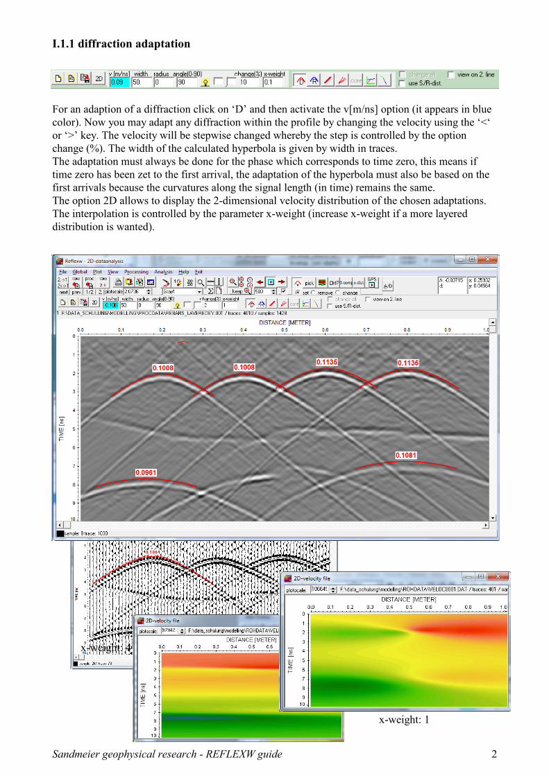
To be considered: it is important to pick the correct phase depending on the used time zero. In the

lower picture the time zero has been set to the positive maximum of the first arrival. It is assumed

that the two picked reflections have the same polarity as the first arrival because in all cases the

reflection is based on a decrease of the velocity of the lower layer (first arrival is the air/surface

reflection in this case). Therefore again the positive maxima have been picked. Of course this must

be adapted to conditions (polarity changes, ...).


II.1 Picking distinct reflectors

In the following the picking of different reflectors within REFLEXW is described including the

different layer discrimination possibilities.

II.1.2 pick a distinct reflector

There are two possibilities for the discrimination of the different picked layers.

The first one is to pick each reflector separately, save the picks for this layer and combine the pick

files together within the layershow (see chap. II.1.3).

The second one is the use of the pick codes. These codes are stored with each pick and may also be

used for a discrimination. The picks are saved within one file and an ASCII-export might be used in

order to generate a text file for all picks for the use within a further interpretation tool.

It is not necessary that the reflector is continuous but it also may consist of several broken parts. In

the following the different steps are described:

1. enter the module 2D-dataanalysis

2. load the wanted GPR or seismic ZO(zero offset) profile - comment: GPR profiles are normally

ZO-lines

3. activate the option pick

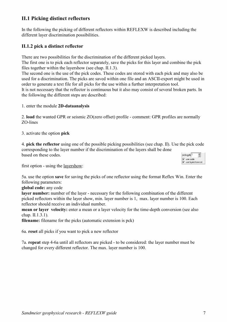
4. pick the reflector using one of the possible picking possibilities (see chap. II). Use the pick code

corresponding to the layer number if the discrimination of the layers shall be done

based on these codes.

first option - using the layershow:

5a. use the option save for saving the picks of one reflector using the format Reflex Win. Enter the

following parameters:

global code: any code

layer number: number of the layer - necessary for the following combination of the different

picked reflectors within the layer show, min. layer number is 1, max. layer number is 100. Each

reflector should receive an individual number.

mean or layer velocity: enter a mean or a layer velocity for the time-depth conversion (see also

chap. II.1.3.1).

filename: filename for the picks (automatic extension is pck)

6a. reset all picks if you want to pick a new reflector

7a. repeat step 4-6a until all reflectors are picked - to be considered: the layer number must be

changed for every different reflector. The max. layer number is 100.


Second option - using the pick codes:

5b. Increase the pickcode and pick the new layer. With each pick the traveltime, distance,

traceheader coordinate, pick code and a velocity are stored. The velocity represents a mean velocity

and not a layer velocity.

6b. repeat step 5b until all reflectors are picked.

7b. Use the option save for saving the picks of all reflectors using the format Reflex Win or any of

the ASCII-formats. The global code and layernumber and the velocities are of no interest.


II.1.3. create a layershow

1. pick a distinct reflector - it is not necessary that the reflector is continuous but it also may consist

of different broken parts (chap. II.1.2)

2. save the picks of one reflector using a special name (e.g. layer 1)- enter the layer number, the

mean velocity and a layer code

3. repeat step 1 and 2 until all reflectors have been picked

4. enter the layer-show

5. create a velocity file if layer velocities shall be used instead of mean velocities (chap. II.1.3.1)

6. create the layer-show (chap. II.1.3.2)

7. create a report (chap. II.1.3.3)

8. activate the option layer-show or under analyse/layer-show - the corresponding ZO-profile

must be loaded - the new layershow parameter panel opens.


II.1.3.1 generate a velocity file for the time-depth conversion (open layershow panel )

For the time-depth conversion using the option create LayerShow

(see section II.1.3.2) it is necessary to take a velocity into account.

You have the choice between mean single velocity, layer single

velocity, velocity file and mean pick velocities.

Choosing "mean single vel." means that the mean velocity

specified at the saving of the picks of the corresponding layer (see also SAVE under PICK) is used

for the time-depth conversion. Only one value for the complete layer is possible. The velocity is

given as the mean velocity and not as the layer velocity. The time-depth conversion of each layer

boundary is independent from the conversion of the upper boundary.

Choosing "layer single vel." means that the velocity specified at the saving of the picks of the

corresponding layer (see also SAVE under PICK) is assumed to be a layer velocity and it is used for

the time-depth conversion. Only one value for the complete layer is possible. The velocity is given

as the layer velocity.Terefore the time-depth conversion of each layer boundary depends on the

conversion of the upper boundary (see also option interpolate layer). The result is the same as using

the option velocity file with a constant velocity for each layer (see below).

Choosing "mean pick velocities" means that the mean velocities stored with the picks are used for

the time-depth conversion. The velocities have been created e.g. using the option multioffset

veloc.det within the pick-menu or by setting the velocities manually. The velocities are given as the

mean velocities and not as the layer velocities. The time-depth conversion of each layer boundary is

independent from the conversion of the upper boundary.

If you want to use any of these three options you may skip this chapter and you may continue with

chapter II.1.3.2.

The second possibility is to use an ASCII velocity datafile (e.g. test.vla). In that case, the velocities

for each layer may vary laterally and they are given as layer velocities in contrast to the mean pick

velocities. Such an ASCII-file contains the following information:

comment line

comment line

1.velocity line

....

n. velocity line

Each velocity line contains:

distance v-layer1 v-layer2 ..... v-layer10 or v-layer 100

The layer velocities may not defined at each desired distance position but the program performs a

linear interpolation between the given values.

Such an ASCII velocity datafile can either be generated

manually using any editor or using core files (see

chapter 6.1.7.4 within the manual) or using the option

create velocity in the LayerShow panel. The latter

option is described below in detail:

1. activate the option create velocity within the

layershow panel - the create velocity menu opens (see

figure on the right).

2. there are five different ways to generate an ASCII

velocity datafile: The layer velocities are set manually,

which implies no lateral change of the velocity in one layer, or the velocities are calculated using an


amplitude calibration of the picked layer boundaries, or the velocities are calculated based on

different multioffset picks or they are taken from core data or takne from the pick velocities. The

second case (amplitude calibration) is only integrated within REFLEXW for completeness. We do

not recommend this method (see manual, chap. 1.12.3.4 ). You may use different ways for the

different layers.

3. Activate the option manual and enter the velocities for the individual layers and the filename for

the velocity file (the velocity file automatically has the extension vla).

4. activate the option start for the generation of the ASCII file. The file is shown in a window and

activate the option close for closing the display of the file.

5. activate the option close for closing the create velocity menu.

6. The ASCII-file can be changed manually using any editor.


II.1.3.2. combine the different picked reflectors into one layer model (open layershow panel)

This option offers the possibility to combine individual pick files stored on file, to plot them

together with the wiggle-files and to output them in report form on printer or file. The maximum

number of combined picks per layer boundary is equal to the max. number of traces per profile. The

maximum number of layer boundaries is 10 (until ver. 2.1) or 100 (from ver. 2.5).

The picked traveltimes of the reflectors are transformed into dephts using either a mean velocity for

a distinct layer or based on a laterally varying velocity file.

In the following the individual steps of creating a layer-show are described.

1. activate the option create within the layershow panel

- the create layer show menu opens (see figure on the

right).

2. activate the option pick files within the layer show

menu and choose all wanted pickfiles (multiple choice

using the shift or str-key) - the choosen pick files are

listed in the textbox on the right.

3. Control the other parameters like start/end position,

increment and the velocity choice for the time-depth

conversion.

If you want to use a velocity file for the time-depth

conversion instead of the mean or layer pick velocity stored with each pick file first you must

create such a velocity file (see section II.1.3.1). Then you must activate the option velocity file and

load the wanted velocity file. The option interpolate layer controls how the special case of broken

reflectors are handled (see below).

4. Enter a filename for the layer-show (extension is automatically lay) and activate the option start

in order to create the layer-show.

5. activate the option close for

closing the create layershowy

menu.

6. the layer-show is displayed in

the lower window - the traveltime

picks are displayed together with

the ZO-profile within the upper

window.

Note: If the option depth axis

within the plotoptions is activated

the depths for the picks of the

upper window are only

comparable to the depths of the

layers in the lower picture if mean

velocity has been used for creating

the layershow and if all mean

velocities of the picks are equal to

the velocity for the depthaxis

display.


7. Any layershow can be reloaded using the option load within the layershow panel.

To be considered: If the mean single velocity or mean pick velocities are used for the time-depth

conversion, the time-depth conversion of each layer boundary is independent from the conversion

of the upper boundary.

In contrast, if an layer single velocity or an ASCII velocity datafile is used, the time-depth

conversion of each layer boundary depends on the conversion of the upper boundary. Therefore, in

that case one has to control how the time-depth conversion for a special layer is done if any upper

layer is not continuously picked. This is done using the option interpolate layer.

If this option is activated every upper layer is assumed to be continuous even if it is not picked and

either an interpolation or an extrapolation both for the layer points and the velocities is done. Based

on these calculated values the time-depth conversion of the actual layer is done.

If the option is deactivated, the velocities of the next upper picked layer are used. This might result

in a sharp step of the depth of the actual layer at the point where any of the upper layers is broken.


II.1.3.2. generate an output report of the layer-show (open layershow panel)

The results of the current layershow can be stored in a report. The output is performed either on a

printer or on a file with an arbitrary name. According to the individual settings, the report contains

information about single layers like e.g. thickness, velocity, amplitudes and coordinates. In addition,

actually loaded coredata and marker comments can be reported. It is also possible to reduce the

information on single points e.g. to represent only material depth between two construction changes.

1. activate the option create report within the

layershow panel - the create report menu opens (see

figure on the right). Precondition: a layershow must be

loaded or just created.

2. enter the necessary parameters for the output:

- start/end position and increment

- layers: enter the numbers of the layers for the report

output: e.g. 1-5 or 1-5,8,9

3. activate the option start in order to start the report

output.


II.2 Picking single objects within REFLEXW

II.2.1. Picking hyperbolas along one profile line

The following flow described one way how to mark single objects (hyperbolas) and to save the

parameters x, z and ID on an ASCII file for a further interpretation with any other CAD-system.

1. enter the module 2D-dataanalysis

2. load the wanted GPR or seismic ZO(zero offset) profile

3. activate the option pick

4. activate the option manual pick

5. enter the ID of the hyperbola within the paramter pickcode

6. click on the cusp of the hyperbola within the profile using the left mouse button

7. repeat step 5-6 until all hyperbola cusps have been picked

8. enter the option save and activate the pickformat ASCII-colums. In addition you also may save

the picks using the REFLEXW-Win format in order to load the picks at a later stage again.

9. Activate the options depths, amplitudes and pick codes.

10. enter the wanted velocity in m/ns for converting the 2-way traveltimes into depths

11. enter the wanted filename and press save

12. each line of the output file contains the following informations:

profiledistance profileconstant-start traveltime depth amplitude code


II.2.2. Use of xy-coordinates

II.2.2.1 Use of xy-coordinates defined within the traceheader for one single profile

The ASCII-output described above does not contain the real xy-coordinates but the distance

coordinates along the profile together with the start coordinate in the profile constant direction.

Therefore these coordinates only correspond to the real xy-coordinates if the profiledirection is

strictly orientated into x- or y-direction. If this does not hold true (e.g. diagonal lines) you must take

into account the so called traceheader coordinates in addition. These coordinates may represent

relative or absolute (GPS) coordinates. The relative coordinates may be generated from the overall

fileheader coordiantes if the lines are straight. The GPS-coordinates may be loaded from differently

formated ASCII-files. Reflexw supports GPS-datafiles from most of the GPR-systems. In addition

time based GPS-data may be imported if the GPR or seismic data also contain time informations.

A. Define the traceheader coordinates from the fileheader:

1. Define the geometry of your file within the fileheader either

during the import or within the edit fileheader menu (option edit

fileheader). The example shows a diagonal line.

2. After having defined the fileheader coordinates (do not forget

so save them before when you have changed the fileheader

coordinates within the fileheader menu) activate the option

ShowTraceHeader.

3. The traceheader menu opens. Here you may actualize the

traceheadercoordinates either based on the fileheader coordinates

or based on different ASCII-files (see also guide for GPS-

coordinates). Enter within the Actualize panel for type fileheader

and press the buttom actualize.

4. Now the traceheader coordinates are defined based on the

given fileheader coordinates. You may check the coordinates

using the trace number edit button.


B. Define the traceheader coordinates using GPS-coordinates:

If GPS-data are simultaneously acquired it is possible to

synchronize the GPR-data with the GPS-coordinates. The

original GPR data may either be time based or based on a

wheel. The different GPR-systems use different

synchronization types. Mala, Utsi, IDS or PulseEkko for

example generate a gps-file which contains both the

tracenumber of the GPR-file and the GPS-coordinates. For

most data acquisitions systems it is possible to

automatically import the gps-data into the Reflexw file

during the import and to

perform a subsequent

UTM-conversion. A

linear interpolation will

be automatically done

where no GPS-data are

present. The option

calculate distancies sums

up the distance along the

gps-line and stores it into

the Reflexw traceheader.

The GPS-coordinates

may be controlled and

edited within the edit

traceheader tabella.

Now the traceheader coordinates are defined based on the given

fileheader coordinates. You may check the coordinates using the

option profile line (trace header coord.) under view.

A subsequent processing step named make equidist.traces under

processing/ TraceInterpolation/ Resorting may be used in

addition to interpolate the non-equidistant data in such a way that

the resulting data are equidistant. The non-equidistant data are

resampled in x-direction based on the filter parameter trace incr.

and the distance values stored in the individual trace headers of

each trace. In addition the start distance and the end distance

(starting and ending position of the new profile) have to be

specified in the given distance dimension. By default the start

distance and the end distance are determined from the

traceheaders. By the manual input you may extract a distinct part

from the profile.


Picking:

1. pick the hyperbolas like described in chapter 1.

2. When saving the picks using the format

ASCII-free format you may activate for exampel

the options trace number, rec. x- and y-pos,

travel times and depths.

3. 12. Now each line of the output file contains

the following informations:

tracenumber rec.x-pos rec.y-pos traveltime

depth

For zero offset data the shot and the receiver

coordinates are the same and you only may

consider one coordinate pair.


II.2.2.2 Use of xy-coordinates for several profiles

It is also possible to save the picks of different 2D-profiles into one ASCII-file.

1. For that purpose first you must save the picks of the 2D-profiles into different Reflexw-pickfiles

using the pick format Reflex Win.

2. You may control the location of

the picks within the interactive

choice menu - enter for that

purpose file/interactive choice

within the 2D-datananalysis - the

interactive 2D-line choice menu

opens

3. Choose the wanted filepath and

press show all lines

4. Click on show picks and choose

the wanted pickfiles (multifile

choice using the shift or strg key)

5. Picks belonging to the same code are connected if the option interpolation is activated. If the

option use code within the 2D-dataanalysis is activated the layershow-colors are used for the display

of the picks.

6. If the picks are correct you may leave the interactive choice menu and enter the pick save menu in

order to save all the picks for the different 2D-lines into one single ASCII-file.

7. Within the save pick menu you must choose the “ASCII-colums” or “ASCII free format” pick

format and you have to activate the option “export several existing picks into 1 ASCII-file”.

8. Click on save and choose all wanted ReflexWin formatted pickfiles (multi filechoice using the

shift or strg key).

9. Each line of the resulting ASCII-file contains for example the following values:

traveltime depth amplitude x-shot y-shot z-shot x-receiver y-receiver z-receiver code(optional)

Depths and amplitudes are set to zero if the corresponding options depth and amplitudes are

deactivated.


II.2.3 Picking linear structures within a 3D-datafile

Reflexw allows a fast picking of single objects within the 3D-datainterpretation.

The following procedure may be applied to all types of single objects like pipes, rebars or other line

structures.

1. Load a 3D-file within the 3D-

datainterpretation and choose Scroll

and the appropriate cut

2. Activate pick and activate use code

and auto cor. based on

corr.max/dist.range (option only act.

code is deactivated). The parameters

for the corr.max/dist.range may be

entered within the global settings menu

(parameter pickcorrect traces which

should be set to 1 for data with a small

cut increment).

3. Click on apply to all codes

4. Pick all elements of one block (e.g.

one set of rebars orientated in one

direction) using different codes (the F4

key may be used in order to increase

the code) within the actual cut

5. Go to the next cut using the right

scroll button (hand)

6. Click on take over - the picks from the

previous cut will be taken over to the actual cut

7. Click on the right arrow in

order to scroll through the

complete 3D-block. The new

picks will be displayed. You

can stop the scrolling at any

time.

8. Control the picks by scrolling back. If any

element will be lost due to a lateral jump for

example (see example on the left for the two last

picks) you may manually change the false pick:

- enter the code of the false pick (here 9)

- activate the option only act code

- change the correction type if necessary

- activate change and click on the correct pick

position

- activate the option take over and scroll using the

right red arrow to the end of the block, the wrong

picks will be changed according to the new

settings.

9. Make the same for all wrong picks (item 8)

10. Save the picks. It is recommended to store all

different picks sets on different files as this

simplifies the semi automatic picking.


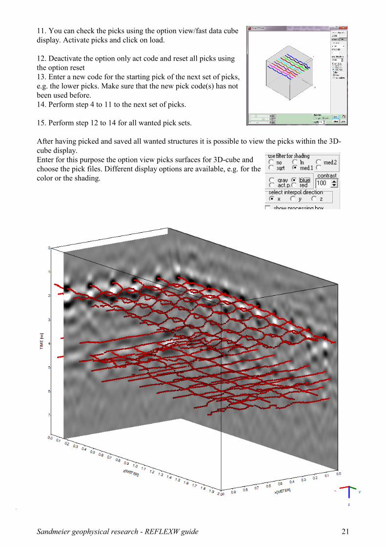
11. You can check the picks using the option view/fast data cube

display. Activate picks and click on load.

12. Deactivate the option only act code and reset all picks using

the option reset

13. Enter a new code for the starting pick of the next set of picks,

e.g. the lower picks. Make sure that the new pick code(s) has not

been used before.

14. Perform step 4 to 11 to the next set of picks.

15. Perform step 12 to 14 for all wanted pick sets.

After having picked and saved all wanted structures it is possible to view the picks within the 3D-

cube display.

Enter for this purpose the option view picks surfaces for 3D-cube and

choose the pick files. Different display options are available, e.g. for the

color or the shading.


Introduction to the interpretation of ZO-data within REFLEXW · time zero has been zet to the first...

Documents

Transcript of Introduction to the interpretation of ZO-data within REFLEXW · time zero has been zet to the first...