Introduction to the GRAPE Algorithm - Research - Michael … · The Basic Idea Acronym GRAPE:...
12
Introduction to the GRAPE Algorithm Michael Goerz June 8, 2010 Michael Goerz Introduction to the GRAPE Algorithm
Transcript of Introduction to the GRAPE Algorithm - Research - Michael … · The Basic Idea Acronym GRAPE:...

Introduction to the GRAPE Algorithm
Michael Goerz
June 8, 2010
Michael Goerz Introduction to the GRAPE Algorithm

Reference: J. Mag. Res. 172, 296 (2005)
Optimal control of coupled spin dynamics: design of NMRpulse sequences by gradient ascent algorithms
Navin Khanejaa,*, Timo Reissb, Cindie Kehletb, Thomas Schulte-Herbruggenb,Ste!en J. Glaserb,*
a Division of Applied Sciences, Harvard University, Cambridge, MA 02138, USAb Department of Chemistry, Technische Universitat Munchen, 85747 Garching, Germany
Received 27 June 2004; revised 23 October 2004Available online 2 December 2005
Abstract
In this paper, we introduce optimal control algorithm for the design of pulse sequences in NMR spectroscopy. This methodologyis used for designing pulse sequences that maximize the coherence transfer between coupled spins in a given specified time, minimizethe relaxation e!ects in a given coherence transfer step or minimize the time required to produce a given unitary propagator, asdesired. The application of these pulse engineering methods to design pulse sequences that are robust to experimentally importantparameter variations, such as chemical shift dispersion or radiofrequency (rf) variations due to imperfections such as rf inhomoge-neity is also explained.! 2004 Elsevier Inc. All rights reserved.
Keywords: Pulse design; Sequence optimization; Time-optimal coherence transfer; Relaxation-optimized experiments; Time-optimal realization ofunitary operators; Quantum gates; GRAPE algorithm; Optimal control theory
1. Introduction
In applications of NMR spectroscopy, it is desirableto have optimized pulse sequences tailored to specificapplications. For example, in multi-dimensional NMRexperiments one is often interested in pulse sequenceswhich maximize the coherence transfer between coupledspins in a given specified time, minimize the relaxatione!ects in a given coherence transfer step or minimizethe time required to produce a given unitary propagator.From an engineering perspective all these problems arechallenges in optimal control [1,2] where one is inter-ested in tailoring the excitation to a dynamical systemto maximize some performance criterion. In this paper,
we present gradient ascent algorithms for optimizingpulse sequences (control laws) for steering the dynamicsof coupled nuclear spins. Similar methods and their vari-ants have been applied in laser spectroscopy [3–7]. InNMR, this approach has been used to design band-se-lective pulses [8–10], robust broadband excitation, andinversion pulses [11–13]. However, previous studies inNMR were limited to uncoupled spin systems whosedynamics is governed by the Bloch equations. It isimportant to note that the optimal control principlesare standard text book material in applied optimal con-trol [1,2]. The focus of this paper is the application ofthese methods for some important problems in NMR.Previously, gradient-based optimizations of NMR pulsesequences for coupled spin systems have almost exclu-sively relied on gradients computed by the di!erencemethod. One important exception are analytical deriva-tives introduced by Levante et al. [14] for pulse sequence
www.elsevier.com/locate/jmr
Journal of Magnetic Resonance 172 (2005) 296–305
1090-7807/$ - see front matter ! 2004 Elsevier Inc. All rights reserved.doi:10.1016/j.jmr.2004.11.004
* Corresponding authors. Fax: +49 89 289 13210.E-mail addresses: [email protected] (N. Khaneja), Glaser@
ch.tum.de (S.J. Glaser).
Michael Goerz Introduction to the GRAPE Algorithm

The Basic Idea
Acronym
GRAPE: Gradient Ascent Pulse Engineering
optimizations, where the performance can be expressedin terms of the eigenvalues and eigenfunctions of the to-tal propagator.
The paper is organized as follows. In Section 2, wepresent the basic theoretical ideas and numerical optimi-zation algorithms directly applicable to the problem ofpulse design. To illustrate the method, we present threesimple but non-trivial applications to coupled spin sys-tems both in the presence and in the absence of relaxa-tion. In Section 3.1, we look at the problem of findingmaximum coherence transfer achievable in a given timeand the design of pulse sequences that achieve this trans-fer. In Section 3.2, the algorithm is used to find relaxa-tion optimized pulse sequences that perform desiredcoherence transfer operations with minimum losses. InSection 3.3, we design pulse sequences that produce adesired unitary propagator in a network of coupledspins in minimal time. In all examples, we compare theresults obtained by the numerical optimization algo-rithm with optimal solutions obtained by analyticalarguments based on geometric optimal control theory.In the conclusion section, we discuss the convergenceproperties of the proposed algorithm and possibleextensions.
2. Theory
2.1. Transfer between Hermitian operators in the absenceof relaxation
To fix ideas, we first consider the problem of pulse de-sign for polarization or coherence transfer in the absenceof relaxation. The state of the spin system is character-ized by the density operator q (t), and its equation ofmotion is the Liouville–von Neuman equation [15]
_q!t" # $i H0 %Xm
k#1
uk!t"Hk
!
; q!t"
" #
; !1"
where H0 is the free evolution Hamiltonian, Hk are theradiofrequency (rf) Hamiltonians corresponding to theavailable control fields and u (t) = (u1 (t), u2 (t), . . .,um (t))represents the vector of amplitudes that can be changedand which is referred to as control vector. The problemis to find the optimal amplitudes uk (t) of the rf fields thatsteer a given initial density operator q (0) = q0 in a spec-ified time T to a density operator q (T) with maximumoverlap to some desired target operator C. For Hermi-tian operators q0 and C, this overlap may be measuredby the standard inner product
hCjq!T "i # tr Cyq!T "! "
: !2"
(For the more general case of non-Hermitian operators,see Section 2.2). Hence, the performance index U0 of thetransfer process can be defined as
U0 # hCjq!T "i: !3"
In the following, we will assume for simplicity thatthe chosen transfer time T is discretized in N equal stepsof duration Dt = T/N and during each step, the controlamplitudes uk are constant, i.e., during the jth step theamplitude uk (t) of the kth control Hamiltonian is givenby uk (j) (cf. Fig. 1). The time-evolution of the spin sys-tem during a time step j is given by the propagator
Uj # exp $iDt H0 %Xm
k#1
uk!j"Hk
!( )
: !4"
The final density operator at time t = T is
q!T " # UN & & &U 1q0Uy1 & & &U
yN ; !5"
and the performance function U0 (Eq. (3)) to be maxi-mized can be expressed as
U0 # hCjUN & & &U 1q0Uy1 & & &U
yN i: !6"
Using the definition of the inner product (cf. Eq. (2))and the fact that the trace of a product is invariant un-der cyclic permutations of the factors, this can be rewrit-ten as
U0 # hU yj%1 & & &U
yNCUN & & &Uj%1|#####################{z#####################}kj
j Uj & & &U 1q0Uy1 & & &U
yj|#################{z#################}
qj
i;
!7"
where qj is the density operator q (t) at time t = jDt andkj is the backward propagated target operator C at thesame time t = jDt. Let us see how the performance U0
changes when we perturb the control amplitude uk (j)at time step j to uk (j) + duk (j). From Eq. (4), the changein Uj to first order in duk (j) is given by
dUj # $iDtduk!j"HkUj !8"
with
HkDt #Z Dt
0
Uj!s"HkUj!$s"ds !9"
Fig. 1. Schematic representation of a control amplitude uk (t),consisting of N steps of duration Dt = T/N. During each step j, thecontrol amplitude uk (j) is constant. The vertical arrows representgradients dU0=duk!j", indicating how each amplitude uk (j) should bemodified in the next iteration to improve the performance function U0.
N. Khaneja et al. / Journal of Magnetic Resonance 172 (2005) 296–305 297
uk (j)
Φ0
original value
at time index j : go in direction of gradient
Pulse Update
uk (j) −→ uk (j) + ε∂Φ0
∂uk (j)
Michael Goerz Introduction to the GRAPE Algorithm

Working in Liouville Space
Density Matrix
|Ψ〉 −→ ρ = |Ψ〉〈Ψ|
Liouville-von Neumann Equation
ρ(t) = −i [H, ρ(t)]− = −i
" H0 +
mXk=1
uk (t)Hk
!, ρ
#−
Time Propagation
Uj = exp
(−i∆t
H0 +
mXk=1
uk (j)Hk
!)
ρ(T ) = UN . . .U1 ρ(0) U†1 . . .U†N
= |Ψ(T )〉〈Ψ(T )| with Ψ(T ) = Un . . .U1Ψ(0)
Michael Goerz Introduction to the GRAPE Algorithm

Definition of Fidelity
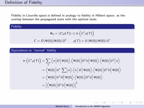
Fidelity in Liouville space is defined in analogy to fidelity in Hilbert space: as theoverlap between the propagated state with the optimal state.
Fidelity
Φ0 = 〈C |ρ(T )〉 ≡ tr“C†ρ(T )
”C = O |Ψ(0)〉〈Ψ(0)|O† ρ(T ) = U |Ψ(0)〉〈Ψ(0)|U†
Equivalence to “normal” fidelity
tr“C†ρ(T )
”=X
n
Dn˛O˛
Ψ(0)ED
Ψ(0)˛O†U
˛Ψ(0)
EDΨ(0)
˛U†˛nE
=D
Ψ(0)˛U†X˛
nED
n˛O˛
Ψ(0)ED
Ψ(0)˛O†U
˛Ψ(0)
E=D
Ψ(0)˛U†O
˛Ψ(0)
EDΨ(0)
˛O†U
˛Ψ(0)
E=˛D
Ψ(0)˛O†U
˛Ψ(0)
E˛2
Michael Goerz Introduction to the GRAPE Algorithm
Definition of Fidelity
Fidelity in Liouville space is defined in analogy to fidelity in Hilbert space: as theoverlap between the propagated state with the optimal state.
Fidelity
Φ0 = 〈C |ρ(T )〉 ≡ tr“C†ρ(T )
”C = O |Ψ(0)〉〈Ψ(0)|O† ρ(T ) = U |Ψ(0)〉〈Ψ(0)|U†
Equivalence to “normal” fidelity
tr“C†ρ(T )
”=X
n
Dn˛O˛
Ψ(0)ED
Ψ(0)˛O†U
˛Ψ(0)
EDΨ(0)
˛U†˛nE
=D
Ψ(0)˛U†X˛
nED
n˛O˛
Ψ(0)ED
Ψ(0)˛O†U
˛Ψ(0)
E=D
Ψ(0)˛U†O
˛Ψ(0)
EDΨ(0)
˛O†U
˛Ψ(0)
E=˛D
Ψ(0)˛O†U
˛Ψ(0)
E˛2
Michael Goerz Introduction to the GRAPE Algorithm

Fidelity through Backward- and Forward-Propagation
A trace is invariant under cyclic permutation of its factors!
Fidelity at T
Φ0 = 〈C |ρ(T )〉 =DC |UN . . .U1ρ(0)U†1 . . .U
†N
E=DU†j+1 . . .U
†NCUN . . .Uj+1|Uj . . .U1ρ(0)U†1 . . .U
†j
EPropagated States → Fidelity at tj
λj ≡ U†j+1 . . .U†NCUN . . .Uj+1 bw. propagated optimal state
ρj ≡ Uj . . .U1ρ(0)U†1 . . .U†j fw. propagated initial state
Φ0 = 〈C |ρ(T )〉 =˙λj |ρj
¸Note: all propagations with guess pulse!
Michael Goerz Introduction to the GRAPE Algorithm

Calculation of Pulse Update
Pulse Update
uk (j) −→ uk (j) + ε∂Φ0
∂uk (j)We need to calculate
∂Φ0
∂uk (j)
Two steps:
For a variation δuk (j), calculate δUj
Use δUj to calculate ∂Φ0∂uk (j)
Calculations are not completely trivial.
Solution:
Gradient
∂Φ0
∂uk (j)= −
˙λj |i∆t[Hk , ρj ]−
¸
Michael Goerz Introduction to the GRAPE Algorithm
Grape Algorithm
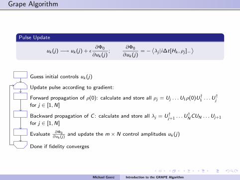
Pulse Update
uk (j) −→ uk (j) + ε∂Φ0
∂uk (j);
∂Φ0
∂uk (j)= −
˙λj |i∆t[Hk , ρj ]−
¸
Guess initial controls uk (j)
Update pulse according to gradient:
Forward propagation of ρ(0): calculate and store all ρj = Uj . . .U1ρ(0)U†1 . . .U†j
for j ∈ [1,N]
Backward propagation of C : calculate and store all λj = U†j+1 . . .U†NCUN . . .Uj+1
for j ∈ [1,N]
Evaluate ∂Φ0∂uk (j)
and update the m × N control amplitudes uk (j)
Done if fidelity converges
Michael Goerz Introduction to the GRAPE Algorithm

Variations
Non-Hermitian Operators
Φ1 = <[Φ0];∂Φ1
∂uk (j)= −
Dλx
j |i∆t[Hk , ρxj
E−Dλy
j |i∆t[Hk , ρyj
EΦ2 = |Φ0|2 ;
∂Φ2
∂uk (j)= −2<
˘˙λj |i∆t[Hk , ρj
¸ ˙ρy
N |C¸¯
Unitary Transformations
Φ3 = <〈UF |U(T )〉 = <DU†j+1 . . .U
†NUF |Uj . . .U1
E= <
˙Pj |Xj
¸∂Φ3
∂uk (j)= −<
˙Pj |i∆tHkXj
¸Φ4 = |〈UF |U(T )〉|2 =
˙Pj |Xj
¸ ˙Xj |Pj
¸∂Φ4
∂uk (j)= −2<
˘˙Pj |i∆tHkXj
¸ ˙Xj |Pj
¸¯Also works with Lindbladt-Operators. Additional energy constraints are possible.
Michael Goerz Introduction to the GRAPE Algorithm
Comparison with OCT
optimizations, where the performance can be expressedin terms of the eigenvalues and eigenfunctions of the to-tal propagator.
The paper is organized as follows. In Section 2, wepresent the basic theoretical ideas and numerical optimi-zation algorithms directly applicable to the problem ofpulse design. To illustrate the method, we present threesimple but non-trivial applications to coupled spin sys-tems both in the presence and in the absence of relaxa-tion. In Section 3.1, we look at the problem of findingmaximum coherence transfer achievable in a given timeand the design of pulse sequences that achieve this trans-fer. In Section 3.2, the algorithm is used to find relaxa-tion optimized pulse sequences that perform desiredcoherence transfer operations with minimum losses. InSection 3.3, we design pulse sequences that produce adesired unitary propagator in a network of coupledspins in minimal time. In all examples, we compare theresults obtained by the numerical optimization algo-rithm with optimal solutions obtained by analyticalarguments based on geometric optimal control theory.In the conclusion section, we discuss the convergenceproperties of the proposed algorithm and possibleextensions.
2. Theory
2.1. Transfer between Hermitian operators in the absenceof relaxation
To fix ideas, we first consider the problem of pulse de-sign for polarization or coherence transfer in the absenceof relaxation. The state of the spin system is character-ized by the density operator q (t), and its equation ofmotion is the Liouville–von Neuman equation [15]
_q!t" # $i H0 %Xm
k#1
uk!t"Hk
!
; q!t"
" #
; !1"
where H0 is the free evolution Hamiltonian, Hk are theradiofrequency (rf) Hamiltonians corresponding to theavailable control fields and u (t) = (u1 (t), u2 (t), . . .,um (t))represents the vector of amplitudes that can be changedand which is referred to as control vector. The problemis to find the optimal amplitudes uk (t) of the rf fields thatsteer a given initial density operator q (0) = q0 in a spec-ified time T to a density operator q (T) with maximumoverlap to some desired target operator C. For Hermi-tian operators q0 and C, this overlap may be measuredby the standard inner product
hCjq!T "i # tr Cyq!T "! "
: !2"
(For the more general case of non-Hermitian operators,see Section 2.2). Hence, the performance index U0 of thetransfer process can be defined as
U0 # hCjq!T "i: !3"
In the following, we will assume for simplicity thatthe chosen transfer time T is discretized in N equal stepsof duration Dt = T/N and during each step, the controlamplitudes uk are constant, i.e., during the jth step theamplitude uk (t) of the kth control Hamiltonian is givenby uk (j) (cf. Fig. 1). The time-evolution of the spin sys-tem during a time step j is given by the propagator
Uj # exp $iDt H0 %Xm
k#1
uk!j"Hk
!( )
: !4"
The final density operator at time t = T is
q!T " # UN & & &U 1q0Uy1 & & &U
yN ; !5"
and the performance function U0 (Eq. (3)) to be maxi-mized can be expressed as
U0 # hCjUN & & &U 1q0Uy1 & & &U
yN i: !6"
Using the definition of the inner product (cf. Eq. (2))and the fact that the trace of a product is invariant un-der cyclic permutations of the factors, this can be rewrit-ten as
U0 # hU yj%1 & & &U
yNCUN & & &Uj%1|#####################{z#####################}kj
j Uj & & &U 1q0Uy1 & & &U
yj|#################{z#################}
qj
i;
!7"
where qj is the density operator q (t) at time t = jDt andkj is the backward propagated target operator C at thesame time t = jDt. Let us see how the performance U0
changes when we perturb the control amplitude uk (j)at time step j to uk (j) + duk (j). From Eq. (4), the changein Uj to first order in duk (j) is given by
dUj # $iDtduk!j"HkUj !8"
with
HkDt #Z Dt
0
Uj!s"HkUj!$s"ds !9"
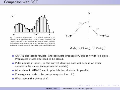
Fig. 1. Schematic representation of a control amplitude uk (t),consisting of N steps of duration Dt = T/N. During each step j, thecontrol amplitude uk (j) is constant. The vertical arrows representgradients dU0=duk!j", indicating how each amplitude uk (j) should bemodified in the next iteration to improve the performance function U0.
N. Khaneja et al. / Journal of Magnetic Resonance 172 (2005) 296–305 297
Ψin Ψtgt
ε(1)
ε(0)
tj
∆u(j) ∼˙Ψbw (tj ) |µ|Ψfw (tj )
¸GRAPE also needs forward- and backward-propagation, but only with old pulse.Propagated states also need to be stored.
Pulse update at point j in the current iteration does not depend on otherupdated pulse values (non-sequential update)
All updates in GRAPE can in principle be calculated in parallel.
Convergence tends to be pretty lousy (so I’m told)
What about the choice of ε?
Michael Goerz Introduction to the GRAPE Algorithm

Thank You!
Michael Goerz Introduction to the GRAPE Algorithm