INTRODUCTION TO THE EDDY COVARIANCE METHOD

1

This introduction has been created to familiarize a beginner with general theoretical principles, requirements, applications, and processing steps of the Eddy Covariance method. It is intended to assist readers in the further understanding of the method and references such as textbooks, network guidelines and journal papers. It is also intended to help students and researchers in the field deployment of the Eddy Covariance method, and to promote its use beyond micrometeorology.

The notes section at the bottom of each slide can be expanded by clicking on the ‘notes’ button located in the bottom of the frame. This section contains text and informal notes along with additional details. Nearly every slide contains references to other web and literature references, additional explanations, and/or examples.

Please feel free to send us your suggestions. We intend to keep the content of this work dynamic and current, and we will be happy to incorporate any additional information and literature references. Please address mail to george.burba at licor.com with the subject “EC Guidelines”.

INTRODUCTION TO THE EDDY COVARIANCE METHOD

G. Burba and D. Anderson

GENERAL GUIDELINES, AND CONVENTIONAL WORKFLOW

LI-COR Biosciences

2

Slide 2 Burba & AndersonBurba & Anderson Slide 2 © LI-COR Biosciences

Introduction_______________________3IntroductionPurposeAcknowledgementsLayout

I. Eddy Covariance Theory Overview_7Flux measurements in generalState of Eddy Covariance methodologyAir flow in ecosystemHow to measure fluxBasic derivations Practical formulasMajor assumptionsMajor sources of errorsError treatmentUse in non-traditional terrainsEddy Covariance theory summary

II. Eddy Covariance Workflow _22

II.1 Experimental design _____________24Purpose and variablesInstrument requirementsEddy Covariance instrumentation (25-55)Data collection and processing softwareLocation requirementsMaintenance planSummary of experimental design

II.2 Experiment implementation ______ 51Tower placementSensor height and sampling frequencyFootprint

- visualizing the concept- effect of measurement height

- effect of canopy roughness - effect of stability- summary of footprint

Testing data collectionTesting data retrievalKeeping up maintenanceExperiment implementation summary

II. 3 Data processing and analysis __ 73Unit conversionDespikingCalibration coefficientsCoordinate rotationTime delayDe-trending

Applying corrections___________________81- frequency response corrections- co-spectra- transfer functions- applying frequency response corrections- time responsesensor separation- tube attenuation- digital sampling- path and volume averaging- hi-pass filteringlow-pass filteringsensor response mismatch- total transfer function- frequency response summary

Choosing time averageWebb-Pearman-Leuning correctionSonic correctionOther correctionsSummary of corrections

II.4 Quality control of Eddy Covariance data 102QC generalQC nighttimeValidation of flux dataFilling-in the dataStorageIntegration

II.5 Eddy covariance workflow summary ___111

III. Alternative methods_____ _____113Eddy AccumulationRelaxed Eddy AccumulationBowen Ratio Energy Balance Aerodynamic methodResistance approachChamber measurementsOther alternative methods

IV. Future development_____ _____ 121Future of Eddy Covariance method

- expansion- airborne- difficult terrains

LIDAR/RADARLaser spectroscopySpaceMultiplexing/Networking

V. Eddy Covariance Review Summary 129VI. Useful resources_____ ____ _131VII. References and future readings __ 134

CONTENTCONTENT

You can expand the index by clicking on the ‘Outline’ button in the lower left of the frame. This index is linked to the contents of each slide and can be used for quick and easy navigation of the contents of these guidelines.

!

the question mark icon and blue font color indicate scientific references, web-links and other information sources covering related to the topic of the slide

the exclamation point icon and red font color indicate warnings and describe potential pitfalls related to the topic of the slide

?

This introduction has been created to familiarize a beginner with general theoretical principles, requirements, applications, and processing steps of the Eddy Covariance method. It is intended to assist readers in further understanding of the method and references such as textbooks, network guidelines and journal papers. It is are also intended to help students and researchers in the field deployment of the Eddy Covariance method, and to promote its use beyond micrometeorology.

The notes section at the bottom of each slide can be expanded by clicking on the ‘notes’ button located in the bottom of the frame. This section contains text and informal notes along with additional details. Nearly every slide contains references to other web and literature references, additional explanations, and/or examples).

Please feel free to send us your suggestions. We intend to keep the content of this work dynamic and current, and we will be happy to incorporate any additional information and literature references. Please address mail to [email protected] with subject “EC Guidelines”.

3


• The Eddy Covariance method is a very useful technique to measure and

calculate turbulent fluxes within the atmospheric boundary layer

• Modern instruments and software can potentially expand the use of the

method beyond micrometeorology to a widely-used tool for biologists,

ecologists, entomologists, etc.

• Main challenge of the method for a non-expert is the shear complexity

of system design, implementation and processing the large volume of

data

INTRODUCTIONINTRODUCTION

Below are few examples of the sources of information on the various methods of flux measurements, specifically the Eddy Covariance method:

Rosenberg, N.J., B.L. Blad & S.B. Verma. 1983. Microclimate. The biological environment. A Wiley-interscience publication. New York. 255-257

Baldocchi, D.D., B.B. Hicks and T.P. Meyers. 1988. 'Measuring biosphere-atmosphere exchanges of biologically related gases with micrometeorological methods', Ecology, 69, 1331-1340

Verma, S.B., 1990. Micrometeorological methods for measuring surface fluxes of mass and energy. Remote Sensing Reviews, 5: 99-115.

Wesely, M.L., D.H. Lenschow and O.T. 1989. Flux measurement techniques. In: Global Tropospheric Chemistry, Chemical Fluxes in the Global Atmosphere. NCAR Report. Eds. DH Lenschow and BB Hicks. pp 31-46

?

4


• Help a non-expert in gaining a basic understanding of the Eddy

Covariance method and point out valuable references

• Provide explanations in a simplified manner first, and then to elaborate

with specific details

• Promote a further understanding of the method via more advanced

sources (textbooks, papers)

• Help design experiments for the specific needs of a new Eddy

Covariance user

PURPOSEPURPOSE

Here we try to help a non-expert to understand the general principles, requirements, applications, and processing steps of the Eddy Covariance method.

Explanations are given in a simplified manner first, and then, elaborated with some specific examples; alternatives to the traditionally used approaches are also mentioned.

The basic information presented here is intended to provide a foundational understanding of the Eddy Covariance method, and to help new Eddy Covariance users design experiments for their specific needs. A deeper understanding of the method can be obtained via more advanced sources, such as textbooks, network guidelines and journal papers.

The specific applications of the Eddy Covariance method are numerous, and may require specific mathematical approaches and processing workflows. This is why there is no one single recipe, and it is important to study further, all aspects of the method in relation to a specific measurement site and a specific scientific purpose.

5


We would like to acknowledge a number of scientists who have contributed to

this review directly via valuable advice and indirectly via scientific papers,

textbooks, data sets, and personal communications

Particularly we thank Drs. Dennis Baldocchi, Dave Billesbach, Robert Clement,

Tanvir Demetriades-Shah, Thomas Foken, Beverly Law, Hank Loescher,

William Massman, Dayle McDermitt, William Munger, Andrew Suyker, Shashi

Verma, Jon Welles and many others for their expertise in this area of flux

studies

We also thank Fluxnet, Canada Flux, and AmeriFlux networks for providing

access to the data from the Eddy Covariance stations

ACKNOWLEDGMENTSACKNOWLEDGMENTS

We also would like to thank numerous other researchers, technicians and students who, through years of use in the field, have developed the Eddy Covariance method to its present level and have proven its effectiveness with studies and scientific publications.

6


I. Eddy Covariance Theory Overview

II. Eddy Covariance Workflow

III. Alternative Methods

IV. Future Developments

V. Summary

VI. Useful Resources

VII. References

MAIN SEGMENTSMAIN SEGMENTS

There are seven main parts to this guide: explanations of the basics of Eddy Covariance Theory; examples of Eddy Covariance Workflow; description of Alternative Flux Methods; discussion of Future Developments; Summary; and a list of Useful Resources and References.

To by-pass chapters, you can use the clickable content of the outline on the left, and go to a specific chapter or slide.

7


Flux measurementsState of methodologyAir flow in ecosystemsHow to measure fluxDerivation of main equationMajor assumptionsMajor sources of errorsError treatment overviewUse in non-traditional terrainsEC theory: summary

I. EDDY COVARIANCE THEORY OVERVIEWI. EDDY COVARIANCE THEORY OVERVIEW

The first part of the seven-part guideline is dedicated to the basics of Eddy Covariance Theory. The

following topics are discussed: Flux Measurements; State of Methodology; Air flow in ecosystems;

How to measure flux; Derivation of main equations; Major assumptions; Major sources of errors;

Error treatment overview; Use in non-traditional terrains; and summary.

Lee, X., Massman, W. and Law, B.E., 2004. Handbook of micrometeorology. A guide for

surface flux measurement and analysis. Kluwer Academic Press, Dordrecht, 250 pp

Swinbank, WC, 1951. The measurement of vertical transfer of heat and water vapor by eddies

in the lower atmosphere. Journal of Meteorology. 8, 135-145

Verma, S.B., 1990. Micrometeorological methods for measuring surface fluxes of mass and

energy. Remote Sensing Reviews, 5: 99-115.

Wyngaard , J.C. 1990. Scalar fluxes in the planetary boundary layer-theory, modeling and

measurement. Boundary Layer Meteorology. 50: 49-75

?

8


Flux measurements are widely used to estimate heat, water, and

CO2 exchange, as well as methane and other trace gases

Eddy Covariance is one of the most direct, and defensible ways to

measure such fluxes

The method is mathematically complex, and requires a lot of care

setting up and processing data - but it is worth it!

FLUX MEASUREMENTSFLUX MEASUREMENTS

Stull, R.B., 1988. An Introduction to Boundary Layer Meteorology. Kluwer Acad. Publ.,

Dordrecht, Boston, London, 666 pp.

Verma, S.B., 1990. Micrometeorological methods for measuring surface fluxes of mass and

energy. Remote Sensing Reviews, 5: 99-115.

Wesely, M.L. 1970. Eddy correlation measurements in the atmospheric surface layer over

agricultural crops. Dissertation. University of Wisconsin. Madison, WI.

?

9


• There is currently no uniform terminology or

a single methodology for EC method

• A lot of effort is being placed by networks

(e.g., Fluxnet) to unify various approaches

• Here we present one of the conventional

ways of implementing EC

STATE OF METHODOLOGYSTATE OF METHODOLOGY

In the past several years, efforts of the flux networks have led to noticeable progress in unification of the terminology and general standardization of processing steps. The methodology itself, however, is difficult to unify. Various experimental sites and different purposes of studies dictate different treatments. For example, if turbulence is the focus of the studies, the density corrections may not be necessary. Meanwhile, if physiology of methane-producing bacteria is the focus, then computing momentum fluxes and wind components spectra may not be crucial.

Here we will describe the conventional ways of implementing the Eddy Covariance method and give some information on newer, less established venues.

http://nature.berkeley.edu/biometlab/espm228/ Baldocchi, D. 2005. Advanced Topics in Biometeorology and Micrometeorology

Lee, X., Massman, W. and Law, B.E., 2004. Handbook of micrometeorology. A guide for surface flux measurement and analysis. Kluwer Academic Press, Dordrecht, 250 pp.

?

10


• Flux – how much of something moves through a unit area per

unit time

• Flux is dependant on: (1) number of things crossing the area;

(2) size of the area being crossed, and (3) the time it takes to

cross this area

WHAT IS FLUX?WHAT IS FLUX?

In very simple terms, flux describes how much of something moves through a unit area per unit time.

For example, if 100 birds fly through 1x1’ window each minute - the flux of birds is 100 birds per 1 square foot per 1 minute (100 B ft-2 min-1). But if the window were 10x10’, the flux would be only 1 bird per 1 square foot per 1 minute (because 100 birds/100 sq. feet = 1), so now the flux is 1 B ft-2 min-1.

Flux is dependant on: (1) number of things crossing an area, (2) size of an area being crossed, and (3) the time it takes to cross this area.

In more scientific terms, flux can be defined as an amount of an entity that passes through a closed (i.e. a Gaussian) surface per unit of time. If net flux is away from the surface, the surface may be called a source. For example lake surface is a source of water released into the atmosphere in the process of evaporation. If the opposite is true, the surface is called a sink. For example, a green canopy may be a sink of CO2 during daytime, because green leaves would uptake CO2 from the atmosphere in the process of photosynthesis.

11


WIND

AIR FLOW IN ECOSYSTEMAIR FLOW IN ECOSYSTEM

• Air flow can be imagined as a horizontal flow of numerous rotating eddies

• Each eddy has 3D components, including a vertical wind component

• The diagram looks chaotic but components can be measured from the tower

Air flow can be imagined as a horizontal flow of numerous rotating eddies. Each eddy has three 3D components, including vertical movement of the air. The Situation looks chaotic at first, but these components can be measured from the tower.

On this picture, the air flow is represented by the large arrow that goes through the tower and consists of different size of eddies. Conceptually, this is the framework for atmospheric eddy transport.

A Simple concept of the atmospheric transport and layers is presented and explained on pages 39-40 in the Campbell Scientific Open Path Eddy Covariance System Operator’s Manual {CSAT3, LI-7500, and KH20 (Campbell Scientific, Inc. 2004-2006.), } available at the following website: http://www.campbellsci.com/documents/manuals/opecsystem.pdf

Kaimal, J.C. and J.J. Finnigan. 1994. Atmospheric Boundary Layer Flows: Their Structure and Measurement. Oxford University Press, Oxford, UK. 289 pp

Swinbank, WC, 1951. The measurement of vertical transfer of heat and water vapor by eddies in the lower atmosphere. Journal of Meteorology. 8, 135-145

Wyngaard , J.C. 1990. Scalar fluxes in the planetary boundary layer-theory, modeling and measurement. Boundary Layer Meteorology. 50: 49-75

?

12


EDDIES AT ONE POINTEDDIES AT ONE POINT

c1

c1

c2

c2

w1 w2

At one point on the tower:

Eddy 1 moves parcel of air c1 down with the speed w1

then Eddy 2 moves parcel c2 up with the speed w2

Each parcel has concentration, temperature, humidityif we know these and the speed – we would know flux

time 1eddy 1

air air

time 2eddy 2

On the previous slide, the air flow was shown to consist of numerous eddies. Here, lets look closely at these eddies at one point on the tower.

At one moment (time 1), eddy number 1 moves air parcel c1 downward with the speed w1. At the next moment (time 2) at the same point, eddy number 2 mover air parcel c2 upward with speed w2. Each air parcel has characteristics, such as gas concentration, temperature, humidity, etc.

If we can measure these characteristics and the speed of the vertical air movement, we would know the vertical upward or downward fluxes of gas concentration, temperature, and humidity.

For example, if at one moment we know that three molecules of CO2 went up, and in the next moment only two molecules of CO2 went down, then we know that the net flux over this time was upward, and equal to one molecule of CO2.

This is the general principle of Eddy Covariance measurements: covariance between concentration of interest and vertical wind speed in the eddies.

13


The general principle:

If we know how many molecules went up with eddies at time 1, andhow many molecules went down with eddies at time 2 at the same point – we could calculate vertical flux at this point and over this time

Essence of method:

Vertical flux can be presented as a covariance of the vertical velocity and concentration of the entity of interest

Instrument challenge:

Turbulent fluctuations happen fast, so measurements of up-&-down movements and of a number of molecules should be done very fast

HOW TO MEASURE FLUXHOW TO MEASURE FLUX

The general principle for flux measurement is to measure how many molecules move and how fast they went up and down over time.

The essence of the method, then, is that vertical flux can be presented as covariance between measurements of vertical velocity, the up and down movements, and concentration of the entity of interest.

Such measurements require very sophisticated instrumentation, because turbulent fluctuations happen very quickly; changes in concentration, density or temperature are small, and need to be measured very fast and with great accuracy.

The traditional Eddy Covariance method (aka, Eddy Correlation, EC) calculates only turbulent vertical flux, involves a lot of assumptions, and requires high-end instruments. On the other hand, it provides nearly direct flux measurements if the assumptions are satisfied.

In the next few slides, we will discuss the math behind the method, and its major assumptions.

14


)''''''''''''( swswswswswswswswF aaaaaaaa ρρρρρρρρ +++++++=

In turbulent flow, vertical flux can be presented as:(s=ρc/ρa is a mixing ratio of substance ‘c’ in the air)

wsF aρ=

Reynolds decomposition is used then to break into means and deviations: )')(')('( sswwF aa +++= ρρ

Averaged deviation from the average is zero

Open parenthesis:

Equation is simplified: )'''''''''( swwsswswswF aaaaa ρρρρρ ++++=

DERIVATIONDERIVATION

In very simple terms, when we have turbulent flow, vertical flux can be presented by the equation at the top of this slide: flux is equal to a mean product of air density, vertical wind speed and the mixing ratio of the gas of interest. Reynolds decomposition can be used to break the left portion of top equation into means and deviations. Air density is presented now as a mean over some time (a half-hour, for example) and an instantaneous deviation from this mean for every time unit, for example, 0.05 or 0.1 seconds (denoted by a prime). A similar procedure is done with vertical wind speed and mixing ratio of the substance of interest.

In the third equation the parenthesis are open, and averaged deviations from the average are removed (because averaged deviation from an average is zero). So, the flux equation is simplified into the form at the bottom of the slide.

Please see lecture number two, specifically pages three and four from the 2005 lecture series by Dennis Baldocchi, called Advanced Topics by Bio Meteorology and Micro Meteorology. You will find he has very detailed and thorough calculations of this portion of the deviation. Link for Lecture 2, pages 3-4 is following: http://nature.berkeley.edu/biometlab/espm228/; Baldocchi, D. 2005. Advanced Topics in Biometeorology and Micrometeorology?

15


Now an important assumption is made (for conventional Eddy Covariance) – i.e. density fluctuations are assumed negligible:

'')'''''''''( swswswwsswswswF aaaaaaa ρρρρρρρ +=++++=

Then another important assumption is made – mean vertical flow is assumed negligible for horizontal homogeneous terrain (no divergence/convergence):

''swF aρ≈

‘Eddy flux’

DERIVATION (CONTINUED)DERIVATION (CONTINUED)

In this slide we see two important assumptions that are made in the conventional Eddy Covariance method. First, the density fluctuations are assumed negligible. But, that doesn’t always work. For example, with strong winds over a mountain ridge, density fluctuations p’w’ may be large, and shouldn’t be ignored. But in most cases when Eddy Covariance is used conventionally over flat and vast spaces, such as fields or plains, the density fluctuations can be safely assumed negligible.

Secondly, the mean vertical flow is assumed negligible for horizontal homogeneous terrain, so that no flow diversions or conversions occur.

There is more and more evidence, however, that if the experimental site is located, even on a small slope, then this second assumption might not work. So one needs to examine the specific experimental site in terms of diversions or conversions and decide how to correct for their effects.

For ideal terrain, diversion and conversions are negligible, so we have the classical equation for the eddy flux. Flux is equal to the product of the mean air density, and the mean covariance between instantaneous deviations in vertical wind speed and mixing ratio.

pp. 147-150 in Lee, X., Massman, W. and Law, B.E., 2004. Handbook of micrometeorology. A guide for surface flux measurement and analysis. Kluwer Academic Press, Dordrecht, 250 pp


?

!

16


'' swF aρ≈

Sensible heat flux:

Latent heat flux:

Carbon dioxide flux:

General equation:

''TwCH paρ=

''/ ewP

MMLE aaw ρλ=

'' cc wF ρ=

Please note: instruments usually do not measure a mixing ratio s, so there is

yet another assumption in the practical formulas (such as: ) ca wsw '''' ρρ =

PRACTICAL FORMULASPRACTICAL FORMULAS

As we saw in the previous slide, the eddy flux is approximately equal to mean air density multiplied by the mean covariance between deviations in instantaneous vertical wind speed and mixing ratio. By analogy, sensible heat flux is equal to the mean air density multiplied by the covariance between deviations in instantaneous vertical wind speed and temperature, and converted to energy units using the specific heat. Latent heat flux is computed in a similar manner using water vapor, and later also converted to energy units. Carbon dioxide flux is presented as the mean covariance between deviations in instantaneous vertical wind speed and density of the CO2 in the air.

Please note that instruments usually do not measure mixing ratios. So yet another assumption is made in the practical formulas. That is that the product of mean air density and mean covariance between deviations in the instantaneous vertical wind speed and mixing ratio is equal to the mean covariance between deviations in instantaneous vertical wind speed and gas density.

More details and references are given in [Rosenberg, N.J., B.L. Blad & S.B. Verma. 1983. Microclimate. The biological environment. A Wiley-interscience publication. New York. 255-257]

?

17


MAJOR ASSUMPTIONSMAJOR ASSUMPTIONS

Measurements at a point can represent an upwind area

Measurements are done inside the boundary layer of interest

Fetch/footprint is adequate – fluxes are measured only at area of interest

Flux is fully turbulent – most of the net vertical transfer is done by eddies

Terrain is horizontal and uniformed: average of fluctuations is zero;

density fluctuations negligible; flow convergence & divergence negligible

Instruments can detect very small changes at very high frequency

In addition to the assumptions listed in the previous three slides, there are other important assumptions in the Eddy Covariance method:

Measurements at the point are assumed to represent an upwind areaMeasurements are assumed to be done inside the boundary layer of interest, and inside the constant flux layer Fetch and footprint are assumed adequate, so flux is measured only from the area of interest Flux is fully turbulent Terrain is horizontal and uniform Density fluctuations are negligible Flow divergences and convergences are negligible And the instruments used can detect very small changes with very high frequency

Some of these assumptions depend on the proper site selection and experiment setup. Others would largely depend on atmospheric conditions and weather. Later we’ll go into the details for each of these assumptions.

http://nature.berkeley.edu/biometlab/espm228/ - Baldocchi, D. 2005. Advanced Topics in Biometeorology and Micrometeorology

http://www.cdas.ucar.edu/may02_workshop/presentations/C-DAS-Lawf.pdf - B. Law, 2006. Flux Networks – Measurement and Analysis Lee, X., Massman, W. and Law, B.E., 2004. Handbook of micrometeorology. A guide for surface flux measurement and analysis. Kluwer Academic Press, Dordrecht, 250 pp.

?

18


Measurements are not perfect: due to assumptions, instrument problems, physical phenomena, and specifics of terrain

There are a number of potential flux errors introduced if not corrected:

Frequency response errors due to:

Time responseSensor separationScalar path averagingTube attenuation High pass filtering Low pass filteringSensor response mismatchDigital sampling

Other key error sources:

Sensors time delaySpikes and noiseUnleveled instrumentationDensity fluctuations (WPL)Sonic heat flux errorsBand-broadeningOxygen in the ‘krypton’ pathData filling

MAJOR SOURCES OF ERRORSMAJOR SOURCES OF ERRORS

Measurements are of course never perfect, because of assumptions, instrumental problems, physical phenomena, and specifics of the particular terrain. As a result, there are a number of potential flux errors, but they can be corrected.

First, there is a family of errors called frequency response errors. They include errors due to instrumental time response, sensor separation, scalar path averaging, tube attenuation, high and low pass filtering, sensor response mismatch and digital sampling.

Time response errors occur because instruments may not be fast enough to catch all the rapid changes that result from the eddy transport. Sensor separation error happens because of physical separation between the places where wind speed and concentration are measured, so covariance is computed for parameters that were not measured at the same point. Path averaging error is caused by the fact that the sensor path is not a point measurement, but rather an integration over some distance, therefore it could average out some of the changes caused by the eddy transport. Tube attenuation error is observed in closed-path analyzers, and caused by attenuation of the instantaneous fluctuation of the concentration in the sampling tube.

There could also be frequency response errors caused by sensor response mismatch, and by filtering and digital sampling.

In addition to frequency response errors, other key sources of errors include sensor time delay (especially important in closed-path analyzers with long intake tubes), spikes and noise in the measurements, unleveled instrumentation, the Webb-Pearman-Leuning density term, sonic heat flux errors, band-broadening, oxygen sensitivity, and data filling errors. Later, in the Data Processing Section, we will go through each of these terms and errors in greater details.

Foken, T. and Oncley, S.P., 1995. Results of the workshop 'Instrumental and methodical problems of land surface flux measurements'. Bulletin of the American Meteorological Society, 76: 1191-1193.

Fuehrer, P.L. and Friehe, C.A., 2002. Flux corrections revisited. Boundary Layer Meteorology, 102: 415-457Massman, W.J. and Lee, X., 2002. Eddy covariance flux corrections and uncertainties in long-term studies of carbon and

energy exchanges. Agricultural and Forest Meteorology, 113(1-4): 121-144.Moncrieff, J.B., Y. Mahli and R. Leuning. 1996. 'The propagation of errors in long term measurements of land atmosphere

fluxes of carbon and water', Global Change Biology, 2, 231-240Twine, T.E. et al., 2000. Correcting eddy-covariance flux underestimates over a grassland. Agricultural and Forest

Meteorology, 103(3): 279-300.

?

19


0-20%

0-10%

0-5%

0-10%

0-50%

0-25%

0-15%

5-15%

5-30%

Range

band-broadening correctionmostly CO2, CH4Band Broadening

oxygen correctionsome H2OOxygen in the path

spike removalallSpikes, noise

Webb-Pearman-Leuning correctionH2O, CO2, CH4Density fluctuation

coordinate rotationallUnleveled instr/flow

adjusting for delayallTime delay

frequency response correctionsallFrequency response

all

sensible heat

Affected fluxes

sonic temperature correctionSonic heat error

Methodology/tests: Monte-Carlo etc.Missing data filling

RemedyErrors due to

• These errors are not trivial - they may combine to over 100% of the flux

• To minimize or avoid such errors a number of procedures could be performed

ERROR TREATMENTERROR TREATMENT

None of these errors is trivial. Combined, they may sum to over one hundred percent of the initial measured flux value. To minimize such errors, a number of procedures exist within the Eddy Covariance technique. Here we show the relative size of errors on a typical summer day over a green vegetative canopy, and then we provide a brief overview of the remedies. Step-by-step instructions on how to apply these corrections are given in the Data Processing Section of this presentation.

Frequency response errors affect all the fluxes. Usually they range between five and thirty percent of the flux, and can be partially remedied by proper experimental set up, and corrected by applying frequency response corrections during data processing. Time delay errors could affect all fluxes, but errors are most severe in closed path systems. They range between five and fifteen percent, and can be fixed by adjusting the time delay during data processing. One could shift the two time series in such a way that the covariance between them is maximized, or one could compute a time delay from the known flow rate and tube diameter.

Spikes and noise may affect all fluxes but usually are not more than fifteen percent of the flux. Proper instrument maintenancealong with a spike removal routine and filtering help to minimize the effect of such errors. An unleveled sonic anemometer will affect all fluxes because of contamination of the vertical wind speed with a horizontal component. The error could be twenty-five percent or more, but is relatively easily fixed using a procedure called coordinate rotation.

Webb-Pearman-Leuning density fluctuations mostly affect gas and water fluxes, and can be corrected by using a Webb-Pearman-Leuning correction term. Size and direction of this added correction varies greatly. It could be three hundred percent of the flux in winter, or it could be only a few percent in summer.

Sonic heat errors affect sensible heat flux, but usually by not more than ten percent, and they are fixed by applying a fairly straightforward sonic heat correction. Band-broadening errors affect gas fluxes, and greatly depend on the instrument used. The error is usually on the order of zero to five percent, and corrections are either applied in the instrument’s software, or described by the manufacture of the instrument. Oxygen in the path affects krypton hygrometer readings, but usually not more than ten percent, and the error is fixed with an oxygen correction.

Missing data will affect all the fluxes, especially if they are integrated over long periods of time. There are a number of different mathematical methods to test and compute what the error is for a specific set of data. One good example is the Monte Carlo Method. Other methods are described in the notes section of this slide.

Also, please note how large the potential is for a cumulative affect of all of these errors, especially for small fluxes and for yearly integrations. You can see how important it is to minimize these errors during experiment set up, when possible, and correct the remaining errors during data processing.

!

20


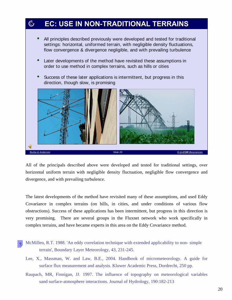
• All principles described previously were developed and tested for traditional settings: horizontal, uniformed terrain, with negligible density fluctuations, flow convergence & divergence negligible, and with prevailing turbulence

• Later developments of the method have revisited these assumptions in order to use method in complex terrains, such as hills or cities

• Success of these later applications is intermittent, but progress in this direction, though slow, is promising

EC: USE IN NONEC: USE IN NON--TRADITIONAL TERRAINSTRADITIONAL TERRAINS

All of the principals described above were developed and tested for traditional settings, over horizontal uniform terrain with negligible density fluctuation, negligible flow convergence and divergence, and with prevailing turbulence.

The latest developments of the method have revisited many of these assumptions, and used Eddy Covariance in complex terrains (on hills, in cities, and under conditions of various flow obstructions). Success of these applications has been intermittent, but progress in this direction is very promising. There are several groups in the Fluxnet network who work specifically in complex terrains, and have became experts in this area on the Eddy Covariance method.

McMillen, R.T. 1988. 'An eddy correlation technique with extended applicability to non- simple terrain', Boundary Layer Meteorology, 43, 231-245.

Lee, X., Massman, W. and Law, B.E., 2004. Handbook of micrometeorology. A guide forsurface flux measurement and analysis. Kluwer Academic Press, Dordrecht, 250 pp.

Raupach, MR, Finnigan, JJ. 1997. The influence of topography on meteorological variables sand surface-atmosphere interactions. Journal of Hydrology, 190:182-213

?

21


• Measures fluxes transported by eddies

• Requires turbulent flow

• Requires state-of-the-art instruments

• Calculated as covariance of w’ and c’

• Many assumptions to satisfy

• Complex calculations

• Most direct way to measure flux

• New developments on the way

EC THEORY: SUMMARYEC THEORY: SUMMARY

The Eddy Covariance is a method to measure vertical flux of heat, water or gases. Flux is calculated as a covariance of instantaneous deviations in vertical wind speed and instantaneous deviations in the entity of interest. The method relies on the prevalence of the turbulent transport, and requires state-of-the-art instruments. It uses complex calculations, and utilizes manyassumptions. However, it is the most direct approach to measuring fluxes. It is rapidly developing its scope and standards, and has promising perspectives for the future use in various natural sciences.

This page is the end of the section on the Eddy Covariance Theory Overview. The practical workflow for the Eddy Covariance method follows.

22


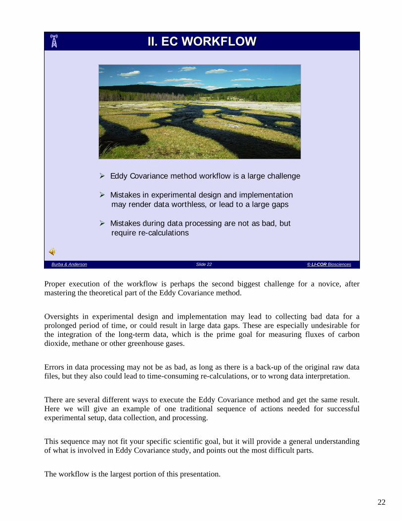
II. EC WORKFLOWII. EC WORKFLOW

Eddy Covariance method workflow is a large challenge

Mistakes in experimental design and implementationmay render data worthless, or lead to a large gaps

Mistakes during data processing are not as bad, butrequire re-calculations

Proper execution of the workflow is perhaps the second biggest challenge for a novice, after mastering the theoretical part of the Eddy Covariance method.

Oversights in experimental design and implementation may lead to collecting bad data for a prolonged period of time, or could result in large data gaps. These are especially undesirable for the integration of the long-term data, which is the prime goal for measuring fluxes of carbon dioxide, methane or other greenhouse gases.

Errors in data processing may not be as bad, as long as there is a back-up of the original raw data files, but they also could lead to time-consuming re-calculations, or to wrong data interpretation.

There are several different ways to execute the Eddy Covariance method and get the same result. Here we will give an example of one traditional sequence of actions needed for successful experimental setup, data collection, and processing.

This sequence may not fit your specific scientific goal, but it will provide a general understanding of what is involved in Eddy Covariance study, and points out the most difficult parts.

The workflow is the largest portion of this presentation.

23


Decide on hardware(instruments, tower etc.)

Decide on software(collection, processing)

Establish location

Place tower

Place instruments

Collect data

Convert Units

Detrend*

Despike

Correct for time delay

Apply calibrations

Apply corrections

Quality Control & Fill-in

Integrate

Analyze/Publish

Average

designdesign implementimplement processprocessinstant datainstant data

averagedaveraged

Set purpose & variables

Test data retrieval

Test data collection

Keep up maintenance

Make maintenance plan

Rotate

TYPICAL WORKFLOW EXAMPLETYPICAL WORKFLOW EXAMPLE

There are several different ways to execute the Eddy Covariance Method and get the same result. Here we give an example of one traditional sequence of actions needed for successful experimental setup, data collection, and processing. One could break the workflow into three major parts: design of the experiment, implementation, and data processing.

The key elements of the design portion of Eddy Covariance experiments are: setting the purpose and variables for the study, deciding on the hardware to be used, creating new or adjusting existing software to collect and process data, establishing appropriate experiment location and a feasible maintenance plan.

The major elements of the implementation portion are: placing the tower, placing the instruments on the tower, testing data collection and retrieval, collecting data, and keeping up the maintenance schedule.

The processing portion includes: processing the real time, “instant” data (usually at a 10-20 Hz sample rate), processing averaged data (usually from one half to two hours), quality control, and long-term integration and analysis.

The main elements of data processing include: converting voltages into units, de-spiking, applying calibrations, rotating the coordinates, correcting for time delay, de-trending if needed, averaging, applying corrections, quality control, filling-in the gaps, integrating, and finally, data analysis and publication.

pp.8-18 inhttp://www.fluxnet-canada.ca/pages/protocols_en/measurement%20protocols_v.1.3_background.pdf -Fluxnet-Canada Measurement Protocols. Working Draft. Version 1.3. 2003.

http://www.geos.ed.ac.uk/homes/rclement/PHD Clement R. 2004. Mass and Energy Exchange of a Plantation Forest in Scotland Using Micrometeorological Methods.

?

24


Purpose and Variables

Hardware

Software

Location

Maintenance plan

Instrument Requirements

Overall Instrumentation

LI-7500

LI-7000

Auxiliary Measurements

EXPERIMENT DESIGNEXPERIMENT DESIGN

Setting the scientific purpose for the experiment will help to determine the list of variables needed

to satisfy that purpose. Variables, in turn, will help to determine what instruments should be used,

and what measurements should be conducted and how.

The scientific purpose may also help to determine the requirements for the specific site, location of

the tower within the site, and instrument placement at the tower.

Once the scientific purpose is adequately defined, data collection and processing programs can be

written or adjusted to accommodate the previously outlined steps, and to process the data.

http://www.cdas.ucar.edu/may02_workshop/presentations/C-DAS-Lawf.pdf - B. Law, 2006.

Flux Networks – Measurement and Analysis?

25


PURPOSE AND VARIABLESPURPOSE AND VARIABLES

Eddy Covariance is a statistical way to compute turbulent fluxes, and

can be used for number of different purposes

Each experimental purpose may require particular settings and a list

of variables for computing and correcting fluxes of interest

Researchers should be aware of the particular requirements, make a

list of required variables, and plan accordingly for a specific project

Eddy Covariance is a statistical method to compute turbulent fluxes, and it can be used for many different purposes. Each experimental purpose will require unique settings and a different list of variables that will be needed for computing and correcting the fluxes of interest. The researcher should be keenly aware of the particular requirements for their experiment, make a list of the variables required, and plan accordingly to insure a successful outcome.

For example, if the main interest of the experiment is in turbulence characteristics of the flow above the wind-shaken canopy, one may not need to collect water and trace gas data, but may need to collect higher frequency (20+ Hz) wind components and temperature data. Instruments may need to be placed on several different levels, including those very close to the canopy.

On the other hand, if one is interested in the response of the evaporation from an alfalfa field to the nitrogen regime, there may not be a need for profiles of atmospheric turbulence, and 10 Hz data may be good enough for sampling. However, such a study would definitely require instantaneous measurements of water vapor along with sonic measurements well above the canopy, but within the fetch for the studied field.

Another example is computing CO2 net ecosystem exchange. This may require not only instantaneous wind speed and CO2 concentration measurements, but also latent and sensible heat flux measurements (for Webb-Pearman-Leuning term), mean temperature, mean humidity and mean pressure (for unit conversions and other corrections).

Mean CO2 concentration profiles would also be highly desirable for computing the CO2 storage term.

26


Air flow can be imagined as a horizontal flow of numerous rotating eddies of different sizes distributed by measurement height:

Lower to the ground – small eddies prevail and transfer most of the fluxHigher above the ground – large eddies prevail and transfer most of the flux

Small eddies rotate at high frequencies, and larger ones rotate slower

Good instruments should be made universal:

Sample fast enough to cover all required frequency ranges Be very sensitive to small changes in quantities Not break large eddies with bulky structure for accurate measurementNot create many small eddies with structureNot average small eddies by large sensing volume

Tower should not be too bulky to obstruct the flow or shadow the sensors

INSTRUMENT REQUIREMENTSINSTRUMENT REQUIREMENTS

Air flow can be imagined as a horizontal flow of numerous rotating eddies of different sizes roughly distributed over the measurement height. Lower to the ground small eddies usually prevail, and they transfer most of the flux. Higher above the ground large eddies transfer most of the flux. Small eddies rotate at very high frequencies, and large eddies rotate slower.

For these reasons, good instruments to use for Eddy Covariance need to be “universal”. They need to sample fast enough to cover all required frequency ranges, but at the same time they need to be very sensitive to small changes in quantities. Instruments should not break large eddies with a bulky structure so they can measure accurately at great heights, and they should be aerodynamic enough to minimize the creation of many small eddies from the instrument structure so they can measure accurately at low heights. They should not average small eddies by using large sensing volumes.

The tower and instrument installation should not be too bulky as to avoid obstructing the flow or shadowing of the sensors from the wind.


http://www.campbellsci.com/documents/manuals/opecsystem.pdf Campbell Scientific, Inc. 2004-2006. Open Path Eddy Covariance System Operator’s Manual CSAT3, LI-7500, and KH20.

?

!

27


Omni-directional Sonic Anemometer

Open Path CO2 / H2O Gas Analyzer

Closed Path CO2 / H2O Gas

Analyzer IntakeFine-wire

Thermocouple

Inclinometer

EDDY COVARIANCE INSTRUMENTATIONEDDY COVARIANCE INSTRUMENTATION

The instrumentation shown in this image is typical of an Eddy Covariance installation, with a 3-dimensional sonic anemometer, an open-path gas analyzer, sample inlet for a closed-path gas analyzer, and a fine-wire thermocouple.

The gas and temperature sensors should be positioned at or slightly below the sonic anemometer. The horizontal separation between the sonic and other sensors should be kept to a minimum, preferably not exceeding 10 to 15 cm. Instrument arrangement should also minimize distortion of the flow going into the sonic anemometer. In the case of open path gas analyzer, the sensor head could be tilted to minimize the amount of precipitation accumulating on the windows.

A very useful field guide on the installation and maintenance of Eddy Covariance instrumentation can be found on the Campbell Scientific web-page:


?

28


Sonic Anemometer

• Uses difference in time it takes for an acoustic signal to travel the same path in opposite directions

• ATI, Campbell, Metek, R.M. Young, Koshin-Denki, Gill Instruments, etc.

Gas Analyzer

• Non-dispersive infrared (NDIR) sensor

• Broadband infrared beam transmitted through cell, with absorption band of 4.26 µm for CO2 & 2.59 µm for H2O

• Beam is modulated to distinguish it from the background using a chopper wheel

Fc = (m s-1) x (mg m-3) = mg m-2 s-1

MEASUREMENT PRINCIPLESMEASUREMENT PRINCIPLES

A sonic anemometer measures the speed of sound in air using a short burst of ultrasound transmitted via a transducer. Another transducer then picks up the reflections of the sound. The delay between the transmitted burst time and the received time could be converted to the speed of sound if the distance between transducers is known. Such perceived speed of sound is actually the speed of sound in static air plus or minus the speed of the wind. In other words, the wind speed causes the difference between the measured speed of sound and the actual speed of sound. The speed of sound in static air is well-known, and depends mostly on the temperature, and to lesser extend, on humidity and gas mixture. Sonic temperature can also be calculated from the speed of sound measured by the anemometer.

Modern fast-response instruments measuring carbon dioxide and water vapor densities utilize absorption of radiation in the infrared region of the electromagnetic spectrum.

Examples of CO2 and H2O NDIR gas analyzers include the LI-COR LI-7000 and LI-7500.

Helpful guide on the installation and maintenance of Eddy Covariance instrumentation: http://www.campbellsci.com/documents/manuals/opecsystem.pdf Campbell Scientific, Inc. 2004-2006. Open Path Eddy Covariance System Operator’s Manual CSAT3, LI-7500, and KH20.

?

29


SONIC ANEMOMETERSSONIC ANEMOMETERS

• Proper installation, leveling and maintenance are important

• Should be installed on firm base facing prevailing wind direction

• Each instrument reacts differently to light rain events, but none

produces accurate readings in heavy precipitation

• Rain, dew, snow and frost on the sonic transducer may change

path length to estimate speed of sound and lead to small errors

Proper installation. leveling and maintenance are important for sonic anemometers. This includes

maintaining a constant orientation to minimize angle of attack errors and keeping the transducers

clean to minimize sonic errors. Each instrument model reacts differently to light rain events, but

none produces accurate readings in heavy precipitation. Rain, dew, snow and frost on the sonic

transducer may change path length to estimate speed of sound and lead to small errors. The

instrument should also be installed on a firm support facing the mean wind direction to minimize

vibration and flow distortion.

http://www.campbellsci.com/documents/manuals/opecsystem.pdf Campbell Scientific, Inc.

2004-2006. Open Path Eddy Covariance System Operator’s Manual CSAT3, LI-7500,

and KH20.

?

30


OPEN VS. CLOSED PATHOPEN VS. CLOSED PATH

50 W (10W + 40 W pump)10 WPower

24-48 hours, could be automated

weeks to months, manual

Calibration

limited by anemometerover 30%Data lost during precipitation

moderate, user cleanableeasy, user cleanableCell cleaning

frequency dampeningspatial separationFlux losses are due to

Closed PathLI-7000

Open PathLI-7500

The choice of an open-path versus a closed-path sensor is largely a function of power availability and frequency of precipitation events.

Closed-path gas analyzers require the sample air to be mechanically drawn to the sample cell by means of a high flow rate air pump, thus increasing system power requirements. The limiting factors in closed-path installation are the capability of the sonic anemometer to operate during precipitation events, and loss of flux due to tube attenuation.

The open-path analyzer measures in situ gas. No external air pump is required thus reducing power consumption. Open path analyzers flux loss are largely due to spatial separation between the sonic and the open path analyzer and due to rain events. Flux calculation based on in-situ density measurement require significant density corrections.

31


LILI--7500 SPECIFICATIONS7500 SPECIFICATIONS

The specifications for the widely-used LI-7500 analyzer are shown in this slide. Designed

specifically for Eddy Covariance applications, this instrument makes sensitive open-path high

speed measurements of in-situ densities of CO2 and H2O vapor. A wide operating temperature

range allows for deployment in any of the world’s ecosystems and data collection interfaces have

been optimized for computers and rugged data loggers.

Further details on the specifications of LI-7500 can be found in the LI-7500 manual:

ftp://ftp.licor.com/perm/env/LI-7500/Manual/LI-7500Manual_V4.pdf

Additional information, updates and downloadable software can also be found at the LI-COR LI-

7500 web-site: http://www.licor.com/env/Products/GasAnalyzers/7500/7500.jsp

?

32


LILI--7500 PERFORMANCE7500 PERFORMANCE

The resolution and performance of the LI-7500 has been optimized for Eddy Covariance applications. The LI-7500 is a single beam dual waveband gas analyzer. It has a single optical path, and continuously alternates between absorbing and non-absorbing wavelengths passing through the sample path by using achopper wheel rotating at 152 times per second to modulate the IR source. Digital signal processing techniques demodulate the signal and convert the raw values into number density.

LI-COR has recently conducted research to investigate an apparent uptake of CO2 during the off-season measured by open-path CO2 analyzers. Results show strong evidence that energy dissipated in the analyzer head can heat a portion of the air in the optical path, and can lead to a small reduction in the release or a small increase in the uptake of CO2. This phenomenon is manifested, at times, as an apparent CO2 uptake and may result in a systematic bias in the estimates of CO2 transport to and from the atmosphere. It is important to note that this effect is most pronounced in colder climates during the winter months, especially below -10 C, and has little impact on data collected in warmer climates.

Detailed description of this phenomena and related correction are below: http://www.licor.com/env/Products/GasAnalyzers/7500/documents/WPLcorrection_canflux.pdf

Overall details on the performance of the LI-7500 can be found in the LI-7500 manual: ftp://ftp.licor.com/perm/env/LI-7500/Manual/LI-7500Manual_V4.pdf

Additional information, updates and downloadable software can also be found at: http://www.licor.com/env/Products/GasAnalyzers/7500/7500.jsp

?

33


TERRESTRIAL AIRBORNE OCEANOGRAPHIC

98% of applications

Designed for stationaryuse

Limited by precipitation, fog, & dew

<1% of applications

Not recommended w/o customized enforcement

Limited by temperature and vibrations

< 1% of applications

Not recommended w/o customized coating, LPS3

Limited by precipitation, dew, & gyroscopic effects

LILI--7500 FLUX APPLICATIONS7500 FLUX APPLICATIONS

A majority of the LI-7500 applications are focused around terrestrial flux applications and widely used by flux networks. Though such applications are usually not associated with vibration issues, airborne and oceanographic installations can experience severe vibration.

It is important to know that the LI-7500 is vibration sensitive to frequencies of 152 Hz ± the bandwidth. Thus, if the bandwidth is 10Hz, the problematic frequency range will be 142 to 162 Hz (and upper harmonics). The instrument is nearly completely insensitive to vibrations slower than this, and only very slightly sensitive to vibrations higher than this.

In land-based installations, a potential source of vibrations could be a light, tall tower with tight guy wires attached at the top. Vibration can be minimized by a larger number of guy wires including ones attached at the middle of the tower. In other settings (aircraft, ships, etc.) vibration can be minimized through appropriate compensating and mounting attachments.

Additional information, updates and downloadable software can be found at the LI-COR LI-7500 web-site: http://www.licor.com/env/Products/GasAnalyzers/7500/7500.jsp

Details on the specific topic related to use of LI-7500 could also be found in the LI-7500 manual: ftp://ftp.licor.com/perm/env/LI-7500/Manual/LI-7500Manual_V4.pdf

?

!

34


Power: +10 to +30VDC @ 2 AmpsRS-232: 9600 to 38,400 (N 81)SDM: Specifically for Campbell Scientific data loggersDAC: To data logger or sonic anemometer analog inputsAUX: Temperature or pressure input

LILI--7500 WIRING7500 WIRING

The LI-7500 has five connections on the bottom of the interface box. One connection is for power and four are for data interface options. Two of the data interfaces are bi-directional digital signals and two are analog representations of the measurement data. The LI-7500 requires an input voltage of +10 to +30 volts DC. Initial current draw can be as high as 2 amps, but typically goes down to less than 1 amp after thermoelectric devices in the sensor head reach the preset temperatures.

RS-232 is a serial interface for connection to computers. Baud rates are available at 9600, 19,200 and 38,400 bits per second. The syntax is documented in the instruction manual for customers who wish to write their own interface software. A Windows application is included for configuration and real time viewing of measurements.

SDM, Synchronous Device for Measurement, is available for connection to Campbell Scientific data loggers. This software-addressable mode includes error checking on data packets with data transfer rates up to 40 times per second or higher. The SDM address must match data logger instruction’s address used to poll the LI-7500 for data. In this mode the data logger synchronizes measurement data from the LI-7500 and sonic anemometer.

Two channels are available for Digital to Analog Conversion, or DAC. This interface is for connection to data loggers or sonic anemometers supporting analog input. The output signal is a user scaleable 0 to +5 VDC signal, and is updated at 300 times per second.

The LI-7500 can measure incoming linear voltage signals representing temperature and pressure with analog auxiliary input. These are primarily used for user zero and span sessions.

Further details on the wiring of LI-7500 can be found in the LI-7500 manual: ftp://ftp.licor.com/perm/env/LI-7500/Manual/LI-7500Manual_V4.pdf

Additional information, updates and downloadable software can also be found at the LI-COR LI-7500 web-site: http://www.licor.com/env/Products/GasAnalyzers/7500/7500.jsp

?

35


LILI--7500 CALIBRATION7500 CALIBRATION

• Factory determined calibration coefficients are good for years

• The zero and span settings make the analyzer's response agree with its previously determined factory response at a minimum of two points

• Calibration requires manual interaction because shroud must be inserted into optical path

Factory determined polynomial calibration coefficients are usually good for several years. However, periodic setting of zero and span is recommended to make sure the instrument performs correctly. The zero and span settings make the analyzer's response agree with its previously determined factory response at a minimum of two points. The calibration requires manual interaction because a shroud must be inserted into the optical path.

Further details on the calibration of the LI-7500 can be found in the LI-7500 manual: ftp://ftp.licor.com/perm/env/LI-7500/Manual/LI-7500Manual_V4.pdf


?

36


• Sample at a rate twice the frequency of physical significance of data

to avoid aliasing

• LI-7500 signals are available at 300 Hz for DAC, 40 Hz for SDM and

20 Hz for RS-232

• Bandwidth setting of 5, 10 or 20 Hz means minimum sampling rate of

10, 20 and 40 Hz respectively

LILI--7500 SAMPLING FREQUENCY7500 SAMPLING FREQUENCY

It is generally recommended to sample at a rate twice the frequency of physical significance of the data to avoid aliasing. Sampling at a rate of 10 or 20 Hz is usually adequate for most land applications, while higher frequencies may be required for airborne applications and in special circumstances (e.g., at very low heights, understory, etc.).

To accommodate a wide range of potential uses, The LI-7500 signals are available at 300 Hz for DAC, 40 Hz for SDM and 20 Hz for RS-232 connections. Bandwidth setting of 5, 10 or 20 Hz indicates a minimum sampling rate of 10, 20 and 40 Hz respectively.

Further details on the sampling by LI-7500 can be found in the LI-7500 manual:

ftp://ftp.licor.com/perm/env/LI-7500/Manual/LI-7500Manual_V4.pdf


?

37


LILI--7000 SPECIFICATIONS7000 SPECIFICATIONS

The specifications for a closed-path LI-7000 analyzer are shown in this slide. This instrument is a high performance, dual cell, differential gas analyzer. It uses a dichroic beam splitter and two separate detectors to measure infrared absorption by CO2 and H2O in the same gas stream. The optical bench can be dismantled and cleaned by the user without the need for factory recalibration.

Further details on the specifications of LI-7000 can be found in the LI-7500 manual: http://www.licor.com/env/Products/GasAnalyzers/7000/documents/LI7000_Manual_V2.pdf


?

38


TERRESTRIAL OCEANOGRAPHICAIRBORNE

Continuous use in flux networks

Limited by sonic dataduring precipitation

Sea-air water and CO2 flux

Interference from gyroscopic effects

Housed in aircraft, air pulled into sample cell

Measurements taken for short time periods

LILI--7000 GEOGRAPHIC USE7000 GEOGRAPHIC USE

Many of the LI-7000 applications are used in terrestrial flux applications in flux networks. Airborne and oceanographic installations are also common.

In land-based installations, the performance is usually limited by sonic anemometer performance during rain and snow events. Airborne and oceanographic applications may require special mounting attachments to compensate for gyroscopic effects, such as wake and heave.


Further details on the deployment and use of LI-7000 in the field are in the LI-7000 manual:

http://www.licor.com/env/Products/GasAnalyzers/7000/documents/LI7000_Manual_V2.pdf

?

39


• An environmental enclosure is required for the LI-7000 to shelter the

instrument from precipitation and dust

• Temperature control is highly advisable to minimize potential span drift

with temperature and to avoid overheating of the instrument which is

designed for temperatures from 0 to +55°C

• All connections should be tested for leaks after instrument installation

and before data collection

LILI--7000 INSTALLATION7000 INSTALLATION

An environmental enclosure is required for the LI-7000 to shelter the instrument from precipitation and dust. Temperature control is also highly advisable to minimize potential span drift with temperature and to avoid overheating of the instrument. It is designed for temperatures from 0 to +55°C.

Leak tests should be provided for all instrument connections after the instrument is installed and before data collection. The simplest leak test can be done by breathing around the instrument connections and away from the intake, and making sure that the CO2 signal does not increase.

Further details on the installation of LI-7000 in the field are in the LI-7500 manual:



?

!

40


• Analog: 4 user-scalable 14 bit DACs, 600 Hz update frequency; feed into

high speed data logger or sonic anemometer

• Auxiliary input channels: 2, ±2.5V, 10 Hz bandwidth; could feed w signal

from sonic anemometer into this input

LILI--7000 ANALOG WIRING7000 ANALOG WIRING

Details on the analog wiring of an LI-7000 in the field can be found in the LI-7000 manual:


Additional information, updates and downloadable software can also be found at the LI-COR LI-7000 web-site:

http://www.licor.com/env/Products/GasAnalyzers/7000/7000.jsp

?

41


• RS-232: 9600-115200 baud, 8, N, 1; supports XON/XOFF & trigger input

• USB: 2.0 compliant; PC must run Windows® 2000 or XP to support USB

• Serial data rates to 50 Hz; instrument grammar is published

LILI--7000 DIGITAL WIRING7000 DIGITAL WIRING

Details on the digital wiring for an LI-7000 in the field can be found in the LI-7000 manual:




?

42


LILI--7000 CALIBRATION7000 CALIBRATION

• Polynomial calibration coefficients determined at the factory are

typically valid for several years

• The zero and span settings make the analyzer's response agree

with its previously determined factory response at a minimum of

two points

• Closed-path instruments could be configured for automatic routine

calibrations

Factory determined polynomial calibration coefficients are usually good for several years. However, periodic setting of zero and span is recommended to make sure the instrument performs correctly. The zero and span settings make the analyzer's response agree with its previously determined factory response at a minimum of two points. The system could be configured for automatic hourly, daily or weekly calibrations.

Further details on the calibration of LI-7000 in the field can be found in the LI-7000 manual:




?

43


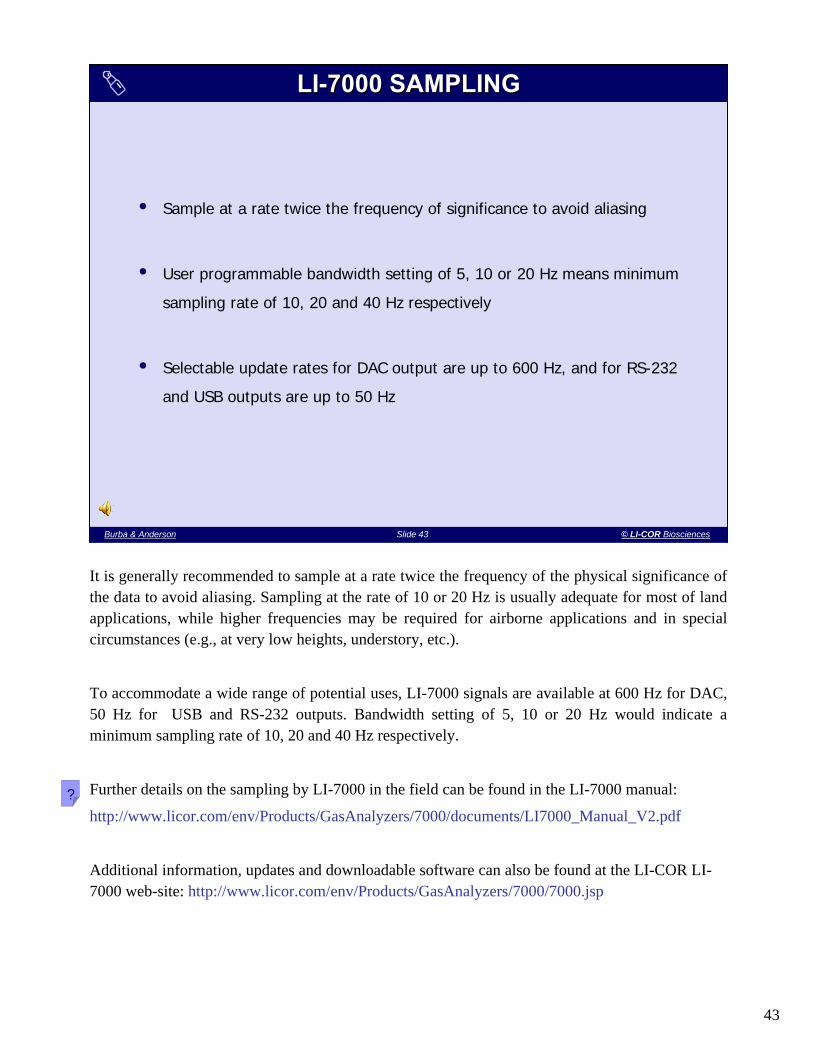
• Sample at a rate twice the frequency of significance to avoid aliasing

• User programmable bandwidth setting of 5, 10 or 20 Hz means minimum

sampling rate of 10, 20 and 40 Hz respectively

• Selectable update rates for DAC output are up to 600 Hz, and for RS-232

and USB outputs are up to 50 Hz

LILI--7000 SAMPLING7000 SAMPLING

It is generally recommended to sample at a rate twice the frequency of the physical significance of the data to avoid aliasing. Sampling at the rate of 10 or 20 Hz is usually adequate for most of land applications, while higher frequencies may be required for airborne applications and in special circumstances (e.g., at very low heights, understory, etc.).

To accommodate a wide range of potential uses, LI-7000 signals are available at 600 Hz for DAC, 50 Hz for USB and RS-232 outputs. Bandwidth setting of 5, 10 or 20 Hz would indicate a minimum sampling rate of 10, 20 and 40 Hz respectively.

Further details on the sampling by LI-7000 in the field can be found in the LI-7000 manual:



?

44


• Net radiation - net radiometers based on thermopile sensor

• Shortwave radiation and PAR: LI-200, LI-190SA

• Soil heat flux - soil heat flux plates and thermometers

AUXILIARY MEASURMENTSAUXILIARY MEASURMENTS

• Photosynthesis: LI-6400

• Soil CO2 Flux: LI-8100, LI-8150

• Leaf Area: LI-3000C, LAI-2000

In addition to a sonic anemometer and gas analyzer, the Eddy Covariance technique may require other meteorological, soil and canopy parameters to help validate and interpret Eddy flux data.

The main variables include net radiation and soil heat flux to construct a full energy budget, shortwave radiation and PAR to quantify the incoming light, leaf-level photosynthesis measurements to help interpret Eddy flux patterns, soil flux measurements and green and total leaf area measurements. Above are some examples of such variables and instruments to measure them.

Also important are soil moisture, soil temperature, relative humidity, air temperature, precipitation etc.

45


• Sample fast to cover all required frequency ranges

• Be very sensitive to small changes in quantities

• Not break large eddies by their bulky structure

• Not create many small eddies with rough structure

• Not average small eddies by large path or volume

HARDWARE: SUMMARYHARDWARE: SUMMARY

In summary, the minimum essential requirements for Eddy Covariance instruments include the

following: instruments need to sample fast enough to cover all required frequency ranges, while at

the same time, they need to be very sensitive to small changes in the quantities of interest;

instruments should not break large eddies with by having a bulky structure, and should be smooth

enough to measure well at low heights; they also should not average small eddies by using large

sensing volumes.

http://www.campbellsci.com/documents/manuals/opecsystem.pdf Campbell Scientific, Inc.

2004-2006. Open Path Eddy Covariance System Operator’s Manual CSAT3, LI-7500,

and KH20.

Foken, T. and Oncley, S.P., 1995. Results of the workshop 'Instrumental and methodical problems

of land surface flux measurements'. Bulletin of the American Meteorological Society, 76:

1191-1193

?

46


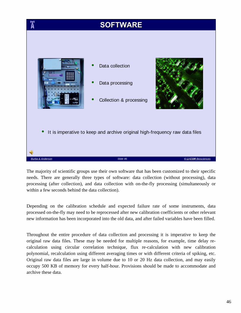
• Data collection

• Data processing

• Collection & processing

SOFTWARESOFTWARE

• It is imperative to keep and archive original high-frequency raw data files

The majority of scientific groups use their own software that has been customized to their specific needs. There are generally three types of software: data collection (without processing), data processing (after collection), and data collection with on-the-fly processing (simultaneously or within a few seconds behind the data collection).

Depending on the calibration schedule and expected failure rate of some instruments, data processed on-the-fly may need to be reprocessed after new calibration coefficients or other relevant new information has been incorporated into the old data, and after failed variables have been filled.

Throughout the entire procedure of data collection and processing it is imperative to keep the original raw data files. These may be needed for multiple reasons, for example, time delay re-calculation using circular correlation technique, flux re-calculation with new calibration polynomial, recalculation using different averaging times or with different criteria of spiking, etc. Original raw data files are large in volume due to 10 or 20 Hz data collection, and may easily occupy 500 KB of memory for every half-hour. Provisions should be made to accommodate and archive these data.

47


• Researchers often write their own software to process their specific data sets

• Recently, comprehensive packages have became available from fluxnetworks, research groups, and manufacturers; some examples are:

Campbell Scientific flux software for data loggersEddysol and EdiRe from University of EdinburgHuskerFlux and HuskerProc from University of NebraskaEC_Processor from University of ToledoEddyMeas & EddySoft from MPI-BGC, Germany TK2.0 from University of BayreuthMASE from Marine Stratus Experiment ETH from Swiss Federal Institute of TechnologyWinFlux from UCSD

• Software and programming can be tested by processing the “GOLD” data file

on the Ameriflux web-site and making sure that results match the “GOLD”

standard output

SOFTWARE (CONTINUED)SOFTWARE (CONTINUED)

Even though researchers often write their own software to process specific data, recently, comprehensive data processing packages have became available from flux networks, research groups and instrument manufacturers.

One example of such a package is EdiRe – a set of comprehensive, flexible, user-definable modulated programs developed by Dr. Robert Clement at the University of Edinburgh. It’s freeware, and can be downloaded from the link given in the notes section.

There are also several other programs including ones from Campbell Scientific, University of Toledo, and the University of Bayreuth in Germany.

Software outputs can be tested by processing the GOLD data file (located on the Ameriflux network web-site), and making sure that results of your data processing code match the GOLD standards. One can also contact Dr. Hank Loescher ([email protected]) for further details on how to use GOLD files.

http://www.geos.ed.ac.uk/abs/research/micromet/EdiRe/ - EdiRe information and downloads.http://public.ornl.gov/ameriflux/sop.shtml - GOLD files location and downloads.http://www.geo.uni-bayreuth.de/mikrometeorologie/ARBERG/ARBERG26.pdf - Mauder, M.

and T. Foken. 2004. Documentation and Instruction Manual of the Eddy Covariance Software Package.

?

48


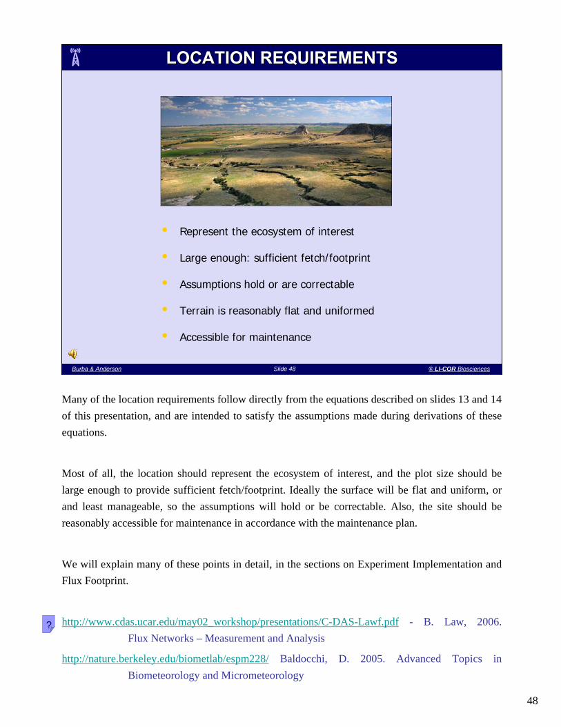
• Represent the ecosystem of interest

• Large enough: sufficient fetch/footprint

• Assumptions hold or are correctable

• Terrain is reasonably flat and uniformed

• Accessible for maintenance

LOCATION REQUIREMENTSLOCATION REQUIREMENTS

Many of the location requirements follow directly from the equations described on slides 13 and 14 of this presentation, and are intended to satisfy the assumptions made during derivations of these equations.

Most of all, the location should represent the ecosystem of interest, and the plot size should be large enough to provide sufficient fetch/footprint. Ideally the surface will be flat and uniform, or and least manageable, so the assumptions will hold or be correctable. Also, the site should be reasonably accessible for maintenance in accordance with the maintenance plan.

We will explain many of these points in detail, in the sections on Experiment Implementation and Flux Footprint.

http://www.cdas.ucar.edu/may02_workshop/presentations/C-DAS-Lawf.pdf - B. Law, 2006. Flux Networks – Measurement and Analysis


?

49


• Sensor cleaning

• Sensor replacement

• Sensor calibrations

• Cable replacements

• System repair

• Maintenance plan is very important to avoid unnecessary data loss

• Each maintenance item may be trivial, while interaction of all

items gets complex: example, 20 sensors to calibrate every year

• One or two spare sensors are desirable for each measurement

MAINTENANCE PLANMAINTENANCE PLAN

After defining the experiment scope and purposes, creating a list of variables and instruments, and selecting the experiment location, but before the actual setup, it is a good idea to create a long-term maintenance plan.

At minimum, a maintenance plan includes: periodic sensor cleaning and replacement, a calibration schedule, planed replacement of damaged cables, and other repairs of the instrument system.

A well designed maintenance plan is very important to avoid unnecessary loss of data in the future, during the data collection process. Each of the maintenance items may seem trivial, however, interaction of all these items gets complex fairly quickly.

For example, a yearly or 6-month recommended factory calibration of 20 different instruments becomes a serious logistical task, and requires optimization of the number of required back-up instruments, trips to the experimental site, and introduces a risk of data loss.

Also if a sensor requires factory service, it may take several weeks, so plans should be made beforehand for a replacement instrument.

In addition to routine maintenance, unforeseen circumstances may complicate the schedule further (fires, lightening strikes, storm damage, rodent damage, power failure, etc.). This is why one or two spare sensors per each variable, and a portable power backup for a few essential measurements are very desirable, especially for remote sites.

The maintenance plan is one on the most overlooked items in the Eddy Covariance setup, especially for first-time users. Proper planning here will help to avoid large potential data losses in the future.!

50


• The design stage is an opportunity to avoid many future complications

• Main parts: purpose, variables, instruments, tower, location, maintenance

• Purpose will determine variables: include all needed for EC corrections

• Variables will determine list of instruments, software needs, infrastructure

• Instruments: fast, sensitive to tiny changes, ‘small’, and ‘aerodynamic’

• Software is generally available, but some portions will have to be written

• Location, desirably: large, flat, uniform, at least - manageable/correctable

• Maintenance plan is a key to good data coverage: needs to be very detailed

EXPERIMENT DESIGN: SUMMARYEXPERIMENT DESIGN: SUMMARY

In summary, the experiment design stage is an opportunity to avoid later complications.

The key parts of the design include defining the purpose, variables, instruments, tower, location, and developing a maintenance plan. The purpose helps to determine a list of variables, including those needed for Eddy Covariance corrections. The list of variables also help to determine the list of instruments, software needs, and infrastructure. Instruments should be fast, sensitive to small changes, ‘small’ in size, and ‘aerodynamic’. Software is generally available, but some portions may have to be written. The site should be large in size, uniform, or at least - manageable. Good maintenance planning is a key to good data coverage, and a well thought out and detailed maintenance plan will be the best insurance that the time invested in the experiment will produce accurate and meaningful data.

51


Placing tower

Placing Instruments

Testing data collection

Testing data retrieval

Collecting data

Keeping up maintenance

EXPERIMENT IMPLEMENTATIONEXPERIMENT IMPLEMENTATION

The Experiment implementation stage comes after the field experiment has been carefully designed and planned.

The main parts of the experiment implementation are: Placing the tower within chosen experiment site, placing instruments of the tower, testing data collection and retrieval processes, collecting scientific data, and keeping up the maintenance.

A particularly good source of the information on tower and instruments set up is available from the AmeriFlux web-site:

http://public.ornl.gov/ameriflux/measurement_standards_4.doc [Munger J.W. and H. W. Loescher. Guidelines for making Eddy Covariance flux measurements]

?

52


• Tower location is restricted by what it

can ‘see’ upwind

• Location should be optimal to represent

ecosystem of interest for most wind

directions or for prevailing winds

• At the very least, location should allow

sampling of representative ecosystem

of interest for prevailing wind directions

TOWER PLACEMENTTOWER PLACEMENT

Tower location is restricted by what it can ‘see’ upwind. If possible, the location of the tower within the site should be optimized to represent the ecosystem of interest for most wind directions, but at the very least, it’s location should represent the ecosystem of interest for the prevailing wind directions.

The size of the area of study, canopy height, and topography may restrict fetch, instrument placement, and thus, affect tower placement criteria. Some helpful information will be given in the following pages, and also can be found in the links in the notes section of this slide:

http://public.ornl.gov/ameriflux/measurement_standards_4.doc - Munger J.W. and H. W. Loescher. Guidelines for making Eddy Covariance flux measurements

http://www.cdas.ucar.edu/may02_workshop/presentations/C-DAS-Lawf.pdf - B. Law, 2006. Flux Networks – Measurement and Analysis

http://www.campbellsci.com/documents/manuals/opecsystem.pdf Campbell Scientific, Inc. 2004-2006. Open Path Eddy Covariance System Operator’s Manual CSAT3, LI-7500, and KH20

Gash, J.H.C. 1986. A note on estimating the effect of limited fetch on micrometeorological evaporation measurements. Boundary-Layer Meteorology 35: 409-413

Horst, T.W., and J.C. Weil. 1994. How far is far enough? The fetch requirement for micrometeorological measurement of surface fluxes. J. Atmos. Oceanic Tech. 11: 1018-1025

?

53


Height of the sensor placement is restricted from both top and bottom:

from the top: By available upwind fetch for area of interest from the bottom: By frequency response errors and corrections

• Sensor located too high may ‘see’ outside the area of interest

• Sensor above boundary layer will ‘see’ flows unaffected by the surface

• Sensor located too low may not register small eddies transferring flux

SENSOR HEIGHT & SAMPLING FREQUENCYSENSOR HEIGHT & SAMPLING FREQUENCY

The height of the sensor placement is restricted from both top and bottom. From the top it is restricted by the available upwind fetch for the area of interest, and from the bottom - by the frequency response errors and related corrections.

A sensor located very high, above the boundary layer, will ‘see’ flows unaffected by the surface. A sensor located too high within boundary layer may ‘see’ some fluxes outside the area of interest. A sensor located too low may see too small of an area and not represent the entire site, and may not register small eddies transporting flux at very high frequencies.

The general rule of thumb is that the measurement height should be 100 times smaller that the desired fetch to avoid sampling outside the area of interest. However during low wind and stable conditions at night, this ratio may grow from 1:100 to 1:500.

The lowest placement height should also be restricted to make sure that the instrument is located above the roughness sub layer. The rule of thumb for the lowest location is that the instrument height should ideally be twice the canopy height. If the terrain is patchy, with scattered bushes or trees, the ratio may need to increase to 5 times the canopy height.

In terms of instrument path length, instrument should be located at the height not less that 5, and desirably, more that 18 times the instrument path length.

Gash, J.H.C. 1986 A note on estimating the effect of limited fetch on micrometeorological evaporation measurements. Boundary Layer Meteorology 35: 409-413


http://www.cdas.ucar.edu/may02_workshop/presentations/C-DAS-Lawf.pdf - B. Law, 2006. Flux Networks –Measurement and Analysis

?

54


EFFECT OF MEASUREMENT HEIGHT (EXAMPLES OF FIELD DATA)

EFFECT OF ROUGHNESS (EXAMPLES OF FIELD DATA)

EFFECT OF THERMAL STABILITY (ADOPTED FROM LITERATURE)OU

TLI

NE

S

FOOTPRINTFOOTPRINT

In very simple terms, flux footprint is the area “seen” by the instrument at the tower. In other words, it is an area upwind from the tower, such that fluxes generated in this area are registered by the tower instruments. Another frequently used term, fetch, usually refers to the distance from the tower when describing the footprint.

Understanding the concept of the flux footprint is essential for proper planning and execution of an Eddy Covariance experiment. Therefore, the next 15 slides will be dedicated exclusively to the concept of footprint, with detailed explanations and practical examples.

First, we will look at how the footprint is affected by measurement height. Then, we’ll look at how the roughness of the surface affects what the instrument could “see”, and finally, how thermal stability affects the footprint.

Burba, G.G., 2001. Illustration of Flux Footprint Estimates Affected by Measurement Height, Surface Roughness and Thermal Stability. In K.G. Hubbard and M.V.K. Sivakumar (Eds.). Automated Weather Stations for Applications in agriculture and Water Resources Management: Current Use and Future Perspectives. World Meteorological Organization publication No.1074. HPCS Lincoln, Nebraska – WMO Geneva, Switzerland, 77-87


Schuepp, P.H., M.Y. Leclerc, J.I. Macpherson, and R.L. Desjardins. 1990. Footprint Predictions of Scalar Fluxes from Analytical Solutions of the Diffusion Equation. Boundary-Layer Meteorology, 50: 355-373

Even more complex situation may exist when area of the footprint is not homogeneous. Schmid, HP, Lloyd, CR. 1999. Spatial representativeness and the location bias of flux footprints over Inhomogeneous areas. Agric. For. Meteorol, 93, 195-209

!

?

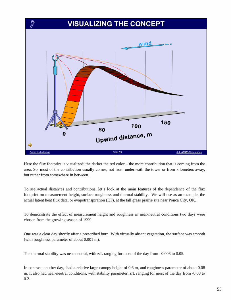
55


050

100150

wind

Upwind distance, m

VISUALIZING THE CONCEPTVISUALIZING THE CONCEPT

Here the flux footprint is visualized: the darker the red color – the more contribution that is coming from the area. So, most of the contribution usually comes, not from underneath the tower or from kilometers away, but rather from somewhere in between.

To see actual distances and contributions, let’s look at the main features of the dependence of the flux footprint on measurement height, surface roughness and thermal stability. We will use as an example, the actual latent heat flux data, or evapotranspiration (ET), at the tall grass prairie site near Ponca City, OK.

To demonstrate the effect of measurement height and roughness in near-neutral conditions two days were chosen from the growing season of 1999.

One was a clear day shortly after a prescribed burn. With virtually absent vegetation, the surface was smooth (with roughness parameter of about 0.001 m).

The thermal stability was near-neutral, with z/L ranging for most of the day from –0.003 to 0.05.

In contrast, another day, had a relative large canopy height of 0.6 m, and roughness parameter of about 0.08 m. It also had near-neutral conditions, with stability parameter, z/L ranging for most of the day from -0.08 to 0.2.

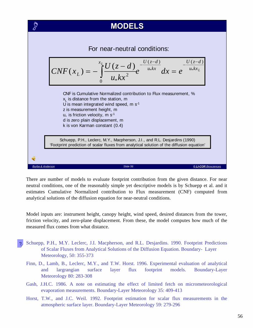
56


CNF x U z du kx

e dx eL

x U z du kx

U z du kx

L

L( ) ( )

*

( ) ( )

* *= −−

=∫−

−−

−

20

CNF is Cumulative Normalized contribution to Flux measurement, %xL is distance from the station, mU is mean integrated wind speed, m s-1

z is measurement height, mu* is friction velocity, m s-1

d is zero plain displacement, mk is von Karman constant (0.4)

Schuepp, P.H., Leclerc, M.Y., Macpherson, J.I., and R.L. Desjardins (1990)‘Footprint prediction of scalar fluxes from analytical solution of the diffusion equation’

For near-neutral conditions:

MODELSMODELS

There are number of models to evaluate footprint contribution from the given distance. For near neutral conditions, one of the reasonably simple yet descriptive models is by Schuepp et al. and it estimates Cumulative Normalized contribution to Flux measurement (CNF) computed from analytical solutions of the diffusion equation for near-neutral conditions.

Model inputs are: instrument height, canopy height, wind speed, desired distances from the tower, friction velocity, and zero-plane displacement. From these, the model computes how much of the measured flux comes from what distance.

Schuepp, P.H., M.Y. Leclerc, J.I. Macpherson, and R.L. Desjardins. 1990. Footprint Predictions of Scalar Fluxes from Analytical Solutions of the Diffusion Equation. Boundary- Layer Meteorology, 50: 355-373

Finn, D., Lamb, B., Leclerc, M.Y., and T.W. Horst. 1996. Experimental evaluation of analytical and largrangian surface layer flux footprint models. Boundary-Layer Meteorology 80: 283-308

Gash, J.H.C. 1986. A note on estimating the effect of limited fetch on micrometeorological evaporation measurements. Boundary-Layer Meteorology 35: 409-413

Horst, T.W., and J.C. Weil. 1992. Footprint estimation for scalar flux measurements in the atmospheric surface layer. Boundary-Layer Meteorology 59: 279-296

?

57


Upwind Distance, m

Cum

ulat

ive

Con

trib

utio

nR

elat

ive

Con

trib

utio

n

ET, m

m d

ay-1

ET, m

m d

ay-1

7/30/99: canopy height = 60 cm

0%

1%

2%

0 100 200 300 400 5000.00

0.03

0.06

0.091.5 m4.5 m

0%

20%

40%

60%

80%

100%

0 100 200 300 400 5000.0

1.0

2.0

3.0

4.0

1.5 m4.5 m

EFFECT OF MEASUREMENT HEIGHTEFFECT OF MEASUREMENT HEIGHT

In this example, the values of latent heat flux that were contributed from the upwind distance are plotted in the figures above.

These plots (and the following similar plots) show how much of the total flux came from each upwind distance such that the integration (area below the curve) of the flux contributions by distance (from zero to infinity) would give the total evapotranspiration from the site.

When measured at the height of 4.5 m, the peak contribution of the ET came from the upwind distance of about 60-65 m, while an area within 20 m from the station did not contribute any of the measured flux. In terms of cumulative contribution, 80% of the total daily flux (3.4 out of 4.2 mm) came from an upwind distance of 20-450 m.

At the height of 1.5 m a dramatic change in the contribution is observed. Peak contribution came from an upwind distance of about 12-18 m. Over 80% of daily ET came from an area within 80 m from the station (versus a 20-450 m zone for the 4.5 m measurement height).


?

58


h=4.5 m h=1.5 m

60% contribution<1% contribution 200 m fetch

200 m

30x30 m fence

HEIGHT: NEAR THE STATIONHEIGHT: NEAR THE STATION

These are the same data as on the previous slide, but plotted as viewed from the top. They demonstrate the potential contribution of the footprint for 4.5 and 1.5 tall towers from all wind directions. The tower is located in the center of each plot.

Looking at the plot on the right, please note how important it is to keep the area around the station undisturbed and representative of the site if the measurement height is low.

59


Footprint strongly increases with measurement height:

at 1.5 m over 80% of the ET came from within 80 m upwind

at 4.5 m over 80% of the ET came from within 450 m upwind

Both sufficient fetch requirement and undisturbed area around instrument are very important for proper footprint at any measurement height

Footprint near the station is also strongly affected:

at 1.5 m, the area 5 m around the instrument did not affect ET

at 4.5 m, the area over 32 m around the instrument did not affect ET

MEASUREMENT HEIGHT SUMMARYMEASUREMENT HEIGHT SUMMARY

Overall, with increased measurement height, the upwind distance to the peak contribution increased (while the magnitude of the peak contribution reduced). The upwind distance covered by the station increased dramatically, as did a zone of “no contribution” around the station.

An important practical implication of the effect of the measurement height on flux footprint is that both sufficient fetch and an undisturbed area around the instrument are very important for the proper footprint at a given measurement height.

!

60


Upwind Distance, m

Cum

ulat

ive

Con

trib

utio

nR

elat

ive

Con

trib

utio

n

7/30/99: canopy height = 60 cm; and 4/8/99: canopy height <5 cm

0%

1%

2%

0 100 200 300 400 500

Canopy height is 0.6 m

Canopy height is <0.05 m

0%

20%

40%

60%

80%

100%

0 100 200 300 400 500


Canopy height is <0.05 m

EFFECT OF ROUGHNESSEFFECT OF ROUGHNESS

The effect of roughness on the flux station footprint is demonstrated in these figures.

For the 1.5 m measurement height, the largest contribution came from 12-18 m (2% of ET) on the day with relatively high roughness (canopy height 60 cm).

For the same measurement height on the day with low roughness (canopy height <5 cm), the peak contribution shifted to about 30-35 m of upwind distance, and was 2 times smaller (0.01% of ET).

In terms of cumulative contribution (the lower figure), for a rough surface, over 80% of the ET (3.4 out of 4.2 mm) came from within 80 m upwind, while for a smooth surface the same contribution came from within 250 m.


?

61


Smooth Rough

60% contribution<1% contribution 200 m fetch

200 m

30x30 m fence

ROUGHNESS: NEAR THE STATIONROUGHNESS: NEAR THE STATION

These are the same data as on the previous slide, plotted as viewed from the top. They demonstrate the potential contribution of the footprint for smooth and rough surfaces from all wind directions. The tower is located in the center of each plot.

The “no contribution” zone was within 5 m around the station for the rough surface, and 10 m for the smooth surface.

Please note again how important it is to keep the area around the station undisturbed under both roughness conditions.

62


Footprint decreases with increased roughness:

at the sensor height of 1.5 m: for rough surface over 80% of the ET came from within 80 m upwindfor smooth surface 80% of ET came from about 300 m upwind

Both sufficient fetch requirement and undisturbed area around instrument are very important for proper footprint at any roughness

Footprint near the station is also affected by roughness:

for rough surface area 5 m around the instrument did not affect ETfor smooth surface area 10 m around the instrument did not affect ET

ROUGHNESS SUMMARYROUGHNESS SUMMARY

Overall, with increased roughness, upwind distance to the peak contribution decreased, the magnitude of the peak contribution increased, while the upwind distance covered by the station and the zone of “no contribution” shrunk in size, as compared to the “smooth” surface.

An important practical implication of the effect of the roughness on flux footprint is that both sufficient fetch and an undisturbed area around the instruments are very important for the proper footprint at any roughness.

!

63


Upwind Distance, m

Rel

ativ

e C

ontr

ibut

ion

Rel

ativ

eC

ontr

ibut

ion

0%

1%

2%

0 100 200 300 400 500

1.5 m4.5 m

0%

1%

2%

0 100 200 300 400 500

1.5 m4.5 m

‘SM

OO

TH’

‘RO

UG

H’

HEIGHT AT DIFFERENT ROUGHNESSESHEIGHT AT DIFFERENT ROUGHNESSES

Here, the contribution from the upwind distance for different measurement heights is shown for the “smooth” surface in top figure, and for the “rough” surface in bottom figure.

For the “rough” surface, the measurement height had a more profound effect on footprint than for the “smooth” surface. The peak contribution increased 3 times with an increase in measurement height on 4/8/99 (for the smooth surface), while for the rough surface, the same increase in measurement height led to a peak contribution increase of 5 times.


?

64


Upwind Distance, m

Rel

ativ

eC

ontr

ibut

ion

Rel

ativ

eC

ontr

ibut

ion

0%

1%

2%

0 100 200 300 400 500


Canopy height is < 0.05 m

0%

1%

2%

0 100 200 300 400 500


Canopy height is < 0.05 m

4.5 m

1.5 m

ROUGHNESS AT DIFFERENT HEIGHTSROUGHNESS AT DIFFERENT HEIGHTS

Contribution from the upwind distance for different roughness is shown for a 4.5 m measurement height in the top figure, and for a 1.5 m measurement height in the bottom figure.

For a 4.5 m measurement height, the peak contribution increased 1.3 times in magnitude and shifted twice as close to the station with increased roughness. For 1.5 m measurement height, the peak increased 2 times (from 0.01 to 0.02 % of ET).

65


HEIGHT AND ROUGHNESSHEIGHT AND ROUGHNESS

For a rough surface, the measurement height has a more profound effect on footprint than for smooth surface

Both factors should be included in calculation for optimal instrument placement

For lower measurement height, the roughness has a more profound effect on footprint than for higher instrument placement

Overall, the rough surface measurement height had a more profound effect on the footprint than for the smooth surface. For a lower measurement height, roughness had an even more profound effect on the footprint than for a higher measurement height.

Therefore, for practical purposes, both measurement height and surface roughness should be regarded for optimal tower positioning and instrument placement.

66


Adopted from Leclerc and Thurtell (1990)Adopted from Leclerc and Thurtell (1990)

Upwind Distance, m

Rel

ativ

eC

ontr

ibut

ion

0%

1%

2%

3%

4%

0 100 200 300 400 5000.00

0.06

0.12

0.18Unstable, L<0Neutral, L ~ 0Stable, L>0

ET, m

m d

ay-1

EFFECT OF STABILITYEFFECT OF STABILITY

The effect of stability on the upwind distance contribution of latent heat flux is shown in this figure. (adopted from Leclerc and Thurtell, 1990).

For the same measurement height and roughness, changes in atmospheric stability can expand the footprint several times.

For the height of 1.5 m and a canopy height of 0.6 m, very unstable conditions can lead to most of the flux footprint being within 50 m from the station.

In near-neutral conditions most of the footprint is located between 5 and 250 m from the station.

And during very stable conditions, the area of flux contribution is located between 15 and 500 m upwind.

Leclerc, M.Y., and G.W. Thurtell. 1990. Footprint prediction of scalar fluxes using a Markovian analysis. Boundary-Layer Meteorology 52: 247-258.

?

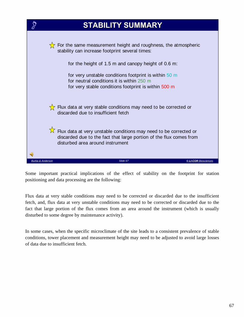
67


STABILITY SUMMARYSTABILITY SUMMARY

For the same measurement height and roughness, the atmospheric stability can increase footprint several times:

for the height of 1.5 m and canopy height of 0.6 m:

for very unstable conditions footprint is within 50 mfor neutral conditions it is within 250 mfor very stable conditions footprint is within 500 m

Flux data at very stable conditions may need to be corrected ordiscarded due to insufficient fetch

Flux data at very unstable conditions may need to be corrected ordiscarded due to the fact that large portion of the flux comes fromdisturbed area around instrument

Some important practical implications of the effect of stability on the footprint for station positioning and data processing are the following:

Flux data at very stable conditions may need to be corrected or discarded due to the insufficient fetch, and, flux data at very unstable conditions may need to be corrected or discarded due to the fact that large portion of the flux comes from an area around the instrument (which is usually disturbed to some degree by maintenance activity).

In some cases, when the specific microclimate of the site leads to a consistent prevalence of stable conditions, tower placement and measurement height may need to be adjusted to avoid large losses of data due to insufficient fetch.

68


FOOTPRINT: SUMMARYFOOTPRINT: SUMMARY

FLUX FOOTPRINT DEPENDS ON:

Measurement heightSurface roughnessThermal stability

AREA NEAR INSTRUMENT TOWER MAY CONTRIBUTE A LOT IF:

Measurement height is lowSurface roughness is highConditions are very unstable

SIZE OF FOOTPRINT INCREASES WITH:

Increased measurement heightDecreased surface roughnessChange in stability from unstable to stable

Flux footprint describes a contributing area upwind from the tower. This is the area that the instruments can “see”.

Flux footprint mainly depends on measurement height, surface roughness and atmospheric thermal stability. The size of the footprint increases with an increase in measurement height, with a decrease in surface roughness, and with changes in thermal stability from unstable to stable.

The area near the tower may contribute a lot, if the measurement height is low, surface roughness is high, or if conditions are very unstable.

It is important to note that both fetch requirement and conditions of the surface in the immediate surroundings of the flux stations can and should be regarded for station placement, maintenance and for data quality control.


Rebmann, C., Göckede, M., Foken, T., Aubinet, M., Aurela, M., Berbigier, P., Bernhofer, C., et al., 2005. Quality analysis applied on eddy covariance measurements at complex forest sites using footprint modeling. Theoretical and Applied Climatology.

Schmid, H.P. 1994. Source areas for scalars and scalar fluxes. Boundary-Layer Meteorology 67: 293-318.Stannard, D.L. 1997. A theoretically based determination of Bowen-ratio fetch requirements. Boundary-Layer

Meteorology 83, 375-406.Swuepp, P.H., Leclerc, M.Y., Macpherson, J.I., and R.L. Desjardins. 1990. Footprint prediction of scalar fluxes

from analytical solution of the diffusion equation. Boundary-Layer Meteorology 50: 355-373.

?

!

69


• Instrument interaction

• Data interruptions

• Power requirements

TESTING DATA COLLECTIONTESTING DATA COLLECTION

Some of the key items to check after the tower and instruments have been set up are instrument interaction, data interruptions, and power conditions.

Since most of the set-ups for Eddy Covariance are made from a number of off-the-shelf instruments, from different manufacturers, it is advisable to make sure that there is no miscommunication, mysterious errors, lockups and other data interruptions when these instruments start interacting. For example, a digital-to-analog converter may need to be reconfigured to accept the signal from a specific instrument.

It is also advisable to assess data interruptions due to weather events, and determine how fast they go away after the event (rain, snow, dew, power interrupt during storm, etc.), and what could be done about it.

Power grid variation, power backup and variation in power consumption are also important items to check, because power load on the tower may vary. One has to make sure that power requirements include the peaks of such variations to avoid blown fuses or deep discharge of backup batteries.

Fluxnet-Canada’s field protocol addresses most of these and other such issues in detail, and can be accessed via PDF file online by following the link: http://www.fluxnet-canada.ca/pages/protocols_en/measurement%20protocols_v.1.3_background.pdf [Fluxnet-Canada Measurement Protocols. Working Draft. Version 1.3. 2003]?

70


• By hand

• Wire

• Wireless

• Daily control

• Online control

TESTING DATA RETRIEVALTESTING DATA RETRIEVAL

Data retrieval is another important process to test. Data can be retrieved by hand by swapping a memory card. They can be delivered by wire through the Internet. The same can be done through wireless Internet or radio.

The better connection one has to the site, the easier it is to do daily control of transmitted data, or online control of the data in real-time.

Properly configured connections may also allow for remote setup of the instruments (change in calibration coefficient, voltage output range, etc.), remote reset of the instrument or PC after lockup, and other numerous useful tasks, saving time and money on travel to the site.

http://www.fluxnet-canada.ca/pages/protocols_en/measurement%20protocols_v.1.3_background.pdf [Fluxnet-Canada Measurement Protocols. Working Draft. Version 1.3. 2003]

?

71


• Important to keep maintenance current for the entire project duration

• Data gaps jeopardize final results

• Events such as lightning, ice storms, wind gusts, and mouse damage will happen

• Spare sensors and emergency protocols are needed to avoid large data losses

KEEPING UP MAINTENANCEKEEPING UP MAINTENANCE

Maintenance is one of the most important parts of the execution of an Eddy Covariance field experiment. This should be done for the duration of the entire project. Planning in the beginning of the experimental design should assure the ability to keep maintenance current.

Events such as lightning, ice storms, wind gusts, and rodent damage are likely to happen several times a year during long-term deployment of the instruments. If not planned beforehand, they may lead to large data gaps.

Each data gap jeopardizes results and affects the final integrated number, so spare sensors and emergency protocols should be a part of routine planning and maintenance to help avoid such data losses.

http://www.fluxnet-canada.ca/pages/protocols_en/measurement%20protocols_v.1.3_background.pdf [Fluxnet-Canada Measurement Protocols. Working Draft. Version 1.3. 2003]

?

!

72


EXPERIMENT IMPLEMENTATION SUMMARYEXPERIMENT IMPLEMENTATION SUMMARY

• Placing tower: maximize useful footprint from all wind directions

• Placing instruments: at a maximum height which still allows useful footprint

• Collecting data: wireless, cable, daily checks

• Testing collection and retrieval: test thoroughly to avoid data gaps

• Maintenance: required throughout the project to avoid data gaps

In summary, experiment implementation requires proper tower and instrument placement, rigorous tests of data collection and retrieval, remote communications with the site, and regular maintenance.

The tower should be placed in such a way that the useful footprint from all wind directions is maximized. If there is one prevailing wind direction, the tower could be placed on the edge of the area of interest to maximize footprint.

Instruments should be placed at maximum height, which still allows for a useful footprint.

Testing the data collection and retrieval should be done thoroughly to avoid data gaps.

Collecting the data should be done by wireless, wire or some other way, preferably allowing for daily checks or even real-time checks.

Maintenance should be kept up throughout the duration of the entire project to avoid collecting bad data over long periods or large data gaps.

73


Instantaneous dataconvert unitsde-spikeapply calibrationsrotatecorrect for time delayde-trendaverage

Averaged dataquality controlfill-inintegrate checkanalyze/publish

Mixed dataapply corrections

DATA PROCESSING & ANALYSISDATA PROCESSING & ANALYSIS

Each research group uses a slightly different way of processing Eddy Covariance data to fit their specific needs, site-specific design, and sampling conditions. Here we will give one particular example of the generalized traditional way to process data. The goal for this method will be to get the flux calculations as close as possible to the reality of what’s actually happening in the field.

The major steps in this process include: converting signals from voltages to physical units; de-spiking; applying calibration coefficients if needed; rotating coordinates; correcting for time delays; de-trending if needed; averaging fast data over 0.5 to 4 hour periods; applying frequency response, density and other corrections; conducting quality control; filling-in missed periods and integrating long-term flux data. It is also recommended to double-check the entire process before analyzing and publishing the data.

There are several useful links in the notes section of this slide as well as several references on the methodology of data processing: http://www.cdas.ucar.edu/may02_workshop/presentations/C-DAS-Lawf.pdf - B. Law, 2006. Flux

Networks – Measurement and Analysishttp://www.fluxnet-canada.ca/pages/protocols_en/measurement%20protocols_v.1.3_background.pdf -

Fluxnet-Canada Measurement Protocols. Working Draft. Version 1.3. 2003Goulden, M.L., Munger, J.W., Fan, S.M., Daube, B.C. and Wofsy, S.C., 1996. Measurements of carbon

sequestration by long-term eddy covariance: Methods and a critical evaluation of accuracy. Global Change Biology, 2(3): 169-182


Twine, T.E. et al., 2000. Correcting eddy-covariance flux underestimates over a grassland. Agricultural and Forest Meteorology, 103(3): 279-300.

?

74


• Check that all units for instantaneous flux calculations are appropriate

and consistent to avoid errors in fluxes/corrections calculated on-line

• Double-check that auxiliary sensors use correct calibration coefficients

to avoid errors in flux corrections, and in mean data

• Some people choose to convert CO2 and H2O signals into mixing ratios

(mol mol-1 dry air) at this stage to avoid the need to apply Web-

Pearman-Leuning correction later on

UNIT CONVERSIONUNIT CONVERSION

Unit conversion involves checking that all of the units for instantaneous outputs are appropriate. Units need to be matched carefully to avoid errors in fluxes calculated on-line or corrections applied later. It is also important to double-check that relevant auxiliary data use the correct calibration equations to avoid errors in flux corrections, or in mean data.

Usually, unit conversion is one of the first steps in processing of the instantaneous data. Some, however, prefer to de-spike the data first, then remove periods with outrageous values, and only then perform unit conversion and the rest of the processing.

If done carefully, such a sequence of steps should yield the same results as the one presented here. However, it is important to note that setting de-spiking criteria on voltages needs to account for non-linearity in some voltage-to-unit conversions. In other words, what may look like a spike in the raw voltage signal may not end up actually being a spike after converting as well as the corollary that what is an actual spike in the converted data may not look like a spike in the raw voltage signal. Therefore the spike criteria may not always be the same for volts and converted units.

Several groups also choose to convert CO2 and H2O signals into mixing ratios (mol mol-1 dry air) at this stage, to avoid the need to apply the Web- Pearman-Leuning correction at a later stage.

It is important to note, however, that point-by-point conversion of the signals to a mixing ratio is associated with large potential uncertainties and errors, because vertical wind measurements and scalar measurements are not done in the same volume, and, because sensor separation and related time delay may change with wind speed and direction within the same averaging period. One needs to be cautious when doing point-by-point corrections, and you may want to compare the results to those with traditional Webb-Pearman-Leuining corrections before finalizing your workflow.

!

75


• High frequency instantaneous data will have occasional spikes due to both electronic and physical noise

• Spikes should be removed and bad points should be replaced with running means to avoid errors in further calculations

• De-spiking can be done on-line immediately after data collection or later during post-processing

• Caution should be used to avoid removing too much data

• Each Eddy Covariance system will have slightly different spike problems

• Researcher should examine instantaneous data periodically to make sure that spike removal is appropriate for the conditions

DESPIKEDESPIKE

High frequency instantaneous data will have occasional spikes due to both electronic noise and some physical reasons.

After these spikes are removed, bad points can be replaced with running means or by some other method to avoid errors in further calculations. The procedure can be done on-line, right after data collection, or during post-processing.

Each Eddy Covariance system will have slightly different spike problems, and the researcher needs to look at instantaneous data periodically to make sure that spike removal criteria are appropriate for the conditions. Caution should be used not to set the criteria too strict, thus removing too much data.

For example, the de-spike criterion could be set to remove signals that are more that 6 times the standard deviation for a given averaging period so that all outliers are considered spikes and removed. While too many spikes usually indicate an instrument or electronic problem, there are conditions, such as nighttime storage release, that may look like spikes, but are in fact natural phenomena.

Vickers, D. and Mahrt, L., 1997. Quality control and flux sampling problems for tower and aircraft data. Journal of Atmospheric and Oceanic Technology, 14: 512-526

Mauder, M. and T. Foken. 2004. Documentation and Instruction Manual of the Eddy Covariance Software Package. http://www.geo.uni-bayreuth.de/mikrometeorologie/ARBERG/ARBERG26.pdf

?

76


• Applying calibration coefficients is not a trivial matter in Eddy Covariance

• Many researchers choose to calibrate closed-path gas analyzers every night

or even more frequently to assure highest data quality

• In such cases, calibration parameters may differ slightly every day and

software should be written to incorporate these changes into the data

• For open-path sensors, calibration coefficients are typically less involved

and with proper factory or lab calibrations every few months, they can

usually be set in the embedded instrument software

CALIBRATION COEFFICIENTSCALIBRATION COEFFICIENTS

Applying calibration coefficients may not be a trivial matter in Eddy Covariance calculations.

Many researchers choose to make a calibration of the closed-path sensor every night, or even more frequently, to assure the highest data quality.

In such cases calibration coefficients will differ a little bit for every day, and the software should be written to incorporate these changes into the data.

For open-path sensors, calibration coefficients are less involved. With proper factory/lab calibration every few months, they can usually be set in the instrument software itself.

77


• Sonic anemometer can not be leveled perfectly, such that its w axis is

exactly perpendicular to the mean flow/mean wind streamlines

• The w signal may be contaminated by other two of 3D wind components

• Several ways

to correct such situation:

1) rotating so that mean w=0

2) using planar fit method

COORDINATE ROTATIONCOORDINATE ROTATION

A sonic anemometer can not be leveled perfectly, such that its w axis is always perpendicular to the mean flow / mean wind streamlines. The w-signal will likely be contaminated by the other two of the 3D wind components. There are traditional and also newer ways to correct this situation. One well-established technique is to rotate the coordinates so that the mean “w” is equal to zero. Another popular way is to use a planar fit method.

Rotation of w’, u’ and v’ at this early stage of data reprocessing may save time at later stages, because one would not need to rotate all the covariance's (e.g. u’w’, w’t’, w’c’, w’q’, etc.).

Useful details on how to do coordinate rotation are provided by Lee, Finnigan and Paw U in Chapter 3 (pp. 33-64) of the Handbook of micrometeorology. A guide for surface flux measurement and analysis. Complete details on the book are available in the notes section of this slide.

It is also important to mention that some models of sonic anemometers may require an additional cross-wind correction before coordinate rotation is done. In other models such a correction is done internally. Please refer to pages 8-9 in the Documentation and Instruction Manual of the Eddy Covariance Software Package for the list of the sonic anemometer models and other details for such corrections, and on pages B-1 - B-2 in Campbell Scientific’s Open Path Eddy Covariance System Operator’s Manual.


http://www.geo.uni-bayreuth.de/mikrometeorologie/ARBERG/ARBERG26.pdf Mauder, M. and T. Foken. 2004. Documentation and Instruction Manual of the Eddy Covariance Software Package.


?

!

78


• Planar fit is somewhat more complex rotation method

• After u, v, and w data have been collected over long period,one could mathematically establish a ‘hypothetical’ plane, so ‘true’vertical flux should be perpendicular to this plane

• It may be particularly helpful when measurements are done over complex terrains (e.g., hillsides, valleys)

• Rotating to ‘mean w=0’ can be done in several stages:

1 stage: rotate to make v=0 (align u and x)2 stage: rotate to make w=0 (align w and z)3 stage: rotate to make w’v’=0 (align z-y plane)–rarely used

COORDINATE ROTATION (CONTINUED)COORDINATE ROTATION (CONTINUED)

Rotating to create a ‘mean w=0’ can be done in several stages: 1st rotation: turn to v=0 (align u and x); 2nd rotation: turn to w=0 (align w and z); 3d rotation: turn w’v’=0 (align z-y plane) – used rarely

The planar fit is a somewhat more complex rotation method, but it may be particularly helpful when measurements are done over complex terrains (e.g., hillsides, valleys). In this method, after u, v, and w data have been collected over a long period, one can mathematically establish a ‘hypothetical’ plane, so that a ‘true’ vertical flux will be perpendicular to this plane. Unlike rotation method, planar fit requires long-term installations with instruments remaining undisturbed over long periods.

A somewhat different approach has been proposed by Wilczak, Oncley, and Stage, in a paper titled “Sonic anemometer tilt correction algorithms.” in Boundary-Layer Meteorology, 1999 pages 127-150.

It is important to mention another anemometer correction: an angle of attack correction that results from an uneven cosine response of some sonic anemometers to the horizontal wind angle. It is not applicable to all anemometers and the correction may be fully or partially applied by manufacturers. Please see factory manuals for the specific anemometer manufacturer and model for details.

Gash, J.H.C., Dolman, A.J., 2003. Sonic anemometer (co)sine response and flux measurement. I. The potential for (co)sine error to affect sonic anemometer-based flux measurements. Agric. For. Meteorol., 119,195–207



van der Molen, M.K., Gash, J.H.C., Elbers, J.A., 2004. Sonic anemometer (co)sine response and flux measurement. II. The effect of introducing an angle of attack dependent calibration. Agric. For. Meteorol., 122,95–109.

?

!

79


• Compensates for time delay in signal acquisition from different instruments

• When using a closed path sensor, air sampled by the sonic anemometer gets to the closed path gas analyzer several seconds later

• Without correcting for this delay, fluctuations in w’ will not correlate with fluctuations in gas concentration, and flux will be drastically underestimated

• Time delay is usually corrected in one of the two ways:

(1) theoretically, via flow rate, tube diameter etc. (2) empirically, by running circular correlation, shifting the delay scan-by-scan until maximum correlation (flux) is found

• For open path sensors time delay may be on the order of a few scans (not seconds), but should still be applied to avoid small flux loss

TIME DELAYTIME DELAY

Matching the time series from a sonic anemometer and from a gas analyzer requires compensating for time delays in the signal acquisition from these instruments.

This is especially true when using a closed path sensor, since air sampled by the sonic anemometer gets to the closed path gas analyzer several seconds later than w-signal. Without correcting for such delays, fluctuations in w’ would not correlate well with fluctuations in gas concentration, and flux could be underestimated or even zeroed.

Time delay is usually corrected in one of the two ways: (1) Theoretically, via the flow rate, tube diameter, etc. or (2) Empirically, by running a circular correlation, and shifting the delay scan-by-scan until a maximum correlation (flux) is found.

For open path sensors time delay may be in the order of a few scans (not seconds), but it also should be compensated for to avoid smaller flux loss.

http://www.geo.uni-bayreuth.de/mikrometeorologie/ARBERG/ARBERG26.pdf - Mauder, M. and T. Foken. 2004. Documentation and Instruction Manual of the Eddy Covariance Software Package.

http://www.fluxnet-canada.ca/pages/protocols_en/measurement%20protocols_v.1.3_background.pdf - Fluxnet-

Canada Measurement Protocols. Working Draft. Version 1.3. 2003

?

80


• Mean values are subtracted from instantaneous values to compute flux

• This requires establishing what would be the mean for given time series

• There are three main ways to look at it and three respective techniques

Block averaging (mean removal)

Linear detrending (linear trend removal)

Non-linear filtering (n-l trend removal)

- Simplest situation- Many prefer this method- May gain artificial flux

- ex., If sensors drift, or - Rapid diurnal changes - May loose some flux

- Complex situation - Same as high pass filter- May loose a lot of flux

DETRENDINGDETRENDING

During de-trending, the mean values are subtracted from instantaneous values to compute flux. This requires establishing what would be the mean for a given time series. There are three main, traditional ways to look at it, along with three respective techniques: block averaging, linear de-trending and non-linear filtering.

Each way may be appropriate for a specific situation. And even though block averaging is the most popular way to de-trend (and sometimes viewed as no de-trending at all), complex terrains and rapid changes in concentrations in some regions may require the use of linear and non-linear filtering. At the same time it is important not to over-filter, because flux contribution in the low frequency part of the co-spectra would be lost as a result of over filtering.

Generally, however, linear and non-linear de-trending is not recommended as it could leave spectral artifacts in the data and could mask improper averaging times.

More information on the best approach to filtering for specific situations can be found in Chapter 2 of the “Handbook of micrometeorology. A guide for surface flux measurement and analysis” and in Baldacci’s article on the web titled “Advanced Topics in Biometeorology and Micrometeorology”:

Chapter 2 by Moncrief, Clement, Finnigan and Meyers (pp. 7-30) of [Lee, X., Massman, W. and Law, B.E., 2004. Handbook of micrometeorology. A guide for surface flux measurement and analysis. Kluwer Academic Press, Dordrecht, 250 pp.]

[http://nature.berkeley.edu/biometlab/espm228/ Baldocchi, D. 2005. Advanced Topics in Biometeorology and Micrometeorology]

Choosing a time constant recursive filter for detrending, especially non-linear, i.e. removing a mean is not the same as choosing an averaging period. However, often people just use block averaging for the same period as averaging.

?

!

81


Use LE1 to apply sonic correction to H: obtain H0

Apply WPL correction to LE0: obtain LE1

Use H1 & u0* to construct co-spectral model M1

Use M1 to apply FR corrections to LE and Fc:

obtain LE2 & Fc0

Use H1 to apply WPL correction to LE2:obtain LE3

Use H1 & LE4 to apply WPLcorrection to Fc0: obtain Fc1

Use M0 to apply frequency response (FR) corrections to raw latent heat flux (LE):

obtain LE0

Apply FR correction to H0: obtain H1 & u0*

Apply O2 & BB correctionto LE3 if needed: obtain LE4

Apply BB correction to Fc1if needed: obtain Fc2

Use raw sensible heat flux (H) & friction wind velocity u* to construct co-spectral

model M0

APPLYING CORRECTIONSAPPLYING CORRECTIONS

Applying corrections can be a complicated and iterative process. Following a fixed sequence of steps is very important. The diagram on this slide gives one example of the workflow for applying the corrections. FR refers to frequency response corrections, WPL – to the Webb-Pearman-Leuning density term, O2 stands for the oxygen correction, and BB stands for the band-broadening correction.

Fortunately, such lengthy sequences are usually done automatically by the processing software, and the user only needs to make sure that the order of steps is appropriate, and that no steps are missing. Please also note that some of the corrections may have been already applied by the instrument manufacturer. Please be sure to consult the factory manuals on this matter.

It appears to be a general consensus that for closed-path measurements, the frequency response corrections are applied before a Webb-Pearman-Leuning correction. For more details refer to Chapter 7 in the “Handbook of micrometeorology. A guide for surface flux measurement and analysis.” We will discuss the details of these corrections in the following slides.

Chapter 7 by Massman (pp. 133-158) in [Lee, X., Massman, W. and Law, B.E., 2004. Handbook of micrometeorology. A guide for surface flux measurement and analysis. Kluwer Academic Press, Dordrecht, 250 pp]

Fuehrer, P.L. and Friehe, C.A., 2002. Flux corrections revisited. Boundary Layer Meteorology, 102:415-457

http://www.eol.ucar.edu/rtf/facilities/isff/heat_fluxes.shtml - Horst, T.W., 2003. Corrections to Sensible and Latent Heat Flux Measurements.

?

82


• Family of corrections compensating for the flux losses at

different frequencies (eddy sizes)

• Number of reasons, all related to sensors and EC system

frequency response

Frequency response corrections:

Time responseSensor separationScalar path averagingTube attenuation High pass filtering Low pass filteringSensor response mismatchDigital sampling

FREQUENCY RESPONSE CORRECTIONSFREQUENCY RESPONSE CORRECTIONS

Frequency response corrections are a family of corrections that compensate for the flux losses at different frequencies of turbulent transport. There are a number of separate reasons for these losses, but all of them are related to the sensor performance and to the frequency response of the Eddy Covariance system. The main frequency response corrections include the following: time response; sensor separation; scalar/vector path averaging; tube attenuation; high pass filtering; low pass filtering; sensor response mismatch; and digital sampling.

Before discussing each of the frequency response corrections, let’s look at an extreme example illustrating the importance of the frequency response in general. Imagine that measurements are taken one foot from the ground with a bulky instrument which has a 100 cm path and a sampling frequency of 5 Hz.

Most of the flux transport at this height would be done by very small eddies at very high frequencies. The described instrument would average out most of the transport in the long path, it would miss a good portion of the transport due to its slow 5 Hz sampling rate, and it may generate a relatively large proportion of its own turbulence that is not representative of the environment of interest. As a result, fluxes may be greatly underestimated even after applying large corrections of the order of several hundred percent. Most real situations will likely be less extreme, but there can still be many factors responsible for missed flux at different frequencies.

One of the cornerstone papers on the subject is by C.J. Moore, titled “Frequency response corrections for eddy correlation systems.” Also, good general resources on the frequency response corrections can be found below:Chapter 4 by Massman, W. and R. Clement (pp. 67-101) in [Lee, X., Massman, W. and Law, B.E., 2004. Handbook

of micrometeorology. A guide for surface flux measurement and analysis. Kluwer Academic Press, Dordrecht, 250 pp.]

Mauder, M. and T. Foken. 2004. Documentation and Instruction Manual of the Eddy Covariance Software Package. http://www.geo.uni-ayreuth.de/mikrometeorologie/ARBERG/ARBERG26.pdf

Moore, C.J., 1986. Frequency response corrections for eddy correlation systems. Boundary-Layer Meteorology, 37: 17-35

?

83


Frequency response corrections are calculated from instantaneous data via

co-spectra (distribution of flux transport by frequency):

Transfer functions describe how each sampling problem would affect ideal

co-spectra at each frequency

0.0001 101

nC(n

)/w

’s’

1

0.01

Area under represents flux

Ideal (H is close)

Actual: H2O, CO2, CH4

Modeled using transfer functions

co-spectra:

Scales: logarithmic

Units: usually non-dimn(z-d)/Uhilo

COCO--SPECTRASPECTRA

As a first step in the frequency response correction process, let’s look at co-spectra. Co-spectra is a distribution of the co-variance of the w’ and scalar by frequency. It is an important component in calculating frequency response corrections. Co-spectra describes how much of the flux is transported at each frequency. It could also be seen as a Fourier transform of the time series into the frequency domain, with the integrated area under the non-dimensional co-spectra curve ideally equal to 1. (representing 100% of the measured flux).

The ideal co-spectra for a given height and condition is usually modeled after Kaimal et al. (1972) and is marked in blue on the plot. Modern sonic anemometers are capable of very fast sampling with small errors over relatively short paths, and, because the instantaneous temperature is derived from the same data as w’, so that no sensor separation or time delay occurs between the two signals, sonic sensible heat flux co-spectra (w’Tsonic’) is often close enough to the ideal to not need correction, especially in the middle of the day with good turbulent exchange.

The actual gas co-spectra curve is usually located below the ideal or sensible heat flux co-spectra, especially at high frequencies. This position of the curve indicates flux losses related to deficiencies in frequency response when measuring co-variances between w’ and instantaneous gas fluctuations. Such deficiencies are due to time response, tube attenuation (for closed path), sensor separation, path averaging, filtering, etc. Functions describing how each of these deficiencies would affect an ideal co-spectra and bring the co-spectra curve down at each frequency are called transfer functions.

Moore, C.J., 1986. Frequency response corrections for eddy correlation systems. Boundary-Layer Meteorology, 37: 17-35.

Kaimal, J.C., Wyngaard, J.C., Izumi, Y. and Coté, O.R., 1972. Spectral characteristics of surface layer turbulence.Quarterly Journal of The Royal Meteorological Society, 98: 563-589

Su, H.-B., Schmid, H.P., Grimmond, C.S.B., Vogel, C.S. and Oliphant, A.J., 2004. Spectral Characteristics and Correction of Long-Term Eddy-Covariance Measurements Over Two Mixed Hardwood Forests in Non-Flat Terrain. Boundary Layer Meteorology, 110: 213-253

?

84


0.0001 101

nC(n

)/w

’s’

1

0.01

Area under represents flux

Ideal (H is close)

Actual: H2O, CO2, CH4

Modeled using transfer functions

Co-spectra:

Scales: logarithmic

Units: usually non-dimn(z-d)/Uhilo

T

1

0.01

Total transfer function:

T=1 – no flux lost at these frequencies

T=0.5 – 50% flux lost at these frequencies

T=0 – 100% flux lost at these frequencies0.0001 101n(z-d)/U

hilo

no flux lost heresome flux lost here

all flux lost here

TRANSFER FUNCTIONSTRANSFER FUNCTIONS

Above is an example of how a transfer function predicts what would happen to the ideal (no loss) co-spectrum at given atmospheric conditions due to diminished frequency response at high frequencies.

Please note how the actual and modeled co-spectra decrease below the ideal co-spectrum when the transfer function goes down from 1 at high frequencies.

The total transfer function is a product of the different transfer functions, each of which describes flux losses at specific frequencies due to a specific reason.

If one knew the effect (or the shape) of the transfer function on the co-spectra, one could correct the shape of the actual co-spectra back to the ideal co-spectra, thus correcting the flux and increasing its magnitude.


Chapter 4 by Massman, W. and R. Clement (pp. 67-101) in [Lee, X., Massman, W. and Law, B.E., 2004. Handbook of micrometeorology. A guide for surface flux measurement and analysis. Kluwer Academic Press, Dordrecht, 250 pp.]

?

85


• Frequency response corrections are applied via transfer functions to:(a) Kaimal-Moore’s co-spectral models, or to (b) actual H co-spectra

• co-spectral models are perhaps more advisable; they are sets of equations (for unstable, stable and neutral conditions)

• Models use stability parameter (z/L), non-dimensional frequency (f=n(z-d)/U), measurement height (z), zero plane displacement (d), and mean wind speed (U) to come up with co-spectral energy per each frequency (nC(n))

• co-spectral models are adjusted for the transfer functions at each frequency, and a correction factor is determined for the entire co-spectrum

• Applying all frequency response corrections can increase fluxes up to 30% or more; correction are often larger at night

APPLYING FREQUENCY RESPONSE CORRECTIONSAPPLYING FREQUENCY RESPONSE CORRECTIONS

In general, frequency response corrections are applied via transfer functions either to Kaimal-Moore’s co-spectral models, or to actual sensible heat flux co-spectra. Using co-spectral models is, perhaps, more advisable, because they are independent of potential errors or instrumental problems with sensible heat flux co-spectra.

co-spectral models are sets of equations for unstable, stable and neutral conditions. They use parameters for: stability (z/L), non-dimensional frequency (f=n(z-d)/U), measurement height (z), zero plane displacement (d), and mean wind speed (U), to come up with co-spectral energy for each frequency (nC(n)).

The co-spectral model is adjusted for the transfer functions at each frequency, and a correction factor is determined for the entire co-spectrum based on the integrated area under the actual co-spectra curve in comparison with the ideal co-spectra (a value of 1).

Applying all frequency response corrections could increase fluxes by up to 30% or more, especially at night.

It is also important to note, there is an alternative method to computing frequency response corrections proposed by Bill Massman in a paper titled “A simple method for estimating frequency response corrections for eddy covariance systems.” A complete reference is listed in the notes section.

Moore, C. 1986. Frequency response corrections For eddy covariance systems. Boundary Layer Meteorology. 37, 17-35

Kaimal, J.C., Wyngaard, J.C., Izumi, Y. and Coté, O.R., 1972. Spectral characteristics of surface layer turbulence. Quarterly Journal of The Royal Meteorological Society, 98: 563-589


?

!

86


• To compensate for the loss of flux due to inability of sensors to respond fast enough to small fluctuations which contribute to the flux

• Time response transfer function is applied to fluxes of H2O, CO2, CH4

2)2(11)(

τπτ

nnT

+=

Tτ – transfer function for time responsen - frequencyτ – dynamic time response of the sensor

TIME RESPONSETIME RESPONSE

Let’s briefly go through the frequency response corrections and the associated transfer functions one-by-one, and construct a total transfer function required for the correction factor that was described on the previous slide.

The first one is a time response correction. This correction compensates for the loss of flux due to the inability of sensors to respond fast enough to small fluctuations contributing to the flux. The associated transfer function is usually applicable to gas and water fluxes. However, theoretically, it is also needed for sensible heat and momentum fluxes, when the measurements are done very close to the ground, or when the time response of the sensor is insufficient.

This and other transfer functions are usually incorporated into the processing software, but it is still useful to understand what factors are responsible for flux reduction. For example, in the case of the time response correction, the key responsible factor is dynamic time response of the sensor, as can be seen from the equation on the slide.



?

87


• To compensate for the loss of flux due to the inability of the vertical wind speed and scalar sensors to sample in the same volume

• Usually applied to fluxes of H2O, CO2, CH4

• Not for H: T is often sampled in same volume as w by sonic anemometer

5.1)/(9.9)( unps

xyenT −=

Ts – transfer function for sensor separationpyx – sensor separation distanceu – mean wind velocity

SENSOR SEPARATIONSENSOR SEPARATION

The horizontal sensor separation correction compensates for the loss of flux due to the inability of the vertical wind speed and scalar sensors to be sampled in exactly the same volume. It is applied to gas and water fluxes, but not to sensible heat (~w’T’) and momentum (~w’u’) fluxes. For momentum and sensible heat fluxes, the sonic anemometer samples vertical and horizontal wind speed and instantaneous temperature in the same volume at the same time so a separation correction is not required.



http://www.eol.ucar.edu/rtf/facilities/isff/heat_fluxes.shtml - Horst, T.W., 2003. Corrections to Sensible and Latent Heat Flux Measurements

?

88


• To compensate for the loss of flux due to the fact that sampling air through the inlet tube attenuates (dampens) small fluctuations

• Required for closed path analyzer fluxes of CO2, H2O, CH4

222 /4)( tuaLnt enT Λ−= π

Tt – transfer function for tube attenuationΛ – attenuation parameter for each gasa – tube radiusL – tube lengthut – mean tube flow velocity

TUBE ATTENUATIONTUBE ATTENUATION

A tube will always attenuate (or dampen) small fluctuations in flow drawn through it. The tube attenuation correction compensates for the loss of flux that occurs due to this damping of the sampled air through the inlet tube. This correction is applied to gas and water fluxes measured with a closed-path sensor.

It also could be used as a tool to determine what intake tube length is sufficient to attenuate most of the temperature fluctuations. In that case the sensible heat portion of the WPL correction would become negligible.

The mean tube flow velocity can be computed as a flow rate divided by the cross-sectional area of the tube. For further details on this and other attenuation parameters, please refer to the Massman (1991) reference below.

A slightly different formulation is provided in [http://nature.berkeley.edu/biometlab/espm228/Baldocchi, D. 2005. Advanced Topics in Biometeorology and Micrometeorology]

Massman, W.J., 1991. The attenuation of concentration fluctuations in turbulent flow through a tube. Journal of Geophysical Research, 96 (D8): 15269-15273


?

89


• To compensate for the aliasing during the digital sampling

• Applies to all fluxes

• Often assumed negligible

3)(1)(nn

nnTs

ds −+= for n<=ns/2

Tds – transfer function for digital samplingns – sampling frequency (ex: 10 or 20 Hz)

DIGITAL SAMPLINGDIGITAL SAMPLING

A digital sample takes a ‘snapshot’ of the value being measured at one instance in time. Some time passes (maybe only a fraction of a second) and then another ‘snapshot’ is taken. Since the measurement is not continuous there can be errors introduced into the final values. The digital sampling correction compensates for digital sampling errors. It applies to all fluxes.

This and other computations are done for the frequencies below the critical, or Nyquist, frequency (n<=ns/2) to avoid aliasing in the rightmost part of co-spectra for frequencies above the Nyquist frequency (>ns/2).

Digital sampling corrections, as well as all subsequent frequency response corrections, are often assumed negligible for modern instruments. However, caution should be exercised when experimenting with novel or custom-made instruments, or non-standard settings and conditions.



?

!

90


• To compensate for the loss of flux due to fact that very little eddies are lost when averaged over a path (not a point)

• Applied to all scalar fluxes

• There is a similar correction for momentum: vector path averaging

upn

upn

upnu

pn

nTs

s

s

s

sp

π

ππ

π

2

))2exp(1)(2

4()2exp(3

)(

−−−−+

=

Tsp – transfer function for scalar path averagingps – scalar path lengthu – mean wind velocity

PATH/VOLUME AVERAGINGPATH/VOLUME AVERAGING

Path or volume averaging corrections compensate for the loss of flux due to the loss of very small eddies. These eddies are lost when averaged over a path and are not sampled in just one point.

This correction applies to all scalar fluxes, and has a special formulation for the case of momentum flux that has a vector path average.


http://www.geo.uni-bayreuth.de/mikrometeorologie/ARBERG/ARBERG26.pdf Mauder, M. and T. Foken. 2004. Documentation and Instruction Manual of the Eddy Covariance Software Package.

?

91


• To compensate for the loss of flux in the low frequency part of co-spectrum due to averaging, linear de-trending, or non-linear filtering

• Applies to all fluxes; example of recursive high-pass filter:

)11(1

)2(1

2)(

2

cf

f

fhi

n

n

nnT

τ

τπ

τπ

+

+

=

Thi – transfer function for high pass filteringτf – high pass filter constantnc – cutoff frequency; ½ sampling frequency

HIGH PASS FILTERINGHIGH PASS FILTERING

High pass filtering corrections can sometimes be used to compensate for the loss of flux that occurs in the low frequency part of a co-spectrum due to: averaging, linear de-trending, or non-linear filtering. It applies to all fluxes. Anti-aliasing filters are often not recommended to be used.



?

92


• To compensate for the loss of flux in the high frequency part of co-spectrum mostly due to use of the anti-aliasing filters

• Applies to all fluxes; example of recursive low-pass filter:

Tlo – transfer function for low-pass filteringτf – low-pass filter constantnc – cutoff frequency; ½ sampling frequency

LOW PASS FILTERINGLOW PASS FILTERING

)11(1

)2(1

21)(

2

cf

f

flo

n

n

nnT

τ

τπ

τπ

+

+

−=

Low pass filtering corrections can sometimes be used to compensate for the loss of flux in the high frequency part of a co-spectrum. These losses are due mostly to the use of anti-aliasing filters. It also applies to all fluxes.



?

93


• Sometimes used in data processing programs (e.g. EdiSol) when slower-response and faster-response instruments work together to compensate for their differences

• Often assumed negligible or incorporated as a part of time delaycorrection when using circular correlation

))2(1())2(1()2(1)(

22

21

212

τπτπττπ

nnnnTm

+++

+=

Tm – transfer function for sensor resp. mismatchτ1 – dynamic time response of sensor 1τ2 – dynamic time response of sensor 2

SENSOR RESPONSE MISMATCHSENSOR RESPONSE MISMATCH

Sensor response mismatch corrections are sometimes used in data processing programs (e.g. EdiSol) when both slower-response and faster-response instruments are used together, to compensate for their differences.

This correction is often assumed negligible or incorporated as a part of time delay correction when using circular correlation.


?

94


)()()()()()()()()( 2 nTnTnTnTnTnTnTnTnT vpsphisdstwcall ττ=

because filtering was done for each of 2 signals

because these functions weredeveloped for the spectrum (loss in signal squared)

Some researches use square root of Tt depending on how they write their Tt function

• Total transfer function is a product of individual transfer functions

• Important moment - to avoid double-correcting or under-correcting

• Depending on particular system - not all transfer functions may be needed

time response for each of two individual signals

TOTAL TRANSFER FUNCTIONTOTAL TRANSFER FUNCTION

Here is an example of the total transfer function, which is the product of several individual transfer functions.

It is important to avoid double-correcting or under-correcting during this process, especially when a flux processing routine is custom written. For example, sensor response mismatch may have already been fully or partially compensated by circular correlations to determine a time delay.

Depending on the particular system - not all transfer functions may be needed. They can be removed from the total equation or set to 1 (which has no effect on flux loss).



?

95


• Intended to compensate for the losses of the flux at different frequencies

due to diminished frequency response of the Eddy Covariance system

• Main corrections include: time response, sensor separation, scalar and

vector path averaging, tube attenuation, high and low pass filtering,

digital sampling, sensor response mismatch

• Applied to a co-spectra via transfer functions describing losses at each

frequency for each individual reason

• Main pitfalls: not correcting, double-correcting, under-correcting

FREQUENCY RESPONSE SUMMARYFREQUENCY RESPONSE SUMMARY

In summary, frequency response corrections are intended to compensate for the losses of the flux at different frequencies due to a diminished frequency response of the Eddy Covariance system.

Key corrections include: time response, sensor separation, scalar and vector path averaging, and tube attenuation. High and low pass filtering, digital sampling, and sensor response mismatch may also be important in some conditions.

Frequency response corrections are usually applied to a co-spectrum via transfer functions that describe losses at each frequency. The main pitfalls during this process are: not correcting, double-correcting, and under-correcting.

The majority of the commercially available software and free software take care of this step internally. In most cases, the researcher just needs to make sure to put the right parameters into the software, and to use this software before WPL and other corrections are applied.


?

96


AVERAGING INTERVALAVERAGING INTERVAL

• Averaging interval should not be too long - non-turbulent transfer couldcontribute, diurnal cycle is not seen, or too small – such hi-pass filteringmay lead to missed input from larger eddies and to a reduction in flux

• Several ways to decide on averaging time, for example:

Mandatory - use standard times 30 min or 1 hour – may not be best for all conditions

Empirical - attempt different reasonable averaging times (e.g., 10 min, 30 min, 1 hr, 2 hrs, 4 hrs); choose the one with largest flux

Ogives method – cumulative co-spectra constructed over range of frequencies; point after which no flux added is used as averaging time

The averaging interval should not be too long. If it is too long, it may include slow, non-turbulent contributions to the turbulent flux. Also, the diurnal cycle of the measured flux may be masked or eliminated by intervals of 5-6 hours or longer.

The averaging interval must also not be too short. If it is too short it could lead to an effect similar to a high pass filter that will result in missed contributions from lower frequencies, and finally to underestimation of the measured flux. There are several ways to choose an averaging time. The most widely used approaches are mandatory, empirical and ogives.

The mandatory approach simply uses standard averaging times of 30 min or 1 hour. It is easy to execute, and it works well for many traditional settings, but it may not be best for all conditions. The empirical approach analyses the data with different (reasonable) averaging times (e.g., 10 min, 30 min, 1 hr, 2 hrs, 4 hrs), and chooses the one with largest flux. The ogives method relies on cumulative co-spectra constructed over a range of frequencies. At some point as the accumulated period is lengthened, no more flux is added. This then becomes the best averaging time. This is, perhaps, the most flexible and justified approach, but it requires substantial data processing and analysis. The method is described in detail in pages 18-21 in the Lee, Massman and Law’s Handbook on Micrometeorology.

It is important to note that while they are usually done together, choosing an averaging period does not have to be the same as choosing a time constant recursive filter for detrending, especially in non-linear cases.

Chapter 2 by Moncrief, Clement, Finnigan and Meyers (pp. 7-30) of the [Lee, X., Massman, W. and Law, B.E., 2004. Handbook of micrometeorology. A guide for surface flux measurement and analysis. Kluwer Academic Press, Dordrecht, 250 pp.]

Finnigan, J.J., Clement, R., Malhi, Y., Leuning, R. and Cleugh, H.A., 2003. A Re-Evaluation of Long-Term Flux Measurement Techniques Part I: Averaging and Coordinate Rotation. Boundary Layer Meteorology, 107: 1-48

?

!

97


warm surfaceno actual flux

cool air warming of same air

300 ppm 300 ppm

Time 1 Time 2

WEBBWEBB--PEARMANPEARMAN--LEUNINGLEUNING

Adopted from Baldocchi, 2006

• Compensates for the effects of fluctuations of temperature and water vapor on measured fluctuations in CO2 and H2O

• One way to understand this process is by imagining a surface with actual zero flux and with warming air of constant gas concentration

• As a result, instrument measures flux because of volume expansion

The Webb-Pearman-Leuning term, (often referred to as WPL or a density term), is used to compensate for the fluctuations of temperature and water vapor that affect the measured fluctuations in CO2, H2O, and other gases. One way to visualize this process is by simply imagining a surface that has an actual zero flux covered with warming air of constant gas concentration. As a result, an instrument would measure a flux simply because of volume expansion.

A more detailed way to visualize the WPL term is to imagine the process at a high frequency scale, for example, 10 Hz. If a CO2-inert surface is warm and wet, then high-frequency updrafts in the vertical wind speed, w’, would be a little warmer and little wetter than downdrafts, because this indicates transport of the heat and water up from the surface into the atmosphere. So then, for CO2 flux, updrafts would have slightly lower CO2 density than downdrafts, even though the averaged numbers may stay the same. This high-frequency process could create an appearance of CO2 uptake when there is no actual CO2 flux, just because surface is warm and or wet, or both.

The original reference for the above correction, also called density corrections, is [Webb, E.K., G. Pearman and R. Leuning. 1980. 'Correction of flux measurements for density effects due to heat and water vapor transfer', Quarterly Journal of Royal Meteorological Society, 106, 85-100]


Ham, J.M. and Heilman, J.L., 2003. Experimental Test of Density and Energy-Balance Corrections on Carbon Dioxide Flux as Measured Using Open-Path Eddy Covariance. Agron J, 95(6): 1393-1403

Leuning and Massman in their respective chapters 6 and 7 (pp. 119-158) of the [Lee, X., Massman, W. and Law, B.E., 2004. Handbook of micrometeorology. A guide for surface flux measurement and analysis. Kluwer Academic Press, Dordrecht, 250 pp.]

?

98


• Relatively small during the growing season and relatively large during the off-season (can reach several times the actual flux)

• Applies to CO2, LE, CH4 or any other trace gas flux

• Equation here is for open path (closed-path is different):

Fc – final corrected fluxFco– uncorrected fluxE – evapotranspirationH – sensible heat flux

Cp – air, specific heatTa– air temperature in Kµ –ratio of mol. masses of air to water, µ=1.6077

a

c

p

d

v

c

do T

qCHqEFcFc

ρρρµρ

µ ++

+=1

qc – mean CO2 densityρd – dry air densityρv – H2O vapor densityρ – total air density

WEBBWEBB--PEARMANPEARMAN--LEUNING (CONTINUED)LEUNING (CONTINUED)

The WPL term is usually relatively small during the growing season and relatively large during the off-season, when it can reach values several times the actual flux. It applies to CO2, LE, CH4 or any other trace gas flux via the general equation for open-path measurements that has been presented here. For closed path instruments, the last portion of the equation (sensible heat flux portion) is usually not used, because temperature fluctuations are assumed to be attenuated in the sampling tube. While this is true for long intake tubes, a sensible heat flux effect may not be entirely eliminated by tubes with lengths less than 500-1000 times the internal diameter.

Please also note the important differences between equations 12 and 24 in the original paper on WPL [Webb, E.K., G. Pearman and R. Leuning. 1980. 'Correction of flux measurements for density effects due to heat and water vapor transfer', Quart. J. Royal Met. Soc., 106, 85-100]. The former equation is for the uncorrected covariance's, while the latter is for the final fluxes. The pressure fluctuation effect is routinely ignored in the above formulations, but may become significant during high winds, at high elevations, and in complex terrain.

Recently, an alternative form of WPL correction was proposed by Liu in “An Alternative Approach for CO2 Flux Correction Caused by Heat and Water Vapour Transfer”. Currently, it remains a subject of debate in the scientific community.

Webb, E.K., G. Pearman and R. Leuning. 1980. 'Correction of flux measurements for density effects due to heat and water vapor transfer', Quarterly Journal of Royal Meteorological Society, 106, 85-100.

Liu H (2005) An Alternative Approach for CO2 Flux Correction Caused by Heat and Water Vapour Transfer. BLM, 115, 151-168


Leuning and Massman in their respective chapters 6 and 7 (pp. 119-158) of the [Lee, X., Massman, W. and Law, B.E., 2004. Handbook of micrometeorology. A guide for surface flux measurement and analysis. Kluwer Academic Press, Dordrecht, 250 pp.]

?

!

99


• To compensate for humidity fluctuations and momentum flux affecting sonic temperature measurements

• Applies to sonic sensible heat flux

• Some instruments have momentum fluctuations portion of the correction applied in their software

50.63012''''51.0'' wuTuCpwTCTwCH a

pa

vpap ρ

ρρρ +

−+=

humidity fluctuationsportion

momentum fluctuationsportion*

SONIC CORRECTIONSONIC CORRECTION

Sonic correction applies to a sensible heat flux measured with sonic anemometer - thermometers. It compensates for humidity fluctuations and momentum flux affecting sonic temperature measurements.

A sonic correction is an additive correction, consisting of the humidity fluctuations and momentum fluctuations combined with a sensible heat flux to produce the final corrected flux value, as shown in the equation on the slide.

Before applying this correction, it is important to refer to the user manual for the specific sonic anemometer to make sure that the correction was not already partially applied by the manufacturer in the instrument software. Momentum fluctuations portion of the correction is instrument-specific and may not be the same as on the example equation on the slide.

It is also important to distinguish the sonic heat flux correction from the sonic temperature correction. A sonic temperature correction is a correction of the sonic temperature measurement and is not a flux correction. However, sonic temperature corrections may still be important for flux calculations, especially if the mean air temperature used in the various calculations comes from the sonic measurements.

Pages B-1 – B-5 in http://www.campbellsci.com/documents/manuals/opecsystem.pdf Campbell Scientific, Inc. 2004-2006. Open Path Eddy Covariance System Operator’s Manual CSAT3, LI-7500, and KH20.

Schontanus, P., Nieuwstadt, F.T.M. and de Bruin, H.A.R. 1983. Temperature measurements with a sonic anemometer and its application to heat and moisture fluxes. Boundary Layer Meteorology. 26, 81-93

http://www.eol.ucar.edu/rtf/facilities/isff/heat_fluxes.shtml - Horst, T.W., 2003. Corrections to Sensible and Latent Heat Flux Measurements

Mauder, M. and T. Foken. 2004. Documentation and Instruction Manual of the Eddy Covariance Software Packagehttp://www.geo.uni-bayreuth.de/mikrometeorologie/ARBERG/ARBERG26.pdf

?

!

100


EXAMPLES OF OTHER CORRECTIONSEXAMPLES OF OTHER CORRECTIONS

• Foreign gas (band broadening) correction:

Compensates for the broadening of CO2 IR absorptions band due to the presence of other gases in the sampling volume

Applies to CO2, may apply to other gases depending on instrument

See Li-Cor application note for details

• Oxygen correction:

Compensates for krypton hygrometer sensitivity to oxygen

Applies to krypton hygrometer’s LE

These are several less common and instrument-specific corrections, such as band broadening and oxygen corrections.

The band broadening correction compensates for the broadening of the CO2 infrared absorption band due to the presence of water molecules in the sampling volume. It applies primarily to CO2 flux measured with infrared gas analyzers, but may apply to other gases depending on the instrument. A similar band-broadening effect of oxygen is usually assumed negligible, since oxygen concentration is not as variable as water vapor.

The latest state of the art gas analyzers (e.g., LI-7000 and LI-7500) have this correction applied automatically in the instrument software. Older instruments or instruments by other manufacturers may require applying this correction. Please refer to specific instrument manuals for details. The principles of band broadening and related practical applications can be further studied in the references found in the notes section.

Oxygen correction compensates for sensitivity to oxygen by a specific instrument, i.e. a krypton hygrometer, and is applied to a latent heat flux measured with this instrument. More information on the oxygen correction can also be found below:

McDermitt, D. K., Welles, J. M., Eckles, R. D., 1993: Effects of temperature, pressure and water vapor on gas phase infrared absorption by CO. LI-COR Application Note.

Chen, W.J., T.A. Black, P.C. Yang, A.G. Barr, H.H. Neumann, Z. Nesic, P.D. Blanken, M.D. Novak, J. Eley, R.J. Ketler, and R. Cuenca. 1999. Effects of climatic variability on the annual carbon sequestration by a boreal aspen forest. Global Change Biology 5: 41-53

Tanner, B.D., Swiatek, E. and Greene, J.P., 1993. Density fluctuations and use of the krypton hygrometer in Surface flux measurements. In: R.G. Allen (Editor), Management of irrigation and drainage systems: integrated perspectives. American Society of Civil Engineers, NY, pp. 945-952.

van Dijk, A., Kohsiek, W. and DeBruin, H.A.R., 2003. Oxygen sensitivity of krypton and Lyman-alpha hygrometers. Journal of Atmospheric and Oceanic Technology, 20: 143-151.

?

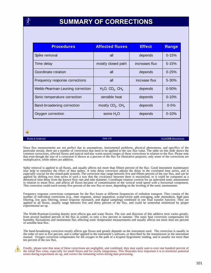
101


depends

depends

depends

depends

increase flux

depends

increases flux

depends

Effect

0-25%allCoordinate rotation

0-15%allSpike removal

5-15%mostly closed pathTime delay

0-10%

0-5%

0-10%

0-50%

5-30%

Range

mostly CO2, CH4Band-broadening correction

some H2OOxygen correction

H2O, CO2, CH4Webb-Pearman-Leuning correction

allFrequency response corrections

sensible heat

Affected fluxes

Sonic temperature correction

Procedures

SUMMARY OF CORRECTIONSSUMMARY OF CORRECTIONS

Since flux measurements are not perfect due to assumptions, instrumental problems, physical phenomena, and specifics of the particular terrain, there are a number of corrections that need to be applied to the raw flux value. The table on this slide shows the common corrections, affected fluxes and typical mid-day warm-season ranges of these corrections in relation to the flux. Please note that even though the size of a correction is shown as a percent of the flux for illustrative purposes, only some of the corrections are multiplicative, while others are additive.

Spike removal is applied to all fluxes, and usually affects not more than fifteen percent of the flux. Good instrument maintenance may help to minimize the effect of data spikes. A time delay correction adjusts the delay in the correlated time series, and is especially crucial for the closed-path systems. The correction may range between five and fifteen percent of the raw flux, and can be applied by shifting two time series in such a way that the covariance between them is maximized, or it could be computed as a theoretical time delay from the known flow rate and tube diameter. Coordinate rotation corrects for an unleveled sonic anemometer in relation to mean flow, and affects all fluxes because of contamination of the vertical wind speed with a horizontal component. This correction could reach twenty-five percent of the raw flux or more, depending on the leveling of the sonic anemometer.

Frequency response corrections compensate for the flux losses at different frequencies of turbulent transport. They consist of the number of individual corrections (e.g., time response, sensor separation, scalar/vector path averaging, tube attenuation, high pass filtering, low pass filtering, sensor response mismatch, and digital sampling) combined in one final transfer function. They areapplied to all fluxes, usually range between five and thirty percent of the flux, and could be somewhat minimized by proper experimental set up.

The Webb-Pearman-Leuning density term affects gas and water fluxes. The size and direction of this additive term varies greatly, from several hundred percent of the flux in winter, to only a few percent in summer. The sonic heat correction compensates for humidity fluctuations and momentum flux affecting sonic temperature measurements and usually affects not more than ten percent of sensible heat flux.

The band-broadening correction mostly affects gas fluxes and greatly depends on the instrument used. The correction is usually in the order of zero to five percent, and is either applied in the instrument’s software, or described by the manufacture in the instrument manual. Oxygen correction compensates for the oxygen in the path of a krypton hygrometer reading, and is usually not more than ten percent of the raw flux.

Finally, please note that none of these corrections are negligible, and combined, they may easily sum to over one hundred percent of the initial flux value, especially for small fluxes and for yearly integrations. This illustrates how important it is to minimize potential errors during experiment set up, and correct the remaining errors during data processing.

!

102


Bad data are removed for these key reasons:

• Instrument malfunctions

• Processing/mathematical artifacts

• Ambient conditions not satisfying EC method

• Winds are not from the footprint of interest

• Heavy precipitation

QUALITY CONTROLQUALITY CONTROL

Removing bad data is an important part of the data quality control process. It ensures that results do not have a bias or errors due to some obvious or common reasons. As a first step, bad data are usually removed for one of the following causes: instrument malfunctions, processing/mathematical artifacts, ambient conditions not satisfying Eddy Covariance method, winds are not from the footprint of interest, and heavy precipitation.

Among these, ambient conditions not satisfying the Eddy Covariance method include: conditions when turbulent transfer does not prevail, non-stationary conditions, periods with significant convergence or divergence, periods with wind directions not from the footprint of interest, etc.

Some particularly good sources of information on Eddy Covariance quality control are available from the web-sites listed in the Note section of this slide:

http://public.ornl.gov/ameriflux/measurement_standards_4.doc [Munger J.W. and H. W. Loescher. Guidelines for making Eddy Covariance flux measurements]

http://www.geo.uni-bayreuth.de/mikrometeorologie/ARBERG/ARBERG26.pdf - Mauder, M. and T. Foken. 2004. Documentation and Instruction Manual of the Eddy Covariance Software Package.

http://www.fluxnet-canada.ca/pages/protocols_en/measurement%20protocols_v.1.3_background.pdf -Fluxnet-Canada Measurement Protocols. Working Draft. Version 1.3. 2003

?

103


QUALITY CONTROL (CONTINUED)QUALITY CONTROL (CONTINUED)• The variety of Various algorithms and protocols are used by different

groups/networks (e.g., Carboeurope, Canadaflux, Ameriflux) have these

features in common:

Ranges of tolerance established for each variable

Data outside tolerance ranges removed or flagged

Precipitation events flagged

U, u*, and/or stationarity tests conducted

Non-stationary periods removed

Data validated via energy budget closure, co-spectral models, etc.

Data gaps filled with back-up instruments, regressions, models

Gas storage below measurements height computed from profiles

Data integrated, uncertainties computed

• Quality control is very much a site- and instrument-specific activity

Various algorithms and protocols are used by different groups and/or networks (e.g., Carboeurope, Fluxnet-Canada, Ameriflux) to automate the bad data removal procedure. These protocols are somewhat different from each other, but they have a number of commonalities.

In general, however, the quality control procedure is very much a site-specific and instrument-specific activity, except for these common steps. Thus, it is important not to overdo bad data removal at one study site based on past experience with a different study site.

For example, the tolerance thresholds for sensible heat flux data will differ greatly between an open-water flux measurement, (which will have generally small sensible heat fluxes), and a desert measurement that has high heat fluxes. Thus, applying a criteria developed for open water fluxes would probably eliminate many good data points if applied to measurements taken over the desert.

This is why it is generally recommended to collect a good amount of data and establish a baseline for a specific site before the removal criteria are established and applied to the original data.

Foken, Th. and B. Wichura. 1995. Tools for quality assessment of surface-based flux measurements', Agricultural and Forest Meteorology, 78, 83-105


Another important part of the quality analysis is making sure that the data have come from the footprint of interest.Examples describing this part of the quality control are given here:Gash, J.H.C. 1986 A note on estimating the effect of limited fetch on micrometeorological evaporation

measurements. Boundary Layer Meteorology 35: 409-413http://public.ornl.gov/ameriflux/measurement_standards_4.doc [Munger J.W. and H. W. Loescher. Guidelines for

making Eddy Covariance flux measurements]

?

104


• Fluxes are small

• Winds may be low, co-spectra bad

• Conditions may be stable

• Turbulence may not prevail

• Storage may be significant

• Advection of the flux, drainage flows

• Divergence, convergence

QUALITY CONTROL: NIGHTTIMEQUALITY CONTROL: NIGHTTIME

Nighttime is usually a separate case for quality control. Special care is required at night, because the winds are usually low, stratification is stable, and turbulence may not be developed. With slow winds and temperature inversions, flow may become non-stationary and advection, drainage, flow convergence and divergence may become dominant.

The footprint may also increase dramatically due to the stable conditions. With a larger footprint the tower instrumentation then would measure some of the fluxes outside the territory of interest.

As a result of these processes, data loss usually increases at night, especially during calm nights and under tall canopies.

A stationarity test is one of the more reliable tests for cleaning nighttime data. This test sets criteria for the behavior of the air flow in such a way that non-stationary periods can be flagged and removed.

Foken, T, and B. Wichura, 1996. Tools for quality assessment of surface-based flux measurements, Agric. Forest Meteorology (78): 83-105

Vickers, D. and L. Mahrt, 1997, Quality control and Flux sampling problems for tower and aircraft data, J. Atmos. Ocean.Technology (14): 512-526



?

105


Short Equation: Rn+H+LE+G≈0

Sketch (d and N)

LELE HH

GG

LELE HH

GG

LE<0LE<0Rn>0Rn>0

H<0H<0G<0G<0

LE<0LE<0Rn<0Rn<0

HH≈≈>>00G>0G>0RnRn RnRn

VALIDATION: ENERGY BUDGETVALIDATION: ENERGY BUDGET

One way to validate fluxes measured with Eddy Covariance is to construct an energy budget for the study site. Two traditional examples (daytime and nighttime) with key components of the energy budget are shown on this slide. Rn is net radiation; LE is latent heat flux; H is sensible heat flux, and G is the sum of soil heat flux and soil heat storage.

These examples also illustrate a short, 4-component, equation for an energy budget where: net radiation is usually measured with net radiometers, or with other radiation sensors, soil heat flux is usually calculated from heat flux plates and soil temperature, and latent and sensible heat fluxes are measured with Eddy Covariance technique.

The idea of validation with an energy budget is simply that if all of these key components sum to zero as required with conservation of energy, then all energy transfers have been successfully accounted for, and sensible and latent heat fluxes were measured correctly. Since the latter was measured correctly, the CO2 or other trace gas fluxes were most likely measured correctly as well.

It’s important to realize, however, that a good (closed) energy budget would not necessarily indicate good measurements of the trace gas flux, while a “non-closing” energy budget would almost certainly indicate a problem in measuring the flux.

A challenge in using energy budget to validate closure is that a good measurement of latent heat flux does not automatically mean a good measurement of the trace gas, because heat transfer for water and for the gas of interest may differ, especially if gases are reactive (such as volatile organic compounds) or significantly differ in sources and sinks from water vapor.

Another challenge in using energy budget is often related to the difficulty in measuring soil heat flux, especially in soil withrelatively rapid change in water content, and in non-uniformed patchy soils or terrains.

In spite of these difficulties, and with proper precautions, surface energy budget remains one of the most convincing ways to assess the quality of Eddy Covariance results, and is widely used in the flux communities.

Wilson, K. et al., 2002. Energy balance closure at FLUXNET sites. Agricultural and Forest Meteorology, 113(1-4): 223-243.Rosset, M., Riedo, M., Grub, A., Geissmann, M., and J. Fuhrer, 1997. Seasonal Variations in radiation and energy balances of

permanent pastures at different altitudes. Agricultural and Forest Meteorology, 86: 245-258.

?

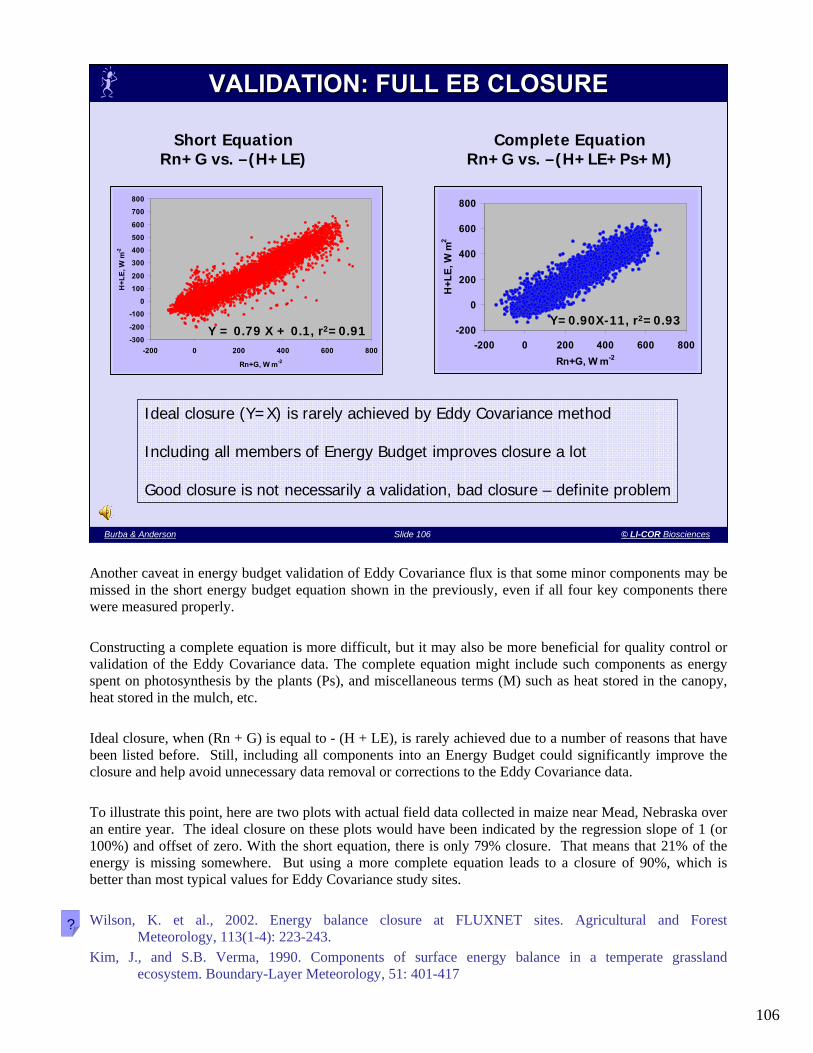
106


Short EquationRn+G vs. –(H+LE)

Complete EquationRn+G vs. –(H+LE+Ps+M)

-300

-200

-100

0

100

200

300

400

500

600

700

800

-200 0 200 400 600 800

Rn+G, W m-2

H+L

E, W

m-2

Y = 0.79 X + 0.1, r2=0.91 -200

0

200

400

600

800

-200 0 200 400 600 800Rn+G, W m-2

H+L

E, W

m2

Y=0.90X-11, r2=0.93

Ideal closure (Y=X) is rarely achieved by Eddy Covariance method

Including all members of Energy Budget improves closure a lot

Good closure is not necessarily a validation, bad closure – definite problem

VALIDATION: FULL EB CLOSUREVALIDATION: FULL EB CLOSURE

Another caveat in energy budget validation of Eddy Covariance flux is that some minor components may be missed in the short energy budget equation shown in the previously, even if all four key components there were measured properly.

Constructing a complete equation is more difficult, but it may also be more beneficial for quality control or validation of the Eddy Covariance data. The complete equation might include such components as energy spent on photosynthesis by the plants (Ps), and miscellaneous terms (M) such as heat stored in the canopy, heat stored in the mulch, etc.

Ideal closure, when (Rn + G) is equal to - (H + LE), is rarely achieved due to a number of reasons that have been listed before. Still, including all components into an Energy Budget could significantly improve the closure and help avoid unnecessary data removal or corrections to the Eddy Covariance data.

To illustrate this point, here are two plots with actual field data collected in maize near Mead, Nebraska over an entire year. The ideal closure on these plots would have been indicated by the regression slope of 1 (or 100%) and offset of zero. With the short equation, there is only 79% closure. That means that 21% of the energy is missing somewhere. But using a more complete equation leads to a closure of 90%, which is better than most typical values for Eddy Covariance study sites.

Wilson, K. et al., 2002. Energy balance closure at FLUXNET sites. Agricultural and Forest Meteorology, 113(1-4): 223-243.

Kim, J., and S.B. Verma, 1990. Components of surface energy balance in a temperate grassland ecosystem. Boundary-Layer Meteorology, 51: 401-417

?

107


• There are many other ways to validate Eddy Covariance flux:

Quality and shape of daytime co-spectra

Similarity theory models (vs. z/L)

Verification with biological data (NEP)

Leaf-up (leaf chamber measurements)

Soil-up (soil chamber measurements)

• None of these methods can guarantee correct data, but all of them combined can show problems or to help defend the flux data

VALIDATION: OTHER METHODSVALIDATION: OTHER METHODS

There are many other ways to validate Eddy Covariance flux.

Quality and shape of daytime gas flux co-spectra in comparison with sensible heat flux co-spectra or with ideal Kaimal-Moore co-spectra helps to understand at what frequencies gas flux may be missed or measured incorrectly. For example, ship-borne and airborne Eddy Covariance studies may find unusual co-spectra shapes for their gas fluxes at the frequencies of ship heave and airplane vibration, and may need to counter these interferences by different sensor arrangements.

Similarity theory models involving Monin-Obukhov stability parameter may help to assess if flux co-variances or momentum characteristics behave in a predictable way and fit established meteorological models.

Verification of tower data with data collected by other techniques (for example, net ecosystem production computations from biomass data, leaf chamber measurements or soil chamber data) can help all the compared techniques reveal inconsistencies and to find their cause.

None of these methods alone will guarantee the correct data, but all of them combined can help to find hidden problems or to defend the flux data.

108


Regressions with backup instrumentsRegressions with nearby sites (when appropriate)Physical restrictions (energy budget, mass budget, etc.)Lookup tables and Ameriflux gap filling strategiesCO2 daytime – light response curves for different GFAI CO2 nighttime – temperature, moisture, for diff GFAI, Q10

• After bad data have been removed, data gap inventory and data filling need to be performed

• Inventory is important for getting an idea on the quality of results and may be useful for computing uncertainties for integrated values

• Filling-in the data is not a trivial process in the Eddy Covariance method –there is always a danger of bias

• Some of established strategies to fill-in missing data are:

FILLINGFILLING--IN MISSING DATAIN MISSING DATA

After bad data have been removed, one has to perform data gap inventory and fill-in the missing periods in order to construct a seasonal or yearly picture of ecosystem exchange.

Bad data inventory is important for getting an idea on the quality of results, and may also be useful for computing uncertainties for integrated values.

Filling-in the data is not a trivial process in the eddy covariance method – there is always a danger of adding bias to the data. Some of the established strategies to “filling-in” missing data are: regressions with backup instruments; regressions with nearby sites; physical restrictions (energy budget, mass budget, etc.); lookup tables and Ameriflux gap filling strategies; CO2 daytime (light response curves for different green leaf area index, GFAI); CO2 nighttime (temperature, moisture, respiration-temperature dependence, Q10, for different green leaf area index).

It is also important to note that nighttime data often need to be filled-in separately from the daytime data for physiological reasons (for example, a different set of processes is responsible for CO2 release/uptake during day than during the night), and because of turbulent exchange problems (see page 115 of this guide)

Falge, E.; D. Baldocchi; R. Olson; P. Anthoni; M. Aubinet; C. Bernhofer; G. Burba; R. Ceulemans; R. Clement; H. Dolman; A. Granier; P. Gross; T. Grunwald; D. Hollinger; N. O. Jensen; G. Katul; P. Keronen; A. Kowalski; C. T. Lai; B. E. Law; T. Meyers; J. Moncrieff; E. Moors, 2001. Gap filling strategies for defensible annual sums of net ecosystem exchange. Agricultural and Forest Meteorology, 107(1), 43-69.

Falge, E.; D. Baldocchi; R. Olson; P. Anthoni; M. Aubinet; C. Bernhofer; G. Burba; G. Ceulemans; R. Clement; H. Dolman; A. Granier; P. Gross; T. Grunwald; D. Hollinger; N. O. Jensen; G. Katul; P. Keronen; A. Kowalski; C. T. Lai; B. E. Law; T. Meyers; J. Moncrieff; E. Moors, 2001. Gap filling strategies for long term energy flux data sets. Agricultural and Forest Meteorology, 107(1), 71-77.

?

!

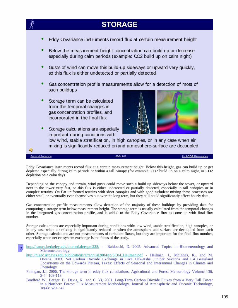
109


STORAGESTORAGE

• Eddy Covariance instruments record flux at certain measurement height

• Below the measurement height concentration can build up or decreaseespecially during calm periods (example: CO2 build up on calm night)

• Gusts of wind can move this build-up sideways or upward very quickly, so this flux is either undetected or partially detected

• Gas concentration profile measurements allow for a detection of most of such buildups

• Storage term can be calculated from the temporal changes in gas concentration profiles, and incorporated in the final flux

• Storage calculations are especially important during conditions with low wind, stable stratification, in high canopies, or in any case when airmixing is significantly reduced or/and atmosphere-surface are decoupled

Eddy Covariance instruments record flux at a certain measurement height. Below this height, gas can build up or get depleted especially during calm periods or within a tall canopy (for example, CO2 build up on a calm night, or CO2 depletion on a calm day).

Depending on the canopy and terrain, wind gusts could move such a build up sideways below the tower, or upward next to the tower very fast, so this flux is either undetected or partially detected, especially in tall canopies or in complex terrains. On flat uniformed terrains with short canopies and with good turbulent mixing these processes are either small or eventually even themselves out over the long term, but they still could significantly affect hourly data.

Gas concentration profile measurements allow detection of the majority of these buildups by providing data for computing a storage term below measurement height. The storage term is usually calculated from the temporal changes in the integrated gas concentration profile, and is added to the Eddy Covariance flux to come up with final flux number.

Storage calculations are especially important during conditions with: low wind, stable stratification, high canopies, or in any case when air mixing is significantly reduced or when the atmosphere and surface are decoupled from each other. Storage calculations are not measurements of turbulent fluxes, but they are important for the final flux number, especially when net ecosystem exchange is the focus of the study.


http://nigec.ucdavis.edu/publications/ar/annual2004/sc/SC04_Heilman.pdf - Heilman, J., McInnes, K., and M. Owens. 2003. Net Carbon Dioxide Exchange in Live Oak-Ashe Juniper Savanna and C4 Grassland Ecosystems on the Edwards Plateau, Texas: Effects of Seasonal and Interannual Changes in Climate and Phenology

Finnigan, J.J, 2006. The storage term in eddy flux calculations. Agricultural and Forest Meteorology Volume 136, 3-4: 108-113

Bradford W., Berger, B., Davis, K., and C. Yi, 2001. Long-Term Carbon Dioxide Fluxes from a Very Tall Tower in a Northern Forest: Flux Measurement Methodology. Journal of Atmospheric and Oceanic Technology, 18(4): 529–542

?

110


• Integrations should be done after the data has been processed,

corrected, quality controlled, validated, and storage term has been

added to a gas flux

• Yearly CO2 integrations are especially unforgiving, because two

similar quantities (photosynthesis/uptake and respiration/release) are

subtracted from each other

• Result is a relatively small number with relatively large uncertainties:

instrumental EC methodology gap filling

• Error analysis should be conducted to estimate uncertainties and

results should be presented as a range, and not as a single number

INTEGRATIONINTEGRATION

Integration should be done after data has been processed, corrected, quality controlled, validated, and a storage has been added.

Yearly CO2 integrations are especially unforgiving, because two large, similar quantities (photosynthesis/uptake and respiration/release) are subtracted from each other. As a result, uncertainties due to instrument performance, EC methodology, quality control and gap filling which seemed small or negligible in comparison with hourly fluxes, now become relatively large in comparison with the integrated seasonal flux number.

Error analysis is highly advisable at this stage. It can help to quantitatively estimate the impact of these uncertainties, and to present resultant integrated flux as realistic range rather than as a single number.

Falge, E.; D. Baldocchi; R. Olson; P. Anthoni; M. Aubinet; C. Bernhofer; G. Burba; R. Ceulemans; R. Clement; H. Dolman; A. Granier; P. Gross; T. Grunwald; D. Hollinger; N. O. Jensen; G. Katul; P. Keronen; A. Kowalski; C. T. Lai; B. E. Law; T. Meyers; J. Moncrieff; E. Moors, 2001. Gap filling strategies for defensible annual sums of net ecosystem exchange. Agricultural and Forest Meteorology, 107(1), 43-69

?

111


• Each experimental site is different and requires unique treatment

• Eddy Covariance is, to a large extent, a site-specific method

• The entire process of experimental design, implementation and data processing should be tailor-made for specific purpose at specific site

WORKFLOW: SUMMARYWORKFLOW: SUMMARY

Overall, perhaps the most important point about Eddy Covariance workflow is the necessity for an individualized customized approach to each experiment, because Eddy Covariance, to a large extent, is a site-specific method.

Each study site is different and requires unique treatment in terms of experimental design, tower placement, instrumental set up, data collection, and processing and analysis.

Built-in flexibility of the Eddy Covariance method, in conjunction with user knowledge and understanding of the method and the study site, will allow for successful implementation of site-specific arrangements that are tailor-made for a specific scientific purpose under specific ambient conditions.

112


• Experiment design: establish purpose, variables, instruments, software, location, maintenance plan

• Implementation: place tower and instruments, test data collection and retrieval, test processing program on the standard file, keep up maintenance throughout the experiment

• Process instantaneous data: convert units, determine best averaging period, de-spike, correct for time delay, apply calibrations, compute rotation coefficients and frequency response corrections, average data

• Process averaged data: apply rotation coefficients, frequency response and other corrections, quality control, fill-in, integrate, compute storage

• Validate data: validate with Energy Budget closure, co-spectra, alternative methods, back-up instruments, biomass data, and light-response curves

• Pre-analyze data: check carefully nighttime data, advection periods, calculate uncertainties for integrated flux numbers

WORKFLOW: SUMMARYWORKFLOW: SUMMARY

The main elements of the Eddy Covariance workflow are: experiment design, implementation, data processing, validation and analysis.

Experiment design consists of establishing purpose, variables, instruments, software, location, and a maintenance plan.

Implementation involves placing the tower and instruments, testing data collection and retrieval, testing processing program, and keeping up maintenance throughout the experiment.

The main steps in processing of instantaneous data are: units’ conversion, determining best averaging period, de-spiking, correcting for time delay, applying calibrations, computing rotation coefficients and frequency response corrections, and averaging the instantaneous data. Further processing includes: applying rotation coefficients, frequency response and other corrections, conducting quality control and gap filling, computing storage term, and integrating long-term data.

Data validation can be done in a number of different ways including: Energy Budget closure, co-spectra, alternative methods, back-up in instruments, biomass data, and light-response curves.

Initial data analysis involves careful checks of data, especially during night, calm and advection periods, and calculating uncertainties for integrated flux numbers.

113


• Environmental conditions may prevent using Eddy Covariance

• Instruments not fast enough for certain gases (ex.: NH4, isotopes etc.)

• Information is needed other than from EC (ex.: soil respiration)

• As a complimentary method to add value, validation, backup to EC

• Below is a quick review of key methods:

Eddy Accumulation

Relaxed Eddy Accumulation

Bowen Ratio

Aerodynamic method

Resistance method

Chamber

Others

III. ALTERNATIVE FLUX METHODSIII. ALTERNATIVE FLUX METHODS

There are a number of situations where the Eddy Covariance method either can not be used to measure fluxes, or is not the best method to do so. These include environmental conditions with a very small area of study, predominantly low winds, complex terrain, point flux sources etc. Also, for some gases such as ammonia, volatile components, and isotopes, the instruments may not be sensitive enough or fast enough to measure small changes at 10 or 20 Hz frequencies. The focus of the experiment itself may prevent a researcher from using the Eddy Covariance method, for example, when it is narrowed down to only one of the components of the flux, such as soil respiration, or canopy transpiration.

In these situations, other methods become more useful scientific tools. They could also be used as complementary methods to add value, validation or backup to the Eddy Covariance method. The next few slides contain a quick overview of some of these methods. We will briefly look at Eddy Accumulation, Bowen Ratio, and a few other methods. Further details on these and other methods to measure fluxes can be found in the sources listed below:




Denmead, O.T. and M.R. Raupach. 1993. Methods for measuring atmospheric gas transport in agricultural and forest systems. In: Agricultural Ecosystem Effects on Trace Gases and Global Climate Change. American Society of Agronomy

Lenschow, DH. 1995. Micrometeorological techniques for measuring biosphere-atmosphere trace gas exchange. In: Biogenic Trace Gases: Measuring Emissions from Soil and Water. Eds. P.A. Matson and R.C. Harriss. Blackwell Sci. Pub. Pp 126-163.

Wesely, M.L., D.H. Lenschow and O.T. 1989. Flux measurement techniques. In: Global Tropospheric hemistry, Chemical Fluxes in the Global Atmosphere. NCAR Report. Eds. DH Lenschow and BB Hicks. pp 31-46

?

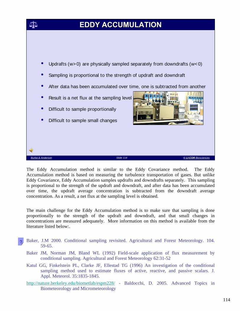
114


EDDY ACCUMULATIONEDDY ACCUMULATION

• Updrafts (w>0) are physically sampled separately from downdrafts (w<0)

• Sampling is proportional to the strength of updraft and downdraft

• After data has been accumulated over time, one is subtracted from another

• Result is a net flux at the sampling level

• Difficult to sample proportionally

• Difficult to sample small changes

The Eddy Accumulation method is similar to the Eddy Covariance method. The Eddy Accumulation method is based on measuring the turbulence transportation of gases. But unlike Eddy Covariance, Eddy Accumulation samples updrafts and downdrafts separately. This sampling is proportional to the strength of the updraft and downdraft, and after data has been accumulated over time, the updraft average concentration is subtracted from the downdraft average concentration. As a result, a net flux at the sampling level is obtained.

The main challenge for the Eddy Accumulation method is to make sure that sampling is done proportionally to the strength of the updraft and downdraft, and that small changes in concentrations are measured adequately. More information on this method is available from the literature listed below:.

Baker, J.M 2000. Conditional sampling revisited. Agricultural and Forest Meteorology. 104. 59-65.

Baker JM, Norman JM, Bland WL (1992) Field-scale application of flux measurement by conditional sampling. Agricultural and Forest Meteorology 62:31-52

Katul GG, Finkelstein PL, Clarke JF, Ellestad TG (1996) An investigation of the conditional sampling method used to estimate fluxes of active, reactive, and passive scalars. J. Appl. Meteorol. 35:1835-1845.


?

115


• Uupdrafts (w>0) are physically sampled separately from downdrafts (w<0)

• Sampling is not proportional to the strength of updraft and downdraft

• Sampling is at constant flow rate

• After data has been accumulated over time, one is subtracted from another

• Result is a net flux at the sampling level

• Difficult to correctly evaluate empirical coefficient required for calculations

• Number of corrections required; difficult to measure small changes

RELAXED EDDY ACCUMULATIONRELAXED EDDY ACCUMULATION

A modification of the Eddy Accumulation method is the Relaxed Eddy Accumulation method. Similar to Eddy Accumulation, the updrafts are sampled separately from the downdrafts. However, this sampling is not proportional to the strength of the updraft and downdraft, and is done at a constant flow rate. After data has been accumulated over time, the updraft average concentration is subtracted from the downdraft. As a result, a net flux at the sampling level is obtained.

The main challenge for the Relaxed Eddy Accumulation method is to make sure that empirical coefficients are evaluated correctly, that corrections are properly applied, and that small changes are sampled adequately.

Nie D, Kleindienst TE, Arnts RR, Sickles JE, 1995. The design and testing of a relaxed eddy accumulation system. JGR. 100: 11,415-11,423

Oncley SP, Delany AC, Horst TW, Tans PP (1993) Verification of flux measurement using relaxed eddy accumulation. Atmos. Environ. 27A:2417-2426

Pattey E, Desjardins RL, Rochette P (1993) Accuracy of the relaxed eddy-accumulation technique, evaluated using CO2 flux measurements. Boundary LayerMeteorology 66:341-355

Pattey E, Desjardins RL, Boudreau F, Rochette P (1992) Impact of density fluctuations on flux measurements of trace gases: implications for the relaxed eddy accumulation technique. Boundary Layer Meteorology 59:195-203

?

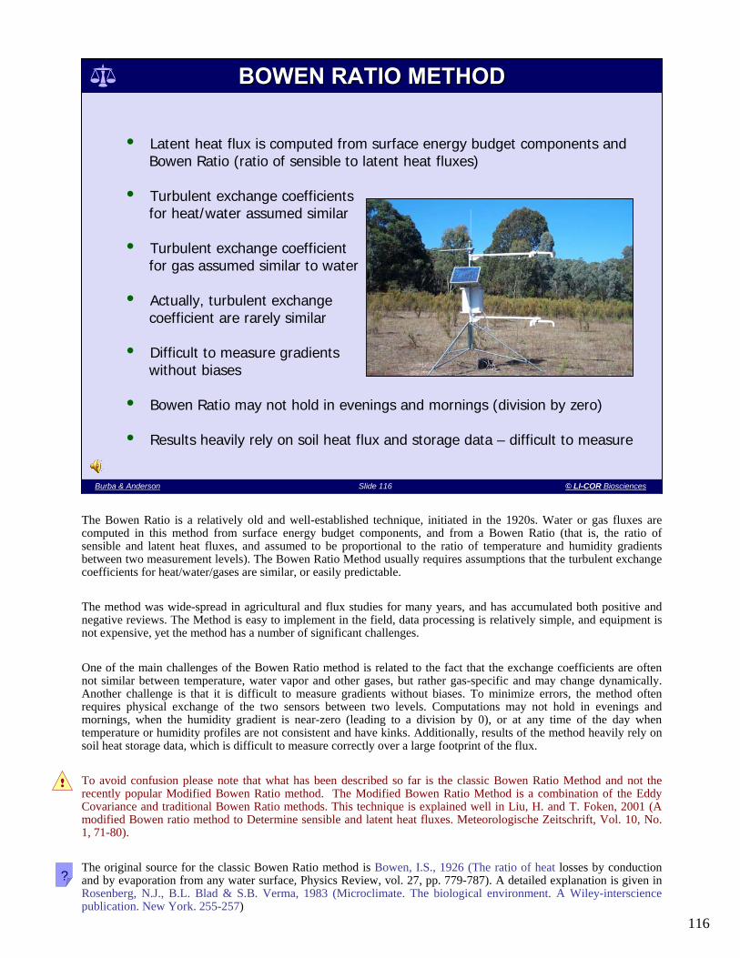
116


BOWEN RATIO METHODBOWEN RATIO METHOD

• Latent heat flux is computed from surface energy budget components and Bowen Ratio (ratio of sensible to latent heat fluxes)

• Turbulent exchange coefficients for heat/water assumed similar

• Turbulent exchange coefficient for gas assumed similar to water

• Actually, turbulent exchange coefficient are rarely similar

• Difficult to measure gradients without biases

• Bowen Ratio may not hold in evenings and mornings (division by zero)

• Results heavily rely on soil heat flux and storage data – difficult to measure

The Bowen Ratio is a relatively old and well-established technique, initiated in the 1920s. Water or gas fluxes are computed in this method from surface energy budget components, and from a Bowen Ratio (that is, the ratio of sensible and latent heat fluxes, and assumed to be proportional to the ratio of temperature and humidity gradients between two measurement levels). The Bowen Ratio Method usually requires assumptions that the turbulent exchange coefficients for heat/water/gases are similar, or easily predictable.

The method was wide-spread in agricultural and flux studies for many years, and has accumulated both positive and negative reviews. The Method is easy to implement in the field, data processing is relatively simple, and equipment is not expensive, yet the method has a number of significant challenges.

One of the main challenges of the Bowen Ratio method is related to the fact that the exchange coefficients are often not similar between temperature, water vapor and other gases, but rather gas-specific and may change dynamically. Another challenge is that it is difficult to measure gradients without biases. To minimize errors, the method often requires physical exchange of the two sensors between two levels. Computations may not hold in evenings and mornings, when the humidity gradient is near-zero (leading to a division by 0), or at any time of the day when temperature or humidity profiles are not consistent and have kinks. Additionally, results of the method heavily rely on soil heat storage data, which is difficult to measure correctly over a large footprint of the flux.

To avoid confusion please note that what has been described so far is the classic Bowen Ratio Method and not the recently popular Modified Bowen Ratio method. The Modified Bowen Ratio Method is a combination of the Eddy Covariance and traditional Bowen Ratio methods. This technique is explained well in Liu, H. and T. Foken, 2001 (A modified Bowen ratio method to Determine sensible and latent heat fluxes. Meteorologische Zeitschrift, Vol. 10, No. 1, 71-80).

The original source for the classic Bowen Ratio method is Bowen, I.S., 1926 (The ratio of heat losses by conduction and by evaporation from any water surface, Physics Review, vol. 27, pp. 779-787). A detailed explanation is given in Rosenberg, N.J., B.L. Blad & S.B. Verma, 1983 (Microclimate. The biological environment. A Wiley-interscience publication. New York. 255-257)

?

!

117


• Flux is computed from wind profile and gas concentration profile

• Turbulent exchange coefficients for momentum, gas are assumed similar

• Alternatively, turbulent exchange coefficients have to be known or modeled

• Difficult to determine turbulent exchange coefficient for momentum

• Turbulent exchange coefficient rarely similar, especially for rare gases

• Atmospheric stability significantly affects calculation

AERODYNAMIC METHODAERODYNAMIC METHOD

In the Aerodynamic method, or family of methods, flux is computed from the vertical profiles of wind speed and gas concentration. Turbulent exchange coefficients for momentum and the gas of interest are either assumed to be similar, are measured, or are modeled.

The main challenges are related to difficulties in determining the turbulent exchange coefficient for momentum, and the fact that the turbulent exchange coefficient between momentum and gases are not always similar, and may in fact, be gas-specific. Atmospheric stability can also significantly affect the flux calculated using the aerodynamic method.

Pruitt, W.O., 1963. Application of several energy balance and aerodynamic evaporation equations under a wide range of stability. Final report to USAEPG, Univ. of California-Davis. pp107-124

Thornthwaite N, Holzman B. 1942. Measurement of evaporation from land and water surfaces, USDA Tech. Bull., No. 817 Webb, E. K.: 1965, ‘Aerial Microclimate’, in. Agricultural Meteorology, Meteor. Monographs, Vol. 6, 28, 27-58

?

118


• Can be considered a version of aerodynamic method

• Computes flux from gradient and resistances to transport

• Need to know aerodynamic and stomatal resistances

• May need to know soil surface resistance

• Resistances are difficult to measure

RESISTANCE APPROACHRESISTANCE APPROACH

The Resistance approach is considered, by some, to be a version of the aerodynamic method. Fluxes in the resistance approach are computed from gradients and resistances to transport. Both aerodynamic and stomatal resistances are usually needed to measure fluxes over live canopies. The soil surface resistance is often required as well, especially in sparse canopies.

With well-developed and tested models (such as Shuttleworth-Wallace and Penman-Montieth) and a good understanding of the processes, the main challenge in using the traditional resistance approach is the great difficulties encountered while attempting to accurately measure the resistances.


Montieth, J. L. 1963. Gas exchange in plant communities. Pages 95-112 in L. T. Evans, ed. Environmental control of plant growth. Academic Press, New York

?

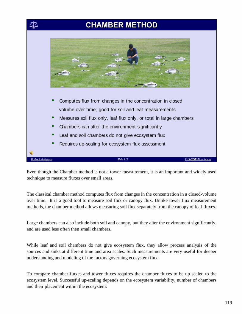
119


CHAMBER METHODCHAMBER METHOD

• Computes flux from changes in the concentration in closed

volume over time; good for soil and leaf measurements

• Measures soil flux only, leaf flux only, or total in large chambers

• Chambers can alter the environment significantly

• Leaf and soil chambers do not give ecosystem flux

• Requires up-scaling for ecosystem flux assessment

Even though the Chamber method is not a tower measurement, it is an important and widely used technique to measure fluxes over small areas.

The classical chamber method computes flux from changes in the concentration in a closed-volume over time. It is a good tool to measure soil flux or canopy flux. Unlike tower flux measurement methods, the chamber method allows measuring soil flux separately from the canopy of leaf fluxes.

Large chambers can also include both soil and canopy, but they alter the environment significantly, and are used less often then small chambers.

While leaf and soil chambers do not give ecosystem flux, they allow process analysis of the sources and sinks at different time and area scales. Such measurements are very useful for deeper understanding and modeling of the factors governing ecosystem flux.

To compare chamber fluxes and tower fluxes requires the chamber fluxes to be up-scaled to the ecosystem level. Successful up-scaling depends on the ecosystem variability, number of chambersand their placement within the ecosystem.

120


• Disjunct Eddy Covariance

• Relaxed Eddy Accumulation with injections

• Mass balance for small areas

• Surface renewal method

• Control volume

• Boundary layer towers

• Virtual towers

• Biological and soil sampling

• Lysimeter

OTHER ALTERNATIVE METHODSOTHER ALTERNATIVE METHODS

There are a larger number of other methods to measure fluxes, in addition to the few methods described in this presentation. They include modifications of the described methods (such as, disjunct eddy covariance, relaxed eddy accumulation with injections, etc.) and completely separate methods (such as, sap flow, virtual towers, lysimetry, etc.). Examples of comparison between some of these methods are given below:

Williams, D.G., W. Cable, K. Hultine, J.C.B. Hoedjes, E. Yepez, V. Simonneaux, S. Er-Raki, G. Boulet, H.A.R. de Bruin, A. Chehbouni, O.K. Hartogensis and F. Timouk, 2004. Components of evapotranspiration determined by stable isotope, sap flow and eddy covariance techniques. Agricultural and Forest Meteorology 125:241-258.

?

121


Disciplines

Gas species

Terrains

Scale expansion

IV. FUTURE DEVELOPMENTIV. FUTURE DEVELOPMENT

The Eddy Covariance method is gaining increased popularity in micrometeorology, and especially, in carbon flux studies. Every year the number of tower sites increases and new experiments are planned.

In the next few slides we will look at several examples of the near-future prospects for the method:

- expansion to disciplines beyond micrometeorology

- expansion to many gases (not just CO2), dust, aerosols

- measuring at difficult terrains (hillsides, mountains, urban)

- expansion in geographic scales of studies.

122


Use of the EC method is currently restricted by complexities with

non-uniform terminology and the lack of a user-friendly,

comprehensive standardized software to give a non-expert user

a choice of settings and parameters to handle eddy flux data

Disciplines such as ecology, geo-ecology, entomology, biology,

ecosystem science etc., would profit greatly from using

standardized methodology, field procedures and equipment

EC EXPANSION: DISCIPLINESEC EXPANSION: DISCIPLINES

Use of the Eddy Covariance method is often restricted by complexities with non-uniformed terminology and the lack of user-friendly, all inclusive software that would give a non-expert user a choice of settings and parameters to handle eddy flux data.

As these challenges are being successfully resolved by flux networks, scientific and educational institutions, disciplines such as ecology, entomology, biology, ecosystem science, hydrology, oceanography etc., would profit greatly from using Eddy Covariance method for their specific applications.

These applications could range widely, from studies on the cicada life cycles and related soil aeration to incorporating gas exchange into GIS modeling, and from remote sensing validation to dissipation of methane through ocean waters and related changes in biodiversity.

123


• Different from LIDAR

• Quantum cascade laser technology can detect ppbs at high frequencies

• Potentially allows multiple gas, fast, and high resolution open-path EC systems

EC EXPANSION: GAS SPECIESEC EXPANSION: GAS SPECIES

Fluxes of momentum, heat, carbon dioxide and water used to be the prime focus of Eddy Covariance. With advances in technological development (such as quantum cascade laser technology, fast digital processing, and wireless, low-power solutions) instruments will be able to detect several parts per billion at high frequencies for many more gas species, faster and with more accuracy.

As a result, Eddy Covariance will be positioned to compute fluxes from multiple gas species in low-power open-path systems, and shed more light on the processes affecting fluxes of volatile components, such as nitrous oxide, methane, and others.

124


• Further understanding the complex flow

• Measure convergence/divergence

• Measure drainage flux/advection/storage

• Use of control volumes and multiplexers

EC EXPANSION: TERRAINSEC EXPANSION: TERRAINS

Photo: CarboEurope

The latest scientific developments have enabled Eddy Covariance to be used in complex terrains (on hills, in cities, and under conditions of various flow obstructions). Success of these applications has been intermittent, but progress in this direction is very promising. Several groups in Fluxnet work specifically in complex terrains, and have became experts in this application of the method.

Eddy covariance studies in complex terrains rely on further understanding the complex flow, measurements of flow convergence and divergence, drainage flux, advection, storage, and on the use of control volumes and multiplexers, and other instrument-intensive techniques. Such developments are especially important for understanding and quantifying fluxes in ever-expanding urban territories and in sparsely studied mountain regions. Both of these areas are vast, and have a very large impact on global fluxes of carbon, water, and aerosols.

McMillen, R.T. 1988. 'An eddy correlation technique with extended applicability to non- simple terrain', Boundary Layer Meteorology, 43, 231-245.

Raupach, MR, Finnigan, JJ. 1997. The influence of topography on meteorological variables and surface-atmosphere interactions. Journal of Hydrology, 190:182-213

?

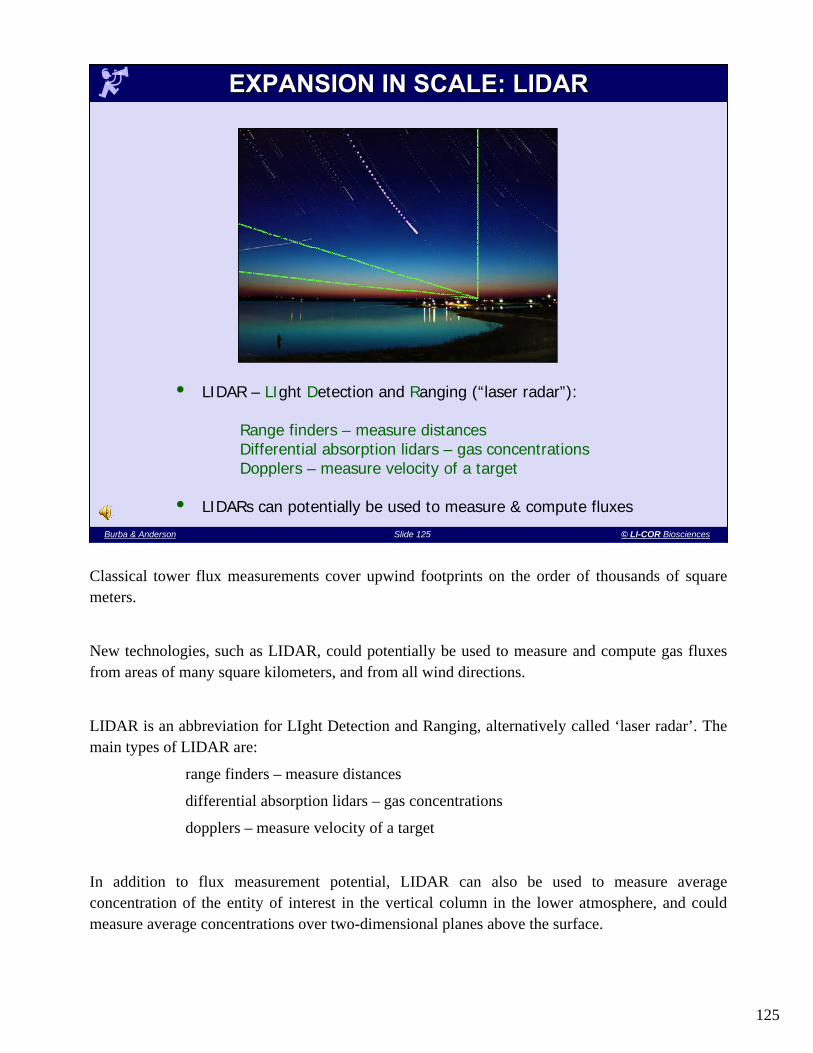
125


• LIDAR – LIght Detection and Ranging (“laser radar”):

Range finders – measure distancesDifferential absorption lidars – gas concentrationsDopplers – measure velocity of a target

• LIDARs can potentially be used to measure & compute fluxes

EXPANSION IN SCALE: LIDAREXPANSION IN SCALE: LIDAR

Classical tower flux measurements cover upwind footprints on the order of thousands of square meters.

New technologies, such as LIDAR, could potentially be used to measure and compute gas fluxes from areas of many square kilometers, and from all wind directions.

LIDAR is an abbreviation for LIght Detection and Ranging, alternatively called ‘laser radar’. The main types of LIDAR are:

range finders – measure distances

differential absorption lidars – gas concentrations

dopplers – measure velocity of a target

In addition to flux measurement potential, LIDAR can also be used to measure average concentration of the entity of interest in the vertical column in the lower atmosphere, and could measure average concentrations over two-dimensional planes above the surface.

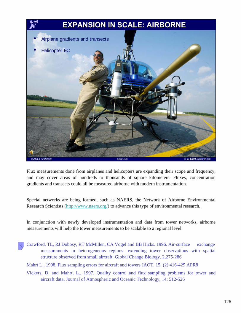
126


• Airplane gradients and transects

• Helicopter EC

EXPANSION IN SCALE: AIRBORNEEXPANSION IN SCALE: AIRBORNE

Flux measurements done from airplanes and helicopters are expanding their scope and frequency, and may cover areas of hundreds to thousands of square kilometers. Fluxes, concentration gradients and transects could all be measured airborne with modern instrumentation.

Special networks are being formed, such as NAERS, the Network of Airborne Environmental Research Scientists (http://www.naers.org/) to advance this type of environmental research.

In conjunction with newly developed instrumentation and data from tower networks, airborne measurements will help the tower measurements to be scalable to a regional level.

Crawford, TL, RJ Dobosy, RT McMillen, CA Vogel and BB Hicks. 1996. Air-surface exchange measurements in heterogeneous regions: extending tower observations with spatial structure observed from small aircraft. Global Change Biology. 2,275-286

Mahrt L., 1998. Flux sampling errors for aircraft and towers JAOT, 15: (2) 416-429 APR8


?

127


• Need for spatial resolution at all scales

• Local: multiplex systems for soil, multiple towers, field remote sensing

• Regional: regional networks (Ameriflux, Fluxnet-Canada, Carboeurope, Neon, etc.)

• Global: global network (iLEAPs/FLUXNET), standardized databases, modeling

• Earth observations intranet

EXPANSION IN SCALE: GLOBAL NETWORKSEXPANSION IN SCALE: GLOBAL NETWORKS

Photo: ESA/NASA Fluxnet

Flux networks unite EC research with various spatial resolution and coverage. Data from many sites are collected in a single archive. They are collected with uniformed collection and reduction methods and stored and maintained with consistent formats. Such data are invaluable for carbon cycle and global climate modeling, and may have multiple uses in other disciplines.

Networks’ archives cover ecosystem flux and related parameters on a variety of scales from: field scale (e.g., short tower data, multiplex systems for soil, field-size remote sensing), to regional scale with networks such as: Ameriflux, Fluxnet-Canada, Carboeurope, Neon, etc., and finally globally with networks like: iLEAPs/FLUXNET. We have listed a group of global and regional flux networks in the notes section, where one can access general network descriptions, recent publications, field data sets, and other useful information:

Fluxnet http://daac.ornl.gov/FLUXNET/AmeriFlux http://public.ornl.gov/ameriflux/AsiaFlux http://www-cger2.nies.go.jp/asiaflux/index.htmlCarboEurope http://www.carboeurope.org/ChinaFlux http://www.chinaflux.org/en/index/index.aspFluxnet-Canada http://www.fluxnet-canada.ca/KoFlux http://koflux.org/home/index.htmlOzFlux http://koflux.org/home/index.html

?

128


• Spectral measurements from space can potentially observe dynamiccontent of entire atmosphere – the ultimate goal of tower networks

• The working example is SCIAMACHY – orbital imaging spectrometer

EXPANSION IN SCALE: PLANETARYEXPANSION IN SCALE: PLANETARY

Photos: ESA

Spectral measurements done from space could potentially observe dynamic content of the entire atmosphere – the ultimate goal of tower networks. Future satellite measurements require development and testing of instruments and data collection systems on the ground, which later could be used for remote sensing. Comparison of field and satellite data (called ground truthing) is very important for developing this approach. With time, satellite instrument systems could reliably determine the dynamics of gases, aerosol and dust for the planet as a whole.

One of the pioneering examples of such a system is the orbital imaging spectrometer SCIAMACHY – Scanning Imaging Absorption Spectrometer for Atmospheric CHartographY.

Sellers, P.J., Hall, F.G, Asrar, G., Strebel, D.E. and R.E. Murphy, 1992. An Overview of the first international satellite land surface climatology project (ISLSCP) field experiment (FIFE). Journal of Geophysical Research, 97: 18345-18371

Gitelson, A.; S.Verma; A.Viña; D. Rundquist; G. Keydan; T. Arkebauer; G. Burba; A. Suyker, 2003. Novel Technique for Remote Estimation of Landscape-level CO2 flux. GRL, 30 (9), 1-4

?

129


• Micrometeorological technique to measure vertical turbulent fluxes in the atmospheric boundary layer: nearly-direct, theoretically solid and proven, very flexible in applications, verifiable by other techniques

• Widely used in micrometeorology to measure H2O, CO2, heat, momentum, started being used to measure CH4, O3, NO3, bVOCs and other gases

• Requires a number of assumptions/corrections, demands careful design, execution and processing custom-fitted to the specific purpose at the specific experimental site

• Continuously develops on conceptual and instrumental levels to allow wider applications in more environments

V. EC REVIEW: SUMMARYV. EC REVIEW: SUMMARY

In this presentation we put together simple guidelines to help a non-expert to understand the general principles, requirements, applications, and processing steps of the Eddy Covariance method. Its goal is to promote further understanding of the method via more advanced sources (e.g., textbooks, papers), and to help design experiment for specific scientific needs.

In summary, Eddy Covariance is a micrometeorological technique to measure vertical turbulent fluxes in the atmospheric boundary layer. It is: nearly-direct, theoretically solid, proven, very flexible in applications, and verifiable by other techniques.

It is widely used in micrometeorology to measure H2O, CO2, heat, and momentum, and has started being used to measure CH4, O3, NO3, volatile organic components and other gases.

The method requires a number of assumptions and corrections. It demands careful design, execution and processing that is fit to the specific purpose at the specific experimental site.

Eddy Covariance continues to develop on conceptual and instrumental levels. It is expanding in application scope and is being used in more diverse environments.

130


• Potentially of great use to many non-meteorological sciences when energy, water or gas exchanges and balances are of interest

• Major flux measurement networks already exist to provide global synthesis, allow interpretation of one particular EC experiment in the context of world-wide observations – new and invaluable scientific tool

V. EC REVIEW: SUMMARY (CONTINIED)V. EC REVIEW: SUMMARY (CONTINIED)

Eddy covariance is potentially of great use to many non-meteorological sciences when energy, water or gas exchanges and balances are of interest. Major flux measurement networks already provide open-access uniformed experimental data from hundreds of tower sites to a variety of natural sciences.

Such network observations are an invaluable global scientific tool which did not exist 20 years ago. Today, it provides modelers and field researches with a wide range of opportunities: from interpretation of one particular Eddy Covariance experiment in the context of world-wide observations to a global synthesis of local and regional flux processes.

131


Handbook of Micrometeorology: A Guide for Surface Flux Measurement and Analysis. X. Lee; W. Massman; B. Law (Eds.). Springer-Verlag

Microclimate: The Biological Environment. N. Rosenberg, B. Blad, S. VermaWiley Publishers

Introduction to Micrometeorology (International Geophysics Series). S. Pal Arya. Academic Press

Advanced topics in Biometeorology and Microclimatology, 2006. By D. Baldocchi. Department of Environmental Science, UC-Berkeley

http://nature.berkeley.edu/biometlab/espm228/

Fluxnet and regional networks’ plans, protocols, and courses:http://daac.ornl.gov/FLUXNET/ http://public.ornl.gov/ameriflux/ http://public.ornl.gov/ameriflux/ http://public.ornl.gov/ameriflux/

Dissertations on the topics of Eddy Covariance methodology:

R. Clement - http://public.ornl.gov/ameriflux/ Z. Barcza - http://nimbus.elte.hu/~bzoli/thesis/

VI. USEFUL RESOURCESVI. USEFUL RESOURCES

Also instructive are the following:

Campbell Scientific, Inc. 2004-2006. Open Path Eddy Covariance System Operator’s Manual CSAT3, LI-7500, and KH20http://www.campbellsci.com/documents/manuals/opecsystem.pdf

Fluxnet-Canada Measurement Protocols. Working Draft. Version 1.3. 2003. http://www.fluxnet-canada.ca/pages/protocols_en/measurement%20protocols_v.1.3_background.pdf

Law, B. 2006. Flux Networks – Measurement and Analysis. http://www.cdas.ucar.edu/may02_workshop/presentations/C-DAS-Lawf.pdf


Horst, T.W., 2003. Corrections to Sensible and Latent Heat Flux Measurements. http://www.eol.ucar.edu/rtf/facilities/isff/heat_fluxes.shtml

?

132


Thank you slide

THANK YOUTHANK YOU

“Introduction to the Eddy Covariance Method: General Guidelines and Conventional Workflow” by G. Burba and D. Anderson of LI-COR Biosciences

Copyright © 2005-2007 LI-COR, Inc. All rights reserved.

Contact LI-COR for permission to redistribute.

LI-COR Biosciences

Eddy covariance is potentially of great use to many non-meteorological sciences when energy, water or gas exchanges and balances are of interest. Major flux measurement networks already provide open-access uniformed experimental data from hundreds of tower sites to a variety of natural sciences.

Such network observations are an invaluable global scientific tool which did not exist 20 years ago. Today, it provides modelers and field researches with a wide range of opportunities: from interpretation of one particular Eddy Covariance experiment in the context of world-wide observations to a global synthesis of local and regional flux processes.

133


LI-COR Biosciences

4467 Superior StreetP.O. Box 4425Lincoln, Nebraska 68504 USAwww.licor.com

Email: [email protected]

CONTACT INFORMATIONCONTACT INFORMATION

Phone: 402.467.3576Toll Free (USA): 800.447.3576

This was a guiding material “Introduction to the Eddy Covariance method: general guidelines and

conventional workflow” by G. Burba and D. Anderson of LI-COR Biosciences. Copyright © 2005-

2007 LI-COR, Inc. All rights reserved. Contact LI-COR for permission to redistribute.

134

References and useful literature sources:

Aubinet, M., A. Grelle, A. Ibrom, U. Rannik, J. Moncrieff, T. Foken, A. Kowalski, P. Martin, P. Berbigier, Ch. Bernhofer, R. Clement, J. Elbers, A. Granier, T. Grunwald, K. Morgenster, K. Pilegaard, C. Rebmann, W. Snijders, R. Valentini and T. Vesala. 2000. 'Estimates of the annual net carbon and water exchange of European forests: the EUROFLUX methodology', Advances of Ecological Research. 113-174

Baldocchi, D., 1994, ‘A comparative study of mass and energy exchange over a closed C3 (wheat) and an open C4 (corn) canopy: I. The partitioning of available energy into latent and sensible heat exchange’, Agricultural and Forest Meteorology 67, 191-220

Baldocchi, D.D., 2003. Assessing the eddy covariance technique for evaluating carbon dioxide exchange rates of ecosystems: past, present and future. Global Change Biol, 9: 479-492


Bremer, D.J. and J.M. Ham, 1999. Effects of spring burning on the surface energy balance in a tall grass prairie. Agricultural and Forest Meteorology, 97: 43-54

Brut A., Legain D., Durand P. and Laville P. 2004 A relaxed eddy accumulator for surface flux measurements on ground-based platforms and aboard research vessels, JAOT, 21: 411-427


Burba, G.G.; S. B. Verma, 2001. Prairie growth, PAR albedo and seasonal distribution of energy fluxes. Agricultural and Forest Meteorology, 107(3), 227-240.

Burba, G.G.; S. B. Verma; J. Kim, 1999. Surface energy fluxes of Phragmites australis in a prairie wetland. Agricultural and Forest Meteorology, 94(1), 31-51.

Businger, J.A. 1986. Evaluation of the accuracy with which dry deposition can be measured with current micrometeorological techniques. Journal of Climate and Applied Meteorology. 25: 1100-1124

Crago R, Brutsaert W. 1996. Daytime evaporation and the self-preservation of the evaporative fraction and the Bowen ratio. Journal of Hydrology 178: 241–2551

Crawford, TL, RJ Dobosy, RT McMillen, CA Vogel and BB Hicks. 1996. Air-surface exchange measurements in heterogeneous regions: extending tower observations with spatial structure observed from small aircraft. Global Change Biology. 2,275-286

Denmead, O.T. 1983. Micrometeorological methods for measuring gaseous losses of nitrogen in the field. In: Gaseous Loss of Nitrogen from plant-soil systems. eds. J.R. Freney and J.R. Simpson. pp 137-155.

Denmead, O.T. and M.R. Raupach. 1993. Methods for measuring atmospheric gas transport in agricultural and forest systems. In: Agricultural Ecosystem Effects on Trace Gases and Global Climate Change. American Society of Agronomy.

Falge, E.; D. Baldocchi; R. Olson; P. Anthoni; M. Aubinet; C. Bernhofer; G. Burba; R. Ceulemans; R. Clement; H. Dolman; A. Granier; P. Gross; T. Grunwald; D. Hollinger; N. O. Jensen; G. Katul; P. Keronen; A. Kowalski; C. T. Lai; B. E. Law; T. Meyers; J. Moncrieff; E. Moors, 2001. Gap filling strategies for defensible annual sums of net ecosystem exchange. Agricultural and Forest Meteorology, 107(1), 43-69.

Falge, E.; D. Baldocchi; R. Olson; P. Anthoni; M. Aubinet; C. Bernhofer; G. Burba; G. Ceulemans; R. Clement; H. Dolman; A. Granier; P. Gross; T. Grunwald; D. Hollinger; N. O. Jensen; G. Katul; P. Keronen; A. Kowalski; C. T. Lai; B. E. Law; T. Meyers; J. Moncrieff; E. Moors, 2001. Gap filling strategies for long term energy flux data sets. Agricultural and Forest Meteorology, 107(1), 71-77.

135

Falge, E.; D. Baldocchi; J. Tenhunen; M. Aubinet; P. Bakwin; P. Berbigier; C. Bernhofer; G. Burba; R. Clement; K. J. Davis; J. A. Elbers; A. H. Goldstein; A. Grelle; A. Granier; J. Guomundsson; D. Hollinger; A. S. Kowalski; G. Katul; B. E. Law; Y. Malhi; T. Meyers; R.K. Monso, 2002. Seasonality of ecosystem respiration and gross primary production as derived from FLUXNET measurements. Agricultural and Forest Meteorology, 113(1-4), 53-74.

Falge, E.; J. Tenhunen; D. Baldocchi; M. Aubinet; P. Bakwin; P. Berbigier; C. Bernhofer; J. M. Bonnefond; G. Burba; R. Clement; K. J. Davis; J. A. Elbers; M. Falk; A. H. Goldstein; A. Grelle; A. Granier; T. Grunwald; J. Gudmundsson; D. Hollinger; I. A. Janssens; P. Keronen, 2002. Phase and amplitude of ecosystem carbon release and uptake potentials as derived from FLUXNET measurements. Agricultural and Forest Meteorology, 113 (1-4), 75-95.

Finkelstein, P.L. and Sims. P.F. 2001. Sampling error in eddy correlation flux measurements, Journal of Geophysical Research. 106, 3503-3509,

Finnigan, J.J., Clement, R., Malhi, Y., Leuning, R. and Cleugh, H.A., 2003. A Re-Evaluation of Long-Term Flux Measurement Techniques Part I: Averaging and Coordinate Rotation. Boundary Layer Meteorology, 107: 1-48.

Flint, A.L., Childs, S.W., 1991. Use of the Priestley-Taylor evaporation equation for soil water limited conditions in a small forest clear cut. Agricultural and Forest Meteorology 56: 247-260.

Foken, Th. and B. Wichura. 1995. Tools for quality assessment of surface-based flux measurements', Agricultural and Forest Meteorology, 78, 83-105.

Fuehrer, P.L. and Friehe, C.A., 2002. Flux corrections revisited. Boundary Layer Meteorology, 102: 415-457

Gilmanov, T.G.; S. B. Verma; P. L. Sims; T. P. Meyers; J. A. Bradford; G. G. Burba; A. E. Suyker, 2003. Gross primary production and light response parameters of four Southern Plains ecosystems estimated using long-term CO2-flux tower measurements. Global Biogeochemical Cycles, 17(2), 401-415

Gitelson, A.; S.Verma; A.Viña; D. Rundquist; G. Keydan; T. Arkebauer; G. Burba; A. Suyker, 2003. Novel Technique for Remote Estimation of Landscape-level CO2 flux. GRL, 30 (9), 1-4

Goulden, M.L., Munger, J.W., Fan, S.M., Daube, B.C. and Wofsy, S.C., 1996. Measurements of carbon sequestration by long-term eddy covariance: Methods and a critical evaluation of accuracy. Global Change Biology, 2(3): 169-182


Hanan, N.; G. Burba; S. B. Verma; J. A. Berry; A. Suyker; E. A. Walter-Shea, 2002. Inversion of net ecosystem CO2 flux measurements for estimation of canopy PAR absorption. Global Change Biology, 8(6), 563-574

Hanan, N.; J.A. Berry; S.B. Verma; E.A. Walter-Shea; A.E. Suyker; G.G. Burba; A. Scott Denning, 2005. Testing a model of CO2, water and energy exchange in Great Plains tall-grass prairie and wheat ecosystems. Agricultural and Forest Meteorology,131: 162-179

Heijmans, M.P.D, W.J. Arp, and F.S. Chapin III, 2004. Carbon dioxide and water vapour exchange from understory species in boreal forest. Agricultural and Forest Meteorology 123:135-147

Horst, T.W. 1997. A simple formula for attenuation of eddy fluxes measured with first order response scalar sensors. BLM. 82, 219-233

Jury, W.A., and C.B. Tanner, 1975. Advection modification of the Priestley and Taylor evapotranspiration formula. Agronomy J. 67: 840–842.

Kaimal, J.C. and J.J. Finnigan. 1994. Atmospheric Boundary Layer Flows: Their Structure and Measurement. Oxford University Press, Oxford, UK. 289 pp

136

Kim, J., and S.B. Verma, 1990. Components of surface energy balance in a temperate grassland ecosystem. Boundary-Layer Meteorology, 51: 401-417

Kimball, B.A., Jackson, R.D., Nakayama, F.S., Idso, S.B. and R.J. Reginato, 1976. Soil-heat flux determination: Temperature gradient method with computed thermal conductivities. Soil Science, 40: 25-28.

Kristensen, K.J. and Jensen, S.E., 1975. A model for estimating actual evapotranspiration from potential transpiration. Nordic Hydrology. 6, 70 - 88

Lee X., T.A. Blacck, and M.D. Novak, 1994. Comparison of flux measurements with open-path and closed-path gas analyzers above an agricultural field and forest floor. BLM, 67: (1-2) 195-202

Lenschow, DH. 1995. Micrometeorological techniques for measuring biosphere atmosphere trace gas exchange. In: Biogenic Trace Gases: Measuring Emissions from Soil and Water. Eds. P.A. Matson and R.C. Harriss. Blackwell Sci. Pub. Pp 126-163.

Lhomme, J.P., 1988. Extension of Penman’s formulae to multi-layer models. Boundary-Layer Meteorology, 42: 281-291.

Liu H (2005) An Alternative Approach for CO2 Flux Correction Caused by Heat and Water Vapour Transfer. BLM, 115, 151-168.

Mahrt L., 1998. Flux sampling errors for aircraft and towers JAOT, 15: (2) 416-429 APR8

Massman, W.J., 1992. A surface energy balance method for partitioning evapotranspiration data into plant and soil components for surface with partial canopy cover. Water resources research, 28(6): 1723-1732

Massman, W.J. 2000. A simple method for estimating frequency response corrections for eddy covariance systems. Agricultural and Forest Meteorology.104, 185-198

Massman, W.J. and Lee, X., 2002. Eddy covariance flux corrections and uncertainties in long-term studies of carbon and energy exchanges. Agricultural and Forest Meteorology, 113(1-4): 121-144.

McAneney, K.J., 1996. Operational limits to the Priestley-Taylor formula. Irrigation Science, 17: 37-43

McMillen, R.T. 1988. 'An eddy correlation technique with extended applicability to non-simple terrain', Boundary Layer Meteorology, 43, 231-245.

Moncrieff, J.B., Y. Mahli and R. Leuning. 1996. 'The propagation of errors in long term measurements of land atmosphere fluxes of carbon and water', Global Change Biology, 2, 231-240

Moore, C. 1986. Frequency response corrections for eddy covariance systems. Boundary Layer Meteorology. 37, 17-35.

Munger J.W., and H. W. Loescher. 2006. Guidelines for making Eddy Covariance flux measurements.http://public.ornl.gov/ameriflux/measurement_standards_4.doc]

Nie D, Kleindienst TE, Arnts RR, Sickles JE, 1995. The design and testing of a relaxed eddy accumulation system. JGR. 100: 11,415-11,423

Pattey E, Desjardins RL, Rochette P (1993) Accuracy of the relaxed eddy-accumulation technique, evaluated using CO2 flux measurements. Boundary Layer Meteorology 66:341-355

Pattey E, Desjardins RL, Boudreau F, Rochette P (1992) Impact of density fluctuations on flux measurements of trace gases: implications for the relaxed eddy accumulation technique. Boundary Layer Meteorology 59:195-203

Penman, H.L., 1948. Natural evapotranspiration from open water, bare soil, and grass. Proc. R. Soc. London, A. 193, pp.120-145.

137

Pereira, A.R., 2004. The Priestley-Taylor parameter and the decoupling factor for estimation reference evapotranspiration. Agricultural and Forest Meteorology, 125: 305-313.

Priestley, C.H.B, and R.J. Taylor, 1972. On the assessment of surface heat flux and evaporation using large-scale parameters. Monthly Weather Review 100: 81–92.

Ripley, E.A., 1979. The fluxes of water and carbon dioxide between a tallgrass prairie grassland and the atmosphere. Bol. Soc. Venez. Cienc. Nat.., XXXV (139): 449-487.

Rosset, M., Riedo, M., Grub, A., Geissmann, M., and J. Fuhrer, 1997. Seasonal Variations in radiation and energy balances of permanent pastures at different altitudes. Agricultural and Forest Meteorology, 86: 245-258.

Sammis, T.W., and L.W. Gay, 1979, Evapotranspiration from an arid zone plant community, Journal of Arid Environment 2: 313-321

Sellers, P.J., Hall, F.G, Asrar, G., Strebel, D.E. and R.E. Murphy, 1992. An Overview of the first international satellite land surface climatology project (ISLSCP) field experiment (FIFE). Journal of Geophysical Research, 97: 18345-18371.

Shuttleworth, W.J., and J.S. Wallace, 1985. Evaporation from sparse crops - an energy combination theory. Quart. J. R. Met. Soc., 111: 839-855.

Slatyer, R. O., and I.C. McIlroy, 1961.”Practical Microclimatology with special reference to the Water Factor in Soil-plant-atmosphere Relationships." (Unesco and Csiro, Australia)

Stannard, D.I., 1993. Comparison of Penman-Monteith, Shuttleworth-Wallace, and Modified Priestley-Taylor evapotranspiration models for wildland vegetation in semiarid rangeland. Water Resources Research, 29(5): 1379-1392.

Stewart, R.B., and W.R. Rose, 1977. Substantiation of the Priestley and Taylor parameter a=1.26 for potential evaporation in high latitudes. Journal of Applied Meteorology, 16: 649-650

Schontanus, P., Nieuwstadt, F.T.M. and de Bruin, H.A.R. 1983. Temperature measurements with a sonic anemometer and its application to heat and moisture fluxes. Boundary Layer Meteorology. 26, 81-93

Su, H.-B., Schmid, H.P., Grimmond, C.S.B., Vogel, C.S. and Oliphant, A.J., 2004. Spectral Characteristics and Correction of Long-Term Eddy-Covariance Measurements Over Two Mixed Hardwood Forests in Non-Flat Terrain. Boundary Layer Meteorology, 110: 213-253.

Suyker, A.E. and S.B. Verma. 1993. Eddy correlation measurement of CO2 flux using a closed path sensor: theory and field tests against an open path sensor. Boundary-Layer Meteorology. 64, 391-407.

Suyker, A.E. ; S. B. Verma; G. G. Burba, 2003. Interannual variability in net CO2 exchange of a native tallgrass prairie. Global Change Biology, 9(2), 255-265.

Suyker, A.E.; S. B. Verma; G. G. Burba; T. J. Arkebauer; D. T. Walters; K. G. Hubbard, 2004. Growing season carbon dioxide exchange in irrigated and rainfed maize. Agricultural and Forest Meteorology, 124(1-2), 1-13

Suyker, A.E., S.B. Verma, G.G. Burba, and T.J. Arkebauer. 2005. Gross primary production and ecosystem respiration of irrigated maize and irrigated soybean during a growing season. Agricultural and Forest Meteorology, 131: 180-190

Swinbank, WC, 1951. The measurement of vertical transfer of heat and water vapor by eddies in the lower atmosphere. Journal of Meteorology. 8, 135-145

Swinbank, W.C. 1955. An experimental study of eddy transport in the lower atmosphere. Division of Meteorological Physics Technical Paper, 2. CSIRO. Melbourne. 29pp.

138

Twine, T.E. et al., 2000. Correcting eddy-covariance flux underestimates over a grassland. Agricultural and Forest Meteorology, 103(3): 279-300.

van Bavel, C.H.M., 1966. Potential evaporation: the combination concept and its experimental verification. Water Resources Research, 2: 455-467

Verhoef, A., Allen, S.J., De Bruin, H.A.R., Jacobs, C.M.J. and B.G. Heusinkveld, 1996. Fluxes of carbon and water vapor from a Sahelian savanna. Agricultural and Forest Meteorology, 80: 231-248.


Verma, S.B., Kim, J., and R.J. Clement, 1989. Carbon dioxide, water vapor and sensible heat fluxes over a tallgrass prairie. BLM, 46: 53-67.

Verma, S.B., Kim, J., and R. J. Clement, 1992. Momentum, water vapor and carbon dioxide exchange at a centrally located prairie site during FIFE. Journal of Geophysical Research, 97: 18629-18639.

Verma, S.; A. Dobermann; K. Cassman; D. Walters; J. Knops; T. Arkebauer; A. Suyker; G. Burba; B. Amos; H. Yang; D. Ginting; K. Hubbard; A. Gitelson; E. Walter-Shea, 2005. Annual carbon dioxide exchange in irrigated and rainfed maize-based agroecosystems. Agricultural and Forest Meteorology, 131: 77-96

Webb, E.K., G. Pearman and R. Leuning. 1980. 'Correction of flux measurements for density effects due to heat and water vapor transfer', Quarterly Journal of Royal Meteorological Society, 106, 85-100.

Williams, D.G., W. Cable, K. Hultine, J.C.B. Hoedjes, E. Yepez, V. Simonneaux, S. Er-Raki, G. Boulet, H.A.R. de Bruin, A. Chehbouni, O.K. Hartogensis and F. Timouk, 2004. Components of evapotranspiration determined by stable isotope, sap flow and eddy covariance techniques. Agricultural and Forest Meteorology 125:241-258.

Wesely, M.L. 1970. Eddy correlation measurements in the atmospheric surface layer over agricultural crops. Dissertation. University of Wisconsin. Madison, WI.

Wesely, M.L., D.H. Lenschow and O.T. 1989. Flux measurement techniques. In: Global Tropospheric Chemistry, Chemical Fluxes in the Global Atmosphere. NCAR Report. Eds. DH Lenschow and BB Hicks. pp 31-46

Wilson, K. et al., 2002. Energy balance closure at FLUXNET sites. Agricultural and Forest Meteorology, 113(1-4): 223-243.

Wyngaard , J.C. 1990. Scalar fluxes in the planetary boundary layer-theory, modeling and measurement. Boundary Layer Meteorology. 50: 49-75.

Yunusa, I.A.M., Walker, R.R., and P. Lu, 2004. Evapotranspiration components from energy budget, sapflow and microlysimetry techniques for an irrigated vineyeard in inland Australia. Agricultural and forest meteorology, 127: 93-107

139

Photo and Image Credits:

Slides 1, 3, 9, 22, 24, 27, 46, 48, 51, 54, 69, 70, 71, 73, 77, 82, 102, 104, 111, 121, 123, 125, 130, 132: George Burba

Slide 20: Courtesy of Campbell Scientific (left); George Burba (right)

Slide 21, 52: Dayle McDermitt

Slides 33, 35, 38, 41, 119: www.licor.com

Slides 44, 45: www.licor.com and George Burba

Slide 49: Courtesy of Dr. Andrew Suyker, University of Nebraska

Slide 114: Courtesy of Aerolab/SCIRO – PERMISSION PENDING (!)

Slide 115: Courtesy of Centre National de Recherches Météorologiques

Slide 116: Courtesy of Campbell Scientific

Slide 124: Courtesy of CarboEurope (left); George Burba (right)

Slide 126: Courtesy of Dr. Roni Avissar, Duke University

Slide 128: Courtesy of ESA/ENVISAT

140

THIS PAGE IS INTENTIONALLY LEFT BLANK

141

THIS PAGE IS INTENTIONALLY LEFT BLANK

INTRODUCTION TO THE EDDY COVARIANCE METHOD

Documents

Transcript of INTRODUCTION TO THE EDDY COVARIANCE METHOD