Introduction to the Conley index theorykfujiwara/sendai/kokubu...Morse decomposition (2) Conley...

Introduction to the Conley index theory

Hiroshi Kokubu (Math, Kyoto Univ / JST CREST)

Sendai Symposium, August 17, 2011

テキスト

Plan of the talk:

(1) Dynamical dichotomy: Gradient-like vs Recurrent

Conley’s fundamental theorem of dynamicsMorse decomposition

(2) Conley index for ODEs and iterated maps

(3) Conley-Morse theory for dynamics

isolated invariant set, index pair

connection matrix, transition matrix

shift equivalence

: metric space

Dynamical system ODE / iterated map

dynamical system of discrete time (iterated map)

xn = fn(ξ)

�=

n timesf ◦ · · · ◦ f (ξ)

�xn+1 = f(xn)

x0 = ξ

dynamical system of continuous time (ODE)dxdt = f(x)

x(0) = ξ

x(t) = ϕ(t; ξ)Existence/Uniqueness of ODE

a flow on with continuous/discrete timeX

ϕt(x) = ϕ(t, ξ) (t ∈ T, ξ ∈ X)

ϕ : T×X → X (T = R or Z)

Dynamical dichotomy: Gradient-like vs. Recurrent

For smooth hyperbolic dynamical systems:

Spectral decomposition theorem [Smale 1960’s]

recurrent dynamics = hyperbolic basic set

gradient-like dynamics = filtration (lattice)

テキスト

(Morse theory):Dynamics of gradient systems is simple

The dynamics of a gradient system can be described by its equilibria and connecting orbits between them

Given a dynamical system, how can one understand its global dynamics?

For more general topological dynamics

Charles C. Conley 1933-1984

Fundamental Theorem of Dynamics [Conley 1978?] Any continuous dynamical system on a compact metric space is gradient-like off of its chain-recurrent set.

: metric space(X, d) T = R or Zϕ : X × T→ X

: a continuous flow on with continuous/discrete timeX

Definition

: an -chain from to for the flow ε x y ϕ = {ϕt}t∈T

{x = x0, x1, x2, . . . , xn = y ; t1, t2, . . . , tn}

def⇔ ∀i = 1, . . . , n; ti ≥ 1 and d(ϕti(xi−1), xi) < ε

(1)

: a chain-recurrent point for x ϕdef⇔ there is an -chain from to itself∀ε > 0; ε x

(2)

chain-recurrent set for ϕR(ϕ) = the set of all chain-recurrent points for ϕ

(3)

ϕt(x) = ϕ(x, t) (x ∈ X, t ∈ T)Notation

テキスト

PropositionThe chain-recurrent set is closed and flow-invariant

Fundamental Theorem of Dynamical Systems [Conley]For a flow on a compact metric space , ϕ = {ϕt}t∈T X

there exists a continuous function L : X → Rwhich is strictly decreasing on ,X \ R(ϕ)and moreover, is totally disconnected.L(R(ϕ))

In particular, the chain-recurrent set is the largest non-trivial invariant set of a dynamical system.

Morse decomposition: a finite analogue of the Conley-type decomposition

Possibly infinitely many components in chain-recurrent set

テキスト

- Morse decomposition can be defined for an isolated invariant set of a flow

- Morse decomposition is not unique in general

- Morse decomposition is robust under perturbation

- Not easy to obtain the decomposition in practice

- Decomposition is NOT robust under perturbation

: an isolating neighborhood of SN

∃N : cpt nbd s.t. S = Inv(N) ⊂ int(N)def⇔

N

S

N

SX

DefinitionAn invariant set is isolatedS(1)

Isolated invariant set and its Morse decomposition

X : a locally compact metric space

S : a compact invariant set of ϕX: a cont/discrete time flow onϕ = {ϕt}t∈T

テキスト

Remark

S = R ∪ Connect(R,A) ∪AIn this case, we have:

R

AS∃U : nbd of A s.t. A = ω(U ∩ S)

R = {x ∈ S | ω(x) ∩A = ∅}

def⇔

Connect(R,A) = {x ∈ S | ω(x) ⊂ A & α(x) ⊂ A}

: AR decomposition of S(2) (A,R)

the set of connecting orbits from to R A

If is not an (absolute) attractor,S

the “attractor” of an AR decomposition of may not be an absolute attractor,

A(⊂ S) S

hence, should be considered as a relative attractor.A

and a strict partial order on satisfying:P<

∀x ∈ S \ (∪p∈P M(p)) ∃p, q ∈ P with p < q

s.t. x ∈ Connect(M(q),M(p))

{M(p) | p ∈ P}a finite collection of disjoint compact invariant subsets of S

a Morse decomposition of an isolated inv set isS(3)

テキスト

Minimal such partial order is calledthe flow-defined order

M(q)

M(p)x

Yet, there are reasons for studying non-recurrent dynamics

Remark

Most interesting (and non-trivial) dynamics is in a recurrent behavior

Morse decomposition describes how recurrent invariant sets are connected

Change of connecting orbits (under perturbation of the flow) often leads to change of global structure of dynamics

In application, connecting orbits sometimes representspecific solutions of interest (e.g. traveling waves of PDEs)

(I) Given a dynamical system, how can one obtain its Morse decomposition?

(2) Once a Morse decomposition is obtained, how can one understand its recurrent dynamics?

Possible answers:

(1) Computer-assisted Morse decompositionsee the second talk

(2) Conley indexan extension of the Morse index

N

S

L

Conley index for continuous time flows (ODEs)

X : a locally compact metric space

S : an isolated invariant set of ϕ: a continuous time flow on Xϕ = {ϕt}t∈R

N : an isolating neighborhood of S

DefinitionL(⊂ N) is an exit set of , ifN

[isolation] N \ L isolates S

as long as they remain in N[pos inv] orbits from must stay in L L

[exit] orbits leaving must go through N L

(N,L) : an index pair of S

NS

L

Conley indexS: isolated inv set, N : isolating nbd of S

L ⊂ N : exit set of N , i.e.[isolation] N \ L isolates S

[positive inv] orbit from L must stay in L

as long as it remains in N

[exit] orbit leaving N must go through L

(N, L): index pair of S

homotopy Conley indexh(S) = homotopy type of the quotient space N/L

homology Conley indexCH∗(S) = H∗(N/L, [L]) ∼= H∗(N, L) (for “good” index pair)

9

Theorem [Conley], [Salamon]

(Ni, Li) (i = 1, 2) : index pairs of an isol inv set S

N1/L1 ∼ N2/L2 (homotopically equivalent)

NS

L









9

NS

L









9

Definition

Remark:(1) h(S) and hence CH∗(S) independent of choice of index pairs(2) Use field coefficient (very often Z2 = Z/2Z)

i.e. CH∗(S) is a graded vector space(3) Conley index is a generalization of Morse index

h(crit pt of Morse index k) = [Sk]

CH∗(crit pt of Morse index k) =

�Z2 (∗ = k)0 (else)

N

S

L

!

S1

(4) h(hyp per orbit with unstable dim k) = [Sk+1] ∨ [Sk]

10





�Z2 (∗ = k)0 (else)

N

S

L

!

S1


10

Conley index for discrete time flows (iterated maps)f : X → X : a continuous map (not necessary a homeo)N ⊂ X : a compact domain

Invf (N) =

x ∈ N

��

∃σ : Z → X s.t.σ(0) = x∀n ∈ Z f(σ(n)) = σ(n + 1)σ(Z) ⊂ N

Definition of isolated invariant set and isolating neighborhood remain the same as the continuous time case.

: an isolating neighborhood of SN

∃N : cpt nbd s.t. S = Inv(N) ⊂ int(N)def⇔An invariant set is isolatedS

Definition of an index pair also remains the same.

L(⊂ N) is an exit set of , ifN

[isolation] N \ L isolates S

[exit] orbits leaving must go through

(N,L) : an index pair (filtration pair) of S

f(L) ∩N \ L = ∅[pos inv]

However, the homotopy type of the quotient space does depend on the choice of index pairs.

N/L





�Z2 (∗ = k)0 (else)

N

S

L

!

S1


10

N/L ∼ S1





�Z2 (∗ = k)0 (else)

N

S

L

!

S1


10

N

N/L ∼ S1 � pt

[exit] L Nis a nbd of in {x ∈ N | f(x) �∈ N}

Shift equivalencea : A→ A b : B → BTwo maps and are shift equivalent,

if s.t. ∃r : A → B, ∃s : B → A

A A

B B

a

b

r rs s� and ∃m ∈ N,r ◦ s = bm

s ◦ r = am

For a linear map on a fin-dim vector space,e : V → Vgker(e) = {v ∈ V | ∃n en(x) = 0}

Prope : V = V/gker(e)→ Ve : V → V and are shift equiv(1)

(2)ei : Vi → Vi (i = 1, 2)

are shift equiv ⇔ei : Vi → Vi (i = 1, 2)

are linearly conjugate

Corei : Vi → Vi (i = 1, 2)

are shift equiv ⇒and have the same non-zero eigenvalues

e1 e2

For an index pair , define the induced map byfQ : (N/L, [L]) �

fQ(x) =�

[f(x)] x �= [L][L] x = [L]

Q = (N,L)

are shift equivalent

Theorem ([Mrozek],[Szymczak],[Franks-Richeson]): index pairs of an isol inv set SQi = (Ni, Li) (i = 1, 2)

fQi : (Ni/Li, [Li]) �

Definition

CH∗(S, f) = [(fQ)∗ : H∗(N,L) �]shift equiv

h(S, f) = [fQ : (N/L, [L]) �]shift equiv

homotopy Conley index for iterated maps

homology Conley index for iterated maps

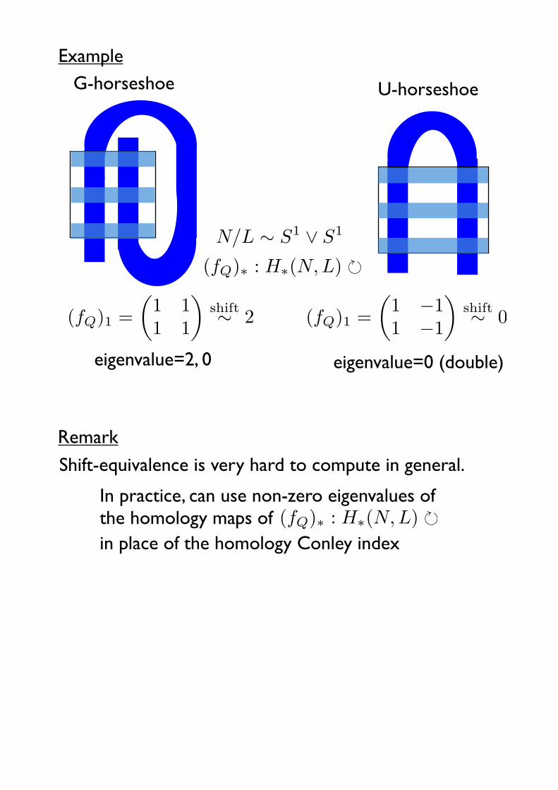
ExampleG-horseshoe

N/L ∼ S1 ∨ S1

(fQ)∗ : H∗(N,L) �

eigenvalue=2, 0

(fQ)1 =�

1 11 1

�shift∼ 2

U-horseshoe

(fQ)1 =�

1 −11 −1

�shift∼ 0

eigenvalue=0 (double)

Shift-equivalence is very hard to compute in general.

Remark

In practice, can use non-zero eigenvalues of the homology maps of (fQ)∗ : H∗(N,L) �in place of the homology Conley index

want to see how much the analogy of (classical) Morse theoryholds true for Morse decomposition of general dynamical systems

Morse theory Morse decompositionfinitely manynon-degenerate critical pts

finitely manyMorse components

entire dynamics =crit pts & connecting orbits

entire dynamics =Morse components & con-necting orbits

Morse index= dim of unstable mfd

Conley index

8

Morse theory Morse decompositiontotal order on crit ptsby Morse function

flow-defined partial order onMorse components

filtration given by level setsof Morse function

index filtration by partiallyordered set [Franzosa]

11

How can one understand dynamics via Conley index?

テキスト“Conley-Morse theory for dynamics”

α ⊂ P : lower set def⇐⇒ [p < q (∃q ∈ α) ⇒ p ∈ α]

L(P ) := set of lower sets in P

I ⊂ P : interval def⇐⇒ [p < r < q (∃p, q ∈ I) ⇒ r ∈ I]

M(I) := ∪p∈IM(p) ∪ (connecting orbits between M(p) (p ∈ I))

Theorem:[Franzosa 1986]

∃ collection of compact subsets {Nα}α∈L(P ) of N , s.t.

(1) Nα ∩Nβ = Nα∩β, Nα ∪Nβ = Nα∪β

(2) ∀ interval I ⊂ P ∃ α, β ∈ L(P ) with α ⊂ β, I = β \ α

s.t. CH∗(M(I)) = H∗(Nβ, Nα)

{Nα}α∈L(P ): index filtration of the Morse decomposition

12テキスト

suppose a Morse decomp is given;{M(p)}p∈P

For a continuous time flow,

attractor-repeller pair:

N

N

N

2

0

1

R

A

def⇐⇒ Morse decomposition consisting ofonly two components {R, A} with R �< A

corresponding index filtration N0 ⊂ N1 ⊂ N2CH∗(S) = H∗(N2, N0),CH∗(R) = H∗(N2, N1),CH∗(A) = H∗(N1, N0)

homology long exact sequence for the triple (N0, N1, N2):

→ H∗+1(N2, N1)∂→ H∗(N1, N0) → H∗(N2, N0) →

CH∗+1(R) CH∗(A) CH∗(S)

→ H∗(N2, N1)∂→ H∗−1(N1, N0) →

CH∗(R) CH∗−1(A)

13


N

N

N

2

0

1

R

A




→ H∗+1(N2, N1)∂→ H∗(N1, N0) → H∗(N2, N0) →


→ H∗(N2, N1)∂→ H∗−1(N1, N0) →


13

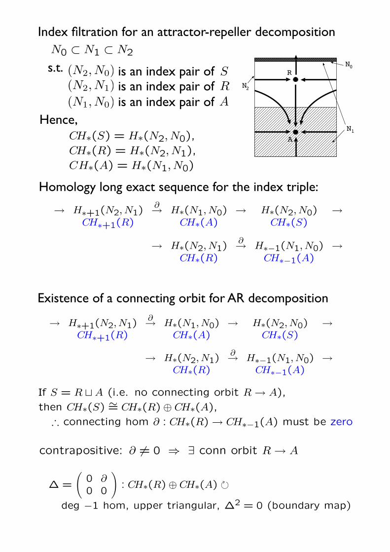
Index filtration for an attractor-repeller decomposition

s.t.

is an index pair of (N1, N0) A(N2, N1) is an index pair of R(N2, N0) is an index pair of S


N

N

N

2

0

1

R

A




→ H∗+1(N2, N1)∂→ H∗(N1, N0) → H∗(N2, N0) →


→ H∗(N2, N1)∂→ H∗−1(N1, N0) →


13

Hence,


N

N

N

2

0

1

R

A




→ H∗+1(N2, N1)∂→ H∗(N1, N0) → H∗(N2, N0) →


→ H∗(N2, N1)∂→ H∗−1(N1, N0) →


13

Homology long exact sequence for the index triple:

Existence of a connecting orbit for AR decomposition


N

N

N

2

0

1

R

A




→ H∗+1(N2, N1)∂→ H∗(N1, N0) → H∗(N2, N0) →


→ H∗(N2, N1)∂→ H∗−1(N1, N0) →


13

Wazewski principleIf S = R �A (i.e. no connecting orbit R → A),then CH∗(S) ∼= CH∗(R)⊕ CH∗(A),

∴ connecting hom ∂ : CH∗(R)→ CH∗−1(A) must be zero

contrapositive: ∂ �= 0 ⇒ ∃ conn orbit R → A

∆ =

�0 ∂0 0

�

: CH∗(R)⊕ CH∗(A) �

deg −1 hom, upper triangular, ∆2 = 0 (boundary map)

14




∆ =

�0 ∂0 0

�

: CH∗(R)⊕ CH∗(A) �


14




∆ =

�0 ∂0 0

�

: CH∗(R)⊕ CH∗(A) �


14

connection complex C∆

Theorem:[Conley] [Franzosa 1989],[Robbin-Salamon 1992]

∃∆ : ⊕p∈PCH(M(p)) � deg −1 hom s.t.(1) ∆ strictly upper triangular

i.e. ∆(p, q) �= 0⇒ p < q

(2) ∆2 = 0 (boundary map)hence C∆ = {⊕CH(M(p)),∆} chain complex

(3) H∗(C∆) ∼= CH∗(S)

∆ is called a connection matrix

16

Morse theory Morse decompositionMorse complexMf = {⊕k∈ZCritk, ∂}[Smale, Witten]

connection complex C∆ withconnection matrix∆ : ⊕p∈PCH∗(M(p)) �

H∗(Mf)∼= H∗(M) H∗(C∆) ∼= CH∗(S)

15

Remark(1) Connection matrix is NOT unique!

∆(p, q) �= 0⇒ p < q(2) , henceexistence of a connecting orbit M(q)→M(p)

Can detect connecting orbits by linear algebra

1

2

3

4 5

Reineck’s example:

non-uniqueness of connection matrix

CH∗(M(p)) = Z2 if

p = 1 and ∗ = 0,1, or

p = 2,3 and ∗ = 1, or

p = 4,5 and ∗ = 2,

else CH∗(M(p)) = 0

∆ =

0 0 1 1 0 0

0 0 0 0 a b

0 0 0 0 1 1

0 0 0 0 1 1

0 0 0 0 0 0

0 0 0 0 0 0

Here (a, b) = (1,0), (0,1) both possible

18

1

2

3

4 5



CH∗(M(p)) = Z2 if

p = 1 and ∗ = 0,1, or

p = 2,3 and ∗ = 1, or

p = 4,5 and ∗ = 2,


∆ =

0 0 1 1 0 0

0 0 0 0 a b

0 0 0 0 1 1

0 0 0 0 1 1

0 0 0 0 0 0

0 0 0 0 0 0


18

1

2

3

4 5



CH∗(M(p)) = Z2 if

p = 1 and ∗ = 0,1, or

p = 2,3 and ∗ = 1, or

p = 4,5 and ∗ = 2,


∆ =

0 0 1 1 0 0

0 0 0 0 a b

0 0 0 0 1 1

0 0 0 0 1 1

0 0 0 0 0 0

0 0 0 0 0 0


18

1

2

3

4 5



CH∗(M(p)) = Z2 if

p = 1 and ∗ = 0,1, or

p = 2,3 and ∗ = 1, or

p = 4,5 and ∗ = 2,


∆ =

0 0 1 1 0 0

0 0 0 0 a b

0 0 0 0 1 1

0 0 0 0 1 1

0 0 0 0 0 0

0 0 0 0 0 0


18

Definition: A flow Φ = {ϕt} on S is semi-conjugate to anotherflow Ψ = {ψt} on Σ, if

∃ ρ : S → Σ continuous surjection, s.t.

Sϕt

→ Sρ ↓ � ↓ ρ

Σψt

→ Σ

(∀t ∈ R)

several results for ∃ of semi-conjugacies in restrictive situations,e.g.

• semi-conj onto gradient flow [McCord-Mischaikow]• semi-conj onto symbolic dynamics [Carbinatto-Kwapisz-

Mischaikow]• semi-conj onto simplicial model flow [McCord]

27

How to represent dynamics? : semi-conjugacy

Can obtain more general representation by semi-conj?

References

C. Conley, Isolated invariant sets and the Morse index, CBMS Lecture Notes 38, AMS, 1978

D. Salamon, Connected simple systems and the Conleyindex of isolated invariant sets, Trans AMS, 291 (1985), 1-41

Z. Arai, Master thesis, 2003 (and references therein).http://www.cris.hokudai.ac.jp/arai/papers/master_thesis.pdf

J. W. Robbin - D. Salamon, Lyapunov maps, simplicial complexes, and the Stone functor, Ergod. Th. Dynam. Sys. 12 (1992), 153-183

Introduction to the Conley index theorykfujiwara/sendai/kokubu...Morse decomposition (2) Conley...

Documents

Transcript of Introduction to the Conley index theorykfujiwara/sendai/kokubu...Morse decomposition (2) Conley...