Introduction to Survey Sampling -...
176
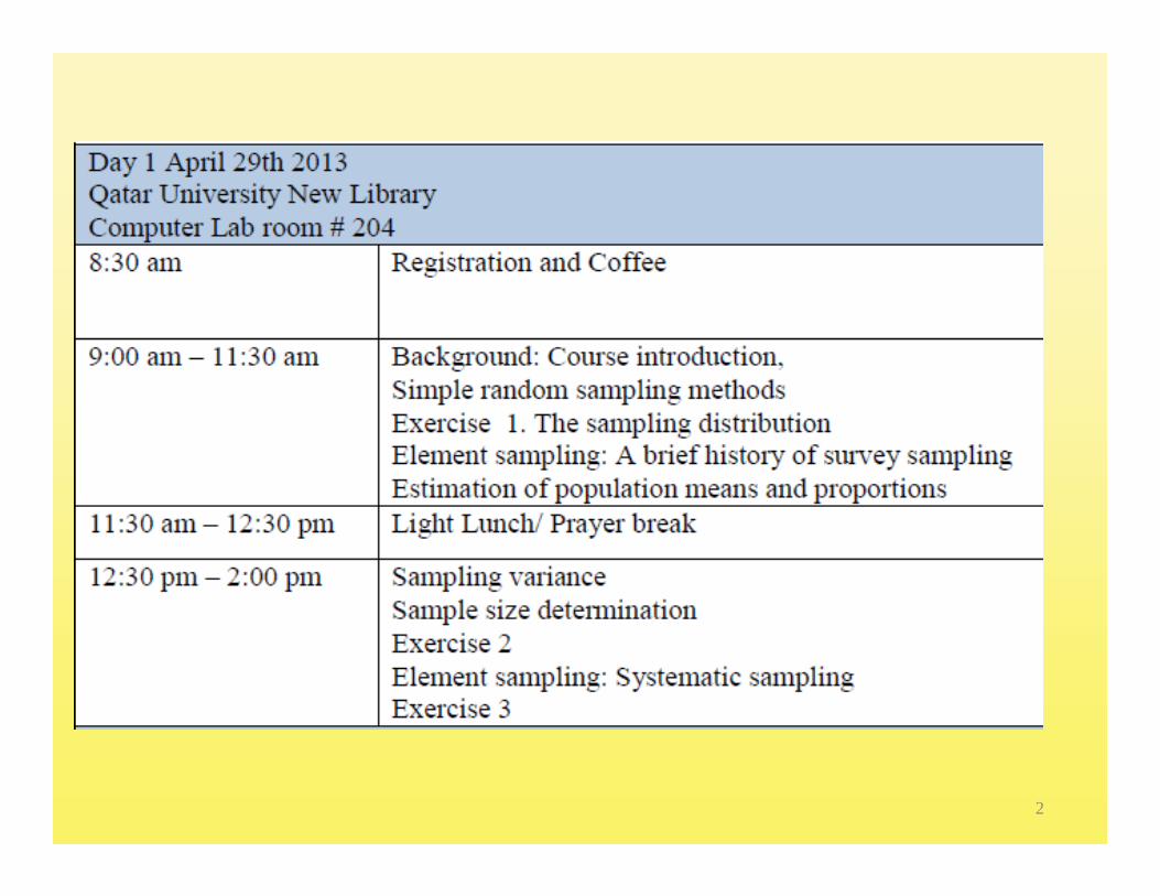
A three‐day short course sponsored by the Social & Economic Research Institute, Qatar University Introduction to Survey Sampling James M. Lepkowski & Michael Traugott Institute for Social Research University of Michigan April 29 – May 1, 2013
Transcript of Introduction to Survey Sampling -...
A three‐day short course sponsored by the Social & Economic Research Institute, Qatar University
Introduction to Survey SamplingJames M. Lepkowski& Michael Traugott
Institute for Social ResearchUniversity of Michigan
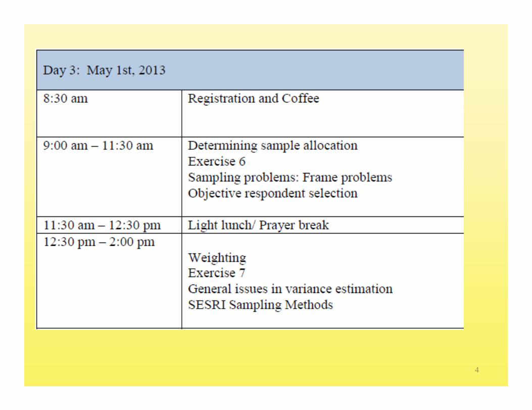
April 29 – May 1, 2013
2

3
4

1. Overview of Surveys & Survey Sampling
• Where does sampling fit in?• Sampling topics to be covered
– Probability v. non‐probability sampling– Population of inference– Sampling frames– Sample designs for list frames or widespread populations– Sample deficiencies– Weighting– Variance estimation for complex sample surveys
5
WHERE DOES SAMPLING FIT IN?
• During conceptualization, a researcher considers the RELEVANT POPULATION for evaluating the theory/hypothesis
• In designing the data collection, the researcher has two concerns in mind:– External validity– Cost/benefit calculations for the overall cost of
the study

DIFFERENCES BETWEEN CENSUSES AND SAMPLES
A census involves an enumeration of a population. When the population is large:
1. It is costly2. It is time consuming3. May not be feasible with precision
(US Census as an example)
A sample involves a selection of a representative subset of a population in order to draw inferences to the population
Collecting data from a sample of a large population is FAR LESS costly and FAR LESS time consuming

Greater Accuracy
• Because of the cost savings, samplingallows a researcher to devote – More resources to the collection of more data
(variables)– The reduction of error in measurement (reliability
and validity)– Better coverage of the units of analysis
• This fits in with the Total Survey Error perspective

Total Survey Error
Probability v. non‐probability sampling
• Non‐probability sampling– Haphazard, convenience, or accidental sampling– Purposive sampling or expert choice– Quota sampling
• Probability sampling
11
Population of inference
• Target population– Geographical boundaries– Age limits– Date
• Survey population– Possible exclusions from target population
• Institutionalized• Homeless• Nomads• Remote sparsely settled areas
12

13
Target
Survey
Frame

Sampling frame
• List frame• Area frame• Problems
– Missing elements– Duplicate listings– Clusters– Blanks or ineligibles
14
Sample designs for compact populations
• Simple random sampling• Systematic sampling• Stratified sampling
– Proportionate allocation– Disproportionate allocation
15

Sample designs for widespread populations
• Cluster sampling– One‐stage (take all)– Two‐stage (subsampling)– Multi‐stage
• Probability proportionate to size sampling• Stratified cluster sampling• Systematic sampling of clusters
16

Sample deficiencies• Nonresponse
– Total/unit– Item
• Noncoverage• Compensation: weighting
– Unequal probabilities– Nonresponse– Noncoverage (poststratification)
• Make the sample distribution conform to known population distribution
17

Variance estimation
• Standard software cannot handle complex sample designs correctly
• Methods of variance estimation– Taylor series approximation– Balanced or Jackknife repeated replication
• Computer software available for these methods– Requires stratum, cluster, and weight on each sample record
18
2. Simple random sampling
• Simple random sampling• Exercise 1• Table of random digits• Faculty salaries
19
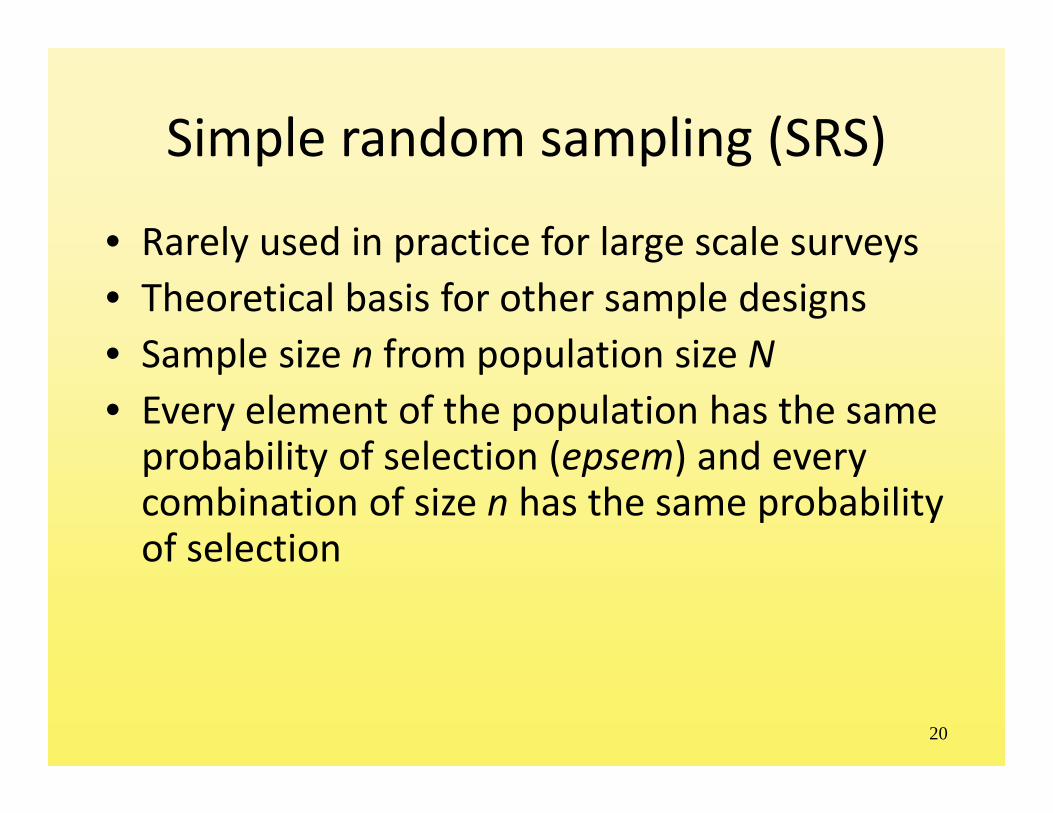
Simple random sampling (SRS)
• Rarely used in practice for large scale surveys• Theoretical basis for other sample designs• Sample size n from population size N• Every element of the population has the same probability of selection (epsem) and every combination of size n has the same probability of selection
20

Selection and estimation
• Use a table of random numbers to select SRS samples
• Sample mean estimates population mean
21
1
1 n
ii
y yn
1
1 N
ii
Y YN
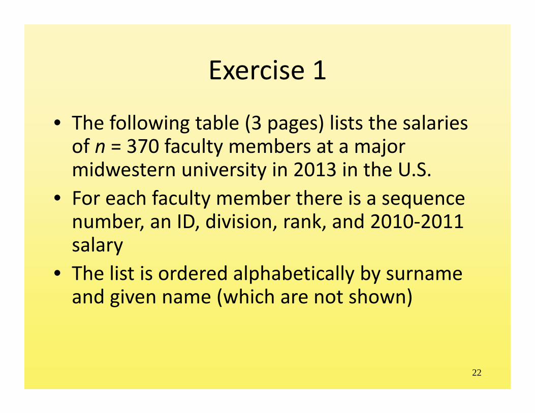
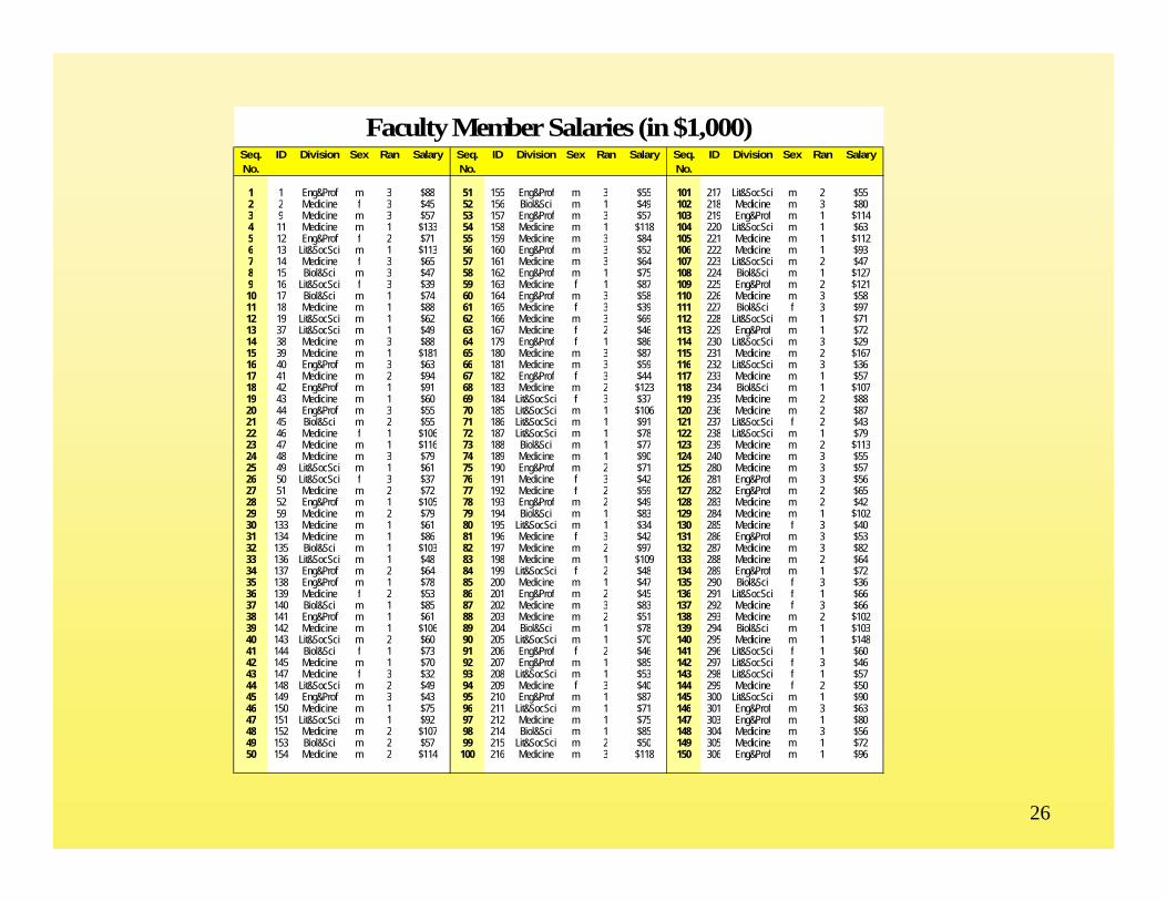
Exercise 1
• The following table (3 pages) lists the salaries of n = 370 faculty members at a major midwestern university in 2013 in the U.S.
• For each faculty member there is a sequence number, an ID, division, rank, and 2010‐2011 salary
• The list is ordered alphabetically by surname and given name (which are not shown)
22

Exercise 1This is a group exercise.Each group should select a simple random sample of n = 20 from the list.Use the accompanying table of random numbers to select the sample.Then compute the sample meanOne member of the group should report the sample mean on behalf of the group.
1
1 n
ii
y yn
23
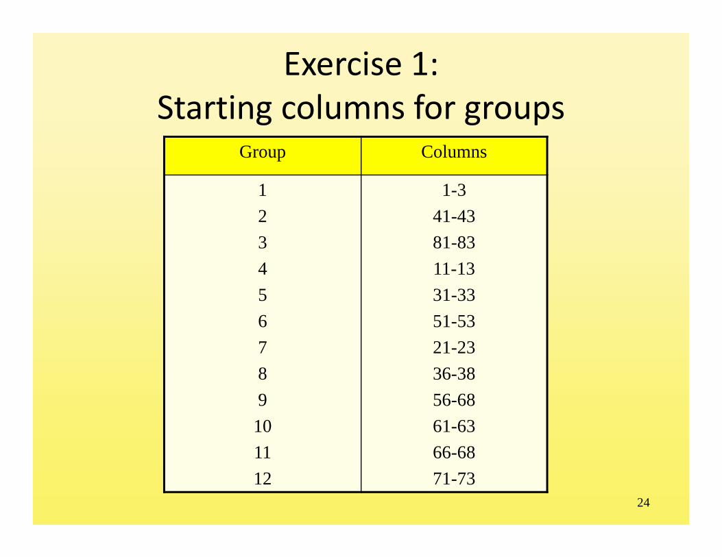
Exercise 1:Starting columns for groups
Group Columns
123456789101112
1-341-4381-8311-1331-3351-5321-2336-3856-6861-6366-6871-73
24

25
Exercise 1: Table of Random Digits
Row Column 1-5 6-10 11-15 16-20 21-25 26-30 31-35 36-40 41-45 46-50 51-55 56-60 61-65 66-70 71-75 76-80 81-85 86-90
1 49018 34042 72000 49522 85941 84723 51072 56454 67420 05025 25234 10671 05579 90906 54706 79486 57057 404682 97294 25351 12331 82557 13834 91334 32510 47165 08535 27491 87064 23579 72223 45164 98781 20189 17391 751453 97638 18356 31198 39366 37340 76043 77528 21714 44751 81797 28670 50973 07915 45259 45334 88904 47365 372494 34525 30477 75462 34635 51422 60669 62413 52524 79883 26235 46933 23381 72335 74702 77289 83419 28761 689965 79619 43993 89902 64817 88397 35390 44558 91500 87656 83603 00491 37693 75524 04058 77373 61598 60059 322416 54778 70353 54134 19513 89074 07807 74520 59684 47494 58194 29810 91489 45410 28737 55504 50467 94953 255657 12256 17900 33754 11853 65033 24106 41833 68345 62300 33076 70119 60498 70180 06929 34567 37075 57735 446028 33297 14796 91080 67108 85984 81892 37533 24643 37522 71461 96220 16177 04449 38396 09675 64290 96410 491179 75083 44991 46851 46383 00695 54453 34156 49854 68163 83123 89928 39667 15632 43854 04707 41766 01876 20016
10 66288 63908 74090 52902 69701 72959 64480 78123 81841 92675 08731 20577 94939 43211 63438 93640 75825 5792211 84578 05698 92016 94285 26563 36372 55989 94790 36338 30640 81337 56599 05695 42896 57115 73143 49959 8490312 55699 23402 30639 39508 41495 44462 11924 70471 97867 82637 18031 38020 70819 64948 17274 67345 31672 6615513 51917 88538 58239 58633 80392 89447 81230 97654 52579 34888 06454 94398 16452 76723 00902 81924 73166 8566914 36779 68538 88591 96616 84918 29413 99116 66987 41334 43877 00185 90070 43292 01754 01505 25362 39548 6093315 49852 36333 84789 65346 46181 61218 54131 57370 64814 44430 43774 72286 11644 33071 74301 02154 37021 0482816 66752 08578 57498 17884 83667 59532 73254 83347 85751 18536 55969 73265 06726 80734 29351 36800 77081 1068717 61689 45570 53663 66779 85627 27662 34436 58824 18902 49414 05020 98033 85987 53127 72623 00983 92504 5468618 19111 76703 32467 51391 85381 48433 68754 89843 02166 59177 80856 71628 27731 90073 04233 34913 46188 2877819 46913 70576 16918 46675 02304 83330 55894 39684 20753 48885 72907 37048 80065 58931 78214 36397 97252 6959320 22224 48264 96826 15434 52010 22811 07914 89541 61620 83346 96204 52742 27485 37716 71756 79244 04517 2083121 84119 49920 29328 03239 15832 72406 94946 45797 70566 19586 26419 40852 70097 02276 93410 87952 71018 9653322 75594 56191 18861 44995 44764 76960 12585 01842 19324 46085 33903 77234 07418 42805 21925 86305 12510 8728123 34821 90491 28843 85959 72301 14576 94229 43353 55740 86145 73278 89446 36093 39173 07384 32388 17494 5273424 23378 01578 09081 20536 31412 00632 16380 14876 26249 00449 26441 14765 05223 08297 54280 35937 02965 7938925 09985 71346 32130 58906 97244 07003 91231 23396 47378 19064 01118 04376 83218 01890 94316 40309 41332 3096626 43814 09227 11841 44516 62348 31284 58895 88559 19567 82425 00614 68626 10523 96822 79297 16858 52693 6388727 26724 80216 75905 54725 46995 75504 79112 50571 57115 02600 35097 04329 78514 02663 48700 57166 30316 9764928 37876 85859 19333 87221 44809 50700 57889 43075 99310 32235 62624 88356 51865 21946 52479 69599 29065 2643429 23634 07454 63628 30531 52979 28534 03208 75663 33587 27738 04018 32256 32259 14042 27624 94889 91414 7265830 10906 61337 16571 98829 96434 25748 01518 97758 93725 64532 79331 25961 82782 23354 47052 36078 12780 7833131 09372 97239 72017 99537 99977 96404 04824 64248 68816 02734 38384 87274 18213 67600 18730 17870 02026 3418032 86659 47171 96123 33853 64659 76657 53911 09900 70918 07733 89084 42345 22250 13583 52020 96144 25382 1087533 78209 23140 94532 89438 43271 89616 63137 85026 15799 62580 70837 50071 74496 94191 45858 13545 66999 7739034 15430 43742 77673 21745 34854 31505 05275 16758 58996 70211 97794 60918 98986 14446 72130 43056 13412 8669135 64947 43432 14105 78393 03682 47498 75738 76250 69143 19799 31068 31261 31912 47359 26853 62917 40581 4077236 71143 09505 65318 29034 89055 17744 48752 69171 08426 08827 14816 61969 68694 19168 67081 26010 68211 8038437 03104 54280 49703 72368 99964 68555 57769 27567 55962 31100 26364 61603 48176 04177 00935 05130 83625 6632338 56085 69548 50876 92855 52293 11580 22797 94044 67994 50651 26397 01782 73341 80486 72738 66943 75883 1010639 41842 68437 92724 67791 21113 47124 28279 50647 09809 26717 48925 14686 24824 38530 62429 57330 33340 0799440 28521 08035 30260 91407 04111 18581 84777 87116 96280 09202 31360 02923 83625 19821 35903 86927 36021 9059341 85133 15310 42745 84831 82992 73756 67473 62066 83254 02735 55402 39765 92121 07338 39944 36882 74892 0014842 28122 35506 71104 96492 90721 22225 23256 30415 63671 27160 19768 08441 38172 15357 73851 53381 20093 4207343 56665 12467 44282 00817 58668 70312 66617 75720 93458 74491 72624 45673 68051 53523 58745 13730 93676 8763644 19871 89889 70142 63766 71799 97398 23855 08350 11993 16729 23096 75940 45632 05786 46643 52563 30407 2833845 48253 37932 79566 98774 02523 54942 15195 01354 03979 36909 21991 08828 45452 75565 90933 08713 36319 7025946 80828 98357 85671 69918 30878 48784 81471 43729 60566 81014 68445 82593 59634 16601 05712 80642 26928 1149647 09863 88615 26990 94808 32784 51992 60048 09830 75745 30593 64917 90209 55266 57533 68877 37486 91998 3005548 05754 47499 53052 86074 01045 90121 12938 84746 55683 64345 22413 08513 04316 38192 73202 99160 56397 7706349 32883 01773 11423 07799 12268 59983 60446 16744 12452 81457 56278 49040 31680 66267 05187 69329 28067 7801750 82869 70040 36427 18798 57316 09565 11637 30597 11151 46114 30048 60952 48736 39133 79698 90272 80447 88785
26
Seq. No.
ID Division Sex Ran Salary Seq. No.
ID Division Sex Ran Salary Seq. No.
ID Division Sex Ran Salary
1 1 Eng&Prof m 3 $88 51 155 Eng&Prof m 3 $55 101 217 Lit&SocSci m 2 $552 2 Medicine f 3 $45 52 156 Biol&Sci m 1 $49 102 218 Medicine m 3 $803 9 Medicine m 3 $57 53 157 Eng&Prof m 3 $57 103 219 Eng&Prof m 1 $1144 11 Medicine m 1 $133 54 158 Medicine m 1 $118 104 220 Lit&SocSci m 1 $635 12 Eng&Prof f 2 $71 55 159 Medicine m 3 $84 105 221 Medicine m 1 $1126 13 Lit&SocSci m 1 $113 56 160 Eng&Prof m 3 $52 106 222 Medicine m 1 $937 14 Medicine f 3 $65 57 161 Medicine m 3 $64 107 223 Lit&SocSci m 2 $478 15 Biol&Sci m 3 $47 58 162 Eng&Prof m 1 $75 108 224 Biol&Sci m 1 $1279 16 Lit&SocSci f 3 $39 59 163 Medicine f 1 $87 109 225 Eng&Prof m 2 $12110 17 Biol&Sci m 1 $74 60 164 Eng&Prof m 3 $58 110 226 Medicine m 3 $5811 18 Medicine m 1 $88 61 165 Medicine f 3 $39 111 227 Biol&Sci f 3 $9712 19 Lit&SocSci m 1 $62 62 166 Medicine m 3 $69 112 228 Lit&SocSci m 1 $7113 37 Lit&SocSci m 1 $49 63 167 Medicine f 2 $46 113 229 Eng&Prof m 1 $7214 38 Medicine m 3 $88 64 179 Eng&Prof f 1 $86 114 230 Lit&SocSci m 3 $2915 39 Medicine m 1 $181 65 180 Medicine m 3 $87 115 231 Medicine m 2 $16716 40 Eng&Prof m 3 $63 66 181 Medicine m 3 $59 116 232 Lit&SocSci m 3 $3617 41 Medicine m 2 $94 67 182 Eng&Prof f 3 $44 117 233 Medicine m 1 $5718 42 Eng&Prof m 1 $91 68 183 Medicine m 2 $123 118 234 Biol&Sci m 1 $10719 43 Medicine m 1 $60 69 184 Lit&SocSci f 3 $37 119 235 Medicine m 2 $8820 44 Eng&Prof m 3 $55 70 185 Lit&SocSci m 1 $106 120 236 Medicine m 2 $8721 45 Biol&Sci m 2 $55 71 186 Lit&SocSci m 1 $91 121 237 Lit&SocSci f 2 $4322 46 Medicine f 1 $106 72 187 Lit&SocSci m 1 $78 122 238 Lit&SocSci m 1 $7923 47 Medicine m 1 $116 73 188 Biol&Sci m 1 $77 123 239 Medicine m 2 $11324 48 Medicine m 3 $79 74 189 Medicine m 1 $90 124 240 Medicine m 3 $5525 49 Lit&SocSci m 1 $61 75 190 Eng&Prof m 2 $71 125 280 Medicine m 3 $5726 50 Lit&SocSci f 3 $37 76 191 Medicine f 3 $42 126 281 Eng&Prof m 3 $5627 51 Medicine m 2 $72 77 192 Medicine f 2 $59 127 282 Eng&Prof m 2 $6528 52 Eng&Prof m 1 $105 78 193 Eng&Prof m 2 $49 128 283 Medicine m 2 $4229 59 Medicine m 2 $79 79 194 Biol&Sci m 1 $83 129 284 Medicine m 1 $10230 133 Medicine m 1 $61 80 195 Lit&SocSci m 1 $34 130 285 Medicine f 3 $4031 134 Medicine m 1 $86 81 196 Medicine f 3 $42 131 286 Eng&Prof m 3 $5332 135 Biol&Sci m 1 $103 82 197 Medicine m 2 $97 132 287 Medicine m 3 $8233 136 Lit&SocSci m 1 $48 83 198 Medicine m 1 $109 133 288 Medicine m 2 $6434 137 Eng&Prof m 2 $64 84 199 Lit&SocSci f 2 $48 134 289 Eng&Prof m 1 $7235 138 Eng&Prof m 1 $78 85 200 Medicine m 1 $47 135 290 Biol&Sci f 3 $3636 139 Medicine f 2 $53 86 201 Eng&Prof m 2 $45 136 291 Lit&SocSci f 1 $6637 140 Biol&Sci m 1 $85 87 202 Medicine m 3 $83 137 292 Medicine f 3 $6638 141 Eng&Prof m 1 $61 88 203 Medicine m 2 $51 138 293 Medicine m 2 $10239 142 Medicine m 1 $106 89 204 Biol&Sci m 1 $78 139 294 Biol&Sci m 1 $10340 143 Lit&SocSci m 2 $60 90 205 Lit&SocSci m 1 $70 140 295 Medicine m 1 $14841 144 Biol&Sci f 1 $73 91 206 Eng&Prof f 2 $46 141 296 Lit&SocSci f 1 $6042 145 Medicine m 1 $70 92 207 Eng&Prof m 1 $85 142 297 Lit&SocSci f 3 $4643 147 Medicine f 3 $32 93 208 Lit&SocSci m 1 $53 143 298 Lit&SocSci f 1 $5744 148 Lit&SocSci m 2 $49 94 209 Medicine f 3 $40 144 299 Medicine f 2 $5045 149 Eng&Prof m 3 $43 95 210 Eng&Prof m 1 $87 145 300 Lit&SocSci m 1 $9046 150 Medicine m 1 $75 96 211 Lit&SocSci m 1 $71 146 301 Eng&Prof m 3 $6347 151 Lit&SocSci m 1 $92 97 212 Medicine m 1 $75 147 303 Eng&Prof m 1 $8048 152 Medicine m 2 $107 98 214 Biol&Sci m 1 $85 148 304 Medicine m 3 $5649 153 Biol&Sci m 2 $57 99 215 Lit&SocSci m 2 $50 149 305 Medicine m 1 $7250 154 Medicine m 2 $114 100 216 Medicine m 3 $118 150 306 Eng&Prof m 1 $96
Faculty Member Salaries (in $1,000)

27
Seq. No.
ID Division Sex Ran Salary Seq. No.
ID Division Sex Ran Salary Seq. No.
ID Division Sex Ran Salary
151 307 Medicine m 3 $65 201 440 Medicine m 1 $108 251 496 Medicine m 3 $60152 308 Lit&SocSci m 3 $37 202 441 Lit&SocSci m 1 $48 252 497 Eng&Prof m 1 $86153 309 Eng&Prof m 1 $127 203 442 Medicine m 3 $85 253 498 Medicine m 1 $134154 310 Lit&SocSci m 1 $90 204 443 Lit&SocSci m 1 $59 254 499 Medicine f 3 $63155 311 Lit&SocSci m 3 $45 205 444 Lit&SocSci f 1 $63 255 500 Medicine m 1 $123156 312 Eng&Prof f 1 $75 206 445 Lit&SocSci f 2 $46 256 501 Medicine m 3 $85157 313 Medicine m 2 $60 207 446 Medicine f 3 $41 257 502 Medicine f 3 $42158 314 Lit&SocSci m 2 $57 208 447 Medicine m 3 $71 258 503 Medicine f 2 $83159 315 Medicine m 1 $129 209 448 Eng&Prof f 3 $44 259 504 Lit&SocSci m 1 $54160 316 Eng&Prof m 1 $102 210 449 Lit&SocSci m 2 $46 260 505 Lit&SocSci f 1 $66161 317 Eng&Prof m 3 $57 211 450 Medicine m 3 $85 261 506 Medicine m 1 $84162 318 Eng&Prof m 3 $61 212 452 Medicine m 1 $119 262 507 Eng&Prof m 3 $46163 319 Eng&Prof m 1 $93 213 453 Medicine m 2 $69 263 508 Eng&Prof m 1 $90164 320 Medicine f 3 $41 214 454 Eng&Prof m 3 $74 264 509 Medicine m 2 $76165 321 Medicine m 1 $181 215 455 Biol&Sci m 1 $59 265 510 Eng&Prof m 1 $88166 322 Medicine f 2 $69 216 456 Biol&Sci m 1 $53 266 515 Medicine f 1 $87167 323 Lit&SocSci m 1 $81 217 457 Medicine f 3 $49 267 516 Eng&Prof m 3 $75168 324 Biol&Sci m 1 $94 218 459 Eng&Prof m 1 $78 268 517 Eng&Prof m 3 $64169 325 Lit&SocSci m 2 $53 219 460 Biol&Sci m 1 $68 269 518 Biol&Sci f 3 $52170 326 Medicine m 3 $48 220 461 Eng&Prof m 1 $83 270 519 Medicine m 2 $109171 327 Lit&SocSci m 1 $83 221 462 Eng&Prof m 1 $105 271 520 Lit&SocSci m 1 $144172 328 Lit&SocSci m 1 $47 222 463 Lit&SocSci m 3 $37 272 521 Eng&Prof m 2 $79173 329 Lit&SocSci m 3 $45 223 464 Medicine m 1 $111 273 522 Biol&Sci m 1 $56174 330 Medicine f 1 $75 224 465 Medicine f 2 $70 274 530 Biol&Sci m 1 $60175 331 Medicine m 3 $49 225 466 Eng&Prof m 1 $57 275 531 Biol&Sci m 3 $52176 333 Medicine m 3 $53 226 467 Eng&Prof m 1 $71 276 532 Lit&SocSci f 2 $45177 334 Eng&Prof m 1 $84 227 468 Biol&Sci m 3 $36 277 533 Lit&SocSci m 1 $59178 335 Eng&Prof m 1 $78 228 469 Eng&Prof f 3 $43 278 534 Eng&Prof m 3 $56179 336 Lit&SocSci m 1 $102 229 470 Eng&Prof m 1 $120 279 535 Medicine m 1 $123180 337 Lit&SocSci f 2 $50 230 471 Lit&SocSci m 1 $66 280 536 Medicine m 2 $75181 338 Medicine f 2 $49 231 472 Eng&Prof m 1 $84 281 537 Eng&Prof m 1 $84182 339 Medicine m 1 $54 232 473 Medicine m 2 $99 282 538 Medicine m 2 $70183 340 Medicine m 3 $35 233 474 Biol&Sci f 1 $91 283 539 Medicine m 3 $84184 341 Medicine m 2 $87 234 475 Eng&Prof m 2 $105 284 540 Eng&Prof m 1 $63185 342 Lit&SocSci m 1 $52 235 476 Medicine f 2 $60 285 541 Eng&Prof m 1 $121186 343 Lit&SocSci m 1 $75 236 477 Medicine f 3 $34 286 542 Medicine m 1 $52187 344 Medicine f 3 $41 237 478 Medicine f 3 $42 287 543 Biol&Sci m 1 $73188 345 Eng&Prof m 2 $62 238 479 Medicine m 2 $80 288 544 Eng&Prof f 3 $32189 346 Medicine m 1 $79 239 480 Medicine m 1 $94 289 545 Eng&Prof f 3 $40190 347 Biol&Sci m 3 $37 240 481 Biol&Sci m 1 $57 290 546 Biol&Sci m 3 $47191 348 Lit&SocSci m 3 $44 241 482 Medicine m 1 $82 291 547 Medicine m 1 $112192 349 Lit&SocSci m 3 $47 242 483 Lit&SocSci m 1 $70 292 548 Biol&Sci m 1 $68193 353 Medicine m 1 $70 243 484 Lit&SocSci m 1 $75 293 550 Medicine m 2 $93194 433 Lit&SocSci m 1 $113 244 485 Medicine m 1 $139 294 551 Medicine m 1 $124195 434 Medicine m 3 $55 245 486 Lit&SocSci m 1 $40 295 552 Lit&SocSci f 2 $49196 435 Lit&SocSci m 1 $50 246 488 Lit&SocSci m 2 $60 296 556 Medicine f 3 $65197 436 Lit&SocSci f 2 $54 247 489 Eng&Prof f 1 $128 297 557 Eng&Prof m 1 $84198 437 Eng&Prof m 3 $53 248 490 Medicine m 3 $47 298 558 Medicine f 2 $71199 438 Biol&Sci m 1 $79 249 491 Eng&Prof m 3 $67 299 559 Medicine f 3 $40200 439 Biol&Sci m 2 $53 250 495 Eng&Prof m 1 $90 300 560 Medicine m 2 $70
Faculty Member Salaries (Continued)

28
Seq. No.
ID Division Sex Ran Salary Seq. No.
ID Division Sex Ran Salary Seq. No.
ID Division Sex Ran Salary
301 561 Eng&Prof m 1 $98 351 636 Lit&SocSci f 1 $72302 562 Lit&SocSci m 1 $89 352 637 Eng&Prof m 1 $94303 563 Medicine f 3 $36 353 638 Eng&Prof m 3 $52304 564 Medicine m 1 $63 354 639 Biol&Sci m 1 $66305 565 Eng&Prof m 2 $74 355 640 Eng&Prof m 3 $68306 566 Medicine f 3 $38 356 641 Lit&SocSci m 1 $89307 567 Eng&Prof m 3 $76 357 642 Medicine m 2 $148308 568 Medicine m 3 $97 358 643 Medicine m 1 $159309 569 Medicine m 1 $76 359 644 Biol&Sci m 1 $62310 570 Eng&Prof m 1 $86 360 645 Lit&SocSci m 1 $70311 571 Medicine m 3 $59 361 646 Medicine f 3 $109312 572 Medicine f 2 $60 362 647 Eng&Prof m 1 $120313 573 Lit&SocSci m 2 $45 363 648 Eng&Prof m 1 $112314 595 Biol&Sci m 2 $56 364 649 Medicine m 2 $90315 596 Lit&SocSci m 1 $63 365 650 Medicine m 1 $108316 597 Lit&SocSci m 1 $69 366 651 Eng&Prof m 1 $152317 598 Eng&Prof m 1 $138 367 652 Medicine f 2 $47318 599 Lit&SocSci f 3 $31 368 653 Medicine m 1 $116319 600 Medicine f 2 $50 369 654 Biol&Sci m 1 $77320 601 Eng&Prof m 1 $89 370 655 Biol&Sci M 1 $57321 602 Eng&Prof m 1 $148322 603 Lit&SocSci m 3 $55323 604 Lit&SocSci m 1 $81324 605 Lit&SocSci m 1 $52325 606 Medicine m 3 $85326 607 Medicine m 1 $132327 608 Lit&SocSci m 1 $85328 609 Eng&Prof m 1 $66329 610 Eng&Prof f 1 $94330 611 Eng&Prof m 2 $77331 612 Medicine f 2 $76332 613 Medicine m 1 $109333 614 Lit&SocSci m 1 $99334 616 Eng&Prof f 2 $78335 617 Eng&Prof m 1 $98336 618 Medicine f 3 $41337 619 Medicine f 3 $37338 620 Eng&Prof m 3 $89339 622 Biol&Sci m 2 $55340 623 Lit&SocSc m 1 $52341 624 Eng&Prof m 3 $42342 625 Biol&Sci m 2 $52343 626 Lit&SocSc m 1 $63344 627 Lit&SocSc m 1 $95345 628 Medicine f 3 $75346 629 Medicine f 3 $106347 630 Lit&SocSc f 3 $44348 631 Lit&SocSc m 1 $58349 632 Lit&SocSc m 1 $79350 633 Lit&SocSc m 1 $135
Faculty Member Salaries (Continued)
3. Historical perspective
• Historical development• The beginnings• Development• Divergence• Framework for comparison• Selection bias• Development, part II• What should we do?
29

Historical development
• Sampling practice:– Result of attempts to solve practical problems
• Function of theory– Formalize implicit assumptions, and confirm, correct, or extend practice
• Origins– Data gathering
• health and social problems• social physics
– Census– Monography
30
The beginnings
• Berne, 1895– Kaier at ISI: Representative method
• Miniature of country• Large number of units• Use prior information in selection
– Von Mayr and others• No calculation where observation is possible• Cf. Godambe, Basu after 1950
– Cheysson and others• Monography: detailed examination of typical cases
31

Development
• 1903 ISI Resolution– Four implicit principles
• Representative• Objective• Measurability• Specification
– Actuality• Multistage proportionate stratified samples (no theory)
32
Divergence
• Representative– Purposive sampling– Expert choice– Balanced sampling
• Objective– Randomized selection– Bowley, 1906 (colleague of R.A. Fisher)
33

Separation
• ISI Commission 1926 report– Sampling established as basis for information collection
– Equal status given to random and purposive sampling
– No theory for unequal sized clusters
• No basis for comparing the two methodologies
34

Framework for comparison
• Neyman, 1934• The sampling distribution
– Properties of sample under repeated sampling• All possible samples and their associated probabilities of occurrence
– The sampling distribution of an estimator
35
Conditions for inference
• Conditions under which different procedures will produce valid estimates– Probability sampling
• “Unbiased” irrespective of population structure
– Purposive/balanced/quota sampling• Tough assumptions about population structure, unlikely to be achieved in practice
36
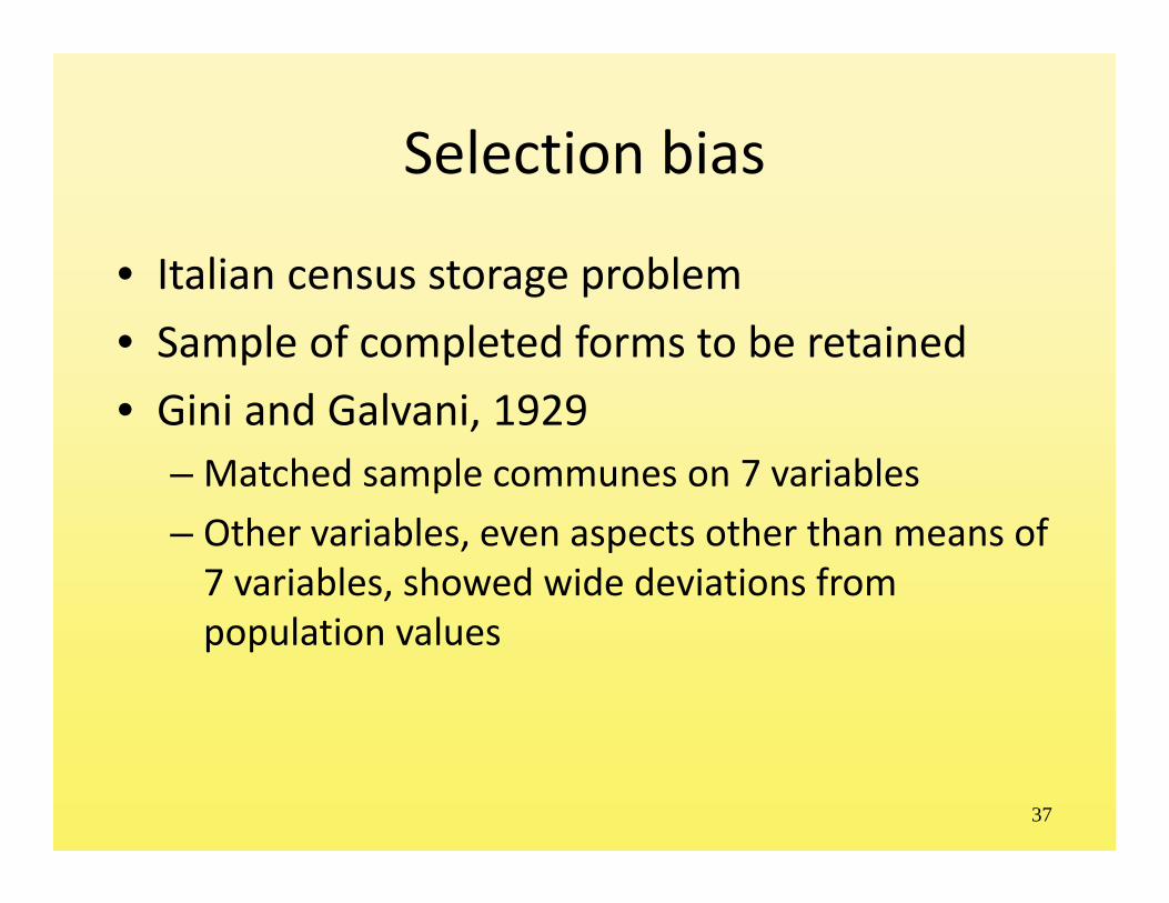
Selection bias
• Italian census storage problem• Sample of completed forms to be retained• Gini and Galvani, 1929
– Matched sample communes on 7 variables– Other variables, even aspects other than means of 7 variables, showed wide deviations from population values
37

What should we do?
• Probability sampling for objectivity• Stratification for precision (representativeness)
• Variance estimation from the sample• Complete and comprehensible description of the sampling procedure
38

39
4. Element samples
• Element samples• The sampling distribution• Properties of the sampling distribution• Central limit theorem• Properties of the sample mean for SRS• Estimation of variance• Determination of sample size• Formulas• Exercise 2

40
Element samples
• A sample design for which the unit of selection is the population element
• Basic framework: Neyman, 1934– Must be applicable to all populations– Must not depend on assumptions about the population structure
– Appropriate for large populations of elements
41
Element samples
• Repeated sampling– Objective (mechanical) selection of elements– Consider possible outcomes of the sampling process
– Evaluation of the whole set of possible outcomes

42
The sampling distribution
• The set of all possible values of the estimator that can be obtained with a given sample design– For a given sample we obtain a particular value, the estimate (such as )
• We want to know …– … how likely is the estimate to be close to the population value
y

43
Sample realization
• In fact, we select just one sample• The estimate may be correct, or incorrect• Want to maximize the probability of a satisfactory estimate

44
Properties of the sampling distribution
• Unbiasedness– Expected value (average value):
• Variability from one sample to another– Variance of the estimator– The square root of the variance is called the standard error of the estimator:
• Measurable design– A design for which the variance can be estimated from the sample itself
E y
( )Var y
( )Var y

45
Central limit theorem
• For large samples, the sampling distribution of is Normal
• Confidence intervals
y
(1 / 2) ( )y z Var y

46
Properties of the sample mean for SRS
• Unbiased • Variance
– Consider•••
– Where and
E y
2
( ) 1 n SVar yN n
1 1 nf
N 2S
n 22
1
11
N
ii
S Y YN
2 1S P P
47
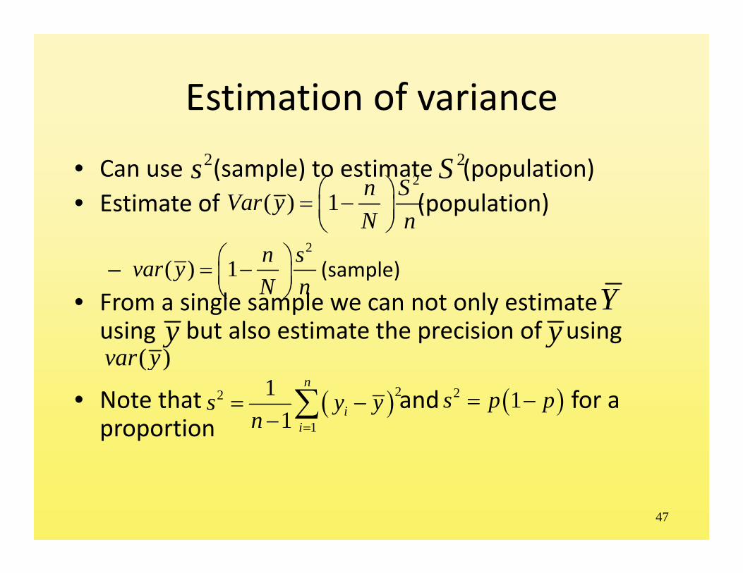
Estimation of variance
• Can use (sample) to estimate (population)• Estimate of (population)
– (sample)• From a single sample we can not only estimate using but also estimate the precision of using
• Note that and for a proportion
2s 2S
2
( ) 1 n svar yN n
2
( ) 1 n SVar yN n
Yy y
( )var y
22
1
11
n
ii
s y yn
2 1s p p

48
Determination of sample size
• What sample size do we need to obtain a given standard error of the estimator?
• population variance known (or guessed)– Census– Other surveys– Administrative records
• Desired standard error– Policy requirements in terms of – Decision making requirements
2S
( )Var y

49
Sample size formulas
• In general,
• For an infinitely large population (or for sampling with replacement), this is
• We can calculate the necessary sample size to achieve variance as
2
( ) 1 n SVar yN n
2
( ) SVar yn
Var y 2n S Var y

50
Sample size formulas (continued)
• In general (that is, not assuming N is large), the variance may be expressed as
– Where
2 2
( ) 1'
n S SVar yN n n
' 1 nn nN

51
Sample size formulas (continued)
• We can compute the necessary as
• To calculate the n necessary for a population of a particular size, we use the formula
''1
nn nN
'n
2
' SnVar y

52
Exercise 2
• The variability in income levels is comparable across many countries
• For a country with a value of (which would give ), we want an estimate of the mean income which has a standard error ( ) of 50.
• Answer the following questions in groups:
2,000S 2 4,000,000S
Var y

53
Exercise 2 (continued)Calculate the sample size needed in China with N = 1,400,000,000?
What about in the US where N = 320,000,000?
What about in Qatar where N = 1,700,000?
What about in a small city where N = 100,000?
What about in a small town where N = 10,000?

54
5. Systematic sampling
• Systematic sampling• Problems with intervals in systematic sampling• Solutions• Exercise 3

55
Systematic sampling
• A simple method of selecting a sample from a list
• Once the first element is chosen, every k th element is selected by counting through the list sequentially
• In probability sampling, the first element is chosen at random

56
Sampling intervals
• Determine the sampling interval • Select a random number (RN) from 1 to k• Add k repeatedly• Example:
– N = 12,000 dwellings in a city– Sample of n = 500 required– k = 12,000/500 = 24– Take a RN from 01 to 24, say 03– Take the third dwelling, and every 24th thereafter: 3, 27, 51, etc.
k N n

57
Problems with intervals
• Take 1 in k where • k may not be an integer• Examples
– N = 9, n = 2, and k = 4.5– N = 952, n = 200, and k = 4.76– N = 170,345, n = 1,250, and k = 136.272
k N n
58
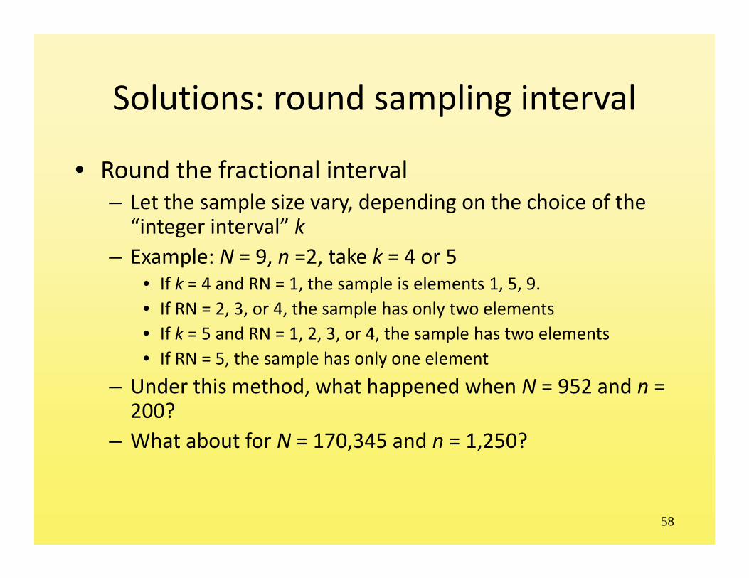
Solutions: round sampling interval
• Round the fractional interval– Let the sample size vary, depending on the choice of the “integer interval” k
– Example: N = 9, n =2, take k = 4 or 5• If k = 4 and RN = 1, the sample is elements 1, 5, 9.• If RN = 2, 3, or 4, the sample has only two elements• If k = 5 and RN = 1, 2, 3, or 4, the sample has two elements• If RN = 5, the sample has only one element
– Under this method, what happened when N = 952 and n = 200?
– What about for N = 170,345 and n = 1,250?
59
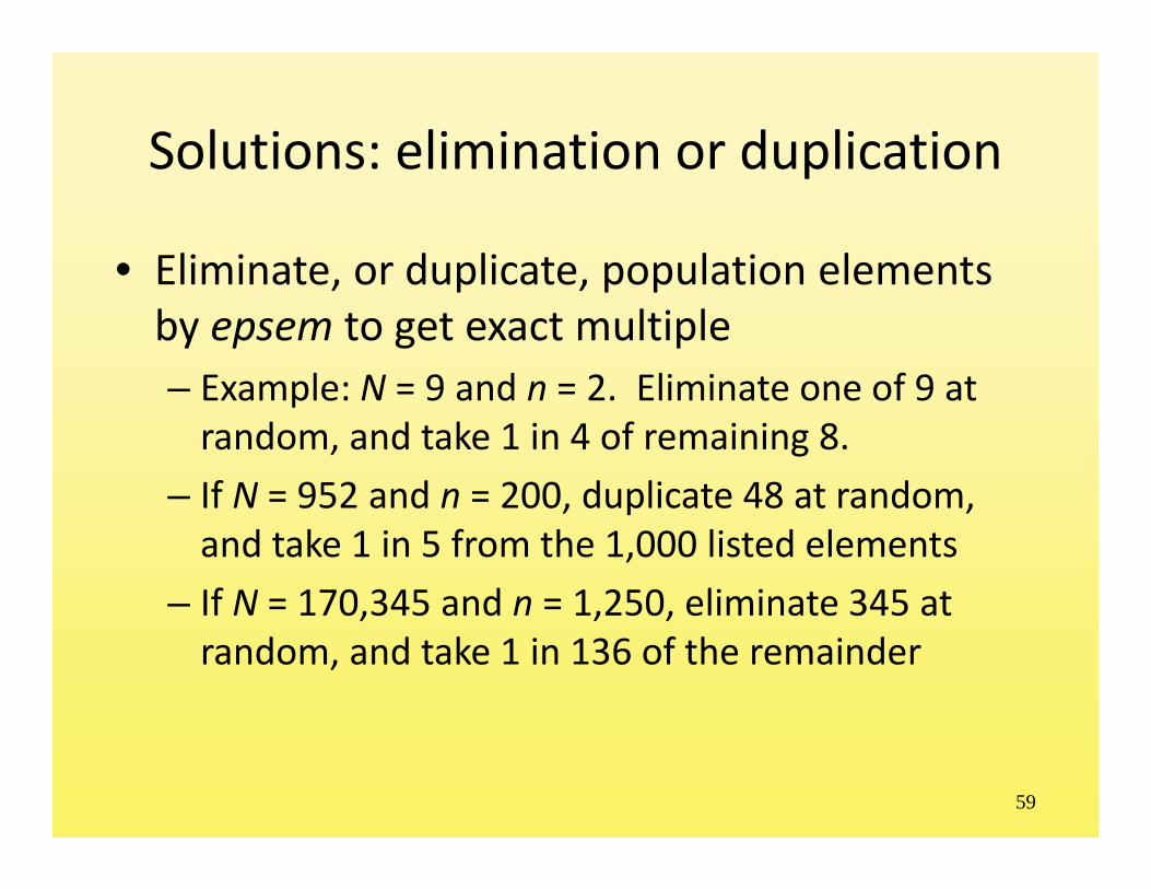
Solutions: elimination or duplication
• Eliminate, or duplicate, population elements by epsem to get exact multiple– Example: N = 9 and n = 2. Eliminate one of 9 at random, and take 1 in 4 of remaining 8.
– If N = 952 and n = 200, duplicate 48 at random, and take 1 in 5 from the 1,000 listed elements
– If N = 170,345 and n = 1,250, eliminate 345 at random, and take 1 in 136 of the remainder

60
Solutions: circular list
• Treat the list as circular• Select one element at random from anywhere on the list
• Take every [k]th thereafeter, where [k] is an integer near N/n, until n selections are made

61
Exercise 3
• Consider again the list of 370 faculty member salaries given in Exercise 1 (slides 23‐25)
• Suppose again we seek a sample of n = 20 from this list
Each group should select two systematic samples of n = 20 from the list using as random starts the next appropriate numbers from the random number table (slide 22) ‐‐ that is, the next random number after the last one used in Exercise 1
62
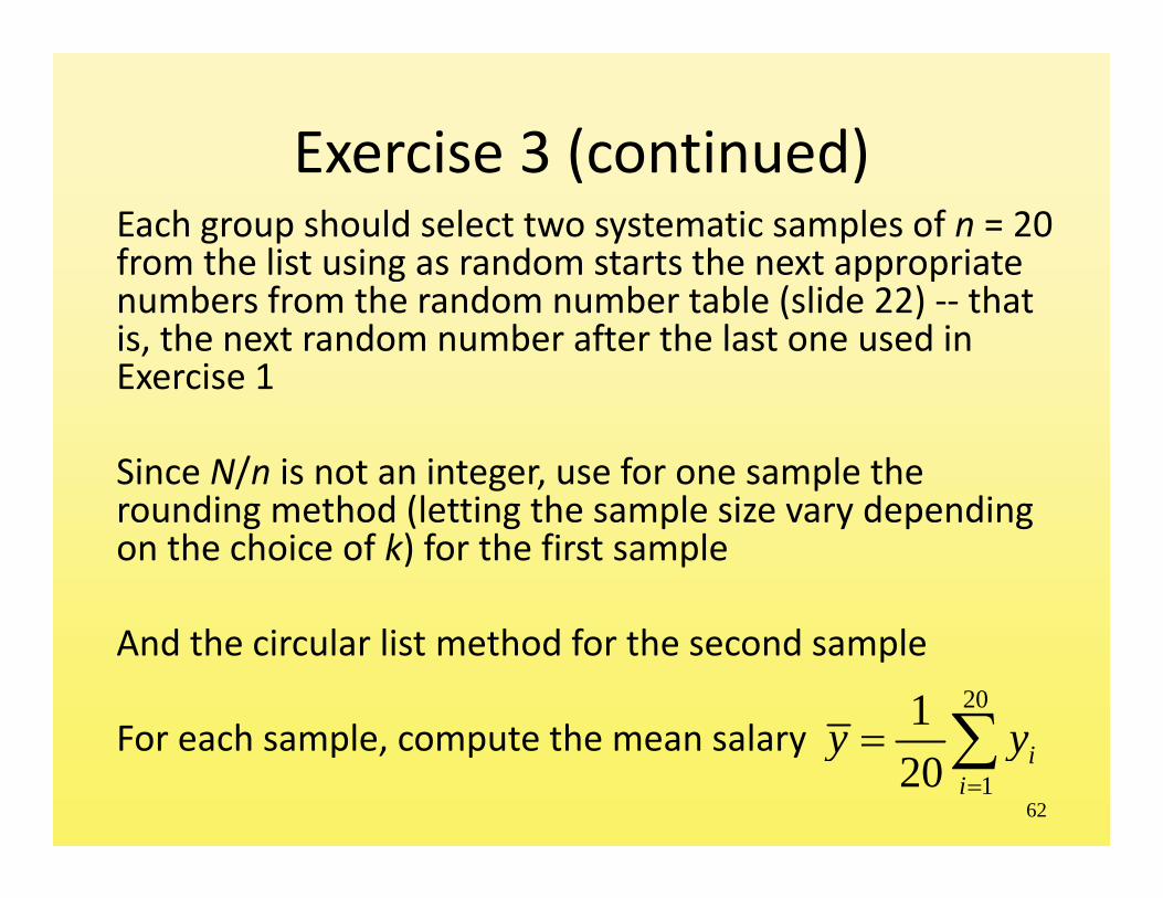
Exercise 3 (continued)Each group should select two systematic samples of n = 20 from the list using as random starts the next appropriate numbers from the random number table (slide 22) ‐‐ that is, the next random number after the last one used in Exercise 1
Since N/n is not an integer, use for one sample the rounding method (letting the sample size vary depending on the choice of k) for the first sample
And the circular list method for the second sample
For each sample, compute the mean salary 20
1
120 i
iy y

63
6. Cluster sampling
• Cluster sampling• Equal‐sized cluster sampling• Effective sample size• Design effect• Intra‐class correlation• Exercise 4

64
Cluster sampling
• Populations widely distributed geographically• Cannot afford to visit n sites drawn randomly from the entire area
• Cluster sampling reduces the cost of data collection– Sample schools and children within them– Sample blocks and households within them
65
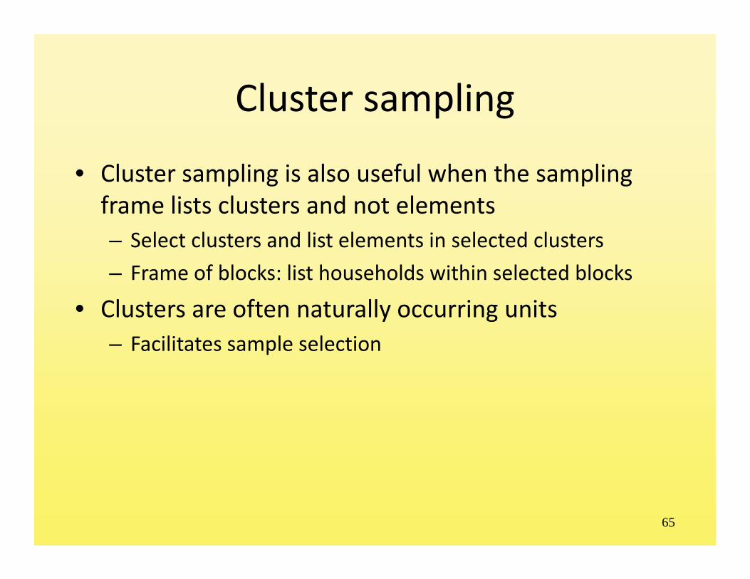
Cluster sampling
• Cluster sampling is also useful when the sampling frame lists clusters and not elements– Select clusters and list elements in selected clusters– Frame of blocks: list households within selected blocks
• Clusters are often naturally occurring units– Facilitates sample selection

66
Cluster sampling
• Suppose we select an SRS of a = 10 classrooms from A = 1,000, and examine the immunization history of all b = 24 children in selected classrooms
• Here• We refer to the A classrooms as primary sampling units or PSU’s
240n a b

67
Cluster sampling
• For each of the a = 10 selected PSU’s, we record the number of children immunized:
• Adding the numerators, there are 160 immunized children
• The overall proportion immunized is
9 11 13 15 16 17 18 20 20 21, , , , , , , , ,24 24 24 24 24 24 24 24 24 24
160 / 240 0.67p
68
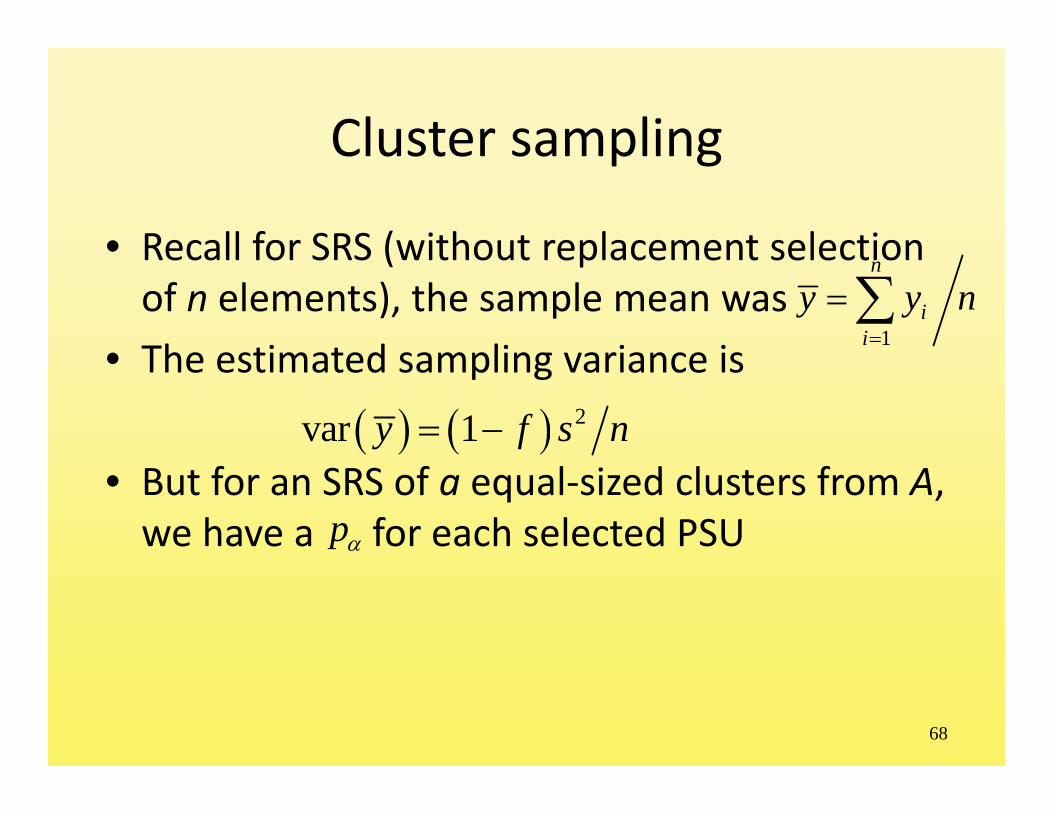
Cluster sampling
• Recall for SRS (without replacement selection of n elements), the sample mean was
• The estimated sampling variance is
• But for an SRS of a equal‐sized clusters from A, we have a for each selected PSU
1
n
ii
y y n
2var 1y f s n
p

69
Cluster sampling: variance estimation
• In cluster sampling, treat the sample as an SRS of a units from A:
– Where
• That is,
21var( ) a
fp s
a
22
11
a
as p p a
/f a A 2
11var( )
1
a
p pfp
a a
70
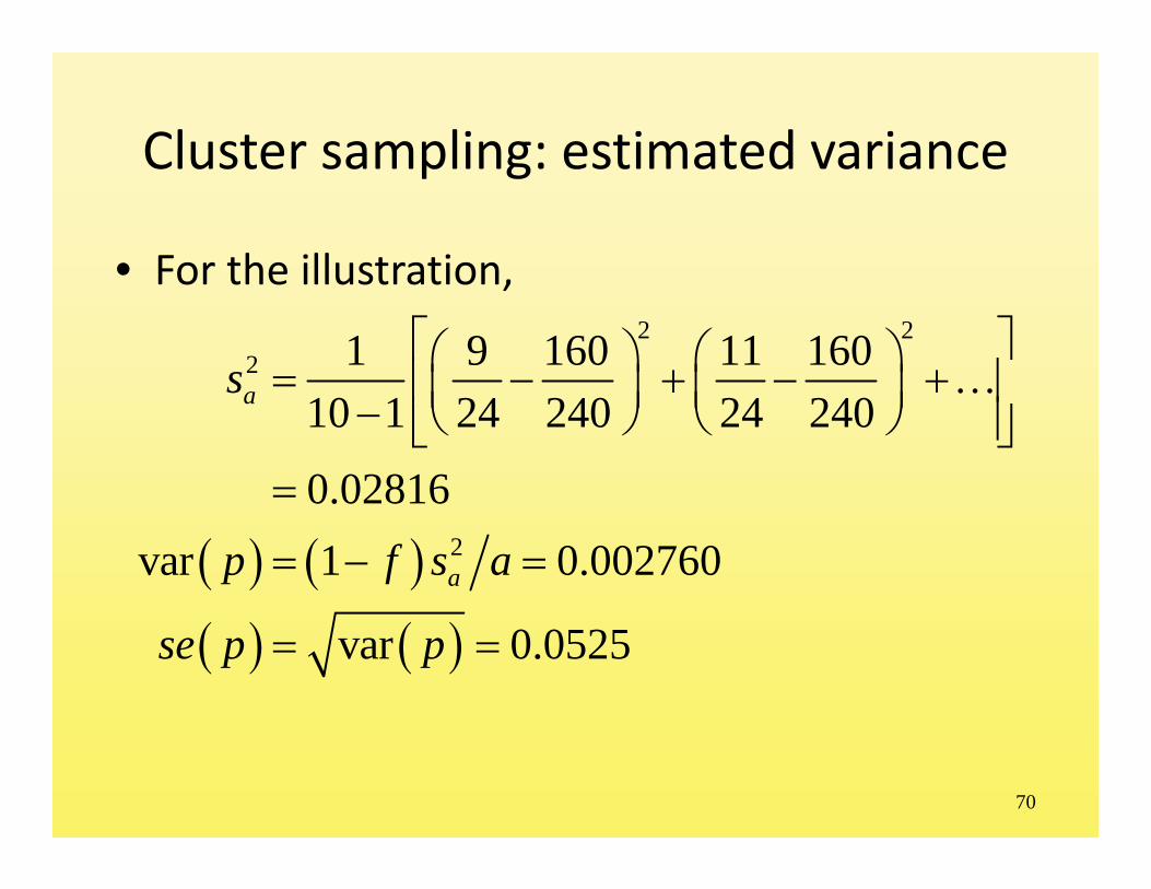
Cluster sampling: estimated variance
• For the illustration,
2 22
2
1 9 160 11 16010 1 24 240 24 240
0.02816var 1 0.002760
var 0.0525
a
a
s
p f s a
se p p

71
Design effect
• If the sample had instead been an SRS of n = 240 children from all schools, then
160 / 240
1var 1
10.0009112
SRS
pp p
p fn

72
Design effect
• Compared to cluster sampling, the estimated variance of p is considerably smaller for SRS
• A ratio quantifies the comparison:
var 0.002760 3.029var 0.0009112SRS
pdeff p
p

73
roh
• The design effect is a function of …– the size of the clusters b– the degree of homogeneity of elements within clusters
• The homogeneity is measured by the intra‐cluster correlation roh
• The design effect is given by
1 1deff p b roh

74
Estimating roh
• The intra‐cluster correlation can be estimated from the design effect:
11
3.029 124 1
0.088
deff proh
b
75
Features of roh
• roh is a property of the clusters and the variable under study
• roh is substantive, not statistical• roh is nearly always positive
– Elements in a cluster tend to resemble one another• Source of roh
– Environment– Self‐selection– Interaction

76
Magnitude of roh
• Magnitude depends on– The characteristic (variable) under study (e.g., disease status, age)
– The nature of the clusters (e.g., households, establishments)
– The size of the cluster (e.g., household, blocks of household, census tracts)
77
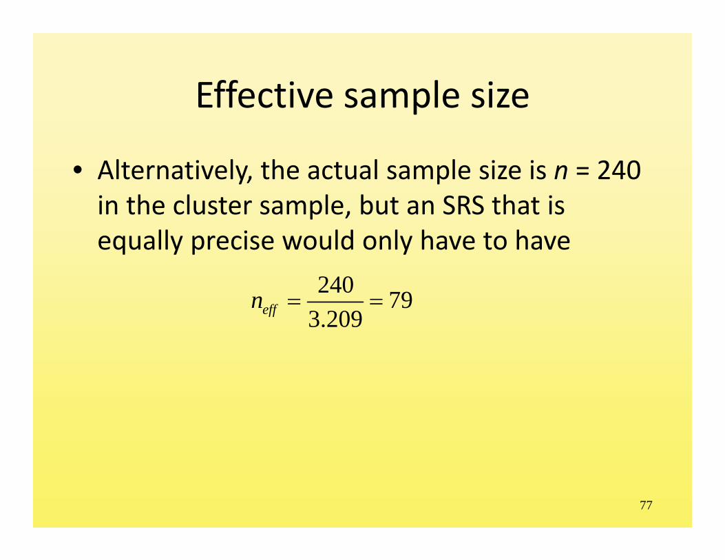
Effective sample size
• Alternatively, the actual sample size is n = 240 in the cluster sample, but an SRS that is equally precise would only have to have
240 793.209effn

78
Examples
• Consider alternative outcomes for our sample of a = 10 classrooms– Homogeneity with, heterogeneity between
0 0 0 16 24 24 24 24 24 24, , , , , , , , ,24 24 24 24 24 24 24 24 24 24
23.90 1 0.99624 1
roh
23.90deff
240 / 23.9 10effn
2 0.2222 var 0.02178as p

79
Examples
• Heterogeneity within, homogeneity among:16 16 16 16 16 16 16 16 16 16, , , , , , , , ,24 24 24 24 24 24 24 24 24 24
0deff
240 / 0effn
2 0.0 var 0.0as p
80
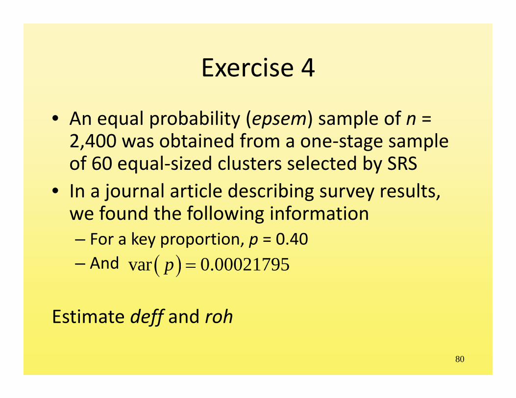
Exercise 4
• An equal probability (epsem) sample of n = 2,400 was obtained from a one‐stage sample of 60 equal‐sized clusters selected by SRS
• In a journal article describing survey results, we found the following information– For a key proportion, p = 0.40– And
Estimate deff and roh
var 0.00021795p

81
7. Two‐stage sampling
• Two‐stage sampling• Portability of roh• Exercise 5

82
Two‐stage sampling
• Selecting many elements per cluster increases variances
• Even small values of roh can be magnified by large b since
• Consider the following for 1 1deff p b roh
240n a b 240 1
1000 24 24000 24000 100a b a bf

83
Subsamples of size b
• Sample a = 20 classrooms and b = 12:
• Sample a = 30 classrooms and b = 8:
• Sample a = 80 classrooms and b = 3:
1 12 1 0.088 1.97 122effdeff p n
1 8 1 0.088 1.62 148effdeff p n
1 3 1 0.088 1.18 204effdeff p n
84
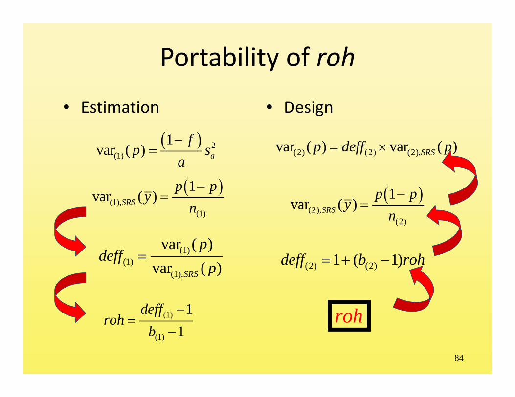
Portability of roh
• Estimation • Design
2(1)
1var ( ) a
fp s
a
(1),
(1)
1var ( )SRS
p py
n
(1)(1)
(1),
var ( )var ( )SRS
pdeff
p
(1)
(1)
11
deffroh
b
roh
(2) (2)1 ( 1)deff b roh
(2),
(2)
1var ( )SRS
p py
n
(2) (2) (2),var ( ) var ( )SRSp deff p
85
Exercise 5
• Suppose the sample described in Exercise 4 (with n = 2,400 and a = 60) is to be repeated with a smaller sample of n =1,200 and in only a = 30 equal‐sized clusters
Project how large the sampling variance of p will be under this new design.

86
Exercise 5 (continued)
• Now suppose the reduced size of n = 1,200 is retained, but we want to consider a = 60 equal‐sized clusters.
Project how large the sampling variance of p will be under this new design.
87
8. Probability proportionate to size sampling
• Unequal‐sized cluster sampling• Sampling with fixed rates• Control of subsample size• Selection of fixed size subsamples• PPS sampling• Systematic PPS sampling• Exercise 6

88
Unequal‐sized cluster sampling
• Naturally occurring clusters tend to be unequal in size
• Fixed sampling rates and unequal sized clusters result in variation in sample size

89
Consider the following sample of 12 schools:
School School
123456
308823146809827775
789
101112
393148321393207850
aB aB

90
Fixed rate sample
• An epsem sample of n = 100 students is to be selected from the N = 6,000 students in the 12 schools:
• Two stages: Select a = 2 schools, say an SRS of a = 2 schools (a rate of 2/12 = 1/6)
• And then choose students at the rate 1/10 within the selected schools
100 6000 1/ 60f
1 6 1/10 1 60f
91
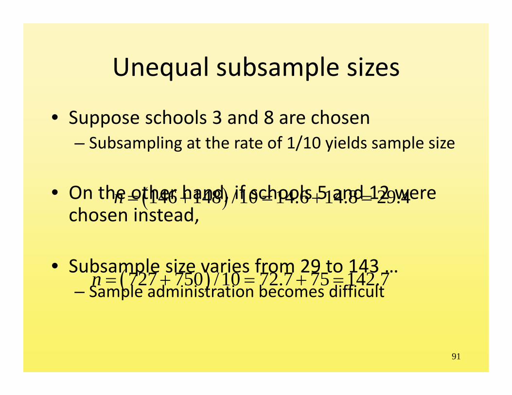
Unequal subsample sizes
• Suppose schools 3 and 8 are chosen– Subsampling at the rate of 1/10 yields sample size
• On the other hand, if schools 5 and 12 were chosen instead,
• Subsample size varies from 29 to 143 …– Sample administration becomes difficult
146 148 /10 14.6 14.8 29.4n
727 750 /10 72.7 75 142.7n

92
Sample size variation
• Variation in the overall sample size is undesirable
• Since n is a random variable, no longer applies
• We need to use a ratio estimator1
1 n
ii
y yn
1
1
a
a
yyrxx
93
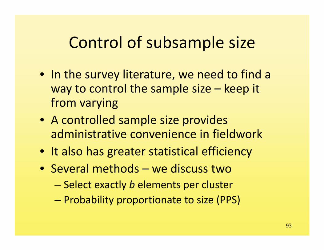
Control of subsample size
• In the survey literature, we need to find a way to control the sample size – keep it from varying
• A controlled sample size provides administrative convenience in fieldwork
• It also has greater statistical efficiency• Several methods – we discuss two
– Select exactly b elements per cluster– Probability proportionate to size (PPS)

94
Selection of fixed subsample sizes• Suppose a = 2 schools are chosen at random
• And b = 50 students are chosen at random per selected school
• Sample size is n = 2 x 50 =100– Sample size does not vary across samples!
• But this design, on average across, all possible samples, over‐represent students in small schools– Why?
95
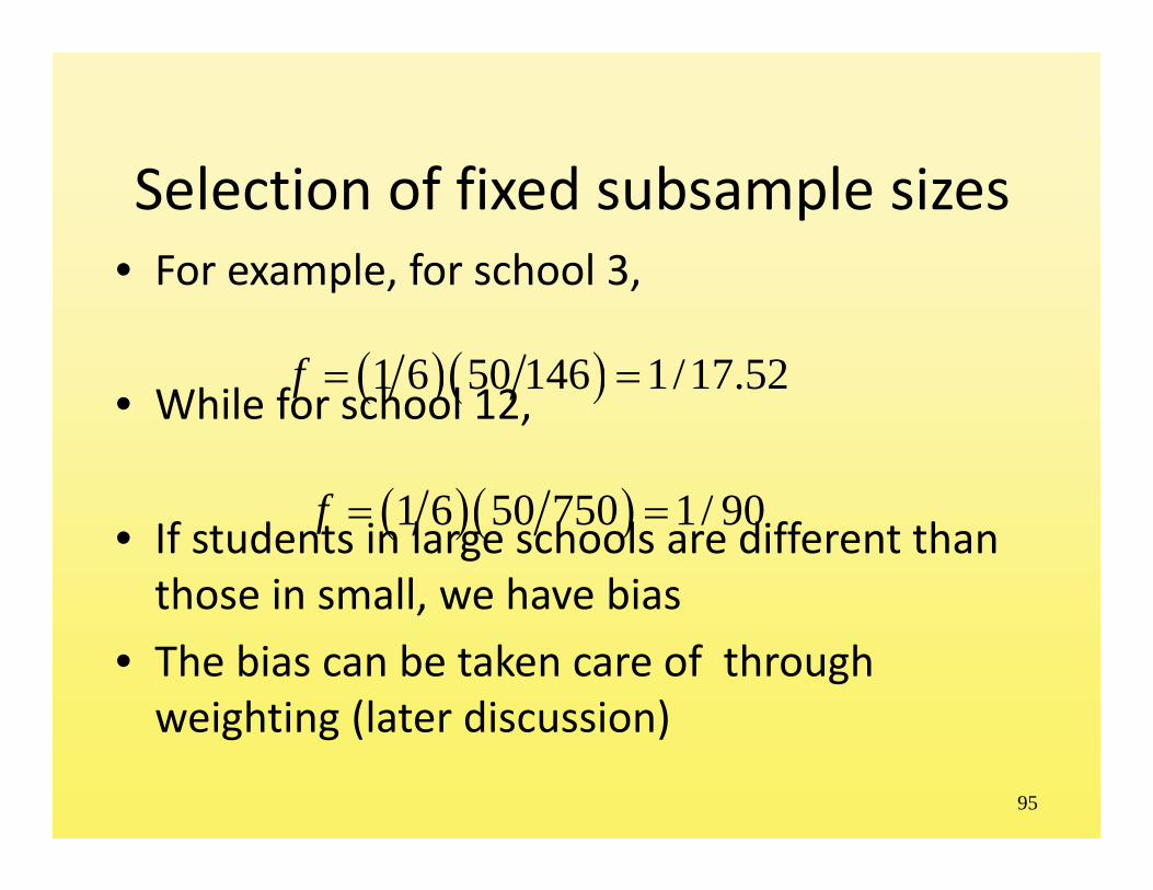
Selection of fixed subsample sizes• For example, for school 3,
• While for school 12,
• If students in large schools are different than those in small, we have bias
• The bias can be taken care of through weighting (later discussion)
1 6 50 146 1/17.52f
1 6 50 750 1/ 90f

96
PPS• Require a method that is equal chance for students (epsem)
• And still achieves equal sized subsamples– And thus achieves fixed sample sizes
• Again, consider a = 2 and b = 50• “Selection equation:”
1 5060
f PB

97
PPS: Achieving epsem
• For example, if school 1 is chosen, then
• In order to make this epsem for students, we need for each school to be selected with probability …
1 50 160 308 6.16
f P P
1 50 160 60 50 3000
B BP OR PB
98
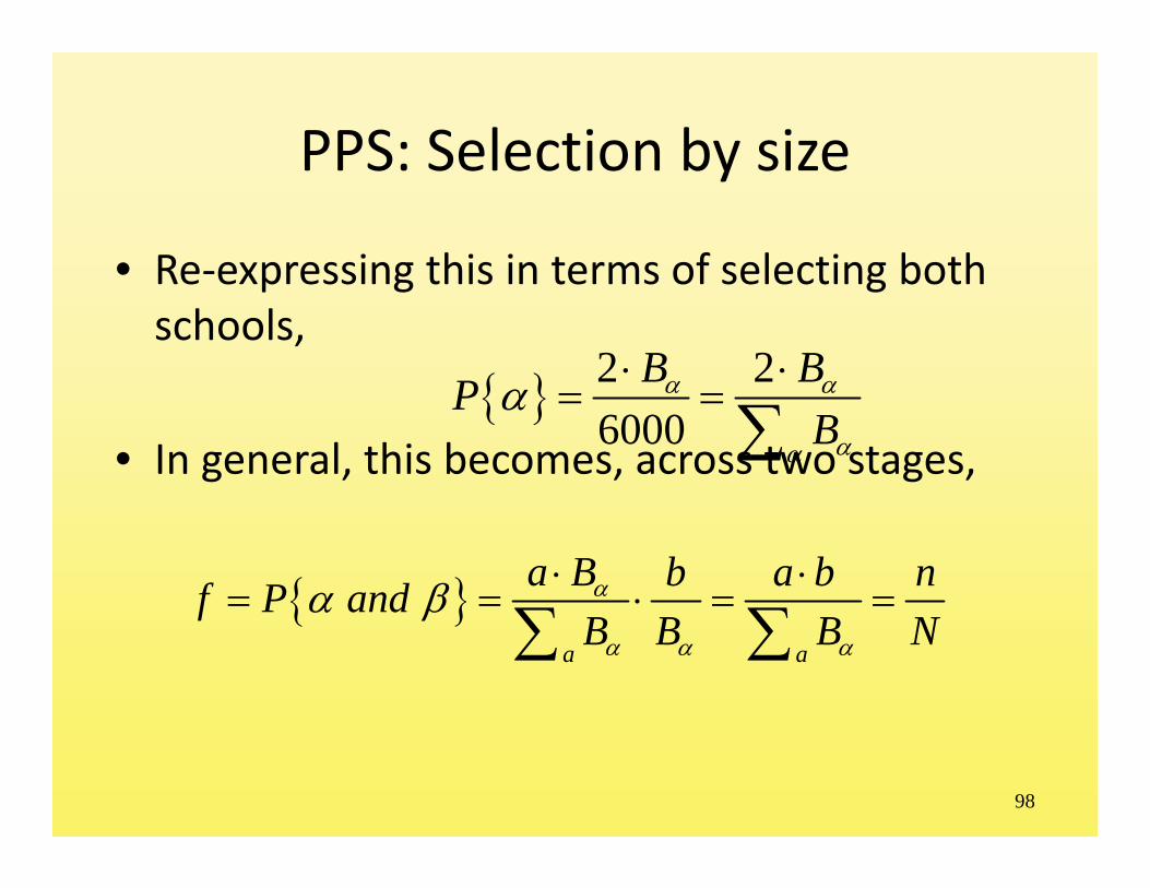
PPS: Selection by size
• Re‐expressing this in terms of selecting both schools,
• In general, this becomes, across two stages, 2 2
6000B BP
B
a a
a B b a b nf P andB B B N

99
PPS selection of schoolsSchool Cum.
123456789101112
308823146809827775393148321393207850
30811311277208629133688408142294550494351506000
702
1744
B B
100
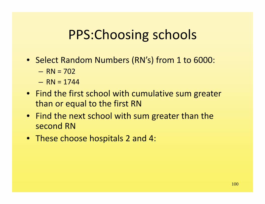
PPS:Choosing schools
• Select Random Numbers (RN’s) from 1 to 6000:– RN = 702– RN = 1744
• Find the first school with cumulative sum greater than or equal to the first RN
• Find the next school with sum greater than the second RN
• These choose hospitals 2 and 4:

101
Systematic PPS
• How can we avoid selecting the same school twice?
• Systematically: select one RN from 1 to the interval 6000/2 = 3000– Say RN = 702
• Find the selected school, as above (school 2)• Add the interval to the RN to obtain 702 + 3000 = 3702
• Find the second school with this selection number, as above, school 7
• RN 702 leads to the selection of schools 2 & 7
102
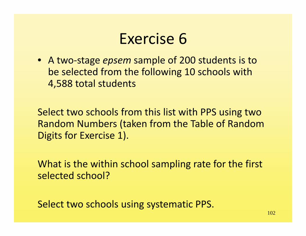
Exercise 6• A two‐stage epsem sample of 200 students is to be selected from the following 10 schools with 4,588 total students
Select two schools from this list with PPS using two Random Numbers (taken from the Table of Random Digits for Exercise 1).
What is the within school sampling rate for the first selected school?
Select two schools using systematic PPS.

103
School
Um HakeemAhmad Bin Hanbal IndependentAlShamalKhaleefaLusailAlTijaraQatar Independent CampusBilal Bin RabahAl Shahhaniya IndependentAlFatat AlMuslima
261677965406427661169285662
75Total 4,588
B

104
9. Stratified random sampling
• Stratification• Advantages• Stratification – an example
• Stratified sample• SRS• Design effect• Effective sample size
• Problems• Multipurpose surveys• Domains of study• Proportionate stratified sampling
• Disproprotionate stratification
• Exercise 7

105
Stratification
• Procedure– Form strata– Independent selection within each– Estimate for stratum h,– Overall estimate
• Where
hy
1
H
h hh
y W y
h hW N N

106
Variance
• For the overall sample estimate
• With estimated variance 2
1
H
h hh
Var y W Var y
2
1
H
h hh
var y W var y

107
Formation of strata
• Strata should be internally homogeneous• Strata should differ as much as possible from each other
• Advantages– Gains in precision– Administrative convenience– Guaranteed representation of important domains– Acceptability/credibility– Flexibility

108
Stratification – an examplePopulation Stratum 1
QatariStratum 2
White & Blue Collar Expatriate (Other)
Size N
1,000,000 200,000 800,000Variance
1,800,000 4,000,000 1,000,000Mean
1,400 3,000 1,000
1N 2N
21S 2
2S
Y 1Y 2Y
2S

109
Stratified sample
• What will be ?1 2240, 960n n ( )Var y
22 2
12 2 2 2
1 1 1 2 2 22 2
( ) 1
0.2 4000000 / 240 0.8 1000000 / 960666.7 666.71333
h h h hh
Var y f W S n
W S n W S n

110
SRS
• For What will be ? 1200n ( )SRSVar y
2118000001 1200 1000000
12001800000 1500
1200
SRSVar y f S n

111
Design effect
• As for cluster sampling,
• For this example,
SRS
Var y for a given designdeff y
Var y of same size
133315000.89
SRS
Var ydeff y
Var y

112
Effective sample size
• What sample size with SRS would be necessary to achieve the same precision (variance) as the given design?
• Effective sample size: • For our example, effn n deff y
12000.891348
effn
113
Problems
• Availability of data– Census– Administrative reports– Other surveys
• Multipurpose surveys– Survey of households in Qatar– Fixed assets, buildings, use of expatriate labor, expenditures, income, health, health care use, psychological well‐being, social integration

114
Problems
• Domains of study– Subpopulations for which separate estimates are required
– Geographic subdivisions such as provinces, districts, subdistricts
– Socio‐demographic characteristics, such as age groups, occupation, income, education
115
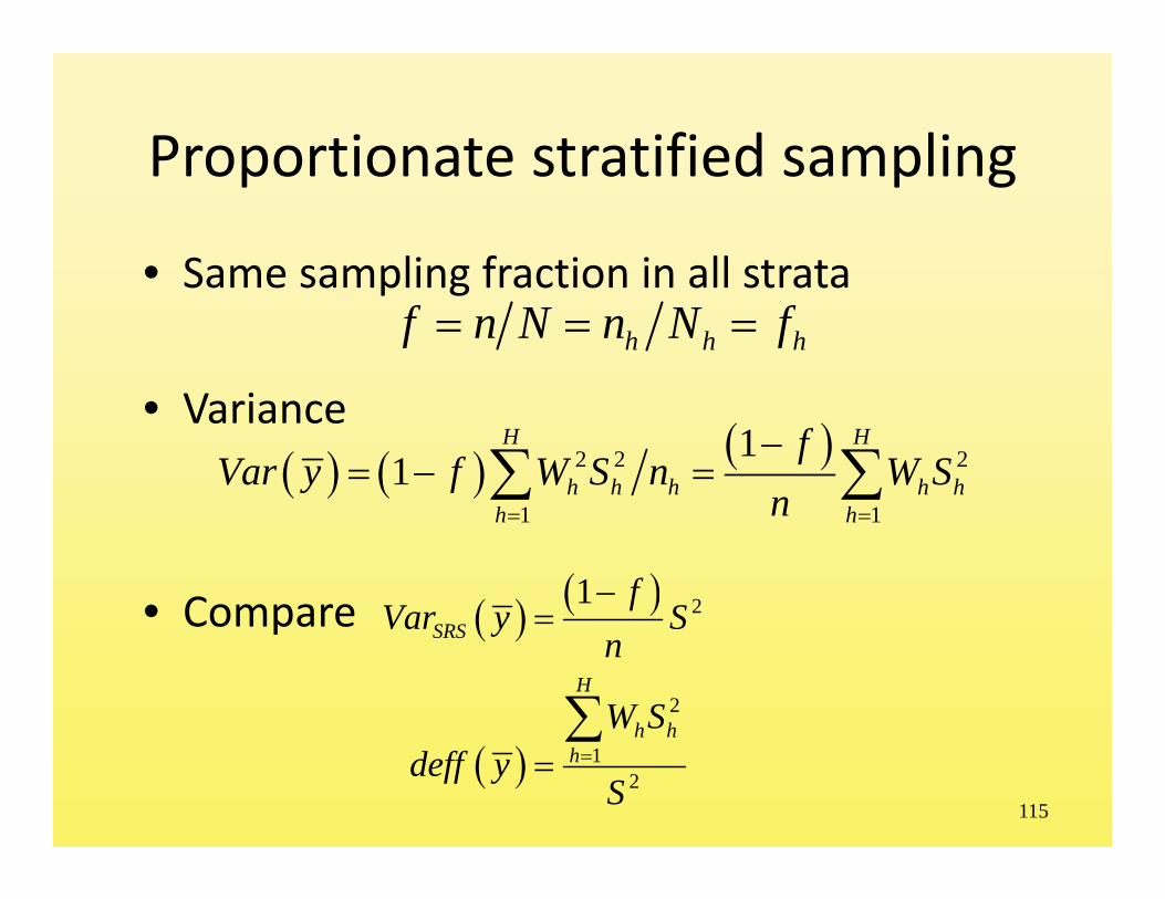
Proportionate stratified sampling
• Same sampling fraction in all strata
• Variance
• Compare
h h hf n N n N f
2 2 2
1 1
11
H H
h h h h hh h
fVar y f W S n W S
n
2
2
12
1SRS
H
h hh
fVar y S
n
W Sdeff y
S

116
Disproportionate stratification
• Purposes– Gains in precision for overall estimator– Precision for comparisons– Precision for domains
• Factors to consider– Size of strata– Variability within strata– Cost within strata
hW2hS
hc
117
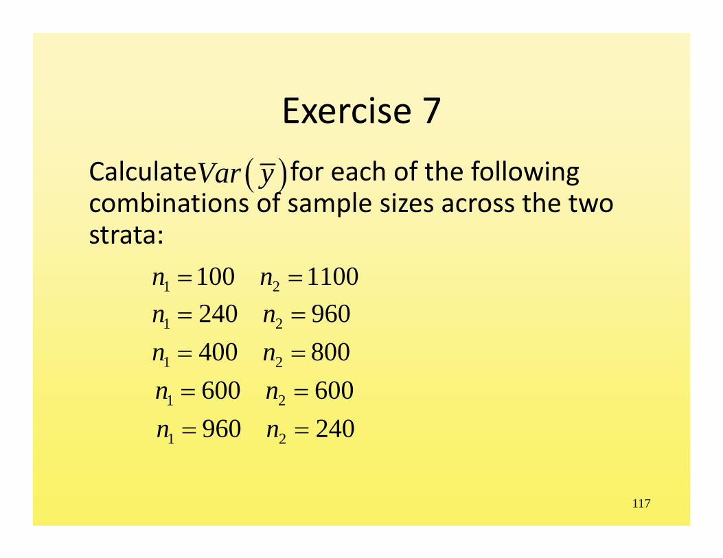
Exercise 7Calculate for each of the following combinations of sample sizes across the two strata:
Var y
1 2100 1100n n
1 2240 960n n
1 2400 800n n
1 2600 600n n
1 2960 240n n

118
10. Frame problems
• Frame problems• Objective respondent selection

119
Frame problems
• Frame: set of materials used to designate a sample of units
• Simple list, or set of materials such as maps, lists, rules for linking frame elements to population elements, etc.
• Accurate, up‐to‐date frames in single location, arranged suitably for selection– Numbered or computerized lists useful
120
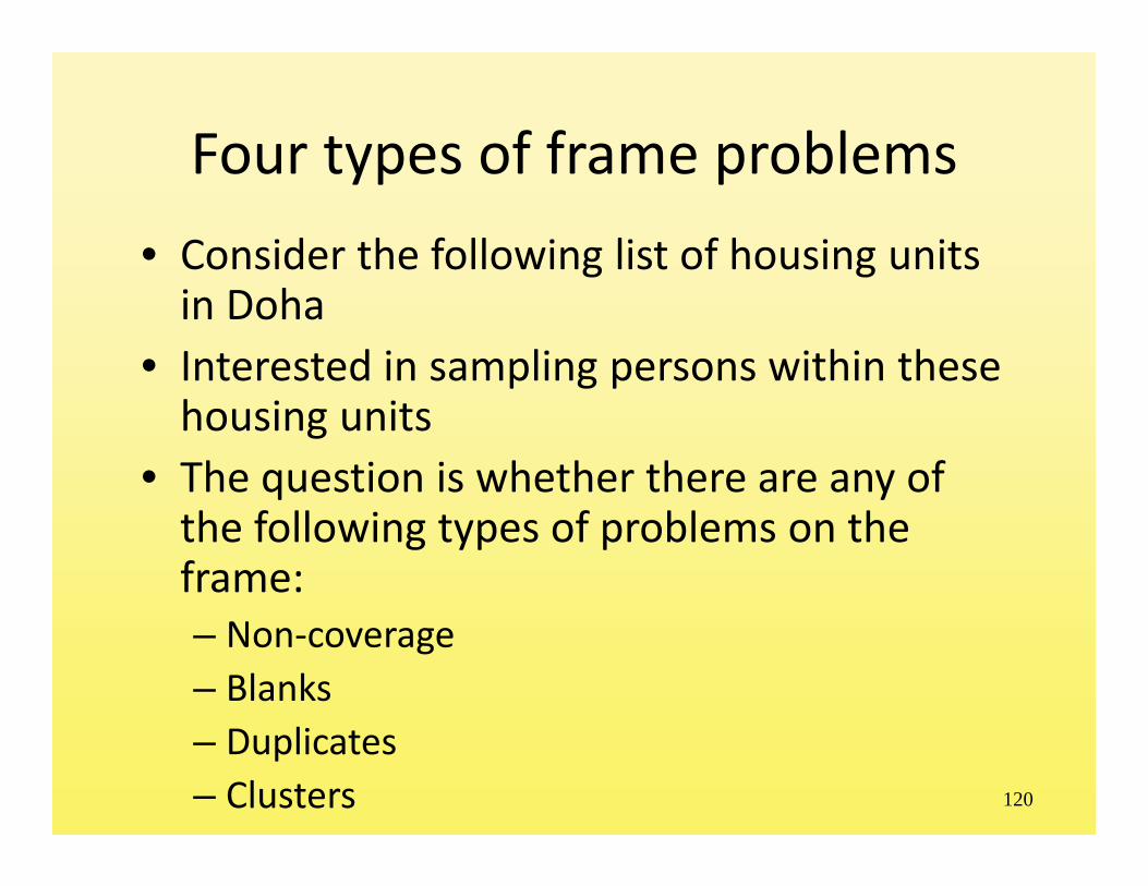
Four types of frame problems• Consider the following list of housing units in Doha
• Interested in sampling persons within these housing units
• The question is whether there are any of the following types of problems on the frame:– Non‐coverage – Blanks– Duplicates– Clusters

121
ResidenceID City Street ResidenceType Nationality Persons1 Doha Wahb Villa Non-Qataris 32 Doha Wahb Villa Non-Qataris 63 Doha Wahb Villa Non-Qataris 34 Doha Wahb Villa Qataris 55 Doha Wahb Villa Non-Qataris 56 Doha Wahb Villa Non-Qataris 57 Doha Wahb Villa Non-Qataris 38 Doha Wahb Villa Non-Qataris 59 Doha Wahb Villa Qataris 1310 Doha Wahb Villa Non-Qataris 611 Doha Wahb Villa Non-Qataris 312 Doha Wahb Villa Non-Qataris 513 Doha Wahb Villa Non-Qataris 414 Doha Wahb Villa Non-Qataris 315 Doha Al Quds Villa Non-Qataris 416 Doha Al Quds Villa Non-Qataris 517 Doha Al Quds Villa Qataris 818 Doha Al Quds Villa Non-Qataris 219 Doha Al Quds Villa Non-Qataris 320 Doha Al Quds Villa Non-Qataris 5

122
ResidenceID City Street ResidenceType Nationality Persons21 Doha Al Quds Villa Non-Qataris 422 Doha Al Quds Villa Non-Qataris 423 Doha Al Quds Villa Non-Qataris 424 Doha Al Quds Villa Qataris 325 Doha Al Quds Villa Non-Qataris 126 Doha Al Quds Villa Non-Qataris 427 Doha Al Quds Villa Qataris 528 Doha Al Quds Villa Non-Qataris 329 Doha Al Quds Villa Non-Qataris 330 Doha Al Quds Villa Non-Qataris 531 Doha Murwab Villa Qataris 432 Doha Murwab Villa Non-Qataris 233 Doha Murwab Villa Non-Qataris 534 Doha Murwab Villa Non-Qataris 235 Doha Murwab Villa Non-Qataris 536 Doha Murwab Villa Non-Qataris 237 Doha Murwab Villa Non-Qataris 338 Doha Murwab Villa Non-Qataris 539 Doha Murwab Villa Non-Qataris 440 Doha Murwab Villa Non-Qataris 4

123
Non‐coverage
• Some elements of the population are not contained on the frame– Housing units not appearing on the list– Remedies
• Use a frame that provides complete coverage• Supplement the existing frame with other frames• Use “population control adjustment weights” to compensate in analysis
124
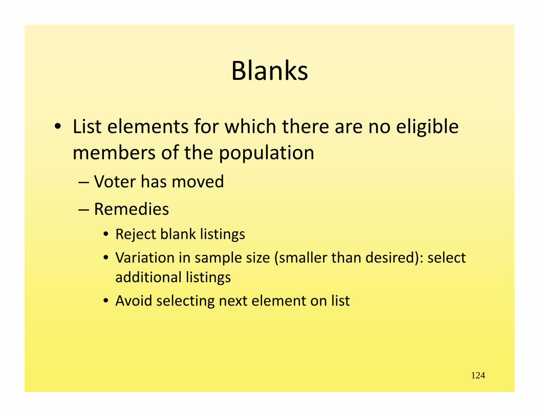
Blanks
• List elements for which there are no eligible members of the population– Voter has moved– Remedies
• Reject blank listings• Variation in sample size (smaller than desired): select additional listings
• Avoid selecting next element on list

125
Duplicates
• Population element appears more than once on the list– Introduces unequal probabilities of selection– Housing unit appears more than once– Person living in two different addresses– Remedies
• Determine number of times element is on list, and weight
• Modify address list to eliminate duplicates

126
Clustering
• More than one population element is associated with a single list element– Variation in sample size– Remedies
• Subsample clusters, and weight results by the inverse of the probability of selection
• Accept variation in sample size

127
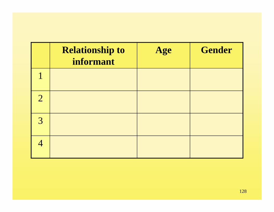
Within Household Selection: Objective Respondent Selection
• Remedy for selecting elements from small clusters, objectively in field settings
• Not epsem• Suppose there are a maximum of four age‐eligible persons per household
• Consider the following listing and selection table:
128
Relationship to informant
Age Gender
1
2
3
4

129
Respondent selection table
If number of eligible subjects is …
… then select subject number …
1234
1233

130
Interviewer instructions
• Interviewer:– List eligible household members by gender and age
– Follow the instructions on the selection table to determine whom to interview
• This scheme is based on a set of 6 tables which are rotated among households to achieve the desired probabilities of selection for each subject:

131
Respondent selection tablesTable A (1/4)
If number of eligible
subjects is
Select subject number
1234
1111
Table B (1/12)
If number of eligible
subjects is
Select subject number
1234
1112
Table C (1/6)
If number of eligible
subjects is
Select subject number
1234
1122
Table D (1/6)
If number of eligible
subjects is
Select subject number
1234
1223
Table E (1/12)
If number of eligible
subjects is
Select subject number
1234
1233
Table F (1/4)
If number of eligible
subjects is
Select subject number
1234
1234

132
11. Weighting
• Weighting to compensate for within household selection
• Exercise 8• Weighting to compensate for unequal selection probabilities: over‐ and under‐sampling
• Weighting to compensate for nonresponse• Poststratification

133
Weighting
• Among four problems, two remedies involve weighting to compensate for unequal selection probabilities
• Weights common in survey practice– Within household selection– *Duplication of elements on the frame*– Over or under sampling– Nonresponse– Poststratification

134
f=n/N F=N/nn
N
Sampling Procedure: List sample
Population
Sample
?N

135
Weighting for within household selection
• As long as the sampling is epsem …–
• Then
• For example, from N = 2000 adults, select n = 20 with epsem
• Each adult represents themselves and 99 others
i f n N
1 2
1 1 1i ny y y yy
n
20 1 1002000 100i iand w

136
Non‐epsem estimation
• But the mapping may not be equal for every element
• A weighted estimator is required:
• When the weights are constant, they cancel
1 2 20100 100 100100 1 100 1 100 1
i iiw
ii
w y y y yyw

137
Within household sampling
• Suppose a sample of 20 households are selected
• For 8 households, 1 adult: 3 reported being outside the country in the past year
• For 6 households, 2 adults: 3 outside• For 4 households, 3 adults: 3 outside• For 2 households, 4 adults: 2 outside
138
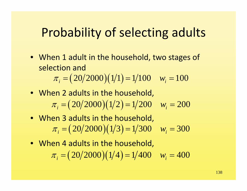
Probability of selecting adults
• When 1 adult in the household, two stages of selection and
• When 2 adults in the household,
• When 3 adults in the household,
• When 4 adults in the household,
20 2000 1 1 1 100 100i iw
20 2000 1 2 1 200 200i iw
20 2000 1 3 1 300 300i iw
20 2000 1 4 1 400 400i iw

139
ID Response (Y) Housing unit prob. No. persons 18+ Weight
1 1 0.01 1 100
2 1 0.01 1 100
3 0 0.01 1 100
4 0 0.01 1 100
5 0 0.01 1 100
6 0 0.01 1 100
7 1 0.01 1 100
8 1 0.01 1 100
9 0 0.01 2 200
10 0 0.01 2 200
11 1 0.01 2 200
12 0 0.01 2 200
13 0 0.01 2 200
14 1 0.01 2 200
15 0 0.01 3 300
16 1 0.01 3 300
17 1 0.01 3 300
18 1 0.01 3 300
19 1 0.01 4 400
20 1 0.01 4 400
140
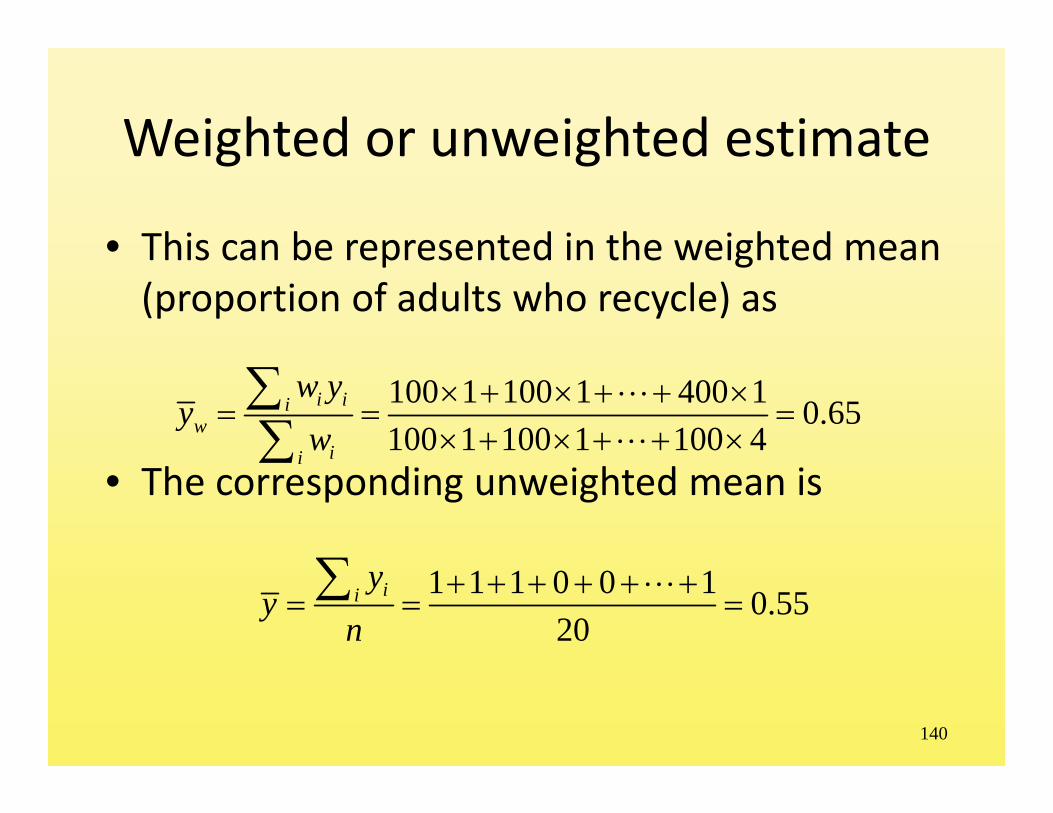
Weighted or unweighted estimate
• This can be represented in the weighted mean (proportion of adults who recycle) as
• The corresponding unweighted mean is
100 1 100 1 400 1 0.65100 1 100 1 100 4
i iiw
ii
w yy
w
1 1 1 0 0 1 0.5520
iiy
yn

141
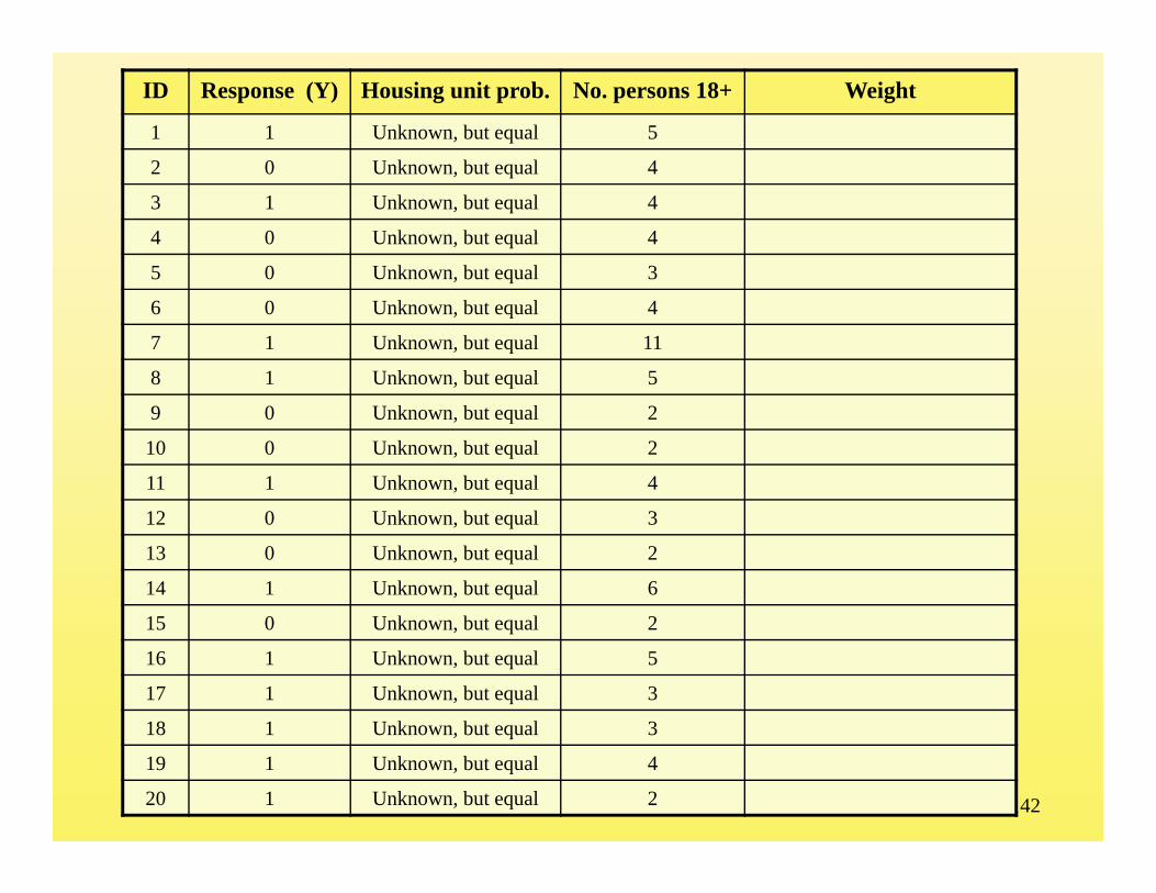
Exercise 8
• Selected a sample of 20 households• Selected one person 15 years or older (15+) in each
• Asked them whether they had been outside Qatar in the past year:
142
ID Response (Y) Housing unit prob. No. persons 18+ Weight
1 1 Unknown, but equal 5
2 0 Unknown, but equal 4
3 1 Unknown, but equal 4
4 0 Unknown, but equal 4
5 0 Unknown, but equal 3
6 0 Unknown, but equal 4
7 1 Unknown, but equal 11
8 1 Unknown, but equal 5
9 0 Unknown, but equal 2
10 0 Unknown, but equal 2
11 1 Unknown, but equal 4
12 0 Unknown, but equal 3
13 0 Unknown, but equal 2
14 1 Unknown, but equal 6
15 0 Unknown, but equal 2
16 1 Unknown, but equal 5
17 1 Unknown, but equal 3
18 1 Unknown, but equal 3
19 1 Unknown, but equal 4
20 1 Unknown, but equal 2

143
Exercise 8 (continued)Compute the weights for each sample person.
Compute an unweighted estimate of the proportion who have been outside in the past year
Compute a weighted estimate of the proportion who have been outside in the past year

144
Over‐ and under‐ sampling
• The basic approach above has been to weight by– Count an element times
• Consider the following population and sample distribution for persons 15 years and older (15+) in Qatar comparing Qatari and White and Blue Collar Expatriates (Other):
1 i1 i

145
Group N n Sampling rate
Weight A
Weight B
QatariOther
150,0001,350,000
125875
1/1,5001/1,500
1,5001,500
11
Total 1,500,000 1,000 1/1,500 1,500 1

146
Sample selection
• This is a proportionate allocation, with equal probabilities in each group
• Some investigators might prefer that the distribution in the sample be equal across the two groups:

147
Group N n Sampling rate
WeightA
WeightB
QatariOther
150,0001,350,000
500500
1/3001/2,700
3002,700
19
Total 1,500,000 1,000 1/1,500 1,500 --

148
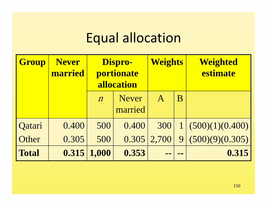
Proportionate v. equal allocation
• The equal allocation would be used for comparing the two groups
• The proportionate allocation would be used to represent the population
• Consider the consequences of the equal allocation when estimating “proportion never married” among, again, 15+, across the two groups:

149
Proportionate allocation
Group Never married
Proportionate allocation
Weights
n Never married
A B
QatariOther
0.4000.305
170830
0.4000.305
1,5001,500
11
Total 0.315 1,000 0.315
150
Equal allocationGroup Never
marriedDispro-
portionateallocation
Weights Weighted estimate
n Never married
A B
QatariOther
0.4000.305
500500
0.4000.305
3002,700
19
(500)(1)(0.400)(500)(9)(0.305)
Total 0.315 1,000 0.353 -- -- 0.315

151
Restoring the balance• Weights will restore the balance to the population distribution:
( )
( )
( )
( )
0.400 0.305 0.353
1 (0.400) 9 (0.305) 0.3151 9
300 (0.400) 2700 (0.
i
i B iw(B)
i B
i A iw(A)
i A
y 500 x + 500 x y = = = n 500 + 500
yw = yw
500 x x + 500 x x = = 500 x + 500 x
y 500 x x + 500 x x w = = yw
305) 0.315300 2700
= 500 x + 500 x
152
Weights in practice
• Is it necessary to weight, even when unequal probabilities are involved?
• Descriptive statistics require weights– Otherwise, estimates will be biased
• Analytic statistics are more controversial– Comparing income between Latino and non‐Latino groups – no need to weight
– Comparing income between male and female respondents in the same sample requires weighting

153
Effect of weights
• Often the effect of weights is not large for descriptive statistics
• If not large, analysts may decide not to use weights– Use of weights more difficult historically because of lack of software to handle weights
– Duplication factors used

154
Weighting for nonresponse
• Suppose that not everyone in the sample of 1,000 drawn from our two groups responded
• Ignoring nonresponse produces slightly biased estimates when averaging across the now disproportionately distributed groups:

155
Group n r Weight A
Never marri
ed
Weightedestimate
QatariOther
500500
450350
19
0.4000.305
(450)(1)(0.400)(350)(9)(0.305)
Total 1,000 800 -- 0.315 0.317

156
Nonresponse weights
• Compute weighted response rates in each group• Adjust the base weights (those computed to compensate for unequal probabilities of selection) for nonresponse
• Assumption: data is missing at random (MAR) within subgroups
• Response rate in each group is a “sampling rate” under the MAR assumption
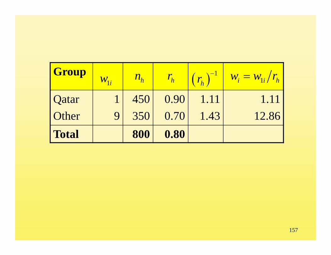
157
Group
QatarOther
19
450350
0.900.70
1.111.43
1.1112.86
Total 800 0.80
hn hr 1hr
1i i hw w r
1iw

158
Nonresponse weights
• These nonresponse adjusted weights ‘restore the balance’:
( )
( )
4 0.400 3 0.305 0.3584 35
45 1.11 (0.400) 35 12.86 (0.305) 0.31545 1.11 35 12.86
i
i B iw(B)
i B
y 50 x + 50 x y = = = n 50 + 0
yw = yw
0 x x + 0 x x = = 0 x + 0 x
159
Poststratification
• Poststratification is used to make the weighted sample distribution conform to a known population distribution
• Adjust the nonresponse adjusted weights• Suppose that gender in the sample does not agree with known gender distributions in the population:

160
GenderMaleFemale
500300
0.6150.375
1,222,000278,000
0.8150.185
1.3200.490
Total 800 1.000 1,500,000 1.000 --
gngNgp
gP g g gw P p
161
A final weight
• In poststratification, the weights for the individuals in groups are adjusted up or down to obtain the distribution of the sum of weights that corresponds to the population distribution
• The final weight is an adjustment of the baseline weight for nonresponse and poststratification:
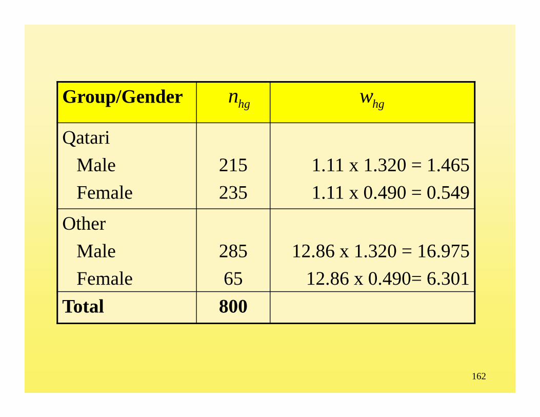
162
Group/Gender
QatariMaleFemale
215235
1.11 x 1.320 = 1.4651.11 x 0.490 = 0.549
OtherMaleFemale
28565
12.86 x 1.320 = 16.97512.86 x 0.490= 6.301
Total 800
hgn hgw

163
12. Variance estimation
• Sampling error• General sample design• Variance estimation• Simple replicated sampling• Problems with simple replicated estimates• Three methods of variance estimation• Comparison of methods• Computer software
164
Sampling error
• Problem– Many variables in a single survey– Many subclasses (domains) of interest– Fairly complex designs– Enormous computing task
• Requirement– Practical and efficient methods of variance estimation– Computer programs to implement them

165
General sample design
• Stratified• Clustered
– Primary stage units– b elements within each PSU
• Weights• Sampling methods
– Over representation of domains– Optimum allocation (rarely)
• Nonresponse• Poststratification

166
Variance estimation
• Durbin, 1952– If clusters (PSU’s) selected independently, variance can be estimated using only PSU totals
– Variance estimate contains the contribution of later stages of subsampling
– For rapid methods of variance estimation, no components of variance are needed

167
Simple replicated subsampling
• Alternative approaches based on ‘repetition’• c independent subsamples (replicates) selected under same design from population
• Estimate some statistic Z• Each replicate provides• Compute iz
2
1
var( ) 1 1
ii
ii
z c z
z c c z z
168
Three general estimators
• Taylor series expansion– Approximate analytic solution
• Balanced repeated replication (BRR)– Based on replicated sampling, but actually replicated subsampling
• Jackknife repeated replication (JRR)– Simplified form of replicate formation: drop out one– General methodology developed for another purpose –has broad application

169
Comparison of methods• Empirical studies conducted for variety of statistics and methods of variance estimation– Mean square errors (MSE) of variance estimates favor Taylor series
– Coverage properties of confidence intervals favor BRR• All three methods reasonably good for
– Correlation coefficients– Ratio means– Regression coefficients
• Taylor series most versatile, with respect to sample designs– Jackknife is the most general approach
170
Computer programs• Standard statistical packages such as SPSS, SAS, Stata, assume SRS by default
• Necessary input to compute sampling errors– PSU for every element– Stratum for every element– Weight for every element– At least two PSU’s per stratum
• See American Statistical Association web site for comprehensive review: http://www.hcp.med.harvard.edu/statistics/survey‐soft/

171
13. Survey sampling textbooks

172
• Barnett, V. (1974). Elements of Sampling Theory. London: English Universities Press. A short introduction to topics in sampling theory.
• Cassell, C‐M., Sarndal, C‐E., and Wretman, J.J. (1977). Foundations of Inference in Survey Sampling. New York: J.W. Wiley and Sons, Inc. Theoretical treatment of survey sampling inference, including issues such as admissibility of estimators.
• Cochran, W.G. (1977). Sampling Techniques, 3rd edition. New York: J.W. Wiley and Sons, Inc. Excellent and widely used text on the basic theory for sampling techniques.
• Deming, W.E. (1950). Some Theory of Sampling. New York: Dover. Text on sampling theory and practice.
• Deming, W.E. (1960). Sample Design in Business Research. New York: J.W. Wiley and Sons, Inc. Text on sampling theory and practice, with emphasis on replicated sampling methods. Recently released by Wiley as a paperback Classics edition.

173
• Hajek, J. (1981). Sampling from a Finite Population. New York: Marcel Dekker. A monograph on sampling theory from an advanced perspective.
• Hansen, M.H., Hurwitz, W.N., and Madow, W.G. (1953). Sample Survey Methods and Theory. Volume I: Methods and Applications. Volume II: Theory.New York: J.W. Wiley and Sons, Inc. Classic two volume text on sampling practice and theory that is considered still to be the standard.
• Jessen, R.J. (1978). Statistical Survey Techniques. New York: J.W. Wiley and Sons, Inc. An intermediate text on sampling with a presentation of lattice sampling methods.
• Kalton, G. (1983). Introduction to Survey Sampling. Beverly Hills, CA: Sage Publications. Short non‐mathematical treatment of sampling. A Sage mongraph.
• Kish, L. (1965). Survey Sampling. New York: J.W. Wiley and Sons, Inc. Comprehensive text on sampling practice, about to be issued as a paperback Classic edition.
174
• Konijn, H.S. (1973). Statistical Theory of Sample Survey Design and Analysis. New York: American Elsevier. Advanced text on sampling theory.
• Levy, P.S. and Lemeshow, S. (1991). Sampling of Populations: Methods and Applications. New York: J.W. Wiley and Sons, Inc. Intermediate level text on sampling methods.
• Lohr, Sharon L. (1999). Sampling: Design and Analysis. Pacific Grove, CA: Duxbury Press. Intermediate level text blending theory and practice, including exercises and sample data sets for analysis of survey data.
• Moser, C.A. and Kalton, G. (1971). Survey Methods in Social Investigation,2nd edition. London: Heinemann. Text on survey methods with a non‐mathematical introduction to sampling methods.
• Murthy, M.N. (1967). Sampling Theory and Methods. Calcultta: Statistical Publishing Society. Advanced text on sampling theory and practice.
• Raj, D. (1968). Sampling Theory. New York: McGraw Hill. Advanced text on sampling theory.

175
• Raj, D. (1972). The Design of Sample Surveys. New York: McGraw‐Hill, Inc. Two part text: the first is an intermediate‐level text on sampling practice, and the second presents surveys applications.
• Särndal, C‐E. SwenÑson, B. and Wretman, J. (1991). Model Assisted Survey Sampling. New York: Springer‐Verlag. Advanced text on sampling methods.
• Scheaffer, R.L., Mendenhall, W., and Ott, L. (1990). Elementary Survey Sampling, 4th edition. Boston: PWS Kent. Elementary text requiring minimal mathematical background.
• Stuart, A. (1984). The Ideas of Survey Sampling, revised edition. London: Griffin. Short text that illustrates the basic concepts of sampling with a small numerical example.
• Sudman, S. (1976). Applied Sampling. New York: Academic Press. Intermediate‐level text on sampling practice.
• Sukhatme, P.V., Sukhatme, B.V., Sukhatme, S., and Asok, C. (1984). Sampling Theory of Surveys with Applications, 3rd edition. Ames, Iowa: Iowa State University Press. Advanced text on sampling theory with important treatments on ratio estimation.

176
• Thompson, S.K. (1992). Sampling. New York: J.W. Wiley and Sons, Inc. Intermediate‐level text on sampling methods, including a number used widely in the natural sciences, and a discussion of adpative sampling techniques.
• Williams, W.H. (1978). A Sampler on Sampling. New York: J.W. Wiley and Sons, Inc. Intermediate‐level treatment of sampling methods.
• Yamane, T. (1967). Elementary Sampling Theory. Englewood Cliffs, NJ: Prentice Hall. An introductory text that provides a mix theory and simple illustrations; useful for students with limited mathematical backgrounds.
• Wolter, K.M. (1985). Introduction to Variance Estimation. New York: Springer‐Verlag. Comprehensive treatment of variance estimation for survey sampling.
• Yates, F. (1981). Sampling Methods for Censuses and Surveys, 4th edition. London: Griffin. Advanced text on sampling practice.