INTRODUCTION TO STATISTICSFOR POLITICAL SCIENCE:

3. Random Variables

Stephen AnsolabehereDepartment of Political Science

Massachusetts Institute of Technology

Fall, 2003

3. Probability

A. Introduction

Any good data analysis begins with a question. Not all questions are amenable to statis-

tical analysis (though that is usually a de¯ciency of the question, not of statistics). Examples

of interesting hypotheses abound in political science. Here are some classic and recent hy-

potheses that have been subjected to data analysis:

Duverger's Law \A majority vote on one ballot is conducive to a two-party system" and

\proportional representation is conducive to a multiparty system." (Duverger, Party

Politics and Pressure Groups (1972), p. 23.)

The Democratic Peace \Democracies almost never engage each other in full-scale war,

and rarely clash with each other in militarized interstate disputes short of war." (Maoz,

\The Controversy over the Democratic Peace," International Security (Summer, 1997),

p. 162.)

Abortion and Crime \Children born after abortion legalization may on average have

lower subsequent rates of criminality" because fewer unwanted births occur. (Donohue

and Levitt, \The Impact of Legalization of Abortion on Crime," Quarterly Journal of

Economics, May 2001, p. 380.)

These hypotheses, while controversial, are fairly typical of the type of questions that statistics

might be helpful in answering.

A testable hypothesis is an empirical claim that can, in principle, be discon¯rmed by the

occurrence of contradictory data. For example, Duverger's claim that single ballot majority

systems have two major parties could be discon¯rmed if we found single ballot majority

systems with three or four parties. There are, of course, many claims in the social sciences

that are not presented in the form of testable hypotheses. Some are just vacuous, but in other

1

cases one just needs to do the necessary work to determine what evidence would support

and contradict the hypothesis. This is not a problem of statistics and we will have little to

say about it. Nonetheless, it is always useful to ask what evidence would be su±cient to

contradict one's favored hypothesis. If you can't think of any, then it's probably not worth

gathering the data that would support your hypothesis.

In practice, discon¯rming a hypothesis is not nearly so straightforward as the preceding

discussion would suggest. When hypotheses are of the form \If A, then B," the simultaneous

occurrence of A and not B discon¯rms the hypothesis. However, few hypotheses in the social

sciences are of this type. Duverger, for instance, did not claim that all single ballot majority

systems have two parties; rather, he claimed that there was a tendency for such systems to

have two parties. It would not disprove Duverger's law for a single country to have, say, three

major parties for a limited period of time. Both the U.S. and U.K. have had signi¯cant third

(and sometimes fourth) parties during certain periods, but we still consider them essentially

two party systems.

In fact, nearly all social science hypotheses are phrased as \If A, then B is more likely

to occur." Social science hypotheses are rarely deterministic. The occurrence of A only

makes B more likely, not inevitable. This is true in part because many factors other than

A can in°uence whether B occurs. For example, workers with more schooling tend to have

higher earnings than those with less, but there are many other factors, such as ability and

experience, that also a®ect earnings. Even if we were to assemble a very long list of factors

and we were able to measure each factor perfectly|two very big \ifs"|it is doubtful that

we could account for all variations in earnings. For this, as for most social phenomena, there

remain elements of arbitrariness and luck that we will never be able to explain.

Even when we can establish that there are systematic di®erences in the value of the

dependent variable for di®erent values of the independent variable, we do not know what

caused these di®erences.

In an experiment, the analyst manipulates one variable (the so-called \independent vari-

able") and observes what happens to the response (the \dependent variable"). If the manip-

2

ulations are properly designed, then one can be con¯dent that observed e®ects are caused

by the independent variable. For example, in medical experiments, subjects are recruited

and randomly assigned to treatment and control groups. The treatment group is given a

drug and the control group receives a placebo. The study is conducted double blind|neither

the subjects nor the experimenter knows who has received what until after the responses

have been recorded. The di®erences between the treatment and control group cannot be

attributed to anything other than the treatment.

In the social sciences, controlled experiments are rare, though increasing in frequency.

The values of the variables are not the result of an intervention by the analyst and the data

may have been collected for a completely di®erent purpose. Electoral systems and abortion

laws are not chosen by political scientists{we only observe what happens under di®erent

electoral rules or abortion laws. We can never be sure that the consequences we observe are

the result of what we think are the causes or by some other factor. In an experiment, by

way of contrast, randomization of treatment ensures that treatment and control group are

unlikely to di®er in any systematic way.

In recent years, experiments have been conducted on a wide range of social phenomena,

such as labor market policies, advertising, and voter mobilization. Economists have also used

laboratory experiments to create arti¯cial markets. Today no one contests the usefulness

of experiments in the social sciences, though many topics of interest (including the three

hypotheses described above) remain beyond the range of experiments.

There is a lively debate in the social sciences about natural experiments (sometimes called

quasi-experiments). Donohue and Levitt's analysis of the relationship between abortion and

crime utilizes a natural experiment: ¯ve states legalized abortion prior to the Supreme

Court's decision in Roe vs. Wade. They compare the di®erences in subsequent crime rates

between these ¯ve states and the remainder. However, because the decision to legalize

abortion was not randomized, many other factors might be responsible for di®erences in

crime rates between these types of states.

Whether the data come from an experiment or an observational study, the method of

3

comparison is used to determine the e®ects of one variable on another. For simplicity, sup-

pose the independent variable is dichotomous (e.g., the type of electoral system is one ballot

simple majority or proportional representation; the political system is democratic or author-

itarian; a state either legalized abortion before Roe vs. Wade or not) and the dependent

variable is quantitative (e.g., the proportion of vote received by the top two parties; the

number of wars between a pair of countries; the murder rate per 100,000 population). The

method of comparison involves comparing the value of the dependent variable under the two

conditions determined by the independent variable. If these values di®er, we have evidence

that independent variable a®ects the dependent variable.

Because of the inherent randomness of social processes, the method of comparison cannot

be applied directly. Data are \noisy," so we must distinguish between systematic and random

variation in our data. The fundamental idea of probability is that random variation can be

eliminated by averaging data. One or two observations can be discrepant, but averaging

a large number of independent observations will eliminate random variation. Instead of

comparing individual observations, we compare averages.

Even if we can establish that there are systematic di®erences in the dependent variable

when the independent variable takes di®erent values, we cannot conclude that the inde-

pendent variable causes the dependent variable (unless the data come from a controlled

experiment). In observational studies, one cannot rule out the presence of confounding vari-

ables. A confounding variable is a third variable which is a cause of both the independent

and dependent variable. For example, authoritarian countries tend to be poorer than democ-

racies. In this case, level of development could be a confounding variable if richer countries

were more willing to ¯ght poorer countries.

Statistics provides a very useful technique for understanding the e®ects of confounding

variables. Ideally, we would be able to run a controlled experiment where, because of random-

ization, the independent and confounding variable are unrelated. In observational studies,

we can use statistical controls by examining the relationship between the independent and

dependent variable for observations that have the same value of the confounding variable.

4

In the Democratic peace example, we could examine the relationship between regime type

and war behavior for countries at the same level of development.

B. Types of Data and Variables

In the examples described above, we have encountered various di®erent types of data.

Roughly data can be classi¯ed as being either qualitative or quantitative. Qualitative data

comes from classi¯cations, while quantitative data arises from some form of measurement.

Classi¯cations such as gender (male or female) or party (Democratic, Republican, Green,

Libertarian, etc.) arise from categorizations. At the other extreme are physical measure-

ments such as time, length, area, and volume which are naturally represented by numbers.

Economic measurements, such as prices and quantities, are also of this type.

We can certainly attach numbers to categories of qualitative variables, but the numbers

serve only as labels for the categories. The category numbers are often referred to as \codes."

For example, if Democrats are coded as 1, Republicans as 2, Greens as 3, and so forth, you

can't add a Democrat and a Republican to get a Green. Quantitative measurements, on the

other hand, are inherently numerical and can be manipulated like numbers. If I have $10

and you have $20, then together we have $10 + $20 = $30.

In between purely qualitative variables, such as gender, and obviously quantitative vari-

ables, such as age, are rankings and counts. For example, ideology might have three cat-

egories (liberal, moderate, and conservative), which we might score as 1, 2 and 3, or as 0,

3 and 10, or any other three numbers which preserve the same ordering. In this case, the

numbers are not entirely arbitrary since they represent an ordering among the categories.

Similarly, we might count the occurrences of a qualitative variable (e.g., whether someone

attends church) to obtain a quantitative variable (e.g., how many times someone attended

church in the past year).

There is a large literature in properties of measures, but it has surprisingly little rele-

vance for statistical practice. Most statistical methods for quantitative measurements can

5

be adapted to handle qualitative measurements without too much di±culty. Furthermore,

measures that might seem naturally quantitative (such as years of schooling) may be just

rankings (or worse) of the variables of theoretical interest (how much more educated is

someone with 16 years of schooling than someone with 12?).

C. Probability and Randomness

Most people have an intuitive understanding of probability. We understand what it

means when a meterologist says that \the probability of rain is 70%," though we probably

don't understand how the probability was calculated. For statistics, it is necessary to be

able to do some elementary (and occasionally not so elementary) probability calculations.

In this lecture, we start by formalizing the concept of probability and deriving some of its

properties. Although the mathematical ideas are very simple, they lead to a surprisingly

rich theory.

[Mosteller studied the meaning of expressions such as \almost surely," \likely," \proba-

bly," \possibly," \might" and so forth. He found that a people give fairly consistent quanti-

tative interpretations to these terms.]

Probability is the key concept in the development of statistics, as we will see in the next

section (D). We will treat data as random variables { variables for which each value of the

variable occurs with a speci¯c frequency or probability. Data analysis consists of studying

the frequency with which the values of a particular variable may occur.

1. Random Experiments

A random experiment is some process whose outcome cannot be predicted with certainty

in advance. The easiest examples are coin tosses (where the outcome is either heads or tails)

or the roll of a die (where the outcome is the number of points showing on the die). These

examples may convey the misimpression that probability is primarily applicable to games of

6

chance. Here are some other examples more relevant to social science.

Random Sampling. We have a population of N elements (usually people) and

we draw a sample of n elements by sampling without replacement. If we have a

listing of the population, we can index the population elements by i = 1; : : : ; N .

To select the ¯rst element in the sample, we draw an integer at random from

f1; : : : ; Ng. Denote the element selected by i1. We then draw the second element

i2 from the remaining N ¡ 1 integers and continue until we have selected n

elements. An outcome is the set of integers selected fi1; : : : ; ing.

This example is repeatable in that we could use the same procedure over again to draw

another sample (and, presumably, to get a di®erent outcome). However, random experiments

need not be repeatable as the following examples illustrate.

² How many missions can a space shuttle complete before a catastrophic failure occurs?

² How many earthquakes of magnitude 3.0 or higher will California have during the

coming year?

² What are the chances of a student with high school GPA of 3.8 and SAT scores of 1500

being admitted to Stanford? MIT?

² Who will win in the California recall?

The ¯rst is an example of destructive testing. Once the failure has occurred, we cannot

repeat the experiment. When the application involves something expendable (such as a light

bulb), we may repeat the experiment with di®erent objects|but this involves an implicit

assumption that the other objects are similar enough to be somehow comparable.

In the second example, we might consider data from past years, but this again involves

an assumption that chances of an earthquake don't vary over time. For Stanford and MIT

admissions, it wouldn't make sense to repeat the experiment by having the same student

reapply the following year (since di®erent admission standards are applied to high school

7

applicants and college transfers). We could consider the admission outcomes of all students

with the same GPA and SAT scores, but this does not constitute any kind of random sample.

The last example is a case where there is no obvious precedent (and, some hope, no

repetition either!). Yet one could not deny that considerable uncertainty surrounds the recall

and statistics, as the science of uncertainty, should have something to say about it. We shall,

in fact, use random experiments to refer to any kind of process involving uncertainty.

2. The Sample Space

In a well-de¯ned random experiment, we should be able to list the possible outcomes. It

makes very little di®erence whether the number of outcomes is small or large. The critical

issue is whether we are able to describe all possible outcomes and, after the experiment is

completed, to determine which outcome has occurred.

Let ! denote an outcome and let W denote the set of all possible outcomes, so ! 2 W .

The set W is called the sample space of the experiment. The outcomes ! are sometimes

called sample points.

The sample space W is an abstract set. This means that the outcomes in the sample

space could be nearly anything. For example, in the experiment of °ipping a coin the sample

space might be W = fHeads; Tailsg.For the experiment of drawing a sample of size n from a population of size N without

replacement, the sample space might be the set of all n-tuples of distinct integers from

f1; : : : ; Ng,W = [(i1; : : : ; in) : ij6= ikifj6= kg:

In general, it is more convenient if the outcomes are numerical. Thus, we may choose to

relabel the outcomes (e.g., Heads = 1 and Tails = 0).

Two people analyzing the same experiment may use di®erent sample spaces, because

their descriptions of the outcomes may di®er. For example, I might prefer the outcomes

from drawing a random sample without replacement to indicate the order in which the

8

sample elements were selected. You, on the other hand, might not care about the order

of selection and let two samples with the same elements selected in di®erent order to be

considered the same outcome. There is no \correct" description of the sample space. It only

matters that the sample space contain all possible outcomes and that we be able to decide

which outcome has occurred in all circumstances.

An example from the study of government formation is instructive.

A parliamentary government is formed by the party that has a majority of seats in the

legislature. When no party has a majority of seats, a coalition government may form. In

theories of bargaining, it is conjectured that Minimum Winning Coalitions will form. A

coalition is minimum winning if the coaltion is winning (has more than half of the seats)

but the removal of any one party makes the coalition losing. Assume that parties cannot be

divided{they vote as a bloc.

Consider the sample space for the formation of coalitions for the following situations.

² a Party A has 100 seats, Party B has 100 seats, and Party C has 1 seat.

² b Party A has 70 seats, Party B has 60 seats, Party C has 50, party D has 10.

² c Party A has 90 seats, Party B has 35 seats, Party C has 30 seats, and party D has

26 seats.

² d Party A has 90 seats, Party B has 50 seats, Party C has 36 seats, Party D has 30

seats, and Party E has 25 seats.

Answer. If we don't care about the order in which coalitions form, the unique coalitions

are: (a) AB, AC, BC, (b) AB, AC, BC, (c) AB, AC, AD, BCD, (d) AB, AC, ADE, BCD. If

we care about the order then we have a longer list: (a) and (b) AB, BA, AC, CA, BC, CB,

(c) AB, BA, AC, CA, AD, DA, BCD, CBD, CDB, etc.

This idea is extended further by political theorists in the analysis of bargaining power

within legislatures. Many situations produce the same sets of coalitions. These situations

9

are equivalent and their equivalence is represented by the \minimum integer voting weights."

For example, the situation where A has 4 seats, B has 3 seats, and C has 2 seats produces the

same sample space (set of possible coalitions) as the situation where A has 100, B has 100,

and C has 1. The minimum integer voting weights are the smallest integer representation

of the votes of parties in a coalition game. In the example where the possible minimum

winning coalitions are AB, AC, and BC, the game with the smallest weights that yields

those coalitions arises when A has 1 vote, B has 1 vote, and C has 1 vote. Hence, the

minimum integer weights are 1, 1, 1. Many theoretical analyses begin with the de¯nition of

the game in terms of minimum integer voting weights (see Morrelli APSR 1999). This makes

theorizing easier because bargaining leverage is a function of what coalitions one might be

in, and only indirectly depends on the number of seats one has.

In situations (b), (c), and (d) the minimum integer voting weights are (b) 1, 1, 1, 0, (c)

2, 1, 1, 1, (d) 4, 3, 3, 2, 1.

3. Events

Because individual outcomes may include lots of irrelevant detail, we will be interested

in agglomerations of outcomes, called events. For example, let the event Ei denote the event

that element i is one of the population elements selected for our sample,

Ei = f(i1; : : : ; in) 2W : ij = iforsomejg:

For instance, if the population size N = 3 and we draw a sample of size n = 2 without

replacement, the sample space is

W = f(1; 2); (1; 3); (2; 1); (2; 3); (3; 1); (3; 2)g

and the event E3 that element 3 is selected is

E3 = f(1; 3); (2; 3); (3; 1); (3; 2)g:

10

In general, an event E is a subset of the sample space ­. We will use the notation

E ½W

to indicate that E is a subset of W . E could contain a single outcome (E = f!g), in which

case E is sometimes called a simple event. When E contains more than one outcome, it is

called a composite event.

Two events have special names in probability theory. The empty set ; is an event (the

event with no outcomes) and is called the impossible event. Similarly, the entire sample space

W , which contains all possible outcomes, is called the certain event. Since the experiment

results in a single outcome, we are guaranteed that ; never occurs and W always occurs.

4. Combining Events

From set theory, you are familiar with the operations of intersections, unions, and com-

plements. Each of these has a natural probabilistic interpretation which we will describe

after we have reviewed the de¯nitions of these operations.

The intersection of sets E and F , denoted E\F , is composed of the elements that belong

to both E and F ,

E \ F = f! 2W : ! 2 Eand! 2 Fg:

For example, suppose W = f1; 2; 3; 4; 5g. If E = f1; 2; 3g and F = f2; 3; 4g, then E \ F =

f2; 3g.The union of sets E and F , denoted E [ F , is composed of the elements that belong to

either E or F or both,

E [ F = f! 2W : ! 2 Eor! 2 Fg:

In the preceding example, E [ F = f1; 2; 3; 4g. Note that we use \or" in the non-exclusive

sense: \! 2 E or ! 2 F " includes outcomes where both ! 2 E and ! 2 F .

The complement of E , denoted Ec, is composed of the elements that do not belong to E ,

Ec = f! 2W : ! =2 Eg:

11

Continuing the preceding example, Ec = f4; 5g. Note that we need to know what elements

are in the sample space ­ before we can compute the complement of a set. The complement

is always taken relative to the sample space which contains all possible outcomes.

As mentioned previously, the set theoretic operations of intersection, union, and com-

plementation have probabilistic interpretations. If E and F are events, the event E \ Fcorresponds to the co-occurrence of E and F . E [ F means that either E or F (or both)

occurs, while Ec means that E does not occur. In the California recall example, let E denote

the event that Governor Davis is recalled and F the event that Bustamante receives the most

votes on the replacement ballot. Then Ec is the event that Davis is not recalled, Ec [ Fmeans that the Democrats retain the governorship, and E \ F is the event that Bustamante

becomes governor.

Two events E and F are said to be mutually exclusive or disjoint if

E \ F = ;:

It is impossible for mutually exclusive events to occur simultaneously. In other words, they

are incompatible. In the California recall example, the events \Bustamante becomes gov-

ernor" and \Schwarzenegger becomes governor" are mutually exclusive. One may occur or

neither may occur, but it is impossible for both to occur.

5. Probability Measures

A probability measure assigns a number P (E) to each event E , indicating its likelihood of

occurrence. Probabilities must be between zero and one, with one indicating (in some sense)

certainty and zero impossibility. The true meaning of probability has generated a great

deal of philosophical debate, but, regardless of one's philosophical position, any probability

measure must satisfy a small set of axioms:

First, like physical measurements of length, probabilities can never be negative.

Axiom I (Non-negativity). For any event E ½ W , P (E) ¸ 0.

12

Second, a probability of one indicates certainty. This is just a normalization{we could equally

well have used the convention that 100 (or some other number) indicates certainty.

Axiom II (Normalization). P (­) = 1.

Third, if two events are mutually exclusive, then the probability that one or the other occurs

is equal to the sum of their probabilities.

Axiom III (Addition Law). If E and F are mutually exclusive events, then

P (E [ F ) = P (E) + P (F ):

(When ­ is not ¯nite, we will need to strengthen this axiom slightly, but we bypass these

technicalities for now.)

It is surprising how rich a theory these three simple (and intuitively obvious) axioms

generate. We start by deriving a few simple results. The ¯rst result is that the probability

that an event does not occur is equal to one minus the probability that it does occur.

Proposition For any event E ½ ­, P (Ec) = 1¡ P (E).

Proof. Since E \Ec = ;, E and Ec are mutually exclusive. Also, E [Ec = W .

By the Addition Law (Axiom III),

P (E) +P (Ec) = P (E [Ec) = P (W ) = 1;

so

P (Ec) = 1 ¡ P (E):

The next result states that the impossible event has probability zero.

Proposition P (;) = 0.

Proof. Since ; = ­c, the preceding proposition and Axiom II imply

P (;) = 1¡ P (W ) = 1 ¡ 1 = 0:

13

Probability measures also possess the property of monotonicity.

PropositionIf E ½ F , then P (E) · P (F ).

Proof. Note that F = E [ (Ec\F ) and E\ (Ec\F ) = so, by the Addition Law,

P (F ) = P (E) +P (Ec \ F ) ¸ P (E)

since P (Ec \ F ) ¸ 0.

The following result generalizes the Addition Law to handle cases where the two events

are not mutually exclusive.

Proposition P (E [ F ) = P (E) +P (F ) ¡ P (E \ F ).

Proof Since F = (E \ F ) [ (Ec \ F ) where E \ F and Ec \ F are mutually

exclusive,

P (F ) = P (E \ F ) + P (E \ F c)

or

P (E \ F ) = P (F )¡ P (E \ F ):

Also E [ F = E [ (Ec \ F ) where E \ (Ec \ F ) = ;, so P (E [ F ) = P (E) +

P (Ec \ F ) = P (E) +P (F ) ¡ P (E \ F ).

The Addition Law also generalizes to more than two events. A collection of events

E1; : : : ; En is mutually exclusive or pairwise disjoint if Ei \Ej = ; when i6= j.

Proposition If the events E1; : : : ; En are mutually exclusive, then

P (E1 [ : : : [En) = P (E1) + : : : P (En):

Proof. The case n = 2 is just the ordinary Addition Law (Axiom III). For

n > 2, the proof is by induction on n. Suppose the result holds for n, and

14

E1; : : : ; En+1 are mutually exclusive. Then the two events F = E1 [ : : : Enand En+1 are mutually exclusive (since Ei \ En+1 = ; for i = 1; : : : ; n implies

F \En+1 = ;) and P (E1 [ : : : [ En+1) = P (F [ En+1) = P (F ) + P (En+1) =

P (E1) + : : :+P (En)+P (En+1), where second equality follows from the ordinary

Addition Law and the last equality follows from the induction hypothesis.

Last, we prove a property called subadditivity.

Proposition. P (E [ F ) · P (E) +P (F ).

Proof. From the Generalized Addition Law, P (E [ F ) = P (E) +P (F )¡P (E \F ) ¸ P (E) + P (F ) since P (E \ F ) ¸ 0.

Question of the Day. Prove Bonferroni's Inequality,

P (E [ F ) ¸ P (E) + P (F )¡ 1:

D. Random Variables

In nearly every ¯eld of social science, we wish to predict and explain the frequency with

which social phenomena occur. Doing so requires that we carefully de¯ne the variables of

interest. What is the range of possible outcomes that can occur? How likely or frequent are

speci¯c events? Variables characterized this way are called random variables: the values of

the variables occur with a frequency or probability.

Examples

² Votes. The vote for a candidate or party re°ects the frequency with which people vote

and the frequency with which they support a particular candidate or party. It may be

the case that every individual is of a known type: voter or not voter; supporter of a

given party or not. The support for a party in an election will re°ect the frequency of

voters and the frequency of supporters. It may also be the case that individuals are

15

not certain about their voting behavior and vote by chance occurence and may even

choose a \random" strategy for their behavior.

² Educational Achievement. There are many ways that we measure educational achieve-

ment, including years of schooling completed Standardized tests are used to measure

educational performance or achievement of each student. Students' abilities to answer

questions vary depending on innate ability, preparation, and conditions of the testing.

Also, there is an element of true randomness because students may guess at answers.

² Crime. In the population at a given time are people who have been victims of crimes.

The FBI measures that amount of crime through the Uniform Crime Reports { a

system of uniform reporting of criminal complaints ¯led with local police departments.

This, of course, may not capture all crimes, as many go unreported. A second measure

of the crime rate is the victimization rate, which consists of the responses to random

sample surveys that ask individuals (anonymously) if they have been the victims of

speci¯c types of crimes.

D.1. De¯nition

More properly a random variable is a function that assigns a probability to each element

and set in the sample space, ­. The random variable X gives a numeric value and a

probability to each element in ­. In statistics we tyically use capital letters toward the end

of the alphabet to denote random variables, i.e., X, Y , and Z. Occassionally, lowercase Greek

letters are used. In regression analysis, ² denotes a particular random variable corresponding

to the \residuals" or unexplained random component in the regression.

Three important features of random variables are the metric and the support. The metric

of the variable is the sort of numbers assigned. Some variable are continuous, such as money,

distance, or shares, and we use the metric of the real numbers to represent the units of

measurement. Some variables are discrete. They may be ordered, as with ranks or counts,

or not, as with categories.

16

The support of the variable X is the set of possible values that it can take. For example,

if X is the number of heads in n tosses, then S = f0; 1; 2; : : : ; ng. Another example is that

the random variable may take any value on the real number line. The support, then, is

[¡1;+1]. We will sharpen the de¯nition later, but for now we will think of the support

of X as being the range of X. Random variables are always real-valued, so their support is

always a subset of the real numbers.

The probability function de¯nes the frequency of speci¯c values of X. The probability

functions of random variables follow the laws of probability. The probability of any element

in the support of X is between 0 and 1. The probability of an event in the support of X is 1.

And, if we divide the entire support of the variable into n exclusive sets, then the sum of the

probability of those n sets is 1. The probability distribution, sometimes used interchangeably

with the probability function, maps the probability function for all values of X.

Unfortunately, two distinct notations are used for random variables that take continuous

values and random variables that take discrete values. When X is discrete, we write the

probability function as P (X = k), where k are the speci¯c values. When X is continuous, we

write f(x) as the probabilty density associated with the speci¯c value of X, i.e., x. We will

develop the concept of the probability function for each type of variable separately. Before

doing so, we think it important to address a common question.

Where does randomness in random variables come from?

There are three potential sources of randomness.

² Nature.

² Uncertainty.

² Design.

First, Nature. Most of what we learn and know derives from observation of a particular

behavior of interest to us. The concept of a random variable is useful for thinking about the

fequency with which events occur in nature. Indeed, probability is often taken as a model of

17

individual behavior. Take the example of crime. Many forces a®ect whether an individual

commits a crime; however, much about crime, especially crimes of passion, appears arbitrary

or random. In a given circumstance an individual might \act as if tossing a coin." The ¯eld of

game theory conjectures the use of \randomized strategies" { called mixed strategies. When

individuals are in a situation where one action does not clearly dominate all others, their

best approach is to take a given action with a probability chosen so as to make the opposition

indi®erent as to the player's choice. In this way, people might even inject randomness into

social phenonmena.

Second, Uncertainty. Researchers are uncertain about the adequacy of their models and

measurements of nature. Randomness and random variables are one way of representing the

researcher's uncertainty. What is not observed, it is hoped, behaves in \random" ways? By

this we mean that it is unrelated to what is in our models of behavior. So, randomness is

often a working assumption for empirical research.

Third, Design. The power of statistics comes from the use of randomness as an instrument

for learning. Often it is infeasible to do an ideal study. It is much too expensive to conduct

a census to ascertain public attitudes on every issue of interest. Instead, researchers conduct

interviews with a relatively small subset of the population. Historically, there were two

approaches to survey research: random samples and representative samples. Representative

samples were drawn by instructing interviewers to ¯nd a certain number of people matching

a set of demographic characteristics (e.g., 500 men and 500 women; 250 college educated

persons, 500 with high school education, and 250 with less than high school education).

Random sampling consists of drawing a random subset of individuals from a list of all

individuals. Many surveys, for example, are conducted by randomly dialing phone numbers.

By injecting randomness into the process, the researcher can expect to draw an appropriately

representative sample { even of characteristics that may not have been thought important

in representative sampling. We will establish exactly why this is the case later in the course.

Random sampling has become the standard approach for survey research.

Experimentation is another important research design where randomness is essential. The

18

idea of a causal e®ect is that we observe the outcome variable when the treatment is present

and when it is not present, everything else held constant. \Everything else held constant"

is, of course, a very substantial caveat. Strictly speaking, everything else cannot be held

constant. One cannot observe the same person both taking a treatment and not taking a

treatment at any given time. The researcher can try to make the conditions under which

the treatment is applied as similar as possible to the conditions under which no treatment

is taken. Alternatively, one can randomly choose when the treatment is taken and when it

is not taken. We expect that the e®ect of the treatment will be the same as if all else is held

constant.

The application of randomness to the design of studies are two fundamental and surprising

advantages of probability. We will treat these as two important examples as we proceed with

the development of random variables.

D.2. Types of Variables

Probability functions assign probability to speci¯c values of the random variable X .

There are an in¯nite variety of probability functions, but in practice statisticians focus on

just a few. We will learn the most fundamental { Bernoulli and Binomial (and Poisson),

Uniform and Normal.

Probability functions are central to statistics. Statistics consists of three core activities {

summarization of data, estimation, and inference. We use probability functions to represent

random variables { that is, to summarize data. We will also need to estimate the features

of probability functions. Probability functions depend on two sorts of numbers { values

of random variables and constants. The constants are called parameters. Parameters are

sometimes equal to quantities that we wish to use immediately, such as probabilities, means,

and variances. Estimation consists of using data to make our best guess about parameters

of the probability functions of interest. Finally, we will use probability functions to make

inferences. Given the estimates we have made using the data at hand, how likely is a

19

hypothesized relationship to be correct or adequate?

Two broad classes of probability functions are discrete and continuous functions. We'll

consider these here.

D.2.a. Discrete

A wide range of discrete random variables are encountered in practical research.

² Categorical Variables. Examples include groups of people, such as ethnicities or reli-

gions.

² Ordered Variables. Examples include rankings, such as school performance from best

to worst.

² Interval Variables. Examples include counts of events, such as the number of accidents

or wars.

To each value of the variable assign a number, indexed X = k, k = 0; 1; 2; 3; :::. We write

the probability assigned to each value of X as P (X = k). We require1X

k=0P (X = k) = 1

i. Bernoulli Random Variables

The building block of discrete random variables is the Bernoulli Random Variable. The

variable X has two values or categories, such as voted or did not vote. We, arbitrarily,

assign k = 1 as the value for one category and k = 0 the value for the other category.

P (X = 1) = p, where p is a speci¯c number and, since the probabalities of all events sum to

one, P (X = 0) = 1 ¡ p. This function can be written in a more compact form:

P (X = k) = pX(1 ¡ p)(1¡X)

Note: If X = 1, the function returns P (X = 1) = p. If X = 0, the function returns

P (X = 0) = (1 ¡ p).

20

ii. Binomial Random Variables

Many sorts of data consist of sums of independent Bernoulli Random Variables, called

Bernoulli trials. The probability function is called the Binomial Distribution. Each random

variable may equal 0 or 1. When a Bernoulli trial equals 1 it is called a \success." Let

X1; X2; :::Xn be a series of independent random variables and the sum of these variables is

X = X1 + X2 + ::: + Xn. The support of this random variable is the set of integers from 0

to n.

What is the probability that X = k? That is, what is the probability that there may be

k successes out of n trials? We can translate this into a set problem. The event of interest is

k successes and n¡k failures. Let us choose one particular sequence of such events. Suppose

that the ¯rst k attempts all led to success and the subsequent n¡ k trials all led to failure.

The probability of this speci¯c sequence is pppp:::p(1¡ p)(1 ¡ p):::(1¡ p) = pk(1¡ p)(n¡k).

This, of course, is just one sequence of possible outcomes, and the series of k successes and

n¡k failures may not have occurred in exactly this sequence. There are, in fact, many ways

in which a subset of exactly k successes may occur in n trials. But, we do not care about

the order in which the k successes occur. To calculate express the binomial probabilities we

must account for the di®erent ways that events might have occurred. From Pascal's triangle

we know the number of subsets with k in and n¡ k not in equals the binomial coe±cient:³nk

´. Hence,

P (X = k) =Ãnk

!pk(1¡ p)(n¡k)

We may map out the entire distribution function by calculating the probabilty function for

each value of k.

Consider two numerical examples. First, a sequence of 10 trials where the probability of

success is .5. The part of the Binomial distribution that depends on p equals :5k:5n¡k = :5n =

:510 = :00097656. The binomial coe±cients require calculation of factorials. The numerator

of³nk

´is 10! = 3; 628; 800. The denominator depends on the value of k. The result of

³nk

´is

shown in the second column of the table. The probability distribution is as follows

21

Binomial Probability CalculationsP (X = k)

k¡nk¢

p= :5 p= :10 1 .001 .3491 10 .010 .3872 45 .044 .1943 120 .117 .0574 210 .205 .0115 252 .246 .0016 210 .205 .0017 120 .117 .0008 45 .044 .0009 10 .010 .00010 1 .001 .000

You can verify that the probabilities sum to 1. The two distributions look quite di®erent

depending on the value of p. When p = :5 the Binomial distribution is symmetric and

centered at 5, which equals np. Deviations from p = :5 create asymmetries or skew in the

distribution. When p = :1, most of the probability concentrates in k = 0 and k = 1. Indeed,

the modal value is k = 1, which equals np and values of k above 6 receive extremely small

probability weight.

STATA provides you with a list of probability functions (type help probfun). The values

of the Binomial Probability function can be generated using the command Binomial(n, k,

p). The numbers n and p are parameters of the distribution function corresponding to the

number of trials and the Bernoulli probability and k is the value of random variable X.

APPLICATION: Random Sampling With Replacement

Suppose we draw a random sample of size n from a population of size N with replacement.

Suppose further that M of the N objects in the population possess some characteristic. For

example M people approve of the job that the president is doing and N ¡ M people do

not. We would like to measure the support for the president in the population. A census

is not worth the cost. Suppose further that we have a list of all people { say the list of all

22

registered voters or the list of all phone numbers { and we assign each individual a number.

We randomly choose n numbers, say from a bin containing all N numbers or using a random

number generator. Each time we draw a number we write down the individual and replace

the number into the bin. (So the number might be drawn again.) We continue drawing

individual numbers this way until there are n numbers. Of the n numbers in the sample

there we may have anywhere from 0 to n supporters of the president (this is the support).

What is the probability of getting a sample where k of the n sample members approve of

the job the president is doing?

We know that there are N n possible ordered samples that we could draw with replace-

ment. How many of these samples have k persons who approve of the job the president is

doing? In selecting the sample, we have n cells or positions to l̄l. How many ways can we

¯ll k of these cells with \approvers" and n¡ k with presidential \non-approvers."

To solve this problem we use the Fundamental Principle of Counting. Divide the task

into three subtasks:

² We select k of the n cells to receive approvers. The remaining n¡ k cells will receive

non-approvers. There are³nk

´ways to complete this task.

² We ¯ll the k cells allocated to approvers with population members who support the

president. Because we are sampling with replacement, there are M choices for each of

the k cells or a total of M k ways to complete this taks.

² We l̄l the remaining n ¡ k cells with non-approvers. By the same logic there are

(N ¡M )(n¡k) ways to complete this task.

This implies that there are Ãnk

!M k(N ¡M )(n¡k)

samples with k approvers and n¡ k non-approvers when we sample with replacement.

We are now in a position to compute the probability of getting exactly k approvers in a

sample of size n drawn with replacement. Since each ordered sample is equally likely, the

23

probability is calculated by dividing the number of favorable outcomesby the total number

of outcomes in the sample space:

P (X = k) =

³nk

´M k(N ¡M )(n¡k)

Nn=Ãnk

!µMN

¶kÃM ¡ kN

!(n¡k)

=Ãnk

!pk(1¡ p)(n¡k):

This expression summarizes the probability of choosing exactly k approvers (or sometimes

we say exactly k successes) when sampling with replacement. It is assumed that we know

M or p. If these are not known then we must estimate the probabilities. How might we

estimate p?

This is an excellent expample of the general problem of statistical estimation. An impor-

tant intellectual leap in statistics is to see how we can use probability to summarize data if

the parameters are known, and we can then, chose the values of the unknown parameters to

make the data most likely. This is Fisher's method of maximum likelihood. We will consider

it now to foreshadow how data can be used to measure parameters generally.

The Binomial probability function above expresses the probability of observing exactly

k successes in n independent trials given the value of the parameter p. Suppose that we

have conducted a survey and observed k successes in a sample of n. How can we use this

information to make our best guess about p? We will now treat p as a variable. Importantly,

it is not a random variable; rather it is a number we will vary so as to ¯nd the value p̂ that

makes it most likely to observe P (X = k).

To ¯nd the value of p that maximizes P (X = k), calculate the ¯rst and second derivatives

of P (X = k) with respect to p. The ¯rst order condition for a maximum is

dP (X = k)dp

=Ãnk

! hkp̂k¡1(1¡ p̂)n¡k ¡ (n¡ k)p̂k(1¡ p̂)n¡k¡1

i= 0

We can simplify this by dividing by³nk

´p̂k¡1(1 ¡ p̂)n¡k¡1. The equation then simpli¯es to

k(1¡ p̂)¡ (n¡ k)p̂ = 0. This yields

p̂ =kn:

24

The distribution that we derived from sampling with replacement, then, led naturally to

a formula for estimating the unknown parameter.

iii. Hypergeometric Probabilities

Closely related to the Binomial Probabilities are the Hypergeometric Probabilities. These

arise in a variety of settings, including the famous capture-recapture problem and sampling

without replacement. I will present them here as the case of sampling without replacement.

The permutations allow us to compute the number of ordered sample when selection

is made without replacement. Now the question is how many of these involve exactly k

successes, e.g., have exactly k people who approve of the job the president is doing? Because

we are sampling without replacement, k · M and n¡ k · N ¡M for this number to be

positive.

As before, we proceed using the Fundamental Principle of Counting.

² Pick k cells or positions to hold the \approvers" and allocate the remaining n¡ k cells

for non-approvers. There are³nk

´ways to pick these k cells.

² There are M!M¡k! wasy to ¯ll the k cells for approvers.

² There are (N¡M)!(N¡M¡(n¡k))! ways to l̄l the n¡ k cells for non-approvers.

Thus, we the total number of ways we can select an ordered sample with k supporters

and n¡ k opponents isÃnk

!M !

M ¡ k!(N ¡M)!

(N ¡M ¡ (n¡ k))!= n!

ÃMk

!ÃN ¡Mn¡ k

!:

It follows that the probability of selecting a sample with exactly k successes is the number

of ways of selecting an ordered sample with k successes and n ¡ k failures divided by the

number of ways of drawing samples of size n without replacement:

P (X = k) =n!³Mk

´³N¡Mn¡k

´

N !=(N ¡ n)!=

³Mk

´³N¡Mn¡k

´

³Nn

´

25

These are called the Hypergeometric Probabilities.

Comments. Sampling without replacement and sampling with replacement lead to very

di®erent formulae for the probability of exactly k successes in n trials. The di®erence between

these formulae stems from the fact that the Binomial probabilities result from a sequence of

independent trials and the Hypergeometric probabilities result from a sequence of dependent

trials, where the dependence arises because once an individual is chosen he or she is set aside

and cannot be selected again.

It turns out that if the sample size is less than 10% of the population size the di®erence

between the Binomial and Hypergeometric probabilities is of little consequence. The ratio

n=N is called the sampling fraction. For public opinion surveys, it is rare for the sampling

fraction to exceed 1%, much less 10 %.

Finally, except when the sample size is quite small (20 or less) the above factorials will be

enormous, making it di±cult to make the calculations above. Instead, we will use approxi-

mations. Importantly, using Stirlings formula leads immediately to the normal distribution

as an approximation to the Binomial.

APPLICATION: Estimation and The Census Undercount

Every decade the U.S. Census conducts an enumeration of the population. These data

are used to determine the apportionment of U.S. House seats, the distribution of public

welfare money, and many other important government functions. The enumeration seeks to

count all persons in the United States as of April 1 of the census year. It is known that the

enumeration misses some people. The question is, how many?

To address this issue the census draws a sample of census tracts and during the subse-

quent summer attempts to enumerate all people in these randomly chosen areas. The Post

Enumeration Survey (or PES) involves a much more intense attempt at enumeration, includ-

ing looking for homeless people. Assume there are N people in the population, M people in

26

the original enumeration, and n people in the PES. What is the probability of observing k

people in both? Again we divide the counting into parts: We compute the number of ways

of observing k people in the PES who were in the enumeration and the number of ways of

observing n ¡ k people in the PES who were not in the enumeration. We divide this by

the number of ways that we could have drawn the post enumeration sample from the total

population, yielding a hypergeometric probability:

P (X = kjN) =

³Mk

´³N¡Mn¡k

´

³Nn

´

The Census actually observes M , n, and k, but not N , which is an unknown parameter

of the distribution. However, as with the Binomial problem, we can estimate N by ¯nding

the value of N , call it N̂ , that makes the probability function as high as possible (again, the

principle of maximum likelihood). That is, ¯nd N̂ such that P (X = kjN̂) = P (X = kjN̂¡1).

To do this we solve: ³Mk

´³N̂¡Mn¡k

´

³N̂n

´ =

³Mk

´³N̂¡1¡Mn¡k

´

³N̂¡1n

´

This looks much nastier than it is. Writing out the Binomial coe±cients fully, there are a

large number of cancellations and simpli¯cations. First,³Mk

´cancels. Second, (n¡ k)! and

n! canel, leaving:

(N̂ ¡M)!=(N̂ ¡M ¡ n¡ k)!N̂ !=(N̂ ¡ n)!

=( ^N ¡ 1 ¡M)!=(N̂ ¡ 1 ¡M ¡ n¡ k)!

(N̂ !¡ 1)=(N̂ ¡ 1 ¡ n)!:

This further reduces to: (N̂ ¡M)(N̂ ¡ n) = N̂ (N̂ ¡M ¡ n¡ k). Solving for N̂ :

N̂ =Mnk

This estimate has an intuitive appeal. From the PES, the Census arrives at an estimate

that someone is contacted through the best e®orts of the Census, which is k=n. The number

of people enumerated equals the population times the probability of being detected by the

Census enumerators. Hence, the population equals the number of people enumerated divided

by the probability of being enumerated.

27

APPLICATION: Inference and Fisher's Taste Testing Experiment

R.A. Fisher demonstrated the principles of randomized experimentation and inference

with the following simple example { tailored to contemporary tastes.

A friend states that she can distinguish between Pepsi and Coke. You bet that she can't

and agree to friendly wager. You will set up 8 glasses. Four glasses are chosen to have

Pepsi and four Coke. All eight are presented to your friend in random order (chosen with

a probability mechanism). Of course she won't know which cups have which softdrink, but

she will know that there will be four of each. If she is just guessing, what is the probability

of identifying all of the glasses correctly?

This can be calculated as the hypergeometric probabilities. The task before our friend is

to divide the glasses into two groups of 4. If she is just guessing, then she arbitrarily divides

the glasses into 4 guesses of one type, leaving 4 of the other type. There are 70 ways of

choosing a group of 4 objects out of 8 (=³

84

´). This is the number of points in the sample

space. The task before our friend is to separate glasses in to Coke guesses and not Coke

guesses; once she has made 4 Coke (or Pepsi) guesses the remaining guesses are determined.

This consists of two tasks: the number of ways of guessing Cokes that are in fact Cokes and

the number of ways of guessing Cokes that are infact Pepsis. There are³

4k

´ways of guessing

k Coke glasses that are in fact Coke and³

44¡k´

ways of guessing 4 ¡ k Coke glasses that are

in fact Pepsis. For example, suppose three Coke guesses are in fact Cokes and 1 Coke guess

is in fact Pepsi. These can occur as follows: actual Cokes are guessed to be CCCP, CCPC,

CPCC, and PCCC (or 4 choose 3 right); and actual Pepsis are guessed to be PPPC, PPCP,

PCPP, and CPPP (or 4 choose 1 wrong).

P (X = k) =

³4k

´³4

4¡k´

³84

´

Hence, P (X = 4) = 1=70; P (X = 3) = 16=70; P (X = 2) = 36=70; P (X = 1) = 16=70; and

P (X = 0) = 1=70. In other words if our friend is guessing she has a 1 in 70 (about one

and a half percent) chance of getting all of the glasses right and a 16 in 70 chance (about

28

23 percent) of getting exactly three Coke and three Pepsi glasses right. About half the time

she will get half of the glasses right.

Comments. This is the distribution of likely outcomes under an assumed hypothesis (that

our friend is guessing) once we have introduced a random element into the test. We can use

this distribution to make inferences and draw conclusions. If our friend guesses all right then

we would be convinced of her ability. We should not be surprised at all if our friend gets two

Coke and two Pepsi right{about half the time that should occur with guessing. If our friend

identi¯es 3 Coke and 3 Pepsi right, then we might also be unconvinced. The probability

that she got at least three (3 or 4) right is almost one in four if she is just guessing. The

distribution of likely outcomes, then, is useful in establishing in advance what you agree is

a fair condition or wager. As a skeptic you might request that the probability of correctly

identifying a set of glasses be very small before you are convinced.

Such is the case generally with statistical inference. Before empirical researchers are con-

vinced that there is something systematic occuring { that is, beyond what might occur just

by chance or because of guessing { we expect that to have observed a very low likelihood of

observing the data given some null hypothesis. This is called a level of con¯dence. Typically

we set the level of con¯dence at .05. That is, if the null hypothesis were true, the probability

of observing a deviation from the expected pattern is less that .05, or a one in twenty chance.

This level is just a convention. You might demand a higher level of con¯dence, such as a

one in one hundred chance.

We can build on this example further. Experimental design and research design generally

involves choosing an appropriate number of observations so as to be able to distinguish the

hypotheses of interest. In this very simple problem, no fewer than 6 glasses would su±ce.

With 6 glasses there is a one in 20 chance of identifying all glasses correctly if one is just

guessing.

iv. Poisson Probabilities

29

A further discrete proability function with considerable practical applications is the Pois-

son distribution. The Poisson distribution is used to model rare event, such as suicide

(Durkheim), accidents, and war (Mans¯eld).

Suppose that a rare event that occurs at a rate per time unit in a population, such as 4

suicides per year in a city of 100,000. We can divide the units of an arbitrarily large sample

(population times time) into n intervals, such as per year in a city of size 100,000. The rate

of occurence is denoted ¸ = np.

The probability of observing k occurence of a rare event in a given time interval is

expressed as:

P (X = k) =¸ke¡¸

k!

Poisson Probability CalculationsP(X = k)

k ¸= :5 ¸= 1 ¸= 40 .606 .368 .0181 .303 .368 .0732 .076 .184 .1473 .013 .061 .1954 .002 .015 .1955 .1566 .1047 .060

8+ .052

The Poisson distribution can be derived as the limit of the Binomial as n tends to in¯nity

where np = ¸.

Bin(n; k; ¸=n) =Ãnk

! øn

!k Ã1 ¡ ¸

n

!n¡k

We can express this again as,

Bin(n; k; ¸=n) =Ãnk

!¸kn¡k

Ã1¡ ¸

n

!n Ã1¡ ¸

n

!¡k

Let us consider the limit as n ! 1. The expression³1 ¡ ¸

n

´n ! e¡¸ and the term ¸k is

constant. The expression³1¡ ¸

n

´¡k ! 1. The remaining term is³nk

´n¡k. Expanding terms

30

we discover that this ratio tends to 1. Hence the limit of the Binomial where the number of

divisions n becomes large is the Poisson.

Mans¯eld (World Politics, 1988) studies the incidence of war over the last 500 years in

Europe as reported by various scholars and cumulated into three data sets. One dataset

shows about .4 new wars per year. One might take this as a simple null hypothesis. Wars

occur at random based on some underlying probability that people ¯ght each other. The

conceptual model is that con°ict is part of the human condition, which has been relatively

unchanged in Europe over the last 500 years.

To test this idea we can compare the actual incidence of wars to the pattern predicted

under the hypothesis. This base rate implies that two-thirds of all years have no new wars;

twenty-seven percent of all years are expected most years have one new war; ¯ve percent of

the years are predicted to have two new wars; and .8 percent are predicted to have more

than two new wars a year.

The data are strikingly close to this simple argument.

31

D.2.b. Continuous Random Variables

A second class of random variables take continuous values. Importantly, we will use

continuous variables to approximate many discrete variables. The notation di®ers slightly.

D.2.b.1. De¯nition

Let X be a continuous random variable and x be a speci¯c value. The probability function

is written f(x) and is called the probability density function. The support of continuous

random variables is assumed to be the entire number line unless otherwise speci¯ed.

The density at any one point of X is vanishingly small, and we care not just about a

single point but also values of the random variable in a neighborhood of points. Typically,

then, we will deal with the cumulative or total probability in an interval or up to a speci¯c

point. That involves the integration of all values of the density function between two points,

say a and b. We write the density as follows:

F (b) =Z b

¡1f(x)dx

The axioms and rules of probability apply to density functions as well as discrete prob-

ability functions. The density and cumulative probability always lie between 0 and 1. The

probability assigned to any two disjoint intervals or points equals the sum of the two prob-

abilities. And, the probability assigned to the entire support of X is 1. That is,Z 1

¡1f (x)dx = 1

Also, the probability assigned to the values of two independent continuous random vari-

ables equals the product of their densities: If X1 and X2 are independent then f(x1; x2) =

f(x1)f(x2).

D.2.b.2. Speci¯c Distributions

i. Uniform

32

A uniformly distributed random variable has constant density for all values. This density

has three purposes. First, it is handy for instruction. Second, computer programs and

formal theorists often use it as an approximation to other distributions. Third, it can be

used to generate random numbers when drawing random numbers for random assignments

in experiments and random samples in surveys.

Let X be uniform on the interval a to b. The density function is constant, so f(x) = c.

The constant is called a constant of integration: it's value is such that the density sums to

1. What is the value of c?

Z b

acdx = xcjba = bc¡ ac = c(b¡ a) = 1

Hence, c = 1b¡a. The uniform density is:

f(x) =1

b¡ a

if a < X · b and 0 otherwise.

The density up to any point x is

F (x) =x

b¡ a

Example. How might we actually draw random numbers to construct random samples?

Suppose we wish to draw 20 random numbers with replacement from 100. We can use

a random number generator. In STATA uniform() returns uniform random numbers on

the interval 0 to 1 for each observation in space dedicated to the variables. To generate

random numbers in the interval 0 to 100, we multiply the random numbers by 100. To get

integer values, we can round the numbers to the nearest integer. The following commands

accomplish these tasks.

set obs 100000

gen x = uniform()

replace x = 100*x

replace x = round(x,1)

33

The ¯rst 20 numbers (indeed any 20 numbers) will be 20 random numbers from 0 to 100

drawn with replacement?

ii. Normal

The central distribution of statistical analysis (indeed, perhaps the only one you really

need to know) is the Normal Distribution. This distribution has a bell-shaped curve de¯ned

by the following formula.

f (x) =1p2¼¾

e¡12 ( x¡¹¾ )2

The parameters ¹ and ¾ are key to statistical modelling. These correspond to the mean and

standard deviation of the distribution function.

Of particular importance is the standard normal. If we let Z = X¡¹¾ , then

f (x) =1p2¼e¡

12z

2:

The cumulative distribution function cannot be expressed in closed form and, in stead,

must be approximated analytically. So long as you can \standardize" a problem, by subtract-

ing the mean and dividing by the standard deviation, you can use the standard normal to

calculate the probability of an interval or event. Your text book includes a table of standard

normal deviates. In section you should review how to read the tables.

An important notation commonly used for the normal distribution is N(¹; ¾) and for

the standard normal N (0; 1), because the standard normal has ¹ = 0 and ¾ = 1. Another

notation sometimes used for the standard normal is the Greek letter Á. The standard normal

density is sometimes written as Á(z) and the standard normal distribution ©(z).

34

Comments.

The normal is important because sums of random variables are approximated by the

Normal Distribution. This means that for large enough n the Binomial and other distri-

butions can be approximated by the Normal. To use this approximation, let ¹ = np and

¾ =qnp(1 ¡ p). The table shows the approximation with n = 20 and p = :5. I present the

part of the distribution over the values 4 ¸ k · 10. The distribution is symmetric around

10 and the probability weight to values less than 4 and greater than 16 is extremely small.

Normal Approximation to the BinomialP(X = k), n = 20

k Binomial Normal4 .005 .0055 .015 .0156 .037 .0367 .074 .0738 .120 .1209 .160 .16110 .176 .178

Sums of random variables of unknown distribution are known to follow the normal. The

Binomial approximation is a special case of the Central Limit Theorem. The process of

adding and averaging regularly leads to the normal distribution. This allows researchers to

build statistical models based on the normal distribution.

Normal random variables are very commonly assumed in modeling data { that is, in

making abstract statements about data.

Example. The distribution of Votes.

For a very wide range of problems the normal distribution describes observed data ex-

tremely well.

In the US, the Republican and Democratic political parties together win over 90 percent

of the vote in any election. Political scientists study American elections as if there were only

two parties, because the two major parties completely dominate the electoral process. The

35

normal distribution is a very good model of the distribution of vote across electoral districts

or counties in the United States. We may think of any individual voter as either a D or an

R.

The vote for any congressional seat, then, is the sum of many voters. This number of D

voters will follow the Binomial. Since congressional districts typically have around 300,000

voters, the number (and percent) of D voters will be approximately normal within districts.

The distribution of votes across congressional districts is not so easily derived from ¯rst

principles. There are a number of complications{di®erent candidates running in di®erent

districts, variation in voters' preferences across areas, etc.

One concept is the normal vote. If the same two candidates ran in every district, how

would their vote vary across districts? The presidential vote involves the same two candidates

running in all districts. The attached graph shows the distribution of the Presidential vote

across congressional districts. The data are for presidential elections from 1988 to 1996. I

have subtracted the average Democratic vote in each year, so values near 0 correspond to

congressional districts where the electoral division is 50-50.

The presidential vote across congressional districts follows the normal distribution ex-

tremely well. This is an important baseline for other analyses. Of note, the data deviate

somewhat from normality in the upper tail. These are districts that An important theoret-

ical question is what is the process by which the distribution of the vote across districts is

normal?

Kendall and Stuart (British Journal of Sociology 1951) provide an excellent discussion

of these issues.

36

Frac

tion

dptystr-.25 -.15 -.05 .05 .15 .25 .5

0

.137389

E. Transformations

Many statistical problems involve transformations of a variable. If we know the distribu-

tion function of the untransformed variable, what is the distribution function of the resulting

variable? The distribution of the transformed data will depend on the original distribution

function and the transformation.

For example, many economic data are converted into a common currency. To compare

income in 1960 with income in 2000, we adjust for in°ation of prices. To compare income or

37

government accounts in one country with income or government accounts in another country

we translate into the currency of one of the countries using the exchange rates. These are

examples of \rescaling" data.

The general method for deriving a new distribution for monotonic transformations can

be derived from the cumulative function. Suppose that Y = h(X ) de¯nes the transformation

and that F (¢) is the cumulative function of X. Let G(¢) be the distribution function of Y .

We can express the density function g(y) in terms of f(¢) and h(¢) as follows:

g(y) =dGdy

=dF (x(y))

dxdxdy

= f(h¡1(y))dxdy;

where h¡1(y) = x is the inverse of the transformation evaluated at the value of Y and x(y)

expresses X as implicitly a function of y.

i. Linear Transformations

A linear transformation consists of multiplying a constant times a random variable and

adding a constant to that product. That is, we create a new variable Y such that

Y = a+ bX

What is the distribution of Y ? Adding a constant to a random variable changes the

location of the center of the distribution { shifting all values by the same amount. Multiplying

by a constant changes the scale or distance between values. For example if the values were

originally 1, 2, 3, etc., and we multiply by 2, then the new values are 2, 4, 6, etc.

Using the result above, X = (Y ¡ a)=b, so

g(y) =1bf ((y¡ a)=b)

Comments. This transformation is very important to understand for using the normal

distribution, because it reveals how the standard normal relates to any normal. Often we

have normally distributed data and we wish to calculate the probability of observing a value

bigger than a speci¯c amount or in a particular interval. The linear transformation formula

38

shows how the standard normal relates to the genearl normal. Let Y be the data and Z be a

standard normal random variable. Suppose that a and b are numbers such that Y = a+ bX .

Then,

g(y) =1bf((y¡ a)=b) =

1b

1p2¼e¡

12 (y¡ab )2

Because the last expression is exactly the form of the general normal, we know that b = ¾

and a = ¹ and g(¢) is the general normal distribution function.

ii. Quadratic Transformations

The general idea for monotonic transformations can be extended to non-monotonic trans-

formations, but we must be careful about the values of the transformed variable. The most

important non-monotonic transformation in statistics is the square of a random variable.

In constructing hypothesis tests, we will usually want to know if an observed value devi-

ates substantially from an hypothesized value. The hypothesized value is a constant and the

data are summarized by a random variable. The squared distance is an obvious measure of

the deviation. How do compute the probability of a big deviation?

For simplicity, let's ignore the hypothesized value. Let Y = X2. How does this transfor-

mation a®ect the data? It does two things. (1) It folds the data. All negative values of X

are now positive: ¡12 = +1. (2) It spreads the values greater than 1 and compresses the

values less than 1: 12

2 = 14 and 22 = 4; 32 = 9; 42 = 16, etc.

The folding of the data means that we need only look at the positive values of the

squareroot of Y in the transformation forumla. But, all else about the formula is the same:

g(y) =dGdy

= f (py)dxdy

=12

1pyf (py);

for y > 0. If y = 0 the function is not de¯ned.

The square of a standard normal random variable results in the Chi-square distribution:

g(y) =12

1py

1p2¼e¡

12 (py)2

=1

py2p

2¼e¡

12y;

for y > 0.

39

The normal gives rise to a family of distributions depending on the transformation of the

Normal variable. The Chi-square is one such distribution and it is essential in hypothesis

testing. In inference we use several such distributions. These are mentioned in the table

below.

Normal Family of DistributionsTransformation Distribution Application

Sum of RVs Normal Means, Di® of MeansSquare of Normal RV Â-squared Variance, Squared Error

Normal/pÂ2 T-Distribution Mean/Standard Deviation

Â2=Â2 F-Distribution Ratio of VariancesComparing Models

40

F. Joint and Conditional Distributions

Distributions of a single variable are extremely useful in inference and many basic prob-

lems (such as the distribution of votes or the census undercount), but most often we are

interested in the relationships among several variables. What is the e®ect of one variable on

another variable? For example, how does information conveyed through the news reports

a®ect people's attitudes toward public a®airs? How does one variable predict another? For

example, can we predict election outcomes with a couple of readily observed variables, such

as economic growth?

We will examine such complicated problems in depth later in the course. Here I will

de¯ne the the key probability concepts and give a couple of examples.

Given two random variables X and Y , the joint distribution de¯nes the probability weight

assigned to any value described by the pair (x, y). That is, f (x; y) is the density associated

with the point X = x and Y = y. The cumulative is the integral over both random variables

up to the level X = x and up to the level Y = y:

F (x; y) =Z x

¡1

Z y

¡1f (u; v)dudv

Also, because this is a proper probability function:Z 1

¡1

Z 1

¡1f(u; v)dudv = 1

Conditional probabilities are the probabilities assigned to values of one variable, say X, given

a particular value of the other variable, say y. We write this as f (xjY = y) or just f(xjy).

Case 1. Discrete Random Variables: Tables.

Suppose there are two variables, Y andX , each of which takes values 0 and 1. The interior

values in the table, P11; P10; P01; P00 show the joint density of X and Y . The univariate

density shown on the margins of the table: P0: = P00 +P01, P1: = P10 +P11, P:0 = P00 +P10,

and P:1 = P11 + P01. These are called the marginal probabilities.

41

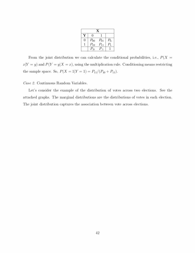
XY 0 10 P00 P01 P0:1 P10 P11 P1:

P:0 P:1 1

From the joint distribution we can calculate the conditional probabilities, i.e., P (X =

xjY = y) and P (Y = yjX = x), using the multiplication rule. Conditioning means restricting

the sample space. So, P (X = 1jY = 1) = P11=(P10 + P11).

Case 2. Continuous Random Variables.

Let's consider the example of the distribution of votes across two elections. See the

attached graphs. The marginal distributions are the distributions of votes in each election.

The joint distribution captures the association between vote across elections.

42

vote

per

cent

dv_00 100

0

100

43

Frac

tion

vote percent0 100

0

.261128

The joint normal distribution provides a framework within which we think about the

relationship among continuous random variables. As with the univariate normal, the density

function depends on parameters of location and spread. To describe association between the

variables, only one new parameter is needed, the correlation.

Two variables, say X1 and X2, follow a joint normal distribution. Their density function

looks like a bell-shaped curve in three dimensions. The exact formula for this distribution

is:

f(x1; x2) =1

2¼q¾2

1¾22(1¡ ½2)

e¡ 1

2(1¡½2)

·³x1¡¹1¾1

´2+³x2¡¹2¾2

´2+2½

³x1¡¹1¾1

´³x2¡¹2¾2

´¸

44

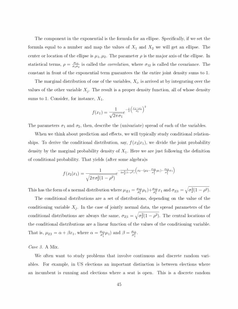
The component in the exponential is the formula for an ellipse. Speci¯cally, if we set the

formula equal to a number and map the values of X1 and X2 we will get an ellipse. The

center or location of the ellipse is ¹1; ¹2. The parameter ½ is the major axis of the ellipse. In

statistical terms, ½ = ¾12¾1¾2

is called the correlation, where ¾12 is called the covariance. The

constant in front of the exponential term guarantees the the entire joint density sums to 1.

The marginal distribution of one of the variables, Xi, is arrived at by integrating over the

values of the other variable Xj. The result is a proper density function, all of whose density

sums to 1. Consider, for instance, X1.

f(x1) =1p

2¼¾1e¡1

2

³x1¡¹1¾1

´2

The parameters ¾1 and ¾2, then, describe the (univariate) spread of each of the variables.

When we think about prediction and e®ects, we will typically study conditional relation-

ships. To derive the conditional distribution, say, f (x2jx1), we divide the joint probability

density by the marginal probability density of X1. Here we are just following the de¯nition

of conditional probability. That yields (after some algebra)s

f (x2jx1) =1

q2¼¾2

2(1 ¡ ½2)e¡ 1

2¾22(1¡½2)

³x2¡(¹2¡ ¾12

¾21¹1)¡ ¾12

¾21x1

´

This has the form of a normal distribution where ¹2j1 = ¾12¾2

1¹1)+¾12

¾21x1 and ¾2j1 =

q¾2

2(1 ¡ ½2).

The conditional distributions are a set of distributions, depending on the value of the

conditioning variable Xj. In the case of jointly normal data, the spread parameters of the

conditional distributions are always the same, ¾2j1 =q¾2

2(1 ¡ ½2). The central locations of

the conditional distributions are a linear function of the values of the conditioning variable.

That is, ¹2j1 = ®+ ¯x1, where ® = ¾12¾2

1¹1) and ¯ = ¾12

¾21

.

Case 3. A Mix.

We often want to study problems that involve continuous and discrete random vari-

ables. For example, in US elections an important distinction is between elections where

an incumbent is running and elections where a seat is open. This is a discrete random

45

variable. Researchers want to know how the vote depends on whether an incumbent runs.

The random variables and data are readily displayed as separate distributions or graphs

(as shown). In fact, the data are from a single joint distribution of an indicator variable

(incumbency status) and a continuous variable vote. The graphs distinguish when a seat is

open (incumb=0), when a Democratic incumbent runs for reelection (incumb=1), and when

a Republican incumbent runs for reelection (incumb=2).

46

Frac

tion

Histograms by incumbvote percent

incumb==0

0

.166667

incumb==1

10 99.9incumb==2

10 99.90

.166667

Density Estimates The histogram is an estimate of the density function. The histogram

is constructed by dividing the range of the random variable into k bins of equal width

(usually between 10 and 50). The frequency of observations in each bin consists of the

estimated density associated with each interval. In STATA you can make a histogram using

the command graph x. You control the bin-width using the option, i.e.: graph x, bin(25).

A more sophisticated approach is Kernel Density estimation. Kernel estimation ¯ts a con-

tinuous function to the data. There are a variety of functions one may ¯t. For presentation

purposes kernel density estimates are more appealing that histograms

47

F. Expected Values

Probability distributions provide a powerful method for describing randomness (and

chaos). In research and life, we most often want to eliminate randomness and focus on

what is systematic and predictable. In statistics, we reduce randomness by averaging. By

now you are familiar with the average value of a set of numbers. Analysis of problems using

random variables requires a more general formulation of averaging, expected value.

This quantity has two interpretations. First, if realizations of a random variable (say an

experiment) were observed a very large number of times, what is the average outcome you

would observe across those many replications. Second, what is the \certainty equivalent"

value of a random variable if there were no randomness. At what point is a risk neutral

person indi®erent between a speci¯c value and the outcome of the random variable?

Set aside statistical questions, for a moment, and consider a simple example.

A lottery pays $1,000 if you win and $0 if you lose. You must pay $1 to play, regardless of

the outcome. Suppose every individual has an equal chance of winning a lottery and 10,000

play the game. The probability that you win is 1/10000. How much money do you expect to

win? We calculate this using the idea of the certainty equivalent discussed in the ¯rst part

of the course. (1/10000)$1,000 + (9999/10000)$0 = $.10. However, you have to pay $1 to

play, so any individual expects to lose $.90. Of, course no one actually loses $.90; rather that

is the certainty equivalent. That many people gamble suggests that they prefer the risk.

From the perspective of the state or the casino, they expect to earn $10,000 from tickets

sold, but must pay $1,000 for the prize. We can arrive at the state's returns another way.

They expect to earn $.90 from each gambler; with 10,000 gamblers, that totals $9,000 =

$.90£10,000.

F.1. De¯nition

Expected value is the average weighted value of a random variable where probabilities

48

serve as weights. It is de¯ned as:

E(X) = 1P (X = 1) + 2P (X = 2) + 3P (X = 3)::: =X

iiP (X = i)

E(X ) =Zxf (x)dx:

This is usually called the mean value of X and denoted ¹. It is the population or theoretical

average value.

We may extend this de¯nition to any function of the values of X . Let h(X) be a function

of X. Then

E(h(X)) = h(1)P (X = 1) + h(2)P (X = 2) + h(3)P (X = 3)::: =X

ih(i)P (X = i)

E(h(X )) =Zh(x)f(x)dx:

Example. Suppose X follows the uniform distribution on [0,1]. What is E(X)? We can

calculate the average value from simple geometry to be .5. We can also integrate:

Z 1

0xdx =

x2

2j10 =

12¡ 0 =

12

What is E(X2)?Z 1

0xdx =

x3

3j10 =

13

Example. Suppose X follows the Binomial distribution. One can prove, after some

algebraic manipulation, that E(X) =Pnk=0

³nk

´pk(1¡p)n¡k = np. (I leave this as an exercise.

The algebra takes some care.)

Statistics focuses on a particular set of expected values, called moments. The moments

of a distribution consist of the expected values of all powers of a random variable. Let X be

a random variable and k be integers 1, 2, 3, 4 .... The moments of the random variable are

E(Xk). That is, E(X), E(X2), E(X3), E(X4), ....

49

We can readily estimate the moments using averages. If we observe a sample of n obser-

vations, then our estimate of E(Xk) = 1nPni=1 xki .

A second sort of moment is \mean-deviated" { e.g., the second moment around the mean,

the third moment around the mean. This is written E[(X¡¹)k]. The second moment around

the mean is the variance; the third moment around the mean is the skew; the fourth moment

is the kurtosis. Higher moments do not have names.

The moments are of interest for two reasons. First, they summarize the data. The

moments of a distribution contain the same information about the random variable as the

density or probability function. One way to understand why this is the case is Taylor's

Theorem. Using Taylor's Theoreme, any function can be written as a polynomial of the

independent variable, where the constants on each polynomial equal the function evaluated

at an arbitrary point. More properly we can summarize a distribution using the moment

generating function, as discussed in Bulmer. This is an advanced topic in probability theory

and one beyond the scope of our course. However, the basic point is important because

it justi¯es using averages data and averages of squares, cubes, etc. of data to summarize

probability.

More simply, you can think about the information contained in the mean, the variance,

the skew, and the kurtosis. For the normal distribution the ¯rst moment equals the paramter

¹ and the second moment is the parameter ¾2. The Third Mean Deviated moment equals 0.

The Fourth Mean Deviated Moment equals 3. Note: these are theoretical quantities. A test

of normality is skew equals 0 and kurtosis equal 3. Consider the distribution of presidential

vote across congressional districts. The mean is normalized to equal 0. The variance is .011

(about 1 percentage point). The skew is 1.06 and the kurtosis if 4.96. The positive number

for the skew means that the tail stretches out to the right. The kurtosis larger than 3 means

that there are more observations out in the tail than predicted by the normal distribution.

Second, moments o®er an approach to estimation. The Method of Moments proceeds

in three steps. (1) Express the moments of a density in terms of the parameters of the

function. For example, for the normal distribution, E(X) = ¹ and E(X 2) = ¾2 + ¹2. (We

50

could continue with more moments, but for this problem 2 is enough.) (2) Substitute the

estimated moments for the theoretical moments. Continuing with the example, 1nPxi = ¹̂

and 1nPx2i = ¾̂2 + ¹̂2. (3) Solve the equations expressing the estimated parameters solely

in terms of the data. In the case of the normal distribution, we get ¹̂ = ¹x = 1nPi xi and

¾̂2 = 1nPi x2

i ¡ ¹x2 = 1nPi(xi ¡ ¹x)2.

F.2. Mean and Variance

Two expected values are central to statistics { the mean and the variance. The mean is

the expected value of X and is commonly denoted using the Greek letter ¹, i.e., ¹ = E(X ).

The variance is expected (squared) distance of any value of X from the mean and is denoted

with the Greek letter ¾2, i.e., ¾2 = E [(X ¡ ¹)2].

These two important parameters capture the central tendency and the spread of the

random variable or data. In other words, the mean describes what is predictable and the

variance describes what is chaotic{the yin and yang of statistics.

There are other measures of central tendency, most notably the median and and mode.

The median is the 50th percentile value; the mode is the value of X with the highest fre-

quency. For a symmetric distribution, such as the normal, these will be the same as the

mean. There are also other measures of shape and spread that use higher ordered mean-

deviated moments: E [(X¡E(X))3], E[(X¡E(X))4],etc. The third-mean deviated moment

is called the skew. It measures the extent to which the data have a disproportionately high

frequency of values above (or below) the mean. Income distributions, for example, are highly

skewed. The fourth mean-deviated moment is called the kurtosis. It measures whether there

are a high frequency of values in the \tails of the distribution." The mean and the variance,

as explained below, are su±cient to characterize most problems of inference.

1. Mean Values

The theoretical mean is the weighted average of the values, where weights are probabil-

51

ities. If the distribution is skewed the mean will lie above the median, which will lie above

the mode. We must distinguish the sample mean ¹x, which is the simple mean of the n

observations in a study, from the population mean. The population or theoretical mean is a

number; it is a ¯xed quantity that we may or may not know. The sample mean is the sum

of n random variables and this is itself a random variable with a probability distribution.

Random variables are often transformed, which alters their mean values. The most

common transformations are linear, and there are two sorts.

² Expected Values of Linear Functions are Linear Functions of Expected Values:

E(a+ bX) = a + bE(X ):

As a demonstration, consider a continuous random variable X .

E(a+ bX) =Z 1

¡1(a + bxf (x))dx =

Z 1

¡1af(x)dx+

Z 1

¡1bxf (x))dx

= aZ 1

¡1f (x)dx+ b

Z 1

¡1xf(x))dx = a + bE(X)

² Expectations of Sums of Random Variables are Sums of Expectations. If X and Y are

random variables, then

E(Y +X ) = E(X) + E(Y )

Assume the variables are continuous with joint density f (x; y).

E(Y +X ) =Z Z

(y + x)f (x; y)dxdy =Zxf(x; y)dxdy+

Zyf (x; y)dxdy

=Zxf(x)dx +

Zyf (y)dy = ¹x + ¹y

These results are immediately helpful in analyzing the mean of random variables that are

themselves sums. Take for example, the Binomial distribution. The Binomial is the sum of

n independent Bernoulli trials. Using the addition rule above allows a simple computation

of the Binomial mean. E(X) = E(X1 +X2 + ::: +Xn) = p+ p + ::: + p = np. Likewise, the

mean of the Poisson is ¸, since ¸ = np. When calculating the normal approximation to the

Binomial we use ¹ = np.

52

2. Variances

The variance is the average squared distance of observations from the data. The Standard

Deviation is the Square Root of the Variance. The standard deviation and the mean are

used in \normalizing" data. The standard deviation measures the \units" of the variable.

Example. X is distributed Uniform(0,1).

V (X) =Z 1

0(x ¡ :5)2dx =

Z 1

0(x2¡ x +

14

)dx =x3

3¡ x + f racx4j10 =

112

Variances of linear functions and sums are essential in statistics.

² E [(X ¡ ¹)2] = E(X2)¡ ¹2.

E [(X¡¹)2] = E[X2¡2X¹+¹2] = E[X2]¡2E [X¹]+¹2 = E[X2]¡2¹2+¹2 = E[X2]¡¹2

² Jentzen's Inequality.

E(X 2) > E(X)2

More generally, for any convex function g(X), E(g(X )) > g(E(X)).Note: This fact

guarantees that variances are always positive. This fact is also very useful in thinking

about risk analysis, as g(¢) can be treated as a utility or loss function.

² V (a+ bX) = b2V (X).

V (a+bX) = E[(a+bX¡a¡b¹)2] = E[(bX¡b¹)2] = E[b2(X¡¹)2] = b2E(X¡¹)2 = b2¾2

² If X and Y are independent V (Y + X) = V (X) + V (Y )

These rules make easier to calculate variances of random variables that are sums of

random variables. Consider the Binomial example. V (X) = V (X1 + X2 + ::: + Xn) =

V (X1) + ::: + V (Xn) = p(1 ¡ p) + :::+ p(1¡ p) = np(1 ¡ p)

Of particular interest is the sample mean. What is the variance of the sample mean? The

sample mean is a random variable, because it is a sum of random variables. We determined

53

that the expected value of the sample mean is ¹. If the observations are independent of one

another (or nearly so, as with samples that are small relative to the population), then we

can calculate the variance of the sample mean using the addition rule for variances.

V (¹x) = V (1n

X

ixi) =

µ 1n

¶2V (X

ixi) =

µ 1n

¶2X

i¾2 =

¾2

n

We have assumed two things in this derivation, both enter in the second to last equality.

First, the observations are independent; hence, V (x1 +x2+:::xn) = V (x1)+V (X2)+ :::V (xn).

Second, the variances are the same for all of the cases. That is the observations are drawn

from the same population. Violations of either assumption, as occurs, for example, with

sampling without replacement, would lead us to alter this formula somewhat.

The interpretation of the two results we have derived about the sample mean are quite

interesting. Were we to conduct the same study repeatedly and estimate the population

mean using the sample mean, the sample mean would vary in a predictable way. The central

tendency of the distribution of sample means would be the population mean, ¹, and the rate

of variation from sample to sample is ¾2

n . These two features of the data are the foundation

for most of statistical inference and design. We can uses these facts to ¯gure out the optimal

sample size for a study and the likelihood of making a disparate observation. We also learn

from these facts that we don't have to do studies repeatedly in order to draw inferences, a

single large survey may do. We will build these ideas in the next section of the course.

Before we turn to statistics proper, I will conclude the discussion of mean and variance

with one important result and one important idea about means and variances. The important

result is Chebychev's inequality.

F.3. Con¯dence Intervals, Chbebychev's Iequality, and the Law of Large Numbers.

Consider the accuracy of the sample mean as an estimate. How close is it to the right

answer? Suppose that we have calculated the sample mean as an estimate of the population

mean. The sample mean does not equal the population mean, unless we are very lucky.

Rather sample means vary randomly around the true mean. The calculation we have just

54

made tells us the rate of variation is ¾2

n . What is the probability of observing a sample mean

that is far from the true mean? That is, if k is a number that we deem \far from ¹, what is

P (j¹x¡ ¹j > k)?

We may ask this question more generally for any random variable X. What is the

probability of observing a large deviation from the mean? The mean and the variance

are powerful tools because they can be used to bound the variation in a random variable.

Chebychev's inequality states that the variance tells us the maximum amount of density

within an interval around the mean for any distribution.

Consider a deviation from the mean jX ¡ ¹j. What is the probability of observing a

deviation from ¹ at least as large as a speci¯c number k? Chebychev's inequality provides

a general formula for this bound, regardless of the underlying distribution:

P (jX ¡¹j > k) <¾2

k2

That is, the probability of observing a deviation from the mean at least as large as k is less

than the variance of X divided by k2. Chebychev's inequality can be rewritten if we let

t¾ = k, where t is a number. Then,

P (jX ¡ ¹j> t¾) <1t2

Reformalated this way, Chebychev's inequality is interpreted as follows. The probability of

observing a value of X more than t standard deviations away from the mean is less that

1=t2. This bound may not be terribly tight for some distributions, but it is generally useful.

Let us consider two sorts of problems.

First, how wide an interval around the mean guarantees that the probability of a large

deviation is less than 5 percent? This is a problem of constructing a con¯dence interval.

We begin with a probability statement about our desired level of con¯dence. We wish to

be highly con¯dent (i.e., at least 95 percent con¯dent) that the population mean lies in an

interval. Given the desired level of con¯dence how wide must the interval be?

Chebychev's inequality tells us what the widest possible interval is. Set the probability

of a deviation of at least t¾ to be less than .05. That is, the probability weight in the \tails"

55

of the distribution must be smaller than .05 The second version of Chebychev's inequality

can be used for this problem. Set the value of the bound 1t2 = :05. Solving this equation,

t =p

20 ¼ 4:5. In other words, 4.5 standard deviations away from the mean guarantees

at least .95 probability of covering the population mean. If we know or estimate ¾ and

we observe a value of x, then we can calculate the widest 95 percent con¯dence interval as

x+ =¡ 4:5¾.

Continuing with this problem, we can ascertain the widest possible con¯dence interval

for the sample mean. What is the interval around the sample mean that one could construct

so as to be sure of covering the true mean with probability .95. We said that the variance

of ¹x is ¾2=n. The standard deviation of ¹x is ¾pn. Hence,

P (j¹x ¡ ¹j > 4:5¾pn< :05

In other words, we are at least 95 percent sure that the interval ¹x + = ¡ 4:5¾n includes the

population mean ¹.

When public opinion pollsters report data on presidential approval, vote intentions, and

other features of public attitudes, then often report a margin of error. The margin of error

is the half-width of the 95 percent con¯dence interval, say +/- 3 percentage points.

For most statistical problems, we will learn below, we can improve on Chebychev's in-

equality, because we know more about the distribution.

Second, how close is the sample mean to the right answer? The ¯rst formulation of

Chebychev's inequality reveals that we can be arbitrarily close to ¹. Again substitute the

formulas for the sample mean and variance of the sample mean into Chebychev's Inequality:

P (j¹x ¡ ¹j > k) <¾2

nk2

The term on the right-hand side depends on a parameter ¾2, a constant k, and the sample

size n. We can increase the sample size to make the term on the right hand side arbitrarily

small. As n becomes in¯nitely large the term on the right hand side approaches 0. Also, we

can choose k to be any arbitrarily small positive number. Hence, by increasing the sample

56

size we can squeeze to 0 the probability that ¹x deviates from ¹ by more than an arbitrarily

small number.

This limiting result is a special case of the Law of Large Numbers. Any statistic that we

calculate that takes the form of an average will be arbitrarily close to the parameter that

the statistic estimates when we have large samples. Generally, this concept is called the

consistency of a statistic.

An important version of the Law of Large Numbers is the Binomial. Suppose that we

wish to study the population frequency of a certain trait or the probability of an event, p.

We collect a sample of size n with replacement from the population. The ratio k=n estimates

p, and k follows the Binomial distribution. The variance of k=n is p(1¡p)n . [Question: Why?]

What is P (jkn ¡ pj > ±)? We know from Chebychev's Inequality that this probability is

smaller than p(1¡p)n± . As n grows the bound approaches 0, and the probability that k=n

deviates from p by more than a tiny amount is 0.

The Law of Large Numbers brings us back to our de¯nition of probability. We said that

there are two common de¯nitions of probability { subjective belief and long-run frequency.

We now have a clear and general de¯nition of long-run frequency. Consider what the Bino-

mial result means for a coin tossing problem. Each time we toss a coin the probability of

heads is p and of tails 1¡p. The true probability is never observed because the sample space

is in¯nite; one could toss the coin forever and never enumerate all possible coin tosses. How-

ever, we might feel that after 100 or 1000 coin tosses the observed frequency is close enough

to the true probability. Chebychev's inequality, then, implies that frequencies approach the

true probability of an event, even when the population or sample space is in¯nite.

F.4. Mean Squared Error

In statistics there is another sort of Variance, called the mean squared error. Mean

squared error is the average or expected error in a statistic. Mean squared error encompasses

two very important measurement concepts, bias and precision.

Statistics are quantities that we can compute using data and that summarize the data,

57

just as the moments summarize the distribution. The average value, ¹x, is the most frequently

used statistic as it measures central tendency. The estimated variance is ¾̂2 = 1nPi(xi¡ ¹x)2;

the sample covariance is ¾̂xy = 1nPi(xi ¡ ¹x)(yi ¡ ¹y);the sample skew is Ã̂ = 1

nPi(xi ¡ ¹x)4

; the sample kurtosis is ·̂ = 1nPi(xi ¡ ¹x)4. There are many other statistics, such as the

median, the range, and the mean absolute deviation, that we might study as well.

Each statistic is taken as a measure of a parameter or theoretical relationship. The sample

average estimates the population mean. A regression estimates a theoretical relationship of

a dependent variable to one or more independent variables. Two important features of all

statistics { their bias and precision. In general, we desire statistics that are unbiased and

precise. An unbiased statistic is one that we expect will give the right answer; a precise

statistic is one that will not vary much from measurement to measurement. Mean squared

error summarizes both of these ideas.

Let us call any statistic T(X ), a function of the data. Let us suppose that T(X) is

constructed so as to estimate µ. T(X) is a random variable because it is a function of

random variables. It will vary from sample to sample. For example, suppose we conduct a

survey of 1000 people to ascertain their attitutdes toward the sitting president. We will get

one estimate of the level of support for the president. If we were to conduct a second survey

using the identical sampling procedures we will get another sample and another, di®erent

estimate because the people in the ¯rst survey di®er from those in the second survey. We

could imagine repeatedly sampling and map out a frequency of estimated levels of support.

This is called the Sampling Distribution.

The bias of a statistic is de¯ned as the expected deviation of the statistic from the param-

eter that the statistic estimates. Assume that E [T(X)] = ¿ . We write Bias= E [T(X )¡µ] =

¿¡ µ. The precision of the statistic is the variance of T (X). ; so V (T(X )) = E[(T(X)¡¿ )2].

Mean squared error is de¯ned as E [(T (X) ¡ µ)]. We can write this in terms of bias and

precision:

E[(T(X)¡ µ)2] = E [(T(X )¡ ¿ + ¿ ¡ µ)2] = E [(T(X )¡ ¿)2 + 2(T (X)¡ ¿ )(¿ ¡ µ) + (¿ ¡ µ)2]

58

= V (T (X)) + (¿ ¡ µ)2

A general goal of statistics is to improve our design and estimation so as to minimize

mean squared error. We will typically be interested in unbiased statistics and then try

to minimizee the variance (or noise) of the statistic. Usually, we will discard unbiased or

inconsistent statistics, so much quantitative work begins with attempts to eliminate bias

from studies.

When repeated measures are available we can measure mean squared error directly as

the variance across measures. For example, if we have 10 surveys conducted using the same

general methodology and questions one measure the variance across the surveys to see if there

are biases due to, say, di®erent ¯rms. Also, this technique is used to callibrate interviewers or

testers. The measure used is just the estimated variance across surveys. Let ¹¹x be the average

of the sample averages and ¹xj be the sample average of one survey. Then the estimated MSE

is1

J ¡ 1

JX

j=1( ¹xj ¡ ¹¹x)2

F.5. Covariance, Correlation, and Reliability of Measures.

When we deal with joint data, the covariance will summarize the joint relationship.

Covariance is de¯ned:

Cov(X;Y ) = E [(X ¡ E(X))(Y ¡ E(Y ))]

Sometimes we denote Cov(X;Y ) = ¾xy. The covariance depends on the units, which makes

for di±cult interpretation when two variables are in di®erent units. The standardized co-

varaince is called the correlation and denoted using the Greek letter ½.

½ =Cov(X;Y )qV (X)V (Y )

= CovÃX¾x;Y¾y

!

Several important features of covariance are useful in algebraic manipulation:

59

² Covariance is de¯ned as Cov(X;Y ) = E [(X ¡ ¹x)(Y ¡¹y)] = E(XY ) ¡ ¹x¹y.

² Cov(a + bX; Y ) = bCov(X;Y ).

² If X and Y are independent, then E(XY ) = E(X)E(Y ). Hence, if X and Y are

independent Cov(X;Y ) = 0.

² Generally, V (X + Y ) = V (X) + V (Y ) + 2Cov(X;Y ).

V (X+Y ) = E [((X+Y )¡(¹x+¹y))2] = E [(X¡¹x)2 +(Y ¡¹y)2 +2(X¡¹x)(Y ¡¹y)]

= V (X) + V (Y ) + 2Cov(X;Y ):

² Cauchy-Schwartz Inequality. E(X2)E(Y 2) > E(X)2E(Y )2. This guarantees that the

correlation always lies between 1 and -1.

We will use covariance to study relationships among variables later in the course. Now I

would like to consider them as providing a third important measurement concept in addition

to bias and precision. A statistic or measurement is said to be reliable if repeated measure-

ments are highly correlated. This idea is very widely applied in educational testing and in

the construction of indexes.

Within political science an important debate has concerned the stability of public opinion.

Converse (1964) argues that public opinion is not very stable or well-grounded. He looked

at three waves of a panel study and correlated answers to the same questions by the same

people in three successive elections (1956, 1958, and 1960). The results were not happy. The

correlations were quite low, typically in the range .3 to .5. From this Converse concluded

that the public does not hold coherent ideologies or beliefs.

Chris Achen (1975) critiques Converse's important conclusions as re°ectin the low reli-

ability of the survey questions, more than instability in people's beliefs. Achen argues that

responses to survey items re°ect systematic components, people's true beliefs, and noise due

60

to poor question wording, also known as measurement error. People try to guess what the

question means, leading to random variation in responses. Let u be the survey response error

and X¤ be the true belief. Then, X = X¤+ u. We can measure responses at di®erent times.

Assuming the measurement error is unrelated to the true attitude, the covariance between

the survey responses at two di®erent times will beCov(X1; X2) = Cov(X¤1; X¤2 )+Cov(u1; u2).

Assume the measurement error is unrelated. The Variance of the question responses at each

time will equal V (X1) = V (X¤1) + V (u1) and V (X2) = V (X ¤2 ) + V (u2). The true correlation

in attitudes is ½¤12 = Cov(X¤1 ;X¤2)p

V (X¤2)V (X¤1 )The correlation between survey questions across the two

times is:

½12 =Cov(X1; X2)qV (X1)V (X2)

=Cov(X¤1; X¤2 )

q(V (X¤2) + V (u2))(V (X¤1 ) + V (u1))

< ½¤12

Achen further argues that the true correlation in attitudes is plausibly as high as .8 to .9 on

most items. The problem he concludes is low reliability in the instrument used to measure

attitudes.

Another important debate within political science concerns the measurement of the pref-

erences of members of Congress. Various roll call voting scores have been constructed by

interest groups, such as Americans for Democratic Action, and by academics, such as Poole

and Rosenthal or Heckman and Snyder. ADA identi¯es 20 key roll call votes and constructs

a \liberalism" measure based on the number of times that members of Congress vote with

the ADA. The academic models consider the correlation between all legislators roll call votes

on all issues and then try to uncover the number of dimensions and score legislatures on these

dimensions. At least on the ¯rst dimension, the di®erent methods produce indexes that are

very highly correlated. The correlation between ADA scores and Poole-Rosenthal scores is

typically around .90 to .95.

Part 3 Summary

So far in this course we have focused on issues that may be broadly thought of as mea-

61

surement. We have de¯ned random variables and developed the key mathematical concepts

with which to study random variables.

² A random variable is a variable whose values occur with a speci¯c frequency. Properly

speaking a random variable is a function which maps values into frequencies.

² A probability function de¯nes the frequency with which each value of a random variable

occurs. This function must satisfy three properties: (1) the probability of any event

lies between 0 and 1, (2) the probability of at least one value occurring is 1, and (3)

the probability of two disjoint events is the sum of the probability of each event.

² Expected value is the weighted average of all values of a function in which we treat the

probabilities as weights.

As examples we have considered many statistical problems, such as maximimum likeli-

hood and method of moments estimation and con¯dence intervals. In the next part of the

course we will use these elements as building blocks of statistical modeling.

62