Introduction

to Sample Size

estimation

Outline of the course

• Definition of Power

• Variables of a power analysis

• Difference between technical and biological

replicates

Power analysis for:• Comparing 2 proportions

• Comparing 2 means

• Comparing more than 2 means

• Correlation

Power analysis

• Definition of power: probability that a statistical test will reject

a false null hypothesis (H0) when the alternative hypothesis (H1) is

true.

• Plain English: statistical power is the likelihood that a test will

detect an effect when there is an effect to be detected.

• Arbitrarily, accepted power: 80%

• Main output of a power analysis:

• Estimation of an appropriate sample size

• Very important for several reasons:

• Too big: waste of resources,

• Too small: may miss the effect (p>0.05)+ waste of resources,

• Grants: justification of sample size,

• Publications: reviewers ask for power calculation evidence.

What does Power look like?

What does Power look like?

• Probability that the observed result occurs if H0 is true

• H0 : Null hypothesis = absence of effect

• H1: Alternative hypothesis = presence of an effect

What does Power look like?

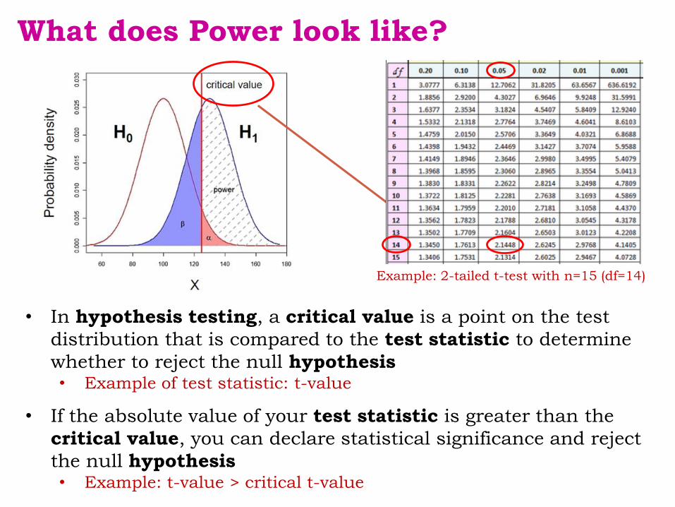
• In hypothesis testing, a critical value is a point on the test

distribution that is compared to the test statistic to determine

whether to reject the null hypothesis• Example of test statistic: t-value

• If the absolute value of your test statistic is greater than the

critical value, you can declare statistical significance and reject

the null hypothesis• Example: t-value > critical t-value

Example: 2-tailed t-test with n=15 (df=14)

What does Power look like?

• α : the threshold value that we measure p-values against.

• For results with 95% level of confidence: α = 0.05

• = probability of type I error

• p-value: probability that the observed statistic occurred by

chance alone

• Statistical significance: comparison between α and the p-value

• p-value < 0.05: reject H0 and p-value > 0.05: fail to reject H0

What does Power look like?

• Type II error (β) is the failure to reject a false H0

• Direct relationship between Power and type II error:

• β = 0.2 and Power = 1 – β = 0.8 (80%)

To recapitulate:

• The null hypothesis (H0): H0 = no effect

• The aim of a statistical test is to reject or not H0.

• Traditionally, a test or a difference are said to be

“significant” if the probability of type I error is: α =< 0.05

• High specificity = low False Positives = low Type I error

• High sensitivity = low False Negatives = low Type II error

Statistical decision True state of H0

H0 True (no effect) H0 False (effect)

Reject H0 Type I error α

False Positive

Correct

True Positive

Do not reject H0 Correct

True Negative

Type II error β

False Negative

Power Analysis

The power analysis depends on the relationship

between 6 variables:

• the difference of biological interest

• the standard deviation

• the significance level (5%)

• the desired power of the experiment (80%)

• the sample size

• the alternative hypothesis (ie one or two-sided test)

Effect size

The effect size: what is it?

• The effect size: minimum meaningful effect of biological relevance.

• Absolute difference + variability

• How to determine it?

• Substantive knowledge

• Previous research

• Conventions

• Jacob Cohen

• Author of several books and articles on power

• Defined small, medium and large effects for different tests

The effect size: how is it calculated?The absolute difference

• It depends on the type of difference and the data• Easy example: comparison between 2 means

• The bigger the effect (the absolute difference), the bigger the power• = the bigger the probability of picking up the difference

http://rpsychologist.com/d3/cohend/

Absolute difference

• The bigger the variability of the data, the smaller the power

The effect size: how is it calculated?The standard deviation

H0 H1

critical value

Power Analysis

The power analysis depends on the relationship

between 6 variables:

• the difference of biological interest

• the standard deviation

• the significance level (5%) (p< 0.05) α

• the desired power of the experiment (80%) β

• the sample size

• the alternative hypothesis (ie one or two-sided test)

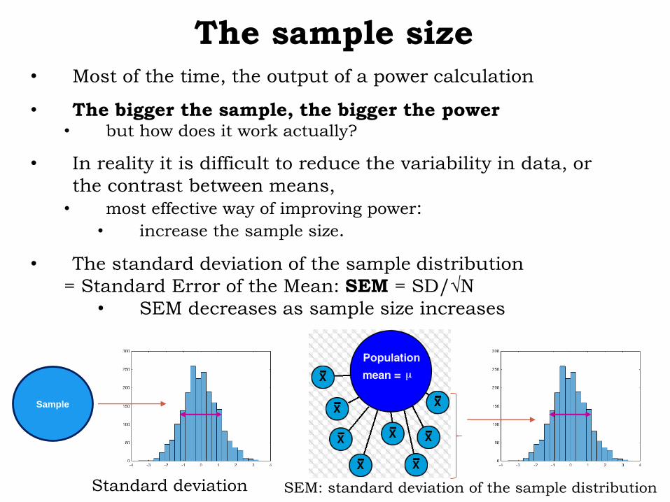
The sample size• Most of the time, the output of a power calculation

• The bigger the sample, the bigger the power• but how does it work actually?

• In reality it is difficult to reduce the variability in data, or

the contrast between means,

• most effective way of improving power:

• increase the sample size.

• The standard deviation of the sample distribution

= Standard Error of the Mean: SEM = SD/√N

• SEM decreases as sample size increases

Sample

Standard deviation SEM: standard deviation of the sample distribution

The sample size

• SEM decreases as sample size increases

• How does it work?

• Sampling distribution of the mean

= If we were to collect an infinite number of samples

from the population of interest and plot the means:

• Probability distribution of the mean

The sample size: the bigger the better?

• What if the tiny difference is

meaningless?

• Beware of overpower

• Nothing wrong with the stats: it is

all about interpretation of the

results of the test.

• Remember the important first step of

power analysis

• What is the effect size of

biological interest?

• It takes huge samples to detect tiny differences but tiny samples

to detect huge differences.

Power Analysis

The power analysis depends on the relationship

between 6 variables:

• the effect size of biological interest

• the standard deviation

• the significance level (5%)

• the desired power of the experiment (80%)

• the sample size

• the alternative hypothesis (ie one or two-sided test)

The alternative hypothesis: what is it?

• One-tailed or 2-tailed test? One-sided or 2-sided tests?

• Is the question:

• Is the there a difference?

• Is it bigger than or smaller than?

• Can rarely justify the use of a one-tailed test

• Two times easier to reach significance

with a one-tailed than a two-tailed

• Suspicious reviewer!

• Fix any five of the variables and a

mathematical relationship can be used to

estimate the sixth.

e.g. What sample size do I need to have a 80% probability (power) to

detect this particular effect (difference and standard deviation) at a

5% significance level using a 2-sided test?

Difference Standard deviation

Sample size

Significance level Power 2-sided test ( )

• Definition of technical and biological depends on the model and

the question

• e.g. mouse, cells …

• Question: Why replicates at all?

• To make proper inference from sample to general population

we need biological samples.

• Example: difference on weight between grey mice and white

mice:

• cannot conclude anything from one grey mouse and one

white mouse randomly selected

• only 2 biological samples

• need to repeat the measurements:

• measure 5 times each mouse: technical replicates

• measure 5 white and 5 grey mice: biological replicates

• Answer: Biological replicates are needed to infer to the general

population

Technical and biological replicates

Technical and biological replicatesAlways easy to tell the difference?

• Definition of technical and biological depends on the model

and the question.

• The model: mouse, rat … mammals in general.

• Easy: one value per individual

• e.g. weight, neutrophils counts …

• What to do? Mean of technical replicates = 1 biological replicate

• The model is still: mouse, rat … mammals in general.

• Less easy: more than one value per individual

• e.g. axon degeneration

• What to do? Not one good answer.

• In this case: mouse = experiment unit• axons = technical replicates, nerve segments = biological replicates

Technical and biological replicatesAlways easy to tell the difference?

… …One measure

Tens of values per mouse

Several axons per segment

Several segments per mouse

One mouse

Technical and biological replicatesAlways easy to tell the difference?

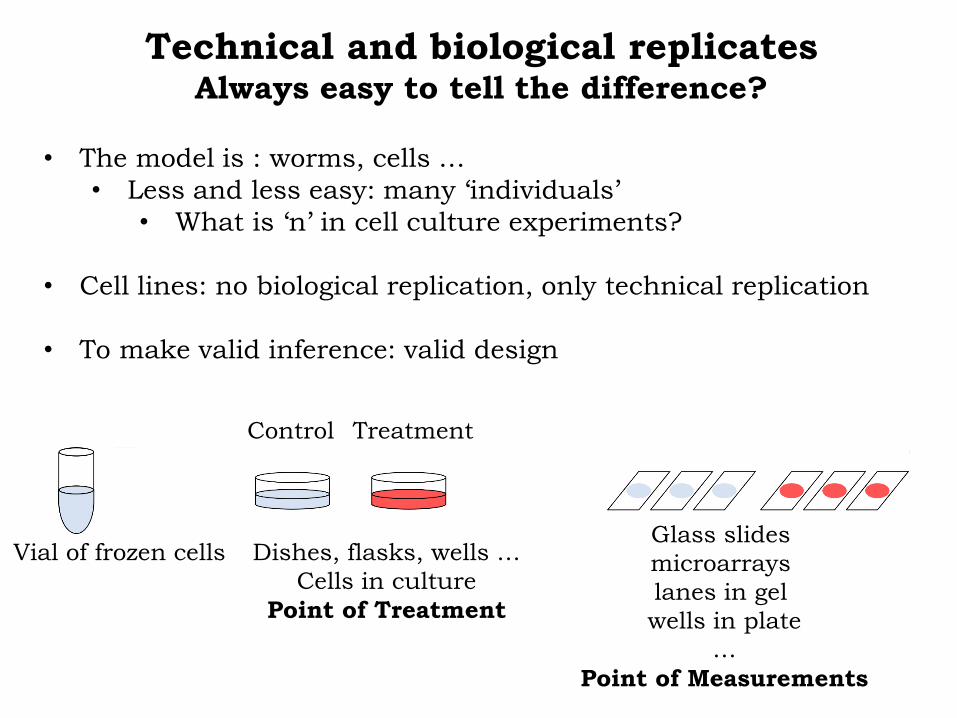
• The model is : worms, cells …

• Less and less easy: many ‘individuals’

• What is ‘n’ in cell culture experiments?

• Cell lines: no biological replication, only technical replication

• To make valid inference: valid design

Vial of frozen cells Dishes, flasks, wells …

Cells in culture

Point of Treatment

Control Treatment

Glass slides

microarrays

lanes in gel

wells in plate

…

Point of Measurements

Technical and biological replicatesCell cultures

• Design 1: As bad as it can get

One value per glass slide

e.g. cell count

• After quantification: 6 values

• But what is the sample size?

• n = 1

• no independence between the slides

• variability = pipetting error

Technical and biological replicatesCell cultures

• Design 2: Marginally better, but still not good enough

• After quantification: 6 values

• But what is the sample size?

• n = 1• no independence between the plates

• variability = a bit better as sample split higher up in the hierarchy

Everything processed

on the same day

Technical and biological replicatesCell cultures

• Design 3: Often, as good as it can get

• After quantification: 6 values

• But what is the sample size?

• n = 3• Key difference: the whole procedure is repeated 3 separate times

• Still technical variability but done at the highest hierarchical level

• Results from 3 days are (mostly) independent

• Values from 2 glass slides: paired observations

Day 1 Day 2 Day 3

Technical and biological replicatesCell cultures

• Design 4: The ideal design

• After quantification: 6 values

• But what is the sample size?

• n = 3• Real biological replicates

person/animal 1 person/animal 2 person/animal 3

Technical and biological replicates

What to remember

• Key things to remember:

• Take the time to identify technical and biological replicates

• Try to make the replications as independent as possible

• Never ever mix technical and biological replicates

• The hierarchical structure of the experiment needs

to be respected in the statistical analysis.

Hypothesis

Experimental design

Choice of a Statistical test

Power analysis

Sample size

Experiment(s)

(Stat) analysis of the results

• Good news:

there are packages that can do the power analysis for

you ... providing you have some prior knowledge of the

key parameters!

difference + standard deviation = effect size

• Free packages:

• G*Power and InVivoStat

• Russ Lenth's power and sample-size page:• http://www.divms.uiowa.edu/~rlenth/Power/

• R

• Cheap package: StatMate (~ £30)

• Not so cheap package: MedCalc (~ £275)

Power AnalysisLet’s do it

• Examples of power calculations:

• Comparing 2 proportions

• Comparing 2 means

• Comparing more than 2 means

• Correlation

• Package: G*Power

Power AnalysisComparing 2 proportions

• Research example:

• A scientist is looking at a new treatment to reduce the development

of tumours in mice.

• Control group: 40% of mice develop tumours

• Aim: reduction to 10%

• Power: 80%, 5% significance

• Effect size: measure of distance between 2 proportions or probabilities

• Comparison between 2 proportions: Fisher’s exact test

Step1: choice of Test family

Four steps to Power

Example case:

Decrease of tumour development

from 40% to 10%.

Power AnalysisComparing 2 proportions

Step 2 : choice of Statistical test

G*Power

Fisher’s exact test or Chi-square for 2x2 tables

Step 3: Type of power analysis

G*Power

Step 4: Choice of Parameters

Tricky bit: need information on the size of the

difference and the variability.

G*Power

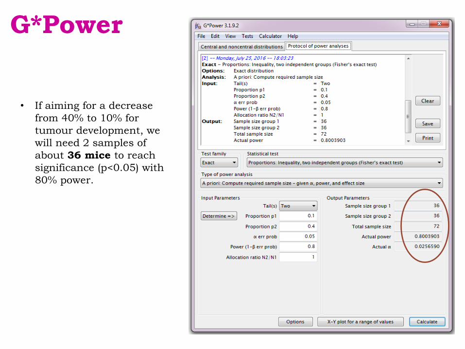
• If aiming for a decrease

from 40% to 10% for

tumour development, we

will need 2 samples of

about 36 mice to reach

significance (p<0.05) with

80% power.

G*Power

For a range of sample sizes:

G*Power

Power AnalysisComparing 2 means

• Research example:

• A scientist is looking at the effect of caffeine on muscle metabolism.

• Metabolism measured via Respiratory Exchange Ratio (RER)

• Pilot study:• Placebo: Mean=100.56, SD=7.70 and Caffeine: Mean=94.22, SD=5.61

• Power: 80%, 5% significance

• Effect size: difference between the 2 means accounting

for the variability (Cohen’s d).

• Comparison between 2 means: t-test

Providing the difference observed in the pilot study is a good estimation

of the real effect size, we need a sample size of n=38 (2*19).

Power Analysis

Power Analysis

H0 H1

For a range of sample sizes:

Power Analysis

Comparison of more than 2 means

ANOVA

• Extension of the t-test as in it compares means accounting for

groups variability but because there are more than 2 means, it

actually compares the variance between groups with the one

within groups (hence ANalysis Of VAriance).

• Output of an ANOVA is 2-fold:

– first, the omnibus part quantifying the overall difference between

the groups and

– second, the pairwise comparisons of interest via post-hoc tests.

• Most of the time, it’s the second bit which is really interesting

– An adjustment needs to be applied to account for multiple

comparisons.

• Different ways to go about power analysis in the

context of ANOVA:

– η2 : explained proportion variance of the total variance.

• Can be translated into effect size d.

• Not very useful: only looking at the omnibus part of the test

– Minimum power specification: looks at the difference

between the smallest and the biggest means.

• All means other than the 2 extreme one are equal to the grand

mean.

– Smallest meaningful difference

• Works like a post-hoc test.

Comparison of more than 2 means

• Minimum power specification

• Research example:

– A researcher is interested in 4 different teaching methods in

the area of mathematics education.

• Effect of these methods on standardized math scores.

– Group 1: the traditional teaching method,

– Group 2: the intensive practice method,

– Group 3: the computer assisted method and,

– Group 4: the peer assistance learning method.

• Standardized test: mean score = 550, SD = 80

• Power: 80%, 5% significance

Power AnalysisComparing more than 2 means

• Research example: Comparison between 4 teaching methods

– Assumptions:

• Equal group sizes and equal variability (SD = 80)

• Prior research:

– Traditional teaching (Group 1): lowest mean score

– Peer assistance (Group 4): highest mean score

• Group 1: mean = 550 (SD = 80)

• Group 4: Difference of interest> +1.2 SD: 550+80*1.2 = 646

• Other 2 groups: mean = grand mean = 598 (= 646+550/2)

Power AnalysisComparing more than 2 means

• Minimum power specification

Each group: n=17

Power Analysis

• Minimum power specification

• If the other 2 means are known, better to use them:

• if more polarized towards the two extreme ends:

• easier to detect the group effect: smaller samples.

Power Analysis

• Different ways to go about power analysis in the

context of ANOVA:

– η2 : explained proportion variance of the total variance.

• Can be translated into effect size d.

– Minimum power specification: looks at the difference

between the smallest and the biggest means.

• All means other than the 2 extreme one are equal to the grand

mean.

– Smallest meaningful difference

• Works like a post-hoc test.

Comparison of more than 2 means

• Research example: Comparison between 4 teaching methods

• Smallest meaningful difference

– Same assumptions:

• Equal group sizes and equal variability (SD = 80)

– 3 comparisons of interest: vs. Group 1

– Smallest meaningful difference: group 1 vs. Group 2

• t-test: Mean 1 = 550, SD = 80 and mean 2 = 598, SD = 80

• Power calculation like for a t-test but with a Bonferroni

correction (adjustment for multiple comparisons)

Power AnalysisComparing more than 2 means

Power AnalysisComparing more than 2 means

Smallest meaningful difference

Bonferroni correction

3 comparisons: 0.05/3 = 0.017

Power AnalysisCorrelation

• Research example:

• A ecologist is looking at the host-parasite relationship in roe deers.

Measures of body weight and parasite load will be collected

from a group of females: Body weight = f(parasite load).

• Pilot study on a small group: r = 0.3

• Power: 80%, 5% significance

• Effect size: Cohen’s r: effect size in correlation

Power AnalysisCorrelation

Power AnalysisUnequal sample sizes

• Scientists often deal with unequal sample sizes

• No simple trade-off:• if one needs 2 groups of 30, going for 20 and 40

will be associated with decreased power.

Unbalanced design = bigger total sample

Solution:

Step 1: power calculation for equal sample size

Step 2: adjustment

• Caffeine example but this time:

placebo group: 2 times smaller than caffeine one:

k=2. Using the formula, we get a total:

N=2*19*(1+2)2/4*2=43

Placebo (n1)=14 and caffeine (n2)=29

Power AnalysisNon-parametric tests

• Non-parametric tests: do not assume data come from a Gaussian distribution.

• Non-parametric tests are based on ranking values from low to high

• Non-parametric tests not always less powerful

• Proper power calculation for non-parametric tests:

• Need to specify which kind of distribution we are dealing with

• Not always easy

• Non-parametric tests never require more than 15% additional subjects

providing 2 assumptions:

• n>=30

• the distribution is not too unusual

• Very crude rule of thumb for non-parametric tests:

• Compute the sample size required for a parametric test and add 15%.

That’s it!